Embed Size (px)
Citation preview
1616 P St. NW Washington, DC 20036 202-328-5000 www.rff.org
August 2016; revised February 2017 RFF DP 16-35-REV
Are Consumers Willing to Pay to Let Cars Drive for Them? Analyzing Response to Autonomous Vehicles
Ric ardo A. Daz ia no, M aur i c io Sa r r ias , and
Be n jami n L ear d
DIS
CU
SSIO
N P
APE
R
Are consumers willing to pay to let cars drive for
them? Analyzing response to autonomous vehicles
Ricardo A. Daziano∗, Mauricio Sarrias†and Benjamin Leard‡
January 2017
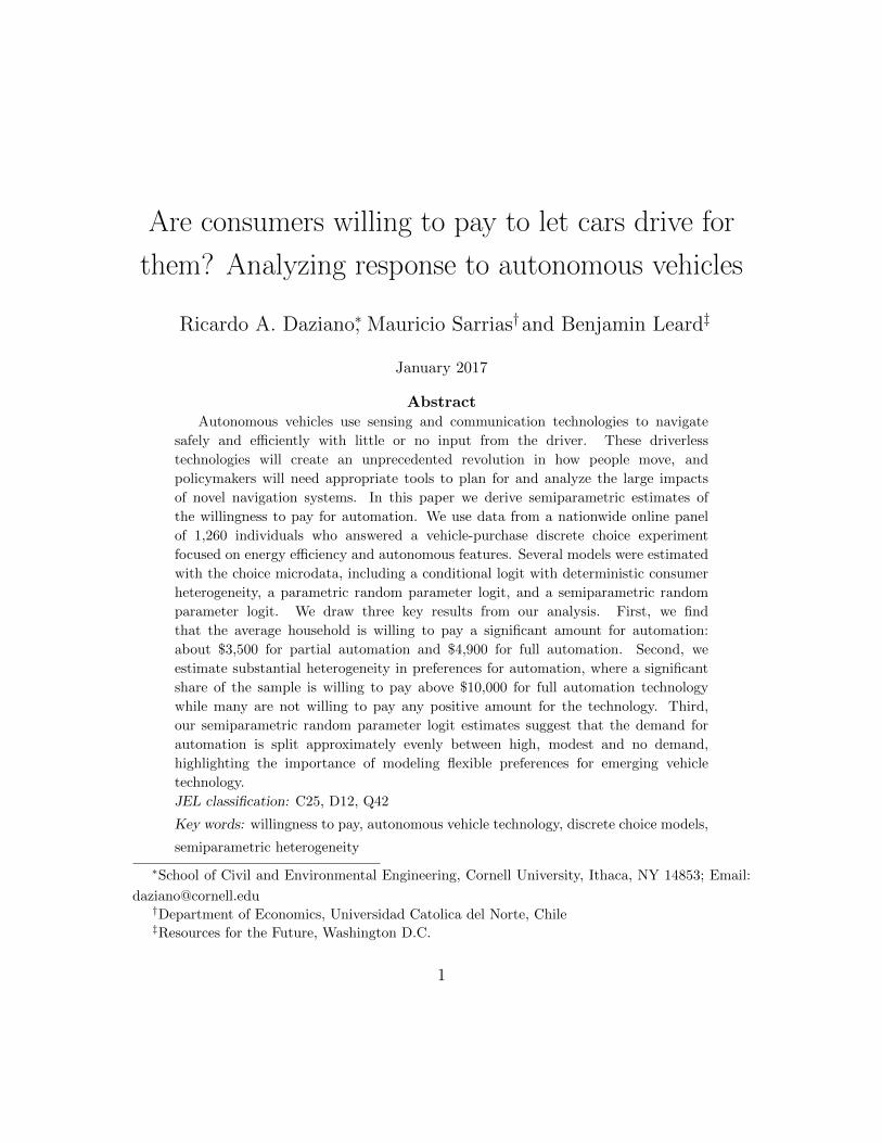
AbstractAutonomous vehicles use sensing and communication technologies to navigate
safely and efficiently with little or no input from the driver. These driverless
technologies will create an unprecedented revolution in how people move, and
policymakers will need appropriate tools to plan for and analyze the large impacts
of novel navigation systems. In this paper we derive semiparametric estimates of
the willingness to pay for automation. We use data from a nationwide online panel
of 1,260 individuals who answered a vehicle-purchase discrete choice experiment
focused on energy efficiency and autonomous features. Several models were estimated
with the choice microdata, including a conditional logit with deterministic consumer
heterogeneity, a parametric random parameter logit, and a semiparametric random
parameter logit. We draw three key results from our analysis. First, we find
that the average household is willing to pay a significant amount for automation:
about $3,500 for partial automation and $4,900 for full automation. Second, we
estimate substantial heterogeneity in preferences for automation, where a significant
share of the sample is willing to pay above $10,000 for full automation technology
while many are not willing to pay any positive amount for the technology. Third,
our semiparametric random parameter logit estimates suggest that the demand for
automation is split approximately evenly between high, modest and no demand,
highlighting the importance of modeling flexible preferences for emerging vehicle
technology.
JEL classification: C25, D12, Q42
Key words: willingness to pay, autonomous vehicle technology, discrete choice models,
semiparametric heterogeneity
∗School of Civil and Environmental Engineering, Cornell University, Ithaca, NY 14853; Email:
[email protected]†Department of Economics, Universidad Catolica del Norte, Chile‡Resources for the Future, Washington D.C.
1
1 Introduction
Personal mobility is about to experience an unprecedented revolution motivated
by technological change in the automotive industry (National Highway Traffic
Safety Administration, 2013; Fagnant and Kockelman, 2014). The introduction of
automated vehicles –in which at least some (and potentially all) control functions
occur without direct input from the driver– will completely change how people move.
The adoption of automated navigation systems has the potential to dramatically
reduce traffic congestion and accidents, while creating substantial improvements in
the overall trip experience as well as providing enhanced accessibility opportunities
to people with reduced mobility (Fagnant and Kockelman, 2015).
Automated vehicles use sensing and communication technologies to navigate
safely and efficiently with little or no human input. Automated navigation technology
comprises any combination of (1) self-driving navigation systems informed by on-
board sensors (autonomous vehicles) vehicle-to-vehicle (V2V) and (2) vehicle-to-
infrastructure (V2I) communication systems that inform navigation and collision
avoidance applications (connected vehicles). The National Highway Traffic Safety
Administration (NHTSA) has suggested five levels of automated navigation: level
0 (no automation), where the driver is in complete control of safety-critical
functions; level 1 (function-specific automation), where the driver cedes limited
control of certain functions to the vehicle especially in crash-imminent situations
(adaptive cruise control, electronic stability control ESC, automatic braking); level
2 (combined-function automation), which enables hands-off-wheel and foot-off-pedal
operations, but the driver is expected to be available at all times to resume control of
the vehicle (adaptive cruise control and lane centering); level 3 (limited self-driving
or conditional automation), where the vehicle potentially controls all safety functions
under certain traffic and environmental conditions, but some conditions require
transition to driver control; and level 4 (driverless or full self-driving automation),
where the vehicle controls all safety functions and monitors conditions for the whole
trip.1
1A six level categorization is proposed by the Society of Automotive Engineers, which further
distinguishes levels within NHTSA level 4.
2
Imminent commercialization of automated cars is best exemplified by the recent
announcement (October 2016) that all new Tesla vehicles will have full self-driving
hardware.2 Several semi-autonomous features are already available in the automotive
market, mostly in the form of in-vehicle crash avoidance upgrades with preventive
warnings or limited automated control of safety functions, such as braking when
danger is detected. Self-parking assist systems are another example of a more
advanced upgrade that is currently available in select makes and models. These
entry-level automation packages are possible as a result of vehicles being equipped
with radar, cameras, and other sensors. Even though technology is still evolving, full
automation is possible with the current stage of development. The Google car and
its more than 2 million miles of driverless driving is the most publicized effort.3
The literature on vehicle-to-vehicle, vehicle-to-infrastructure, and control systems
for safe navigation is extensive. Regulation, insurance, and liability are other areas
where there is strong debate. However, little attention has been devoted to the
analysis of automated vehicles as marketable products. Consumer acceptance is
critical to forecast adoption rates, especially if one considers that there may be
strong barriers to entry (potential high costs, concerns that technology may fail).
Our work contributes to two strands of literature on the demand for new
technology. The first area is the recent development in understanding the demand,
penetration, and policy implications of autonomous vehicle technology. Several
recent studies attempt to understand how consumer preferences for attributes such
as safety, travel time, and performance shape the demand for driverless cars.
Kyriakidis et al. (2015) conducted an international public opinion questionnaire of
5,000 respondents from 109 countries. Responses were diverse: 22 percent of the
respondents did not want to pay any additional price for a fully automated navigation
system, whereas 5 percent indicated they would be willing to pay more than $30,000.
Payre et al. (2014) conducted a similar survey of 421 French drivers with questions
eliciting the acceptance of fully automated driving. Among those surveyed, 68.1
percent accepted fully automated driving unconditionally, with higher acceptance
2Source: https://www.tesla.com/blog/all-tesla-cars-being-produced-now-have-
full-self-driving-hardware3Source: https://www.google.com/selfdrivingcar/faq/
3
conditional on the type of driving, including usage of highway driving, in the presence
of traffic congestion, and for automated parking. Similar results were obtained in
a survey of Berkeley, California, residents conducted by Howard and Dai (2013).
Individuals in this survey were most attracted to the potential safety, parking, and
multi-tasking benefits. Schoettle and Sivak (2014) conducted a much larger and
more internationally based survey of residents from China, India, Japan, the United
States, the United Kingdom, and Australia. The authors found that respondents
expressed high levels of concern about riding in self-driving vehicles, with the most
pressing issues involving those related to equipment or system failure. While most
expressed a desire to own an autonomous vehicle, many respondents stated that they
were unwilling to pay extra for the technology.
A paper related to our own is that by Bansal et al. (2016), which estimates
willingness to pay for different levels of automation. They find that for their sample
of 347 residents of Austin, Texas, willingness to pay (WTP) for full automation
is $7,253, which is substantially higher than our own estimate. The authors also
estimate WTP for partial automation of $3,300, which is similar to our estimate.
Our demand estimates contribute to the assessment of the social costs and benefits
of autonomous vehicles. Fagnant and Kockelman (2015) estimate the external net
benefits from autonomous vehicle penetration. They find that the social net benefits
including crash savings, travel time reduction from less congestion, fuel efficiency
savings, and parking benefits total between $2,000 and $4,000 per vehicle. These
estimates, however, greatly depend on how the presence of autonomous vehicles will
impact both vehicle ownership and utilization. For example if autonomous vehicles
make owning a vehicle more desirable, then the stock and use of vehicles may increase,
reducing the external net benefits.
We designed a web-based survey with a discrete choice experiment to determine
early-market empirical estimates of the structural parameters that characterize
current preferences for autonomous and semi-autonomous electric vehicles. The
discrete choice experiment contained as experimental attributes three levels of
automation: no automation, some or partial automation (“automated crash
avoidance”), and full automation (“Google car”). Automation was allowed for
alternative powertrains (hybrid electric, plug-in hybrid and full battery electric).
4
Based on the results from this experiment, we estimate WTP for automation. Our
estimates of WTP for privately owned autonomous vehicles take a first step to
understanding the demand for this technology, which is critical for understanding
how aggregate demand for vehicles and vehicle miles traveled will respond to the
technology over time.4
In addition to the discrete choice experiment of vehicle purchase, the survey
also contained an experiment to elucidate the subjective discount rate of potential
vehicle buyers. Expanding on the work of Newell and Siikamaki (2013), we used
the individual-level experimental discount rate to determine the present value of fuel
costs for each alternative.
To derive flexible estimates of the heterogeneity distribution of the willingness to
pay for automation, we implemented the maximum simulated likelihood estimator
of a logit-based model with discrete continuous heterogeneity distributions, in
which the parameters (mean and standard deviation) of continuous heterogeneity
distributions have associated discrete, unknown probabilities. The approach adopted
to unobserved preference heterogeneity in this paper thus takes into consideration
a mixed-mixed logit model (Bujosa et al., 2010; Greene and Hensher, 2013; Keane
and Wasi, 2013), where the random willingness-to-pay parameters are distributed
according to a Gaussian mixture. The weights of the Gaussian mixture can
include individual-specific covariates that allow us to identify clusters with differing
willingness to pay for automation. The estimator was implemented with analytical
expressions of the score for computation efficiency.
Methodologically, we highlight the importance of allowing for flexible distribu-
tions of preferences for vehicle attributes such as automation by comparing estimates
from a standard mixed logit specification with a more flexible mixed-mixed logit spec-
ification. We find richer heterogeneity estimates with the more flexible specification,
4We do not explore demand for autonomous commercial vehicles or for autonomous public
transportation. Initial work in this area includes a study by Greenblatt and Saxena (2015)
which simulates the greenhouse gas impact of autonomous vehicle taxis and finds that they can
dramatically reduce greenhouse gas emissions relative to conventional taxis. A promising area of
future research involves incorporating our survey and econometric methods for eliciting WTP to
determine how households tradeoff cost savings, travel time, safety, and other desirable attributes
with alternative travel modes with and without a human driver.
5
where demand for automation appears evenly split between high, modest and no
demand.
The remainder of the paper is organized as follows. In section 2, we present a
series of discrete choice models that we use to estimate how consumers value personal
vehicle automation. In section 3, we discuss the survey data and provide summary
statistics of the sample. We then present the empirical models and estimation results
in section 4 and draw conclusions based on our results in section 5.
2 Structural Vehicle Choice Models
The purchase of an automated vehicle can be modeled as the consumer choice to
adopt high technology, durable goods. The use of discrete choice models to analyze
vehicle purchases in general dates back to the earliest econometric applications of
the principle of random utility maximization. Within this literature, great interest in
modeling the adoption of battery electric vehicles has emerged in the last five years
(for literature reviews, see Rezvani et al., 2015; Al-Alawi and Bradley, 2013).
Because the transition to energy efficiency in personal transportation is
characterized by the trade-off between higher purchase prices and lower operating
costs, a specific avenue of research has been taking into account time preferences to
represent how consumers discount future savings. Seminal work on the problem of
estimating individual discount rates with discrete choice models includes Hausman
(1979), Lave and Train (1979), and the technical reports cited in Train (1985).
In addition, recent literature reviews are provided by Frederick et al. (2002) and
Cameron and Gerdes (2005). Expanding on Jaffe and Stavins (1994), several
resource and energy economists have added to the debate about the energy paradox
(Newell and Siikamaki, 2013; Allcott and Greenstone, 2012; Ansar and Sparks, 2009;
Van Soest and Bulte, 2001; DeCanio, 1998; Hassett and Metcalf, 1993). As reviewed
in Wang and Daziano (2015), there are two approaches to introducing discount rates
in discrete choice models: endogenous discounting, in which discount rate estimates
are derived from the marginal rate of substitution between price and operating cost,
and exogenous discounting, in which the discount rate is assumed as known.
Working with exogenous discount rates has been proposed in the energy
economics literature to avoid confounding effects in the determination of discount
6
rate estimates coming from market failures (Allcott and Wozny, 2014; Newell and
Siikamaki, 2013). Exogenous discounting takes as known the discount rate of
individual i, making it straightforward to calculate the present value of future costs
of product j, PVFCij. Moving future cash flows to the present allows the researcher
to use a static discrete choice specification. If in addition to monetary attributes,
vehicle design attributes xij are considered (such as power, drivetrain, refueling time,
and driving range), then the conditional indirect utility for individual i choosing
alternative j can be specified as
Uij = x′ijωx,i − αipriceij − γPVFC,iPVFCij + εij. (1)
Equation (1) represents our benchmark specification and is formulated in preference
space. ωx,i is the change in utility from marginal improvements in the (nonmonetary)
vehicle design attributes that are captured in the vector xij, αi is the marginal utility
of income, and γPVFC,i is the change in utility from a marginal change in the present
value of fuel costs. For a rational consumer γPVFC,i = αi, since both priceij and
PVFCij are monetary attributes at the time of purchase. If γPVFC,i < αi, then there
is evidence for myopic consumption (as consumers weigh more than saving one dollar
in purchase price than the same dollar in discounted future costs), and γPVFC,i > αi
reveals that consumers overvalue fuel costs. In our benchmark specification, we
assume that the idiosyncratic error term εij is i.i.d. distributed Type 1 extreme
value, so that predicted probabilities take on the conditional logit form.
In this paper, in addition to standard assumptions of unobserved heterogeneity
in the parameters (such as normally and lognormally distributed parameters),
we consider a semi-parametric discrete-continous mixture for the heterogeneity
distributions. In fact, we adopt and implement the idea of the mixed-mixed logit
model (MM-MNL) that represents heterogenous preferences as a weighted average
of normals (Bujosa et al., 2010; Greene and Hensher, 2013; Keane and Wasi, 2013).5
If θ′i = (αi, γPVFC,i,ω′x,i) represents the full vector of parameters of interest,
the heterogeneity distribution assumption is the following Gaussian mixture with
Q components: θi ∼ N (θq,Σq) with probability wiq for q ∈ {1, . . . , Q} or fΘ(θi) =
5Any continuous distribution can be approximated by a discrete mixture of normal distributions
(Train, 2008).
7
Q∑q=1
wiqfq(θi), where fΘ is the density function of the heterogeneity distribution of the
parameters of interest and fq(θi) is the multivariate normal density with parameters
θq and Σq. The weights of the mixture wiq can be interpreted as class assignment
probabilities, and can be constant or a function of covariates. In particular, the
weights can be specified as a function wiq = wiq(zi|δ), where zi is a vector of
individual-specific characteristics and δ is a vector of parameters. As in latent class
discrete choice models, a possibility is to assume a logit-type specification for the
mixture weights:
wiq =exp(z′iδq)Q∑q=1
exp(z′iδq)
, (2)
where the vector component-specific (or class-specific) parameter vector is normalized
for identification. For example, normalizing δ1 = 0 ensures that the parameters for
the rest of the components are identified.
Assume that we observe T choices made by individual i. We denote the choice
made by individual i by yijt = 1 if individual i chose alternative j in choice occasion
t and yijt = 0 otherwise. Furthermore, assume that εijt is i.i.d. type 1 extreme value
for t ∈ {1, . . . , T} , the MM-MNL probability of the sequence of choices is given by:
Pi =
Q∑q=1
wiq(δ)
∫ T∏t=1
J∏j=1
exp(x′ijωx,i − αipriceij − γPVFC,iPVFCij
)∑Jj=1 exp
(x′ijωx,i − αipriceij − γPVFC,iPVFCij
)yijt fq(θi)dθi. (3)
As in a mixed logit model, the above probability can be approximated using MonteCarlo integration:
Pi =1
R
Q∑q=1
wiq(δ)
R∑r=1
T∏t=1
J∏j=1
exp(x′ijω
′(r)x,i,q − α
(r)i,q priceij − γ
(r)PVFC,i,qPVFCij
)∑Jj=1 exp
(x′ijω
′(r)x,i,q − α
(r)i,q priceij − γ
(r)PVFC,i,qPVFCij
)yijt , (4)
where (α(r)i,q , γ
(r)PVFC,i,q,ω
′(r)x,i,q) represents random draw r ∈ {1, . . . , R} from the normal
density fq(θi|θq,Σq).
Finally, using the Monte Carlo approximation of the probability of the sequence
of choices by individual i, it is possible to find the maximum simulated likelihood
estimator by maximizing the following simulated likelihood:
˜(θQ, δQ,ΣQ; y|X,Z,price,PVFC) =N∏i=1
Pi, (5)
8
where θQ = (θ1, . . . ,θQ), δQ = (δ2, . . . , δQ) (if the first component is normalized),
and ΣQ = (Σ1, . . . ,ΣQ).
3 Vehicle Choice Data
3.1 The survey
To support design of the survey, we first conducted two focus groups where new
vehicle preferences and attitudes toward automated cars were discussed by randomly
selected potential car buyers.6 15 participants in Upstate New York (aged 18-62)
and 12 participants in New York City (aged 18-55) discussed benefits and eventual
dangers of automation. All participants had a driving license, and in the case of
Upstate New York, all commuted by car daily. Only 4 of the participants in New
York City drove a car daily, whereas 6 drove a car occasionally. Diverse income
levels were represented, but the median household income was around $50,000 in
both groups. There were 9 males in the Upstate New York group, and 8 in the New
York City group.
Among the benefits, participants mentioned fewer traffic jams, increased mobility
independence, and easier and quicker parking. Another benefit of automation that
was discussed was the possibility of multitasking and increased productivity. One
of the most relevant features that people look for in a new car is safety (Koppel
et al., 2008; Daziano, 2012). Participants of the focus groups confirmed that safety
is a major concern. However, their perceptions about driverless cars and safety were
divided. Some participants agreed that automation has great potential to reduce
accidents, but a majority also said that unfortunately systems fail. Concerns about
lighter vehicles being more dangerous also were raised. The qualitative information
that was collected in the focus groups was used to design an attitudinal module of
the survey, which supplements the data that were collected using the discrete choice
experiment.
3.2 The data
We used the Qualtrics online platform to collect the survey data. We surveyed
a sample of individuals who provided valid responses for personal characteristics
questions and all of the vehicle choice experiments. Qualtrics is a private market
research company that offers online surveying software as well as management of
6Recruitment of participants was facilitated by the Cornell Survey Research Institute.
9
online panels of respondents that match specific requirements.7 We collected several
waves of responses among adults with a driving license between September 12, 2014,
and October 2, 2014, for a total of 1,260 individuals.8
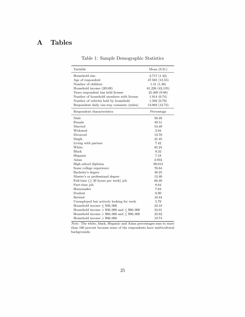
Table 1 reports demographic statistics for respondents in our sample. The sample
is broadly representative of the U.S. population. Mean and median household
incomes are $61,226 and $55,000, respectively, which are close to reported estimates
from the 2013 American Community Survey;9 the sample’s fraction of married adults
well represents the estimates of the U.S. marriage rate of around 50 percent; the
unemployment rate of 5.79 percent among our sample respondents is close to the most
recently reported national unemployment rate for September 2014 of 5.9 percent.10
The sample appears to only slightly over-represent white respondents and slightly
under-represent minorities; the U.S. Census reports that 77.7 percent of U.S. citizens
are white, while our sample includes 85 percent.11 Our sample is slightly more
educated relative to the average for U.S. citizens; 38 percent of respondents state
that they have earned at least a bachelor’s degree, while only about 30 percent
of U.S. citizens have done so. These small differences can be explained by the
screening process of our survey. Two screening questions, whether the respondent
has a driver’s license and whether the respondent has access to a household vehicle,
likely disproportionately discourage minorities and less educated individuals from
taking our survey. Fortunately, however, this effect appears to be quite mild as
suggested by the descriptive statistics of our sample.
Table 2 reports statistics for the vehicle holdings data in our sample. These data
represent vehicles that are driven most often among all vehicles held by respondent
households. We merge survey responses on the model year, make, model and trim of
the vehicle with trim-level characteristics data from Ward’s Automotive.12 Vehicle
7More information in this platform is available at https://www.qualtrics.com/8Out of the sample of 1,260, 549 responses were collected between September 12 and September
15, 214 were collected between September 19 and September 23, and the remaining responses were
collected between September 29 and October 2.9These estimates are available at http://www.census.gov/content/dam/Census/library/
publications/2014/acs/acsbr13-02.pdf.10See http://data.bls.gov/timeseries/LNS14000000.11See http://quickfacts.census.gov/qfd/states/00000.html.12The Ward’s Automotive data include detailed characteristics of vehicles identified by model
year, make, model, series, body style, fuel type, and drive type. Data for vehicles with model years
1996-2014 were purchased from WardsAuto.com.
10
age and annual vehicle miles traveled (VMT) are based on two questions in our
survey.
The average age among all vehicles is seven years, which is about two years
younger than the average age of all autos held by households in 2008.13 This seems
reasonable considering that the reported vehicle holding in our survey is conditional
on being the vehicle that is driven most often and not simply a random vehicle chosen
from the full set of household vehicle holdings.14 For the same reason, annual VMT
is slightly over 15, 000 miles, which is close to the average reported VMT of new
cars and light trucks.15 The selection is also a reason why the average vehicle fuel
economy in our sample is remarkably high.16 Average fuel economy of automobiles
sold in 2007–the average model year of vehicles in our sample–was around 20 miles
per gallon. Households in our sample, however, likely optimize their fleet utilization
choices by driving their relatively fuel efficient vehicles more than their relatively fuel
inefficient vehicles. Therefore, the vehicles that respondents report are more likely
to have high fuel economy.
Patterns in vehicle characteristics across the different styles are in line with
expectations. Fuel efficiency measured in miles per gallon is higher for smaller cars
including coupes, sedans, and wagons and lower for larger, more powerful autos
including trucks and SUVs. Trucks are older than the average vehicle by about
three years, which is also in line with data from the 2009 National Household
Transportation Survey.17 Trucks are generally driven more per year and over the
entire vehicle lifetime than cars, which is consistent with the reported travel data
from our survey.18
13This is based on the 2009 National Household Transportation Survey, Summary of Travel
Trends: http://nhts.ornl.gov/2009/pub/stt.pdf14It is well documented that vehicles with more annual miles traveled are generally newer. See
Lu (2006), http://www-nrd.nhtsa.dot.gov/Pubs/809952.pdf, for more details.15Lu (2006) documents that the average VMT for new cars is 14,231, which falls to 12,325
by age seven; the average VMT for new trucks is 16,085, which falls to 12,356 by year 10. See
http://www-nrd.nhtsa.dot.gov/Pubs/809952.pdf.16In fact, it is close to the average record high 24.9 miles per gallon fuel economy of new 2013
model year vehicles. See http://www.umich.edu/~umtriswt/EDI_sales-weighted-mpg.html.17See http://nhts.ornl.gov/2009/pub/stt.pdf..18For more details, see Lu (2006), http://www-nrd.nhtsa.dot.gov/Pubs/809952.pdf.
11
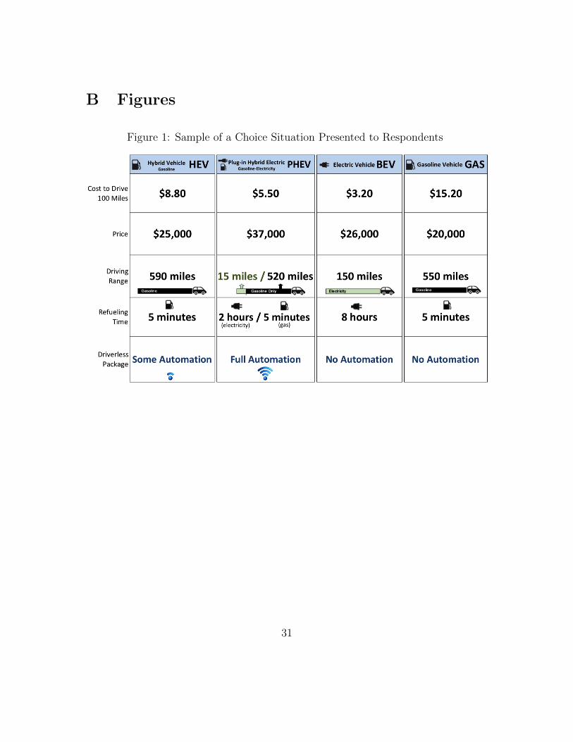
3.3 Design of the choice experiment
The discrete choice experiment that we designed is based on a labeled experiment
with quasi-customized alternative attributes. The alternatives are constructed
according to general new vehicle preferences, including stated price thresholds. The
experiment attributes include purchase price, fuel cost expenses, driving range,
recharging time, and levels of hybridization and automation. Levels are described
in Table 3. Note that purchase price in the experiment was customized to the
threshold stated by the respondent (validated according to household income) when
asked about the willingness to spend in buying a new vehicle.
For automation we considered an aggregation of the technology NHTSA levels
in three groups: no automation (base), some automation (“automated crash
avoidance”), and full automation (“Google car”). The decision to aggregate the
automation levels was based on that technical attributes are not necessarily the
same as consumer-level attributes, that two markets aggregating the automated
levels into semi- and full automation have already been identified (Grush et al.,
2016), and that participants in the two focus groups agreed in a straightforward
understanding of these two automation levels. Additionally, examples for each level
(e.g., “automated crash avoidance” for some automation), and the connected icon to
graphically represent automation in the discrete choice experiment were discussed in
the focus groups. An example of the image that participants saw during one choice
situation appears in Figure 1.
Attribute levels were combined into specific choice situations according to a
Bayesian D-efficient design (Bliemer and Rose, 2010), with priors taken from a pre-
test of the survey (with sample size N=100).
3.4 Elicited subjective discounting
As reviewed in Wang and Daziano (2015), laboratory and field time preferences
experiments have been used in experimental economics to elucidate subjective
discount rates. Expanding on the work of Newell and Siikamaki (2013), who
implemented and used the Multiple Price List (MPL) method of Coller and Williams
(1999) to analyze consumers’ response to energy efficiency labels on water heaters,
in our survey we implemented a modified version of the MPL method. MPL is
organized as a series of binary choices between an immediate and a delayed reward,
in which increasing exogenous discount rates are used to determine the values of the
12
rewards (cf. Kirby et al., 1999). In our survey, only one binary choice was shown to
participants at a time, with scenarios being displayed at an increasing interest rate.
Assuming transitivity in intertemporal preferences, the experiment ended as soon as
the respondent accepted the delayed reward, and the associated discount rate at the
accepted delayed reward was set as the individual’s subjective discount rate. Further
details about the survey implementation of the MPL method (such as avoidance of
immediacy bias) are discussed in Wang and Daziano (2015) with data from a pretest.
The elicited subjective discount rate resulting from the MPL experiment has a
mean of 12.18 percent, standard deviation of 12.86 percent, and a median of 10
percent. Both the median and mean are higher than market interest rates for the
automotive market, but are lower than some subjective discount rates that have been
found using the endogenous discounting approach. Newell and Siikamaki (2013) in
their experiment found a mean of 19 percent, standard deviation of 23 percent, and
median of 11 percent.
As in Newell and Siikamaki (2013), we combine discrete choice models with the
elicited intertemporal preferences, by calculating the expected present value of future
costs as
PVFCij = E
[Li∑l=1
operating costij(1 + ρi)l
], (6)
where Li is the total ownership time stated in the survey by individual i, ρi is the
elicited subjective discount rate, and E is the expectation operator.19
19Our measure of the present value of fuel costs does not consider lifetime fuel costs since we
do not survey whether respondents perceive fuel costs beyond their ownership period. If survey
respondents value these costs beyond their ownership period–for example, if they expect to sell their
vehicle and when they sell, they expect that fuel costs are capitalized in used vehicle prices – then
our measure of fuel costs will be an underestimate of the respondents’ expectations. This will lead
us to overestimate WTP of the present value of fuel costs. We expect this bias to be small since a
large majority of fuel costs are incurred during the initial years of ownership. Furthermore, no prior
papers directly examined whether households value post-ownership fuel costs when purchasing a
new vehicle, although indirect evidence indicates that used vehicle markets do capitalize these costs
(Allcott and Wozny, 2014; Busse et al., 2013; Sallee et al., 2016).
13
4 Model Specification, Estimation, and Inference
4.1 Base models
In Table 4 we report estimates for our benchmark conditional logit model with fixed
coefficients defined in Equation (1). We provide three separate versions of the model,
with each version having a different method of defining fuel costs. In the first two
versions, we replace the present value of fuel costs with alternative measures of
fuel cost. The first version allows fuel cost to enter as a monthly cost, which is
based on the respondent’s expected amount of monthly driving and the cost per mile
attribute.20 The second version is only the cost per mile as a simple attribute. The
third version includes the expected present value of fuel costs (PVFC) as a function
of the respondent’s elicited discount rate, expected length of ownership, expected
amount of driving during ownership and the cost per mile attribute. We note that to
avoid convergence issues in the search for the maximum likelihood estimate, different
tables may scale the attributes differently. The actual scale for each attribute is
discussed in the notes under each table.
In each model, the coefficients on the vehicle attributes are estimated to have the
expected sign. We report these coefficients in the first panel of Table 4. Respondents
dislike higher purchase prices, higher operating costs, and longer charging times
and like longer ranges and both levels of automation. Purchase price sensitivity
has a point estimate ranging from −0.77 to −0.772 and enters significantly at the
5 percent confidence level in each model. All three forms of operating costs enter
significantly and with the expected negative sign. Preference parameters for both
forms of automation are statistically significant at the 5 percent confidence level,
where both forms are preferred over no automation and where full automation is
preferred over partial automation.
To convert the preference parameters into dollar terms, we compute willingness
to pay for an additional unit of each attribute by dividing the marginal utility of
each attribute by the marginal utility of purchase price. Respondents are willing to
pay about $34 in a higher purchase price to reduce the monthly operating cost by
$1. This willingness to pay approximately represents a three-year payback window,
which is consistent with recent survey evidence on the consumer valuation of fuel
20We model expected monthly driving as exogenous to the choice made by each respondent.
This is consistent with assumptions made in Allcott and Wozny (2014).
14
costs (Greene et al., 2013).21
Respondents are willing to pay slightly more than $3,500 for partial levels of
automation and about $4,900 for full automation. Are these estimates plausible?
The estimate of willingness to pay for partial automation appears close to the
reported price for Tesla’s autopilot system available for $3,000, which was announced
a couple of weeks after the survey data were collected. The cost of downloading this
system has since been increased to $3,500.22 This autopilot system is closer to our
partial automation option as it involves software that helps avoid collisions from the
front or sides or from leaving the road. The only fully autonomous package that
appears close to market is an add-on package called Cruise RP-1, which is a driving
program capable of full automation on certain highways. The current price tag for
this program is $10,000.23
4.2 WTP models using parametric and semi-parametric
heterogeneity distributions
The base models were extended to mixed logit specifications in preference space.
Table 5 presents the results of a mixed logit model where key parameters are normally
distributed, where we interact key parameters with respondent characteristics,
and where some parameters are normally distributed and others are log-normally
distributed. For the model with respondent characteristics interactions, interactions
of sociodemographics with the levels of automation were considered to determine
potential deterministic preference variations.24 To compute WTP for automation
and other variables, we estimate a fixed parameter for vehicle purchase price then
divide the preference parameters by the purchase price parameter.
21The empirical literature on how consumers value fuel cost savings is mixed and varies widely
depending on method, time span, and unit of analysis (Greene, 2010). Several recent studies in
the economics literature that leverage variation in gasoline prices, however, suggest that consumers
fully value or only slightly undervalue fuel cost savings in new vehicle markets and only moderately
undervalue these savings in used vehicle markets (Allcott and Wozny, 2014; Busse et al., 2013;
Sallee et al., 2016).22Source: https://electrek.co/2016/08/24/tesla-quietly-increases-price-
autopilot-new-hardware/23Source: https://www.wired.com/2014/06/cruise-self-driving-car-startup/24Interactions between respondent characteristics and vehicle attributes represent how prefer-
ences for vehicle attributes vary according to respondent characteristics, e.g., high income house-
holds may prefer electric vehicles more than low income households.
15
In the column labeled MIXL-N, we estimate normally distributed coefficients for
the natural log of range, charging time, and the two levels of automation. The
parameter estimates with (µ) next to them represent estimates of the mean of each
coefficient, while the parameter estimates with (σ) next to them represent estimates
of the standard deviation of each coefficient. Each coefficient has the expected sign,
as respondents dislike higher prices, higher fuel costs and greater charging times
while they like longer ranges and automation. The implied WTP for both levels of
automation are large and significant. Both, however, are substantially smaller than
the estimates from our fixed coefficient logit models in Table 4. Furthermore, the
mean WTP for the first level of automation, $1,453, exceeds the mean WTP for
the second level of automation, $990, which is unexpected and runs contrary to our
benchmark model results.
In the column labeled MIXL-N-OH, we present results of the same model but
with respondent interaction terms. We interact the two levels of automation with
several respondent characteristics: whether the respondent has heard of the Google
car, whether the respondent is male, the number of years of experience driving, and
geographic region.25 The implied WTP estimates for this model seem more plausible.
For some subsets of households, however, the implied WTP is much higher than the
average estimates from the models in Table 4. For example, we estimate that wealthy
female respondents living in the Midwest with little driving experience that have
heard of the Google car are willing to pay in excess of $20,000 for full automation
technology. This seems plausible given the degree of differentiation among household
preferences.
In the next two columns labeled MIXL-LN-I and MIXL-LN-II, we present models
for results where we assume the coefficients for both levels of automation are log-
normally distributed. We report the implied mean of these distributions. Our
estimates indicate that respondents are willing to pay about $1,000 for either level of
automation. Note that all of the models with parametric heterogeneity fit the choice
data better than the conditional logit specifications, as indicated by comparing the
log likelihood values for the models. The log likelihood values for the parametric
heterogeneity models range from -10,699 to -10,277, which are significantly higher
than the values for the conditional logit specifications, which range from -12,466 to
-12,415.
25Urban/suburban/rural interactions were tested, but no significant differences were found.
16
We summarize the estimates for willingness to pay for automation from the
parametric heterogeneity models in Figure 2. The left and right panels in Figure 2
show the distribution of willingness to pay for the first and second levels of
automation, respectively. We can see from both panels that the heterogeneity in
WTP is large, even for the log normal specifications. These estimates are at odds
with our fixed coefficient model estimates and are likely driven by model fit. This
motivates the use of more flexible methods for estimating heterogeneous preferences
for automation, which we explore next with estimates from semi-parametric discrete-
continuous mixture models.
Table 6 presents the results of mixed-mixed multinomial logit specifications with
three classes. For the column labeled Class 1, class assignment is set as base, whereas
for Classes 2 and 3, class assignment is a function of socioeconomic covariates. For
example, the respondent stating that he or she has heard of the Google car increases
the likelihood that the respondent has preferences represented by Class 2 or Class 3,
as inferred by the positive coefficient for the Google car covariate for these classes.
Class 1 includes slightly less than a third of the sample at 29 percent and Class 3
includes slightly more than a third at 38 percent.
As expected, each class dislikes higher prices and fuel costs and likes longer driving
range. The classes, however, have extremely different preferences for automation.
Class 1 respondents have a mean estimate for WTP for automation that is not
statistically different from zero. These respondents vary widely in their WTP for
both types of automation, with each having a standard deviation higher than $10,000.
This class is likely composed of households that are not aware of driverless car
technology or are skeptical of the technology, as these households are less likely
to have heard of the Google car and own fewer vehicles. Hence many households in
this group are not willing to pay a positive amount for the technology.26
Class 2 respondents are, on average, willing to pay a substantial amount for
automation. These respondents are willing to pay an average of $2,784 and $6,580 for
partial and full automation, respectively. These values are in the range of the values
from our benchmark estimates appearing in Table 4. This group of respondents
appears to be eager to purchase automation technology once it becomes affordable.
Their preferences are driven by knowledge of the Google car, driving long distances,
26The variation in WTP could be caused by the design and presentation of the choice
experiments. We thank a referee for suggesting this possibility.
17
vehicle ownership, and higher education. It is important to note that the standard
deviation for full automation for Class 2 is statistically significant and is $15,526,
which is more than twice as large as the point estimate for the mean. This implies
that some respondents in this group remain skeptical of the technology and are
not willing to pay anything for it. On the other hand, the large standard deviation
implies that some respondents are willing to pay large sums of money–on the order of
$10,000–for full automation. Households in the United States that share preferences
with these respondents will likely be the first to adopt fully autonomous vehicles
when they become commercially available.
Class 3 respondents appear to have moderate desire for automation and represent
a middle group between Classes 1 and 2. This group, which includes the largest
number of respondents, is willing to pay $1,187 and $1,422 for partial and full
automation, values that are substantially less than mean WTP for Class 2 and are less
than the mean WTP for both groups of automation from our benchmark models.
This group appears to be composed of individuals who have heard of the Google
car and that have driving experience. Class 3 individuals are also more likely to
be married and prefer driving. The price of automation must drop dramatically
before this group completely adopts the technology. Similarly to individuals in
Classes 1 and 2, individuals in Class 3 vary considerably in their preferences for
automation, as the standard deviation estimates for both types are large and
statistically significant. This result solidifies the notion that because automation
is a relatively new technology, preferences for the technology will vary widely until
it becomes more mainstream and consumers gain experience with it. Based on log
likelihood values, the mixed-mixed logit model appears to have the best fit of the
data among all of the types of models considered, with a log likelihood of -9,075.5.
We plot the implied distributions of WTP for both levels of automation
in Figure 3. Similar to our results from models with parametric hetergeneity,
these distributions illustrate that households vary considerably in their desire
for autonomous features. Furthermore, these distributions appear more intuitive
than those from the parametric heterogeneity estimates. The mean estimates
of each distribution have the following intuitive appeal. The average Class 1
household dislikes automation and especially dislike full automation; the average
Class 2 household is willing to pay a high premium for automation, especially full
automation; the average Class 3 household is willing to pay a modest amount for
either type of automation. These results, which are not obvious from the models
18
with parametric heterogeneity, suggest a fairly even segmentation of the demand for
automation, where about one-third of the population highly desires the technology,
one-third has mild interest, and one-third does not want the technology.
5 ConclusionsWe have taken an initial attempt to quantify how households currently perceive
and value automated vehicle technologies. Our work has combined current discrete
choice experimental methodologies with recent developments in the discrete choice
literature to quantify how much households are willing to pay for multiple levels of
automation. One strength of our approach is that we are able to have full control
over attributes of alternatives faced by consumers, which allows us to identify how
consumers value attributes not yet fully available in the new vehicle market, namely
multiple levels of automation. Currently, only a few vehicles offer any form of
automation, and the types of automation are not observed in standard datasets of
vehicle attributes.27 This makes a revealed preference approach to identifying how
consumers value automation impossible until this attribute becomes more widely
available in the market for new vehicles and observable to researchers.
We estimate that the average household is willing to pay a significant amount
for automation: $3,500 for partial automation and $4,900 for full automation. Our
estimate for WTP for full automation differs from the estimate found in Bansal et al.
(2016). Differences in WTP estimates stem from two differences in methodology.
First, Bansal et al. estimate preferences for an unrepresentative sample of the
U.S. population, while our sample is representative along many observed household
demographics. Second, Bansal et al.’s empirical model is based on a stated preference
experiment that does not include an option for selecting a vehicle with conventional
(non-autonomous) technology. In sharp contrast, in our choice experiments, many of
the cases include at least one option that has no automation technology. We believe
that this feature of our experiments is crucial to elicit how respondents trade off
other attributes that differ between alternatives with and without automation.
We also find that households vary widely in their valuation of the technology.
Some are not willing to pay anything for either type. Others that are more
knowledgeable about current abilities of automation are willing to pay a great
27For example, in the Ward’s Automotive vehicle characteristics data, we do not observe
automation features.
19
deal for full automation; we estimate that a significant fraction of households are
willing to pay above $10,000 for full automation. In our semiparametric random
parameter logit specifications, we estimate that the demand for automation is
split approximately evenly between high, modest and no demand, highlighting the
importance of modeling flexible preferences for emerging vehicle technology. This
variation may stem from a large difference in understanding of the technology, given
that various forms of automation are relatively new vehicle attributes. Alternatively,
the variation may be a product of the design of our choice experiments. In future
work, we plan to alter the design of the experiments–by offering more alternatives
to choose from, offering more levels of automation, or presenting precise forms of
automation – to test this hypothesis.
A weakness of our approach, which is common to all discrete choice experiments,
is that respondents in our study are making hypothetical choices that may not
perfectly correspond to the choices they would make when purchasing a vehicle.
Nevertheless, given the plausible magnitudes of the estimates of WTP for automation
that we have found, we believe that the discrete choice experiment approach adopted
here provides useful information to policymakers for better understanding and
predicting the market penetration of this technology.
We suggest proceeding in this area of research with caution, given our estimates
and the highly diverse preferences for automation as evidenced by the extremely
large standard deviations of the random parameters. However, we expect to see less
extreme heterogeneity as automated technology matures in the market, knowledge
of the technology spreads, and consumers learn about its benefits and costs.
AcknowledgmentsThis research is based upon work supported by the National Science Foundation
Award No. CMMI-1462289.
20
References
Al-Alawi, B. and Bradley, T. (2013). Review of hybrid, plug-in hybrid, and electric
vehicle market modeling studies. Renewable and Sustainable Energy Reviews,
21:190–203.
Allcott, H. and Greenstone, M. (2012). Is there an energy efficiency gap? Journal
of Economic Perspectives, 14(5):3–28.
Allcott, H. and Wozny, N. (2014). Gasoline prices, fuel economy, and the energy
paradox. Review of Economics and Statistics, 96:779–795.
Ansar, J. and Sparks, R. (2009). The experience curve, option value, and the energy
paradox. Energy Policy, 37(3):1012–1020.
Bansal, P., Kockelman, K., and Singh, A. (2016). Assessing public opinions of
an interest in new vehicle technologies: An Austin perspective. Transportation
Research Part C.
Bliemer, M. and Rose, J. (2010). Construction of experimental designs for mixed
logit models allowing for correlation across choice observations. Transportation
Research Part B: Methodological, 44:720–734.
Bujosa, A., Riera, A., and Hicks, R. L. (2010). Combining discrete and
continuous representations of preference heterogeneity: A latent class approach.
Environmental and Resource Economics, 47(4):477–493.
Busse, M., Knittel, C., and Zettelmeyer, F. (2013). Are consumers myopic? Evidence
from new and used car purchases. American Economic Review, 103(1):220–256.
Cameron, T. A. and Gerdes, G. R. (2005). Individual subjective discounting: Form,
context, format, and noise. Unpublished manuscript, Department of Economics,
University of Oregon. Eugene, OR.
Coller, M. and Williams, M. B. (1999). Eliciting individual discount rates.
Experimental Economics, 2(2):107–127.
Daziano, R. (2012). Taking account of the role of safety on vehicle choice using a
new generation of discrete choice models. Safety Science, 10(1):103–112.
21
DeCanio, S. J. (1998). The efficiency paradox: Bureaucratic and organizational
barriers to profitable energy-saving investments. Energy Policy, 26(5):441–454.
Fagnant, D. and Kockelman, K. (2014). The travel and environmental implications
of shared autonomous vehicles, using agent-based model scenarios. Transportation
Research Part C: Emerging Technologies, 40:1–13.
Fagnant, D. and Kockelman, K. (2015). Preparing a nation for autonomous vehicles:
Opportunities, barriers and policy implications. Transportation Research Part A,
77:167–181.
Frederick, S., Loewenstein, G., and O’Donoghue, T. (2002). Time discounting and
time preference: A critical review. Journal of Economic Literature, pages 351–401.
Greenblatt, J. and Saxena, S. (2015). Autonomous taxis could greatly reduce
greenhouse-gas emissions of US light-duty vehicles. Nature Climate Change, 5:860–
865.
Greene, D. (2010). How Consumers Value Fuel Economy: A Literature Review.
Office of Transportation and Air Quality, U.S. Environmental Protection Agency,
Report EPA-420-R-10-008.
Greene, D., Evans, D., and Hiestand, J. (2013). Survey Evidence on the Willingness
of U.S. Consumers to Pay for Automotive Fuel Economy. Energy Policy, 61:1539–
1550.
Greene, W. H. and Hensher, D. A. (2013). Revealing additional dimensions of
preference heterogeneity in a latent class mixed multinomial logit model. Applied
Economics, 45(14):1897–1902.
Grush, B., Niles, J., and Baum, E. (2016). Ontario must prepare for vehicle
automation: Automated vehicles can influence urban form, congestion and
infrastructure delivery. Technical report, Residential and Civil Construction
Alliance of Ontario (RCCAO).
Hassett, K. A. and Metcalf, G. E. (1993). Energy conservation investment: Do
consumers discount the future correctly? Energy Policy, 21(6):710–716.
22
Hausman, J. A. (1979). Individual discount rates and the purchase and utilization
of energy-using durables. The Bell Journal of Economics, pages 33–54.
Howard, D. and Dai, D. (2013). Public perceptions of self-driving cars: The case of
berkeley, california. Annual Meeting of the Transportation Research Board.
Jaffe, A. B. and Stavins, R. N. (1994). The energy paradox and the diffusion of
conservation technology. Resource and Energy Economics, 16(2):91–122.
Keane, M. and Wasi, N. (2013). Comparing alternative models of heterogeneity in
consumer choice behavior. Journal of Applied Econometrics, 28(6):1018–1045.
Kirby, K., Petry, N., and Bickel, W. (1999). Heroin addicts have higher discount
rates for delayed rewards than non-drug-using controls. Journal of Experimental
Psychology: General, 128:78–87.
Koppel, S., Charlton, J., Fildes, B., and Fitzharris, M. (2008). How important
is vehicle safety in the new vehicle purchase process? Accident Analysis and
Prevention, 40:994–1004.
Kyriakidis, M., Happee, R., and de Winter, J. (2015). Public opinion on automated
driving: Results of an international questionnaire among 5000 respondents.
Transportation Research Part F, 32:127–140.
Lave, C. A. and Train, K. (1979). A disaggregate model of auto-type choice.
Transportation Research Part A: general, 13(1):1–9.
Lu, S. (2006). Vehicle Survivability and Travel Mileage Schedules. NHTSA technical
report, Department of Economics, UCB.
National Highway Traffic Safety Administration (2013). Preliminary statement of
policy concerning automated vehicles.
Newell, R. G. and Siikamaki, J. V. (2013). Nudging energy efficiency behavior: The
role of information labels. National Bureau of Economic Research(working paper
No. 19224).
Payre, W., Cestac, J., and Delhomme, P. (2014). Intention to use a fully automated
car: Attitudes and a priori acceptability. Transportation Research Part F, 27:252–
263.
23
Rezvani, Z., Jansson, J., and Bodin, J. (2015). Advances in consumer electric vehicle
adoption research: A review and research agenda. Transportation Research Part
D: Transport and Environment, 34:122–136.
Sallee, J., West, S., and Fan, W. (2016). Do consumers recognize the value of fuel
economy? Evidence from used car prices and gasoline price fluctuations. Journal
of Public Economics.
Schoettle, B. and Sivak, M. (2014). Public opinion about self-driving vehicles in
China, India, Japan, the U.S., the U.K., and Australia. University of Michigan
Transportation Research Institute, pages 1–31.
Train, K. (1985). Discount rates in consumers’ energy-related decisions: a review of
the literature. Energy, 10(12):1243–1253.
Train, K. E. (2008). EM algorithms for nonparametric estimation of mixing
distributions. Journal of Choice Modelling, 1(1):40–69.
Van Soest, D. P. and Bulte, E. H. (2001). Does the energy-efficiency paradox exist?
Technological progress and uncertainty. Environmental and Resource Economics,
18(1):101–112.
Wang, C. and Daziano, R. (2015). On the problem of measuring discount rates in
intertemporal transportation choices. Transportation, 42(6):1019–1038.
24
A Tables
Table 1: Sample Demographic Statistics
Variable Mean (S.D.)
Household size 2.717 (1.32)
Age of respondent 47.565 (13.55)
Number of children 1.41 (1.36)
Household income (2014$) 61,226 (42,135)
Years respondent has held license 25.409 (9.98)
Number of household members with license 1.914 (0.74)
Number of vehicles held by household 1.592 (0.79)
Respondent daily one-way commute (miles) 13.903 (12.72)
Respondent characteristics Percentage
Male 50.49
Female 49.51
Married 54.49
Widowed 2.94
Divorced 13.70
Single 21.45
Living with partner 7.42
White 85.24
Black 8.32
Hispanic 7.18
Asian 2.934
High school diploma 98.613
Some college experience 76.84
Bachelor’s degree 38.25
Master’s or professional degree 12.40
Full-time (≥ 30 hours per week) job 66.40
Part-time job 8.64
Homemaker 7.83
Student 0.90
Retired 10.44
Unemployed but actively looking for work 5.79
Household income ≤ $30, 000 22.43
Household income > $30, 000 and ≤ $60, 000 34.01
Household income > $60, 000 and ≤ $90, 000 23.82
Household income > $90, 000 19.74
Note: The white, black, Hispanic and Asian percentages sum to more
than 100 percent because some of the respondents have multicultural
backgrounds.
25
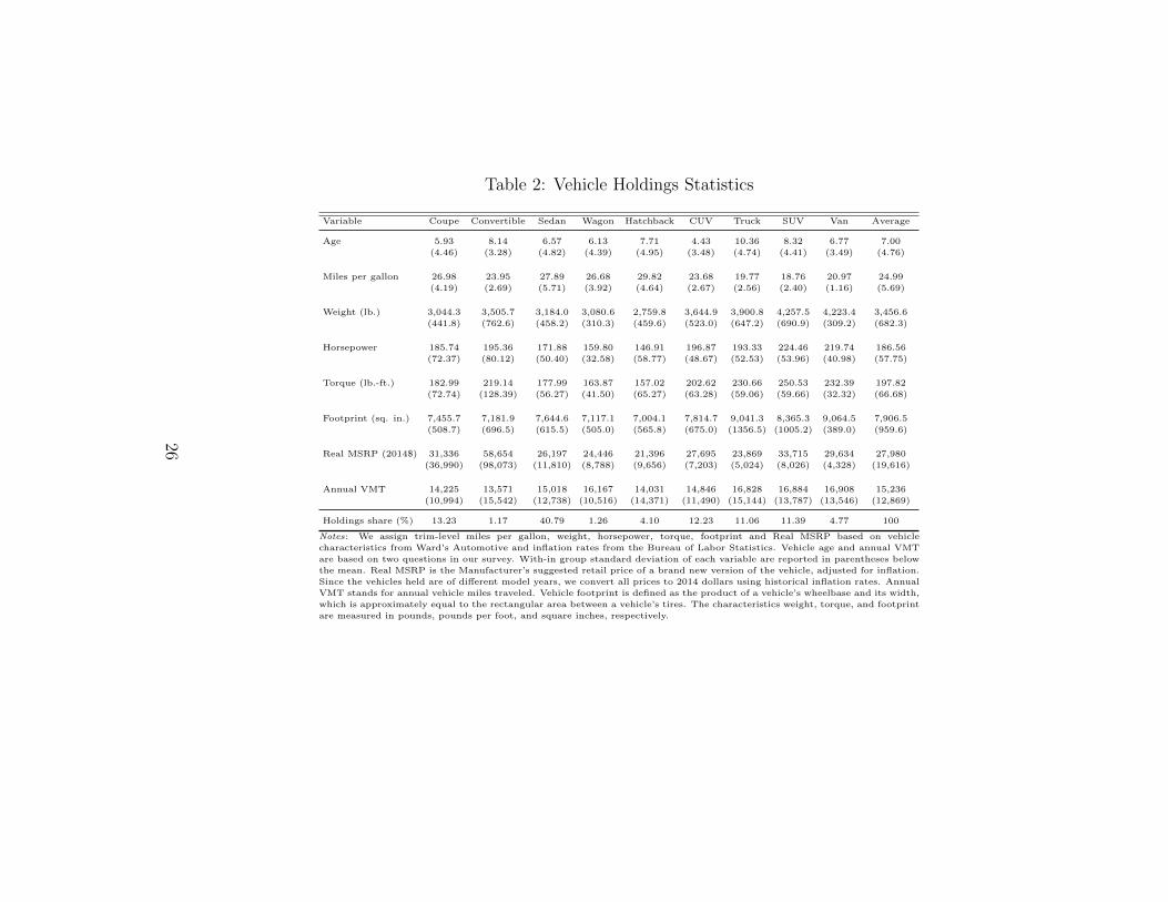
Table 2: Vehicle Holdings Statistics
Variable Coupe Convertible Sedan Wagon Hatchback CUV Truck SUV Van Average
Age 5.93 8.14 6.57 6.13 7.71 4.43 10.36 8.32 6.77 7.00
(4.46) (3.28) (4.82) (4.39) (4.95) (3.48) (4.74) (4.41) (3.49) (4.76)
Miles per gallon 26.98 23.95 27.89 26.68 29.82 23.68 19.77 18.76 20.97 24.99
(4.19) (2.69) (5.71) (3.92) (4.64) (2.67) (2.56) (2.40) (1.16) (5.69)
Weight (lb.) 3,044.3 3,505.7 3,184.0 3,080.6 2,759.8 3,644.9 3,900.8 4,257.5 4,223.4 3,456.6
(441.8) (762.6) (458.2) (310.3) (459.6) (523.0) (647.2) (690.9) (309.2) (682.3)
Horsepower 185.74 195.36 171.88 159.80 146.91 196.87 193.33 224.46 219.74 186.56
(72.37) (80.12) (50.40) (32.58) (58.77) (48.67) (52.53) (53.96) (40.98) (57.75)
Torque (lb.-ft.) 182.99 219.14 177.99 163.87 157.02 202.62 230.66 250.53 232.39 197.82
(72.74) (128.39) (56.27) (41.50) (65.27) (63.28) (59.06) (59.66) (32.32) (66.68)
Footprint (sq. in.) 7,455.7 7,181.9 7,644.6 7,117.1 7,004.1 7,814.7 9,041.3 8,365.3 9,064.5 7,906.5
(508.7) (696.5) (615.5) (505.0) (565.8) (675.0) (1356.5) (1005.2) (389.0) (959.6)
Real MSRP (2014$) 31,336 58,654 26,197 24,446 21,396 27,695 23,869 33,715 29,634 27,980
(36,990) (98,073) (11,810) (8,788) (9,656) (7,203) (5,024) (8,026) (4,328) (19,616)
Annual VMT 14,225 13,571 15,018 16,167 14,031 14,846 16,828 16,884 16,908 15,236
(10,994) (15,542) (12,738) (10,516) (14,371) (11,490) (15,144) (13,787) (13,546) (12,869)
Holdings share (%) 13.23 1.17 40.79 1.26 4.10 12.23 11.06 11.39 4.77 100
Notes: We assign trim-level miles per gallon, weight, horsepower, torque, footprint and Real MSRP based on vehicle
characteristics from Ward’s Automotive and inflation rates from the Bureau of Labor Statistics. Vehicle age and annual VMT
are based on two questions in our survey. With-in group standard deviation of each variable are reported in parentheses below
the mean. Real MSRP is the Manufacturer’s suggested retail price of a brand new version of the vehicle, adjusted for inflation.
Since the vehicles held are of different model years, we convert all prices to 2014 dollars using historical inflation rates. Annual
VMT stands for annual vehicle miles traveled. Vehicle footprint is defined as the product of a vehicle’s wheelbase and its width,
which is approximately equal to the rectangular area between a vehicle’s tires. The characteristics weight, torque, and footprint
are measured in pounds, pounds per foot, and square inches, respectively.
26
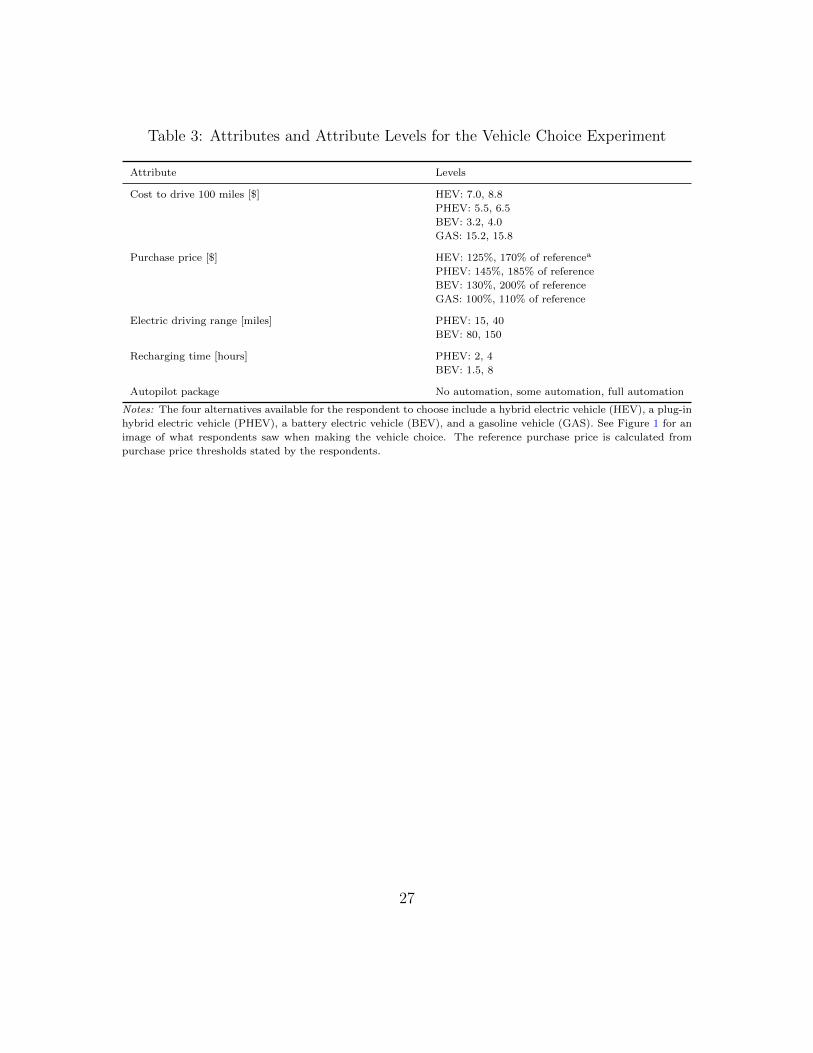
Table 3: Attributes and Attribute Levels for the Vehicle Choice Experiment
Attribute Levels
Cost to drive 100 miles [$] HEV: 7.0, 8.8
PHEV: 5.5, 6.5
BEV: 3.2, 4.0
GAS: 15.2, 15.8
Purchase price [$] HEV: 125%, 170% of referencea
PHEV: 145%, 185% of reference
BEV: 130%, 200% of reference
GAS: 100%, 110% of reference
Electric driving range [miles] PHEV: 15, 40
BEV: 80, 150
Recharging time [hours] PHEV: 2, 4
BEV: 1.5, 8
Autopilot package No automation, some automation, full automation
Notes: The four alternatives available for the respondent to choose include a hybrid electric vehicle (HEV), a plug-in
hybrid electric vehicle (PHEV), a battery electric vehicle (BEV), and a gasoline vehicle (GAS). See Figure 1 for an
image of what respondents saw when making the vehicle choice. The reference purchase price is calculated from
purchase price thresholds stated by the respondents.
27
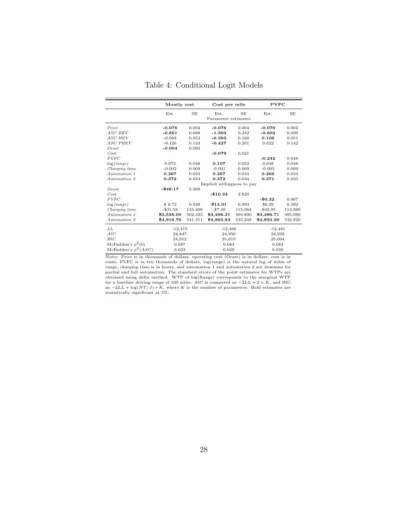
Table 4: Conditional Logit Models
Montly cost Cost per mile PVFC
Est. SE Est. SE Est. SE
Parameter estimates
Price -0.076 0.004 -0.076 0.004 -0.076 0.004
ASC BEV -0.851 0.098 -1.303 0.242 -0.602 0.096
ASC HEV -0.068 0.053 -0.393 0.166 0.106 0.051
ASC PHEV -0.126 0.143 -0.427 0.201 0.022 0.142
Ocost -0.004 0.000
Cost -0.079 0.021
PVFC -0.242 0.049
log(range) 0.073 0.048 0.107 0.052 0.048 0.048
Charging time -0.002 0.009 -0.001 0.009 -0.003 0.009
Automation 1 0.267 0.034 0.267 0.034 0.266 0.034
Automation 2 0.372 0.033 0.372 0.034 0.371 0.033
Implied willingness to pay
Ocost -$48.17 5.209
Cost -$10.34 2.820
PVFC -$0.32 0.067
log(range) $ 9.72 6.549 $14.01 6.993 $6.29 6.392
Charging time -$31.58 116.409 -$7.49 115.664 -$43.95 114.980
Automation 1 $3,538.00 502.423 $3,498.31 494.890 $3,486.71 495.980
Automation 2 $4,916.76 541.311 $4,863.83 533.248 $4,850.39 532.820
LL -12,415 -12,466 -12,461
AIC 24,847 24,950 24,939
BIC 24,912 25,015 25,004
McFadden’s ρ2(0) 0.087 0.083 0.084
McFadden’s ρ2(ASC) 0.033 0.029 0.030
Notes: Price is in thousands of dollars, operating cost (Ocost) is in dollars, cost is in
cents, PVFC is in ten thousands of dollars, log(range) is the natural log of miles of
range, charging time is in hours, and automation 1 and automation 2 are dummies for
partial and full automation. The standard errors of the point estimates for WTPs are
obtained using delta method. WTP of log(Range) corresponds to the marginal WTP
for a baseline driving range of 100 miles. AIC is computed as −2LL+ 2×K, and BIC
as −2LL + log(NT/J) ∗K, where K is the number of parameters. Bold estimates are
statistically significant at 5%.
28
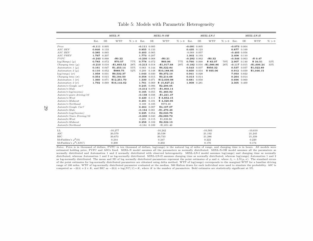
Table 5: Models with Parametric Heterogeneity
MIXL-N MIXL-N-OH MIXL-LN-I MIXL-LN-II
Est. SE WTP % > 0 Est. SE WTP % > 0 Est. SE WTP % > 0 Est. SE WTP % > 0
Price -0.111 0.005 -0.111 0.005 -0.091 0.005 -0.073 0.004
ASC BEV 0.846 0.133 0.855 0.133 0.435 0.123 0.877 0.100
ASC HEV 0.385 0.065 0.403 0.065 -0.069 0.057 -0.403 0.056
ASC PHEV 1.767 0.207 1.773 0.207 1.302 0.193 2.408 0.110
PVFC -0.243 0.068 -$0.22 -0.230 0.068 -$0.21 -0.292 0.062 -$0.32 -0.346 0.063 -$ 0.47
log(Range) (µ) 0.783 0.072 $70.57 77% 0.778 0.072 $69.96 77% 0.760 0.068 $ 83.07 79% 2.907 0.140 $ 34.51 53%
Charging time (µ) -0.210 0.018 -$1,893.52 28% -0.213 0.018 -$1,917.68 28% -0.182 0.016 -$1,986.86 28% -0.117 0.015 -$1,606.24 33%
Automation 1 (µ) 0.161 0.047 $1,453.14 55% 0.063 0.144 $6,322.84 0.543 0.037 $956.32 0.537 0.037 $1,022.89
Automation 2 (µ) 0.110 0.052 $989.75 52% 0.209 0.148 $10,188.95 0.830 0.034 $ 935.06 0.912 0.039 $1,046.15
log(range) (σ) 1.058 0.031 $9,532.37 1.043 0.030 $9,372.10 0.941 0.028 7.053 0.822
Charging time (σ) 0.354 0.015 $3,184.50 0.358 0.015 $3,214.68 0.313 0.014 0.264 0.014
Automation 1 (σ) 1.360 0.071 $12,251.70 1.339 0.071 $12,039.98 0.681 0.058 0.696 0.060
Automation 2 (σ) 1.792 0.069 $16,144.62 1.761 0.069 $ 15,827.21 1.908 0.281 2.305 0.400
Autom1×Google car? 0.245 0.086 $2,206.05
Autom1×Male -0.212 0.079 -$1,903.14
Autom1×log(income) 0.165 0.055 $1,483.92
Autom1×years driving/10 -0.138 0.038 -$1,241.47
Autom1×West 0.429 0.111 $ 3,852.15
Autom1×Midwest 0.481 0.101 $ 4,320.95
Autom1×Northeast 0.108 0.105 $972.40
Autom2×Google Car? 0.464 0.087 $4,167.07
Autom2×Male -0.164 0.081 -$1,476.46
Autom2×Log(Income) 0.225 0.054 $2,023.78
Autom2×Years Driving/10 -0.230 0.040 -$2,069.72
Autom2×West 0.205 0.115 $1,838.86
Autom2×Midwest 0.258 0.102 $2,322.13
Autom2×Northeast -0.184 0.109 -$1,651.46
LL -10,277 -10,242 -10,583 -10,610
AIC 20,579 20,538 21,192 21,245
BIC 20,673 20,733 21,286 21,339
McFadden’s ρ2(0) 0.244 0.247 0.222 0.220
McFadden’s ρ2(ASC) 0.200 0.202 0.176 0.174
Notes: Price is in thousand of dollars, PVFC in ten thousand of dollars, log(range) is the natural log of miles of range, and charging time is in hours. All models were
estimated holding price, PVFC and ASCs fixed. MIXL-N model assumes all the parameters as normally distributed. MIXL-N-OH model assumes all the parameters as
normally distributed and Automation 1 and 2 normally distributed with observed heterogeneity. MIXL-LN-I model assumes log(range) and charging time as normally
distributed, whereas Automation 1 and 2 as log-normally distributed. MIXL-LN-II assumes charging time as normally distributed, whereas log(range) Automation 1 and 2
as log-normally distributed. The mean and SD of log normally distributed parameters represent the point estimates of µ and σ, where βi ∼ LN(µ, σ). The standard errors
of the point estimates for log-normally distributed parameters are obtained using delta method. WTP of log(range) corresponds to the marginal WTP for a baseline driving
range of 100 miles. WTP of log-normally distributed parameter evaluated at the median. 500 Halton draws for each individual were used to simulate the probability. AIC is
computed as −2LL + 2×K, and BIC as −2LL + log(NT/J) ∗K, where K is the number of parameters. Bold estimates are statistically significant at 5%.
29
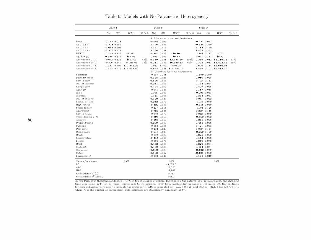
Table 6: Models with No Parametric Heterogeneity
Class 1 Class 2 Class 3
Est. SE WTP % > 0 Est. SE WTP % > 0 Est. SE WTP % > 0
A: Mean and standard deviations
Price -0.119 0.018 -0.043 0.005 -0.227 0.012
ASC BEV -2.328 0.580 1.796 0.157 -0.624 0.260
ASC HEV -2.663 0.204 1.151 0.117 2.788 0.160
ASC PHEV -2.320 0.973 2.256 0.221 1.422 0.392
PVFC -0.747 0.126 -$0.63 -0.344 0.153 -$0.80 -0.168 0.137 -$0.07
log(Range) 0.685 0.339 $57.56 0.039 0.067 $9.13 0.022 0.137 $0.99
Automation 1 (µ) -0.072 0.325 -$607.49 48% 0.119 0.051 $2,784.15 100% 0.269 0.082 $1,186.76 67%
Automation 2 (µ) -0.506 0.347 -$4,248.05 38% 0.281 0.053 $6,580.23 66% 0.322 0.083 $1,422.42 59%
Automation 1 (σ) 1.231 0.300 $10,342.25 0.022 1.462 $508.26 0.609 0.144 $2,686.01
Automation 2 (σ) 1.612 0.276 $13,541.52 0.663 0.088 $15,526.13 1.469 0.103 $6,484.70
B: Variables for class assignment
Constant -0.193 0.288 -1.559 0.270
Days 80 miles 0.128 0.026 0.080 0.025
Own a car? 0.596 0.156 0.192 0.133
No. of vehicles 0.211 0.065 0.133 0.064
Google car? 0.794 0.067 0.407 0.068
Age/ 10 -0.041 0.045 0.187 0.045
Male 0.106 0.064 -0.293 0.063
Married 0.123 0.065 0.333 0.063
No. of children 0.120 0.024 0.041 0.022
Comp. college 0.212 0.075 -0.034 0.070
High school -0.429 0.084 -0.615 0.080
Single family -0.227 0.118 -0.091 0.126
Apartment -0.783 0.148 0.269 0.146
Own a house -0.040 0.079 0.012 0.079
Years driving / 10 -0.398 0.059 -0.450 0.062
Accident -0.168 0.059 0.215 0.058
Prefer driving 0.299 0.069 0.451 0.066
Fulltime -0.163 0.088 0.124 0.083
Part time -0.232 0.123 0.069 0.117
Homemaker -0.515 0.129 -0.759 0.129
White -0.130 0.083 0.325 0.090
Conservative -0.415 0.068 0.154 0.066
Liberal -0.056 0.078 0.370 0.078
West 0.462 0.088 0.320 0.084
Midwest 0.480 0.080 0.474 0.074
Northeast 0.302 0.080 -0.162 0.079
Urban 0.163 0.062 -0.181 0.060
Log(income) -0.013 0.046 0.196 0.049
Shares for classes 29% 33% 38%
LL -9,075.5
AIC 18,323
BIC 18,941
McFadden’s ρ2(0) 0.333
McFadden’s ρ2(ASC) 0.293
Notes: Price is in thousands of dollars, PVFC in ten thousands of dollars, log(range) is the natural log of miles of range, and charging
time is in hours. WTP of log(range) corresponds to the marginal WTP for a baseline driving range of 100 miles. 500 Halton draws
for each individual were used to simulate the probability. AIC is computed as −2LL+ 2×K, and BIC as −2LL+ log(NT/J) ∗K,
where K is the number of parameters. Bold estimates are statistically significant at 5%.
30
B Figures
Figure 1: Sample of a Choice Situation Presented to Respondents
31
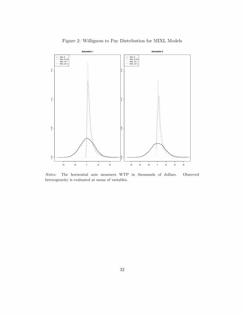
Figure 2: Willigness to Pay Distribution for MIXL Models
−40 −20 0 20 40
0.0
00
.05
0.1
00
.15
Automation 1
MIXL−N
MXIL−N−OH
MIXL−LN−I
MIXL−LN−II
−60 −40 −20 0 20 40 60
0.0
00
.05
0.1
00
.15
Automation 2
MIXL−N
MIXL−N−OH
MIXL−LN−I
MIXL−LN−II
Notes: The horizontal axis measures WTP in thousands of dollars. Observed
heterogeneity is evaluated at mean of variables.
32
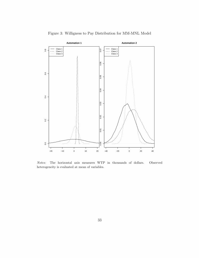
Figure 3: Willigness to Pay Distribution for MM-MNL Model
−20 −10 0 10 20
0.0
0.2
0.4
0.6
0.8
Automation 1
WTP / 1000
Den
sity
Class 1Class 2Class 3
−40 −20 0 20 40
0.00
0.01
0.02
0.03
0.04
0.05
0.06
0.07
Automation 2
WTP / 1000
Den
sity
Class 1Class 2Class 3
Notes: The horizontal axis measures WTP in thousands of dollars. Observed
heterogeneity is evaluated at mean of variables.
33


![Hitting the Target - Texas State Universitygato-docs.its.txstate.edu/jcr:3538f670-8312-4d77-8cf6-1b2e69c5649… · presentation/packaging “[Consumers are] willing to pay more for](https://img.pdfslide.net/doc/110x75/602a7ba59a216e0131172de5/hitting-the-target-texas-state-universitygato-docsits-3538f670-8312-4d77-8cf6-1b2e69c5649.jpg)