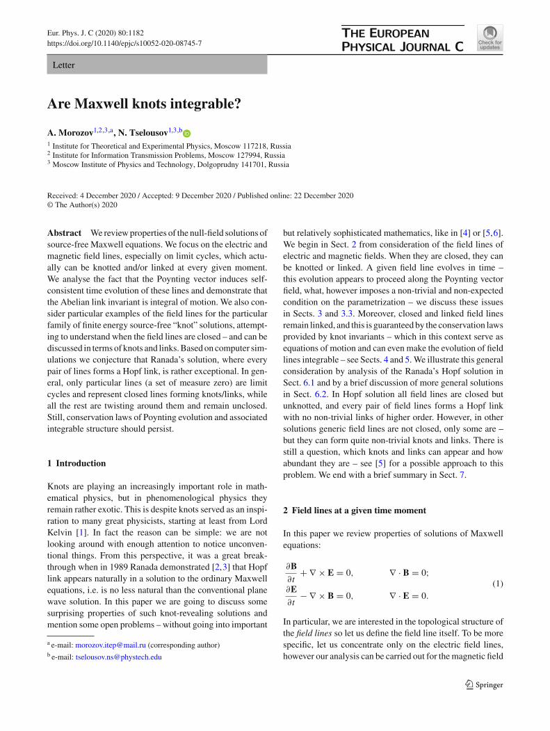
Eur. Phys. J. C (2020) 80:1182https://doi.org/10.1140/epjc/s10052-020-08745-7

Letter

Are Maxwell knots integrable?

A. Morozov1,2,3,a, N. Tselousov1,3,b

1 Institute for Theoretical and Experimental Physics, Moscow 117218, Russia2 Institute for Information Transmission Problems, Moscow 127994, Russia3 Moscow Institute of Physics and Technology, Dolgoprudny 141701, Russia

Received: 4 December 2020 / Accepted: 9 December 2020 / Published online: 22 December 2020© The Author(s) 2020

Abstract We review properties of the null-field solutions ofsource-free Maxwell equations. We focus on the electric andmagnetic field lines, especially on limit cycles, which actu-ally can be knotted and/or linked at every given moment.We analyse the fact that the Poynting vector induces self-consistent time evolution of these lines and demonstrate thatthe Abelian link invariant is integral of motion. We also con-sider particular examples of the field lines for the particularfamily of finite energy source-free “knot” solutions, attempt-ing to understand when the field lines are closed – and can bediscussed in terms of knots and links. Based on computer sim-ulations we conjecture that Ranada’s solution, where everypair of lines forms a Hopf link, is rather exceptional. In gen-eral, only particular lines (a set of measure zero) are limitcycles and represent closed lines forming knots/links, whileall the rest are twisting around them and remain unclosed.Still, conservation laws of Poynting evolution and associatedintegrable structure should persist.

1 Introduction

Knots are playing an increasingly important role in math-ematical physics, but in phenomenological physics theyremain rather exotic. This is despite knots served as an inspi-ration to many great physicists, starting at least from LordKelvin [1]. In fact the reason can be simple: we are notlooking around with enough attention to notice unconven-tional things. From this perspective, it was a great break-through when in 1989 Ranada demonstrated [2,3] that Hopflink appears naturally in a solution to the ordinary Maxwellequations, i.e. is no less natural than the conventional planewave solution. In this paper we are going to discuss somesurprising properties of such knot-revealing solutions andmention some open problems – without going into important

a e-mail: morozov.itep@mail.ru (corresponding author)b e-mail: tselousov.ns@phystech.edu

but relatively sophisticated mathematics, like in [4] or [5,6].We begin in Sect. 2 from consideration of the field lines ofelectric and magnetic fields. When they are closed, they canbe knotted or linked. A given field line evolves in time –this evolution appears to proceed along the Poynting vectorfield, what, however imposes a non-trivial and non-expectedcondition on the parametrization – we discuss these issuesin Sects. 3 and 3.3. Moreover, closed and linked field linesremain linked, and this is guaranteed by the conservation lawsprovided by knot invariants – which in this context serve asequations of motion and can even make the evolution of fieldlines integrable – see Sects. 4 and 5. We illustrate this generalconsideration by analysis of the Ranada’s Hopf solution inSect. 6.1 and by a brief discussion of more general solutionsin Sect. 6.2. In Hopf solution all field lines are closed butunknotted, and every pair of field lines forms a Hopf linkwith no non-trivial links of higher order. However, in othersolutions generic field lines are not closed, only some are –but they can form quite non-trivial knots and links. There isstill a question, which knots and links can appear and howabundant they are – see [5] for a possible approach to thisproblem. We end with a brief summary in Sect. 7.

2 Field lines at a given time moment

In this paper we review properties of solutions of Maxwellequations:

∂B∂t

+ ∇ × E = 0, ∇ · B = 0;∂E∂t

− ∇ × B = 0, ∇ · E = 0.

(1)

In particular, we are interested in the topological structure ofthe field lines so let us define the field line itself. To be morespecific, let us concentrate only on the electric field lines,however our analysis can be carried out for the magnetic field

123

1182 Page 2 of 11 Eur. Phys. J. C (2020) 80 :1182

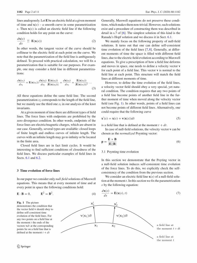
lines analogously. LetE be an electric field at a given momentof time and x(s) – a smooth curve in some parametrizations. Then x(s) is called an electric field line if the followingcondition holds for any point on the curve:

dx(s)ds

� E(x(s)) (2)

In other words, the tangent vector of the curve should becollinear to the electric field at each point on the curve. Wenote that the parametrization of the field line is ambiguouslydefined. To proceed with practical calculation, we will fix aparametrization that is suitable for our purposes. For exam-ple, one may consider a field line in different parametriza-tions:

dx(s1)

ds1= E(x(s1))

dx(s2)

ds2

E(x(s2))

|E(x(s2))| = dx(s3)

ds3= E(x(s3))

|E(x(s3))|2 . . .

(3)

All these equations define the same field line. The secondparametrization s2 corresponds to the length of the field line,but we mainly use the third one s3 in our analysis of the knotinvariants.

At a given moment of time there are different types of fieldlines. The force lines with endpoints are prohibited by thezero divergence condition. In other words, endpoints of theforce lines are electric/magnetic charges, which are absent inour case. Generally, several types are available: closed loopsof finite length and endless curves of infinite length. Thecurves with an infinite length may go to infinity or be locatedin the finite area.

Closed field lines are in fact limit cycles. It would beinteresting to find sufficient conditions of closedness of thefield lines. We discuss particular examples of field lines inSects. 6.1 and 6.2.

3 Time evolution of force lines

In our paper we consider only null-field solutions of Maxwellequations. This means that at every moment of time and atevery point in space the following conditions hold:

E · B = 0, E2 = B2. (4)

Generally, Maxwell equations do not preserve these condi-tions, which makes them non-trivial. However, such solutionsexist and a procedure of constructing them was described indetail in s.7 of [6]. The simplest solution of this kind is theRanada’s Hopf solution and we discuss it in Sect. 6.1.

We mainly focus on the following property of null-fieldsolutions. It turns out that one can define self-consistenttime evolution of the field lines [7,8]. Generally, at differ-ent moments of time the space is filled with different fieldlines, due to the electric field evolution according to Maxwellequations. To give a prescription of how a field line deformsand moves in space, one needs to define a velocity vector vfor each point of a field line. This vector v is normal to thefield line at each point. This structure will match the fieldlines at different moments of time.

However, to define the time evolution of the field lines,a velocity vector field should obey a very special, yet natu-ral condition. The condition requires that any two points ofa field line become points of another field line in the fur-ther moment of time when moved along the velocity vectorfield (see Fig. 1). In other words, points of a field lines cannot become points of different field lines. Alternatively, onecould require that the following curve

x′(s) = x(s) + v(x(s))dt (5)

is a field line that is defined at the moment t + dt .In case of null-field solutions, the velocity vector v can be

chosen as the normalized Poynting vector:

p = E × B|E||B| (6)

3.1 Poynting time evolution

In this section we demonstrate that the Poyting vector ina null-field solution induces self-consistent time evolutionof the force lines. To do this, we explicitly check the self-consistency of the condition from the previous section.

We consider an electric field line x(s) of a null-field solu-tion at the moment t . In this section we fix the parametrizations by the following equation:

dx(s)ds

= E(x(s), t) (7)

Fig. 1 The picturedemonstrates the condition thatthe vector field v should obey todefine self-consistent timeevolution of the field lines. Forany two points on a field line atthe moment t the ends of thevectors vdt at the correspondingpoints lie on a field line that isdefined at the moment t + dt

123

Eur. Phys. J. C (2020) 80 :1182 Page 3 of 11 1182

Then we consider an auxiliary line x′(s) that is obtained fromx(s) by a slight shift along the Poynting vector p:

x′(s) = x(s) + p(x(s), t)dt (8)

Note that we shift along the Poynting vector by dt . The mainclaim is that x′(s) coincides as geometrical objects with somefield line at the moment t + dt . Namely, a tangent vector ofthe line x′(s) is collinear to the electric field at the momentt + dt , it means that they define the same field line:

dx′(s)ds

� E(x′(s), t + dt) (9)

We should note that this collinearity holds only in the firstorder in dt . To explicitly see this, we compute the corre-sponding cross product:

dx′(s)ds

× E(x′(s), t + dt) =(E + (E · ∇)p dt

)

×(E + (p · ∇)E dt + ∂E

∂tdt + o(dt)

)=

= dt E ×(

(p · ∇)E − (E · ∇)p + ∂E∂t

)+ o(dt) = o(dt)

(10)

To simplify the formulas, we omit the explicit coordinate andtime dependence of the fields meaning E = E(x(s), t) andp = p(x(s), t). We compute the expression in the bracketsusing the following identity for null-field solutions:

Eβpα − Eαpβ = εαβγ Bγ (11)

Taking the derivative of (11) and using the Maxwell equa-tions, we obtain the expression of the form:

(p · ∇)E − (E · ∇)p + ∂E∂t

= −(∇ · p)E (12)

The r.h.s is collinear to the electric field E that ensures (10).Finally, we conclude that the Poynting vector defines theself-consistent time evolution of the field line. Therefore, wecan think of a field line as a strand where each point moveswith the velocity vector p. From now we understand the timedependence of the field lines x(s, t) as it is induced by thePoynting vector:

dx(s, t)dt

= p(x(s, t), t) (13)

It is evident now why we consider the normalized Poytingvector. If one chooses another normalization for the Poyntingvector it will spoil (12).

3.2 Examples

For demonstrative purposes let us discuss plane wave null-field solutions of Maxwell equations to analyse the structure

of the field lines and its time evolution induced by the Poynt-ing vector.

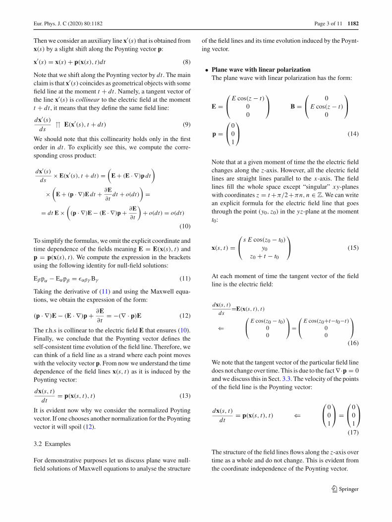
• Plane wave with linear polarizationThe plane wave with linear polarization has the form:

E =⎛⎝ E cos(z − t)

00

⎞⎠ B =

⎛⎝ 0

E cos(z − t)0

⎞⎠

p =⎛⎝ 0

01

⎞⎠ (14)

Note that at a given moment of time the the electric fieldchanges along the z-axis. However, all the electric fieldlines are straight lines parallel to the x-axis. The fieldlines fill the whole space except “singular” xy-planeswith coordinates z = t +π/2+πn, n ∈ Z. We can writean explicit formula for the electric field line that goesthrough the point (y0, z0) in the yz-plane at the momentt0:

x(s, t) =⎛⎝ s E cos(z0 − t0)

y0

z0 + t − t0

⎞⎠ (15)

At each moment of time the tangent vector of the fieldline is the electric field:

dx(s, t)ds

=E(x(s, t), t)

⇐⎛⎝ E cos(z0 − t0)

00

⎞⎠ =

⎛⎝ E cos(z0+t−t0−t)

00

⎞⎠

(16)

We note that the tangent vector of the particular field linedoes not change over time. This is due to the fact ∇·p = 0and we discuss this in Sect. 3.3. The velocity of the pointsof the field line is the Poynting vector:

dx(s, t)dt

= p(x(s, t), t) ⇐⎛⎝ 0

01

⎞⎠ =

⎛⎝ 0

01

⎞⎠

(17)

The structure of the field lines flows along the z-axis overtime as a whole and do not change. This is evident fromthe coordinate independence of the Poynting vector.

123

1182 Page 4 of 11 Eur. Phys. J. C (2020) 80 :1182

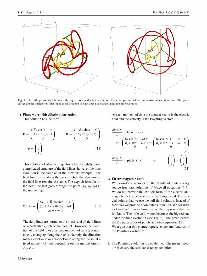
Fig. 2 The little yellow knot becomes the big red one under time evolution. There are pictures of two successive moments of time. The greencurves are the trajectories. The topological structure of knot does not change under the time evolution

• Plane wave with elliptic polarizationThis solution has the form:

E =⎛⎝ Ex cos(z − t)

Ey sin(z − t)0

⎞⎠ B =

⎛⎝−Ey sin(z − t)

Ex cos(z − t)0

⎞⎠

p =⎛⎝ 0

01

⎞⎠ (18)

This solution of Maxwell equations has a slightly morecomplicated structure of the field lines, however the timeevolution is the same as in the previous example – thefield lines move along the z-axis, while the structure ofthe field lines remains the same. The explicit formula forthe field line that goes through the point (x0, y0, z0) atthe moment t0:

x(s, t) =⎛⎝ x0 + s Ex cos(z0 − t0)

y0 + s Ey sin(z0 − t0)z0 + t − t0

⎞⎠ (19)

The field lines are normal to the z-axis and all field lineson a particular xy-plane are parallel. However, the direc-tion of the field lines at a fixed moment of time is contin-uously changing along the z-axis. Namely, the directionrotates clockwise or anticlockwise along the z-axis at afixed moment of time depending on the mutual sign ofEx , Ey .

At each moment of time the tangent vector is the electricfield and the velocity is the Poynting vector:

dx(s, t)ds

= E(x(s, t), t)

⇐⎛⎝ Ex cos(z0 − t0)

Ey sin(z0 − t0)0

⎞⎠ =

⎛⎝ Ex cos(z0 + t − t0 − t)

Ey sin(z0 + t − t0 − t)0

⎞⎠

(20)

dx(s, t)dt

= p(x(s, t), t) ⇐⎛⎝ 0

01

⎞⎠ =

⎛⎝ 0

01

⎞⎠

(21)

• Electromagnetic knotWe consider a member of the family of finite energysource-free knot solutions of Maxwell equations [5,6].We do not provide the explicit form of the electric andmagnetic fields, because its is too complicated. The cru-cial point is that we use the null-field solution. Instead offormulas we provide a computer simulation. We considera closed field lines - limit cycles, that represent the tre-foil knots. The little yellow knot becomes the big red oneunder the time evolution (see Fig. 2). The green curvesare the trajectories of points and obey equation (13).We argue that this picture represents general features ofthe Poynting evolution:

1. The Poynting evolution is well defined. The green trajec-tories ensure the self-consistency condition.

123

Eur. Phys. J. C (2020) 80 :1182 Page 5 of 11 1182

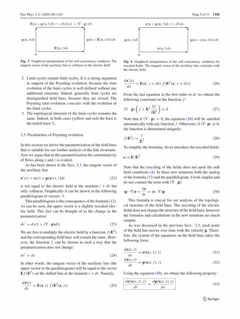
Fig. 3 Graphical interpretation of the self-consistency condition. Thetangent vector of the auxiliary line is collinear to the electric field

2. Limit cycles remain limit cycles. It is a strong argumentin support of the Poynting evolution, because the timeevolution of the limit cycles is well defined without anyadditional structure. Indeed, generally limit cycles aredistinguished field lines, because they are closed. ThePoynting time evolution coincides with the evolution ofthe limit cycles.

3. The topological structure of the limit cycles remains thesame. Indeed, in both cases (yellow and red) the knot isthe trefoil knot 31.

3.3 Peculiarities of Poynting evolution

In this section we derive the parametrization of the field linesthat is suitable for our further analysis of the link invariants.Also we argue that in this parametrization the commutativityof flows along s and t is evident.

As has been shown in the Sect. 3.1, the tangent vector ofthe auxiliary line

x′(s) = x(s) + p(x(s), t)dt (22)

is not equal to the electric field at the moment t + dt butonly collinear. Graphically it can be shown in the followingparallelogram of vectors 3.

This parallelogram is the consequence of the formula (12).As can be seen, the upper vector is a slightly rescaled elec-tric field. This fact can be thought of as the change in theparametrization:

ds′ = ds(1 + (∇ · p)dt) (23)

We are free to multiply the electric field by a function f (E2)

and the corresponding field lines will remain the same. How-ever, the function f can be chosen in such a way that theparametrization does not change:

ds′ = ds (24)

In other words, the tangent vector of the auxiliary line (theupper vector in the parallelogram) will be equal to the vectorE f (E2) on the shifted line at the moment t + dt . Namely:

dx(s)ds

= E(x, t) f (E2(x, t)) (25)

Fig. 4 Graphical interpretation of the self-consistency condition forrescaled fields. The tangent vector of the auxiliary line coincides withthe electric field

dx′(s)ds

= E(x′, t + dt) f (E2(x′, t + dt)) (26)

From the last equation in the first order in dt we obtain thefollowing constraint on the function f :

(∇ · p)

(f + E2 ∂ f

∂E2

)= 0 (27)

Note that if (∇ · p) = 0, the equation (26) will be satisfiedautomatically with any function f . Otherwise, if (∇ ·p) �= 0,the function is determined uniquely:

f (E2) = 1

E2 (28)

To simplify the formulas, let us introduce the rescaled fields:

e :=E/E2 (29)

Note that the rescaling of the fields does not spoil the nullfield conditions (4). In these new notations both the analogof the formula (12) and the parallelogram 4 look simpler anddo not contain the term with (∇ · p):

(p · ∇)e + ∂e∂t

= (e · ∇)p (30)

This formula is crucial for our analysis of the topologi-cal structure of the field lines. The rescaling of the electricfields does not change the structure of the field lines, howeverthe formulas and calculations in the new notations are muchsimpler.

As was discussed in the previous Sect. 3.1, each pointof the field line moves over time with the velocity p. There-fore, the system of the equations on the field lines takes thefollowing form:

dx(s, t)ds

= e(x(s, t), t) (31)

dx(s, t)dt

= p(x(s, t), t) (32)

Using the equation (30), we obtain the following property:

de(x(s, t), t)dt

= dp(x(s, t), t)ds

(33)

123

1182 Page 6 of 11 Eur. Phys. J. C (2020) 80 :1182

This property ensures commutativity of flows along s and tin the chosen parametrization.

4 Knot invariants as invariants of motion

There are solutions of Maxwell equations that exhibit topo-logically nontrivial structure of the electric field lines thatmakes them worth studying. Firstly, some solutions have theproperty that all/some of the field lines are closed loops –limit cycles. Secondly, a particular closed field line can betopologically nontrivial i.e. it can be a knot. Thirdly, a pairof closed field lines can be linked.

A closed field line could be identified with some stringor strand. Each element of the string moves with velocityequal to the Poynting vector at the corresponding point of thespace. As soon as one identifies the field lines with movingstrands, natural questions appear. One can ask if the topolog-ical structure of the strands is preserved over time. Namely, ifa strand was knotted, can it become a different knot? If a pairof strands was linked together, can they become unlinked ata further moment of time? These questions are quite similarand refer to the situation that involves crossings of strands.

There are tools to address this type of questions. They arecalled knot and link invariants. These invariants are preservedunder smooth deformations of knots and links that do notadmit crossings of lines. In our work we use the Gauss linkingintegral [9] which is an example of a link invariant:

Linkx,y =∮

dxα

∮dyβ εαβγ

xγ − yγ|x − y|3 (34)

We show that the linking integral computed for a pair ofelectric field lines does not change over time, i.e. it is anintegral of the Poynting evolution. This fact gives the answerfor the second question, while the answer for the first oneinvolves non-Abelian generalization of the Gauss integraland we leave it for future studies.

In this section we consider an application of the Gausslinking integral to the study of the evolution of the field lines.We show that the linking integral applied for a pair of limitcycles is preserved under the time evolution of the field linesinduces by the Poynting vector.

The linking integral is a topological invariant and it isdefined for a pair of closed lines x(sx ), y(sy):

Linkx,y =∫

dsx dsy εαβγ

dxα

dsx

dyβdsy

xγ − yγ|x − y|3 (35)

where sx , sy are parametrizations and their indices x, yreflect belonging to the particular line. The linking integralcomputes a numerical invariant widely known as the linkingnumber. Therefore, up to the normalization factor this inte-gral is integer-valued. The linking number shows how manytimes one line winds around another.

We consider a null-field solution of the Maxwell equa-tions. As was shown in Sect. 3.3, time independent parametriza-tion of the electric field lines is obtained by rescaling the fieldsas (29):

e = E/E2 (36)

In this parametrization a field line obeys the following equa-tions:

dx(s, t)ds

= e(x(s, t), t) (37)

dx(s, t)dt

= p(x(s, t), t) (38)

The crucial property of this parametrization is that the flowsalong s and t commute:

de(x(s, t), t)dt

= dp(x(s, t), t)ds

(39)

We pick up two distinct limit cycles x(sx , t), y(sy, t) and con-sider the corresponding linking integral. Taking into accountthe fact that the tangent vectors to the field lines are rescaledelectric fields (37), we represent the linking integral in theform:

Linkx(t),y(t) = −∫

dsx dsy εαβγ exα eyβ

∂

∂xγ

1

|x − y| (40)

where we simplify the notation exα:=eα(x(sx , t), t) andxγ :=xγ (sx , t). The time dependence of the whole linkingintegral is encoded in the time dependence of the field lines.Time evolution of the field lines in turn is induced by thePoynting vector (38). We also used the fact that the ratio inthe integrand (35) is a total derivative:

xγ − yγ|x − y|3 = − ∂

∂xγ

1

|x − y| (41)

To show that the integral (40) is time independent, we calcu-late its time derivative:

d

dtLinkx(t),y(t) =

∫dsx dsy εαβγ

[dexαdt

eyβ∂

∂xγ

1

|x − y|

+exαdeyβdt

∂

∂xγ

1

|x − y| + exα eyβ

d

dt

∂

∂xγ

1

|x − y|

](42)

For the first two terms in the integrand we change the deriva-tives of time to the derivatives along the field line using theproperty (39). Integrating these terms by parts, we obtain thefollowing expression:

d

dtLinkx(t),y(t) =

∫dsxdsy εαβγ

[eyβ

(pxλe

xα − pxαe

xλ

)

−exα(pyλe

yβ − pyβe

yλ

)] ∂

∂xγ

∂

∂xλ

1

|x − y|(43)

123

Eur. Phys. J. C (2020) 80 :1182 Page 7 of 11 1182

Using the properties of the null-field solutions (11), we havean expression of the form:

d

dtLinkx(t),y(t) =

∫dsxdsy

[(exαB

yα + eyαB

xα

) ∂

∂xλ

∂

∂xλ

1

|x − y|−

(eyαB

xβ + exαB

yβ

) ∂

∂xα

∂

∂xβ

1

|x − y|]

(44)

In the first terms 3d Dirac delta function appears:

∂

∂xλ

∂

∂xλ

1

|x − y| = −4πδ(3)(x − y) (45)

The last terms turn out to be total derivatives and finally weobtain the following:

d

dtLinkx(t),y(t) = −

∫dsxdsy 4πδ(3)(x − y)

((ex · By)

+ (ey · Bx ))

−∫

dsxdsy

[d

dsy(Bx · ∇x )

1

|x − y|+ d

dsx(By · ∇ y)

1

|x − y|]

(46)

The first integral may contribute because of the presence ofthe delta function, but it is multiplied by ex · By and ey · Bx

vanishing when x−y = 0 due to the null-field condition (4),so the integrand is zero. The second integral is zero becausethe integrand is a sum of total derivatives and the integral isalong the closed line. So we conclude that the linking integralof a pair of electric limit cycles is preserved under the timeevolution:

d

dtLinkx(t),y(t) = 0 (47)

We note that the conservation of the linking integral is aconsequence of the null-field condition and closeness of thelines. Our reasoning does not involve a direct verification thatthe field lines do not cross.

5 Integrability

It is a well known fact that the Gauss linking integral is con-nected to the electric/magnetic helicity [10]:

he =∫R3

dx∫R3

dy E(x) · E(y) × (x − y)|x − y|3 (48)

hm =∫R3

dx∫R3

dy B(x) · B(y) × (x − y)|x − y|3 (49)

These formulas are similar to the Gauss linking integral fortwo closed field lines (40). In this terms the helicity can beobtained by “summing” the linking integrals over all pairs of

field lines:

he =∑i �= j

∮dsi

∮ds j E(xi ) · E(x j ) × (xi − x j )

|xi − x j |3 (50)

Beside the fact that the sum over field lines is not rigorouslydefined, one can think of the helicity as the average linkingnumber of field lines. It turns out that these quantities areintegrals of motion in the null-field solutions of Maxwellequations:

dhedt

= dhmdt

=∫R3

dx E(x) · B(x) = 0 (51)

If we believe in conservation on knot/link invariants forclosed field lines, then the invariants of knots/links shouldbe connected with nontrivial integrals of motion. It wouldimply that the system of Maxwell equations coupled withnull-field condition is actually integrable.

6 Electromagnetic knots

In this section we consider particular examples of solutions ofthe Maxwell equations that exhibit nontrivial behaviour of thefield lines. In recent papers [5,6] a family of source-free finiteaction solutions of Maxwell equations was constructed. Thesolutions are interesting because the field lines are similar toknots and links. The electric and magnetic fields as functionsof the coordinates are the rational functions and thereforethe solutions are called rational electromagnetic fields. Wenote that the zeros of the denominator are complex, so thesolutions do not have singularities.

6.1 Ranada’s Hopf solution

Our main example is the celebrated Hopf-Ranada solution:

E + iB = 1((t − i)2 − r2

)3

⎛⎝ (x − iy)2 − (t − i − z)2

i(x − iy)2 + i(t − i − z)2

−2(x − iy)(t − i − z)

⎞⎠(52)

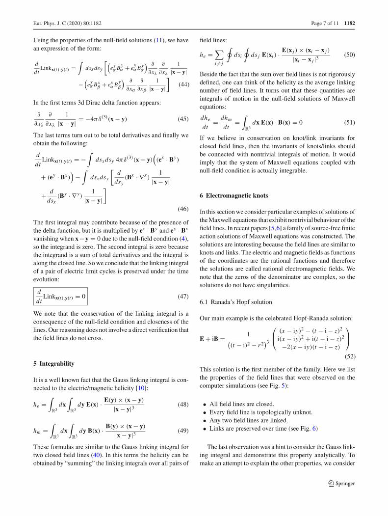
This solution is the first member of the family. Here we listthe properties of the field lines that were observed on thecomputer simulations (see Fig. 5):

• All field lines are closed.• Every field line is topologically unknot.• Any two field lines are linked.• Links are preserved over time (see Fig. 6)

The last observation was a hint to consider the Gauss link-ing integral and demonstrate this property analytically. Tomake an attempt to explain the other properties, we consider

123

1182 Page 8 of 11 Eur. Phys. J. C (2020) 80 :1182

Fig. 5 The yellow sphere is the light cone x2 + y2 + z2 = t2. The red lines are electric field lines at the moment t = 30. A part of the field linelies on the equator of the sphere. The other part tends to form a circle

Fig. 6 The yellow lines evolve into red lines over time. There are pictures of two successive moments of time. The green and the blue curves arethe trajectories. The link is preserved over time

the simplified version of the electric field, namely the elec-tric field far from the origin. On the coordinate scales muchlarger that the time t the electric field has the form:

E∞(x) = 1

r6

⎛⎝−x2 + y2 + z2

−2xy−2xz

⎞⎠ (53)

This electric field defines an integrable system of differentialequations on the field lines and the solution has the followingform:

x2 + (y cos θ + z sin θ − b)2 = b2 (54)

where all values of the radius b and the angle θ are possible.The circles are normal to the plane yz, pass through the origin

123

Eur. Phys. J. C (2020) 80 :1182 Page 9 of 11 1182

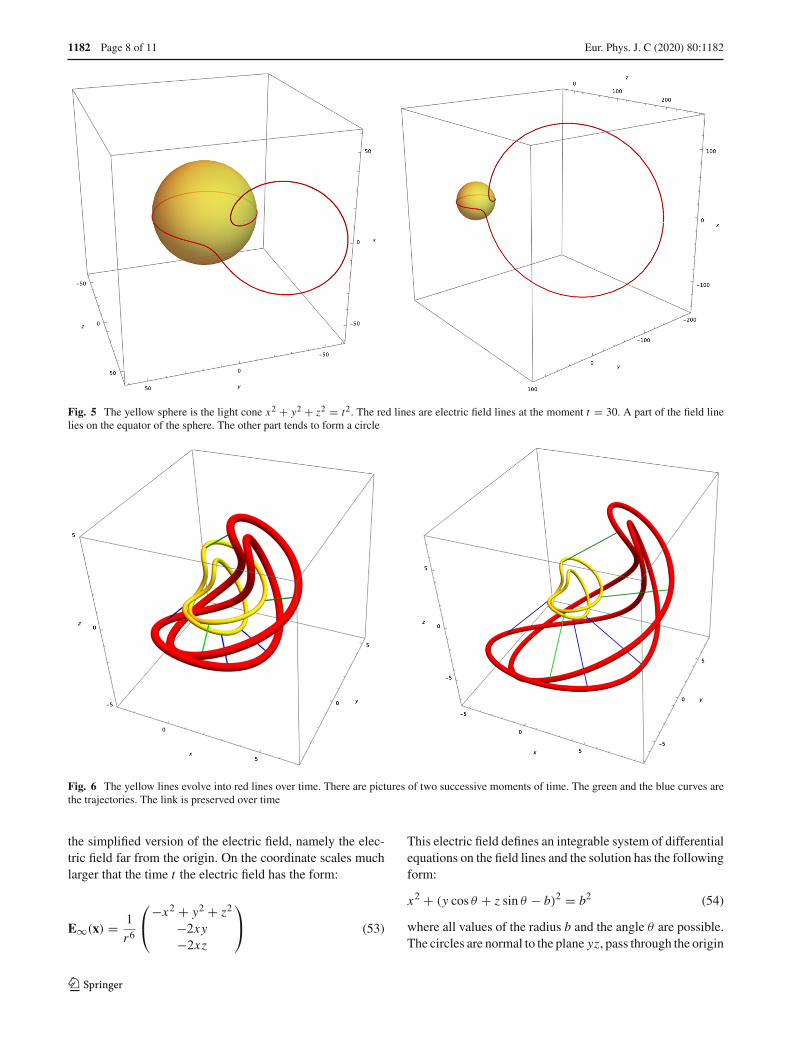
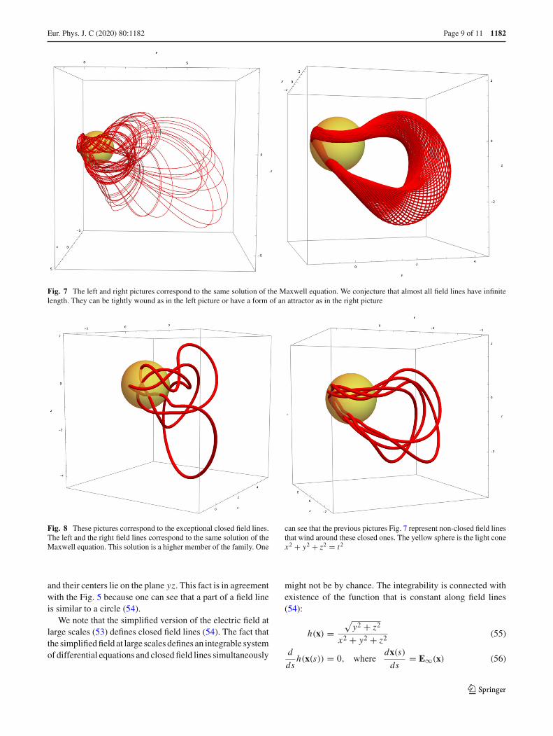
Fig. 7 The left and right pictures correspond to the same solution of the Maxwell equation. We conjecture that almost all field lines have infinitelength. They can be tightly wound as in the left picture or have a form of an attractor as in the right picture

Fig. 8 These pictures correspond to the exceptional closed field lines.The left and the right field lines correspond to the same solution of theMaxwell equation. This solution is a higher member of the family. One

can see that the previous pictures Fig. 7 represent non-closed field linesthat wind around these closed ones. The yellow sphere is the light conex2 + y2 + z2 = t2

and their centers lie on the plane yz. This fact is in agreementwith the Fig. 5 because one can see that a part of a field lineis similar to a circle (54).

We note that the simplified version of the electric field atlarge scales (53) defines closed field lines (54). The fact thatthe simplified field at large scales defines an integrable systemof differential equations and closed field lines simultaneously

might not be by chance. The integrability is connected withexistence of the function that is constant along field lines(54):

h(x) =√y2 + z2

x2 + y2 + z2 (55)

d

dsh(x(s)) = 0, where

dx(s)ds

= E∞(x) (56)

123

1182 Page 10 of 11 Eur. Phys. J. C (2020) 80 :1182

The simplified version of the field (53) is effectively twodimensional and one “integral of motion” h(x) is sufficientto determine the field lines. In case of the full Hopf-Ranadasolution two “integrals” might explain the closedness of thefield lines.

6.2 Other knots/links

The higher members of the family of knot solutions exhibitmore complicated structure of the field lines. There are rareclosed limit cycles in space and they represent various knots(see Fig. 8). Almost all field lines are tightly wound aroundthe limit cycles and we conjecture that they have infinitelength (see Fig. 7).

It would be interesting to find an efficient description ofthis complicated structure and classify knots and links thatappear in null-field solutions. For a possible approach to theproblem see [6].

7 Conclusion

Long ago hidden integrability was predicted to be one of thegoverning principles for dynamics in stringy models [11–14]. Since then this was proved to be the case in quite anumber of examples. For a recent review of appearing ofthe integrable properties in various contexts see [15,16]. Inthis paper we suggest to search for integrability in genericsolutions of Maxwell equations. The point is to reformulateMaxwell dynamics in terms of behavior of the field lines.Behaviour of the field lines was also discussed in [17–20]. Ata given time we can define a system of non-intersecting worldlines, and Maxwell dynamics convert them onto a system ofworld surfaces. Accordingly there are two directions s andt and two kinds of dynamics and, potentially, integrability –for s and t-evolutions. We provided some evidence that bothkinds of integrability are really present, and t-integrability isrelated to conservation of topological invariants. It would bevery interesting to develop these arguments into a full-fledgedtheory – most probably this will include non-Abelian consid-erations. One of the possible fruitful directions is establishingthe connection with the rapidly developing area of knot poly-nomials, especially colored HOMFLY polynomials [21,22].Secondly, at the SU (2) level one can exploit peculiar prop-erties of Lorentz and conformal groups in 4d [5]. Thirdly,one can relate evolution of field lines with loop equationsand integrability of eigenvalue matrix models [23–25]. Wehope for a new and profound progress on these issues, whichwould enrich our understanding of integrability of effectivetheories with the help of a very concrete and down-to-earthstory of Maxwell equations.

Acknowledgements We appreciate clarifying discussions with N. Kol-ganov, S. Mironov, V. Mishnyakov, And. Morozov, A. Popolitiov, A.Sleptsov and N. Ushakov at early stages of this project. Our work waspartly supported by the grant of the Foundation for the Advancementof Theoretical Physics “BASIS” 20-1-2-36-2 (N.T.), by RFBR grants19-02-00815 (A.M.), 20-01-00644 (N.T.), by joint RFBR grants 19-51-53014-GFEN (A.M.), 19-51-18006-Bolg (A.M.), 21-51-46010-CT(A.M, N.T.).

Data Availability Statement This manuscript has no associated dataor the data will not be deposited. [Authors’ comment: All the existingevidence and arguments are presented in the body of the paper, thus nosupplements are needed.]

Open Access This article is licensed under a Creative Commons Attri-bution 4.0 International License, which permits use, sharing, adaptation,distribution and reproduction in any medium or format, as long as yougive appropriate credit to the original author(s) and the source, pro-vide a link to the Creative Commons licence, and indicate if changeswere made. The images or other third party material in this articleare included in the article’s Creative Commons licence, unless indi-cated otherwise in a credit line to the material. If material is notincluded in the article’s Creative Commons licence and your intendeduse is not permitted by statutory regulation or exceeds the permit-ted use, you will need to obtain permission directly from the copy-right holder. To view a copy of this licence, visit http://creativecommons.org/licenses/by/4.0/.Funded by SCOAP3.

References

1. S.W. Thomson, On vortex atoms. In: Proceedings of the RoyalSociety of Edinburgh VI, pp. 94–105 (1867)

2. A.F. Ranada, Knotted solutions of the Maxwell equations in vac-uum. J. Phys. A Math. Gen. 23(16), L815–L820 (1990). https://doi.org/10.1088/0305-4470/23/16/007

3. A.F. Ranada, A topological theory of the electromagnetic field.Lett. Math. Phys. 18, 97–106 (1989). https://doi.org/10.1007/BF00401864

4. J. Niemi Antti, L. Faddeev, Stable knot-like structures in classicalfield theory. Nature 387, 58–61 (1997). https://doi.org/10.1038/387058a0

5. O. Lechtenfeld, G. Zhilin, A new construction of rational electro-magnetic knots. Phys. Lett. A 382, 1528–1533 (2018). https://doi.org/10.1016/j.physleta.2018.04.027. arXiv:1711.11144 [hep-th]

6. K. Kumar, O. Lechtenfeld, On rational electromagnetic fields.Phys. Lett. A 384, 126445 (2020). https://doi.org/10.1016/j.physleta.2020.126445. arXiv:2002.01005 [hep-th]

7. W.A. Newcomb, Motion of magnetic lines of force. Ann. Phys. 3,347–385 (1958). https://doi.org/10.1016/0003-4916(58)90024-1

8. W.T.M. Irvine, Linked and knotted beams of light, conservation ofhelicity and the flow of null electromagnetic fields. J. Phys. A Math.Theor. 43, 385203 (2010). https://doi.org/10.1088/1751-8113/43/38/385203. arXiv:1110.5408

9. C.F. Gauss, Zur Mathematischen Theorie der ElectrodynamischeWirkungen. In: Collected Works, Vol. 5, 2nd edn. KoniglichenGesellschaft des Wissenschaften, Gottingen, p. 601 (1833). https://doi.org/10.1007/978-3-642-49319-5_42

10. M. Arrayas, D. Bouwmeester, J.L. Trueba. Knots in electromag-netism. Phys. Rep. 667, 1–61 (2017). ISSN:0370-1573. https://doi.org/10.1016/j.physrep.2016.11.001

11. A.Yu. Morozov, String theory: what is it? Sov. Phys.Usp. 35, 671–714 (1992). https://doi.org/10.1070/PU1992v035n08ABEH002255

123

Eur. Phys. J. C (2020) 80 :1182 Page 11 of 11 1182

12. A. Morozov, Matrix models as integrable systems. In: CRM-CAPSummer School on Particles and Fields ’94, pp. 127–210 (1995).arXiv:hep-th/9502091

13. A. Mironov. 2-d gravity and matrix models. 1. 2-d gravity. Int.J. Mod. Phys. A 9, 4355–4406 (1994). https://doi.org/10.1142/S0217751X94001746. arXiv:hep-th/9312212

14. A. Mironov, Quantum deformations of t-functions, bilinear iden-tities and representation theory. Electron. Res. Announc. AMS 9,219–238 (1996). arXiv:hep-th/9409190

15. A. Andreev et al., Genus expansion of matrix models and hexpansion of KP hierarchy. JHEP (2020). https://doi.org/10.1007/JHEP12(2020)038. arXiv:2008.06416 [hep-th]

16. P. Dunin-Barkowski et al., Topological recursion for the extendedOoguri–Vafa partition function of colored HOMFLY-PT polyno-mials of torus knots (2020). arXiv:2010.11021 [math-ph]

17. H. Jehle, Relationship of flux quantization to charge quantizationand the electromagnetic coupling constant. Phys. Rev. D 3, 306–345 (1971). https://doi.org/10.1103/PhysRevD.3.306

18. H. Jehle, Flux quantization and particle physics. Phys. Rev. D 6,441–457 (1972). https://doi.org/10.1103/PhysRevD.6.441

19. H. Jehle, Flux quantization and fractional charges of quarks. Phys.Rev. D 11, 2147 (1975). https://doi.org/10.1103/PhysRevD.11.2147

20. H. Jehle, The electron–muon puzzle and the electromagnetic cou-pling constant. Phys. Rev. D 15, 3727 (1977). https://doi.org/10.1103/PhysRevD.15.3727

21. L. Bishler et al., Difference of mutant knot invariants and their dif-ferential expansion. Zh. Eksp. Teor. Fiz.111, N9 (2020). https://doi.org/10.1134/S0021364020090015. arXiv:2004.06598 [hep-th]

22. L. Bishler et al., Distinguishing mutant knots. J. Geom. Phys.159, 103928 (2021). ISSN:0393-0440. https://doi.org/10.1016/j.geomphys.2020.103928

23. A. Morozov, Integrability and matrix models. Phys. Usp. 37, 1–55(1994). https://doi.org/10.1070/PU1994v037n01ABEH000001.arXiv:hep-th/9303139

24. A. Morozov, Challenges of matrix models. In: NATO AdvancedStudy Institute and EC Summer School on String Theory: FromGauge Interactions to Cosmology, p. 129162 (2005). https://doi.org/10.1007/1-4020-3733-3_6. arXiv:hep-th/0502010

25. A. Mironov, Matrix models of two-dimensional gravity. Phys. Part.Nucl. 33, 537–582 (2002)

123