Embed Size (px)
Citation preview
Are Multiple Modes Helpful? Balancing Reduction of Nonresponse
and Sampling Error against Mode Effects
Benjamin Phillips, Ph.D., Abt SRBI
Chase Harrison, Ph.D., Harvard Business School
Chintan Turakhia, MBA, Abt SRBI
Introduction
• Various reasons for using sequential multimode designs
– Reduce costs/increase sample size
– Reduce nonresponse error
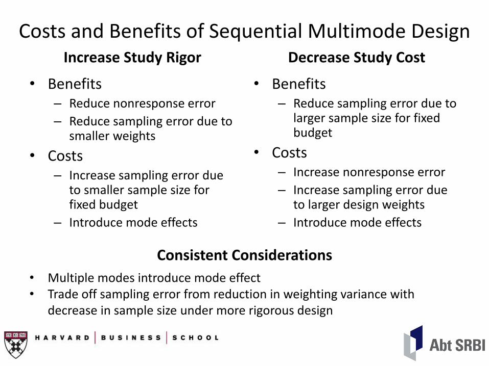
Costs and Benefits of Sequential Multimode Design Increase Study Rigor
• Benefits – Reduce nonresponse error
– Reduce sampling error due to smaller weights
• Costs – Increase sampling error due
to smaller sample size for fixed budget
– Introduce mode effects
Decrease Study Cost
• Benefits – Reduce sampling error due to
larger sample size for fixed budget
• Costs – Increase nonresponse error
– Increase sampling error due to larger design weights
– Introduce mode effects
Consistent Considerations
• Multiple modes introduce mode effect • Trade off sampling error from reduction in weighting variance with
decrease in sample size under more rigorous design

Sections
• Study description
• Methods
• Results
• Findings
• Conclusions

Sections
• Study description
• Methods
• Results
• Findings
• Conclusions

1. Designed to assess executive sentiment among HBS alumni (typically senior business leaders) on U.S. competitiveness and related issues;
2. Designed to include all alumni (N=70,000+);
3. Primary mode: web SAQ;
4. Short field period: 30 days;
5. Included embedded randomly selected core sample (n=4,000 selected) to measure nonresponse bias.
http://www.hbs.edu/competitiveness/

U.S. Competitiveness Study
Core Sample
• Interviewer-assisted address look-up;
• Paper prenotification letter;
• Invitation email;
• Two email reminders;
• Telephone follow-up and reminders;
• Telephone interviews.
Noncore Sample
• Invitation email;
• Two email reminders.
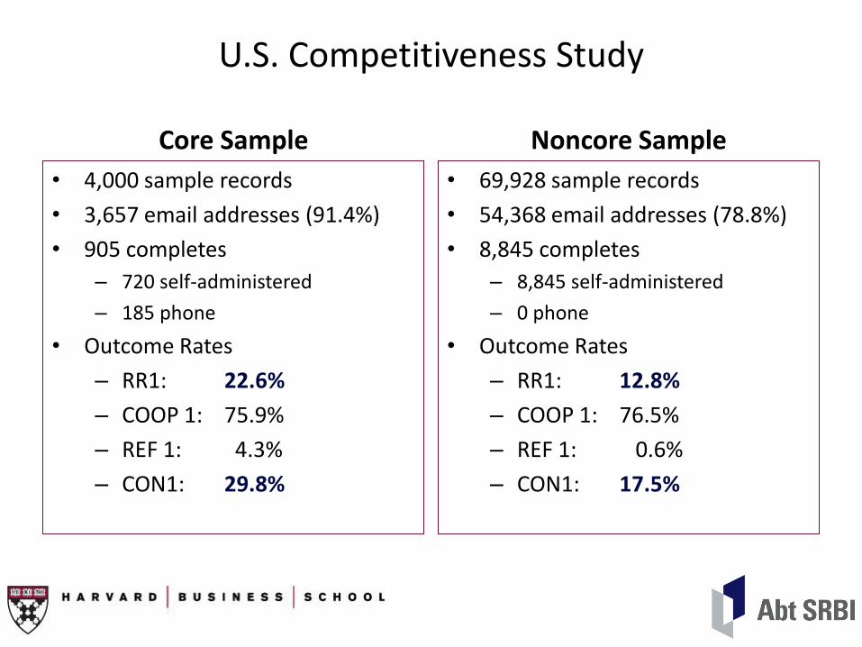
U.S. Competitiveness Study
Core Sample
• 4,000 sample records
• 3,657 email addresses (91.4%)
• 905 completes
– 720 self-administered
– 185 phone
• Outcome Rates
– RR1: 22.6%
– COOP 1: 75.9%
– REF 1: 4.3%
– CON1: 29.8%
Noncore Sample
• 69,928 sample records
• 54,368 email addresses (78.8%)
• 8,845 completes
– 8,845 self-administered
– 0 phone
• Outcome Rates
– RR1: 12.8%
– COOP 1: 76.5%
– REF 1: 0.6%
– CON1: 17.5%

Sections
• Study description
• Methods
• Results
• Findings
• Conclusions
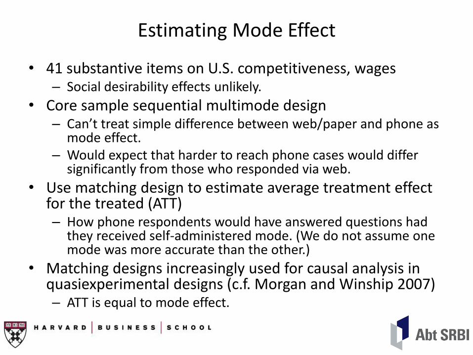
Estimating Mode Effect
• 41 substantive items on U.S. competitiveness, wages – Social desirability effects unlikely.
• Core sample sequential multimode design – Can’t treat simple difference between web/paper and phone as
mode effect. – Would expect that harder to reach phone cases would differ
significantly from those who responded via web.
• Use matching design to estimate average treatment effect for the treated (ATT) – How phone respondents would have answered questions had
they received self-administered mode. (We do not assume one mode was more accurate than the other.)
• Matching designs increasingly used for causal analysis in quasiexperimental designs (c.f. Morgan and Winship 2007) – ATT is equal to mode effect.
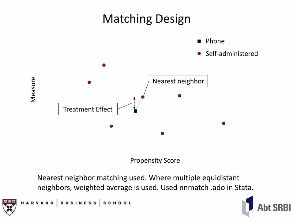
Matching Design
Propensity Score
Mea
sure
Phone
Self-administered
Nearest neighbor
Treatment Effect
Nearest neighbor matching used. Where multiple equidistant neighbors, weighted average is used. Used nnmatch .ado in Stata.
Distance Measure
• Mode predicted by logit model:
– Age
– Employment status
– Firm not based in U.S.
– Company exposed to international competition
• Resulting propensity scores used in matching algorithm.
• Efron pseudo-R2=.135 for logit model.

Sections
• Study description
• Methods
• Results
• Findings
• Conclusions
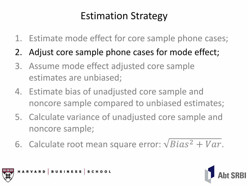
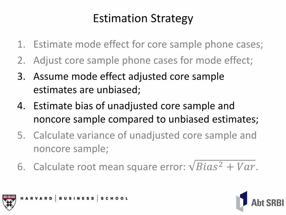
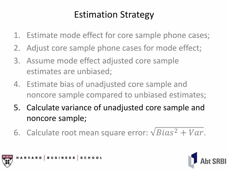
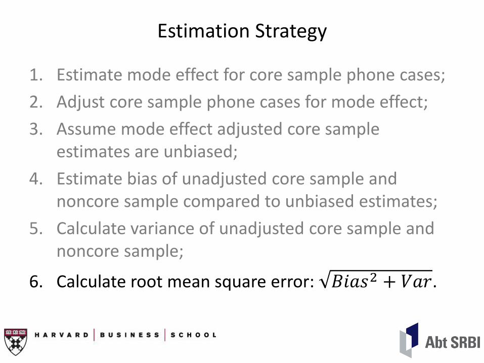
Estimation Strategy
1. Estimate mode effect for core sample phone cases;
2. Adjust core sample phone cases for mode effect;
3. Assume mode effect adjusted core sample estimates are unbiased;
4. Estimate bias of unadjusted core sample and noncore sample compared to unbiased estimates;
5. Calculate variance of unadjusted core sample and noncore sample;
6. Calculate root mean square error: 𝐵𝑖𝑎𝑠2 + 𝑉𝑎𝑟.
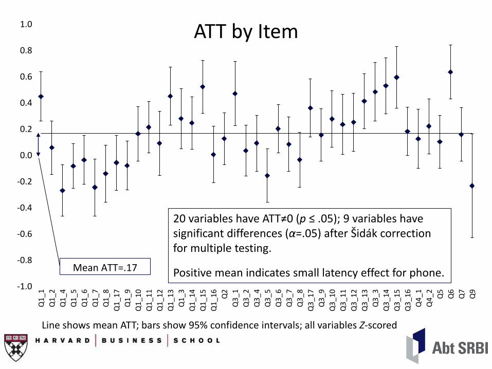
ATT by Item
Line shows mean ATT; bars show 95% confidence intervals; all variables Z-scored
-1.0
-0.8
-0.6
-0.4
-0.2
0.0
0.2
0.4
0.6
0.8
1.0
Q1
_1
Q1
_2
Q1
_4
Q1
_5
Q1
_6
Q1
_7
Q1
_8
Q1
_17
Q1
_9
Q1
_10
Q1
_11
Q1
_12
Q1
_13
Q1
_3
Q1
_14
Q1
_15
Q1
_16
Q2
Q3
_1
Q3
_2
Q3
_4
Q3
_5
Q3
_6
Q3
_7
Q3
_8
Q3
_17
Q3
_9
Q3
_10
Q3
_11
Q3
_12
Q3
_13
Q3
_3
Q3
_14
Q3
_15
Q3
_16
Q4
_1
Q4
_2 Q5
Q6
Q7
Q9
Mean ATT=.17
20 variables have ATT≠0 (p ≤ .05); 9 variables have significant differences (α=.05) after Šidák correction for multiple testing.
Positive mean indicates small latency effect for phone.
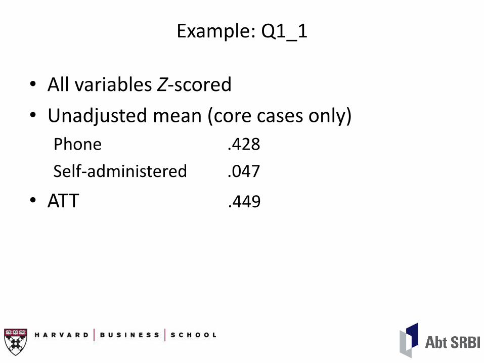
Example: Q1_1
• All variables Z-scored
• Unadjusted mean (core cases only)
Phone .428
Self-administered .047
• ATT .449
Estimation Strategy
1. Estimate mode effect for core sample phone cases;
2. Adjust core sample phone cases for mode effect;
3. Assume mode effect adjusted core sample estimates are unbiased;
4. Estimate bias of unadjusted core sample and noncore sample compared to unbiased estimates;
5. Calculate variance of unadjusted core sample and noncore sample;
6. Calculate root mean square error: 𝐵𝑖𝑎𝑠2 + 𝑉𝑎𝑟.
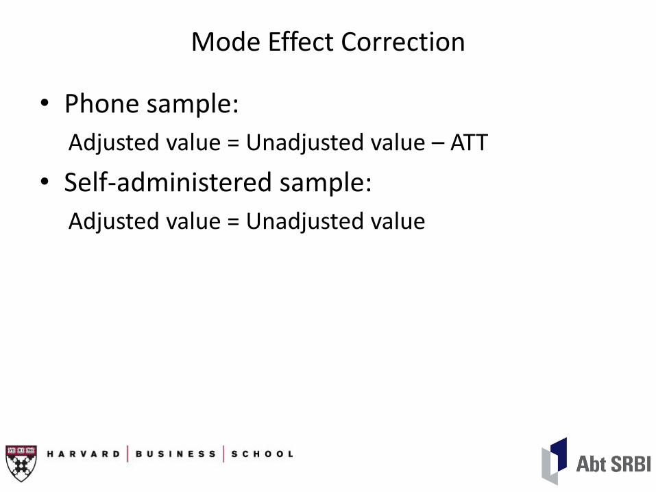
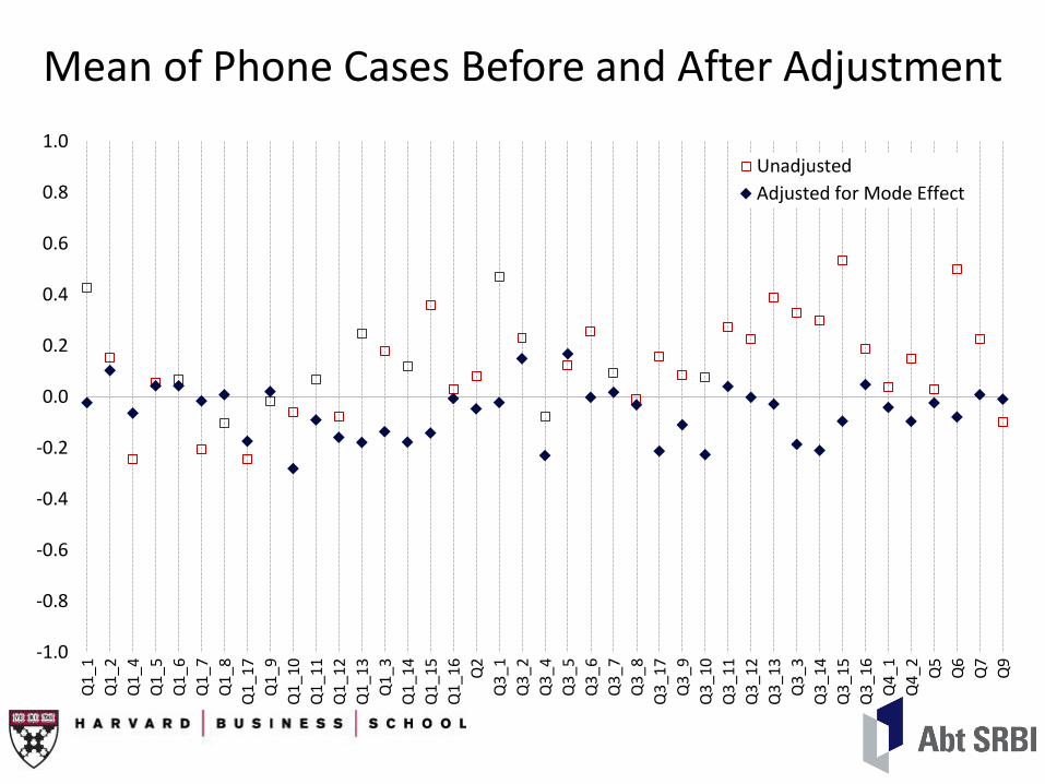
Mode Effect Correction
• Phone sample:
Adjusted value = Unadjusted value – ATT
• Self-administered sample:
Adjusted value = Unadjusted value
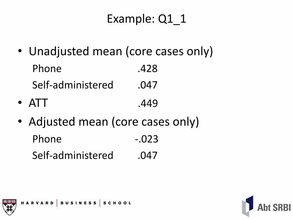
Example: Q1_1
• Unadjusted mean (core cases only)
Phone .428
Self-administered .047
• ATT .449
• Adjusted mean (core cases only)
Phone -.023
Self-administered .047
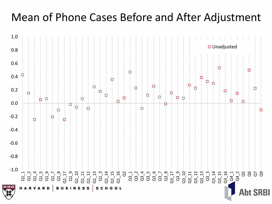
Mean of Phone Cases Before and After Adjustment
-1.0
-0.8
-0.6
-0.4
-0.2
0.0
0.2
0.4
0.6
0.8
1.0
Q1
_1
Q1
_2
Q1
_4
Q1
_5
Q1
_6
Q1
_7
Q1
_8
Q1
_17
Q1
_9
Q1
_10
Q1
_11
Q1
_12
Q1
_13
Q1
_3
Q1
_14
Q1
_15
Q1
_16
Q2
Q3
_1
Q3
_2
Q3
_4
Q3
_5
Q3
_6
Q3
_7
Q3
_8
Q3
_17
Q3
_9
Q3
_10
Q3
_11
Q3
_12
Q3
_13
Q3
_3
Q3
_14
Q3
_15
Q3
_16
Q4
_1
Q4
_2 Q5
Q6
Q7
Q9
Unadjusted
Adjusted for Mode Effect
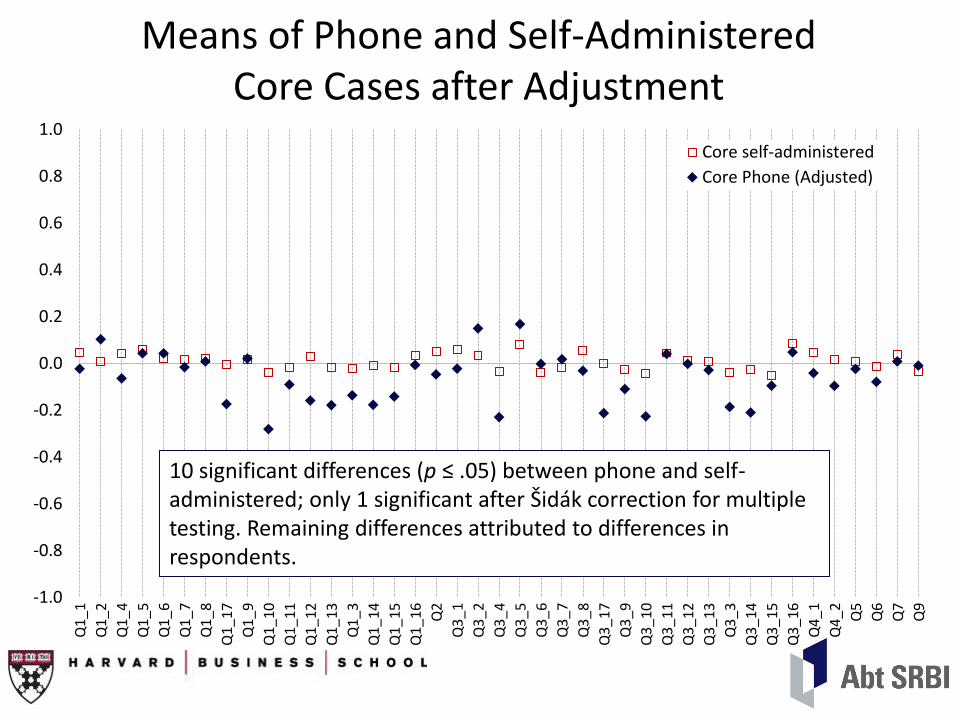
Means of Phone and Self-Administered Core Cases after Adjustment
-1.0
-0.8
-0.6
-0.4
-0.2
0.0
0.2
0.4
0.6
0.8
1.0
Q1
_1
Q1
_2
Q1
_4
Q1
_5
Q1
_6
Q1
_7
Q1
_8
Q1
_17
Q1
_9
Q1
_10
Q1
_11
Q1
_12
Q1
_13
Q1
_3
Q1
_14
Q1
_15
Q1
_16
Q2
Q3
_1
Q3
_2
Q3
_4
Q3
_5
Q3
_6
Q3
_7
Q3
_8
Q3
_17
Q3
_9
Q3
_10
Q3
_11
Q3
_12
Q3
_13
Q3
_3
Q3
_14
Q3
_15
Q3
_16
Q4
_1
Q4
_2 Q5
Q6
Q7
Q9
Core self-administered
Core Phone (Adjusted)
10 significant differences (p ≤ .05) between phone and self-administered; only 1 significant after Šidák correction for multiple testing. Remaining differences attributed to differences in respondents.
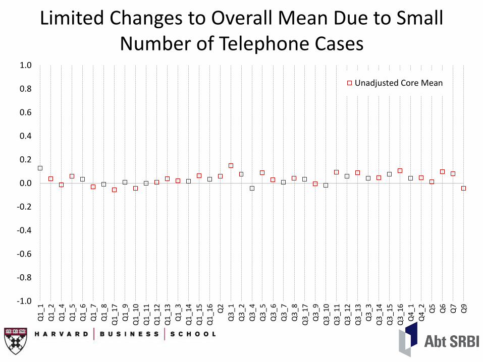
Limited Changes to Overall Mean Due to Small Number of Telephone Cases
-1.0
-0.8
-0.6
-0.4
-0.2
0.0
0.2
0.4
0.6
0.8
1.0
Q1
_1
Q1
_2
Q1
_4
Q1
_5
Q1
_6
Q1
_7
Q1
_8
Q1
_17
Q1
_9
Q1
_10
Q1
_11
Q1
_12
Q1
_13
Q1
_3
Q1
_14
Q1
_15
Q1
_16
Q2
Q3
_1
Q3
_2
Q3
_4
Q3
_5
Q3
_6
Q3
_7
Q3
_8
Q3
_17
Q3
_9
Q3
_10
Q3
_11
Q3
_12
Q3
_13
Q3
_3
Q3
_14
Q3
_15
Q3
_16
Q4
_1
Q4
_2 Q5
Q6
Q7
Q9
Unadjusted Core Mean
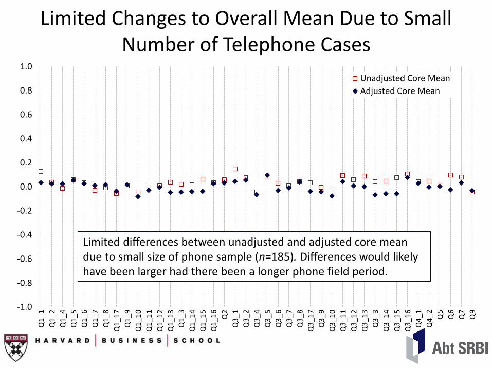
Adjusted Core Mean
Limited differences between unadjusted and adjusted core mean due to small size of phone sample (n=185). Differences would likely have been larger had there been a longer phone field period.
Estimation Strategy
1. Estimate mode effect for core sample phone cases;
2. Adjust core sample phone cases for mode effect;
3. Assume mode effect adjusted core sample estimates are unbiased;
4. Estimate bias of unadjusted core sample and noncore sample compared to unbiased estimates;
5. Calculate variance of unadjusted core sample and noncore sample;
6. Calculate root mean square error: 𝐵𝑖𝑎𝑠2 + 𝑉𝑎𝑟.
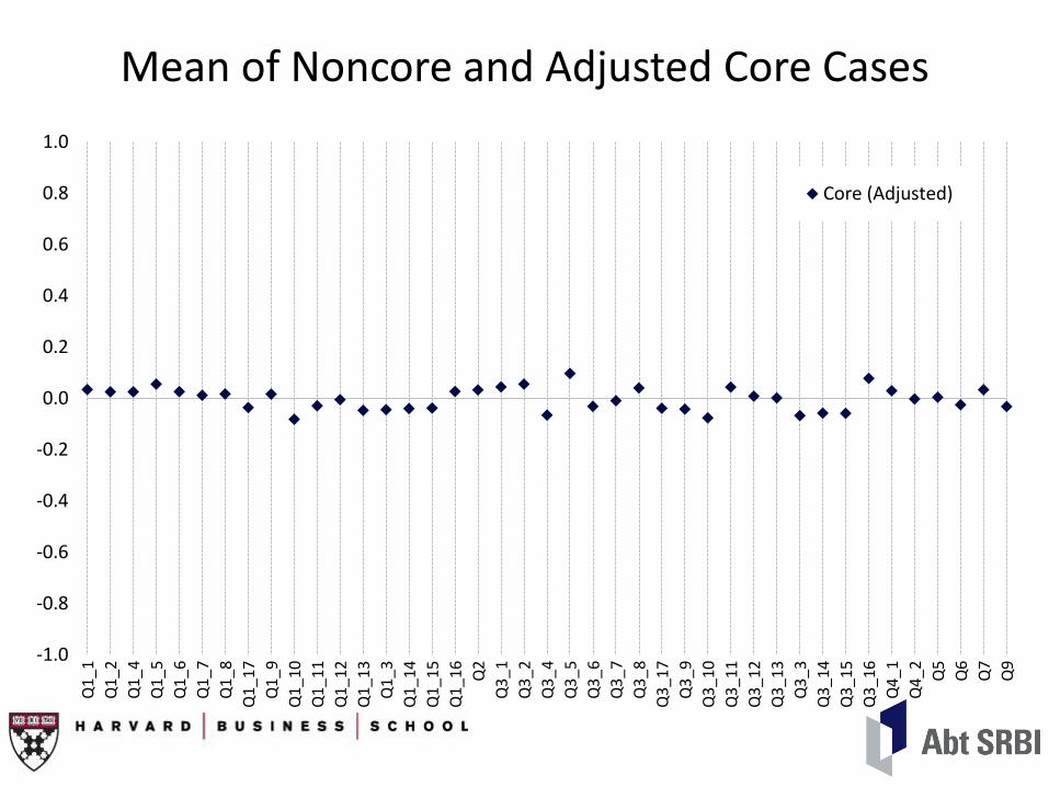
Mean of Noncore and Adjusted Core Cases
-1.0
-0.8
-0.6
-0.4
-0.2
0.0
0.2
0.4
0.6
0.8
1.0
Q1
_1
Q1
_2
Q1
_4
Q1
_5
Q1
_6
Q1
_7
Q1
_8
Q1
_17
Q1
_9
Q1
_10
Q1
_11
Q1
_12
Q1
_13
Q1
_3
Q1
_14
Q1
_15
Q1
_16
Q2
Q3
_1
Q3
_2
Q3
_4
Q3
_5
Q3
_6
Q3
_7
Q3
_8
Q3
_17
Q3
_9
Q3
_10
Q3
_11
Q3
_12
Q3
_13
Q3
_3
Q3
_14
Q3
_15
Q3
_16
Q4
_1
Q4
_2 Q5
Q6
Q7
Q9
Core (Adjusted)
-1.0
-0.8
-0.6
-0.4
-0.2
0.0
0.2
0.4
0.6
0.8
1.0
Q1
_1
Q1
_2
Q1
_4
Q1
_5
Q1
_6
Q1
_7
Q1
_8
Q1
_17
Q1
_9
Q1
_10
Q1
_11
Q1
_12
Q1
_13
Q1
_3
Q1
_14
Q1
_15
Q1
_16
Q2
Q3
_1
Q3
_2
Q3
_4
Q3
_5
Q3
_6
Q3
_7
Q3
_8
Q3
_17
Q3
_9
Q3
_10
Q3
_11
Q3
_12
Q3
_13
Q3
_3
Q3
_14
Q3
_15
Q3
_16
Q4
_1
Q4
_2 Q5
Q6
Q7
Q9
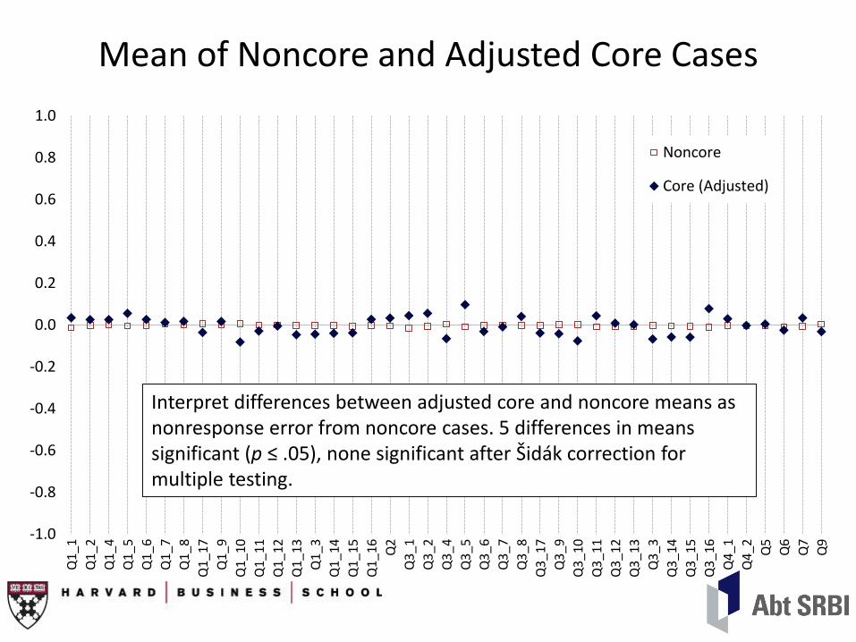
Noncore
Core (Adjusted)
Mean of Noncore and Adjusted Core Cases
Interpret differences between adjusted core and noncore means as nonresponse error from noncore cases. 5 differences in means significant (p ≤ .05), none significant after Šidák correction for multiple testing.
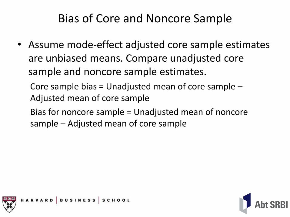
Bias of Core and Noncore Sample
• Assume mode-effect adjusted core sample estimates are unbiased means. Compare unadjusted core sample and noncore sample estimates.
Core sample bias = Unadjusted mean of core sample – Adjusted mean of core sample
Bias for noncore sample = Unadjusted mean of noncore sample – Adjusted mean of core sample
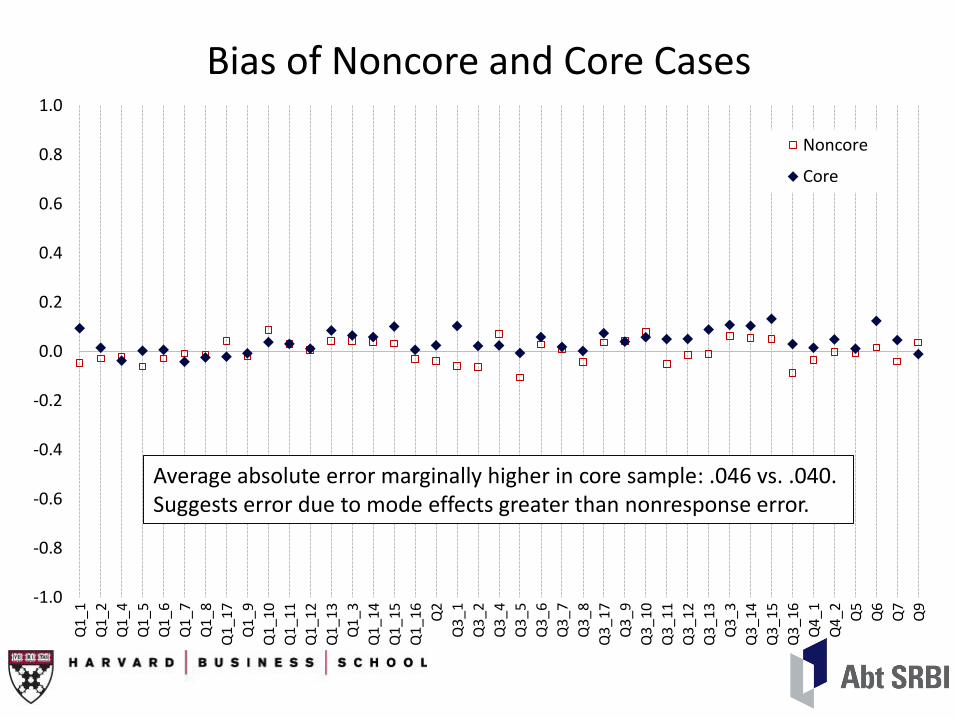
Bias of Noncore and Core Cases
-1.0
-0.8
-0.6
-0.4
-0.2
0.0
0.2
0.4
0.6
0.8
1.0
Q1
_1
Q1
_2
Q1
_4
Q1
_5
Q1
_6
Q1
_7
Q1
_8
Q1
_17
Q1
_9
Q1
_10
Q1
_11
Q1
_12
Q1
_13
Q1
_3
Q1
_14
Q1
_15
Q1
_16
Q2
Q3
_1
Q3
_2
Q3
_4
Q3
_5
Q3
_6
Q3
_7
Q3
_8
Q3
_17
Q3
_9
Q3
_10
Q3
_11
Q3
_12
Q3
_13
Q3
_3
Q3
_14
Q3
_15
Q3
_16
Q4
_1
Q4
_2 Q5
Q6
Q7
Q9
Noncore
Core
Average absolute error marginally higher in core sample: .046 vs. .040. Suggests error due to mode effects greater than nonresponse error.
Estimation Strategy
1. Estimate mode effect for core sample phone cases;
2. Adjust core sample phone cases for mode effect;
3. Assume mode effect adjusted core sample estimates are unbiased;
4. Estimate bias of unadjusted core sample and noncore sample compared to unbiased estimates;
5. Calculate variance of unadjusted core sample and noncore sample;
6. Calculate root mean square error: 𝐵𝑖𝑎𝑠2 + 𝑉𝑎𝑟.
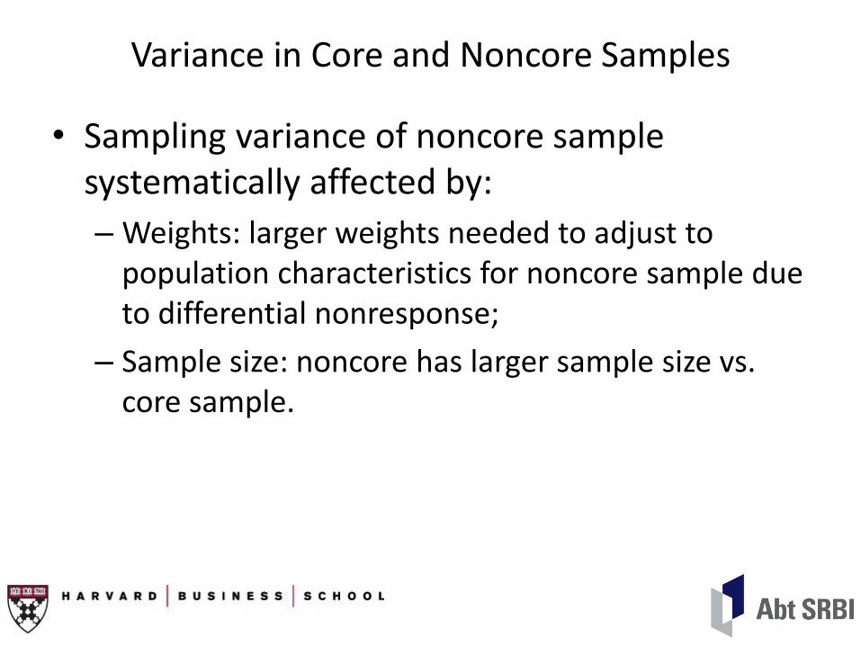
Variance in Core and Noncore Samples
• Sampling variance of noncore sample systematically affected by:
– Weights: larger weights needed to adjust to population characteristics for noncore sample due to differential nonresponse;
– Sample size: noncore has larger sample size vs. core sample.
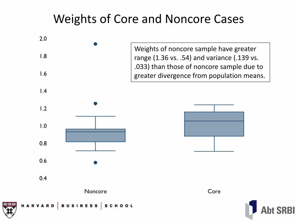
Weights of Core and Noncore Cases
0.4
0.6
0.8
1.0
1.2
1.4
1.6
1.8
2.0
Noncore Core
Weights of noncore sample have greater range (1.36 vs. .54) and variance (.139 vs. .033) than those of noncore sample due to greater divergence from population means.
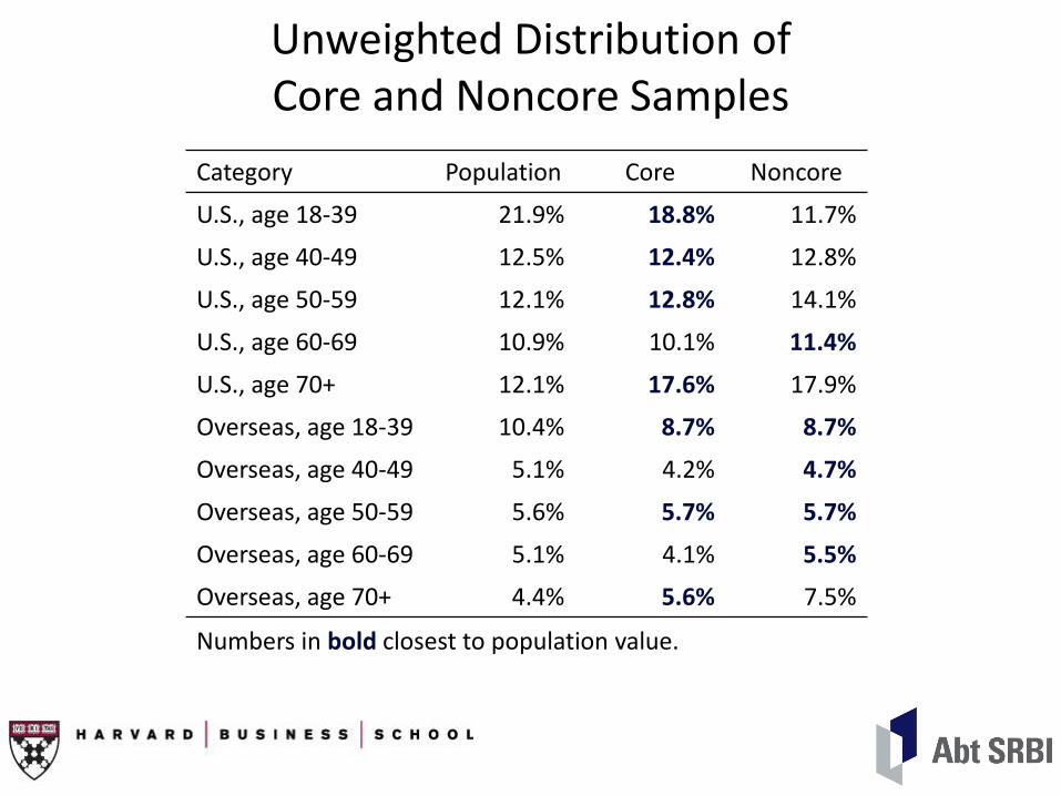
Unweighted Distribution of Core and Noncore Samples
Numbers in bold closest to population value.
Category Population Core Noncore
U.S., age 18-39 21.9% 18.8% 11.7%
U.S., age 40-49 12.5% 12.4% 12.8%
U.S., age 50-59 12.1% 12.8% 14.1%
U.S., age 60-69 10.9% 10.1% 11.4%
U.S., age 70+ 12.1% 17.6% 17.9%
Overseas, age 18-39 10.4% 8.7% 8.7%
Overseas, age 40-49 5.1% 4.2% 4.7%
Overseas, age 50-59 5.6% 5.7% 5.7%
Overseas, age 60-69 5.1% 4.1% 5.5%
Overseas, age 70+ 4.4% 5.6% 7.5%
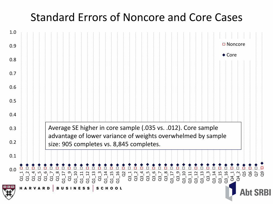
Standard Errors of Noncore and Core Cases
0.0
0.1
0.2
0.3
0.4
0.5
0.6
0.7
0.8
0.9
1.0
Q1
_1
Q1
_2
Q1
_4
Q1
_5
Q1
_6
Q1
_7
Q1
_8
Q1
_17
Q1
_9
Q1
_10
Q1
_11
Q1
_12
Q1
_13
Q1
_3
Q1
_14
Q1
_15
Q1
_16
Q2
Q3
_1
Q3
_2
Q3
_4
Q3
_5
Q3
_6
Q3
_7
Q3
_8
Q3
_17
Q3
_9
Q3
_10
Q3
_11
Q3
_12
Q3
_13
Q3
_3
Q3
_14
Q3
_15
Q3
_16
Q4
_1
Q4
_2 Q5
Q6
Q7
Q9
Noncore
Core
Average SE higher in core sample (.035 vs. .012). Core sample advantage of lower variance of weights overwhelmed by sample size: 905 completes vs. 8,845 completes.
Estimation Strategy
1. Estimate mode effect for core sample phone cases;
2. Adjust core sample phone cases for mode effect;
3. Assume mode effect adjusted core sample estimates are unbiased;
4. Estimate bias of unadjusted core sample and noncore sample compared to unbiased estimates;
5. Calculate variance of unadjusted core sample and noncore sample;
6. Calculate root mean square error: 𝐵𝑖𝑎𝑠2 + 𝑉𝑎𝑟.
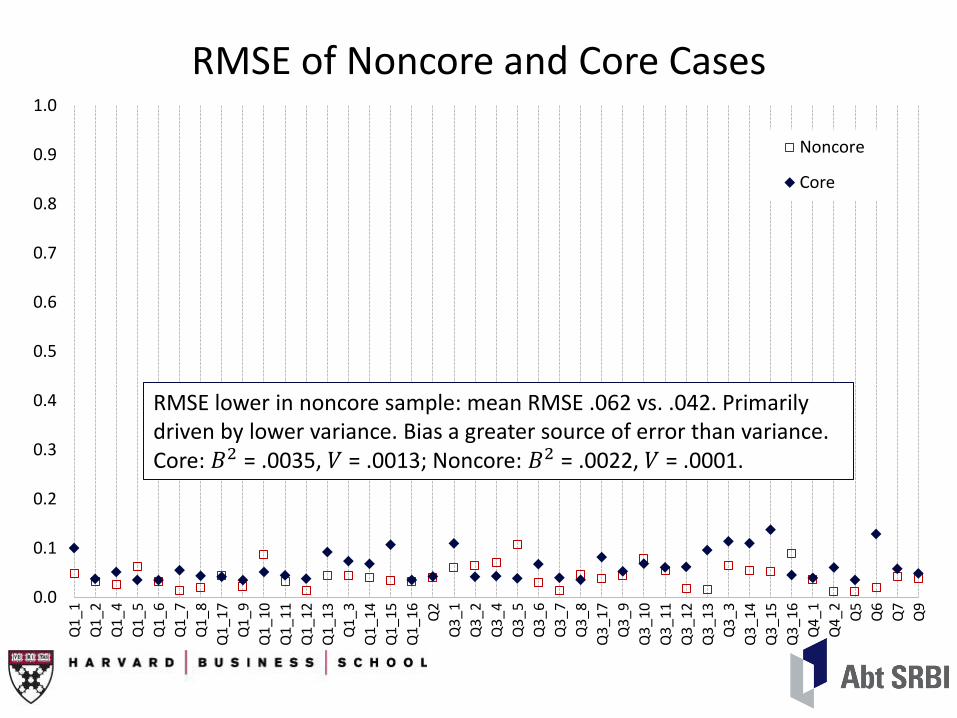
RMSE of Noncore and Core Cases
0.0
0.1
0.2
0.3
0.4
0.5
0.6
0.7
0.8
0.9
1.0
Q1
_1
Q1
_2
Q1
_4
Q1
_5
Q1
_6
Q1
_7
Q1
_8
Q1
_17
Q1
_9
Q1
_10
Q1
_11
Q1
_12
Q1
_13
Q1
_3
Q1
_14
Q1
_15
Q1
_16
Q2
Q3
_1
Q3
_2
Q3
_4
Q3
_5
Q3
_6
Q3
_7
Q3
_8
Q3
_17
Q3
_9
Q3
_10
Q3
_11
Q3
_12
Q3
_13
Q3
_3
Q3
_14
Q3
_15
Q3
_16
Q4
_1
Q4
_2 Q5
Q6
Q7
Q9
Noncore
Core
RMSE lower in noncore sample: mean RMSE .062 vs. .042. Primarily driven by lower variance. Bias a greater source of error than variance. Core: 𝐵2 = .0035, 𝑉 = .0013; Noncore: 𝐵2 = .0022, 𝑉 = .0001.

Sections
• Study description
• Methods
• Results
• Findings
• Conclusions
Findings
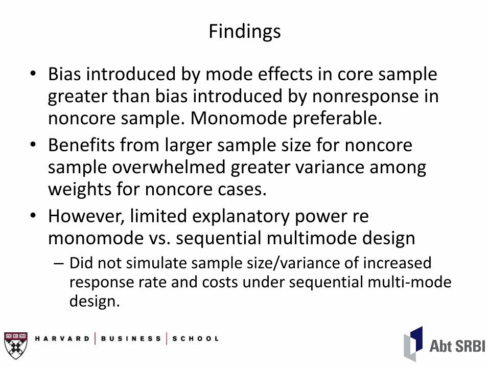
• Bias introduced by mode effects in core sample greater than bias introduced by nonresponse in noncore sample. Monomode preferable.
• Benefits from larger sample size for noncore sample overwhelmed greater variance among weights for noncore cases.
• However, limited explanatory power re monomode vs. sequential multimode design – Did not simulate sample size/variance of increased
response rate and costs under sequential multi-mode design.

Sections
• Study description
• Methods
• Results
• Findings
• Conclusions
Conclusions
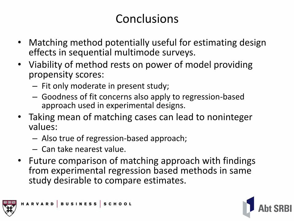
• Matching method potentially useful for estimating design effects in sequential multimode surveys.
• Viability of method rests on power of model providing propensity scores: – Fit only moderate in present study; – Goodness of fit concerns also apply to regression-based
approach used in experimental designs.
• Taking mean of matching cases can lead to noninteger values: – Also true of regression-based approach; – Can take nearest value.
• Future comparison of matching approach with findings from experimental regression based methods in same study desirable to compare estimates.

Contact Information
Benjamin Phillips ([email protected])
Chase Harrison ([email protected])
Chintan Turakhia ([email protected])

Appendices
Matching
• Nearest neighbor matching using Stata nnmatch command (Abadie et al. 2004
Matching Model
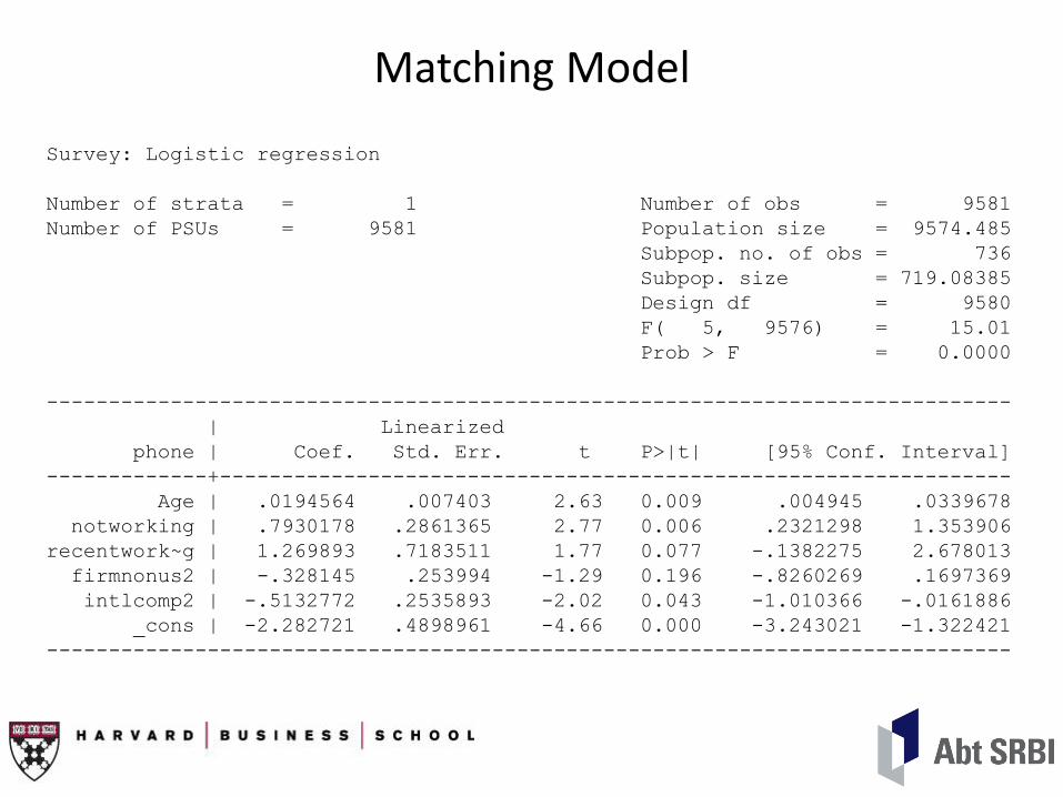
Survey: Logistic regression
Number of strata = 1 Number of obs = 9581
Number of PSUs = 9581 Population size = 9574.485
Subpop. no. of obs = 736
Subpop. size = 719.08385
Design df = 9580
F( 5, 9576) = 15.01
Prob > F = 0.0000
------------------------------------------------------------------------------
| Linearized
phone | Coef. Std. Err. t P>|t| [95% Conf. Interval]
-------------+----------------------------------------------------------------
Age | .0194564 .007403 2.63 0.009 .004945 .0339678
notworking | .7930178 .2861365 2.77 0.006 .2321298 1.353906
recentwork~g | 1.269893 .7183511 1.77 0.077 -.1382275 2.678013
firmnonus2 | -.328145 .253994 -1.29 0.196 -.8260269 .1697369
intlcomp2 | -.5132772 .2535893 -2.02 0.043 -1.010366 -.0161886
_cons | -2.282721 .4898961 -4.66 0.000 -3.243021 -1.322421
------------------------------------------------------------------------------
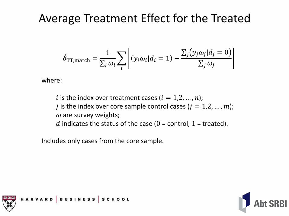
Average Treatment Effect for the Treated
𝛿 TT,match =1
𝜔𝑖𝑖
𝑦𝑖𝜔𝑖|𝑑𝑖 = 1 − 𝑦𝑗𝜔𝑗|𝑑𝑗 = 0𝑗
𝜔𝑗𝑗𝑖
where:
𝑖 is the index over treatment cases (𝑖 = 1,2, … , 𝑛); 𝑗 is the index over core sample control cases (𝑗 = 1,2, … , 𝑚); 𝜔 are survey weights; 𝑑 indicates the status of the case (0 = control, 1 = treated).
Includes only cases from the core sample.
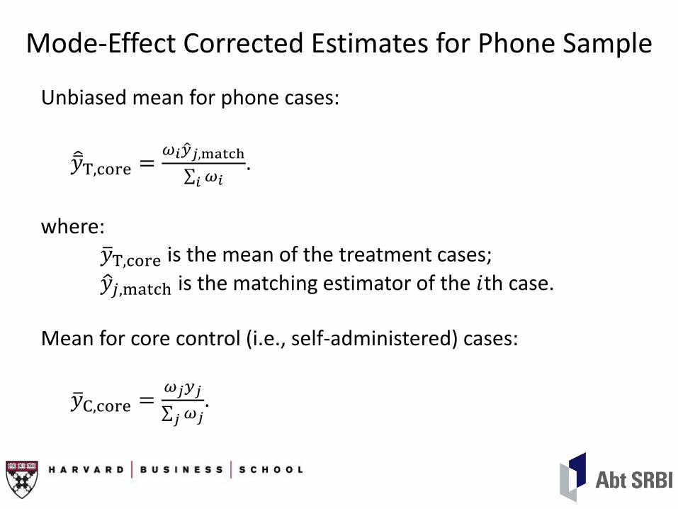
Mode-Effect Corrected Estimates for Phone Sample
Unbiased mean for phone cases:
𝑦 T,core =𝜔𝑖𝑦 𝑗,match
𝜔𝑖𝑖.
where:
𝑦 T,core is the mean of the treatment cases;
𝑦 𝑗,match is the matching estimator of the 𝑖th case. Mean for core control (i.e., self-administered) cases:
𝑦 C,core =𝜔𝑗𝑦𝑗
𝜔𝑗𝑗.
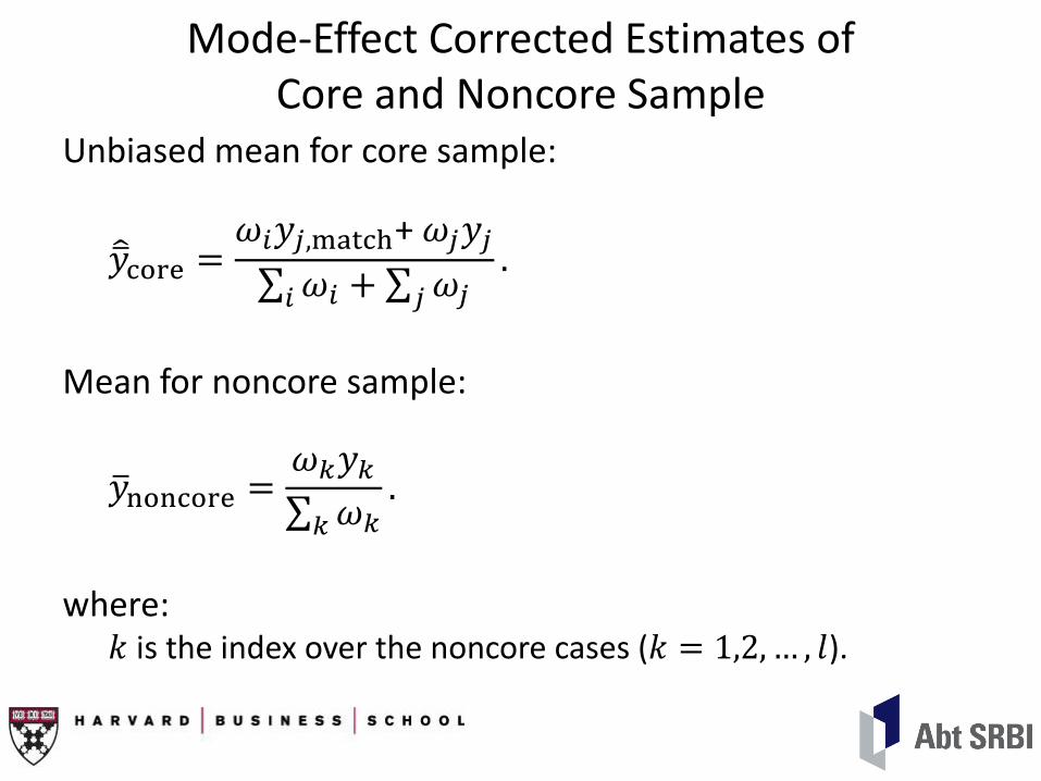
Mode-Effect Corrected Estimates of Core and Noncore Sample
Unbiased mean for core sample:
𝑦 core =𝜔𝑖𝑦𝑗,match+ 𝜔𝑗𝑦𝑗
𝜔𝑖𝑖 + 𝜔𝑗𝑗
.
Mean for noncore sample:
𝑦 noncore =𝜔𝑘𝑦𝑘
𝜔𝑘𝑘
.
where:
𝑘 is the index over the noncore cases (𝑘 = 1,2, … , 𝑙).

Bias of Core and Noncore Sample
Bias for core sample:
𝐵 𝑦core = 𝑦 core − 𝑦 core.
Bias for noncore sample:
𝐵 𝑦noncore = 𝑦 noncore − 𝑦 core.
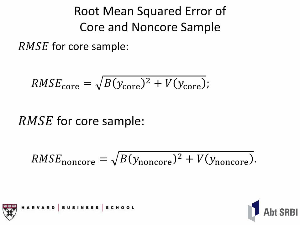
Root Mean Squared Error of Core and Noncore Sample
𝑅𝑀𝑆𝐸 for core sample:
𝑅𝑀𝑆𝐸core = 𝐵 𝑦core2 + 𝑉 𝑦core ;
𝑅𝑀𝑆𝐸 for core sample:
𝑅𝑀𝑆𝐸noncore = 𝐵 𝑦noncore2 + 𝑉 𝑦noncore .
References
Abadie, Alberto, David Drukker, Jane L. Herr, and Guido W. Imbens. 2004. “Implementing Matching Estimators for Average Treatment Effects in Stata.” Stata Journal 4:290-311.
Morgan, Stephen L. and Christopher Winship. 2007. Counterfactuals and Causal Inference: Methods and Principals for Social Research. New York: Cambridge University Press.