1

Are RTA agreements with

environmental provisions reducing

emissions?

Leila Baghdadi1,

Inmaculada Martinez-Zarzoso2*,

Habib Zitouna3

(16.11.2012)

Preliminary version, please do not quote without permission

1 LIM, MES cluster, Tunisia Polytechnic School, University Carthage, El Khawerzmi street, B.P. 743, 2078, La Marsa, Tunisia

and Tunis Business School, Tunis University, Tunisia. Email: leila.baghdadi@tbs.rnu.tn . Tel.: (216) 71.470.570. Fax.: (216) 71.477.555. 2 Corresponding author. Department of Economics, Georg-August University of Göttingen and Institute of International

Economics, Universitat Jaume I, Campus del Riu Sec, 12071 Castellón, Spain. Email: martinei@eco.uji.es. 3 Tunisia Polytechnic School, University of Carthage. El Khawerzmi street, B.P. 743, 2078, La Marsa, Tunisia. Email:

hzitouna@gmail.com. *Financial support received from CREMed Center and from the Ministry of Science and Innovation is gratefully acknowledge (ECO 2010-15863). The authors also would like to thank the participants of the Second CREMed workshop on Economics of the Mediterranean held in Barcelona for their helpful comments and suggestions.

2

Are RTA agreements with environmental provisions reducing emissions?

Abstract

This paper investigates whether RTAs with environmental provisions embedded affect relative and

absolute pollution levels. With this aim, the determinants of carbon dioxide emissions convergence

are estimated for a cross-section of 182 countries over the period 1980 to 2008. To effectively

isolate the effect of the Regional Trade Agreement (RTA) variable, a propensity score matching

approach is combined with difference-in-differences techniques. The usual controls for scale,

composition and technique effects are added to the estimated model and endogeneity of income

and trade variables is modelled using instruments. The main results indicate that CO2 emissions of

the pairs of countries that belong to an RTA with environmental provisions tend to converge and are

lower in absolute values, but this is not the case for RTAs without environmental provisions. As

regards specific agreements, we find that emissions converge more rapidly for EU-27 countries than

for Euro-Med countries. We find consistent evidence that only RTAs with environmental

harmonization policies embedded affect relative and absolute pollution levels.

Keywords: regional trade agreements, environmental provisions, convergence, CO2 emissions,

matching, difference-in-differences

JEL Classification: F 18, O13, L60, Q43

I. Introduction

One of the most controversial debates in trade policy concerns the impact of trade liberalization on

the environment. Trade liberalization can be implemented unilaterally, with a single country

reducing its trade barriers against all its trading partners, or regionally, with a group of countries

forming a Regional Trade Agreement (RTA) to eliminate trade barriers among them. The latter form

of trade liberalization has been predominant since the early 1990s and there is increasing interest in

assessing the effects stemming from this new regionalism. Not only direct trade and income effects

3

are important, but also the impact on the environment. In this respect, it is important to distinguish

between RTAs with environmental provisions (EP) and the rest of RTAs that do not include any

harmonization in environmental standards as part of the agreements.

After two decades of research, it is commonly accepted that the effects of trade liberalization on

the environment are complex and can be classified into scale, composition and technique effects

and that there may also be interaction between these effects (Copeland and Taylor, 2003). Most of

the recent literature used changes in trade openness as a proxy for trade liberalization (Frankel and

Rose, 2005) and many studies have focused on the effects of NAFTA on the environment (Grossman

and Krueger, 1991; Stern, 2007). Contrary to expectations, the early findings point to positive

effects. Surprisingly, few studies have been devoted to other regional trade agreements and to the

best of our knowledge there are no studies using RTAs as a trade policy variable that could influence

pollution levels. This is precisely the strategy we propose in this paper to investigate the effects of

trade on the environment, namely to directly include an RTA variable in an emissions equation.

Moreover, we hypothesize that the effect should be different for RTAs with and without

environmental provisions and only the former agreements should have a direct effect on pollution

levels or on convergence, whereas the latter should not have an effect once we control for changes

in trade openness. A problem related to the estimation of RTA effects is that countries possibly

select into trade agreements, which could generate an endogeneity bias. In a different context,

Badinger (2008), who specified an RTA variable in a productivity equation, addressed the

endogeneity issue using an instrumental variable approach. The main shortcoming of this approach

in our context is the difficulty to find adequate instruments that are exogenous to the model. Hence

we will propose an alternative strategy.

In this paper we depart from the previous literature in two important respects. First, we specifically

investigate whether RTAs with environmental provisions may have a direct “harmonization” effect

on pollution. In this way we will be able to determine whether the signing of an RTA with

environmental provisions leads governments to impose guidelines that affect relative and absolute

4

pollution levels and whether this induces pollution convergence. Second, the identification strategy

is based on the use of matched samples and difference-in-differences estimation techniques to

better isolate these harmonization convergence rules. In addition, we follow the recent literature to

correctly account for the complex effects of income and openness on pollution levels. In particular,

the underlying control variables, namely openness and income levels are instrumented away

(Frankel and Romer, 1999; Frankel and Rose, 2005), since both might be influenced by RTAs

formation. Finally, results for specific agreements are also presented and compared.

The main results show evidence of RTAs with environmental provisions explaining statistically

convergence of pollution levels across pair of countries. Moreover, more advanced integration

agreements (EU-27) are converging at a higher rate than less advanced ones. Conversely, RTAs

without environmental provisions do not affect relative or absolute pollution levels, indicating that

controlling for bilateral trade levels and overall openness, the trade policy variable do not have a

direct effect on emissions convergence for this type of agreements.

The paper is organized as follows. Section 2 states the main theoretical prediction and Section 3

reviews the main empirical literature. Section 4 describes the empirical strategy and the data,

variables and main results are presented in Section 5. Finally, Section 6 concludes.

II. Regional Integration and Emission Convergence: Theoretical Predictions

1. Trade and the Environment

The negotiations for the North American Free Trade Agreement (NAFTA) were followed by fears

about its consequences on the environment. Indeed, the literature between trade and

environmental quality has emerged in this period. Grossman and Kruger (1991) was the first paper

to decompose the total impact of trade on the environment into three different effects: scale,

technique and composition effects.

The scale effect is assumed to have a negative effect on the environment. According to general

belief, trade liberalization leads to an expansion in economic activity and, all other things being

5

equal (composition and techniques of production), the total amount of pollution will then increase

(for example, economic growth, due to trade, raises the demand for energy and boosts

transportation, which is one of the main emitting sectors). It is worth noting that this pass-through

between trade and the environment assumes a positive effect of trade liberalization on economic

growth4. The income effects of trade are linked to the literature on the Environmental Kuznets Curve

(EKC), which assumes an inverted U-shaped relationship between per capita income and pollution:

Pollution increases in the early stages of development until it reaches a turning point and then

declines (Copland and Gulati, 2006).5 However, it is nowadays generally accepted that an EKC for CO2

does not exist for most economies (Carson, 2010).

The second pass-through between trade and the environment is the so-called technique effect.

Holding the scale of the economy and the mix of goods produced constant, a reduction in the

intensity of emissions – measured in terms of emissions by unit of output - results in a decline in

pollution. Three main arguments are behind this effect. First, increased trade promotes the transfer

of modern (cleaner) technologies from developed to developing countries. Second, if trade raises

income, individuals may demand higher environmental quality (if the latter is a normal good). Third,

according to the Porter-hypothesis (Porter and van der Linde, 1995), increased globalization will

increase competition. In order to stay competitive, firms have to invest in the newest and most

efficient technologies. Thus, more stringent environmental policy can increase international

competitiveness. In summary, the technique effect has a positive impact on the environment.

Third, comparative advantage is also an important factor that could explain the relationship

between trade and the environment. The economy will pollute more if it devotes more resources to

the production of pollution-intensive goods, holding the scale of the economy and emission

intensities constant. The composition effect –also referred to as the trade-composition or trade-

4 A large body of empirical literature provides empirical evidence of this positive effect of openness (see for

example Dollar (1992), Ben-David (1993), Sachs and Warner (1995), Edwards (1998), Frankel and Romer (1999) or Rodriguez and Rodrik (2003) for a critical review). 5 The name of the environmental Kuznets curve relates to the work by Kuznets (1955), who found a similar

inverted U-shaped relationship between income inequality and GDP per capita (Kuznets, 1955).

6

induced composition effect– is caused by changes in trade policy. Through trade liberalization,

countries specialize in the sectors where they enjoy a comparative advantage. Among the sources of

comparative advantage, we find classical factor endowment differences or unit cost differences and

those based on differences in institutions or regulations between countries. On the one hand, the

factor endowment hypothesis (FEH) states that environmental policy has no significant effect on

trade patterns, factor endowments determining trade instead. This implies that relatively capital-

abundant countries will export pollution-intensive goods, since most pollution-intensive goods are

capital-intensive. On the other hand, the Pollution Haven Hypothesis (PHH) states that differences in

environmental regulations are the main motivation for trade and that trade liberalization causes

pollution-intensive industries to relocate from high income countries with stringent environmental

regulations to low income countries with lax environmental regulations (Taylor, 2004). Hence, with

trade liberalization, high income countries will specialize in the production of clean goods and

pollution in these countries will decline, while low income countries will specialize in producing dirty

goods and their level of pollution will increase.

In general, we expect countries to differ in both factor endowments and environmental policy. High-

income countries tend to be capital-abundant and also have stricter environmental regulations than

low-income countries. On the one hand, the North could become a dirty-good importer (as it has

stricter environmental policy) and, on the other hand, it might become a dirty-good exporter

(because of its capital abundance). The interaction of these two effects determines the pattern of

trade. If pollution haven motives are more important than factor endowment motives, the North will

import the dirty good from the South. On the contrary, trade could cause the North to specialize in

the production and exportation of the pollution-intensive good when factor endowment differences

dominate regulatory differences, despite having the stricter environmental regulations (Copeland

and Taylor, 2003).

7

In summary, according to previous literature we could expect comparative advantage to be

determined jointly by differences in regulatory policy and factor endowments. If the PHH dominates,

following a liberalization process between a developing and a developed country, per-capita

emissions will tend to converge. If FEH motives dominate, per-capita emissions should diverge.

An issue that has been overlooked in the theoretical literature is that trade policy negotiations have

increasingly been accompanied by environmental policy measures. Those policy measures are

planned in most cases to avoid the potential trade effects that could emerge as a consequence of

differences in regulations. In particular, a number of recently signed RTAs include environmental

provisions and these provisions can directly affect the levels of emissions in the countries involved.

This pass-trough could be considered as an additional explanation of the trade-environment

relationship. In what follows, we focus on the link between regional integration and emissions and

the differences encountered between specific agreements with respect to environmental provisions.

2. Regional Integration and the Environment

In the specific case of regional integration agreements (RTA), the deepness of the agreement is

particularly important. More specifically, when countries sign an RTA, not only tariff dismantling is

planned, but also cooperation in other areas, namely the protection of the environment and cross-

border investments are sometimes included, among other issues. For example, in the case of NAFTA,

in order to address public concerns about its environmental impact, a side agreement on the

environment was signed. The North American Agreement on Environmental Cooperation (NAAEC)

stipulates that “… each Party shall ensure that its laws and regulations provide for high levels of

environmental protection and shall strive to continue to improve those laws and regulations”6. The

NAAEC stands out for the commitment by the three governments to account internationally for the

enforcement of their environmental laws. Moreover, in order to avoid a race to the bottom in

6 North American Agreement on Environmental Cooperation between the government of Canada, the

government of the United Mexican States and the government of the United States of America, part 2: Obligations, article 3: levels of protection. http://www.sice.oas.org/trade/nafta/Env-9141.asp#TWO.

8

environmental regulation among the three countries, the North American Commission for

Environmental Cooperation (CEC) was created in 1994. The CEC pays a crucial role in promoting

regional environmental cooperation and provides the basis for promoting mitigations policies that

address the possible negative environmental effects of market integration and proactive policies

that enhance its beneficial effects7. Despite all the progress made in terms of institutional

framework, the three NAFTA countries have failed to develop an international consensus on how to

integrate environmental considerations into their respective trade policies. Still in the 2000s trade

policy decisions are more influenced by economical consideration than by environmental concerns8.

Perhaps another reason for this little progress is that in general race-to-the-bottom and pollution-

haven scenarios have not materialized. It is also worth noting that out of the three NAFTA members,

Mexico has probably benefited the most from the Agreement, which facilitated the progress in

pesticide control and pollution prevention and invested in Mexico’s enhanced environmental

management capacities. However, the impact of these initiatives can hardly be assessed since the

effectiveness of these efforts has not been tracked and no baseline was established to systematically

measure the capacity development effects.

These institutions and mechanisms, created in the case of NAFTA, illustrate the possible policy

responses to potential effects of regional integration on the environment. In particular, there could

be two effects at work depending on the type of agreement. First, in case of agreements that do not

include environmental provisions, country members, and especially southern countries, can adopt

lax environmental legislations to gain competitiveness once trade barriers are eliminated or to

attract multinationals and favor a relocation of economic activity from the developed partner. This

relocation of “dirty” activities leads to convergence in the level of emissions. Second, regional

integration that include environmental provisions can lead to the harmonization of rules and

7 One of the three principal bodies of the CEC is the Joint Public Advisory Committee (JPAC), which launched in

2005 a strategic plan for the period 2006-2010 based on three working principals, namely transparency, outreach and engagement and three main pillars (information for decision making, capacity building and trade and the environment). 8 Ten Years of North American Environmental Cooperation, Ten-year Review and Assessment Committee

(TRAC, 2004).

9

standards, which could also lead to convergence in emissions. The first effect will result in the South

having a comparative advantage in dirty industries with respect to the North, once trade barriers are

dismantled. However, holding constant the volume of trade between South and North countries, the

direct effect on emissions convergence should not be present. Conversely, RTAs with environmental

provisions could indeed have a direct effect on emissions convergence, holding constant bilateral

trade, openness and income levels. This is precisely what we hypothesize and we will test in the

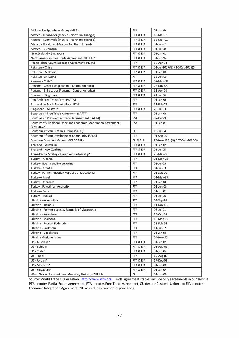
empirical part of the paper. Table A.1 in the Appendix lists RTAs in force by type and distinguishes

between agreements with environmental provisions and those without. We define RTA with

environmental provisions as those that according to the Regional Trade Agreements Information

System (RTA-IS) of the World Trade Organization (WTO) cover the topic “environment”.

In what follows we focus on two additional selected RTAs, namely the European Union (EU) and the

Euro-Med agreements, and describe the climate policies that have been included in the specific

agreements. Starting with the EU, an important number of climate-related initiatives have been

taken within the framework of this agreement since the early 1990s. Among them are the first

Community strategy to reduce CO2 emissions and improve energy efficiency in 1991 (materialized

into a Directive to promote electricity from renewable energy, voluntary commitments by car

makers to reduce CO2 emissions by 25 percent and proposals on the taxation of energy products)

and the European Climate Change Programme (ECCP) launched by the Commission in 2000. While

one of the most important initiatives of the ECCP I (2000-2004) was the EU Emissions Trading

System, the ECCP II explored other options to reduce Greenhouses Gas Emissions (GHG), as for

example carbon capture and storage. In 2007 an integrated approach to climate and energy policy

was launched with the commitment to convert the EU into a low carbon economy. With this aim, a

number of climate and energy targets have been set to be met by 2020. The three main targets,

known as the “20-20-20” targets are: a reduction in EU greenhouse gas emissions of at least 20

percent below 1990 levels; a 20 percent of EU energy consumption to come from renewable

10

resources; and a 20 percent reduction in primary energy use compared with projected levels, to be

achieved by improving energy efficiency.

As regards the EU-Mediterranean climate policy, three initiatives deserve to be mentioned in the

context of the Euro-Mediterranean Partnership. First, the DG Environment’s LIFE-Third Countries

programme that provided technical assistance and co-financed around 3506 environmental and

conservation projects in the Mediterranean region during the period 1992 to 2006. Second, the

Short and Medium Term Priority Environmental Action Programme (SMAP), which constitute the

common basis for environmental actions related to policies and funding at the regional and national

level and was financed by the MEDA programme (2000-2006). Finally, the “Horizon 2020” initiative

launched by the Commission in 2005 aimed at reducing pollution by 2020. This initiative targets

Mediterranean countries covered by the European Neighbourhood Policy (Algeria, Egypt, Israel,

Jordan, Lebanon, Libya, Morocco, Palestinian Authority, Syria and Tunisia), EU Member States and

the accession countries, which must also apply EU environment legislation. Existing environmental

instruments will be used to fulfil the commitments agreed upon under the Barcelona Convention. In

particular, this common initiative will finance projects to reduce pollution, includes also capacity-

building measures as the development of legislation and institutions to protect the environment and

includes monitoring and management of the initiative. It is worth noting that according to WTO only

two of these countries have environmental provisions in their interim agreements with the EU,

namely Tunisia and Jordan. However, as we have described above, since 2005 a number of projects

that target environmental issues has been financed by the EU in most of the Mediterranean

countries.

III. Trade, Regional Integration and Emissions: A Survey

After describing the theoretical mechanisms and the environmental provisions of selected RTAs, this

section briefly surveys the econometric studies dealing with the link between trade, regional

integration and the environment.

11

Antweiler et al. (2001), a widely cited study, extends the work of Grossman and Krueger (1991) and

develop a theoretical model based on the decomposition of the effect of trade on the environment

into scale, composition and technique effects. They estimate and add up these effects to explore the

overall effect of increased trade on the environment, thereby allowing for pollution haven and factor

endowment motives. Their results show that trade intensity per se is not significant. But, when

interacted with country characteristics, the estimated effect is positive, statistically significant and

small. When they add up the estimates of scale, technique and composition effects, they find that

increased trade causes a decline in sulfur dioxide concentrations concluding that freer trade seems

to be good for the environment. Dean (2002) uses a simple Heckscher-Ohlin model of international

trade with endogenous factor supply that can be affected by trade policy. It consists of a two-

equation system that captures the effect of trade liberalization on the environment through two

channels: its direct effect on the composition of output (the composition effect) and its indirect

effect via income growth (the technique effect). The author finds that a fall in trade restrictions has a

direct negative effect on environmental quality via the composition effect and an indirect positive

effect via the technique effect, the latter outweighs the former, suggesting that trade is good for

the environment. Cole and Elliot (2003) rely on Antweiler et al. (2001) to empirically test for the

effects of trade on emissions per capita, emission intensities and concentration levels for different

air and water pollutants. They find that results depend on how the dependent variable is measured

(concentrations versus emissions) and also vary by pollutant. Frankel and Rose (2005) use an EKC

framework to estimate the effects of trade on pollution concentration levels. As regressors they

consider per capita income and its square, trade, institutional quality9 and land area. They take into

account the endogeneity of income and trade, the former by adding lagged values of income and the

latter by using instrumental variables derived from the gravity model of bilateral trade. Their results

show that controlling for endogeneity does not affect the earlier findings. They find that trade has a

positive impact on air quality, but they do not find evidence for a ‘race to the bottom’ driven by

9 This variable is proxied by an indicator for democracy (polity), which ranges from -10 (strongly autocratic) to

+10 (strongly democratic) and is taken from the Polity IV project.

12

trade or support for the PHH. A shortcoming of this paper is that it uses a cross-section approach,

instead of using a panel data approach as most recent papers do. This means the study has a

possible weakness, since they do not control for unobserved heterogeneity that is time-invariant.

More recently, Managi et al. (2009) combine the specification derived from Antweiler et al. (2001)

and the use of instrumental variable estimations to correct for the endogeneity of income and trade.

They find that trade has a beneficial effect on the environment depending on the pollutant and the

country. OECD countries benefit from trade, whereas trade increases emissions in the case of Non

OECD countries. In addition, the net effect of a increase in international trade flows is also likely to

be determined by the subsequent change in trade patterns (composition effect) in which

connectivity may play a crucial role (Bensassi et al., 2011).

In this paper we will follow Managi et al. (2009) strategy to correct for the endogeneity of income

and trade in the emissions equation, but in addition we include RTAs with environmental provisions

as policy variable that could also affect emissions directly.

Stern (2007) is, to the best of our knowledge, the only study addressing the link between regional

integration and emissions convergence. The author investigates, using data from 1971 to 2003,

whether or not entry into NAFTA has led to a convergence in energy use and emissions of pollutants

in Mexico, the United States and Canada. Results show strong evidence of convergence for all

intensity indicators across the three countries towards a lower level. Although intensity initially rises

for some variables in Mexico, it eventually begins to fall after NAFTA comes into force. Per capita

measures for two pollutants (sulfur and NOx) also show convergence, but this is not the case for

energy and carbon. The latter variables drift moderately upwards. The state of technology in energy

efficiency and sulfur abatement is improving in all countries, although there is little, if any, sign of

convergence and NAFTA has no effect on the trend of technology diffusion. According to these

results, Mexico’s technology is improving at a slower rate than its two northern neighbors.

IV. Empirical Strategy

IV.1. Model Specification

13

First, along the same lines as Stern (2007), we aim to explore whether emissions converge for

countries involved in an RTA. In particular, we distinguish between agreements with and without

environmental provisions. We depart from Stern (2007) by adopting matching and difference-in-

differences estimation techniques that allow us to control for the endogeneity of the RTA variable in

the emissions equation and by using instrumental variables to address the endogeneity of other

control variables. Second, we will also examine the direct effect of RTAs on absolute pollution levels

to be able to infer whether converge is towards a lower or towards a higher level of emissions.

Our starting point is a simplified version of the determinants of emissions. Per-capita emissions

depend on population, land area per-capita, per-capita GDP and an openness ratio. These variables

are assumed to control for the scale, technique and composition effects10. Given that all the well-

established theories linking environment with income and openness indicate that the variables back

and forth between one another, we will control for the endogeneity of income and openness.

In order to test for the convergence of emissions, we estimate a log-linear emissions equation in

relative terms in which the dependent variable is the log of CO2 emissions of country i relative to

country j in period t (Emit/Emjt). The estimated model is given by,

where and refer to countries, and to the year. represents the pollution emissions gap

between a pair of countries . Popit (Popjt) is population in number of inhabitants in country i (j) in

year t. Landcapit (Landcapjt) is land area in squared kilometres per-capita, GDPcapit (GDPcapjt) is GDP

per capita at constant US dollars in country i (j) in year t. Openit (Openjt) refers to the openness ratio

measured as the sum of exports and imports divided by gross domestic product. Since GDPcap is

endogenously determined we use a set of instrumental variables for income taken from the growth

10

Our model considers the main factors affecting emissions in line with Martínez-Zarzoso and Maurotti (2011) and with Frankel and Rose (2005).

14

literature. Openness is endogenous too. We thus use a second set of instrumental variables for this

variable based on the estimation of a gravity model of trade using a large dataset on pair wise trade,

in particular we use Badinger’s specification of the model (Badinger, 2008). The exponent of the

fitted values across bilateral trading partners is aggregated to obtain a prediction of total trade for a

given country. A detail explanation is given in Section IV.2 below.

The absolute value of each relative term is considered in order to have only one interpretation of an

increase in the value of the variable, since any increase (decrease) implies divergence (convergence)

between both countries. For example, an increase in the left-hand-side variable in equation (1),

means that there is divergence in the emissions of countries. Two bilateral variables, namely

bilateral trade between countries i and j and the variable 11, are added to the basic

specification: is the amount of trade (exports and imports) between countries i and j in

year t and is a dummy variable taking the value of 1 if countries are involved in a regional

trade agreement in the considered year and zero otherwise. The sign of allows to test for the

convergence hypothesis. A positive sign means that the emissions gap between a pair of countries

that have an RTA increases, whereas a negative sign suggests convergence in the emissions gap of

countries linked by an RTA.

In order to assess the effect of RTAs effectively, its effect has to be isolated from any other variables

that might impact pollution level convergence as a result of RTAs. For instance, relative per-capita

GDPs, trade openness and bilateral trade variables might be influenced by RTAs. We also address

RTA endogeneity due to self selection intro agreements.

Next, the strategy we use to examine the direct effect of RTAs on absolute pollution levels is to

estimate Equation (1) above in absolute terms. The estimated equation is given by,

(2)

11

will be denoted as for simplicity.

itti

ititititit

RTA

OpenGDPLandcapPopEm

lnlnlnlnln 5432

15

where Emit, the natural logarithms of emissions in country i at time t, is the dependent variable. The

independent variables are the same as in Equation (1) in absolute terms, namely population, land

per capita, GDP per capita and multilateral openness in country i at time t, and RTAit is generated as

a weighted average using emissions in the partner countries as weights.

IV.2. Endogeneity issues

As emphasized by Frankel and Rose (2005), trade flows, regional agreements, pollutants’ emissions

and environmental regulations may affect income. Thereby, we instrument income with a number

of variables, namely lagged income (conditional convergence hypothesis), population, rates of

investment and human capital formation. The latter is approximated by the rate of school enrolment

(at the primary and secondary level). The predicted values of this equation are used to calculate

GDPcapit, GDPcapjt.We use a second set of instrumental variables for the openness ratio and the

bilateral trade variable based on the estimation of a gravity model of trade using a large dataset on

pair-wise trade flows. The standard gravity model states that trade between countries is positively

determined by their size (GDP, population and land area) and negatively determined by geographical

and cultural distance. The geographical variables are exogenously determined and hence are

suitable instruments for trade (Frankel and Romer (1999)). We follow the Badinger’s (2008)

specification of the gravity model. Real bilateral openness is regressed on population, land area,

distance, a common border dummy and a landlocked variable (which is the sum of a landlocked

dummy of countries i and j). Two other variables are included in order to be consistent with the

theoretical model: a measure of similarity of country size ( ) and remoteness

from the rest of the world (Remote).12 Finally, the exponent of the fitted values across bilateral

trading partners is aggregated to obtain a prediction of total trade for a given country.

The endogeneity of the RTA variable is addressed using matching techniques. These techniques

provide a simple way to deal with the selection induced by RTAs. Baier and Bergstrand (2004) give

evidence that country pairs involved in RTAs tend to share common economic and geographic

characteristics. Few studies use matching techniques to deal with the endogeneity of RTAs. Egger et

al. (2008) used a difference-in-differences panel matching estimator to examine primarily the effect

12

.

Where is a common continent dummy. This variable will then be equal to zero if countries are on the same

continent. Remote is then the log of the average value of the mean distances of countries i and j from all other countries.

16

of RTA formation on changes in shares of intra-industry trade. Baier and Bergstrand (2009) provide

the first cross section estimates of long-run treatment effects of free trade agreements (FTA) on

members’ bilateral international trade flows using non parametric matching econometrics. Their

findings show that matching estimators provide plausible estimates of the average treatment effects

of an RTA on the trade of members that actually form one. We follow a similar methodology to

match pairs of countries that have an RTA with similar pairs of countries that are not linked by any

RTA.

After obtaining the matched samples for each year, we use a difference-in-differences estimator to

evaluate the effect of the treated RTA variable on emissions convergence.

The effect of an RTA on the outcome13 ( which is the pollution emissions gap) of a pair of

countries is defined as the difference between the pollution emissions gap of a pair of countries

after enforcing an RTA and the outcome that these countries would have without an RTA. Put

differently, the impact of an RTA is measured by the change in the pair of countries’ outcome, which

is attributable to the RTA only.

The difference-in-differences (hereafter DID) approach is well suited to dealing with this question

(Meyer, 1994; Heckman et al., 1997). Considering the RTA process as a natural experiment, the DID

method evaluates the average effect of the treatment (here the RTA) on treated units (pairs of

countries linked by an RTA and denoted by ). The idea is that comparing the outcome of a pair

of countries before and after an RTA is not satisfactory because we do not have a counterfactual

(outcome variable for the pair of countries if they had not entered the RTA). In order to control for

this skew, the DID method compares the difference in outcome before and after the RTA for

participating countries to that for a control group. The latter is composed of pairs of countries that

have never been part of an RTA. These countries are referred to hereafter as .

13

We follow Bertrand and Zitouna (2008) in this section and adapt their empirical strategy to RTAs.

17

Formally, let be the outcome in period for a pair of countries which has been member of an

RTA. We denote the outcome for the same country pair assuming it was not linked by an RTA.

The effect of the RTA for this pair is then measured by

.

The average impact of the RTA is described by . Unfortunately, we cannot observe the

outcome for the same pair of countries both as a participant and as a nonparticipant in an RTA. In

other words, we cannot ascertain the outcome of the event of nonparticipation for a pair of

countries that signed a trade agreement or conversely. In order to overcome this difficulty, we

compare the evolution of the groups RTA and NRTA over time, assuming that they would have been

identical in the absence of RTA:

The terms and refer respectively to the period before and after the RTA. Hence, the

missing counterfactual value could be replaced by the state of country pairs before the agreement,

adjusted to take into account the growth in aggregate outcome:

Where

denotes the DID estimator that

assesses the impact of an RTA on participating countries. We obtain it by regressing data pooled

across the treatment (country pairs with RTA) and the control group (country pair without RTA). The

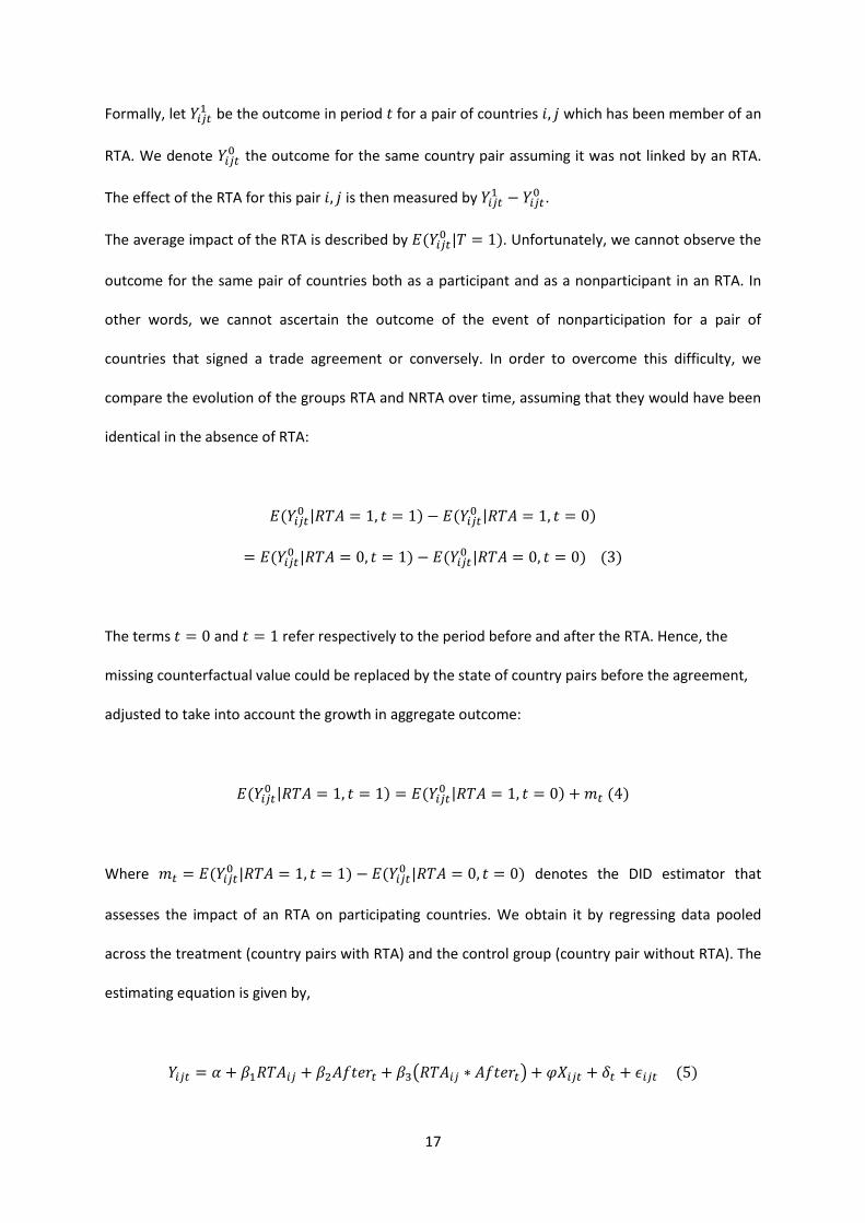
estimating equation is given by,

18

is a dummy variable taking a value 1 for treated country pairs and 0 otherwise. It controls for

differences in constant outcome between treated pairs of countries and the control group. We

define the dummy variable as taking a value 1 in the post-RTA years and 0 otherwise for both

RTA and non-RTA countries. This dummy variable controls for time effects on outcome . Finally,

the term is an interaction term between and . Its coefficient, ,

represents the DID estimator of the effect of an RTA on the treated group. A vector of the

characteristic ratio of a country’s pair is included to control for differences in observable attributes

between the treated and control group. The vector represents the ratio of some observable

features of a pair of countries at time . These observables are population, land area per capita,

GDP per capita, openness ratios and bilateral trade as presented in equation (1). denotes time-

specific dummies that control for factors common to all countries. is an idiosyncratic error term

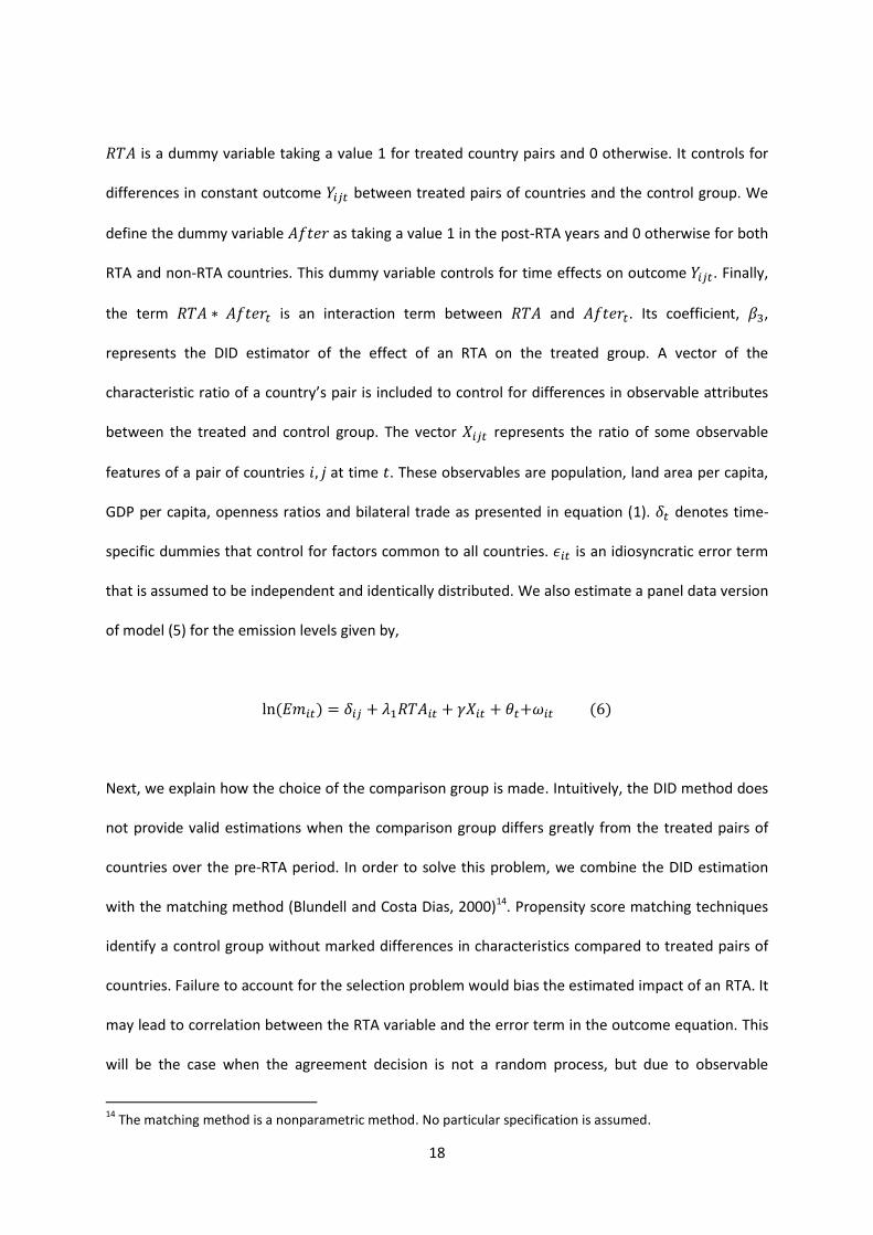
that is assumed to be independent and identically distributed. We also estimate a panel data version

of model (5) for the emission levels given by,

Next, we explain how the choice of the comparison group is made. Intuitively, the DID method does

not provide valid estimations when the comparison group differs greatly from the treated pairs of

countries over the pre-RTA period. In order to solve this problem, we combine the DID estimation

with the matching method (Blundell and Costa Dias, 2000)14. Propensity score matching techniques

identify a control group without marked differences in characteristics compared to treated pairs of

countries. Failure to account for the selection problem would bias the estimated impact of an RTA. It

may lead to correlation between the RTA variable and the error term in the outcome equation. This

will be the case when the agreement decision is not a random process, but due to observable

14

The matching method is a nonparametric method. No particular specification is assumed.

19

characteristics associated to a given trading pair of countries, such as distance, which also influences

the post-liberalization outcome. The propensity score method therefore controls for selection based

on observed characteristics. Furthermore, matching pairs of countries directly could require

comparing the groups RTA and NRTA across a large number of observable pre-liberalization

characteristics. The propensity score method reduces the dimensionality issue by capturing all the

information from these characteristics on a single basis (Rosenbaum and Rubin, 1983). In particular,

it measures the probability of signing the agreement according to a vector of pair wise variables. The

estimation of this probability value is as follows:

We use propensity score matching (PSM) to construct a statistical comparison group that is based on

a model of the probability of participating in the treatment, using observed characteristics.

Participants are then matched on the basis of this probability, or propensity score, to non

participants. We estimate a probit model given by,

where RGDPij denotes the sum of the real GDP of countries i and j .

Disij denotes the great circle distance between countries i and j.

Contiguity takes a value of one for countries that share a border, zero otherwise.

Common language takes a value of one for countries that have the same official language.

Once the propensity scores are estimated, observations from the treated group and the control

group are matched. Each treated pair of countries is associated with a pair of control countries

endowed with a similar propensity score15. We apply this econometric methodology to match pair of

countries linked and not linked by an RTA (with and without EPs) during the period 1980-2008.

15

We use the “calliper” matching method to select the control pairs of countries.

20

The validity of PSM depends on two conditions:

(a) Conditional independence (namely, that unobserved factors do not affect participation).

(b) Sizeable common support or overlap in propensity scores across the participant and non

participant sample.

The assumption of common support or overlap condition for matching on the propensity score is

that the estimated score is smaller than unity throughout. This condition ensures that treatment

observations have comparison observations “nearby” in the propensity score distribution (Heckman,

Lalonde, and Smith, 1999). The probability model provides us with an estimate of the propensity

score . In our case, the latter is to be interpreted as the likelihood of entering an RTA,

conditional on the observables. Next, we have to ensure that the treated units (new RTA members)

and the control units (the comparable subgroup of non-members) are similar with respect to every

observable . Thus, balancing tests will be conducted to verify whether the average propensity score

and mean is the same16.

We base our choice of explanatory variables in the probability model on Baier and Bergstrand

(2004). These authors show that gravity variables, namely GDP and distance, are the main

determinants of the formation of RTAs:

(i) Distance is used as a proxy for transport costs: two countries that are geographically

close will have lower transport costs. The lower the transport costs between countries,

the more each country can consume the other country’s varieties, enhancing trade

creation regionally and the formation of RTAs.

(ii) Incomes are used as a proxy of the economic size of the participating countries.

Other Variables that are associated to a higher probability of forming RTAs are contiguity and

common language, as proxies for trade facilitation.

16

A balancing score test and a T-test were conducted to check the differences within bands of the propensity score between treated and untreated country pairs.

21

V. Data, stylized Facts and Main Results

1. Data and Stylized Facts

The RTA data are taken from WTO website17. Distance, common language, contiguity and landlocked

dummies come from CEPII18. Bilateral trade flows are from UN-COMTRADE database and income,

investment, land area, population, school enrolment and emissions data are from the World

Development Indicators (World Bank, 2009).The sample covers 182 countries listed in Table A.2 and

the period dating from 1980 to 2008.

The main variables used in the emissions equation are per capita real gross domestic product

(GDPcap); per capita carbon dioxide emissions (Em) as a proxy for the level of pollution and

environmental degradation; the openness ratio (Open), which is calculated as exports plus imports

over GDP; total population (Pop), land area per capita in squared kilometers (Landcap), bilateral

trade as a share of total trade (Biltrade) and the RTA variable that takes a value of one if a pair of

countries is participating in the same RTA (with or without EP) and zero otherwise. The date of entry

into force of the RTAs is considered in the construction of this variable. All variables, apart from RTA,

are transformed by taking natural logarithms, such that the associated coefficients in the estimated

model can be interpreted as elasticities. Table A.3 in the Appendix shows the summary statistics for

the described variables.

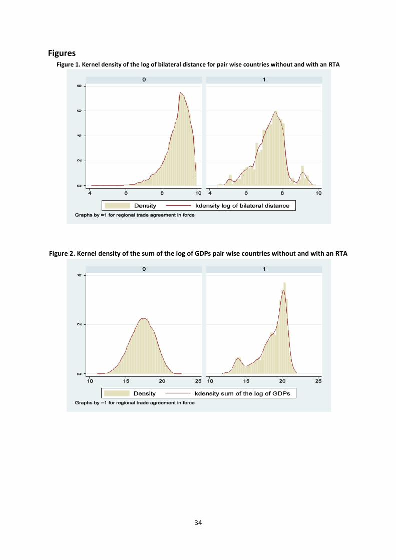
As shown by Baier and Bergstrand (2009), closer countries with a similar level of wealth are more

likely to join a free trade agreement. Table (1) reveals that the means of (ln) distance, sum of (ln)

gross domestic products and language and adjacency differ between countries linked by an RTA and

pairs of countries without an RTA. Countries linked by RTAs tend to be closer and richer. Moreover,

they are more likely to have common borders and share the same language than the rest19.

17

WTO web site (http://www.wto.org/english/tratop_e/region_e/region_e.htm). Programs for constructing data on RTAs are available at http://jdesousa.univ.free.fr/data.htm. 18

www.cepii.fr

22

Table 1. Summary of covariate means

Figures (1) and (2) show some differences in the bilateral distances between pairs of countries

involved and not involved in RTAs. Figure (1) shows that pairs of countries with an RTA are closer

than those without an RTA. The kernel densities function of (ln) bilateral distances for non-RTA pairs

of countries is more centered to the right in relation to the kernel density function of (ln) bilateral

distances for RTA pairs of countries.

Figure 1. Kernel density of the log of bilateral distance for pair wise countries without and with an

RTA

Figure (2) shows that country pairs with an RTA tend to be larger economically. The Kernel density

function for countries with an RTA is centered to the right in comparison to pairs without one.

Figure 2. Kernel density of the sum of the log of GDPs pair wise countries without and with an RTA

2. Main Results

The matching was implemented for each single year. Country pairs for each year in which there was

at least one agreement (year by year) are matched with country pairs without an agreement using

propensity matching scores and then a dataset was created with the matched data20.

Based on the pooled cross-section data, Table A.4 in the Appendix displays the efficiency of the

matching procedure for RTAs. The balancing property is verified21. The reduction in bias22 is drastic

20

The Stata command pscore was used to check that the balancing property is satisfied (number of blocks between 5 and 8) and the command psmatch2 with a calliper (0.01) was used for the matching (years with matching and common support satisfied: 1981, 1983, 1986, 1991, 1992, 1993, 1994, 1995, 1996, 1997-1998 and 1999-2008). 21 For each independent variable, the difference between target and control countries is checked by employing

a T-test on the differences within bands of the propensity score. 22

The bias could be defined as the difference of the sample mean in the treated and non treated sub-samples divided by the square root of the average of the sample variances in the treated and non treated groups.

23

when the bias is initially high. Thus, this method provides a valid group of countries to which we will

compare changes in target countries’ performance.

In order to illustrate the estimations used for the matching, the first column of Table 2 shows the

results from pooled cross-section estimations for the determinants of the decision to enter into an

RTA for all country pairs (equation 8). It supports the stylized facts and shows that economic

characteristics and geographic conditions are the main determinants of the decision to join an RTA

for the whole sample. Column 2 (Table 2) shows that the same set of factors are statistically

significant for the selected (matched) sample (Results in Table 2 are obtained for all RTAs).

Table 2. Determinants of RTAs

Next, Equation (5) is estimated using OLS with time dummies. The main results are shown in Table 3.

Columns (1) and (2) show the results for all RTAs for the matched sample and for the whole sample,

respectively. Next, columns (3) and (4) show the same two sets of results for RTAs with EPs and

columns (5) and (6) for RTAs without EPs. The time effects are included in order to capture time

trends that may affect emissions and are common for all countries.

Table 3. Emissions pollution gap and economic integration

Looking at the results for the matched sample, the coefficient of the target variable, interaction

variable (RTAij*Aftert), is negative and statistically significant only when RTAs with EPs are considered

(column 3). Countries involved in RTAs with EP converge in terms of CO2 emissions after the entry

into force of the agreements. This negative sign can be interpreted as supporting evidence for

emission convergence. Our preferred specification, with the difference-in-differences and matching

techniques, displays a coefficient of -0.20. Hence, the gap in emissions per capita between countries

involved in an RTA with EP is around 20 percent lower than for countries without an RTA. We have

24

to underline the fact that the effect of RTA participation is not statistically significant for agreements

that do not include environmental provisions, indicating that emissions do not seem to converge due

to RTA participation in agreements that do not include EPs.

The results obtained for the whole sample (without matching) indicated that the RTA effect was very

similar for the RTAs with EPs (estimated coefficient is significant and equal to 0.247 versus 0.202 in

the matched sample) but not for the RTAs without. In this case the effect was statistically significant

at the one percent level with a magnitude equal to 0.36323 supporting a convergence in pollution

levels.

With respect to the control variables, our results show that population and gross domestic product

per capita ratios are positively related to the emissions gap. These variables are used as control

variables and are assumed to capture the scale and technique effect respectively. Convergence in

the scale of the economy as well as in technology is positively correlated to convergence in

emissions of CO2 for pairs of countries. As regards the land-ratio, countries that have a more similar

land allocation tend to have more similar emission levels. Concerning the openness ratio, the

corresponding estimated coefficient is negative, indicating that greater differences in trade

openness tend to reduce the emissions gap between trading partners. Conversely, bilateral trade is

negatively related to the emissions gap, indicating that countries that trade relatively more with

each other tend to have higher emission gaps. In a second step, similar estimations are obtained for

the Euro-Med agreements (European Union countries and southern Mediterranean countries:

Morocco, Algeria, Tunisia, Egypt, Jordan and Turkey). This agreement is of special interest because

the EU has been providing with funds to the South Mediterranean countries to improve their

environmental standards since the 1990s, even before the bilateral interim agreements entered into

force. Estimates of equation 5 with time effects are shown in columns (1) and (2) in Table 4. As

before, we first estimate equation (5) for the matched sample, namely the pairs of countries linked

by a Euro-Med agreement (treated units) and pairs of similar countries (selected control group) in

23

Results are available upon request from the authors.

25

column (1). Second, Equation (5) is estimated for all pairs of countries, namely those involved in

Euro-Med agreements (treated sample) and those not involved in any RTA in column (2). The results

shown in Table 4 indicate that the RTA effect is negative and significant and similar in magnitude to

the one obtained for environmental agreements with EPs in Table 3. Indeed, the interaction variable

(EUROMEDij*Aftert) that proxies the Euro-Med membership effect on the emissions gap displays a

coefficient of (-0.20) in the preferred specification. Hence, the gap in per capita emissions between

countries involved in a Euro-Med agreement is almost 25 percent ((exp(-0.204)-1)*100) lower than

for similar countries without an RTA. Therefore, the Euro-Med agreement fosters convergence of

CO2 emissions.

Table 4. Emissions pollution gap and specific agreements

Similarly, columns (3) and (4) in Table 4 show the results obtained when comparing EU-27 countries

to countries not involved in any RTA. In this case the estimated coefficient of (EUij*Aftert) is also

negative and statistically significant and larger than for EUROMED (0.32 versus 0.20). It is worth

noting that the EU-27 agreement entail higher convergence of emissions than the average effect of

all RTAs.

Columns (5) and (6) in Table 4 show the effect of being a NAFTA member on emissions convergence.

Interestingly, whereas both the results for the whole sample (column (5)) as well as the results of the

matched sample (column (6)) show a non-significant effect of NAFTA, the estimations using the

whole sample displaying a stronger negative effect. Indeed very few comparison countries were

found using the matching techniques, which restricted the sample to only 107 observations. Finally,

Columns (7) and (8) in Table 4 show the effect of being an AFTA member on emissions convergence.

Not surprisingly, both the results for the whole sample (column (8)) as well as the results of the

matched sample (column (7)) show a non-significant effect of AFTA, the estimations using matching

and difference-in-difference techniques displaying a lower negative effect.

26

Finally, Table 5 presents the estimates obtained when model (6) is estimated. The main results

indicate that emissions are around 3 percent lower for countries that have RTAs with EPs, whereas

the effect is not statistically significant for countries with RTAs without EPs. Hence emissions

converge to a lower level when both countries belong to the same RTA and the RTA includes

environmental provisions.

VI. Conclusions

This paper examines the impact of regional integration on CO2 emissions. We adopted a reduced-

form specification linked to the emissions convergence hypothesis in which relative emissions are

explained using income, population, land area, openness in relative terms, bilateral trade and a

dummy for RTA agreements. The model is estimated using a difference-in-differences approach

paying special attention to the potential selection induced by RTAs and to the endogeneity of

income and trade variables. A propensity matching technique is used to treat RTAs and to extract a

sub-sample containing only matched pairs of countries that share similar characteristics.

Our results consistently indicate that RTAs that specifically include environmental provisions foster

convergence of CO2 emissions. In particular, the gap in emissions per capita is about twenty percent

lower for pairs of countries with RTAs with environmental harmonization policies embedded than

for the rest when the matched sample is used.

As regards to specific agreements our estimations indicate that the emissions pollution gap is 20

percent lower for pairs of countries involved in Euro-Mediterranean Agreements than for similar

pairs of countries not involved in RTAs. The effect is more pronounced for EU-27 pairs of countries,

for which the emission gap is more than thirty percent lower than for similar non-EU-27 countries. It

is worth noting that reductions in the emissions gap stemming from a deeper integration agreement,

like the EU, are larger than those related to a North-South trade agreement such as the Euro-

Mediterranean agreement. One final result indicates that we are not able to precisely identify an

effect for NAFTA due to the lack of appropriate comparison pair of countries.

27

The main economic policy recommendation that can be derived from our results is that only regional

integration processes that include environmental harmonization policies will be able to help

reducing or at least controlling emissions levels.

Moreover, higher levels of integration usually go hand in hand with more strict environmental

regulations that are common for all its members, namely the EU integration, appear to be linked to

greater reductions in the above mentioned pollution gap in comparison to other agreements.

Further research concerning other pollutants is also desirable to ascertain whether the link between

regional trade agreements and pollution convergence is in place.

28

References

Antweiler W., B. R. Copeland and M. S. Taylor, (2001), “Is free trade good for the environment?”, American Economic Review, 91(4), 877-908.

Badinger H., (2008), “Trade policy and productivity”, European Economic Review, 52, 867-891.

Baier S.L. and J.H. Bergstrand, (2009), “Estimating the effects of free trade agreements on international trade flows using matching econometrics”, Journal of International Economics, 77, 63–76.

Baier S.L. and J. H. Bergstrand, (2004), “Economic determinants of free trade agreements”, Journal of International Economics, 64(1), 29–63.

Ben-David D., (1993), “Equalizing Exchange: trade Liberalization and income convergence”, Quarterly Journal of Economics, 108(3), 653-679.

Bertrand O. and H. Zitouna (2008), “Domestic versus cross-border acquisitions: which impact on the target firms’ performance”, Applied Economics, 40, 2221-2238.

Bensassi, S., L. Márquez-Ramos, I. Martínez-Zarzoso and H. Zitouna, (2011), “The geography of trade and the environment: The case of CO2 emissions”, Cremed Working Paper 9, Center for Research on the Economies of the Mediterranean, Barcelona, Spain.

Blundell R. and M. Costa Dias, (2000), “Evaluation methods for non-experimental data”, Fiscal Studies, 21, 427–68.

Copeland B.R. and S. Gulati, (2006), “Trade and the environment in developing countries”, in R. Lopez and M.A. Toman (eds), Economic Development and Environmental Sustainability: New Policy Options, Oxford: Oxford University Press, 178-216.

Cole M.A. and R.J.R. Elliott, (2003), “Determining the trade-environment composition effect: the role of capital, labor and environmental regulations”, Journal of Environmental Economics and Management, 46(3), 363-83.

Copeland B.R. and M.S. Taylor, (2003), “Trade and the environment: theory and evidence”, Princeton, NJ: Princeton University Press.

Dean J. M., (2002), “Does trade liberalization harm the environment? a new test'”, Canadian Journal of Economics, 35, 819-842.

Dollar D., (1992), “Outward-oriented developing economies really do grow more rapidly: evidence from 95 LDCs, 1976-1985”, Economic Development and Cultural Change, 523-544.

Edwards S., (1998), “Openness, productivity and growth: what do we really know?”, Economic Journal, 108, 383-398.

Egger H., P. Egger, and D. Greenaway, (2008), “The trade structure effects of endogenous regional trade agreements”, Journal of International Economics, 74, 278-298.

Frankel J. and D. Romer, (1999), “Does trade cause growth?”, American Economic Review, 89(3), 379-399.

Frankel J.A. and A.K. Rose, (2005), “Is trade good or bad for the environment? Sorting out the causality”, The Review of Economics and Statistics, 87, 85-91.

Grossman G.M. and A.B. Krueger, (1991), “Environmental impacts of the North American Free Trade Agreement”, NBER working paper 3914.

Heckman J., H. Ichimura, J. Smith and P. Todd, (1997), “Matching as an econometric evaluation estimator: evidence from evaluating a job training programme”, Review of Economic Studies, 64, 605–54.

29

Heckman J., R. LaLonde, and J. Smith, (1999), “The economics and econometrics of active labor market programs.”, Handbook of Labor Economics, 31865-2097. Amsterdam: North-Holland.

Jakob M., M. Haller and R. Marschinski, (2011), “Will history repeat itself? Economic convergence and convergence of energy use patterns”, Potsdam Institute for Climate Impact Research (PIK), Energy Economics, forthcoming.

Kuznets S., (1955), “Economic growth and income inequality”, The American Economic Review, 45(1), 1-28.

Managi S., A. Hibiki and T. Tsurumi, (2009), “Does trade openness improve environmental quality?”, Journal of Environmental Economics and Management, 58(3), 346-363.

Martínez-Zarzoso and Maurotti, (2011) “The Impact of Urbanization on CO2 Emissions: Evidence from Developing Countries”, Ecological Economics 70, 1344-1353.

Mathys N., (2002), “In search of evidence for the pollution haven hypothesis”, Mémoire de Licence, Université de Neuchâtel.

Meyer B. D., (1994), “Natural and quasi-experiments in economics”, NBER Technical Working Paper 170.

Porter M.E. and C. Van der Linde, (1995), “Toward a new conception of the environment-competitiveness relationship”, Journal of Economic Perspectives, 9, 97-118.

Rodriguez F. and D. Rodrik, (2000), “Trade policy and economic growth: a skeptic's guide to the cross-national evidence”. NBER Macroeconomics Annual 2000. Washington, D.C.

Rosenbaum P. and D. B. Rubin, (1983), “The central role of the propensity score in observational studies for causal effects”, Biometrika, 70, 41–55.

Sachs J. and A. Warner, (1995), “Economic reform and the process of global integration”, Brookings Papers on Economic Activity, 1-118.

Stern D., (2007), “The effect of NAFTA on energy and environmental efficiency in Mexico”, The Policy Studies Journal, 35(2), 291-322.

Taylor S.M., (2004), “Unbundling the pollution haven hypothesis”, Advances in Economic Analysis and Policy, 4(2).

30

Tables

Table 1: Summary of covariate means

Country pairs with an RTA Country pairs without an RTA

Ln of distance 7.34 8.86

Sum of the ln of GDPs 18.64 17.31

Adjacency dummy 0.13 0.009

Language dummy 0.26 0.15

Table 2. Determinants of RTAs

Model 1 Model 2

All Matched

Sum of the ln of GDPs 0.205*** 0.127***

[0.0034] [0.0059]

Ln distance -0.955*** -0.212***

[0.00708] [0.011]

Contiguity 0.0620** 0.297***

[0.0262] [0.0383]

Common language 0.102*** 0.110***

[0.0151] [0.0239]

Pseudo R2 0.395 0.032

Observations 201,558 25,629

Standard errors in parentheses. *** p<0.01, ** p<0.05, * p<0.1

31

Table 3. Emissions pollution gap and economic integration for RTAs with and without

environmental provisions (EP)

All RTAs All RTAs With EP With EP Without EP Without EP

VARIABLES Matched All Matched All Matched All

RTAij*Aftert -0.0367 -0.324*** -0.202*** -0.247*** -0.00858 -0.363***

[0.0473] [0.0420] [0.0561] [0.0454] [0.0464] [0.0468]

Abs Ln population ratio 0.837*** 0.694*** 0.841*** 0.680*** 0.847*** 0.682***

[0.00838] [0.00448] [0.00868] [0.00495] [0.00733] [0.00468]

Abs Ln land per capita ratio 0.0666*** 0.0542*** 0.0604*** 0.0434*** 0.0623*** 0.0556***

[0.00924] [0.00507] [0.00960] [0.00569] [0.00782] [0.00527]

Abs Ln GDP per capita 0.124*** 0.381*** 0.207*** 0.414*** 0.0990*** 0.376***

predicted ratio [0.0116] [0.00543] [0.0116] [0.00573] [0.0106] [0.00561]

Abs Ln Openness -0.0829*** -0.138*** 0.0249 -0.138*** -0.102*** -0.153***

predicted ratio [0.0189] [0.0110] [0.0204] [0.0123] [0.0165] [0.0113]

Abs Ln bilateral trade 0.160*** 0.126*** 0.133*** 0.129*** 0.124*** 0.133***

predicted (ij) [0.00477] [0.00306] [0.00433] [0.00356] [0.00421] [0.00340]

Time Fixed Effects Yes Yes Yes Yes Yes Yes

Observations 13,449 61,945 12,715 52,969 15,873 56,898

R-squared 0.581 0.437 0.606 0.416 0.592 0.421

Robust standard errors in brackets

*** p<0.01, ** p<0.05, * p<0.1

32

Table 4. Emissions pollution gap and specific agreements

EUROMED EUROMED EU27 EU27 NAFTA NAFTA AFTA AFTA

VARIABLES Matched All Matched All Matched All Matched All

RTAij*Aftert -0.204*** -0.520*** -0.318*** -0.239*** -0.0105 -0.397 -0.175 -0.240

[0.0649] [0.0536] [0.0808] [0.0446] [0.188] [0.256] [0.129] [0.154]

Abs Ln population 0.814*** 0.661*** 0.808*** 0.679*** 0.675*** 0.664*** 0.827*** 0.663***

ratio [0.0100] [0.00509] [0.0105] [0.00499] [0.0905] [0.00522] [0.0270] [0.00520]

Abs Ln land per capita 0.119*** 0.0478*** 0.116*** 0.0442*** -0.845*** 0.0421*** 0.0338 0.0426***

ratio [0.0106] [0.00580] [0.0121] [0.00574] [0.0463] [0.00593] [0.0374] [0.00593]

Abs Ln GDP per capita 0.0623*** 0.402*** 0.109*** 0.412*** -0.421*** 0.409*** 0.0714** 0.408***

predicted ratio [0.0142] [0.00580] [0.0187] [0.00588] [0.101] [0.00592] [0.0328] [0.00591]

Abs Ln Openness -0.148*** -0.172*** 0.0200 -0.140*** -0.0361 -0.157*** -0.543*** -0.158***

predicted ratio [0.0236] [0.0125] [0.0262] [0.0124] [0.409] [0.0127] [0.0818] [0.0127]

Abs Ln bilateral trade 0.156*** 0.144*** 0.0773*** 0.128*** 0.216*** 0.139*** 0.0844*** 0.139***

predicted (ij) [0.00551] [0.00381] [0.00468] [0.00366] [0.0179] [0.00400] [0.0145] [0.00399]

Constant -1.840*** -1.927*** -0.871*** -1.727*** -1.351*** -1.872*** -0.656* -1.878***

[0.141] [0.0903] [0.145] [0.0883] [0.359] [0.0938] [0.363] [0.0937]

Time Fixed Effects Yes Yes Yes Yes Yes Yes

Observations 9,187 50,921 7,685 51,599 107 47,988 Yes Yes

R-squared 0.600 0.403 0.629 0.414 0.956 0.391 1,569 48,125

Robust standard errors in brackets 0.556 0.392

*** p<0.01, ** p<0.05, * p<0.1

Robust standard errors in brackets

*** p<0.01, ** p<0.05, * p<0.1

33

Table 5. Emissions and economic integration for RTAs with and without environmental provisions

(EP)

Effect on Total Emissions

ALL RTAs RTAs with Environmental Prov RTAs without Environmental Prov

Matched All Matched All Matched All

RTA Effect -.0151** -.000317* -.025*** -.00306** .0000373 -.000747

(0.006) (0.000) (0.007) (0.001) (0.001) (0.001)

Ln population -1.45 .818 -5.44*** .8 00 -2.36** .835

(0.987) (1.213) (1.495) (1.237) (0.987) (1.225)

Ln land per capita -3.01*** -.799 -6.55*** -.754 -3.71*** -.785

(1.028) (1.191) (1.281) (1.217) (1.016) (1.204)

Ln GDP per capita .265 .830*** .884*** .833*** .485** .829***

predicted (0.179) (0.107) (0.269) (0.105) (0.213) (0.107)

Ln Openness -.00718 -.0754 -.0168 -.0812 -.125 -.0696

predicted (0.137) (0.102) (0.123) (0.102) (0.112) (0.104)

N 845 2227 521 2227 324 2227

R-squared 0.738 0.707 0.714 0.712 0.741 0.707

Robust standard errors in brackets *** p<0.01, ** p<0.05, * p<0.1

34

Figures Figure 1. Kernel density of the log of bilateral distance for pair wise countries without and with an RTA

Figure 2. Kernel density of the sum of the log of GDPs pair wise countries without and with an RTA

35

Appendix

Table A.1. List of RTA types and dates of entry into force

RTA Name Type Date of entry into force

Andean Community (CAN) CU 25-May-88

Armenia - Kazakhstan FTA 25-Dec-01

Armenia - Moldova FTA 21-Dec-95

Armenia - Russian Federation FTA 25-Mar-93

Armenia - Turkmenistan FTA 07-Jul-96

Armenia - Ukraine FTA 18-Dec-96

ASEAN - China PSA & EIA 01-Jan-2005(G) / 01-Jul-2007(S)

ASEAN Free Trade Area (AFTA) FTA 28-Jan-92

Asia Pacific Trade Agreement (APTA) PSA 17-Jun-76

Asia Pacific Trade Agreement (APTA) - Accession of China PSA 01-Jan-02

Australia - New Zealand (ANZCERTA) FTA & EIA 01-Jan-1983(G) / 01-Jan-1989(S)

Australia - Papua New Guinea (PATCRA) FTA 01-Feb-77

Canada - Chile* FTA & EIA 05-Jul-97

Canada - Costa Rica* FTA 01-Nov-02

Canada - Israel FTA 01-Jan-97

Caribbean Community and Common Market (CARICOM) CU & EIA 01-Aug-1973(G) / 04-Jul-2002(S)

Central American Common Market (CACM) CU 04-Jun-61

Central European Free Trade Agreement (CEFTA) 2006 FTA 01-May-07

Chile - China* FTA & EIA 01-Oct-2006(G) / 01-Aug-2010(S)

Chile - Costa Rica (Chile - Central America) FTA & EIA 15-Feb-02

Chile - El Salvador (Chile - Central America) FTA & EIA 01-Jun-02

Chile - Japan* FTA & EIA 03-Sep-07

Chile - Mexico* FTA & EIA 01-Aug-99

China - Hong Kong, China FTA & EIA 29-Jun-03

China - Macao, China FTA & EIA 17-Oct-03

Common Economic Zone (CEZ) FTA 20-May-04

Common Market for Eastern and Southern Africa (COMESA)* CU 08-Dec-94

Commonwealth of Independent States (CIS) FTA 30-Dec-94

Costa Rica - Mexico* FTA & EIA 01-Jan-95

Dominican Republic - Central America - United States Free Trade Agreement (CAFTA-DR)

FTA & EIA 01-Mar-06

East African Community (EAC) CU 07-Jul-00

EC (10) Enlargement CU 01-Jan-81

EC (12) Enlargement CU 01-Jan-86

EC (15) Enlargement CU & EIA 01-Jan-95

EC (25) Enlargement CU & EIA 01-May-04

EC (27) Enlargement CU & EIA 01-Jan-07

EC (9) Enlargement CU 01-Jan-73

EC Treaty CU & EIA 01-Jan-58

Economic and Monetary Community of Central Africa (CEMAC)* CU 24-Jun-99

Economic Community of West African States (ECOWAS) CU 24-Jul-93

Economic Cooperation Organization (ECO) PSA 17-Feb-92

EFTA - Chile FTA & EIA 01-Dec-04

EFTA - Croatia FTA 01-Jan-02

EFTA - Egypt FTA 01-Aug-07

EFTA - Former Yugoslav Republic of Macedonia FTA 01-May-02

EFTA - Israel FTA 01-Jan-93

EFTA - Jordan FTA 01-Sep-02

EFTA - Korea, Republic of FTA & EIA 01-Sep-06

EFTA - Lebanon FTA 01-Jan-07

EFTA - Mexico FTA & EIA 01-Jul-01

EFTA - Morocco FTA 01-Dec-99

EFTA - Palestinian Authority FTA 01-Jul-99

EFTA - SACU FTA 01-May-08

EFTA - Singapore FTA & EIA 01-Jan-03

36

EFTA - Tunisia FTA 01-Jun-05

EFTA - Turkey FTA 01-Apr-92

EFTA accession of Iceland FTA 01-Mar-70

Egypt - Turkey FTA 01-Mar-07

EU - Albania FTA & EIA 01-Dec-2006(G) / 01-Apr-2009(S)

EU - Algeria FTA 01-Sep-05

EU - Andorra CU 01-Jul-91

EU - Bosnia and Herzegovina FTA 01-Jul-08

EU - Chile FTA & EIA 01-Feb-2003(G) / 01-Mar-2005(S)

EU - Croatia FTA & EIA 01-Mar-2002(G) / 01-Feb-2005(S)

EU - Egypt FTA 01-Jun-04

EU - Faroe Islands FTA 01-Jan-97

EU - Former Yugoslav Republic of Macedonia FTA & EIA 01-Jun-2001(G) / 01-Apr-2004(S)

EU - Iceland FTA 01-Apr-73

EU - Israel FTA 01-Jun-00

EU - Jordan* FTA 01-May-02

EU - Lebanon FTA 01-Mar-03

EU - Mexico FTA & EIA 01-Jul-2000(G) / 01-Oct-2000(S)

EU - Montenegro FTA & EIA 01-Jan-2008(G) / 01-May-2010(S)

EU - Morocco FTA 01-Mar-00

EU - Norway FTA 01-Jul-73

EU – Overseas Countries and Territories (OCT) FTA 01-Jan-71

EU - Palestinian Authority FTA 01-Jul-97

EU - South Africa FTA 01-Jan-00

EU - Switzerland - Liechtenstein FTA 01-Jan-73

EU - Syria FTA 01-Jul-77

EU - Tunisia* FTA 01-Mar-98

EU - Turkey CU 01-Jan-96

Eurasian Economic Community (EAEC) CU 08-Oct-97

European Economic Area (EEA) EIA 01-Jan-94

European Free Trade Association (EFTA) FTA & EIA 03-May-1960(G) / 01-Jun-2002(S)

Faroe Islands - Norway FTA 01-Jul-93

Faroe Islands - Switzerland FTA 01-Mar-95

Georgia - Armenia FTA 11-Nov-98

Georgia - Azerbaijan FTA 10-Jul-96

Georgia - Kazakhstan FTA 16-Jul-99

Georgia - Russian Federation FTA 10-May-94

Georgia - Turkmenistan FTA 01-Jan-00

Georgia - Ukraine FTA 04-Jun-96

Global System of Trade Preferences among Developing Countries (GSTP) PSA 19-Apr-89

Gulf Cooperation Council (GCC) CU 01-Jan-03

Iceland - Faroe Islands FTA & EIA 01-Nov-06

India – Bhutan FTA 29-Jul-06

India – Singapore FTA & EIA 01-Aug-05

India - Sri Lanka FTA 15-Dec-01

Israel – Mexico FTA 01-Jul-00

Japan - Malaysia* FTA & EIA 13-Jul-06

Japan - Mexico* FTA & EIA 01-Apr-05

Japan – Singapore FTA & EIA 30-Nov-02

Jordan – Singapore FTA & EIA 22-Aug-05

Korea, Republic of – Chile FTA & EIA 01-Apr-04

Korea, Republic of - Singapore* FTA & EIA 02-Mar-06

Kyrgyz Republic – Armenia FTA 27-Oct-95

Kyrgyz Republic – Kazakhstan FTA 11-Nov-95

Kyrgyz Republic – Moldova FTA 21-Nov-96

Kyrgyz Republic - Russian Federation FTA 24-Apr-93

Kyrgyz Republic – Ukraine FTA 19-Jan-98

Kyrgyz Republic – Uzbekistan FTA 20-Mar-98

Lao People's Democratic Republic - Thailand PSA 20-Jun-91

Latin American Integration Association (LAIA) PSA 18-Mar-81

37

Melanesian Spearhead Group (MSG) PSA 01-Jan-94

Mexico - El Salvador (Mexico - Northern Triangle) FTA & EIA 15-Mar-01

Mexico - Guatemala (Mexico - Northern Triangle) FTA & EIA 15-Mar-01

Mexico - Honduras (Mexico - Northern Triangle) FTA & EIA 01-Jun-01

Mexico – Nicaragua FTA & EIA 01-Jul-98

New Zealand – Singapore FTA & EIA 01-Jan-01

North American Free Trade Agreement (NAFTA)* FTA & EIA 01-Jan-94

Pacific Island Countries Trade Agreement (PICTA) FTA 13-Apr-03

Pakistan – China FTA & EIA 01-Jul-2007(G) / 10-Oct-2009(S)

Pakistan – Malaysia FTA & EIA 01-Jan-08

Pakistan - Sri Lanka FTA 12-Jun-05

Panama - Chile* FTA & EIA 07-Mar-08

Panama - Costa Rica (Panama - Central America) FTA & EIA 23-Nov-08

Panama - El Salvador (Panama - Central America) FTA & EIA 11-Apr-03

Panama – Singapore FTA & EIA 24-Jul-06

Pan-Arab Free Trade Area (PAFTA) FTA 01-Jan-98

Protocol on Trade Negotiations (PTN) PSA 11-Feb-73

Singapore – Australia FTA & EIA 28-Jul-03

South Asian Free Trade Agreement (SAFTA) FTA 01-Jan-06

South Asian Preferential Trade Arrangement (SAPTA) PSA 07-Dec-95

South Pacific Regional Trade and Economic Cooperation Agreement (SPARTECA)

PSA 01-Jan-81

Southern African Customs Union (SACU) CU 15-Jul-04

Southern African Development Community (SADC) FTA 01-Sep-00

Southern Common Market (MERCOSUR) CU & EIA 29-Nov-1991(G) / 07-Dec-2005(S)

Thailand – Australia FTA & EIA 01-Jan-05

Thailand - New Zealand FTA & EIA 01-Jul-05

Trans-Pacific Strategic Economic Partnership* FTA & EIA 28-May-06

Turkey – Albania FTA 01-May-08

Turkey - Bosnia and Herzegovina FTA 01-Jul-03

Turkey – Croatia FTA 01-Jul-03

Turkey - Former Yugoslav Republic of Macedonia FTA 01-Sep-00

Turkey – Israel FTA 01-May-97

Turkey – Morocco FTA 01-Jan-06

Turkey - Palestinian Authority FTA 01-Jun-05

Turkey – Syria FTA 01-Jan-07

Turkey – Tunisia FTA 01-Jul-05

Ukraine – Azerbaijan FTA 02-Sep-96

Ukraine – Belarus FTA 11-Nov-06

Ukraine - Former Yugoslav Republic of Macedonia FTA 05-Jul-01

Ukraine - Kazakhstan FTA 19-Oct-98

Ukraine - Moldova FTA 19-May-05

Ukraine - Russian Federation FTA 21-Feb-94

Ukraine - Tajikistan FTA 11-Jul-02

Ukraine - Uzbekistan FTA 01-Jan-96

Ukraine -Turkmenistan FTA 04-Nov-95

US - Australia* FTA & EIA 01-Jan-05

US - Bahrain FTA & EIA 01-Aug-06

US - Chile* FTA & EIA 01-Jan-04

US - Israel FTA 19-Aug-85

US - Jordan* FTA & EIA 17-Dec-01

US - Morocco* FTA & EIA 01-Jan-06

US - Singapore* FTA & EIA 01-Jan-04

West African Economic and Monetary Union (WAEMU) CU 01-Jan-00

Source: World Trade Organization. http://www.wto.org. Trade agreements tables include only agreements in our sample. PTA denotes Partial Scope Agreement, FTA denotes Free Trade Agreement, CU denote Customs Union and EIA denotes Economic Integration Agreement. *RTAs with environmental provisions.

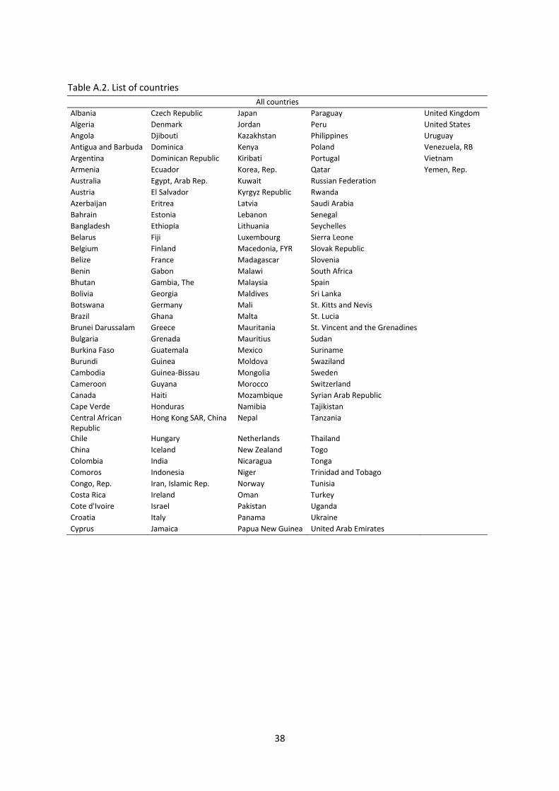
38

Table A.2. List of countries

All countries

Albania Czech Republic Japan Paraguay United Kingdom

Algeria Denmark Jordan Peru United States

Angola Djibouti Kazakhstan Philippines Uruguay

Antigua and Barbuda Dominica Kenya Poland Venezuela, RB

Argentina Dominican Republic Kiribati Portugal Vietnam

Armenia Ecuador Korea, Rep. Qatar Yemen, Rep.

Australia Egypt, Arab Rep. Kuwait Russian Federation

Austria El Salvador Kyrgyz Republic Rwanda

Azerbaijan Eritrea Latvia Saudi Arabia

Bahrain Estonia Lebanon Senegal

Bangladesh Ethiopia Lithuania Seychelles

Belarus Fiji Luxembourg Sierra Leone

Belgium Finland Macedonia, FYR Slovak Republic

Belize France Madagascar Slovenia

Benin Gabon Malawi South Africa

Bhutan Gambia, The Malaysia Spain

Bolivia Georgia Maldives Sri Lanka

Botswana Germany Mali St. Kitts and Nevis

Brazil Ghana Malta St. Lucia

Brunei Darussalam Greece Mauritania St. Vincent and the Grenadines

Bulgaria Grenada Mauritius Sudan

Burkina Faso Guatemala Mexico Suriname

Burundi Guinea Moldova Swaziland

Cambodia Guinea-Bissau Mongolia Sweden

Cameroon Guyana Morocco Switzerland

Canada Haiti Mozambique Syrian Arab Republic

Cape Verde Honduras Namibia Tajikistan

Central African Republic

Hong Kong SAR, China Nepal Tanzania

Chile Hungary Netherlands Thailand

China Iceland New Zealand Togo

Colombia India Nicaragua Tonga

Comoros Indonesia Niger Trinidad and Tobago

Congo, Rep. Iran, Islamic Rep. Norway Tunisia

Costa Rica Ireland Oman Turkey

Cote d'Ivoire Israel Pakistan Uganda

Croatia Italy Panama Ukraine

Cyprus Jamaica Papua New Guinea United Arab Emirates

39

Table A.2. List of countries (Continued) South Mediterranean

Europe

Algeria Austria

Egypt Belgium

Israel Bulgaria

Jordan Cyprus

Lebanon Czech Republic

Morocco Denmark

Tunisia Estonia

Turkey Finland

France

Germany

Greece

Hungary

Ireland

Italy

Latvia

Lithuania

Luxembourg

Malta

Netherlands

Poland

Portugal

Romania*

Slovak Republic

Slovenia

Spain

Sweden

UK

*Romania was dropped because of missing values in the data

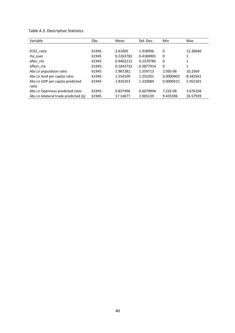
40

Table A.3. Descriptive Statistics

Variable Obs Mean Std. Dev. Min Max

lCO2_ratio 61945 2.61605 1.918996 0 12.30646

rta_ever 61945 0.2263782 0.4184901 0 1

after_rta 61945 0.9402212 0.2370785 0 1

effect_rta 61945 0.1843732 0.3877914 0 1

Abs Ln population ratio 61945 1.987282 1.559713 2.93E-06 10.2569

Abs Ln land per capita ratio 61945 1.554109 1.232201 0.0000403 8.342561

Abs Ln GDP per capita predicted ratio

61945 1.835353 1.320084 0.0000415 5.951501

Abs Ln Openness predicted ratio 61945 0.837496 0.6079994 7.22E-06 3.676194

Abs Ln bilateral trade predicted (ij) 61945 17.14677 2.005139 9.435596 26.57939

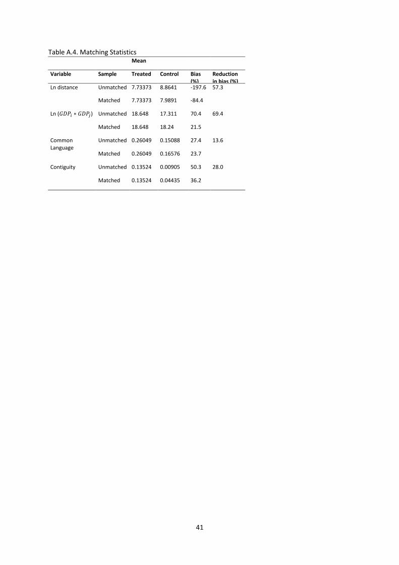
41

Table A.4. Matching Statistics Mean

Variable Sample Treated Control Bias (%)

Reduction in bias (%)

Ln distance Unmatched 7.73373 8.8641 -197.6 57.3

Matched 7.73373 7.9891 -84.4

Ln ( ) Unmatched 18.648 17.311 70.4 69.4

Matched 18.648 18.24 21.5

Common Language

Unmatched 0.26049 0.15088 27.4 13.6

Matched 0.26049 0.16576 23.7

Contiguity Unmatched 0.13524 0.00905 50.3 28.0

Matched 0.13524 0.04435 36.2