Area EstimatesArizona

by LANDSAT:1979

byMichael E.CraigCharles E. Miller

Statistical Research DivisionEconomics, Statistics, and Cooperatives ServiceU.S. Department of AgricultureWashington, D. C. 20250

January 1980

AREA ESTIMATES BY LANDSAT: ARIZONA 1979. By Michael E. Craig andCharles E. Miller; Statistical Research Division; Economics, Statistics,and Cooperatives Service, U.S. Department of Agriculture; Washington,D.C. 20250; January 1980.

ABSTRACT

This report describes how data-from NASA earth resources monitoringsatellites, LANDSAT II and III, were used in conjunction with conven-tionally gathered-ground data to estimate planted crop areas in the ninesouthern-most counties in Arizona. Estimates using LANDSAT and grounddata jointly were more precise than those obtained utilizing ground infor-mation alone. The major emphasis of the project was to improve cotton,sorghum and localized corn area estimates. Availability of LANDSAT dataand lack of sufficient ground data for classifier training hampered thecomplete success of the project.

Key words: LANDSAT, NASA, cloud cover, regression estimate, direct expansion.

************************************************************************* ** ** *~ This paper was prepared for limited distribution to ~~ the research community outside the U.S. Department of ~: Agriculture. ~* ** *************************************************************************

CONTENTS

INTRODUCTION ..............................•............................ 1

GROUND DATA COLLECTION AND EDITING 1

LANDSAT DATA ACQUISITION AND MANAGEMENT 3

ANALYSIS PROCEDURES AND RESULTS 4

SU~RY •••••••••••••••••••••••••••••••• ~.•• I ••••••••••••••••••••••••••• 6

APPENDIX A 8

ACKNOWLEDGEMENTS

The authors wish to extend special thanks to David K1eweno, Ray Luebbe,Sue Faerman, Sherman Winings and George Hanuschak, ESCS, for their assistanceduring the project; Sample Materials Group, Fairfax Unit, ESCS for providingstrata information; and Tricia Brookman for her fine typing efforts. Thanksalso too the Support Group: Sandy Stutson, George Harrell, Lillian Schwartz,Tjuana Fisher, and Pearl Jackson.

INTRODUCTION

The objective of this project was to gain LANDSAT analysis experiencepertaining to crops in Arizona. The primary emphasis was on improvingcotton and sorghum area estimates. The target area was defined as thenine southernmost counties in Arizona. In addition to the previouslyoutlined objectives, another goal was to make corn estimates in the easternportion of Arizona, primarily Cochise County. In some counties, estimateswere also made for alfalfa and minor crops. This paper covers the projectin the following phases:

I. Ground Data Collection and Editing

II. LANDSAT Data Acquisition and Management

III. Analysis Procedures and Results

IV. Summary

Any questions on general analysis procedures, statistical theory, orcurrent (non-research) ESCS procedures are referred to the paper byHanuschak, et. al.l!

I. Ground Data Collection and Editing

Accurately located ground information on a probability basis isessential as data input to LANDSAT analysis. Field level data from the JuneEnumerative Survey (JES) were used to correlate crop and land-use withdigital LANDSAT data and to evaluate the accuracy of the classificationresults.

presurvey preparation for the JES included questionnaire modification,enumerator training, and testing of field level edit programs. The question-naire for Arizona was altered fTom the normal JES design to allow for fieldlevel data entry. Additional information collected included the fieldnumber, waste area per field, and total field area. In order to extract asmuch information as possible for analysis, enumerators were instructed torecord as separate field all continous waste, wooded, or water coveredareas which exceeded 2.02 hectares (5 acres). Remote Sensing Branch (RSB)personnel provided assistance in the State JES training session forenumerators. Most phases of the field level edit programs and data transferoperations were tested prior to the survey to insure efficient data handling.

Data transfer procedures were established by RSB personnel to acquirethe ground data in Arizona and subsequently transfer the information to theBolt, Beranek and Newman, Inc. (BBN) computer system where the LANDSATanalysis work is done. These procedures involved three computer systems:1) Computer Science Corporation (INFONET), 2) Washington Computer Center(WCC), and 3) the BBN system. Data was loaded as usual for the JES ontothe INFONET system. Next the data set was stripped of all non-crop

1

information (such as livestock and economic data). This abbreviated dataset was written to a tape file at the Systems Branch RMT9 terminal. Thistape was then used as input to the Generalized Edit System Reformat andString programs and to a SAS field level edit program.

During the actual survey period, assistance was provided to theArizona SSO by RSB for questionnaire checking and to answer questionspertaining to the LANDSAT project. At this time the task was undertakento copy the JES segment photos (8" = 1 mile). This was done by PhoenixBlueprint Company in Phoenix, Arizona using a process known as PhotoMechanical Transfer. The photos were copied as soon as they were returnedby the enumerators in lots of 50-60 at a scale of 3 3/4" = 1 mile. Uponreceipt of the original and photo copies the SSO staff transferredsegment, tract and field boundaries to the copies with appropriate colorsof ink and checked each field for reasonableness and consistency withthe corresponding questionnaire. These copied photos were then mailed toRSB.

Upon completion of the JES by the Arizona SSO, the field level cropdata were transferred to the WCC as described earlier. At WCC, the fieldlevel SAS edits were executed and error listings generated. Tract levelupdates made by the SSO during the survey were listed for comparisonpurposes. Using the copied photos, SAS error listings, and SSO updates;problems were rectified and batch jobs were submitted to update the SASdataset at the field level.

A follow up survey was conducted for those fields which were not yetplanted at the time of the JES visit (called intentions fields). Updatesresulting from the survey were also made to the SAS dataset. When theediting and updating were completed, an output tape was created. Thistape was mailed to BBN on August 27, 1979.

Segment, tract, and field boundaries were digitized from the segmentphotos to a map base by the RSB support staff after the editing processwas complete. This process gave another check on the ground truth dataset by locating inconsistencies in reported versus digitized areas. Anyredigitizing or updating of ground truth needed was done at this point.

Methods Staff provided a master listing of segments for the ArizonaJES which contained such information as JES District, county, and plani-metered acreage for each segment. These data were incorporated at BBN tocreate a file called a segment catalog. Additional information for thisfile contained map type and map name from digitization and was added bythe RSB support staff.

The Fairfax Sampling Unit provided files containing area samplingframe boundaries for the nine Arizona counties (called county network files).In addition to these files, they compiled a listing of the tot~l number offrame units by county by strata. Using this listing, a frame unit file wascreated at BBN. This concluded the ground data phase of the project.

2

II. LANDSAT Data Acquisition and Management

In order to cover completely the 9 Arizona counties with LANDSAT data,13 scene locations were required. A standing order for all cloud free ,(less than 20%) imagery over this area during the period July 1, 1979through September 1, 1979 was sent to the EROS Data Center (Distributionof U.S. LANDSAT Data) and a copy to the manager of Earth Resources Programat NASA/Johnson Space Center in Texas. This standing order requestedthe CCT's (Computer Compatible Tapes) and 1:1;000,000 black and whitepositive film transparencies for three multispectral scanner bands besent to us automatically.

Counting passes by both LANDSAT II and LANDSAT III, we should havehad available seven dates of imagery for each of the thirteen locations,giving a total of 91 scenes to choose from before checking cloud cover.By mid-December only 16 of the 91 possibilities had been received by EROSData Center from NASA Goddard (the actual supplier). These 16 scenescoveredll locations with five locations duplicated on two dates. One ofthe locations covered by only one date had a defective tape plus cloudcover problems, leaving effectively ten of our original 13 locationscovered by LANDSAT imagery. Of the 15 scenes covering the ten areas, threehad 70 percent or more cloud cover. Appendix A, Table Al lists sceneidentifiers and specific dates of acquisition for the ten chosen scenes.Figure I shows approximate scene locations by path and row.

Figure I. Approximate scene locations.

3

Included in the area not covered by LANDSAT were the entire countiesof Greenlee, Cochise and Santa Cruz, plus parts (county mapsheets 9, 11,and 12) of Pima County. One additional scene was received December 26,1979 at EROS but arrived too late to be analyzed. The scene covered onlyGreenlee County. Sources at NASA Goddard explained the missing data asa throughput problem at their Image Processing Facility (IPF). At" lastreport, d~7a shipped to EROS are approximately 60 percent of the dataacquired.- NASA also felt that in addition to backlog, some of the sceneswere permanently lost due to data retrieval problems associated with highdensity tapes at NASA Goddard.

Upon receipt of the raw data CCT's from EROS, several tasks wereinitiated. The raw data tapes were received in the EROS BIL (Band Inter-leave by Line) format and reformatted to the EDITOR system format(Band Interleave by pixel). Parameters were calculated for the amountof filler added to the scanner data for processing by EROS. Reformattingwas done at the WCC and a copy of each EDITOR Format output tape wassent to BBN by mail. The first EROS copy arrived at RSB on July 26, 1979and the last EDITOR reformat was mailed to BBN on August 27, 1979.

Reformat programs were also initiated to take the EDITOR format tapesand output tapes acceptable to the ILLIAC IV computer in California. Thesetapes were mailed in one group on November 9, 1979.

Using the 1:1,000,000 scale transparencies for each scene, the registrationof LANDSAT data to a map base was begun. As an added aid to the registrationprocess; 1:500,000 scale paper products were ordered for Band 5. Initialpoints corresponding to known map points were selected on the LANDSAT paperproducts. Grayscale printouts of the area surrounding the initial pointswere made. Comparisons of the map points and grayscale prints allowed moreexact location of the corresponding points. For each scene, relationshipbetween row-column and latitude-longitude was then estimated using a thirdorder polynomial. These polynomials were used to create precision calibrationfiles for each scene.

The precision" calibration files in conjunction with the digitizedsegment files were then used to predict the segment locations in the LANDSATdata. Grayscales of the predicted locations of segments were producedand checked against plotter output at the same scale showing segment andfield boundaries. A local calibration was done for each discrepancybetween the predicted and actual location of a segment. Seldom were shiftslarger than 2 pixels needed, with the vast majority of shifts needing onlyan approximately one pixel shift. When the segment shifting was completedwe were ready to proceed with analysis.

III. Analysis Procedures and ResultsThe first step in analysis was to define the areas to be estimated

within the individual scenes. Images from the same date (same path) wereanalyzed together and overlapping area designated into/a specific scene.An analysis district was then defined for each path using county mapsheet

4

boundaries when overlap area splitting was necessary. The four analysisdistricts were labeled: AZ38L, AZ39LM, AZ40KLM, and AZ4IKL. Table A2contains descriptions of the analysis districts, counties contained, andthe number of segments contained in each.

Each of the four analysis districts was analyzed separately. Non-Agriculture strata areas were eliminated from the analysis. Within aspecific analysis district, all segment data were "packed" together intoone tile and tabulated to determine the number of pixels present ofdifferent cover types. The unequal prior probabilities used in lateranalysis came from this tabulation, and were labelled PUR priors (forpriors Proportional to Unexpanded Reported Area). Signature informationwas computed for any cover type having approximately 100 pixels availableafter boundary pixels and pixels in questionable fields were eliminated.Table A3 gives the tabulation of all available segment data by cover typesfor all analysis districts.

Several approaches were evaluated in order to create the final setof statistics (signatures) needed for pixel classification. Use of PURprior probabilities versus using no or Equal Priors (EP) gave two possibleoptions. Also considered was using a single category per cover (SCPC)versus multiple categories per cover (MCPC) to determine signatures. Thusfour different statistics files were evaluated for each analysis district.Table A4 gives the number of training pixels available after eliminationof boundary and questionable field pixels. Also in Table A4 are the numberof categories used to describe signatures under the MCPC option as deter-mined by our clustering methods. Notice from Table A4 that very littletraining data were available for sorghum and Pima cotton as compared toupland cotton and alfalfa (except for Pima cotton in AZ38L). Also noticethat analysis districts A239LM and AZ40KLM cover parts of Maricopa countyand when making a cover type estimate for this area, the cover type mustbe present in both analysis districts (Pima cotton is present in AZ39LMbut not in AZ40KLM).

After creating the various statistics needed for each classificationapproach, all pixels interior to the segment boundaries were classifiedusing the corresponding signatures. These categorizations would be usedfor evaluating each classifier and calculating regression parameters forestimation, called the small scale analysis.

The most important evaluator of classifier performance is notnecessarily the percent of pixels correctly classified, but it is how wellcrop area is estimated for the area of interest. We use a regressionestimator with JES data as the dependent variable and LANDSAT classifiedpixels as the independent variable. Maximization of the R-square valuesminimizes the variance of the regression estimates resulting from a classi-fication. Thus, the major criterion used to compare classifier performancewas the respective R-squares. Another measure of classifier performance isto measure how much better the regression estimator is than the correspondingdirect expansion estimator for the same area. This measure can be expressedby the relative efficiency (RE) and is defined as the ratio of the varianceof the direct expansion to the variance of the regression estimator. TablesAS, A6, A7, and A8 give R-squares, RE, and percent correct measures forthe major crops by analysis district.

S

Using the indicators mentioned above, one set of signatures waschosen for further analysis in each analysis district. In district AZ38L,the multiple category per crop, equal prior probabilities (MCPC-EP)classifier was judged "best". In the other three districts, the MCPC-PURclassifier was chosen, although the distinction between MCPC and SCPCusing PUR priors was very small. The chosen classifier was then trans-ferred to the ILLIAC IV computer in Ames, California where a full frameclassification was done for each corresponding scene.

Pixels from the full frame classifications were then aggregated bycounty, area frame strata, and category. The aggregations for agriculturestrata were then used with regression parameters from the small scaleanalysis to produce large scale estimates (analysis district and countylevel). Table A9 gives the large scale regression estimates versus theircorresponding direct expansion estimates by crop and by analysis district.Notice that these estimates represent agriculture strata only. Table AlOgives estimates by crop at the county level where data for non-agriculturestrata was prorated in from the JES expansion. In this table a directexpansion was used for the area in Pima County not covered by LANDSAT data.

IV. SUMMARY

The major emphasis of this project was to improve cotton and sorghumestimates in Arizona. Lack of training data for sorghum was a major problem,with 213 pixels being the most available in anyone analysis district. Oneanalysis district (covering Yuma County) contained no segments with sorghum.

In contrast to sorghum, large amounts of training data were availablefor upland cotton (ranging from 971 pixels in Graham County to 25,564 pixelsin Maricopa). In addition, 1154 pixels were available for Pima cotton inGraham County. Both upland cotton and all cotton estimates were made foreach analysis district, plus a Pima cotton estimate for Graham county.Classification accuracy was very good for all cotton, ranging from 66 to89 percent correct over the four analysis districts. The relativeefficiencies with respect to direct expansion were also very good, rangingfrom 2.02 to 6.07. R-squares for all cotton ranged from .53 to .84.

Comparison of the regression estimates for cotton with 1978 SSOestimates shows a substantial difference in level; with the regressionestimates being lower. Comparing cotton regression estimates versus directexpansion (ground data only) for agricultural strata, the regression comesout larger than direct expansion but the direct expansion is within twostandards errors of the regression.

LANDSAT coverage was not available for Cochise, Greenlee, and SantaCruz counties; plus part of Pima County. Since Cochise is the largest cornproducing county in Arizona, no corn estimates were available using LANDSATdata.

Estimates were made for minor crops in some counties. Alfalfa estimatesin four counties followed a pattern similar to cotton, with regressionestimates lower than 1978 SSO figures but higher than corresponding direct

6

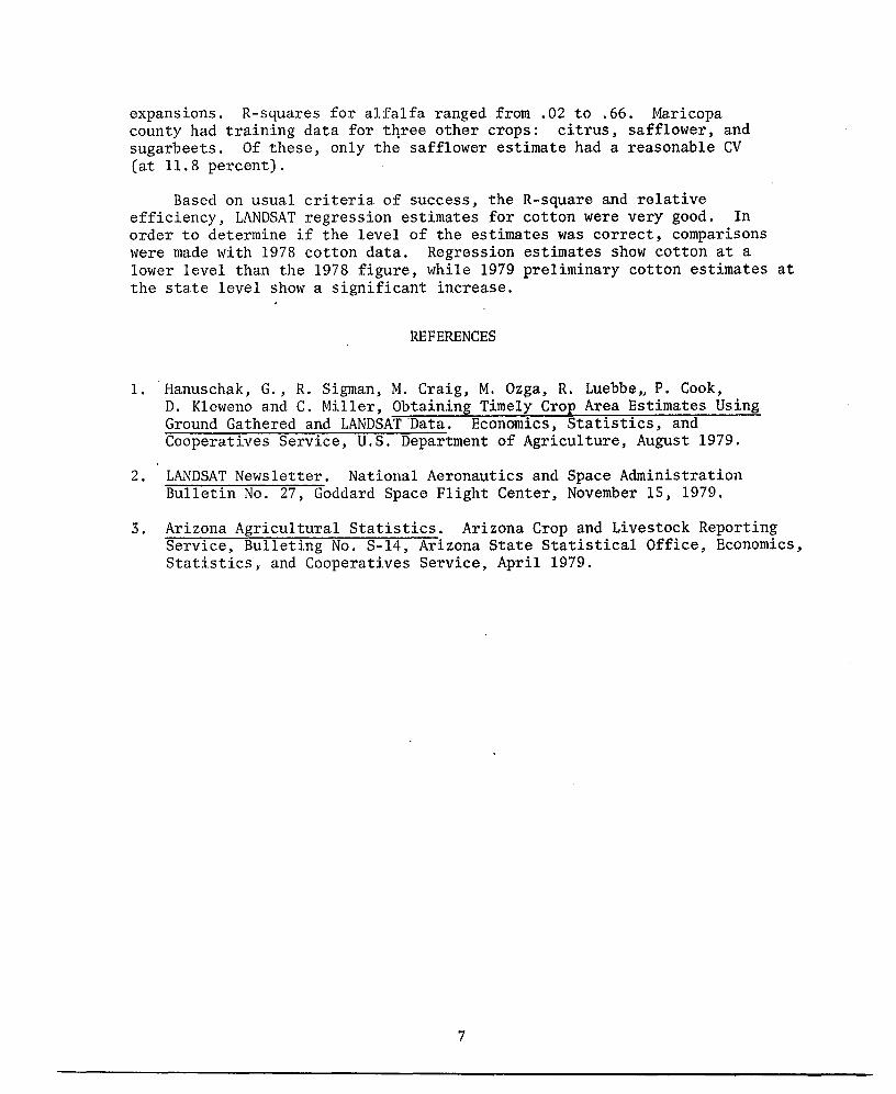
expansions. R-squares for alfalfa ranged from .02 to .66. Maricopacounty had training data for tqree other crops: citrus, safflower, andsugarbeets. Of these, only the safflower estimate had a reasonable CV(at 11.8 percent).

Based on usual criteria of success, the R-square and relativeefficiency, LANDSAT regression estimates for cotton were very good. Inorder to determine if the level of the estimates was correct, comparisonswere made with 1978 cotton data. Regression estimates show cotton at alower level than the 1978 figure, while 1979 preliminary cotton estimates atthe state level show a significant increase.

REFERENCES

1. Hanuschak, G., R. Sigman, M. Craig, M. Ozga, R. Luebbe" P. Cook,D. Kleweno and C. Miller, Obtaining Timely Crop Area Estimates UsingGround Gathered and LANDSAT 'Data. Economics, Statistics, andCooperatives Service, U.S. Department of Agriculture, August 1979.

2. LANDSAT Newsletter. National Aeronautics and Space AdministrationBulletin No. 27, Goddard Space Flight Center, November 15, 1979.

3. Arizona Agricultural Statistics. Arizona Crop and Livestock ReportingService, Bulleting No. S-14, Arizona State Statistical Office, Economics,Statistics, and Cooperatives Service, April 1979.

7

APPENDIX A

8

Table AI. LANDSAT Acquisitions Over Arizona

Image 'Cloud BandScene Identifier Date (1979): Cover(%) Quality Path Row

21646-17085 July 26 10 8888 38 3621646-17092 July 26 10 8888 38 3721629-17142 July 9 20 5555 39 3621629-17145 July 9 10 8888 39 3721629-17151 July 9 10 8888 39 3821630-17201 July 10 0 8885 40 3621630-17203 July 10 10 8888 40 3721630-17210 July 10 10 8888 40 3830484-17321 July 2 10 5888 41 3630484-17323 July 2 10 5555 41 37

Table A2. Analysis District Descriptions

Labe1* Counties Contained Agric. Strata Number of Segments

AZ38L Graham 35 9AZ39LM Maricopa** 15 38

Pima*** 30 5Pinal 20 52

AZ40KLM Maricopa** 15 52AZ41KL Yuma 25 24

*The label was formed using this format: AZXXYYYAZ - State Abbreviation for ArizonaXX - Path NumberYYY - Letters Describing row(s) used (K=36, L-37, M=38)

**Path 39 contained county map sheets 1, 2, and 7; Path 40 the rest of Maricopa***No LANDSAT coverage available for county map sheets 9, 11, and 12

9

Table A3: Tabulation of Segment Data By Cover Type and AnalysisDistrict (Values Shown are Reported Area in Pixels)

Cover Type AZ38L AZ39LM AZ40KLM AZ41KL

Alfalfa 539 3387 2556 3941Barley 116 925 594Citrus 1433 488 569Corn 495 186Durum Wheat 1098 106 443Hay 513 402 17Other Crops 36 2439 970 1157Pasture 217 902 673 930Pima Cotton 1844 1093 41 38Potatoes 446Safflower - 1184 513Sorghum 144 478 227Sugar Beets 475 218Summer Fallow 70 1785 2333 417Unknown 6 466 4 29Upland Cotton 1391 21357 16938 5279Waste Land 1689 32125 11379 3995Winter Wheat 1144 792 2832Woodland 29 21 5

Total 6052 71774 38441 19652

10

Table A4: Tabulation of Usable Training Data and Corresponding MCPC Categories by Cover Type

Cover Type AZ38L AZ39LM AZ40KLM AZ41KLTraining Number of Training Number of Training Nwnber of Training Number of

Pixels Categories Pixels Categories Pixels Categories Pixels Categories

Alfalfa 346 4 1813 3 1727 6 2281 5Barley 77 3 432 3 368 4Citrus 1045 8 252 2 34Corn 89 143 3Durham Wheat 652 2 149 3Hay 61 299 4

Other Crops 12 1143 2 540 4 634 3Pasture 142 4 547 4 191 4 2Pima Cotton 1154 8 559 2 26Potatoes 302 2

•....• Safflower 732 3 319 3•....•

Sorghum 114 2 213 5 111 1Sugar Beets 275 2 162 2"Summer Fallow 4 1130 3 1478 6Unknown 2 321 16Upland Cotton 971 8 13430 5 12134 8 2907 8Urb an* 105 1 76 2 • 273 2Waste Land 473 4 12217 6 6001 6 2219 7Water* 588 1 588 1 763 1 2311 5Winter Wheat 517 3 611 4 1647 8Woodland 19 7 1

*Added. not found in segment data

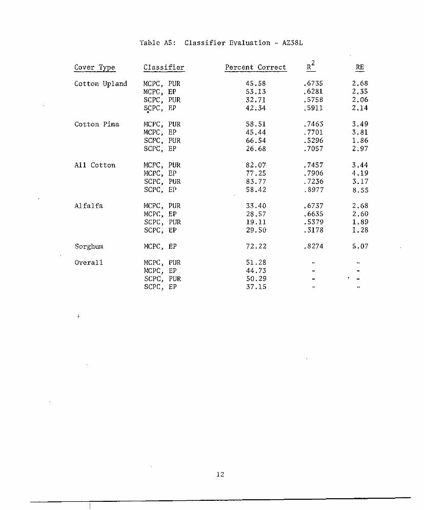
Table AS: Classifier Evaluation - AZ38L

Cover Type Classifier Percent Correct R2 RE

Cotton Upland MCPC, PUR 45.58 .6735 2.68MCPC, EP 53.13 .6281 2.35SCPC, PUR 32.71 .5758 2.06S~PC , EP 42.34 .5911 2.14

Cotton Pima MCPC, PUR 58.51 .7463 3.49MCPC, EP 45.44 .7701 3.81SCPC, PUR 66.54 .5296 1.86SCPC, EP 26.68 .7057 2.97

All Cotton MCPC, PUR 82.07 .7457 3.44MCPC, EP 77 .25 .7906 4.19SCPC, PUR 83.77 .7236 3.17SCPC, EP 58.42 .8977 8.55

Alfalfa MCPC, PUR 33.40 .6737 2.68MCPC, EP 28.57 .6635 2.60SCPC, PUR 19.11 .5379 1.89SCPC, EP 29.50 .3178 1.28

Sorghum MCPC, EP 72.22 .8274 5.07

Overall MCPC, PUR 51. 28MCPC, EP 44.73SCPC, PUR 50.29SCPC, EP 37.15

12

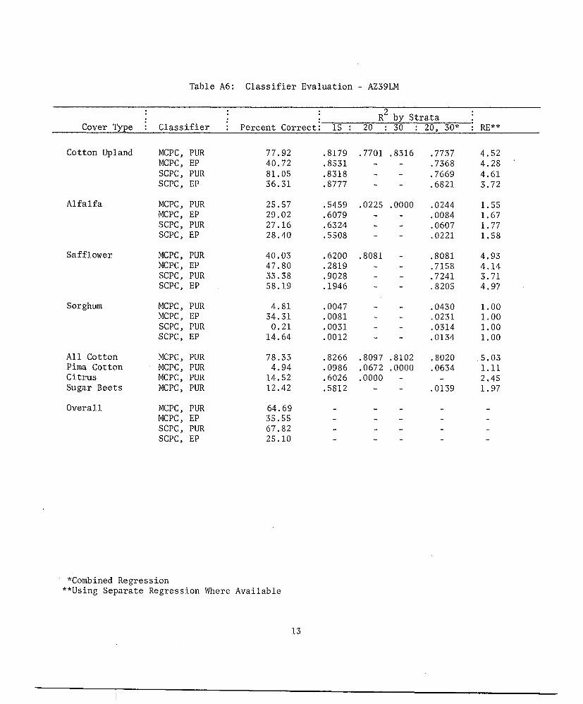
Table A6: Classifier Evaluation - AZ39LM

R2 by StrataCover Type Classifier Percent Correct 15 : 20 30 20, 30* RE**

Cotton Upland MCPC, PUR 77 .92 .8179 .7701 .8316 .7737 4.52MCPC, EP 40.72 .8531 .7368 4.28SCPC, PUR 81. 05 .8318 .7669 4.61SCPC, EP 36.31 .8777 .6821 3.72

Alfalfa MCPC, PUR 25.57 .5459 .0225 .0000 .0244 1.55MCPC, EP 29.02 .6079 .0084 1.67SCPC, PUR 27.16 .6324 .0607 1.77SCPC, EP 28.40 .5508 .0221 1.58

Safflower MCPC, PUR 40.03 .6200 .8081 .8081 4.93MCPC, EP 47.80 .2819 .7158 4.14SCPC, PUR 33.38 .9028 .7241 3.71SCPC, EP 58.19 .1946 .8205 4.97

Sorghum MCPC, PUR 4.81 .0047 .0430 1.00MCPC, EP 34.31 .0081 .0231 1.00SCPC, PUR 0.21 .0031 .0314 1.00SCPC, EP 14.64 .0012 .0134 1.00

All Cotton MCPC, PUR 78.33 .8266 .8097 .8102 .8020 .5.03Pima Cotton MCPC, PUR 4.94 .0986 .0672 .0000 .0634 1.11Citrus MCPC, PUR 14.52 .6026 .0000 2.45Sugar Beets MCPC, PUR 12.42 .5812 .0139 1.97Overall MCPC, PUR 64.69

MCPC, EP 35.55SCPC, PUR 67.82SCPC, EP 25.10

*Combined Regression**Using Separate Regression Where Available

13

Table A7: Classifier Evaluation - AZ40KLM

Cover Type Classifier Percent Correct R2 RE

Upland Cotton MCPC, PUR 88.68 .8377 6.04MCPC, EP 57.06 .8636 7.19SCPC, PUR 90.64 .8102 5.17SCPC, EP 45.01 .8087 5.12

Alfalfa MCPC, PUR 35.76 .6600 2.88MCPC, EP 48.55 .5057 1.98SCPC, PUR 23.98 .6394 2.72SCPC, EP 30.05 .2519 1.31

Safflower MCPC, PUR 57.89 .9562 22.:18MCPC, EP 69.20 .8712 7.61SCPC, PUR 49.51 .9231 12.75SCPC, EP 58.87 .6952 3.22

Sorghum MCPC, PUR 44.93 .7991 4.88MCPC, EP 46.26 .7854 4.57SCPC, PUR 44.93 .7913· 4.70SCPC, EP 48.02 .6385 2.71

All Cot ton MCPC, PUR 88.62 .8385 6.07Sugar Beets MCPC, PUR 1.83 .1663 1.18Citrus MCPC, PUR 23.98 .7500 3.92Overall MCPC, PUR 65.22

MCPC, EP 44.74SCPC, PUR 65.78SCPC, EP 34.56

14

Table A8: Classifier Evaluation - AZ41KL

Cover Type Classifier Percent Correct R2 RE

Upland Cotton MCPC, PUR 65.79 .5343 2.05MCPC, EP 57.13 .4496 1.74SCPC, PUR 73.16 .5123 1.96SCPC, EP 44.52 .5181 1.98

Al fa1 fa MCPC, PUR 48.16 .5617 2.18MCPC, EP 42.25 .5449 2.10SCPC, PUR 35.22 .5790 2.27SCPC, EP 52.07 .4702 1.81

Durham Wheat MCPC, PUR 26.64 .6001 2.39MCPC, EP 41.99 .3662 1.51SCPC, PUR 4.74 .1764 1.16SCPC, EP 29.12 .3029 1.37

All Cotton MCPC, PUR 65.79 .5321 2.04

Overall MCPC, PUR 48.16MCPC, EP 52.17SCPC, PUR 56.30SCPC, EP 49.95

15

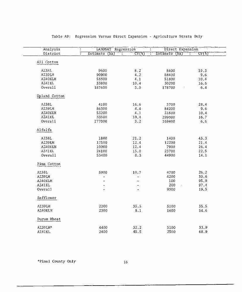
Table A9: Regression Versus Direct Expansion - Agriculture Strata Only

Analysis LANDSAT Regression Direct ExpansionDistrict Estimate (ha) CV('!o) EstImate (ha) CV('!o)

All Cotton

AZ38L 9600 8.2 8400 19.3AZ39LM 90900 4.2 88400 9.6AZ40KLM 53300 4.1 51800 10.4AZ41KL 33800 10.4 30200 16.6Overall 187600 3.0 178700 6.4

Upland Cotton

AZ38L 4100 16.6 3700 28.4AZ39LM 86300 4.4 84200 9.6AZ40KLM 53200 4.1 51600 10.4AZ41KL 33500 10.4 299000 16.7Overall 177000 3.2 169400 6.6

Alfalfa

AZ38L 1800 21.2 1400 43.3AZ39LM 17500 12.4 12200 21.4AZ40KLM 10000 12.4 7900 26.4AZ41KL 24100 15.0 23700 22.5Overall 53400 8.3 44900 14.1

Pima Cotton

AZ38L 5900 10.7 4700 26.2AZ39LM 4200 30.6AZ40KLM 100 95.0AZ41KL 200 97.4Overall 9300 19.5

Safflower

AZ39LM 2200 35.5 5100 35.5AZ40KLM 2300 8.1 1600 54.6

Durum Wheat

AZ39LM* 4400 32.2 5100 33.9AZ41KL 2400 45.5 2500 68.9

*Pina1 County Only 16

Table A9 Continued

Analysis LANDSAT Regression Direct ExpansionDistrict Estimate (ha) CV(%) Estimate (ha) CV (%)

Sugar Beets

AZ39LM** 1200 43.9 1200 64.1AZ40KLM 400 97.1 700 66.6

Citrus

AZ39LM** 2700 54.0 5000 45.2AZ40KLM 1600 26.3 1600 55.3

Sorghum

AZ38L 900 23.5 500 94.2AZ39LM 2100 49.7AZ40KLM 500 39.4 700 65.9AZ41KL 0 0Overall 3300 37.3

**Maricopa County Only17

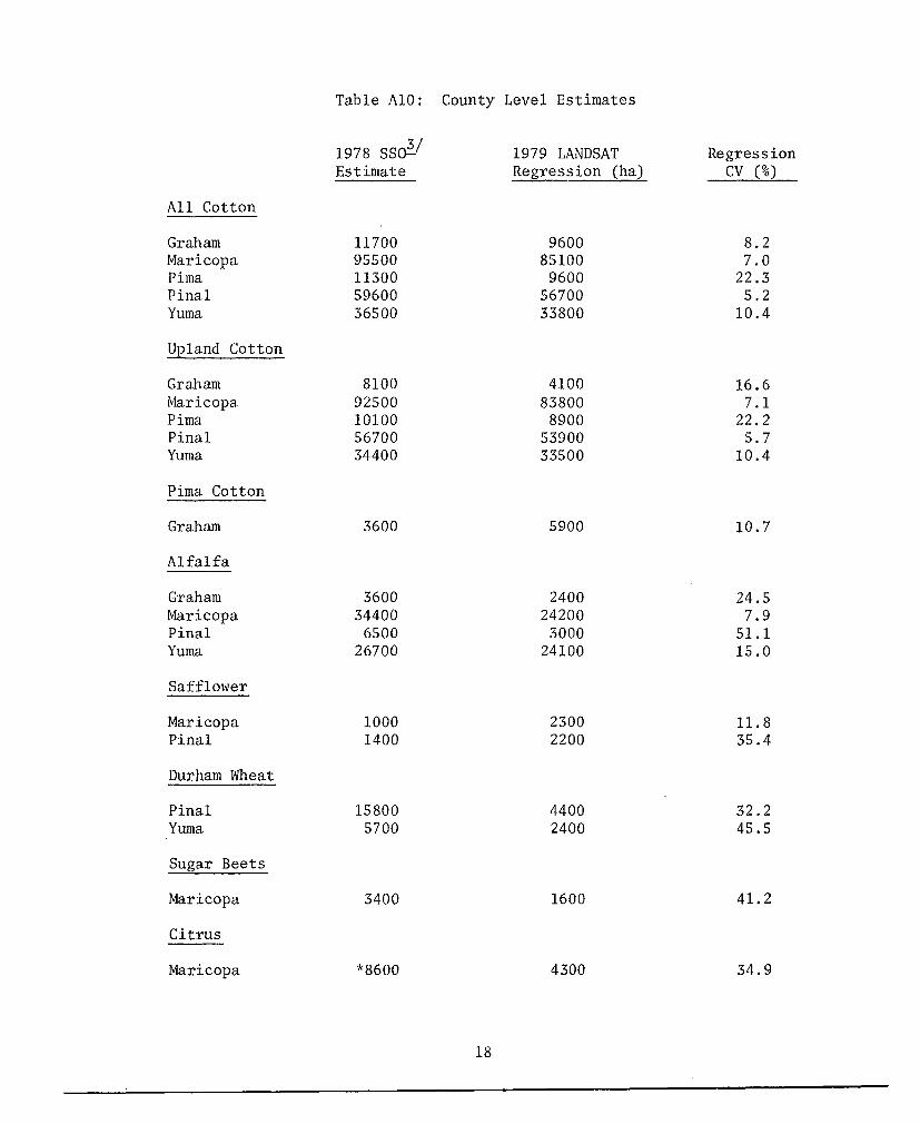
Table AlO: County Level Estimates

1978 SSO'§/ 1979 LANDSAT RegressionEstimate Regression (ha) CV (%)

All Cotton

Graham 11700 9600 8.2Maricopa. 95500 85100 7.0Pima 11300 9600 22.3Pinal 59600 56700 5.2Yuma 36500 33800 10.4

Upland Cotton

Graham 8100 4100 16.6Maricopa 92500 83800 7.1Pima 10100 8900 22.2Pinal 56700 53900 5.7Yuma 34400 33500 10.4

Pima Cotton

Graham 3600 5900 10.7Alfalfa

Graham 3600 2400 24.5Maricopa 34400 24200 7.9Pinal 6500 3000 51.1Yuma 26700 24100 15.0

Safflower

Maricopa 1000 2300 11. 8Pinal 1400 2200 35.4

Durham Wheat

Pinal 15800 4400 32.2Yuma 5700 2400 45.5

Sugar Beets

Maricopa 3400 1600 41.2

Citrus

Maricopa *8600 4300 34.9

18

Table AID Continued

1978 SSO§J 1979 LANDSAT RegressionEstimate Regression (ha) CV (%)

Sorghum

Graham 3200 900 22.9

*1978 Bearing Area

19