Embed Size (px)
Citation preview
ARES+MOOGFrom EWs to stellar parameters
Sérgio Sousa (CAUP)ExoEarths Team (http://www.astro.up.pt/exoearths/)
Wroclaw – Poland – 2013
Kepler 10 – Artistic View
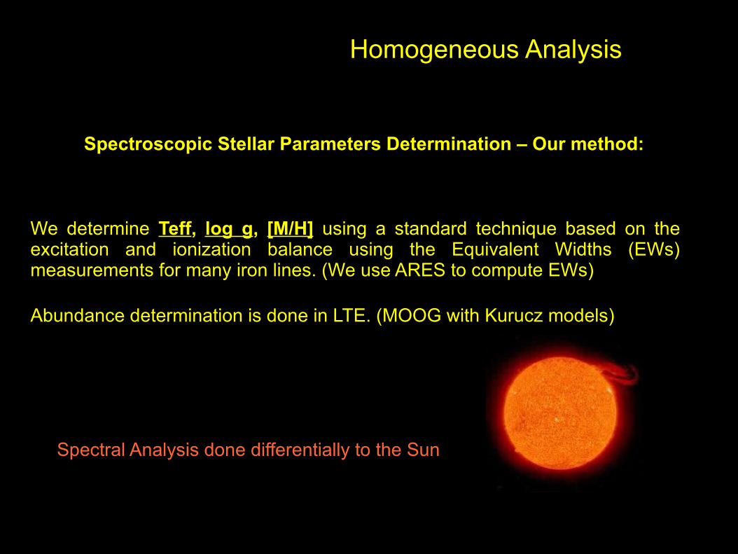
Homogeneous Analysis
Spectroscopic Stellar Parameters Determination – Our method:
We determine Teff, log g, [M/H] using a standard technique based on the excitation and ionization balance using the Equivalent Widths (EWs) measurements for many iron lines. (We use ARES to compute EWs)
Abundance determination is done in LTE. (MOOG with Kurucz models)
Spectral Analysis done differentially to the Sun
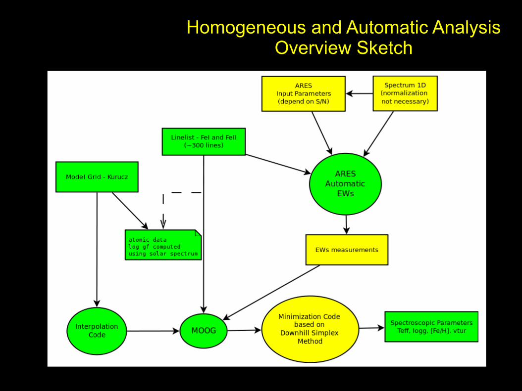
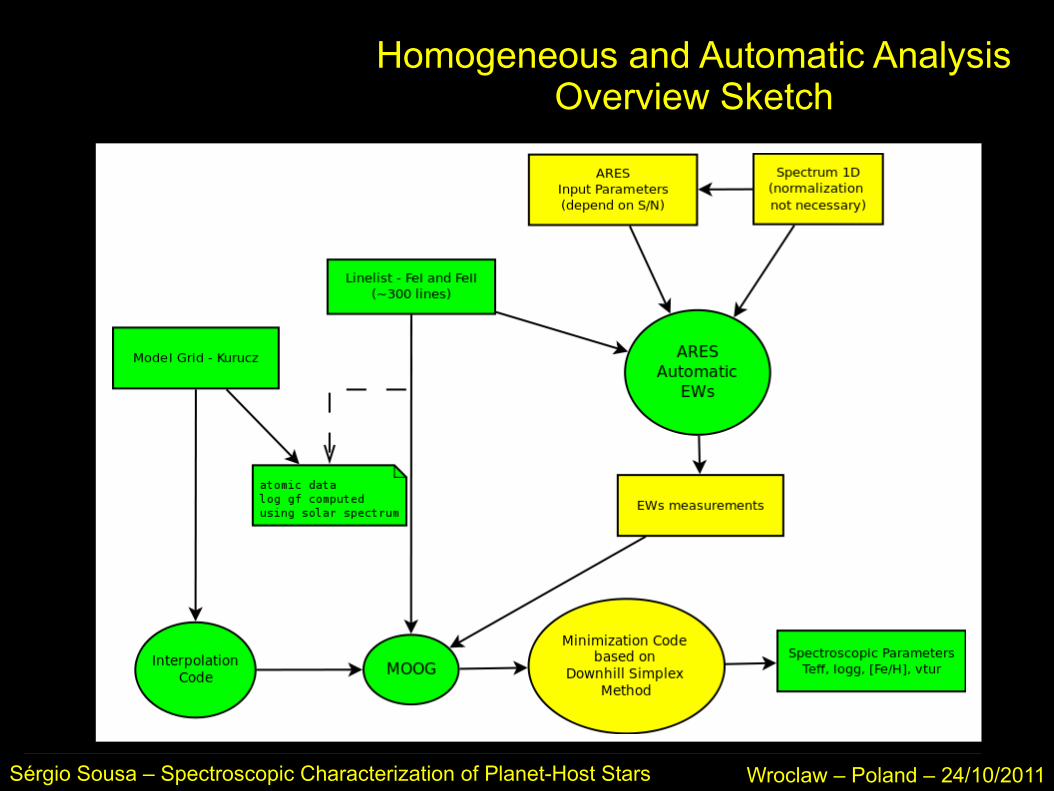
Homogeneous and Automatic AnalysisOverview Sketch
Homogeneous and Automatic AnalysisOverview Sketch
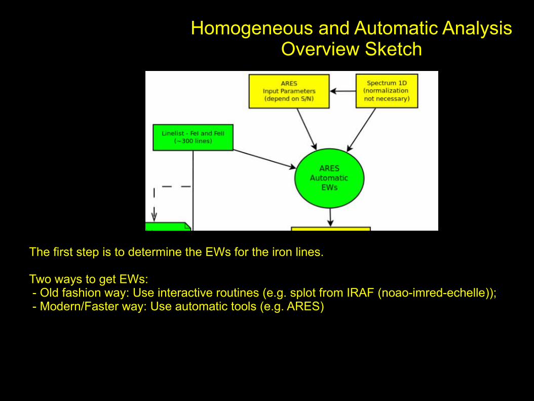
The first step is to determine the EWs for the iron lines.
Two ways to get EWs: - Old fashion way: Use interactive routines (e.g. splot from IRAF (noao-imred-echelle)); - Modern/Faster way: Use automatic tools (e.g. ARES)
Homogeneous and Automatic Analysis
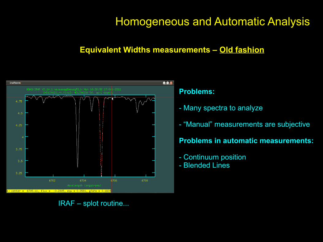
Equivalent Widths measurements – Old fashion
IRAF – splot routine...
Problems:
- Many spectra to analyze
- “Manual” measurements are subjective
Problems in automatic measurements:
- Continuum position- Blended Lines

Homogeneous and Automatic Analysis
http://www.astro.up.pt/~sousasag/ares/
Modern/Faster way:
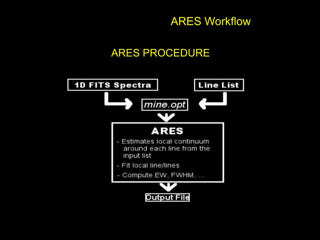
ARES PROCEDURE
ARES Workflow

Homogeneous and Automatic AnalysisOverview Sketch
Summarizing again, to run ARES you need:
1- The file mine.opt with the input parameters;2- A 1D Fits spectra, corrected in radial Velocity. (normalization not required)3- A list of iron lines to measure the EWs
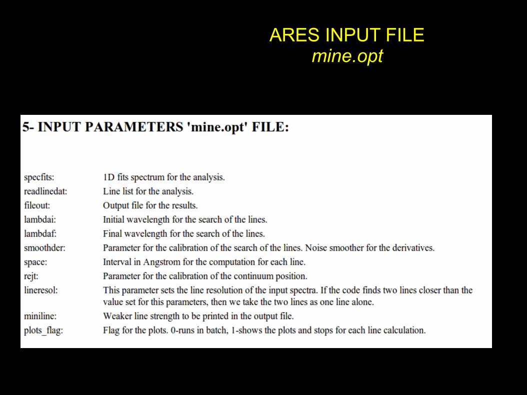
ARES INPUT FILEmine.opt

Rejt input parameter:
calibrates position of the continuum level
ARES Continuum position
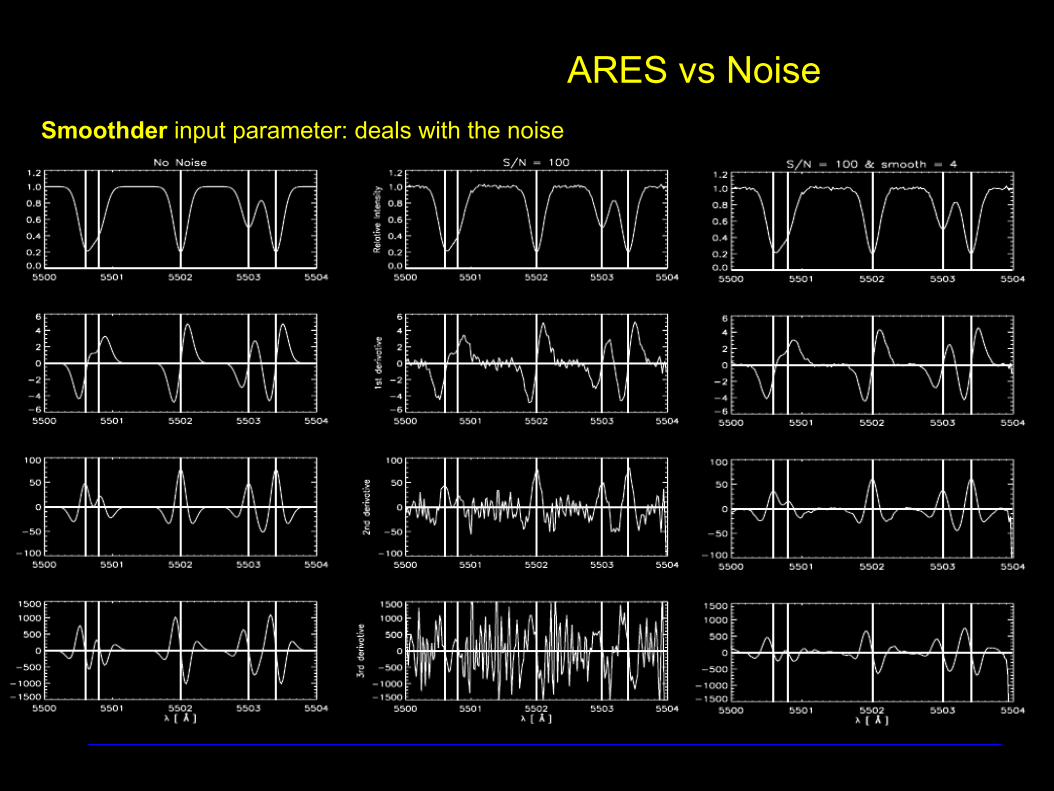
Smoothder input parameter: deals with the noise
ARES vs Noise
Homogeneous and Automatic AnalysisOverview Sketch
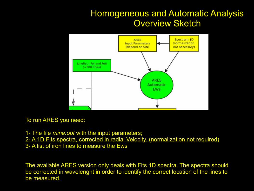
To run ARES you need:
1- The file mine.opt with the input parameters;2- A 1D Fits spectra, corrected in radial Velocity. (normalization not required)3- A list of iron lines to measure the Ews
The available ARES version only deals with Fits 1D spectra. The spectra should be corrected in wavelenght in order to identify the correct location of the lines to be measured.

Homogeneous and Automatic AnalysisOverview Sketch
To run ARES you need:
1- The file mine.opt with the input parameters;2- A 1D Fits spectra, corrected in radial Velocity. (normalization not required)3- A list of iron lines to measure the Ews
The list of lines to be measure is only a list of the wavelenght to get the EW.However this is an important step of the method. You have to make a careful selection of the lines and have atomic data for each line to derive abundances later with MOOG.
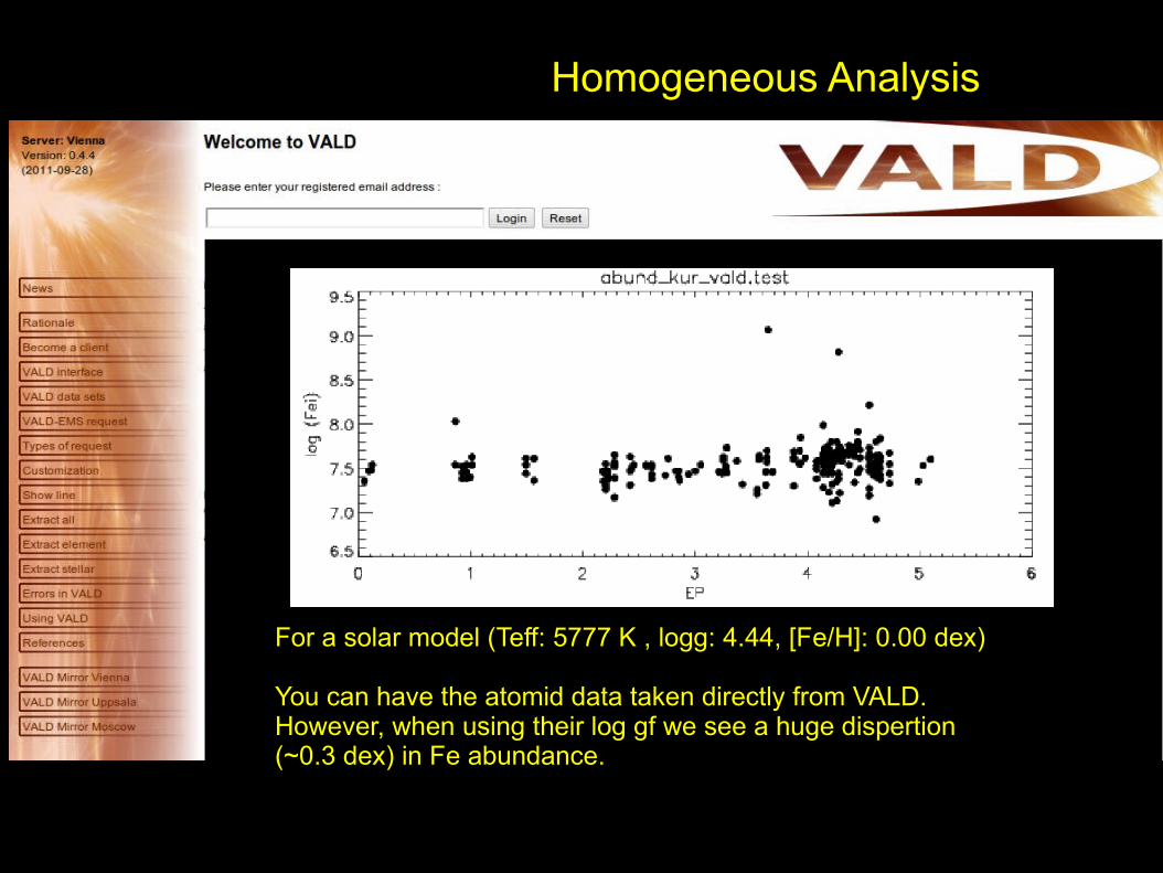
Homogeneous Analysis
For a solar model (Teff: 5777 K , logg: 4.44, [Fe/H]: 0.00 dex)
You can have the atomid data taken directly from VALD.However, when using their log gf we see a huge dispertion (~0.3 dex) in Fe abundance.
Homogeneous Analysis
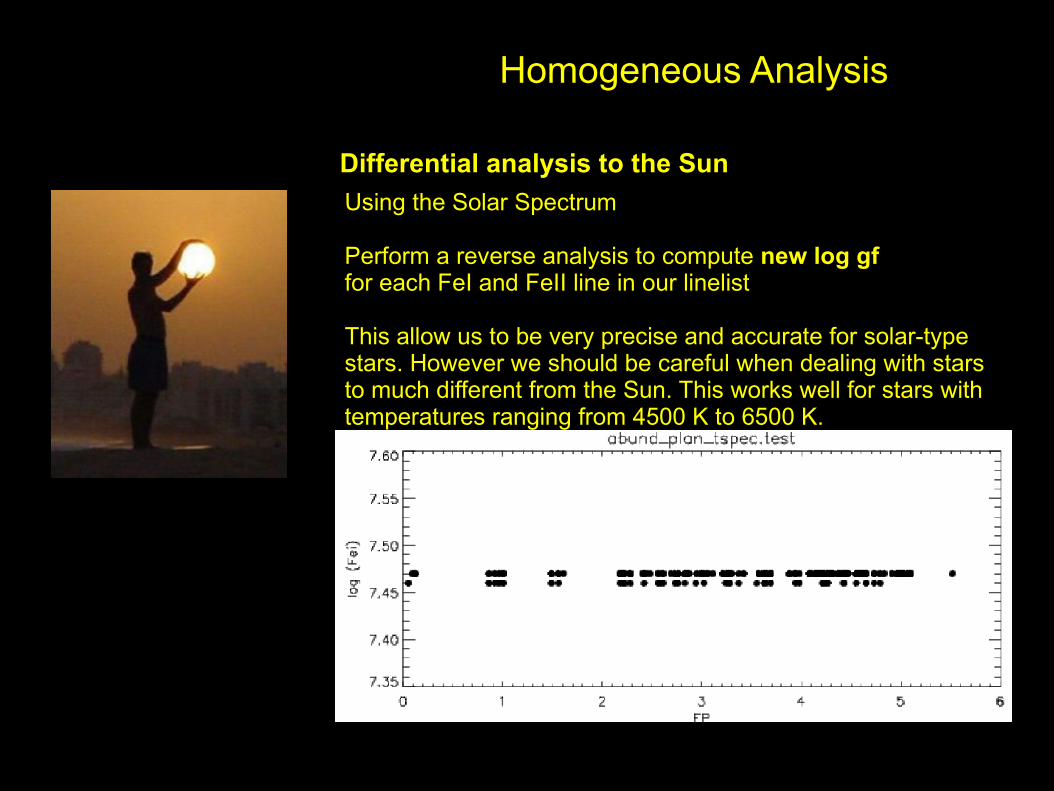
Differential analysis to the Sun
Using the Solar Spectrum
Perform a reverse analysis to compute new log gf for each FeI and FeII line in our linelist
This allow us to be very precise and accurate for solar-type stars. However we should be careful when dealing with stars to much different from the Sun. This works well for stars with temperatures ranging from 4500 K to 6500 K.
Homogeneous and Automatic Analysis
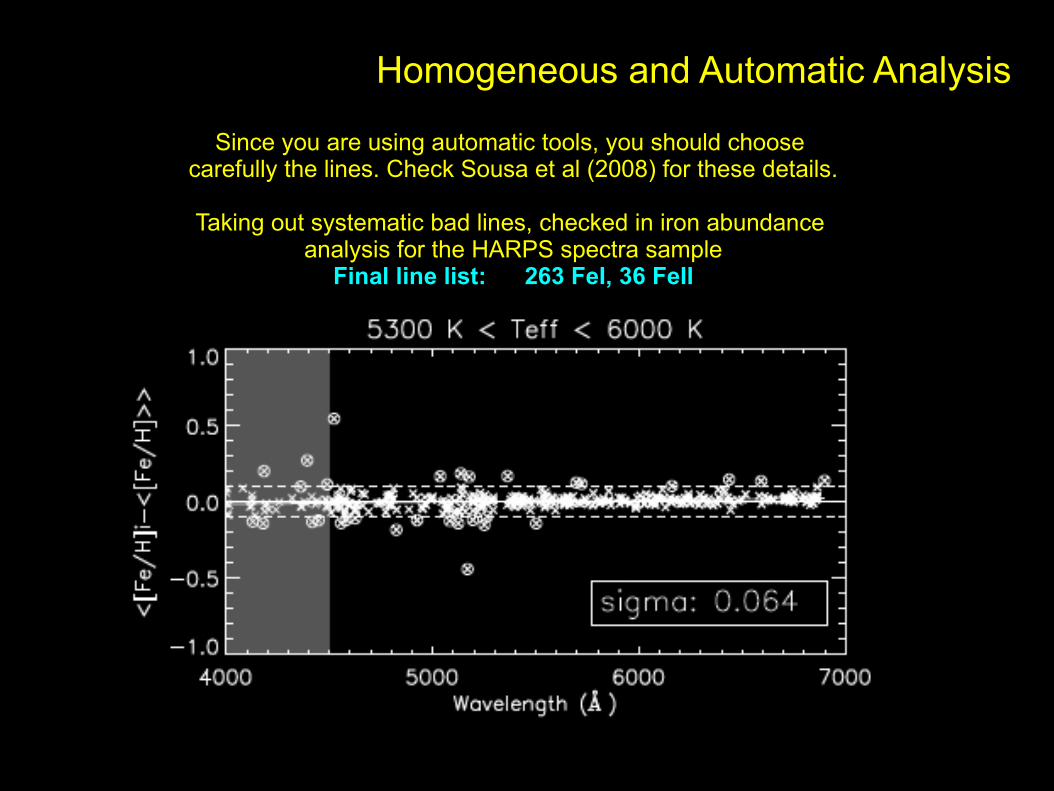
Since you are using automatic tools, you should choose carefully the lines. Check Sousa et al (2008) for these details.
Taking out systematic bad lines, checked in iron abundance analysis for the HARPS spectra sample
Final line list: 263 FeI, 36 FeII

Taking out systematic bad lines, checked in iron abundance analysis for the HARPS
spectra sample
Final line list: 263 FeI, 36 FeII

Homogeneous and Automatic AnalysisOverview Sketch
With the Ews determined you need to have tools to have specific stellar atmospheric models (Kurucs in this case)
And format the input of the Ews into MOOG.
Tools: format ARES output to MOOG
Tools: interpolation of a grid of models
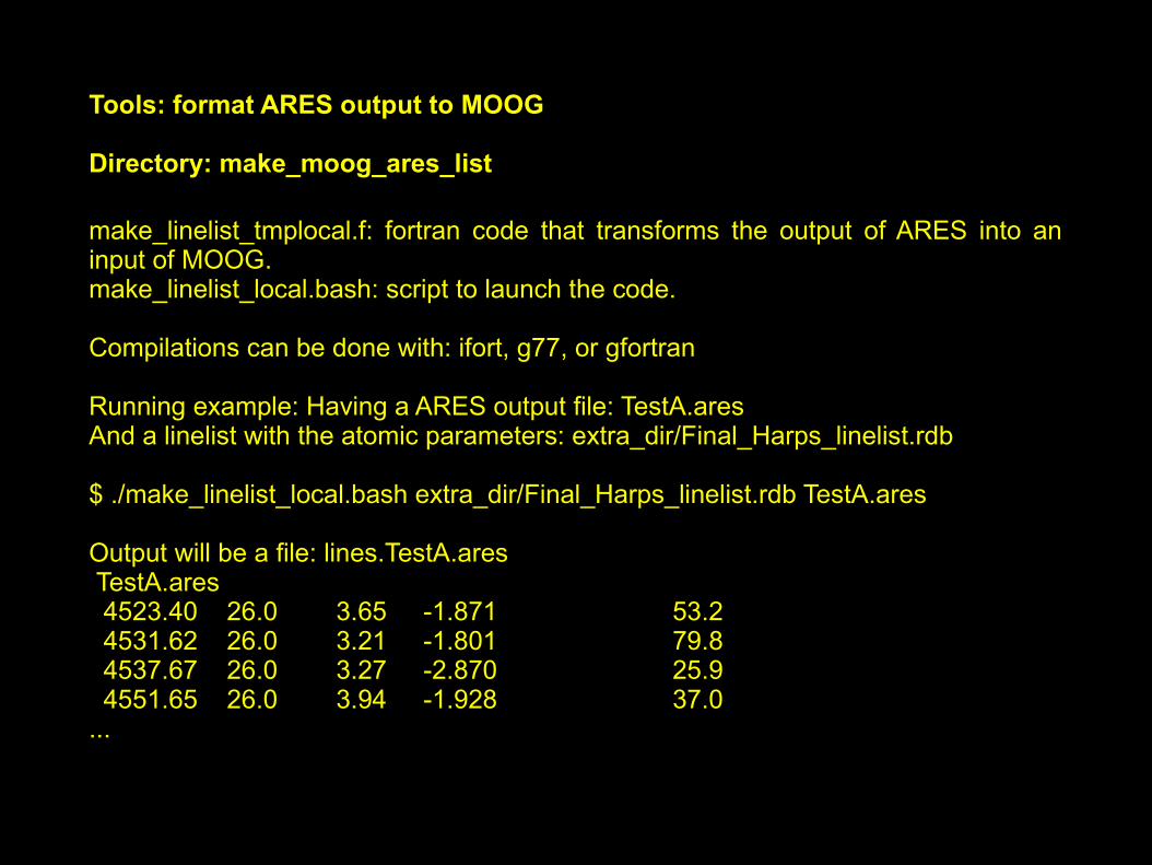
Tools: format ARES output to MOOG
Directory: make_moog_ares_list
make_linelist_tmplocal.f: fortran code that transforms the output of ARES into an input of MOOG.make_linelist_local.bash: script to launch the code.
Compilations can be done with: ifort, g77, or gfortran
Running example: Having a ARES output file: TestA.aresAnd a linelist with the atomic parameters: extra_dir/Final_Harps_linelist.rdb
$ ./make_linelist_local.bash extra_dir/Final_Harps_linelist.rdb TestA.ares
Output will be a file: lines.TestA.ares TestA.ares 4523.40 26.0 3.65 -1.871 53.2 4531.62 26.0 3.21 -1.801 79.8 4537.67 26.0 3.27 -2.870 25.9 4551.65 26.0 3.94 -1.928 37.0...

Tools: interpolation of a grid of models
Directory: interpol_models
There are to fortran codes to be used to interpolate the Kurucz grid in the directory and format the model to feed into MOOG:intermod.f: selects the 4 models and interpolates them maintaining the same format.transform.f: formats the interpolated model and include the microtubulence to be used in MOOG
Both can be compiled with g77 or ifort. Check README file.There is also a script file:make_model.bash
Use of the script for the case of a solar model atmosphere:
$./make_model.bash 577 4.44 0.0 1.0
It generates a file: out.atm which will be read by MOOG
KURUCZ Teff= 5777 log g= 4.44NTAU 72 0.50274684E-03 3704.8 0.138E+02 0.275E+10 0.265E-03 0.783E-01 0.200E+06 0.65798400E-03 3728.1 0.181E+02 0.355E+10 0.308E-03 0.823E-01 0.200E+06 0.83702774E-03 3750.0 0.231E+02 0.445E+10 0.355E-03 0.849E-01 0.200E+06…
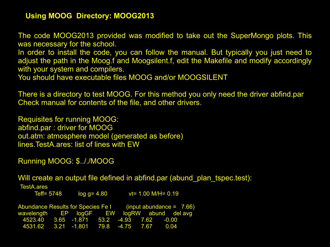
Using MOOG Directory: MOOG2013
The code MOOG2013 provided was modified to take out the SuperMongo plots. This was necessary for the school.In order to install the code, you can follow the manual. But typically you just need to adjust the path in the Moog.f and Moogsilent.f, edit the Makefile and modify accordingly with your system and compilers.You should have executable files MOOG and/or MOOGSILENT
There is a directory to test MOOG. For this method you only need the driver abfind.parCheck manual for contents of the file, and other drivers.
Requisites for running MOOG:abfind.par : driver for MOOGout.atm: atmosphere model (generated as before)lines.TestA.ares: list of lines with EW
Running MOOG: $.././MOOG
Will create an output file defined in abfind.par (abund_plan_tspec.test): TestA.ares Teff= 5748 log g= 4.80 vt= 1.00 M/H= 0.19
Abundance Results for Species Fe I (input abundance = 7.66)wavelength EP logGF EW logRW abund del avg 4523.40 3.65 -1.871 53.2 -4.93 7.62 -0.00 4531.62 3.21 -1.801 79.8 -4.75 7.67 0.04

Using MOOG Directory: MOOG2013
The file abund_plan_tspec.test can be used to see some plots with a provided Python script.
Directory: plot_moog_result
Example: $./read_moog_plot.py ../MOOG2013/testMOOG/abund_plan_tspec.test 1or just checking the correlations from the slopes:$./read_moog_plot.py ../MOOG2013/testMOOG/abund_plan_tspec.test 0
-----------------------------| Slope E.P. :0.005| Slope R.W. :-0.139| Fe I - Fe II:-0.28-----------------------------
The idea is to iterate with different atmospheric models until we find no correllations between:
- Abundances vs. Excitation potential (fitting the temperature)
- Abundances vs. Reduced Wavelenght (fitting microturbulence)
- Abundances of Fe I and Fe II consistent forcing ionization balance (fitting the surface gravity)
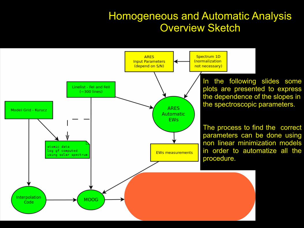
Homogeneous and Automatic AnalysisOverview Sketch
In the following slides some plots are presented to express the dependence of the slopes in the spectroscopic parameters.
The process to find the correct parameters can be done using non linear minimization models in order to automatize all the procedure.
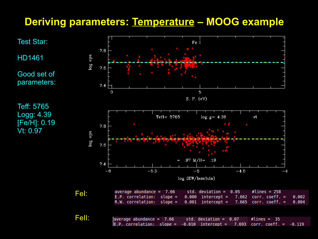
Test Star:
HD1461
Good set of parameters:
Teff: 5765Logg: 4.39[Fe/H]: 0.19Vt: 0.97
FeI:
FeII:
Deriving parameters: Temperature – MOOG example

Test Star:
HD1461
Teff: 5765Logg: 4.39[Fe/H]: 0.19Vt: 0.97
FeI:
FeII:
Deriving parameters: Temperature – MOOG example
Using lower Temperature for the modelTeff: 5600 K.
Slope Ab vs Ep > 0
If this slope is positive, then temperature of the correct model should be higher

Test Star:
HD1461
Teff: 5765Logg: 4.39[Fe/H]: 0.19Vt: 0.97
FeI:
FeII:
Deriving parameters: Temperature – MOOG example
Using higher TemperatureTeff: 5900 K.
Slope Ab vs Ep < 0
If this slope is negative, then temperature of the correct model should be lower

Test Star:
HD1461
Teff: 5765Logg: 4.39[Fe/H]: 0.19Vt: 0.97
FeI:
FeII:
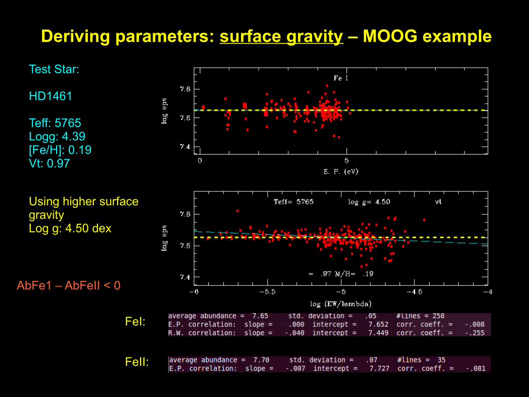
Deriving parameters: surface gravity – MOOG example

Test Star:
HD1461
Teff: 5765Logg: 4.39[Fe/H]: 0.19Vt: 0.97
FeI:
FeII:
Deriving parameters: surface gravity – MOOG example
Using lower surface gravityLog g: 4.10 dex
AbFe1 – AbFeII > 0
Test Star:
HD1461
Teff: 5765Logg: 4.39[Fe/H]: 0.19Vt: 0.97
FeI:
FeII:
Deriving parameters: surface gravity – MOOG example
AbFe1 – AbFeII < 0
Using higher surface gravityLog g: 4.50 dex
Test Star:
HD1461
Teff: 5765Logg: 4.39[Fe/H]: 0.19Vt: 0.97
FeI:
FeII:
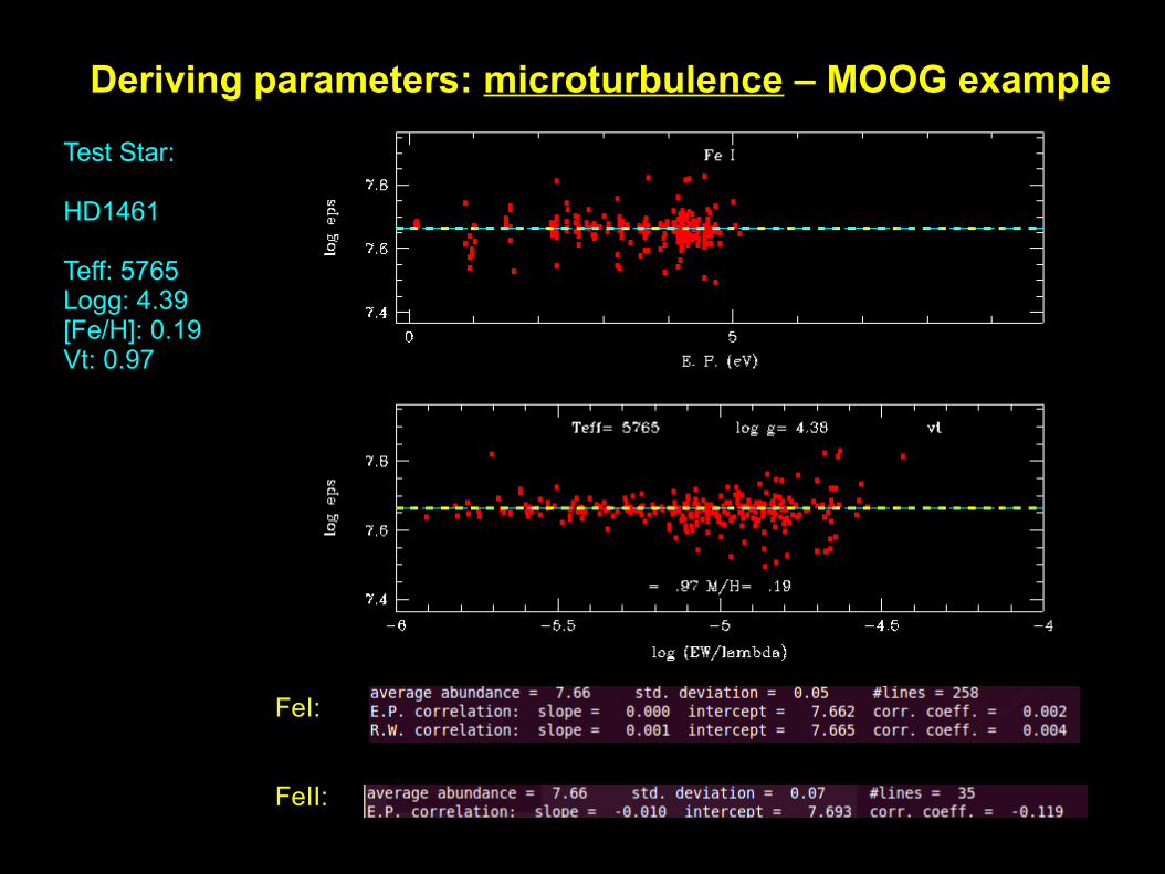
Deriving parameters: microturbulence – MOOG example
Test Star:
HD1461
Teff: 5765Logg: 4.39[Fe/H]: 0.19Vt: 0.97
FeI:
FeII:
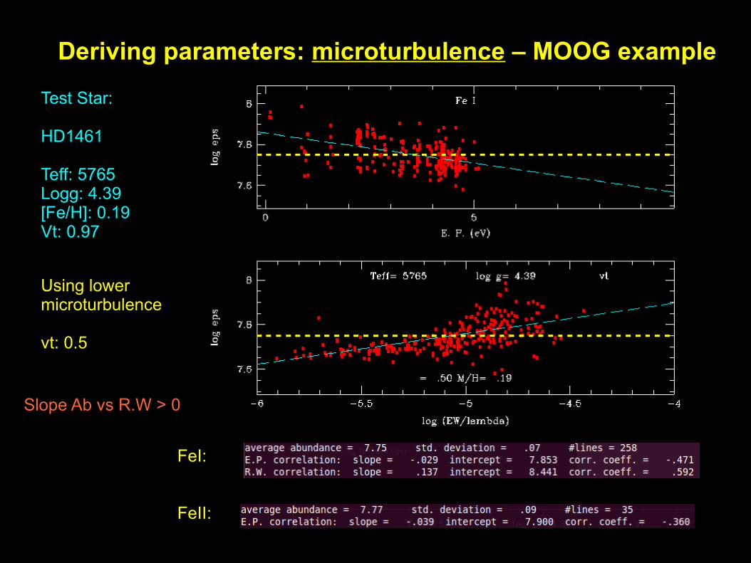
Deriving parameters: microturbulence – MOOG example
Using lower microturbulence
vt: 0.5
Slope Ab vs R.W > 0
Test Star:
HD1461
Teff: 5765Logg: 4.39[Fe/H]: 0.19Vt: 0.97
FeI:
FeII:
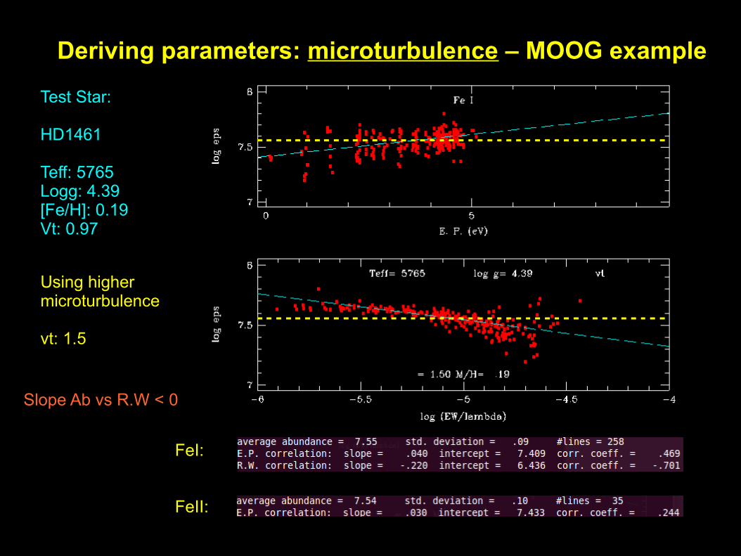
Deriving parameters: microturbulence – MOOG example
Slope Ab vs R.W < 0
Using higher microturbulence
vt: 1.5

Test Star: HD1461Teff: 5765, Logg: 4.39 [Fe/H]: 0.19 Vt: 0.97
FeI:
FeII:
Deriving parameters: Summary of method
1 – Measure Ews for FeI and FeII lines2 – Iteritive Loop:
2.1 – Built an atmosphere model (Teff, logg, [Fe/H], vt)2.2 – Compute the abundances (LTE is fine for solar type stars)2.3 – Check the slopes (AbFeI vs. EP, AbFeI vs. EW/l)2.4 – Check the ionization balance (AbFeI – AbFeII)
3 – If Slopes are 0 and exists ionization balance (AbFeI – AbFeII == 0)3.1 YES: Solution found3.2 NO: GO TO 2
Wroclaw – Poland – 24/10/2011Sérgio Sousa – Spectroscopic Characterization of Planet-Host Stars
Homogeneous and Automatic AnalysisOverview Sketch
From EWs to stellar parameters
Sérgio Sousa (CAUP)ExoEarths Team (http://www.astro.up.pt/exoearths/)
Kepler 10 – Artistic View
QUESTIONS?Email: [email protected]