AReview of Planetary Boundary Layer Parameterization Schemes and Their Sensitivity inSimulating Southeastern U.S. Cold Season Severe Weather Environments

ARIEL E. COHEN

NOAA/NWS/NCEP/Storm Prediction Center, and School of Meteorology, University of Oklahoma, Norman, Oklahoma

STEVEN M. CAVALLO

School of Meteorology, University of Oklahoma, Norman, Oklahoma

MICHAEL C. CONIGLIO AND HAROLD E. BROOKS

NOAA/National Severe Storms Laboratory, Norman, Oklahoma

(Manuscript received 4 September 2014, in final form 2 January 2015)

ABSTRACT

The representation of turbulent mixing within the lower troposphere is needed to accurately portray the

vertical thermodynamic and kinematic profiles of the atmosphere in mesoscale model forecasts. For meso-

scale models, turbulence is mostly a subgrid-scale process, but its presence in the planetary boundary layer

(PBL) can directly modulate a simulation’s depiction of mass fields relevant for forecast problems. The

primary goal of this work is to review the various parameterization schemes that the Weather Research and

Forecasting Model employs in its depiction of turbulent mixing (PBL schemes) in general, and is followed by

an application to a severe weather environment. Each scheme represents mixing on a local and/or nonlocal

basis. Local schemes only consider immediately adjacent vertical levels in the model, whereas nonlocal

schemes can consider a deeper layer covering multiple levels in representing the effects of vertical mixing

through the PBL. As an application, a pair of cold season severe weather events that occurred in the

southeastern United States are examined. Such cases highlight the ambiguities of classically defined PBL

schemes in a cold season severe weather environment, though characteristics of the PBL schemes are ap-

parent in this case. Low-level lapse rates and storm-relative helicity are typically steeper and slightly smaller

for nonlocal than local schemes, respectively. Nonlocal mixing is necessary to more accurately forecast the

lower-tropospheric lapse rates within the warm sector of these events. While all schemes yield over-

estimations of mixed-layer convective available potential energy (MLCAPE), nonlocal schemes more

strongly overestimate MLCAPE than do local schemes.

1. Introduction

One substantial source of forecast inaccuracy in

mesoscale models1 is the representation of lower-

tropospheric thermodynamic and kinematic structures

(Jankov et al. 2005; Stensrud 2007; Hacker 2010; Hu

et al. 2010; Nielsen-Gammon et al. 2010). The accurate

representation of these structures is critical in improving

forecasts of high-impact weather phenomena for which

model output can aid in the assessment of whether

necessary conditions for such phenomena would be met

(e.g., Kain et al. 2003, 2005, 2013). As an example, for

organized severe thunderstorms [those producing wind

gusts of at least 26m s21, tornadoes, and/or hail of at

least 25.4mm (1 in.) in diameter], the necessary condi-

tions are moisture, lift, instability, and vertical wind

shear, which are highly variable across the wide spec-

trum of convection that ensues (e.g., Johns and Doswell

1992; Rasmussen and Blanchard 1998; Thompson et al.

2003; Craven and Brooks 2004; Schneider and Dean

2008). A simulation of the particular intricacies of such

Corresponding author address: Ariel Cohen, Storm Prediction

Center, 120 David L. Boren Blvd., Norman, OK 73072.

E-mail: ariel.cohen@noaa.gov

1Herein, we refer to models with grid spacing fine enough to

allow explicit representation of convection (;1–4 km) as meso-

scale models because the smallest fully resolvable scales are typi-

cally in the meso-g-scale range.

JUNE 2015 COHEN ET AL . 591

DOI: 10.1175/WAF-D-14-00105.1

an environment is heavily influenced by its depiction of

the planetary boundary layer (PBL)—that portion of

the lower troposphere directly affected by the earth’s

surface via troposphere–surface exchanges of heat,

moisture, andmomentum on subhourly time scales (e.g.,

Stull 1988; Stensrud 2007).

Exchanges of moisture, heat, and momentum occur

within the PBL through mixing associated with turbu-

lent eddies. These eddies influence the way in which

lower-tropospheric thermodynamic and kinematic

structures evolve. Such eddies operate on spatiotem-

poral scales that cannot be explicitly represented on

grid scales and time steps employed in most mesoscale

models. As such, their effects are expressed in these

models via the use of PBL parameterization schemes,

whose theoretical development is outlined in multiple

sources addressing the subject (e.g., Stull 1988; Holton

2004; Stensrud 2007).

This paper reviews the processes for which meso-

scale models represent the evolution of turbulent mo-

tions within the lower troposphere. Characteristics of

several PBL schemes within the Advanced Research

version of the Weather Research and Forecasting

(WRF) Model (ARW; Skamarock et al. 2008) are

summarized, first in the general sense for a variety of

environmental stability conditions. This summary is

synthesized through the larger body of contemporary

PBL-related research. As an example of an application

of the aforementioned synthesis, we examine PBL-

scheme sensitivity for a situation that is notably chal-

lenging for the forecasting of severe convective storms:

the southeastern U.S. cold season severe thunderstorm

environment.

During cold season tornado events in the south-

eastern United States, Guyer et al. (2006) and Guyer

and Dean (2010) note that buoyancy tends to be lim-

ited and vertical wind shear tends to be large in the near-

storm environment. Ashley (2007) concludes that this

part of the country is particularly vulnerable to tornado

fatalities owing to the mutual overlap of favorable cli-

matological, land-use, and societal patterns, which high-

lights the need for improving forecast accuracy of these

events. In a study of tornadoes rated as category 2 or

higher on the Fujita scale (F2) that occurred across the

southeastern United States during the cold season

from 15 October to 15 February 1984–2004, Guyer

et al. (2006) highlight modest moisture and instability

as the primary mitigating factors for organized se-

vere convection amid a background synoptic environ-

ment more commonly supporting strong vertical wind

shear. However, in some circumstances, sufficient, albeit

limited, CAPE does develop for deep convection with

significant tornadoes, and they conjecture that this

CAPE originates from the relatively warm and moist

low levels within the warm sector of an extratropical

cyclone.

The prediction of severe thunderstorms can be par-

ticularly challenging for environments in which one or

more of the necessary conditions are marginally sup-

portive of severe weather, in which small errors can be

very meaningful (e.g., Vescio and Thompson 1998). This

may be a reason why southeastern U.S. cold season se-

vere weather has not been extensively studied, espe-

cially in regard to mesoscale modeling and related PBL

schemes. Factors like shear-driven eddies and large-

scale vertical motion influence the thermodynamic and

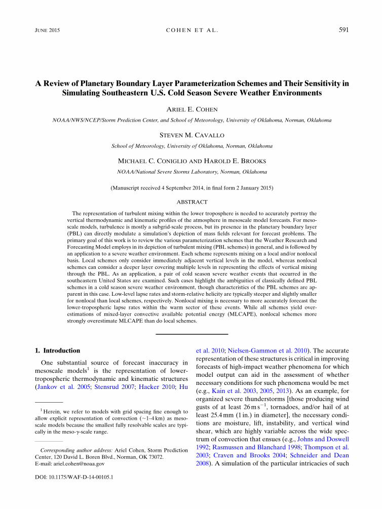
FIG. 1. Constituents of the PBL and their evolution through the diurnal and nocturnal cycles [from Kis and Straka

(2010) and Stull (1988)].

592 WEATHER AND FORECAST ING VOLUME 30

kinematic properties of the PBL in this regime, in ad-

dition to heat fluxes from diurnal heating. In fact,

through field observations and computer visualizations,

Schneider and Lilly (1999) specifically identify vertical

wind shear as a contributor to the production of turbu-

lence, which influences the makeup of the PBL, and it is

uncertain how these complicating effects are manifest in

the accuracy of PBL schemes. Thus, examining the

characteristics among the PBL schemes for the south-

eastern U.S. cold season severe weather environment is

a step toward identifying their potential weaknesses that

may lead to forecast bias.

2. Theoretic foundation of PBL parameterizationschemes

Among other texts, Stensrud (2007) and Stull (1988)

provide explanations of the process by which turbu-

lence is mathematically represented in numerical

weather prediction models. There are two major

components of this process: the order of turbulence

closure and whether a local or nonlocal mixing ap-

proach is employed.

a. Order of turbulence closure

The theoretical development of PBL parameterization

schemes requires the decomposition of variables of the

equations of motion into mean and perturbation compo-

nents. The mean components represent the time-averaged

conditions that characterize the background atmospheric

state. The perturbation components represent deviations,

or turbulent fluctuations, from the background mean state,

which are inherent to turbulent motions (i.e., what the

perturbations describe) within the PBL. Equations per-

taining to turbulence modeling will always contain more

unknown terms than known terms, where the unknown

term is always of one order above themaximum among the

other terms. Because of this, turbulence closure requires

empirically relating the unknown term of moment n1 1 to

lower-moment known terms. This is referred to as nth-

order turbulence closure, where n is an integer. Some PBL

schemes are considered noninteger orders. For example,

1.5-order closure parameterization schemes predict second-

order turbulent kinetic energy (TKE) by diagnosing

second-ordermoments for some variables (i.e., variances of

potential temperature and mixing ratio and their related

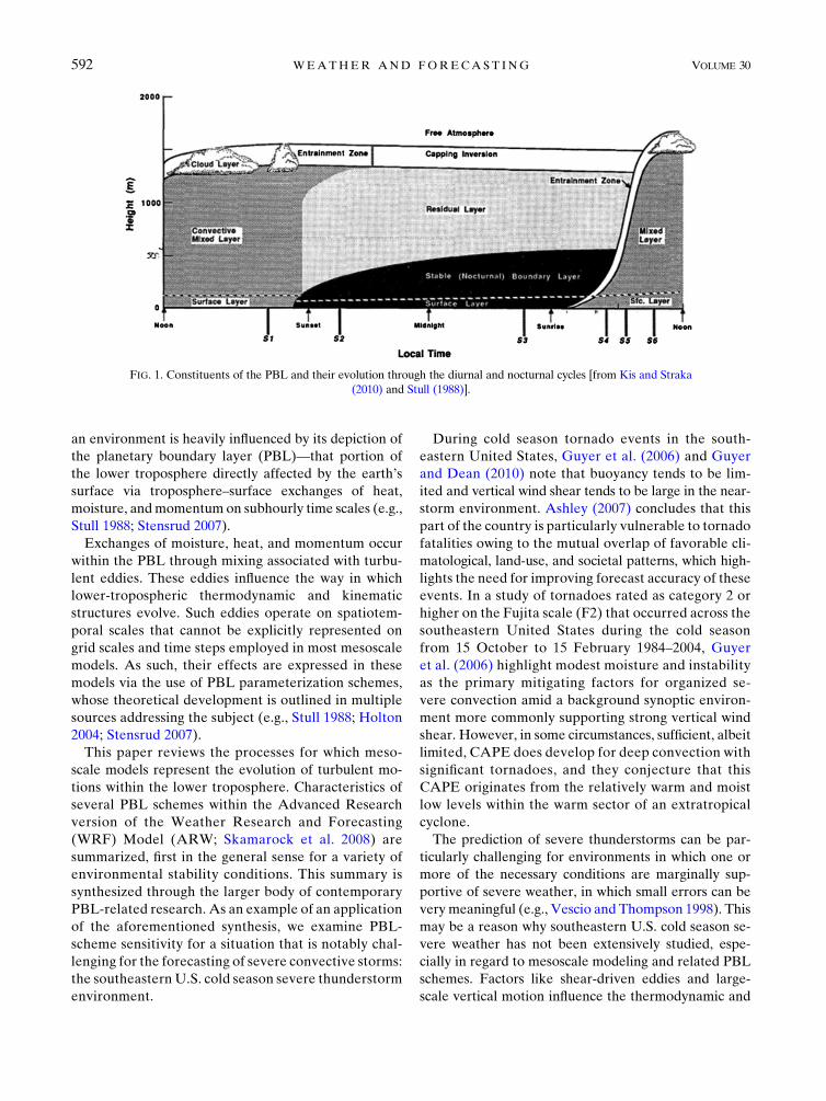
FIG. 2. Depiction of the mechanics of the ACM and ACM2 schemes regarding PBL interactions [from Pleim

(2007a)]. Arrows depict exchanges of atmospheric quantities between various layers within the simulated PBL.

JUNE 2015 COHEN ET AL . 593

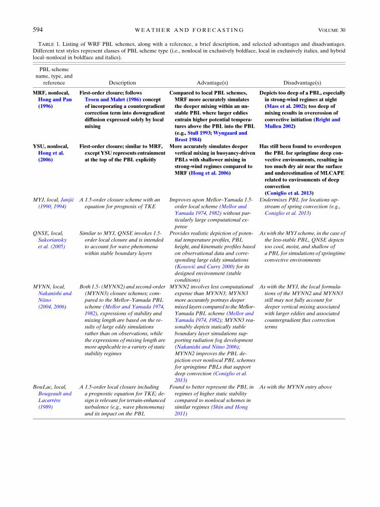
TABLE 1. Listing of WRF PBL schemes, along with a reference, a brief description, and selected advantages and disadvantages.

Different text styles represent classes of PBL scheme type (i.e., nonlocal in exclusively boldface, local in exclusively italics, and hybrid

local–nonlocal in boldface and italics).

PBL scheme

name, type, and

reference Description Advantage(s) Disadvantage(s)

MRF, nonlocal,Hong and Pan

(1996)

First-order closure; followsTroen and Mahrt (1986) concept

of incorporating a countergradient

correction term into downgradient

diffusion expressed solely by localmixing

Compared to local PBL schemes,MRF more accurately simulates

the deeper mixing within an un-

stable PBL where larger eddies

entrain higher potential tempera-tures above the PBL into the PBL

(e.g., Stull 1993; Wyngaard and

Brost 1984)

Depicts too deep of a PBL, especiallyin strong-wind regimes at night

(Mass et al. 2002); too deep of

mixing results in overerosion of

convective initiation (Bright andMullen 2002)

YSU, nonlocal,Hong et al.

(2006)

First-order closure; similar to MRF,exceptYSU represents entrainment

at the top of the PBL explicitly

More accurately simulates deepervertical mixing in buoyancy-driven

PBLs with shallower mixing in

strong-wind regimes compared toMRF (Hong et al. 2006)

Has still been found to overdeepenthe PBL for springtime deep con-

vective environments, resulting in

too much dry air near the surfaceand underestimation of MLCAPE

related to environments of deep

convection

(Coniglio et al. 2013)MYJ, local, Janji�c

(1990, 1994)

A 1.5-order closure scheme with an

equation for prognosis of TKE

Improves upon Mellor–Yamada 1.5-

order local scheme (Mellor and

Yamada 1974, 1982) without par-

ticularly large computational ex-

pense

Undermixes PBL for locations up-

stream of spring convection (e.g.,

Coniglio et al. 2013)

QNSE, local,

Sukoriansky

et al. (2005)

Similar to MYJ, QNSE invokes 1.5-

order local closure and is intended

to account for wave phenomena

within stable boundary layers

Provides realistic depiction of poten-

tial temperature profiles, PBL

height, and kinematic profiles based

on observational data and corre-

sponding large eddy simulations

(Kosovi�c and Curry 2000) for its

designed environment (stable

conditions)

As with theMYJ scheme, in the case of

the less-stable PBL, QNSE depicts

too cool, moist, and shallow of

a PBL for simulations of springtime

convective environments

MYNN, local,

Nakanishi and

Niino

(2004, 2006)

Both 1.5- (MYNN2) and second-order

(MYNN3) closure schemes; com-

pared to the Mellor–Yamada PBL

scheme (Mellor and Yamada 1974,

1982), expressions of stability and

mixing length are based on the re-

sults of large eddy simulations

rather than on observations, while

the expressions of mixing length are

more applicable to a variety of static

stability regimes

MYNN2 involves less computational

expense than MYNN3; MYNN3

more accurately portrays deeper

mixed layers compared to theMellor–

Yamada PBL scheme (Mellor and

Yamada 1974, 1982); MYNN3 rea-

sonably depicts statically stable

boundary layer simulations sup-

porting radiation fog development

(Nakanishi and Niino 2006);

MYNN2 improves the PBL de-

piction over nonlocal PBL schemes

for springtime PBLs that support

deep convection (Coniglio et al.

2013)

As with the MYJ, the local formula-

tions of the MYNN2 and MYNN3

still may not fully account for

deeper vertical mixing associated

with larger eddies and associated

countergradient flux correction

terms

BouLac, local,

Bougeault and

Lacarrère(1989)

A 1.5-order local closure including

a prognostic equation for TKE; de-

sign is relevant for terrain-enhanced

turbulence (e.g., wave phenomena)

and its impact on the PBL

Found to better represent the PBL in

regimes of higher static stability

compared to nonlocal schemes in

similar regimes (Shin and Hong

2011)

As with the MYNN entry above

594 WEATHER AND FORECAST ING VOLUME 30

covariances) (e.g., Stensrud 2007; Coniglio et al. 2013) and

first-ordermoments for other variables. TKE quantifies the

perturbation component of motion, characterizing the

magnitude of turbulence in the PBL owing to vertical wind

shear, buoyancy, turbulent transport, and dampening

driven by molecular viscosity (e.g., Holton 2004).

b. Local versus nonlocal PBL parameterizationschemes

One important way that PBL schemes differ is

according to the depth over which these known variables

are allowed to affect a given point, determined on the

sole basis of the vertical gradient of the perturbation

quantities at the point and not horizontal gradients (e.g.,

Ching et al. 2014). In the case of local closure schemes,

only those vertical levels that are directly adjacent to

a given point directly affect variables at the given point.

On the other hand, multiple vertical levels (e.g., those

within the PBL) can be used to determine variables at a

given point in nonlocal closure schemes. It is well un-

derstood that local schemes can offer a substantial dis-

advantage regarding their depiction of the PBL because

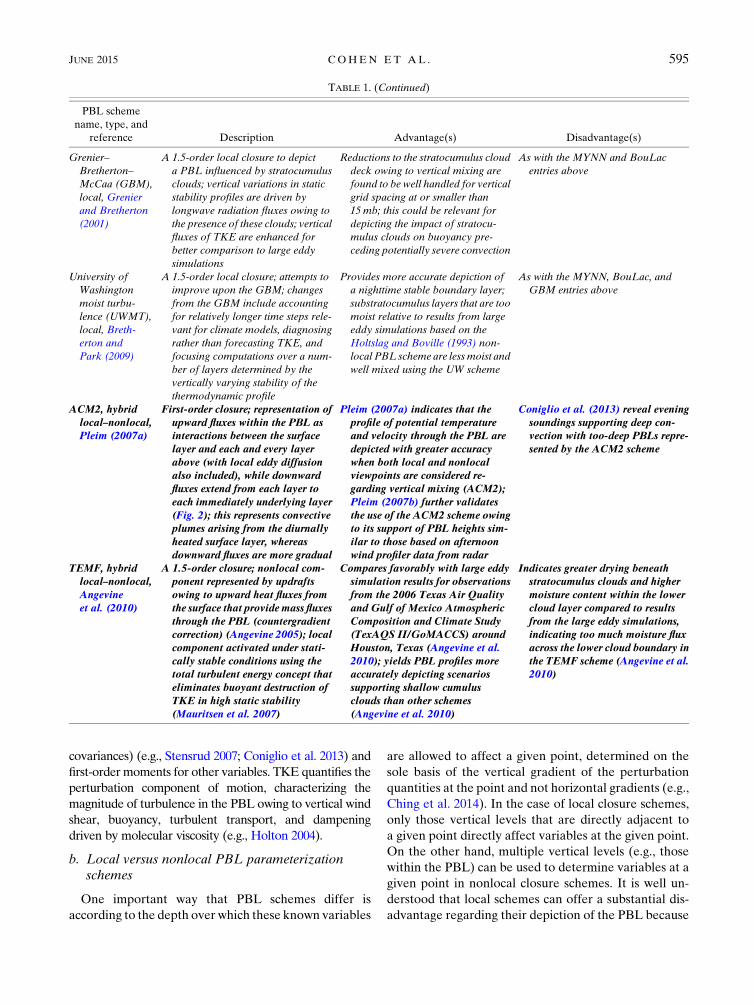
TABLE 1. (Continued)

PBL scheme

name, type, and

reference Description Advantage(s) Disadvantage(s)

Grenier–

Bretherton–

McCaa (GBM),

local, Grenier

and Bretherton

(2001)

A 1.5-order local closure to depict

a PBL influenced by stratocumulus

clouds; vertical variations in static

stability profiles are driven by

longwave radiation fluxes owing to

the presence of these clouds; vertical

fluxes of TKE are enhanced for

better comparison to large eddy

simulations

Reductions to the stratocumulus cloud

deck owing to vertical mixing are

found to be well handled for vertical

grid spacing at or smaller than

15mb; this could be relevant for

depicting the impact of stratocu-

mulus clouds on buoyancy pre-

ceding potentially severe convection

As with the MYNN and BouLac

entries above

University of

Washington

moist turbu-

lence (UWMT),

local, Breth-

erton and

Park (2009)

A 1.5-order local closure; attempts to

improve upon the GBM; changes

from the GBM include accounting

for relatively longer time steps rele-

vant for climate models, diagnosing

rather than forecasting TKE, and

focusing computations over a num-

ber of layers determined by the

vertically varying stability of the

thermodynamic profile

Provides more accurate depiction of

a nighttime stable boundary layer;

substratocumulus layers that are too

moist relative to results from large

eddy simulations based on the

Holtslag and Boville (1993) non-

local PBL scheme are lessmoist and

well mixed using the UW scheme

As with the MYNN, BouLac, and

GBM entries above

ACM2, hybrid

local–nonlocal,

Pleim (2007a)

First-order closure; representation of

upward fluxes within the PBL as

interactions between the surface

layer and each and every layer

above (with local eddy diffusion

also included), while downward

fluxes extend from each layer to

each immediately underlying layer

(Fig. 2); this represents convective

plumes arising from the diurnally

heated surface layer, whereas

downward fluxes are more gradual

Pleim (2007a) indicates that the

profile of potential temperature

and velocity through the PBL are

depicted with greater accuracy

when both local and nonlocal

viewpoints are considered re-

garding vertical mixing (ACM2);

Pleim (2007b) further validates

the use of the ACM2 scheme owing

to its support of PBL heights sim-

ilar to those based on afternoon

wind profiler data from radar

Coniglio et al. (2013) reveal evening

soundings supporting deep con-

vection with too-deep PBLs repre-

sented by the ACM2 scheme

TEMF, hybrid

local–nonlocal,

Angevine

et al. (2010)

A 1.5-order closure; nonlocal com-

ponent represented by updrafts

owing to upward heat fluxes from

the surface that providemass fluxes

through the PBL (countergradient

correction) (Angevine 2005); local

component activated under stati-

cally stable conditions using the

total turbulent energy concept that

eliminates buoyant destruction of

TKE in high static stability

(Mauritsen et al. 2007)

Compares favorably with large eddy

simulation results for observations

from the 2006 Texas Air Quality

and Gulf of Mexico Atmospheric

Composition and Climate Study

(TexAQS II/GoMACCS) around

Houston, Texas (Angevine et al.

2010); yields PBL profiles more

accurately depicting scenarios

supporting shallow cumulus

clouds than other schemes

(Angevine et al. 2010)

Indicates greater drying beneath

stratocumulus clouds and higher

moisture content within the lower

cloud layer compared to results

from the large eddy simulations,

indicating too much moisture flux

across the lower cloud boundary in

the TEMF scheme (Angevine et al.

2010)

JUNE 2015 COHEN ET AL . 595

localized stability maxima through the vertical thermal

profile are not necessarily representative of the overall

state of mixing in the PBL (Stensrud 2007). Vertical

mixing throughout the depth of the PBL is primarily

accomplished by the largest eddies, which are often only

minimally affected by local variations in static stability.

In local schemes, the PBL grows minimally in the

presence of localized static stability maxima, in which

the fluxes are downward from higher potential temper-

ature to lower potential temperature. This is especially

the case at the top of the simulated daytime PBL owing

to higher static stability within the entrainment zone

beneath the free atmosphere (Fig. 1). In the observed

atmosphere, large eddies can transport heat upward

from the diurnally heated surface layer regardless of the

localized stability maxima and produce what are called

countergradient fluxes (i.e., counter to the downward

direction of heat fluxes accompanying stability maxima)

(Stull 1988). These large eddies can penetrate the top of

the mixed layer and entrain properties of the free

atmosphere well into themixed layer, thereby bolstering

PBL depth. Nonlocal schemes account for these

countergradient fluxes and, thus, generally represent

deep PBL circulations more accurately than local

schemes (Stull 1991). However, in some circumstances,

the utility of local schemes can improve by invoking

higher orders of closure (e.g., Mellor and Yamada 1982;

Nakanishi and Niino 2009; Coniglio et al. 2013), though

usually at a higher computational cost. Some schemes

simultaneously represent both nonlocal and local mixing

concepts [e.g., Asymmetric Convective Model, versions

1 and 2 (ACM and ACM2, respectively) in Fig. 2].

3. PBL schemes in the Weather Research andForecasting Model

Operational forecasting needs have increasingly

placed emphasis on using the output of high-resolution

numerical models to simulate meso- and storm-scale

processes accurately (e.g., Weiss et al. 2008). The

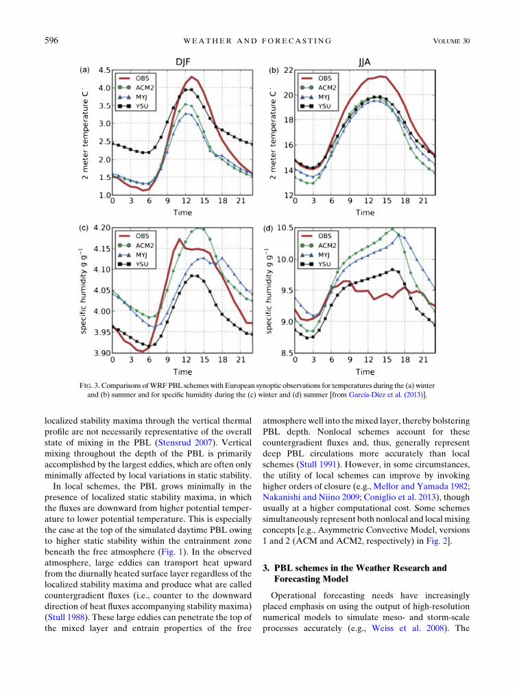
FIG. 3. Comparisons ofWRFPBL schemes with European synoptic observations for temperatures during the (a) winter

and (b) summer and for specific humidity during the (c) winter and (d) summer [from García-Díez et al. (2013)].

596 WEATHER AND FORECAST ING VOLUME 30

parameterization of the PBL by these models directly

influences the models’ portrayal of buoyancy and ver-

tical wind shear, as well as precipitation evolution (e.g.,

Hong et al. 2006). Here, we investigate how the PBL

evolves within the ARW, version 3.3.1, using 4-km grid

spacing (e.g., Skamarock et al. 2008). Several studies

have compared the performance of WRF PBL schemes

in influencing the depicted PBL state, highlighting the

sensitivity of the PBL state to the selected PBL scheme,

and some of their more salient findings are summarized

here for the benefit of the weather and forecasting

community. These studies do not focus on the south-

eastern U.S. cold season severe thunderstorm environ-

ment, which will be a focus in subsequent sections. As

a supplement, Table 1 defines the acronyms for the

schemes used in WRF and provides a detailed overview

of the schemes.

Xie et al. (2012) compare local and nonlocal schemes

for simulations over Hong Kong and find that nonlocal-

influenced schemes [i.e., ACM2 and Yonsei University

(YSU)] yield deeper andmore accurate PBLs than those

depicted by local schemes [i.e., Mellor–Yamada–Janji�c

(MYJ) and Bougeault–Lacarrère (BouLac)]. These arerelated to differences in parameters relevant to severestorm forecasting, such as buoyancy via surface-layermodulations to potential temperature and mixing ratioassociated with variability in the depth of stronger mix-ing. Likewise, Hu et al. (2010) find that, over the south-

central United States in summer, the nonlocal YSU

scheme and hybrid local–nonlocal ACM2 scheme yield

the smallest biases in temperature and moisture in the

lower atmosphere owing to diurnal mixing. YSU and

ACM2 are generally characterized by warmer and drier

daytime PBLs, which are more consistent with obser-

vations, while the MYJ scheme’s purely local treatment

of larger-scale eddies prevents the PBL from mixing as

deeply to produce cooler and moister conditions. Simi-

larly, Gibbs et al. (2011) find that the nonlocal YSU

scheme and the hybrid local–nonlocal ACM2 scheme

produces a drier PBL in a dry convective boundary layer

(CBL) than the local MYJ scheme, with YSU and

ACM2 better depicting the observed PBL than MYJ.

Regarding marine boundary layers, Huang et al.

(2013) compare the total energy–mass flux (TEMF),

YSU, MYJ, Mellor–Yamada–Nakanishi–Niino (MYNN),

and Medium-Range Forecast Model (MRF) schemes to

observations collected from three field experiments;

MYNN, and especially TEMF, provide the least-biased

thermodynamic structures. Huang et al. (2013) conclude

that the inclusion of both local and nonlocal processes

in TEMF results in more accurate PBL depictions in

regimes for which stratocumulus and shallow cumulus

clouds are present.

Ching et al. (2014) describe the inability for high-

resolution models to reliably simulate convectively in-

duced secondary circulations (CISCs; e.g., convective

rolls) owing to the disparity between the smaller spatial

scale related to the CISCs and the model’s larger grid

length. Model-simulated CISCs can arise as numerical

artifacts, which have similar characteristics to those that

naturally occur. However, these are in violation of the

assumption that only vertical gradients in perturbation,

turbulent quantities are considered by PBL schemes, as

previously addressed. Ching et al. (2014) advocate the

use of nonlocal PBL parameterization schemes to en-

hance themodel’s simulation of heat extraction from the

surface while still representing fluxes associated with the

secondary circulations. Without the representation of

these processes, local PBL parameterization schemes

reproduce the artifact, model CISCs, most prominently

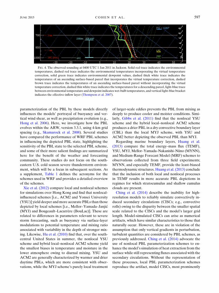
FIG. 4. The observed sounding at 0400 UTC 1 Jan 2011 in Jackson. Solid red trace indicates the environmental

temperatures, dashed red trace indicates the environmental temperatures incorporating the virtual temperature

correction, solid green trace indicates environmental dewpoint values, dashed thick white trace indicates the

temperatures of an ascending surface-based parcel that incorporates the virtual temperature correction, dashed

brown trace indicates the temperatures of an ascending surface-based parcel without incorporating the virtual

temperature correction, dashed thin white trace indicates the temperatures for a descending parcel, light-blue trace

between environmental temperature and dewpoint indicates wet-bulb temperatures, and vertical light-blue bracket

indicates the effective-inflow layer (Thompson et al. 2007).

JUNE 2015 COHEN ET AL . 597

using the local MYJ and quasi-normal scale elimination

(QNSE) schemes across southeastern Louisiana and

southeastern Mississippi.

4. The PBL in relation to southeastern U.S. coldseason severe weather environments

Agoal of this study is to address the lack of analyses of

PBL-scheme sensitivity in environments that support

severe weather in the southeastern United States during

the cool season. However, there have been studies that

examine PBL-scheme behavior in European warm

season environments (e.g., García-Díez et al. 2013).These studies are relevant to the present work because

there are many similarities between southeastern U.S.

cold season severe weather environments and European

(primarily warm season) severe storm environments.

Brooks (2009) shows that CAPE and deep-layer shear

combinations associated with significantly severe thun-

derstorms in Europe are more similar to those associ-

ated with the southeastern U.S. cold season than the

entire full-U.S. distribution. These environments are

exhibited by limited buoyancy along with low-altitude

lifting condensation levels (LCLs). Strong large-scale

forcing for ascent provides the backdrop for European

severe storm environments to offset the limited buoy-

ancy, as is often the case with southeastern U.S. cold

season severe storm environments (Brooks 2009).

Therefore, comparisons between PBL scheme perfor-

mance during European warm and cold seasons could

provide direction for anticipating the effects of choosing

a given PBL scheme representing southeasternU.S. cold

season severe thunderstorm environments.

García-Díez et al. (2013) highlight the diurnal, sea-

sonal, and geographical sensitivities of PBL schemes

over Europe (Fig. 3), and show cold biases in surface

temperatures throughout the summer. TheMYJ scheme

results in the most substantial cold biases during the

daytime, compared to the YSU and ACM2 schemes,

with the YSU scheme most commonly exhibiting the

warmest temperatures among the three schemes

throughout the day and night. This relatively low bias in

using YSU is attributed to its ability to more accurately

account for the stronger entrainment processes within

the PBL, consistent with our expectation that YSU’s

nonlocal treatment of PBL processes should promote

a relatively deeper PBL. Furthermore, YSU is found to

yield a significantly deeper PBL during the daytime.

When compared to gridded precipitation and 2-m tem-

perature observations over Europe, Haylock et al.

(2008) further substantiate the findings of García-Díezet al. (2013) and conclude that the warm season cold bias

is relatively lower when using the YSU scheme.

Therefore, we believe that the YSU scheme, which is

a nonlocal scheme, could offer some utility in forecasts for

southeastern U.S. cold season severe weather environ-

ments among the other PBL schemes currently available

in the WRF Model. Furthermore, García-Díez et al.(2013) stress that long-term statistical studies have a ten-

dency of masking important biases among PBL schemes

owing to bias cancellation on smaller spatiotemporal

scales. As such, they specifically encourage studies that

support the advancement of PBL schemes in environments

that have not been examined thoroughly (e.g., the south-

eastern U.S. cold season severe weather environment).

To illustrate a vertical profile for cold season severe

weather events in the United States, we present the

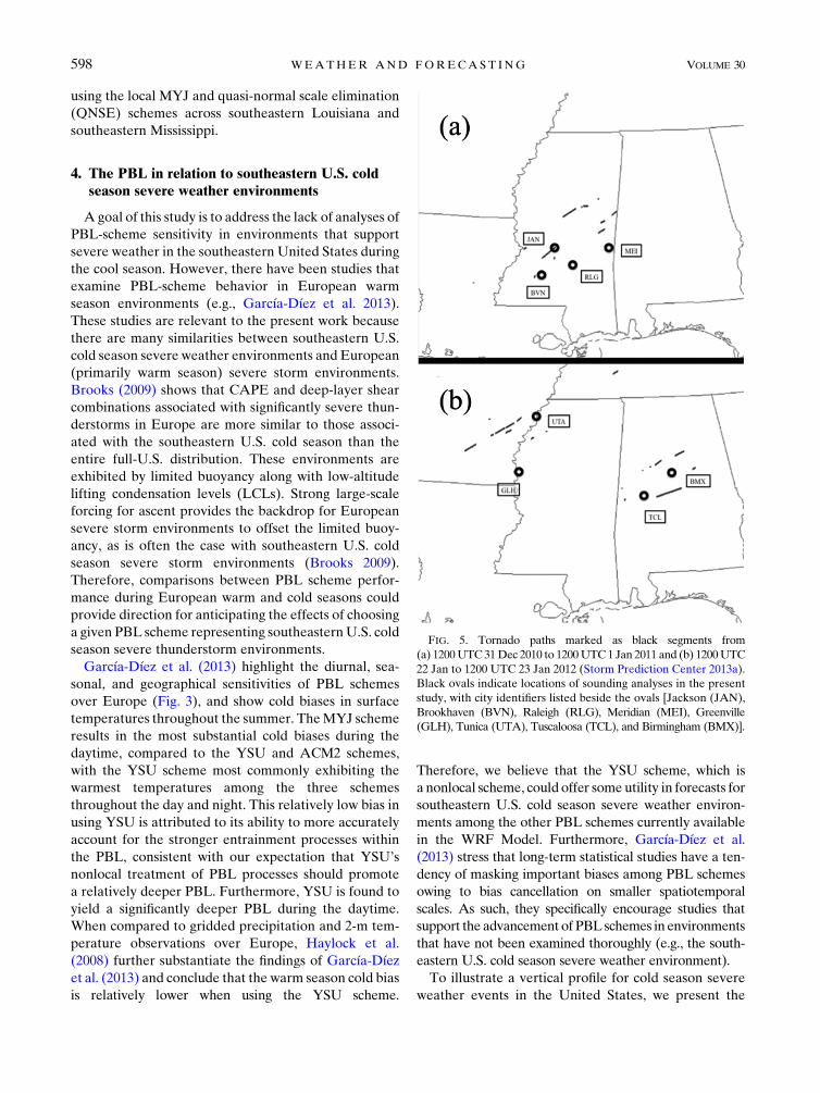
FIG. 5. Tornado paths marked as black segments from

(a) 1200UTC31Dec 2010 to 1200UTC1 Jan 2011 and (b) 1200UTC

22 Jan to 1200 UTC 23 Jan 2012 (Storm Prediction Center 2013a).

Black ovals indicate locations of sounding analyses in the present

study, with city identifiers listed beside the ovals [Jackson (JAN),

Brookhaven (BVN), Raleigh (RLG), Meridian (MEI), Greenville

(GLH), Tunica (UTA), Tuscaloosa (TCL), and Birmingham (BMX)].

598 WEATHER AND FORECAST ING VOLUME 30

sounding provided by a special radiosonde that was

launched at 0400 UTC 1 January 2011 in Jackson, Mis-

sissippi (Fig. 4), within relatively close spatiotemporal

proximity (within 100km and 3h) to some of the central

Mississippi tornadoes, with simulations of this event

later addressed in this paper. This sounding appears to

be representative of the inflow to related storms and

highlights some of the complexities regarding the char-

acterization of the PBL structure for this particular en-

vironment. A shallow layer, extending from the surface

to around 0.5kmabove the ground, features relatively steep

lapse rates within a deeper layer of small temperature–

dewpoint spread (i.e., moist layer) below ;750mb in

which potential temperature increases with height and

mixing ratio also decreases with height, aside from the

little variability in mixing ratio within the lowest 100mb.

Despite the lack of steeper lapse rates that would oth-

erwise be associated with stronger mixing, moisture is

sufficient in the low levels to support nonzero buoyancy.

Surmounting themoist layer aremultiple layers of lower

static stability and vertical moisture gradients, repre-

sentative of the free atmosphere illustrated in Fig. 1. The

event corresponding to this profile is simulated with

results addressed in subsequent sections.

The vertical wind profile is not consistent with our

expectations of a well-mixed PBL through the afore-

mentioned moist layer (extending from the surface to

around the 700-mb level in Fig. 4). This is attributed to

jet-induced vertical wind shear associated with a large-

scale extratropical cyclone. In terms of this southeastern

U.S. cold season environment, the poorly mixed vertical

wind profile is one in which both wind speed and di-

rection vary with increasing height through the moist

layer. In particular, relatively weak southerly flow near

the surface veers to southwesterly flow with a speed

around 26ms21 [50 knots (kt; 1 kt 5 0.51m s21)] at

850mb. The backed surface flow relative to that aloft

and the increase in wind speeds with heights, perhaps

bolstered by friction-inducedweakening of the flow near

the surface, supports large storm-relative helicity (SRH;

e.g., Davies-Jones et al. 1990) of 375–425m2 s22 within

the 0–1- and 0–3-km layers.

The 1 January 2011 example highlights the compli-

cations in defining an upper bound of the PBL in

a sample southeastern U.S. cold season severe storm

environment. Vertical potential temperature, mixing

ratio, and wind profiles are not well mixed throughout

the lower troposphere, and there is no clear demarcation

of any atmospheric variables that might characterize the

‘‘top’’ of the PBL. Using the cloud base, or the LCL for

the purposes of this work, to define the PBL top (e.g.,

Stull 1988) may exclude the role that the poorly mixed

vertical wind profile and accompanying shear-driven,

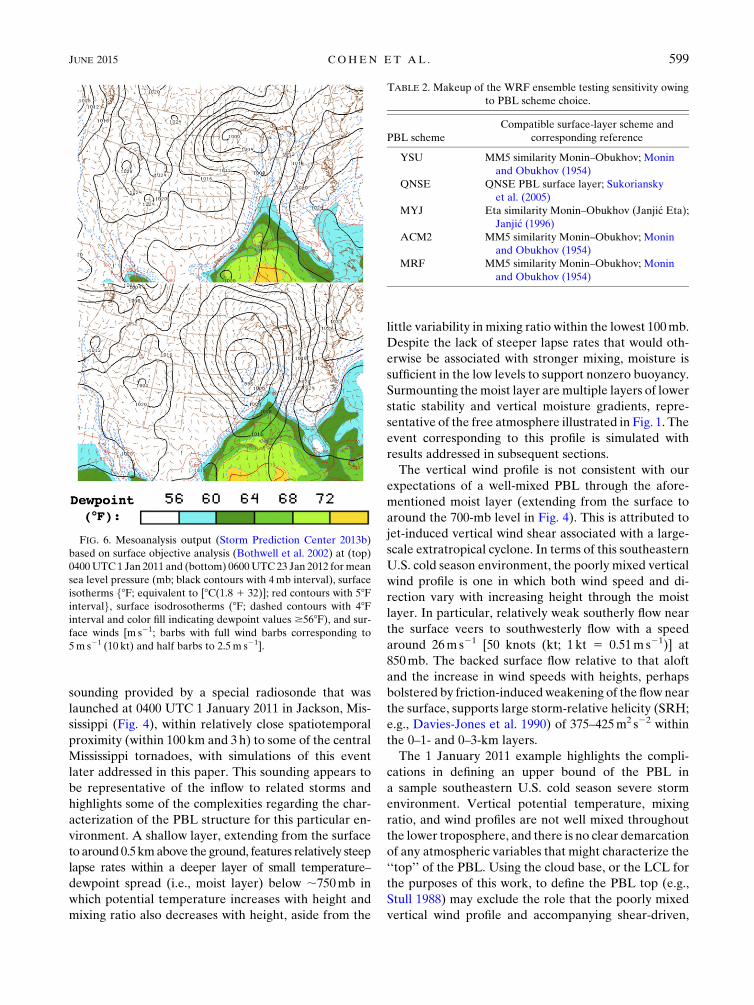
FIG. 6. Mesoanalysis output (Storm Prediction Center 2013b)

based on surface objective analysis (Bothwell et al. 2002) at (top)

0400UTC 1 Jan 2011 and (bottom) 0600UTC 23 Jan 2012 formean

sea level pressure (mb; black contours with 4mb interval), surface

isotherms f8F; equivalent to [8C(1.8 1 32)]; red contours with 58Fintervalg, surface isodrosotherms (8F; dashed contours with 48Finterval and color fill indicating dewpoint values $568F), and sur-

face winds [m s21; barbs with full wind barbs corresponding to

5m s21 (10 kt) and half barbs to 2.5m s21].

TABLE 2. Makeup of the WRF ensemble testing sensitivity owing

to PBL scheme choice.

PBL scheme

Compatible surface-layer scheme and

corresponding reference

YSU MM5 similarity Monin–Obukhov; Monin

and Obukhov (1954)

QNSE QNSE PBL surface layer; Sukoriansky

et al. (2005)

MYJ Eta similarity Monin–Obukhov (Janji�c Eta);

Janji�c (1996)

ACM2 MM5 similarity Monin–Obukhov; Monin

and Obukhov (1954)

MRF MM5 similarity Monin–Obukhov; Monin

and Obukhov (1954)

JUNE 2015 COHEN ET AL . 599

mechanical production of turbulence offer in commu-

nicating surface forcing upward to define a PBL. Me-

chanically produced turbulence communicates surface

conditions through the lower troposphere such that

thermodynamic profiles may provide few clues re-

garding the bounds of the PBL, as they would otherwise

do through a large part of the literature review pre-

viously discussed, complicating their utility in the

southeastern U.S. cold season severe thunderstorm en-

vironment regime for defining the PBL.

5. PBL schemes for southeastern U.S. cold seasonsevere weather environments

a. Evaluation methodology

In a somewhat analogous manner to WRF scheme

comparisons for the European PBL, PBL-scheme be-

havior is examined for two southeastern U.S. tornado

events that occurred in the lower Mississippi River val-

ley and central Gulf Coast region: 1) from 31 December

2010 to 1 January 2011 and 2) from 22 to 23 January 2012

(tornado reports in Fig. 5). These case studies are pre-

sented here to illustrate the PBL scheme concepts that

are potentially relevant to southeastern U.S. severe

weather, and are part of an analysis of a much larger set

of cases that is ongoing and will be presented in a future

study. Most of the tornado reports corresponding to the

first event occurred from 2200 UTC 31 December 2010

to 1000 UTC 1 January 2011, and most of the tornado

reports corresponding to the second event occurred af-

ter 0100 UTC 23 January 2012. The surface pattern

during both of these severe weather events promoted

strong poleward heat and moisture transport inland of

the Gulf of Mexico. In each case, a roughly wedge-

shaped warm sector characterized by rich Gulf moisture

extending inland well to the south-southeast of an ex-

tratropical cyclone centered over the upper Mississippi

River valley (Fig. 6).

First, we investigate the sensitivity of five WRF PBL

schemes in simulating severe convection–relevant pa-

rameters for these cases. This is accomplished by pro-

ducing WRF forecasts with varying PBL schemes but

otherwise identical experiment configurations, as shown

in Table 2. Initial and boundary conditions are from the

National Centers for Environmental Prediction Final

(FNL) Operational Global Analysis (NCAR 2013). The

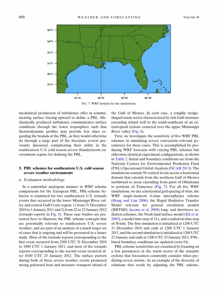
simulations contain 50 vertical levels across a horizontal

domain that extends from the northern Gulf of Mexico

northward to areas extending from parts of Oklahoma

to portions of Tennessee (Fig. 7). For all five WRF

simulations, we use a horizontal grid spacing of 4 km, the

WRF single-moment 6-class microphysics scheme

(Hong and Lim 2006), the Rapid Radiative Transfer

Model relevant for general circulation models

(RRTMG; Iacono et al. 2008) long- and shortwave ra-

diation schemes, the Noah land surface model (Ek et al.

2003), amodel time step of 12 s, and a radiation time step

of 30min. The first simulation is initialized at 1200 UTC

31 December 2010 and ends at 1200 UTC 1 January

2011, and the second simulation is initialized at 1200UTC

22 January and ends at 1200 UTC 23 January 2012. FNL-

based boundary conditions are updated every 6h.

PBL-scheme sensitivities are examined by focusing on

a few parameters in the warm sector of the synoptic

cyclone that forecasters commonly consider when pre-

dicting severe storms. As an example of the diversity of

solutions that result by adjusting the PBL scheme,

FIG. 7. WRF domain for the simulations.

600 WEATHER AND FORECAST ING VOLUME 30

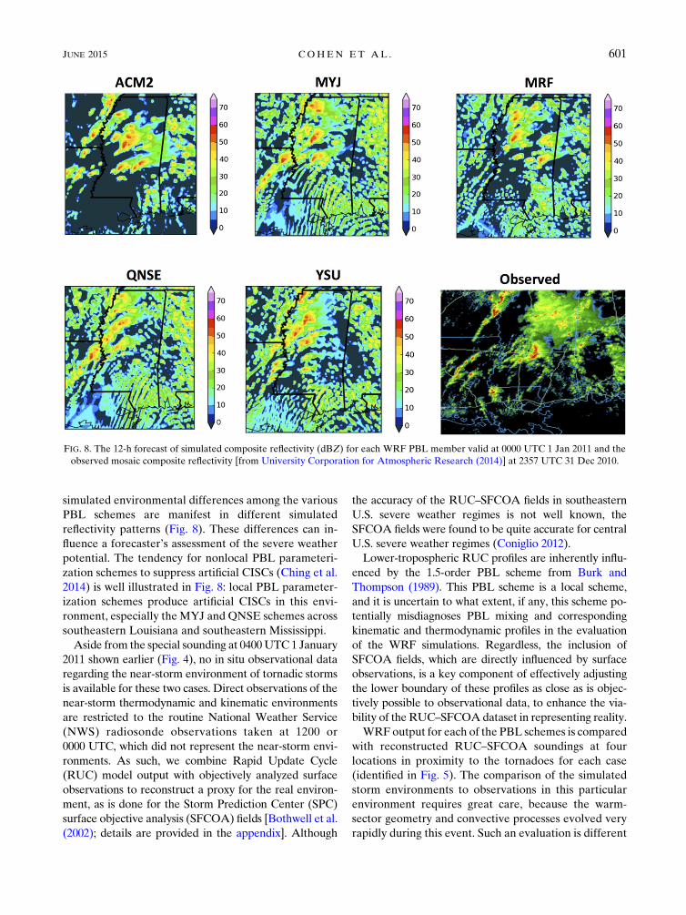
simulated environmental differences among the various

PBL schemes are manifest in different simulated

reflectivity patterns (Fig. 8). These differences can in-

fluence a forecaster’s assessment of the severe weather

potential. The tendency for nonlocal PBL parameteri-

zation schemes to suppress artificial CISCs (Ching et al.

2014) is well illustrated in Fig. 8: local PBL parameter-

ization schemes produce artificial CISCs in this envi-

ronment, especially the MYJ and QNSE schemes across

southeastern Louisiana and southeastern Mississippi.

Aside from the special sounding at 0400UTC 1 January

2011 shown earlier (Fig. 4), no in situ observational data

regarding the near-storm environment of tornadic storms

is available for these two cases. Direct observations of the

near-storm thermodynamic and kinematic environments

are restricted to the routine National Weather Service

(NWS) radiosonde observations taken at 1200 or

0000 UTC, which did not represent the near-storm envi-

ronments. As such, we combine Rapid Update Cycle

(RUC) model output with objectively analyzed surface

observations to reconstruct a proxy for the real environ-

ment, as is done for the Storm Prediction Center (SPC)

surface objective analysis (SFCOA) fields [Bothwell et al.

(2002); details are provided in the appendix]. Although

the accuracy of the RUC–SFCOA fields in southeastern

U.S. severe weather regimes is not well known, the

SFCOA fields were found to be quite accurate for central

U.S. severe weather regimes (Coniglio 2012).

Lower-tropospheric RUC profiles are inherently influ-

enced by the 1.5-order PBL scheme from Burk and

Thompson (1989). This PBL scheme is a local scheme,

and it is uncertain to what extent, if any, this scheme po-

tentially misdiagnoses PBL mixing and corresponding

kinematic and thermodynamic profiles in the evaluation

of the WRF simulations. Regardless, the inclusion of

SFCOA fields, which are directly influenced by surface

observations, is a key component of effectively adjusting

the lower boundary of these profiles as close as is objec-

tively possible to observational data, to enhance the via-

bility of theRUC–SFCOAdataset in representing reality.

WRF output for each of the PBL schemes is compared

with reconstructed RUC–SFCOA soundings at four

locations in proximity to the tornadoes for each case

(identified in Fig. 5). The comparison of the simulated

storm environments to observations in this particular

environment requires great care, because the warm-

sector geometry and convective processes evolved very

rapidly during this event. Such an evaluation is different

FIG. 8. The 12-h forecast of simulated composite reflectivity (dBZ) for each WRF PBL member valid at 0000 UTC 1 Jan 2011 and the

observed mosaic composite reflectivity [from University Corporation for Atmospheric Research (2014)] at 2357 UTC 31 Dec 2010.

JUNE 2015 COHEN ET AL . 601

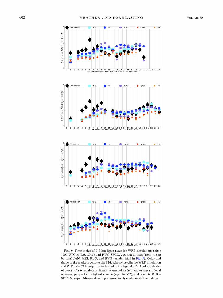
FIG. 9. Time series of 0–3-km lapse rates for WRF simulations (after

1200 UTC 31 Dec 2010) and RUC–SFCOA output at sites (from top to

bottom) JAN, MEI, RLG, and BVN (as identified in Fig. 5). Color and

shape of the markers denotes the PBL scheme used in theWRF simulation

and RUC–SFCOA output, as indicated in the legends. Cool colors (shades

of blue) refer to nonlocal schemes, warm colors (red and orange) to local

schemes, purple to the hybrid scheme (e.g., ACM2), and black to RUC–

SFCOA output. Missing data imply convectively contaminated soundings.

602 WEATHER AND FORECAST ING VOLUME 30

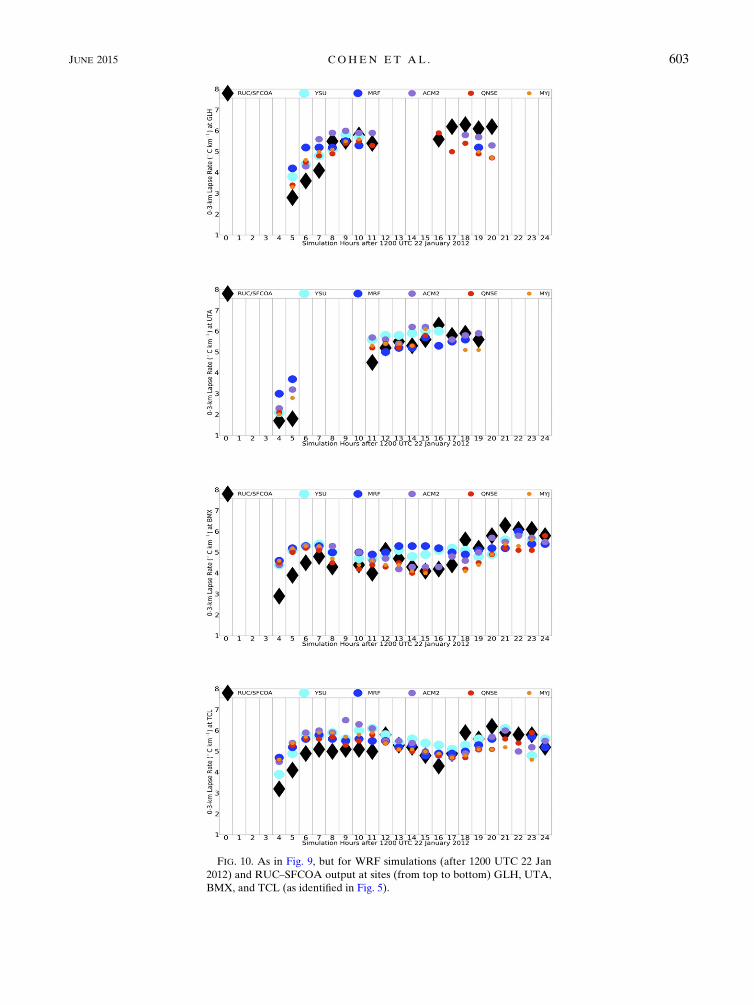
FIG. 10. As in Fig. 9, but for WRF simulations (after 1200 UTC 22 Jan

2012) and RUC–SFCOA output at sites (from top to bottom) GLH, UTA,

BMX, and TCL (as identified in Fig. 5).

JUNE 2015 COHEN ET AL . 603

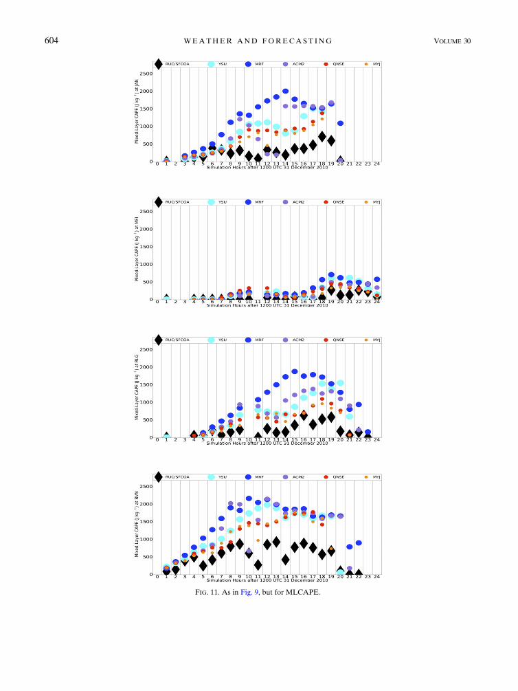
FIG. 11. As in Fig. 9, but for MLCAPE.

604 WEATHER AND FORECAST ING VOLUME 30

than those studies that evaluate PBL schemes in a more

ideal, slowly spatiotemporally evolving PBL in convec-

tive boundary layers. To select locations for comparison,

it is important to represent the warm-sector environ-

ment upstream from convection that has not been con-

taminated by convection. At a given time, any one

location may not have these conditions satisfied among

all fiveWRF simulations and RUC–SFCOA. Therefore,

the choice is made to focus on four sounding locations

for each case owing to the intensive work needed to

ensure that the near-storm environment sampled by the

sounding had positive buoyancy and was not contami-

nated by convection in six different datasets and because

relatively homogeneous conditions within the warm

sector outside of convection would lead to redundancies

in the analysis that four points resolves sufficiently. The

0–3-km temperature lapse rate (hereafter referred to as

the 0–3-km lapse rate), 0–3-km storm-relative helicity2

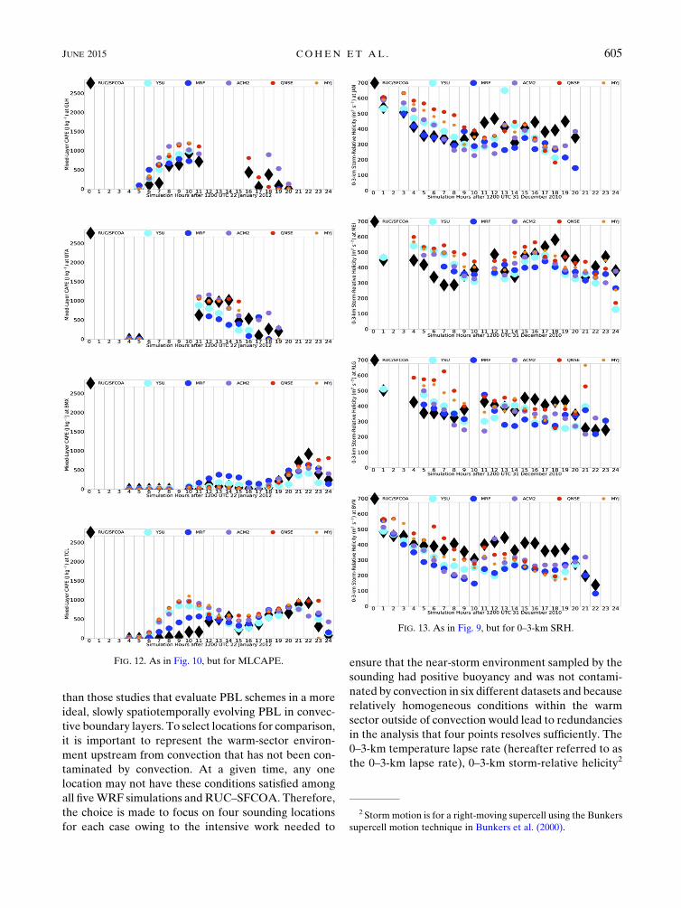
FIG. 12. As in Fig. 10, but for MLCAPE.

FIG. 13. As in Fig. 9, but for 0–3-km SRH.

2 Stormmotion is for a right-moving supercell using the Bunkers

supercell motion technique in Bunkers et al. (2000).

JUNE 2015 COHEN ET AL . 605

(SRH), and mixed-layer CAPE derived from the mean

conditions in the lowest 100mb of the profile are com-

puted from all soundings. These parameters provide

clues in the diagnosis of the potential for severe weather

(e.g., Thompson et al. 2003; Craven and Brooks 2004).

Statistical comparisons between simulated parame-

ters and those derived from the RUC–SFCOA output

are provided using a framework for error analysis.While

this framework is often applied in economic forecast

analysis (e.g., Theil 1961, 1966; Clements and Frenkel

1980; Pindyck and Rubinfeld 1981), its statistical appli-

cability is broader among other fields (Trnka et al. 2006).

Theil’s inequality coefficient is defined as

U5

ffiffiffiffiffiffiffiffiffiffiffiffiffiffiffiffiffiffiffiffiffiffiffiffiffiffiffiffiffiffiffiffiffiffiffi1

T�T

t51

(Yst 2Ya

t )2

sffiffiffiffiffiffiffiffiffiffiffiffiffiffiffiffiffiffiffiffiffiffiffiffi1

T�T

t51

(Yst )

2

s1

ffiffiffiffiffiffiffiffiffiffiffiffiffiffiffiffiffiffiffiffiffiffiffiffi1

T�T

t51

(Yat )

2

s . (1)

Model forecasts and observations are indicated by Yst

andYat , respectively, while T represents the total sample

size. The numerator represents the root-mean-square

error (RMSE), and the quotient to determine U repre-

sents a normalized form of the RMSE. The benefit of

considering a normalized form of the RMSE as opposed

to strictly the RMSE is that the former permits stan-

dardization of error comparisons among parameters

whose magnitudes vary greatly. Specifically, U can the-

oretically be as low as zero, representing a perfect

forecast, with progressively higher values indicating

poorer forecast quality. The bias proportion of U is de-

fined as

Um 5(Ys 2Ya)2

(1/T)�(Yst 2Ya

t )2. (2)

The quantityUm represents that component of the error

that is systematic (i.e., the bias). Values of this compo-

nent roughly in excess of 0.1 or 0.2 indicate the presence

of bias inherent in the forecast model. Since differences

for thermodynamic and kinematic profiles among the

WRF simulations do not become apparent until after

the first hour of the simulation, comparisons between

forecast and RUC–SFCOA output are not analyzed

until at least 1 h into the simulation cycles.

b. Evaluation discussion

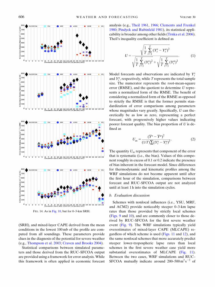
Schemes with nonlocal influences (i.e., YSU, MRF,

and ACM2) provide noticeably steeper 0–3-km lapse

rates than those provided by strictly local schemes

(Figs. 9 and 10), and are commonly closer to those de-

rived by RUC–SFCOA for the first severe weather

event (Fig. 9). The WRF simulations typically yield

overestimates of mixed-layer CAPE (MLCAPE) re-

gardless of which scheme is used (Figs. 11 and 12), and

the same nonlocal schemes that more accurately predict

steeper lower-tropospheric lapse rates than local

schemes in the first severe weather case yield more

substantial overestimates of MLCAPE (Fig. 11).

Between the two cases, WRF simulations and RUC–

SFCOA mutually indicate around 200–500m2 s22 of

FIG. 14. As in Fig. 10, but for 0–3-km SRH.

606 WEATHER AND FORECAST ING VOLUME 30

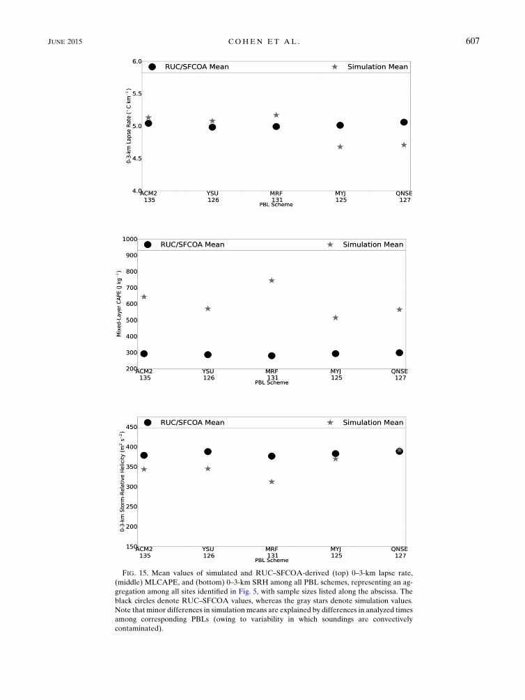
FIG. 15. Mean values of simulated and RUC–SFCOA-derived (top) 0–3-km lapse rate,

(middle) MLCAPE, and (bottom) 0–3-km SRH among all PBL schemes, representing an ag-

gregation among all sites identified in Fig. 5, with sample sizes listed along the abscissa. The

black circles denote RUC–SFCOA values, whereas the gray stars denote simulation values.

Note that minor differences in simulationmeans are explained by differences in analyzed times

among corresponding PBLs (owing to variability in which soundings are convectively

contaminated).

JUNE 2015 COHEN ET AL . 607

0–3-km SRH (Figs. 13 and 14), with the nonlocal

schemes often yielding relatively less SRH.

These overall differences are reflected in Fig. 15.

Mean values of the low-level lapse rates are typically

greater and more accurate for nonlocal schemes than

local schemes. This is largely consistent with the results

documented in many of the previously discussed studies

that find stronger, deeper vertical mixing (which

steepens lapse rates) as portrayed by the nonlocal

schemes to more accurately represent the thermody-

namic profile of a simulation compared to strictly local

schemes. The vertical mixing tends environmental lapse

rates toward dry adiabatic, and deeper mixing expands

the vertical extent of these steeper environmental lapse

rates. The strictly local schemes (i.e., MYJ and QNSE)

exhibit greater bias than the nonlocal schemes for 0–3-km

lapse rate (Table 3) and are associated with less steep

0–3-km lapse rates (Fig. 15). The MRF accentuates

these characteristics, which is particularly evident with

biases in its overestimation of the lower-tropospheric

lapse rates (Table 3). This is entirely consistent with the

tendency for this nonlocal scheme to represent too

strong vertical mixing in strong-wind regimes, as sug-

gested by Hong et al. (2006), yielding too much

smoothing of the vertical wind profile and too small of

SRH (Fig. 15), with SRH biases apparent in Table 3.

TABLE 3. Theil’s inequality coefficient and the bias component for WRF simulations and RUC–SFCOA-derived 0–3-km lapse rate,

MLCAPE, and 0–3-km SRH among all PBL schemes, representing an aggregation among all sites identified in Fig. 5.

Parameter ACM2 YSU MRF MYJ QNSE

0–3-km lapse rate U 5 0.07 U 5 0.07 U 5 0.07 U 5 0.08 U 5 0.08

Um 5 0.02 Um 5 0.02 Um 5 0.06 Um 5 0.17 Um 5 0.20

MLCAPE U 5 0.43 U 5 0.42 U 5 0.52 U 5 0.34 U 5 0.35

Um 5 0.40 Um 5 0.32 Um 5 0.42 Um 5 0.35 Um 5 0.44

0–3-km SRH U 5 0.13 U 5 0.16 U 5 0.15 U 5 0.14 U 5 0.15

Um 5 0.13 Um 5 0.12 Um 5 0.34 Um 5 0.02 Um , 0.01

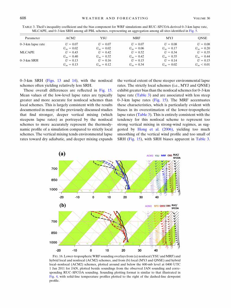
FIG. 16. Lower-troposphericWRF sounding overlays from (a) nonlocal (YSU andMRF) and

hybrid local and nonlocal (ACM2) schemes, and from (b) local (MYJ and QNSE) and hybrid

local–nonlocal (ACM2) schemes, plotted around and below the 600-mb level at 0400 UTC

1 Jan 2011 for JAN, plotted beside soundings from the observed JAN sounding and corre-

sponding RUC–SFCOA sounding. Sounding plotting format is similar to that illustrated in

Fig. 4, with solid-line temperature profiles plotted to the right of the dashed-line dewpoint

profile.

608 WEATHER AND FORECAST ING VOLUME 30

Otherwise, for 0–3-km SRH, neither error nor bias

among the local or nonlocal schemes is particularly

large.

Sensitivities in MLCAPE owing to the vertical in-

tegration of thermodynamic profiles through a deep

layer of the troposphere provide a challenge in assessing

the relative effect of modulations to the profiles by the

PBL schemes, as such a parameter may be more influ-

enced by secondary differences among the WRF simu-

lations (e.g., convective evolution) to which a more

simple lapse rate calculation would be more resistant.

These concepts are associated with notably larger errors

and biases in MLCAPE among all WRF simulations

than the other aforementioned variables (Table 3).

Many of these statistical results are highlighted by the

overlay of WRF soundings provided in Fig. 16, which

also provides comparisons with the sounding output also

plotted in Fig. 4 (observed sounding) and the corre-

sponding RUC–SFCOA reconstructed sounding, all for

the same time and location. The local schemes depict

greater static stability in the near-surface layer, with

greater directional shear, below the 850-mb level. On

the other hand, the nonlocal schemes more accurately

highlight warmer surface temperatures, less static sta-

bility, and a somewhat smoother vertical profile in the

lower troposphere.

6. General discussion and conclusions

This study summarizes key characteristics that explain

the differences among WRF PBL schemes along with

advantages and disadvantages to using each scheme.

Particular emphasis is placed on evaluating the perfor-

mance of these schemes inmodeling the lower-tropospheric

thermodynamic and kinematic profile for southeasternU.S.

cold season severe weather environments.

The primary difference between these schemes in-

volves their representation of the vertical mixing pro-

cess, in terms of the determination of whichmodel layers

influence atmospheric conditions at a given model level.

Local schemes only permit nearby model layers to in-

fluence these conditions, precluding the direct inclusion

of the effects that larger turbulent eddies yield in mixing

atmospheric properties within much more vertically

expansive depths of the lower troposphere. Nonlocal

schemes consider the effect of these larger eddies on the

dispersion of heat, moisture, and momentum through-

out the depth of the PBL. As such, they are more likely

to properly simulate the diurnally growing PBL owing to

their inclusion of thermally driven turbulence associated

with the diabatically heated surface layer. This is despite

the potential for localized layers of relatively higher

static stability to exist that may not have deleterious

effects in building the PBL. Local schemes have more of

a tendency to stunt the growth of the PBL owing to the

presence of these statically stable layers when, in reality,

the larger turbulent eddies can still mix through such

localized layers.

As an example, through a test of five different PBL

schemes for two southeastern U.S. cold season tornado

events, WRF simulations that employ nonlocal param-

eterizations of the PBL produce 0–3-km lapse rates that

are more accurate, less biased, and steeper than those

that employ local-only schemes. This is consistent with

the previously mentioned findings with respect to warm

season, European PBLs, in which the nonlocal PBL

scheme reduces biases in temperature forecasts in as-

sociation with its ability to better simulate entrainment

processes within the PBL, yielding a relatively deeper

PBL during the daytime. As an extension to the vertical

wind profile, these nonlocal schemes accurately indicate

a large, low-level SRH environment, albeit slightly

smaller than what local schemes indicate, suggesting

that the deepermixing did not unrealistically smooth the

strong vertical wind shear in this environment. At the

same time, both nonlocal and local schemes typically

overestimateMLCAPE, though these overestimates are

more prominent with nonlocal schemes.

There may not be a one-size-fits-all approach to the

selection of such a ‘‘best’’ scheme. However, this study is

intended to be a first step in gaining a better un-

derstanding of the relatively unexplored behavior of the

PBL, and its representation in numerical weather models,

for cold season severe weather environments. Future

work is ongoing to expand and generalize the results of

the case studies discussed here to include a wide array of

cases, allowing a more substantial number of warm-sector

points to be considered in cold season severe weather

environments, among many other events.

Acknowledgments. Output displays use formats from

the National Centers Advanced Weather Interactive

Processing System Skew T Hodograph Analysis and

Research Program (NSHARP; Hart et al. 1999). The

authors thank Dr. Israel Jirak of the Storm Prediction

Center, along with three anonymous reviewers, for their

reviews of this paper and comments that have contrib-

uted to its improvement. The lead author thanks his

father, Mr. Joel Cohen, an economist, for numerous

discussions and insight regarding forecast evaluation.

This work was originally inspired by the lead author’s

doctoral committee at the University of Oklahoma

School of Meteorology for his Ph.D. General Examina-

tion. Committee members include Dr. Steven Cavallo,

Dr. Harold Brooks, Dr. Frederick Carr, Dr. Kevin

Kloesel, and Dr. John Greene.

JUNE 2015 COHEN ET AL . 609

APPENDIX

Procedure for Constructing RUC–SFCOASoundings for Comparison with WRF Simulations

Gridded RUC output, at 20-km grid spacing, is

provided by the NOAA National Model Archive and

Distribution System (NOAA/NCDC 2014a,b). Basic

thermodynamic and kinematic variables (i.e., tempera-

ture, relative humidity, and horizontal wind compo-

nents) are extracted from the RUC vertical profile at

25-mb increments above the surface on an hourly basis

through the 24-h simulation period. All calculations

relating these variables are performed using the NCAR

Command Language (NCL; NCAR 2014). Four profiles

are selected for each hour, corresponding to the each of

the sites identified in Fig. 5. The surface pressure and

corresponding thermodynamic and kinematic values

at each hour are provided from the SFCOA output

(Bothwell et al. 2002). All data at higher pressures than

this SFCOA baseline are deleted, effectively setting the

SFCOA-related information as the base of the vertical

profile (i.e., at the surface of the earth). All calculations

related to integrated, composite parameters are performed

on the subsequent merged soundings, following pro-

cedures applied in Coniglio et al. (2013), for example.

REFERENCES

Angevine,W.M., 2005:An integrated turbulence scheme for boundary

layers with shallow cumulus applied to pollutant transport.

J. Appl. Meteor., 44, 1436–1452, doi:10.1175/JAM2284.1.

——, H. Jiang, and T. Mauritsen, 2010: Performance of an eddy

diffusivity–mass flux scheme for shallow cumulus boundary

layers. Mon. Wea. Rev., 138, 2895–2912, doi:10.1175/

2010MWR3142.1.

Ashley, W. S., 2007: Spatial and temporal analysis of tornado fa-

talities in the United States: 1880–2005. Wea. Forecasting, 22,1214–1228, doi:10.1175/2007WAF2007004.1.

Bothwell, P. D., J. A. Hart, and R. L. Thompson, 2002: An in-

tegrated three-dimensional objective analysis scheme in use at

the Storm Prediction Center. Preprints, 21st Conf. on Severe

Local Storms/19th Conf. on weather Analysis and Forecasting/

15th Conf. on Numerical Weather Prediction, San Antonio,

TX, Amer. Meteor. Soc., JP3.1. [Available online at https://

ams.confex.com/ams/pdfpapers/47482.pdf.]

Bougeault, P., and P. Lacarrère, 1989: Parameterization of orography-

induced turbulence in a mesobeta-scale model. Mon. Wea.

Rev., 117, 1872–1890, doi:10.1175/1520-0493(1989)117,1872:

POOITI.2.0.CO;2.

Bretherton, C. S., and S. Park, 2009: A new moist turbulence pa-

rameterization in the Community Atmosphere Model. J. Cli-

mate, 22, 3422–3448, doi:10.1175/2008JCLI2556.1.

Bright, D. R., and S. L. Mullen, 2002: The sensitivity of the nu-

merical simulation of the southwest monsoon boundary layer

to the choice of PBL turbulenceparameterization inMM5.Wea.

Forecasting, 17, 99–114, doi:10.1175/1520-0434(2002)017,0099:

TSOTNS.2.0.CO;2.

Brooks, H. E., 2009: Proximity soundings for Europe and the

United States from reanalysis data. Atmos. Res., 93, 546–553,

doi:10.1016/j.atmosres.2008.10.005.

Bunkers, M. J., B. A. Klimowski, J. W. Zeitler, R. L. Thompson,

and M. L. Weisman, 2000: Predicting supercell motion using

a new hodograph technique. Wea. Forecasting, 15, 61–79,

doi:10.1175/1520-0434(2000)015,0061:PSMUAN.2.0.CO;2.

Burk, S. D., and W. T. Thompson, 1989: A vertically nested re-

gional numerical weather prediction model with second-order

closure physics. Mon. Wea. Rev., 117, 2305–2324, doi:10.1175/

1520-0493(1989)117,2305:AVNRNW.2.0.CO;2.

Ching, J., R. Rotunno, M. LeMone, A. Martilli, B. Kosovic, P. A.

Jimenez, and J. Dudhia, 2014: Convectively induced second-

ary circulations in fine-grid mesoscale numerical weather

prediction models. Mon. Wea. Rev., 142, 3284–3302,

doi:10.1175/MWR-D-13-00318.1.

Clements, K. W., and J. A. Frenkel, 1980: Exchange rates, money

and relative prices: The dollar–pound in the 1920s. J. Int.

Econ., 10, 249–262, doi:10.1016/0022-1996(80)90057-4.Coniglio,M. C., 2012: Verification of RUC0–1-h forecasts and SPC

mesoscale analyses using VORTEX2 soundings. Wea. Fore-

casting, 27, 667–683, doi:10.1175/WAF-D-11-00096.1.

——, J. Correia, P. T. Marsh, and F. Kong, 2013: Verification of

convection-allowing WRF Model forecasts of the planetary

boundary layer using sounding observations. Wea. Fore-

casting, 28, 842–862, doi:10.1175/WAF-D-12-00103.1.

Craven, J. P., and H. E. Brooks, 2004: Baseline climatology of

sounding derived parameters associated with deep, moist

convection. Natl. Wea. Dig., 28, 13–24.

Davies-Jones, R. P., D. Burgess, and M. Foster, 1990: Test of

helicity as a forecasting parameter. Preprints, 16th Conf. on

Severe Local Storms, Kananaskis Park, AB, Canada, Amer.

Meteor. Soc., 588–592.

Ek, M. B., K. E. Mitchell, Y. Lin, P. Grunmann, E. Rodgers,

G. Gayno, and V. Koren, 2003: Implementation of the up-

graded Noah land surface model in the NCEP operational

mesoscale Eta model. J. Geophys. Res., 108, 8851, doi:10.1029/2002JD003296.

García-Díez, M., J. Fernández, L. Fita, and C. Yagüe, 2013: Sea-sonal dependence of WRF Model biases and sensitivity to

PBL schemes over Europe. Quart. J. Roy. Meteor. Soc., 139,501–514, doi:10.1002/qj.1976.

Gibbs, J. A., E. Fedorovich, andA.M. J. van Eijk, 2011: Evaluating

Weather Research and Forecasting (WRF)Model predictions

of turbulent flow parameters in a dry convective boundary

layer. J. Appl. Meteor. Climatol., 50, 2429–2444, doi:10.1175/

2011JAMC2661.1.

Grenier, H., and C. S. Bretherton, 2001: A moist PBL parameter-

ization for large-scalemodels and its application to subtropical

cloud-toppedmarine boundary layers.Mon.Wea. Rev., 129, 357–

377, doi:10.1175/1520-0493(2001)129,0357:AMPPFL.2.0.CO;2.

Guyer, J. L., and A. R. Dean, 2010: Tornadoes within weak CAPE

environments across the continental United States. Preprints,

25th Conf. on Severe Local Storms, Denver, CO, Amer. Me-

teor. Soc., 1.5. [Available online at http://ams.confex.com/ams/

pdfpapers/175725.pdf.]

——, D. A. Imy, A. Kis, and K. Venable, 2006: Cool season sig-

nificant (F2–F5) tornadoes in the Gulf Coast states. Preprints,

23rd Conf. on Severe Local Storms, St. Louis, MO, Amer.

Meteor. Soc., 4.2. [Available online at https://ams.confex.com/

ams/pdfpapers/115320.pdf.]

Hacker, J. P., 2010: Spatial and temporal scales of boundary

layer wind predictability in response to small-amplitude land

610 WEATHER AND FORECAST ING VOLUME 30

surface uncertainty. J. Atmos. Sci., 67, 217–233, doi:10.1175/

2009JAS3162.1.

Hart, J. A., J. Whistler, R. Lindsay, and M. Kay, 1999: NSHARP,

version 3.10. Storm Prediction Center, National Centers for

Environmental Prediction, Norman, OK, 33 pp.

Haylock, M. R., N. Hofstra, A. M. G. Klein Tank, E. J. Klok, P. D.

Jones, and M. New, 2008: A European daily high-resolution

gridded dataset of surface temperature and precipitation.

J. Geophys. Res., 113, D20119, doi:10.1029/2008JD010201.

Holton, J. R., 2004: Introduction to Dynamic Meteorology. 4th ed.

Elsevier, 535 pp.

Holtslag, A. A. M., and B. A. Boville, 1993: Local versus nonlocal

boundary-layer diffusion in a global climate model. J. Cli-

mate, 6, 1825–1842, doi:10.1175/1520-0442(1993)006,1825:

LVNBLD.2.0.CO;2.

Hong, S.-Y., and H.-L. Pan, 1996: Nonlocal boundary layer vertical

diffusion in a medium-range forecast model.Mon. Wea. Rev.,

124, 2322–2339, doi:10.1175/1520-0493(1996)124,2322:

NBLVDI.2.0.CO;2.

——, and J. O. J. Lim, 2006: The WRF single-moment 6-class

microphysics scheme (WSM6). J. Korean Meteor. Soc., 42,

129–151.

——, S. Y. Noh, and J. Dudhia, 2006: A new vertical diffusion

package with an explicit treatment of entrainment processes.

Mon. Wea. Rev., 134, 2318–2341, doi:10.1175/MWR3199.1.

Hu, X.-M., J.W. Nielsen-Gammon, and F. Zhang, 2010: Evaluation

of three planetary boundary layer schemes in the WRF

Model. J. Appl. Meteor. Climatol., 49, 1831–1844, doi:10.1175/

2010JAMC2432.1.

Huang, H.-Y., A. Hall, and J. Teixeira, 2013: Evaluation of the

WRF PBL parameterizations for marine boundary layer

clouds: Cumulus and stratocumulus. Mon. Wea. Rev., 141,

2265–2271, doi:10.1175/MWR-D-12-00292.1.

Iacono, M. J., J. S. Delamere, E. J. Mlawer, M. W. Shephard, S. A.

Clough, and W. D. Collins, 2008: Radiative forcing by long-

lived greenhouse gases: Calculations with the AER radiative

transfer models. J. Geophys. Res., 113, D13103, doi:10.1029/

2008JD009944.

Janji�c, Z. I., 1990: The step-mountain coordinate: Physical

package. Mon. Wea. Rev., 118, 1429–1443, doi:10.1175/

1520-0493(1990)118,1429:TSMCPP.2.0.CO;2.

——, 1994: The step-mountain eta coordinate model: Further

developments of the convection, viscous sublayer, and turbu-

lence closure schemes. Mon. Wea. Rev., 122, 927–945,

doi:10.1175/1520-0493(1994)122,0927:TSMECM.2.0.CO;2.

——, 1996: The surface layer in the NCEP Eta Model. Preprints,

11th Conf. on Numerical Weather Prediction, Norfolk, VA,

Amer. Meteor. Soc., 354–355.

Jankov, I., W. A. Gallus, M. Segal, B. Shaw, and S. E. Koch, 2005:

The impact of different WRF Model physical para-

meterizations and their interactions on warm season MCS

rainfall. Wea. Forecasting, 20, 1048–1060, doi:10.1175/

WAF888.1.

Johns, R. H., and C. A. Doswell III, 1992: Severe local storms

forecasting. Wea. Forecasting, 7, 588–612, doi:10.1175/

1520-0434(1992)007,0588:SLSF.2.0.CO;2.

Kain, J. S., M. E. Baldwin, P. R. Janish, S. J. Weiss, M. P. Kay, and

G. W. Carbin, 2003: Subjective verification of numerical

models as a component of a broader interaction between re-

search and operations. Wea. Forecasting, 18, 847–860,

doi:10.1175/1520-0434(2003)018,0847:SVONMA.2.0.CO;2.

——, S. J. Weiss, M. E. Baldwin, G. W. Carbin, D. A. Bright, J. J.

Levit, and J. A. Hart, 2005: Evaluating high-resolution

configurations of the WRF Model that are used to forecast

severe convective weather: The 2005 SPC/NSSL Spring Pro-

gram. Preprints, 21st Conf. on Weather Analysis and Fore-

casting/17th Conf. on Numerical Weather Prediction,

Washington, DC,Amer.Meteor. Soc., 2A.5. [Available online

at http://ams.confex.com/ams/pdfpapers/94843.pdf.]

——, and Coauthors, 2013: A feasibility study for probabilistic

convection initiation forecasts based on explicit

numerical guidance. Bull. Amer. Meteor. Soc., 94, 1213–1225,

doi:10.1175/BAMS-D-11-00264.1.

Kis, A. K., and J. M. Straka, 2010: Nocturnal tornado climatology.

Wea. Forecasting, 25, 545–561, doi:10.1175/2009WAF2222294.1.

Kosovi�c, B., and J. A. Curry, 2000: A large eddy simulation study of a

quasi-steady stably stratified atmospheric boundary layer. J. At-

mos. Sci., 57, 1052–1068, doi:10.1175/1520-0469(2000)057,1052:

ALESSO.2.0.CO;2.

Mass, C. F., D. Ovens, K. Westrick, and B. A. Colle, 2002: Does

increasing horizontal resolution produce more skillful fore-

casts? Bull. Amer. Meteor. Soc., 83, 407–430, doi:10.1175/

1520-0477(2002)083,0407:DIHRPM.2.3.CO;2.

Mauritsen, T., G. Svensson, S. S. Zilitinkevich, I. Esau, L. Enger,

and B. Grisogono, 2007: A total turbulent energy closure

model for neutrally and stably stratified atmospheric bound-

ary layers. J. Atmos. Sci., 64, 4113–4126, doi:10.1175/

2007JAS2294.1.

Mellor, G. L., and T. Yamada, 1974: A hierarchy of turbulence

closure models for planetary boundary layers. J. Atmos. Sci.,

31, 1791–1806, doi:10.1175/1520-0469(1974)031,1791:

AHOTCM.2.0.CO;2.

——, and ——, 1982: Development of a turbulence closure model

for geophysical fluid problems.Rev. Geophys. Space Phys., 20,

851–875, doi:10.1029/RG020i004p00851.

Monin, A. S., and A. M. Obukhov, 1954: Basic laws of turbulent

mixing in the surface layer of the atmosphere (in Russian). Tr.

Geofiz. Inst., Akad. Nauk SSSR, 24, 1963–1967.

Nakanishi, M., and H. Niino, 2004: An improved Mellor–Yamada

level-3 model with condensation physics: Its design and veri-

fication. Bound.-Layer Meteor., 112, 1–31, doi:10.1023/

B:BOUN.0000020164.04146.98.

——, and——, 2006: An improvedMellor–Yamada level-3 model:

Its numerical stability and application to a regional prediction

of advection fog. Bound.-Layer Meteor., 119, 397–407,

doi:10.1007/s10546-005-9030-8.

——, and ——, 2009: Development of an improved turbulence

closure model for the atmospheric boundary layer. J. Meteor.

Soc. Japan, 87, 895–912, doi:10.2151/jmsj.87.895.

NCAR, cited 2013: NCEP FNL operational model global tropo-

spheric analyses, continuing from July 1999. Computational

and Information Systems Laboratory, National Center for

Atmospheric Research. [Available online at http://rda.ucar.

edu/datasets/ds083.2/.]

——, cited 2014: NCARCommand Language. [Available online at

http://www.ncl.ucar.edu/.]

Nielsen-Gammon, J.W., X.-M.Hu, F. Zhang, and J. E. Pleim, 2010:

Evaluation of planetary boundary layer scheme sensitivities

for the purpose of parameter estimation.Mon.Wea. Rev., 138,3400–3417, doi:10.1175/2010MWR3292.1.

NOAA/NCDC, cited 2014a: Model Data Inventories. NOAA/

National Operational Model Archive and Distribution Sys-

tem. [Available online at http://nomads.ncdc.noaa.gov/data.

php?name5inventory.]

——, cited 2014b: RUC online archive. [Available online at http://

nomads.ncdc.noaa.gov/data/ruc/.]

JUNE 2015 COHEN ET AL . 611

Pindyck, R. S., andD. L. Rubinfeld, 1981:EconometricModels and

Economic Forecasts. 2nd ed. McGraw-Hill, 630 pp.

Pleim, J. E., 2007a: A combined local and nonlocal closure model

for the atmospheric boundary layer. Part I: Model description

and testing. J. Appl. Meteor. Climatol., 46, 1383–1395,

doi:10.1175/JAM2539.1.

——, 2007b: A combined local and nonlocal closure model for the

atmospheric boundary layer. Part II: Application and evalu-

ation in a mesoscale meteorological model. J. Appl. Meteor.

Climatol., 46, 1396–1409, doi:10.1175/JAM2534.1.

Rasmussen, E. N., and D. O. Blanchard, 1998: A baseline clima-

tology of sounding-derived supercell and tornado forecast

parameters. Wea. Forecasting, 13, 1148–1164, doi:10.1175/

1520-0434(1998)013,1148:ABCOSD.2.0.CO;2.

Schneider, J. M., and D. K. Lilly, 1999: An observational and

numerical study of a sheared, convective boundary layer.

Part I: Phoenix II observations, statistical description, and

visualization. J. Atmos. Sci., 56, 3059–3078, doi:10.1175/

1520-0469(1999)056,3059:AOANSO.2.0.CO;2.

Schneider, R. S., and A. R. Dean, 2008: A comprehensive 5-year

severe storm environment climatology for the continental

United States. Preprints, 24th Conf. on Severe Local Storms,

Savannah, GA, Amer. Meteor. Soc., 16A.4. [Available online

at http://ams.confex.com/ams/pdfpapers/141748.pdf.]

Shin, H. H., and S.-Y. Hong, 2011: Intercomparison of planetary

boundary-layer parameterizations in the WRF Model for

a single day fromCASES-99.Bound.-LayerMeteor., 139, 261–

281, doi:10.1007/s10546-010-9583-z.

Skamarock, W. C., and Coauthors, 2008: A description of the

Advanced Research WRF version 3. NCAR Tech. Note TN-

4751STR, 113 pp. [Available online at http://www2.mmm.

ucar.edu/wrf/users/docs/arw_v3.pdf.]

Stensrud, D. J., 2007: Parameterization Schemes: Keys to Un-

derstanding Numerical Weather Prediction Models. Cam-

bridge University Press, 459 pp.

Storm Prediction Center, cited 2013a: SPC hourly mesoscale analysis.

[Available online at http://www.spc.noaa.gov/exper/ma_archive/.]

——, cited 2013b: Storm Prediction Center National Severe

Weather database browser: Online SeverePlot 3.0. [Available

online at http://www.spc.noaa.gov/climo/online/sp3/plot.php.]

Stull, R. B., 1988:An Introduction to Boundary LayerMeteorology.

Kluwer Academic, 666 pp.

——, 1991: Static stability—An update. Bull. Amer. Meteor.

Soc., 72, 1521–1529, doi:10.1175/1520-0477(1991)072,1521:

SSU.2.0.CO;2.

——, 1993: Review of non-local mixing in turbulent atmospheres:

Transilient turbulence theory. Bound.-Layer Meteor., 62, 21–

96, doi:10.1007/BF00705546.

Sukoriansky, S., B. Galperin, and V. Perov, 2005: Applica-

tion of a new spectral theory of stably stratified

turbulence to the atmospheric boundary layer over sea

ice. Bound.-Layer Meteor., 117, 231–257, doi:10.1007/

s10546-004-6848-4.

Theil, H., 1961: Economic Forecasts and Policy. 2nd Ed. North-

Holland, 567 pp.

——, 1966:Applied Economic Forecasting.North-Holland, 474 pp.

Thompson, R. L., R. Edwards, J. A. Hart, K. L. Elmore, and

P. Markowski, 2003: Close proximity soundings within

supercell environments obtained from the Rapid Update

Cycle. Wea. Forecasting, 18, 1243–1261, doi:10.1175/

1520-0434(2003)018,1243:CPSWSE.2.0.CO;2.

——, C. M. Mead, and R. Edwards, 2007: Effective storm-

relative helicity and bulk shear in supercell thunderstorm

environments. Wea. Forecasting, 22, 102–115, doi:10.1175/

WAF969.1.

Trnka,M., J. Eitzinger, G. Gruszczynski, K. Buchgraber, R. Resch,

and A. Schaumberger, 2006: A simple statistical model

for predicting herbage production from permanent

grassland. Grass Forage Sci., 61, 253–271, doi:10.1111/

j.1365-2494.2006.00530.x.

Troen, L., and L. Mahrt, 1986: A simple model of the atmospheric

boundary layer: Sensitivity to surface evaporation. Bound.-

Layer Meteor., 37, 129–148, doi:10.1007/BF00122760.

University Corporation for Atmospheric Research, cited

2014: Image archive meteorological case study collection

kit. [Available online at http://www2.mmm.ucar.edu/

imagearchive/.]

Vescio, M. D., and R. L. Thompson, 1998: Some meteorological

conditions associated with isolated F3–F5 tornadoes in the

cool season. Preprints, 19th Conf. on Severe Local Storms,

Minneapolis, MN, Amer. Meteor. Soc., 2–4.

Weiss, S. J., M. E. Pyle, Z. Janji�c, D. R. Bright, andG. J. DiMego,

2008: The operational high resolution window WRF Model

runs at NCEP: Advantages of multiple model runs for se-

vere convective weather forecasting. Preprints, 24th Conf.

on Severe Local Storms, Savannah, GA, Amer. Meteor.

Soc., P10.8. [Available online at http://ams.confex.com/ams/

pdfpapers/142192.pdf.]

Wyngaard, J. C., and R. A. Brost, 1984: Top-down and bottom-up

diffusion of a scalar in the convective boundary layer. J. At-

mos. Sci., 41, 102–112, doi:10.1175/1520-0469(1984)041,0102:

TDABUD.2.0.CO;2.

Xie, B., J. C.-H. Fung,A. Chan, andA.K.-H. Lau, 2012: Evaluation

of nonlocal and local planetary boundary layer schemes in the

WRF Model. J. Geophys. Res., 117, D12103, doi:10.1029/

2011JD017080.

612 WEATHER AND FORECAST ING VOLUME 30