Embed Size (px)
Citation preview
ARISTOTLE UNIVERSITY OF THESSALONIKI
SCHOOL OF ENGINEERING
DEPARTMENT OF ELECTRICAL AND COMPUTER ENGINEERING
DOCTORAL DISSERTATION
Development of New Model-Based Adaptive Predictive Control Algorithms and
Their Implementation on Real-Time Embedded Systems
Vincent Andrew Akpan
B.Sc. (Physics), M. Tech. (Instrumentation)
Supervisor: Professor George Hassapis
THESSALONIKI, GREECE, 2011.
Development of New Model-Based Adaptive Predictive Control Algorithms and
Their Implementation on Real-Time Embedded Systems
Doctoral Dissertation
Vincent Andrew Akpan
Examination Committee:
George Hassapis, Professor, Department of Electrical and Computer Engineering, School of Engineering,
Aristotle University of Thessaloniki, T.K. 54124 Thessaloniki, Greece.
Alkiviadis Hatzopoulos, Professor, Department of Electrical and Computer Engineering, School of Engineering,
Aristotle University of Thessaloniki, T.K. 54124 Thessaloniki, Greece.
Loukas Petrou, Associate Professor, Department of Electrical and Computer Engineering, School of Engineering,
Aristotle University of Thessaloniki, T.K. 54124 Thessaloniki, Greece.
Vasilios Petridis, Professor, Department of Electrical and Computer Engineering, School of Engineering,
Aristotle University of Thessaloniki, T.K. 54124 Thessaloniki, Greece.
Zoe Doulgeri, Professor, Department of Electrical and Computer Engineering, School of Engineering, Aristotle
University of Thessaloniki, T.K. 54124 Thessaloniki, Greece.
John Theocharis, Professor, Department of Electrical and Computer Engineering, School of Engineering,
Aristotle University of Thessaloniki, T.K. 54124 Thessaloniki, Greece.
Olga Kosmidou, Associate Professor, Department of Electrical and Computer Engineering, School of
Engineering, Democritus University of Thrace, T.K. 67100 Xanthi, Greece.
Abstract
i
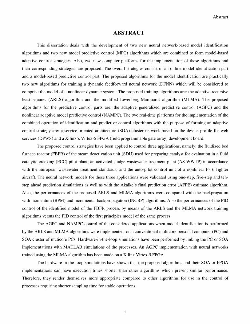
ABSTRACT
This dissertation deals with the development of two new neural network-based model identification
algorithms and two new model predictive control (MPC) algorithms which are combined to form model-based
adaptive control strategies. Also, two new computer platforms for the implementation of these algorithms and
their corresponding strategies are proposed. The overall strategies consist of an online model identification part
and a model-based predictive control part. The proposed algorithms for the model identification are practically
two new algorithms for training a dynamic feedforward neural network (DFNN) which will be considered to
comprise the model of a nonlinear dynamic system. The proposed training algorithms are: the adaptive recursive
least squares (ARLS) algorithm and the modified Levenberg-Marquardt algorithm (MLMA). The proposed
algorithms for the predictive control parts are: the adaptive generalized predictive control (AGPC) and the
nonlinear adaptive model predictive control (NAMPC). The two real-time platforms for the implementation of the
combined operation of identification and predictive control algorithms with the purpose of forming an adaptive
control strategy are: a service-oriented architecture (SOA) cluster network based on the device profile for web
services (DPWS) and a Xilinx’s Virtex-5 FPGA (field programmable gate array) development board.
The proposed control strategies have been applied to control three applications, namely: the fluidized bed
furnace reactor (FBFR) of the steam deactivation unit (SDU) used for preparing catalyst for evaluation in a fluid
catalytic cracking (FCC) pilot plant; an activated sludge wastewater treatment plant (AS-WWTP) in accordance
with the European wastewater treatment standards; and the auto-pilot control unit of a nonlinear F-16 fighter
aircraft. The neural network models for these three applications were validated using one-step, five-step and ten-
step ahead prediction simulations as well as with the Akaike’s final prediction error (AFPE) estimate algorithm.
Also, the performances of the proposed ARLS and MLMA algorithms were compared with the backprogation
with momentum (BPM) and incremental backpropagation (INCBP) algorithms. Also the performances of the PID
control of the identified model of the FBFR process by means of the ARLS and the MLMA network training
algorithms versus the PID control of the first principles model of the same process.
The AGPC and NAMPC control of the considered applications when model identification is performed
by the ARLS and MLMA algorithms were implemented on a conventional mulitcore personal computer (PC) and
SOA cluster of muticore PCs. Hardware-in-the-loop simulations have been performed by linking the PC or SOA
implementations with MATLAB simulations of the processes. An AGPC implementation with neural networks
trained using the MLMA algorithm has been made on a Xilinx Virtex-5 FPGA.
The hardware-in-the-loop simulations have shown that the proposed algorithms and their SOA or FPGA
implementations can have execution times shorter than other algorithms which present similar performance.
Therefore, they render themselves more appropriate compared to other algorithms for use in the control of
processes requiring shorter sampling time for stable operations.

Acknowledgement
ii
ACKNOWLEDGEMENT
My sincere appreciation and gratitude goes to my project supervisor, Professor George Hassapis, who conceived
and supervised the work contained in this dissertation. I also thank him for his technical and financial supports,
encouragements and fatherly roles throughout the course of this work. I will always remain grateful to him for his
advice, suggestions, intuitive comments, patience and untiring efforts in reading through my manuscripts with
necessary corrections from conception through algorithm developments, problem formulations, implementations,
and several simulations and analyses which have resulted in this dissertation.
I also thank Professor Alkiviadis Hatzopoulos and Associate Professor Loukas Petrou for their co-supervisory
roles in this work. My sincere thanks to Associate Professor Loukas Petrou for his technical supports and
comments as well as his efforts and time devoted to this work from inception to completion.
I specially acknowledge and thank the Greek State Scholarships’ Foundation (I.K.Y.) that provided the
scholarship as well as the major funding for this research. I also thank the Federal Government of Nigeria for their
financial support towards the Bilateral Educational Agreement with I.K.Y. and the Federal University of
Technology, Akure – Nigeria for their financial supports which has made this scholarship a reality leading to the
successful completion of my doctorate degree programme. My acknowledgment also goes to Ambassador of
Nigeria to Greece, His Excellency (Dr.) Etim U. Uyie for his love, care and financial assistance.
My special thanks go to the Staff of the School of Electrical and Computer Engineering, AUTH, Greece. I
gratefully acknowledge Dr. Simeonidis Andreas for his comments and encouragements, and to Mr. George
Voukalis for his technical assistance. I also wish to thank my colleagues at the Laboratory of Computer Systems
Architecture: Maria Koukourli, Ioakeim Samaras, Babis Serenis, Manos Tsardoulias and Nikos Sismanis for their
technical support, comments and contributions towards the successful completion of this project.
I am highly indebted to my mother Mrs. Cecilia Andrew Akpan; my mother-in-law Mrs. Titilayo Nathaniel
Oyewo, and my siblings Justine, Sylvester, Emmanuel and Justina for their sacrifices and prayers.
Words are not enough to thank my wife, Mrs. Rachael Oyenike Vincent–Akpan, for all her sacrifices, financial
support, prayers, and encouragements throughout the period of this study. Just know that I love you.
Finally, I am most grateful to God Almighty for His infinite mercy, divine grace and sound health.
Vincent Andrew Akpan
July, 2011.
Table of Contents
iii
TABLE OF CONTENTS
CONTENTS PAGES
Abstract i
Acknowledgement ii
Table of Contents iii
List of Figures xiii
List of Tables xxiii
List of Acronyms xxv
Chapter 1 Introduction 1
1.1 Introduction 1
1.2 Research Objectives 3
1.3 Scientific Contributions 4
1.4 Thesis Organization and Structure 6
1.5 Scientific Publications 7
Chapter 2 Background of the Research 9
2.1 Introduction 9
2.2 Model Predictive Control (MPC) 11
2.2.1 Historical Background of MPC 11
2.2.2 Overview of MPC Strategy 12
2.3 MPC Process Models 15
2.4 Neural Networks: An Overview 18
2.4.1 Neural Networks 18
2.4.2 Multilayer Perceptron (MLP) Neural Networks 19
2.4.3 Supervised and Unsupervised Learning Methods Using Neural Networks 20
2.4.3.1 Dynamic Neural Networks for Supervised Learning 21
2.4.3.1.1 Dynamic Feedforward Multilayer Perceptron Neural Networks (DFNN) 21
2.4.3.1.2 Recurrent Neural Networks (RNN) 22
2.4.3.1.2.1 The Hopfield Network 23
2.4.3.1.2.2 The Jordan Network 25
2.4.3.1.2.3 The Elman Network 26
2.4.3.1.3 Tapped Delay Neural Networks 27
2.4.3.2 Neural Networks Based on Unsupervised Learning 28
2.4.3.2.1 Generalized Regression Neural Network (GRNN) 30
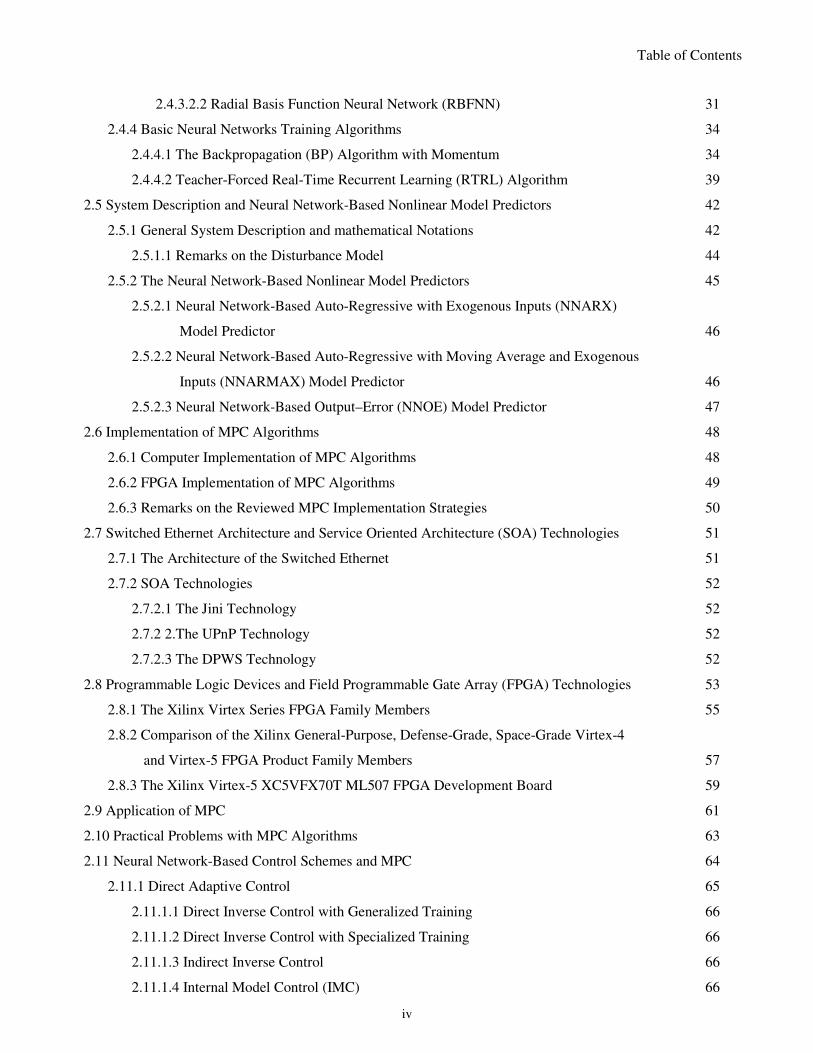
Table of Contents
iv
2.4.3.2.2 Radial Basis Function Neural Network (RBFNN) 31
2.4.4 Basic Neural Networks Training Algorithms 34
2.4.4.1 The Backpropagation (BP) Algorithm with Momentum 34
2.4.4.2 Teacher-Forced Real-Time Recurrent Learning (RTRL) Algorithm 39
2.5 System Description and Neural Network-Based Nonlinear Model Predictors 42
2.5.1 General System Description and mathematical Notations 42
2.5.1.1 Remarks on the Disturbance Model 44
2.5.2 The Neural Network-Based Nonlinear Model Predictors 45
2.5.2.1 Neural Network-Based Auto-Regressive with Exogenous Inputs (NNARX)
Model Predictor 46
2.5.2.2 Neural Network-Based Auto-Regressive with Moving Average and Exogenous
Inputs (NNARMAX) Model Predictor 46
2.5.2.3 Neural Network-Based Output–Error (NNOE) Model Predictor 47
2.6 Implementation of MPC Algorithms 48
2.6.1 Computer Implementation of MPC Algorithms 48
2.6.2 FPGA Implementation of MPC Algorithms 49
2.6.3 Remarks on the Reviewed MPC Implementation Strategies 50
2.7 Switched Ethernet Architecture and Service Oriented Architecture (SOA) Technologies 51
2.7.1 The Architecture of the Switched Ethernet 51
2.7.2 SOA Technologies 52
2.7.2.1 The Jini Technology 52
2.7.2 2.The UPnP Technology 52
2.7.2.3 The DPWS Technology 52
2.8 Programmable Logic Devices and Field Programmable Gate Array (FPGA) Technologies 53
2.8.1 The Xilinx Virtex Series FPGA Family Members 55
2.8.2 Comparison of the Xilinx General-Purpose, Defense-Grade, Space-Grade Virtex-4
and Virtex-5 FPGA Product Family Members 57
2.8.3 The Xilinx Virtex-5 XC5VFX70T ML507 FPGA Development Board 59
2.9 Application of MPC 61
2.10 Practical Problems with MPC Algorithms 63
2.11 Neural Network-Based Control Schemes and MPC 64
2.11.1 Direct Adaptive Control 65
2.11.1.1 Direct Inverse Control with Generalized Training 66
2.11.1.2 Direct Inverse Control with Specialized Training 66
2.11.1.3 Indirect Inverse Control 66
2.11.1.4 Internal Model Control (IMC) 66
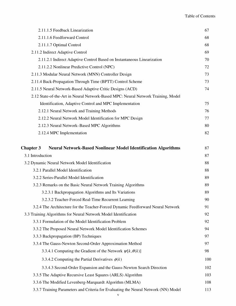
Table of Contents
v
2.11.1.5 Feedback Linearization 67
2.11.1.6 Feedforward Control 68
2.11.1.7 Optimal Control 68
2.11.2 Indirect Adaptive Control 69
2.11.2.1 Indirect Adaptive Control Based on Instantaneous Linearization 70
2.11.2.2 Nonlinear Predictive Control (NPC) 72
2.11.3 Modular Neural Network (MNN) Controller Design 73
2.11.4 Back-Propagation Through Time (BPTT) Control Scheme 73
2.11.5 Neural Network-Based Adaptive Critic Designs (ACD) 74
2.12 State-of-the-Art in Neural Network-Based MPC: Neural Network Training, Model
Identification, Adaptive Control and MPC Implementation 75
2.12.1 Neural Network and Training Methods 76
2.12.2 Neural Network Model Identification for MPC Design 77
2.12.3 Neural Network–Based MPC Algorithms 80
2.12.4 MPC Implementation 82
Chapter 3 Neural Network-Based Nonlinear Model Identification Algorithms 87
3.1 Introduction 87
3.2 Dynamic Neural Network Model Identification 88
3.2.1 Parallel Model Identification 88
3.2.2 Series-Parallel Model Identification 89
3.2.3 Remarks on the Basic Neural Network Training Algorithms 89
3.2.3.1 Backpropagation Algorithms and Its Variations 89
3.2.3.2 Teacher-Forced Real-Time Recurrent Learning 90
3.2.4 The Architecture for the Teacher-Forced Dynamic Feedforward Neural Network 91
3.3 Training Algorithms for Neural Network Model Identification 92
3.3.1 Formulation of the Model Identification Problem 92
3.3.2 The Proposed Neural Network Model Identification Schemes 94
3.3.3 Backpropagation (BP) Techniques 97
3.3.4 The Gauss-Newton Second-Order Approximation Method 97
3.3.4.1 Computing the Gradient of the Network [ , ( )]k kψ θ 98
3.3.4.2 Computing the Partial Derivatives ( )kφ 100
3.3.4.3 Second-Order Expansion and the Gauss-Newton Search Direction 102
3.3.5 The Adaptive Recursive Least Squares (ARLS) Algorithm 103
3.3.6 The Modified Levenberg-Marquardt Algorithm (MLMA) 108
3.3.7 Training Parameters and Criteria for Evaluating the Neural Network (NN) Model 113
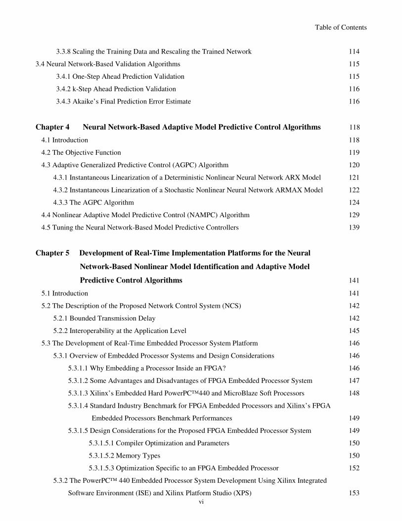
Table of Contents
vi
3.3.8 Scaling the Training Data and Rescaling the Trained Network 114
3.4 Neural Network-Based Validation Algorithms 115
3.4.1 One-Step Ahead Prediction Validation 115
3.4.2 k-Step Ahead Prediction Validation 116
3.4.3 Akaike’s Final Prediction Error Estimate 116
Chapter 4 Neural Network-Based Adaptive Model Predictive Control Algorithms 118
4.1 Introduction 118
4.2 The Objective Function 119
4.3 Adaptive Generalized Predictive Control (AGPC) Algorithm 120
4.3.1 Instantaneous Linearization of a Deterministic Nonlinear Neural Network ARX Model 121
4.3.2 Instantaneous Linearization of a Stochastic Nonlinear Neural Network ARMAX Model 122
4.3.3 The AGPC Algorithm 124
4.4 Nonlinear Adaptive Model Predictive Control (NAMPC) Algorithm 129
4.5 Tuning the Neural Network-Based Model Predictive Controllers 139
Chapter 5 Development of Real-Time Implementation Platforms for the Neural
Network-Based Nonlinear Model Identification and Adaptive Model
Predictive Control Algorithms 141
5.1 Introduction 141
5.2 The Description of the Proposed Network Control System (NCS) 142
5.2.1 Bounded Transmission Delay 142
5.2.2 Interoperability at the Application Level 145
5.3 The Development of Real-Time Embedded Processor System Platform 146
5.3.1 Overview of Embedded Processor Systems and Design Considerations 146
5.3.1.1 Why Embedding a Processor Inside an FPGA? 146
5.3.1.2 Some Advantages and Disadvantages of FPGA Embedded Processor System 147
5.3.1.3 Xilinx’s Embedded Hard PowerPC™440 and MicroBlaze Soft Processors 148
5.3.1.4 Standard Industry Benchmark for FPGA Embedded Processors and Xilinx’s FPGA
Embedded Processors Benchmark Performances 149
5.3.1.5 Design Considerations for the Proposed FPGA Embedded Processor System 149
5.3.1.5.1 Compiler Optimization and Parameters 150
5.3.1.5.2 Memory Types 150
5.3.1.5.3 Optimization Specific to an FPGA Embedded Processor 152
5.3.2 The PowerPC™ 440 Embedded Processor System Development Using Xilinx Integrated
Software Environment (ISE) and Xilinx Platform Studio (XPS) 153
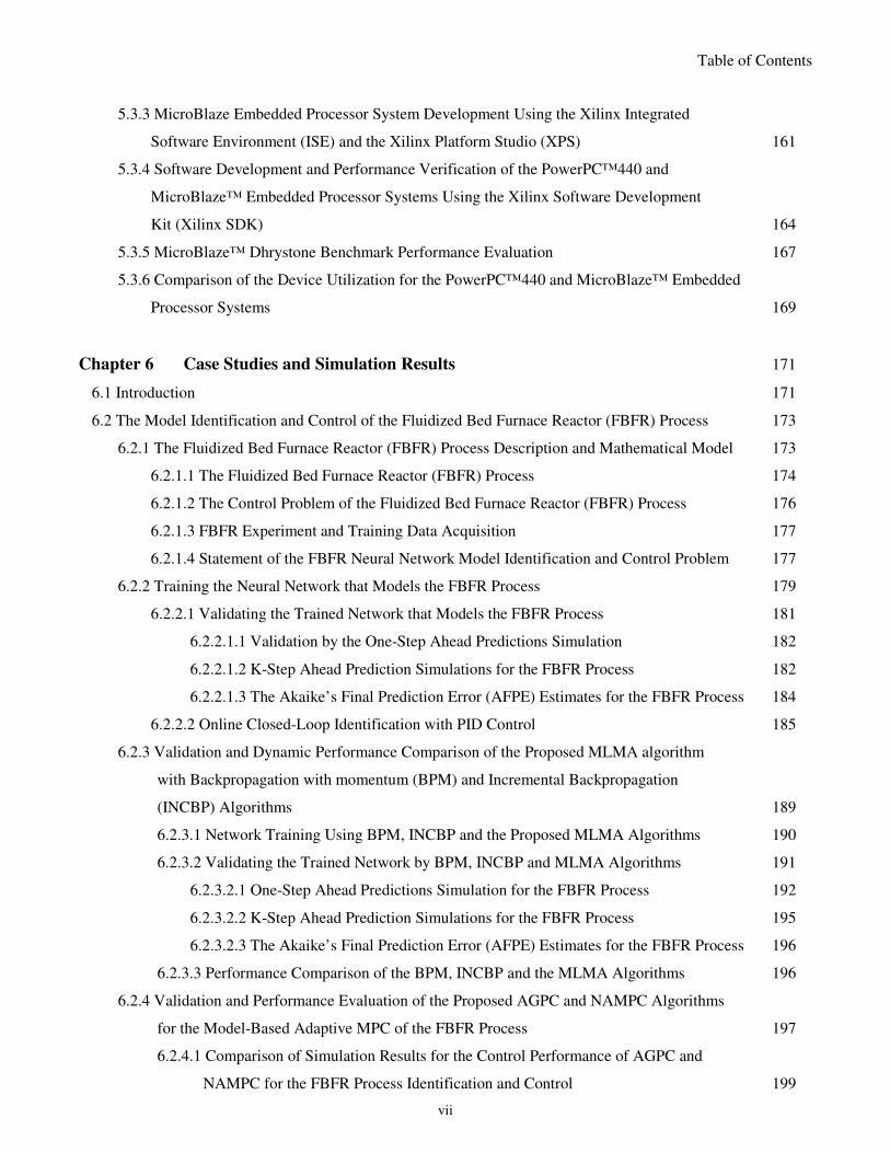
Table of Contents
vii
5.3.3 MicroBlaze Embedded Processor System Development Using the Xilinx Integrated
Software Environment (ISE) and the Xilinx Platform Studio (XPS) 161
5.3.4 Software Development and Performance Verification of the PowerPC™440 and
MicroBlaze™ Embedded Processor Systems Using the Xilinx Software Development
Kit (Xilinx SDK) 164
5.3.5 MicroBlaze™ Dhrystone Benchmark Performance Evaluation 167
5.3.6 Comparison of the Device Utilization for the PowerPC™440 and MicroBlaze™ Embedded
Processor Systems 169
Chapter 6 Case Studies and Simulation Results 171
6.1 Introduction 171
6.2 The Model Identification and Control of the Fluidized Bed Furnace Reactor (FBFR) Process 173
6.2.1 The Fluidized Bed Furnace Reactor (FBFR) Process Description and Mathematical Model 173
6.2.1.1 The Fluidized Bed Furnace Reactor (FBFR) Process 174
6.2.1.2 The Control Problem of the Fluidized Bed Furnace Reactor (FBFR) Process 176
6.2.1.3 FBFR Experiment and Training Data Acquisition 177
6.2.1.4 Statement of the FBFR Neural Network Model Identification and Control Problem 177
6.2.2 Training the Neural Network that Models the FBFR Process 179
6.2.2.1 Validating the Trained Network that Models the FBFR Process 181
6.2.2.1.1 Validation by the One-Step Ahead Predictions Simulation 182
6.2.2.1.2 K-Step Ahead Prediction Simulations for the FBFR Process 182
6.2.2.1.3 The Akaike’s Final Prediction Error (AFPE) Estimates for the FBFR Process 184
6.2.2.2 Online Closed-Loop Identification with PID Control 185
6.2.3 Validation and Dynamic Performance Comparison of the Proposed MLMA algorithm
with Backpropagation with momentum (BPM) and Incremental Backpropagation
(INCBP) Algorithms 189
6.2.3.1 Network Training Using BPM, INCBP and the Proposed MLMA Algorithms 190
6.2.3.2 Validating the Trained Network by BPM, INCBP and MLMA Algorithms 191
6.2.3.2.1 One-Step Ahead Predictions Simulation for the FBFR Process 192
6.2.3.2.2 K-Step Ahead Prediction Simulations for the FBFR Process 195
6.2.3.2.3 The Akaike’s Final Prediction Error (AFPE) Estimates for the FBFR Process 196
6.2.3.3 Performance Comparison of the BPM, INCBP and the MLMA Algorithms 196
6.2.4 Validation and Performance Evaluation of the Proposed AGPC and NAMPC Algorithms
for the Model-Based Adaptive MPC of the FBFR Process 197
6.2.4.1 Comparison of Simulation Results for the Control Performance of AGPC and
NAMPC for the FBFR Process Identification and Control 199
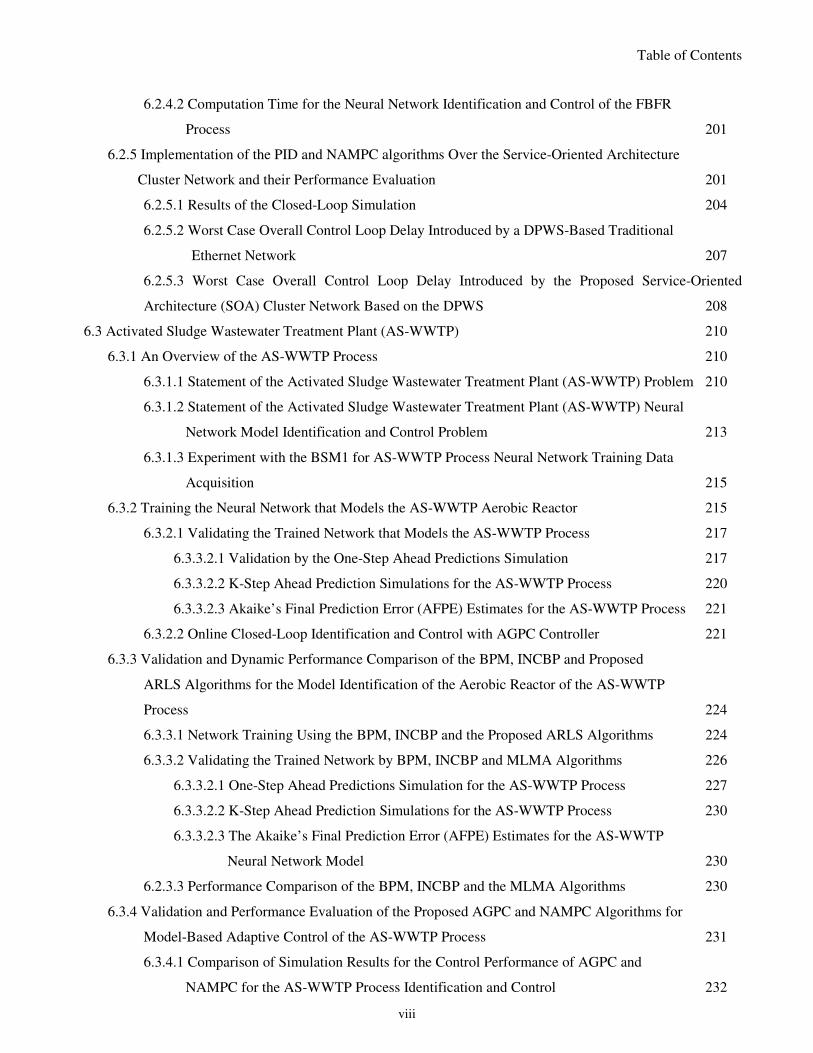
Table of Contents
viii
6.2.4.2 Computation Time for the Neural Network Identification and Control of the FBFR
Process 201
6.2.5 Implementation of the PID and NAMPC algorithms Over the Service-Oriented Architecture
Cluster Network and their Performance Evaluation 201
6.2.5.1 Results of the Closed-Loop Simulation 204
6.2.5.2 Worst Case Overall Control Loop Delay Introduced by a DPWS-Based Traditional
Ethernet Network 207
6.2.5.3 Worst Case Overall Control Loop Delay Introduced by the Proposed Service-Oriented
Architecture (SOA) Cluster Network Based on the DPWS 208
6.3 Activated Sludge Wastewater Treatment Plant (AS-WWTP) 210
6.3.1 An Overview of the AS-WWTP Process 210
6.3.1.1 Statement of the Activated Sludge Wastewater Treatment Plant (AS-WWTP) Problem 210
6.3.1.2 Statement of the Activated Sludge Wastewater Treatment Plant (AS-WWTP) Neural
Network Model Identification and Control Problem 213
6.3.1.3 Experiment with the BSM1 for AS-WWTP Process Neural Network Training Data
Acquisition 215
6.3.2 Training the Neural Network that Models the AS-WWTP Aerobic Reactor 215
6.3.2.1 Validating the Trained Network that Models the AS-WWTP Process 217
6.3.3.2.1 Validation by the One-Step Ahead Predictions Simulation 217
6.3.3.2.2 K-Step Ahead Prediction Simulations for the AS-WWTP Process 220
6.3.3.2.3 Akaike’s Final Prediction Error (AFPE) Estimates for the AS-WWTP Process 221
6.3.2.2 Online Closed-Loop Identification and Control with AGPC Controller 221
6.3.3 Validation and Dynamic Performance Comparison of the BPM, INCBP and Proposed
ARLS Algorithms for the Model Identification of the Aerobic Reactor of the AS-WWTP
Process 224
6.3.3.1 Network Training Using the BPM, INCBP and the Proposed ARLS Algorithms 224
6.3.3.2 Validating the Trained Network by BPM, INCBP and MLMA Algorithms 226
6.3.3.2.1 One-Step Ahead Predictions Simulation for the AS-WWTP Process 227
6.3.3.2.2 K-Step Ahead Prediction Simulations for the AS-WWTP Process 230
6.3.3.2.3 The Akaike’s Final Prediction Error (AFPE) Estimates for the AS-WWTP
Neural Network Model 230
6.2.3.3 Performance Comparison of the BPM, INCBP and the MLMA Algorithms 230
6.3.4 Validation and Performance Evaluation of the Proposed AGPC and NAMPC Algorithms for
Model-Based Adaptive Control of the AS-WWTP Process 231
6.3.4.1 Comparison of Simulation Results for the Control Performance of AGPC and
NAMPC for the AS-WWTP Process Identification and Control 232
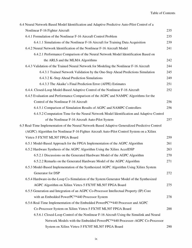
Table of Contents
ix
6.4 Neural Network-Based Model Identification and Adaptive Predictive Auto-Pilot Control of a
Nonlinear F-16 Fighter Aircraft 235
6.4.1 Formulation of the Nonlinear F-16 Aircraft Control Problem 235
6.4.1.1 Simulations of the Nonlinear F-16 Aircraft for Training Data Acquisition 239
6.4.2 Neural Network Identification of the Nonlinear F-16 Aircraft Model 241
6.4.2.1 Performance Comparison of the Neural Network Model Identification Based on
the ARLS and the MLMA Algorithms 242
6.4.3 Validation of the Trained Neural Network for Modeling the Nonlinear F-16 Aircraft 244
6.4.3.1 Trained Network Validation by the One-Step Ahead Predictions Simulation 245
6.4.3.2 K–Step Ahead Prediction Simulations 249
6.4.3.3 The Akaike’s Final Prediction Error (AFPE) Estimates 251
6.4.4. Closed-Loop Model-Based Adaptive Control of the Nonlinear F-16 Aircraft 252
6.4.5 Evaluation and Performance Comparison of the AGPC and NAMPC Algorithms for the
Control of the Nonlinear F-16 Aircraft 256
6.4.5.1 Comparison of Simulation Results of AGPC and NAMPC Controllers 256
6.4.5.2 Computation Time for the Neural Network Model Identification and Adaptive Control
of the Nonlinear F-16 Aircraft Auto-Pilot System 257
6.5 Real-Time Implementation of the Neural Network-Based Adaptive Generalized Predictive Control
(AGPC) Algorithm for Nonlinear F-16 Fighter Aircraft Auto-Pilot Control System on a Xilinx
Virtex-5 FX70T ML507 FPGA Board 259
6.5.1 Model-Based Approach for the FPGA Implementation of the AGPC Algorithm 261
6.5.2 Hardware Synthesis of the AGPC Algorithm Using the Xilinx AccelDSP 263
6.5.2.1 Discussions on the Generated Hardware Model of the AGPC Algorithm 270
6.5.2.2 Remarks on the Generated Hardware Model of the AGPC Algorithm 271
6.5.3 Model-Based Implementation of the Synthesized AGPC Algorithm Using Xilinx System
Generator for DSP 272
6.5.4 Hardware-in-the-Loop Co-Simulation of the System Generator Model of the Synthesized
AGPC Algorithm on Xilinx Virtex-5 FX70T ML507 FPGA Board 275
6.5.5 Generation and Integration of an AGPC Co-Processor Intellectual Property (IP) Core
with an Embedded PowerPC™440 Processor System 278
6.5.6 Real-Time Implementation of the Embedded PowerPC™440 Processor and AGPC
Co-Processor System on Xilinx Virtex-5 FX70T ML507 FPGA Board 288
6.5.6.1 Closed-Loop Control of the Nonlinear F-16 Aircraft Using the Simulink and Neural
Network Models with the Embedded PowerPC™440 Processor–AGPC Co-Processor
System on Xilinx Virtex-5 FX70T ML507 FPGA Board 290
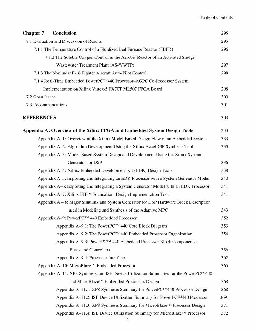
Table of Contents
x
Chapter 7 Conclusion 295
7.1 Evaluation and Discussion of Results 295
7.1.1 The Temperature Control of a Fluidized Bed Furnace Reactor (FBFR) 296
7.1.2 The Soluble Oxygen Control in the Aerobic Reactor of an Activated Sludge
Wastewater Treatment Plant (AS-WWTP) 297
7.1.3 The Nonlinear F-16 Fighter Aircraft Auto-Pilot Control 298
7.1.4 Real-Time Embedded PowerPC™440 Processor–AGPC Co-Processor System
Implementation on Xilinx Virtex-5 FX70T ML507 FPGA Board 298
7.2 Open Issues 300
7.3 Recommendations 301
REFERENCES 303
Appendix A: Overview of the Xilinx FPGA and Embedded System Design Tools 333
Appendix A–1: Overview of the Xilinx Model-Based Design Flow of an Embedded System 333
Appendix A–2: Algorithm Development Using the Xilinx AccelDSP Synthesis Tool 335
Appendix A–3: Model-Based System Design and Development Using the Xilinx System
Generator for DSP 336
Appendix A–4: Xilinx Embedded Development Kit (EDK) Design Tools 338
Appendix A–5: Importing and Integrating an EDK Processor with a System Generator Model 340
Appendix A–6: Exporting and Integrating a System Generator Model with an EDK Processor 341
Appendix A–7: Xilinx IST™ Foundation: Design Implementation Tool 341
Appendix A – 8: Major Simulink and System Generator for DSP Hardware Block Description
used in Modeling and Synthesis of the Adaptive MPC 343
Appendix A–9: PowerPC™ 440 Embedded Processor 352
Appendix A–9.1: The PowerPC™ 440 Core Block Diagram 353
Appendix A–9.2: The PowerPC™ 440 Embedded Processor Organization 354
Appendix A–9.3: PowerPC™ 440 Embedded Processor Block Components,
Buses and Controllers 356
Appendix A–9.4: Processor Interfaces 362
Appendix A–10: MicroBlaze™ Embedded Processor 365
Appendix A–11: XPS Synthesis and ISE Device Utilization Summaries for the PowerPC™440
and MicroBlaze™ Embedded Processors Design 368
Appendix A–11.1: XPS Synthesis Summary for PowerPC™440 Processor Design 368
Appendix A–11.2: ISE Device Utilization Summary for PowerPC™440 Processor 369
Appendix A–11.3: XPS Synthesis Summary for MicroBlaze™ Processor Design 371
Appendix A–11.4: ISE Device Utilization Summary for MicroBlaze™ Processor 372
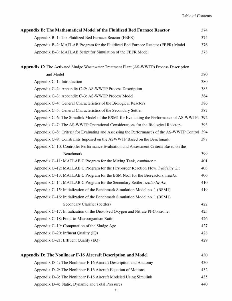
Table of Contents
xi
Appendix B: The Mathematical Model of the Fluidized Bed Furnace Reactor 374
Appendix B–1: The Fluidized Bed Furnace Reactor (FBFR) 374
Appendix B–2: MATLAB Program for the Fluidized Bed Furnace Reactor (FBFR) Model 376
Appendix B–3: MATLAB Script for Simulation of the FBFR Model 378
Appendix C: The Activated Sludge Wastewater Treatment Plant (AS-WWTP) Process Description
and Model 380
Appendix C–1: Introduction 380
Appendix C–2: Appendix C–2: AS-WWTP Process Description 383
Appendix C–3: Appendix C–3: AS-WWTP Process Model 384
Appendix C–4: General Characteristics of the Biological Reactors 386
Appendix C–5: General Characteristics of the Secondary Settler 387
Appendix C–6: The Simulink Model of the BSM1 for Evaluating the Performance of AS-WWTPs 392
Appendix C–7: The AS-WWTP Operational Considerations for the Biological Reactors 393
Appendix C–8: Criteria for Evaluating and Assessing the Performances of the AS-WWTP Control 394
Appendix C–9: Constraints Imposed on the ASWWTP Based on the Benchmark 397
Appendix C–10: Controller Performance Evaluation and Assessment Criteria Based on the
Benchmark 399
Appendix C–11: MATLAB C Program for the Mixing Tank, combiner.c 401
Appendix C–12: MATLAB C Program for the First-order Reaction Flow, hyddelayv2.c 403
Appendix C–13: MATLAB C Program for the BSM No.1 for the Bioreactors, asm1.c 406
Appendix C–14: MATLAB C Program for the Secondary Settler, settler1dv4.c 410
Appendix C–15: Initialization of the Benchmark Simulation Model no. 1 (BSM1) 419
Appendix C–16: Initialization of the Benchmark Simulation Model no. 1 (BSM1)
Secondary Clarifier (Settler) 422
Appendix C–17: Initialization of the Dissolved Oxygen and Nitrate PI-Controller 425
Appendix C–18: Food-to-Microorganism Ratio 426
Appendix C–19: Computation of the Sludge Age 427
Appendix C–20: Influent Quality (IQ) 428
Appendix C–21: Effluent Quality (EQ) 429
Appendix D: The Nonlinear F-16 Aircraft Description and Model 430
Appendix D–1: The Nonlinear F-16 Aircraft Description and Anatomy 430
Appendix D–2: The Nonlinear F-16 Aircraft Equation of Motions 432
Appendix D–3: The Nonlinear F-16 Aircraft Modeled Using Simulink 435
Appendix D–4: Static, Dynamic and Total Pressures 440
Table of Contents
xii
Appendix D–5: The MATLAB C Program for the Nonlinear F-16 Aircraft Model, nlpant.c 442
Appendix D–6: The MATLAB Program for the F-16 Model Trimming Routine, trim_F16.m 453
Appendix D–7: The MATLAB Program for Computing the Initial States of the Nonlinear
F-16 Model Used in the Trimming Routine, trimfun.m 455
Appendix D–8: MATLAB script for the Simulation of the Nonlinear F-16 Aircraft,
F-16_Simulations.m 458
Appendix D–9: MATLAB Script for Implementing the Nonlinear F-16 Aircraft Simulation,
F16_aircraft_model.m 460
Appendix E: Embedded PowerPC™440 Processor–AGPC Co-Processor System XPS
Synthesis and Xilinx ISE™ Device Utilization Summaries 462
Appendix E – 1: XPS Synthesis Summary for the Embedded PowerPC™440 Processor–AGPC
Co-Processor System 462
Appendix E – 2: Xilinx ISE™ Device Utilization Summary for the Embedded PowerPC™440
Processor–AGPC Co-Processor System 463
Appendix E – 3: Summary and Table of Contents of the Embedded PowerPC™440
Processor–AGPC Co-Processor System 465
Appendix E–4: The AGPC Co-Processor (f16_nagpc_ipcore_plbw_0) System Device Utilization 466
Appendix E–5: The EDK Processor API for the AGPC Co-Processor IP Core Drivers and
Software Development Guide 468
Appendix E–6: Software for Initializing the Embedded System Driver and Implementing the
Embedded PowerPC™440 Processor and the AGPC Co-Processor System on
Virtex-5 FX70T ML507 FPGA Board 480
List of Figures
xiii
List of Figures
Fig. 2.1: Basic structure of MPC scheme 13
Fig. 2.2: The general MPC control strategy 14
Fig. 2.3: A nonlinear model of a neuron 19
Fig. 2.4: Feedforward multilayer perceptron neural network with one hidden and output layer 20
Fig. 2.5: Dynamic feedforward neural network (DFNN) structure 21
Fig. 2.6: The schematic diagram of the Hopfield network 24
Fig. 2.7: The basic architecture of the Jordan network 25
Fig. 2.8: Unfolding action of recurrent neural networks with additional layer at each time step 25
Fig. 2.9: The basic architecture of the Elman network 26
Fig. 2.10: Tapped delayed neural network (TDNN) 27
Fig. 2.11: Generalized regression neural network (GRNN) 31
Fig. 2.12: Radial basis function neural network (RBFNN) 32
Fig. 2.13: NNARX model predictor 46
Fig. 2.14: NNARMAX model predictor 46
Fig. 2.15: NNOE model predictor 46
Fig. 2.16: The Virtex-5 ML507 FPGA embedded system development board: (a) Top view and
(b) Bottom view 60
Fig. 2.17: Model reference adaptive control scheme: ( )U k is the control input, ( )R k is the desired
reference, ( )E k is the error between the reference model and the system output ( )Y k 65
Fig. 2.18: The principle of internal model control (IMC) implemented with two neural networks:
A model of the system (M) and an inverse model (C) with disturbance ( )d k acting on the
output of the system 67
Fig. 2.19: Indirect model-based adaptive control scheme: ( )U k is the control input, ( )R k is the
desired reference, ( )E k is the error between the reference model and the system output ( )Y k 69
Fig. 2.20: Indirect control based on instantaneous linearization of the neural network model 70
Fig. 2.21: Basic structure of the backpropagation through time (BPTT) control scheme 73
Fig. 2.22: The structure of an action-dependent heuristic dynamic programming form of adaptive
critic design (ACD) 74
Fig. 3.1: Neural network parallel model identification structure 88
Fig. 3.2: Neural network series-parallel model identification structure 88
Fig. 3.3: Teacher-forced dynamic feedforward neural network (TF-DFNN) architecture 91
Fig. 3.4: The architecture of the dynamic feedforward neural network (DFNN) model 94
Fig. 3.5: Neural network model identification based on the teacher-forcing method for (a): NNARX
List of Figures
xiv
and (b) NNARMAX model predictors 94
Fig. 4.1: The proposed NN-based AGPC scheme 120
Fig. 4.2: The proposed NN-based NAMPC strategy with a NN model 130
Fig. 5.1: General structure of the proposed network control system (NCS) 143
Fig. 5.2: Structure of a SOAP message 144
Fig. 5.3: The Xilinx ISE “New Project Summary” and the BSB Welcome, System, and Processor
design stages for the embedded PowerPC™440 processor system 154
Fig. 5.4: The BSB: the Peripheral and Summary design stages for the embedded PowerPC™440
processor system 156
Fig. 5.5: The XPS graphical user interface (GUI) for the creation and initial compilation of the
embedded processor system 157
Fig. 5.6: A section of the Xilinx ISE™ graphical user interface from where the PowerPC™440
embedded processor system design is instantiated 159
Fig. 5.7: The block diagram of the PowerPC™440 embedded processor system with associated memory
types, peripherals, clock generator, buses, hardware and software specifications and key/symbols 160
Fig. 5.8: The BSB: the Peripheral and Summary design stages for the embedded MicroBlaze™
processor system 162
Fig. 5.9: The block diagram of the MicroBlaze™ embedded processor system with associated memory types,
peripherals, clock generator, buses, hardware and software specifications and key/symbols 163
Fig. 5.10: Xilinx software development kit graphical user interface for software development
and programming the Virtex-5 ML507 FPGA using the “Debug on Hardware” option 165
Fig. 5.11: The MicroBlaze™ processor: (a) memory and (b) peripheral test results on the
HyperTerminal window 166
Fig. 5.12: The XPS for creating, compiling and initializing the Dhrystone benchmark program to
load from on-board BRAM for benchmark performance evaluation of MicroBlaze™
embedded processor on Virtex-5 ML507 FPGA 168
Fig. 6.1: Simplified diagram of the steam deactivation unit (SDU) of the FCC pilot plant with the FBFR 175
Fig. 6.2: Schematic of the vertical cross-section of the cylindrical fluidized bed furnace reactor (FBFR) 175
Fig. 6.3: Temperature distribution and variation across the six sections of the FBFR system:
(a) temperature distribution across the FBFR and (b) temperature variations showing
the maximum temperatures for Tirw, Tbrwh, Th and Tormw with the minimum
and maximum temperatures for Tri and Tins 176
Fig. 6.4: Neural network-based FBFR model identification schemes (a) NNARX model and
(b) NNARMAX model 178
Fig. 6.5: Network convergence using the ARLS and the MLMA algorithms (performance index vs. epoch) 180
Fig. 6.6: Comparison of Tri and Th training data predictions by the network trained using ARLS and
List of Figures
xv
MLMA algorithms for 10 Epochs 181
Fig. 6.7: Comparison of Tri and Th training data predictions by the network trained using ARLS and
MLMA algorithms for 100 Epochs 181
Fig. 6.8: Comparison of Tri and Th test data predictions by the network trained using ARLS and
MLMA algorithms for 10 Epochs 183
Fig. 6.9: Comparison of Tri and Th test data predictions by the network trained using ARLS and
MLMA algorithms for 100 Epochs. 183
Fig. 6.10: 5-step ahead Tri and Th output predictions (red--*) comparison with original unscaled training
data (blue-) using the network trained using ARLS and MLMA algorithms for 10 epochs 184
Fig. 6.11: 5-step ahead Tri and Th output predictions (red--*) comparison with original unscaled training
data (blue-) using the network trained using ARLS and MLMA algorithms for 100 epochs 184
Fig. 6.12: The PID control scheme 185
Fig. 6.13: PID control performance with the first principles validated model of the FBFR process:
(a) Th and (b) Tri output predictions, and (c) Th and (d) Tri predictions without disturbances
on the model 187
Fig. 6.14: PID control performance with the first principles validated model of the FBFR process
under disturbances: (a) Th and (b) Tri output predictions, and (c) HRP and (d) DWP control
signals 187
Fig. 6.15: Closed-loop PID control performance of the FBFR process using NN model trained with ARLS
(dotted red lines) and MLMA (black dashed dotted lines) for 10 epochs: (a) Th and (b) Tri
output predictions, (c) HRP and (d) DWP control signals 188
Fig. 6.16: Closed-loop PID control performance of the FBFR process using NN model trained with ARLS
(dotted red lines) and MLMA (black dashed dotted lines) for 100 epochs: (a) Th and (b) Tri
output predictions, (c) HRP and (d) DWP control signals 188
Fig. 6.17: Network convergence using the BPM, INCBP and the MLMA algorithms (performance
index vs. epoch) 191
Fig. 6.18: Comparison of (a) Tri and (b) Th training data predictions by the network trained using
backpropagation with momentum (BPM), incremental backpropagation (INCBP), and the
MLMA algorithms 193
Fig. 6.19: Comparison of (a) Tri and (b) Th test data predictions by the network trained using
backpropagation with momentum (BPM), incremental backpropagation (INCBP), and the
MLMA algorithms 194
Fig. 6.20: Comparison of the 5-step ahead output predictions (red --*) of the NN for (a) Tri and (b) Th
when it is trained by the BPM, (INCBP), and the MLMA algorithms with the original unscaled
training data (blue-) 195
Fig. 6.21: FBFR temperature predictions by AGPC (blue--) and NAMPC (red -) for (a) Th and (b) Tri
List of Figures
xvi
with the manipulated signals (c) HRP and (d) DWP to track the desired reference signal
(green .-) 200
Fig. 6.22: Computation time for the parallel implementation of the identification and control strategies
at each time sample: (a) AGPC for the FBFR process and (c) NAMPC for the FBFP process 201
Fig. 6.23: FBFR temperature predictions by the PID controller (blue--) and NAMPC (red) for (a) Th and
(b) Tri with the control signals (c) HRP and (d) DWP for tracking the reference signal
(pink -.-) together with output prediction errors in (e) and (f) for Th and Tri respectively due to
both controllers for k = 350 samples 205
Fig. 6.24: 1 2tr tr
D D+ delay between the FBFR process and the control system obtained by NS-2 207
Fig. 6.25: Online identification and control of the FBFR process over the DPWS implemented over a
traditional Ethernet network: (a) Th and (b) Tri predictions with their respective control signals
(c) HRP and (d) DWP 208
Fig. 6.26: Online identification and control of the FBFR process over the proposed Fieldbus: (a) Th and
(b) Tri predictions with their respective control signals (c) HRP and (d) DWP 208
Fig. 6.27: Computation time for the FBFR model identification and control at each time sample 209
Fig. 6.28: The AS-WWTP with dissolved oxygen concentration and the nitrate control loops 212
Fig. 6.29: The neural network model identification scheme for AS-WWTP based on NNARMAX model 214
Fig. 6.30: Network convergence for the AS-WWTP using the ARLS and the MLMA algorithms 217
Fig. 6.31: Comparison of soluble oxygen (SO) data predictions with the training data by the network
trained using ARLS and MLMA algorithms for 10 Epochs 218
Fig. 6.32: Comparison of soluble oxygen (SO) data predictions with the training data by the network
trained using ARLS and MLMA algorithms for 100 Epochs 218
Fig. 6.33: Comparison of soluble oxygen (SO) validation data predictions by the network trained using
ARLS and MLMA algorithms for 10 Epochs 219
Fig. 6.34: Comparison of soluble oxygen (SO) validation data predictions by the network trained using
ARLS and MLMA algorithms for 100 Epochs 219
Fig. 6.35: 5-step ahead soluble oxygen (SO) output predictions (red--*) comparison with original
unscaled training data (blue-) using the network trained using ARLS and MLMA algorithms
for 10 Epochs 220
Fig. 6.36: 5-step ahead soluble oxygen (SO) output predictions (red--*) comparison with original
unscaled training data (blue -) using the network trained using ARLS and MLMA algorithms
for 100 Epochs 220
Fig. 6.37: The closed-loop AGPC scheme used for the soluble oxygen (SO) in order to evaluate the
online model identification based on ARLS and MLMA algorithms 222
Fig. 6.38: Closed-loop AGPC control performance of the AS-WWTP process using NN model
trained with ARLS and MLMA for (a) 10 and (c) 100 epochs with their respective control
List of Figures
xvii
signals in (b) and (d) 222
Fig. 6.39: Network convergence using the BPM, INCBP and the ARLS algorithms (performance
index vs. epoch) 226
Fig. 6.40: Comparison of the one-step ahead prediction of the soluble oxygen (SO) training data by the
network trained using backpropagation with momentum (BPM), incremental
backpropagation (INCBP), and the proposed ARLS algorithms 227
Fig. 6.41: Comparison of the one-step ahead prediction of the soluble oxygen (SO) validation data
using the network trained with backpropagation with momentum (BPM), incremental
backpropagation (INCBP), and the proposed ARLS algorithms 228
Fig. 6.42: Comparison of the ten-step ahead prediction of the soluble oxygen (SO) unscaled training
data by the network trained with backpropagation with momentum (BPM),
incremental backpropagation (INCBP), and the proposed ARLS algorithms 229
Fig. 6.43: The closed-loop NAMPC scheme used for the soluble oxygen (SO) in order to evaluate the
online model identification based on ARLS and MLMA algorithms 231
Fig. 6.44: The soluble oxygen predictions and the oxygen transfer coefficient control by (a) AGPC and
NAMPC with the control signal (b) for the manipulated variable, oxygen transfer coefficient
(KLa5) for the alternating AS-WWTP process. Computation time for the parallel implementation
of the identification and control strategies for the AS-WWTP process at each sampling instant
sample: (c) AGPC with an average computation time of 0.6594 seconds and (d) NAMPC
with an average computation time of 1.7316 seconds 233
Fig. 6.45: The soluble oxygen control predictions and control by AGPC and NAMPC with the control
signal (b) for the manipulated variable, oxygen transfer coefficient (KLa5) AS-WWTP process
with sinusoidal disturbances 234
Fig. 6.46: The F-16 aircraft surfaces for the control of the thrust, roll rate (p), pitch rate (q), yaw rate (r),
( , , )b b b
x y z are the body axes, ( , , )u v w are the velocities along the body axes, (L) is the
rolling moment, (M) is the pitching moment, (N) is the awing moment, ( , , )n n n
x y z is the
navigation frame, cm
O is the center of mass, ( , , )φ ϑ ψ are the Euler angles for aileron,
elevator and rudder deflections respectively 236
Fig. 6.47: Definition of the angle of attack, α ( 0α > ) and sideslip, β ( 0β > ). , ,n n n
x y z are the
North, East and South orientation of the navigation frame 236
Fig. 6.48: The desired reference trajectories for the roll rate (p), pitch rate (q) and the yaw rate (r)
as well as the thrust (t) for the nonlinear F-16 aircraft 237
Fig. 6.49: Convergence of the NN used to model the F-16 aircraft when it is trained with the ARLS
and the MLMA algorithms (sum of squares error vs. epoch) 243
Fig. 6.50: Comparison of the output predictions of the scaled training data using the network trained by
List of Figures
xviii
ARLS and MLMA: (a) roll rate prediction, (b) pitch rate prediction, (c) yaw rate prediction and
(d) thrust prediction for 20 epochs 245
Fig. 6.51: Comparison of the outpredictions of the scaled training data using the network trained by ARLS
and MLMA: (a) roll rate prediction, (b) pitch rate prediction, (c) yaw rate prediction and (d)
thrust prediction for 100 Epochs 246
Fig. 6.52: Comparison of the unscaled data predictions of the trained network the using by ARLS and
MLMA for (a) roll rate prediction, (b) pitch rate prediction, (c) yaw rate prediction and (d)
thrust prediction for 20 Epochs 247
Fig. 6.53: Comparison of the output predictions of the unscaled validation data using the network trained
by ARLS and MLMA: (a) roll rate prediction, (b) pitch rate prediction, (c) yaw rate prediction
and (d) thrust prediction for 100 Epochs 248
Fig. 6.54: 5-step ahead output predictions (red--*) comparison with the original unscaled training data
(blue -) using the Network trained by the ARLS and MLMA algorithms for 20 Epochs: (a) roll
rate prediction, (b) pitch rate prediction, (c) yaw rate prediction and (d) thrust prediction 249
Fig. 6.55: 5-step ahead output predictions (red--*) comparison with the original unscaled training data
(blue -) using the Network trained by the ARLS and MLMA algorithms for 100 Epochs: (a) roll
rate prediction, (b) pitch rate prediction, (c) yaw rate prediction and (d) thrust prediction 250
Fig. 6.56: The nonlinear F-16 model: (a) neural network model identification and (b) neural
network-based adaptive control scheme using the NAMPC control strategy 252
Fig. 6.57: Responses of controlled variables and time variations of the manipulated variables when NN
is trained with ARLS and MLMA algorithms for 20 epochs: (a) roll rate, pitch rate, yaw rate and
thrust and (b) aileron deflection, elevator deflection, rudder deflection and the throttle setting 254
Fig. 6.58: Responses of controlled variables and time variations of the manipulated variables when NN is
trained with ARLS and MLMA algorithms for 100 epochs: (a) roll rate, pitch rate, yaw rate and
the thrust and (b) aileron deflection, elevator deflection, rudder deflection and the throttle setting 255
Fig. 6.59: The AGPC (blue--) and NAMPC (red -) responses of (a) roll rate p, (b) pitch rate q, (c) yaw rate r,
and (d) the throttle setting t with their respective manipulated variables (e) aileron deflections,
(f) elevator deflections, (g) rudder deflections and (h) the thrust command to track the reference
signal (green .-) 257
Fig. 6.60: Computation time for the parallel implementation of the identification and control strategies for
the nonlinear F-16 auto-pilot control system at each time sample: (a) AGPC and (d) NAMPC 258
Fig. 6.61: The proposed scheme for the FPGA implementation, verification and performance evaluation
of a neural network-based adaptive generalized predictive control (AGPC) algorithm on a
Xilinx Virtex-5 FX70T ML507 FPGA board 260
Fig. 6.62: The block diagram for the proposed model-based design flow for the FPGA implementation
of the AGPC algorithm on Virtex-5 FX70T ML507 FPGA development board 262
List of Figures
xix
Fig. 6.63: The block diagram of the AGPC modeling and Synthesis using MATLAB and Xilinx
AccelDSP synthesis tool 264
Fig. 6.64: AccelDSP design flow to generate the System Generator block model that encrypts the
AGPC algorithm 265
Fig. 6.65: Floating-point simulation results of the F-16 aircraft control using the MATLAB AGPC
algorithm with a total computation time of 104.8105 seconds 267
Fig. 6.66: AccelDSP fixed-point simulation of the F-16 aircraft control using the C++ AGPC algorithm
with a total computation time 100.17 seconds 267
Fig. 6.67: The System Generator block model of the AGPC algorithm generated by Xilinx AccelDSP
synthesis tool. Output sequence 1, 2 and 3 corresponds to aileron – roll, elevator – pitch and
rudder – yaw respectively 269
Fig. 6.68: The AccelDSP Synthesis Tool description of the generated hardware model of the AGPC
algorithm “agpc_acceldsp_model” 269
Fig. 6.69: The complete System Generator model for the generated hardware model
“agpc_acceldsp_model” for the AGPC algorithm 273
Fig. 6.70: The nonlinear F-16 aircraft control simulation results using the System Generator model
of the AGPC algorithm of Fig. 6.69 274
Fig. 6.71: (a) System Generator token (left) and the six System Generator compilation options with the
Hardware Co-Simulation options for Virtex-5 ML507 and (b) Hardware Co-Simulation block 274
Fig. 6.72: The System Generator model of the AGPC algorithm for the nonlinear F-16 aircraft auto-pilot
control with the generated Hardware Co-Simulation block 276
Fig. 6.73: Hardware-in-the-loop co-simulation results produced by the generated Hardware
Co-Simulation block model evaluated on the Xilinx Virtex-5 ML507 FPGA board over
JTAG cable. In the top plots, the output predictions (yellow) are compared to the reference
signal (red).The bottom plots are the control signals. (a), (b), and (c) are the simulation results
for the aileron-roll, elevator-pitch and rudder-yaw prediction and control respectively 277
Fig. 6.74: The System Generator model for the AGPC algorithm with the EDK Processor block used
for to generate the AGPC Co-Processor IP core. The model here is renamed as
“f16_nagpc_ipcore” to distinguish it from Fig. 6.69 279
Fig. 6.75: The generated AGPC Co-processor IP core that will be integrated with a PowerPC™440
processor system 281
Fig. 6.76: The XPS graphical user interface for the connecting and configuring the embedded
PowerPC™440 processor and the AGPC Co-Processor system 283
Fig. 6.77: The Xilinx ISE™ software for the synthesis, implementation and generation of the
programming file for the embedded PowerPC™440 processor – AGPC Co-Processor system 284
Fig. 6.78: The block diagram of the embedded PowerPC™440–AGPC Co-Processor system with their
List of Figures
xx
associated memory types, peripherals, clock generator, buses, hardware and software
specifications and key/symbols 286
Fig. 6.79: Xilinx SDK GUI for software development and programming the Virtex-5 FX70T ML507
FPGA board for embedded PowerPC™440 processor–AGPC Co-Processor system 289
Fig. 6.80: Memory allocation and generation of the linker script for the embedded PowerPC™440
processor–AGPC Co-processor system 290
Fig. 6.81: F-16 aircraft auto-pilot closed-loop control simulations on the embedded PowerPC™440
processor–AGPC Co-processor system running on Virtex-5 FPGA for 14,560 samples 291
Fig. 6.82: F-16 aircraft auto-pilot closed-loop control simulations on the embedded PowerPC™440
processor–AGPC Co-processor system running on Virtex-5 FPGA for 58,240 samples 291
Fig. 6.83: Computation time by the embedded PowerPC™440 processor–AGPC Co-processor system
at each time sample: (a) 14,560 samples for first control simulation and (b) 58,240 samples
for second control simulation 293
Fig. A.1: Embedded system design flow: IP – Intellectual Property, AD – algorithm developer, SE – system
engineer, HSE – hardware/software engineer, NDSPHE – Non-DSP hardware engineer, EDK–
Embedded Development Kit, XPS – Xilinx Platform Studio, XSDK – Xilinx Software
Development Kit, RTM – RTL Top-Level Module, ISE – Integrated Software Environment 333
Fig. A.2: System modeling, development, Simulation and validation 334
Fig. A.3: AccelDSP design routine at the Electronic System Level (ESL) 334
Fig. A.4: From system specification and algorithm/model development to Xilinx AccelDSP synthesis
design flow option implementations 335
Fig. A.5: System Generator token (left) and the six System Generator compilation options (right) with
available Hardware Co-Simulation options without the Virtex-5 ML507 FPGA board 336
Fig. A.6: HDL Co-Simulation with ModelSim and FPGA Hardware-in-the-Loop (HIL) Simulation with
ISE using System Generator in MATLAB/Simulink modeling environment 337
Fig. A.7: The basic embedded system design flow using the Xilinx EDK via the Xilinx ISETM
338
Fig. A.8: EDK Embedded processor import and export options within the Xilinx System Generator 339
Fig. A.9: Basic structure, interface and communication between an embedded processor system and
an PI core, user-defined or custom logic 339
Fig. A.10: Typical Xilinx ISE™ design implementation flowchart 342
Fig. A.11: The internal architecture of the DES48E multiplier for embedding into a Virtex-5 FPGAs 351
Fig. A.12: Including the DSP48E into FPGA with non DSP48 hardware primitive using the
“Use Synthesizable Model” highlighted with broken red lines 351
Fig. A.13: The Pipeline parameters tab for pipelining the Xilinx DSP48E embedded multiplier 351
Fig. A.14: The PowerPC™ 440 Core system on a chip with two-level bus structure and additional
peripherals 352
List of Figures
xxi
Fig. A.15: The PowerPC™ 440 embedded processor core block diagram 353
Fig. A.16: The logical organization of the PowerPC™ 440 embedded processor 354
Fig. A.17: The seven-stage pipelines included in the PowerPC™ 440 embedded processor core CPU 355
Fig. A.18: Power PC™ 440 Embedded Processor Block in Virtex-5 FPGAs 356
Fig. A.19: The architectural implementation of the embedded PowerPC™ processor and connection
to the associated peripherals in the Virtex-5 ML507 FX70T FPGA as well as the Virtex-5
FPGA family members 362
Fig. A.20: The architecture of the Xilinx MicroBlaze™ processor core, the core interfaces, buses 366
Fig. C.1: The schematic of the AS-WWTP process 381
Fig. C.2: Open-loop steady-state benchmark simulation model No.1 (BSM1) with constant influent 392
Fig. C.3: Simulink model of the bioreactor model 393
Fig. C.4: Simulink model of the flow splitter 393
Fig. C.5: Simulink model of the secondary settler 393
Fig. D.1: The four right positive control deflections of a nonlinear F-16 aircraft control surfaces with
the direction of positive thrust, roll rate (p), pitch rate (q), yaw rate (r), ( , , )b b b
x y z body
axes, velocities ( , , )u v w along the body axes, rolling moment (L), pitching moment (M),
yawing moment (N), navigation frame ( , , )n n n
x y z , the center of mass cm
O , the Euler
angles ( , , )φ ϑ ψ for aileron, elevator and rudder deflections respectively 430
Fig. D.2: The navigation frame and the Euler angles 431
Fig. D.3: The Euler angles and frame transformation 431
Fig. D.4: Definition of the angle of attack and sideslip, 0α > and 0β > 431
Fig. D.5: The schematic of the Simulink® model of the nonlinear F-16 aircraft of Fig. D.1 435
Fig. D.6: The Simulink model of the F-16 aircraft cockpit of Fig. D.5 435
Fig. D.7: The Simulink model of the leading edge flap for the F-16 aircraft 437
Fig. D.8: The Simulink model for creating the ( qbar ) and ( ps ) for the F-16 aircraft 437
Fig. D.9: The Simulink actuator model for the aileron, elevator, rudder, thrust and the leading edge flap
for the F-16 aircraft 437
Fig. D.10: The aileron, elevator, rudder and thrust disturbances model. The step time “Step1”, “Step2”
and “Step3” for aileron, elevator, rudder and thrust are all set to 1, 3 and 5 respectively 437
Fig. D.11: The Simulink model of the F-16 nonlinear dynamics together with its inputs defined by the
MATLAB Function “nlplant.c” given in Appendix D – 5 438
Fig. D.12: The F-16 aircraft state outputs sampled at 0.5 second using the Simulink zero-order-hold
(ZOH) block 438
Fig. D.13: Static ( ps ) and total (T
p ) pressures together with the airflow a
v , b
v and c
v 441
Fig. D.14: The measurement of static ( ps ), dynamic ( qbar ) and total pressure (T
p ) using the pitot tube 441
List of Tables
xxii
List of Tables
Table 2.1: Comparison of the Xilinx General-Purpose, Defense-Grade, Space-Grade
Virtex-4 and Virtex-5 FPGA Product Family Members in terms of their available
hardware resources and capabilities 58
Table 2.2: Summary of linear MPC applications by areas (estimates based on vendor survey; estimates
do no include applications by companies who have licensed vendor technology – Source
[Qin and Badgwell, 2003] 61
Table 2.3: Summary of nonlinear MPC applications by areas (estimates based on vendor survey;
Estimates do no include applications by companies who have licensed vendor technology)
– Source [Qin and Badgwell, 2003] 62
Table 3.1: Iterative Algorithm for Estimating the Covariance Noise Matrix 96
Table 3.2: An algorithm for placing the roots of the time-varying filter of a NNARMAX model
predictor within the unit circle for stability 99
Table 3.3: Iterative algorithm for selecting the Levenberg-Marquardt parameter, τλ 110
Table 3.4: The modified Levenberg-Marquardt algorithm (MLMA) incorporating the Trust Region
algorithm for updating ˆ( )kθ 112
Table 4.1: Iterative algorithm for selecting ( )τλ for guaranteed positive definiteness of the
Gauss–Newton Hessian Matrix 136
Table 4.2: The implementation steps for the nonlinear adaptive model predictive control (NAMPC)
algorithm 138
Table 5.1: The Xilinx platform studio (XPS) PowerPC™440 and MicroBlaze™ embedded processor
systems synthesis summary 169
Table 5.2: The Xilinx ISE™ device utilization summary used by the PowerPC™440 and
MicroBlaze™ embedded processor systems 170
Table 6.1: Summary of training results for ARLS and MLMA algorithms 180
Table 6.2: Input and output constraints on the PID control of the FBFR process 185
Table 6.3: Summary of training results for the BPM, INCBP and the MLMA algorithms 191
Table 6.4: Constraints for the FBFR Process 198
Table 6.5: The AGPC and the NAMPC Tuning parameters for the FBFR Process 198
Table 6.6: FBFR Process Constraints 203
Table 6.7: Tuning Parameters 203
Table 6.8: Size volume of the DPWS (in bytes) from the FBFR process 206
Table 6.9: Summary of the training results by ARLS and MLMA algorithms for the AS-WWTP process 217
Table 6.10: The AGPC process control and tuning parameters for the AS-WWTP process 222
Table 6.11: Summary of training results for the BPM, INCBP and the ARLS algorithms 226
List of Tables
xxiii
Table 6.12: Constraints on the soluble oxygen (SO) concentration control in the aerobic reactor
of the AS-WWTP Process 232
Table 6.13: The AGPC and the NAMPC tuning parameters for the SO control in the aerobic reactor
of the AS-WWTP process SO control 232
Table 6.14: Nonlinear F-16 aircraft model simulation parameters for data acquisition 240
Table 6.15: Summary of training results using the ARLS and MLMA algorithms for nonlinear F-16 aircraft 243
Table 6.16: Input and output constraints on the nonlinear F-16 aircraft 253
Table 6.17: Tuning parameters for the NAMPC controller 253
Table 6.18: Constraints for the nonlinear F-16 aircraft 256
Table 6.19: Tuning parameters for GPC and NAMPC controllers 256
Table 6.20: The total resources used by the AccelDSP Synthesis and System Generator for DSP
modeling tools for synthesizing, modeling and generating the AGPC Co-Processor system 285
Table 6.21: Comparison of the hardware resources used by the Xilinx platform studio (XPS) for the
AGPC Co-Processor systems synthesis 287
Table 6.22: Comparison of the hardware resources used by the Xilinx ISE™ for the implementation
of the AGPC Co-Processor system 287
Table 6.23: Summary of the computation times at various stages of the AGPC Co-Processor system
development as well as the complete embedded PowerPC™ processor–AGPC Co-Processor
system 293
Table C.1: The AS-WWTP Nomenclatures and Parameter Definitions 383
Table C.2: Stiochiometric parameters with their units and values 385
Table C.3: Kinetic parameters with their units and values 385
Table C.4: The double-exponential settling velocity function parameters with their definition,
units and values 388
Table C.5: Numerical values of the constraints available control handles and their limitations 398
List of Acronyms
xxiv
List of Acronyms
ACD Adaptive Critic Design
AFPE Akaike’s Final Prediction Error
AGPC Adaptive Generalized Predictive Control
AIL_PRED Roll Rate Output Predictions
AIL_REF Roll Rate Reference Signal
AIL_ROLL_CONT Aileron Control Signal
ALU Arithmetic Logic Unit
API Application Programming Interface
APU Auxiliary Processing Unit
ARGMC Adaptive Robust Generic Model Controller
ARIX Integrated Autoregressive with Exogenous Inputs
ARLS Adaptive Recursive Least Squares
ARMAX Autoregressive Moving Average with Exogenous inputs
ARX Autoregressive with Exogenous Inputs
AS Address Space
ASIC Application-Specific Integrated Circuit
ASP Activated Sludge Process
ASSP Application Specific Standard Part
AS-WWTP Activated Sludge Wastewater Treatment Plant
BFGS Broyden-Fletcher-Goldfrab-Shanno
BOD Biochemical Oxygen Demand
BP Backpropagation
BPM Backpropagation with momentum
BPTT Bacpropagation Through Time
BRAM Block RAM
BSB Base System Builder
BSM1 Benchmark Simulation Model Number 1
BTAC Branch Target Address Cache
CAD Computer-Aided Design
CAE Computer-Aided Engineering
CARIMA Controlled Autoregressive Integrated moving average
COD Chemical Oxygen Demand
CPERI Chemical Process Engineering Research Institute
List of Acronyms
xxv
CPLD Complex Programmable Logic Device
CPU Central Processing Unit
CR Condition Register
CSMA/CD Carrie Sense Multiple Access with Collision Detection
CV Control Variable
DAMRC Direct Adaptive Model Reference Control
DBCR Debug Counter Register
DCC Data Cache Controller
DCE Data Circuit-Terminating Equipment
DCR Device Configuration Register (and Device Control Register)
DCS Distributed Control System
DDR SRAM Double Data Rate Static Random Access Memory
DEC Decrementer
DFMLPNN Dynamic Feedforward Multilayer Perceptron Neural Network
DFNN Dynamic Feedforward Neural Network
DFNN Dynamic Feedforward Neural Network
DISS Decode/Issue
DLL Data Link Layer
DMA Direct Memory Acces
DMC Dynamic Matrix Control
DMIPs Dhrystone Million Instructions Per Second
DO Dissolved Oxygen
DPPC Dynamic Performance Predictive Control
DPWS Device Profile for Web Services
DSP Digital Signal Processor (Digital Signal Processing)
DTE Data Terminal Equipment
DTLB Data Shadow Translation Lookaside Buffer
DWP Deionized Water Pump
EDIF Electronic Data Interchange Format
EDK Embedded Development Kit
ELEV_PITCH_CONT Elevator Control Signal
ELEV_PRED Pitch Rate Output Predictions
ELEV_REF Pitch Rate Reference Signal
EXE1/AGEN Execute stage 1 and generate load/store address
EXE2/CRD Execute stage 2
List of Acronyms
xxvi
FBFR Fluidized Bed Furnace Reactor
FCC Fluid Catalytic Cracking
FIT Fixed Interval Timer
FNN Feedforward Neural Network
FPGA Field Programmable Gate Array
FPU Floating-Point Unit
FSL Fast Simplex Link
GAL Generic Array Logic
GCC GNU Compiler Collection
GMVC Generalized Minimum Variance Control
GNU Unix-Like Operating System
GPC Generalized Predictive Control
GPR General Purpose Register
GRNN Generalized Regression Neural Network
GUI Graphical User Interface
HDL Hardware Description Language
HIECOM Hierarchical Constraint Control
HIL Hardware-in-the-Loop
HRP High Resistance Potentiometer
HTTP Hypertext Transfer Protocol
HW Co-Sim Hardware Co-Simulation
I/O Input-Output
IBM International Business Machines
IC Integrated Circuit
ICC Instruction Cache Controller
ICI Initial Control Input
ICT Information and Communication Technology
IDCOM Identification and Command
IFTH Fetch instructions from instruction cache
IMC Internal Model Control
INCBP Incremental Backpropagation
IP Internet Protocol (and Intellectual Property)
IPO Initial Predicted Output
ISE Integrated Software Environment
ITLB Instruction Shadow Translation Lookaside Buffer

List of Acronyms
xxvii
JTAG Joint Test Action Group
LEF Leading Edge Flap
LMA Levenberg-Marquardt Algorithm
LMB Local Memory Block
LMS Least Mean Squares
LQG Linear Quadratic Gaussian
LQGPC Linear Quadratic Generalized Predictive Control
LQR Linear Quadratic Regulator
LUT Look-Up-Table
MAC Model Algorithmic Control (and Media Access Control)
MDM Microprocessor Debug Module
MHz Mega Hertz
MIMO Multiple-Inputs Multiple-Outputs
MLMA Modified Levenberg-Marquardt Algorithm
MLP Multilayer Perceptron
MLSS Mixed Liquor Suspended Solids
MLVSS Mixed Liquor Volatile Suspended Solids
MMU Memory Management Unit
MNN Modular Neural Network
MPC Model Predictive Control
MPHC Model Predictive Heuristic Control
Mp-QP Multi-Parametric Programming
MRAC Model Reference Adaptive Control
MSE Mean Square Error
MSR Machine State Register
MSR[DS] Data Access Address Space
MSR[IS] Instruction Fetch Address Space
MURHAC Multivariable Receding Horizon Adaptive Control
MUSMAC Multistep Multivariable Adaptive Control
MV Manipulated Variable
MVPE Mean Value of K-Step Ahead Prediction Error
NAMPC Nonlinear Adaptive Model Predictive Control
NCF Netlist Constraint File
NCS Network Control System
NGC Netlist with Logical Design Data and Constraints

List of Acronyms
xxviii
NMPC Nonlinear Model Predictive Control
NN Neural Network
NNARMAX Neural Network-Based Nonlinear Autoregressive Moving Average with Exogenous Inputs
NNARX Neural Network-Based Nonlinear Autoregressive with Exogenous Inputs
NNOE Neural Network-Based Nonlinear Output Error
NPC Nonlinear Predictive Control
OE Output Error
OPB On-Chip Peripheral Bus
OSI Open Systems Interconnection
OTP One-Time Programmable
PAL Programmable Array Logic
PAO Phosphorus-Accumulating Organisms
PC Preview Control
PCI Peripheral Component Interconnect
PCT Predictive Control Technology
PDCD Pre-decode
PFC Predictive Functional Control
PHA Ploy-β Hydroxyl Alkanoates
PID Proportional-Integral-Derivative (and Process Identity)
PLB Processor Local Bus
PLC Programmable Logic Controller
PNN Probabilistic Neural Network
QDMC Quadratic Dynamic Matrix Control
RACC Register Access
RAM Random Access Memory
RAS Recycled (Returned) Activated Sludge
RBF Radial Basis Function
RBFNN Radial Basis Function Neural Network
RISC Reduced Instruction Set Computer
RLS Recursive Least Squares
RMPCT Robust Model Predictive Control Technology
RNN Recurrent Neural Network
RTL Register Transfer Level
RTRL Real Time Recurrent Learning
RUDD_PRED Yaw Rate Output Predictions
List of Acronyms
xxix
RUDD_REF Yaw Rate Reference Signal
RUDD_YAW_CONT Rudder Control Signal
SDK Software Development Kit
SDRAM Single Data Rate RAM
SDU Steam Deactivation Unit
SLC Single-Loop Controller
SO Soluble Oxygen
SOA Service-Oriented Architecture
SOAP Simple Object Access Protocol
SoC System-on-a-Chip
SQP Sequential Quadratic Programming
SRAM Static RAM
TCP Transfer Control Protocol
TCR Timer Control Register
TDL Tapped Delay Lines
TDNN Tapped Delayed Neural Network
TLB Translation Lookaside Buffer
TSR Timer Status Register
UART Universal Asynchronous Transmitter and Receiver
UAV Unmanned Aerial Vehicle
UCS Unit Cell Size
UDP User Datagram Protocol
UPC Unified Predictive Control
UPnP Universal Plug-n-Play
VFA Volatile Fatty Acid
VHDL Very-High-Speed Hardware Description Language
WAS Waste Activated Sludge
WB WriteBack
WS Web Services
WSDL Web Services Description Language
WWTP Wastewater Treatment Plant
XCL Xilinx Cache Link
XML Extensible Markup Language
XPS Xilinx Platform Studio
XST Xilinx Synthesis Tool
Chapter 1 Introduction
1
CHAPTER 1
INTRODUCTION
1.1 Introduction
Model predictive control (MPC) is an established advanced control strategy based on the optimization of
an objective function within a specified horizon and has been recognized as the winning alternative for
constrained multivariable control systems ([Dones et al., 2010]; [Maciejowski, 2002]; [Normey-Rico and
Camacho, 2007]; [Seborg et al., 2004]; [Wang, 2009]). Its main strength is when it is applied to problems with
large number of manipulated and controlled variables, constraints imposed on both manipulated and controlled
variables, changing control objectives and/or equipment failures, and time delays [Grimble and Ordys, 2001].
MPC was originally developed in the 1970s [García et al., 1989] to meet the specialized needs of power plants
and petroleum industries but it is now widely adopted in industries as an effective means to deal with large
multivariable constrained control problems.
The most straightforward MPC design techniques are those that are based on a linear mathematical model
of the controlled process [Muske and Rawlings, 1993]. However, the characteristics of many industrial
applications in areas such as robotics, aerospace, batch processing, petrochemicals, automotives, chemicals, e.t.c;
are highly nonlinear and time-varying in nature. In these cases the linear MPC design techniques result to
inefficient control algorithms [Kalra and Georgaki, 1994] and methods based on nonlinear models of the
processes are preferred ([Dones et al., 2010]; [Potočnik and Grabec, 2002]). In either of the linear or nonlinear
cases, the use of a model of the process does not fully reflect the actual process operation over long periods of
time. Therefore, the algorithms obtained by MPC design techniques which are based on a mathematical model of
the controlled process [Muske and Rawlings, 1993] are not very efficient because these methods cannot guarantee
stable control outside the range of the model validity ([Kalra and Georgaki, 1994]; [Su and Wu, 2009]). For these
reasons adaptive algorithms which could be based on a continuous model updating process and redesign of the
MPC strategy before a new control action is applied to the real plant would result to a better plant performance.
Up to now the development of such algorithms was very much restrained to systems with large sampling time
because of their high computation time [Dones et al., 2010]. When this high computation time is longer than the
time constant of the controlled variables, the application of such algorithms is of no use. These MPC algorithms
include many calculations that can be executed in parallel and therefore their execution time can be significantly
reduced below the time constants of the controlled variables in a number of industrial applications, especially in
the chemical and petrochemical industry, if parallel processing techniques are applied. However, up to the recent
past, using parallel computing facilities merely for control applications was not cost wise feasible.
The recent development and availability of multi-core processors, the Service Oriented Architecture
(SOA) for clustering multicore processors and the Field Programmable Gate Array (FPGA) technologies at very
Chapter 1 Introduction
2
competitive prices make us to rethink the possibility of developing adaptive MPC algorithms. These MPC control
strategies would first involve the frequent updating of the model used to design the MPC algorithms, at every
sampling instant if possible, and next the application of the design method by using the updated model to
reconfigure the algorithm and compute the next control action by using the reconfigured algorithm.
Even if this approach is used, the use of traditional modeling methods used in several variations of the
MPC designs ([Camacho and Bordons, 2007]; [Grimble and Ordys, 2001]; [Maciejowski, 2002]) cannot model
accurately the strong interactions among the process variables as well as the short and tight operating constraints.
The best approach would be the use of highly complicated validated models of groups of nonlinear differential
and partial differential equations, and the invention of new MPC design methods based on these models. However
the computational burden for modeling dynamic systems with relatively short sampling interval becomes
enormous to be handled even by the new multi-core, clustering and FPGA technologies. In order to exploit these
technologies, instead of using groups of differential equations, one could consider developing other accurate
nonlinear models, the computational burden of which would be of course higher than the linear models but less
than that of the groups of differential equations. If, however, this computational burden is kept to a certain level,
then the development of model-based adaptive MPC control algorithms might become feasible for certain classes
of applications with the current multi-core computers, service-oriented architecture (SOA) clustering networks
and FPGA technologies.
A recent approach to modeling nonlinear dynamical systems is the use of neural networks (NN). The
application of neural networks (NN) for model identification and adaptive control of dynamic systems has been
studied extensively ([Jin and Su, 2008]; [Mjalli, 2006]; [Narendra and Parthasarathy, 1990]; [Nørgaard et al.,
2000]; [Omidvar and Elliott, 1997]; [Salahshoor et al., 2010]; [Sarangapani, 2006]; [Spooner et al., 2002]; [Su
and Wu, 2009]; [Suárez et al., 2010]; [Yu and Yu, 2007]). As demonstrated in [Nørgaard et al., 2000], [Omidvar
and Elliott, 1997], [Sarangapani, 2006] and [Spooner et al., 2002], neural networks can approximate any nonlinear
function to an arbitrary high degree of accuracy. The adjustment of the NN parameters results in different shaped
nonlinearities achieved through a gradient descent approach on an error function that measures the difference
between the output of the NN and the output of the true system for given input data or input-output data pairs
(training data).
In the absence of operating data from the transient and steady state operation of the system to be
controlled, data for training and testing the NN model can be obtained from the system by simulating the
validated model of the groups of differential equations which are usually derived from the first principles on
which the operation of the physical process is based. Such approaches are reported in [Jin and Su, 2008], [Su and
Wu, 2009], [Suárez et al., 2010], [Guarneri et al., 2008] and [Yüzgeç et al., 2008]. The use of the nonlinear NN
models can replace the first principles model equally well and it can reduce the computational burden as argued in
[Yüzgeç et al., 2008] and [Lu and Tsai, 2008]. This is because a nonlinear discrete NN model of high accuracy is
available immediately after or at each instant of the network training process
Chapter 1 Introduction
3
The aim of the research work presented in this thesis was at providing new model-based adaptive MPC
algorithms and computer system architectures for their implementation with the purpose to achieve algorithm
execution times well below the limits of sampling times that are required for the stable operation of typical
industrial processes. The specific research objectives and the claimed scientific contributions are presented in the
next sections.
1.2 Research Objectives
The following are the specific objectives of the research:
1. To develop new and efficient but less computational intensive neural network-based model identification
algorithms for modeling nonlinear dynamical systems. In this framework, two neural network-based
identification algorithms are proposed, namely: the adaptive recursive least square (ARLS) algorithm and the
modified Levenberg-Marquardt algorithm (MLMA).
2. To develop new and efficient but less computational intensive neural network-based model predictive control
(MPC) algorithms for nonlinear dynamical system control. In this research, two MPC algorithms are
proposed, namely: the neural network-based adaptive generalized predictive control (AGPC) and neural
network-based nonlinear adaptive model predictive control (NAMPC). The AGPC is based on the recursive
solution of a Diophantine equation combined with a constrained sequential quadratic programming (SQP)
optimization technique to obtain the AGPC optimal control signal. The nonlinear adaptive model predictive
control (NAMPC) algorithm on the other hand is based on the trust-region method which uses the full-
Newton method and guarantees the positive definiteness of the second-order Hessian matrix by determining λ
iteratively in an open neighbourhood of a global minimum. The NAMPC optimal control signal is obtained
by a direct nonlinear second-order optimization technique.
3. Performance evaluation of the proposed neural network-based identification and control algorithms by applying
them on three highly nonlinear dynamic systems considered as the case studies of this work, namely:
i) A fluidized bed furnace reactor (FBFR) of the steam deactivation unit (SDU) used for preparing catalyst for
evaluation in a fluid catalytic cracking (FCC) pilot plant;
ii) An activated sludge wastewater treatment plant (AS-WWTP) in accordance with the European wastewater
treatment standard, and
iii) The auto-pilot control unit of a nonlinear F-16 fighter aircraft.
Chapter 1 Introduction
4
4. To propose computer system architectures for the implementation of the proposed neural network-based
identification and model-based predictive control algorithms and assess the feasibility of the implementation
by performing hardware-in-the-loop simulations (HIL). The following two architectures are proposed:
i) A service-oriented architecture (SOA) network based on the device profile for web services (DPWS); and
ii) A real-time embedded processor platform based on the Xilinx Virtex-5 FX70T ML507 FGPA board.
1.3 Scientific Contributions
1. A new proposed neural network-based adaptive recursive least squares (ARLS) model identification algorithm
can be used to effectively identify nonlinear dynamic systems with sampling intervals as low as 2.5 minutes.
2. A new proposed neural network-based modified Levenberg-Marquardt algorithm (MLMA) model
identification algorithm which can be used to accurately identify the model time-varying systems with
sampling intervals as low as 5 seconds.
3. A new adaptive generalized predictive control (AGPC) algorithm with low computational requirements which
can be used for the adaptive control of linear systems as well as systems with smooth nonlinearities and short
sampling intervals.
4. A new nonlinear adaptive model predictive control (NAMPC) algorithm which can be used to efficiently
control nonlinear systems with non-smooth nonlinearities at the expense of higher computation time than the
adaptive generalized predictive control (AGPC) algorithm.
5. A networked control system which utilizes the service-oriented architecture (SOA) technology based on device
profile for web services (DPWS) for the implementation of the proposed algorithms in (1) to (4) with reduced
data transmission overhead compared to that of a conventional SOA architecture.
6. A comparison of the processing speed and hardware resource utilization for the realization of an embedded
MicroBlaze soft processor system versus an embedded PowerPC™440 hard processor system on a Virtex-5
Xilinx FPGA based. This comparison has shown that the IBM PowerPC™440 processor outperforms the
Xilinx MicroBlaze processor in terms of processing speed and hardware resource utilization, rendering it more
appropriate for applications such as those proposed algorithms in (1) to (4). The FPGA-industry standard
Dhrystone benchmark validation tests demonstrates the compliance and high performance embedded processor
systems design reported in this dissertation.
Chapter 1 Introduction
5
7. A proposed new technique for the synthesis and generation of a hardware intellectual property (IP) core for the
adaptive generalized predictive control (AGPC) algorithm using the Xilinx AccelDSP synthesis tool.
8. The development of a System Generator model of the AGPC using the AGPC IP core in (7) above and a FPGA
hardware-in-the-loop simulator for verifying the MPC-based control system using the Xilinx Virtex-5 FX70T
ML507 FPGA board.
9. Hardware and software techniques for embedding a hard-core PowerPC™ 440 processor in a Xilinx FPGA and
programming an adaptive generalized predictive control (AGPC) algorithm on a FPGA either with the Power
PC core or the MicroBlaze processor in an FPGA by using the EDK development kit (EDK). This design
methodology presents a new way for integrating and embedding MPC algorithms into embedded processor
systems.
10. The closed-loop implementation and application of the proposed model identification and adaptive MPC
control algorithms listed in (1) to (4) to the three industrial case studies as follows:
i) The temperature control of the fluidized bed furnace reactor (FBFR) implementation using a personal
computer;
ii) The temperature control of the fluidized bed furnace reactor (FBFR) over the proposed service-oriented
architecture (SOA) cluster network based on the device profile for web services (DPWS);
iii) The dissolved oxygen concentration control in the third aerobic reactor of an activated sludge wastewater
treatment plant (AS-WWTP) implementation using a personal computer;
iv) The auto-pilot control system of a nonlinear F-16 fighter aircraft implementation using a personal
computer system; and
v) The embedded PowerPC™440 processor–AGPC co-processor system implementation on a Xilinx Virtex-5
FX70T ML507 FPGA board for the auto-pilot control system of a nonlinear F-16 fighter aircraft.
These closed-loop implementations have demonstrated that: 1) the proposed neural network-based model
identification and adaptive control algorithms can be applied for the control of any nonlinear dynamic system,
2) the proposed service-oriented architecture (SOA) cluster network based on the device profile for web
services (DPWS) can be used in industrial network control system environment with the algorithms listed in
(1) to (4), and 3) the FPGA is a suitable platform for implementing the algorithms listed in (1) to (4) for the
nonlinear F-16 aircraft auto-pilot control.
Chapter 1 Introduction
6
1.4 Thesis Organization and Structure
The thesis is organized into seven (7) chapters and an appendix under four different headings. The thesis
begins with the Introduction in Chapter 1 and ends with Chapter 7 where the evaluation of results, discussions,
conclusions and recommendation are given. The rest of the thesis is organized as follows.
In this Chapter 1 the problem to be researched, the objectives of the research and their scientific
contributions mad were presented.
Chapter 2 gives a literature survey on the researched problem and a concise and comprehensive treatment
of the basic concepts and the background knowledge required for reading this thesis.
Chapter 3 presents the proposed in this thesis two neural network based identification algorithms, namely:
the adaptive recursive least squares (ARLS) and the modified Levenberg-Marquardt algorithm (MLMA). Three
validation techniques are also introduced and briefly discussed. The parameters for evaluating the performance of
the training algorithms are introduced and discussed in this chapter.
Then in Chapter 4, two model-based predictive control algorithms are proposed and formulated, namely:
the adaptive generalized predictive control (AGPC) and the nonlinear adaptive model predictive control
(NAMPC).
Chapter 5 presents the development of computing platforms for which the neural network-based nonlinear
model identification and adaptive model predictive can be realized.
Chapter 6 investigates the performance of the proposed algorithms when they are applied them to three
industrial case studies, namely:
i) The temperature control of the fluidized bed furnace reactor (FBFR) of the steam deactivation unit of a
fluid catalytic cracking (FCC) pilot plant;
ii) The soluble oxygen (dissolved oxygen concentration) control of the third aerobic reactor of an
activated sludge wastewater treatment plant (AS-WWTP);
iii) The auto-pilot control system of a nonlinear F-16 fighter aircraft.
The performances are assessed by employing hardware in the loop simulation techniques.
Chapter 7 concludes the thesis. In this chapter the results are evaluated and discussed. Conclusions are
drawn and recommendations for further work are given. The main contributions and some limitations of the work
presented in this thesis are highlighted and briefly discussed.
Chapter 1 Introduction
7
Appendix A gives an overview of Xilinx FPGA synthesis, model-based and embedded system design
tools including brief description of some blocks used from the MATLAB/Simulink, A System Generator for DSP
libraries and a detailed description of the IBM PowerPC™ 440 embedded processor are also explained.
Appendix B gives the mathematical model of the first case study; that is, the fluidized bed furnace reactor
(FBFR) of the steam deactivation unit (SDU) of a fluid catalytic cracking (FCC) pilot plant.
Appendix C discusses second case study which is consider in this work; that is, the activated sludge
wastewater treatment plant (AS-WWTP) together with its complete model description within the framework of
the European wastewater management requirement.
In Appendix D, the main components of the nonlinear F-16 fighter aircraft together with their
descriptions and mathematical model are presented.
Finally, Appendix E presents the synthesis results and device utilization for mapping an adaptive
generalized predictive control (AGPC) to an embedded FPGA processor system. The embedded processor
application programmer interface (API) for the synthesized AGPC algorithm is also presented in this Appendix E.
1.5 Scientific Publications
The following is the list of the scientific publications that have been made within the framework of this
work. Four papers have been published in refereed conference proceedings, two in refereed journals and one
submitted. These papers are listed under the following three categories:
1). Published Papers in Refereed Conference Proceedings
1. [Akpan and Hassapis, 2009] Akpan, V. A. and Hassapis, G. (2009). “Adaptive predictive control using
recurrent neural network identification”. In the Proceedings of the 17th Mediterranean Conference on
Control and Automation, Thessaloniki, Greece, 24 – 26, June 2009, pp. 61 – 66.
2. [Akpan and Hassapis, 2010] Akpan, V. A. and Hassapis, G. D. (2010). “Adaptive Recurrent Neural
Network Training Algorithm for Nonlinear Model Identification using Supervised Learning”. In the
Proceedings of the 2010 American Control Conference (ACC2010), Baltimore, Maryland, USA, 30 June –
02 July, 2010, pp. 4937 – 4942.
3. [Akpan et al., 2010] Akpan, V. A., Samaras, I. K., and Hassapis, G. D. (2010). “Implementation of Neural
Network-Based Nonlinear Adaptive Model Predictive Control over a Service-Oriented Computer
Network”. In the Proceedings of the 2010 American Control Conference (ACC2010), Baltimore,
Maryland, USA, 30 June – 02 July 2010, pp. 5495 – 5500.
Chapter 1 Introduction
8
4. [Samaras et al., 2009] Samaras, I. K., Gialelis, J. V., Hassapis, G. D. and Akpan, V. A. (2009). “Utilizing
semantic web services in factory automation towards integrating resource constrained devices into
enterprise information systems”. In the Proceedings of the 14th IEEE International Conference on
Emerging Technologies and Factory Automation (ETFA’2009), Palma de Mallorca, Spain, 22 – 26 Sept.,
2009, pp. 1 – 8.
2). Published Papers in Refereed Journals
1. [Akpan and Hassapis, 2011] Akpan, V. A. and Hassapis, G. D. (2011). “Nonlinear model identification and
adaptive model predictive control using neural networks”. ISA Transactions, vol. 50, no. 2, pp. 177 – 194.
2. [Akpan and Hassapis, 2011] Akpan, V. A. and Hassapis, G. D. (2011). “Training dynamic feedforward
neural networks for online nonlinear model identification and control applications”. International Reviews
of Automatic Control: Theory & Applications, vol. 4, no. 3, pp. 335 – 350.
3). Papers Submitted
1. [Akpan et al., 2011] Akpan, V. A., Samaras, I. K., and Hassapis, G. D. (2011). “A service-oriented
architecture cluster network for industrial control applications”. European Journal of Control (Submitted).
Chapter 2 Background of the Research
9
CHAPTER 2
BACKGROUND OF THE RESEARCH
2.1 Introduction
In this chapter, concise and comprehensive background knowledge is presented on the dynamic modeling
of industrial processes, the design of control algorithms and platforms and techniques used for their
implementation. This knowledge is considered fundamental for the non-expert to understand the research work
presented in this thesis. In the following, the major contents of each of the 11 sections of this chapter are briefly
presented.
Section 2.2 introduces the historical background of modern control engineering and extends these
concepts to model predictive control (MPC). The argument for introducing MPC is briefly highlighted. An
overview of the MPC is first presented and then the basic MPC control strategy is illustrated schematically.
In Section 2.3, the three basic types of process models used for modeling systems intended for MPC
applications, namely: empirical, state space, input-output models are briefly introduced. It is argued in this section
that neural networks (NN) have proven to be a universal approximator for modeling nonlinear systems based on
the input-output model type.
Neural networks (NN) are discussed in Section 2.4. The section begins with an overview of NN with the
concept of perceptron for single layer perceptron and multilayer perceptron (MLP). The various forms of
supervised and unsupervised methods using NN are mentioned and the methods that are widely used in dynamic
system modeling for MPC designs and applications are briefly discussed with emphasis on their advantages and
disadvantages over the other methods considered. Although, both the supervised and unsupervised methods are
applicable in diverse application areas, it is argued in this section that the supervised method is suitable for the
present work in which system models are used for MPC design. The concept of NN training is briefly introduced
using two basic NN training algorithms, namely: 1) backpropagation with momentum (BPM) for training static
and feedforward NN, and 2) teacher-forced method derived from real-time recurrent learning for training dynamic
NN in real-time. Based on the remarks from the two training methods, the teacher-forced RTRL method is
adopted for use in the present work; and its proposed structure is presented and briefly discussed.
For the input-output model type adopted in the current work, nonlinear dynamical system modeling using
NN typically involves mapping a set of input-output data to a particular model type or structure. Thus, in Section
2.5, a general system description is presented in terms of a family of dynamic model structures and the meaning
of the mathematical notations that defines the model structures.
A brief remark on disturbances, which is the characteristics of industrial processes, is also given in this
section. On the basis of the disturbance model, three model structures are identified and briefly discussed for use
Chapter 2 Background of the Research
10
with NN in this study, namely: neural network-based nonlinear autoregressive with exogenous inputs (NNARX)
model, neural network-based nonlinear autoregressive moving average with exogenous inputs (NNARMAX)
model, and the neural network-based nonlinear output error (NNOE) model.
Having introduced the basic MPC strategy and modeling techniques, the different technologies, platforms
and techniques for implementing MPC algorithms are investigated in Section 2.6. In this section, computer
implementation of MPC algorithms, related technologies for implementing MPC algorithms, and field
programmable gate array (FPGA) implementation of MPC algorithms are considered. It is argued in the remarks
on the reviewed implementation strategies that service oriented network based fieldbuses and FPGAs could be
novel platforms for implementing and evaluating the performance of MPC algorithms. The former is suitable for
industrial network control systems (NCS) while the latter is suitable for the implementation of MPC algorithms
targeting real-time embedded control applications.
Section 2.7 gives an overview of the switched Ethernet architecture which is used in this study for
realizing a service-oriented architecture (SOA) cluster network based on device profile foe web services (DPWS)
and outlines the benefits of their utilization in a NCS.
The field programmable gate array (FPGA), the second platform for implementing the MPC algorithms,
forms the discussions of Section 2.8. After careful analysis and product evaluation, the Xilinx FPGAs is selected
for use in this work. Overview of the Xilinx model-based and embedded system design flow together with the
relevant tools and design capabilities are introduced and discussed in this section.
The applications of MPC are outlined in Section 2.9 while practical problems associated with current
MPC algorithms are highlighted in Section 2.10.
In Section 2.11, several NN control techniques proposed in literature to address some of the issues raised
in the Section 2.10 are presented. In this section, these NN-based techniques are classified and discussed under
four main classes, namely: direct adaptive control, indirect adaptive control, modular neural network (MNN)
controller design, backpropagation through time (BPTT) control scheme, and neural network-based adaptive
control designs. The advantages and disadvantages of the different control techniques are highlighted with some
remarks.
Section 2.12 concludes this chapter with state-of-the-art review of the main concepts of this chapter. The
successes and drawbacks of existing techniques on NN-based MPC and their implementations are reviewed.
Then, general frameworks of the new techniques proposed in this work to improve on existing techniques and at
the same time address the reported drawbacks are presented.
Chapter 2 Background of the Research
11
2.2 Model Predictive Control (MPC)
2.2.1 Historical Background of MPC
The development of modern optimal control methods can be traced back to the work of Kalman in the
early 1960’s [Kalman, 1960a] who studied a Linear Quadratic Regulator (LQR) designed to minimize a quadratic
objective function. The solution to the LQR problem was shown to have powerful stabilizing properties for any
reasonable linear plant. A dual theory was then developed to estimate the plant states from noisy input and output
measurements, using what is now known as the Kalman Filter [Kalman, 1960b]. The combined LQR and Kalman
filter is called Linear Quadratic Gaussian (LQG) controller. Constraints on the process inputs, states, and outputs
were not considered in the development of the LQG theory. Although, the LQG theory provides an elegant and
powerful solution to the problems of controlling unconstrained linear plants, it had little impact on control
technology development in the process industries. The most significant reasons that the LQG theory failed have
been related to the culture of the industrial process control communities at that time in which instrument
technicians and control engineers either had no exposure to LQG concepts or regarded the LQG as impractical.
This led to the development in industry by [Cutler and Ramaker, 1980] of a more flexible, very powerful
and general criterion-based control method which does not suffer from all the above mentioned drawbacks and in
which the optimization problem is solved on-line at each control interval ([Grimble and Ordys, 2001] and
Badgwell, 2003]). This new method was based on a linear model of the plant and it was called Dynamic Matrix
Control (DMC). The basic idea is to use the convolution of the time-domain step-responses of the process to
predict the future controlled variables (CVs) and to obtain the optimal movement of the manipulated variables
(MVs). Each different version of this new method is now generally referred to as Model Predictive Control
(MPC) ([Clarke et al, 1987a]; [Clarke et al, 1987b]; [Clarke and Mohtadi, 1989]; [García and Morshedi, 1986];
[García et al., 1989]; [Richalet et al., 1978]). In addition to development of the MPC method, new process
identification technologies have also been proposed and developed to allow quick estimation of empirical
dynamic models from test data, thereby substantially reducing the cost of model development (see for example
[Camacho and Bordons, 2007]; [Ljung, 1999]; [Maciejowski, 2002]; [Normey-Rico and Camacho, 2007];
[Omidvar and Elliott, 1997]; [Nørgaard et al., 2000]; [Seborg et al., 2004]; [Spooner et al., 2002]; and [Wang,
2009]).
It has been shown in [Lewis and Syrmos, 2003] that the two optimal control design methods, LQG and
MPC, can guarantee closed-loop stability; but MPC explicitly takes into account the process model and
constraints, which is an important feature in many industrial processes ([Camacho and Bordons, 2007];
[Maciejowski, 2002]; [Seborg et al., 2004]; [Zheng and Morari, 1995]). Together with proportional-integral-
derivative (PID) controllers of different degree of freedom (DOF) [Normey-Rico and Camacho, 2007], MPC is
the most widely used control technique in process control industries ([Camacho and Bordons, 2007]; [Seborg et
al., 2004]; [Wang, 2009]). Indeed, in its basic unconstrained form, MPC is closely related to LQG control. In the
Chapter 2 Background of the Research
12
constrained case, however, MPC leads to an optimization problem which is solved on-line at each sampling
interval, and takes full advantage of the computational power available in today’s control computer hardware.
Although, the development and application of MPC was driven by process industry, the idea of controlling a
system by solving a sequence of open-loop dynamic optimization problems was not new. Propoi [Propoi, 1963]
described a moving horizon controller in 1963 while Lee and Markus [Lee and Markus, 1967] anticipated the
current MPC practice in 1967 and the later model predictive heuristic control proposed by Richalet and co-
workers [Richalet et al., 1978]. Nowadays, MPC application extends to a number of other embedded system
applications for biomedical instrumentation, telecommunication systems, automotive controls ([Bemporad and
Morari, 1999], [Dones et al., 2010], [Froisy, 1994], [Qin and Badgwell, 2003]).
2.2.2 Overview of MPC Strategy
MPC is an established advanced control strategy based on the optimization of an objective function
within a specified horizon and has been recognized as the winning alternative for difficult multivariable control
systems with tight constraints ([García et al., 1989] and [Zheng and Morari, 1995]). MPC refers to a wide class of
optimal control algorithms that make use of explicit process model to predict future plant behaviour.
Although, MPC is suitable for almost any kind of problem, it displays its main strength when applied to
problems with large number of manipulated and controlled variables, constraints imposed on both manipulated
and controlled variables, changing control objectives and/or equipment (sensor/actuator) failures, and long time
delays. The many algorithms associated with MPC include: Model Predictive Heuristic Control (MPHC)
[Richalet et al., 1978], Dynamic Matrix Control (DMC), Quadratic Dynamic Matrix Control (QDMC), Model
Algorithmic Control (MAC), Predictive Functional Control (PFC), Preview Control (PC), Generalized Predictive
Control (GPC), Linear Quadratic Generalized Predictive Control (LQGPC), Dynamic Performance Predictive
Control (DPPC), Predictive Control Technology (PCT), Hierarchical Constraint Control (HIECOM),
Identification and Command (IDCOM), Multistep Multivariable Adaptive Control (MUSMAC), Multivariable
Receding Horizon Adaptive Control (MURHAC), robust model predictive control technology (RMPCT), Unified
Predictive Control (UPC), e.t.c. More details on these algorithms can be found in [Bemporad and Morari, 1999];
[Camacho and Bordons, 2007], [Froisy, 1994]; [Grimble and Ordys, 2001]; [Qin and Badgwell, 2003].
The most significant feature that distinguishes MPC from other control algorithms is its receding control
approach and its long range prediction concept. In addition, the superior performance of MPC in handling
constraint violations in a natural and systematic way, where constraints can be incorporated directly into the
objective function, makes it theoretically a perfect real-time optimal control strategy.
While the many MPC algorithms differ in certain details, the main ideas behind them are very similar.
The basic structure of MPC scheme is shown in Fig. 2.1; where '( ),R k ( ),R k ( ),E k ( )U k , ( )Y k and ( )d k are the
desired reference signal, filtered reference signal, prediction error, control input, system output, predicted output
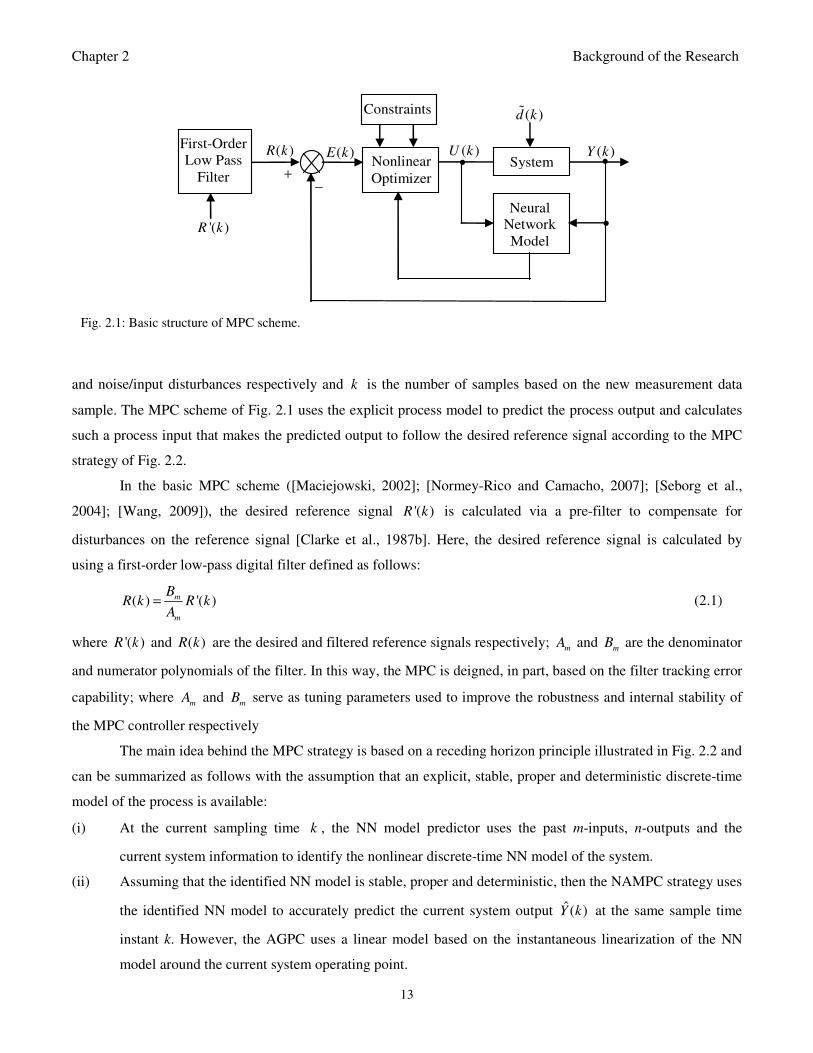
Chapter 2 Background of the Research
13
and noise/input disturbances respectively and k is the number of samples based on the new measurement data
sample. The MPC scheme of Fig. 2.1 uses the explicit process model to predict the process output and calculates
such a process input that makes the predicted output to follow the desired reference signal according to the MPC
strategy of Fig. 2.2.
In the basic MPC scheme ([Maciejowski, 2002]; [Normey-Rico and Camacho, 2007]; [Seborg et al.,
2004]; [Wang, 2009]), the desired reference signal '( )R k is calculated via a pre-filter to compensate for
disturbances on the reference signal [Clarke et al., 1987b]. Here, the desired reference signal is calculated by
using a first-order low-pass digital filter defined as follows:
( ) '( )m
m
BR k R k
A= (2.1)
where '( )R k and ( )R k are the desired and filtered reference signals respectively; m
A and m
B are the denominator
and numerator polynomials of the filter. In this way, the MPC is deigned, in part, based on the filter tracking error
capability; where m
A and m
B serve as tuning parameters used to improve the robustness and internal stability of
the MPC controller respectively
The main idea behind the MPC strategy is based on a receding horizon principle illustrated in Fig. 2.2 and
can be summarized as follows with the assumption that an explicit, stable, proper and deterministic discrete-time
model of the process is available:
(i) At the current sampling time k , the NN model predictor uses the past m-inputs, n-outputs and the
current system information to identify the nonlinear discrete-time NN model of the system.
(ii) Assuming that the identified NN model is stable, proper and deterministic, then the NAMPC strategy uses
the identified NN model to accurately predict the current system output ˆ( )Y k at the same sample time
instant k. However, the AGPC uses a linear model based on the instantaneous linearization of the NN
model around the current system operating point.
System ( )Y k ( )U k
•
Neural
Network
Model
Nonlinear
Optimizer •
+ −
( )E k
•
Constraints ( )d k
( )R k
'( )R k
First-Order
Low Pass
Filter
Fig. 2.1: Basic structure of MPC scheme.
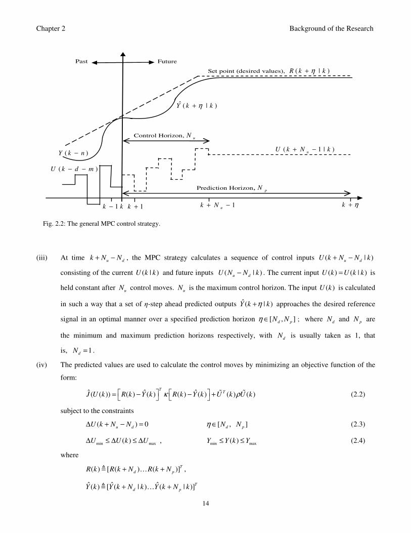
Chapter 2 Background of the Research
14
(iii) At timeu d
k N N+ − , the MPC strategy calculates a sequence of control inputs ( | )u d
U k N N k+ −
consisting of the current ( | )U k k and future inputs ( | )u d
U N N k− . The current input ( ) ( | )U k U k k= is
held constant after u
N control moves. u
N is the maximum control horizon. The input ( )U k is calculated
in such a way that a set of η-step ahead predicted outputs ˆ( | )Y k kη+ approaches the desired reference
signal in an optimal manner over a specified prediction horizon [ , ]d pN Nη ∈ ; where d
N and pN are
the minimum and maximum prediction horizons respectively, with d
N is usually taken as 1, that
is, 1d
N = .
(iv) The predicted values are used to calculate the control moves by minimizing an objective function of the
form:
ˆ ˆ ˆ( ( )) ( ) ( ) ( ) ( ) ( ) ( )T
TJ U k R k Y k R k Y k U k U kκ ρ = − − +
(2.2)
subject to the constraints
( ) 0u d
U k N N∆ + − = [ , ]d pN Nη ∈ (2.3)
min max( )U U k U∆ ≤ ∆ ≤ ∆ , min max( )Y Y k Y≤ ≤ (2.4)
where
( ) [ ( ) ( )]T
d pR k R k N R k N+ + … ,
ˆ ˆ ˆ( ) [ ( | ) ( | )]T
d pY k Y k N k Y k N k+ + …
Past Future
Set point (desired values), ( | )R k kη+
( 1 | )u
U k N k+ −
Control Horizon,u
N
Prediction Horizon,p
N
k 1k −
( )U k d m− −
( )Y k n−
ˆ ( | )Y k kη+
1u
k N+ − k η+ 1k +
Fig. 2.2: The general MPC control strategy.
Chapter 2 Background of the Research
15
ˆ( ) ( ) ( ) [ ( | ) ( | )]T
d pE k R k Y k E k N k E k N k = − + + … ,
( ) [ ( ) ( )]T
u dU k U k U k N N∆ ∆ + − …
where U∆ is the change in control signal vector; κ and ρ are two weighting matrices penalizing
changes on ˆ( )Y k and ( )U k in (2.2).
Although a sequence of u
N moves is calculated at each sampling instant, only the first control move
( ) ( | )U k U k k= is actually implemented and applied to control the process. The remaining control signals are not
applied because at the next sampling instant 1k k= + a new output ( 1)Y k + is known based on new
measurements. The MPC strategy enters a new optimization loop while the remaining control signals
( 1| )u
U N k− are used to initialize the optimizer. This is indeed the receding horizon principle inherent in MPC
strategy.
2.3 MPC Process Models
MPC is a model-based control strategy which depends on the accuracy of the process model. Accurate
process model predictions can provide early warnings of potential problems whereas inaccurate process model
will not lead only to process control failure but can also lead to expensive economic loss and environmental
hazards.
The majority of the MPC algorithms used in industry are based on a linear mathematical model of the
controlled process ([Camacho and Bordons, 2007], [Froisy, 1994], [Seborg et al., 2004], [Qin and Badgwell,
2003]). However, the characteristics of many industrial systems are highly nonlinear. Therefore, algorithms
obtained by MPC design techniques which are based on a linear mathematical model of the controlled process are
not very efficient because these methods cannot guarantee stable control outside the range of the model validity
([Kalra and Georgakis, 1994], [Su and Yu, 2009]). For these reason adaptive algorithms which would be based on
a continuous updating of the nonlinear process model and redesign of the MPC strategy online before a new
control action is applied to the process would be the preferred ones. As noted in [Seborg et al., 2004], the benefits
of MPC algorithms lie on the accuracy of the process model; and for this reason, accurate nonlinear identification
of the process model forms an integral part of MPC development.
In practice, every possible form of process modeling appears in any given MPC formulation. A detailed
treatment of MPC formulation using linear models can be found in [Camacho and Bordons, 2007], [Maciejowski,
2002], [Normey-Rico and Camacho, 2007], [Seborg et al., 2004], and [Wang, 2009]. The most commonly used
linear models are the impulse response (convolution) model, the step response model, the transfer function model,
and the state-space models.
Chapter 2 Background of the Research
16
There are two main reasons for using linear models in MPC. On one hand, the control of a linear process
is relatively easy and, on the other hand, linear models provide good results when the plant operating point is in
the neighborhood of the model validity. If this is not the case, nonlinear models must be used. The control of
nonlinear systems is more complex, especially when the nonlinear process exhibits a dead time, because the
difficulties of handling dead times have to be added to the difficulties of controlling nonlinear processes.
Nonlinear systems are systems whose outputs are nonlinear function of their inputs. Models can be
classified into first-principle input-output models, derived from the physiochemical laws governing the
relationship among their variables, or empirical models, derived from data obtained from the process. A major
mathematical obstacle to a complete theory of nonlinear processes is the lack of a superposition principle for
nonlinear systems. Because of this, the determination of models from process input/output data becomes a very
difficult task. The number of plant tests required to identify a nonlinear plant is much greater than that needed for
a linear plant. In an ideal situation, if the plant is linear, only a step test has to be performed in order to know the
step response of the plant. Because of the superposition principle, the response to a different size step can be
obtained by multiplying the response to the step test by the ratio of the step sizes. The use of nonlinear models for
MPC design is currently an active area of research which is also an objective in the current work. Some
approaches for modeling nonlinear systems for MPC design includes the empirical, state space, and the input-
output approaches ([Camacho and Bordons, 2007], [Ljung, 1999], [Maciejowski, 2002], [Normey-Rico and
Camacho, 2007], [Rossiter, 2004], [Zhu, 2001]). Next, we provide brief descriptions of the type of the linear and
nonlinear input-output modeling technique that have been used in this work and may be needed by the reader to
understand this research work.
Discrete Time Input − Output Models
The nonlinear discrete-time models used for control can be viewed as mappings between those variables
that are available for predicting system behaviour up to the current time and those to be predicted at or after that
instant. This kind of model can be represented as a Nonlinear AutoRegressive Moving Average with eXogenous
input (NARMAX) model given by the following general form:
( ) [ ( 1), , ( ), ( 1), , ( ), ( 1), , ( )]Y k J U k d U k d m Y k Y k n D k D k n= − − − − − − − − … … … (2.8)
where ( , , )J ⋅ ⋅ ⋅ is a nonlinear mapping function, ( )Y k is the output, ( )U k is the input, d is the delay and ( )D k is
the noise/disturbance input at a sampling instant k . The suitability of this model depends on the choice of
function ( , , )J ⋅ ⋅ ⋅ and the order parameters m and n. It should be noted that this equation covers a wide range of
descriptions, depending mainly on function ( , , )J ⋅ ⋅ ⋅ . Different choices of this function give rise to certain models
that are able to provide attractive formulations for predictive control ([Camacho and Bordons, 1993], [Camacho
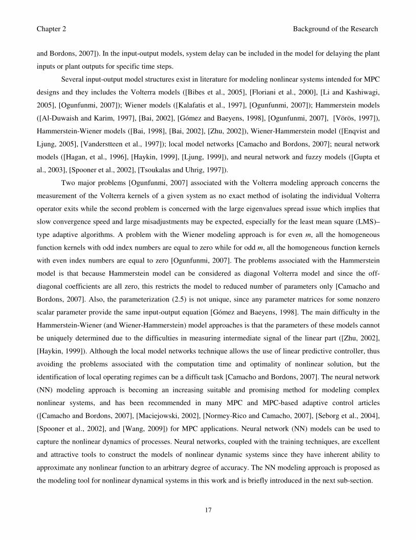
Chapter 2 Background of the Research
17
and Bordons, 2007]). In the input-output models, system delay can be included in the model for delaying the plant
inputs or plant outputs for specific time steps.
Several input-output model structures exist in literature for modeling nonlinear systems intended for MPC
designs and they includes the Volterra models ([Bibes et al., 2005], [Floriani et al., 2000], [Li and Kashiwagi,
2005], [Ogunfunmi, 2007]); Wiener models ([Kalafatis et al., 1997], [Ogunfunmi, 2007]); Hammerstein models
([Al-Duwaish and Karim, 1997], [Bai, 2002], [Gómez and Baeyens, 1998], [Ogunfunmi, 2007], [Vörös, 1997]),
Hammerstein-Wiener models ([Bai, 1998], [Bai, 2002], [Zhu, 2002]), Wiener-Hammerstein model ([Enqvist and
Ljung, 2005], [Vanderstteen et al., 1997]); local model networks [Camacho and Bordons, 2007]; neural network
models ([Hagan, et al., 1996], [Haykin, 1999], [Ljung, 1999]), and neural network and fuzzy models ([Gupta et
al., 2003], [Spooner et al., 2002], [Tsoukalas and Uhrig, 1997]).
Two major problems [Ogunfunmi, 2007] associated with the Volterra modeling approach concerns the
measurement of the Volterra kernels of a given system as no exact method of isolating the individual Volterra
operator exits while the second problem is concerned with the large eigenvalues spread issue which implies that
slow convergence speed and large misadjustments may be expected, especially for the least mean square (LMS)–
type adaptive algorithms. A problem with the Wiener modeling approach is for even m, all the homogeneous
function kernels with odd index numbers are equal to zero while for odd m, all the homogeneous function kernels
with even index numbers are equal to zero [Ogunfunmi, 2007]. The problems associated with the Hammerstein
model is that because Hammerstein model can be considered as diagonal Volterra model and since the off-
diagonal coefficients are all zero, this restricts the model to reduced number of parameters only [Camacho and
Bordons, 2007]. Also, the parameterization (2.5) is not unique, since any parameter matrices for some nonzero
scalar parameter provide the same input-output equation [Gómez and Baeyens, 1998]. The main difficulty in the
Hammerstein-Wiener (and Wiener-Hammerstein) model approaches is that the parameters of these models cannot
be uniquely determined due to the difficulties in measuring intermediate signal of the linear part ([Zhu, 2002],
[Haykin, 1999]). Although the local model networks technique allows the use of linear predictive controller, thus
avoiding the problems associated with the computation time and optimality of nonlinear solution, but the
identification of local operating regimes can be a difficult task [Camacho and Bordons, 2007]. The neural network
(NN) modeling approach is becoming an increasing suitable and promising method for modeling complex
nonlinear systems, and has been recommended in many MPC and MPC-based adaptive control articles
([Camacho and Bordons, 2007], [Maciejowski, 2002], [Normey-Rico and Camacho, 2007], [Seborg et al., 2004],
[Spooner et al., 2002], and [Wang, 2009]) for MPC applications. Neural network (NN) models can be used to
capture the nonlinear dynamics of processes. Neural networks, coupled with the training techniques, are excellent
and attractive tools to construct the models of nonlinear dynamic systems since they have inherent ability to
approximate any nonlinear function to an arbitrary degree of accuracy. The NN modeling approach is proposed as
the modeling tool for nonlinear dynamical systems in this work and is briefly introduced in the next sub-section.
Chapter 2 Background of the Research
18
2.4 Neural Networks: An Overview
2.4.1 Neural Networks
A neural network is a massively parallel distributed processor made up of simple processing neurons (also
called units), which has a natural propensity for storing experimental knowledge acquired from its environment
through a learning process and making it available for use ([Gupta et al., 2003], [Hagan et al., 1996], [Haykin,
1999]). Neural networks are composed of many of these neurons. The standard neuron, shown in Fig. 2.3 is a
processing element whose output ˆi
y is calculated by multiplying its inputs l
u by individual weights ,i lw ; add the
bias term ,0i
w which takes care of the offset in the process model, summing up the results to obtain a
as a
function of the input signals, and applying a nonlinear activation function ( )i
f a
to the sum a
. The mathematical
interpretation can be expressed as follows:
, ,0
1
l
i j j i
j
a w u w=
= +∑
(2.9)
, ,0
1
ˆ ( )l
i i i i j j i
j
y f a f w u w=
= = +
∑
(2.10)
where 1 2, , ,l
u u u… are the input signals; ,1 ,2 ,, , ,i i i lw w w… are the synaptic weights of the neuron i ; ,0iw is a fixed
input clamped to +1, called the bias, and can be interpreted as a weight applied to the input. The activation
function ( )i i
f v in terms of the activation potential i
v is most often monotonic and can take any of the following
forms:
Logistic (standard sigmoid) : 1
( )1
j af a
eα−
=+
i
(2.11)
Hyperbolic tangent sigmoid : 2
2( ) 1
1j a
f ae
−= −
−i
(2.12)
Linear : ( )jf a a=
(2.13)
Signum (step) :
1, 0
( ) sgn( ) 0 0
1 0
j
a
f a a a
a
>
= = =− <
(2.14)
where α is the slope parameter of the sigmoid logistic functions.
The adjustment of the weights is called the training or learning process. For the simple single layer neuron
of Fig. 2.3 given by (2.10), the perceptron learning rule is adopted and stated as follows:
1 For 1j = to l
Chapter 2 Background of the Research
19
( )i
f a
,i lw
,1iw
ˆi
y
, 0 1i
w = +
1u
2u
lu
a
∑ , 2i
w
Fig. 2.3 A nonlinear model of a neuron.
Initialize the weights, ,i jw with small random vector and set ,0iw to small initial number.
End For
2. Compute (2.10)
3. If ˆi iy y≠ (the desired output)
4. For 1j = to l
(i) Modify the weight, , ,j i j i i jw w y u= + ⋅
(ii). The bias, ,0 ,0i i i lw w y u= + ⋅
End For
6. Go to 2.
7. If ˆi iy y= , End.
The original perceptron (Fig. 2.3) proposed by Rosenblatt [Rosenblatt, 1959] and the later Adaline
(adaptive linear element) proposed by Widrow and Hoff [Widrow and Hoff, 1960] were modified by Minsky and
Papet [Minsky and Papet, 1969].
2.4.2 Multilayer Perceptron (MLP) Neural Networks
The single input neuron of Fig. 2.3 can be combined with other single input neurons to form several
layers and architectures in different fashions ([Gupta et al., 2003], [Hertz et al., 1991], [Hagan et al., 1996],
[Haykin, 1999]) and resulting in this way to a more complex network. The most common of these architectures is
the multilayer perceptron (MLP) neural networks where the output of the previous unit serves as the input to the
next unit and so on. A MLP NN with two, three or four-units is usually referred to as two, three or four- layer
network. The typical structure of a two layer multi-input multi-output network is shown in Fig. 2.4, where the first
layer is the hidden layer since it is between the inputsl
u , and the output layer that produces the output ˆ ( )i
y k .
The MLP NN is fully connected since all its inputs and all units in one layer are all connected to all units in the
Chapter 2 Background of the Research
20
,0jw
1ˆ ( )y k
0 1u = +
1u
2u
lu
1( )f a∑
2 ( )f a∑
( )j
f a∑
1,0w
1,1w
2,0w
1,2w
,1jw
,j lw
,2jw
1,lw
2,1w
2,lw 2,2
w
,0iW
1( )F b∑
1,0W
1,1W
2,0W
1,2W
,1iW
,i jW
,2iW
1, jW
2,1W
2, jW
2,2W
0 1U = +
2( )F b∑
( )i
F b∑
2ˆ ( )y k
ˆ ( )iy k
•
•
•
•
•
•
•
•
•
•
••
•
•
•
Fig. 2.4: Feedforward multilayer perceptron neural network with a hidden and an output layer.
next layer and this network is often referred to as feedforward network due to its structure. For a given set of
inputsl
u , the thi output ˆ ( )
iy k of the MLP NN of Fig. 2.4 can be expressed mathematically as:
, , ,0 ,0
1 1
ˆ ( )h un n
i i i j j j l l j i
j l
y k F W f w u w W= =
= + +
∑ ∑ (2.15)
and the term a
defined in (2.9) is given here from (2.15) as
, ,0
1
un
j l l j
l
a w u w=
= +∑
(2.16)
where every ,j l
w and every ,i j
W are the hidden and output weights respectively; ,0j
w and ,0i
W are the hidden and
output biases; [1, ]h
j n∈ is the number of hidden neurons; [1, ]u
l n∈ is the number of inputs, [1, ]o
i n∈ is the ith
number of output neurons and also correspond to the number of the system outputs; Every ( )j
f i is the hidden
layer sigmoidal activation function which can be (2.11) or (2.12) and ( )i
F i is the output layer linear activation
function which can be (2.13) or (2.14).
2.4.3 Supervised and Unsupervised Learning Methods Using Neural Networks
This sub-section briefly discusses supervised and unsupervised NNs with emphasis on types that are widely
used in dynamic system modeling and adaptive control applications. The types of supervised learning methods
discussed here are: the dynamic feedforward multilayer perceptron neural network (DFMLPNN), recurrent neural
network (RNN) and the tapped delay neural network (TDNN). Two types of unsupervised methods of interest
discussed here are the generalized regression neural network (GRNN) and the radial basis function neural network
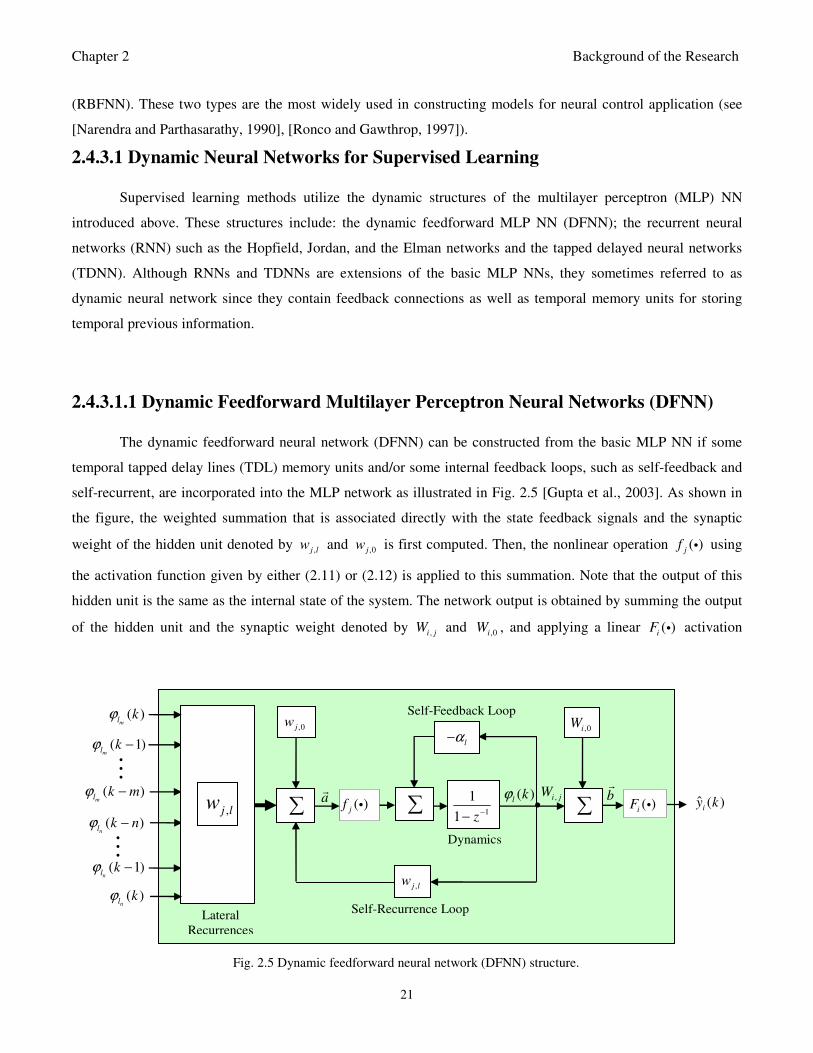
Chapter 2 Background of the Research
21
( 1)ml
kϕ −
( )ml
k mϕ −
( )nl
k nϕ −
( 1)nl
kϕ −
1
1
1 z−
−
,0jw,0iW
lα−
•
Self-Feedback Loop
Self-Recurrence Loop
ˆ ( )iy k ( )iF i
Dynamics
b
∑ ( )jf ia
∑
,j lw
,i jW ( )l kϕ
,j lw
( )ml
kϕ
( )nl
kϕ
Lateral
Recurrences
∑
Fig. 2.5 Dynamic feedforward neural network (DFNN) structure.
(RBFNN). These two types are the most widely used in constructing models for neural control application (see
[Narendra and Parthasarathy, 1990], [Ronco and Gawthrop, 1997]).
2.4.3.1 Dynamic Neural Networks for Supervised Learning
Supervised learning methods utilize the dynamic structures of the multilayer perceptron (MLP) NN
introduced above. These structures include: the dynamic feedforward MLP NN (DFNN); the recurrent neural
networks (RNN) such as the Hopfield, Jordan, and the Elman networks and the tapped delayed neural networks
(TDNN). Although RNNs and TDNNs are extensions of the basic MLP NNs, they sometimes referred to as
dynamic neural network since they contain feedback connections as well as temporal memory units for storing
temporal previous information.
2.4.3.1.1 Dynamic Feedforward Multilayer Perceptron Neural Networks (DFNN)
The dynamic feedforward neural network (DFNN) can be constructed from the basic MLP NN if some
temporal tapped delay lines (TDL) memory units and/or some internal feedback loops, such as self-feedback and
self-recurrent, are incorporated into the MLP network as illustrated in Fig. 2.5 [Gupta et al., 2003]. As shown in
the figure, the weighted summation that is associated directly with the state feedback signals and the synaptic
weight of the hidden unit denoted by ,j lw and ,0jw is first computed. Then, the nonlinear operation ( )jf i using
the activation function given by either (2.11) or (2.12) is applied to this summation. Note that the output of this
hidden unit is the same as the internal state of the system. The network output is obtained by summing the output
of the hidden unit and the synaptic weight denoted by ,i jW and ,0iW , and applying a linear ( )i
F i activation
Chapter 2 Background of the Research
22
function given by (2.13) or (2.14). The lateral recurrences block consists of the initial weights of the network and
multipliers for multiplying the network input-output signals with weights.
The mathematical description for the output of the network of Fig. 2.5 can be expressed as:
, ,0
1
ˆ ( ) ( ) ( )hn
i i i i j j i
j
y k F b F W f a W=
= = +
∑
(2.17)
where , ,0
1
( )ln
j l l j
l
a w k wϕ=
= +∑
(2.18)
where for simplicity 1α = , but its significance as an adaptation parameter is discussed later in sub-section 2.4.4.1
chapter, ( ) [ ( ) ( )]m nl l lk k kϕ ϕ ϕ= and
m nl l l= + is the length of the input vector to the network.
2.4.3.1.2 Recurrent Neural Networks (RNN)
In the context of models development for dynamic systems, when the MLP feed-forward neural network
discussed in the previous sub-section is augmented with external feedback loops, then the network is referred as
recurrent neural network (RNN). Unlike the feed-forward NN, where there is algebraic relationship between the
input and output, the RNN architecture contains internal time delayed feedback connections.
In recurrent neural networks the activation values in the network are repeatedly updated until a stable
point is reached after which the weights are adapted. There are, however, recurrent networks where the learning
rule is used after each propagation (where an activation value is transversed over each weight only once), while
external inputs are included in each propagation. In such networks, the recurrent connections can be regarded as
extra inputs to the network, the values of which are computed by the network itself.
Suppose a network that must generate a control command depending on an external input is to be
constructed, which is a time series ( ), ( 1) , ( 2), , ( )U k U k U k U k m− − −… . With a feed-forward NN there are two
approaches: 1) create inputs ( 1) , ( 2), , ( )k k k mϕ ϕ ϕ− − −… which constitute the first m values of the input vector
or 2) create inputs , ', '', , mϕ ϕ ϕ ϕ… . Besides the current input ( )U k , the first, second, up to m -derivatives are
also added as inputs. Naturally, computation of these derivatives is not a trivial task for higher-order derivatives.
The disadvantage of these two approaches is that the input dimensionality of the feed-forward network is
multiplied with ,n leading to a very large network, which is slow and difficult to train as pointed out in [Bengio et
al., 1994], [Pearlmutter, 1995], [Song, 2010], and [Williams and Zipser, 1989] . The RNN provides a solution to
this problem due to its recurrent connections. A window of inputs does not need to be input anymore; instead, the
network is supposed to learn the influence of the previous time steps itself. One of the earliest RNN is the auto-
associator ([Anderson, 1977] and [Kohonen, 1977]); which consisted of a pool of neurons with weighted
connections between each unit i and ( )j i j≠ . In 1982, Hopfield [Hopfield, 1982] brings together several
Chapter 2 Background of the Research
23
earlier ideas concerning these networks and presents a complete mathematical analysis based on Ising-spin
models [Amit et al., 1986]. However, the two most common RNN designs are the Jordan network [Jordan, 1986a]
and the Elman network [Elman, 1990].
2.4.3.1.2.1 The Hopfield Network
The Hopfield dynamic neural network is a nonlinear dynamic system that has the potential for exhibiting
a wide range of complex behaviour depending on how the network parameters are chosen. The Hopfield network
shown in Fig. 2.6 consists of a set of n interconnected neurons which update their activation values
asynchronously and independently of other neurons. All neurons are both input ( )j and output ( )i neurons. The
activation values are binary. Originally, Hopfield [Hopfield, 1982] chose activation values of 1 and 0, but using
values +1 and -1 presents some advantages discussed as below.
Suppose that the state of the system is given by the activation values ˆ ˆ( ) ( )i
Y k Y k= . The net input
( 1)i
a k +
of a neuron i at cycle 1k + is a weighted sum given by:
, ,0( 1) ( )l
i j j i i
j i
a k U k w w≠
+ = +∑
(2.19)
Suppose, a simple logistic sigmoidal function (2.11) is applied to the net input to obtain the new activation value
ˆ ( 1)i
Y k + at time 1k + defined as:
1 ( 1)
ˆ ( 1) 1 ( 1)
ˆ ,( )
i
i i
i
if a t U
Y k if a t U
OtherwiseY t
+ + >
+ = − + <
(2.20)
i.e., ˆ ( 1) ( ( 1))i j
Y k f a k+ = +
. A neuron i in the Hopfield network is called stable at time k if, in accordance with
equations (2.19) and (2.20),
ˆ ( ) ( ( 1))i j iY k f a k= +
(2.21)
In the Hopfield scheme, a state α is called stable if, when the network is in state α , all neurons are stable. A
pattern ( )pU k is called stable if, when ( )p
U k is clamped, all neurons are stable. When the extra restriction
, ,j i i jw w= is made, the behaviour of a dynamic system can be described by the following computational energy
function [Hopfield, 1984]:
, ,0
1 1 1
1 ˆ ˆ ˆ( ) ( ) ( ) ( )2
n m l
j i i j i i
i j i
k Y k Y k w w Y k= = =
ℑ = − −∑∑ ∑ (2.22)
The advantage of a 1 / 1+ − model over a 1 / 0 model then is symmetry of the states of the network. When some
pattern ( )U k is stable, its inverse is also stable, whereas in the 1 / 0 model this is not always true. For example, as
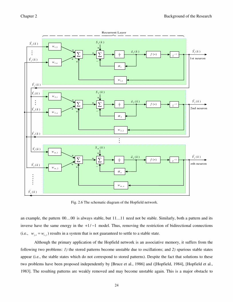
Chapter 2 Background of the Research
24
1 ( )S k
1ˆ ( )Y k
∑ ∑ 1ℑ
1z
−
+
+ +
+
+
–
+
1,1w
1α 1, nw
1, 2w
1st neuron
1 ( )a k
( )f i
2 ( )S k
2ˆ ( )Y k
∑ ∑ 1ℑ
1z
−
+
+ +
+
+
–
+
2 , 2w
2α 2 , nw
2 ,1w
2nd neuron
2 ( )a k
( )f i
( )mS k
ˆ ( )nY k ∑ ∑ 1
ℑ 1
z−
+
+ +
+
+
–
+
,m nw
nα , 2mw
,1mw
nth neuron
( )na k
( )f i
•
•
•
• • •
• • •
• • •
2ˆ ( )Y k
ˆ ( )n
Y k
1ˆ ( )Y k
ˆ ( )n
Y k
1ˆ ( )Y k
2ˆ ( )Y k
ˆ ( )n
Y k
Recurrent Layer
2ˆ ( )Y k
ˆ ( )n
Y k
Fig. 2.6 The schematic diagram of the Hopfield network.
an example, the pattern 00 00… is always stable, but 11 11… need not be stable. Similarly, both a pattern and its
inverse have the same energy in the 1 / 1+ − model. Thus, removing the restriction of bidirectional connections
(i.e., , ,j i i jw w= ) results in a system that is not guaranteed to settle to a stable state.
Although the primary application of the Hopfield network is an associative memory, it suffers from the
following two problems: 1) the stored patterns become unstable due to oscillations; and 2) spurious stable states
appear (i.e., the stable states which do not correspond to stored patterns). Despite the fact that solutions to these
two problems have been proposed independently by [Bruce et al., 1986] and ([Hopfield, 1984], [Hopfield et al.,
1983]. The resulting patterns are weakly removed and may become unstable again. This is a major obstacle to
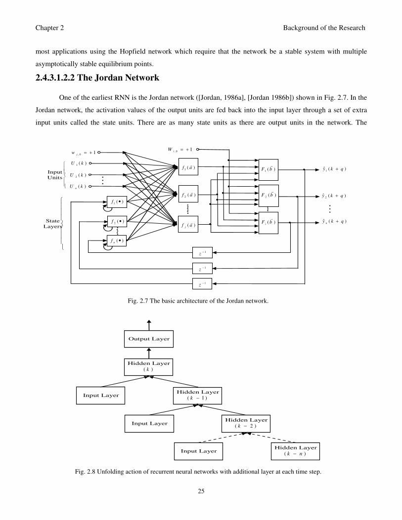
Chapter 2 Background of the Research
25
, 0 1j
w = +
1 ( )f a
2 ( )f a
( )j
f a
, 0 1i
W = +
•
•
•
••
•
••
•
1z
−
1z
−
1z
−
1 ( )U k•
•
•
1 ( )F b
2 ( )F b
( )i
F b
1ˆ ( )y k q+
•
•
2ˆ ( )y k q+
ˆ ( )n
y k q+
2 ( )U k
( )n
U k
•
•
•
2 ( )f •
1 ( )f •
( )n
f •
State
Layers
Input
Units
Fig. 2.7 The basic architecture of the Jordan network.
Output Layer
Hidden Layer
( )k
Input Layer Hidden Layer
( 1 )k −
Input Layer
Input Layer Hidden Layer
( )k n−
•
•
•
Hidden Layer
( 2 )k −
Fig. 2.8 Unfolding action of recurrent neural networks with additional layer at each time step.
most applications using the Hopfield network which require that the network be a stable system with multiple
asymptotically stable equilibrium points.
2.4.3.1.2.2 The Jordan Network
One of the earliest RNN is the Jordan network ([Jordan, 1986a], [Jordan 1986b]) shown in Fig. 2.7. In the
Jordan network, the activation values of the output units are fed back into the input layer through a set of extra
input units called the state units. There are as many state units as there are output units in the network. The
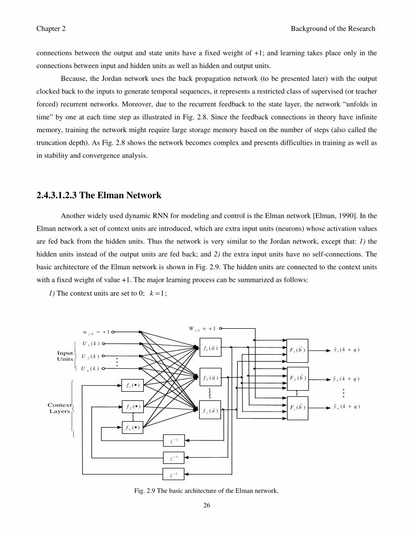
Chapter 2 Background of the Research
26
, 0 1j
w = +
1 ( )f a
2 ( )f a
( )j
f a
, 01
iW = +
•
•
•
••
•
••
•
1z
−
1z
−
1z
−
1 ( )U k•
•
•
1 ( )F b
2 ( )F b
( )i
F b
1ˆ ( )y k q+
•
•
2ˆ ( )y k q+
ˆ ( )ny k q+
2( )U k
( )n
U k
•
•
•
2 ( )f •
1 ( )f •
( )nf •
Context
Layers
Input
Units
Fig. 2.9 The basic architecture of the Elman network.
connections between the output and state units have a fixed weight of +1; and learning takes place only in the
connections between input and hidden units as well as hidden and output units.
Because, the Jordan network uses the back propagation network (to be presented later) with the output
clocked back to the inputs to generate temporal sequences, it represents a restricted class of supervised (or teacher
forced) recurrent networks. Moreover, due to the recurrent feedback to the state layer, the network “unfolds in
time” by one at each time step as illustrated in Fig. 2.8. Since the feedback connections in theory have infinite
memory, training the network might require large storage memory based on the number of steps (also called the
truncation depth). As Fig. 2.8 shows the network becomes complex and presents difficulties in training as well as
in stability and convergence analysis.
2.4.3.1.2.3 The Elman Network
Another widely used dynamic RNN for modeling and control is the Elman network [Elman, 1990]. In the
Elman network a set of context units are introduced, which are extra input units (neurons) whose activation values
are fed back from the hidden units. Thus the network is very similar to the Jordan network, except that: 1) the
hidden units instead of the output units are fed back; and 2) the extra input units have no self-connections. The
basic architecture of the Elman network is shown in Fig. 2.9. The hidden units are connected to the context units
with a fixed weight of value +1. The major learning process can be summarized as follows:
1) The context units are set to 0; 1k = ;
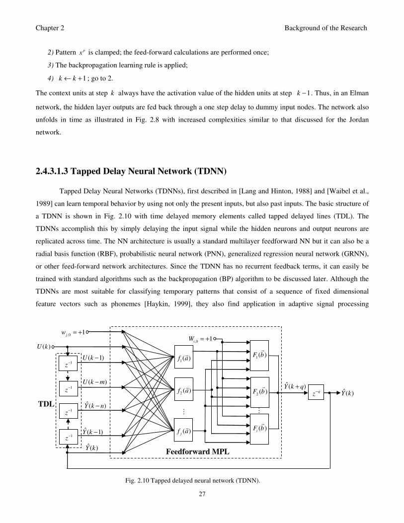
Chapter 2 Background of the Research
27
,0 1
jw = +
( )U k
1( )f a
2 ( )f a
( )j
f a
,0 1i
W = +
•
•
•
••
•
•
•ˆ( )Y kq
z− •
ˆ( )Y k
1z
−
1z
−
1z
−
1z
− ˆ( 1)Y k −
ˆ( )Y k n−
( )U k m−
( 1)U k − •
•
•
1( )F b
2 ( )F b
( )i
F b
ˆ( )Y k q+
•
•
•
TDL
Feedforward MPL
Fig. 2.10 Tapped delayed neural network (TDNN).
2) Pattern px is clamped; the feed-forward calculations are performed once;
3) The backpropagation learning rule is applied;
4) 1k k← + ; go to 2.
The context units at step k always have the activation value of the hidden units at step 1k − . Thus, in an Elman
network, the hidden layer outputs are fed back through a one step delay to dummy input nodes. The network also
unfolds in time as illustrated in Fig. 2.8 with increased complexities similar to that discussed for the Jordan
network.
2.4.3.1.3 Tapped Delay Neural Network (TDNN)
Tapped Delay Neural Networks (TDNNs), first described in [Lang and Hinton, 1988] and [Waibel et al.,
1989] can learn temporal behavior by using not only the present inputs, but also past inputs. The basic structure of
a TDNN is shown in Fig. 2.10 with time delayed memory elements called tapped delayed lines (TDL). The
TDNNs accomplish this by simply delaying the input signal while the hidden neurons and output neurons are
replicated across time. The NN architecture is usually a standard multilayer feedforward NN but it can also be a
radial basis function (RBF), probabilistic neural network (PNN), generalized regression neural network (GRNN),
or other feed-forward network architectures. Since the TDNN has no recurrent feedback terms, it can easily be
trained with standard algorithms such as the backpropagation (BP) algorithm to be discussed later. Although the
TDNNs are most suitable for classifying temporary patterns that consist of a sequence of fixed dimensional
feature vectors such as phonemes [Haykin, 1999], they also find application in adaptive signal processing
Chapter 2 Background of the Research
28
[Tsoukalas and Uhrig, 1997] and they have been widely used in identification and control applications (see
[Narendra and Parthasarathy, 1990])
As shown in Fig. 2.10, the TDNN consists of a multilayer feedforward neural network (MFNN) with
some backward shift delay operators. Compared with the Hopfield, Jordan and Elaman networks, although the
TDNN has time-delayed feedback of the network outputs, its training presents less complexity, requires less
computational time and memory requirement. The main disadvantage to use TDNN is that a prior knowledge
about the system is necessary. Since there is no state feedback, the TDNN can be trained with the basic
backpropagation algorithm.
Consider that ˆ( )Y k ∈ℜ in Fig. 2.10 is an internal state variable at time instant k . The delayed states
ˆ ˆ ˆ( ), ( 1), , ( )Y k Y k Y k n− −… fed as inputs to the TDNN can be used to define specific applications such as time-
series predictions and analysis, identification and adaptive control, communication channels, nonlinear input-
output function approximations, etc. Since this work is concerned with identification and adaptive control, the
input-output equations of the TDNN illustrated in Fig. 2.10 with relative degree one and η step ahead output
predictions can be expressed as follows:
ˆ ˆ( 1) [ ( ), ( )]Y k J k kθ ϕ+ = (2.23)
ˆ ˆ( ) [ ( ), ( )]Y k J k kη θ ϕ+ = (2.24)
where ˆ( , )J ⋅ ⋅ is a nonlinear continuous and differentiable function, ( )kθ denotes the weights and biases of the
network parameters, ( ) [ ( ), ( )]m nl ik k kϕ ϕ ϕ= denotes the state vector with ( ) [ ( ), ( 1), , ( )]
nik Y k Y k Y k nϕ = − −…
containing the time-delayed samples of the NN outputs and ( ) [ ( ), ( 1), , ( )]ml
k U k d U k d U k d mϕ = − − − − −…
containing the current NN inputs, and d the system delay. The sampling time T is assumed to be one i.e. 1T = .
2.4.3.2 Neural Networks Based on Unsupervised Learning
The supervised learning methods just discussed are applied to cases where the inputs and target outputs
are available or can be obtained for NN training and are usually characterized by multilayer neurons. An
unsupervised learning rule is one in which no target outputs are given and are mostly single layer neurons. This
discussion in this section explores unsupervised learning methods based on the Hebbian learning rule [Hebb,
1949] which states that “When the synaptic input and the neuron output are both active, the strength of the
connection between the input and the output is enhanced.” This implies that if the output of the single layer
network is active when the input is active, the weight connecting the two active nodes is enhanced. This allows
the network to associate relationships between inputs and outputs, hence the name associative networks. The
simplest unsupervised Hebb rule can be expressed mathematically as follows:
Chapter 2 Background of the Research
29
ABn ABoW W xyβ= + (2.25)
where AB
W is the weight connecting input A to output ,B β is the learning constant, x is the input, and y is the
output. The learning constant β controls the rate at which the network learns. If β is made large, few number of
observations are needed to learn an association but if β is made small, many observations are needed.
If the weights between active neurons are only allowed to be enhanced, as in the equation above, there is no limit
to their magnitude. Therefore, Grossberg [Grossberg, 1982] proposes the following weight changing rule that will
allow both learning and forgetting to be implemented as follows:
(1 )ABn ABo
W W xyα β= − + (2.26)
In (2.26), α is the forgetting constant and controls the rate at which the memory of old information ( )ABo
W is
allowed to decay away or be forgotten. Using this update rule, the network constantly forgets old information and
continuously learns new information. The values of β and α control the speed of learning and forgetting
respectively and are usually set in the interval [0 1]. The updating rule can be rewritten as:
T
AB ABW W xyα β∆ = − + (2.27)
This rule limits the magnitude of the weights to a value determined by α and .β Thus, solving (2.27) by setting,
0AB
W∆ = , we find the maximum weight to be /β α when x and y are both active.
Several types of unsupervised learning methods exist such as the instar and outstar learning which can be
combined to form an associative memory ([Kohonen, 1977], [Tsoukalas and Uhrig, 1997]); bi-directional
associative memory (BAM) composed of associative network architecture with a crossbar structure [Kosko,
1988]; competitive networks [Hertz et al., 1991]; self organizing maps (SOM) [Kohonen, 1982, 1984, 1995];
probabilistic neural network (PNN) [Masters, 1993a, 1993b]; radial basis function (RBF); and the generalized
regression neural network (GRNN) [Specht, 1991].
While these neural networks can be used interchangeably for diverse applications, their superior
performance can be derived in certain only applications. For example, the SOM (also called Kohonen network)
maps a high dimension input vector into a smaller dimensional pattern of dimension one or two. The PNN is a
Bayesian classifier integrated into neural network architecture and it is best suited for pattern classification where
a representative training set is available. RBF has been proven to be a universal function approximator [Park and
Sandberg, 1991] and can perform similar function mappings as a MLP neural network except that it has
architecture and functionality. GRNN is best suited for function approximation task such as system modeling and
prediction. For more detail on these networks see the references [Gupta et al., 2003], [Hagan et al., 1996] and
[Haykin, 1999].
Among the above mentioned unsupervised methods, the use of radial basis function (RBF) for modeling
and identification of nonlinear dynamic plants has been reported in [Seng et at., 2002] while the application of the
combination of the RBF with GRNN in identification and control has been reported in [Seng et al, 1998]. Also,
the use of GRNN combined with model-based and/or direct adaptive control of diverse applications has been
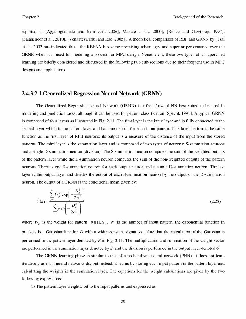
Chapter 2 Background of the Research
30
reported in [Aggelogiannaki and Sarimveis, 2006], Manzie et al., 2000], [Ronco and Gawthrop, 1997],
[Salahshoor et al., 2010], [Venkateswarlu, and Rao, 2005]). A theoretical comparison of RBF and GRNN by [Tsai
et al., 2002 has indicated that the RBFNN has some promising advantages and superior performance over the
GRNN when it is used for modeling a process for MPC design. Nonetheless, these two types of unsupervised
learning are briefly considered and discussed in the following two sub-sections due to their frequent use in MPC
designs and applications.
2.4.3.2.1 Generalized Regression Neural Network (GRNN)
The Generalized Regression Neural Network (GRNN) is a feed-forward NN best suited to be used in
modeling and prediction tasks, although it can be used for pattern classification [Specht, 1991]. A typical GRNN
is composed of four layers as illustrated in Fig. 2.11. The first layer is the input layer and is fully connected to the
second layer which is the pattern layer and has one neuron for each input pattern. This layer performs the same
function as the first layer of RFB neurons: its output is a measure of the distance of the input from the stored
patterns. The third layer is the summation layer and is composed of two types of neurons: S-summation neurons
and a single D-summation neuron (division). The S-summation neuron computes the sum of the weighted outputs
of the pattern layer while the D-summation neuron computes the sum of the non-weighted outputs of the pattern
neurons. There is one S-summation neuron for each output neuron and a single D-summation neuron. The last
layer is the output layer and divides the output of each S-summation neuron by the output of the D-summation
neuron. The output of a GRNN is the conditional mean given by:
2
21
2
21
exp2
ˆ( )
exp2
NpT
p
p
Np
p
DW
Y kD
σ
σ
=
=
−
=
−
∑
∑ (2.28)
where pW is the weight for pattern [1, ]p N∈ , N is the number of input pattern, the exponential function in
brackets is a Gaussian function D with a width constant sigma σ . Note that the calculation of the Gaussian is
performed in the pattern layer denoted by P in Fig. 2.11. The multiplication and summation of the weight vector
are performed in the summation layer denoted by S, and the division is performed in the output layer denoted O.
The GRNN learning phase is similar to that of a probabilistic neural network (PNN). It does not learn
iteratively as most neural networks do, but instead, it learns by storing each input pattern in the pattern layer and
calculating the weights in the summation layer. The equations for the weight calculations are given by the two
following expressions:
(i) The pattern layer weights, set to the input patterns and expressed as:
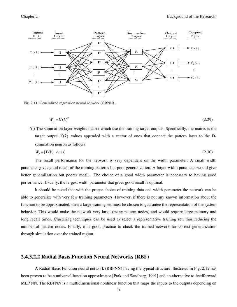
Chapter 2 Background of the Research
31
1 ( )U k 1ˆ ( )Y k
•
•
•
P
P
P
P
P
P
ˆ ( )N
Y k
O
2ˆ ( )Y k O
O
•
•
•
S
S
S
•
•
•
I
I
I
•
•
•
•
•
•
2 ( )U k
( )N
U k
Inputs
( )U k Outputs
ˆ ( )Y k
•
•
•
•
•
•
•
•
•
Input
Layer
Pattern
Layer Summation
Layer
Output
Layer
Fig. 2.11: Generalized regression neural network (GRNN).
( )T
pW U k= (2.29)
(ii) The summation layer weights matrix which use the training target outputs. Specifically, the matrix is the
target output ( )Y k values appended with a vector of ones that connect the pattern layer to the D-
summation neuron as follows:
[ ( ) ]s
W Y k ones= (2.30)
The recall performance for the network is very dependent on the width parameter. A small width
parameter gives good recall of the training patterns but poor generalization. A larger width parameter would give
better generalization but poorer recall. The choice of a good width parameter is necessary to having good
performance. Usually, the largest width parameter that gives good recall is optimal.
It should be noted that with the proper choice of training data and width parameter the network can be
able to generalize with very few training parameters. However, if there is not any known information about the
function to be approximated, then a large training set must be chosen to guarantee the representation of the system
behavior. This would make the network very large (many pattern nodes) and would require large memory and
long recall times. Clustering techniques can be used to select a representative training set, thus reducing the
number of pattern nodes. Finally, it is good practice to check the trained network for correct generalization
through simulation over the trained region.
2.4.3.2.2 Radial Basis Function Neural Networks (RBF)
A Radial Basis Function neural network (RBFNN) having the typical structure illustrated in Fig. 2.12 has
been proven to be a universal function approximator [Park and Sandberg, 1991] and an alternative to feedforward
MLP NN. The RBFNN is a multidimensional nonlinear function that maps the inputs to the outputs depending on
Chapter 2 Background of the Research
32
ˆ ( ) [ ( )]y k f kϕ= ( )kϕ
i
i
i
1w
2w
mw
( )φ i
( )φ i
( )φ i
∑
∑
∑∑
1c
2c
mc
Fig. 2.12: Radial basis function neural network (RBFNN).
the distance between the input vector and the center vector. Therefore, it can perform similar function mappings
as a MLP but its architecture and functionality are very different. In the following, a brief discussion on the
RBFNN is first presented and then the differences between the feedforward MLP NN and the RBFNN are
discussed.
Consider that the RBFNN shown in Fig. 2.12 with m − dimensional input ( ) mkϕ ∈ℜ and a single output
ˆ( )y k ∈ℜ can be represented by the weighted summation of a finite number of radial basis functions as follows:
( )1
ˆ( ) [ ( )] ( ) ( ) ; 1,2, ,m
j j j j
j
y k f k w k c k j mϕ φ ϕ=
= − =∑ … (2.31)
where ( )φ i is an arbitrary nonlinear function, i is the norm that is usually assumed to be Euclidean, ( )m
jc k ∈ℜ
denotes known vectors that represent the centers of the radial basis functions, ,j iw is the weight parameter, and
( ) ( )j jk c kϕ − is the radial basis function of ( )j kϕ at time k obtained by shifting ( )j kϕ by ( )jc k . However,
if the individual elements of the input vector belong to different classes, then a weighted norm can be introduced
from [Gupta et al., 2003] as follows:
,
1
ˆ( ) [ ( )] ( ) ( )j
m
j j i j j jK
j
y k f k w k c kϕ φ ϕ=
= −
∑ (2.32)
where m m
iK×∈ℜ is a weight matrix and the weighted Euclidean norm is given by:
( )
( ) ( )
22( ) ( ) ( ) ( )
( ) ( ) ( ) ( )
jj
j j j jK
T
j j j j j j
k c k K k c k
k c k K K k c k
ϕ ϕ
ϕ ϕ
− = −
= − −
(2.33)
A RBF network is a two layer network that has different types of neurons in the hidden layer and the
output layer. The hidden layer, which corresponds to a MLP hidden layer, is a non-linear local mapping. This
layer contains radial basis function neurons which most commonly use a Gaussian activation function ( )g x .
These functions are centered over receptive fields. Receptive fields are areas in the input space which activate the
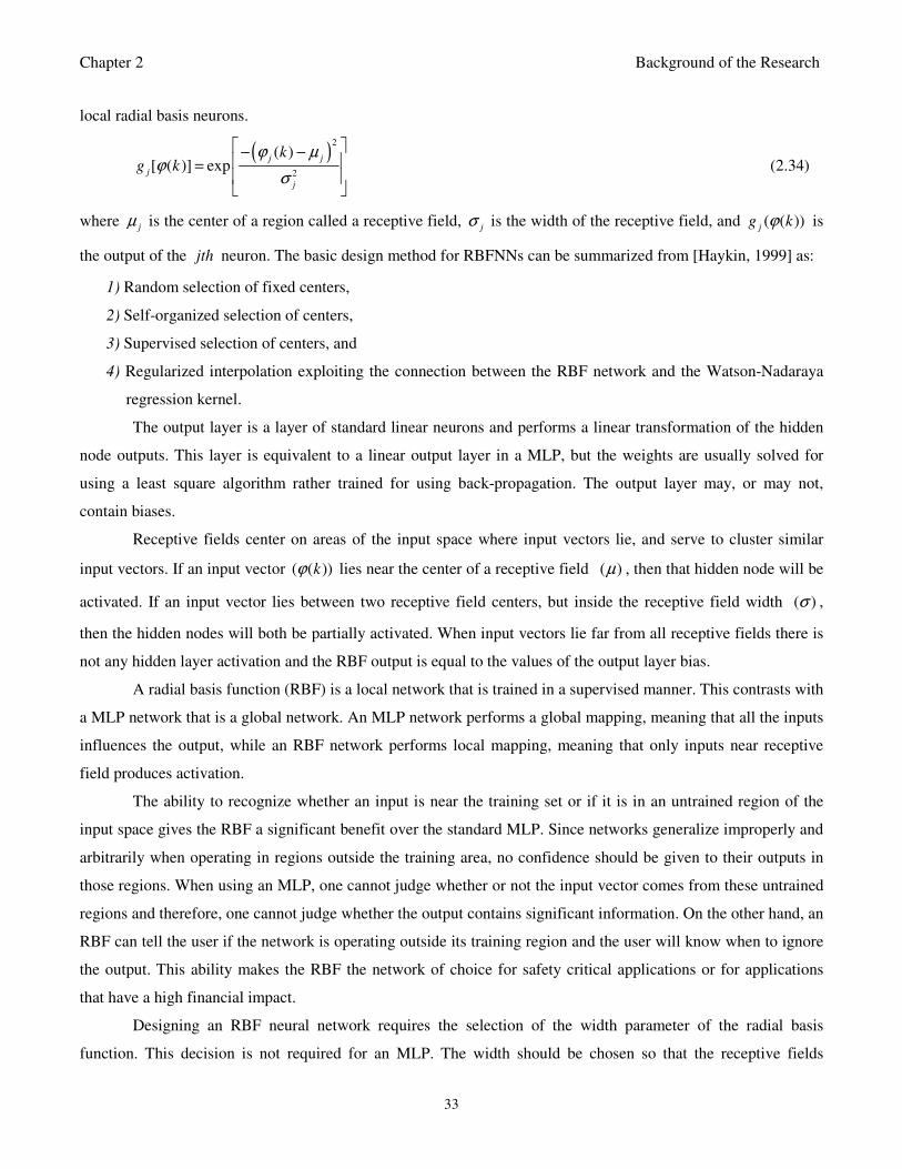
Chapter 2 Background of the Research
33
local radial basis neurons.
( )2
2
( )[ ( )] exp
j j
j
j
kg k
ϕ µϕ
σ
− − =
(2.34)
where jµ is the center of a region called a receptive field, jσ is the width of the receptive field, and ( ( ))jg kϕ is
the output of the jth neuron. The basic design method for RBFNNs can be summarized from [Haykin, 1999] as:
1) Random selection of fixed centers,
2) Self-organized selection of centers,
3) Supervised selection of centers, and
4) Regularized interpolation exploiting the connection between the RBF network and the Watson-Nadaraya
regression kernel.
The output layer is a layer of standard linear neurons and performs a linear transformation of the hidden
node outputs. This layer is equivalent to a linear output layer in a MLP, but the weights are usually solved for
using a least square algorithm rather trained for using back-propagation. The output layer may, or may not,
contain biases.
Receptive fields center on areas of the input space where input vectors lie, and serve to cluster similar
input vectors. If an input vector ( ( ))kϕ lies near the center of a receptive field ( )µ , then that hidden node will be
activated. If an input vector lies between two receptive field centers, but inside the receptive field width ( )σ ,
then the hidden nodes will both be partially activated. When input vectors lie far from all receptive fields there is
not any hidden layer activation and the RBF output is equal to the values of the output layer bias.
A radial basis function (RBF) is a local network that is trained in a supervised manner. This contrasts with
a MLP network that is a global network. An MLP network performs a global mapping, meaning that all the inputs
influences the output, while an RBF network performs local mapping, meaning that only inputs near receptive
field produces activation.
The ability to recognize whether an input is near the training set or if it is in an untrained region of the
input space gives the RBF a significant benefit over the standard MLP. Since networks generalize improperly and
arbitrarily when operating in regions outside the training area, no confidence should be given to their outputs in
those regions. When using an MLP, one cannot judge whether or not the input vector comes from these untrained
regions and therefore, one cannot judge whether the output contains significant information. On the other hand, an
RBF can tell the user if the network is operating outside its training region and the user will know when to ignore
the output. This ability makes the RBF the network of choice for safety critical applications or for applications
that have a high financial impact.
Designing an RBF neural network requires the selection of the width parameter of the radial basis
function. This decision is not required for an MLP. The width should be chosen so that the receptive fields
Chapter 2 Background of the Research
34
overlap but so that one function does not cover the entire input space. This means that several radial basis neurons
have some activation to each input but all radial basis neurons are not highly active for a single input.
Another choice to be made is the number of radial basis neurons. Depending on the training algorithm
used to implement the RBF, this may, or may not, be a decision made by the designer. For example, the
MATLAB Neural Network Toolbox [The MathWorks, 2010a] has two training algorithms. The first algorithm
centers a radial basis neuron on each input vector. This leads to an extremely large network for input data
composed of many patterns. The second algorithm incrementally adds radial basis neurons to reduce the training
error to the preset goal. There are several network architectures that will meet a specified error criterion. These
architectures consist of different combinations of the radial basis function widths and the number of radial basis
functions in the network.
The maximum number of neurons is the number of input patterns; the minimum is related to the error
tolerance and the complexity of the mapping. This minimum must be experimentally determined. A more
complex map and a smaller tolerance require more neurons. The minimum width constant should overlap the
input patterns and the maximum should not cover the entire input space. Excessively large widths can sometimes
give good results for data with no noise, but these systems usually fail under real world conditions in which noise
exists. The reason that the system can train well with noise free cases is that a linear method is used to provide
solutions for the second layer weights. The use of a regression method will minimize the error, but usually at the
expense of large weights and significant over-fitting. This over-fitting is apparent when there is noise in the
system. A smaller width will do a better job of alerting that an input vector is outside the training space, while a
larger width may result in a network of smaller size and faster execution time.
2.4.4 Basic Neural Network Training Algorithms
The basic neural network training algorithms for feedforward neural networks is the basic
backpropagation (BP) algorithm and its variations such as the delta-rule, generalized delta-rule, backpropagation
with momentum (BPM), e.t.c. The basic training algorithms for recurrent neural networks are the back-
propagation through time (BPTT) and the real-time recurrent learning (RTRL) algorithms. While the BPTT is an
extension of the BP algorithm, the RTRL utilizes the generality of the BPTT to derive a real-time training
algorithm for online applications while not suffering its growing memory requirements of the BPTT due to its
unfolding action.
In the following, two variations of the BP algorithm called the back-propagation with momentum (BPM)
and the teacher-forced real-time recurrent learning (RTRL) algorithms derived from the RTRL method are first
presented together. The former is presented to facilitate the derivation of the latter.
2.4.4.1 The Back-Propagation (BP) Algorithm with Momentum
Chapter 2 Background of the Research
35
An important generalization of the perceptron training algorithm was presented by Widrow and Hoff
[Widrow and Hoff, 1960] as least mean squares (LMS) learning procedure, also known as the delta rule. While
the perceptron learning rule uses the output of the activation function (either -1 0r 1) for learning, the delta rule
uses the net output without further mapping into output values -1 or 1. The adaptive operation introduced by the
delta rule [Widrow and Hoff, 1960] implies a mechanism by which iW can be adjusted, usually iteratively, to
attain the correct values.
Minsky and Papet [Minsky and Papet, 1969] showed that a two layer feedforward network can overcome
many restrictions, but did not provide a learning rule on how to adjust the weights from the input to the hidden
layers. The problem here is how to determine the coefficients , 1,2, ,iW i n= … such that the input-output
response is correct for a large number of data sets. The idea behind this solution is that the errors for the units of
the hidden layer are determined by back-propagating the errors of the units of the output layer. For this reason the
method is often called the back-propagation learning rule and can also be considered as a generalization of the
delta rule for non-linear activation functions and multilayer networks. It should be noted that when linear
activation functions are used, the multi-layer network is not more powerful than a single-layer network.
For a given set of input-output training data pair
[ ] ( ), ( ) , 1,2,3, ,N
Z U p Y p p N= = … (2.35)
where ( )U N and ( )Y N are the input and desired (or target) output values. Thus, for every given input-output
data, the output of the network ˆ( )Y k differs from the target value ( )Y k by ˆ[ ( ) ( )]Y k Y k− at the time instant k .
The delta-rule uses a cost- or error-function based on these differences to adjust the weights. The error function E
is defined as a total square error given as:
2
1 1
1 ˆ( ) ( ) ( ) ( )N N
p p p
p p
E k E k Y k Y kN= =
= = − ∑ ∑ (2.36)
where the index p ranges over the set of input patterns N and ( )pE k represents the error on pattern p . In high
dimensional input spaces, the least mean squares (LMS) procedure is used to find the values of all the weights
that minimize the error function by a method called gradient descent. The activation units are considered as a set
of nonlinear continuous and differentiable functions ( )p
j jf a
of the total inputs given by (2.11) or (2.12), so that
the network output can be expressed as:
ˆ ( ) ( )p p
j jY k f a=
(2.37)
where , ,0
1
( )m
p
j j l l j
l
a w k wϕ=
= +∑
(2.38)
where [1, ]h
j n∈ is the number of hidden neurons and [1, ]l m∈ is the length of the input vector to the network.
The idea is to make a change in the weight proportional to the negative of the derivative of the error as measured
on the current pattern with respect to each weight. Thus for the generalized delta rule, we have:
Chapter 2 Background of the Research
36
,
,
( )p
j l
j l
E kw
wγ
∂∆ = −
∂ (2.39)
where γ is a proportionality constant called the learning rate. Let the error measure pE be defined as the total
quadratic error for pattern p at the output units:
2
1
1 ˆ( ) ( ) ( )2
oN
p p p
o o
o
E k Y k Y k=
= − ∑ (2.40)
where ( )p
oY k is the desired output for unit o when pattern p is clamped. The partial derivative of ( )P
E k in
(2.39) can also be expressed as:
, ,
pp pj
p
j l j j l
aE E
w a w
∂∂ ∂=
∂ ∂ ∂
(2.41)
From Eq. (2.38), the second factor in (2.41) can be expressed as
,
ˆ ( )
p
j p
j
j l
aY k
w
∂=
∂
(2.42)
By defining
pp
j p
j
E
aδ
∂= −
∂ (2.43)
An update rule which is equivalent to the delta rule is obtained, resulting in a gradient descent on the error surface
if the weight changes are made according to ([Phansalkar and Sastry, 1994]; [Wang et al., 2004]; [Yu et al.,
1993]):
,ˆ ( )
p p
j l j jw Y kγδ∆ = (2.44)
where ˆ( ) ( )p p p
j Y k Y kδ = − is the difference between the target output and the actual output for pattern p .
The idea here is to investigate the value of p
jδ for each unit j in the network. This implies that there is a
simple recursive computation of these 'sδ which can be implemented by propagating error signals backward
through the network.
To compute p
jδ in (2.43), the partial derivative is expressed as the product of two factors using chain
rule, one factor reflecting the change in error as a function of the output of the unit and one reflecting the change
in the output as a function of change in the input. The computation can be expressed as follows:
ˆ
ˆ
pp pjp
j p ppj jj
YE E
a aYδ
∂∂ ∂= − = −
∂ ∂∂ (2.45)
The second factor in (2.45) is computed using (2.37) and it can be seen that
'ˆ
( )
p
j p
j jp
j
Yf a
a
∂=
∂
(2.46)
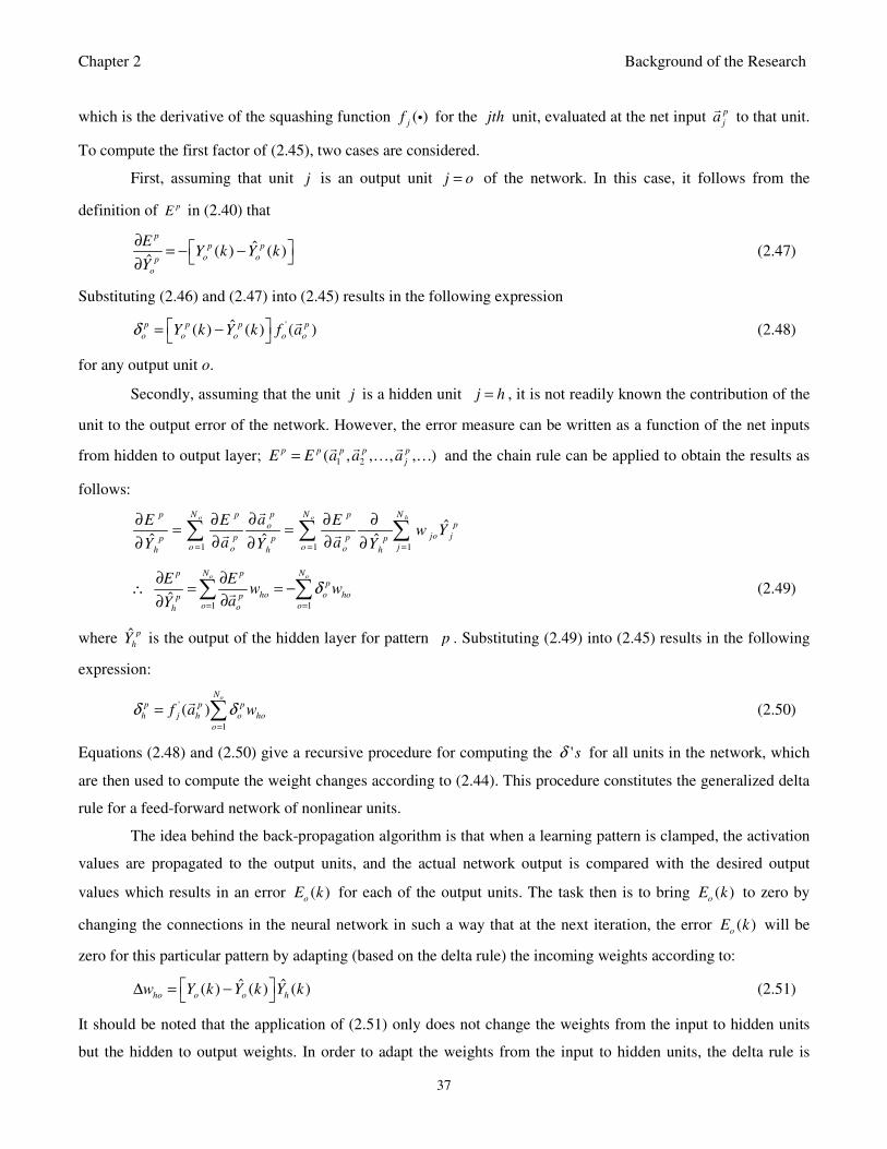
Chapter 2 Background of the Research
37
which is the derivative of the squashing function ( )jf i for the jth unit, evaluated at the net input p
ja
to that unit.
To compute the first factor of (2.45), two cases are considered.
First, assuming that unit j is an output unit j o= of the network. In this case, it follows from the
definition of pE in (2.40) that
ˆ( ) ( )ˆ
pp p
o op
o
EY k Y k
Y
∂ = − − ∂
(2.47)
Substituting (2.46) and (2.47) into (2.45) results in the following expression
'ˆ( ) ( ) ( )p p p p
o o o o oY k Y k f aδ = −
(2.48)
for any output unit o.
Secondly, assuming that the unit j is a hidden unit j h= , it is not readily known the contribution of the
unit to the output error of the network. However, the error measure can be written as a function of the net inputs
from hidden to output layer; 1 2( , , , , )p p p p p
jE E a a a=
… … and the chain rule can be applied to obtain the results as
follows:
1 1 1
ˆˆ ˆ ˆ
o o hpN N Np p ppo
jo jp pp p po o jo oh h h
aE E Ew Y
a aY Y Y= = =
∂∂ ∂ ∂ ∂= =
∂ ∂∂ ∂ ∂∑ ∑ ∑
1 1ˆ
o oN Np pp
ho o hoppo ooh
E Ew w
aYδ
= =
∂ ∂∴ = = −
∂∂∑ ∑ (2.49)
where ˆ p
hY is the output of the hidden layer for pattern p . Substituting (2.49) into (2.45) results in the following
expression:
'
1
( )oN
p p p
h j h o ho
o
f a wδ δ=
= ∑
(2.50)
Equations (2.48) and (2.50) give a recursive procedure for computing the 'sδ for all units in the network, which
are then used to compute the weight changes according to (2.44). This procedure constitutes the generalized delta
rule for a feed-forward network of nonlinear units.
The idea behind the back-propagation algorithm is that when a learning pattern is clamped, the activation
values are propagated to the output units, and the actual network output is compared with the desired output
values which results in an error ( )o
E k for each of the output units. The task then is to bring ( )o
E k to zero by
changing the connections in the neural network in such a way that at the next iteration, the error ( )o
E k will be
zero for this particular pattern by adapting (based on the delta rule) the incoming weights according to:
ˆ ˆ( ) ( ) ( )ho o o h
w Y k Y k Y k ∆ = − (2.51)
It should be noted that the application of (2.51) only does not change the weights from the input to hidden units
but the hidden to output weights. In order to adapt the weights from the input to hidden units, the delta rule is
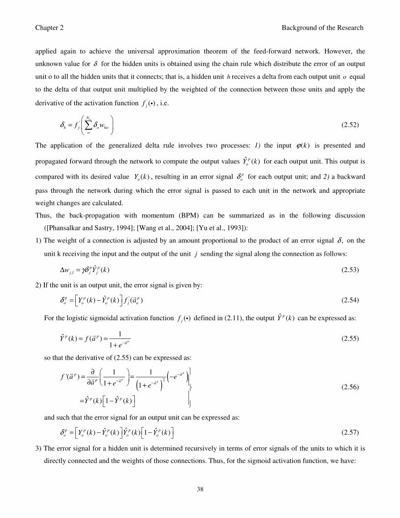
Chapter 2 Background of the Research
38
applied again to achieve the universal approximation theorem of the feed-forward network. However, the
unknown value for δ for the hidden units is obtained using the chain rule which distribute the error of an output
unit o to all the hidden units that it connects; that is, a hidden unit h receives a delta from each output unit o equal
to the delta of that output unit multiplied by the weighted of the connection between those units and apply the
derivative of the activation function ' ( )jf i , i.e.
'oN
h j o ho
o
f wδ δ
= ∑ (2.52)
The application of the generalized delta rule involves two processes: 1) the input ( )kϕ is presented and
propagated forward through the network to compute the output values ˆ ( )p
oY k for each output unit. This output is
compared with its desired value ( )o
Y k , resulting in an error signal p
oδ for each output unit; and 2) a backward
pass through the network during which the error signal is passed to each unit in the network and appropriate
weight changes are calculated.
Thus, the back-propagation with momentum (BPM) can be summarized as in the following discussion
([Phansalkar and Sastry, 1994]; [Wang et al., 2004]; [Yu et al., 1993]):
1) The weight of a connection is adjusted by an amount proportional to the product of an error signal ,δ on the
unit k receiving the input and the output of the unit j sending the signal along the connection as follows:
,ˆ ( )
p p
j l j jw Y kγδ∆ = (2.53)
2) If the unit is an output unit, the error signal is given by:
'ˆ( ) ( ) ( )p p p p
o o o j oY k Y k f aδ = −
(2.54)
For the logistic sigmoidal activation function ( )jf i defined in (2.11), the output ˆ ( )pY k can be expressed as:
1ˆ ( ) ( )1
p
p p
aY k f a
e−
= =+
(2.55)
so that the derivative of (2.55) can be expressed as:
( )( )2
1 1'( )
1 1
ˆ ˆ( ) 1 ( )
p
pp
p a
p aa
p p
f a ea e e
Y k Y k
−
−−
∂ = = −
∂ + +
= −
(2.56)
and such that the error signal for an output unit can be expressed as:
ˆ ˆ ˆ( ) ( ) ( ) 1 ( )p p p p p
o o o o oY k Y k Y k Y kδ = − − (2.57)
3) The error signal for a hidden unit is determined recursively in terms of error signals of the units to which it is
directly connected and the weights of those connections. Thus, for the sigmoid activation function, we have:
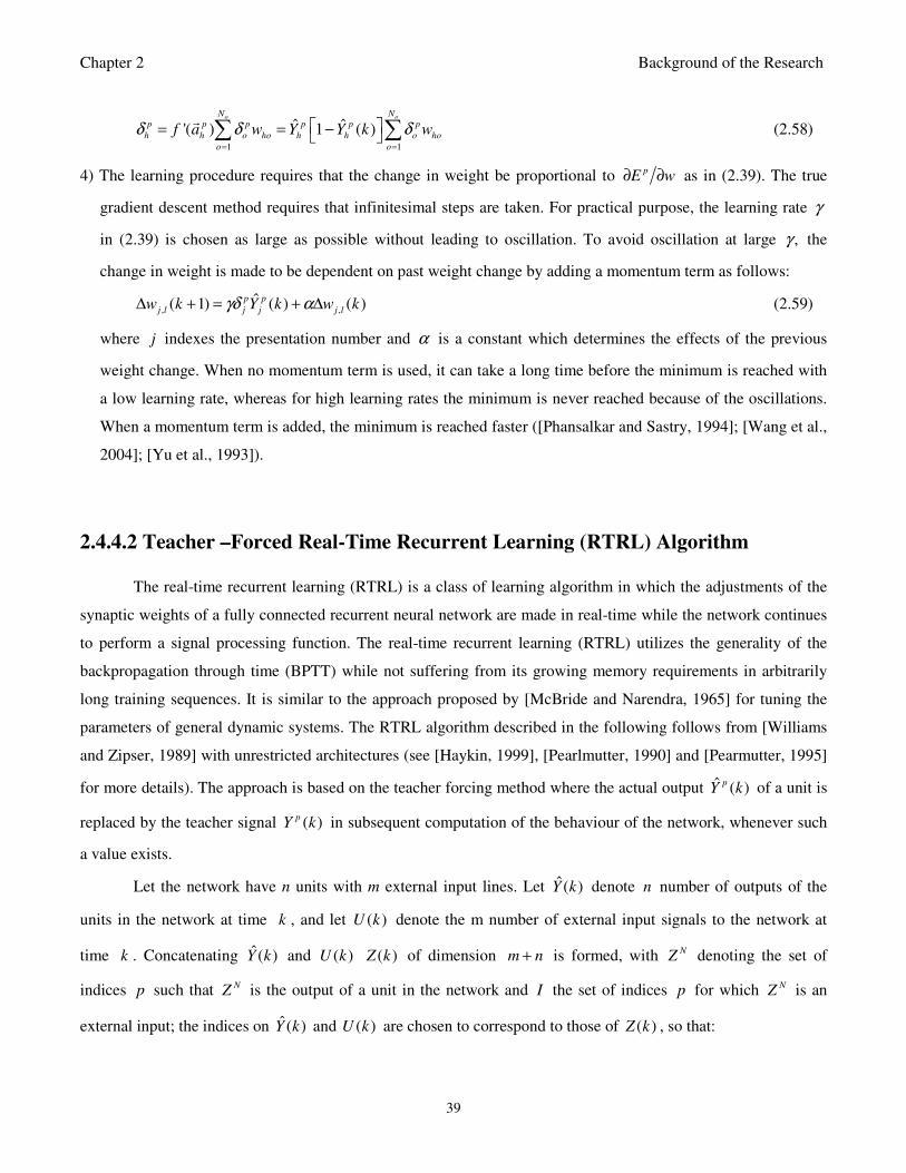
Chapter 2 Background of the Research
39
1 1
ˆ ˆ'( ) 1 ( )o oN N
p p p p p p
h h o ho h h o ho
o o
f a w Y Y k wδ δ δ= =
= = − ∑ ∑
(2.58)
4) The learning procedure requires that the change in weight be proportional to pE w∂ ∂ as in (2.39). The true
gradient descent method requires that infinitesimal steps are taken. For practical purpose, the learning rate γ
in (2.39) is chosen as large as possible without leading to oscillation. To avoid oscillation at large ,γ the
change in weight is made to be dependent on past weight change by adding a momentum term as follows:
, ,ˆ( 1) ( ) ( )
p p
j l j j j lw k Y k w kγδ α∆ + = + ∆ (2.59)
where j indexes the presentation number and α is a constant which determines the effects of the previous
weight change. When no momentum term is used, it can take a long time before the minimum is reached with
a low learning rate, whereas for high learning rates the minimum is never reached because of the oscillations.
When a momentum term is added, the minimum is reached faster ([Phansalkar and Sastry, 1994]; [Wang et al.,
2004]; [Yu et al., 1993]).
2.4.4.2 Teacher –Forced Real-Time Recurrent Learning (RTRL) Algorithm
The real-time recurrent learning (RTRL) is a class of learning algorithm in which the adjustments of the
synaptic weights of a fully connected recurrent neural network are made in real-time while the network continues
to perform a signal processing function. The real-time recurrent learning (RTRL) utilizes the generality of the
backpropagation through time (BPTT) while not suffering from its growing memory requirements in arbitrarily
long training sequences. It is similar to the approach proposed by [McBride and Narendra, 1965] for tuning the
parameters of general dynamic systems. The RTRL algorithm described in the following follows from [Williams
and Zipser, 1989] with unrestricted architectures (see [Haykin, 1999], [Pearlmutter, 1990] and [Pearmutter, 1995]
for more details). The approach is based on the teacher forcing method where the actual output ˆ ( )pY k of a unit is
replaced by the teacher signal ( )pY k in subsequent computation of the behaviour of the network, whenever such
a value exists.
Let the network have n units with m external input lines. Let ˆ( )Y k denote n number of outputs of the
units in the network at time k , and let ( )U k denote the m number of external input signals to the network at
time k . Concatenating ˆ( )Y k and ( )U k ( )Z k of dimension m n+ is formed, with NZ denoting the set of
indices p such that NZ is the output of a unit in the network and I the set of indices p for which NZ is an
external input; the indices on ˆ( )Y k and ( )U k are chosen to correspond to those of ( )Z k , so that:

Chapter 2 Background of the Research
40
( ),
( ) ( ),
ˆ ( )( ),
p
p p N
Np
U k if p I
Z k Y k if p Z
if k Z T kY k
∈
= ∈ ∈ −
(2.60)
Let W denote the weight matrix for the network, with a unique weight between every pair of units and
also from each input line to each unit. Let the net input to the pth unit at time k , for Np Z∈ be given by:
, ( )N
p p l l
l Z I
a w Z k∈ ∪
= ∑
(2.61)
So that the output at the next time step can be expressed as:
ˆ ( 1) ( ( ))p
p pY k f a t+ =
(2.62)
where ( )pf i is the unit’s activation function and the external input at time k does not influence the output of any
unit until time 1k + . Let ( )T k denote the set of indices Np Z∈ for which there exist a specified target value
( )pY k of the pth output unit at time k , so that the time-varying error ( )p
E k can be expressed as:
ˆ ( )( ) ( ),( )
0,
p pp
if k T kY k Y kE k
otherwise
∈−=
(2.63)
This allows the target values to be specified at different times. Let the overall network error at time k be given
by:
2
1
1( ) ( )
2
m np
p
J k E k+
=
= ∑ (2.64)
The minimization of (2.63) is achieved using the gradient descent method by adjusting the joint weights W along
the negative of 0
( , 1)total
WJ k k∇ + based on the following objective function:
1
0
0 1
1
( , ) ( )k
total
k k
J k k J k= +
= ∑ (2.65)
So that the overall weight change for any particular weight ,i jw in the network can be written as:
1
0
, ,
1
( )k
i j i j
k k
w w k= +
∆ = ∆∑ (2.66)
where ,
,
( )( )i j
i j
J kw k
wα
∂∆ = −
∂ and α is a fixed positive learning rate. So that the gradient with respect to the weight
becomes:
, ,
ˆ( ) ( )( )
pp
p Ui j i j
J k Y kE k
w w∈
∂ ∂− =
∂ ∂∑ (2.67)
where ,( ) i jJ k w∂ ∂ can be computed by differentiating (2.61) and (2.62) to obtain:
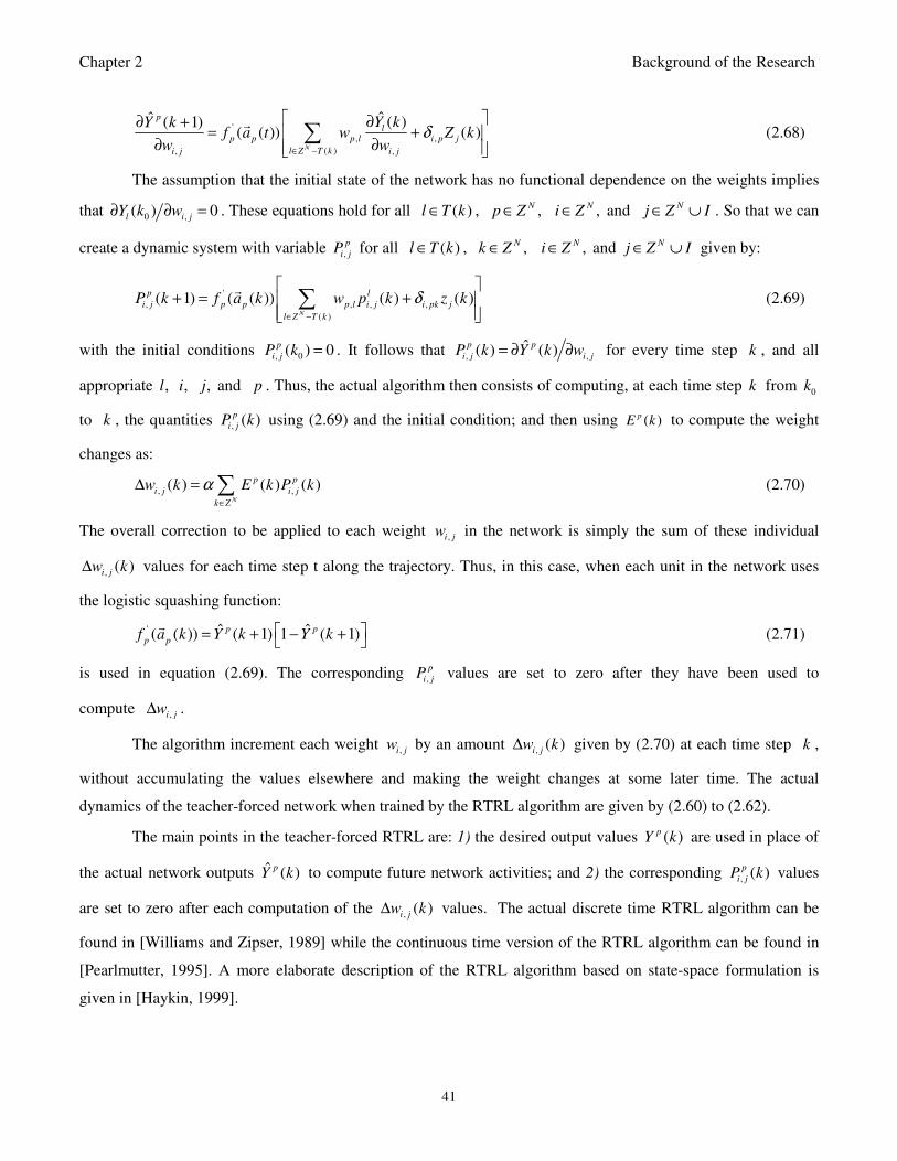
Chapter 2 Background of the Research
41
'
, ,
( ), ,
ˆˆ ( )( 1)( ( )) ( )
N
p
l
p p p l i p j
l Z T ki j i j
Y kY kf a t w Z k
w wδ
∈ −
∂∂ += +
∂ ∂ ∑
(2.68)
The assumption that the initial state of the network has no functional dependence on the weights implies
that 0 ,( ) 0l i jY k w∂ ∂ = . These equations hold for all ( )l T k∈ , ,Np Z∈ ,N
i Z∈ and Nj Z I∈ ∪ . So that we can
create a dynamic system with variable ,
p
i jP for all ( )l T k∈ , ,Nk Z∈ ,N
i Z∈ and Nj Z I∈ ∪ given by:
'
, , , ,
( )
( 1) ( ( )) ( ) ( )N
p l
i j p p p l i j i pk j
l Z T k
P k f a k w p k z kδ∈ −
+ = +
∑
(2.69)
with the initial conditions , 0( ) 0p
i jP k = . It follows that , ,ˆ( ) ( )
p p
i j i jP k Y k w= ∂ ∂ for every time step k , and all
appropriate , , ,l i j and p . Thus, the actual algorithm then consists of computing, at each time step k from 0
k
to k , the quantities , ( )p
i jP k using (2.69) and the initial condition; and then using ( )pE k to compute the weight
changes as:
, ,( ) ( ) ( )N
p p
i j i j
k Z
w k E k P kα∈
∆ = ∑ (2.70)
The overall correction to be applied to each weight ,i jw in the network is simply the sum of these individual
, ( )i jw k∆ values for each time step t along the trajectory. Thus, in this case, when each unit in the network uses
the logistic squashing function:
' ˆ ˆ( ( )) ( 1) 1 ( 1)p p
p pf a k Y k Y k = + − +
(2.71)
is used in equation (2.69). The corresponding ,
p
i jP values are set to zero after they have been used to
compute ,i jw∆ .
The algorithm increment each weight ,i jw by an amount , ( )i jw k∆ given by (2.70) at each time step k ,
without accumulating the values elsewhere and making the weight changes at some later time. The actual
dynamics of the teacher-forced network when trained by the RTRL algorithm are given by (2.60) to (2.62).
The main points in the teacher-forced RTRL are: 1) the desired output values ( )pY k are used in place of
the actual network outputs ˆ ( )pY k to compute future network activities; and 2) the corresponding , ( )p
i jP k values
are set to zero after each computation of the , ( )i jw k∆ values. The actual discrete time RTRL algorithm can be
found in [Williams and Zipser, 1989] while the continuous time version of the RTRL algorithm can be found in
[Pearlmutter, 1995]. A more elaborate description of the RTRL algorithm based on state-space formulation is
given in [Haykin, 1999].
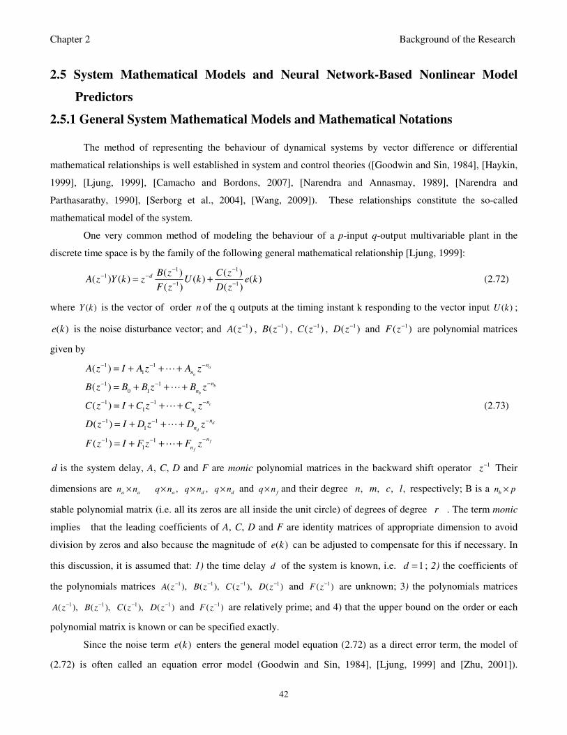
Chapter 2 Background of the Research
42
2.5 System Mathematical Models and Neural Network-Based Nonlinear Model
Predictors
2.5.1 General System Mathematical Models and Mathematical Notations
The method of representing the behaviour of dynamical systems by vector difference or differential
mathematical relationships is well established in system and control theories ([Goodwin and Sin, 1984], [Haykin,
1999], [Ljung, 1999], [Camacho and Bordons, 2007], [Narendra and Annasmay, 1989], [Narendra and
Parthasarathy, 1990], [Serborg et al., 2004], [Wang, 2009]). These relationships constitute the so-called
mathematical model of the system.
One very common method of modeling the behaviour of a p-input q-output multivariable plant in the
discrete time space is by the family of the following general mathematical relationship [Ljung, 1999]:
1 11
1 1
( ) ( )( ) ( ) ( ) ( )
( ) ( )
d B z C zA z Y k z U k e k
F z D z
− −− −
− −= + (2.72)
where ( )Y k is the vector of order n of the q outputs at the timing instant k responding to the vector input ( )U k ;
( )e k is the noise disturbance vector; and 1( )A z− , 1( )B z
− , 1( )C z− , 1( )D z
− and 1( )F z− are polynomial matrices
given by
1 1
1
1 1
0 1
1 1
1
1 1
1
1 1
1
( )
( )
( )
( )
( )
a
a
b
b
c
c
d
d
f
f
n
n
n
n
n
n
n
n
n
n
A z I A z A z
B z B B z B z
C z I C z C z
D z I D z D z
F z I F z F z
−− −
−− −
−− −
−− −
−− −
= + + +
= + + +
= + + +
= + + +
= + + +
(2.73)
d is the system delay, A, C, D and F are monic polynomial matrices in the backward shift operator 1z
− Their
dimensions are a a
n n× , ,a d d
q n q n q n× × × and f
q n× and their degree , , , ,n m c l respectively; B is a b
n p×
stable polynomial matrix (i.e. all its zeros are all inside the unit circle) of degrees of degree r . The term monic
implies that the leading coefficients of A, C, D and F are identity matrices of appropriate dimension to avoid
division by zeros and also because the magnitude of ( )e k can be adjusted to compensate for this if necessary. In
this discussion, it is assumed that: 1) the time delay d of the system is known, i.e. 1d = ; 2) the coefficients of
the polynomials matrices 1 1 1 1( ), ( ), ( ), ( )A z B z C z D z− − − − and 1( )F z
− are unknown; 3) the polynomials matrices
1 1( ), ( ),A z B z− − 1 1( ), ( )C z D z
− − and 1( )F z− are relatively prime; and 4) that the upper bound on the order or each
polynomial matrix is known or can be specified exactly.
Since the noise term ( )e k enters the general model equation (2.72) as a direct error term, the model of
(2.72) is often called an equation error model (Goodwin and Sin, 1984], [Ljung, 1999] and [Zhu, 2001]).
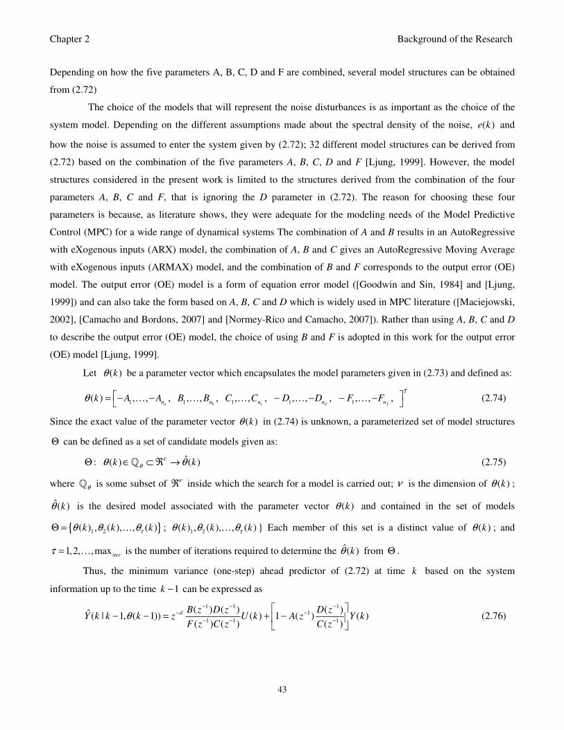
Chapter 2 Background of the Research
43
Depending on how the five parameters A, B, C, D and F are combined, several model structures can be obtained
from (2.72)
The choice of the models that will represent the noise disturbances is as important as the choice of the
system model. Depending on the different assumptions made about the spectral density of the noise, ( )e k and
how the noise is assumed to enter the system given by (2.72); 32 different model structures can be derived from
(2.72) based on the combination of the five parameters A, B, C, D and F [Ljung, 1999]. However, the model
structures considered in the present work is limited to the structures derived from the combination of the four
parameters A, B, C and F, that is ignoring the D parameter in (2.72). The reason for choosing these four
parameters is because, as literature shows, they were adequate for the modeling needs of the Model Predictive
Control (MPC) for a wide range of dynamical systems The combination of A and B results in an AutoRegressive
with eXogenous inputs (ARX) model, the combination of A, B and C gives an AutoRegressive Moving Average
with eXogenous inputs (ARMAX) model, and the combination of B and F corresponds to the output error (OE)
model. The output error (OE) model is a form of equation error model ([Goodwin and Sin, 1984] and [Ljung,
1999]) and can also take the form based on A, B, C and D which is widely used in MPC literature ([Maciejowski,
2002], [Camacho and Bordons, 2007] and [Normey-Rico and Camacho, 2007]). Rather than using A, B, C and D
to describe the output error (OE) model, the choice of using B and F is adopted in this work for the output error
(OE) model [Ljung, 1999].
Let ( )kθ be a parameter vector which encapsulates the model parameters given in (2.73) and defined as:
1 1 1 1 1( ) , , , , , , , , , , , , , , ,a b c d f
T
n n n n nk A A B B C C D D F Fθ = − − − − − − … … … … … (2.74)
Since the exact value of the parameter vector ( )kθ in (2.74) is unknown, a parameterized set of model structures
Θ can be defined as a set of candidate models given as:
ˆ: ( ) ( )k kν
θθ θΘ ∈ ⊂ ℜ → (2.75)
where θ is some subset of νℜ inside which the search for a model is carried out; ν is the dimension of ( )kθ ;
ˆ( )kθ is the desired model associated with the parameter vector ( )kθ and contained in the set of models
1 2( ) , ( ), , ( )k k kτθ θ θΘ = … ; 1 2
( ) , ( ), , ( )k k kτθ θ θ… Each member of this set is a distinct value of ( )kθ ; and
1,2, ,maxiter
τ = … is the number of iterations required to determine the ˆ( )kθ from Θ .
Thus, the minimum variance (one-step) ahead predictor of (2.72) at time k based on the system
information up to the time 1k − can be expressed as
1 1 11
1 1 1
( ) ( ) ( )ˆ( | 1, ( 1)) ( ) 1 ( ) ( )( ) ( ) ( )
d B z D z D zY k k k z U k A z Y k
F z C z C zθ
− − −− −
− − −
− − = + −
(2.76)
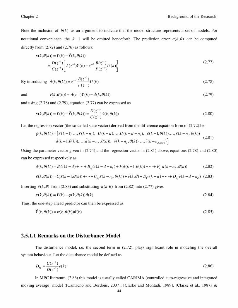
Chapter 2 Background of the Research
44
Note the inclusion of ( )kθ as an argument to indicate that the model structure represents a set of models. For
notational convenience, the 1k − will be omitted henceforth. The prediction error ( , )kε θ can be computed
directly from (2.72) and (2.76) as follows:
1 11
1 1
ˆ( , ( )) ( ) ( , ( ))
( ) ( )( ) ( ) ( )
( ) ( )
d
k k Y k Y k k
D z B zA z Y k z U k
C z F z
ε θ θ
− −− −
− −
= −
= −
(2.77)
By introducing 1
1
( )( , ( )) ( )
( )
d B zd k k z U k
F zθ
−−
−= (2.78)
and 1( , ( )) ( ) ( ) ( , ( ))v k k A z Y k d k kθ θ−= − (2.79)
and using (2.78) and (2.79), equation (2.77) can be expressed as
1
1
( )ˆ( , ( )) ( ) ( , ( )) ( , ( ))( )
D zk k Y k Y k k v k k
C zε θ θ θ
−
−= − = (2.80)
Let the regression vector (the so-called state vector) derived from the difference equation form of (2.72) be:
[
, ( )
( , ( )) ( 1), , ( ), ( ), , ( ), ( 1, ( )), , ( , ( ))
( 1, ( )), , ( , ( )), ( , ( )), , ( )
a b c
f d d k
k k Y k Y k n U k d U k d n k k k n k
d k k d k n k v k n k v k n θ
ϕ θ ε θ ε θ
θ θ θ
= − − − − − − −
− − − −
… … …
… … (2.81)
Using the parameter vector given in (2.74) and the regression vector in (2.81) above, equations (2.78) and (2.80)
can be expressed respectively as:
1 1( , ( )) ( ) ( ) ( 1, ( )) ( , ( ))b fn b n f
d k k BU k d B U k d n F d k k F d k n kθ θ θ= − + + − − + − + + − (2.82)
1 1( , ( )) ( 1, ( )) ( , ( )) ( , ) ( ) ( )c dn c n dk k C k k C k n k v k D v k d D v k d nε θ ε θ ε θ θ= − + + − + + − + + − − (2.83)
Inserting ( , )v k θ from (2.83) and substituting ( , )d k θ from (2.82) into (2.77) gives
( , ( )) ( ) ( , ( )) ( )k k Y k k k kε θ ϕ θ θ= − (2.84)
Thus, the one-step ahead predictor can then be expressed as:
ˆ( , ( )) ( , ( )) ( )Y k k k k kθ ϕ θ θ= (2.85)
2.5.1.1 Remarks on the Disturbance Model
The disturbance model, i.e. the second term in (2.72), plays significant role in modeling the overall
system behaviour. Let the disturbance model be defined as
1
1
( )( )
( )M
C zD e k
D z
−
−= (2.86)
In MPC literature, (2.86) this model is usually called CARIMA (controlled auto-regressive and integrated
moving average) model ([Camacho and Bordons, 2007], [Clarke and Mohtadi, 1989], [Clarke et al., 1987a &
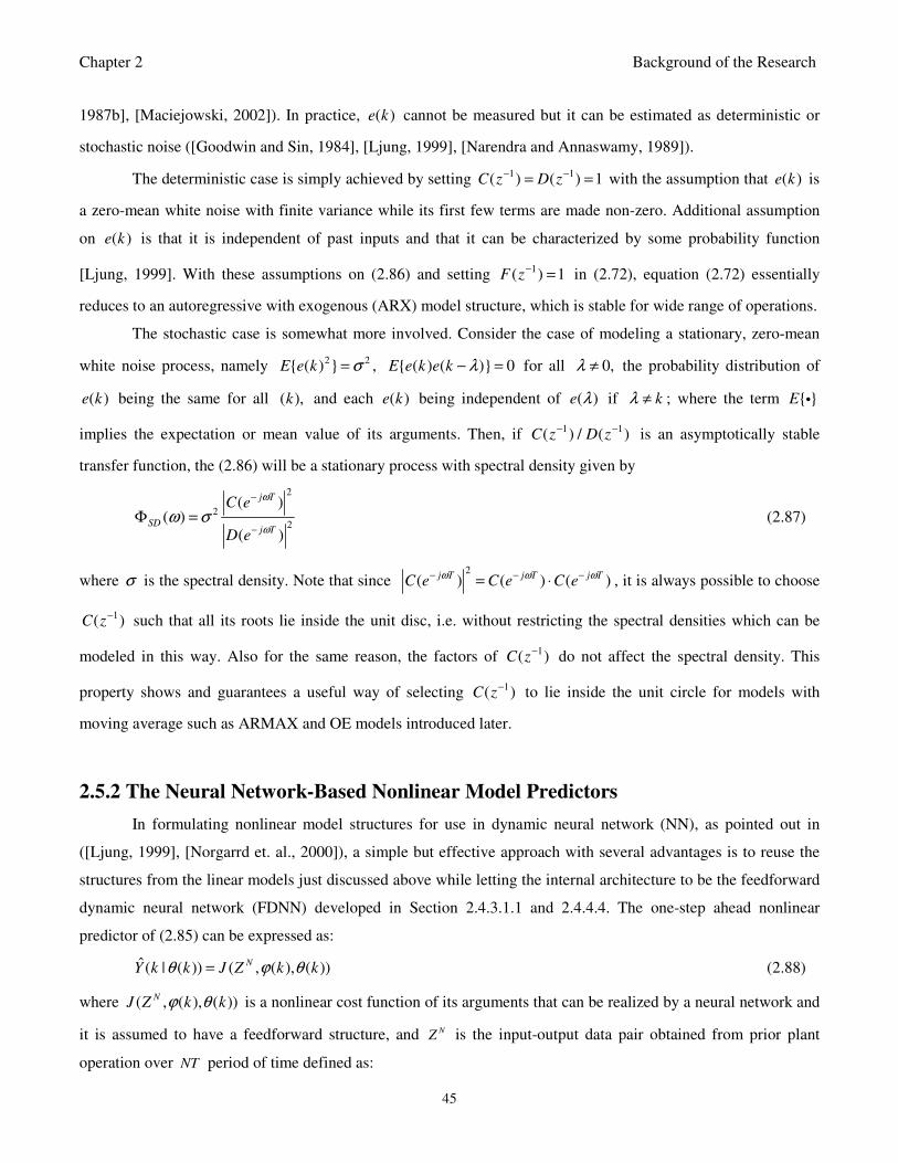
Chapter 2 Background of the Research
45
1987b], [Maciejowski, 2002]). In practice, ( )e k cannot be measured but it can be estimated as deterministic or
stochastic noise ([Goodwin and Sin, 1984], [Ljung, 1999], [Narendra and Annaswamy, 1989]).
The deterministic case is simply achieved by setting 1 1( ) ( ) 1C z D z− −= = with the assumption that ( )e k is
a zero-mean white noise with finite variance while its first few terms are made non-zero. Additional assumption
on ( )e k is that it is independent of past inputs and that it can be characterized by some probability function
[Ljung, 1999]. With these assumptions on (2.86) and setting 1( ) 1F z− = in (2.72), equation (2.72) essentially
reduces to an autoregressive with exogenous (ARX) model structure, which is stable for wide range of operations.
The stochastic case is somewhat more involved. Consider the case of modeling a stationary, zero-mean
white noise process, namely 2 2 ( ) E e k σ= , ( ) ( ) 0E e k e k λ− = for all 0,λ ≠ the probability distribution of
( )e k being the same for all ( ),k and each ( )e k being independent of ( )e λ if kλ ≠ ; where the term E i
implies the expectation or mean value of its arguments. Then, if 1 1( ) / ( )C z D z− − is an asymptotically stable
transfer function, the (2.86) will be a stationary process with spectral density given by
2
2
2
( )( )
( )
j T
SDj T
C e
D e
ω
ωω σ
−
−Φ = (2.87)
where σ is the spectral density. Note that since2
( ) ( ) ( )j T j T j TC e C e C e
ω ω ω− − −= ⋅ , it is always possible to choose
1( )C z− such that all its roots lie inside the unit disc, i.e. without restricting the spectral densities which can be
modeled in this way. Also for the same reason, the factors of 1( )C z− do not affect the spectral density. This
property shows and guarantees a useful way of selecting 1( )C z− to lie inside the unit circle for models with
moving average such as ARMAX and OE models introduced later.
2.5.2 The Neural Network-Based Nonlinear Model Predictors
In formulating nonlinear model structures for use in dynamic neural network (NN), as pointed out in
([Ljung, 1999], [Norgarrd et. al., 2000]), a simple but effective approach with several advantages is to reuse the
structures from the linear models just discussed above while letting the internal architecture to be the feedforward
dynamic neural network (FDNN) developed in Section 2.4.3.1.1 and 2.4.4.4. The one-step ahead nonlinear
predictor of (2.85) can be expressed as:
ˆ( | ( )) ( , ( ), ( ))NY k k J Z k kθ ϕ θ= (2.88)
where ( , ( ), ( ))NJ Z k kϕ θ is a nonlinear cost function of its arguments that can be realized by a neural network and
it is assumed to have a feedforward structure, and NZ is the input-output data pair obtained from prior plant
operation over NT period of time defined as:
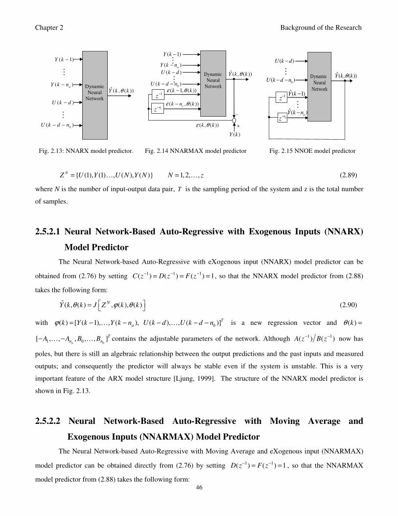
Chapter 2 Background of the Research
46
(1), (1) , ( ), ( ) 1,2, ,NZ U Y U N Y N N z= =… … (2.89)
where N is the number of input-output data pair, T is the sampling period of the system and z is the total number
of samples.
2.5.2.1 Neural Network-Based Auto-Regressive with Exogenous Inputs (NNARX)
Model Predictor
The Neural Network-based Auto-Regressive with eXogenous input (NNARX) model predictor can be
obtained from (2.76) by setting 1 1 1( ) ( ) ( ) 1C z D z F z− − −= = = , so that the NNARX model predictor from (2.88)
takes the following form:
ˆ( , ( ) , ( ), ( )NY k k J Z k kθ ϕ θ = (2.90)
with ( ) [ ( 1), , ( ), ( ), , ( )]T
a bk Y k Y k n U k d U k d nϕ = − − − − −… … is a new regression vector and ( )kθ =
1 0[ , , , , , ]a b
T
n nA A B B− −… … contains the adjustable parameters of the network. Although 1 1( ) ( )A z B z− − now has
poles, but there is still an algebraic relationship between the output predictions and the past inputs and measured
outputs; and consequently the predictor will always be stable even if the system is unstable. This is a very
important feature of the ARX model structure [Ljung, 1999]. The structure of the NNARX model predictor is
shown in Fig. 2.13.
2.5.2.2 Neural Network-Based Auto-Regressive with Moving Average and
Exogenous Inputs (NNARMAX) Model Predictor
The Neural Network-based Auto-Regressive with Moving Average and eXogenous input (NNARMAX)
model predictor can be obtained directly from (2.76) by setting 1 1( ) ( ) 1D z F z− −= = , so that the NNARMAX
model predictor from (2.88) takes the following form:
Dynamic
Neural
Network
( 1)Y k −
( )a
Y k n−
( )b
U k d n− −
ˆ ( , ( ))Y k kθ
( )U k d−
Dynamic
Neural
Network ( 1, ( ))k kε θ−
( , ( ))c
k n kε θ−
( )Y k
ˆ( , ( ))Y k kθ
( , ( ))k kε θ
–
+
•
cnz
−
1z
−
( )b
U k d n− −
( )U k d−
( )a
Y k n−
( 1)Y k −
•
Dynamic
Neural
Network ˆ( 1)Y k −
ˆ( )aY k n−
( )U k d−
( )b
U k d n− −
anz
−
1z
−
ˆ( , ( ))Y k kθ •
•
Fig. 2.13: NNARX model predictor. Fig. 2.14 NNARMAX model predictor Fig. 2.15 NNOE model predictor
Chapter 2 Background of the Research
47
ˆ( , ( ) , ( , ( )), ( )NY k k J Z k k kθ ϕ θ θ = (2.91)
where [ ]( , ( )) ( 1), , ( ), ( ), , ( ), ( , ( )), , ( , ( ))T
a b ck k Y k Y t n U k d U k d n k k k n kϕ θ ε θ ε θ= − − − − − −… … … is the new
regression vector and 1 0 1( ) , , , , , , , ,a b c
T
n n nk A A B B C Cθ = − − … … … contains the adjustable parameters of the
network. Due to the presence of the 1( )C z− polynomial in (2.72), the predictor now has poles. Thus 1( )C z
− must
have its roots inside the unit circle for the predictor to be stable. Also, the poles imply that the regression vector
depends on the model parameters, which make the estimation of the model parameters ( )kθ more complicated
due to the feedback structure. The model dependency on 1( )C z− is indicated by including ( )kθ as an argument
in ( , ( ))k kϕ θ .
The typical structure of a NNARMAX model predictor is shown in Fig. 2.14. The stability of the
predictor of the linear ARMAX depends on the values of the roots of the 1( )C z− polynomial. The approach of
(2.87) can be employed to initialize the disturbance in a natural way. These problems can be partially alleviated
when used in conjunction with the teacher-forced RTRL method discussed earlier since the actual system outputs
will be used in the subsequent computations in the recurrent network rather than the predicted outputs in a
feedforward fashion.
2.5.2.3 Neural Network-Based Output-Error (NNOE) Model Predictor
The output error model structure has been widely used in situations where the only noise affecting the
system is white measurement noise (Camacho and Bordons, 2007], [Maciejowski, 2002]). The Neural Network-
based Output Error (NNOE) model predictor can be obtained directly from (2.76) by setting 1( )A z− =
1 1( ) ( ) 1C z D z− −= = . In this case (2.88) takes the following form:
ˆ( , ( ) , ( , ( )), ( )NY k k J Z k k kθ ϕ θ θ = (2.92)
where ˆ ˆ( , ( )) ( 1, ( )), , ( , ( )), ( ), , ( )T
a bk k Y k k Y t n k U k d U k d nϕ θ θ θ = − − − − − … … is the new regression vector
and 0 1( ) , , , , ,b f
T
n nk B B F Fθ = − − … … contains the adjustable parameters of the network. The regressor in the
NNOE model depends on past output information as shown in Fig. 2.15. The model dependency on 1( )F z− is
indicated by including ( )kθ as an argument in ( , ( ))k kϕ θ . Thus, for the predictor to be stable, the roots of F
must lie inside the unit circle. The discussion based on (2.87) can be employed to chose and initialize the
disturbance model. Although, the NNOE model predictor is has the same problems with the NNARMAX model
Chapter 2 Background of the Research
48
predictor, these problems are partially alleviated when the network is combined with the teacher-forced RTRL
structure discussed earlier [Haykin, 1999].
The NNOE structure depicted in Fig. 2.15 is sometimes considered a fully recurrent neural network used
for formulating the real-time recurrent learning algorithm and/or recurrent nonlinear ARX (NARX) model
[Haykin, 1999].
2.6 Implementation of MPC Algorithms
2.6.1 Computer Implementation of MPC Algorithms
The early forms of implementing MPC algorithms were based on the use of process control computers.
For a brief historical overview of early MPC implementation techniques, see Appendix A of [Seborg et al, 2004].
Technological advancements in the last three decades have led to the development of sophisticated distributed
control systems (DCS) and NCS for implementing MPC designs. The revolutionary developments in
microelectronics and telecommunications have led to the evolution of distributed computer networks for MPC
implementation in the process industries where computers are configured into a network for process control.
Industrial process control networks can be distributed both geographically and logically. Geographically,
distributed network implies computers that are physically located in different plant areas to control nearby plants
whereas logically distributed network implies the distribution of control functions over more than one computer
or devices to control the plant. The control applications often utilize a variety of digital devices such as
workstations, personal computers, single-loop controllers (SLC), and programmable logic controllers (PLC). In a
distributed control system (DCS) or NCS, a fieldbus, which is a low-cost protocol, can be used to perform
necessary communication between the DCS (or NCS) and the plant’s sensors (or smart devices) efficiently in a
platform independent fashion.
MPC was originally developed to meet the specialized needs of power plants and the petroleum refineries
but now it finds applications in wide areas including robotics, aerospace, chemicals, food processing, as well as
paper and pulp industry. MPC, as well as control based on online optimization has long been recognized as the
winning alternative for constrained multivariable system control but its applicability has been limited to slow
systems with long sampling time because of the huge optimization algorithm which must be solved repeatedly at
each sampling time. Even with the currently available multicore computers and processors, several techniques and
implementation strategies are still been exploited to speed-up the online computation of the MPC optimization for
its application to nonlinear dynamical systems with relatively short sampling time. These techniques are
presented in the next two sub-sections.
Chapter 2 Background of the Research
49
2.6.2 FPGA Implementation of MPC Algorithms
In its basic form, model predictive control (MPC) is a computationally intensive online optimization
control strategy based on the system process model. Since this online optimization must be repeated at each
sample time, the computation must be completed within the sampling time of the system under control. The
online optimization is even more involved for the nonlinear system control. Thus, extensive research has been on
ways to speed up the MPC computation while some research seeks alternative implementation of the MPC
algorithm. For example, Tøndel and co-workers ([Tøndel et al., 2003] and [Hegrenæs et al., 2005]) have shown
that it is possible to adopt multi-parametric quadratic programming (mp-QP) as an alternative to the online MPC
optimization for fast systems with relatively short sampling time. Felt [Felt, 2006] applied stochastic techniques to
speed up the MPC online computation and recommended its parallel implementation. Multi-modal and
decentralized techniques [Magni and Scattolini, 2006] as well as multiplexed MPC [Ling et al., 2005] and
distributed nonlinear MPC [Dunbar and Desa, 2005] have been reported to speed up the MPC online optimization
problem in sequential computations. Efforts made to reduce the MPC computational load has led to the extension
of MPC into multirate situations with additional causality constraints ([Halldrosson and Unbehauen, 2001], [Ling
et al., 2004], [Sheng et al., 2002]).
In the last few years there have been significant efforts towards the implementation of MPC as a system-
on-a-chip (SoC), or application-specific integrated circuit (ASIC), on a digital signal processor (DSP), and/or on
a field programmable gate array (FPGA). The main differences between ASIC and FPGA implementation is that
the ASIC can be fast with low power consumption and can include both analog and digital signals but the ASIC
implementation is expensive with long development cycle. FPGA implementations are less expensive, more
flexible with short development cycle but with limited speed which can be improved using multiple processor
architecture.
Several papers on MPC implementation on FPGAs have been reported ([Bleris et al., 2006], [Daniel and
Ruano, 1999], [Garcia et al., 2004], [He and Ling, 2005], [Johansen et al., 2007], [Ling et al., 2006], [Ling et al.,
2008], [Vouzis et al., 2006]). In these papers FPGAs have been proposed to have great potentials for meeting the
needs of real-time computational and optimization problems. In [Johansen et al., 2007], the explicit MPC
optimization is solved off-line and during runtime the solutions are only invoked from a local memory. The major
disadvantage of this approach is that the memory requirements increase exponentially as the size of the problem
increases and is applicable to small scale embedded applications. In [Daniel and Ruano, 1999], the computational
load on the DSP processor designed for the unconstrained generalized predictive controller (GPC) will increase if
the proposed architecture is applied to constrained nonlinear MPC (NMPC). Moreover, the GPC suffers from
instability when the process operates outside the neighbourhood of its operating range. In [He and Ling, 2005],
[Ling et al., 2006] and [Ling et al., 2008] a novel technique for FPGA hardware design tailored to solve
constrained MPC problems is presented and hardware-in-the-loop (HIL) simulation is used to verify the
Chapter 2 Background of the Research
50
functionality and performance of the design. The problem envisaged with the linear MPC used in the last three
papers is computational efficiency and performance degradation outside the validity regime of the process model
when compared with constrained nonlinear MPC control system. In [Bleris et al., 2006], [Garcia et al., 2004] and
[Vouzis et al., 2006], a hardware/software FPGA implementation of MPC has been presented based on a
logarithmic number system (LNS) architecture with several precautions and limitations regarding its precision.
In general terms, an embedded system [Ganssle and Barr, 2003] is composed of an embedded processor
(or microcontroller) system with dedicated hardware and software portions of the design properly partitioned
within the embedded system. As pointed out in [Fletcher, 2005] and recommended in [Xilinx, 2010], an
embedded processor offers several advantages such as customization, obsolescence migitation, component and
cost reduction, and hardware acceleration for the implementation/application when compared to typical
microprocessors. All the FPGA implementation of MPC algorithms reported so far are all based on linear process
models and these MPC algorithms are implemented directly using Xilinx Logic Cells only [Xilinx, 2010]. The
FPGA implementation of the MPC algorithm proposed in this work is developed and modeled as hardware
peripheral. The hardware peripheral is validated via a hardware-in-the-loop co-simulation with a FPGA board.
Next, the validated hardware peripheral is exported and attached to a pre-designed embedded processor system to
complete the hardware portion. Next, software is written for initializing the hardware drivers and executing the
MPC algorithm embedded in the processor system. To the best of my knowledge as at the time of this write up, no
neural network-based and\or constrained MPC implementation on a FPGA embedded processor system has been
reported and this is one of the objectives that are being exploited in the present study.
2.6.3 Remarks on the Reviewed MPC Implementation Strategies
As noted in Section 2.6.1, a fieldbus based network control system (NCS) could be a possible platform
for running model predictive control (MPC) algorithm for nonlinear systems control. Fieldbuses have greater
functionality, resulting in reduced setup time, improved control, combined functionality of separated devices, and
smart sensor diagnostic capabilities together with the added advantage of digital communication which allows the
control system to be completely distributed. Depending on the constraints on the computation time, a more
advanced platform with emphasis on computational efficiency could be sought. In view of the above requirement,
two implementation platforms are proposed in this work. The first platform is based on service oriented
architecture (SOA) which utilizes the device profile for web services (DPWS) on a computer clustered network.
The second real-time implementation platform is based on a FPGA. The selection of FPGA for MPC
implementation depends on the MPC formulation and intended application ([Shoukry et al., 2010a], [Shoukry et
al., 2010a] and [Meloni et al., 2010]). The term “MPC formulation” implies whether the process model to be used
is linear or nonlinear and whether the MPC algorithm is adaptive or non-adaptive. Also the term “intended
Chapter 2 Background of the Research
51
application” implies whether the application is a single-input single-output (SISO) or multiple-input multiple-
output (MIMO) and whether the system has slow dynamics with large sample time or fast dynamics with relative
short sample time.
The choice of an FPGA as well as its vendor is critical in an embedded system design. Oldfield and Dorf
[Oldfiel and Dorf, 1995] outlined efficient 2–stage 14–points guidelines for choosing an FPGA for implementing
an embedded application from a number of FPGA manufacturer catalogues. Based on the survey on the FPGA
computing power conducted by [Guccione, 2000] together with the additional selection considerations provided
by [Fletcher, 2005], places the Xilinx FPGAs [Xilinx, 2010].
In the next two sub-sections, an overview of the switched Ethernet architecture, the available service
oriented architecture (SOA) technologies as well as a brief overview of programming logic devices with emphasis
on FPGAs are presented.
2.7 Switched Ethernet Architecture and SOA Technologies
2.7.1 The Architecture of the Switched Ethernet
Ethernet specification defines a number of wiring and signaling standards for the physical layer of the
open systems interconnection (OSI) networking model as well as a media access control (MAC) algorithm and a
common addressing format at the data link layer (DLL). However, it is impossible to guarantee a bounded
message transmission time mostly due to its weakness to handle collisions.
In switched Ethernet data is transmitted and received on different wires and the hub is replaced by an
Ethernet switch. The carrier sense multiple access with collision detection (CSMA/CD) MAC protocol is no
longer used in switched Ethernet. The switch regenerates the information and forwards it only to the port on
which the destination is attached. It complies with the IEEE 802.3 MAC protocol when relaying the frames and
creates different collision domain per switch port whereas in the hubs all the nodes have to share the bandwidth of
a half-duplex connection. If a frame is already being transmitted on the output port, the newly received frame is
queued and will be transmitted again when the medium becomes idle. In addition, all cables are point to point,
from one station to a switch and vice versa. So it is allowed to have dedicated bandwidth on each point to point
connection with every node running in a full duplex mode with no collisions. This characteristic renders the
switched Ethernet appropriate for industrial applications where the response time is a crucial matter. Furthermore,
apart from the cases in which overflows occur [Decotignie, 2005] in the switches, transmission bounds can be
predicted. However, overflows may occur if for example the combined traffic destined to the same destination
may exceed the capacity of the link between the switch and destination. The excess traffic accumulates in the
switch until its output buffer overflows. In such a case no strict bound can be considered on the transmission
delay.
Chapter 2 Background of the Research
52
2.7.2 SOA technologies
Nowadays, service-oriented architecture (SOA) has become the state of the art solution for implementing
autonomous and interoperable systems as it provides web-based and modular implementation of complex and
distributed software systems [Erl, 2005]. The interoperability at the application level that it offers due to its
loosely coupled nature renders it a desirable element when developing information and communication
technology (ICT) systems.
Several device level SOA technologies have been proposed, most notably Jini [Jini, 2010], universal
plug-n-play (UPnP) [UPnP, 2010] and device profile for web services (DPWS) [DPWS, 2006].
2.7.2.1 The Jini Technology
Jini Jini [Jini, 2010] offers the ability to register, discover, and use services. However is highly rooted in
Java and therefore is not designed for completely language and platform independency.
2.7.2.2 The UPnP Technology
The UPnP architecture leverages Internet and Web technologies including Internet protocol (IP), transfer
control protocol (TCP), user datagram protocol (UDP), hypertext transfer protocol (HTTP), simple object access
protocol (SOAP), and extensible markup language (XML). However, it is not fully compatible with web services
(WS) technology. Furthermore it uses specific protocols for discovery and event notification purposes.
2.7.2.3 The DPWS Technology
The DPWS has adopted WSs technology [Jammes and Smit, 2005a] and therefore it provides plug-n-play
connectivity and completely language and platform independency. For these reasons, the DPWS is the preferred
implementation vehicle for SOA technology in the present study.
DPWS utilizes Internet and web technologies including IP, TCP, UDP, HTTP, simple object access
protocol (SOAP), extensible markup language (XML) as well as web services description language (WSDL) 1.1.
As it is documented in [Jammes and Smit, 2005b], the core WSs standards are the following: WSDL, XML
Schema, SOAP, WS-Addressing, WS-Policy, WS-MetadataExchange and WS-Security. Apart from the standard
core WSs, DPWS adds WS-Discovery for WS discovery and WS-Eventing for subscription mechanisms. A
detailed description of these protocols can be found in [DPWS, 2006] and [Jammes and Smit, 2005b].
Chapter 2 Background of the Research
53
2.8 Programmable Logic Devices and Field Programmable Gate Array (FPGA)
Technologies
A typical embedded system design involves a significant amount of custom logic circuitry with pre-
designed hardware components, such as processor, memory units and various types of input/output (I/O)
interfaces as well as integrated modular software partitioned to the various hardware components within the
embedded system and running under by a real-time operating system [Xilinx, 2010]. For multivariable systems
with relatively short sampling time, the embedded system design becomes a complex and complicated task when
real-time constraints must be satisfied.
Traditionally, early systems were controlled by mechanical means using cams, gear, levers and other
basic mechanical devices. As system complexity increases, the programmable logic controller (PLC) was
introduced which provided an easy way for system control using “ladder logic” (and sometimes C) programs and
can be reprogrammed rather than rewiring the control system. Unlike computers, PLCs are rugged computer that
controls a part of an industrial control system and can typically withstand shock, vibration, elevated temperatures,
and electrical noise which are the characteristics of industrial and manufacturing systems [Jack, 2003].
Furthermore, as the computational burden for the control of multivariable systems coupled with
interactive strong nonlinearities and complexities increase, new computing platforms began to evolve as
programmable logic devices which include logic manipulations with varying computational efficiency. These
computing platforms have evolved within four decades from simple programmable logic devices (PLDs) such as
programmable array logic (PAL), generic array logic (GAL), complex programmable logic devices (CPLDs) to
the currently most widely used field programmable gate arrays (FPGAs). The PLDs (PAL, GAL and CPLD) and
FPGAs are all programmable devices which mean that they are integrated circuits that are used to create a circuit
in which the internal design is not defined until after it has been programmed.
It is important to note here that PLC and PLD are two distinct entities. While the former is the brain of
industrial manufacturing process, the latter is an integrated circuit that can be used to implement a digital logic
design in hardware [Ganssle and Barr, 2003]. A similarity is that both are programmable. We also note that PLDs
contain relatively limited number of logic gates and the functions they can implement are less and simpler when
compared to FPGAs.
Moreover, the internal architecture of PLDs is predetermined by the manufacturer, but the PLDs are
created in such a way that they can be configured in the field to perform a variety of different functions. On the
other hand, FPGAs are digital integrated circuits that contain configurable (programmable) blocks of logic gates
along with configurable interconnects between these blocks. Depending on how the FPGAs are implemented,
some may be programmed only once (one-time programmable, OTP), while others may be reprogrammed several
times. The term “field programmable” refers to the fact that FPGA programming takes place in the field as
opposed to devices whose internal functionality is hardwired by the manufacturer such as application-specific
integrated circuits (ASICs) and application-specific standard parts (ASSPs) [Maxfield, 2004]. Thus, FPGAs can
Chapter 2 Background of the Research
54
be configured or reprogrammed while are residing in a higher-level system or in an electronic system that has
been deployed to the outside world.
ASICs and ASSPs are also programmable devices that can contain hundreds of millions of logic gates and
can be used to implement incredibly large and complex functions. ASICs and ASSPs are based on the same
design processes and manufacturing technologies. Both are custom-designed and tailored to address specific
applications. The only difference being that an ASIC is designed and built by a specific company, while an
ASSP is designed for multiple customers. Although ASICs offer the ultimate in terms of logic gate, complexity,
and performance, designing and building one is an extremely time-consuming and expensive process, with the
added disadvantage that the final design cannot be modified once it has been fabricated (frozen in silicon).
FPGAs lie between PLDs and ASICs because their functionality can be customized in the field like PLDs,
and they can contain millions of logic gates that can be used to implement extremely large and complex functions
that could previously be realized using ASICs only ([Dubey, 2009], [Kilts, 2007]). In comparison to ASIC, FPGA
is cheaper even in small quantities, implementing design changes is much easier, and the time to complete the
overall system design, implementation, verification and deployment (i.e., time to market) is faster.
FPGAs are a good choice for implementing digital systems because, as in [Akpan, 2010] and [Cardenas
and Troncoso, 2008]: 1) FPGAs offer large logic capacity, exceeding several million equivalent logic gates, and
include dedicated memory resources; 2) they include special hardware circuitry that is often needed in digital
systems, such as digital signal processing (DSP) blocks (with multiply and accumulate functionality) and phase-
locked loops (PLLs) (or delay-locked loops (DLLs)) that support complex clocking schemes; and 3) they also
support a wide range of interconnection standards, such as double data rate static random access memory (DDR
SRAM), peripheral component interconnect (PCI) and high-speed serial protocols. In addition to the above
features, FPGAs provide a significant benefit as “off-the-shelf” chips that are programmed by the end user.
On an FPGA, hard- and soft- processors are available for implementation ([Akpan, 2010], [Kilts, 2007],
[Xilinx, 2010]). A hard processor is a pre-designed circuit that is fabricated within the FPGA chip. A more
flexible alternative is to use a soft processor. In this case, the processor exists as code written in a hardware
description language (HDL), and it is implemented along with the rest of the system by using the logic and
memory resources in the FPGA fabric. One disadvantage of this approach is that the hardware resources on the
FPGA fabrics are consumed by the processor whereas these components are actually needed by the system. It is
also possible to include multiple soft processors in the FPGA when desired ([Virtex-4, 2010], [Virtex-5, 2010],
[Virtex-6], [Virtex-7]).
FPGA are semiconductor devices containing programmable logic components and programmable
interconnects. The programmable logic components can be programmed to duplicate the functionality of basic
logic gates such as AND, OR, XOR, NOT or more complex combinatorial functions such as decoders or simple
math functions. In most FPGAs, these programmable logic components (or logic blocks in FPGA parlance) also
include memory elements, which may be simple flip-flops or more complete blocks of memories. A hierarchy of
Chapter 2 Background of the Research
55
programmable interconnects allows the logic blocks of an FPGA to be interconnected as needed by the system
designer, somewhat like a one-chip programmable breadboard. These logic blocks and interconnects can be
programmed after the manufacturing process by the engineer/designer (hence the term "field programmable"), so
that the FPGA can perform whatever logical function is needed. Applications of FPGAs include DSP, software-
defined radio, aerospace and defense systems, ASIC prototyping, medical imaging, computer vision, speech
recognition, cryptography, bio-informatics, computer hardware emulation and a growing range of other areas.
FPGAs now find applications in areas that require the use of massive parallelism offered by their architectures
[Maxfield, 2004], [Kilts, 2007].
In the traditional approach for designing such systems, a new integrated circuit (IC) chip is created for the
custom logic circuits, but each pre-designed component is included as a separate chip. Because many products
contain hardware and software components the difficulty of generating a design from a set of requirements and
specifications increases as the product becomes complex. These difficulties led to the development of electronic
system level (ESL) design and verification which is an algorithm modeling methodology that focuses on a higher
abstraction level using high-level languages such as C, C++, or MATLAB® to model the entire behaviour of the
system with no initial link to its implementation [Moretti, 2003], [Martin, 2002]. The ESL design and verification
has evolved into an industry standard complementary methodology that enables to design verify and debug
embedded systems either as a custom system-on-a-chip or a system-on-FPGA or system-on-board. The details of
the model-based ESL design and verification techniques used in this work which combines MATLAB/Simulink
from The MathWorks with AccelDSP and System Generator for DSP from Xilinx are discussed in Appendix A.
2.8.1 The Xilinx Virtex Series FPGA Family Members
A careful study of Xilinx’s latest products list by function categories together with their data sheets and
performance capabilities of Xilinx FPGAs published in [Guccione, 2000] and [Xilinx, 2011] reveals that one of
the Xilinx’s Virtex FPGA family members can be considered for use in this work. In this discussion, Virtex,
Virtex-II, Virtex-II Pro, and Virtex-II Pro X are not included since they have been enhanced into Virtex-4 FPGA
family members. Among the Xilinx’s Virtex FPGA family members are Virtex-4, Virtex-5, Virtex-6 and Virtex-
7. The main differences and application areas of the Xilinx Virtex family members can be summarized as follows:
1). The Virtex-4 FPGA family members include [Virtex-4, 2010]:
i). The Virtex-4 LX is optimized for high-performance logic applications solution.
ii). The Virtex-4 SX is optimized for high-performance solution for digital signal processing (DSP)
applications.
iii). The Virtex-4 FX is optimized for high-performance, full-featured solution for embedded system platform
applications.
Chapter 2 Background of the Research
56
2). The Virtex-5 FPGA family members include [Virtex-5, 2009]:
i). The Virtex-5 LX is optimized for high-performance general logic applications.
ii). The Virtex-5 LXT is optimized for high-performance logic applications with advanced serial connectivity.
iii). The Virtex-5 SXT is optimized for high-performance digital signal processing (DSP) applications with
advanced serial connectivity.
iv). Virtex-5 TXT is optimized for high-performance systems with advanced serial connectivity.
v). Virtex-5 FXT is optimized for high-performance, full-featured solution for embedded system platform
applications advanced serial connectivity.
3). The Virtex-6 FPGA family members include [Virtex-6, 2011]:
i). The Virtex-6 CXT is optimized for high-performance digital signal processing applications with low-
power serial connectivity and high performance GTX transceivers for niche applications.
ii). The Virtex-6 LXT is optimized for high-performance logic applications with advanced serial connectivity.
iii). The Virtex-6 SXT is optimized for high-performance solution for digital signal processing (DSP)
applications.
iv). The Virtex-6 HXT is optimized for applications that require ultra high-speed serial connectivity. It
offers the highest bandwidth with advanced serial connectivity.
4). The Virtex-7 FPGA family members include [Virtex-7, 2011]:
i). The Virtex-7 T offers 12.5Gb/s advanced serial connectivity, greatest parallel input/output bandwidth and
ultra high-end logic capacity for advanced systems requiring the highest performance and highest
bandwidth connectivity.
ii). The Virtex-7 XT offers extended capabilities including 13.1 Gb/s serial connectivity, higher DSP-to-logic
ratio, and higher block RAM-to-cell ration for advanced systems requiring the highest performance and
highest bandwidth connectivity.
iii). The Virtex-7 HT combines 28Gb/s and 13.1Gb/s serial connectivity for 400GHz communications line
cards for advanced systems requiring the highest performance and highest bandwidth connectivity.
Since the FPGA development concerned in the work is geared towards a platform which would support
embedded processor system development, it is obvious that the Virtex-4 and Virtex-5 FPGA family members
would be appropriate for the embedded processor system design as desired in this work.
However, in addition to the Virtex-4 and Virtex-5 FPGA family members introduced above, Xilinx has
also recently introduced additional Virtex-4 and Virtex-5 FPGAs family members, namely the “Defense-grade”
Virtex-4Q and Virtex-5Q FPGAs as well as the “Space-grade” Virtex-4QV and Virtex-5QV FPGAs”. The
difference between the Virtex-4 and Virtex-5 above to their Defense-grade and Space-grade counterpart lies in
Chapter 2 Background of the Research
57
their application environments. While the Virtex-4 and Virtex-5 FPGAs are for general purpose in their specific
application areas in diverse environment; the Defense-grade Virtex-4Q [Virtex-4Q, 2010] and Virtex-5Q [Virtex-
5Q, 2010] FPGA family members, as the name implies, are for mission critical aerospace and defense
applications. The radiation-hardened Space-grade Virtex-4QV [Virtex-4QV, 2010] and Virtex-5QV [Virtex-5Q,
2010] FPGA family members, on the other hand, are for applications involving sensor processing, reconfigurable
computing platforms, and modem and communication systems.
While the general purpose, Defense-grade, and the Space-grade categories of Xilinx’s Virtex-4 and
Virtex-5 FPGA family members still retains their respective designations, they differ in some ways in terms of
their available hardware resources and consequently their costs.
2.8.2 Comparison of the Xilinx General-Purpose, Defense-Grade, Space-Grade
Virtex-4 and Virtex-5 FPGA Product Family Members
In the following, some comparisons between the general-purpose Virtex-4 and Virtex-5 FPGA family
members are made in terms of their available hardware resources while references to the Defense-grade and the
Space-grade are made where there are differences for completeness. An overview of the hardware resources
embedded within the general-purpose Virtex-4 and Virtex-5 FPGA family members and some of their capabilities
are shown in the Table 2.1. Then, on the basis of the general-purpose Virtex-4 and Virtex-5 FPGAs, references
under Table 2.1 are then made to the respective Defense-grade and Space-grade FPGA family members with
respect to the general-purpose Virtex-4 and Virtex-5 FPGAs using superscripts discussed in the 17–point Notes
below Table 2.1.
In the following discussion, since the available FPGA hardware resources increases from the first device
part number on the left to the right for the Virtex-4 and Virtex-5 FPGA family members; the Virtex-4 XC4VFX20
and Virtex-5 XC5VFXT30T would form the basis for comparisons and they would simply be referred to as
Virtex-4 and Virtex-5 FPGAs respectively, except where otherwise stated.
Thus, comparing the combined least resources provided by the configurable logic blocks (CLBs) in Table
2.1 for the Virtex-4 and Virtex-5 FPGA family members, it is obvious that those provided by the later exceed that
provided by the former. As noted in Note (1), the combined logic cells and slices in Virtex-4 are 111,072 whereas
that provided by the Virtex-5 slices computed from Note (3) is 81,920. Again, comparing the Arrays [Rows x
Columns] and maximum distributed random access memory (RAM) indicates that the Virtex-5 has more available
hardware resources.
Another key difference between the Virtex-4 and Virtex-5 FPGA is that while the Virtex-4 utilizes the
XtremeDSP slices (see Note (4) under Table 2.1) to implement a primitive of the DSP48 complex multipliers, the
Virtex-5 embeds an enhanced DSP48E slices (see Note (5) under Table 2.1) with optional bitwise logical
functionality, dedicated cascade connections, and resources twice the amount of those in Virtex-4 FPGAs.
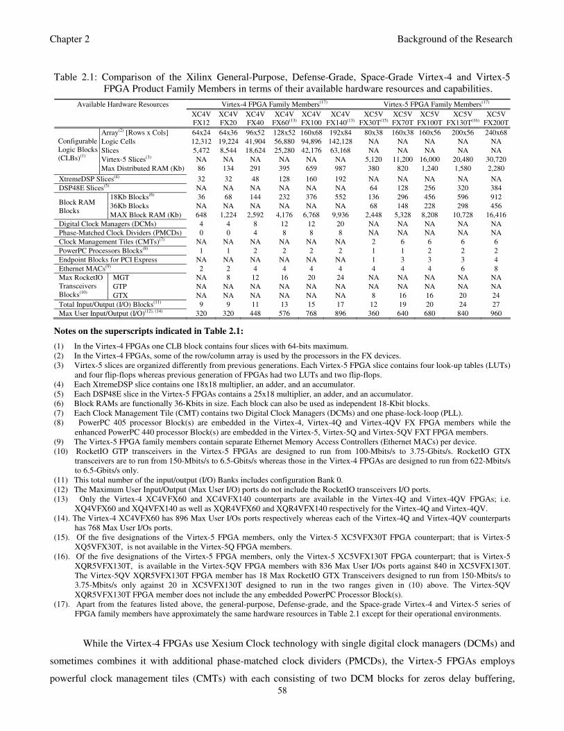
Chapter 2 Background of the Research
58
While the Virtex-4 FPGAs use Xesium Clock technology with single digital clock managers (DCMs) and
sometimes combines it with additional phase-matched clock dividers (PMCDs), the Virtex-5 FPGAs employs
powerful clock management tiles (CMTs) with each consisting of two DCM blocks for zeros delay buffering,
Table 2.1: Comparison of the Xilinx General-Purpose, Defense-Grade, Space-Grade Virtex-4 and Virtex-5
FPGA Product Family Members in terms of their available hardware resources and capabilities.
Virtex-4 FPGA Family Members(17) Virtex-5 FPGA Family Members(17) Available Hardware Resources
XC4V
FX12
XC4V
FX20
XC4V
FX40
XC4V
FX60(13)
XC4V
FX100
XC4V
FX140(13)
XC5V
FX30T(15)
XC5V
FX70T
XC5V
FX100T
XC5V
FX130T(16)
XC5V
FX200T
Array(2) [Rows x Cols] 64x24 64x36 96x52 128x52 160x68 192x84 80x38 160x38 160x56 200x56 240x68
Logic Cells 12,312 19,224 41,904 56,880 94,896 142,128 NA NA NA NA NA
Slices 5,472 8,544 18,624 25,280 42,176 63,168 NA NA NA NA NA
Virtex-5 Slices(3) NA NA NA NA NA NA 5,120 11,200 16,000 20,480 30,720
Configurable
Logic Blocks
(CLBs)(1)
Max Distributed RAM (Kb) 86 134 291 395 659 987 380 820 1,240 1,580 2,280
XtremeDSP Slices(4) 32 32 48 128 160 192 NA NA NA NA NA
DSP48E Slices(5) NA NA NA NA NA NA 64 128 256 320 384
18Kb Blocks(6) 36 68 144 232 376 552 136 296 456 596 912
36Kb Blocks NA NA NA NA NA NA 68 148 228 298 456
Block RAM
Blocks MAX Block RAM (Kb) 648 1,224 2,592 4,176 6,768 9,936 2,448 5,328 8,208 10,728 16,416
Digital Clock Managers (DCMs) 4 4 8 12 12 20 NA NA NA NA NA
Phase-Matched Clock Dividers (PMCDs) 0 0 4 8 8 8 NA NA NA NA NA
Clock Management Tiles (CMTs)(7) NA NA NA NA NA NA 2 6 6 6 6
PowerPC Processors Blocks(8) 1 1 2 2 2 2 1 1 2 2 2
Endpoint Blocks for PCI Express NA NA NA NA NA NA 1 3 3 3 4
Ethernet MACs(9) 2 2 4 4 4 4 4 4 4 6 8
MGT NA 8 12 16 20 24 NA NA NA NA NA
GTP NA NA NA NA NA NA NA NA NA NA NA
Max RocketIO
Transceivers
Blocks(10) GTX NA NA NA NA NA NA 8 16 16 20 24
Total Input/Output (I/O) Blocks(11) 9 9 11 13 15 17 12 19 20 24 27
Max User Input/Output (I/O)(12), (14) 320 320 448 576 768 896 360 640 680 840 960
Notes on the superscripts indicated in Table 2.1:
(1) In the Virtex-4 FPGAs one CLB block contains four slices with 64-bits maximum.
(2) In the Virtex-4 FPGAs, some of the row/column array is used by the processors in the FX devices.
(3) Virtex-5 slices are organized differently from previous generations. Each Virtex-5 FPGA slice contains four look-up tables (LUTs)
and four flip-flops whereas previous generation of FPGAs had two LUTs and two flip-flops.
(4) Each XtremeDSP slice contains one 18x18 multiplier, an adder, and an accumulator.
(5) Each DSP48E slice in the Virtex-5 FPGAs contains a 25x18 multiplier, an adder, and an accumulator.
(6) Block RAMs are functionally 36-Kbits in size. Each block can also be used as independent 18-Kbit blocks.
(7) Each Clock Management Tile (CMT) contains two Digital Clock Managers (DCMs) and one phase-lock-loop (PLL).
(8) PowerPC 405 processor Block(s) are embedded in the Virtex-4, Virtex-4Q and Virtex-4QV FX FPGA members while the
enhanced PowerPC 440 processor Block(s) are embedded in the Virtex-5, Virtex-5Q and Virtex-5QV FXT FPGA members.
(9) The Virtex-5 FPGA family members contain separate Ethernet Memory Access Controllers (Ethernet MACs) per device.
(10) RocketIO GTP transceivers in the Virtex-5 FPGAs are designed to run from 100-Mbits/s to 3.75-Gbits/s. RocketIO GTX
transceivers are to run from 150-Mbits/s to 6.5-Gbits/s whereas those in the Virtex-4 FPGAs are designed to run from 622-Mbits/s
to 6.5-Gbits/s only.
(11) This total number of the input/output (I/O) Banks includes configuration Bank 0.
(12) The Maximum User Input/Output (Max User I/O) ports do not include the RocketIO transceivers I/O ports.
(13) Only the Virtex-4 XC4VFX60 and XC4VFX140 counterparts are available in the Virtex-4Q and Virtex-4QV FPGAs; i.e.
XQ4VFX60 and XQ4VFX140 as well as XQR4VFX60 and XQR4VFX140 respectively for the Virtex-4Q and Virtex-4QV.
(14). The Virtex-4 XC4VFX60 has 896 Max User I/Os ports respectively whereas each of the Virtex-4Q and Virtex-4QV counterparts
has 768 Max User I/Os ports.
(15). Of the five designations of the Virtex-5 FPGA members, only the Virtex-5 XC5VFX30T FPGA counterpart; that is Virtex-5
XQ5VFX30T, is not available in the Virtex-5Q FPGA members.
(16). Of the five designations of the Virtex-5 FPGA members, only the Virtex-5 XC5VFX130T FPGA counterpart; that is Virtex-5
XQR5VFX130T, is available in the Virtex-5QV FPGA members with 836 Max User I/Os ports against 840 in XC5VFX130T.
The Virtex-5QV XQR5VFX130T FPGA member has 18 Max RocketIO GTX Transceivers designed to run from 150-Mbits/s to
3.75-Mbits/s only against 20 in XC5VFX130T designed to run in the two ranges given in (10) above. The Virtex-5QV
XQR5VFX130T FPGA member does not include the any embedded PowerPC Processor Block(s).
(17). Apart from the features listed above, the general-purpose, Defense-grade, and the Space-grade Virtex-4 and Virtex-5 series of
FPGA family members have approximately the same hardware resources in Table 2.1 except for their operational environments.

Chapter 2 Background of the Research
59
frequency synthesis and clock phase shifting as well as a phase-lock-loop (PLL) which offers the function of the
PMCDs together with input jitter filtering.
The PowerPC processor block(s) in Virtex-4 is the IBM PowerPC™ 405 Core while that in Virtex-5 is
the IBM PowerPC™ 440 core ([IBM PPC405C, 2006]; [XPPC405C Virtex-4, 2010]). The PowerPC™ 405 core
is a scalar 5-stage pipeline 32-bit reduced instruction set computer (RISC) central processing unit (CPU) core
providing up to 400-MHz and 608-DIMPS (distributed integrated message processing system) performance as
implemented in IBM’s advanced 90-nm copper CMOS technology. The PowerPC™405 processor core employs
the scalable and flexible Power Architecture technology optimized for embedded applications with 16-bit x 16-bit
MAC. The PowerPC™ 440, on the other hand, is also a 32-bit RISC CPU core but with support for two
instructions per clock and providing up to 667-MHz and 1,334 DIMPS performance as implemented in IBM’s
advanced 90-nm copper CMOS technology ([IBM PPC440C, 2006]; [XEPB Virtex-5, 2010]). The PowerPC™
440 core integrates a superscalar 7-stage pipeline with out-of-order issue, execution and completion. PowerPC™
440 employs the scalable and flexible Book E enhanced Power Architecture optimized for embedded applications
with single cycle throughput 32-bit x 32-bit MACs. For detail description of the PowerPC™ 440 embedded
processor core, processor block architecture, organization, associated peripherals, and controllers see Appendix 9.
Thus, the PowerPC™ 440 processor cores embedded in Virtex-5 offer more enhancements and performance with
low-power compared to the Virtex-4 family members. Finally, the Virtex-5 FPGAs offer higher number of total
input-output blocks as well as maximum user input-output ports when compared to the Virtex-4 family of FPGAs.
2.8.3 The Xilinx Virtex-5 XC5VFX70T ML507 FPGA Development Board
It is obvious that the comparison of the hardware resources available on the Virtex-5 FXT FPGA family
members with those available on the Virtex-4 FX FPGA family members, makes the former suitable for use in
developing the proposed embedded PowerPC™ processor system platform in this work. Since this work is
concerned with the development of an embedded processor system platform for the implementation of adaptive
model predictive control algorithm, the multi-processor system is not desired for use at the current state of the
work rather a single embedded processor system would be exploited this implementation. Among the Xilinx
embedded system development boards in the Virtex-5 FXT FPGA family members is the Virtex-5 XC5VFX70T
ML507 FPGA development board. For simplicity and convenience, this board shall be referred to as the Virtex-5
ML507 FPGA board. The top and bottom views of the Virtex-5 ML507 FPGA board that will be used in this
work are shown Fig. 2.16(a) and (b) respectively.
The ML507 is a general purpose FPGA, RocketIO™ GTX, and embedded system development board
that: provides feature-rich general purpose evaluation and development platform, it includes on-board memory
and industry standard connectivity interfaces, and delivers a versatile development platform for embedded
applications. The key physical features of the Virtex-5 ML507 FPGA board shown in Fig. 2.16 include:

Chapter 2 Background of the Research
60
XC5VFX70TFFG1136, 256-MB DDR2 SODIMM, 1-Mbit ZBT SRAM, 32-MB linear flash card, System ACE™
CF technology (CompactFlash), platform flash, SPI Flash, JTAG programming interface, external clocking (2
differential pairs), 2 universal serial bus interface for host development platform and peripheral, 2 PS/2 keyboard
inputs, mouse input, RJ-45 10/100/1000-Mbit/s port for networking, RS-232 (Male) serial port, 2 Audio In lines,
microphone input, 2 Audio Out lines, amp, SPDIF, piezo speaker, Rotary encoder, Video Input, DVI/VGA video
output, Single-ended and differential I/O , expansion, 8 GPIO DIP switches, 8 light emitting diodes (LEDs)
outputs display, push buttons (5), MII, GMII, RGMII, and SGMII Ethernet PHY interfaces, 1 Endpoint PCI
(a) Top view
(b) Bottom view
Fig. 2.16: The Virtex-5 ML507 FPGA embedded system development board: (a) Top view and (b) Bottom view.
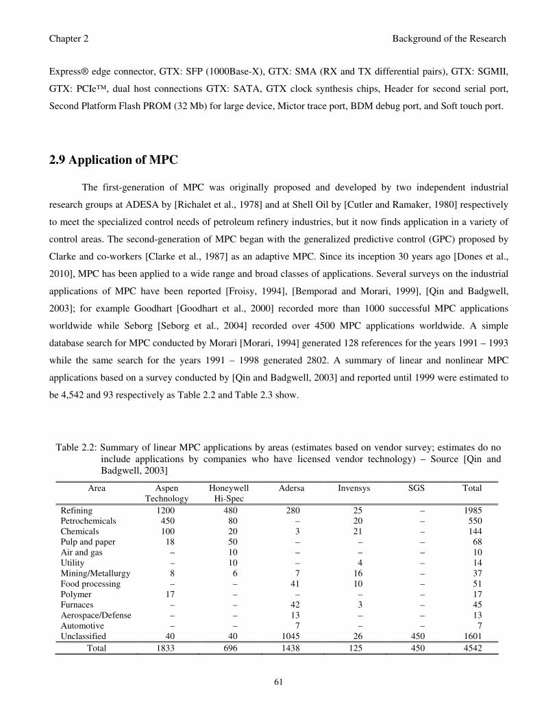
Chapter 2 Background of the Research
61
Express® edge connector, GTX: SFP (1000Base-X), GTX: SMA (RX and TX differential pairs), GTX: SGMII,
GTX: PCIe™, dual host connections GTX: SATA, GTX clock synthesis chips, Header for second serial port,
Second Platform Flash PROM (32 Mb) for large device, Mictor trace port, BDM debug port, and Soft touch port.
2.9 Application of MPC
The first-generation of MPC was originally proposed and developed by two independent industrial
research groups at ADESA by [Richalet et al., 1978] and at Shell Oil by [Cutler and Ramaker, 1980] respectively
to meet the specialized control needs of petroleum refinery industries, but it now finds application in a variety of
control areas. The second-generation of MPC began with the generalized predictive control (GPC) proposed by
Clarke and co-workers [Clarke et al., 1987] as an adaptive MPC. Since its inception 30 years ago [Dones et al.,
2010], MPC has been applied to a wide range and broad classes of applications. Several surveys on the industrial
applications of MPC have been reported [Froisy, 1994], [Bemporad and Morari, 1999], [Qin and Badgwell,
2003]; for example Goodhart [Goodhart et al., 2000] recorded more than 1000 successful MPC applications
worldwide while Seborg [Seborg et al., 2004] recorded over 4500 MPC applications worldwide. A simple
database search for MPC conducted by Morari [Morari, 1994] generated 128 references for the years 1991 – 1993
while the same search for the years 1991 – 1998 generated 2802. A summary of linear and nonlinear MPC
applications based on a survey conducted by [Qin and Badgwell, 2003] and reported until 1999 were estimated to
be 4,542 and 93 respectively as Table 2.2 and Table 2.3 show.
Table 2.2: Summary of linear MPC applications by areas (estimates based on vendor survey; estimates do no
include applications by companies who have licensed vendor technology) – Source [Qin and
Badgwell, 2003]
Area Aspen
Technology
Honeywell
Hi-Spec
Adersa Invensys SGS
Total
Refining 1200 480 280 25 – 1985
Petrochemicals 450 80 – 20 – 550
Chemicals 100 20 3 21 – 144
Pulp and paper 18 50 – – – 68
Air and gas – 10 – – – 10
Utility – 10 – 4 – 14
Mining/Metallurgy 8 6 7 16 – 37
Food processing – – 41 10 – 51
Polymer 17 – – – – 17
Furnaces – – 42 3 – 45
Aerospace/Defense – – 13 – – 13
Automotive – – 7 – – 7
Unclassified 40 40 1045 26 450 1601
Total 1833 696 1438 125 450 4542
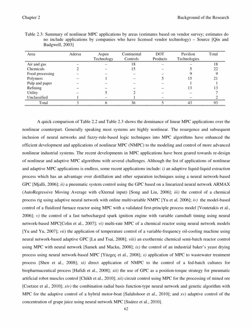
Chapter 2 Background of the Research
62
A quick comparison of Table 2.2 and Table 2.3 shows the dominance of linear MPC applications over the
nonlinear counterpart. Generally speaking most systems are highly nonlinear. The resurgence and subsequent
inclusion of neural networks and fuzzy-rule-based logic techniques into MPC algorithms have enhanced the
efficient development and applications of nonlinear MPC (NMPC) to the modeling and control of more advanced
nonlinear industrial systems. The recent developments in MPC applications have been geared towards re-design
of nonlinear and adaptive MPC algorithms with several challenges. Although the list of applications of nonlinear
and adaptive MPC applications is endless, some recent applications include: i) an adaptive liquid-liquid extraction
process which has an advantage over distillation and other separation techniques using a neural network-based
GPC [Mjalli, 2006]; ii) a pneumatic system control using the GPC based on a linearized neural network ARMAX
(AutoRegressive Moving Average with eXternal input) [Song and Liu, 2006]; iii) the control of a chemical
process rig using adaptive neural network with online multivariable NMPC [Yu et al. 2006]; iv) the model-based
control of a fluidized furnace reactor using MPC with a validated first-principle process model [Voutetakis et al.,
2006]; v) the control of a fast turbocharged spark ignition engine with variable camshaft timing using neural
network-based MPC[Colin et al., 2007]; vi) multi-rate MPC of a chemical reactor using neural network models
[Yu and Yu, 2007]; vii) the application of temperature control of a variable-frequency oil-cooling machine using
neural network-based adaptive GPC [Lu and Tsai, 2008]; viii) an exothermic chemical semi-batch reactor control
using MPC with neural network [Samek and Macku, 2008]; ix) the control of an industrial baker’s yeast drying
process using neural network-based MPC [Yüzgeç et al., 2008]; x) application of MPC to wastewater treatment
process [Shen et al., 2008]; xi) direct application of NMPC to the control of a fed-batch cultures for
biopharmaceutical process [Hafidi et al., 2008]; xii) the use of GPC as a position-torque strategy for pneumatic
artificial robot muscles control [Chikh et al., 2010]; xii) circuit control using MPC for the processing of mined ore
[Coetzee et al., 2010]; xiv) the combination radial basis function-type neural network and genetic algorithm with
MPC for the adaptive control of a hybrid motor-boat [Salahshoor et al., 2010]; and xv) adaptive control of the
concentration of grape juice using neural network MPC [Suárez et al., 2010].
Table 2.3: Summary of nonlinear MPC applications by areas (estimates based on vendor survey; estimates do
no include applications by companies who have licensed vendor technology) – Source [Qin and
Badgwell, 2003]
Area Adersa Aspen
Technology
Continental
Controls
DOT
Products
Pavilion
Technologies
Total
Air and gas – – 18 – – 18
Chemicals 2 – 15 – 5 22
Food processing – – – – 9 9
Polymers – 1 – 5 15 21
Pulp and paper – – – – 1 1
Refining – – – – 13 13
Utility – 5 2 – – 7
Unclassified 1 – 1 – – 2
Total 3 6 36 5 43 93
Chapter 2 Background of the Research
63
Again, a comparison of Table 2.2 and Table 2.3 indicates that until 1999 there was not any reports on
nonlinear MPC control in petrochemicals, mining and metallurgy, aerospace/defense and automotive. After 2006
some MPC applications have been proposed for the aerospace/defense and automobile industry which deal with
nonlinearity by either combining neural networks with simple PID [Savran et al., 2006] or reinforcement
learning algorithms [Jiang and Kamel, 2007] or using recurrent neurocontrollers trained with simultaneous
perturbation stochastic approximation and adaptive critic [Prokhorov, 2007].
2.10 Practical Problems with MPC Algorithms
Model predictive control (MPC) is an advanced digital control technique that has been developed for the
control of constrained multivariable systems with dead time (i.e. time delay) that are met in most of the real world
industrial processes. A comprehensive treatment of dead-time control using MPC can be found in [Normey-Rico
and Camacho, 2007]. In the basic MPC formulation, it is assumed that the system under control will never react
immediately to a control input until after the time delay has elapsed. It is evident that the MPC algorithms are
suitable for systems with long time constants while are unsuitable for systems with fast dynamics for the control
of which short sampling times of the controlled variables are required. Have high computational demands which
cannot be carried out within the short sampling times that the control of the systems with fast dynamics requires.
As pointed in [Camacho and Bordons, 2007], [Froisy, 1994], [Hugo, 2000], [Qin and Badgwell, 2003]
and [Seborg et al., 2004], many commercial industrial MPC packages are based on linear process models which
might not accurately represent or cover the entire operating range of the system [Kalra and Georgakis, 1994]. The
paper of Maciejowski [Maciejowski, 2002] proposed the use of neural networks for modeling nonlinear dynamics
and their use in the MPC design. As mentioned earlier, the majority of MPC research employing NN uses a
linearized NN model for GPC design (GPC is a celebrated class of MPC algorithm with less computational
requirements). The comparison of GPC schemes using linear and nonlinear models have also been investigated by
[Roa et al., 2009], and it has been shown that the latter outperforms the former. Introducing NN into the MPC
scheme for nonlinear MPC design increases the overall design effort in terms of proper model and training
algorithm selection, the arrangement of the NN model amongst other.
Despite the success of MPC, Hugo [Hugo, 2000] has noted several limitations of it in industrial
applications related with controller justification, installation and maintenance expenses, controller structure ill-
conditioning, and operator interface. As pointed out in [Froisy, 1994], [Hugo, 2000], [Maciejowski, 2002], [Qin
and Badgwell, 2003] and [Seborg et al., 2004], ill-conditioning is a major drawback in MPC implementation and
has disabled many MPC controllers. The idea of the ill-conditioning arises due to the multivariable nature of
MPC. Ill-conditioning occurs when the available inputs have very similar effects on two or more outputs. As a
result, the process gain matrix is nearly singular, and large input movements are required to control the outputs
Chapter 2 Background of the Research
64
independently. Consequently, it becomes imperative to check for ill-conditioning at each control sequence.
Although, some strategies have been proposed in [Hugo, 2000], [Maciejowski, 2002], [Qin and Badgwell, 2003]
and [Seborg et al., 2004] to address this issue their proposed strategy basically utilizes linear models off-line.
According to the following statement posed in the abstract of [Nikolaou, 2001]: “After several years of
efforts, the constrained model predictive control (MPC), the de facto standard algorithm for advanced control in
process industries, has finally succumbed to rigorous analysis. Successful practical implementations of MPC
were already in place almost two decades before a rigorous stability proof for constrained MPC was published.
What is then the importance of recent theoretical results for practical MPC applications?” In conclusion,
Nikolaou [Nikolaou, 2001] pointed out that several open issues need to be addressed such as robustness,
adaptation, nonlinearity handling, performance monitoring, model building, computation, and implementation. In
addition Quin and Badwell [Qin and Badgwell, 2003] also pointed out that the current MPC suffers from the
following: limited model choice, sub-optimal feedback, lack of nominal stability, sub-optimal or inefficient
solution of the dynamic optimization, difficulty in tuning the controller for stable processes in the presence of
severe constraints, exploiting MPC to handle significantly larger and/or faster processes, and model uncertainty.
Other issues raised in [Qin and Badgwell, 2003] concern current model identification techniques which include
poor plant test signals they do not have tools to determine whether the collected plant data represent the system
dynamics for MPC design, lack of model validation methods to ascertain the accuracy of the model for MPC
design. There is a need to develop improved identification algorithms which will not be based on other than least
squares and convolution models.
In the light of the above discussion, neural networks were selected for modeling nonlinear systems in the
current work. Given information based on prior tests performed on the system in order to obtain the input-output
training data, the main MPC problem can be summarized as follows: obtain a suitable dynamic neural network
model of a nonlinear system; find an efficient training algorithm, design an MPC algorithm by using the NN
model.
Since 1990, the application of NN to nonlinear system control has been studied extensively. In the next
sub-section, the basic NN-based control schemes are briefly discussed and comparisons are made with NN-based
MPC control strategy.
2.11 Neural Network-Based Control Schemes and MPC
Based on NN learning methods which could be supervised learning, unsupervised learning or
reinforcement learning four (4) NN-based control schemes can be identified namely: neural network-based
adaptive control, modular NN controller design, back-propagation through time control scheme, and adaptive
critic designs. The first two schemes utilize the supervised learning method; the third utilizes the unsupervised
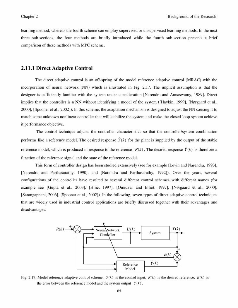
Chapter 2 Background of the Research
65
learning method, whereas the fourth scheme can employ supervised or unsupervised learning methods. In the next
three sub-sections, the four methods are briefly introduced while the fourth sub-section presents a brief
comparison of these methods with MPC scheme.
2.11.1 Direct Adaptive Control
The direct adaptive control is an off-spring of the model reference adaptive control (MRAC) with the
incorporation of neural network (NN) which is illustrated in Fig. 2.17. The implicit assumption is that the
designer is sufficiently familiar with the system under consideration [Narendra and Annaswamy, 1989]. Direct
implies that the controller is a NN without identifying a model of the system ([Haykin, 1999], [Nørgaard et al.,
2000], [Spooner et al., 2002]). In this scheme, the adaptation mechanism is designed to adjust the NN causing it to
match some unknown nonlinear controller that will stabilize the system and make the closed-loop system achieve
it performance objective.
The control technique adjusts the controller characteristics so that the controller/system combination
performs like a reference model. The desired response ˆ( )Y k for the plant is supplied by the output of the stable
reference model, which is produced in response to the reference ( )R k . The desired response ˆ( )Y k is therefore a
function of the reference signal and the state of the reference model.
This form of controller design has been studied extensively (see for example [Levin and Narendra, 1993],
[Narendra and Parthasarathy, 1990], and [Narendra and Parthasarathy, 1992]). Over the years, several
configurations of the controller have resulted to several different control schemes with different names (for
example see [Gupta et al., 2003], [Hine, 1997], [Omidvar and Elliot, 1997], [Nørgaard et al., 2000],
[Sarangapnani, 2006], [Spooner et al., 2002]). In the following, seven types of direct adaptive control techniques
that are widely used in industrial control applications are briefly discussed together with their advantages and
disadvantages.
( )Y k
• ( )U k
System Neural Network
Controller
( )kε
( )R k +
−
−
+
•
Reference
Model
• •
ˆ( )Y k
Fig. 2.17: Model reference adaptive control scheme: ( )U k is the control input, ( )R k is the desired reference, ( )E k is
the error between the reference model and the system output ( )Y k .
Chapter 2 Background of the Research
66
2.11.1.1 Direct Inverse Control with Generalized Training
In the direct inverse control with generalized training scheme ([Nørgaard et al., 2000] and [Gupta et al.,
2003]) the neural network is trained off-line to minimize the mean error between a control signal applied to the
system in an initial experiment and the control signal produced by the neural network. After the neural network
correctly models the inverse of the system, it is then used as a forward controller. Although the closed-loop
response is fast with little computational load, the deadbeat response is not a good choice. In addition, a more a
priori knowledge about the system is required for control purpose.
2.11.1.2 Direct Inverse Control with Specialized Training
The direct inverse control scheme with specialized training, unlike the direct inverse control scheme with
generalized training, utilizes a recursive network as the inverse model and the training is done on-line. The
recursive training paradigm follows from the recursive pseudo-linear regression method described in [Ljung,
1999]. With this training method the controller can be optimized for a specific trajectory and is suitable for time-
varying systems. However, there are several drawbacks with this approach, namely: 1) the method does not work
for systems with unstable inverse which often occurs when using high sampling frequency, 2) lack of tuning
options, and 3) the controller shows high sensitivity to disturbances and noise. A detailed treatment of this control
method can be found in [Nørgaard et al., 2000].
2.11.1.3 Indirect Inverse Control
Unlike the two indirect schemes above where the network is trained to model the inverse of the system, in
the direct inverse control scheme the neural network is first trained as a feedforward network (in the general case).
Next, the trained network is inverted and used as a controller. This method is also subject to the problems with the
direct inverse methods mentioned above. Additional requirement is that the inverted model (i.e. the controller)
must be well-damped.
2.11.1.4 Internal Model Control (IMC)
Internal model control (IMC) based on neural network requires a forward model as well as the inverse
model of the system. The principle of the IMC with an output disturbance ( )d k is illustrated in Fig. 2.18. Note
that instead of a direct output feedback, the error between the system output and the model is fed back. Suppose
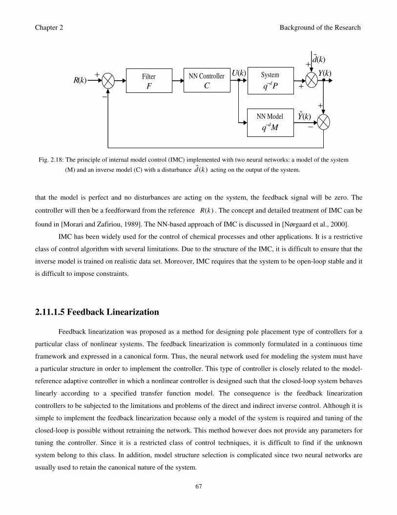
Chapter 2 Background of the Research
67
that the model is perfect and no disturbances are acting on the system, the feedback signal will be zero. The
controller will then be a feedforward from the reference ( )R k . The concept and detailed treatment of IMC can be
found in [Morari and Zafiriou, 1989]. The NN-based approach of IMC is discussed in [Nørgaard et al., 2000].
IMC has been widely used for the control of chemical processes and other applications. It is a restrictive
class of control algorithm with several limitations. Due to the structure of the IMC, it is difficult to ensure that the
inverse model is trained on realistic data set. Moreover, IMC requires that the system to be open-loop stable and it
is difficult to impose constraints.
2.11.1.5 Feedback Linearization
Feedback linearization was proposed as a method for designing pole placement type of controllers for a
particular class of nonlinear systems. The feedback linearization is commonly formulated in a continuous time
framework and expressed in a canonical form. Thus, the neural network used for modeling the system must have
a particular structure in order to implement the controller. This type of controller is closely related to the model-
reference adaptive controller in which a nonlinear controller is designed such that the closed-loop system behaves
linearly according to a specified transfer function model. The consequence is the feedback linearization
controllers to be subjected to the limitations and problems of the direct and indirect inverse control. Although it is
simple to implement the feedback linearization because only a model of the system is required and tuning of the
closed-loop is possible without retraining the network. This method however does not provide any parameters for
tuning the controller. Since it is a restricted class of control techniques, it is difficult to find if the unknown
system belong to this class. In addition, model structure selection is complicated since two neural networks are
usually used to retain the canonical nature of the system.
( )Y k
•
NN Controller
C
( )U k
System d
q P−
NN Model d
q M−
Filter
F
( )d k
ˆ( )Y k
( )R k +
−
−
+
+
+
•
Fig. 2.18: The principle of internal model control (IMC) implemented with two neural networks: a model of the system
(M) and an inverse model (C) with a disturbance ( )d k acting on the output of the system.
Chapter 2 Background of the Research
68
2.11.1.6 Feedforward Control
Unlike the adaptive controllers discussed until now, the feedforward controller does not have feedback
but is governed only by the reference signal. However, feedback can be included when the feedforward is used for
reference tracking and the feedback is used for stabilizing the system and for suppressing disturbances. Three
following types of feedforward control exist, namely [Nørgaard et al., 2000]: 1) the static feedforward where the
feedforward controller is governed only by the reference signal without feedback when stability problems do not
exist, 2) dynamic feedforward where the feedforward controller is an inverse model with inverse model related
problems, and 3) steady-state feedforward where the feedforward controller is a function of the steady-state
reference in which the steady-state gain of the inverse model multiplied by the reference returns.
Although, the implementation of the feedforward controller is simple and reference tracking is improved
without any increase in noise sensitivity, a fundamental requirement is a feedback controller to be present. This
control method does not reduce the effect of disturbances acting on the system and a poor feedback may reduce
the performance of the system instead of enhancing it.
2.11.1.7 Optimal Control
Optimal control is a goal directed control technique that deals with the problem of finding a control law
that minimizes certain criterion to obtain the control input or signal. In contrast with all the control techniques
discussed until now which make to pole placement with full zero cancellation and problems and result to poorly
damped or unstable systems, the optimal control is an optimization strategy which uses a specialized recursive
algorithm to train the neural network. The optimal control strategy minimizes a criterion of the following form:
22
1
( ) ( ) ( ) 0N
p p p
p
J R k Y k U kρ ρ=
= − + ≥ ∑ (2.93)
where ( )R k , ( )U k , ( )Y k and ρ are the desired reference, the system input, the system output, and a tuning
parameter for penalizing changes in the control input; N specifies the length (finite horizon) of the desired
reference at each time step k .
The controller is implemented as an extension to the specialized training of the direct inverse model
controller. The extension consists of the second term in (2.93) for penalizing squared control inputs with a price in
the deterioration of the reference tracking. Compared with the direct and indirect inverse model controllers the
goal-directed optimal controller is easy to tune, applicable to a large class of time-varying systems and suitable
for designing controllers with a specified reference trajectory. A major drawback is that the network must be
trained again each time the penalty factor ρ is changed or modified. Because the network is trained on-line,
initialization of the network is difficult.
Chapter 2 Background of the Research
69
2.11.2 Indirect Adaptive Control
In the direct adaptive control discussed above, the neural network (NN) is the controller itself and there is
not any method to directly adjust the controller weights with the purpose of reducing the error. Although its
implementation is simple, the on-line retraining of the network is difficult every time a design parameter is
modified. The design of indirect adaptive control is always model-based. The basic principle of the indirect
adaptive control scheme is illustrated in Fig. 2.19. This scheme usually employs a NN to model the physical
system which from now on will be called the identified NN model. Then, this model is employed for controller
design based on a NN model of the physical system. The identified NN model is trained in advance but then it
becomes a part of the control strategy which involves the computation of the output error between the physical
system and the prediction of the NN model every time an updated measurement of the output of the physical
system is received, Next, the adjustment of its parameters is performed so that the error is minimized. By using
the modified NN model new controller parameters are computed so that the deviation of the system output from
the required reference is also minimized ([Hines, 1997], [Tsoukalas and Uhrig, 1997].
The influence of the nonlinearity of the NN model has led to different types of indirect controller designs
and implementations for different applications. The different achitectures for indirect adaptive controller design
which have been reported in the literature ([Gupta et al., 2003], [Hine, 1997], [Omidvar and Elliot, 1997],
[Nørgaard et al., 2000], [Sarangapnani, 2006], [Spooner et al., 2002]), can be grouped into two main classes,
namely: indirect adaptive control design based on the finding of a linear approximation of the physical system
and indirect adaptive control design based on the tuning of the initial nonlinear NN model at every output an
updated output measurement becomes available. The former class comprises pole placement controller,
generalized minimum variance control (GMVC) and the well-known generalized predictive controllers (GPC)
whereas the latter class is nonlinear predictive controller (NPC). These two classes are briefly discussed in the
following two sub-sections and some remarks on their performance are made.
( )Y k
• ( )U k
System
Neural Network
Controller
( )kε
( )R k +
−
−
+
•
Prediction
Model
•
•
Identification Model
•
•
+
−
( )kε
ˆ ( )Y k
Fig. 2.19: Indirect model-based adaptive control scheme: ( )U k is the control input, ( )R k is the desired reference,
( )E k is the error between the reference model and the system output ( )Y k .
Chapter 2 Background of the Research
70
In the direct adaptive control scheme shown in Fig. 2.19, the neural identification model is used to model
the system which is assumed here to be nonlinear. If necessary, this model may be updated to track the system.
The error signal is then backpropagated through the identification model to train the neural network controller so
that the system response is equal to that of the reference model. Note that this method uses two neural networks,
one for model or system identification and the other for model reference adaptive control (MRAC) [Hines, 1997].
2.11.2.1 Indirect Adaptive Control Based on Instantaneous Linearization
The idea behind instantaneous linearization is to extract a linear model from a nonlinear NN model at
each sampling instant. The linearization of nonlinear models is a technique often used to simplify the design of
controllers for nonlinear systems. The basic principle of controller design based on instantaneous linearization is
shown in Fig. 2.20. This control scheme is adapted from Fig. 2.19 except that the nonlinear NN model is extracted
and linearized around a specific operating regime. The characteristics of the nonlinearities and size of the
operating regime determines whether it is sufficient to use a single linear model, or it is necessary to model by
linearizating around a larger set of operating points with banks of controllers and some switching rules as in the
so-called gain scheduling controllers [Åström and Witternmark, 1995].
Assuming that a nonlinear NN model based on any of the structures described in Section 2.5 has been
obtained through an off-line training process, the instantaneous linearization has been applied to directly obtain an
approximate pole placement controller with compensation for disturbance based on a so-called internal model
principle in [Nørgaard et al., 2000]. In the pole placement scheme, the desired behaviour is specified in terms of a
transfer function or a set of closed-loop poles with possible oscillatory and damping related problems.
Another type of controller design based on the instantaneous linearization is the so-called generalized
minimum variance controller (GMVC). Unlike the pole placement technique, the GMVC can be specified in terms
of a criterion which should be minimized to obtain the control signal ( )U k . The criterion-based design may be
Controller
Design
Extract
Linear Model
Controller
System
Linearized model parameters
ˆ ( )Y k ( )U k
( )R k • •
Fig. 2.20: Indirect control based on instantaneous linearization of the neural network model.
Chapter 2 Background of the Research
71
advantageous in that tuning becomes simple and intuitive. It appears to be a natural way of designing controllers
for stochastic systems in the context of self-tuning regulators [Åström and Witternmark, 1995]. The basic GMVC
controller is usually designed to solve a servo problem rather than only a regulation problem. Assuming that the
NNARMAX model discussed in Section 2.5.2.2 has been obtained, the objective might be to compensate for
stochastic disturbances. To cover a wider class of systems, the criterion that is often minimized by the GMV is of
the form:
21 1 1 2ˆ( ) ( ) ( ) ( ) ( ) ( ) ( )G G G kJ k E P z Y k d W z R k Q z U k I
− − − = + − + (2.93)
where ,G GP W and GQ are rational transfer functions, and ( ), ( 1), , (0), ( ), ( 1), ,kI Y k Y k Y U k U k= − −… …
( ), ( 1), , (0)U k U k U− … . A simplified form of (2.93) is given from [Isermann et al., 1992] and [Nørgaard et al.,
2000] as:
[ ] 2 2ˆ( ) ( ) ( ) ( ) kJ k E Y k d R k U k Iρ = + − + ∆ (2.94)
The minimizing solution for (2.94) can be expressed as:
1 1 1 1
1 1
( ) ( ) ( ) ( )
( ) ( )
G G
G
R z B z R z C z
T z C z
ρ− − − −
− −
= ∆ + ∆
= (2.95)
where the 1( )GR z− and 1( )GS z
− can be found from the following Diophantine equation: [Åström and
Witternmark, 1995]:
1 1 1 1( ) ( ) ( ) ( )d
G GC z A z R z z S z− − − − −= ∆ + and 1 1 1( ) ( ) ( )G GR z R z B z
− − −= ∆
with deg( ) 1GR d= − and deg( ) max( , )G a cS n n d= − .
The GMV control is a fairly general approach with many design parameters and can be used to control
systems with unstable inverse by choosing suitable design parameter. The reason for penalizing the differenced
control inputs is to accomplish the desired integral action; that is, ∆ becomes a factor of 1( )GR z− . This scheme
is well-suited for real-time control in that the linearization and the controller design can be performed in between
time samples. It also provides a useful physical interpretation of the dynamics of the system. A major
disadvantage of this method is that the linearized model might be valid only for a very narrow region around the
current operating point.
The third class of controllers based on the linearization considered here is the so-called generalized
predictive control (GPC) proposed by Clarke and co-workers [Clarke et al., 1987]. The GPC is a class of model
predictive (MPC) algorithms and was proposed in the context of adaptive control and it has been widely used in
many advanced and industrial control applications with successful results. It is a criterion-based design and
follows the basic structure shown in Fig. 2.33. The GPC includes an integral action to account for regular constant
disturbances as well as for operating point dependent bias component, which shall be defined as ( ')d k . This is
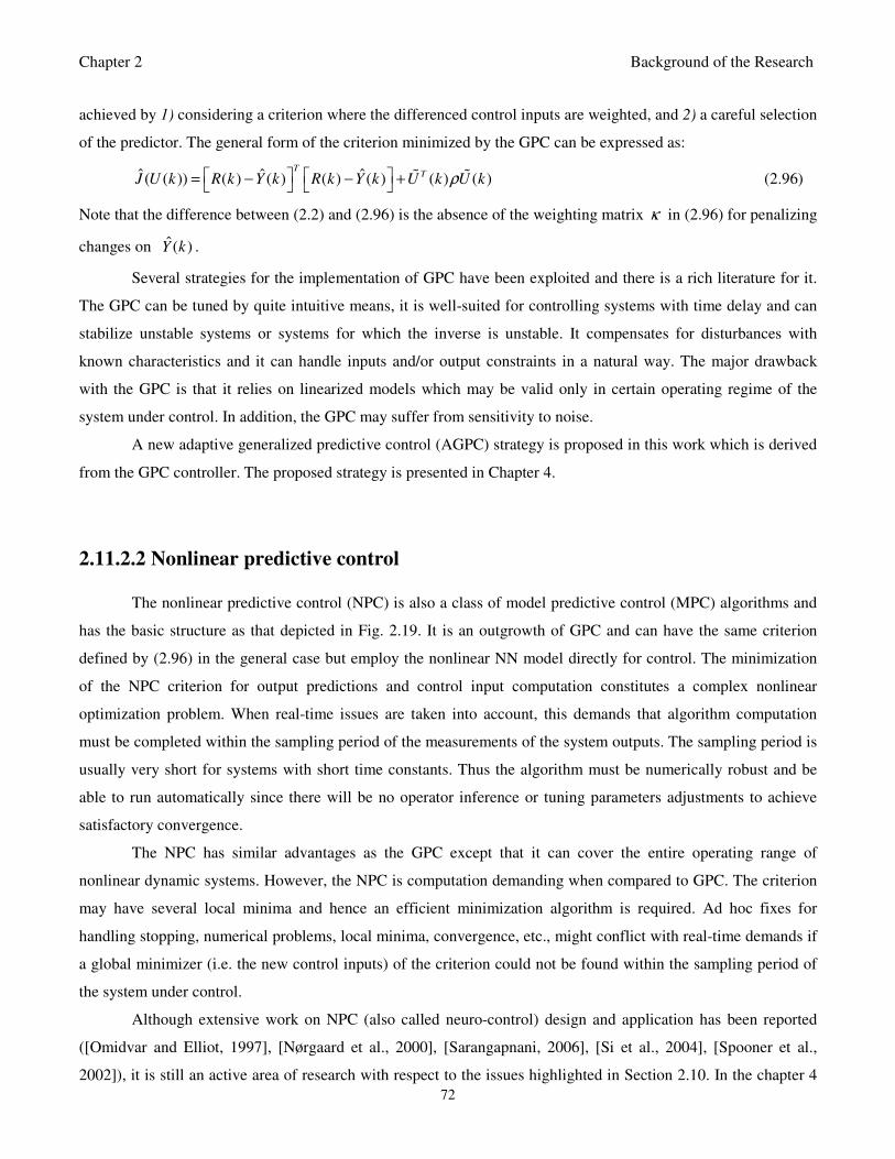
Chapter 2 Background of the Research
72
achieved by 1) considering a criterion where the differenced control inputs are weighted, and 2) a careful selection
of the predictor. The general form of the criterion minimized by the GPC can be expressed as:
ˆ ˆ ˆ( ( )) ( ) ( ) ( ) ( ) ( ) ( )T
TJ U k R k Y k R k Y k U k U kρ = − − +
(2.96)
Note that the difference between (2.2) and (2.96) is the absence of the weighting matrix κ in (2.96) for penalizing
changes on ˆ( )Y k .
Several strategies for the implementation of GPC have been exploited and there is a rich literature for it.
The GPC can be tuned by quite intuitive means, it is well-suited for controlling systems with time delay and can
stabilize unstable systems or systems for which the inverse is unstable. It compensates for disturbances with
known characteristics and it can handle inputs and/or output constraints in a natural way. The major drawback
with the GPC is that it relies on linearized models which may be valid only in certain operating regime of the
system under control. In addition, the GPC may suffer from sensitivity to noise.
A new adaptive generalized predictive control (AGPC) strategy is proposed in this work which is derived
from the GPC controller. The proposed strategy is presented in Chapter 4.
2.11.2.2 Nonlinear predictive control
The nonlinear predictive control (NPC) is also a class of model predictive control (MPC) algorithms and
has the basic structure as that depicted in Fig. 2.19. It is an outgrowth of GPC and can have the same criterion
defined by (2.96) in the general case but employ the nonlinear NN model directly for control. The minimization
of the NPC criterion for output predictions and control input computation constitutes a complex nonlinear
optimization problem. When real-time issues are taken into account, this demands that algorithm computation
must be completed within the sampling period of the measurements of the system outputs. The sampling period is
usually very short for systems with short time constants. Thus the algorithm must be numerically robust and be
able to run automatically since there will be no operator inference or tuning parameters adjustments to achieve
satisfactory convergence.
The NPC has similar advantages as the GPC except that it can cover the entire operating range of
nonlinear dynamic systems. However, the NPC is computation demanding when compared to GPC. The criterion
may have several local minima and hence an efficient minimization algorithm is required. Ad hoc fixes for
handling stopping, numerical problems, local minima, convergence, etc., might conflict with real-time demands if
a global minimizer (i.e. the new control inputs) of the criterion could not be found within the sampling period of
the system under control.
Although extensive work on NPC (also called neuro-control) design and application has been reported
([Omidvar and Elliot, 1997], [Nørgaard et al., 2000], [Sarangapnani, 2006], [Si et al., 2004], [Spooner et al.,
2002]), it is still an active area of research with respect to the issues highlighted in Section 2.10. In the chapter 4
Chapter 2 Background of the Research
73
of this work, a new nonlinear adaptive model predictive control (NAMPC) algorithm is proposed and the
complete formulation as well as implementation details is also presented in the chapter.
2.11.3 Modular Neural Network (MNN) Controller Design
Modular neural networks perform a spatial clustering of input space in order to select and dispatch the
input vector to various modules. The most advanced algorithm in this respect is the local model network (LMN).
The LMN consists of a number of single layer NN, each one of them having the same architecture and trained to
model a system behavior around a local point (local plant) and a gating system often composed of radial basis
functions (RBF). The various local models are activated by a time-varying input vector X that usually
corresponds to the vector of parameters of a NARMAX model given in (2.8). Note that NARMAX model is a
lagged version of the NARX model and other model structures can as well be used for this purpose.
The construction of the local models into a multiple model structure and the controller structure including
possible switching techniques is discussed in [Ronco and Gawthrop, 1997]. A comprehensive treatment of the
modular and multiple model methods with several extensions and remarks on their implementation can be found
in the book “Predictive Modular Neural Networks” [Petridis and Kehagias, 1998]. This form of control has been
extended to include fuzzy rule-based logic to enhance switching between multiple models and controllers as
discussed in [Petridis and Kehagias, 1998] and [Ronco and Gawthrop, 1997]. Recent extensions of the multiple
models technique to adaptive control using neural networks have also been reported [Chen and Narendra, 2001].
2.11.4 Back-Propagation Through Time (BPTT) Control Scheme
The backpropagation through time (BPTT), besides being used for recurrent neural network training, can
also be used for neural control [Werbos, 1990]. The BPTT can be used to move a system from one state to another
state in a finite number of steps, provided that the system is controllable. The typical structure of this control
scheme is shown in Fig. 2.21; where X is the state vector, U is the control signal, C is the controller, P is the
( 1)U k −
'( )X k(0)X
•
C
P
C
P
C
P
C
P
∑
• • •
( )U i (1)U (0)U
(1)X ( )X i ( 1)X k − ( )X k
Initial
State Final
State
Fig. 2.21: Basic structure of the backpropagation through time (BPTT) control scheme.
Chapter 2 Background of the Research
74
plant model, '( )X k is the desired target state, and ( )E k is the error signal. Generally, the BPTT training takes
place in the following two steps:
1). The plant motion stage, where the plant model takes k time steps from the initial state (0)X to state
( )X k as shown in Fig. 2.21.
2). The weight adjustment stage, where the weights of the controller are adjusted to make the final state to
approach the target state.
In the BPTT scheme, the neural network must be trained so that the error signals can be propagated through it to
the controller, then the controller can be trained with the BPTT algorithm. Note that there is only on set of
weights to be adjusted since there is only one controller. Thus, several iterations are executed until the desired
performance is achieved.
2.11.5 Neural Network-Based Adaptive Critic Designs
Neural network-based adaptive critic designs can be supervised or unsupervised [Sarangapani, 2006].
However, in a more general case, typical neural network-based adaptive critic design (ACD) consists of three
neural networks: critic network (for evaluation), the model network (for prediction), and the action network (for
decision) as well as the real plant as illustrated in the action-dependent heuristic dynamic programming (ADHDP)
form of ACD ([Liu, 2002]; [Mohagheghi et al., 2006]) shown in Fig. 2.22. Consider a discrete-time nonlinear
time-varying system described by the following equation:
[ ]( 1) ( ), ( ),x k F x k u k k+ = (2.97)
where nx∈ℜ is the state vector and m
u ∈ℜ denotes the control action. Suppose that the performance index or
( 1)x k +
Critic Network
Model Network
Action Network
Plant
( )u k
( )u k
ˆ ( 1)J k +
( )x k
• •
Fig. 2.22: The structure of an action-dependent heuristic dynamic programming form of adaptive critic design.
Chapter 2 Background of the Research
75
cost associated with the system (2.97) can be expressed as
[ ]( ( ), ) ( ), ( ),p
p
J x U x p u p pτ
τ
τ τ γ∞
−
=
=∑ (2.98)
where U is the utility or local cost function and [0,1]γ ∈ is the discount factor. Note that J is dependent on the
initial time τ and the initial state ( )x τ and it is referred to as the cost-to-go of state ( )x τ . The objective then is
to choose the control sequence ( ),u p , 1, 2, ,p τ τ τ= + + … such that the function J in (2.98) is minimized.
The training of the critic network is achieved by minimizing the error function of the following form:
ˆ ˆ( ) ( ) ( ) ( 1)c
k
E k J k U k J kγ = − − + ∑ (2.99)
where [ ]ˆ ˆ( ) ( ), ( ), ,c
J k J x k u k k W= and c
W denotes the NN parameters (i.e. the weights) of the model network If
the ( ) 0c
E k = for all k , then (2.99) takes the form:
ˆ ˆ( ) ( ) ( 1) ( )p
p
J k U k J k U pτ
τ
γ γ∞
−
=
= + + =∑ (2.100)
Thus, training a NN which minimizes (2.99) produces the estimate of (2.99) defined by (2.100). The minimization
of (2.99) can be achieved with the standard back-propagation algorithm.
Next, the action network is trained with the objective of minimizing ˆ( 1)J k + through the use of the
action signal [ ]( ) ( ), , Au k u x k k W= . At the end of the training process, the action network generates control signals
which are optimal. The training of the action network is done through weight updates while keeping the weights
of the critic and the model networks fixed.
Most often in ACDs, decision has to be taken without having an accurate assessment of the effectiveness
of the control actions. The critic network evaluates the results of the control action from the action network: if it is
good, the action is reinforced and if it is poor, the action is weakened. This type of training the action network is
called reinforcement learning [Sutton and Barto, 1998]. This is rather a trial and error method which uses active
exploration when the gradient of the evaluation system in terms of control action is not available. Several
techniques for training neural network-based ACDs are discussed in [Omidvar et al., 1997], [Prokhorov, 2007],
[Sarangapani, 2006] and [Si et al., 2004].
2.12 State-of-the-Art in Neural Network-Based MPC: Neural Network Training,
Model Identification, Adaptive Control and MPC Implementation
This sub-section critically examines the main concepts of all the materials discussed in the chapter. State-
of-the-art overview on neural network-based MPC strategies is reviewed in terms of neural network training,
model identification techniques, neural network-based MPC scheme, and MPC implementation techniques. The
Chapter 2 Background of the Research
76
successes and drawbacks of these approaches are presented and discussed. Then, new strategies proposed in this
research are presented to improve on the reported successes while correcting the drawbacks reported.
2.12.1Neural Network and Training Methods
As it has been widely discussed and demonstrated in [Narendra and Parthasarathy, 1990], [Nørgaard et
al., 2000], [Omidvar and Elliott, 1997], [Spooner et al., 2002] and [Chiong, 2010], the accuracy of a nonlinear NN
model depends on the structure of the nonlinear function that will be used to describe the dynamics of the system
to be identified; the NN architecture; the selection of the inputs to the NN; the NN training algorithm; and the NN
model identification scheme.
Over time, different architectures of NNs have evolved (see [Gupta et al., 2003], [Hagan et al., 1996] and
[Haykin, 1999]) and it has been shown that a multilayer perceptron (MLP) NN with one hidden and output layers
is capable of approximating any continuous and/or nonlinear functions reasonably well with an arbitrary degree of
accuracy. The most widely used NN architecture for dynamic system modeling is the dynamic feedforward NN
(DFNN) ([Yüzgeç et al., 2008]; [Colin et al., 2007] and [Samek and Macku, 2008] and [Pan and Wang, 2008]).
The use of recurrent NN (RNN) for modeling nonlinear dynamic systems has also been reported in several
research papers such as in [Lu and Tsai, 2008], [Pan and Wang, 2008], [Wang and Thomas, 2006] and [Zhang
and Quan, 2009].
On the other hand, recurrent neural networks (RNNs) are more powerful than DFNNs because they
contain the basic FNN structure with feedback connections from the output to the input layer via a state layer (the
so-called Jordan network [Pearlmutter, 1995]) or from the output unit to the input unit of the hidden layer via a
context layer as in the so-called Elman network [Song, 2010]. However, training these networks presents
difficulties due to their feedback structures ([Bengio et al., 1994]; [Pearlmutter, 1990 and 1995]). The usual
methods for training RNNs are: 1) the real-time recurrent learning (RTRL) discussed in [Williams and Zipser,
1989] with further extensions in [Pearlmutter, 1995] is an unrestrictive on-line, exact, stable but computationally
expensive method for determining the derivatives of the state functions of a dynamic system with respect to the
internal parameters of the system; and 2) the backpropagation through time (BPTT) [Werbos, 1990] where the
network is unfolded into a multilayer feedforward network that increases by one at each time step with growing
memory requirements as shown in [Pearlmutter, 1995] and [Song, 2010]. Both RTRL and BPTT are variations of
the backpropagation (BP) algorithm originally proposed by [Rumelhart et al., 1986] as a basic gradient descent
algorithm detailed in [Boyd and Vandenberghe, 2007], [Antoniou and Lu, 2007], [Dennis and Schnabel, 1996],
and [Kelley, 1995 and 1999].
However, Williams and Zipser [Williams and Zipser, 1989] extended the RTRL to teacher-forcing RTRL
method. According to this method, the feedbacks to the network input (state layer) in subsequent computations
Chapter 2 Background of the Research
77
are the actual outputs from the system rather than those from the network outputs. This architecture places the
system in parallel with the NN model resulting in a series-parallel model structure which has been shown in
[Narendra and Parthasarathy, 1990], [Omidvar and Elliott, 1997] and [Spooner et al., 2002] to be suitable for
stable adaptive control systems design. By teacher forcing the output units, no real recurrent paths exist, so that
the basic BP through a single time step can be used for training the resulting network in a feedforward fashion.
The main disadvantage of this method (i.e., the state to be retrained by the network across time) is alleviated in
the control applications if a small stack proposed in [Dias et al., 2005] or a sliding window proposed in
[Pearlmutter, 1995] and [Savran et al., 2006] of the output values at previous time steps are cycled back to the
state layer during network training.
2.12.2 Neural Network Model Identification for MPC Design
Neural network model identification for use in MPC applications has been reported using feedforward
neural network (FNN) ([Colin et al., 2007]; [Pan and Wang, 2008]; [Samek and Macku, 2008]; [Yüzgeç et al.,
2008]) and recurrent neural network (RNN) ([Jin and Su, 2008]; [Lu and Tsai, 2008]; [Wang and Thomas, 2006];
[Zhang and Quan, 2009]). The MPC methods reported in these papers all uses the linearized form of the identified
nonlinear NN model and employ the generalized predictive control (GPC) techniques originally proposed by
Clarke and co-workers [Clarke et al, 1987a and 1987b] except that in [Lu and Tsai, 2008] the GPC control actions
are updated online in real-time for a relatively slow process with long sampling time using a recursive least
squares (RLS) adaptation rule that is obtained from a network trained with the basic BP algorithm. Although, the
GPC was proposed by Clarke and co-workers [Clarke et al, 1987a and 1987b] in the context of adaptive control, it
is well-known the control performance can degrade if the system is operated outside its valid linear or operating
region.
Since 1990, the design of control algorithms for nonlinear dynamical systems which is based on the use
of neural network (NN) models of the plant dynamics has been studied extensively with some successful results
reported in research papers such as the ones in [Chiong, 2010], [Narendra and Parthasarathy, 1990], [Narendra
and Parthasarathy, 1992], [Nørgaard et al., 2000], [Petridis and Kehagias, 1998] and [Ronco and Gawthrop,
1997]. In these cases, the major issues that arise are the structure of the nonlinear function that will be used to
describe the dynamics of the system, the NN architecture, the training algorithm for adjusting the NN parameters,
the way the controller and the NN are used within the control loop, and how the control algorithm will be
updated. Neural network (NN) parameters, for instance, are the weights and biases of the network. The
adjustments of NN parameters can be achieved by minimizing the errors between the outputs of the neural
network and the desired outputs ([Gupta et al., 2003]; [Hagan, 1996]; [Haykin, 1999]). This minimization is
called the neural network training process which is performed by an algorithm.
Chapter 2 Background of the Research
78
Over the years, different NN architectures and training algorithms have been proposed in several research
papers such as those in ([Chiong, 2010]; [Hagan and Menhaj, 1994]; [Haykin, 1999]; [Wu, 2008]; [Narendra and
Parthasarathy, 1990]; [Nørgaard et al., 2000]; [Petridis and Kehagias, 1998]; [Prokhorov, 2007]; [Rumelhart et al.,
1986]; [Werbos, 1990]; [Williams and Zipser, 1989]). Among these, the most common NN architecture is the
feedforward NN (FNN) while the backpropagation (BP) algorithm ([Rumelhart et al., 1986]; [Werbos, 1990]) and
the Levenberg-Marquardt algorithm (LMA) ([Hagan and Menhaj, 1994]; [Marquardt, 1963]) are two common
NN training algorithms. Although, the BP has been widely used in training FNNs due to the simplicity and ease of
its implementation, it has been reported to be characterized by large network parameters, poor convergence, long
training cycles (epoch) and not being robust when compared to the Levenberg-Marquardt algorithm (LMA).
Another widely used method which is increasingly been used for model identification or parameter
estimation incorporating neural networks is the recursive least squares (RLS) algorithm. While the
backpropagation and the Levenberg-Marquardt algorithms evaluates all the training data set at each epoch in an
off-line manner, the recursive least squares algorithms evaluates each input-output data pair as new measurements
are acquired in an on-line manner. Thus, the RLS algorithms have been widely used in adaptive control, adaptive
filtering, adaptive signal processing, adaptive prediction, etc. ([Goodwin and Sin, 1984], [Ljung, 1999]). The
major challenge in implementing the RLS algorithm is that the on-line computation must be computed in such a
way that the processing of the measurements from one sampling instant must be completed during one sampling
interval with certainty. The use of RLS for on-line model and parameter estimations have been studied
extensively ([Chen, 2009], [Goodwin and Sin, 1984], [Ljung, 1999], [Salgado et al., 1988]). The extensions of the
RLS with neural networks are recent developments ([Bouchard, 2001], [Lu and Tsai, 2008], [Mirikitani and
Nikolaev, 2007]). The integration of the RLS into neural network framework has resulted in several formulations
of neural network-based RLS algorithms [Bouchard, 2001]. Attempt has also been made to incorporate the RLS
algorithm into the Levenberg-Marquardt algorithm for training recurrent neural networks [Mirikitani and
Nikolaev, 2007]. A close study of the algorithm proposed in [Mirikitani and Nikolaev, 2007] is the basic
Levenberg-Marquardt algorithm with extra regularization term and a recursive covariance update rule at the
expense of high computational complexities and requirements. However, as noted by Bouchard [Bouchard, 2001],
the two key issues that arise from the use of neural network-based RLS algorithms for adaptive control
applications are: 1) they do not solve the problem of finding a nonlinear model of the system that will be valid for
most control signals, and 2) it is characterized by poor numerical robustness and slow convergence.
One way to overcome these problems is to formulate the RLS algorithm as off-line model identification
or parameter estimation algorithm where all the input-output data set are evaluated for a specific number of times
at each time sample as new measurements are acquired and added to the data set. Although, this idea is not new in
the general framework of RLS algorithm formulations ([Ljung, 1999], [Salgado et al., 1988]), and can be
extended to the neural network schemes for formulating RLS algorithms. Since neural network is data-driven
application, improved numerical robustness and convergence can be improved with the assumption that the
Chapter 2 Background of the Research
79
computations will be completed within the sampling time of the system under consideration. Also, rather than
training the network to infinity as in [Chen, 2009] and for long-term stability as [Bouchard, 2001], and a nonlinear
model of the system can be identified for a specified number of iterations that will be suitable and valid for
control applications. Since new measurements are acquired on-line at each time sample, the next issue to be
addressed is on the weight update for the time-varying system. The point here is that as new measurements are
acquired, old information must be discarded to avoid redundant information during the updated weight as this
could lead to inaccurate process model. The effect of inaccurate process model is more severe in model predictive
control strategy as is evident in [Bouchard, 2001], [Lu and Tsai, 2008], and [Mirikitani and Nikolaev, 2007].
The basic RSL algorithms are well known to have optimal properties when the parameters are time-
invariant and the gain of the RLS algorithm converges to zeros ([Goodwin and Sin, 1984], [Narendra and Driollet,
2001]). In the neural network framework, the data must be properly excited in order for the RLS algorithm to
track time-varying signals. However, as proposed in [Salgado et al., 1988], if an adaptive scheme is incorporated
to discard obsolete information as new ones are acquired, time-varying signals can accurately be tracked even
when the data are poorly excited. In [Salgado et al., 1988], three methods for discarding obsolete information in
basic RLS algorithms, namely: forgetting factor method, constant trace method, and the exponential forgetting
and resetting method. Simulation studies in [Salgado et al., 1988] shows that the exponential forgetting and
resetting method proved superior over the other two methods. With this methods, the gain convergence of the
does not go to zeros.
Irrespective of using the backpropagation (BP) algorithm, Levenberg-Marquardt algorithm (LMA) or the
recursive least squares (RLS) algorithm; an alternative way to train a NN with the purpose of modeling the
behaviour of a controlled process could be to place the true system in parallel with the network and establish a
feedback loop from the true system output to the NN inputs, and then apply the BP or LMA training algorithms.
In literature ([Gupta et al., 2003]; [Haykin, 1999]; [Pearlmutter, 1995]; [Williams and Zipser, 1989]), this
approach is referred to as the teacher forcing method. As pointed out earlier and noted also in [8], the difficulty
with this method is that the state to be retrained must be manifested throughout the network training process.
In this work, to overcome this problem, the FNN is augmented with appropriate tapped delay line (TDL)
memory units to form a dynamic FNN (DFNN) while a short temporal window is also created to store not just the
current states but also few states from the previous time steps in a first-in first-out fashion. Both the BP and the
LMA algorithms are standard algorithms where all the input-output data set are evaluated in batch mode at each
epoch. Recursive least squares algorithms, on the other hand, are sequential algorithms where each input-output
data pair is evaluated at each epoch. In order to adapt the standard algorithms for DFNN training, the same
approximation obtainable in the sequential methods must be made. The main drawback in adapting standard
algorithms for online training is the difficulty in inverting and searching for a region where the Hessian matrix is
guaranteed to be positive definite. This drawback has been investigated in several literature and different
techniques to solve this problem have been reported by many authors including [Antoniou and Lu, 2007], [Boyd
Chapter 2 Background of the Research
80
and Vandenberghe, 2007], [Chiong, 2010], [Dennis and Schnabel, 1996], [Fletcher, 1987]; [Kelley, 1996 and
1999], [Marquardt, 1963], [Sagaldo et al., 1988]; [Scales, 1985], [Wu, 2008].
Such a Hessian matrix is formed during the solution of the optimization problem that a training algorithm
involves. Also, in this work, a modified LMA (MLMA) is proposed which alleviates the above drawback and is
adapted to DFNN architecture. Also a new adaptive recursive least square (ARLS) identification algorithm is
proposed for training the DFNN.
2.12.3 Neural Network–Based MPC Algorithms
Furthermore, a nonlinear adaptive model predictive control (NAMPC) algorithm is presented which
depends on the neural network model of the process obtained from the online identification of a nonlinear model
of the controlled process. Then, by using the updated model, it solves the optimal control problem online in order
to determine the control strategy on which the next control action will be applied. The model identification is
based on a neural network which is trained by using data from the prior operation of the plant and then used
online to adjust itself to monitored changes of the plant dynamics over the time.
The use of a neural network model instead of the actual nonlinear plant model derived from first
principles and expressed by ordinary and/or partial differential equations simplifies considerably the computations
of MPC actions at every sampling instant and makes it appropriate for use in an adaptive MPC algorithm ([Colin
et al., 2007]; [Lu and Tsai, 2008]). The simulation of differential equations and dynamic models to obtain training
and test data for neural network model development for use in different applications together with their merits
have been reported ([Guarneri et al., 2008]; [Savran et al., 2006]). While this approach allows for perturbations of
the mathematical model to account for plant uncertainty, it also reduces computational burden for real-time
control implementation ([Colin et al., 2007]; [Lu and Tsai, 2008]; [Prokhorov, 2007]) as a nonlinear discrete
neural network model is available immediately after the network training ([Nørgaard et al., 2000]; [Sarangapani,
2006]).
The optimization of the proposed MPC control actions can be based on the Newton’s method, quasi-
Newton’s method or the Broyden-Fletcher-Goldfarb-Shanno (BFGS’s) method described in several literature
([Dennis and Schnabel, 1996], [Fletcher, 1987]; [Kelley, 1995 and 1999]; [Scales, 1985]). While the BFGS’s
method approximates the derivatives of the Hessian matrix, the quasi-Newton assumes a fixed step size in search
for the minimum of the minimization. On the other hand, it is well-known that the Newton’s method does not
suffer from poor scaling of the Jacobian matrix and converges rapidly without need for a line search when the
initial solution is near the optimal solution. The well-known problems associated with the Newton’s method is
that the Hessian matrix occasionally becomes ill-conditioned or singular and is not guaranteed to be positive
definite in an open neighbourhood of a minimum. On the other hand, the Levenberg-Marquardt algorithm is
Chapter 2 Background of the Research
81
known for robustness and fast convergence except for the selection of the Levenberg-Marquardt parameter, (λ) to
achieve them.
The backprogation algorithm is usually the most common algorithm for neural network training. It is a
pure gradient algorithm and is characterized by poor performance which has led to the adoption of the Newton
method. While the first-order derivative (Jacobian matrix) of the Newton method is guaranteed to be positive
definite the second-order derivative (Hessian matrix) is not. Thus, the Gauss-Newton method approximates the
Hessian matrix based on the Jacobian matrix. In order to obtain the optimal network parameter ˆ( )kθ (where k is
time samples), the Gauss-Newton Hessian matrix must be inverted and this sometimes causes the optimal network
parameters to be trapped in several local minima due to ill-conditioning or singularity of the Hessian matrix. To
alleviate this difficulty led to the Levenberg-Marquardt formulations which added a non-negative parameter ( λ )
to the diagonal of the Gauss-Newton Hessian with a new update rule. The backpropagation (BP) algorithm and
the Levenberg-Marquardt algorithm (LMA) are both standard algorithms where ˆ( )kθ is updated after all the data
set have been are evaluated whereas the recursive algorithms are sequential algorithm where ˆ( )kθ is updated
after a single input-output data pair is evaluated.
In this work, two neural network training algorithms are proposed, namely: adaptive recursive least
quares (ARLS) and modified Levenberg-Marquardt algorithm (MLMA) algorithms. The ARLS is an online
estimation algorithm and is proposed here as a standard algorithm while the MLMA algorithm is proposed as an
online algorithm. The similarity is that both are operated and implemented as standard algorithms. The difficulties
in adapting the MLMA for online identification are due to the inability to invert the Hessian matrix and searching
for the region where the optimal value of the nonlinear function could be found in an open neighbourhood of the
global minimum.
The proposed ARLS and MLMA algorithms for nonlinear neural network model identification use both
the series-parallel and parallel identification schemes. The ARLS and MLMA algorithms are used to approximate
neural network-based nonlinear autoregressive with exogenous inputs (NNARX), nonlinear autoregressive
moving average with exogenous inputs (NNARMAX), and nonlinear output error (NNOE) model structures
through minimization procedures. Initially, the neural network (NN) is trained off-line to determine suitable
network parameters. Next, the identification scheme is applied online for NN model identification at each
sampling instant. Ideally, adaptive training requires that one input-output data pair be evaluated at each sample
time, but because NN is a data driven application, the resulting model will not capture the underlying system
dynamics. Thus, a sliding stack window is used to store a short history of the training patterns and this stack is
updated continuously at each sample time in a first-in first-out fashion. With the proposed technique, old data is
discarded as new data is progressively added according to an exponential forgetting and resetting algorithm
incorporated in the proposed ARLS. Moreover, the ARLS is approximated by a Gauss-Newton method without
the inversion of the Gauss-Newton Hessian matrix. In this way the computational burden of matrix inversion is
Chapter 2 Background of the Research
82
avoided and at the same time the convergence and stability of the network training in the presence of
nonlinearities and uncertainties is guaranteed due to the continuously differentiable nature of the hidden layer
activation function of the MLP NN.
In order to utilize the above mentioned NNARX, NNARMAX and the NNOE model trained with the
proposed ARLS and the MLMA algorithms, two new adaptive control algorithms have been proposed, namely:
adaptive generalized predictive control (AGPC) and nonlinear adaptive model predictive control (NAMPC). The
AGPC is adapted from the generalized predictive control (GPC) originally formulated by Clarke and Co-workers
[Clarke et al.., 1987a and 1987b]. The GPC is a well-celebrated class of MPC algorithms with less computational
requirements. The AGPC is formulated as an adaptive neural network-based constrained GPC algorithm based on
the instantaneous linearization of an identified NN model in an adaptive context by solving a set of recursive
Diophantine equations ([Camacho and Bordons, 2007]; [Clarke et al.., 1987a and 1987b]; [Maciejowski, 2002])
and then applies sequential quadratic programming (SQP) technique implemented in order to obtain the optimal
control signal for the AGPC.
Different from the online unconstrained minimization used by the MLMA algorithm, the proposed
NAMPC is an online constrained optimization control strategy based on the full Newton method. It is well-known
that the full Newton Hessian matrix is not guaranteed to be positive definite in an open neighbourhood of a global
minimum during its inversion. Thus, the NAMPC incorporates a new iterative strategy for guaranteed positive
definiteness of the full Newton Hessian matrix for online adaptation. The adaptive updating rule used by the
NAMPC is based on the Levenberg-Marquardt method which is a second-order trust region optimization method
known for robustness and fast convergence as reported in some literature ([Guarneri et al., 2008]; [Wu, 2008]). A
difficulty with the Levenberg-Marquardt method is the selection of an adaptive updating parameter as noted by
many researchers ([Chiong, 2010]; [Dias et al., 2005]; [Hagan and Menhaj, 1994]). In this work, a modification is
made to the Levenberg-Marquardt method by incorporating into the NAMPC a strategy for iteratively selecting
the updating parameter and updating the control sequence accordingly. The main difference between the proposed
NAMPC and the AGPC is that the former uses a nonlinear NN model directly to compute the optimal control
signal whereas the latter uses a linearized version of a nonlinear NN model.
2.12.4 MPC Implementation
The next issue is on the implementation and validation of the proposed identification and adaptive MPC
algorithms. Traditionally, industrial systems are controlled using programmable logic controllers (PLCs) which
provide easy way for system control using ladder logic (and sometimes C programs). PLCs can be used to control
part of an industrial control system; and they can typically withstand shock, vibrations, elevated temperatures and
electrical noise which are the characteristics of industrial control system. Due to the advent of communication
Chapter 2 Background of the Research
83
technologies and smart sensors, computers are now the most widely and commonly used platform for
implementing varieties of control algorithms including MPC algorithms. Depending on the number of computers
used for control, the configuration of these computers and how these computers communicate with the system
under control; a network control system (NCS) can be established.
In the context of network control system (NCS), it is now common in industrial control to use computer
networks for passing measurements collected from sensors to the controllers, that is, the computing facilities
which execute the control algorithms and transmitting the commands produced by the controllers to the actuators
which adjust the values of the controlled variables. Furthermore, a second level of computer networks is used for
the communication of the controllers with higher level computers which perform operations management and
supervisory or cell control. Usually, the systems that consist of sensors, actuators, controllers and supervisory
computers which communicate between each over a computer network are called Networked Control Systems
(NCS). The uses of computer networks in industrial control applications has the benefits of reduced wiring and
eases of maintenance and are usually build with special architectures and protocols ([Chow and Tipsuwan, 2001];
[DDCMC, 1999]; [Lee et al., 2006]) which provide a bounded transmission delay. However they suffer from high
hardware and software cost, and the inability to be linked directly to ordinary IP networks, build around the IEEE
802.3 Ethernet technology which would allows them to communicate with ordinary computing facilities available
off-the self at low cost or are used an industrial organization [Jammes and Smit, 2005b] for office or computer-
aided design/computer-aided engineering (CAD/CAE) functions. Such facilities can offer enhanced computing
power, sophisticated graphics and mathematical processing software. The recent advances on service oriented
architectures (SOA) for networks [Jammes and Smit, 2005b] build again over IP networks and offered in the form
of standardized off the shell solutions make even more attractive the replacement of the special high cost
architectures of the NCS with such architectures. SOA architectures offer high degree of flexibility,
interoperability, ease of use and application development over the IP protocol, and complete language and
platform independency. However, as it might be expected, it offers all these advantages at the cost of higher
communication overhead. To use it in NCS there must be found ways of implementing these concepts at lower
communication costs so the time limits imposed on the exchange of information in a NCS must be met. To this
end a protocol stack was developed to embed the SOA technology, based on web services (WS), into sensors and
actuators. It was called the device profile for web services (DPWS) [DPWS, 2006] and presented an SOA
implementation with reduced bandwidth requirements. However, to extend the SOA concepts to advanced control
strategies, such as predictive and adaptive control a further reduction in the bandwidth requirements is needed
[Cucinotta et al., 2009].
As it is demonstrated in this work such a reduction can be achieved if a proposed new computer network
architecture for NCSs is used. In this architecture the DPWS technology is modified by introducing a new format
for the exchange of messages in the network and is combined with the use of switched Ethernet. In this way an
overall bounded transmission delay among the sensing and actuating devices is achieved. The performance of this
Chapter 2 Background of the Research
84
network has been evaluated by considering the fluidized bed furnace reactor (FBFR) of the steam deactivation
unit (SDU) of a fluid catalytic cracking (FCC) pilot plant. The performance evaluation of the process involve the
implementation of the proposed identification and the adaptive predictive control algorithms for the model
identification and adaptive control of the FBFR process with the purpose of investigating if the closed
identification and control satisfy the real-time constraints of the process.
Over the years, as the complexities of industrial systems increases, the complexity of control algorithms
have also increased considerably and hence the computational requirements have also increased. The complexities
of industrial control systems has led to their decomposition into different sub-systems and termed the name
multivariable control systems having multiple inputs and multiple outputs (MIMO) with several constraints. MPC
algorithms have been recognized for handling difficult multivariable control systems with hard constraints.
However, the computational requirements inherent in MPC algorithms have limited their use to multivariable
systems with large sampling time. The advents of multi-core computers have made possible the extension of MPC
algorithms to the control of systems with short sampling times a recent research interest in diverse fields
especially in aircraft auto-pilot control, unmanned aerial vehicles (UAVs) and robotics. Despite the computational
power of modern multi-core computers, the nonlinear MPC (NMPC) computations are hardly completed within
the sampling times of the just mentioned three application areas due to their relatively short time constants when
compared to the computationally intensive optimization associated with NMPC algorithms.
Recently, investigations and surveys on the use of FPGAs in industrial control applications have been
reported ([Malinowski and Yu, 2011]; [Meloni et al., 2010]; [Monmasson et al., 2011]); where it has been
proposed that FPGAs can be configured to solve computationally intensive tasks for real-time applications. For
example, an FPGA-based framework for prototyping of multi-core embedded architectures have been proposed in
[Meloni et al., 2010] although no embedded processor was design nor implemented. The comparison of
embedded system design for industrial applications using FPGAs, microprocessors, microcontrollers, application
specific integrated circuits (ASICs), and digital signal processors (DSPs) indicated that FPGAs are more suitable
for such tasks and several references are provided for justification ([Malinowski and Yu, 2011]; [Monmasson et
al., 2011]). It is noted that no embedded processor(s) have been incorporated in these reported papers.
Furthermore, significant efforts have also been made towards FPGA implementation of predictive
controllers ([Lin-Shi et al., 2007]; [Naouar et al., 2008]; [Pérez et al., 2009]). While linear proportional-integral
(PI) controller FPGA implementations have been demonstrated in these papers under the name of predictive
control, additional optimization technique has been used in [Lin-Shi et al., 2007] to select the optimal control
signal. Although, no embedded processor(s) were included in the FPGA implementations; however, the results
obtained in these papers shows the computational efficiency of the FPGA.
While the PI-controllers may not provide efficient control performances as evident in these papers ([Lin-
Shi et al., 2007]; [Naouar et al., 2008]; [Pérez et al., 2009]), several techniques have been proposed in literature
for FPGA implementation of MPC algorithms with diverse objectives. A close study of the papers published on
Chapter 2 Background of the Research
85
MPC implementations on FPGA reveals that different implementation has different objectives. For example,
while the objective of some implementation are to: 1) achieve efficient control performance in tracking the
desired reference signal with reduction in computation time ([Bleris et al., 2006]; [Joos and Fichter, 2011]), 2)
some are to create portable MPC algorithm as a system-on-a-chip (SoC) for modularity ([He and Ling, 2005];
[Shoukry et al, 2010]), 3) some are implemented to achieve reduction in the MPC computation time ([He et al.,
2006]; [Jian et al., 2010]; [Ling et al., 2008]), and 4) some are just to exploit the possibility of implementing an
MPC algorithm on an FPGA ([Ling et al., 2006]; [Shoukry et al, 2010b]).
Some common features in all these papers on FPGA implementation of MPC algorithm reveal that: 1)
they are all based on the use of a static first principles model of the system which may degrade the performance of
the MPC when operated outside the operating region of the system; 2) majority of the papers implements linear
MPC for the control of highly nonlinear system and in most case no constraints are imposed which grades the
results presented; all the FPGA implementations are simple where look-up-tables (LUT) are used for multiply and
add matrix operations without employing dedicated multipliers such the XtremelDSP slices, DSP48E slices or any
DSP multiplier for enhanced computational efficiency; 3) as reported in [Fletcher, 2005], an embedded processor
improves the performances of FPGA-based designs, whereas the implementation discussed until now does not
include such or any embedded processor(s); 4) although it is sometimes necessary to off-load certain
computational intensive part of an algorithm to a dedicate computing machine, but majority of the reported paper
implements relatively small portion of the MPC on their so-called FPGA which can easily be implemented by a
single XtremeDSP or DSP48E slice; 5) there are several misuse of MPC and FPGA terminologies such as calling
linear quadratic Gaussian (LQG) controller a nonlinear MPC [Joos and Fichter, 2005], calling a set of registers an
embedded multicore system ([Meloni et al., 2010]; [Shoukry et al., 2010a], etc.
In this work, two real-time platforms are proposed for the implementation for the proposed neural
network-based nonlinear model identification and adaptive MPC algorithms. The two proposed real-time
implementation platforms are: 1) a service-oriented architecture (SOA) cluster computer network based on device
profile for web services (DPWS), and 2) a Xilinx Virtex-5 FX70T ML507 FPGA development system
incorporating an IBM PowerPC™ 440 embedded hard processor core with the MPC core as a co-processing
system.
The embedded system design proposed in this work is approached as a digital signal processing problem
from a model-based design view point. Thus, the proposed embedded processor system begins with the modeling
and synthesis of the adaptive MPC algorithm using the Xilinx AccelDSP synthesis tool in conjunction with
MATLAB from The MAthWorks [MathWorks, 2009]. In order to evaluate and know how the developed System
Generator model of the adaptive MPC algorithm will perform when deployed on to the FPGA, a hardware co-
simulation block representative of the adaptive MPC System Generator model is generated and a hardware-in-the-
loop co-simulation with the Xilinx Virtex-5 FX70TML507 FPGA development board in closed loop is
performed; and its performance is compare to that of the System Generator model of the adaptive MPC. If the
Chapter 2 Background of the Research
86
observed control performance is acceptable, the embedded system design proceed to the next stage, otherwise the
adaptive MPC model and synthesis using the AccelDSP tool is repeated. This synthesis results in the generation
of an AccelDSP block model which is used to design a complete System Generator model of the adaptive MPC
algorithm using the Xilinx System Generator for DSP with additional blocks from Xilinx System Generator for
DSP and Simulink libraries. The Simulink is also from The MathWorks [MathWorks, 2009]. Next, using the
System Generator token from the Xilinx System Generator for DSP library, a complete intellectual property (IP)
core that encrypts the adaptive MPC algorithm is generated which can be readily integrated and attached as a co-
processor to an embedded processor system.
However, prior to the synthesis of the adaptive MPC algorithm using the Xilinx AccelDSP synthesis tool,
two processor systems are designed using the Xilinx platform studio (XPS) based on: 1) the Xilinx MicroBlaze
soft–core embedded processor system, and 2) the IBM PowerPC™ 440 hard–core processor system; and the
performance comparisons are made. As shown in Chapter 5, the IBM PowerPC™440 embedded processor system
is preferred to the Xilinx MicroBlaze embedded processor system.
Thus, the generated adaptive MPC IP core is exported from the MATLAB/Simulink – System Generator
for DSP environment to and integrated with the IBM PowerPC™ 440 embedded processor system within the
Xilinx platform studio (XPS). Software for initializing and implementing the complete embedded system is also
written here within the XPS environment. Finally, the complete hardware-software embedded PowerPC™ 440
and the integrated MPC algorithm are exported to the Xilinx software development platform (Xilinx SDK) for
software development and programming the Xilinx Virtex-5 FX70T ML507 FPGA. The performance evaluation
of the proposed embedded processor system is used for the control of a nonlinear F-16 fighter aircraft which is the
third and last case study considered in this work.
Chapter 3 Neural Network Model Identification Algorithms
87
CHAPTER 3
NEURAL NETWORK MODEL IDENTIFICATION ALGORITHMS
3.1 Introduction
The term neural network (NN) model identification refers to the technique used for finding the weights of
a Neural Network which will predict the time changes of the outputs of a physical system, i.e. an industrial plant,
when the same time sequences of inputs that are fed to the physical system are also fed to the inputs of the NN.
Also, errors computed between the predicted by the NN outputs and the physical system outputs are taken into
consideration for improving the accuracy of the prediction by updating the weights at successive iterations. This
technique shall involve first the selection of a structure for feeding inputs and output errors to the NN inputs and
next an algorithm (training algorithm) that will find the weights at each successive iteration.
In this chapter two new algorithms are presented for training three different families of neural networks
in two known identification structure which are explained in 3.2.1 and 3.2.2. The developed algorithms are
modifications of existing training algorithms and have been made with the purpose of reducing the computation
load that the other algorithms require. The computation load reduction will make them appropriate for use as part
of an adaptive MPC control strategy applied at almost every time new samples of the controlled system outputs
are taken.
The considered neural networks (NN) families are: 1) the neural network autoregressive with exogenous
inputs (NNARX) networks and 2) the autoregressive moving average with exogenous input (NNARMAX) neural
networks.
The proposed training algorithms have been given the names: 1) the adaptive recursive least square
(ARLS) algorithm and a modified Levenberg-Marquardt algorithm (MLMA). They are extensions of the basic
backpropagation algorithm but are derived from the Gauss-Newton method. In order to understand their
derivation, the reader must be familiar with the backpropagation algorithm and the Gauss-Newton algorithms.
For this reason these algorithms are briefly explained in Sections 3.3.3 and 3.3.4 respectively.
The success of any training algorithm depends on how the derivatives of the network outputs with respect
to the inputs are ordered and computed ([Gupta et al., 2003], [Haykin, 1999], [Nørgaard et al., 2000]). The
approach for these computations is presented in Sections 3.3.4.1 and 3.3.4.2 with extensions which make them
applicable to the considered two identification structures. The adaptive recursive least squares (ARLS) and
modified Levenberg-Marquardt algorithm (MLMA) algorithms are presented in Sections 3.3.5 and 3.3.6
respectively.
In order to assess how well the considered neural networks (NNs) predict a modeled system when they
are trained by the developed algorithms, in this work three model validation methods were used. These are the
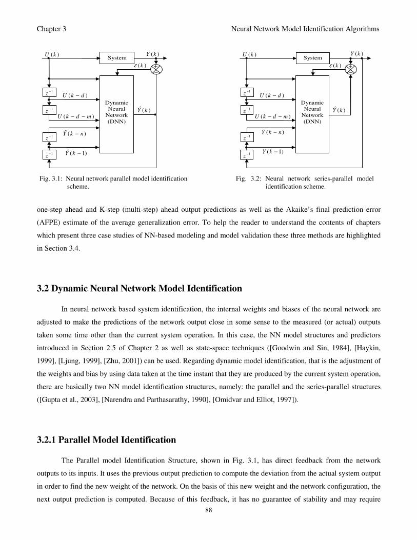
Chapter 3 Neural Network Model Identification Algorithms
88
Dynamic
Neural
Network
(DNN)
System
ˆ ( )Y k
( )U k
•
1z
−
1z
−
1z
−
1z
− ˆ ( 1)Y k −
ˆ ( )Y k n−
( )U k d m− −
( )U k d−
( )kε
( )Y k
•
•
• •
•
+ −
Dynamic
Neural
Network
(DNN)
System
ˆ ( )Y k
( )U k •
1z
−
1z
−
1z
−
1z
− ( 1)Y k −
( )Y k n−
( )U k d m− −
( )U k d−
( )kε
( )Y k
•
•
• •
•
+ −
Fig. 3.1: Neural network parallel model identification Fig. 3.2: Neural network series-parallel model
scheme. identification scheme.
one-step ahead and K-step (multi-step) ahead output predictions as well as the Akaike’s final prediction error
(AFPE) estimate of the average generalization error. To help the reader to understand the contents of chapters
which present three case studies of NN-based modeling and model validation these three methods are highlighted
in Section 3.4.
3.2 Dynamic Neural Network Model Identification
In neural network based system identification, the internal weights and biases of the neural network are
adjusted to make the predictions of the network output close in some sense to the measured (or actual) outputs
taken some time other than the current system operation. In this case, the NN model structures and predictors
introduced in Section 2.5 of Chapter 2 as well as state-space techniques ([Goodwin and Sin, 1984], [Haykin,
1999], [Ljung, 1999], [Zhu, 2001]) can be used. Regarding dynamic model identification, that is the adjustment of
the weights and bias by using data taken at the time instant that they are produced by the current system operation,
there are basically two NN model identification structures, namely: the parallel and the series-parallel structures
([Gupta et al., 2003], [Narendra and Parthasarathy, 1990], [Omidvar and Elliot, 1997]).
3.2.1 Parallel Model Identification
The Parallel model Identification Structure, shown in Fig. 3.1, has direct feedback from the network
outputs to its inputs. It uses the previous output prediction to compute the deviation from the actual system output
in order to find the new weight of the network. On the basis of this new weight and the network configuration, the
next output prediction is computed. Because of this feedback, it has no guarantee of stability and may require
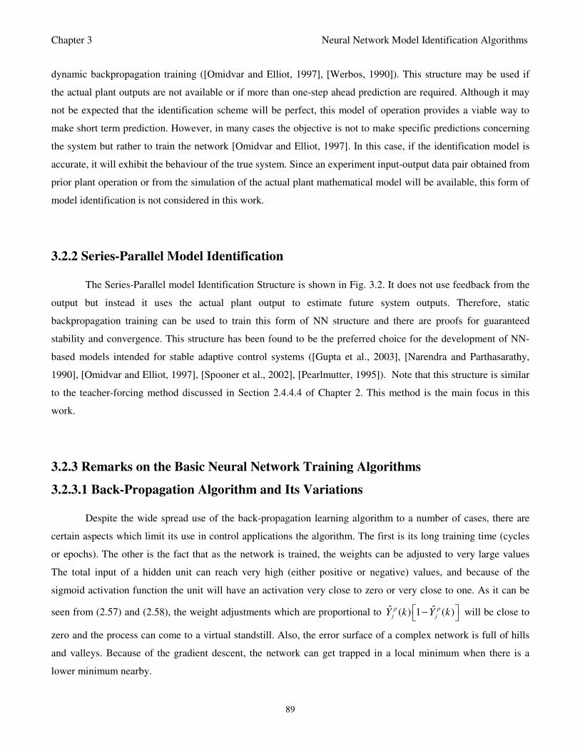
Chapter 3 Neural Network Model Identification Algorithms
89
dynamic backpropagation training ([Omidvar and Elliot, 1997], [Werbos, 1990]). This structure may be used if
the actual plant outputs are not available or if more than one-step ahead prediction are required. Although it may
not be expected that the identification scheme will be perfect, this model of operation provides a viable way to
make short term prediction. However, in many cases the objective is not to make specific predictions concerning
the system but rather to train the network [Omidvar and Elliot, 1997]. In this case, if the identification model is
accurate, it will exhibit the behaviour of the true system. Since an experiment input-output data pair obtained from
prior plant operation or from the simulation of the actual plant mathematical model will be available, this form of
model identification is not considered in this work.
3.2.2 Series-Parallel Model Identification
The Series-Parallel model Identification Structure is shown in Fig. 3.2. It does not use feedback from the
output but instead it uses the actual plant output to estimate future system outputs. Therefore, static
backpropagation training can be used to train this form of NN structure and there are proofs for guaranteed
stability and convergence. This structure has been found to be the preferred choice for the development of NN-
based models intended for stable adaptive control systems ([Gupta et al., 2003], [Narendra and Parthasarathy,
1990], [Omidvar and Elliot, 1997], [Spooner et al., 2002], [Pearlmutter, 1995]). Note that this structure is similar
to the teacher-forcing method discussed in Section 2.4.4.4 of Chapter 2. This method is the main focus in this
work.
3.2.3 Remarks on the Basic Neural Network Training Algorithms
3.2.3.1 Back-Propagation Algorithm and Its Variations
Despite the wide spread use of the back-propagation learning algorithm to a number of cases, there are
certain aspects which limit its use in control applications the algorithm. The first is its long training time (cycles
or epochs). The other is the fact that as the network is trained, the weights can be adjusted to very large values
The total input of a hidden unit can reach very high (either positive or negative) values, and because of the
sigmoid activation function the unit will have an activation very close to zero or very close to one. As it can be
seen from (2.57) and (2.58), the weight adjustments which are proportional to ˆ ˆ( ) 1 ( )p p
j jY k Y k − will be close to
zero and the process can come to a virtual standstill. Also, the error surface of a complex network is full of hills
and valleys. Because of the gradient descent, the network can get trapped in a local minimum when there is a
lower minimum nearby.
Chapter 3 Neural Network Model Identification Algorithms
90
Probabilistic methods can help to avoid this trap, but they tend to be slow. Another suggested possibility
is to increase the number of hidden units. Although this may work well because of the higher dimensionality of
the error space, and the chance to get trapped is smaller, it appears that there is some upper limit on the number of
hidden units which, when exceeded, results in having the network trapped in local minima. This can lead to
network overtraining and result in the peaking effects.
Several advanced algorithms based on the back-propagation learning and its variations have been
proposed over the years and many researchers have devised improvements of and extensions to the basic back-
propagation learning algorithms ([Wang et al., 2004]; [Werbos, 1990]). One major improvement by the addition
of adaptation parameters which has resulted in the widely used backpropagation with momentum (BPM) version
of the algorithm discussed in Section 2.4.4.1 ([Phansalkar and Sastry, 1994]; [Yu et al., 2006]). Another obvious
improvement is to the replacement of the primitive steepest descent method with a direction set minimization
method which has led to other several minimization algorithms ([Chiong, 2010]; [Hagan and Menhaj, 1994];
[Wu, 2008]). One of the objectives of this work is an extension of the back-propagation learning algorithm by
investigating a new minimization technique of the direction set in order to achieve a global minimum of the joint
weights, i.e. weight and biases.
3.2.3.2 Teacher-Forced Real-Time Recurrent Learning
The teacher-forced real-time recurrent learning (RTRL) consists of jamming the desired output values
into the network units as the network is being trained; thus the output units are forced to have the correct states
even during the network training phase. This technique is applied to discrete time clocked network because only
in this case only the concept of changing the state of the output unit at each time step makes sense [Pearlmutter,
1990] and [Pearmutter, 1995].
The errors in the teacher-forced RTRL method are usually measured before the output units are forced,
and not after that. Thus, this method leads to faster training because it is assumed that the network has learned
correctly the dynamics in the previous time steps [Haykin, 1999]. As noted in [Zipser and Williams, 1989] and
[Pearmutter, 1995], the computation time is radically reduced in contrast with the original computationally
intensive RTRL algorithm. Note that since the actual outputs of the system are fed back rather than the network,
no real recurrent path exists in the network; the backpropagation algorithm can readily be applied to train the
network as dynamic feedforward neural network (DFNN). In addition, the training does not diverge in an unstable
way. In fact, if the network is trained in a closed-loop manner with the true system, the weights at the beginning
of the training are randomly distributed and the predicted state may be quite different from the desired one. These
erroneous outputs are recursively fed back to the input layer to predict new states and so on until convergence
occurs [Guarneri et al., 2008].
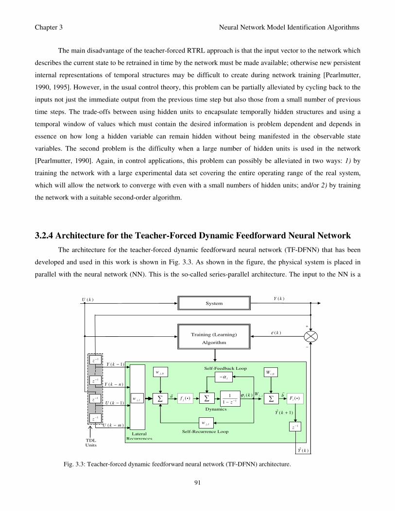
Chapter 3 Neural Network Model Identification Algorithms
91
1
1
1 z −−
,0jw,0iW
lα−
•
Self-Feedback Loop
Self-Recurrence Loop
ˆ ( )Y k
( )iF i
Dynamics
b
∑ ( )jf i
a
∑
,j lw
,i jW ( )l kϕ
1z −
Lateral
Recurrences
∑
( 1)Y k −
( )Y k n−
( 1)U k −
( )U k m−
( )U k ( )Y k
Training (Learning)
Algorithm
System
ˆ ( 1)Y k + 1z −
•
−
•
•
•
1z −
1z −
+
( )kε
1z −
TDL
Units
,j lw
Fig. 3.3: Teacher-forced dynamic feedforward neural network (TF-DFNN) architecture.
The main disadvantage of the teacher-forced RTRL approach is that the input vector to the network which
describes the current state to be retrained in time by the network must be made available; otherwise new persistent
internal representations of temporal structures may be difficult to create during network training [Pearlmutter,
1990, 1995]. However, in the usual control theory, this problem can be partially alleviated by cycling back to the
inputs not just the immediate output from the previous time step but also those from a small number of previous
time steps. The trade-offs between using hidden units to encapsulate temporally hidden structures and using a
temporal window of values which must contain the desired information is problem dependent and depends in
essence on how long a hidden variable can remain hidden without being manifested in the observable state
variables. The second problem is the difficulty when a large number of hidden units is used in the network
[Pearlmutter, 1990]. Again, in control applications, this problem can possibly be alleviated in two ways: 1) by
training the network with a large experimental data set covering the entire operating range of the real system,
which will allow the network to converge with even with a small numbers of hidden units; and/or 2) by training
the network with a suitable second-order algorithm.
3.2.4 Architecture for the Teacher-Forced Dynamic Feedforward Neural Network
The architecture for the teacher-forced dynamic feedforward neural network (TF-DFNN) that has been
developed and used in this work is shown in Fig. 3.3. As shown in the figure, the physical system is placed in
parallel with the neural network (NN). This is the so-called series-parallel architecture. The input to the NN is a
Chapter 3 Neural Network Model Identification Algorithms
92
state vector of the previous inputs and outputs via a bank of tapped delay line (TDL) memory units. With this
architecture, the state to be retrained is constituted by the previous state in time and replacing those values with
the new outputs from the system in a first-in first out-fashion. Thus, the TDL memory unit forms a sliding
window for the state vector. Note that in the proposed architecture, the system time delay has been assumed to be
one, 1.
The NN training or learning process basically involves the use a set of input-output data pair which are
obtained from a specific nonlinear function modeling the behaviour of the physical system. A more detailed
treatment and discussion of the proposed DFNN architecture together with its mathematical description and the
training (learning) algorithms will be presented successively in the next two chapters.
3.3 Training Algorithms for Neural Network Model Identification
3.3.1 Formulation of the Model Identification Problem
It was shown in Section 2.5 of Chapter 2 that the output ( )Y k of a p-input q-output for discrete-time
nonlinear multivariable system at time k responding to input ( )U k with disturbance ( )d k could be represented
in the following form:
( ) [ ( , ( ), ( )] ( )Y k J k k k d kϕ θ θ= + (3.1)
where ( , , )J i i i is a nonlinear function of its arguments, NZ is the set of input-output data (observations) pairs
obtained from prior system operation or experiment over NT period of time defined as
(1), (1) , ( ), ( ) 1,2, ,NZ U Y U N Y N k N= =… … (3.2)
where N is the number of input-output data pairs and T is the sampling period of the system, ( , ( ))k kϕ θ is the
regression (state) vector given as:
[
]
( , ( )) ( 1), , ( ), ( ), , ( ), ( 1, ( )), , ( , ( ))
( 1, ( )), , ( , ( )), ( 1, ( )), , ( , ( ))
a b c
T
f d
k k Y k Y k n U k d U k d n k k k n k
d k k d k n k v k k v k n k
ϕ θ ε θ ε θ
θ θ θ θ
= − − − − − − −
− − − −
… … …
… … (3.3)
( )kθ is an unknown parameter vector which contains the model parameters of (3.1) to be determined. Since ( )kθ
is unknown, let a parameterized set of model structures Θ that contains a set of candidate models be defined as:
ˆ: ( ) ( )k kν
θθ θΘ ∈ ⊂ ℜ → (3.4)
where θ is some subset of νℜ inside which the search for a model is carried out; ν is the dimension of ( )kθ ;
ˆ( )kθ is the desired model associated with the unknown parameter vector ( )kθ contained in the set of model
structures 1 2( ) , ( ), , ( )k k kτθ θ θΘ = … ; 1 2( ) , ( ), , ( )k k kτθ θ θ… are distinct values of ( )kθ ; and 1,2, ,maxiter
τ = … is
the number of iterations required to determine the ˆ( )kθ from within the set of models in Θ .
Chapter 3 Neural Network Model Identification Algorithms
93
As in Section 2.5 of Chapter 2, the one-step ahead predictor form of model (3.1) based on the information
up to time 1k − can be expressed in the following compact form ([Goodwin and Sin, 1984], [Ljung, 1999], [Zhu,
200]) as:
[ ]ˆ( | 1, ( )) ( , ( )), ( )Y k k k J k k kθ ϕ θ θ− = (3.5)
Note that as discussed in Chapter 2, the nonlinear model structures and predictors considered in this work are
those based on NNARX and NNARMAX models. These various models are distinguished in terms of the
regression vector being used in (3.5). Thus, the regression vector corresponding to NNARX and NNARMAX
models for use in the predictor model of (3.5) are given respectively as:
( ) [ ( 1), , ( ), ( ), , ( )]T
a bk Y k Y k n U k d U k d nϕ = − − − − −… … (3.6)
[ ]( , ( )) ( 1), , ( ), ( ), , ( ), ( , ( )), , ( , ( ))T
a b ck k Y k Y k n U k d U k d n k k k n kϕ θ ε θ ε θ= − − − − − −… … … (3.7)
Note that ( )kϕ in (3.6) does not contain ( )kθ as an argument which is an indication that the predictor is pure
dynamic feedforward NN without feedback (see Fig. 2.13), whereas ( , ( ))k kϕ θ in (3.7) contains ( )kθ with
feedback loops as shown in Fig. 2.14. The ( )kθ in (3.7) is an indication of the dependence of ( , ( ))k kϕ θ on the
error estimate based on the moving average inputs while ( )kθ in (3.8) is an indication of the dependence of
( , ( ))k kϕ θ on a priori predicted outputs. Although, the form of NNARMAX regressor in (3.7) corresponds to the
series-parallel scheme of Fig. 3.2 and the teacher forcing method can be imposed, it also contains additional
feedback which depends on past error estimates (see Fig. 2.14). On the other hand, the NNARX model structure
(see Fig. 2.13) can easily be configured to the series-parallel structure of Fig. 3.2 and it has been the most widely
used structure in literature.
Let the parameter vector corresponding to the true system (3.1) be 0( ) ( )k kθ θ= and so that (3.1) becomes
0 0 0( ) [ ( , ( ), ( )] ( )Y k J k k k d kϕ θ θ= + (3.8)
Assuming that, ,a b
n n and c
n are known, and given (3.2), the unknown parameter vector ( )kθ can be
determined in such a way that ˆ( | 1, ( )) ( )Y k k k Y kθ− ≈ using a suitable minimization procedure, in terms of the
error [ , ( )]k kε θ between (3.8) and (3.5) and defined as:
ˆ[ , ( )] ( ) ( , ( ))k k Y k Y k kε θ θ= − (3.9)
Then, the minimization problem of (3.9) can be formulated as a mean square error (MSE) type cost function
stated as:
( ) 21, ( ) [ ( , ( ))]
2
NN
k
J Z k k kN
θ ε θ= ∑ (3.10)
The minimization of (3.10) can be approached in several ways such as using numerical optimization algorithms,
recursive algorithms, evolutionary and genetic algorithms. In this work, two adaptive minimization algorithms are
proposed for solving (3.10).
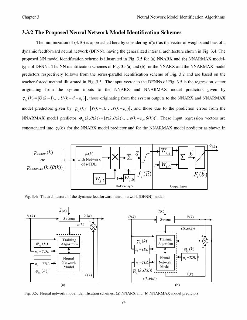
Chapter 3 Neural Network Model Identification Algorithms
94
3.3.2 The Proposed Neural Network Model Identification Schemes
The minimization of (3.10) is approached here by considering ˆ( )kθ as the vector of weights and bias of a
dynamic feedforward neural network (DFNN), having the generalized internal architecture shown in Fig. 3.4. The
proposed NN model identification scheme is illustrated in Fig. 3.5 for (a) NNARX and (b) NNARMAX model-
type of DFNNs. The NN identification schemes of Fig. 3.5(a) and (b) for the NNARX and the NNARMAX model
predictors respectively follows from the series-parallel identification scheme of Fig. 3.2 and are based on the
teacher-forced method illustrated in Fig. 3.3.. The input vector to the DFNNs of Fig. 3.5 is the regression vector
originating from the system inputs to the NNARX and NNARMAX model predictors given by
[ ]( ) ( 1), , ( )bn bk U k U k d nϕ = − − −… , those originating from the system outputs to the NNARX and NNARMAX
model predictors given by [ ]( ) ( 1), , ( )an ak Y k Y k nϕ = − −… , and those due to the prediction errors from the
NNARMAX model predictor ( , ( )) [ ( , ( )), , ( , ( ))]cn ck k k k k n kϕ θ ε θ ε θ= −… . These input regression vectors are
concatenated into ( )l
kϕ for the NNARX model predictor and for the NNARMAX model predictor as shown in
,0jw
∑ ,i j
W
Hidden layer
1
1
( )i
F b
( )j
f a
Output layer
b
a
ˆ( )Y k
( )
( , ( ( ))
NNARX
NNARMAX
k
or
k k
ϕ
ϕ θ
,j lw
×
,0iW
∑
( )l
kϕ
with Network
of l-TDL
Fig. 3.4: The architecture of the dynamic feedforward neural network (DFNN) model.
Training
Algorithm
Neural
Network
Model
bn TDL−
System
( )kε
ˆ ( )Y k
( )Y k ( )U k • •
•
• +
−
( )bn
kϕ
an TDL−
( )an
kϕ
( )d k
Training
Algorithm
Neural
Network
Model
b
n TDL−
a
n TDL−
System
( , ( ))k kε θ
ˆ( )Y k
( )Y k ( )U k • •
•
•
•
+
−
( )bn
kϕ
( )an kϕ
c
n TDL−
( , ( ))cn k kϕ θ
( )d k
•
( , ( ))k kε θ
(a) (b)
Fig. 3.5: Neural network model identification schemes: (a) NNARX and (b) NNARMAX model predictors.
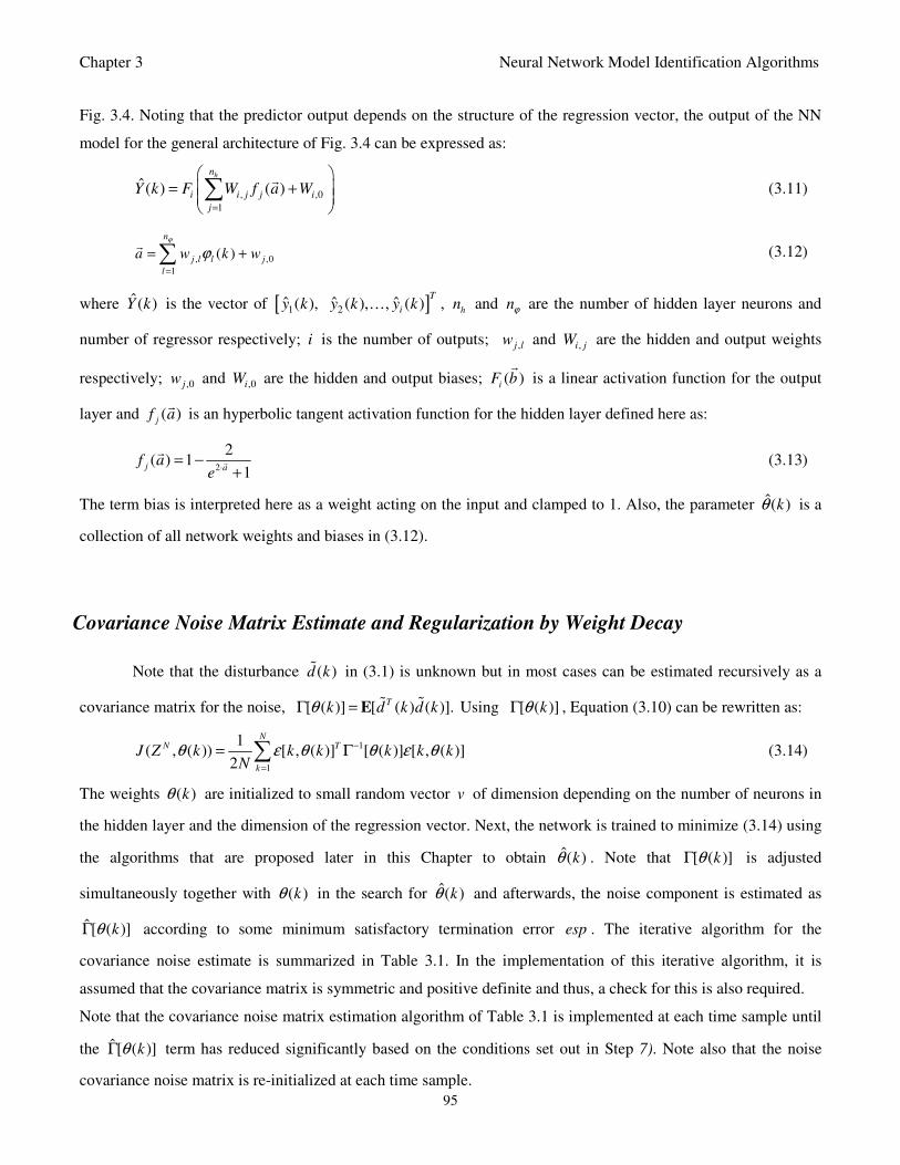
Chapter 3 Neural Network Model Identification Algorithms
95
Fig. 3.4. Noting that the predictor output depends on the structure of the regression vector, the output of the NN
model for the general architecture of Fig. 3.4 can be expressed as:
, ,0
1
ˆ( ) ( )hn
i i j j i
j
Y k F W f a W=
= +
∑
(3.11)
, ,0
1
( )
n
j l l j
l
a w k wϕ
ϕ=
= +∑
(3.12)
where ˆ( )Y k is the vector of [ ]1 2ˆ ˆ ˆ( ), ( ), , ( )
T
iy k y k y k… , h
n and nϕ are the number of hidden layer neurons and
number of regressor respectively; i is the number of outputs; ,j lw and ,i jW are the hidden and output weights
respectively; ,0jw and ,0iW are the hidden and output biases; ( )i
F b
is a linear activation function for the output
layer and ( )jf a
is an hyperbolic tangent activation function for the hidden layer defined here as:
2
2( ) 1
1j a
f ae
⋅= −
+
(3.13)
The term bias is interpreted here as a weight acting on the input and clamped to 1. Also, the parameter ˆ( )kθ is a
collection of all network weights and biases in (3.12).
Covariance Noise Matrix Estimate and Regularization by Weight Decay
Note that the disturbance ( )d k in (3.1) is unknown but in most cases can be estimated recursively as a
covariance matrix for the noise, [ ( )] [ ( ) ( )].Tk d k d kθΓ = E Using [ ( )]kθΓ , Equation (3.10) can be rewritten as:
1
1
1( , ( )) [ , ( )] [ ( )] [ , ( )]
2
NN T
k
J Z k k k k k kN
θ ε θ θ ε θ−
=
= Γ∑ (3.14)
The weights ( )kθ are initialized to small random vector v of dimension depending on the number of neurons in
the hidden layer and the dimension of the regression vector. Next, the network is trained to minimize (3.14) using
the algorithms that are proposed later in this Chapter to obtain ˆ( )kθ . Note that [ ( )]kθΓ is adjusted
simultaneously together with ( )kθ in the search for ˆ( )kθ and afterwards, the noise component is estimated as
ˆ[ ( )]kθΓ according to some minimum satisfactory termination error esp . The iterative algorithm for the
covariance noise estimate is summarized in Table 3.1. In the implementation of this iterative algorithm, it is
assumed that the covariance matrix is symmetric and positive definite and thus, a check for this is also required.
Note that the covariance noise matrix estimation algorithm of Table 3.1 is implemented at each time sample until
the ˆ[ ( )]kθΓ term has reduced significantly based on the conditions set out in Step 7). Note also that the noise
covariance noise matrix is re-initialized at each time sample.
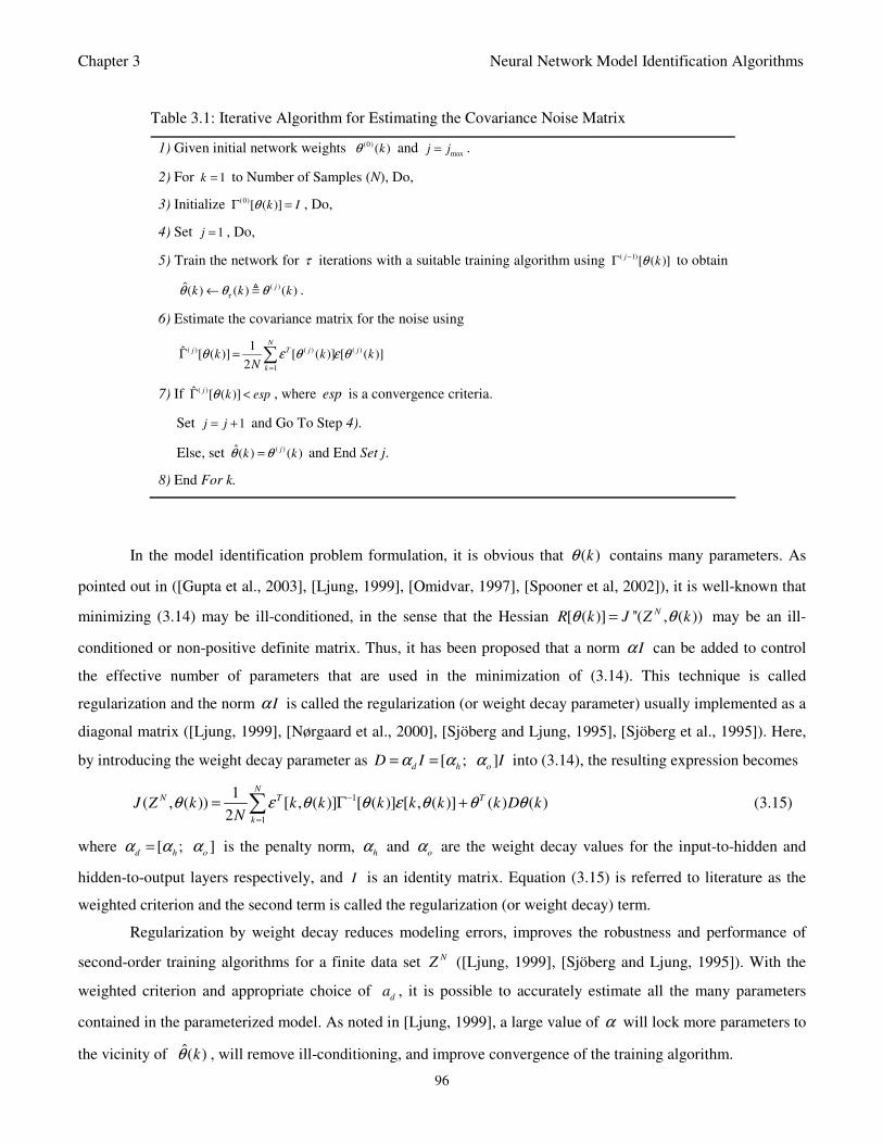
Chapter 3 Neural Network Model Identification Algorithms
96
In the model identification problem formulation, it is obvious that ( )kθ contains many parameters. As
pointed out in ([Gupta et al., 2003], [Ljung, 1999], [Omidvar, 1997], [Spooner et al, 2002]), it is well-known that
minimizing (3.14) may be ill-conditioned, in the sense that the Hessian [ ( )] ''( , ( ))NR k J Z kθ θ= may be an ill-
conditioned or non-positive definite matrix. Thus, it has been proposed that a norm Iα can be added to control
the effective number of parameters that are used in the minimization of (3.14). This technique is called
regularization and the norm Iα is called the regularization (or weight decay parameter) usually implemented as a
diagonal matrix ([Ljung, 1999], [Nørgaard et al., 2000], [Sjöberg and Ljung, 1995], [Sjöberg et al., 1995]). Here,
by introducing the weight decay parameter as [ ; ]d h o
D I Iα α α= = into (3.14), the resulting expression becomes
1
1
1( , ( )) [ , ( )] [ ( )] [ , ( )] ( ) ( )
2
NN T T
k
J Z k k k k k k k D kN
θ ε θ θ ε θ θ θ−
=
= Γ +∑ (3.15)
where [ ; ]d h o
α α α= is the penalty norm, h
α and o
α are the weight decay values for the input-to-hidden and
hidden-to-output layers respectively, and I is an identity matrix. Equation (3.15) is referred to literature as the
weighted criterion and the second term is called the regularization (or weight decay) term.
Regularization by weight decay reduces modeling errors, improves the robustness and performance of
second-order training algorithms for a finite data set NZ ([Ljung, 1999], [Sjöberg and Ljung, 1995]). With the
weighted criterion and appropriate choice ofd
a , it is possible to accurately estimate all the many parameters
contained in the parameterized model. As noted in [Ljung, 1999], a large value of α will lock more parameters to
the vicinity of ˆ( )kθ , will remove ill-conditioning, and improve convergence of the training algorithm.
Table 3.1: Iterative Algorithm for Estimating the Covariance Noise Matrix
1) Given initial network weights (0) ( )kθ and maxj j= .
2) For 1k = to Number of Samples (N), Do,
3) Initialize (0)[ ( )]k IθΓ = , Do,
4) Set 1j = , Do,
5) Train the network for τ iterations with a suitable training algorithm using ( 1)[ ( )]
jkθ−
Γ to obtain
( )ˆ( ) ( ) ( )jk k kτθ θ θ← .
6) Estimate the covariance matrix for the noise using
( ) ( ) ( )
1
1ˆ [ ( )] [ ( )] [ ( )]2
Nj T j j
k
k k kN
θ ε θ ε θ=
Γ = ∑
7) If ( )ˆ [ ( )]j
k espθΓ < , where esp is a convergence criteria.
Set 1j j= + and Go To Step 4).
Else, set ( )ˆ( ) ( )j
k kθ θ= and End Set j.
8) End For k.
Chapter 3 Neural Network Model Identification Algorithms
97
In the weighted criterion given by (3.15), note that both 1[ ( )]kθ−Γ and D are adjusted simultaneously
together with ( )kθ and used to update ˆ( )kθ . The next task is how to train the proposed neural network model
identification schemes illustrated in Fig. 3.5.
3.3.3 Backpropagation (BP) Techniques
The minimization of (3.15) is based on an iterative procedure which starts with a randomly initialized
0( ) ( )k kθ θ= and updates ˆ( )kθ iteratively according to the following typical updating rule
ˆ( ) ( ) ( )k k kτ τθ θ θ= + ∆ (3.16)
where ( )kτθ denotes the adjustable parameters of the network at the current iteration ,τ ( )kτθ∆ is the searching
direction. The algorithm of (3.16) is terminated if certain criteria or stopping conditions are satisfied.
As mentioned earlier, the most commonly used method for updating ˆ( )kθ is the BP algorithm introduced
in Chapter 2 ([Rumelhart et al, 1986], [Werbos, 1990]). This algorithm uses the gradient method and sets the
( )kτθ∆ directly proportional to the negative of the gradient of (3.10) evaluated at ( ) ( )k kτθ θ= . Using (3.10) and
(3.16), the BP algorithm can easily be stated as:
( ) ( )
[ ( )]ˆ( ) ( )( )
k k
dJ kk k
d kτ
τ τ
θ θ
θθ θ µ
θ=
= − (3.17)
where the second term in (3.17) corresponds to the search direction ( )kτθ∆ and τµ the step size. NN training
using the BP algorithm, with an approximate steepest descent rule, has been reported to be characterized by poor
performance in terms of poor convergence, poor robustness, long training cycle, and the trapping of several local
minima within the cost function ([Chiong, 2010], [Guarneri et al., 2008], [Song, 2010], [Wu, 2008]). To improve
the performance of the BP algorithm, the Gauss-Newton method has been widely used as a starting point for this
purpose. The ARLS and the MLMA algorithms proposed in this work are both derived from the Gauss-Newton
method.
3.3.4 The Gauss-Newton Second-Order Approximation Method
The quadratic criterion used for deriving the search direction of the Gauss-Newton method is briefly
reviewed to facilitate the formulation of the ARLS and MLMA algorithms. The Gauss-Newton method uses the
linear approximation error [ , ( )]k kτε θ to the [ , ( )]k kε θ in (3.9) which can be expressed as:

Chapter 3 Neural Network Model Identification Algorithms
98
[ ]
[ ]
( ) ( )
( ) ( )
[ , ( )][ , ( )] [ , ( )] ( ) ( )
( )
ˆ( | ( ))[ , ( )] ( ) ( )
( )
T
k k
T
k k
d k kk k k k k k
d k
dY k kk k k k
d k
τ
τ
τ τ τ
θ θ
τ τ
θ θ
ε θε θ ε θ θ θ
θ
θε θ θ θ
θ
=
=
= + −
= − −
(3.18)
where the coefficient of ( )kθ in the second term is the negative derivative of the network output ˆ( , ( ))Y k kθ with
respect to ( )kθ evaluated at ( ) ( )k kτθ θ= . Let [ , ( )]k kτψ θ be the derivative of the network output with respect to
( )kθ given in (3.18) and be defined as
ˆ( | ( ))[ , ( )]
( )
dY k kk k
d k
θψ θ
θ= (3.19)
The computation of (3.19) is carried out in a backpropagation fashion for the input-to-hidden layer and for the
hidden-to-output layers respectively for the two-layer NN considered in this work. The derivatives of the (3.19)
with respect to weights ( )kθ is the only component that impedes the implementation of the training algorithms
proposed in this work.
3.3.4.1 Computing the Gradient of the Network ψ[k,θ(k)]
Note that the three NN model predictors considered in this work are the NNARX and the NNARMAX
model predictors. Their main distinguishing feature is the structure of the regression vector ( , ( ))k kϕ θ . Using
(3.6) and (3.7), the derivatives for the NNARX and the NNARMAX model predictors can be expressed from
(3.19) as in the following computations. For notational convenience, the covariance matrix and the weight decay
terms are not included but their inclusion in the final result is straightforward as shown in sub-section 3.3.4.3.
The Derivative of the NNARX Model Predictor
Using (3.19), the derivative for the NNARX model predictor can be expressed as
ˆ( , ( ))[ , ( )]
( )NNARX
dY k kk k
d k
θψ θ
θ= (3.20)
Note that in the NNARX model predictor, the regression vector (3.6) does not depend on the weight as there is no
feedback, so it is straight forward to compute the partial derivatives of the network denoted as ( )kφ which
constitutes (3.20). Thus, Equation (3.20) can be rewritten as
ˆ ˆ( | ( )) ( | ( ))[ , ( )] ( )
( ) ( )NNARX
dY k k Y k kk k k
d k k
θ θψ θ φ
θ θ
∂= = =
∂ (3.21)
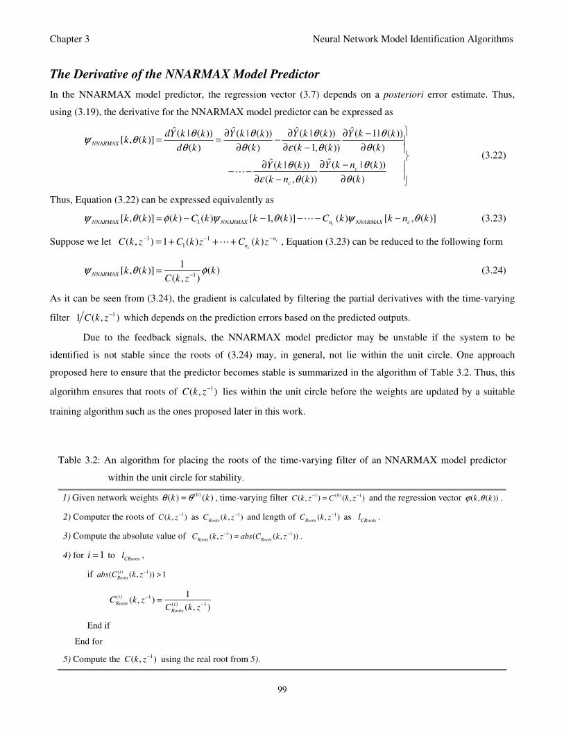
Chapter 3 Neural Network Model Identification Algorithms
99
The Derivative of the NNARMAX Model Predictor
In the NNARMAX model predictor, the regression vector (3.7) depends on a posteriori error estimate. Thus,
using (3.19), the derivative for the NNARMAX model predictor can be expressed as
ˆ ˆ ˆ ˆ( | ( )) ( | ( )) ( | ( )) ( 1| ( ))[ , ( )]
( ) ( ) ( 1, ( )) ( )
ˆˆ ( | ( ))( | ( ))
( , ( )) ( )
NNARMAX
c
c
dY k k Y k k Y k k Y k kk k
d k k k k k
Y k n kY k k
k n k k
θ θ θ θψ θ
θ θ ε θ θ
θθ
ε θ θ
∂ ∂ ∂ −= = −
∂ ∂ − ∂
∂ −∂ − − ∂ − ∂
(3.22)
Thus, Equation (3.22) can be expressed equivalently as
1[ , ( )] ( ) ( ) [ 1, ( )] ( ) [ , ( )]cNNARMAX NNARMAX n NNARMAX ck k k C k k k C k k n kψ θ φ ψ θ ψ θ= − − − − − (3.23)
Suppose we let 1 1
1( , ) 1 ( ) ( ) c
c
n
nC k z C k z C k z−− −= + + + , Equation (3.23) can be reduced to the following form
1
1[ , ( )] ( )
( , )NNARMAX k k k
C k zψ θ φ
−= (3.24)
As it can be seen from (3.24), the gradient is calculated by filtering the partial derivatives with the time-varying
filter 11 ( , )C k z− which depends on the prediction errors based on the predicted outputs.
Due to the feedback signals, the NNARMAX model predictor may be unstable if the system to be
identified is not stable since the roots of (3.24) may, in general, not lie within the unit circle. One approach
proposed here to ensure that the predictor becomes stable is summarized in the algorithm of Table 3.2. Thus, this
algorithm ensures that roots of 1( , )C k z− lies within the unit circle before the weights are updated by a suitable
training algorithm such as the ones proposed later in this work.
Table 3.2: An algorithm for placing the roots of the time-varying filter of an NNARMAX model predictor
within the unit circle for stability.
1) Given network weights (0)( ) ( )k kθ θ= , time-varying filter 1 (0) 1( , ) ( , )C k z C k z
− −= and the regression vector ( , ( ))k kϕ θ .
2) Computer the roots of 1( , )C k z
− as 1( , )Roots
C k z− and length of 1( , )Roots
C k z− asCRoots
l .
3) Compute the absolute value of 1 1( , ) ( ( , ))Roots Roots
C k z abs C k z− −= .
4) for 1i = toCRoots
l ,
if ( ) 1( ( , )) 1i
Rootsabs C k z− >
( ) 1
( ) 1
1( , )
( , )
i
Roots i
Roots
C k zC k z
−
−=
End if
End for
5) Compute the 1( , )C k z− using the real root from 5).
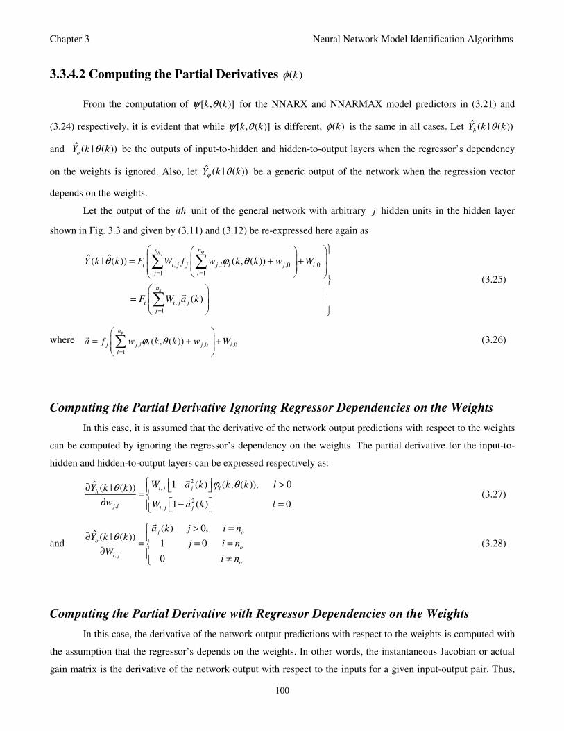
Chapter 3 Neural Network Model Identification Algorithms
100
3.3.4.2 Computing the Partial Derivatives ( )kφ
From the computation of [ , ( )]k kψ θ for the NNARX and NNARMAX model predictors in (3.21) and
(3.24) respectively, it is evident that while [ , ( )]k kψ θ is different, ( )kφ is the same in all cases. Let ˆ ( | ( ))h
Y k kθ
and ˆ ( | ( ))o
Y k kθ be the outputs of input-to-hidden and hidden-to-output layers when the regressor’s dependency
on the weights is ignored. Also, let ˆ ( | ( ))Y k kϕ θ be a generic output of the network when the regression vector
depends on the weights.
Let the output of the ith unit of the general network with arbitrary j hidden units in the hidden layer
shown in Fig. 3.3 and given by (3.11) and (3.12) be re-expressed here again as
, , ,0 ,0
1 1
,
1
ˆˆ( | ( )) ( , ( ))
( )
h
h
nn
i i j j j l l j i
j l
n
i i j j
j
Y k k F W f w k k w W
F W a k
ϕ
θ ϕ θ= =
=
= + +
=
∑ ∑
∑
(3.25)
where , ,0 ,0
1
( , ( ))
n
j j l l j i
l
a f w k k w Wϕ
ϕ θ=
= + + ∑
(3.26)
Computing the Partial Derivative Ignoring Regressor Dependencies on the Weights
In this case, it is assumed that the derivative of the network output predictions with respect to the weights
can be computed by ignoring the regressor’s dependency on the weights. The partial derivative for the input-to-
hidden and hidden-to-output layers can be expressed respectively as:
2
,
2, ,
1 ( ) ( , ( )), 0ˆ ( | ( ))
1 ( ) 0
i j j lh
j l i j j
W a k k k lY k k
w W a k l
ϕ θθ − >∂ =
∂ − =
(3.27)
and ,
( ) 0,ˆ ( | ( ))
1 0
0
j o
o
o
i j
o
a k j i nY k k
j i nW
i n
θ> =
∂ = = =
∂ ≠
(3.28)
Computing the Partial Derivative with Regressor Dependencies on the Weights
In this case, the derivative of the network output predictions with respect to the weights is computed with
the assumption that the regressor’s depends on the weights. In other words, the instantaneous Jacobian or actual
gain matrix is the derivative of the network output with respect to the inputs for a given input-output pair. Thus,
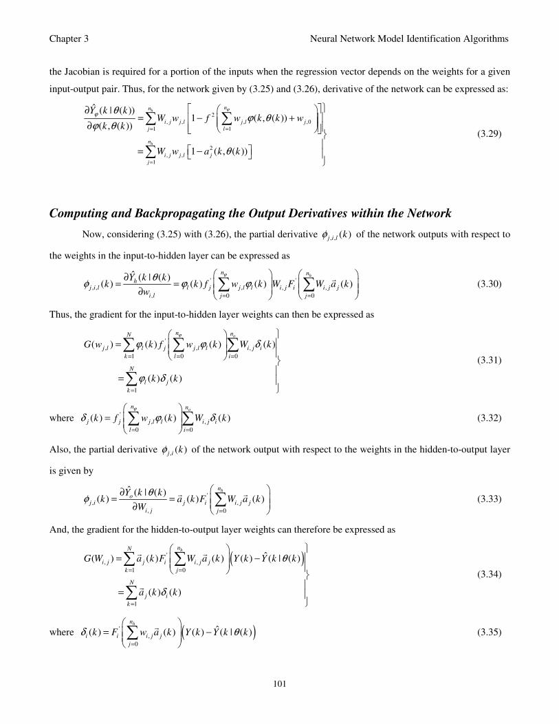
Chapter 3 Neural Network Model Identification Algorithms
101
the Jacobian is required for a portion of the inputs when the regression vector depends on the weights for a given
input-output pair. Thus, for the network given by (3.25) and (3.26), derivative of the network can be expressed as:
2
, , , ,0
1 1
2
, ,
1
ˆ ( | ( ))1 ( , ( ))
( , ( ))
1 ( , ( ))
h
h
nn
i j j l j l j
j l
n
i j j l j
j
Y k kW w f w k k w
k k
W w a k k
ϕ
ϕ θϕ θ
ϕ θ
θ
= =
=
∂= − + ∂
= −
∑ ∑
∑
(3.29)
Computing and Backpropagating the Output Derivatives within the Network
Now, considering (3.25) with (3.26), the partial derivative , , ( )j i l kφ of the network outputs with respect to
the weights in the input-to-hidden layer can be expressed as
' ', , , , ,
, 0 0
ˆ ( | ( )( ) ( ) ( ) ( )
hn n
hj i l l j j l l i j i i j j
i l j j
Y k kk k f w k W F W a k
w
ϕθφ ϕ ϕ
= =
∂= =
∂ ∑ ∑
(3.30)
Thus, the gradient for the input-to-hidden layer weights can then be expressed as
', , ,
1 0 0
1
( ) ( ) ( ) ( )
( ) ( )
on nN
j l l j j l l i j i
k l i
N
l j
k
G w k f w k W k
k k
ϕ
ϕ ϕ δ
ϕ δ
= = =
=
=
=
∑ ∑ ∑
∑ (3.31)
where ', ,
0 0
( ) ( ) ( )o
n n
j j j l l i j i
l i
k f w k W kϕ
δ ϕ δ= =
=
∑ ∑ (3.32)
Also, the partial derivative , ( )j i kφ of the network output with respect to the weights in the hidden-to-output layer
is given by
', ,
, 0
ˆ ( | ( )( ) ( ) ( )
hn
oj i j i i j j
i j j
Y k kk a k F W a k
W
θφ
=
∂= =
∂ ∑
(3.33)
And, the gradient for the hidden-to-output layer weights can therefore be expressed as
( )', ,
1 0
1
ˆ( ) ( ) ( ) ( ) ( | ( )
( ) ( )
hnN
i j j i i j j
k j
N
j i
k
G W a k F W a k Y k Y k k
a k k
θ
δ
= =
=
= −
=
∑ ∑
∑
(3.34)
where ( )',
0
ˆ( ) ( ) ( ) ( | ( )hn
i i i j j
j
k F w a k Y k Y k kδ θ=
= −
∑
(3.35)
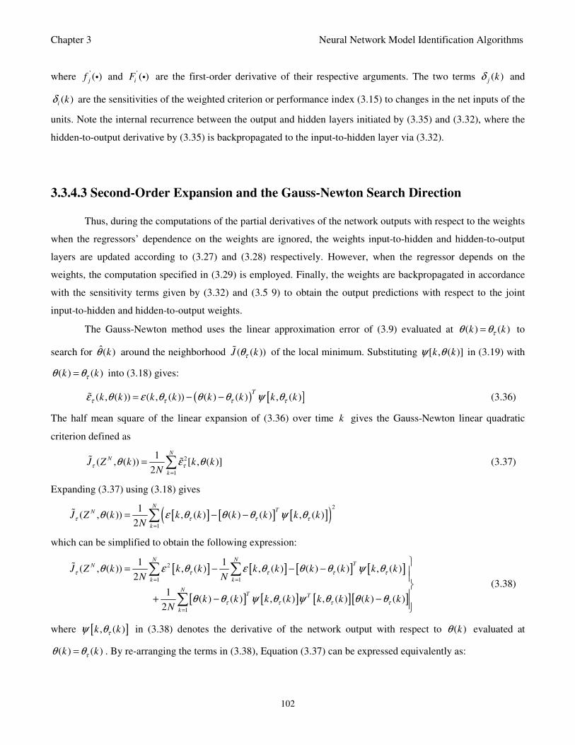
Chapter 3 Neural Network Model Identification Algorithms
102
where '( )jf i and ' ( )iF i are the first-order derivative of their respective arguments. The two terms ( )j kδ and
( )i kδ are the sensitivities of the weighted criterion or performance index (3.15) to changes in the net inputs of the
units. Note the internal recurrence between the output and hidden layers initiated by (3.35) and (3.32), where the
hidden-to-output derivative by (3.35) is backpropagated to the input-to-hidden layer via (3.32).
3.3.4.3 Second-Order Expansion and the Gauss-Newton Search Direction
Thus, during the computations of the partial derivatives of the network outputs with respect to the weights
when the regressors’ dependence on the weights are ignored, the weights input-to-hidden and hidden-to-output
layers are updated according to (3.27) and (3.28) respectively. However, when the regressor depends on the
weights, the computation specified in (3.29) is employed. Finally, the weights are backpropagated in accordance
with the sensitivity terms given by (3.32) and (3.5 9) to obtain the output predictions with respect to the joint
input-to-hidden and hidden-to-output weights.
The Gauss-Newton method uses the linear approximation error of (3.9) evaluated at ( ) ( )k kτθ θ= to
search for ˆ( )kθ around the neighborhood ( ( ))J kτθ of the local minimum. Substituting [ , ( )]k kψ θ in (3.19) with
( ) ( )k kτθ θ= into (3.18) gives:
( ) [ ]( , ( )) ( , ( )) ( ) ( ) , ( )T
k k k k k k k kτ τ τ τε θ ε θ θ θ ψ θ= − − (3.36)
The half mean square of the linear expansion of (3.36) over time k gives the Gauss-Newton linear quadratic
criterion defined as
2
1
1( , ( )) [ , ( )]
2
NN
k
J Z k k kN
τ τθ ε θ=
= ∑ (3.37)
Expanding (3.37) using (3.18) gives
[ ] [ ] [ ]( )2
1
1( , ( )) , ( ) ( ) ( ) , ( )
2
NTN
k
J Z k k k k k k kN
τ τ τ τθ ε θ θ θ ψ θ=
= − −∑
which can be simplified to obtain the following expression:
[ ] [ ] [ ] [ ]
[ ] [ ] [ ][ ]
2
1 1
1
1 1( , ( )) , ( ) , ( ) ( ) ( ) , ( )
2
1( ) ( ) , ( ) , ( ) ( ) ( )
2
N NTN
k k
NT T
k
J Z k k k k k k k k kN N
k k k k k k k kN
τ τ τ τ τ
τ τ τ τ
θ ε θ ε θ θ θ ψ θ
θ θ ψ θ ψ θ θ θ
= =
=
= − − −
+ − −
∑ ∑
∑
(3.38)
where [ ], ( )k kτψ θ in (3.38) denotes the derivative of the network output with respect to ( )kθ evaluated at
( ) ( )k kτθ θ= . By re-arranging the terms in (3.38), Equation (3.37) can be expressed equivalently as:
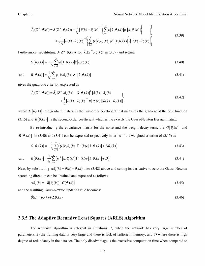
Chapter 3 Neural Network Model Identification Algorithms
103
[ ] [ ] [ ]
[ ] [ ] [ ] [ ]
1
1
1( , ( )) ( , ( )) ( ) ( ) , ( ) , ( )
1( ) ( ) , ( ) , ( ) ( ) ( )
2
NTN N
k
NT T
k
J Z k J Z k k k k k k kN
k k k k k k k kN
τ τ τ τ τ
τ τ τ τ
θ θ θ θ ε θ ψ θ
θ θ ψ θ ψ θ θ θ
=
=
= − −
+ − −
∑
∑
(3.39)
Furthermore, substituting ( , ( ))NJ Z kτθ for ( , ( ))N
J Z kτ τθ in (3.39) and setting
[ ] [ ] [ ]1
1( ) , ( ) , ( )
N
k
G k k k k kN
τ τ τθ ψ θ ε θ=
= − ∑ (3.40)
and [ ] [ ] [ ]1
1( ) , ( ) , ( )
NT
k
R k k k k kN
τ τ τθ ψ θ ψ θ=
= ∑ (3.41)
gives the quadratic criterion expressed as
[ ] [ ]
[ ] [ ][ ]
( , ( )) ( , ( )) ( ) ( ) ( )
1( ) ( ) ( ) ( ) ( )
2
TN N
T
J Z k J Z k G k k k
k k R k k k
τ τ τ τ τ
τ τ τ
θ θ θ θ θ
θ θ θ θ θ
= + −
+ − −
(3.42)
where [ ]( )G kτθ , the gradient matrix, is the first-order coefficient that measures the gradient of the cost function
(3.15) and [ ]( )R kτθ is the second-order coefficient which is the exactly the Gauss-Newton Hessian matrix.
By re-introducing the covariance matrix for the noise and the weight decay term, the [ ]( )G kτθ and
[ ]( )R kτθ in (3.40) and (3.41) can be expressed respectively in terms of the weighted criterion of (3.15) as
[ ] [ ] [ ]( )1
1
1( ) , ( ) ( ) , ( ) ( )
N
k
G k k k k k k D kN
τ τ τ τθ ψ θ ε θ θ−
=
= − Γ +∑ (3.43)
and [ ] [ ] [ ]( )1
1
1( ) , ( ) ( ) , ( )
NT
k
R k k k k k k DN
τ τ τθ ψ θ ψ θ−
=
= Γ +∑ (3.44)
Next, by substituting ( ) ( ) ( )k k kτ τθ θ θ∆ = − into (3.42) above and setting its derivative to zero the Gauss-Newton
searching direction can be obtained and expressed as follows
1( ) [ ( )] [ ( )]k R k G kτ τ τθ θ θ−∆ = − (3.45)
and the resulting Gauss-Newton updating rule becomes:
ˆ( ) ( ) ( )k k kτ τθ θ θ= + ∆ (3.46)
3.3.5 The Adaptive Recursive Least Squares (ARLS) Algorithm
The recursive algorithm is relevant in situations: 1) when the network has very large number of
parameters, 2) the training data is very large and there is lack of sufficient memory, and 3) where there is high
degree of redundancy in the data set. The only disadvantage is the excessive computation time when compared to
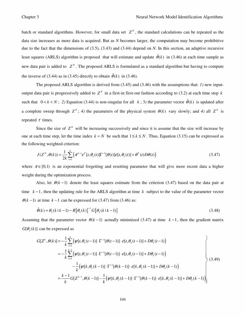
Chapter 3 Neural Network Model Identification Algorithms
104
batch or standard algorithms. However, for small data set NZ , the standard calculations can be repeated as the
data size increases as more data is acquired. But as N becomes larger, the computation may become prohibitive
due to the fact that the dimensions of (3.5), (3.43) and (3.44) depend on N. In this section, an adaptive recursive
least squares (ARLS) algorithm is proposed that will estimate and update ˆ( )kθ in (3.46) at each time sample as
new data pair is added to NZ . The proposed ARLS is formulated as a standard algorithm but having to compute
the inverse of (3.44) as in (3.45) directly to obtain ˆ( )kθ in (3.46).
The proposed ARLS algorithm is derived from (3.45) and (3.46) with the assumptions that: 1) new input-
output data pair is progressively added to NZ in a first-in first-out fashion according to (3.2) at each time step k
such that 0 k N< < ; 2) Equation (3.44) is non-singular for all k ; 3) the parameter vector ˆ( )kθ is updated after
a complete sweep through NZ ; 4) the parameters of the physical system ( )kθ vary slowly; and 4) all NZ is
repeated τ times.
Since the size of NZ will be increasing successively and since it is assume that the size will increase by
one at each time step, let the time index k N= be such that 1 k N≤ ≤ . Thus, Equation (3.15) can be expressed as
the following weighted criterion:
( )1
1
1( , ( )) [ , ( )] [ ( )] [ , ( )] ( ) ( )
2
kN k T T
J Z k Dk
ι
τ τ
ι
θ π ε ι θ ι θ ι ε ι θ ι θ ι θ ι− −
=
= Γ +∑ (3.47)
where [0,1)π ∈ is an exponential forgetting and resetting parameter that will give more recent data a higher
weight during the optimization process.
Also, let ( 1)kθ − denote the least squares estimate from the criterion (3.47) based on the data pair at
time 1k − , then the updating rule for the ARLS algorithm at time k subject to the value of the parameter vector
( 1)kθ − at time 1k − can be expressed for (3.47) from (3.46) as:
[ ] [ ]1ˆ( ) ( | 1) ( ) ( | 1)k k k R k G k kτ τ τθ θ θ θ
−= − − − (3.48)
Assuming that the parameter vector ( 1)kθ − actually minimized (3.47) at time 1k − , then the gradient matrix
[ ( )]G kτθ can be expressed as
( )
( )
( )
1
1
11
1
1
1
1[ , ( )] [ , ( 1)] [ ( 1)] [ , ( 1)] ( 1)
1[ , ( 1)] [ ( 1)] [ , ( 1)] ( 1)
1[ , ( 1)] [ ( 1)] [ , ( 1)] ( 1)
1 1[ , ( 1)] [ , (
kk
k
k
G Z k Dk
Dk
k k k k k D kk
kG Z k k
k k
τ τ τ
ι
τ τ τ
ι
τ τ τ
τ
θ ψ ι θ ι θ ι ε ι θ ι θ ι
ψ ι θ ι θ ι ε ι θ ι θ ι
ψ θ θ ε θ θ
θ ψ θ
−
=
−−
=
−
−
= − − ⋅Γ − ⋅ − + −
= − − ⋅Γ − ⋅ − + −
− − ⋅ Γ − ⋅ − + −
−= − −
∑
∑
( )11)] [ ( 1)] [ , ( 1)] ( 1)k k k k D kτ τθ ε θ θ−
− ⋅Γ − ⋅ − + −
(3.49)
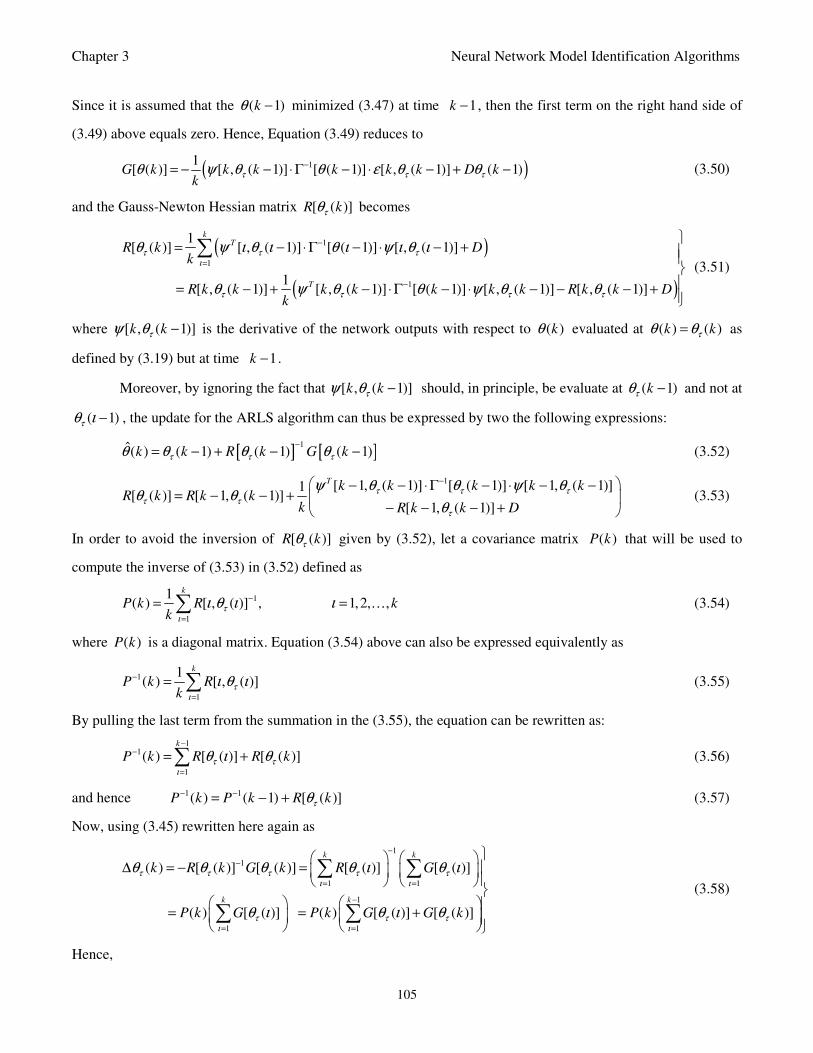
Chapter 3 Neural Network Model Identification Algorithms
105
Since it is assumed that the ( 1)kθ − minimized (3.47) at time 1k − , then the first term on the right hand side of
(3.49) above equals zero. Hence, Equation (3.49) reduces to
( )11[ ( )] [ , ( 1)] [ ( 1)] [ , ( 1)] ( 1)G k k k k k k D k
kτ τ τθ ψ θ θ ε θ θ−
= − − ⋅ Γ − ⋅ − + − (3.50)
and the Gauss-Newton Hessian matrix [ ( )]R kτθ becomes
( )
( )
1
1
1
1[ ( )] [ , ( 1)] [ ( 1)] [ , ( 1)]
1[ , ( 1)] [ , ( 1)] [ ( 1)] [ , ( 1)] [ , ( 1)]
kT
T
R k Dk
R k k k k k k k R k k Dk
τ τ τ
ι
τ τ τ τ
θ ψ ι θ ι θ ι ψ ι θ ι
θ ψ θ θ ψ θ θ
−
=
−
= − ⋅ Γ − ⋅ − +
= − + − ⋅Γ − ⋅ − − − +
∑ (3.51)
where [ , ( 1)]k kτψ θ − is the derivative of the network outputs with respect to ( )kθ evaluated at ( ) ( )k kτθ θ= as
defined by (3.19) but at time 1k − .
Moreover, by ignoring the fact that [ , ( 1)]k kτψ θ − should, in principle, be evaluate at ( 1)kτθ − and not at
( 1)τθ ι − , the update for the ARLS algorithm can thus be expressed by two the following expressions:
[ ] [ ]1ˆ( ) ( 1) ( 1) ( 1)k k R k G kτ τ τθ θ θ θ
−= − + − − (3.52)
1[ 1, ( 1)] [ ( 1)] [ 1, ( 1)]1[ ( )] [ 1, ( 1)]
[ 1, ( 1)]
Tk k k k k
R k R k kk R k k D
τ τ τ
τ τ
τ
ψ θ θ ψ θθ θ
θ
− − − ⋅Γ − ⋅ − −= − − +
− − − + (3.53)
In order to avoid the inversion of [ ( )]R kτθ given by (3.52), let a covariance matrix ( )P k that will be used to
compute the inverse of (3.53) in (3.52) defined as
1
1
1( ) [ , ( )] , 1,2, ,
k
P k R kk
τ
ι
ι θ ι ι−
=
= =∑ … (3.54)
where ( )P k is a diagonal matrix. Equation (3.54) above can also be expressed equivalently as
1
1
1( ) [ , ( )]
k
P k Rk
τ
ι
ι θ ι−
=
= ∑ (3.55)
By pulling the last term from the summation in the (3.55), the equation can be rewritten as:
11
1
( ) [ ( )] [ ( )]k
P k R R kτ τ
ι
θ ι θ−
−
=
= +∑ (3.56)
and hence 1 1( ) ( 1) [ ( )]P k P k R kτθ− −= − + (3.57)
Now, using (3.45) rewritten here again as
1
1
1 1
1
1 1
( ) [ ( )] [ ( )] [ ( )] [ ( )]
( ) [ ( )] ( ) [ ( )] [ ( )]
k k
k k
k R k G k R G
P k G P k G G k
τ τ τ τ τ
ι ι
τ τ τ
ι ι
θ θ θ θ ι θ ι
θ ι θ ι θ
−
−
= =
−
= =
∆ = − =
= = +
∑ ∑
∑ ∑ (3.58)
Hence,
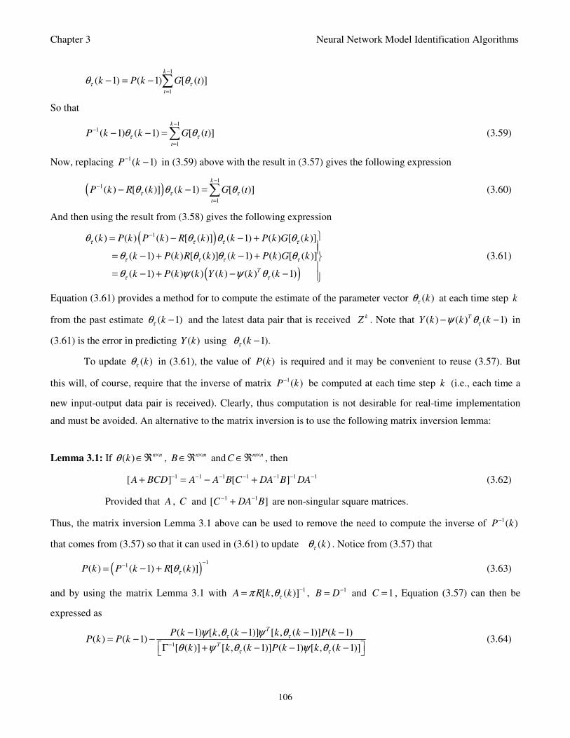
Chapter 3 Neural Network Model Identification Algorithms
106
1
1
( 1) ( 1) [ ( )]k
k P k Gτ τ
ι
θ θ ι−
=
− = − ∑
So that
11
1
( 1) ( 1) [ ( )]k
P k k Gτ τ
ι
θ θ ι−
−
=
− − =∑ (3.59)
Now, replacing 1( 1)P k− − in (3.59) above with the result in (3.57) gives the following expression
( )1
1
1
( ) [ ( )] ( 1) [ ( )]k
P k R k k Gτ τ τ
ι
θ θ θ ι−
−
=
− − =∑ (3.60)
And then using the result from (3.58) gives the following expression
( )
( )
1( ) ( ) ( ) [ ( )] ( 1) ( ) [ ( )]
( 1) ( ) [ ( )] ( 1) ( ) [ ( )]
( 1) ( ) ( ) ( ) ( ) ( 1)T
k P k P k R k k P k G k
k P k R k k P k G k
k P k k Y k k k
τ τ τ τ
τ τ τ τ
τ τ
θ θ θ θ
θ θ θ θ
θ ψ ψ θ
− = − − +
= − + − +
= − + − −
(3.61)
Equation (3.61) provides a method for to compute the estimate of the parameter vector ( )kτθ at each time step k
from the past estimate ( 1)kτθ − and the latest data pair that is received kZ . Note that ( ) ( ) ( 1)T
Y k k kτψ θ− − in
(3.61) is the error in predicting ( )Y k using ( 1).kτθ −
To update ( )kτθ in (3.61), the value of ( )P k is required and it may be convenient to reuse (3.57). But
this will, of course, require that the inverse of matrix 1( )P k− be computed at each time step k (i.e., each time a
new input-output data pair is received). Clearly, thus computation is not desirable for real-time implementation
and must be avoided. An alternative to the matrix inversion is to use the following matrix inversion lemma:
Lemma 3.1: If ( ) n nkθ ×∈ℜ , n m
B×∈ℜ and m n
C×∈ℜ , then
1 1 1 1 1 1 1[ ] [ ]A BCD A A B C DA B DA− − − − − − −+ = − + (3.62)
Provided that A , C and 1 1[ ]C DA B− −+ are non-singular square matrices.
Thus, the matrix inversion Lemma 3.1 above can be used to remove the need to compute the inverse of 1( )P k−
that comes from (3.57) so that it can used in (3.61) to update ( )kτθ . Notice from (3.57) that
( )1
1( ) ( 1) [ ( )]P k P k R kτθ−
−= − + (3.63)
and by using the matrix Lemma 3.1 with 1[ , ( )]A R k kτπ θ −= , 1B D−= and 1C = , Equation (3.57) can then be
expressed as
1
( 1) [ , ( 1)] [ , ( 1)] ( 1)( ) ( 1)
[ ( )] [ , ( 1)] ( 1) [ , ( 1)]
T
T
P k k k k k P kP k P k
k k k P k k k
τ τ
τ τ
ψ θ ψ θ
θ ψ θ ψ θ−
− − − −= − −
Γ + − − − (3.64)
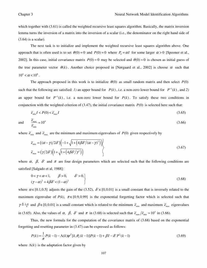
Chapter 3 Neural Network Model Identification Algorithms
107
which together with (3.61) is called the weighted recursive least squares algorithm. Basically, the matrix inversion
lemma turns the inversion of a matrix into the inversion of a scalar (i.e., the denominator on the right hand side of
(3.64) is a scalar).
The next task is to initialize and implement the weighted recursive least squares algorithm above. One
approach that is often used is to set (0) 0θ = and (0) 0P = where 0
P Iα= for some larger 0α > [Spooner et al.,
2002]. In this case, initial covariance matrix (0) 0P = may be selected and (0) 0θ = is chosen as initial guess of
the true parameter vector ( )kθ . Another choice proposed in [Nørgaard et al., 2002] is choose α such that
4 810 10α< < .
The approach proposed in this work is to initialize (0)θ as small random matrix and then select (0)P
such that the following are satisfied: 1) an upper bound for ( )P k , i.e. a non-zero lower bound for 1( )P k− , and 2)
an upper bound for 1( )P k− , i.e. a non-zero lower bound for ( )P k . To satisfy these two conditions in
conjunction with the weighted criterion of (3.47), the initial covariance matrix (0)P is selected here such that:
min max(0)e I P e I< < (3.65)
and 4max
min
10e
e (3.66)
where min
e and max
e are the minimum and maximum eigenvalues of (0)P given respectively by
( ) ( )( )( ) ( )( )
2
min
2
max
( ) 2 ' 1 1 4 ' ( )
2 ' 1 1 4 '
e
e
α γ δ βδ α γ
γ δ βδ γ
= − − + + −= + +
(3.67)
where ,α ,β 'δ and π are four design parameters which are selected such that the following conditions are
satisfied [Salgado et al, 1988]:
2 2
0 1, 0, ' 0,
( ) 4 ' (1 )
γ α β δ
γ α βδ α
< < < > >
− + < − (3.68)
where [0.1,0.5]α ∈ adjusts the gain of the (3.52), ' [0,0.01]δ ∈ is a small constant that is inversely related to the
maximum eigenvalue of P(k), [0.9,0.99]π ∈ is the exponential forgetting factor which is selected such that
1 ππ
γ − and [0,0.01]β ∈ is a small constant which is related to the minimum min
e and maximum max
e eigenvalues
in (3.65). Also, the values of ,α ,β 'δ and π in (3.68) is selected such that 4
max min 10e e in (3.66).
Thus, the new formula for the computation of the covariance matrix of (3.68) based on the exponential
forgetting and resetting parameter in (3.47) can be expressed as follows:
21( ) ( 1) ( ) [ , ( 1)] ( 1) ' ( 1)T
P k P k k k k P k I P kτψ θ β δπ
= − − Λ − − + − − (3.69)
where ( )kΛ is the adaptation factor given by
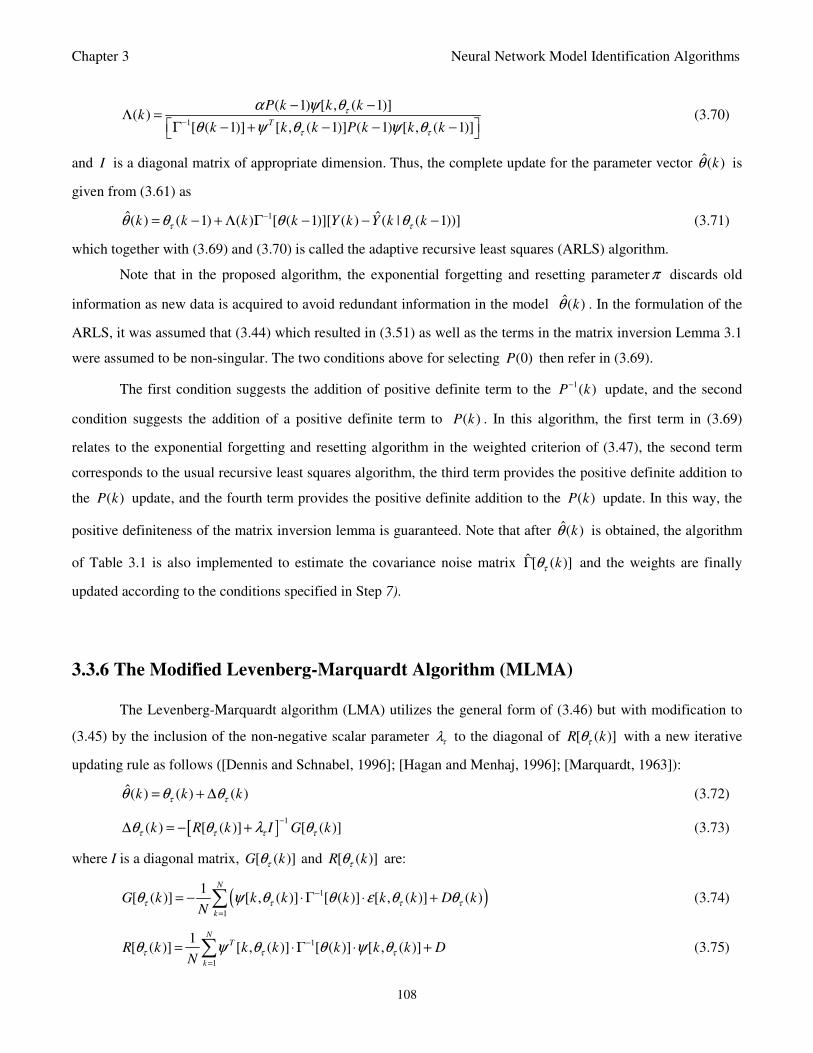
Chapter 3 Neural Network Model Identification Algorithms
108
1
( 1) [ , ( 1)]( )
[ ( 1)] [ , ( 1)] ( 1) [ , ( 1)]T
P k k kk
k k k P k k k
τ
τ τ
α ψ θ
θ ψ θ ψ θ−
− −Λ =
Γ − + − − − (3.70)
and I is a diagonal matrix of appropriate dimension. Thus, the complete update for the parameter vector ˆ( )kθ is
given from (3.61) as
1ˆ ˆ( ) ( 1) ( ) [ ( 1)][ ( ) ( | ( 1))]k k k k Y k Y k kτ τθ θ θ θ−= − + Λ Γ − − − (3.71)
which together with (3.69) and (3.70) is called the adaptive recursive least squares (ARLS) algorithm.
Note that in the proposed algorithm, the exponential forgetting and resetting parameterπ discards old
information as new data is acquired to avoid redundant information in the model ˆ( )kθ . In the formulation of the
ARLS, it was assumed that (3.44) which resulted in (3.51) as well as the terms in the matrix inversion Lemma 3.1
were assumed to be non-singular. The two conditions above for selecting (0)P then refer in (3.69).
The first condition suggests the addition of positive definite term to the 1( )P k− update, and the second
condition suggests the addition of a positive definite term to ( )P k . In this algorithm, the first term in (3.69)
relates to the exponential forgetting and resetting algorithm in the weighted criterion of (3.47), the second term
corresponds to the usual recursive least squares algorithm, the third term provides the positive definite addition to
the ( )P k update, and the fourth term provides the positive definite addition to the ( )P k update. In this way, the
positive definiteness of the matrix inversion lemma is guaranteed. Note that after ˆ( )kθ is obtained, the algorithm
of Table 3.1 is also implemented to estimate the covariance noise matrix ˆ[ ( )]kτθΓ and the weights are finally
updated according to the conditions specified in Step 7).
3.3.6 The Modified Levenberg-Marquardt Algorithm (MLMA)
The Levenberg-Marquardt algorithm (LMA) utilizes the general form of (3.46) but with modification to
(3.45) by the inclusion of the non-negative scalar parameter τλ to the diagonal of [ ( )]R kτθ with a new iterative
updating rule as follows ([Dennis and Schnabel, 1996]; [Hagan and Menhaj, 1996]; [Marquardt, 1963]):
ˆ( ) ( ) ( )k k kτ τθ θ θ= + ∆ (3.72)
[ ]1
( ) [ ( )] [ ( )]k R k I G kτ τ τ τθ θ λ θ−
∆ = − + (3.73)
where I is a diagonal matrix, [ ( )]G kτθ and [ ( )]R kτθ are:
( )1
1
1[ ( )] [ , ( )] [ ( )] [ , ( )] ( )
N
k
G k k k k k k D kN
τ τ τ τθ ψ θ θ ε θ θ−
=
= − ⋅Γ ⋅ +∑ (3.74)
1
1
1[ ( )] [ , ( )] [ ( )] [ , ( )]
NT
k
R k k k k k k DN
τ τ τθ ψ θ θ ψ θ−
=
= ⋅Γ ⋅ +∑ (3.75)
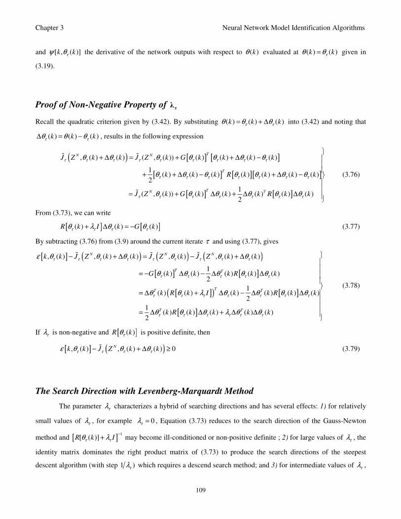
Chapter 3 Neural Network Model Identification Algorithms
109
and [ , ( )]k kτψ θ the derivative of the network outputs with respect to ( )kθ evaluated at ( ) ( )k kτθ θ= given in
(3.19).
Proof of Non-Negative Property of τλ
Recall the quadratic criterion given by (3.42). By substituting ( ) ( ) ( )k k kτ τθ θ θ= + ∆ into (3.42) and noting that
( ) ( ) ( )k k kτ τθ θ θ∆ = − , results in the following expression
( ) [ ] [ ]
[ ] [ ][ ]
[ ] [ ]
, ( ) ( ) ( , ( )) ( ) ( ) ( ) ( )
1( ) ( ) ( ) ( ) ( ) ( ) ( )
2
1( , ( )) ( ) ( ) ( ) ( ) ( )
2
TN N
T
TN T
J Z k k J Z k G k k k k
k k k R k k k k
J Z k G k k k R k k
τ τ τ τ τ τ τ τ τ
τ τ τ τ τ τ τ
τ τ τ τ τ τ τ
θ θ θ θ θ θ θ
θ θ θ θ θ θ θ
θ θ θ θ θ θ
+ ∆ = + + ∆ −
+ + ∆ − + ∆ −
= + ∆ + ∆ ∆
(3.76)
From (3.73), we can write
[ ] [ ]( ) ( ) ( )R k I k G kτ τ τ τθ λ θ θ+ ∆ = − (3.77)
By subtracting (3.76) from (3.9) around the current iterate τ and using (3.77), gives
[ ] ( ) ( ) ( )
[ ] [ ]
[ ]( ) [ ]
[ ]
, ( ) , ( ) ( ) , ( ) , ( ) ( )
1( ) ( ) ( ) ( ) ( )
2
1( ) ( ) ( ) ( ) ( ) ( )
2
1( ) ( ) ( ) ( ) ( )
2
N N N
T T
TT T
T T
k k J Z k k J Z k J Z k k
G k k k R k k
k R k I k k R k k
k R k k k k
τ τ τ τ τ τ τ τ τ
τ τ τ τ τ
τ τ τ τ τ τ τ
τ τ τ τ τ τ
ε θ θ θ θ θ θ
θ θ θ θ θ
θ θ λ θ θ θ θ
θ θ θ λ θ θ
− + ∆ = − + ∆
= − ∆ − ∆ ∆
= ∆ + ∆ − ∆ ∆
= ∆ ∆ + ∆ ∆
(3.78)
If τλ is non-negative and [ ]( )R kτθ is positive definite, then
[ ] ( ), ( ) , ( ) ( ) 0Nk k J Z k kτ τ τ τε θ θ θ− + ∆ ≥ (3.79)
The Search Direction with Levenberg-Marquardt Method
The parameter τλ characterizes a hybrid of searching directions and has several effects: 1) for relatively
small values of τλ , for example 0τλ = , Equation (3.73) reduces to the search direction of the Gauss-Newton
method and [ ]1
[ ( )]R k Iτ τθ λ−
+ may become ill-conditioned or non-positive definite ; 2) for large values of τλ , the
identity matrix dominates the right product matrix of (3.73) to produce the search directions of the steepest
descent algorithm (with step 1 )τλ which requires a descend search method; and 3) for intermediate values of τλ ,
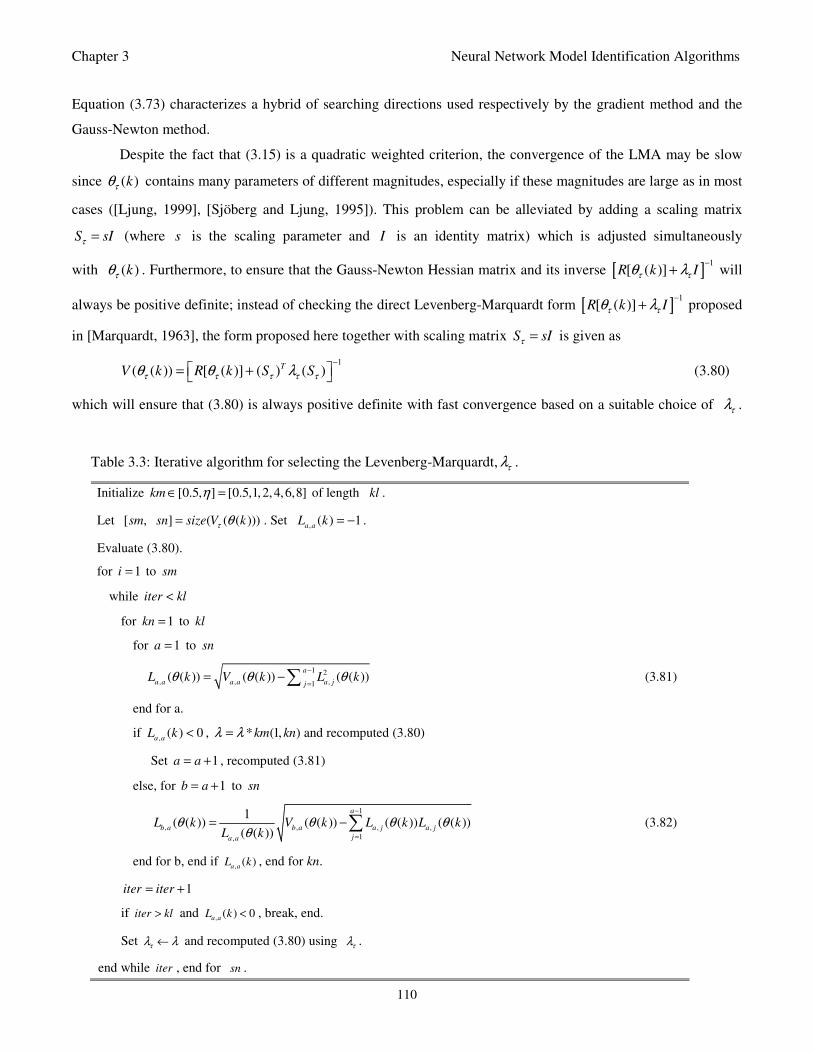
Chapter 3 Neural Network Model Identification Algorithms
110
Equation (3.73) characterizes a hybrid of searching directions used respectively by the gradient method and the
Gauss-Newton method.
Despite the fact that (3.15) is a quadratic weighted criterion, the convergence of the LMA may be slow
since ( )kτθ contains many parameters of different magnitudes, especially if these magnitudes are large as in most
cases ([Ljung, 1999], [Sjöberg and Ljung, 1995]). This problem can be alleviated by adding a scaling matrix
S sIτ = (where s is the scaling parameter and I is an identity matrix) which is adjusted simultaneously
with ( )kτθ . Furthermore, to ensure that the Gauss-Newton Hessian matrix and its inverse [ ]1
[ ( )]R k Iτ τθ λ−
+ will
always be positive definite; instead of checking the direct Levenberg-Marquardt form [ ]1
[ ( )]R k Iτ τθ λ−
+ proposed
in [Marquardt, 1963], the form proposed here together with scaling matrix S sIτ = is given as
1
( ( )) [ ( )] ( ) ( )TV k R k S Sτ τ τ τ τθ θ λ
−
= + (3.80)
which will ensure that (3.80) is always positive definite with fast convergence based on a suitable choice of τλ .
Table 3.3: Iterative algorithm for selecting the Levenberg-Marquardt, τλ .
Initialize [0.5, ] [0.5,1,2,4,6,8]km η∈ = of length kl .
Let [ , ] ( ( ( )))sm sn size V kτ θ= . Set,
( ) 1a a
L k = − .
Evaluate (3.80).
for 1i = to sm
while iter kl<
for 1kn = to kl
for 1a = to sn
1 2
, , ,1( ( )) ( ( )) ( ( ))
a
a a a a a jjL k V k L kθ θ θ
−
== −∑ (3.81)
end for a.
if ,
( ) 0a a
L k < , * (1, )km knλ λ= and recomputed (3.80)
Set 1a a= + , recomputed (3.81)
else, for 1b a= + to sn
1
, , , ,
1,
1( ( )) ( ( )) ( ( )) ( ( ))
( ( ))
a
b a b a a j a j
ja a
L k V k L k L kL k
θ θ θ θθ
−
=
= −∑ (3.82)
end for b, end if , ( )a aL k , end for kn.
1iter iter= +
if iter kl> and , ( ) 0a aL k < , break, end.
Set τλ λ← and recomputed (3.80) using τλ .
end while iter , end for sn .
Chapter 3 Neural Network Model Identification Algorithms
111
This problem is one reason why the LMA is not being used online. Thus, if the Gauss-Newton matrix is singular
or indefinite, the algorithm of Table 3.3 will fail and the value of τλ will be increased until non-singularity and/or
positive definiteness is achieved. Thus, the proposed algorithm can be used effectively to check whether or not a
symmetric matrix is positive definite. Once the positive definiteness of (3.80) is achieved, the Cholesky factors
,( ( ))
b aL kθ in (3.82) are produced whose inverse is guaranteed to be positive definite as well.
Different from other methods ([Chong, 2010], [Dennis and Schnabel, 1996], [Kelly, 1999], [Nørgaard et
al, 2000], the method proposed here uses the Cholesky factorization algorithm ([Antoniou and Lu, 2007], [Boyd
and Vandenberghe, 2007] which is implemented in such a way as to iteratively select τλ to guarantee the positive
definiteness of (3.80) for online application. First, (3.80) is computed and the check is performed. If (3.80) is
positive definite, the algorithm is terminated, otherwise λ is increased iteratively until this is achieved. The
method is summarized in Table 3.3. The key parameter in the algorithm is η and how τλ is to be updated at each
iteration. Next, the Cholesky factors , ( ( ))b aL kθ given by (3.82) in Table 3.3 is reused to compute the search
direction from (3.73) in two stage forward and backward substitution procedures given respectively as:
, [( ( )] ( ) [ ( )]b aL k k G kτ τ τθ θ θ∆ = (3.83)
( )1
,( ) [( ( )] [ ( )]T
b ak L k G kτ τ τθ θ θ
−
∆ = (3.84)
The convergence of the LMA using (3.72) to (3.75), (3.83), (3.84) with the algorithm of Table 3.3 may again be
slowed if the initial guess (0) ( )kθ too far from the optimum value ˆ( )kθ . Thus, the LMA is sometimes combined
with the trust region method so that the search for ˆ( )kθ is constrained around a trusted region τδ . The problem
can be defined as:
( ) ( )
( ) arg min ( , ( ))N
k k
k J Z kτ
τ τθ θ
θ θ= ∈Θ
= (3.85)
Subject to ( )( ) ( )S k kτ τ τθ θ δ− ≤ (3.86)
where ( , ( ))NJ Z kτ θ is the second-order Gauss-Newton quadratic criterion given by (3.42) which is expected to
be valid only in a neighborhood around the current iterate evaluated at ( ) ( )k kτθ θ= . Thus, with this modified
Levenberg-Marquardt approach and the trust region method, and using the results from (3.84); Equation (3.72) is
rewritten as
ˆ( ) ( ) ( )k k kτ τθ θ θ= + ∆ (3.87)
The choice of selecting and/or adjusting τδ and τλ has led to the coding of several algorithms ([Chiong, 2010],
Colin et al., 2007], [Dennis and Schnabel, 1996], [Guarneri et al., 2008], Fletcher, 1987], [Nørgaard et al., 2000],
[Wu, 2008]). In stead of adjusting τδ directly, this paper develops on the indirect approach proposed in [Fletcher,
1987] but reuses τλ computed in Table 3.3 to update the weighted criterion (3.15).
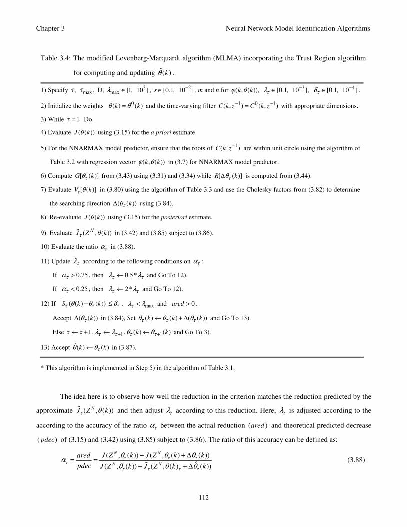
Chapter 3 Neural Network Model Identification Algorithms
112
The idea here is to observe how well the reduction in the criterion matches the reduction predicted by the
approximate ( , ( ))NJ Z kτ θ and then adjust τλ according to this reduction. Here, τλ is adjusted according to the
according to the accuracy of the ratio τα between the actual reduction ( )ared and theoretical predicted decrease
( )pdec of (3.15) and (3.42) using (3.85) subject to (3.86). The ratio of this accuracy can be defined as:
( , ( )) ( , ( ) ( ))
ˆ( , ( )) ( , ( ) ( ))
N N
N N
J Z k J Z k kared
pdec J Z k J Z k k
τ τ ττ
τ τ τ τ
θ θ θα
θ θ θ
− + ∆= =
− + ∆ (3.88)
Table 3.4: The modified Levenberg-Marquardt algorithm (MLMA) incorporating the Trust Region algorithm
for computing and updating ˆ( )kθ .
1) Specify ,τ max ,τ D, 3max [1, 10 ]λ ∈ , 2
[0.1, 10 ]s−
∈ , m and n for ( , ( )),k kϕ θ 3 4[0.1, 10 ], [0.1, 10 ]τ τλ δ− −∈ ∈ .
2) Initialize the weights 0( ) ( )k kθ θ= and the time-varying filter 1 0 1( , ) ( , )C k z C k z− −= with appropriate dimensions.
3) While 1,τ = Do.
4) Evaluate ( ( ))J kθ using (3.15) for the a priori estimate.
5) For the NNARMAX model predictor, ensure that the roots of 1( , )C k z− are within unit circle using the algorithm of
Table 3.2 with regression vector ( , ( ))k kϕ θ in (3.7) for NNARMAX model predictor.
6) Compute [ ( )]G kτθ from (3.43) using (3.31) and (3.34) while [ ( )]R kτθ∆ is computed from (3.44).
7) Evaluate [ ( )]V kτ θ in (3.80) using the algorithm of Table 3.3 and use the Cholesky factors from (3.82) to determine
the searching direction ( ( ))kτθ∆ using (3.84).
8) Re-evaluate ( ( ))J kθ using (3.15) for the posteriori estimate.
9) Evaluate ( , ( ))NJ Z kτ θ in (3.42) and (3.85) subject to (3.86).
10) Evaluate the ratio τα in (3.88).
11) Update τλ according to the following conditions on τα :
If 0.75τα > , then 0.5*τ τλ λ← and Go To 12).
If 0.25τα < , then 2*τ τλ λ← and Go To 12).
12) If ( ( ) ( ))S k kτ τ τθ θ δ− ≤ , maxτλ λ< and 0ared > .
Accept ( ( ))kτθ∆ in (3.84), Set ( ) ( ) ( ( ))k k kτ τ τθ θ θ← + ∆ and Go To 13).
Else 1τ τ← + , 1τ τλ λ +← , 1( ) ( )k kτ τθ θ +← and Go To 3).
13) Accept ˆ( ) ( )k kτθ θ← in (3.87).
* This algorithm is implemented in Step 5) in the algorithm of Table 3.1.
Chapter 3 Neural Network Model Identification Algorithms
113
Now, if the ratio is close to one, ˆ( , ( ) ( ))NJ Z k kτ τ τθ θ+ ∆ may be a reasonable approximation to ( , ( ))N
J Z kτθ and
τλ should be reduced by some factor and thereby increasing the trust-region indirectly. On the other hand, if τα
is small or negative, then τλ should be increased by some factor thereby reducing the trust-region indirectly.
The complete modified Levenberg-Marquardt – trust region algorithm for updating ˆ( )kθ is summarized
in Table 3.4. Note that after ˆ( )kθ is obtained, the algorithm of Table 3.1 is implemented until the conditions set
out in Step 7) of the Table 3.1 algorithm is satisfied.
3.3.7 Training Parameters and Criteria for Evaluating the Neural Network (NN) Model
In order to train the neural network (NN) models proposed in this work, the training parameters for the
adaptive recursive least squares (ARLS) algorithm and the modified Levenberg-Marquardt algorithms (MLMA)
must be specified. It is also necessary to specify the parameters of NN structure of Fig. 3.3 and Fig. 3.4 in terms
of the NN inputs, number of hidden and output layer neurons, and the activation function of each layer. To fulfill
these requirements, the correct number of regressor as well as the number of hidden neurons must first be selected
but unfortunately there are not specific rules for these selections ([Gupta et al., 2003], [Hagan et al., 1996],
[Haykin, 1999]). In many applications ([Gomm et al., 1997], [Guarneri et al., 2008], [Vieira et al., 2005],
[Zamarreñ0 and Vega, 1999]), the number of neurons for the hidden layer is selected based on trial-and-error
method usually starting with small initial network. Even the so-called optimal brain surgeon (OBS) [Haykin,
1999] and optimal brain damage (OBD) [Nørgaard et al., 2000] rules for automating network architecture requires
an initial large network.
In this study, the number of past inputs ( )b
n and output ( )a
n and the estimated prediction errors ( )c
n that
constitutes the regression vector of length nϕ is selected initially by trial-and-error method starting with an initial
small value. Note that the regression vector is the input to the NN. For the two–layer NN considered in this work,
hα ,
oα and the number of hidden layer neurons
hn are also selected using this same method starting with initial
small values while the number of output neurons o
n corresponds exactly to the number of system outputs. The
parameter vector ( )kθ is initialized to small random matrix of appropriate dimension ν as (0)θ . The initial
(0)[ , ( )]k kθΓ is initialized as diagonal matrix of dimensionso
n , the number of iterations j for the algorithm of
Table 3.1 and the number iterations τ for implementing the ARLS and the MLMA identification algorithms must
also be specified. In addition, where the NNARMAX model predictor is used, the time-varying filter (0) 1( , )C k z−
is initialized as a diagonal matrix of dimension c
n consisting of random small numbers and the number of
iterations i for the algorithm of Table 3.2 must be specified.

Chapter 3 Neural Network Model Identification Algorithms
114
The training parameters for the adaptive recursive least squares (ARLS) algorithm discussed in Section
3.3.5 of Chapter 3 that must be defined include π , α , β , 'δ which are used to compute, γ as well as min
e and
maxe to chose the initial diagonal of (0)P . Also, the training parameters for the modified Levenberg-Marquardt
algorithms (MLMA) that must be specified include λ , s and δ .
The performance and evaluation of the trained is subject to satisfying certain criteria during the network
training process. The criteria considered in this work include:
1) The Minimum Criterion,min
:crit This shall be the minimum value of the weighted mean square error (MSE)
cost function given by (3.15) evaluated at each iteration until the network training is terminated. Equation
(3.15) shall simply be referred to as the criterion and the minimum values of the criterion shall be called the
performance index. The performance index is actually the criteria which shall be used to judge the
convergence rate of the training algorithms at each iteration. The training algorithms shall be terminated if the
minimum value of the criterion is less than a specified value ofmin
crit .
2) The Change in Criterions, :crit∆ This shall be the change in the criterions evaluated between two successive
iterations. If the change in the criterions between two successive iterations is less than ,crit∆ then the
training algorithms will be terminated.
3) The Maximum Gradient,max
:grad This shall be related to the value of the largest element in the gradient term
evaluated at any given iteration. If the value of the largest element in the gradient terms given by (3.50) and
(3.74) for the ARLS and MLMA algorithms respectively is less thanmax
,grad then the network training will
be terminated.
4) The Change in Weight,max
:θ∆ This shall be the largest value of the change in the value of the parameter
vector ( )kτθ between two successive iterations. If the largest parameter change is belowmax
,θ∆ then the
training algorithms will be terminated.
3.3.8 Scaling the Training Data and Rescaling the Trained Network
Due to the fact the input and outputs of a process may, in general, have different physical units and
magnitudes; the scaling of all signals to the same variance is necessary to prevent signals of largest magnitudes
from dominating the identified model. Moreover, scaling improves the numerical robustness of the training
Chapter 3 Neural Network Model Identification Algorithms
115
algorithm, leads to faster convergence and gives better models. The training data are scaled to unit variance using
their mean values and standard deviations according to the following equations:
( )
( )
( )
( )
( ) ( )( )
( ) ( )( )
s
U k
S
Y k
U k U kU k
Y k Y kY k
σ
σ
−=
− =
(3.89)
where ( ),U k ( )Y k and ( )U kσ , ( )Y kσ are the mean and standard deviation of the input and output training data
pair; and ( ) ( )SU k and ( ) ( )S
Y k are the scaled inputs and outputs respectively. Also, after the network training, the
joint weights are rescaled according to the expression
( )ˆ ˆˆ ˆ( , ( )) ( , ( )) ( )Y kY k k Y k k Y kθ θ σ= + (3.90)
so that the trained network can work with other unscaled validation data and test data not used for training.
However, for notational convenience, ( )( ) ( )SU k U k= and ( )( ) ( )S
Y k Y k= shall be used.
3.4 Neural Network-Based Validation Algorithms
A trained network generalizes well if it is able to predict correctly both data that were used for training
and data that were not used during training. This process is called network validation. During the validation
process, tests are performed to access to what extend the developed model represents the operational dynamics of
the underlying system. The NN models identified by the proposed ARLS and the MLMA algorithms are validated
in this work using three validation methods, namely: 1) the one-step ahead output predictions of the scaled
training and unscaled validation data as well as unscaled test data from the operation of the real system under
consideration, where such test data is available; 2) K-step (that is, multi-step) ahead output predictions of the
unscaled training data; and 3) the Akaike’s final prediction error (AFPE) estimate of the average generalization
based on the weighted (or regularized) criterion.
3.4.1 One-Step Ahead Prediction Validation
The one-step ahead predictions of the network performance is the most widely used validation method
mostly because the predictors designed in most cases are one-step ahead model predictors. With this method, the
unscaled training data, validation data as well as available test data can be used to simulate the trained network for
network output prediction comparison and the assessment of the corresponding prediction errors. While the one-
step ahead validation is simple and give intuitive insight about the performance of the trained network, it might
Chapter 3 Neural Network Model Identification Algorithms
116
not reveal the suitability or accuracy of the trained network for more distant predictions such as in multi-step
ahead predictions which are widely used in controller design. Thus, the K-step ahead validation might be useful.
3.4.2 K-Step Ahead Output Prediction Simulation
The K-step ahead output prediction simulation is a validation technique which is particularly useful as far
as model validation for predictive control strategies are concerned and in situations where the sampling period of
the plant is high compared to the dynamics and time constants of the controlled variables. In the K-step ahead
prediction simulations, the output predictions of the trained network are compared with the unscaled training data
where the output of the one-step ahead NN predictor is calculated K-step ahead.
The inspection of one-step ahead output predictions might not reveal the model inaccuracy for multi-step
output or distant predictions. The K-step ahead predictor follows from the one-step ahead NN model predictor
given in (3.5) except that ˆ( , ( )) ( , ( ))k k k K kϕ θ ϕ θ= + , so that the K-step ahead predictor take the following form:
( ) ( )( )ˆ ˆ ˆˆ ˆ ˆ| , ( ) , , ( ) , ( )NY k K k k J Z k K k kθ ϕ θ θ+ = + (3.91)
where J is now known in terms of ˆ( )kθ and ˆˆ( , ( ))k K kϕ θ+ is now the K-step ahead predictor regression vector
( ) ( ) ( ) ( )
( ) ( )
ˆ , ( ) 1 , , , ( ), , max( ,0) ,
ˆ ˆˆ ˆ1, ( ) , , 1 min( , ), ( )
b a
T
a
k K k U k K U k K n Y k Y k n k
Y k K k Y k K k n k
ϕ θ
θ θ
+ = + − + − − −
+ − + + −
… …
… (3.92)
The mean value of the K-step ahead prediction error (MVPE) between the outputs predicted by the trained
network and the outputs of the actual system in terms of the unscaled training data set is computed as follows:
( )ˆˆ( ) | , ( )100%
( )
N
k k K
Y k Y k K k kMVPE mean
Y k
θ
= +
− + = ×
∑ (3.93)
where ( )Y k corresponds to the actual outputs and ˆˆ(( ) | , ( ))Y k K k kθ+ is the K-step ahead output predictions.
3.4.3 Akaike’s Final Prediction Error Estimate
The Akaike’s Final Prediction Error (AFPE) is used to verify the accuracy of the trained network by
computing the average generalization error estimate. The AFPE estimate is useful for selecting a suitable model
based on the weighted criterion by trying different values of the weight decay parameter D in (3.15). A smaller
value of the AFPE estimate indicates that the trained network models and captures all the dynamics of the
underlying system and also measure how well the identified model will perform when presented with actual data
taken during normal system operation. The AFPE estimate algorithm used here is adopted from [Ljung, 1999],
[Sjöberg and Ljung, 1995], and [Nørgaard et al., 2000].
Chapter 3 Neural Network Model Identification Algorithms
117
The average generalization error, ˆˆ ( , ( ))NF Z kθ as a function of the model quality is considered here to be
the expectation ˆ ( , )NE J Zθ [Ljung, 1999] of the one-step ahead NN predictor error ˆ( , )kε θ with respect to the
regression vector ( )kϕ and the noise contribution ( ).v k For the regularized criterion considered in this paper with
multiple weight decay parameter D in (3.15), the AFPE estimate of ˆˆ ( , ( ))NF Z kθ has been derived in [Ljung,
1999] and [Sjöberg and Ljung, 1995] as a function of the noise variance 2ˆe
σ which is given here as:
( ) 21ˆˆ ˆ, ( ) 12
N a
e
PF Z k
Nθ σ γ
= + +
(3.94)
where 2ˆe
σ is the noise variance given as
( )2 ˆˆ 2 ( , ( ))2
N
e
a b
NJ Z k
N P Pσ θ γ= −
+ −
1 1
ˆ ˆ ˆ ˆ[ ( )] [ ( ) [ ( )] ( )ap R k R k D R k V Dθ θ θ θ− −
= + + tr
11ˆ ˆ[ ( )] [ ( )]bp R k R k DN
θ θ
− = +
tr
and γ is a positive quantity that improves the accuracy of the estimate and is computed by the relationship:
1 1
2
1 1 1ˆ ˆ ˆ ˆ ˆ( ) [ ( )] [ ( )] [ ( )] ( )Tk D R k D R k R k D D k
N N Nγ θ θ θ θ θ
− −
= + +
and tr i is the trace of its arguments and it is computed as the sum of the diagonal elements of its arguments.
In (3.94), the ˆ( , ( ))k kε θ portion of (3.15) is evaluated using the identified NN model ˆ( )kθ and taking the
expectation ˆ ( , ( ))NJ Z kθE with respect to ( , ( ))k kϕ θ and ( )d k . The term expectation E i is the mean or
average vale of its arguments. The above AFPE estimate algorithm is evaluated on unscaled validation data as
well as on unscaled test data where available.
Chapter 4 Adaptive Model-Based Predictive Control Algorithms
118
CHAPTER 4
NEURAL NETWORK-BASED ADAPTIVE MODEL PREDICTIVE
CONTROL ALGORITHMS
4.1 Introduction
This chapter presents the developed two new NN-based adaptive MPC algorithms both consisting of an
on-line process identification part and a predictive control part. Both parts are executed at each sampling instant.
The predictive control part of the first algorithm is a nonlinear adaptive model predictive control (NAMPC)
strategy and the control part of the second algorithm is an adaptive generalized predictive control (AGPC)
strategy. In the identification parts of both algorithms, the process model is approximated by a neural network
which is trained either by the modified Levenberg-Marquardt algorithm (MLMA) or the adaptive recursive least
squares (ARLS) algorithms presented in Chapter 3.
In the proposed NN-based identification and control scheme, any deviations in system outputs at each
sampling instant due to disturbances ( )d k or change in the operating conditions are considered to correspond to
equivalent model changes. As discussed in Section 2.11.1.2 of Chapter 2, both AGPC and NAMPC are indirect
adaptive control strategies where the NN is used as a nonlinear approximator (or identifier in adaptive control
literature [Omidvar and Elliot, 1997], [Spooner et al., 2002]) of the system at each sampling instant k . The
identified NN model is then employed in the AGPC and NAMPC design at the same sampling instant.
The proposed NN-based AGPC algorithm is based on the instantaneous linearization of an identified
nonlinear NN which models the process at each sampling instant, the subsequent solution of a set of recursive
Diophantine equations and the application of a quadratic programming method to obtain the control signal under
tight input and output constraints. On the other hand, the proposed NAMPC is a constrained online optimization
control strategy based on the full Newton method ([Dennis and Schnabel, 1996], [Kelley, 1995], [Kelley, 1999],
[Omidvar and Elliot, 1997], [Scales, 1985]). It is well-known that the full Newton Hessian matrix is not
guaranteed to be positive definite in an open neighbourhood of a global minimum during its inversion. Thus, the
NAMPC incorporates a new iterative strategy for guaranteed positive definiteness of the full Newton Hessian
matrix making the on line optimization computations always feasible. The optimization algorithm used by the
NAMPC is based on the Levenberg-Marquardt method which is a second-order trust region optimization method
known for robustness and fast convergence ([Fletcher, 1987], [Hagan and Menhaj, 1994], [Marquardt, 1963],
[Wu, 2008]). A difficulty with the Levenberg-Marquardt method is the selection of the adaptation parameter for
updating the minimization process ([Chiong, 2010], [Dennis and Schnabel, 1996], [Kelley, 1999], [Scales, 1985]).
In this work, a modification is made to the Levenberg-Marquardt method by incorporating into the NAMPC a
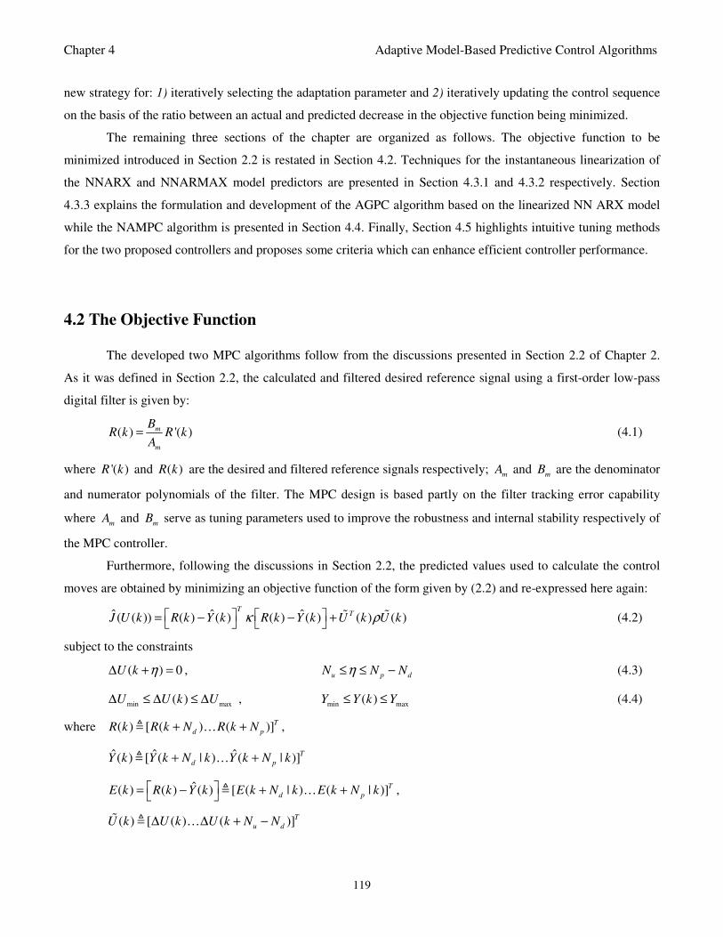
Chapter 4 Adaptive Model-Based Predictive Control Algorithms
119
new strategy for: 1) iteratively selecting the adaptation parameter and 2) iteratively updating the control sequence
on the basis of the ratio between an actual and predicted decrease in the objective function being minimized.
The remaining three sections of the chapter are organized as follows. The objective function to be
minimized introduced in Section 2.2 is restated in Section 4.2. Techniques for the instantaneous linearization of
the NNARX and NNARMAX model predictors are presented in Section 4.3.1 and 4.3.2 respectively. Section
4.3.3 explains the formulation and development of the AGPC algorithm based on the linearized NN ARX model
while the NAMPC algorithm is presented in Section 4.4. Finally, Section 4.5 highlights intuitive tuning methods
for the two proposed controllers and proposes some criteria which can enhance efficient controller performance.
4.2 The Objective Function
The developed two MPC algorithms follow from the discussions presented in Section 2.2 of Chapter 2.
As it was defined in Section 2.2, the calculated and filtered desired reference signal using a first-order low-pass
digital filter is given by:
( ) '( )m
m
BR k R k
A= (4.1)
where '( )R k and ( )R k are the desired and filtered reference signals respectively; m
A and m
B are the denominator
and numerator polynomials of the filter. The MPC design is based partly on the filter tracking error capability
where m
A and m
B serve as tuning parameters used to improve the robustness and internal stability respectively of
the MPC controller.
Furthermore, following the discussions in Section 2.2, the predicted values used to calculate the control
moves are obtained by minimizing an objective function of the form given by (2.2) and re-expressed here again:
ˆ ˆ ˆ( ( )) ( ) ( ) ( ) ( ) ( ) ( )T
TJ U k R k Y k R k Y k U k U kκ ρ = − − +
(4.2)
subject to the constraints
( ) 0U k η∆ + = , u p dN N Nη≤ ≤ − (4.3)
min max( )U U k U∆ ≤ ∆ ≤ ∆ , min max( )Y Y k Y≤ ≤ (4.4)
where ( ) [ ( ) ( )]T
d pR k R k N R k N+ + … ,
ˆ ˆ ˆ( ) [ ( | ) ( | )]T
d pY k Y k N k Y k N k+ + …
ˆ( ) ( ) ( ) [ ( | ) ( | )]T
d pE k R k Y k E k N k E k N k = − + + … ,
( ) [ ( ) ( )]T
u dU k U k U k N N∆ ∆ + − …
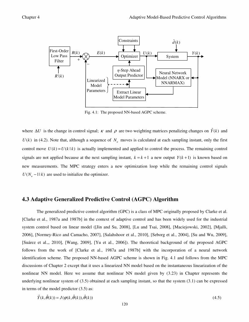
Chapter 4 Adaptive Model-Based Predictive Control Algorithms
120
where U∆ is the change in control signal; κ and ρ are two weighting matrices penalizing changes on ˆ( )Y k and
( )U k in (4.2). Note that, although a sequence of u
N moves is calculated at each sampling instant, only the first
control move ( ) ( | )U k U k k= is actually implemented and applied to control the process. The remaining control
signals are not applied because at the next sampling instant, 1k k= + a new output ( 1)Y k + is known based on
new measurements. The MPC strategy enters a new optimization loop while the remaining control signals
( 1| )u
U N k− are used to initialize the optimizer.
4.3 Adaptive Generalized Predictive Control (AGPC) Algorithm
The generalized predictive control algorithm (GPC) is a class of MPC originally proposed by Clarke et al.
[Clarke et al., 1987a and 1987b] in the context of adaptive control and has been widely used for the industrial
system control based on linear model ([Jin and Su, 2008], [Lu and Tsai, 2008], [Maciejowski, 2002], [Mjalli,
2006], [Normey-Rico and Camacho, 2007], [Salahshoor et al., 2010], [Seborg et al., 2004], [Su and Wu, 2009],
[Suárez et al.,, 2010], [Wang, 2009], [Yu et al., 2006]). The theoretical background of the proposed AGPC
follows from the work of [Clarke et al., 1987a and 1987b] with the incorporation of a neural network
identification scheme. The proposed NN-based AGPC scheme is shown in Fig. 4.1 and follows from the MPC
discussions of Chapter 2 except that it uses a linearized NN model based on the instantaneous linearization of the
nonlinear NN model. Here we assume that nonlinear NN model given by (3.23) in Chapter represents the
underlying nonlinear system of (3.5) obtained at each sampling instant, so that the system (3.1) can be expressed
in terms of the model predictor (3.5) as:
ˆ ˆ ˆˆ( , ( )) ( ( , ( )), ( ))Y k k J k k kθ ϕ θ θ= (4.5)
System ( )Y k ( )U k
•
Neural Network
Model (NNARX or
NNARMAX)
Optimizer • +
−
( )E k
•
Constraints ( )d k
η-Step Ahead
Output Predictor
Linearized
Model
Parameters
'( )R k
First-Order
Low Pass
Filter
( )R k
Extract Linear
Model Parameters
Fig. 4.1: The proposed NN-based AGPC scheme.
Chapter 4 Adaptive Model-Based Predictive Control Algorithms
121
4.3.1 Instantaneous Linearization of a Deterministic Nonlinear Neural Network
ARX Model
Suppose that the input-output model of the system to be controlled is available and can be defined as the
prediction model of (4.5). The regression vector for the NNARX model can be expressed from (3.6) as
[ ]( ) ( 1), , ( ), ( 1), , ( )T
a bk Y k Y k n U k U k d nϕ = − − − − −… … (4.6)
Here, the idea of the instantaneous linearization is to extract a linear model from the nonlinear neural network
model at each sample time. The extracted model linear model is then used for controller design.
By interpreting the regression vector ( )kϕ of (4.6) as the vector defining the state of the system and at
time 'k k= the nonlinear system of (4.5) is linearized around the current state ( ')kϕ to obtain the approximate
linearized model expressible as
1 0( ) ( 1) ( ) ( ) ( )a bn a n bY k AY k A Y k n B U k d B U k d n= − − − − − + − + + − − (4.7)
where anA and
bnB are the linearized model parameters obtained from (4.5) by taking the partial derivatives of the
nonlinear model with respect to the output and input parts of the regression vector respectively as follows. Let Aτ
and Bτ of orders a
n and b
n respectively be two parameters associated with anA and
bnB of orders a
n and b
n
respectively in (4.5) defined as follows:
( ) ( ')
( ) ( ')
( ( )), 0,1, ,
( )
( ( )), 0,1, ,
( )
a
n na a
b
n nb b
n
a
k k
n
b
k k
J kA n
Y k
J kB n
U k d
τ
ϕ ϕ
τ
ϕ ϕ
ϕτ
τ
ϕτ
τ
=
=
∂= − =
∂ −
∂ = = ∂ − −
…
…
(4.8)
where ( )a
Y k n− and ( )b
U k n− in (4.7) are defined respectively by
( ) ( ) ( ' ), 0,1, ,
( ) ( ) ( ' ), 0,1, ,
a
b
Y k Y k Y k n
U k U k U k n
τ τ τ τ
τ τ τ τ
− = − − − =
− = − − − =
…
… (4.9)
Note that the coefficients of Aτ and Bτ corresponds to those of 1( )A z− and 1( )B z
− defined in (2.73) and re-
written here as
1 1
1
1 1
0 1
( )
( )
a
a
b
b
n
n
n
n
A z I A z A z
B z B B z B z
−− −
−− −
= + + +
= + + +
(4.10)
By separating the ( ')an kϕ and ( ')
bn kϕ components of the current regression vector ( ')kϕ at time 'k which
constitutes the bias term ˆ( ')d k around the current operating point, the linearized model from (4.5) can then be
expressed equivalently as:
1 1 ˆ( ) [1 ( )] ( ) ( ) ( ) ( ) ( ')dY k A z Y k z B z U k e k d k
− − −= − + + + (4.11)
Chapter 4 Adaptive Model-Based Predictive Control Algorithms
122
where ( )e k is a deterministic white noise and the bias term ˆ( ')d k is given by
1 1ˆ( ') ( ') ( ' 1) ( ' ) ( ' ) ( ' )
a bn a n bd k Y k AY k A Y k n BU k d B U k d n= + − + + − − − − − − − (4.12)
The system outputs are extracted from the NN model at each sampling instant as the derivative of the network
outputs with respect to the inputs ( ) [ ( ) ( )]a b
T
n nk k kτϕ ϕ ϕ= . The derivative of the NN outputs with respect to the
inputs ( )kτϕ is given from (3.15) with ˆ( ) ( )k kθ θ= by
2
, , ,0
1 1
ˆ( )1 ( )
( )
h a bn n n
j j l j l l j
j l
Y kW w f w k w
kτ
ϕϕ
+
= =
∂= − + ∂ ∑ ∑ (4.13)
where ( )f i is an hyperbolic tangent sigmoid function defined in (3.16).
Here, the approximate linearized model given by (4.11) can be interpreted as a linear model affected by
an integrated white noise and a constant disturbance ˆ( ')d k which depends on the current operating point. Thus,
Equation (4.11) can be expressed by the following integrated autoregressive with exogenous input (ARIX) model
given as:
1 1 ( )( ) ( ) ( ) ( )d e k
A z Y k z B z U k d− − −= − +
∆ (4.14)
where 11 z−∆ = − is an integrator which is included to compensate for linearization errors as well as for the
deterministic noise and the constant disturbance ˆ( ')d k . Note that in this case, the constant disturbance term is
evaluated depending on the current operating point. Note also that (4.14) corresponds to a more general form
where 1 1
1( ) c
c
n
nC z I C z C z−− −= + + + , defined and discussed in section 2.5.1, can be truncated and absorbed into
1( )A z− and 1( )B z
− polynomial matrices. A detailed treatment of this techniques can be found in [Camacho and
Bordons, 2007], [Clarke et al., 1987b], [Goodwin and Sin, 1984], [Ljung, 1999], [Maciejowski, 2002], [Normey-
Rico and Camacho, 2007], [Rossiter, 2004] and [Wang, 2009]. Note that by removing the integrator term ∆ ,
Equation (4.14) corresponds exactly to an ARX model with ( )e k assumed to be white noise [Ljung, 1999].
4.3.2 Instantaneous Linearization of a Stochastic Nonlinear Neural Network
ARMAX Model
Unlike the instantaneous linearization of the NARX model affected by deterministic noise, the
instantaneous linearization is here applied to systems affected by stochastic noise. Consider that (4.5) correspond
to the one-step ahead predictor of a nonlinear neural network autoregressive with moving average exogenous
input (NNARMAX) model of a nonlinear system. The regression vector for the NNARMAX model can be
expressed from (3.7) as:
Chapter 4 Adaptive Model-Based Predictive Control Algorithms
123
[ ]( , ( )) ( 1), , ( ), ( 1), , ( ), ( 1, ( )), , ( , ( ))T
a b ck k Y k Y k n U k U k d n k k k n kϕ θ ε θ ε θ= − − − − − − −… … … (4.15)
Next, by interpreting the regression vector ( , ( ))k kϕ θ of the NNARMAX model predictor of (4.5) as a vector
defining the state of the nonlinear system, so that at time 'k k= the nonlinear system of (4.5) is linearized around
the current state ( ', ( '))k kϕ θ to obtain the approximate linearized model predictor expressible as:
1 0
1
( ) ( 1) ( ) ( ) ( )
( , ( )) ( , ( ))
a b
c
n a n b
n c
Y k AY k A Y k n B U k d B U k d n
C k k C k n kε θ ε θ
= − − − − − + − + + − −
+ + + −
(4.16)
where anA ,
bnB and cnC are the linearized model parameters obtained from (4.16) by taking the partial derivatives
of the nonlinear model with respect to the output and input parts of the regression vector respectively as follows.
Let Aτ , Bτ and Cτ of orders a
n , b
n and c
n respectively denote the three parameters associated with anA ,
bnB and
cnC of orders a
n , b
n and b
n respectively in (4.5) defined as follows:
( ) ( ')
( ) ( ')
( ) ( ')
( ( , ( ))), 0,1, ,
( )
( ( , ( ))), 0,1, ,
( )
( ( , ( ))), 0,1, ,
( )
a
n na a
b
n nb b
c
n nc c
n
a
k k
n
b
k k
n
c
k k
J k kA n
Y k
J k kB n
U k d
J k kC n
k
τ
ϕ ϕ
τ
ϕ ϕ
τ
ϕ ϕ
ϕ θτ
τ
ϕ θτ
τ
ϕ θτ
ε τ
=
=
=
∂= − =
∂ − ∂
= = ∂ − −
∂
= = ∂ −
…
…
…
(4.17)
where ( )a
Y k n− , ( )b
U k n− and ( , ( ))c
k n kε θ− in (4.16) are defined respectively by
( ) ( ) ( ' ), 0,1, ,
( ) ( ) ( ' ), 0,1, ,
( , ( )) ( , ( )) ( ' , ( ')), 0,1, ,
a
b
c
Y k Y k Y k n
U k U k U k n
k k k k k k n
τ τ τ τ
τ τ τ τ
ε τ θ ε τ θ ε τ θ τ
− = − − − =
− = − − − = − = − − − =
…
…
…
(4.18)
Note that the coefficients of Aτ , Bτ and Cτ corresponds to those of 1( )A z− , 1( )B z
− and 1( )C z− defined in
(2.73) and re-written here as
1 1
1
1 1
0 1
1 1
1
( )
( )
( )
a
a
b
b
c
c
n
n
n
n
n
n
A z I A z A z
B z B B z B z
C z I C z C z
−− −
−− −
−− −
= + + +
= + + +
= + + +
(4.19)
By separating the ( ', ( '))an k kϕ θ , ( ', ( '))
bn k kϕ θ and ( ', ( '))cn k kϕ θ components of the current regression vector
( ', ( '))k kϕ θ at time 'k k= which constitutes the bias term ˆ( ')d k around the current operating point, the
approximate linearized model from (4.5) can then be expressed equivalently as
1 1 1 ˆ( ) [1 ( )] ( ) ( ) ( ) [ ( ) 1] ( , ( )) ( ')dY k A z Y k z B z U k C z k k d kε θ− − − −= − + + − + (4.20)
Chapter 4 Adaptive Model-Based Predictive Control Algorithms
124
where the third term on the right side of (4.20) constitute the stochastic noise term affecting the system and the
last term ˆ( ')d k is the bias term given as
1 1
1
ˆ( ') ( ') ( ' 1) ( ' ) ( ' )
( ' ) ( ' 1) ( ' )
a
b c
n a
n b n c
d k Y k AY k A Y k n BU k d
B U k d n C k C k nε ε
= + − + + − − − −
− − − + − + + −
(4.21)
The system outputs are extracted from the linearized neural network model at each sampling instant as the
derivatives of the network outputs with respect to the inputs ( , ( )) [ ( , ( )) ( , ( ))a bn nk k k k k kτϕ θ ϕ θ ϕ θ=
( , ( ))]c
T
n k kϕ θ . The derivative of the neural network outputs with respect to the inputs ( , ( ))k kτϕ θ is given from
(3.15) with ˆ( ) ( )k kθ θ= by
2
, , ,0
1 1
ˆ( | ( ))1 ( , ( ))
( , ( ))
h a b cn n n n
j j l j l l j
j l
Y k kW w f w k k w
k kτ
θϕ θ
ϕ θ
+ +
= =
∂= − + ∂ ∑ ∑ (4.22)
where ( )f i is an hyperbolic tangent sigmoid function defined in (3.16).
Here, the approximate linearized model given by (4.20) can be interpreted as a linear model affected by
an integrated white noise and a time-varying disturbance ˆ( ')d k which depends on the current operating point.
Thus, Equation (4.20) can be expressed by the following controlled autoregressive integrated moving average
(CARIMA) model given in [Clarke et al., 1987] which is widely used in most GPC formulations:
1 1 1 ( )( ) ( ) ( ) ( ) ( )d e k
A z Y k z B z U k d C z− − − −= − +
∆ (4.23)
where 11 z−∆ = − is an integrator which is included to compensate for linearization errors as well as the integrated
moving average disturbance ˆ( ')d k and ( )e k is a white noise sequence independent of past control inputs. In this
case as well, the constant disturbance term is evaluated depending on the current operating point or region. Note
here again that by removing the integrator term ∆ , Equation (4.23) corresponds to an ARMAX model.
4.3.3 The AGPC Algorithm
The AGPC Predictor
Consider the linearized ARIX model given by (4.14) in Section 4.3.1. Note that the same formulations
presented below also apply for the linearized CARIMA model given by (4.23). There are several methods of
computing the output predictions using (4.14) to determine the sequence of future control signals such as those
discussed in [Albertos and Ortega, 1989], [Clarke et al., 1987a and 1987b], [Camacho and Bordons, 2007], and
[Rossiter, 2004].
Although, it is not an objective in this study to compare and contrast the different methods of solving
(4.14) or (4.23); however it is worth marking few remarks about existing methods. A popular method of solution
Chapter 4 Adaptive Model-Based Predictive Control Algorithms
125
is the recursions of Diophantine equation [Clarke et al., 1987a and 1987b]. Rossiter [Rossiter, 2004] argued that
the method based on the recursion of the Diophantine equation: 1) tends to be obscure how the predictions are
obtained, 2) appears confusing and can pose difficulty for those not familiar with GPC, and 3) that the historical
reason for this method is unclear; and then introduced a method based on matrix manipulations which appears
more difficult from computational efficiency view point. Albertos and Ortega [Albertos and Ortega, 1989]
proposed two methods based on: 1) a multirate state-space formulation of the process model, and 2) iteration of
the process difference equations; where both methods involve matrix inversion without provisions for ill-
condition, robustness and stability of the system. The method used in [Camacho and Bordons, 2007] follows
closely from that in [Clarke et al., 1987a and 1987b]. While all these methods seek the same result, a simplified
approach based on the Diophantine equation followed by its recursion is presented below.
To obtain the η -step ahead predictor for the AGPC criterion given in (4.2), consider the output
predictions from the ARIX model of (4.14) at time k η+ , derived from the linearized deterministic input-output
NNARX model, given as
1 1( ) ( ) ( ) ( ) ( )dA z Y k z B z U k e kη η η− − −∆ + = ∆ + + + (4.24)
Note that similar result of (4.24) for the CARIMA model of (4.23) can be obtained where the second term in
(4.23) is incorporated into the second term ( )e k η+ in (4.24) (see for example [Clarke et al., 1987a and 1987b],
[Camacho and Bordons, 2007], [Maciejowski, 2002], and [Rossiter, 2004]). Thus, in order to solve (4.24), the
following Diophantine equation is introduced
1 1 11 ( ) ( ) ( )A z E z z F z
η
η η
− − − −= ∆ + (4.25)
where 1( )E zη
− and 1( )F zη
− are polynomial matrices of degree d
Nη − and a
n given respectively by
1 1 ( 1)
,0 ,1 , 1( )E z E E z E z
η
η η η η η
− − − −
−= + + +
1 1
,0 ,1 ,( ) a
a
n
nF z F F z F zη η η η
−− −= + + +
By multiplying both sides of (4.24) by 1( )E zη
− and using (4.25) one obtains
1 1 1 1( ) ( ) ( ) ( ) ( ) ( ) ( ) ( )
dY k z E z B z U k F z Y k E z e kη η ηη η η− − − − −
+ = ∆ + + + + (4.26)
Since the degree of 1( )
dE z Nη η−
= − , it follows from (4.26) that the noise terms are all in the future. Note that the
only known terms in (4.26) are the sequence of future control inputs ( )U k η∆ + . Thus, the minimum variance
predictor of (4.26) can be expressed as the expectation conditioned on the available information with ( ) 0E e k =
up to time k given as:
1 1ˆ( | ) ( ) ( ) ( ) ( )Y k k G z U k d F z Y kη ηη η− −+ = ∆ + − + (4.27)
where 1 1 1( ) ( ) ( )G z E z B zη η
− − −= is a polynomial matrix of degree
b dn Nη+ − . Suppose that both sides of (4.25) are
multiplied by 1 1( ) ( )B z A z− −∆ to obtain
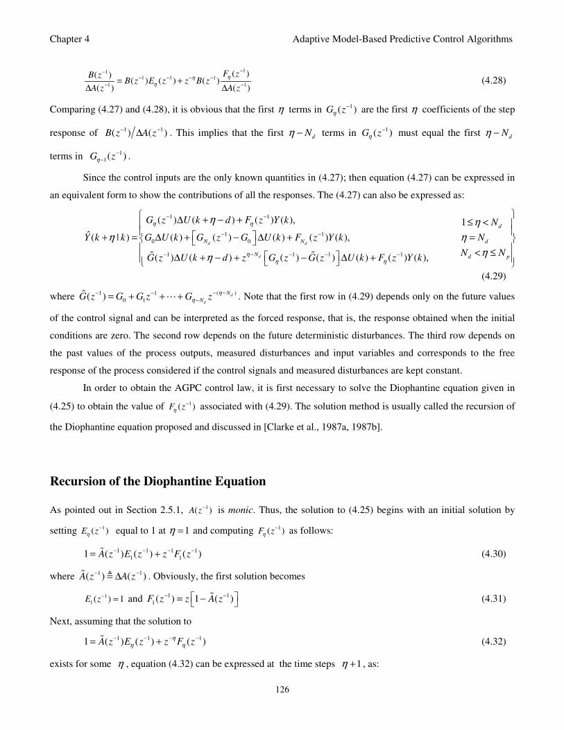
Chapter 4 Adaptive Model-Based Predictive Control Algorithms
126
111 1 1
1 1
( )( )( ) ( ) ( )
( ) ( )
F zB zB z E z z B z
A z A z
ηη
η
−−− − − −
− −= +
∆ ∆ (4.28)
Comparing (4.27) and (4.28), it is obvious that the first η terms in 1( )G zη
− are the first η coefficients of the step
response of 1 1( ) ( )B z A z− −∆ . This implies that the first
dNη − terms in 1( )G zη
− must equal the first d
Nη −
terms in 1
1( )G zη
−
− .
Since the control inputs are the only known quantities in (4.27); then equation (4.27) can be expressed in
an equivalent form to show the contributions of all the responses. The (4.27) can also be expressed as:
1 1
1 1
0 0
1 1 1 1
( ) ( ) ( ) ( ), 1
ˆ( | ) ( ) ( ) ( ) ( ) ( ),
( ) ( ) ( ) ( ) ( ) ( ) ( ),
d d
d
d
N N d
N d p
G z U k d F z Y k N
Y k k G U k G z G U k F z Y k N
N NG z U k d z G z G z U k F z Y k
η η
η
η η
η η
η η
ηη
− −
− −
−− − − −
∆ + − + ≤ <
+ = ∆ + − ∆ + = < ≤ ∆ + − + − ∆ +
(4.29)
where ( )1 1
0 1( ) d
d
N
NG z G G z G zη
η
− −− −
−= + + + . Note that the first row in (4.29) depends only on the future values
of the control signal and can be interpreted as the forced response, that is, the response obtained when the initial
conditions are zero. The second row depends on the future deterministic disturbances. The third row depends on
the past values of the process outputs, measured disturbances and input variables and corresponds to the free
response of the process considered if the control signals and measured disturbances are kept constant.
In order to obtain the AGPC control law, it is first necessary to solve the Diophantine equation given in
(4.25) to obtain the value of 1( )F zη
− associated with (4.29). The solution method is usually called the recursion of
the Diophantine equation proposed and discussed in [Clarke et al., 1987a, 1987b].
Recursion of the Diophantine Equation
As pointed out in Section 2.5.1, 1( )A z− is monic. Thus, the solution to (4.25) begins with an initial solution by
setting 1( )E zη
− equal to 1 at 1η = and computing 1( )F zη
− as follows:
1 1 1 1
1 11 ( ) ( ) ( )A z E z z F z− − − −= + (4.30)
where 1 1( ) ( )A z A z− −∆ . Obviously, the first solution becomes
1
1( ) 1E z
− = and 1 1
1( ) 1 ( )F z z A z− − = −
(4.31)
Next, assuming that the solution to
1 1 11 ( ) ( ) ( )A z E z z F z
η
η η
− − − −= + (4.32)
exists for some η , equation (4.32) can be expressed at the time steps 1η + , as:
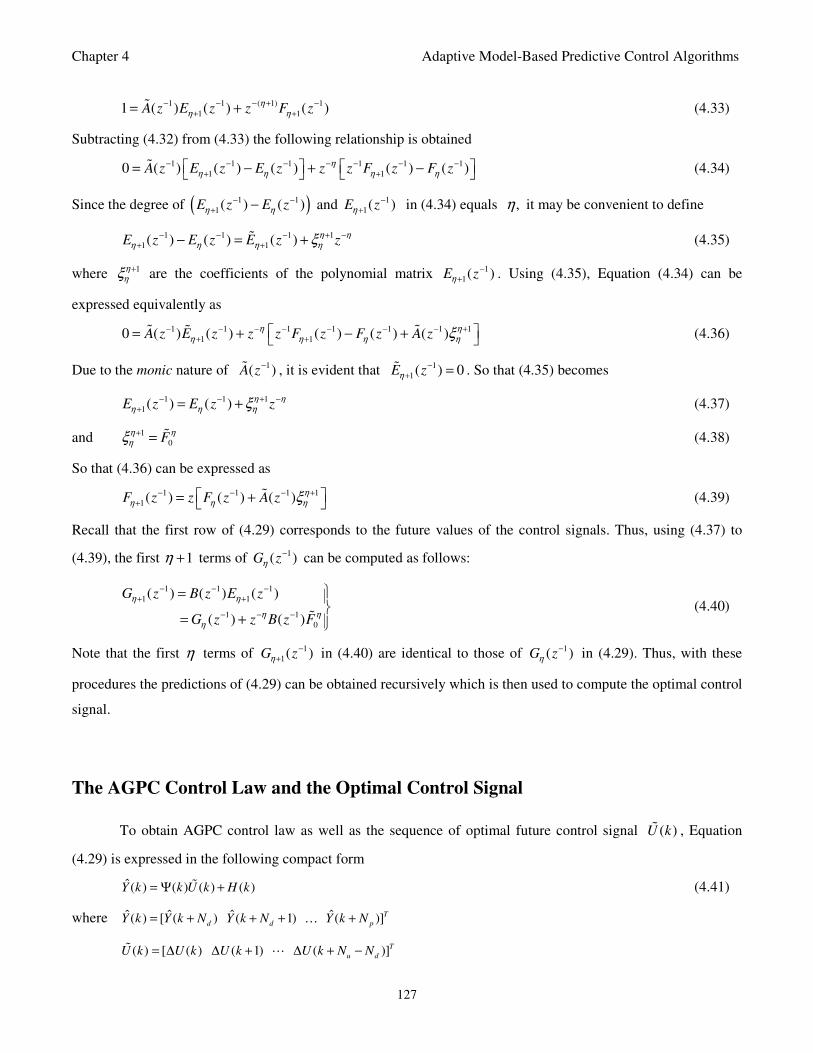
Chapter 4 Adaptive Model-Based Predictive Control Algorithms
127
1 1 ( 1) 1
1 11 ( ) ( ) ( )A z E z z F zη
η η
− − − + −
+ += + (4.33)
Subtracting (4.32) from (4.33) the following relationship is obtained
1 1 1 1 1 1
1 10 ( ) ( ) ( ) ( ) ( )A z E z E z z z F z F zη
η η η η
− − − − − − −
+ + = − + −
(4.34)
Since the degree of ( )1 1
1( ) ( )E z E zη η
− −
+ − and 1
1( )E zη
−
+ in (4.34) equals ,η it may be convenient to define
1 1 1 1
1 1( ) ( ) ( )E z E z E z zη η
η η η ηξ− − − + −
+ +− = + (4.35)
where 1η
ηξ + are the coefficients of the polynomial matrix 1
1( )E zη
−
+ . Using (4.35), Equation (4.34) can be
expressed equivalently as
1 1 1 1 1 1 1
1 10 ( ) ( ) ( ) ( ) ( )A z E z z z F z F z A zη η
η η η ηξ− − − − − − − +
+ + = + − +
(4.36)
Due to the monic nature of 1( )A z− , it is evident that 1
1( ) 0E zη
−
+ = . So that (4.35) becomes
1 1 1
1( ) ( )E z E z zη η
η η ηξ− − + −
+ = + (4.37)
and 1
0Fη η
ηξ + = (4.38)
So that (4.36) can be expressed as
1 1 1 1
1( ) ( ) ( )F z z F z A zη
η η ηξ− − − +
+ = +
(4.39)
Recall that the first row of (4.29) corresponds to the future values of the control signals. Thus, using (4.37) to
(4.39), the first 1η + terms of 1( )G zη
− can be computed as follows:
1 1 1
1 1
1 1
0
( ) ( ) ( )
( ) ( )
G z B z E z
G z z B z F
η η
η η
η
− − −
+ +
− − −
=
= +
(4.40)
Note that the first η terms of 1
1( )G zη
−
+ in (4.40) are identical to those of 1( )G zη
− in (4.29). Thus, with these
procedures the predictions of (4.29) can be obtained recursively which is then used to compute the optimal control
signal.
The AGPC Control Law and the Optimal Control Signal
To obtain AGPC control law as well as the sequence of optimal future control signal ( )U k , Equation
(4.29) is expressed in the following compact form
ˆ( ) ( ) ( ) ( )Y k k U k H k= Ψ + (4.41)
where ˆ ˆ ˆ ˆ( ) [ ( ) ( 1) ( )]T
d d pY k Y k N Y k N Y k N= + + + +…
( ) [ ( ) ( 1) ( )]T
u dU k U k U k U k N N= ∆ ∆ + ∆ + −
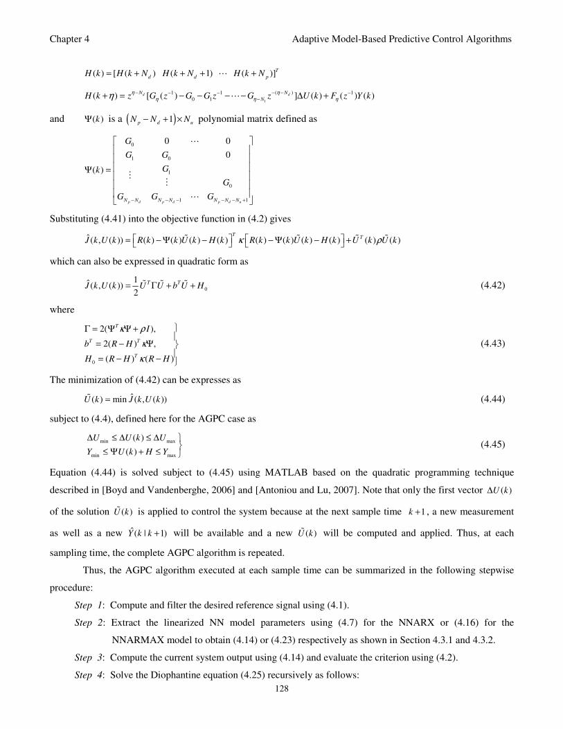
Chapter 4 Adaptive Model-Based Predictive Control Algorithms
128
( ) [ ( ) ( 1) ( )]T
d d pH k H k N H k N H k N= + + + +
1
( )1 1 1
0 1( ) [ ( ) ] ( ) ( ) ( )d dN N
NH k z G z G G z G z U k F z Y kη η
η η ηη − − −− − −
−+ = − − − − ∆ +
and ( )kΨ is a ( )1p d uN N N− + × polynomial matrix defined as
0
1 0
1
0
1 1
0 0
0
( )
p d p d p d uN N N N N N N
G
G G
Gk
G
G G G− − − − − +
Ψ =
Substituting (4.41) into the objective function in (4.2) gives
ˆ( , ( )) ( ) ( ) ( ) ( ) ( ) ( ) ( ) ( ) ( ) ( )T
TJ k U k R k k U k H k R k k U k H k U k U kκ ρ = − Ψ − − Ψ − +
which can also be expressed in quadratic form as
0
1ˆ( , ( ))2
T TJ k U k U U b U H= Γ + + (4.42)
where
0
2( ),
2( ) ,
( ) ( )
T
T T
T
I
b R H
H R H R H
κ ρ
κ
κ
Γ = Ψ Ψ +
= − Ψ
= − −
(4.43)
The minimization of (4.42) can be expresses as
ˆ( ) min ( , ( ))U k J k U k= (4.44)
subject to (4.4), defined here for the AGPC case as
min max
min max
( )
( )
U U k U
Y U k H Y
∆ ≤ ∆ ≤ ∆
≤ Ψ + ≤ (4.45)
Equation (4.44) is solved subject to (4.45) using MATLAB based on the quadratic programming technique
described in [Boyd and Vandenberghe, 2006] and [Antoniou and Lu, 2007]. Note that only the first vector ( )U k∆
of the solution ( )U k is applied to control the system because at the next sample time 1k + , a new measurement
as well as a new ˆ( | 1)Y k k + will be available and a new ( )U k will be computed and applied. Thus, at each
sampling time, the complete AGPC algorithm is repeated.
Thus, the AGPC algorithm executed at each sample time can be summarized in the following stepwise
procedure:
Step 1: Compute and filter the desired reference signal using (4.1).
Step 2: Extract the linearized NN model parameters using (4.7) for the NNARX or (4.16) for the
NNARMAX model to obtain (4.14) or (4.23) respectively as shown in Section 4.3.1 and 4.3.2.
Step 3: Compute the current system output using (4.14) and evaluate the criterion using (4.2).
Step 4: Solve the Diophantine equation (4.25) recursively as follows:
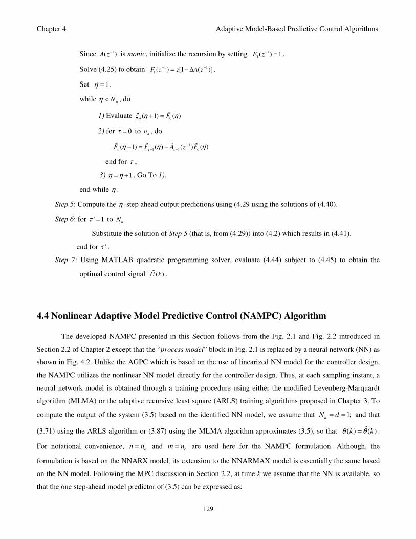
Chapter 4 Adaptive Model-Based Predictive Control Algorithms
129
Since 1( )A z− is monic, initialize the recursion by setting 1
1( ) 1E z
− = .
Solve (4.25) to obtain 1 1
1( ) [1 ( )]F z z A z
− −= − ∆ .
Set 1.η =
while p
Nη < , do
1) Evaluate 0
( 1) ( )Fηξ η η+ =
2) for 0τ = to a
n , do
1
1 1 0( 1) ( ) ( ) ( )F F A z Fτ τ τη η η−
+ ++ = −
end for τ ,
3) 1η η= + , Go To 1).
end while η .
Step 5: Compute the η -step ahead output predictions using (4.29 using the solutions of (4.40).
Step 6: for ' 1τ = to u
N
Substitute the solution of Step 5 (that is, from (4.29)) into (4.2) which results in (4.41).
end for 'τ .
Step 7: Using MATLAB quadratic programming solver, evaluate (4.44) subject to (4.45) to obtain the
optimal control signal ( )U k .
4.4 Nonlinear Adaptive Model Predictive Control (NAMPC) Algorithm
The developed NAMPC presented in this Section follows from the Fig. 2.1 and Fig. 2.2 introduced in
Section 2.2 of Chapter 2 except that the “process model” block in Fig. 2.1 is replaced by a neural network (NN) as
shown in Fig. 4.2. Unlike the AGPC which is based on the use of linearized NN model for the controller design,
the NAMPC utilizes the nonlinear NN model directly for the controller design. Thus, at each sampling instant, a
neural network model is obtained through a training procedure using either the modified Levenberg-Marquardt
algorithm (MLMA) or the adaptive recursive least square (ARLS) training algorithms proposed in Chapter 3. To
compute the output of the system (3.5) based on the identified NN model, we assume that 1;d
N d= = and that
(3.71) using the ARLS algorithm or (3.87) using the MLMA algorithm approximates (3.5), so that ˆ( ) ( )k kθ θ= .
For notational convenience, a
n n= and b
m n= are used here for the NAMPC formulation. Although, the
formulation is based on the NNARX model, its extension to the NNARMAX model is essentially the same based
on the NN model. Following the MPC discussion in Section 2.2, at time k we assume that the NN is available, so
that the one step-ahead model predictor of (3.5) can be expressed as:
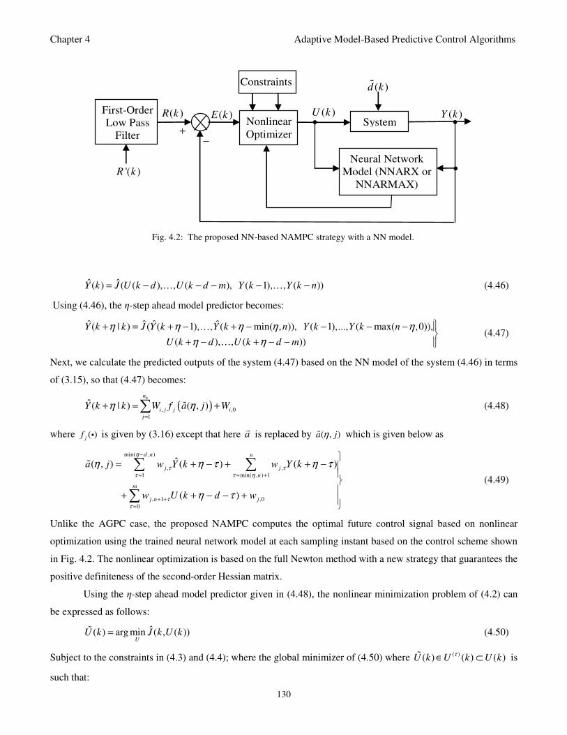
Chapter 4 Adaptive Model-Based Predictive Control Algorithms
130
ˆ ˆ( ) ( ( ), , ( ), ( 1), , ( ))Y k J U k d U k d m Y k Y k n= − − − − −… … (4.46)
Using (4.46), the η-step ahead model predictor becomes:
ˆ ˆ ˆ ˆ( | ) ( ( 1), , ( min( , )), ( 1),..., ( max( ,0)),
( ), , ( ))
Y k k J Y k Y k n Y k Y k n
U k d U k d m
η η η η η
η η
+ = + − + − − − −
+ − + − −
…
… (4.47)
Next, we calculate the predicted outputs of the system (4.47) based on the NN model of the system (4.46) in terms
of (3.15), so that (4.47) becomes:
( ), ,0
1
ˆ( | ) ( , )hn
i j j i
j
Y k k W f a j Wη η=
+ = +∑ (4.48)
where ( )j
f i is given by (3.16) except that here a
is replaced by ( , )a jη which is given below as
min( , )
, ,
1 min( , ) 1
, 1 ,0
0
ˆ( , ) ( ) ( )
( )
d n n
j j
n
m
j n j
a j w Y k w Y k
w U k d w
η
τ ττ τ η
τ
τ
η η τ η τ
η τ
−
= = +
+ +
=
= + − + + −
+ + − − +
∑ ∑
∑
(4.49)
Unlike the AGPC case, the proposed NAMPC computes the optimal future control signal based on nonlinear
optimization using the trained neural network model at each sampling instant based on the control scheme shown
in Fig. 4.2. The nonlinear optimization is based on the full Newton method with a new strategy that guarantees the
positive definiteness of the second-order Hessian matrix.
Using the η-step ahead model predictor given in (4.48), the nonlinear minimization problem of (4.2) can
be expressed as follows:
ˆ( ) arg min ( , ( ))U
U k J k U k= (4.50)
Subject to the constraints in (4.3) and (4.4); where the global minimizer of (4.50) where ( )( ) ( ) ( )U k U k U kτ∈ ⊂ is
such that:
System ( )Y k ( )U k
•
Neural Network
Model (NNARX or
NNARMAX)
Nonlinear
Optimizer •
+ −
'( )R k
( )E k
•
Constraints
First-Order
Low Pass
Filter
( )d k
( )R k
Fig. 4.2: The proposed NN-based NAMPC strategy with a NN model.
Chapter 4 Adaptive Model-Based Predictive Control Algorithms
131
( ) ( )ˆ ˆ( , ( )) ( , ( )), ( ) ( )J k U k J k U k U k U kτ τ≤ ∀ ∈ .
The algorithm proposed for solving (4.50) uses the full Newton method based on the Levenberg-
Marquardt algorithm with the following adaptive updating rule:
( ) ( )( ) ( ) ( )U k U k kτ τζ= + (4.51)
which is applied for updating the sequence of future optimal control signal ( )U k , ( ) ( )U kτ is the current iterate of
the control sequence, and ( ) ( )kτζ the search direction given by the following expression:
( )1
( ) ( ) ( ) ( )( ) [ ( )] [ ( )]k H U k I G U kτ τ τ τζ λ
−
= − + (4.52)
where ( )τλ is the adaptation parameter, I is a diagonal matrix; ( )[ ( )]G U kτ and ( )[ ( )]H U k
τ are the Jacobian and
Newton Hessian matrices given respectively as:
( )
( )
( )
( ) ( )
( )
( ) ( )
ˆ( , ( ))[ ( )]
( )
( )2 [ ( )] ( ) 2 ( )
( )
U k U k
T
U k U k
J k U kG U k
U k
U kU k E k U k
U k
τ
τ
τ
τκ ρ
=
=
∂=
∂
∂ = − ⋅ ⋅Φ ⋅ + ⋅ ⋅ ∂
(4.53)
( )
( )
2( )
2
( ) ( )
( ) ( )
ˆ( , ( ))( )
( )
ˆ ( ) ( ) ( )( ) 2
( ) ( ) ( ) ( )
U k U k
T T
U k U k
J k U kH U k
U k
Y k U k U kE k
U k U k U k U k
τ
τ
τ
κ ρ
=
=
∂ = ∂
∂ ∂ ∂ ∂
= ⋅ + ⋅ ⋅ ∂ ∂ ∂ ∂
(4.54)
The Φ in (4.53) is the partial derivatives of (4.48) with respect to the predicted outputs. The computation of Φ
and the future control signals are explained below.
Computation of Φ and the Future Control Signal
Consider the optimal control signal, search direction, the Jacobian matrix and the Hessian matrix given by
(4.51) through (4.54) respectively. To simplify the computation of Φ in (4.53), the control signal ( )U k is
decomposed into the past and future control signals ˆ( , )a jη given below as:
min( , ) min( 2, 1)
, ,
1 1
min( , ) min( , )
, 1 ,
2 1
, , 1
1 1
ˆˆ( , ) ( ) ( 1)
ˆ( ) ( )
( ) ( )
d d u
d
d u d
d
N n N N m
j j n u
N m n
j n d j
N N N
n m
j j n d
N
a j w Y k w U k N
w U k N w Y k
w Y k w U k N w
η η
τ ττ τ
η η
τ ττ η τ η
τ ττ η τ η
η η τ
η τ η τ
η τ η τ
− − − + +
+
= =
−
+ +
= − − + = − +
+ +
= + = − +
= + − + + −
+ − + − + + −
+ + − + − + − +
∑ ∑
∑ ∑
∑ ∑ ,0j
(4.55)
Chapter 4 Adaptive Model-Based Predictive Control Algorithms
132
The first three sums of (4.55) depend on future control signals while the last three sums depend on past control
signals.
The computation of ( ) ( )U k U k∂ ∂ appearing in (4.53) and (4.54) follows from the constraint specified in
(4.3) for the control horizon, so that the derivative of ( ) ( )U k U k∂ ∂ evaluated at ( ) ( )U k U kτ= can be expressed
directly as:
( )( ) ( )
1 0 0 0 0
1 1 0 0 0( )
0( )
0 0 1 1 0
0 0 0 1 1
U k U k
U k
U k τ=
− ∂ =
∂ −
−
(4.56)
Note that since ( ) ( ) ( 1)U k U k U k∆ = − − , Equation (4.73) is a matrix of dimensionu u
N N× .
Next, the computation for ˆ( ) ( )Y k U k∂ ∂ appearing in (4.54) evaluated at ( ) ( )U k U kτ= is expressed as:
( )( ) ( )
ˆ ˆ( ) ( )
( ) ( 1)ˆ ( )
( )ˆ ˆ( ) ( )
( ) ( 1)
d d
u
U k U k
p p
u
Y k N Y k N
U k U k NY k
U kY k N Y k N
U k U k N
τ=
∂ + ∂ +
∂ ∂ + − ∂ =
∂ ∂ + ∂ + ∂ ∂ + −
(4.57)
Thus, Equation (4.57) is a polynomial matrix of dimension ( 1)u p dN N N× − + . Note that the past control signals
do not contribute to the output predictions because new measurements will be available at the next sampling
instant 1k + . Thus, Φ is computed based only on the future control signals for all [ , ]d pN Nη ∈ and for all
[0,min( 1, 1)]u
l Nη∈ − − ; and can be defined from (4.57) as:
1
ˆ( ) ˆˆ'( ( , )) ( , , )( )
hn
j
j
Y kW f a j b l j
U k l
ηη η
=
∂ +Φ = = ⋅
∂ +∑ (4.58)
where ˆ( , )a jη is computed from (4.55) while ˆ( , , )b l jη for all [0,min( 1, 1)]u
l Nη∈ − − is computed using the first
three sum of ˆ( , )a jη in (4.55) since these terms corresponds to the future control signals and is defined here as:
min( , ) min( 2, 1)
, ,
1 1
min( , )
, 1
2
ˆ ( )( )ˆ( , , )( ) ( )
( )
( )
d d u
d
d u
N n N N m
u
j j n
N m
d
j n
N N
U k NY kb l j w w
U k l U k l
U k Nw
U k l
η η
τ ττ τ
η
ττ η
τη τη
η τ
− − − + +
+
= =
−
+ +
= − − +
∂ + −∂ + −= +
∂ + ∂ +
∂ − + − +∂ +
∑ ∑
∑ (4.59)
Note that from (4.59), the three partial derivative terms can be evaluated respectively as follows:
ˆ( )0, 1
( )d
Y kl N
U k l
η τη τ
∂ + −= ≥ − − +
∂ + (4.60)
Chapter 4 Adaptive Model-Based Predictive Control Algorithms
133
1,( )
0,( )
uul NU k N
OtherwiseU k l
ητ = −∂ + −=
∂ + (4.61)
1,( )
0,( )
ddl NU k N
OtherwiseU k l
η τη τ = − −∂ − + −=
∂ + (4.62)
Using (4.77) to (4.60), Equation (4.59) can be reduced to the following form defined by ˆ( , , )c l jη given below as:
min( , ) min( 2, 1)
, ,
1 1
min( , )
, , 1
1
min( , )
,
1
ˆ ( )( )ˆ( , , ) , 1
( ) ( )
ˆ( ), max(0, ) 2
( )
ˆ
d d u
d
d
d
N l n N N m
u
j j n u
N l n
j j n N l d u
N l n
j
U k NY kc l j w w l N
U l U k l
Y kw w N m l N
U l
Yw
η η
τ ττ τ
η
τ ητ
η
ττ
τη τη
τ
η τη
τ
− − − − + +
+
= =
− −
+ − − +
=
− −
=
∂ + −∂ + −= + = −
∂ + ∂ +
∂ + −= + − − ≤ ≤ −
∂ +
∂=
∑ ∑
∑
∑ , 1
( ), 0 max(0, )
( ) dj n N l d
kw l N m
U lη
η τη
τ+ − − +
+ −+ ≤ ≤ − −
∂ +
(4.63)
Thus, using (4.63), the computation of the first-order derivative in (4.58) can be reduced to
1
ˆ( )ˆ ˆ'( ( , )) ( , , )
( )
hn
j
j
Y kW f a j c l j
U k l
ηη η
=
∂ +Φ = = ⋅
∂ +∑ (4.64)
Note that ˆ'( ( , ))f a jη is the first-order derivative of (3.16) evaluated for the ˆ( , )a jη contained in (4.64) which can
be expressed in a simplified form as
2ˆ ˆ'( ( , )) 1 ( ( , ))f a j f a jη η= − (4.65)
Finally, the computation of the second-order derivative ˆ ( )
( )( ) ( )
TY k
E kU k U k
∂ ∂ ∂ ∂
appearing in (4.54)
evaluated at ( ) ( )U k U kτ= begins with the vector inside the parenthesis which is expressed as follows:
2ˆ ˆ( ) ( )
( ) ........ ..... ( )( ) ( )
ˆ ( )( )
( )ˆ ˆ( ) ( )
( ) ... ( )( 1) ( 1)
d
d p
T
d p
d p
u u
Y k N Y k NE k N E k N
U k U kY k
E kU k
Y t N Y k NE k N E k N
U k N U k N
∂ + ∂ + + + + +
∂ ∂ ∂ =
∂ ∂ + ∂ +
+ + + + ∂ + − ∂ + −
(4.66)
Next, taking the derivative of (4.66) with respect to ( )U k results in the following u u
N N× matrix:
2 2
2
2 2
2
ˆ ˆ( ) ( )( ) ( )
( ) ( ) ( 1)ˆ ˆ ˆ( ) ( ) ( )
( )( ) ( ) ( ) ( )
ˆ ˆ( ) ( )( ) ( )
( ) ( 1) ( 1)
T T
uT T
T T
u u
Y k Y kE k E k
U k U k U k NY k Y k Y k
E kU k U k U k U k
Y k Y tE k E k
U k U k N U k N
∂ ∂
∂ ∂ ∂ + − ∂ ∂ ∂ ∂ = − ∂ ∂ ∂ ∂ ∂ ∂
∂ ∂ + − ∂ + −
(4.67)
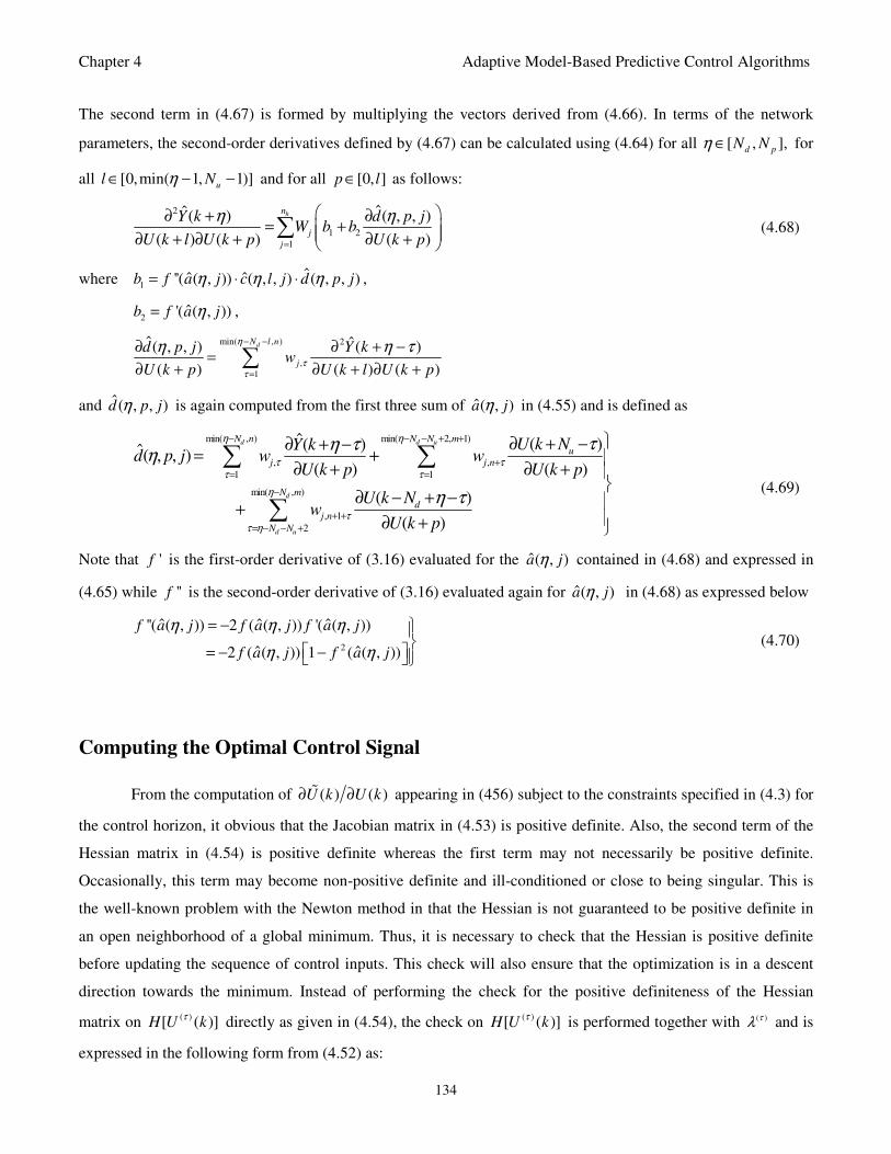
Chapter 4 Adaptive Model-Based Predictive Control Algorithms
134
The second term in (4.67) is formed by multiplying the vectors derived from (4.66). In terms of the network
parameters, the second-order derivatives defined by (4.67) can be calculated using (4.64) for all [ , ],d pN Nη ∈ for
all [0,min( 1, 1)]u
l Nη∈ − − and for all [0, ]p l∈ as follows:
2
1 2
1
ˆˆ( ) ( , , )
( ) ( ) ( )
hn
j
j
Y k d p jW b b
U k l U k p U k p
η η
=
∂ + ∂= + ∂ + ∂ + ∂ + ∑ (4.68)
where 1ˆˆ ˆ''( ( , )) ( , , ) ( , , )b f a j c l j d p jη η η= ⋅ ⋅ ,
2ˆ'( ( , ))b f a jη= ,
min( , ) 2
,
1
ˆ ˆ( , , ) ( )
( ) ( ) ( )
dN l n
j
d p j Y kw
U k p U k l U k p
η
ττ
η η τ− −
=
∂ ∂ + −=
∂ + ∂ + ∂ +∑
and ˆ( , , )d p jη is again computed from the first three sum of ˆ( , )a jη in (4.55) and is defined as
min( , ) min( 2, 1)
, ,
1 1
min( , )
, 1
2
ˆ ( )( )ˆ( , , )( ) ( )
( )
( )
d d u
d
d u
N n N N m
u
j j n
N m
dj n
N N
U k NY kd p j w w
U k p U k p
U k Nw
U k p
η η
τ ττ τ
η
ττ η
τη τη
η τ
− − − + +
+
= =
−
+ +
= − − +
∂ + −∂ + −= +
∂ + ∂ +
∂ − + − +∂ +
∑ ∑
∑ (4.69)
Note that 'f is the first-order derivative of (3.16) evaluated for the ˆ( , )a jη contained in (4.68) and expressed in
(4.65) while ''f is the second-order derivative of (3.16) evaluated again for ˆ( , )a jη in (4.68) as expressed below
2
ˆ ˆ ˆ''( ( , )) 2 ( ( , )) '( ( , ))
ˆ ˆ2 ( ( , )) 1 ( ( , ))
f a j f a j f a j
f a j f a j
η η η
η η
= −
= − − (4.70)
Computing the Optimal Control Signal
From the computation of ( ) ( )U k U k∂ ∂ appearing in (456) subject to the constraints specified in (4.3) for
the control horizon, it obvious that the Jacobian matrix in (4.53) is positive definite. Also, the second term of the
Hessian matrix in (4.54) is positive definite whereas the first term may not necessarily be positive definite.
Occasionally, this term may become non-positive definite and ill-conditioned or close to being singular. This is
the well-known problem with the Newton method in that the Hessian is not guaranteed to be positive definite in
an open neighborhood of a global minimum. Thus, it is necessary to check that the Hessian is positive definite
before updating the sequence of control inputs. This check will also ensure that the optimization is in a descent
direction towards the minimum. Instead of performing the check for the positive definiteness of the Hessian
matrix on ( )[ ( )]H U kτ directly as given in (4.54), the check on ( )[ ( )]H U k
τ is performed together with ( )τλ and is
expressed in the following form from (4.52) as:
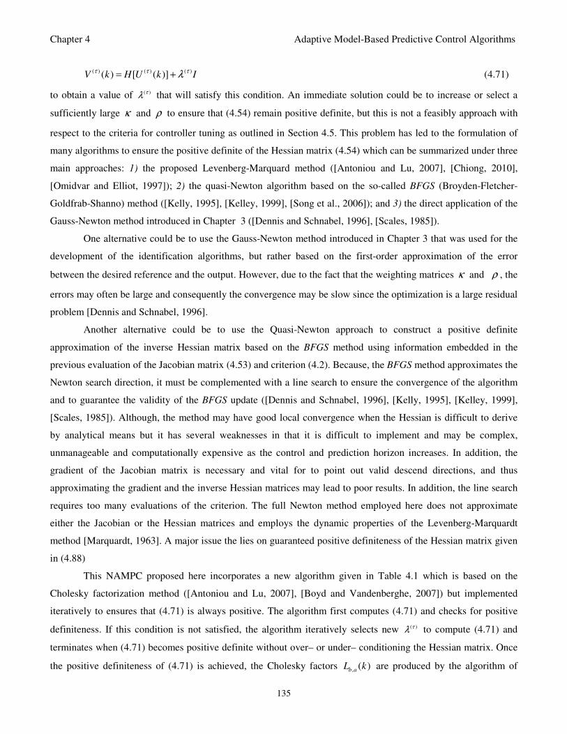
Chapter 4 Adaptive Model-Based Predictive Control Algorithms
135
( ) ( ) ( )( ) [ ( )]V k H U k Iτ τ τλ= + (4.71)
to obtain a value of ( )τλ that will satisfy this condition. An immediate solution could be to increase or select a
sufficiently large κ and ρ to ensure that (4.54) remain positive definite, but this is not a feasibly approach with
respect to the criteria for controller tuning as outlined in Section 4.5. This problem has led to the formulation of
many algorithms to ensure the positive definite of the Hessian matrix (4.54) which can be summarized under three
main approaches: 1) the proposed Levenberg-Marquard method ([Antoniou and Lu, 2007], [Chiong, 2010],
[Omidvar and Elliot, 1997]); 2) the quasi-Newton algorithm based on the so-called BFGS (Broyden-Fletcher-
Goldfrab-Shanno) method ([Kelly, 1995], [Kelley, 1999], [Song et al., 2006]); and 3) the direct application of the
Gauss-Newton method introduced in Chapter 3 ([Dennis and Schnabel, 1996], [Scales, 1985]).
One alternative could be to use the Gauss-Newton method introduced in Chapter 3 that was used for the
development of the identification algorithms, but rather based on the first-order approximation of the error
between the desired reference and the output. However, due to the fact that the weighting matrices κ and ρ , the
errors may often be large and consequently the convergence may be slow since the optimization is a large residual
problem [Dennis and Schnabel, 1996].
Another alternative could be to use the Quasi-Newton approach to construct a positive definite
approximation of the inverse Hessian matrix based on the BFGS method using information embedded in the
previous evaluation of the Jacobian matrix (4.53) and criterion (4.2). Because, the BFGS method approximates the
Newton search direction, it must be complemented with a line search to ensure the convergence of the algorithm
and to guarantee the validity of the BFGS update ([Dennis and Schnabel, 1996], [Kelly, 1995], [Kelley, 1999],
[Scales, 1985]). Although, the method may have good local convergence when the Hessian is difficult to derive
by analytical means but it has several weaknesses in that it is difficult to implement and may be complex,
unmanageable and computationally expensive as the control and prediction horizon increases. In addition, the
gradient of the Jacobian matrix is necessary and vital for to point out valid descend directions, and thus
approximating the gradient and the inverse Hessian matrices may lead to poor results. In addition, the line search
requires too many evaluations of the criterion. The full Newton method employed here does not approximate
either the Jacobian or the Hessian matrices and employs the dynamic properties of the Levenberg-Marquardt
method [Marquardt, 1963]. A major issue the lies on guaranteed positive definiteness of the Hessian matrix given
in (4.88)
This NAMPC proposed here incorporates a new algorithm given in Table 4.1 which is based on the
Cholesky factorization method ([Antoniou and Lu, 2007], [Boyd and Vandenberghe, 2007]) but implemented
iteratively to ensures that (4.71) is always positive. The algorithm first computes (4.71) and checks for positive
definiteness. If this condition is not satisfied, the algorithm iteratively selects new ( )τλ to compute (4.71) and
terminates when (4.71) becomes positive definite without over– or under– conditioning the Hessian matrix. Once
the positive definiteness of (4.71) is achieved, the Cholesky factors , ( )b aL k are produced by the algorithm of
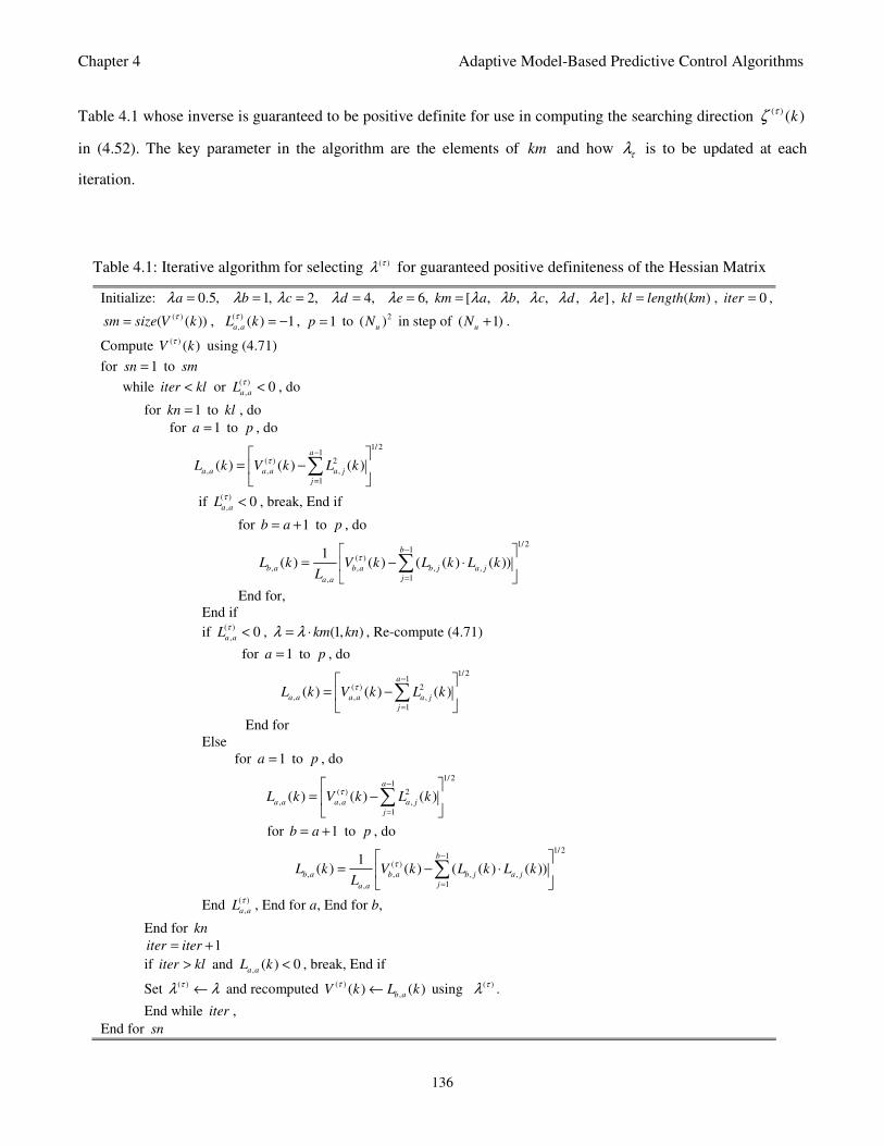
Chapter 4 Adaptive Model-Based Predictive Control Algorithms
136
Table 4.1: Iterative algorithm for selecting ( )τλ for guaranteed positive definiteness of the Hessian Matrix
Initialize: 0.5,aλ = 1,bλ = 2,cλ = 4,dλ = 6,eλ = [ , , , , ]km a b c d eλ λ λ λ λ= , ( )kl length km= , 0iter = ,
( )( ( ))sm size V kτ= ,
( )
,( ) 1
a aL k
τ= − , 1p = to 2( )
uN in step of ( 1)
uN + .
Compute ( ) ( )V kτ using (4.71)
for 1sn = to sm
while iter kl< or ( )
,0
a aL
τ< , do
for 1kn = to kl , do
for 1a = to p , do
1/ 21
( ) 2
, , ,
1
( ) ( ) ( )a
a a a a a j
j
L k V k L kτ−
=
= −
∑
if ( )
,0
a aL
τ< , break, End if
for 1b a= + to p , do
1/ 21
( )
, , , ,
1,
1( ) ( ) ( ( ) ( ))
b
b a b a b j a j
ja a
L k V k L k L kL
τ−
=
= − ⋅
∑
End for,
End if
if ( )
,0
a aL
τ< , (1, )km knλ λ= ⋅ , Re-compute (4.71)
for 1a = to p , do
1/ 21
( ) 2
, , ,
1
( ) ( ) ( )a
a a a a a j
j
L k V k L kτ−
=
= −
∑
End for
Else
for 1a = to p , do
1/ 21
( ) 2
, , ,
1
( ) ( ) ( )a
a a a a a j
j
L k V k L kτ−
=
= −
∑
for 1b a= + to p , do
1/ 21
( )
, , , ,
1,
1( ) ( ) ( ( ) ( ))
b
b a b a b j a j
ja a
L k V k L k L kL
τ−
=
= − ⋅
∑
End ( )
,a aL
τ, End for a, End for b,
End for kn
1iter iter= +
if iter kl> and ,
( ) 0a a
L k < , break, End if
Set ( )τλ λ← and recomputed ( )
,( ) ( )
b aV k L k
τ← using ( )τλ .
End while iter ,
End for sn
Table 4.1 whose inverse is guaranteed to be positive definite for use in computing the searching direction ( ) ( )kτζ
in (4.52). The key parameter in the algorithm are the elements of km and how τλ is to be updated at each
iteration.
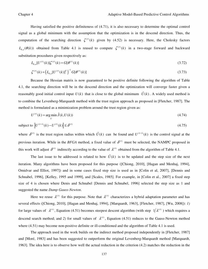
Chapter 4 Adaptive Model-Based Predictive Control Algorithms
137
Having satisfied the positive definiteness of (4.71), it is also necessary to determine the optimal control
signal as a global minimum with the assumption that the optimization is in the descend direction. Thus, the
computation of the searching direction ( ) ( )kτζ given by (4.52) is necessary. Here, the Cholesky factors
, ( ( ))b aL kθ obtained from Table 4.1 is reused to compute ( ) ( )kτζ in a two-stage forward and backward
substitution procedures given respectively as:
( ) ( ) ( )
, [ ( )] ( ) [ ( )]b aL U k k G kτ τ τζ θ= (3.72)
( )1
( ) ( ) ( )
,( ) [ ( )] [ ( )]T
b ak L U k G k
τ τ τζ θ−
= (3.73)
Because the Hessian matrix is now guaranteed to be positive definite following the algorithm of Table
4.1, the searching direction will be in the descend direction and the optimization will converge faster given a
reasonably good initial control input ( )U k that is close to the global minimum ( )U k . A widely used method is
to combine the Levenberg-Marquardt method with the trust region approach as proposed in [Fletcher, 1987]. The
method is formulated as a minimization problem around the trust region given as:
( ) ˆ( ) arg min ( , ( ))U
U k J k U kτ = (4.74)
subject to ( 1) ( ) ( )( ) ( )U k U kτ τ τδ− − ≤ (4.75)
where ( )τδ is the trust region radius within which ( )U k can be found and ( 1) ( )U kτ − is the control signal at the
previous iteration. While in the BFGA method, a fixed value of ( )τδ must be selected, the NAMPC proposed in
this work will adjust ( )τδ indirectly according to the value of ( )τλ obtained from the algorithm of Table 4.1.
The last issue to be addressed is related to how ( )U k is to be updated and the step size of the next
iteration. Many algorithms have been proposed for this purpose ([Chiong, 2010], [Hagan and Menhaj, 1994],
Omidvar and Elliot, 1997]) and in some cases fixed step size is used as in [Colin et al, 2007], [Dennis and
Schnabel, 1996], [Kelley, 1995 and 1999], and [Scales, 1985]. For example, in [Colin et al., 2007] a fixed step
size of 4 is chosen where Denis and Schnabel [Dennis and Schnabel, 1996] selected the step size as 1 and
suggested the name Damp Gauss-Newton.
Here we reuse ( )τλ for this purpose. Note that ( )τλ characterizes a hybrid adaptation parameter and has
several effects ([Chiong, 2010], [Hagan and Menhaj, 1994], [Marquardt, 1963], [Fletcher, 1987], [Wu, 2008]): 1)
for large values of ( )τλ , Equation (4.51) becomes steepest descent algorithm (with step ( )1 τλ ) which requires a
descend search method; and 2) for small values of ( )τλ , Equation (4.51) reduces to the Gauss-Newton method
where (4.51) may become non-positive definite or ill-conditioned and the algorithm of Table 4.1 is used.
The approach used in the work builds on the indirect method proposed independently in [Fletcher, 1987]
and [Moré, 1983] and has been suggested to outperform the original Levenberg-Marquardt method [Marquardt,
1963]. The idea here is to observe how well the actual reduction in the criterion (4.2) matches the reduction in the
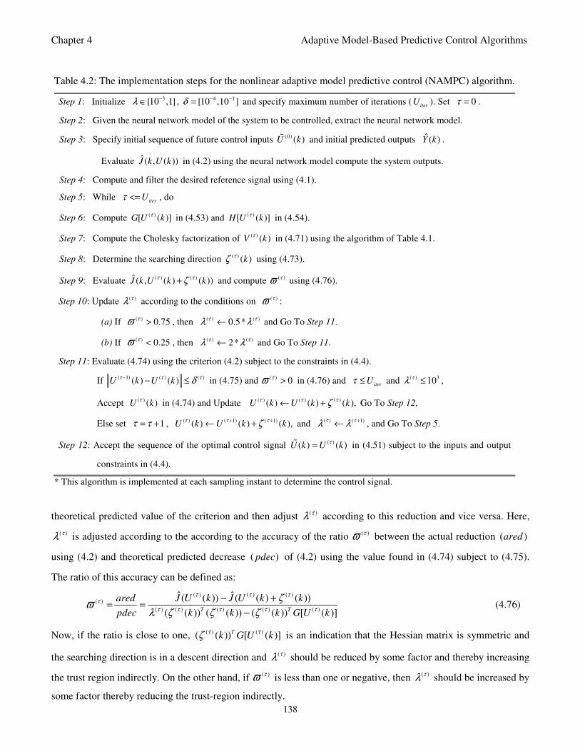
Chapter 4 Adaptive Model-Based Predictive Control Algorithms
138
Table 4.2: The implementation steps for the nonlinear adaptive model predictive control (NAMPC) algorithm.
Step 1: Initialize 3[10 ,1]λ −∈ , 4 1[10 ,10 ]δ − −= and specify maximum number of iterations (iter
U ). Set 0τ = .
Step 2: Given the neural network model of the system to be controlled, extract the neural network model.
Step 3: Specify initial sequence of future control inputs (0) ( )U k and initial predicted outputs ˆ( )Y k .
Evaluate ˆ( , ( ))J k U k in (4.2) using the neural network model compute the system outputs.
Step 4: Compute and filter the desired reference signal using (4.1).
Step 5: Whileiter
Uτ <= , do
Step 6: Compute ( )[ ( )]G U kτ in (4.53) and ( )[ ( )]H U k
τ in (4.54).
Step 7: Compute the Cholesky factorization of ( ) ( )V kτ in (4.71) using the algorithm of Table 4.1.
Step 8: Determine the searching direction ( ) ( )kτζ using (4.73).
Step 9: Evaluate ( ) ( )ˆ( , ( ) ( ))J k U k kτ τζ+ and compute ( )τϖ using (4.76).
Step 10: Update ( )τλ according to the conditions on ( )τϖ :
(a) If ( ) 0.75τϖ > , then ( ) ( )0.5*τ τλ λ← and Go To Step 11.
(b) If ( ) 0.25τϖ < , then ( ) ( )2*τ τλ λ← and Go To Step 11.
Step 11: Evaluate (4.74) using the criterion (4.2) subject to the constraints in (4.4).
If ( 1) ( ) ( )
( ) ( )U k U kτ τ τδ−
− ≤ in (4.75) and ( ) 0τϖ > in (4.76) anditer
Uτ ≤ and ( ) 310τλ ≤ ,
Accept ( ) ( )U kτ in (4.74) and Update ( ) ( ) ( )( ) ( ) ( ),U k U k k
τ τ τζ← + Go To Step 12,
Else set 1τ τ= + , ( ) ( 1) ( 1)( ) ( ) ( ),U k U k kτ τ τζ+ +← + and ( ) ( 1)τ τλ λ +← , and Go To Step 5.
Step 12: Accept the sequence of the optimal control signal ( )( ) ( )U k U kτ= in (4.51) subject to the inputs and output
constraints in (4.4).
* This algorithm is implemented at each sampling instant to determine the control signal.
theoretical predicted value of the criterion and then adjust ( )τλ according to this reduction and vice versa. Here,
( )τλ is adjusted according to the according to the accuracy of the ratio ( )τϖ between the actual reduction ( )ared
using (4.2) and theoretical predicted decrease ( )pdec of (4.2) using the value found in (4.74) subject to (4.75).
The ratio of this accuracy can be defined as:
( ) ( ) ( )( )
( ) ( ) ( ) ( ) ( )
ˆ ˆ( ( )) ( ( ) ( ))
( ( )) ( ( )) ( ( )) [ ( )]T T
ared J U k J U k k
pdec k k k G U k
τ τ ττ
τ τ τ τ τ
ζϖ
λ ζ ζ ζ
− += =
− (4.76)
Now, if the ratio is close to one, ( ) ( )( ( )) [ ( )]Tk G U k
τ τζ is an indication that the Hessian matrix is symmetric and
the searching direction is in a descent direction and ( )τλ should be reduced by some factor and thereby increasing
the trust region indirectly. On the other hand, if ( )τϖ is less than one or negative, then ( )τλ should be increased by
some factor thereby reducing the trust-region indirectly.
Chapter 4 Adaptive Model-Based Predictive Control Algorithms
139
Thus, the NAMPC algorithm executed at each sampling instant k can be summarized in the stepwise
procedure given in Table 4.2. How the parameter ( )τλ should be reduced or increased depends on the criterion.
Suppose that the searching direction found in Step 5 does not lead to a reduction in the criterion, then ( ) 0τϖ <
and consequently the inequality in Step 10(b) is satisfied. Thus, the parameter ( )τλ should be increased until there
is a predicted decrease in the criterion. On the other hand, if the searching direction found in Step 5 reduces the
predicted value of the criterion sufficiently, then ( ) 0τϖ > and consequently the inequality in Step 10(a) is
satisfied. Thus, the parameter ( )τλ must be decreased until there is a predicted increase in the criterion. The main
drawback here is that the searching direction must be recomputed each time ( )τλ is reduced or increased for the
criterion to be evaluated, and hence significant amount of computation is required due to this process.
4.5 Tuning the Neural Network-Based Adaptive Model Predictive Controllers
After the design and possible implementation of the controllers developed in the two preceding sub-
sections, the next issue is towards the practical use of these controllers which involves the selection of the design
parameters 1 2, , ,
uN N N κ and ρ through a tuning process. In addition to the four parameters, the two parameters
( 1( )m
A z− and 1( )
mB z
− ) of the first-order low-pass digital filter are also considered here as tuning parameters
since they are used to calculate and filter the desired reference signals, and thus influence the stability and
robustness of the two controllers. The two horizons 1
N and 2
N have substantial impact on the time needed to
compute the control inputs. Unlike the AGPC, the NAMPC computation time is also influenced by the choice of
the additional design parameters δ and iter
U as well as the initial value of λ . The initial values of the control
inputs 0
( )U and predicted outputs 0
( )Y also influence the convergence rate of the two control algorithms.
Several research reports on MPC explain different routines and techniques for tuning MPC controllers
depending on the control objectives (disturbance and/or noise rejection, stability, robustness) [Clarke et al.,
1987a], [Clarke et al., 1987b], [Nørgaard et al., 2000], [Rossiter, 2004], and [Soeterboek, 1992]). In the following,
the conceptual guidelines for tuning the two controllers developed in the two preceding sub-sections are
highlighted and discussed below.
(i) Minimum prediction horizon,1
:N
This parameter is always selected to model time delay ( )d . It must not be chosen to be smaller because the
1d − first predictions depend upon past control inputs only and thus cannot be influenced. On the other hand,
choosing it to be bigger can lead to quite unpredictable results.
Chapter 4 Adaptive Model-Based Predictive Control Algorithms
140
(ii) Maximum prediction horizon,2
:N
To ensure stabilization of systems with an unstable inverse, it should be at least as many time steps as there
are past control inputs fed into the network model. Usually it is selected a bit longer and close to the rise time of
the system response (if it is stable). However, it is not often possible to choose it that long because the
optimization problem will become too computationally demanding compared with the selected sampling period.
(iii) Control horizon, :u
N
In the linear case, it is easy to select this parameter to be equal to or exceed the number of unstable or
poorly damped poles. However, in the nonlinear case where the computational burden increases tremendously as
uN is increased, this is leads to a somewhat long control horizon. Unless the sampling period is very long, it is
always a good practice to use the smallest viable value.
(v) The penalty factor on the control input ρ and predicted output :κ
For reasons of numerical robustness, this parameter should be selected as 0κ > to prevent the Hessian from
becoming singular [Soeterboek, 1992]. However, it is primarily used for controlling the magnitude and
smoothness of the control signal and in practice it can be selected from simulation studies.
Note that the tuning rules described above are valid for both the NAMPC and the AGPC cases but the
computational demands associated with selecting long prediction and control horizons may be significantly less p
in the AGPC case. However, for systems where the nonlinearities are not necessarily smooth, selecting a long
prediction horizon is absurd. A remote future prediction will be completely unreliable and using it for calculating
the present control action intuitively may be meaningless.
Chapter 5 Development of Real-Time Implementation Platforms
141
CHAPTER FIVE
DEVELOPMENT OF REAL-TIME IMPLEMENTATION PLATFORMS FOR
THE NEURAL NETWORK-BASED NONLINEAR MODEL IDENTIFICATION
AND ADAPTIVE MODEL PREDICTIVE CONTROL ALGORITHMS
5.1 Introduction
In order to demonstrate the feasibility of the proposed identification and control strategies in an industrial
environment, an industrial network which utilizes the service-oriented architecture (SOA) technology based on
device profile for web services (DPWS) and a real-time embedded system development based on a field
programmable gate array (FPGA) are considered.
Systems that utilize networks for communication between industrial systems and controllers are called
network control systems (NCS). By this way reduction of wiring and ease of maintenance is achieved. However
an appropriate SOA technology for NCS must provide a bounded transmission delay and interoperability between
different components of the NCS. Several efforts have been made for embedding a SOA technology into
industrial control loops ([Chow and Tipsuwan, 2001]; [IEC, 1999]; ([Lee et al., 2006]) but none of them can
provide both the desired characteristics. Next it is described how the proposed SOA based on DPWS can be
implemented in this work and how this industrial network fulfills the aforementioned real-time characteristics for
industrial network control systems.
While the above SOA based on DPWS may be feasible for systems with long sampling interval, real-time
embedded processor systems that could implement part or an entire algorithm that control systems with relatively
short sampling times is introduced. The real-time embedded processor systems are based on the field
programmable gate array (FPGA) with two choices of embedded processors. The first is IBM PowerPC™440
embedded hard processor core and the second is the Xilinx MicroBlaze™ embedded soft processor core. Both
processors are realized on the Xilinx Virtex-5 FX70T ML507 FPGA development board.
An overview of the embedded processor systems and their design considerations are presented. The
overview answers why embedded processor systems are necessary, give some advantages and disadvantages of
FPGA embedded processor systems, and the industry standard benchmark for evaluating the performance of a
typical embedded processor in an FPGA. Several strategies are proposed to achieve enhanced performance from
an FPGA embedded processor system such as compiler optimization, choices of memory types and peripheral,
logic optimization and reduction, hardware co-processing, etc.
Furthermore, detailed techniques for the PowerPC™440 and MicroBlaze™ embedded processor system
design and testing are presented. The implementation and evaluation of the Dhrystone FPGA performance
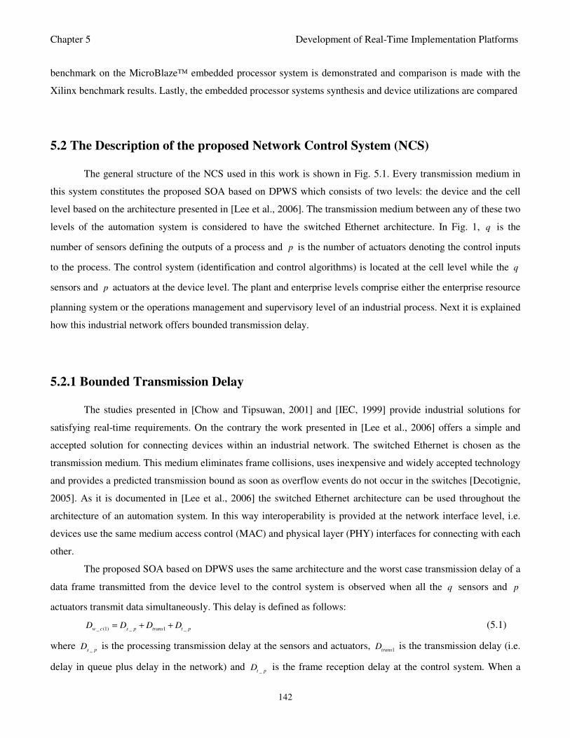
Chapter 5 Development of Real-Time Implementation Platforms
142
benchmark on the MicroBlaze™ embedded processor system is demonstrated and comparison is made with the
Xilinx benchmark results. Lastly, the embedded processor systems synthesis and device utilizations are compared
5.2 The Description of the proposed Network Control System (NCS)
The general structure of the NCS used in this work is shown in Fig. 5.1. Every transmission medium in
this system constitutes the proposed SOA based on DPWS which consists of two levels: the device and the cell
level based on the architecture presented in [Lee et al., 2006]. The transmission medium between any of these two
levels of the automation system is considered to have the switched Ethernet architecture. In Fig. 1, q is the
number of sensors defining the outputs of a process and p is the number of actuators denoting the control inputs
to the process. The control system (identification and control algorithms) is located at the cell level while the q
sensors and p actuators at the device level. The plant and enterprise levels comprise either the enterprise resource
planning system or the operations management and supervisory level of an industrial process. Next it is explained
how this industrial network offers bounded transmission delay.
5.2.1 Bounded Transmission Delay
The studies presented in [Chow and Tipsuwan, 2001] and [IEC, 1999] provide industrial solutions for
satisfying real-time requirements. On the contrary the work presented in [Lee et al., 2006] offers a simple and
accepted solution for connecting devices within an industrial network. The switched Ethernet is chosen as the
transmission medium. This medium eliminates frame collisions, uses inexpensive and widely accepted technology
and provides a predicted transmission bound as soon as overflow events do not occur in the switches [Decotignie,
2005]. As it is documented in [Lee et al., 2006] the switched Ethernet architecture can be used throughout the
architecture of an automation system. In this way interoperability is provided at the network interface level, i.e.
devices use the same medium access control (MAC) and physical layer (PHY) interfaces for connecting with each
other.
The proposed SOA based on DPWS uses the same architecture and the worst case transmission delay of a
data frame transmitted from the device level to the control system is observed when all the q sensors and p
actuators transmit data simultaneously. This delay is defined as follows:
_ (1) _ 1 _w c s p trans t pD D D D= + + (5.1)
where _s pD is the processing transmission delay at the sensors and actuators,
1transD is the transmission delay (i.e.
delay in queue plus delay in the network) and _t pD is the frame reception delay at the control system. When a
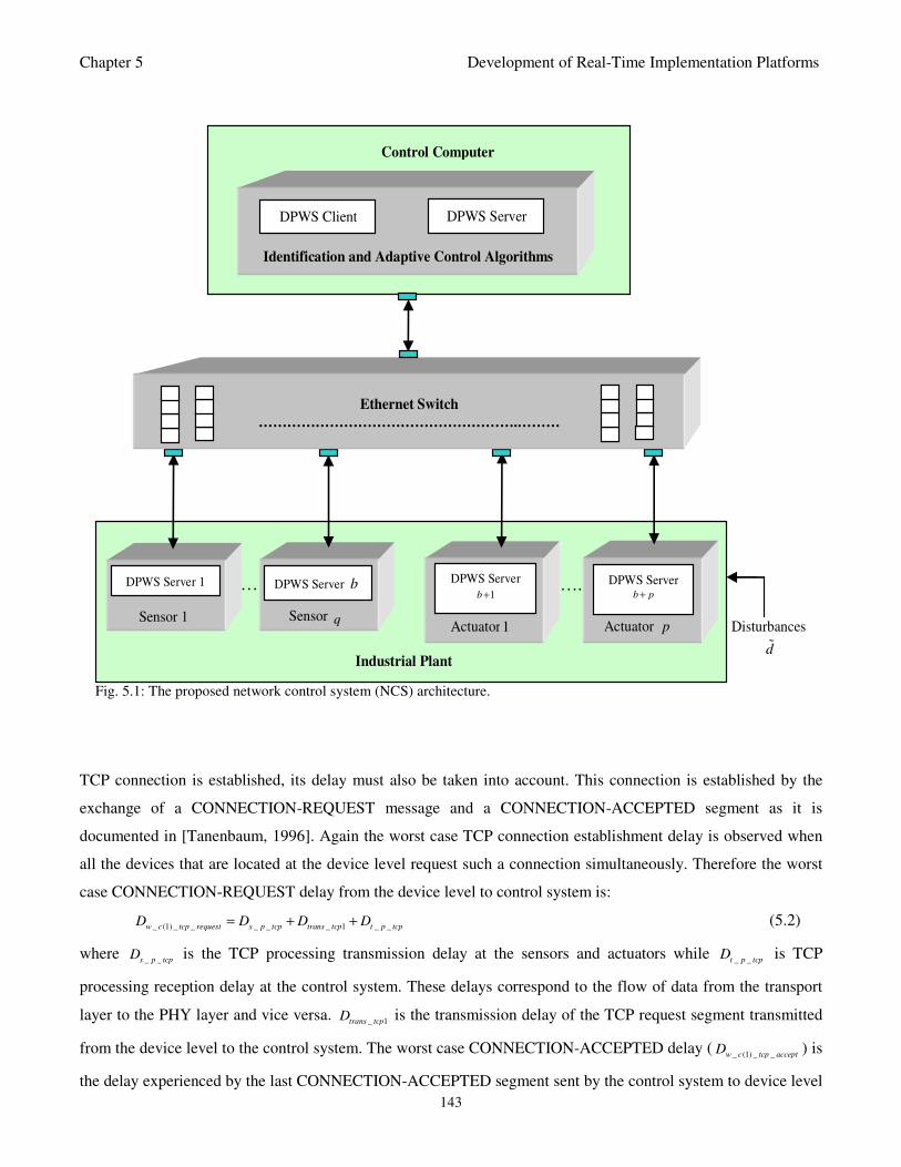
Chapter 5 Development of Real-Time Implementation Platforms
143
TCP connection is established, its delay must also be taken into account. This connection is established by the
exchange of a CONNECTION-REQUEST message and a CONNECTION-ACCEPTED segment as it is
documented in [Tanenbaum, 1996]. Again the worst case TCP connection establishment delay is observed when
all the devices that are located at the device level request such a connection simultaneously. Therefore the worst
case CONNECTION-REQUEST delay from the device level to control system is:
_ (1) _ _ _ _ _ 1 _ _w c tcp request s p tcp trans tcp t p tcpD D D D= + + (5.2)
where _ _s p tcpD is the TCP processing transmission delay at the sensors and actuators while
_ _t p tcpD is TCP
processing reception delay at the control system. These delays correspond to the flow of data from the transport
layer to the PHY layer and vice versa. _ 1trans tcpD is the transmission delay of the TCP request segment transmitted
from the device level to the control system. The worst case CONNECTION-ACCEPTED delay (_ (1) _ _w c tcp acceptD ) is
the delay experienced by the last CONNECTION-ACCEPTED segment sent by the control system to device level
….
Industrial Plant
Identification and Adaptive Control Algorithms
Sensor 1
DPWS Server 1
DPWS Client
Sensor q
DPWS Server b
Actuator1
DPWS Server
1b +
Actuator p
DPWS Server b p+ ….
Ethernet Switch
……………………………………………….………
DPWS Server
Disturbances
d
Control Computer
Fig. 5.1: The proposed network control system (NCS) architecture.
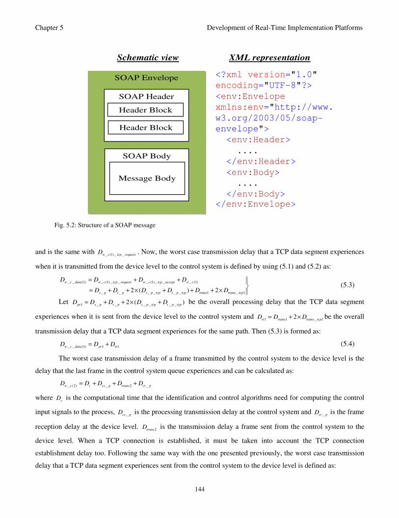
Chapter 5 Development of Real-Time Implementation Platforms
144
and is the same with _ (1) _ _w c tcp requestD . Now, the worst case transmission delay that a TCP data segment experiences
when it is transmitted from the device level to the control system is defined by using (5.1) and (5.2) as:
_ _ (1) _ (1) _ _ _ (1) _ _ _ (1)
_ _ _ _ _ _ 1 _ 12 ( ) 2
w c data w c tcp request w c tcp accept w c
s p t p s p tcp t p tcp trans trans tcp
D D D D
D D D D D D
= + +
= + + × + + + × (5.3)
Let 1 _ _ _ _ _ _2 ( )
pr s p t p s p tcp t p tcpD D D D D= + + × + be the overall processing delay that the TCP data segment
experiences when it is sent from the device level to the control system and 1 1 _ 12
tr trans trans tcpD D D= + × be the overall
transmission delay that a TCP data segment experiences for the same path. Then (5.3) is formed as:
_ _ (1) 1 1w c data pr trD D D= + (5.4)
The worst case transmission delay of a frame transmitted by the control system to the device level is the
delay that the last frame in the control system queue experiences and can be calculated as:
_ (2) _ 2 _w c c cs p trans ct pD D D D D= + + +
where c
D is the computational time that the identification and control algorithms need for computing the control
input signals to the process, _cs p
D is the processing transmission delay at the control system and _ct p
D is the frame
reception delay at the device level. 2trans
D is the transmission delay a frame sent from the control system to the
device level. When a TCP connection is established, it must be taken into account the TCP connection
establishment delay too. Following the same way with the one presented previously, the worst case transmission
delay that a TCP data segment experiences sent from the control system to the device level is defined as:
Schematic view XML representation
SOAP Envelope
SOAP Header
Header Block
Header Block
SOAP Body
Message Body
<?xml version="1.0" encoding="UTF-8"?>
<env:Envelope
xmlns:env="http://www.
w3.org/2003/05/soap-
envelope">
<env:Header>
....
</env:Header>
<env:Body>
....
</env:Body> </env:Envelope>
Fig. 5.2: Structure of a SOAP message
Chapter 5 Development of Real-Time Implementation Platforms
145
_ _ (2) _ (2) _ _ _ (2) _ _ _ (2)
_ _ _ _ _ _ 2 _ 22 ( ) 2
w c data w c tcp request w c tcp accept w c
c cs p ct p s p tcp t p tcp trans trans tcp
D D D D
D D D D D D D
= + +
= + + + × + + + × (5.5)
where _ 2trans tcp
D is the transmission delay of the TCP request segment transmitted from control system to the
device level. Let 2 _ _ _ _ _ _2 ( )
pr c cs p ct p s p tcp t p tcpD D D D D D= + + + × + be the overall processing delay a TCP data
segment experiences transmitted by the control system to the device level and 2 2 _ 22
tr trans trans tcpD D D= + × which is
the overall transmission delay a TCP data segment experiences for the same path. Then (5) is formed as:
_ _ (2) 2 2w c data pr trD D D= + (5.6)
The combination of (5.4) and (5.6) determines the worst case overall control loop delay of the proposed SOA
based on DPWS:
_ _ _ _ (1) _ _ (2) 1 2 1 2w c data w c data w c data pr pr tr trD D D D D D D= + = + + + (5.7)
From the above it is understood that the proposed SOA based on DPWS can be used in an industrial
application if data is transmitted with TCP connection and the real time requirement is below the _ _w c data
D as this
is the bounded delay that it can offer.
5.2.2 Interoperability at the Application Level
Up to this point interoperability is provided at the network interface level by the proposed SOA based on
DPWS. In order to enable every component in the proposed NCS to interact with any other node regardless the
language or implementation platform, the interoperability feature must be provided at the application level too.
Therefore the DPWS must be adopted by all the components of the proposed SOA based on DPWS as it provides
the aforementioned interoperability and it was explained in Section 2.7.2.3.
All the components in the proposed SOA based on DPWS conform to the DPWS specification
implemented on top of switched Ethernet architecture. The sensors and actuators have DPWS server interfaces
and so are DPWS servers, while the control system has DPWS client interface and therefore is DPWS client as it
is shown in Fig. 5.1. As it is claimed in [Jammes and Smit, 2005a], the device-level SOA interaction patterns can
be categorized according to six levels of functionality: addressing, discovery, description, control, eventing and
presentation. After the discovery phase where the DPWS client has discovered the sensors and actuators, it
subscribes to the events of them by publishing the required sampling period using the eventing level interaction.
Every DPWS server assumes that whenever this time expires, there is a change in its state and so it informs the
DPWS client with the new values using the WS-Eventing protocol. Moreover, the DPWS client informs the
actuators with the new control signals as soon as the control algorithms have finished their execution, by using
control level interaction. The network can be considered real-time only if the worst case overall control loop delay
is bounded and less than the sampling period. Lastly, Fig. 5.2 illustrates the structure that all the exchanged
Chapter 5 Development of Real-Time Implementation Platforms
146
messages have in the proposed NCS. Since in this network all the components conform to the DPWS
implemented on top of Ethernet specification, all the exchanged messages have the SOAP structure. The root
element of a SOAP message is the Envelope. It encloses one or two child elements: an optional Header and a
Body. The Header element carries information that does not directly belong to the payload of the message, while
the Body element contains the actual payload of the message. Finally, a namespace is used in the XML
representation for using unambiguous data formats.
5.3 The Development of Real-Time Embedded Processor System Platform
This sub-section is considers the development of a embedded processors on an field programmable gate
array (FPGA), notably Xilinx MicroBlaze (MB) and IBM PowerPC™440 embedded processor systems using the
Xilinx embedded development kit (EDK) design tools which incorporates the Xilinx platform studio (XPS) and
the Xilinx software development kit (SDK). Next, the performances of the two embedded processor system are
investigated and a choice is made as to which is suitable for this work. The embedded processor systems are
design using the XPS via the ISETM
while the peripherals and memories of the processor are tested within the
Virtex-5 FXT ML507 FPGA board via the Xilinx SDK.
5.3.1 Overview of Embedded Processor Systems and Design Considerations
5.3.1.1 Why Embedding a Processor Inside an FPGA?
Embedding a processor inside an FPGA has many advantages. Specific peripherals can be chosen to
improve performance based on the application with unique user-defined peripherals been easily attached.
Likewise, large banks of external memory can be connected to the FPGA and accessed by the embedded
processor system using included memory controllers. A variety of memory controllers enhance the FPGA
embedded processor system’s interface capabilities. FPGA embedded processors use general-purpose FPGA logic
to construct internal memory, processor buses, internal peripherals, and external peripheral controllers including
external memory controllers. As more pieces of buses, memory controllers, peripherals and peripheral controllers
are added to the embedded processor system, the system becomes increasingly more powerful and useful.
However, it is worth noting that the additions of large banks of external memory may increase the latency
to access this external memory and may have negative impact on performance. In addition, adding many pieces of
peripherals and memory as well as their respective controllers may reduce performance and increase the
embedded system cost that consumes the FPGA resources.
FPGA manufacturers often publish embedded processor performance benchmarks. The manufacturers
obviously know what must be done in order to get the best out of their FPGAs that performs the best for each

Chapter 5 Development of Real-Time Implementation Platforms
147
specific benchmark, and they take full advantage of every possible enhancement strategies when benchmarking. A
clue to these strategies is that the FPGA embedded processor system constructed to run the benchmark has very
few peripherals and runs exclusively using internal memory. However, no easy formula or chart exists that shows
how to compare the performance and cost for different memory strategies and peripheral sets. The usual
performance benchmark is the Dhrystone benchmark implementation to evaluate the Dhrystone million
instructions per second (DMIPs) performance measured in terms of the maximum FPGA operating frequency
(fmax) in (MHz). It is then left for the users of such FPGAs to achieve the frequency and DMIPs set out by the
manufacturers.
5.3.1.2 Some Advantages and Disadvantages of FPGA Embedded Processor System
The embedded systems are normally defined as the software implemented in hardware in order to realize
specified real-time functionalities. The normally used soft-core processing hardware includes microcontrollers,
microprocessors, FPGAs, digital signal processors (DSPs), and application-specific integrated circuits (ASICs),
each of which has its own properties. Although, FPGA hardware technologies have attracted an always increasing
interest and have significantly disrupted the embedded system design technologies, it is worth considering some
advantages and disadvantages may be derived or incurred by the use of FPGA embedded technologies.
Here, some advantages of an FPGA embedded processor system when compared to an off-the-shelf
processor are summarized in the following:
1) Hardware Acceleration: The most compelling reason for FPGA embedded processor is the ability to make
trade-offs between hardware and software to maximize efficiency and performance. Suppose an algorithm is
identified as bottleneck, a custom co-processor can be designed in the FPGA specifically for that algorithm.
Then, this co-processor can be attached as a peripheral to the FPGA embedded processor as a co-processing
engine through special, low-latency channels, and custom instructions can be defined to implemented the co-
processor.
2) Peripheral Customization: FPGA embedded processor-based system offers and allow complete flexibility for
the selection of any combination of peripherals or controllers. In fact, new unique peripherals can be design
and connected directly to the processor’s bus with the assumption that there are no standard requirements for
the peripherals.
3) Components and Cost Reduction: With the versatility of the FPGA embedded processor, a previous system that
required multiple components can be replaced with a single FPGA such as in the case when an auxiliary
input/output (I/O) chip or a co-processor is required next to an off-the-shelf processor. By reducing the
Chapter 5 Development of Real-Time Implementation Platforms
148
components count in the design, a reduced board size and inventory management, both of which can save
design time-to-market and cost.
4) Component Obsolescence Mitigation: Obsolescence mitigation is a difficult issue when a design requirement
must ensure that a product lifespan be much longer than the typical lifespan of a standard electronics product.
In this case, FPGA embedded soft-processors could be an excellent solution since the HDL source code for the
soft-processor can be purchased and owned thereby guaranteeing the lifespan of the product.
Additionally, some disadvantages and challenges of an FPGA embedded processor system when compared to an
off-the-shelf processor are discussed in the following.
First, it is worth noting FPGA embedded processor is not without disadvantages. When compared to an
off-the-shelf processor, the hardware platform for the FPGA embedded processor must be designed as above,
which is a challenging hardware-software co-design task. Because of the integration of the hardware and software
platform, the design tools are more complex especially when a co-processing custom peripheral is involved. The
increased tool complexities and design methodologies require that critical decisions be made and adequate
attention be invested.
Next, since FPGA embedded processor software design is still relatively new compared to software
design for standard processors; the software design tools are likewise relatively immature, although workable with
several challenges.
Finally, in terms of design cost, if the desired task can be achieved with a standard off-the-shelf that is
less expensive compared to the FPGA, then using a large FPGA with unused gates or hard processor makes the
FPGA embedded processor system cost inconsequential.
5.3.1.3 Xilinx’s Embedded Hard PowerPC™440 and MicroBlaze Soft Processors
A processor built from dedicated silicon is referred to as a “hard” processor such as the IBM
PowerPC™440 embedded processor core inside the Xilinx Virtex-5 FXT family of FPGAs. On the other hand, a
“soft” processor is built using the FPGA’s general-purpose logic such as the Xilinx MicroBlaze™ embedded
processor core available an intellectual property (IP) for implementation in several Xilinx series of FPGAs. The
soft processor is typically described in a hardware description language (HHL) or netlist. Unlike the hard
processor, the soft processor must be synthesized and fit into the FPGA fabric. In both hard and soft processor
systems, the local memory, internal peripherals, peripheral and memory controllers, and processor buses must be
built from the FPGA’s general-purpose logic.

Chapter 5 Development of Real-Time Implementation Platforms
149
5.3.1.4 Standard Industry Benchmark for FPGA Embedded Processors and Xilinx’s
FPGA Embedded Processors Benchmark Performances
The industry standard benchmark for FPGA embedded processors is Dhrystone MIPs (DMIPs). Xilinx
quote DMIPs for almost all their available embedded processors including MicroBlaze™ and the PowerPC™440
embedded processors. The maximum operating frequency and DMIPs achievable from the Virtex-5 FXT family
of FPGAs as quoted by Xilinx for MicroBlaze™ are 210 MHz and 240 DMIPs respectively. Similar results for
the PowerPC™440 are 550MHz and 1,100 DMIPs for a single processor system. According to Xilinx, this
performance is twice with dual embedded PowerPC™ processors as 1,100MHz and 2,200 DMIPs. The achieved
DMIPs reported by Xilinx are based on several factors to maximize the benchmark results. Such factors include:
1) optimal compiler optimization level, fastest available device family; 2) fastest speed grade in that device
family; 3) executing from the fastest and lowest latency memory which is typically an on-chip memory; 4)
optimization of the embedded processor’s parameterizable features; and so on.
In fact, the FPGA manufacturer, which in this case is Xilinx, knows what must be done to get the most
out of their FPGAs and they take full advantage of every possible enhancement techniques when benchmarking.
Thus, it is also necessary to employ the best enhancement techniques in the embedded processor design proposed
in this work as much as possible, although the task is complicated.
5.3.1.5 Design Considerations for the Proposed FPGA Embedded Processor System
Since the Xilinx base system builder (BSB) wizard provides an efficient way to create an FPGA embedded
processor system, the choice of the memory types, memory controllers, peripherals, peripheral controllers, size
and type of instruction and data cache memories, the optimization levels, and processor clock frequency and size
of local memory. The discussions here are specific to the peripheral that may be considered for the design of the
proposed FPGA embedded processor systems to achieve the following design objectives: high-performance and
optimized speed in terms of operating frequency at reduced cost in terms of FPGA fabric resources consumption.
To be more specific, the proposed FPGA embedded processor system will incorporate a co-processing
system that will be attached to the processor local bus (PLB), a memory and memory controller are required.
Because instruction and data will be read in and written out, the size of the instruction and data cache memories
and peripherals together with their respective controllers must be configured. The initialization of the processor
programs also needs memory and memory controllers. The universal asynchronous receiver and transmitter
(UART) and joint test action group (JTAG) ports are required, and the UART must also be configured properly
for communication. During synthesis, simulation and compilation of the embedded processor system, an
appropriate optimization scheme must be selected to achieve the above design objectives. While the processor
timer is internal, the clock and reset are external. Among other memories and peripherals and their respective
Chapter 5 Development of Real-Time Implementation Platforms
150
controllers, the most important is whether an interrupt and a debug logic controllers will be required. These issues
and other critical considerations for the embedded processor system design are considered in the following.
5.3.1.5.1 Compiler Optimization and Parameters
Compiler optimizations are available in Xilinx platform studio (XPS) based on GNU compiler collections
(GCC). These compilers have several levels of optimization including Levels 0, 1, 2, and 3 as well as size
reduction optimization. The strategies for these different levels of optimizations as given below:
Level 0: This level does not apply any optimization to the design compilation.
Level 1: This is the first and the lowest (Low -01) level of optimization that performs jump and pop
optimization.
Level 2: this the second level of optimization and is designated as Medium (-02). This level activates
nearly all optimizations that do not involve a speed-space trade-off and so the executables do not
increase in size. The compiler doe not perform loop unrolling, function in-lining or strict aliasing
optimizations. This is the standard level used that can be used for all program deployment.
Level 3: This level offers the highest level and is designated High (-03). This level adds more expensive
options, including those that increase code size. In some cases, this optimization level actually
produces code that is less efficient the Level 2, and as such may be used with cautions.
Size Optimized (-0s): This option produces the smallest code size as much as possible.
Note in general, however, that both any of the optimization level and debug option are used, the information
obtained from the optimization process may not correlate with the generated source code.
5.3.1.5.2 Memory Types
The FPGA embedded processor provide access to fast, local memory as well as an interface to slower,
external memory. The way the memory is used has a significant effect on performance. However, the memory
usage can be manipulated using the Linker Script.
Local Memory Only: The local memory provides the fasted option in accessing memory. Xilinx FPGA
local memory is made up of large FPGA memory blocks called BlockRAM (BRAM). Embedded processor
Chapter 5 Development of Real-Time Implementation Platforms
151
accesses BRAM in a single bus cycle. Since the processor and the bus run at the same frequency in MicroBlaze,
instructions stored in BRAM are executed at the full MicroBlaze processor frequency. In the MicroBlaze
processor system, BRAM is essentially equivalent in performance to a Level 1 (L1) cache. On the other hand, the
PowerPC™ can run at frequencies greater than the bus and has true built-in L1 cache. Therefore, BRAM in a
PowerPC™ processor system is equivalent in performance to a Level 2 (L2) cache. Thus, if the program for a
particular embedded processor system design fits entirely within the local memory, then the design is likely to
achieve optimal memory performance, although it is mostly likely that the embedded programs will exceed the
local memory capacity.
External Memory Only: Xilinx FPGAs provides several memory controllers that interface with a variety
of external memory devices. These memory controllers are connected to the processor’s peripheral bus. The three
types of volatile memory are supported by Xilinx FPGAs are static RAM (SRAM), single-data-rate RAM
(SDRAM), and the double-data-rate RAM (DDR) SRAM. The SRAM controller is the smallest and simplest
inside the FPGA while the SDRAM is the most expensive of the three memory types. The DDR SDRAM
controller is the largest and most expensive inside the FPGA, but requires fewer FPGA input-output (I/O) ports
and is least expensive per megabyte.
In addition to the memory access time, the peripheral also incurs some latency. In MicroBlaze, for
example, the memory controllers are attached to the on-chip peripheral bus (OPB). The OPB SDRAM controller
requires about eight to ten cycle latency for a read operation and four to six cycle latency for a write operation
depending on the clock frequency. Thus, it is obvious that the worst possible program performance would be
achieved by having the entire program reside in external memory. Since optimizing execution speed is a typical in
the embedded processor system design, an entire program, should rarely be targeted solely at external memory.
Instruction and Data Cache Memory: The PowerPC™ in Xilinx FPGAs has instruction and data cache
built directly into the silicon of the hard processor. Enabling this cache is almost always a performance advantage
for the PowerPC™ [Fletcher, 2005]. On the other hand, the MicoBlaze™ cache architecture is not on the
dedicated silicon chip rather the instruction and data cache controllers are selectable parameters in the MicroBlaze
configuration. When these controllers are included, the cache memory is built from BRAM. Therefore, enabling
the cache is likely to consume more BRAM than local memory for the same storage size because the cache
architecture requires address line tag storage. Additionally, enabling the cache may also consume general-purpose
FPGA logic to build the cache controllers. The consequences are that the achievable system frequency may be
reduced when the cache is enabled as more logic may be added and the complexity of the design may increase
during the FPGA place and route operation. Despite these consequences in enabling the MicroBlaze cache,
especially the instruction cache, may improve performance, even when the system is likely to run at lower
frequency. Finally, enabling the cached memory is always worth an experiment to justify different trade-offs.
Chapter 5 Development of Real-Time Implementation Platforms
152
Combination of Internal, External and Cache Memory: As discussed earlier, the memory that provides
the best performance is one that only has local memory. However, this architecture may not always be practical
since many useful and efficient embedded programs exceed the available local memory capacity. On the other
hand, running from externally memory exclusively may have more than eight times performance disadvantage
due to the peripheral bus latency.
Caching the external memory is an excellent choice for embedded PowerPC™ processor systems. For
embedded MicroBlaze processor systems, perhaps the optimal memory configuration may be to wisely partition
the program code, maximizing the system frequency and local memory size. Critical data, instructions and stack
can also be placed in local memory. Data cache may not be used so as to allow for a larger local memory bank.
Suppose that the local memory is not large enough; then the instruction cache can be enabled for the address rang
in the external memory used for instructions. By not consuming BRAM in data cache, the local memory can be
increased to contain more space. An instruction cache for the instructions assigned to external memory could be
very effective. Alternatively, experimentation or profiling could show which code fragments are most heavily
accessed; and assigning these fragments to local memory could provide a greater performance improvement than
caching.
5.3.1.5.3 Optimization Specific to an FPGA Embedded Processor
Since the one of the objective of the proposed embedded processor system design using the Xilinx Virtex-
5 FX70T FPGA is to improve the performance of the hardware, additional techniques must be exploited to
achieve this objective. Given the fact that the FPGA embedded processor resides next to additional FPGA
hardware resources, one here technique is to consider a custom co-processor designed specifically to target the
implementation of a core algorithm in the design.
Logic Optimization and Reduction: The key point here is that only peripheral and buses that are
necessary and required should be connected. Suppose that the intended design does will not store and run any
instructions using external memory; then connecting the instruction side of the peripheral bus is not necessary.
Connecting both the instruction and data side of the processor to a single bus may create a multi-master system
which requires an arbiter. Optimal bus performance is achieved when a single master resides on the bus.
Furthermore, debug logic requires resources in the FPGA and may be the hardware bottleneck. When the
design is completely debugged, the debug logic can be removed from the final system, which will potentially
increase the system’s performance. For example, in an embedded MicroBlaze processor system with the cache
enabled, the debug logic will typically be the critical path that will slow down the entire design [Fletcher, 2005].
Chapter 5 Development of Real-Time Implementation Platforms
153
Area and Timing Constraints: Xilinx FPGA place and route tools as well as the Xilinx’s PlanAhead tool
perform much better when the design objectives are well specified. In these Xilinx tools, the desired clock
frequency, pin location, and logic element location can be specified. By providing these details, the design tools
can be able to make efficient, optimized and smarter trade-offs during hardware design implementation.
Therefore, a careful study of the datasheets for each peripheral together with the design guidelines goes a long
way in this regard and it is a necessity.
Hardware Acceleration: Dedicated hardware outperforms software at the expense of FPGA resources for
dramatic performance improvements. Therefore, the FPGA’s ability to accelerate the processor performance with
dedicated hardware should be considered. Provided the hardware divider and the hardware barrel-shifter are
enabled, embedded MicroBlaze™ processor can be customized to use a hardware divider and a hardware barrel-
shifter rather than performing these functions in software. Although, enabling these processor capabilities may
consume FPGA resources, but the performance improvements can be extraordinary.
Co-Processing Hardware: Custom hardware logic can be designed to offload an FPGA embedded
processor. For example, a software bottleneck identified in an algorithm can be converted into a custom hardware.
Then, custom software instructions can be defined to operate the hardware co-processor.
Both MicroBlaze™ and PowerPC™ include very low latency point into the processor, which are ideal for
connecting custom co-processing hardware. For example, the auxiliary processing unit available in the Virtex-5
FPGA provides a direct connection from the PowerPC™440 to co-processing hardware. In MicroBlaze™, the
low-latency interface is called the Fast Simplex Link (FSL) bus which are dedicated channels so that no
arbitration or bus mastering is required. This allows extremely fast interface to the processor except that Xilinx
has announced that the FSL will be discontinued in the future [Xilinx, 2010].
Any operation that is algorithmic, mathematical, or parallel is a good candidate for a hardware co-
processor which is the subject of the proposed embedded processor system design in this work. FPGA logic can
be traded for performance but the advantages can be enormous and performance can be improved significantly.
5.3.2 The PowerPC™ 440 Embedded Processor System Development Using Xilinx
Integrated Software Environment (ISE) and Xilinx Platform Studio (XPS)
The embedded processor designs considered here follows closely from the design considerations outlined
and discussed in Section 5.3.1.4. The embedded processor systems design using the IBM PowerPC™ 440 and the
Xilinx MicroBlaze™ cores is instantiated from the Xilinx ISE which then initializes the XPS where the actual
processor systems’ designs are done. The Xilinx ISE is started and the project name is assigned on the “New
Project Wizard”. The name assigned here for the PowerPC™ processor system is “emb_ppc440_processor”. The
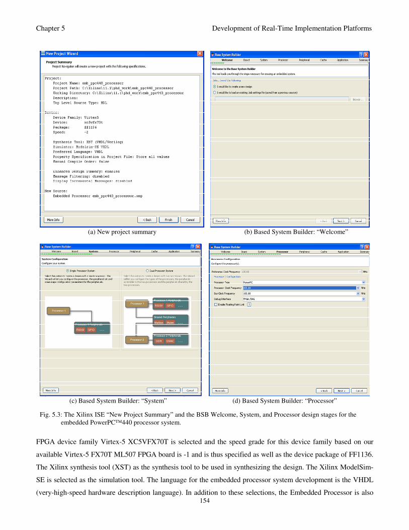
Chapter 5 Development of Real-Time Implementation Platforms
154
FPGA device family Virtex-5 XC5VFX70T is selected and the speed grade for this device family based on our
available Virtex-5 FX70T ML507 FPGA board is -1 and is thus specified as well as the device package of FF1136.
The Xilinx synthesis tool (XST) as the synthesis tool to be used in synthesizing the design. The Xilinx ModelSim-
SE is selected as the simulation tool. The language for the embedded processor system development is the VHDL
(very-high-speed hardware description language). In addition to these selections, the Embedded Processor is also
(a) New project summary (b) Based System Builder: “Welcome”
(c) Based System Builder: “System” (d) Based System Builder: “Processor”
Fig. 5.3: The Xilinx ISE “New Project Summary” and the BSB Welcome, System, and Processor design stages for the
embedded PowerPC™440 processor system.
Chapter 5 Development of Real-Time Implementation Platforms
155
added as a “New Source” in this project wizard. The “emb_ppc440_proceesor” project summary is shown in Fig.
5.3(a).
When the “New Project Wizard” is completed, the ISE initializes and automatically starts up the Xilinx
platform studio (XPS) since it was added as a “New Source”. The XPS in turn initializes and brings up the Base
System Builder (BSB) which is an automated tool that can be used to create an embedded processor system. The
processor design based on the BSB is an eight-stage procedure, namely: Welcome, Board, System, Processor,
Peripheral, Cache, Application, and the Summary.
The “Welcome” allows new processor(s) to be design or an existing pre-designed processor system to be
loaded as shown in Fig. 5.3(b). The “Board” stage allows the FPGA device family and package to be specified, if
different from that specified in the “New Project Wizard”. This is sometimes useful if a custom FPGA board
different from the pre-configured Xilinx FPGA development boards. It is also useful if the processor design was
not initialized and started using the Xilinx ISE. The advantages of initializing and starting an embedded processor
system design from the ISE are many as discussed in Appendix A. The “System” stage shown in Fig. 5.3(c) allows
a single- or dual-processor system to be specified and designed. The Virtex-5 XC5VFX70T devices family
currently supports single processor systems design. Thus, a single processor system is the target in this work. Then
in the “Processor” stage, the choices of selecting a PowerPC™ or a MicroBlaze™ processor are available. Thus, in
this sub-section, a PowerPC™440 is selected as the intended processor as shown in Fig. 5.3(d) whereas in the next
sub-section the MicroBlaze™ processor will be selected.
The “Peripheral” stage allows different memory types and peripherals to be added or removed from the
proposed embedded processor system. Once a memory or peripheral is selected, the associated controller is
automatically added. Furthermore, if the “Interrupt” check box is selected, the interrupt controller is also included
which must be configured in the XPS after the BSB have created embedded processor system. As discussed in
Section 5.3.1.4.2 under memory types as well as hardware and optimization specific to an FPGA embedded
processor in Section 5.3.1.4.3; the choice of memory and hardware peripheral including their respective controllers
have significant effects on the embedded systems performance. Here, peripherals that are not needed are removed.
The actual size of the embedded program is yet to be known and this makes the choice of the memory difficult to
select. In this regard, the embedded processor local memory is selected first. Next, the external DDR SRAM and
the on-board SRAM are added. In this, the serial port is needed to print out all results to the host development
computer. Thus, the only peripheral added here is the UART (RS323_Uart_1) and it is configured as follows: Buat
Rate = 115200, Data Bits = 8, Parity = None, and the Interrupt is not used (that is, it is left unchecked). The BSB
dialog for the “Peripheral” stage and the selected memory types and peripherals is shown in Fig. 5.4(a).
The “Cache” stage allows the instruction and data caches memory types and controllers to be enabled. As
mentioned earlier, the PowerPC™440 embedded in the Virtex-5 series of FPGAs provides 32-Kbit of caches which
are built directly into the silicon of the hard PowerPC™440 core. Normally, these caches are enabled in software
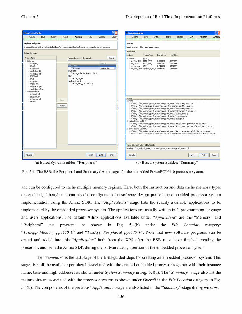
Chapter 5 Development of Real-Time Implementation Platforms
156
and can be configured to cache multiple memory regions. Here, both the instruction and data cache memory types
are enabled, although this can also be configure in the software design part of the embedded processor system
implementation using the Xilinx SDK. The “Applications” stage lists the readily available applications to be
implemented by the embedded processor system. The applications are usually written in C programming language
and users applications. The default Xilinx applications available under “Application” are the “Memory” and
“Peripheral” test programs as shown in Fig. 5.4(b) under the File Location category:
“TestApp_Memory_ppc440_0” and “TestApp_Peripheral_ppc440_0”. Note that new software programs can be
crated and added into this “Application” both from the XPS after the BSB must have finished creating the
processor, and from the Xilinx SDK during the software design portion of the embedded processor system.
The “Summary” is the last stage of the BSB-guided steps for creating an embedded processor system. This
stage lists all the available peripheral associated with the created embedded processor together with their instance
name, base and high addresses as shown under System Summary in Fig. 5.4(b). The “Summary” stage also list the
major software associated with the processor system as shown under Overall in the File Location category in Fig.
5.4(b). The components of the previous “Application” stage are also listed in the “Summary” stage dialog window.
(a) Based System Builder: “Peripheral” (b) Based System Builder: “Summary”
Fig. 5.4: The BSB: the Peripheral and Summary design stages for the embedded PowerPC™440 processor system.
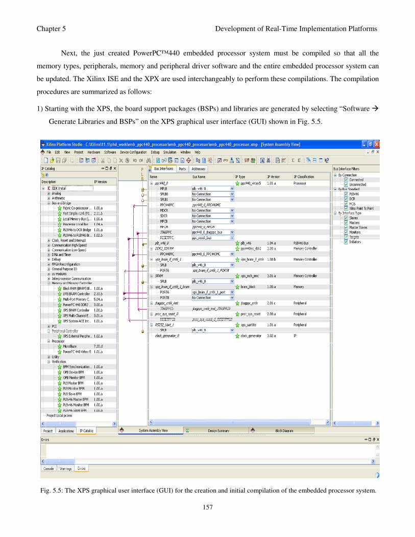
Chapter 5 Development of Real-Time Implementation Platforms
157
Next, the just created PowerPC™440 embedded processor system must be compiled so that all the
memory types, peripherals, memory and peripheral driver software and the entire embedded processor system can
be updated. The Xilinx ISE and the XPX are used interchangeably to perform these compilations. The compilation
procedures are summarized as follows:
1) Starting with the XPS, the board support packages (BSPs) and libraries are generated by selecting “Software
Generate Libraries and BSPs” on the XPS graphical user interface (GUI) shown in Fig. 5.5.
Fig. 5.5: The XPS graphical user interface (GUI) for the creation and initial compilation of the embedded processor system.
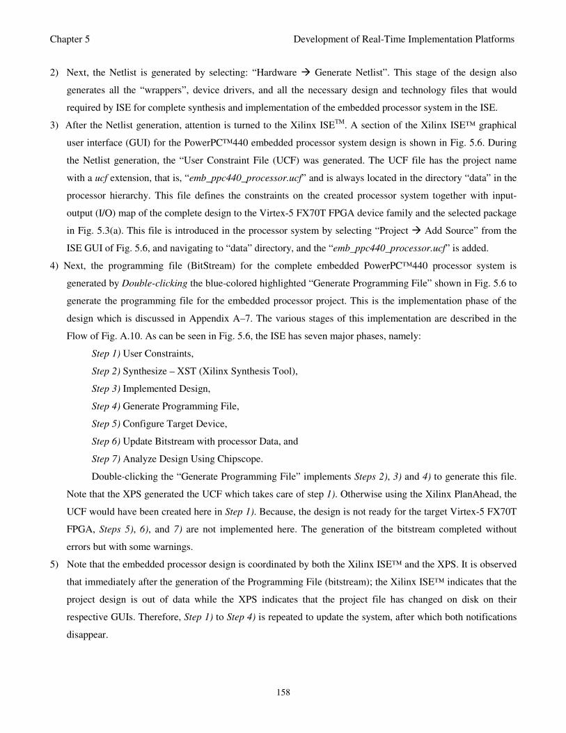
Chapter 5 Development of Real-Time Implementation Platforms
158
2) Next, the Netlist is generated by selecting: “Hardware Generate Netlist”. This stage of the design also
generates all the “wrappers”, device drivers, and all the necessary design and technology files that would
required by ISE for complete synthesis and implementation of the embedded processor system in the ISE.
3) After the Netlist generation, attention is turned to the Xilinx ISETM
. A section of the Xilinx ISE™ graphical
user interface (GUI) for the PowerPC™440 embedded processor system design is shown in Fig. 5.6. During
the Netlist generation, the “User Constraint File (UCF) was generated. The UCF file has the project name
with a ucf extension, that is, “emb_ppc440_processor.ucf” and is always located in the directory “data” in the
processor hierarchy. This file defines the constraints on the created processor system together with input-
output (I/O) map of the complete design to the Virtex-5 FX70T FPGA device family and the selected package
in Fig. 5.3(a). This file is introduced in the processor system by selecting “Project Add Source” from the
ISE GUI of Fig. 5.6, and navigating to “data” directory, and the “emb_ppc440_processor.ucf” is added.
4) Next, the programming file (BitStream) for the complete embedded PowerPC™440 processor system is
generated by Double-clicking the blue-colored highlighted “Generate Programming File” shown in Fig. 5.6 to
generate the programming file for the embedded processor project. This is the implementation phase of the
design which is discussed in Appendix A–7. The various stages of this implementation are described in the
Flow of Fig. A.10. As can be seen in Fig. 5.6, the ISE has seven major phases, namely:
Step 1) User Constraints,
Step 2) Synthesize – XST (Xilinx Synthesis Tool),
Step 3) Implemented Design,
Step 4) Generate Programming File,
Step 5) Configure Target Device,
Step 6) Update Bitstream with processor Data, and
Step 7) Analyze Design Using Chipscope.
Double-clicking the “Generate Programming File” implements Steps 2), 3) and 4) to generate this file.
Note that the XPS generated the UCF which takes care of step 1). Otherwise using the Xilinx PlanAhead, the
UCF would have been created here in Step 1). Because, the design is not ready for the target Virtex-5 FX70T
FPGA, Steps 5), 6), and 7) are not implemented here. The generation of the bitstream completed without
errors but with some warnings.
5) Note that the embedded processor design is coordinated by both the Xilinx ISE™ and the XPS. It is observed
that immediately after the generation of the Programming File (bitstream); the Xilinx ISE™ indicates that the
project design is out of data while the XPS indicates that the project file has changed on disk on their
respective GUIs. Therefore, Step 1) to Step 4) is repeated to update the system, after which both notifications
disappear.
Chapter 5 Development of Real-Time Implementation Platforms
159
Fig. 5.6: A section of the Xilinx ISE™ graphical user interface from where the PowerPC™440 embedded processor
system design is instantiated.
In addition to the Programming File, an important file is also generated called the “Block Memory Map
(BMM)” file with extension bmm. For the current PowerPC™440 project, this file is edkBmmFile_bd.bmm.
The BMM file is a text file that has syntactic descriptions of how individual block RAMs constitutes a
contiguous logical data space. The Xilinx Data2MEM [XD2M, 2009] use BMM files to direct the translation
of data into the proper initialization form. Note that since a BMM file is a text file, it is directly editable. This
file together with the bitstream and all the generated device drivers will be required to program the Virtex-5
during the software design portion of the embedded processor system. The BMM file is located in the top
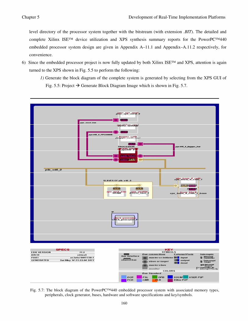
Chapter 5 Development of Real-Time Implementation Platforms
160
Fig. 5.7: The block diagram of the PowerPC™440 embedded processor system with associated memory types,
peripherals, clock generator, buses, hardware and software specifications and key/symbols.
level directory of the processor system together with the bitstream (with extension .BIT). The detailed and
complete Xilinx ISE™ device utilization and XPS synthesis summary reports for the PowerPC™440
embedded processor system design are given in Appendix A–11.1 and Appendix–A.11.2 respectively, for
convenience.
6) Since the embedded processor project is now fully updated by both Xilinx ISE™ and XPS, attention is again
turned to the XPS shown in Fig. 5.5 to perform the following:
1) Generate the block diagram of the complete system is generated by selecting from the XPS GUI of
Fig. 5.5: Project Generate Block Diagram Image which is shown in Fig. 5.7.
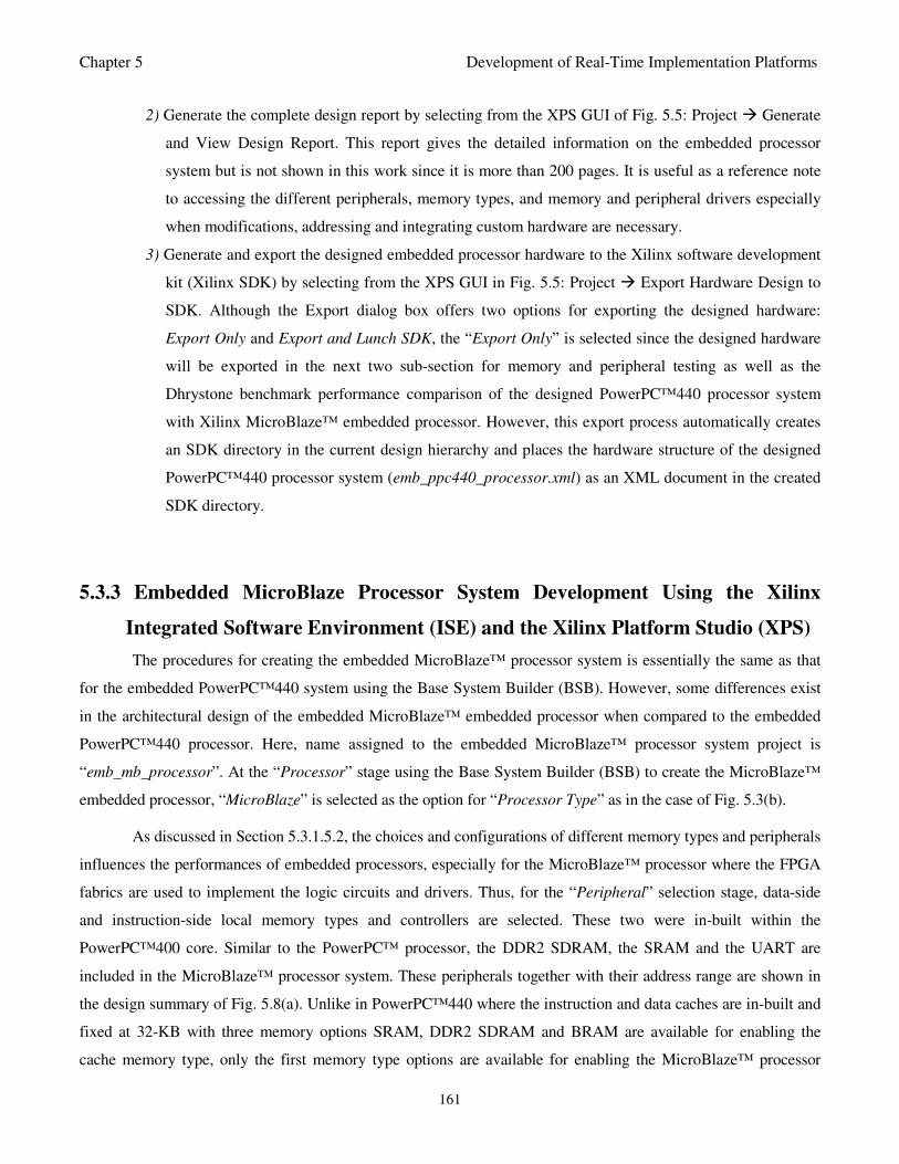
Chapter 5 Development of Real-Time Implementation Platforms
161
2) Generate the complete design report by selecting from the XPS GUI of Fig. 5.5: Project Generate
and View Design Report. This report gives the detailed information on the embedded processor
system but is not shown in this work since it is more than 200 pages. It is useful as a reference note
to accessing the different peripherals, memory types, and memory and peripheral drivers especially
when modifications, addressing and integrating custom hardware are necessary.
3) Generate and export the designed embedded processor hardware to the Xilinx software development
kit (Xilinx SDK) by selecting from the XPS GUI in Fig. 5.5: Project Export Hardware Design to
SDK. Although the Export dialog box offers two options for exporting the designed hardware:
Export Only and Export and Lunch SDK, the “Export Only” is selected since the designed hardware
will be exported in the next two sub-section for memory and peripheral testing as well as the
Dhrystone benchmark performance comparison of the designed PowerPC™440 processor system
with Xilinx MicroBlaze™ embedded processor. However, this export process automatically creates
an SDK directory in the current design hierarchy and places the hardware structure of the designed
PowerPC™440 processor system (emb_ppc440_processor.xml) as an XML document in the created
SDK directory.
5.3.3 Embedded MicroBlaze Processor System Development Using the Xilinx
Integrated Software Environment (ISE) and the Xilinx Platform Studio (XPS)
The procedures for creating the embedded MicroBlaze™ processor system is essentially the same as that
for the embedded PowerPC™440 system using the Base System Builder (BSB). However, some differences exist
in the architectural design of the embedded MicroBlaze™ embedded processor when compared to the embedded
PowerPC™440 processor. Here, name assigned to the embedded MicroBlaze™ processor system project is
“emb_mb_processor”. At the “Processor” stage using the Base System Builder (BSB) to create the MicroBlaze™
embedded processor, “MicroBlaze” is selected as the option for “Processor Type” as in the case of Fig. 5.3(b).
As discussed in Section 5.3.1.5.2, the choices and configurations of different memory types and peripherals
influences the performances of embedded processors, especially for the MicroBlaze™ processor where the FPGA
fabrics are used to implement the logic circuits and drivers. Thus, for the “Peripheral” selection stage, data-side
and instruction-side local memory types and controllers are selected. These two were in-built within the
PowerPC™400 core. Similar to the PowerPC™ processor, the DDR2 SDRAM, the SRAM and the UART are
included in the MicroBlaze™ processor system. These peripherals together with their address range are shown in
the design summary of Fig. 5.8(a). Unlike in PowerPC™440 where the instruction and data caches are in-built and
fixed at 32-KB with three memory options SRAM, DDR2 SDRAM and BRAM are available for enabling the
cache memory type, only the first memory type options are available for enabling the MicroBlaze™ processor
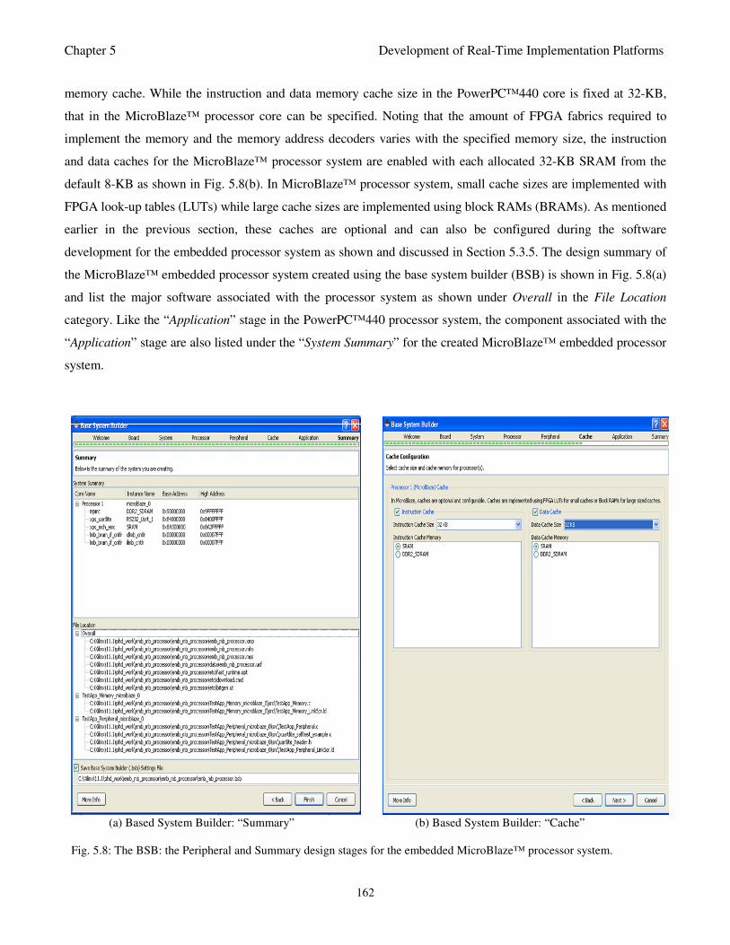
Chapter 5 Development of Real-Time Implementation Platforms
162
memory cache. While the instruction and data memory cache size in the PowerPC™440 core is fixed at 32-KB,
that in the MicroBlaze™ processor core can be specified. Noting that the amount of FPGA fabrics required to
implement the memory and the memory address decoders varies with the specified memory size, the instruction
and data caches for the MicroBlaze™ processor system are enabled with each allocated 32-KB SRAM from the
default 8-KB as shown in Fig. 5.8(b). In MicroBlaze™ processor system, small cache sizes are implemented with
FPGA look-up tables (LUTs) while large cache sizes are implemented using block RAMs (BRAMs). As mentioned
earlier in the previous section, these caches are optional and can also be configured during the software
development for the embedded processor system as shown and discussed in Section 5.3.5. The design summary of
the MicroBlaze™ embedded processor system created using the base system builder (BSB) is shown in Fig. 5.8(a)
and list the major software associated with the processor system as shown under Overall in the File Location
category. Like the “Application” stage in the PowerPC™440 processor system, the component associated with the
“Application” stage are also listed under the “System Summary” for the created MicroBlaze™ embedded processor
system.
(a) Based System Builder: “Summary” (b) Based System Builder: “Cache”
Fig. 5.8: The BSB: the Peripheral and Summary design stages for the embedded MicroBlaze™ processor system.
Chapter 5 Development of Real-Time Implementation Platforms
163
Fig. 5.9: The block diagram of the MicroBlaze™ embedded processor system with associated memory types, peripherals,
clock generator, buses, hardware and software specifications and key/symbols.
The software associated with the just created MicroBlaze™ embedded processor system is then compiled
so that all the memory types, peripherals, memory and peripheral driver software as well as the entire embedded
processor system are updated. The compilation procedures are similar that described for the PowerPC™440
embedded processor system where the Xilinx ISE and the XPX are used interchangeably to perform these
compilations.
Chapter 5 Development of Real-Time Implementation Platforms
164
As in the previous sub-section, the wrappers and hardware drivers, Libraries and the board support
packages (BSPs) as well as the Netlist are generated using the XPS via its GUI while the Synthesis, programming
file (Bitstream), block memory file (BMM), all other implementation files and the device utilization summary are
generated using the Xilinx ISE™ software via its GUI. Next, the XPS via its GUI is used to create the SDK
directory in the top level hierarchy of the MicroBlaze™ processor project directory and the hardware description
text file that encrypts the MicroBlaze™ embedded processor system is exported to this SDK directory. Finally,
the block diagram image and the XPS synthesis summary are generation using the XPS via its GUI. The
MicroBlaze™ embedded processor system created is shown in Fig. 5.9. The detailed and complete Xilinx ISE™
device utilization and XPS synthesis summary reports for the MicroBlaze™ embedded processor system design
are given in Appendix A–11.3 and Appendix–A.11.4 respectively, for convenience.
5.3.4 Software Development and Performance Verification of the PowerPC™440
and MicroBlaze™ Embedded Processor Systems Using the Xilinx Software
Development Kit (Xilinx SDK)
In this sub-section, the embedded PowerPC™440 and MicroBlaze™ processor system are tested. The test
includes: memory, peripheral and the evaluation of the Dhrystone benchmark performance. Unfortunately, only
the Dhrystone benchmark evaluation program for MicroBlaze is included. As discussed in the previous sub-
sections, the hardware description files (emb_ppc440_processor.xml and emb_mb_processor.xml) have been
placed in their respective SDK directories. These tests are performed using the Xilinx software development kit
(SDK). The procedures for creating the software platforms and programming the FPGA are summarized as
follows.
Beginning with the embedded MicroBlaze™ processor system, the Xilinx SDK software is launched and
the hardware description is imported independently into the Xilinx SDK workspace via the SDK GUI. This
process automatically builds and initializes all the embedded processor drivers.
First, a new “Software Platform” is created on the embedded MicroBlaze™ processor system using the
Xilinx SDK GUI. A new “Manage Make C Application Project” is then created under the “Software Platform”
and the “Memory Tests” application is selected which uses the “TestApp_Memory.c” shown in Fig. 5.8(a). The
Xilinx SDK automatically builds and compiles the software application project and reports any error(s).
Next, the Virtex-5 ML507 FPGA board is connected, turned ON and program by selecting Tools
Program FPGA from the SDK GUI. This process requires the MicroBlaze processor programming file (bitstream)
generated in the previous sub-section named “emb_mb_processor.bit” and the block memory map
(edkBmmFile.bmm).
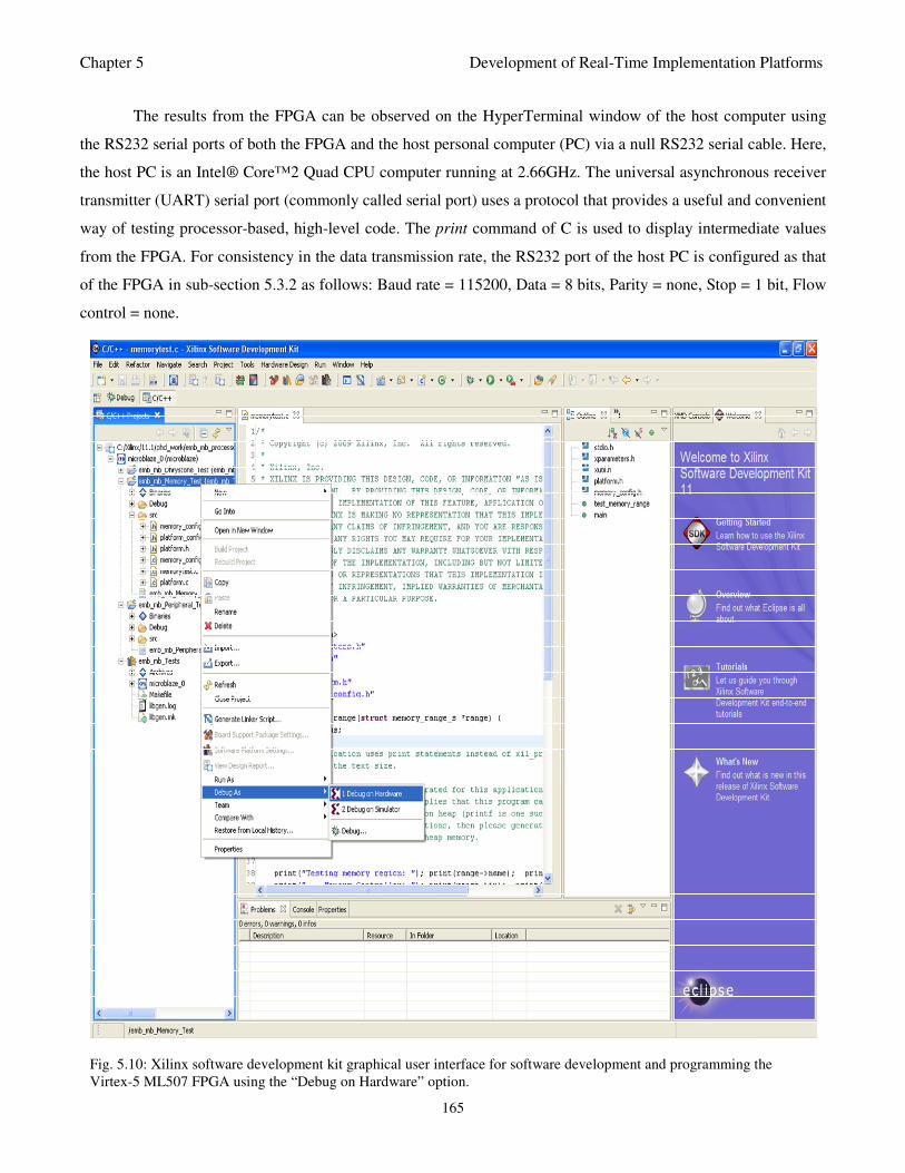
Chapter 5 Development of Real-Time Implementation Platforms
165
The results from the FPGA can be observed on the HyperTerminal window of the host computer using
the RS232 serial ports of both the FPGA and the host personal computer (PC) via a null RS232 serial cable. Here,
the host PC is an Intel® Core™2 Quad CPU computer running at 2.66GHz. The universal asynchronous receiver
transmitter (UART) serial port (commonly called serial port) uses a protocol that provides a useful and convenient
way of testing processor-based, high-level code. The print command of C is used to display intermediate values
from the FPGA. For consistency in the data transmission rate, the RS232 port of the host PC is configured as that
of the FPGA in sub-section 5.3.2 as follows: Baud rate = 115200, Data = 8 bits, Parity = none, Stop = 1 bit, Flow
control = none.
Fig. 5.10: Xilinx software development kit graphical user interface for software development and programming the
Virtex-5 ML507 FPGA using the “Debug on Hardware” option.
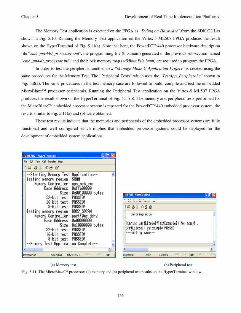
Chapter 5 Development of Real-Time Implementation Platforms
166
The Memory Test application is executed on the FPGA as “Debug on Hardware” from the SDK GUI as
shown in Fig. 5.10. Running the Memory Test application on the Virtex-5 ML507 FPGA produces the result
shown on the HyperTerminal of Fig. 5.11(a). Note that here, the PowerPC™440 processor hardware description
file “emb_ppc440_processor.xml”, the programming file (bitstream) generated in the previous sub-section named
“emb_pp440_processor.bit”, and the block memory map (edkBmmFile.bmm) are required to program the FPGA.
In order to test the peripherals, another new “Manage Make C Application Project” is created using the
same procedures for the Memory Test. The “Peripheral Tests” which uses the “TestApp_Peripheral.c” shown in
Fig. 5.8(a). The same procedures in the test memory case are followed to build, compile and test the embedded
MicroBlaze™ processor peripherals. Running the Peripheral Test application on the Virtex-5 ML507 FPGA
produces the result shown on the HyperTerminal of Fig. 5.11(b). The memory and peripheral tests performed for
the MicroBlaze™ embedded processor system is repeated for the PowerPC™440 embedded processor system, the
results similar to Fig. 5.11(a) and (b) were obtained.
These test results indicate that the memories and peripherals of the embedded processor systems are fully
functional and well configured which implies that embedded processor systems could be deployed for the
development of embedded system applications.
(a) Memory test (b) Peripheral test
Fig. 5.11: The MicroBlaze™ processor: (a) memory and (b) peripheral test results on the HyperTerminal window.
Chapter 5 Development of Real-Time Implementation Platforms
167
5.3.5 MicroBlaze™ Dhrystone Benchmark Performance Evaluation
The Dhrystone is a benchmark test program used to evaluate the performance of embedded processor
system and its performance is compared to that of the manufacturer to measure how well the memory types,
peripheral and optimization techniques have been employed to create the embedded processor system for
enhanced performance. As mentioned in Section 5.3.1.1, the performance for the Dhrystone benchmark
evaluation are usually measured in terms of the maximum FPGA operating frequency (fmax) and the Dhrystone
million instructions per second (DMIPs). Unfortunately, only the Dhrystone benchmark program for evaluating
embedded MicroBlaze™ processor system is available here for evaluation. However, since essentially the same
memory types, peripheral and their respective controllers, the results for the benchmarking of the MicroBlaze™
processor system could be used to judge the PowerPC™440 processor system and noting that the PowerPC™ is
know for higher speed performance running at a maximum frequency of 550MHz and 1,100 DMIPs when
compared to MicroBlaze™ of 210MHz and 240 DMIPs as discussed in sub-section 5.3.1.4 ([XEPB Virtex-5,
2010], [XMBPRG, 2010]).
To enhance the performance of the Dhrystone benchmarking of the design MicroBlaze™ embedded
processor system, the Dhrystone is configured to load directly into the on-board BlockRAMs (BRAMs) from the
Xilinx platform studio (XPS) for speed performance at maximum operating frequency and DMIPs execution. In
this work, the Dhrystone program is first implemented in the SDK similar to the Memory and Peripheral test
programs to ensure that it is free of errors. A copy of the just tested MicroBlaze™ processor system is made. Next
the XPS is opened via the Xilinx ISE GUI following the same way in which it was created. A new directory
called Dhrystone_TestApp_microblaze_0 is created within the XPS emb_mb_processor hierarchy. A new
software application is then created in the XPS created also called “Dhrystone_TestApp_microblaze_0” as shown
in Fig. 5.12. The Dhrystone benchmark program is then imported into the new “Dhrystone_
TestApp_microblaze_0” software application. As discussed in sub-section 5.3.1.5.1, the medium optimization
Level 02 (Medium (–O2)) is selected as the compiler optimization option as shown in the lower right-hand corner
of Fig. 5.12. The new project is then compiled by right-clicking the new Dhrystone_TestApp_microblaze_0
application selecting “Build Project”. This action creates the executable and linkable (EFL) file for the project.
Since the copied project has change, the Xilinx ISE™ project has also changed and it shows out of data.
Thus, the complete MicroBlaze™ embedded processor project is agian fully recompiled using both the XPS and
the Xilinx ISE™ software according following the 9-Step procedures summarized in sub-section 5.3.2. New
board support packages (BSPs), Netlist, programming file (bitstream), block memory map (BMM), hardware
description file (emb_mb_processor.xml) are generated and exported to the software development kit (SDK).
The Xilinx SDK is again opened. A new software platform is created called “Dhrystone_Test”. A new
“Manage Make C Application Project” is also created. This time around, the just created and compiled
“Dhrystone_Test” software application is selected. Next, the Virtex-5 ML507 is programmed and the Dhrystone
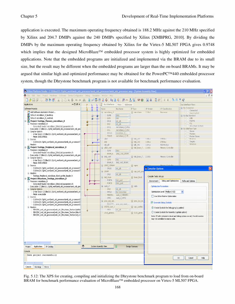
Chapter 5 Development of Real-Time Implementation Platforms
168
application is executed. The maximum operating frequency obtained is 188.2 MHz against the 210 MHz specified
by Xilinx and 204.7 DMIPs against the 240 DMIPs specified by Xilinx [XMBPRG, 2010]. By dividing the
DMIPs by the maximum operating frequency obtained by Xilinx for the Virtex-5 ML507 FPGA gives 0.9748
which implies that the designed MicroBlaze™ embedded processor system is highly optimized for embedded
applications. Note that the embedded programs are initialized and implemented via the BRAM due to its small
size, but the result may be different when the embedded programs are larger than the on-board BRAMs. It may be
argued that similar high and optimized performance may be obtained for the PowerPC™440 embedded processor
system, though the Dhrystone benchmark program is not available for benchmark performance evaluation.
Fig. 5.12: The XPS for creating, compiling and initializing the Dhrystone benchmark program to load from on-board
BRAM for benchmark performance evaluation of MicroBlaze™ embedded processor on Virtex-5 ML507 FPGA.
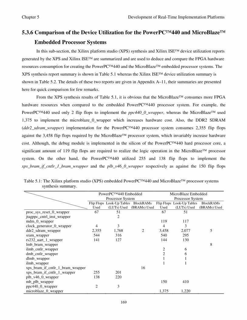
Chapter 5 Development of Real-Time Implementation Platforms
169
5.3.6 Comparison of the Device Utilization for the PowerPC™440 and MicroBlaze™
Embedded Processor Systems
In this sub-section, the Xilinx platform studio (XPS) synthesis and Xilinx ISE™ device utilization reports
generated by the XPS and Xilinx ISE™ are summarized and are used to deduce and compare the FPGA hardware
resources consumption for creating the PowerPC™440 and the MicroBlaze™ embedded processor systems. The
XPS synthesis report summary is shown in Table 5.1 whereas the Xilinx ISE™ device utilization summary is
shown in Table 5.2. The details of these two reports are given in Appendix A–11, their summaries are presented
here for quick comparison for few remarks.
From the XPS synthesis results of Table 5.1, it is obvious that the MicroBlaze™ consumes more FPGA
hardware resources when compared to the embedded PowerPC™440 processor system. For example, the
PowerPC™440 used only 2 flip flops to implement the ppc440_0_wrapper, whereas the MicroBlaze™ used
1,375 to implement the microblaze_0_wrapper which increases hardware cost. Also, the DDR2 SDRAM
(ddr2_sdram_wrapper) implementation for the PowerPC™440 processor system consumes 2,355 flip flops
against the 3,458 flip flops required by the MicroBlaze™ processor system, which invariably increase hardware
cost. Although, the debug module is implemented in the silicon of the PowerPC™440 hard processor core, a
significant amount of 119 flip flops are required to realize the logic operation in the MicroBlaze™ processor
system. On the other hand, the PowerPC™440 utilized 255 and 138 flip flops to implement the
xps_bram_if_cntlr_1_bram_wrapper and the plb_v46_0_wrapper respectively as against the 150 flip flops
Table 5.1: The Xilinx platform studio (XPS) embedded PowerPC™440 and MicroBlaze™ processor systems
synthesis summary.
PowerPC™440 Embedded
Processor System
MicroBlaze Embedded
Processor System
Flip Flops
Used
Look-Up Tables
(LUTs) Used
BlockRAMs
(BRAMs) Used
Flip Flops
Used
Look-Up Tables
(LUTs) Used
BlockRAMs
(BRAMs) Used
proc_sys_reset_0_wrapper 67 51 67 51
jtagppc_cntrl_inst_wrapper 2
mdm_0_wrapper 119 117
clock_generator_0_wrapper 4 3 4 3
ddr2_sdram_wrapper 2,355 1,768 2 3,458 2,077 5
sram_wrapper 544 316 540 295
rs232_uart_1_wrapper 141 127 144 130
lmb_bram_wrapper 8
ilmb_cntlr_wrapper 2 6
dmb_cntlr_wrapper 2 6
dlmb_wrapper 1 1
ilmb_wrapper 1 1
xps_bram_if_cntlr_1_bram_wrapper 16
xps_bram_if_cntlr_1_wrapper 255 201
plb_v46_0_wrapper 138 220
mb_plb_wrapper 150 410
ppc440_0_wrapper 2 3
microblaze_0_wrapper 1,375 1,220
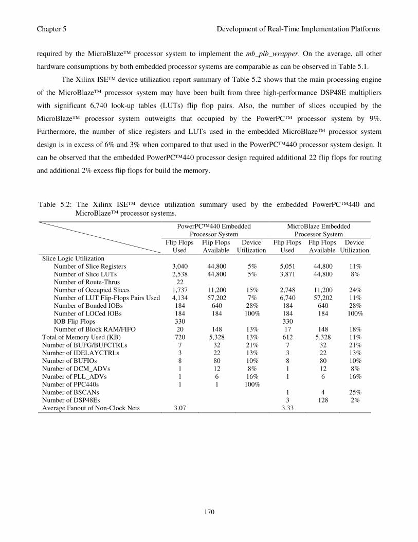
Chapter 5 Development of Real-Time Implementation Platforms
170
required by the MicroBlaze™ processor system to implement the mb_plb_wrapper. On the average, all other
hardware consumptions by both embedded processor systems are comparable as can be observed in Table 5.1.
The Xilinx ISE™ device utilization report summary of Table 5.2 shows that the main processing engine
of the MicroBlaze™ processor system may have been built from three high-performance DSP48E multipliers
with significant 6,740 look-up tables (LUTs) flip flop pairs. Also, the number of slices occupied by the
MicroBlaze™ processor system outweighs that occupied by the PowerPC™ processor system by 9%.
Furthermore, the number of slice registers and LUTs used in the embedded MicroBlaze™ processor system
design is in excess of 6% and 3% when compared to that used in the PowerPC™440 processor system design. It
can be observed that the embedded PowerPC™440 processor design required additional 22 flip flops for routing
and additional 2% excess flip flops for build the memory.
Table 5.2: The Xilinx ISE™ device utilization summary used by the embedded PowerPC™440 and
MicroBlaze™ processor systems.
PowerPC™440 Embedded
Processor System
MicroBlaze Embedded
Processor System
Flip Flops
Used
Flip Flops
Available
Device
Utilization
Flip Flops
Used
Flip Flops
Available
Device
Utilization
Slice Logic Utilization
Number of Slice Registers 3,040 44,800 5% 5,051 44,800 11%
Number of Slice LUTs 2,538 44,800 5% 3,871 44,800 8%
Number of Route-Thrus 22
Number of Occupied Slices 1,737 11,200 15% 2,748 11,200 24%
Number of LUT Flip-Flops Pairs Used 4,134 57,202 7% 6,740 57,202 11%
Number of Bonded IOBs 184 640 28% 184 640 28%
Number of LOCed IOBs 184 184 100% 184 184 100%
IOB Flip Flops 330 330
Number of Block RAM/FIFO 20 148 13% 17 148 18%
Total of Memory Used (KB) 720 5,328 13% 612 5,328 11%
Number of BUFG/BUFCTRLs 7 32 21% 7 32 21%
Number of IDELAYCTRLs 3 22 13% 3 22 13%
Number of BUFIOs 8 80 10% 8 80 10%
Number of DCM_ADVs 1 12 8% 1 12 8%
Number of PLL_ADVs 1 6 16% 1 6 16%
Number of PPC440s 1 1 100%
Number of BSCANs 1 4 25%
Number of DSP48Es 3 128 2%
Average Fanout of Non-Clock Nets 3.07 3.33
Chapter 6 Case Studies and Simulation Results
171
Chapter 6
Case Studies and Simulation Results
6.1 Introduction
In this chapter, the two proposed neural network (NN) model identification algorithms, the adaptive
recursive least squares (ARLS) and the modified Levenberg-Marquardt algorithm (MLMA), and the two adaptive
predictive control algorithms, the adaptive generalized predictive control (AGPC) and the nonlinear adaptive
model predictive control (NAMPC), are applied to three selected industrial applications as the case studies
considered in this study. The three case studies are: 1) the fluidized bed furnace reactor (FBFR) of the steam
deactivation unit (SDU) of a fluid catalytic cracking (FCC) pilot plant, 2) aerobic reactor unit of an activated
sludge wastewater treatment plant (AS-WWTP), and the auto-pilot control system of a nonlinear F-16 fighter
aircraft.
Section 6.2 is concerned with the NN model identification and adaptive MPC temperature control of the
FBFR process. A brief description of the FBFR process is presented sub-section 6.2.1while its mathematical
model is given in Appendix B. The control objectives are also presented in this section 6.2.1. The neural network
training and validation using the ARLS and the MLMA algorithms as well as their closed-loop identification and
PID control for the FBFR process together with their results are presented in sub-section 6.2.2. Validation and
dynamic performance comparisons of the proposed MLMA algorithm with backpropagation with momentum
(BPM) and the incremental backpropagation (INCBP) algorithms together with their results are presented in sub-
section 6.2.3. Then in sub-section 6.2.4, the validation and performance evaluation of the proposed AGPC and the
NAMPC algorithms for the model-based adaptive control of the temperature of the FBFR process using the
ARLS algorithm as well as their control performances are presented. Sub-section 6.2.5 concludes this section with
implementation and performance evaluation of a PID controller with the proposed NAMPC algorithm over the
proposed service-oriented architecture (SOA) cluster network with their closed-loop simulation results.
Section 6.3 deals with the NN model identification and adaptive MPC control of the soluble oxygen (the
so-called dissolved oxygen concentration, DO) in the aerobic reactor unit of an activated sludge wastewater
treatment plant (AS-WWTP) process. An overview of the AS-WWTP process and a statement of the
identification and control problem are first presented in sub-section 6.3.1 while the detailed AS-WWTP process
description and complete mathematical model is provided in Appendix C. The training and validation results of
the NN that models the AS-WWTP process using the ARLS and the MLMA algorithms as well as their online
closed-loop identification and control performances with the proposed AGPC controller are presented in sub-
section 6.3.2. The validation and dynamic performance comparisons of the proposed ARLS algorithm with the
backpropagation with momentum (BPM) and the incremental backpropagation (INCBP) algorithms together with
their results for the AS-WWTP process are presented in sub-section 6.3.3. The validation and performance
Chapter 6 Case Studies and Simulation Results
172
evaluation of the proposed AGPC and the NAMPC algorithms for the model-based adaptive control of the
dissolved oxygen concentration (DO) in the aerobic reactor unit of the AS-WWTP process using the MLMA
algorithm as well as their control performances are presented in sub-section 6.3.4.
Section 6.4 presents the neural network-based model identification and adaptive MPC control of the auto-
pilot control system of a nonlinear F-16 fighter aircraft. A brief description of the F-16 aircraft and formulation of
the control problem are first presented in sub-section 6.4.1 while the detailed description of the F-16 aircraft and
its detailed mathematical model is given in Appendix D. The training and validation results of the NN that models
the auto-pilot control system of the nonlinear F-16 fighter aircraft using the ARLS and the MLMA algorithms are
presented in sub-section 6.4.3 whereas the online closed-loop model identification and control performances of
the ARLS and the MLMA algorithms with proposed NAMPC controller are presented in sub-section 6.4.4. The
validation and performance evaluation of the proposed AGPC and the NAMPC algorithms for the model-based
adaptive control of the auto-pilot control system of the nonlinear F-16 aircraft using the ARLS algorithm as well
as their control performances are presented in sub-section 6.4.5.
Section 6.5 concludes this chapter. This section is concerned with the real-time implementation of
implementation of the neural network-based AGPC algorithm for the nonlinear F-16 auto-pilot control system on
a Xilinx Virtex-5 FX70T ML507 FPGA board. The model-based for the FPGA implementation of the AGPC
algorithm is presented first in sub-section 6.5.1. Then the hardware synthesis of the AGPC algorithm using the
Xilinx AccelDSP tool is presented in sub-section 6.5.2 together with some discussions and remarks. The model-
based implementation of the synthesized AGPC algorithm using the Xilinx System Generator for DSP is given in
sub-section 6.5.3. Then in sub-section 6.5.4, the hardware-in-the-loop co-simulation of the synthesized AGPC
System Generator model with the Virtex-5 FX70T ML507 FPGA board is presented together with the simulation
results. The synthesis and generation of the AGPC algorithm as a co-processor form the synthesized AGPC
System Generator model together with the techniques for integrating the generated AGPC co-processor with the
embedded PowerPC™440 processor system developed and tested in section 5.3.2 in Chapter 5 are presented in
sub-section 6.5.5. Sub-section 6.5.6 is the last sub-section and it details the real-time implementation of the
embedded PowerPC™440 processor system and the synthesized AGPC System Generator model as a co-
processor on Xilinx Virtex-5 FX70T ML507 FPGA board. The complete closed-loop control of the nonlinear F-
16 aircraft auto-pilot control system using the validated Simulink model, the neural network model based on the
MLMA algorithm and the combined embedded PowerPC™440 processor–AGPC co-processor system. Details of
the hardware utilization, application programming interface (API) for the AGPC co-processor as well as the
software for implementing the complete embedded PowerPC™440 processor–AGPC co-processor system are
provided in Appendix E.
Chapter 6 Case Study 1: The Fluidized Bed Furnace Reactor
173
6.2 The Model Identification and Control Problem of the Fluidized Bed Furnace
Reactor (FBFR) Process
6.2.1 The Fluidized Bed Furnace Reactor (FBFR) Process Description and
Mathematical Model
The cyclic propylene steam deactivation procedure is used to prepare fluid catalytic cracking (FCC)
catalysts for evaluation that will be purchased for use in normal production FCC plants. The FCC process is a
vital part of every modern refinery. Through this process the heavy residue of the atmospheric and vacuum
distillations is catalytically converted from heavy to lighter hydrocarbon products, thus increasing the gasoline
and diesel yield of the refinery. The main task of the FCC is catalyst benchmarking procedures which require that
the catalyst be evaluated at constant conversion levels through accurate temperature control. In order to evaluate
such catalyst in bench scale units and pilot plants, it is necessary to have pre-processed samples from vendor
supplied catalysts that accurately simulate the state of a “used” catalyst which is actually present at any given time
inside the commercial FCC unit. This catalyst state is called “equilibrium catalyst” and all major catalyst vendors
carry out research into finding processes that produce such variation of the produced catalyst. This process is
called “catalyst preparation through metal deactivation”. During this process, the catalyst is impregnated with
metals such as vanadium or nickel from a source such as metal naphthenates before steaming.
The steamers are designed to hydrothermally deactivate cracking catalyst and to simultaneously
deactivate metals deposited on the catalyst. Deactivation involves the exposure of the catalyst to streams
containing steam, propylene, sulphur IV oxide (SO2) and air, and nitrogen (N2) alternatively for a specified
number of cycles at high temperatures. The predefined process procedures must be accurately followed during the
initial heat up and the deactivation stage. Even relatively small overshoots in temperature might give final product
properties that would not be acceptable. At the end of the deactivation procedure that lasts more than 22 hours in
total, excluding the wet impregnation stage, the catalyst must have exact macroscopic properties that match the
catalyst drawn from the industrial process. The most important properties include: unit cell size (UCS) of the
contained zeolite, total surface area (TSA), target metals level. Some properties such as the unit cell size (UCS)
are irreversibly affected by treatment temperature overshoots of only 2%. Thus, an efficient control of the
temperatures inside a furnace heated reactor used in the deactivation of the catalyst during the catalyst processing
experiments is of paramount importance. This reactor will be referred to as the fluidized bed furnace reactor
(FBFR).
Chapter 6 Case Study 1: The Fluidized Bed Furnace Reactor
174
6.2.1.1 The Fluidized Bed Furnace Reactor (FBFR) Process
The pilot plant scale steam deactivation unit (SDU) is a pilot plant fitted with automated controls for
temperature and gas supply switching as illustrated in Fig. 6.1. The operation is coordinated by a state of the art
industrial control system and software. Three gas lines each consisting of filter, pressure regulator, pressure
indicator and check valve are fed to a single mass flow controller. An on–off solenoid valve manages the flow of
each line. An accurate deionized water pump (DWP) supplies the water that is required for steam generation
through the upper part of the line entering the FBFR reactor. The complete description of the deactivation
procedure is given in [Voutetakis et al., 2006]. Accurate control of temperature and energy requirements of the
fluidized bed furnace reactor (FBFR) of the cyclic propylene steam deactivation unit that is part of an FCC pilot
plant is of paramount importance.
The fluidized bed furnace reactor (FBFR) considers heat transfer in the radial direction for a structure
consisting of successive cylindrical layers as shown in Fig. 6.2. Electric heaters are embedded in ceramic material
in the heater section to generate the necessary heat for the process. The electric heaters are regulated by
manipulating a high resistance potentiometer (HRP). Heat is then transported in the radial direction towards the
centre of the reactor and the insulator section. A dynamic distributed heat transfer model is used for the interior of
the reactor, the air in the gap between the inner reactor wall and the heater and the insulator. The dynamic
behaviour of the temperature is hence expressed as a set of partial differential equations. A lumped model (e.g.,
radial temperature gradients assumed negligible) is used for the inner reactor wall, the heater and the outer reactor
wall sections. The lumped models then result in a set of ordinary differential equations. The dynamics of the
system are hence consist of a series of fast and slow modes depending on the heat capacity and thermal
conductivities of the different layers (i.e. material properties) in the reactor. The complete mathematical model for
the energy balance of the FBFR is expressed as a set of nonlinear partial differential equations with respect to Fig.
6.2 and is given in Appendix B.
The solution of the FBFR mathematical model given by Equations (B.1) – (B.6) in Appendix B–1 was
implemented in MATLAB. The MATLAB program that translates the FBFR mathematical model described by
Equations (B.1)–(B.6) is given in Appendix B–2 together with the FBFR parameters. The MATLAB script that is
used to implement the FBFR model of Appendix B–2 is given in Appendix B–3. The parameters of the FBFR
were obtained from Chemical Process Engineering Research Institute (CPERI), Thermi – Thessaloniki, Greece
where the FCC pilot plant, the SDU and the FBFR are located.
The temperature distribution across the FBFR based on the simulation of (B.1) – (B.6) using the
MATLAB programs of Appendix B–2 and B–3 are given in Fig. 6.3. As can be seen in Fig. 6.3, the temperatures
across the FBFR increases sharply at the initial phase of the deactivation process and gradually reduce to steady-
state values. For the deactivation process to be successful, the temperatures must be maintained at some
prescribed levels throughout the entire deactivation process, and this requires keeping the temperatures to some
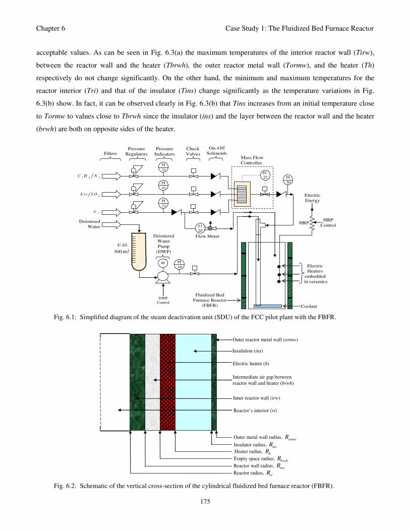
Chapter 6 Case Study 1: The Fluidized Bed Furnace Reactor
175
acceptable values. As can be seen in Fig. 6.3(a) the maximum temperatures of the interior reactor wall (Tirw),
between the reactor wall and the heater (Tbrwh), the outer reactor metal wall (Tormw), and the heater (Th)
respectively do not change significantly. On the other hand, the minimum and maximum temperatures for the
reactor interior (Tri) and that of the insulator (Tins) change significantly as the temperature variations in Fig.
6.3(b) show. In fact, it can be observed clearly in Fig. 6.3(b) that Tins increases from an initial temperature close
to Tormw to values close to Tbrwh since the insulator (ins) and the layer between the reactor wall and the heater
(brwh) are both on opposite sides of the heater.
Deionized
Water
3 8 2C H N
2A i r S O
2N
PI
10
PI
31
PI
41
PI
21
F1
20
Mass Flow
Controller
FC
22
Pressure
Indicators
Pressure
Regulators Filters Check
Valves
On–Off
Solenoids
V-10
500 ml
M
Deionized
Water
Pump
(DWP)
PI
50
Coolant
Fluidized Bed
Furnace Reactor
(FBFR)
Flow Meter
. . . DWP
Control
Electric
Heaters
embedded
in ceramics
Electric
Energy
HRP HRP
Control
Fig. 6.1: Simplified diagram of the steam deactivation unit (SDU) of the FCC pilot plant with the FBFR.
Outer reactor metal wall (ormw)
Insulation (ins)
Electric heater (h)
Intermediate air gap between
reactor wall and heater (brwh)
Inner reactor wall (irw)
Reactor’s interior (ri)
Outer metal wall radius, ormwR
Insulator radius, insR
Heater radius, hR
Empty space radius, brwhR
Reactor wall radius, irw
R
Reactor radius, riR
Fig. 6.2: Schematic of the vertical cross-section of the cylindrical fluidized bed furnace reactor (FBFR).
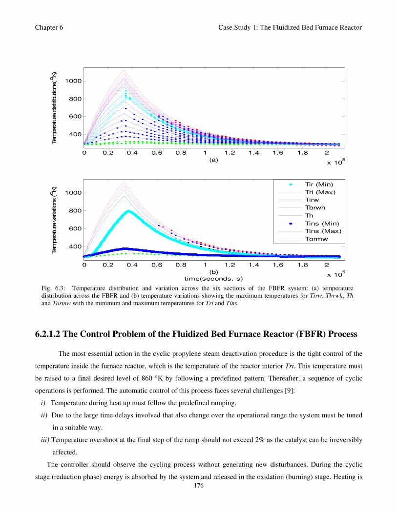
Chapter 6 Case Study 1: The Fluidized Bed Furnace Reactor
176
6.2.1.2 The Control Problem of the Fluidized Bed Furnace Reactor (FBFR) Process
The most essential action in the cyclic propylene steam deactivation procedure is the tight control of the
temperature inside the furnace reactor, which is the temperature of the reactor interior Tri. This temperature must
be raised to a final desired level of 860 °K by following a predefined pattern. Thereafter, a sequence of cyclic
operations is performed. The automatic control of this process faces several challenges [9]:
i) Temperature during heat up must follow the predefined ramping.
ii) Due to the large time delays involved that also change over the operational range the system must be tuned
in a suitable way.
iii) Temperature overshoot at the final step of the ramp should not exceed 2% as the catalyst can be irreversibly
affected.
The controller should observe the cycling process without generating new disturbances. During the cyclic
stage (reduction phase) energy is absorbed by the system and released in the oxidation (burning) stage. Heating is
0 0.2 0.4 0.6 0.8 1 1.2 1.4 1.6 1.8 2
x 105
400
600
800
1000
(a)
Tem
pera
ture
distributions( oK)
0 0.2 0.4 0.6 0.8 1 1.2 1.4 1.6 1.8 2
x 105
400
600
800
1000
(b)
time(seconds, s)
Tem
pera
ture
variations ( oK)
Tir (Min)
Tri (Max)
Tirw
Tbrwh
Th
Tins (Min)
Tins (Max)
Tormw
Fig. 6.3: Temperature distribution and variation across the six sections of the FBFR system: (a) temperature
distribution across the FBFR and (b) temperature variations showing the maximum temperatures for Tirw, Tbrwh, Th
and Tormw with the minimum and maximum temperatures for Tri and Tins.
Chapter 6 Case Study 1: The Fluidized Bed Furnace Reactor
177
provided through the independent electric resistance heaters, as shown in the diagram of Fig. 6.1. Excessive
heating in the initial phase of the experiment would both increase the energy requirements and further result in
overshooting the desired temperature level where the deactivation cycle will take place [Voutetakis et al., 2006].
The two objectives here are: 1) to develop a neural network that will accurately model the FBFR process, and
2) to use the resulting neural network model to design a controller that will accurately control the temperatures of
the heater (Th) and the reactor interior (Tri) with quick response and with overshoots not exceeding 2% of the
nominal steady state value.
6.2.1.3 FBFR Experiment and Training Data Acquisition
In the previous work presented in [Voutetakis et al., 2006], a well-tuned PID and MPC controllers were
developed to operate the FBFR process in the range of 3.76 and 3.66 kW respectively out of the total 5.04 kW
(kilo Watts) heat energy available for the process with dionized water flow rate of 500 /ml s (milliliter per
second). A sampling time (T) of one minute was considered for 22 hours operating cycles. This means that 1320
data samples can be obtained from the process in every operating cycle. In order to develop a neural network to
accurately model the FBFR process, the heat and the deionized water flow rate supplied to the FBFR were varied
from their minimum up to the 30% above their normal operating values. This variation is to allow for the
coverage of the entire operating range of the FBFR, during both initial heat-up and deactivation, and to account
for the possible uncertainties in the plant model outside the operating region. The minimum and upper valued for
Q are 0 kW and 6.552 kW respectively and were varied in steps of 936 Watts (W). The lower and upper values of
DWP are 0 ml/s and 650 ml/s respectively and were varied in steps of 92.8571 (milliliter per second, ml/s).
Using the validated first principles mathematical model of the FBFR process and the MATLAB programs
for solving the nonlinear partial differential equations for this model given in Appendix B, the FBFR was
simulated in open-loop. For the 8 different combinations of each step changes in Q and DWP using the step
defined above, the six corresponding temperatures were obtained which resulted in the desired 1320 input-output
data pairs. All the 1320 data pairs obtained, were used for network training while the 300 input-output test data
pairs obtained directly from the FBFR were used for the validation of the trained network.
6.2.1.4 Statement of the FBFR Neural Network Model Identification and Control
Problem
As it has been explained above the most essential control action is to make sure that the temperature of
the reactor interior (Tri) is not exceeding 860°K. In this study, the control input for the control of the FBFR is the
electrical energy (Q) to the heater via the high resistant potentiometers (HRP) and the deionized water pump
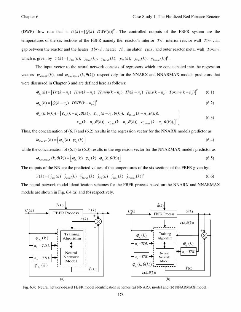
Chapter 6 Case Study 1: The Fluidized Bed Furnace Reactor
178
(DWP) flow rate that is ( ) [ ( ) ( )]TU k Q k DWP k= . The controlled outputs of the FBFR system are the
temperatures of the six sections of the FBFR namely the: reactor’s interior Tri , interior reactor wall Tirw , air
gap between the reactor and the heater Tbrwh , heater Th , insulator Tins , and outer reactor metal wall Tormw
which is given by ( ) [ ( ); ( ); ( ); ( ); ( ); ( )]T
Tri Tirw Tbrwh Th Tins TormwY k y k y k y k y k y k y k= .
The input vector to the neural network consists of regressors which are concatenated into the regression
vectors ( )NNARX
kϕ , and ( , ( ))NNARMAX
k kϕ θ respectively for the NNARX and NNARMAX models predictors that
were discussed in Chapter 3 and are defined here as follows:
[ ]( ) ( ) ( ) ( ) ( ) ( ) ( )a
T
n a a a a a ak Tri k n Tirw k n Tbrwh k n Th k n Tins k n Tormw k nϕ = − − − − − − (6.1)
[ ]( ) ( ) ( )b
T
n b bk Q k n DWP k nϕ = − − (6.2)
[
]
( , ( )) ( , ( )), ( , ( )), ( , ( )),
( , ( )), ( , ( )), ( , ( )),
cn Tri c Tirw c Tbrwh c
T
Th c Tins c Tormw c
k k k n k k n k k n k
k n k k n k k n k
ϕ θ ε θ ε θ ε θ
ε θ ε θ ε θ
= − − −
− − −
(6.3)
Thus, the concatenation of (6.1) and (6.2) results in the regression vector for the NNARX models predictor as
( ) ( ) ( )a bNNARX n n
k k kϕ ϕ ϕ = (6.4)
while the concatenation of (6.1) to (6.3) results in the regression vector for the NNARMAX models predictor as
( , ( )) ( ) ( ) ( , ( ))a b cNNARMAX n n n
k k k k k kϕ θ ϕ ϕ ϕ θ = (6.5)
The outputs of the NN are the predicted values of the temperatures of the six sections of the FBFR given by:
ˆ ˆ ˆ ˆ ˆ ˆ ˆ( ) [ ( ) ( ) ( ) ( ) ( ) ( )]T
Tri Tirw Tbrwh Th Tins TormwY k y k y k y k y k y k y k= (6.6)
The neural network model identification schemes for the FBFR process based on the NNARX and NNARMAX
models are shown in Fig. 6.4 (a) and (b) respectively.
Training
Algorithm
Neural
Network
Model
b
n T D L−
FBFR Process
( )kε
ˆ ( )Y k
( )Y k ( )U k • •
•
• +
−
( )bn kϕ
a
n T D L−
( )an
kϕ
( )d k
Training
Algorithm
Neural
Network
Model
b
n TDL−
a
n TDL−
FBFR Process
( , ( ))k kε θ
ˆ( )Y k
( )Y k ( )U k • •
•
•
•
+
−
( )bn
kϕ
( )an
kϕ
c
n TDL−
( , ( ))cn
k kϕ θ
( )d k
•
( , ( ))k kε θ
(a) (b)
Fig. 6.4: Neural network-based FBFR model identification schemes (a) NNARX model and (b) NNARMAX model.
Chapter 6 Case Study 1: The Fluidized Bed Furnace Reactor
179
6.2.2 Training the Neural Network that Models the FBFR Process
The input vector to the neural network is the NNARMAX model regression vector ( , ( ))NNARMAX
k kϕ θ
defined by (6.4). The vector ( , ( ))cn k kϕ θ , is not known in advance and it is initialized to a small positive random
matrix of dimension c
n byc
n . The outputs ˆ( )Y k of the NN are the predicted values of the process given by
(6.6). However, because from the control point of view the temperatures of interest are those of the heater (Th)
and the reactor interior (Tri), only the simulation results for Th and Tri are presented throughout in this study. So
the predicted outputs of interest are then given as elements of the vector ˆ ˆ ˆ( ) [ ( ); ( )]T
Th TriY k y k y k= .
For assessing the convergence performance, the network was trained for τ = 10, 50, 100 and 500 epochs
(number of iterations) with the following selected parameters: 2p = , 6q = , 3a
n = , 3b
n = , 3c
n = , 24nϕ = and
42nϕ = for NNARX and NNARMAX model predictors respectively, 10h
n = , 6o
n = , 1 5h
eα = − and 1 4o
eα = − .
The details of these parameters are discussed in section 3.3.2 of Chapter 3; where p and q are the number of
inputs and outputs of the system, ,a b
n n and c
n are the orders of the regressors, nϕ is the total number of
regressors (that is, the total number of inputs to the network), h
n and o
n are the number of hidden and output
layers neurons, and h
α and o
α are the hidden and output layers weight decay terms. The four design parameters
for adaptive recursive least squares (ARLS) algorithm defined in (3.68) are selected to be: α=0.5, β=5e-3, 'δ =1e-
5 and π=0.99 resulting to γ=0.0101. The initial values for ēmin and ēmax in (3.67) are equal to 0.0102 and 1.0106e+3
respectively and were evaluated using (3.67). Thus, the ratio ēmin/ēmax in (3.66) is 9.9018e+4 which imply that the
parameters are well selected. Also 0.001τλ = , 0.05s = and 0.01δ = were selected to initialize the modified
Levenberg-Marquardt algorithm (MLMA).
The training data is first scaled using equation (3.89) and the network is trained for 10, 50, 100τ = and
500 epochs using the adaptive recursive least squares (ARLS) and the modified Levenberg-Marquardt (MLMA)
algorithms proposed in Chapter 3. After network training, the trained network is again rescaled according to
(3.90), so that the resulting network can work with unscaled FBFR data. The convergences of the ARLS and
MLMA algorithms for (a) 10, (b) 50, (c) 100 and (d) 500 epochs is shown in Fig. 6.5. One can observe that even
at 10 epochs the two algorithms converge to acceptable performance indexes of approximately 10-3
while a better
convergence is achieved as the number of epochs is increasing until it reaches the convergence limit of 10-6
after
200 epochs.
By comparing Fig. 6.5 (a), (b), (c) and (d), it can be seen that the ARLS has a faster convergence than the
MLMA after approximately 6 epochs. Since real-time identification and control is the primary aim of this work, it
is necessary to investigate the performance of networks trained with relative small number of iterations (epoch).
Thus, the evaluation of the network performance trained with 10 and 100 epochs is investigated here for the
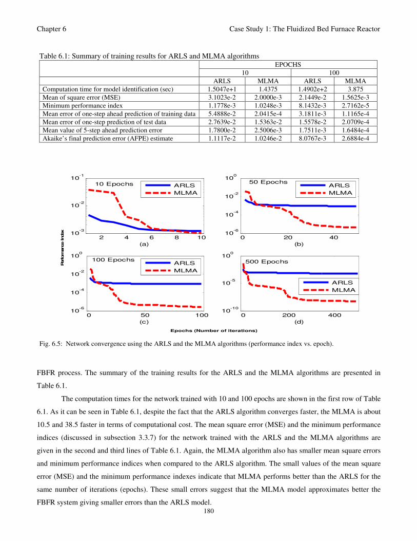
Chapter 6 Case Study 1: The Fluidized Bed Furnace Reactor
180
FBFR process. The summary of the training results for the ARLS and the MLMA algorithms are presented in
Table 6.1.
The computation times for the network trained with 10 and 100 epochs are shown in the first row of Table
6.1. As it can be seen in Table 6.1, despite the fact that the ARLS algorithm converges faster, the MLMA is about
10.5 and 38.5 faster in terms of computational cost. The mean square error (MSE) and the minimum performance
indices (discussed in subsection 3.3.7) for the network trained with the ARLS and the MLMA algorithms are
given in the second and third lines of Table 6.1. Again, the MLMA algorithm also has smaller mean square errors
and minimum performance indices when compared to the ARLS algorithm. The small values of the mean square
error (MSE) and the minimum performance indexes indicate that MLMA performs better than the ARLS for the
same number of iterations (epochs). These small errors suggest that the MLMA model approximates better the
FBFR system giving smaller errors than the ARLS model.
Table 6.1: Summary of training results for ARLS and MLMA algorithms EPOCHS
10 100
ARLS MLMA ARLS MLMA
Computation time for model identification (sec) 1.5047e+1 1.4375 1.4902e+2 3.875
Mean of square error (MSE) 3.1023e-2 2.0000e-3 2.1449e-2
1.5625e-3
Minimum performance index 1.1778e-3 1.0248e-3 8.1432e-3 2.7162e-5
Mean error of one-step ahead prediction of training data 5.4888e-2 2.0415e-4 3.1811e-3
1.1165e-4
Mean error of one-step prediction of test data 2.7639e-2 1.5363e-2 1.5578e-2 2.0709e-4
Mean value of 5-step ahead prediction error 1.7800e-2 2.5006e-3 1.7511e-3 1.6484e-4
Akaike’s final prediction error (AFPE) estimate 1.1117e-2 1.0246e-2 8.0767e-3 2.6884e-4
2 4 6 8 1010
-3
10-2
10-1
10 Epochs
(a)
ARLS
MLMA
0 20 4010
-6
10-4
10-2
100
50 Epochs
(b)
ARLS
MLMA
0 50 10010
-6
10-4
10-2
100
100 Epochs
(c)
ARLS
MLMA
0 200 40010
-10
10-5
100
500 Epochs
(d)
ARLS
MLMA
Perform
ance Index
Epochs (Number of iterations)
Fig. 6.5: Network convergence using the ARLS and the MLMA algorithms (performance index vs. epoch).
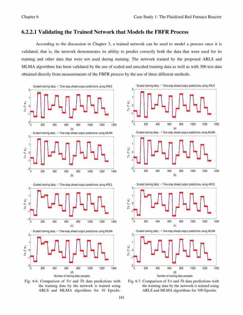
Chapter 6 Case Study 1: The Fluidized Bed Furnace Reactor
181
0 200 400 600 800 1000 1200 1400-2
-1
0
1
2
Tri
(o
K)
(a)
- Scaled training data; --* One-step ahead output predictions using ARLS
0 200 400 600 800 1000 1200 1400-2
-1
0
1
2
Tri
(o K
)
(b)
- Scaled training data; --* One-step ahead output predictions using MLMA
0 200 400 600 800 1000 1200 1400-2
-1
0
1
2
Th
(o K
)
(c)
- Scaled training data; --* One-step ahead output predictions using ARLS
0 200 400 600 800 1000 1200 1400-2
-1
0
1
2
Th
(o
K)
- Scaled training data; --* One-step ahead output predictions using MLMA
(d)
Number of training data samples
(a 10)
0 200 400 600 800 1000 1200 1400-2
-1
0
1
2
Tri
(o
K)
(a)
- Scaled training data; --* One-step ahead output predictions using ARLS
0 200 400 600 800 1000 1200 1400-2
-1
0
1
2
Tri
(o
K)
(b)
- Scaled training data; --* One-step ahead output predictions using MLMA
0 200 400 600 800 1000 1200 1400-2
-1
0
1
2
Th
(o
K)
(c)
- Scaled training data; --* One-step ahead output predictions using ARLS
0 200 400 600 800 1000 1200 1400-2
-1
0
1
2
Th
(o
K)
- Scaled training data; --* One-step ahead output predictions using MLMA
(d)
Number of training data samples
(a 100)
Fig. 6.6: Comparison of Tri and Th data predictions with
the training data by the network is trained using
ARLS and MLMA algorithms for 10 Epochs.
Fig. 6.7: Comparison of Tri and Th data predictions with
the training data by the network is trained using
ARLS and MLMA algorithms for 100 Epochs.
6.2.2.1 Validating the Trained Network that Models the FBFR Process
According to the discussion in Chapter 3, a trained network can be used to model a process once it is
validated, that is, the network demonstrates its ability to predict correctly both the data that were used for its
training and other data that were not used during training. The network trained by the proposed ARLS and
MLMA algorithms has been validated by the use of scaled and unscaled training data as well as with 300 test data
obtained directly from measurements of the FBFR process by the use of three different methods.
Chapter 6 Case Study 1: The Fluidized Bed Furnace Reactor
182
6.2.2.1.1 Validation by the One-Step Ahead Predictions Simulation
In the one-step ahead prediction method, the errors obtained from one-step ahead output predictions of the
trained network are assessed. In Fig. 6.6 (a) and (b) graphs for the Tri one-step ahead predictions of the scaled
training data (blue -) against the trained network output predictions (red --*) using the neural network model
trained by ARLS and the MLMA algorithms are shown for 10 epochs while the one-step ahead predictions of the
Th training data are shown in Fig. 6.6 (c) and (d) respectively for 10 epochs as well. Similar results for 100
epochs using both ARLS and the MLMA algorithms for Tri and Th are also shown in Fig. 6.7 (a)–(d).
The one-step ahead prediction errors are given in the fourth line of Table 6.1 for the 10 and 100 epochs
respectively. It can be seen in Fig. 6.6 (a)–(d) and Fig. 6.7 (a)–(d) that the network predictions of the training data
generally match closely the original training data used for Tri and Th. However, in the case of the ARLS
algorithm, the error is a bit larger than that of the MLMA algorithm. This observation is better shown in the fourth
line of Table 6.1. These small one-step ahead prediction errors are indications that both trained networks capture
and approximate the nonlinear dynamics of the FBFR accurately. This is further justified by the small mean
values of the MSE obtained using ARLS and MLMA algorithms for Tri and Th respectively.
Furthermore, the suitability of the proposed ARLS and MLMA algorithms for neural network model
identification for use in the FBFR industrial environment is investigated by validating the trained network with
300 unscaled test data obtained directly from the real FBFR process. Graphs of the trained network predictions
(red --*) of the test data with the actual test data (blue -) for 10 epochs for each one of the ARLS and the MLMA
algorithms are shown in Fig. 6.8 (a) and (b) for Tri and in Fig. 6.8(c) and (d) for Th respectively. Similar results
for 100 epochs are shown in Fig. 6.9 (a) and (b) for Tri and Fig. 6.9 (c) and (d) Th respectively. The almost
identical prediction of these data proves the effectiveness of the proposed approach. The prediction accuracies of
the unscaled test data by the networks trained using ARLS and the MLMA algorithm evaluated by the computed
mean prediction errors shown in the fifth line of Table 6.1. One can observe that the test data prediction errors
using MLMA are a bit smaller than those obtained by using the ARLS algorithm. These predictions of the
unscaled test data are given in Figs. 6.8 and 6.9 as well as the prediction errors in Table 6.1 verify the network
ability to model accurately the dynamics of the FBFR.
6.2.2.1.2 K–Step Ahead Prediction Simulations for the FBFR Process
The results of the K-step ahead output predictions (red --*) using the K-step ahead prediction validation
method discussed in Chapter 3 for 5-step ahead output predictions (K = 5) compared with the unscaled training
data (blue -) are shown in Fig. 6.10(a)–(d) and Fig. 6.11(a)–(d) for 10 and 100 epochs respectively. The (a) and
(c) pairs in both figures correspond to the results of the network that was trained by the ARLS while the (b) and
(d) pairs correspond to the MLMA algorithm. The value K = 5 is chosen since it is a typical value used in most
model predictive control (MPC) applications. The comparison of the 5-step ahead output predictions performance
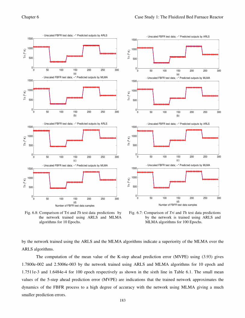
Chapter 6 Case Study 1: The Fluidized Bed Furnace Reactor
183
0 50 100 150 200 250 3000
500
1000
1500
Tri
(o K
)
(a)
- Unscaled FBFR test data; --* Predicted outputs by ARLS
0 50 100 150 200 250 3000
500
1000
1500
Tri
(o K
)
- Unscaled FBFR test data; --* Predicted outputs by MLMA
(b)
0 50 100 150 200 250 3000
500
1000
1500
Th
(o K
)
(c)
- Unscaled FBFR test data; --* Predicted outputs by ARLS
0 50 100 150 200 250 3000
500
1000
1500
Th
(o K
)
- Unscaled FBFR test data; --* Predicted outputs by MLMA
(d)
Number of FBFR test data samples
0 50 100 150 200 250 3000
500
1000
1500
Tri
(o K
)
(a)
- Unscaled FBFR test data; --* Predicted outputs by ARLS
0 50 100 150 200 250 3000
500
1000
1500
Tri
(o K
)
- Unscaled FBFR test data; --* Predicted outputs by MLMA
(b)
0 50 100 150 200 250 3000
500
1000
1500T
h (
o K
)
(c)
- Unscaled FBFR test data; --* Predicted outputs by ARLS
0 50 100 150 200 250 3000
500
1000
1500
Th
(o K
)
- Unscaled FBFR test data; --* Predicted outputs by MLMA
(d)
Number of FBFR test data samples
(a 100)
Fig. 6.8: Comparison of Tri and Th test data predictions by
the network trained using ARLS and MLMA
algorithms for 10 Epochs.
Fig. 6.7: Comparison of Tri and Th test data predictions
by the network is trained using ARLS and
MLMA algorithms for 100 Epochs.
by the network trained using the ARLS and the MLMA algorithms indicate a superiority of the MLMA over the
ARLS algorithms.
The computation of the mean value of the K-step ahead prediction error (MVPE) using (3.93) gives
1.7800e-002 and 2.5006e-003 by the network trained using ARLS and MLMA algorithms for 10 epoch and
1.7511e-3 and 1.6484e-4 for 100 epoch respectively as shown in the sixth line in Table 6.1. The small mean
values of the 5-step ahead prediction error (MVPE) are indications that the trained network approximates the
dynamics of the FBFR process to a high degree of accuracy with the network using MLMA giving a much
smaller prediction errors.
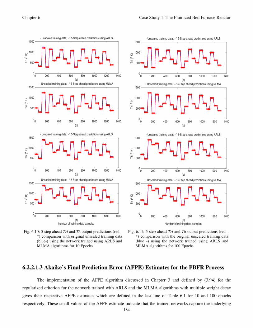
Chapter 6 Case Study 1: The Fluidized Bed Furnace Reactor
184
0 200 400 600 800 1000 1200 14000
500
1000
1500
(a)
Tri
(o
K)
- Unscaled training data; --* 5-Step ahead predictions using ARLS
0 200 400 600 800 1000 1200 14000
500
1000
1500
Tri
(o
K)
- Unscaled training data; --* 5-Step ahead predictions using MLMA
(b)
0 200 400 600 800 1000 1200 14000
500
1000
1500
(c)
Th
(o
K)
- Unscaled training data; --* 5-Step ahead predictions using ARLS
0 200 400 600 800 1000 1200 14000
500
1000
1500
Th
(o K
)
- Unscaled training data; --* 5-Step ahead predictions using MLMA
(d)
Number of training data samples
(a 10)
0 200 400 600 800 1000 1200 14000
500
1000
1500
(a)
Tri
(o K
)
- Unscaled training data; --* 5-Step ahead predictions using ARLS
0 200 400 600 800 1000 1200 14000
500
1000
1500
Tri
(o K
)
- Unscaled training data; --* 5-Step ahead predictions using MLMA
(b)
0 200 400 600 800 1000 1200 14000
500
1000
1500
(c)
Th
(o K
)- Unscaled training data; --* 5-Step ahead predictions using ARLS
0 200 400 600 800 1000 1200 14000
500
1000
1500
Th
(o K
)
- Unscaled training data; --* 5-Step ahead predictions using MLMA
(d)
Number of training data samples
(a 100)
Fig. 6.10: 5-step ahead Tri and Th output predictions (red--
*) comparison with original unscaled training data
(blue-) using the network trained using ARLS and
MLMA algorithms for 10 Epochs.
Fig. 6.11: 5-step ahead Tri and Th output predictions (red--
*) comparison with the original unscaled training data
(blue -) using the network trained using ARLS and
MLMA algorithms for 100 Epochs.
6.2.2.1.3 Akaike’s Final Prediction Error (AFPE) Estimates for the FBFR Process
The implementation of the AFPE algorithm discussed in Chapter 3 and defined by (3.94) for the
regularized criterion for the network trained with ARLS and the MLMA algorithms with multiple weight decay
gives their respective AFPE estimates which are defined in the last line of Table 6.1 for 10 and 100 epochs
respectively. These small values of the AFPE estimate indicate that the trained networks capture the underlying
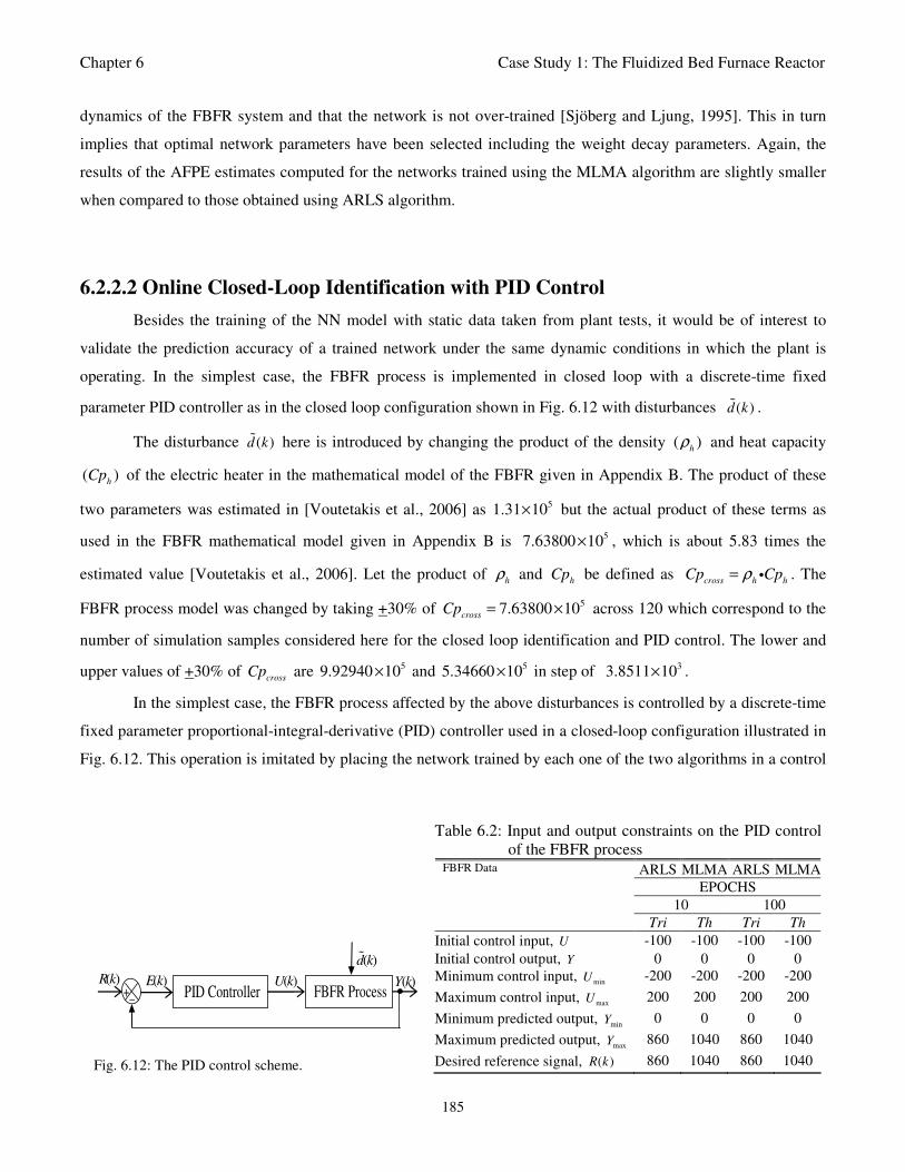
Chapter 6 Case Study 1: The Fluidized Bed Furnace Reactor
185
dynamics of the FBFR system and that the network is not over-trained [Sjöberg and Ljung, 1995]. This in turn
implies that optimal network parameters have been selected including the weight decay parameters. Again, the
results of the AFPE estimates computed for the networks trained using the MLMA algorithm are slightly smaller
when compared to those obtained using ARLS algorithm.
6.2.2.2 Online Closed-Loop Identification with PID Control
Besides the training of the NN model with static data taken from plant tests, it would be of interest to
validate the prediction accuracy of a trained network under the same dynamic conditions in which the plant is
operating. In the simplest case, the FBFR process is implemented in closed loop with a discrete-time fixed
parameter PID controller as in the closed loop configuration shown in Fig. 6.12 with disturbances ( )d k .
The disturbance ( )d k here is introduced by changing the product of the density ( )h
ρ and heat capacity
( )h
Cp of the electric heater in the mathematical model of the FBFR given in Appendix B. The product of these
two parameters was estimated in [Voutetakis et al., 2006] as 51.31 10× but the actual product of these terms as
used in the FBFR mathematical model given in Appendix B is 57.63800 10× , which is about 5.83 times the
estimated value [Voutetakis et al., 2006]. Let the product of h
ρ and h
Cp be defined ascross h h
Cp Cpρ= i . The
FBFR process model was changed by taking +30% of 57.63800 10cross
Cp = × across 120 which correspond to the
number of simulation samples considered here for the closed loop identification and PID control. The lower and
upper values of +30% of cross
Cp are 59.92940 10× and 55.34660 10× in step of 33.8511 10× .
In the simplest case, the FBFR process affected by the above disturbances is controlled by a discrete-time
fixed parameter proportional-integral-derivative (PID) controller used in a closed-loop configuration illustrated in
Fig. 6.12. This operation is imitated by placing the network trained by each one of the two algorithms in a control
Table 6.2: Input and output constraints on the PID control
of the FBFR process
ARLS MLMA ARLS MLMA
EPOCHS
10 100
FBFR Data
Tri Th Tri Th
Initial control input, U -100 -100 -100 -100
Initial control output, Y 0 0 0 0
Minimum control input, minU -200 -200 -200 -200
Maximum control input, maxU 200 200 200 200
Minimum predicted output, minY 0 0 0 0
Maximum predicted output, maxY 860 1040 860 1040
Desired reference signal, ( )R k 860 1040 860 1040
PID Controller FBFR Process ( )R k ( )E k ( )Y k ( )U k
( )d k
• + –
Fig. 6.12: The PID control scheme.
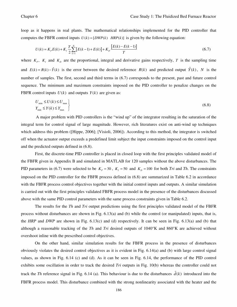
Chapter 6 Case Study 1: The Fluidized Bed Furnace Reactor
186
loop as it happens in real plants. The mathematical relationships implemented for the PID controller that
computes the FBFR control inputs ( ) [ ( ) ( )]U k DWP k HRP k= is given by the following equation:
[ ][ ]
1
( ) ( 1)( ) ( ) ( 1) ( )
2
N
P I D
k
E k E kTU k K E k K E k E k K
T=
− −= + − + +∑ (6.7)
where ,P I
K K and D
K are the proportional, integral and derivative gains respectively, T is the sampling time
and ˆ( ) ( ) ( )E k R k Y k= − is the error between the desired reference ( )R k and predicted output ˆ( )Y k , N is the
number of samples. The first, second and third terms in (6.7) corresponds to the present, past and future control
sequence. The minimum and maximum constraints imposed on the PID controller to penalize changes on the
FBFR control inputs ( )U k and outputs ( )Y k are given as:
min max
min max
( )
( )
U U k U
Y Y k Y
≤ ≤
≤ ≤ (6.8)
A major problem with PID controllers is the “wind up” of the integrator resulting in the saturation of the
integral term for control signal of large magnitude. However, rich literatures exist on anti-wind up techniques
which address this problem ([Hippe, 2006]; [Visioli, 2006]). According to this method, the integrator is switched
off when the actuator output exceeds a predefined limit subject the input constraints imposed on the control input
and the predicted outputs defined in (6.8).
First, the discrete-time PID controller is placed in closed loop with the first principles validated model of
the FBFR given in Appendix B and simulated in MATLAB for 120 samples without the above disturbances. The
PID parameters in (6.7) were selected to be 30P
K = , 50I
K = and 100D
K = for both Tri and Th. The constraints
imposed on the PID controller for the FBFR process defined in (6.8) are summarized in Table 6.2 in accordance
with the FBFR process control objectives together with the initial control inputs and outputs. A similar simulation
is carried out with the first principles validated FBFR process model in the presence of the disturbances discussed
above with the same PID control parameters with the same process constraints given in Table 6.2.
The results for the Th and Tri output predictions using the first principles validated model of the FBFR
process without disturbances are shown in Fig. 6.13(a) and (b) while the control (or manipulated) inputs, that is,
the HRP and DWP are shown in Fig. 6.13(c) and (d) respectively. It can be seen in Fig. 6.13(a) and (b) that
although a reasonable tracking of the Th and Tri desired outputs of 1040°K and 860°K are achieved without
overshoot inline with the prescribed control objectives.
On the other hand, similar simulation results for the FBFR process in the presence of disturbances
obviously violates the desired control objectives as it is evident in Fig. 6.14(a) and (b) with large control signal
values, as shown in Fig. 6.14 (c) and (d). As it can be seen in Fig. 6.14, the performance of the PID control
exhibits some oscillation in order to track the desired Tri outputs in Fig. 10(b) whereas the controller could not
track the Th reference signal in Fig. 6.14 (a). This behaviour is due to the disturbances ( )d k introduced into the
FBFR process model. This disturbance combined with the strong nonlinearity associated with the heater and the
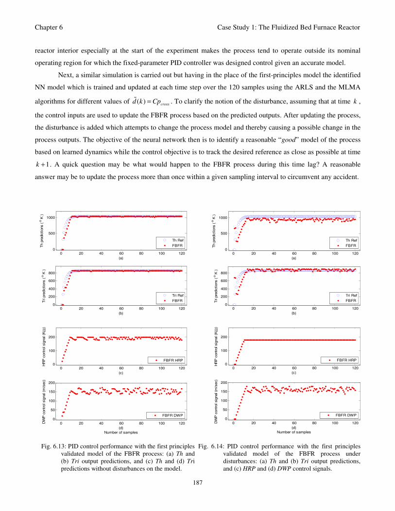
Chapter 6 Case Study 1: The Fluidized Bed Furnace Reactor
187
reactor interior especially at the start of the experiment makes the process tend to operate outside its nominal
operating region for which the fixed-parameter PID controller was designed control given an accurate model.
Next, a similar simulation is carried out but having in the place of the first-principles model the identified
NN model which is trained and updated at each time step over the 120 samples using the ARLS and the MLMA
algorithms for different values of ( )cross
d k Cp= . To clarify the notion of the disturbance, assuming that at time k ,
the control inputs are used to update the FBFR process based on the predicted outputs. After updating the process,
the disturbance is added which attempts to change the process model and thereby causing a possible change in the
process outputs. The objective of the neural network then is to identify a reasonable “good” model of the process
based on learned dynamics while the control objective is to track the desired reference as close as possible at time
1k + . A quick question may be what would happen to the FBFR process during this time lag? A reasonable
answer may be to update the process more than once within a given sampling interval to circumvent any accident.
0 20 40 60 80 100 1200
500
1000
(a)
Th p
redic
tions (
o K
)
0 20 40 60 80 100 1200
200
400
600
800
(b)
Tri p
redic
tions (
o K
)
Th Ref
FBFR
Tri Ref
FBFR
0 20 40 60 80 100 1200
100
200
(c)
HR
P c
ontr
ol sig
nal (K
Ω)
0 20 40 60 80 100 1200
50
100
150
200
(d)
Number of samples
DW
P c
ontr
ol sig
nal (m
/sec)
FBFR HRP
FBFR DWP
0 20 40 60 80 100 1200
500
1000
(a)
Th p
redic
tions ( o
K )
0 20 40 60 80 100 1200
200
400
600
800
(b)
Tri p
redic
tions (
o K
)
Th Ref
FBFR
Tri Ref
FBFR
0 20 40 60 80 100 1200
100
200
(c)
HR
P c
ontr
ol sig
nal (K
Ω)
0 20 40 60 80 100 1200
50
100
150
200
(d)
Number of samples
DW
P c
ontrol sig
nal (m
/sec)
FBFR HRP
FBFR DWP
Fig. 6.13: PID control performance with the first principles
validated model of the FBFR process: (a) Th and
(b) Tri output predictions, and (c) Th and (d) Tri
predictions without disturbances on the model.
Fig. 6.14: PID control performance with the first principles
validated model of the FBFR process under
disturbances: (a) Th and (b) Tri output predictions,
and (c) HRP and (d) DWP control signals.
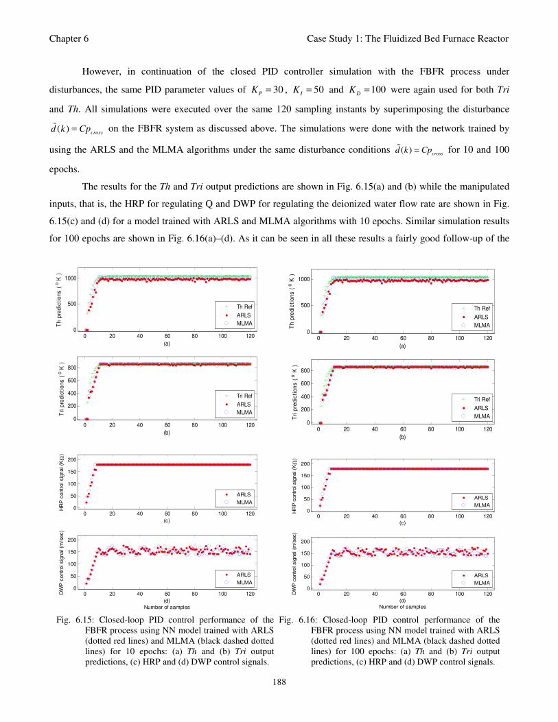
Chapter 6 Case Study 1: The Fluidized Bed Furnace Reactor
188
However, in continuation of the closed PID controller simulation with the FBFR process under
disturbances, the same PID parameter values of 30P
K = , 50I
K = and 100D
K = were again used for both Tri
and Th. All simulations were executed over the same 120 sampling instants by superimposing the disturbance
( )cross
d k Cp= on the FBFR system as discussed above. The simulations were done with the network trained by
using the ARLS and the MLMA algorithms under the same disturbance conditions ( )cross
d k Cp= for 10 and 100
epochs.
The results for the Th and Tri output predictions are shown in Fig. 6.15(a) and (b) while the manipulated
inputs, that is, the HRP for regulating Q and DWP for regulating the deionized water flow rate are shown in Fig.
6.15(c) and (d) for a model trained with ARLS and MLMA algorithms with 10 epochs. Similar simulation results
for 100 epochs are shown in Fig. 6.16(a)–(d). As it can be seen in all these results a fairly good follow-up of the
0 20 40 60 80 100 1200
500
1000
(a)
Th
pre
dic
tio
ns
( o
K )
0 20 40 60 80 100 1200
200
400
600
800
(b)
Tri
pre
dic
tio
ns
( o
K )
Th Ref
ARLS
MLMA
Tri Ref
ARLS
MLMA
0 20 40 60 80 100 1200
50
100
150
200
(c)
HR
P c
ontr
ol sig
nal (K
Ω)
0 20 40 60 80 100 1200
50
100
150
200
(d)
Number of samples
DW
P c
ontr
ol sig
nal (m
/sec)
ARLS
MLMA
ARLS
MLMA
0 20 40 60 80 100 1200
500
1000
(a)
Th
pre
dic
tio
ns
( o
K )
0 20 40 60 80 100 1200
200
400
600
800
(b)
Tri
pre
dic
tio
ns
( o
K )
Th Ref
ARLS
MLMA
Tri Ref
ARLS
MLMA
0 20 40 60 80 100 1200
50
100
150
200
(c)
HR
P c
ontr
ol sig
nal (K
Ω)
0 20 40 60 80 100 1200
50
100
150
200
(d)
Number of samples
DW
P c
ontr
ol sig
nal (m
/sec)
ARLS
MLMA
ARLS
MLMA
Fig. 6.15: Closed-loop PID control performance of the
FBFR process using NN model trained with ARLS
(dotted red lines) and MLMA (black dashed dotted
lines) for 10 epochs: (a) Th and (b) Tri output
predictions, (c) HRP and (d) DWP control signals.
Fig. 6.16: Closed-loop PID control performance of the
FBFR process using NN model trained with ARLS
(dotted red lines) and MLMA (black dashed dotted
lines) for 100 epochs: (a) Th and (b) Tri output
predictions, (c) HRP and (d) DWP control signals.
Chapter 6 Case Study 1: The Fluidized Bed Furnace Reactor
189
first principles model response is achieved by both the ARLS and MLMA models for 10 epochs. It can be
observed that the model based on ARLS exhibits oscillatory behaviour in Th predictions as in Fig. 6.15(a) and (b)
as well as in Fig. 6.16(a) and (b). This behaviour is not unusual because of the strong nonlinearity associated with
the heater and the reactor interior especially at the start of the experiment [Voutetakis et al., 2006]. This effect can
also be observed in Fig. 6.13 (a) and (b) as well as in Fig. 6.14(a) and (b) based on the true first principles
validated FBFR process model. Similar results are obtained with networks trained over 100 epochs. For space
saving reasons these results are not presented.
Comparing the FBFR control performance of Fig. 6.13 and Fig. 6.14 with Fig. 6.15 and Fig. 6.16, it is
evident that the models obtained with the two proposed identification algorithms give good control performances
even with the fixed parameter PID controller under disturbances. With the ARLS and the MLMA training
algorithms proposed in this work, changes on the process dynamics seem to be captured adequately. Furthermore,
the study has shown that the control performance based on the NN model trained using the MLMA outperforms
that based on the ARLS method as this becomes evident in Fig 6.15(a) and Fig. 6.16(a).
6.2.3 Validation and Dynamic Performance Comparison of the Proposed MLMA
algorithm with Backpropagation with momentum (BPM) and Incremental
Backpropagation (INCBP) Algorithms
The backpropagation with momentum (BPM) is a widely used neural network training algorithm. A
version of this algorithm presented in Section 2.4.4.1 of Chapter 2 and is implemented in this work in order to
compare its performance with the identification algorithms proposed in this work. The modified Levenberg-
Marquardt algorithm (MLMA) is considered here for this comparison due to its superior performance over the
adaptive recursive least squares (ARLS) algorithm which is a true online identification algorithm. The third
algorithm included in this comparison is the incremental or online backpropagation (INCBP) algorithm originally
proposed by [Hertz et al., 1991]. The incremental backpropagation (INCBP) algorithm is easily derived by setting
the covariance matrix ( )P k Iµ= on the left hand side of (3.54) in Section 3.3.5 of Chapter under the formulation
of the ARLS algorithm; that is:
1
1
1[ , ( )]
k
I R kk
τ τ
ι
µ ι θ −
=
= ∑ (6.9)
where µ is the step size and I is an identity matrix of appropriate dimension. Next, Equation (3.17) in Section
3.3.3 of Chapter 3 is used to update the algorithm, that is:
( ) ( )
[ ( )]ˆ( ) ( )( )
k k
dJ kk k
d kτ
τ τ
θ θ
θθ θ µ
θ=
= − (6.10)
Chapter 6 Case Study 1: The Fluidized Bed Furnace Reactor
190
All that is required is to specify a suitable step size µ and carry out the recursive computation of the gradient
given by (6.10).
6.2.3.1 Network Training Using BPM, INCBP and the Proposed MLMA Algorithms
Due to the simplicity and generality of the backpropagation with momentum (BPM) algorithm discussed
in Section 2.4.4.1 in Chapter 2 and the incremental backpropagation (INCBP) algorithm just discussed above in
Section 6.2.3, the NNARX model regression vector ( )NNARX
kϕ defined by (6.4) is used as the input vector to the
neural network. The outputs of the NN are the predicted values of ˆ( )Y k given by (6.6). The simulation results for
Th and Tri are presented, and the predicted outputs of interest is then given as ˆ ˆ ˆ( ) [ ( ) ( )]T
Th TriY k y k y k= .
The two design parameters for the BPM algorithm defined in (2.59) are the learning rate 1 4eγ = − (i.e.
the step size) and momentum term 1 3eα = − . The design parameter for the INCBP is the step size 1 4eµ = − .
Finally, the design parameters for initializing the MLMA algorithm were selected as 0.001τλ = , 0.05s = and
0.01δ = . It was shown in Section 6.2.2 that the performance of the ARLS and the MLMA algorithms converges
to acceptable values after approximately 100 epochs. In order to assess the convergence performance of the
network trained by the three algorithms, the network was also trained for τ = 100 epochs with the following
selected parameters: 2p = , 6q = , 3a
n = , 3b
n = , 24nϕ = , 10h
n = , 6o
n = , 1 5h
eα = − and 1 4o
eα = − .
The training data is first scaled using (3.89) and the network is trained for 100τ = epochs using the
backpropagation with momentum (BPM), the incremental backpropagation (INCBP) and the modified
Levenberg-Marquardt algorithm (MLMA) algorithms. After network training, the trained network is again
rescaled according to (3.90), so that the resulting network can work with unscaled FBFR data. The convergences
of the BPM, INCBP and the MLMA algorithms for 100 epochs are shown in Fig. 6.17 and are evaluated in terms
of the performance index. It can observe that only the MLMA algorithm meets the training goal of 10-6
while the
BPM and the INCBP tend to remain around 10-2
within the prescribed 100 epochs with slow convergence.
By comparing the convergences of the BPM, INCBP and MLMA algorithms in Fig. 6.17, it can be seen
that the BPM and INCBP algorithms converges faster to almost the same values than the MLMA algorithm. It can
also be seen in this figure that the performance index obtained by the network trained using MLMA algorithm has
a much smaller value when compared to that obtained by the network when it is trained using the BPM and the
INCBP algorithms. The summary of the network training results using the BPM, INCBP and the MLMA
algorithms are presented in Table 6.3 for quick comparison of the performances of the network when it is trained
by the three mentioned methods.
The computation time for training the network for 100 epochs using each one from the three algorithms
are shown in the first row of Table 6.3. As it can be seen, despite the fact that the BPM and the INCBP algorithms
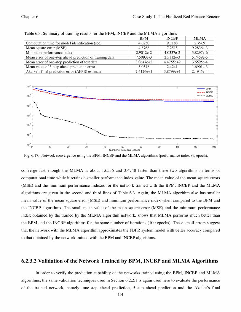
Chapter 6 Case Study 1: The Fluidized Bed Furnace Reactor
191
Table 6.3: Summary of training results for the BPM, INCBP and the MLMA algorithms BPM INCBP MLMA
Computation time for model identification (sec) 4.6250 9.7188 2.7969
Mean square error (MSE) 4.8768 7.2515 9.2836e-3
Minimum performance index 2.9012e-2 4.0337e-2 3.8297e-6
Mean error of one-step ahead prediction of training data 7.5093e-3 2.5112e-3 5.7459e-5
Mean error of one-step prediction of test data 3.0647e+2 4.4755e+2 3.6595e-4
Mean value of 5-step ahead prediction error 3.0548 2.4241 1.6901e-3
Akaike’s final prediction error (AFPE) estimate 2.4126e+1 3.8799e+1 2.4945e-4
0 10 20 30 40 50 60 70 80 90 10010
-6
10-5
10-4
10-3
10-2
10-1
100
Number of iterations (epoch)
BPM
INCBP
MLMA
Fig. 6.17: Network convergence using the BPM, INCBP and the MLMA algorithms (performance index vs. epoch).
converge fast enough the MLMA is about 1.6536 and 3.4748 faster than these two algorithms in terms of
computational time while it retains a smaller performance index value. The mean value of the mean square errors
(MSE) and the minimum performance indexes for the network trained with the BPM, INCBP and the MLMA
algorithms are given in the second and third lines of Table 6.3. Again, the MLMA algorithm also has smaller
mean value of the mean square error (MSE) and minimum performance index when compared to the BPM and
the INCBP algorithms. The small mean value of the mean square error (MSE) and the minimum performance
index obtained by the trained by the MLMA algorithm network, shows that MLMA performs much better than
the BPM and the INCBP algorithms for the same number of iterations (100 epochs). These small errors suggest
that the network with the MLMA algorithm approximates the FBFR system model with better accuracy compared
to that obtained by the network trained with the BPM and INCBP algorithms.
6.2.3.2 Validation of the Network Trained by BPM, INCBP and MLMA Algorithms
In order to verify the prediction capability of the networks trained using the BPM, INCBP and MLMA
algorithms, the same validation techniques used in Section 6.2.2.1 is again used here to evaluate the performance
of the trained network, namely: one-step ahead prediction, 5-step ahead prediction and the Akaike’s final
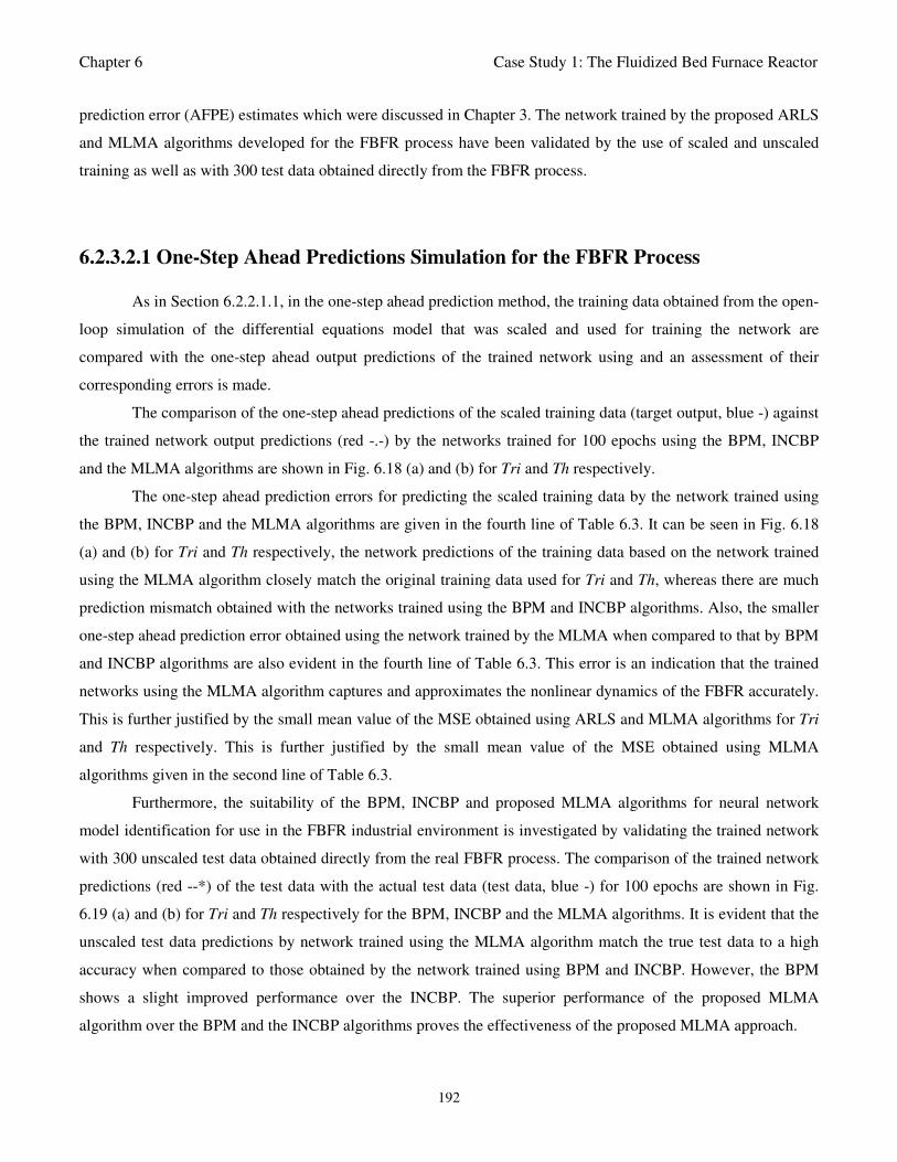
Chapter 6 Case Study 1: The Fluidized Bed Furnace Reactor
192
prediction error (AFPE) estimates which were discussed in Chapter 3. The network trained by the proposed ARLS
and MLMA algorithms developed for the FBFR process have been validated by the use of scaled and unscaled
training as well as with 300 test data obtained directly from the FBFR process.
6.2.3.2.1 One-Step Ahead Predictions Simulation for the FBFR Process
As in Section 6.2.2.1.1, in the one-step ahead prediction method, the training data obtained from the open-
loop simulation of the differential equations model that was scaled and used for training the network are
compared with the one-step ahead output predictions of the trained network using and an assessment of their
corresponding errors is made.
The comparison of the one-step ahead predictions of the scaled training data (target output, blue -) against
the trained network output predictions (red -.-) by the networks trained for 100 epochs using the BPM, INCBP
and the MLMA algorithms are shown in Fig. 6.18 (a) and (b) for Tri and Th respectively.
The one-step ahead prediction errors for predicting the scaled training data by the network trained using
the BPM, INCBP and the MLMA algorithms are given in the fourth line of Table 6.3. It can be seen in Fig. 6.18
(a) and (b) for Tri and Th respectively, the network predictions of the training data based on the network trained
using the MLMA algorithm closely match the original training data used for Tri and Th, whereas there are much
prediction mismatch obtained with the networks trained using the BPM and INCBP algorithms. Also, the smaller
one-step ahead prediction error obtained using the network trained by the MLMA when compared to that by BPM
and INCBP algorithms are also evident in the fourth line of Table 6.3. This error is an indication that the trained
networks using the MLMA algorithm captures and approximates the nonlinear dynamics of the FBFR accurately.
This is further justified by the small mean value of the MSE obtained using ARLS and MLMA algorithms for Tri
and Th respectively. This is further justified by the small mean value of the MSE obtained using MLMA
algorithms given in the second line of Table 6.3.
Furthermore, the suitability of the BPM, INCBP and proposed MLMA algorithms for neural network
model identification for use in the FBFR industrial environment is investigated by validating the trained network
with 300 unscaled test data obtained directly from the real FBFR process. The comparison of the trained network
predictions (red --*) of the test data with the actual test data (test data, blue -) for 100 epochs are shown in Fig.
6.19 (a) and (b) for Tri and Th respectively for the BPM, INCBP and the MLMA algorithms. It is evident that the
unscaled test data predictions by network trained using the MLMA algorithm match the true test data to a high
accuracy when compared to those obtained by the network trained using BPM and INCBP. However, the BPM
shows a slight improved performance over the INCBP. The superior performance of the proposed MLMA
algorithm over the BPM and the INCBP algorithms proves the effectiveness of the proposed MLMA approach.
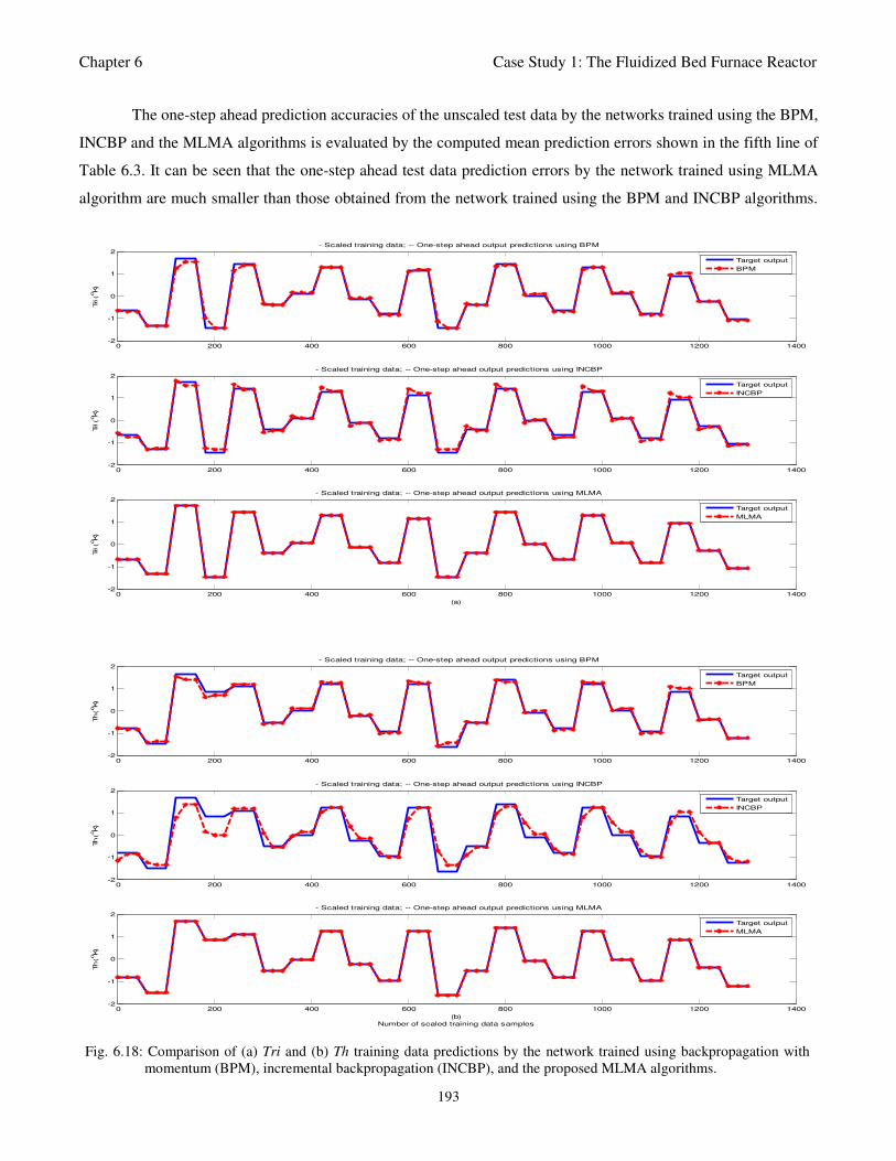
Chapter 6 Case Study 1: The Fluidized Bed Furnace Reactor
193
0 200 400 600 800 1000 1200 1400-2
-1
0
1
2
Tri ( oK)
- Scaled training data; -- One-step ahead output predictions using BPM
Target output
BPM
0 200 400 600 800 1000 1200 1400-2
-1
0
1
2
Tri ( oK)
- Scaled training data; -- One-step ahead output predictions using INCBP
Target output
INCBP
0 200 400 600 800 1000 1200 1400-2
-1
0
1
2
Tri ( oK)
- Scaled training data; -- One-step ahead output predictions using MLMA
(a)
Target output
MLMA
0 200 400 600 800 1000 1200 1400-2
-1
0
1
2
Th ( oK)
- Scaled training data; -- One-step ahead output predictions using BPM
Target output
BPM
0 200 400 600 800 1000 1200 1400-2
-1
0
1
2
Th ( oK)
- Scaled training data; -- One-step ahead output predictions using INCBP
Target output
INCBP
0 200 400 600 800 1000 1200 1400-2
-1
0
1
2
Th ( oK)
- Scaled training data; -- One-step ahead output predictions using MLMA
(b)
Number of scaled training data samples
Target output
MLMA
Fig. 6.18: Comparison of (a) Tri and (b) Th training data predictions by the network trained using backpropagation with
momentum (BPM), incremental backpropagation (INCBP), and the proposed MLMA algorithms.
The one-step ahead prediction accuracies of the unscaled test data by the networks trained using the BPM,
INCBP and the MLMA algorithms is evaluated by the computed mean prediction errors shown in the fifth line of
Table 6.3. It can be seen that the one-step ahead test data prediction errors by the network trained using MLMA
algorithm are much smaller than those obtained from the network trained using the BPM and INCBP algorithms.
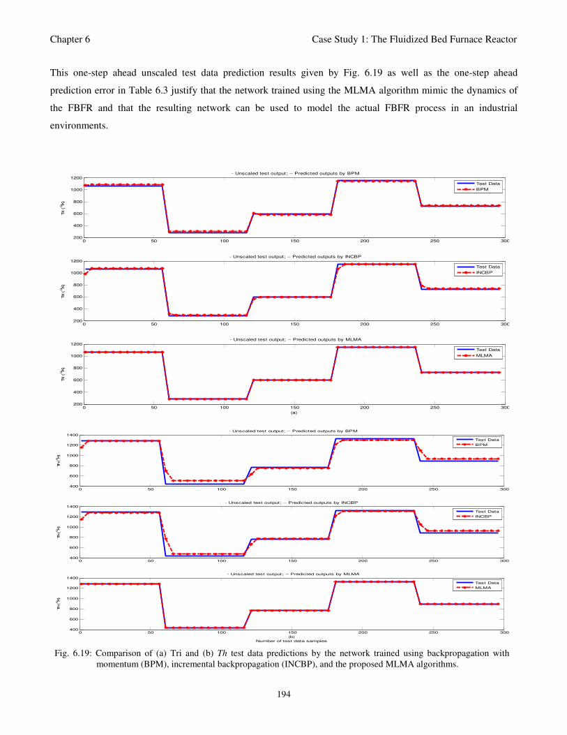
Chapter 6 Case Study 1: The Fluidized Bed Furnace Reactor
194
This one-step ahead unscaled test data prediction results given by Fig. 6.19 as well as the one-step ahead
prediction error in Table 6.3 justify that the network trained using the MLMA algorithm mimic the dynamics of
the FBFR and that the resulting network can be used to model the actual FBFR process in an industrial
environments.
0 50 100 150 200 250 300200
400
600
800
1000
1200
Tri ( oK)
- Unscaled test output; -- Predicted outputs by BPM
Test Data
BPM
0 50 100 150 200 250 300200
400
600
800
1000
1200
Tri ( oK)
- Unscaled test output; -- Predicted outputs by INCBP
Test Data
INCBP
0 50 100 150 200 250 300200
400
600
800
1000
1200
Tri ( oK)
- Unscaled test output; -- Predicted outputs by MLMA
(a)
Test Data
MLMA
0 50 100 150 200 250 300400
600
800
1000
1200
1400
Th ( oK)
- Unscaled test output; -- Predicted outputs by BPM
Test Data
BPM
0 50 100 150 200 250 300400
600
800
1000
1200
1400
Th ( oK)
- Unscaled test output; -- Predicted outputs by INCBP
Test Data
INCBP
0 50 100 150 200 250 300400
600
800
1000
1200
1400
Th ( oK)
- Unscaled test output; -- Predicted outputs by MLMA
(b)
Number of test data samples
Test Data
MLMA
Fig. 6.19: Comparison of (a) Tri and (b) Th test data predictions by the network trained using backpropagation with
momentum (BPM), incremental backpropagation (INCBP), and the proposed MLMA algorithms.
Chapter 6 Case Study 1: The Fluidized Bed Furnace Reactor
195
6.2.3.2.2 K–Step Ahead Prediction Simulations for the FBFR Process
The results of the K-step ahead output predictions (red --*) using the K-step ahead prediction validation
method discussed in Chapter 3 for 5-step ahead output predictions (K = 5) compared with the unscaled training
data (target output) are shown in Fig. 6.20 (a) and (b) for Tri and Th respectively for the network trained using the
BPM, INCBP and MLMA algorithms. Again, the value K = 5 is chosen since it is a typical value used in most
0 200 400 600 800 1000 1200 1400200
400
600
800
1000
1200
1400
Tri ( oK)
- Unscaled training data; -- 5-Step ahead output predictions by BPM
Target output
BPM
0 200 400 600 800 1000 1200 1400200
400
600
800
1000
1200
1400
Tri ( oK)
- Unscaled training data; -- 5-Step ahead output predictions by INCBP
Target output
INCBP
0 200 400 600 800 1000 1200 1400200
400
600
800
1000
1200
1400
Tri ( oK)
- Unscaled training data; -- 5-Step ahead output predictions by MLMA
(a)
Target output
MLMA
0 200 400 600 800 1000 1200 1400400
600
800
1000
1200
1400
1600
Th ( oK)
- Unscaled training data; -- 5-Step ahead output predictions by BPM
Target output
BPM
0 200 400 600 800 1000 1200 1400400
600
800
1000
1200
1400
1600
Th ( oK)
- Unscaled training data; -- 5-Step ahead output predictions by INCBP
Target output
INCBP
0 200 400 600 800 1000 1200 1400400
600
800
1000
1200
1400
1600
Th ( oK)
- Unscaled training data; -- 5-Step ahead output predictions by MLMA
(b)
Number of training data samples
Target output
MLMA
Fig. 6.20: Comparison of the 5-step ahead output predictions (red --*) of the NN for (a) Tri and (b) Th when it is trained
by the BPM, (INCBP), and the proposed MLMA algorithms with the original unscaled training data (blue-).
Chapter 6 Case Study 1: The Fluidized Bed Furnace Reactor
196
model predictive control (MPC) applications. The comparison of the 5-step ahead output predictions performance
by the network trained using BPM, INCBP and the MLMA algorithms shows the superior performance of the
MLMA algorithm over the BPM, INCBP algorithms for use in distant or multi-step ahead predictions.
The computation of the mean value of the K-step ahead prediction error (MVPE) using (3.93) gives
3.0548, 2.4241 and 1.6901e-3 respectively by the network trained using the BPM, INCBP and MLMA algorithms
as shown in the sixth line in Table 6.3. The relatively small MVPE obtained by the network trained with the
MLMA algorithm is indications that the trained network approximates the dynamics of the FBFR process to a
high degree of accuracy.
6.2.3.2.3 Akaike’s Final Prediction Error (AFPE) Estimates for the FBFR Process
The implementation of the AFPE algorithm discussed in Chapter 3 and defined by (3.94) for the
regularized criterion for the network trained with the BPM, INCBP and the MLMA algorithms with multiple
weight decay gives the respective AFPE estimates of the three algorithms as defined in the last line of Table 6.3.
These small values of the AFPE estimate indicate that the trained networks capture the underlying dynamics of
the FBFR system and that the network is not over-trained [Sjöberg and Ljung, 1995]. This in turn implies that
optimal network parameters have been selected including the weight decay parameters. Again, the results of the
AFPE estimates obtained with the networks trained using the MLMA algorithm are slightly smaller when
compared to those obtained using BPM and INCBP algorithms.
6.2.3.3 Performance Comparison of the BPM, INCBP and the MLMA Algorithms
The simulation results for the neural network training using the BPM, INCBP and MLMA algorithms as
well as the network validation result for the FBFR process are shown in Fig. 6.17, Fig. 6.18, Fig. 6.19, and Fig.
6.20 respectively; whereas numerical results for these three algorithms are presented in Table 6.3.
The numerical results summarized in Table 6.3 show that when the network is trained by using the
MLMA algorithm presents the best performance as the least values in all of the six properties are achieved. In
addition, the least value of the AFPE is obtained using the MLMA algorithm which indicates that the MLMA
algorithm captures the essential dynamics of the process and that the identified NN model approximates the true
system to a high degree of accuracy. The small mean value of the 5-step ahead prediction error (MVPE) is an
indication that the MLMA algorithm can be used in adaptive predictive control applications due to its accurate 5-
step ahead predictions when compared to BPM and INCBP algorithms. Furthermore, as the relative small
performance index is obtained within a relatively short time of 100 epochs, makes this algorithm more appropriate
for applications with real time requirements.
Chapter 6 Case Study 1: The Fluidized Bed Furnace Reactor
197
6.2.4 Validation and Performance Evaluation of the Proposed AGPC and NAMPC
Algorithms for the Model-Based Adaptive MPC of the FBFR Process
In Chapter 4, an adaptive generalized predictive control algorithm (AGPC) and a nonlinear adaptive
predictive control algorithm (NAMPC) were proposed. In this sub-section, the performances of both control
algorithms are evaluated. The model structure considered here is the NNARMAX model which was used in
Section 6.2.2 to investigate the efficiencies of the ARLS and the MLMA algorithms in neural network training.
The main control objective here is to ensure that by manipulating the high resistance potentiometer (HRP)
and the deionized water pump (DWP) flow rate, the temperatures of the electric heater (Th) and the reactor
interior (Tri) should not exceed 1040 °K and 860 °K respectively without any overshoots throughout the catalyst
processing and deactivation process. As it is stated in [Voutetakis et al, 2006], a relatively small overshoot above
2% might give unacceptable final product properties.
Before implementing the AGPC and the NAMPC control strategies explained in Chapter 4, the neural
network model obtained using adaptive recursive least squares (ARLS) algorithm in Section 6.2.2 and validated in
Section 6.2.2.1 is used to tune the two controllers subject to the constraints in Table 6.4. The model trained using
ARLS algorithm is used because of its simplicity and because it is a truly online identification algorithm. As
shown in Table 6.4, minimum and maximum input and output constraints are imposed for the efficient and tight
control of the FBFR such that the controlled outputs will follow the desired reference signal without any
overshoot provided that these constraints are not violated. Once an initially tuned controller becomes available
then the adaptive implementation of the AGPC and NAMPC control algorithms is considered by using on-line the
ARLS algorithm for training the NN each time new data becomes available from the closed loop plant operation.
The AGPC and NAMPC algorithms are shown pictorially in Fig. 4.1 and Fig. 4.4 respectively in Chapter
4. Here, the system in Fig. 4.1 and Fig. 4.4 both correspond to the FBFR process. The neural network model in
both Fig. 4.1 and Fig. 4.4 are based on the NNARMAX model identification scheme illustrated in Fig. 3.4 (b) in
Chapter 3.
First, the optimal closed loop tuning parameters for the AGPC and the NAMPC controllers based on the
use of the identified neural network model which was trained with the ARLS algorithm are given in Table 6.5.
The initial control input (ICI) and initial predicted output (ICO) are used to initialize the iterative solutions of the
two controllers. The remaining tuning parameters are discussed in Chapter 4 where d
N , u
N , pN is the minimum,
control and prediction horizons respectively; κ and ρ are weighting factors for penalizing changes on the
control inputs ( )U k and predicted outputs ˆ( )Y k ; λ is the Levenberg-Marquardt parameter which is also the
adaptation parameter for the NAMPC controller; m
A and m
B are the first-order digital reference filter design
parameters; δ is the trust-region algorithm radius within which the optimal control signal can be found and a
design parameter used in the NAMPC algorithm; and iter
U is the maximum number of iterations required to
determine the optimal control signal at each sampling instant. These controller tuning parameters are obtained a
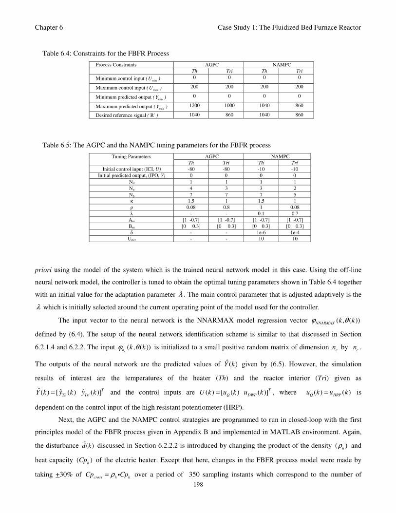
Chapter 6 Case Study 1: The Fluidized Bed Furnace Reactor
198
Table 6.4: Constraints for the FBFR Process
Process Constraints AGPC NAMPC
Th Tri Th Tri
Minimum control input (minU ) 0 0 0 0
Maximum control input (maxU ) 200 200 200 200
Minimum predicted output (minY ) 0 0 0 0
Maximum predicted output (maxY ) 1200 1000 1040 860
Desired reference signal ( R' ) 1040 860 1040 860
Table 6.5: The AGPC and the NAMPC tuning parameters for the FBFR process
AGPC NAMPC Tuning Parameters
Th Tri Th Tri
Initial control input (ICI, U) -80 -80 -10 -10
Initial predicted output, (IPO, Y) 0 0 0 0
Nd 1 1 1 1
Nu 4 3 3 2
Np 7 7 7 5
κ 1.5 1 1.5 1
ρ 0.08 0.8 1 0.08
λ - - 0.1 0.7
Am [1 -0.7] [1 -0.7] [1 -0.7] [1 -0.7]
Bm [0 0.3] [0 0.3] [0 0.3] [0 0.3]
δ - - 1e-6 1e-4
Uiter - - 10 10
priori using the model of the system which is the trained neural network model in this case. Using the off-line
neural network model, the controller is tuned to obtain the optimal tuning parameters shown in Table 6.4 together
with an initial value for the adaptation parameter λ . The main control parameter that is adjusted adaptively is the
λ which is initially selected around the current operating point of the model used for the controller.
The input vector to the neural network is the NNARMAX model regression vector ( , ( ))NNARMAX
k kϕ θ
defined by (6.4). The setup of the neural network identification scheme is similar to that discussed in Section
6.2.1.4 and 6.2.2. The input ( , ( ))cn k kϕ θ is initialized to a small positive random matrix of dimension
cn by
cn .
The outputs of the neural network are the predicted values of ˆ( )Y k given by (6.5). However, the simulation
results of interest are the temperatures of the heater (Th) and the reactor interior (Tri) given as
ˆ ˆ ˆ( ) [ ( ) ( )]T
Th TriY k y k y k= and the control inputs are ( ) [ ( ) ( )]T
Q DWPU k u k u k= , where ( ) ( )Q HRPu k u k= is
dependent on the control input of the high resistant potentiometer (HRP).
Next, the AGPC and the NAMPC control strategies are programmed to run in closed-loop with the first
principles model of the FBFR process given in Appendix B and implemented in MATLAB environment. Again,
the disturbance ( )d k discussed in Section 6.2.2.2 is introduced by changing the product of the density ( )h
ρ and
heat capacity ( )h
Cp of the electric heater. Except that here, changes in the FBFR process model were made by
taking +30% of cross h h
Cp Cpρ= i over a period of 350 sampling instants which correspond to the number of
Chapter 6 Case Study 1: The Fluidized Bed Furnace Reactor
199
simulation samples considered here for the closed loop identification and adaptive control of the process. The
lower and upper values of +30% of cross
Cp are 59.92940 10× and 55.34660 10× in steps of 31.3131 10× each.
At time k , the initial control input ( )U k and the disturbances ( )d k in Fig. 4.1 and Fig. 4.4 are applied
to the system to obtain a priori system output which is used in accordance with the known system output to
identify the neural network model of the system by the neural network-based ARLS training algorithm considered
here. On the basis of the identified neural network model, the AGPC and the NAMPC control signal is computed
and applied to the system such that the predicted output will follow the desired reference signal. At time 1k + , the
new control input and the disturbance are applied to the system and the entire identification and control strategy is
repeated for another control input which will make the predicted output to track the desired reference signal. Note
that the control input and the disturbance influence the system’s output. The neural network identification scheme
then attempts to identify this new model using the teacher forcing method with known system output from
experimental data. The function of the adaptive control strategies is to compute a control which will make the
predicted system output to follow the desired reference signal.
All the training data are first scaled using (3.89), the network is trained for 100τ = epochs using the
adaptive recursive least squares (ARLS) and then the trained network is again rescaled according to (3.90). In this
way, the resulting weights of the network can be applied to unscaled control inputs that are calculated by the
controller. As in Section 6.2.2, here the following network parameters were selected: 2p = , 6q = , 3a
n = , 3b
n = ,
3c
n = , 42nϕ = , 10h
n = , 6o
n = , 1 5h
eα = − and 1 4o
eα = − . The four design parameters for adaptive recursive
least squares (ARLS) algorithm defined in (3.68) are selected to be: α=0.5, β=5e-3, 'δ =1e-5 and π=0.99 resulting
to γ=0.0101. The initial values for ēmin and ēmax in (3.67) are equal to 0.0102 and 1.0106e+3 respectively and were
evaluated using (3.67). Thus, the ratio ēmin/ēmax in (3.66) is 9.9018e+4 which imply that the parameters are well
selected.
6.2.4.1 Comparison of Simulation Results for the Control Performance of AGPC
and NAMPC for the FBFR Process Identification and Control
The Th and Tri predictions from the closed loop AGPC and the NAMPC control are shown in Fig. 6.21
(a) – (b) while the control inputs, that is, the HRP and DWP are shown in Fig. 6.21 (c) – (d). In this simulation,
we allow the constraints on the maximum predicted outputs to be 1200°K and 1000°K for Th and Tri respectively
as can be seen in Table 6.4 so that any overshoot can easily be observed.
The identification and control simulation results shown in Fig. 6.21 indicates the observed predicted
outputs based on the computation of the control inputs in response to the desired setpoint changes in the presence
of the disturbances applied to the system as discussed in the previous sub-section. The idea here is observe and
compare the tracking of the desired reference signal by the AGPC and the NAMPC control strategies.
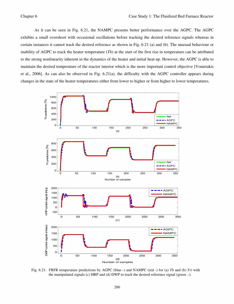
Chapter 6 Case Study 1: The Fluidized Bed Furnace Reactor
200
0 50 100 150 200 250 300 3500
200
400
600
800
1000
(a)
Th p
redic
tions (oK)
Ref
AGPC
NAMPC
0 50 100 150 200 250 300 3500
200
400
600
800
(b)
Number of samples
Tri p
redic
tions (oK
)
Ref
AGPC
NAMPC
0 50 100 150 200 250 300 350
-50
0
50
100
150
200
(c)
HRP c
ontrol signal (K
Ω)
AGPC
NAMPC
0 50 100 150 200 250 300 350
0
50
100
150
200
(d)
Number of samples
DW
P c
ontrol signal (m
/sec)
AGPC
NAMPC
Fig. 6.21: FBFR temperature predictions by AGPC (blue--) and NAMPC (red -) for (a) Th and (b) Tri with
the manipulated signals (c) HRP and (d) DWP to track the desired reference signal (green .-).
As it can be seen in Fig. 6.21, the NAMPC presents better performance over the AGPC. The AGPC
exhibits a small overshoot with occasional oscillations before tracking the desired reference signals whereas in
certain instances it cannot track the desired reference as shown in Fig. 6.21 (a) and (b). The unusual behaviour or
inability of AGPC to track the heater temperature (Th) at the start of the first rise in temperature can be attributed
to the strong nonlinearity inherent in the dynamics of the heater and initial heat-up. However, the AGPC is able to
maintain the desired temperature of the reactor interior which is the more important control objective [Voutetakis
et al., 2006]. As can also be observed in Fig. 6.21(a), the difficulty with the AGPC controller appears during
changes in the state of the heater temperatures either from lower to higher or from higher to lower temperatures.
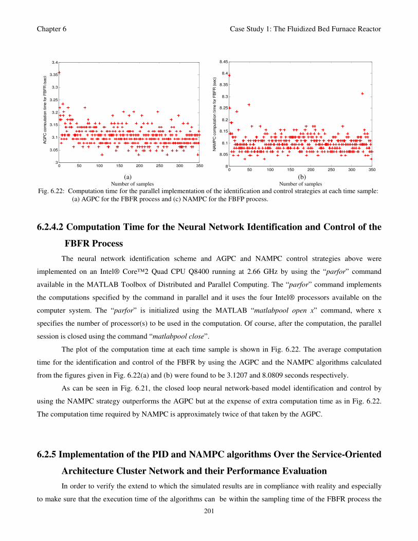
Chapter 6 Case Study 1: The Fluidized Bed Furnace Reactor
201
0 50 100 150 200 250 300 3503
3.05
3.1
3.15
3.2
3.25
3.3
3.35
3.4
(a)
GP
C c
om
puta
tion tim
e f
or
FB
FR
(sec)
AG
PC
com
puta
tion tim
e for
FB
FR
(sec)
0 50 100 150 200 250 300 3508
8.05
8.1
8.15
8.2
8.25
8.3
8.35
8.4
8.45
(c)
NA
MP
C c
om
puta
tion t
ime f
or
FB
FR
(sec)
(a) (b)
Number of samples Number of samples
Fig. 6.22: Computation time for the parallel implementation of the identification and control strategies at each time sample:
(a) AGPC for the FBFR process and (c) NAMPC for the FBFP process.
6.2.4.2 Computation Time for the Neural Network Identification and Control of the
FBFR Process
The neural network identification scheme and AGPC and NAMPC control strategies above were
implemented on an Intel® Core™2 Quad CPU Q8400 running at 2.66 GHz by using the “parfor” command
available in the MATLAB Toolbox of Distributed and Parallel Computing. The “parfor” command implements
the computations specified by the command in parallel and it uses the four Intel® processors available on the
computer system. The “parfor” is initialized using the MATLAB “matlabpool open x” command, where x
specifies the number of processor(s) to be used in the computation. Of course, after the computation, the parallel
session is closed using the command “matlabpool close”.
The plot of the computation time at each time sample is shown in Fig. 6.22. The average computation
time for the identification and control of the FBFR by using the AGPC and the NAMPC algorithms calculated
from the figures given in Fig. 6.22(a) and (b) were found to be 3.1207 and 8.0809 seconds respectively.
As can be seen in Fig. 6.21, the closed loop neural network-based model identification and control by
using the NAMPC strategy outperforms the AGPC but at the expense of extra computation time as in Fig. 6.22.
The computation time required by NAMPC is approximately twice of that taken by the AGPC.
6.2.5 Implementation of the PID and NAMPC algorithms Over the Service-Oriented
Architecture Cluster Network and their Performance Evaluation
In order to verify the extend to which the simulated results are in compliance with reality and especially
to make sure that the execution time of the algorithms can be within the sampling time of the FBFR process the
Chapter 6 Case Study 1: The Fluidized Bed Furnace Reactor
202
implementation of the algorithms on the hardware in the loop simulator, discussed in chapter 5 was attempted.
The objective here is to investigate whether the proposed identification and control strategies can meet real-time
constraints of the FBFR process in an industrial environment with respect to the sampling time of the FBFR
process in the presence of process constraints and external disturbances ( )d k .
As it was shown in the previous sub-section 6.2.4, the NAMPC control performance outperforms the
AGPC algorithm. The implementation here is restricted to this NAMPC algorithm and the classical PID algorithm
used in the current control system of the real plant. As far as the neural network model identification scheme is
concerned, again the implementation restricted to the best of the two neural network-based model identification
algorithms studied; that is, the modified Levenberg-Marquardt algorithm (MLMA) and the related NNARMAX
model identification scheme.
In order to evaluate the online performance of the proposed identification and control strategies for the
FBFR process the proposed NAMPC is considered due to its superior control performance over the AGPC
controller as it was shown in the previous sub-section 6.2.4. Here, the neural network-based NAMPC control
strategy of Fig. 4.4 and the PID control scheme of Fig. 6.12 are used together with the neural network model
identification scheme of Fig. 3.5(b) in closed loop with the FBFR process in order to evaluate the implementation
of the identification and control strategy on the hardware in the loop simulator.
The reference or setpoint signal used for evaluating the performance of the NAMPC and the PID
controllers for the FBFR process is based on a first-order temperature set-point variations similar to the one used
in the original FBFR problem formulation in [Voutetakis et al., 2006] and is again given here as:
[ ]'( ) 1 exp( 80 / 500)start step
R k T T k= + − − (6.11)
where start
T and step
T denotes the temperature level before the initiation of the experiment and the final set point
value in the temperature. Note that the coefficients in the exponential term influence the first-order change of the
set point. start
T for the heater (Th) and reactor interior (Tri) are both 0 oK whereas
stepT for Th and Tri are 1040 o
K
and 860 oK respectively. One advantage of this first-order change is to avoid abrupt changes in the control inputs
arising from a large step change in the reference signal.
The closed loop identification and control scheme considered here for the PID controller is the one shown
in Fig. 6.12 while that for the NAMPC control scheme is the one shown in Fig. 4.4. The FBFR process shown in
Fig. 6.12 is replaced by the neural network model of Fig. 3.5(b) based on the NNARMAX model identification
scheme illustrated by Fig. 3.5 (b) in Chapter 3. Similarly, the neural network model used in Fig. 4.4 is also based
on the same NNARMAX model identification scheme.
The input vector to the neural network is the NNARMAX model regression vector ( , ( ))NNARMAX
k kϕ θ
defined by (6.5). The setup of the neural network identification scheme here is the same as that discussed in
Section 6.2.2. The input ( , ( ))cn k kϕ θ is initialized to small positive random matrix of values (0, 0.05) with
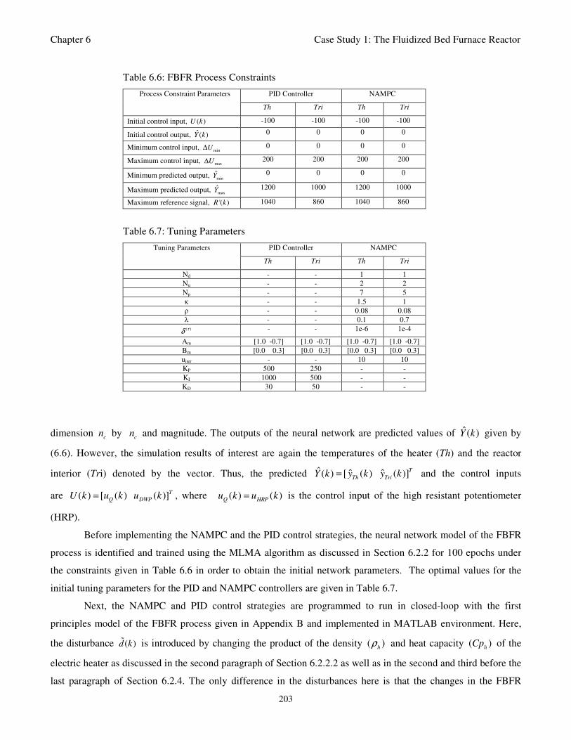
Chapter 6 Case Study 1: The Fluidized Bed Furnace Reactor
203
Table 6.6: FBFR Process Constraints
PID Controller NAMPC Process Constraint Parameters
Th Tri Th Tri
Initial control input, ( )U k -100 -100 -100 -100
Initial control output, ˆ( )Y k 0 0 0 0
Minimum control input, minU∆ 0 0 0 0
Maximum control input, maxU∆ 200 200 200 200
Minimum predicted output, min
Y 0 0 0 0
Maximum predicted output, max
Y 1200 1000 1200 1000
Maximum reference signal, '( )R k 1040 860 1040 860
Table 6.7: Tuning Parameters
PID Controller NAMPC Tuning Parameters
Th Tri Th Tri
Nd - - 1 1
Nu - - 2 2
Np - - 7 5
κ - - 1.5 1
ρ - - 0.08 0.08
λ - - 0.1 0.7 ( )τδ - - 1e-6 1e-4
Am [1.0 -0.7] [1.0 -0.7] [1.0 -0.7] [1.0 -0.7]
Bm [0.0 0.3] [0.0 0.3] [0.0 0.3] [0.0 0.3]
uiter - - 10 10
KP 500 250 - -
KI 1000 500 - -
KD 30 50 - -
dimension c
n byc
n and magnitude. The outputs of the neural network are predicted values of ˆ( )Y k given by
(6.6). However, the simulation results of interest are again the temperatures of the heater (Th) and the reactor
interior (Tri) denoted by the vector. Thus, the predicted ˆ ˆ ˆ( ) [ ( ) ( )]T
Th TriY k y k y k= and the control inputs
are ( ) [ ( ) ( )]T
Q DWPU k u k u k= , where ( ) ( )Q HRPu k u k= is the control input of the high resistant potentiometer
(HRP).
Before implementing the NAMPC and the PID control strategies, the neural network model of the FBFR
process is identified and trained using the MLMA algorithm as discussed in Section 6.2.2 for 100 epochs under
the constraints given in Table 6.6 in order to obtain the initial network parameters. The optimal values for the
initial tuning parameters for the PID and NAMPC controllers are given in Table 6.7.
Next, the NAMPC and PID control strategies are programmed to run in closed-loop with the first
principles model of the FBFR process given in Appendix B and implemented in MATLAB environment. Here,
the disturbance ( )d k is introduced by changing the product of the density ( )h
ρ and heat capacity ( )h
Cp of the
electric heater as discussed in the second paragraph of Section 6.2.2.2 as well as in the second and third before the
last paragraph of Section 6.2.4. The only difference in the disturbances here is that the changes in the FBFR
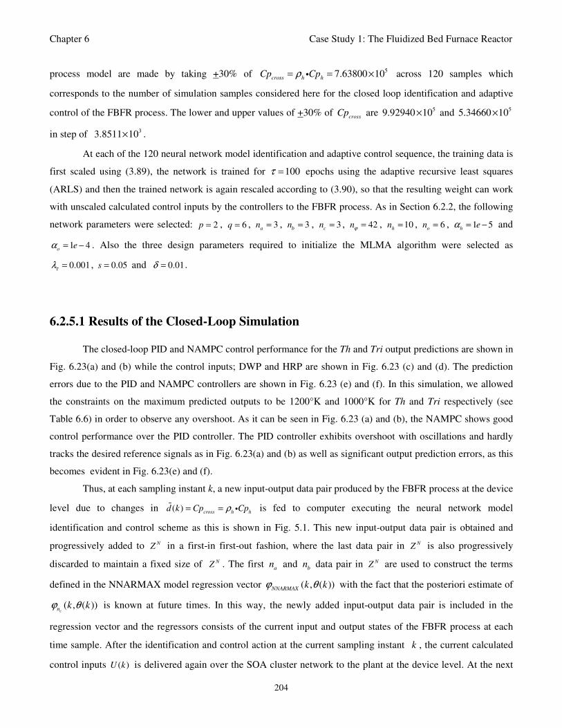
Chapter 6 Case Study 1: The Fluidized Bed Furnace Reactor
204
process model are made by taking +30% of 57.63800 10cross h h
Cp Cpρ= = ×i across 120 samples which
corresponds to the number of simulation samples considered here for the closed loop identification and adaptive
control of the FBFR process. The lower and upper values of +30% of cross
Cp are 59.92940 10× and 55.34660 10×
in step of 33.8511 10× .
At each of the 120 neural network model identification and adaptive control sequence, the training data is
first scaled using (3.89), the network is trained for 100τ = epochs using the adaptive recursive least squares
(ARLS) and then the trained network is again rescaled according to (3.90), so that the resulting weight can work
with unscaled calculated control inputs by the controllers to the FBFR process. As in Section 6.2.2, the following
network parameters were selected: 2p = , 6q = , 3a
n = , 3b
n = , 3c
n = , 42nϕ = , 10h
n = , 6o
n = , 1 5h
eα = − and
1 4o
eα = − . Also the three design parameters required to initialize the MLMA algorithm were selected as
0.001τλ = , 0.05s = and 0.01δ = .
6.2.5.1 Results of the Closed-Loop Simulation
The closed-loop PID and NAMPC control performance for the Th and Tri output predictions are shown in
Fig. 6.23(a) and (b) while the control inputs; DWP and HRP are shown in Fig. 6.23 (c) and (d). The prediction
errors due to the PID and NAMPC controllers are shown in Fig. 6.23 (e) and (f). In this simulation, we allowed
the constraints on the maximum predicted outputs to be 1200°K and 1000°K for Th and Tri respectively (see
Table 6.6) in order to observe any overshoot. As it can be seen in Fig. 6.23 (a) and (b), the NAMPC shows good
control performance over the PID controller. The PID controller exhibits overshoot with oscillations and hardly
tracks the desired reference signals as in Fig. 6.23(a) and (b) as well as significant output prediction errors, as this
becomes evident in Fig. 6.23(e) and (f).
Thus, at each sampling instant k, a new input-output data pair produced by the FBFR process at the device
level due to changes in ( )cross h h
d k Cp Cpρ= = i is fed to computer executing the neural network model
identification and control scheme as this is shown in Fig. 5.1. This new input-output data pair is obtained and
progressively added to NZ in a first-in first-out fashion, where the last data pair in N
Z is also progressively
discarded to maintain a fixed size of NZ . The first
an and
bn data pair in N
Z are used to construct the terms
defined in the NNARMAX model regression vector ( , ( ))NNARMAX
k kϕ θ with the fact that the posteriori estimate of
( , ( ))cn k kϕ θ is known at future times. In this way, the newly added input-output data pair is included in the
regression vector and the regressors consists of the current input and output states of the FBFR process at each
time sample. After the identification and control action at the current sampling instant k , the current calculated
control inputs ( )U k is delivered again over the SOA cluster network to the plant at the device level. At the next
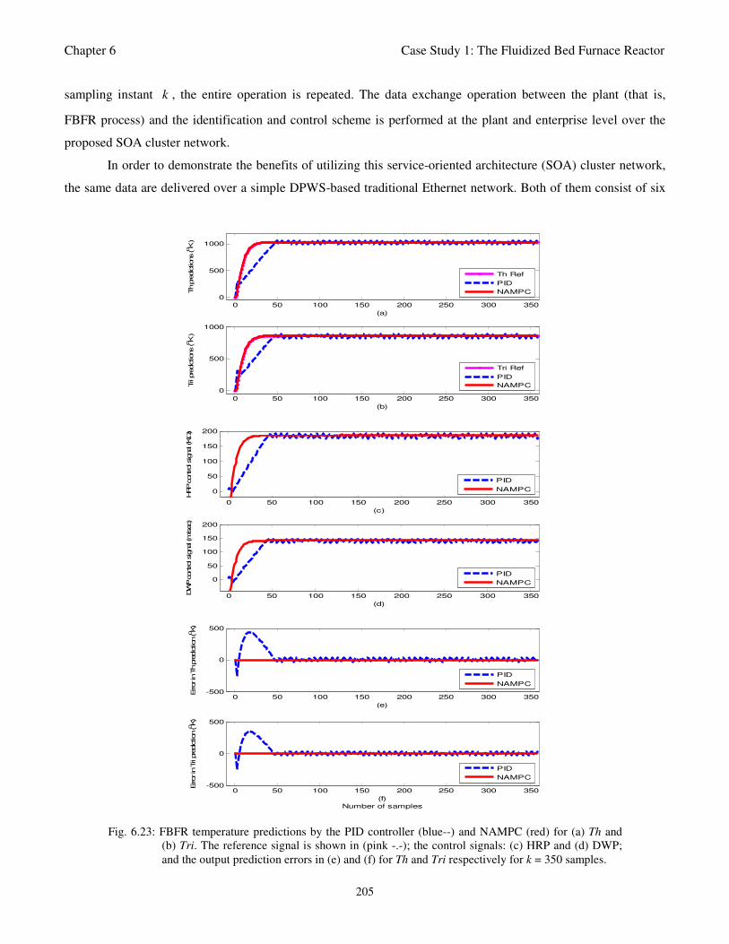
Chapter 6 Case Study 1: The Fluidized Bed Furnace Reactor
205
0 50 100 150 200 250 300 350
0
500
1000
(a)
Th predictions (oK )
Th Ref
PID
NAMPC
0 50 100 150 200 250 300 350
0
500
1000
(b)
Tri pre
dictions (oK )
Tri Ref
PID
NAMPC
0 50 100 150 200 250 300 350
0
50
100
150
200
(c)
HRP control signal (K
Ω)
PID
NAMPC
0 50 100 150 200 250 300 350
0
50
100
150
200
(d)
DW
P control signal (m
/sec)
PID
NAMPC
0 50 100 150 200 250 300 350-500
0
500
(e)
Error in T
h p
rediction (oK)
PID
NAMPC
0 50 100 150 200 250 300 350-500
0
500
(f)
Number of samples
Error in T
ri prediction (oK)
PID
NAMPC
Fig. 6.23: FBFR temperature predictions by the PID controller (blue--) and NAMPC (red) for (a) Th and
(b) Tri. The reference signal is shown in (pink -.-); the control signals: (c) HRP and (d) DWP;
and the output prediction errors in (e) and (f) for Th and Tri respectively for k = 350 samples.
sampling instant k , the entire operation is repeated. The data exchange operation between the plant (that is,
FBFR process) and the identification and control scheme is performed at the plant and enterprise level over the
proposed SOA cluster network.
In order to demonstrate the benefits of utilizing this service-oriented architecture (SOA) cluster network,
the same data are delivered over a simple DPWS-based traditional Ethernet network. Both of them consist of six
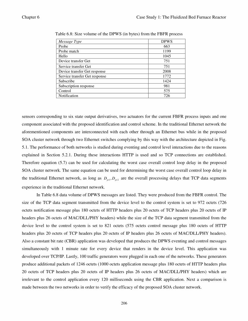
Chapter 6 Case Study 1: The Fluidized Bed Furnace Reactor
206
Table 6.8: Size volume of the DPWS (in bytes) from the FBFR process
Message Type DPWS
Probe 663
Probe match 1199
Hello 1045
Device transfer Get 751
Service transfer Get 751
Device transfer Get response 2008
Service transfer Get response 1772
Subscribe 1424
Subscription response 981
Control 575
Notification 726
sensors corresponding to six state output derivatives, two actuators for the current FBFR process inputs and one
component associated with the proposed identification and control scheme. In the traditional Ethernet network the
aforementioned components are interconnected with each other through an Ethernet bus while in the proposed
SOA cluster network through two Ethernet switches complying by this way with the architecture depicted in Fig.
5.1. The performance of both networks is studied during eventing and control level interactions due to the reasons
explained in Section 5.2.1. During these interactions HTTP is used and so TCP connections are established.
Therefore equation (5.7) can be used for calculating the worst case overall control loop delay in the proposed
SOA cluster network. The same equation can be used for determining the worst case overall control loop delay in
the traditional Ethernet network, as long as 1 2,pr prD D are the overall processing delays that TCP data segments
experience in the traditional Ethernet network.
In Table 6.8 data volume of DPWS messages are listed. They were produced from the FBFR control. The
size of the TCP data segment transmitted from the device level to the control system is set to 972 octets (726
octets notification message plus 180 octets of HTTP headers plus 20 octets of TCP headers plus 20 octets of IP
headers plus 26 octets of MAC/DLL/PHY headers) while the size of the TCP data segment transmitted from the
device level to the control system is set to 821 octets (575 octets control message plus 180 octets of HTTP
headers plus 20 octets of TCP headers plus 20 octets of IP headers plus 26 octets of MAC/DLL/PHY headers).
Also a constant bit rate (CBR) application was developed that produces the DPWS eventing and control messages
simultaneously with 1 minute rate for every device that renders in the device level. This application was
developed over TCP/IP. Lastly, 100 traffic generators were plugged in each one of the networks. These generators
produce additional packets of 1246 octets (1000 octets application message plus 180 octets of HTTP headers plus
20 octets of TCP headers plus 20 octets of IP headers plus 26 octets of MAC/DLL/PHY headers) which are
irrelevant to the control application every 120 milliseconds using the CBR application. Next a comparison is
made between the two networks in order to verify the efficacy of the proposed SOA cluster network.
Chapter 6 Case Study 1: The Fluidized Bed Furnace Reactor
207
0 20 40 60 80 100 1200
20
40
60
80
100
120
Number of samples
Delay (sec)
DPWS over Ethernet
DPWS over Switched Ethernet
Fig. 6.24: 1 2tr tr
D D+ delay (in seconds) between the FBFR process and the control system obtained by SOA
cluster network.
6.2.5.2 Worst Case Overall Control Loop Delay Introduced by a DPWS-Based
Traditional Ethernet Network
In the simple DPWS-based traditional Ethernet network all the components comply with the DPWS
specification. The simulation results obtained are shown in Fig. 6.24. As it is shown, the network never reached a
stable state and so no predictions could be made about the transmission delay1 2
( )tr tr
D D+ . As it can also be seen
in Fig. 6.24, the transmission delay some times exceeds the sampling period of the FBFR process with its
maximum value being 120.2790 seconds. _ _ _ _s p t p cs p ct pD D D D= = = which is the DPWS protocol stack response
time and is defined to be approximately 10 ms [Jammes et al. 2005]. Also _ _ _ _s p tcp t p tcpD D= and is observed to be
approximately 300 sµ while the average cD is approximately 2.7 seconds and so 1 2
2.7424pr pr
D D+ = seconds.
Therefore, the worst case overall control loop delay is calculated using (5.7) to be equal with 123.0214 seconds
and the DPWS-based traditional Ethernet network cannot fulfill the real time characteristics of the FBFR process
as evident in the online closed-loop simulation result of Fig. 6.25.
The slightly poor performance of the NAMPC in tracking the desired reference is due to the transmission
delays introduced by the network. As it is depicted in Fig. 6.25, the NAMPC sometimes tracks and sometimes
does not track the desired reference according to the transmission delay introduced by the network which is
sometimes below or above the sampling time of the FBFR process (see Fig. 6.24).
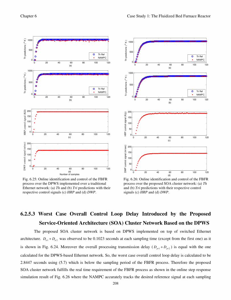
Chapter 6 Case Study 1: The Fluidized Bed Furnace Reactor
208
0 20 40 60 80 100 120
0
500
1000
(a)
Th p
redic
tions (
o K
)
0 20 40 60 80 100 120
0
500
1000
(b)
Tri p
redic
tions (
o K
)
Th Ref
NAMPC
Tri Ref
NAMPC
0 20 40 60 80 100 1200
50
100
150
200
(c)
HR
P c
ontr
ol sig
nal
0 20 40 60 80 100 1200
50
100
150
200
(d)
Number of samples
DW
P c
ontr
ol sig
nal
H
RP
co
ntr
ol
sign
al (
KΩ
)
DW
P c
on
tro
l si
gn
al (
m/s
ec)
0 20 40 60 80 100 120
0
500
1000
(a)
Th
pre
dic
tio
ns
( o
K )
0 20 40 60 80 100 120
0
500
1000
(b)
Tri
pre
dic
tio
ns
( o
K )
Th Ref
NAMPC
Tri Ref
NAMPC
0 20 40 60 80 100 1200
50
100
150
200
(c)
HR
P c
ontr
ol sig
nal (K
Ω)
0 20 40 60 80 100 1200
50
100
150
200
(d)
Number of samples
DW
P c
ontr
ol sig
nal (m
/sec)
Fig. 6.25: Online identification and control of the FBFR Fig. 6.26: Online identification and control of the FBFR
process over the DPWS implemented over a traditional process over the proposed SOA cluster network: (a) Th
Ethernet network: (a) Th and (b) Tri predictions with their and (b) Tri predictions with their respective control
respective control signals (c) HRP and (d) DWP. signals (c) HRP and (d) DWP.
6.2.5.3 Worst Case Overall Control Loop Delay Introduced by the Proposed
Service-Oriented Architecture (SOA) Cluster Network Based on the DPWS
The proposed SOA cluster network is based on DPWS implemented on top of switched Ethernet
architecture. 1 2tr tr
D D+ was observed to be 0.1023 seconds at each sampling time (except from the first one) as it
is shown in Fig. 6.24. Moreover the overall processing transmission delay (1 2pr pr
D D+ ) is equal with the one
calculated for the DPWS-based Ethernet network. So, the worst case overall control loop delay is calculated to be
2.8447 seconds using (5.7) which is below the sampling period of the FBFR process. Therefore the proposed
SOA cluster network fulfills the real time requirement of the FBFR process as shown in the online step response
simulation result of Fig. 6.26 where the NAMPC accurately tracks the desired reference signal at each sampling
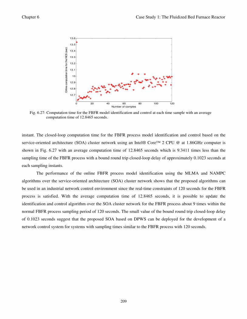
Chapter 6 Case Study 1: The Fluidized Bed Furnace Reactor
209
0 20 40 60 80 100 120
12.7
12.8
12.9
13
13.1
13.2
13.3
13.4
13.5
13.6
Onlin
e c
om
puta
tion tim
e for th
e N
CS
(sec)
Number of samples
Fig. 6.27: Computation time for the FBFR model identification and control at each time sample with an average
computation time of 12.8465 seconds.
instant. The closed-loop computation time for the FBFR process model identification and control based on the
service-oriented architecture (SOA) cluster network using an Intel® Core™ 2 CPU @ at 1.86GHz computer is
shown in Fig. 6.27 with an average computation time of 12.8465 seconds which is 9.3411 times less than the
sampling time of the FBFR process with a bound round trip closed-loop delay of approximately 0.1023 seconds at
each sampling instants.
The performance of the online FBFR process model identification using the MLMA and NAMPC
algorithms over the service-oriented architecture (SOA) cluster network shows that the proposed algorithms can
be used in an industrial network control environment since the real-time constraints of 120 seconds for the FBFR
process is satisfied. With the average computation time of 12.8465 seconds, it is possible to update the
identification and control algorithm over the SOA cluster network for the FBFR process about 9 times within the
normal FBFR process sampling period of 120 seconds. The small value of the bound round trip closed-loop delay
of 0.1023 seconds suggest that the proposed SOA based on DPWS can be deployed for the development of a
network control system for systems with sampling times similar to the FBFR process with 120 seconds.
Chapter 6 Case Study 2: Activated Sludge Wastewater Treatment Plant
210
6.3 Activated Sludge Wastewater Treatment Plant (AS-WWTP)
6.3.1 An Overview of the AS-WWTP Process
Activated sludge wastewater treatment plants (WWTPs) are large complex nonlinear multivariable
systems, subject to large disturbances, where different physical and biological phenomena take place. Many
control strategies have been proposed for wastewater treatment plants but their evaluation and comparison are
difficult. This is partly due to the variability of the influent, the complexity of the physical and biochemical
phenomena, and the large range of time constants (from a few minutes to several days) inherent in the activated
sludge process. Additional complication in the evaluation is the lack of standard evaluation criteria.
With the tight effluent requirements defined by the European Union and to increase the acceptability of
the results from wastewater treatment analysis, the generally accepted COST Actions 624 and 682 benchmark
simulation model No. 1 (BSM1) model [Henze et al., 1996] is considered. The BS1 model uses eight basic
different processes to describe the biological behaviour of the AS-WWTP processes. The combinations of the
eight basic processes results in thirteen different observed conversion rates as described in Appendix C. These
components are classified into soluble components ( )S and particulate components ( )X . The nomenclatures and
parameter definitions used for describing the AS-WWTP in this work are given in Table C6.1. Moreover, four
fundamental processes are considered: the growth and decay of biomass (heterotrophic and autotrophic),
ammonification of organic nitrogen and the hydrolysis of particulate organics. The complete BSM1 used to
describe the AS-WWTP considered here is given in Appendix C.
6.3.1.1 Statement of the Activated Sludge Wastewater Treatment Plant (AS-WWTP)
Problem
The activated sludge wastewater treatment plant considered here is strictly based on the benchmark
simulation model no. 1 (BSM1) proposed by the European Working Groups of COST Action 624 and 682 in
conjunction with the International Water Association (IWA) Task Group on Benchmarking of Control Strategies
for wastewater treatment plants (WWTPs) ([Coop, 2000], [COST, 2000], [COST, 2008]). This implementation of
the benchmark simulation model no. 1 (BSM1) follows the methodology specified in [COST, 2008] especially
from the viewpoint of control performances. The complete description of the conventional activated sludge
wastewater treatment plant (AS-WWTP) based on the benchmark simulation model no. 1 (BSM1) is given in
Appendix C together with the mathematical model of the benchmark simulation model no. 1 (BSM1) and the
MATLAB/Simulink programs that implements the mathematical model of the BSM1.
Since the introduction of the benchmark simulation model no. 1 (BSM1) by Henze and co-workers
[Henze et al., 1996] and later by the COST Action Groups [Coop, 2000], [COST, 2000] and [COST, 2008];
Chapter 6 Case Study 2: Activated Sludge Wastewater Treatment Plant
211
extensive research and surveys based on simulation with the BSM1 have been reported. For example, ([Ekman et
al., 2006], [Holenda et al., 2008], [Gernaes et al., 2004], [Lee et al., 1999], [Lee et al., 2006], [Shen et al., 2008],
[Stare et al., 2006 and 2007], [Yong et al., 2006]). Dissolved oxygen (DO) concentration and nitrogen
concentration are the frequently investigated controlled variables; whereas oxygen transfer coefficients, internal
recycled nitrate flow rate ( Qa ), recycled activated sludge (RAS) flow rate, waste activated sludge flow rate
(WAS) and external carbon dosing rate [Yong et al., 2006] are also the frequently investigated manipulated
variables in these wastewater treatment plants. Nevertheless, the dissolved oxygen (DO) control is the most wide-
spread in real-life, since the DO level in the aerobic reactors has significant influence on the behaviour and
activity of the heterotrophic and autotrophic microorganisms living in the activated sludge.
The dissolved oxygen (DO) concentration in the aerobic part of the activated sludge process should be
sufficiently high to supply enough oxygen to the microorganisms in the sludge, so that organic matter is degraded
and ammonium is converted to nitrate. On the other hand, an excessively high DO concentration which requires a
air flow rate lead to high energy consumption and may also deteriorate the sludge quality. In addition, a high DO
in the internally recirculated wastewater also makes the denitrification less effective.
However, in an activated sludge wastewater treatment plant designed for tertiary treatment, beside the
conventional dissolved oxygen concentration control, an additional objective is to remove biological nutrients,
suspended solids and organic matter ([Lee et al., 1999 and 2006], [Spellman, 2003]). During the last few decades,
the importance of nutrient removal has increased as a result of the necessity to avoid eutrophication of water
bodies receiving untreated waste water and the effluent of wastewater treatment plants (WWTPs). The term
eutrophication is the slow, natural nutrient enrichment of streams and lakes and water reservoirs. For this reason,
many new WWTPs are now designed for tertiary treatments [Spellman, 2003]. Apart from the important
repercussions on the effluent quality, tertiary treatment also has a beneficial influence on the performance of the
wastewater treatment process itself. This is particularly noticeable in the case of nitrogen removal [Spellman,
2003]. Moreover, the development of nitrification in an activated sludge process is practically unavoidable when
the sewage reaches temperatures of 22°C to 24°C, which will be the case for at least part of the year in tropical
and sub-tropical regions. The formed nitrate can be used by microorganisms in the activated sludge as a substitute
to dissolved oxygen. In an anoxic environment, characterized by the presence of nitrate and the absence of
dissolved oxygen, the nitrate ion can be reduced by organic matter to nitrogen gas: this process is called
denitrification.
Some successful conventional dissolved oxygen (DO) control schemes have been reported ([Ekman et al.,
2006], [Holenda et al., 2008]). Advances towards nitrogen removal have also been reported ([Stare et al., 2006
and 2007], [Yong et al., 2006]) as well as complete biological nutrient removal (BNR) [Lee et al., 1999 and
2006]. In this section, the proposed adaptive recursive least squares (ARLS) algorithm and the modified
Levenberg-Marquardt algorithm (MLMA) are used to train a neural network in order to identify an approximate
neural network model of the third aerobic tank (Unit 5) of the activated sludge wastewater treatment plant (AS-
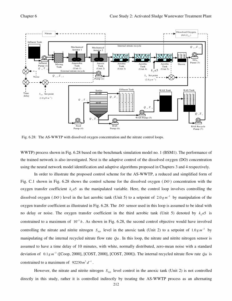
Chapter 6 Case Study 2: Activated Sludge Wastewater Treatment Plant
212
WWTP) process shown in Fig. 6.28 based on the benchmark simulation model no. 1 (BSM1). The performance of
the trained network is also investigated. Next is the adaptive control of the dissolved oxygen (DO) concentration
using the neural network model identification and adaptive algorithms proposed in Chapters 3 and 4 respectively.
In order to illustrate the proposed control scheme for the AS-WWTP, a reduced and simplified form of
Fig. C.1 shown in Fig. 6.28 shows the control scheme for the dissolved oxygen ( DO ) concentration with the
oxygen transfer coefficient 5L
k a as the manipulated variable. Here, the control loop involves controlling the
dissolved oxygen ( DO ) level in the last aerobic tank (Unit 5) to a setpoint of 32.0 g m− by manipulation of the
oxygen transfer coefficient as illustrated in Fig. 6.28. The DO sensor used in this loop is assumed to be ideal with
no delay or noise. The oxygen transfer coefficient in the third aerobic tank (Unit 5) denoted by 5L
k a is
constrained to a maximum of 310 h− . As shown in Fig. 6.28, the second control objective would have involved
controlling the nitrate and nitrite nitrogen NO
S level in the anoxic tank (Unit 2) to a setpoint of 31.0 g m− by
manipulating of the internal recycled nitrate flow rate Qa . In this loop, the nitrate and nitrite nitrogen sensor is
assumed to have a time delay of 10 minutes, with white, normally distributed, zero-mean noise with a standard
deviation of 30.1g m− ([Coop, 2000], [COST, 2000], [COST, 2008]). The internal recycled nitrate flow rate Qa is
constrained to a maximum of 3 192230 m d− .
However, the nitrate and nitrite nitrogen NO
S level control in the anoxic tank (Unit 2) is not controlled
directly in this study, rather it is controlled indirectly by treating the AS-WWTP process as an alternating
m=10
m=1
m=6
Aerobic
Tank
(Unit 4)
Aerobic
Tank
(Unit 3)
Aerobic
Tank
(Unit 5)
Anoxic
Tank
(Unit 2)
Anaerobic
Tank
(Unit 1)
Deoxic Mixing
Tank
Influent
Pump (1)
Influent Tank
Settler Effluent Tank WAS Tank RAS Tank
WAS Pump (5)
Feed
Pump (4)
RAS
Pump (6)
NOX
Pump (3)
Internal nitrate recycle
External nitrate recycle
Pump (2)
e eQ Z
f fQ Z
1 1a aQ Z
u uQ Z
r rQ Z
w wQ Z
RAS Recycle
Pump (7)
Mechanical
Aerator 1 Mechanical
Aerator 2
5L
k a
i n i nQ Z
2 2a aQ Z
Nitrate Dissolved Oxygen,
( )NO
DO S
OS Set point
3(2.0 )g m−
NOS Set point
3(1.0 )gN m−
Time
delay
Noise
Fig. 6.28: The AS-WWTP with dissolved oxygen concentration and the nitrate control loops.
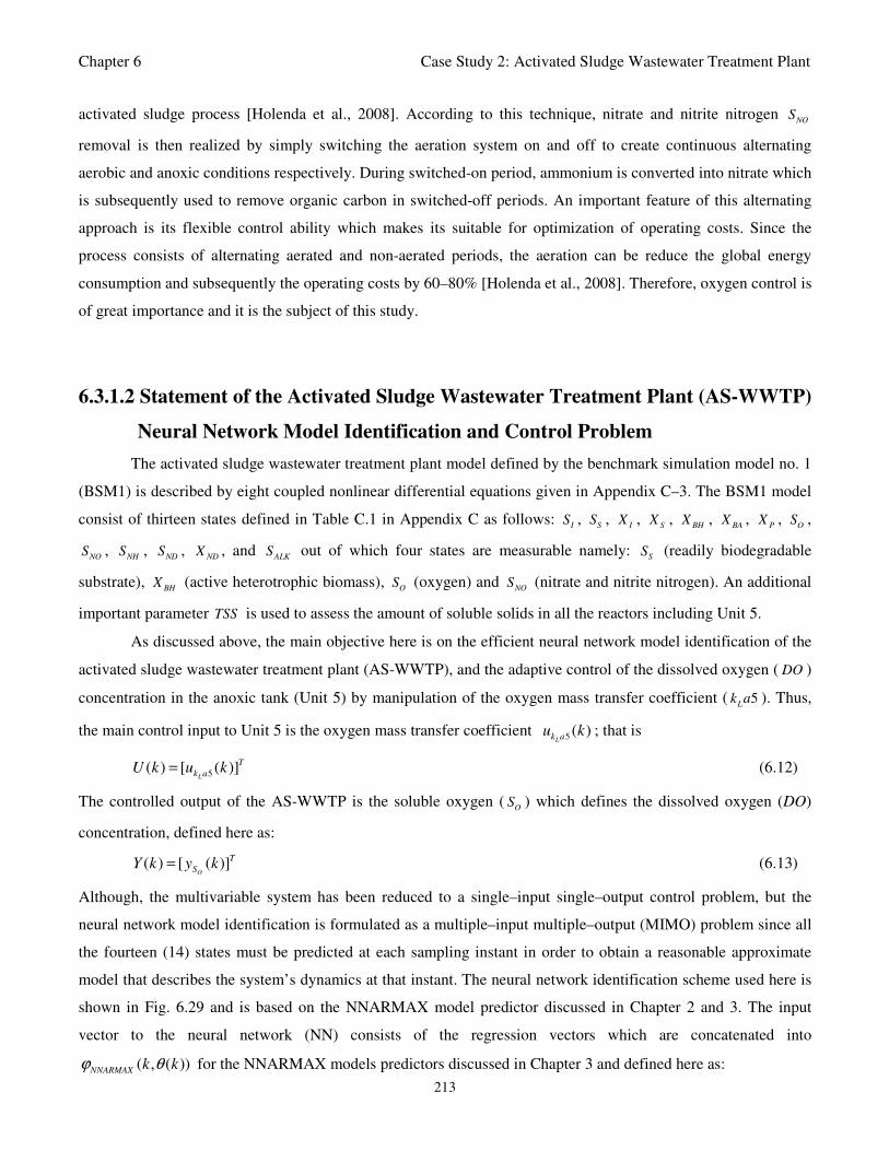
Chapter 6 Case Study 2: Activated Sludge Wastewater Treatment Plant
213
activated sludge process [Holenda et al., 2008]. According to this technique, nitrate and nitrite nitrogen NO
S
removal is then realized by simply switching the aeration system on and off to create continuous alternating
aerobic and anoxic conditions respectively. During switched-on period, ammonium is converted into nitrate which
is subsequently used to remove organic carbon in switched-off periods. An important feature of this alternating
approach is its flexible control ability which makes its suitable for optimization of operating costs. Since the
process consists of alternating aerated and non-aerated periods, the aeration can be reduce the global energy
consumption and subsequently the operating costs by 60–80% [Holenda et al., 2008]. Therefore, oxygen control is
of great importance and it is the subject of this study.
6.3.1.2 Statement of the Activated Sludge Wastewater Treatment Plant (AS-WWTP)
Neural Network Model Identification and Control Problem
The activated sludge wastewater treatment plant model defined by the benchmark simulation model no. 1
(BSM1) is described by eight coupled nonlinear differential equations given in Appendix C–3. The BSM1 model
consist of thirteen states defined in Table C.1 in Appendix C as follows: I
S , S
S , I
X , S
X , BH
X , BA
X , P
X , O
S ,
NOS ,
NHS ,
NDS ,
NDX , and
ALKS out of which four states are measurable namely:
SS (readily biodegradable
substrate), BH
X (active heterotrophic biomass), O
S (oxygen) and NO
S (nitrate and nitrite nitrogen). An additional
important parameter TSS is used to assess the amount of soluble solids in all the reactors including Unit 5.
As discussed above, the main objective here is on the efficient neural network model identification of the
activated sludge wastewater treatment plant (AS-WWTP), and the adaptive control of the dissolved oxygen ( DO )
concentration in the anoxic tank (Unit 5) by manipulation of the oxygen mass transfer coefficient ( 5L
k a ). Thus,
the main control input to Unit 5 is the oxygen mass transfer coefficient 5 ( )Lk au k ; that is
5( ) [ ( )]L
T
k aU k u k= (6.12)
The controlled output of the AS-WWTP is the soluble oxygen (O
S ) which defines the dissolved oxygen (DO)
concentration, defined here as:
( ) [ ( )]O
T
SY k y k= (6.13)
Although, the multivariable system has been reduced to a single–input single–output control problem, but the
neural network model identification is formulated as a multiple–input multiple–output (MIMO) problem since all
the fourteen (14) states must be predicted at each sampling instant in order to obtain a reasonable approximate
model that describes the system’s dynamics at that instant. The neural network identification scheme used here is
shown in Fig. 6.29 and is based on the NNARMAX model predictor discussed in Chapter 2 and 3. The input
vector to the neural network (NN) consists of the regression vectors which are concatenated into
( , ( ))NNARMAX
k kϕ θ for the NNARMAX models predictors discussed in Chapter 3 and defined here as:
Chapter 6 Case Study 2: Activated Sludge Wastewater Treatment Plant
214
[
]
( ) ( ) ( ) ( ) ( ) ( ) ( )
( ) ( ) ( ) ( ) ( ) ( )
( ) ( )
an I a S a I a S a BH a BA a
P a O a NO a NH a ND a ND a
T
ALK a a
k S k n S k n X k n X k n X k n X k n
X k n S k n S k n S k n S k n X k n
S k n TSS k n
ϕ = − − − − − −
− − − − − −
− −
(6.14)
[ ]( ) 5( )b
T
n L bk k a k nϕ = − (6.15)
( , ( )) ( , ( )) ( , ( )) ( , ( )) ( , ( ))
( , ( )) ( , ( )) ( , ( )) ( , ( ))
( , ( )) ( , ( )) ( , ( )) ( , ( ))
( ,
c I S I S
BH BA P O
NO NH ND ND
ALK
n S c S c X c X c
X c X c X c S c
S c S c S c X c
S c
k k k n k k n k k n k k n k
k n k k n k k n k k n k
k n k k n k k n k k n k
k n
ϕ θ ε θ ε θ ε θ ε θ
ε θ ε θ ε θ ε θ
ε θ ε θ ε θ ε θ
ε θ
= − − − −
− − − −
− − − −
− ( )) ( , ( ))T
TSS ck k n kε θ
−
(6.16)
( , ( )) ( ) ( ) ( , ( ))a b cNNARMAX n n n
k k k k k kϕ θ ϕ ϕ ϕ θ = (6.17)
The outputs of the neural network for the AS-WWTP process are the predicted values of the thirteen states
together with the amount of total soluble solids (TSS), thus resulting in fourteen states to be predicted at each
sampling instant given by:
ˆ ˆ ˆ ˆ ˆ ˆ ˆ ˆ( ) ( ) ( ) ( ) ( ) ( ) ( ) ( )
ˆ ˆ ˆ ˆ ˆ ˆ ˆ( ) ( ) ( ) ( ) ( ) ( ) ( )
I S I S BH BA P
O NO NH ND ND ALK
S S X X X X X
T
S S S S X S TSS
Y k y k y k y k y k y k y k y k
y k y k y k y k y k y k y k
=
(6.18)
However, only the simulation results for the desired output defined by (6.13) for the soluble oxygen (SO), which
defines the dissolved oxygen (DO) concentration, are presented for convenience.
Since disturbances play an important role in the evaluation of controller performances, three influent
disturbance data are defined for different weather conditions, namely: dry-weather data, rain weather data, and
storm weather data. The data for these three influent disturbances are provided by the European COST Actions for
Training
Algorithm
Neural
Network
Model
b
n TDL−
a
n TDL−
AS-WWTP Process
( , ( ))k kε θ
ˆ( )Y k
( )Y k ( )U k • •
•
•
•
+
−
( )bn
kϕ
( )an
kϕ
c
n TDL−
( , ( ))cn
k kϕ θ
( )d k
•
( , ( ))k kε θ
Fig. 6.29: The neural network model identification scheme for AS-WWTP based on NNARMAX model.
Chapter 6 Case Study 2: Activated Sludge Wastewater Treatment Plant
215
evaluating controller performances ([Coop, 2000], [COST, 2000], [COST, 2008]). In this study, the dry weather
influent data is used in order to measure how well the trained neural network mimic the dynamics of the As-
WWTP process to meet the control requirement specified above. The dry weather data contains two weeks of
influent data at 15 minutes sampling interval. Although, disturbances ( )d k affecting the AS-WWTP are
incorporated into dry-weather data provided by the COST Action Group, additional sinusoidal disturbances with
non-smooth nonlinearities are introduced in the last sub-section of this section to further investigate the closed-
loop controllers’ performances based on an updated neural network model at each sampling time instants.
6.3.1.3 Experiment with the BSM1 for AS-WWTP Process Neural Network
Training Data Acquisition
For the efficient control of the activated sludge wastewater treatment plant (AS-WWTP) using neural
network, a neural network (NN) model of the AS-WWTP process is needed which requires that the NN be trained
with dynamic data obtained from the AS-WWTP process. In other to obtain dynamic data for the NN training, the
validated and generally accepted COST Actions 624 benchmark simulation model (BSM1) is implemented and
simulated using MATLAB and Simulink. The complete benchmark simulation model no. 1 (BSM1) for the AS-
WWTP process is detailed in Appendix C.
A two-step simulation procedure defined in the simulation benchmark ([Coop, 2000], [COST, 2000],
[COST, 2008]) is used in this study. The first step is the steady state simulation using the constant influent flow
(CONSTINFLUENT) for 150 days as shown and implemented in Fig. C.2. Note that each “Clock” of the AS-
WWTP Simulink model in Fig. C.2 corresponds to one day. In the second step, starting from the steady state
solution obtained with the CONSTINFLUENT data and using the dry-weather influent weather data
(DRYINFLUENT) as inputs. The AS-WWTP process is then simulated for 14 days using the same Simulink
model of Fig. C.2 but by replacing the CONSTINFLUENT influent data with the DRYINFLUENT influent data.
This second simulation generates 1345 dynamic data in which 80% (1076) is used for NN training and 20% (269)
is reserved for the trained NN validation.
6.3.2 Training the Neural Network that Models the AS-WWTP Aerobic Reactor
The NN input vector to the neural network (NN) is the NNARMAX model regression vector
( , ( ))NNARMAX
k kϕ θ defined by (6.17). The input ( , ( ))cn k kϕ θ , that is the initial error estimates ( , ( ))k kε θ given by
(6.16), is not known in advance and it is initialized to small positive random matrix of dimension c
n byc
n . The
outputs of the NN are predicted values of ˆ( )Y k given by (6.18). However, the results for the soluble oxygen (SO)
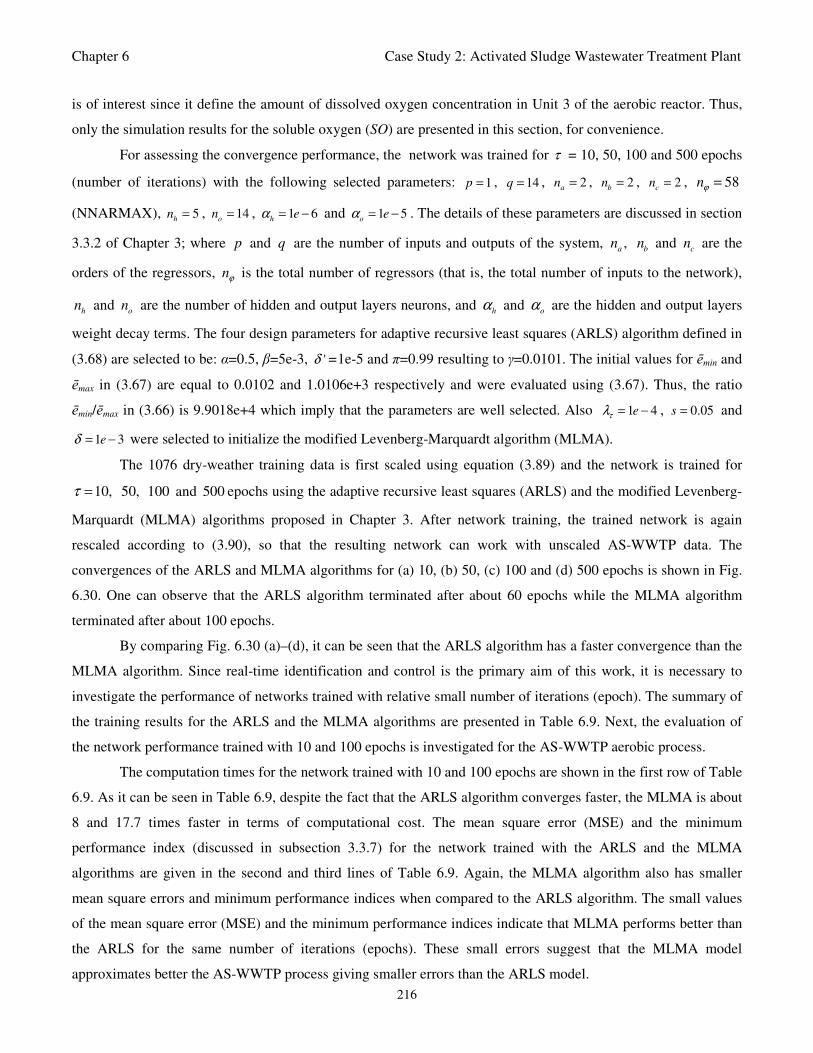
Chapter 6 Case Study 2: Activated Sludge Wastewater Treatment Plant
216
is of interest since it define the amount of dissolved oxygen concentration in Unit 3 of the aerobic reactor. Thus,
only the simulation results for the soluble oxygen (SO) are presented in this section, for convenience.
For assessing the convergence performance, the network was trained for τ = 10, 50, 100 and 500 epochs
(number of iterations) with the following selected parameters: 1p = , 14q = , 2a
n = , 2b
n = , 2c
n = , 58nϕ =
(NNARMAX), 5h
n = , 14o
n = , 1 6h
eα = − and 1 5o
eα = − . The details of these parameters are discussed in section
3.3.2 of Chapter 3; where p and q are the number of inputs and outputs of the system, ,a b
n n and c
n are the
orders of the regressors, nϕ is the total number of regressors (that is, the total number of inputs to the network),
hn and
on are the number of hidden and output layers neurons, and
hα and
oα are the hidden and output layers
weight decay terms. The four design parameters for adaptive recursive least squares (ARLS) algorithm defined in
(3.68) are selected to be: α=0.5, β=5e-3, 'δ =1e-5 and π=0.99 resulting to γ=0.0101. The initial values for ēmin and
ēmax in (3.67) are equal to 0.0102 and 1.0106e+3 respectively and were evaluated using (3.67). Thus, the ratio
ēmin/ēmax in (3.66) is 9.9018e+4 which imply that the parameters are well selected. Also 1 4eτλ = − , 0.05s = and
1 3eδ = − were selected to initialize the modified Levenberg-Marquardt algorithm (MLMA).
The 1076 dry-weather training data is first scaled using equation (3.89) and the network is trained for
10, 50, 100τ = and 500 epochs using the adaptive recursive least squares (ARLS) and the modified Levenberg-
Marquardt (MLMA) algorithms proposed in Chapter 3. After network training, the trained network is again
rescaled according to (3.90), so that the resulting network can work with unscaled AS-WWTP data. The
convergences of the ARLS and MLMA algorithms for (a) 10, (b) 50, (c) 100 and (d) 500 epochs is shown in Fig.
6.30. One can observe that the ARLS algorithm terminated after about 60 epochs while the MLMA algorithm
terminated after about 100 epochs.
By comparing Fig. 6.30 (a)–(d), it can be seen that the ARLS algorithm has a faster convergence than the
MLMA algorithm. Since real-time identification and control is the primary aim of this work, it is necessary to
investigate the performance of networks trained with relative small number of iterations (epoch). The summary of
the training results for the ARLS and the MLMA algorithms are presented in Table 6.9. Next, the evaluation of
the network performance trained with 10 and 100 epochs is investigated for the AS-WWTP aerobic process.
The computation times for the network trained with 10 and 100 epochs are shown in the first row of Table
6.9. As it can be seen in Table 6.9, despite the fact that the ARLS algorithm converges faster, the MLMA is about
8 and 17.7 times faster in terms of computational cost. The mean square error (MSE) and the minimum
performance index (discussed in subsection 3.3.7) for the network trained with the ARLS and the MLMA
algorithms are given in the second and third lines of Table 6.9. Again, the MLMA algorithm also has smaller
mean square errors and minimum performance indices when compared to the ARLS algorithm. The small values
of the mean square error (MSE) and the minimum performance indices indicate that MLMA performs better than
the ARLS for the same number of iterations (epochs). These small errors suggest that the MLMA model
approximates better the AS-WWTP process giving smaller errors than the ARLS model.
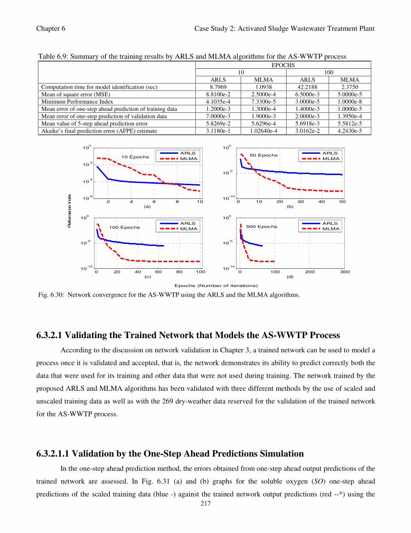
Chapter 6 Case Study 2: Activated Sludge Wastewater Treatment Plant
217
6.3.2.1 Validating the Trained Network that Models the AS-WWTP Process
According to the discussion on network validation in Chapter 3, a trained network can be used to model a
process once it is validated and accepted, that is, the network demonstrates its ability to predict correctly both the
data that were used for its training and other data that were not used during training. The network trained by the
proposed ARLS and MLMA algorithms has been validated with three different methods by the use of scaled and
unscaled training data as well as with the 269 dry-weather data reserved for the validation of the trained network
for the AS-WWTP process.
6.3.2.1.1 Validation by the One-Step Ahead Predictions Simulation
In the one-step ahead prediction method, the errors obtained from one-step ahead output predictions of the
trained network are assessed. In Fig. 6.31 (a) and (b) graphs for the soluble oxygen (SO) one-step ahead
predictions of the scaled training data (blue -) against the trained network output predictions (red --*) using the
Table 6.9: Summary of the training results by ARLS and MLMA algorithms for the AS-WWTP process
EPOCHS
10 100
ARLS MLMA ARLS MLMA
Computation time for model identification (sec) 8.7969 1.0938 42.2188 2.3750
Mean of square error (MSE) 8.8100e-2 2.5000e-4 6.5000e-3 5.0000e-5
Minimum Performance Index 4.1035e-4 7.3300e-5 3.0000e-5 1.0000e-8
Mean error of one-step ahead prediction of training data 1.2000e-3 1.3000e-4 1.4000e-3 1.0000e-5
Mean error of one-step prediction of validation data 7.0000e-3 1.9000e-3 2.0000e-3 1.3950e-4
Mean value of 5-step ahead prediction error 5.8269e-2 5.6296e-4 5.6918e-3 5.5812e-5
Akaike’s final prediction error (AFPE) estimate 3.1180e-1 1.02640e-4 3.0162e-2 4.2430e-5
2 4 6 8 1010
-6
10-4
10-2
100
10 Epochs
(a)
ARLS
MLMA
0 10 20 30 40 5010
-10
10-5
100
50 Epochs
(b)
ARLS
MLMA
0 20 40 60 80 10010
-10
10-5
100
100 Epochs
(c)
ARLS
MLMA
0 100 200 30010
-10
10-5
100
500 Epochs
(d)
ARLS
MLMA
Perform
ance Index
Epochs (Number of iterations)
Fig. 6.30: Network convergence for the AS-WWTP using the ARLS and the MLMA algorithms.
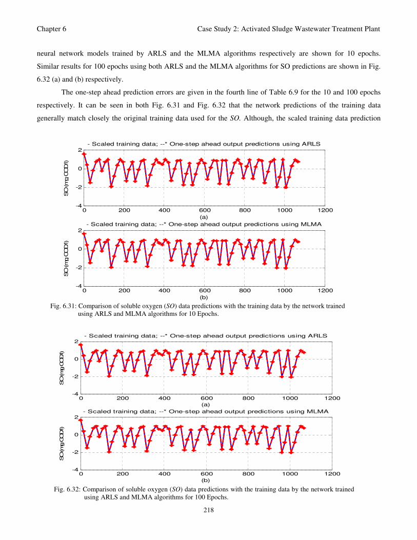
Chapter 6 Case Study 2: Activated Sludge Wastewater Treatment Plant
218
neural network models trained by ARLS and the MLMA algorithms respectively are shown for 10 epochs.
Similar results for 100 epochs using both ARLS and the MLMA algorithms for SO predictions are shown in Fig.
6.32 (a) and (b) respectively.
The one-step ahead prediction errors are given in the fourth line of Table 6.9 for the 10 and 100 epochs
respectively. It can be seen in both Fig. 6.31 and Fig. 6.32 that the network predictions of the training data
generally match closely the original training data used for the SO. Although, the scaled training data prediction
0 200 400 600 800 1000 1200-4
-2
0
2
SO (m
g C
OD/l)
(a)
- Scaled training data; --* One-step ahead output predictions using ARLS
0 200 400 600 800 1000 1200-4
-2
0
2
SO
(m
g C
OD/l)
(b)
- Scaled training data; --* One-step ahead output predictions using MLMA
Fig. 6.31: Comparison of soluble oxygen (SO) data predictions with the training data by the network trained
using ARLS and MLMA algorithms for 10 Epochs.
0 200 400 600 800 1000 1200-4
-2
0
2
SO (mg C
OD/l)
(a)
- Scaled training data; --* One-step ahead output predictions using ARLS
0 200 400 600 800 1000 1200-4
-2
0
2
SO (mg C
OD/l)
(b)
- Scaled training data; --* One-step ahead output predictions using MLMA
Fig. 6.32: Comparison of soluble oxygen (SO) data predictions with the training data by the network trained
using ARLS and MLMA algorithms for 100 Epochs.
Chapter 6 Case Study 2: Activated Sludge Wastewater Treatment Plant
219
errors by both algorithms are small, the MLMA algorithm appears to have a much smaller error when compared
to the ARLS algorithm. These observations are better shown in the fourth line of Table 6.9. These small one-step
ahead prediction errors are indications that both trained networks capture and approximate the nonlinear dynamics
of the aerobic reactor of the AS-WWTP process accurately. This is further justified by the small mean values of
the MSE obtained using ARLS and MLMA algorithms for the SO.
Furthermore, the suitability of the proposed ARLS and MLMA algorithms for neural network model
identification for use in the real AS-WWTP industrial environment is investigated by validating the trained
network with the 269 unscaled dynamic data obtained from the dry-weather data provided by the COST Action
Group. Graphs of the trained network predictions (red --*) of the validation data with the true data (blue -) for 10
epochs for each one of the ARLS and the MLMA algorithms are shown in Fig. 6.33 (a) and (b) for the SO.
Similar results for 100 epochs are shown in Fig. 6.34 (a) and (b). The almost identical prediction of these data
proves the effectiveness of the proposed approach. The prediction accuracies of the unscaled test data by the
networks trained using ARLS and the MLMA algorithm evaluated by the computed mean prediction errors shown
in the fifth line of Table 6.9. Again, one can observe that the validation data prediction errors obtained by both
algorithms are small, the validation data predictions errors with the model by the MLMA algorithm appears
smaller compared to those obtained by using the ARLS algorithm. These predictions of the unscaled validation
data given in Figs. 6.33 and 6.34 as well as the prediction errors in Table 6.9 verify the neural network ability to
model accurately the dynamics of the third aerobic reactor of the AS-WWTP based on dry-weather influent data.
0 50 100 150 200 250 3000
2
4
6
SO
(m
g C
OD
/l)
(a)
- Unscaled target output; --* Predicted outputs by ARLS
0 50 100 150 200 250 3000
2
4
6
SO
(m
g C
OD
/l)
- Unscaled target output; --* Predicted outputs by MLMA
(b)
0 50 100 150 200 250 3000
2
4
6
SO
(m
g C
OD
/l)
(a)
- Unscaled target output; --* Predicted outputs by ARLS
0 50 100 150 200 250 3000
2
4
6
SO
(m
g C
OD
/l)
- Unscaled target output; --* Predicted outputs by MLMA
(b)
Fig. 6.33: Comparison of soluble oxygen (SO) validation
data predictions by the network trained using
ARLS and MLMA algorithms for 10 Epochs.
Fig. 6.34: Comparison of soluble oxygen (SO) validation
data predictions by the network trained using
ARLS and MLMA algorithms for 100 Epochs.
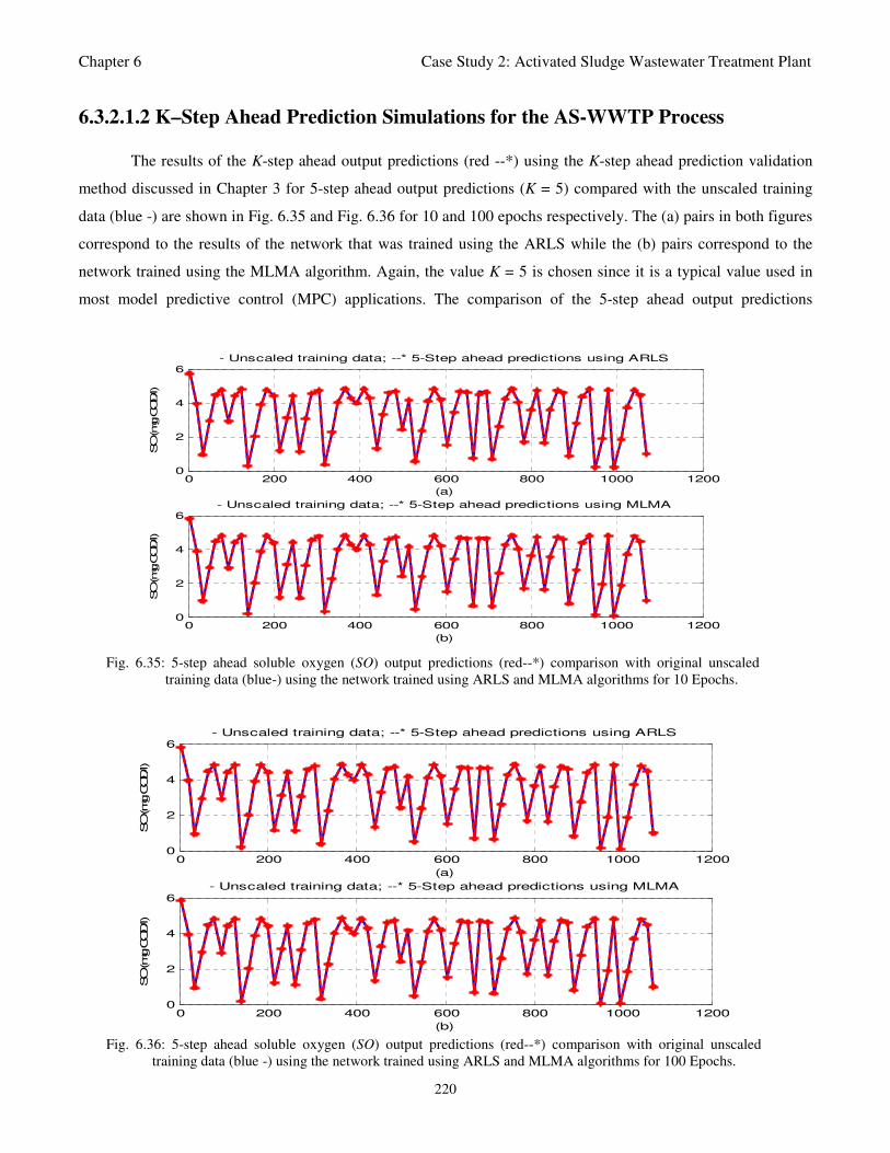
Chapter 6 Case Study 2: Activated Sludge Wastewater Treatment Plant
220
6.3.2.1.2 K–Step Ahead Prediction Simulations for the AS-WWTP Process
The results of the K-step ahead output predictions (red --*) using the K-step ahead prediction validation
method discussed in Chapter 3 for 5-step ahead output predictions (K = 5) compared with the unscaled training
data (blue -) are shown in Fig. 6.35 and Fig. 6.36 for 10 and 100 epochs respectively. The (a) pairs in both figures
correspond to the results of the network that was trained using the ARLS while the (b) pairs correspond to the
network trained using the MLMA algorithm. Again, the value K = 5 is chosen since it is a typical value used in
most model predictive control (MPC) applications. The comparison of the 5-step ahead output predictions
0 200 400 600 800 1000 12000
2
4
6
(a)
SO (mg C
OD/l)
- Unscaled training data; --* 5-Step ahead predictions using ARLS
0 200 400 600 800 1000 12000
2
4
6
SO (mg C
OD/l)
- Unscaled training data; --* 5-Step ahead predictions using MLMA
(b)
Fig. 6.35: 5-step ahead soluble oxygen (SO) output predictions (red--*) comparison with original unscaled
training data (blue-) using the network trained using ARLS and MLMA algorithms for 10 Epochs.
0 200 400 600 800 1000 12000
2
4
6
(a)
SO (mg C
OD/l)
- Unscaled training data; --* 5-Step ahead predictions using ARLS
0 200 400 600 800 1000 12000
2
4
6
SO (mg C
OD/l)
- Unscaled training data; --* 5-Step ahead predictions using MLMA
(b)
Fig. 6.36: 5-step ahead soluble oxygen (SO) output predictions (red--*) comparison with original unscaled
training data (blue -) using the network trained using ARLS and MLMA algorithms for 100 Epochs.
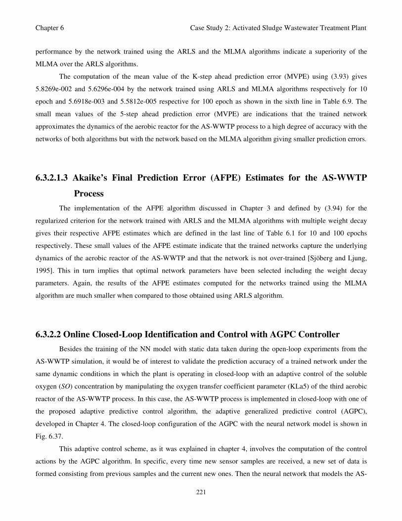
Chapter 6 Case Study 2: Activated Sludge Wastewater Treatment Plant
221
performance by the network trained using the ARLS and the MLMA algorithms indicate a superiority of the
MLMA over the ARLS algorithms.
The computation of the mean value of the K-step ahead prediction error (MVPE) using (3.93) gives
5.8269e-002 and 5.6296e-004 by the network trained using ARLS and MLMA algorithms respectively for 10
epoch and 5.6918e-003 and 5.5812e-005 respective for 100 epoch as shown in the sixth line in Table 6.9. The
small mean values of the 5-step ahead prediction error (MVPE) are indications that the trained network
approximates the dynamics of the aerobic reactor for the AS-WWTP process to a high degree of accuracy with the
networks of both algorithms but with the network based on the MLMA algorithm giving smaller prediction errors.
6.3.2.1.3 Akaike’s Final Prediction Error (AFPE) Estimates for the AS-WWTP
Process
The implementation of the AFPE algorithm discussed in Chapter 3 and defined by (3.94) for the
regularized criterion for the network trained with ARLS and the MLMA algorithms with multiple weight decay
gives their respective AFPE estimates which are defined in the last line of Table 6.1 for 10 and 100 epochs
respectively. These small values of the AFPE estimate indicate that the trained networks capture the underlying
dynamics of the aerobic reactor of the AS-WWTP and that the network is not over-trained [Sjöberg and Ljung,
1995]. This in turn implies that optimal network parameters have been selected including the weight decay
parameters. Again, the results of the AFPE estimates computed for the networks trained using the MLMA
algorithm are much smaller when compared to those obtained using ARLS algorithm.
6.3.2.2 Online Closed-Loop Identification and Control with AGPC Controller
Besides the training of the NN model with static data taken during the open-loop experiments from the
AS-WWTP simulation, it would be of interest to validate the prediction accuracy of a trained network under the
same dynamic conditions in which the plant is operating in closed-loop with an adaptive control of the soluble
oxygen (SO) concentration by manipulating the oxygen transfer coefficient parameter (KLa5) of the third aerobic
reactor of the AS-WWTP process. In this case, the AS-WWTP process is implemented in closed-loop with one of
the proposed adaptive predictive control algorithm, the adaptive generalized predictive control (AGPC),
developed in Chapter 4. The closed-loop configuration of the AGPC with the neural network model is shown in
Fig. 6.37.
This adaptive control scheme, as it was explained in chapter 4, involves the computation of the control
actions by the AGPC algorithm. In specific, every time new sensor samples are received, a new set of data is
formed consisting from previous samples and the current new ones. Then the neural network that models the AS-
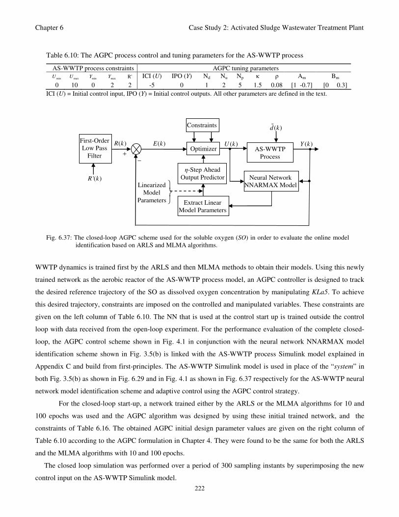
Chapter 6 Case Study 2: Activated Sludge Wastewater Treatment Plant
222
Table 6.10: The AGPC process control and tuning parameters for the AS-WWTP process
AS-WWTP process constraints AGPC tuning parameters
minU maxU
minY maxY R' ICI (U) IPO (Y) Nd Nu Np κ ρ Am Bm
0 10 0 2 2 -5 0 1 2 5 1.5 0.08 [1 -0.7] [0 0.3]
ICI (U) = Initial control input, IPO (Y) = Initial control outputs. All other parameters are defined in the text.
AS-WWTP
Process
( )Y k ( )U k •
Neural Network
NNARMAX Model
Optimizer • +
−
( )E k
•
Constraints ( )d k
η-Step Ahead
Output Predictor
Linearized
Model
Parameters
'( )R k
First-Order
Low Pass
Filter
( )R k
Extract Linear
Model Parameters
Fig. 6.37: The closed-loop AGPC scheme used for the soluble oxygen (SO) in order to evaluate the online model
identification based on ARLS and MLMA algorithms.
WWTP dynamics is trained first by the ARLS and then MLMA methods to obtain their models. Using this newly
trained network as the aerobic reactor of the AS-WWTP process model, an AGPC controller is designed to track
the desired reference trajectory of the SO as dissolved oxygen concentration by manipulating KLa5. To achieve
this desired trajectory, constraints are imposed on the controlled and manipulated variables. These constraints are
given on the left column of Table 6.10. Τhe NN that is used at the control start up is trained outside the control
loop with data received from the open-loop experiment. For the performance evaluation of the complete closed-
loop, the AGPC control scheme shown in Fig. 4.1 in conjunction with the neural network NNARMAX model
identification scheme shown in Fig. 3.5(b) is linked with the AS-WWTP process Simulink model explained in
Appendix C and build from first-principles. The AS-WWTP Simulink model is used in place of the “system” in
both Fig. 3.5(b) as shown in Fig. 6.29 and in Fig. 4.1 as shown in Fig. 6.37 respectively for the AS-WWTP neural
network model identification scheme and adaptive control using the AGPC control strategy.
For the closed-loop start-up, a network trained either by the ARLS or the MLMA algorithms for 10 and
100 epochs was used and the AGPC algorithm was designed by using these initial trained network, and the
constraints of Table 6.16. The obtained AGPC initial design parameter values are given on the right column of
Table 6.10 according to the AGPC formulation in Chapter 4. They were found to be the same for both the ARLS
and the MLMA algorithms with 10 and 100 epochs.
The closed loop simulation was performed over a period of 300 sampling instants by superimposing the new
control input on the AS-WWTP Simulink model.
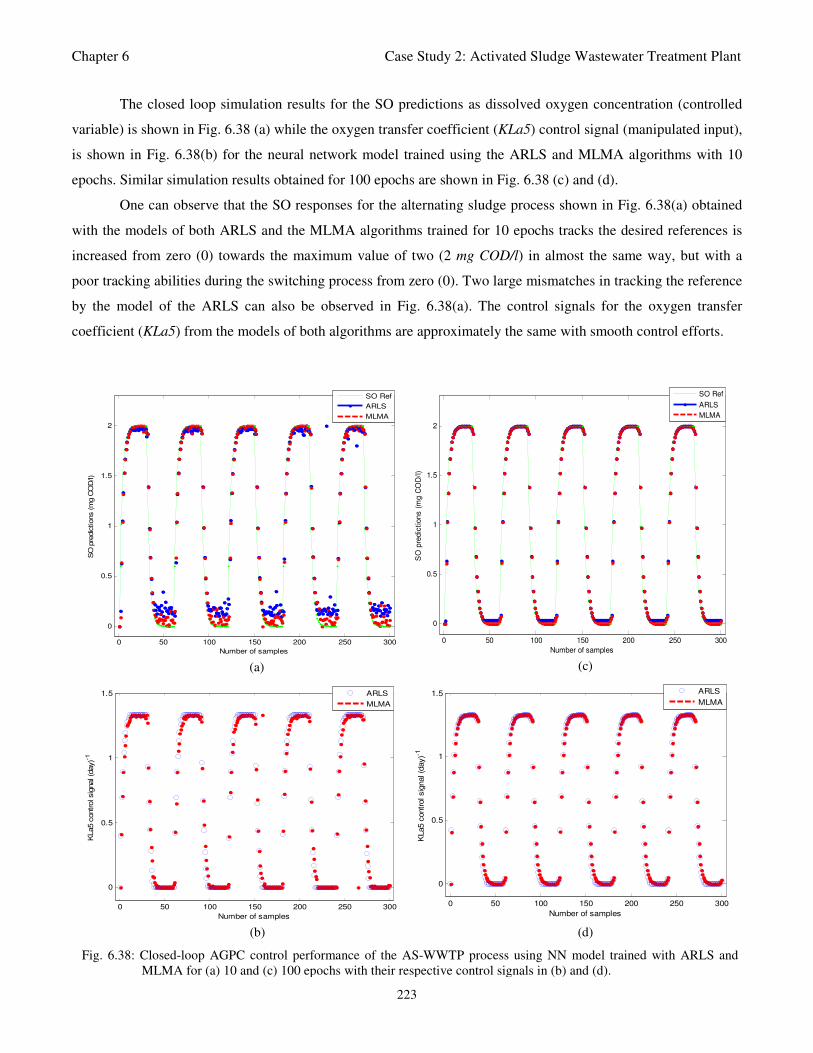
Chapter 6 Case Study 2: Activated Sludge Wastewater Treatment Plant
223
0 50 100 150 200 250 300
0
0.5
1
1.5
2
Number of samples
SO
pre
dic
tions (m
g C
OD
/l)
SO Ref
ARLS
MLMA
(a)
0 50 100 150 200 250 300
0
0.5
1
1.5
2
Number of samples
SO
pre
dic
tion
s (
mg
CO
D/l
)
SO Ref
ARLS
MLMA
(c)
0 50 100 150 200 250 300
0
0.5
1
1.5
Number of samples
KLa5 c
ontrol sig
nal (d
ay)-1
ARLS
MLMA
(b)
0 50 100 150 200 250 300
0
0.5
1
1.5
Number of samples
KLa5 c
ontr
ol sig
nal (d
ay)-1
ARLS
MLMA
(d)
Fig. 6.38: Closed-loop AGPC control performance of the AS-WWTP process using NN model trained with ARLS and
MLMA for (a) 10 and (c) 100 epochs with their respective control signals in (b) and (d).
The closed loop simulation results for the SO predictions as dissolved oxygen concentration (controlled
variable) is shown in Fig. 6.38 (a) while the oxygen transfer coefficient (KLa5) control signal (manipulated input),
is shown in Fig. 6.38(b) for the neural network model trained using the ARLS and MLMA algorithms with 10
epochs. Similar simulation results obtained for 100 epochs are shown in Fig. 6.38 (c) and (d).
One can observe that the SO responses for the alternating sludge process shown in Fig. 6.38(a) obtained
with the models of both ARLS and the MLMA algorithms trained for 10 epochs tracks the desired references is
increased from zero (0) towards the maximum value of two (2 mg COD/l) in almost the same way, but with a
poor tracking abilities during the switching process from zero (0). Two large mismatches in tracking the reference
by the model of the ARLS can also be observed in Fig. 6.38(a). The control signals for the oxygen transfer
coefficient (KLa5) from the models of both algorithms are approximately the same with smooth control efforts.
Chapter 6 Case Study 2: Activated Sludge Wastewater Treatment Plant
224
However, the SO predictions for the alternating sludge process shown in Fig. 6.38(c) for 100 epochs
indicates that the models obtained with the MLMA algorithm tracks accurately the desired SO references when
compared to the model obtained with the ARLS during the switching from zero(0) to the maximum allowable
reference value of two (2 mg COD/l). The control signals shown in Fig. 6.38(b) are essentially the same for the
oxygen transfer coefficient (KLa5) with minimum control efforts.
Although, the simulation results from the aerobic reactor model identification for 10 and 100 epochs
showed almost identical performances, it is obvious in the closed-loop identification control that the models
obtained in 100 epochs are more accurate than those of the 10 epochs as can be observed by comparing the SO
control performance results of Fig. 6.38(a)-(b) with that of Fig. 6.38(c)-(d). By comparing the control signals in
Fig. 6.38(b) and Fig. 6.58(d) which indicates the control efforts (aeration energy) obtained with the models of
both algorithms trained for 10 and 100 epochs respectively, one can conclude that the SO control consumes less
energy when compared to the maximum available control energy of 10 day-1
.
It is apparent from the above discussion that the performance of the proposed model-based AGPC control
algorithm based on a model trained with the MLMA algorithm outperforms that of the ARLS algorithm. As in
Fig. 6.38, the identification and control performance based on the models obtained using both the ARLS and the
MLMA with 100 epochs shows the efficiency and reliability of the proposed AGPC algorithm. It can also be
observed that the control performances based on the network trained using both ARLS and the MLMA algorithms
perform indistinguishably well and also justify the effectiveness of the AGPC controller.
6.3.3 Validation and Dynamic Performance Comparison of the BPM, INCBP and
the Proposed ARLS Algorithms for the Model Identification of the Aerobic
Reactor of the AS-WWTP Process
Validation and dynamic performance comparison of the proposed ARLS algorithm, the backpropagation
with momentum (BPM) and the incremental backpropagation (INCBP) algorithms for the third aerobic reactor of
the AS-WWTP process model Identification is investigated in this section. The version of the back-propagation
with momentum (BPM) algorithm used here is presented in Section 2.4.4.1 of Chapter 2. The ARLS algorithm is
considered here which is a true online identification algorithm. The third incremental backpropagation (INCBP)
algorithm given by (6.9) and (6.10) in Section 6.2.3 is used here again for this comparison.
6.3.3.1 Network Training Using BPM, INCBP and the Proposed ARLS Algorithms
Due to the simplicity and generality of the backpropagation with momentum (BPM) algorithm discussed
in Section 2.4.4.1 in Chapter 2 and the incremental backpropagation (INCBP) algorithm discussed in Section
Chapter 6 Case Study 2: Activated Sludge Wastewater Treatment Plant
225
6.2.3, the NNARMAX model regression vector ( , ( ))NNARMAX
k kϕ θ defined by (6.17) is used as the input vector to
the neural network. The outputs of the NN are the predicted values of ˆ( )Y k given by (6.18). The simulation
results for the soluble oxygen (SO) which defines the dissolved oxygen concentration are again presented here.
The two design parameters for the BPM algorithm defined in (2.59) are the learning rate 1 5eγ = − (i.e.
the step size) and momentum term 1 4eα = − was selected. The design parameter for the INCBP is the step
size 1 4eµ = − . As in section 6.3.2, the four design parameters for ARLS algorithm defined in (3.68) are selected
to be: α=0.5, β=5e-3, 'δ =1e-5 and π=0.99 resulting to γ=0.0101. The initial values for ēmin and ēmax in (3.67) are
equal to 0.0102 and 1.0106e+3 respectively and were evaluated using (3.67). Thus, the ratio ēmin/ēmax in (3.66) is
9.9018e+4 which implied that the parameters are well selected.
It was shown in Section 6.3.2 that the performance of the ARLS and the MLMA algorithms converges to
acceptable values after approximately 100 epochs. In order to assess the convergence performance of the network
trained by the three algorithms, the network was also trained for τ = 100 epochs with the following selected
parameters: 1p = , 14q = , 2a
n = , 2b
n = , 2c
n = , 58nϕ = , 5h
n = , 14o
n = , 1 6h
eα = − and 1 5o
eα = − .
The training data is scaled using (3.89) and the network is trained for 100τ = epochs using the
backpropagation with momentum (BPM), the incremental backpropagation (INCBP) and the ARLS algorithms.
After network training, the trained network is again rescaled according to (3.90), so that the resulting network can
work with unscaled AS-WWTP data. The convergences of the BPM, INCBP and the ARLS algorithms for 100
epochs are shown in Fig. 6.39 and are evaluated in terms of the performance index. It can observe that only the
ARLS algorithm meets the training goal of 10-6
while the BPM and the INCBP converges slowly within the
prescribed 100 epochs.
By comparing the convergences of the BPM, INCBP and ARLS algorithms in Fig. 6.39, it can be seen
that the BPM and INCBP algorithms converges faster to almost the same values than the ARLS algorithm. It can
also be seen in this figure that the performance index obtained by the network trained using ARLS algorithm has a
much smaller value when compared to that obtained by the network when it is trained using the BPM and the
INCBP algorithms. The summary of the network training results using the BPM, INCBP and the ARLS
algorithms are presented in Table 6.11 for quick comparison of the performances of the network when it is trained
by the three mentioned methods.
The computation time for training the network for 100 epochs using each one from the three algorithms
are shown in the first row of Table 6.11. As it can be seen, despite the fact that the BPM and the INCBP
algorithms converge fast enough than the ARLS algorithm and the ARLS is about 1.6536 and 3.4748 slower than
the BPM and INCBP respectively two algorithms in terms of computational time, but the ARLS retains the
smallest performance index value of 2.6453e-5 as shown in Table 6.11. The mean value of the mean square errors
(MSE) and the minimum performance indexes for the network trained with the BPM, INCBP and the ARLS
algorithms are given in the second and third lines of Table 6.11. Again, the ARLS algorithm also has smaller
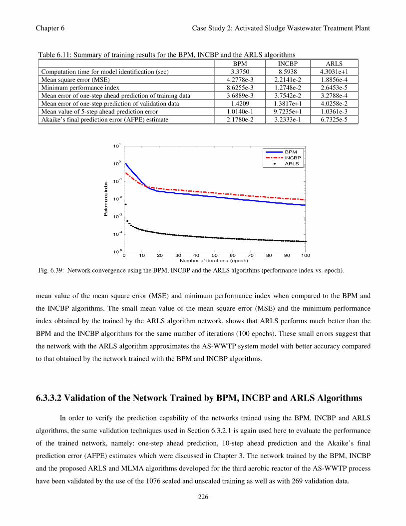
Chapter 6 Case Study 2: Activated Sludge Wastewater Treatment Plant
226
Table 6.11: Summary of training results for the BPM, INCBP and the ARLS algorithms
BPM INCBP ARLS
Computation time for model identification (sec) 3.3750 8.5938 4.3031e+1
Mean square error (MSE) 4.2778e-3 2.2141e-2 1.8856e-4
Minimum performance index 8.6255e-3 1.2748e-2 2.6453e-5
Mean error of one-step ahead prediction of training data 3.6889e-3 3.7542e-2 3.2788e-4
Mean error of one-step prediction of validation data 1.4209 1.3817e+1 4.0258e-2
Mean value of 5-step ahead prediction error 1.0140e-1 9.7235e+1 1.0361e-3
Akaike’s final prediction error (AFPE) estimate 2.1780e-2 3.2333e-1 6.7325e-5
0 10 20 30 40 50 60 70 80 90 10010
-5
10-4
10-3
10-2
10-1
100
101
Number of iterations (epoch)
Perform
ance index
BPM
INCBP
ARLS
Fig. 6.39: Network convergence using the BPM, INCBP and the ARLS algorithms (performance index vs. epoch).
mean value of the mean square error (MSE) and minimum performance index when compared to the BPM and
the INCBP algorithms. The small mean value of the mean square error (MSE) and the minimum performance
index obtained by the trained by the ARLS algorithm network, shows that ARLS performs much better than the
BPM and the INCBP algorithms for the same number of iterations (100 epochs). These small errors suggest that
the network with the ARLS algorithm approximates the AS-WWTP system model with better accuracy compared
to that obtained by the network trained with the BPM and INCBP algorithms.
6.3.3.2 Validation of the Network Trained by BPM, INCBP and ARLS Algorithms
In order to verify the prediction capability of the networks trained using the BPM, INCBP and ARLS
algorithms, the same validation techniques used in Section 6.3.2.1 is again used here to evaluate the performance
of the trained network, namely: one-step ahead prediction, 10-step ahead prediction and the Akaike’s final
prediction error (AFPE) estimates which were discussed in Chapter 3. The network trained by the BPM, INCBP
and the proposed ARLS and MLMA algorithms developed for the third aerobic reactor of the AS-WWTP process
have been validated by the use of the 1076 scaled and unscaled training as well as with 269 validation data.
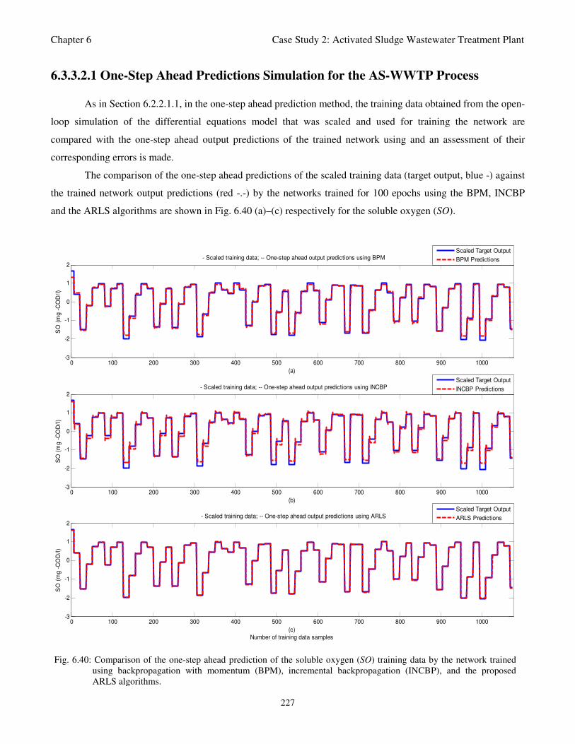
Chapter 6 Case Study 2: Activated Sludge Wastewater Treatment Plant
227
0 100 200 300 400 500 600 700 800 900 1000-3
-2
-1
0
1
2
SO
(m
g -
CO
D/l
)
- Scaled training data; -- One-step ahead output predictions using BPM
(a)
Scaled Target Output
BPM Predictions
0 100 200 300 400 500 600 700 800 900 1000-3
-2
-1
0
1
2
SO
(m
g -
CO
D/l
)
- Scaled training data; -- One-step ahead output predictions using INCBP
(b)
Scaled Target Output
INCBP Predictions
0 100 200 300 400 500 600 700 800 900 1000-3
-2
-1
0
1
2
SO
(m
g -
CO
D/l
)
- Scaled training data; -- One-step ahead output predictions using ARLS
(c)
Number of training data samples
Scaled Target Output
ARLS Predictions
Fig. 6.40: Comparison of the one-step ahead prediction of the soluble oxygen (SO) training data by the network trained
using backpropagation with momentum (BPM), incremental backpropagation (INCBP), and the proposed
ARLS algorithms.
6.3.3.2.1 One-Step Ahead Predictions Simulation for the AS-WWTP Process
As in Section 6.2.2.1.1, in the one-step ahead prediction method, the training data obtained from the open-
loop simulation of the differential equations model that was scaled and used for training the network are
compared with the one-step ahead output predictions of the trained network using and an assessment of their
corresponding errors is made.
The comparison of the one-step ahead predictions of the scaled training data (target output, blue -) against
the trained network output predictions (red -.-) by the networks trained for 100 epochs using the BPM, INCBP
and the ARLS algorithms are shown in Fig. 6.40 (a)–(c) respectively for the soluble oxygen (SO).
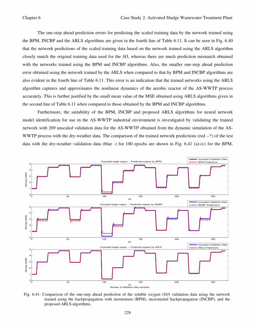
Chapter 6 Case Study 2: Activated Sludge Wastewater Treatment Plant
228
0 50 100 150 200 2500
1
2
3
4
5
SO
(m
g -CO
D/l)
- Unscaled target output; -- Predicted outputs by BPM
(a)
Unscaled Validation Data
BPM Predictions
0 50 100 150 200 2500
1
2
3
4
5
SO
(m
g -CO
D/l)
- Unscaled target output; -- Predicted outputs by INCBP
(b)
Unscaled Validation Data
INCBP Predictions
0 50 100 150 200 2500
1
2
3
4
5
SO
(m
g -CO
D/l)
- Unscaled target output; -- Predicted outputs by ARLS
(c)
Number of validation data samples
Unscaled Validation Data
ARLS Predictions
Fig. 6.41: Comparison of the one-step ahead prediction of the soluble oxygen (SO) validation data using the network
trained using the backpropagation with momentum (BPM), incremental backpropagation (INCBP), and the
proposed ARLS algorithms.
The one-step ahead prediction errors for predicting the scaled training data by the network trained using
the BPM, INCBP and the ARLS algorithms are given in the fourth line of Table 6.11. It can be seen in Fig. 6.40
that the network predictions of the scaled training data based on the network trained using the ARLS algorithm
closely match the original training data used for the SO, whereas there are much prediction mismatch obtained
with the networks trained using the BPM and INCBP algorithms. Also, the smaller one-step ahead prediction
error obtained using the network trained by the ARLS when compared to that by BPM and INCBP algorithms are
also evident in the fourth line of Table 6.11. This error is an indication that the trained networks using the ARLS
algorithm captures and approximates the nonlinear dynamics of the aerobic reactor of the AS-WWTP process
accurately. This is further justified by the small mean value of the MSE obtained using ARLS algorithms given in
the second line of Table 6.11 when compared to those obtained by the BPM and INCBP algorithms.
Furthermore, the suitability of the BPM, INCBP and proposed ARLS algorithms for neural network
model identification for use in the AS-WWTP industrial environment is investigated by validating the trained
network with 269 unscaled validation data for the AS-WWTP obtained from the dynamic simulation of the AS-
WWTP process with the dry-weather data. The comparison of the trained network predictions (red --*) of the test
data with the dry-weather validation data (blue -) for 100 epochs are shown in Fig. 6.41 (a)-(c) for the BPM,
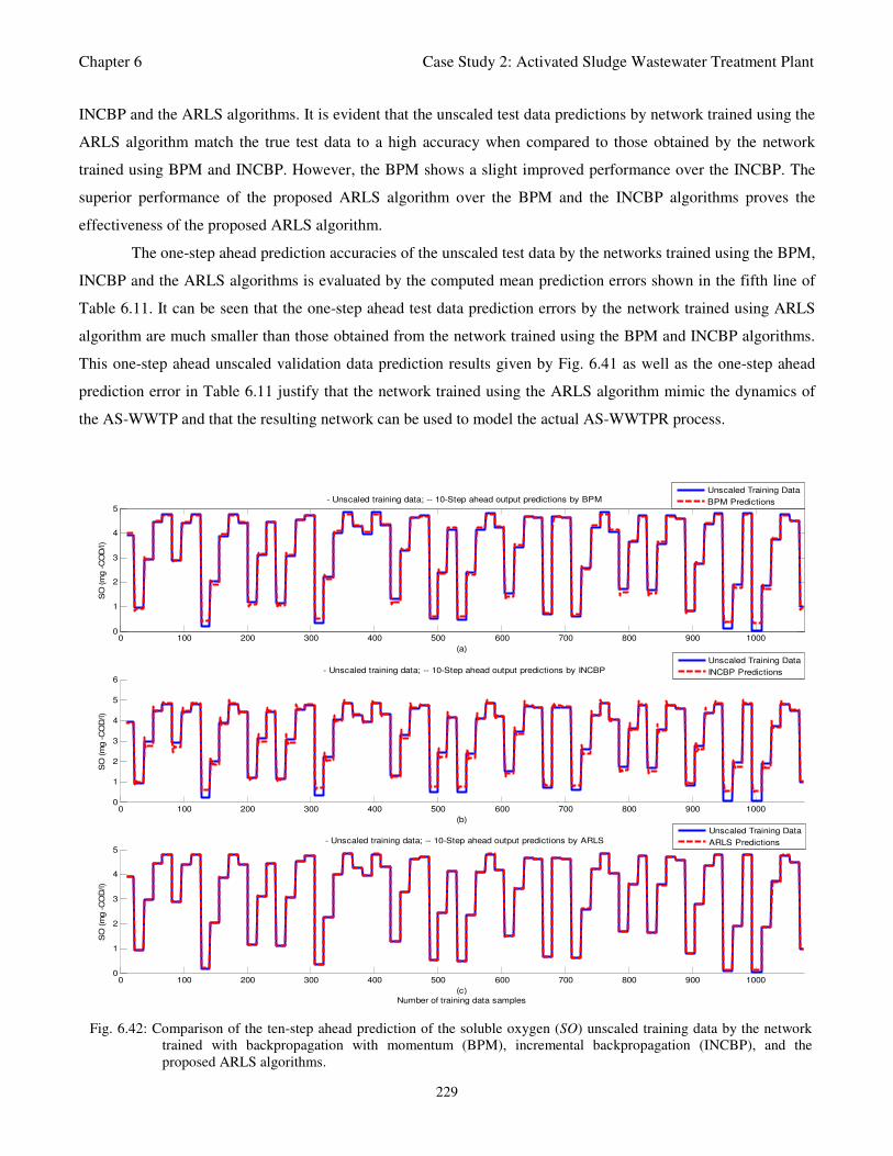
Chapter 6 Case Study 2: Activated Sludge Wastewater Treatment Plant
229
0 100 200 300 400 500 600 700 800 900 10000
1
2
3
4
5
SO
(m
g -C
OD
/l)
- Unscaled training data; -- 10-Step ahead output predictions by BPM
(a)
Unscaled Training Data
BPM Predictions
0 100 200 300 400 500 600 700 800 900 10000
1
2
3
4
5
6
SO
(m
g -
CO
D/l)
- Unscaled training data; -- 10-Step ahead output predictions by INCBP
(b)
Unscaled Training Data
INCBP Predictions
0 100 200 300 400 500 600 700 800 900 10000
1
2
3
4
5
SO
(m
g -
CO
D/l)
- Unscaled training data; -- 10-Step ahead output predictions by ARLS
(c)
Number of training data samples
Unscaled Training Data
ARLS Predictions
Fig. 6.42: Comparison of the ten-step ahead prediction of the soluble oxygen (SO) unscaled training data by the network
trained with backpropagation with momentum (BPM), incremental backpropagation (INCBP), and the
proposed ARLS algorithms.
INCBP and the ARLS algorithms. It is evident that the unscaled test data predictions by network trained using the
ARLS algorithm match the true test data to a high accuracy when compared to those obtained by the network
trained using BPM and INCBP. However, the BPM shows a slight improved performance over the INCBP. The
superior performance of the proposed ARLS algorithm over the BPM and the INCBP algorithms proves the
effectiveness of the proposed ARLS algorithm.
The one-step ahead prediction accuracies of the unscaled test data by the networks trained using the BPM,
INCBP and the ARLS algorithms is evaluated by the computed mean prediction errors shown in the fifth line of
Table 6.11. It can be seen that the one-step ahead test data prediction errors by the network trained using ARLS
algorithm are much smaller than those obtained from the network trained using the BPM and INCBP algorithms.
This one-step ahead unscaled validation data prediction results given by Fig. 6.41 as well as the one-step ahead
prediction error in Table 6.11 justify that the network trained using the ARLS algorithm mimic the dynamics of
the AS-WWTP and that the resulting network can be used to model the actual AS-WWTPR process.
Chapter 6 Case Study 2: Activated Sludge Wastewater Treatment Plant
230
6.3.3.2.2 K–Step Ahead Prediction Simulations for the AS-WWTP Process
The results of the K-step ahead output predictions (red --*) using the K-step ahead prediction validation
method discussed in Chapter 3 for 10-step ahead output predictions (K = 10) compared with the unscaled training
data (target output) are shown in Fig. 6.42 (a)–(b) for the network trained using the BPM, INCBP and ARLS
algorithms. The comparison of the 10-step ahead output predictions performance by the network trained using
BPM, INCBP and the ARLS algorithms shows the superior performance of the ARLS algorithm over the BPM,
INCBP algorithms for use in distant or multi-step ahead predictions.
The computation of the mean value of the 10-step ahead prediction error (MVPE) using (3.93) gives
1.0140e-1, 9.7235e+1 and 1.0361e-3 by the network trained using the BPM, INCBP and ARLS algorithms as
shown in the sixth line in Table 6.11. The relatively small MVPE obtained by the network trained with the ARLS
algorithm is indications that the trained network approximates the dynamics of the AS-WWTP process to a high
degree of accuracy.
6.3.3.2.3 Akaike’s Final Prediction Error (AFPE) Estimates for the AS-WWTP
Neural Network Model
The implementation of the AFPE algorithm discussed in Chapter 3 and defined by (3.94) for the
regularized criterion for the network trained with the BPM, INCBP and the ARLS algorithms with multiple
weight decay gives the respective AFPE estimates of the three algorithms as defined in the last line of Table 6.11.
These small values of the AFPE estimate indicate that the trained networks capture the underlying dynamics of
the third aerobic reactor of the AS-WWTP system and that the network is not over-trained [Sjöberg and Ljung,
1995]. This in turn implies that optimal network parameters have been selected including the weight decay
parameters. Again, the results of the AFPE estimates obtained with the networks trained using the ARLS
algorithm are slightly smaller when compared to those obtained using BPM and INCBP algorithms.
6.3.3.3 Performance Comparison of the BPM, INCBP and the ARLS Algorithms
The simulation results for the neural network training using the BPM, INCBP and ARLS algorithms as
well as the network validation result for the AS-WWTP process are shown in Fig. 6.39, Fig. 6.40, Fig. 6.41, and
Fig. 6.42 respectively; whereas numerical results for these three algorithms are presented in Table 6.11.
The numerical results summarized in Table 6.11 show that when the network is trained by using the
ARLS algorithm presents the best performance as the least values in all of the six properties are achieved. In
addition, the least value of the AFPE is obtained using the ARLS algorithm indicates that the ARLS algorithm
captures the essential dynamics of the process and that the identified NN model approximates the true system to a
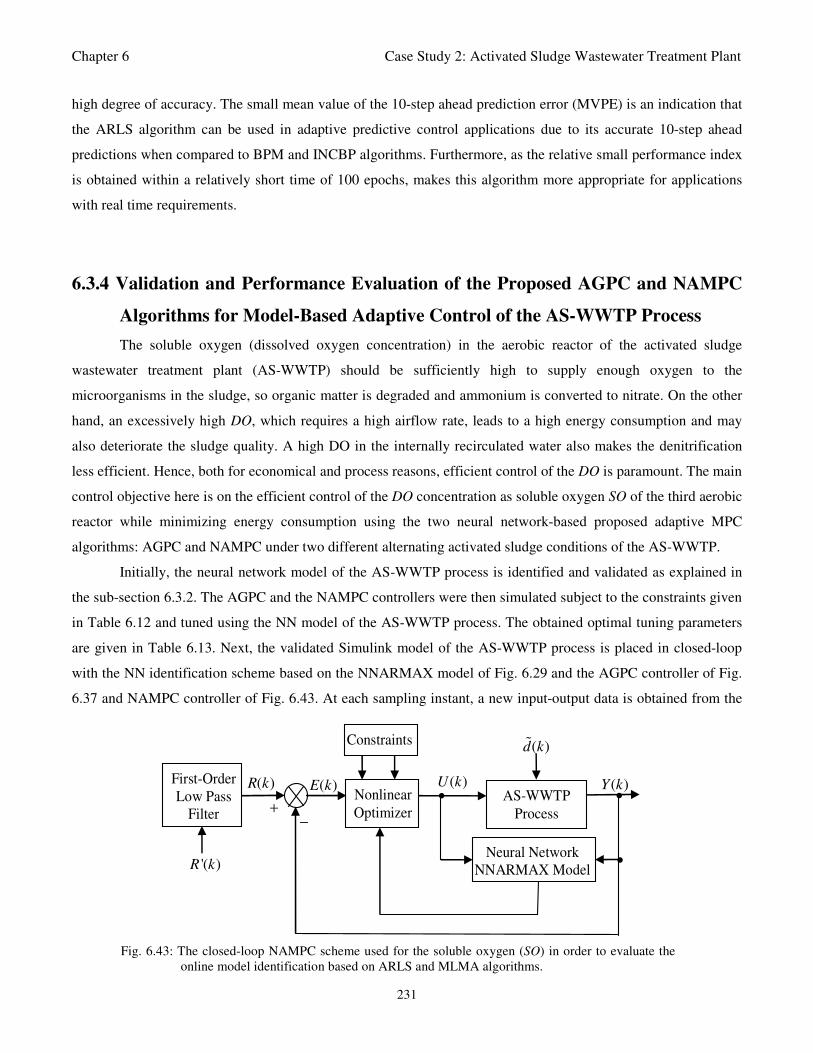
Chapter 6 Case Study 2: Activated Sludge Wastewater Treatment Plant
231
AS-WWTP
Process
( )Y k ( )U k •
Neural Network
NNARMAX Model
Nonlinear
Optimizer •
+ −
'( )R k
( )E k
•
Constraints
First-Order
Low Pass
Filter
( )d k
( )R k
Fig. 6.43: The closed-loop NAMPC scheme used for the soluble oxygen (SO) in order to evaluate the
online model identification based on ARLS and MLMA algorithms.
high degree of accuracy. The small mean value of the 10-step ahead prediction error (MVPE) is an indication that
the ARLS algorithm can be used in adaptive predictive control applications due to its accurate 10-step ahead
predictions when compared to BPM and INCBP algorithms. Furthermore, as the relative small performance index
is obtained within a relatively short time of 100 epochs, makes this algorithm more appropriate for applications
with real time requirements.
6.3.4 Validation and Performance Evaluation of the Proposed AGPC and NAMPC
Algorithms for Model-Based Adaptive Control of the AS-WWTP Process
The soluble oxygen (dissolved oxygen concentration) in the aerobic reactor of the activated sludge
wastewater treatment plant (AS-WWTP) should be sufficiently high to supply enough oxygen to the
microorganisms in the sludge, so organic matter is degraded and ammonium is converted to nitrate. On the other
hand, an excessively high DO, which requires a high airflow rate, leads to a high energy consumption and may
also deteriorate the sludge quality. A high DO in the internally recirculated water also makes the denitrification
less efficient. Hence, both for economical and process reasons, efficient control of the DO is paramount. The main
control objective here is on the efficient control of the DO concentration as soluble oxygen SO of the third aerobic
reactor while minimizing energy consumption using the two neural network-based proposed adaptive MPC
algorithms: AGPC and NAMPC under two different alternating activated sludge conditions of the AS-WWTP.
Initially, the neural network model of the AS-WWTP process is identified and validated as explained in
the sub-section 6.3.2. The AGPC and the NAMPC controllers were then simulated subject to the constraints given
in Table 6.12 and tuned using the NN model of the AS-WWTP process. The obtained optimal tuning parameters
are given in Table 6.13. Next, the validated Simulink model of the AS-WWTP process is placed in closed-loop
with the NN identification scheme based on the NNARMAX model of Fig. 6.29 and the AGPC controller of Fig.
6.37 and NAMPC controller of Fig. 6.43. At each sampling instant, a new input-output data is obtained from the
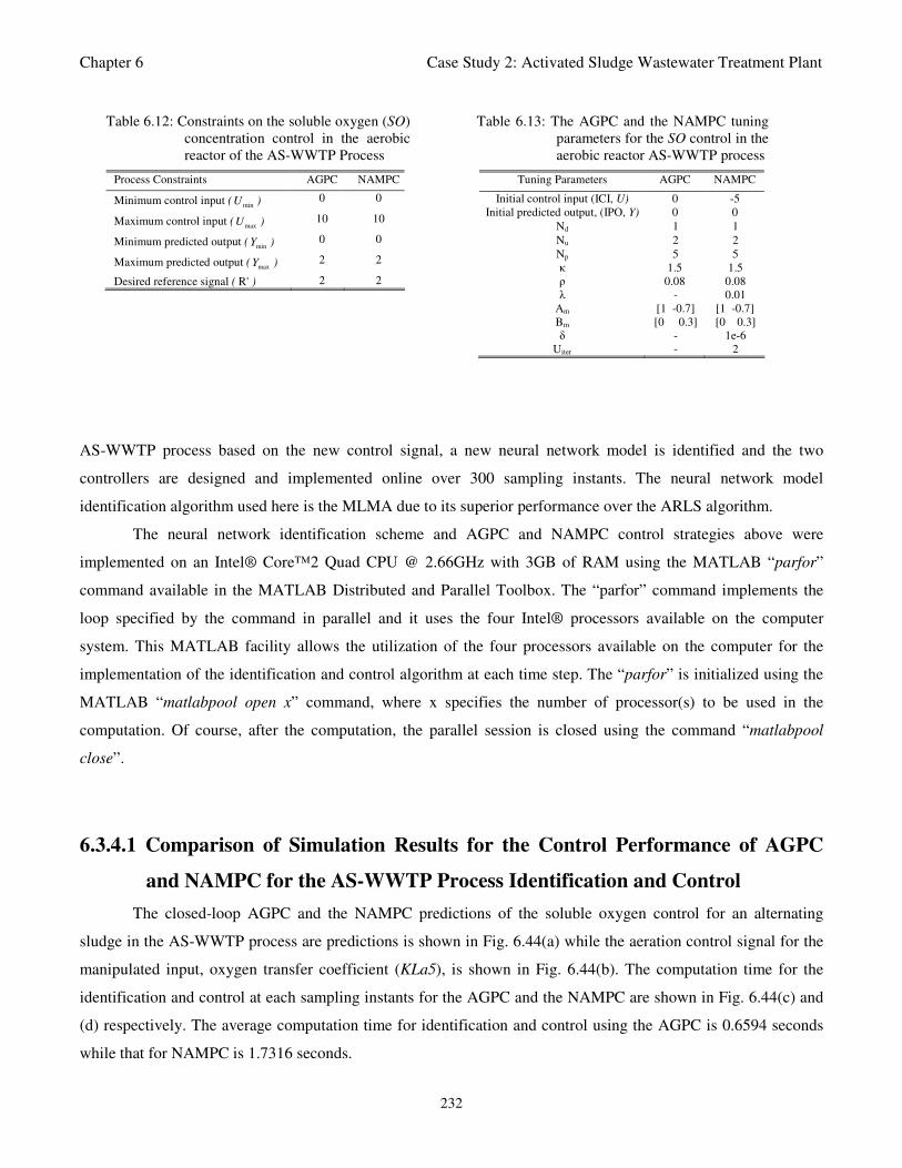
Chapter 6 Case Study 2: Activated Sludge Wastewater Treatment Plant
232
Table 6.12: Constraints on the soluble oxygen (SO)
concentration control in the aerobic
reactor of the AS-WWTP Process
Process Constraints AGPC NAMPC
Minimum control input (minU ) 0 0
Maximum control input (maxU ) 10 10
Minimum predicted output (minY ) 0 0
Maximum predicted output (maxY ) 2 2
Desired reference signal ( R' ) 2 2
Table 6.13: The AGPC and the NAMPC tuning
parameters for the SO control in the
aerobic reactor AS-WWTP process
Tuning Parameters AGPC NAMPC
Initial control input (ICI, U) 0 -5
Initial predicted output, (IPO, Y) 0 0
Nd 1 1
Nu 2 2
Np 5 5
κ 1.5 1.5
ρ 0.08 0.08
λ - 0.01
Am [1 -0.7] [1 -0.7]
Bm [0 0.3] [0 0.3]
δ - 1e-6
Uiter - 2
AS-WWTP process based on the new control signal, a new neural network model is identified and the two
controllers are designed and implemented online over 300 sampling instants. The neural network model
identification algorithm used here is the MLMA due to its superior performance over the ARLS algorithm.
The neural network identification scheme and AGPC and NAMPC control strategies above were
implemented on an Intel® Core™2 Quad CPU @ 2.66GHz with 3GB of RAM using the MATLAB “parfor”
command available in the MATLAB Distributed and Parallel Toolbox. The “parfor” command implements the
loop specified by the command in parallel and it uses the four Intel® processors available on the computer
system. This MATLAB facility allows the utilization of the four processors available on the computer for the
implementation of the identification and control algorithm at each time step. The “parfor” is initialized using the
MATLAB “matlabpool open x” command, where x specifies the number of processor(s) to be used in the
computation. Of course, after the computation, the parallel session is closed using the command “matlabpool
close”.
6.3.4.1 Comparison of Simulation Results for the Control Performance of AGPC
and NAMPC for the AS-WWTP Process Identification and Control
The closed-loop AGPC and the NAMPC predictions of the soluble oxygen control for an alternating
sludge in the AS-WWTP process are predictions is shown in Fig. 6.44(a) while the aeration control signal for the
manipulated input, oxygen transfer coefficient (KLa5), is shown in Fig. 6.44(b). The computation time for the
identification and control at each sampling instants for the AGPC and the NAMPC are shown in Fig. 6.44(c) and
(d) respectively. The average computation time for identification and control using the AGPC is 0.6594 seconds
while that for NAMPC is 1.7316 seconds.
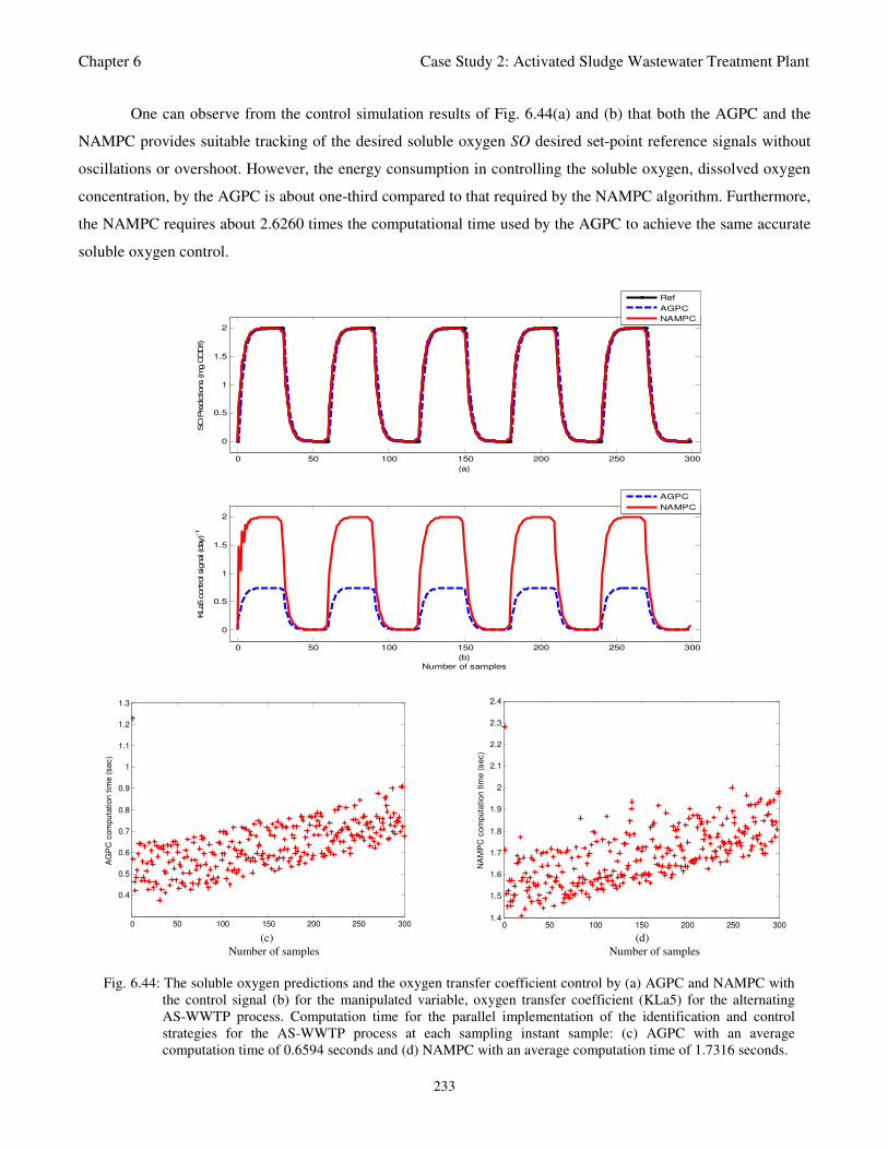
Chapter 6 Case Study 2: Activated Sludge Wastewater Treatment Plant
233
0 50 100 150 200 250 300
0
0.5
1
1.5
2
(a)
SO
Pre
dic
tions (m
g C
OD/l)
Ref
AGPC
NAMPC
0 50 100 150 200 250 300
0
0.5
1
1.5
2
KLa5 c
ontrol sig
nal (d
ay)-1
(b)
Number of samples
AGPC
NAMPC
0 50 100 150 200 250 300
0.4
0.5
0.6
0.7
0.8
0.9
1
1.1
1.2
1.3
(a)
AG
PC
com
puta
tion t
ime (
sec)
0 50 100 150 200 250 3001.4
1.5
1.6
1.7
1.8
1.9
2
2.1
2.2
2.3
2.4
NA
MP
C c
om
puta
tion t
ime (
sec)
(c) (d)
Number of samples Number of samples
Fig. 6.44: The soluble oxygen predictions and the oxygen transfer coefficient control by (a) AGPC and NAMPC with
the control signal (b) for the manipulated variable, oxygen transfer coefficient (KLa5) for the alternating
AS-WWTP process. Computation time for the parallel implementation of the identification and control
strategies for the AS-WWTP process at each sampling instant sample: (c) AGPC with an average
computation time of 0.6594 seconds and (d) NAMPC with an average computation time of 1.7316 seconds.
One can observe from the control simulation results of Fig. 6.44(a) and (b) that both the AGPC and the
NAMPC provides suitable tracking of the desired soluble oxygen SO desired set-point reference signals without
oscillations or overshoot. However, the energy consumption in controlling the soluble oxygen, dissolved oxygen
concentration, by the AGPC is about one-third compared to that required by the NAMPC algorithm. Furthermore,
the NAMPC requires about 2.6260 times the computational time used by the AGPC to achieve the same accurate
soluble oxygen control.
Chapter 6 Case Study 2: Activated Sludge Wastewater Treatment Plant
234
0 50 100 150 200 250 300 350
0
0.5
1
1.5
2
(a)
SO
Pre
dic
tions (m
g C
OD
/l)
Ref
AGPC
NAMPC
0 50 100 150 200 250 300 350
0
0.5
1
1.5
2
KLa5 c
ontrol sig
nal (d
ay)-1
(b)
Number of samples
AGPC
NAMPC
Fig. 6.45: The soluble oxygen control predictions and control by AGPC and NAMPC with the
control signal (b) for the manipulated variable, oxygen transfer coefficient (KLa5) AS-
WWTP process with sinusoidal disturbances.
In the second simulation, the soluble oxygen is increasing and reducing as a sinusoid. This behaviour is
not unusual when dealing with disturbance rejection and noise arising in the AS-WWTP due to excessive
dissolved oxygen concentration [Azwar et al., 2006]. Here, the desired reference is superimposed with a non-
negative sinusoidal disturbance of unit amplitude and the control objective is to track this desired reference and
keeping the SO (that is the dissolved oxygen, DO) concentration at the prescribed level of 2.0 mg COD/l without
any overshoot or generating additional noise as oscillations. The SO predictions and the KLa5 control signals
obtained by the AGPC and the NAMPC algorithms are shown in Fig. 6.45 respectively.
It can be observed in Fig. 6.45 that the NAMPC shows better control performance over the AGPC where
the magnitude of the throttle setting is very large. Actually, the AGPC exhibits some oscillatory overshoots and
hardly track the fast changing sinusoidal reference signal for the SO. These results demonstrates the efficiency of
the proposed NAMPC based on its adaptive optimization strategy for tracking and controlling difficult nonlinear
non-smooth and control applications with relatively fast changing dynamics while the control signal is kept at
minimum to minimize operational costs.
Chapter 6 Case Study 3: Nonlinear F-16 Fighter Aircraft
235
6.4 Neural Network-Based Model Identification and Adaptive Predictive Auto-Pilot
Control of a Nonlinear F-16 Fighter Aircraft
To demonstrate the application of the neural network-based identification and control algorithms to a
highly nonlinear system with relative fast dynamics and short sampling time, the auto-pilot control system of a
nonlinear F-16 fighter aircraft is considered.
The nonlinear F-16 aircraft dynamics is, in general nonlinear, time-varying and uncertain. Traditionally,
aircraft flight control systems are designed by using the mathematical model of the aircraft linearized at various
flight conditions. The aircraft motion variables are sensed and fed into the aircraft control system which adjusts
the s surface actuators via some feedback gains. The adjustment process is called gain scheduling. Since controller
designs are performed off-line using a limited number of linear and time-invariant models, extensive gain
scheduling computation is required. While this approach may handle mild nonlinearities, it is not suitable for
highly nonlinear problems associated with the aircraft. The gain scheduling approach may produce a control law
that is applicable around the current design operating points but not globally. Thus, as aircrafts become more
complex, traditional design methods have not yielded acceptable performance. To overcome these problems,
nonlinear control techniques such as feedback linearization discussed in Section 2.11.1.5 in Chapter 2 have been
studied as alternatives to gain scheduling ([Khalil, 1996]; [Morari and Zafiriou, 1989]; [Nørgaard et al., 2000]).
The use of these techniques is difficult because they depend heavily on accurate knowledge of the aircraft
dynamics. Thus, a totally different approach to the nonlinear F-16 aircraft flight control is presented in this work
based on the use of neural network-based nonlinear modeling and adaptive control techniques.
6.4.1 Formulation of the Nonlinear F-16 Aircraft Control Problem
The F-16 aircraft can be controlled by manipulating the deflections of the aileron, elevator and the rudder
surfaces as well as the thrust illustrated in Fig. 6.46 while the definition of the angle of attack α and the angle of
side slip β together with respect to the orientation of the navigation frame are shown in Fig. 6.47. A positive
aileron, elevator or rudder deflections gives a decrease in roll rate p, pitch rate q or yaw rate r respectively while a
positive thrust t causes an increase in acceleration along the longitudinal body axis. The control of the nonlinear
F-16 aircraft is discussed here with respect to the right control surfaces shown in Fig. 6.46 and Fig. 6.47.
The main objective here for the nonlinear F-16 aircraft is on neural network model identification and
adaptive model-based control of the auto-pilot control system based on the orientations of the three right control
surfaces; that is, the aileron, elevator and the rudder deflection control by manipulating the roll, pitch and the yaw
actuator rates respectively as well as the throttle command for controlling the thrust according to the desired flight
route. The desired routes of the proposed flight are illustrated in Fig. 6.48 and are described below as follows:
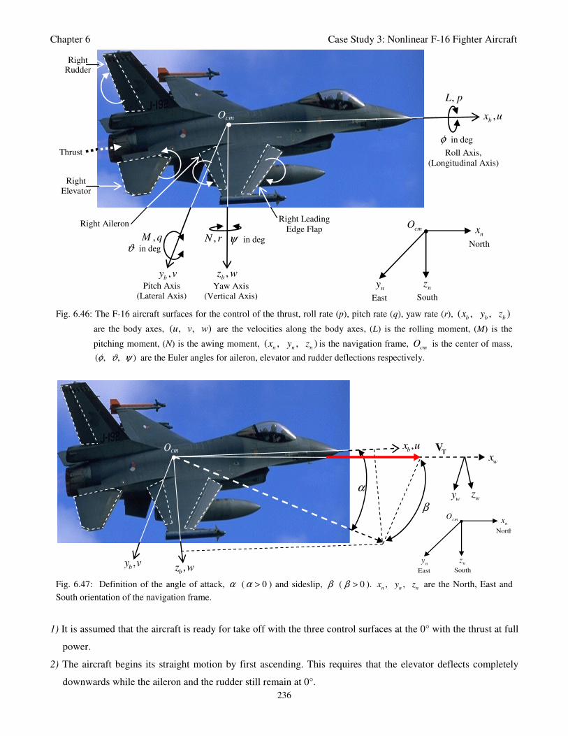
Chapter 6 Case Study 3: Nonlinear F-16 Fighter Aircraft
236
Right Aileron Right Leading
Edge Flap
Right
Elevator
Right Rudder
Pitch Axis
(Lateral Axis)
Roll Axis,
(Longitudinal Axis)
Yaw Axis
(Vertical Axis)
Thrust
φ in deg
ψ in deg ϑ in deg
,M q
,L p
,N r
,bz w
,b
x u
,b
y v
• cmO
nx
North
nz
South
ny
East
. Ocm
Fig. 6.46: The F-16 aircraft surfaces for the control of the thrust, roll rate (p), pitch rate (q), yaw rate (r), ( , , )b b b
x y z
are the body axes, ( , , )u v w are the velocities along the body axes, (L) is the rolling moment, (M) is the
pitching moment, (N) is the awing moment, ( , , )n n n
x y z is the navigation frame, cm
O is the center of mass,
( , , )φ ϑ ψ are the Euler angles for aileron, elevator and rudder deflections respectively.
,b
z w
,b
x u
,b
y v
. Ocm
α
β
wz
wy
wx
TV
•
cmO
nx
North
nz
South n
y
East
Fig. 6.47: Definition of the angle of attack, α ( 0α > ) and sideslip, β ( 0β > ). , ,n n n
x y z are the North, East and
South orientation of the navigation frame.
1) It is assumed that the aircraft is ready for take off with the three control surfaces at the 0° with the thrust at full
power.
2) The aircraft begins its straight motion by first ascending. This requires that the elevator deflects completely
downwards while the aileron and the rudder still remain at 0°.
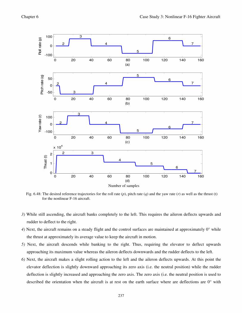
Chapter 6 Case Study 3: Nonlinear F-16 Fighter Aircraft
237
0 20 40 60 80 100 120 140 160
-100
0
100R
oll
rate
(p)
(a)
2
3
4
5
6
7
0 20 40 60 80 100 120 140 160
-50
0
50
Pitch rate
(q)
(b)
2
3
4
5
67
0 20 40 60 80 100 120 140 160
-100
0
100
Yaw
rate
(r)
(c)
2
3
4
56
7
0 20 40 60 80 100 120 140 1600
1
2
x 104
Thru
st (t)
2 3
45
67
(d)
Number of samples
Fig. 6.48: The desired reference trajectories for the roll rate (p), pitch rate (q) and the yaw rate (r) as well as the thrust (t)
for the nonlinear F-16 aircraft.
3) While still ascending, the aircraft banks completely to the left. This requires the aileron deflects upwards and
rudder to deflect to the right.
4) Next, the aircraft remains on a steady flight and the control surfaces are maintained at approximately 0° while
the thrust at approximately its average value to keep the aircraft in motion.
5) Next, the aircraft descends while banking to the right. Thus, requiring the elevator to deflect upwards
approaching its maximum value whereas the aileron deflects downwards and the rudder deflects to the left.
6) Next, the aircraft makes a slight rolling action to the left and the aileron deflects upwards. At this point the
elevator deflection is slightly downward approaching its zero axis (i.e. the neutral position) while the rudder
deflection is slightly increased and approaching the zero axis. The zero axis (i.e. the neutral position is used to
described the orientation when the aircraft is at rest on the earth surface where are deflections are 0° with
Chapter 6 Case Study 3: Nonlinear F-16 Fighter Aircraft
238
respect to the center of mass. This behaviour of the elevator and the rudder indicates that the aircraft descends
slightly with a slight turning to the left.
7) Finally, the aircraft descends and all the deflection surfaces approach to 0° as the aircraft is landing and comes
to rest. The thrust is also reduced to its minimum value of zero as the aircraft comes to rest.
It is important to note that while the aircraft can roll completely about the longitudinal axis using the ailerons, the
turning of the aircraft about vertical axis is accomplished not only by the rudders but also in conjunction with the
ailerons [Anderson and Eberhardt, 2001 and 2010]. The desired reference trajectories for the six intermediate
routes discussed in step 2) to step 7) above are illustrated in the figure of Fig. 6.48 together with the desired thrust
variations.
In state space form ([Ducard, 2009]; [Nelson, 1989]; [Stevens and Lewis, 2003]), the motion of the
nonlinear F-16 aircraft can be represented by the following nonlinear vector differential equation:
( , , )X g U X C= (6.19)
where g is a nonlinear function, U , X and C are the input vector, state vector, and the aerodynamic coefficients
respectively. The thirteen states that are used to describe the rigid-body motion of the nonlinear F-16 aircraft over
a flat Earth is given by:
[ ]T
N E T lefX p p h V p q rφ ϑ ψ α β δ= (6.20)
where N
p , E
p , h , φ , ϑ , ψ , T
V , α , β , p , q , r and LEF
δ are the north position, east position, altitude, roll
angle, pitch angle, yaw angle, velocity, angle of attack, angle of side-slip, roll rate, pitch rate, yaw rate and the
deflection of the leading edge flap respectively. A complete description of the nonlinear F-16 aircraft dynamics is
given in Appendix D. Also, these dynamics are modeled and implemented using Simulink and MATLAB C
programs. The complete model and implementation programs are given in Appendix D.
The aerodynamic coefficients are functions of some of the states, namely: the damping coefficients are
functions of the angle of attack α ; the body-axis aerodynamic force coefficients are functions of α , β , a
δ , e
δ
and r
δ ; the moment coefficients are functions of α , β and e
δ ; the coefficients of the rolling moment due to the
ailerons and the rudder deflections as well as the coefficients of the yawing moment due to the ailerons and the
rudder deflections are functions of α and β [Stevens and Lewis, 2003]. The input vector to the nonlinear F-16
aircraft model is
( ) [ ]T
a e r tU k δ δ δ δ= (6.21)
where a
δ , e
δ , r
δ and t
δ are the aileron deflection, elevator deflection, rudder deflection and throttle setting
respectively. The eighteen outputs of the nonlinear F-16 model are: the twelve derivatives of the state variables of
Np ,
Ep , h , φ , ϑ , ψ ,
TV , α , β , p , q , r ; three normalized acceleration coordinates
nxA ,
nyA ,
nzA ; Mach
number M; dynamic pressure ( )qbar ; and static pressure ( )s
p . The definition of the static and dynamic pressures
Chapter 6 Case Study 3: Nonlinear F-16 Fighter Aircraft
239
as well as their differences and measurement techniques are discussed Appendix D–4. The LEF
δ is a function
of α , qbar ands
p as detailed in Appendix D–3 which allows the F-16 aircraft to fly at higher angle of attack
[Nguyen et al., 1979]. The definition of the angle of attack α with respect to the orientation of the navigation
frame is shown in Fig. 6.47 while the details are given in Appendices D–1 and D–3. The inclusion or not of the
deflection of the leading edge flap LEF
δ in F-16 aircraft simulation results to two types of models for the F-16
aircraft, that is the low fidelity and high fidelity models [Russell, 2003]. The low fidelity model excludes the
effects of the LEF
δ [Stevens and Lewis, 2003] whereas the high fidelity model considers the full effects of the
LEFδ [Nguyen et al., 1979]. The differences between these two types of models are based on the data used to
model the aircraft and is discussed in Appendix D–3.
6.4.1.1 Simulation of the Nonlinear F-16 Aircraft for Training Data Acquisition
The F-16 turbofan engine model consists of a first-order dynamic model, a throttle command shaping
function and tables of nonlinear thrust functions of the operating power level, altitude, and Mach number at
different altitudes h as shown in Table VI in Nguyen et al. [Nguyen et al., 1979]. There is one table for each of
the power level called the idle, military, and the maximum ([Nguyen et al., 1979]; [Stevens and Lewis, 2003]). In
the thrust lookup tables, Mach number variation is from 0 to 1 in steps of 0.2 as shown in Tables VI (a) and (b) in
Nguyen et al. [Nguyen et al., 1979]. Altitude variation is from 0 to 50,000ft in steps of 10,000ft as shown in Table
VI (b) in Nguyen et al. [Nguyen et al., 1979].
The aerodynamic data for the high fidelity model used in this work are based on the wind-tunnel tests on
a scaled model of the nonlinear F-16 aircraft provided in [Nguyen et al., 1979] and [Russell, 2003]. The values of
the dimensionless aerodynamic coefficients are presented in multi-dimensional lookup tables associated with
linear interpolation algorithms in the Table III of [Nguyen et al., 1979]. The aerodynamic data are referenced to
the nominal position of the center of gravity XCG = 0.35. The angle of attack ranges from -10° to 45° in steps of
5°, the sideslip angle ranges from -30° to 30° in steps of 5°, and the speed upper limit is 0.6 Mach. The limits of
the actuators used to control:
• the aileron, elevator, rudder and the leading edge flap deflections (LEF
δ ) are +21.5°, +25°, +30° and 0 to
25° respectively,
• the thrust of the turbofan engine are from 1,000 to 19,000 lbs ,
• the throttle setting rate is +10,000 lbs , and
• the roll, pitch, yaw and the LEF
δ actuator rate are +80°, +60°, +120° and +25° respectively.
In order to model the nonlinear F-16 aircraft that could fly at higher angle of attack, the NASA data for
the high fidelity nonlinear F-16 aircraft model [Nguyen et al., 1979] is used in this simulation study. The National
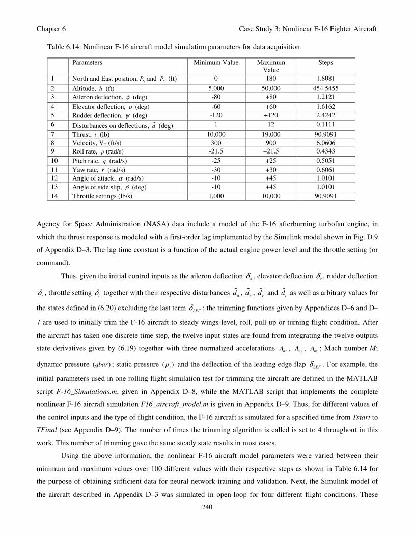
Chapter 6 Case Study 3: Nonlinear F-16 Fighter Aircraft
240
Table 6.14: Nonlinear F-16 aircraft model simulation parameters for data acquisition
Parameters Minimum Value Maximum
Value
Steps
1 North and East position,NP and
EP (ft) 0 180 1.8081
2 Altitude, h (ft) 5,000 50,000 454.5455
3 Aileron deflection, φ (deg) -80 +80 1.2121
4 Elevator deflection, ϑ (deg) -60 +60 1.6162
5 Rudder deflection, ψ (deg) -120 +120 2.4242
6 Disturbances on deflections, d (deg) 1 12 0.1111
7 Thrust, t (lb) 10,000 19,000 90.9091
8 Velocity, VT (ft/s) 300 900 6.0606
9 Roll rate, p (rad/s) -21.5 +21.5 0.4343
10 Pitch rate, q (rad/s) -25 +25 0.5051
11 Yaw rate, r (rad/s) -30 +30 0.6061
12 Angle of attack, α (rad/s) -10 +45 1.0101
13 Angle of side slip, β (deg) -10 +45 1.0101
14 Throttle settings (lb/s) 1,000 10,000 90.9091
Agency for Space Administration (NASA) data include a model of the F-16 afterburning turbofan engine, in
which the thrust response is modeled with a first-order lag implemented by the Simulink model shown in Fig. D.9
of Appendix D–3. The lag time constant is a function of the actual engine power level and the throttle setting (or
command).
Thus, given the initial control inputs as the aileron deflection a
δ , elevator deflection e
δ , rudder deflection
rδ , throttle setting
tδ together with their respective disturbances
ad ,
ed ,
rd and
td as well as arbitrary values for
the states defined in (6.20) excluding the last term LEF
δ ; the trimming functions given by Appendices D–6 and D–
7 are used to initially trim the F-16 aircraft to steady wings-level, roll, pull-up or turning flight condition. After
the aircraft has taken one discrete time step, the twelve input states are found from integrating the twelve outputs
state derivatives given by (6.19) together with three normalized accelerations nx
A , ny
A , nz
A ; Mach number M;
dynamic pressure ( )qbar ; static pressure ( )s
p and the deflection of the leading edge flap LEF
δ . For example, the
initial parameters used in one rolling flight simulation test for trimming the aircraft are defined in the MATLAB
script F-16_Simulations.m, given in Appendix D–8, while the MATLAB script that implements the complete
nonlinear F-16 aircraft simulation F16_aircraft_model.m is given in Appendix D–9. Thus, for different values of
the control inputs and the type of flight condition, the F-16 aircraft is simulated for a specified time from Tstart to
TFinal (see Appendix D–9). The number of times the trimming algorithm is called is set to 4 throughout in this
work. This number of trimming gave the same steady state results in most cases.
Using the above information, the nonlinear F-16 aircraft model parameters were varied between their
minimum and maximum values over 100 different values with their respective steps as shown in Table 6.14 for
the purpose of obtaining sufficient data for neural network training and validation. Next, the Simulink model of
the aircraft described in Appendix D–3 was simulated in open-loop for four different flight conditions. These
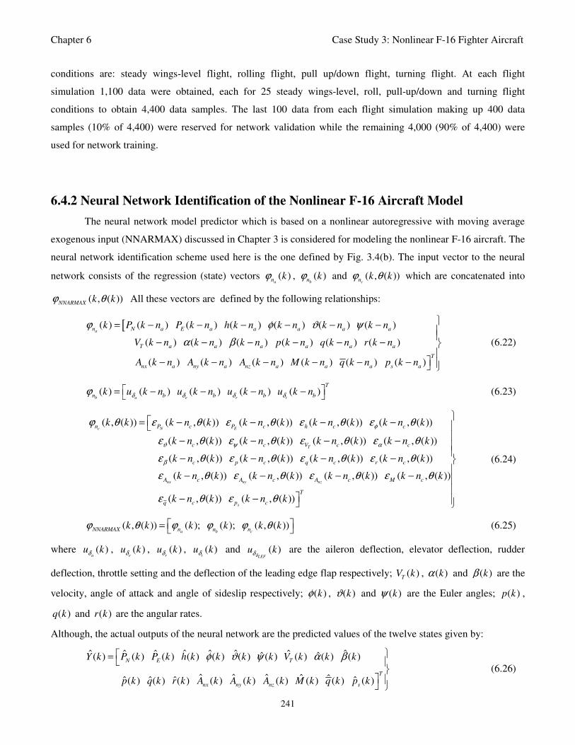
Chapter 6 Case Study 3: Nonlinear F-16 Fighter Aircraft
241
conditions are: steady wings-level flight, rolling flight, pull up/down flight, turning flight. At each flight
simulation 1,100 data were obtained, each for 25 steady wings-level, roll, pull-up/down and turning flight
conditions to obtain 4,400 data samples. The last 100 data from each flight simulation making up 400 data
samples (10% of 4,400) were reserved for network validation while the remaining 4,000 (90% of 4,400) were
used for network training.
6.4.2 Neural Network Identification of the Nonlinear F-16 Aircraft Model
The neural network model predictor which is based on a nonlinear autoregressive with moving average
exogenous input (NNARMAX) discussed in Chapter 3 is considered for modeling the nonlinear F-16 aircraft. The
neural network identification scheme used here is the one defined by Fig. 3.4(b). The input vector to the neural
network consists of the regression (state) vectors ( )an kϕ , ( )
bn kϕ and ( , ( ))cn k kϕ θ which are concatenated into
( , ( ))NNARMAX
k kϕ θ All these vectors are defined by the following relationships:
[( ) ( ) ( ) ( ) ( ) ( ) ( )
( ) ( ) ( ) ( ) ( ) ( )
( ) ( ) ( ) ( ) ( ) ( )
an N a E a a a a a
T a a a a a a
T
nx a ny a nz a a a s a
k P k n P k n h k n k n k n k n
V k n k n k n p k n q k n r k n
A k n A k n A k n M k n q k n p k n
ϕ φ ϑ ψ
α β
= − − − − − −
− − − − − −
− − − − − −
(6.22)
( ) ( ) ( ) ( ) ( )b a e r t
T
n b b b bk u k n u k n u k n u k nδ δ δ δϕ = − − − − (6.23)
( , ( )) ( , ( )) ( , ( )) ( , ( )) ( , ( ))
( , ( )) ( , ( )) ( , ( )) ( , ( ))
( , ( )) ( , ( )) ( , ( )) ( , ( ))
( , ( )) ( , (
c N E
T
nx ny
n P c P c h c c
c c V c c
c p c q c r c
A c A c
k k k n k k n k k n k k n k
k n k k n k k n k k n k
k n k k n k k n k k n k
k n k k n
φ
ϑ ψ α
β
ϕ θ ε θ ε θ ε θ ε θ
ε θ ε θ ε θ ε θ
ε θ ε θ ε θ ε θ
ε θ ε θ
= − − − −
− − − −
− − − −
− − )) ( , ( )) ( , ( ))
( , ( )) ( , ( ))
nz
s
A c M c
T
q c p c
k k n k k n k
k n k k n k
ε θ ε θ
ε θ ε θ
− −
− −
(6.24)
( , ( )) ( ); ( ); ( , ( ))a b cNNARMAX n n n
k k k k k kϕ θ ϕ ϕ ϕ θ = (6.25)
where ( )a
u kδ , ( )e
u kδ , ( )r
u kδ , ( )t
u kδ and ( )LEF
u kδδ are the aileron deflection, elevator deflection, rudder
deflection, throttle setting and the deflection of the leading edge flap respectively; ( )T
V k , ( )kα and ( )kβ are the
velocity, angle of attack and angle of sideslip respectively; ( )kφ , ( )kϑ and ( )kψ are the Euler angles; ( )p k ,
( )q k and ( )r k are the angular rates.
Although, the actual outputs of the neural network are the predicted values of the twelve states given by:
ˆ ˆ ˆ ˆˆ ˆ ˆ ˆˆ ˆ( ) ( ) ( ) ( ) ( ) ( ) ( ) ( ) ( ) ( )
ˆ ˆ ˆ ˆ ˆˆ ˆ ˆ ˆ( ) ( ) ( ) ( ) ( ) ( ) ( ) ( ) ( )
N E T
T
nx ny nz s
Y k P k P k h k k k k V k k k
p k q k r k A k A k A k M k q k p k
φ ϑ ψ α β =
(6.26)
Chapter 6 Case Study 3: Nonlinear F-16 Fighter Aircraft
242
which are also used for the error predictions of (6.24), for simplicity reasons, the results of the simulations that
follow are only for the predicted values of the three angular rates and the throttle setting given by:
ˆ ˆˆ ˆ ˆ( ) [ ( ) ( ) ( ) ( )]TY k p k q k r k t k= (6.27)
where ˆ ( )p k , ˆ ( )q k , ˆ ( )r k , and ˆ( )t k are the predicted values of the roll rate, pitch rate, yaw rate and the throttle
setting respectively. Although the fifth output of the controller; that is, the deflection of the leading edge flap
LEFδ , contributes to the performance of the F-16 aircraft, it is left out in the simulation results since it is not
directly available for manipulation by the pilot but depends on α , qbar ands
p (Fig. D–4 in Appendix D).
The neural network model identification problem here is to train a neural network in order to determine
the optimal parameters of the network which will provide the same values of the controlled variables with those
obtained from the aircraft when both neural network and aircraft are subjected to the same input stimuli. Then, the
trained network will be employed as the model of the aircraft on which the computations of the control actions
will be based at each sampling instant in this will be also the model that will be upgraded each time a new set of
input-output data become available from the actual operation of the aircraft. The disturbances considered here are
variations in the parameters of the validated nonlinear F-16 aircraft model build by first principles.
6.4.2.1 Performance Comparison of the Neural Network Model Identification Based
on the ARLS and the MLMA Algorithms
The input vector to the neural network is the regression vector ( , ( ))NNARMAX
k kϕ θ defined by (6.25). The
regressors of the moving average input vector ( , ( ))cn k kϕ θ , are not usually known in advance and it is initialized
to small positive random matrix of dimension c
n byc
n . The outputs of the neural network are predicted values
of ˆ( )Y k given by (6.26). However, as discussed earlier, the simulation results for the output predictions presented
here are for the roll rate ˆ ( )p k , pitch rate ˆ( )q k , yaw rate ˆ( )r k and for the thrust ˆ( )t k as defined in (6.27).
For assessing the convergence performance of the network, the network was trained for τ = 20, 50, 100
and 500 epochs with the following selected parameters: 4p = , 18q = , 2a
n = , 2b
n = , 2c
n = , 80nϕ = , 10h
n = ,
18o
n = , 1 7h
eα = − and 1 6o
eα = − . The four design parameters for adaptive recursive least squares (ARLS)
algorithm defined in (3.68) are selected to be: : α=0.5, β=5e-3, 'δ =1e-5 and π=0.99 resulting to γ=0.0101. The
initial values for ēmin and ēmax in (3.67) are equal to 0.0102 and 1.0106e+3 respectively and were evaluated using
(3.67). Thus, the ratio ēmin/ēmax in (3.66) is 9.9018e+4 which imply that the parameters are well selected.
Also 1 3eτλ = − , 5 2s e= − and 1 3eδ = − were selected to initialize the modified Levenberg-Marquardt algorithm
(MLMA).
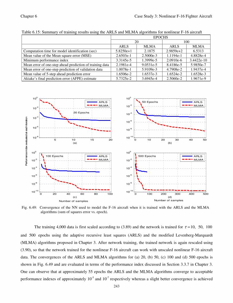
Chapter 6 Case Study 3: Nonlinear F-16 Fighter Aircraft
243
The training 4,000 data is first scaled according to (3.89) and the network is trained for 10, 50, 100τ =
and 500 epochs using the adaptive recursive least squares (ARLS) and the modified Levenberg-Marquardt
(MLMA) algorithms proposed in Chapter 3. After network training, the trained network is again rescaled using
(3.90), so that the network trained for the nonlinear F-16 aircraft can work with unscaled nonlinear F-16 aircraft
data. The convergences of the ARLS and MLMA algorithms for (a) 20, (b) 50, (c) 100 and (d) 500 epochs is
shown in Fig. 6.49 and are evaluated in terms of the performance index discussed in Section 3.3.7 in Chapter 3.
One can observe that at approximately 55 epochs the ARLS and the MLMA algorithms converge to acceptable
performance indexes of approximately 10-5
and 10-7
respectively whereas a slight better convergence is achieved
Table 6.15: Summary of training results using the ARLS and MLMA algorithms for nonlinear F-16 aircraft
EPOCHS
20 100
ARLS MLMA ARLS MLMA
Computation time for model identification (sec) 5.8250e+1 2.1875 2.9859e+2 6.5313
Mean value of the Mean square error (MSE) 2.6503e-1 2.5000e-3 1.1194e-1 4.8828e-4
Minimum performance index 3.3145e-5 1.3999e-5 2.0910e-6 3.4422e-10
Mean error of one-step ahead prediction of training data 2.1981e-4 9.0531e-5 8.4186e-5
5.9850e-7
Mean error of one-step prediction of validation data 1.0078e-1 5.9109e-3 4.7908e-2
1.9437e-4
Mean value of 5-step ahead prediction error 1.6506e-2 1.6537e-3 1.6524e-2 1.6528e-3
Akiake’s final prediction error (AFPE) estimate 5.7325e-2 3.6945e-4 2.5060e-2 1.9671e-9
5 10 15 2010
-8
10-6
10-4
10-2
100
20 Epochs
(a)
ARLS
MLMA
0 10 20 30 40 5010
-10
10-8
10-6
10-4
10-2
100
50 Epochs
(b)
ARLS
MLMA
0 20 40 60 80 10010
-10
10-8
10-6
10-4
10-2
100
100 Epochs
(c)
Number of samples
ARLS
MLMA
0 100 200 300 400 50010
-10
10-8
10-6
10-4
10-2
100
500 Epochs
(d)
Perform
ance index e
valuate
d a
t each ite
ration
Number of samples
ARLS
MLMA
Fig. 6.49: Convergence of the NN used to model the F-16 aircraft when it is trained with the ARLS and the MLMA
algorithms (sum of squares error vs. epoch).
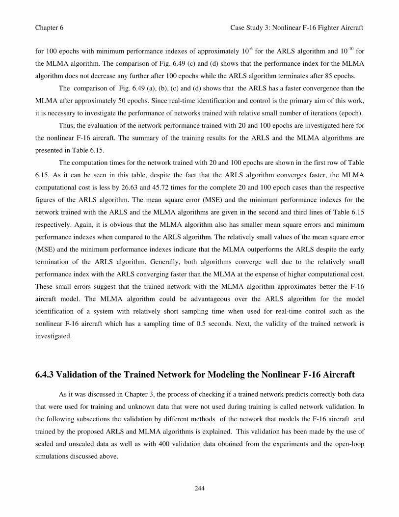
Chapter 6 Case Study 3: Nonlinear F-16 Fighter Aircraft
244
for 100 epochs with minimum performance indexes of approximately 10-6
for the ARLS algorithm and 10-10
for
the MLMA algorithm. The comparison of Fig. 6.49 (c) and (d) shows that the performance index for the MLMA
algorithm does not decrease any further after 100 epochs while the ARLS algorithm terminates after 85 epochs.
The comparison of Fig. 6.49 (a), (b), (c) and (d) shows that the ARLS has a faster convergence than the
MLMA after approximately 50 epochs. Since real-time identification and control is the primary aim of this work,
it is necessary to investigate the performance of networks trained with relative small number of iterations (epoch).
Thus, the evaluation of the network performance trained with 20 and 100 epochs are investigated here for
the nonlinear F-16 aircraft. The summary of the training results for the ARLS and the MLMA algorithms are
presented in Table 6.15.
The computation times for the network trained with 20 and 100 epochs are shown in the first row of Table
6.15. As it can be seen in this table, despite the fact that the ARLS algorithm converges faster, the MLMA
computational cost is less by 26.63 and 45.72 times for the complete 20 and 100 epoch cases than the respective
figures of the ARLS algorithm. The mean square error (MSE) and the minimum performance indexes for the
network trained with the ARLS and the MLMA algorithms are given in the second and third lines of Table 6.15
respectively. Again, it is obvious that the MLMA algorithm also has smaller mean square errors and minimum
performance indexes when compared to the ARLS algorithm. The relatively small values of the mean square error
(MSE) and the minimum performance indexes indicate that the MLMA outperforms the ARLS despite the early
termination of the ARLS algorithm. Generally, both algorithms converge well due to the relatively small
performance index with the ARLS converging faster than the MLMA at the expense of higher computational cost.
These small errors suggest that the trained network with the MLMA algorithm approximates better the F-16
aircraft model. The MLMA algorithm could be advantageous over the ARLS algorithm for the model
identification of a system with relatively short sampling time when used for real-time control such as the
nonlinear F-16 aircraft which has a sampling time of 0.5 seconds. Next, the validity of the trained network is
investigated.
6.4.3 Validation of the Trained Network for Modeling the Nonlinear F-16 Aircraft
As it was discussed in Chapter 3, the process of checking if a trained network predicts correctly both data
that were used for training and unknown data that were not used during training is called network validation. In
the following subsections the validation by different methods of the network that models the F-16 aircraft and
trained by the proposed ARLS and MLMA algorithms is explained. This validation has been made by the use of
scaled and unscaled data as well as with 400 validation data obtained from the experiments and the open-loop
simulations discussed above.
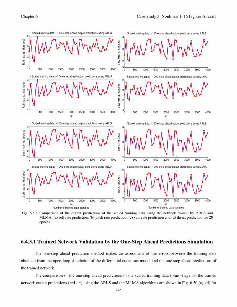
Chapter 6 Case Study 3: Nonlinear F-16 Fighter Aircraft
245
0 500 1000 1500 2000 2500 3000 3500 4000-4
-2
0
2
Ro
ll ra
te (
p,
de
g/s
ec
)
- Scaled training data; --* One-step ahead output predictions using ARLS
0 500 1000 1500 2000 2500 3000 3500 4000-4
-2
0
2
Ro
ll ra
te (
p,
de
g/s
ec
)
(a)
- Scaled training data; --* One-step ahead output predictions using MLMA
0 500 1000 1500 2000 2500 3000 3500 4000-3
-2
-1
0
1
2
pit
ch
ra
te (
q,
de
g/s
ec
)
- Scaled training data; --* One-step ahead output predictions using ARLS
0 500 1000 1500 2000 2500 3000 3500 4000-4
-2
0
2
pit
ch
ra
te (
q,
de
g/s
ec
)
- Scaled training data; --* One-step ahead output predictions using MLMA
(b)
Number of training data samples
0 500 1000 1500 2000 2500 3000 3500 4000-3
-2
-1
0
1
2
Ya
w r
ate
(r,
de
g/s
ec
)
- Scaled training data; --* One-step ahead output predictions using ARLS
0 500 1000 1500 2000 2500 3000 3500 4000-4
-2
0
2
Ya
w r
ate
(r,
de
g/s
ec
)(c)
- Scaled training data; --* One-step ahead output predictions using MLMA
0 500 1000 1500 2000 2500 3000 3500 4000-2
-1
0
1
2
Th
rus
t (l
b/s
ec
)
- Scaled training data; --* One-step ahead output predictions using ARLS
0 500 1000 1500 2000 2500 3000 3500 4000-2
-1
0
1
2
Th
rus
t (l
b/s
ec
)
- Scaled training data; --* One-step ahead output predictions using MLMA
(d)
Number of training data samples
Fig. 6.50: Comparison of the output predictions of the scaled training data using the network trained by ARLS and
MLMA: (a) roll rate prediction, (b) pitch rate prediction, (c) yaw rate prediction and (d) thrust prediction for 20
epochs.
6.4.3.1 Trained Network Validation by the One-Step Ahead Predictions Simulation
The one-step ahead prediction method makes an assessment of the errors between the training data
obtained from the open-loop simulation of the differential equations model and the one-step ahead predictions of
the trained network.
The comparison of the one-step ahead predictions of the scaled training data (blue -) against the trained
network output predictions (red --*) using the ARLS and the MLMA algorithms are shown in Fig. 6.50 (a)–(d) for
Chapter 6 Case Study 3: Nonlinear F-16 Fighter Aircraft
246
the roll rate ˆ( )p , pitch rate ˆ( )q , yaw rate ˆ( )r and the thrust ˆ( )t respectively for 20 epochs. Similar one-step
validation results for 100 epochs are also shown in Fig. 6.51 (a)–(d).
The one-step ahead prediction errors for the scaled training data or 20 and 100 epochs when the network
is trained by using the ARLS and the MLMA algorithms are given in the fourth line of Table 6.15. It can be seen
in Fig. 6.50 (a)–(c) and Fig. 6.51 (a)–(c) that the network predictions of the roll rate ˆ( )p , pitch rate ˆ( )q , yaw rate
ˆ( )r and the thrust ˆ( )t training data closely match the original data used for the network training. A slight
prediction mismatch is observed in Fig. 6.50 (d) and Fig. 6.51(d) when the ARLS algorithm is used. Also, the
0 500 1000 1500 2000 2500 3000 3500 4000-4
-2
0
2
Ro
ll ra
te (
p,
de
g/s
ec
)
- Scaled training data; --* One-step ahead output predictions using ARLS
0 500 1000 1500 2000 2500 3000 3500 4000-4
-2
0
2
Ro
ll ra
te (
p,
de
g/s
ec
)
(a)
- Scaled training data; --* One-step ahead output predictions using MLMA
0 500 1000 1500 2000 2500 3000 3500 4000-3
-2
-1
0
1
2
pit
ch
ra
te (
q,
de
g/s
ec
)
- Scaled training data; --* One-step ahead output predictions using ARLS
0 500 1000 1500 2000 2500 3000 3500 4000-4
-2
0
2
pit
ch
ra
te (
q,
de
g/s
ec
)
- Scaled training data; --* One-step ahead output predictions using MLMA
(b)
Number of training data samples
0 500 1000 1500 2000 2500 3000 3500 4000-3
-2
-1
0
1
2
Ya
w r
ate
(r,
de
g/s
ec
)
- Scaled training data; --* One-step ahead output predictions using ARLS
0 500 1000 1500 2000 2500 3000 3500 4000-4
-2
0
2
Ya
w r
ate
(r,
de
g/s
ec
)
(c)
- Scaled training data; --* One-step ahead output predictions using MLMA
0 500 1000 1500 2000 2500 3000 3500 4000-2
-1
0
1
2
Th
rus
t (l
b/s
ec
)- Scaled training data; --* One-step ahead output predictions using ARLS
0 500 1000 1500 2000 2500 3000 3500 4000-2
-1
0
1
2
Th
rus
t (l
b/s
ec
)
- Scaled training data; --* One-step ahead output predictions using MLMA
(d)
Number of training data samples
Fig. 6.51: Comparison of the outpredictions of the scaled training data using the network trained by ARLS and MLMA: (a)
roll rate prediction, (b) pitch rate prediction, (c) yaw rate prediction and (d) thrust prediction for 100 Epochs.
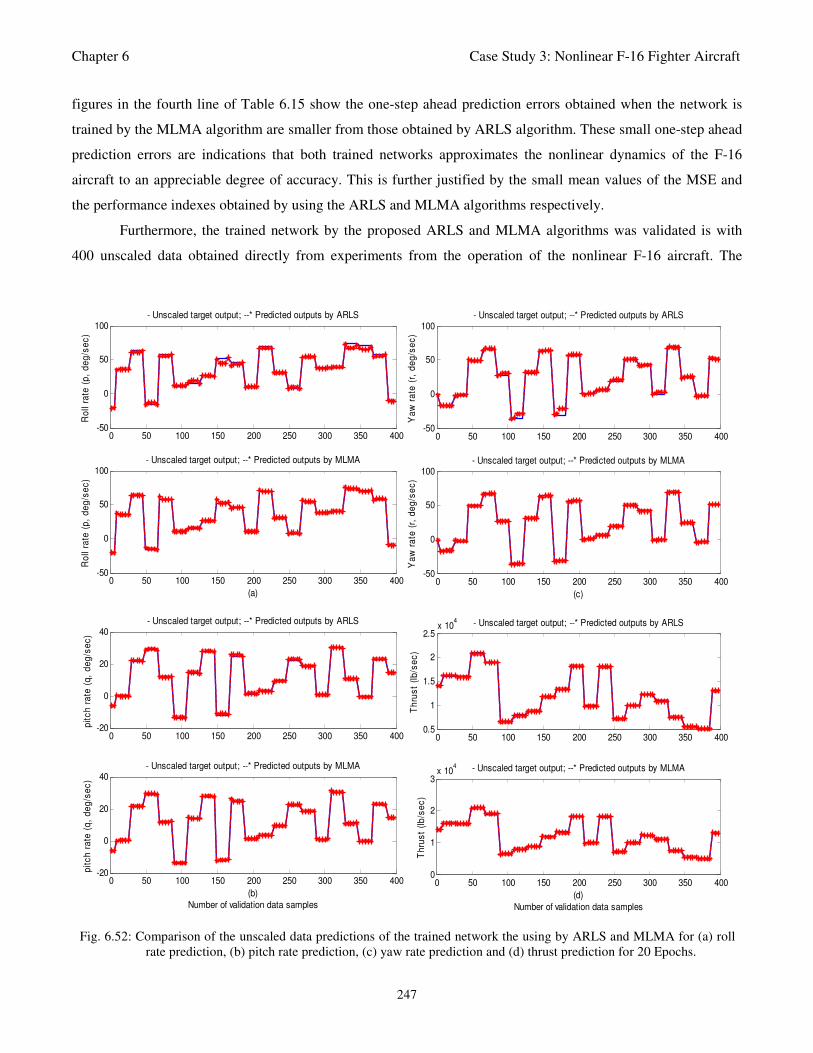
Chapter 6 Case Study 3: Nonlinear F-16 Fighter Aircraft
247
figures in the fourth line of Table 6.15 show the one-step ahead prediction errors obtained when the network is
trained by the MLMA algorithm are smaller from those obtained by ARLS algorithm. These small one-step ahead
prediction errors are indications that both trained networks approximates the nonlinear dynamics of the F-16
aircraft to an appreciable degree of accuracy. This is further justified by the small mean values of the MSE and
the performance indexes obtained by using the ARLS and MLMA algorithms respectively.
Furthermore, the trained network by the proposed ARLS and MLMA algorithms was validated is with
400 unscaled data obtained directly from experiments from the operation of the nonlinear F-16 aircraft. The
0 50 100 150 200 250 300 350 400-50
0
50
100
Ro
ll ra
te (
p,
de
g/s
ec
)
- Unscaled target output; --* Predicted outputs by ARLS
0 50 100 150 200 250 300 350 400-50
0
50
100
Ro
ll ra
te (
p,
de
g/s
ec
)
- Unscaled target output; --* Predicted outputs by MLMA
(a)
0 50 100 150 200 250 300 350 400-20
0
20
40
pit
ch
ra
te (
q,
de
g/s
ec
)
- Unscaled target output; --* Predicted outputs by ARLS
0 50 100 150 200 250 300 350 400-20
0
20
40
pit
ch
ra
te (
q,
de
g/s
ec
)
- Unscaled target output; --* Predicted outputs by MLMA
(b)
Number of validation data samples
0 50 100 150 200 250 300 350 400-50
0
50
100
Ya
w r
ate
(r,
de
g/s
ec
)
- Unscaled target output; --* Predicted outputs by ARLS
0 50 100 150 200 250 300 350 400-50
0
50
100
Ya
w r
ate
(r,
de
g/s
ec
)
- Unscaled target output; --* Predicted outputs by MLMA
(c)
0 50 100 150 200 250 300 350 4000.5
1
1.5
2
2.5x 10
4
Th
rus
t (l
b/s
ec
)
- Unscaled target output; --* Predicted outputs by ARLS
0 50 100 150 200 250 300 350 4000
1
2
3x 10
4
Th
rus
t (l
b/s
ec
)
- Unscaled target output; --* Predicted outputs by MLMA
(d)
Number of validation data samples
Fig. 6.52: Comparison of the unscaled data predictions of the trained network the using by ARLS and MLMA for (a) roll
rate prediction, (b) pitch rate prediction, (c) yaw rate prediction and (d) thrust prediction for 20 Epochs.
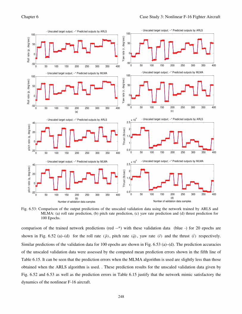
Chapter 6 Case Study 3: Nonlinear F-16 Fighter Aircraft
248
comparison of the trained network predictions (red --*) with these validation data (blue -) for 20 epochs are
shown in Fig. 6.52 (a)–(d) for the roll rate ˆ( )p , pitch rate ˆ( )q , yaw rate ˆ( )r and the thrust ˆ( )t respectively.
Similar predictions of the validation data for 100 epochs are shown in Fig. 6.53 (a)–(d). The prediction accuracies
of the unscaled validation data were assessed by the computed mean prediction errors shown in the fifth line of
Table 6.15. It can be seen that the prediction errors when the MLMA algorithm is used are slightly less than those
obtained when the ARLS algorithm is used. . These prediction results for the unscaled validation data given by
Fig. 6.52 and 6.53 as well as the prediction errors in Table 6.15 justify that the network mimic satisfactory the
dynamics of the nonlinear F-16 aircraft.
0 50 100 150 200 250 300 350 400-50
0
50
100
Ro
ll ra
te (
p,
de
g/s
ec
)- Unscaled target output; --* Predicted outputs by ARLS
0 50 100 150 200 250 300 350 400-50
0
50
100
Ro
ll ra
te (
p,
de
g/s
ec
)
- Unscaled target output; --* Predicted outputs by MLMA
(a)
0 50 100 150 200 250 300 350 400-20
0
20
40
pit
ch
ra
te (
q,
de
g/s
ec
)
- Unscaled target output; --* Predicted outputs by ARLS
0 50 100 150 200 250 300 350 400-20
0
20
40
pit
ch
ra
te (
q,
de
g/s
ec
)
- Unscaled target output; --* Predicted outputs by MLMA
(b)
Number of validation data samples
0 50 100 150 200 250 300 350 400-50
0
50
100
Ya
w r
ate
(r,
de
g/s
ec
)
- Unscaled target output; --* Predicted outputs by ARLS
0 50 100 150 200 250 300 350 400-50
0
50
100
Ya
w r
ate
(r,
de
g/s
ec
)
- Unscaled target output; --* Predicted outputs by MLMA
(c)
0 50 100 150 200 250 300 350 4000.5
1
1.5
2
2.5x 10
4
Th
rus
t (l
b/s
ec
)
- Unscaled target output; --* Predicted outputs by ARLS
0 50 100 150 200 250 300 350 4000.5
1
1.5
2
2.5x 10
4
Th
rus
t (l
b/s
ec
)
- Unscaled target output; --* Predicted outputs by MLMA
(d)
Number of validation data samples
Fig. 6.53: Comparison of the output predictions of the unscaled validation data using the network trained by ARLS and
MLMA: (a) roll rate prediction, (b) pitch rate prediction, (c) yaw rate prediction and (d) thrust prediction for
100 Epochs.
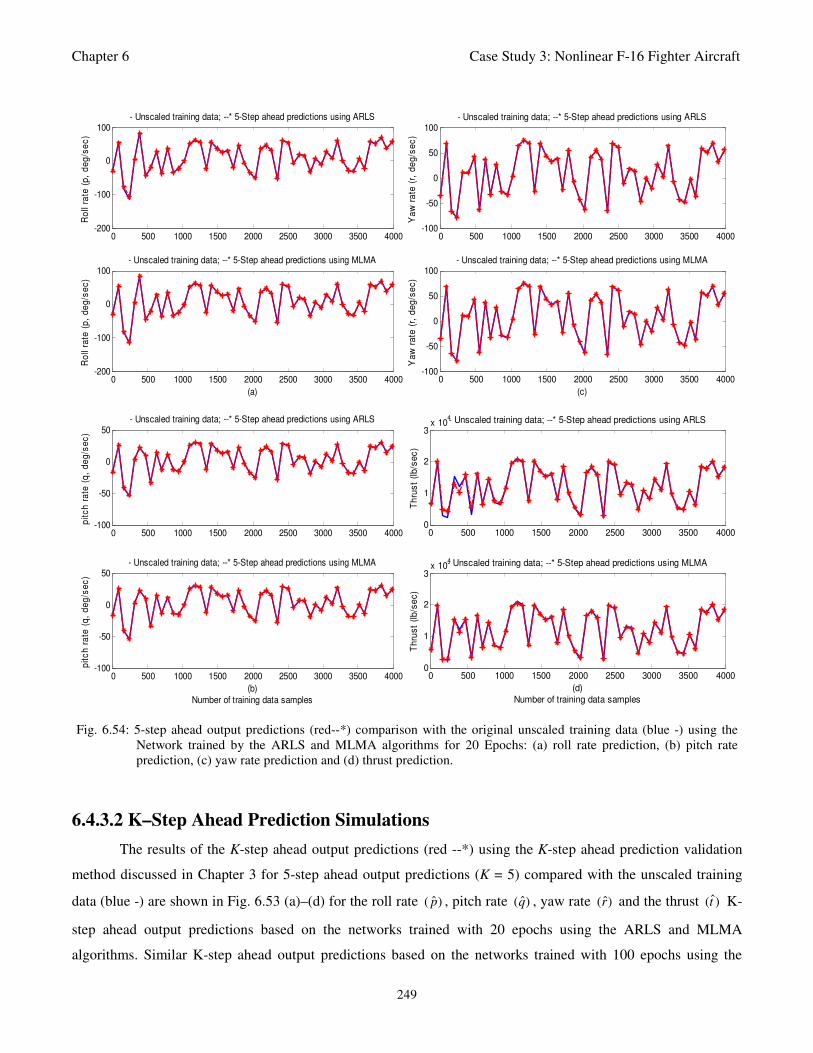
Chapter 6 Case Study 3: Nonlinear F-16 Fighter Aircraft
249
6.4.3.2 K–Step Ahead Prediction Simulations
The results of the K-step ahead output predictions (red --*) using the K-step ahead prediction validation
method discussed in Chapter 3 for 5-step ahead output predictions (K = 5) compared with the unscaled training
data (blue -) are shown in Fig. 6.53 (a)–(d) for the roll rate ˆ( )p , pitch rate ˆ( )q , yaw rate ˆ( )r and the thrust ˆ( )t K-
step ahead output predictions based on the networks trained with 20 epochs using the ARLS and MLMA
algorithms. Similar K-step ahead output predictions based on the networks trained with 100 epochs using the
0 500 1000 1500 2000 2500 3000 3500 4000-200
-100
0
100
Ro
ll ra
te (
p,
de
g/s
ec
)
- Unscaled training data; --* 5-Step ahead predictions using ARLS
0 500 1000 1500 2000 2500 3000 3500 4000-200
-100
0
100
Ro
ll ra
te (
p,
de
g/s
ec
)
- Unscaled training data; --* 5-Step ahead predictions using MLMA
(a)
0 500 1000 1500 2000 2500 3000 3500 4000-100
-50
0
50
pit
ch
ra
te (
q,
de
g/s
ec
)
- Unscaled training data; --* 5-Step ahead predictions using ARLS
0 500 1000 1500 2000 2500 3000 3500 4000-100
-50
0
50
pit
ch
ra
te (
q,
de
g/s
ec
)
- Unscaled training data; --* 5-Step ahead predictions using MLMA
(b)
Number of training data samples
0 500 1000 1500 2000 2500 3000 3500 4000-100
-50
0
50
100
Ya
w r
ate
(r,
de
g/s
ec
)
- Unscaled training data; --* 5-Step ahead predictions using ARLS
0 500 1000 1500 2000 2500 3000 3500 4000-100
-50
0
50
100
Ya
w r
ate
(r,
de
g/s
ec
)
- Unscaled training data; --* 5-Step ahead predictions using MLMA
(c)
0 500 1000 1500 2000 2500 3000 3500 40000
1
2
3x 10
4T
hru
st
(lb
/se
c)
- Unscaled training data; --* 5-Step ahead predictions using ARLS
0 500 1000 1500 2000 2500 3000 3500 40000
1
2
3x 10
4
Th
rus
t (l
b/s
ec
)
- Unscaled training data; --* 5-Step ahead predictions using MLMA
(d)
Number of training data samples
Fig. 6.54: 5-step ahead output predictions (red--*) comparison with the original unscaled training data (blue -) using the
Network trained by the ARLS and MLMA algorithms for 20 Epochs: (a) roll rate prediction, (b) pitch rate
prediction, (c) yaw rate prediction and (d) thrust prediction.
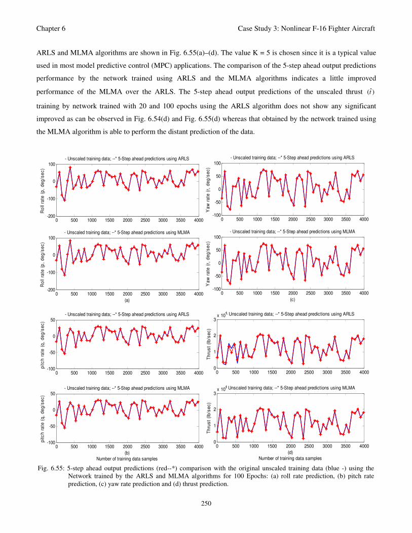
Chapter 6 Case Study 3: Nonlinear F-16 Fighter Aircraft
250
ARLS and MLMA algorithms are shown in Fig. 6.55(a)–(d). The value K = 5 is chosen since it is a typical value
used in most model predictive control (MPC) applications. The comparison of the 5-step ahead output predictions
performance by the network trained using ARLS and the MLMA algorithms indicates a little improved
performance of the MLMA over the ARLS. The 5-step ahead output predictions of the unscaled thrust ˆ( )t
training by network trained with 20 and 100 epochs using the ARLS algorithm does not show any significant
improved as can be observed in Fig. 6.54(d) and Fig. 6.55(d) whereas that obtained by the network trained using
the MLMA algorithm is able to perform the distant prediction of the data.
0 500 1000 1500 2000 2500 3000 3500 4000-200
-100
0
100
Ro
ll ra
te (
p,
de
g/s
ec
)
- Unscaled training data; --* 5-Step ahead predictions using ARLS
0 500 1000 1500 2000 2500 3000 3500 4000-200
-100
0
100
Ro
ll ra
te (
p,
de
g/s
ec
)
- Unscaled training data; --* 5-Step ahead predictions using MLMA
(a)
0 500 1000 1500 2000 2500 3000 3500 4000-100
-50
0
50
pit
ch
ra
te (
q,
de
g/s
ec
)
- Unscaled training data; --* 5-Step ahead predictions using ARLS
0 500 1000 1500 2000 2500 3000 3500 4000-100
-50
0
50
pit
ch
ra
te (
q,
de
g/s
ec
)
- Unscaled training data; --* 5-Step ahead predictions using MLMA
(b)
Number of training data samples
0 500 1000 1500 2000 2500 3000 3500 4000-100
-50
0
50
100
Ya
w r
ate
(r,
de
g/s
ec
)
- Unscaled training data; --* 5-Step ahead predictions using ARLS
0 500 1000 1500 2000 2500 3000 3500 4000-100
-50
0
50
100
Ya
w r
ate
(r,
de
g/s
ec
)
- Unscaled training data; --* 5-Step ahead predictions using MLMA
(c)
0 500 1000 1500 2000 2500 3000 3500 40000
1
2
3x 10
4
Th
rus
t (l
b/s
ec
)
- Unscaled training data; --* 5-Step ahead predictions using ARLS
0 500 1000 1500 2000 2500 3000 3500 40000
1
2
3x 10
4
Th
rus
t (l
b/s
ec
)
- Unscaled training data; --* 5-Step ahead predictions using MLMA
(d)
Number of training data samples
Fig. 6.55: 5-step ahead output predictions (red--*) comparison with the original unscaled training data (blue -) using the
Network trained by the ARLS and MLMA algorithms for 100 Epochs: (a) roll rate prediction, (b) pitch rate
prediction, (c) yaw rate prediction and (d) thrust prediction.
Chapter 6 Case Study 3: Nonlinear F-16 Fighter Aircraft
251
The computation of the mean value of the 5-step ahead prediction error (MVPE) using (3.93) gives
1.6506e-002 and 1.6537e-003 by the network trained using ARLS and MLMA algorithms for 20 epoch and
1.6524e-2 and 1.6528e-3 for 100 epoch respectively as shown in the sixth line in Table 6.15. The small mean
values of the 5-step ahead prediction error (MVPE) are indications that the trained network approximates the
dynamics of the nonlinear F-16 aircraft to an appreciable degree of accuracy with the network using MLMA
giving smaller prediction errors.
By comparing the one-step output prediction of the scaled thrust ˆ( )t training in Fig. 6.50(d) and Fig.
6.51(d) with the 5-step ahead output predictions of the unsclaed thrust ˆ( )t data in terms of Fig. 6.54(d) and Fig.
6.55(d), the network trained using the ARLS algorithm does not predict accurately the thrust ˆ( )t data. This is also
justified by the respective one-step and 5-step ahead predictions errors on the fourth and sixth lines on Table 6.15
respectively. This is due to the magnitude of the thrust ˆ( )t data despite the scaling as in Fig. 6.52. On the other
hand, the MLMA algorithm provides additional scaling based on the scaling parameter s in the formulation of the
MLMA algorithm in Chapter 3. This pre-scaling property introduced in the MLMA is evident in the accurate
prediction of the thrust ˆ( )t data with relatively small prediction errors when compared to that obtained using the
ARLS. However, the small output predictions errors obtained by the networks of both the ARLS and MLMA
algorithms are acceptable but the further verification of these algorithms for online identification and control will
be investigated to further justify their performances.
6.4.3.3 The Akaike’s Final Prediction Error (AFPE) Estimates
The implementation of the AFPE algorithm discussed in Chapter 3 and defined by (3.94) resulted to the
estimates which are given in the last line of Table 6.15 for 20 and 100 epochs. This implementation concerns the
network that is trained with ARLS and the MLMA algorithms with multiple weight decay for the regularized
criterion. These small values of the AFPE estimates indicate that the trained captures the underlying dynamics of
the nonlinear F-16 aircraft and is not over-trained [Sjöberg and Ljung, 1995]. This in turn implies that optimal
network parameters have been selected including the weight decay parameters. Again, the results of the AFPE
estimates computed for the networks trained using the MLMA algorithm are much smaller when compared to
those obtained using ARLS algorithm.
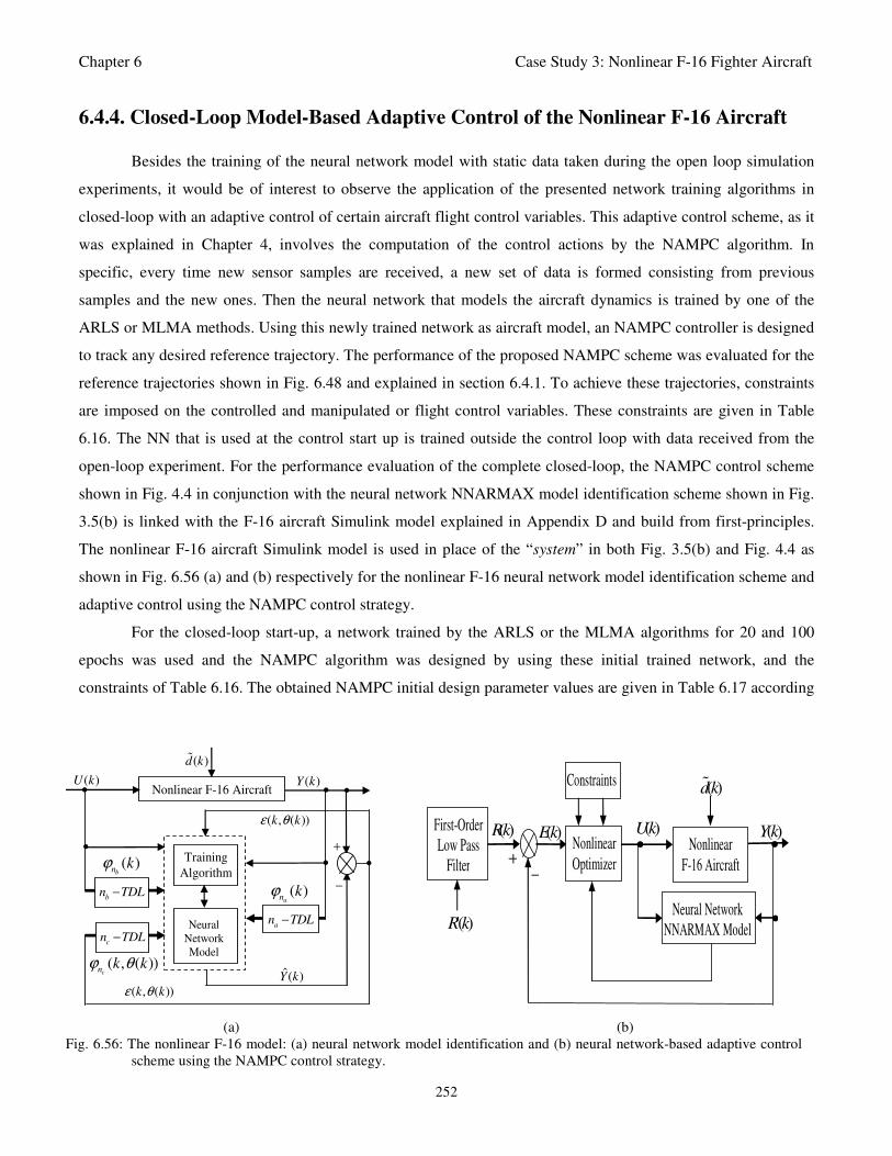
Chapter 6 Case Study 3: Nonlinear F-16 Fighter Aircraft
252
Training
Algorithm
Neural
Network
Model
b
n TDL−
a
n TDL−
Nonlinear F-16 Aircraft
( , ( ))k kε θ
ˆ( )Y k
( )Y k ( )U k • •
•
•
•
+
−
( )bn
kϕ
( )an
kϕ
cn TDL−
( , ( ))cn k kϕ θ
( )d k
•
( , ( ))k kε θ
Nonlinear
F-16 Aircraft
( )Yk ( )Uk •
Neural Network
NNARMAX Model
Nonlinear
Optimizer •
+ −
'( )R k
( )Ek
•
Constraints
First-Order
Low Pass
Filter
( )dk
( )Rk
(a) (b)
Fig. 6.56: The nonlinear F-16 model: (a) neural network model identification and (b) neural network-based adaptive control
scheme using the NAMPC control strategy.
6.4.4. Closed-Loop Model-Based Adaptive Control of the Nonlinear F-16 Aircraft
Besides the training of the neural network model with static data taken during the open loop simulation
experiments, it would be of interest to observe the application of the presented network training algorithms in
closed-loop with an adaptive control of certain aircraft flight control variables. This adaptive control scheme, as it
was explained in Chapter 4, involves the computation of the control actions by the NAMPC algorithm. In
specific, every time new sensor samples are received, a new set of data is formed consisting from previous
samples and the new ones. Then the neural network that models the aircraft dynamics is trained by one of the
ARLS or MLMA methods. Using this newly trained network as aircraft model, an NAMPC controller is designed
to track any desired reference trajectory. The performance of the proposed NAMPC scheme was evaluated for the
reference trajectories shown in Fig. 6.48 and explained in section 6.4.1. To achieve these trajectories, constraints
are imposed on the controlled and manipulated or flight control variables. These constraints are given in Table
6.16. Τhe NN that is used at the control start up is trained outside the control loop with data received from the
open-loop experiment. For the performance evaluation of the complete closed-loop, the NAMPC control scheme
shown in Fig. 4.4 in conjunction with the neural network NNARMAX model identification scheme shown in Fig.
3.5(b) is linked with the F-16 aircraft Simulink model explained in Appendix D and build from first-principles.
The nonlinear F-16 aircraft Simulink model is used in place of the “system” in both Fig. 3.5(b) and Fig. 4.4 as
shown in Fig. 6.56 (a) and (b) respectively for the nonlinear F-16 neural network model identification scheme and
adaptive control using the NAMPC control strategy.
For the closed-loop start-up, a network trained by the ARLS or the MLMA algorithms for 20 and 100
epochs was used and the NAMPC algorithm was designed by using these initial trained network, and the
constraints of Table 6.16. The obtained NAMPC initial design parameter values are given in Table 6.17 according
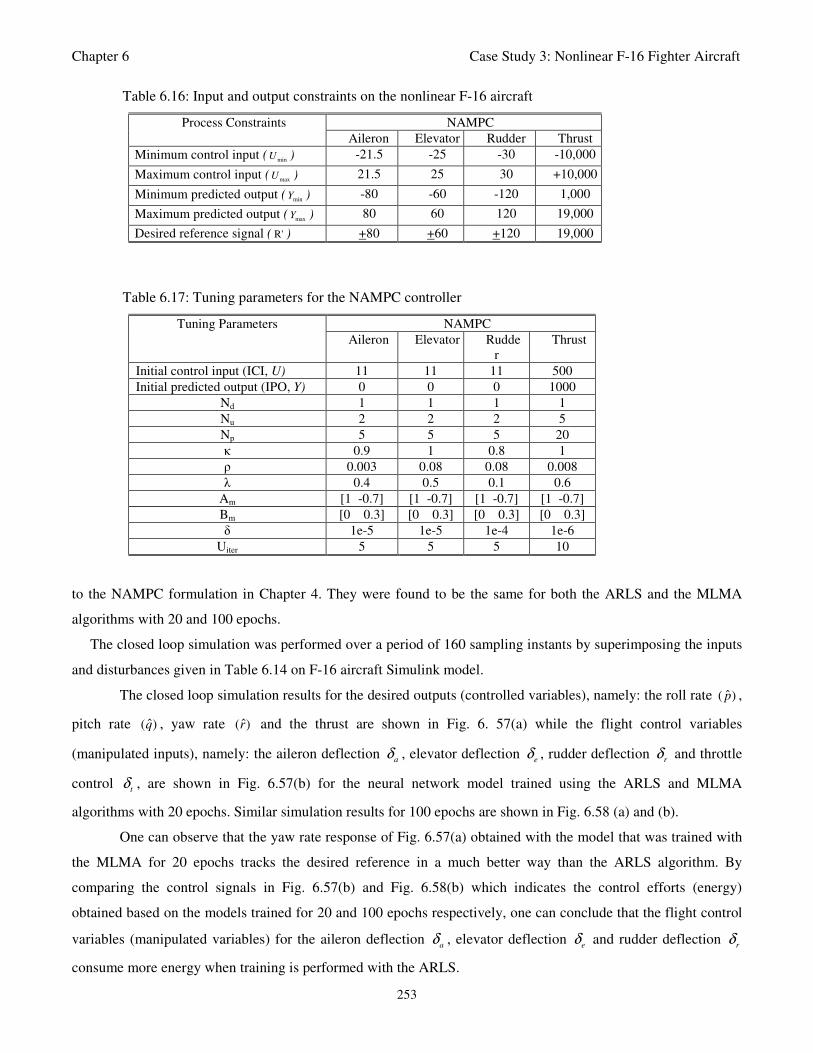
Chapter 6 Case Study 3: Nonlinear F-16 Fighter Aircraft
253
Table 6.16: Input and output constraints on the nonlinear F-16 aircraft
NAMPC Process Constraints
Aileron Elevator Rudder Thrust
Minimum control input (minU ) -21.5 -25 -30 -10,000
Maximum control input (maxU ) 21.5 25 30 +10,000
Minimum predicted output (minY ) -80 -60 -120 1,000
Maximum predicted output (maxY ) 80 60 120 19,000
Desired reference signal ( R' ) +80 +60 +120 19,000
Table 6.17: Tuning parameters for the NAMPC controller
NAMPC Tuning Parameters
Aileron Elevator Rudde
r
Thrust
Initial control input (ICI, U) 11 11 11 500
Initial predicted output (IPO, Y) 0 0 0 1000
Nd 1 1 1 1
Nu 2 2 2 5
Np 5 5 5 20
κ 0.9 1 0.8 1
ρ 0.003 0.08 0.08 0.008
λ 0.4 0.5 0.1 0.6
Am [1 -0.7] [1 -0.7] [1 -0.7] [1 -0.7]
Bm [0 0.3] [0 0.3] [0 0.3] [0 0.3]
δ 1e-5 1e-5 1e-4 1e-6
Uiter 5 5 5 10
to the NAMPC formulation in Chapter 4. They were found to be the same for both the ARLS and the MLMA
algorithms with 20 and 100 epochs.
The closed loop simulation was performed over a period of 160 sampling instants by superimposing the inputs
and disturbances given in Table 6.14 on F-16 aircraft Simulink model.
The closed loop simulation results for the desired outputs (controlled variables), namely: the roll rate ˆ( )p ,
pitch rate ˆ( )q , yaw rate ˆ( )r and the thrust are shown in Fig. 6. 57(a) while the flight control variables
(manipulated inputs), namely: the aileron deflection a
δ , elevator deflection e
δ , rudder deflection r
δ and throttle
control t
δ , are shown in Fig. 6.57(b) for the neural network model trained using the ARLS and MLMA
algorithms with 20 epochs. Similar simulation results for 100 epochs are shown in Fig. 6.58 (a) and (b).
One can observe that the yaw rate response of Fig. 6.57(a) obtained with the model that was trained with
the MLMA for 20 epochs tracks the desired reference in a much better way than the ARLS algorithm. By
comparing the control signals in Fig. 6.57(b) and Fig. 6.58(b) which indicates the control efforts (energy)
obtained based on the models trained for 20 and 100 epochs respectively, one can conclude that the flight control
variables (manipulated variables) for the aileron deflection a
δ , elevator deflection e
δ and rudder deflection r
δ
consume more energy when training is performed with the ARLS.
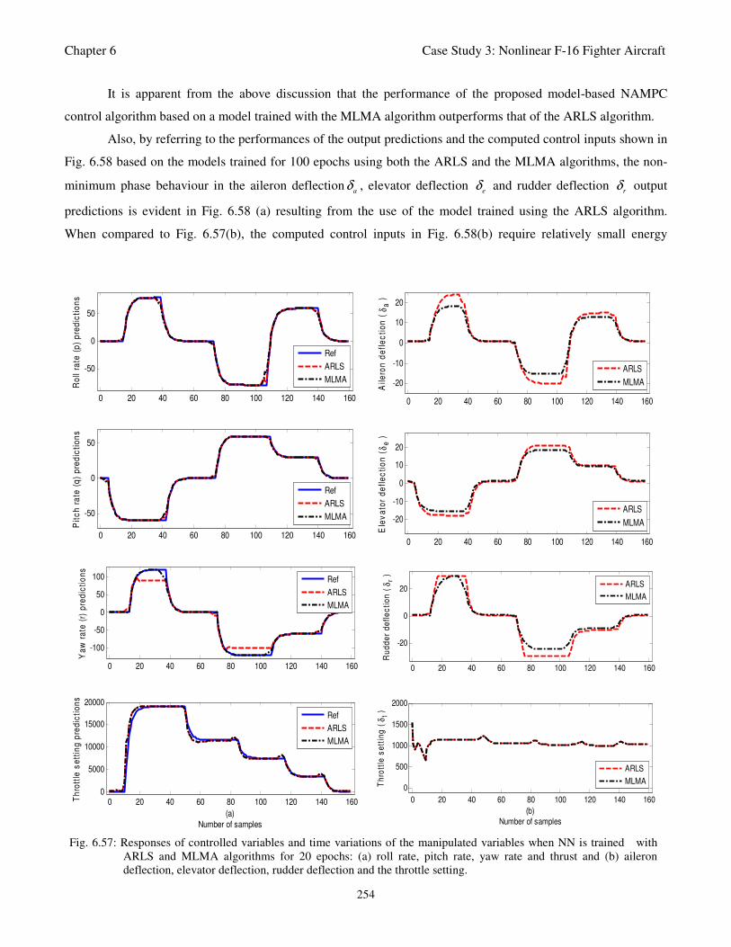
Chapter 6 Case Study 3: Nonlinear F-16 Fighter Aircraft
254
It is apparent from the above discussion that the performance of the proposed model-based NAMPC
control algorithm based on a model trained with the MLMA algorithm outperforms that of the ARLS algorithm.
Also, by referring to the performances of the output predictions and the computed control inputs shown in
Fig. 6.58 based on the models trained for 100 epochs using both the ARLS and the MLMA algorithms, the non-
minimum phase behaviour in the aileron deflectiona
δ , elevator deflection e
δ and rudder deflection r
δ output
predictions is evident in Fig. 6.58 (a) resulting from the use of the model trained using the ARLS algorithm.
When compared to Fig. 6.57(b), the computed control inputs in Fig. 6.58(b) require relatively small energy
0 20 40 60 80 100 120 140 160
-50
0
50
Ro
ll ra
te (
p)
pre
dic
tio
ns
Ref
ARLS
MLMA
0 20 40 60 80 100 120 140 160
-50
0
50
Pit
ch
ra
te (
q)
pre
dic
tio
ns
Ref
ARLS
MLMA
0 20 40 60 80 100 120 140 160
-100
-50
0
50
100
Ya
w r
ate
(r)
pre
dic
tio
ns
Ref
ARLS
MLMA
0 20 40 60 80 100 120 140 1600
5000
10000
15000
20000
(a)
Number of samples
Th
rott
le s
ett
ing
pre
dic
tio
ns
Ref
ARLS
MLMA
0 20 40 60 80 100 120 140 160
-20
-10
0
10
20
Aile
ron
de
fle
cti
on
( δ
a )
ARLS
MLMA
0 20 40 60 80 100 120 140 160
-20
-10
0
10
20
Ele
va
tor
de
fle
cti
on
( δ
e )
ARLS
MLMA
0 20 40 60 80 100 120 140 160
-20
0
20
Ru
dd
er
de
fle
cti
on
( δ
r )
ARLS
MLMA
0 20 40 60 80 100 120 140 160
0
500
1000
1500
2000
(b)
Number of samples
Th
rott
le s
ett
ing
( δ
t )
ARLS
MLMA
Fig. 6.57: Responses of controlled variables and time variations of the manipulated variables when NN is trained with
ARLS and MLMA algorithms for 20 epochs: (a) roll rate, pitch rate, yaw rate and thrust and (b) aileron
deflection, elevator deflection, rudder deflection and the throttle setting.
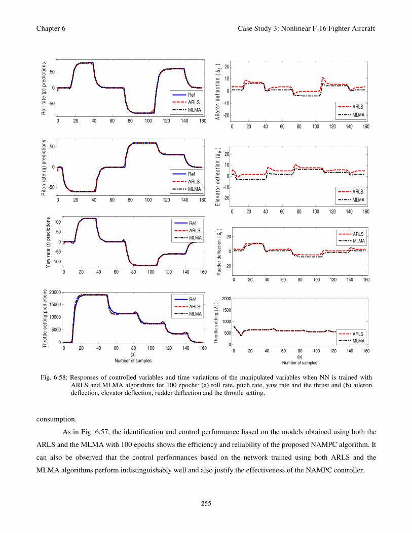
Chapter 6 Case Study 3: Nonlinear F-16 Fighter Aircraft
255
consumption.
As in Fig. 6.57, the identification and control performance based on the models obtained using both the
ARLS and the MLMA with 100 epochs shows the efficiency and reliability of the proposed NAMPC algorithm. It
can also be observed that the control performances based on the network trained using both ARLS and the
MLMA algorithms perform indistinguishably well and also justify the effectiveness of the NAMPC controller.
0 20 40 60 80 100 120 140 160
-50
0
50
Ro
ll ra
te (
p)
pre
dic
tio
ns
Ref
ARLS
MLMA
0 20 40 60 80 100 120 140 160
-50
0
50
Pit
ch
ra
te (
q)
pre
dic
tio
ns
Ref
ARLS
MLMA
0 20 40 60 80 100 120 140 160
-100
-50
0
50
100
Ya
w r
ate
(r)
pre
dic
tio
ns
Ref
ARLS
MLMA
0 20 40 60 80 100 120 140 1600
5000
10000
15000
20000
(a)
Number of samples
Th
rott
le s
ett
ing
pre
dic
tio
ns
Ref
ARLS
MLMA
0 20 40 60 80 100 120 140 160
-20
-10
0
10
20
Aile
ron
de
fle
cti
on
( δ
a )
ARLS
MLMA
0 20 40 60 80 100 120 140 160
-20
-10
0
10
20
Ele
va
tor
de
fle
cti
on
( δ
e )
ARLS
MLMA
0 20 40 60 80 100 120 140 160
-20
0
20
Ru
dd
er
de
fle
cti
on
( δ
r )
ARLS
MLMA
0 20 40 60 80 100 120 140 160
0
500
1000
1500
2000
(b)
Number of samples
Th
rott
le s
ett
ing
( δ
t )
ARLS
MLMA
Fig. 6.58: Responses of controlled variables and time variations of the manipulated variables when NN is trained with
ARLS and MLMA algorithms for 100 epochs: (a) roll rate, pitch rate, yaw rate and the thrust and (b) aileron
deflection, elevator deflection, rudder deflection and the throttle setting.

Chapter 6 Case Study 3: Nonlinear F-16 Fighter Aircraft
256
Table 6.18: Constraints for the nonlinear F-16 aircraft
AGPC NAMPC Process Constraints
Aileron Elevator Rudder Thrust Aileron Elevator Rudder Thrust
Minimum control input (minU ) -21.5 -25 -30 -10,000 -21.5 -25 -30 -10,000
Maximum control input (maxU ) 21.5 25 30 10,000 21.5 25 30 10,000
Minimum predicted output (minY ) -80 -60 -120 1,000 -80 -60 -120 1,000
Maximum predicted output (maxY ) 80 60 120 190000 80 60 120 190000
Desired reference signal ( R' ) +80 +60 +120 19000 +80 +60 +120 19000
Table 6.19: Tuning parameters for GPC and NAMPC controllers
AGPC NAMPC Tuning Parameters
Aileron Elevator Rudder Thrust Aileron Elevator Rudder Thrust
Initial control input (ICI, U) 11 11 11 500 11 11 11 500
Initial predicted output (IPO, Y) 0 0 0 1000 0 0 0 1000
Nd 1 1 1 1 1 1 1 1
Nu 2 2 2 3 2 2 2 5
Np 4 4 4 7 5 5 5 20
κ 2 1 1.3 4.8 0.9 1 0.8 1
ρ 1 0.8 0.8 1.2 0.003 0.08 0.08 0.008
λ - - - - 0.4 0.5 0.1 0.6
Am [1 -0.7] [1.05 -0.7] [1 -0.7] [1 -0.7] [1 -0.7] [1 -0.7] [1 -0.7] [1 -0.7]
Bm [0 0.3] [0 0.3] [0 0.3] [0 0.3] [0 0.3] [0 0.3] [0 0.3] [0 0.3]
δ - - - - 1e-5 1e-5 1e-4 1e-6
Uiter - - - - 5 5 5 10
6.4.5 Evaluation and Performance Comparison of the AGPC and NAMPC
Algorithms for the Control of the Nonlinear F-16 Aircraft Auto-Pilot System
Initially, the neural network model of the F-16 aircraft is identified and validated as explained in the sub-
section 6.4.1. The controllers were then simulated subject to the constraints given in Table 6.18 and tuned using
the NN model of the aircraft. The obtained optimal tuning parameters are given in Table 6.19. Next, the nonlinear
F-16 aircraft model is placed in closed-loop with the NN identification scheme based on the ARLS algorithm and
the AGPC and NAMPC controllers. At each sampling instant, a new input-output data is obtained from the
aircraft, a neural network model is identified and the two controllers are designed and implemented online.
6.4.5.1Comparison of Simulation Results of AGPC and NAMPC Controllers
The closed-loop AGPC and the NAMPC responses for the roll rate, pitch rate, yaw rate and the throttle
setting are shown in Fig. 6.59(a) – (d) while the time variations of the manipulated variables, that is, the aileron
deflection, elevator deflection, rudder deflection and the thrust are shown in Fig. 6.59(e) – (h).
For the roll, pitch and yaw rate, the AGPC and the NAMPC perform very well as can be seen in Fig.
6.59(a)–(c). However, in Fig. 6.59(d) one can observe that the NAMPC shows better control performance over the
AGPC where the magnitude of the throttle setting is very large. Actually, the AGPC exhibits some oscillatory
overshoots and hardly tracks the desired reference signal for the throttle.
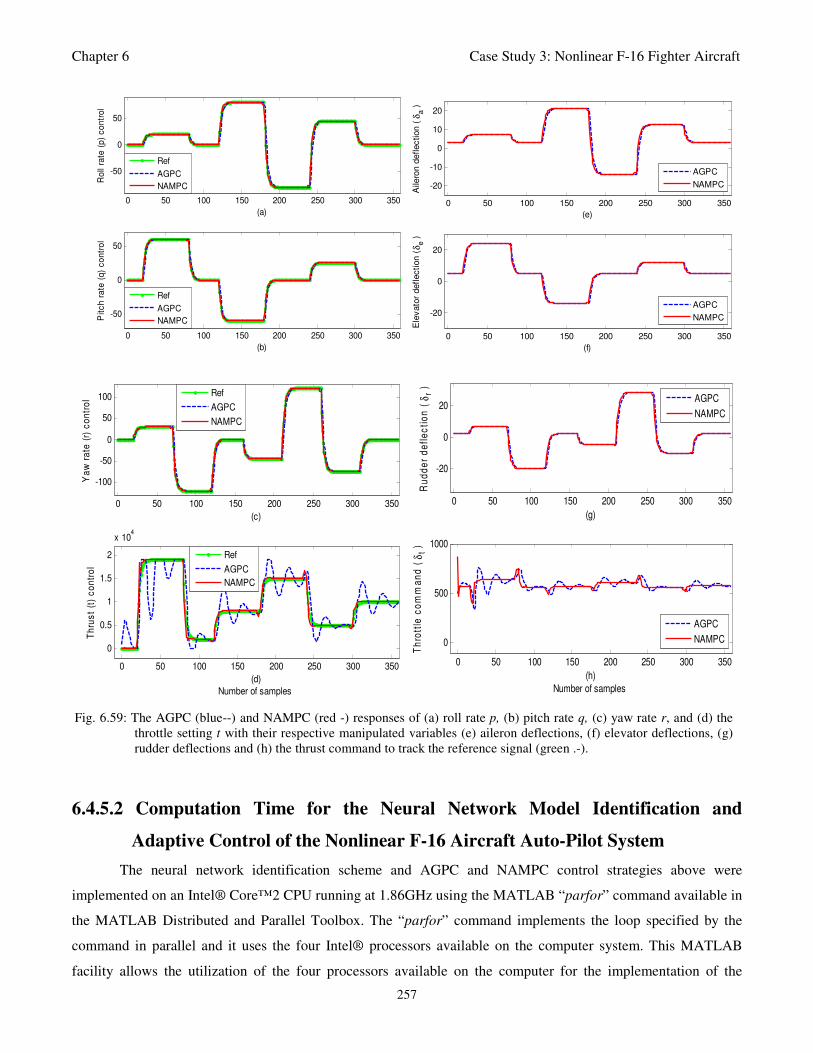
Chapter 6 Case Study 3: Nonlinear F-16 Fighter Aircraft
257
0 50 100 150 200 250 300 350
-50
0
50
(a)
Ro
ll ra
te (
p)
co
ntr
ol
Ref
AGPC
NAMPC
0 50 100 150 200 250 300 350
-50
0
50
(b)
Pit
ch
ra
te (
q)
co
ntr
ol
Ref
AGPC
NAMPC
0 50 100 150 200 250 300 350
-20
-10
0
10
20
(e)
Aile
ron d
eflection (
δa )
AGPC
NAMPC
0 50 100 150 200 250 300 350
-20
0
20
(f)
Ele
vato
r deflection (
δe )
AGPC
NAMPC
0 50 100 150 200 250 300 350
-100
-50
0
50
100
(c)
Ya
w r
ate
(r)
co
ntr
ol
Ref
AGPC
NAMPC
0 50 100 150 200 250 300 350
0
0.5
1
1.5
2
x 104
(d)
Number of samples
Th
rus
t (t
) c
on
tro
l
Ref
AGPC
NAMPC
0 50 100 150 200 250 300 350
-20
0
20
(g)
Ru
dd
er
de
fle
cti
on
( δ
r )
AGPC
NAMPC
0 50 100 150 200 250 300 350
0
500
1000
(h)
Number of samples
Th
rott
le c
om
ma
nd
( δ
t )
AGPC
NAMPC
Fig. 6.59: The AGPC (blue--) and NAMPC (red -) responses of (a) roll rate p, (b) pitch rate q, (c) yaw rate r, and (d) the
throttle setting t with their respective manipulated variables (e) aileron deflections, (f) elevator deflections, (g)
rudder deflections and (h) the thrust command to track the reference signal (green .-).
6.4.5.2 Computation Time for the Neural Network Model Identification and
Adaptive Control of the Nonlinear F-16 Aircraft Auto-Pilot System
The neural network identification scheme and AGPC and NAMPC control strategies above were
implemented on an Intel® Core™2 CPU running at 1.86GHz using the MATLAB “parfor” command available in
the MATLAB Distributed and Parallel Toolbox. The “parfor” command implements the loop specified by the
command in parallel and it uses the four Intel® processors available on the computer system. This MATLAB
facility allows the utilization of the four processors available on the computer for the implementation of the
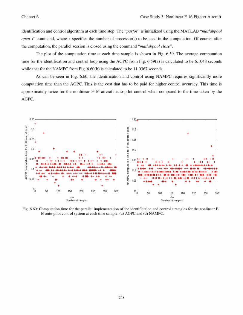
Chapter 6 Case Study 3: Nonlinear F-16 Fighter Aircraft
258
0 50 100 150 200 250 300 3506
6.05
6.1
6.15
6.2
6.25
6.3
6.35
(b)
GP
C c
om
pu
tati
on
tim
e f
or
F-1
6 a
irc
raft
(s
ec
)
AG
PC
co
mp
uta
tio
n t
ime
fo
r F
-16
air
cra
ft (
se
c)
0 50 100 150 200 250 300 350
11
11.05
11.1
11.15
11.2
11.25
11.3
11.35
(d)
NA
MP
C c
om
pu
tati
on
tim
e f
or
F-1
6 a
irc
raft
(s
ec
)
(a) (b)
Number of samples Number of samples
Fig. 6.60: Computation time for the parallel implementation of the identification and control strategies for the nonlinear F-
16 auto-pilot control system at each time sample: (a) AGPC and (d) NAMPC.
identification and control algorithm at each time step. The “parfor” is initialized using the MATLAB “matlabpool
open x” command, where x specifies the number of processor(s) to be used in the computation. Of course, after
the computation, the parallel session is closed using the command “matlabpool close”.
The plot of the computation time at each time sample is shown in Fig. 6.59. The average computation
time for the identification and control loop using the AGPC from Fig. 6.59(a) is calculated to be 6.1048 seconds
while that for the NAMPC from Fig. 6.60(b) is calculated to be 11.0367 seconds.
As can be seen in Fig. 6.60, the identification and control using NAMPC requires significantly more
computation time than the AGPC. This is the cost that has to be paid for higher control accuracy. This time is
approximately twice for the nonlinear F-16 aircraft auto-pilot control when compared to the time taken by the
AGPC.
Chapter 6 Case Study 4: FPGA Implementation of NN–Based AGPC Algorithm
259
6.5 Real-Time Implementation of the Neural Network-Based Adaptive Generalized
Predictive Control (AGPC) Algorithm for Nonlinear F-16 Fighter Aircraft
Auto-Pilot Control System on a Xilinx Virtex-5 FX70T ML507 FPGA Board
In Section 6.4.2, the adaptive recursive least squares (ARLS) algorithm and the modified Levenberg-
Marquardt algorithm (MLMA) were applied for the nonlinear neural network model identification of a
NNARMAX model of a nonlinear F-16 fighter aircraft (or which would be referred to as F-16 aircraft for
simplicity). The validation results of Section 6.4.3 showed that although both algorithms performed excellently
but the MLMA algorithm outperformed the ARLS algorithm especially in terms of the lower computation time
which is very critical in the F-16 aircraft model identification and control. The suitability of the ARLS and
MLMA algorithms for closed-loop F-16 aircraft was investigated in Section 6.4.4, and the results also showed
that the MLMA algorithm outperformed the ARLS algorithm. Then in Section 6.4.5, the performance comparison
of the proposed neural network-based adaptive generalized predictive (AGPC) and the nonlinear adaptive model
predictive control (NAMPC) algorithms for the F-16 aircraft auto-pilot system control was investigated, where the
NAMPC showed improved control performance when compared to that obtained using the AGPC but at the
expense of approximately twice the computation time required by the AGPC.
In Section 6.4.5.2, the average computation time for the neural network-based model identification and
adaptive control of the nonlinear F-16 aircraft were found to be 6.1048 and 11.0367 seconds for the AGPC and
the NAMPC algorithms respectively. These obtained computation times are much higher than the 0.5 seconds
time constants (sampling time) of the F-16 aircraft [Russel, 2003]. It is possible that the parallelization of these
algorithms could result in significant reduction of the computation time but this aspect is not considered within
the framework of the current study. Also, the two proposed neural network-based nonlinear model identification
algorithms have also not been considered within the framework of the current study.
However, since the AGPC showed acceptable control performance of the F-16 aircraft auto-pilot control
system that not as efficient as that obtained using the NAMPC but with reduced computation time when compared
to the NAMPC, the effort in this work is directed towards the real-time implementation of the neural network-
based AGPC algorithm to achieve a further reduced computation time that would be less than the time constant of
0.5 seconds for the nonlinear F-16 aircraft. The second reason why the AGPC algorithm is considered here for
FPGA implementation is due to its simplicity which may facilitate its hardware realization and analysis by
exploiting hardware trade-off and speed for improved performances.
In the present study, the FPGA realization and implementation of the AGPC algorithm is investigated
using Virtex-5 FX70T FPGA development board of Fig. 2.16 which was introduced and discussed in Section
2.8.4 of Chapter 2. The verification and performance evaluation of the proposed FPGA implementation of the
AGPC algorithm on the Virtex-5 FX70T ML507 FPGA development board is performed in closed-loop with the
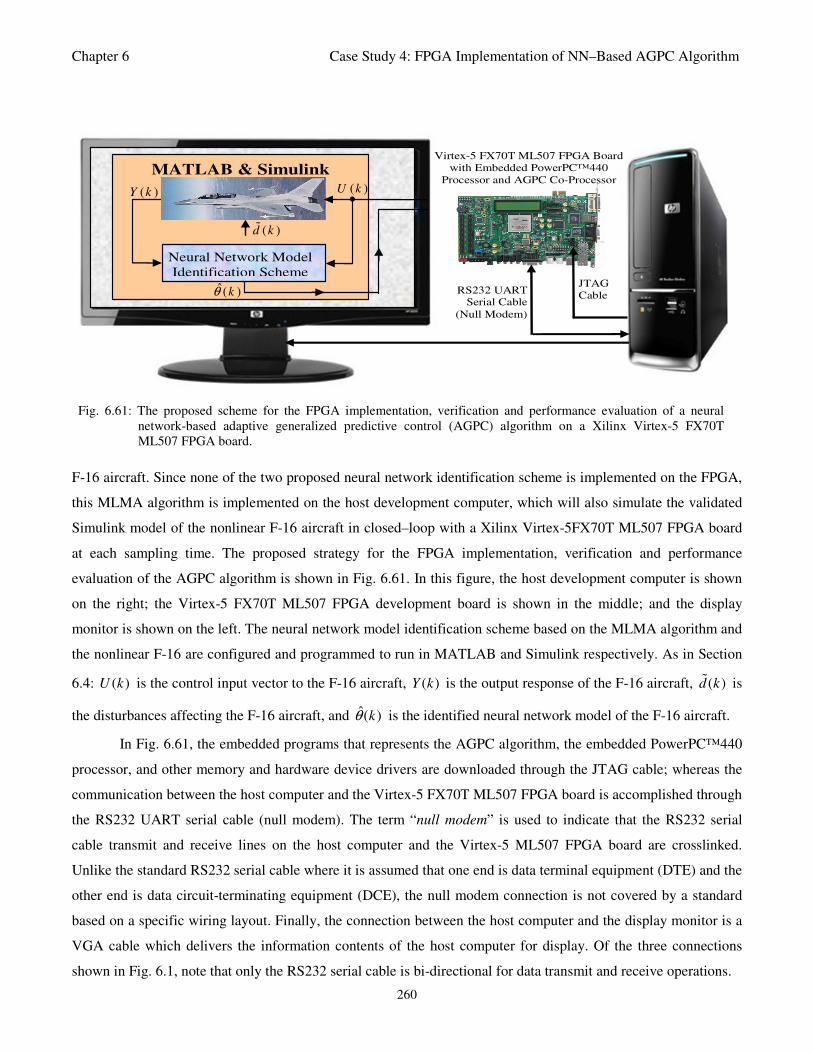
Chapter 6 Case Study 4: FPGA Implementation of NN–Based AGPC Algorithm
260
MATLAB & Simulink
•
Neural Network Model
Identification Scheme
RS232 UART
Serial Cable
(Null Modem)
JTAG
Cable
Virtex-5 FX70T ML507 FPGA Board
with Embedded PowerPC™440
Processor and AGPC Co-Processor ( )U k ( )Y k
( )d k
ˆ( )kθ
Fig. 6.61: The proposed scheme for the FPGA implementation, verification and performance evaluation of a neural
network-based adaptive generalized predictive control (AGPC) algorithm on a Xilinx Virtex-5 FX70T
ML507 FPGA board.
F-16 aircraft. Since none of the two proposed neural network identification scheme is implemented on the FPGA,
this MLMA algorithm is implemented on the host development computer, which will also simulate the validated
Simulink model of the nonlinear F-16 aircraft in closed–loop with a Xilinx Virtex-5FX70T ML507 FPGA board
at each sampling time. The proposed strategy for the FPGA implementation, verification and performance
evaluation of the AGPC algorithm is shown in Fig. 6.61. In this figure, the host development computer is shown
on the right; the Virtex-5 FX70T ML507 FPGA development board is shown in the middle; and the display
monitor is shown on the left. The neural network model identification scheme based on the MLMA algorithm and
the nonlinear F-16 are configured and programmed to run in MATLAB and Simulink respectively. As in Section
6.4: ( )U k is the control input vector to the F-16 aircraft, ( )Y k is the output response of the F-16 aircraft, ( )d k is
the disturbances affecting the F-16 aircraft, and ˆ( )kθ is the identified neural network model of the F-16 aircraft.
In Fig. 6.61, the embedded programs that represents the AGPC algorithm, the embedded PowerPC™440
processor, and other memory and hardware device drivers are downloaded through the JTAG cable; whereas the
communication between the host computer and the Virtex-5 FX70T ML507 FPGA board is accomplished through
the RS232 UART serial cable (null modem). The term “null modem” is used to indicate that the RS232 serial
cable transmit and receive lines on the host computer and the Virtex-5 ML507 FPGA board are crosslinked.
Unlike the standard RS232 serial cable where it is assumed that one end is data terminal equipment (DTE) and the
other end is data circuit-terminating equipment (DCE), the null modem connection is not covered by a standard
based on a specific wiring layout. Finally, the connection between the host computer and the display monitor is a
VGA cable which delivers the information contents of the host computer for display. Of the three connections
shown in Fig. 6.1, note that only the RS232 serial cable is bi-directional for data transmit and receive operations.
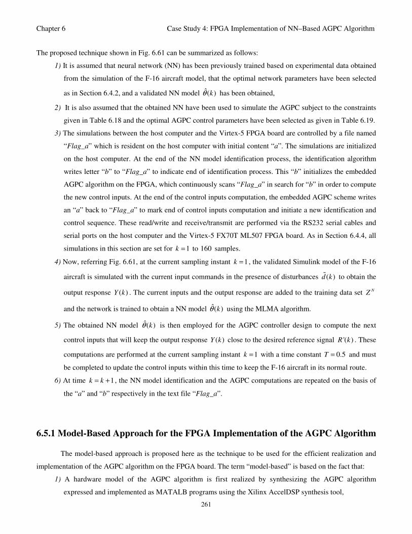
Chapter 6 Case Study 4: FPGA Implementation of NN–Based AGPC Algorithm
261
The proposed technique shown in Fig. 6.61 can be summarized as follows:
1) It is assumed that neural network (NN) has been previously trained based on experimental data obtained
from the simulation of the F-16 aircraft model, that the optimal network parameters have been selected
as in Section 6.4.2, and a validated NN model ˆ( )kθ has been obtained,
2) It is also assumed that the obtained NN have been used to simulate the AGPC subject to the constraints
given in Table 6.18 and the optimal AGPC control parameters have been selected as given in Table 6.19.
3) The simulations between the host computer and the Virtex-5 FPGA board are controlled by a file named
“Flag_a” which is resident on the host computer with initial content “a”. The simulations are initialized
on the host computer. At the end of the NN model identification process, the identification algorithm
writes letter “b” to “Flag_a” to indicate end of identification process. This “b” initializes the embedded
AGPC algorithm on the FPGA, which continuously scans “Flag_a” in search for “b” in order to compute
the new control inputs. At the end of the control inputs computation, the embedded AGPC scheme writes
an “a” back to “Flag_a” to mark end of control inputs computation and initiate a new identification and
control sequence. These read/write and receive/transmit are performed via the RS232 serial cables and
serial ports on the host computer and the Virtex-5 FX70T ML507 FPGA board. As in Section 6.4.4, all
simulations in this section are set for 1k = to 160 samples.
4) Now, referring Fig. 6.61, at the current sampling instant 1k = , the validated Simulink model of the F-16
aircraft is simulated with the current input commands in the presence of disturbances ( )d k to obtain the
output response ( )Y k . The current inputs and the output response are added to the training data set NZ
and the network is trained to obtain a NN model ˆ( )kθ using the MLMA algorithm.
5) The obtained NN model ˆ( )kθ is then employed for the AGPC controller design to compute the next
control inputs that will keep the output response ( )Y k close to the desired reference signal '( )R k . These
computations are performed at the current sampling instant 1k = with a time constant 0.5T = and must
be completed to update the control inputs within this time to keep the F-16 aircraft in its normal route.
6) At time 1k k= + , the NN model identification and the AGPC computations are repeated on the basis of
the “a” and “b” respectively in the text file “Flag_a”.
6.5.1 Model-Based Approach for the FPGA Implementation of the AGPC Algorithm
The model-based approach is proposed here as the technique to be used for the efficient realization and
implementation of the AGPC algorithm on the FPGA board. The term “model-based” is based on the fact that:
1) A hardware model of the AGPC algorithm is first realized by synthesizing the AGPC algorithm
expressed and implemented as MATALB programs using the Xilinx AccelDSP synthesis tool,
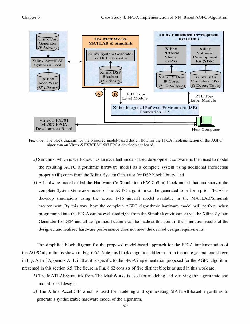
Chapter 6 Case Study 4: FPGA Implementation of NN–Based AGPC Algorithm
262
The MathWorks
MATLAB & Simulink
Xilinx Integrated Software Environment (ISE)
Foundation 11.5
Virtex-5 FX70T
ML507 FPGA
Development Board
Xilinx AccelDSP
Synthesis Tool
Xilinx
AccelWare
(IP Library)
Xilinx Core
Generator
(IP Library)
•
Xilinx Embedded Development
Kit (EDK)
B A RTL Top-
Level Module
Xilinx System Generator
for DSP Generator
Xilinx DSP
Blockset
(IP Library)
Xilinx
Platform
Studio
(XPS)
Xilinx & User
IP Cores
(IP Catalogue)
Xilinx
Software
Development
Kit (SDK)
Xilinx SDK
Compilers, OSs,
& Debug Tools
Host Computer
RTL Top-
Level Module
Fig. 6.62: The block diagram for the proposed model-based design flow for the FPGA implementation of the AGPC
algorithm on Virtex-5 FX70T ML507 FPGA development board.
2) Simulink, which is well-known as an excellent model-based development software, is then used to model
the resulting AGPC algorithmic hardware model as a complete system using additional intellectual
property (IP) cores from the Xilinx System Generator for DSP block library, and
3) A hardware model called the Hardware Co-Simulation (HW-CoSim) block model that can encrypt the
complete System Generator model of the AGPC algorithm can be generated to perform prior FPGA-in-
the-loop simulations using the actual F-16 aircraft model available in the MATLAB/Simulink
environment. By this way, how the complete AGPC algorithmic hardware model will perform when
programmed into the FPGA can be evaluated right from the Simulink environment via the Xilinx System
Generator for DSP, and all design modifications can be made at this point if the simulation results of the
designed and realized hardware performance does not meet the desired design requirements.
The simplified block diagram for the proposed model-based approach for the FPGA implementation of
the AGPC algorithm is shown in Fig. 6.62. Note this block diagram is different from the more general one shown
in Fig. A.1 of Appendix A–1, in that it is specific to the FPGA implementation proposed for the AGPC algorithm
presented in this section 6.5. The figure in Fig. 6.62 consists of five distinct blocks as used in this work are:
1) The MATLAB/Simulink from The MathWorks is used for modeling and verifying the algorithmic and
model-based designs,
2) The Xilinx AccelDSP which is used for modeling and synthesizing MATLAB-based algorithms to
generate a synthesizable hardware model of the algorithm,
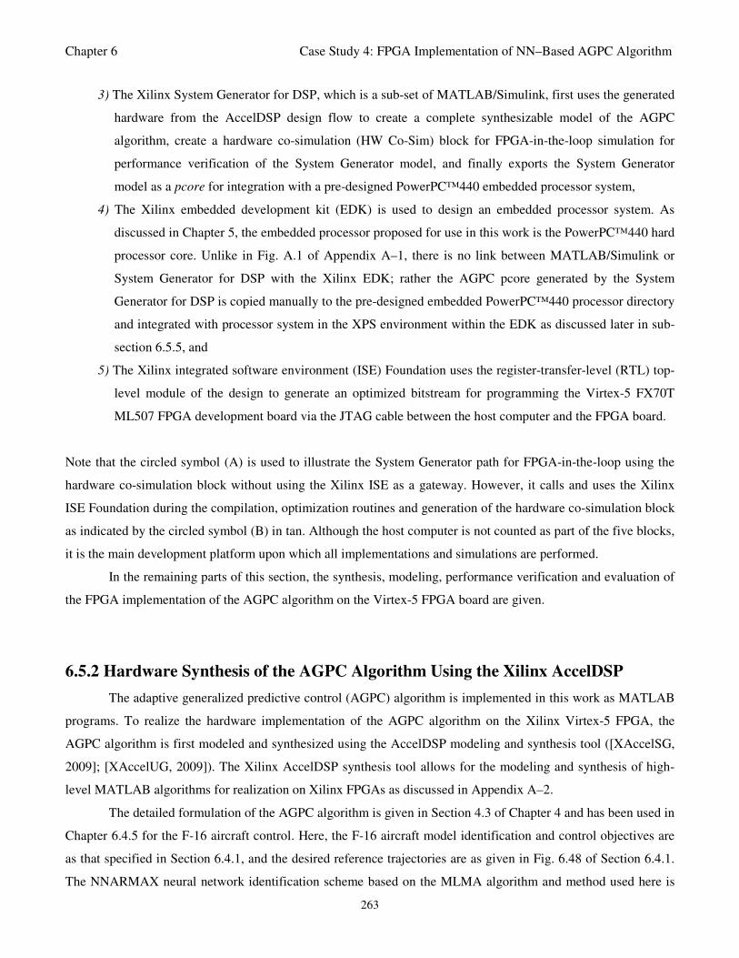
Chapter 6 Case Study 4: FPGA Implementation of NN–Based AGPC Algorithm
263
3) The Xilinx System Generator for DSP, which is a sub-set of MATLAB/Simulink, first uses the generated
hardware from the AccelDSP design flow to create a complete synthesizable model of the AGPC
algorithm, create a hardware co-simulation (HW Co-Sim) block for FPGA-in-the-loop simulation for
performance verification of the System Generator model, and finally exports the System Generator
model as a pcore for integration with a pre-designed PowerPC™440 embedded processor system,
4) The Xilinx embedded development kit (EDK) is used to design an embedded processor system. As
discussed in Chapter 5, the embedded processor proposed for use in this work is the PowerPC™440 hard
processor core. Unlike in Fig. A.1 of Appendix A–1, there is no link between MATLAB/Simulink or
System Generator for DSP with the Xilinx EDK; rather the AGPC pcore generated by the System
Generator for DSP is copied manually to the pre-designed embedded PowerPC™440 processor directory
and integrated with processor system in the XPS environment within the EDK as discussed later in sub-
section 6.5.5, and
5) The Xilinx integrated software environment (ISE) Foundation uses the register-transfer-level (RTL) top-
level module of the design to generate an optimized bitstream for programming the Virtex-5 FX70T
ML507 FPGA development board via the JTAG cable between the host computer and the FPGA board.
Note that the circled symbol (A) is used to illustrate the System Generator path for FPGA-in-the-loop using the
hardware co-simulation block without using the Xilinx ISE as a gateway. However, it calls and uses the Xilinx
ISE Foundation during the compilation, optimization routines and generation of the hardware co-simulation block
as indicated by the circled symbol (B) in tan. Although the host computer is not counted as part of the five blocks,
it is the main development platform upon which all implementations and simulations are performed.
In the remaining parts of this section, the synthesis, modeling, performance verification and evaluation of
the FPGA implementation of the AGPC algorithm on the Virtex-5 FPGA board are given.
6.5.2 Hardware Synthesis of the AGPC Algorithm Using the Xilinx AccelDSP
The adaptive generalized predictive control (AGPC) algorithm is implemented in this work as MATLAB
programs. To realize the hardware implementation of the AGPC algorithm on the Xilinx Virtex-5 FPGA, the
AGPC algorithm is first modeled and synthesized using the AccelDSP modeling and synthesis tool ([XAccelSG,
2009]; [XAccelUG, 2009]). The Xilinx AccelDSP synthesis tool allows for the modeling and synthesis of high-
level MATLAB algorithms for realization on Xilinx FPGAs as discussed in Appendix A–2.
The detailed formulation of the AGPC algorithm is given in Section 4.3 of Chapter 4 and has been used in
Chapter 6.4.5 for the F-16 aircraft control. Here, the F-16 aircraft model identification and control objectives are
as that specified in Section 6.4.1, and the desired reference trajectories are as given in Fig. 6.48 of Section 6.4.1.
The NNARMAX neural network identification scheme based on the MLMA algorithm and method used here is
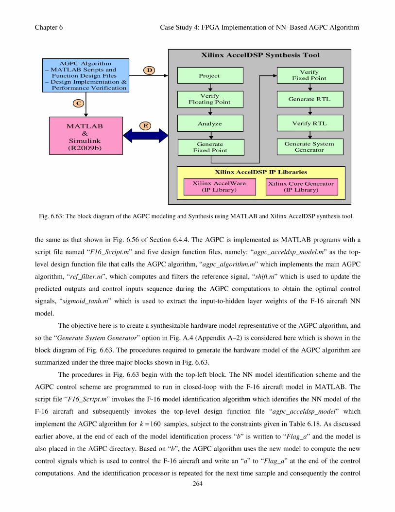
Chapter 6 Case Study 4: FPGA Implementation of NN–Based AGPC Algorithm
264
MATLAB
&
Simulink (R2009b)
AGPC Algorithm
– MATLAB Scripts and
Function Design Files
– Design Implementation &
Performance Verification
Xilinx AccelDSP Synthesis Tool
Generate RTL
Verify
Fixed Point
Generate
Fixed Point
Project
Verify
Floating Point
Analyze
Verify RTL
Xilinx AccelDSP IP Libraries
Xilinx AccelWare
(IP Library)
Xilinx Core Generator
(IP Library)
D
E
C
Generate System
Generator
Fig. 6.63: The block diagram of the AGPC modeling and Synthesis using MATLAB and Xilinx AccelDSP synthesis tool.
the same as that shown in Fig. 6.56 of Section 6.4.4. The AGPC is implemented as MATLAB programs with a
script file named “F16_Script.m” and five design function files, namely: “agpc_acceldsp_model.m” as the top-
level design function file that calls the AGPC algorithm, “agpc_algorithm.m” which implements the main AGPC
algorithm, “ref_filter.m”, which computes and filters the reference signal, “shift.m” which is used to update the
predicted outputs and control inputs sequence during the AGPC computations to obtain the optimal control
signals, “sigmoid_tanh.m” which is used to extract the input-to-hidden layer weights of the F-16 aircraft NN
model.
The objective here is to create a synthesizable hardware model representative of the AGPC algorithm, and
so the “Generate System Generator” option in Fig. A.4 (Appendix A–2) is considered here which is shown in the
block diagram of Fig. 6.63. The procedures required to generate the hardware model of the AGPC algorithm are
summarized under the three major blocks shown in Fig. 6.63.
The procedures in Fig. 6.63 begin with the top-left block. The NN model identification scheme and the
AGPC control scheme are programmed to run in closed-loop with the F-16 aircraft model in MATLAB. The
script file “F16_Script.m” invokes the F-16 model identification algorithm which identifies the NN model of the
F-16 aircraft and subsequently invokes the top-level design function file “agpc_acceldsp_model” which
implement the AGPC algorithm for 160k = samples, subject to the constraints given in Table 6.18. As discussed
earlier above, at the end of each of the model identification process “b” is written to “Flag_a” and the model is
also placed in the AGPC directory. Based on “b”, the AGPC algorithm uses the new model to compute the new
control signals which is used to control the F-16 aircraft and write an “a” to “Flag_a” at the end of the control
computations. And the identification processor is repeated for the next time sample and consequently the control
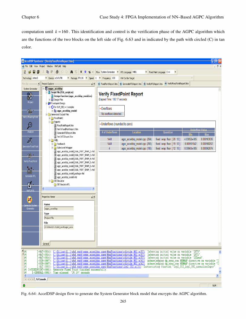
Chapter 6 Case Study 4: FPGA Implementation of NN–Based AGPC Algorithm
265
computation until 160k = . This identification and control is the verification phase of the AGPC algorithm which
are the functions of the two blocks on the left side of Fig. 6.63 and in indicated by the path with circled (C) in tan
color.
Fig. 6.64: AccelDSP design flow to generate the System Generator block model that encrypts the AGPC algorithm.
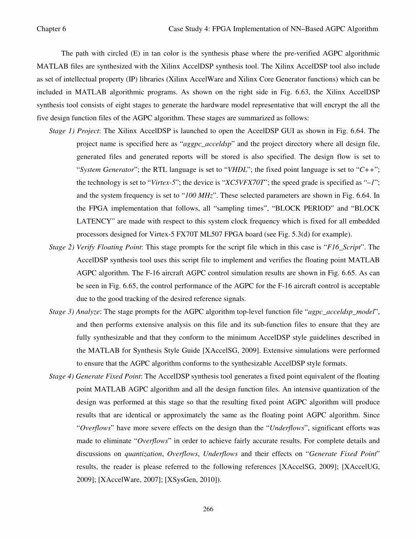
Chapter 6 Case Study 4: FPGA Implementation of NN–Based AGPC Algorithm
266
The path with circled (E) in tan color is the synthesis phase where the pre-verified AGPC algorithmic
MATLAB files are synthesized with the Xilinx AccelDSP synthesis tool. The Xilinx AccelDSP tool also include
as set of intellectual property (IP) libraries (Xilinx AccelWare and Xilinx Core Generator functions) which can be
included in MATLAB algorithmic programs. As shown on the right side in Fig. 6.63, the Xilinx AccelDSP
synthesis tool consists of eight stages to generate the hardware model representative that will encrypt the all the
five design function files of the AGPC algorithm. These stages are summarized as follows:
Stage 1) Project: The Xilinx AccelDSP is launched to open the AceelDSP GUI as shown in Fig. 6.64. The
project name is specified here as “aggpc_acceldsp” and the project directory where all design file,
generated files and generated reports will be stored is also specified. The design flow is set to
“System Generator”; the RTL language is set to “VHDL”; the fixed point language is set to “C++”;
the technology is set to “Virtex-5”; the device is “XC5VFX70T”; the speed grade is specified as “–1”;
and the system frequency is set to “100 MHz”. These selected parameters are shown in Fig. 6.64. In
the FPGA implementation that follows, all “sampling times”, “BLOCK PERIOD” and “BLOCK
LATENCY” are made with respect to this system clock frequency which is fixed for all embedded
processors designed for Virtex-5 FX70T ML507 FPGA board (see Fig. 5.3(d) for example).
Stage 2) Verify Floating Point: This stage prompts for the script file which in this case is “F16_Script”. The
AccelDSP synthesis tool uses this script file to implement and verifies the floating point MATLAB
AGPC algorithm. The F-16 aircraft AGPC control simulation results are shown in Fig. 6.65. As can
be seen in Fig. 6.65, the control performance of the AGPC for the F-16 aircraft control is acceptable
due to the good tracking of the desired reference signals.
Stage 3) Analyze: The stage prompts for the AGPC algorithm top-level function file “agpc_acceldsp_model”,
and then performs extensive analysis on this file and its sub-function files to ensure that they are
fully synthesizable and that they conform to the minimum AccelDSP style guidelines described in
the MATLAB for Synthesis Style Guide [XAccelSG, 2009]. Extensive simulations were performed
to ensure that the AGPC algorithm conforms to the synthesizable AccelDSP style formats.
Stage 4) Generate Fixed Point: The AccelDSP synthesis tool generates a fixed point equivalent of the floating
point MATLAB AGPC algorithm and all the design function files. An intensive quantization of the
design was performed at this stage so that the resulting fixed point AGPC algorithm will produce
results that are identical or approximately the same as the floating point AGPC algorithm. Since
“Overflows” have more severe effects on the design than the “Underflows”, significant efforts was
made to eliminate “Overflows” in order to achieve fairly accurate results. For complete details and
discussions on quantization, Overflows, Underflows and their effects on “Generate Fixed Point”
results, the reader is please referred to the following references [XAccelSG, 2009]; [XAccelUG,
2009]; [XAccelWare, 2007]; [XSysGen, 2010]).
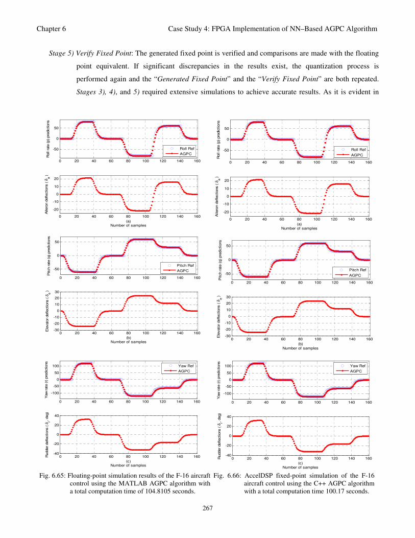
Chapter 6 Case Study 4: FPGA Implementation of NN–Based AGPC Algorithm
267
Stage 5) Verify Fixed Point: The generated fixed point is verified and comparisons are made with the floating
point equivalent. If significant discrepancies in the results exist, the quantization process is
performed again and the “Generated Fixed Point” and the “Verify Fixed Point” are both repeated.
Stages 3), 4), and 5) required extensive simulations to achieve accurate results. As it is evident in
0 20 40 60 80 100 120 140 160
-50
0
50
Roll
rate
(p) pre
dic
tions
0 20 40 60 80 100 120 140 160
-20
-10
0
10
20
(a)Number of samples
Aile
ron d
eflections ( δ
a )
Roll Ref
AGPC
0 20 40 60 80 100 120 140 160
-50
0
50
Pitch rate
(q) pre
dic
tions
0 20 40 60 80 100 120 140 160-30
-20
-10
0
10
20
30
(b)Number of samples
Ele
vato
r deflections ( δ
e )
Pitch Ref
AGPC
0 20 40 60 80 100 120 140 160
-100
-50
0
50
100
Yaw
rate
(r) p
redic
tions
0 20 40 60 80 100 120 140 160-40
-20
0
20
40
(c)Number of samples
Rudder deflections ( δ
r, deg)
Yaw Ref
AGPC
0 20 40 60 80 100 120 140 160
-50
0
50
Roll
rate
(p) pre
dic
tions
0 20 40 60 80 100 120 140 160
-20
-10
0
10
20
(a)Number of samples
Aile
ron d
eflections ( δ
a )
Roll Ref
AGPC
0 20 40 60 80 100 120 140 160
-50
0
50
Pitch rate
(q) pre
dic
tions
0 20 40 60 80 100 120 140 160-30
-20
-10
0
10
20
30
(b)Number of samples
Ele
vato
r deflections ( δ
e )
Pitch Ref
AGPC
0 20 40 60 80 100 120 140 160
-100
-50
0
50
100
Yaw
rate
(r)
pre
dic
tions
0 20 40 60 80 100 120 140 160-40
-20
0
20
40
(c)Number of samples
Rudder
deflections ( δ
r, deg)
Yaw Ref
AGPC
Fig. 6.65: Floating-point simulation results of the F-16 aircraft
control using the MATLAB AGPC algorithm with
a total computation time of 104.8105 seconds.
Fig. 6.66: AccelDSP fixed-point simulation of the F-16
aircraft control using the C++ AGPC algorithm
with a total computation time 100.17 seconds.
Chapter 6 Case Study 4: FPGA Implementation of NN–Based AGPC Algorithm
268
Fig. 6.64, the “Overflows” were completely eliminated while three “Underflows” could not be
eliminated. The “Verify Fixed Point” simulation results for the F-16 aircraft AGPC control is shown
in Fig. 6.66. By comparing the floating point simulation results of Fig. 6.65 and the fixed point
results, it can be observed that the AGPC control performance of the fixed point closely follows
those obtained by the floating point AGPC algorithm good tracking of the desired reference signals.
During the Verify Fixed Point, the AccelDSP Synthesis tool captures the data stream on the design
inputs and outputs which will be used for “bit-true” comparison in later stages of the design.
Stage 6) Generate RTL: This stage generates the register-transfer-level (RTL) model in VHDL from the in-
memory design data base. During the “Generate RTL” process”, all hardware logic based on the
design specification and configurations specified during the modification of the design in Step 3), are
automatically generated and inferred. The inputs and outputs (I/O) ports for the design are also
mapped and implemented. This stage also generates a VHDL “Testbench.vhd” file and is stored in
the Testbbench directory shown in Fig. 6.64 that will be used to verify the RTL model. The
generated Testbench is the VHDL equivalent verification constructs of the MATLAB input and
output data stream captured during the Verify Fixed Point stage. Several of the hardware used in this
hardware synthesis and generation are discussed in the next sub-section 6.5.3 and in Appendix E–2.
Stage 7) Verify RTL: The AccelDSP synthesis tool automatically invoke the Xilinx ISE simulator (ISim)
which first compile the VHDL files of the RTL model ([XISim, 2009]; [XISET, 2010]). Next, it
verifies the generated VHDL file of the RTL model by applying the generated verification constructs
in the Testbench, and monitors and compares the output results. The Verify RTL stage reports a
“FAILED” or PASSED” depending on the outputs comparison result. A PASSED was reported
during the Verify RTL simulation which implied that the AGPC algorithm has been correctly mapped
to its RTL model.
Stage 8) Generate System Generator: This stage generates the synthesized hardware model of the AGPC
algorithm shown in Fig. 6.67. As shown in Fig. 6.67, the inputs to the AGPC hardware model are the
NN model parameters as well as the number of samples. The inputs are passed in parallel so that on
a single global clock pulse, all the inputs are used in a frame-based fashion to produce the outputs.
The hardware resources use to create the hardware model of the AGPC algorithm is given in
Appendices E–1, E–2, and E–4 for convenience.
The generated hardware model of the AGPC algorithm will be referred to as “agpc_accelsdp_model”
which was the name of the top-level function used in creating the hardware model. The AccelDSP Synthesis Tool
description of the generated hardware model “agpc_accelsdp_model” is summarized in Fig. 6.68. The block
period is 91 clock pulses of the 100-MHz reference clock frequency which is the sampling period of the generated
hardware model while the latency is 92 by adding one clock pulse to the block period in order to register the
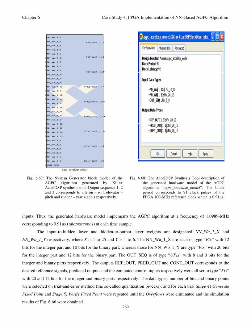
Chapter 6 Case Study 4: FPGA Implementation of NN–Based AGPC Algorithm
269
NN_Wa_1_1
NN_Wa_1_2
NN_Wa_1_3
NN_Wa_1_4
NN_Wa_1_5
NN_Wa_1_6
NN_Wa_1_7
NN_Wa_1_8
NN_Wa_1_9
NN_Wa_1_10
NN_Wa_1_11
NN_Wa_1_12
NN_Wa_1_13
NN_Wa_1_14
NN_Wa_1_15
NN_Wa_1_16
NN_Wa_1_17
NN_Wa_1_18
NN_Wa_1_19
NN_Wa_1_20
NN_Wa_1_21
NN_Wa_1_22
NN_Wa_1_23
NN_Wa_1_24
NN_Wa_1_25
NN_Wb_1_1
NN_Wb_1_2
NN_Wb_1_3
NN_Wb_1_4
NN_Wb_1_5
NN_Wb_1_6
OUT_SEQ
REF_OUT_1_1
REF_OUT_1_2
REF_OUT_1_3
PRED_OUT_1_1
PRED_OUT_1_2
PRED_OUT_1_3
CONT_OUT_1_1
CONT_OUT_1_2
CONT_OUT_1_3
agpc_acceldsp_model
Fig. 6.67: The System Generator block model of the
AGPC algorithm generated by Xilinx
AccelDSP synthesis tool. Output sequence 1, 2
and 3 corresponds to aileron – roll, elevator –
pitch and rudder – yaw signals respectively.
Fig. 6.68: The AccelDSP Synthesis Tool description of
the generated hardware model of the AGPC
algorithm “agpc_acceldsp_model”. The block
period corresponds to 91 clock pulses of the
FPGA 100-MHz reference clock which is 0.91µs.
inputs. Thus, the generated hardware model implements the AGPC algorithm at a frequency of 1.0989-MHz
corresponding to 0.91µs (microseconds) at each time sample.
The input-to-hidden layer and hidden-to-output layer weights are designated NN_Wa_1_X and
NN_Wb_1_Y respectively, where X is 1 to 25 and Y is 1 to 6. The NN_Wa_1_X are each of type “Fix” with 12
bits for the integer part and 10 bits for the binary part; whereas those for NN_Wb_1_Y are type “Fix” with 20 bits
for the integer part and 12 bits for the binary part. The OUT_SEQ is of type “UFix” with 8 and 0 bits for the
integer and binary parts respectively. The outputs REF_OUT, PRED_OUT and CONT_OUT corresponds to the
desired reference signals, predicted outputs and the computed control inputs respectively were all set to type “Fix”
with 20 and 12 bits for the integer and binary parts respectively. The data types, number of bits and binary points
were selected on trial-and-error method (the so-called quantization process); and for each trial Stage 4) Generate
Fixed Point and Stage 5) Verify Fixed Point were repeated until the Overflows were eliminated and the simulation
results of Fig. 6.66 were obtained.

Chapter 6 Case Study 4: FPGA Implementation of NN–Based AGPC Algorithm
270
6.5.2.1 Discussions on the Generated Hardware Model of the AGPC Algorithm
The “Fix” and “UFix” are signed and unsigned fixed point modes. The “Fix” is used to provide greater
range for the positive and negative values of the NN weight as well as the outputs which are usually unknown in
nature. The “UFix” is used to provide greater range since the number of sample will always be positive numbers.
An Overflow occurs when the magnitude of a number assigned to a variable exceeds the number of bits allocated
to the integer part of the fixed-point word. On the other hand, an Underflow occurs when a very small fractional
number gets rounded to zero. Underflows are usually more common and less serious than Overflows
([XAccelDSP, 2009]; [XSysGen, 2010]). For example, the observed minimum values of the NN input-to-hidden
layer weights were in the order of 10-5
, and this posed more challenges on quantizing their fixed point equivalent.
The amount of error between the floating and the fixed point design is called quantization error. Because
AccelDSP Auto-Quantizer recognizes the MATLAB 53-bit limit for simulating bit-true fixed point arithmetic, the
maximum “Fix” and “UFix” bits were limited to these value. Additional, challenge was to ensure that no addition,
division or multiplication of two variables in the AGPC algorithm resulted in value greater than 53-bits. As the
resulting hardware cost increases with the number of bits, and the numbers of bits for the integer part must be
greater than the numbers of bits for the binary parts; significant efforts were made to keep the number of bits as
small as possible while ensuring the accuracy of the resulting fixed-point algorithm without Overflows.
In addition to the hardware and as shown in Table 2.1, the maximum number of input-output (I/O) ports
available for use on the Virtex-5 FX70T ML507 FPGA board is 640. Here, the maximum input-output (I/O) ports
used by the generated hardware model are 613 out of the 640 ports. In addition to the 608 I/O ports used which
can be calculated from Fig. 6.68, five additional “UFix” data type ports were created with number of bits 1 and
binary point 0 respectively. Four of these ports are input ports while the fifth is an output port, which listed
consecutively as follows:
1). Clock: The generated hardware model for the AGPC algorithm has one global clock input. Data transfer
on each data ports are synchronized to the clock. The clock frequency corresponds to the 100-MHz
specified in Fig. 6.64.
2). ClockEnable: The ClockEnable enables the clock.
3). Reset: The global reset must be held active high for at least one clock cycle and returns all registers to
known state. The “Generate System Generator” option for the AccelDSP synthesis flow used in this
work (see Fig. 6.63 and Fig. 6.64), processes the all data at fixed rate and has a constant throughput.
Constant throughput means that all required tasks must be completed within the specified block sample
period. This was verified by the “PASSED” issued by the Verify RTL stage of the hardware synthesis.
When the “Generate System Generator” option is specified, it is expected that the generated
hardware model will be part of a larger System Generator design, as it is in this work. Therefore, the
generated hardware model must process and deliver data placed at its input ports to the output pots
within the block sample period. This input-output communication is controlled by an interface protocol,
Chapter 6 Case Study 4: FPGA Implementation of NN–Based AGPC Algorithm
271
namely: the full handshake protocol and the push-mode handshake protocol. Unlike the full handshake
protocol supported by the ISE option (that is the Verify Gate Level in Fig. A.4) which can be used when
the design does not have constant throughput, the Generate System Generator option implements the
push-mode handshake protocol. Unlike the full handshake protocol, the push-mode handshake protocol
does not rely on input request from the generated hardware before data is sent and output
acknowledgement that data has been received by the output device. This is because the push-mode
protocol is limited to designs with a constant throughput ([XAccelUG, 2007]; [XSysGen, 2010]).
Note that if the AccelDSP is unable to the push-mode protocol, the full handshake is implemented
and the AccelDSP design flow switches to Verify Gate Level option. Experiences have shown that the
resulting Gate level design produce errors when used in the Xilinx ISE Foundation to generate the
programming file. Thus, the MATLAB programs must be modified and all the AccelDSP flow repeated.
4). ac_InputAvail: The ac_InputAvail is simply the input availability. A question here may be from where
and how the input is available, and what is the output device? Let the input and output devices be the
Xilinx “From Register” and “To Register” blocks respectively that are discussed in Appendix A–8. The
data from the input register is presented at the output and the hardware model captures and processes the
data; and then writes the results to the output register. Latency may then be defined here as the time
between when the data is presented and when it is received. Hence, a latency of 1 clock is added in order
to compensate for this time lag.
5). ac_OutputAvail: Also ac_OutputAvail is simply the output availability. The processed data from the
hardware model is written to the output register. The output register also have a latency of 1 clock cycle.
6.5.2.2 Remarks on the Generated Hardware Model of the AGPC Algorithm
By comparing the nonlinear F-16 control simulation results of Fig. 6.65 and Fig. 6.66, it can be observed
that the fixed point C++ program of the AGPC algorithm closely follow the floating point MATLAB due to the
high accuracy quantization of the floating point algorithm. It can also be observed that C++ program took 100.17
seconds as shown by the Verify FixedPoint Report in Fig. 6.64 against the 104.8015 seconds used by the floating
point algorithm, which indicates that the fixed point is 4.6315 second faster than the flowing point counterpart.
By dividing these computation times by the total number of samples being 160, then the average time
required at each sampling instant to compute the control inputs are 0.6550 and 0.6261 seconds for the floating and
fixed point AGPC algorithms respectively. Note that time excludes that for the neural network model
identification. The sampling time of the generated hardware model of the AGPC algorithm in Fig. 6.68 shows the
block period to be 91 based on the specified frequency of 100-MHz for the Virtex-5 XC5VFX70T FPGA.
The block period of 91 implies that the “agpc_acceldsp_model” block model produces an output for a
given input sample after 91 clock cycles. The block period is the time it takes the “agpc_acceldsp_model” block
Chapter 6 Case Study 4: FPGA Implementation of NN–Based AGPC Algorithm
272
model to process data presented at its input to the time it produces the results. Thus, given the neural network
model, the “agpc_acceldsp_model” block model implements the AGPC algorithm at a frequency of 1.0989MHz
which is 0.91µs (microseconds) at each time sample. Note that since the generated hardware model implements
the AGPC algorithm at 0.91µs with 91 clock pulses and the expected number of samples is 160, then the total
number of simulation samples is 14560 samples as implemented by the generated hardware model.
In the next sub-section, the generated hardware model of the AGPC algorithm is combined with the “To
Register” and “From Register” shared memory registers blocks as well as other blocks from the Simulink and
System Generator block libraries to build and test the complete AGPC algorithm model with memory interfaces.
6.5.3 Model-Based Implementation of the Synthesized AGPC Algorithm Using
Xilinx System Generator for DSP
The generated hardware model that encrypts the AGPC algorithm shown in Fig. 6.67 is employed in this
subsection to build the complete System Generator model of the AGPC algorithm. The input and output interfaces
to the agpc_accelsdp_model are the shared memories “From Register” and “From Register” blocks which are
taken from the System Generator library block in the Simulink library browser. The complete System Generator
model of the AGPC algorithm is shown in Fig. 6.69. These shared memories are used so that an addressable
memory mapped interface can be created which can be used to write to and read from the agpc_accelsdp_model.
The agpc_accelsdp_model receives the neural network weights via a bank of 31 shared memory “To
Register” blocks. As shown in Fig. 6.69, the input-to-hidden layer weights are grouped as sub-system into the
block Wa_Input_Regs while the hidden-to-output weights are grouped into the block Wb_Input_Regs. The
initialization and implementation of the complete System Generator model for the AGPC algorithm of Fig. 6.69 is
controlled by the “Flag_a” via the input “c” as discussed previously. If “c = a”, the model identification process
is implemented. On completion, the model identification algorithm writes a “b” to the file “Flag_a”, which is
used to initialize and implements the AGPC algorithm of Fig. 6.69. On completion, the AGPC algorithm writes an
“a” which is used to repeat the model identification process for the number of samples, k = 14560 samples. The
number of samples is specified via a “Counter Limiter” as 14560 samples. Then, the Xilinx Gateway In block,
discussed in Appendix A–8 and shown in Fig. 6.69 as “IN_OUT_SEQ”, is used to convert the Simulink integer,
double and fixed point data type from the Counter Limiter into System Generator fixed point data type.
The outputs of the “agpc_acceldsp_model” are connected to nine shared memory “From Register”
blocks, namely: AIL_REF, ELEV_REF, RUDD_REF for the reference signals; AIL_PRED, ELEV_PRED,
RUDD_PRED for the predicted outputs; and AIL_ROLL_CONT, ELEV_PITCH_CONT, RUDD_YAW_CONT
for the control signals. Where AIL, ELEV and RUDD represents aileron, elevator and rudder respectively. Again,
these shared memories are used so that an addressable memory mapped interface can be created through which
these registers can be accessed for a write operation by the “agpc_acceldsp_model” and read operation by a
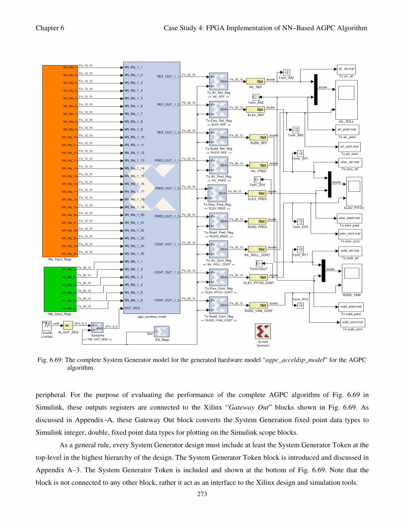
Chapter 6 Case Study 4: FPGA Implementation of NN–Based AGPC Algorithm
273
NN_Wa_1_1
NN_Wa_1_2
NN_Wa_1_3
NN_Wa_1_4
NN_Wa_1_5
NN_Wa_1_6
NN_Wa_1_7
NN_Wa_1_8
NN_Wa_1_9
NN_Wa_1_10
NN_Wa_1_11
NN_Wa_1_12
NN_Wa_1_13
NN_Wa_1_14
NN_Wa_1_15
NN_Wa_1_16
NN_Wa_1_17
NN_Wa_1_18
NN_Wa_1_19
NN_Wa_1_20
NN_Wa_1_21
NN_Wa_1_22
NN_Wa_1_23
NN_Wa_1_24
NN_Wa_1_25
NN_Wb_1_1
NN_Wb_1_2
NN_Wb_1_3
NN_Wb_1_4
NN_Wb_1_5
NN_Wb_1_6
OUT_SEQ
REF_OUT_1_1
REF_OUT_1_2
REF_OUT_1_3
PRED_OUT_1_1
PRED_OUT_1_2
PRED_OUT_1_3
CONT_OUT_1_1
CONT_OUT_1_2
CONT_OUT_1_3
agpc_acceldsp_model
NN_Wb_1
NN_Wb_2
NN_Wb_3
NN_Wb_4
NN_Wb_5
NN_Wb_6
Wb_Input_Regs
NN_Wa_1
NN_Wa_2
NN_Wa_3
NN_Wa_4
NN_Wa_5
NN_Wa_6
NN_Wa_7
NN_Wa_8
NN_Wa_9
NN_Wa_10
NN_Wa_11
NN_Wa_12
NN_Wa_13
NN_Wa_14
NN_Wa_15
NN_Wa_16
NN_Wa_17
NN_Wa_18
NN_Wa_19
NN_Wa_20
NN_Wa_21
NN_Wa_22
NN_Wa_23
NN_Wa_24
NN_Wa_25
Wa_Input_Regs
rudd_ref.mat
To rudd_ref
rudd_pred.mat
To rudd_pred
rudd_cont.mat
To rudd_cont
elev_ref.mat
To elev_ref
elev_pred.mat
To elev_pred
elev_cont.mat
To elev_cont
ai l_ref.mat
To ai l_ref
ail_pred.mat
To ai l_pred
ail_cont.mat
To ai l_cont
din
en
dout
To Rudd_Ref_Reg
<< 'RUDD_REF' >>
din
en
dout
To Rudd_Pred_Reg
<< 'RUDD_PRED' >>
din
en
dout
To Rudd_Cont_Reg
<< 'RUDD_YAW_CONT' >>
din
en
dout
To Elev_Ref_Reg
<< 'ELEV_REF' >>
din
en
dout
To Elev_Pred_Reg
<< 'ELEV_PRED' >>
din
en
dout
To Elev_Cont_Reg
<< 'ELEV_PITCH_CONT' >>
din
en
dout
To Ail_Ref_Reg
<< 'AIL_REF' >>
din
en
dout
To Ail_Pred_Reg
<< 'AIL_PRED' >>
din
en
dout
To Ail_Cont_Reg
<< 'AIL_ROLL_CONT' >>
Terminator7
Termi_EP1
Term_RY3
Term_RY1
Term_EP3
Term_EP2
Term_AR3
Term_AR2
Term_AR1
din
endout
Samples
<< 'HW_OUT_SEQ' >>
Out
RUDD_YAW_CONT
RUDD_YAW
Out
RUDD_REF
Out
RUDD_PRED
In
IN_OUT_SEQ 1
EN_Regs
Out
ELEV_REF
Out
ELEV_PRED
Out
ELEV_PITCH_CONT
ELEV_PITCH
lim
Counter
Limited
Out
AIL_ROLL_CONT
AIL_ROLL
Out
AIL_REF
Out
AIL_PRED
Sy stem
Generator
Fix_12_10
Fix_12_10
Fix_12_10
Fix_12_10
Fix_12_10
Fix_12_10
Fix_12_10
Fix_12_10
Fix_12_10
Fix_12_10
Fix_12_10
Fix_12_10
Fix_12_10
Fix_12_10
Fix_12_10
Fix_12_10
Fix_12_10
Fix_12_10
Fix_12_10
Fix_12_10
Fix_12_10
Fix_12_10
Fix_12_10
Fix_12_10
Fix_12_10
Fix_20_12
Fix_20_12
Fix_20_12
Fix_20_12
Fix_20_12
Fix_20_12
uint8 UFix_8_0UFix_8_0
Fix_20_12
Fix_20_12
Fix_20_12
Fix_20_12
Fix_20_12
Fix_20_12
Fix_20_12
Fix_20_12
Fix_20_12
Fix_20_12
Fix_20_12
Fix_20_12
double
double
double
double
double
double
double
double
Fix_20_12
Fix_20_12
Fix_20_12
Fix_20_12
Fix_20_12
Fix_20_12
double
double
double
double
Bool
Fig. 6.69: The complete System Generator model for the generated hardware model “agpc_acceldsp_model” for the AGPC
algorithm.
peripheral. For the purpose of evaluating the performance of the complete AGPC algorithm of Fig. 6.69 in
Simulink, these outputs registers are connected to the Xilinx “Gateway Out” blocks shown in Fig. 6.69. As
discussed in Appendix–A, these Gateway Out block converts the System Generation fixed point data types to
Simulink integer, double, fixed point data types for plotting on the Simulink scope blocks.
As a general rule, every System Generator design must include at least the System Generator Token at the
top-level in the highest hierarchy of the design. The System Generator Token block is introduced and discussed in
Appendix A–3. The System Generator Token is included and shown at the bottom of Fig. 6.69. Note that the
block is not connected to any other block, rather it act as an interface to the Xilinx design and simulation tools.
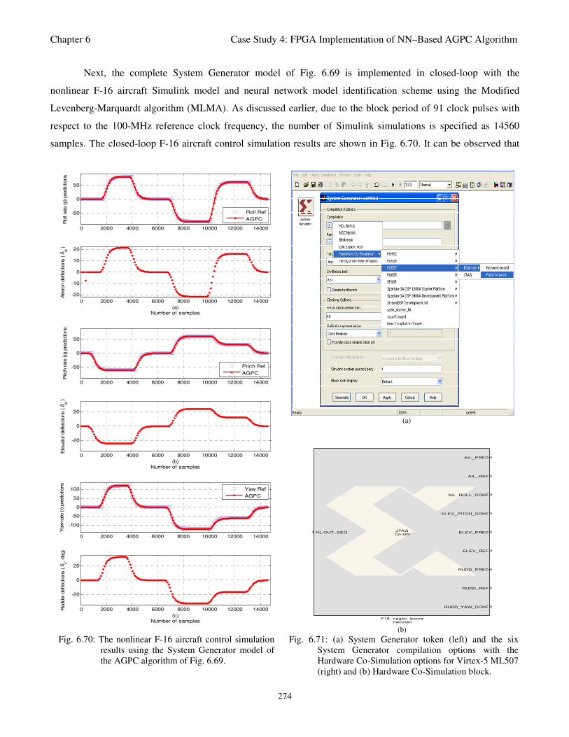
Chapter 6 Case Study 4: FPGA Implementation of NN–Based AGPC Algorithm
274
0 2000 4000 6000 8000 10000 12000 14000
-50
0
50
Roll
rate
(p) pre
dic
tions
Roll Ref
AGPC
0 2000 4000 6000 8000 10000 12000 14000
-20
-10
0
10
20
(a)Number of samples
Aile
ron d
eflections ( δ
a )
0 2000 4000 6000 8000 10000 12000 14000
-50
0
50
Pitch rate
(q) pre
dic
tions
Pitch Ref
AGPC
0 2000 4000 6000 8000 10000 12000 14000
-20
0
20
(b)Number of samples
Ele
vato
r deflections ( δ
e )
0 2000 4000 6000 8000 10000 12000 14000
-100
-50
0
50
100
Yaw
rate
(r) p
redic
tions
Yaw Ref
AGPC
0 2000 4000 6000 8000 10000 12000 14000
-20
0
20
(c)Number of samples
Rudder deflections ( δ
r, deg)
(a)
IN_OUT_SEQ
AIL_PRED
AIL_REF
AIL_ROLL_CONT
ELEV_PITCH_CONT
ELEV_PRED
ELEV_REF
RUDD_PRED
RUDD_REF
RUDD_YAW_CONT
JTAGCo-sim
F16_nagpc_ipcorehwcosim
(b)
Fig. 6.70: The nonlinear F-16 aircraft control simulation
results using the System Generator model of
the AGPC algorithm of Fig. 6.69.
Fig. 6.71: (a) System Generator token (left) and the six
System Generator compilation options with the
Hardware Co-Simulation options for Virtex-5 ML507
(right) and (b) Hardware Co-Simulation block.
Next, the complete System Generator model of Fig. 6.69 is implemented in closed-loop with the
nonlinear F-16 aircraft Simulink model and neural network model identification scheme using the Modified
Levenberg-Marquardt algorithm (MLMA). As discussed earlier, due to the block period of 91 clock pulses with
respect to the 100-MHz reference clock frequency, the number of Simulink simulations is specified as 14560
samples. The closed-loop F-16 aircraft control simulation results are shown in Fig. 6.70. It can be observed that
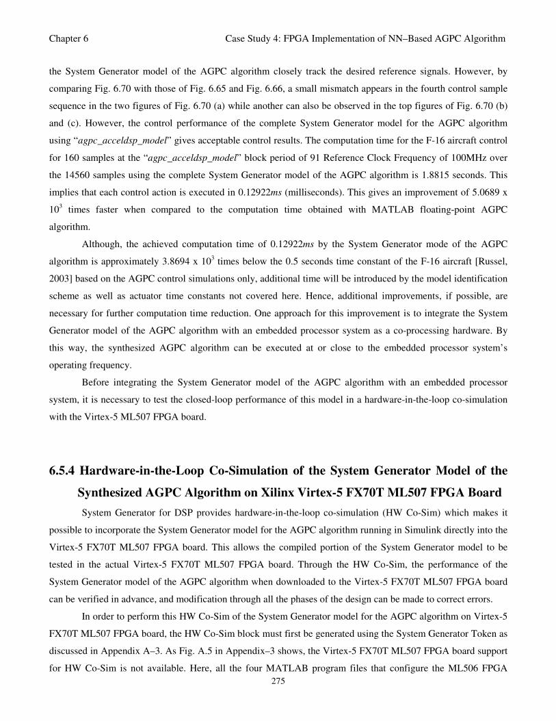
Chapter 6 Case Study 4: FPGA Implementation of NN–Based AGPC Algorithm
275
the System Generator model of the AGPC algorithm closely track the desired reference signals. However, by
comparing Fig. 6.70 with those of Fig. 6.65 and Fig. 6.66, a small mismatch appears in the fourth control sample
sequence in the two figures of Fig. 6.70 (a) while another can also be observed in the top figures of Fig. 6.70 (b)
and (c). However, the control performance of the complete System Generator model for the AGPC algorithm
using “agpc_acceldsp_model” gives acceptable control results. The computation time for the F-16 aircraft control
for 160 samples at the “agpc_acceldsp_model” block period of 91 Reference Clock Frequency of 100MHz over
the 14560 samples using the complete System Generator model of the AGPC algorithm is 1.8815 seconds. This
implies that each control action is executed in 0.12922ms (milliseconds). This gives an improvement of 5.0689 x
103 times faster when compared to the computation time obtained with MATLAB floating-point AGPC
algorithm.
Although, the achieved computation time of 0.12922ms by the System Generator mode of the AGPC
algorithm is approximately 3.8694 x 10³ times below the 0.5 seconds time constant of the F-16 aircraft [Russel,
2003] based on the AGPC control simulations only, additional time will be introduced by the model identification
scheme as well as actuator time constants not covered here. Hence, additional improvements, if possible, are
necessary for further computation time reduction. One approach for this improvement is to integrate the System
Generator model of the AGPC algorithm with an embedded processor system as a co-processing hardware. By
this way, the synthesized AGPC algorithm can be executed at or close to the embedded processor system’s
operating frequency.
Before integrating the System Generator model of the AGPC algorithm with an embedded processor
system, it is necessary to test the closed-loop performance of this model in a hardware-in-the-loop co-simulation
with the Virtex-5 ML507 FPGA board.
6.5.4 Hardware-in-the-Loop Co-Simulation of the System Generator Model of the
Synthesized AGPC Algorithm on Xilinx Virtex-5 FX70T ML507 FPGA Board
System Generator for DSP provides hardware-in-the-loop co-simulation (HW Co-Sim) which makes it
possible to incorporate the System Generator model for the AGPC algorithm running in Simulink directly into the
Virtex-5 FX70T ML507 FPGA board. This allows the compiled portion of the System Generator model to be
tested in the actual Virtex-5 FX70T ML507 FPGA board. Through the HW Co-Sim, the performance of the
System Generator model of the AGPC algorithm when downloaded to the Virtex-5 FX70T ML507 FPGA board
can be verified in advance, and modification through all the phases of the design can be made to correct errors.
In order to perform this HW Co-Sim of the System Generator model for the AGPC algorithm on Virtex-5
FX70T ML507 FPGA board, the HW Co-Sim block must first be generated using the System Generator Token as
discussed in Appendix A–3. As Fig. A.5 in Appendix–3 shows, the Virtex-5 FX70T ML507 FPGA board support
for HW Co-Sim is not available. Here, all the four MATLAB program files that configure the ML506 FPGA
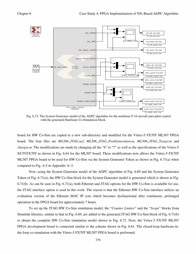
Chapter 6 Case Study 4: FPGA Implementation of NN–Based AGPC Algorithm
276
rudd_ref_hw.mat
To rudd_ref_hw
rudd_pred_hw.mat
To rudd_pred_hw
rudd_cont_hw.mat
To rudd_cont_hw
elev_ref_hw.mat
To elev_ref_hw
elev_pred_hw.mat
To elev_pred_hw
elev_cont_hw.mat
To elev_cont_hw
ail_ref_hw.mat
To ail_ref_hw
ail_pred_hw.mat
To ail_pred_hw
ail_cont_hw.mat
To ail_cont_hw
RUDD_YAW_HW
IN_OUT_SEQ
AIL_PRED
AIL_REF
AIL_ROLL_CONT
ELEV_PITCH_CONT
ELEV_PRED
ELEV_REF
RUDD_PRED
RUDD_REF
RUDD_YAW_CONT
JTAGCo-sim
F16_nagpc_ipcorehwcosim
ELEV_PITCH_HW
lim
CounterLimited
AIL_ROLL_HW
SystemGenerator
Fig. 6.72: The System Generator model of the AGPC algorithm for the nonlinear F-16 aircraft auto-pilot control
with the generated Hardware Co-Simulation block.
board for HW Co-Sim are copied to a new sub-directory and modified for the Virtex-5 FX70T ML507 FPGA
board. The four files are ML506_JTAG.ucf, ML506_JTAG_PostGeneration.m, ML506_JTAG_Target.m and
xltarget.m. The modifications are made by changing all the “6” to “7” as well as the specifications of the Virtex-5
XC5VFX70T as shown in Fig. 6.64 for the ML507 board. These modifications now allows the Virtex-5 FX70T
ML507 FPGA board to be used for HW Co-Sim via the System Generator Token as shown in Fig. 6.71(a) when
compared to Fig. A.5 in Appendix A–3.
Now, using the System Generator model of the AGPC algorithm of Fig. 6.69 and the System Generator
Token of Fig. 6.71(a), the HW Co-Sim block for the System Generator model is generated which is shown in Fig.
6.71(b). As can be seen in Fig. 6.71(a), both Ethernet and JTAG options for the HW Co-Sim is available for use,
the JTAG interface option is used in this work. The reason is that the Ethernet HW Co-Sim interface utilizes an
evaluation version of the Ethernet MAC IP core which becomes dysfunctional after continuous, prolonged
operation in the FPGA board for approximately 7 hours.
To set up the JTAG HW Co-Sim simulation model, the “Counter Limiter” and the “Scope” blocks from
Simulink libraries, similar to that in Fig. 6.69, are added to the generated JTAG HW Co-Sim block of Fig. 6.71(b)
to obtain the complete HW Co-Sim simulation model shown in Fig. 6.72. Next, the Virtex-5 FX70T ML507
FPGA development board is connected similar to the scheme shown in Fig. 6.61. The closed-loop hardware-in-
the-loop co-simulation with the Virtex-5 FX70T ML507 FPGA board is performed.
Chapter 6 Case Study 4: FPGA Implementation of NN–Based AGPC Algorithm
277
0 2000 4000 6000 8000 10000 12000 14000
-50
0
50
Roll ra
te (p) pre
dictions
Roll Ref
HW-CoSim
0 2000 4000 6000 8000 10000 12000 14000
-20
-10
0
10
20
(a)
Aile
ron d
eflections ( δ
a )
0 2000 4000 6000 8000 10000 12000 14000
-50
0
50
Pitch rate
(q) pre
dictions
Pitch Ref
HW-CoSim
0 2000 4000 6000 8000 10000 12000 14000
-20
0
20
(b)
Elevato
r deflections ( δe )
0 2000 4000 6000 8000 10000 12000 14000
-100
-50
0
50
100
Yaw rate
(r) p
redictions
Yaw Ref
HW-CoSim
0 2000 4000 6000 8000 10000 12000 14000
-20
0
20
(c)
Number of samples
Rudder deflections ( δ
r, deg)
Fig. 6.73: Hardware-in-the-loop co-simulation results produced by the generated Hardware Co-Simulation
block model evaluated on the Xilinx Virtex-5 ML507 FPGA board over JTAG cable. In the top
plots, the output predictions (yellow) are compared to the reference signal (red).The bottom
plots are the control signals. (a), (b), and (c) are the simulation results for the aileron-roll,
elevator-pitch and rudder-yaw prediction and control respectively.
The control simulation results are shown in Fig. 6.73. Comparing the control results of Fig. 6.73 to those
of Fig. 6.65, Fig. 6.66 and Fig. 6.70; it can be observed that the JTAG HW Co-Sim gives similar good and
acceptable control performances. This is an indication that the design System Generator model of the AGPC
algorithm is a good representative of the original floating pointing MATLAB algorithm. This also justify that a

Chapter 6 Case Study 4: FPGA Implementation of NN–Based AGPC Algorithm
278
good performance will be achieved from the System Generator model of the AGPC algorithm when it is
programmed into the Virtex-5 FX70T ML507 FPGA.
The computation time for the F-16 aircraft control for 14560 samples with the “agpc_acceldsp_model”
using the JTAG HW Co-Sim block generated from the System Generator model of the AGPC algorithm is 9.2561
seconds. This implies that AGPC control action is executed in 0.63572ms at each time sample. Although this give
an improvement of 1.0303 x 10³ times faster over the original floating point MATLAB algorithm. Also, the
achieved computation time of 0.63572ms by the HW Co-Sim block model is approximately 7.8651x 10² times
below the 0.5 seconds time constant of the F-16 aircraft [Russel, 2003] based on the control simulations only. The
comparing the computation time of 0.63572ms obtained with the HW Co-Sim block model with the 0.12922ms
obtained with System Generator model, it is obvious that the HW Co-Sim block model has increased computation
time of 4.9197 seconds. Thus, the System Generator model implementation is about 5 times faster than the
hardware-in-the-loop implementation of the synthesized AGPC algorithmic model than the HW Co-Sim block
model. This increase in computation time is not unusual [XSysGen, 2010].
The possible reasons for increased computation time are: 1) because the HW Co-Sim block is in effect
producing the clock signal for the Virtex-5 FPGA board only when Simulink initializes it, 2) the overhead
associated with the rest of the Simulink model’s simulation, and 3) the communication overhead due to bus
latency between Simulink and the Virtex-5 FPGA can significantly limit the performance achieved including
increased computation time. In addition to the Gate-Level wrapper generated for “agpc_acceldsp_model” by the
AccelDSP synthesis tool (see Fig. 6.64), System Generator for DSP also generate the memory-map interfaces for
the “agpc_acceldsp_model”, and provides the necessary hardware interfaces and software drivers for the System
Generator model. Although a brief discussion on HW Co-Sim is given in Appendix A–3, a more complete detail
on the Hw Co-Sim block generation process can be found in ([XAccelUG, 2009]; [XSysGen, 2010]).
The next sub-section deals with the generation of the AGPC Co-Processor IP core (pcore) from the
System Generator model of the Synthesized AGPC algorithmic model and the integration of this pcore as a co-
processing hardware with an embedded PowerPC™440 processor system.
6.5.5 Generation and Integration of an AGPC Co-Processor Intellectual Property
(IP) Core with an Embedded PowerPC™440 Processor System
This sub-section develops on the embedded PowerPC™440 processor system developed and tested in
Section 5.3.2 of Chapter 5. Based on the discussions in Section 5.3, the IBM PowerPC™ hard processor core is
the proposed embedded used here. Then, the System Generator model of the AGPC algorithm is used to generate
an IP core which shall be referred to as “AGPC Co-Processor” in this work, since it is a highly optimized
algorithm processing hardware. The AGPC Co-Processor is then exported and integrated with a copy of the pre-
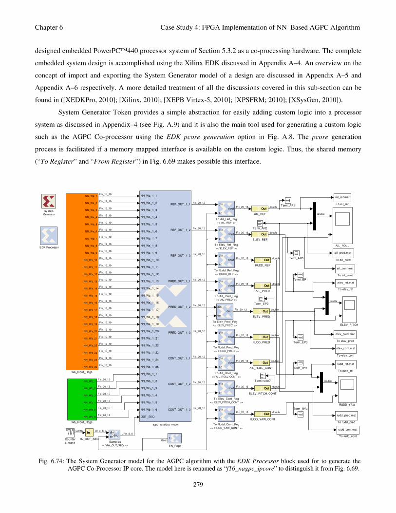
Chapter 6 Case Study 4: FPGA Implementation of NN–Based AGPC Algorithm
279
NN_Wa_1_1
NN_Wa_1_2
NN_Wa_1_3
NN_Wa_1_4
NN_Wa_1_5
NN_Wa_1_6
NN_Wa_1_7
NN_Wa_1_8
NN_Wa_1_9
NN_Wa_1_10
NN_Wa_1_11
NN_Wa_1_12
NN_Wa_1_13
NN_Wa_1_14
NN_Wa_1_15
NN_Wa_1_16
NN_Wa_1_17
NN_Wa_1_18
NN_Wa_1_19
NN_Wa_1_20
NN_Wa_1_21
NN_Wa_1_22
NN_Wa_1_23
NN_Wa_1_24
NN_Wa_1_25
NN_Wb_1_1
NN_Wb_1_2
NN_Wb_1_3
NN_Wb_1_4
NN_Wb_1_5
NN_Wb_1_6
OUT_SEQ
REF_OUT_1_1
REF_OUT_1_2
REF_OUT_1_3
PRED_OUT_1_1
PRED_OUT_1_2
PRED_OUT_1_3
CONT_OUT_1_1
CONT_OUT_1_2
CONT_OUT_1_3
agpc_acceldsp_model
NN_Wb_1
NN_Wb_2
NN_Wb_3
NN_Wb_4
NN_Wb_5
NN_Wb_6
Wb_Input_Regs
NN_Wa_1
NN_Wa_2
NN_Wa_3
NN_Wa_4
NN_Wa_5
NN_Wa_6
NN_Wa_7
NN_Wa_8
NN_Wa_9
NN_Wa_10
NN_Wa_11
NN_Wa_12
NN_Wa_13
NN_Wa_14
NN_Wa_15
NN_Wa_16
NN_Wa_17
NN_Wa_18
NN_Wa_19
NN_Wa_20
NN_Wa_21
NN_Wa_22
NN_Wa_23
NN_Wa_24
NN_Wa_25
Wa_Input_Regs
rudd_ref.mat
To rudd_ref
rudd_pred.mat
To rudd_pred
rudd_cont.mat
To rudd_cont
elev_ref.mat
To elev_ref
elev_pred.mat
To elev_pred
elev_cont.mat
To elev_cont
ail_ref.mat
To ail_ref
ail_pred.mat
To ail_pred
ail_cont.mat
To ail_cont
din
en
dout
To Rudd_Ref_Reg
<< 'RUDD_REF' >>
din
en
dout
To Rudd_Pred_Reg
<< 'RUDD_PRED' >>
din
en
dout
To Rudd_Cont_Reg
<< 'RUDD_YAW_CONT' >>
din
en
dout
To Elev_Ref_Reg
<< 'ELEV_REF' >>
din
en
dout
To Elev_Pred_Reg
<< 'ELEV_PRED' >>
din
en
dout
To Elev_Cont_Reg
<< 'ELEV_PITCH_CONT' >>
din
en
dout
To Ail_Ref_Reg
<< 'AIL_REF' >>
din
en
dout
To Ail_Pred_Reg
<< 'AIL_PRED' >>
din
en
dout
To Ail_Cont_Reg
<< 'AIL_ROLL_CONT' >>
Terminator7
Termi_EP1
Term_RY3
Term_RY1
Term_EP3
Term_EP2
Term_AR3
Term_AR2
Term_AR1
din
endout
Samples
<< 'HW_OUT_SEQ' >>
Out
RUDD_YAW_CONT
RUDD_YAW
Out
RUDD_REF
Out
RUDD_PRED
In
IN_OUT_SEQ 1
EN_Regs
Out
ELEV_REF
Out
ELEV_PRED
Out
ELEV_PITCH_CONT
ELEV_PITCH
EDK Processor
lim
Counter
Limited
Out
AIL_ROLL_CONT
AIL_ROLL
Out
AIL_REF
Out
AIL_PRED
Sy stem
Generator
Fix_12_10
Fix_12_10
Fix_12_10
Fix_12_10
Fix_12_10
Fix_12_10
Fix_12_10
Fix_12_10
Fix_12_10
Fix_12_10
Fix_12_10
Fix_12_10
Fix_12_10
Fix_12_10
Fix_12_10
Fix_12_10
Fix_12_10
Fix_12_10
Fix_12_10
Fix_12_10
Fix_12_10
Fix_12_10
Fix_12_10
Fix_12_10
Fix_12_10
Fix_20_12
Fix_20_12
Fix_20_12
Fix_20_12
Fix_20_12
Fix_20_12
uint16 UFix_8_0UFix_8_0
Fix_20_12
Fix_20_12
Fix_20_12
Fix_20_12
Fix_20_12
Fix_20_12
Fix_20_12
Fix_20_12
Fix_20_12
Fix_20_12
Fix_20_12
Fix_20_12
double
double
double
double
double
double
double
double
Fix_20_12
Fix_20_12
Fix_20_12
Fix_20_12
Fix_20_12
Fix_20_12
double
double
double
double
Bool
Fig. 6.74: The System Generator model for the AGPC algorithm with the EDK Processor block used for to generate the
AGPC Co-Processor IP core. The model here is renamed as “f16_nagpc_ipcore” to distinguish it from Fig. 6.69.
designed embedded PowerPC™440 processor system of Section 5.3.2 as a co-processing hardware. The complete
embedded system design is accomplished using the Xilinx EDK discussed in Appendix A–4. An overview on the
concept of import and exporting the System Generator model of a design are discussed in Appendix A–5 and
Appendix A–6 respectively. A more detailed treatment of all the discussions covered in this sub-section can be
found in ([XEDKPro, 2010]; [Xilinx, 2010]; [XEPB Virtex-5, 2010]; [XPSFRM; 2010]; [XSysGen, 2010]).
System Generator Token provides a simple abstraction for easily adding custom logic into a processor
system as discussed in Appendix–4 (see Fig. A.9) and it is also the main tool used for generating a custom logic
such as the AGPC Co-processor using the EDK pcore generation option in Fig. A.8. The pcore generation
process is facilitated if a memory mapped interface is available on the custom logic. Thus, the shared memory
(“To Register” and “From Register”) in Fig. 6.69 makes possible this interface.
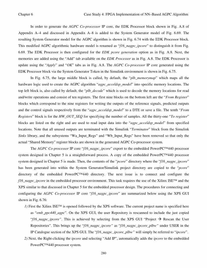
Chapter 6 Case Study 4: FPGA Implementation of NN–Based AGPC Algorithm
280
In order to generate the AGPC Co-processor IP core, the EDK Processor block shown in Fig. A.8 of
Appendix A–4 and discussed in Appendix A–8 is added to the System Generator model of Fig. 6.69. The
resulting System Generator model for the AGPC algorithm is shown in Fig. 6.74 with the EDK Processor block.
This modified AGPC algorithmic hardware model is renamed as “f16_nagpc_ipcore” to distinguish it from Fig.
6.69. The EDK Processor is then configured for the EDK pcore generation option as in Fig. A.8. Next, the
memories are added using the “Add” tab available on the EDK Processor as in Fig. A.8. The EDK Processor is
update using the “Apply” and “OK” tabs as in Fig. A.8. The AGPC Co-processor IP core generated using the
EDK Processor block via the System Generator Token in the Simulink environment is shown in Fig. 6.75.
In Fig. 6.75, the large middle block is called, by default, the “plb_memorymap” which maps all the
hardware logic used to create the AGPC algorithm “agpc_acceldsp_model” into specific memory locations. The
top left block is, also called by default, the “plb_decode” which is used to decode the memory locations for read
and/write operations and consist of ten registers. The first nine blocks on the bottom left are the “From Register”
blocks which correspond to the nine registers for writing the outputs of the reference signals, predicted outputs
and the control signals respectively from the “agpc_acceldsp_model” to a DTE or save a file. The tenth “From
Registers” block is for the HW_OUT_SEQ for specifying the number of samples. All the thirty-one “To register”
blocks are listed on the right and are used to read input data into the “agpc_acceldsp_model” from specified
locations. Note that all unused outputs are terminated with the Simulink “Terminator” block from the Simulink
Sinks library, and the subsystems “Wa_Input_Regs” and “Wb_Input_Regs” have been removed so that only the
actual “Shared Memory” register blocks are shown in the generated AGPC Co-processor system.
The AGPC Co-processor IP core “f16_nagpc_ipcore” export to the embedded PowerPC™440 processor
system designed in Chapter 5 is a straightforward process. A copy of the embedded PowerPC™440 processor
system designed in Chapter 5 is made. Then, the contents of the “pcore” directory where the “f16_nagpc_ipcore”
has been generated into within the System Generator/Simulink project directory are copied to the “pcore”
directory of the embedded PowerPC™440 directory. The next issue is to connect and configure the
f16_nagpc_ipcore in the embedded processor environment. This task requires the use of the Xilinx ISE™ and the
XPS similar to that discussed in Chapter 5 for the embedded processor design. The procedures for connecting and
configuring the AGPC Co-processor IP core “f16_nagpc_ipcore” are summarized below using the XPS GUI
shown in Fig. 6.76:
1) First the Xilinx ISE™ is opened followed by the XPS software. The current project name is specified here
as “emb_ppc440_agpc”. On the XPS GUI, the user Repository is rescanned to include the just copied
“f16_nagpc_ipcore”. This is achieved by selecting from the XPS GUI “Project Rescan the User
Repositories”. This brings up the “f16_nagpc_ipcore” as “f16_nagpc_ipcore_plbw” under USER in the
IP Catalogue section of the XPS GUI. The “f16_nagpc_ipcore_plbw” will simply be referred to “ipcore”.
2) Next, the Right-clicking the ipcore and selecting “Add IP”, automatically adds the ipcore to the embedded
PowerPC™440 processor system.
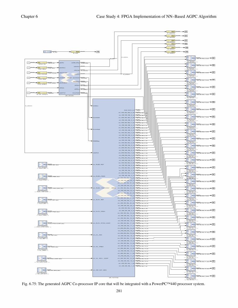
Chapter 6 Case Study 4: FPGA Implementation of NN–Based AGPC Algorithm
281
In
sg_plb_addrpref
wrDBus
bankAddr
linearAddr
RNWReg
addrAck
sm_RUDD_REF
sm_RUDD_PRED
sm_RUDD_YAW_CONT
sm_ELEV_REF
sm_ELEV_PRED
sm_ELEV_PITCH_CONT
sm_AIL_REF
sm_AIL_PRED
sm_AIL_ROLL_CONT
sm_HW_OUT_SEQ
read_bank_out
sm_HW_NN_Wb_6_din
sm_HW_NN_Wb_6_en
sm_HW_NN_Wb_5_din
sm_HW_NN_Wb_5_en
sm_HW_NN_Wb_4_din
sm_HW_NN_Wb_4_en
sm_HW_NN_Wb_3_din
sm_HW_NN_Wb_3_en
sm_HW_NN_Wb_2_din
sm_HW_NN_Wb_2_en
sm_HW_NN_Wb_1_din
sm_HW_NN_Wb_1_en
sm_HW_NN_Wa_9_din
sm_HW_NN_Wa_9_en
sm_HW_NN_Wa_8_din
sm_HW_NN_Wa_8_en
sm_HW_NN_Wa_7_din
sm_HW_NN_Wa_7_en
sm_HW_NN_Wa_6_din
sm_HW_NN_Wa_6_en
sm_HW_NN_Wa_5_din
sm_HW_NN_Wa_5_en
sm_HW_NN_Wa_4_din
sm_HW_NN_Wa_4_en
sm_HW_NN_Wa_3_din
sm_HW_NN_Wa_3_en
sm_HW_NN_Wa_25_din
sm_HW_NN_Wa_25_en
sm_HW_NN_Wa_24_din
sm_HW_NN_Wa_24_en
sm_HW_NN_Wa_23_din
sm_HW_NN_Wa_23_en
sm_HW_NN_Wa_22_din
sm_HW_NN_Wa_22_en
sm_HW_NN_Wa_21_din
sm_HW_NN_Wa_21_en
sm_HW_NN_Wa_20_din
sm_HW_NN_Wa_20_en
sm_HW_NN_Wa_2_din
sm_HW_NN_Wa_2_en
sm_HW_NN_Wa_19_din
sm_HW_NN_Wa_19_en
sm_HW_NN_Wa_18_din
sm_HW_NN_Wa_18_en
sm_HW_NN_Wa_17_din
sm_HW_NN_Wa_17_en
sm_HW_NN_Wa_16_din
sm_HW_NN_Wa_16_en
sm_HW_NN_Wa_15_din
sm_HW_NN_Wa_15_en
sm_HW_NN_Wa_14_din
sm_HW_NN_Wa_14_en
sm_HW_NN_Wa_13_din
sm_HW_NN_Wa_13_en
sm_HW_NN_Wa_12_din
sm_HW_NN_Wa_12_en
sm_HW_NN_Wa_11_din
sm_HW_NN_Wa_11_en
sm_HW_NN_Wa_10_din
sm_HW_NN_Wa_10_en
sm_HW_NN_Wa_1_din
sm_HW_NN_Wa_1_en
xlmax
plb_memmap
plbRst
plbABus
plbPAValid
plbRNW
plbWrDBus
rdData
addrPref
wrDBusReg
addrAck
rdComp
wrDAck
bankAddr
RNWReg
rdDAck
rdDBus
linearAddr
xlmax
plb_decode
din
en
dout
To Register9<< 'HW_NN_Wa_6' >>
din
en
dout
To Register8<< 'HW_NN_Wa_7' >>
din
en
dout
To Register7<< 'HW_NN_Wa_8' >>
din
en
dout
To Register6<< 'HW_NN_Wa_9' >>
din
en
dout
To Register5<< 'HW_NN_Wb_1' >>
din
en
dout
To Register4<< 'HW_NN_Wb_2' >>
din
en
dout
To Register30<< 'HW_NN_Wa_1' >>
din
en
dout
To Register3<< 'HW_NN_Wb_3' >>
din
en
dout
To Register29<< 'HW_NN_Wa_10' >>
din
en
dout
To Register28<< 'HW_NN_Wa_11' >>
din
en
dout
To Register27<< 'HW_NN_Wa_12' >>
din
en
dout
To Register26<< 'HW_NN_Wa_13' >>
din
en
dout
To Register25<< 'HW_NN_Wa_14' >>
din
en
dout
To Register24<< 'HW_NN_Wa_15' >>
din
en
dout
To Register23<< 'HW_NN_Wa_16' >>
din
en
dout
To Register22<< 'HW_NN_Wa_17' >>
din
en
dout
To Register21<< 'HW_NN_Wa_18' >>
din
en
dout
To Register20<< 'HW_NN_Wa_19' >>
din
en
dout
To Register2<< 'HW_NN_Wb_4' >>
din
en
dout
To Register19<< 'HW_NN_Wa_2' >>
din
en
dout
To Register18<< 'HW_NN_Wa_20' >>
din
en
dout
To Register17<< 'HW_NN_Wa_21' >>
din
en
dout
To Register16<< 'HW_NN_Wa_22' >>
din
en
dout
To Register15<< 'HW_NN_Wa_23' >>
din
en
dout
To Register14<< 'HW_NN_Wa_24' >>
din
en
dout
To Register13<< 'HW_NN_Wa_25' >>
din
en
dout
To Register12<< 'HW_NN_Wa_3' >>
din
en
dout
To Register11<< 'HW_NN_Wa_4' >>
din
en
dout
To Register10<< 'HW_NN_Wa_5' >>
din
en
dout
To Register1<< 'HW_NN_Wb_5' >>
din
en
dout
To Register<< 'HW_NN_Wb_6' >>
Out
Sl_wrDAck
Out
Sl_wrComp
Out
Sl_wait
Out
Sl_rdDBus
Out
Sl_rdDAck
Out
Sl_rdComp
Out
Sl_addrAck
In
SPLB_Rst
In
PLB_wrDBus
In
PLB_RNW
In
PLB_PAValid
In
PLB_ABus
dout
From Register9<< 'HW_OUT_SEQ' >>
dout
From Register8<< 'AIL_ROLL_CONT' >>
dout
From Register7<< 'AIL_PRED' >>
dout
From Register6<< 'AIL_REF' >>
dout
From Register5<< 'ELEV_PITCH_CONT' >>
dout
From Register4<< 'ELEV_PRED' >>
dout
From Register3<< 'ELEV_REF' >>
dout
From Register2<< 'RUDD_YAW_CONT' >>
dout
From Register1<< 'RUDD_PRED' >>
dout
From Register<< 'RUDD_REF' >>
1
0
1
1
1
1
1
Sl_addrAck
double
Sl_addrAck
Sl_wrDAck
double
Sl_wrDAck
doubleHW_NN_Wa_1_en
double
HW_NN_Wa_1_din
double
HW_NN_Wa_10_en
double
HW_NN_Wa_10_din
double
HW_NN_Wa_11_en
doubleHW_NN_Wa_11_din
doubleHW_NN_Wa_12_en
double
HW_NN_Wa_12_din
double
HW_NN_Wa_13_en
double
HW_NN_Wa_13_din
double
HW_NN_Wa_14_en
doubleHW_NN_Wa_14_din
doubleHW_NN_Wa_15_en
double
HW_NN_Wa_15_din
double
HW_NN_Wa_16_en
double
HW_NN_Wa_16_din
double
HW_NN_Wa_17_en
double
HW_NN_Wa_17_din
doubleHW_NN_Wa_18_en
double
HW_NN_Wa_18_din
double
HW_NN_Wa_19_en
double
HW_NN_Wa_19_din
double
HW_NN_Wa_2_en
double
HW_NN_Wa_2_din
doubleHW_NN_Wa_20_en
double
HW_NN_Wa_20_din
double
HW_NN_Wa_21_en
double
HW_NN_Wa_21_din
double
HW_NN_Wa_22_en
double
HW_NN_Wa_22_din
doubleHW_NN_Wa_23_en
double
HW_NN_Wa_23_din
double
HW_NN_Wa_24_en
double
HW_NN_Wa_24_din
double
HW_NN_Wa_25_en
double
HW_NN_Wa_25_din
doubleHW_NN_Wa_3_en
doubleHW_NN_Wa_3_din
double
HW_NN_Wa_4_en
double
HW_NN_Wa_4_din
double
HW_NN_Wa_5_en
double
HW_NN_Wa_5_din
doubleHW_NN_Wa_6_en
doubleHW_NN_Wa_6_din
double
HW_NN_Wa_7_en
double
HW_NN_Wa_7_din
double
HW_NN_Wa_8_en
double
HW_NN_Wa_8_din
doubleHW_NN_Wa_9_en
doubleHW_NN_Wa_9_din
double
HW_NN_Wb_1_en
double
HW_NN_Wb_1_din
double
HW_NN_Wb_2_en
double
HW_NN_Wb_2_din
double
HW_NN_Wb_3_en
doubleHW_NN_Wb_3_din
double
HW_NN_Wb_4_en
double
HW_NN_Wb_4_din
double
HW_NN_Wb_5_en
double
HW_NN_Wb_5_din
double
HW_NN_Wb_6_en
doubleHW_NN_Wb_6_din
double
rdData
double
HW_OUT_SEQ_dout
double
AIL_ROLL_CONT_dout
double
AIL_PRED_dout
doubleAIL_REF_dout
double
ELEV_PITCH_CONT_dout
double
ELEV_PRED_dout
double
ELEV_REF_dout
double
RUDD_YAW_CONT_dout
doubleRUDD_PRED_dout
double
RUDD_REF_dout
doubleRNWReg
double
linearAddr
double
bankAddr
double
wrDBusReg
double
HW_NN_Wa_1_dout
doubleHW_NN_Wa_10_dout
double
HW_NN_Wa_11_dout
doubleHW_NN_Wa_12_dout
double
HW_NN_Wa_13_dout
double
HW_NN_Wa_14_dout
double
HW_NN_Wa_15_dout
double
HW_NN_Wa_16_dout
double
HW_NN_Wa_17_dout
double
HW_NN_Wa_18_dout
double
HW_NN_Wa_19_dout
double
HW_NN_Wa_2_dout
doubleHW_NN_Wa_20_dout
double
HW_NN_Wa_21_dout
doubleHW_NN_Wa_22_dout
double
HW_NN_Wa_23_dout
doubleHW_NN_Wa_24_dout
double
HW_NN_Wa_25_dout
double
HW_NN_Wa_3_dout
double
HW_NN_Wa_4_dout
double
HW_NN_Wa_5_dout
double
HW_NN_Wa_6_dout
double
HW_NN_Wa_7_dout
double
HW_NN_Wa_8_dout
double
HW_NN_Wa_9_dout
double
HW_NN_Wb_1_dout
double
HW_NN_Wb_2_dout
doubleHW_NN_Wb_3_dout
double
HW_NN_Wb_4_dout
doubleHW_NN_Wb_5_dout
double
HW_NN_Wb_6_dout
double
Sl_rdDBus
double
Sl_rdDAck
double
Sl_rdComp
double
addrPref
doublePLB_wrDBus
double
PLB_RNW
double
PLB_PAValid
doublePLB_ABus
double
SPLB_Rst
double
doubleSl_wait
double
double
double
double
double
double
double
double double
double
double
double
Fig. 6.75: The generated AGPC Co-processor IP core that will be integrated with a PowerPC™440 processor system.
Chapter 6 Case Study 4: FPGA Implementation of NN–Based AGPC Algorithm
282
3) Next, the just ipcore is connected to and configured with the PowerPC™440 processor system through the
processor local bus (PLB) using the “System Assembly View” of the XPS GUI as follows.
i). On the XPS GUI, the Bus Interfaces is selected and the ipcore is located. The ipcore is connected to
the PLB by selecting “plb_v46_0”.
ii). Next, the Ports tab on the System Assembly View of the XPX GUI is selected and the ipcore is located.
All the eleven (11) ports of the just added ipcore are made external by selecting “Make External” for
each of the ports.
iii). Finally, to complete the configuring process, the ipcore must be assigned a valid address in the
embedded system. This is achieved by selecting the “Addresses” tab on the System Assembly View of
the XPS GUI and clicking the “Generate Addresses”. This action automatically creates a memory map
for added ipcore and integrates the ipcore into the embedded processor system. Although there is no
port address conflict in this implementation, but if it exists an immediate choice is to manually re-
assign the memory addresses of conflicting ports.
4) To verify that no error(s) occurred for the connected ipcore, the complete embedded PowerPC™440-
AGPC Co-Processor (f16_nagpc_ipcore_plbw) is compiled using the XPS and the Xilinx ISE™ similar
to the procedures to the 9–Step procedures outlined in Section 5.3.2 of Chapter 5.
According these procedures, the board support packages and the libraries are generated by selecting
“Software Generate the Libraries and BSPs” on the XPS GUI as well as the Netlist by selecting
“Hardware Generate Netlist”. Next, the complete XPS project is saved and the Xilinx ISETM
is used to
generate the bitstream by selecting and double clicking on “Generate Programming File” on the Xilinx
ISE™ GUI similar to that on Fig. 5.6. All signals were completely routed, all timing constraints were met
and no error(s) were recorded as shown on the XPS and the Xilinx ISE™ synthesis results in Appendix
E–1 and E–2 respectively. Appendix E – 3 gives the summary of the main contents of the embedded
PowerPC™440–AGPC Co-Processor system. It can be seen in Appendix E–3 that the AGPC Co-
Processor has been added as a peripheral. Its main function is to implement the synthesized and
embedded AGPC algorithmic function.
5). Next, the complete embedded system must be compiled so that it can run on the Virtex-5 FPGA board.
This involves writing software that will initialize the hardware and peripheral drivers. During the AGPC
ipcore generation, the System Generator for DSP generated a complete application programmer interface
(API) that can be used to develop the software required to implement the f16_nagpc_ipcore_plbw
together with the embedded processor system using the Xilinx software development kit (Xilinx SDK).
The generated API is shown in Appendix E – 5. The API simplifies the software development process for
the ipcore since all the associated shared memories and specifications for writing the software are given.
The complete software for implementing the embedded PowerPC™440 processor–AGPC Co-
Processor system is given in Appendix E–6. The software reads the neural network model from the
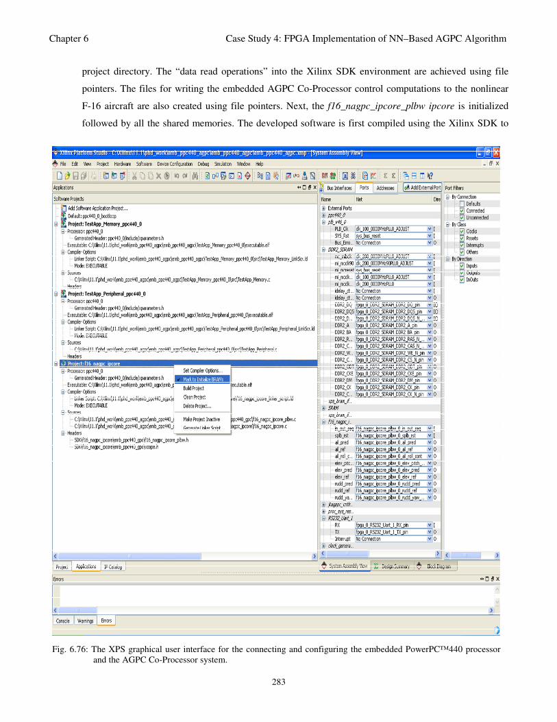
Chapter 6 Case Study 4: FPGA Implementation of NN–Based AGPC Algorithm
283
Fig. 6.76: The XPS graphical user interface for the connecting and configuring the embedded PowerPC™440 processor
and the AGPC Co-Processor system.
project directory. The “data read operations” into the Xilinx SDK environment are achieved using file
pointers. The files for writing the embedded AGPC Co-Processor control computations to the nonlinear
F-16 aircraft are also created using file pointers. Next, the f16_nagpc_ipcore_plbw ipcore is initialized
followed by all the shared memories. The developed software is first compiled using the Xilinx SDK to
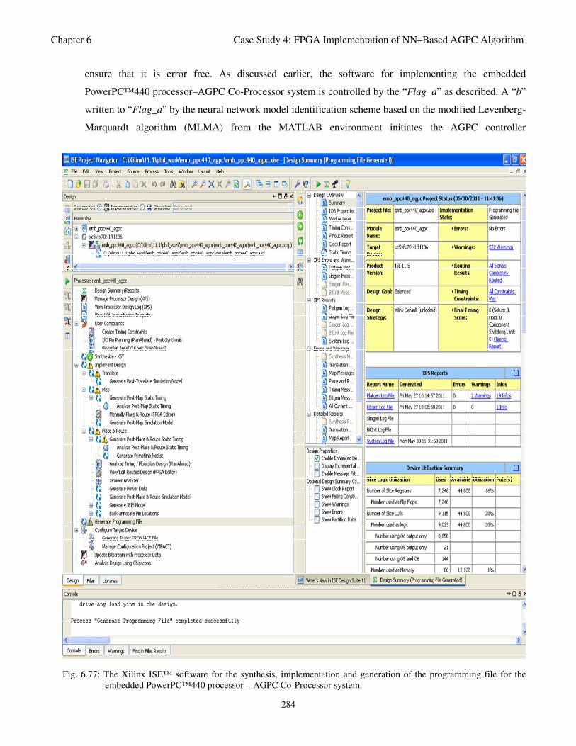
Chapter 6 Case Study 4: FPGA Implementation of NN–Based AGPC Algorithm
284
Fig. 6.77: The Xilinx ISE™ software for the synthesis, implementation and generation of the programming file for the
embedded PowerPC™440 processor – AGPC Co-Processor system.
ensure that it is error free. As discussed earlier, the software for implementing the embedded
PowerPC™440 processor–AGPC Co-Processor system is controlled by the “Flag_a” as described. A “b”
written to “Flag_a” by the neural network model identification scheme based on the modified Levenberg-
Marquardt algorithm (MLMA) from the MATLAB environment initiates the AGPC controller
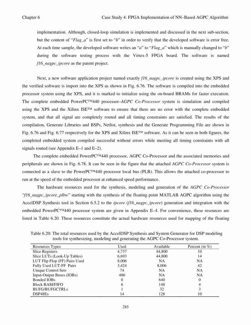
Chapter 6 Case Study 4: FPGA Implementation of NN–Based AGPC Algorithm
285
implementation. Although, closed-loop simulation is implemented and discussed in the next sub-section,
but the content of “Flag_a” is first set to “b” in order to verify that the developed software is error free.
At each time sample, the developed software writes an “a” to “Flag_a” which is manually changed to “b”
during the software testing process with the Virtex-5 FPGA board. The software is named
f16_nagpc_ipcore as the parent project.
Next, a new software application project named exactly f16_nagpc_ipcore is created using the XPS and
the verified software is import into the XPS as shown in Fig. 6.76. The software is compiled into the embedded
processor system using the XPS, and it is marked to initialize using the on-board BRAMs for faster execution.
The complete embedded PowerPC™440 processor–AGPC Co-Processor system is simulation and compiled
using the XPS and the Xilinx ISE™ software to ensure that there are no error with the complete embedded
system, and that all signal are completely routed and all timing constraints are satisfied. The results of the
compilation, Generate Libraries and BSPs, Netlist, synthesis and the Generate Programming File are shown in
Fig. 6.76 and Fig. 6.77 respectively for the XPS and Xilinx ISE™ software. As it can be seen in both figures, the
completed embedded system compiled successful without errors while meeting all timing constraints with all
signals routed (see Appendix E–1 and E–2).
The complete embedded PowerPC™440 processor, AGPC Co-Processor and the associated memories and
peripherals are shown in Fig. 6.78. It can be seen in the figure that the attached AGPC Co-Processor system is
connected as a slave to the PowerPC™440 processor local bus (PLB). This allows the attached co-processor to
run at the speed of the embedded processor at enhanced speed performance.
The hardware resources used for the synthesis, modeling and generation of the AGPC Co-Processor
“f16_nagpc_ipcore_plbw” starting with the synthesis of the floating point MATLAB AGPC algorithm using the
AccelDSP Synthesis tool in Section 6.5.2 to the ipcore (f16_nagpc_ipcore) generation and integration with the
embedded PowerPC™440 processor system are given in Appendix E–4. For convenience, these resources are
listed in Table 6.20. These resources constitute the actual hardware resources used for mapping of the floating
Table 6.20: The total resources used by the AccelDSP Synthesis and System Generator for DSP modeling
tools for synthesizing, modeling and generating the AGPC Co-Processor system.
Resources Types Used Available Percent (in %)
Slice Registers 4,737 44,800 10
Slice LUTs (Look-Up Tables) 6,693 44,800 14
LUT Flip Flop (FF) Pairs Used 8,006 NA NA
Fully Used LUT-FF Pairs 3,424 8,006 42
Unique Control Sets 74 NA NA
Input-Output Buses (IOBs) 486 NA NA
Bonded IOBs 0 640 0
Block RAM/FIFO 6 148 4
BUFG/BUFGCTRLs 1 32 3
DSP48Es 14 128 10
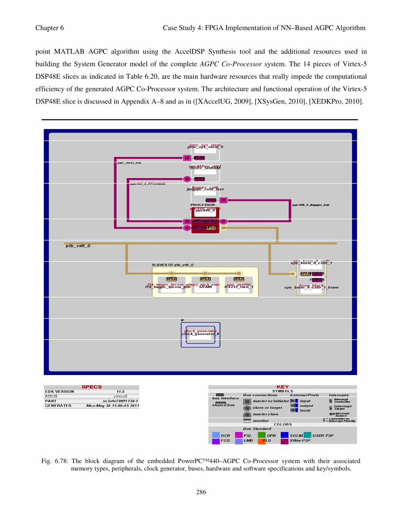
Chapter 6 Case Study 4: FPGA Implementation of NN–Based AGPC Algorithm
286
Fig. 6.78: The block diagram of the embedded PowerPC™440–AGPC Co-Processor system with their associated
memory types, peripherals, clock generator, buses, hardware and software specifications and key/symbols.
point MATLAB AGPC algorithm using the AccelDSP Synthesis tool and the additional resources used in
building the System Generator model of the complete AGPC Co-Processor system. The 14 pieces of Virtex-5
DSP48E slices as indicated in Table 6.20, are the main hardware resources that really impede the computational
efficiency of the generated AGPC Co-Processor system. The architecture and functional operation of the Virtex-5
DSP48E slice is discussed in Appendix A–8 and as in ([XAccelUG, 2009], [XSysGen, 2010], [XEDKPro, 2010].
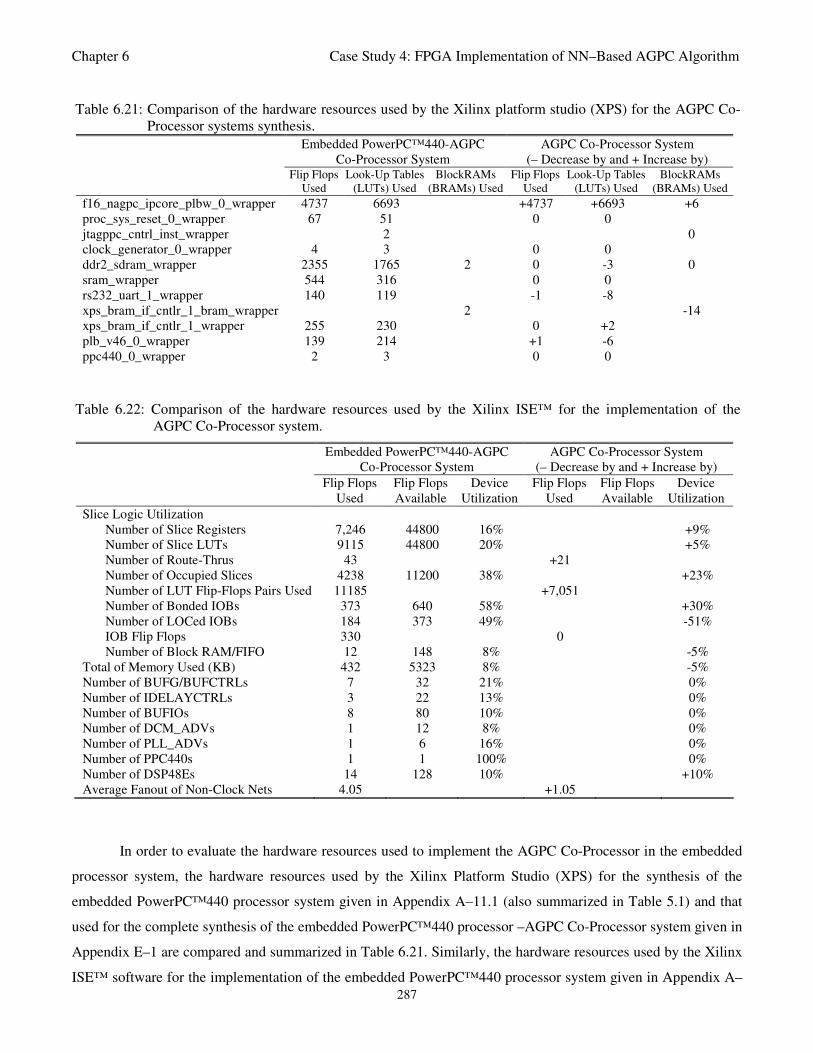
Chapter 6 Case Study 4: FPGA Implementation of NN–Based AGPC Algorithm
287
In order to evaluate the hardware resources used to implement the AGPC Co-Processor in the embedded
processor system, the hardware resources used by the Xilinx Platform Studio (XPS) for the synthesis of the
embedded PowerPC™440 processor system given in Appendix A–11.1 (also summarized in Table 5.1) and that
used for the complete synthesis of the embedded PowerPC™440 processor –AGPC Co-Processor system given in
Appendix E–1 are compared and summarized in Table 6.21. Similarly, the hardware resources used by the Xilinx
ISE™ software for the implementation of the embedded PowerPC™440 processor system given in Appendix A–
Table 6.21: Comparison of the hardware resources used by the Xilinx platform studio (XPS) for the AGPC Co-
Processor systems synthesis.
Embedded PowerPC™440-AGPC
Co-Processor System
AGPC Co-Processor System
(– Decrease by and + Increase by)
Flip Flops
Used
Look-Up Tables
(LUTs) Used
BlockRAMs
(BRAMs) Used
Flip Flops
Used
Look-Up Tables
(LUTs) Used
BlockRAMs
(BRAMs) Used
f16_nagpc_ipcore_plbw_0_wrapper 4737 6693 +4737 +6693 +6
proc_sys_reset_0_wrapper 67 51 0 0
jtagppc_cntrl_inst_wrapper 2 0
clock_generator_0_wrapper 4 3 0 0
ddr2_sdram_wrapper 2355 1765 2 0 -3 0
sram_wrapper 544 316 0 0
rs232_uart_1_wrapper 140 119 -1 -8
xps_bram_if_cntlr_1_bram_wrapper 2 -14
xps_bram_if_cntlr_1_wrapper 255 230 0 +2
plb_v46_0_wrapper 139 214 +1 -6
ppc440_0_wrapper 2 3 0 0
Table 6.22: Comparison of the hardware resources used by the Xilinx ISE™ for the implementation of the
AGPC Co-Processor system.
Embedded PowerPC™440-AGPC
Co-Processor System
AGPC Co-Processor System
(– Decrease by and + Increase by)
Flip Flops
Used
Flip Flops
Available
Device
Utilization
Flip Flops
Used
Flip Flops
Available
Device
Utilization
Slice Logic Utilization
Number of Slice Registers 7,246 44800 16% +9%
Number of Slice LUTs 9115 44800 20% +5%
Number of Route-Thrus 43 +21
Number of Occupied Slices 4238 11200 38% +23%
Number of LUT Flip-Flops Pairs Used 11185 +7,051
Number of Bonded IOBs 373 640 58% +30%
Number of LOCed IOBs 184 373 49% -51%
IOB Flip Flops 330 0
Number of Block RAM/FIFO 12 148 8% -5%
Total of Memory Used (KB) 432 5323 8% -5%
Number of BUFG/BUFCTRLs 7 32 21% 0%
Number of IDELAYCTRLs 3 22 13% 0%
Number of BUFIOs 8 80 10% 0%
Number of DCM_ADVs 1 12 8% 0%
Number of PLL_ADVs 1 6 16% 0%
Number of PPC440s 1 1 100% 0%
Number of DSP48Es 14 128 10% +10%
Average Fanout of Non-Clock Nets 4.05 +1.05
Chapter 6 Case Study 4: FPGA Implementation of NN–Based AGPC Algorithm
288
11.2 (also summarized in Table 5.1) and that used for the complete synthesis of the embedded PowerPC™440
processor –AGPC Co-Processor system given in Appendix E–2 are also compared and summarized in Table 6.22.
The results of Table 6.21 indicates that addition 6 Block RAMs used for the “f16_nagpc_ipcore” wrapper
have been added to the embedded system. Note that this wrapper was generated by the AccelDSP synthesis tool
during the synthesis of the MATLAB AGPC algorithm to generate a synthesized hardware model of the AGPC
algorithm and was also used by the System Generator for DSP to generate the AGPC Co-Processor IP core which
was imported into the embedded processor system. The main results of Table 6.22 are the additional increase in
hardware resources of about 30% for the bonded input-output blocks (Bonded IOBs) used by the AGPC Co-
Processor for read/write operations thereby reducing the number of locked (LOCed) IOBs by 51%. Furthermore,
additional 14 flip-flops have constituting about 10% increases the hardware cost for implementing the Virtex-5
DSP48E slices which are the main components that impedes the computational efficiency of the synthesized
AGPC algorithm, and hence the name “AGPC Co-Processor” as a co-processor is derived from the use of the
Virtex-5 DSP48E slices which are by themselves dedicated processors.
6.5.6 Real-Time Implementation of the Embedded PowerPC™440 Processor and
AGPC Co-Processor System on Xilinx Virtex-5 FX70T ML507 FPGA Board
The real-time implementation of the embedded PowerPC™440 processor–AGPC Co-Processor system on
the Virtex-5 FX70T ML507 FPGA development board and the closed-loop FPGA-in-the-loop simulation of the
validated nonlinear F-16 aircraft Simulink model together with the identified neural network model using the
MLMA algorithm are performed at each time sample are discussed in this sub-section. The simulation results are
also presented and discussed. The implementation procedures are outlined as follows.
1). The already developed and compiled embedded PowerPC™440 processor–AGPC Co-Processor system,
discussed in the last sub-section, is opened via the Xilinx ISE™ and the XPS software GUIs as shown in Fig.
6.76 and Fig. 6.77 respectively.
2). Using the XPS software GUI of Fig. 6.76, the hardware description file for the embedded PowerPC™440
processor–AGPC Co-Processor system “emb_ppc440_agpc.xml” is exported to the Xilinx software
development kit (Xilinx SDK) by selecting Project Export Hardware Design to SDK and clicking Export
Only. This automatically creates the SDK directory in the current project (emb_ppc440_agpc) hierarchy, and
stores the generated hardware description file. A new directory for the software development is then manually
created within the SDK directory and it is given the name of the ipcore as “f16_nagpc_ipcore”.
3). The Xilinx SDK software is opened. This automatically request that the hardware description file
“emb_ppc440_agpc.xml” file of the embedded system be specified. Specifying and including the hardware
description file into the Xilinx SDK project, automatically launch the Xilinx SDK GUI shown in Fig. 6.79.
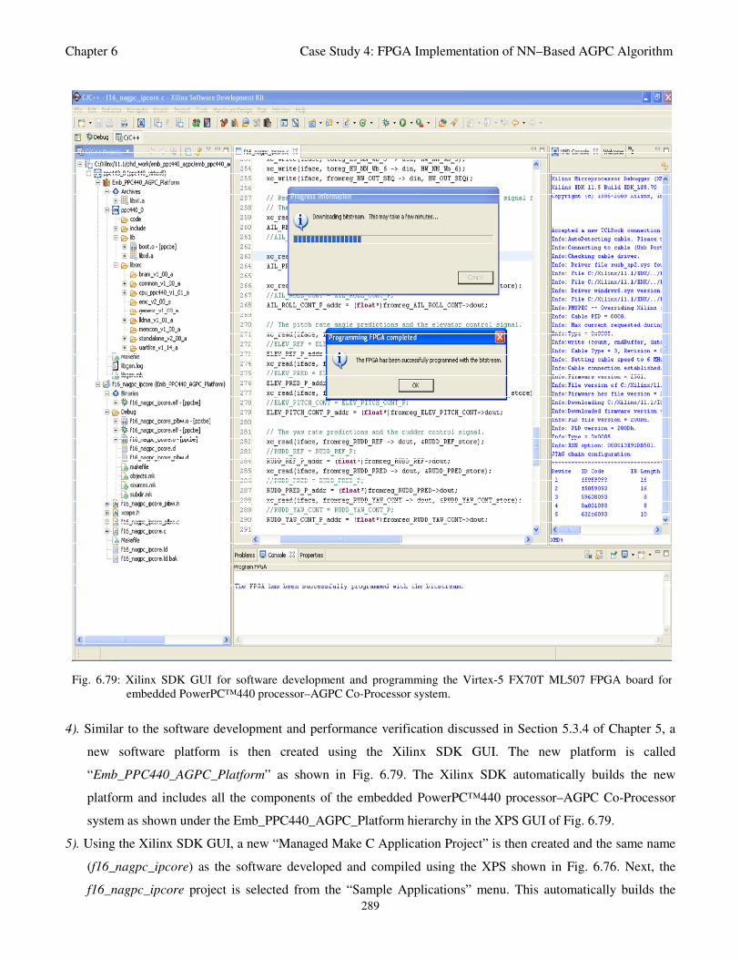
Chapter 6 Case Study 4: FPGA Implementation of NN–Based AGPC Algorithm
289
Fig. 6.79: Xilinx SDK GUI for software development and programming the Virtex-5 FX70T ML507 FPGA board for
embedded PowerPC™440 processor–AGPC Co-Processor system.
4). Similar to the software development and performance verification discussed in Section 5.3.4 of Chapter 5, a
new software platform is then created using the Xilinx SDK GUI. The new platform is called
“Emb_PPC440_AGPC_Platform” as shown in Fig. 6.79. The Xilinx SDK automatically builds the new
platform and includes all the components of the embedded PowerPC™440 processor–AGPC Co-Processor
system as shown under the Emb_PPC440_AGPC_Platform hierarchy in the XPS GUI of Fig. 6.79.
5). Using the Xilinx SDK GUI, a new “Managed Make C Application Project” is then created and the same name
(f16_nagpc_ipcore) as the software developed and compiled using the XPS shown in Fig. 6.76. Next, the
f16_nagpc_ipcore project is selected from the “Sample Applications” menu. This automatically builds the
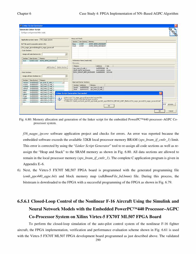
Chapter 6 Case Study 4: FPGA Implementation of NN–Based AGPC Algorithm
290
Fig. 6.80: Memory allocation and generation of the linker script for the embedded PowerPC™440 processor–AGPC Co-
processor system.
f16_nagpc_ipcore software application project and checks for errors. An error was reported because the
embedded software exceeds the available 32KB local processor memory BRAM (xps_bram_if_cntlr_1) limit.
This error is corrected by using the “Linker Script Generator” tool to re-assign all code sections as well as re-
assign the “Heap and Stack” to the SRAM memory as shown in Fig. 6.80. All data sections are allowed to
remain in the local processor memory (xps_bram_if_cntlr_1). The complete C application program is given in
Appendix E–6.
6). Next, the Virtex-5 FX70T ML507 FPGA board is programmed with the generated programming file
(emb_ppc440_agpc.bit) and block memory map (edkBmmFile_bd.bmm) file. During this process, the
bitstream is downloaded to the FPGA with a successful programming of the FPGA as shown in Fig. 6.79.
6.5.6.1 Closed-Loop Control of the Nonlinear F-16 Aircraft Using the Simulink and
Neural Network Models with the Embedded PowerPC™440 Processor–AGPC
Co-Processor System on Xilinx Virtex-5 FX70T ML507 FPGA Board
To perform the closed-loop simulation of the auto-pilot control system of the nonlinear F-16 fighter
aircraft, the FPGA implementation, verification and performance evaluation scheme shown in Fig. 6.61 is used
with the Virtex-5 FX70T ML507 FPGA development board programmed as just described above. The validated
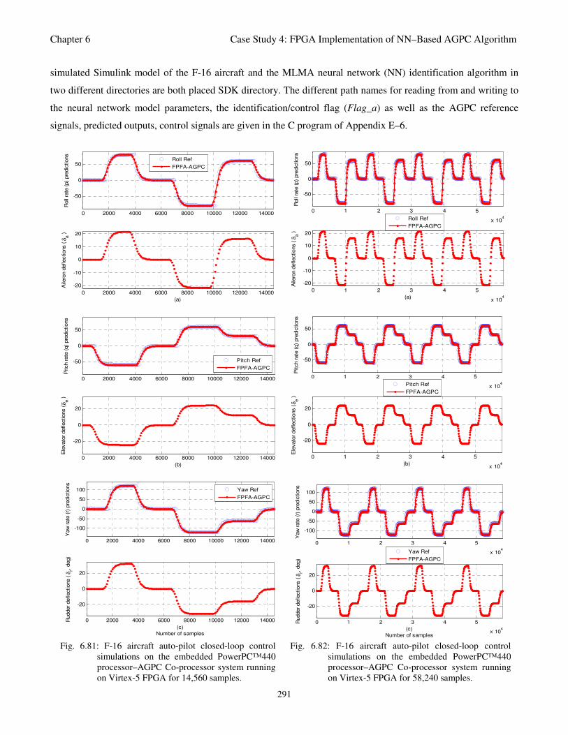
Chapter 6 Case Study 4: FPGA Implementation of NN–Based AGPC Algorithm
291
0 2000 4000 6000 8000 10000 12000 14000
-50
0
50
Roll
rate
(p)
pre
dic
tions
Roll Ref
FPFA-AGPC
0 2000 4000 6000 8000 10000 12000 14000
-20
-10
0
10
20
(a)
Aile
ron d
eflections (
δa )
0 2000 4000 6000 8000 10000 12000 14000
-50
0
50
Pitch rate
(q)
pre
dic
tions
Pitch Ref
FPFA-AGPC
0 2000 4000 6000 8000 10000 12000 14000
-20
0
20
(b)
Ele
vato
r deflections (
δe )
0 2000 4000 6000 8000 10000 12000 14000
-100
-50
0
50
100
Yaw
rate
(r)
pre
dic
tions
Yaw Ref
FPFA-AGPC
0 2000 4000 6000 8000 10000 12000 14000
-20
0
20
(c)
Number of samples
Rudder
deflections (
δr,
deg)
0 1 2 3 4 5
x 104
-50
0
50
Roll
rate
(p)
pre
dic
tions
Roll Ref
FPFA-AGPC
0 1 2 3 4 5
x 104
-20
-10
0
10
20
(a)A
ilero
n d
eflections ( δ
a )
0 1 2 3 4 5
x 104
-50
0
50
Pitch r
ate
(q)
pre
dic
tions
Pitch Ref
FPFA-AGPC
0 1 2 3 4 5
x 104
-20
0
20
(b)
Ele
vato
r deflections (
δe )
0 1 2 3 4 5
x 104
-100
-50
0
50
100
Yaw
rate
(r)
pre
dic
tions
Yaw Ref
FPFA-AGPC
0 1 2 3 4 5
x 104
-20
0
20
(c)
Number of samples
Rudder
deflections (
δr,
deg)
Fig. 6.81: F-16 aircraft auto-pilot closed-loop control
simulations on the embedded PowerPC™440
processor–AGPC Co-processor system running
on Virtex-5 FPGA for 14,560 samples.
Fig. 6.82: F-16 aircraft auto-pilot closed-loop control
simulations on the embedded PowerPC™440
processor–AGPC Co-processor system running
on Virtex-5 FPGA for 58,240 samples.
simulated Simulink model of the F-16 aircraft and the MLMA neural network (NN) identification algorithm in
two different directories are both placed SDK directory. The different path names for reading from and writing to
the neural network model parameters, the identification/control flag (Flag_a) as well as the AGPC reference
signals, predicted outputs, control signals are given in the C program of Appendix E–6.
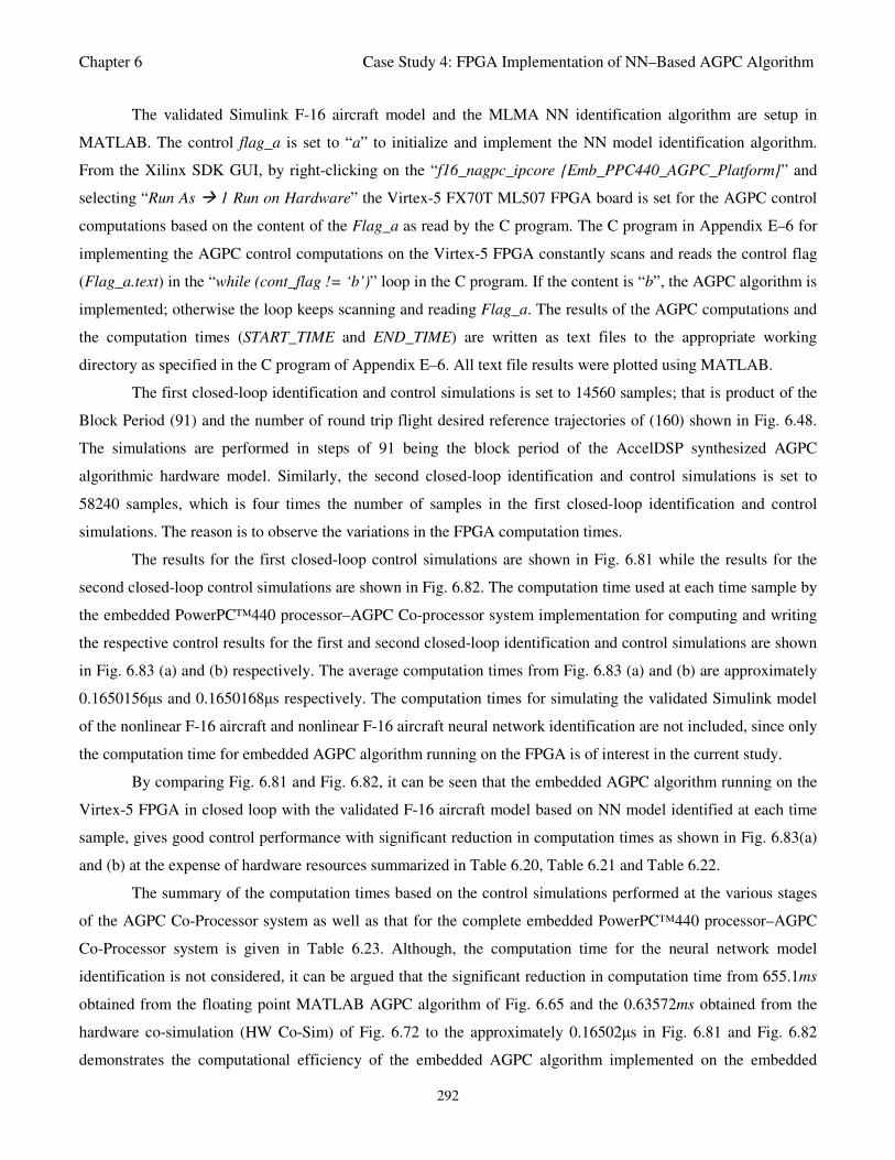
Chapter 6 Case Study 4: FPGA Implementation of NN–Based AGPC Algorithm
292
The validated Simulink F-16 aircraft model and the MLMA NN identification algorithm are setup in
MATLAB. The control flag_a is set to “a” to initialize and implement the NN model identification algorithm.
From the Xilinx SDK GUI, by right-clicking on the “f16_nagpc_ipcore Emb_PPC440_AGPC_Platform” and
selecting “Run As 1 Run on Hardware” the Virtex-5 FX70T ML507 FPGA board is set for the AGPC control
computations based on the content of the Flag_a as read by the C program. The C program in Appendix E–6 for
implementing the AGPC control computations on the Virtex-5 FPGA constantly scans and reads the control flag
(Flag_a.text) in the “while (cont_flag != ‘b’)” loop in the C program. If the content is “b”, the AGPC algorithm is
implemented; otherwise the loop keeps scanning and reading Flag_a. The results of the AGPC computations and
the computation times (START_TIME and END_TIME) are written as text files to the appropriate working
directory as specified in the C program of Appendix E–6. All text file results were plotted using MATLAB.
The first closed-loop identification and control simulations is set to 14560 samples; that is product of the
Block Period (91) and the number of round trip flight desired reference trajectories of (160) shown in Fig. 6.48.
The simulations are performed in steps of 91 being the block period of the AccelDSP synthesized AGPC
algorithmic hardware model. Similarly, the second closed-loop identification and control simulations is set to
58240 samples, which is four times the number of samples in the first closed-loop identification and control
simulations. The reason is to observe the variations in the FPGA computation times.
The results for the first closed-loop control simulations are shown in Fig. 6.81 while the results for the
second closed-loop control simulations are shown in Fig. 6.82. The computation time used at each time sample by
the embedded PowerPC™440 processor–AGPC Co-processor system implementation for computing and writing
the respective control results for the first and second closed-loop identification and control simulations are shown
in Fig. 6.83 (a) and (b) respectively. The average computation times from Fig. 6.83 (a) and (b) are approximately
0.1650156µs and 0.1650168µs respectively. The computation times for simulating the validated Simulink model
of the nonlinear F-16 aircraft and nonlinear F-16 aircraft neural network identification are not included, since only
the computation time for embedded AGPC algorithm running on the FPGA is of interest in the current study.
By comparing Fig. 6.81 and Fig. 6.82, it can be seen that the embedded AGPC algorithm running on the
Virtex-5 FPGA in closed loop with the validated F-16 aircraft model based on NN model identified at each time
sample, gives good control performance with significant reduction in computation times as shown in Fig. 6.83(a)
and (b) at the expense of hardware resources summarized in Table 6.20, Table 6.21 and Table 6.22.
The summary of the computation times based on the control simulations performed at the various stages
of the AGPC Co-Processor system as well as that for the complete embedded PowerPC™440 processor–AGPC
Co-Processor system is given in Table 6.23. Although, the computation time for the neural network model
identification is not considered, it can be argued that the significant reduction in computation time from 655.1ms
obtained from the floating point MATLAB AGPC algorithm of Fig. 6.65 and the 0.63572ms obtained from the
hardware co-simulation (HW Co-Sim) of Fig. 6.72 to the approximately 0.16502µs in Fig. 6.81 and Fig. 6.82
demonstrates the computational efficiency of the embedded AGPC algorithm implemented on the embedded
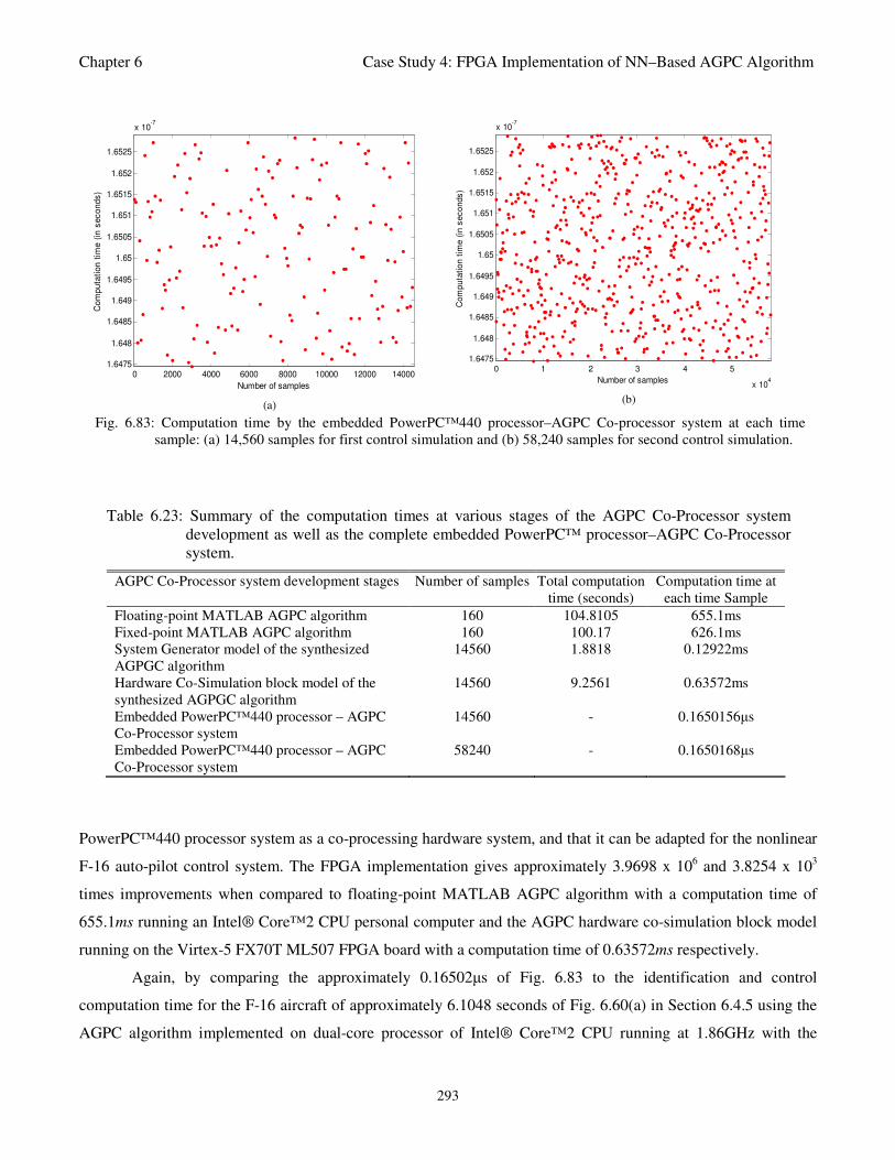
Chapter 6 Case Study 4: FPGA Implementation of NN–Based AGPC Algorithm
293
0 2000 4000 6000 8000 10000 12000 140001.6475
1.648
1.6485
1.649
1.6495
1.65
1.6505
1.651
1.6515
1.652
1.6525
x 10-7
Number of samples
Co
mp
uta
tion
tim
e (
in s
ec
on
ds
)
(a)
0 1 2 3 4 5
x 104
1.6475
1.648
1.6485
1.649
1.6495
1.65
1.6505
1.651
1.6515
1.652
1.6525
x 10-7
Number of samples
Com
pu
tatio
n t
ime (
in s
eco
nds
)
(b)
Fig. 6.83: Computation time by the embedded PowerPC™440 processor–AGPC Co-processor system at each time
sample: (a) 14,560 samples for first control simulation and (b) 58,240 samples for second control simulation.
PowerPC™440 processor system as a co-processing hardware system, and that it can be adapted for the nonlinear
F-16 auto-pilot control system. The FPGA implementation gives approximately 3.9698 x 10⁶ and 3.8254 x 10
3
times improvements when compared to floating-point MATLAB AGPC algorithm with a computation time of
655.1ms running an Intel® Core™2 CPU personal computer and the AGPC hardware co-simulation block model
running on the Virtex-5 FX70T ML507 FPGA board with a computation time of 0.63572ms respectively.
Again, by comparing the approximately 0.16502µs of Fig. 6.83 to the identification and control
computation time for the F-16 aircraft of approximately 6.1048 seconds of Fig. 6.60(a) in Section 6.4.5 using the
AGPC algorithm implemented on dual-core processor of Intel® Core™2 CPU running at 1.86GHz with the
Table 6.23: Summary of the computation times at various stages of the AGPC Co-Processor system
development as well as the complete embedded PowerPC™ processor–AGPC Co-Processor
system.
AGPC Co-Processor system development stages Number of samples Total computation
time (seconds)
Computation time at
each time Sample
Floating-point MATLAB AGPC algorithm 160 104.8105 655.1ms
Fixed-point MATLAB AGPC algorithm 160 100.17 626.1ms
System Generator model of the synthesized
AGPGC algorithm
14560 1.8818 0.12922ms
Hardware Co-Simulation block model of the
synthesized AGPGC algorithm
14560 9.2561 0.63572ms
Embedded PowerPC™440 processor – AGPC
Co-Processor system
14560 - 0.1650156µs
Embedded PowerPC™440 processor – AGPC
Co-Processor system
58240 - 0.1650168µs
Chapter 6 Case Study 4: FPGA Implementation of NN–Based AGPC Algorithm
294
MATLAB “parfor” for parallel implementation, it may also be argued that the FPGA implementation appears to
be a suitable implementation platform due to the significant reduction in computation time.
A major drawback with the FPGA implementation technique demonstrated in this study is that as the size
of the neural network model parameters increases, the number of input-output ports increases which may exceed
the available 640 input-output (I/O) ports on the Virtex-5. Although, the proposed identification algorithms have
been formulated and demonstrated to train the networks using small network parameters for all the examples
considered in this study, but these may not generally be the case for other multivariable systems with several
inputs and outputs. Thus, investigating the FPGA implementation of the neural network-based model
identification algorithms and the nonlinear adaptive model predictive control (NAMPC) algorithm would be a
possible solution to this drawback. In that case, only a streaming measurement data would be required for
implementing the identification and control algorithm running on the FPGA, thus reducing the number of I/O
ports required. Unlike the AGPC algorithm, the NN-based model identification algorithms as well as the NAMPC
algorithm are based on iterative optimizations. This will definitely increase the “BLOCK PERIOD”,
“LATENCY” and consequently FPGA hardware resources. Experiences acquired in this study have shown that
the design will not have a constant throughput required to generate the System Generator block model. A solution
to the aforementioned problem would be the parallelization of these iterative algorithms before their syntheses.
Chapter 7 Evaluation and Discussion of Results, Open Issues and Recommendations
295
CHAPTER 7
CONCLUSIONS
7.1 Evaluation and Discussion of Results
In this thesis, new comprehensive neural network (NN) based algorithms were developed for the model
identification and model predictive control of processes with the purpose of being combined to form adaptive
model predictive control strategy with reduced computational time. Also, new network control system and FPGA
architectures are proposed for further reducing the overhead of the strategies implementation on conventional
network control systems. The identification algorithms are based on a class of dynamic feedforward neural
networks (DFNN) trained with two different methods, namely: the adaptive recursive least square (ARLS)
method and the modified Levenberg-Marquardt algorithm (MLMA). For the model predictive control two
algorithms have been developed, namely: the adaptive generalized predictive control (AGPC) algorithm and the
nonlinear adaptive model predictive control (NAMPC) algorithm.
The adaptive model predictive control strategy involves first the training of the neural network (NN) by
any of the considered training algorithms, the selection of the optimal network parameters and the validation of
the trained network by using any of three different methods, namely: one-step prediction of the training and
validation (test) data, 5-step and 10-step ahead prediction of the training data, and the Akaike’s final prediction
error (AFPE) estimate. Next, the validated NN is used as the process model with which the parameters of the
adaptive model predictive control algorithms are tuned. This strategy is performed every time new samples of the
measured controlled variables are obtained. New control actions are computed by the tuned model predictive
control algorithm.
Hardware in the loop simulations of the implementation of the possible strategies on conventional, SOA
network control system and FPGA architectures have been performed for three highly nonlinear systems, namely:
1) the temperature control of a fluidized bed furnace reactor (FBFR) of the steam deactivation unit (SDU) of a
fluid catalytic cracking (FCC) pilot plant, 2) the soluble oxygen (the so called dissolved oxygen concentration)
control of the third aerobic reactor of an activated sludge wastewater treatment plant (AS-WWTP) process), and
3) the auto-pilot control system of a nonlinear F-16 fighter aircraft.
The obtained results show that the combination of the ARLS or the MLMA algorithms with the NAMPC
algorithms when they are implemented on multi-core and SOA architectures result to the best control performance
for the first two cases. For systems with lower sampling times, like the nonlinear F-16 auto-pilot control system,
requires the same combination of algorithms when it is implemented on an FPGA unit presents improved
performance and is realized within this short sampling time. All the discussions below are made with reference to
the work presented in Chapter 6 and are explained in detail as presented in the following.
Chapter 7 Evaluation and Discussion of Results, Open Issues and Recommendations
296
7.1.1 The Temperature Control of a Fluidized Bed Furnace Reactor (FBFR)
The results that are discussed here concern the model identification and adaptive control of the FBFR
temperatures presented in Section 6.2. The sampling time of the FBFR should not be higher than 120 seconds.
The total computation time of the neural network model identification of the FBFR process using the ARLS and
MLMA algorithms were 149.02 and 3.875 seconds respectively for 100 iterations (epochs) and for 1320 samples.
This implies that the FBFR process model can be identified at each time sample in 0.1129 and 0.0029 seconds
using the ARLS and MLMA algorithms respectively. The network training results in Section 6.2.2 showed that
although the ARLS has faster convergence property, the MLMA has smaller prediction errors than the ARLS.
Also, it was observed in Fig. 6.15 and Fig. 6.16 that the results of the FBFR reactor and heater temperatures
predictions in tracking the respective desired temperatures obtained using the model trained with the MLMA
algorithm outperformed those trained using the ARLS algorithm.
Furthermore, to compare the efficiency of the MLMA algorithm, it was compared with two well-known
existing neural network training algorithms, namely: the backpropagation with momentum (BPM) and the
incremental backproagation (INCBP). Simulation results over 1320 samples showed that the MLMA algorithm
had the best prediction performance and the least computation time of 0.0016 seconds at each time sample
followed by the BPM with 0.0035 seconds, and lastly the INCBP algorithm with 0.0074 seconds.
The overall worst case turnaround time of the closed loop control by the proposed AGPC and NAMPC
algorithms when the model is identified by the ARLS algorithm were found to be 3.1207 and 8.0809 seconds
respectively, when these two algorithms are implemented on a typical four core PC. As turnaround time is defined
as the time elapsed from the moment new samples of the controlled variables are read until the moment the
corrections of the values of the manipulated variables are computed and become available. The results of the
FBFR reactor and heater temperatures predictions in tracking the respective desired temperatures showed that the
NAMPC outperforms the AGPC at the expense of 2.5895 times the computation time used by the AGPC
algorithm as evident in Fig. 6.22. The monitored performance and turnaround times of the considered algorithms
imply that the current personal computer technologies are adequate to solve computationally intensive tasks for
process control applications requiring sampling times much shorter than the upper limit of the FBFR process.
Finally, because of the superior control performance of the NAMPC algorithm when it is combined with
MLMA algorithm for the Neural network model identification, its suitability for the FBFR process model
identification and control over a service-oriented architecture (SOA) cluster network based on the device profile
for web services (DPWS) was investigated . The worst case overall control loop turnaround time was 12.8465
seconds. This result shows that the proposed MLMA model identification and the NAMPC control algorithms
implementation over the SOA cluster network based on the DPWS meets by far the limit imposed by the upper
limit of the FBFR sampling time and therefore they can be deployed for the FBFR process control in an industrial
environment.
Chapter 7 Evaluation and Discussion of Results, Open Issues and Recommendations
297
7.1.2 The Soluble Oxygen Control in the Aerobic Reactor of the Process of an
Activated Sludge Wastewater Treatment Plant (AS-WWTP)
The results that are presented and discussed here follow from the model identification and adaptive
dissolved oxygen concentration control in the aerobic reactor of the AS-WWTP process of Section 6.3. The
sampling time required for the closed loop control of the validated simulation in Simulink of the AS-WWTP
process is 15 minutes which corresponds to the time over which dry-weather data was collected. The total
computation time to obtain the neural network model of the aerobic reactor for the AS-WWTP process using the
ARLS and MLMA algorithms were 42.2188 and 2.3750 seconds respectively over 1,076 training data samples for
100 iterations (epochs). This implies that the NN model of the aerobic reactor of the AS-WWTP process can be
identified in 0.0392 and 0.0022 seconds at each time sample by the ARLS and MLMA algorithms respectively.
The network training and validation have shown that the ARLS has faster convergence while the MLMA has
overall smaller prediction errors. It was also observed that the MLMA algorithm terminated after 100 epochs
when the maximum number of epochs was specified to be 500 while the ARLS terminated earlier just after about
65 epochs. The on-line closed-loop model identification and adaptive AGPC control of the dissolved oxygen
concentration in the aerobic reactor for the AS-WWTP process using the ARLS and MLMA algorithms for 100
epochs in Section 6.3.2.2 showed that the dissolved oxygen concentration predictions in tracking the desired
reference signals using the model trained with the MLMA algorithm outperformed those based on the model
obtained with the ARLS algorithm as evident in Fig. 6.38 performances.
A comparison of the validation results of a network trained for 100 epochs by the ARLS model
identification algorithm with the backpropagation with momentum (BPM) and the incremental backproagation
(INCBP) algorithms showed that, except for the high computation time of 0.0399 for implementing the ARLS
algorithm at each time sample instant), the ARLS algorithm gave the least prediction errors when compared to the
BPM and the INCBP algorithms. The high computation time obtained with the ARLS algorithm is still about
2.2556 x 10⁴ times less than the 15 minutes sampling time of the AS-WWTP process and therefore the use of the
BMP and INCP are of no use for the aerobic reactor NN model identification of the AS-WWTP since the
computation time and prediction performances of the ARLS algorithm is acceptable.
With respect to the control performance the NAMPC outperforms the AGPC at the expense of higher
computation time than that of the AGPC algorithm by 2.6260 times. The observed computation times for both
AGPC and NAMPC algorithms show that the current multi-core PC technologies can be used for implementing
the proposed neural network-based model identification and adaptive model predictive control strategies for the
case of the AS-WWTP with improved control benefits from their applications.
Chapter 7 Evaluation and Discussion of Results, Open Issues and Recommendations
298
7.1.3 The Nonlinear F-16 Fighter Aircraft Auto-Pilot Control
The results discussed here refer to the work presented Section 6.4. The stability analysis of any closed
loop control operation requires a sampling time of the controlled variables of the F-16 aircraft auto pilot is to be
not higher than 0.5 seconds. The computation time for the NN model identification of the F-16 aircraft auto-pilot
by the ARLS and MLMA algorithms were found to be 298.59 and 6.5313 respectively for 100 iterations (epochs)
over 4,000 training data samples. This implies that the neural network model of the nonlinear F-16 aircraft can be
identified in 0.0746 and 0.0016 seconds at each time sample by the ARLS and MLMA algorithms respectively.
The network training and validation results showed the ARLS converges faster while the lower prediction errors
was achieved with the MLMA algorithm. It was also observed that good predictions accuracy was achieved by
having the ARLS algorithm terminating in almost 85 epochs when the maximum number of epochs was specified
to be 500. The computation times for implementing both algorithms were found to be less than the 0.5 seconds
sampling time limit of the nonlinear F-16 aircraft.
The online closed-loop of the nonlinear F-16 aircraft model identification using the ARLS and the
MLMA algorithms and adaptive control of the auto-pilot control system using the proposed nonlinear adaptive
model predictive control (NAMPC) controller showed the roll rate, pitch rate, yaw rate and the throttle setting
predictions compared with the desired reference trajectories and their respective control input signals obtained
using the models obtained by both ARLS and MLMA algorithms gave essentially the same results.
The computation times of the proposed AGPC and NAMPC algorithms when model identification is
performed with the ARLS algorithm were found to be 6.1048 and 11.0367 seconds respectively at each time
sample over 350 simulation samples. The adaptive AGPC and NAMPC control results of Fig. 6.59 showed that
although the nonlinear F-16 aircraft desired reference trajectory predictions and their respective control inputs
computations obtained by both controllers for the roll, pitch and yaw rate predictions are essentially the same, but
the NAMPC outperformed the AGPC in the throttle and thrust control at the expense of an additional time of
1.8079 time more than the computation time used by the AGPC algorithm. However, these computation times for
the identification and adaptive control of the nonlinear F-16 aircraft auto-pilot by algorithms violates the sampling
time of 0.5 and indicates that the typical multi-core computer technologies are inadequate to solve the less
computationally intensive task of the AGPC or the more computationally intensive task of the NAMPC algorithm
within the auto-pilot sampling time requirements. For this reason a more efficient real-time computing platform
was proposed that could meet the 0.5 seconds time constraints for control of the nonlinear F-16 aircraft.
7.1.4 Real-Time Embedded PowerPC™440 Processor–AGPC Co-Processor System
Implementation on Xilinx Virtex-5 FX70T ML507 FPGA Board
In order to meet the real-time constraint of 0.5 seconds of the nonlinear F-16 aircraft control , a real-time
embedded platform which consists of an embedded PowerPC™440 processor system combined with the AGPC
Chapter 7 Evaluation and Discussion of Results, Open Issues and Recommendations
299
algorithm as a co-processor implemented on a field programmable gate array (FPGA) was proposed, developed
and implemented.
The choice for selecting the AGPC algorithm was made because of its lower computational burden
compared to that of the NAMPC and because it presents almost identical performance with that of NAMPC when
it is applied to the F-16 control. The real-time embedded processor platform was developed and implemented
using the Xilinx Virtex-5FX70T ML507 FPGA board detailed in Chapter 5.3.
Also, the choice of the hard core embedded PowerPC™440 processor for use with Xilinx families of
FPGA including the Virtex-5 FX70T ML507 FPGA board used in this work against the Xilinx’s soft-core
embedded MicroBlaze™ processor was made because the conducted Dhrystone benchmarks on both processors
indicated a high DMIPS number for the PowerPC™440 (1100 against 240 of MicroBlaze).
With the last paragraph in mind, the embedded PowerPC™440 processor system was first designed by
using the basic intellectual properties (IPs) cores required for the AGPC realization on the FPGA. The IP cores
are basically hardware peripheral drivers. The embedded IPs cores used for the embedded processor system
design included: the PowerPC™440 BRAM local memory driver, Virtex-5 XC5VFX70T FPGA on-board SRAM
driver, external DDR2 SRAM driver and a RS232 UART driver.
Then in Chapter 6.5, the AGPC algorithm is synthesized to obtain a register-transfer-level (RTL)
hardware model representative of the AGPC algorithm, by using the Xilinx’s AccelDSP Synthesis tool. The
resulting hardware model of the AGPC algorithm was then used to build a complete System Generator model of
the AGPC algorithm with input and output memory-mapped interfaces from which the AGPC co-processor
intellectual property core (pcore) was generated using the Xilinx’s System Generator for DSP modeling tool.
In order to verify how the System Generator model of the synthesized AGPC algorithm would perform
when deployed to the Virtex-5 FPGA, an FPGA-in-the-loop simulation was performed with a generated hardware
co-simulation (HW Co-Sim) block running on the Virtex-5 FPGA board while the nonlinear F-16 aircraft model
and the identification algorithm were simulated in the MATLAB Simulink environment. As Fig. 6.73 shows,
good predictions and tracking of the roll, pitch and yaw rates reference signal were achieved with a computation
time of 0.63572 microseconds (ms) at each time sample. The FPGA hardware co-simulation computation time is
1.0305 x 10³ times faster than the floating-point realization of the AGPC algorithm in MATLAB implemented on
a multicore computer.
Finally, the AGPC co-processor is imported and integrated with an embedded PowerPC™440 processor
system to form the real-time embedded processor platform that is used together with the nonlinear F-16 aircraft
model and the neural network identification scheme to evaluate the real-time control performance of the nonlinear
F-16 aircraft auto-pilot control system. The computation time for the embedded AGPC algorithm for each time
sample was approximately 0.16502µs. Therefore, the FPGA implementation resulted in approximately 3.9698 x
106 and 3.8524 x 10
3 times improvements when compared to the 655.1ms and 0.63572ms computation times
Chapter 7 Evaluation and Discussion of Results, Open Issues and Recommendations
300
obtained respectively by using the floating-point MATLAB AGPC algorithm running on a multicore computer
and the AGPC hardware co-simulation block model running on the Xilinx Virtex-5 FX70T ML507 FPGA board.
Although, the computation time for the neural network model identification is not considered, it was
mentioned in Section 7.1.3 that the computation times for the nonlinear F-16 aircraft model identification at each
time sample were 0.0746 and 0.0016 seconds using the ARLS and MLMA algorithms respectively based on their
respective MATLAB floating-point implemented on an Intel® Core™2 CPU @ 1.86GHz computer. The obtained
computation time of 0.16502µs demonstrates the computational efficiency of the real-time embedded
PowerPC™440 processor–AGPC Co-Processor hardware system implementation of the AGPC algorithm on the
Xilinx Virtex-5 FX70T ML507 FPGA board and that it can be adapted for the nonlinear F-16 aircraft auto-pilot
control system.
By adding the achieved 1.6502µs to the approximately 0.0746 or 0.0016 seconds required for the
nonlinear F-16 NN model identification using the ARLS or MLMA algorithm gives 0.0746 and 0.0016 seconds
respectively at each time sample which is about 6.7024 and 312.5 times the nonlinear F-16 aircraft time constant
of 0.5 seconds. Thus, it is evident that the combined model identification and AGPC control computation time of
approximately 6.1048 seconds has been significantly reduced to the time required only for model identification
since the AGPC computation time has become negligible (1.6502µs) due to computational power of the FPGA
and the efficient hardware/software co-design design methodologies.
7.2 Open Issues
Vast number of literature based on several techniques ranging from first principles models, neural
networks, fuzzy logic approaches, neural-fuzzy approaches, adaptive control, adaptive PID control techniques,
evolutionary approaches for modeling and control of the fluidized bed furnace reactor, steam deactivation unit and
fluid catalytic cracking as well as activated sludge wastewater treatment plants. However, literature is scare, if not
unavailable concerning neural network model identification and MPC control of the nonlinear F-16 aircraft
control. This makes if difficult to make a good comparison of the results obtained in this work with the proposed
techniques. Moreover, all of the literature on FPGA implementation of MPC algorithms and its variations
reviewed in this work are based on static first-order models of the F-16 aircraft combine with linear MPC
controllers, thus making it difficult to compare the results obtained in this work with existing techniques and
results.
Service-oriented architecture (SOA) technology based on device profile for web services (DPWS) has
become the state of the art solution for implementing autonomous and interoperable systems and networks
[Jammes and Smit, 2005b]. Moreover, several device level technologies have been proposed, most notably Jini
[Jini, 2010], universal plug-n-play (UPnP) [UPnP, 2010] and the DPWS [Jammes and Smit, 2005a]. In particular,
Chapter 7 Evaluation and Discussion of Results, Open Issues and Recommendations
301
the DPWS has adopted the well-established web services technology [DPWS, 2006]. However, researchers are
yet to fully exploit the application of these novel SOA technologies at the device level for the realization of
efficient networked control system based on the MPC algorithms. As a result, literature concerning MPC
implementation over SOA networks based on DPWS is scare and performance comparisons of the SOA cluster
network approach based on DPWS used in this work cannot be made.
The Dhrystone millions instructions per second (DMIPs) was not used to evaluate the performance of the
designed embedded PowerPC™ processor system in order to compare its operating frequency based on the FPGA
benchmark available in literature. Of all the literature reviewed in this work concerning FPGA implementation of
the different variations of MPC algorithm, none includes an embedded processor talk less of Dhrystone
benchmark performance evaluation. This makes standard literature on FPGA implementation scare for
performance comparisons.
A major drawback with the FPGA implementation technique demonstrated in this study is that as the size
of the neural network model parameters increases, the number of input-output ports increases which may exceed
the available 640 input-output (I/O) ports on the Virtex-5. Although, the proposed identification algorithms have
been formulated and demonstrated to train the networks using small network parameters for all the examples
considered in this study, but these may not generally be the case for other multivariable systems with several
inputs and outputs. Thus, investigating the FPGA implementation of the neural network-based model
identification algorithms and the nonlinear adaptive model predictive control (NAMPC) algorithm would be a
possible solution to this drawback. In that case, only a streaming measurement data would be required for
implementing the identification and control algorithm running on the FPGA, thus reducing the number of I/O
ports required. Unlike the AGPC algorithm, the NN-based model identification algorithms as well as the NAMPC
algorithm are based on iterative optimizations. This will definitely increase the “BLOCK PERIOD”,
“LATENCY” and consequently FPGA hardware resources. Experiences acquired in this study have shown that
the design will not have a constant throughput required to generate the System Generator block model. A solution
to the aforementioned problem could be the parallelization of these iterative algorithms before their syntheses.
7.3 Recommendations
1). The stability properties of the identification and control algorithms have not been investigated in this work and
can be the subject of future work.
2). Rather than using the large training data set at each model identification sequence, the Markovian modeling
approach could be investigated which can depend on few past state(s) of the system only to predict a suitable
model for use in the controller design. In this way, the concept of reinforcement learning could be applied to
recursively train the neural network and then a model-based adaptive critic controller can be proposed.
Chapter 7 Evaluation and Discussion of Results, Open Issues and Recommendations
302
3). The major difficulty in implementing the nonlinear adaptive model predictive control (NAMPC) algorithm
proposed in this work is related to an observed extremely high “Block Period” in the order of 104. Due to the
high “Block Period”, the hardware synthesis of the NAMPC algorithm resulted in a design with a non-constant
throughput. As a result of the high “Block Period”, the generation of the Hardware Co-Simulation block failed
due to the available 4GB DDR RAM compared to the 8GB RAM memory requirement to synthesize and
generate the NAMPC Hardware Co-Simulation block. The high “Block Period” is as a result of the extensive
iterative optimization and complex matrix manipulations performed by the NAMPC algorithm. Rather than
increasing the DDR RAM memory size, an efficient approach could be to: 1) parallelize the NAMPC
algorithm and 2) efficient pipelining of the NAMPC algorithm. This would reduce the number of “Function
Calls” and consequently the resulting synthesized NAMPC hardware “Block Period”.
4). The parallelization of the NAMPC and AGPC algorithms could reduce the computation time of the control
algorithms, and this can enhance the deployment of the proposed control algorithms for the control of dynamic
systems with relative short sampling times.
5). The hardware realization and FPGA implementation of the adaptive recursive least squares (ARLS) algorithm
or the modified Levenberg-Marquardt algorithm (MLMA) nonlinear neural network model identification
algorithms have not been implemented in this work. It is not rule-of-thumb that only the MPC algorithms be
implemented on FPGAs. All related literature on FPGA implementation considered and reviewed in this work
uses static first principles process models to evaluate MPC implementation on FPGA. The parallelization and
hardware realization of these efficient identification algorithms for implementation on an FPGA could also be
considered as future work.
6). Suppose that the System Generator models of the two identification algorithms are implemented as multiple-
input single-output (MISO) system and the representative pcore are generated. Then several instances of the
generated pcore can be instantiated in the embedded processor system for each system outputs. Thus, a
multiple-input multiple-output (MIMO) system can be realized. This realization of the MIMO system is based
on the assumption that there are no strong interactions between the inputs and the outputs of the system under
consideration. Otherwise, a complete MIMO hardware realization of the identification algorithm should be
considered. In a similar manner, the proposed control algorithms can be mapped as single-input single-output
(SISO) system during hardware synthesis while the MIMO realization can be accomplished in the embedded
processor environment.
Based on the above proposition, if the MISO and SISO hardware synthesis of the identification and
control algorithms could result in a MIMO system identification and control realization and implementation in
the processor environment, then a multiprocessor system can be proposed.

References
303
REFERENCES
A
[Akpan, 2009] Akpan, V. A. (Nov., 2009). “FPGA Embedded Systems Design Technologies: with an Overview
of Xilinx Systems Design Tools”. Department of Electrical and Computer Engineering, Aristotle University of
Thessaloniki, Greece, pp. 1 – 31. [Online] Available: http://users.auth.gr/~iosamar/technicalreports.htm
[Akpan and Hassapis, 2009] Akpan, V. A. and Hassapis, G. (2009). “Adaptive predictive control using recurrent
neural network identification”. In the Proceedings of the 17th Mediterranean Conference on Control and
Automation, Thessaloniki, Greece, 24 – 26, June 2009, pp. 61 – 66.
[Akpan and Hassapis, 2010] Akpan, V. A. and Hassapis, G. D. (2010). “Adaptive Recurrent Neural Network
Training Algorithm for Nonlinear Model Identification using Supervised Learning”. In the Proceedings of the
2010 American Control Conference (ACC2010), Baltimore, Maryland, USA, 30 June – 02 July, 2010, pp. 4937 –
4942.
[Akpan and Hassapis, 2011] Akpan, V. A. and Hassapis, G. D. (2010). “Nonlinear model identification and
adaptive model predictive control using neural networks”. ISA Transactions, vol. 50, no. 2, pp. 177 – 194.
[Akpan and Hassapis, 2011] Akpan, V. A. and Hassapis, G. D. (2011). “Training dynamic feedforward neural
networks for online nonlinear model identification and control applications”. International Reviews of Automatic
Control: Theory & Applications, vol. 4, no. 3, pp. 335 – 350.
[Akpan et al., 2010] Akpan, V. A., Samaras, I. K., and Hassapis, G. D. (2010). “Implementation of Neural
Network-Based Nonlinear Adaptive Model Predictive Control over a Service-Oriented Computer Network”. In
the Proceedings of the 2010 American Control Conference (ACC2010), Baltimore, Maryland, USA, 30 June – 02
July 2010, pp. 5495 – 5500.
[Akpan et al., 2011] Akpan, V. A., Samaras, I. K., and Hassapis, G. D. (2011). “A service-oriented computer
network for industrial control applications”. European Journal of Control, (Submitted).
[Al-Duwaish and Karim, 1997] Al-Duwaish, H. and Karim, M. N. (1997). “A new method for the identification
of Hammerstein model”. Automatica, vol. 33, no. 10, pp. 1871-1875.

References
304
[Albertos and Ortega, 1989] Albertos, P. and Ortega, R. (1989). “On generalized predictive control: Two
alternative formulations”. Automatica, vol. 25, no. 5, pp. 753 – 755.
[Amit et al., 1986] Amit, D. J., Gutfreund, H. and Sompolinsky, H. (1985). “Spin-Glass Models of Neural
Networks. Physical Review A, vol. 32, no. 2, pp. 1007 – 1018.
[Anderson and Eberhardt, 2001] Anderson, D. F. and Eberhardt, S. (2001). “Understanding Flight”. New York,
U.S.A.: McGraw-Hill.
[Anderson and Eberhardt, 2010] Anderson, D. F. and Eberhardt, S. (2010). “Understanding Flight”. 2nd Ed., New
York, U.S.A.: McGraw-Hill.
[Anderson and Rosenfeld, 1988] Anderson, J. A., & Rosenfeld, E. (1988). “Neurocomputing: Foundations of
Research”. Cambridge, MA: The MIT Press.
[Aggelogiannaki and Sarimveis, 2006] Aggelogiannaki, E. and Sarimveis, H. (2006). “Affine radial basis function
neural network for robust control of hyperbolic distributed parameter systems”. World Academy of Science,
Engineering and Technology, vol. 22, pp. 162 – 168.
[Antoniou and Lu, 2007] Antoniou, A. and Lu, W. (2007). “Practical Optimization: Algorithms and Engineering
Applications”. New York, USA: Springer.
[Åström and Witternmark, 1995] Åström, K. J. and Witternmark, B. (1995). “Adaptive Control”. 2nd Ed.,
Reading, MA: Addison-Wesley.
[Azwar et al., 2006] Azwar, Hussain, M. A. and Ramachandran, K. B. (2006). “The study of neural network-
based controller for controlling dissolved oxygen concentration in a sequencing batch reactor”. Bioproc. Biosys.
Eng., vol. 28, pp. 251 – 265.

References
305
B
[Bai, 1998] Bai, E. (1998). “An optimal two-stage identification algorithm for Hammerstein-Wiener nonlinear
systems”. Automatica, vol. 34(3), pp. 333-338.
[Bai, 2002] Bai, E. (2002). “A blind approach to the Hammerstein-Weiner model identification”. Automatica, vol.
38, pp. 967-979.
[Bemporad and Morari, 1999] Bemporad, A and M. Morari, M. (1999), “Robust model predictive control: A
Survey”. Springer Lecture Notes in Control and Information Sciences: Robustness in Identification and Control,
vol. 245, pp. 207 – 226.
[Bleris et al., 2006] Bleris, L. G., Vouzis, P. D., Arnold, M. G. and Kothare, M. V. (2006). “A co-processor FPGA
platform for the implementation of real-time model predictive control”. In Proc. American Contr. Conf.,
Minneapolis, Minnesota, U.S.A., 14 – 16 June, 2006.
[Bengio et al., 1994] Bengio, Y., Simard, P. and Frasconi, P. (1994). “Learning long-term dependencies with
gradient descent is difficult”. IEEE Trans. Neural Newt., vol. 5, no. 2, pp. 157 – 166.
[Bibes et al., 2005] Bibes, G., Ouvrard, R., Coirault, P., Rambault, L. and Trigeassou, J. C. (2005). “An optimized
regularization method using Volterra model application to atrazine oxidation process”. In Proceedings of the 2005
IEEE Conference on Control Applications, August 28-31, 2005, Toronto, Canada.
[Bohlin, 2006] Bohlin, T. (2006). “Practical Grey-Box Process Identification”. London: Springer-Verlag.
[Bouchard, 2001] Bouchard, M. (2001). “New recursive-least squares algorithms for nonlinear active control of
sound and vibration using neural networks”. IEEE Trans. Neural Newt., vol. 12, no. 1, pp. 135 – 147.
[Boyd and Vandenberghe, 2007] Boyd, S and Vandenberghe, L. (2006). “Convex Optimization”. Cambridge,
UK: Cambridge University Press.
[Bruce et al., 1986] Bruce, A. D., Canning, A., Forrest, B., Gardner, E. and Wallace, D. J. (1986). “Learning and
Memory Properties in Fully Connected Networks”. AIP Conference Proceedings 151, Neural Networks for
Computing, pp. 65 - 70.

References
306
C
[Camacho and Bordons, 2007] Camacho, E. F. and Bordons, C. (2007). “Model Predictive Control”. 2nd ed.,
London: Springer-Verlag.
[Cakici and Bayramolu, 1995] Cakici, A. and Bayramolu, M. (1995). “An approach to controlling sludge age in
the activated sludge process”. Water Research, vol. 94, pp. 1093 – 1097.
[Cardenas and Romero-Troncoso, 2008] Cardenas, E. O. and Romero-Troncoso, R. J. (2008). “MLP neural
network and on-line backpropagation learning implementation in a low-cost FPGA,” In Proc. of the 18 ACM
Great Lakes Symposium on VLSI (GLSVLSI’08), Orlando, Florida, USA, May 4 – 6, 2008, pp. 333 – 338.
[Chen, 2009] Chen, H. F. (2009). “Recursive system identification”. Acta Mathematica Scientia, vol. 29B, no. 3,
pp. 650 – 672.
[Chen and Narendra, 2001] Chen, L. and Narendra, K. S. (2001). “Nonlinear adaptive control using neural
networks and multiple models”. Automatica, vol. 37, pp. 1245 – 1255.
[Chikh et al., 2010] Chikh, L., Poignet, P., Pierrot, F. and Michelin, M. (2010). “A predictive robust cascade
position-torque control strategy for pneumatic artificial muscles”. In 2010 American Control Conference, USA,
Jun. 30 – Jul. 02, 2010, pp. 6022 – 6028.
[Chiong, 2010] Chiong, R. (2010). “Intelligent Systems for Automated Learning and Adaptation: Emerging
Trends and Applications”. Hershey PA, USA: Information Science Reference, ch. 4.
[Chotkowski et al., 2005] Chotkowski, W., Brdys, M. A. and Konarczak, K. (Oct. 10, 2005). “Dissolved oxygen
control for activated sludge processes”. Intl. J. of Sys. Sci., vol. 36, No. 12, pp. 727 – 736.
[Chow and Tipsuwan, 2001] Chow, M. Y. and Tipsuwan, Y. (2001), “Network-based control systems: A
tutorial”. In Proc. 27th Annu. Conf. IEEE Ind. Electron. Soc., 2001, pp. 1593 – 1602.
[Clarke and Mohtadi, 1989] Clarke, D. W. and Mohtadi, C. (1989), “Properties of generalized predictive control”.
Automatica, vol. 25, no. 6, pp. 859 – 875.

References
307
[Clarke et al, 1987a] Clarke, D. W., Mohtadi, C. and Tuffs, P. S. (1987), “Generalized predictive control – Part I.
The basic algorithm,” Automatica, vol. 23, no. 2, pp. 137 – 148.
[Clarke et al, 1987b] Clarke, D. W., Mohtadi, C. and Tuffs, P. S. (1987), “Generalized predictive control – Part II.
Extensions and Interpretations,” Automatica, vol. 23, no. 2, pp. 149 – 160.
[Coetzee et al., 2010] Coetzee, L. C., Craig, I. K. and Kerrigan, E. C. (2010). “Robust nonlinear model predictive
control of a run-of-mine ore milling circuit”. IEEE Trans. On Control System Tech., vol. 18, no. 1, pp. 222 – 229.
[Colin et al., 2007] Colin, G. Chamaillard, Y., Bloch, G. and Corde, G. (2007). “Neural control of fast nonlinear
systems – Application to a turbogharged SI engine with VCT”. IEEE Trans. Neural Networks, vol. 18, no. 4, pp.
1101 – 1114.
[Coop, 2000] J. B. Coop. (2000, Sept.). The COST Simulation Benchmark: Description and Simulation Manual (a
product of COST Action 624 & COST Action 628. [Online]: http://www.ensic.inpl-nancy.fr/COSTWWTP/.
[COST, 2000] Working Groups of COST Actions 632 and 624. (Sept., 2000). IWA Task Group on Benchmarking
of Control Strategies for WWTPs. http://www.ensic.inplnancy.fr/benchmarkWWTP/Bsm1/Benchmark1.htm
[COST, 2008] Working Groups of COST Actions 632 and 624. (Apr., 2008). IWA Task Group on Benchmarking
of Control Strategies for WWTPs: http://www.ensic.inplnancy.fr/benchmarkWWTP/Bsm1/Benchmark1.htm
[Cote et al., 1995] Cote, M., Grandjean, B. P. A., Lessard, P. and Thibault, J. (1995). “Dynamic modelling of the
activated sludge process: improving prediction using neural networks”. Wat. Res., vol. 29, No. 4, pp.995 – 1004.
[Crocker and Collin, 2007] Crocker, D. and Collin, P. (2007). “Dictionary of Aviation”, 2nd Edition. Spain: A&C
Black Publishers Ltd.
[Cutler and Ramaker, 1980] Cutler, C. R. and Ramaker, B. L. (1980), “Dynamic matrix control – A computer
control algorithm”. In Proc. Joint Automatic Control Conference, San Francisco, CA, August 13 – 15, 1980.
[Cucinotta et al., 2009] Cucinotta, T., Mancina, A., Anastasi, G., Lipari, G., Mangeruca, L., Checcozzo, R. and
Rusinà, F. (2009). “A real-time service-oriented architecture for industrial automation”. IEEE Transactions
Industrial Informatics, vol. 5, no. 3, pp. 267 – 277.

References
308
D
[Daniel and Ruano, 1999] Daniel, H. A. and Ruano, A. E. B. (1999). “Performance comparison of parallel
architectures for real-time control”. Microproc. Microsys., vol. 23, pp. 325 – 336.
[Decotignie, 2005] Decotignie, A. J. D. (2005), “Ethernet-based real-time and industrial communications”. In
Proc. IEEE. vol. 93, no. 6, pp. 1102 – 1117.
[DDCMC, 1999] Digital Data Communications for Measurement and Control – Fieldbus for Use in Industrial
Control Systems – Part 4: Data Link Protocol Specification, IEC 61158-4, 1999.
[Dennis and Schnabel, 1996] Dennis, J. E. and Schnabel, R.B. (1996). “Numerical Methods for Unconstrained
Optimization and Nonlinear Equations”. Englewood Cliffs, NJ: SIAM, Prentice-Hall.
[Dias et al., 2005] Dias, F. M., Antunes, A., Vieira, J. and Mota, A. M. (2005). “On-line training of neural
networks: A sliding window approach for the Levenberg-Marquardt algorithm”. IWINAC 2005, LNCS 3562,
Berlin Heidelberg: Springer-Verlag, pp. 577 – 585.
[Dones et al., 2010] Dones, I., Manenti, F., Preisig, H. A. and Buzzi-Ferraris, G. (2010). “Nonlinear model
predictive control: A self-adaptive approach”. Ind. Eng. Chem. Res., vol. 49, no. 10, pp. 4782 – 4791.
[DPWS, 2006] Microsoft devices profile for web services specifications. [Online]. Available:
http://msdn2.microsoft.com/en-us/library/ms951214.aspx February 2006.
[Dubey, 2009] Dubey, R. (2009). “Introduction to Embedded System Design Using Field Programmable Gate
Arrays”. London: Springer-Verlag.
[Dunbar and Desa, 2005] Dunbar, W. B. and Desa, S. (2005). “Distributed model predictive control for dynamical
supply chain management”. In Proc. Int. Workshop on Assessment and Fault Directions of NMPC, Freudentadt-
Lauterbad, Germany, 26 – 30 Aug., 2005.
[Ducard, 2009] Ducard, G. J. J. (2009). “Fault-Tolerant Flight Control and Guidance Systems: Practical Methods
for Small Unmanned Aerial Vehicles”. London: Springer-Verlag Ltd.

References
309
E
[Ekman et al., 1999] Ekman, M., Björlenius, B. and Andersson, M. (2006). “Control of the aeration volume in an
activated sludge process using supervisory control strategies”. Wat. Res., vol. 40, pp. 1668 – 1676.
[Elman, 1990] Elman, J. (1990), “Finding Structure in Time”. Cognitive Science, vol. 14, pp. 179 - 211.
[Enqvist and Ljung, 2005] Enqvist, M. and Ljung, L. (2005). “Linear approximations of nonlinear FIR systems
for separable input processes”. Automatica, vol. 41, pp. 459-473.
[Erl, 2005] Erl, T. (2005), “Service-Oriented Architecture: Concepts, Technology, and Design”. Upper Saddle
River, New Jersey: Prentice-Hall.
[Etkin and Reid, 1996] Etkin, B. and Reid, L. D. (1996). “Dynamics of Flight: Stability and Control”, 3rd ed.
Toronto, Canada: John Wiley & Sons, Inc.
F
[Felt, 2006] Felt, A. J. (2006). “Stochastic linear model predictive control using nested decomposition”.
Department of Mathematics and Computing, University of Wisconsin – Stevens Point, U.S.A., 2006.
[Fletcher, 1987] Fletcher, R. (1987). “Practical Methods of Optimization”. 2nd ed., Chichester: Wiley & Sons.
[Fletcher, 2005] Fletcher, B. H. (2005). “FPGA embedded processors: Revealing true system performance”.
Embedded Training Program, Embedded System Conference, San Francisco, USA, 6 – 10 Mar., 2005, ETP–367,
pp. 1 – 18.
[Floriani et al., 2000] Floriani, E., Dudok de Wit, T. and Le Gal, P. (2000). “Nonlinear interactions in a rotating
disk flow: From a Volterra model to the Ginzburg-Landau equation”. CHAOS, vol. 10(4), pp. 834 – 847.
[Froisy, 1994] Froisy, J. B. (1994). “Model predictive control: Past, present and future”. ISA Trans. 33, pp. 235 –
243.

References
310
G
[Galluzzo et al., 2001] Galluzzo, M., Ducato, R., Bartolozzi, V. and Picciotto, A. (2001). “Expert control of DO in
the aerobic reactor of an activated sludge process”. Comp. & Chem. Eng, vol. 25, pp. 619 – 625.
[Ganssle and Barr, 2003] Ganssle, J. and Barr, M. (2003). “Embedded Systems Dictionary”. CA 95020, USA:
CMP Books.
[García and Morshedi, 1986] García, C. E. and Morshedi, A. M. (1986), “Quadratic programming solution of
dynamic matrix control (QDMC)”. Chem. Eng. Commun. Vol. 46, pp 73 – 87.
[García et al., 1989] García, C. E., Prett, D. M. and Morari, M. (1989), “Model Predictive Control: Theory and
Practice – A Survey”. Automatica, vol. 25, no. 3, 1989, pp. 335 – 348.
[Garcia et al., 2004] Garcia, J., Bleris, L., Arnold, M. G. and Kothare, M. V. (2004). “LNS architectures for
embedded model predictive control processors”. In Proc. CASES’04, Washington, DC, U.S.A., 22 – 25 Sep.,
2004, pp. 79 – 84.
[Gernaey et al., 2004] Gernaey, K. V., van Loosdrecht, M. C. M., Henze, M., Lind, M. and Jørgensen, B. (2004).
“Activated sludge wastewater treatment plant modelling and simulation: state of the art”. Environmental
Modelling and Software, vol. 19, pp. 763 – 783.
[Gómez and Baeyens, 1998] Gómez, J. C. and Baeyens, E. (1998). “Analysis of Dynamic System Identification
using Rational Orthonormal Bases”. Ph.D Dissertation, Department of Electrical and Computer Engineering, The
University of Newcastle, Australia.
[Gomm et al., 1997] Gomm, J. B., Evans, J. T. and Williams, D. (1997). “Development and performance of a
neural-network predictive controller”. Control Eng. Pract., vol. 5, no. 1, pp. 49 – 59.
[Goodhart et al., 2000] Goodhart, S., Nishizawa, J. Yano, K. and Yada, H. (2000), “Advanced control in
cogeneration utility management”. Computing & Control Engineering Journal, vol. 11, no. 6, pp. 273 – 282.
[Goodwin and Sin, 1984] Goodwin, G. C. and Sin, K. S. (1984). “Adaptive Filtering, Prediction and Control”.
New Jersey, USA: Prentice-Hall.

References
311
[Grimble and Ordys, 2001] Grimble, M. J. and Ordys, A. W. (2001), “Predictive control for industrial
applications”. Annual Reviews in Control, vol. 25, pp. 13-24, 2001.
[Grossberg, 1982] Grossberg, S. (1982). “Studies of the Mind and Brain”. Holland: Reidel Press, Drodrecht.
[Guarneri et al., 2008] Guarneri, P., Rocca, G. and Gobbi, M. (2008). “A neural network-based model for the
dynamic simulation of the tire/suspension system while traversing road irregularities”. IEEE Trans. Neural Netw.,
vol.19, no. 9, pp. 1549 – 1563.
[Guccione, 2000] Guccione, S. (2000) “List of FPGA-Based Computing Machines, [Online] Available:
http://www.io.com/~guccione/HW-list.html.
[Gupta et al., 2003] Gupta, M. M., Jin, L. and Homma, N. (2003). “Static and Dynamic Neural Networks: From
Fundamental to Advanced Theory”. Hoboken, New Jersey: John Wiley & Sons.
H
[Hafidi et al., 2008] Hafidi, G., Tabbani, E., Dumur, D. and Vande, A. (2008). “Robust analysis of nonlinear
predictive control of fed-batch E. coil cultures”. In 16th Med. Conf. on Control and Automation, France, Jun. 25 –
27, 2008, pp. 564 – 569.
[Hagan and Menhaj, 1994] Hagan, M. T. and Menhaj, M. B. (1994). “Training feedforward network with the
Marquardt algorithm”. IEEE Trans. Neural Netw., vol. 5, no. 6, pp. 989 – 993.
[Hagan et al., 1996] Hagan, M. T., Demuth, H. B. and Beale, M. (1996). “Neural Network Design”. U.S.A.: PWS
Publishing Company.
[Halldrosson and Unbehauen, 2001] Halldrosson, U and Unbehauen, F. H. (2001). “Multirate approach to
nonlinear predictive control”. In Proc. 13th Int. Conf. on Process Control, Štrnské Pleso, Slovakia, 11 – 14 June,
2001.
[Hamilton et al., 2006] Hamilton, R., Braun, B., Dare, R., Koopman, B. and Svoronos, S. (Aug., 2006). “Control
issues and challenges in wastewater treatment plants: Conserving energy and improving performance”. IEEE
Control Systems Magazine, pp. 63 – 69.

References
312
[Haykin, 1999] Haykin, S. (1999). “Neural Networks: A Comprehensive Foundation”. 2nd ed. Upper Saddle
River, NJ: Prentice-Hall.
[He and Ling, 2005] He, M. and Ling, K. V. (2005). “Model predictive control on a chip”. In Proc. Int. Conf.
Contr. Automation, Budapest, Hungary, 27 – 29 June, 2005, pp. 528 – 532.
[He et al., 2006] He, M., Chen, C. and Zhang, X. (2006). “FPGA implementation of a recursive rank one updating
matrix inversion algorithm for constrained MPC”. In Proc. of the 6th World Congress on Intelligent Control and
Automation, Dalian, China, 21 – 23 June, pp. 733 – 737.
[Hebb, 1949] Hebb, D. O. (1949) “Organization of Behavior”. New York: John Wiley.
[Hegrenæs et al., 2005] Hegrenæs, Ø., Gravdahl, J. T. and Tøndel, P. (2005). “Spacecraft altitude control using
explicit model predictive control”. Automatica, vo. 41, pp. 2107 – 2114.
[Henze et al., 1996] Henze, M. Harremoës, P., Jansen, J. and Arvin, E. (1996). “Wastewater Treatment:
Biological and Chemical Processes”. 2nd ed., Berlin: Springer Verlag.
[Hertz et al., 1991] Hertz, J., Krough, A. and R. G. Palmer, R. G. (1991). “Introduction to the Theory of Neural
Computing, Redwood City, California: Addison-Wesley.
[Hines, 1997] Hines, J. W. (1997). “Fuzzy and Neural Approaches in Engineering: MATLAB Supplement”. New
York: John Wiley & Sons.
[Hippe, 2006] Hippe, P. (2006). “Windup in Control”. Germany: Springer-Verlag Ltd.
[Hoerner, 1965] Hoerner, S. F. (1965). “Fluid – Dynamic Drag: Theoretical, Experimental and Statistical
Information”. Bakersfield, USA: Hoerner Fluid Dynamics.
[Holenda et al., 2008] Holenda, B., Domokos, E., Rédey, Á. and Fazakas, J. (2008). “Dissolved oxygen control of
the activated sludge wastewater treatment process using model predictive control”. Comp. & Chem. Eng, vol. 32,
pp. 1270 – 1278.
[Hopfield, 1982] Hopfield, J. J. (1982). “Neural networks and physical systems with emergent collective
computational Abilities”. In Proceedings of the National Academy of Sciences, vol. 79, pp. 2554 - 2558.

References
313
[Hopfield, 1984] Hopfield, J. J. (1984). “Neurons with graded response have collective computational properties
like those of two-state neurons”. In Proceedings of the National Academy of Sciences, No. 81, pp. 3088 - 3092.
[Hopfield et al., 1983] Hopfield, J. J., Feinstein, D. I. and Palmer, R. G. (1983). “Unlearning has a stabilizing
effect in collective memories”. Nature, vol. 304, pp. 159 - 159.
[Hugo, 2000] Hugo, A. (2000). “Limitations of model predictive controllers”. Hydrocarbon Processing, vol. 79,
no. 83, pp. 83 – 88.
I
[IBM PEPC440, 2010] PowerPC 440x6 Embedded Processor Core. User’s Manual, v7.1, September 29, 2010, pp.
1–601. https://www-01.ibm.com/chips/techlib/techlib.nsf/techdocs/2D417029AE3F3089872570F8006D4E99
[IBM PPC405C, 2006] IBM PowerPC 405 Embedded Core. IBM Systems and Technology Group, New York.
pp. 1 – 2. https://www-01.ibm.com/chips/techlib/techlib.nsf/techdocs/852569B20050FF778525699300651D97
[IBM PPC440C, 2006] IBM PowerPC 440 Embedded Core. IBM Systems and Technology Group, New York.
pp. 1 – 4. https://www-01.ibm.com/chips/techlib/techlib.nsf/techdocs/F72367F770327F8A87256E63006CB7EC
[IBM TPPC440C, 1999] IBM PowerPC 440 Core: A high-performance, superscalar processor core for embedded
application. IBM Microelectronics Division, Research Triangle Park, NC. September 19, 1999, pp. 1 – 18.
https://www-01.ibm.com/chips/techlib/techlib.nsf/techdocs/F72367F770327F8A87256E63006CB7EC
[IEC, 1999] IEC 61158–4 (1999). “Digital Data Communications for Measurement and Control—Fieldbus for
Use in Industrial Control Systems” Part 4: Data Link Protocol Specification, IEC 61158 – 4.
[Ilin et al., 2008] Ilin, R., Kozma, R. and Werbos, P. J. (2008). “Beyond feedforward models trained by
backpropagation: A practical training tool for a more efficient universal approximator”. IEEE Trans. Neural
Networks, vol. 19, no. 6, pp. 929 – 937.
[Isermann et al., 1992] Isermann, R., Lachmann, K. and Matko, D. (1992). “Adaptive Control Systems”. Systems
and Control Engineering. New York, NY: Prentice-Hall.

References
314
J
[Jack, 2003] Jack, H. (2003). “Automating Manufacturing System with PLCs”. Version 4.2, April 3, 2003,
http://clay-more.engineer.gvsu.edu/~jackh/books.html.
[Jammes et al., 2005] Jammes, F, Mensch, A. and Smit, H. (2005). “Service-oriented device communications
using the device profile for web services”. In Proc. 3rd
Int’l. Workshop on Middleware for Pervasive and Ad-Hoc
Comput., MPAC05, Poznan, Poland, Nov. 2005, pp. 1 – 8.
[Jammes and Smit, 2005a] Jammes, F. and Smit, H. (2005a), “Service-oriented architectures for devices - the
SIRENA view”. In Proc. 3rd IEEE Int. Conf. Ind. Informat.- INDIN ‘05, Aug. 10-12, 2005, pp. 140 – 147.
[Jammes and Smit, 2005b] Jammes, F. and Smit, H. (2005b), “Service-oriented paradigms in industrial
automation”. IEEE Trans. Ind. Informat., vol. 1, no. 1, pp. 62 – 70.
[Jian et al., 2010] Jian, L., Dewei, L. and Yugeng, X. (2010). “Implementation of dynamic control on FPGA”. In
Proc. of the 29th Chinese Control Conf., Beijing, China, 29 – 31 July, 2010, pp. 5970 – 5974.
[Jiang and Kamel, 2007] Jiang, J. and Kamel, S. (2007). “Pitch control of an aircraft with aggregate reinforcement
learning algorithms”. In Proc. Int’l Joint Conf. on Neural Networks, USA, Aug. 12 – 17, 2007, pp. 41 – 46.
[Jin and Su, 2008] Jin, Y. and Su, C. (2008). “Adaptive model predictive control using diagonal recurrent neural
network”. Fourth Int’l. Conf. on Natural Computation, Jinan, Oct. 18-20, 2008, pp. 276 – 280.
[Jini, 2010] The community resource for Jini technology. [Online]. Available : http://www.jini.org/.
[Johansen et al., 2007] Johansen, T. A., Jackson, W., Schreiber, R. and Tøndel, P. (2007). “Hardware synthesis of
explicit model predictive controllers”. IEEE Trans. Neural Networks, vol. 15, no. 1, pp. 191 – 197.
[Joos and Fichter, 2011] Joos, A. and Fichter, W. (2011). “Parallel implementation of constrained nonlinear
model predictive control for an FPGA-based onboard flight computer”. Advances in Aerospace Guidance,
Navigation and Control, II, pp. 273 – 286.
[Jordan, 1986a] Jordan, M. (1986). “Attractor Dynamics and Parallelism in a Connectionist Sequential Machine”.
In Proceedings of the Eighth Annual Conference on Cognitive Science Society, Hillsdale, NJ, pp. 531-546.

References
315
[Jordan, 1986b] Jordan, M. I. (1986b). “Serial OPrder: A Parallel Distributed Processing Approach”. Technical
Report No. 8604, Institute for Cognitive Science, University of California, San Diego, CA.
K
[Kalafatis et al., 1997] Kalafatis, A. D., Wang, L. and Cluett, W. R. (1997). “Identification of Wiener-type
nonlinear systems in a noisy environment”. Int. Journal of Control, vol. 66, pp. 923-941.
[Kalman, 1960a] Kalman, R. E. (1960). “Contributions to the theory of optimal control”. Bull. Soc. Math. Mex. 5,
pp. 102 – 119.
[Kalman, 1960b] Kalman, R. E. (1960). “A new approach to linear filtering and prediction problems”. Trans.
ASME, J. Basic Engineering, pp. 35 – 45.
[Kalra and Georgaki, 1994] Kalra, L and Georgakis, C. (1994). “Effects of process nonlinearity on the
performance of linear model predictive controllers for the environmentally safe operation of a fluid catalytic
cracking unit”. Ind. Eng. Chem. Res, vol. 33, pp. 3063 – 3069.
[Kelley, 1995] Kelley, C. T. (1995). “Iterative Methods for Linear and Nonlinear Equations”. Philadelphia:
SIAM.
[Kelley, 1999] Kelley, C. T. (1999). “Iterative Methods for Optimization”. Philadelphia: SIAM.
[Kendig, 1984] Kendig, W. C. (Aug. 21,1984). “Aircraft thrust control scheme for terrain following system”.
United States Patent [19], Patent Number 4,467,429, 10 pages.
[Khalil, 1996] Khalil, H. K. (1996). “Nonlinear Systems”. Upper Saddle River, NJ: Prentice-Hall.
[Kilts, 2007] Kilts, S. (2007). “Advanced FPGA Design: Architecture, Implementation, and Optimization”. New
Jersey, USA: John Wiley & Sons.
[Kohonen, 1977] Kohonen, T. (1977). “Associative Memory: A System-Theoretical Approach”. Berlin: Springer-
Verlag.

References
316
[Kohonen, 1982] Kohonen, T. (1982). “Self-organized formation of topologically correct feature maps”.
Biological Cybernetics, vol. 43, pp. 59 - 69.
[Kohonen, 1984] Kohonen, T. (1984). “Self - Organization and Associative Memory”. Berlin: Springer-Verlag.
[Kohonen, 1995] Kohonen, T. (1995). “Self-Organizing Maps”. London: Springer.
[Kosko, 1988] Kosko, B. (1988). “Bidirectional Associative Memories”. IEEE Trans. Systems, Man and
Cybernetics, vol. 18(1), pp. 49-60.
L
[Lee et al., 1999] Lee, T. T., Wang, F. Y., Islam, A. and Newell, R. B. (1999). “Generic distributed parameter
model control of a biological nutrient removal (BNR) activated sludge process”. J. of Pro. Cont., vol. 9, pp. 505 –
525.
[Lee et al., 2006] Lee, K. C., Lee, S. and Lee, M. H. (2006), “Worst case communication delay of real-time
industrial switched Ethernet with multiple levels”. IEEE Trans. Ind. Electron., vol. 53, no. 5, pp. 1669 – 1676.
[Lee et al., 2006(a)] Lee, T. T., Wang, F. Y., Islam, A. and Newell, R. B. (2006). “Advances in distributed
parameter approach to the dynamics and control of activated sludge processes for wastewater treatment”. Wat.
Res., vol. 40, pp. 853 – 869.
[Lee and Markus, 1967] Lee, E. B. and Markus, L. (1967). “Foundations of Optimal Control Theory”. New York:
John Wiley and Sons.
[Levin and Narendra, 1993] Levin, A. U. and Narendra, K. S. (1993). “Control of nonlinear dynamical systems
using neural networks: controllability and stabilization”. IEEE Trans. Neural Networks, vol. 4, no. 2, pp. 192 –
206.
[Lewis and Syrmos, 2003] Lewis, F. L. and Syrmos, V. L. (2003), “Optimal Control”. 2nd ed., New York: John
Wiley & Sons.

References
317
[Li and Kashiwagi, 2005] Li, Y. and Kashiwagi, H. (2005). “High-order Volterra model predictive control and its
application to nonlinear polymerisation process”. International Journal of Automation and Computing, vol. 2, pp.
208 – 214.
[Ling et al., 2004] Ling, K. V., Bingfang, W. U., Minghua, H. E. and Yu, Z. (2004)“A model predictive controller
for multirate cascaded systems”. In Proc. American Control. Conf., Boston, USA, 30 Jun. – 2 Jul., 2004, pp.
1575 – 1579.
[Ling et al., 2005] Ling, K. V., Maciejowski, J. M. and Wu, B. F. (2005). “Multiplexed model predictive control”.
In Proc. 16th IFAC World Congress, Prague, July, 2005.
[Ling et al., 2006] Ling, K. V., Yue, S. P. and Maciejowski, J. M. (2006). “A FPGA implementation of model
predictive control”. In Proc. American Contr. Conf., Minneapolis, Minnesota, U.S.A., 14 – 16 June, 2006, pp.
1930 – 1935.
[Ling et al., 2008] Ling, K. V., Wu, B. F. and Maciejowski, J. M. (2008). “Embedded model predictive control
(MPC) using a FPGA”. In Proc. 17th World Congress, The International Fed. of Aut. Control, Seoul, Korea, July
6 – 11, 2008, pp. 15250 – 15255.
[Lin-Shi et al., 2007] Lin-Shi, X., Morel, F., Lior, A. M., Allard, B. and Rétif, J. M. (2007). “Implementation of
hybrid control for motor drives”. IEEE Transactions on Ind. Elect., vol. 54, no. 4, pp. 1946 – 2126.
[Liu, 2002] Liu, D. (2002). “Neural network-based adaptive critic designs for self-learning control”. In Proc. 9th
International Conf. Neural Information Processing, Singapore, 18 – 22 Nov., 2002, vol. 3, pp. 1252 – 1256.
[Ljung, 1999] Ljung, L. (1999). “System Identification: Theory for the User”, 2nd ed., Upper Saddle River, NJ:
Prentice-Hall.
[Lu and Tsai, 2008] Lu, C. H. and Tsai, C. C. (2008). “Adaptive predictive control with recurrent neural network
for industrial process: An application to temperature control of a variable-frequency oil-cooling machine”. IEEE
Trans. Industrial Electronics, vol. 55, no. 3, pp. 1366 – 1375.
[Lukasse and Keesman, 1999] Lukasse, L. J. S. and Keesman, K. J. (1999). “Optimised operation and design of
alternating activated sludge processes for N-removal”. Wat. Res., vol. 33, No. 11, pp. 2651 – 2659.

References
318
M
[Maciejowski, 2002] Maciejowski, J. M. (2002). “Predictive Control with Constraints”. England: Pearson
Education Limited.
[Maeda and Wakamura, 2005] Maeda Y. and Wakamura, M. (2005). “Simultaneous perturbation learning rule for
recurrent neural networks and its GPGA implementation”. IEEE Trans. Neural netw., vol. 16, no. 6, pp. 1664 –
1672.
[Magni and Scattolini, 2006] Magni, L. and R. Scattolini, R. (2006). “Stabilizing decentralized model predictive
control of nonlinear systems”. Automatica, vol. 42, pp. 1231 – 1236.
[Malinowski and Yu, 2011] Malinowski, A. and Yu, H. (2011). “Comparison of embedded system design for
industrial applications”. IEEE Transactions on Industrial Informatics, vol. 7, no. 2, pp. 244 – 254.
[Manzie et al., 2000] Manzie, C., Palaniswami, M. and Watson, H. (2000). “Model predictive control of a fuel
injection system with a radial basis function network observer”. In Proc. IEEE-INNS-ENNS International Joint
Conference on Neural Networks, Como, Italy, July 24 – 27, vol. 4, pp. 359 – 364.
[Marquardt, 1963] Marquardt, D. W. (1963). “An algorithm for least-squares estimation of nonlinear parameters”.
J. Soc. Ind. Appl. Math., vol. 11, no. 2, pp. 431-441.
[Masters, 1993a] Masters, T. (1993a), “Practical Neural Network Recipes in C++”. San Diego, CA: Academic
Press.
[Masters, 1993b] Masters, T. (1993b). “Advanced Algorithms for Neural Networks”. New York: John Wiley &
Sons.
[MathWorks, 2009] The MathWorks Inc., MATLAB & Simulink R2009b, Natick, USA. www.mathworks.com.
[MathWorks, 2010] The MathWorks Inc., MATLAB & Simulink R2010a, Natick, USA. www.mathworks.com.
[Martin, 2002] Martin, G. (2002). “The future of high-level modelling and system level design: Some possible
methodology scenarios”. [Online] Available: http://www.eda.org/edps/edp02/PAPERS/edp02-s1_1.pdf

References
319
[Maxfield, 2004] Maxfield, C. (2004). “The Design Warrior’s Guide to FPGAs: Devices, Tools and Flows”.
Oxford, UK: Newnes – Elsevier.
[McBride and Narendra, 1965] McBride, L. E., Jr. and Narendra, K. S. (1965). “Optimization of time-varying
systems”. IEEE Transactions on Automatic Control, vol. 10, no. 3, pp. 289 – 294.
[Meloni et al., 2010] Meloni, P., Secchi, S. and Raffo, L. (2010). “An FPGA-based framework for technology-
aware prototyping of multicore embedded architectures”. IEEE Embedded Syst. Letters, vol. 2, no. 1, pp. 5 – 9.
[Mensch and Rouges, 2009] Mensch, A & Rouges, S. (2009). DPWS Core version 2.1 User Guide.
[DPWS, 2006] Microsoft device profile for web services specification. [Online]. Available:
http://msdn2.microsoft.com/en-us/library/ms951214.aspx February 2006.
[Minsky and Pappert, 1969] Minsky, M. and Pappert, S. (1969). “Perceptrons: An Introduction to Computational
Geometry”. Cambridge, MA: MIT Press.
[Mirikitani and Nikolaev, 2007] Mirikitani, D. and Nikolaev, N. (2007). “Recursive Bayesian Levenberg-
Marquardt training of recurrent neural networks”. In. Proc. of Int’l Joint Conf. on Neural Network, Orlando,
Florida, USA, 12 – 17 August, 2007, pp. 282 – 287.
[Mjalli, 2006] Mjalli, F. S. (2006), “Adaptive and predictive control of liquid-liquid extractors using neural-based
instantaneous linearization technique”. Chem. Eng. Technol., vol. 29, no. 5, pp. 539 – 549.
[Mohagheghi et al., 2006] Mohagheghi, S., Venayagamoorthy, G. K. and Harley, R. G. (2006). “Adaptive critic
design based on neuro-fuzzy controller for a static compensator in a multimachine power system”. IEEE Trans.
Power Systems, vol. 21, no. 4, pp. 1744 – 1754.
[Monmasson et al., 2011] Monmasson, E., Idkhajine, L., Cirstea, M. N., Bahri, I., Tisan, A. and Naouar, M. W.
(2011). “FPGAs in industrial control applications”. IEEE Transactions on Industrial Informatics, vol. 7, no. 2, pp.
224 – 242.
[Morari, 1994] Morari, M. (1994), “Model predictive control: Multivariable control technique of choice in the
1990s”. In: Advances in Model-Based Predictive Control, New York: Oxford University Press, pp. 22 – 37.

References
320
[Morari and Zafiriou, 1989] Morari, M. and Zafiriou, E. (1989). “Robust Process Control”. Englewood Cliffs, NJ:
Prentice-Hall.
[Moretti, 2003] G. Moretti, System-level design merits a closer look: the complexity of today's designs requires
system-level, EDN Asia, February, 01 2002, pp. 22-28. [Online] Available: http://www.ednasia.com/article-1129-
systemleveldesignmeritsacloserlook-Asia.html.
[Moré, 1983] Moré, J. J. (1983). “Recent developments in algorithms and software for trust region methods”. In
mathematical programming: The State of the Art, A.Bachem, M. Grötschel and B. Korte Eds. Berlin: Springer-
Verlag, pp. 258-287.
[Muske and Rawlings, 1993] Muske, K. R. and Rawlings, J. B. (1993). “Model predictive control with linear
models”. AIChE Journal, vol. 39, pp. 262-287.
N
[Naouar et al., 2008] Naouar, M. W., Naassani, A. A., Monmasson, E. and Belkhodja, I. S. (2008). “FPGA-based
predictive current controller for synchronous machine speed drive”. IEEE Transactions on Power Electronics,
vol. 23, no. 4, pp. 2115 – 2126.
[Narendra and Annaswamy, 1989] Narendra, K. S. and Annaswamy, A. M. (1989). “Stable Adaptive Systems”.
Englewood Cliff, NJ: Prentice-Hall.
[Narendra and Driollet, 2001] Narendra, K. S. and Driollet, O. A. (2001). “Stochastic adaptive control using
multiple estimation models”. In Proc. of the 2001 American Control Conference (ACC2001), Arlington, VA, 25 –
27 June, 2001, pp. 1539 – 1544.
[Narendra and Parthasarathy, 1990] Narendra, K. S. and Parthasarathy, K. (1990). “Identification and control of
dynamical systems using neural networks”. IEEE Trans. Neural Networks, vol. 1, no. 1, pp. 4 – 27.
[Narendra and Parthasarathy, 1992] Narendra, K. S. and Parthasarathy, K. (1992). “Neural network and
Dynamical systems”. International J. Approximate Reasoning, vol. 6, pp. 109 – 131.
[Nelson, 1989] Nelson, R. C. (1989). “Flight Stability and Automatic Control”. New York: McGraw-Hill, Inc.

References
321
[Nguyen et al., 1979] Nguyen, L. T., Ogburn, M. E., Gilbert, W. P., Kibler, K. S., Brown, P. W. and Deal, P. L.
(1979). “Simulator Study of Stall/Post-Stall Characteristics of a Fighter Airplane With Relaxed Longitudinal
Static Stability”. NASA Technical Paper 1538, Dec., 1979, 233 pages.
[Nikolaou, 2001] Nikolaou, M. (2001). “Model predictive controllers: A critical synthesis of theory and industrial
needs”. Advances in Chemical Engineering, vol. 26, pp. 131 – 204.
[Ning et al., 2000] Ning, Z., Patry, G. G. and Spanjers, H. (2000) “Identification and quantification of nitrogen
nutrient deficiency in the activated sludge process using respirometry”. Wat. Res., vol. 34, No. 13, pp. 3345 –
3354.
[Nørgaard et al., 2000] Nørgaard, M., Ravn, O., Poulsen, N. K. and L.K. Hansen, L. K. (2000) “Neural Networks
for Modelling and Control of Dynamic Systems: A Practitioner’s Handbook”. London: Springer-Verlag.
[Normey-Rico and Camacho, 2007] Normey-Rico, J. E. and E.F. Camacho, E. F. (2007). “Control of Dead-Time
Processes”. London: Springer-Verlag.
O
[Ogunfunmi, 2007] Ogunfunmi, T. (2007). “Adaptive Nonlinear System Identification: The Volterra and Wiener
Model Approaches”. New York: Springer.
[Oldfield and Dorf, 1995] Oldfield, J. V. and Dorf, R. C. (1995). “Field Programmable Gate Arrays:
reconfigurable Logic for Rapid Prototyping and Implementation of Digital Systems”. New York: John Wiley &
Sons, Inc.
[Omidvar and Elliott, 1997] Omidvar, O. M. and Elliott, D. L. (Feb., 1997) “Neural systems for control”.
Academic Press, San Diego. [Online] Available: http://www.isr.umd.edu/~delliot/NeuralSystemsForControl.pdf.
P
[Pan and Wang, 2008] Pan, Y. and Wang, J. (2008). “Two neural network approaches to model predictive
control”. In Proc. 2008 American Control Conference, Washington, USA, Jun. 11-13, 2008, pp. 1685 – 1690.

References
322
[Park and Sandberg, 1991] Park, J., and Sandberg, I. (1991). “Universal Approximation Using Radial-Basis-
Function Networks” Neural Computation, vol. 3, pp. 246-257.
[Pearlmutter, 1990] Pearlmutter, B. A. (1990). “Dynamic Recurrent Neural Networks”. Technical Report
(Supersedes CMU-CS-88-191), School of Computer Science, Carnegie Mellon University, Pittsburgh, PA 15213.
[Pearlmutter, 1995] Pearlmutter, B. A. (1995). “Gradient calculations for recurrent neural networks: A survey”.
IEEE Trans. Neural Networks, vol. 6, no. 5, pp. 1212 – 1228.
[Pérez et al., 2009] Pérez, M., Vásquez, M., Rodríguez, J. and Pontt, J (2009). “FPGA-based predictive current
control of a three-phase active front end rectifier”. IEEE Int’l Conf. on Ind. Tech., Gippsland, 10 – 13 Feb., 2009,
pp. 1 – 6.
[Petridis and Kehagias, 1998] Petridis, V. and Kehagias, A., (1998). “Predictive Modular Neural Networks:
Application to Time Series”. Massachusetts, USA: Kluwer Academic Publishers.
[Phansalkar and Sastry, 1994] Phansalkar, V. V. and Sastry, P. S. (1994). “Analysis of the Back-Propagation
Algorithm with Momentum”. IEEE Transactions on Neural Networks, vol. 5, no. 3, pp. 505 – 506.
[Piotrowski et al., 2008] Piotrowski, P., Brdys, M. A., Konarczak, K., Duzinkiewicz, K. and Chotkowski, W.
(2008). “Hierarchical dissolved oxygen control for activated sludge processes”. Cont. Eng. Pract., vol. 16, pp.
114 – 131.
[Potočnik and Grabec, 2002] Potočnik, P. and Grabec, I. (2002). “Nonlinear model predictive control of a cutting
process”. Neurocomputing, vol. 43, pp. 107 – 126.
[Prokhorov, 2007] Prokhorov, D. V. (2007) “Training recurrent neurocontrollers for real-time applications”. IEEE
Trans. Neural Networks, vol. 18, no. 4, pp. 1003 – 1015.
[Propoi, 1963] Propoi, A. I. (1963). “Use of LP methods for synthesizing sampled-data automatic systems”.
Automation and Remote Control, vol. 24, pp. 912 – 920.

References
323
Q
[Qin and Badgwell, 2003] Qin, S. J. and Badgwell, T. A. (2003). “A Survey of model predictive control
technology”. Control Engineering Practice, vol. 11, pp. 733 – 764.
R
[Richalet et al., 1978] Richalet, J., Rault, A., Testud, J. L. and J. Papon, “Model predictive heuristic control:
Applications to industrial processes”, Automatica 14, pp. 413 – 428.
[Rodrigo et al., 1999] Rodrigo, M. A., Seco, A., Ferrer, J., Penya-Roja, J. M. and Valverde, J. L. (1999).
“Nonlinear control of an activated sludge aeration process: use of fuzzy techniques for tuning PID controllers”.
ISA Transactions, vol. 38, pp. 231 – 241.
[Ronco and Gawthrop, 1997] Ronco, E. and Gawthrop, P. J. (1997). “Neural networks for modelling and
control”. Dept. of Mechanical Engineering, University of Glasgow, UK, Technical Report: csc97008, Nov. 10,
1997.
[Rosenblatt, 1959] Rosenblatt, F. (1959). “Principles of Neurodynamics”. New York: Spartan Books.
[Roskam, 1998] Roskam, J. (1998). “Airplane flight dynamics and automatic flight controls”. Kansas, USA: DAR
Corporation.
[Rossiter, 2004] Rositter, J. A. (2004). “Model-Based Predictive Control”. Florida 33431, USA: CRC Press LLC.
[Rumelhart et al., 1986] Rumelhart, D. E., Hinton, G. E. and Williams, R. J. (1986). “Learning representations by
back-propagating errors”. Nature, vol. 323, pp. 533 – 536.
[Russel, 2003] Russel, R. S. (2003). “Non-linear F-16 Simulation using Simulink and Matlab, Ver. 1.0”.
Technical Report, University of Minnesota.

References
324
S
[Salahshoor et al., 2010] Salahshoor, K., Safari, E. and Samadi, M. F. (2010). “Adaptive model predictive control
of a hybrid motorboat using self-organizing GAP-RBF neural network and GA algorithm”. 2nd IEEE Int’l Conf.
on Adv. Computer Control, Shenyang, China, Mar. 27-29, 2010, pp. 588 – 592.
[Salgado et al., 1988] Salgado, M., Goodwin, G. and Middleton, R. (1988). “Modified least squares algorithm
incorporating exponential forgetting and resetting”. Int. J. Control, vol. 47, no. 2, pp. 477 – 491.
[Samaras et al., 2009] Samaras, I. K., Gialelis, J. V., Hassapis, G. D. and Akpan, V. A. (2009). “Utilizing
semantic web services in factory automation towards integrating resource constrained devices into enterprise
information systems”. In the Proceedings of the 14th IEEE International Conference on Emerging Technologies
and Factory Automation (ETFA’2009), Palma de Mallorca, Spain, 22 – 26 Sept., 2009, pp. 1 – 8.
[Samek and Macku, 2008] Samek, D. and Macku, L. (2008) “Semi-batch reactor predictive control using artificial
neural network”. In Proc. 16th Mediterranean Conference on Control and Automation, Ajaccio, France, June 25-
27, 2008, pp. 1532 – 1537.
[Sarangapani, 2006] Sarangapani, J. (2006). “Neural Network Control of Discrete-Time Systems”. Boca Raton:
CRC Press, 2006.
[Savran et al., 2006] Savran, A., Tasaltin, R. and Becerikli, Y. (2006). “Intelligent adaptive nonlinear flight
control for a high performance aircraft with neural networks”. ISA Transactions, vol. 45, no. 2, pp. 225 – 247.
[Scales, 1985] Scales, L. E. (1985). “Introduction to Non-Linear Optimization”. New York: Springer–Verlag.
[Schlimmer, 2009] Schlimmer, J (2004). A technical introduction to the Devices Profile for Web Services.
Microsoft Corporation. [Online] Available: http://msdn.microsoft.com/en-us/library/ms996400.aspx.
[Seborg et al., 2004] Seborg, D. E., Edgar, T. F. and Mellichamp, D. A. (2004). “Process Dynamics and Control”.
2nd ed., U.S.A.: John Wiley & Sons.
[Seng et al., 1998] Seng, T L., Khalid, M., Yusof, R. and Omatu, S. (1998). “Adaptive neuro-fuzzy control system
by RBF and GRNN neural networks”. J. of Intelligent and Robotic Systems, vol. 23, pp. 267 – 289.

References
325
[Seng et al., 2002] Seng, T L., Khalid, M., Yusof, R. and Omatu, S. (1998). “Adaptive GRNN for the modelling
of dynamic plants”. In Proc. 2002 IEEE International Symposium on Intelligent Control, Vancouver, Canada,
Oct. 27 – 30, 2002, pp. 217 – 222.
[Shen et al., 2008] Shen, W., Chen, X. and Jean, J. C. (2008). “Application of model predictive control to the
BSM1 benchmark of wastewater treatment process”. Computers and Chem. Eng., vol. 32, pp. 2849 – 2856.
[Sheng et al., 2002]. Sheng, J. Chen, T. and Shah, S. L. (2002). “Generalized predictive control for non-uniformly
sampled systems”. J. of Proc. Cont., vol. 12, pp. 875 – 885.
[Shoukry et al., 2010a] Shoukry, Y., El-Kharashi, M. W. and Hammad, S. (2010). “MPC-on-chip: An embedded
GPC coprocessor for automotive active suspension systems”. IEEE Embedded Systems Letters, vol. 2, no. 2, pp.
31 – 34, Jun. 2010.
[Shoukry et al., 2010b] Shoukry, Y., El-Kharashi, M. W. and Hammad, S. (2010). “Networked embedded
generalized predictive control for an active suspension system”. 2010 American Control Conference, Baltimore,
MD, USA, June 30 – July 2, 2010, pp. 4570 – 4575.
[Si et al., 2004] Si, J., Barto, A., Powell, W. and Wunsch, D. (2004) “Handbook of Learning and Approximate
Dynamic Programming”. Piscataway, NJ: IEEE Press.
[Sjöberg and Ljung, 1995] Sjöberg, J and Ljung, L. (1995). “Overtraining, regularization, and searching for
minimum in neural networks”. Int’l J. of Contr., vol. 62, pp. 1391 – 1408.
[Sjöberg et al., 1995] Sjöberg, J., Zhang, Q., Ljung, L., Benveniste, A., Delyon, B., Pierre-Yves, G., Hjalmarsson,
H. and Juditsky, A. (1995). “Nonlinear black-box modeling in system identification: A unified overview”.
Automatica, vol. 31 (12), pp. 1691-1724.
[Soeterboek, 1992] Soeterboek, R. (1992). “Predictive Control: A Unified Approach”. New York, USA: Prentice–
Hall.
[Song, 2010] Song, Q. (2010). “On the weight convergence of Elman networks”. IEEE Trans. Neural Networks,
vol. 21, no. 3, pp. 463 – 480.

References
326
[Song and Liu, 2006] Song, Q. and Liu, F. (2006). “The direct approach to unified GPC based on
ARMAX/CARIMA/CARMA model and application for pneumatic actuator control”. In Proc. First Int’l Conf. on
Innovative Computing, Information and Control, China, 30 Aug. – 01 Sep., 2006, vol. 1, pp. 336 – 339.
[Song et al., 2006] Song, Q., Lui, F. and Findlay, R. D. (2006). “Generalized predictive control for a pneumatic
system based on an optimized ARMAX model with an artificial neural network”. IEEE CIMCA-IAWTIC’06,
Sydney, Australia, pp. 223 – 228.
[Specht, 1991] Specht, D. (1991), “A General Regression Neural Network”. IEEE Transactions on Neural
Networks, vol. 2(5), pp. 568-576.
[Spellman, 2003] Spellman, F. R. (2003). “Handbook of Water and Wastewater Treatment Plant Operations”.
Boca Raton, Florida: CRC Press LLC, 2003.
[Spooner et al., 2002] Spooner, J. T., Maggiore, M., Ordóñez, R. and Passino, K. M. (2002), “Stable Adaptive
Control and Estimation for Nonlinear Systems: Neural and Fuzzy Approximator Techniques”. New York: John
Wiley & Sons.
[Stare et al., 2006] Stare, A., Vrečko, D. and Hvala, N. (2006). “Modeling, identification, and validation of
models for predictive ammonia control in a wastewater treatment plant – A case study”. ISA Transactions, vol.
45, no. 2, pp. 159 – 174.
[Stare et al., 2007] Stare, A., Vrečko, D., Hvala, N. and Strmčnik, S. (2007). “Comparison of control strategies for
nitrogen removal in an activated sludge process in terms of operating cost: A simulation study”. Wat. Res., vol.
41, pp. 2004 – 2014.
[Steffens and Lant, 1999] Steffens, M. A. and Lant, P. A. (1999). “Multivariable control of nutrient-removing
activated sludge systems”. Wat. Res, vol. 33, No. 12, pp. 2864 – 2878.
[Stevens and Lewis, 2003] Stevens, B. L. and Lewis, F. L. (2003). “Aircraft Control and Simulation”. 2nd ed.,
New York: John Wiley & Sons, Inc.
[Su and Wu, 2009] C. Su and Y. Wu, “Adaptive neural network predictive control based on PSO algorithm,”
Chinese Control and Decision Conference, Guilin, China, June 17-19, 2009, pp. 5829 – 5833.

References
327
[Suárez et al., 2010] Suárez, G. I., Ortiz, O. A., Aballay, P. M. and Aros, N. H. (2010), “Adaptive neural model
predictive control for the grape juice concentration process,” 2010 IEEE Int’l Conf. on Industrial Tech., Vi a del
Mar, Mar. 14-17, 2010, pp. 57 – 63.
T
[Tanenbaum, 1996] Tanenbaum, A. (1996). “Computer Networks”. 3rd
Edition, Upper Saddle River, New Jersey:
Prentice-Hall.
[Tao, 2003] Tao, G. (2003). “Adaptive Control Design and Analysis”. Hoboken, New Jersey: John Wiley & Sons.
[The community resource for Jini technology, 2007] The community resource for Jini technology. (2007).
http://www.jini.org/.
[The DPWS, 2009] The DPWS Core Project (2009). https://forge.soa4d.org/projects/dpwscore/.
[The Network Simulator, 2009] The Network Simulator – ns-2 [Online]. Available: http://www.isi.edu/nsnam/ns/.
[Tøndel et al., 2003] Tøndel, P., Johansen, T. A. and Bemporad, A. (2003). “An algorithm for multi-parametric
quadratic programming and explicit MPC solutions,” Automatica, vol. 39, pp. 489 – 497.
[Tsai et al., 2002] Tsai, P F., Chu, J. Z., Jang S. S. and Shieh, S. S. (2002). “Developing a robust model predictive
control architecture through regional knowledge analysis of artificial neural networks”. J. of Process Control, vol.
13, pp. 423 – 435.
[Tsoukalas and Uhrig, 1997] Tsoukalas, L. H. and Uhrig, R. E. (1997). “Fuzzy and Neural Approaches in
Engineering”. New York: John Wiley & Sons.
U
[UPnP, 2010] The UPnP forum. [Online]. Available: http://www.upnp.org/.

References
328
V
[van Engelen and Gallivang, 2002] van Engelen R. and Gallivang K. (2002). The gSOAP toolkit for web services
and peer-to-peer computing networks, in 2nd IEEE/ACM International Symposium Cluster Computing and the
Grid, pp. 128 – 128.
[Vanderstteen et al., 1997] Vanderstteen, G., Rolain, Y. and Schoukens, J. (1997). “Non-linear estimation of the
frequency-response functions of the linear blocks of a Wiener-Hammerstein model”. Automatica, vol. 33(7), pp.
1351 – 1355.
[Venkateswarlu, and Rao, 2005] Venkateswarlu, C. and Rao, K. V. (2005) “Dynamic recurrent radial basis
function network model predictive control of unstable nonlinear processes”. Chemical Engineering Science., vol.
60, pp. 6718 – 6732.
[Vieira et al., 2005] Vieira, W. G., Santos, V. M. L., Carvalho, F. R., Pereira, J. A. F. R. and Fileti, A. M. F.
(2005). “Identification and predictive control of a FCC unit using a MIMO neural network”. Chem. Eng. & Proc.,
vol. 44, pp. 855 – 868.
[Virtex-4, 2010] Virtex-4 (2010). “Virtex-4 Family Overview: Product Specification”. DS112 (v3.1), August 30,
2010, pp. 1 – 9. http://www.xilinx.com/support/documentation/data_sheets/ds112.pdf
[Virtex-4Q, 2010] Virtex-4Q (2010). “Defense-Grade Virtex-4Q Family Overview: Product Specification”. 2010,
pp. 1. http://www.xilinx.com/publications/prod_mktg/Virtex4QLX_product_table.pdf
[Virtex-4QV, 2010] Virtex-4QV (2010). “Space-Grade Virtex-4QV Family Overview: Product Specification”.
DS653 (v2.0), April 12, 2010, pp. 1 – 8. http://www.xilinx.com/support/documentation/data_sheets/ds653.pdf
http://www.xilinx.com/products/silicon-devices/fpga/virtex-4q/index.htm
[Virtex-5, 2010] Virtex-5 (2010). “Virtex-5 Family Overview: Product Specification”. DS100 (v5.0), February 6,
2010, pp. 1 – 13. http://www.xilinx.com/support/documentation/data_sheets/ds100.pdf
[Virtex–5, 2010] Virtex–5 FXT FPGAs Documentations (2010). http://www.xilinx.com/products/virtex5/fxt.htm.
[Virtex-5Q, 2010] Virtex-5Q (2010). “Defense-Grade Virtex-5Q Family Overview: Product Specification”.
DS174 (v2.0), March 22, 2010, pp. 1 – 13. http://www.xilinx.com/support/documentation/data_sheets/ds174.pdf

References
329
[Virtex-5QV, 2010] Virtex-5QV (2010). “Space-Grade Virtex-5QV Family Overview: Product Specification”.
DS192 (v1.1), August 30, 2010, pp. 1 – 15.
http://www.xilinx.com/support/documentation/data_sheets/ds192_V5QV_Device_Overview.pdf
[Virtex-6, 2011] Virtex-6 (2011). “Virtex-6 Family Overview: Product Specification”. DS150 (v2.3), March 24,
2011, pp. 1 – 11. http://www.xilinx.com/support/documentation/data_sheets/ds150.pdf
http://www.xilinx.com/products/silicon-devices/fpga/virtex-6/cxt.htm
[Virtex-7, 2011] Virtex-7 (2011). “Virtex-7 Family Overview: Product Specification”. DS180 (v1.6), March 28,
2011, pp. 1 – 14. http://www.xilinx.com/support/documentation/data_sheets/ds180_7Series_Overview.pdf
http://www.xilinx.com/products/silicon-devices/fpga/virtex-7/index.htm
[Visioli, 2006] Visioli, A. (2006). “Practical PID Control”. London: Springer-Verlag Ltd.
[Vörös, 1997] Vörös, J. (1997). “Parameter identification of discontinuous Hammerstein systems”. Automatica.
Vol. 33(6), pp. 1141 – 1146.
[Voutetakis et al., 2006] Voutetakis, S. S., Serferlis, P., Papadopoulou, S. and Kyriakos, Y. (2006) “Model-based
control of temperature and energy requirements in a fluidized furnace reactor,” Energy, vol. 31, pp. 2418 – 2427.
[Vouzis et al., 2006] Vouzis, P., Bleris, L. G., Arnold, M. and Kothare, M. V. (2006). “A custom-made
algorithmic-specific processor for model predictive control”. In Proc. Int. Sym. Ind. Elect., Montreal, Canada, 9 –
13 June, 2006.
W
[Wang, 2009] Wang, L. (2009). “Model Predictive Control System Design and Implementation Using
MATLAB”. London: Springer-Verlag.
[Wang and Thomas, 2006] Wang, J. and Thomas, G. (2006). “A model based predictive control scheme for
nonlinear process”. In Proc. 2006 American Control Conference, Minneapolis, Minnesota, USA., June 14-16,
2006, pp. 4842 – 4847.

References
330
[Wang and Thomas, 2009] Wang, J. and Thomas, G. (2009). “Model predictive control for nonlinear affine
systems based on the simplified dual neural network”. In Proc. 2009 IEEE Internation Symposium on Intelligent
Control, Saint Petersburg, Russia, July 8-10, 2009, pp. 683 – 688.
[Wang et al., 2004] Wang, X. G., Tang, Z., Tamura, H., Ishii, M. and Sun, W. D. (2004). “An improved
backpropagation algorithm to avoid the local minima problem”. Neurocomputing, vol. 56, pp. 455 – 460.
[Werbos, 1990] Werbos, P. J. (1990). “Backpropagation through time: What it does and how to do it”. In Proc.
IEEE, vol. 78, no. 10, pp. 1550 – 1560.
[Widrow and Hoff, 1960] Widrow, B. and Hoff, M. E. (1960). “Adaptive switching circuits”. In Proceedings of
the Western Electronic Show Convention, vol. 4, pp. 96 – 104.
[Williams and Zipser, 1989] Williams, R. J. and Zipser, D. (1989). “A learning algorithm for continually running
fully recurrent neural networks”. Neural Comp., vol. 1, pp. 270 – 280.
[Wu, 2008] Wu, J. (2008). “Multilayer potts perceptrons with Levenberg-Marquardt learning”. IEEE
Transactions on Neural Networks, vol. 19, no. 12, pp. 2032 – 2043.
X
[XAccelSG, 2009] MATLAB for Synthesis: Style Guide, v11.4, December 2, 2009, pp. 1 – 232.
[XAccelUG, 2009] Xilinx AccelDSP Synthesis Tool: User Guide, v11.4, December 2, 2009, pp. 1 – 222.
[XAccelWare, 2007] AccelWare DSP IP Toolkits: User Guide, Release 9.2.00, August, 2007, pp. 1 – 290.
[XD2M, 2009] Data2MEM: User Guide (2009), UG658, Version 1.0, April 27, 2009, pp. 1 – 44.
[XEDKProf, 2010], EDK Profiling User Guide: A Guide to Profiling in EDK, UG448, April 19, 2010, pp. 1 – 32.
[XEPB Virtex-5, 2010] Embedded Processor Block in Virtex-5 FPGAs. Reference Guide, v1.7, October 6, 2010,
pp. 1 – 347. http://www.xilinx.com/support/documentation/user_guides/ug200.pdf

References
331
[Xilinx, 2010] Xinix Inc. (2010). www.xilinx.com.
[XISET, 2010] Xilinx ISE In-Dept Tutorial, v12.1, April 19, 2010, pp. 1 – 152.
[XISim, 2009] ISE Simulator (ISim): In-Dept Tutorial, v1.0, April 27, 2009, pp. 1 – 62.
[XMBPRG, 2010] MicroBlaze Processor Reference Guide: Embedded Development Kit (EDK), v11.0, April 19,
2010, pp. 1 – 210. http://www.xilinx.com/support/documentation/sw_manuals/xilinx12_1/mb_ref_guide.pdf
[XPPC405C- Virtex-4, 2010] PowerPC405 Processor Block Reference Guide: Embedded Development Kit. V2.2,
January 11, 2010, pp. 1 – 252. http://www.xilinx.com/support/documentation/user_guides/ug018.pdf
[XPSFRM, 2010] Platform Specification Format Reference Manual: Embedded Development Kit (EDK), v12.1,
April 19, 2010, pp. 1 – 140. http://www.xilinx.com/support/documentation/sw_manuals/xilinx12_1/psf_rm.pdf
[XSysGen, 2010] Xilinx System Generator for DSP: User Guide, v12.1, April 19, 2010, pp. 1 – 414.
Y
[Yang and Paindavoine, 2003] Yang, F. and Paindavoine, M. (2003). “Implementation of an RBF neural network
on embedded systems: real-time face tracking and identity verification”. IEEE Trans. Neural Networks, vol. 14,
no. 5, pp. 1162 – 1175.
[Yu and Yu, 2007] Yu, D. W. and Yu, D. L, (2007). “Multi-rate model predictive control of a chemical reactor
based on three neural models”. Biochemical Engineering Journal, vol. 37, pp. 86 – 97.
[Yu et al., 1993] Yu, X., Loh, N. K. and Miller, W. C. (1993). “A new acceleration technique for the back
propagation algorithm”. In Proc. Int’l Conf. on Neu. Netw., San Francisco, 28th March -1
st April, pp. 1157 – 1161.
[Yu et al., 2006] Yu, D. L., Yu, D. W. and Gomm, J. B. (2006). “Neural model adaptation and predictive control
of a chemical process rig”. IEEE Trans. Cont. Sys. Tech., vol. 14, no. 5, pp. 828 – 840.
[Yong et al., 2006] Yong, M., Yongzhen, P. and Jeppsson, U. (2006). “Dynamic evaluation of integrated control
strategies for enhanced nitrogen removal in activated sludge processes”. Cont. Eng. Pract., vol. 14, pp. 1269 –
1278.

References
332
[Yüzgeç et al., 2008] Yüzgeç, U., Becerikli, Y. and Türker, M. (2008). “Dynamic neural-network-based model
predictive control of an industrial baker’s yeast drying process”. IEEE Trans.Neural Networks, vol. 19, no. 7, pp.
1231 – 1242.
Z
[Zamarreño and Vega, 1999] Zamarreño, J. M. and Vega, P. (1999). “Neural predictive control: Application to a
highly non-linear system”. Eng. Appl. of Art. Intell., vol. 12, pp. 149 – 158.
[Zhang and Quan, 2009] Zhang, L. and Quan, S. (2009) “Model predictive control of nonlinear hybrid system
based on neural network optimization”. In Proc. 7th Asian Control Conference, Hong Kong, China, Aug. 27 – 29,
2009, pp. 1097 – 1102.
[Zhao, 1999] Zhao, H., Hao, O. J. and McAvoy, T. J. (1999). “Approaches to modeling nutrients dynamics:
ASM2, simplified model and neural nets”. Wat. Sci. Tech., vol. 39, no. 1, pp. 227 – 234.
[Zheng and Morari, 1995] Zheng, A. and Morari, M. (1995). “Stability of model predictive control with mixed
constraints”. IEEE Trans. Auto. Cont. vol. 40, 1818 – 1823.
[Zhu, 2001] Zhu, Y. (2001). “Multivariable System Identification for Process Control”. Oxford, UK: Elsevier
Science.
[Zhu, 2002] Zhu, Y. (2002). “Estimation of an N-L-N Hammerstein-Wiener model”. Automatica, vol. 38, pp.
1607-1614.

Appendix A Overview of Xilinx FPGA and Embedded System Design Tools
333
APPENDIX A: Overview of Xilinx FPGA and Embedded System Design Tools
Appendix A–1: Overview of the Xilinx Model-Based Design Flow of an Embedded
System
The integration of Simulink and MATLAB from The MathWorks, Inc. [MathWorks, 2010] and the Xilinx
FPGA design suite of tools [Xilinx, 2010] now allows the development of model-based design of a system on a
FPGA. Recently a lot of research work has been carried for the implementation of model predictive control
(MPC) algorithms on a FPGA. They involve the solution s of a computationally intensive online optimization
problem at a very short time interval. Some recent results can be found in ([Bleris et al., 2006], [Garcia et al.,
2004], [Ling et al., 2008], [Meloni et al., 2010], [Shoukry et al., 2010a], [Shoukry et al., 2010b], [Vouzis et al.,
2006]). Additionally, as nonlinearity is the characteristic of many industrial systems, FPGA implementation of
neural network algorithms, which seems to be an efficient method for modeling the dynamics of nonlinear
systems have also been reported in [Cardenas and Troncoso, 2008] and [Maeda and Wakamura, 2009].
MATLAB
Simulink
ModelSim
PE
Xilinx ISE Foundation 11.5
Virtex-5 FXT ML507
FPGA Board
Xilinx System
Generator for DSP
Generator
Xilinx AccelDSP
Synthesis Tool
Xilinx
AccelWare
(IP Library)
Xilinx DSP
Blockset
(IP Library)
Xilinx Core
Generator
(IP Library)
Xilinx EDK
(XPS & XSDK)
Xilinx & User
IP Core
(IP Catalogue)
AD
SE
HSE
NDHE
•
• RTL Module
RTM RTM RTM RTM
Development
Computer
Fig. A.1: Embedded system design flow: IP – Intellectual Property, AD – algorithm developer, SE – system
engineer, HSE – hardware/software engineer, NDSPHE – Non-DSP hardware engineer, EDK –
Embedded Development Kit, XPS – Xilinx Platform Studio, XSDK – Xilinx Software
Development Kit, RTM – RTL Top-Level Module, ISE – Integrated Software Environment.

Appendix A Overview of Xilinx FPGA and Embedded System Design Tools
334
A flow diagram showing a model-based design methodology is shown in Fig. A.1. A related but reduced
architecture from an ASIC point of view has been reported in [Meloni et al, 2010]. As shown in Fig. A.1, four
design approaches can be identified for implementing an FPGA-based design. One is from the point of view of an
algorithm developer (AD), another from the point of view of a system engineer (SE) or a hardware/software
engineer (HSE) or a non-DSP hardware engineer (NDHE). In this work, the first three FPGA-based design and
implementation approaches are presented from an AD, a SE and a HSE view points using model-based design
methodologies. The term “model-based design” here refers to design problems formulated as algorithms and
developed using MATLAB and Simulink from The MathWorks [MathWorks, 2010].
Validated Design
System-Level Design Environment
Fig. A.2: System modeling, development, Simulation and validation.
Fig. A.3: AccelDSP design routine at the Electronic System Level (ESL).

Appendix A Overview of Xilinx FPGA and Embedded System Design Tools
335
Appendix A–2: Algorithm Development Using the Xilinx AccelDSP Synthesis Tool
From an algorithm development and ESL design point of view, the problem is specified, formulated and
developed as a synthesizable MATALB algorithmic model using MATLAB and the Xilinx AccelWare functions.
Once the MATLAB-Simulink algorithm is validated as shown in Fig. A.2 and its performance satisfy the design
specifications, the floating-point MATLAB algorithm is then implemented using the Xilinx AccelDSP synthesis
tool. As illustrated in Fig A.3, the Xilinx AccelDSP tool is an advanced ESL design tool which converts the
synthesizable floating-point MATLAB model to a fixed-point MATLAB and C++ functions, and automatically
generates a verified synthesizable RTL model directly from the fixed-point MATLAB model.
At this point three implementation options are available as illustrated in Fig. A.4, namely: the ISE Verify
Gate Level implementation for programming the FPGA via the Xilinx Integrated Software Environment (ISE)
Foundation, the creation of an IP core for export and integration into a Xilinx System Generator model, or
performing Hardware Co-Simulation (HW Co-Sim). In the present study, only the second option, i.e. the option
with Generate System Generator is considered at this level of the design since the generated System Generator
model is to be integrated with other peripherals to form a complete model-based system.
Verify RTL
Generate RTL
Verify
Fixed Point
Generate
Fixed Point
Project
MATLAB/Simulink
Implementation and
Design Validation
Xilinx AccelDSP Synthesis Design Flow
Verify
Floating Point
Xilinx AccelWare
(IP Library)
Xilinx Core Generator
(IP Library)
System Specification,
Algorithm/Model Development
Analyze
Generate
System Generator
Verify RTL
Generate RTL
Verify
Fixed Point
Generate
Fixed Point
Project
Verify
Floating Point
Analyze
Synthesize RTL
Implement RTL
Verify Gate Level
Verify RTL
Generate RTL
Verify
Fixed Point
Generate
Fixed Point
Project
Verify
Floating Point
Analyze
Generate
HW Co-Sim
•
System Modeling and Development Tools
ISE Gate Level Implementation
Generation of the System Generator IP Core
Generation of the HW Co-Sim Block
Fig. A.4: From system specification and algorithm/model development to Xilinx AccelDSP design synthesis.

Appendix A Overview of Xilinx FPGA and Embedded System Design Tools
336
The AccelDSP IP Core Generators provide a direct path to hardware implementation for complex
MATLAB built-in and toolbox functions, which when used with the AccelDSP synthesis tool produce
synthesizable and pre-verified IP cores that enable algorithmic synthesis either directly on to a Xilinx FPGAs or
into a larger embedded system design using the Xilinx System Generator for DSP as discussed below.
Appendix A–3: Model-Based System Design and Development Using the Xilinx
System Generator for DSP
From the point of view of model-based system design and development, the Xilinx System Generator for
digital signal processing (DSP) enables the use of Simulink-MATLAB modeling and simulation environment for
FPGA design by providing a smooth path from initial design capture via the System Generator token (shown on
the left-hand side of Fig.A.5) to Xilinx FPGA implementation and analysis.
Double clicking on the System Generator token opens up the figure shown on the left-hand side of Fig.
A.5. As shown in this figure, the System Generator provides six compilation options for exploring FPGAs,
Fig. A.5: System Generator token (left) and the six System Generator compilation options (right) with available
Hardware Co-Simulation options without the Virtex-5 ML507 FPGA board.

Appendix A Overview of Xilinx FPGA and Embedded System Design Tools
337
namely: 1) HDL Netlist generation, 2) NGC Netlist generation, 3) Bitstream generation, 4) EDK Export Tool for
exporting an EDK processor IP core or for importing a pre-designed soft IP core of the MicroBlaze (MB)
processor, 5) Hardware Co-Simulation, and 6) Timing and Power Analysis. Only two options are demonstrated in
this report, namely: 1) HDL netlist generation and 2) EDK export Tool – for importing and exporting a EDK
processor IP core. The third option of Bitstream generation is implemented using the Xilinx ISETM
Foundation
throughout the demonstration in this report. System Generator also seamlessly integrates with ModelSim for
Hardware Co-Simulation (HW Co-Sim) and the ISE for FPGA hardware-in-the-loop (HIL) simulation as
illustrated in Fig. A.6.
In this work, the HW Co-Sim block is not generated using the AccelDSP modeling tool but rather using
the System Generator for DSP from within the MATLAB/Simulink environment and the HIL co-simulation is
also performed in this same environment.
The Xilinx DSP blockset, provided with System Generator, contains over 90 DSP building blocks that are
available from the Simulink modeling environment [Xilinx, 2010]. These blocks include filters, correlators,
trigonometric functions, modulation/demodulation, error correction, arithmetic, memories, co-processing
operations, etc; and they produce optimized and synthesized logic for programming the Xilinx FPGA. System
Generator provides three ways for importing processor(s) into a model, namely: as a black box block, as a
PicoBlaze Microcontroller block, and as an EDK Processor block mentioned earlier.
Fig. A.6: HDL Co-Simulation with ModelSim and FPGA Hardware-in-the-Loop (HIL) Simulation with ISE using
System Generator in MATLAB/Simulink modeling environment.

Appendix A Overview of Xilinx FPGA and Embedded System Design Tools
338
Appendix A–4: Xilinx Embedded Development Kit (EDK) Design Tools
The embedded development kit (EDK) is a suite of tools and collections of IP that are used to design a
complete embedded processor system for implementation in a Xilinx FPGA. The EDK is made up of the Xilinx
platform studio (XPS) that is used for designing the hardware portion of the embedded processor system and the
Xilinx software development kit (Xilinx SDK) which is an integrated development environment that is used for
the creation and verification of C/C++ embedded software applications. The EDK also includes hardware IP for
Xilinx embedded processors, drivers and libraries for the embedded software development, GNU compiler and
debugger for C/C++ software development for MicroBlaze (MB) and PowerPC (PPC) processors and utilities to
support all phases of the embedded processor development.
An embedded system design is a complex task since it consists of the hardware and software portions as
shown in the flow chart of the basic EDK design process of an embedded system as shown in Fig. A.7. The task
becomes more complicated when integrating an imported algorithmic IP core or user-defined logic into the
embedded processor system or integrating an exported embedded processor system into an existing system and/or
IP core outside the XPS or the EDK. The communications between the processor and the IP core or user-defined
logic often occur over a shared bus. The information conveyed frequently consists of different types of data such
as data for processing, data denoting the status of IP core or data affecting the mode of operation. Thus, the Xilinx
EDK automates the embedded processor design process using the Base System Builder (BSB) as well as the
import/export process to and from the System Generator or exporting to the Xilinx SDK.
As shown in Fig. A.1 and Fig. A.7, the EDK can also communicate interactively with the Xilinx ISE. The
ISETM
can be viewed as an interface between the completed embedded processor system design and the target
Export
Hardware
Platform to
Xilinx SDK
FPGA Configuration
Design
Implementation
Processor Hardware
Development
XPS
Software Debug
FPGA Configuration
Software Profiling
Software
Development
Xilinx SDK
Verification File
Generation
Xilinx ISETM Foundation
Xilinx EDK
Fig. A.7: The basic embedded system design flow using the EDK via ISETM
.

Appendix A Overview of Xilinx FPGA and Embedded System Design Tools
339
FPGA device. It is good practice to start the embedded processor system design using the ISE because it manages
the complete XPS project (see the embedded system design flow using the EDK via the ISE in Fig. A.7). Starting
the embedded processor system design from the ISE automatically include the EDK user constraint file (UCF)
that defines the FPGA input-output pin configurations and connections as well as several FPGA programming,
simulation and verification files. It is necessary that the interface between the processor and the IP core or user-
defined logic be specified via shared-memories. Shared-memories are used to provide storage locations that can
be referenced by name and allows a memory map and the associated software drives to be generated by the EDK
tools during the embedded processor design phase.
Fig. A.8: EDK import and export options within the System Generator.
MicroBlaze
(MB) Processor
Bus A
dapte
r
Memory
Map
RAM
FIFO
Reg <<’Status’>> Reg
FIFO <<’Stream’>>
RAM <<’Data’>>
IP Core,
User-Defined
or Custom
Logic
Export System Generator Model as Pcore to a Pre-Designed Processor System in XPS
Import a Pre-Designed Processor System from XPS as
HDL Netlist into System Generator Model
In
Out
Fig. A.9: Basic structure, memory map interface and communication between an embedded processor system and an
IP core, user-defined or built with custom logic.

Appendix A Overview of Xilinx FPGA and Embedded System Design Tools
340
The EDK processor development within the System Generator supports two modes of operation shown in
Fig. A.8, namely: the HDL netlisting mode for importing a pre-design EDK processor from the XPS to System
Generator model as a netlist and EDK Pcore generation mode for exporting a System Generator model as a Pcore
to the XPS. These two modes of operations are illustrated in Fig. A.9. Note that as at the time of this report, the
Xilinx EDK and System Generator support only the import of a MB processor system. The exported Pcore can be
integrated into an existing embedded MB processor, PowerPC processor or multi-processor systems.
This work is concerned with the EDK Export Tool for generating, exporting and integrating a custom
logic or intellectual property (IP) core into a pre-designed processor system in the EDK environment. The IP core
or custom is generated within the MATLAB/Simulink environment and imported into the pre-designed
MicroBlaze processor system within the EDK environment. In this work, the System Generator Model of the
adaptive generalized predictive control (AGPC) algorithm is exported as an IP core and integrated with a pre-
designed MicroBlaze processor system in the EDK environment.
Appendix A–5: Importing and Integrating an Embedded Development Kit (EDK)
Processor with a System Generator Model
When the HDL netlisting mode in Fig. A.8 is selected and used with the EDK Export Tool selected via
the System Generator token of Fig. A.5, the processor system will be imported into System Generator as a black
box. The assumption here is that the MB processor has been designed prior its importation into System Generator
model. The creation of a complete processor system is an automated process using the Xilinx Base System
Builder (BSB) Wizard.
The imported EDK processor is also augmented with bus interfaces necessary to connect the System
Generator memory map to the processor. During netlisting within the MATLAB/Simulink environment using
System Generator for DSP, the MicroBlazeTM
processor and the generated memory-mapped hardware are both
nestlisted into hardware. The structure of the EDK processor system imported into the System Generator model is
shown in Fig. A.9 .
It is necessary to note that once the EDK processor is imported into System Generator, in order to work
inside the System Generator (no matter in which the location of EDK project directory is) modifications are made
to the original processor system in the EDK project. Thus, it may be necessary to retain a copy of the original
EDK project before the import process. On the other hand, the EDK processor exported to the Xilinx SDK shown
in Fig. A.7 does not alter the EDK project but rather the software application runs on the embedded processor
system. However, in both the System Generator and Xilinx SDK cases, the processor system must be re-imported
if any changes are made or will be made after the initial import process.

Appendix A Overview of Xilinx FPGA and Embedded System Design Tools
341
Appendix A–6: Exporting and Integrating a System Generator Model with an
Embedded Development Kit (EDK) Processor
When the EDK pcore generation mode is selected in Fig. A.8 and used with the EDK Export Tool
selected via the System Generator token of Fig. A.5, System Generator is able to create a pcore from the given
System Generator model. The structure of the model generated as pcore to the EDK is shown by the portion
enclosed by the upper bracket of Fig. A.9.
In this mode, the assumption is that the MB processor added to the model is just a place-holder. Its actual
implementation is elaborated and filled in by the EDK when the peripheral is finally added into an EDK project.
As such the pcore that is created consists of custom logic, the generated memory map and virtual connections to
the custom logic, and the bus adaptor. The pcore also contains a collection of files describing the peripheral’s
hardware, software drivers, bus connectivity and documentation. Thus, the EDK allows peripherals to be attached
to processors created within the EDK based on the above peripheral information.
Appendix A–7: Xilinx ISETM
Foundation
Design implementation is the process of translating, mapping, place and route, and generating a bitstream
file for the design. With the Xilinx Fmax Technology, the Xilinx ISE™ Foundation provides the solution for
optimal design performance in the least amount of time. The ISE™ learning curve is greatly reduced because the
design implementation tools are conveniently available in ISETM
for easy access and project management, and this
can significantly reduce the project completion time. As shown in Fig. A.1, ISE™ is the bridge between the
complete design and the FPGA device. It provides a complete RTL design environment for Xilinx FPGAs that
includes: design capture using schematics, RTL language templates and RTL editors, simulations, synthesis, place
and route, bitstream generation, and programming of the FPGA as well as supports for real-time in-circuit
debugging of the programmed FPGA using Xilinx ChipScopeTM
Pro. The typical ISE™ design implementation is
summarized in the flowchart of Fig. A.10.
The Xilinx’s Xplorer Script (XST) tool allows for the observation of maximum design performance for
any clock in a design by running the various combinations of implementation tool options. The Xilinx Timing-
Driven Place and Route is enhanced for programmable logic prototyping and implementation. In ISETM
when
specifying timing requirements for critical paths, performance is dramatically improved through tools such as
Timing Analyzer, Constraints Editor with Time Specs, FPGA Editor, and the FloorplannerTM
. The PlanAheadTM
Design Analysis Tools is also used in the design implementation and configuration as an optional hierarchical
FloorplannerTM
and design analysis tool that decreases design time and increases performance by simplifying
logic synthesis through the physical design.

Appendix A Overview of Xilinx FPGA and Embedded System Design Tools
342
Translate and Map facility is also provided by the ISETM
which performs all the steps necessary to read a
netlist file in EDIF format and creates an output file describing the logical design (a logical design is in terms of
logic elements such as AND gates, OR gates, decoders, flip-flops, and RAMs). The ISE™ Timing-Driven Map
technology helps to lower device cost. With an exclusive Timing-Driven Map option, better design utilization for
FPGA device can be achieved, particularly if the device is already more than 90% utilized. Timing-Driven Map is
a next-generation enhancement to ISETM
physical synthesis, and combines placement with logic slice packing to
improve placement quality for “unrelated logic.” Device Configuration is also supported when configuring the
programmable logic device. As the last step in design methodology, a bitstream is generated from the physical
place and route information and is transferred through cables to the target device as shown in Fig. A.1 and Fig.
A.10. The ISETM
Project Navigator guides the designer through a simple Push-Button Design Flow to implement
designs automatically. For more complex designs, designer has to complete control over every aspect of the
design flow process. High Speed Design is fully supported because almost every high-performance logic system
being developed today contains a high-speed memory interface to logic. With DDR and QDR clock timing and
accuracy demands, the most robust design is achieved with no room for error in the interfaces. The ISETM
also
include High Speed input/output (I/O) synthesis optimization of paths to/from a 10.3125 gigabyte per second
(Gb/s) input/output (I/O) ports. The ISE libraries include 1-, 2- and 4-byte versions of Xilinx high-speed protocols
which can readily be included into a HDL code.
RTL Architectural and
Design Verification
RTL Design and
Optimization
RTL Simulation
Synthesis
Place and Route
Static Timing and
Performance Analysis
Program and Debug
Virtex-5 FPGA
Place and Route
Optimization
Synthesis
Optimization •
•
ChipScope Pro
(Optional)
ModelSim
(Optional)
Fig. A.10: Typical ISE™ design implementation flowchart.

Appendix A Overview of Xilinx FPGA and Embedded System Design Tools
343
APPENDIX A – 8: Major Simulink and System Generator for DSP Hardware Block
Description used in Modeling and Synthesis of the Adaptive MPC
Simulink Counter Limiter Block
The “Counter Limited” block, from the Simulink Library, is a counter that wraps back to zero
after it has output the specified upper limit. The count is always initialized to zero. The output is
normally an unsigned inter of 8, 16 or 32 bits. The smallest number of bits needed to represent the
upper limit is used.
Xilinx Gateway In Block
The Xilinx “Gateway In” block is the input into the Xilinx portion of the Simulink design. This
block convert Simulink integer, double and fixed point data types into the System Generator fixed
point data type. The block defines a top-level input port in the HDL design generated by the Xilinx
System Generator.
While converting a double data type to a System Generator fixed point type, the “Gateway In” block uses the
selected overflow and quantization options. For overflow, the options are to saturate to the largest
positive/smallest negative value, to wrap (i.e. to discard bits to the left of the most significant representable bit),
or to flag an overflow as a Simulink error during simulation. For quantization, the options are to round to the
nearest representable value (or to the value furthest from zero if there are two equidistant nearest representable
values), or to truncate (i.e. to discard bits to the right of the least significant bit).
It is important to note that overflow and quantization do not take place in the hardware rather they take place
in the block itself before entering the hardware phase.
The Xilinx “Gateway In” block has several functions. It converts data from Simulink integer, double and
fixed point data type to the System Generator fixed point data type during simulation in Simulink. It defines the
top-level input in the HDL design generated by System Generator. It also defines a testbench stimuli when the
“Create Testbench” box is checked in the System Generator block (see Fig. A.5 for the “Create Testbench” box).
In this case, during HDL code generation, the inputs to the block that occur duringSimulink simulation are logged
as logic vector in a data file. During HDL simulation, an entity that is inserted in the top-level testbench checks
this vector and the corresponding vectors produced by the “Gateway Out” block against the expected results.
Finally, the “Gateway In” also names the corresponding port in the top-level HDL entity.
l im
Counter
Limited
In
Gateway In

Appendix A Overview of Xilinx FPGA and Embedded System Design Tools
344
Xilinx Gateway Out Block
The Xilinx “Gateway Out” block is the output from the Xilin portion of the Simulink design.
This block converts the System Generator fixed point data type into Simulink integer, double and
fixed point data type. This block defines the input/output ports for the top-level of the HDL design
generated by System Generator as well as a top-level output port. It also define the testbench result vectors when
the System Generator “Create Testbench” box is checked. In this case, during HDL code generation, the outputs
from the block that occur during Simulink simulation are logged as logic vectors in a data file. For each top-level
port, an HDL component is inserted in the top-level testbench that checks this vector against expected results
during HDL simulation. Finally, the “Gateway Out” bloch names the corresponding output port on the top-level
HDL entity.
Xilinx From Register Block
The Xilinx “From Register” block implements the trailing half of a D flip-flop based register.
The “From Register” is a shared memory that reads data to a shared memory register. The
physical register can be shared among two designs or two portions of the same design. The block
reads data from a register that is written to by the corresponding “To Register” block. The “dout”
port presents the output of the register. The bit width specified on the mask must match the width
of the corresponding “To Register” block. The “From Register” has a delay of one sample period.
There must be exactly one “To Register” and exactly one “From Register” block for a particular register
name. In addition, the name must be distinct from all other shared memory names in the design. An initial value
specifies the initial value of the register. The register can be Locally Owned and initialized or Owned and
initialized elsewhere. A block that is locally owned is responsible for creating an instance of the register. A block
that is owned elsewhere attaches itself to a register instance that has already been created. As a result, if two
shared register blocks are used in two different models during simulation, the model containing the locally owned
block has to be started first. The “To Register” block is implemented as a synthesizable VHDL module. It does
not use a Xilinx LogiCORE.
Xilinx To Register Block
The Xilinx “To Register” block implements the leading half of D flip-flop based register,
having latency of one sample period. The “To Register” writes data to a shared memory register.
The register can be shared among multiple designs or section of a design. The block has two input
ports. The initial output value is specified by the user in the block parameter dialog box. When the
enable port “en” is asserted, data presented at the input port “din” appears at the output port “dout” after one
sample period. When “en” is not asserted, the last value written to the register is presented at the output port.
dout
From Register
<< 'NN_Weight' >>
din
en
dout
To Register
<< 'Output' >>
Out
Gateway Out

Appendix A Overview of Xilinx FPGA and Embedded System Design Tools
345
addra
dina
wea
addrb
dinb
web
A
B
Dual Port RAM
There must be exactly only one “To Register” block for a particular register. In addition, the shared memory
name must be distinct from all other shared memory names in the design. An initial value specifies the initial
value of the register. The register can be Locally Owned and initialized or Owned and initialized elsewhere. A
block that is locally owned is responsible for creating an instance of the register. A block that is owned elsewhere
attaches itself to a register instance that has already been created. As a result, if two shared register blocks are
used in two different models during simulation, the model containing the locally owned block has to be started
first. The “To Register” block is implemented as a synthesizable VHDL module. It does not use a Xilinx
LogiCORE.
Xilinx Constant Block (EN_Regs)
The Xilinx “Constant” block generates a constant that can be a fixed-point value, a Boolean
value or a DSP48 instruction when set in the DSP48 Instruction Mode. This block is similar to the
Simulink constant except that it can be used here to directly drive the input ports or asserts signal
ports on Xilinx blocks. In this work, the “Constant” block is only used to assert the “To Register”
for synchronization at each sample instance of the clock. The aspect of generating a DSP48 instruction is not used
in this work and is not treated here. The interested reader is referred to Xilinx System Generator User’s Guide
[Xilinx, 2010]. The “Constant” block does not use a Xilinx LogiCORE.
Xilinx Dual Port RAM Block
The Xilinx “Dual Port RAM” block implements a random access memory (RAM). Dual
ports enable simultaneously access to the memory space at different sample rates using
multiple data widths. The block has two independent sets of ports (A and B) for simultaneous
reading and writing operation. Independent address, data and write enable ports allow shared
access to a single memory space. Each port set has one output port and three input ports for
address (“addra” and “addrb”), input data (“dina” and “dinb”)and write enable (“wea” and
“web”). The result of simultaneous access to both ports is as described below:
1). If both ports read simultaneously from the same memory cell, the read operation is successful.
2). If both ports try to write simultaneously to the same memory cell, both outputs are marked as
indeterminate and the operation is unsuccessful.
3). If one port writes and the other reads from the same memory cell, the write operation succeeds and the
read operation results in an indeterminate state except in the case when the write port is in the Read
before Write mode.
The “Dual Port RAM” block also supports various Form Factors (FF). Form factor is defined as:
1
EN_Regs

Appendix A Overview of Xilinx FPGA and Embedded System Design Tools
346
B
A
WFF
W=
where B
W is the data width of port B and A
W is the data width of Port A.
( ) , 0A A BMod D W W = i
for a given FF where A
D is the depth specified for Port A.
The depth of Port B is inferred from the specified form factor as follows:
AB
DD
FF=
The data input ports on Port A and B can have different arithmetic type and binary point position for a form
factor of 1. For form factors greater than 1, the data input ports on Port A and Port B should have an unsigned
arithmetic type with binary point at 0. The output ports labeled A and B have the same types as the corresponding
input data ports.
The location in the memory block can be accessed for reading or writing by providing the valid address on
each individual address port. A valid address is an unsigned integer from 0 to 1d − , where d denotes the depth
of the RAM (number of words in the RAM) for the particular port. An attempt to read past the end of the memory
is caught as an error in simulation. The initial RAM contents can be specified through a block parameter. Each
write enable port must be a Boolean value. When the “we” port is 1, the value on the data input is written to the
location indicated by the address line.
The output during a write operation depends on the write mode. When “we” is 0, the output port has the value
at the location specified by the address line. During a write operation (i.e. “we” asserted), the data presented on
the input port is stored in memory at the location selected by the port’s address input. During a write cycle, the
user can configure the behaviour of the data output ports A/B to one of the following:
1). Read After Write
2). Read Before Write
3). No Read On Write
The “Dual Port RAM” always uses a Xilinx LogiCORE as “Dual Port Block Memory” or “Distributed
Memory”. For “Dual Port Block Memory”, the address width must be equal to 2log d ; where d denotes the
memory depth. The maximum width of data words in the block memory depends on the depth specified and the
maximum depth depends on the target device family.
On the other hand, when the “Distributed Memory” parameter is selected, LogiCORE Distributed Memory is
used. The depth must be between 16 and 65,536 for Virtex-II, Virtex-II Pro, Spartan-3 and Virtex-4. For all other
Xilinx FPGA families, the depth must be between 16 to 4096 inclusive. However, the word with must between 1
to 1024 inclusive.

Appendix A Overview of Xilinx FPGA and Embedded System Design Tools
347
addr
data
we
z-1
Single Port RAM
Xilinx Single Port RAM Block
The Xilinx “Single Port RAM” block implements a random memory access (RAM) with
one data input and one data output port. The block has one output port and three input ports one
for address (“addr”), input data (“data”) and write enable (“we”). Values in a “Single Port
RAM” are stored by word and all words have the same arithmetic type, width and binary
position.
A “Single Port RAM” can be implemented using either block memory or distributed
memory resources in the FPGA fabric. Each data word is associated with exactly one address that must be an
unsigned integer in the range 0 to 1d − , where d is the RAM depth (i.e. number of words in the RAM). An
attempt to read past the end of the memory is caught as an error in the simulation. Although, if a block memory
implementation is chosen, it may be possible to read beyond the specified address range in the hardware (with
unpredictable results). The initial RAM contents can be specified through the block parameters. The behaviour of
the output port depends on the write mode selected. When the “we” is 0, the output port has the value at the
location specified by the address line.
During a write operation (“we” asserted), the data presented to the data input is stored in memory at the
location selected by the address input. The user can configure the behaviour of the data output port upon a write
operation to one of the following modes:
1). Read After Write
2). Read Before Write
3). No Read On Write
The distributed memory LogiCORE supports only the Read Before Write mode. The Xilinx “Single Port RAM”
block also allows distributed memory write mode option set to Read After Write when the specified latency is
greater than 0. The Read After Write mode for the distributed memory is achieved by using extra hardware
resources such as a multiplexer (MUX) at the output of the distributed memory to latch data during a write
operation.
The “Single Port RAM” always uses a Xilinx LogiCORE as “Single Port Block Memory” or “Distributed
Memory”. For “Single Port Block Memory”, the address width must be equal to 2log d ; where d denotes the
memory depth. The maximum width of data words in the block memory depends on the depth specified and the
maximum depth depends on the target device family.
When the “Distributed Memory” parameter is selected, LogiCORE Distributed Memory is used. The depth
must be between 16 and 65,536 for Virtex-II, Virtex-II Pro, Spartan-3 and Virtex-4. For all other Xilinx FPGA
families, the depth must be between 16 to 4096 inclusive. However, the word with must between 1 to 1024
inclusive.

Appendix A Overview of Xilinx FPGA and Embedded System Design Tools
348
Sy stem
Generator
Xilinx System Generator Block
Xilinx “System Generator” block is the main interface between MATLAB/Simulink and
Xilinx design and development tools. Xilinx System Generator automatically compiles designs
into low-level representations using the “System Generator” block.
Before System Generator design can be simulated or translated into hardware, the design must
include the “System Generator” block. A design must contain at least one “System Generator”
block, but can contain several “System Generator” blocks on different levels (one per level). A “System
Generator” block that is underneath another in the hierarchy is a slave; one that is not slave is a master. The scope
of a “System Generator” consist of the level of hierarchy into which it is embedded and all subsystems below that
level and all simulation parameters must be specified in the master “System Generator” block.
Once the “System Generator” block is added, it is possible to specify how code generation and simulation can
be handled. Such code generation and simulation options based on the compilation type as illustrated in Fig. A.5.
Pressing the Generate button in Fig. A.5, which is assumed to be located at the top of the design, instructs
System Generator to compile the design into equivalent low-level results. The compilation type (under
Compilation) specifies the type of result produced. The possible compilations types are:
1). Netlists: Two types of netlist compilation are available, namely: HDL Netlist and NGC Netlist.
HDL (hardware description language) Netlist result is a collection of HDL and EDIF (Electronic Data
Interchange Format) file, and a few auxiliary files that simplifies the downstream processing. The
collection is ready to be processed by a synthesis tool such as the Xilinx Synthesis Tool (XST), and then
fed to the Xilinx physical design tools to produce a configuration bitstream for a Xilinx FPGA.
NGC is similar to the HDL Netlist but the resulting files are NGC files instead of HDL files. The
NGC file is a netlist that contains both logical design data and constraints. This file replaces both EDIF
and NCF (Netlist Constraint File) files.
2). Bitstream which produces an FPGA configuration bitstream that is ready to run in a hardware FPGA
platform.
3). EDK Export Tool which generates programming file that can be exported to and integrated with a pre-
designed embedded processor system as a custom logic (Pcore) in the Xilinx Embedded Development Kit
(EDK) or that can be used to import and integrate a pre-designed embedded processor with the System
Generator model within the Simulink environment for various hardware simulations on the FPGA device.
4). Hardware Co-Simulation: When this compilation type is selected with variety of hardware co-simulation,
the System Generator produces an FPGA configuration bitstream that is ready to run in a hardware FPGA
platform. The particular platform depends on the variety chosen. System Generator also produces a
hardware co-simulation block to which the bitstream is associated and the generated block will be able to
participate in Simulink simulations. The generated hardware is functionally equivalent to the portion of the
design from which it was derived, but is implemented by bitstream. In a simulation, the block delivers the

Appendix A Overview of Xilinx FPGA and Embedded System Design Tools
349
EDK Processor
same results as those produced by the portion except that the results are calculated in working hardware
running on the FPGA device.
5). The Timing and Power Analysis option give a detailed and comprehensive report on the timing and power
consumption of the design.
Xilinx EDK Processor Block
The Xilinx “EDK Processor” block allows user logic developed in System Generator to be
attached to embedded processor systems created using the Xilinx Embedded Development Kit
(EDK) and the Xilinx Platform Studio (XPS) tool suite. As shown in Fig. A.8, the Xilinx “EDK
Processor” block supports two design flows: EDK Pcore generation and HDL netlisting. In EDK
Pcore generation flow, the System Generator models are exported as a Pcore, which can later be imported into
EDK projected and attached to embedded processors. In HDL netlisting flow, the embedded processor systems
created using the EDK tool are imported into System Generator models.
The “EDK” processor block automatically generates a Shared-Memory based memory map interface for the
embedded processor and the user logic using System Generator to communicate with each other. Device drivers
written in C programming language are also automatically generated by “EDK Processor” block in order for the
embedded processors to access the attached shared memories.
Fig.A.9 shows the memory map interface generated by the “EDK Processor” block. The user logic developed
in System Generator is connected to a set of shared memories. These shared memories can be added to the “EDK
Processor” block through the block dialog box of Fig. A.8. The “EDK Processor” block automatically generates
the other half of the shared memories and a memory map interface that connects the shared memories to the
embedded processor system through a pair of Processor Local Bus (PLB) or Fast Simplex Link (FSL) but the
former is used in this work since the later is deprecated. C program device drivers are also automatically
generated so that the embedded processor systems can get access to these shared-memories, by their names or
their locations in the memory map interface.
The memory map interface is generated by the “EDK Processor” block in either the EDK Pcore generation or
HDL netlisting flow. In the EDK Pcore generation flow, on the hardware to the right of the Bus Adaptor is
netlisted into the exported Pcore. In the HDL netlisting flow, all the hardware shown in Fig. A.9 including the
MicroBlaze processor, the memory map interface, the shared memories and the use-defined or custom logic is
enlisted together, just like any other System Generator designs.
It should be noted that only one “EDK Processor” block per design is supported as at the time of this work.
For the HDL netlisting flow, the software based simulation only supports a subset of the MicroBlaze hardware
peripherals and NOT the PowerPC hardware peripherals. Only one MicroBlaze processor per design is supported.
The use of multiple MicroBlaze embedded processors per design and the embedded PowerPC processor are not
supported in the HDL netlisting flow.

Appendix A Overview of Xilinx FPGA and Embedded System Design Tools
350
However, in the XPS environment, multiple processor systems design is supported. Currently, dual
MicroBlaze embedded processors or the combinations of a MicroBlaze embedded processor and an embedded
PowerPC440 processor is support. Thus, a generated System Generator Pcore using the “EDK Proceesor” block
in the EDK Pcore generation flow in System Generator can be imported an attached to these embedded multiple
processors system.
Xilinx DSP48E Block
The Xilinx “DSP48E” block is an efficient building block for DSP applications that uses
Xilinx Virtex-5 device such as in this work. The internal architecture of the Xilinx “DSP48E”
multiplier is shown in Fig. A.11. The DSP48E combines an 18-bit by 25-bit signed multiplier
with a 48-bit adder and a programmable multiplexer to select the adder’s input. Operations can
be selected dynamically. Optional input and multiplier pipeline registers can be selected as
well as registers for the arithmetic logic unit (ALU) mode (ALUMODE), CARRYIN and
OPMODE ports. The Xilinx “DSP48E” block can also target devices that do not contain the DSP48E hardware
primitive if the “Use Synthesizable Model” option is selected on the “Implementation” tab that comes up in the
dialog box when the DSP48E block is double-clicked as shown below in Fig. A.12.
Pipelining the Xilinx “DSP48E” block can be accomplished by using the “Pipelining” tab that comes up in
the dialog box when the DSP48E block is double-clicked as shown below in Fig. A.13. Parameters specific to the
Pipelining tab are:
1). Length of a/acin pipeline: specifies the length of the pipeline on input register A. A pipeline of length 0
removes the register on the input.
2). Length of b/bCIN pipeline: specifies the length of the pipeline for the b input whether it is read from b or bcin.
3). Length of acout pipeline: specifies the length of the pipeline between the a/acin input and the acout output
port. A pipeline of length 0 removes the register from the acout pipeline length. Must be less than or equal to
the length of the a/acin pipeline.
4). Length of bcout pipeline: specifies the length of the pipeline between the b/bcin input and the bcout output
port. A pipeline of length 0 removes the register from the bcout pipeline length. Must be less than or equal to
the length of the b/bcin pipeline.
5). Pipeline c: indicates whether the input from the c port should be registered.
6). Pipeline p: indicates whether the outputs p and pcout should be registered.
7). Pipeline multiplier: indicates whether the internal multiplier should register its output.
8). Pipeline opmode: indicates whether the opmode port should be registered.
9). Pipeline alumode: indicates whether the alumode port should be registered.
10). Pipeline carry in: indicates whether the carry in port should be registered.
11). Pipeline carry in select: indicates whether the carry in select port should be registered
a
b
opmode
alumode
carryin
carryinsel
p
DSP48E

Appendix A Overview of Xilinx FPGA and Embedded System Design Tools
351
Fig. A.11: The internal architecture of the DES48E multiplier for embedding into a Virtex-5 FPGAs.
Fig. A.12: Including the DSP48E into FPGA with non Fig. A.13: The Pipeline parameters tab for pipelining the
DSP48 hardware primitive using the “Use Xilinx DSP48E embedded multiplier.
Synthesizable Model” highlighted with broken
red lines.

Appendix A Overview of Xilinx FPGA and Embedded System Design Tools
352
APPENDIX A–9: PowerPC™ 440 Embedded Processor
The Xilinx Virtex®-5 FXT FPGAs introduce an embedded processor block for PowerPC™ 440
(PPC440) processor designs [XEPB Virtex-5, 2010]. This block contains the PowerPC™ 440x5 32-bit embedded
processor developed by IBM ([IBM PEPC440, 2010]; [IBM TPPC440C, 1999]). The PowerPC 440x5 processor
implements the IBM Book E: Enhanced PowerPC™ Architecture. The PowerPC™ 440’s high-speed, superscalar
design and Book E Enhanced PowerPC™ architecture put it at the leading edge for high performance system-on-
a-chip (SOC) designs. The PowerPC™ 440 core combines the performance and features of standalone
microprocessors with the flexibility, low power, and modularity of embedded CPU cores.
A typical system on a chip design with the PPC440 Core uses the IBM CoreConnect™ bus structure for
system level communication [IBM PEPC440, 2010]. High bandwidth peripherals and the PPC440 core
communicate with one another over the processor local bus (PLB). Less demanding peripherals share the on-chip
peripheral bus (OPB) and communicate to the PLB through the OPB Bridge. The PLB and OPB provide common
interfaces for peripherals and enable quick turnaround, custom solutions for high volume applications. The typical
architectural example of the PPC440 Core-based system on a chip, illustrating the two-level bus structure and
modular core-based design is shown in Fig. A.14.
The PowerPC™ 440 embedded processor contains a dual-issue, superscalar 32-bit reduced instruction set
computer (RISC) central processing unit (CPU), pipelined processing unit, along with other functional elements
Fig. A.14: The PowerPC™ 440 Core system on a chip with two-level bus structure and additional peripherals.

Appendix A Overview of Xilinx FPGA and Embedded System Design Tools
353
required to implement embedded system-on-a-chip solutions. These other functions include memory
management, cache control, timers, and debug facilities. In addition to three separate 128-bit Processor Local Bus
(PLB) interfaces, the embedded processor provides interfaces for custom coprocessors and floating-point
functions, along with separate 32 KB instruction and 32 KB data caches [XEPB Virtex-5, 2010].
APPENDIX A–9.1: The PowerPC™ 440 Core Block Diagram
The PPC440 Core, as a member of the PowerPC™ 400 Family, is supported by the IBM PowerPC™
Embedded Tools™ program, in which over 80 third party vendors have combined with IBM to provide a
complete tools solution including Xilinx [IBM TPPC440C, 1999]. Development tools for the PPC440 include
C/C++ compilers, debuggers, bus functional models, hardware/software co-simulation environments, and real-
time operating systems. As part of the tools program, IBM maintains a complete set of development tools by
offering the High C/C++ Compiler, RISCWatch™ debugger with RISCTrace™ trace interface, VHDL and
Verilog simulation models and a PPC440 Core Superstructure development kit [IBM PEPC440, 2010]. The
PPC440 CPU operates on instructions in a dual issue, seven-stage pipeline, capable of dispatching two
instructions per clock to multiple execution units and to optional Auxiliary Processor Units (APUs). The PPC440
core block diagram is shown in Fig. A.15.
The PowerPC™ 440 embedded processor implements the full, 32-bit fixed-point subset of the IBM Book
E: Enhanced PowerPC™ architecture. The PowerPC™ 440 embedded processor fully complies with this
Fig. A.15: The PowerPC™ 440 embedded processor core block diagram.

Appendix A Overview of Xilinx FPGA and Embedded System Design Tools
354
architectural specification. The 64-bit operations of the architecture are not supported, and the embedded
processor does not implement the floating-point operations, although a floating-point unit (FPU) can be attached
(using the APUs interface). Within the embedded processor, the 64-bit operations and the floating-point
operations are trapped, and the floating-point operations can be emulated using software.
The PowerPC™ 440 embedded processor implemented in Xilinx Virtex-5 devices and discussed in
Xilinx’s documentations differs from the Book E architecture specification in the use of bit numbering for
architected registers ([IBM PEPC440, 2010]; [XEPB Virtex-5, 2010]). Specifically, Book E defines the full, 64-
bit instruction set architecture, where all registers have bit numbers from 0 to 63, with bit 63 being the least
significant. This document describes the PowerPC 440 embedded processor, which is a 32-bit subset
implementation of the architecture. Accordingly, all architected registers are 32 bits in length, with the bits
numbered from 0 to 31, where bit 31 is the least significant. Therefore, references to register bit numbers from 0
to 31 in this document correspond to bits 32 to 63 of the same register in the Book E architecture specification
([IBM PEPC440, 2010]; [XEPB Virtex-5, 2010]).
APPENDIX A–9.2: The PowerPC™ 440 Embedded Processor Organization
The PowerPC 440 embedded processor includes a seven-stage pipelined PowerPC™ 440 processor,
which consists of a three-stage, dual- issue instruction fetch and decode unit with attached branch unit, together
DTLB Load / Store
Queues I-Cache Controller ITLB
Instruction
Unit
Dispatch Dispatch
(Issue 0) (Issue 1)
Branch
Unit
Target
Address
Cache
512
BHT
(4KB)
Complex
Integer
Pipe
DCR Bus
JTAG
Debug
Trace
Interrupt
and
Timers
Clocks
and
Power
Management
MAC
Simple
Integer
Pipe
GPR
File
GPR
File
Load /
Store
Unit
D-Cache Controller
Instruction Cache
(32KB) Data Cache
(32KB)
Memory
Management
Unit
(MMU)
64-Entry
133MH Processor Local Bus (PLB) 128-Bit
128-Bit 128-Bit
Fig. A.16: The logical organization of the PowerPC™ 440 embedded processor.

Appendix A Overview of Xilinx FPGA and Embedded System Design Tools
355
with three independent, four-stage pipelines for complex integer, simple integer, and load/store operations,
respectively. The PowerPC™ 440 embedded processor also includes a memory management unit (MMU),
separate instruction and data cache units, JTAG, debug, and trace logic, and timer facilities. The logical
organization of the PowerPC™ 440 embedded processor is shown in Fig. A.16. The seven-stage pipelines
included in the PowerPC™ 440 embedded processor core central processing unit (CPU) are illustrated as shown
in Fig. A.17. The basic seven-stage pipelines of the PowerPC™ 440 can be outlined as follows ([IBM PEPC440,
2010]; [IBM PPC440C, 2006]; [IBM TPPC440C, 1999]; [XEPB Virtex-5, 2010]):
1). IFTH – Fetch instructions from instruction cache
2). PDCD – Pre-decode; partial instruction decode
3). DISS – Decode/Issue; final decode and issue to units
4). RACC – Register Access; read from multi-ported General Purpose Register (GPR) file
5). EXE1/AGEN – Execute stage 1; complete simple arithmetics, generate load/store address
6). EXE2/CRD – Execute stage 2; multiplex in results from units in preparation for writing into GPR file, Data
Cache access
7). WB – Writeback; write results into GPR file from integer operation or load operation
Stage 1:
Instruction Fetch (IFTH)
Stage 2:
Pre-decode (PDCD)
Stage 3:
Decode/Issue (DISS)
Stage 4:
Register Access (RACC)
Stage 5: Address Generation /
Execute 1(AGEN/EXE1)
Stage 6:
Cache Read / Execute 2
(CRD/EXE2)
Stage 7:
Writeback (WB)
Fig. A.17: The seven-stage pipelines included in the PowerPC™ 440 embedded processor core CPU.

Appendix A Overview of Xilinx FPGA and Embedded System Design Tools
356
APPENDIX A–9.3: PowerPC™ 440 Embedded Processor Block Components, Buses
and Controllers
The main components of the embedded processor block in Virtex-5 FXT FPGAs are the processor, the
crossbar and its interfaces, the Auxiliary Processing Unit (APU) controller, and the control (clock and reset)
module [XEPB Virtex-5, 2010]. The embedded processor block and its components are shown in Fig. A.18.
The PowerPC™ embedded processor has been described above. The processor has three PLB interfaces:
one for instruction reads, one for data reads, and one for data writes. Typically, all three interfaces access a single
large external memory. Peripheral access in PowerPC 440 systems is memory mapped, and the data PLB
interfaces typically connect to various peripherals directly or via bridges. Some of these peripherals might have
Direct Memory Access (DMA) capability to improve data bandwidth and performance. Other peripherals might
rely on a separate DMA engine to provide this improved data bandwidth between the peripheral and memory.
Peripherals can be implemented in soft logic, using the lookup tables (LUTs) and other primitive logic elements
provided by the FPGA, or the peripherals can be implemented in silicon.
Fig. A.18: Power PC™ 440 Embedded Processor Block in Virtex-5 FPGAs.

Appendix A Overview of Xilinx FPGA and Embedded System Design Tools
357
Peripherals are hardened or implemented in silicon if they are likely to be used by a large number of
customers, or if hardening is necessary for performance reasons. Some peripherals are implemented in Virtex-5
FXT silicon, such as integrated endpoints for PCI Express designs and tri-mode Ethernet MACs implemented in
silicon. These peripherals have a LocalLink interface for high-bandwidth data transfers.
Superscalar Instruction Unit
The instruction unit of the PowerPC 440 embedded processor fetches, decodes, and issues two
instructions per cycle to any combination of the three execution pipelines and/or the APU interface. The
instruction unit includes a branch unit, which provides dynamic branch prediction using a branch history table
(BHT), as well as a branch target address cache (BTAC). These mechanisms greatly improve the branch
prediction accuracy and reduce the latency of taken branches, such that the target of a branch can usually be
executed immediately after the branch itself, with no penalty.
Execution Pipelines
The PowerPC 440 embedded processor contains three execution pipelines: complex integer, simple
integer, and load/store. Each pipeline consists of four stages and can access the nine-ported (six read, three write)
GPR file. There are two identical copies of the GPR file to improve performance and avoid contention for it. One
copy is dedicated to the complex integer pipeline, while the other is shared by the simple integer and the
load/store pipelines.
The complex integer pipeline handles all arithmetic, logical, branch, and system management instructions
(such as interrupt and TLB management, move to/from system registers, and so on). The pipeline also handles
multiply-and-divide operations, and 24 DSP instructions that perform a variety of multiply-accumulate
operations. The complex integer pipeline multiply unit can perform 32-bit x 32-bit multiply operations with single
cycle throughput and three-cycle latency; 16-bit x 32-bit multiply operations have only two-cycle latency. Divide
operations take 33 cycles.
The simple integer pipeline can handle most arithmetic and logical operations, which do not update the
Condition Register (CR). The load/store pipeline handles all load, store, and cache management instructions. All
misaligned operations are handled in hardware with no penalty on any operation contained within an aligned 16-
byte region. The load/store pipeline supports all operations to both big-endian and little-endian data regions.
Instruction and Data Cache Controllers
The PowerPC 440 embedded processor provides separate instruction and data cache controllers and 32
KB arrays, which allow concurrent access and minimize pipeline stalls. Both cache controllers have 32-byte lines,

Appendix A Overview of Xilinx FPGA and Embedded System Design Tools
358
and both are 64-way set-associative. Both caches support parity checking on the tags and data in the memory
arrays to protect against soft errors. If a parity error is detected, the CPU causes a machine check exception.
The PowerPC instruction set provides a rich set of cache management instructions for software-enforced
coherency. The PowerPC 440 implementation also provides special debug instructions that can directly read the
tag and data arrays. The instruction cache controller connects to the instruction-side PLB interface of the
processor. The data cache controller connects to the data read and data write PLB interfaces.
Instruction Cache Controller (ICC)
The instruction cache controller (ICC) delivers two instructions per cycle to the instruction unit of the
PowerPC 440 embedded processor. The ICC also handles the execution of the PowerPC instruction cache
management instructions for coherency. The ICC includes a speculative pre-fetch mechanism. These speculative
pre-fetches can be abandoned if the instruction execution branches away from the original instruction stream.
Note that the speculative pre-fetching should not be used with this version of the PowerPC 440 processor because
of known errors documented by IBM.
The ICC supports cache line locking at 16-line granularity. In addition, the notion of a “transient” portion
of the cache is supported, in which the cache can be configured such that only a limited portion is used for
instruction cache lines from memory pages designated by a storage attribute from the MMU as being transient in
nature. Such memory pages would contain code that is unlikely to be reused once the processor moves on to the
next series of instruction lines. Thus performance may be improved by preventing each series of instruction lines
from overwriting all of the “regular” code in the instruction cache.
Data Cache Controller (DCC)
The data cache controller (DCC) handles all load and store data accesses, as well as the PowerPC data
cache management instructions. All misaligned accesses are handled in hardware. Those accesses contained
within a half-line (16 bytes) are handled as a single request. Load and store accesses that cross a 16-byte boundary
are broken into two separate accesses by the hardware.
The DCC interfaces to the APU port to provide direct load/store access to the data cache for APU load
and store operations. Such APU load and store instructions can access up to 16 bytes (one quad word) in a single
cycle. The data cache can be operated in a store-in (copy-back) or write-through manner, according to the write-
through storage attribute specified for the memory page by the MMU. The DCC also supports both store-with-
allocate and store-without-allocate operations, such that store operations that miss in the data cache can either
“allocate” the line in the cache by reading it in and storing the new data into the cache, or alternatively bypass the
cache on a miss and simply store the data to memory. This characteristic can also be specified on a page-by-page
basis by a storage attribute in the MMU.

Appendix A Overview of Xilinx FPGA and Embedded System Design Tools
359
The DCC also supports cache line locking and “transient” data in the same manner as the ICC. The DCC
provides extensive load, store, and flush queues, such that up to three outstanding line fills and up to four
outstanding load misses can be pending, and the DCC can continue servicing subsequent load and store hits in an
out-of-order fashion. Store gathering can also be performed on caching inhibited, write-through, and without-
allocate store operations for up to 16 contiguous bytes. Finally, each cache line has four separate dirty bits (one
per double word), so that the amount of data flushed on cache line replacement can be minimized.
Memory Management Unit (MMU)
The PowerPC 440 MMU generates a 36-bit real address as part of the translation process from the 32-bit
effective address, which is calculated by the processor as an instruction fetch or load/store address. However, only
a 32-bit (4 GB) address space is accessible in Xilinx EDK systems. The high-order 4 bits of the 36-bit real address
must be all zeros.
The MMU provides address translation, access protection, and storage attribute control for embedded
applications. The MMU supports demand paged virtual memory and other management schemes that require
precise control of logical to physical address mapping and flexible memory protection. Working with appropriate
system-level software, the MMU provides the following functions:
1). Translation of the 32-bit effective address space into the 36-bit real address space.
2). Page level read, write, and execute access control.
3). Storage attributes for cache policy, byte order (endianness), and speculative memory access.
4). Software control of page replacement strategy.
The translation lookaside buffer (TLB) is the primary hardware resource involved in the control of
translation, protection, and storage attributes. It consists of 64 entries, each specifying the various attributes of a
given page of the address space. The TLB is fully associative; the entry for a given page can be placed anywhere
in the TLB. The TLB tag and data memory arrays are parity protected against soft errors. If a parity error is
detected, the CPU causes a machine check exception.
Software manages the establishment and replacement of TLB entries, which gives system software
significant flexibility in implementing a custom page replacement strategy. For example, to reduce TLB thrashing
or translation delays, software can reserve several TLB entries for globally accessible static mappings. The
instruction set provides several instructions for managing TLB entries. These instructions are privileged and the
processor must be in supervisor state for them to be executed.
The first step in the address translation process is to expand the effective address into a virtual address.
The 32-bit effective address is appended to an 8-bit process identity (PID) as well as a 1-bit “address space” (AS)
identifier. The PID value is provided by the PID register. The AS identifier is provided by the Machine State
Register (MSR), which contains separate bits for the instruction fetch address space (MSR[IS]) and the data

Appendix A Overview of Xilinx FPGA and Embedded System Design Tools
360
access address space (MSR[DS]). Together, the 32-bit effective address, the 8-bit PID, and the 1-bit AS form a
41-bit virtual address. This 41-bit virtual address is then translated into the 36-bit real address using the TLB.
The MMU divides the address space (effective, virtual, or real) into pages. Eight page sizes (1 KB, 4 KB,
16 KB, 64 KB, 256 KB, 1 MB, 16 MB, 256 MB) are simultaneously supported, such that at any given time the
TLB can contain entries for any combination of page sizes. For an address translation to occur, a valid entry for
the page containing the virtual address must be in the TLB. An attempt to access an address for which no TLB
entry exists causes an Instruction (for fetches) or Data (for load/store accesses) TLB Error exception.
To improve performance, both the instruction cache and the data cache maintain separate shadow TLBs.
The instruction shadow TLB (ITLB) contains four entries, while the data shadow TLB (DTLB) contains eight.
These shadow arrays minimize TLB contention between instruction fetch and data load/store operations. The
instruction fetch and data access mechanisms only access the main 64-entry unified TLB when a miss occurs in
the respective shadow TLB. The penalty for a miss in either of the shadow TLBs is three cycles. Hardware
manages the replacement and invalidation of both the ITLB and DTLB. No system software action is required.
Each TLB entry provides separate user state and supervisor state read, write, and execute permission
controls for the memory page associated with the entry. If software attempts to access a page for which it does not
have the necessary permission, an Instruction (for fetches) or Data (for load/store accesses) Storage exception
occurs.
Each TLB entry also provides a collection of storage attributes for the associated page. These attributes
control cache policy (such as cachability and write-through as opposed to copy-back behavior), byte order (big
endian as opposed to little endian), and enabling of speculative access for the page. In addition, a set of four, user-
definable storage attributes is provided. These attributes can be used to control various system-level behaviors,
such as instruction compression using IBM CodePack technology. They can also be configured to control whether
data cache lines are allocated upon a store miss, and whether accesses to a given page should use the normal or
transient portions of the instruction or data cache.
Timers
The PowerPC 440 embedded processor contains a time base and three timers: a decrementer (DEC), a
fixed interval timer (FIT), and a Watchdog Timer. The time base is a 64-bit counter that gets incremented at a
frequency either equal to the processor clock rate or as controlled by a separate asynchronous timer clock input to
the embedded processor. No interrupt is generated as a result of the time base wrapping back to zero.
The DEC is a 32-bit register that is decremented at the same rate at which the time base is incremented.
The user loads the DEC register with a value to create the desired interval. When the register is decremented to
zero, a number of actions occur: the DEC stops decrementing, a status bit is set in the Timer Status register (TSR),
and a decrementer exception is reported to the interrupt mechanism of the PowerPC 440 embedded processor.
Optionally, the DEC can be programmed to automatically reload the value contained in the Decrementer Auto-

Appendix A Overview of Xilinx FPGA and Embedded System Design Tools
361
Reload register (DECAR), after which the DEC resumes decrementing. The Timer Control register (TCR)
contains the interrupt enable for the decrementer interrupt.
The FIT generates periodic interrupts based on the transition of a selected bit from the time base. Users
can select one of four intervals for the FIT period by setting a control field in the TCR to select the appropriate bit
from the time base. When the selected time base bit transitions from 0 to 1, a status bit is set in the TSR, and a
Fixed Interval Timer exception is reported to the interrupt mechanism of the PowerPC 440 embedded processor.
The FIT interrupt enable is contained in the TCR.
Similar to the FIT, the watchdog timer also generates a periodic interrupt based on the transition of a
selected bit from the time base. Users can select one of four intervals for the watchdog period, again by setting a
control field in the TCR to select the appropriate bit from the time base. Upon the first transition from 0 to 1 of
the selected time base bit, a status bit is set in the TSR, and a watchdog timer exception is reported to the interrupt
mechanism of the PowerPC 440 embedded processor. The watchdog timer can also be configured to initiate a
hardware reset if a second transition of the selected time base bit occurs prior to the first watchdog exception
being serviced. This capability provides an extra measure of recoverability from potential system lock-ups.
Debug Facilities
The PowerPC 440 debug facilities include debug modes for the various types of debugging used during
hardware and software development. Also included are debug events that allow developers to control the debug
process. Debug modes and debug events are controlled using debug registers in the embedded processor. The
debug registers are accessed either through software running on the processor or through the JTAG port. The next
subsection provides a brief overview of the debug modes and development tool support.
Debug Modes
The PowerPC 440 embedded processor supports four debug modes: internal, external, real-time trace, and
debug wait. Each mode supports a different type of debug tool used in embedded systems development. Internal
debug mode supports software-based ROM monitors, and external debug mode supports a hardware emulator
type of debug. Realtime trace mode uses the debug facilities to indicate events within a trace of processor
execution in real time. Debug wait mode enables the processor to continue to service real-time critical interrupts
while instruction execution is otherwise stopped for hardware debug. The debug modes are controlled by Debug
Control Register 0 (DBCR0) and the setting of bits in the Machine State Register (MSR).
Internal debug mode supports accessing architected processor resources, setting hardware and software
breakpoints, and monitoring processor status. In internal debug mode, debug events can generate debug
exceptions, which can interrupt normal program flow so that monitor software can collect processor status and
alter processor resources.

Appendix A Overview of Xilinx FPGA and Embedded System Design Tools
362
Internal debug mode relies on exception-handling software running on the processor along with an
external communications path to debug software problems. This mode is used while the processor continues
executing instructions and enables debugging of problems in application or operating system code. Access to
debugger software executing in the processor while in internal debug mode can be established through a
communications port in the system, such as a serial port or Ethernet connection.
External debug mode supports stopping, starting, and single-stepping the processor, accessing architected
processor resources, setting hardware and software breakpoints, and monitoring processor status. In external
debug mode, debug events can architecturally “freeze” the processor. While the processor is frozen, normal
instruction execution stops, and the architected processor resources can be accessed and altered using a debug tool
attached through the JTAG port. This mode is useful for debugging hardware and low-level control software
problems.
APPENDIX A–9.4: Processor Interfaces
The PowerPC™ 440 embedded processor core has many interfaces as shown above in the logical organization of
the processor in Fig. A.16. A more compact architecture of the PowerPC™ interfaces on the Virtex-5 FPGA is
shown in Fig. A.19. Some major interfaces to the PowerPC™ 440 embedded processor include:
1). Processor Local Bus (PLB)
2). Device configuration register (DCR) interface
Fig. A.19: The architectural implementation of the embedded PowerPC™ processor and connection to the
associated peripherals in the Virtex-5 ML507 FX70T FPGA as well as the Virtex-5 FPGA family
members.

Appendix A Overview of Xilinx FPGA and Embedded System Design Tools
363
3). Auxiliary processor unit (APU) port
4). JTAG, debug, and trace ports
5). Interrupt interface
6). Clock and power management interface
These interfaces are described briefly in the following sub-headings below. Because the discussion can be
cannot be exhausted here, more additional and detailed information on these and other interfaces offered by the
PowerPC™ 440 embedded processor core can be found in [IBM PEPC440, 2010]; [IBM PPC440C, 2006], [IBM
TPPC440C, 1999], and [XEPB Virtex-5, 2010].
Processor Local Bus (PLB)
There are three independent 128-bit PLB interfaces to the PowerPC 440 embedded processor. One PLB
interface supports instruction cache reads, while the other two support data cache reads and writes. All three PLB
interfaces are connected as masters to the crossbar in the embedded processor block in Virtex-5 FPGAs.
The data cache PLB interfaces make requests for 32-byte lines, as well as for 1 to 15 bytes
within a 16-byte (quadword) aligned region. A 16-byte line request is used for quadword APU load
operations to caching inhibited pages, and for quadword APU store operations to caching inhibited, write-through,
or without allocate pages. The instruction cache controller makes 32-byte line read requests.
Each of the PLB interfaces fully supports the address pipelining capabilities of the PLB, and in fact can
go beyond the pipeline depth and minimum latency that the PLB supports. Specifically, each interface supports up
to three pipelined request/acknowledge sequences prior to performing the data transfers associated with the first
request. For the data cache, if each request must be broken into three separate transactions (for example, for a
misaligned doubleword request to a 32-bit PLB slave), then the interface actually supports up to nine outstanding
request/acknowledge sequences prior to the first data transfer. Furthermore, each PLB interface tolerates a zero-
cycle latency between the request and the address and data acknowledge (that is, the request, address
acknowledge, and data acknowledge may all occur in the same cycle).
The PLB interfaces described above are not directly visible to the Virtex-5 FXT FPGA user. The Virtex-5
FXT FPGA user sees only the external interfaces on the embedded processor block, which includes the PowerPC
440 and the crossbar interfaces.
Device Control Register (DCR) Interface
The DCR interface provides a mechanism for the PowerPC 440 embedded processor to set up and check
status of other hardware facilities in the embedded processor block in the Virtex-5 FPGA and elsewhere in the
system. DCRs are accessed through the PowerPC mfdcr and mtdcr instructions.

Appendix A Overview of Xilinx FPGA and Embedded System Design Tools
364
The interface is interlocked with control signals such that it can be connected to peripheral units that can
be clocked at different frequencies from the embedded processor. The DCR interface also allows the PowerPC
440 embedded processor to communicate with peripheral devices without using the PLB interface, avoiding the
impact to the primary system bus bandwidth, and without additional segmentation of the usable address map.
Auxiliary Processor Unit (APU) Port
This interface provides the PowerPC 440 embedded processor with the flexibility for attaching a tightly
coupled, coprocessor-type macro incorporating instructions that go beyond those provided within the embedded
processor itself. The APU port provides sufficient functionality for attachment of various coprocessor functions,
such as a fully compliant PowerPC floating-point unit, or other custom function implementing algorithms
appropriate for specific system applications. The APU interface supports dual issue pipeline designs, and can be
used with macros that contain their own register files, or with simpler macros that use the CPU GPR file for
source and/or target operands. APU load and store instructions can directly access the PowerPC 440 data cache
with operands of up to a quadword (16 bytes) in length.
The APU interface provides the capability for a coprocessor to execute concurrently with the PowerPC
440 embedded processor instructions that are not part of the PowerPC instruction set. Accordingly, areas have
been reserved within the architected instruction space to allow for these customer-specific or application-specific
APU instruction set extensions.
JTAG Port
The JTAG port is enhanced to support the attachment of a debug tool. Through the JTAG test access port,
and using the debug facilities designed into the PowerPC 440 embedded processor, a debug tool can single-step
the processor and interrogate internal processor state to facilitate hardware and software debugging. The
enhancements, which comply with the IEEE 1149.1 specification for vendor-specific extensions, are therefore
compatible with standard JTAG hardware for Boundary-Scan system testing.
Crossbar and its Interfaces
The crossbar and its interfaces allow the processor with its three PLB interfaces, soft peripherals with
PLB interfaces, and peripherals with LocalLink interfaces to share access to a high-performance memory
controller. As shown in Fig. A.18, the crossbar has:
1). Five PLB slave interfaces where three for the PLB interfaces from the processor and two for soft peripherals
with PLB interfaces to allow these peripherals to access the high-speed memory controller interface.
2). Four full-duplex LocalLink channels with built-in DMA control and access to the memory controller interface.

Appendix A Overview of Xilinx FPGA and Embedded System Design Tools
365
3). One high-speed memory controller interface that hardens several parts of a typical memory controller but
leaves the physical interface to the memory to be implemented as soft logic for reasons of flexibility.
4). One PLB master interface to allow the processor to connect to other peripherals in the FPGA logic.
Auxiliary Processor Unit Controller
The embedded processor block in Virtex-5 FPGAs includes a hardened Auxiliary Processor Unit (APU)
controller driven by the APU interface on the processor. The APU interface on the processor allows users to build
an auxiliary processor to execute instructions that are not part of the PowerPC 440 instruction set. However, this
interface requires the auxiliary processor to be clocked at the CPU speed and also be in complete lock-step with
the processor pipeline. The processor can run much faster than a soft core implemented on the FPGA logic, so an
auxiliary processor implemented in soft logic would force the processor to run at a lower speed, reducing the
performance gain. The APU controller directs and synchronizes the CPU pipeline, allowing the soft auxiliary
processor and the CPU to run at different clock rates. Additionally, the APU controller can decode the instructions
on behalf of the soft auxiliary processor unit, resulting in faster overall instruction execution for the instructions
using the auxiliary processor.
Direct Memory Access Controller
The processor block includes a hardened Direct Memory Access (DMA) controller that allows peripherals
to directly transfer data to and from a memory controller connected to the processor block via the memory
controller interface or the PLB interface. The DMA controller can be monitored and controlled through its Device
Control Registers (DCRs). The DMA controller has LocalLink data interfaces to peripherals.
APPENDIX A–10: MicroBlaze™ Embedded Processor
This sub-section gives a brief overview of the basic features and architecture of the Xilinx MicroBlaze™
embedded processor version 7.20 currently support for Xilinx MicroBlaze™ embedded processor development
within the Embedded Development Kit (EDK) 11.4 for Xilinx Virtex-5 FX70T GPGA being used in this work.
Like the IBM PowerPC™, The MicroBlaze™ soft core processor is a 32-bit reduced instruction set
computer (RISC). The processor includes the Big-Endian bit reversed format, 32-bit general purpose registers,
virtual-memory management, cache software support, and Fast Simplex Link (FSL) interfaces.The MicroBlaze
core is organized as a Harvard architecture with separate bus interface units for data and instruction accesses. The
following three memory interfaces are supported: Local Memory Bus (LMB), the IBM Processor Local Bus
(PLB), and Xilinx® CacheLink (XCL). The LMB provides single-cycle access to on-chip dual-port block RAM.

Appendix A Overview of Xilinx FPGA and Embedded System Design Tools
366
The PLB interfaces provide a connection to both on-chip and off-chip peripherals and memory. The CacheLink
interface is intended for use with specialized external memory controllers. MicroBlaze also supports up to 16 Fast
Simplex Link (FSL) ports, each with one master and one slave FSL interface. The architecture of the Xilinx
MicroBlaze™ processor core, the core interfaces, buses, memory and peripherals are shown in Fig. A.20
[XMBPRG, 2010].
The acronyms of the core interfaces shown in Fig. A.20 are defined as follows [XMBPRG, 2010]:
DPLB: Data interface, Processor Local Bus,
DLMB: Data interface, Local Memory Bus (BRAM only),
IPLB: Instruction interface, Processor Local Bus,
ILMB: Instruction interface, Local Memory Bus (BRAM only),
MFSL 0..15: FSL master interfaces,
DWFSL 0..15: FSL master direct connection interfaces,
SFSL 0..15: FSL slave interfaces,
DRFSL 0..15: FSL slave direct connection interfaces,
DXCL: Data side Xilinx CacheLink interface (FSL master/slave pair),
IXCL: Instruction side Xilinx CacheLink interface (FSL master/slave pair),
Core: Miscellaneous signals for: clock, reset, debug, and trace.
Fig. A.20: The architecture of the Xilinx MicroBlaze™ processor core, the core interfaces, buses.

Appendix A Overview of Xilinx FPGA and Embedded System Design Tools
367
The Xilinx MicroBlaze™ soft core processor is highly configurable and allows the section of a specific or
fixed set of features required by the design for embedded processor system development. The fixed features of the
processor includes: 1) thirty-two 32-bit general purpose registers, 2) 32-bit instruction word with three operands
and two addressing mode, 3) a 32-bit address bus, and a single issue pipeline. In addition to these fixed features,
the MicroBlaze™ processor is parameterized to allow selective enabling of additional functionality.
The MicroBlaze™ processor can be configured with the following bus interfaces: 1) A 32-bit version of
the PLB V4.6 interface, 2) LMB provides simple synchronous protocol for efficient block RAM transfers, 3) FSL
provides a fast non-arbitrated streaming communication mechanism, 4) XCL provides a fast slave-side arbitrated
streaming interface between caches and external memory controllers, 5) Debug interface for use with the
Microprocessor Debug Module (MDM) core, and 6) Trace interface for performance analysis.
The processor local bus (PLB) interfaces are implemented as byte-enable capable 32-bit masters. The
MicroBlaze™ on-chip peripheral bus (OPB) interfaces are implemented as byte-enable capable masters. The local
memory bus (LMB) is a synchronous bus used primarily to access on-chip block RAM. It uses a minimum
number of control signals and a simple protocol to ensure that local block RAM are accessed in a single clock
cycle. All the LMB signals are usually active high.
As a note on the embedded MicroBlaz™ processor system clocks and resets signals, the following should
be taken into considerations for improved performances. Although, the overall embedded system reset designated
here as “Reset” and the MicroBlaze™ reset designated here as “MB_Signal” signals are functionality equivalent,
the Reset is primarily intended for use with the on-chip peripheral bus (OPB) interface, whereas the MB_Reset is
intended for the processor local bus (PLB) interfaces. Furthermore, the MicroBlaz™ processor is a synchronous
design clocked with the overall system clock designated here as “Clk” signal, except for the hardware debug
logic, which is clocked with the debug clock signal designated here as “Debug_Clk”. If the hardware debug logic
is not used, there is no minimum frequency limit for the Clk. However, if hardware debug logic is used, there are
signals transferred between the two clock regions. In this case, Clk must have a higher frequency than the debug
clock Debg_Clk [XMBPRG, 2010].

Appendix A Overview of Xilinx FPGA and Embedded System Design Tools
368
APPENDIX A–11: XPS Synthesis and ISE Device Utilization Summaries for the
PowerPC™440 and MicroBlaze™ Embedded Processors Design
APPENDIX A–11.1: XPS Synthesis Summary for PowerPC™440 Processor Design

Appendix A Overview of Xilinx FPGA and Embedded System Design Tools
369
APPENDIX A–11.2: ISE Device Utilization Summary for PowerPC™440 Processor

Appendix A Overview of Xilinx FPGA and Embedded System Design Tools
370

Appendix A Overview of Xilinx FPGA and Embedded System Design Tools
371
APPENDIX A–11.3: XPS Synthesis Summary for MicroBlaze™ Processor Design

Appendix A Overview of Xilinx FPGA and Embedded System Design Tools
372
APPENDIX A–11.4: ISE Device Utilization Summary for MicroBlaze™ Processor

Appendix A Overview of Xilinx FPGA and Embedded System Design Tools
373

Appendix B The Mathematical Model of the FBFR
374
APPENDIX B: The Mathematical Model of the Fluidized Bed Furnace Reactor
Appendix B–1: The Fluidized Bed Furnace Reactor (FBFR)
The complete mathematical model for the energy balance of the FBFR can be expressed by the following
nonlinear partial differential equations with respect to Fig. 6.2 from [Voutetakis et al., 2006] as:
Energy balance in the reactor interior (Tri):
( )
10,
0, ( )0
ri ri
ri ri ri
ri ri
ri ri dwf ri ri irw
ri
T TCp rk
t r r r
T Tk h d T R T
r Rrr r
ρ∂ ∂∂
− = ∂ ∂ ∂
∂ ∂ = − = −
==∂ ∂
(B.1)
Energy balance in the interior reactor wall (Tirw):
( ) ( ) ( )2 2 2 ( ) 2 ( )irw
irw irw irw r r r r r irw irw irw irw brwh irw
TCp R R R h T R T R h T T R
rρ
∂− = − − −
∂ (B.2)
Energy balance in the gap between reactor wall and electric heater (Tbrwh):
( )
( )
10,
( ) ,
( )
brwh brwh
brwh brwh brwh
brwh
brwh irw irw brwh irw
irw
brwhbrwh brwh brwh brwh h
brwh
T TCp rk
t r r r
Tk h T T R
r Rr
Tk h T R T
r Rr
ρ∂ ∂∂
+ = ∂ ∂ ∂
∂ − = −
=∂
∂ − = −=∂
(B.3)
Energy balance in the heater (Th):
( ) ( ) ( ) ( )2 2
,2 ( ) 2 ( ) 2h
h h h brwh brwh brwh brwh h h h h h ins h h mean
TCp R R R h T R T R h T T R R Q A
tρ
∂− = − − − +
∂ (B.4)
Energy balance in the insulator (Tins):
( ) ( )
10,
( ) , ( )
ins ins
ins ins ins
ins ins
ins h h ins h ins ins ins ins ormw
h ins
T TCp rk
t r r r
T Tk h T T R k h T R T
r R r Rr r
ρ∂ ∂∂
+ = ∂ ∂ ∂
∂ ∂ − = − − = −
= =∂ ∂
(B.5)
Energy balance in the outer reactor metal wall (Tormw):
( ) ( ) ( )2 2 2 ( ) 2ormw
ormw ormw ormw ins ins ins ins ins ormw ormw ormw ormw out
TCp R R R h T R T R h T T
tρ
∂− = − − −
∂ (B.6)

Appendix B The Mathematical Model of the FBFR
375
where ρ denotes density in kg.m-3
, Cp is heat capacity in J.(kg.K)-1
, k is heat conductivity in J.(K.m.s)-1
, h is heat
transfer coefficient in J.K.(m2.s)
-1, T is temperature in K, R is radius in m, Q is heating power in kW, and A is
heating area in m2. The subscripts refer to the different cylindrical layers that constitute the reactor sections of the
fluidized furnace reactor where r is for interior (inside) of the reactor, irw is for interior reactor wall, brwh is for
between the reactor wall and heater, h is for heater, ins is for insulator, and ormw is for outer reactor metal wall.

Appendix B The Mathematical Model of the FBFR
376
Appendix B–2: MATLAB Program for the Fluidized Bed Furnace Reactor (FBFR)
Model
function HEAT = fluidised_reactor(t,T) global Q dwf Cpcross
% Parameters specification from the physical system Cmon = 900; kmon = 0.00019*((T(17)+T(26))/2); pmon = 761.4; hr = 0.0019*T(17); pf = 8055; Cpf = 480; hf = 15000; pw = 9055; Cpw = 480; hw = 15; Rtout = 0.108; Rtin = 0.088; Rmin = 0.13; Rr = 0.111; Rw = 0.268; Rmout = 0.266; L = 0.45; Tout = 293; A = 3.14*(Rmin+Rr)*L; pi = 3.142;
% dwf = 500;
% pr = 840; % Cpr = 950;
% Cpcross = pr*Cpr;
%********************************************************************** % 1. -----Air inside reactor [N = 1 to 10]------ x1 = Rtin/10; hair1 = ((0.000024*(T(2) + T(10))/2 + 0.00618)*1.73); Ca = 0.0000006*((T(2) + T(10))/2) + 0.00082; pair = 0.00096*(T(2) + T(10))/2 + 1.449; U1 = 100; Ua = 1; Aa = pi*(x1^2 + (Rtin^2 - (9*x1)^2))/2; HEAT(1,1) = T(2)-T(1);
HEAT(2,1) = (hair1/pair*Ca)*(((1/x1)*((T(3)-T(2))/x1))+... ((T(3)-2*T(2)+dwf*T(1))/(x1^2)))+Ua*Aa*(Tout-T(2));
for i = 3:1:10; HEAT(i,1) = (hair1/pair*Ca)*(((1/(i*x1))*((T(i+1)-T(i))/(i*x1)))+... ((T(i+1)-2*T(i)+T(i-1))/(x1^2)))+Ua*Aa*(Tout-T(i)); end
%********************************************************************** % 2. ------Metal of reactor (N = 1)-------- Ab = pi*(Rtout^2-Rtin^2);

Appendix B The Mathematical Model of the FBFR
377
Ub = 1; HEAT(11,1) = 1/((pf*Cpf*L)*(Rtout^2-Rtin^2))*(2*Rtin*hair1*(T(10)-T(11))+... 2*Rtout*hf*(T(12)-T(11)))+Ub*Ab*(Tout-T(11));
%********************************************************************** % 3. --------Air between reactor and R (N = 1 to 3) hair2 = ((0.000024*(T(12)+T(15))/2+0.00618)*1.73); x2 = (Rr-Rtout)/4; Ca2 = 0.0000006*((T(12)+T(15))/2)+0.00082; pair2 = 0.00096*(T(12)+T(15))/2+1.449; Ac = pi*((((Rtout+x2)^2-Rtout^2)+(Rr^2-(Rtout+3*x2)^2))/2); Uc = 0.1;
HEAT(12,1) = (hair2/pair2*Ca2)*(((1/Rtout+x2))*((T(13)-T(12)/x2))+... ((T(13)-2*T(12)+T(11))/(x2^2)))+Ua*Ac*(Tout-T(12)); HEAT(13,1) = (hair2/pair2*Ca2)*(((1/Rtout+x2))*((T(14)-T(13)/x2))+... ((T(14)-2*T(13)+T(12))/(x2^2)))+Ua*Ac*(Tout-T(13)); HEAT(14,1) = (hair2/pair2*Ca2)*(((1/Rtout+x2))*((T(15)-T(14)/x2))+... ((T(15)-2*T(14)+T(13))/(x2^2)))+Ua*Ac*(Tout-T(14)); HEAT(15,1) = (hair2/pair2*Ca2)*(((1/Rtout+x2))*((T(16)-T(15)/x2))+... ((T(16)-2*T(15)+T(14))/(x2^2)))+Ua*Ac*(Tout-T(15));
%********************************************************************** % 4. -------------Resistance (N = 1)--------------- Ad = pi*(Rmin^2-Rr^2); Ud = 0.08; HEAT(16,1) = 1/((Cpcross*L)*(Rmin^2-Rr^2))*((-Q/A)+2*Rr*hair1*(T(17)-T(16))+... 2*Rmin*hr*(T(15)-T(16)))+Ud*Ad*(Tout-T(16));
%********************************************************************** % 5. ------Insulator (N = 1 to 10) x3 = (Rmout-Rmin)/11; HEAT(17,1) = (kmon/pmon*Cmon)*(((1/(Rmin+x3))*((T(18)-T(17))/x3))+... ((T(18)-2*T(17)+T(16))/(x3^2))); HEAT(18,1) = (kmon/pmon*Cmon)*(((1/(Rmin+x3))*((T(19)-T(18))/x3))+... ((T(19)-2*T(18)+T(17))/(x3^2)));
for i = 19:1:26 for j = 2:1:10 HEAT(i,1) = (kmon/pmon*Cmon)*(((1/(Rmin+(j*x3)))*... ((T(i+1)-T(i))/x3))+((T(i+1)-2*T(i)+T(i-1))/(x3^2))); end end
%********************************************************************** % 6. -------Reactor's wall (N = 1)------------------ Ae = pi*(Rw^2-Rmout^2); Ue = 20; HEAT(27,1) = 1/((pw*Cpw*L)*(Rw^2-Rmout^2))*(2*Rmout*hw*(T(26)-T(27))+... 2*Rw*Ue*(Tout-T(27))); U4 = 1; HEAT(28,1) = 1/((pw*Cpw*L)*(Rw^2-Rmout^2))*(2*Rmout*hw*(T(27)-T(28))+... 2*Rw*Ue*(Tout-T(28)));

Appendix B The Mathematical Model of the FBFR
378
Appendix B–3: MATLAB Script for Simulation of the FBFR Model
global Q dwf T = zeros(1,28); initial = zeros(1,28);
for i = 1:1:28 m = 293; T(11,i) = m; end
for j = 0:433:210005 tspan = j:1:j+10; if j > 143300 Q = 0;
dwf = 0;
elseif j > 33180 Q = 0;
dwf = 0;
elseif j < 33180 Q = -880;
dwf = -70;
end for i = 1:1:28 initial(i) = T(11,i); end
Ma = eye(28,28); Ma(10,10) = 0; Ma(12,12) = 0; Ma(15,15) = 0; Ma(17,17) = 0; Ma(26,26) = 0; Ma(28,28) = 0;
options = odeset('MassConstant',Ma); [t, T] = ode15s('fluidised_reactor', tspan, initial,options);
figure(1) subplot(2,1,1) plot([j j+433], [T(1,2) T(11,2)],'c',... [j j+433], [T(1,3) T(11,3)], 'c',... [j j+433], [T(1,4) T(11,4)], 'c',... [j j+433], [T(1,5) T(11,5)], 'c',... [j j+433], [T(1,6) T(11,6)], 'c',... [j j+433], [T(1,7) T(11,7)], 'c',... [j j+433], [T(1,8) T(11,8)], 'c',... [j j+433], [T(1,9) T(11,9)], 'c',... [j j+433], [T(1,10) T(11,10)], 'c',... [j j+433], [T(1,11) T(11,11)], 'k',... [j j+433], [T(1,12) T(11,12)], 'm',... [j j+433], [T(1,13) T(11,13)], 'm',... [j j+433], [T(1,14) T(11,14)], 'm',... [j j+433], [T(1,15) T(11,15)], 'm',... [j j+433], [T(1,16) T(11,16)], 'r'); hold on

Appendix B The Mathematical Model of the FBFR
379
plot([j j+433], [T(1,17) T(11,17)], 'b',... [j j+433], [T(1,18) T(11,18)], 'b',... [j j+433], [T(1,19) T(11,19)], 'b',... [j j+433], [T(1,20) T(11,20)], 'b',... [j j+433], [T(1,21) T(11,21)], 'b',... [j j+433], [T(1,22) T(11,22)], 'b',... [j j+433], [T(1,23) T(11,23)], 'b',... [j j+433], [T(1,24) T(11,24)], 'b',... [j j+433], [T(1,25) T(11,25)], 'b',... [j j+433], [T(1,26) T(11,26)], 'b',... [j j+433], [T(1,27) T(11,27)], 'g',... [j j+433], [T(1,28) T(11,28)], 'g'); xlabel('(a)') ylabel('Temperature distributions( ^oK)') axis([0 2.15e5 250 1150]);
subplot(2,1,2) plot([j j+433], [T(1,1) T(11,1)],'c.',... [j j+433], [T(1,10) T(11,10)],'c',... [j j+433], [T(1,11) T(11,11)], 'k',... [j j+433], [T(1,15) T(11,15)], 'm',... [j j+433], [T(1,16) T(11,16)], 'r'); hold on
plot([j j+433], [T(1,26) T(11,26)], 'b.',... [j j+433], [T(1,17) T(11,17)], 'b',... [j j+433], [T(1,27) T(11,27)], 'g'); xlabel('(b)';'time(seconds, s)') ylabel('Temperature variations ( ^oK)') axis([0 2.15e5 250 1150]); legend('Tir (Min)','Tri (Max)','Tirw','Tbrwh','Th','Tins (Min)','Tins
(Max)','Tormw','Location','NorthEast') end

Appendix C Activated Sludge Wastewater Treatment Plant (AS-WWTP)
380
APPENDIX C: The Activated Sludge Wastewater Treatment Plant (AS-WWTP)
Process Description and Model
Appendix C–1: Introduction
The wastewater treatment plants are large nonlinear systems subject to large perturbations in influent flow
rate and pollutant load, together with uncertainties concerning the composition of the incoming wastewater.
Wastewater normally contains thousands of different organics and a measurement of each individual organic
matter would be impossible rather a different collective analyses are used which comprise a greater or minor part
of the organics. Activated sludge wastewater treatment processes are difficult to control because of their
complexity; nonlinear behaviour; large uncertainty in uncontrolled inputs and in the model parameters and
structures, and multiple time scales of the dynamics and multivariable input-output structure. The activated sludge
process aims to achieve, at minimum costs, a sufficiently low concentration of biodegradable in the effluent
together with minimal sludge production; and this is achieved through efficient control of the process. The first
control opportunity in ASWWTP is regulating the influent flow-rate which implies that control issues in
wastewater treatment facilities pertain primarily to aeration control for energy usage and satisfying process
demands.
While the dissolve oxygen concentration is considered as the most important control parameter in
activated sludge process (ASP), the control of dissolved oxygen level in the ASWWTP reactors plays an
important role in the operation of the plant. DO concentration control of the ASP has been recognized as a
rewarding and meaningful control, both from economical and biological point of view ([Spellman, 2003],
[Steffens and Lant, 1999]). Some successful conventional and advanced DO control schemes such as PID control
by manipulating the air flow-rate, waste activated sludge (WAS) or return activated sludge (RAS) in full-scale
ASPs as well as the application of adaptive robust generic model controller (ARGMC) based on fuzzy
supervisory control, direct adaptive model reference controller (DAMRC), and model predictive control (MPC)
have been reported in [Cakici and Bayramolu, 1995], [Chotkowski et al., 2005], [Galluzzo et al., 2001], [Holenda
et al., 2008], [Piotrowski et al., 2008] and [Shen et al., 2008].
Most WWTPs tend to exhibit large variations in nitrogen nutrient concentrations, and generally require
the addition or removal of nitrogen and/or phosphorus in order to promote a healthy activated sludge
environment. To remove nitrogen from wastewater in an ASP, two biological processes: nitrification and
denitrification may be used. By nitrification, we mean a microbiological process that converts ammonium into
nitrite and eventually nitrites to nitrates provided that the nitrifying bacteria (a limited group of autotrophic micro-
organisms) exist while denitrification on the other hand, which is a key process for removing nitrate nitrogen,
refers to a process where micro-organisms convert nitrate into atmospheric nitrogen and the process is anaerobic
as nitrate is the oxidizing agent. When nitrate is the oxidizing agent and oxygen is liberated, the process becomes

Appendix C Activated Sludge Wastewater Treatment Plant (AS-WWTP)
381
anoxic and it should be noted that this process is inhibited by oxygen. Nitrogen removal is realized by switching
the aeration system on and off to create continuous alternating aerobic and anoxic conditions respectively. During
switched-on periods, ammonium is converted into nitrate which is subsequently used to remove organic carbon in
switched-off periods.
In order to achieve a satisfying nitrification in the aerobic environment, several issues must be considered
such as an adequately large aeration volume together with a sufficiently high concentration of dissolved oxygen
(DO) to cover the oxygen demand of the microorganisms and to avoid the formation of dinitrous oxide (N2O).
Generally, the aeration causes high energy costs and constitutes the major expenditure of an ASP plant. Also a
very high DO level may unfavorably influence the denitrification rate in the anoxic compartments. According to
[Spellman, 2003] and [Steffens and Lant, 1999], for process control reasons as well as on economical grounds, it
is therefore important to control the DO level and limit the aeration as much as possible. The addition of an
excessive uncontrolled amount of nitrogen is obviously not desirable since such practice is not only expensive
because of the waste of excessive nutrient and the cost resulting from the extra oxygen required for nitrification
but it is also environmentally detrimental to receiving waters. On the other hand, an insufficient amount of
nitrogen will result in incomplete oxidation of the waste and deteriorating sludge settling properties ([Ning et al.,
2000], [Spellman, 2003]). Majority of plants accomplish only organic matter removal but increasing regulatory
pressure to remove nutrients such as nitrogen and phosphorus requires more complicated control processes, which
presents optimization and several control issues [Hamilton et al., 2006]. Some conventional control schemes for
nitrogen nutrient removal using supervisory PI controller [Ekman et al., 1999], simple feedforward controller
[Lukasse and Keesman, 1999], absolute PID controllers [Yong et al., 2006] as well as some advanced control
strategies such as the generic distributed parameter model-based control ([Lee et al., 1999 and 2006(a)]) and a
MPC combined with PI and feedforward controllers ([Stare et al., 2007], [Steffens and Lant, 1999] have been
reported.
The reference model of biochemical reactions in the bioreactors is the activated sludge model no.1
(ASM1) ([Henze et al., 1996], [Coop, 2000], [COST, 2000], [COST, 2008]). The success of this model has
prompted widespread interest in biochemical modeling of wastewater in both academia and industry. The overall
WWTP model consists of two main parts: the hydraulic model, which represents reactor behaviour, flow rates and
recirculation; and the second primary component of WWTP model, is the activated sludge model, which portrays
microbial growth, death and nutrient consumption. These models are necessarily approximations to the vast
number of biological processes occurring in each bioreactor. Selection of the proper model allows adequate
description of those processes most relevant to a particular WWTP. The development of accurate models is a
prerequisite for applying model predictive control techniques for the whole process control and dynamic
optimization.
It is well known that the application of advanced control strategies to ASWWTPs is at their infancy
([Coop, 2000], [COST 2000], [COST, 2008]). The inclusion of neural network for nonlinear model identification

Appendix C Activated Sludge Wastewater Treatment Plant (AS-WWTP)
382
and a neural network-based model-based predictive control for the absolute control of the ASWWTP has been
proposed in this work. Several papers on the application of neural networks techniques to activated sludge process
(ASP) model identification have been published ([Cote et al., 1995], [Zhao, 1999]). Although, the application of
neural network controllers for controlling dissolved oxygen concentration in a sequencing batch reactor [Azwar et
al., 2006] and activation sludge aeration process has been reported [Rodrigo et al., 1999] using internal model
control (IMC), inverse model control (IMC) and a combination of inverse model control in parallel with PI
controller by the former authors while the later employed a PID controller tuned using fuzzy techniques and
internal model control (IMC). The disadvantage of these strategies lies in the two IMC controllers because these
controllers have been reported of poor performance in the presence of disturbances, does not work for system with
unstable inverse which unfortunately often occur when using a high sampling frequency, and lack of tuning
options among others [Nørgaard et al., 2000].
Excess nitrogen and phosphorus in surface waters and nitrogen in groundwater causes eutrophication
(excess algae growth) in surface waters and health related problems in humans and livestock as a result of high
intake of nitrogen in its nitrate form. Also the effluent quality from industrial wastewater treatment plants are now
subjected to tighter regulation as a result of these nutrients as well as nitrogen and phosphorus in both public and
receiving waters [Spellman, 2003].
m=10
m=1
m=6
Aerobic
Tank
(Unit 4)
Aerobic
Tank
(Unit 3)
Aerobic
Tank
(Unit 5)
Anoxic
Tank
(Unit 2)
Anaerobic
Tank
(Unit 1)
Deoxic Mixing
Tank
Influent
Pump (1)
Influent Tank
Settler Effluent Tank WAS Tank RAS Tank
WAS Pump (5)
Feed
Pump (4)
RAS
Pump (6)
NOX
Pump (3)
Internal nitrate recycle
External nitrate recycle
Pump (2)
e eQ Z
f fQ Z
1 1a aQ Z
u uQ Z
r rQ Z
w wQ Z
RAS Recycle
Pump (7)
Mechanical
Aerator 1
Mechanical
Aerator 2
AF3 AF2 AF1 2 2a aQ Z
Fig. C.1: The schematic of the AS-WWTP process.

Appendix C Activated Sludge Wastewater Treatment Plant (AS-WWTP)
383
Appendix C–2: AS-WWTP Process Description
The typical schematic of an AS-WWTP is shown in Fig. C.1. It consists of anaerobic, anoxic and aerobic
zones and a secondary settler in a back-to-back scheme with multiple recycle streams. To ensure that plug flow
conditions prevail in the bioreactors, the basins are usually partitioned such that back-mixing is minimized. The
biological processes within the different zones of the reactors are briefly presented below.
In the anaerobic zone, fermentable organic from the influent wastewater are mixed with the returned
activated sludge (RAS) and converted to volatile fatty acids (VFA) by heterotrophic organisms. The latter is
consumed by phosphorus-accumulating organisms (PAO) and stored internally as poly-β hydroxyl alkanoates
(PHA). Concurrently, poly phosphate and hence energy for volatile fatty acids (VFA) accumulation are internally
released. Denitrification in this zone results in a net reduction of alkalinity and hence there is an increase in pH
due to acids production. If the amount of volatile fatty acids (VFA) is insufficient, additional acids from external
source may be added to maintain a maximum poly-β hydroxyl alkanoates (PHA) uptake by the biological
phosphate organisms. It is also common to install an activated primary sedimentation tank to allow production of
volatile fatty acids (VFA) by fermentation of readily substrate in the incoming sewage.
Table C.1: The AS-WWTP Nomenclatures and Parameter Definitions
Parameters Definition Parameters Definition
SI* Soluble inert organic matter COD Chemical oxygen demand
SS* Readily biodegradable substrate BOD Biochemical oxygen demand
XI* Particulate inert organic matter IQ Influent (inf) quality
XS* Slowly biodegradable substrate EQ Effluent (e) quality
XBH* Active heterotrophic biomass QIN Influent flow rate
XBA* Active autotrophic biomass F_M_R Food-to-microorganisms ratio
XP* Particulate products arising from biomass decay Ntotal Total nitrogen
SO* Oxygen AF1,AF2,AF3 Aeration control points for the aerated reactors
SNO* Nitrate and nitrite nitrogen Qa1 Internal recycled nitrate (IRN) flow rates
SNH* Ammonia and ammonium nitrogen Qa2 External recycled nitrate (ERN) flow rates
SND* Soluble biodegradable organic nitrogen Qf Feed flow rates
XND* Particulate biodegradable organic nitrogen Qw Waste activated sludge (WAS) flow rate
SALK* Alkalinity Qr Recycled activated sludge (RAS) flow rates
TSS Total soluble solids Qe Effluent flow rate
MA1,MA2 Mechanical aerators of the anaerobic and anoxic reactors Qu Sludge under flow rates
MLVSS Mixed liquor volatile suspended solids KLa Mass transfer coefficient of the aerated reactors
IRN Internal recycled nitrate ERN External recycled nitrate
Zf Feed concentration Ze Effluent concentration
Zu Settler underflow concentration Zw Waste activated sludge (WAS) concentration
Zr Recycled activated sludge (RAS) concentration PE Pumping energy
AE Aeration energy DO Dissolved oxygen
Za1 Internal recycled nitrate (IRN) concentration Za2 External recycled nitrate (ERN) concentration
Note: (i) The numerical values of 1, 2, 3, 4, and 5 in front of each parameter correspond to the parameter description in
the anaerobic, anoxic and the three aerated reactors respectively.
(ii) The inf and E (and sometimes e) refers to influent and effluent respectively.
(iii) Other parameters are introduced and defined as they are needed.
(iv) Notations with asterisk (*) are the state variables

Appendix C Activated Sludge Wastewater Treatment Plant (AS-WWTP)
384
In the anoxic zone, nitrate (SNO) which is recycled from the aerobic zone is converted to dinitrogen by
facultative heterotrophic organisms. Denitrification in this zone results in the release of alkalinity and hence there
is an increase in pH value. There is also evidence of a pronounced removal of phosphorus in this zone.
In the partially-treated wastewater arriving the aerobic zone, virtually all the readily biodegradable
organic (referred to as biodegradable COD) in the partially-treated wastewater has been consumed by
heterotrophic organisms in the aerobic and anoxic zones. Thus in this aerobic zone, two major processes occur. In
the presence of dissolved oxygen (DO), the released phosphate is taken up by phosphorus-accumulating
organisms (PAO) growing on the stored poly-β hydroxyl alkanoates (PHA). The phosphorus is stored internally
as poly phosphate. This results in a net reduction in phosphate in the wastewater. The second process occurring in
this zone is nitrification of ammonia to nitrate in the wastewater by the autotrophic organisms. In order to
minimize the amount of dissolved oxygen (DO) going into the anoxic zone, the last compartment is typically
aerated. Part of the sludge, which contains phosphorus to be removed, is wasted while the remainder is returned to
the anaerobic zone after thickening in the settler and additional denitrification in the recycled activated sludge
(RAS) tank.
Appendix C–3: AS-WWTP Process Model
As mentioned in above, the BSM1 model involves eight (8) different chemical reactions ( )jρ
incorporating thirteen (13) different components ([Henze et al., 1996], [Coop, 2000], [COST 2000], [COST,
2008]). These components are classified into soluble components ( )S and particulate components ( )X . The
nomenclatures and parameter definitions used for describing the AS-WWTP in this work are given in Table D.1.
The Moreover, four fundamental processes are considered: the growth and decay of biomass (heterotrophic and
autotrophic), ammonification of organic nitrogen and the hydrolysis of particulate organics. The typical schematic
of the AS-WWTP is shown in Fig. C.1.
The eight basic processes that are used to describe the biological behaviour of the AS-WWTP process are:
1j = : Aerobic growth of heterotrophs
1 ,S O
H B H
S S S O
S SX
K S K Sρ µ
=
+ + (C.1)
2j = : Anoic growth of heterotrophs
,
2 ,
,
O HS NO
H g B H
S S O H O NO NO
KS SX
K S K S K Sρ µ η
= + + +
(C.2)
3j = : Aerobic growth of autotrophs

Appendix C Activated Sludge Wastewater Treatment Plant (AS-WWTP)
385
3 ,
,
NH O
H B A
NH NH O A O
S SX
K S K Sρ µ
= + +
(C.3)
4j = : Decay of heterotrophs
4 ,H B Hb Xρ = (C.4)
5j = : Decay of autotrophs
5 ,A B Ab Xρ = (C.5)
6j = : Ammonification of soluble organic nitrogen
6 ,a ND B Hk S Xρ = (C.6)
7j = : Hydrolysis of entrapped organics
( ), ,
7 ,
, ,,
S B H O HO NO
h h B H
O H O O H O NO NOX S B H
X X KS Sk X
K S K S K SK X Xρ η
= + + + ++
(C.7)
Table C.2: Stiochiometric parameters with their units and values
Parameters Unit Value
AY g cell COD formed.(g N oxidized)-1 0.24
HY g cell COD formed.(g COD oxidized)-1 0.67
Pf Dimensionless 0.08
XBi g N.(g COD)-1 in biomass 0.08
XPi g N.(g COD)-1 in particulate products 0.06
Table C.3: Kinetic parameters with their units and values
Parameters Unit Value
Hµ (day)-1 4.0
SK g COD.m-3 10.0
,O HK g (–COD).m-3 0.2
NOK g
3NO − N.m-3 0.5
Hb (day)-1 0.3
gη Dimensionless 0.8
hη Dimensionless 0.8
hk g slowly biodegradable COD.(g cell COD.day)-1 3.0
XK g slowly biodegradable COD.(g cell COD)-1 0.1
Aµ (day)-1 0.5
NHK g
3NH − N.m-3 1.0
Ab (day)-1 0.05
,O AK G (COD).m-3 0.4
ak m-3.(g COD.day)-1 0.05

Appendix C Activated Sludge Wastewater Treatment Plant (AS-WWTP)
386
8j = : Hydrolysis of entrapped organic nitrogen
( )( ), ,
8 ,
, ,,
S B H O HO NO
h h B H ND S
O H O O H O NO NOX S B H
X X KS Sk X X X
K S K S K SK X Xρ η
= + + + ++
(C.8)
The observed thirteen conversion rates ( )i
r result from combinations of basic processes (C.1) to (C.8) as follows:
( 1)I
S i = : 1 0r = (C.9)
( 2)S
S i = : 2 1 2 7
1 1
H H
rY Y
ρ ρ ρ= − − + (C.10)
( 3)I
X i = : 3 0r = (C.11)
( 4)S
X i = : ( ) ( )4 4 5 71 1P Pr f fρ ρ ρ= − + − − (C.12)
, ( 5)B HX i = : 5 1 2 4r ρ ρ ρ= + − (C.13)
, ( 6)B AX i = : 6 3 5r ρ ρ= − (C.14)
( 7)P
X i = : 7 4 5P Pr f fρ ρ= + (C.15)
( 8)O
S i = : 8 1 3
1 4.57H A
H A
Y Yr
Y Yρ ρ
− −= − − (C.16)
( 9)NO
S i = : 9 2 3
1 1
2.86
H
H A
Yr
Y Yρ ρ
−= − + (C.17)
( 10)NH
S i = : 10 1 2 3 6
1XB XB XB
A
r i i iY
ρ ρ ρ ρ
= − − − + +
(C.18)
( 11)ND
S i = : 11 6 8r ρ ρ= − + (C.19)
( 12)ND
X i = : ( ) ( )12 4 5 8XB P XP XB P XPr i f i i f iρ ρ ρ= − + − − (C.20)
( 13)ALK
S i = : 13 1 2 3 6
1 1 1
14 14 2.86 14 14 7 14
XB H XB XB
H A
i Y i ir
Y Yρ ρ ρ ρ
−= − + − − + +
× (C.21)
The biological parameter values used in the BSM1 correspond approximately to a temperature of 15°C. The
stiochiometric parameters are listed in Table C.2 and the kinetic parameters are listed in Table C.3.
Appendix C–4: General Characteristics of the Biological Reactors
As shown in Fig. C.1, the general characteristics of the biological reactors for the default case are five
compartments where the first two (Unit 1 and Unit 2) are non-aerated compartments whereas the last three (Unit
3, Unit 4 and Unit 5) are aerated compartments.

Appendix C Activated Sludge Wastewater Treatment Plant (AS-WWTP)
387
Unit 3 and Unit 4 of the aerated compartments have a fixed oxygen transfer coefficient of
1 110 240L
K a h day− −= = . In Unit 5, the dissolved oxygen (DO) concentration is controlled at a level of
32 ( ).g COD m−− by manipulation of the
LK a . Each of the five compartments has a flow rate
kQ , the
concentrationk
Z , and the reaction ratek
r ; where 1,2, ,5k = … is the number of compartments. The volume of
the non-aerated compartments is 31,000m each while the volume of the aerated compartments is 31,333m .
The general equation for the reactor mass balances is given as:
For 1k = (Unit 1)
( )10 0 1 1 1 1
1
1a a r r
dZQ Z Q Z Q Z Q Z rV
dt V= + + − + (C.22)
1 0a rQ Q Q Q= + + (C.23)
For 2k = to 5 (Unit 2, Unit3, Unit 4 and Unit 5)
( )1 , 1
1k
k O k k k k k
k
dZQ S Q Z r V
dt V− −= − + (C.24)
1k kQ Q −= (C.25)
Special case for oxygen ,( )O kS :
( ) ( )( )*
1 , 1 , ,
1k
k O k k k L k O O k k O kk
k
dZQ S r V K a V S S Q S
dt V− −= + + − − (C.26)
where the saturation concentration for oxygen is * 30.8 .O
S g m−= .
Also,
5aZ Z= (C.27)
5fZ Z= (C.28)
w rZ Z= (C.29)
5f a e r w
e u
Q Q Q Q Q Q
Q Q
= − = + +
= + (C.30)
Appendix C–5: General Characteristics of the Secondary Settler
The secondary settler is modeled as a ten layers non-reactive unit, that is, no biological reactions in the
secondary settler. The 6th layer, counting from the top, is the feed layer as can be seen in Fig. C.1. The settler has
an area (A) of 21,500m . The height ( )m
z of each layer ( )m is 0.4m , for a total height of 4m . Therefore, the
settler has total volume equal to3
6,000m .

Appendix C Activated Sludge Wastewater Treatment Plant (AS-WWTP)
388
The solid flux due to gravity is
( )s s
J v X X= (C.31)
where X is the total sludge concentration and ( )s
v X is a double-exponential settling velocity function defined
as:
( ) ( )( ) minmin'
0 0( ) max 0,min , phr X Xr X X
sv X v v e e
−− = −
(C.32)
where min ns fX f X= . The parameter values for the non-exponential settling velocity function (C.32) are given in
Table C.4.
Thus, the mass balances for the sludge are expressed as:
For the feed layer ( 6)m = :
( ) ( ), 1 , , 1min ,f f
clar m up dn m s m s mm
m
Q XJ v v X J J
dX A
dt z
+ −+ − − −
= (C.33)
For the intermediate layers below the feed layer ( 2)m = to ( 5)m = :
( ) ( ) ( )1 , , 1 , , 1min , min ,dn m m s m s m s m s mm
m
v X X J J J JdX
dt z
+ + −− + −= (C.34)
For the bottom layer ( 1)m = :
( ) ( )2 1 ,2 ,11
1
min ,dn s s
v X X J JdX
dt z
− += (C.35)
For the intermediate clarification layers above the feed layer ( 7)m = to ( 9)m = :
Table C.4: The double-exponential settling velocity function parameters with their definition, units and values
Parameters Definition Units Value '
0v Maximum settling
velocity
m.(day)-1
250.0
0v Maximum Vesilind
settling velocity
m.(day)-1
474
hr Hindered zone settling
parameter
m3.(g SS)
-1 0.000576
pr Flocculant zone settling
parameter
m3.(g SS)
-1 0.00286
nsf Non-settleable fraction Dimensionless 0.00228

Appendix C Activated Sludge Wastewater Treatment Plant (AS-WWTP)
389
( )
( )
1 , 1 ,
, , 1 1 1
,
1,
min , ,
,
up m m clar m clar mm
m
s j j s j j j t
clar j
j ts j j
v X X J JdX
dt z
v X v X if X XJ
if X Xv X
− +
− − −
−
− + − =
>
= ≤
(C.36)
For the top layer ( 10)m = :
( )
( )
9 10 ,1010
10
,10 10 ,9 9 9
,10
9,10 10
min , ,
,
up clar
s s t
clar
ts
v X X JdX
dt z
v X v X if X XJ
if X Xv X
− − =
>
= ≤
(C.37)
The threshold concentration 33,000 .t
X g m−= .
For the soluble components (including dissolved oxygen), each layer represents a completely mixed
volume and the concentrations of soluble components are given accordingly as:
For the feed layer ( 6)m = :
( )f f
dn up mm
m
Q Xv v Z
dZ A
dt z
− +
= (C.38)
For the intermediate layers below the feed layer ( 1)m = to ( 5)m = :
( )1dn m mm
m
v Z ZdZ
dt z
+ −= (C.39)
For the intermediate layers above the feed layer ( 7)m = to ( 10)m = :
( )1up m mm
m
v Z XdZ
dt z
− −= (C.40)
where
u r w
dn
e
up
Q Q Qv
A A
Qv
A
+ = =
=
(D.41)
The concentrations in the recycle and waste flow are equal to those of the first layer ( 1)m = , that is, 1uZ Z= .
The sludge concentration from the concentrations in Unit 5 of Fig. C.1 can be computed from:
( )
( )
,5 ,5 ,5 , ,5 , ,5
,5 ,5 ,5 , ,5 , ,5
1
0.75
f S P I B H B A
COD SS
S P I B H B A
X X X X X Xfr
X X X X X
−
= + + + +
= + + + +
(C.42)

Appendix C Activated Sludge Wastewater Treatment Plant (AS-WWTP)
390
since 4 / 3 0.75COD SS
fr − = = . The same calculation is applied for u
X in the settler underflow and e
X at the plant
exit.
To calculate the distribution of particulate concentrations in the recycled and waste flows, their ratios with
respect to the total solid concentration are assumed to remain constant across the settler:
,5 ,
,5
,
S S u
f u
S
S u u
f
X X
X X
XX X
X
=
=
(C.43)
Equation (C.43) is also true for ,P uX , ,I uX , , ,B H uX , , ,B A uX and ,ND uX . The assumption made here means that the
dynamics of the fractions of particulate concentrations in the inlet of the settler will be directly propagated to the
settler underflow, without taking into account the normal retention time in the settler ([Henze et al., 1996], [Coop,
2000], [COST, 2000], [COST, 2008]).
Sludge Age
(A) Sludge Age Based on Total Amount of Biomass
In the steady-state case, the sludge age calculation is based on the total amount of biomass present in the
system that is in the reactor and settler:
a s
Age
e w
TX TXSludge
φ φ
+=
+ (C.44)
where a
TX is the total amount of biomass present in the reactor and it is expressed as:
( ), , , ,
1
, 5n
a B H i B A i i
i
TX X X V n=
= + =∑ (C.45)
sTX is the total amount of biomass present in the effluent and it is expressed as:
( ), , , ,
1
, 10m
s B H i B A i j
j
TX X X z A m=
= + =∑ (C.46)
eφ is the loss rate of biomass in the effluent and it is expressed as:
( ), , , , , 10e B H m B A m eX X Q mφ = + = (C.47)
wφ is the loss rate of biomass in the waste flow and it is expressed as:
( ), , , ,w B H u B A u wX X Qφ = + (C.48)

Appendix C Activated Sludge Wastewater Treatment Plant (AS-WWTP)
391
(B) Sludge Age Based on Total Amount of Solids
In an actual AS-WWTP, the sludge age is measured based on the total amount of solid present in the
system. Thus,
fa fs
Age
fe fw
TX TXSludge
φ φ
+=
+ (C.49)
where faTX is the total amount of solids present in the reactor and can be expressed as:
,
1
, 5n
fa f i i
i
TX X V n=
= =∑ (C.50)
where ( ), , , , , , , ,
1f i S i P i I i B H i B A i
COD SS
X X X X X Xfr −
= + + + + (D.51)
fsTX is the total amount of solids present in the settler and can be expressed as:
,
1
, 10m
fs f i j
j
TX X z A m=
= =∑ (C.52)
where ( ), , , , , , , ,
1f j S j P j I j B H j B A j
COD SS
X X X X X Xfr −
= + + + + (C.53)
feφ is the loss rate of solids in the effluent and can be expressed as:
, , 10fe f m eX Q mφ = = (C.54)
where ( ), , , , , , , ,
1f m S m P m I m B H m B A m
COD SS
X X X X X Xfr −
= + + + + (C.55)
wφ is the loss rate of solids in the waste flow and can be expressed as:
,fw f u wX Qφ = (C.56)
where ( ), , , , , , , ,
1f u S u P u I u B H u B A u
COD SS
X X X X X Xfr −
= + + + + (C.57)

Appendix C Activated Sludge Wastewater Treatment Plant (AS-WWTP)
392
Appendix C–6: The Simulink Model of the BSM1 for Evaluating the Performance of
AS-WWTPs
The Simulink model of the BSM1 for AS-WWTPs is shown in Fig. C.2. The model of Fig. C.2 is used for
steady state open-loop simulation of the BSM1 model with constant influent data for 150 days. By comparing Fig.
C.1 and Fig. C.2, the combiner corresponds to the Mixing tank. The combiner is implemented as a MATLAB C
program, combiner.c, given in Appendix C–9. The Flow_comb1 and Flow_comb2 are implemented by combine.c
with different inputs. In the Hyd_delay block of Fig. C.2, the load from the Flow_comb2 is first calculated and the
first order reaction is used for the load and flow concentration. The Hyd_delay behaviour is also model and
implemented as a MATLAB C program given in Appendix C–10 as hyddelayv2.c. Subsequent load flow and
concentration are recalculated based on the delayed flow and load concentration. The bioreactors are indicated by
Bioreactor_1 to Bioreactor_5. The Simulink model for each of the five bioreactors is shown in Fig. C.3 where
LK a corresponds to the mechanical aerators for manipulating the five bioreactors. The bioreactors are
implemented as a single MATLAB C program, asm1.c, given in Appendix C–11. The Deoxic in Fig. C.1 could be
described as the flow splitter (Flow_splitter) in Fig. C.2. The Simulink model for the flow splitter is shown in Fig.
C.4. Finally, Simulink model for the secondary settler is shown in Fig. C.5. The settler is actually implemented as
a MATLAB C program, settler1dv4.c, given in Appendix C–12.
UY
underflow
reac4
To Workspace8
reac3
To Workspace7
reac2
To Workspace6
reac1
To Workspace5
in
To Workspace4
settler
To Workspace3
reac5
To Workspace2
rec
To Workspace10
feed
To Workspace
f eed
Qr
Qw
output
Settler_1D
270
Qw
25000
Qr
Qintr
Qintr
Mux
Qin, Qr and Qintr
Mux Qin and Qr
CONSTINFLUENT
Plant input
-C-
KLa5
-C-
KLa4
-C-
KLa3
-C-
KLa2
-C-
KLa1
hyddelayv2
Hyd_delay
f low
set_1
f low1
f low2
Flow_spl itter
combiner
Flow_comb2
combiner Flow_comb1
150
Clock
input
KLaoutput
Bioreactor_5
input
KLaoutput
Bioreactor_4
input
KLaoutput
Bioreactor_3
input
KLaoutput
Bioreactor_2
input
KLaoutput
Bioreactor_1
Fig. C.2: Open-loop steady-state benchmark simulation model No.1 (BSM1) with constant influent.

Appendix C Activated Sludge Wastewater Treatment Plant (AS-WWTP)
393
Appendix C–7: The AS-WWTP Operational Considerations for the Biological
Reactors
The activated sludge process generally requires more sampling and testing to maintain adequate process
control than any of the other unit processes in the wastewater treatment system. During periods of operational
problems, both the parameters tested and the frequency of testing may increase substantially. Process control
testing may include the following: settleability testing to determine the settled sludge volume; suspended solids
testing to determine the influent flow and mixed liquor volatile suspended solids (MLVSS); recycled activated
sludge (RAS) solids and waste activated sludge (WAS) concentrations; determination of the volatile content of
the mixed liquor suspended solids; dissolved oxygen (DO) and pH of the aeration tank; biochemical oxygen
demand (BOD) and chemical oxygen demand (COD) of the aeration tank influent and process effluent; and
microscopic evaluation of the activated sludge to determine the predominant organism. To maintain the working
organisms in the activated sludge process, a suitable environment must be maintained by being aware of the many
1
output
Mux
add KLa
asm1
Bioreactor_12
KLa
1
input
Fig. C.3: Simulink model of the bioreactor model.
2
flow2
1
flow1
Sum
U Y
Selector1
U Y
Selector
Mux
Mux1
Mux
Mux
2
set_1
1
flow
Fig. C.4: Simulink model of the flow splitter.
1
output
Mux
add Qr and Qw
settler1dv4
Settler_1D3
Qw
2
Qr
1
feed
Fig. C.5: Simulink model of the secondary settler.

Appendix C Activated Sludge Wastewater Treatment Plant (AS-WWTP)
394
factors influencing the process and by monitoring them repeatedly. Control is defined here as maintaining the
proper solids (also called the floc mass) concentration in the aerator for the incoming wastewater (food) flow by
adjusting the return and waste sludge pumping rates and regulating the oxygen supply to maintain a satisfactory
level of dissolved oxygen (DO) in the process.
The activated sludge process must receive sufficient aeration to keep the activated sludge in suspension
and to satisfy the organism oxygen requirements. Insufficient mixing results in dead spots, septic conditions, and
loss of activated sludge. The activated sludge process also requires sufficient alkalinity to ensure that pH of the
mixed liquor remains within the acceptable range. If organic nitrogen and ammonia are being converted to nitrate
(nitrification), sufficient alkalinity must also be available to support this process as well.
Finally, the microorganisms of the activated sludge process require nutrients (nitrogen, phosphorus, iron,
and other trace metals) to function. Also as temperature decreases, activity of the organisms will also decrease.
However, cold temperatures require longer recovery time for systems that have been upset while warm
temperatures tend to favor denitrification and filamentous growth. It should also be noted that the activity level of
bacteria within the activated sludge process increases with rise in temperature [Spellman, 2003].
Appendix C–8: Criteria for Evaluating and Assessing the Performances of the AS-
WWTP Control
The activated sludge process generally requires more sampling and testing to maintain adequate process
control than any of the other unit processes in the wastewater treatment system. During periods of operational
problems, both the parameters tested and the frequency of testing may increase substantially. Process control
testing may include the following: settleability testing to determine the settled sludge volume; suspended solids
testing to determine influent and MLSS; RAS solids and WAS concentrations; determination of the volatile
content of the mixed liquor suspended solids; DO and pH of the aeration tank; BOD and COD of the aeration tank
influent and process effluent; and microscopic evaluation of the activated sludge to determine the predominant
organism. To maintain the working organisms in the activated sludge process, it is necessary to ensure that a
suitable environment is maintained by being aware of the many factors influencing the process and by monitoring
them repeatedly. Control, in this case, can be defined as maintaining the proper solids (floc mass) concentration in
the aerator for the incoming wastewater flow by adjusting the return and waste sludge pumping rate and
regulating the oxygen supply to maintain a satisfactory level of DO in the process.
(A) Influent Quality (IQ)
As a check on the IQ calculation, an influent quality index (IQ) can be calculated by applying the above
equations to the influent file but the BOD coefficient must be changed from 0.25 to 0.65. It is defined as:

Appendix C Activated Sludge Wastewater Treatment Plant (AS-WWTP)
395
( )14
0 0 ,0 ,0 5,0 _
7
1. . ( ) ( ) ( ) ( ) ( ) 3 * ( )
1000
t days
SS COD NKj NKj NO NO BOD in tr
t days
I Q B SS t B COD t B S t B S t B BOD t Q t dtT
=
=
= ⋅ + ⋅ + ⋅ + ⋅ + ⋅ ⋅⋅ ∫
where the composition variables are calculated as follows:
,0 ,0 ,0 ,0 , ,0 , ,0 ,0 ,0( ) ( )NKj NH ND ND XB B H B A XP P i
S S S X i X X i X X= + + + + + +
( )0 ,0 ,0 , ,0 , ,0 ,00.75S I B H B A P
SS X X X X X= ⋅ + + + +
( )0 ,0 ,0 , ,0 , ,00.65 (1 ) ( )S S P B H B A
BOD S X f X X= ⋅ + + − ⋅ +
0 ,0 ,0 ,0 ,0 , ,0 , ,0 ,0S I S I B A B A PCOD S S X X X X X= + + + + + +
(B) Effluent Quality (EQ)
The effluent quality (E.Q.) (kg pollution unit/d) is averaged over the period of observation ( )T d (i.e. the
second week or 7 last days for each weather file) based on a weighting of the effluent loads of compounds that
have a major influence on the quality of the receiving water and that are usually included in regional legislation. It
is defined as ([Coop, 2000], [COST 2000], [COST, 2008]):
( )14
, , 5,
7
1. . ( ) ( ) ( ) ( ) ( ) ( )
1000
t days
TSS e COD e NKj NKj e NO NO e BOD e e
t days
E Q B TSS t B COD t B S t B S t B BOD t Q t dtT
=
=
= ⋅ + ⋅ + ⋅ + ⋅ + ⋅ ⋅⋅ ∫
where the composition variables are calculated as follows:
, , , , , , , , , ,( ) ( )
NKj e NH e ND e ND e XB B H e B A e XP P e I eS S S X i X X i X X= + + + + + +
( ), , , , , , ,0.75e S e I e B H e B A e P e
TSS X X X X X= ⋅ + + + +
( ), , , , , ,0.25 (1 ) ( )e S e S e P B H e B A eBOD S X f X X= ⋅ + + − ⋅ +
, , , , , , , , ,e S e I e S e I e B H e B A e P eCOD S S X X X X X= + + + + + +
, ,e NKj e NO eNtotal S S= +
where i
B are weighting factors for the different types of pollution to convert them into pollution units (3/g m )
and were chosen to reflect these calculated fractions as follows: 2,TSS
B = 1,COD
B = 20,NKj
B = 20NO
B =
and 5 2.BOD
B =
The major operating cost in biological nutrient removal process as well as nitrogen removing ASPs is
blower energy consumption. If the DO set-point is reduced by a control strategy, significant energy saving can be
achieved. Operational issues are considered through three items: sludge production, pumping energy and aeration
energy (integrations performed on the final 7 days of weather simulations (i.e. from day 22 to day 28 of weather
file simulations, 7T days= ).

Appendix C Activated Sludge Wastewater Treatment Plant (AS-WWTP)
396
(C) The Sludge production to be disposed ( / )kg d :
This is the sludge production, ,sludge
P is calculated from the total solid flow from wastage and solid accumulated
in the system over the period of time considered ( 7f
t = for each weather file). The amount of solids in the
system at time t is given by:
( )( ) ( )( ) ( )( )system reactor ssttlerM TSS t M TSS t M TSS t= +
where ( )( )reactor
M TSS t is the amount of solids in the reactor given by:
( )5
, , , , , , ,( )( ) 0.75i
reactor S i I i B H i B A i P i i
i l
M TSS t X X X X X V=
=
= ⋅ + + + + ⋅∑
( )( )settler
M TSS t is the amount of solids in the settler given by:
( )7
, , , , , , ,( )( ) 0.75
j
settler S j I j B H j B A j P j i
j l
M TSS t X X X X X z A=
=
= + + + +∑
( )system
M TSS∆ the change in system sludge mass from the end of day 7 to the end of day 14 given by:
14 7( ) ( ) ( )
system system days system daysM TSS M TSS M TSS∆ = −
and ( )( )watse
M TSS t the amount of waste sludge is given by:
( )14
, , , , , , ,
7
( )( ) 0.75 ( )
t days
watse S w I w B H w B A w P w w
t days
M TSS t X X X X X Q t dt
=
=
= + + + + ⋅∫
So that the total sludge to be disposed becomes:
( )1
( )( ) ( )( )sludge system watse
P M TSS t M TSS tT
= ∆ +
(D) The Total Sludge production ( /kg d ):
The total sludge production takes into account the sludge to be disposed and the sludge lost to the weir and is
calculated as follows:
_( )
total sludge sludge eP P M TSS= +
where ( )14
, , , , , , ,
7
0.75( ) ( )
t days
e S e I e B H e B A e P e e
t days
M T SS X X X X X Q t dtT
=
=
= + + + + ⋅∫
(E) The Pumping Energy (PE):
The pumping energy in /kWh d is calculated as follows:
( )14
7
0.04( ) ( ) ( )
t days
a r w
t days
PE Q t Q t Q t dtT
=
=
= + + ⋅∫

Appendix C Activated Sludge Wastewater Treatment Plant (AS-WWTP)
397
where ( )a
Q t is internal recycle flow rate at time 3 1( ) ,t m d −
( )r
Q t is the return sludge recycle flow rate at time
3 1( ) ,t m d − and ( )
wQ t is the waste sludge flow rare at time
3 1( ).t m d −
(F) The Aeration Energy (AE):
The aeration energy (AE) in /kWh d takes into account the plant peculiarities (type of diffuser, bubble size,
depth of submersion, etc,) and is calculated from the l
k a in the three aerated tanks according to the following
relation, valid for Degrémont DP230 porous disks at an immersion depth of 4 :m
( ) ( )( )1 4 5
2
37
240.4032 7 .4408
t d ays i
l li iit days
A E k a k a dtT
= =
==
= + ⋅∑∫
where l
k a in 1
h−
and where i is the compartment number.
The increase in capacity which could be obtained using the proposed control strategy should be evaluated.
This factor is relative to investment costs if the plant would simply be extended to deal with increased load. This
is expressed by the relative increase in the influent flow rate, ,a which can be applied while maintaining the
reference effluent quality index ( )refEQ for the three weather conditions ( 7T = days for each). refEQ is
calculated from the above equation in open loop. 0, 0,( ) * ( )i iQ t a Q t= with 1i = for dry weather, 2i = for storm
weather and 3i = for rain weather. Operation variables such as ,w r
Q Q and L
k a in compartments 3 and 4
remains unchanged.
Appendix C–9: Constraints Imposed on the ASWWTP Based on the Benchmark
(A) Constraints on control handle:
As stated in [15], for reasons of simplicity all available control handles are considered to be ideal with
regard to their behaviour. In the closed-loop test case only two control handles were used: the internal
recirculation flow-rate ( )a
Q and the oxygen transfer rate in the fifth reactor i.e. Unit 5 ( 5).L
K a The following
control handles are considered to exist for implementation of new control strategies with the benchmark
simulation model no. 1(BSM1):
(i) Internal flow recirculation rate ( )a
Q ;
(ii) Return sludge flow rate ( )r
Q ;
(iii) Wastage flow rate ( )w
Q ;

Appendix C Activated Sludge Wastewater Treatment Plant (AS-WWTP)
398
(iv) Anoxic/aerobic volume – all five biological reactors are equipped with both aerators and mechanical
mixing devices, i.e. in a discrete fashion the volumes for anoxic and aerobic behaviour can be modified;
(v) Aeration intensity individually for each reactor ( 1, 2, 3, 4, 5)L L L L L
K a K a K a K a K a ;
(vi) External carbon (ext_car) source flow rate _ 1 _ 2 _ 3 _ 4 _ 5( , , , , )ext car ext car ext car ext car ext car
Q Q Q Q Q , where
the carbon source is considered to consist of readily biodegradable substrate, i.e. ;S
S
(vii) Influent distribution by use of step feed (fractions of the influent flow to each of the five biological
reactors: inf 1 inf 2 inf 3 inf 4 inf 5, , , ,Q low Q low Q low Q low Q low
f f f f f );
(viii) Distribution of internal flow recirculation (fractions of the internal recirculation flow to each of the five
biological reactors: 1 2 3 4 5, , , ,Qa Qa Qa Qa Qa
f f f f f );
(ix) Distribution of return sludge flow (fractions of the return sludge flow to each of the five biological
reactors: 1, 2 3 4 5, , ,Qr Qr Qr Qr Qr
f f f f f ).
Table C.5: Numerical values of the constraints available control handles and their limitations
Control handle Minimum
Value
Maximum
Value
Comments
3 1( )a
Q m d− 0 92230 Max = 500% of
0 , s ta bQ
3 1( )r
Q m d− 0 36892 Max = 2500% of
0 , s ta bQ
3 1( )w
Q m d− 0 1844.6 Max = 10% of
0 , s ta bQ
11( )L
K a d− 0 360 Reactor 1(Unit 1)
12 ( )L
K a d− 0 360 Reactor 2(Unit 2)
13( )L
K a d− 0 360 Reactor 3(Unit 3)
14 ( )L
K a d− 0 360 Reactor 4(Unit 4)
15 ( )L
K a d− 0 360 Reactor 5(Unit 5)
3 1
_ 1 ( )e x t c a rQ m d− 0 5 Reactor 1(Unit 1)
Carbon source concentration 14 0 0 , 0 0 0 m g C O D l−⋅
Available as S
S (e.g. 25% ethanol solution)
3 1
_ 2 ( )e x t c a rQ m d− 0 5 Reactor 2(Unit 2) ) – Otherwise same as above
3 1
_ 3 ( )e x t c a rQ m d− 0 5 Reactor 3(Unit 3) – Otherwise same as above
3 1
_ 4 ( )e x t c a rQ m d− 0 5 Reactor 4(Unit 4) ) – Otherwise same as above
3 1
_ 5 ( )e x t c a rQ m d− 0 5 Reactor 5(Unit 5) ) – Otherwise same as above
1 2 3
4 5
, , ,
,
Q in Q in Q in
Q in Q in
f f f
f f
0 1 Part of the influent flow rate distributed to each biological reactor.
Note: the sum of all five must always equal one.
1 2 3
4 5
, , ,
,
Q a Q a Q a
Q a Q a
f f f
f f
0 1 Part of the internal recirculation flow rate distributed to each biological reactor.
Note: the sum of all five must always equal one.
1 2 3
4 5
, , ,
,
Q r Q r Q r
Q r Q r
f f f
f f
0 1 Part of the sludge return flow rate distributed to each biological reactor.
Note: the sum of all five must always equal one.

Appendix C Activated Sludge Wastewater Treatment Plant (AS-WWTP)
399
The above selection gives about 30 individual control handles with which to manipulate the defined COST 624
benchmark plant and dramatically increases its flexibility. Although these number of available control handles
may not be realistic for a real plant but is defined for the benchmark plant in order to allow for basically any type
of general control strategies and this is the main purpose of the COST benchmark [15, 16]. The numerical values
of these constraints defining the limitations for the different control handles are given in Table C.5.
(B) Constraints on the Effluent Quality:
The flow average values of the effluent concentrations over the three test periods (dry, rain and storm
weather: 7 days for each) should be constrained for the five effluent components within the following limit: total
nitrogen 3
, ,( 18 ),total NO e NKj e
N S S g m−= + < ⋅ total COD 3( 100 ),eCOD g m−< ⋅ ammonia 3
,( 4 ),NH eS g m−< ⋅ suspended
solids 3( 30 )eTSS g m
−< ⋅ and 5BOD 3( 10 ).e
BOD g m−< ⋅
(C) Operating costs
The major operating cost in biological nutrient removal as well as nitrogen removing ASPs is blower
energy consumption. If the DO set-point is reduced by a control strategy, significant energy saving can be
achieved.
Appendix C–10: Controller Performance Evaluation and Assessment Criteria Based
on the Benchmark
This is the first level of performance assessment which concerns the local control loops, integral of the
absolute error (IAE) and the integral of the squared error (ISE) criteria, by maximal deviation from set-points and
by error variance. Basically this serves as a proof that the proposed control strategy has been applied properly.
(A) Controlled variable performance
(i) Integral of absolute error (IAE) :0
lt
i it
IAE e dt= ⋅∫ ,
where i
e is the error given by intsetpo measured
i i ie Z Z= − , 7l = days and the subscript i is meant to distinguish
different controlled variables in the same system.
(ii) Integral of square error (ISE) :0
2lt
i it
ISE e dt= ⋅∫
(iii) Maximum deviation from setpoint: ( ) max maxerror
i iDev e=

Appendix C Activated Sludge Wastewater Treatment Plant (AS-WWTP)
400
(iv) Variance in the controlled variable error : ( )2
2( )i i i
Var e e e= − ,
with 0
lt
it
i
e d te
T
⋅=∫ and 0
2
2
lt
it
i
e d te
T
⋅=∫
(B) Manipulated variable performance
(i) Maximum deviation from setpoint: ( ) ,max ,minmax error
i i iDev u u= −
where i
u is the value of the manipulated variable ( )MV and the minimum and the maximum are determined
during the 7 days of interest defined above where the subscript i is meant to distinguish different manipulated
variables in the same system.
(ii) Maximum deviation in the change in manipulated variable: ( )max max( )iu
i iDev u
∆= ∆
where ( ) ( )i i iu u t dt u t∆ = + −
(iii) Variance in the change in manipulated variable: ( )2
2( )i i i
Var u u u∆ = ∆ − ∆
where 0 0
2
2,
l lt t
i it t
i i
u d t u d tu and u
T T
∆ ⋅ ∆ ⋅∆ = ∆ =
∫ ∫

Appendix C Activated Sludge Wastewater Treatment Plant (AS-WWTP)
401
Appendix C–11: MATLAB C Program for the Mixing Tank, combiner.c
/* * flowcombiner.c calculates the concentrations when adding two flow * streams together. * */
#define S_FUNCTION_NAME combiner
#include "simstruc.h"
/* * mdlInitializeSizes - initialize the sizes array */ static void mdlInitializeSizes(SimStruct *S) ssSetNumContStates( S, 0); /* number of continuous states */ ssSetNumDiscStates( S, 0); /* number of discrete states */ ssSetNumInputs( S, 30); /* number of inputs */ ssSetNumOutputs( S, 15); /* number of outputs */ ssSetDirectFeedThrough(S, 1); /* direct feedthrough flag */ ssSetNumSampleTimes( S, 1); /* number of sample times */ ssSetNumSFcnParams( S, 0); /* number of input arguments */ ssSetNumRWork( S, 0); /* number of real work vector elements */ ssSetNumIWork( S, 0); /* number of integer work vector elements*/ ssSetNumPWork( S, 0); /* number of pointer work vector elements*/
/* * mdlInitializeSampleTimes - initialize the sample times array */ static void mdlInitializeSampleTimes(SimStruct *S) ssSetSampleTime(S, 0, CONTINUOUS_SAMPLE_TIME); ssSetOffsetTime(S, 0, 0.0);
/* * mdlInitializeConditions - initialize the states */ static void mdlInitializeConditions(double *x0, SimStruct *S)
/* * mdlOutputs - compute the outputs */
static void mdlOutputs(double *y, double *x, double *u, SimStruct *S, int tid) y[0]=(u[0]*u[14] + u[15]*u[29])/(u[14]+u[29]); y[1]=(u[1]*u[14] + u[16]*u[29])/(u[14]+u[29]); y[2]=(u[2]*u[14] + u[17]*u[29])/(u[14]+u[29]);

Appendix C Activated Sludge Wastewater Treatment Plant (AS-WWTP)
402
y[3]=(u[3]*u[14] + u[18]*u[29])/(u[14]+u[29]); y[4]=(u[4]*u[14] + u[19]*u[29])/(u[14]+u[29]); y[5]=(u[5]*u[14] + u[20]*u[29])/(u[14]+u[29]); y[6]=(u[6]*u[14] + u[21]*u[29])/(u[14]+u[29]); y[7]=(u[7]*u[14] + u[22]*u[29])/(u[14]+u[29]); y[8]=(u[8]*u[14] + u[23]*u[29])/(u[14]+u[29]); y[9]=(u[9]*u[14] + u[24]*u[29])/(u[14]+u[29]); y[10]=(u[10]*u[14] + u[25]*u[29])/(u[14]+u[29]); y[11]=(u[11]*u[14] + u[26]*u[29])/(u[14]+u[29]); y[12]=(u[12]*u[14] + u[27]*u[29])/(u[14]+u[29]); y[13]=(u[13]*u[14] + u[28]*u[29])/(u[14]+u[29]); y[14]=(u[14]+u[29]);
/* * mdlUpdate - perform action at major integration time step */
static void mdlUpdate(double *x, double *u, SimStruct *S, int tid)
/* * mdlDerivatives - compute the derivatives */ static void mdlDerivatives(double *dx, double *x, double *u, SimStruct *S, int tid)
/* * mdlTerminate - called when the simulation is terminated. */ static void mdlTerminate(SimStruct *S)
#ifdef MATLAB_MEX_FILE /* Is this file being compiled as a MEX-file? */ #include "simulink.c" /* MEX-file interface mechanism */ #else #include "cg_sfun.h" /* Code generation registration function */ #endif

Appendix C Activated Sludge Wastewater Treatment Plant (AS-WWTP)
403
Appendix C–12: MATLAB C Program for the First-order Reaction Flow, hyddelayv2.c
/* * hyddelay is a C-file S-function for first order reaction of flow and conc. * In this version hyddelayv2 the loads are first calculated and the first order
reaction is used for the load and flow. After this the concentrations
recalculated based on the delayed flow and load. Better according to Jens Alex. */
#define S_FUNCTION_NAME hyddelayv2
#include "simstruc.h"
#define XINIT ssGetArg(S,0) #define PAR ssGetArg(S,1) #define T ssGetArg(S,2)
/* * mdlInitializeSizes - initialize the sizes array */ static void mdlInitializeSizes(SimStruct *S) ssSetNumContStates( S, 14); /*13 number of continuous states */ ssSetNumDiscStates( S, 0); /* number of discrete states */ ssSetNumInputs( S, 15); /* number of inputs */ ssSetNumOutputs( S, 15); /* number of outputs */ ssSetDirectFeedThrough(S, 0); /* direct feedthrough flag */ ssSetNumSampleTimes( S, 1); /* number of sample times */ ssSetNumSFcnParams( S, 3); /* number of input arguments */ ssSetNumRWork( S, 0); /* number of real work vector elements */ ssSetNumIWork( S, 0); /* number of integer work vector elements*/ ssSetNumPWork( S, 0); /* number of pointer work vector elements*/
/* * mdlInitializeSampleTimes - initialize the sample times array */ static void mdlInitializeSampleTimes(SimStruct *S) ssSetSampleTime(S, 0, CONTINUOUS_SAMPLE_TIME); ssSetOffsetTime(S, 0, 0.0);
/* * mdlInitializeConditions - initialize the states */ static void mdlInitializeConditions(double *x0, SimStruct *S) int i;
for (i = 0; i < 14; i++) x0[i] = mxGetPr(XINIT)[i];

Appendix C Activated Sludge Wastewater Treatment Plant (AS-WWTP)
404
/* * mdlOutputs - compute the outputs */
static void mdlOutputs(double *y, double *x, double *u, SimStruct *S, int tid) double X_I2TSS, X_S2TSS, X_BH2TSS, X_BA2TSS, X_P2TSS; int i;
X_I2TSS = mxGetPr(PAR)[19]; X_S2TSS = mxGetPr(PAR)[20]; X_BH2TSS = mxGetPr(PAR)[21]; X_BA2TSS = mxGetPr(PAR)[22]; X_P2TSS = mxGetPr(PAR)[23];
for (i = 0; i < 13; i++) y[i] = x[i]/x[13];
y[13]=(X_I2TSS*x[2]+X_S2TSS*x[3]+X_BH2TSS*x[4]+X_BA2TSS*x[5]+X_P2TSS*x[6])/x[13]; y[14]=x[13];
/* * mdlUpdate - perform action at major integration time step */
static void mdlUpdate(double *x, double *u, SimStruct *S, int tid)
/* * mdlDerivatives - compute the derivatives */ static void mdlDerivatives(double *dx, double *x, double *u, SimStruct *S, int tid) int i; double timeconst;
timeconst = mxGetPr(T)[0]; if (timeconst > 0.000001) dx[0] = (u[0]*u[14]-x[0])/timeconst; dx[1] = (u[1]*u[14]-x[1])/timeconst; dx[2] = (u[2]*u[14]-x[2])/timeconst; dx[3] = (u[3]*u[14]-x[3])/timeconst; dx[4] = (u[4]*u[14]-x[4])/timeconst; dx[5] = (u[5]*u[14]-x[5])/timeconst; dx[6] = (u[6]*u[14]-x[6])/timeconst; dx[7] = (u[7]*u[14]-x[7])/timeconst; dx[8] = (u[8]*u[14]-x[8])/timeconst; dx[9] = (u[9]*u[14]-x[9])/timeconst; dx[10] = (u[10]*u[14]-x[10])/timeconst; dx[11] = (u[11]*u[14]-x[11])/timeconst; dx[12] = (u[12]*u[14]-x[12])/timeconst; dx[13] = (u[14]-x[13])/timeconst; else dx[0] = 0;

Appendix C Activated Sludge Wastewater Treatment Plant (AS-WWTP)
405
dx[1] = 0; dx[2] = 0; dx[3] = 0; dx[4] = 0; dx[5] = 0; dx[6] = 0; dx[7] = 0; dx[8] = 0; dx[9] = 0; dx[10] = 0; dx[11] = 0; dx[12] = 0; dx[13] = 0; x[0] = u[0]*u[14]; x[1] = u[1]*u[14]; x[2] = u[2]*u[14]; x[3] = u[3]*u[14]; x[4] = u[4]*u[14]; x[5] = u[5]*u[14]; x[6] = u[6]*u[14]; x[7] = u[7]*u[14]; x[8] = u[8]*u[14]; x[9] = u[9]*u[14]; x[10] = u[10]*u[14]; x[11] = u[11]*u[14]; x[12] = u[12]*u[14]; x[13] = u[14];
/* * mdlTerminate - called when the simulation is terminated. */ static void mdlTerminate(SimStruct *S)
#ifdef MATLAB_MEX_FILE /* Is this file being compiled as a MEX-file? */ #include "simulink.c" /* MEX-file interface mechanism */ #else #include "cg_sfun.h" /* Code generation registration function */ #endif

Appendix C Activated Sludge Wastewater Treatment Plant (AS-WWTP)
406
Appendix C–13: MATLAB C Program for the BSM No.1 for the Bioreactors,
asm1.c
/* * ASM1 is a C-file S-function for IAWQ AS Model No 1. * */
#define S_FUNCTION_NAME asm1
#include "simstruc.h" #include <math.h>
#define XINIT ssGetArg(S,0) #define PAR ssGetArg(S,1) #define V ssGetArg(S,2) #define SOSAT ssGetArg(S,3)
/* * mdlInitializeSizes - initialize the sizes array */ static void mdlInitializeSizes(SimStruct *S) ssSetNumContStates( S, 13); /*13 number of continuous states */ ssSetNumDiscStates( S, 0); /* number of discrete states */ ssSetNumInputs( S, 16); /* number of inputs */ ssSetNumOutputs( S, 15); /* number of outputs */ ssSetDirectFeedThrough(S, 1); /* direct feedthrough flag */ ssSetNumSampleTimes( S, 1); /* number of sample times */ ssSetNumSFcnParams( S, 4); /* number of input arguments */ ssSetNumRWork( S, 0); /* number of real work vector elements */ ssSetNumIWork( S, 0); /* number of integer work vector elements*/ ssSetNumPWork( S, 0); /* number of pointer work vector elements*/
/* * mdlInitializeSampleTimes - initialize the sample times array */ static void mdlInitializeSampleTimes(SimStruct *S) ssSetSampleTime(S, 0, CONTINUOUS_SAMPLE_TIME); ssSetOffsetTime(S, 0, 0.0);
/* * mdlInitializeConditions - initialize the states */ static void mdlInitializeConditions(double *x0, SimStruct *S) int i;
for (i = 0; i < 13; i++) x0[i] = mxGetPr(XINIT)[i];

Appendix C Activated Sludge Wastewater Treatment Plant (AS-WWTP)
407
/* * mdlOutputs - compute the outputs */
static void mdlOutputs(double *y, double *x, double *u, SimStruct *S, int tid) double X_I2TSS, X_S2TSS, X_BH2TSS, X_BA2TSS, X_P2TSS; int i;
X_I2TSS = mxGetPr(PAR)[19]; X_S2TSS = mxGetPr(PAR)[20]; X_BH2TSS = mxGetPr(PAR)[21]; X_BA2TSS = mxGetPr(PAR)[22]; X_P2TSS = mxGetPr(PAR)[23];
for (i = 0; i < 13; i++) y[i] = x[i];
y[13]=X_I2TSS*x[2]+X_S2TSS*x[3]+X_BH2TSS*x[4]+X_BA2TSS*x[5]+X_P2TSS*x[6]; y[14]=u[14]; /* x[13] */
/* * mdlUpdate - perform action at major integration time step */
static void mdlUpdate(double *x, double *u, SimStruct *S, int tid)
/* * mdlDerivatives - compute the derivatives */ static void mdlDerivatives(double *dx, double *x, double *u, SimStruct *S, int tid)
double mu_H, K_S, K_OH, K_NO, b_H, mu_A, K_NH, K_OA, b_A, ny_g, k_a, k_h, K_X,
ny_h; double Y_H, Y_A, f_P, i_XB, i_XP; double proc1, proc2, proc3, proc4, proc5, proc6, proc7, proc8, proc3x; double reac1, reac2, reac3, reac4, reac5, reac6, reac7, reac8, reac9, reac10,
reac11, reac12, reac13; double vol, SO_sat, T; double xtemp[13]; int i;
mu_H = mxGetPr(PAR)[0]; K_S = mxGetPr(PAR)[1]; K_OH = mxGetPr(PAR)[2]; K_NO = mxGetPr(PAR)[3]; b_H = mxGetPr(PAR)[4]; mu_A = mxGetPr(PAR)[5]; K_NH = mxGetPr(PAR)[6];

Appendix C Activated Sludge Wastewater Treatment Plant (AS-WWTP)
408
K_OA = mxGetPr(PAR)[7]; b_A = mxGetPr(PAR)[8]; ny_g = mxGetPr(PAR)[9]; k_a = mxGetPr(PAR)[10]; k_h = mxGetPr(PAR)[11]; K_X = mxGetPr(PAR)[12]; ny_h = mxGetPr(PAR)[13]; Y_H = mxGetPr(PAR)[14]; Y_A = mxGetPr(PAR)[15]; f_P = mxGetPr(PAR)[16]; i_XB = mxGetPr(PAR)[17]; i_XP = mxGetPr(PAR)[18]; vol = mxGetPr(V)[0]; SO_sat = mxGetPr(SOSAT)[0];
for (i = 0; i < 13; i++) if (x[i] < 0) xtemp[i] = 0; else xtemp[i] = x[i];
if (u[15] < 0) x[7] = fabs(u[15]);
proc1 = mu_H*(xtemp[1]/(K_S+xtemp[1]))*(xtemp[7]/(K_OH+xtemp[7]))*xtemp[4]; proc2 =
mu_H*(xtemp[1]/(K_S+xtemp[1]))*(K_OH/(K_OH+xtemp[7]))*(xtemp[8]/(K_NO+xtemp[8]))*ny
_g*xtemp[4]; proc3 = mu_A*(xtemp[9]/(K_NH+xtemp[9]))*(xtemp[7]/(K_OA+xtemp[7]))*xtemp[5]; /* in GPS-X they use proc3x instead of proc3 in the oxygen equation */ /* proc3x = mu_A*(xtemp[9]/(K_NH+xtemp[9]))*(xtemp[7]/(K_OH+xtemp[7]))*xtemp[5]; */ proc4 = b_H*xtemp[4]; proc5 = b_A*xtemp[5]; proc6 = k_a*xtemp[10]*xtemp[4]; proc7 =
k_h*((xtemp[3]/xtemp[4])/(K_X+(xtemp[3]/xtemp[4])))*((xtemp[7]/(K_OH+xtemp[7]))+ny_
h*(K_OH/(K_OH+xtemp[7]))*(xtemp[8]/(K_NO+xtemp[8])))*xtemp[4]; proc8 = proc7*xtemp[11]/xtemp[3];
reac1 = 0; reac2 = (-proc1-proc2)/Y_H+proc7; reac3 = 0; reac4 = (1-f_P)*(proc4+proc5)-proc7; reac5 = proc1+proc2-proc4; reac6 = proc3-proc5; reac7 = f_P*(proc4+proc5); reac8 = -((1-Y_H)/Y_H)*proc1-((4.57-Y_A)/Y_A)*proc3; reac9 = -((1-Y_H)/(2.86*Y_H))*proc2+proc3/Y_A; reac10 = -i_XB*(proc1+proc2)-(i_XB+(1/Y_A))*proc3+proc6; reac11 = -proc6+proc8; reac12 = (i_XB-f_P*i_XP)*(proc4+proc5)-proc8; reac13 = -i_XB/14*proc1+((1-Y_H)/(14*2.86*Y_H)-(i_XB/14))*proc2-
((i_XB/14)+1/(7*Y_A))*proc3+proc6/14;
dx[0] = 1/vol*(u[14]*(u[0]-x[0]))+reac1; dx[1] = 1/vol*(u[14]*(u[1]-x[1]))+reac2; dx[2] = 1/vol*(u[14]*(u[2]-x[2]))+reac3;

Appendix C Activated Sludge Wastewater Treatment Plant (AS-WWTP)
409
dx[3] = 1/vol*(u[14]*(u[3]-x[3]))+reac4; dx[4] = 1/vol*(u[14]*(u[4]-x[4]))+reac5; dx[5] = 1/vol*(u[14]*(u[5]-x[5]))+reac6; dx[6] = 1/vol*(u[14]*(u[6]-x[6]))+reac7; if (u[15] < 0) dx[7] = 0; else dx[7] = 1/vol*(u[14]*(u[7]-x[7]))+reac8+u[15]*(SO_sat-x[7]); dx[8] = 1/vol*(u[14]*(u[8]-x[8]))+reac9; dx[9] = 1/vol*(u[14]*(u[9]-x[9]))+reac10; dx[10] = 1/vol*(u[14]*(u[10]-x[10]))+reac11; dx[11] = 1/vol*(u[14]*(u[11]-x[11]))+reac12; dx[12] = 1/vol*(u[14]*(u[12]-x[12]))+reac13; /*dx[13] = (u[14]-x[13])/T; low pass filter for flow, avoid algebraic loops */
/* * mdlTerminate - called when the simulation is terminated. */ static void mdlTerminate(SimStruct *S)
#ifdef MATLAB_MEX_FILE /* Is this file being compiled as a MEX-file? */ #include "simulink.c" /* MEX-file interface mechanism */ #else #include "cg_sfun.h" /* Code generation registration function */ #endif

Appendix C Activated Sludge Wastewater Treatment Plant (AS-WWTP)
410
Appendix C–14: MATLAB C Program for the Secondary Settler, settler1dv4.c
/* * SETTLER1D is a C-file S-function for defining a 10 layer settler model. * can simulate 0, 1 or 10 layers for the solubles by using MODELTYPE */
#define S_FUNCTION_NAME settler1dv4
#include "simstruc.h" #include <math.h>
#define XINIT ssGetArg(S,0) #define PAR ssGetArg(S,1) #define DIM ssGetArg(S,2) #define LAYER ssGetArg(S,3) #define MODELTYPE ssGetArg(S,4)
/* * mdlInitializeSizes - initialize the sizes array */ static void mdlInitializeSizes(SimStruct *S) ssSetNumContStates( S, 80); /* number of continuous states */ ssSetNumDiscStates( S, 0); /* number of discrete states */ ssSetNumInputs( S, 17); /* number of inputs */ ssSetNumOutputs( S, 113); /* number of outputs */ ssSetDirectFeedThrough(S, 1); /* direct feedthrough flag */ ssSetNumSampleTimes( S, 1); /* number of sample times */ ssSetNumSFcnParams( S, 5); /* number of input arguments */ ssSetNumRWork( S, 0); /* number of real work vector elements */ ssSetNumIWork( S, 0); /* number of integer work vector elements*/ ssSetNumPWork( S, 0); /* number of pointer work vector elements*/
/* * mdlInitializeSampleTimes - initialize the sample times array */ static void mdlInitializeSampleTimes(SimStruct *S) ssSetSampleTime(S, 0, CONTINUOUS_SAMPLE_TIME); ssSetOffsetTime(S, 0, 0.0);
/* * mdlInitializeConditions - initialize the states */ static void mdlInitializeConditions(double *x0, SimStruct *S) int i;
for (i = 0; i < 80; i++) x0[i] = mxGetPr(XINIT)[i];

Appendix C Activated Sludge Wastewater Treatment Plant (AS-WWTP)
411
/* * mdlOutputs - compute the outputs */
static void mdlOutputs(double *y, double *x, double *u, SimStruct *S, int tid) double gamma, gamma_eff, modeltype; int i;
gamma = x[9]/u[13]; gamma_eff = x[0]/u[13];
modeltype = mxGetPr(MODELTYPE)[0];
if (modeltype < 0.5) /* underflow */ y[0]=x[19]; y[1]=x[29]; y[2]=u[2]*gamma; y[3]=u[3]*gamma; y[4]=u[4]*gamma; y[5]=u[5]*gamma; y[6]=u[6]*gamma; y[7]=x[39]; /* use oxygen in return sludge flow */ y[8]=x[49]; y[9]=x[59]; y[10]=x[69]; y[11]=u[11]*gamma; y[12]=x[79]; y[13]=x[9]; y[14]=u[15]; /* Q_r */ y[15]=u[16]; /* Q_w */
/* effluent */ y[16]=x[10]; y[17]=x[20]; y[18]=u[2]*gamma_eff; y[19]=u[3]*gamma_eff; y[20]=u[4]*gamma_eff; y[21]=u[5]*gamma_eff; y[22]=u[6]*gamma_eff; y[23]=x[30]; /* use oxygen in effluent flow */ y[24]=x[40]; y[25]=x[50]; y[26]=x[60]; y[27]=u[11]*gamma_eff; y[28]=x[70]; y[29]=x[0]; y[30]=u[14]-u[15]-u[16]; /* Q_e */
/* internal TSS states */ y[31]=x[0]; y[32]=x[1]; y[33]=x[2]; y[34]=x[3];

Appendix C Activated Sludge Wastewater Treatment Plant (AS-WWTP)
412
y[35]=x[4]; y[36]=x[5]; y[37]=x[6]; y[38]=x[7]; y[39]=x[8]; y[40]=x[9];
y[41]=gamma; y[42]=gamma_eff;
for (i = 10; i < 80; i++) y[i+33] = x[i];
else if ((modeltype > 0.5) && (modeltype < 1.5)) /* underflow */ y[0]=x[10]; y[1]=x[20]; y[2]=u[2]*gamma; y[3]=u[3]*gamma; y[4]=u[4]*gamma; y[5]=u[5]*gamma; y[6]=u[6]*gamma; y[7]=x[30]; /* use oxygen in return sludge flow */ y[8]=x[40]; y[9]=x[50]; y[10]=x[60]; y[11]=u[11]*gamma; y[12]=x[70]; y[13]=x[9]; y[14]=u[15]; /* Q_r */ y[15]=u[16]; /* Q_w */
/* effluent */ y[16]=x[10]; y[17]=x[20]; y[18]=u[2]*gamma_eff; y[19]=u[3]*gamma_eff; y[20]=u[4]*gamma_eff; y[21]=u[5]*gamma_eff; y[22]=u[6]*gamma_eff; y[23]=x[30]; /* use oxygen in effluent flow */ y[24]=x[40]; y[25]=x[50]; y[26]=x[60]; y[27]=u[11]*gamma_eff; y[28]=x[70]; y[29]=x[0]; y[30]=u[14]-u[15]-u[16]; /* Q_e */
/* internal TSS states */ y[31]=x[0]; y[32]=x[1]; y[33]=x[2]; y[34]=x[3]; y[35]=x[4]; y[36]=x[5]; y[37]=x[6];

Appendix C Activated Sludge Wastewater Treatment Plant (AS-WWTP)
413
y[38]=x[7]; y[39]=x[8]; y[40]=x[9];
y[41]=gamma; y[42]=gamma_eff;
for (i = 10; i < 20; i++) y[i+33] = x[10]; for (i = 20; i < 30; i++) y[i+33] = x[20]; for (i = 30; i < 40; i++) y[i+33] = x[30]; for (i = 40; i < 50; i++) y[i+33] = x[40]; for (i = 50; i < 60; i++) y[i+33] = x[50]; for (i = 60; i < 70; i++) y[i+33] = x[60]; for (i = 70; i < 80; i++) y[i+33] = x[70];
else if (modeltype > 1.5) /* underflow */ y[0]=u[0]; y[1]=u[1]; y[2]=u[2]*gamma; y[3]=u[3]*gamma; y[4]=u[4]*gamma; y[5]=u[5]*gamma; y[6]=u[6]*gamma; y[7]=u[7]; /* use oxygen in return sludge flow */ y[8]=u[8]; y[9]=u[9]; y[10]=u[10]; y[11]=u[11]*gamma; y[12]=u[12]; y[13]=x[9]; y[14]=u[15]; /* Q_r */ y[15]=u[16]; /* Q_w */
/* effluent */ y[16]=u[0]; y[17]=u[1]; y[18]=u[2]*gamma_eff; y[19]=u[3]*gamma_eff; y[20]=u[4]*gamma_eff; y[21]=u[5]*gamma_eff; y[22]=u[6]*gamma_eff; y[23]=u[7]; /* use oxygen in effluent flow */ y[24]=u[8]; y[25]=u[9]; y[26]=u[10]; y[27]=u[11]*gamma_eff; y[28]=u[12]; y[29]=x[0]; y[30]=u[14]-u[15]-u[16]; /* Q_e */

Appendix C Activated Sludge Wastewater Treatment Plant (AS-WWTP)
414
/* internal TSS states */ y[31]=x[0]; y[32]=x[1]; y[33]=x[2]; y[34]=x[3]; y[35]=x[4]; y[36]=x[5]; y[37]=x[6]; y[38]=x[7]; y[39]=x[8]; y[40]=x[9];
y[41]=gamma; y[42]=gamma_eff;
for (i = 10; i < 20; i++) y[i+33] = u[0]; for (i = 20; i < 30; i++) y[i+33] = u[1]; for (i = 30; i < 40; i++) y[i+33] = u[7]; for (i = 40; i < 50; i++) y[i+33] = u[8]; for (i = 50; i < 60; i++) y[i+33] = u[9]; for (i = 60; i < 70; i++) y[i+33] = u[10]; for (i = 70; i < 80; i++) y[i+33] = u[12];
/* * mdlUpdate - perform action at major integration time step */
static void mdlUpdate(double *x, double *u, SimStruct *S, int tid)
/* * mdlDerivatives - compute the derivatives */ static void mdlDerivatives(double *dx, double *x, double *u, SimStruct *S, int tid)
double v0_max, v0, r_h, r_p, f_ns, X_t, area, h, feedlayer, volume, modeltype; double Q_f, Q_e, Q_u, v_up, v_dn, v_in, eps; int i; double vs[10]; double Js[11]; double Jstemp[10]; double Jflow[11];
v0_max = mxGetPr(PAR)[0]; v0 = mxGetPr(PAR)[1];

Appendix C Activated Sludge Wastewater Treatment Plant (AS-WWTP)
415
r_h = mxGetPr(PAR)[2]; r_p = mxGetPr(PAR)[3]; f_ns = mxGetPr(PAR)[4]; X_t = mxGetPr(PAR)[5]; area = mxGetPr(DIM)[0]; h = mxGetPr(DIM)[1]/mxGetPr(LAYER)[1]; feedlayer = mxGetPr(LAYER)[0]; modeltype = mxGetPr(MODELTYPE)[0]; volume = area*mxGetPr(DIM)[1];
eps = 0.01; v_in = u[14]/area; Q_f = u[14]; Q_u = u[15] + u[16]; Q_e = u[14] - Q_u; v_up = Q_e/area; v_dn = Q_u/area;
for (i = 0; i < 10; i++) vs[i] = v0*(exp(-r_h*(x[i]-f_ns*u[13]))-exp(-r_p*(x[i]-f_ns*u[13]))); if (vs[i] > v0_max) vs[i] = v0_max; else if (vs[i] < 0) vs[i] = 0;
for (i = 0; i < 10; i++) Jstemp[i] = vs[i]*x[i];
for (i = 0; i < 11; i++) if (i < (feedlayer-eps)) Jflow[i] = v_up*x[i]; else Jflow[i] = v_dn*x[i-1];
Js[0] = 0; Js[10] = 0; for (i = 0; i < 9; i++) if ((i < (feedlayer-1-eps)) && (x[i+1] <= X_t)) Js[i+1] = Jstemp[i]; else if (Jstemp[i] < Jstemp[i+1]) Js[i+1] = Jstemp[i]; else Js[i+1] = Jstemp[i+1];
for (i = 0; i < 10; i++) if (i < (feedlayer-1-eps)) dx[i] = (-Jflow[i]+Jflow[i+1]+Js[i]-Js[i+1])/h; else if (i > (feedlayer-eps)) dx[i] = (Jflow[i]-Jflow[i+1]+Js[i]-Js[i+1])/h; else dx[i] = (v_in*u[13]-Jflow[i]-Jflow[i+1]+Js[i]-Js[i+1])/h;

Appendix C Activated Sludge Wastewater Treatment Plant (AS-WWTP)
416
/* soluble component S_I */ if (modeltype < 0.5) for (i = 10; i < 20; i++) if (i < (feedlayer-1+10-eps)) dx[i] = (-v_up*x[i]+v_up*x[i+1])/h; else if (i > (feedlayer+10-eps)) dx[i] = (v_dn*x[i-1]-v_dn*x[i])/h; else dx[i] = (v_in*u[0]-v_up*x[i]-v_dn*x[i])/h; else if ((modeltype > 0.5) && (modeltype < 1.5)) dx[10] = (Q_f*(u[0]-x[10]))/volume; for (i = 11; i < 20; i++) dx[i] = 0; else if (modeltype > 1.5) for (i = 10; i < 20; i++) dx[i] = 0;
/* soluble component S_S */ if (modeltype < 0.5) for (i = 20; i < 30; i++) if (i < (feedlayer-1+20-eps)) dx[i] = (-v_up*x[i]+v_up*x[i+1])/h; else if (i > (feedlayer+20-eps)) dx[i] = (v_dn*x[i-1]-v_dn*x[i])/h; else dx[i] = (v_in*u[1]-v_up*x[i]-v_dn*x[i])/h; else if ((modeltype > 0.5) && (modeltype < 1.5)) dx[20] = (Q_f*(u[1]-x[20]))/volume; for (i = 21; i < 30; i++) dx[i] = 0; else if (modeltype > 1.5) for (i = 20; i < 30; i++) dx[i] = 0;
/* soluble component S_O */ if (modeltype < 0.5) for (i = 30; i < 40; i++) if (i < (feedlayer-1+30-eps)) dx[i] = (-v_up*x[i]+v_up*x[i+1])/h; else if (i > (feedlayer+30-eps)) dx[i] = (v_dn*x[i-1]-v_dn*x[i])/h; else dx[i] = (v_in*u[7]-v_up*x[i]-v_dn*x[i])/h; else if ((modeltype > 0.5) && (modeltype < 1.5)) dx[30] = (Q_f*(u[7]-x[30]))/volume; for (i = 31; i < 40; i++) dx[i] = 0;

Appendix C Activated Sludge Wastewater Treatment Plant (AS-WWTP)
417
else if (modeltype > 1.5) for (i = 30; i < 40; i++) dx[i] = 0;
/* soluble component S_NO */ if (modeltype < 0.5) for (i = 40; i < 50; i++) if (i < (feedlayer-1+40-eps)) dx[i] = (-v_up*x[i]+v_up*x[i+1])/h; else if (i > (feedlayer+40-eps)) dx[i] = (v_dn*x[i-1]-v_dn*x[i])/h; else dx[i] = (v_in*u[8]-v_up*x[i]-v_dn*x[i])/h; else if ((modeltype > 0.5) && (modeltype < 1.5)) dx[40] = (Q_f*(u[8]-x[40]))/volume; for (i = 41; i < 50; i++) dx[i] = 0; else if (modeltype > 1.5) for (i = 40; i < 50; i++) dx[i] = 0;
/* soluble component S_NH */ if (modeltype < 0.5) for (i = 50; i < 60; i++) if (i < (feedlayer-1+50-eps)) dx[i] = (-v_up*x[i]+v_up*x[i+1])/h; else if (i > (feedlayer+50-eps)) dx[i] = (v_dn*x[i-1]-v_dn*x[i])/h; else dx[i] = (v_in*u[9]-v_up*x[i]-v_dn*x[i])/h; else if ((modeltype > 0.5) && (modeltype < 1.5)) dx[50] = (Q_f*(u[9]-x[50]))/volume; for (i = 51; i < 60; i++) dx[i] = 0; else if (modeltype > 1.5) for (i = 50; i < 60; i++) dx[i] = 0;
/* soluble component S_ND */ if (modeltype < 0.5) for (i = 60; i < 70; i++) if (i < (feedlayer-1+60-eps)) dx[i] = (-v_up*x[i]+v_up*x[i+1])/h; else if (i > (feedlayer+60-eps)) dx[i] = (v_dn*x[i-1]-v_dn*x[i])/h; else dx[i] = (v_in*u[10]-v_up*x[i]-v_dn*x[i])/h;

Appendix C Activated Sludge Wastewater Treatment Plant (AS-WWTP)
418
else if ((modeltype > 0.5) && (modeltype < 1.5)) dx[60] = (Q_f*(u[10]-x[60]))/volume; for (i = 61; i < 70; i++) dx[i] = 0; else if (modeltype > 1.5) for (i = 60; i < 70; i++) dx[i] = 0;
/* soluble component S_ALK */ if (modeltype < 0.5) for (i = 70; i < 80; i++) if (i < (feedlayer-1+70-eps)) dx[i] = (-v_up*x[i]+v_up*x[i+1])/h; else if (i > (feedlayer+70-eps)) dx[i] = (v_dn*x[i-1]-v_dn*x[i])/h; else dx[i] = (v_in*u[12]-v_up*x[i]-v_dn*x[i])/h; else if ((modeltype > 0.5) && (modeltype < 1.5)) dx[70] = (Q_f*(u[12]-x[70]))/volume; for (i = 71; i < 80; i++) dx[i] = 0; else if (modeltype > 1.5) for (i = 70; i < 80; i++) dx[i] = 0;
/* * mdlTerminate - called when the simulation is terminated. */ static void mdlTerminate(SimStruct *S)
#ifdef MATLAB_MEX_FILE /* Is this file being compiled as a MEX-file? */ #include "simulink.c" /* MEX-file interface mechanism */ #else #include "cg_sfun.h" /* Code generation registration function */ #endif

Appendix C Activated Sludge Wastewater Treatment Plant (AS-WWTP)
419
Appendix C–15: Initialization of the Benchmark Simulation Model no. 1 (BSM1)
Qin0 = 18446; Qintr = 3*Qin0;
S_I1 = 30; S_S1 = 3.2439; X_I1 = 1149.1683; X_S1 = 98.6029; X_BH1 = 2552.1095; X_BA1 = 151.6721; X_P1 = 446.9249; S_O1 = 0.0076964; S_NO1 = 3.5133; S_NH1 = 11.8312; S_ND1 = 1.3621; X_ND1 = 6.1775; S_ALK1 = 5.3399; Q1 = Qin0*2+Qintr;
S_I2 = 30; S_S2 = 1.6707; X_I2 = 1149.1683; X_S2 = 91.7032; X_BH2 = 2552.3711; X_BA2 = 151.5303; X_P2 = 448.0838; S_O2 = 6.0271e-05; S_NO2 = 1; S_NH2 = 12.5482; S_ND2 = 0.78899; X_ND2 = 5.9537; S_ALK2 = 5.5706; Q2 = Qin0*2+Qintr;
S_I3 = 30; S_S3 = 1.2195; X_I3 = 1149.1683; X_S3 = 69.6594; X_BH3 = 2560.2025; X_BA3 = 152.6873; X_P3 = 449.6336; S_O3 = 1.635; S_NO3 = 6.2289; S_NH3 = 7.3197; S_ND3 = 0.8307; X_ND3 = 4.7131; S_ALK3 = 4.8236; Q3 = Qin0*2+Qintr;
S_I4 = 30; S_S4 = 0.97326; X_I4 = 1149.1683; X_S4 = 54.4484; X_BH4 = 2563.3104; X_BA4 = 153.7108; X_P4 = 451.1852;

Appendix C Activated Sludge Wastewater Treatment Plant (AS-WWTP)
420
S_O4 = 2.4745; S_NO4 = 11.0693; S_NH4 = 2.7825; S_ND4 = 0.75276; X_ND4 = 3.8403; S_ALK4 = 4.1538; Q4 = Qin0*2+Qintr;
S_I5 = 30; S_S5 = 0.80801; X_I5 = 1149.1683; X_S5 = 44.4828; X_BH5 = 2562.8514; X_BA5 = 154.163; X_P5 = 452.7367; S_O5 = 2; S_NO5 = 13.5243; S_NH5 = 0.67193; S_ND5 = 0.6645; X_ND5 = 3.2605; S_ALK5 = 3.8277; Q5 = Qin0*2+Qintr;
XINIT1 = [ S_I1 S_S1 X_I1 X_S1 X_BH1 X_BA1 X_P1 S_O1 S_NO1
S_NH1 S_ND1 X_ND1 S_ALK1 Q1 ]; XINIT2 = [ S_I2 S_S2 X_I2 X_S2 X_BH2 X_BA2 X_P2 S_O2 S_NO2
S_NH2 S_ND2 X_ND2 S_ALK2 Q2 ]; XINIT3 = [ S_I3 S_S3 X_I3 X_S3 X_BH3 X_BA3 X_P3 S_O3 S_NO3
S_NH3 S_ND3 X_ND3 S_ALK3 Q3 ]; XINIT4 = [ S_I4 S_S4 X_I4 X_S4 X_BH4 X_BA4 X_P4 S_O4 S_NO4
S_NH4 S_ND4 X_ND4 S_ALK4 Q4 ]; XINIT5 = [ S_I5 S_S5 X_I5 X_S5 X_BH5 X_BA5 X_P5 S_O5 S_NO5
S_NH5 S_ND5 X_ND5 S_ALK5 Q5 ];
XINIT1 = XINIT1.*(rand(1, 14)/2); XINIT2 = XINIT2.*(rand(1, 14)/2); XINIT3 = XINIT3.*(rand(1, 14)/2); XINIT4 = XINIT4.*(rand(1, 14)/2); XINIT5 = XINIT5.*(rand(1, 14)/2);
% temperature = 15 degrees Celsius % mu_H = 4.0; % K_S = 10.0; % K_OH = 0.20; % K_NO = 0.50; % b_H = 0.3; % mu_A = 0.5; % K_NH = 1.0; % K_OA = 0.4; % b_A = 0.05; % ny_g = 0.8; % k_a = 0.05; % k_h = 3.0; % K_X = 0.1; % ny_h = 0.8; % else temperature = 10 degrees Celsius mu_H = 3.0; K_S = 20.0; K_OH = 0.20; K_NO = 0.50; b_H = 0.20; mu_A = 0.3; K_NH = 1.0; K_OA = 0.4; b_A = 0.05;

Appendix C Activated Sludge Wastewater Treatment Plant (AS-WWTP)
421
ny_g = 0.8; k_a = 0.04; k_h = 1.0; K_X = 0.01; ny_h = 0.4; % else temperature = 20 degrees Celsius % mu_H = 6.0; % K_S = 20.0; % K_OH = 0.20; % K_NO = 0.50; % b_H = 0.62; % mu_A = 0.8; % K_NH = 1.0; % K_OA = 0.4; % b_A = 0.05; % ny_g = 0.8; % k_a = 0.08; % k_h = 3.0; % K_X = 0.03; % ny_h = 0.4;
Y_H = 0.67; Y_A = 0.24; f_P = 0.08; i_XB = 0.08; i_XP = 0.06;
X_I2TSS = 0.75; X_S2TSS = 0.75; X_BH2TSS = 0.75; X_BA2TSS = 0.75; X_P2TSS = 0.75;
PAR1 = [ mu_H K_S K_OH K_NO b_H mu_A K_NH K_OA b_A ny_g k_a
k_h K_X ny_h Y_H Y_A f_P i_XB i_XP X_I2TSS X_S2TSS X_BH2TSS
X_BA2TSS X_P2TSS ]; PAR2 = PAR1; PAR3 = PAR1; PAR4 = PAR1; PAR5 = PAR1;
VOL1 = 1000; VOL2 = VOL1; VOL3 = 1333; VOL4 = VOL3; VOL5 = VOL3;
SOSAT1 = 8; SOSAT2 = SOSAT1; SOSAT3 = SOSAT1; SOSAT4 = SOSAT1; SOSAT5 = SOSAT1;
KLa1 = 0; KLa2 = 0; KLa3 = 10; KLa4 = 10; KLa5 = 10;
delaySNO2 = 1/144; T = 0.0001; QintrT = T*5;

Appendix C Activated Sludge Wastewater Treatment Plant (AS-WWTP)
422
Appendix C–16: Initialization of the Benchmark Simulation Model no. 1 (BSM1)
Secondary Clarifier (Settler)
TSS_1 = 12.5016; TSS_2 = 18.1183; TSS_3 = 29.548; TSS_4 = 69.0015; TSS_5 = 356.2825; TSS_6 = 356.2825; TSS_7 = 356.2825; TSS_8 = 356.2825; TSS_9 = 356.2825; TSS_10 = 6399.2981;
SI_1 = 30; SI_2 = 30; SI_3 = 30; SI_4 = 30; SI_5 = 30; SI_6 = 30; SI_7 = 30; SI_8 = 30; SI_9 = 30; SI_10 = 30;
SS_1 = 0.80801; SS_2 = 0.80801; SS_3 = 0.80801; SS_4 = 0.80801; SS_5 = 0.80801; SS_6 = 0.80801; SS_7 = 0.80801; SS_8 = 0.80801; SS_9 = 0.80801; SS_10 = 0.80801;
SO_1 = 2; SO_2 = 2; SO_3 = 2; SO_4 = 2; SO_5 = 2; SO_6 = 2; SO_7 = 2; SO_8 = 2; SO_9 = 2; SO_10 = 2;
SNO_1 = 13.5243; SNO_2 = 13.5243; SNO_3 = 13.5243; SNO_4 = 13.5243; SNO_5 = 13.5243; SNO_6 = 13.5243; SNO_7 = 13.5243; SNO_8 = 13.5243; SNO_9 = 13.5243; SNO_10 = 13.5243;

Appendix C Activated Sludge Wastewater Treatment Plant (AS-WWTP)
423
SNH_1 = 0.67193; SNH_2 = 0.67193; SNH_3 = 0.67193; SNH_4 = 0.67193; SNH_5 = 0.67193; SNH_6 = 0.67193; SNH_7 = 0.67193; SNH_8 = 0.67193; SNH_9 = 0.67193; SNH_10 = 0.67193;
SND_1 = 0.6645; SND_2 = 0.6645; SND_3 = 0.6645; SND_4 = 0.6645; SND_5 = 0.6645; SND_6 = 0.6645; SND_7 = 0.6645; SND_8 = 0.6645; SND_9 = 0.6645; SND_10 = 0.6645;
SALK_1 = 3.8277; SALK_2 = 3.8277; SALK_3 = 3.8277; SALK_4 = 3.8277; SALK_5 = 3.8277; SALK_6 = 3.8277; SALK_7 = 3.8277; SALK_8 = 3.8277; SALK_9 = 3.8277; SALK_10 = 3.8277;
SETTLERINIT = [ TSS_1 TSS_2 TSS_3 TSS_4 TSS_5 TSS_6 TSS_7 TSS_8 TSS_9... TSS_10 SI_1 SI_2 SI_3 SI_4 SI_5 SI_6 SI_7 SI_8 SI_9 SI_10 SS_1... SS_2 SS_3 SS_4 SS_5 SS_6 SS_7 SS_8 SS_9 SS_10 SO_1 SO_2 SO_3 SO_4... SO_5 SO_6 SO_7 SO_8 SO_9 SO_10 SNO_1 SNO_2 SNO_3 SNO_4 SNO_5 SNO_6... SNO_7 SNO_8 SNO_9 SNO_10 SNH_1 SNH_2 SNH_3 SNH_4 SNH_5 SNH_6 SNH_7... SNH_8 SNH_9 SNH_10 SND_1 SND_2 SND_3 SND_4 SND_5 SND_6 SND_7 SND_8... SND_9 SND_10 SALK_1 SALK_2 SALK_3 SALK_4 SALK_5 SALK_6 SALK_7... SALK_8 SALK_9 SALK_10];
v0_max = 250; v0 = 474; r_h = 0.000576; r_p = 0.00286; f_ns = 0.00228; X_t = 3000;
SETTLERPAR = [ v0_max v0 r_h r_p f_ns X_t ];
area = 1500; height = 4;
DIM = [ area height ]; feedlayer = 5;

Appendix C Activated Sludge Wastewater Treatment Plant (AS-WWTP)
424
nooflayers = 10;
LAYER = [ feedlayer nooflayers ]; % to use model with 10 layers for solubles use type 0 (COST Benchmark) % to use model with 1 layer for solubles use type 1 (GSP-X implementation) % to use model with 0 layers for solubles use type 2 (WEST implementation)
MODELTYPE = [ 0 ];

Appendix C Activated Sludge Wastewater Treatment Plant (AS-WWTP)
425
Appendix C–17: Initialization of the Dissolved Oxygen and Nitrate PI-Controller
% continuous PI O2-controller KSO5 = 500; % Amplification TiSO5 = 0.001; % I-part time constant, integral time constant TtSO5 = 0.0002; % Antiwindup time constant, tracking time constant SO5intstate = 50; % initial value of I-part SO5awstate = 0; % initial value of antiwindup I-part SO5ref = 2.5; % setpoint for controller useantiwindupSO5 = 1; % 0=no antiwindup, 1=use antiwindup for oxygen control
% continuous PI Qintr-controller KQintr = 15000; % Amplification TiQintr = 0.05; % I-part time constant, integral time constant TtQintr = 0.03; % Antiwindup time constant, tracking time constant Qintrintstate = 0; % initial value of I-part Qintrawstate = 0; % initial value of antiwindup I-part SNO2delayinit = 1; % initial value of delayed measurement value SNO2ref = 1; % setpoint for controller useantiwindupQintr = 1; % 0=no antiwindup, 1=use antiwindup for Qintr control Kfeedforward = 0; % 1.2 Amp. for feedforward of Qin to Qintr (0=off) % K=Kfeedforward*(SNOref/(SNOref+1))*(Qffref*Qin0-55338) Qffref = 3;
usenoiseSNO2 = 1; % 0=no noise, 1=use noise for nitrate sensor
noiseseedSNO2 = 1; noisevarianceSNO2 = 0.01; noisemeanSNO2 = 0;

Appendix C Activated Sludge Wastewater Treatment Plant (AS-WWTP)
426
Appendix C–18: Food-to-Microorganism Ratio
% --------Compute the influent Quality Index (Decision parameter)---------
% Beta factor specification BTSS = 2; BCOD = 1; BNK_j = 20; BNO = 20; BBOD = 2;
% Compute the decision functions SNO_inf = SNO_inf_tr; TKN_inf = SNH_inf_tr + SND_inf_tr + XND_inf_tr + i_XB*(XBH_inf_tr + XBA_inf_tr) +
i_XP*(XP_inf_tr + XI_inf_tr); TSS_inf = 0.75*(XS_inf_tr + XI_inf_tr + XBH_inf_tr + XBA_inf_tr + XP_inf_tr); BOD_inf = 0.65*(SS_inf_tr + XS_inf_tr + 0.94*(XBH_inf_tr + XBA_inf_tr)); COD_inf = SS_inf_tr + SI_inf_tr + XS_inf_tr + XI_inf_tr + XBH_inf_tr + XBA_inf_tr
+ XP_inf_tr; Q_inf = Qin_tr;
% Compute total nitrogen %Ntotal_inf = TKN_inf + SNO_inf;
% Compute influent quality inf_qua = (BNK_j*TKN_inf + BTSS*TSS_inf + BCOD*COD_inf + BBOD*BOD_inf +
BNO*SNO_inf).*Q_inf/1000;
% Compute the total sludge tot_slu = TSS_r1_tr*VOL1 + TSS_r2_tr*VOL2 + TSS_r3_tr*VOL3 + TSS_r4_tr*VOL4 +
TSS_r5_tr*VOL5;
% Compute food-to-microorganisms ration F_to_M = Qin_tr.*BOD_inf./tot_slu;
% Compute the amount of microorganisms (MLVSS) MLVSS = BOD_inf./F_to_M;
%====================================================================
startindex=max(find(t <= starttime)); stopindex=min(find(t >= stoptime));
time = t(startindex:stopindex); feedx = feed(startindex:stopindex,:); recx = rec(startindex:stopindex,:); settlerx = settler(startindex:stopindex,:); inx = in(startindex:stopindex,:);
[n,m] = size(reac1);
BODinfluent = 0.65.*(inx(n,2)+inx(n,4)+0.92.*(inx(n,5)+inx(n,6))); sludge = reac1(n,14)*VOL1 + reac2(n,14)*VOL2 + reac3(n,14)*VOL3 ... + reac4(n,14)*VOL4 + reac5(n,14)*VOL5; F_to_M=inx(n,15).*BODinfluent/sludge

Appendix C Activated Sludge Wastewater Treatment Plant (AS-WWTP)
427
Appendix C–19: Computation of the Sludge Age
[n,m] = size(reac1); sludge = reac1(n,14)*VOL1 + reac2(n,14)*VOL2 + reac3(n,14)*VOL3 ... + reac4(n,14)*VOL4 + reac5(n,14)*VOL5; waste = settler(n,14)*settler(n,16) + settler(n,30)*settler(n,31); sludge_age = sludge/waste

Appendix C Activated Sludge Wastewater Treatment Plant (AS-WWTP)
428
Appendix C–20: Influent Quality (IQ)
% Beta factor specification BTSS = 2; BCOD = 1; BNK_j = 20; BNO = 20; BBOD = 2; f_p = 1;
% Compute the decision functions SNO_0 = SNO_inf_tr; TKN_j0 = SNH_inf_tr + SND_inf_tr + XND_inf_tr + i_XB*(XBH_inf_tr + XBA_inf_tr) +
i_XP*(XP_inf_tr + XI_inf_tr); TSS_0 = 0.75*(XS_inf_tr + XI_inf_tr + XBH_inf_tr + XBA_inf_tr + XP_inf_tr); BOD_50 = 0.65*(SS_inf_tr + XS_inf_tr + (1-f_p)*(XBH_inf_tr + XBA_inf_tr)); COD_0 = SS_inf_tr + SI_inf_tr + XS_inf_tr + XI_inf_tr + XBH_inf_tr + XBA_inf_tr +
XP_inf_tr;
Ntotal_0 = TKN_j0 + SNO_0; Q_inf = Qin_tr;
% Compute effluent qua;ity inf_quality = (BNK_j*TKN_j0 + BTSS*TSS_0 + BCOD*COD_0 + BBOD*BOD_50 +
BNO*SNO_0).*Q_inf/1000;

Appendix C Activated Sludge Wastewater Treatment Plant (AS-WWTP)
429
Appendix C–21: Effluent Quality (EQ)
% --------Compute the effluent Quality Index (Decision parameter)---------
% Beta factor specification BTSS = 2; BCOD = 1; BNK_j = 20; BNO = 20; BBOD = 2; f_p = 1;
% Compute the decision functions SNO_e = SNO_se_tr; TKN_je = SNH_se_tr + SND_e_tr + XND_se_tr + i_XB*(XBH_se_tr + XBA_se_tr) +
i_XP*(XP_se_tr + XI_se_tr); TSS_e = 0.75*(XS_se_tr + XI_se_tr + XBH_se_tr + XBA_se_tr + XP_se_tr); BOD_5e = 0.65*(SS_se_tr + XS_se_tr + (1-f_p)*(XBH_se_tr + XBA_se_tr)); COD_e = SS_se_tr + SI_se_tr + XS_se_tr + XI_se_tr + XBH_se_tr + XBA_se_tr +
XP_se_tr;
% Compute total nitrogen Ntotal_e = TKN_je + SNO_e; Q_eff = Qe_tr;
% Compute effluent quality E_Q = (BNK_j*TKN_je + BTSS*TSS_e + BCOD*COD_e + BBOD*BOD_5e +
BNO*SNO_e).*Q_eff/1000);

Appendix D The Nonlinear F-16 Aircraft Description and Model
430
Right Aileron Right Leading
Edge Flap
Right
Elevator
Right Rudder
Pitch Axis
(Lateral Axis)
Roll Axis,
(Longitudinal Axis)
Yaw Axis
(Vertical Axis)
Thrust
φ in deg
ψ in deg ϑ in deg
,M q
,L p
,N r
,b
z w
,b
x u
,b
y v
• cm
O n
x
North
nz
South n
y
East
. Ocm
Fig. D.1: The four right positive control deflections of a nonlinear F-16 aircraft control surfaces with the direction of
positive thrust, roll rate (p), pitch rate (q), yaw rate (r), ( , , )b b b
x y z body axes, velocities ( , , )u v w
along the body axes, rolling moment (L), pitching moment (M), yawing moment (N), navigation frame
( , , )n n n
x y z , the center of mass cm
O , the Euler angles ( , , )φ ϑ ψ for aileron, elevator and rudder
deflections respectively.
APPENDIX D: The Nonlinear F-16 Aircraft Description and Model
Appendix D–1: The Nonlinear F-16 Aircraft Description and Anatomy
The basic F-16 aircraft is shown in Fig. D.1 with the main control components, the body axes and the Euler
angles. The main control components considered here are the ailerons, elevators, rudders and the engine thrust.
Only the right aileron, elevator and rudder are shown in Fig. D.1. The ailerons control the rotation about the
longitudinal axis, the elevators are used to adjust or control the pitch (up/down altitude) about the lateral axis, the
rudders are used to make small directional change and turns (left/right) about the vertical axis. By controlling the
pitch of the aircraft, the elevator also control the angle of attack ( )α of the wind.
The body axes of the F-16 aircraft are conventional. The positive x-axis points forward along the
aircraft’s longitudinal axis, the positive y-axis is directed along the right wing, the positive z-axis is normal to the
x and y axes and points vertically downward when the aircraft is at rest or in level flight. The origin cm
O is
located at the aircraft’s center of mass. This defines a right-handed orthogonal body coordinate frame
( , , )b b b
x y z attached to the aircraft as shown in Fig. D.1. Moments about the x-, y-, and z-axis are labeled L, N

Appendix D The Nonlinear F-16 Aircraft Description and Model
431
n
n
n
x
y
z
1
1
1 n
x
y
z z
=
2
2 1
n
x
y y
z
=
2b
b
b
x x
y
z
=
Yaw Angle
ψ
ϑ
φ
Pitch Angle
Roll Angle
Navigation
Frame
Intermediate
Frame1
Intermediate
Frame2 Aircraft’s Body
Fixed Frame
Fig. D.2: The navigation frame and the Euler angles.
ψ n
z
nx
1y
ny
ψ
1x
2 1y y=
1 nz z=
2z
1x
ϑ
2x
ϑ
•
2 bx x=
2z
bz
2y
φ
• φ
by
Fig. D.3: The Euler angles and frame transformation.
,b
z w
,b
x u
,b
y v
. Ocm
α
β
wz
wy
wx
TV
•
cmO
nx
North
nz
South
ny
East
Fig. D.4: Definition of the angle of attack and sideslip, 0α > and 0β > .
and N respectively. The moment axes obey the right hand about each axis. The body rates ( , , )p q r and the
Euler angles ( , , )φ ϑ ψ are also measured using the right-hand rule about each axis.
The orientation of the navigation frame is North, East and South ( , , )n n n
x y z . The three Euler angle
( , , )φ ϑ ψ rotations continuously relate the orientation of the aircraft’s body frame to the navigation frame as
shown in Figs. D.2 and D.3. As shown in Figs. D.2 and D.3, the navigation coordinate is first transformed into the
intermediate frame 1 via a rotation about the n
z axis by the angle ψ , which defines the aircraft’s heading. This is

Appendix D The Nonlinear F-16 Aircraft Description and Model
432
followed by a rotation about the new 1y axis by the angle ,ϑ which defines the aircraft’s elevation. Finally, the
aircraft bank angle φ defines the rotation about the new 2x axis.
The air flow acting on the airframe is responsible for the aerodynamic forces. The air flow is described by
the air speed vectorT
V . Its norm is the total velocity TV = TV and its direction relative to the airframe is
defined by two angles, namely: the angle of attack α and the sideslip angle β as illustrated in Fig. D.4. As
shown in the figure, the angle of attack α is the angle between the projection of the airspeed vector T
V onto the
( , )b b
x z plane and the b
x axis. The sideslip angle β is the angle between the projection of the airspeed vector
TV onto the ( , )
b bx z plane and the airspeed vector itself. The wind axes coordinate system is such that the
wx
axis points along the airspeed vectorT
V .
Appendix D–2: The Nonlinear F-16 Aircraft Equation of Motions
The six-degree-of-freedom (6-DOF) equations of motion for the F-16 aircraft over a flat non-rotating
Earth can be summarized [Stevens and Lewis, 2003] as:
Force Equations:
sinx
qSu rv qw g C
mϑ= − − + (D.1)
sin cosy
qSv pw ru g C
mφ ϑ= − + + (D.2)
cos cosz
qSw qu pv g C
mφ ϑ= − + + (D.3)
Moment Equations:
( )1 2 3 4p q J r J p J L J N= + + + (D.4)
( )2 2
5 6 7q J pr J q p r J M= − − + (D.5)
( )8 2 4 9r q J p J r J L J N= − + + (D.6)
Kinematic Equations:
tan sin tan cosp q rφ ϑ φ ϑ φ= + + (D.7)
cos sinq rϑ φ φ= − (D.8)
cos sec sin secr qψ φ ϑ φ ϑ= + (D.9)
Navigation Equations:
( ) ( )cos cos cos sin sin sin cos sin sin cos sin cosNp u v wϑ ψ φ ψ φ ϑ ψ φ ψ φ ϑ ψ= + − + + + (D.10)

Appendix D The Nonlinear F-16 Aircraft Description and Model
433
( ) ( )cos sin cos cos sin sin sin sin cos cos sin sinEp u v wϑ ψ φ ψ φ ϑ ψ φ ψ φ ϑ ψ= + + + − + (D.11)
( ) ( )sin sin cos cos cosh u v wϑ φ ϑ φ ϑ= − − (D.12)
where ( , , )u v w are the velocities in the ( , , )b b b
x y z body axes, φ is the roll angle, ϑ is the pitch angle, ψ is
the yaw angle, p is the roll rate, q is the pitch rate, r is the yaw rate, N
p is the north position, E
p is the east
position, and h is the altitude. The terms regarding moments of inertia are defined as:
( )2 2
1
y z z xzI I I I
J− −
=Γ
(D.13)
( )2
x y z xzI I I IJ
− +=
Γ (D.14)
3z
IJ =
Γ (D.15)
4xzI
J =Γ
(D.16)
( )5
z x
y
I IJ
I
−= (D.17)
6xz
y
IJ
I= (D.18)
7
1
y
JI
= (D.119)
( ) 2
8
x x y xzI I I IJ
− +=
Γ (D.20)
9xI
J =Γ
(D.21)
with 2
x z xzI I IΓ = − (D.22)
where ( , , )x y zI I I are the moments of inertia of the body axis system ( , , )b b b
x y z , and xz
I is the ( )b b
x z−
body axis product of inertia. Since the F-16 aircraft is symmetric with respect to the xz plane, xyI and yzI are
both zero. This is also true for aircrafts in general ([Ducard, 2009], [Etkin and Reid, 1996], [Stevens and Lewis,
2003]).
The aerodynamic forces ( , , )a a a
x y z and the moments ( , , )a a a
L M N acting on the aircraft are given
in terms of the dimensionless aerodynamic force and moment coefficients as:
a x
a y
a z
x qSC
y qSC
z qSC
=
=
=
(D.23)

Appendix D The Nonlinear F-16 Aircraft Description and Model
434
and
a l
a m
a n
L qSbC
M qScC
N qSbC
=
=
=
(D.24)
where q is the dynamic pressure (qbar), S is the reference area, c is the average geometric chord, b is the
reference span, x
C is the x body-axis aerodynamic side-force coefficient, yC is the aerodynamic side-force
coefficient, z
C is the z body-axis aerodynamic force coefficient, ,l m
C C and n
C are the aerodynamic rolling,
pitching and yawing moment coefficients respectively. For convenient, the velocities ( , , )u v w are expressed in
terms of the total aircraft velocity ( )T
V , the angle of attack ( )α and the sideslip angle ( )β as derived in the
following:
( )T
T
uu vv wwV
V
+ +=
(D.25)
( )2 cos
T T
T
uV vV
Vβ
β
+=
(D.26)
2 2
uw wu
u wα
−=
+
(D.27)
cos cos , sin , sin cosT T T
u V v V w Vα β β α β= = = (D.28)
A comprehensive formulation and treatment of the F-16 aircraft equations of motion can be found in [Nguyen et
al., 1979] and [Stevens and Lewis, 2003].
The aerodynamic coefficients from the aerodynamic force moments equations in Appendix D–4, are
functions of various variables. The damping coefficients ( )xqC α , ( )yrC α , ( )ypC α , ( )zqC α , ( )lr
C α , ( )lpC α ,
( )mqC α , ( )nr
C α and ( )npC α are expressed as functions of the angle of attack α . The body-axis aerodynamic
force coefficients ( , )x e
C α δ , ( , , )y a rC β δ δ and ( , )z e
C α δ are functions of α , β , a
δ , e
δ andr
δ . The moment
coefficients ( , )M e
C α δ , ( , )l
C α β and ( , )N
C α β are functions of α , β ande
δ . The coefficients of the rolling
moment due to the ailerons ( , )alC δ α β and due to the rudder ( , )
rlC δ α β as well as the coefficients of the yawing
moment due to the ailerons ( , )aNC δ α β and due to the rudder ( , )
rNC δ α β are expressed as functions of α
and β . The engine thrust is expressed as a function of the power level, altitude and the Mach number together
with the acceleration components and the dynamic and static pressures of the engine ([Kendig, 1984]; [Nguyen et
al., 1979]; [Stevens and Lewis, 2003]).

Appendix D The Nonlinear F-16 Aircraft Description and Model
435
rad2deg
State Outputs
T
Simulation Time
Pilot/Control Input
"The Cockpit"
statedelta_lef (deg)
Leading Edge Flap
1
s
F16 State
Derivatives
F-16 Non-linear
Plant
Demux
0
Clock
Fig. D.5: The schematic of the Simulink® model of the nonlinear F-16 aircraft of Fig. D.1.
Units: lbs.
Units: deg.
Units: deg.
Units: deg.
1
Out1
nf16_surfs_1.mat
f16_surfs_1Zero-Order
Hold18
-C-
Thrust Trim Setting
In1 Out1
Thrust
Model
-C-
Rudder Trim Setting
Out1
Rudder Disturbance Rudder
Scope
In1 Out1
Rudder
Actuator
-C-
Elevator Trim Setting
Out1
Elevator Disturbance Elevator
Scope
In1 Out1
Elevator
Actuator
surfaces
Control Surface Deflections
-C-
Aileron Trim Setting
Out1
Aileron Disturbance Aileron
Scope
In1 Out1
Aileron
Actuator
trim
dist
Fig. D.6: The Simulink model of the F-16 aircraft cockpit of Fig. D.5.
Appendix D–3: The Nonlinear F-16 Aircraft Modeled Using Simulink
The nonlinear F-16 aircraft is modeled using Simulink from The MathWorks [MathWorks, 2009] and is
shown in Fig. D.5 while the functional Simulink model of Fig. D.5 is shown in Fig. D.6. The Simulink model for
the F-16 cockpit, that is, the pilot/control input, is shown in Fig. D.6 while the Simulink model for the leading
edge flap (LEF) is shown in Fig. D.7. The Simulink model for the creating the dynamic ( )qbar and static
pressures ( )ps in the “Creating /qbar ps block model of Fig. D.7 is shown in Fig. D.8.

Appendix D The Nonlinear F-16 Aircraft Description and Model
436
All the F-16 aircraft’s four actuators for the ailerons, elevator, rudder, and leading edge flap, as well as
the F-16 thrust model are modeled as first-order lag with a gain (K) and limits on the deflection and rates. The
Simulink model for the actuator with the command and rate saturators is shown in Fig. D.9. The aileron has a gain
of 20.2020 and rate limits of +80 measure in degrees per second (deg/ )s . The elevator has a gain of 20.2020 and
rate limits of +60 deg/ s . The rudder has a gain limit of 20.2020 and rate limits of +120 deg/ s . The thrust
model has a unity gain and a rate limit of +10,000 measured in pounds per second ( / )lbs s . The leading edge
flap has a gain of 7.5329 and deflection rate limits of +25 deg. The aileron, elevator and the rudder all uses same
disturbance model shown in Fig. D.10.
The Simulink model for the complete nonlinear F-16 aircraft dynamics is shown in Fig. D.11 as a
nonlinear plant model (F16 nlsim nlplant) with the states, controls, the deflection of the leading edge flap (LEF),
and the fidelity flag as inputs. The nonlinear F-16 aircraft is implemented as a nonlinear plant in MATLAB C
program, nlplant.c, given in Appendix D–5 using the Simulink MATLAB Function block.
The F-16 nonlinear plant model has thirteen state inputs, namely: north position, (PN), east position (PE),
altitude (h), roll angle ( )φ , pitch angle ( )ϑ , yaw angle ( )ψ , total velocity ( )T
V , angle of attack ( )α , angle of
sideslip ( )β , roll rate (p), pitch rate (q), yaw rate (r), and the deflection of the leading edge flap ( )LEF
δ . The
outputs of the nonlinear plant model are twelve state derivatives of the thirteen state inputs excluding theLEF
δ ,
Mach number (M), dynamic pressure ( , )qbar q , static pressure ( )s
p and three normalized accelerations
( , , )x y zn n n in the ( , , )x y z directions respectively. The Simulink model for the F-16 nonlinear plant state
outputs is shown in Fig. D.12. The initial states of the nonlinear plant model constitute the initial conditions of the
F-16 aircraft and can be specified arbitrarily. After the nonlinear plant has taken one discrete time step, the twelve
input states are found from integrating the twelve output state derivatives. However, the initial states of the F-16
nonlinear plant are obtained here through trimming procedures outlined in the trimming algorithms implemented
as MATLAB programs given in Appendix D–6 and Appendix D–7.
The nonlinear F-16 aircraft model allows for control over aileron, elevator, rudder and thrust. The thrust
is measured in pound ( )lb and acts positively along the positive x-axis. Positive thrust causes increase in
acceleration along the body x-axis. The limit on the thrust setting is from 1000 to 19,000 lbs . The aileron,
elevator and rudder deflections are controlled by their respective actuators discussed earlier. Positive aileron
deflection gives a decrease in the roll rate (p), and this requires that the right aileron deflects downward and the
left aileron deflects upward. A positive elevator deflection results in a decrease in pitch rate (q) and requires that
the elevator deflects downward. A positive deflection of the rudder decreases the yaw rate (r) and can be
described as a deflection to the right. In general, positive deflection gives a decrease in the body rates. The limits
for the control inputs on the aileron, elevator and rudder are +21.5, +25 and +30 degrees respectively. The
positive orientations for each control surface are shown in Fig. D.1.

Appendix D The Nonlinear F-16 Aircraft Description and Model
437
Same as atmos() in nlplant...c
Initial ize LF_state with -alpha0 value in degrees!!!!
1
delta_lef
(deg)
9.05
180/pi
nf16_dlef_1.mat
f16_dlef_1
1.45
Zero-Order
Hold18
1
s
LF_state
d_LF
LEF deflection
In1 Out1
LEF
Actuator
1.387.25
2
Demux
alt
V
qbar / ps
Creating qbar / ps
1
state
phi, theta, psi
x, y
beta, p, q, r
alpha
V
alt
Fig. D.7: The Simulink model of the leading edge flap for the F-16 aircraft.
1
qbar / ps2.377e-3
rho0
1715
0.5
5190.703e-5
Switch
u2
uv
4.14
390
1
2
V
1
alt
tf ac
rho
temp
ps
qbar
Fig. D.8: The Simulink model for creating the ( qbar ) and ( ps ) for the F-16 aircraft.
1
Out1Rate
Saturation
1
s
Integrator
-K-
GainCommand
Saturation
1
In1
1
Out1
Step3
Step2
Step1
Fig. D.9: The Simulink actuator model for the aileron, elevator, Fig. D.10: The aileron, elevator, rudder and
rudder, thrust and the leading edge flap for the F-16 aircraft. thrust disturbances model. The step time
“Step1”, “Step2” and “Step3” for aileron,
elevator, rudder and thrust are all set to 1, 3
and 5 respectively.
The deflection of the leading edge flap ( )LEF
δ is not controlled directly nor can it be changed by the pilot,
but it is dependent on the angle of attack ( )α as well as on the dynamic pressure ( , )qbar q and static pressure
( )s
p for which the F-16 aircraft is flying. The dynamic and static pressures are both measured in pounds per

Appendix D The Nonlinear F-16 Aircraft Description and Model
438
1
Out1
-C-
Fidelity Flag
MATLAB
Function
F16 nlsim
nlplant3
LEF
2
Controls
1
States
Fig. D.11: The Simulink model of the F-16 nonlinear dynamics together with its inputs defined by the MATLAB
Function “nlplant.c” given in Appendix D – 5.
PNPEAltPhiThetaPsiVelAlphaBetapqrNXNYNZMachQbarPs
State Outputs via
Zero-order-hold (ZOH)
Scope5
Scope4
Scope3
Scope2
Scope1
Scope
y_sim
F16-States
Demux1
In1
npos (f t)npos (f t)
epos (f t)epos (f t)
alt (f t)alt (f t)
theta (deg)theta (deg)
psi (deg)psi (deg)
v el (f t/s)v el (f t/s)
alpha( deg)alpha( deg)
beta (deg)beta (deg)
p (deg/s)p (deg/s)
q (deg/s)q (deg/s)
r (deg/s)r (deg/s)
nx (g)nx (g)
ny (g)ny (g)
nz (g)nz (g)
phi (deg)phi (deg)
machmach
qbar (lb/f t f t)qbar (lb/f t f t)
ps (lb/f t f t)ps (lb/f t f t)
Fig. D.12: The F-16 aircraft state outputs sampled at 0.5 second using the Simulink zero-order-hold (ZOH) block.
square feet 2( / )lb ft . The deflection of the leading edge flap ( )LEF
δ is governed by the following transfer
function:
2 7.251.38 9.05 1.45
7.25LEF
s
s q
s pδ α
+= − +
+ (D.29)
In term of the leading edge flap, two nonlinear F-16 aircraft model can be identified, namely: low fidelity model
and high fidelity model [Russell, 2003]. These two model types are distinguished based on the data tables used to
compute the force and moment coefficients in the “Lookup Table” found in the MATLAB C program nlplant.c

Appendix D The Nonlinear F-16 Aircraft Description and Model
439
given in Appendix D–5. The aerodynamic data used to find the force and moment coefficients is tabulated as a
function of the angle of attack ( )α , angle of sideslip ( )β and the elevator deflection ( )e
δ . The force and
moment coefficients are then found by interpolating the entries for a given angle of attack ( )α , angle of sideslip
( )β and the elevator deflection ( )e
δ .
The low fidelity F-16 model does not include the effects of the leading edge flap and there is a complete
decoupling between the longitudinal and lateral direction. The angle of attack ( )α range is -10 to 45 degrees
while the angle of sideslip ( )β range is from +30 degrees. The aerodynamic data for the low fidelity F-16 model
is given in the Appendix of [Stevens and Lewis, 1992]. On the other hand, the high fidelity F-16 model includes
the effect of the leading edge flap and there is complete coupling between the longitudinal and lateral directions
which approximates a real F-16 aircraft. The angle of attack ( )α ranges from -20 to 90 degrees and the angle of
sideslip ( )β ranges from +30 degrees. The aerodynamic data for the high fidelity F-16 model is given in Table III
of the NASA report [Nguyen et al., 1979]. Thus, the high fidelity F-16 model allows the F-16 aircraft to fly at
higher angles of attack ( )α .
Although, both low and high fidelity F-16 models are included in the nlplant.c of Appendix D–5, this
work focuses on the simulation of the high fidelity F-16 aircraft model due to its complete coupling between the
longitudinal and lateral directions. The limit on the deflections of the leading edge flap ( )LEF
δ is from 0 to 25
degrees.
One important parameter in describing high-speed flight of the F-16 aircraft is the Mach number (M)
defined simply as the ratio of the airspeed to the speed of sound:
T T
m m
V VM
a RTγ= = (D.30)
p
m
v
C
Cγ = , (D.31)
0m mT T hλ= + , (D.32)
and 0
aR
RM
= (D.33)
where T
V is the airspeed (total velocity), a is the speed of sound, 1.4m
γ ≈ is the ratio of the specific heat of a gas
at constant pressure ( )pC to that at constant volumev
C , m
T is the air temperature which decrease linearly with
increasing altitude h in the troposphere, 0 288.15 oT K≈ is the air temperature at sea level,
mλ is the temperature
gradient in the troposphere, R is specific gas constant, 1 18314.32a
R JK kmol− −≈ is molar gas constant, and
1
0 28.9644M kg kmol−≈ is molecular weight of air at sea level. Thus, if the F-16 aircraft is traveling at a Mach

Appendix D The Nonlinear F-16 Aircraft Description and Model
440
number of 2, then it is going twice the speed of sound. Also, if the F-16 aircraft is flying at Mach number less
than 1, then the pressure disturbances travel faster than the aircraft and influence the air ahead of the aircraft.
Appendix D–4: Static, Dynamic and Total Pressures
According to the dictionary of aviation [Crocker and Collin, 2007], the dynamic pressure is the pressure
created by the forward movement of the aircraft while the static pressure is the pressure of a fluid acting on and
moving with the aircraft. The total pressure is the sum of the static and dynamic pressures. It is also necessary to
note that airflow is the movement of air over the aircraft as it travels through the atmosphere; the airspeed is the
speed of the aircraft relative to the air around it; airstream is the flow of air caused by the movement of the aircraft
through the air; and the static port which is a small hole in the side of the aircraft which senses static pressure
[Crocker and Collin, 2007]. In order to distinguish between static, dynamic and total pressures as well as how
they are measured, consider air passing through a tube that narrows as in Fig. D.13. In this discussion, it is assume
that the air is moving at speeds below about Mach 0.3 (i.e. three-tenths the speed of sound), where the air can be
considered incompressible [Anderson and Eberhardt, 2001 and 2010].
Thus, as the area of the tube in Fig. D.13 narrows, the velocity must increase. If no other force acts on the
fluid, the pressure at point A must be greater than the pressure at point B. This is the Bernoulli relationship that
explains the lift of flight ([Etkin and Reid, 1996], [Hoerner, 1965], [Roskam, 1998]).
Unlike in physics, from aeronautical point of view, the pressure at point A is measured perpendicular to
the direction of flow as the total pressure (T
p ). Again, unlike in physics, there are also two other pressures
associated with the pressure at point A, namely the static ( ps ) and dynamic ( qbar ) pressures. The static pressure
remains constant while the total pressure increases due to increase in the dynamic pressure due to the airstream.
The first of the three pressures associated with the airstream to consider is the total pressure (T
p ). This is
measured by brining the flowing air to a stop. In Fig. D.13, this is measured by placing a tube facing into the
airflow. The air stops in the tube, and the total pressure is measured as T
p in Fig. D.13. For the situation in the
figure, T
p is the same at both points A and B. In the language of pilots, this is known as the pitot pressure, and the
figure illustrates a pitot tube. The second pressure to considere is the static pressure (T
p ), which is measured
perpendicular to the airflow through a hole in the wall. In Fig. D.13, the static pressure is higher at point A than at
point B. The third pressure is the dynamic pressure ( qbar ), which is the pressure owing to the motion of the air
and is parallel to the flow of air. The dynamic pressure is proportional to the kinetic energy in the air. Thus the
faster the airstream, the higher is the dynamic pressure.
In summary, the total pressure is the sum of static and dynamic pressures, i.e. T
p ps qbar= + . Fig. D.13
shows how the static and total pressure can be determined. Next, it is necessary to know how the dynamic

Appendix D The Nonlinear F-16 Aircraft Description and Model
441
A
sP
TP
bv
av B
C
Fan
• •
• c
v
Propeller
Fig. D.13: Static ( ps ) and total (T
p ) pressures together with the airflow a
v , b
v and c
v .
•
TP measured here
(Pitot tube)
qbar measured here
(Differential pressure gauge) sP measured here
(Static port)
Flowing air
Fig. D.14: The measurement of static ( ps ), dynamic ( qbar ) and total pressure (
Tp ) using the pitot tube.
pressure can be measured. In order to measure the dynamic pressure, the setup of Fig. D.14 is considered.
Between the pitot tube that measures the total pressure and the static port that measures the static pressure, there is
placed a differential pressure gauge. This is a gauge that measures the difference in pressure between the two
ports, which is the difference between the total and static pressures. The gauge is calibrated in speed. Thus, the
difference between the total and the static pressures is the dynamic pressure.
If no energy is added to the air by some mechanism means such as a propeller, the total pressure remains
the same, and an increase in dynamic pressure causes a decrease in static pressure. Thus, when the pressure of the
air decreases because the aircraft is going faster, the pressure referred to is the static pressure. However, if energy
is added to the air by a propeller activated fan as shown in the lower right-hand corner of Fig. D.13. what happens
to the air at point C is that the fan is accelerating air, thus work is done on the air. Therefore, the dynamic pressure
has increased. Since the air is not confined, the static pressure is the same as the surrounding environment and has
not changed. Thus, the total pressure has increased due to increase in dynamic pressure but not due to static
pressure. Hence, air pressure of moving air refers to the static pressure. Also, it does not follow that because air is
flowing faster, the static pressure has decreased [Anderson and Eberhardt, 2001 and 2010].

Appendix D The Nonlinear F-16 Aircraft Description and Model
442
Appendix D–5: The MATLAB C Program for the Nonlinear F-16 Aircraft Model,
nlpant.c
#include "math.h"
/* Merging the nlplant.c (lofi) and nlplant_hifi.c to use same equations of motion, navigation equations and use own look-up tables decided by a flag. */
void atmos(double,double,double*); /* Used by both */ void accels(double*,double*,double*); /* Used by both */
#include "lofi_F16_AeroData.c" /* LOFI Look-up header file*/ #include "hifi_F16_AeroData.c" /* HIFI Look-up header file*/
void nlplant(double*,double*);
/*########################################*/ /*### Added for mex function in matlab ###*/ /*########################################*/
int fix(double); int sign(double);
void mexFunction(int nlhs, mxArray *plhs[], int nrhs, const mxArray *prhs[])
#define XU prhs[0] #define XDOTY plhs[0]
int i; double *xup, *xdotp;
if (mxGetM(XU)==18 && mxGetN(XU)==1)
/* Calling Program */ xup = mxGetPr(XU); XDOTY = mxCreateDoubleMatrix(18, 1, mxREAL); xdotp = mxGetPr(XDOTY);
nlplant(xup,xdotp);
/* debug for (i=0;i<=14;i++) printf("xdotp(%d) = %e\n",i+1,xdotp[i]); end debug */
/* End if */ else mexErrMsgTxt("Input and/or output is wrong size."); /* End else */ /* end mexFunction */

Appendix D The Nonlinear F-16 Aircraft Description and Model
443
/*########################################*/ /*########################################*/
void nlplant(double *xu, double *xdot)
int fi_flag;
/* #include f16_constants */ double g = 32.17; /* gravity, ft/s^2 */ double m = 636.94; /* mass, slugs */ double B = 30.0; /* span, ft */ double S = 300.0; /* planform area, ft^2 */ double cbar = 11.32; /* mean aero chord, ft */ double xcgr = 0.35; /* reference center of gravity as a fraction of cbar */ double xcg = 0.30; /* center of gravity as a fraction of cbar. */
double Heng = 0.0; /* turbine momentum along roll axis. */ double pi = acos(-1); double r2d; /* radians to degrees */
/*NasaData %translated via eq. 2.4-6 on pg 80 of Stevens and Lewis*/ double Jy = 55814.0; /* slug-ft^2 */ double Jxz = 982.0; /* slug-ft^2 */ double Jz = 63100.0; /* slug-ft^2 */ double Jx = 9496.0; /* slug-ft^2 */
double *temp;
double npos, epos, alt, phi, theta, psi, vt, alpha, beta, P, Q, R; double sa, ca, sb, cb, tb, st, ct, tt, sphi, cphi, spsi, cpsi; double T, el, ail, rud, dail, drud, lef, dlef; double qbar, mach, ps; double U, V, W, Udot,Vdot,Wdot; double L_tot, M_tot, N_tot, denom;
double Cx_tot, Cx, delta_Cx_lef, dXdQ, Cxq, delta_Cxq_lef; double Cz_tot, Cz, delta_Cz_lef, dZdQ, Czq, delta_Czq_lef; double Cm_tot, Cm, eta_el, delta_Cm_lef, dMdQ, Cmq, delta_Cmq_lef, delta_Cm,
delta_Cm_ds; double Cy_tot, Cy, delta_Cy_lef, dYdail, delta_Cy_r30, dYdR, dYdP; double delta_Cy_a20, delta_Cy_a20_lef, Cyr, delta_Cyr_lef, Cyp, delta_Cyp_lef; double Cn_tot, Cn, delta_Cn_lef, dNdail, delta_Cn_r30, dNdR, dNdP, delta_Cnbeta; double delta_Cn_a20, delta_Cn_a20_lef, Cnr, delta_Cnr_lef, Cnp, delta_Cnp_lef; double Cl_tot, Cl, delta_Cl_lef, dLdail, delta_Cl_r30, dLdR, dLdP, delta_Clbeta; double delta_Cl_a20, delta_Cl_a20_lef, Clr, delta_Clr_lef, Clp, delta_Clp_lef;
temp = (double *)malloc(9*sizeof(double)); /*size of 9.1 array*/
r2d = 180.0/pi; /* radians to degrees */
/* %%%%%%%%%%%%%%%%%%% States %%%%%%%%%%%%%%%%%%% */ npos = xu[0]; /* north position */

Appendix D The Nonlinear F-16 Aircraft Description and Model
444
epos = xu[1]; /* east position */ alt = xu[2]; /* altitude */ phi = xu[3]; /* orientation angles in rad. */ theta = xu[4]; psi = xu[5];
vt = xu[6]; /* total velocity */ alpha = xu[7]*r2d; /* angle of attack in degrees */ beta = xu[8]*r2d; /* sideslip angle in degrees */ P = xu[9]; /* Roll Rate --- rolling moment is Lbar */ Q = xu[10]; /* Pitch Rate--- pitching moment is M */ R = xu[11]; /* Yaw Rate --- yawing moment is N */
sa = sin(xu[7]); /* sin(alpha) */ ca = cos(xu[7]); /* cos(alpha) */ sb = sin(xu[8]); /* sin(beta) */ cb = cos(xu[8]); /* cos(beta) */ tb = tan(xu[8]); /* tan(beta) */
st = sin(theta); ct = cos(theta); tt = tan(theta); sphi = sin(phi); cphi = cos(phi); spsi = sin(psi); cpsi = cos(psi);
if (vt <= 0.01) vt = 0.01;
/* %%%%%%%%%%%%%%%%%%% Control inputs %%%%%%%%%%%%%%%%%%% */ T = xu[12]; /* thrust */ el = xu[13]; /* Elevator setting in degrees. */ ail = xu[14]; /* Ailerons mex setting in degrees. */ rud = xu[15]; /* Rudder setting in degrees. */ lef = xu[16]; /* Leading edge flap setting in degrees */
fi_flag = xu[17]/1; /* fi_flag */
/* dail = ail/20.0; aileron normalized against max angle */ /* The aileron was normalized using 20.0 but the NASA report and S&L both have 21.5 deg. as maximum deflection. */ /* As a result... */ dail = ail/21.5; drud = rud/30.0; /* rudder normalized against max angle */ dlef = (1 - lef/25.0); /* leading edge flap normalized against max angle */
/* %%%%%%%%%%%%%%%%%% Atmospheric effects sets dynamic pressure and mach number %%%%%%%%%%%%%%%%%% */ atmos(alt,vt,temp); mach = temp[0]; qbar = temp[1]; ps = temp[2];

Appendix D The Nonlinear F-16 Aircraft Description and Model
445
/* %%%%%%%%%%%%%%%%%%%%%%%%%%%%%%%%%%%%%%%%%%%%%%%%%%%%%%%%%%%%%%%%%%%%% %%%%%%%%%%%%%%%%Dynamics%%%%%%%%%%%%%%%%%%%%%%%%%%%%%%%%%%%%%%%%%%%%% %%%%%%%%%%%%%%%%%%%%%%%%%%%%%%%%%%%%%%%%%%%%%%%%%%%%%%%%%%%%%%%%%%%%% */
/* %%%%%%%%%%%%%%%%%% Navigation Equations %%%%%%%%%%%%%%%%%% */ U = vt*ca*cb; /* directional velocities. */ V = vt*sb; W = vt*sa*cb;
/* nposdot */ xdot[0] = U*(ct*cpsi) + V*(sphi*cpsi*st - cphi*spsi) + W*(cphi*st*cpsi + sphi*spsi);
/* eposdot */ xdot[1] = U*(ct*spsi) + V*(sphi*spsi*st + cphi*cpsi) + W*(cphi*st*spsi - sphi*cpsi);
/* altdot */ xdot[2] = U*st - V*(sphi*ct) - W*(cphi*ct);
/* %%%%%%%%%%%%%%%%%%% Kinematic equations %%%%%%%%%%%%%%%%%%% */ /* phidot */ xdot[3] = P + tt*(Q*sphi + R*cphi);
/* theta dot */ xdot[4] = Q*cphi - R*sphi;
/* psidot */ xdot[5] = (Q*sphi + R*cphi)/ct;
/* %%%%%%%%%%%%%%%%%% Lookup Table %%%%%%%%%%%%%%%%%% */ if (fi_flag == 1) /* HIFI Table */ hifi_C(alpha,beta,el,temp); Cx = temp[0]; Cz = temp[1]; Cm = temp[2]; Cy = temp[3]; Cn = temp[4]; Cl = temp[5];
hifi_damping(alpha,temp); Cxq = temp[0]; Cyr = temp[1];

Appendix D The Nonlinear F-16 Aircraft Description and Model
446
Cyp = temp[2]; Czq = temp[3]; Clr = temp[4]; Clp = temp[5]; Cmq = temp[6]; Cnr = temp[7]; Cnp = temp[8];
hifi_C_lef(alpha,beta,temp); delta_Cx_lef = temp[0]; delta_Cz_lef = temp[1]; delta_Cm_lef = temp[2]; delta_Cy_lef = temp[3]; delta_Cn_lef = temp[4]; delta_Cl_lef = temp[5];
hifi_damping_lef(alpha,temp); delta_Cxq_lef = temp[0]; delta_Cyr_lef = temp[1]; delta_Cyp_lef = temp[2]; delta_Czq_lef = temp[3]; delta_Clr_lef = temp[4]; delta_Clp_lef = temp[5]; delta_Cmq_lef = temp[6]; delta_Cnr_lef = temp[7]; delta_Cnp_lef = temp[8];
hifi_rudder(alpha,beta,temp); delta_Cy_r30 = temp[0]; delta_Cn_r30 = temp[1]; delta_Cl_r30 = temp[2];
hifi_ailerons(alpha,beta,temp); delta_Cy_a20 = temp[0]; delta_Cy_a20_lef = temp[1]; delta_Cn_a20 = temp[2]; delta_Cn_a20_lef = temp[3]; delta_Cl_a20 = temp[4]; delta_Cl_a20_lef = temp[5];
hifi_other_coeffs(alpha,el,temp); delta_Cnbeta = temp[0]; delta_Clbeta = temp[1]; delta_Cm = temp[2]; eta_el = temp[3]; delta_Cm_ds = 0; /* ignore deep-stall effect */
else if (fi_flag == 0) /* ############################################## ##########LOFI Table Look-up ################# ##############################################*/
/* The lofi model does not include the leading edge flap. All terms multiplied dlef have been set to zero but just to

Appendix D The Nonlinear F-16 Aircraft Description and Model
447
be sure we will set it to zero. */ dlef = 0.0;
damping(alpha,temp); Cxq = temp[0]; Cyr = temp[1]; Cyp = temp[2]; Czq = temp[3]; Clr = temp[4]; Clp = temp[5]; Cmq = temp[6]; Cnr = temp[7]; Cnp = temp[8];
dmomdcon(alpha,beta, temp); delta_Cl_a20 = temp[0]; /* Formerly dLda in nlplant.c */ delta_Cl_r30 = temp[1]; /* Formerly dLdr in nlplant.c */ delta_Cn_a20 = temp[2]; /* Formerly dNda in nlplant.c */ delta_Cn_r30 = temp[3]; /* Formerly dNdr in nlplant.c */
clcn(alpha,beta,temp); Cl = temp[0]; Cn = temp[1];
cxcm(alpha,el,temp); Cx = temp[0]; Cm = temp[1];
Cy = -.02*beta + .021*dail + .086*drud;
cz(alpha,beta,el,temp); Cz = temp[0]; /*##################################################
/*################################################## ## Set all higher order terms of hifi that are ## ## not applicable to lofi equal to zero. ######## ##################################################*/
delta_Cx_lef = 0.0; delta_Cz_lef = 0.0; delta_Cm_lef = 0.0; delta_Cy_lef = 0.0; delta_Cn_lef = 0.0; delta_Cl_lef = 0.0; delta_Cxq_lef = 0.0; delta_Cyr_lef = 0.0; delta_Cyp_lef = 0.0; delta_Czq_lef = 0.0; delta_Clr_lef = 0.0; delta_Clp_lef = 0.0; delta_Cmq_lef = 0.0; delta_Cnr_lef = 0.0; delta_Cnp_lef = 0.0; delta_Cy_r30 = 0.0; delta_Cy_a20 = 0.0;

Appendix D The Nonlinear F-16 Aircraft Description and Model
448
delta_Cy_a20_lef= 0.0; delta_Cn_a20_lef= 0.0; delta_Cl_a20_lef= 0.0; delta_Cnbeta = 0.0; delta_Clbeta = 0.0; delta_Cm = 0.0; eta_el = 1.0; /* Needs to be one. See equation for Cm_tot*/ delta_Cm_ds = 0.0;
/*################################################## ##################################################*/
/* %%%%%%%%%%%%%%%%%%%%%%%%%%%%%%%%%%%%%%%%%%%%%%%%%%%%%%%%%% compute Cx_tot, Cz_tot, Cm_tot, Cy_tot, Cn_tot, and Cl_tot (as on NASA report p37-40) %%%%%%%%%%%%%%%%%%%%%%%%%%%%%%%%%%%%%%%%%%%%%%%%%%%%%%%%%% */
/* XXXXXXXX Cx_tot XXXXXXXX */ dXdQ = (cbar/(2*vt))*(Cxq + delta_Cxq_lef*dlef);
Cx_tot = Cx + delta_Cx_lef*dlef + dXdQ*Q;
/* ZZZZZZZZ Cz_tot ZZZZZZZZ */ dZdQ = (cbar/(2*vt))*(Czq + delta_Cz_lef*dlef);
Cz_tot = Cz + delta_Cz_lef*dlef + dZdQ*Q;
/* MMMMMMMM Cm_tot MMMMMMMM */
dMdQ = (cbar/(2*vt))*(Cmq + delta_Cmq_lef*dlef);
Cm_tot = Cm*eta_el + Cz_tot*(xcgr-xcg) + delta_Cm_lef*dlef + dMdQ*Q + delta_Cm +
delta_Cm_ds;
/* YYYYYYYY Cy_tot YYYYYYYY */
dYdail = delta_Cy_a20 + delta_Cy_a20_lef*dlef;
dYdR = (B/(2*vt))*(Cyr + delta_Cyr_lef*dlef);
dYdP = (B/(2*vt))*(Cyp + delta_Cyp_lef*dlef);
Cy_tot = Cy + delta_Cy_lef*dlef + dYdail*dail + delta_Cy_r30*drud + dYdR*R +
dYdP*P;
/* NNNNNNNN Cn_tot NNNNNNNN */ dNdail = delta_Cn_a20 + delta_Cn_a20_lef*dlef;
dNdR = (B/(2*vt))*(Cnr + delta_Cnr_lef*dlef);
dNdP = (B/(2*vt))*(Cnp + delta_Cnp_lef*dlef);
Cn_tot = Cn + delta_Cn_lef*dlef - Cy_tot*(xcgr-xcg)*(cbar/B) + dNdail*dail +
delta_Cn_r30*drud + dNdR*R + dNdP*P + delta_Cnbeta*beta;

Appendix D The Nonlinear F-16 Aircraft Description and Model
449
/* LLLLLLLL Cl_tot LLLLLLLL */
dLdail = delta_Cl_a20 + delta_Cl_a20_lef*dlef;
dLdR = (B/(2*vt))*(Clr + delta_Clr_lef*dlef);
dLdP = (B/(2*vt))*(Clp + delta_Clp_lef*dlef);
Cl_tot = Cl + delta_Cl_lef*dlef + dLdail*dail + delta_Cl_r30*drud + dLdR*R + dLdP*P
+ delta_Clbeta*beta;
/* %%%%%%%%%%%%%%%%%%%%%%%%%%%%%%%%%%%%%%%%%%%%%%% compute Udot,Vdot, Wdot,(as on NASA report p36) %%%%%%%%%%%%%%%%%%%%%%%%%%%%%%%%%%%%%%%%%%%%%%% */ Udot = R*V - Q*W - g*st + qbar*S*Cx_tot/m + T/m;
Vdot = P*W - R*U + g*ct*sphi + qbar*S*Cy_tot/m;
Wdot = Q*U - P*V + g*ct*cphi + qbar*S*Cz_tot/m;
/* %%%%%%%%%%%%%%%%%%%%%%%%%%%%%%% vt_dot equation (from S&L, p82) %%%%%%%%%%%%%%%%%%%%%%%%%%%%%%% */ xdot[6] = (U*Udot + V*Vdot + W*Wdot)/vt;
/* %%%%%%%%%%%%%%%%%% alpha_dot equation %%%%%%%%%%%%%%%%%% */ xdot[7] = (U*Wdot - W*Udot)/(U*U + W*W);
/* %%%%%%%%%%%%%%%%% beta_dot equation %%%%%%%%%%%%%%%%% */ xdot[8] = (Vdot*vt - V*xdot[6])/(vt*vt*cb);
/* %%%%%%%%%%%%%%%%%%%%%%%%%%%%%%%%%%%%%%%%%%%%%%%%%%%%%%%%%% compute Pdot, Qdot, and Rdot (as in Stevens and Lewis p32) %%%%%%%%%%%%%%%%%%%%%%%%%%%%%%%%%%%%%%%%%%%%%%%%%%%%%%%%%% */ L_tot = Cl_tot*qbar*S*B; /* get moments from coefficients */ M_tot = Cm_tot*qbar*S*cbar; N_tot = Cn_tot*qbar*S*B;
denom = Jx*Jz - Jxz*Jxz;
/* %%%%%%%%%%%%%%%%%%%%%%% Pdot %%%%%%%%%%%%%%%%%%%%%%% */ xdot[9] = (Jz*L_tot + Jxz*N_tot - (Jz*(Jz-Jy)+Jxz*Jxz)*Q*R + Jxz*(Jx-Jy+Jz)*P*Q +
Jxz*Q*Heng)/denom;
/* %%%%%%%%%%%%%%%%%%%%%%% Qdot %%%%%%%%%%%%%%%%%%%%%%% */ xdot[10] = (M_tot + (Jz-Jx)*P*R - Jxz*(P*P-R*R) - R*Heng)/Jy;

Appendix D The Nonlinear F-16 Aircraft Description and Model
450
/* %%%%%%%%%%%%%%%%%%%%%%% Rdot %%%%%%%%%%%%%%%%%%%%%%% */ xdot[11] = (Jx*N_tot + Jxz*L_tot + (Jx*(Jx-Jy)+Jxz*Jxz)*P*Q - Jxz*(Jx-Jy+Jz)*Q*R +
Jx*Q*Heng)/denom;
/*########################################*/ /*### Create accelerations anx_cg, any_cg */ /*### ans anz_cg as outputs ##############*/ /*########################################*/ accels(xu,xdot,temp);
xdot[12] = temp[0]; /* anx_cg */ xdot[13] = temp[1]; /* any_cg */ xdot[14] = temp[2]; /* anz_cg */ xdot[15] = mach; xdot[16] = qbar; xdot[17] = ps;
/*########################################*/ /*########################################*/ free(temp);
; /*##### END of nlplant() ####*/
/*########################################*/ /*### Called Sub-Functions ##############*/ /*########################################*/
/*########################################*/ /* Function for mach and qbar */ /*########################################*/ void atmos(double alt, double vt, double *coeff )
double rho0 = 2.377e-3; double tfac, temp, rho, mach, qbar, ps;
tfac =1 - .703e-5*(alt); temp = 519.0*tfac; if (alt >= 35000.0) temp=390;
rho=rho0*pow(tfac,4.14); mach = (vt)/sqrt(1.4*1716.3*temp); qbar = .5*rho*pow(vt,2); ps = 1715.0*rho*temp;
if (ps == 0) ps = 1715;
coeff[0] = mach; coeff[1] = qbar;

Appendix D The Nonlinear F-16 Aircraft Description and Model
451
coeff[2] = ps;
/*########################################*/ /*### Port from matlab fix() function ####*/ /*########################################*/ int fix(double in) int out;
if (in >= 0.0) out = (int)floor(in); else if (in < 0.0) out = (int)ceil(in); return out;
/* port from matlab sign() function */ int sign(double in) int out;
if (in > 0.0) out = 1; else if (in < 0.0) out = -1; else if (in == 0.0) out = 0; return out; /*########################################*/ /*########################################*/
/*########################################*/ /*### Calculate accelerations from states */ /*### and state derivatives. ############ */ /*########################################*/ void accels(double *state, double *xdot, double *y)
#define grav 32.174
double sina, cosa, sinb, cosb ; double vel_u, vel_v, vel_w ; double u_dot, v_dot, w_dot ; double nx_cg, ny_cg, nz_cg ;
sina = sin(state[7]) ; cosa = cos(state[7]) ; sinb = sin(state[8]) ; cosb = cos(state[8]) ; vel_u = state[6]*cosb*cosa ;

Appendix D The Nonlinear F-16 Aircraft Description and Model
452
vel_v = state[6]*sinb ; vel_w = state[6]*cosb*sina ; u_dot = cosb*cosa*xdot[6] - state[6]*sinb*cosa*xdot[8] - state[6]*cosb*sina*xdot[7] ; v_dot = sinb*xdot[6] + state[6]*cosb*xdot[8] ; w_dot = cosb*sina*xdot[6] - state[6]*sinb*sina*xdot[8] + state[6]*cosb*cosa*xdot[7] ; nx_cg = 1.0/grav*(u_dot + state[10]*vel_w - state[11]*vel_v) + sin(state[4]) ; ny_cg = 1.0/grav*(v_dot + state[11]*vel_u - state[9]*vel_w) - cos(state[4])*sin(state[3]) ; nz_cg = -1.0/grav*(w_dot + state[9]*vel_v - state[10]*vel_u) + cos(state[4])*cos(state[3]) ;
y[0] = nx_cg ; y[1] = ny_cg ; y[2] = nz_cg ;
/*########################################*/

Appendix D The Nonlinear F-16 Aircraft Description and Model
453
Appendix D–6: The MATLAB Program for the F-16 Model Trimming Routine,
trim_F16.m
function [trim_state, trim_thrust, trim_control, dLEF, xu] =... trim_F16(thrust, elevator, alpha, ail, rud, vel, alt) %================================================ % F16 nonlinear model trimming routine % for longitudinal motion, steady level flight % This trim function can now trim at three % additional flight conditions % - Steady Turning Flight given turn rate % - Steady Pull-up flight - given pull-up rate % - Steady Roll - given roll rate %================================================
global altitude velocity fi_flag_Simulink global phi psi p q r phi_weight theta_weight psi_weight
altitude = alt; velocity = vel; alpha = alpha*pi/180; %convert to radians
% OUTPUTS: trimmed values for states and controls % INPUTS: guess values for thrust, elevator, alpha (assuming steady level flight)
% Initial Guess for free parameters UX0 = [thrust; elevator; alpha; ail; rud];
% Initialize some varibles % phi = 0; psi = 0; p = 0; q = 0; r = 0; phi_weight = 10; theta_weight = 10; psi_weight = 10;
disp('At what flight condition would you like to trim the F-16?'); disp('1. Steady Wings-Level Flight.'); disp('2. Steady Turning Flight.'); disp('3. Steady Pull-Up Flight.'); disp('4. Steady Roll Flight.'); FC_flag = input('Your Selection: ');
switch FC_flag case 1 % do nothing case 2 r = input('Enter the turning rate (deg/s): '); psi_weight = 0; case 3 q = input('Enter the pull-up rate (deg/s): '); theta_weight = 0; case 4 p = input('Enter the Roll rate (deg/s): '); phi_weight = 0; otherwise disp('Invalid Selection') end

Appendix D The Nonlinear F-16 Aircraft Description and Model
454
% Initializing optimization options and running optimization: OPTIONS = optimset('TolFun',1e-10,'TolX',1e-
10,'MaxFunEvals',5e+04,'MaxIter',1e+04);
iter = 1; while iter == 1
[UX,FVAL,EXITFLAG,OUTPUT] = fminsearch('trimfun',UX0,OPTIONS);
[cost, Xdot, xu] = trimfun(UX);
disp('Trim Values and Cost:'); disp(['cost = ' num2str(cost)]) disp(['thrust = ' num2str(xu(13)) ' lb']) disp(['elev = ' num2str(xu(14)) ' deg']) disp(['ail = ' num2str(xu(15)) ' deg']) disp(['rud = ' num2str(xu(16)) ' deg']) disp(['alpha = ' num2str(xu(8)*180/pi) ' deg']) disp(['dLEF = ' num2str(xu(17)) ' deg']) disp(['Vel. = ' num2str(velocity) 'ft/s']) flag = input('Continue trim rountine iterations? (y/n): ','s'); if flag == 'n' iter = 0; end UX0 = UX; end
% For simulink: trim_state=xu(1:12); trim_thrust=UX(1); trim_ele=UX(2); trim_ail=UX(4); trim_rud=UX(5); trim_control=[UX(2);UX(4);UX(5)]; dLEF = xu(17);

Appendix D The Nonlinear F-16 Aircraft Description and Model
455
Appendix D–7: The MATLAB Program for Computing the Initial States of the
Nonlinear F-16 Model Used in the Trimming Routine, trimfun.m
function [cost, Xdot, xu] = trimfun(UX0)
%========================================================================= % F16 nonlinear model trim cost function for longitudinal motion, % steady level flight (cost = sum of weighted squared state derivatives) % for the High Fidelity (HIFI) F_16 Model % %=========================================================================
global phi psi p q r phi_weight theta_weight psi_weight global altitude velocity fi_flag_Simulink
% Implementing limits: % Thrust limits if UX0(1) > 19000 UX0(1) = 19000; elseif UX0(1) < 1000 UX0(1) = 1000; end;
% elevator limits if UX0(2) > 25 UX0(2) = 25; elseif UX0(2) < -25 UX0(2) = -25; end;
% angle of attack limits if (fi_flag_Simulink == 0) if UX0(3) > 45*pi/180 UX0(3) = 45*pi/180; elseif UX0(3) < -10*pi/180 UX0(3) = -10*pi/180; end elseif (fi_flag_Simulink == 1) if UX0(3) > 90*pi/180 UX0(3) = 90*pi/180; elseif UX0(3) < -20*pi/180 UX0(3) = -20*pi/180; end end
% Aileron limits if UX0(4) > 21.5 UX0(4) = 21.5; elseif UX0(4) < -21.5 UX0(4) = -21.5; end;
% Rudder limits if UX0(5) > 30 UX0(5) = 30; elseif UX0(5) < -30 UX0(5) = -30;

Appendix D The Nonlinear F-16 Aircraft Description and Model
456
end;
if (fi_flag_Simulink == 1) % Calculating qbar, ps and steady state leading edge flap deflection: % (see pg. 43 NASA report) rho0 = 2.377e-3; tfac = 1 - 0.703e-5*altitude; temp = 519*tfac; if (altitude >= 35000) temp = 390; end; rho = rho0*tfac^4.14; qbar = 0.5*rho*velocity^2; ps = 1715*rho*temp; dLEF = 1.38*UX0(3)*180/pi - 9.05*qbar/ps + 1.45;
elseif (fi_flag_Simulink == 0) dLEF = 0.0; end
% Verify that the calculated leading edge flap have not been violated. if (dLEF > 25) dLEF = 25; elseif (dLEF < 0) dLEF = 0; end;
xu = [ 0 ... %npos (ft) 0 ... %epos (ft) altitude ... %altitude (ft) phi*(pi/180) ... %phi (rad) UX0(3) ... %theta (rad) psi*(pi/180) ... %psi (rad) velocity ... %velocity (ft/s) UX0(3) ... %alpha (rad) 0 ... %beta (rad) p*(pi/180) ... %p (rad/s) q*(pi/180) ... %q (rad/s) r*(pi/180) ... %r (rad/s) UX0(1) ... %thrust (lbs) UX0(2) ... %ele (deg) UX0(4) ... %ail (deg) UX0(5) ... %rud (deg) dLEF ... %dLEF (deg) fi_flag_Simulink ...% fidelity flag ]';
OUT = feval('nlplant',xu); Xdot = OUT(1:12,1);
% Create weight function weight = [ 0 ...%npos_dot 0 ...%epos_dot 5 ...%alt_dot phi_weight ...%phi_dot theta_weight ...%theta_dot psi_weight ...%psi_dot 2 ...%V_dot 10 ...%alpha_dpt 10 ...%beta_dot 10 ...%P_dot

Appendix D The Nonlinear F-16 Aircraft Description and Model
457
10 ...%Q_dot 10 ...%R_dot ];
cost = weight*(Xdot.*Xdot);

Appendix D The Nonlinear F-16 Aircraft Description and Model
458
Appendix D–8: MATLAB script for the Simulation of the Nonlinear F-16 Aircraft,
F-16_Simulations.m
% The main Nonlinear F-16 Aircraft simulation script file
global altitude velocity global flight_condition num_trim turning_rate pitch_rate roll_rate
%========================================================================= % Flight_condition must be: % 1 for steady wings-level flight % 2 for truning flights (left or right) using rudder for yaw rate control, % 3 for pulling up flights (up or down) using the elevation for ptich rate control % 4 for rolling flights (360 degress) using the aileron for roll rate control flight_condition = 3; turning_rate = 10; % r in deg pitch_rate = 10; % q in deg roll_rate = 10; % p in deg Elev = 5; % Elevator disturbance deflection cause by pitching up or
down vertically along body axis (in deg) Aile = 5; % Aileron disturbance deflection caused by rolling up or
down longitudinally (in deg) Rudd = 5; % Rudder disturbance deflection caused by yawing left or
right laterally (in deg)
%--------------- delta_T = 0.5; % 0.001 Sampling time of F-16 aircraft TStart = 0; % Start of simulation TFinal = 30; % End of simulation
%--------------- % Trim aircraft to desired altitude and velocity altitude = 50000; % F-16 altitude for the simulation (ft) velocity = 850; % F-16 velocity for the simulation in (ft/s) num_trim = 4;
%--------------- % Initial Conditions for trim routine. % The following values seem to trim to mostflight condition. % But if the F16 does not trim Change these values. thrust = 5000; % thrust, lbs elevator = -0.09; % elevator, degrees alpha = 8.49; % AOA, degrees rudder = -0.01; % rudder angle, degrees aileron = 0.01; % aileron, degrees
%=========================================================================
% Simulate the Nonlinear F-16 Aircraft Model F16_aircraft_model;
%========================================================================= d_LF1 = d_LF; surfaces1 = surfaces; y_sim1 = y_sim; save nf16_orig_1 d_LF1 surfaces1 y_sim1

Appendix D The Nonlinear F-16 Aircraft Description and Model
459
% ======================================================================== % --- Firstly, model_lef; % --- Secondly, extr_comb_1; % --- Thirdly, load or_f16s % Original experimental results load f16_zoh % From ZOH of Simulink f16_comp_2; % Compile the network training data %========================================================================= % Load the data decrsibing the new state new_F16_states; close all

Appendix D The Nonlinear F-16 Aircraft Description and Model
460
Appendix D–9: MATLAB Script for Implementing the Nonlinear F-16 Aircraft
Simulation, F16_aircraft_model.m
%===================================================================== % MATLAB Script File used to implement the non-linear F-16 Simulation. % The results will also be saved to a file and plotted. % ====================================================================
global altitude fi_type velocity fi_flag_Simulink; global surface1 surface2 surface3; global ElevatorDis AileronDis RudderDis; global flight_condition
%--------------- surface1 = 'ele_'; surface2 = 'ail_'; surface3 = 'rud_'; fi_type = 'hifi'; fi_flag_Simulink = 1;
if flight_condition==1 DisEle_1 = 0; DisEle_2 = 0; DisEle_3 = 0; DisAil_1 = 0; DisAil_2 = 0; DisAil_3 = 0; DisRud_1 = 0; DisRud_2 = 0; DisRud_3 = 0; ElevatorDis = 0; AileronDis = 0; RudderDis = 0; surfacedef = 'none'; elseif flight_condition==2 || flight_condition==3 || flight_condition==4 ElevatorDis = Elev; DisEle_1 = ElevatorDis; DisEle_2 = -2*ElevatorDis; DisEle_3 =
ElevatorDis; surfacedef = 'elevator'; %elseif flight_condition==3 AileronDis = Aile; DisAil_1 = AileronDis; DisAil_2 = -2*AileronDis; DisAil_3 = AileronDis;
surfacedef = 'aileron'; %elseif flight_condition==4 RudderDis = Rudd; DisRud_1 = RudderDis; DisRud_2 = -2*RudderDis; DisRud_3 = RudderDis;
surfacedef = 'rudder'; else disp('Error: Invalid Selection') end
%-----The main simulation: trimming and optimization loop-------- [trim_state, trim_thrust, trim_control, dLEF, UX] = ... trim_F16(thrust, elevator, alpha, aileron, rudder, velocity, altitude); open('F16Block') sim( 'F16Block' ,[TStart TFinal]); trim_file = sprintf('%s%.3f%s%.3f%s%.3f_%smodel_alt%0.f_vel%.0f.txt', surface1, ... ElevatorDis, surface2, AileronDis, surface3, RudderDis, fi_type, altitude,
velocity); fid_trim = fopen(trim_file, 'w'); heading1 = sprintf('%% \n\t\t %s DATA Trim-Doublet on %s: Alt %.0f, Alpha
%.0f\n\n', fi_type, surfacedef, altitude, alpha);

Appendix D The Nonlinear F-16 Aircraft Description and Model
461
heading2 =
sprintf('\ntime,npos,epos,alt,phi,theta,psi,vel,alpha,beta,p,q,r,nx,ny,nz,mach,qbar
,ps,\n\n'); fprintf(fid_trim,heading1); fprintf(fid_trim,heading2);
fid_trim = fopen(trim_file, 'a'); for row = 1 : 1 : length(y_sim(:,1)) fprintf(fid_trim,'%8.5f,',T(row,:)); for column = 1 : 1 : length(y_sim(1,:)) fprintf(fid_trim,'%8.5f,',y_sim(row,column)); end for column = 1:1:length(surfaces(1,:)) fprintf(fid_trim,'%8.5f,',surfaces(row,column)); end fprintf(fid_trim,'\n'); end fclose(fid_trim);
% Plot simulation results warning off all graphF16;

Appendix E Embedded PowerPC™440–AGPC Co-Processor Synthesis Summaries
462
APPENDIX E: Embedded PowerPC™440 Processor–AGPC Co-Processor System
XPS Synthesis and Xilinx ISE™ Device Utilization Summaries
APPENDIX E – 1: XPS Synthesis Summary for the Embedded PowerPC™440 Processor–AGPC
Co-Processor System

Appendix E Embedded PowerPC™440–AGPC Co-Processor Synthesis Summaries
463
APPENDIX E – 2: Xilinx ISE™ Device Utilization Summary for the Embedded PowerPC™440
Processor–AGPC Co-Processor System

Appendix E Embedded PowerPC™440–AGPC Co-Processor Synthesis Summaries
464

Appendix E Embedded PowerPC™440–AGPC Co-Processor Synthesis Summaries
465
APPENDIX E – 3: Summary and Table of Contents of the Embedded PowerPC™440 Processor–
AGPC Co-Processor System

Appendix E Embedded PowerPC™440–AGPC Co-Processor Synthesis Summaries
466
APPENDIX E–4: The AGPC Co-Processor (f16_nagpc_ipcore_plbw_0) System Device Utilization

Appendix E Embedded PowerPC™440–AGPC Co-Processor Synthesis Summaries
467

Appendix E Embedded PowerPC™440–AGPC Co-Processor Synthesis Summaries
468
APPENDIX E–5: The EDK Processor API for the AGPC Co-Processor IP Core
Drivers and Software Development Guide

Appendix E Embedded PowerPC™440–AGPC Co-Processor Synthesis Summaries
469

Appendix E Embedded PowerPC™440–AGPC Co-Processor Synthesis Summaries
470

Appendix E Embedded PowerPC™440–AGPC Co-Processor Synthesis Summaries
471

Appendix E Embedded PowerPC™440–AGPC Co-Processor Synthesis Summaries
472

Appendix E Embedded PowerPC™440–AGPC Co-Processor Synthesis Summaries
473

Appendix E Embedded PowerPC™440–AGPC Co-Processor Synthesis Summaries
474

Appendix E Embedded PowerPC™440–AGPC Co-Processor Synthesis Summaries
475

Appendix E Embedded PowerPC™440–AGPC Co-Processor Synthesis Summaries
476

Appendix E Embedded PowerPC™440–AGPC Co-Processor Synthesis Summaries
477

Appendix E Embedded PowerPC™440–AGPC Co-Processor Synthesis Summaries
478

Appendix E Embedded PowerPC™440–AGPC Co-Processor Synthesis Summaries
479

Appendix E Embedded PowerPC™440–AGPC Co-Processor Synthesis Summaries
480
APPENDIX E–6: Software for Initializing the Embedded System Driver and
Implementing the Embedded PowerPC™440 Processor and the AGPC
Co-Processor System on Virtex-5 FX70T ML507 FPGA Board
/* The program for the initialization and implementation of a neural network-based adaptive
generalized predictive control (AGPC) algorithm embedded in a MicroBlaze processor system
for the auto-pilot control system of a nonlinear F-16 aircraft. */
#include "xparameters.h"
#include "xutil.h"
#include "stdio.h"
#include "f16_nagpc_ipcore_plbw.h"
#include "xcope.h"
#include "time.h"
int main(void)
/*==================================Initialize pointers===========================*/
FILE *Flag_a;
//
FILE *HW_NN_Wa;
FILE *HW_NN_Wb;
//
FILE *AIL_REF_P;
FILE *AIL_PRED_P;
FILE *AIL_ROLL_CONT_P;
FILE *ELEV_REF_P;
FILE *ELEV_PRED_P;
FILE *ELEV_PITCH_CONT_P;
FILE *RUDD_REF_P;
FILE *RUDD_PRED_P;
FILE *RUDD_YAW_CONT_P;
//
FILE *START_TIME_P;
FILE *END_TIME_P;
FILE *CLOCKS_PER_SEC_P;
// =========Define the integer to hold the number of iterations===========
char cont_flag, stop_flag;
int BLOCK_PERIOD, HW_OUT_SEQ, NUMBER_OF_SAMPLES, SIM_NUMBER;
BLOCK_PERIOD = 91;
HW_OUT_SEQ = 160;
NUMBER_OF_SAMPLES = BLOCK_PERIOD * HW_OUT_SEQ;
SIM_NUMBER = 0;
Clock_t START_TIME, END_TIME;
//=========================================================================
// Define data to be loaded and written to the inputs of the registers
float HW_NN_Wa_1, HW_NN_Wa_2, HW_NN_Wa_3, HW_NN_Wa_4, HW_NN_Wa_5,
HW_NN_Wa_6, HW_NN_Wa_7, HW_NN_Wa_8, HW_NN_Wa_9, HW_NN_Wa_10,
HW_NN_Wa_11, HW_NN_Wa_12, HW_NN_Wa_13, HW_NN_Wa_14, HW_NN_Wa_15,
HW_NN_Wa_16, HW_NN_Wa_17, HW_NN_Wa_18, HW_NN_Wa_19, HW_NN_Wa_20,
HW_NN_Wa_21, HW_NN_Wa_22, HW_NN_Wa_23, HW_NN_Wa_24, HW_NN_Wa_25;
float HW_NN_Wb_1, HW_NN_Wb_2, HW_NN_Wb_3, HW_NN_Wb_4, HW_NN_Wb_5, HW_NN_Wb_6;
// Define data to be read and written to the output peripherals.
uint32_t AIL_REF, AIL_PRED, AIL_ROLL_CONT,
ELEV_REF, ELEV_PRED, ELEV_PITCH_CONT,
RUDD_REF, RUDD_PRED, RUDD_YAW_CONT;

Appendix E Embedded PowerPC™440–AGPC Co-Processor Synthesis Summaries
481
// Define the values to be read from the peripherals
uint32_t AIL_REF_store, AIL_PRED_store, AIL_ROLL_CONT_store,
ELEV_REF_store, ELEV_PRED_store, ELEV_PITCH_CONT_store,
RUDD_REF_store, RUDD_PRED_store, RUDD_YAW_CONT_store;
// Define the values to be read from the peripherals
float *AIL_REF_P_addr, *AIL_PRED_P_addr, *AIL_ROLL_CONT_P_addr,
*ELEV_REF_P_addr, *ELEV_PRED_P_addr, *ELEV_PITCH_CONT_P_addr,
*RUDD_REF_P_addr, *RUDD_PRED_P_addr, *RUDD_YAW_CONT_P_addr;
//==Begin reading and computation of the AGPC algorithm via the embedded PowerPC440
processor system==
HW_NN_Wa =
fopen("C:\\Xilinx\\11.1\\phd_work\\emb_ppc440_agpc\\emb_ppc440_agpc\\f16_nagpc_ipcore\\F16_NN
_Wa.text","r");
HW_NN_Wb =
fopen("C:\\Xilinx\\11.1\\phd_work\\emb_ppc440_agpc\\emb_ppc440_agpc\\f16_nagpc_ipcore\\F16_NN
_Wb.text","r");
//==================================================================
AIL_REF_P =
fopen("C:\\Xilinx\\11.1\\phd_work\\emb_ppc440_agpc\\emb_ppc440_agpc\\f16_nagpc_ipcore\\fpga_a
gpc_outputs\\AIL_REF.text","w");
AIL_PRED_P =
fopen("C:\\Xilinx\\11.1\\phd_work\\emb_ppc440_agpc\\emb_ppc440_agpc\\f16_nagpc_ipcore\\fpga_a
gpc_outputs\\AIL_PRED.text","w");
AIL_ROLL_CONT_P =
fopen("C:\\Xilinx\\11.1\\phd_work\\emb_ppc440_agpc\\emb_ppc440_agpc\\f16_nagpc_ipcore\\fpga_a
gpc_outputs\\AIL_ROLL_CONT.text","w");
ELEV_REF_P =
fopen("C:\\Xilinx\\11.1\\phd_work\\emb_ppc440_agpc\\emb_ppc440_agpc\\f16_nagpc_ipcore\\fpga_a
gpc_outputs\\ELEV_REF.text","w");
ELEV_PRED_P =
fopen("C:\\Xilinx\\11.1\\phd_work\\emb_ppc440_agpc\\emb_ppc440_agpc\\f16_nagpc_ipcore\\fpga_a
gpc_outputs\\ELEV_PRED.text","w");
ELEV_PITCH_CONT_P =
fopen("C:\\Xilinx\\11.1\\phd_work\\emb_ppc440_agpc\\emb_ppc440_agpc\\f16_nagpc_ipcore\\fpga_a
gpc_outputs\\ELEV_PITCH_CONT.text","w");
RUDD_REF_P =
fopen("C:\\Xilinx\\11.1\\phd_work\\emb_ppc440_agpc\\emb_ppc440_agpc\\f16_nagpc_ipcore\\fpga_a
gpc_outputs\\RUDD_REF.text","w");
RUDD_PRED_P =
fopen("C:\\Xilinx\\11.1\\phd_work\\emb_ppc440_agpc\\emb_ppc440_agpc\\f16_nagpc_ipcore\\fpga_a
gpc_outputs\\RUDD_PRED.text","w");
RUDD_YAW_CONT_P =
fopen("C:\\Xilinx\\11.1\\phd_work\\emb_ppc440_agpc\\emb_ppc440_agpc\\f16_nagpc_ipcore\\fpga_a
gpc_outputs\\RUDD_YAW_CONT.text","w");
//==================================================================
START_TIMEP_P =
fopen("C:\\Xilinx\\11.1\\phd_work\\emb_ppc440_agpc\\emb_ppc440_agpc\\f16_nagpc_ipcore\\fpga_a
gpc_outputs\\START_TIME.text","w");
END_TIME_P =
fopen("C:\\Xilinx\\11.1\\phd_work\\emb_ppc440_agpc\\emb_ppc440_agpc\\f16_nagpc_ipcore\\fpga_a
gpc_outputs\\END_TIME.text","w");
CLOCKS_PER_SEC_P =
fopen("C:\\Xilinx\\11.1\\phd_work\\emb_ppc440_agpc\\emb_ppc440_agpc\\f16_nagpc_ipcore\\fpga_a
gpc_outputs\\CLOCK_PER_SECOND.text","w");
//==================================================================
//===========Load the F-16 neural network model to the register locations ===========
fscanf(HW_NN_Wa,"%f",&HW_NN_Wa_1); //printf("%10.10f\n", HW_NN_Wa_1);

Appendix E Embedded PowerPC™440–AGPC Co-Processor Synthesis Summaries
482
fscanf(HW_NN_Wa,"%f",&HW_NN_Wa_2); //printf("%10.10f\n", HW_NN_Wa_2);
fscanf(HW_NN_Wa,"%f",&HW_NN_Wa_3); //printf("%10.10f\n", HW_NN_Wa_3);
fscanf(HW_NN_Wa,"%f",&HW_NN_Wa_4); //printf("%10.10f\n", HW_NN_Wa_4);
fscanf(HW_NN_Wa,"%f",&HW_NN_Wa_5); //printf("%10.10f\n", HW_NN_Wa_5);
fscanf(HW_NN_Wa,"%f",&HW_NN_Wa_6); //printf("%10.10f\n", HW_NN_Wa_6);
fscanf(HW_NN_Wa,"%f",&HW_NN_Wa_7); //printf("%10.10f\n", HW_NN_Wa_7);
fscanf(HW_NN_Wa,"%f",&HW_NN_Wa_8); //printf("%10.10f\n", HW_NN_Wa_8);
fscanf(HW_NN_Wa,"%f",&HW_NN_Wa_9); //printf("%10.10f\n", HW_NN_Wa_9);
fscanf(HW_NN_Wa,"%f",&HW_NN_Wa_10); //printf("%10.10f\n", HW_NN_Wa_10);
fscanf(HW_NN_Wa,"%f",&HW_NN_Wa_11); //printf("%10.10f\n", HW_NN_Wa_11);
fscanf(HW_NN_Wa,"%f",&HW_NN_Wa_12); //printf("%10.10f\n", HW_NN_Wa_12);
fscanf(HW_NN_Wa,"%f",&HW_NN_Wa_13); //printf("%10.10f\n", HW_NN_Wa_13);
fscanf(HW_NN_Wa,"%f",&HW_NN_Wa_14); //printf("%10.10f\n", HW_NN_Wa_14);
fscanf(HW_NN_Wa,"%f",&HW_NN_Wa_15); //printf("%10.10f\n", HW_NN_Wa_15);
fscanf(HW_NN_Wa,"%f",&HW_NN_Wa_16); //printf("%10.10f\n", HW_NN_Wa_16);
fscanf(HW_NN_Wa,"%f",&HW_NN_Wa_17); //printf("%10.10f\n", HW_NN_Wa_17);
fscanf(HW_NN_Wa,"%f",&HW_NN_Wa_18); //printf("%10.10f\n", HW_NN_Wa_18);
fscanf(HW_NN_Wa,"%f",&HW_NN_Wa_19); //printf("%10.10f\n", HW_NN_Wa_19);
fscanf(HW_NN_Wa,"%f",&HW_NN_Wa_20); //printf("%10.10f\n", HW_NN_Wa_20);
fscanf(HW_NN_Wa,"%f",&HW_NN_Wa_21); //printf("%10.10f\n", HW_NN_Wa_21);
fscanf(HW_NN_Wa,"%f",&HW_NN_Wa_22); //printf("%10.10f\n", HW_NN_Wa_22);
fscanf(HW_NN_Wa,"%f",&HW_NN_Wa_23); //printf("%10.10f\n", HW_NN_Wa_23);
fscanf(HW_NN_Wa,"%f",&HW_NN_Wa_24); //printf("%10.10f\n", HW_NN_Wa_24);
fscanf(HW_NN_Wa,"%f",&HW_NN_Wa_25); //printf("%10.10f\n", HW_NN_Wa_25);
//==================================================
fscanf(HW_NN_Wb,"%f",&HW_NN_Wb_1); //printf("%10.10f\n", HW_NN_Wb_1);
fscanf(HW_NN_Wb,"%f",&HW_NN_Wb_2); //printf("%10.10f\n", HW_NN_Wb_2);
fscanf(HW_NN_Wb,"%f",&HW_NN_Wb_3); //printf("%10.10f\n", HW_NN_Wb_3);
fscanf(HW_NN_Wb,"%f",&HW_NN_Wb_4); //printf("%10.10f\n", HW_NN_Wb_4);
fscanf(HW_NN_Wb,"%f",&HW_NN_Wb_5); //printf("%10.10f\n", HW_NN_Wb_5);
fscanf(HW_NN_Wb,"%f",&HW_NN_Wb_6); //printf("%10.10f\n", HW_NN_Wb_6);
/*=================================================================================*/
printf("==================================================\n");
printf("========== Start of computation ==========\n");
/*=================================================================================*/
/* Initialize the software drivers for the AGPC Pcore devices
with ID 0 and allocate appropraite memory space*/
xc_iface_t *iface;
F16_NAGPC_IPCORE_PLBW_Config F16_NAGPC_IPCORE_PLBW_ConfigTable[160];
xc_create(&iface, &F16_NAGPC_IPCORE_PLBW_ConfigTable[160]);
while (SIM_NUMBER < NUMBER_OF_SAMPLES)
Flag_a =
fopen("C:\\Xilinx\\11.1\\phd_work\\emb_ppc440_agpc\\emb_ppc440_agpc\\f16_nagpc_ipcore\\Flag_a
.text","r");
fscanf(Flag_a,"%c",&cont_flag);
printf("Flag_a = %c\n",cont_flag);
fclose(Flag_a);
while (cont_flag != 'b')
Flag_a =
fopen("C:\\Xilinx\\11.1\\phd_work\\emb_ppc440_agpc\\emb_ppc440_agpc\\f16_nagpc_ipcore\\Flag_a
.text","r");
fscanf(Flag_a,"%c",&cont_flag);
printf("Flag_a = %c\n",cont_flag);
fclose(Flag_a);
if (cont_flag == 'b')

Appendix E Embedded PowerPC™440–AGPC Co-Processor Synthesis Summaries
483
START_TIME = clock();
/*=================================================================================*/
// Software drivers, shared memories and AGPC Pcore device declarations:
// First, for the input registers
xc_to_reg_t *toreg_HW_NN_Wa_1, *toreg_HW_NN_Wa_2, *toreg_HW_NN_Wa_3,
*toreg_HW_NN_Wa_4, *toreg_HW_NN_Wa_5, *toreg_HW_NN_Wa_6,
*toreg_HW_NN_Wa_7, *toreg_HW_NN_Wa_8, *toreg_HW_NN_Wa_9,
*toreg_HW_NN_Wa_10, *toreg_HW_NN_Wa_11, *toreg_HW_NN_Wa_12,
*toreg_HW_NN_Wa_13, *toreg_HW_NN_Wa_14, *toreg_HW_NN_Wa_15,
*toreg_HW_NN_Wa_16, *toreg_HW_NN_Wa_17, *toreg_HW_NN_Wa_18,
*toreg_HW_NN_Wa_19, *toreg_HW_NN_Wa_20, *toreg_HW_NN_Wa_21,
*toreg_HW_NN_Wa_22, *toreg_HW_NN_Wa_23, *toreg_HW_NN_Wa_24,
*toreg_HW_NN_Wa_25;
xc_to_reg_t *toreg_HW_NN_Wb_1, *toreg_HW_NN_Wb_2, *toreg_HW_NN_Wb_3,
*toreg_HW_NN_Wb_4, *toreg_HW_NN_Wb_5, *toreg_HW_NN_Wb_6;
xc_to_reg_t *fromreg_HW_OUT_SEQ;
// Second, for the output registers
xc_from_reg_t *fromreg_AIL_REF, *fromreg_AIL_PRED, *fromreg_AIL_ROLL_CONT;
xc_from_reg_t *fromreg_ELEV_REF, *fromreg_ELEV_PRED, *fromreg_ELEV_PITCH_CONT;
xc_from_reg_t *fromreg_RUDD_REF, *fromreg_RUDD_PRED, *fromreg_RUDD_YAW_CONT;
/*==================================================================================*/
// Next, the memory locations for storing the settings of the registers are obtained:
// First, for the inputs
xc_get_shmem(iface, "toreg_HW_NN_Wa_1", (void **) &toreg_HW_NN_Wa_1);
xc_get_shmem(iface, "toreg_HW_NN_Wa_2", (void **) &toreg_HW_NN_Wa_2);
xc_get_shmem(iface, "toreg_HW_NN_Wa_3", (void **) &toreg_HW_NN_Wa_3);
xc_get_shmem(iface, "toreg_HW_NN_Wa_4", (void **) &toreg_HW_NN_Wa_4);
xc_get_shmem(iface, "toreg_HW_NN_Wa_5", (void **) &toreg_HW_NN_Wa_5);
xc_get_shmem(iface, "toreg_HW_NN_Wa_6", (void **) &toreg_HW_NN_Wa_6);
xc_get_shmem(iface, "toreg_HW_NN_Wa_7", (void **) &toreg_HW_NN_Wa_7);
xc_get_shmem(iface, "toreg_HW_NN_Wa_8", (void **) &toreg_HW_NN_Wa_8);
xc_get_shmem(iface, "toreg_HW_NN_Wa_9", (void **) &toreg_HW_NN_Wa_9);
xc_get_shmem(iface, "toreg_HW_NN_Wa_10", (void **) &toreg_HW_NN_Wa_10);
xc_get_shmem(iface, "toreg_HW_NN_Wa_11", (void **) &toreg_HW_NN_Wa_11);
xc_get_shmem(iface, "toreg_HW_NN_Wa_12", (void **) &toreg_HW_NN_Wa_12);
xc_get_shmem(iface, "toreg_HW_NN_Wa_13", (void **) &toreg_HW_NN_Wa_13);
xc_get_shmem(iface, "toreg_HW_NN_Wa_14", (void **) &toreg_HW_NN_Wa_14);
xc_get_shmem(iface, "toreg_HW_NN_Wa_15", (void **) &toreg_HW_NN_Wa_15);
xc_get_shmem(iface, "toreg_HW_NN_Wa_16", (void **) &toreg_HW_NN_Wa_16);
xc_get_shmem(iface, "toreg_HW_NN_Wa_17", (void **) &toreg_HW_NN_Wa_17);
xc_get_shmem(iface, "toreg_HW_NN_Wa_18", (void **) &toreg_HW_NN_Wa_18);
xc_get_shmem(iface, "toreg_HW_NN_Wa_19", (void **) &toreg_HW_NN_Wa_19);
xc_get_shmem(iface, "toreg_HW_NN_Wa_20", (void **) &toreg_HW_NN_Wa_20);
xc_get_shmem(iface, "toreg_HW_NN_Wa_21", (void **) &toreg_HW_NN_Wa_21);
xc_get_shmem(iface, "toreg_HW_NN_Wa_22", (void **) &toreg_HW_NN_Wa_22);
xc_get_shmem(iface, "toreg_HW_NN_Wa_23", (void **) &toreg_HW_NN_Wa_23);
xc_get_shmem(iface, "toreg_HW_NN_Wa_24", (void **) &toreg_HW_NN_Wa_24);
xc_get_shmem(iface, "toreg_HW_NN_Wa_25", (void **) &toreg_HW_NN_Wa_25);
xc_get_shmem(iface, "toreg_HW_NN_Wb_1", (void **) &toreg_HW_NN_Wb_1);
xc_get_shmem(iface, "toreg_HW_NN_Wb_2", (void **) &toreg_HW_NN_Wb_2);
xc_get_shmem(iface, "toreg_HW_NN_Wb_3", (void **) &toreg_HW_NN_Wb_3);
xc_get_shmem(iface, "toreg_HW_NN_Wb_4", (void **) &toreg_HW_NN_Wb_4);
xc_get_shmem(iface, "toreg_HW_NN_Wb_5", (void **) &toreg_HW_NN_Wb_5);
xc_get_shmem(iface, "toreg_HW_NN_Wb_6", (void **) &toreg_HW_NN_Wb_6);
// For the outputs
xc_get_shmem(iface, "fromreg_AIL_REF", (void **) &fromreg_AIL_REF);
xc_get_shmem(iface, "fromreg_AIL_PRED", (void **) &fromreg_AIL_PRED);
xc_get_shmem(iface, "fromreg_AIL_ROLL_CONT", (void **) &fromreg_AIL_ROLL_CONT);
xc_get_shmem(iface, "fromreg_ELEV_REF", (void **) &fromreg_ELEV_REF);
xc_get_shmem(iface, "fromreg_ELEV_PRED", (void **) &fromreg_ELEV_PRED);

Appendix E Embedded PowerPC™440–AGPC Co-Processor Synthesis Summaries
484
xc_get_shmem(iface, "fromreg_ELEV_PITCH_CONT", (void **) &fromreg_ELEV_PITCH_CONT);
xc_get_shmem(iface, "fromreg_RUDD_REF", (void **) &fromreg_RUDD_REF);
xc_get_shmem(iface, "fromreg_RUDD_PRED", (void **) &fromreg_RUDD_PRED);
xc_get_shmem(iface, "fromreg_RUDD_YAW_CONT", (void **) &fromreg_RUDD_YAW_CONT);
xc_get_shmem(iface, "fromreg_HW_OUT_SEQ", (void **) &fromreg_HW_OUT_SEQ);
// Write the data for identified neural network model to the peripheral
xc_write(iface, toreg_HW_NN_Wa_1 -> din, HW_NN_Wa_1);
xc_write(iface, toreg_HW_NN_Wa_2 -> din, HW_NN_Wa_2);
xc_write(iface, toreg_HW_NN_Wa_3 -> din, HW_NN_Wa_3);
xc_write(iface, toreg_HW_NN_Wa_4 -> din, HW_NN_Wa_4);
xc_write(iface, toreg_HW_NN_Wa_5 -> din, HW_NN_Wa_5);
xc_write(iface, toreg_HW_NN_Wa_6 -> din, HW_NN_Wa_6);
xc_write(iface, toreg_HW_NN_Wa_7 -> din, HW_NN_Wa_7);
xc_write(iface, toreg_HW_NN_Wa_8 -> din, HW_NN_Wa_8);
xc_write(iface, toreg_HW_NN_Wa_9 -> din, HW_NN_Wa_9);
xc_write(iface, toreg_HW_NN_Wa_10 -> din, HW_NN_Wa_10);
xc_write(iface, toreg_HW_NN_Wa_11 -> din, HW_NN_Wa_11);
xc_write(iface, toreg_HW_NN_Wa_12 -> din, HW_NN_Wa_12);
xc_write(iface, toreg_HW_NN_Wa_13 -> din, HW_NN_Wa_13);
xc_write(iface, toreg_HW_NN_Wa_14 -> din, HW_NN_Wa_14);
xc_write(iface, toreg_HW_NN_Wa_15 -> din, HW_NN_Wa_15);
xc_write(iface, toreg_HW_NN_Wa_16 -> din, HW_NN_Wa_16);
xc_write(iface, toreg_HW_NN_Wa_17 -> din, HW_NN_Wa_17);
xc_write(iface, toreg_HW_NN_Wa_18 -> din, HW_NN_Wa_18);
xc_write(iface, toreg_HW_NN_Wa_19 -> din, HW_NN_Wa_19);
xc_write(iface, toreg_HW_NN_Wa_20 -> din, HW_NN_Wa_20);
xc_write(iface, toreg_HW_NN_Wa_21 -> din, HW_NN_Wa_21);
xc_write(iface, toreg_HW_NN_Wa_22 -> din, HW_NN_Wa_22);
xc_write(iface, toreg_HW_NN_Wa_23 -> din, HW_NN_Wa_23);
xc_write(iface, toreg_HW_NN_Wa_24 -> din, HW_NN_Wa_24);
xc_write(iface, toreg_HW_NN_Wa_25 -> din, HW_NN_Wa_25);
xc_write(iface, toreg_HW_NN_Wb_1 -> din, HW_NN_Wb_1);
xc_write(iface, toreg_HW_NN_Wb_2 -> din, HW_NN_Wb_2);
xc_write(iface, toreg_HW_NN_Wb_3 -> din, HW_NN_Wb_3);
xc_write(iface, toreg_HW_NN_Wb_4 -> din, HW_NN_Wb_4);
xc_write(iface, toreg_HW_NN_Wb_5 -> din, HW_NN_Wb_5);
xc_write(iface, toreg_HW_NN_Wb_6 -> din, HW_NN_Wb_6);
xc_write(iface, fromreg_HW_OUT_SEQ -> din, HW_OUT_SEQ);
// Read the reference signal, predicted output and the control signal from their
peripherals:
// The roll rate predictions and the aileron control signal.
xc_read(iface, fromreg_AIL_REF -> dout, &AIL_REF_store);
AIL_REF_P_addr = (float*)fromreg_AIL_REF->dout;
xc_read(iface, fromreg_AIL_PRED -> dout, &AIL_PRED_store);
AIL_PRED_P_addr = (float*)fromreg_AIL_PRED->dout;
xc_read(iface, fromreg_AIL_ROLL_CONT -> dout, &AIL_ROLL_CONT_store);
AIL_ROLL_CONT_P_addr = (float*)fromreg_AIL_ROLL_CONT->dout;
// The pitch rate angle predictions and the elevator control signal.
xc_read(iface, fromreg_ELEV_REF -> dout, &ELEV_REF_store);
ELEV_REF_P_addr = (float*)fromreg_ELEV_REF->dout;
xc_read(iface, fromreg_ELEV_PRED -> dout, &ELEV_PRED_store);
ELEV_PRED_P_addr = (float*)fromreg_ELEV_PRED->dout;
xc_read(iface, fromreg_ELEV_PITCH_CONT -> dout, &ELEV_PITCH_CONT_store);
ELEV_PITCH_CONT_P_addr = (float*)fromreg_ELEV_PITCH_CONT->dout;
// The yaw rate predictions and the rudder control signal.
xc_read(iface, fromreg_RUDD_REF -> dout, &RUDD_REF_store);

Appendix E Embedded PowerPC™440–AGPC Co-Processor Synthesis Summaries
485
RUDD_REF_P_addr = (float*)fromreg_RUDD_REF->dout;
xc_read(iface, fromreg_RUDD_PRED -> dout, &RUDD_PRED_store);
RUDD_PRED_P_addr = (float*)fromreg_RUDD_PRED->dout;
xc_read(iface, fromreg_RUDD_YAW_CONT -> dout, &RUDD_YAW_CONT_store);
RUDD_YAW_CONT_P_addr = (float*)fromreg_RUDD_YAW_CONT->dout;
// Print the reference signals, output predictions and the control signals at each
time sample to the RS232 serial port
//printf("%d, AIL_REF = %3.4f, AIL_PRED = %3.4f, AIL_ROLL_CONT = %3.4f \n\r",
HW_OUT_SEQ, AIL_REF, AIL_PRED, AIL_ROLL_CONT);
//printf("%d, ELEV_REF = %3.4f, ELEV_PRED = %3.4f, ELEV_PITCH_CONT = %3.4f \n\r",
HW_OUT_SEQ, ELEV_REF, ELEV_PRED, ELEV_PITCH_CONT);
//printf("%d, RUDD_REF = %3.4f, RUDD_PRED = %3.4f, RUDD_YAW_CONT = %3.4f \n\r",
HW_OUT_SEQ, RUDD_REF, RUDD_PRED, RUDD_YAW_CONT);
fprintf(AIL_REF_P, "%3.4f\n", AIL_REF_P_addr);
fprintf(AIL_PRED_P, "%3.4f\n", AIL_PRED_P_addr);
fprintf(AIL_ROLL_CONT_P, "%3.4f\n", AIL_ROLL_CONT_P_addr);
fprintf(ELEV_REF_P, "%3.4f\n", ELEV_REF_P_addr);
fprintf(ELEV_PRED_P, "%3.4f\n", ELEV_PRED_P_addr);
fprintf(ELEV_PITCH_CONT_P, "%3.4f\n", ELEV_PITCH_CONT_P_addr);
fprintf(RUDD_REF_P, "%3.4f\n", RUDD_REF_P_addr);
fprintf(RUDD_PRED_P, "%3.4f\n", RUDD_PRED_P_addr);
fprintf(RUDD_YAW_CONT_P, "%3.4f\n", RUDD_YAW_CONT_P_addr);
//===========================================
fclose(HW_NN_Wa);
fclose(HW_NN_Wb);
//
fclose(AIL_REF_P);
fclose(AIL_PRED_P);
fclose(AIL_ROLL_CONT_P);
fclose(ELEV_REF_P);
fclose(ELEV_PRED_P);
fclose(ELEV_PITCH_CONT_P);
fclose(RUDD_REF_P);
fclose(RUDD_PRED_P);
fclose(RUDD_YAW_CONT_P);
//=============================================================================
fprintf(START_TIME_P, "%2.16e\n", START_TIME);
fprintf(END_TIME_P, "%2.16e\n", END_TIME);
fprintf(CLOKCS_PER_SEC_P, "%d\n", CLOCKS_PER_SEC);
// ------ End_Clock--------------------
END_TIME = clock();
//=============================================================================
fclose(START_TIME_P);
fclose(END_TIME_P);
fclose(CLOCKS_PER_SEC_P);
printf(" Start Time = %2.16e\n\n",START_TIME);
printf(" End Time = %2.16e\n\n",END_TIME);
printf(" Clocks per second = %2.16e\n\n",CLOCKS_PER_SEC);
printf(" Number of simulation = %d\n\n",SIM_NUMBER);

Appendix E Embedded PowerPC™440–AGPC Co-Processor Synthesis Summaries
486
//=================================================================================
stop_flag = 'a';
Flag_a =
fopen("C:\\Xilinx\\11.1\\phd_work\\emb_ppc440_agpc\\emb_ppc440_agpc\\f16_nagpc_ipcore\\Flag_a
.text","w+");
fprintf(Flag_a,"%c",stop_flag);
fclose(Flag_a);
//===== Increment the control loop according to the number of samples====
SIM_NUMBER = SIM_NUMBER + BLOCK_PERIOD;
//=================================================================================
printf(" ========== End of computation ==========\n\n");
printf(" BLOCK_PERIOD = %d\n\n",BLOCK_PERIOD);
printf(" Number of samples = %d\n\n",SIM_NUMBER/BLOCK_PERIOD);
return 0;