Arla Life cycle inventory report 20120514(js) - 2.-0 LCA consultants · Preface This report documents the input data used in the Arla model (Schmidt and Dalgaard 2012) to calculate

PrefaceThis report documents the input data used in the Arla model (Schmidt and Dalgaard 2012) to calculate

carbon footprint of Danish and Swedish milk in 2005. The current report includes no results or

interpretations. This is presented in Schmidt and Dalgaard (2012). The current report serves as an extended

appendix to Schmidt and Dalgaard (2012).

The report is carried out by Randi Dalgaard and Jannick H Schmidt,

2.‐0 LCA consultants, Aalborg, Denmark

When citing the current report, please use the following reference:

Dalgaard R and Schmidt J H (2012), National and farm level carbon footprint of milk ‐ Life cycle inventory

for Danish and Swedish milk 2005 at farm gate. Arla Foods, Aarhus, Denmark

Aalborg 14th May 2012

4

TableofContentsPreface ...................................................................................................................................................... 3

1 Introduction ...................................................................................................................................... 7

2 General activities and data ................................................................................................................ 9

2.1 Services (general) .............................................................................................................................. 9

2.2 Capital goods (general) ...................................................................................................................... 9

2.3 Electricity ......................................................................................................................................... 10

2.4 Fertilisers and other chemicals ........................................................................................................ 12

2.5 Fuels and burning of fuels ............................................................................................................... 13

2.6 Transport ......................................................................................................................................... 14

2.7 Capital goods and services in cattle and crop farms ....................................................................... 15

2.8 Capital goods and services in the food industry activities .............................................................. 15

2.9 Indirect land use changes (ILUC) ..................................................................................................... 16

3 The cattle system............................................................................................................................. 19

3.1 Overview of the cattle system ......................................................................................................... 19

Cattle turnover, stock and related parameters: Denmark ...................................................................... 19

Cattle turnover, stock and related parameters: Sweden ........................................................................ 21

Cattle turnover, stock and related parameters: Brazil ............................................................................ 25

3.2 Inventory of feed inputs to the cattle system ................................................................................. 28

Determination of feed requirements: Denmark ..................................................................................... 28

Determination of feed requirements: Sweden ....................................................................................... 29

Determination of feed requirements: Brazil ........................................................................................... 31

Distribution of total feed on different feedstuffs: Denmark ................................................................... 32

Distribution of total feed on different feedstuffs: Sweden ..................................................................... 34

Distribution of total feed on different feedstuffs: Brazil ......................................................................... 35

3.3 Inventory of other inputs to the cattle system ............................................................................... 35

Manure treatment ................................................................................................................................... 36

Destruction of fallen cattle ...................................................................................................................... 39

3.4 Emissions ......................................................................................................................................... 39

Methane emissions from enteric fermentation: Denmark ..................................................................... 39

Methane emissions from enteric fermentation: Sweden ....................................................................... 40

Methane emissions from enteric fermentation: Brazil ........................................................................... 40

Methane and nitrous oxide emissions from manure management: Denmark ....................................... 41

Methane and nitrous oxide emissions from manure management: Sweden ......................................... 44

Methane and nitrous oxide emissions from manure management: Brazil ............................................. 47

3.5 Summary of the LCI of cattle system ............................................................................................... 48

3.6 Parameters relating to switch between modelling assumptions .................................................... 53

4 The plant cultivation system ............................................................................................................ 55

4.1 Inputs and outputs of products ....................................................................................................... 55

Barley ....................................................................................................................................................... 55

Wheat, oat, corn and soybean ................................................................................................................ 57

Rapeseed, sunflower, sugar beet and oil palm ....................................................................................... 59

Permanent grass incl. grass ensilage ....................................................................................................... 60

6

Rotation grass incl. grass ensilage and roughage, maize ensilage .......................................................... 62

4.2 Utilisation of crop residues .............................................................................................................. 63

4.3 Emissions ......................................................................................................................................... 64

Barley ....................................................................................................................................................... 64

Wheat, oat, corn and soybean ................................................................................................................ 66

Rapeseed, sunflower, sugar beet and oil palm ....................................................................................... 67

Permanent grass incl. grass ensilage ....................................................................................................... 70

Rotation grass incl. grass ensilage and roughage, maize ensilage .......................................................... 72

4.4 Summary of the LCI of plant cultivation .......................................................................................... 73


5 The food industry system ................................................................................................................ 81

5.1 Inventory of soybean meal system (soybean meal) ........................................................................ 81

5.2 Inventory of rapeseed oil system (rapeseed meal) ......................................................................... 81

5.3 Inventory of sunflower oil system (sunflower meal) ....................................................................... 82

5.4 Inventory of palm oil system (palm oil and palm kernel meal) ....................................................... 83

5.5 Inventory of sugar system (molasses and beet pulp) ...................................................................... 85

5.6 Inventory of wheat flour system (wheat bran) ............................................................................... 86


6 References....................................................................................................................................... 91

Appendix A: Fuel and substance properties ............................................................................................. 95

Appendix B: Feed and crop properties ..................................................................................................... 97

Appendix C: Prices................................................................................................................................... 99

C.1 Cattle system ......................................................................................................................................... 99

C.2 Plant cultivation system ...................................................................................................................... 102

C.3 Food industry system .......................................................................................................................... 103

7

1 IntroductionIn this report input parameters used for the calculation of carbon footprints of Danish and Swedish milk are

presented. It should be noticed that all results and interpretations for the carbon footprints of Danish and

Swedish milk are presented in Schmidt and Dalgaard (2012). Further, the used terms, definitions and

methodological framework is also described in Schmidt and Dalgaard (2012).

In Chapter 1 general activities and data (e.g. electricity, fertilisers, capital goods etc.) are presented. In

Chapter 0 the Danish and Swedish milk and beef systems and the Brazilian beef system are presented. The

plant cultivation system, which includes 12 different crops from various countries, is presented in Chapter

4. Finally, the food industry system is presented in Chapter 1.

9

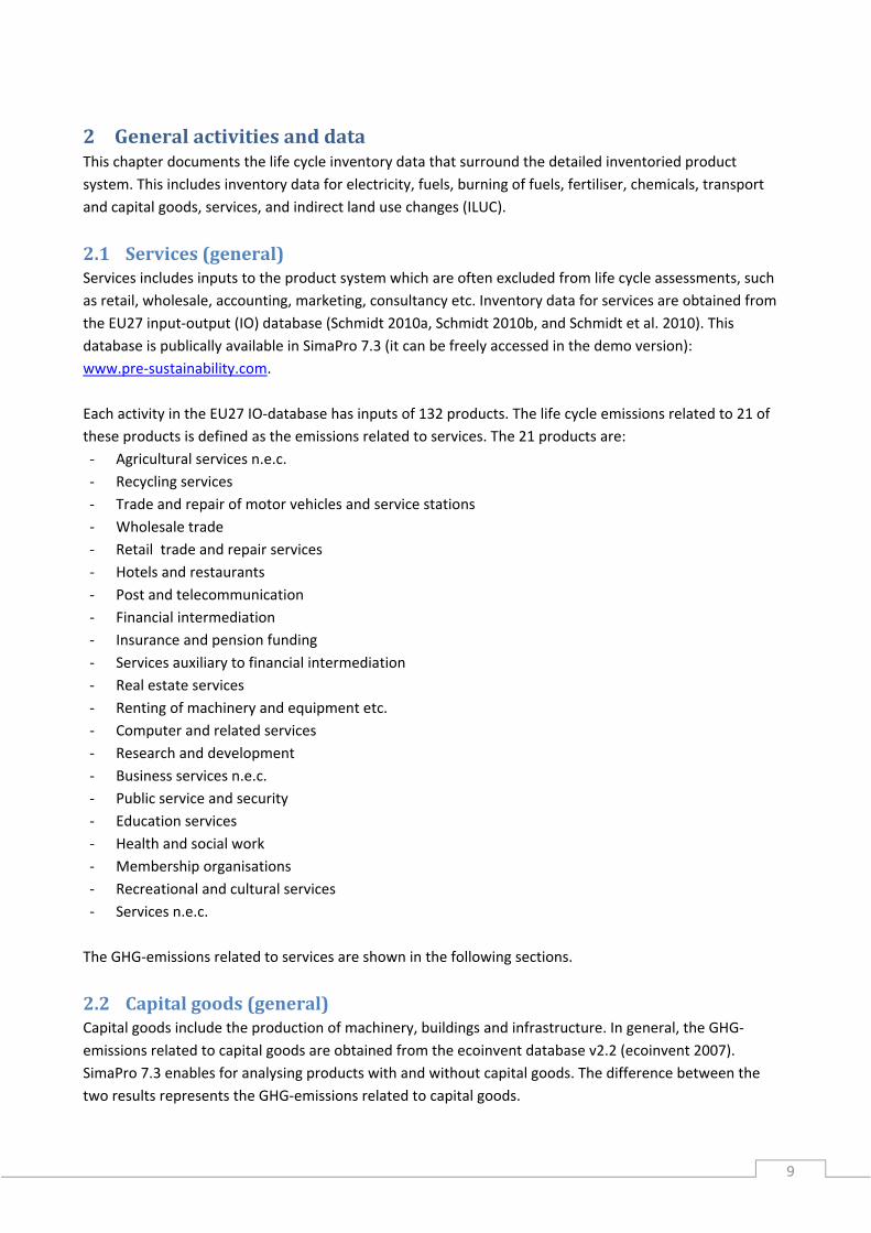
2 GeneralactivitiesanddataThis chapter documents the life cycle inventory data that surround the detailed inventoried product

system. This includes inventory data for electricity, fuels, burning of fuels, fertiliser, chemicals, transport

and capital goods, services, and indirect land use changes (ILUC).

2.1 Services(general)Services includes inputs to the product system which are often excluded from life cycle assessments, such

as retail, wholesale, accounting, marketing, consultancy etc. Inventory data for services are obtained from

the EU27 input‐output (IO) database (Schmidt 2010a, Schmidt 2010b, and Schmidt et al. 2010). This

database is publically available in SimaPro 7.3 (it can be freely accessed in the demo version):

www.pre‐sustainability.com.

Each activity in the EU27 IO‐database has inputs of 132 products. The life cycle emissions related to 21 of

these products is defined as the emissions related to services. The 21 products are:

‐ Agricultural services n.e.c.

‐ Recycling services

‐ Trade and repair of motor vehicles and service stations

‐ Wholesale trade

‐ Retail trade and repair services

‐ Hotels and restaurants

‐ Post and telecommunication

‐ Financial intermediation

‐ Insurance and pension funding

‐ Services auxiliary to financial intermediation

‐ Real estate services

‐ Renting of machinery and equipment etc.

‐ Computer and related services

‐ Research and development

‐ Business services n.e.c.

‐ Public service and security

‐ Education services

‐ Health and social work

‐ Membership organisations

‐ Recreational and cultural services

‐ Services n.e.c.

The GHG‐emissions related to services are shown in the following sections.

2.2 Capitalgoods(general)Capital goods include the production of machinery, buildings and infrastructure. In general, the GHG‐

emissions related to capital goods are obtained from the ecoinvent database v2.2 (ecoinvent 2007).

SimaPro 7.3 enables for analysing products with and without capital goods. The difference between the

two results represents the GHG‐emissions related to capital goods.

10

In cases where no ecoinvent data are available, some the capital goods are estimated by use of the EU27

IO‐database. Each activity in the EU27 IO‐database has inputs of 132 products. The life cycle emissions

related to 16 of these products are defined as the emissions related to capital goods. The 16 products are:

‐ Sand, gravel and stone from quarry

‐ Clay and soil from quarry

‐ Concrete, asphalt and other mineral products

‐ Bricks

‐ Fabricated metal products, except machinery

‐ Machinery and equipment n.e.c.

‐ Office machinery and computers

‐ Electrical machinery n.e.c.

‐ Radio, television and communication equipment

‐ Instruments, medical, precision, optical, clocks

‐ Motor vehicles and trailers

‐ Transport equipment n.e.c.

‐ Furniture and other manufactured goods n.e.c.

‐ Buildings, residential

‐ Buildings, non‐residential

‐ Infrastructure, excluding buildings

The GHG‐emissions related to services are shown in the following sections.

2.3 ElectricityElectricity is used in most life cycle stages of milk production. Generally, electricity at medium voltage is

used in all activities. This includes production, high voltage grid and medium voltage grid. Grid losses are

considered.

The methodology for the inventory of electricity is described in Schmidt et al. (2011). For the switch for

ISO14040/44, i.e. consequential modelling, the affected suppliers are identified as the proportion of the

growth for each suppliers in the period 2008‐2020. The electricity generation in 2020 is identified by use of

energy plans. The switches for average, PAS2050 and IDF all use average electricity mix in year 2008.

The methodology for inventorying electricity is further described in Schmidt et al. (2011) which can be

freely accessed here: http://www.lca‐net.com/projects/electricity_in_lca/

11

The country specific inventory data are included for the following countries and are obtained from the

following data sources:

‐ Denmark: Merciai et al. (2011a)

‐ Sweden: See Table 2.1 below

‐ Brazil: Merciai et al. (2011b)

‐ France: Merciai et al. (2011c)

‐ Malaysia: Merciai et al. (2011d)

‐ Europe: Merciai et al. (2011e)

‐ World: Merciai et al. (2011f)

The selection of the included countries is based on the countries in which inventoried:

‐ cattle farms are located (Denmark, Sweden, Brazil), and

‐ food industries are located (Denmark, Sweden, Brazil, France, Malaysia, Europe average. The global

electricity mix is included for cases where activities outside these countries/regions are involved in the

inventory)

‐ Further, it should be noticed that electricity in countries where only crop cultivation takes place has

not been specifically inventoried because the use of electricity in crop cultivation is insignificant

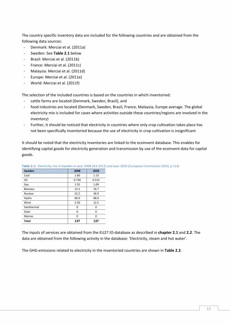
It should be noted that the electricity inventories are linked to the ecoinvent database. This enables for

identifying capital goods for electricity generation and transmission by use of the ecoinvent data for capital

goods.

Table 2.1: Electricity mix in Sweden in year 2008 (IEA 2012) and year 2020 (European Commission 2010, p 114) Sweden 2008 2020

Coal 1.60 1.13

Oil 0.730 0.515

Gas 1.55 1.09

Biomass 12.2 16.7

Nuclear 52.2 36.9

Hydro 66.0 68.0

Wind 2.50 12.5

Geothermal 0 0

Solar 0 0

Marine 0 0

Total 137 137

The inputs of services are obtained from the EU27 IO‐database as described in chapter 2.1 and 2.2. The

data are obtained from the following activity in the database: ‘Electricity, steam and hot water’.

The GHG‐emissions related to electricity in the inventoried countries are shown in Table 2.2.

12

Table 2.2: GHG‐emissions related to electricity production and distribution. Electricity GHG‐emissions (kg

CO2‐eq.)

Elec DK Elec SE Elec BR Elec FR Elec MY Elec EU GLO

Reference flow 1 kWh 1 kWh 1 kWh 1 kWh 1 kWh 1 kWh 1 kWh

Switch 1: ISO 14044/44

Process data, ex infrastructure 0.225 0.0706 0.385 0.222 1.32 0.134 0.612

Capital goods 0.0123 0.0122 0.00640 0.0163 0.00888 0.0209 0.0107

Services 0.00195 0.00195 0.00195 0.00195 0.00195 0.00195 0.00195

Switch 2: average/allocation


Capital goods 0.0100 0.00558 0.00725 0.00517 0.00607 0.00930 0.00973

Services 0.00195 0.00195 0.00195 0.00195 0.00195 0.00195 0.00195

Switch 3: PAS2050


Capital goods n.a. n.a. n.a. n.a. n.a. n.a. n.a.

Services n.a. n.a. n.a. n.a. n.a. n.a. n.a.

Switch 4: IDF


Capital goods 0.0100 0.00558 0.00725 0.00517 0.00607 0.00930 0.00973

Services 0.00195 0.00195 0.00195 0.00195 0.00195 0.00195 0.00195

2.4 FertilisersandotherchemicalsInventory data (process data and capital goods) for fertilisers and other chemicals are obtained from

ecoinvent (2007). The following fertilisers and chemicals are included in the inventory. The reference flow is

shown, and the used ecoinvent‐activities are specified in brackets:

‐ Ammonia, kg N (Ammonia, liquid, at regional storehouse/RER)*

‐ Urea, kg N (Urea, as N, at regional storehouse/RER)

‐ Ammonium nitrate (AN), kg N (Ammonium nitrate, as N, at regional storehouse/RER)

‐ Calcium ammonium nitrate (CAN), kg N (Calcium ammonium nitrate, as N, at regional storehouse/RER)

‐ Ammonium sulphate (AS), kg N (Ammonium sulphate, as N, at regional storehouse/RER)

‐ Triple super phosphate (TSP), kg P2O5 (Triple superphosphate, as P2O5)

‐ Rock phosphate, kg P2O5 (Phosphate rock, as P2O5, beneficiated, wet, at plant/US)

‐ Potassium chloride, kg K2O (Potassium chloride, as K2O, at regional storehouse/RER)

‐ Other chemicals, kg (Chemicals inorganic, at plant/GLO)

* the ecoinvent process for ammonia has reference flow kg NH3. This is adjusted to kg N by dividing by

0.822 which is the N content in ammonia (IFA 2012a).


data are obtained from the following activities in the database:

‐ N‐fertilisers: ‘Fertiliser, N’. N‐content: 0.3 is assumed based on N‐content in the most widely used N‐

fertilisers (IFA 2012a)

‐ Triple super phosphate: ‘Fertiliser, other than N’. P2O5‐content: 0.46 (IFA 2012a)

‐ Potassium chloride: ‘Fertiliser, other than N’. K2O‐content: 0.6 (IFA 2012a)

‐ Rock phosphate: ‘Minerals from mine n.e.c.’. P2O5‐content: 0.309 (IFA 2012a)

‐ Other chemicals: ‘Chemicals n.e.c.’

13

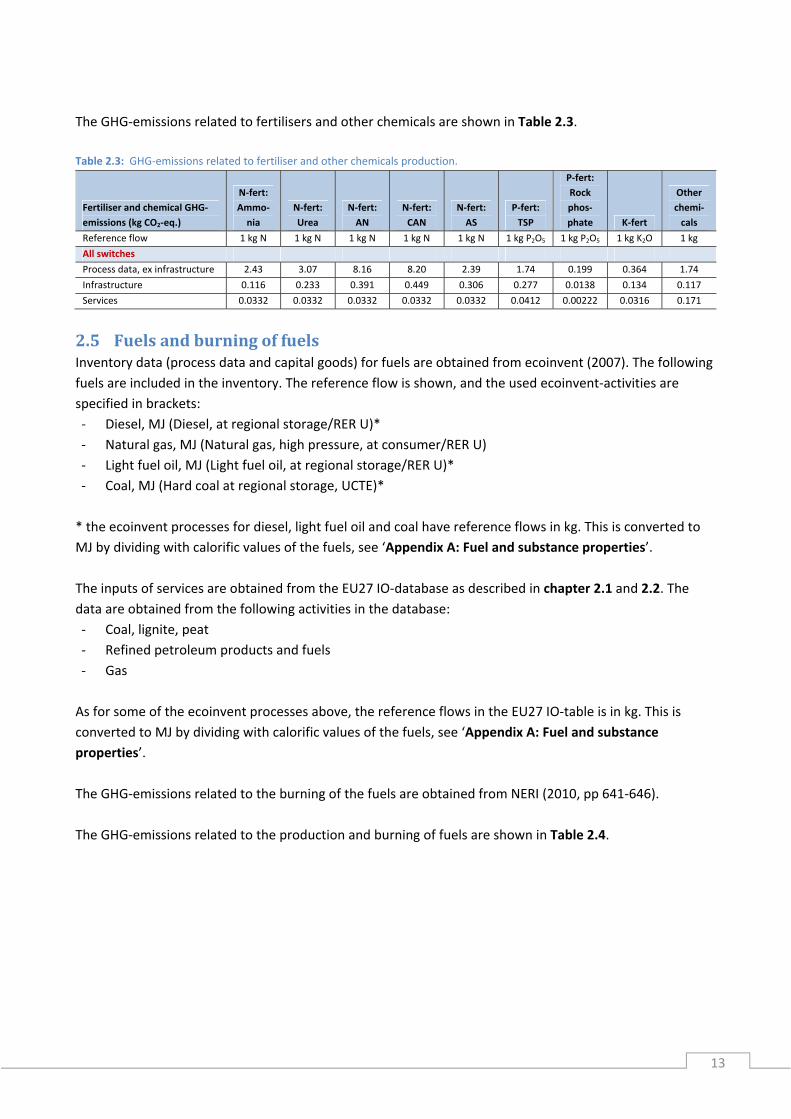
The GHG‐emissions related to fertilisers and other chemicals are shown in Table 2.3.

Table 2.3: GHG‐emissions related to fertiliser and other chemicals production.

Fertiliser and chemical GHG‐

emissions (kg CO2‐eq.)

N‐fert:

Ammo‐

nia

N‐fert:

Urea

N‐fert:

AN

N‐fert:

CAN

N‐fert:

AS

P‐fert:

TSP

P‐fert:

Rock

phos‐

phate K‐fert

Other

chemi‐

cals

Reference flow 1 kg N 1 kg N 1 kg N 1 kg N 1 kg N 1 kg P2O5 1 kg P2O5 1 kg K2O 1 kg

All switches

Process data, ex infrastructure 2.43 3.07 8.16 8.20 2.39 1.74 0.199 0.364 1.74

Infrastructure 0.116 0.233 0.391 0.449 0.306 0.277 0.0138 0.134 0.117

Services 0.0332 0.0332 0.0332 0.0332 0.0332 0.0412 0.00222 0.0316 0.171

2.5 FuelsandburningoffuelsInventory data (process data and capital goods) for fuels are obtained from ecoinvent (2007). The following

fuels are included in the inventory. The reference flow is shown, and the used ecoinvent‐activities are

specified in brackets:

‐ Diesel, MJ (Diesel, at regional storage/RER U)*

‐ Natural gas, MJ (Natural gas, high pressure, at consumer/RER U)

‐ Light fuel oil, MJ (Light fuel oil, at regional storage/RER U)*

‐ Coal, MJ (Hard coal at regional storage, UCTE)*

* the ecoinvent processes for diesel, light fuel oil and coal have reference flows in kg. This is converted to

MJ by dividing with calorific values of the fuels, see ‘Appendix A: Fuel and substance properties’.



‐ Coal, lignite, peat

‐ Refined petroleum products and fuels

‐ Gas

As for some of the ecoinvent processes above, the reference flows in the EU27 IO‐table is in kg. This is

converted to MJ by dividing with calorific values of the fuels, see ‘Appendix A: Fuel and substance

properties’.

The GHG‐emissions related to the burning of the fuels are obtained from NERI (2010, pp 641‐646).

The GHG‐emissions related to the production and burning of fuels are shown in Table 2.4.

14

Table 2.4: GHG‐emissions related to production and burning of fuels. Fuels GHG‐emissions Diesel Natural gas Light fuel oil Coal

Reference flow MJ MJ MJ MJ

All switches

Process data, ex infrastructure, kg CO2‐eq. 0.0100 0.0108 0.010 0.011

Infrastructure, kg CO2‐eq. 0.00194 0.000599 0.0019 0.0007

Services, kg CO2‐eq. 0.000126 0.000200 0.000126 0.000027

Burning fuel, kg CO2 0.0740 0.0570 0.0740 0.0950

Burning fuel, kg CH4 0.00000150 0.000465 0.00000150 0.00000150

Burning fuel, kg N2O 0.00000200 0.00000140 0.00000300 0.00000200

2.6 TransportInventory data (process data and capital goods) for transport are obtained from ecoinvent (2007). The

following transport activities are included in the inventory. The reference flow is shown, and the used

ecoinvent‐activities are specified in brackets:

‐ Road transport/lorry, tkm (Transport, lorry 16‐32t, EURO3/RER)

‐ Ship transport, tkm (Transport, barge/RER)



‐ Land transport and transport via pipelines

‐ Transport by ship

The reference flow of the transport activities in the EU27 IO‐database is EUR2003. This is converted to tkm

by use of prices. The price of road transport is estimated by comparing the total monetary value of road

transport in EU27 in 2003 (495.5 thousand MEUR2003, data are available in the EU27 IO‐database in

SimaPro) by the total transport in EU27 in 2003 in units of tkm (1625 billion tkm of which road transport is

68.8%, Eurostat, 2009). The price of ship transport is calculated relative to road transport; according to

Rodrigue et al. (2009), the price of ship transport is 2.79% of the price of road transport. The prices of road

and ship transport are 0.210 EUR2003/tkm and 0.00585 EUR2003/tkm respectively.

The GHG‐emissions related to transport are shown in Table 2.5.

Table 2.5: GHG‐emissions related to transport. Transport GHG‐emissions (kg CO2‐eq.) Lorry Ship

Reference flow 1 tkm 1 tkm

All switches

Process data, ex infrastructure 0.153 0.0347

Infrastructure 0.0313 0.0117

Services 0.0138 0.000229

15

2.7 CapitalgoodsandservicesincattleandcropfarmsCapital goods and service inputs to cattle farms and crops farms are obtained from the EU27 IO‐database as

described in chapter 2.1 and 2.2. The data are obtained from the following two activities in the database:

‐ Bovine meat and milk

‐ Grain crops

The reference flow for the ‘Bovine milk and meat’ activity in the database is dry matter meat (live weight)

plus dry matter milk. The EU27 total production volume in 2003 is 37.35 million tonne (data available in the

database in SimaPro). The GHG‐emissions from this quantity for capital goods and services are then

normalised by the total number of cattle in EU27 in 2003. According to FAOSTAT (2012), this is 92.8 million

heads. In

Table 2.6, the GHG‐emissions for capital goods and services are shown per head. This can be linked in the

model, where number of heads is a parameter in the animal activities.

The reference flow for the ‘Grain crops’ activity in the database is dry matter crops. The EU27 total

production volume in 2003 is 728 million tonne (data available in the database in SimaPro). The GHG‐

emissions from this quantity for capital goods and services are then normalised by the total cultivated area

of grain crops in EU27 in 2003. According to FAOSTAT (2012), this is 55.5 million ha. In

Table 2.6, the GHG‐emissions for capital goods and services are shown per ha. This can be linked in the

model, where the cultivated area is a parameter in the crop cultivation activities.

Table 2.6: GHG‐emissions for capital goods and services in animal and crop farms Capital goods and services GHG‐emissions (kg CO2‐eq.) Animal farm Crop farm

Reference flow 1 head 1 ha

All switches

Capital goods 95.1 108

Services 126 126

Notice that no distinction between GHG‐emissions related to capital goods and services is considered for

animal farms and crop farms. Further, it should be noted that no distinction between countries is

considered, and that capital goods and services per hectare of grain crops are assumed to be

representative for all crops.

2.8 CapitalgoodsandservicesinthefoodindustryactivitiesThe following activities in the food industry are involved in the inventory:

‐ Vegetable oil mills (palm oil, soybean oil, palm kernel oil, rapeseed oil, sun flower oil)

‐ Refinery of vegetable oil (palm oil, palm kernel oil, soybean oil, rapeseed oil)

‐ Sugar manufacturing

‐ Flour mill

‐ Destruction of dead animals

16

Data on capital goods are based on

‐ Vegetable oil mills (Schmidt 2007, p 154)

‐ Refinery of vegetable oil (Schmidt 2007, p 187)

‐ Sugar manufacturing (‘Sugar, from sugar beet, at sugar refinery/CH U’, ecoinvent 2007)

‐ Flour mill (Assumed same per kg flour as per kg sugar from sugar manufacturing)

‐ Destruction of dead animals (Assumed same per kg flour as per kg sugar from sugar manufacturing)

Service inputs to the food industry activities are obtained from the EU27 IO‐database as described in

chapter 2.1 and 2.2. The data are obtained from the following activities in the database:

‐ Vegetable and animal oils and fats (used for oil mils and oil refineries)

‐ Sugar (used for sugar manufacturing and destruction of dead animals

‐ Flour

In Table 2.7, the GHG‐emissions for capital goods and services are shown per head.

Table 2.7: GHG‐emissions for capital goods and services in food industry activities Capital goods and services

GHG‐emissions (kg CO2‐eq.) Oil mill Oil refinery Sugar Flour Destruction

Reference flow 1 kg crude oil 1 kg refined oil 1 kg sugar 1 kg flour 1 kg animal (live weight)

All switches

Capital goods 0.00201 0.00152 0.000477 0.000477 0.000181

Services 0.0393 0.0393 0.0380 0.0385 0.0144

Note that the inputs to the animal destruction activity are implemented as the inputs to the sugar activity

multiplied with 0.38 which is the dry matter content of the treated animals (DAKA 2006). Then the output

of the animal destruction is comparable with the output of the sugar manufacturing in terms of dry weight.

Notice that no distinction between GHG‐emissions related to capital goods and services is considered for

food industries in different countries. The general vegetable oil industry in the EU27 is regarded as

representative for oil mills and refineries for soybean oil and palm oil in Brazil and Malaysia. And also inputs

of capital goods and services to the sugar industry (per kg sugar) are presumed as being representative for

the inputs of capital goods and services to the animal destruction industry (per kg dry by‐product output).

Destruction of animals in Brazil is presumed to take place without any inputs of capital goods and services.

2.9 Indirectlandusechanges(ILUC)Indirect land use changes are caused by occupation of land in the animal and crop cultivation activities. The

applied inventory data are obtained from the ILUC‐project version 3 (Schmidt et al. 2012). The ILUC model

in Schmidt et al. (2012) enables for consequential and attributional modelling.

ILUC are inventoried for three different markets for land:

‐ Land tenure, arable

‐ Land tenure, intensive forest land

‐ Land tenure, rangeland

17

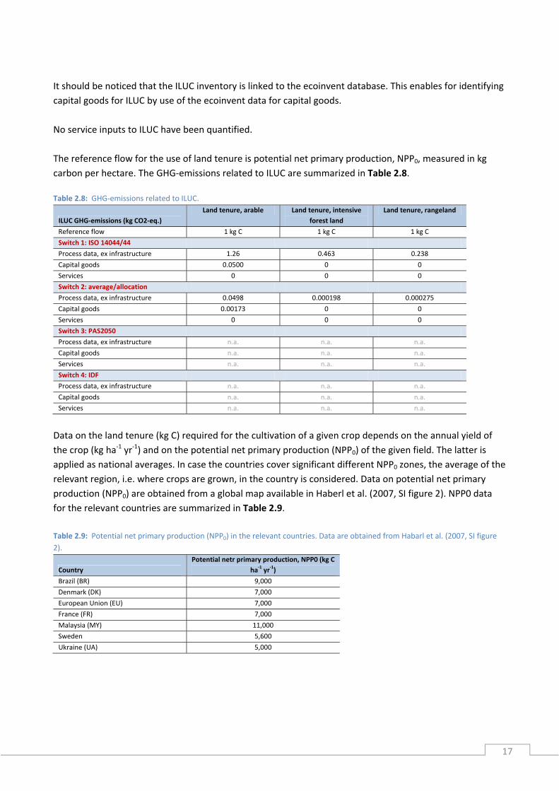
It should be noticed that the ILUC inventory is linked to the ecoinvent database. This enables for identifying

capital goods for ILUC by use of the ecoinvent data for capital goods.

No service inputs to ILUC have been quantified.

The reference flow for the use of land tenure is potential net primary production, NPP0, measured in kg

carbon per hectare. The GHG‐emissions related to ILUC are summarized in Table 2.8.

Table 2.8: GHG‐emissions related to ILUC.

ILUC GHG‐emissions (kg CO2‐eq.)

Land tenure, arable Land tenure, intensive

forest land

Land tenure, rangeland

Reference flow 1 kg C 1 kg C 1 kg C


Process data, ex infrastructure 1.26 0.463 0.238

Capital goods 0.0500 0 0

Services 0 0 0

Switch 2: average/allocation

Process data, ex infrastructure 0.0498 0.000198 0.000275

Capital goods 0.00173 0 0

Services 0 0 0

Switch 3: PAS2050

Process data, ex infrastructure n.a. n.a. n.a.

Capital goods n.a. n.a. n.a.

Services n.a. n.a. n.a.

Switch 4: IDF

Process data, ex infrastructure n.a. n.a. n.a.

Capital goods n.a. n.a. n.a.

Services n.a. n.a. n.a.

Data on the land tenure (kg C) required for the cultivation of a given crop depends on the annual yield of

the crop (kg ha‐1 yr‐1) and on the potential net primary production (NPP0) of the given field. The latter is

applied as national averages. In case the countries cover significant different NPP0 zones, the average of the

relevant region, i.e. where crops are grown, in the country is considered. Data on potential net primary

production (NPP0) are obtained from a global map available in Haberl et al. (2007, SI figure 2). NPP0 data

for the relevant countries are summarized in Table 2.9.

Table 2.9: Potential net primary production (NPP0) in the relevant countries. Data are obtained from Habarl et al. (2007, SI figure

2).

Country

Potential netr primary production, NPP0 (kg C

ha‐1 yr

‐1)

Brazil (BR) 9,000

Denmark (DK) 7,000

European Union (EU) 7,000

France (FR) 7,000

Malaysia (MY) 11,000

Sweden 5,600

Ukraine (UA) 5,000

19

3 ThecattlesystemThe target activity of the Arla model is the milk producing activity, i.e. the dairy cow.

3.1 OverviewofthecattlesystemCattleturnover,stockandrelatedparameters:DenmarkFigure 3.1 and Figure 3.2 present cattle turnover and stocks in the Danish milk and beef system. For more

details on the included activities see Schmidt and Dalgaard (2012, Table 6.1). Data are mainly obtained

from a representative sample of Danish farm accounts from 2005. All data are collected by Kristensen

(2011).

Figure 3.1: Milk system turnover in Denmark 2005. Values on arrows are flows. Bracketed values are stocks. Unit: 1000 heads.

Dairy cow(564)

Bull calf231

Slaughtered210

Raising newborn bull (29)

Raising bull calf(199)

Newborn heifer284

Raising heifer(566)

Slaughtered32

Dairy cow199

Destruction29

Raised263 Raised

285

Death born21

Destruction30

Death born23

Destruction21

Calves592

Slaughtered168

Exported dairy cows1

Destruction30

Exported bull calf24

Slaughterhouse

Exported heifer3

Newborn bull308

Destruction

Dairy cows

Calves

Export

20

Figure 3.2: Beef system turnover in Denmark 2005. Values on arrows are flows. Bracketed values are stocks. Unit: 1000 heads.

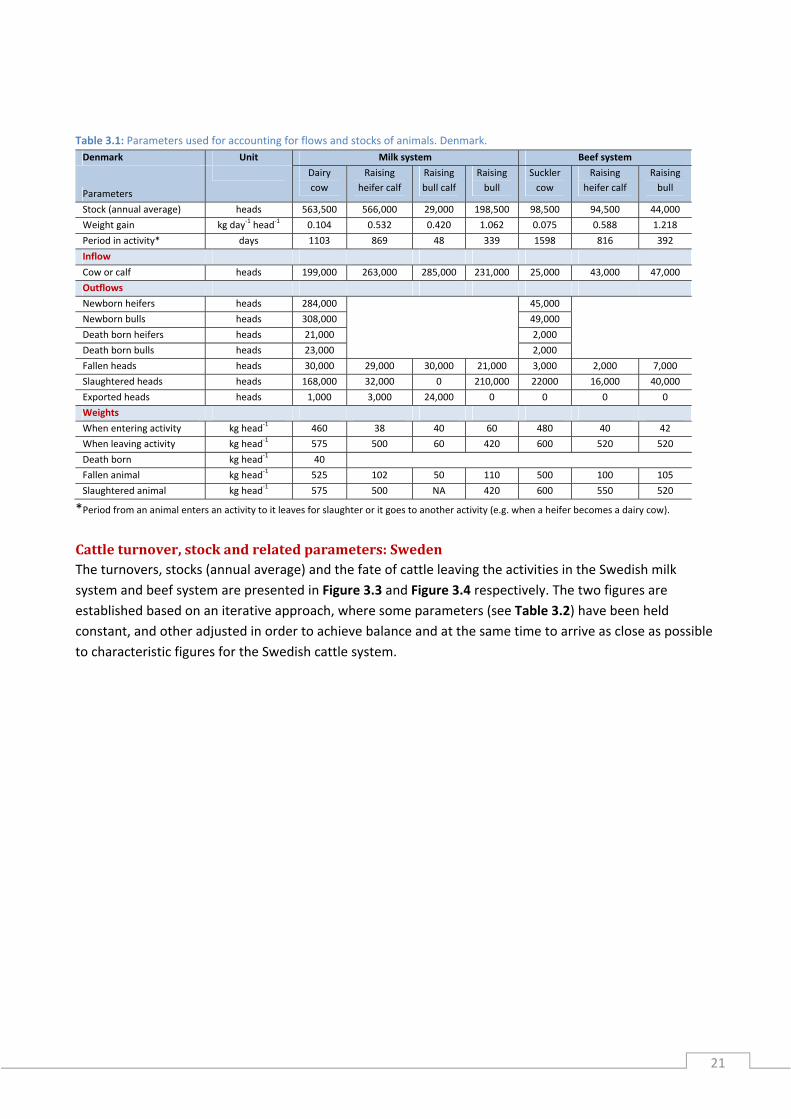
The inflow and outflows for each animal activity are presented in Table 3.1 together with data on weights

etc.

Suckler cow(99)

Slaughtered40


Newborn heifer45

Raising heifer calf(12)

Slaughtered16

Suckler cow25

Destruction2

Raised43 Raised

47

Death born2

Destruction7

Death born2

Calves94

Slaughtered22

Destruction3

Slaughterhouse

Newborn bull49

Destruction

Suckler cows

Calves

21

Table 3.1: Parameters used for accounting for flows and stocks of animals. Denmark. Denmark Unit Milk system Beef system

Parameters

Dairy

cow

Raising

heifer calf

Raising

bull calf

Raising

bull

Suckler

cow

Raising

heifer calf

Raising

bull

Stock (annual average) heads 563,500 566,000 29,000 198,500 98,500 94,500 44,000

Weight gain kg day‐1 head

‐1 0.104 0.532 0.420 1.062 0.075 0.588 1.218

Period in activity* days 1103 869 48 339 1598 816 392

Inflow

Cow or calf heads 199,000 263,000 285,000 231,000 25,000 43,000 47,000

Outflows

Newborn heifers heads 284,000 45,000

Newborn bulls heads 308,000 49,000

Death born heifers heads 21,000 2,000

Death born bulls heads 23,000 2,000

Fallen heads heads 30,000 29,000 30,000 21,000 3,000 2,000 7,000

Slaughtered heads heads 168,000 32,000 0 210,000 22000 16,000 40,000

Exported heads heads 1,000 3,000 24,000 0 0 0 0

Weights

When entering activity kg head‐1 460 38 40 60 480 40 42

When leaving activity kg head‐1 575 500 60 420 600 520 520

Death born kg head‐1 40

Fallen animal kg head‐1 525 102 50 110 500 100 105

Slaughtered animal kg head‐1 575 500 NA 420 600 550 520

*Period from an animal enters an activity to it leaves for slaughter or it goes to another activity (e.g. when a heifer becomes a dairy cow).

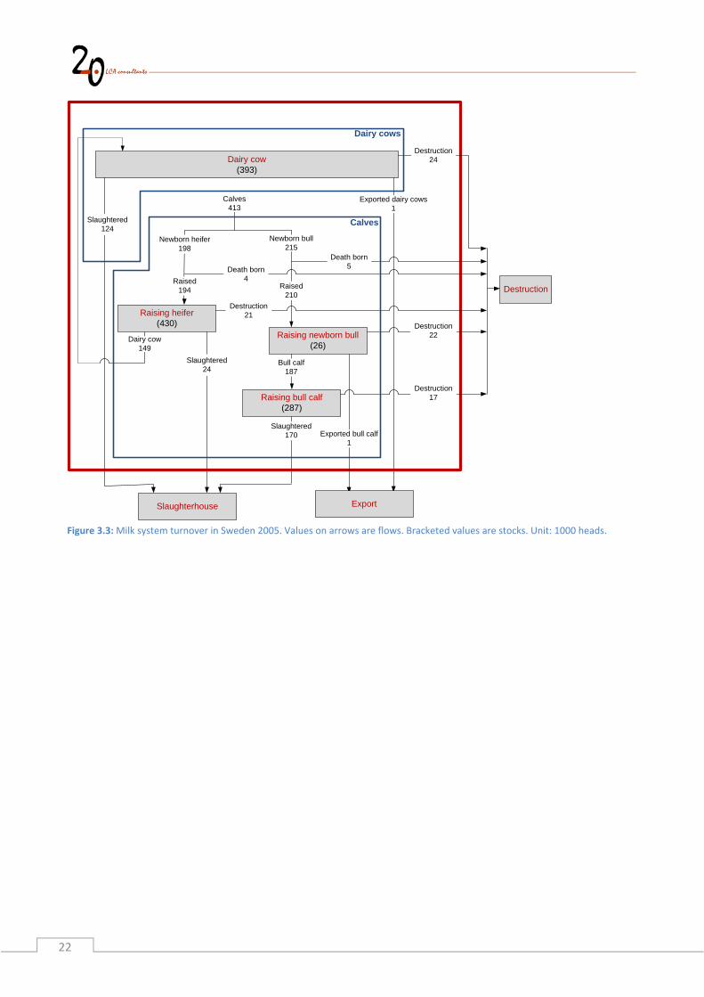
Cattleturnover,stockandrelatedparameters:SwedenThe turnovers, stocks (annual average) and the fate of cattle leaving the activities in the Swedish milk

system and beef system are presented in Figure 3.3 and Figure 3.4 respectively. The two figures are

established based on an iterative approach, where some parameters (see Table 3.2) have been held

constant, and other adjusted in order to achieve balance and at the same time to arrive as close as possible

to characteristic figures for the Swedish cattle system.

22

Figure 3.3: Milk system turnover in Sweden 2005. Values on arrows are flows. Bracketed values are stocks. Unit: 1000 heads.

Dairy cow(393)

Bull calf187

Slaughtered170

Raising newborn bull (26)


Newborn heifer198

Raising heifer(430)

Slaughtered24

Dairy cow149

Destruction21

Raised194 Raised

210

Death born4

Destruction22

Death born5

Destruction17

Calves413

Slaughtered124

Exported dairy cows1

Destruction24

Exported bull calf1

Slaughterhouse

Newborn bull215

Destruction

Dairy cows

Calves

Export

23

Figure 3.4: Beef system turnover in Sweden 2005. Values on arrows are flows. Bracketed values are stocks. Unit: 1000 heads.

Table 3.2: Parameters used for accounting for flows and stocks of animals. Sweden.

Sweden Unit Milk system Beef system

Parameters

Dairy

cow

Raising

heifer calf

Raising

bull calf

Raising

bull

Suckler

cow

Raising

heifer calf

Raising

bull

Stock (annual average) heads 393,268 429,851 25,593 286,717 177,000 181,286 111,742


‐1 0.076 0.530 0.837 0.828 0.064 0.530 1.035

Period in activity* days 961 854 47 587 1891 854 513

Inflow

Cow or calf heads 149,000 194,438 209,795 186,711 51,200 79,327 85,938

Outflows

Newborn heifers heads 198,204 80,863

Newborn bulls heads 214,954 88,051

Death born heifers heads 3,766 1,536

Death born bulls heads 5,159 2,113

Fallen heads heads 24,000 21,440 22,084 16,974 6,000 3,690 12,799

Slaughtered heads heads 124,000 24,000 0 169,738 36,000 24,637 73,138

Exported heads heads 1,000 0 1,000 0 4,000 0 0

Weights

When entering activity kg head‐1 453 40 40 79 453 40 40

When leaving activity kg head‐1 525 493 79 565 575 493 571

Death born kg head‐1 40 40

Fallen animal kg head‐1 489 266 60 322 514 266 305

Slaughtered animal kg head‐1 525 493 79 565 575 493 571


Suckler cow (change in herd size: + 5) (177)

Slaughtered73

Raising bull calf (112)

Newborn heifer81

Raising heifer calf(181)

Slaughtered24

Suckler cow51

Destruction4

Raised79 Raised

86

Death born2

Destruction13

Calves169

Slaughtered36

Destruction6

Slaughterhouse

Newborn bull88

Destruction

Suckler cows

Calves

Death born2

Exported suckler cows4

Export

24

Stock (annual average) and live weight animals to slaughter are numbers that determines most of the

environmental efficiency (enteric fermentation, manure emissions, and feed intake) of cattle production in

Sweden. Other parameters in Figure 3.3 and Figure 3.4 are just intermediate flows, e.g. animal transactions

between animal activities, which do not influence the result of the model. These intermediate flows have

been included in order to ensure that the modelled system reflects the actual system, e.g. it is ensured that

the number of born calves is higher than the number of slaughtered heads (given that the system is in a

steady‐state mode). Further, relationships between slaughtered weight, number of slaughtered animals,

total live weight meat production, life times of cattle, weight gain etc. have been ensured.

The starting point for establishment of the turnover and stock is data from Flysjö et al. (2011) and

Cederberg et al. (2009a). However, calves, heifers, bulls and steers from these data sources are not divided

into milk and beef system. Thus, it is necessary to adjust data before entering them into the model. To

improve the quality of these adjustments, data on number of slaughtered heads disaggregated in different

cattle races from Taurus (2007) are used. These data represent slaughtering statistic from 2006, and are

used because data from 2005 not are available. Data on calf mortality are from Svensson (2007). Data on

calves born per cow per year, percentage of destructed/discarded cattle are assumed equal to the Danish

cattle system due to data lack.

To ensure coherency in the established flow and stock data, these were checked against data on cattle

stock from UNFCCC (2007), in which it is reported that the stock in Sweden in 2005 was 393,000 dairy cows

and 1,212,000 other cattle (heifers, bulls, steers). For each of the activities, the relationship between the

flow of animals, the stock and the time period in which each animal is in the activity can be described by

the following equation: Equation 3.1

Stock inflow ∙ period Where:

Stock = The average number of animals in the activity during one year, animals

Inflow = The number of animals entering the activity during one year, animals year‐1

Period = The average time an animal spends in the activity, year.

Only stocks of calves, heifers and bulls are calculated from Equation 3.1. Stocks of dairy and suckler cows

are taken directly from Cederberg et al. (2009a). Periods used for the stock calculation are based on

slaughter ages and other information from Cederberg et al. (2009a, p 89). It is assumed that the period of

time the calves in the ‘Raising newborn bull calves’ is in the milk system is the same as for the Danish new

born bulls (=48 days). Also it was taken into account that part of the cattle in all activities are leaving before

expected. For example 24 of the 194 heifers entering the activity ‘Raising heifer’ in the ‘Milk system’ (Figure

3.3) are destructed. It is assumed all destructed cattle as an average leave an activity in the middle of the

period.

A cross check of the first calculation of the total stock was performed by adding stocks from all activities

and compare it to the stock data from UNFCCC (2007). It was 2.1% lower than the data from UNFCCC

25

(2007). To overcome this discrepancy, the time bulls from milking and suckler cows spend in the activity is

prolonged by 9.6%. By this adjustment 100% accordance to the data from UNFCCC (2007) is obtained.

The coherency of the established data is also checked against data on the total production of beef meat as

of Cederberg et al. (2009a, p 38), and it is found the data are underestimated by 0.9 %. This is considered to

be low, and indicates the established flows and stocks are representative for the Swedish cattle production.

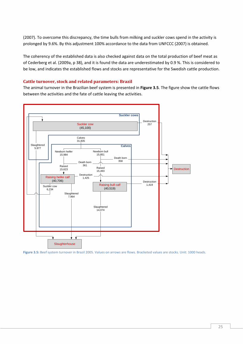
Cattleturnover,stockandrelatedparameters:BrazilThe animal turnover in the Brazilian beef system is presented in Figure 3.5. The figure show the cattle flows

between the activities and the fate of cattle leaving the activities.

Figure 3.5: Beef system turnover in Brazil 2005. Values on arrows are flows. Bracketed values are stocks. Unit: 1000 heads.

Suckler cow(45,100)

Slaughtered14,074

Raising bull calf(40,519)

Newborn heifer15,984

Raising heifer calf(40,706)

Slaughtered7,964

Suckler cow6,234

Destruction1,425

Raised15,623 Raised

15,493

Death born361

Destruction1,419

Death born358

Calves31,835

Slaughtered5,977

Destruction257

Slaughterhouse

Newborn bull15,851

Destruction

Suckler cows

Calves

26

Table 3.3: Parameters used for accounting for flows and stocks of animals in Brazil.

Brazil Unit Beef system

Parameters Suckler cow Raising heifer calf Raising bull

Stock (annual average) heads 45,100,000 40,705,816 40,518,838


‐1 0.074 0.237 0.275

Period in activity* days 2190 1095 1278

Inflow

Cow or calf heads 6,234,000 15,623,004 15,492,812

Outflows

Newborn heifers heads 15,984,248

Newborn bulls heads 15,851,046

Death born heifers heads 361,244

Death born bulls heads 358,234

Fallen heads heads 256,619 1,425,343 1,418,796

Slaughtered heads heads 5,976,953 7,964,090 14,074,017

Exported heads heads 0 0 0

Weights

When entering activity kg head‐1 260 40 40

When leaving activity kg head‐1 422 300 391

Death born kg head‐1 40

Fallen animal kg head‐1 400 190 209

Slaughtered animal kg head‐1 422 351 391


Figure 3.5 is established based on an iterative approach where some important parameters have been held

constant, and other adjusted in order to achieve balance and at the same time to arrive as close as possible

to characteristic figures for the Brazilian beef system.

The important parameters, which have been held constant, are:

‐ Number of heads in the herd (annual average)

‐ Live weight animals to slaughterhouse

In the model, these numbers determine most of the environmental efficiency (enteric fermentation,

manure emissions, and feed intake) of beef production in Brazil. Other parameters in Figure 3.5 are just

intermediate flows, e.g. animal transactions between animal activities, which do not influence the result of

the model. These intermediate flows have been included in order to ensure that the modelled system

reflects the actual system, e.g. it is ensured that the number of born calves is higher than the number of

slaughtered heads (given that the system is in a steady‐state mode). Further, relationships between

slaughtered weight, number of slaughtered animals, total live weight meat production, life times of cattle,

weight gain etc. have been ensured.

The number of heads in the herd is based on figures from Cederberg et al. (2009b). The total herd has been

allocated to the beef and dairy systems as of Table 3.4. The 73% allocation of the cows and bulls in the herd

to the beef system is calculated based on figures in Cederberg et al. (2009b, p 20). The 71% allocation of

the younger animals to the beef system is calculated based on the total number of suckler cows and dairy

cows and calving intervals (months between calving) for suckler cows and dairy cows in Denmark. All older

steers are presumed to belong to the beef system.

27

Table 3.4: Allocation of the total cattle herd to the beef and milk system. Category Age Heads (million) Beef system Milk system

Cows (suckler + dairy) 61.6 73% 27%

Bulls 2.3 73% 27%

Calves (heifer) 0‐12 months 24 71% 29%

Calves (bulls) 0‐12 months 23.8 71% 29%

Heifers, younger 1‐2 years 20.5 71% 29%

Heifers, older 2‐3 years 13.1 71% 29%

Bulls and steers, younger 1‐2 years 17 71% 29%

Bulls and steers, older 2‐3 years 9.2 71% 29%

Steers, older 3‐4 years 2.9 100% 0%

Steers, older >4 years 0.6 100% 0%

Total 175

The weight gain in Table 3.3 is calculated as the difference in weight when the animals are leaving and

entering the activity divided by the ‘period in activity’.

In Table 3.3, the ‘period in activity’ for the three animal categories in the beef system is based on estimated

figures:

‐ 6 years for suckler cows

‐ 3 years for heifer calves

‐ 3.5 years for bull calves

The number of newborn calves (bulls and heifers) in Table 3.3 is based on an estimated calving interval in

the Brazilian beef system at 17 months and the number of cows in the beef system. Cederberg et al.

(2009b) specify a calving interval at 21 months. However, when applying this number it is difficult to make

the animal turnover balance because there are too few calves for maintaining the herd and for producing

the meat as of the statistics.

The total number of fallen heads is based on a ‘mortality to weaning and post weaning’ rate of 12%

according to Landers (2007). The 12% is applied to the number of newborn calves. This total is subdivided

into death born calves, and fallen cows, heifer calves and bull calves. The number of death born calves and

cows is based on same mortality rates as for Denmark and Sweden (average). The remaining fallen heads

are heifer calves and bull calves. The distribution between heifers and bulls is based on Table 3.4.

28

The numbers of slaughtered heads are determined as follows:

‐ Annual suckler cows to slaughterhouse:

‐ Stock divided with period of time the suckler cows are in the activity

‐ minus fallen heads during the time the cows are in the activity

‐ Annual heifer calves to slaughterhouse:

‐ Animals entering the activity

‐ minus heifers to suckler cow: calculated to ensure balance in the suckler cow category; heifers

in = slaughtered and fallen out

‐ minus fallen heifers

‐ Annual bull calves to slaughterhouse:

‐ Animals entering the activity

‐ minus fallen heifers

The slaughtered animal weights are calculated iteratively to ensure that the total number of slaughtered

animals multiplied with weights equals the total supply of beef (live weight) from the beef system. In this

iteration it has been assumed that the ratio between the slaughtered weight of suckler cows, heifer calves

and bull calves is the same as in Denmark. According to Cederberg et al. (2009b, appendix 2), the total

Brazilian supply of cattle meat in 2005 is 8.152 million tonne CW (carcass weight). It is assumed that 73% of

this is supplied by the beef system, and that the rest is supplied by the milk system (the 73% is explained in

relation to Table 3.4). The carcass weight (CW) to live weight (LW) ratio is 0.55. Hence the supply of cattle

meat from the beef system can be determined as 10.82 million tonne live weight.

The other weights have been estimated.

3.2 InventoryoffeedinputstothecattlesystemThe parameters used for calculation of net energy requirements are presented in the two following

sections. One method (Kristensen, 2011) is used for the milking cows in Denmark and Sweden and another

method (IPCC 2006) is used for all other cattle activities. However, IPCC parameters are also presented for

the milking cows because they are used for the calculation of methane emission from enteric fermentation.

Determinationoffeedrequirements:DenmarkParameters used for calculation of net energy requirements are presented in Table 3.5. The total net

energy (NE) is calculated as a sum of net energy used for maintenance, activity, lactation, growth etc. and is

highest for the milking and suckler cows. More than 50% of total net energy (NE) required by the dairy

cows derives from net energy for lactation (NEl). For the other cattle types, net energy required for

maintenance (NEm) is the largest contributor. Net energy for work (NEwork) is 0 for all bovines, because it is

not relevant for commercial milk and beef cattle. The net energy parameters (NEm, NEa, NEl, NEwork, NEp and

NEg) are calculated from IPCC (2006) formulas.

The parameters ‘FEreq’ are used for calculation of feed intake and as explained previously ‘FEreq’ for dairy

cows are calculated from the milk yield (Schmidt et al. 2012, Equation 6.2), whereas ‘FEreq’ for all other

categories of cattle are calculated according to IPCC (2006), see Schmidt and Dalgaard (2012, Equation 6.1).

29

Table 3.5: Parameters used for calculating feed requirements in Denmark. (*): In Schmidt and Dalgaard (2012).

Denmark Unit Milk system Beef system Source

Parameters

Dairy

cow

Raising

heifer

calf

Raising

bull calf

Raising

bull

Suckler

cow

Raising

heifer

calf

Raising

bull

NE MJ hd‐1 day

‐1 128 30.6 8.74 35.1 44.1 33.4 41.1 Equation 6.1(*)

NEm MJ hd‐1 day

‐1 41.9 21.4 6.96 22.6 36.1 22.9 25.4 Equation 6.9(*)

NEa MJ hd‐1 day

‐1 3.56 1.82 0.591 1.92 3.07 1.95 2.16 Equation 6.10(*)

NEl MJ hd‐1 day

‐1 76.7 0 0 0 0 0 0 Equation 6.11(*)

NEwork MJ hd‐1 day

‐1 0 0 0 0 0 0 0 Equation 6.12(*)

NEp MJ hd‐1 day

‐1 4.19 0 0 0 3.61 0 0 Equation 6.13(*)

NEg MJ hd‐1 day

‐1 2.01 7.37 1.19 10.7 1.41 8.54 13.5 Equation 6.15(*)

FEreq million MJ yr‐1 27,704 6,316 92.5 2,546 1,587 1,152 659 Equation 6.2(*)

FEreq/hd MJ hd‐1 yr

‐1 49,164 11,159 3,189 12,824 16,114 12,193 14,984 Equation 6.2(*)

FEreq/hd/day MJ hd‐1 day

‐1 135 30.6 8.74 35.1 44.1 33.4 41.1 Equation 6.2(*)

ECM million kg yr‐1 4,756 0 0 0 0 0 0

Kristensen (2011)

XXXStatistikbanken??

XXX

ECM/head kg hd‐1 yr‐1 8,440 0 0 0 0 0 0

Kristensen (2011)


XXX

Cfi MJ day‐1 kg

‐1 0.386 0.322 0.370 0.370 0.322 0.322 0.370 IPCC (2006, Table 10.4)

Weight kg 518 269 50.0 240 540 295 281 Table 3.1. See text

Ca Dim. less 0.085 0.085 0.085 0.085 0.085 0.085 0.085 See text

Milk kg day‐1 24.0 0 0 0 0 0 0

Kristensen (2011)


XXX

Fat % 4.30 0 0 0 0 0 0

Kristensen (2011)


XXX

Cpregnancy Dim. less 0.100 0 0 0 0.100 0 0 IPCC (2006, Table 10.7)

BW kg 518 269 50.0 240 540 295 281 Table 3.1. See text

C Dim. less 0.800 0.800 1.20 1.20 0.800 0.800 1.20 IPCC (2006, p 10.17)

MW kg 575 575 575 575 600 600 600 Estimated

WG kg day‐1 0.104 0.532 0.420 1.06 0.075 0.588 1.22 Table 3.1. See text

The last 10 parameters in Table 3.5 are further described in Section 6.5 (Inventory of methane from enteric

fermentation) in Schmidt and Dalgaard (2012). The parameters ‘Weight’ and ‘BW’ are both calculated as an

average of the parameters ‘When entering activity’ and ‘ When leaving activity’ from Table 3.1. The

parameter Ca, which is used for calculation of net energy for animal activity (NEa), is calculated as an

average for ‘Stall’ (Ca =0.00) and ‘Pasture’ (Ca =0.17) (IPCC, 2006, Table 10.5). The parameter ‘WG’ is equal

to ‘Weight gain’ in Table 3.1.

Determinationoffeedrequirements:SwedenParameters used for calculation of net energy requirements are presented in Table 3.6. The total net

energy (NE) is calculated as a sum of net energy used for maintenance, activity, lactation, growth etc. and is

highest for the milking and suckler cows. More than 50% of total net energy (NE) required by the dairy

cows derives from net energy for lactation (NEl). For the other cattle types, net energy required for

maintenance (NEm) is the largest contributor. Net energy for work (NEwork) is 0 for all bovines, because it is

not relevant for commercial milk and beef cattle. The net energy parameters (NEm, NEa, NEl, NEwork, NEp and

NEg) are calculated from IPCC (2006) formulas.

30




31

Table 3.6: Parameters used for calculating feed requirements in Sweden. (*): In Schmidt and Dalgaard (2012).

Sweden Unit Milk system Beef system Source

Parameters

Dairy

cow

Raising

heifer

calf

Raising

bull calf

Raising

bull

Suckler

cow

Raising

heifer

calf

Raising

bull

NE MJ hd‐1 day

‐1 124 30.3 11.5 40.7 42.3 30.1 41.4 Equation 6.1(*)

NEm MJ hd‐1 day

‐1 40.1 21.2 7.9 28.2 34.7 21.2 27.0 Equation 6.9(*)

NEa MJ hd‐1 day

‐1 3.41 1.80 0.675 2.39 2.95 1.80 2.30 Equation 6.10(*)

NEl MJ hd‐1 day

‐1 74.7 0 0 0 0 0 0 Equation 6.11(*)


‐1 0 0 0 0 0 0 0 Equation 6.12(*)

NEp MJ hd‐1 day

‐1 4.01 0 0 0 3.47 0 0 Equation 6.13(*)

NEg MJ hd‐1 day

‐1 1.36 7.29 2.89 10.1 1.14 7.06 12.0 Equation 6.15(*)

FEreq million MJ yr‐1 18,995 4,757 108 4,255 2,734 1,991 1,687 Equation 6.2(*)


‐1 48,300 11,067 4,201 14,841 15,444 10,984 15,095 Equation 6.2(*)


‐1 132 30.3 11.5 40.7 42 30.1 41.4 Equation 6.2(*)

ECM million kg yr‐1 3,253 0 0 0 0 0 0 Cederberg et al. (2009a)

ECM/head kg hd‐1 yr‐1 8,271 0 0 0 0 0 0 Cederberg et al. (2009a)

Cfi MJ day‐1 kg

‐1 0.386 0.322 0.370 0.370 0.322 0.322 0.370 IPCC (2006, Table 10.4)

Weight kg 489 266 59.7 322 514 266 305 Table 3.2. See text

Ca Dim. less 0.085 0.085 0.085 0.085 0.085 0.085 0.085 See text

Milk kg day‐1 23.6 0 0 0 0 0 0 Cederberg et al. (2009a)

Fat % 4.25 0 0 0 0 0 0 Cederberg et al. (2009a)

Cpregnancy Dim. less 0.100 0 0 0 0.100 0 0 IPCC (2006, Table 10.7)

BW kg 489 266 59.7 322 514 266 305.5 Table 3.2. See text

C Dim. less 0.800 0.800 1.20 1.20 0.800 0.800 1.20 IPCC (2006, p 10.17)

MW kg 575 575 575 575 600 600 600 Estimated

WG kg day‐1 0.076 0.530 0.837 0.828 0.064 0.530 1.04 Table 3.2. See text







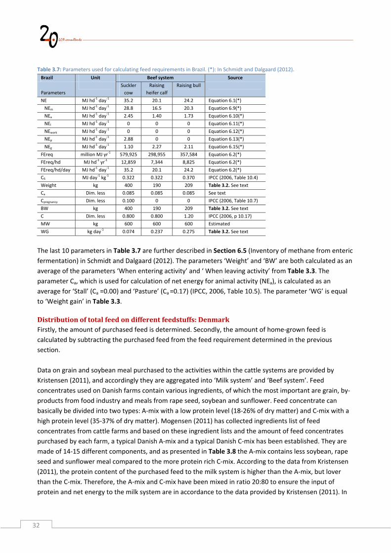
Determinationoffeedrequirements:BrazilParameters used for calculation of net energy requirements are presented in Table 3.6. The total net ener‐

gy (NE) is calculated as a sum of net energy used for maintenance, activity, lactation, growth etc. The net

energy required for maintenance (NEm) is the largest contributor the total net energy (NE). Net energy for

work (NEwork) is 0 for all bovines, because it is not relevant for commercial milk and beef cattle. The net

energy parameters (NEm, NEa, NEl, NEwork, NEp and NEg) are calculated from IPCC (2006) formulas.




32

Table 3.7: Parameters used for calculating feed requirements in Brazil. (*): In Schmidt and Dalgaard (2012).

Brazil Unit Beef system Source

Parameters

Suckler

cow

Raising

heifer calf

Raising bull

NE MJ hd‐1 day

‐1 35.2 20.1 24.2 Equation 6.1(*)

NEm MJ hd‐1 day

‐1 28.8 16.5 20.3 Equation 6.9(*)

NEa MJ hd‐1 day

‐1 2.45 1.40 1.73 Equation 6.10(*)

NEl MJ hd‐1 day

‐1 0 0 0 Equation 6.11(*)


‐1 0 0 0 Equation 6.12(*)

NEp MJ hd‐1 day

‐1 2.88 0 0 Equation 6.13(*)

NEg MJ hd‐1 day

‐1 1.10 2.27 2.11 Equation 6.15(*)

FEreq million MJ yr‐1 579,925 298,955 357,584 Equation 6.2(*)


‐1 12,859 7,344 8,825 Equation 6.2(*)


‐1 35.2 20.1 24.2 Equation 6.2(*)

Cfi MJ day‐1 kg

‐1 0.322 0.322 0.370 IPCC (2006, Table 10.4)

Weight kg 400 190 209 Table 3.2. See text

Ca Dim. less 0.085 0.085 0.085 See text

Cpregnancy Dim. less 0.100 0 0 IPCC (2006, Table 10.7)

BW kg 400 190 209 Table 3.2. See text

C Dim. less 0.800 0.800 1.20 IPCC (2006, p 10.17)

MW kg 600 600 600 Estimated

WG kg day‐1 0.074 0.237 0.275 Table 3.2. See text







Distributionoftotalfeedondifferentfeedstuffs:DenmarkFirstly, the amount of purchased feed is determined. Secondly, the amount of home‐grown feed is

calculated by subtracting the purchased feed from the feed requirement determined in the previous

section.

Data on grain and soybean meal purchased to the activities within the cattle systems are provided by

Kristensen (2011), and accordingly they are aggregated into ‘Milk system’ and ‘Beef system’. Feed

concentrates used on Danish farms contain various ingredients, of which the most important are grain, by‐

products from food industry and meals from rape seed, soybean and sunflower. Feed concentrate can

basically be divided into two types: A‐mix with a low protein level (18‐26% of dry matter) and C‐mix with a

high protein level (35‐37% of dry matter). Mogensen (2011) has collected ingredients list of feed

concentrates from cattle farms and based on these ingredient lists and the amount of feed concentrates

purchased by each farm, a typical Danish A‐mix and a typical Danish C‐mix has been established. They are

made of 14‐15 different components, and as presented in Table 3.8 the A‐mix contains less soybean, rape

seed and sunflower meal compared to the more protein rich C‐mix. According to the data from Kristensen

(2011), the protein content of the purchased feed to the milk system is higher than the A‐mix, but lover

than the C‐mix. Therefore, the A‐mix and C‐mix have been mixed in ratio 20:80 to ensure the input of

protein and net energy to the milk system are in accordance to the data provided by Kristensen (2011). In

33

order to limit the LCIs of purchased feed components, only feed components which contribute with more

than 5% to the A‐mix, C‐mix or the Swedish feed concentrates are modeled. This means feed components

contributing with less than 5% are presented with a different crop LCI. E.g. ‘Distillers grains, barley based,

dried’ is modeled as ‘Soybean meal’ as shown in Table 3.8. When an alternative crop LCI is applied in the

model it is selected according protein and energy content to ensure that the characteristics of the original

feed ingredient are as far as possible identical to the characteristics of the chosen alternative crop

ingredient.

Table 3.8: Composition of feed concentrates used in Danish cattle production (Mogensen 2011) and name of applied LCI in the current model. Feed concentrate used on Danish dairy farms (Mogensen 2011) LCI applied in the current model

Ingredients A‐mix, %

(weight)

C‐mix, %

(weight)

Ingredients

Barley 19.3 12.0 Barley

Rapeseed cake/meal 17.5 26.0 Rapeseed cake/meal

Beet pulp, dried 15.8 5.0 Beet pulp, dried

Corn 8.3 2.0 Corn

Soybean meal 8.0 26.0 Soybean meal

Wheat bran 7.3 1.0 Wheat bran

Sunflower meal/cake 6.0 22.5 Sunflower meal

Distillers grains, barley based, dried 4.3 0.0 Soybean meal

Citrus pulp, dried 4.0 0.0 Barley

Soya bean hulls etc 3.6 0.0 Barley

Dried grass pellets 2.0 0.0 Rapeseed cake/meal

Molasses, beet 1.8 2.5 Molasses, beet

Palm fat and vegetable fat 1.2 2.0 Palm oil

Fodder Urea 0.0 0.5 Other chemicals. Section 2.4

Minerals 1.1 0.5 Other chemicals. Section 2.4

By combining the data from Kristensen (2011) with the data on feed concentrate ingredients (Mogensen,

2011) the feed inputs to the ‘Milk system’ and ‘Beef system’ are obtained as presented in Table 3.9. ‘FEreq’

for ‘Milk system’ and ‘Beef system’ equal the sum of ‘FEreq’ parameters in Table 3.5. The intake of feed

urea and minerals are presented in Table 3.28 and Table 3.29.

34

Table 3.9: Feed requirement and intake. Denmark. Denmark Milk system Beef system

Feed requirement/intake

TJ net

energy

1000 tons

protein

TJ net

energy

1000 tons

protein

Feed requirement

FEreq 36,658 3,399

FPreq 799,596 78,933

Feed intake

Barley 6,965 86,664 638.19 7,940.38

Corn 396 3,983 0 0

Soybean meal 3,246 158,642 245 11,982

Rape seed/cake 2,979 112,025 0 0

Sunflower meal 2,103 104,803 0 0

Beet pulp, dried 731 8,976 0 0

Molasses 197 3,334 0 0

Palm oil 590 0.00 0 0

Wheat bran 199 5,242 0 0

Feed urea 0 15,131 0 308

Permanent grass 601 17,875 746 22,175

Maize ensilage 15,058 172,867 923 10,602

Rotation grass 3,592 110,055 846 25,927

Total feed intake 36,658 799,596 3,399 78,933

Distributionoftotalfeedondifferentfeedstuffs:SwedenLike the Danish data, the amount of purchased feed is firstly determined. Secondly, the amount of home‐

grown feed is calculated by subtracting the purchased feed from the feed requirement (FEreq) presented in

Table 3.6. Data are based on Cederberg et al. (2009a, p 69‐71), but the number of different ingredients in

the feed concentrate have been reduced, so only feed ingredients contributing with more than 5% are

modelled. Feed ingredients contributing with less than 5% are represented by LCI shown in Table 3.10.

Table 3.10: Ingredients in feed concentrates used in Swedish cattle production (Cederberg et al. 2009a) and name of applied LCI in

the current model

Ingredients in feed

concentrate used on

Swedish cattle farms

(Cederberg et al. 2009a)

LCI applied in the current

model

Ingredients in feed

concentrate used on

Swedish cattle farms

(Cederberg et al. 2009a)

LCI applied in the current

model

Wheat Wheat Rapeseed, meal Rapeseed cake/meal

Tritical, rye Wheat Soymeal Soybean meal

Barley Barley Potatoe protein Soybean meal

Oat Oat Lucernemeal Soybean meal

Grain midlings Wheat bran Grassmeal Soybean meal

Grain bran Wheat bran Peas /horsebean Soybean meal

Maize gluten Corn Palm kernel Palm kernel cake

DDGS Soybean meal Fatty acids Palm oil

Bakery pasta prod. Rapeseed cake/meal Milk powder Palm kernel cake

Beet pulp Beet pulp CaCO3 Other chemicals

Molasses Molasses, beet Salt Other chemicals

Beet sugar Beet pulp Div minerals Other chemicals

Rapeseed, whole Rapeseed cake/meal

35

The feed intake of the Swedish ‘Milk system’ and ‘Beef system’ is presented in Table 3.11. The intake of

feed urea and minerals are presented in Table 3.30 and Table 3.31.

Table 3.11: Feed requirement and intake. Sweden. Sweden Milk system Beef system


TJ net energy

1000 tons protein TJ net energy

1000 tons protein

Feed requirement

FEreq 28,115 6,412

FPreq 606,742 146,184

Feed intake

Barley 3,164 39,373 120 1,487

Wheat 1,034 12,561 188 2,287

Oat 2,193 31,437 32.7 468

Corn 35.5 357 5.43 54.6

Soybean meal 1,489 72,745 264 12,905

Rape seed/cake 1,568 58,963 277 10,424

Beet pulp 116 1,509 20.5 267

Molasses 154 2,617 27.2 462

Palm oil 556.71 0 98.24 0

Palm kernel meal 488 12,784 108 2,834

Wheat bran 495 13,006 84.6 2,224

Permanent grass 3,139 93,341 1,526 45,393

Maize ensilage 7,891 90,590 2,335 26,808

Rotation grass 5,792 177,459 1,324 40,571

Total feed intake 28,115 606,742 6,412 146,184

Distributionoftotalfeedondifferentfeedstuffs:Brazil

The feed intake of Brazilian ‘Beef system’ is based on Cederberg et al. (2009b) and is presented in Table

3.12. According to Cederberg et al. (2009b) the Brazilian beef system is almost purely feed by permanent

grass. Therefore, in accordance, the feed intake is based on 100% permanent grass. Only some minor

additional supplements of mineral feed are included. This is presented in Table 3.32.

Table 3.12: Feed intake. Brazil. Sweden Beef system


TJ net

energy

1000 tons

protein

Feed requirement

FEreq 1,236,465

FPreq 36,771,087

Feed

Permanent grass 1,236,465 36,771,087

Total feed intake 1,236,465 36,771,087

3.3 InventoryofotherinputstothecattlesystemIt is assumed the same amount of diesel and electricity is used in Denmark and Sweden. Data on diesel use

in stables for feeding, handling of manure and straw, livestock management etc. are from Cederberg et al.

36

(2009a, p 17). For dairy cows 0.0032 litre diesel is used per kg milk and for other cattle 13 litre per head *

year is used. The use of electricity is also based on Cederberg et al. (2009a, p 18).

All purchased feed is assumed to be transported 200 km by lorry.

The uses of diesel, electricity and lorry in the Danish, Swedish and Brazilian cattle system are presented in

the summary of LCI in Section 3.5.

ManuretreatmentWithin the cattle system there are two types of treatment activities. These two types receive manure for

treatment and fallen cattle for destruction respectively. There are six processes for manure treatment and

one process for destruction of fallen cattle.

The manure treatment processes are presented in Table 3.13. The two first two processes are used when

manure is deposited outdoor as dung and urine. The next three manure treatment processes are used

when manure from storage (as liquid/slurry, solid or deep litter) is used for fertilisation of crops. The last

treatment process is applied when liquid /slurry from storage is used for biogasification and subsequently

used for fertilisation of crops. The reference flow is 1 kg manure N for all manure treatment process.

The manure treatment processes are to be considered as treatment processes representing the difference

of using manure and artificial fertiliser for fertilisation of crops. E.g. the application of manure, which is a

by‐product from milk and meat production, results in displacement of fertiliser, see by‐products in Table

3.13. The unit for manure treatment is one kg N, but the P and K content in the manure is also taking into

account resulting in a displacement of P‐fert and K‐fert.

37

Table 3.13: Manure treatment processes. Reference product is 1 kg N in manure.

Treatment process:

Manure deposited outdoor Manure land application Manure

biogas and

land

application

Type of manure: Dung + urine

Liquid +

slurry Solid Deep litter

Liquid +

slurry

Country: DK/SE BR DK/SE DK/SE DK/SE DK/SE

Unit

Output of products

Determining product:

Manure for treatment kg N 1 1 1 1 1 1

By‐products:

Market for N‐fertiliser kg N ‐0.650 0 ‐0.700 ‐0.650 ‐0.450 ‐0.700

P‐fert: TSP kg P2O5 ‐0.267 0 ‐0.288 ‐0.267 ‐0.185 ‐0.288

K‐fert: KCl kg K2O ‐0.739 0 ‐0.796 ‐0.739 ‐0.512 ‐0.796

Elec DK/SE kWh 0 0 0 0 0 9.22

Distr. heat MJ 0 0 0 0 0 34.4

Input of products Unit:

Elec DK/SE MJ 0 0 0 0 0 0.348

Diesel MJ 0 0 2.585 2.677 2.064 2.59

Emissions Unit:

Methane kg CH4 0 0 0 0 0 ‐0.171

Dinitrogen monoxide

(direct) kg N2O 0.0212 0.0314 0.0047 0.0055 0.0086 ‐0.177

Dinitrogen monoxide

(indirect) kg N2O 0.0227 0.0345 0.0074 0.0075 0.0112 ‐0.0027

Ammonia kg NH3 0.0692 0.0850 0.2075 0.1299 0.1348 0.2075

The amount of the by‐product N fertiliser (named ‘Market for N‐fertiliser’) produced per kg N in manure is

from Plantedirektoratet (2004) and express the expected plant available N per kg manure N. This means for

each kg N deposited outdoor, as urine and dong, 0.65 kg N in fertiliser is displaced. In other words, the

farmer can apply 0.65 kg N fertiliser less, every time a cow excretes 1 kg N on pasture. Liquid/slurry has the

highest level of plant available N (=0.7 kg N/kg N) whereas deep litter has the lowest (=0.45 kg N/kg N).

Permanent grass areas in Brazil are much more extensively used compared to permanent grass areas in

Denmark and Sweden, and it is assumed permanent grass in Brazil not is fertilised. Hence, the deposition of

dung and urine in Brazil does not displace fertiliser. Displaced P‐fert and K‐fert is calculated on basis of N, P

and K content in manure (Poulsen et al. 2001, Table 11.7 – 11.10) and are assumed to have the same

displacement rates as N. For example 1 kg N in ‘Liquid/slurry’ displaces 0.288 kg P2O5, because 1 kg N in

corresponds to 0.188 kg P, of which 0.7 is plant available for plants, and the molar conversion factor is 2.29

P2O5 per P2O5‐P (1*0.18 * 0.7 * 2.29 = 0.288 kg P2O5).

The by‐products Elec DK/SE and Distr. heat are from energy production based on biogas from manure, and

the input of Elec DK/SE to ‘Manure biogas and land application’ is for processing manure in the biogas

plant. Energy outputs and inputs related to manure based biogas production are based on Nielsen et al.

(2005). The diesel use for application of manure to fields is 0.4 litres per ton is from Cederberg et al.

(2009a, p 19). The methane emitted from land application of manure is calculated as part of the cattle

system (section 3.4) according to IPCC (2006, p 10‐35). Mikkelsen et al. (2011, p 67) conclude that the

methane emission from slurry applied to fields is reduced by 77% if it is treated in a biogas plant. This is

38

included in the calculations by a negative methane emission from the manure treatment process, and

thereby it is subtracted from the manure deposited on pasture calculated in the cattle activites. N

emissions from manure treatment processes are presented in Table 3.13 and are more deeply described in

Table 3.14.

Table 3.14: Calculation of N emissions from manure treatment processes. Reference product is 1 kg N in manure.

Treatment process: Manure deposited

outdoor

Manure land application Manure biogas and land

application

Type of manure: Dung + urine

Liquid +

slurry Solid Deep litter Liquid + slurry

Country:

Unit

DK/SE BR DK/SE DK/SE DK/SE DK/SE

Applied manure

Manure, N kg N 1 1 1 1 1 1

Dinitrogen monoxide (direct)

From manure kg N 0.0200 0.0200 0.010 0.010 0.010 0.010

From displaced fertiliser kg N ‐0.0065 0 ‐0.007 ‐0.0065 ‐0.0045 ‐0.007

From biogasification kg N ‐0.0064

From manure treatment Kg N 0.0135 0.0200 0.003 0.0035 0.0055 ‐0.0034

Ammonia

From manure kg N 0.070 0.070 0.185 0.120 0.120 0.185


From manure treatment kg N 0.060 0.070 0.171 0.107 0.111 0.171

Nitrate

From manure kg N 0.300 0.300 0.300 0.300 0.300 0.300



Dinitrogen monoxide (indirect)


Summary of N emissions

Dinitrogen monoxide (direct) kg N2O 0.0212 0.0314 0.0047 0.0055 0.0086 ‐0.0053

Dinitrogen monoxide (indirect) kg N2O 0.0015 0.0031 0.0027 0.0020 0.0025 0.0027

Ammonia kg NH3 0.0692 0.0850 0.2075 0.1299 0.1348 0.2075

The direct dinitrogen monoxide emission from manure are calculated using the emission factors from IPCC

(2006, Table 11.1). The emission factor from manure deposited outdoor and fertiliser is 0.02 and 0.01 kg

N2O‐N per kg N respectively. The emissions named ‘From manure treatment’ are calculated as the

difference of emissions from manure and fertiliser. Treatment of manure in a biogas plant reduces the

dinitrogen monoxide emission by 64% (Mikkelsen et al. 2011, p 81) and this is accounted for by subtracting

the reduced emission from direct dinitrogen monoxide.

39

Ammonia and nitrate emissions are calculated in order to enable calculation of indirect dinitrogen

monoxide emissions. The fraction of N lost as ammonia and nitrate is based on the following Danish data

sources:

‐ Ammonia from manure deposited outdoor: 0.07 (Mikkelsen et al. 2011, p 49).

‐ Ammonia from manure land application, liquid + slurry: 0.18. Based on Hansen et al. (2008).

‐ Ammonia from manure land application, solid and deep litter: 0.12. Based on Hansen et al. (2008).

‐ Ammonia from N fertiliser: 0.02 (Mikkelsen et al. 2011, p 49).

‐ Nitrate from all types of manure/fertiliser: 0.30 (IPCC 2006, Table 11.3).

The emission factors for calculating the indirect dinitrogen monoxide emission related to ammonia and

nitrate are the following:

‐ 0.01 kg N2O‐N per kg NH3‐N + NOx‐N volatilized (IPCC 2006, Table 11.3). The emissions of NOx‐N is

taking into account using data from IFA (2001) as explained in Schmidt and Dalgaard (2012, Section

7.4).

‐ 0.0075 kg N2O‐N per kg N leaching/runoff (IPCC 2006, Table 11.3)

DestructionoffallencattleThe inventory of fallen animals in Denmark and Sweden is based on DAKA (2006). In Brazil, the only

considered input in the destruction activity is transport. The inventory data are summarised in Table 3.15. Table 3.15: Destruction of fallen animals. Reference product is 1 kg live weight (LW) animal.

Treatment process: Destruction of fallen

animals (industry)

Destruction of fallen

animals (low tech.)

Country: DK/SE BR

Output of products Unit:


Destruction of fallen animals kg LW 1 1

By‐products:

Distr. heat MJ 0.0202

Burning coal MJ 4.45

Burning fuel oil MJ 4.93

Input of products Unit:

Elec DK/SE MJ 0.0223

Natural gas MJ 0.0197

Fuel oil MJ 0.0219

Lorry tkm 0.200 0.200

3.4 EmissionsMethaneemissionsfromentericfermentation:DenmarkThe parameters used for calculation of methane emissions from enteric fermentation are presented in

Table 3.16.The emission factor (EF) is calculated from the gross energy intake (GE), which again is

calculated from the net energy intake (Schmidt et al. 2012, Section 6.4). DE% (digestibility of feed in

percent) is calculated as a weighted average of DE% for each of the used feedstuffs. The parameter Ca,

which is used for calculation of net energy for animal activity (NEa), is calculated as an average for ‘Stall’ (Ca

=0) and ‘Pasture’ (Ca =0.17) (IPCC, 2006, Table 10.5).

40

Table 3.16: Parameters used for calculating methane emissions from enteric fermentation in Denmark. (*): In Schmidt and

Dalgaard (2012).

Denmark Unit Milk system Beef system Source

Para‐

meters

Dairy

cow

Raising

heifer

calf

Raising

bull calf

Raising

litre bull

Suckler

cow

Raising

heifer

calf

Raising

bull

EF kg CH4 hd‐1 yr

‐1 140 31.72 9.06 36.5 47.3 35.8 44.0 Equation 6.7(*)

GE MJ hd‐1 day

‐1 328 74.4 21.3 100 111 84.0 103.2 See text

Ym % 6.50 6.50 6.50 6.50 6.50 6.50 6.50 IPCC (2006, Table 10.12)

NEm MJ day‐1 41.9 21.4 6.96 22.6 36.1 22.9 25.4 Table 3.5

NEa MJ day‐1 3.56 1.82 0.591 1.92 3.07 1.95 2.16 Table 3.5

NEl MJ day‐1

76.7 0 0 0 0 0 0

Table 3.5

NEwork MJ day‐1 0 0 0 0 0 0 0 Table 3.5

NEp MJ day‐1 4.19 0 0 0 3.61 0 0 Table 3.5

NEg MJ day‐1 2.01 7.37 1.19 10.7 1.41 8.54 13.5 Table 3.5

REM Dim. less 0.541 0.541 0.541 0.541 0.540 0.540 0.540 Equation 6.14(*)

REG Dim. less 0.353 0.353 0.353 0.353 0.350 0.350 0.350 Equation 6.16(*)

DE% % 75.3 75.3 75.3 75.3 74.4 74.4 74.4 See text

Methaneemissionsfromentericfermentation:SwedenThe parameters used for calculation of methane emissions from enteric fermentation are presented in






Table 3.17: Parameters used for calculating methane emissions from enteric fermentation in Sweden. (*): In Schmidt and Dalgaard

(2012). Sweden Unit Milk system Beef system Source

Para‐

meters

Dairy

cow

Raising

heifer

calf

Raising

bull calf

Raising

litre bull

Suckler

cow

Raising

heifer

calf

Raising

bull

EF kg CH4 hd‐1 yr

‐1 141 32.4 12.3 43.5 46.6 33.1 45.5 Equation 6.7(*)

GE MJ hd‐1 day

‐1 332 76.0 28.9 102 109 77.7 107 See text

Ym % 6.50 6.50 6.50 6.50 6.50 6.50 6.50 IPCC (2006, Table 10.12)

NEm MJ day‐1 40.1 21.2 7.94 28.2 34.7 21.2 27.0 Table 3.6

NEa MJ day‐1 3.41 1.80 0.675 2.39 2.95 1.80 2.30 Table 3.6

NEl MJ day‐1 74.7 0 0 0 0 0 0 Table 3.6

NEwork MJ day‐1 0 0 0 0 0 0 0 Table 3.6

NEp MJ day‐1 4.01 0 0 0 3.47 0 0 Table 3.6

NEg MJ day‐1 1.36 7.29 2.89 10.1 1.14 7.06 12.0 Table 3.6

REM Dim. less 0.539 0.539 0.539 0.539 0.537 0.537 0.537 Equation 6.14(*)

REG Dim. less 0.348 0.348 0.348 0.348 0.345 0.345 0.345 Equation 6.16(*)

DE% % 74.0 74.0 74.0 74.0 73.2 73.2 73.2 See text

Methaneemissionsfromentericfermentation:BrazilThe parameters used for calculation of methane emissions from enteric fermentation are presented in



41




Table 3.18: Parameters used for calculating methane emissions from enteric fermentation in Brazil. (*): In Schmidt and Dalgaard

(2012).

Brazil Unit Beef system Source

Para‐

meters

Suckler

cow

Raising

heifer

calf

Raising

bull

EF kg CH4 hd‐1 yr

‐1 41.3 23.6 28.3 Equation 6.7(*)

GE MJ hd‐1 day

‐1 96.8 55.3 66.4 See text

Ym % 6.50 6.50 6.50 IPCC (2006, Table 10.12)

NEm MJ day‐1 28.8 16.5 20.3 Table 3.7

NEa MJ day‐1 2.45 1.40 1.73 Table 3.7

NEl MJ day‐1 0 0 0 Table 3.7

NEwork MJ day‐1 0 0 0 Table 3.7

NEp MJ day‐1 2.88 0 0 Table 3.7

NEg MJ day‐1 1.10 2.27 2.11 Table 3.7

REM Dim. less 0.533 0.533 0.533 Equation 6.14(*)

REG Dim. less 0.339 0.339 0.339 Equation 6.16(*)

DE% % 71.44 71.44 71.44 See text

Methaneandnitrousoxideemissionsfrommanuremanagement:DenmarkThe distribution of manure management system within each activity is from Nielsen et al. (2011, p. 1075‐

1075) as presented in Table 3.19. Data represent year 2005 and show e.g. 66% of the dairy cows were

stabled in loose‐holding system, and deep litter systems were preferred for suckler cows, heifers and bulls.

Table 3.19: Distribution of cattle between different manure management systems within each activity. Source: Nielsen et al. (2011, p. 1075‐1078).Unit: % Denmark System: Milk system Beef system

Activity:

Manure management system

Dairy cow Raising

heifer calf

Raising

bull calf

Raising

bull

Suckler

cow

Raising

heifer calf

Raising

bull

Deep litter (all) 2 30 0 47 35 30 47

Deep litter (boxes) 0 0 95 0 0 0 0

Deep litter, long eating space 0 1 0 0 0 1 0

Deep litter, slatted floor 4 3 0 1 0 3 1

Deep litter, slatted floor, scrapes 2 3 0 0 0 3 0

Deep litter, solid floor 0 0 5 8 35 0 8

Deep litter, solid floor, scrapes 0 2 0 2 0 2 2

Loose‐holding with beds, slatted floor 44 19 0 0 0 19 0

Loose‐holding with beds, slatted floor, scrapes 11 0 0 0 0 0 0

Loose‐holding with beds, solid floor 11 0 0 0 0 0 0

Loosing‐holding with beds, solid floor with tilt 0 0 0 0 0 0 0

Slatted floor‐boxes 0 23 0 31 0 23 31

Tethered urine and solid manure 12 14 0 9 30 14 9

Tethered with slurry 14 5 0 2 0 5 2

Total 100 100 100 100 100 100 100

The parameters used for calculating CH4 emissions from manure management in Denmark are presented in

42

Table 3.20. The CH4 emission factor (EF(T)) is 23.5 kg CH4 per head per year for dairy cows, but considerable

lower for the other types of cattle. This is to a large extent because the feed intake and thereby the volatile

solid excreted (VS(T)) is highest for the dairy cows. Furthermore, the type of manure managements system

also has an impact. The parameter MS(Pasture, 10°C) shows that the dairy cows were on pasture 15% of the

year, whereas heifer calves raised in the milk system and all cattle in the beef systems were on pasture 54%

and 61% of the year respectively. The other MS parameters (MS(Liquid, 10°C) MS(Solid, 10°C) MS(Deep bed., 10°C)) are

calculated from Table 3.19 and the percentages of manure types from each manure management system

presented by Schmidt and Dalgaard (2012, Table 6.5). Table 3.20: Parameters used for calculating CH4 emissions from Danish manure management systems. MMS: Manure Management System. (*): In Schmidt and Dalgaard (2012). Denmark Unit Milk system Beef system Source

Parameters

Dairy

cow

Raising

heifer

calf

Raising

bull calf

Raising

bull

Suckler

cow

Raising

heifer

calf

Raising

bull

EF(T) Kg CH4 hd‐1

yr‐1

23.5 2.82 2.28 7.32 4.29 2.86 3.96 Equation 6.17(*)

VS(T) Kg DM hd‐1

day‐1

4.69 1.06 0.304 1.22 1.64 1.24 1.52 Equation 6.18(*)

Bo(T) m3 CH4 (kgVS

excreted)‐1

0.240 0.180 0.180 0.180 0.180 0.180 0.180 IPCC (2006, p 10.77‐8)

MCF(Pasture,10°C) % 1 1 1 1 1 1 1

IPCC (2006, Table 10.17) MCF(Liquid, 10°C) % 10 10 10 10 10 10 10

MCF(Solid, 10°C) % 2 2 2 2 2 2 2

MCF(Deep bed., 10°C) % 17 17 17 17 17 17 17

MS(Pasture, 10°C) Dim. less 15.0 54.0 0 0 61.0 61.0 61.0 Nielsen et al. (2011, p.

1075) Illerup et al.

(2005, p. 361‐2)

MS(Liquid, 10°C) Dim. less 75.7 26.7 0 39.0 5.85 22.6 15.2

MS(Solid, 10°C) Dim. less 5.10 3.22 0 4.50 5.85 2.73 1.76

MS(Deep bed., 10°C) Dim. less 4.25 16.1 100 56.5 27.3 13.7 22.0

GE MJ day‐1 328 74.4 21.3 85.5 111 84.0 103 Table 3.16

DE% % 75.3 75.3 75.3 75.3 74.4 74.4 74.4 Table 3.16

UE Dim. less 0.04 0.04 0.04 0.04 0.04 0.04 0.04 IPCC (2006, eq 10.24)

ASH Dim. less 8.00 8.00 8.00 8.00 8.00 8.00 8.00 IPCC (2006, p 10.42)

The parameter values used for calculation of N2O emissions from manure management systems are

presented in Table 3.21. The direct N2O (N2OD(mm)) comprises 84‐91% of the N2O emissions from manure

management systems, leaving the indirect N2O (N2Og(mm)) to be of minor importance.

43

Table 3.21: Parameters used for calculating N2O emissions from Danish manure management systems. (*): In Schmidt and Dalgaard (2012). Denmark Unit Milk system Beef system Source

Parameters

Dairy

cow

Raising

heifer

calf

Raising

bull calf

Raising

bull

Suckler

cow

Raising

heifer

calf

Raising

bull

N2O(mm) kg N2O yr‐1 582,089 108,206 4,722 80,867 38,812 16,549 7,796 Equation 6.19(*)

N2OD(mm) kg N2O yr‐1 498,464 96,537 4,378 73,308 35,719 14,764 7,067 Equation 6.20(*)

N2OG(mm) kg N2O yr‐1 83,625 11,669 344 7,560 3,093 1,785 729 Equation 6.21(*)

NT heads 563,500 566,000 29,000 198,500 98,500 94,500 44,000 Table 3.1

N2O(mm)/head kg N2O hd‐1 yr

‐1 1.03 0.191 0.163 0.407 0.394 0.175 0.177 N2O(mm)/ NT

Nex(T) kg N hd‐1 yr

‐1 125 33.6 9.61 29.0 67.7 36.3 32.4 Equation 6.21 (*)

MS(Liquid) Dim. less 0.749 0.246 0 0.342 0.050 0.208 0.133 From MS parameters

in Table 3.20 and Poul‐

sen et al. (2001). See

text.

MS(Solid) Dim. less 0.049 0.029 0 0.038 0.048 0.024 0.015

MS(Deep bed.) Dim. less

0.053 0.186 1.00 0.620 0.292 0.157 0.242

EF3(Liquid/solid) Kg N2O‐N

kg N‐1

0.005 0.005 0.005 0.005 0.005 0.005 0.005

IPCC (2006, Table

10.21) EF3(Solid storage)

Kg N2O‐N

kg N‐1

0.005 0.005 0.005 0.005 0.005 0.005 0.005

EF3(deep bed.) Kg N2O‐N

kg N‐1

0.01 0.01 0.010 0.01 0.01 0.01 0.01

Nintake(T) kg N hd‐1 yr

‐1 174 38.7 13.6 39.1 68.4 41.9 43.9

From protein content

in feed

Nretention(T) kg N hd‐1 yr

‐1 49.0 5.05 3.99 10.1 0.713 5.58 11.6 Equation 6.22 (*)

Nmilk kg N hd‐1 yr

‐1 48.0 0 0 0 0 0 0 Equation 6.22 (*)

Nweight gain kg N hd‐1 yr

‐1 0.990 5.05 3.99 10.1 0.713 5.58 11.6 Equation 6.22 (*)

Nvolatilization‐MMS Kg N hd‐1 yr

‐1 9.44 1.31 0.755 2.42 2.00 1.20 1.05 Equation 6.22 (*)

EF4 Kg N2O‐N

kg N‐1

0.01 0.01 0.01 0.01 0.01 0.01 0.01 IPCC (2006, Table 11.3)

The parameters MS(Liquid), MS(Solid)v and MS(Deep bed.) describe the share of indoor deposited manure‐N handled

as liquid (incl. slurry), solid and deep bedding respectively. They are calculated on basis of MS(Pasture, 10°C)

MS(Liquid, 10°C) and MS(Solid, 10°C) from Table 3.20 by taking into account the N‐contents vary amongst the three

types of manure. The N‐ contents used were: 5.75 kg N per ton liquid/slurry, 5.55 kg N per ton solid manure

and 7.20 kg N per ton deep litter. These values were calculated on basis of Poulsen et al. (2001, Table 11.7

and Table 11.8).

The amount of N that is lost due to volatization (Nvolatilization‐MMS) is calculated on basis FracGasMS (Schmidt et

al. 2012, Table 7.4) from the respective manure management systems. Furthermore it was assumed all

slurry tanks were covered.

The N inputs, outputs and emissions related to the Danish milk and beef system are presented in Table

3.22. The N balance is calculated as N inputs minus the sum of N outputs and N emissions. When the N

balance equals 0, it means all N is accounted for.

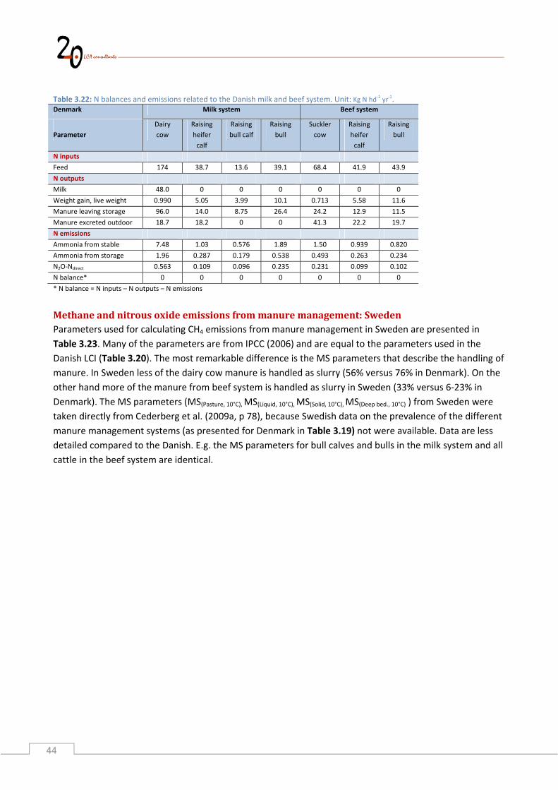
44

Table 3.22: N balances and emissions related to the Danish milk and beef system. Unit: Kg N hd‐1

yr‐1.

Denmark Milk system Beef system

Parameter

Dairy

cow

Raising

heifer

calf

Raising

bull calf

Raising

bull

Suckler

cow

Raising

heifer

calf

Raising

bull

N inputs

Feed 174 38.7 13.6 39.1 68.4 41.9 43.9

N outputs

Milk 48.0 0 0 0 0 0 0

Weight gain, live weight 0.990 5.05 3.99 10.1 0.713 5.58 11.6

Manure leaving storage 96.0 14.0 8.75 26.4 24.2 12.9 11.5

Manure excreted outdoor 18.7 18.2 0 0 41.3 22.2 19.7

N emissions

Ammonia from stable 7.48 1.03 0.576 1.89 1.50 0.939 0.820

Ammonia from storage 1.96 0.287 0.179 0.538 0.493 0.263 0.234

N2O‐Ndirect 0.563 0.109 0.096 0.235 0.231 0.099 0.102

N balance* 0 0 0 0 0 0 0

* N balance = N inputs – N outputs – N emissions

Methaneandnitrousoxideemissionsfrommanuremanagement:SwedenParameters used for calculating CH4 emissions from manure management in Sweden are presented in

Table 3.23. Many of the parameters are from IPCC (2006) and are equal to the parameters used in the

Danish LCI (Table 3.20). The most remarkable difference is the MS parameters that describe the handling of

manure. In Sweden less of the dairy cow manure is handled as slurry (56% versus 76% in Denmark). On the

other hand more of the manure from beef system is handled as slurry in Sweden (33% versus 6‐23% in

Denmark). The MS parameters (MS(Pasture, 10°C), MS(Liquid, 10°C), MS(Solid, 10°C), MS(Deep bed., 10°C) ) from Sweden were

taken directly from Cederberg et al. (2009a, p 78), because Swedish data on the prevalence of the different

manure management systems (as presented for Denmark in Table 3.19) not were available. Data are less

detailed compared to the Danish. E.g. the MS parameters for bull calves and bulls in the milk system and all

cattle in the beef system are identical.

45

Table 3.23: Parameters used for calculating CH4 emissions from Swedish manure management systems (MMS). (*): In Schmidt and Dalgaard (2012). Sweden Unit Milk system Beef system Source

Parameters

Dairy

cow

Raising

heifer

calf

Raising

bull calf

Raising

bull

Suckler

cow

Raising

heifer

calf

Raising

bull

EF(T) Kg CH4 hd‐1

yr‐1

18.3 2.40 1.77 6.24 6.86 4.88 6.71 Equation 6.17(*)

VS(T) Kg DM hd‐1

day‐1

4.97 1.14 0.432 1.53 1.68 1.19 1.64 Equation 6.18(*)

Bo(T) m3 CH4 (kgVS

excreted)‐1

0.240 0.180 0.180 0.180 0.180 0.180 0.180 IPCC (2006, p 10.77‐8)

MCF(Pasture,10°C) % 1 1 1 1 1 1 1

IPCC (2006, Table 10.17) MCF(Liquid, 10°C) % 10 10 10 10 10 10 10

MCF(Solid, 10°C) % 2 2 2 2 2 2 2

MCF(Deep bed., 10°C) % 17 17 17 17 17 17 17

MS(Pasture, 10°C) Dim. less 20.0 46.0 30.0 30.0 30.0 30.0 30.0

Cederberg et al. (2009a,

p 78)

MS(Liquid, 10°C) Dim. less 56.0 35.0 33.0 33.0 33.0 33.0 33.0

MS(Solid, 10°C) Dim. less 24.0 16.0 4.0 4.0 4.0 4.0 4.0

MS(Deep bed., 10°C) Dim. less 0 3.0 33.0 33.0 33.0 33.0 33.0

GE MJ day‐1 332 76.0 28.9 101.9 109.2 77.7 106.8 Table 3.17

DE% % 74.0 74.0 74.0 74.0 73.2 73.2 73.2 Table 3.16

UE Dim. less 0.04 0.04 0.04 0.04 0.04 0.04 0.04 IPCC (2006, eq 10.24)

ASH Dim. less 8.00 8.00 8.00 8.00 8.00 8.00 8.00 IPCC (2006, p 10.42)

Parameters used for calculation of N2O emissions from Swedish cattle are presented in Table 3.24. The

fractions of N excreted handled as liquid, solid and deep bedding are calculated from the MS parameters in

Table 3.23 by using same procedure as in the Danish LCI.

46

Table 3.24: Parameters used for calculating N2O emissions from Swedish manure management systems. (*): In Schmidt and Dalgaard (2012). Sweden Unit Milk system Beef system Source

Parameters

Dairy

cow

Raising

heifer

calf

Raising

bull calf

Raising

bull

Suckler

cow

Raising

heifer

calf

Raising

bull

N2O(mm) kg N2O yr‐1 338,875 73,855 3,679 106,027 113,714 58,674 38,039 Equation 6.19(*)

N2OD(mm) kg N2O yr‐1 302,311 65,178 3,062 88,246 94,643 48,834 31,659 Equation 6.20(*)

N2OG(mm) kg N2O yr‐1 36,563 8,677 617 17,782 19,071 9,840 6379 Equation 6.21(*)

NT heads 393,268 429,851 25,593 286,717 177,000 181,286 111,742 Table 3.2

N2O(mm)/head kg N2O hd‐1 yr

‐1 0.862 0.172 0.144 0.370 0.642 0.324 0.340 N2O(mm)/ NT

Nex(T) kg N hd‐1 yr

‐1 124 33.3 10.0 37.4 64.9 32.7 34.4 Equation 6.21 (*)

MS(Liquid) Dim. less 0.560 0.35 0.42 0.29 0.29 0.29 0.29 From MS parameters

in Table 3.23 and Poul‐

sen et al. (2001). See

text.

MS(Solid) Dim. less 0.232 0.15 0.05 0.03 0.03 0.03 0.03

MS(Deep bed.) Dim. less 0 0.04 0.53 0.36 0.36 0.36 0.36

EF3(Liquid/solid) Kg N2O‐N

kg N‐1

0.005 0.005 0.005 0.005 0.005 0.005 0.005

IPCC (2006, Table

10.21) EF3(Solid storage)

Kg N2O‐N

kg N‐1

0.005 0.005 0.005 0.005 0.005 0.005 0.005

EF3(deep bed.) Kg N2O‐N

kg N‐1

0.01 0.01 0.01 0.01 0.01 0.01 0.01

Nintake(T) kg N hd‐1 yr

‐1 171 38.3 17.9 45.2 65.6 37.7 44.2

From protein content

in feed

Nretention(T) kg N hd‐1 yr

‐1 47.2 5.03 7.95 7.86 0.611 5.03 9.8 Equation 6.22 (*)

Nmilk kg N hd‐1 yr

‐1 46.5 0 0 0 0 0 0 Equation 6.22 (*)

Nweight gain kg N hd‐1 yr

‐1 0.719 5.03 7.95 7.86 0.611 5.03 9.83 Equation 6.22 (*)

Nvolatilization‐MMS Kg N yr‐1 5.92 1.28 1.53 3.95 6.86 3.45 3.63 Equation 6.22 (*)

EF4 Kg N2O‐N

kg N‐1

0.01 0.01 0.01 0.01 0.01 0.01 0.01 IPCC (2006, Table 11.3)

The N inputs, outputs and emissions related to the Swedish milk and beef system are presented in Table

3.25. The N balance is calculated as N inputs minus the sum of N outputs and N emissions. When the N


Table 3.25: N balances and emissions related to the Swedish milk and beef system. Unit: Kg N hd‐1

yr‐1.

Sweden Milk system Beef system

Parameter

Dairy

cow

Raising

heifer

calf

Raising

bull calf

Raising

bull

Suckler

cow

Raising

heifer

calf

Raising

bull

N inputs

Feed 171 38.3 17.9 45.2 65.6 37.7 44.2

N outputs

Milk 46.5 0 0 0 0 0 0

Weight gain, live weight 0.719 5.03 7.95 7.86 0.611 5.03 9.83

Manure leaving storage 91.4 16.7 8.35 21.5 37.3 18.8 19.8

Manure excreted outdoor 25.7 15.3 0 11.8 20.4 10.3 10.8

N emissions

Ammonia from stable 4.05 0.944 1.36 3.51 6.09 3.07 3.23

Ammonia from storage 1.87 0.340 0.170 0.438 0.762 0.384 0.404

N2O‐Ndirect 0.489 0.096 0.076 0.196 0.340 0.171 0.180

N balance* 0 0 0 0 0 0 0


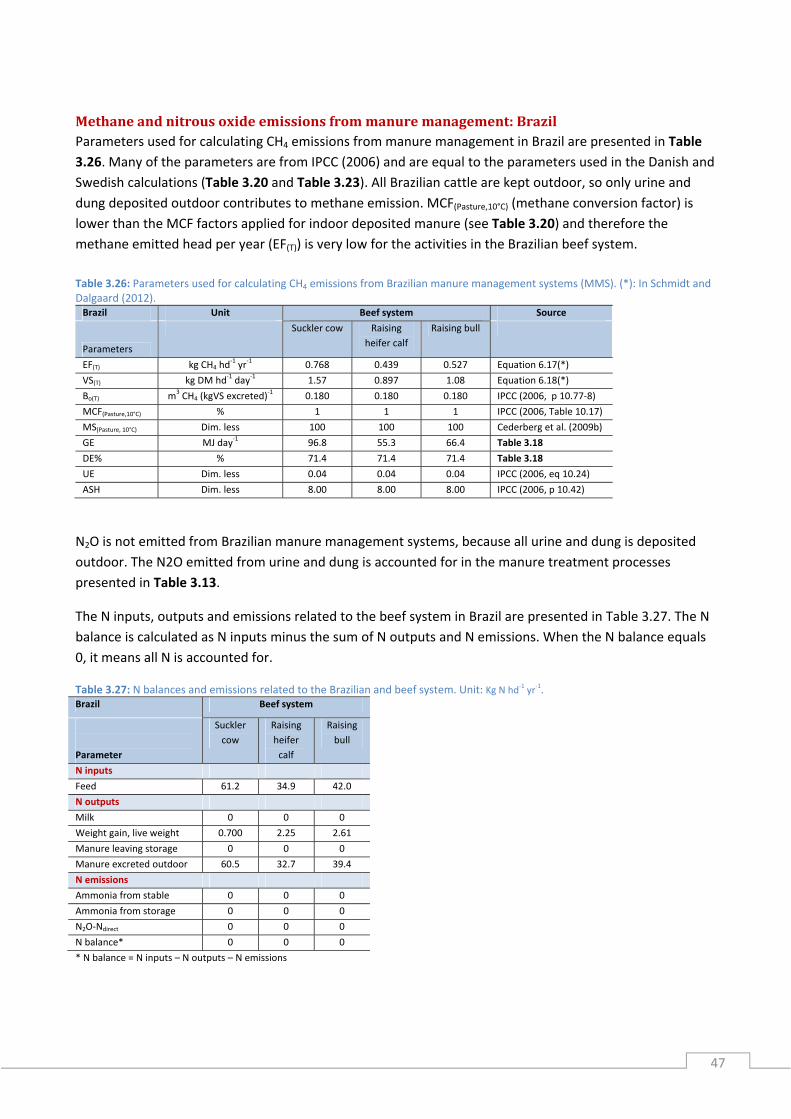
47

Methaneandnitrousoxideemissionsfrommanuremanagement:BrazilParameters used for calculating CH4 emissions from manure management in Brazil are presented in Table

3.26. Many of the parameters are from IPCC (2006) and are equal to the parameters used in the Danish and

Swedish calculations (Table 3.20 and Table 3.23). All Brazilian cattle are kept outdoor, so only urine and

dung deposited outdoor contributes to methane emission. MCF(Pasture,10°C) (methane conversion factor) is

lower than the MCF factors applied for indoor deposited manure (see Table 3.20) and therefore the

methane emitted head per year (EF(T)) is very low for the activities in the Brazilian beef system.

Table 3.26: Parameters used for calculating CH4 emissions from Brazilian manure management systems (MMS). (*): In Schmidt and Dalgaard (2012). Brazil Unit Beef system Source

Parameters

Suckler cow Raising

heifer calf

Raising bull

EF(T) kg CH4 hd‐1 yr

‐1 0.768 0.439 0.527 Equation 6.17(*)

VS(T) kg DM hd‐1 day

‐1 1.57 0.897 1.08 Equation 6.18(*)

Bo(T) m3 CH4 (kgVS excreted)

‐1 0.180 0.180 0.180 IPCC (2006, p 10.77‐8)

MCF(Pasture,10°C) % 1 1 1 IPCC (2006, Table 10.17)

MS(Pasture, 10°C) Dim. less 100 100 100 Cederberg et al. (2009b)

GE MJ day‐1 96.8 55.3 66.4 Table 3.18

DE% % 71.4 71.4 71.4 Table 3.18

UE Dim. less 0.04 0.04 0.04 IPCC (2006, eq 10.24)

ASH Dim. less 8.00 8.00 8.00 IPCC (2006, p 10.42)

N2O is not emitted from Brazilian manure management systems, because all urine and dung is deposited

outdoor. The N2O emitted from urine and dung is accounted for in the manure treatment processes

presented in Table 3.13.

The N inputs, outputs and emissions related to the beef system in Brazil are presented in Table 3.27. The N

balance is calculated as N inputs minus the sum of N outputs and N emissions. When the N balance equals

0, it means all N is accounted for.

Table 3.27: N balances and emissions related to the Brazilian and beef system. Unit: Kg N hd‐1 yr

‐1. Brazil Beef system

Parameter

Suckler

cow

Raising

heifer

calf

Raising

bull

N inputs

Feed 61.2 34.9 42.0

N outputs

Milk 0 0 0

Weight gain, live weight 0.700 2.25 2.61

Manure leaving storage 0 0 0

Manure excreted outdoor 60.5 32.7 39.4

N emissions

Ammonia from stable 0 0 0

Ammonia from storage 0 0 0

N2O‐Ndirect 0 0 0

N balance* 0 0 0


48

3.5 SummaryoftheLCIofcattlesystemSummaries of LCI of the Danish milk and beef systems are presented in Table 3.28 and Table 3.29.

Summaries of LCI of the Swedish milk and beef systems are presented in Table 3.30 and Table 3.31.

Summary of LCI of the Brazilian beef systems is in Table 3.32.

Notice that in the following tables for the beef systems, the meat from the raised calves is shown as if it

was by‐products from the ‘raising heifer’ and ‘raising bull’ activities. In reality, this meat is not by‐products;

it is part of the determining product output from the beef system. Hence, in the modelling, this meat is

moved from the raising activities to the determining product output of the suckler cow. In the following

tables, the meat from the offspring is shown as by‐products only with the purpose for being able to see

how much meat is supplied from the different activities in the beef system.

49

Table 3.28: LCI for the activities in the Danish milk system. The data represent 1 dairy cow during one year. Total is calculated by adding the four activities and up scaling them by the number of dairy cows in 2005 (= 563,500). Denmark. Milk system.

Exchanges

Activity:

Unit:

LCI data per dairy cow incl. offspring during one year LCI data per 563,000 dairy

cows incl. offspring

Dairy cow Raising

heifer calf

Raising

bull calf

Raising

bull

Total

Output of products


Milk kg 8,440 4.76E+09

Animals to raising XXX units XXX

også de andre tabeller XXX

animal

days

405 24 153 3.28E8

Meat, live weight kg ‐

By‐product:

Meat, live weight kg 171 28.4 0 157 2.01E+08

Exported animals for raising, live weight kg 0.918 1.43 2.56 0 2.76E+06

Material for treatment:

Manure deposited outdoor kg N 16.9 16.6 0 0 1.89E+07

Manure land application, liquid/slurry kg N 84.6 0 0 3.17 4.94E+07

Manure land application, solid kg N 5.51 0.878 0 0 3.80E+06

Manure land application, deep litter kg N 5.95 5.69 0.451 5.76 1.01E+07

Destruction of fallen cattle kg 31.1 5.25 2.66 4.10 2.43E+07

Input of products

Barley kg 1,266 289 4.23 116 9.44E+08

Corn kg 63.6 14.5 0.212 5.84 4.74E+07

Soybean meal kg 455 104 1.52 41.8 3.39E+08

Rapeseed cake/meal kg 483 110 1.61 44.4 3.60E+08

Sunflower meal kg 379 86.3 1.26 34.8 2.82E+08

Beet pulp, dried kg 140 32.0 0 12.9 1.05E+08

Molasses kg 46.5 10.6 0.155 4.27 3.47E+07

Palm oil kg 36.2 8.26 0.121 3.33 2.70E+07

Wheat bran kg 44.1 10.1 0.147 4.05 3.29E+07

Feed urea kg 8.90 2.03 2.97E‐02 0.818 6.64E+06

Minerals, salt etc. kg 13.7 3.13 4.58E‐02 1.26 1.02E+07

Permanent grass kg 666 152 2.22 61.2 4.97E+08

Maize ensilage kg 8,893 2,027 29.7 817 6.63E+09

Rotation grass kg 3,667 836 12.2 337 2.73E+09

Lorry tkm 587 134 1.96 54.0 4.38E+08

Electricity kWh 1,300 0 0 0 7.33E+08

Diesel MJ 967 223 24.9 170 7.81E+08

Emissions

Methane kg CH4 163 34.7 0.584 15.4 1.21E+08

Dinitrogen monoxide (direct) kg N2O 0.885 0.171 0.008 0.130 6.73E+05

Dinitrogen monoxide (indirect) kg N2O 0.148 2.07E‐02 6.11E‐04 1.34E‐02 1.03E+05

Ammonia kg NH3 11.5 1.60 0.047 1.04 7.97E+06

50

Table 3.29: LCI for the activities in the Danish beef system. The data represent 1 suckler cow during one year. Total is calculated by adding the four activities and up scaling them by the number of suckler cows in 2005 (=98,500). Denmark. Beef system.

Exchanges

Activity:

Unit:

LCI data per suckler cow during one year LCI data per 98,500

suckler cows

Suckler

cow

Raising

heifer calf

Raising bull Total

Output of products


Animals to raising p 0.959 0.447 1.39E+05

Meat, live weight kg 134 1.32E+07

By‐product:

Meat, live weight kg 89.3 211 4.28E+07


Manure deposited outdoor kg N 37.8 19.3 8.01 6.41E+06

Manure land application, liquid/slurry kg N 3.09 6.59 1.750 1.13E+06

Manure land application, solid kg N 2.99 0.768 0.195 3.89E+05

Manure land application, deep litter kg N 18.1 4.98 3.18 2.59E+06

Destruction of fallen cattle kg 16.9 2.03 7.46 2.60E+06

Input of products

Barley kg 410 298 170.3 8.65E+07

Soybean meal kg 121 88.2 50.5 2.56E+07

Feed urea kg 0.640 0.465 0.266 1.35E+05

Minerals, salt etc. kg 0.986 0.716 0.410 2.08E+05

Permanent grass kg 2,920 2,120 1,213 6.16E+08

Maize ensilage kg 1,928 1,400 801 4.07E+08

Rotation grass kg 3,054 2,217 1,269 6.44E+08

Lorry tkm 107 77.4 44.3 2.25E+07

Electricity kWh 90.0 0 0 8.87E+06

Diesel MJ 188 181 84.1 4.46E+07

Emissions

Methane kg CH4 51.6 37.1 21.4 1.08E+07

Dinitrogen monoxide (direct) kg N2O 0.363 1.50E‐01 7.17E‐02 5.76E+04

Dinitrogen monoxide (indirect) kg N2O 3.14E‐02 1.81E‐02 7.40E‐03 5.61E+03

Ammonia kg NH3 2.43 1.40 0.572 4.33E+05

51

Table 3.30: LCI for the activities in the Swedish milk system. The data represent 1 dairy cow during one year. Total is calculated by adding the four activities and up scaling them by the number of dairy cows in 2005 (= 393,268). Sweden. Milk system.

Exchanges

Activity:

Unit:

LCI data per dairy cow incl. offspring during one year LCI data per 393,268 dairy

cows incl. offspring

Dairy cow Raising

heifer calf

Raising

bull calf

Raising

bull

Total

Output of products


Milk kg 8,271 3.25E+09

Animals to raising p 1.09 6.51E‐02 0.729 7.42E+05

By‐product:

Meat, live weight kg 30.1 0 244 1.73E+08

Exported animals for raising, live weight kg 1.24 0 0.202 0 5.68E+05


Manure deposited outdoor kg N 24.1 15.4 0 7.19 1.83E+07

Manure land application, liquid/slurry kg N 64.7 11.8 0.229 6.61 3.27E+07

Manure land application, solid kg N 26.8 5.193 0.027 0.774 1.29E+07

Manure land application, deep litter kg N 0 1.26 0.287 8.280 3.87E+06

Destruction of fallen cattle kg 30.8 14.5 3.35 13.9 2.46E+07

Input of products

Barley kg 737 185 4.17 165 4.29E+08

Wheat kg 221 55.3 1.25 49.5 221

Oat kg 623 156 3.53 140 623

Corn kg 7.30 1.83 4.13E‐02 1.64 7.30

Soybean meal kg 267 66.9 1.51 59.9 267

Rapeseed cake/meal kg 326 81.5 1.84 72.9 326

Beet pulp kg 215 53.8 1.22 48.1 215

Molasses kg 46.7 11.7 0.264 10.5 46.7

Palm oil kg 43.8 11.0 0.248 9.81 43.8

Palm kernel meal kg 143 35.7 0.807 31.9 143

Wheat bran kg 140 35.1 0.793 31.4 140

Minerals, salt etc. kg 50.2 12.6 0.284 11.2 50.2

Permanent grass kg 4,454 1,116 25.2 998 4,454

Maize ensilage kg 5,970 1,495 33.8 1337 5,970

Rotation grass kg 7,574 1,897 42.9 1697 7,574

Lorry tkm 564 141 3.19 126.3 564

Electricity kWh 1,300 ‐ 0 0 1,300

Diesel MJ 956 286 31.4 241 956

Emissions

Methane kg CH4 160 38.0 0.916 36.2 160

Dinitrogen monoxide (direct) kg N2O 0.769 0.166 0.008 0.224 0.769

Dinitrogen monoxide (indirect) kg N2O 9.30E‐02 2.21E‐02 1.57E‐03 4.52E‐02 9.30E‐02

Ammonia kg NH3 7.18 1.70 0.121 3.49 7.18

52

Table 3.31: LCI for the activities in the Swedish beef system. The data represent 1 suckler cow during one year. Total is calculated by adding the four activities and up scaling them by the number of suckler cows in 2005 (= 177,000). Sweden. Beef system.

Exchanges

Activity:

Unit:

LCI data per suckler cow during one year LCI data per 177,000

suckler cows

Suckler

cow

Raising

heifer calf

Raising bull Total

Output of products



Meat, live weight kg 117 2.07E+07

By‐product:


Exported animals for raising, live weight kg 11.6 0 0 2.05E+06



Manure land application, liquid/slurry kg N 15.7 8.13 5.27 5.16E+06

Manure land application, solid kg N 1.84 0.951 0.617 6.04E+05

Manure land application, deep litter kg N 19.7 10.2 6.60 6.46E+06


Input of products

Barley kg 39.0 28.4 24.1 1.62E+07

Wheat kg 56.4 41.1 34.8 2.34E+07

Oat kg 13.0 9.47 8.03 5.40E+06

Corn kg 1.57 1.14 0.966 6.50E+05

Soybean meal kg 66.5 48.4 41.0 2.76E+07

Rapeseed cake/meal kg 80.7 58.8 49.8 3.35E+07

Beet pulp kg 53.2 38.8 32.8 2.21E+07

Molasses kg 11.6 8.42 7.13 4.80E+06

Palm oil kg 10.8 7.90 6.69 4.50E+06

Palm kernel meal kg 44.3 32.3 27.3 1.84E+07

Wheat bran kg 33.6 24.5 20.7 1.40E+07



Maize ensilage kg 2,477 1,804 1,528 1.03E+09

Rotation grass kg 2,428 1,769 1,498 1.01E+09

Lorry tkm 84.6 61.6 52.2 3.51E+07


Diesel MJ 331 339 209 1.56E+08

Emissions

Methane kg CH4 53.4 38.9 33.0 2.22E+07

Dinitrogen monoxide (direct) kg N2O 0.535 0.276 0.179 1.75E+05

Dinitrogen monoxide (indirect) kg N2O 0.108 0.056 0.036 3.53E+04

Ammonia kg NH3 8.33 4.30 2.79 2.73E+06

53

Table 3.32: LCI for the activities in the Brazilian beef system. The data represent 1 suckler cow during one year. Total is calculated by adding the four activities and up scaling them by the number of suckler cows in 2005 (= 45,100,000). Brazil. Beef system.

Exchanges

Activity:

Unit:

LCI data per suckler cow during one year LCI data per 45,100,000

suckler cows

Suckler

cow

Raising

heifer calf

Raising bull Total

Output of products



Meat, live weight kg 55.9 2.52E+09

By‐product:





Input of products



Lorry tkm 3.31 1.71 2.04 3.18E+08


Emissions

Methane kg CH4 42.0 21.7 25.9 4.04E+09

3.6 ParametersrelatingtoswitchbetweenmodellingassumptionsThe allocation factors used for switching between the four modelling assumptions are presented in Table

3.33. Overviews of the milk and beef system are presented in Schmidt and Dalgaard (2012, Figure 6.1 and

6.2).

Switch 1: Allocation is avoided by substitution. Consequently, milk production results in avoided production

of e.g. cattle meat and fertilisers.

Switch 2: Co‐products are modelled using allocation at the point of substitution. The allocation factors are

obtained by combining the product amounts (Section 3.4 and 3.6) with the relevant product prices from

Appendix C: Prices.

Switch 3 and 4: Co‐products are modelled using allocation at the point of substitution or at other points as

defined in PAS2050 and IDF. The allocation factors are obtained by combining the product amounts

(Section 3.4 and 3.6) with the relevant product prices from Appendix C: Prices. However, the allocation

factor between milk and meat for IDF is special, i.e. it is based on the supply of milk and meat and the

following formula (IDF 2010, p 20): Equation 3.2

af 1 5.7717 ∙MM

where:

‐ af is the allocation factor for milk

‐ Mmeat is the sum of live weight of all animals sold including bull calves and culled mature animals

‐ Mmilk is the sum of ECM sold

54

Table 3.33: Allocation factors used for allocation of products produced in the milk and beef systems. Unit: Fraction

System: Milk system Beef system

Country: DK SE DK SE BR

Switch 1: ISO 14040/44 consequential


Milk 1 1

Meat 1 1 1

Switch 2: Average/allocation attributional


Milk 0.816 0.839

Meat 0.889 0.782 1

By‐products at point of substitution:

Cattle meat, live weight 1.43E‐01 1.25E‐01

Exported animals for raising, live weight 7.90E‐03 1.74E‐03 9.48E‐02

N fert as N 1.72E‐02 1.61E‐02 5.83E‐02 5.67E‐02

P fert as P2O5 3.29E‐03 7.26E‐03 1.11E‐02 2.56E‐02

K fert as K2O 1.16E‐02 9.56E‐03 3.94E‐02 3.37E‐02

Heat 3.78E‐06 5.72E‐06 1.18E‐05 2.74E‐05

Burning coal 1.25E‐04 3.51E‐04 3.90E‐04 1.68E‐03

Burning fuel oil 6.03E‐04 1.05E‐03 1.88E‐03 5.03E‐03

Switch 3: PAS2050


Milk 0.844 0.869

Meat 1.00 0.892 1

By‐products:

Cattle meat, live weight 0.148 0.130

Exported animals for raising, live weight 8.17E‐03 1.80E‐03 0.108

Switch 4: IDF


Milk 0.863 0.863

Meat 1.00 0.892 1

By‐products:

Cattle meat, live weight 0.137 0.137

Exported animals for raising, live weight 0.108

55

4 TheplantcultivationsystemThe plant production activities supplies the main feedstock input to the cattle system. It is also the plant

production activities that occupy the most land, i.e. these activities causes the indirect land use change

effects.

4.1 InputsandoutputsofproductsThe inputs and outputs of products related to grass, ensilage and crop cultivation are presented and

documented in the following sections.

BarleyThe inputs and outputs of products related to barley cultivation are presented in Table 4.1. The barley

yields are calculated by linear regression over the period 1995‐2009. Data on yields are obtained from

FAOSTAT (2012). Yields for the specific year 2005 are not used because yields can vary considerable

amongst years due to drought, diseases etc. As seen in the table, yields in Ukraine (UA) are lower compared

to the yields in the European countries.

Material for treatment is straw and it only includes straw used for energy purposes. Straw used for bedding

is not presented in Table 4.1. The amount of straw produced in the fields is calculated according to Schmidt

and Dalgaard (2012, eq. 7.4). According to Statistics Denmark (2012), 75.0 % of the straw from spring barley

was removed from the field and 40.4% of all straw removed was used for energy purposes. The same

percentages are used for Swedish straw use. The use of straw for energy purposes in the other countries is

considered negligible.

Table 4.1: Outputs and inputs of products. Barley cultivation. The data represent 1 ha year.

Crop: Barley

Outputs and inputs

of products

Country:

Unit: DK SE UA EU

Output of products Determining product: Barley

kg 5,157 4,198 2,191 4,259

Material for treatment: Straw

kg 1,741 1,456 ‐ ‐

Input of products

N‐fert: Ammonia kg N 2.83 0 0 0.070

N‐fert: Urea kg N 4.53 0 8.76 16.5

N‐fert: AN kg N 6.23 6.45 49.5 19.2

N‐fert: CAN kg N 42.5 63.7 0 22.9

N‐fert: AS kg N 1.70 4.84 1.74 3.35

Manure Kg N 99.2 0 21.3 93.1

P fert: TSP kg P2O5 50.4 50.4 137 50.4

K fert: KCl kg K2O 66.3 66.3 72.3 66.3

Pesticides kg (a.s.) 0.509 0.509 0.509 0.509

Lorry tkm 83.8 100 119 83.1

Diesel MJ 3,046 3,046 3,046 3,046

Light fuel oil for drying MJ 1.10 1.10 1.10 1.10

Land tenure, arable kg C 7,000 5,600 5,000 7,000

56

The amount of fertiliser and manure applied are also presented in Table 4.1. Data are obtained from:

‐ Sweden: N fertiliser is from Cederberg et al. (2009a). Distribution of N –fertiliser between different

fertiliser types is based on IFA (2012b), as presented in Table 4.2. P and K fertiliser is assumed equal to

Danish data.

‐ Ukraine: FAO (2005, p 40))

‐ Denmark and EU: See explanation below.

Table 4.2: Distribution of N between different types of artificial n fertiliser types. Based on IFA(2012b).

Fertiliser types DK SE UA EU

N‐fert: Ammonia 4.90% 0% 0% 0%

N‐fert: Urea 7.84% 0% 14.6% 26.6%

N‐fert: AN 10.8% 8.60% 82.5% 30.9%

N‐fert: CAN 73.5% 84.9% 0% 36.9%

N‐fert: AS 2.94% 6.45% 2.89% 5.41%

Total 100% 100% 100% 100%

Only one type of P fertiliser and one type of K fertiliser is used. For further details see section 2.4.

The amount of N fertiliser applied per hectare is correlated to the amount of manure applied. In general,

fields that receive a lot of manure will not require as much N fertiliser as fields that not receive manure. To

account for this, the manure applied per hectare in each country is estimated. Firstly, default values on N

ab storage per animal in Denmark are estimated. Data on N excreted yearly per animal type (Mikkelsen et

al. 2006) are divided by number of animals (stocks of cattle, pigs, poultry, horses and sheep) obtained from

FAOSTAT (2012). These default data on N excreted per animal in Denmark (see Table 4.3) are then assumed

to be representative for animals in the other countries and the total N excretion form livestock in each

country can then be calculated by multiplying with number of animals from FAOSTAT (2012).

Table 4.3: N excretion per animal. Calculated from Mikkelsen et al. (2006) and FAOSTAT (2012).

Animal type N excretion, kg N per animal

Cattle 74.0

Pigs 9.22

Poultry 0.80

Horses 129

Sheep 12.4

Obviously a calf excretes much less N per year than a cow. But by using data from FAO (2012) these

differences are counterbalanced, because the population distribution of cattle of different size and age are

most likely to be the same in all countries.

Afterwards, the N losses from stable and storage based on Poulsen et al. (2001) is deducted the N

excretion, which again is divided by the arable land area (FAOSTAT 2012). The results are presented in

Table 4.4.

57

Table 4.4: Estimated manure application at arable land in different countries. Unit: kg N ha‐1 yr‐1.

DK SE RU UA FR EU

Manure applied 99.2 54.8 18.5 21.3 95.0 93.1

The amount of N fertiliser applied in DK and EU are based on Danish regulation and guidelines regarding

fertiliser application to arable land in the 2005 (Plantedirektoratet, 2004, Table 1). The N quota for barley is

127 kg N and the recommended use of P and K is 22 kg P and 55 kg K per ha. However, for each kg N in

manure applied per ha, 0.7 kg less N fertiliser can be applied. Consequently, the Danish barley can be

applied 58 kg N fertiliser per ha (=127 – (0.7*99)). The same procedure is used for Swedish barley, but

taking into account the manure application only is 54 kg N per ha.

The distribution of N fertiliser between different fertiliser types is based on data from IFA (2012b) and

presented in Table 4.2. Data from Ukraine are not available from FAOSTAT (2012), hence data from Russia

are used.

Amount of pesticides are from Flysjö et al. (2008, p 31) and same amount are applied for barley cultivation

in all countries. Fertilisers and pesticides are assumed to be transported 200 km by lorry. The mass of

pesticides is 3 kg pesticide per kg active ingredient (a.s), and is estimated based on pesticide use for

different crops in Schmidt (2007). The total mass to nutrient content (N, P2O5 or KCl) ratio of fertilisers are

based on IFA (2012a).

The diesel used per ha for field operations is obtained from Cederberg et al (2009a, p 66) and equals 82

litres per ha. Same amount is used for barley cultivation in all countries.

Light fuel oil for drying barley is from Cederberg et al. (2009a, p 19). Same amount is used for barley

cultivation in all countries regardless of the yield and differences in moisture content.

The input of land tenure is obtained from Table 2.9.

Wheat,oat,cornandsoybeanThe inputs and outputs of products related to wheat, oat, corn and soybean cultivation are presented in

Table 4.5. All yields are calculated by linear regression over the period 1995‐2009. Data on yields are

obtained from FAOSTAT (2012). As seen in the table, yields in Sweden are lower than yields in Denmark.


is not presented in Table 4.5. The amount of straw produced at the fields is calculated according to Schmidt

and Dalgaard (2012, eq. 7.4). According to Statistics Denmark (2012) 54.4 % and 32.9% of wheat and oat

straw respectively are removed from the field and 40.4% of all straw removed was used for energy

purposes. Due to data lack the same percentages are used for Swedish straw use. The use of straw for

energy purposes in the other countries is considered negligible.

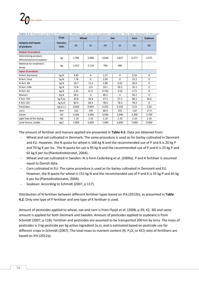
58

Table 4.5: Outputs and inputs of products. Wheat, oat, corn and soybean cultivation. The data represent 1 ha year.

Crop: Wheat Oat Corn Soybean

Outputs and inputs

of products

Country:

Unit: DK SE DK SE EU BR

Output of products


Wheat/oat/corn/soybean kg 7,296 5,986 4,646 3,817 6,577 2,575


Straw kg 2,552 2,118 700 600 ‐ ‐

Input of products

N‐fert: Ammonia kg N 4.85 0 1.27 0 0.10 0

N‐fert: Urea kg N 7.76 0 2.04 0 23.2 0

N‐fert: AN kg N 10.7 11.6 2.80 6.02 26.9 0

N‐fert: CAN kg N 72.8 115 19.1 59.5 32.1 0

N‐fert: AS kg N 2.91 8.71 0.763 4.52 4.71 0

Manure Kg N 99.2 0 99.2 0 93.1 0

P fert: TSP kg P2O5 45.8 45.8 57.3 57.3 80.2 36.6

K fert: KCl kg K2O 84.4 84.4 78.3 78.3 78.3 0

Pesticides kg (a.s.) 0.603 0.603 0.355 0.355 3.53 2.50

Lorry tkm 116 149 68.9 103 118 17.4

Diesel MJ 3,306 3,306 3,046 3,046 3,306 1,709

Light fuel oil for drying MJ 1.10 1.10 1.10 1.10 1.10 1.10

Land tenure, arable kg C 7,000 5,600 7,000 5,600 7,000 9,000

The amount of fertiliser and manure applied are presented in Table 4.5. Data are obtained from:

‐ Wheat and oat cultivated in Denmark: The same procedure is used as for barley cultivated in Denmark

and EU. However, the N quota for wheat is 168 kg N and the recommended use of P and K is 20 kg P

and 70 kg K per ha. The N quota for oat is 95 kg N and the recommended use of P and K is 25 kg P and

65 kg K per ha (Plantedirektoratet, 2004).

‐ Wheat and oat cultivated in Sweden: N is form Cederberg et al. (2009a). P and K fertiliser is assumed

equal to Danish data.

‐ Corn cultivated in EU: The same procedure is used as for barley cultivated in Denmark and EU.

However, the N quota for wheat is 152 kg N and the recommended use of P and K is 35 kg P and 65 kg

K per ha (Plantedirektoratet, 2004).

‐ Soybean: According to Schmidt (2007, p 117).

Distribution of N fertiliser between different fertiliser types based on IFA (2012b), as presented in Table

4.2. Only one type of P fertiliser and one type of K fertiliser is used.

Amount of pesticides applied to wheat, oat and corn is from Flysjö et al. (2008, p 29; 42; 30) and same

amount is applied for both Denmark and Sweden. Amount of pesticides applied to soybeans is from

Schmidt (2007, p 118). Fertiliser and pesticides are assumed to be transported 200 km by lorry. The mass of

pesticides is 3 kg pesticide per kg active ingredient (a.s), and is estimated based on pesticide use for

different crops in Schmidt (2007). The total mass to nutrient content (N, P2O5 or KCl) ratio of fertilisers are

based on IFA (2012a).

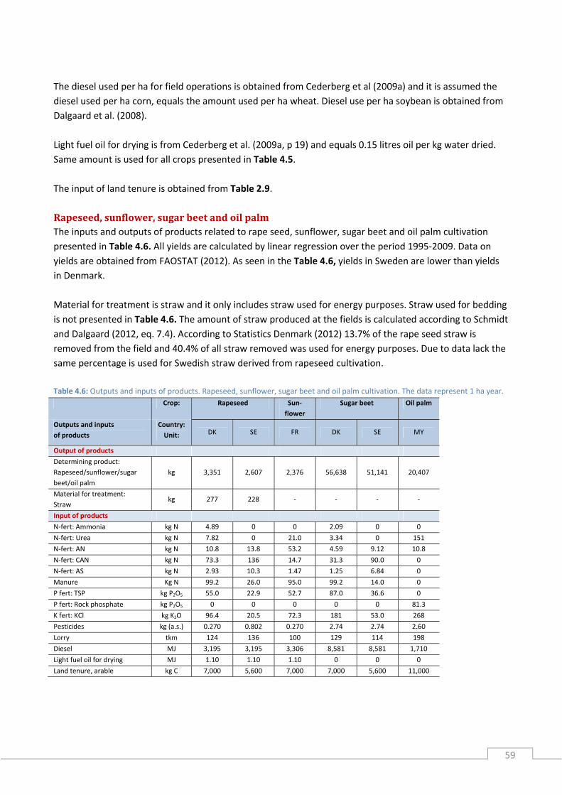
59

The diesel used per ha for field operations is obtained from Cederberg et al (2009a) and it is assumed the

diesel used per ha corn, equals the amount used per ha wheat. Diesel use per ha soybean is obtained from

Dalgaard et al. (2008).

Light fuel oil for drying is from Cederberg et al. (2009a, p 19) and equals 0.15 litres oil per kg water dried.

Same amount is used for all crops presented in Table 4.5.


Rapeseed,sunflower,sugarbeetandoilpalmThe inputs and outputs of products related to rape seed, sunflower, sugar beet and oil palm cultivation

presented in Table 4.6. All yields are calculated by linear regression over the period 1995‐2009. Data on

yields are obtained from FAOSTAT (2012). As seen in the Table 4.6, yields in Sweden are lower than yields

in Denmark.


is not presented in Table 4.6. The amount of straw produced at the fields is calculated according to Schmidt

and Dalgaard (2012, eq. 7.4). According to Statistics Denmark (2012) 13.7% of the rape seed straw is

removed from the field and 40.4% of all straw removed was used for energy purposes. Due to data lack the

same percentage is used for Swedish straw derived from rapeseed cultivation.

Table 4.6: Outputs and inputs of products. Rapeseed, sunflower, sugar beet and oil palm cultivation. The data represent 1 ha year.

Crop: Rapeseed Sun‐

flower

Sugar beet Oil palm

Outputs and inputs

of products

Country:

Unit: DK SE FR DK SE MY

Output of products


Rapeseed/sunflower/sugar

beet/oil palm

kg 3,351 2,607 2,376 56,638 51,141 20,407


Straw kg 277 228 ‐ ‐ ‐ ‐

Input of products

N‐fert: Ammonia kg N 4.89 0 0 2.09 0 0

N‐fert: Urea kg N 7.82 0 21.0 3.34 0 151

N‐fert: AN kg N 10.8 13.8 53.2 4.59 9.12 10.8

N‐fert: CAN kg N 73.3 136 14.7 31.3 90.0 0

N‐fert: AS kg N 2.93 10.3 1.47 1.25 6.84 0

Manure Kg N 99.2 26.0 95.0 99.2 14.0 0

P fert: TSP kg P2O5 55.0 22.9 52.7 87.0 36.6 0

P fert: Rock phosphate kg P2O5 0 0 0 0 0 81.3

K fert: KCl kg K2O 96.4 20.5 72.3 181 53.0 268

Pesticides kg (a.s.) 0.270 0.802 0.270 2.74 2.74 2.60

Lorry tkm 124 136 100 129 114 198

Diesel MJ 3,195 3,195 3,306 8,581 8,581 1,710

Light fuel oil for drying MJ 1.10 1.10 1.10 0 0 0


60

The amount of fertiliser and manure applied are presented in Table 4.6. Data are obtained from:

‐ Rapeseed cultivated in Denmark: The same procedure is used as for barley cultivated in Denmark and

EU. However, the N quota for wheat is 169 kg N and the recommended use of P and K is 24 kg P and


‐ Rapeseed cultivated in Sweden: Flysjö et al. (2008, p 39; Crop: Höstraps. Syd).

‐ Rapeseed cultivated in Denmark: The same procedure is used as for barley cultivated in Denmark and



‐ Sugar beet cultivated in Denmark: The same procedure is used as for barley cultivated in Denmark and



‐ Sugar beet cultivated in Sweden: Flysjö et al. (2008, p 51).

‐ Oil palm cultivation: Schmidt et al. (2011)

Distribution of N fertiliser between different fertiliser types based on IFA (2012b), as presented in Table

4.2. Only one type of K fertiliser is used. The P fertiliser rock phosphate is used for oil palm cultivation,

whereas the P fertiliser TSP is used for all other crops.

The amount of pesticides applied to rapeseeds in Denmark and Sweden are from Schmidt (2007, p 65) and

Flysjö et al. (2008, p 39) respectively. Pesticide application to sunflower, sugar beet and oil palm is from

Schmidt (2007, p 65), Flysjö et al. (2008, p 51) and Schmidt (2007, p 93) respectively. It was assumed the

same amount of pesticides is applied to Danish and Swedish sugar beets. Fertiliser and pesticides are

assumed to be transported 200 km by lorry. The mass of pesticides is 3 kg pesticide per kg active ingredient

(a.s), and is estimated based on pesticide use for different crops in Schmidt (2007). The total mass to

nutrient content (N, P2O5 or KCl) ratio of fertilisers are based on IFA (2012a).

Diesel used per ha field operations are from the following data sources:

‐ Rapeseed cultivated in Denmark and Sweden: Cederberg et al. (2009a, p 66).

‐ Sunflower: Cederberg et al (2009a, p 66). Due to data lack assumed to be the same as for winter

wheat.

‐ Sugar beet cultivated in Denmark and Sweden: Based on the process ‘Sugar beets IP, at farm/CH’ from

Ecoinvent (2007).

‐ Oil palm: Based on Schmidt (2011, p 42)

Light fuel oil for drying is from Cederberg et al. (2009, p 19) and equals 0.15 litres oil per kg water dried.

Same amount is used for all crops presented in Table 4.6.


Permanentgrassincl.grassensilageThe inputs and outputs of products related production of ‘Permanent grass incl. grass ensilage’ are

presented in Table 4.7. The yields of permanent grass are seldom measured, thus these yields are to be

considered as less precise, compared to the previously presented yields. The Danish yields are from

61

Knowledge Centre for Agriculture (2012), and the Swedish yields are assumed to be 20% lower. The yield of

permanent grass in Brazil is estimated based on the total pasture area for beef production at 142,000,000

ha (Cederberg et al. 2009b, p 37), the calculated net feed energy requirement (see Table 3.3 and Table 3.7),

the net energy content of dry matter permanent grass (see Appendix B: Feed and crop properties), and the

dry matter content of permanent grass (see Appendix B: Feed and crop properties).

Table 4.7: Outputs and inputs of products. Permanent grass incl. grass ensilage cultivation. The data represent 1 ha year.

Crop: Permanent grass incl. grass ensilage

Outputs and inputs

of products

Country:

Unit: DK SE BR

Output of products


Permanent grass incl. grass ensilage kg 11,628 9,302 7,193

Input of products

N‐fert: Ammonia kg N 3.46 0 0

N‐fert: Urea kg N 5.53 0 0

N‐fert: AN kg N 7.61 8.74 0

N‐fert: CAN kg N 51.9 86.3 0

N‐fert: AS kg N 2.08 6.56 0

Manure Kg N 99.2 54.8 39.8

P fert: TSP kg P2O5 32.1 32.1 0

K fert: KCl kg K2O 121 121 0

Lorry tkm 102 130 ‐

Diesel MJ 557.2 557.2 31.4

Land tenure, arable kg C 7,000 2,800 ‐

Land tenure, int. forest land kg C 0 2,800 0

Land tenure, rangeland kg C 0 0 9,000

The amount of fertiliser and manure applied are presented in Table 4.7. Data are obtained from the

following sources:

‐ Permanent grass incl. grass ensilage in Denmark and Sweden: The same procedure is used as for

barley cultivated in Denmark and EU. However, the N quota for permanent grass is 140 kg N and the

recommended use of P and K is 14 kg P and 100 kg K per ha (Plantedirektoratet, 2004).

‐ Only dung and urine deposited from grazing cattle is applied to the permanent grass in Brazil. Based

on the area of permanent grass and the amount of N excreted it is estimated to 54.8 kg N per ha.

Distribution of N fertiliser between different fertiliser types is based on IFA (2012b), as presented in Table


Fertilisers are assumed to be transported 200 km by lorry. The total mass to nutrient content (N, P2O5 or

KCl) ratio of fertilisers are based on IFA (2012a).

Diesel for fields operations in Denmark and Sweden is from Cederberg et al. (2009a, p 66) and diesel use in

Brazil is based on Cederberg at al. (2009b, p 48).


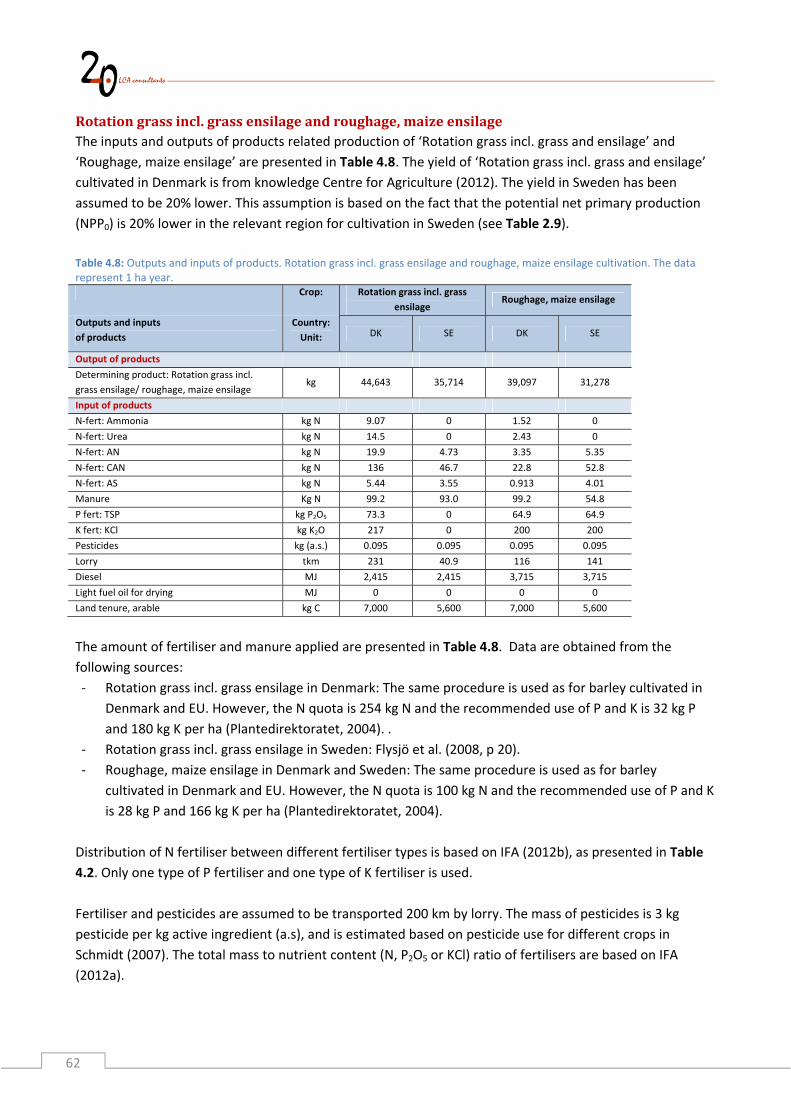
62

Rotationgrassincl.grassensilageandroughage,maizeensilageThe inputs and outputs of products related production of ‘Rotation grass incl. grass and ensilage’ and

‘Roughage, maize ensilage’ are presented in Table 4.8. The yield of ‘Rotation grass incl. grass and ensilage’

cultivated in Denmark is from knowledge Centre for Agriculture (2012). The yield in Sweden has been

assumed to be 20% lower. This assumption is based on the fact that the potential net primary production

(NPP0) is 20% lower in the relevant region for cultivation in Sweden (see Table 2.9).

Table 4.8: Outputs and inputs of products. Rotation grass incl. grass ensilage and roughage, maize ensilage cultivation. The data represent 1 ha year.

Crop: Rotation grass incl. grass

ensilage Roughage, maize ensilage

Outputs and inputs

of products

Country:

Unit: DK SE DK SE

Output of products

Determining product: Rotation grass incl.

grass ensilage/ roughage, maize ensilage kg 44,643 35,714 39,097 31,278

Input of products

N‐fert: Ammonia kg N 9.07 0 1.52 0

N‐fert: Urea kg N 14.5 0 2.43 0

N‐fert: AN kg N 19.9 4.73 3.35 5.35

N‐fert: CAN kg N 136 46.7 22.8 52.8

N‐fert: AS kg N 5.44 3.55 0.913 4.01

Manure Kg N 99.2 93.0 99.2 54.8

P fert: TSP kg P2O5 73.3 0 64.9 64.9

K fert: KCl kg K2O 217 0 200 200

Pesticides kg (a.s.) 0.095 0.095 0.095 0.095

Lorry tkm 231 40.9 116 141

Diesel MJ 2,415 2,415 3,715 3,715

Light fuel oil for drying MJ 0 0 0 0


The amount of fertiliser and manure applied are presented in Table 4.8. Data are obtained from the

following sources:

‐ Rotation grass incl. grass ensilage in Denmark: The same procedure is used as for barley cultivated in

Denmark and EU. However, the N quota is 254 kg N and the recommended use of P and K is 32 kg P

and 180 kg K per ha (Plantedirektoratet, 2004). .

‐ Rotation grass incl. grass ensilage in Sweden: Flysjö et al. (2008, p 20).

‐ Roughage, maize ensilage in Denmark and Sweden: The same procedure is used as for barley

cultivated in Denmark and EU. However, the N quota is 100 kg N and the recommended use of P and K

is 28 kg P and 166 kg K per ha (Plantedirektoratet, 2004).

Distribution of N fertiliser between different fertiliser types is based on IFA (2012b), as presented in Table


Fertiliser and pesticides are assumed to be transported 200 km by lorry. The mass of pesticides is 3 kg

pesticide per kg active ingredient (a.s), and is estimated based on pesticide use for different crops in

Schmidt (2007). The total mass to nutrient content (N, P2O5 or KCl) ratio of fertilisers are based on IFA

(2012a).

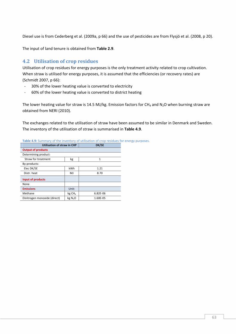
63

Diesel use is from Cederberg et al. (2009a, p 66) and the use of pesticides are from Flysjö et al. (2008, p 20).


4.2 UtilisationofcropresiduesUtilisation of crop residues for energy purposes is the only treatment activity related to crop cultivation.

When straw is utilised for energy purposes, it is assumed that the efficiencies (or recovery rates) are

(Schmidt 2007, p 66):

‐ 30% of the lower heating value is converted to electricity

‐ 60% of the lower heating value is converted to district heating

The lower heating value for straw is 14.5 MJ/kg. Emission factors for CH4 and N2O when burning straw are

obtained from NERI (2010).

The exchanges related to the utilisation of straw have been assumed to be similar in Denmark and Sweden.

The inventory of the utilisation of straw is summarised in Table 4.9.

Table 4.9: Summary of the inventory of utilisation of crop residues for energy purposes.

Utilisation of straw in CHP DK/SE

Output of products


Straw for treatment kg 1

By‐products:

Elec DK/SE kWh 1.21

Distr. heat MJ 8.70

Input of products

None

Emissions Unit:

Methane kg CH4 6.82E‐06

Dinitrogen monoxide (direct) kg N2O 1.60E‐05

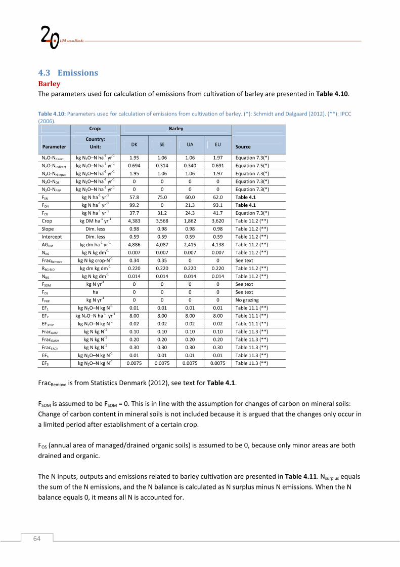
64

4.3 EmissionsBarleyThe parameters used for calculation of emissions from cultivation of barley are presented in Table 4.10.

Table 4.10: Parameters used for calculation of emissions from cultivation of barley. (*): Schmidt and Dalgaard (2012). (**): IPCC (2006).

Crop: Barley

Parameter

Country:

Unit: DK SE UA EU

Source

N2O‐Ndirect kg N2O–N ha‐1 yr

‐1 1.95 1.06 1.06 1.97 Equation 7.3(*)

N2O‐Nindirect kg N2O–N ha‐1 yr

‐1 0.694 0.314 0.340 0.691 Equation 7.5(*)

N2O‐NN input kg N2O–N ha‐1 yr

‐1 1.95 1.06 1.06 1.97 Equation 7.3(*)

N2O‐NOS kg N2O–N ha‐1 yr

‐1 0 0 0 0 Equation 7.3(*)

N2O‐NPRP kg N2O–N ha‐1 yr

‐1 0 0 0 0 Equation 7.3(*)

FSN kg N ha‐1 yr

‐1 57.8 75.0 60.0 62.0 Table 4.1

FON kg N ha‐1 yr

‐1 99.2 0 21.3 93.1 Table 4.1

FCR kg N ha‐1 yr

‐1 37.7 31.2 24.3 41.7 Equation 7.3(*)

Crop kg DM ha‐1 yr

‐1 4,383 3,568 1,862 3,620 Table 11.2 (**)

Slope Dim. less 0.98 0.98 0.98 0.98 Table 11.2 (**)

Intercept Dim. less 0.59 0.59 0.59 0.59 Table 11.2 (**)

AGDM kg dm ha‐1 yr

‐1 4,886 4,087 2,415 4,138 Table 11.2 (**)

NAG kg N kg dm‐1 0.007 0.007 0.007 0.007 Table 11.2 (**)

FracRemove kg N kg crop‐N‐1 0.34 0.35 0 0 See text

RBG‐BIO kg dm kg dm‐1 0.220 0.220 0.220 0.220 Table 11.2 (**)

NBG kg N kg dm‐1 0.014 0.014 0.014 0.014 Table 11.2 (**)

FSOM kg N yr‐1 0 0 0 0 See text

FOS ha 0 0 0 0 See text

FPRP kg N yr‐1 0 0 0 0 No grazing

EF1 kg N2O–N kg N‐1 0.01 0.01 0.01 0.01 Table 11.1 (**)

EF2 kg N2O–N ha‐1 yr

‐1 8.00 8.00 8.00 8.00 Table 11.1 (**)

EF3PRP kg N2O–N kg N‐1 0.02 0.02 0.02 0.02 Table 11.1 (**)

FracGASF kg N kg N‐1 0.10 0.10 0.10 0.10 Table 11.3 (**)

FracGASM kg N kg N‐1 0.20 0.20 0.20 0.20 Table 11.3 (**)

FracEACH kg N kg N‐1 0.30 0.30 0.30 0.30 Table 11.3 (**)



FracRemove is from Statistics Denmark (2012), see text for Table 4.1.

FSOM is assumed to be FSOM = 0. This is in line with the assumption for changes of carbon on mineral soils:

Change of carbon content in mineral soils is not included because it is argued that the changes only occur in

a limited period after establishment of a certain crop.

FOS (annual area of managed/drained organic soils) is assumed to be 0, because only minor areas are both

drained and organic.

The N inputs, outputs and emissions related to barley cultivation are presented in Table 4.11. Nsurplus equals

the sum of the N emissions, and the N balance is calculated as N surplus minus N emissions. When the N


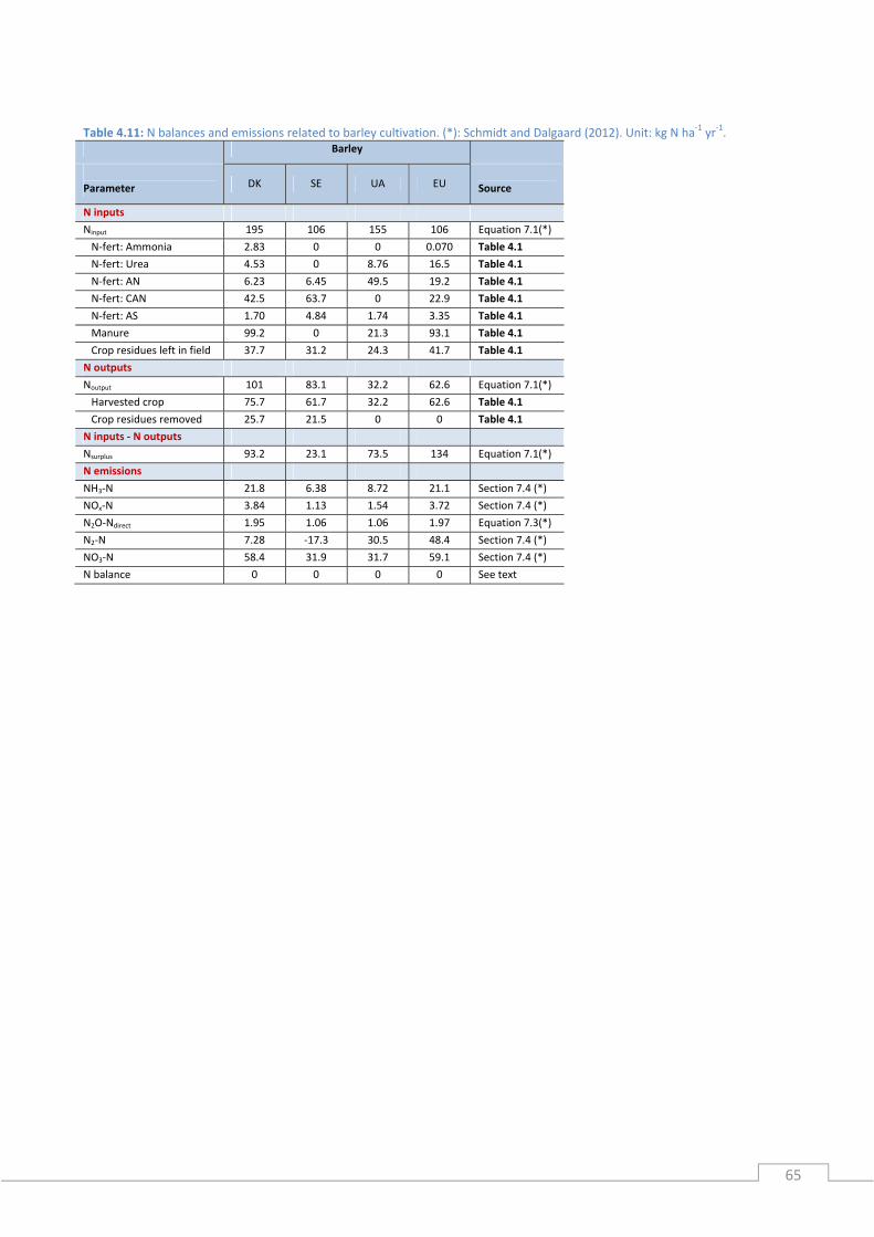
65

Table 4.11: N balances and emissions related to barley cultivation. (*): Schmidt and Dalgaard (2012). Unit: kg N ha‐1 yr‐1. Barley

Parameter DK SE UA EU

Source

N inputs

Ninput 195 106 155 106 Equation 7.1(*)

N‐fert: Ammonia 2.83 0 0 0.070 Table 4.1

N‐fert: Urea 4.53 0 8.76 16.5 Table 4.1

N‐fert: AN 6.23 6.45 49.5 19.2 Table 4.1

N‐fert: CAN 42.5 63.7 0 22.9 Table 4.1

N‐fert: AS 1.70 4.84 1.74 3.35 Table 4.1

Manure 99.2 0 21.3 93.1 Table 4.1

Crop residues left in field 37.7 31.2 24.3 41.7 Table 4.1

N outputs

Noutput 101 83.1 32.2 62.6 Equation 7.1(*)

Harvested crop 75.7 61.7 32.2 62.6 Table 4.1

Crop residues removed 25.7 21.5 0 0 Table 4.1

N inputs ‐ N outputs

Nsurplus 93.2 23.1 73.5 134 Equation 7.1(*)

N emissions

NH3‐N 21.8 6.38 8.72 21.1 Section 7.4 (*)

NOx‐N 3.84 1.13 1.54 3.72 Section 7.4 (*)

N2O‐Ndirect 1.95 1.06 1.06 1.97 Equation 7.3(*)

N2‐N 7.28 ‐17.3 30.5 48.4 Section 7.4 (*)

NO3‐N 58.4 31.9 31.7 59.1 Section 7.4 (*)

N balance 0 0 0 0 See text

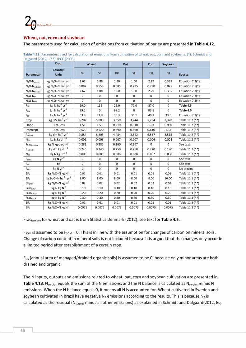
66

Wheat,oat,cornandsoybeanThe parameters used for calculation of emissions from cultivation of barley are presented in Table 4.12. Table 4.12: Parameters used for calculation of emissions from cultivation of wheat, oat, corn and soybeans. (*): Schmidt and Dalgaard (2012). (**): IPCC (2006).


Parameter

Country:

Unit: DK SE DK SE EU BR

Source


‐1 2.62 1.88 1.60 1.00 2.29 0.335 Equation 7.3(*)


‐1 0.887 0.558 0.585 0.295 0.790 0.075 Equation 7.5(*)


‐1 2.62 1.88 1.60 1.00 2.29 0.335 Equation 7.3(*)


‐1 0 0 0 0 0 0 Equation 7.3(*)


‐1 0 0 0 0 0 0 Equation 7.3(*)

FSN kg N ha‐1 yr

‐1 99.0 135 26.0 70.0 87.0 0 Table 4.5

FON kg N ha‐1 yr

‐1 99.2 0 99.2 0 93.1 0 Table 4.5

FCR kg N ha‐1 yr

‐1 63.9 52.9 35.3 30.1 49.3 33.5 Equation 7.3(*)


‐1 6,202 5,088 3,950 3,244 5,754 2,328 Table 11.2 (**)

Slope Dim. less 1.51 1.51 0.910 0.910 1.03 0.930 Table 11.2 (**) Intercept Dim. less 0.520 0.520 0.890 0.890 0.610 1.35 Table 11.2 (**) AGDM kg dm ha

‐1 yr

‐1 9,884 8,203 4,484 3,842 6,537 3,515 Table 11.2 (**)

NAG kg N kg dm‐1 0.006 0.006 0.007 0.007 0.006 0.008 Table 11.2 (**)

FracRemove kg N kg crop‐N‐1 0.283 0.286 0.160 0.167 0 0 See text

RBG‐BIO kg dm kg dm‐1 0.240 0.240 0.250 0.250 0.220 0.190 Table 11.2 (**)

NBG kg N kg dm‐1 0.009 0.009 0.008 0.008 0.007 0.008 Table 11.2 (**)

FSOM kg N yr‐1 0 0 0 0 0 0 See text

FOS ha 0 0 0 0 0 0 See text

FPRP kg N yr‐1 0 0 0 0 0 0 No grazing

EF1 kg N2O–N kg N‐1 0.01 0.01 0.01 0.01 0.01 0.01 Table 11.1 (**)


‐1 8.00 8.00 8.00 8.00 8.00 16.00 Table 11.1 (**)

EF3PRP kg N2O–N kg N‐1 0.02 0.02 0.02 0.02 0.02 0.02 Table 11.1 (**)

FracGASF kg N kg N‐1 0.10 0.10 0.10 0.10 0.10 0.10 Table 11.3 (**)

FracGASM kg N kg N‐1 0.20 0.20 0.20 0.20 0.20 0.20 Table 11.3 (**)

FracEACH kg N kg N‐1 0.30 0.30 0.30 0.30 0.30 0.30 Table 11.3 (**)



FracRemove for wheat and oat is from Statistics Denmark (2012), see text for Table 4.5.






The N inputs, outputs and emissions related to wheat, oat, corn and soybean cultivation are presented in

Table 4.13. Nsurplus equals the sum of the N emissions, and the N balance is calculated as Nsurplus minus N

emissions. When the N balance equals 0, it means all N is accounted for. Wheat cultivated in Sweden and

soybean cultivated in Brazil have negative N2 emissions according to the results. This is because N2 is

calculated as the residual (Nsurplus minus all other emissions) as explained in Schmidt and Dalgaard(2012, Eq.

67

7.2). Nevertheless, N2 cannot become negative, but the reasons for becoming negative in the Arla model

are presumable some of the following:

‐ FSOM is assumed to be 0, but might be higher, which will result in an increased Nsurplus. In particular soil

used for soybean cultivation is impoverished due to overuse.

‐ Atmospheric N deposition is not included in the Arla model, because it is not a consequence of crop

cultivation and would have been there, although the areas not were cultivated. If atmospheric N

deposition was part of the model, this would increase Nsurplus.

‐ IPCC (2006) does not consider N‐fixing crops, such as soybean.

‐ According to IPCC (2006) 10% and 30% of the N inputs to the fields is evaporated/leached as ammonia

and nitrate respectively. These values are high, and will in reality differ amongst cultivation systems. If

lower values are used, the N2 residual will be smaller.

‐ It is worthwhile to notice that the negative N2 emission not impacts the impact assessment.

Table 4.13: N balances and emissions related to wheat, oat, corn and soybean cultivation. (*): Schmidt and Dalgaard (2012). Unit: kg N ha‐1 yr‐1.

Wheat Oat Corn Soybean

Parameter DK SE DK SE EU BR

Source

N inputs

Ninput 262 188 160 100 229 33.5 Equation 7.1(*)

N‐fert: Ammonia 4.85 0 1.27 0 0.099 0 Table 4.5 N‐fert: Urea 7.76 0 2.04 0 23.2 0 Table 4.5 N‐fert: AN 10.7 11.6 2.80 6.02 26.9 0 Table 4.5 N‐fert: CAN 72.8 115 19.1 59.5 32.1 0 Table 4.5 N‐fert: AS 2.91 8.71 0.763 4.52 4.71 0 Table 4.5 Manure 99.2 0 99.2 0 93.1 0 Table 4.5 Crop residues left in field 63.9 52.9 35.3 30.1 49.3 33.5 Table 4.5 N outputs

Noutput 146 120 74.8 61.8 88.4 153 Equation 7.1(*) Harvested crop 114 93.6 64.5 52.9 88.4 153 Table 4.5 Crop residues removed 32.2 26.8 10.3 8.84 0 0 Table 4.5 N inputs ‐ N outputs

Nsurplus 116 67.5 85.7 38.3 141 ‐120 Equation 7.1(*) N emissions

NH3‐N 25.3 11.5 19.1 5.95 23.2 0 Section 7.4 (*)

NOx‐N 4.46 2.03 3.37 1.05 4.10 0 Section 7.4 (*)

N2O‐Ndirect 2.62 1.88 1.60 1.00 2.29 0.335 Equation 7.3(*)

N2‐N 4.74 ‐4.24 13.5 0.283 42.6 ‐130 Section 7.4 (*)

NO3‐N 78.6 56.4 48.1 30.0 68.8 10.0 Section 7.4 (*)

N balance 0 0 0 0 0 0 See text

Rapeseed,sunflower,sugarbeetandoilpalmThe parameters used for calculation of emissions from cultivation of rapeseed, sunflower, sugar beet and

oil palms are presented in Table 4.14.

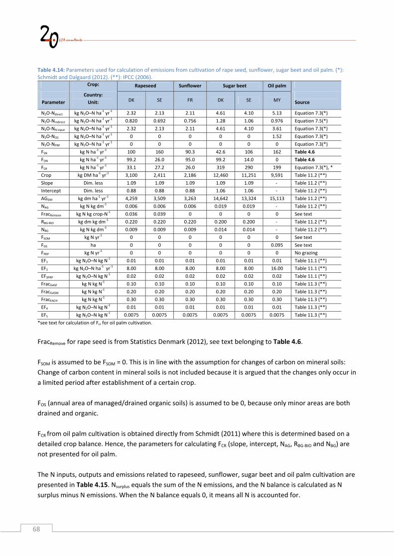
68

Table 4.14: Parameters used for calculation of emissions from cultivation of rape seed, sunflower, sugar beet and oil palm. (*): Schmidt and Dalgaard (2012). (**): IPCC (2006).

Crop: Rapeseed Sunflower Sugar beet Oil palm

Parameter

Country:

Unit: DK SE FR DK SE MY

Source


‐1 2.32 2.13 2.11 4.61 4.10 5.13 Equation 7.3(*)


‐1 0.820 0.692 0.756 1.28 1.06 0.976 Equation 7.5(*)


‐1 2.32 2.13 2.11 4.61 4.10 3.61 Equation 7.3(*)


‐1 0 0 0 0 0 1.52 Equation 7.3(*)


‐1 0 0 0 0 0 0 Equation 7.3(*)

FSN kg N ha‐1 yr

‐1 100 160 90.3 42.6 106 162 Table 4.6

FON kg N ha‐1 yr

‐1 99.2 26.0 95.0 99.2 14.0 0 Table 4.6

FCR kg N ha‐1 yr

‐1 33.1 27.2 26.0 319 290 199 Equation 7.3(*), *


‐1 3,100 2,411 2,186 12,460 11,251 9,591 Table 11.2 (**)

Slope Dim. less 1.09 1.09 1.09 1.09 1.09 ‐ Table 11.2 (**)

Intercept Dim. less 0.88 0.88 0.88 1.06 1.06 ‐ Table 11.2 (**)

AGDM kg dm ha‐1 yr

‐1 4,259 3,509 3,263 14,642 13,324 15,113 Table 11.2 (**)

NAG kg N kg dm‐1 0.006 0.006 0.006 0.019 0.019 ‐ Table 11.2 (**)

FracRemove kg N kg crop‐N‐1 0.036 0.039 0 0 0 0 See text

RBG‐BIO kg dm kg dm‐1 0.220 0.220 0.220 0.200 0.200 ‐ Table 11.2 (**)

NBG kg N kg dm‐1 0.009 0.009 0.009 0.014 0.014 ‐ Table 11.2 (**)

FSOM kg N yr‐1 0 0 0 0 0 0 See text

FOS ha 0 0 0 0 0 0.095 See text

FPRP kg N yr‐1 0 0 0 0 0 0 No grazing



‐1 8.00 8.00 8.00 8.00 8.00 16.00 Table 11.1 (**)

EF3PRP kg N2O–N kg N‐1 0.02 0.02 0.02 0.02 0.02 0.02 Table 11.1 (**)

FracGASF kg N kg N‐1 0.10 0.10 0.10 0.10 0.10 0.10 Table 11.3 (**)

FracGASM kg N kg N‐1 0.20 0.20 0.20 0.20 0.20 0.20 Table 11.3 (**)

FracEACH kg N kg N‐1 0.30 0.30 0.30 0.30 0.30 0.30 Table 11.3 (**)



*see text for calculation of Fcr for oil palm cultivation.

FracRemove for rape seed is from Statistics Denmark (2012), see text belonging to Table 4.6.






FCR from oil palm cultivation is obtained directly from Schmidt (2011) where this is determined based on a

detailed crop balance. Hence, the parameters for calculating FCR (slope, intercept, NAG, RBG‐BIO and NBG) are

not presented for oil palm.

The N inputs, outputs and emissions related to rapeseed, sunflower, sugar beet and oil palm cultivation are

presented in Table 4.15. Nsurplus equals the sum of the N emissions, and the N balance is calculated as N

surplus minus N emissions. When the N balance equals 0, it means all N is accounted for.

69

Table 4.15: N balances and emissions related to rapeseed, sunflower, sugar beet and oil palm cultivation. (*): Schmidt and Dalgaard (2012). Unit: kg N ha‐1 yr‐1.

Rapeseed

Sun‐

flower Sugar beet Oil palm

Parameter DK SE FR DK SE MY

Source

N inputs

Ninput 232 213 211 461 410 361 Equation 7.1(*)

N‐fert: Ammonia 4.89 0 0 2.09 0 0 Table 4.6 N‐fert: Urea 7.82 0 21.0 3.34 0 151 Table 4.6 N‐fert: AN 10.8 13.8 53.2 4.59 9.12 10.8 Table 4.6 N‐fert: CAN 73.3 136 14.7 31.3 90.0 0 Table 4.6 N‐fert: AS 2.93 10.3 1.47 1.25 6.84 0 Table 4.6 Manure 99.2 26.0 95.0 99.2 14.0 0.581 Table 4.6 Crop residues left in field 33.1 27.2 26.0 319 290 199 Table 4.6 N outputs

Noutput 99.7 77.7 64.4 118 106 52.8 Equation 7.1(*) Harvested crop 96.2 74.9 64.4 118 106 52.8 Table 4.6 Crop residues removed 3.50 2.89 0 0 0 0 Table 4.6 N inputs ‐ N outputs

Nsurplus 132 135 147 343 304 309 Equation 7.1(*) N emissions

NH3‐N 25.3 18.0 23.8 20.5 11.4 13.8 Section 7.4 (*)

NOx‐N 4.47 3.18 4.20 3.61 2.01 2.44 Section 7.4 (*)

N2O‐Ndirect 2.32 2.13 2.11 4.61 4.10 5.13 Equation 7.3(*)

N2‐N 30.6 48.2 53.4 176 164 179 Section 7.4 (*)

NO3‐N 69.6 64.0 63.4 138 123 108 Section 7.4 (*)

N balance 0 0 0 0 0 0 See text

70

Permanentgrassincl.grassensilageThe parameters used for calculation of emissions from cultivation of permanent grass incl. grass ensilage

are presented in Table 4.16.

Table 4.16: Parameters used for calculation of emissions from cultivation of permanent grass incl. grass ensilage. (*): Schmidt and Dalgaard (2012). (**): IPCC (2006).


Parameter

Country:

Unit: DK SE BR

Source


‐1 1.85 1.69 0.494 Equation 7.3(*)


‐1 0.686 0.591 0.191 Equation 7.5(*)


‐11.85 1.69 0.494 Equation 7.3(*)


‐10 0 0 Equation 7.3(*)


‐10 0 0 Equation 7.3(*)

FSN kg N ha‐1 yr

‐1 70.6 102 0 Table 4.7

FON kg N ha‐1 yr

‐1 0 0 0 Table 4.7

FCR kg N ha‐1 yr

‐1 15.4 12.4 9.6 Equation 7.3(*)


‐1 2,093 1,674 1,295 Table 11.2 (**)

Slope Dim. less 0.30 0.30 0.30 Table 11.2 (**) Intercept Dim. less 0 0 0 Table 11.2 (**) AGDM kg dm ha

‐1 yr

‐1 628 502 388 Table 11.2 (**)

NAG kg N kg dm‐1 0.015 0.015 0.015 Table 11.2 (**)

FracRemove kg N kg crop‐N‐1 0 0 0 See text

RBG‐BIO kg dm kg dm‐1 0.800 0.800 0.800 Table 11.2 (**)

NBG kg N kg dm‐1 0.012 0.012 0.012 Table 11.2 (**)

FSOM kg N yr‐1 0 0 0 See text

FOS ha 0 0 0 See text

FPRP kg N yr‐1 0 0 0 No grazing

EF1 kg N2O–N kg N‐1 0.01 0.01 0.01 Table 11.1 (**)


‐1 8.00 8.00 8.00 Table 11.1 (**)

EF3PRP kg N2O–N kg N‐1 0.02 0.02 0.02 Table 11.1 (**)

FracGASF kg N kg N‐1 0.10 0.10 0.10 Table 11.3 (**)

FracGASM kg N kg N‐1 0.20 0.20 0.20 Table 11.3 (**)

FracEACH kg N kg N‐1 0.30 0.30 0.30 Table 11.3 (**)








The N inputs, outputs and emissions related to cultivation of permanent grass incl. grass ensilage are

presented in Table 4.17. Nsurplus equals the sum of the N emissions, and the N balance is calculated as N

surplus minus N emissions. When the N balance equals 0, it means all N is accounted for. The N2 emission

from Permanent grass in Brazil is negative. The most likely reason for this is that the non‐fertilised

rangeland is impoverished due to overuse.

71

Table 4.17: N balances and emissions related to cultivation of permanent grass incl. grass ensilage. (*): Schmidt and Dalgaard (2012). Unit: kg N ha‐1 yr‐1.

Permanent grass incl. grass ensilage

Parameter DK SE BR

Source

N inputs

Ninput 185 169 49.4 Equation 7.1(*)

N‐fert: Ammonia 3.46 0 0 Table 4.7 N‐fert: Urea 5.53 0 0 Table 4.7 N‐fert: AN 7.61 8.74 0 Table 4.7 N‐fert: CAN 51.9 86.3 0 Table 4.7 N‐fert: AS 2.08 6.56 0 Table 4.7 Manure 99.2 54.8 39.8 Table 4.7 Crop residues left in field 15.4 12.4 9.56 Table 4.7 N outputs

Noutput 67.0 53.6 41.4 Equation 7.1(*) Harvested crop 67.0 53.6 41.4 Table 4.7 Crop residues removed 0 0 0 Table 4.7 N inputs ‐ N outputs

Nsurplus 118 115 7.9 Equation 7.1(*) N emissions

NH3‐N 22.9 18.0 6.77 Section 7.4 (*)

NOx‐N 4.03 3.17 1.19 Section 7.4 (*)

N2O‐Ndirect 2.84 2.24 0.892 Equation 7.3(*)

N2‐N 32.9 41.2 ‐15.7 Section 7.4 (*)

NO3‐N 55.6 50.6 14.8 Section 7.4 (*)

N balance 0 0 0 See text

72

Rotationgrassincl.grassensilageandroughage,maizeensilageThe parameters used for calculation of emissions from cultivation of rotation grass incl. grass ensilage and

roughage, maize ensilage are presented in Table 4.18.

Table 4.18: Parameters used for calculation of emissions from cultivation of rotation grass incl. grass ensilage and roughage, maize ensilage. (*): Schmidt and Dalgaard (2012). (**): IPCC (2006).

Crop: Rotation grass incl. grass ensilage Roughage, maize ensilage

Parameter

Country:

Unit: DK SE DK SE

Source


‐1 3.89 2.32 2.13 1.83 Equation 7.3(*)


‐1 1.26 0.762 0.710 0.584 Equation 7.5(*)


‐1 3.89 2.32 2.13 1.83 Equation 7.3(*)


‐1 0 0 0 0 Equation 7.3(*)


‐1 0 0 0 0 Equation 7.3(*)

FSN kg N ha‐1 yr

‐1 185 55.0 31.0 62.1 Table 4.8

FON kg N ha‐1 yr

‐1 0 0 99.2 54.8 Table 4.8

FCR kg N ha‐1 yr

‐1 105 83.6 83.1 66.5 Equation 7.3(*)


‐1 7,813 6,250 12,902 10,322 Table 11.2 (**)

Slope Dim. less 0.30 0.30 0.30 0.30 Table 11.2 (**) Intercept Dim. less 0 0 0 0 Table 11.2 (**) AGDM kg dm ha

‐1 yr

‐1 2,344 1,875 3,871 3,097 Table 11.2 (**)

NAG kg N kg dm‐1 0.027 0.027 0.015 0.015 Table 11.2 (**)

FracRemove kg N kg crop‐N‐1 0 0 0 0 See text

RBG‐BIO kg dm kg dm‐1 0.800 0.800 0.540 0.540 Table 11.2 (**)

NBG kg N kg dm‐1 0.022 0.022 0.012 0.012 Table 11.2 (**)

FSOM kg N yr‐1 0 0 0 0 See text

FOS ha 0 0 0 0 See text

FPRP kg N yr‐1 0 0 0 0 No grazing



‐1 8.00 8.00 8.00 8.00 Table 11.1 (**)

EF3PRP kg N2O–N kg N‐1 0.02 0.02 0.02 0.02 Table 11.1 (**)

FracGASF kg N kg N‐1 0.10 0.10 0.10 0.10 Table 11.3 (**)

FracGASM kg N kg N‐1 0.20 0.20 0.20 0.20 Table 11.3 (**)

FracEACH kg N kg N‐1 0.30 0.30 0.30 0.30 Table 11.3 (**)








The N inputs, outputs and emissions related to barley cultivation are presented in Table 4.19. Nsurplus equals

the sum of the N emissions, and the N balance is calculated as Nsurplus minus N emissions. When the N

balance equals 0, it means all N is accounted for. The N2 emissions are negative, se text belonging to Table

4.13 for further details.

73

Table 4.19: N balances and emissions related cultivation of rotation grass incl. grass ensilage and roughage, maize ensilage. (*): Schmidt and Dalgaard (2012). Unit: kg N ha‐1 yr‐1.

Rotation grass incl. grass ensilage Roughage, maize ensilage

Parameter DK SE DK SE

Source

N inputs

Ninput 389 232 213 183 Equation 7.1(*)

N‐fert: Ammonia 9.07 0 1.52 0 Table 4.8 N‐fert: Urea 14.5 0 2.43 0 Table 4.8 N‐fert: AN 19.9 4.73 3.35 5.35 Table 4.8 N‐fert: CAN 136 46.7 22.8 52.8 Table 4.8 N‐fert: AS 5.44 3.55 0.91 4.01 Table 4.8 Manure 99.2 93.0 99.2 54.8 Table 4.8 Crop residues left in field 105 83.6 83.1 66.5 Table 4.8 N outputs

Noutput 288 230 163 130 Equation 7.1(*) Harvested crop 288 230 163 130 Table 4.8 Crop residues removed 0 0 0 0 Table 4.8 N inputs ‐ N outputs

Nsurplus 101 2 50.3 53 Equation 7.1(*) N emissions

NH3‐N 32.6 20.5 19.5 14.6 Section 7.4 (*)

NOx‐N 5.75 3.62 3.44 2.58 Section 7.4 (*)

N2O‐Ndirect 4.88 3.25 2.13 1.83 Equation 7.3(*)

N2‐N ‐58.6 ‐95.2 ‐38.8 ‐21.1 Section 7.4 (*)

NO3‐N 117 69.5 64.0 55.0 Section 7.4 (*)

N balance 0 0 0 0 See text

4.4 SummaryoftheLCIofplantcultivationLCIs of for the different crops in the plant cultivation system are presented in Table 4.20 to Table 4.24. All

data sources and calculations are documented in the previous sections.

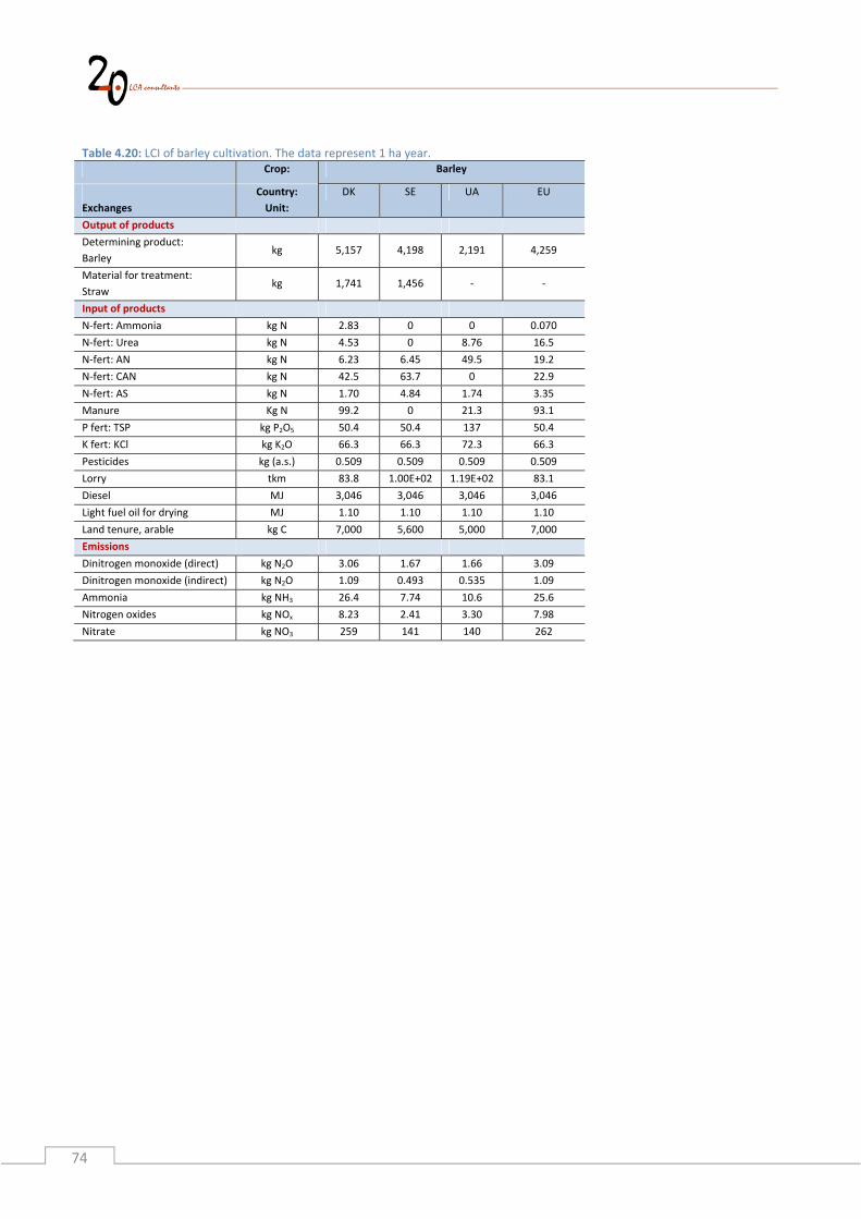
74

Table 4.20: LCI of barley cultivation. The data represent 1 ha year.

Crop: Barley

Exchanges

Country:

Unit:

DK SE UA EU

Output of products


Barley kg 5,157 4,198 2,191 4,259


Straw kg 1,741 1,456 ‐ ‐

Input of products

N‐fert: Ammonia kg N 2.83 0 0 0.070

N‐fert: Urea kg N 4.53 0 8.76 16.5

N‐fert: AN kg N 6.23 6.45 49.5 19.2

N‐fert: CAN kg N 42.5 63.7 0 22.9

N‐fert: AS kg N 1.70 4.84 1.74 3.35

Manure Kg N 99.2 0 21.3 93.1

P fert: TSP kg P2O5 50.4 50.4 137 50.4

K fert: KCl kg K2O 66.3 66.3 72.3 66.3

Pesticides kg (a.s.) 0.509 0.509 0.509 0.509

Lorry tkm 83.8 1.00E+02 1.19E+02 83.1

Diesel MJ 3,046 3,046 3,046 3,046

Light fuel oil for drying MJ 1.10 1.10 1.10 1.10


Emissions

Dinitrogen monoxide (direct) kg N2O 3.06 1.67 1.66 3.09

Dinitrogen monoxide (indirect) kg N2O 1.09 0.493 0.535 1.09

Ammonia kg NH3 26.4 7.74 10.6 25.6

Nitrogen oxides kg NOx 8.23 2.41 3.30 7.98

Nitrate kg NO3 259 141 140 262

75

Table 4.21: LCI of wheat, oat corn and soybean cultivation. The data represent 1 ha year.


Exchanges

Country:

Unit:

DK SE DK SE EU BR

Output of products


Wheat/oat/corn/soybean kg 7,296 5,986 4,646 3,817 6,577 2,575


Straw kg 2,552 2,118 700 600 ‐ ‐

Input of products

N‐fert: Ammonia kg N 4.85 0 1.27 0 0.10 0

N‐fert: Urea kg N 7.76 0 2.04 0 23.2 0

N‐fert: AN kg N 10.7 11.6 2.80 6.02 26.9 0

N‐fert: CAN kg N 72.8 115 19.1 59.5 32.1 0

N‐fert: AS kg N 2.91 8.71 0.763 4.52 4.71 0

Manure Kg N 99.2 0 99.2 0 93.1 0

P fert: TSP kg P2O5 45.8 45.8 57.3 57.3 80.2 36.6

K fert: KCl kg K2O 84.4 84.4 78.3 78.3 78.3 0

Pesticides kg (a.s.) 0.603 0.603 0.355 0.355 3.53 2.50

Lorry tkm 116 149 68.9 103 118 17.4

Diesel MJ 3,306 3,306 3,046 3,046 3,306 1,709

Light fuel oil for drying MJ 1.10 1.10 1.10 1.10 1.10 1.10


Emissions

Dinitrogen monoxide (direct) kg N2O 4.12 2.95 2.52 1.57 3.61 0.526


Ammonia kg NH3 30.7 13.9 23.2 7.23 28.2 0

Nitrogen oxides kg NOx 9.56 4.34 7.21 2.25 8.78 0

Nitrate kg NO3 348 250 213 133 305 44.5

76

Table 4.22: LCI of rapeseed, sunflower, sugar beet and oil palm cultivation. The data represent 1 ha year. Crop: Rapeseed Sunflower Sugar beet Oil palm

Exchanges

Country:

Unit:

DK SE FR DK SE MY

Output of products


Rapeseed/sunflower/sugar

beet/fresh fruit bunches

kg 3,351 2,607 2,376 56,638 51,141 20,407


Straw kg 277 228 ‐ ‐ ‐ ‐

Input of products

N‐fert: Ammonia kg N 4.89 0 0 2.09 0 0

N‐fert: Urea kg N 7.82 0 21.0 3.34 0 151

N‐fert: AN kg N 10.8 13.8 53.2 4.59 9.12 10.8

N‐fert: CAN kg N 73.3 136 14.7 31.3 90.0 0

N‐fert: AS kg N 2.93 10.3 1.47 1.25 6.84 0

Manure Kg N 99.2 26.0 95.0 99.2 14.0 0

P fert: TSP kg P2O5 55.0 22.9 52.7 87.0 36.6 0

P fert: Rock phosphate kg P2O5 0 0 0 0 0 81.3

K fert: KCl kg K2O 96.4 20.5 72.3 181 53.0 268

Pesticides kg (a.s.) 0.270 0.802 0.270 2.74 2.74 2.60

Lorry tkm 124 136 100 129 114 198

Diesel MJ 3,195 3,195 3,306 8,581 8,581 1,710

Light fuel oil for drying MJ 1.10 1.10 1.10 0 0 0


Emissions

Dinitrogen monoxide (direct) kg N2O 3.65 3.35 3.32 7.24 6.45 8.07


Ammonia kg NH3 30.8 21.9 28.9 24.9 13.8 16.8

Nitrogen oxides kg NOx 9.58 6.81 9.01 7.75 4.31 5.23

Nitrate kg NO3 308 283 281 612 545 480

77

Table 4.23: LCI of permanent grass incl. grass ensilage cultivation. The data represent 1 ha year.


Exchanges

Country:

Unit:

DK SE BR

Output of products

Determining product: Perman‐

ent grass incl. grass ensilage kg 11,628 9,302 7,193

Input of products

N‐fert: Ammonia kg N 3.46 0 0

N‐fert: Urea kg N 5.53 0 0

N‐fert: AN kg N 7.61 8.74 0

N‐fert: CAN kg N 51.9 86.3 0

N‐fert: AS kg N 2.08 6.56 0

Manure Kg N 99.2 54.8 39.8

P fert: TSP kg P2O5 32.1 32.1 0

K fert: KCl kg K2O 121 121 0

Lorry tkm 102 130 ‐

Diesel MJ 557.2 557.2 31.4

Light fuel oil for drying MJ 0 0 0

Land tenure, arable kg C 7,000 2,800 ‐

Land tenure, int. forest land kg C 0 2,800 0

Land tenure, rangeland kg C 0 0 9,000

Emissions

Dinitrogen monoxide (direct) kg N2O 4.47 3.51 1.402

Dinitrogen monoxide (indirect) kg N2O 1.08 0.929 0.300

Ammonia kg NH3 27.8 21.8 8.22

Nitrogen oxides kg NOx 8.65 6.79 2.56

Nitrate kg NO3 246 224 65.6

78

Table 4.24: LCI of rotation grass incl. grass ensilage and roughage, maize ensilage cultivation. The data represent 1 ha year.

Crop: Rotation grass incl. grass

ensilage Roughage, maize ensilage

Exchanges

Country:

Unit:

DK SE DK SE

Output of products


Rotation grass/roughage kg 44,643 35,714 39,097 31,278

Input of products

N‐fert: Ammonia kg N 9.07 0 1.52 0

N‐fert: Urea kg N 14.5 0 2.43 0

N‐fert: AN kg N 19.9 4.73 3.35 5.35

N‐fert: CAN kg N 136 46.7 22.8 52.8

N‐fert: AS kg N 5.44 3.55 0.913 4.01

Manure Kg N 99.2 93.0 99.2 54.8

P fert: TSP kg P2O5 73.3 0 64.9 64.9

K fert: KCl kg K2O 217 0 200 200

Pesticides kg (a.s.) 0.095 0.095 0.095 0.095

Lorry tkm 231 41 116 141

Diesel MJ 2,415 2,415 3,715 3,715

Light fuel oil for drying MJ 0 0 0 0


Emissions

Dinitrogen monoxide (direct) kg N2O 7.67 5.10 3.35 2.88

Dinitrogen monoxide (indirect) kg N2O 1.98 1.20 1.12 0.918

Ammonia kg NH3 39.6 24.9 23.7 17.7

Nitrogen oxides kg NOx 12.3 7.75 7.38 5.52

Nitrate kg NO3 516 308 284 244


4.25 and Table 4.26. Allocation factors are only relevant, when more than one product is produced.

Therefore, data are only presented for crops, where the straw is removed. Point of displacement is more

detailed explained in Schmidt and Dalgaard (2012, Figure 3.2).

Switch 1: Allocation is avoided by substitution. Consequently, production of 1 kg crop displaces electricity

and heat due to utilisation of straw in CHP.


obtained by combining straw/crop ratio (e.g. barley: Table 4.1), energy/straw ratio (Table 4.9) with the

relevant prices from Appendix C: Prices.


defined in PAS2050 and IDF. The allocation factors are obtained by combining the straw/crop ratio (e.g.

barley: Table 4.1) with the relevant prices from Appendix C: Prices.

79

Table 4.25: Allocation factors used for allocation of products from barley and wheat cultivation. Unit: Fraction

Barley Wheat

Allocation factors DK SE DK SE


Determining product: Barley/wheat 1 1 1 1

Switch 2: Average/allocation

Determining product: Barley/wheat 0.602 0.564 0.584 0.573

By‐product at point of subst.: Elec DK/SE 0.170 0.186 0.177 0.182

By‐product at point of subst.: Distr. heat 0.229 0.250 0.239 0.245

Switch 3: PAS2050


Material for treatment: Straw 0.174 0.197 0.185 0.192

Switch 4: IDF



Table 4.26: Allocation factors used for allocation of products from oat and rapeseed cultivation. Unit: Fraction

Oat Rapeseed

Allocation factors DK SE DK SE


Determining product: Oat/rapeseed 1 1 1 1


Determining product: Oat/rapeseed 0.763 0.733 0.923 0.923

By‐product at point of subst.: Elec DK/SE 0.101 0.114 0.033 0.033

By‐product at point of subst.: Distr. heat 0.136 0.153 0.044 0.044

Switch 3: PAS2050

Determining product: Oat/rapeseed 0.910 0.896 0.974 0.974


Switch 4: IDF

Determining product Oat/rapeseed 0.910 0.896 0.974 0.974


81

5 ThefoodindustrysystemThe activities in the food industry system supplies several concentrate feed input to the cattle system. All

activities in the food industry are characterised by being multiple product output activities.

Opposed to the milk and beef systems and the plant cultivation system, the inventories of the food industry

system are based on other life cycle assessments. Therefore, compared to chapter 0 and 4, this chapter

contains less parameters and calculations and more literature references.

5.1 Inventoryofsoybeanmealsystem(soybeanmeal)The inventories for activities in the soybean meal system are presented in Table 5.1. An overview of

transactions within the production system is presented in Schmidt and Dalgaard (2012, section 8.3). The

inventory is based on Dalgaard et al. (2008) and Schmidt (2010c). The utilisation of FFA activity is

established based on data in Appendix B: Feed and crop properties.

Table 5.1: LCI of soybean meal activities. FFA: Free fatty acids. NBD oil: neutralized, bleached and deodorized oil.

Activity: Soybean oil mill Soybean oil

refinery

Utilisation of

FFA as feed

Exchanges

Country:

Unit:

BR BR GLO

Output of products


Soybean meal kg 0.773

Crude soybean oil for treatment kg 1

FFA for treatment kg 1

By‐product:

Crude soybean oil for treatment kg 0.192

FFA for treatment kg 1.18E‐02

NBD oil kg 0.983

Feed energy MJ net energy 18.0

Input of products/material for treatment

Soybeans kg 1

Lorry tkm 6.96E‐04 6.10E‐03

Other chemicals kg 4.02E‐4 1.36E‐2

Electricity kWh 1.22E‐02 2.87E‐02

Natural gas, burned MJ 0.282

Fuel oil, burned MJ 0.145 0.247

Oil mill, capital goods kg 0.192

Oil mill, services kg 0.192

Oil refinery, capital goods kg 0.983

Oil refinery, services kg 0.983

5.2 Inventoryofrapeseedoilsystem(rapeseedmeal)The inventories for activities in the rapeseed oil system are presented in Table 5.2. An overview of

transactions within the production system is presented in Schmidt and Dalgaard (2012, section 8.4). The

inventory is based on Schmidt (2010c). The utilisation of rapeseed meal activity is established based on

data in Appendix B: Feed and crop properties.

82

Table 5.2: LCI of rapeseed oil activities. FFA: Free fatty acids. NBD oil: Neutralized, bleached and deodorized oil.

Activity: Rapeseed oil

mill

Utilisation of rapeseed

meal as feed

Exchanges

Country:

Unit:

DK/SE GLO

Output of products


Crude rapeseed oil kg 0.419

Rapeseed meal for treatment kg 1

By‐product:

Rapeseed meal for treatment kg 0.564


Feed protein kg 0.311


Rapeseed kg 1

Lorry tkm 0.00599

Other chemicals kg 0.000498

Electricity kWh 0.0387

Fuel oil, burned MJ 0.761



5.3 Inventoryofsunfloweroilsystem(sunflowermeal)The inventories for activities in the sunflower oil system are presented in Table 5.3. An overview of

transactions within the production system is presented in Schmidt and Dalgaard (2012, section 8.5). The oil

extraction rate is estimated by comparing the total use of sunflower seed and the total production of

sunflower oil in France in FAOSTAT (2012). The loss is estimated as being the same as for rapeseed oil mills

(Schmidt 2010c) and the meal is calculated as the remaining output. Inputs of energy etc. to the sunflower

oil mill are assumed to be the same per kg oil as of rapeseed mills (see section 5.2). The utilisation of

sunflower meal activity is established based on data in Appendix B: Feed and crop properties.

83

Table 5.3: LCI of sunflower oil activities.

Activity: Sunflower oil mill Utilisation of

sunflower meal as feed

Exchanges

Country:

Unit:

FR GLO

Output of products


Crude sunflower oil kg 0.314

Sunflower meal for treatment kg 1

By‐product:

Sunflower meal for treatment kg 0.669




Sunflower kg 1

Lorry tkm 0.00599

Other chemicals kg 4.98E‐4

Electricity kWh 0.0387

Fuel oil, burned MJ 0.761



5.4 Inventoryofpalmoilsystem(palmoilandpalmkernelmeal)The inventories for activities in the palm oil system are presented in Table 5.4 and Table 5.5. An overview

of transactions within the production system is presented in Schmidt and Dalgaard (2012, section 8.6). The

inventory for ‘Utilisation of FFA as feed’ is presented in Table 5.1, because it also is part of the soybean

meal system. The inventory of the activities in the palm oil system is based on Schmidt (2010c). The

utilisation of palm kernel meal (PKM) activity is established based on data in Appendix B: Feed and crop

properties.

84

Table 5.4: LCI of palm oil activities. Part 1. POME: Palm oil mill effluent. EFB: empty fruit bunches.

Activity: Palm oil mill Palm kernel

oil mill

Palm oil

refinery

Palm kernel

oil refinery

Exchanges

Country:

Unit:

MY MY MY MY

Output of products


Crude palm oil kg 0.203

Kernel for treatment kg 1

NBD oil kg 0.953

Crude palm kernel oil for treatment kg 1

By‐product:

Kernel for treatment kg 5.23E‐02

POME for treatment kg 0.700

EFB for treatment kg 0.220

Electricity kWh 4.36E‐03

Crude palm kernel oil kg 0.449

Palm kernel meal kg 0.529

Free fatty acids kg 4.59E‐02 4.59E‐02

NBD oil kg 0.953

Input of products

Fresh fruit bunches kg 1

Crude palm oil kg 1

Crude palm kernel oil kg 1

Lorry tkm 0.0174 0.0996 0.0517 0.0517

Other chemicals kg 0.0216 0.0216

Electricity kWh 0.0941 0.0262 0.0262

Diesel, burned MJ 1.46 0.331 0.331


Oil mill, capital goods kg 0.203 0.449 0.953 1

Oil mill, services kg 0.203 0.449 0.953 1

Oil refinery, capital goods kg 0.203 0.449 0.953 1

Oil refinery, services kg 0.203 0.449 0.953 1

Emissions

Dinitrogen monoxide kg 8.73E‐06

Methane kg 8.68E‐03

85

Table 5.5: LCI of palm oil activities. Part 2. EFB: Empty fruit bunches. POME: Palm oil mill effluent. PKM: Palm Kernel meal.

Activity: Utilisation

of EFB as

fertiliser

Utilisation

of POME as

fertiliser

Utilisation

of PKM as

feed

Exchanges

Country:

Unit:

MY MY GLO

Output of products


EFB for treatment kg 1

POME for treatment kg 1

Palm kernel meal for treatment kg 1

By‐product:

N‐fert: Urea kg N 1.32E‐03 9.50E‐04

P‐fert: Rock phosphate kg P2O5 3.63E‐04 3.44E‐04

K‐fert kg K2O 5.77E‐03 2.05E‐03



5.5 Inventoryofsugarsystem(molassesandbeetpulp)The inventories for activities in the sugar system are presented in Table 5.6. An overview of transactions

within the production system is presented in Schmidt and Dalgaard (2012, section 8.7). The inventory is

based on Nielsen et al. (2005). The utilisation of rapeseed meal activity is established based on data in

Appendix B: Feed and crop properties.

Table 5.6: LCI of sugar system activities.

Activity: Sugar mill Sugar mill Utilisation of

molasses (74.0

% DM) as feed

Utilisation of beet

pulp, dried (89.4%

DM) as feed

Exchanges

Country:

Unit:

DK SE GLO GLO

Output of products


Sugar kg 0.137 0.137

Molasses (74% DM) for treatment kg 1

Beet pulp (89.4% DM) for treatment kg 1

By‐product:

Molasses (74% DM) for treatment kg 3.29E‐02 3.29E‐02

Beet pulp, dried (89.4% DM) for treatment kg 4.52E‐02 4.52E‐02

Feed energy MJ net energy 5.67 6.99

Feed protein kg 9.62E‐02 8.58E‐02

Input of products

Sugar beet kg 1 1

Lorry tkm 0.0700 0.0700

Electricity kWh 0.00315 0.00315

Natural gas, burned MJ 0.928 0.928

Coal, burned MJ 0.503 0.503


Sugar mill, capital goods kg 0.137 0.137

Sugar mill, services kg 0.137 0.137

86

5.6 Inventoryofwheatfloursystem(wheatbran)The inventories for activities in the sugar system are presented in Table 5.7. An overview of transactions

within the production system is presented in Schmidt and Dalgaard (2012, section 8.8). The inventory is

based on Nielsen et al. (2005). The utilisation of wheat bran activity is established based on data in

Appendix B: Feed and crop properties. Table 5.7: LCI of wheat flour activities.

Activity: Flour mill Utilisation of wheat bran

(87.1% DM) as feed

Exchanges

Country:

Unit:

DK/SE GLO

Output of products


Wheat flour kg 0.800

Wheat bran for treatment kg 1

By‐product:

Wheat bran for treatment kg 0.200



Input of products

Wheat Kg 1

Lorry tkm 7.00E‐02

Electricity kWh 8.00E‐02

Natural gas, burned kg 0.400

Water kg 1.00E‐02

Flour mill, capital goods kg 0.800

Flour mill, services kg 0.800


5.8 to Table 5.13. The point where allocation is done is described for all activities in Schmidt and Dalgaard

(2012, section 8).

Switch 1: Allocation is avoided by substitution.


obtained by combining the product flows in Table 5.1 to Table 5.7 with the relevant prices from Appendix

C: Prices.


defined in PAS2050 and IDF. The allocation factors are obtained by combining the product flows in Table

5.1 to Table 5.7 with the relevant prices from Appendix C: Prices.

87

Table 5.8: Allocation factors related to products from the soybean meal system. Unit: Fraction.

Soybean oil mill Soybean oil refinery

Products BR BR



Soybean meal 1

Crude soybean oil for treatment 1



Soybean meal 0.679

Crude soybean oil for treatment 1


NBD oil 0.319

Feed energy 2.01E‐03

Switch 3: PAS2050


Soybean meal 0.758

By‐products:

Crude soybean oil for treatment 0.242

NBD oil 0.990

FFA 9.69E‐03

Switch 4: IDF


Soybean meal 0.758

By‐products:

Crude soybean oil for treatment 0.242

NBD oil 0.990

FFA 9.69E‐03

Table 5.9: Allocation factors related to products from the rapeseed oil system. Unit: Fraction.

Rapeseed oil mill Rapeseed oil mill

Products DK SE



Crude rapeseed oil 1 1



Crude rapeseed oil 0.761 0.752


Feed protein 9.56E‐02 9.89E‐02

Feed energy 0.144 0.149

Switch 3: PAS2050



By‐products

Rapeseed meal 0.232 0.293

Switch 4: IDF



By‐products:

Rapeseed meal 0.232 0.293

88

Table 5.10: Allocation factors related to products from the sunflower oil system Sunflower oil mill

Products FR



Crude sunflower oil 1



Crude sunflower oil 0.706


Feed protein 0.137

Feed energy 0.156

Switch 3: PAS2050



By‐products:

Utilisation of sunflower meal as feed 0.264

Switch 4: IDF



By‐products:

Utilisation of sunflower meal as feed 0.264

89

Table 5.11: Allocation factors related to products from the palm oil system. Unit: Fraction.

Palm oil mill Palm kernel oil mill Palm oil refinery Palm kernel oil refinery

Products MY MY MY MY



Crude palm oil 1

Kernel for treatment 1

NBD oil 1

Crude palm kernel oil for treatment 1



Crude palm oil 0.806

Kernel for treatment 1

NBD oil 0.975

Crude palm kernel oil for treatment 1


NBD oil 0.143

Feed energy 2.17E‐02 2.47E‐02

Feed protein 8.94E‐03

N‐fert: Urea 5.26E‐03

P fert 7.42E‐04

K fert 1.13E‐02

Elec MY 3.31E‐03

Switch 3: PAS2050



Crude palm kernel oil for treatment 0.917

NBD oil 0.962

By‐products:

Kernel for treatment 0.155

EFB for land application 7.25E‐03

POME for land application 1.05E‐02

Free fatty acids (FFA) for treatment 3.78E‐02 2.48E‐02

NBD oil 0.975

Elec MY 3.38E‐03

Palm kernel meal for treatment 8.33E‐02

Switch 4: IDF



Crude palm kernel oil 0.917

NBD oil 0.962

By‐products:

Kernel for treatment 0.155

EFB for land application 7.25E‐03

POME for land application 1.05E‐02

Free fatty acids (FFA) for treatment 3.78E‐02 2.48E‐02

NBD oil 0.975

Elec MY 3.38E‐03

Palm kernel meal for treatment 8.33E‐02

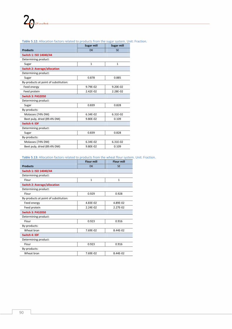
90

Table 5.12: Allocation factors related to products from the sugar system. Unit: Fraction.

Sugar mill Sugar mill

Products DK SE



Sugar 1 1



Sugar 0.878 0.885




Switch 3: PAS2050


Sugar 0.839 0.828

By‐products:

Molasses (74% DM) 6.34E‐02 6.31E‐02

Beet pulp, dried (89.4% DM) 9.80E‐02 0.109

Switch 4: IDF


Sugar 0.839 0.828

By‐products:

Molasses (74% DM) 6.34E‐02 6.31E‐02

Beet pulp, dried (89.4% DM) 9.80E‐02 0.109

Table 5.13: Allocation factors related to products from the wheat flour system. Unit: Fraction.

Flour mill Flour mill

Products DK SE



Flour 1 1



Flour 0.929 0.928




Switch 3: PAS2050


Flour 0.923 0.916

By‐products:

Wheat bran 7.69E‐02 8.44E‐02

Switch 4: IDF


Flour 0.923 0.916

By‐products:

Wheat bran 7.69E‐02 8.44E‐02

91

6 ReferencesCederberg C, Sonesson U, Henriksson M, Sund V, Davis J (2009a), Greenhouse gas emissions from Swedish

production of meat, milk and eggs 1990 and 2005. SIK Report No 793. ISBN 978‐91‐7290‐284‐8.

Cederberg C, Sonesson U, Henriksson M, Sund V, Davis J (2009b), Life cycle inventory of greenhouse gas

emissions and use of land and energy in Brazilian beef production. SIK Report No 792. ISBN 978‐91‐7290‐

283‐1.

DAKA (2006), Grønt regnskab 2005‐2006 (English: Green account 2005‐2006). DAKA.

http://www.daka.dk/lib/files.asp?ID=468 (Accessed January 2012)

Dalgaard R, Schmidt J, Halberg N, Christensen P, Thrane M, Pengue W A (2008), LCA of soybean meal. Int J

LCA (3) 240‐254.

Ecoinvent (2007), ecoinvent data v2.2. ecoinvent reports No. 1‐25. Swiss Centre for Life Cycle Inventories,

Dübendorf

European Commission (2010), The Swedish National Action Plan for the promotion of the use of renewable

energy in accordance with Directive 2009/28/EC and the Commission Decision of 30.06.2009.

http://ec.europa.eu/energy/renewables/transparency_platform/action_plan_en.htm (accessed: February

2012)

Eurostat (2009), Panorama of transport. 2009 edition. Eurostat, European Commission.

http://epp.eurostat.ec.europa.eu/cache/ITY_OFFPUB/KS‐DA‐09‐001/EN/KS‐DA‐09‐001‐EN.PDF (accessed

February 2012)

FAO (2005), Fertilizer use by crop in Ukraine. Food and Agriculture Organization of United Nations, Rome.

ftp://ftp.fao.org/agl/agll/docs/fertuseukraine.pdf (Accessed March 2012)

FAOSTAT (2012), FAOSTAT, Food and agriculture organization of the United Nations. http://faostat.fao.org/

(Accessed January 2012)

Flysjö A, Cederberg C, Henriksson M, Ledgard S (2011) How does co‐product handling affect the carbon

footprint of milk? Case study of milk production in New Zealand and Sweden. Int J LCA (16) 420‐430.

Flysjö A, Cederberg C, Strid, I (2008), LCA‐databas för konventionella fodermedel –miljöpåverkan i

samband med produktion. SIK Report No 772. ISBN 978‐91‐7290‐265‐7. In Swedish.

Haberl H, Heinz Erb K, Krausmann F, Gaube V, Bondeau A, Plutzar C, Gingrich S, Lucht W and Fischer‐

Kowalski M (2007), Quantifying and mapping the human appropriation of net primary production in earths

terrestrial ecosystems. PNAS, vol. 104, no. 31, pp 12942–12947

92

Hansen M N, Sommer S G, Hutchings N J, Sørensen P (2008), Emission factors for calculation of ammonia

volatization by storage and application of animal manure. Det jordbrugsvidenskabelige Fakultet. Aarhus

Universitet. DJF Husdyrbrug nr. 84. In Danish.

IEA (2012), Sweden: Statistics, Electricity/Heat. International Energy Agency. http://iea.org (Accessed

February 2012)

IFA (2012a), Conversion factors – Nutrients as % of product. International Fertilizer Association.

http://www.fertilizer.org/ifa/HomePage/STATISTICS/Conversions‐factors (Accessed February 2012)

IFA (2012b), Statistics. International Fertilizer Association.

http://www.fertilizer.org/ifa/HomePage/STATISTICS (Accessed February 2012)

Illerup J B, Lyck E, Nielsen M, Winther M, Mikkelsen M H, Hoffmann L, Gyldenkærne S, Sørensen P B, Fauser P, Thomsen M, and Vesterdal L (2005), Denmark’s National Inventory Report 2005 – Submitted under the United Nations Framework Convention on Climate Change. 1990‐2003. Emission Inventories. National Environmental Research Institute, Denmark. 416 p. – Research Notes from NERI no. 211. Accessed September 2011: http://www2.dmu.dk/1_viden/2_Publikationer/3_arbrapporter/rapporter/AR211.pdf IPCC (2006), 2006 IPCC Guidelines for national greenhouse gas inventories, Prepared by the National

Greenhouse Gas Inventories Programme, Eggleston H S, Buendia L, Miwa K, Ngara T and Tanabe K (eds).

IGES, Japan. Accessed 20100923, http://www.ipcc‐nggip.iges.or.jp/public/2006gl/vol4.html.

Knowledge Centre for Agriculture (2012), Farmtal online. Budget estimates on crops.

http://www.farmtalonline.dk Accessed March 2012.

Kristensen T (2011), Senior Researcher Troels Kristensen, Department of Agroecology ‐ Farming systems.

Aarhus University.

Landers J (2007), Tropical crop‐livestock systems in conservation agriculture. The Brazilian experience.

Integrated Crop Management Vol. 5‐2007. Food and Agriculture Organization to the United Nations, Rome,

Italy. ISBN 978‐92‐5‐105695‐9

Merciai S, Schmidt J H and Dalgaard R (2011a), Inventory of country specific electricity in LCA – Denmark.

Inventory report v2. 2.‐0 LCA consultants, Aalborg http://www.lca‐net.com/projects/electricity_in_lca/

Merciai S, Schmidt J H and Dalgaard R (2011b), Inventory of country specific electricity in LCA – Brazil.


Merciai S, Schmidt J H and Dalgaard R (2011c), Inventory of country specific electricity in LCA – France.


Merciai S, Schmidt J H and Dalgaard R (2011d), Inventory of country specific electricity in LCA – Malaysia.


93

Merciai S, Schmidt J H and Dalgaard R (2011e), Inventory of country specific electricity in LCA – Europe.


Merciai S, Schmidt J H and Dalgaard R (2011f), Inventory of country specific electricity in LCA – World.


Mikkelsen M H, Albrektesen R, Gyldenkærne S (2011), Danish emission inventory for agriculture.

Inventories 1985‐2009. NERI Technical Report no. 810. Accessed January 2012:

http://www2.dmu.dk/pub/fr810.pdf

Mogensen L (2011), Senior Researcher Lisbeth Mogensen, Department of Agroecology ‐ Farming systems.

Aarhus University.

Møller J, Thøgersen R, Helleshøj M E, Weisbjerg M R, Søegaard K and Hvelplund T (2005), Fodermiddel‐

tabel 2005. Rapport nr. 112. Dansk Kvæg. Dansk Landbrugsrådgivning.

NERI (2010), Denmark’s National Inventory Report 2010, Emission Inventories 1990‐2008 – Submitted

under the United Nations Framework Convention on Climate Change and the Kyoto Protocol.

Nielsen P H, A M Nielsen, B P Weidema, R Dalgaard and N Halberg N (2005), LCA food database.

www.lcafood.dk. The database is available in the LCA software SimaPro 7.

Nielsen O, Mikkelsen M H, Hoffmann L, Gyldenkærne S, Winther M, Nielsen M, Fauser P, Thomsen M, Plejdrup M S, Albrektsen R, Hjelgaard R, Bruun H G, Johannesen V K, Nord‐Larsen T, Bastrup‐Birk A, Vesterdal L, Møller I S, Rasmussen E, Arfaoui K, Baunbæk L and Hansen M G (2011), Denmark’s National Inventory Report 2011 – Emission Inventories 1990‐2009 – Submitted under the United Nations Framework Convention on Climate Change and the Kyoto Protocol. National Environmental Research Institute, Aarhus University, Denmark. 1199 pp. Accessed September 2011: http://www.dmu.dk/Pub/FR827.pdf Plantedirektoratet (2004), Vejledning og skemaer. Gødningsplanlægning, gødningsregnskab, plantedække,

harmoniregler, ændringer i ejer‐ og brugerforhold. 2004/2005. Ministeriet for Fødevarer, Landbrug og

Fiskeri.

Poulsen H D, Børsting C F, Rom H B and Sommer S G (2001), Kvælstof, fosfor og kalium i husdyrgødning – normtal 2000. DJF rapport Husdyrbrug 36. 154 pp. (In Danish).

Rodrigue J P, Comtois C, Slack B (2009), The Geography of Transport Systems. Hofstra University,

Department of Global Studies & Geography, http://people.hofstra.edu/geotrans/ (accessed February

2012).

Schmidt J H and Dalgaard R (2012), National and farm level carbon footprint of milk ‐ Methodology and

results for Danish and Swedish milk 2005 at farm gate. Arla Foods, Aarhus, Denmark

94

Schmidt (2011), Life Cycle Assessment of Palm Oil at United Plantations Berhad 2004‐2011. United

Plantations Berhad, Teluk Intan, Malaysia

Schmidt J H (2007), Life assessment of rapeseed oil and palm oil. Ph.D. thesis, Part 3: Life cycle inventory of

rapeseed oil and palm oil. Department of Development and Planning, Aalborg University, Aalborg. Accessed

October 2010: http://vbn.aau.dk/fbspretrieve/10388016/inventory_report

Schmidt J H (2010a), Documentation of the data consolidation, calibration, and scenario parameterisation.

Deliverable 6‐1 of the EU FP6‐project FORWAST. http://forwast.brgm.fr/

Schmidt J H (2010b), Contribution analysis, uncertainty assessment, and policy recommendation.

Deliverable 6‐3 of the EU FP6‐project FORWAST. http://forwast.brgm.fr/

Schmidt J H (2010c), Comparative Life Cycle Assessment of Rapeseed Oil and Palm Oil. International Journal

of Life Cycle Assessment 15:183–197

Schmidt J H, Weidema B P, and Suh S (2010), Documentation of the final model used for the scenario

analyses. Deliverable 6‐4 of the EU FP6‐project FORWAST. http://forwast.brgm.fr/

Schmidt J H, Merciai S, Thrane M and Dalgaard R (2011), Inventory of country specific electricity in LCA –

Consequential and attributional scenarios. Methodology report v2. 2.‐0 LCA consultants, Aalborg

http://www.lca‐net.com/projects/electricity_in_lca/

Schmidt J H, Reinhard J, and Weidema B P (2012), Modelling of indirect land use changes in LCA, report v3

(draft version). 2.‐0 LCA consultants, Aalborg, http://www.lca‐net.com/projects/iluc_model/

Statistics Denmark (2012), http://www.dst.dk/

Svensson U (2007), Animal health 2006. Sveriges officiella statistik. Statistiska Meddelanden. JO 25 SM

0701. ISSN 1404‐5834. Serie JO. In Swedish.

Taurus (2007), Slaktstatistik. (Slaughter Statistics). Accessed January 2012:

http://www.taurus.mu/sitebase/default.aspx?idnr=su01K5C8AMDHDGzNQTXadbehlorv259CFCFIMPSWZca

hou5CBIPVcdjq17EK

UNFCCC (2007), National Inventory Submissions 2007. Sweden. Available online at:

http://unfccc.int/national_reports/annex_i_ghg_inventories/national_inventories_submissions/items/3929

.php

95

AppendixA:Fuelandsubstanceproperties Appendix table 1: Densities are from Andersen et al. (1981, p 119, 218) and for methane UN CDM project no 1153 (2006). Calorific values (lower heating value) are from NERI (2010, p 639-640). Fuel Density Energy content

Fuel oil 0.95 tonne/m3 40.7 MJ/kg 38.6 MJ/litre

Diesel 0.87 tonne/m3 42.7 MJ/kg 36.4 MJ/litre

Motor Gasoline 0.72 tonne/m3 43.8 MJ/kg 30.8 MJ/litre

Natural gas 0.80 tonne/m3 49.6 MJ/kg 39.7 MJ/litre

Hard coal (not for electricity plant) ‐ 26.5 MJ/kg ‐

Methane 0.713 kg/ m3 50.2 MJ/kg 35.8 MJ/Nm3

Appendix table 2: Molar masses of substances.

Substances/material Molar mass, M (g/mol)

Hydrogen (H) 1

Carbon (C) 12

Nitrogen (N) 14

Oxygen (O) 16

Phosphorus (P) 31

Sulphur (S) 32

Potassium (K) 39

97

AppendixB:Feedandcropproperties Appendix table 3: Feed characteristics. Feed code refers to the feed code (Danish: Foderkode) in Møller et al. (2005).

Feed:

Barley

Wheat

Oat

Corn

Soybean m

eal

Rapeseed cake/meal

Sunflower m

eal

Beet pulp, dried

Beet pulp

Molasses, beet

Palm oil

Palm kernel m

eal

Wheat bran

Feed

urea

Minerals, salt etc.

Permanen

t grass

Maize ensilage

Rotation grass

AppendixB

:Feedan

dcrop

prop

erties

Feed code:

Unit 201 203 202 204 154 144 165 283 282 277 347 136 232 760 458 593 425

Input parameters

Dry matter content kg DM/kg 0.850 0.850 0.850 0.875 0.874 0.889 0.890 0.894 0.115 0.740 0.990 0.906 0.871 1.000 1.000 0.180 0.330 0.175

Raw protein kg/kg DM 0.108 0.115 0.102 0.096 0.535 0.35 0.417 0.096 0.105 0.130 0 0.170 0.183 2.28 0 0.200 0.079 0.230

Raw fat kg/kg DM 0.031 0.024 0.053 0.046 0.028 0.105 0.030 0.012 0.016 0.001 1 0.082 0.046 0 0 0.039 0.022 0.041

Carbohydrate kg/kg DM 0.838 0.842 0.819 0.843 0.361 0.475 0.467 0.822 0.817 0.742 0 0.707 0.713 0 0 0.661 0.863 0.633

Ash kg/kg DM 0.023 0.018 0.026 0.015 0.076 0.07 0.086 0.07 0.062 0.127 0 0.041 0.058 1 1 0.100 0.036 0.096

Digestible energy MJ/kg DM 15.2 16.0 13.4 16.2 18.0 16.2 15.1 14.6 14.8 13.6 32.2 12.8 13.1 0 0 13.2 13.3 14.1

Feed energy content SFU/kg DM 1.11 1.21 0.91 1.22 1.40 1.19 1.07 1.00 1.03 0.98 2.82 0.83 0.89 0 0 0.86 0.88 0.96

Calculated parameters

Gross energy MJ/kg DM 19.2 19.2 19.5 19.6 20.6 21.1 19.8 18.0 18.2 16.9 36.6 20.2 19.3 0 0 18.5 18.7 18.8

Digestible energy * MJ/MJ 0.79 0.83 0.69 0.83 0.87 0.77 0.76 0.81 0.81 0.80 0.88 0.63 0.68 0 0 0.71 0.71 0.75

Feed energy (net energy) MJ/kg DM 8.68 9.46 7.12 9.54 10.95 9.31 8.37 7.82 8.05 7.66 22.05 6.49 6.96 0 0 6.73 6.88 7.51

*expressed as a percentage of gross energy

99

AppendixC:Prices

C.1Cattlesystem Cattle system

Prices Unit DK SE BR

Milk (ECM) EUR2005 kg ECM milk‐1 0.309 0.311

Meat live weight EUR2005 kg live weight‐1 1.28 0.872 0.631

Live animal: cow EUR2005 kg head‐1 1162 1971

Live animal: heifer EUR2005 kg head‐1 1162 1971

Live animal: small bull EUR2005 kg head‐1 399 125

Live animal: bull EUR2005 kg head‐1 399 125

Dead animal EUR2005 kg live weight‐1 0 0 0

Ammonium nitrate, as N EUR2005 kg N‐1 0.533 0.421

Urea, as N EUR2005 kg N‐1 0.406

Triple superphosphate, as P2O5 EUR2005 kg P2O5‐1 0.248 0.463

Potassium chloride, as K2O EUR2005 kg K2O‐1 0.317 0.220

Electricity EUR2005 kWh electricity‐1 0.0741 0.0741

Heat EUR2005 MJ heat‐1 0.0139 0.0139

Coal EUR2005 MJ‐1 0.00209 0.00386

Fuel oil EUR2005 MJ‐1 0.00905 0.01044

Cattle system

Data sources DK SE BR

Milk (ECM) Production price (DK): 'Cow milk, whole, fresh'.

FAOSTAT (2012), FAOSTAT producer prices.

http://faostat.fao.org/ (Accessed 9/2‐2012)

Production price (SE): 'Cow milk, whole, fresh'.

FAOSTAT (2012), FAOSTAT producer prices.


Meat live weight Production price (DK): 'Cattle Live Weight'. FAOSTAT

(2012), FAOSTAT producer prices.


Production price (SE): 'Cattle Live Weight'. FAOSTAT



Production price (BR): 'Cattle Live Weight'. FAOSTAT



Live animal: cow Export price (DK): 'Bovine animals, live pure‐bred

breeding'. UNSD (2012), Commodity Trade Statistics

Database. United Nations Statistics Division.

http://data.un.org/Browse.aspx?d=ComTrade

(Accessed 9/2‐2012)

Export price (SE): 'Bovine animals, live pure‐bred





Live animal: heifer Export price (DK): 'Bovine animals, live pure‐bred Export price (SE): 'Bovine animals, live pure‐bred

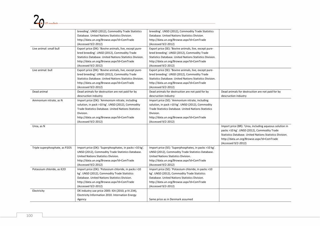
100









Live animal: small bull Export price (DK): 'Bovine animals, live, except pure‐

bred breeding'. UNSD (2012), Commodity Trade

Statistics Database. United Nations Statistics Division.



Export price (SE): 'Bovine animals, live, except pure‐





Live animal: bull Export price (DK): 'Bovine animals, live, except pure‐





Export price (SE): 'Bovine animals, live, except pure‐





Dead animal Dead animals for destruction are not paid for by

descruction industry

Dead animals for destruction are not paid for by


Dead animals for destruction are not paid for by


Ammonium nitrate, as N Import price (DK): 'Ammonium nitrate, including

solution, in pack >10 kg'. UNSD (2012), Commodity

Trade Statistics Database. United Nations Statistics

Division.



Import price (SE): 'Ammonium nitrate, including

solution, in pack >10 kg'. UNSD (2012), Commodity


Division.



Urea, as N

Import price (BR): 'Urea, including aqueous solution in

packs >10 kg'. UNSD (2012), Commodity Trade




Triple superphosphate, as P2O5 Import price (DK): 'Superphosphates, in packs >10 kg'.

UNSD (2012), Commodity Trade Statistics Database.

United Nations Statistics Division.



Import price (SE): 'Superphosphates, in packs >10 kg'.





Potassium chloride, as K2O Import price (DK): 'Potassium chloride, in packs >10

kg'. UNSD (2012), Commodity Trade Statistics




Import price (SE): 'Potassium chloride, in packs >10

kg'. UNSD (2012), Commodity Trade Statistics




Electricity DK industry use price 2005: IEA (2010, p IV.234),

Electricity Information 2010. Internation Energy

Agency Same price as in Denmark assumed

101

Heat DK industry use of district heating in DKK and MJ in

2005: Danmarks Statistik (2012), Statistikbanken, Miljø

og energi. Statistics Denmark,

http://www.statistikbanken.dk (accessed February

2012) Same price as in Denmark assumed

Coal Import price (DK): 'Coal except anthracite or

bituminous, not agglomerate'. UNSD (2012),

Commodity Trade Statistics Database. United Nations

Statistics Division.



Import price (SE): 'Bituminous coal, not agglomerated'.





Fuel oil Import price (DK): 'Oils petroleum, bituminous,

distillates, except crude'. UNSD (2012), Commodity


Division.



Import price (SE): 'Oils petroleum, bituminous,

distillates, except crude'. UNSD (2012), Commodity


Division.



102

C.2PlantcultivationsystemPlant cultivation system

Prices Unit DK SE

Barley EUR2005/kg crop 0.107 0.094

Wheat EUR2005/kg crop 0.103 0.100

Oat EUR2005/kg crop 0.102 0.091

Rapeseed EUR2005/kg crop 0.208 0.222

Crop residue EUR2005/kg straw 0.0669 0.0669

Electricity EUR2005 kWh electricity‐1 0.0741 0.0741

Heat EUR2005 MJ heat‐1 0.0139 0.0139

Plant cultivation system

Data sources DK SE

Barley

Production price (DK): 'Barley'. FAOSTAT (2012), FAOSTAT producer prices.


Production price (SE): 'Barley'. FAOSTAT (2012), FAOSTAT producer prices.


Wheat

Production price (DK): 'wheat'. FAOSTAT (2012), FAOSTAT producer prices.


Production price (SE): 'wheat'. FAOSTAT (2012), FAOSTAT producer prices.


Oat

Production price (DK): 'oats'. FAOSTAT (2012), FAOSTAT producer prices.


Production price (SE): 'oats'. FAOSTAT (2012), FAOSTAT producer prices.


Rapeseed

Production price (DK): 'oats'. FAOSTAT (2012), FAOSTAT producer prices.


Production price (SE): 'oats'. FAOSTAT (2012), FAOSTAT producer prices.


Crop residue

10% VA (rogh assumption) added to addition to costs obtained from: Hinge

J and Maegaard E (2005) Prisen på halm til kraftvarme (English: The price on

straw for combined heat and power). Dansk Landbrugsrådgivning, Aarhus

Assumed same price as in Denmark

Electricity

DK industry use price 2005: IEA (2010, p IV.234), Electricity Information

2010. Internation Energy Agency

Same price as in Denmark assumed

Heat

DK industry use of district heating in DKK and MJ in 2005: Danmarks

Statistik (2012), Statistikbanken, Miljø og energi. Statistics Denmark,

http://www.statistikbanken.dk (accessed February 2012)

Same price as in Denmark assumed

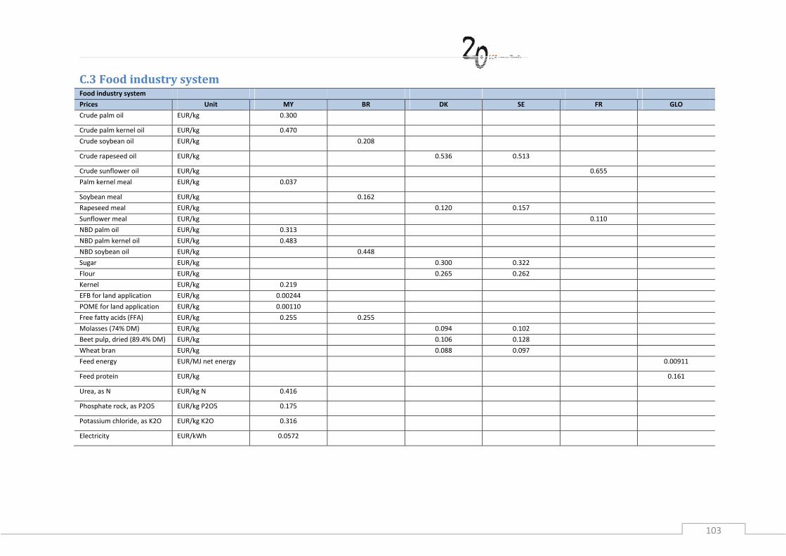
103

C.3FoodindustrysystemFood industry system

Prices Unit MY BR DK SE FR GLO

Crude palm oil EUR/kg 0.300

Crude palm kernel oil EUR/kg 0.470

Crude soybean oil EUR/kg 0.208

Crude rapeseed oil EUR/kg 0.536 0.513

Crude sunflower oil EUR/kg 0.655

Palm kernel meal EUR/kg 0.037

Soybean meal EUR/kg 0.162

Rapeseed meal EUR/kg 0.120 0.157

Sunflower meal EUR/kg 0.110

NBD palm oil EUR/kg 0.313

NBD palm kernel oil EUR/kg 0.483

NBD soybean oil EUR/kg 0.448

Sugar EUR/kg 0.300 0.322

Flour EUR/kg 0.265 0.262

Kernel EUR/kg 0.219

EFB for land application EUR/kg 0.00244

POME for land application EUR/kg 0.00110

Free fatty acids (FFA) EUR/kg 0.255 0.255

Molasses (74% DM) EUR/kg 0.094 0.102

Beet pulp, dried (89.4% DM) EUR/kg 0.106 0.128

Wheat bran EUR/kg 0.088 0.097

Feed energy EUR/MJ net energy 0.00911

Feed protein EUR/kg 0.161

Urea, as N EUR/kg N 0.416 Phosphate rock, as P2O5 EUR/kg P2O5 0.175 Potassium chloride, as K2O EUR/kg K2O 0.316 Electricity EUR/kWh 0.0572

104

Food industry system

Data sources MY BR DK SE FR GLO

Crude palm oil MPOB (2006),

MALAYSIAN OIL PALM

STATISTICS 2005.

Malaysian Palm Oil

Board.

http://econ.mpob.go

v.my/economy/ei_sta

tistics05_old.htm

(accessed 1771‐2012)

Crude palm kernel oil MPOB (2006),

MALAYSIAN OIL PALM

STATISTICS 2005.

Malaysian Palm Oil

Board.

http://econ.mpob.go

v.my/economy/ei_sta

tistics05_old.htm


Crude soybean oil

Production price

(Brazil): 'Oil, soya‐

bean, crude'. UNSD

(2012), Industrial

Commodity Statistics

Database. United

Nations Statistics

Division.

http://data.un.org/Br

owse.aspx?d=ComTra

de (Accessed 18/1‐

2012)

Crude rapeseed oil

Export price

(Denmark): 'Canola,

rape, colza or

mustard oil, crude'.

UNSD (2012),

Commodity Trade

Statistics Database.

United Nations

Export price

(Sweden): 'Canola,

rape, colza or

mustard oil, crude'.

UNSD (2012),

Commodity Trade


United Nations

105



owse.aspx?d=ComTra


2012)



owse.aspx?d=ComTra


2012)

Crude sunflower oil

Export price (France):

'Sunflower‐seed or

safflower oil, crude'.

UNSD (2012),

Commodity Trade


United Nations



owse.aspx?d=ComTra


2012)

Palm kernel meal MPOB (2006),

MALAYSIAN OIL PALM

STATISTICS 2005.

Malaysian Palm Oil

Board.

http://econ.mpob.go

v.my/economy/ei_sta

tistics05_old.htm


Soybean meal

Export price (Brazil):

'Soya‐bean oil‐cake

and other solid

residues'. UNSD

(2012), Commodity

Trade Statistics

Database. United

Nations Statistics

Division.


owse.aspx?d=ComTra


2012)

Rapeseed meal Export price Export price

106

(Denmark): 'Rape or

colza seed oil‐cake

and other solid

residues'. UNSD

(2012), Commodity

Trade Statistics

Database. United

Nations Statistics

Division.


owse.aspx?d=ComTra


2012)

(Sweden): 'Rape or

colza seed oil‐cake

and other solid

residues'. UNSD

(2012), Commodity

Trade Statistics

Database. United

Nations Statistics

Division.


owse.aspx?d=ComTra


2012)

Sunflower meal

Export price (France):

'Sunflower seed oil‐

cake and other solid

residues'. UNSD

(2012), Commodity

Trade Statistics

Database. United

Nations Statistics

Division.


owse.aspx?d=ComTra


2012)

NBD palm oil MPOB (2006),

MALAYSIAN OIL PALM

STATISTICS 2005.

Malaysian Palm Oil

Board.

http://econ.mpob.go

v.my/economy/ei_sta

tistics05_old.htm


NBD palm kernel oil NBD PKO: Price for

refining step of 1 kg is

assumed same as for

crude palm oil. This is

added to CPKO

107

NBD soybean oil

NBD SBO: Production

price (Brazil): 'Oil,

soya‐bean,refined'.

UNSD (2012),

Industrial Commodity


United Nations



owse.aspx?d=ComTra


2012)

Sugar

Production price

(Denmark): 'Wheat or

meslin flour'. UNSD

(2012), Industrial


Database. United

Nations Statistics

Division.


owse.aspx?d=ComTra


2012)

Production price

(Sweden): 'Wheat or

meslin flour'. UNSD

(2012), Industrial


Database. United

Nations Statistics

Division.


owse.aspx?d=ComTra


2012)

Flour

Production price

(Denmark): 'Wheat or

meslin flour'. UNSD

(2012), Industrial


Database. United

Nations Statistics

Division.


owse.aspx?d=ComTra


2012)

Production price

(Sweden): 'Wheat or

meslin flour'. UNSD

(2012), Industrial


Database. United

Nations Statistics

Division.


owse.aspx?d=ComTra


2012)

Kernel MPOB (2006),

MALAYSIAN OIL PALM

STATISTICS 2005.

Malaysian Palm Oil

108

Board.

http://econ.mpob.go

v.my/economy/ei_sta

tistics05_old.htm


EFB for land application Calculated based on

fertiliser prices and

nutrient content of

EFB

POME for land application Calculated based on

fertiliser prices and

nutrient content of

POME

Free fatty acids (FFA) MPOB (2006),

MALAYSIAN OIL PALM

STATISTICS 2005.

Malaysian Palm Oil

Board.

http://econ.mpob.go

v.my/economy/ei_sta

tistics05_old.htm


Assumed as same as

FFA in Malaysia

Molasses (74% DM)

Import price

(Denmark):

'Molasses, except

cane molasses'. UNSD

(2012), Commodity

Trade Statistics

Database. United

Nations Statistics

Division.


owse.aspx?d=ComTra


2012)

Import price

(Sweden): 'Molasses,

except cane

molasses'. UNSD

(2012), Commodity

Trade Statistics

Database. United

Nations Statistics

Division.


owse.aspx?d=ComTra


2012)

Beet pulp, dried (89.4% DM)

Import price

(Denmark): 'Beet‐

pulp, bagasse & other

waste of sugar

manufacture'. UNSD

Import price

(Sweden): 'Beet‐pulp,

bagasse & other

waste of sugar

manufacture'. UNSD

109

(2012), Commodity

Trade Statistics

Database. United

Nations Statistics

Division.


owse.aspx?d=ComTra


2012)

(2012), Commodity

Trade Statistics

Database. United

Nations Statistics

Division.


owse.aspx?d=ComTra


2012)

Wheat bran

Import price

(Denmark): 'Wheat

bran, sharps, other

residues'. UNSD

(2012), Commodity

Trade Statistics

Database. United

Nations Statistics

Division.


owse.aspx?d=ComTra


2012)

Import price

(Sweden): 'Wheat

bran, sharps, other

residues'. UNSD

(2012), Commodity

Trade Statistics

Database. United

Nations Statistics

Division.


owse.aspx?d=ComTra


2012)

Feed energy

Calculated based on

price of soybean meal

in Brazil 2005 export

price (UNSD 2012,

Commodity Trade

Statistics Database)

and price of barley,

average of Russia,

Ukraine and France in

2005 (FAOSTAT

2012). These data are

combined with data

on the content of

protein and net

energy in the two

feed commodities.

Feed protein

Calculated based on

price of soybean meal

110

in Brazil 2005 export

price (UNSD 2012,

Commodity Trade

Statistics Database)

and price of barley,

average of Russia,

Ukraine and France in

2005 (FAOSTAT

2012). These data are

combined with data

on the content of

protein and net

energy in the two

feed commodities.

Urea, as N Import prices

(Malaysia): UNSD

(2012), Commodity

Trade Statistics

Database. United

Nations Statistics

Division.


owse.aspx?d=ComTra


2012)

Phosphate rock, as P2O5 Import prices

(Malaysia): UNSD

(2012), Commodity

Trade Statistics

Database. United

Nations Statistics

Division.


owse.aspx?d=ComTra


2012)

Potassium chloride, as K2O Import prices

(Malaysia): UNSD

(2012), Commodity

Trade Statistics

111

Database. United

Nations Statistics

Division.


owse.aspx?d=ComTra


2012)

Electricity Average use price in

Malaysia in 2007.

Wikipedia (2012),

Electricity pricing,

http://en.wikipedia.o

rg/wiki/Electricity_pri

cing (accessed 19/1‐

2012)

Documents

Arla Life cycle inventory report 20120514(js) - 2.-0 LCA consultants · Preface This report documents the input data used in the Arla model (Schmidt and Dalgaard 2012) to calculate