Army of Botnets

8/6/2019 Army of Botnets

http://slidepdf.com/reader/full/army-of-botnets 1/13

Army of Botnets

Ryan Vogt, John Aycock, and Michael J. Jacobson, Jr.Department of Computer Science, University of Calgary

2500 University Drive N.W., Calgary, Alberta, Canada T2N 1N4

{vogt,aycock,jacobs}@cpsc.ucalgary.ca

Abstract

The trend toward smaller botnets may be more danger-

ous than large botnets, in terms of large-scale attacks like

distributed denials of service. We examine the possibility

of “super-botnets,” networks of independent botnets that

can be coordinated for attacks of unprecedented scale. For

an adversary, super-botnets would also be extremely ver-

satile and resistant to countermeasures. As such, super-

botnets must be examined by the research community, so

that defenses against this threat can be developed proac-

tively. Our simulation results shed light on the feasibility

and structure of super-botnets and some properties of their

command-and-control mechanism. New forms of attack that

super-botnets can launch are explored, and possible de-

fenses against the threat of super-botnets are suggested.

1 Introduction

Big botnets are big news. Botnets involving over

100,000 zombie computers have been claimed [6, 8, 21],

and there was even one case involving 1.5 million compro-

mised computers [19]. However, from an adversary’s per-

spective,1 big botnets are bad from the standpoint of sur-

vivability: someone is likely to notice a big botnet and take

steps to dismantle it.

The recent trend is toward smaller botnets with only sev-

eral hundred to several thousand zombies [5]. This may

reflect better defenses — the malware creating new zom-

bies may not be as eff ective — but it may be a consciousdecision by adversaries to limit botnet size, and try to avoid

detection. It has also been suggested that the wider avail-

ability of broadband access makes smaller botnets as capa-

ble as the larger botnets of old [5].

We suggest that there is a new threat posed by smaller

botnets: namely, an adversary can create a large number of

1In this paper, we generically refer to people creating and using botnets

as adversaries.

small, independent botnets. By themselves, the smaller bot-

nets can be exploited by the adversary in the usual way, such

as being rented to spammers. The discovery and disabling

of some of the adversary’s botnets is not a concern, either,

because the botnets are independent and numerous.

The new threat arises if the botnets are designed to be

coordinated into a network of botnets, which we call a

super-botnet . For example, an adversary could command

the super-botnet to launch a massive DDoS attack on a cho-

sen target, or to pummel a critical piece of the Internet’s

infrastructure like the DNS. A super-botnet design poten-

tially allows an adversary to surreptitiously amass enough

machines for attacks of enormous scale.

In the remainder of this paper we explore super-botnets

and potential defenses against them. Section 2 describes

work related to super-botnets. Section 3 discusses the vul-

nerabilities inherent in traditional botnet design, to motivate

why adversaries would utilize a super-botnet. Section 4 ad-

dresses whether it is feasible for adversaries to constructlarge super-botnets, and Section 5 discusses the communi-

cation mechanisms employed in such super-botnets. Sec-

tion 6 discusses a new type of time-delayed attack that can

be launched using a super-botnet. Section 7 discusses how

defenders can combat both this new form of attack, and

super-botnets in general. Finally, we conclude and discuss

future research directions in Section 8.

2 Related Work

Many diff erent command-and-control (C&C) mecha-

nisms for botnets are being seen and suggested [5]. Forexample, an IRC server could be used to send commands

to compromised machines; or, a zombie could even receive

commands covertly by making a DNS request to a domain

under the adversary’s control [9]. There is continuous evo-

lution of the control mechanisms used within a botnet.

Control mechanisms for co-ordinating multiple botnets

have also been discussed in the literature. Nazario et al.

talk about communicating worms that isolate themselves in



small groups, to limit the impact of an infected machine be-

ing discovered [12]. The possibility of independent botnets

being operated in a tree-like structure has also been sug-

gested [16]. Dagon et al. classified diff erent botnets struc-

tures into a taxonomy [6], and the super-botnet structure

(described in detail in Section 5) constitutes a special case

of a random graph botnet. Empirical studies have even beendone on the diff erent connectivity models of botnets [14].

Also described in Section 5, a super-botnet’s communi-

cation structure can be formed through opportunistic data

exchanges between individual botnets that occur during re-

dundant infection attempts. A similar idea for worms was

briefly mentioned in [18]. Other methods of exchanging

information between infected hosts, such as Chen and Ji’s

client-server model [4], have also been discussed.

Because of the myriad of related botnet mechanisms al-

ready available to adversaries, super-botnets must be con-

sidered as a possible future evolution of today’s botnets. As

such, it is necessary to investigate what threat super-botnets

will pose in the future, and what defenders can do proac-tively to protect themselves and others.

3 Vulnerabilities of Traditional Botnets

Before we consider why a trend toward super-botnets is

dangerous, it is first important to understand some weak-

nesses exhibited by traditional botnets. By recognizing how

the traditional botnets of old can be detected and disabled, it

will become clearer why a decentralized super-botnet poses

such a threat.

A traditional botnet uses some C&C channel to receive

commands: for instance, an IRC server. Alternately, a bot-net may periodically poll an information source that is un-

likely to be blocked or raise suspicion, such as accessing

a web site (perhaps located via a web search engine), or

making a DNS request to a domain under the adversary’s

control [9].

It is this command-and-control mechanism that consti-

tutes a weak point for defenders to target. There are five

main goals that defenders could have:

1. Locate or identify the adversary. The adversary is

vulnerable to detection when they issue commands to

the botnet via this C&C channel. Defenders may not

know the nature of the adversary’s commands in ad-vance, but assuming some of the zombies have been

detected and analyzed, the source of the adversary’s

commands will be known and alarms can be triggered

when commands are sent. For example, a defender

may know that botnet commands will be found by

periodically performing Google searches for “haggis

gargling” and sifting through the avalanche of results

for the adversary’s commands. Monitoring when and

where Google finds such a web site may provide a lead

as to the whereabouts of the adversary. In turn, an ad-

versary may try to obfuscate their trail by issuing bot-

net commands through proxies or anonymity networks

like Tor [7].

2. Reveal all the infected machines. Again, if the zombiesare polling a known location for the adversary’s com-

mands, then the polling activity will reveal infected

machines. Meeting this goal and the previous one may

require cooperation between law enforcement and the

private sector.

3. Command the botnet. A defender could attempt to

send a command to the botnet to shut it down. A re-

lated concern for the adversary is that another adver-

sary may try to usurp control of the botnet. For these

reasons, as pointed out by Staniford et al. [18],2 the

adversary must digitally sign or encrypt botnet com-mands using asymmetric encryption (described in Sec-

tion 8.1 of Menezes et al. [11, p.283]), so that the com-

promise of an infected machine does not reveal a secret

key. Generating a public / private key pair in advance,

the adversary could send the public key along with the

worm, solving the key distribution problem.

4. Disable the botnet. If a defender can shut down the

C&C channel (along with any redundant channels),

the entire botnet will be rendered useless in a single

blow. With the zombies unable to receive commands,

the botnet will cease to operate.

5. Disrupt botnet commands. If the C&C channel is one

that cannot easily be shut down, such as Google, other

defense methods can be employed. The adversary’s

commands can be intentionally garbled by a defender

regardless of whether or not they are encrypted or

signed — changing a few bits is sufficient to achieve

this goal, leaving the adversary unable to control the

botnet. This defense can be applied locally, e.g., by

IPS / firewall rules, or globally if a defender has enough

access to the botnet’s command source.

Large traditional botnets are vulnerable to defenders be-cause of the easily-targeted C&C channel. The benefits to

the adversary of decentralizing their botnet into a super-

botnet — a network of independent botnets — are clear.

But, we must still explore whether it is feasible for an ad-

versary to create a large super-botnet.

2Staniford et al. presented their work in the context of updating worms,

but the technique could be applied to controlling botnets.



4 Super-Botnet Feasibility

Are large super-botnets feasible? To answer this ques-

tion, we must consider how a super-botnet can be con-

structed. We begin by abstracting away some details:

1. For simplicity, we assume that the super-botnet is con-structed using only one worm. This does not imply

that the worm’s code is uniform across infections, of

course, because the worm could be polymorphic or

metamorphic in nature.

More than one worm may be involved in practice. A

single adversary could create multiple worms, or worm

variants; multiple adversaries could conspire to cre-

ate multiple worms based on a common super-botnet

specification. Neither possibility is farfetched. For

some malware, creating variants is practically a cot-

tage industry — Spybot, for example, has thousands of

variants [3]. Adversaries have collaborated in the past

on malware [20], and N -version programming [2] of

worms by adversaries within a single organization is

definitely possible in the context of information war-

fare. Implementation diversity can make worm detec-

tion more difficult for signature-based detection meth-

ods.

2. The infection vector(s) the worm uses are not relevant

to the analysis and are not considered. We also ig-

nore failures to propagate in our simulations. While

these considerations are important in real worm prop-

agation, we are only interested in the resulting super-

botnet structure.

3. The exact C&C mechanism(s) used within individual

botnets does not matter. We assume a centralized IRC-

based C&C for concreteness, but it could just as easily

be a peer-to-peer architecture or some other method.

One way to establish a super-botnet is with a two-phase

process. In the first phase, a worm is released which makes

every new infection a C&C machine for a new, independent

botnet. In the second phase, after enough C&C machines

have been created, new infections populate the C&C ma-

chines’ botnets. This method is risky for an adversary, be-

cause the “backbone” of the super-botnet’s C&C infrastruc-

ture is all established by direct infections; discovery of oneC&C machine can easily lead to others using information

from firewall logs, for example.

Instead, we use a tree-structured algorithm that is depen-

dent on three constants: BOTNETS, HOSTS_PER_BOTNET,

and SPREAD. This algorithm creates BOTNETS individual

botnets, each consisting of HOSTS_PER_BOTNET zombies.

As each zombie is infected, it learns how many additional

zombies it will be responsible for adding to its botnet (to

D( x, y)

1 Distribute x fairly into y slots

2 for i ← 0 to y − 13 do L[i] ← x/ y

4 for i ← 0 to ( x mod y) − 1

5 do L[i] ← L[i] + 1

6 return L

P(nti, bts, cc)

1 nti − 1 is the number of new hosts to add to this

botnet

2 bts is the number of new botnets that need to be

started

3 cc is the IP address of the C&C server

4 if nti = 0

5 then Establish a new C&C server

6 bts ← bts − 1

7 Start IRC server

8 cc ← my IP address

9 nti ←

10 else Use existing C&C server

11 Connect to cc

12 ntichild ← D(nti − 1, )

13 btschild ← D(bts, )

14 for i ← 0 to − 1

15 do if ntichild [i] = 0 and btschild [i] = 0

16 then continue

17 repeat target ← a host chosen by a random

scan

18 until target is a vulnerable, uninfected host

19 Infect target

20 target runs P(ntichild [i], btschild [i], cc)

I-I()

1 The code run by the initial infection

2 P(0, , 0.0.0.0)

Figure 1. Worm pseudocode for super-botnetcreation.



T6T3

T2T1T0

…

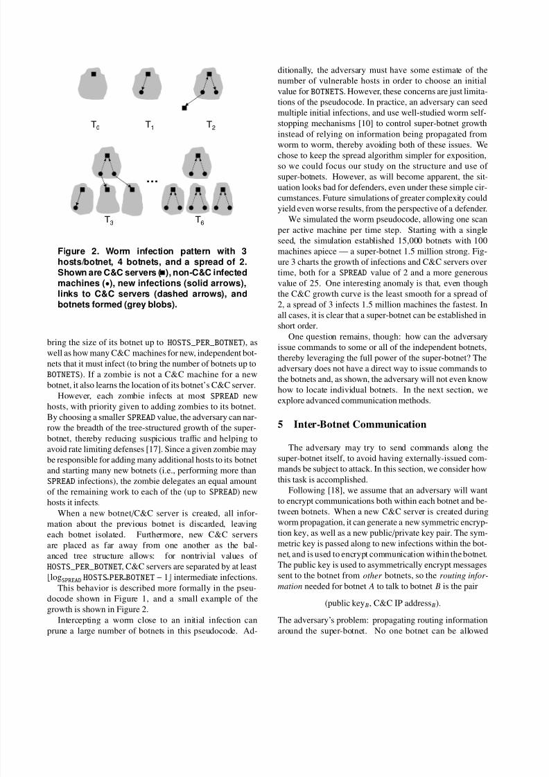
Figure 2. Worm infection pattern with 3hosts/botnet, 4 botnets, and a spread of 2.

Shown are C&C servers ( ), non-C&C infectedmachines (•), new infections (solid arrows),links to C&C servers (dashed arrows), andbotnets formed (grey blobs).

bring the size of its botnet up to HOSTS_PER_BOTNET), as

well as how many C&C machines for new, independent bot-

nets that it must infect (to bring the number of botnets up to

BOTNETS). If a zombie is not a C&C machine for a new

botnet, it also learns the location of its botnet’s C&C server.

However, each zombie infects at most SPREAD new

hosts, with priority given to adding zombies to its botnet.By choosing a smaller SPREAD value, the adversary can nar-

row the breadth of the tree-structured growth of the super-

botnet, thereby reducing suspicious traffic and helping to

avoid rate limiting defenses [17]. Since a given zombie may

be responsible for adding many additional hosts to its botnet

and starting many new botnets (i.e., performing more than

SPREAD infections), the zombie delegates an equal amount

of the remaining work to each of the (up to SPREAD) new

hosts it infects.

When a new botnet / C&C server is created, all infor-

mation about the previous botnet is discarded, leaving

each botnet isolated. Furthermore, new C&C servers

are placed as far away from one another as the bal-anced tree structure allows: for nontrivial values of

HOSTS_PER_BOTNET, C&C servers are separated by at least

logSPREAD HOSTS PER BOTNET − 1 intermediate infections.

This behavior is described more formally in the pseu-

docode shown in Figure 1, and a small example of the

growth is shown in Figure 2.

Intercepting a worm close to an initial infection can

prune a large number of botnets in this pseudocode. Ad-

ditionally, the adversary must have some estimate of the

number of vulnerable hosts in order to choose an initial

value for BOTNETS. However, these concerns are just limita-

tions of the pseudocode. In practice, an adversary can seed

multiple initial infections, and use well-studied worm self-

stopping mechanisms [10] to control super-botnet growth

instead of relying on information being propagated fromworm to worm, thereby avoiding both of these issues. We

chose to keep the spread algorithm simpler for exposition,

so we could focus our study on the structure and use of

super-botnets. However, as will become apparent, the sit-

uation looks bad for defenders, even under these simple cir-

cumstances. Future simulations of greater complexity could

yield even worse results, from the perspective of a defender.

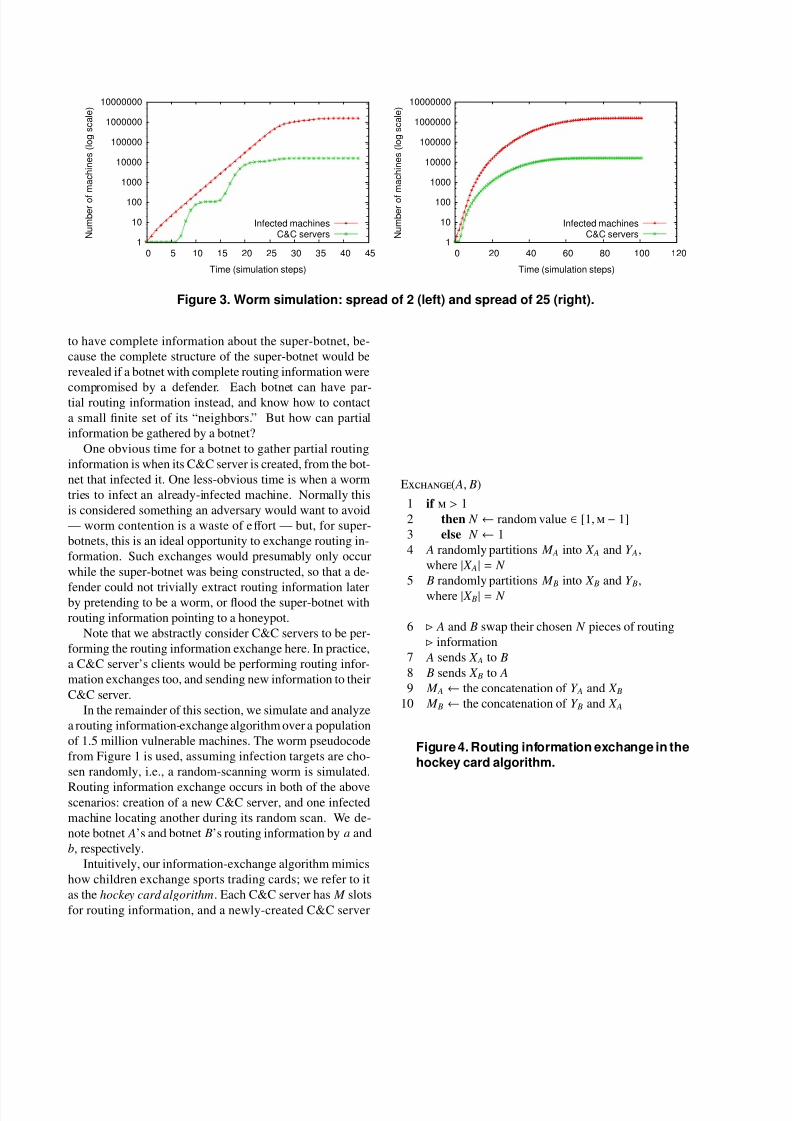
We simulated the worm pseudocode, allowing one scan

per active machine per time step. Starting with a single

seed, the simulation established 15,000 botnets with 100

machines apiece — a super-botnet 1.5 million strong. Fig-

ure 3 charts the growth of infections and C&C servers over

time, both for a SPREAD value of 2 and a more generousvalue of 25. One interesting anomaly is that, even though

the C&C growth curve is the least smooth for a spread of

2, a spread of 3 infects 1.5 million machines the fastest. In

all cases, it is clear that a super-botnet can be established in

short order.

One question remains, though: how can the adversary

issue commands to some or all of the independent botnets,

thereby leveraging the full power of the super-botnet? The

adversary does not have a direct way to issue commands to

the botnets and, as shown, the adversary will not even know

how to locate individual botnets. In the next section, we

explore advanced communication methods.

5 Inter-Botnet Communication

The adversary may try to send commands along the

super-botnet itself, to avoid having externally-issued com-

mands be subject to attack. In this section, we consider how

this task is accomplished.

Following [18], we assume that an adversary will want

to encrypt communications both within each botnet and be-

tween botnets. When a new C&C server is created during

worm propagation, it can generate a new symmetric encryp-

tion key, as well as a new public / private key pair. The sym-

metric key is passed along to new infections within the bot-net, and is used to encrypt communication within the botnet.

The public key is used to asymmetrically encrypt messages

sent to the botnet from other botnets, so the routing infor-

mation needed for botnet A to talk to botnet B is the pair

(public key B, C&C IP address B).

The adversary’s problem: propagating routing information

around the super-botnet. No one botnet can be allowed



1

10

100

1000

10000

100000

1000000

10000000

0 5 10 15 20 25 30 35 40 45

N u m b e r o f

m a c h i n e s ( l o g s c a l e )

Time (simulation steps)

Infected machinesC&C servers

1

10

100

1000

10000

100000

1000000

10000000

0 20 40 60 80 100 120

N u m b e r o f

m a c h i n e s ( l o g s c a l e )

Time (simulation steps)

Infected machinesC&C servers

Figure 3. Worm simulation: spread of 2 (left) and spread of 25 (right).

to have complete information about the super-botnet, be-

cause the complete structure of the super-botnet would be

revealed if a botnet with complete routing information were

compromised by a defender. Each botnet can have par-tial routing information instead, and know how to contact

a small finite set of its “neighbors.” But how can partial

information be gathered by a botnet?

One obvious time for a botnet to gather partial routing

information is when its C&C server is created, from the bot-

net that infected it. One less-obvious time is when a worm

tries to infect an already-infected machine. Normally this

is considered something an adversary would want to avoid

— worm contention is a waste of eff ort — but, for super-

botnets, this is an ideal opportunity to exchange routing in-

formation. Such exchanges would presumably only occur

while the super-botnet was being constructed, so that a de-

fender could not trivially extract routing information laterby pretending to be a worm, or flood the super-botnet with

routing information pointing to a honeypot.

Note that we abstractly consider C&C servers to be per-

forming the routing information exchange here. In practice,

a C&C server’s clients would be performing routing infor-

mation exchanges too, and sending new information to their

C&C server.

In the remainder of this section, we simulate and analyze

a routing information-exchange algorithm over a population

of 1.5 million vulnerable machines. The worm pseudocode

from Figure 1 is used, assuming infection targets are cho-

sen randomly, i.e., a random-scanning worm is simulated.

Routing information exchange occurs in both of the abovescenarios: creation of a new C&C server, and one infected

machine locating another during its random scan. We de-

note botnet A’s and botnet B’s routing information by a and

b, respectively.

Intuitively, our information-exchange algorithm mimics

how children exchange sports trading cards; we refer to it

as the hockey card algorithm. Each C&C server has M slots

for routing information, and a newly-created C&C server

E( A, B)

1 if > 1

2 then N ← random value ∈ [1, − 1]

3 else N ← 1

4 A randomly partitions M A into X A and Y A,

where | X A| = N

5 B randomly partitions M B into X B and Y B,

where | X B| = N

6 A and B swap their chosen N pieces of routing

information

7 A sends X A to B

8 B sends X B to A

9 M A ← the concatenation of Y A and X B10 M B ← the concatenation of Y B and X A

Figure 4. Routing information exchange in thehockey card algorithm.



for botnet A begins with all its slots ( M A) initialized to a.

Thereafter, when either of the two opportunities arise to ex-

change information between botnets A and B, the two bot-

nets first agree on a random number N , then A and B each

select N random slots and trade them as described in Fig-

ure 4. This code maintains M links to each botnet within

the super-botnet. Although a botnet may end up with dupli-cates and self-links, our simulations showed that this does

not have any negative eff ects.

We assume that the adversary knows the addresses of

seed infections, and that they will want to communicate

through the super-botnet as surreptitiously as possible. In

other words, the adversary will not broadcast a command to

all seeds, but will select one seed and send a super-botnet

command through it. The important metric to the adversary

is thus the amount of connectivity from some seed. That is,

how many botnets will a command reach?

To evaluate this metric, we fixed three simulation pa-

rameters on the basis that the adversary would want

a large, quickly-constructed super-botnet: 15,000 bot-

nets, 100 seeds, and a spread of 3 — so, the initial

code run by each seed, with reference to Figure 1, is

PROPAGATE(0, 150, 0.0.0.0). Two parameters were

adjusted, however. First, the value of M was varied from

1 to 30 in increments to ascertain its eff ect on connectivity.

Second, the number of hosts per botnet was varied in in-

crements from 25 to 100 to study diff erent probabilities of

finding other botnets during propagation. All simulations

were repeated five times to minimize the eff ects of random-

ness.

The results were dramatic. In every simulation run where

M was greater than 1, the amount of connectivity from anysingle seed was 100%. An adversary would be able to com-

mand all the botnets comprising the super-botnet using any

one seed.

M does play a role in the resistance of the super-botnet

to defensive measures. In particular, a defender may try to

prevent an adversary from commanding their super-botnet

by reducing connectivity. Here we define the degree of a

botnet to be the sum of its useful in- and out-degrees, which

are the links remaining once self-links and duplicate links

are removed.

Following research on attacks against both random and

scale-free networks [1], we consider a defender who will

try to disable a super-botnet using two diff erent strategies.First, a defender may disable high-degree botnets first. This

i s a n eff ort to reduce super-botnet connectivity more quickly

than simply disabling botnets at random. It is important to

stress that this is the absolute best case, where a defender

has oracular knowledge of the super-botnet’s connectivity.

Second, a defender may disable botnets at random. This

is perhaps a more likely case, where uncoordinated defend-

ers would simply be shutting down botnets randomly upon

discovery.

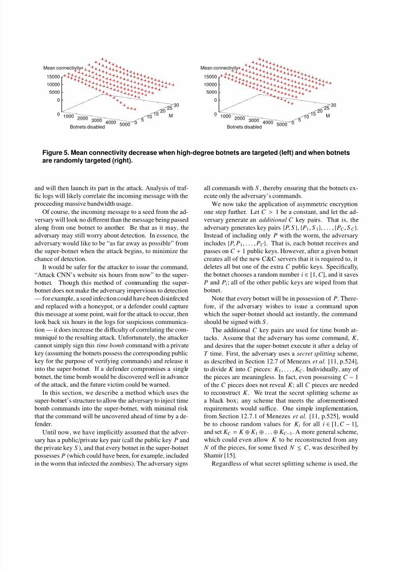
The results are shown in Figure 5, for both high-degree

first targeting and random selection. We have only pre-

sented the data for 25 hosts per botnet here, because the

results were almost identical for the diff erent numbers of

hosts per botnet we ran. Results were averaged over five

runs to compensate for randomness.The strategy used by the defender does not seem to mat-

ter. Once M ≥ 5, a defender able to disable one-third of the

botnets in a super-botnet still leaves the adversary able to

contact one-third of their original botnets from some seed,

on average. This is still enough for a sizeable attack to be

launched with the super-botnet. Two conclusions can be

drawn:

• The adversary would set M to at least 5. However,

there is a tradeoff between robustness and disclosure.

Too large a value for M would reveal the location of a

large number of other botnets, if a defender discovers

one botnet.

• Communication through a super-botnet is robust to a

defender’s countermeasures. Finding and disabling

5000 botnets, randomly or otherwise, would be a dif-

ficult task. The only defense that is deployed widely

enough to feasibly do this is anti-virus software.

This simulation also assumes that an adversary will

only communicate through one of the initial seeds.

Botnets could announce their (encrypted) routing in-

formation to an adversary instead; this would give the

adversary many more communication endpoints to use

at the risk of leaking information to a defender. An ad-

versary may also use a small number of seeds for com-munication, rather than just one, or alternate which

seed receives the command each time a command is

sent. Either variation by the adversary should reduce

the eff ectiveness of the defender’s countermeasures.

These conclusions suggest that new, large-scale defenses

are needed for the super-botnet threat. We discuss defenses

against the super-botnet threat in Section 7. First, however,

we discuss a novel application of the super-botnet’s decen-

tralized structure that allows for a new form of attack to

be launched. Understanding how this new form of attack

works will further reveal the methodology that must be used

to defend against super-botnets.

6 Time Bombs

Even with the decentralized structure of the super-botnet,

the adversary is still vulnerable to detection when a com-

mand is injected into the super-botnet. When the adversary

gives the command, “Attack CNN’s website” to a seed in-

fection, the seed will pass the command on to other botnets,



0 1000 2000 3000 4000 5000Botnets disabled

05

1015

2025

30

M

0

5000

10000

15000

Mean connectivity

0 1000 2000 3000 4000 5000Botnets disabled

05

1015

2025

30

M

0

5000

10000

15000

Mean connectivity

Figure 5. Mean connectivity decrease when high-degree botnets are targeted (left) and when botnetsare randomly targeted (right).

and will then launch its part in the attack. Analysis of traf-

fic logs will likely correlate the incoming message with the

proceeding massive bandwidth usage.

Of course, the incoming message to a seed from the ad-

versary will look no diff erent than the message being passed

along from one botnet to another. Be that as it may, the

adversary may still worry about detection. In essence, the

adversary would like to be “as far away as possible” from

the super-botnet when the attack begins, to minimize the

chance of detection.

It would be safer for the attacker to issue the command,

“Attack CNN’s website six hours from now” to the super-

botnet. Though this method of commanding the super-

botnet does not make the adversary impervious to detection

— for example, a seed infection could have been disinfectedand replaced with a honeypot, or a defender could capture

this message at some point, wait for the attack to occur, then

look back six hours in the logs for suspicious communica-

tion — it does increase the difficulty of correlating the com-

munique to the resulting attack. Unfortunately, the attacker

cannot simply sign this time bomb command with a private

key (assuming the botnets possess the corresponding public

key for the purpose of verifying commands) and release it

into the super-botnet. If a defender compromises a single

botnet, the time bomb would be discovered well in advance

of the attack, and the future victim could be warned.

In this section, we describe a method which uses the

super-botnet’s structure to allow the adversary to inject timebomb commands into the super-botnet, with minimal risk

that the command will be uncovered ahead of time by a de-

fender.

Until now, we have implicitly assumed that the adver-

sary has a public / private key pair (call the public key P and

the private key S ), and that every botnet in the super-botnet

possesses P (which could have been, for example, included

in the worm that infected the zombies). The adversary signs

all commands with S , thereby ensuring that the botnets ex-

ecute only the adversary’s commands.

We now take the application of asymmetric encryption

one step further. Let C > 1 be a constant, and let the ad-

versary generate an additional C key pairs. That is, the

adversary generates key pairs {P, S }, {P1, S 1}, . . . , {PC , S C }.

Instead of including only P with the worm, the adversary

includes {P, P1, . . . , PC }. That is, each botnet receives and

passes on C + 1 public keys. However, after a given botnet

creates all of the new C&C servers that it is required to, it

deletes all but one of the extra C public keys. Specifically,

the botnet chooses a random number i ∈ [1,C ], and it saves

P and Pi; all of the other public keys are wiped from that

botnet.

Note that every botnet will be in possession of P. There-fore, if the adversary wishes to issue a command upon

which the super-botnet should act instantly, the command

should be signed with S .

The additional C key pairs are used for time bomb at-

tacks. Assume that the adversary has some command, K ,

and desires that the super-botnet execute it after a delay of

T time. First, the adversary uses a secret splitting scheme,

as described in Section 12.7 of Menezes et al. [11, p.524],

to divide K into C pieces: K 1, . . . , K C . Individually, any of

the pieces are meaningless. In fact, even possessing C − 1

of the C pieces does not reveal K ; all C pieces are needed

to reconstruct K . We treat the secret splitting scheme as

a black box; any scheme that meets the aforementionedrequirements would suffice. One simple implementation,

from Section 12.7.1 of Menezes et al. [11, p.525], would

be to choose random values for K i for all i ∈ [1,C − 1],

and set K C = K ⊕ K 1 ⊕ . . . ⊕ K C −1. A more general scheme,

which could even allow K to be reconstructed from any

N of the pieces, for some fixed N ≤ C , was described by

Shamir [15].

Regardless of what secret splitting scheme is used, the



adversary constructs the following message after the com-

mand is split:

{ DS 1( DS (K 1)), . . . , DS C

( DS (K C )), DS (T )} ,

where DS ( x) is a digital signature scheme with message

recovery, using private key S on message x, that incor-porates a suitable, non-multiplicative redundancy func-

tion. One example of such a scheme is RSA with

ISO / IEC 9796 formatting, described in Section 11.3.5 of

Menezes et al. [11, pp.442–444]. The redundancy function

is necessary since the pieces of K look random; without it,

it would be impossible to distinguish a valid signature from

garbage [11, p.430].

This message is delivered into the super-botnet as usual,

and each botnet decodes what part of the message it can.

Since each botnet possesses only a single, randomly-chosen

Pi, it can decrypt only the corresponding DS (K i). That is,

after the message has travelled through the entire super-

botnet, each botnet will be in possession of a signed copyof T , and a signed copy of one of the C pieces of K .

After a delay of T has elapsed, each botnet floods its

DS (K i) into the super-botnet. Since K i is signed by S , each

botnet can confirm that any piece of K that it receives is,

in fact, one of the original C pieces created by the adver-

sary. After receiving and confirming all C pieces of K , each

botnet can perform the command.

This scheme is highly resistant to attacks by individual

defenders. There are two tasks that a defender may wish to

accomplish against this scheme:

• Reconstruct the command before it is executed. To

do so, the defender would require all C public keys,P1, . . . PC . It would be difficult for a defender to cap-

ture all C public keys during the construction of the

super-botnet. Each botnet deletes all but one of these

values after it finishes spreading, and compromising a

botnet to extract all C keys while it is still spreading

would require either a honeypot capturing the worm

while it spreads, or near-instantaneous response from

a defender to an infection. Short of a honeypot captur-

ing the worm, a defender’s best chance for capturing

all C keys (or, all C of the DS (K i)) is, for each public

key, to compromise at least one botnet that knows that

key. Then, the key can be extracted from the compro-

mised botnet.

• Destroy at least one part of the command in the super-

botnet, so that the command cannot be reconstructed

and executed. To do so, a defender would have to dis-

able each botnet that knows Pi for some i ∈ [1,C ].

Assuming that a defender does not have oracular knowl-

edge about how to find botnets that match one of these two

goals, and that botnets are compromised or disabled ran-

domly (as they are found by the defender), how many bot-

nets can the defender expect to have to locate and attack, on

average, before accomplishing either of the goals?

We can answer these questions probabilistically. Com-

puting an expected value for the number of botnets that a

defender must compromise to reconstruct the command isthe subject of Appendix A.1, and computing an expected

value for the number of botnets that a defender must disable

to destroy one part of the command is the subject of Ap-

pendix A.2. Numerical simulations support the results de-

rived in the appendices.

As an example of the analysis in Appendix A.1 and Ap-

pendix A.2, let us assume that there are 15,000 botnets in

the super-botnet, and that the command is split into 100

pieces (so, the values of R and C used in the appendices are

150 and 100, respectively). To reconstruct the command,

a defender would have to compromise, on average, 509.38

botnets — roughly 3.4% of the entire super-botnet. This

sizeable task would likely be beyond the capabilities of asingle defender. Destroying a single piece of the command

would require the defender to disable, on average, 14491.62

botnets — roughly 96.6% of the entire super-botnet. This

number is so large that, in practice, the super-botnet struc-

ture would become so partitioned before the defender suc-

ceeded in eradicating one piece of the command, that the

command could not be reassembled anyway.

Clearly, defending against creative uses of the super-

botnet structure is beyond the capabilities of a single

defender, or multiple defenders working without shared

knowledge or co-ordination. To combat this new threat, new

defenses must be developed.

7 Defense Against Super-Botnets

We now turn to defense. There would be no sense for

an adversary to build a super-botnet for immediate use; a

traditional worm would be more eff ective in that scenario.

The strength of the decentralized super-botnet design is, af-

ter all, its resistance to defenders’ attacks over time. It is

reasonable to assume, therefore, that super-botnets would

be deployed in advance of an attack. Traditional anti-virus

software would thus be useful against super-botnets, as anti-

virus software would have time for updates and detection.

Aside from the obvious use of anti-virus software, whatdefenses can be constructed to specifically target super-

botnets? As revealed by the resistance of the super-botnet’s

communication structure to the failure of individual botnets

(discussed in Section 5), and the super-botnet’s ability to

distribute its attack plans beyond the reach of a single de-

fender (discussed in Section 6), super-botnets cannot be dis-

abled by a single defender.

One solution to the threat of super-botnets is centralized



hop 1hop 2

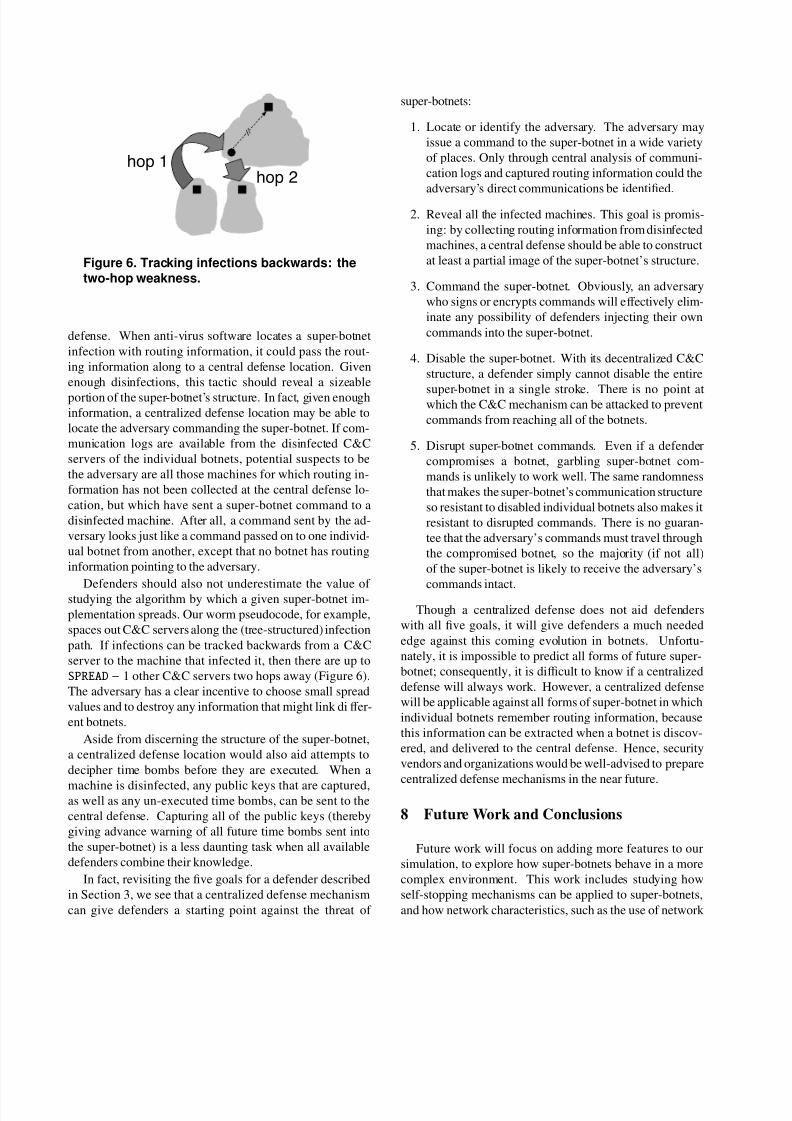
Figure 6. Tracking infections backwards: thetwo-hop weakness.

defense. When anti-virus software locates a super-botnet

infection with routing information, it could pass the rout-

ing information along to a central defense location. Given

enough disinfections, this tactic should reveal a sizeable

portion of the super-botnet’s structure. In fact, given enough

information, a centralized defense location may be able to

locate the adversary commanding the super-botnet. If com-

munication logs are available from the disinfected C&C

servers of the individual botnets, potential suspects to be

the adversary are all those machines for which routing in-

formation has not been collected at the central defense lo-

cation, but which have sent a super-botnet command to a

disinfected machine. After all, a command sent by the ad-

versary looks just like a command passed on to one individ-

ual botnet from another, except that no botnet has routing

information pointing to the adversary.

Defenders should also not underestimate the value of studying the algorithm by which a given super-botnet im-

plementation spreads. Our worm pseudocode, for example,

spaces out C&C servers along the (tree-structured) infection

path. If infections can be tracked backwards from a C&C

server to the machine that infected it, then there are up to

SPREAD − 1 other C&C servers two hops away (Figure 6).

The adversary has a clear incentive to choose small spread

values and to destroy any information that might link diff er-

ent botnets.

Aside from discerning the structure of the super-botnet,

a centralized defense location would also aid attempts to

decipher time bombs before they are executed. When a

machine is disinfected, any public keys that are captured,as well as any un-executed time bombs, can be sent to the

central defense. Capturing all of the public keys (thereby

giving advance warning of all future time bombs sent into

the super-botnet) is a less daunting task when all available

defenders combine their knowledge.

In fact, revisiting the five goals for a defender described

in Section 3, we see that a centralized defense mechanism

can give defenders a starting point against the threat of

super-botnets:

1. Locate or identify the adversary. The adversary may

issue a command to the super-botnet in a wide variety

of places. Only through central analysis of communi-

cation logs and captured routing information could the

adversary’s direct communications be identified.

2. Reveal all the infected machines. This goal is promis-

ing: by collecting routing information from disinfected

machines, a central defense should be able to construct

at least a partial image of the super-botnet’s structure.

3. Command the super-botnet. Obviously, an adversary

who signs or encrypts commands will eff ectively elim-

inate any possibility of defenders injecting their own

commands into the super-botnet.

4. Disable the super-botnet. With its decentralized C&C

structure, a defender simply cannot disable the entire

super-botnet in a single stroke. There is no point atwhich the C&C mechanism can be attacked to prevent

commands from reaching all of the botnets.

5. Disrupt super-botnet commands. Even if a defender

compromises a botnet, garbling super-botnet com-

mands is unlikely to work well. The same randomness

that makes the super-botnet’s communication structure

so resistant to disabled individual botnets also makes it

resistant to disrupted commands. There is no guaran-

tee that the adversary’s commands must travel through

the compromised botnet, so the majority (if not all)

of the super-botnet is likely to receive the adversary’s

commands intact.

Though a centralized defense does not aid defenders

with all five goals, it will give defenders a much needed

edge against this coming evolution in botnets. Unfortu-

nately, it is impossible to predict all forms of future super-

botnet; consequently, it is difficult to know if a centralized

defense will always work. However, a centralized defense

will be applicable against all forms of super-botnet in which

individual botnets remember routing information, because

this information can be extracted when a botnet is discov-

ered, and delivered to the central defense. Hence, security

vendors and organizations would be well-advised to prepare

centralized defense mechanisms in the near future.

8 Future Work and Conclusions

Future work will focus on adding more features to our

simulation, to explore how super-botnets behave in a more

complex environment. This work includes studying how

self-stopping mechanisms can be applied to super-botnets,

and how network characteristics, such as the use of network



address translation, can aff ect the spread of a super-botnet,

possibly providing an additional line of defense [13]. We

also wish to examine in more detail the relative strengths

and weaknesses of a super-botnet design, relative to peer-

to-peer botnets, both for the adversary and for defenders.

In any form, super-botnets provide adversaries with an

enormous amount of virtual firepower that is easy to con-struct yet hard to shut down, as there is no single C&C chan-

nel for defenders to target. The loss of individual botnets

(which can, by themselves, be farmed out for spamming

and other traditional uses) is not catastrophic.

The trend toward smaller botnets can be seen as an evo-

lutionary step leading to super-botnets. This means that at-

tacks by millions of machines on the Internet’s infrastruc-

ture can appear from nowhere, as multiple small botnets

join forces. Super-botnets must be considered a serious

threat that must be defended against with new centralized

defense mechanisms.

9 Acknowledgments

The authors’ research is supported in part by grants from

the Natural Sciences and Engineering Research Council of

Canada. The authors would also like to thank the anony-

mous reviewers for their helpful comments for improving

this paper.

References

[1] R. Albert, H. Jeong, and A.-L. Barabasi. Error and attack

tolerance of complex networks. Nature, 406:378–382, 2000.[2] A. Avizienis. The N -version approach to fault-tolerant soft-

ware. IEEE Transactions on Software Engineering, SE-

11(12):1491–1501, 1985.[3] J. Canavan. The evolution of malicious IRC bots. In Virus

Bulletin Conference, pages 104–114, 2005.[4] Z. Chen and C. Ji. A self-learning worm using importance

scanning. In Proceedings of the 2005 ACM Workshop on

Rapid Malcode, pages 22–29, 2005.[5] E. Cooke, F. Jahanian, and D. McPherson. The zombie

roundup: Understanding, detecting, and disrupting botnets.

In USENIX SRUTI Workshop, pages 39–44, 2005.[6] D. Dagon, G. Gu, C. Zou, J. Grizzard, S. Dwivedi, W. Lee,

and R. Lipton. A taxonomy of botnets. Unpublished paper,

c. 2005.[7] R. Dingledine, N. Mathewson, and P. Syverson. Tor: The

second-generation onion router. In Proceedings of the 13thUSENIX Security Symposium, pages 303–320, 2004.

[8] A. Householder and R. Danyliw. Increased activity targeting

Windows shares. CERT Advisory CA-2003-08, 11 March

2003.[9] N. Ianelli and A. Hackworth. Botnets as a Vehicle for Online

Crime. CERT Coordination Center, 2005.[10] J. Ma, G. M. Voelker, and S. Savage. Self-stopping worms.

In Proceedings of the 2005 ACM Workshop on Rapid Mal-

code, pages 12–21, 2005.

[11] A. J. Menezes, P. C. van Oorschot, and S. A. Vanstone.

Handbook of Applied Cryptography. CRC Press, 5th edi-

tion, 2001.

[12] J. Nazario, J. Anderson, R. Wash, and C. Connelly. The

future of Internet worms. In Black Hat USA, 2001.

[13] M. Rajab, F. Monrose, and A. Terzis. On the impact of dy-

namic addressing on malware propagation. In Proceedings

of the 2006 ACM Workshop on Recurring Malcode, pages

51–56, 2006.

[14] M. Rajab, J. Zarfoss, F. Monrose, and A. Terzis. A multi-

faceted approach to understanding the botnet phenomenon.

In Proceedings of the 6th ACM SIGCOMM on Internet mea-

surement , pages 41–52, 2006.

[15] A. Shamir. How to share a secret. Communications of the

ACM , 22(11):612–613, 1979.

[16] A. Solomon and G. Evron. The world of botnets. Virus

Bulletin, pages 10–12, September 2006.

[17] S. Staniford, D. Moore, V. Paxson, and N. Weaver. The

top speed of flash worms. In Proceedings of the 2004 ACM

Workshop on Rapid Malcode, pages 33–42, 2004.

[18] S. Staniford, V. Paxson, and N. Weaver. How to 0wn the

Internet in your spare time. In Proceedings of the 11thUSENIX Security Symposium, pages 149–167, 2002.

[19] T. Sterling. Prosecutors say Dutch suspects hacked 1.5 mil-

lion computers worldwide. Associated Press, 20 October

2005.

[20] P. Szor and P. Ferrie. Hunting for metamorphic. In Virus

Bulletin Conference, pages 123–144, 2001.

[21] United States v. Ancheta. Case CR05-1060, Indictment,

U.S. District Court, Central District of California, February

2005.

[22] Coupon collector’s problem – from Wolfram Math-

World. http://mathworld.wolfram.com/

CouponCollectorsProblem.html, last accessed 31

August 2006.

Appendix A Statistical Algorithms

Assume that there are B individual botnets in a super-

botnet, and that a secret is split into C pieces, with each

botnet knowing one random piece of the secret. How many

botnets would a defender have to compromise, on average,

to learn the entire secret? How many botnets would a de-

fender have to disable, on average, to destroy one piece of

the secret entirely?

So long as which piece of the secret each botnet knows is

chosen randomly, there are approximately R = B/C botnets

that know each piece of the secret.As such, the problems of how many botnets need be

compromised or disabled reduce to more easily-stated prob-

lems. Namely, assume that there are C diff erent colors of

marbles, and R marbles of each color are placed into a bag.

What is the expected number of marbles that would have to

be drawn from the bag, without replacement, until at least

one of each color of marble has been drawn? Similarly,

what is the expected number of marbles that would have to



be drawn from the bag, without replacement, until all the

marbles of one color have been drawn?

While one could analyse both of these problems using

a geometric distribution, that form of analysis assumes that

each marble is placed back into the bag after being drawn.

So, while using a geometric distribution would provide a

good approximation to the expected number of marblesthat would have to be drawn, the following methods are

more accurate. We have confirmed the analysis with two

independently-coded simulations of drawing marbles from

a bag without replacement.

Appendix A.1 One of Each Color

First, we investigate the problem of how many marbles

one would expect to draw in order to have drawn at least

one of each color. We present a solution to this problem, a

non-trivial variant of the collector’s problem [22].

Imagine that, instead of stopping drawing marbles from

the bag once one of each color has finally been drawn, the

marbles are drawn one at a time from the bag and placed on

a table from left to right, until there are no marbles left in

the bag. Denote the first color of marble that is drawn as

color 1. One may or may not draw additional marbles of

color 1 before drawing a diff erent color. Denote this next

color as color 2. Continue as such, denoting the final new

color of marble that is drawn as color C .

Using this notation, we have a way of describing T , the

total number of marbles drawn before we have at least one

of each color. Namely, T is the number of marbles drawn

up to and including the first time a marble of color C was

drawn.Obviously, T ≥ C , since we need to draw at least one

marble of each color. The question is: how many extra mar-

bles of colors 1 . . .C −1 are drawn before the first marble of

color C ? We denote the number of extra marbles of color i

drawn as ei. Hence:

T = C +

C −1

i=1

ei

where ei ≥ 0 ∀i ∈ [1,C − 1].

To compute the expected value of T , denoted E (T ), we

need only compute the expected values for the ei, E (ei). We

start by computing E (eC −1).Envision the marbles lying on the table, sorted from left

to right in the order they were drawn. Now, take away all of

the marbles except those of color C and the leftmost marble

of color C − 1. If we were to put the R − 1 missing marbles

of color C − 1 back on the table where they were just lying,

where would we expect to find them?

Since all R − 1 of those marbles must have been drawn

from the bag after the first marble of color C − 1, all of the

C-1 C CC

R marbles of color C

R+1 placement spots

Figure 7. Marble placement spots for themissing marbles of color C-1.

missing marbles must appear to the right of the lone mar-

ble of color C − 1. However, as demonstrated by Figure 7,

there are R + 1 distinct placement positions (relative to the

remaining marbles of color C ) to the right of the lone mar-

ble of color C − 1 into which any of the missing marbles

of color C − 1 could be placed (note that multiple missingmarbles may occupy a single placement position once they

are returned to the table). Namely, a missing marble will be

placed to the left of λ marbles of color C , where λ ∈ [0, R].

Note that only one of those R + 1 positions is to the left

of all of the marbles of color C . So, we expect that 1 R+1

of

the missing marbles will appear to the left of the marbles of

color C . Since there are R−1 missing marbles, we conclude:

E (eC −1) =1

R + 1· ( R − 1) .

A similar argument can be made to compute the value of

E (eC −2) (for expository purposes, we assume C ≥ 3). This

time, when we start with all of the marbles on the table,

sorted from left to right by draw order, we take a slightly

diff erent course of action. We take away all of the marbles

except those of colors C and C − 1, and the leftmost marble

of color C − 2. Where would we expect to find the missing

R−1 marbles of color C − 2 were they replaced? This time,

there are 2 R+1 possible placement locations for the missing

marbles. But, how many of them lie to the left of the first

marble of color C ?

Obviously the location directly to the right of the lone

marble of color C − 2, as well as the location directly to the

right of the first marble of color C −1 both meet this criteria.

Do not forget, however, that we expect to find E (eC −1) extramarbles of color C − 1 to the left of the marbles of color

C ; the locations directly to the right of those marbles are

also on the left side of the marbles of color C . As such,

2 + E (eC −1) of the possible 2 R + 1 placement locations for

the R − 1 missing marbles are located to the left of the first

marble of color C , yielding:

E (eC −2) =2 + E (eC −1)

2 R + 1· ( R − 1) .



C-ET(C , R)

1 sum ← 0

2 for i ← 1 to C − 1

3 do sum ← sum + (sum + i)( R − 1)/(iR + 1)

4 return sum + C

Figure 8. A fast algorithm for computing E(T).

The general form of the above argument yields:

E (eC −i) =i +i−1

j=1 E (eC − j)

iR + 1· ( R − 1) .

Inserting the now-computable values for the E (ei) into

E (T ) = C +

C −1

i=1

E (ei)

yields the final solution to our problem. A fast pseudocode

algorithm for computing E (T ) is included in Figure 8.

Appendix A.2 All of One Color

Next, we investigate the problem of how many marbles

one would expect to draw in order to have drawn all of the

marbles of one color. The solution is, in fact, quite similar

in form.

Again, imagine that the marbles are drawn one at a time

from the bag and placed on a table from left to right, until

there are no marbles left in the bag. We number the colorsfrom 1 to C ; however, this time we use a diff erent scheme

to assign the numbers. Denote the first color of marble for

which we succeed in drawing all R marbles as color 1. The

next color of marble for which we drew all R marbles is

denoted color 2. Continuing as such, the color of the last

marble drawn is denoted as color C .

Using this numbering scheme, we want to describe S ,

the total number of marbles drawn before we have all the

marbles of one color. Namely, S is the number of marbles

drawn up to and including the last time a marble of color 1

was drawn.

As before, we have an obvious lower bound: S ≥ R,

since there are R marbles of color 1. The question is: howmany marbles of colors 2 . . .C are drawn before the last

marble of color 1? We denote the number of marbles of

color i drawn before the last marble of color 1 as xi. Hence:

S = R +

C

i=2

xi

where xi ≥ 0 ∀i ∈ [2,C ].

1 11

R marbles of color 1

R+1 placement spots

2

Figure 9. Marble placement spots for themissing marbles of color 2.

Similar to before, we wish to calculate E (S ) by comput-

ing the E ( xi). We start with E ( x2).

Envision the marbles lying on the table, sorted from left

to right in the order they were drawn. Now, take away all of

the marbles except those of color 1 and the rightmost marble

of color 2. If we were to put theR −

1 missing marbles of color 2 back on the table where they were just lying, where

would we expect to find them?

Since all R − 1 of those marbles must have been drawn

from the bag before the last marble of color 2, all of the

missing marbles must appear to the left of the lone marble

of color 2. However, as demonstrated by Figure 9, there are

R+ 1 distinct placement positions (relative to the remaining

marbles of color 1) to the left of the lone marble of color

2 into which any of the missing marbles of color 2 could

be placed (as before, multiple missing marbles may occupy

a single placement position once they are returned to the

table). Namely, a missing marble will be placed to the left

of λ marbles of color 1, where λ ∈ [0, R].Note that all but one of those R+1 positions is to the left

of some of the marbles of color 1. So, we expect that R R+1

of the missing marbles will appear to the left of a marble of

color 1. Since there are R−1 missing marbles, we conclude:

E ( x2) =R

R + 1· ( R − 1) .

Unsurprisingly, a similar argument can be made to com-

pute the value of E ( x3) (as before, for expository purposes,

we assume C ≥ 3). This time, when we start with all of the

marbles on the table, sorted from left to right by draw order,

we take away all of the marbles except those of colors 1 and

2, and the rightmost marble of color 3. Where would we ex-pect to find the missing R − 1 marbles of color 3 were they

replaced? This time, there are 2 R + 1 possible placement

locations for the missing marbles. But, how many of them

lie to the left of the last marble of color 1?

Obviously, the locations directly to the left of any of the

marbles of color 1 meet this criteria. Do not forget, how-

ever, that we expect to find E ( x2) marbles of color 2 to the

left of the last marble of color 1; the locations directly to



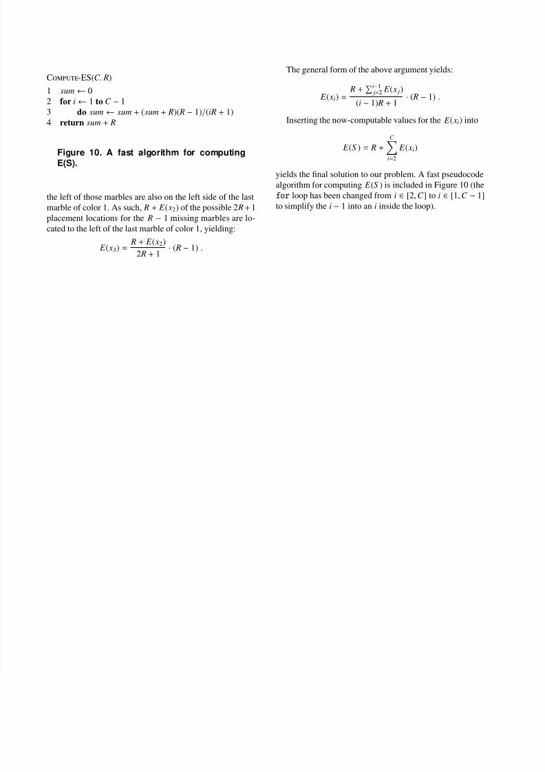
C-ES(C , R)

1 sum ← 0

2 for i ← 1 to C − 1

3 do sum ← sum + (sum + R)( R − 1)/(iR + 1)

4 return sum + R

Figure 10. A fast algorithm for computingE(S).

the left of those marbles are also on the left side of the last

marble of color 1. As such, R + E ( x2) of the possible 2 R+1

placement locations for the R − 1 missing marbles are lo-

cated to the left of the last marble of color 1, yielding:

E ( x3) =R + E ( x2)

2 R + 1· ( R − 1) .

The general form of the above argument yields:

E ( xi) = R +i−1

j=2 E ( x j)

(i − 1) R + 1· ( R − 1) .

Inserting the now-computable values for the E ( xi) into

E (S ) = R +

C

i=2

E ( xi)

yields the final solution to our problem. A fast pseudocode

algorithm for computing E (S ) is included in Figure 10 (the

for loop has been changed from i ∈ [2,C ] to i ∈ [1,C − 1]

to simplify the i − 1 into an i inside the loop).

Documents

Army of Botnets