Artery active mechanical response: High order finiteelement implementation and investigation

Zohar Yosibash∗ and Elad Priel1

Dept. of Mechanical Engrg., Ben-Gurion Univ. of the Negev, Beer-Sheva, 84105, Israel

Abstract

The active mechanical response of an artery wall resulting from the contraction of thesmooth muscle cells (SMCs) is represented by a strain energyfunction (SEDF) that aug-ments the passive SEDF recently reported in Yosibash Z. and Priel E., “p-FEMs for hyper-elastic anisotropic nearly incompressible materials under finite deformations with applica-tions to arteries simulation”,Int. Jour. Num. Meth. Eng., 88:11521174, 2011. The passive-active hyperelastic, anisotropic, nearly-incompressible problem is solved using high-orderfinite element methods (p-FEMs). A new iterative algorithm, named “p-prediction”, isintroduced that accelerates considerably the Newton-Raphson algorithm when combinedwith p-FEMs. Verification of the numerical implementation is conducted by comparisonto problems with analytic solutions and the advantages ofp-FEMs are demonstrated byconsidering both degrees of freedom and CPU.

The passive and active material parameters are fitted to bi-axial inflation-extension testsconducted on rabbit carotid arteries reported in Wagner H.P. and Humphrey J.D., “Differen-tial passive and active biaxial mechanical behavior of muscular and elastic arteries: Basilarversus common carotid”,Jour. Biomech. Eng., 133, 2011. Article number: 051009. Ourstudy demonstrates that the proposed SEDF is capable of describing the coupled passive-active response as observed in experiments. Artery-like structures are thereafter investi-gated and the effect of the activation level on the stress anddeformation are reported. Theactive contribution reduces overall stress levels across the artery thickness and along theartery inner boundary.

Keywords: active response; p-FEM; artery; anisotropic Neo-Hooke material; hy-perelasticity

∗ Corresponding author: zohary@bgu.ac.il1 Equal contribution

Preprint submitted to Elsevier Science 9 May 2012

1 INTRODUCTION

Artery walls are anisotropic and nearly incompressible andconsist of two main thinlayers made of an elastin matrix embedded with stiff collagen fibers and smoothmuscle cells (SMCs). In addition to the passive mechanical response due to theelastin and collagen fibers (well investigated in past studies), the SMCs contract inresponse to chemical stimulus thereby augment the passive response. Experimentsshow that the amount of tension generated by the SMCs is a function of the concen-tration of the chemical stimulus (does-tension relation) and the amount of stretchexerted on the muscle fiber (tension-stretch relation) [1].

Artery walls are considered as being hyperelastic, thus a strain energy density func-tion (SEDF) is sought which determines the constitutive equation (stress-strain re-lationship). Numerous studies propose different SEDFs forthe passive mechanicalresponse [2,3,4]. Some are phenomenological based, so the SEDFs are formulatedto result in a stress-strain response that mimics the experimentally observed re-sponse [2], or semi-structural [5,6] in which some terms in the SEDF are related tothe tissue microstructure. A fully-structural model, in which each component of theartery wall is modeled, individually, best describes the overall passive response, seee.g. the recent work by Hollander et al. [6]. However, fully structural models arevery difficult to formulate because they require knowledge of arterial microstruc-ture which is in most cases unavailable. Therefore, semi-structural models are pre-ferred, and herein we modify the semi-structuralincompressiblehyperelastic SEDFby Holzapfel et. al [5] for the passive part of the artery-wall response.

The active response and its numerical treatment were scarcely addressed in pastpublications comparing to publications on the passive response. One of the earlyworks on the subject is by Rachev&Hayashi [7] in which the SMCs contributionwas considered by an additional term to the Cauchy stress in the circumferential di-rection. The magnitude of the added stress depends on the chemical concentrationand the circumferential stretch ratio. There, no clear relation was provided betweenthe concentration of the stimulating chemical and the developed active stress. Thestudy showed that incorporation of SMCs resulted in a reduction of the circumfer-ential Cauchy stresses. The “added stress” proposed in [7] was utilized by Massonet al [8] to model the active response and to fit active material parameters fromin-vivo monitoring of the time dependent pressure responseof a human carotidartery, assuming as in [7], that the SMCs fibers were circumferentially oriented.A different functional representation for the added activestress was used by Wag-ner&Humphrey [9] for simulation of inflation-extension experiments on the basilarand common carotid arteries of New-Zealand white rabbits. The functional rep-resentation for tension-dose relation was more specific, enabling the modeling ofpartial SMCs contraction. An incompressible one-layer cylindrical tube-like arteryundergoing pure radial deformation (enabling an analytical solution to be obtained)was considered.

2

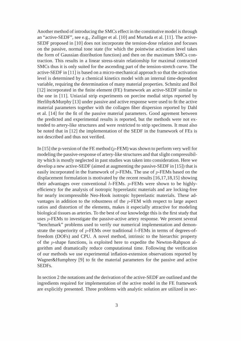
Another method of introducing the SMCs effect in the constitutive model is throughan “active-SEDF”, see e.g., Zulliger et al. [10] and Murtadaet al. [11]. The active-SEDF proposed in [10] does not incorporate the tension-doserelation and focuseson the passive, normal tone state (for which the pointwise activation level takesthe form of Gaussian distribution function) and then on the maximum SMCs con-traction. This results in a linear stress-strain relationship for maximal contractedSMCs thus it is only suited for the ascending part of the tension-stretch curve. Theactive-SEDF in [11] is based on a micro-mechanical approachso that the activationlevel is determined by a chemical kinetics model with an internal time-dependentvariable, requiring the determination of many material properties. Schmitz and Bol[12] incorporated in the finite element (FE) framework an active-SEDF similar tothe one in [11]. Uniaxial strip experiments on porcine medial strips reported byHerlihy&Murphy [13] under passive and active response wereused to fit the activematerial parameters together with the collagen fiber dispersion reported by Dahlet al. [14] for the fit of the passive material parameters. Good agrement betweenthe predicted and experimental results is reported, but themethods were not ex-tended to artery-like structures and were restricted to strip specimens. It must alsobe noted that in [12] the implementation of the SEDF in the framework of FEs isnot described and thus not verified.

In [15] the p-version of the FE method (p-FEM) was shown to perform very well formodeling the passive-response of artery-like structures and that slight compressibil-ity which is mostly neglected in past studies was taken into consideration. Here wedevelop a new active-SEDF (aimed at augmenting the passive-SEDF in [15]) that iseasily incorporated in the framework ofp-FEMs. The use ofp-FEMs based on thedisplacement formulation is motivated by the recent results [16,17,18,15] showingtheir advantages over conventionalh-FEMs. p-FEMs were shown to be highly-efficiency for the analysis of isotropic hyperelastic materials and are locking-freefor nearly incompressible Neo-Hook isotropic hyperelastic materials. These ad-vantages in addition to the robustness of thep-FEM with respect to large aspectratios and distortion of the elements, makes it especially attractive for modelingbiological tissues as arteries. To the best of our knowledgethis is the first study thatusesp-FEMs to investigate the passive-active artery response. We present several”benchmark” problems used to verify our numerical implementation and demon-strate the superiority ofp-FEMs over traditionalh-FEMs in terms of degrees-of-freedom (DOFs) and CPU. A novel method, intrinsic to the hierarchic propertyof the p-shape functions, is exploited here to expedite the Newton-Rahpson al-gorithm and dramatically reduce computational time. Following the verificationof our methods we use experimental inflation-extension observations reported byWagner&Humphrey [9] to fit the material parameters for the passive and activeSEDFs.

In section 2 the notations and the derivation of the active-SEDF are outlined and theingredients required for implementation of the active model in the FE frameworkare explicitly presented. Three problems with analytic solution are utilized in sec-

3

tion 3 to verify our numerical implementation and to investigate the performanceof thep- andh-FEMs. Fitting of passive and active model material parameters toexperiments is outlined in section 4. There we also investigate thep-FEM perfor-mance for a more realistic bi-layer artery-like structure.In section 5 we emphasizethe effect of the various active parameters on the artery wall. We summarize ourwork and draw several conclusions in section 6.

2 NOTATIONS AND IMPLEMENTATION OF AN ACTIVE-SEDF IN THEFRAMEWORK OF FEMs

The point of departure is a brief description of our notations for a fiber reinforcedhyper-elastic material. The basic quantity is the deformation gradientF = Grad x(X, t)= ∂xk(X1, X2, X3, t)/∂XKgi ⊗GK , wherex(X, t) defines the placement of thepointX at timet. XK , k = 1, 2, 3, are the material (reference) coordinates,gi arethe tangent andGK the gradient vectors in the current and the reference config-uration. Customary, the displacement vectorU(X, t)

def= (UX , UY , UZ)T is intro-

duced, i.e.x = X + U(X, t), and with this notationF = I + Grad U(X, t). WeinterchangeX1, X2, X3 with X, Y, Z when appropriate. A general strain-energydensity function (SEDF) for an isotropic hyperelastic material with two families offibers used to model the passive response is denoted by,ψpassive(C,M0,M 1) =Ψpassive(IC, IIC, III C, IVC,VIC), following Holzapfel et al. [5]. It depends on theinvariants of the right Cauchy-Green tensorC = F T F = (I + GradU)T (I + GradU),and two unit direction vectors along collagen fiber directionsM 0, andM 1. For ex-ample, using the Cartesian coordinate system in Figure 1, the fibers directions areM 0 = (sin β,− cosβ Y√

Y 2+Z2 , cosβ Z√Y 2+Z2 )

T , M 1 = (− sin β,− cosβ Y√Y 2+Z2 , cosβ Z√

Y 2+Z2 )T .

The invariants of the Cauchy-Green tensor are

Fig. 1. Coordinate system in a typical artery.

4

IC = trC, IIC =1

2((trC)2 − trC2), III C = det C = (det F )2 def

= J2,

(1)wheretrC symbolizes the trace operator and the invariants that represent stretch inthe fiber directions are

IVC = M 0 · C · M 0, VIC = M 1 · C · M 1, (2)

Following [5] we consider a strain-energy density functioncomposed of three partsfor modeling the passive response, an isochoric isotropic and a volumetric isotropicNeo-Hook parts representing the elastic matrix, and a transversely isotropic partrepresenting the collagen fibers in the artery wall

Ψpassive(IC, III C, IVC,VIC) = [Ψisoch(IC, III C) + Ψvol(III C)]+Ψfibers(IVC,VIC),(3)

The isochoric isotropic and volumetric isotropic parts arerepresented by a nearlyincompressible Neo-Hookean SEDF:

Ψisoch = c1(ICIII −1/3C

− 3), Ψvol =1

D1(III 1/2

C− 1)2 (4)

c1 andD1 are constants related to the shear modulusµ and to the bulk modulusκ

c1 =µ

2, D1 =

2

κ. (5)

The transversely isotropic part for modeling the collagen fiber contribution is [19]:

Ψfibers =k1

2k2

[

exp[

k2 (IVC − 1)2]

− 1]

(6)

+k1

2k2

[

exp[

k2 (VIC − 1)2]

− 1]

, IVC,VIC ≥ 1

Remark 1 In some publicationsΨfibers is expressed in terms of the invariantsof the unimodular right Cauchy-Green tensorC = (det C)−1/3C, i.e., IV

C=

IVCIII −1/3C

, VIC

= VICIII −1/3C

(see [5]). This representation is inappropriate be-cause no stresses are generated when an unimodular deformation is prescribedresulting in a homogeneous deformation that stretches the collagen fibers.

For modeling the active response we construct a SEDF based on[7]. The first Piola-Kirchhoff stress component due to SMCs contraction was found to be proportionalto the concentration of the vasoconstrictor[A], as well as the stretch ratio in theSMCs-fibers directionMMF , denoted byλf :

P activeff = S([A])f(λf) (7)

whereS([A]) is the tension-dose relationship andf(λf) is the tension-stretch rela-tion. The tension-dose relationship is usually available from ring-tests, as given for

5

example in [1], so that:

S([A]) = Smax[A]m

[A]m + ECm50

(8)

wherem is the slope parameter,Smax the maximum value of contraction (saturationlevel) andEC50 is the concentration at which50% of maximum generated tensionis obtained. In Figure 2 a representative tension-dose relation is presented. It shows

Fig. 2. Representative tension-dose relation usingEC50 = 0.000015 [mol/liter], m = 1taken from [1] andSmax = 100 kPa taken from [7].

that under a vasoconstrictor threshold concentration no induced active response isgenerated and on the other end the active response reaches a saturation level beyonda given vasoconstrictor concentration.

The tension-stretch relation is adopted from the work by Rachev&Hayashi [7], seee.g. Figure 11:

f(λf) =

[

1 −(

λm−λf

λm−λ0

)2]

, λ1 > λf > λ0

0, Otherwise(9)

with λm being the stretch at which maximum contraction is possible and λ0 andλ1 = λ0+2(λm−λ0) being the minimum and maximum stretches at which contrac-tion can be generated. This relationship is obtained from experiments at saturationlevels so forλm:

P activeff = Smax (10)

Inserting (8) and (9) in (7) one obtains:

P activeff =

Smax[A]m

[A]m+ECm50

[

1 −(

λm−λf

λm−λ0

)2]

, λ1 > λf > λ0

0, Otherwise(11)

6

Remark 2 The expression given in(11) results in different active stress values forthe same chemical concentration provided that the SMCs are under different stretchratios as demonstrated in experiments [13].

Defining the direction of the SMCs after deformation asmMF , one can computeλf from the initial fiber direction and the right Cauchy-Green deformation tensor,see [20, (6.200)]:

λ2f = (mMF )T · (mMF ) = (FMMF )T · (FMMF ) = MMF · (CMMF ) = IVMF

C

(12)Assuming the existence of an active-SEDFΨactive, the first Piola-Kirchhoff stressin the SMC-fiber direction can be derived directly from the SEDF [20, (16.47)]:

P activeff =

∂ψactive

∂λf(13)

Inserting (11) in (13) then integrating, on may obtain an expression forψactive:

ψactive(λf , [A]) =

Smax[A]m

[A]m+ECm50

[

(λm−λf )3

3(λm−λ0)2+ λf

]

, λ1 > λf > λ0

0, Otherwise(14)

Substituting (12) in (14), a general form of the active-SEDFis obtained:

Ψactive(IVMFC

, [A]) =

Smax[A]m

[A]m+ECm50

[

(λm−√

IVMFC

)3

3(λm−λ0)2+√

IVMFC

]

, λ21 > IVMF

C> λ2

0

0, Otherwise(15)

The dependency ofΨactive on IVMFC

assures that the active stress is in the SMCsdirection only, with zero components perpendicular to it. In Appendix A we demon-strate that for the incompressible case(J = 1) the SEDF (15) results in the Cauchystress term for the active response given in [7], even if the deformation of the tissueis not in the SMC fiber direction.

The passive-active SEDF is the sum of the passive and active SEDFs:

Ψtissue = Ψpassive + Ψactive (16)

For the purposes of implementation in a finite element code itis necessary to obtainexpressions for the second- Piola- Kirchhoff stressS and the elasticity tensorC =∂S

∂C. In [15] explicit expressions forSpassive andCpassive are provided. Using (15)

one obtains explicit expressions for the active componentsrequired.

Sactive = Smax[A]m

[A]m + ECm50

(

IVMFC

)− 12

1 −

λm −√

IVMFC

λm − λ0

2

[

MMF ⊗ MMF

]

(17)

7

Cactive =Smax[A]m

[A]m + ECm50

2(

IVMFC

)−1 (λm −√

IVMFC

)

(λm − λ0)2(18)

−(

IVMFC

)− 32

1 −

λm −√

IVMFC

λm − λ0

2

[

MMF ⊗ MMF

] [

MMF ⊗ MMF

]

The expressions forSactive andCactive are necessary for the ”tangent stiffness ma-trix” and ”out of balance” vector at each Newton-Raphson iteration used in the FEframework:

S = Spassive + Sactive, C = Cpassive + Cactive (19)

3 VERIFICATION OF THE IMPLEMENTATION

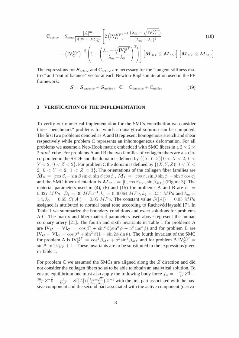
To verify our numerical implementation for the SMCs contribution we considerthree ”benchmark” problems for which an analytical solution can be computed.The first two problems denoted as A and B represent homogenousstretch and shearrespectively while problem C represents an inhomogeneous deformation. For allproblems we assume a Neo-Hook matrix embedded with SMC fibersin a 2 × 2 ×2 mm3 cube. For problems A and B the two families of collagen fibers are also in-corporated in the SEDF and the domain is defined by(X, Y, Z)| 0 < X < 2, 0 <Y < 2, 0 < Z < 2. For problem C the domain is defined by(X, Y, Z)| 0 < X <2, 0 < Y < 2, 1 < Z < 3. The orientations of the collagen fiber families areM 0 = [cosβ,− sin β sin φ, sinβ cosφ], M 1 = [cosβ, sin β sin φ,− sinβ cosφ]and the SMC fiber orientation isMMF = [0, cosβMF , sin βMF ] (Figure 3). Thematerial parameters used in (4), (6) and (15) for problems A and B arec1 =0.027 MPa, D1 = 30 MPa−1, k1 = 0.00064 MPa, k2 = 3.54 MPa andλm =1.4, λ0 = 0.65, S([A]) = 0.05 MPa. The constant valueS([A]) = 0.05 MPaassigned is attributed to normal basal tone according to Rachev&Hayashi [7]. InTable 1 we summarize the boundary conditions and exact solutions for problemsA-C. The matrix and fiber material parameters used above represent the humancoronary artery [21]. The fourth and sixth invariants in Table 1 for problems Aare IVC = VIC = cos β2 + sin2 β(sin2 φ + a2 cos2 φ) and for problem B areIVC = VIC = cosβ2 + sin2 β(1 − sin 2φ sin θ). The fourth invariant of the SMCfor problem A is IVMF

C= cos2 βMF + a2 sin2 βMF and for problem B IVMF

C=

sin θ sin 2βMF + 1 . These invariants are to be substituted in the expressions givenin Table 1.

For problem C we assumed the SMCs are aligned along theZ direction and didnot consider the collagen fibers so as to be able to obtain an analytical solution. Toensure equilibrium one must also apply the following body forcefZ = −4c1

18Z

43 −

20c118Z− 7

3 − 1D1Z

− S([A])(

λm−√

Zλm−λ0

)

Z−1 with the first part associated with the pas-sive component and the second part associated with the active component (deriva-

8

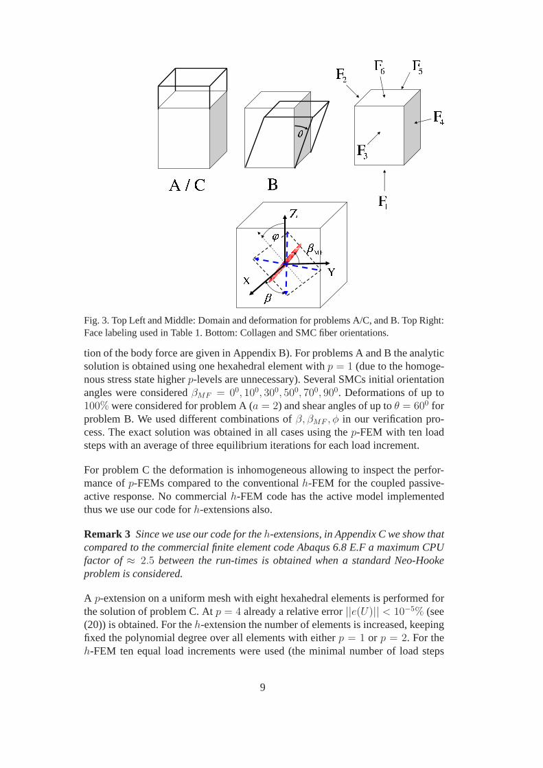
Fig. 3. Top Left and Middle: Domain and deformation for problems A/C, and B. Top Right:Face labeling used in Table 1. Bottom: Collagen and SMC fiber orientations.

tion of the body force are given in Appendix B). For problems Aand B the analyticsolution is obtained using one hexahedral element withp = 1 (due to the homoge-nous stress state higherp-levels are unnecessary). Several SMCs initial orientationangles were consideredβMF = 00, 100, 300, 500, 700, 900. Deformations of up to100% were considered for problem A (a = 2) and shear angles of up toθ = 600 forproblem B. We used different combinations ofβ, βMF , φ in our verification pro-cess. The exact solution was obtained in all cases using thep-FEM with ten loadsteps with an average of three equilibrium iterations for each load increment.

For problem C the deformation is inhomogeneous allowing to inspect the perfor-mance ofp-FEMs compared to the conventionalh-FEM for the coupled passive-active response. No commercialh-FEM code has the active model implementedthus we use our code forh-extensions also.

Remark 3 Since we use our code for theh-extensions, in Appendix C we show thatcompared to the commercial finite element code Abaqus 6.8 E.Fa maximum CPUfactor of ≈ 2.5 between the run-times is obtained when a standard Neo-Hookeproblem is considered.

A p-extension on a uniform mesh with eight hexahedral elementsis performed forthe solution of problem C. Atp = 4 already a relative error||e(U)|| < 10−5% (see(20)) is obtained. For theh-extension the number of elements is increased, keepingfixed the polynomial degree over all elements with eitherp = 1 or p = 2. For theh-FEM ten equal load increments were used (the minimal numberof load steps

9

required for convergence) and up to four equilibrium iterations were required foreach load step.

For thep-FEM we use a novel iterative scheme denoted “p-prediction”. In this casefor p = 1 the regular Newton-Raphson iterative algorithm is used. For a nearly-incompressible material, since thep-FEM encounters locking untilp = 4, then thefirst p-FE solution starts atp = 4 by a regular Newton-Raphson algorithm. Forp ≥ 2 (andp ≥ 5 for a nearly incompressible material), the converged solution atp− 1 is used as the ”initial guess” to the iterative algorithm, sothat the entire loadis not sub-divided in sub-loads. This results in a very fast convergence, usually withone load step. The “p-prediction” algorithm is shown in Figure 4.

Fig. 4. The “p-prediction” algorithm.

To verify the numerical results we consider both global and pointwise values. Theperformance ofp- andh-FEMs is demonstrated by inspecting the convergence of

10

the relative error in energy norm [22] .

||e(U)||(%) =

√

√

√

√

∫

Ω Ψ(C)dΩFE − ∫

Ω Ψ(C)dΩExact∫

Ω Ψ(C)dΩExact

× 100 (20)

and pointwise by inspecting the convergence ofUz andσzz, σxx at points A and B(see Figure 5). In Figure 6 the convergence in the relative error in strain energy as

Fig. 5. Mesh used for problem C. Left: Uniform mesh for thep-FEM and points A and B.Right: Example of an uniform mesh for theh-FEM (2744 elements).

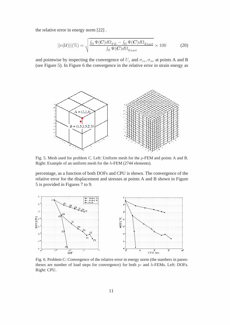
percentage, as a function of both DOFs and CPU is shown. The convergence of therelative error for the displacement and stresses at points Aand B shown in Figure5 is provided in Figures 7 to 9.

Fig. 6. Problem C: Convergence of the relative error in energy norm (the numbers in paren-theses are number of load steps for convergence) for bothp- andh-FEMs. Left: DOFs.Right: CPU.

11

Fig. 7. Problem C: Convergence inUZ for point A=(2,2,3) (top) and pointB=(1.5,1.5,2.5)(bottom).

Fig. 8. Problem C: Convergence inσzz for point A=(2,2,3) (top) and point B=(1.5,1.5,2.5)(bottom).

As evident from Figures 6 to 9 thep-FEM is considerably more efficient for solv-ing the passive-active mechanical response especially when computations of stressvalues are of interest.

12

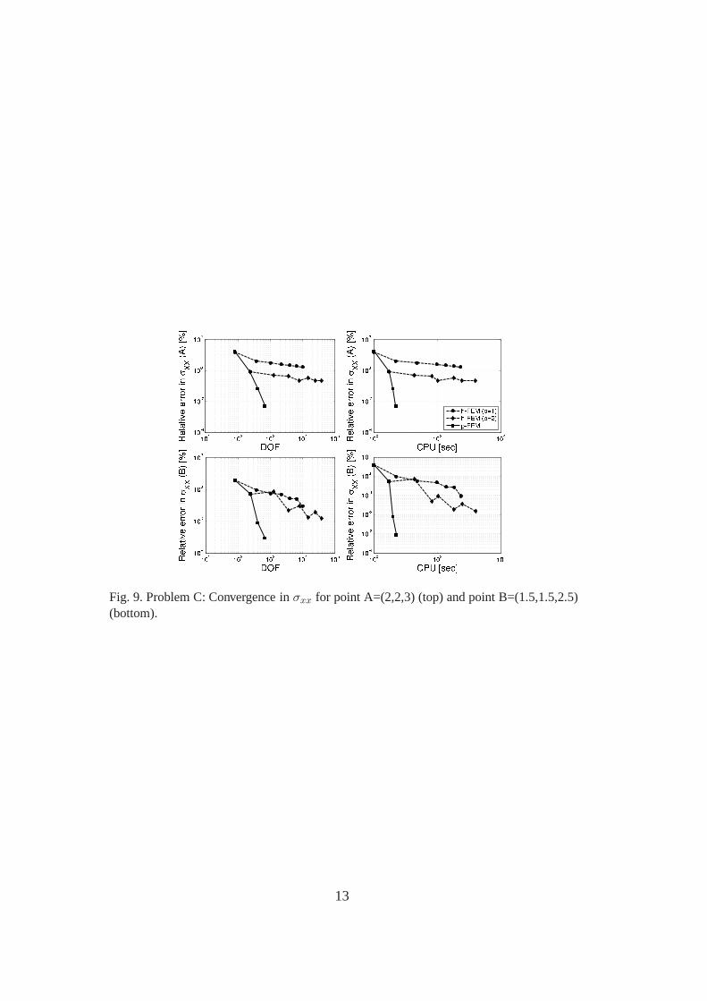
Fig. 9. Problem C: Convergence inσxx for point A=(2,2,3) (top) and point B=(1.5,1.5,2.5)(bottom).

13

Table 1. Tractions and exact solution for problem A.Problem Ω0 Boundary conditions applied to faces F1-F6 Solution

F1 : uX = uY = uZ = 0

0 ≤ X ≤ 2 F2 : tY = −[

23c1

(

a−2

3 − a4

3

)

+ 2D1

(

a2 − a)

−4k1 [IVC − 1] ×(

sin2 β cos φ sinφ)

expk2(IVC−1)2

+S([A])(

IVMFC

)

−1

2

(

1 −

(

λm−

√

IVMF

C

λm−λ0

)2)

cos2 βMF

]

x = X, y = Y, z = aZ

tZ = −[

4k1 [IVC − 1] ×(

sin2 β cos2 φ)

expk2(IVC−1)2

+S([A]) · a(

IVMFC

)

−1

2

(

1 −

(

λm−

√

IVMF

C

λm−λ0

)2)

cos βMF sin βMF

]

A 0 ≤ Y ≤ 2 F3 : tX = 23c1

(

a−2

3 − a4

3

)

+ 2D1

(

a2 − a)

uX = 0

+4k1 [IVC − 1] ×(

cos2 β)

expk2(IVC−1)2

0 ≤ Z ≤ 2 F4 : tY = 23c1

(

a−2

3 − a4

3

)

+ 2D1

(

a2 − a)

+4k1 [IVC − 1] ×(

sin2 β cos φ sinφ)

expk2(IVC−1)2

+S([A])(

IVMFC

)

−1

2

(

1 −

(

λm−

√

IVMF

C

λm−λ0

)2)

cos2 βMF

)

uY = 0

tZ =[

4k1 [IVC − 1] ×(

sin2 β cos2 φ)

expk2(IVC−1)2

+S([A]) · a(

IVMFC

)

−1

2

(

1 −

(

λm−

√

IVMF

C

λm−λ0

)2)

cos βMF sin βMF

F5 : tX = −(

23c1

(

a−2

3 − a4

3

)

+ 2D1

(

a2 − a)

)

uZ = Z(a − 1)

−4k1 [IVC − 1] ×(

cos2 β)

expk2(IVC−1)2

F6 : tZ = 43c1

(

a1

3 − a5

3

)

+ 2D1

(a − 1)

+4k1 [IVC − 1] ×(

sin2 β cos2 φ)

expk2(IVC−1)2

+S([A])a(

IVMFC

)

−1

2

(

1 −

(

λm−

√

IVMF

C

λm−λ0

)2)

sin2 βMF

)

tY = −4k1a [IVC − 1] ×(

sin2 β cos φ sinφ)

expk2(IVC−1)2

−S([A])(

IVMFC

)

−1

2

(

1 −

(

λm−

√

IVMF

C

λm−λ0

)2)

cos βMF sinβMF

14

Continuation of Table 1: Tractions and exact solution for problem B.Problem Ω0 Boundary conditions applied to faces F1-F6 Solution

F1 : uX = uY = uZ = 0

F2 : tY = −(

2c1

(

cos−2

3 (θ) − cos−8

3 (θ)(1 + sin2(θ))

)

+ 2D1

(

sin(θ)cos(θ)

− sin(θ) + cos(θ) − 1)

)

x = X, y = Y + Zsin(θ)

+4k1 [IVC − 1] × ek2(IVC−1)2 sin2 β[

sin2 φ − sin θ sin φ cos φ]

+S([A])(

IVMFC

)

−1

2

(

1 +

(

λm−

√

IVMF

C

λm−λ0

)2)

[

cos2 βMF + sin θ sinβMF cos βMF

]

)

z = Zcos(θ)

tZ = −2c1

(

cos−8

3 (θ)sin(θ) + cos1

3 (θ) − cos−5

3 (θ)

)

+ 2D1

(

sin(θ)cos(θ)

− sin(θ) + cos(θ) − 1)

−4k1 [IVC − 1] sin2 β sinφ cos φ cos θ × expk2(IVC−1)2

0 ≤ X ≤ 2 +S([A])(

IVMFC

)

−1

2

(

1 +

(

λm−

√

IVMF

C

λm−λ0

)2)

cos θ cos βMF sin βMF

)

uX = 0

B 0 ≤ Y ≤ 2 F3 : tX = 2D1

(

cos2(θ) − cos(θ))

+ 4k1 [IVC − 1] cos2 β × expk2(IVC−1)2 uY = Zsin(θ)

0 ≤ Z ≤ 2 F4 : tY = 2c1

(

cos−2

3 (θ) − cos−8

3 (θ)(1 + sin2(θ))

)

+ 2D1

(

1 − cos−1(θ) + sin2(θ)(cos−1(θ) − 1))

uZ = Z(cos(θ) − 1)

+4k1 [IVC − 1] × ek2(IVC−1)2 sin2 β[

sin2 φ − sin θ sin φ cos φ]

+S([A])(

IVMFC

)

−1

2

(

1 +

(

λm−

√

IVMF

C

λm−λ0

)2)

[

cos2 βMF + sin θ sin βMF cos βMF

]

)

tZ = 2c1

(

cos−8

3 (θ)sin(θ) + cos1

3 (θ) − cos−5

3 (θ))

)

+ 2D1

(

sin(θ)cos(θ)

− sin(θ) + cos(θ) − 1))

−4k1 [IVC − 1] sin2 β sinφ cos φ cos θ × expk2(IVC−1)2

+S([A])(

IVMFC

)

−1

2

(

1 +

(

λm−

√

IVMF

C

λm−λ0

)2)

cos θ cos βMF sin βMF

)

F5 : tX = −(

2D1

(

cos2(θ) − cos(θ)))

− 4k1 [IVC − 1] cos2 β × expk2(IVC−1)2

F6 : tZ = 2c1

(

cos1

3 (θ) − cos−5

3 (θ)

)

+ 2D1

(cos(θ) − 1)

4k1 [IVC − 1] sin2 β sin2 φ cos θ × expk2(IVC−1)2

+S([A])(

IVMFC

)

−1

2

(

1 +

(

λm−

√

IVMF

C

λm−λ0

)2)

cos θ sin2 βMF

)

tY = 2c1cos−5

3 (θ)sin(θ) + 2D1

(sin(θ) − cos(θ)sin(θ))

−4k1 [IVC − 1] sin2 β sinφ cos φ cos θ × expk2(IVC−1)2

+S([A])(

IVMFC

)

−1

2

(

1 +

(

λm−

√

IVMF

C

λm−λ0

)2)

[

sin θ sin2 βMF + sin βMF cos βMF

]

)

15

Continuation of Table 1: Tractions and exact solution for problem C.Problem Ω0 Boundary conditions applied to faces F1-F6 Solution

F1 : uX = uY = uZ = 0

0 ≤ X ≤ 2 F2 : tY = −(

23c1

(

Z−2

6 − Z4

6

)

+ 2D1

(

Z −√

Z)

)

x = X, y = Y, z = 23Z

3

2 + 13

C 0 ≤ Y ≤ 2 F3 : tX = 23c1

(

Z−2

6 − Z4

6

)

+ 2D1

(

Z −√

Z)

uX = 0

1 ≤ Z ≤ 3 F4 : tY = 23c1

(

Z−2

6 − Z4

6

)

+ 2D1

(

Z −√

Z)

uY = 0

F5 : tX = −(

23c1

(

Z−2

6 − Z4

6

)

+ 2D1

(

Z −√

Z)

)

uZ = 23Z

3

2 − Z + 13

F6 : tZ = 43c1

(

Z1

6 − Z5

6

)

+ 2D1

(√Z − 1

)

+ S([A])

(

1 +

(

λm−

√

Zλm−λ0

)2)

16

4 FITTING MATERIAL PARAMETERS TO INFLATION-EXTENSIONEXPERIMENTS

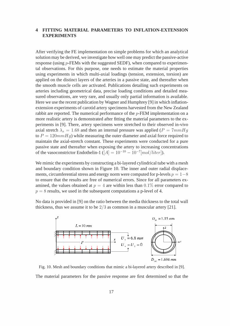
After verifying the FE implementation on simple problems for which an analyticalsolution may be derived, we investigate how well one may predict the passive-activeresponse (usingp-FEMs with the suggested SEDF), when compared to experimen-tal observations. For this purpose, one needs to estimate the material propertiesusing experiments in which multi-axial loadings (tension,extension, torsion) areapplied on the distinct layers of the arteries in a passive state, and thereafter whenthe smooth muscle cells are activated. Publications detailing such experiments onarteries including geometrical data, precise loading conditions and detailed mea-sured observations, are very rare, and usually only partialinformation is available.Here we use the recent publication by Wagner and Humphrey [9]in which inflation-extension experiments of carotid artery specimens harvested from the New Zealandrabbit are reported. The numerical performance of thep-FEM implementation on amore realistic artery is demonstrated after fitting the material parameters to the ex-periments in [9]. There, artery specimens were stretched totheir observed in-vivoaxial stretchλx = 1.68 and then an internal pressure was applied (P = 7mmHgtoP = 120mmHg) while measuring the outer diameter and axial force required tomaintain the axial-stretch constant. These experiments were conducted for a purepassive state and thereafter when exposing the artery to increasing concentrationsof the vasoconstrictor Endothelin-1 ([A] = 10−10 − 10−7[mol/liter]).

We mimic the experiments by constructing a bi-layered cylindrical tube with a meshand boundary condition shown in Figure 10. The inner and outer radial displace-ments, circumferential stress and energy norm were computed for p-levelsp = 1−8to ensure that the results are free of numerical errors. Since for all parameters ex-amined, the values obtained atp = 4 are within less than0.1% error compared top = 8 results, we used in the subsequent computations a p-level of4.

No data is provided in [9] on the ratio between the media thickness to the total wallthickness, thus we assume it to be2/3 as common in a muscular artery [21].

Fig. 10. Mesh and boundary conditions that mimic a bi-layered artery described in [9].

The material parameters for the passive response are first determined so that the

17

outer diameter and axial force measured correspond to the ones computed whenthe pre-stretch is applied and internal pressure is increased. The compressibilityparameterD1 is determined by assuming that under physiological pressure, therelative change of volume is≈ 1% as reported in [23] for the rabbit aorta. Thefitted material properties for the passive response are provided in Table 2 and thecomparison between the predicted response and the experimental observations isdepicted in Figure 12 by the solid line.

Table 2Material parameters fitted to a slightly compressible passive SEDF.

Layer c1 D1 k1 k2 βM

[MPa] [MPa−1] [MPa] [0]

Media 0.01 3 0.0006 1.2 ±20

Adventitia 0.005 3 0.0004 1.2 ±64

To determine the active material parameters we fitted the data for the tension-stretchand tension-dose relationship reported in [9] as presentedin Figure 11. These pa-rameters are summarized in Table 3.Table 3Material parameters fitted to the coupled passive-active SEDF.

λm λ0 Smax m EC50

[MPa] [mol/liter]

1.49 0.85 0.045 5.9 10−10

Neither the density nor the orientation of SMCs is available, thus we assumed thatthese are uniformly distributed so a similar active response is obtained in the entireartery and that SMC are oriented circumferentially, i.e.βMF = 0. With these as-sumptions, and using the already determined passive and active material properties,we predict the pressure-diameter and pressure-axial forceresponse when the arteryis activated by a vasoconstrictor. In Figure 12 we present the predicted response ascompared to the experimental observations extracted from [9] for different inter-nal pressures and a given axial stretch ofλx = 1.68. The axial force is computedby the integral of the Cauchy stress over the deformed cross section area of theartery. One may observe that the passive-active predicted response is close to theexperimental observations. However, below a pressure of about 40 mmHg in thepassive state, and70 mmHg in the active state, an unclear phenomenon in the ex-perimental observations is visible, namely, the axial force increases as the pressuredecreases. This phenomenon in the experimental observations in [9] is unclear tous and cannot be explained by the proposed SEDF.

An important experimental observation associated with theactive response of theSMCs is the phenomenon of reduced contraction (at a fixed concentration of the

18

Fig. 11. Fitting of tension-stretch and tension-dose relationships: Circles - experimentalresults extracted from [9], Squares - fitted data using (9) and (8).

vasoconstrictor) beyond a given stretch ratio (λm). This observation is clearly shownby Herlihy&Murphy [13]. There uniaxial tension experiments of stimulated stripsharvested from the media layer of the swine carotid artery are reported. In AppendixD we demonstrate that our analyses simulate well this phenomena.

4.1 Verification of thep − FE implementation on a representative bi-layeredartery

Using the fitted material parameters given in Tables 2 and 3 weconsider the bi-layered artery having the dimensions and boundary conditions as in Figure 10.Since we only considerβMF = 0, a circumferential segment can be used, and we

19

Fig. 12. Comparison of the predicted and experimental observed response of a New Zealandrabbit carotid artery in passive and passive-active statesreported in [9]. Left: Diameter–pressure response atX = 5 mm for a constantλx = 1.68. Right: Pressure-axial forceresponse.

chose one fourth with appropriate symmetry boundary conditions. A physiolog-ical pressure ofP = 100mmHg is applied on the internal surface and a SMCactivation caused by a vasoconstrictor concentration[A] = 10 · 10−11. A ”bench-mark” solution is obtained by solving the problem using240 hexahedral elements(4 × 6 × 10 in θ, R,X directions) andp = 8. The convergence in energy normfor the ”benchmark” solution is given in Figure 13. The problem is solved also

Fig. 13. Convergence in energy norm forp = 1 to 7 in comparison to the benchmarksolution atp = 8.

by h-extension and p-extension with and without the p-prediction algorithm. Incase of h-extension meshes with12, 150, 300, 480, 1200, 4800 elements were used,whereas for p-extensions we use a coarse mesh, see Figure 14.For both theh-FEMandp-FEM without p-prediction, the load was applied in thirty equal load steps.In Figures 1516 and 17 the convergence in energy norm, radialdisplacement and

20

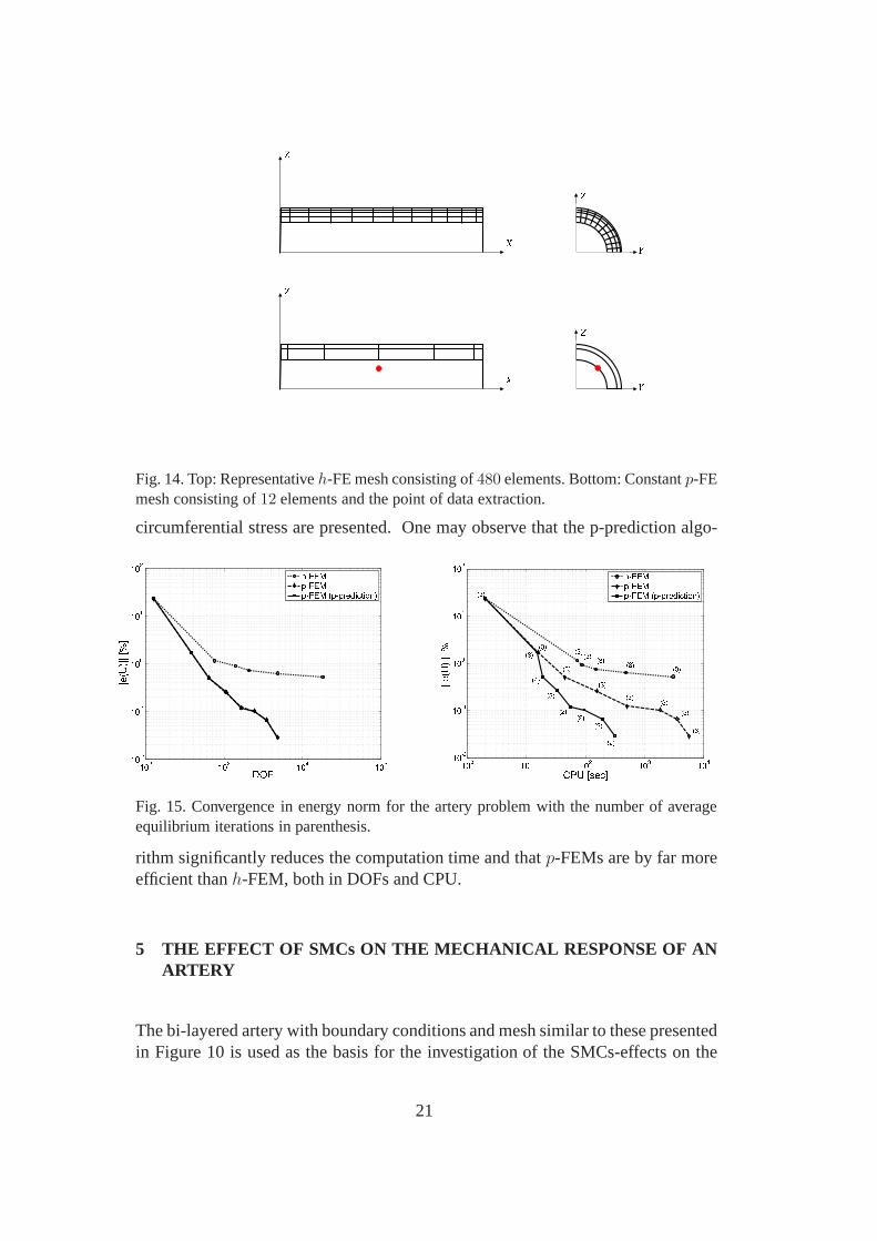
Fig. 14. Top: Representativeh-FE mesh consisting of480 elements. Bottom: Constantp-FEmesh consisting of12 elements and the point of data extraction.

circumferential stress are presented. One may observe thatthe p-prediction algo-

Fig. 15. Convergence in energy norm for the artery problem with the number of averageequilibrium iterations in parenthesis.

rithm significantly reduces the computation time and thatp-FEMs are by far moreefficient thanh-FEM, both in DOFs and CPU.

5 THE EFFECT OF SMCs ON THE MECHANICAL RESPONSE OF ANARTERY

The bi-layered artery with boundary conditions and mesh similar to these presentedin Figure 10 is used as the basis for the investigation of the SMCs-effects on the

21

Fig. 16. Convergence in radial displacement at the point of interest for the artery problem.

Fig. 17. Convergence in circumferential Cauchy stress at the point of interest for the arteryproblem.

mechanical response. The material parameters are those in Tables 2 and 3 and theSMCs are assumed to be oriented in the circumferential direction βMF = 0. To in-vestigate the effect of the vasoconstrictor concentrationlevels we increase[A] froma pure passive state until saturation level[A] = 10 ·10−12, [A] = 8.3×10−11, 10×10−11, 12 × 10−11, 10 × 10−8[mol/liter]. The activation levels chosen representvalues of0, 25, 50, 75, 100% on the tension-dose curve (Figure 11). To investigatethe effect of the tension-stretch relation we fix the vasoconstrictor concentration at[A] = 10 ·10−11 and investigate different pressure values in the physiological rangeP = 80, 100, 120 mmHg. In all cases the radial displacement and circumferen-tial Cauchy stress across the artery wall thickness (atX = 5 mm) are computed.In Figure 18 the effect of increased activation level on the circumferential stressand stretch ratio is shown. The dashed vertical line in Figure 18-Top represents themedia-adventitia-interface, whereas the horizontal dashed line in 18-Bottom rep-resents the value ofλm = 1.49. Figure 18 demonstrates that an increase in theconcentration of the vasoconstrictor results in the ”flattening” of the stress distribu-tion across the artery wall. One may observe a decrease in thecircumferential stressat the inner boundary of the media and an increase at the outerboundary of the me-

22

Fig. 18. Top: Circumferential Cauchy stress distribution across artery wall for differentSMCs activation levels andβMF = 00, P = 100 mmHg. Bottom: Stretch ratio across theartery wall atX = 5 for different SMC activation levels, with tension-stretchrelationshippresented in the inner caption.

dia and across the adventitia. The contraction is inhomogeneous across the arterythickness due to the circumferential stretch ratios (in theSMC direction). In Figure18-Bottom atR = 0.63 − 0.67 mm a transition for all activation levels occurs,so that the circumferential stretch ratio which is initially greater thenλm decreasesbellowλm. Since at the boundary of the inner mediaλθ > λm, then as the stretch ra-tio decreases across the artery wall the effect of SMC contraction increases. Once apoint is reached in the artery wall wereλθ = λm any further decrease inλθ resultsin a decrease in the effect of SMC contraction. In Figure 19 the Cauchy stressesacross the artery thickness forβMF = 00 andA = 10 × 10−11[mol/liter] fordifferent pressures are shown. Figure 19 demonstrates thateven under a constantactivation level the SMC contraction is inhomogeneous across the artery thicknessas a result of the different stretch ratios induced on the SMCs.

23

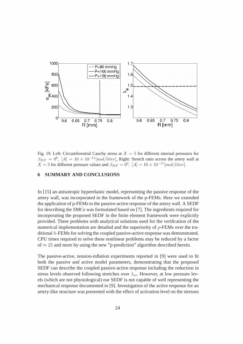
Fig. 19. Left: Circumferential Cauchy stress atX = 5 for different internal pressures forβMF = 00, [A] = 10 × 10−11[mol/liter], Right: Stretch ratio across the artery wall atX = 5 for different pressure values andβMF = 00, [A] = 10 × 10−11[mol/liter].

6 SUMMARY AND CONCLUSIONS

In [15] an anisotropic hyperelastic model, representing the passive response of theartery wall, was incorporated in the framework of the p-FEMs. Here we extendedthe application of p-FEMs to the passive-active response ofthe artery wall. A SEDFfor describing the SMCs was formulated based on [7]. The ingredients required forincorporating the proposed SEDF in the finite element framework were explicitlyprovided. Three problems with analytical solutions used for the verification of thenumerical implementation are detailed and the superiorityof p-FEMs over the tra-ditionalh-FEMs for solving the coupled passive-active response was demonstrated.CPU times required to solve these nonlinear problems may be reduced by a factorof ≈ 25 and more by using the new ”p-prediction” algorithm described herein.

The passive-active, tension-inflation experiments reported in [9] were used to fitboth the passive and active model parameters, demonstrating that the proposedSEDF can describe the coupled passive-active response including the reduction instress levels observed following stretches overλm. However, at low pressure lev-els (which are not physiological) our SEDF is not capable of well representing themechanical response documented in [9]. Investigation of the active response for anartery-like structure was presented with the effect of activation level on the stresses

24

and deformations.

Proper description of the mechanical response of the arterywall in-vivo requires theincorporation of SMCs contribution, because experimentalobservations demon-strate that their activation is notable [13]. Our proposed active SEDF, althoughphenomenological, incorporates the distinct features of SMCs contraction as ob-served in experiments (tension-dose and tension-stretch relationships), and requiresfive material parametersλ0, λm, EC50, Smax, m and one microstructural parameterβMF . The active response reduces significantly the circumferential stress distribu-tion across the artery thickness and along the artery length. The reduction in cir-cumferential stress value is not surprising and has been reported in [7] and [10] (inboth cases the tissue was assumed to be incompressible). Furthermore we observedthat for high activation levels the stress gradients acrossthe artery thickness mayincrease compared to moderate activation levels due to reduction of active stressgeneration at high stretches. On a side note, whenβMF > 00 for a constant stimu-lation level (not reported in this manuscript) the contraction forces which limit ar-terial inflation are reduced, enabling a greater arterial deformation which increasesactive stress generation as there is a ”climb” along the tension-stretch curve pro-vided thatλθ < λm. This results in an increase in both axial and circumferentialstress values for increasing values ofβMF .

Past studies [24,25] also suggested that the stress level may drive growth and re-modeling of the tissue to maintain homeostatic baseline stress values. Since wenoticed that SMCs contraction largely affects the stresses, these may have a largeeffect on growth and remodeling. This aspect will be investigated in a future study.

With respect to the tension-stretch curve it has been shown in several studies thatthe value ofλm differs greatly when different species are analyzed. In ourstudiesbased on [9] a value ofλm = 1.49 was determined for the carotid artery of theNew Zealand rabbit, whereas in [13]λm = 1.25 is reported for the swine carotidartery and in [8]λm = 1.7 andλm = 1.62 are reported for the human carotidartery. Some studies refer to the stress generated at the midpoint of the tension-dose curve as the basal tone value as reported in [7] and more recently in [8] butsince the coupling between the active and passive states is mainly dependent on thetension-stretch relation, it is reasonable to assume that basal tone values will differfrom one specimen to another even if the tension-dose relation is similar.

In this study we chose to use a simple SEDF not incorporating the chemical kineticsas proposed in [11] and [26]. For models incorporating the chemical kinetics onehas to determine seven different rate constants which adds to the model’s complex-ity. The work in [12] which utilized an SEDF similar to the oneproposed in [26]for modeling the experiments reported in [13] assumed a converged contractionprocess and as a result did not have to solve the rate equations. It is our opinion thatthe activation level can be properly incorporated via the tension-dose relationshipwhen time independent problems are considered.

25

In our analysis we neglected both axial and circumferentialresidual stress as we didnot want to complicate the two effects. We also assumed only one SMCs helix layerin our analysis whereas several layers with different pitchangles may exist in themedia layer. The main ”bottle neck” in further research is the lack of experimentsreported on the coupled response especially for human arteries. More experimentalwork is necessary for both passive and active parameter identification to pursuemore elaborate simulations for investigation of in-vivo artery response.

One of the limitations of our study is the use of non-systematic method for the deter-mination of the material properties. Optimization algorithms as the ones suggestedby Hartmann [27] and Hollander et al. [6] will be implementedfor a systematicoptimization of the material parameters.

We may conclude that the SMCs-effect greatly influences the state of stress anddeformation in artery walls and thatp-FEMs may be utilized to investigate theirpassive-active response, resulting in fast and accurate results. Future work is aimedat further validating of the proposed active SEDF by experimental observation. Thepossibility of introducing varying active response levelsfor each layer based on theaverage volume fraction of the SMC constituents in the mediaand adventitia, willalso be investigated. Finally, the role the active stress field plays in the pathologyof vascular disease such as arterioscleroses or the development of aneurisms mayonly be addressed once a validated model for the coupled mechanical response in ahealthy artery will be provided.

Acknowledgements

The authors gratefully acknowledge the anonymous refereesfor their valuable andconstructive comments, leading to improvements in the presentation and context.

26

References

[1] P. Chamiot-Clerc, X. Copie, J.F. Renaud, M. Safer, and X.Girerd. Comparativereactivity amd mechanical properties of human isolated internal mammary and radialarteries.Cardiovascular Resrearch, 37:811–819, 1998.

[2] Y.C. Fung, K. Fronek, and P. Patitucci. Pseudoelasticity of arteries and the choice ofits mathematical expression.American Journal of Physiology, 237(5):H620–H631,1979.

[3] A. Delfino, N. Stergiopulos, J. E. Moore, and J. J. Meister. Residual strain effects onthe stress field in a thick wall finite element model of the human carotid bifurcation.Jour. Biomech., 30(8):777–786, 1997.

[4] M.A Zulliger, P. Fridez, K. Hayashi, and N. Stergiopulos. A strain energy functionfor arteries accounting for wall composition and structure. Jour. Biomech., 37(7):989–1000, 2004.

[5] G.A. Holzapfel, T.C. Gasser, and R.W. Ogden. A new constitutive framework forarterial wall mechanics and a comparative study of materialmodels.Jour. Elasticity,61:1–48, 2000.

[6] Y. Hollander, D. Durban, X. Lu, GS. Kassab, and Y. Lanir. Constitutive modeling ofcoronary arterial media - comparison of three model classes. Jour. Biomech. Eng.,133:1–12, 2011. Article number: 061008.

[7] A. Rachev and K. Hayashi. Theoretical study of the effects of vascular smoothmuscle contraction on strain and stress distributions in arteries.Annals of BiomedicalEngineering, 27(4):459–468, 1999.

[8] I. Masson, P. Boutouyrie, S. Laurent, J.D. Humphery, andZ. Mustapha.Characterization of arterial wall mechanical behavior andstresses from human clinicaldata.Jour. Biomech., 41:2618–2627, 2008.

[9] H.P. Wagner and J.D. Humphrey. Differential passive andactive biaxial mechanicalbehavior of muscular and elastic arteries: Basilar versus common carotid. Jour.Biomech. Eng., 133, 2011. Article number: 051009.

[10] M.A. Zulliger, A. Rachev, and N. Stergiopulos. A constitutive formulation of arterialmechanics including vascular smooth muscle tone.Am J. Physiol. Heart Circ. Physiol,287:H1335–H1343, 2004.

[11] S.I. Murtada, M. Kroon, and G.A. Holzapfel. A calcium-driven mechanochemicalmodel for prediction of force generation in smooth muscle.Biomech. Model.Mechanobiology, 9:749–762, 2010.

[12] A. Schmitz and M. Bol. On a phenomecnological model foractive smooth musclecontration.Jour. Biomech., 44:2090–2095, 2011.

[13] J.T. Herlihy and R.A. Murphy. Length-tension relationship of smooth-muscle of hog-carotid artery.Circ. Research, 33:275–283, 1973.

27

[14] S.L.M. Dahl, M.E. Vaughn, and L.E. Niklason. An ultrastructural analysis of collagenin tissue engineered arteries.Annals Biomed. Eng., 35:1749–1755, 2007.

[15] Z. Yosibash and E. Priel. p-FEMs for hyperelastic anisotropic nearly incompressiblematerials under finite deformations with applications to arteries simulation.Int. Jour.Numer. Meth. Engrg., 88:1152–1174, 2011.

[16] A. Duster, S. Hartmann, and E. Rank. p-FEM applied to finite isotropic hyperelasticbodies.Computer Meth. Appl. Mech. Engrg., 192:5147–5166, 2003.

[17] Z. Yosibash, S. Hartmann, U. Heisserer, A. Duester, E. Rank, and M. Szanto.Axisymmetric pressure boundary loading for finite deformation analysis using p-FEM.Computer Meth. Appl. Mech. Engrg., 196:1261 1277, 2007.

[18] U. Heisserer, S. Hartmann, A. Duster, and Z. Yosibash.On volumetric locking-freebehavior of p-version finite elements under finite deformations. CommunicationsNumer. Meth. Engrg., 24(11):1019–1032, 2008.

[19] G.A. Holzapfel and R.W. Ogden. Constitutive modellingof arteries.Proc. R. Soc. A,466:15511597, 2010.

[20] G.A. Holzapfel. Nonlinear solid mechanics. A continuum approach for engineering.John Wiley and Sons,Ltd, England, 2000.

[21] T.C. Gasser, C.A.J. Schulz-Bauer, and G.A. Holzapfel.A three dimensional finiteelement model for arterial clamping.Jour. Biomech. Eng., 124:355–363, 2002.

[22] B. A. Szabo and I. Babuska.Finite Element Analysis. John Wiley & Sons, New York,1991.

[23] C.J. Chuong and Y.C Fung. Compressibility and constitutive equation of arterial wallin radial compression experiments.Jour. Biomech., 17(1):35–40, 1984.

[24] S.Q. Liu and Y.C. Fung. Indicial functions of arterial remodeling in response to locallyaltered blood pressure.Heart Circ. Physiology, 270(4):H1323–H1333, 1996.

[25] A. Rachev. Theroetical study of the effect of stress-dependent remodeling on arterialgeometry under hypertensive conditions.Jour. Biomech., 30(8):819–827, 1997.

[26] S.I. Murtada, M. Kroon, and G.A. Holzapfel. Modeling the dispersion effect ofcontractile fibers in smooth muscles.Jour. Mech. Phys. Solids, 58:2065–2082, 2010.

[27] S. Hartmann. Parameter estimation of hyperelasticityrelations of generalizedpolynomial-type with constraint conditions.Int. Jour. Solids and Structures, 38(44–45):7999–8018, 2001.

[28] Karlsson Hibbitt and Sorensen Inc.ABAQUS manual version 6.82EF. 2009.

A The active SEDF assuming incompressibility

In this section we wish to demonstrate that the active SEDF provides the activeCauchy stress term given in [7] for a general incompressibledeformation of the

28

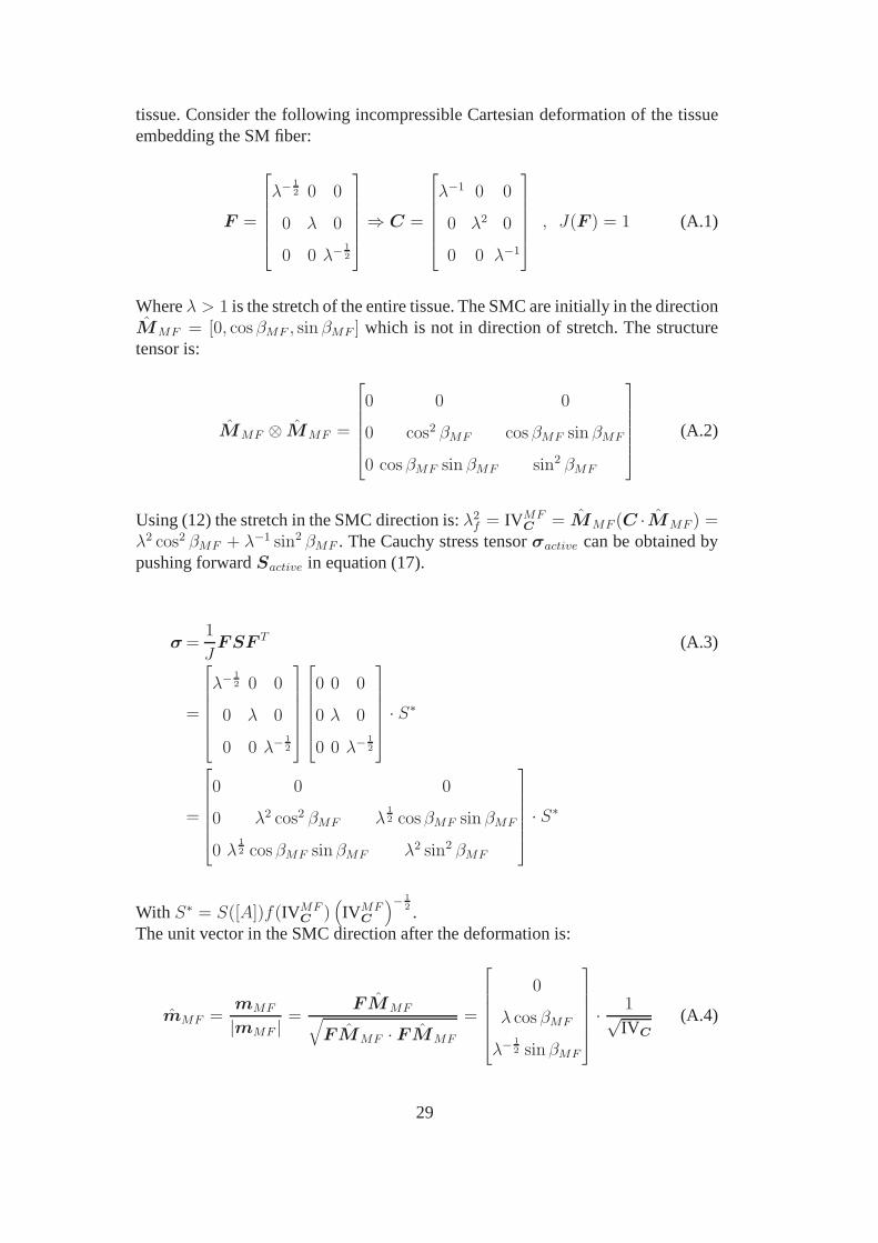
tissue. Consider the following incompressible Cartesian deformation of the tissueembedding the SM fiber:

F =

λ−12 0 0

0 λ 0

0 0 λ−12

⇒ C =

λ−1 0 0

0 λ2 0

0 0 λ−1

, J(F ) = 1 (A.1)

Whereλ > 1 is the stretch of the entire tissue. The SMC are initially in the directionMMF = [0, cosβMF , sin βMF ] which is not in direction of stretch. The structuretensor is:

MMF ⊗ MMF =

0 0 0

0 cos2 βMF cosβMF sin βMF

0 cosβMF sin βMF sin2 βMF

(A.2)

Using (12) the stretch in the SMC direction is:λ2f = IVMF

C= MMF (C ·MMF ) =

λ2 cos2 βMF + λ−1 sin2 βMF . The Cauchy stress tensorσactive can be obtained bypushing forwardSactive in equation (17).

σ =1

JFSF T (A.3)

=

λ−12 0 0

0 λ 0

0 0 λ−12

0 0 0

0 λ 0

0 0 λ−12

· S∗

=

0 0 0

0 λ2 cos2 βMF λ12 cosβMF sin βMF

0 λ12 cosβMF sin βMF λ2 sin2 βMF

· S∗

With S∗ = S([A])f(IVMFC

)(

IVMFC

)− 12 .

The unit vector in the SMC direction after the deformation is:

mMF =mMF

|mMF |=

FMMF√

FMMF · FMMF

=

0

λ cosβMF

λ−12 sin βMF

· 1√IVC

(A.4)

29

Thus the component of the Cauchy stress in the SMC direction is:

σMF = (σ · mMF )·mMF = S∗IVMFC

= S([A])f(IVMFC

)√

IVC = S([A])f(λf)λf

(A.5)This is in accordance with the expression for the Cauchy stress provided in [7] fora stretch in the SMC direction.

B Derivation of the body force term for problem C

The equilibrium equations in Cartesian coordinates are:

∂σij

∂xi= fj →

∂σij

∂Xk

∂Xk

∂xi= fj →

∂σij

∂XkF−1

ki = fj (B.1)

The Cauchy stress tensor is computed byσ = 1JFSF T = 2

JF ∂Ψ

∂CF T . With the

deformation gradientF and left Cauchy-Green deformation tensorC for problemC given as:

F =

1 0 0

0 1 0

0 0 Z12

⇒ C =

1 0 0

0 1 0

0 0 Z

⇒ C−1 =

1 0 0

0 1 0

0 0 Z−1

, J = det F = Z12

(B.2)Using equations (4)(6)(15) one can obtain an expression forS in the form:

S =Z− 13 c1

(

−2

3C−1 (2 + Z) + 2I

)

+2

D1

C−1(

Z − Z− 12

)

(B.3)

+S([A])(

IVMFC

)− 12

1 −

λm −√

IVMFC

λm − λ0

2

[

MMF ⊗ MMF

]

With MMF = [0, 0, 1] and IVMFC

=[

MMF ⊗ MMF

]

: C = Z. The Cauchystress takes the form:

σ =Z16 c1

(

−2

3C−1 (2 + Z) + 2I

)

+2

D1

C−1(

Z32 − 1

)

(B.4)

+S([A])

1 −(

λm −√Z

λm − λ0

)2

[

MMF ⊗ MMF

]

Using (B.1) and (B.4) the body force component required to maintain equilibriumcan be computed.

30

fx =−(

∂σxx

∂x+∂σyx

∂y+∂σzx

∂z

)

= 0 (B.5)

fy =−(

∂σxy

∂x+∂σyy

∂y+∂σzy

∂z

)

= 0

fz =−(

∂σxz

∂x+∂σyz

∂y+∂σzz

∂z

)

= −∂σzz

∂z= −∂σzz

∂Z

∂Z

∂z=

− 4c118Z− 4

3 − 20c118

Z− 73 − 1

D1Z− S([A])

(

λm −√Z

λm − λ0

)

Z−1

C Comparison of our code to Abaqus using h-extension

Here we wish to compare between the performance of our code and the commercialcode Abaqus [28] when h-extension is used. To that end we use problem C givenin Table 1 but with no SMC contribution (not available in Abaqus) similar to theproblem presented in [15]. In Abaqus an automatic load stepping was used result-ing in 17 load increments with an average of3 equilibrium iterations per a step. Inour code we used20 equal load steps resulting in an average of three equilibriumiterations per step. In Figure C.1 the relative error inuZ andσZZ extracted at pointX = 2, Y = 2, Z = 2 is compared as a function of CPU using both our codeand Abaqus. It can be seen that both our code and Abaqus cannotconverge to theexact solution when onlyp = 1 is utilized for the h-extension used (8 to 1000 ele-ments). When stresses are considered both codes reached a minimum relative errorof ∼ 3.5%. In terms of CPU times Abaqus requires shorter CPU times up toa factorof ≈ 2.5 for the h-extension considered. This can be attributed in part to the auto-matic load stepping algorithm implemented in Abaqus and notyet implemented inour code. It should be noted however that when p-extension isconsidered for thesame problem and p-FEM is compared to h-FEM our code out performs Abaqus asdemonstrated in [15].

D Simulation of uniaxial extension experiments

In this section we wish to demonstrate that our proposed SEDFcan model thereduction in active force generation observed in uniaxial-extension experiments re-ported in [13]. Finite element models simulating the uniaxial stretch-tension exper-iments were generated. The boundary conditions and mesh used for computationare shown in Figure D.1.

Remark 4 It is reported in [13] that examination of the tissue showed that theSMCs are arranged in a helix like structure with a pitch of angle θ = 4.50 with

31

Fig. C.1. Relative error in displacement and stress using our code and Abaqus 6.8 E.F.

Fig. D.1. Boundary conditions and mesh for the uniaxial tension of an arterial strip.

respect to the circumferential direction. The specimens were cut so as to have theSMCs aligned with the extension direction and therefore in our FE model the col-

32

lagen fibers families are not symmetric with respect to the stretch direction as de-picted in Figure D.1.

All analyses for the fitting process were conducted usingp = 4 following conver-gence tests for which‖|e(U)|| < 0.1%. Displacement boundary conditions werespecified at one end of the strip while the other end was clamped and a constantvalue[A] = 0.005 [mol/liter] was applied as reported in [13]. The fitted materialparameters and stress-stretch response for both passive and active states are givenin Table D.1 and Figure D.2 respectively. As evident from Figure D.2 the pro-

Table D.1Material parameters fitted to a slightly compressible passive-active SEDF.

c1 D1 k1 k2 βM λ0 λ1 λm m EC50 Smax

[MPa] [MPa−1] [MPa] [0] [mol/liter] [kPa]

0.007 2 0.025 4.3 ±35 0.4 2.1 1.25 1 0.00075 222

Fig. D.2. Stress-stretch relationship for a swine carotid media strip - Model and experimentsfrom [13] for pure passive and coupled passive-active state, [A] = 0.005 [mol/liter].

posed active SEDF is capable of predicting the softening branch of the active curvefollowing λ > λm.

33