ARTICLE OPEN

Logarithmic sensing in Bacillus subtilis aerotaxisFilippo Menolascina1,2, Roberto Rusconi3,4, Vicente I Fernandez3,4, Steven Smriga3,4, Zahra Aminzare5, Eduardo D Sontag6

and Roman Stocker3,4

Aerotaxis, the directed migration along oxygen gradients, allows many microorganisms to locate favorable oxygen concentrations.Despite oxygen’s fundamental role for life, even key aspects of aerotaxis remain poorly understood. In Bacillus subtilis, for example,there is conflicting evidence of whether migration occurs to the maximal oxygen concentration available or to an optimalintermediate one, and how aerotaxis can be maintained over a broad range of conditions. Using precisely controlled oxygengradients in a microfluidic device, spanning the full spectrum of conditions from quasi-anoxic to oxic (60 n mol/l–1 mmol/l), weresolved B. subtilis’ ‘oxygen preference conundrum’ by demonstrating consistent migration towards maximum oxygenconcentrations (‘monotonic aerotaxis’). Surprisingly, the strength of aerotaxis was largely unchanged over three decades in oxygenconcentration (131 n mol/l–196 μmol/l). We discovered that in this range B. subtilis responds to the logarithm of the oxygenconcentration gradient, a rescaling strategy called ‘log-sensing’ that affords organisms high sensitivity over a wide range ofconditions. In these experiments, high-throughput single-cell imaging yielded the best signal-to-noise ratio of any microbial taxisstudy to date, enabling the robust identification of the first mathematical model for aerotaxis among a broad class of alternativemodels. The model passed the stringent test of predicting the transient aerotactic response despite being developed on steady-state data, and quantitatively captures both monotonic aerotaxis and log-sensing. Taken together, these results shed new light onthe oxygen-seeking capabilities of B. subtilis and provide a blueprint for the quantitative investigation of the many other forms ofmicrobial taxis.

npj Systems Biology and Applications (2017) 3, 16036; doi:10.1038/npjsba.2016.36; published online 19 January 2017

INTRODUCTIONOxygen mediates the conversion of carbon sources to cellularenergy and is the most common electron acceptor used in cellularrespiration. In order to locate optimal oxygen conditions in theirenvironment, several species of bacteria have evolved the abilityto sense and migrate along oxygen gradients, a strategy calledaerotaxis.1 Aerotaxis is fundamental to many ecological processes.Within microbial mats at the sediment–water interface, thefilamentous bacteria Beggiatoa use aerotaxis to glide along steepvertical oxygen gradients toward preferred micro-oxic depths.2

The sulfur-reducing bacteria Desulfovibrio swim to accumulate inregions of specific, low oxygen concentration (~500 n mol/l or0.04%), where conditions are thermodynamically favorable foranaerobic respiration.3 An important phytopathogenic bacterium,Ralstonia solanacearum, uses aerotaxis to attack the roots of itsplant hosts, including tomato and banana plants, causing theirwilting and death.4 Escherichia coli, a common inhabitant of thelower digestive tract of warm blooded animals, has been found toexploit aerotaxis to cross the mucosal layer protecting epithelialsurface in the intestine and expedite its colonization.5 Morerecently, Caulobacter crescentus, a monotrichous bacteriumfound in aquatic environments, has been observed to performaerotaxis, adjusting its motility based on a dynamic rescalingof oxygen gradients.6 Besides its role in energy harvesting,aerotaxis is involved in collective bacterial migrations, includingbioconvection, where bacteria that swim up oxygen gradients

accumulate and render water denser, causing convection andmixing.7,8

Aerotaxis was the first of all microbial taxis behaviors (i.e.,directional migration responses to external stimuli) to bedescribed, when in 1881 Theodor Engelmann observed bacteriamoving towards the chloroplasts of algae in response to theoxygen produced by photosynthesis.9 Despite its early discovery,however, our understanding of aerotaxis has remained ratherpoor and mostly qualitative. For example, even for themodel bacterium Bacillus subtilis it has remained unclear whethercells seek an optimal, intermediate oxygen concentration (e.g.,200 μmol/l or ~ 15%;1,10 percentage values are based on oxygensaturation in water under laboratory conditions (temperature25 °C and pressure 100 kPa)) or swim towards the highest oxygenconcentration available (1.3 m mol/l or 100%),11 a strategy withpotentially detrimental physiological effects.12 Beyond this‘oxygen preference conundrum’, even the obligately aerobicnature of B. subtilis,13 once believed to be a robust trait of thisorganism, has recently been put to question by results document-ing its anaerobic growth.14 This lack of understanding ofconcentration preferences in aerotaxis, in turn, prevents quanti-tative predictions of population dynamics in oxygen gradients.Sensing mechanisms for aerotaxis fall in two categories.

A first mechanism is based on the sensing of the intracellularenergy status to determine the need for additional oxygen.This mechanism belongs to the class of energy-tactic behaviors,1 is

1Institute for Bioengineering, School of Engineering, The University of Edinburgh, Scotland, UK; 2SynthSys—Centre for Synthetic and Systems Biology, The University ofEdinburgh, Scotland, UK; 3Ralph M Parsons Laboratory, Department of Civil and Environmental Engineering, Massachusetts Institute of Technology, Cambridge, MA, USA;4Institute of Environmental Engineering, Department of Civil, Environmental and Geomatic Engineering, Zurich, Switzerland; 5The Program in Applied and ComputationalMathematics, Princeton, NJ, USA and 6Department of Mathematics, Hill Center Rutgers, The State University of New Jersey, Piscataway, NJ, USA.Correspondence: F Menolascina (filippo.menolascina@ed.ac.uk) or ED Sontag (eduardo.sontag@rutgers.edu) or R Stocker (romanstocker@ethz.ch)Received 21 June 2016; revised 13 September 2016; accepted 5 October 2016

www.nature.com/npjsba

Published in partnership with the Systems Biology Institute

found in E. coli, Azospirillum brasilense, Salmonella tiphymuriumand Pseudomonas aeruginosa, and has received considerableattention.15,16 In E. coli, aerotaxis is mediated by the receptors Aerand Tsr. The former has recently been proposed to monitor thecell’s metabolic state by gauging the activity of the electrontransport system,17 whereas Tsr has been speculated to sense theproton-motive force, a measure of the potential energy stored inthe cell.18 A second mechanism for aerotaxis is based on thesensing of extracellular oxygen via its direct binding to heme-containing receptors like HemAT. This mechanism, independent ofmetabolism and similar to classic chemotaxis,19 is found forexample in B. subtilis and Halobacterium salinarum, and hasreceived limited attention to date.6,19 For both forms of aerotaxis,there are no quantitative models of the cellular response tooxygen gradients.Here we present a high-resolution experimental characteriza-

tion of aerotaxis, focusing on the case of direct oxygen sensing inB. subtilis, a gram positive bacterium that is widespread in a broadrange of environments.12 The robustness of the data and thebreadth of conditions examined allowed us to identify aquantitative population model for aerotaxis in B. subtilis and toresolve the oxygen preference conundrum for this bacterium bydemonstrating that cells seek the highest oxygen concentrationavailable under the full spectrum of conditions tested.Traditional techniques to study aerotaxis have only enabled

very limited quantification of this migration strategy. Observationsof bacterial populations in capillaries, sealed at one end andexposed to a controlled oxygen concentration at the other end,revealed the formation of bacterial bands.1 These bands havebeen interpreted as evidence for preferred oxygen concentrationsby bacteria, yet conclusive interpretation and a quantitativeanalysis have remained difficult, because oxygen gradients aregoverned by both diffusion and respiration and thus poorlyquantifiable with this approach. Oxygen measurements with

microelectrodes20 partially addressed this problem but have thedrawback of being invasive, altering the distribution of bothbacteria and oxygen. In contrast, initial applications of microfluidicdevices to chemotaxis21 and aerotaxis6,16 have demonstrated thepotential of this approach to control gradients for taxis studies,while simultaneously visualizing population responses.Here we used a new microfluidic device and computer-

controlled gas mixers to generate precise, linear oxygenconcentration profiles over oxygen conditions ranging fromanoxic to oxic, and we applied video microscopy and imageanalysis to accurately quantify the response of extremely largenumbers of individual cell coordinates. We observed that B. subtilisalways swims towards the highest available oxygen concentrationand, notably, displays the same magnitude of aerotaxis overoxygen gradients (∇C) spanning three orders of magnitude whenthe relative gradient (∇C/C) is conserved, indicating this bacteriumrescales its response to oxygen gradients via logarithmic sensing.We show that the vastly improved level of environmental controland data robustness of this approach over traditional ones permitsthe identification of a predictive mathematical model of aerotaxisin B. subtilis that captures logarithmic sensing and providesa blueprint for the quantitative study of other forms ofmicrobial taxis.

RESULTS AND DISCUSSIONTo study the aerotactic response of B. subtilis we exposed thebacteria to linear concentration profiles of oxygen across amicrochannel and quantified the spatial distribution of cells alongthe width of the channel, B(x), at steady state. We devised anew microfluidic device made of polydimethylsiloxane (PDMS)featuring three parallel channels sealed by glass slides on the topand bottom (Figure 1a). The central ‘test’ channel hosts the cells,whereas the flanking ‘oxygen control’ channels each carry a flow

0%-0.01% 0%-0.025% 0%-0.05% 0%-0.075%

0%-0.1% 0%-0.25% 0%-0.5% 0%-1%

0%-2.5% 0%-5% 0%-10% 0%-20%

0%-30% 0%-40% 0%-50% 0%-60% 0%-70% 0%-80% 0%-90%

0%-100% 5%-10% 5%-15% 10%-15% 10%-30% 10%-50% 10%-70%

10%-90% 15%-20% 20%-40% 20%-60% 20%-80% 30%-50% 30%-70%

Glass

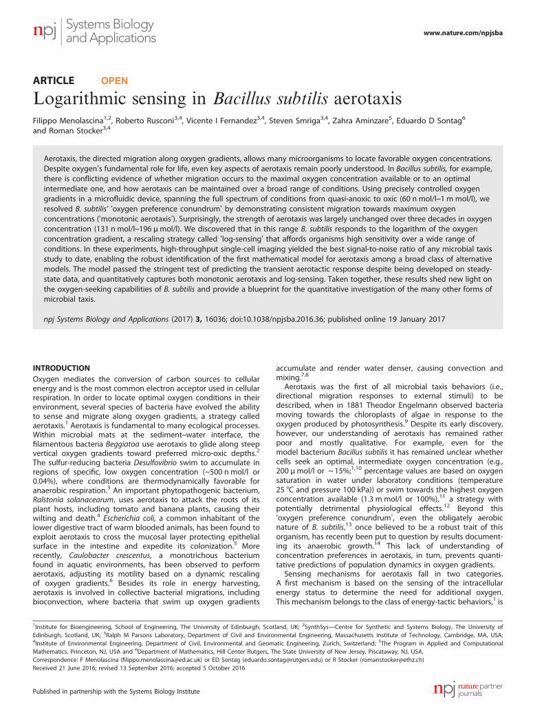
Figure 1. Aerotactic response of Bacillus subtilis. (a) The microfluidic device used to probe aerotaxis in B. subtilis consists of three parallelchannels fabricated in polydimethylsiloxane (PDMS), with top and bottom glass surfaces. Flowing oxygen at prescribed concentrations in thesource (green) and sink (red) channels created a linear oxygen concentration profile ([O2(x)]) in the test channel, where the bacterial responsewas monitored by video microscopy. (b) Steady-state distribution of bacteria across the test channel, B(x) (blue circles), for the 0–20% gradient(sink concentration—source concentration), along with the best exponential fit (red). (c) Steady-state aerotactic response, B(x), for all33 oxygen conditions tested. For each panel, the x axis represents the test channel width (0oxo460 μm) and the y axis representsB(x) (0oB(x)o6). A uniform bacterial distribution would correspond to B(x)= 1. Open circles are experimental data, thin solid lines are modelpredictions, the shaded envelope represents plus/minus one standard deviation on the predictions. The oxygen concentrations in the sinkand source channels are reported for each condition and a symbol is assigned to each condition for reference in subsequent figures.

Logarithmic sensing in B. subtilis aerotaxisF Menolascina et al

2

npj Systems Biology and Applications (2017) 16036 Published in partnership with the Systems Biology Institute

of oxygen at a prescribed concentration, higher in the ‘source’channel and lower in the ‘sink’ channel (Figure 1a). Oxygendiffuses from the source channel to the sink channel throughthe PDMS (which is oxygen permeable22) and the test channel,where it thereby forms a gradient. The two glass slides, beingimpermeable to gas, force oxygen diffusion to occur onlysideways, which leads to a linear oxygen profile. This providesless flexibility in setting up arbitrary gradients, compared withprior approaches,16 but has the advantage of extreme fabricationsimplicity (single-layer, two oxygen boundary conditions).A mathematical model of oxygen diffusion in this system(implemented in COMSOL Multiphysics 4.4; see ‘Derivation andidentification of the mathematical model’ in SupplementaryMaterials and Methods), which also accounts for the top andbottom glass surfaces that are impermeable to oxygen, provides aquantitative prediction of the oxygen concentration and gradientthat bacteria experience at every position in the test channeland confirms that the oxygen concentration profile is linear(Supplementary Figure S1). The model also shows that cells in thedevice are exposed to 490% of the total oxygen gradient

between sink and source channels (see ‘Oxygen diffusion withinthe device’ and Supplementary Table S1).To quantify aerotaxis we probed B. subtilis’ response at steady

state in 33 different gradients, spanning four decades in gradientmagnitude (from 0.26 n mol/l/μm to 2.56 μmol/l/μm) and rangingfrom 0%–0.01% to 0%–100%. Experiments therefore covered alarge spectrum of the oxygen conditions that B. subtilis mayexperience in nature, from quasi-anoxic to fully oxygenated.For all conditions tested, B. subtilis moved towards the highest

oxygen concentration available (Figure 1c). Accumulation profilesB(x) were mostly exponentially shaped (Figure 1b). Positiveaerotaxis was observed even when the highest oxygen concen-tration in the test channel was near saturation (0%–100% gradient,Figure 1c). In contrast to previous reports of a preferredoxygen concentration of 200 μmol/l (i.e., ~ 15%) for B. subtilis,10

we consistently (19 experiments, Figure 1c) observed accumula-tion of cells to higher concentrations than 200 μmol/l (althoughwe did observe a decrease in the accumulation strength foroxygen concentrations above 20%; Figure 2a). These findingsresolve the oxygen preference conundrum in B. subtilis and

0 100 200 300 4000

2

4

6B

(x)

x [μm]

0 200 4000

1

2

3

4

ΔCR

= 20%

B(x

)

x [μm]0 200 400

0

1

2

3

4

CR0

= 30%

B(x

)

x [μm]

0%−0.01%0%−1%0%−10%0%−30%0%−40%0%−70%0%−100%

0%−20%10%−30%20%−40%30%−50%

0%−60%10%−50%20%−40%30%−30%

0 20 40 600.4

0.6

0.8

6

CM

CC

R0 [%]

10 20 30 400

0.2

0.4

0.6

CM

C

CR0

[%]0 20 40 60

0

0.2

0.4

CM

C C

RΔ

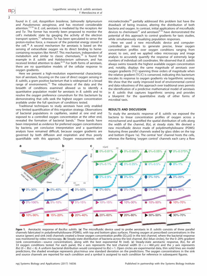
Figure 2. Oxygen preference in B. subtilis aerotaxis. (a) Normalized bacterial density profiles across the width of the test channel, B(x), for asubset of the experiments of the form 0%–X% (sink concentration—source concentration). Open circles are experimental data, solid lines are asmoothed version of the same data obtained with a Savitzky–Golay filter. Inset: The Chemotactic Migration Coefficient (CMC) for the sameexperiments, as a function of the oxygen concentration CR0 at mid-channel (x= 230 μm). Color-coding of the data in the inset corresponds tothe main panel, whereas gray circles are all other experiments of the form 0%–X%. (b) Aerotactic response, B(x), in experiments in which theoxygen gradient was kept constant (ΔCR= 20% between source and sink channels) and the absolute oxygen concentration CR0 was varied.Inset: the CMC decreases with increasing absolute oxygen concentration. (c) Aerotactic response, B(x), in experiments in which the oxygengradient (i.e., ΔCR) was varied and the absolute oxygen concentration CR0 was kept constant. Inset: the CMC increases with increasing oxygengradient.

Logarithmic sensing in B. subtilis aerotaxisF Menolascina et al

3

Published in partnership with the Systems Biology Institute npj Systems Biology and Applications (2017) 16036

demonstrate that these bacteria always swim towards the highestavailable oxygen concentration.Aerotaxis was strongest at very low oxygen concentrations, in

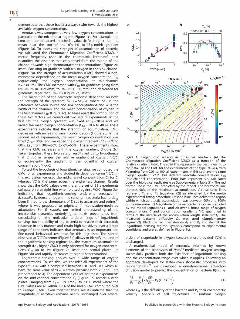
particular in the micromolar regime (Figure 1c). For example, theconcentration of bacteria reached a value six-fold higher than themean near the top of the 0%–1% (0–13 μmol/l) gradient(Figure 2a). To assess the strength of accumulation of bacteria,we calculated the Chemotactic Migration Coefficient (CMC), ametric frequently used in the chemotaxis literature21 thatquantifies the distance that cells travel from the middle of thechannel towards high chemoattractant concentrations (Figure 2a,inset). Focusing on gradients with 0% oxygen in the sink channel(Figure 2a), the strength of accumulation (CMC) showed a non-monotonic dependence on the mean oxygen concentration, CR0(equivalently, the oxygen concentration at mid-channel,x= 230 μm). The CMC increased with CR0 for gradients going from0%–0.01% (0.015%/mm) to 0%–1% (1.5%/mm) and decreased forgradients larger than 0%–1% (Figure 2a, inset).The magnitude of the aerotactic response depended on both

the strength of the gradient, ∇C ( =ΔCR/W, where ΔCR is thedifference between source and sink concentrations and W is thewidth of the channel), and the mean concentration of oxygen inthe test channel, CR0 (Figure 1c). To tease apart the contribution ofthese two factors, we carried out two sets of experiments. In thefirst set, the oxygen gradient was fixed (ΔCR = 20%) and wevaried the mean oxygen concentration (CR0 = 10% to 40%). Theseexperiments indicate that the strength of accumulation, CMC,decreases with increasing mean concentration (Figure 2b). In thesecond set of experiments, the mean oxygen concentration wasfixed (CR0 = 30%) and we varied the oxygen gradient (ΔCR = 0% to60%, i.e., from 30%–30% to 0%–60%). These experiments showthat the CMC increases with the oxygen gradient (Figure 2c).Taken together, these two sets of results led us to hypothesizethat B. subtilis senses the relative gradient of oxygen, ∇C/C,or equivalently the gradient of the logarithm of oxygenconcentration, ∇logC.To test the hypothesis of logarithmic sensing, we computed the

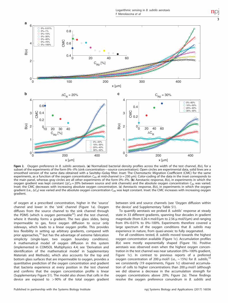
CMC for all experiments and studied its dependence on ∇C/C. Inthis expression we used the mid-channel concentration C0 for C,whereas ∇C is the same across the entire test channel. Resultsshow that the CMC values over the entire set of 33 experimentscollapse on a straight line when plotted against ∇C/C (Figure 3a),indicating that logarithmic-sensing underpins aerotaxis inB. subtilis. Evidence of logarithmic sensing in bacteria has to datebeen limited to the chemotaxis of E. coli to aspartate and serine,23

where it was proposed to originate in methylation-mediatedadaptation. For B. subtilis, our limited understanding of theintracellular dynamics underlying aerotaxis prevents us fromspeculating on the molecular underpinnings of logarithmicsensing, but the ability of the bacteria to rescale their aerotacticresponse in this manner and retain high sensitivity over a broadrange of conditions indicates that aerotaxis is an important andfine-tuned behavioral response for this organism. The spreadobserved at ∇C/C= 4/mm (Figure 3a) allows to identify the end ofthe logarithmic sensing regime, i.e., the maximum accumulationstrength (i.e., higher CMC) is only observed for oxygen concentra-tions CR0 up to 1% (Figure 2a, inset and central plateau inFigure 3b) and rapidly decreases at higher concentrations.Logarithmic sensing applies over a wide range of oxygen

concentrations. To see this, we consider all experiments of thetype 0%–X%, with X comprised between 0.01 and 100, which allhave the same value of ∇C/C= 4/mm (because both ∇C and C areproportional to X). The dependence of CMC for these experimentson the mid-channel concentration C0 (Figure 3b) reveals a wideplateau ranging from C0 = 0.19 μmol/l to 73.0 μmol/l where theCMC values are all within ± 7% of the mean CMC computed overthis range (0.68). Taken together these results indicate that themagnitude of aerotaxis remains nearly unchanged over several

orders of magnitude in oxygen concentration, provided ∇C/C isunchanged.A mathematical model of aerotaxis, informed by known

elements of the biophysics of HemAT-mediated oxygen sensing,successfully predicts both the existence of logarithmic sensingand the concentration range over which it applies. Following anapproach developed for state-driven stochastic processes withre-orientations,24 we developed a one-dimensional advectiondiffusion model to predict the concentration of bacteria B(x,t), as

∂B∂t

¼ ∂∂x

DB∂B∂x

- VC C;∇Cð ÞB� �

ð1Þ

where DB is the diffusivity of the bacteria and VC their chemotacticvelocity. Analysis of cell trajectories in uniform oxygen

Figure 3. Logarithmic sensing in B. subtilis aerotaxis. (a) TheChemotactic Migration Coefficient (CMC) as a function of therelative gradient ∇C/C. The solid line represents the best linear fit tothe data. (b) The CMC for the experiments of the type 0%–X%, withX ranging from 0.01 to 100: all experiments in this set have the sameoxygen gradient ∇C/C, but different absolute concentrations CR0(mid-channel concentration). Error bars represent s.e. calculatedover the biological replicates (see Supplementary Table S1). The reddotted line is the CMC predicted by the model. The horizontal linedenotes 90% of the maximum accumulation. Vertical solid linesrepresent K1 and K2 (equation (2)) as identified by the multi-experimental fitting procedure. Dashed blue lines delimit the regionwithin which aerotactic accumulation was between 90% and 100%of the maximum. (c) Magnitude of the aerotactic response predictedby the model (equations (1 and 2)) over a broad range of oxygenconcentrations C and concentration gradients ∇C, quantified interms of the inverse of the accumulation length scale Vc/DB. Themeasured bacteria diffusivity DB was used (SupplementaryFigure S2). Black dashed lines denote K1 and K2 and delimit thelogarithmic sensing regime. Symbols correspond to experimentalconditions and are as defined in Figure 1c).

Logarithmic sensing in B. subtilis aerotaxisF Menolascina et al

4

npj Systems Biology and Applications (2017) 16036 Published in partnership with the Systems Biology Institute

concentrations showed that the diffusivity, which results from therandom component of motility, is nearly constant betweenoxygen concentrations of 390 μmol/l and 1.3 mmol/l, anddiminishes below 26 μmol/l (Supplementary Figure S2; seeSupplementary Information for an in-depth analysis). This leavesonly the chemotactic velocity VC to be determined in order tohave a complete model of aerotaxis.The fundamental element of the aerotaxis model is the

functional dependence of VC on the oxygen concentration Cand concentration gradient ∇C. Although many different func-tional forms of VC have been proposed, they nearly all fall in threecategories: Keller–Segel models (KS), where VC = χ0∇C/C and χ0 isthe chemotactic sensitivity coefficient; Lapidus–Schiller models(LS), where VC = χ0/(K+C)

2 and K is the chemoreceptor-liganddissociation constant; and Rivero–Tranquillo–Buettner–Lauffen-burger models (RTBL), where VC ¼ 2

3V tanhðKχ02V∇C= K þ Cð Þ2Þ andV is swimming speed. Interestingly, although all these modelshave been developed to study chemotaxis in E. coli, they all fail tocapture an important feature of chemotaxis in this microorganism:logarithmic sensing over a finite range of concentrations.23 KSpredicts logarithmic sensing (i.e., rescaling C by a constant leavesVC unchanged) for any oxygen concentration, whereas neither LSnor RTBL support logarithmic sensing for any concentration.We propose a new model for VC that captures logarithmic

sensing in B. subtilis’ aerotaxis over a finite range of oxygenconcentrations (Materials and Methods). We started from a one-dimensional Fokker-Planck model24,25 to capture the temporalevolution of the spatial distribution of bacteria in an oxygengradient (Supplementary Information, Supplementary Equation(5)), modeling the exploration of the one-dimensional domain as avelocity jump process, where bacteria can either run with constantspeed in the positive or negative x direction, or tumble (i.e.,instantaneously change direction). The probability of tumbling iscontrolled by an intracellular variable, the receptor methylationstate, which in turn depends on the extracellular oxygenconcentration (Supplementary Information, SupplementaryEquation (54)). Moment closure and parabolic/hyperbolic scalingtechniques then yielded (see Supplementary Information for thefull derivation):

VC ¼ χ01

K1 þ Cð Þ K2 þ Cð Þ∇C ð2Þ

where χ0 is a chemotactic sensitivity coefficient as in the KS, LS andRTBL models and the oxygen concentrations K1 and K2 aretraditionally interpreted as the dissociation constants for thereceptor, which here is HemAT.26 Importantly, K1 and K2 representthe boundaries of the logarithmic sensing regime, because foroxygen concentrations such that K1≪C≪K2, equation (2) reducesto VC≈(χ0/K2)∇C/C. Therefore, our model predicts logarithmicsensing in the range of concentrations delimited by K1 and K2,but not outside this range, in line with our experimentalobservations.The model’s ability to predict the observed bacterial distribu-

tions and the logarithmic sensing regime is not only qualitative,but also quantitative. We tested this by determining theconcentrations K1 and K2 and the sensitivity χ0 by fitting thesteady-state version of equation (1)—with DB from experiments(Supplementary Figure S2) and VC from equation (2)—to the entiredata set of 33 steady-state bacterial distributions, B(x) (Figure 1b)(Materials and Methods). The best fit yielded K1 = 131 n mol/l,K2 = 196 μmol/l and χ0 = 1.43 × 10− 3 μm2/s. For these parametervalues the model predicts B(x) accurately over the vast majority ofthe conditions tested, with an average error of 11% and only 1 outof 33 cases having an error 430%, and thus accurately capturesthe dependence of the CMC on oxygen conditions (Figure 3b,red dashed line). An empirical verification of the extent of thelogarithmic sensing regime can be obtained by determining the

range of experiments in which the CMC was within 10% ofthe maximum (Figure 3b, region between the dashed blue lines).Given the structural properties of the model (see discussionabove), we expect K1 and K2 to approximate the two boundaries ofthe logarithmic sensing regime. Indeed, we observe an excellentagreement between the inferred dissociation constants (Figure 3b,solid blue lines) and the empirical estimates.Repeating the fitting procedure to B(x) for the three classes

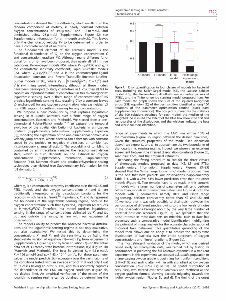
of chemotaxis models proposed to date (KS, LS and RTBL;Supplementary Information, Supplementary Figures S3–S5)showed that the ‘finite range log-sensing’ model proposed hereis the one that best predicts our observations (SupplementaryTable S1), with a 23%–61% lower prediction error than the othermodels (Figure 4). Two remarks have to be made in this context:(i) models with a larger number of parameters will tend performbetter than models with fewer parameters (see Figure 4: both themodels with 2 parameters, namely RTBL and Finite rangelog-sensing, perform consistently better than KS and LS) and(ii) we note that it was only possible to distinguish between theperformance of different models owing to the low levels of noisein the observations brought about by the very large number ofbacterial positions recorded (Figure 1c). We speculate that thenoise intrinsic in most data sets on microbial taxis to date hasprevented such a comparative model identification, highlightingthe potential of image analysis for the accurate characterization ofmicrobial taxis behaviors. This quantitative grounding of themodel then allows one to apply it to predict the steady-statedistributions of bacteria over the entire spectrum of oxygenconcentrations and (linear) gradients (Figure 3c).The most stringent validation of the model, which was derived

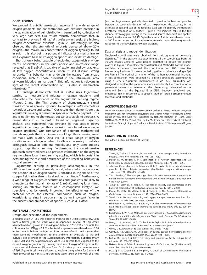
based solely on steady-state data, was carried out by testing itsperformance in predicting the full aerotaxis dynamics in a transientexperiment. In this experiment we exposed a B. subtilis population toa time-varying oxygen gradient beginning from uniform conditions(21%–21%) and ending after ~ 4 min with a gradient at low oxygenconcentration (0%–0.05%) (Figure 5a). The spatial distribution ofcells, B(x,t), was tracked over time (Materials and Methods) as theoxygen gradient formed, showing bacteria migrating towards thehigher oxygen region (Figures 5b and d). The timing of the onset

KS model LS model RTBL model

Finite rangelog-sensing

model

0.1

0.2

0.3

0.4

SS

E

Figure 4. Error quantification in four classes of models for bacterialtaxis, including the Keller–Segel model (KS), the Lapidus–Schillermodel (LS), the Rivero–Tranquillo–Buettner–Lauffenburger model(RTBL), and the ‘finite range log-sensing’ model proposed here. Foreach model the graph shows the sum of the squared (weighted)errors (SSE, equation (5)) of the best solution identified among 100iterations of the parameter optimization routine (black bars;Supplementary Information). The box plot summarizes the statisticsof the 100 solutions obtained for each model: the median of theweighted SSE is in red, the extent of the blue box shows the first andlast quartiles of the distribution, and the whiskers indicate the bestand worst solution identified.

Logarithmic sensing in B. subtilis aerotaxisF Menolascina et al

5

Published in partnership with the Systems Biology Institute npj Systems Biology and Applications (2017) 16036

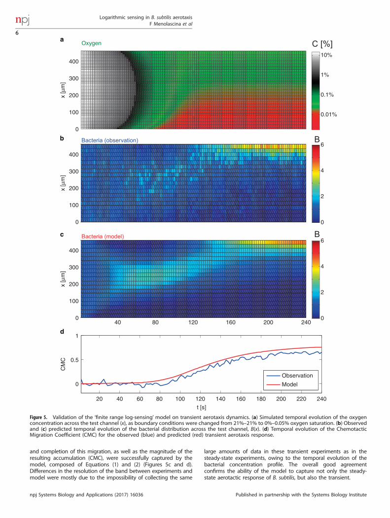
and completion of this migration, as well as the magnitude of theresulting accumulation (CMC), were successfully captured by themodel, composed of Equations (1) and (2) (Figures 5c and d).Differences in the resolution of the band between experiments andmodel were mostly due to the impossibility of collecting the same

large amounts of data in these transient experiments as in thesteady-state experiments, owing to the temporal evolution of thebacterial concentration profile. The overall good agreementconfirms the ability of the model to capture not only the steady-state aerotactic response of B. subtilis, but also the transient.

40 80 120 160 200 2400

100

200

300

400

x [μ

m]

0

2

4

6

0

100

200

300

400

x [μ

m]

0

2

4

6

Oxygen

Bacteria (model)

C [%]

B

0

100

200

300

400x

[μm

]

0.01%

0.1%

1%

10%

Bacteria (observation) B

20 40 60 80 100 120 140 160 180 200 220 240

0

0.5

1

t [s]

CM

C

Observation

Model

Figure 5. Validation of the ‘finite range log-sensing’ model on transient aerotaxis dynamics. (a) Simulated temporal evolution of the oxygenconcentration across the test channel (x), as boundary conditions were changed from 21%–21% to 0%–0.05% oxygen saturation. (b) Observedand (c) predicted temporal evolution of the bacterial distribution across the test channel, B(x). (d) Temporal evolution of the ChemotacticMigration Coefficient (CMC) for the observed (blue) and predicted (red) transient aerotaxis response.

Logarithmic sensing in B. subtilis aerotaxisF Menolascina et al

6

npj Systems Biology and Applications (2017) 16036 Published in partnership with the Systems Biology Institute

CONCLUSIONSWe probed B. subtilis’ aerotactic response in a wide range ofoxygen gradients and concentrations, with exquisite precision inthe quantification of cell distributions permitted by collection ofvery large data sets. Our results robustly demonstrate that, incontrast to previous findings,1 B. subtilis always seeks the highestoxygen concentration available (Figure 2). Interestingly, we alsoobserved that the strength of aerotaxis decreased above 20%oxygen—the maximum concentration of oxygen typically foundin soil;27 this also being a potential indicator of a mechanism tolimit exposure to reactive oxygen species and oxidative damage.Short of only being capable of exploiting oxygen-rich environ-

ments, observations in the quasi-anoxic and micro-oxic rangerevealed that B. subtilis is capable of exploiting shallow gradientsat low oxygen concentrations, where it still displays strongaerotaxis. This behavior may underpin the escape from anoxicconditions, such as those prevalent in the intraluminal areaof warm blooded animal guts.28 This information is relevant inlight of the recent identification of B. subtilis in mammalianmicrobiota.29

Our findings demonstrate that B. subtilis uses logarithmicsensing to measure and migrate in oxygen gradients andestablishes the boundaries of the logarithmic sensing regime(Figures 2 and 3b). This property of chemoattractant signaltransduction was previously found to underpin E. coli’s chemotaxistowards aspartate and serine.23 Our results then demonstrate thatlogarithmic sensing is present in species of bacteria beyond E. coliand is not limited to chemotaxis but can also apply to aerotaxis. Arecent study in C. crescentus, based on single-cell trajectoryanalysis, also suggested that aerotaxis in that species obeyslogarithmic sensing, yet this conclusion was based on a singleoxygen gradient.6 Our comparison of different mathematicalmodels suggests that such inferences of logarithmic sensing mustbe made with caution. Data over a broad range of oxygenconditions and a large number of cells are necessary to reliablydistinguish between different models, and only some modelssupport logarithmic sensing. Furthermore, the data-intensiveapproach presented here also provides information on the oxygenregime where logarithmic sensing applies, which is important indetermining the role and occurrence of this rescaling behavior innatural environments.Logarithmic sensing is particularly advantageous in the

diffusion-dominated microscale world, where information aboutthe position of an oxygen source is encoded in the shape of theoxygen field rather than in its absolute magnitude.30 Furthermore,a wide range of oxygen concentrations and gradients are likely tocharacterize the natural habitats of B. subtilis, making logarithmicsensing an effective feature of a cosmopolitan lifestyle. Wespeculate that, by greatly improving the effectiveness of thebacterial search for essential compounds such as oxygen,logarithmic sensing in aerotaxis may be an important factor inthe success and abundance of species such as B. subtilis.

MATERIALS AND METHODSDesign and execution of the experimentsB. subtilis strain OI1085 was obtained from George Ordal’s laboratory. Cellsfrom a frozen (−80 °C) stock were resuspended in 2 ml of Cap AssayMinimal media,31 grown in a shaking incubator at 37 °C, 250 r.p.m. until theculture reached OD600 = 0.3. The bacterial suspension was then diluted 1:10in fresh media before the injection into the microfluidic device (note thatthere were no modifications to the ambient air available to the cellcultures, see Methods in the Supplementary Information, SupplementaryFigure S10 and the Supplementary Video). Cells were then exposed to thedesired oxygen gradient by flowing mixtures of oxygen/nitrogen in thesource and sink channels (Figures 1 and 5). For steady-state measurementsof B(x) (Figure 1) cells were allowed to explore the gradient for 5 min andthen 30 000 phase contrast micrographs were taken at intervals of 67 ms

(such settings were empirically identified to provide the best compromisebetween a reasonable duration of each experiment, the accuracy in theestimate of B(x) and size of the resulting data set). To quantify the transientaerotactic response of B. subtilis (Figure 5) we injected cells in the testchannel (21% oxygen flowing in the sink and source channels) and applieda 0% O2 to the sink and 0.05% O2 in the source. A video was then acquiredat 100 frames per second for 4 min to locate cells during their migration inresponse to the developing oxygen gradient.

Data analysis and model identificationSingle-cell coordinates were obtained from micrographs as previouslydescribed.32 In the steady-state experiments all the coordinates from the30 000 images acquired were pooled together to obtain the profilesplotted in Figure 1 (Supplementary Materials and Methods). For the modelvalidation experiment, instead, the coordinates from 200 consecutiveframes (acquired over 2 s) were pooled together to calculate a single B(x),see Figure 5. The optimal parameters of the mathematical models includedin this comparison were obtained via a fitting procedure accomplishedusing a Genetic Algorithm implemented in MATLAB. This routine wasdesigned to explore the parameter space and identify the combination ofparameter values that minimized the discrepancy, calculated as theweighted Sum of the Squared Error (SSE), between predicted andmeasured B(x) in response to a specific gradient profile (SupplementaryMaterials and Methods).

ACKNOWLEDGEMENTSWe thank Andrew Babbin, Francesco Carrara, Jeffrey S Guasto, Anupam Sengupta,Kwangmin Son, for stimulating discussions and George Ordal for supplying Bacillussubtilis OI1085. This work was supported by National Institutes of Health Grant1R01GM100473-01 (to RS and EDS), by the Wellcome Trust-University of EdinburghInstitutional Strategic Support Fund and a Royal Society of Edinburgh—MoST grant(to FM).

COMPETING INTERESTSThe authors declare no conflict of interest.

REFERENCES1. Taylor, B., Zhulin, I. & Johnson, M. Aerotaxis and other energy-sensing behavior in

bacteria. Annu. Rev. Microbiol. 53, 103–128 (1999).2. Møller, M. M., Nielsen, L. P. & Jørgensen, B. B. Oxygen Responses and Mat

Formation by Beggiatoa spp. Appl. Environ. Microbiol. 50, 373–382 (1985).3. Johnson, M. S., Zhulin, I. B., Gapuzan, M. E. & Taylor, B. L. Oxygen-dependent

growth of the obligate anaerobe Desulfovibrio vulgaris Hildenborough.J. Bacteriol. 179, 5598–5601 (1997).

4. Yao, J. & Allen, C. The plant pathogen Ralstonia solanacearum needs aerotaxis fornormal biofilm formation and interactions with its tomato host. J. Bacteriol. 189,6415–6424 (2007).

5. Tamar, E., Koler, M. & Vaknin, A. The role of motility and chemotaxis in thebacterial colonization of protected surfaces. Sci. Rep. 6, 19616 (2016).

6. Morse, M., Colin, R., Wilson, L. G. & Tang, J. X. The Aerotactic Response ofCaulobacter crescentus. Biophys. J. 110, 2076–2084 (2016).

7. Tuval, I. et al. Bacterial swimming and oxygen transport near contact lines. Proc.Natl Acad. Sci. USA 102, 2277–2282 (2005).

8. Hillesdon, A. J., Pedley, T. J. & Kessler, J. O. The development of concentrationgradients in a suspension of chemotactic bacteria. Bull. Math. Biol. 57, 299–344(1995).

9. Engelmann, T. W. Neue Methode zur Untersuchung der Sauerstoffausscheidungpflanzlicher und thierischer Organismen. Pflügers Arch. Gesamte Physiol. MenschenThiere 25, 285–292 (1881).

10. Wong, L. S., Johnson, M. S., Zhulin, I. B. & Taylor, B. L. Role of methylation inaerotaxis in Bacillus subtilis. J. Bacteriol. 177, 3985–3991 (1995).

11. Wong, L. S. Aerotaxis in Bacillus subtilis. PhD thesis (1995).12. Garrity, L. F. & Ordal, G. W. Chemotaxis in Bacillus subtilis: how bacteria monitor

environmental signals. Pharmacol. Ther. 68, 87–104 (1995).13. Earl, A. M., Losick, R. & Kolter, R. Ecology and genomics of Bacillus subtilis. Trends

Microbiol. 16, 269–275 (2008).14. Nakano, M. M. & Zuber, P. Anaerobic growth of a ‘strict aerobe’ (Bacillus subtilis).

Annu. Rev. Microbiol. 52, 165–190 (1998).15. Mazzag, B. C., Zhulin, I. B. & Mogilner, A. Model of bacterial band formation in

aerotaxis. Biophys. J. 85, 3558–3574 (2003).

Logarithmic sensing in B. subtilis aerotaxisF Menolascina et al

7

Published in partnership with the Systems Biology Institute npj Systems Biology and Applications (2017) 16036

16. Adler, M., Erickstad, M., Gutierrez, E. & Groisman, A. Studies of bacterial aerotaxisin a microfluidic device. Lab Chip 12, 4835–4847 (2012).

17. Bibikov, S. I., Barnes, L. A., Gitin, Y. & Parkinson, J. S. Domain organization andflavin adenine dinucleotide-binding determinants in the aerotaxis signaltransducer Aer of Escherichia coli. Proc. Natl Acad. Sci. USA 97, 5830–5835 (2000).

18. Rebbapragada, A. et al. The Aer protein and the serine chemoreceptor Tsrindependently sense intracellular energy levels and transduce oxygen, redox,and energy signals for Escherichia coli behavior. Proc. Natl Acad. Sci. USA 94,10541–10546 (1997).

19. Alexandre, G. Coupling metabolism and chemotaxis-dependent behaviours byenergy taxis receptors. Microbiology 156, 2283–2293 (2010).

20. Zhulin, I. B., Bespalov, V. A., Johnson, M. S. & Taylor, B. L. Oxygen taxis and protonmotive force in Azospirillum brasilense. J. Bacteriol. 178, 5199–5204 (1996).

21. Ahmed, T., Shimizu, T. S. & Stocker, R. Microfluidics for bacterial chemotaxis.Integr. Biol 2, 604 (2010).

22. Merkel, T. C., Bondar, V. I., Nagai, K., Freeman, B. D. & Pinnau, I. Gas sorption,diffusion, and permeation in poly(dimethylsiloxane). J. Polym. Sci. Part B Polym.Phys. 38, 415–434 (2000).

23. Kalinin, Y. V., Jiang, L., Tu, Y. & Wu, M. Logarithmic sensing in Escherichia colibacterial chemotaxis. Biophys. J. 96, 2439–2448 (2009).

24. Grünbaum, D. Advection-diffusion equations for internal state-mediatedrandom walks. SIAM J. Appl. Math. 61, 43–73 (2000).

25. Wakano, J. Y., Nowak, M. A. & Hauert, C. Spatial dynamics of ecologicalpublic goods. Proc. Natl Acad. Sci. USA 106, 7910–7914 (2009).

26. Zhang, W., Olson, J. & Phillips, G. N. Jr. Biophysical and kinetic characterization ofHemAT, an aerotaxis receptor from Bacillus subtilis. Biophys. J. 88, 2801–2814 (2005).

27. Lüdemann, H., Arth, I. & Liesack, W. Spatial changes in the bacterial communitystructure along a vertical oxygen gradient in flooded paddy soil cores. Appl.Environ. Microbiol. 66, 754–762 (2000).

28. Espey, M. G. Role of oxygen gradients in shaping redox relationships betweenthe human intestine and its microbiota. Free Radic. Biol. Med. 55, 130–140(2013).

29. Qin, J. et al. A human gut microbial gene catalog established by metagenomicsequencing. Nature 464, 59–65 (2010).

30. Shoval, O. et al. Fold-change detection and scalar symmetry of sensoryinput fields. Proc. Natl Acad. Sci. USA 107, 15995–16000 (2010).

31. Glekas, G. D. et al. Elucidation of the multiple roles of CheD in Bacillus subtilischemotaxis. Mol. Microbiol. 86, 743–756 (2012).

32. Rusconi, R., Guasto, J. S. & Stocker, R. Bacterial transport suppressed byfluid shear. Nat. Phys. 10, 212–217 (2014).

This work is licensed under a Creative Commons Attribution 4.0International License. The images or other third party material in this

article are included in the article’s Creative Commons license, unless indicatedotherwise in the credit line; if the material is not included under the Creative Commonslicense, users will need to obtain permission from the license holder to reproduce thematerial. To view a copy of this license, visit http://creativecommons.org/licenses/by/4.0/

© The Author(s) 2017

Supplementary Information accompanies the paper on the npj Systems Biology and Applications website (http://www.nature.com/npjsba)

Logarithmic sensing in B. subtilis aerotaxisF Menolascina et al

8

npj Systems Biology and Applications (2017) 16036 Published in partnership with the Systems Biology Institute

Supplementary Information

Filippo Menolascina1,2, Roberto Rusconi3,4, Vicente I. Fernandez3,4, Steve P. Smriga3,4, Zahra

Aminzare5, Eduardo D. Sontag6 & Roman Stocker3,4

1Institute for Bioengineering, School of Engineering, The University of Edinburgh, EH9 3DW

Edinburgh, Scotland, UK

2SynthSys - Centre for Synthetic and Systems Biology, The University of Edinburgh, EH9 3BF

Edinburgh, Scotland, UK

3Institute of Environmental Engineering, Department of Civil, Environmental and Geomatic Engi-

neering, ETH Zurich, 8093 Zurich, Switzerland

4Ralph M. Parsons Laboratory, Department of Civil and Environmental Engineering, Mas-

sachusetts Institute of Technology, Cambridge, MA 02139, USA

5The Program in Applied and Computational Mathematic, Fine Hall, Washington Road, Princeton,

NJ 08544, USA

6Department of Mathematics, Hill Center, 110 Frelinghuysen Rd, Rutgers, The State University of

New Jersey, Piscataway, NJ 08854, USA

SI Results

Oxgen diffusion within the device Oxygen diffusion within the microfluidic device was studied

combining in-silico simulations and in-vitro experiments. To this aim a 1D model was developed

1

in COMSOL Multiphysics 4.4 (see Materials and Methods). Oxygen diffusion dynamics in the

test channel were simulated for two gradients: 0%-20% and 0%-10% oxygen (dashed lines in Fig.

S1). We then set out to quantify how the spatial profile of oxygen varied as a function of time for

both gradients.

To measure oxygen concentrations in the test channel we flowed in the test channel a 167 ppm

solution of ruthenium tris(2,2’-dypiridyl) dichloride hexahydrate (RTDP) in 66% ethanol in water,

at a flow rate of 200 nL/min. RTDP is a fluorescent dye sensitive to oxygen: the larger the oxygen

concentration, the smaller the intensity of the fluorescence that RTDP emits. Consistently with pre-

vious studies16 we used the Stern-Volmer equation I0/I = 1 +Kq[O2] to convert the fluorescence

intensity I in an oxygen concentration [O2]. First we need to estimate I0, the fluorescence inten-

sity in absence of oxygen (100% nitrogen) and the quenching constant Kq. To do so we flowed

pure nitrogen (0% oxygen) in the source and sink channels, waited 10 minutes to make sure the

gas concentration in the channel was equilibrated to uniform, and then acquired a fluorescence

image of the channel. Background estimation and correction was carried out as in16; to this aim

we extracted background fluorescence in the test channel fitting a second order polynomial across

the x axis (i.e. the direction of the gradient) to intensities of areas 100 µm in the left and right

PDMS walls -as there is no dye in the PDMS, and PDMS is not autofluorescent at the RTDP emis-

sion wavelength, we reasoned that any fluorescence in these areas can be classified as background.

This procedure yielded an estimate of background fluorescence in the test channel -obtained using

the fitted polynomial- that we used for correction by subtraction to all the intensity profiles we

acquired16. As commonly noted, the quality of the micrographs decreased quickly in the vicinity

2

of PDMS walls; as this made a reliable measurements of signals very close to the boundaries of

the test channel challenging, we decided to analyse oxygen concentrations between 10 and 450

µm. In the same manner we measured a second reference intensity, Iair, by flowing air (20.8%

oxygen) in both the source and sink channels. This allowed us to calculate the quenching constant

Kq by inverting the Stern-Volmer equation and plugging in the measurements of I0 and I = Iair.

This yieldedKq = (I0/Iair − 1)/20.8% = 6.02. With this value of Kq, any generic value of RTDP

intensity I can be converted in an oxygen concentration solving the Stern-Volmer equation for the

oxygen concentration, [O2] = (I0/I − 1)/Kq.

To assess the accuracy of our mathematical model in predicting the spatiotemporal profile of oxy-

gen, we generated (in two separate experiments) the two gradients simulated with our model,

namely 0%-10% and 0%-20% oxygen. For each case, we quantified the background fluorescence,

flowed in the source and sink the gas mixes appropriate to generate the desired gradient (e.g. ni-

trogen in the sink and 20% oxygen in the source for 0%-20%) and acquired fluorescence images

every 10 seconds for 5 minutes. We then converted the fluorescence intensity values into oxygen

concentrations with the procedure described above. The results of this approach are presented in

Fig. S1 (solid line in panel A and squares in panel B). These measurements confirm that (i) the

steady-state oxygen profile in the device is indeed linear, and (ii) both the steady-state (Fig. S1A)

and the transients of oxygen diffusion (Fig. S1B) are well predicted by the mathematical model.

We note that, in the device used for our experiments, if we denote by Osource and Osink the concen-

tration (expressed in %) of oxygen flown in the source and sink channels, respectively, cells are

exposed to >90% of the gradient from Osink to Osource, and <10% of the gradient occurs within

3

the lateral PDMS boundaries separating the source and sink channels from the test channel. This

can be easily observed in Table 1. When Osource =100% and Osink =0%, the boundary conditions

in the test channel are C(0 µm)= 6.04E-5 M, i.e. 4.7% of 1.3E-3 M (oxygen saturation in water in

the lab), and C(460 µm)= 1.24E-3 M, i.e. 95.4% of 1.3E-3 M. This corresponds to a total drop in

oxygen concentration within the test channel of ∼90.7%, to be compared to a 100% drop between

the source and sink channels. This also means that∼ 9.3% of the gradient is retained in the PDMS

walls and is not available to the cells.

Bacterial diffusivityDB In order to measure the diffusivity of B. subtilis we tracked and analyzed

bacterial trajectories in uniform concentrations of oxygen ranging from 0% to 100% (Fig. S2).The

(2D projection) Mean Squared Displacement (MSD) of cell, subjected rotational can be written as:

MSD(t) =V 2τ 2R

2

(2t

τR+ e−2t/τR − 1

)(1)

where V is cell’s swimming speed, t is time and τR is the characteristic time-scale associated to

rotational diffusion. We measure V directly (Fig. S2C) from bacterial trajectories and obtain τt

and, therefore τR via fitting 33 ,32. In agreement with what has been reported in literature 34 we

measure a tumbling time τt = 12τR ' 0.71s at low oxygen concentrations (O2 <1%) and higher

tumbling times τt ' 1.18s for O2 > 1% (Fig. S2B). Consistently with previous reports our data

also suggest the swimming speed increases with the concentration of oxygen (see Fig. S2C) up to

∼1% O2. We can use these observations to derive the translational diffusion coefficient:

4

DB =V 2 τt

2(2)

We found that the translational diffusion coefficient shows a roughly constant value (336 µm2/s)

between 30% and 100% O2. An additional constant DB regime can be identified at lower O2

concentration DB ' 181 µm2/s for 0%< O2 ≤1%, while at intermediate O2 concentrations (1%<

O2 <30%) DB rapidly increases and decreases.

Mechanistic derivation of advection-diffusion equation In this section, we will show how an

advection-diffusion equation for densities, of the type that we fit to data, might be reasonable. As

little is known about the mechanistic basis of B. subtilis aerotaxis 35 our approach is as follows.

We will first review an accepted and experimentally validated model of E. coli, and show how it

leads to an advection-diffusion equation of the desired form. We will then see how this mecha-

nism would be modified by incorporating knowledge about the differences between E. coli and B.

subtilis chemotaxis, and we will show that the same advection-diffusion equation results in spite

of this difference (albeit with very different parameters). As aerotaxis and chemotaxis in B. sub-

tilis employs the same receptor mechanism [11], we will postulate that this same model applies to

aerotaxis.

We organize this section by first discussing a general approach to advection-diffusion approxima-

tions, before specializing to the E. coli and B. subtilis models.

5

Preliminaries Let p(x, y, ν, t) be a density function describing a population of “particles” or

agents (for example, bacteria), modeled in a 2N + m dimensional phase space, where at time

t, x = (x1, . . . , xN) ∈ RN (N = 1, 2, 3; we soon specialize to N = 1) denotes the position of

the agent, y = (y1, . . . , ym) ∈ Y ⊂ Rm≥0 denotes the internal states of the agent (we will soon

specialize to m = 1), and ν ∈ V ⊂ RN denotes its velocity. Also, S(x) = (S1, . . . , SM) ∈ RM

denotes the concentration of signals in the environment which are sensed by each agent at space

location x (we will soon specialize to M = 1). The external signal S is assumed to be constant in

time (steady state assumption on chemoattractant), but is allowed to depend on space coordinates.

We assume that the following system of ordinary differential equations describes the evolution of

the intracellular state, in the presence of the extracellular signal S(x) at the current location of the

agent:

dy

dt= f(y, ν, S(x), S ′(x)), (3)

where f :Rm × RN × RM × RM → Rm is a continuously differentiable function with respect to

each component, i.e., f ∈ C1(Rm×RN ×RM ×RM). The derivative S ′(x) indicates derivative of

S with respect to space (local gradient of chemoattractant). In most models, f depends explicitly

only on y and S, but we allow this additional generality in the theory.

We assume also given an instantaneous reorientation (“tumbling”) rate λ = λ(y, S(x), S ′(x))

(often, λ depends only on certain combinations of y and S(x), represented by the “activity” of re-

6

ceptors), the evolution of p is governed by the following transport (or “Fokker-Planck” or “forward

Kolmogorov”) equation 36 (omitting arguments of functions p and f , for readability):

∂p

∂t+∇x · νp+∇y · fp = −λ(y, S(x), S ′(x))p+∫

V

λ(y, S(x), S ′(x))T (y, ν, ν ′)p(x, y, ν ′, t) dν ′ (4)

where the nonnegative kernel T (y, ν, ν ′) is the probability that the agent changes the velocity from

ν ′ to ν if a change of direction occurs. Also∫VT (y, ν, ν ′) dν = 1.

The main goal here is to derive an approximate macroscopic model for chemotaxis using the mi-

croscopic model (4), i.e., we want to find an equation to approximately describe the evolution of

the marginal density:

n(x, t) =

∫V

∫Y

p(x, y, ν, t) dydν, (5)

by adapting methods from Grunbaum [24] and Othmer [25]. We will assume that the external signal

is isotropic in two state directions, so that in effect we can study one-dimensional motion.

A general equation in one dimension From now on, we study the movement of agents in one

dimension have constant speed, so that the velocities are ν ∈ {ν,−ν}, where ν is a positive

number, which we’ll think of as a parameter in the equations. We will write f+(y, ν, S, S ′) instead

of f(y, ν, S, S ′) and f−(y, ν, S, S ′) instead of f(y,−ν, S, S ′), and omit the bars from ν from now

7

on. Similarly, for p, we let p±(x, y, t) denote the density of particles that at time t, are located at

position x, with the internal state y, and with the constant speed ν, and moving to the right (+) or

left (−) respectively.

The internal state evolves according to the following ODE system:

dy

dt= f±(y, ν, S, S ′), (6)

where f±:R≥0 × R × R × R → R are continuously differentiable functions in each argument

that describe the evolution of internal state of agents which move to the right (+) and left (−)

respectively.

Note that we are allowing f to depend on the direction of movement as well as ν and S ′, the

derivative of S with respect to space. In our examples, f+ = f− only depends on y and S, but we

can consider the more general dependence in these preliminary derivations.

We describe the tumbling rate by introducing:

λ(y, S, S ′) = g(y, S, S ′), (7)

where g is a continuous function.

Then, according to Equation (4), p±(x, y, t) satisfy the following coupled first-order partial differ-

8

ential equations:

∂p+

∂t+ ν

∂p+

∂x+

∂

∂y

[f+(y, ν, S, S ′) p+

]= g(y, S, S ′)(−p+ + p−) (8)

∂p−

∂t− ν

∂p−

∂x+

∂

∂y

[f−(y, ν, S, S ′) p−

]= g(y, S, S ′)(p+ − p−). (9)

See [25] for existence and uniqueness of solutions of (8)-(9)

We assume given a forward-invariant set I ⊂ R≥0, i.e., if y(0) ∈ I , then y(t) ∈ I , for all t ≥ 0,

with the property that p±0 (x, y) are supported on I , i.e., p±0 (x, y) = 0, when y /∈ I . (In each of the

examples to be considered below, such a set I will be constructed, by appealing to Lemma 1 in

Section below). In other words,

p±(x, y, t) = 0, ∀x, y /∈ I, t ≥ 0. (10)

The objective is to derive an approximate equation for the macroscopic density function

n(x, t) =

∫R≥0

p+(x, y, t) + p−(x, y, t) dy, (11)

using the microscopic model (8)-(9), by adapting a technique from [25]. To this end we introduce

a flux variable j as well as moments associated to n and j:

9

j(x, t) =

∫R≥0

ν(p+(x, y, t)− p−(x, y, t)

)dy,

ni(x, t) =

∫R≥0

yi(p+(x, y, t) + p−(x, y, t)

)dy, for i = 1, 2, . . .

ji(x, t) =

∫R≥0

yiν(p+(x, y, t)− p−(x, y, t)

)dy, for i = 1, 2, . . . .

(12)

Note that by Equation (10) all the moments are well defined.

Next, we assume f+ = f0 + νf1, and f− = f0 − νf1, where the Taylor expansions of f0 and f1,

with respect to the internal state y, are given as follows:

f0 = A0 + A1y + A2y2 + · · · , (13)

f1 = B0 +B1y +B2y2 + · · · , (14)

for some Ai’s and Bi’s that are functions of S, S ′, and ν2. (We formally assume that these expan-

sions exist.) Also we consider the following Taylor expansion for g(y, S, S ′):

g(y, S, S ′) = a0 + a1y + a2y2 + · · · , (15)

where the ai’s are functions of S, and S ′.

In addition, we assume A0 = 0, because this is satisfied in our examples. Then by multiplying

10

(8) and (9) by 1, ν, and/or y, adding or subtracting, and integrating with respect to y on R≥0, and

applying the fundamental theorem of calculus and integration by parts, we obtain the following

equations for macroscopic density and flux and their first moments:

∂n

∂t+∂j

∂x= 0, (16)

∂j

∂t+ ν2

∂n

∂x= −2a0j − 2a1j1 − 2

∑k≥2

akjk, (17)

∂n1

∂t+∂j1∂x

= B0j + A1n1 +B1j1 +∑k≥2

Aknk +∑k≥2

Bkjk, (18)

∂j1∂t

+ ν2∂n1

∂x= ν2B0n+ ν2B1n1 + (A1 − 2a0)j1 (19)

+ ν2∑k≥2

Bknk +∑k≥2

(Ak − 2ak−1)jk

Note that by Equation (10), p± = 0 outside the interval I , therefore, for any i = 0, 1, . . .

limy→∞

yi(p+ ± p−) = 0, limy→0

yi(p+ ± p−) = 0.

Parabolic scaling

In this section, we introduce a parabolic scaling to derive an approximate chemotaxis equation from

the moment equations (16)-(19). Let L, T , ν0, y0, and N0 be scale factors for the length, time,

velocity, internal state, and particle density respectively, and define the following dimensionless

11

parameters (we use hats to denote the dimensionless forms of the parameters):

ν =ν

ν0, y =

y

y0, (20)

n =n

y0N0

, j =j

y0N0ν0, (21)

ni =ni

yi+10 N0

, ji =ji

yi+10 N0ν0

, for i = 1, 2, . . . (22)

ai = yi0T ai, Ai = yi−10 T Ai, Bi = yi−10 L Bi, for i = 0, 1, . . . (23)

The parabolic scales of space and time are given by:

x =

(εL

ν0T

)x

L, t = ε2

t

T, (24)

for any arbitrary ε.

Now assume that under appropriate conditions to be verified in particular examples, for any i ≥ 2,

the ji’s and ni’s are much smaller than j1 and n1 and can be neglected. (For example see the

definition of shallow gradient in Example below.)

Therefore, the dimensionless form of moment equations (16)-(19), for ε =Tν0L

, become:

12

ε2∂n

∂t+ ε

∂j

∂x= 0, (25)

ε2∂j

∂t+ εν2

∂n

∂x= −2a0j − 2a1j1, (26)

ε2∂n1

∂t+ ε

∂j1∂x

= εB0j + A1n1 + εB1j1, (27)

ε2∂j1

∂t+ εν2

∂n1

∂x= εν2B0n+ εν2B1n1 + (A1 − 2a0)j1. (28)

Next, we write Equations (25)-(28) in a matrix form, as follows:

ε2∂w

∂t+ ε

∂

∂xP w = εQw +Rw, (29)

where w =(n, j, n1, j1

)Tand the matrices P , Q, and R defined as follows:

P =

0 1 0 0

ν2 0 0 0

0 0 0 1

0 0 ν2 0

, Q =

0 0 0 0

0 0 0 0

0 B0 0 B1

ν2B0 0 ν2B1 0

, R =

0 0 0 0

0 −2a0 0 −2a1

0 0 A1 0

0 0 0 A1 − 2a0

.

Assuming the regular perturbation expansion for w,

w = w0 + εw1 + ε2w2 + . . . , where wi =(ni, ji, ni1, j

i1

)T,

and comparing the terms of equal order in ε in (29), we get:

13

ε0 : Rw0 = 0 ⇒ w0 = (n0, 0, 0, 0)T (30)

ε1 : Rw1 = −Qw0 +∂

∂xP w0

⇒

0

−2a0j1 − 2a1j

11

A1n11

(A1 − 2a0)j11 + ν2B0n

0

=

0

ν2 ∂∂xn0

0

0

. (31)

From the last equality of Equation (31), we can derive the following equation for j11 :

j11 = − ν2B0

A1 − 2a0n0.

By substituting j11 into the second equality of Equation (31), we obtain the following equation

j1 = − ν2

2a0

∂n0

∂x+

a1B0ν2

a0(A1 − 2a0)n0. (32)

Now we compare the terms with order ε2:

ε2 : Rw2 = −Qw1 +∂

∂xP w1 +

∂

∂tw0. (33)

Note that (1, 0, 0, 0)T is in the kernel of R and the right hand side of (33) is in the image of R.

14

Therefore their inner product is zero:

∂

∂xj1 +

∂

∂tn0 = 0. (34)

Equation (32) together with Equation (34) give the following equation for n0 in the dimensionless

variables:

∂n0

∂t=

∂

∂x

(ν2

2a0

∂n0

∂x− a1B0ν

2

a0(A1 − 2a0)n0

). (35)

Since n(x, t) = n0(x, t) +O(ε), if we neglect the O(ε) term, Equation (35) leads to the following

chemotaxis equation in dimensionless variables:

∂n

∂t=

∂

∂x

(ν2

2a0

∂n

∂x− a1B0ν

2

a0(A1 − 2a0)n

). (36)

Changing back to the original (dimensional) variables, we obtain the following PDE:

∂n

∂t=

∂

∂x

(ν2

2a0

∂n

∂x− a1B0ν

2

a0(A1 − 2a0)n

). (37)

Examples

15

E.coli

The following simplified one-dimensional model provides a phenomenologically accurate model

of the chemotactic response of E.coli bacteria to MeAsp; see for example 39, 37. The internal state

evolves according to an ordinary differential equation:

dm

dt= Kr(1− a)−Kba

which describes the methylation state of receptors, where a is a number between 0 and 1 that

quantifies the fraction of active receptors, and is written as follows:

a =1

1 + (FmFl)N

in terms of free energy differences due to methylation and ligand respectively:

Fm = exp(α(1−m)) , Fl =1 + S/KI

1 + S/KA

,

where KI and KA are dissociation constants for inactive and active Tar receptors, respectively.

This arises from an MWC 38 model of clusters of N receptors that rapidly switch between active

and inactive states, In summary, we write:

16

a =1

1 +K

(S +KI

(S +KA) y

)N

and K, KI , and KA are nonnegative constants and KI < KA.

With appropriate parameter choices 39, 37, this model fits very well the response of E. coli to the

ligand α-methylaspartate.

E. coli tumbling rate is controlled by the concentration of cheY-P. In this simplified model, one

thinks of phosphorylation state of cheY as directly proportional to activity, assuming fast phospho-

transfer. Thus, one takes the jump (or “tumbling” for bacteria) rate in the form:

λ(y, S) =1

τ

(a

a0

)H.

Here a0 denotes a steady-state kinase activity, H a motor amplification coefficient, and τ the aver-

age run time. We write

λ(y, S) = RaH , (38)

where R = (τaH0 )−1.

It is convenient to use y = eαm as a state variable, instead of the methylation level m. So the

17

equations can be rewritten as follows:

dy

dt= αy (Kr(1− a)−Kba) = py(q − a), (39)

provided that we pick

p = α(Kr +Kb) , q =Kr

Kr +Kb

.

Observe that Fm = eα/y when expressed in terms of the new variable y. The parameters p, q, K,

N , and H are all positive, and, from its definition, it is clear that q is between 0 and 1.

The objective is to derive a parabolic equation for the macroscopic density function. It is conve-

nient to define a new internal state variable as follows:

w = p(a− q). (40)

Then, a simple calculation shows that

dw

dt=

N

p(w + pq)(w + pq − p)

(w ± νS ′ (KA −KI)

(KA + S) (KI + S)

), (41)

and

18

λ(w) =R

pH(w + pq)H . (42)

For convenience of notation, let us define G(S) := log

(S +KI

S +KA

).

Lemma 1. Let c = min{pq, p− pq}. If |G′(S)| ≤ cν

and |w(0)|≤ c, then |w(t)|≤ c for all t ≥ 0.

See 57 for a proof.

Let L, T , ν0, andN0 be scale factors for the length, time, velocity, and particle density respectively,

and define the following dimensionless quantities: A simple calculation shows that:

G′(S)G′(S) = LG′(S), N = N, p = Tp, w = Tw, q = q

R = TR, KA =KA

L, KI =

KI

L, z = Tz.

(43)

All other parameters remain the same as in Equations (20)-(22), and Equation (24), for y0 = 1T

.

Note that for ε =ν0T

L, we have the following analogous result to Lemma 1, in hyperbolic scale:

∣∣∣G′(S)G′(S)∣∣∣ ≤ c

ν

1

ε, w(0) ≤ c ⇒ w(t) ≤ c, t > 0. (44)

Definition 1 (shallow condition). If∣∣∣G′(S)G′(S)

∣∣∣ ≤ K, where K = O(1), we say S has a

shallow gradient.

19

Lemma 2. Assume that

∣∣∣G′(S)G′(S)∣∣∣ ≤ c

ν, (45)

i.e., S has a shallow gradient. Then, for any i ≥ 1,

jin≤ Ciεi, and

nin≤ Diεi,

for some constants Ci = O(1), and Di = O(1).

See 57 for a proof.

Remark 1. Equation (45) is equivalent to the following condition for G′(S):

|G′(S)| ≤ c

νε, (46)

or equivalently

ν

c

∣∣∣∣ (KA −KI)S′

(S +KA) (S +KI)

∣∣∣∣ ≤ ε. (47)

Note that for exponential signal S(x) = eρx, using condition (47), when ρ is small enough, we are

in a shallow gradient regime. For linear signal S(x) = ax + b, using condition (47), when a is

small enough, we are in a shallow gradient regime.

20

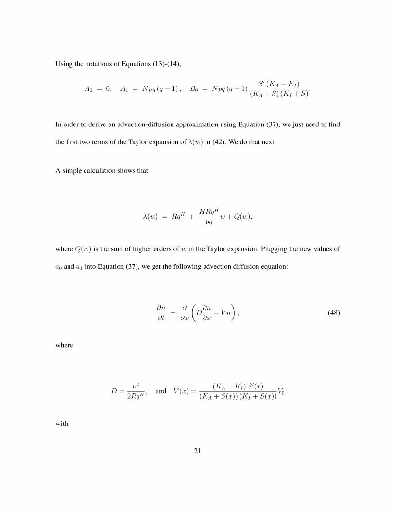
Using the notations of Equations (13)-(14),

A0 = 0, A1 = Npq (q − 1) , B0 = Npq (q − 1)S ′ (KA −KI)

(KA + S) (KI + S).

In order to derive an advection-diffusion approximation using Equation (37), we just need to find

the first two terms of the Taylor expansion of λ(w) in (42). We do that next.

A simple calculation shows that

λ(w) = RqH +HRqH

pqw +Q(w),

where Q(w) is the sum of higher orders of w in the Taylor expansion. Plugging the new values of

a0 and a1 into Equation (37), we get the following advection diffusion equation:

∂n

∂t=

∂

∂x

(D∂n

∂x− V n

), (48)

where

D =ν2

2RqH, and V (x) =

(KA −KI)S′(x)

(KA + S(x)) (KI + S(x))V0

with

21

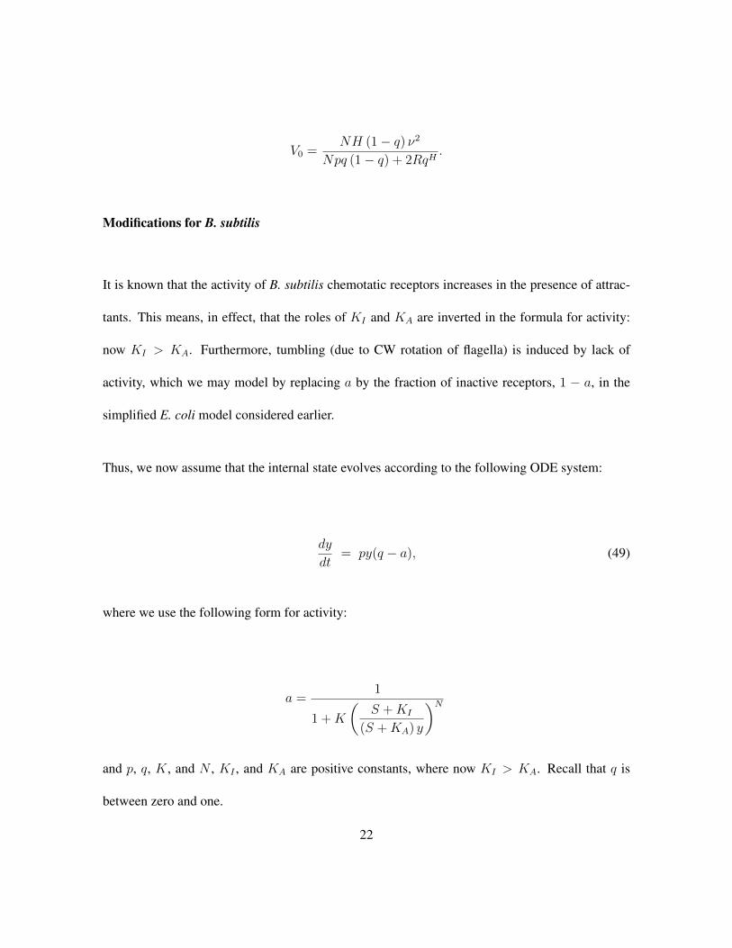
V0 =NH (1− q) ν2

Npq (1− q) + 2RqH.

Modifications for B. subtilis

It is known that the activity of B. subtilis chemotatic receptors increases in the presence of attrac-

tants. This means, in effect, that the roles of KI and KA are inverted in the formula for activity:

now KI > KA. Furthermore, tumbling (due to CW rotation of flagella) is induced by lack of

activity, which we may model by replacing a by the fraction of inactive receptors, 1 − a, in the

simplified E. coli model considered earlier.

Thus, we now assume that the internal state evolves according to the following ODE system:

dy

dt= py(q − a), (49)

where we use the following form for activity:

a =1

1 +K

(S +KI

(S +KA) y

)N

and p, q, K, and N , KI , and KA are positive constants, where now KI > KA. Recall that q is

between zero and one.

22

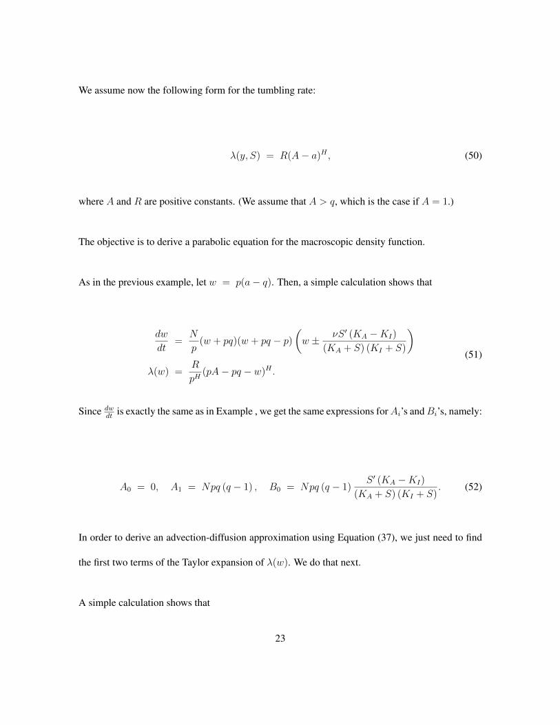
We assume now the following form for the tumbling rate:

λ(y, S) = R(A− a)H , (50)

where A and R are positive constants. (We assume that A > q, which is the case if A = 1.)

The objective is to derive a parabolic equation for the macroscopic density function.

As in the previous example, let w = p(a− q). Then, a simple calculation shows that

dw

dt=

N

p(w + pq)(w + pq − p)

(w ± νS ′ (KA −KI)

(KA + S) (KI + S)

)λ(w) =

R

pH(pA− pq − w)H .

(51)

Since dwdt

is exactly the same as in Example , we get the same expressions forAi’s andBi’s, namely:

A0 = 0, A1 = Npq (q − 1) , B0 = Npq (q − 1)S ′ (KA −KI)

(KA + S) (KI + S). (52)

In order to derive an advection-diffusion approximation using Equation (37), we just need to find

the first two terms of the Taylor expansion of λ(w). We do that next.

A simple calculation shows that

23

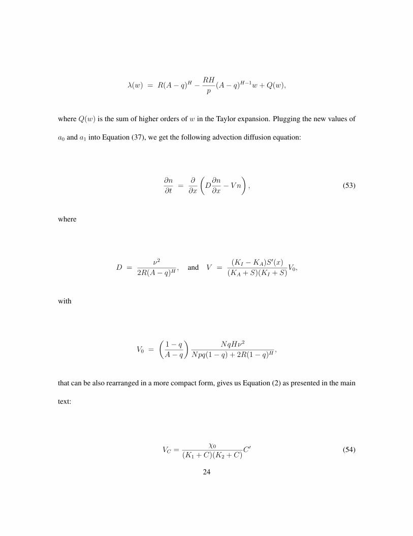
λ(w) = R(A− q)H − RH

p(A− q)H−1w +Q(w),

where Q(w) is the sum of higher orders of w in the Taylor expansion. Plugging the new values of

a0 and a1 into Equation (37), we get the following advection diffusion equation:

∂n

∂t=

∂

∂x

(D∂n

∂x− V n

), (53)

where

D =ν2

2R(A− q)H, and V =

(KI −KA)S ′(x)

(KA + S)(KI + S)V0,

with

V0 =

(1− qA− q

)NqHν2

Npq(1− q) + 2R(1− q)H,

that can be also rearranged in a more compact form, gives us Equation (2) as presented in the main

text:

VC =χ0

(K1 + C)(K2 + C)C ′ (54)

24

with

VC = V,K1 = KI , K2 = KA, C = Sχ0 = V0(KI −KA).

Thus, a formula of exactly the same form as for E. coli has been obtained.

Our mathematical model best captures aerotaxis in B. subtilis In order to assess how the model

we propose compares to alternative solutions in literature we grouped previous advection-diffusion

chemotaxis models in 3 main classes: KS, LS and RTBL models (see following section). Each of

these models has a different expression of the chemotactic speed VC and they range from fully

phenomenological (e.g. KS) to biophysically-informed approaches (like RTBL). The vast majority

of the other advection-diffusion models used to capture chemotaxis can be derived from the ones

we consider in the following.

We compared the performance of the models by plotting the prediction (Fig. S3-S9) of the best

combination of parameters the optimization algorithm found over 100 iterations and its prediction

error (Fig. 5, see Eq. 5 in the main text). For each model we also plot the distribution of prediction

errors of the 100 solutions to the optimization problem.

Notably, for the KS model the genetic algorithm consistently identified a single solution to the

parameter optimization problem (Fig. S3), hence the tight distribution in Fig. 5. Similar results in

terms of prediction accuracy (and therefore SSE, see Fig. 5) can be achieved using the best solution

identified for the LS model (Fig. S4). A significant improvement, instead, can be achieved using

25

the RTBL model (Fig. S5 and Fig. 5): the best parameter set found in this case achieves an SSE

significantly smaller than in the previous cases (0.95·10−1 compared to 1.84 ·10−1 for the LS and

1.90 ·10−1 for the KS models). However the model we propose displays the smallest prediction

error (0.73 ·10−1, Fig. 5) and therefore best captures the body of experimental data we describe

(Fig. 1C).

1 SI Materials and Methods

Growth protocol

B. subtilis strain OI1085 cells from a frozen (-80◦C) stock were resuspended in 2 mL of Cap As-

say Minimal media (50 mM KH2PO4, 50 mM K2HPO4, 1 mM MgCl2, 1 mM NH4SO4, 0.14

mM CaCl2, 0.01 mM MnCl2, 0.20 mM MgCl2), adding 15 µL HMT (5 mg/mL each of histidine,

methionine, and tryptophan, filter sterilized), 50 muL Tryptone Broth (10 g Tryptone (Difco) and

5 g NaCl in 1 L of distilled water), and 50 µL 1 M Sorbitol (filter sterilized). The culture was

incubated at 37◦C while shaking at 250 rpm until OD600 = 0.3 was reached. The culture was

then diluted 1:10 in fresh media before injection in the microfluidic device, to ensure cells were in

sufficiently low abundance to not affect the oxygen gradient via respiration.

26

2 Microfluidic fabrication, experimental operation and image analysis

In order to generate oxygen gradients, the source and sink channels were each connected to a

gas-mixing unit, supplied by gas tanks (Air Gas, MA). We used 100% nitrogen as well as 0.1%,

1%, 20% and 100% oxygen/nitrogen mixtures. Each gas-mixing unit was composed of two high-

precision flow controllers (Cole Parmer, IL), one for the appropriate mixture of oxygen and the

other for nitrogen, controlled by a MATLAB routine to achieve the final oxygen concentration that

would be flown into the source or sink channel. The sum of the flow rates in each line was set to

10 mL/min, while the ratio was set to achieve the desired oxygen concentration. The outlets of

the two flow controllers in each mixer were connected using a Y-junction, and low oxygen per-

meability tubing (C-flex Ultra, Cole Parmer, IL) was used to connect all the components to the

microfluidic device. To fabricate the microfluidic device we devised a precision cutting strategy

based on piezoelectric actuation to remove three 38 mm-long bands from a 200 µm thick PDMS

sheet. This yielded three parallel grooves piercing through the full depth of the PDMS sheet: the

central one (‘test channel’, 460 µm wide) was separated from each of the flanking ones (‘sink

channel’ and ‘source channel’) by a 220 µm thick PDMS wall. We then used a handheld plasma

bonder (BD20AC, ETP) to irreversibly bond the PDMS structure to two 2x3 inch glass slides, one

at the top and one at the bottom. Inlets and outlets were obtained by drilling holes (�=1 mm) in

the glass slides before bonding. In a typical experiment, we flowed the desired oxygen mixtures

in the source and sink channels and allowed them to diffuse within the device. Of note, the pres-

ence of the 220 µm thick PDMS wall separating the test channel from the sink channel implied

that the minimum oxygen concentration in the test channel was higher than the concentration in

27

the sink channel. Similarly, the maximum concentration in the test channel was lower than the

concentration in the source channel. For example, a 0%-100% case (0 M in the sink channel and

≈ 8 mM, on the other end, at the interface between PDMS and the source channel) corresponds to

an oxygen gradient ranging from 4.6% (60 µM) to 95% (1.24 mM, 100% oxygen in water corre-

sponding to 1.3 mM) in the test channel (see Table 1 in the Supplementary Information). Bacteria

were then injected in the test channel and glass coverslips were used to seal its inlet and outlet of

the test channel to suppress any residual flow. Cells reached steady state distribution within 5 min-

utes after the injection (Fig. 4). We then used an automated acquisition routine to capture 30,000

phase-contrast images of the same location along the test channel (equidistant from the inlet and

outlet) at 67 ms intervals over 33 min (20 objective; Andor Zyla camera with 6.5 µm/pixel (leading

to 0.33 µm/pixel resolution); see Materials and Methods). Each image contained 30-80 individ-

ual cells, making for (1-3)·106 total recorded cell positions and an estimated 380-1020 individual

bacteria included in the analysis. From these, we quantified the concentration of bacteria B(x)

in the direction x across the channel, normalized to a mean of 1 for comparison among different

conditions (see Materials and Methods; Fig. 1C). The large number of bacterial positions recorded

in each experiment enabled the quantification of B(x) with a spatial (x) resolution of 4.6 µm and

minimal noise (Fig. 1B,C), which proved fundamental for robust model identification. We imaged

the bacteria at channel mid-depth using an inverted microscope (Eclipse TE2000-E; Nikon) with

a 20 phase-contrast objective (NA = 0.45) and an sCMOS camera (Andor Zyla). A custom MAT-

LAB (Mathworks, MA) algorithm was used for image analysis to accurately identify individual

cell coordinates. The normalized bacterial concentration, B(x), was obtained from the histogram

28

of the number of bacteria in one hundred bins along the x direction, each 4.6 µm wide and together

covering the 460 µm width of the test channel, and then normalizing this distribution to a mean of

1. The uncertainty in the estimate of B(x) was obtained via bootstrapping bacterial x coordinates

from all the experiments available for each of the 33 gradients were pooled together. One million

samples of 10,000 coordinates each were then analyzed for each gradient to obtain an equivalent

number of estimates of B(x). The extents of the shaded area in Fig. 1C are obtained as the average

B(x) plus/minus its standard deviation calculated over 106 B(x) bootstrapped profiles.

Derivation and identification of the mathematical model

Starting from a Fokker-Planck approximation of the motion of B. subtilis in an oxygen gradient

(Supplementary Information) we derived the expression of VC reported in Eq. 2 in the main text.

In order to fully characterize the model we need to identify each of its three parameters K1, K2 and

χ0 - note that DB is measured experimentally (see Supplementary Information and Fig. S2). To

this aim we developed a genetic-algorithm-based multi-experimental fitting procedure designed to

find the combination of parameter values that minimized the sum of the squared errors between

model predictions and experimental data

SSE(K1, K2, χ0) =n∑i=1

√(BE(x)−BS(x))2 · w(x)

n(55)

where n = 33 is the number of experimental designs, w(x) is a vector of weights increasing

29

linearly from 1 to 1000 (empirically found to ensure the best results in terms of prediction error

were attained), BE(x) are the experimental data and BS(x) the simulated accumulation profiles

via numerical integration (∆x = 10 nm) of:

B(x) =eχ0∇CDB

∫ x0 f(ξ)dξ∫W

0f(ξ)dξ

(56)

with test channel width W = 460 µm and f(ξ) = 1/((K1 +C(ξ))(K2 +C(ξ))) for the model in

Eq. 2 in the main text. This expression of B(x) can be obtained plugging Eq. 2 in Eq. 1 in the main

text, using the linearity of the oxygen gradient (i.e. ∇C independent of ξ) and posing ∂B∂t

= 0. At

each iteration the genetic algorithm generated a number of random solutions, ranked them based

on Eq. 55, the worst solutions, selected the best ones and applied “cross-over” and “mutation”

to obtain new solutions to be evaluated at the next iteration 50. The search for a solution stopped

when a stall was detected, i.e., when the average change in SSE(χ0, K1, K2) over 50 iterations

was smaller than 10−6. The reported parameter set is the best combination identified over 100

repetitions of this procedure. We adopted the same method to identify the parameter values for all

models (see Supplementary Information).

Robustness analysis of parameter estimates

Although very powerful at solving complex optimization problems, Genetic Algorithms do not

provide any guarantee of convergence. As a consequence of this, a set of “optimal parameters”

30

obtained as a result of the optimization, might actually be a local, rather than a global solution

- these are solutions that optimize the objective function in a sufficiently large neighborhood of,

but not the entire, space of parameters. Yet, at the end of the parameter optimization process we

would ideally identify a set of values that minimizes the cost function (Eq. S62) globally rather

than locally.

To assess whether the values obtained from the Genetic Algorithm could be outcompeted by other

combinations of values, we decided to adopt a Naive Grid Search approach. The principle behind

this method is simple: the set of values each parameter can take is discretized and all the com-

bination of discretized parameters are evaluated using the cost function. The more fine-grained

the discretization is, the more this approach resembles an exhaustive search. The main limitation

of this approach is that for large numbers of parameters and/or parameter values the number of

objective function evaluations quickly increases and ultimately makes the problem intractable.

As customary in these cases, we assigned to each parameter identification task (i.e., each model

among the ones we considered) a budget of “function evaluations” equal to 105. For each of the i

parameters in that model, we identified a physically feasible set of values, and discretized it into

M values, with M being the closest integer to 105i . We then evaluated the cost function for each

of these combinations and, for each model, the value of the minimum cost identified by the Naive

Grid Search method was compared to the minimum found by the Genetic Algorithm (Fig. S10).

For both the KS and the LS models (1 and 2 parameters, respectively) we confirmed that the Naive

Grid Search identified values of the optimal parameters substantially undistinguishable from the

ones returned by the Genetic Algorithm. For the RTBL and the Finite Range Log-sensing regime,

31

instead, the Naive Grid Search algorithm returned values different from the Genetic Algorithm

and, in both cases, characterized by higher value the cost function - suggesting that the parameter

values identified by the Naive Grid Search are not global optima. These results indicate that it is

unlikely that the parameter sets identified by the Genetic Algorithm for our model represent local

optima and that they are instead the global optima we sought.

Model validation on transient aerotaxis

As a stringent validation of the model, we tested its performance in predicting the population mi-

gration in a transient aerotaxis experiment. At the start of the experiment, sink and source channels

both contained a flow of 21% oxygen and cells were allowed time to equilibrate to their steady state

distribution, which was uniform given the uniform oxygen concentration (Fig. 4). At time zero we

started flowing 0% and 0.05% oxygen in the sink and source channels, respectively, and recorded

the spatial distribution of bacteria across the test channel at 100 frames/s for 4 min To produce

B(x), we binned 200 frames (2 s) in one time point, in order to minimize noise. The model predic-

tion was obtained by integrating Eqs. 2 and 1 numerically with COMSOL (Comsol Inc., MA). We

modeled oxygen dynamics using the diffusion equation and representing the microfluidic device as

a one-dimensional domain with three parts: the 460 µm wide test channel (460 µm wide) and the

two, 220 µm wide, flanking PDMS walls, at the outer end of which the experimentally imposed

source and sink oxygen concentrations were prescribed. We note that, given the relative composi-

tion of the Cap Assay Minimal medium (essentially water supplemented with very small quantities

of salts, amino acids and sorbitol) and, coherently with what has been previously reported16, we

32

approximated the growth medium as water for the purpose of our simulations; therefore we set

the diffusion coefficient of oxygen in water to 2 · 10−9 m2/s. We observe that: (a) temperature

fluctuations have been ignored here as all the experiments have been carried out under temperature

control, (b) the density of bacteria was low enough10 (OD600=0.03) to allow us to ignore the effect

of respiration on the gradient and (c) although we do not expect inhomogeneity to be introduced

in the PDMS matrix as part of the microfabrication process, we did not assess how any residual

heterogeneities would have affected the diffusion dynamics. Oxygen profiles obtained as a result

of the simulations were then used as input in the bacterial transport equation (Eqs. 1 and 2), which

was solved in the test channel with a time step of 0.1 s and a spatial resolution of 4.6 µm, af-

ter ensuring these choices were sufficient to have a converged solution. The models used in our

comparative analysis are introduced and discussed in this section.

KS model

Developed in the early 70s by Keller and Segel 41, this was the first mathematical model that aimed

at quantitatively capturing chemotaxis. Studying slime molds the authors observed that chemo-

taxis is the result of random (diffusion) and directed motility (advection) of microorganisms and

consequently decided to use advection-diffusion models to capture it. When it came to the choice

of an expression for the advection (i.e. chemotactic) speed, VC , Keller and Segel took a phe-

nomenological approach and assumed it was directly proportional to the chemoattractant gradient

∇C (rescaled by a constant χ0) and inversely proportional to C the chemoattractant concentration:

33

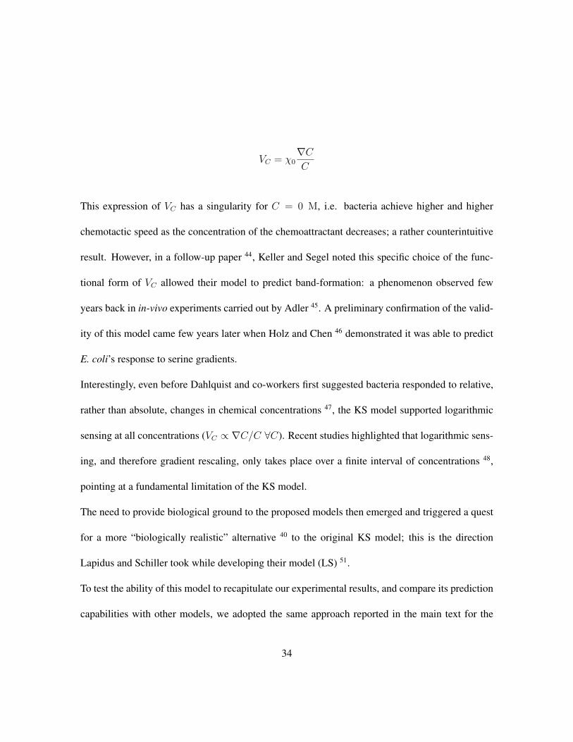
VC = χ0∇CC

This expression of VC has a singularity for C = 0 M, i.e. bacteria achieve higher and higher

chemotactic speed as the concentration of the chemoattractant decreases; a rather counterintuitive

result. However, in a follow-up paper 44, Keller and Segel noted this specific choice of the func-

tional form of VC allowed their model to predict band-formation: a phenomenon observed few

years back in in-vivo experiments carried out by Adler 45. A preliminary confirmation of the valid-

ity of this model came few years later when Holz and Chen 46 demonstrated it was able to predict

E. coli’s response to serine gradients.

Interestingly, even before Dahlquist and co-workers first suggested bacteria responded to relative,

rather than absolute, changes in chemical concentrations 47, the KS model supported logarithmic

sensing at all concentrations (VC ∝ ∇C/C ∀C). Recent studies highlighted that logarithmic sens-

ing, and therefore gradient rescaling, only takes place over a finite interval of concentrations 48,

pointing at a fundamental limitation of the KS model.

The need to provide biological ground to the proposed models then emerged and triggered a quest

for a more “biologically realistic” alternative 40 to the original KS model; this is the direction

Lapidus and Schiller took while developing their model (LS) 51.

To test the ability of this model to recapitulate our experimental results, and compare its prediction

capabilities with other models, we adopted the same approach reported in the main text for the

34

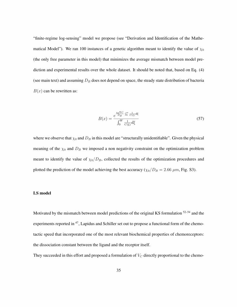
“finite-regime log-sensing” model we propose (see “Derivation and Identification of the Mathe-

matical Model”). We ran 100 instances of a genetic algorithm meant to identify the value of χ0

(the only free parameter in this model) that minimizes the average mismatch between model pre-

diction and experimental results over the whole dataset. It should be noted that, based on Eq. (4)

(see main text) and assumingDB does not depend on space, the steady state distribution of bacteria

B(x) can be rewritten as:

B(x) =eχ0∇CDB

·∫ x0

1C(ξ)

dξ∫W0

1C(ξ)

dξ(57)

where we observe that χ0 andDB in this model are “structurally unidentifiable”. Given the physical

meaning of the χ0 and DB we imposed a non negativity constraint on the optimization problem

meant to identify the value of χ0/DB, collected the results of the optimization procedures and

plotted the prediction of the model achieving the best accuracy (χ0/DB = 2.66 µm, Fig. S3).

LS model

Motivated by the mismatch between model predictions of the original KS formulation 52–54 and the

experiments reported in 47, Lapidus and Schiller set out to propose a functional form of the chemo-

tactic speed that incorporated one of the most relevant biochemical properties of chemoreceptors:

the dissociation constant between the ligand and the receptor itself.

They succeeded in this effort and proposed a formulation of VC directly proportional to the chemo-

35

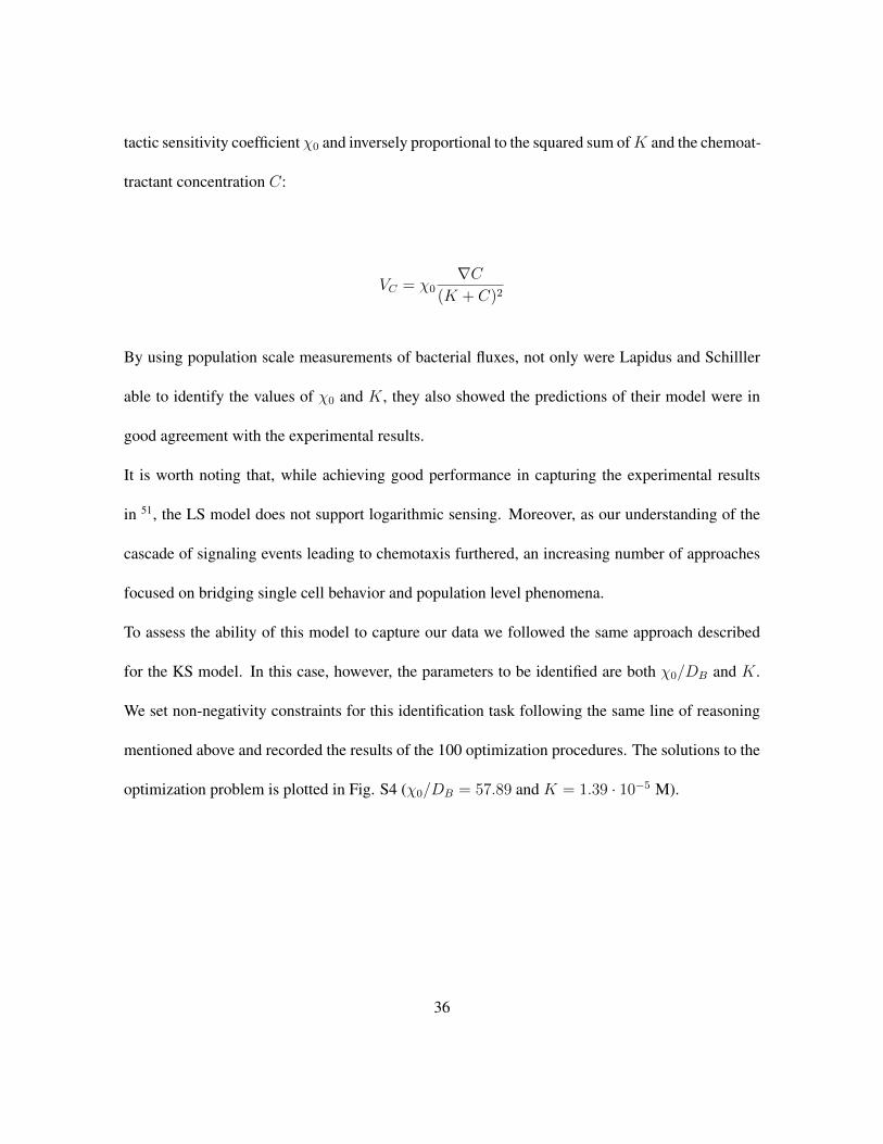
tactic sensitivity coefficient χ0 and inversely proportional to the squared sum ofK and the chemoat-

tractant concentration C:

VC = χ0∇C

(K + C)2

By using population scale measurements of bacterial fluxes, not only were Lapidus and Schilller

able to identify the values of χ0 and K, they also showed the predictions of their model were in

good agreement with the experimental results.

It is worth noting that, while achieving good performance in capturing the experimental results

in 51, the LS model does not support logarithmic sensing. Moreover, as our understanding of the

cascade of signaling events leading to chemotaxis furthered, an increasing number of approaches

focused on bridging single cell behavior and population level phenomena.

To assess the ability of this model to capture our data we followed the same approach described

for the KS model. In this case, however, the parameters to be identified are both χ0/DB and K.

We set non-negativity constraints for this identification task following the same line of reasoning

mentioned above and recorded the results of the 100 optimization procedures. The solutions to the

optimization problem is plotted in Fig. S4 (χ0/DB = 57.89 and K = 1.39 · 10−5 M).

36

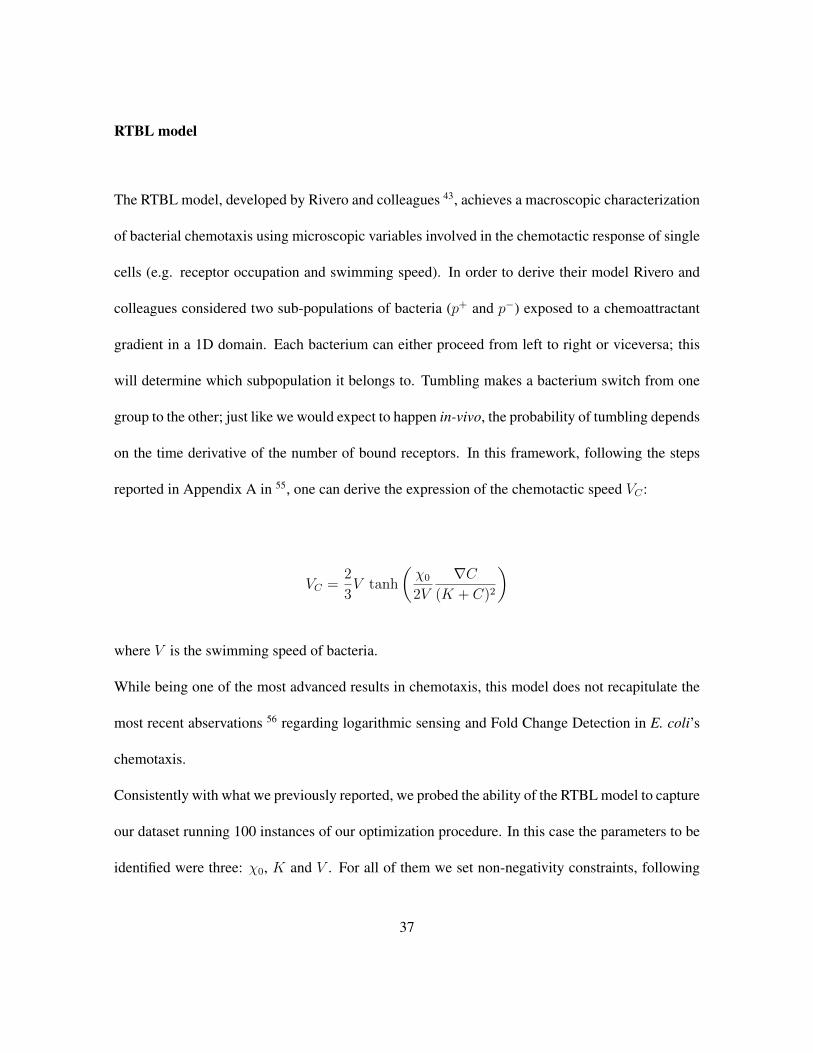
RTBL model

The RTBL model, developed by Rivero and colleagues 43, achieves a macroscopic characterization

of bacterial chemotaxis using microscopic variables involved in the chemotactic response of single

cells (e.g. receptor occupation and swimming speed). In order to derive their model Rivero and

colleagues considered two sub-populations of bacteria (p+ and p−) exposed to a chemoattractant

gradient in a 1D domain. Each bacterium can either proceed from left to right or viceversa; this

will determine which subpopulation it belongs to. Tumbling makes a bacterium switch from one

group to the other; just like we would expect to happen in-vivo, the probability of tumbling depends

on the time derivative of the number of bound receptors. In this framework, following the steps

reported in Appendix A in 55, one can derive the expression of the chemotactic speed VC :

VC =2

3V tanh

(χ0

2V

∇C(K + C)2

)

where V is the swimming speed of bacteria.

While being one of the most advanced results in chemotaxis, this model does not recapitulate the

most recent abservations 56 regarding logarithmic sensing and Fold Change Detection in E. coli’s

chemotaxis.

Consistently with what we previously reported, we probed the ability of the RTBL model to capture

our dataset running 100 instances of our optimization procedure. In this case the parameters to be

identified were three: χ0, K and V . For all of them we set non-negativity constraints, following

37

the considerations we previously discussed; moreover we restricted V , the swimming speed, to

not exceed 40 µm/s (we set this constraint according to experimental quantification of bacterial

swimming speed we obtained while measuringDB). Also in this case we collected statistics on the

prediction error of the solutions identified during the 100 runs of the optimization procedure (Fig.

5) and we plotted the results from the simulation of the best among the 100 solutions identified by

the genetic algorithm in Fig. S5 (χ0 = 7.10 · 10−8 m2/s, K = 7.01 · 10−6 M and V = 39.4 · 10−5

m/s).

References

33. J.R. Howse,R.A.L. Jones, A.J. Ryan,T. Gough, R. Vafabakhsh, and R. Golestanian, Self-Motile

Colloidal Particles: From Directed Propulsion to Random Walk Physical Review Letters, 99.

doi:10.1103/PhysRevLett.99.048102 (2007).

34. A. Sokolov, and I.S. Aranson,Physical properties of collective motion in suspensions of bac-

teria Physical Review Letters, 109. doi:10.1103/PhysRevLett.109.248109 (2012).

35. D.S. Bischoff, and G.W. Ordal Bacillus subtilis chemotaxis: a deviation from the Escherichia

coli paradigm. Molecular Microbiology, 6(1), 2328. doi:10.1111/j.1365-2958.1992.tb00833.x

36. Othmer H. G., Dunbar S. R., and Alt W. Models of dispersal in biological systems. J Math

Biol, 26(3):263–98, 1988.

37. L. Jiang, Q. Ouyang, and Y. Tu. Quantitative modeling of escherichia coli chemotactic quan-

titative modeling of escherichia coli chemotactic motion in environments varying in space and

38

time. PLoS Computational Biology, 6(4):e1000735, 2010.

38. J. Monod, J. Wyman, and J. P. Changeux. On the nature of allosteric transitions: a plausible

model. J. Mol. Biol., 12:88–118, May 1965.

39. Y. Tu, T. S. Shimizu, and H. C. Berg. Modeling the chemotactic response of Escherichia coli

to time-varying stimuli. Proc. Natl. Acad. Sci. U.S.A., 105:14855–14860, 2008.

40. M. Tindall, P. Maini,S. Porter, and J. Armitage Overview of mathematical approaches used

to model bacterial chemotaxis II: bacterial populations, Bulletin of Mathematical Biology,

70(6), 15701607 (2008).

41. E. Keller, and L. Segel Model for chemotaxis, J. Theor. Biol. 30(2), 225234 (1971).

42. M.A. Rivero-Hudec, and D. Lauffenburger Quantification of bacterial chemotaxis by measure-

ment of model parameters using the capillary assay Biotech. Bioeng. 28, 11781190 (1986).

43. M.A. Rivero, R.T. Tranquillo, H.M. Buettner, and D.A. Lauffenburger Transport models for

chemotactic cell-populations based on individual cell behavior Chem. Eng. Sci. 44:28812897

(1989).

44. E. Keller,and L. Segel, Traveling bands of chemotactic bacteria: a theoretical analysis Journal

of Theoretical Biology. 30(2), 235248 (1971).

45. J. Adler, Chemotaxis in bacteria Science 153, 708716 (1966).

46. M. Holz, and S.H. Chen, Spatio-temporal structure of migrating chemotactic band of Es-

cherichia coli. I. Traveling band profile Biophysical Journal, 26, 243261 (1979).

39

47. F.W. Dahlquist, P. Lovely and D.E. Koshland Quantitative analysis of bacterial migration in

chemotaxis Nat. New Biol. 1972;236:120123 (1972).

48. Y.V. Kalinin, L. Jiang, Y. Tu, and M. Wu, Logarithmic sensing in Escherichia coli bacterial

chemotaxis, Biophys. J. 96, 24392448 (2009).

49. T. Scribner,L. Segel and E. Rogers, A numerical study of the formation and propagation of

travelling bands of chemotactic bacteria J. Theor. Biol. 46, 189219 (1974).

50. Z. Michalewicz,Genetic Algorithms, Numerical Optimization, and Constraints Proc. sixth Int.

Conf. Genet. algorithms 195, 151158 (1995).

51. R. Lapidus and R. Schiller, Model for the chemotactic response of a bacterial population

Biophys. J. 16, 779789 (1976).

52. Nossal, R.,Weis, G., 1973. Analysis of a densitometry assay for bacterial chemotaxis. J. Theor.

Biol. 41(1), 143147.

53. Segel, L., Jackson, L., 1973. Theoretical analysis of chemotactic movements in bacteria. J.

Mechanochem. Cell Motility 2, 2534.

54. Lapidus, R., Schiller, R., 1974. A mathematical model for bacterial chemotaxis. Biophys. J.

14, 825834.

55. Ahmed, T., and Stocker, R. (2008). Experimental verification of the behavioral foundation of

bacterial transport parameters using microfluidics. Biophysical Journal, 95, 44814493.

40

56. Lazova, M. D., Ahmed, T., Bellomo, D., Stocker, R., and Shimizu, T. S. (2011). Response

rescaling in bacterial chemotaxis. Proceedings of the National Academy of Sciences of the

United States of America, 108, 1387013875.

57. Aminzare, Z., and Sontag, E.D. (2013). Remarks on a population-level model of chemotaxis:

advection-diffusion approximation and simulations. arXiv:1302.2605v1.

41

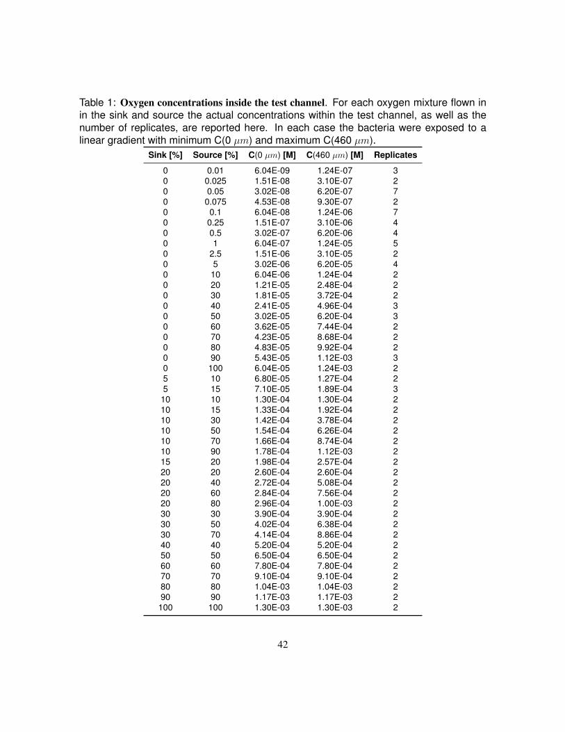
Table 1: Oxygen concentrations inside the test channel. For each oxygen mixture flown inin the sink and source the actual concentrations within the test channel, as well as thenumber of replicates, are reported here. In each case the bacteria were exposed to alinear gradient with minimum C(0 µm) and maximum C(460 µm).

Sink [%] Source [%] C(0 µm) [M] C(460 µm) [M] Replicates

0 0.01 6.04E-09 1.24E-07 30 0.025 1.51E-08 3.10E-07 20 0.05 3.02E-08 6.20E-07 70 0.075 4.53E-08 9.30E-07 20 0.1 6.04E-08 1.24E-06 70 0.25 1.51E-07 3.10E-06 40 0.5 3.02E-07 6.20E-06 40 1 6.04E-07 1.24E-05 50 2.5 1.51E-06 3.10E-05 20 5 3.02E-06 6.20E-05 40 10 6.04E-06 1.24E-04 20 20 1.21E-05 2.48E-04 20 30 1.81E-05 3.72E-04 20 40 2.41E-05 4.96E-04 30 50 3.02E-05 6.20E-04 30 60 3.62E-05 7.44E-04 20 70 4.23E-05 8.68E-04 20 80 4.83E-05 9.92E-04 20 90 5.43E-05 1.12E-03 30 100 6.04E-05 1.24E-03 25 10 6.80E-05 1.27E-04 25 15 7.10E-05 1.89E-04 3

10 10 1.30E-04 1.30E-04 210 15 1.33E-04 1.92E-04 210 30 1.42E-04 3.78E-04 210 50 1.54E-04 6.26E-04 210 70 1.66E-04 8.74E-04 210 90 1.78E-04 1.12E-03 215 20 1.98E-04 2.57E-04 220 20 2.60E-04 2.60E-04 220 40 2.72E-04 5.08E-04 220 60 2.84E-04 7.56E-04 220 80 2.96E-04 1.00E-03 230 30 3.90E-04 3.90E-04 230 50 4.02E-04 6.38E-04 230 70 4.14E-04 8.86E-04 240 40 5.20E-04 5.20E-04 250 50 6.50E-04 6.50E-04 260 60 7.80E-04 7.80E-04 270 70 9.10E-04 9.10E-04 280 80 1.04E-03 1.04E-03 290 90 1.17E-03 1.17E-03 2100 100 1.30E-03 1.30E-03 2

42

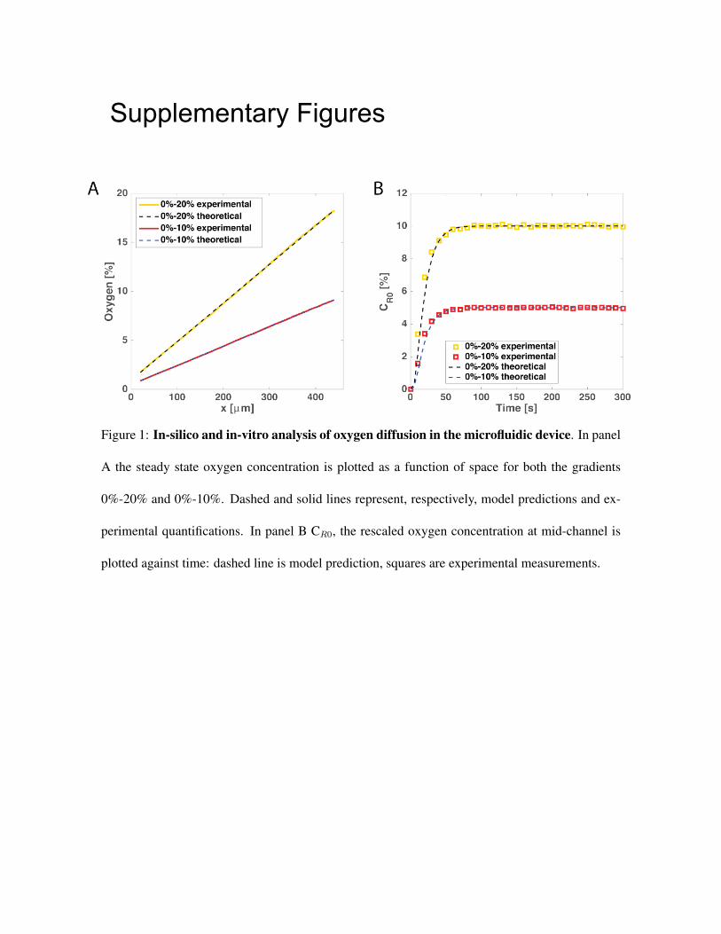
Figure 1: In-silico and in-vitro analysis of oxygen diffusion in the microfluidic device. In panel

A the steady state oxygen concentration is plotted as a function of space for both the gradients

0%-20% and 0%-10%. Dashed and solid lines represent, respectively, model predictions and ex-

perimental quantifications. In panel B CR0, the rescaled oxygen concentration at mid-channel is

plotted against time: dashed line is model prediction, squares are experimental measurements.

Supplementary Figures

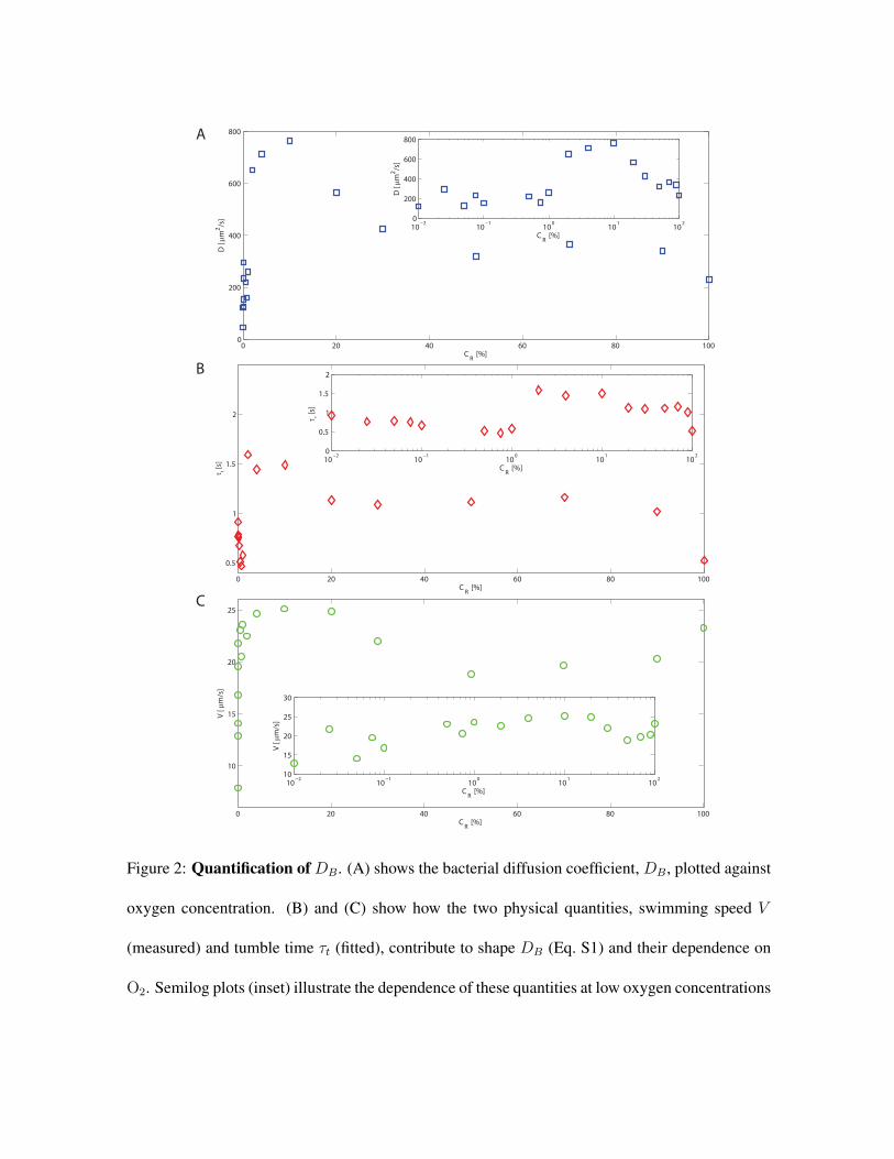
Figure 2: Quantification of DB. (A) shows the bacterial diffusion coefficient, DB, plotted against

oxygen concentration. (B) and (C) show how the two physical quantities, swimming speed V

(measured) and tumble time τt (fitted), contribute to shape DB (Eq. S1) and their dependence on

O2. Semilog plots (inset) illustrate the dependence of these quantities at low oxygen concentrations

0 20 40 60 80 1000

200

400

600

800

CR

[%]

D [µ

m2

/s]

10−2

10−1

100

101

102

0

200

400

600

800

CR

[%]

D [µ

m2

/s]

0 20 40 60 80 100

10

15

20

25

CR

[%]

V [µ

m/s

]

10−2

10−1

100

101

102

10

15

20

25

30

CR

[%]

V [µ

m/s

]

0 20 40 60 80 100

0.5

1

1.5

2

CR

[%]

τ t [s]

10−2

10−1

100

101

102

0

0.5

1

1.5

2

CR

[%]

τ τ [

s]

A

B

C

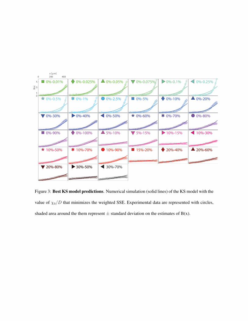
Figure 3: Best KS model predictions. Numerical simulation (solid lines) of the KS model with the

value of χ0/D that minimizes the weighted SSE. Experimental data are represented with circles,

shaded area around the them represent ± standard deviation on the estimates of B(x).

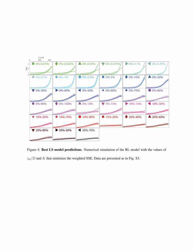
Figure 4: Best LS model predictions. Numerical simulation of the RL model with the values of

χ0/D and K that minimize the weighted SSE. Data are presented as in Fig. S3.

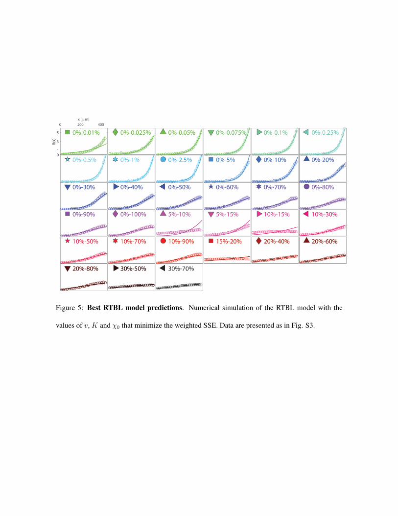
Figure 5: Best RTBL model predictions. Numerical simulation of the RTBL model with the

values of v, K and χ0 that minimize the weighted SSE. Data are presented as in Fig. S3.

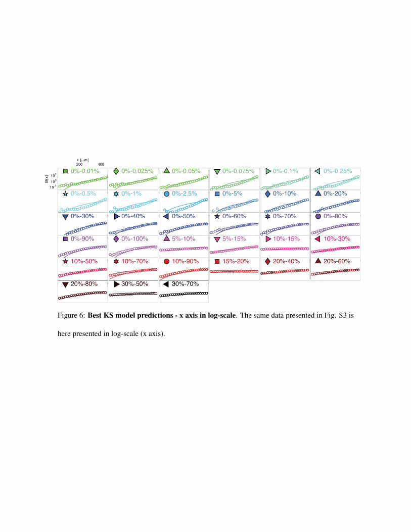
Figure 6: Best KS model predictions - x axis in log-scale. The same data presented in Fig. S3 is

here presented in log-scale (x axis).

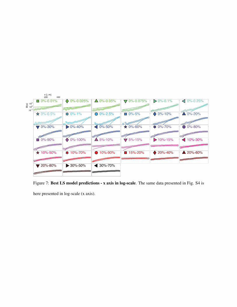
Figure 7: Best LS model predictions - x axis in log-scale. The same data presented in Fig. S4 is

here presented in log-scale (x axis).

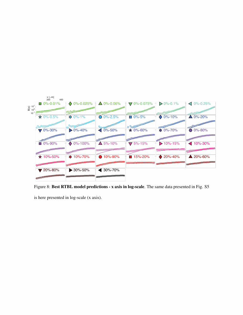
Figure 8: Best RTBL model predictions - x axis in log-scale. The same data presented in Fig. S5

is here presented in log-scale (x axis).

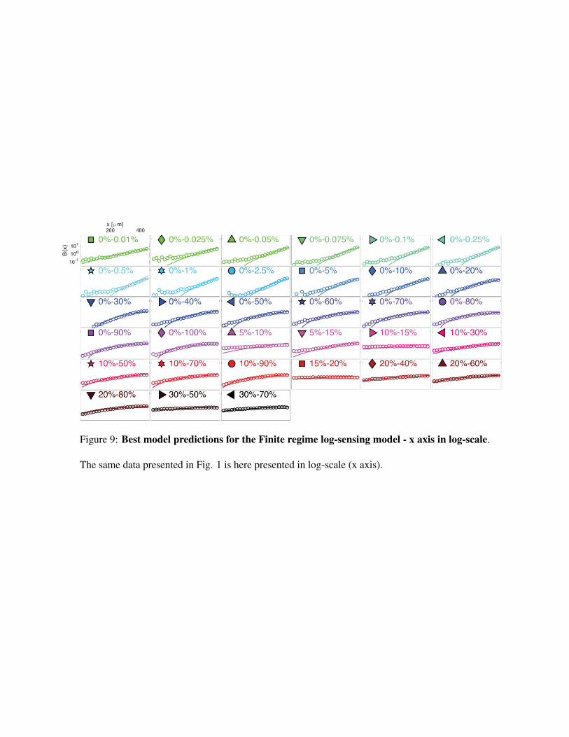
Figure 9: Best model predictions for the Finite regime log-sensing model - x axis in log-scale.

The same data presented in Fig. 1 is here presented in log-scale (x axis).

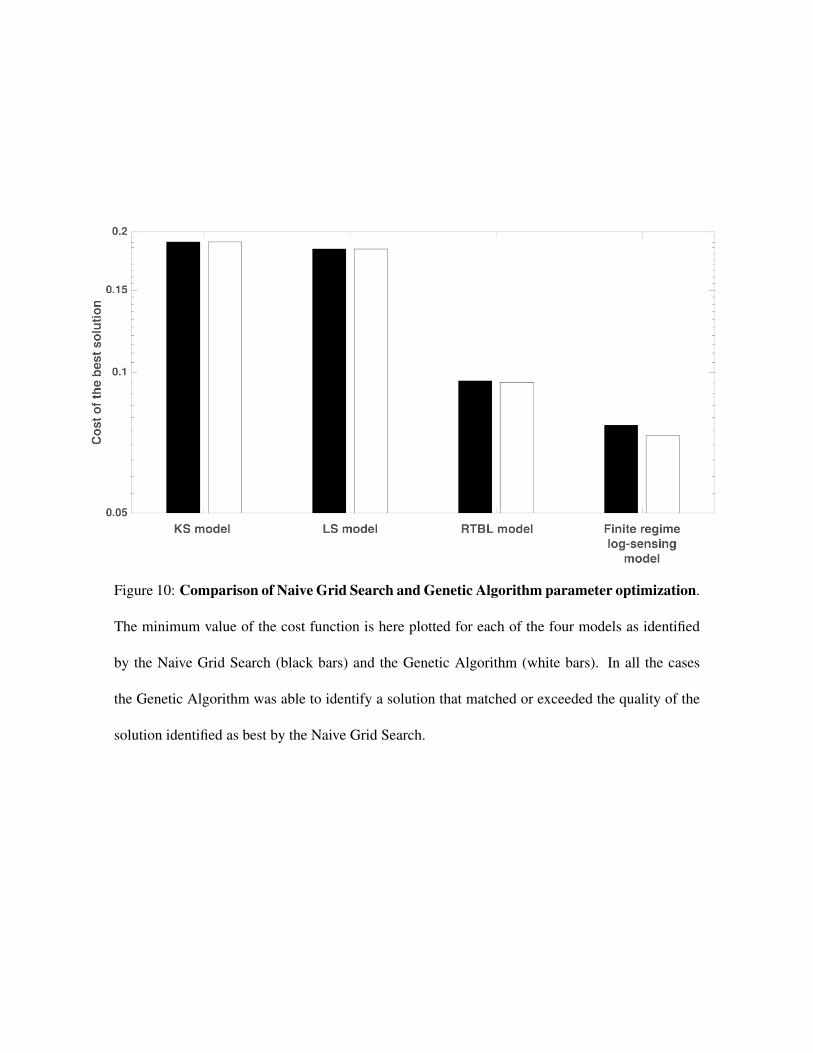
Figure 10: Comparison of Naive Grid Search and Genetic Algorithm parameter optimization.

The minimum value of the cost function is here plotted for each of the four models as identified

by the Naive Grid Search (black bars) and the Genetic Algorithm (white bars). In all the cases

the Genetic Algorithm was able to identify a solution that matched or exceeded the quality of the

solution identified as best by the Naive Grid Search.

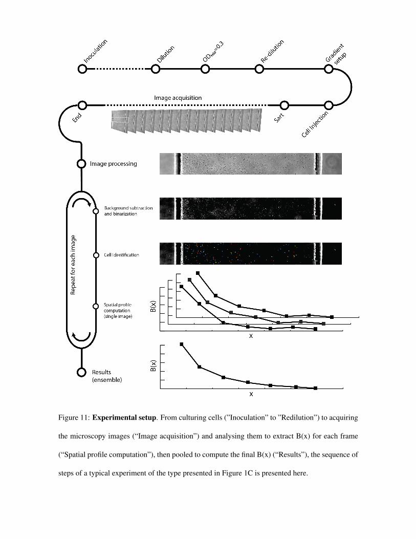
Figure 11: Experimental setup. From culturing cells (”Inoculation” to ”Redilution”) to acquiring

the microscopy images (“Image acquisition”) and analysing them to extract B(x) for each frame

(“Spatial profile computation”), then pooled to compute the final B(x) (“Results”), the sequence of

steps of a typical experiment of the type presented in Figure 1C is presented here.

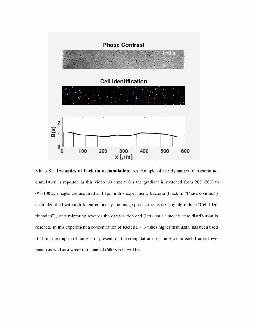
Video S1: Dynamics of bacteria accumulation. An example of the dynamics of bacteria ac-

cumulation is reported in this video. At time t=0 s the gradient is switched from 20%-20% to

0%-100%; images are acquired at 1 fps in this experiment. Bacteria (black in “Phase contrast”),

each identified with a different colour by the image processing processing algorithm (“Cell Iden-

tification”), start migrating towards the oxygen rich end (left) until a steady state distribution is

reached. In this experiment a concentration of bacteria ∼ 3 times higher than usual has been used

(to limit the impact of noise, still present, on the computational of the B(x) for each frame, lower

panel) as well as a wider test channel (600 µm in width).