Article Pre-Print The following article is a “pre-print” of an article accepted for publication in an

Elsevier journal.

Planning and Scheduling of Steel Plates Production. Part I. Estimation of

Production Times via Hybrid Bayesian Networks for Large Domain of

Discrete Variables, Comp Chem Eng,, 79 113-134 (2015)

The pre-print is not the final version of the article. It is the unformatted version

which was submitted for peer review, but does not contain any changes made

as the result of reviewer feedback or any editorial changes. Therefore, there may

be differences in substance between this version and the final version of record.

The final, official version of the article can be downloaded from the journal’s

website via this DOI link when it becomes available (subscription or purchase

may be required):

doi:10.1016/j.compchemeng.2015.02.005

This post-print has been archived on the author’s personal website

(macc.mcmaster.ca) in compliance with the National Sciences and Engineering

Research Council (NSERC) policy on open access and in compliance with

Elsevier’s academic sharing policies.

This post-print is released with a Creative Commons Attribution Non-

Commercial No Derivatives License.

Date Archived: June 1, 2016

Planning and Scheduling of Steel Plates Production.Part I: Estimation of Production Times via HybridBayesian Networks for Large Domain of Discrete

Variables

Junichi Mori and Vladimir Mahalec∗

Department of Chemical Engineering

McMaster University, Hamilton, Ontario, Canada L8S 4L7

Abstract

Knowledge of the production loads and production times is an essential ingredient

for making successful production plans and schedules. In steel production, the pro-

duction loads and the production times are impacted by many uncertainties, which

necessitates their prediction via stochastic models. In order to avoid having separate

prediction models for planning and for scheduling, it is helpful to develop a single pre-

diction model that allows us to predict both production loads and production times.

In this work, Bayesian network models are employed to predict the probability dis-

tributions of these variables. First, network structure is identified by maximizing the

Bayesian scores that include the likelihood and model complexity. In order to handle

large domain of discrete variables, a novel decision-tree structured conditional prob-

ability table based Bayesian inference algorithm is developed. We present results for

real-world steel production data and show that the proposed models can accurately

predict the probability distributions.

Keywords: Production load, production time, hybrid Bayesian network, structure

∗Corresponding author. Email: mahalec@mcmaster.ca

1

learning, large domain variable, decision tree, maximum likelihood estimation, steel plate

production

1 Introduction

Accurate estimation of the production loads and the total production times in manufac-

turing processes is crucial for optimal operations of real world industrial systems. In this

paper, a production load represents the number of times that a product is processed in

the corresponding process unit and a production time is defined as the length of time from

production start to completion. Production planning and scheduling for short, medium and

long term time horizons employ various optimization models and algorithms that require

accurate knowledge of production loads and total production times from information at each

of the processing steps. The approaches to predict the production loads and total produc-

tion times can be either based on mechanistic model or can employ data-driven techniques.

Model-based prediction methods may be applied only if accurate mechanistic models of the

processes can be developed. First principal models require in-depth knowledge of the pro-

cesses and still cannot take into consideration all uncertainties that exist in the processes.

Therefore, mechanistic models may not work well for prediction of production loads and

production times of the real-world industrial processes. On the other hand, data-driven

approaches do not require in-depth process knowledge and some advanced techniques can

deal with the process uncertainties.

The most straightforward approach is to use the classical statistical models (e.g. re-

gression models) that estimate the values of new production loads and a production time

from the past values in the historical process data. The relationships between the targeted

variables and other relevant variables are used to compute the statistical model that can

predict the production loads and production times. However, such models are too simple

to predict the nonlinear behaviour and estimate the system uncertainties. An alternative

2

simple method is to compute the average of these values per each production group that has

similar production properties and then utilize the average values of each production group

as the prediction (Ashayeria et al., 2006). In this case the prediction accuracy significantly

depends on the rules that govern creation of production groups and it may be challenging

to find the appropriate rules from process knowledge only. To overcome this limitation, su-

pervised classification techniques such as artificial neural networks (ANN), support vector

machine, Fisher discriminant analysis and K-nearest neighbours (KNN) may be useful to

design the rules to make production groups from historical process data. However, even

though we can accurately classify the historical process data into an appropriate number

of production groups, these methods do not consider model uncertainties and cannot han-

dle missing values and unobserved variables. In addition, we are typically forced to have

multiple specific models tailored for specific purposes, e.g. for production planning or for

scheduling, which causes model maintenance issues and lack of model consistency.

Bayesian network (BN) models offer advantages of having single prediction model for pre-

dicting the production loads and total process times in planning and scheduling. Bayesian

networks are also called directed graphical models where the links of the graphs repre-

sent direct dependence among the variables and are described by arrows between links

(Pearl, 1988; Bishop, 2006). Bayesian network models are popular for representing condi-

tional independencies among random variables under system uncertainty. They are popular

in the machine learning communities and have been applied to various fields including med-

ical diagnostics, speech recognition, gene modeling, cancer classification, target tracking,

sensor validation, and reliability analysis.

The most common representations of conditional probability distributions (CPDs) at

each node in BNs are conditional probability tables (CPTs), which specify marginal prob-

ability distributions for each combination of values of its discrete parent nodes. Since the

real industrial plant data often include discrete variables which have large discrete domains,

3

the number of parameters becomes too large to represent the relationships by the CPTs.

In order to reduce the number of parameters, context-specific independence representa-

tions are useful to describe the CPTs (Boutilier et al., 1996). Efficient inference algorithm

that exploits context-specified independence (Poole and Zhang, 2003) and the learning

methods for identification of parameters of context-specific independence (Friedman and

Goldszmidt, 1996; Chickering et al., 1997) have been developed. The restriction of these

methods is that all discrete values must be already grouped at an appropriate level of

domain size since learning structured CPTs is NP-hard. However, typically discrete pro-

cess variables have large domains and the task of identifying a reasonable set of groups

that distinguish well the values of discrete variables requires in-depth process knowledge.

To overcome this limitation, attribute − value hierarchies (AVHs) that capture meaningful

groupings of values in a particular domain are integrated with the tree-structured CPTs

(DesJardins and Rathod, 2008). However, since some discrete process variables do not

contain hierarchal structures and thus AVHs cannot capture the useful abstracts of values

in that domain. In addition, this model cannot handle the continuous variables without

discretizing them. Furthermore, the authors do not describe how to apply AVH-derived

CPTs to Bayesian inference. Therefore, this method has difficulty predicting probability

distributions of production loads and total process time from observed process variables in

the real-world industrial processes. Efficient alternative inference methods in Bayesian Net-

works containing CPTs that are represented as decision trees have been developed (Sharma

and Poole, 2003). The inference algorithm is based on variable elimination (VE) algorithm.

However, because the computational complexity of the exact inference such as VE grows

exponentially with the size of the network, this method may not be appropriate for Bayesian

networks for large scale industrial data sets. In addition, the method does not deal with

application of the decision-tree structured CPTs to hybrid Bayesian networks, where both

discrete and continuous variables appear simultaneously.

In hybrid Bayesian networks, the most commonly used model that allows exact in-

4

ference is the conditional linear Gaussian (CLG) model (Lauritzen, 1992; Lauritzen and

Jensen, 2001). However, the proposed network model does not allow discrete variables to

have continuous parents. To overcome this limitation, the CPDs of these nodes are typi-

cally modeled as softmax function, but there is no exact inference algorithm. Although an

approximate inference via Monte Carlo method has been proposed (Koller et al., 1999), the

convergence can be quite slow in Bayesian Networks with large domain of discrete variables.

The other approach is to discretize all continuous variables in a network and treat them as

if they are discrete (Kozlov and Koller, 1997). Nevertheless, it is typically impossible to

discretize the continuous variables as finely as needed to obtain reasonable solutions and

the discretization leads to a trade-off between accuracy of the approximation and cost of

computation. As another alternative, the mixture of truncated exponential (MTE) model

has been introduced to handle the hybrid Bayesian networks (Moral et al., 2001; Rumi

and Salmeron, 2007; Cobb et al., 2007). MTE models approximate arbitrary probability

distribution functions (PDFs) using exponential terms and allow implementation of infer-

ence in hybrid Bayesian networks. The main advantage of this method is that standard

propagation algorithms can be used. However, since the number of regression coefficients

in exponential functions linearly grows with the domain size of discrete variables, MTE

model may not work well for the large Bayesian networks that are required to represent the

industrial processes.

Production planning and scheduling in the steel industry are recognized as challenging

problems. In particular, the steel plate production is one of the most complicated pro-

cesses because steel plates are high-variety low-volume products manufactured on order

and they are used in many different applications. Although there have been several stud-

ies on scheduling and planning problems in steel production, such as continuous casting

(Tang et al., 2000; Santos et al., 2003), smelting process (I. Harjunkoski, 2001) and batch

annealing (Moon and Hrymak, 1999), few studies have dealt with steel plate production

scheduling. Steel rolling processes manufacture various size of plates from a wide range of

5

materials. Then, at the finishing and inspection processes, malfunctions occurred in the

upstream processes (e.g. smelting processes) are repaired, and additional treatments such

as heat treatment and primer coating are applied such that the plates satisfy the intended

application needs and satisfy the demanded properties. In order to obtain successful plans

and schedules for steel plate production, it is necessary to determine the production starting

times that meet both the customer shipping deadlines and the production capacity. This

requires prediction models that can accurately predict the production loads of finishing and

inspection lines and the total process time. However, due to the complexity and uncertain-

ties that exist in the steel production processes, it is difficult to build the precise prediction

models. These difficulties have been discussed in the literature (Nishioka et al., 2012).

In our work, in order to handle the complicated interaction among process variables and

uncertainties, Bayesian networks are employed for predicting of the production loads and

prediction of the total production time. Since the steel production data have large do-

main of discrete variables, their CPDs are described by tree structured CPTs. In order to

compute the tree structured CPTs, we use decision trees algorithm (Breiman et al., 1984)

that is able to group the discrete values to capture important distinctions of continuous or

discrete variables. If Bayesian networks include continuous parent nodes with a discrete

child node, the corresponding continuous variables can be discretized as finely as needed,

because the domain size of discretized variable does not increase the number of parameters

in intermediate factors due to decision-tree structured CPTs. Since the classification algo-

rithms are typically greedy ones, the computational task for learning the structured CPTs

is not expensive. Then, the intermediate factors can be described compactly using a simple

parametric representation called the canonical table representation.

As for Bayesian network structure, if the cause-effect relationship is clearly identified

from process knowledge, knowledge based network identification approach is well-suited.

However, the identification of cause-effect relationships may require in-depth knowledge of

6

the processes to characterize the complex physical, chemical and biological phenomena. In

addition, it can be time-consuming to build precise graphical model for complex processes,

and it is also challenging to verify the identified network structure. Therefore, data-driven

techniques are useful to systematically identify the network structure from historical process

data. The basic idea of learning the network structure is to search for the graph so that the

likelihood based score function is maximized. Since this is a combinational optimization

problem which is known as NP -hard, it is challenging to compute the precise network

structure for industrial plants where there are a large number of process variables and

historical data sets. In order to restrict the solution space, we fix the root and leaf nodes

by considering the properties of the process variables. In addition, we take into account

two types of Bayesian network structures, which are: (i) a graph where a node of the total

production time is connected with all nodes of the production loads and (ii) a graph where

a node of the total production time is connected with all nodes of the individual production

time on each production load and the nodes of these individual process time are connected

to the nodes of the total production time. In the latter Bayesian network structure, the

training data set that contains each production period of all production processes is needed

in order to directly compute the parameters of conditional probability distributions of each

production period.

We also propose the decision-tree structured CPT based Bayesian inference algorithm,

which employs belief propagation algorithm to handle hybrid Bayesian networks with large

domain of discrete variables. In order to reduce the computational effort required for multi-

plying and marginalizing factors during belief propagation, the operations via dynamically

construct structured CPTs are proposed. Since the inference task is to predict the cause of

production loads and the total production time from the effect of other process variables,

we need the causal reasoning which can be carried out by using the sum-product algorithm

from top node factors to bottom node factors. In addition, other types of inference such as

diagnostic and intercausal reasoning are also investigated in the case when we need to infer

7

some other process variables such as operating conditions given production loads.

The organization of this paper is as follows. Section 2 introduces the plate steel pro-

duction problem. Section 3 proposes the structure identification algorithm for steel plate

production processes. Section 4 describes the proposed decision-tree structured CPTs based

Bayesian inference algorithm and section 5 proposes the inference algorithm. The presented

method is applied to the steel plate production process data in section 6. Finally, the con-

clusions are presented in Section 7. Appendix Appendices A describes algorithm to find the

network structure that maximizes the score function, Appendix B describes computation

of causal reasoning, Appendix C deals with diagnostic and causal reasoning, and Appendix

D describes belief propagation with evidence.

2 Problem Definition

The plate steel mills studied in this paper consist of rolling machines, finishing and inspec-

tion processes. The purpose of the plate mills is to manufacture the steel plates, which are

end products made from steel slabs via continuous casting processes. The slabs are sent to

the rolling machines which include roughing mill, finishing mill and hot levelling machine

through continuous or batch reheating furnace. To manufacture the high-strength steel

plates, Accelerated Cooling (ACC) process which is based on the combination of controlled

rolling and controlled cooling is used. After rolling or cooling, the plates are sent to the fin-

ishing and inspection processes, where defects that have occurred in the upstream processes

such as smelting processes are repaired. Here, additional treatments such as heat treatment

and primer coating are carried out as needed so that the plates have the properties required

for their intended usages. The process is illustrated in Fig. 1.

One of the most important goals for production planning and scheduling is to use in

the best possible manner the subsystems which are the bottlenecks, since the total plant

8

capacity is determined by the bottleneck capacity. In the plate mills, bottlenecks typically

occur in the finishing and inspection lines. Therefore, an effective way to approach the

planning and scheduling in the plate mills is to determine the rolling starting time of

each order in such a manner that the limiting capacities are used to their maximum and

that the customer demanded shipment deadlines are satisfied. For this purpose, when

sales department staff receive orders from the customers, they must take into account

the plate mills capacities and production times to avoid creating supply bottlenecks and

to meet the customer deadlines. Similarly, the staff in the manufacturing department

prepare the production plans and schedules while considering the production capacities

and production times. However, due to the complicated and stochastic processes of the

finishing and inspection lines, there is no deterministic way to predict the production loads

and production time that are required to determine the production start times as required

to avoid the bottlenecks and meet the customer deadline. In this paper, production loads

represent the number of times that one plate or a set of total plates per day is processed

at the corresponding production process unit. For instance, if 10 plates are processed

at process A per day, then the production load of process A is computed as 10 per day.

Production time for each plate or each customer order represents the time required to

manufacture a product, starting from slabs to the finished products. In this paper, since

the processing time in the inspection and finishing lines is a large part of the production

time, the production time represents the period from production start to completion as

shown in Fig. 1.

When a steel plate manufacturer receives orders from a customer, the product demand

is known while the operating conditions, which are required to manufacture this specific

product (order), are not available. On the other hand, at the manufacturing stage, all

information about customer demands and detailed operating conditions is known.

Motivated by the above considerations, we can divide the tasks in plate steel production

9

planning and scheduling into two parts: (i) accurate prediction of the production loads and

production time and (ii) optimization of the manufacturing plans and schedules based on

the production time prediction models. In this paper, we focus on the development of the

prediction model for production loads and production time. The prediction model needs to

enable:

1. Estimation of the probability distributions of production loads and production time,

since the finishing and inspection lines include various sources of uncertainties and thus

stochastic prediction models are desirable.

2. Dealing with unobservable (unavailable) variables, because it is desirable to have a

single model and avoid multiple models that meet with specific problems.

Having a single model with above properties enables planning and scheduling based on the

same model which improves consistency of decisions between planning and scheduling and

also simplifies model maintenance.

3 Identification of Bayesian Networks Structure for

Steel Plate Production

In order to build a model which has the properties mentioned in the previous section, we

develop the methods to compute probability distributions of unknown states of production

loads and production times by using Bayesian network. Methodology to build the model

will be illustrated by an example which has 21 discrete variables and 5 continuous variables

as shown in Table 1. Each production load is assigned a binary variable having value of 1

if the corresponding production process is not needed, otherwise it is 2.

In this section, we propose the knowledge based date-driven structure learning algorithm

to construct the Bayesian network structure. In the subsequent sections, we will propose

10

the parameter estimation and inference approaches with the constructed Bayesian network

structure.

The computational task for structure learning is to find the optimal graph such that the

maximized Bayesian scores can be obtained, which is known as NP-hard problem. In order

to reduce the computational effort, we allow some variables to be set at the root nodes or

the leaf nodes and also impose some constraints about orders of subsets of system variables.

First and the most important task for Bayesian inference is to synthesize the precise

network structure. The most straightforward method is to design the network structure from

process knowledge. However, by-hand structure design requires in-depth process knowledge

because identification of cause-effect relationships is needed to characterize the complex

physical, chemical and biological phenomena in systems. On the other hand, data-driven

based techniques such as score function based structure learning are useful when there is

lack of process knowledge or considered processes are too complicated to analyze.

The goal of structure learning is to find a network structure G that is a good estimator

for the data x. The most common approach is score-based structure learning , which defines

the structure learning problem as an optimization problem (Koller and Friedman, 2009). A

score function score(G : D) that measures how well the network model fits the observed data

D is defined. The computational task is to solve the combinational optimization problem of

finding the network that has the highest score. The detailed algorithm to find the network

structure that maximizes the score function is explained in Appendix A. It should be noted

that this combinational optimization problem is known to be NP -hard (Chickering, 1996).

Therefore, it is challenging to obtain the optimal graph for industrial plants which often

include a large number of process variables.

In order to reduce the computational cost, we incorporate the fundamental process knowl-

edge into the network structure learning framework. As shown in the variable list of Table

11

1, all of our system variables belong to either customer demands or operating conditions or

production loads or production time. One can immediately notice that customer demands

can be considered “cause variables′′ of all system variables in the Bayesian network and

are never impacted by either operating conditions, production loads or production time.

Therefore, the nodes of variables belonging to the customer demands should be placed on

the root nodes in the Bayesian network. Similarly, production loads are affected by the

customer demands, operating conditions or both and not vice versa. Taking into account

above considerations, we propose two types of Bayesian networks as shown in Fig. 2. In

both Bayesian networks, the nodes related to the customer demands are placed at the root

nodes followed by operating conditions, production loads and production time. The differ-

ence between two structures is that in the second BN structure, the nodes associated with

the production time at each production process are added between the nodes of production

loads and total production time while in the first BN structure, total production time is

directly connected to the production loads.

In addition, we propose some predetermined variable ordering ≺ over x to reduce further

the computational cost further. If the ordering covers order relationships over all variables

as x1 ≺ x2, . . . , xI and the maximum number of parents for each node set to be at most d,

then the number of possible parent sets for xi is at most

(i− 1d

)rather than 2I−1 (Koller

and Friedman, 2009). In practice, nevertheless, these complete orderings are very difficult

to identify from process knowledge. Instead of identification of complete orderings, we

proposed incomplete orderings that do not cover order relationships over all variables but

restrict the ordering over subsets of variables. The following is an example of the incomplete

ordering.

{x1, x2} ≺ {x3, x4, x5} ≺ {x6, x7} (1)

This incomplete ordering suggests that a computed network should be consistent with the

order relationships where x1 and x2 precede x3, x4, x5, x6 and x7, but any constraints about

orders within each subset {x1, x2}, {x3, x4, x5} and {x6, x7} are not imposed. Although

12

the incomplete orderings are optional to set for the structure learning, they can further

restrict the solution space because they make the combinational search space much smaller.

Therefore, our optimization task is to search for the optimal edges between the nodes of

customer demands, operating conditions and production loads so that the BIC scores are

maximized and the computed network is consistent with the fixed root and leaf nodes and

the incomplete orderings. Consequently, we can further reduce the computational cost due

to these constraints.

The search space in our optimization is restricted to the neighbouring graphs that can

be obtained by either adding one edge or deleting one edge or reversing the existing edge.

It should be noted that the neighbouring graphs should satisfy the constraints including

fixed root and leaf nodes and graph to be acyclic. Therefore, the illegal graphs that violate

these constraints are removed from neighbouring solutions during search. Tabu search

algorithm (Glover, 1986) is employed to make a decision whether the neighbouring graphs

are accepted. This algorithm uses a neighbourhood search to move from one solution

candidate to an improved solution in the search space unless the termination criterion is

satisfied. In order to avoid local optima as much as possible, a solution candidate is allowed

to move to a worse solution unless that solution is included in tabu list which is a set of

solutions that have been visited over the last t iterations, where t is termed as tabu size

(set to be 100 in this work). The detailed algorithm for network identification is presented

in Table 2.

4 Parameter Estimation for Bayesian Network with

Large Domain of Discrete Variables

The major issue that is encountered when applying the proposed Bayesian networks is that

some discrete variables have large discrete domains, which causes less robust inference. Let

us assume that we have the conditional probability distribution of the node of UST load

13

whose parent nodes are customer demand A, B, C, D, F, G, H, I, and operating condition A.

Since the product of cardinalities of all variables is 12×2×20×20×10×10×10×10×5 = 480

million, it requires a huge amount of training data to compute the appropriate parameters

for all elements in the table.

In order to overcome this issue, we propose the decision tree structured CPDs based

Bayesian inference techniques that can handle a large number of discrete values. As for

second issue of unobservable production time of each process, we utilize the maximum

log-likelihood strategies to estimate the parameters of the probability distributions of each

process time, as discussed in section 6.

The network structures studied in this work include both continuous and discrete vari-

able nodes, and hence are called hybrid Bayesian networks. We represents sets of random

variables by X = Γ ∪ ∆ where Γ denotes the continuous variables and ∆ represents the

discrete variables. Random discrete variables are denoted by upper case letters from the

beginning of the alphabet (A,B,A1) while continuous variables are denoted by upper case

letters near the end of the alphabet (X, Y,X1). Their actual values are represented by the

lower case letters (e.g. a,x,etc.). We denote sets of variables by bold upper case letters

(X) and the assignments of those sets by the bold lower case letters (x). We use Val(X) to

represent the set of values that a random variable X can take.

The conditional linear Gaussian (CLG) model is widely used for representation of hybrid

Bayesian networks. Let X ⊆ Γ be a continuous node, A ∈ pa(X)∩∆ be its discrete parent

nodes and Y1, . . . , Yk ∈ pa(X) ∩ Γ be its continuous parent nodes where pa(X) denotes a

state of parent nodes of X. A Gaussian distribution of X for every instantiation a ∈ Val(A)

can be represented in moment form as:

p(X|pa(X)) = P (X |pa(X); Θa ) = N

(X

∣∣∣∣∣k∑j

wa,jyj + ba, σ2a

)(2)

where wa,j and ba are parameters controlling the mean, σa is the standard deviation of the

14

conditional distribution for X, and Θa = {wa,j, ba, σa} is the set of model parameters for

instantiation a. This representation can also be rewritten in more convenient canonical

form as follows (Lauritzen and Wermuth, 1989):

C(X;Ka, ha, ga) = exp

(−1

2XTKaX + hTaX + ga

)(3)

where Ka, ha and ga represent parameters of a-th instantiation in canonical table repre-

sentations. The canonical table representation can express both the canonical form used

in continuous networks and the table factors used in discrete networks. Specifically, when

A = ∅, only a single canonical form (a = 1) is obtained. Meanwhile, when X = ∅, pa-

rameters of Ka and ha are vacuous and only canonical forms exp(ga) remain for every

instantiation a.

The limitation of the canonical table representation is that discrete child nodes cannot

have continuous parents. In our Bayesian networks shown in Figs. 10 and 11, since the

variables related to size of plates such as height, width, length and weight are continuous

nodes with discrete child nodes, they are converted into discrete variables. It is true that

there is a trade-off between the accuracy of the approximation and the domain size of

discretized variables, but due to the proposed decision-tree structured CPTs, we can deal

with a large number of values in discrete variables when they are the root nodes in the

Bayesian network. In our Bayesian networks, although the variables of height, width, length

and weight are continuous ones with discrete child nodes, they do not have the parent nodes

and thus we can discretize them as finely as we like.

Before computing the parameters of the canonical table, we need to define the instantia-

tions of the set of discrete variables. The simplest approach is to use the traditional CPTs.

However, the number of parameters required to describe such CPTs exponentially increases

with the domain size. To overcome this limitation, it is useful to capture conditional inde-

pendence that holds only in certain contexts in the Bayesian networks. Although several

works about structured CPTs have been reported to capture this independence (Boutilier

15

et al., 1996; Poole and Zhang, 2003), all of these methods assume that all discrete variables

are already grouped at an appropriate level of domain size.

In this work, classification trees algorithm (Breiman et al., 1984) is employed to learn

the structured CPTs. Classification trees can predict the values of the target variables by

following decisions in the tree from the root nodes down to the leaf nodes. Their structures

are identified by choosing a split so that the minimized statistical measures such as Gini

impurity or entropy can be obtained.

First, we consider a factor that contains both continuous nodes X and discrete nodes D

with continuous child node Y as shown in Fig. 3. Continuous variables are described as

rectangles while discrete variables are ovals. The classification tree T classifies the discrete

variable set D into a small number of subsets A = {a1, a2, . . . , aL} in accordance with

the decision a = T (d) where L is the number of the leaves in the tree T . For example,

the decision tree provided in Fig. 4 means that if D1 ∈ {4, 5, 6}, D3 ∈ {4, 5}, then the

corresponding records are assigned the instantiation a5 regardless of the value of D3. It

should be noted that the tree representation requires only |Val(A)| = 6 parameters to

describe the behavior of target variable Y . In the example, if the traditional CPTs are used,

the number of parameters becomes |Val(D1)| × |Val(D2)| × |Val(D3)| = 216, which is much

larger than that of the tree structured CPTs. Therefore, the tree structured CPTs need

much smaller number of training data to learn the parameters of the conditional probability

distributions and also lead to more robust estimation compared to the traditional CPT

representation.

After giving instantiations ai ∈ A to all samples in the training data by following the

decision in the constructed tree, parameters of the canonical for each instantiations si can

16

be computed as follows:

Kai = Σ−1i

hai = Σ−1i µi (4)

gai = −12µTi Σi

−1µi − log((2π)n/2|Σi|1/2

)with

Σi = cov [Zi] (5)

µi = mean [Zi] (6)

where Z = X ∪ Y , Zi = {z : T (d) = ai} and cov [Zi] and mean [Zi] are the covariance

matrix and mean vector of Zi respectively.

Next, let us consider the case when a factor contains discrete nodes D with discrete child

node B as shown in Fig. 5. The classification tree classifies discrete variables D into a small

number of subsets A = {a1, a2, . . . , aL} by the following the rules a = T (d) with L being the

number of leaves so that the values of a discrete child node B can be categorized well. While

the decision tree can well categorize the discrete parent variables D, a discrete child variable

B that is used as a dependent variable in the tree T is not included in the nodes of the

decision tree. As a result, the obtained decision tree T can classify values of discrete parent

variables D only and it excludes a discrete child variable B from the branching nodes in

the tree T . Since we need to classify values of all discrete variables that the factor includes,

the discrete child node is placed at all leaf nodes in the tree T to continue categorizing

discrete variables by using their values. Specifically, all values of a discrete child variable

b1 . . . bL ∈ B are used as categorical splits at the leaf nodes in the tree T and thus the

number of branches at each leaf node is same as the domain size of Val(B) = L. Therefore,

the total number of instantiations assigned in the new decision tree Tnew is Val(B) times

as large as the number of leaves in the original tree T . Fig. 6 shows the example of a

decision tree when a factor contains a discrete child node. The decision tree gives us the

17

rule where if D1 ∈ {4, 5, 6}, D3 ∈ {4, 5} and B ∈ {1}, then the corresponding records are

assigned the instantiation a4L+1 regardless of the value of D2. The number of instantiations

are Val(B)×6 = 6L rather than |Val(D1)|× |Val(D2)|× |Val(D3)|× |Val(B)| = 216L which

is the number of parameters required to describe the traditional CPT of discrete variables

D ∪B.

Using the instantiations ai ∈ A assigned by following the decision Tnew, parameters gai

of the canonical table representation can be computed as follows:

gai = log1

Nai

∑z

1(f(d) = ai) (7)

where 1 represents an indicator function, Nai is the number of samples belonging to the

instantiation ai. The other canonical parameters Kai and hai are vacuous since the factor

does not include any continuous nodes.

5 Inference in Bayesian Network with Large Domain

of Discrete Variables

5.1 Types of Reasoning

Bayesian inference answers the conditional probability query , P (X|E = e) where the evi-

dence E ⊆ X is a subset of random variables in the Bayesian network and e ∈ Val(E) is the

set of values given to these variables. The four major reasoning patterns in Bayesian infer-

ence are causal reasoning , diagnostic reasoning , intercausal reasoning and mixed reasoning .

The causal reasoning predicts the downstream effects of factors from top nodes to bottom

nodes while the diagnostic reasoning predicts the upstream causes of factors from bottom

nodes to top nodes. The intercausal reasoning is the inference where different causes of

the same effect can interact. The mixed inference is the combination of two or more of the

above reasoning. In order to implement the causal inference, the conditional probability of

18

effects for given causes is computed by means of the sum-product algorithm from top node

factors to bottom node factors.

Inferences other than causal reasoning, e.g. diagnostic, intercausal and mixed reasoning

cannot be carried out in logic which is monotonic. Therefore, the fundamental algorithm

for exact inference for these reasonings in graphical models is variable elimination (VE).

VE can be carried out in a clique tree and each clique in the clique tree corresponds to

the factors in VE. Since the computational cost of the clique tree algorithm exponentially

grows with the width of the network, the inference cannot be achieved in large width

networks that represent many real-world industrial problems. Hence, one needs to employ

approximate inference algorithms such as loopy belief propagation (LBP) algorithm, since

they are tractable for many real-world graphical models. Consequently, we will employ

LBP algorithm to infer the probability distributions of unobserved variables, except for

the causal reasoning. All of the above inference techniques require the computation of

multiplying factors and marginalizing variables in factors.

Since our purpose for employing Bayesian inference is to estimate the downstream effects

of production loads and production time from upstream causes of the customer demands or

the operating conditions, we need to be able to carry out causal reasoning computations.

We can carry out such Bayesian inference in the very straightforward way by applying

the sum-product algorithm from top node factors to bottom node factors. However, it

is also very useful to estimate the probability distributions of operating conditions given

the customer demands and production loads in the case when we need to find the best

operating conditions that satisfy both the customer demands and production capacities.

Hence, besides the causal reasoning, in this work we take into account the other types of

inference such as intercausal reasoning.

19

5.2 Multiplying Factors and Marginalizing Over Variables in Fac-tors

In order to compute potentials of final and intermediate factors including messages be-

tween clusters, the operations of multiplying and marginalizing factors are needed. These

operations require us to divide the large domain of discrete variables by following the tree

structure. In this section, we develop two main operations: (i) multiplying factors and (ii)

marginalizing over variables in factors.

The simplest approach is to convert the tree structured CPTs into traditional conditional

probability tables which can be analyzed by using standard multiplying and marginalizing

techniques. However, the number of rows in the converted traditional CPT of a factor expo-

nentially increases both with the domain size and with the number of discrete variables that

a factor includes. Therefore, this approach easily runs out of available computer memory

for large Bayesian networks where factors contain a large number of discrete variables (huge

domain of discrete variables). Instead of converting to the traditional CPTs, we propose

more compact form of conditional probability tables.

Let us consider the simple example of multiplying two factors described in Fig. 7.

First we convert the tree structured CPTs into conditional probability tables where each

row corresponds to each instantiation in the tree and each entry represents a probability

distribution in the corresponding instantiation as shown in Tables 3 and 4. We named

this conditional probability table as compact conditional probability table (compact CPT)

since this representation is more compact than the traditional one in terms of the number

of rows. We combine the two compact CPTs into a single CPT to be able to make all

distinctions that original two CPTs make. Therefore, the compact CPT for factor B is

combined with each row of the compact CPT for factor A as shown in Table 5. Since the

combined CPT contains redundant rows whose cardinalities conflict each other, we eliminate

these inconsistent rows. Finally, the canonical table representation of a new factor C after

20

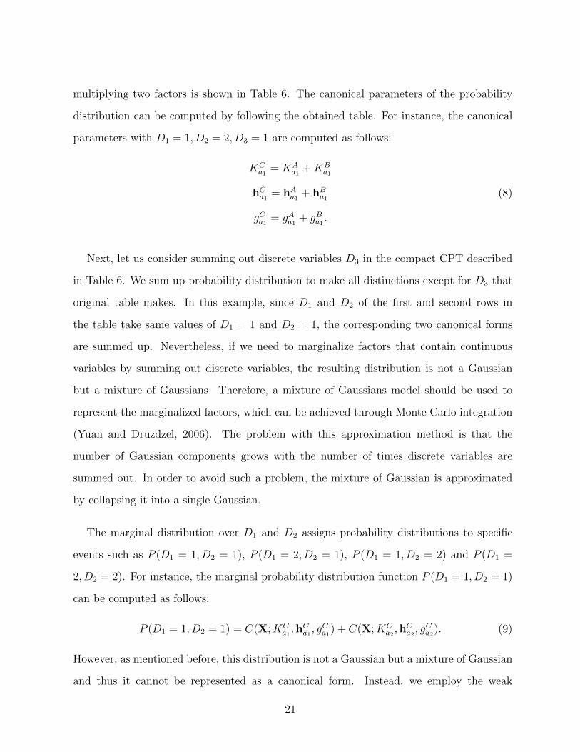
multiplying two factors is shown in Table 6. The canonical parameters of the probability

distribution can be computed by following the obtained table. For instance, the canonical

parameters with D1 = 1, D2 = 2, D3 = 1 are computed as follows:

KCa1

= KAa1

+KBa1

hCa1 = hAa1 + hBa1 (8)

gCa1 = gAa1 + gBa1 .

Next, let us consider summing out discrete variables D3 in the compact CPT described

in Table 6. We sum up probability distribution to make all distinctions except for D3 that

original table makes. In this example, since D1 and D2 of the first and second rows in

the table take same values of D1 = 1 and D2 = 1, the corresponding two canonical forms

are summed up. Nevertheless, if we need to marginalize factors that contain continuous

variables by summing out discrete variables, the resulting distribution is not a Gaussian

but a mixture of Gaussians. Therefore, a mixture of Gaussians model should be used to

represent the marginalized factors, which can be achieved through Monte Carlo integration

(Yuan and Druzdzel, 2006). The problem with this approximation method is that the

number of Gaussian components grows with the number of times discrete variables are

summed out. In order to avoid such a problem, the mixture of Gaussian is approximated

by collapsing it into a single Gaussian.

The marginal distribution over D1 and D2 assigns probability distributions to specific

events such as P (D1 = 1, D2 = 1), P (D1 = 2, D2 = 1), P (D1 = 1, D2 = 2) and P (D1 =

2, D2 = 2). For instance, the marginal probability distribution function P (D1 = 1, D2 = 1)

can be computed as follows:

P (D1 = 1, D2 = 1) = C(X;KCa1,hCa1 , g

Ca1

) + C(X;KCa2,hCa2 , g

Ca2

). (9)

However, as mentioned before, this distribution is not a Gaussian but a mixture of Gaussian

and thus it cannot be represented as a canonical form. Instead, we employ the weak

21

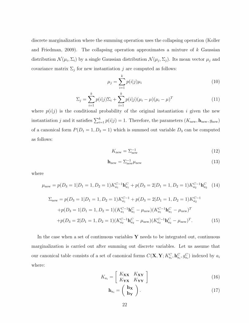
discrete marginalization where the summing operation uses the collapsing operation (Koller

and Friedman, 2009). The collapsing operation approximates a mixture of k Gaussian

distribution N (µi,Σi) by a single Gaussian distribution N (µj,Σj). Its mean vector µj and

covariance matrix Σj for new instantiation j are computed as follows:

µj =k∑i=1

p(i|j)µi (10)

Σj =k∑i=1

p(i|j)Σi +k∑i=1

p(i|j)(µi − µ)(µi − µ)T (11)

where p(i|j) is the conditional probability of the original instantiation i given the new

instantiation j and it satisfies∑k

i=1 p(i|j) = 1. Therefore, the parameters (Knew,hnew, gnew)

of a canonical form P (D1 = 1, D2 = 1) which is summed out variable D3 can be computed

as follows:

Knew = Σ−1new (12)

hnew = Σ−1newµnew (13)

where

µnew = p(D3 = 1|D1 = 1, D2 = 1)KC−1a1

hCa1 + p(D3 = 2|D1 = 1, D2 = 1)KC−1a2

hCa2 (14)

Σnew = p(D3 = 1|D1 = 1, D2 = 1)KC−1a1

+ p(D3 = 2|D1 = 1, D2 = 1)KC−1a2

+p(D3 = 1|D1 = 1, D2 = 1)(KC−1a1

hCa1 − µnew)(KC−1a1

hCa1 − µnew)T

+p(D3 = 2|D1 = 1, D2 = 1)(KC−1a2

hCa2 − µnew)(KC−1a2

hCa2 − µnew)T . (15)

In the case when a set of continuous variables Y needs to be integrated out, continuous

marginalization is carried out after summing out discrete variables. Let us assume that

our canonical table consists of a set of canonical forms C(X,Y;KCai,hCai , g

Cai

) indexed by ai

where:

Kai =

[KXX KXY

KYX KYY

](16)

hai =

(hX

hY

). (17)

22

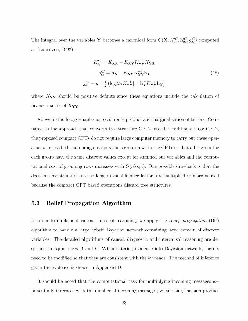
The integral over the variables Y becomes a canonical form C(X;K ′Cai ,h′Cai, g′Cai ) computed

as (Lauritzen, 1992):

K ′Cai = KXX −KXYK−1YYKYX

h′Cai = hX −KXYK−1YYhY (18)

g′Cai = g + 12

(log|2πK−1

YY|+ hTYK−1YYhY

)where KYY should be positive definite since these equations include the calculation of

inverse matrix of KYY.

Above methodology enables us to compute product and marginalization of factors. Com-

pared to the approach that converts tree structure CPTs into the traditional large CPTs,

the proposed compact CPTs do not require large computer memory to carry out these oper-

ations. Instead, the summing out operations group rows in the CPTs so that all rows in the

each group have the same discrete values except for summed out variables and the compu-

tational cost of grouping rows increases with O(nlogn). One possible drawback is that the

decision tree structures are no longer available once factors are multiplied or marginalized

because the compact CPT based operations discard tree structures.

5.3 Belief Propagation Algorithm

In order to implement various kinds of reasoning, we apply the belief propagation (BP)

algorithm to handle a large hybrid Bayesian network containing large domain of discrete

variables. The detailed algorithms of causal, diagnostic and intercausal reasoning are de-

scribed in Appendices B and C. When entering evidence into Bayesian network, factors

need to be modified so that they are consistent with the evidence. The method of inference

given the evidence is shown in Appenxid D.

It should be noted that the computational task for multiplying incoming messages ex-

ponentially increases with the number of incoming messages, when using the sum-product

23

algorithm. This is the case when the diagnostic, intercausal or mixed inferences are carried

out because the LBP requires a large number of calculations for factor multiplication and

marginalization. To reduce the computational cost in LBP algorithm, we make use of the

property of Bethe cluster graph. In a Bethe cluster graph, the scope of messages covers

single variable since any large clusters are connected each other. If we give the evidence to

some variable Xi = e, the message departed from the corresponding singleton cluster Ci

remains the same during iterations. In other word, we can peg the message δi→k to evidence

e and thus we can skip the computation of Eq. (25). The proposed loopy belief propagation

algorithm is shown in Table 7.

6 Application Example

6.1 Comparison with SVM and ANN

A simulated example is used to evaluate the validity and performance of the Bayesian

networks compared to ANN and SVM. The input and output data are generated from the

simple system described in Fig. 9. In this example, [X1, X2, X3, Y1, Y2] are input variables

while Z is an output variable. Variables are linearly dependent when they are connected

with the arcs. Further, all variables are binarized and thus the domain size of each variable

is two.

The radial basis kernel function is used for SVM and its parameters are determined

automatically using the heuristic method described in the literature (Caputo et al., 2002).

As for ANN, the number of hidden variables is determined from cross-validation. The

classification accuracies, which are the proportion of true results, along with the number

of hidden variables are shown in Table 8. It can be seen that accuracy remains same even

when we increase the number of hidden variables. We set the number of hidden variables

to be four for ANN.

24

The computational results are shown in Table 9. When all variables can be observed

except for output variables, the accuracies for test data of BN, ANN and SVM are greater

than 0.9, which means all methods can accurately predict the output variables. On the

other hand, when input data are partially known, both ANN and SVM predict the output

variable for test data with lower accuracies of 0.734 and 0.734 respectively. Meanwhile, BN

predicts the output variable with the high accuracy of 0.848 even though partial input data

can be observed. These computational results demonstrate that BN is superior to SVM

and ANN in terms of accuracy with partially observed data.

It is true that SVM is known as one of the strongest classification machine and it works

equally to or better than BNs for classification problems with fully observed data. However,

as the computational results show, if only partial input data are observed, BN performs bet-

ter than SVM. In addition, if we need to predict multiple variables, SVM requires multiple

models which meet the specific situations, while BN can work for any situations (e.g. fully

or partially observed) by using single model. Furthermore, SVM works only for classifica-

tion problems and thus it is not be able to predict both continuous and discrete variables

simultaneously.

6.2 Bayesian Network Model Identification

The real-world plate steel production data are utilized to examine the effectiveness of the

proposed Bayesian network based prediction models. All the case studies have been com-

puted on a DELL Optiplex 990 (Intel(R) Core(TM) i-7-2600 CPU, 3.40GHz and 8.0 Gb

RAM). First, we use the training data set consisting of 10, 000 steel plates to learn the net-

work structure. The Bayesian network structures are identified by maximizing BIC scores

as shown in Figs. 10 and 11. The execution time for the network identification was 1, 353[s].

Then, we use the training data set consisting of 100, 000 steel plates to learn the decision-

tree structured CPTs while we use the test data set of another 100, 000 plates to evaluate

25

prediction accuracy. The first and second Bayesian networks are mainly different in the

form of the conditional probability of total production time.

6.3 Prediction of Production Loads and Total Production Time

In the first test scenario, we assume that the variables corresponding to the customer

demands are known and the other variables are unknown. This situation occurs when

persons in the sales department receive orders from customers, since the sales planning

staff need to know the production loads and the process time of these orders as required to

satisfy the customer demands and within constraints of the production capacity. The task

of this inference is to predict the effects of production loads and a process time given the

causes of the customer demands, which means that the type of inference is causal reasoning.

In order to compute the true probability distributions which are required for comparison

to the prediction, we classify the test data into production groups which contain plates

that have the same customer specifications and operating conditions and then compute the

probability distribution for each production group. The production groups containing more

than 100 plates are chosen for comparison while the other production groups are not selected

because we cannot compute the reliable probability distributions from a small number of

samples. The total number of the production groups that are used for comparison is 106.

First, we predict the production loads and the production time by using the first Bayesian

network structure shown in Fig. 10. Fig. 12 shows the scatter plots between the predicted

and true probabilities with production loads being 2. Further, the Kullback-Leibler (KL)

divergence, which measures the difference between the predicted probability distributions

and actual ones is shown in Fig. 13. It can be observed that the difference between

the predicted and true probability distributions of the variables of process A, process B,

process C, process D, process E, process F and process G are relatively small while the

predicted probabilities with process H and process I values being 2 are zero in all production

26

groups. Moreover, the scatter plots between the predicted and true parameters of means

and standard deviations of the production time are shown in 14 , and their KL divergences

are provided in Fig. 15. It can be seen that the means of the predicted distributions are

relatively close to the true means but the variances of the predicted distributions largely

differ from the actual ones. Somewhat inaccurate prediction of the production loads of

process E, process F, process H and process I can be considered a cause of these differences

in the production time.

Next, the probability distributions of the production loads and the production time are

computed via the second type of Bayesian network, shown in Fig. 11. The difference

between the two structures is that the nodes associated with the production time at each

production process are added between the nodes of production loads and total production

time in the second type on Bayesian network. Similarly to the first model, we provide the

scatter plots of the predicted and true parameters of means and standard deviations and

their KL divergences in Figs. 16 and 17, respectively. It can be observed that the prediction

accuracy does not improve at all from the first Bayesian network. The cause of inaccurate

prediction of the variances of the total production time is the low accurate prediction of

the production loads.

In the second test case, we consider the situation where the variables associated with

both customer demands and operating conditions are known and the variables of both

production loads and process time are unknown. In this situation, we want to predict the

probability distributions of the production loads and the process time given all information

except for these target variables. Such situation often arises at the production scheduling

stage. Similarly to the previous test scenario, the types of inference is causal reasoning

and we make use of the same decision-tree structured CPTs as the previous test case. Fig.

18 shows the scatter plots between the predicted and actual probability of the production

loads. In addition, their KL divergences are provided in Fig. 19. It can be observed that the

27

predicted and true probability distributions are almost same. In particular, the accuracy of

the predicted distributions of loads of process D, process E, process F, process G, process

H and process I loads are significantly improved compared to the first test scenario. All of

their RMSEs are less than 0.1 and the correlations are also much higher than those in the

first test scenario. This is mainly because we know the additional values of the operating

conditions that are considered having a significant influence on these production loads.

However, in spite of the accurate prediction of production loads, the means of the predicted

probability distributions of the production times are not improved as shown in Figs. 20

and 21.

The second type of Bayesian network shown as Fig. 11 is also used to predict the pro-

duction time. The scatter plots between the predicted and actual parameters of means and

standard variances and their KL divergences are given in Figs. 16 and 17. One can readily

see that the KL divergences between the predicted and actual probability distribution are

smaller than all the above results. In particular, the predicted means are very close to the

actual ones. As for the accuracy of the predicted standard variances, the second Bayesian

network model can accurately predict the standard deviations in most production groups.

In some production groups, the differences between the predicted and actual standard de-

viations are somewhat large. In order to improve further, it may be desirable to add other

nodes of variables such as the amount of in-process inventory, the number of workers and

the failure rate of each machine in Bayesian networks, which should have an impact on the

process time.

All the results indicate that even though our Bayesian network includes large domain of

discrete variables, the causal reasoning can be carried out by using the proposed decision-

tree structured conditional probability table representations. Moreover, a single Bayesian

network model can carry out the most plausible reasoning and its accuracy depends on

using the values of known variables. This means that we can avoid having multiple specific

28

models tailored for specific purposes. Therefore, the proposed Bayesian network model

satisfies the properties required for plate steel production scheduling and planning.

6.4 Prediction of Operating Conditions

Up to now we have dealt with prediction of the probability distributions of the production

loads and the total production time. In this last test case, we assume that the values

of the customer demands and production loads are known while the operating conditions

are unknown. Such situation arises when we want to analyze the relationship between the

production loads and the operating conditions, or we need to design the operating conditions

so that both the customer demands and production capacity constraints can be satisfied.

Unlike the previous test scenarios, the type of the inference is mixed reasoning and thus the

loopy belief propagation algorithm is carried out. Similarly to the previous two scenarios, we

evaluate the prediction accuracy for each production of steel plates with the same customer

demands and production loads. We select the production groups containing more than 100

plates to compute the true probability distributions, which are then used for comparison

with the predicted probability distributions. The number of production groups that are used

in this comparison is 90. The probability of cardinality of the predicted and true operating

conditions is shown in Fig. 24. In addition, their KL divergences are shown in Fig. 25.

One can readily see that most KL divergences are small; hence, the proposed inference

algorithm can accurately predict the probability distributions of unknown variables in the

mixed reasoning. Above results demonstrate that the proposed Bayesian inference method

can carry out the mixed reasoning even though Bayesian networks have large domain of

discrete variables.

Average execution times for all the above test scenarios are provided in Table 10. Com-

paring the execution time of the first and the second Bayesian networks, we note that the

average execution time of the second model is less than 1[s], which is much smaller than

29

that of the first Bayesian network model. That is because in the first model, the node of

total production time is connected to the all nodes of the production loads as their child

and thus we need a large number of multiplication of factors to compute the final potential

of the production time, which leads to high computational effort since the computational

cost of factor multiplication increases with the number of variables contained in the factor.

For the mixed reasoning, the average execution time is less than 2[s], which is small enough

to use it in practical applications.

7 Conclusion

In this study, we propose the Bayesian network models for prediction of the production loads

and the production time in manufacturing of steel plates. In order to identify the network

structure from historical process data, we search for the graph such that the maximized

Bayesian scores are obtained. Since the network contains both continuous and discrete

system variables and some of discrete variables have large cardinalities, the decision-tree

structured CPTs based hybrid Bayesian inference technique is proposed. Once the Bayesian

network structure is constructed, we compute the context-specific conditional probability

tables represented by decision trees from historical process data set by using classifica-

tion tree algorithm. Then, operators for computing multiplication and marginalization of

factors represented by decision-tree structure based CPTs are developed. The Bayesian in-

ference is carried out using belief propagation algorithms with the proposed multiplying and

marginalizing operators. The causal reasoning is carried out by means of the sum-product

algorithm whose direction is downstream from the top node variables to the bottom nodes

variables. Other types of reasoning are carried out by the loopy belief propagation.

Real life steel production process data have been used to examine the effectiveness of the

proposed inference algorithms. Even though our Bayesian network contains large domain

of discrete variable nodes, the results show that the proposed algorithm can be successfully

30

applied to industrial scale Bayesian networks and it can predict the probability distributions

of unobserved variables such as the production loads and the production times in the steel

plate production.

Results of this work will be applied to production planning and scheduling in manufac-

turing of steel plates.

Appendix A Structure Learning

Several kinds of scoring functions have been developed. Most of them have a decomposable

score function as follows:

score(G) =I∑i=1

score(xi, paG(xi)) (19)

where paG(xi) are the parent nodes of xi given graph G. Among various kinds of score

functions, the BIC score (for Bayesian information criterion) is widely used; it is defined as

scoreBIC(G : D) = `(θ̂G : D)− LogM

2Dim[G] (20)

where θ̂G denotes the maximum likelihood parameters given a graph G, `(θ̂G : D) denotes

the logarithm of the likelihood function, M is the number of samples, and Dim[G] is the

model dimension that is equal to the number of parent nodes. The term of model dimension

is introduced in the score function in order to handle a tradeoff between the likelihood and

model complexity. Since the BIC scores are decomposable, they can be restated as follows:

scoreBIC(G : D) = M

N∑i=1

I(xi; paG(xi))−MN∑i=1

H(xi)−LogM

2Dim[G] (21)

where I(xi; paG(xi)) is the mutual information between xi and paG(xi), and H(xi) is the

marginal entropy of xi.

Score decomposability is important property for network structure learning because if

the decomposability is satisfied, a local change such as adding, deleting or reversing an

31

edge in the structure does not change the score of other parts of the structure that remain

same. It also should be pointed out that the mutual information term grows linearly in M

while the model complexity term grows logarithmically, and thus the larger M leads to an

obtained graph which better represents data (Koller and Friedman, 2009).

With the score function defined as above, the optimal graph G∗ can be computed as

follows:

G∗ = argmaxGscoreBIC(G : D). (22)

Appendix B Causal Reasoning

The computational task of causal reasoning is to estimate the downstream effects of factors

given the evidence of their ancestor variables. In our example, causal reasoning predicts the

probability distributions of production loads and total production time from the evidence of

customer demands, operating conditions or both. Conditional probability can be computed

through a local message passing algorithm known as sum-product algorithm in downstream

direction from the root nodes to the leaf nodes. Since our Bayesian network contains

both discrete and continuous variables, a final potential P̃Φ(Ci) of factor Ci = Ai ∪Xi is

computed using sum and integral operators as follows:

P̃Φ(Ci) =

∫ ∑Ai−Ai

ψi∏

k∈pa(i)

PΦ(Ck)dx1dx2 . . . dxM (23)

where:

• ψi is the initial potential of Ci, PΦ(Ck) is the normalized final potential of Ck,

• xm ∈ {Xi −Xi} are variables that we integrate out, and

• Xi or Ai is the child node of the factor Ci where if the child node variable is continuous,

Ai = ∅, otherwise Xi = ∅.

32

First, we compute the initial potentials ψi for all factors. Each node in the Bayesian

network is assigned one factor and thus the number of factors is equal to the number of

nodes. A factor belonging to a set of top root nodes is assigned a singleton factor that

contains a variable of the corresponding node. Since evidence is given to all singleton

factors in the causal reasoning, their initial and final potentials have cardinality of one and

their probabilities are always 1. Note that a factor corresponding to a node that is not

placed on the top root node is assigned a non-singleton factor that contains a variable of

the corresponding node and its all parent nodes. Therefore, the initial potentials for non-

singleton factors are equal to the conditional probability distributions of its corresponding

variable given its parent node variables. After computing initial potentials of all factors,

the sum-product algorithm proceeds in the downstream direction from the top factors to

the bottom factors in order to compute the final potentials of all factors. The causal

reasoning algorithm searches for the non-singleton factor for which all parent nodes are

assigned final potentials and then computes the final potential for that non-singleton factor

by using Eq. (23). Since the final potential P̃Φ(Ci) in Eq. (23) is not normalized, we need

to normalize it and obtain PΦ(Ci) every time after computing the final potentials. This

algorithm continues computing final potentials using the sum-product algorithm until final

potentials of all factors are computed. Since the computation of final potentials is carried

out from top node factors to bottom node factors, the probability propagation directions

are the same as the arcs in Bayesian networks. The computed final potentials PΦ(Ck) are

equal to the conditional probability distributions of the corresponding variable given the

evidence.

Appendix C Diagnostic and Intercausal Reasoning

While causal reasoning is carried out by simply applying the sum-product algorithm from

the top nodes to the bottom nodes, conditional probability for diagnostic, intercausal and

33

mixed reasoning can be computed by iteratively carrying out the sum-product algorithm

until convergence in the loopy belief propagation (LBP). LBP schemes use a cluster graph

rather than a clique tree that is used for VE (Murphy et al., 1999). Since the constraints

defining the clique tree are indispensable for exact inference, the answers of message passing

scheme are approximate queries in LBP.

First, we create the singleton factors for all nodes and then each singleton factor is

assigned an initial potential of the prior probability of the corresponding variable. Also, we

create the intermediate factors for all nodes that have parent nodes and then each factor is

assigned an initial potential of the conditional probability distribution of the corresponding

variable given its parent variables. Therefore, the number of factors is larger than the

number of nodes. Given the cluster graph, we assign each factor φk to a cluster Cα(k) so

that scope(φk) ⊆ Cα(k). Then the initial potentials ψi can be computed as follows:

ψi =∏

k:α(k)=i

φk. (24)

In LBP, one factor communicates with another factor by passing messages between them.

The messages have canonical form representation and their potentials are initialized as

{K,h, g} = {1, 0, 0}. A message from cluster Ci = Ai∪Xi to another factor Cj = Aj ∪Xj

is computed using sum and integral operators as follows:

δi→j =

∫ ∑Ai−Si,j

ψi∏

k∈Nbi−{j}

δk→idx1dx2 . . . dxM (25)

where:

• xm ∈ {Xi − S′i,j} are integrated variables,

• Si,j = Ai ∩Aj is the sepset of discrete variables,

• S′i,j = Xi ∩Xj is the sepset of continuous variables, and

• Nbi is the set of indices of factors that are neighbors of Ci.

34

The messages are updated by using Eq. (25) in accordance with some message passing

schedule until the canonical parameters of all messages are converged. Using all incoming

messages, a final potential P̃Φ(Ci) can be computed by multiplying them with the initial

potential as follows:

P̃Φ(Ci) = ψi∏k∈Nbi

δk→i. (26)

Similar to the causal reasoning, the final potential P̃Φ(Ci) needs normalization.

In order to carry out the LBP algorithm, we have to create a cluster graph in ad-

vance such that it satisfies the family preservation property. For this purpose, the Bethe

cluster graph which is a bipartite graph and holds the family preservation property is widely

used. The first layer of the Bethe cluster graph consists of large clusters Ck = scope(φk)

while the second layer consists of singleton clusters Xi. Then, edges are placed between

a large cluster Ck and a singleton cluster Xi if Xi ∈ Ck. Fig. 8 shows an example of

the Bethe cluster graph. In this example, the Bethe cluster graph has 6 singleton clus-

ters {A}, {B}, {C}, {D}, {E}, {F} and 3 large clusters {A,B,D}, {B,C,E}, {D,E}. For

instance, due to {B} ∈ {A,B,D} and {B} ∈ {B,C,E}, the edges between cluster 2 and 7

and between cluster 2 and 8 are placed.

Appendix D Belief Propagation with Evidence

When initializing the factor ψi given the discrete evidence e ∈ E ∩∆, we delete all sets of

canonical parameters K,h, g in the factor ψi that conflict the evidence e.

Next, let us consider initializing the factor ψi given the continuous evidence e ∈ E∩Γ. If

the factor does not have any discrete variables, a canonical form of the factor ψi is reduced

to a context representing the evidence e. In Eq. (16), we set Y = y with y being the value

of the evidence e, then the new canonical form given continuous evidence is described as

35

follows (Lauritzen, 1992):

K ′ = KXX

h′ = hX −KXYy (27)

g′ = g + hTYy − 12yTKYYy.

If the factor has discrete variables and does not have a continuous variable except for

scope(E), the canonical parameter gai is modified for each instantiation ai as follows:

gai = −1

2yKaiy + hTaiy + gai . (28)

The canonical parameters Kai and hai become vacuous because the new factor contains no

continuous variable. If the factor contains both discrete and continuous variables except for

scope(E), the parameters of the canonical form are computed for each instantiation ai using

Eq. (27). After modifying all factors so that all of them are consistent with the evidence,

the reasoning algorithms mentioned above can be carried out.

36

References

Ashayeria, J., R.J.M. Heutsa, H.G.L. Lansdaalb and L.W.G. Strijbosch (2006). Cyclic pro-

ductioninventory planning and control in the pre-deco industry: A case study. Int. J.

Prod. Econ. 103, 715–725.

Bishop, C.M. (2006). Pattern Recognition and Machine Learning. Springer-Verlag, New York,

NY.

Boutilier, C., N. Friedman, M. Goldszmidt and D. Koller (1996). Context-specific indepen-

dence in Bayesian networks. In: Proceedings of UAI-96. pp. 115–123.

Breiman, L., J.H. Friedman, R.A. Olshen and C.G. Stone (1984). Classication and Regression

Trees. Wadsworth International Group. Belmont.

Caputo, B., K. Sim, F. Furesjo and A. Smola (2002). Appearance-based object recognition

using svms: which kernel should i use?. In: Proceedings of NIPS workshop on Statitsical

methods for computational experiments in visual processing and computer vision.

Chickering, D.M. (1996). Learning bayesian networks is np-complete. In: Learning from

Data: Artificial Intelligence and Statistics. Chap. 12. Springer-Verlag.

Chickering, D.M., D. Heckerman and C. Meek (1997). A bayesian approach to learning

Bayesian networks with local structure. In: Proceedings of UAI-97. pp. 80–89.

Cobb, B.R., R. Rumi and A. Salmeron (2007). Bayesian Network Models with Discrete and

Continuous Variables. SpringerVerlag. Berlin.

DesJardins, M. and P. Rathod (2008). Learning structured Bayesian networks: Combin-

ing abstraction hierarchies and tree-structured conditional probability tables. Comput.

Intell. 24, 1–22.

37

Friedman, N. and M. Goldszmidt (1996). Learning Bayesian networks with local structure.

In: Proceedings of UAI-96. pp. 252–262.

Glover, F. (1986). Future paths for integer programming and links to artificial intelligence.

Comput. Oper. Res. 13, 533–549.

I. Harjunkoski, I.E. Grossmann (2001). A decomposition approach for the scheduling of a

steel plant production. Comput. Chem. Eng. 25, 1647–1660.

Koller, D. and N. Friedman (2009). Probabilistic Graphical Models: Principles and Tech-

niques. MIT Press.

Koller, D., U. Lerner and D. Angelov (1999). A general algorithm for approximate inference

and its application to hybrid bayes nets. In: Proceedings of UAI-99. pp. 324–333.

Kozlov, A. and D. Koller (1997). Nonuniform dynamic discretization in hybrid networks. In:

Proceedings of UAI-97. pp. 314–325.

Lauritzen, S. (1992). Propagation of probabilities, means and variances in mixed graphical

association models. J. Amer. Stat. Assoc. 87, 1098–1108.

Lauritzen, S.L. and F. Jensen (2001). Stable local computation with conditional gaussian

distribution. Stat. Comput. 11, 191–203.

Lauritzen, S.L. and N. Wermuth (1989). Graphical models for associations between variables,

some of which are qualitative and some quantitative. Ann. Stat. 17, 31–57.

Moon, S. and A.N. Hrymak (1999). Scheduling of the batch annealing processdeterministic

case. Comput. Chem. Eng. 23, 1193–1208.

Moral, S., R. Rumi and A. Salmern (2001). Mixtures of Truncated Exponentials in Hybrid

Bayesian Networks. SpringerVerlag. Berlin.

38

Murphy, K.P., Y.Weiss and M.I. Jordan (1999). Nonuniform dynamic discretization in hybrid

networks. In: Proceedings of UAI-99. pp. 467–475.

Nishioka, K., Y. Mizutani, H. Ueno, H. Kawasaki and Y. Baba (2012). Toward the integrated

optimization of steel plate production process : A proposal for production control by

multi-scale hierarchical modeling (in Japanese). Synthesiology 5, 98–112.

Pearl, J. (1988). Probabilistic Reasoning in Intelligent Systems: Networks of Plausible Infer-

ence. Morgan-Kaufmann. San Francisco.

Poole, D. and N.L. Zhang (2003). Exploiting contextual independence in probabilistic infer-

ence. J. Artif. Intell. Res. 18, 263–313.

Rumi, R. and A. Salmeron (2007). Approximate probability propagation with mixtures of

truncated exponentials. Int. J. Approx. Reason. 45, 191–210.

Santos, C.A., J.A. Spim and A. Garci (2003). Mathematical modeling and optimization

strategies (genetic algorithm and knowledge base) applied to the continuous casting of

steel. Eng. Appl. Artif. Intel. 16, 511–527.

Sharma, R. and D. Poole (2003). Efficient inference in large discrete domains. In: Proceedings

of UAI-2003. pp. 535–542.

Tang, L., J. Liu, A. Rong and Z. Yang (2000). A mathematical programming model for

scheduling steelmaking continuous casting production. Eur. J. Oper. Re. 120, 423–435.

Yuan, C. and M. J. Druzdzel (2006). Hybrid loopy belief propagation. In: Proceedings of the

Third European Workshop on Probabilistic Graphical Models (PGM’06). pp. 317–324.

39

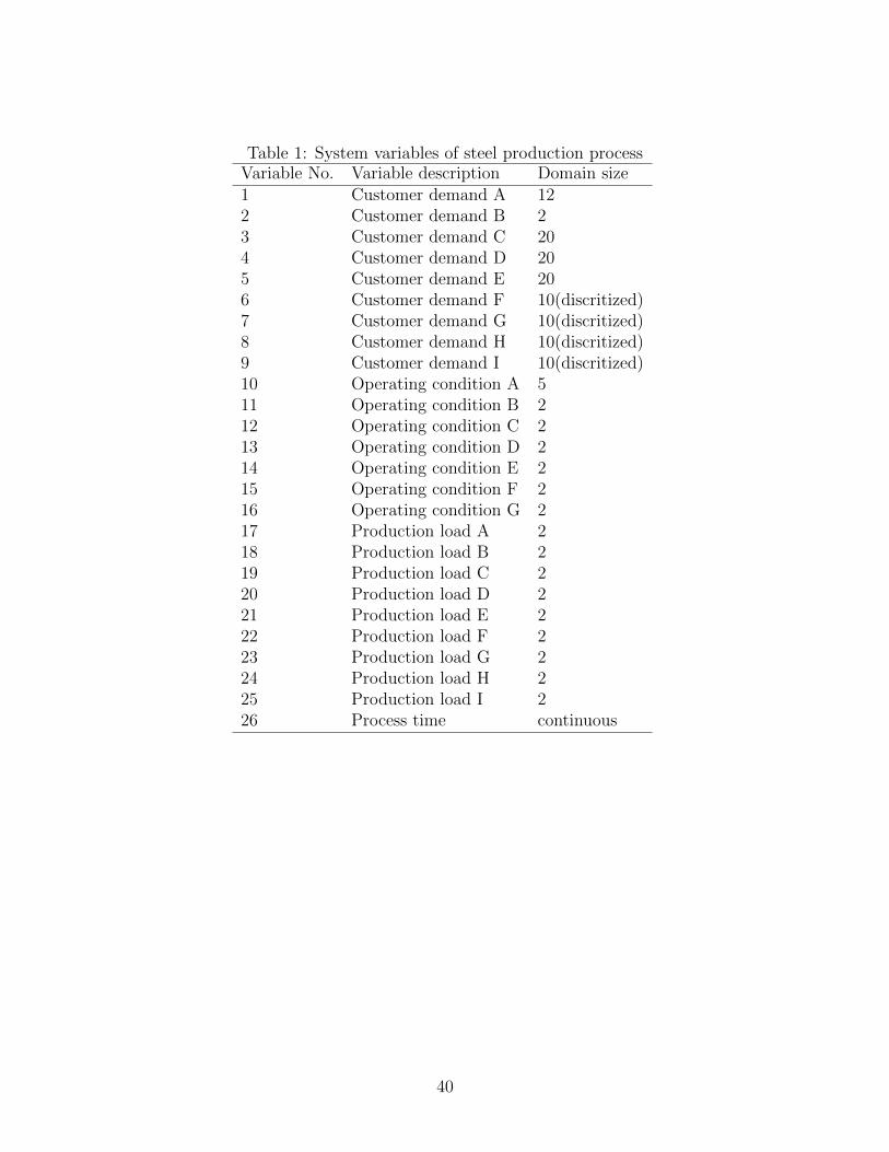
Table 1: System variables of steel production processVariable No. Variable description Domain size1 Customer demand A 122 Customer demand B 23 Customer demand C 204 Customer demand D 205 Customer demand E 206 Customer demand F 10(discritized)7 Customer demand G 10(discritized)8 Customer demand H 10(discritized)9 Customer demand I 10(discritized)10 Operating condition A 511 Operating condition B 212 Operating condition C 213 Operating condition D 214 Operating condition E 215 Operating condition F 216 Operating condition G 217 Production load A 218 Production load B 219 Production load C 220 Production load D 221 Production load E 222 Production load F 223 Production load G 224 Production load H 225 Production load I 226 Process time continuous

40

Table 2: Algorithm 1. Network identification algorithmProcedure Network-Identification (D // training data setG0 // initial network structureR // a set of fixed root nodesL // a set of fixed leaf nodes≺ // a set of incomplete orderingsglobal TabuList // tabu list)

1 Tabulist← ∅2 G ← Search(G0,R,L,≺)3 Gbest ← G4 for i = 1, ... until convergence5 G ← Search(G,R,L,≺)6 if scoreBIC(G : D) > scoreBIC(Gbest : D)7 Gbest ← G8 return Gbest

Procedure Search (G // network structureR // a set of fixed root nodesL // a set of fixed leaf nodes≺ // a set of incomplete orderings)

1 while new graph is not obtained2 Select indices i and j (i 6= j) at random3 if edge i→ j exists in G4 Delete edge i→ j or reverse edge i→ j at random and then get Gnew

5 else if edge j → i exists in G6 Delete edge j → i, add new edge i→ j and then get Gnew

7 else8 Add new edge i→ j and then get Gnew

9 if Gnew is cyclic10 continue11 if Gnew is in TabuList12 continue13 if Gnew conflicts either R or L or ≺14 continue15 Add Gnew to TabuList16 return Gnew

41

Table 3: Compact CPT for Factor AD1 D2 Probability

Distribution1 1 C(X;KA

a1,hAa1 , g

Aa1

)1 2 C(X;KA

a2,hAa3 , g

Aa2

)2 1,2 C(X;KA

a3,hAa2 , g

Aa3

)

42

Table 4: Compact CPT for Factor BD2 D3 Probability

Distribution1 1 C(X;KB

a1,hBa1 , g

Ba1

)1 2 C(X;KB

a2,hBa2 , g

Ba2

)2 1,2 C(X;KB

a3,hBa3 , g

Ba3

)

43

Table 5: Combined Compact CPT of Factor A and BFactor A Factor B ProbabilityD1 D2 D2 D3 Distribution

1 1 C(X;KCa1,hCa1 , g

Ca1

) = C(X;KAa1,hAa1 , g

Aa1

) · C(X;KBa1,hBa1 , g

Ba1

)1 1 1 2 C(X;KC

a2,hCa2 , g

Ca2

) = C(X;KAa1,hAa1 , g

Aa1

) · C(X;KBa2,hBa2 , g

Ba2

)2 1,2 inconsistent1 1 inconsistent

1 2 1 2 inconsistent2 1,2 C(X;KC

a3,hCa3 , g

Ca3

) = C(X;KAa2,hAa2 , g

Aa2

) · C(X;KBa3,hBa3 , g

Ba3

)1 1 C(X;KC

a4,hCa4 , g

Ca4

) = C(X;KAa3,hAa3 , g

Aa3

) · C(X;KBa1,hBa1 , g

Ba1

)2 1,2 1 2 C(X;KC

a5,hCa5 , g

Ca5

) = C(X;KAa3,hAa3 , g

Aa3

) · C(X;KBa2,hBa2 , g

Ba2

)2 1,2 C(X;KC

a6,hCa6 , g

Ca6

) = C(X;KAa3,hAa3 , g

Aa3

) · C(X;KBa2,hBa2 , g

Ba2

)

44

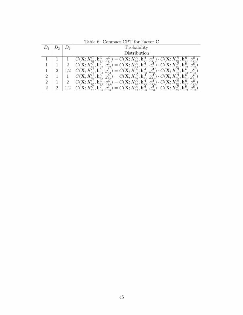
Table 6: Compact CPT for Factor CD1 D2 D3 Probability

Distribution1 1 1 C(X;KC

a1,hCa1 , g

Ca1

) = C(X;KAa1,hAa1 , g

Aa1

) · C(X;KBa1,hBa1 , g

Ba1

)1 1 2 C(X;KC

a2,hCa2 , g

Ca2

) = C(X;KAa1,hAa1 , g

Aa1

) · C(X;KBa2,hBa2 , g

Ba2

)1 2 1,2 C(X;KC

a3,hCa3 , g

Ca3

) = C(X;KAa2,hAa2 , g

Aa2

) · C(X;KBa3,hBa3 , g

Ba3

)2 1 1 C(X;KC

a4,hCa4 , g

Ca4

) = C(X;KAa3,hAa3 , g

Aa3

) · C(X;KBa1,hBa1 , g

Ba1

)2 1 2 C(X;KC

a5,hCa5 , g

Ca5

) = C(X;KAa3,hAa3 , g

Aa3

) · C(X;KBa2,hBa2 , g

Ba2

)2 2 1,2 C(X;KC

a6,hCa6 , g

Ca6

) = C(X;KAa3,hAa3 , g

Aa3

) · C(X;KBa2,hBa2 , g

Ba2

)

45

Table 7: Algorithm 2. Hybrid loopy belief propagation algorithmProcedure Hybrid-LBP (Φ // Set of factorse // EvidenceGcluster // Bethe cluster graph)

1 Set E to be set of edges in Gcluster

2 Initialize all factors so that all of them are consistent with the evidence e3 Initialize all messages as {Kai ,hai , gai} = {1, 0, 0} for each instantiation ai4 while any one of messages are not converged5 Select (i, j) ∈ E by following message schedule6 if scope(ψi) = scope(e)7 continue8 Update message µi→j from Eq. (25)

9 Compute final potential P̃Φ(Ci) from (26)

10 Normalize P̃Φ(Ci) and get PΦ(Ci)11 return PΦ(Ci)

46

Table 8: Results of the cross-validation (ANN)

The number of 1 2 3 4 5 6 7 8 9 10hidden variables

Accuracy 0.928 0.928 0.928 0.930 0.926 0.930 0.928 0.930 0.928 0.928

47

Table 9: Results of BN, ANN and SVM for the simple systemknown variables BN ANN SVM

[X1, X2, X3, Y1, Y2] (Fully observed) 0.970 0.958 0.958[X1, X2, X3] Partially observed) 0.838 0.734 0.734

48

Table 10: Average of execution time for inference [s]Case No. Reasoning Type First model Second model

1 causal 4.33 0.852 causal 4.06 0.563 mixed 1.52

49

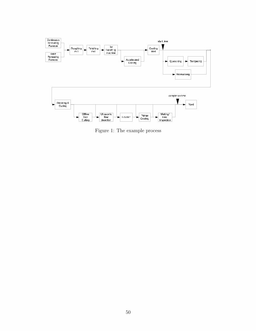
ContinuousReheatingFurnaceBatchReheatingFurnace Roughingmill Finishingmill HotLevellingmachine AcceleratedCooling Quenching TemperingNormalizingShearing &Cutting OfflineGasCutting Ultrasonicflawdetection Leveler PrimerCoating Yard

start time

completion timeMaking/FinalInspection

CoolingBed

Figure 1: The example process

50

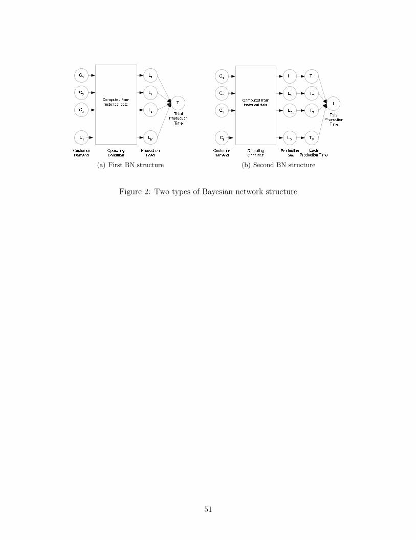
C1C2C3CIL1L2L3LM

TCustomerDemand ProductionLoad

TotalProductionTimeOperatingConditionComputed fromhistorical data

(a) First BN structure

C1C2C3CIL1L2L3LM

TCustomerDemand ProductionLoad EachProduction TimeOperatingCondition

Computed fromhistorical data T1T2T3TM TotalProductionTime(b) Second BN structure

Figure 2: Two types of Bayesian network structure

51

D1 DN... ...X1 XMYFigure 3: Bayesian network that contains continuous child node

52

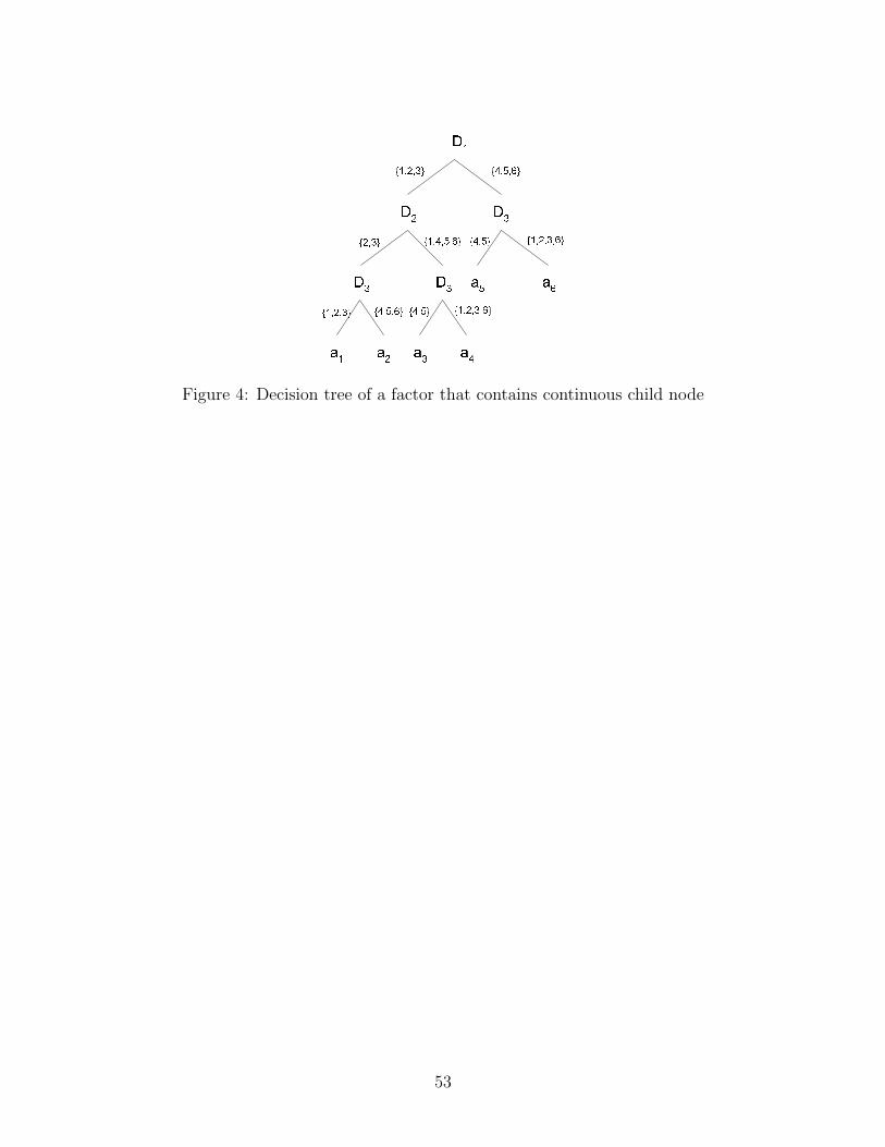
D1D2D3 D3 D3a1 a2 a3 a4a5 a6

{1,2,3} {4,5,6}{2,3} {1,4,5,6}{1,2,3} {4,5,6} {4,5} {1,2,3,6}{4,5} {1,2,3,6}Figure 4: Decision tree of a factor that contains continuous child node

53

D1 DN...BFigure 5: Bayesian network that contains discrete child node

54

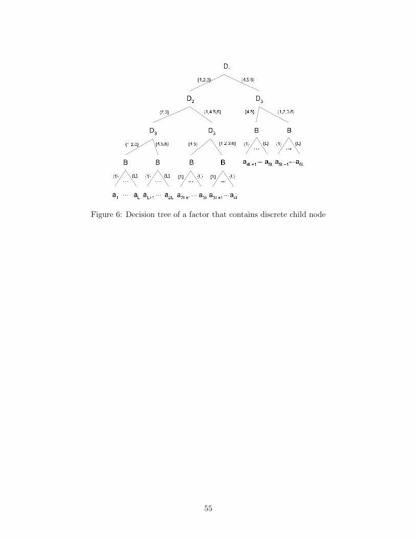
D1D2D3 D3 D3a1 aL

{1,2,3} {4,5,6}{2,3} {1,4,5,6}{1,2,3} {4,5,6} {4,5} {1,2,3,6} {4,5} {1,2,3,6}B B B B B B......{1} {L} aL+1 a2L......{1} {L} a2L+1 a3L......{1} {L} a3L+1 a4L......{1} {L} ...{1} {L} ...{1} {L}a4L+1 a5L... a5L+1 a6L...

Figure 6: Decision tree of a factor that contains discrete child node

55

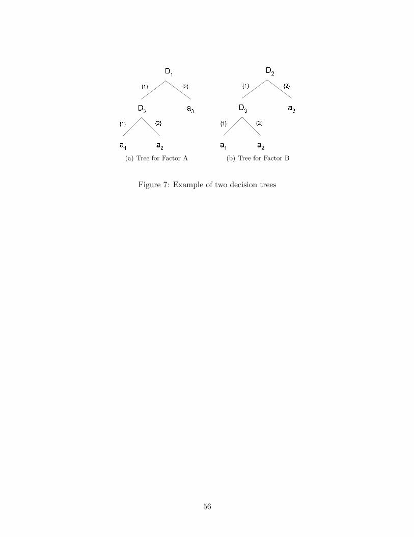
D1D2a1 a3a2{1} {2}{1} {2}

(a) Tree for Factor A

D2D3a1 a3{1} {2}{1} {2}a2(b) Tree for Factor B

Figure 7: Example of two decision trees

56

A B CD EF(a) Bayesian Network

1:A 2:B 3:C 4:D 5:E 6:F7:A, B, D 8:B, C, E 9:D, F(b) Bethe Cluster Graph

Figure 8: Example of Bethe Cluster Graph

57

Z

Y1

Y2

X1

X2

X3

Figure 9: Simple system

58

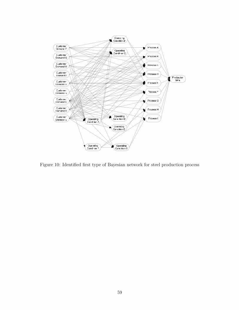
CustomerDemand ACustomerDemand D

CustomerDemand FCustomerDemand GCustomerDemand HCustomerDemand I

CustomerDemand E

Process AProcess BProcess CProcess DProcess FProcess EProcess IProcess GProcess H

ProductiontimeCustomerDemand BCustomerDemand COperatingCondition A OperatingCondition D

OperatingCondition C

OperatingCondition FOperatingCondition EOperatingCondition G

OperatingCondition B

Figure 10: Identified first type of Bayesian network for steel production process

59

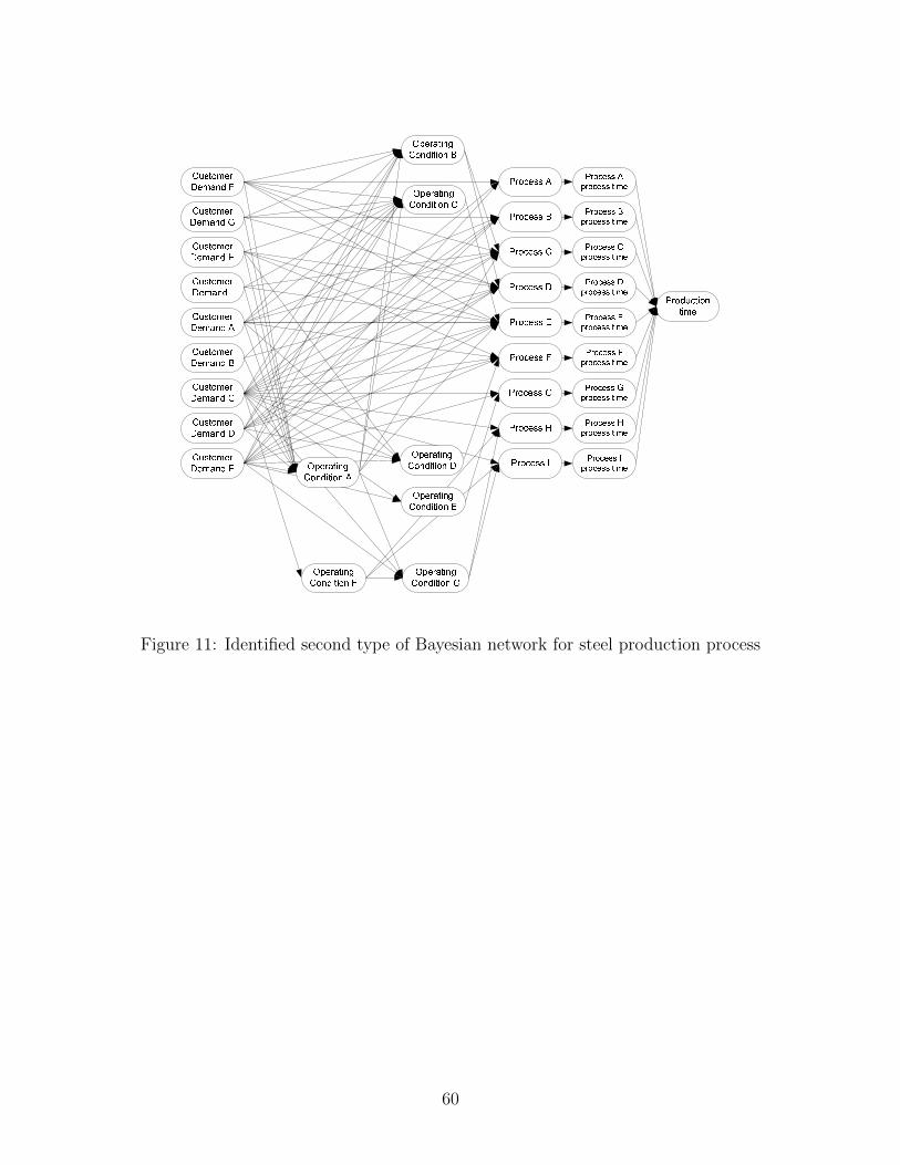
CustomerDemand ACustomerDemand D

CustomerDemand FCustomerDemand GCustomerDemand HCustomerDemand I

CustomerDemand E

Process AProcess BProcess CProcess DProcess FProcess EProcess IProcess GProcess H

CustomerDemand BCustomerDemand COperatingCondition A OperatingCondition D

OperatingCondition C

OperatingCondition FOperatingCondition EOperatingCondition G

OperatingCondition BProductiontime

Process Aprocess timeProcess Bprocess timeProcess Cprocess timeProcess Dprocess timeProcess Fprocess timeProcess Eprocess timeProcess Iprocess timeProcess Gprocess timeProcess Hprocess time

Figure 11: Identified second type of Bayesian network for steel production process

60

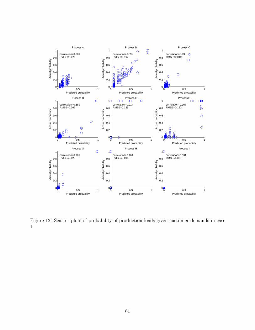
0 0.5 10

0.2

0.4

0.6

0.8

1correlation=0.681RMSE=0.076

Process A

Predicted probability

Act

ual p

roba

bilit

y

0 0.5 10

0.2

0.4

0.6

0.8

1correlation=0.892RMSE=0.107

Process B

Predicted probability

Act

ual p

roba

bilit

y

0 0.5 10

0.2

0.4

0.6

0.8

1correlation=0.93RMSE=0.049

Process C

Predicted probability

Act

ual p

roba

bilit

y

0 0.5 10

0.2

0.4

0.6

0.8

1correlation=0.889RMSE=0.097

Process D

Predicted probability

Act

ual p

roba

bilit

y

0 0.5 10

0.2

0.4

0.6

0.8

1correlation=0.914RMSE=0.185

Process E

Predicted probability

Act

ual p

roba

bilit

y

0 0.5 10

0.2

0.4

0.6

0.8

1correlation=0.957RMSE=0.123

Process F

Predicted probability

Act

ual p

roba

bilit

y

0 0.5 10

0.2

0.4

0.6

0.8

1correlation=0.981RMSE=0.028

Process G

Predicted probability

Act

ual p

roba

bilit

y

0 0.5 10

0.2

0.4

0.6

0.8

1correlation=0.164RMSE=0.098

Process H

Predicted probability

Act

ual p

roba

bilit

y

0 0.5 10

0.2

0.4

0.6

0.8

1correlation=0.031RMSE=0.097

Process I

Predicted probability

Act

ual p

roba

bilit

y

Figure 12: Scatter plots of probability of production loads given customer demands in case1

61

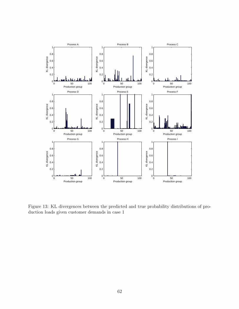
0 50 1000

0.2

0.4

0.6

0.8

1Process A

Production group

KL

dive

rgen

ce

0 50 1000

0.2

0.4

0.6

0.8

1Process B

Production group

KL

dive

rgen

ce

0 50 1000

0.2

0.4

0.6

0.8

1Process C

Production group

KL

dive

rgen

ce

0 50 1000

0.2

0.4

0.6

0.8

1Process D

Production group

KL

dive

rgen

ce

0 50 1000

0.2

0.4

0.6

0.8

1Process E

Production group

KL

dive

rgen

ce

0 50 1000

0.2

0.4

0.6

0.8

1Process F

Production group

KL

dive

rgen

ce

0 50 1000

0.2

0.4

0.6

0.8

1Process G

Production group

KL

dive

rgen

ce

0 50 1000

0.2

0.4

0.6

0.8

1Process H

Production group

KL

dive

rgen

ce

0 50 1000

0.2

0.4

0.6

0.8

1Process I

Production group

KL

dive

rgen

ce

Figure 13: KL divergences between the predicted and true probability distributions of pro-duction loads given customer demands in case 1

62

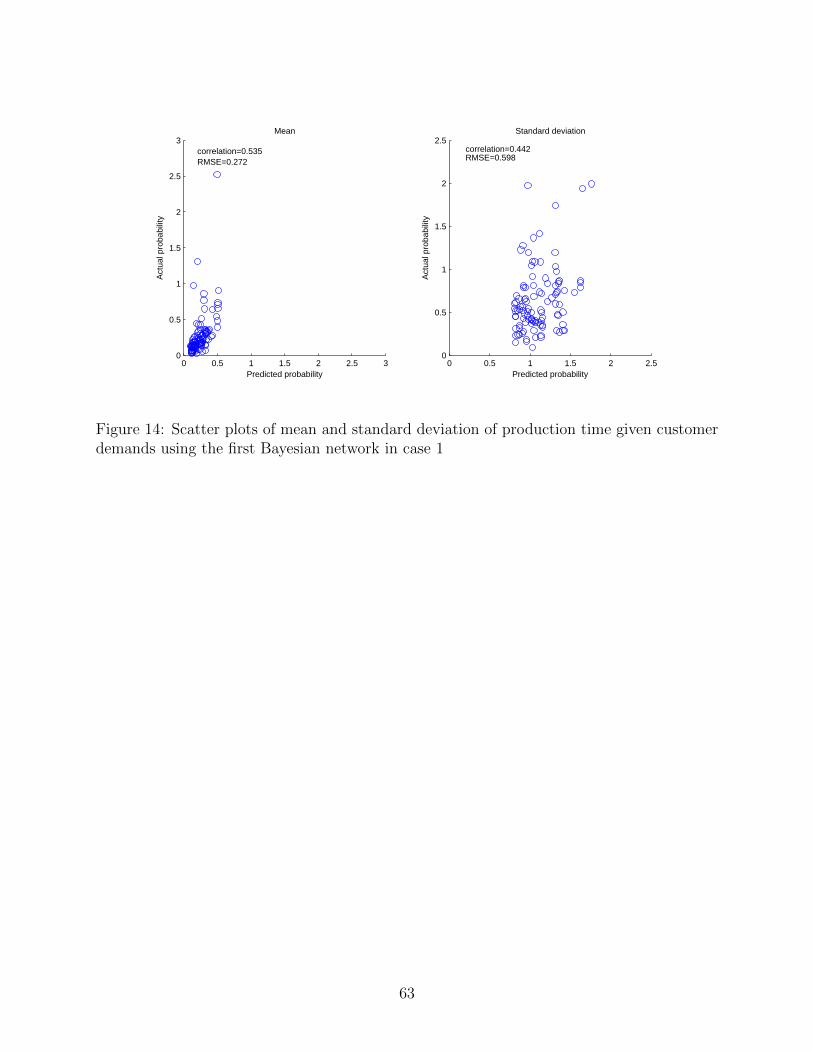
0 0.5 1 1.5 2 2.5 30

0.5

1

1.5

2

2.5

3correlation=0.535RMSE=0.272

Mean

Predicted probability

Act

ual p

roba

bilit

y

0 0.5 1 1.5 2 2.50

0.5

1

1.5

2

2.5correlation=0.442RMSE=0.598

Standard deviation

Predicted probability

Act

ual p

roba

bilit

yFigure 14: Scatter plots of mean and standard deviation of production time given customerdemands using the first Bayesian network in case 1

63

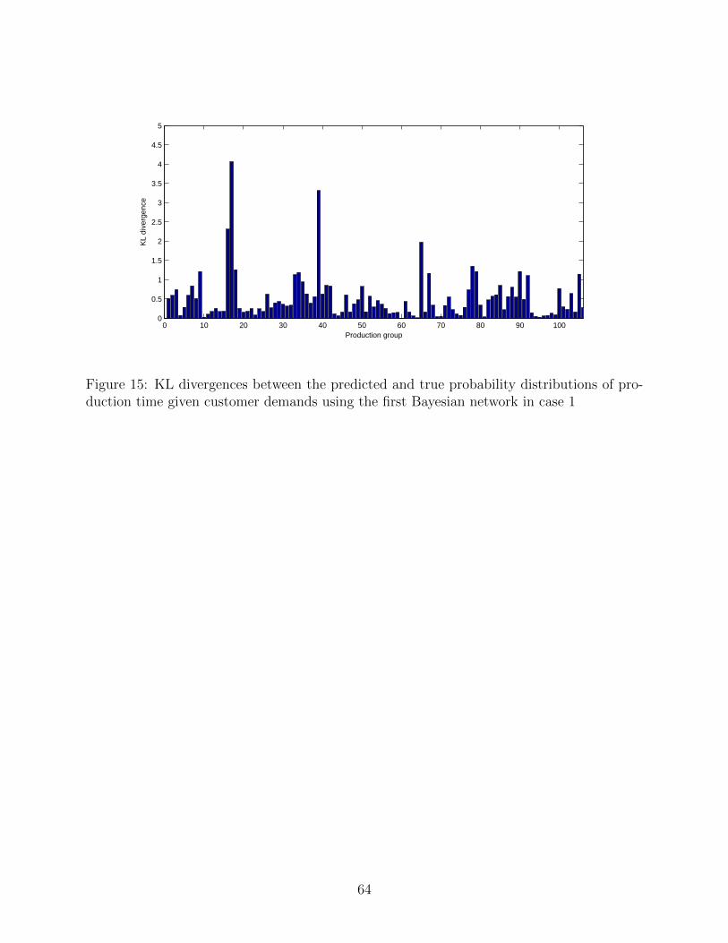
0 10 20 30 40 50 60 70 80 90 1000

0.5

1

1.5

2

2.5

3

3.5

4

4.5

5

Production group

KL

dive

rgen

ce

Figure 15: KL divergences between the predicted and true probability distributions of pro-duction time given customer demands using the first Bayesian network in case 1

64

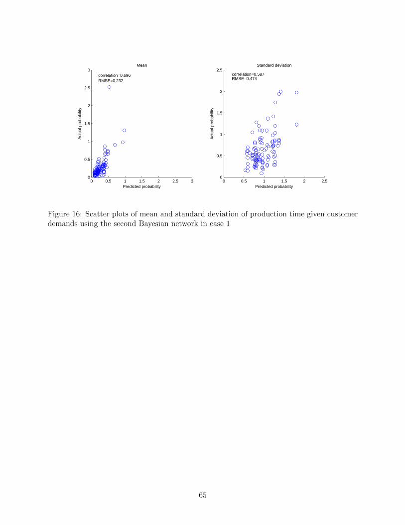
0 0.5 1 1.5 2 2.5 30

0.5

1

1.5

2

2.5

3correlation=0.696RMSE=0.232

Mean

Predicted probability

Act

ual p

roba

bilit

y

0 0.5 1 1.5 2 2.50

0.5

1

1.5

2

2.5correlation=0.587RMSE=0.474

Standard deviation

Predicted probability

Act

ual p

roba

bilit

yFigure 16: Scatter plots of mean and standard deviation of production time given customerdemands using the second Bayesian network in case 1

65

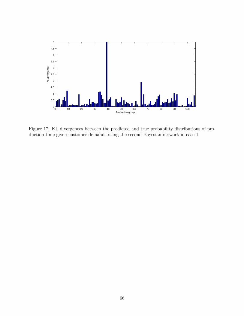
0 10 20 30 40 50 60 70 80 90 1000

0.5

1

1.5

2

2.5

3

3.5

4

4.5

5

Production group

KL

dive

rgen

ce

Figure 17: KL divergences between the predicted and true probability distributions of pro-duction time given customer demands using the second Bayesian network in case 1

66

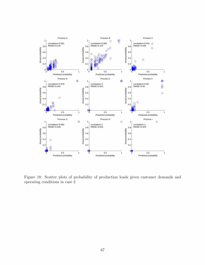
0 0.5 10

0.2

0.4

0.6

0.8

1correlation=0.681RMSE=0.076

Process A

Predicted probability

Act

ual p

roba

bilit

y

0 0.5 10

0.2

0.4

0.6

0.8

1correlation=0.892RMSE=0.107

Process B

Predicted probability

Act

ual p

roba

bilit

y

0 0.5 10

0.2

0.4

0.6

0.8

1correlation=0.931RMSE=0.049

Process C

Predicted probability

Act

ual p

roba

bilit

y

0 0.5 10

0.2

0.4

0.6

0.8

1correlation=0.978RMSE=0.041

Process D

Predicted probability

Act

ual p

roba

bilit

y

0 0.5 10

0.2

0.4

0.6

0.8

1correlation=1RMSE=0.001

Process E

Predicted probability

Act

ual p

roba

bilit

y

0 0.5 10

0.2

0.4

0.6

0.8

1correlation=0.99RMSE=0.06

Process F

Predicted probability

Act

ual p

roba

bilit

y

0 0.5 10

0.2

0.4

0.6

0.8

1correlation=0.982RMSE=0.028

Process G

Predicted probability

Act

ual p

roba

bilit

y

0 0.5 10

0.2

0.4

0.6

0.8

1correlation=1RMSE=0.001

Process H

Predicted probability

Act

ual p

roba

bilit

y

0 0.5 10

0.2

0.4

0.6

0.8

1correlation=1RMSE=0.023

Process I

Predicted probability

Act

ual p

roba

bilit

y

Figure 18: Scatter plots of probability of production loads given customer demands andoperating conditions in case 2

67

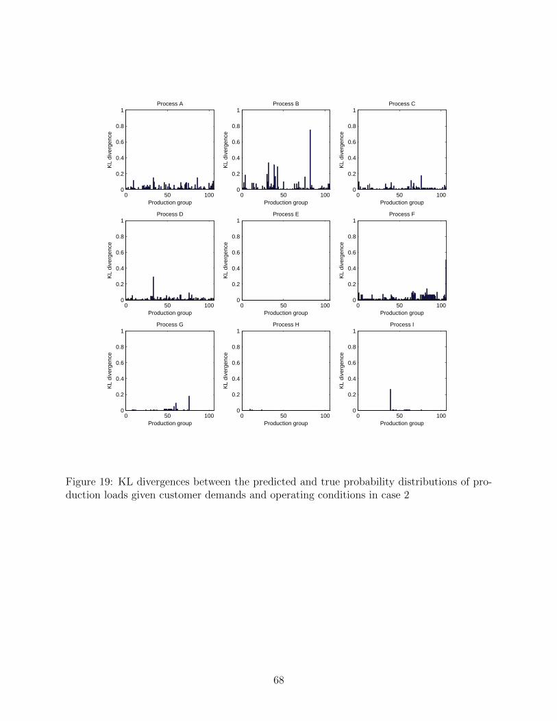
0 50 1000

0.2

0.4

0.6

0.8

1Process A

Production group

KL

dive

rgen

ce

0 50 1000

0.2

0.4

0.6

0.8

1Process B

Production group

KL

dive

rgen

ce

0 50 1000

0.2

0.4

0.6

0.8

1Process C

Production group

KL

dive

rgen

ce

0 50 1000

0.2

0.4

0.6

0.8

1Process D

Production group

KL

dive

rgen

ce

0 50 1000

0.2

0.4

0.6

0.8

1Process E

Production group

KL

dive

rgen

ce

0 50 1000

0.2

0.4

0.6

0.8

1Process F

Production group

KL

dive

rgen

ce

0 50 1000

0.2

0.4

0.6

0.8

1Process G

Production group

KL

dive

rgen

ce

0 50 1000

0.2

0.4

0.6

0.8

1Process H

Production group

KL

dive

rgen

ce

0 50 1000

0.2

0.4

0.6

0.8

1Process I

Production group

KL

dive

rgen

ce

Figure 19: KL divergences between the predicted and true probability distributions of pro-duction loads given customer demands and operating conditions in case 2

68

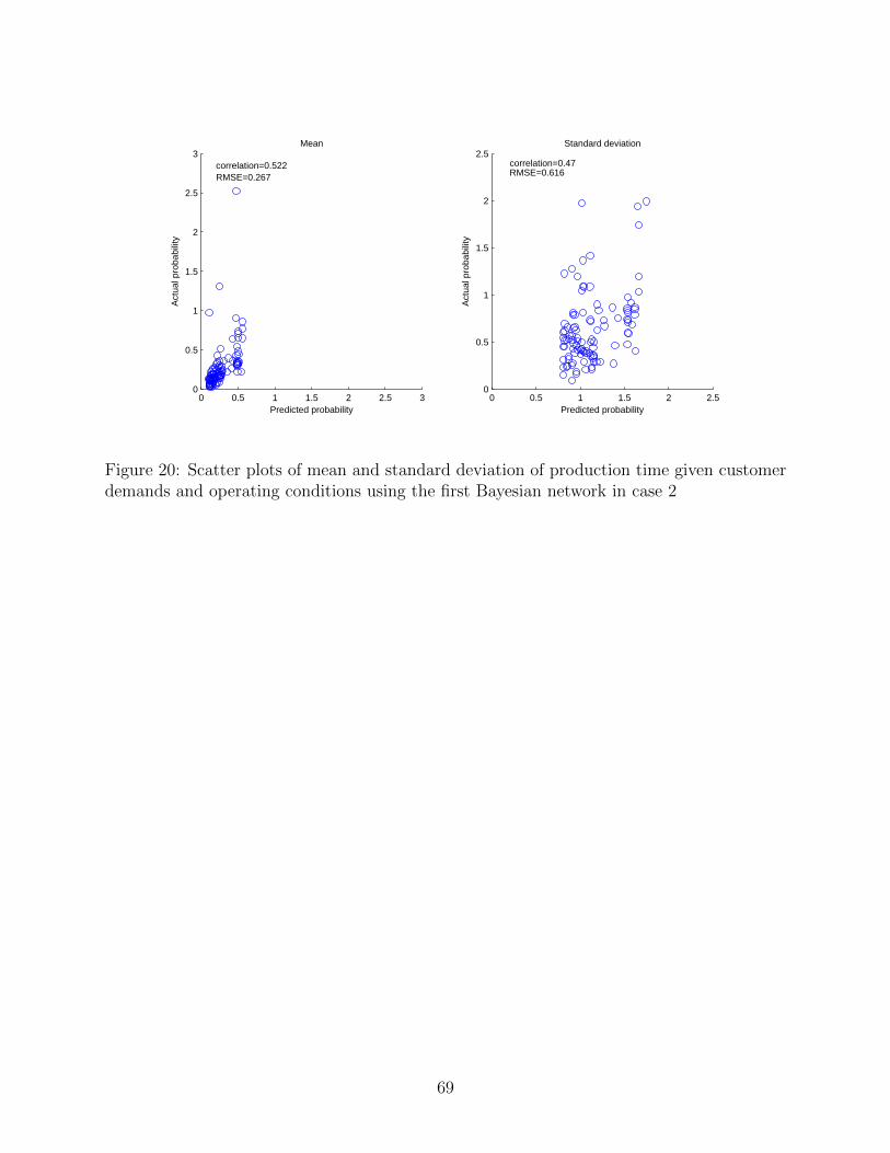
0 0.5 1 1.5 2 2.5 30

0.5

1

1.5

2

2.5

3correlation=0.522RMSE=0.267

Mean

Predicted probability

Act

ual p

roba

bilit

y

0 0.5 1 1.5 2 2.50

0.5

1

1.5

2

2.5correlation=0.47RMSE=0.616

Standard deviation

Predicted probability

Act

ual p

roba

bilit

yFigure 20: Scatter plots of mean and standard deviation of production time given customerdemands and operating conditions using the first Bayesian network in case 2

69

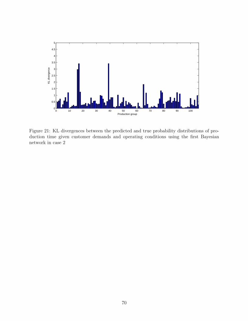
0 10 20 30 40 50 60 70 80 90 1000

0.5

1

1.5

2

2.5

3

3.5

4

4.5

5

Production group

KL

dive

rgen

ce

Figure 21: KL divergences between the predicted and true probability distributions of pro-duction time given customer demands and operating conditions using the first Bayesiannetwork in case 2

70

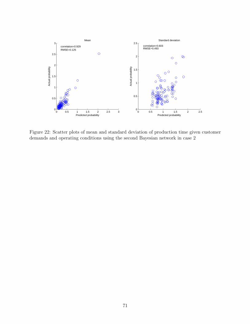
0 0.5 1 1.5 2 2.5 30

0.5

1

1.5

2

2.5

3correlation=0.929RMSE=0.125

Mean

Predicted probability

Act

ual p

roba

bilit

y

0 0.5 1 1.5 2 2.50

0.5

1

1.5

2

2.5correlation=0.603RMSE=0.493

Standard deviation

Predicted probability

Act

ual p

roba

bilit

yFigure 22: Scatter plots of mean and standard deviation of production time given customerdemands and operating conditions using the second Bayesian network in case 2

71

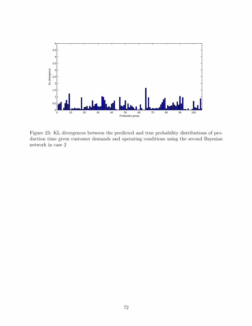
0 10 20 30 40 50 60 70 80 90 1000

0.5

1

1.5

2

2.5

3

3.5

4

4.5

5

Production group

KL

dive

rgen

ce

Figure 23: KL divergences between the predicted and true probability distributions of pro-duction time given customer demands and operating conditions using the second Bayesiannetwork in case 2

72

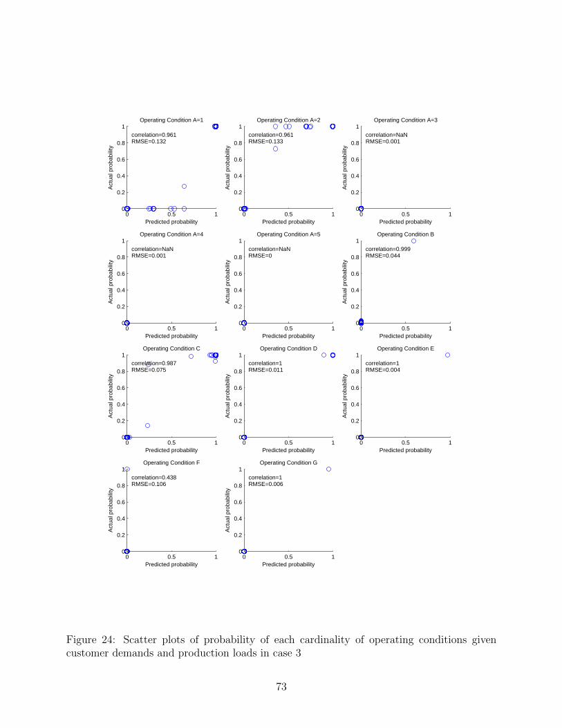
0 0.5 10

0.2

0.4

0.6

0.8

1correlation=0.961RMSE=0.132

Operating Condition A=1

Predicted probability

Act

ual p

roba

bilit

y

0 0.5 10

0.2

0.4

0.6

0.8

1correlation=0.961RMSE=0.133

Operating Condition A=2

Predicted probabilityA

ctua

l pro

babi

lity

0 0.5 10

0.2

0.4

0.6

0.8

1correlation=NaNRMSE=0.001

Operating Condition A=3

Predicted probability

Act

ual p

roba

bilit

y

0 0.5 10

0.2

0.4

0.6

0.8

1correlation=NaNRMSE=0.001

Operating Condition A=4

Predicted probability

Act

ual p

roba

bilit

y

0 0.5 10

0.2

0.4

0.6

0.8

1correlation=NaNRMSE=0

Operating Condition A=5

Predicted probability

Act

ual p

roba

bilit

y

0 0.5 10

0.2

0.4

0.6

0.8

1correlation=0.999RMSE=0.044

Operating Condition B

Predicted probabilityA

ctua

l pro

babi

lity

0 0.5 10

0.2

0.4

0.6

0.8

1correlation=0.987RMSE=0.075

Operating Condition C

Predicted probability

Act

ual p

roba

bilit

y

0 0.5 10

0.2

0.4

0.6

0.8

1correlation=1RMSE=0.011

Operating Condition D

Predicted probability

Act

ual p

roba

bilit

y

0 0.5 10

0.2

0.4

0.6

0.8

1correlation=1RMSE=0.004

Operating Condition E

Predicted probability

Act

ual p

roba

bilit

y

0 0.5 10

0.2

0.4

0.6

0.8

1correlation=0.438RMSE=0.106

Operating Condition F

Predicted probability

Act

ual p

roba

bilit

y

0 0.5 10

0.2

0.4

0.6

0.8

1correlation=1RMSE=0.006

Operating Condition G

Predicted probability

Act

ual p

roba

bilit

y

Figure 24: Scatter plots of probability of each cardinality of operating conditions givencustomer demands and production loads in case 3

73

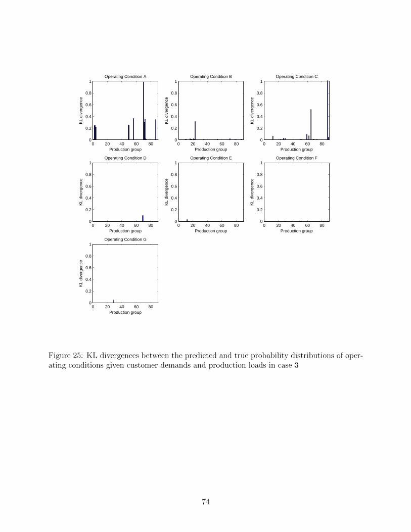
0 20 40 60 800

0.2

0.4

0.6

0.8

1

Production group

KL

dive

rgen

ceOperating Condition A

0 20 40 60 800

0.2

0.4

0.6

0.8

1

Production group

KL

dive

rgen

ce

Operating Condition B

0 20 40 60 800

0.2

0.4

0.6

0.8

1

Production group

KL

dive

rgen

ce

Operating Condition C

0 20 40 60 800

0.2

0.4

0.6

0.8

1

Production group

KL

dive

rgen

ce

Operating Condition D

0 20 40 60 800

0.2

0.4

0.6

0.8

1

Production group

KL

dive

rgen

ce

Operating Condition E

0 20 40 60 800

0.2

0.4

0.6

0.8

1

Production group

KL

dive

rgen

ce

Operating Condition F

0 20 40 60 800

0.2

0.4

0.6

0.8

1

Production group

KL

dive

rgen

ce

Operating Condition G

Figure 25: KL divergences between the predicted and true probability distributions of oper-ating conditions given customer demands and production loads in case 3

74