Am

Sa

b

a

ARR1AA

KABSSCV

1

togtfs

paucA

asEt

(

1h

Applied Soft Computing 17 (2014) 167–175

Contents lists available at ScienceDirect

Applied Soft Computing

j ourna l h o mepage: www.elsev ier .com/ locate /asoc

rtificial chromosomes with genetic algorithm 2 (ACGA2) for singleachine scheduling problems with sequence-dependent setup times

hih-Hsin Chena,∗, Min-Chih Chenb, Yeong-Cheng Lioua

Department of Information Management, Cheng Shiu University, No. 840, Chengcing Rd., Niaosong Dist., Kaohsiung City 83347, Taiwan, ROCInstitute of Manufacturing Engineering, National Cheng Kung University, Tainan 70101, Taiwan, ROC

r t i c l e i n f o

rticle history:eceived 7 April 2011eceived in revised form8 December 2013ccepted 22 December 2013vailable online 18 January 2014

eywords:CGA

a b s t r a c t

Artificial chromosomes with genetic algorithm (ACGA) is one of the latest versions of the estimationof distribution algorithms (EDAs). This algorithm has already been applied successfully to solve differ-ent kinds of scheduling problems. However, due to the fact that its probabilistic model does not considervariable interactions, ACGA may not perform well in some scheduling problems, particularly if sequence-dependent setup times are considered. This is due to the fact that the previous job will influence theprocessing time of the next job. Simply capturing ordinal information from the parental distribution isnot sufficient for a probabilistic model. As a result, this paper proposes a bi-variate probabilistic model toadd into the ACGA. This new algorithm is called the ACGA2 and is used to solve single machine scheduling

i-variate EDAscheduling problemsequence-dependent setup timesommon due-dateariable neighborhood search

problems with sequence-dependent setup times in a common due-date environment. A theoretical anal-ysis is given in this paper. Some heuristics and local search algorithm variable neighborhood search (VNS)are also employed in the ACGA2. The results indicate that the average error ratio of this ACGA2 is half theerror ratio of the ACGA. In addition, when ACGA2 is applied in combination with other heuristic methodsand VNS, the hybrid algorithm achieves optimal solution quality in comparison with other algorithms inthe literature. Thus, the proposed algorithms are effective for solving the scheduling problems.

. Introduction

In our previous studies [1–3], the ACGA algorithm was applied inhe solving of several scheduling problems. The main characteristicf ACGA is that it alternates the EDAs and genetic operators in eacheneration. Since other EDAs [4–8] do not use genetic operators,his is a distinguishing feature of ACGA. This approach is beneficialor EDAs to have a diversified population [9]; GA-EDA [10] used aimilar framework.

ACGA utilizes a univariate probabilistic model which extractsarental distribution from previous searches when the EDAs oper-tor is responsible for generating offspring. After extraction thenivariate probabilistic model is used to sample new solutionsalled artificial chromosomes. These prior studies show that theCGA algorithm is able to provide satisfactory results.

The univariate probabilistic model of ACGA assumes that therere no dependencies between/among variables. However, some

tudies have pointed out that when variable interactions exist,DAs may employ bi-variate or even multi-variate probabilis-ic models [11,12,5,13]. This research studied single machine

∗ Corresponding author.E-mail addresses: shchen@csu.edu.tw (S.-H. Chen), cthunter@wfu.edu.tw

M.-C. Chen), ycliou@csu.edu.tw (Y.-C. Liou).

568-4946/$ – see front matter © 2014 Elsevier B.V. All rights reserved.ttp://dx.doi.org/10.1016/j.asoc.2013.12.019

© 2014 Elsevier B.V. All rights reserved.

scheduling problems with sequence-dependent setup times in acommon due date environment [14]. Because a prior job influencesthe processing time of the next job when we consider the setuptimes, there exists strong interaction between the jobs. If ACGAis used to solve this scheduling problem, a satisfactory result maynot be achieved. Stem from Jarboui et al. [15], a new bi-variateprobabilistic model in conjunction with the univariate probabilisticmodel was adopted into the proposed algorithm, named ACGA2. Asa result, ACGA2 is able to capture a more accurate parental distri-bution from the two probabilistic models and thus produce betteroffspring.

To provide more comparable result, some heuristic approachesand a famous local search algorithm, i.e., variable neighborhoodsearch (VNS), are both employed in the ACGA2. The resultant algo-rithms could obtain better solution quality when we compare itwith others in literature.

The organization of this paper is as follows: Section 2 discussesthe importance of the scheduling problems in question and pro-vides a problem definition. The related works of EDAs and VNS arealso discussed in this section. The details of the ACGA2 and the the-oretical analysis of using the univariate and bi-variate probabilistic

models are introduced in Section 3. In Section 4 we make exten-sive comparisons with other algorithms in the literature that arecommonly used to solve the scheduling problems under discussion.Finally, we present our conclusions in Section 5.

1 ft Computing 17 (2014) 167–175

2

wrtlss

2

smcB[rtrs

joatoapaotaas

idnEtj

m

tpaaarsattrdstrh

68 S.-H. Chen et al. / Applied So

. Background to the scheduling problems with setup costs

This research discusses single machine scheduling problemsith sequence-dependent setup time in a common due date envi-

onment. The objective was to minimize the total earliness andardiness cost. To explain the importance of these scheduling prob-ems, Section 2.1 presents a literature survey and the problemtatement. In Section 2.2, we further explain the model of thecheduling problem.

.1. Review and problem statements

Single-machine scheduling problems are one of the well-tudied problems by many researchers. The application of singleachine scheduling with setups can be found in minimizing the

ycle time for pick and place (PAP) operations in Printed Circuitoard manufacturing company [16]; in a steel wire factory in China17] and a sequencing problem in the weaving industry [18]. Theesults developed in the literature not only provide the insights intohe single machine problem but also for more complicated envi-onment such as flow shop or job shop. For the detail review of thecheduling problems with setup costs, it is available in [19].

The problem considered in this paper is to schedule a set of nobs {j1, j2, . . ., jn} on a single machine that is capable of processingnly one job at a time without preemption. As explained in [20,14],ll jobs are available at time zero, and a job j requires a processingime Pj . Job j belongs to a group gj ∈ {1, . . ., q} (with q ≤ n). Setupr changeover times, which are given as two q × q matrices, aressociated to these groups. This means that in a schedule where jj isrocessed immediately after ji where i, j ∈ {1, 2, . . ., n}, there must be

setup time of at least Sij time units between the completion timef ji, denoted by Ci, and the start time of jj, which is Cj− Pj. Duringhis setup period, no other task can be performed by the machinend we assume that the cost of the setup operation is c(gi ; gj) ≥ 0nd let it be equal to machine setup time Sij which is included asequence dependent.

Apart from the sequence-dependent setup times, the objectives to complete all the jobs as close as possible to a large, commonue date d. To accomplish this objective, the summation of earli-ess and tardiness is minimized. The earliness of job j is denoted asj = max(0, d − Cj) and its tardiness as Tj = max(Cj− d, 0), where Cj ishe completion time of job j. Earliness and tardiness penalties forob j are weighted equally. The objective function is given by:

in Z =n∑

j=1

(Ej + Tj) =n∑

j=1

|d − Cj| (1)

The inclusion of both earliness and tardiness costs in the objec-ive function is compatible with the philosophy of just-in-timeroduction, which emphasizes producing goods only when theyre needed. The early cost may represent the cost of completing

product early, the deterioration cost for a perishable goods or holding (stock) cost for finished goods. The tardy cost can rep-esent rush shipping costs, lost sales and loss of goodwill. Somepecific examples of production settings with these characteristicsre provided by Ow and Morton [21]. The set of jobs is assumedo be ready for processing at the beginning which is a characteris-ic of the deterministic problem. The set of jobs is assumed to beeady for processing at the beginning which is a characteristic of theeterministic problem. As a generalization of weighted tardiness

cheduling, the problem is strongly NP-hard in [22]. Consequently,he early/tardy problem is also a strong NP-hard problem. It is theeason why this work attempts to use eACGA to conquer this NP-ard problem in a reasonable time.

Fig. 1. The total earliness and total tardiness for a pre-assigned due-date d.

2.2. Formulations of the scheduling model

An example of the application of the common due date modelwould be an assembly system in which the components of the prod-uct should be ready at the same time, or to a shop where severaljobs constitute a single customer’s order [23]. Kanet [24] showsthat the optimal sequence is when the bth job is completed at thedue-date. The value of b is given by:

b ={

n/2 if n is even,

(n + 1)/2 if n is odd,(2)

The common due-date (k*) is the sum of processing times of jobsin the first b positions in the sequence; i.e.,

k∗ = Cb (3)

As soon as the common due date is assigned, see Fig. 1, jobs canbe classified into two groups that are early and tardy which areat position from 1 to b and b+1 to n respectively. The followingnotations are employed in the latter formulations.

j: job in position j.A: the job set of tardy jobs.B: the job set of early jobs.S[j][j+1]: Setup time of a job in position [j+1] follows a job in position[j].AP[j][j+1]: Adjusted processing time for the job in position j followedby the job in position [j+1].b: the median position.AP[j][j+1] is actually the processing time of job j + 1 with setup time.Thus, the original form of AP[j][j+1] is written as:

AP[j][j+1] = S[j][j+1] + Pj+1 (4)

Our objective is to minimize the total earliness/tardiness cost.The formulation is given below.

Minimize f (x) =n∑

j=1

(Ej + Tj) = TT + TE (5)

where TT is total tardiness for a job sequence; TE is total earliness fora job sequence; and TT and TE can be transformed into the followingequations based on the pre-defined adjusted processing time.

TT =n−1∑j=b

(n − j)AP[j][j+1] (6)

TE =b∑

j=1

(j − 1)AP[j−1][j] (7)

2.3. Related works of EDAs, VNS, and the combination of EDAsand VNS

In recent years, EDAs is one of the most popular evolution-ary algorithms [25,26,15,7,27]. EDAs explicitly learn and build a

probabilistic model to capture the parental distribution, and thensamples new solutions from the probabilistic model [28]. Samp-ling from probabilistic models avoids the disruption of partialdominant solutions represented by the model, contrary to what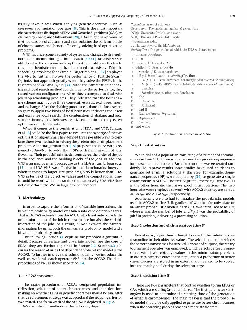

ft Computing 17 (2014) 167–175 169

ucccmop

batstOritjiasaso

eobpnfliV[wVIn

3

bToiib

dEcAwp

3

tmtw

Population: solutionsofsetAGenerations : generationsofnumber maximumTheOP(t): modelProbabilisticUnivariateDP(t): modelProbabilisticBi-variatet index Generation:k interval EDAtheofexecutionThe:startingGen runtostart willEDAthewhichatgenerationThe:1: Initialize Population2: t ← 03: Initialize OP(t) and DP (t)4: while Generations <t do5: Elitism(Population)/Selection6: if g % k 0== startingGen>tand then7: OP(t 1) + ←BuildUni variateProbabili tyM odel(Selected Chromosomes )8: DP(t 1) + ←BuildBi VariateProbabili tyM odel(Selected Chromosomes )9: Learning

10: PopulationintosolutionsnewSampling11: else12: Crossover()13: Mutation()14: ifend15: (Population )EvaluateFitness16: Replacement()17: t ← t 1+

S.-H. Chen et al. / Applied So

sually takes places when applying genetic operators, such asrossover and mutation operator [8]. This is the most importantharacteristic to distinguish EDAs and Genetic Algorithms (GAs). Aslaimed by Zhang and Muhlenbein [29], EDAs might be a promisingethod capable of capturing and manipulating the building blocks

f chromosomes and, hence, efficiently solving hard optimizationroblems.

VNS has undergone a variety of systematic changes to its neigh-orhood structure during a local search [30,31]. Because VNS isble to solve the combinatorial optimization problems effectively,his meta-heuristic method has been used extensively. Take thecheduling problems for example, Tasgetiren et al. [32] employedhe VNS to further improve the performance of Particle Swarmptimization approach greatly when they solve the PFSPs. In the

esearch of Sevkli and Aydin [33], since the combination of shak-ng and local search method could influence the performance, theyested various configurations when they attempted to deal withob shop scheduling problems. They indicated that the best shak-ng scheme may involve three consecutive steps: exchange, insert,nd exchange. After the shaking procedure is done, the local searchtage may apply two kinds of local heuristics, including the insertnd exchange local search. The combination of shaking and localearch scheme yields the lowest relative error ratio and the greatestptimum value for hit ratio.

When it comes to the combination of EDAs and VNS, Santanat al. [8] could be the first paper to evaluate the synergy of the twoptimization algorithms. They defined three possible ways to com-ine these two methods in solving the protein side chain placementroblem. After that, Jarboui et al. [15] proposed the EDAs with VNS,amed (EDA-VNS) to solve the PFSPs with minimization of totalowtime. Their probabilistic model considered the order of the job

n the sequence and the building blocks of the jobs. In addition,NS is an improvement procedure as the EDA is run. Jarboui et al.

15] found EDA-VNS was effective in small benchmarks; however,hen it comes to larger size problems, VNS is better than EDA-NS in terms of the objective values and the computational time.

t could be worthwhile to examine the reason why EDA-VNS doesot outperform the VNS in large size benchmarks.

. Methodology

In order to capture the information of variable interactions, thei-variate probability model was taken into consideration as well.hat is, ACGA2 extends from the ACGA, which not only collects therder information of the job in the sequence but also the variablenteraction of the jobs. As a result, ACGA2 extracts the parentalnformation by using both the univariate probability model and ai-variate probability model.

The following Section 3.1 explains the proposed algorithm inetail. Because univariate and bi-variate models are the core ofDAs, they are further explained in Section 3.2. Section 3.3 dis-usses the reason of using the dependent probabilistic model in theCGA2. To further improve the solution quality, we introduce theell-known local search operator VNS into the ACGA2. The detailrocedures of VNS is shown in Section 3.4.

.1. ACGA2 procedures

The major procedures of ACGA2 comprised population ini-ialization, selection of better chromosomes, and then decision-

aking on whether EDAs or genetic operators should be ran. Afterhat, a replacement strategy was adopted and the stopping criterionas tested. The framework of the ACGA2 is depicted in Fig. 2.

We describe our methods in the following steps.

18: whileend

Fig. 2. Algorithm 1: main procedure of ACGA2.

Step 1: initialization

We initialized a population consisting of a number of chromo-somes in Line 1. A chromosome represents a processing sequencefor the scheduling problem. Each chromosome was generated ran-domly. To improve results some studies have used heuristics togenerate better initial solutions at this step. For example, domi-nance properties (DP) were adopted by [34] to generate a singlechromosome in ACGA2. Shortest Adjusted Processing Time (SAPT)is the other heuristic that gives good initial solutions. The twoheuristics were employed to work with ACGA2 and they are namedACGA2DP and ACGA2SAPT, respectively.

Additionally we also had to initialize the probabilistic modelsused in ACGA2 in Line 3. Regardless of whether for univariate orbi-variate probabilistic models, each Pij(t) was initialized to be 1/n,where n was the number of jobs and Pij(t) was the probability ofjob i in position j delivering a promising solution.

Step 2: selection and elitism strategy (Line 5)

Evolutionary algorithms attempt to select fitter solutions cor-responding to their objective values. The selection operator selectsthe better chromosomes for survival. For ease of purpose, the binarytournament operator was employed, which selects better chromo-somes with lower objective values in this minimization problem.In order to preserve elites in the population, a proportion of betterchromosomes are stored in an external archive and to be copiedinto the mating pool during the selection stage.

Step 3: decision (Line 6)

There are two parameters that control whether to run EDAs orGAs, which are startingGen and interval. The first parameter start-

ingGen is used to determine the starting time of the generationof artificial chromosomes. The main reason is that the probabilis-tic model should be only applied to generate better chromosomeswhen the searching process reaches a more stable state.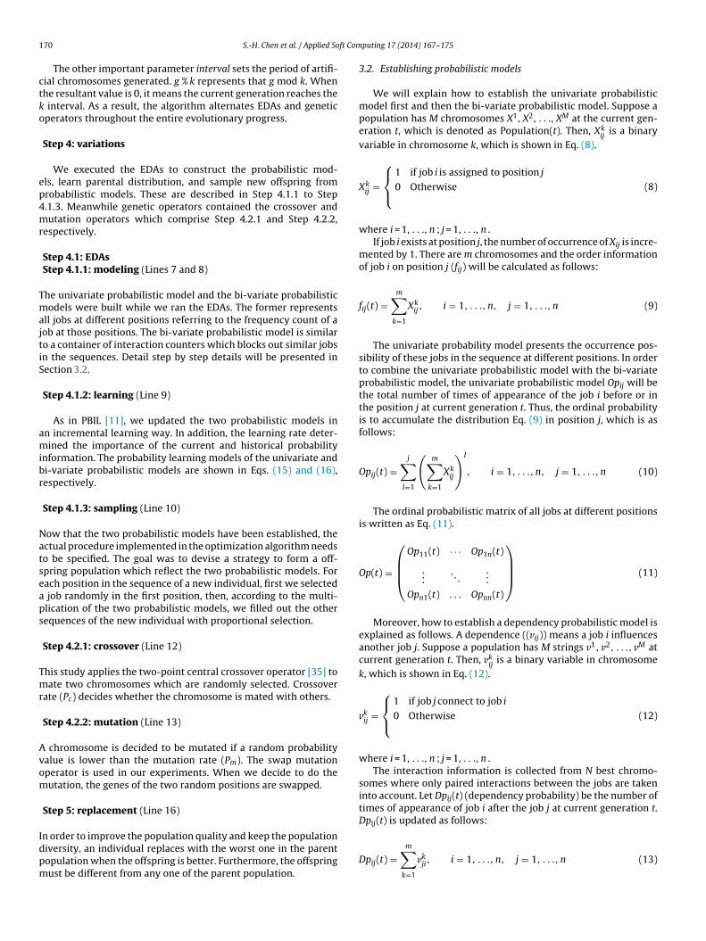

1 ft Com

ctko

ep4mr

TmajtiS

amibr

Natseaps

Tmr

Avom

Idpm

70 S.-H. Chen et al. / Applied So

The other important parameter interval sets the period of artifi-ial chromosomes generated. g % k represents that g mod k. Whenhe resultant value is 0, it means the current generation reaches the

interval. As a result, the algorithm alternates EDAs and geneticperators throughout the entire evolutionary progress.

Step 4: variations

We executed the EDAs to construct the probabilistic mod-ls, learn parental distribution, and sample new offspring fromrobabilistic models. These are described in Step 4.1.1 to Step.1.3. Meanwhile genetic operators contained the crossover andutation operators which comprise Step 4.2.1 and Step 4.2.2,

espectively.

Step 4.1: EDAsStep 4.1.1: modeling (Lines 7 and 8)

he univariate probabilistic model and the bi-variate probabilisticodels were built while we ran the EDAs. The former represents

ll jobs at different positions referring to the frequency count of aob at those positions. The bi-variate probabilistic model is similaro a container of interaction counters which blocks out similar jobsn the sequences. Detail step by step details will be presented inection 3.2.

Step 4.1.2: learning (Line 9)

As in PBIL [11], we updated the two probabilistic models inn incremental learning way. In addition, the learning rate deter-ined the importance of the current and historical probability

nformation. The probability learning models of the univariate andi-variate probabilistic models are shown in Eqs. (15) and (16),espectively.

Step 4.1.3: sampling (Line 10)

ow that the two probabilistic models have been established, thectual procedure implemented in the optimization algorithm needso be specified. The goal was to devise a strategy to form a off-pring population which reflect the two probabilistic models. Forach position in the sequence of a new individual, first we selected

job randomly in the first position, then, according to the multi-lication of the two probabilistic models, we filled out the otherequences of the new individual with proportional selection.

Step 4.2.1: crossover (Line 12)

his study applies the two-point central crossover operator [35] toate two chromosomes which are randomly selected. Crossover

ate (Pc) decides whether the chromosome is mated with others.

Step 4.2.2: mutation (Line 13)

chromosome is decided to be mutated if a random probabilityalue is lower than the mutation rate (Pm). The swap mutationperator is used in our experiments. When we decide to do theutation, the genes of the two random positions are swapped.

Step 5: replacement (Line 16)

n order to improve the population quality and keep the populationiversity, an individual replaces with the worst one in the parentopulation when the offspring is better. Furthermore, the offspringust be different from any one of the parent population.

puting 17 (2014) 167–175

3.2. Establishing probabilistic models

We will explain how to establish the univariate probabilisticmodel first and then the bi-variate probabilistic model. Suppose apopulation has M chromosomes X1, X2, . . ., XM at the current gen-eration t, which is denoted as Population(t). Then, Xk

ijis a binary

variable in chromosome k, which is shown in Eq. (8).

Xkij =

⎧⎨⎩

1 if job i is assigned to position j

0 Otherwise (8)

where i = 1, . . ., n ; j = 1, . . ., n .If job i exists at position j, the number of occurrence of Xij is incre-

mented by 1. There are m chromosomes and the order informationof job i on position j (fij) will be calculated as follows:

fij(t) =m∑

k=1

Xkij, i = 1, . . ., n, j = 1, . . ., n (9)

The univariate probability model presents the occurrence pos-sibility of these jobs in the sequence at different positions. In orderto combine the univariate probabilistic model with the bi-variateprobabilistic model, the univariate probabilistic model Opij will bethe total number of times of appearance of the job i before or inthe position j at current generation t. Thus, the ordinal probabilityis to accumulate the distribution Eq. (9) in position j, which is asfollows:

Opij(t) =j∑

l=1

(m∑

k=1

Xkij

)l

, i = 1, . . ., n, j = 1, . . ., n (10)

The ordinal probabilistic matrix of all jobs at different positionsis written as Eq. (11).

Op(t) =

⎛⎜⎜⎝

Op11(t) · · · Op1n(t)

.... . .

...

Opn1(t) . . . Opnn(t)

⎞⎟⎟⎠ (11)

Moreover, how to establish a dependency probabilistic model isexplained as follows. A dependence ((vij)) means a job i influencesanother job j. Suppose a population has M strings v1, v2, . . ., vM atcurrent generation t. Then, vk

ijis a binary variable in chromosome

k, which is shown in Eq. (12).

vkij =

⎧⎨⎩

1 if job j connect to job i

0 Otherwise (12)

where i = 1, . . ., n ; j = 1, . . ., n .The interaction information is collected from N best chromo-

somes where only paired interactions between the jobs are takeninto account. Let Dpij(t) (dependency probability) be the number oftimes of appearance of job i after the job j at current generation t.Dpij(t) is updated as follows:

Dpij(t) =m∑

k=1

vkji, i = 1, . . ., n, j = 1, . . ., n (13)

ft Com

j

D

tttebs

O

D

jccitT0i

3

nmitbp

juhrpwv

d

x2: A local optimal generated by an insertion local search operator.F(xbest): The objective value of the solution xbest.k: The current number of VNS iteration.kmax: The maximum number of VNS iteration.

S.-H. Chen et al. / Applied So

The dependency probabilistic matrix of paired interaction of allobs are written as Eq. (14).

p(t) =

⎛⎜⎜⎜⎜⎝

0 Dp12(t) · · · Dp1n(t)

Dp21(t) 0 · · · Dp2n(t)

......

. . ....

Dpn1(t) Dpn2(t) . . . 0

⎞⎟⎟⎟⎟⎠ (14)

Furthermore, the above two probabilities with learning can con-inue to modify the search space to improve the performance ofhe algorithm. The equation is presented as Eqs. (15) and (16). Inhis research, the ordinal learning rate (�OP ∈ (0, 1)) and depend-nt learning rate (�DP ∈ (0, 1)) of the two parameters were decidedy the design-of-experiment (DOE), which we discuss in the nextection.

pij(t) = Opij(t) × (1.0 − �Op) + Opij(t − 1) × �Op (15)

pij(t) = Dpij(t) × (1.0 − �Dp) + Dpij(t − 1) × �Dp (16)

As soon as the ordinal Op and dependent probability Dp are built,obs are assigned onto each position. As far as diversification is con-erned, there are three methods for creating diversified artificialhromosomes. The first is for random selection at the first positionn the sequence. The second is for proportional selection to be usedo mitigate the probability of job i being assigned to a position j.he third is zero value transformation which is used to transform

into 1/n in dependent probability when jobs do not have anynteractions. The assignment procedure is determined as follows:

S: A set of shuffled sequence which determines the sequence ofeach position is assigned a job.˝: The set of un-arranged jobs.J: The set of arranged jobs. J is empty in the beginning.�: A random probability is drawn from U(0, 1).i: A selected job by proportional selection.k: The element index of the set S.

1: S← shuffled the job number [1, . . ., n]2: J ← ˚3: while k /= do4: � ← U(0, 1)5: Select a job i satisfies � ≤ OPik × DPiJ(k−1)/

∑OP(i, k) × DP(i, J(k − 1)),

where i ∈ ˝6: J(k) ← i7: ← \ i8: S ← S \ k9: end while

.3. Theoretical analysis

The inclusion of the dependency probabilistic (Eq. (14)) is quiteecessary to extract the interaction among the pair-wised jobs. Theajor reason is that the adjusted processing time AP[j][j+1] in Eq. (4)

s not equal to Pj+1 because the setup time S[j][j+1] is not zero inhe studied problem. It is apparently that there exists interactionsetween the jobs. Simply capturing ordinal information from thearental distribution is not sufficient for the studied problem.

In addition, when ACGA2 selects an appropriate job j after theob i, the statistic information in the two probabilistic models aresed. In particular, the bi-variate model may forbid a job k whichas a higher setup cost when job k is scheduled after job i. As aesult, the solution space would be reduced due to the bi-variaterobability model is employed in the ACGA2. As a result, ACGA2

ould perform better than the ACGA since ACGA ignores all the

ariable interactions.On the other hand, Zhang and Mühlenbein [29] proved that if the

istribution of the new solutions matches that of the parent set, the

puting 17 (2014) 167–175 171

algorithm will converge to the global optimal when we apply theproportional selection, truncation selection, and the tournamentselection model. Even though both the ACGA and ACGA2 utilize thebinary tournament, the models used by ACGA2 would provide moreand accurate parental distribution during the generations owing tothe interaction information is preserved. To understand the dis-tribution generated by ACGA and ACGA2, we employ the entropyproposed by Shannon [36]. Suppose the information gains of ACGAand ACGA2 at generation t are I(Opt

ij) in Eq. (17) and I(Optij ∗ Dpt

ij) inEq. (18), respectively.

I(Optij) = −

n∑i=1

logbP(Optij)

n(17)

I(Optij ∗ Dpt

ij) = −n∑

i=1

logbP(Optij ∗ Dpt

ij)

n

= −n∑

i=1

[logbP(Optij) + logbP(Dpt

ij)]

n(18)

where b is the base of the logarithm.Because the probability values of P(Opt

ij) and P(Dptij) are less than

1, the log value of logbP(Optij) and logbP(Dpt

ij) are definitely nega-

tive. Consequently, I(Optij) is less than I(Opt

ij ∗ Dptij) while the later

one has more information of logbP(Dptij). The sampled distribution

yielded by eACGA may match the better parental distribution thanthe one of ACGA.

3.4. VNS procedures

In order to improve the solution quality, VNS is hybridized intothe searching process in this research since many researches haveproved that VNS is effective in solving the PFSPs [37,32]. In thispaper, we have included the version of Jarboui et al. [37] in ourresearch. Meanwhile, the combination of the ACGA2 and VNS isnamed ACGA2VNS in this paper.

In the beginning of the VNS procedures, a VNS parameter Penhdecides the probability to execute the VNS in the main procedure ofACGA2VNS. We generate a random probability and to test whether itis less than or equal to the Penh. If the random value is less than orequal to the Penh, VNS procedure is thus executed and a current bestsolution xbest is selected to do the perturbation. The perturbationscheme is to produce neighborhood from current best solution. Thenew solution is represented as x1. After that, the swap local search isused first to modify the solution of x1 and then insertion local searchis employed later. The two local search strategies were introducedby Jarboui et al. [37].

xbest: A selected elite chromosome.x1: We change the neighborhood structure of xbest.x2: A local optimal improved by a swap local search operator.′

1: k← 12: while k < kmax do3: x1← generate a neighborhood solution of xbest

4: x2← swapLocalSearch(x1)

1 ft Com

ViIcitarbscxasp

4

[Ta1mlwaabtostt2

Te

TV

72 S.-H. Chen et al. / Applied So

5: x′2 ← insertionLocalSearch(x2)6: if F(x′2) < F(xbest) then7: xbest← x′28: k← 19: else10: k← k + 111: end if12: end while

The number of kmax is set as the stopping criterion of theNS. Because the number of kmax is dependent on the benchmark

nstance, we determine this parameter by design-of-experiment.n the loop of VNS, a new solution is created by the shaking pro-edure. The neighborhood structure comprises steps of exchange,nsert, and exchange to variate a current best solution. By usinghis method suggested by Sevkli and Aydin [33], we thus creatend further improve the new solution x1 by a swap local search. Theesultant solution of swap local search is x2 that might be improvedy a swap local search. Then, an insertion local search acts on theolution x2 so that it generates a new solution x′2. The final step is toompare the fitness of the solution x′2 with the current best solutionbest. If the new solution x′2 is better than xbest, it replaces the xbestnd k is reset to one. Otherwise, k is increased by one. Through theystematic exploration and exploitation, VNS could improve theerformance of the proposed ACGA2VNS.

. Experimental results

The basic testing instances are as designed by Rabadi et al.38] and the job size of each instance includes 10, 15, 20 and 25.he properties of the processing time range contain low, mediannd high values, which are based on Uniform(10, 60), Uniform(10,10) and Uniform(10, 160), respectively. Moreover, these instancesight not be sufficient to demonstrate the complexity of the prob-

em. We apply similar concept to generate large size of problems,hich include 50 and 100 jobs. The distribution of these instances is

lso based on the processing time range that includes low, mediannd high. Each combination has 15 similar instances, the total num-er of instances is 270 (6 × 3 ×15). Each instance is replicated 30imes for our proposed algorithm and the compared algorithms. Inrder to configure the parameter settings, we utilized the DOE to

elect the best setting of ACGA2 parameters. Tables 1 and 2 showhe parameter settings of the ACGA2 and VNS experiment, respec-ively. We coded the algorithm in Java and ran it on a Windows003 server (Intel Xeon 3.2 GHz).

able 1ACGA parameters setting.

Factor Default

Crossover rate 0.5Mutation rate 0.3Starting generation 0Interval 2Ordinal probability learning rate 0.1Dependent probability learning rate 0.5Population size 100Generations 1000

able 2NS parameters setting.

Job size Penh kmax

10 0.1 2015 0.1 2020 0.1 5025 0.1 5050 0.1 100

100 0.1 100

puting 17 (2014) 167–175

In order to evaluate the performance of ACGA2, comparison wascarried out with some algorithms in the literature. We divided thesealgorithms into two groups; stand-alone algorithms and hybridalgorithms. To test the efficiency of the proposed ACGA2 algorithmagainst stand-alone algorithms, we compared the SGA [39], ACGA[40] and SAPT [41]. We also selected some hybrid algorithms, suchas SGADP [34], ACGADP [40] and SASAPT [41]. In addition, when theACGA2 was combined with two heuristic algorithms DPs [34] andSAPT [41] because they generate good initial solutions, we namedthem ACGA2DP and ACGA2SAPT, respectively. A brief summary ofthese algorithms is as follows:

• SGA [39]: This is a standard genetic algorithm that follows anelitist strategy. The genetic operators are binary tournamentselection, two-point central operator and swap mutation oper-ator. During the selection stage, 10% of elites in the populationare reserved for the next generation. We use the data from [34]for comparison.• ACGA [40]: We have already mentioned that ACGA does not con-

sider the dependencies between/among variables. When usingACGA to solve the benchmark problems of this study, we wereable to distinguish performance differences when we employedthe bi-variate probabilistic model together with the univariateprobabilistic model.• SAPT [41]: Shortest Adjusted Processing Time (SAPT) is based

on the concept that jobs to be scheduled with shorter adjustedprocessing times should be closer to the median position inan optimal job sequence. In the study mentioned SAPT wasalso combined with the simulated annealing (SA) algorithm,called SAPT-SA. Since the presented data of SAPT-SA [41] are notcomplete and the termination criterion was different from ourexperiments, we only used the SAPT data from [41] for compari-son.• SGADP [34]: Dominance properties (DPs) were developed by

swapping neighboring jobs. DPs are very efficient when com-bined with GAs. We take the results from [34] for comparison.• ACGADP [34]: According to past research on ACGA [40] and DPs

[34], we combined both algorithms to solve the single machinescheduling problems with setup costs. DPs were utilized to gen-erate a set of good initial solutions. ACGA takes advantage ofthese good initial solutions and then continues the evolutionaryprogress. According to our evaluation ACGADP should performbetter than ACGA.• ACGA2SAPT: SAPT is used to generate good initial solutions and

ACGA2 improves the solution quality given by SAPT.• ACGA2SAPT+VNS: It is similar to ACGA2SAPT; however, VNS is used

to further improve the solution quality in the search.

To compare the performance of these algorithms, we employedthe average relative error ratio and each algorithm evaluates100,000 solutions. In the literature, the average relative error ratiois often used to evaluate the performance of algorithms, wherebythe error ratio (ERi) of a solution (Xi) generated by an algorithm iscalculated as follows:

ERi =Objavg(Xi) − Opti

Opti× 100, (19)

where Opti is the objective value of the best known or optimalsolution which is available by Sourd [14] who applied Branch-and-Bound algorithm to derive the solution. For the larger size problems(i.e., 50 and 100 jobs), we aggregated the experiment results of thecompared algorithms among the 30 replications while each algo-

rithm applied more than 10 times of regular computation time. Theobtained current best objective values is shown in Table 3. Finally,the Objavg(Xi) is the Xi average objective value where we replicateeach algorithm for 30 times.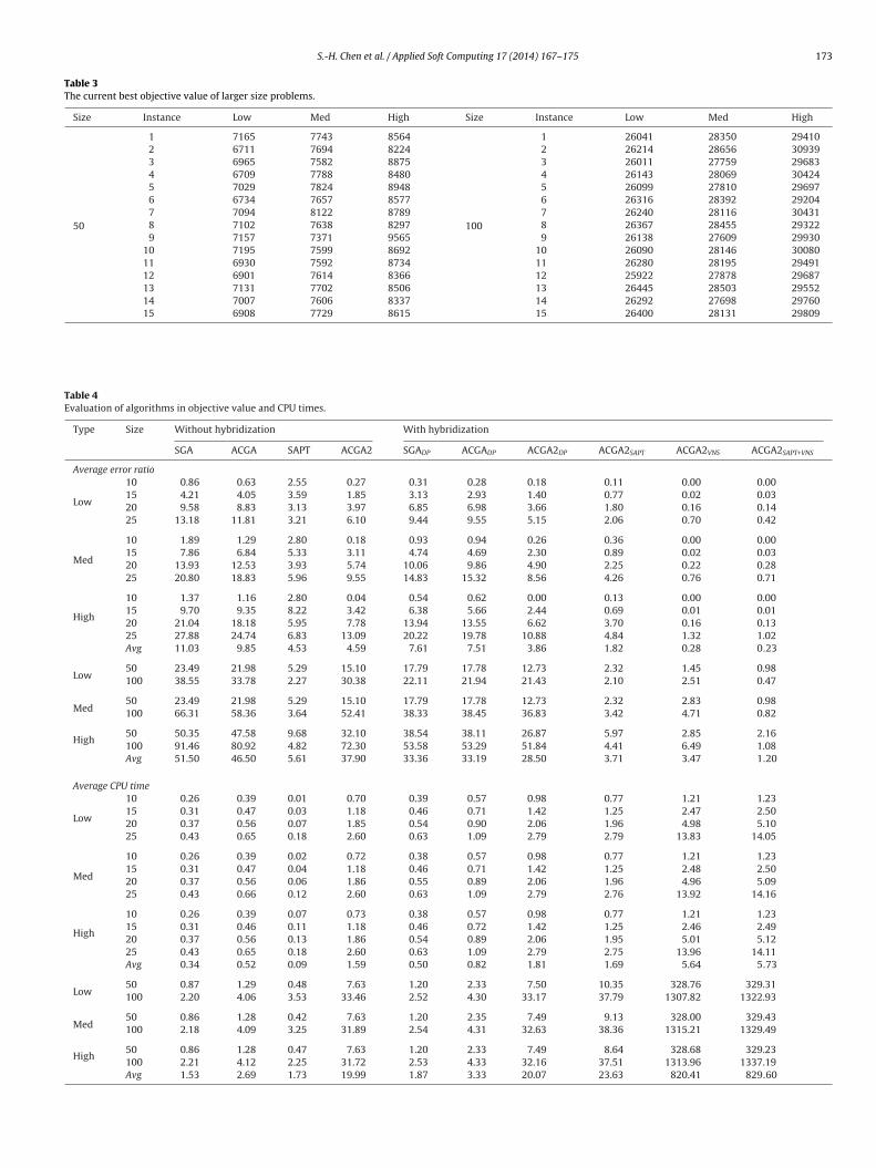

S.-H. Chen et al. / Applied Soft Computing 17 (2014) 167–175 173

Table 3The current best objective value of larger size problems.

Size Instance Low Med High Size Instance Low Med High

50

1 7165 7743 8564

100

1 26041 28350 294102 6711 7694 8224 2 26214 28656 309393 6965 7582 8875 3 26011 27759 296834 6709 7788 8480 4 26143 28069 304245 7029 7824 8948 5 26099 27810 296976 6734 7657 8577 6 26316 28392 292047 7094 8122 8789 7 26240 28116 304318 7102 7638 8297 8 26367 28455 293229 7157 7371 9565 9 26138 27609 29930

10 7195 7599 8692 10 26090 28146 3008011 6930 7592 8734 11 26280 28195 2949112 6901 7614 8366 12 25922 27878 2968713 7131 7702 8506 13 26445 28503 2955214 7007 7606 8337 14 26292 27698 2976015 6908 7729 8615 15 26400 28131 29809

Table 4Evaluation of algorithms in objective value and CPU times.

Type Size Without hybridization With hybridization

SGA ACGA SAPT ACGA2 SGADP ACGADP ACGA2DP ACGA2SAPT ACGA2VNS ACGA2SAPT+VNS

Average error ratio

Low

10 0.86 0.63 2.55 0.27 0.31 0.28 0.18 0.11 0.00 0.0015 4.21 4.05 3.59 1.85 3.13 2.93 1.40 0.77 0.02 0.0320 9.58 8.83 3.13 3.97 6.85 6.98 3.66 1.80 0.16 0.1425 13.18 11.81 3.21 6.10 9.44 9.55 5.15 2.06 0.70 0.42

Med

10 1.89 1.29 2.80 0.18 0.93 0.94 0.26 0.36 0.00 0.0015 7.86 6.84 5.33 3.11 4.74 4.69 2.30 0.89 0.02 0.0320 13.93 12.53 3.93 5.74 10.06 9.86 4.90 2.25 0.22 0.2825 20.80 18.83 5.96 9.55 14.83 15.32 8.56 4.26 0.76 0.71

High

10 1.37 1.16 2.80 0.04 0.54 0.62 0.00 0.13 0.00 0.0015 9.70 9.35 8.22 3.42 6.38 5.66 2.44 0.69 0.01 0.0120 21.04 18.18 5.95 7.78 13.94 13.55 6.62 3.70 0.16 0.1325 27.88 24.74 6.83 13.09 20.22 19.78 10.88 4.84 1.32 1.02Avg 11.03 9.85 4.53 4.59 7.61 7.51 3.86 1.82 0.28 0.23

Low50 23.49 21.98 5.29 15.10 17.79 17.78 12.73 2.32 1.45 0.98100 38.55 33.78 2.27 30.38 22.11 21.94 21.43 2.10 2.51 0.47

Med50 23.49 21.98 5.29 15.10 17.79 17.78 12.73 2.32 2.83 0.98100 66.31 58.36 3.64 52.41 38.33 38.45 36.83 3.42 4.71 0.82

High50 50.35 47.58 9.68 32.10 38.54 38.11 26.87 5.97 2.85 2.16100 91.46 80.92 4.82 72.30 53.58 53.29 51.84 4.41 6.49 1.08Avg 51.50 46.50 5.61 37.90 33.36 33.19 28.50 3.71 3.47 1.20

Average CPU time

Low

10 0.26 0.39 0.01 0.70 0.39 0.57 0.98 0.77 1.21 1.2315 0.31 0.47 0.03 1.18 0.46 0.71 1.42 1.25 2.47 2.5020 0.37 0.56 0.07 1.85 0.54 0.90 2.06 1.96 4.98 5.1025 0.43 0.65 0.18 2.60 0.63 1.09 2.79 2.79 13.83 14.05

Med

10 0.26 0.39 0.02 0.72 0.38 0.57 0.98 0.77 1.21 1.2315 0.31 0.47 0.04 1.18 0.46 0.71 1.42 1.25 2.48 2.5020 0.37 0.56 0.06 1.86 0.55 0.89 2.06 1.96 4.96 5.0925 0.43 0.66 0.12 2.60 0.63 1.09 2.79 2.76 13.92 14.16

High

10 0.26 0.39 0.07 0.73 0.38 0.57 0.98 0.77 1.21 1.2315 0.31 0.46 0.11 1.18 0.46 0.72 1.42 1.25 2.46 2.4920 0.37 0.56 0.13 1.86 0.54 0.89 2.06 1.95 5.01 5.1225 0.43 0.65 0.18 2.60 0.63 1.09 2.79 2.75 13.96 14.11Avg 0.34 0.52 0.09 1.59 0.50 0.82 1.81 1.69 5.64 5.73

Low50 0.87 1.29 0.48 7.63 1.20 2.33 7.50 10.35 328.76 329.31100 2.20 4.06 3.53 33.46 2.52 4.30 33.17 37.79 1307.82 1322.93

Med50 0.86 1.28 0.42 7.63 1.20 2.35 7.49 9.13 328.00 329.43100 2.18 4.09 3.25 31.89 2.54 4.31 32.63 38.36 1315.21 1329.49

High50 0.86 1.28 0.47 7.63 1.20 2.33 7.49 8.64 328.68 329.23100 2.21 4.12 2.25 31.72 2.53 4.33 32.16 37.51 1313.96 1337.19Avg 1.53 2.69 1.73 19.99 1.87 3.33 20.07 23.63 820.41 829.60

174 S.-H. Chen et al. / Applied Soft Computing 17 (2014) 167–175

a

Aatsde

ferAt2tsiw

ratOmntwSSwnc

5

ratpaos

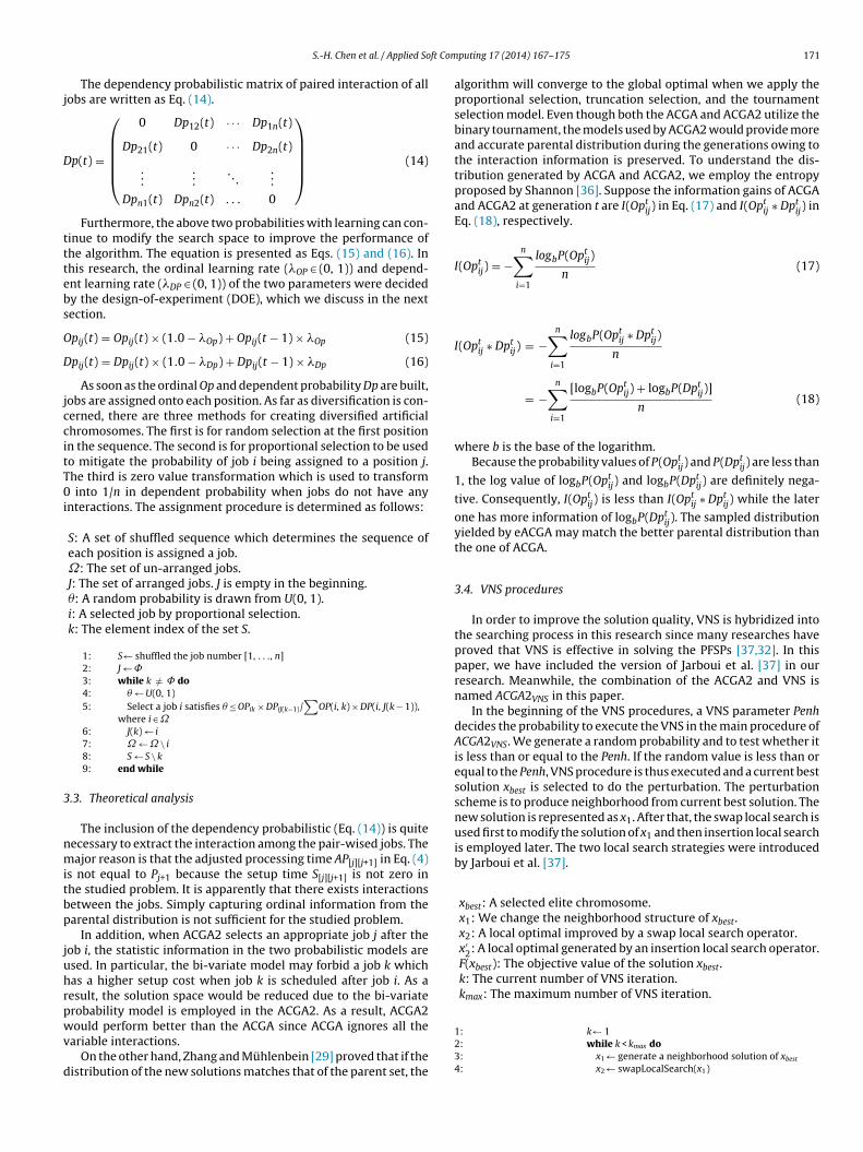
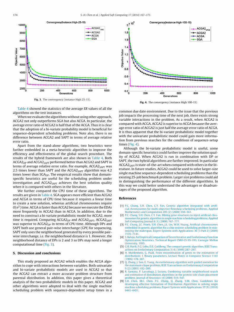
Fig. 3. The convergency (instance High 25-15).

Table 4 showed the statistics of the average ER values of all thelgorithms on the test instances.

When we evaluate the algorithms without using other approach,CGA2 not only outperforms SGA but also ACGA. In particular, theverage error ratio of ACGA2 is half that of the ACGA. Thus it is clearhat the adoption of a bi-variate probability model is beneficial forequence-dependent scheduling problems. Note also, there is noifference between ACGA2 and SAPT in terms of average relativerror ratio.

Apart from the stand-alone algorithms, two heuristics wereurther embedded in a meta-heuristic algorithm to improve thefficiency and effectiveness of the global search procedure. Theesults of the hybrid framework are also shown in Table 4. BothCGA2DP and ACGA2SAPT performed better than ACGA2 and SAPT in

erms of average relative error ratio. For example, ACGA2SAPT was.5 times lower than SAPT and the ACGA2SAPT algorithm was 4.2imes lower than SGADP. The empirical results show that domain-pecific heuristics are useful for the scheduling problem undernvestigation and ACGA2SAPT achieves the best solution quality

hen it is compared with others in the literature.We further compared the CPU time of these algorithms. The

esults are given in Table 4. SGA appears more efficient than ACGA2nd ACGA in terms of CPU time because it requires a linear timeo create a new solution, whereas artificial chromosomes require(n2) time. ACGA is faster than ACGA2 because we execute the EDAsore frequently in ACGA2 than in ACGA. In addition, due to the

eed to construct a bi-variate probabilistic model for ACGA2, moreime is required. Comparing ACGA2DP and ACGA2SAPT, ACGA2SAPTas superior to ACGA2DP in terms of CPU time. Although DPs and

APT both use general pair-wise interchange (GPI) for sequencing,APT only uses the neighborhood generated by every possible pair-ise interchange, i.e. the neighborhood distance is 1. However, theeighborhood distance of DPs is 2 and 3 so DPs may need a longeromputational time (Fig. 3).

. Discussion and conclusions

This study proposed an ACGA2 which enables the ACGA algo-ithm to cope with interactions between variables. Both univariatend bi-variate probabilistic models are used in ACGA2 so thathe ACGA2 can extract a more accurate problem structure from

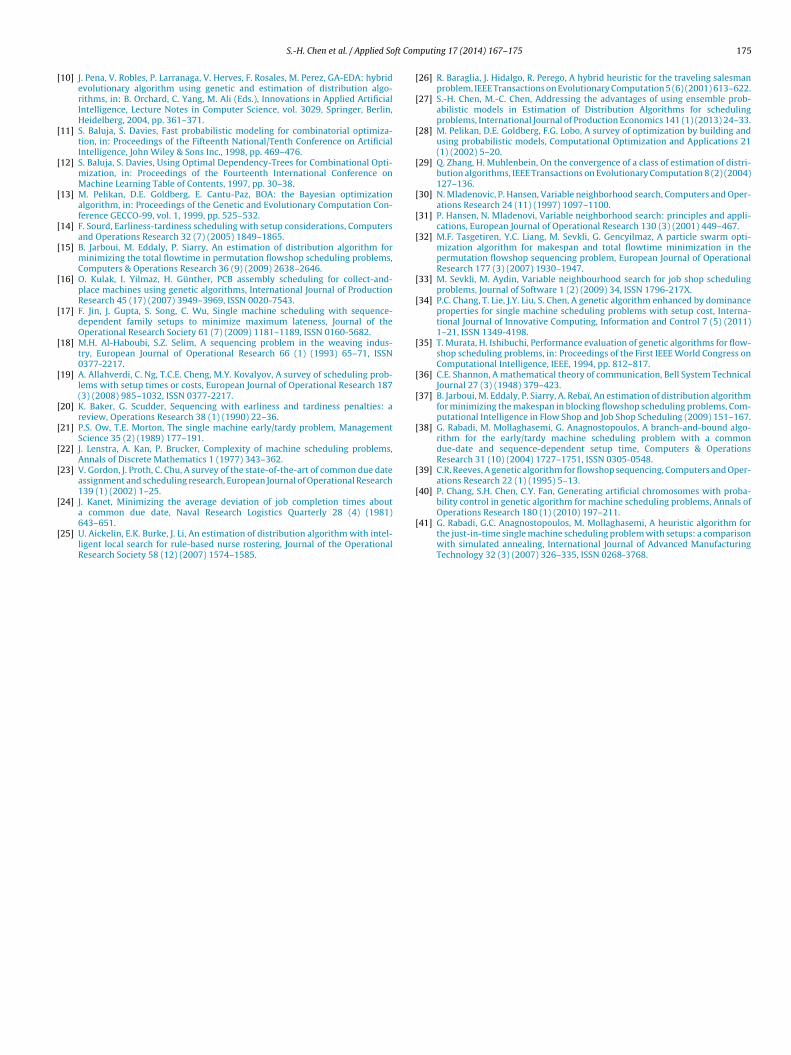
arental distribution. In addition, this paper gives a theoreticalnalysis of the two probabilistic models in this paper. ACGA2 andther algorithms were adopted to deal with the single machinecheduling problem with sequence-dependent setup times in a

Fig. 4. The convergency (instance High 100-15)

common due date environment. Due to the issue that the previousjob impacts the processing time of the next job, there exists strongvariable interactions in the problem. As a result, when ACGA2 iscompared with ACGA, ACGA2 is superior to ACGA because the aver-age error ratio of ACGA2 is just half the average error ratio of ACGA.It is thus apparent that the bi-variate probabilistic model togetherwith the univariate probabilistic model could gain more informa-tion from previous searches for the conditions of sequence-setuptimes (Fig. 4).

Although the bi-variate probabilistic model is useful, somedomain-specific heuristics could further improve the solution qual-ity of ACGA2. When ACGA2 is run in combination with DP orSAPT, the two hybrid algorithms are further improved. In particularACGA2SAPT is state-of-the-art when compared with others in the lit-erature. In future studies, ACGA2 could be used to solve larger-sizesingle machine sequence-dependent scheduling problems than theexisting 25-job benchmark problem. Larger size problems could aidin distinguishing the performance of the different algorithms. Inthis way we could better understand the advantages or disadvan-tages of the proposed algorithm.

References

[1] P.C. Chang, S.H. Chen, C.Y. Fan, Genetic algorithm integrated with artifi-cial chromosomes for multi-objective flowshop scheduling problems, AppliedMathematics and Computation 205 (2) (2008) 550–561.

[2] P.C. Chang, S.H. Chen, C.Y. Fan, Mining gene structures to inject artificial chro-mosomes for genetic algorithm in single machine scheduling problems, AppliedSoft Computing Journal 8 (1) (2008) 767–777.

[3] P.C. Chang, J.C. Hsieh, S.H. Chen, J.L. Lin, W.H. Huang, Artificial chromosomesembedded in genetic algorithm for a chip resistor scheduling problem in min-imizing the makespan, Expert Systems with Applications 36 (3 Part 2) (2009)7135–7141.

[4] S. Baluja, An Empirical Comparison of Seven Iterative and Evolutionary FunctionOptimization Heuristics, Technical Report CMU-CS-95-193, Carnegie MellonUniversity, 1995.

[5] G.R. Harik, F.G. Lobo, D.E. Goldberg, The compact genetic algorithm, IEEE Trans-actions on Evolutionary Computation 3 (4) (1999) 287–297.

[6] H. Muhlenbein, G. Paaß, From recombination of genes to the estimation ofdistributions: I. Binary parameters, Lecture Notes in Computer Science 1141(1996) 178–187.

[7] Q. Zhang, J. Sun, E. Tsang, An evolutionary algorithm with guided mutation forthe maximum clique problem, IEEE Transactions on Evolutionary Computation9 (2) (2005) 192–200.

[8] R. Santana, P. Larranaga, J. Lozano, Combining variable neighborhood searchand estimation of distribution algorithms in the protein side chain placement

problem, Journal of Heuristics 14 (2008) 519–547.

[9] S.H. Chen, M.C. Chen, P.C. Chang, Q. Zhang, Y.M. Chen, Guidelines fordeveloping effective Estimation of Distribution Algorithms in solving singlemachine scheduling problems, Expert Systems with Applications 37 (9) (2010)6441–6451.

ft Com

[

[

[

[

[

[

[

[

[

[

[

[

[

[

[

[

[

[

[

[

[

[

[

[

[

[

[

[

[

[

[

S.-H. Chen et al. / Applied So

10] J. Pena, V. Robles, P. Larranaga, V. Herves, F. Rosales, M. Perez, GA-EDA: hybridevolutionary algorithm using genetic and estimation of distribution algo-rithms, in: B. Orchard, C. Yang, M. Ali (Eds.), Innovations in Applied ArtificialIntelligence, Lecture Notes in Computer Science, vol. 3029, Springer, Berlin,Heidelberg, 2004, pp. 361–371.

11] S. Baluja, S. Davies, Fast probabilistic modeling for combinatorial optimiza-tion, in: Proceedings of the Fifteenth National/Tenth Conference on ArtificialIntelligence, John Wiley & Sons Inc., 1998, pp. 469–476.

12] S. Baluja, S. Davies, Using Optimal Dependency-Trees for Combinational Opti-mization, in: Proceedings of the Fourteenth International Conference onMachine Learning Table of Contents, 1997, pp. 30–38.

13] M. Pelikan, D.E. Goldberg, E. Cantu-Paz, BOA: the Bayesian optimizationalgorithm, in: Proceedings of the Genetic and Evolutionary Computation Con-ference GECCO-99, vol. 1, 1999, pp. 525–532.

14] F. Sourd, Earliness-tardiness scheduling with setup considerations, Computersand Operations Research 32 (7) (2005) 1849–1865.

15] B. Jarboui, M. Eddaly, P. Siarry, An estimation of distribution algorithm forminimizing the total flowtime in permutation flowshop scheduling problems,Computers & Operations Research 36 (9) (2009) 2638–2646.

16] O. Kulak, I. Yilmaz, H. Günther, PCB assembly scheduling for collect-and-place machines using genetic algorithms, International Journal of ProductionResearch 45 (17) (2007) 3949–3969, ISSN 0020-7543.

17] F. Jin, J. Gupta, S. Song, C. Wu, Single machine scheduling with sequence-dependent family setups to minimize maximum lateness, Journal of theOperational Research Society 61 (7) (2009) 1181–1189, ISSN 0160-5682.

18] M.H. Al-Haboubi, S.Z. Selim, A sequencing problem in the weaving indus-try, European Journal of Operational Research 66 (1) (1993) 65–71, ISSN0377-2217.

19] A. Allahverdi, C. Ng, T.C.E. Cheng, M.Y. Kovalyov, A survey of scheduling prob-lems with setup times or costs, European Journal of Operational Research 187(3) (2008) 985–1032, ISSN 0377-2217.

20] K. Baker, G. Scudder, Sequencing with earliness and tardiness penalties: areview, Operations Research 38 (1) (1990) 22–36.

21] P.S. Ow, T.E. Morton, The single machine early/tardy problem, ManagementScience 35 (2) (1989) 177–191.

22] J. Lenstra, A. Kan, P. Brucker, Complexity of machine scheduling problems,Annals of Discrete Mathematics 1 (1977) 343–362.

23] V. Gordon, J. Proth, C. Chu, A survey of the state-of-the-art of common due dateassignment and scheduling research, European Journal of Operational Research139 (1) (2002) 1–25.

24] J. Kanet, Minimizing the average deviation of job completion times about

a common due date, Naval Research Logistics Quarterly 28 (4) (1981)643–651.

25] U. Aickelin, E.K. Burke, J. Li, An estimation of distribution algorithm with intel-ligent local search for rule-based nurse rostering, Journal of the OperationalResearch Society 58 (12) (2007) 1574–1585.

[

puting 17 (2014) 167–175 175

26] R. Baraglia, J. Hidalgo, R. Perego, A hybrid heuristic for the traveling salesmanproblem, IEEE Transactions on Evolutionary Computation 5 (6) (2001) 613–622.

27] S.-H. Chen, M.-C. Chen, Addressing the advantages of using ensemble prob-abilistic models in Estimation of Distribution Algorithms for schedulingproblems, International Journal of Production Economics 141 (1) (2013) 24–33.

28] M. Pelikan, D.E. Goldberg, F.G. Lobo, A survey of optimization by building andusing probabilistic models, Computational Optimization and Applications 21(1) (2002) 5–20.

29] Q. Zhang, H. Muhlenbein, On the convergence of a class of estimation of distri-bution algorithms, IEEE Transactions on Evolutionary Computation 8 (2) (2004)127–136.

30] N. Mladenovic, P. Hansen, Variable neighborhood search, Computers and Oper-ations Research 24 (11) (1997) 1097–1100.

31] P. Hansen, N. Mladenovi, Variable neighborhood search: principles and appli-cations, European Journal of Operational Research 130 (3) (2001) 449–467.

32] M.F. Tasgetiren, Y.C. Liang, M. Sevkli, G. Gencyilmaz, A particle swarm opti-mization algorithm for makespan and total flowtime minimization in thepermutation flowshop sequencing problem, European Journal of OperationalResearch 177 (3) (2007) 1930–1947.

33] M. Sevkli, M. Aydin, Variable neighbourhood search for job shop schedulingproblems, Journal of Software 1 (2) (2009) 34, ISSN 1796-217X.

34] P.C. Chang, T. Lie, J.Y. Liu, S. Chen, A genetic algorithm enhanced by dominanceproperties for single machine scheduling problems with setup cost, Interna-tional Journal of Innovative Computing, Information and Control 7 (5) (2011)1–21, ISSN 1349-4198.

35] T. Murata, H. Ishibuchi, Performance evaluation of genetic algorithms for flow-shop scheduling problems, in: Proceedings of the First IEEE World Congress onComputational Intelligence, IEEE, 1994, pp. 812–817.

36] C.E. Shannon, A mathematical theory of communication, Bell System TechnicalJournal 27 (3) (1948) 379–423.

37] B. Jarboui, M. Eddaly, P. Siarry, A. Rebaï, An estimation of distribution algorithmfor minimizing the makespan in blocking flowshop scheduling problems, Com-putational Intelligence in Flow Shop and Job Shop Scheduling (2009) 151–167.

38] G. Rabadi, M. Mollaghasemi, G. Anagnostopoulos, A branch-and-bound algo-rithm for the early/tardy machine scheduling problem with a commondue-date and sequence-dependent setup time, Computers & OperationsResearch 31 (10) (2004) 1727–1751, ISSN 0305-0548.

39] C.R. Reeves, A genetic algorithm for flowshop sequencing, Computers and Oper-ations Research 22 (1) (1995) 5–13.

40] P. Chang, S.H. Chen, C.Y. Fan, Generating artificial chromosomes with proba-bility control in genetic algorithm for machine scheduling problems, Annals of

Operations Research 180 (1) (2010) 197–211.

41] G. Rabadi, G.C. Anagnostopoulos, M. Mollaghasemi, A heuristic algorithm forthe just-in-time single machine scheduling problem with setups: a comparisonwith simulated annealing, International Journal of Advanced ManufacturingTechnology 32 (3) (2007) 326–335, ISSN 0268-3768.