Embed Size (px)
Citation preview
ISSN(Online): 2319 - 8753
ISSN (Print) :2347 - 6710
International Journal of Innovative Research in Science,
Engineering and Technology
(An ISO 3297: 2007 Certified Organization)
Vol. 4, Issue 1, January 2015
DOI: 10.15680/IJIRSET.2015.0401031 www.ijirset.com 18846
Artificial Intelligence Based Fault Diagnosis of
Power Transformer-A Probabilistic Neural
Network and Interval Type-2 Support Vector
Machine Approach Nisha Barle, Manoj Kumar Jha, M. F. Qureshi
Department of Mathematics, Govt Science College, Raipur, India.
Department of Applied Mathematics, RSR Rungta College of Engg. & Tech., Raipur, India
Department of Electrical Engg., Govt. Polytechnic College Dhamtari, India
ABSTRACT: Power transformers has an important role in electrical power transmission and its interruption has
financial losses, thus its condition monitoring is essential and performance of this equipment is effective for power
system reliability. In this paper, proposed method has advantages of both probabilistic neural network (PNN) and
Interval Type-2 Fuzzy Support Vector Machine (IT2FSVM). Firstly, main feature is extracted from primary and
secondary three phase currents and search coils differential voltage by wavelet transform and this information is used as
probabilistic neural network inputs. AI techniques are applied to establish classification features for faults in the
transformers based on the collected gas data. The features are applied as input data to PNN and IT2FSVM combination
of classifiers for faults classification. The experimental data from NTPC Korba-India is used to evaluate the
performance of proposed method. The results of the various DGA methods are classified using AI techniques. In
comparison to the results obtained from the AI techniques, the PNN plus IT2SVM has been shown to possess the most
excellent performance in identifying the transformer fault type. The test results indicate that the PNN plus IT2SVM
approach can significantly improve the diagnosis accuracies for power transformer fault classification. In addition, the
study aims to study the joint effect of PNN and IT2SVM on the classification performance when used together.
KEYWORDS: Probabilistic Neural Network (PNN), Interval Type-2 Fuzzy Logic, Support Vector Machines,
Dissolved gas analysis, Transformer Fault Diagnosis.
I. INTRODUCTION
Power transformer has an important role in electrical network. This equipment is a main element in electrical
power transmission, because of power source, transmission and distribution lines and consumer in different voltage
levels are connected by transformer. Much kind of faults damage it. Most of them are short circuit winding faults and
tab changer fault. Internal fault generates heat that causes deterioration insulation and decomposes oil and releases
various gases such as hydrogen (H2), methane (CH4), ethane (C2H6), ethylene (C2H4), acetylene (C2H2),carbon
monoxide (CO),carbon dioxide(CO2). Winding fault, overheating and partial discharge is detected through the
dissolved gas analysis (DGA). Released gas ratio is used as a fault indicator. DGA results that are combined with
probability neural network classifier are widely used for fault detection. Other signals - used for fault detection is
electrical signals such as three phase currents and if search coils are installed, their voltages. Search coils differential
voltages are used for early detection and location of internal winding of transformer. Wavelet results are as
probabilistic neural network inputs in order to detect inrush current. Interval type-2 Fuzzy SVM classifier is used for
fault detection. Key point for fault detection is the feature extraction from raw signals. The wide varieties of electrical
and thermal stresses often age the transformers and subject them to incipient faults. If an incipient failure of a
transformer is detected before it leads to a catastrophic failure, predictive maintenance can be deployed to minimize the
risk of failures and further prevent loss of services. In industrial practice, dissolved gas analysis (DGA) is a very

ISSN(Online): 2319 - 8753
ISSN (Print) :2347 - 6710
International Journal of Innovative Research in Science,
Engineering and Technology
(An ISO 3297: 2007 Certified Organization)
Vol. 4, Issue 1, January 2015
DOI: 10.15680/IJIRSET.2015.0401031 www.ijirset.com 18847
efficient tool for such purposes since it can warn about an impendent problem, provide an early diagnosis, and ensure
transformers‘ maximum uptime. The DGA methods ana1yse and interpret the attributes acquired: ratios of specific
dissolved gas concentrations, their generation rates and total combustible gases are used to conclude the fault situations.
Recently, artificial intelligence techniques have been extensively used with the purpose of developing more accurate
diagnostic tools based on DGA data. R. Naresh, et al (2008) presents a new and efficient integrated neural fuzzy
approach for transformer fault diagnosis using dissolved gas analysis. The proposed approach formulates the modeling
problem of higher dimensions into lower dimensions by using the input feature selection based on competitive learning
and neural fuzzy model. Then, the fuzzy rule base for the identification of fault is designed by applying the subtractive
clustering method which is efficient at handling the noisy input data. V.Miranda (2005) et al describes how mapping a
neural network into a rule-based fuzzy inference system leads to knowledge extraction. This mapping makes explicit
the knowledge implicitly captured by the neural network during the learning stage, by transforming it into a set of rules.
This method is applied to transformer fault diagnosis using dissolved gas-in-oil analysis. A.Shintemirov (2009) et al
presents an intelligent fault classification approach to power transformer dissolved gas analysis (DGA), dealing with
highly versatile or noise-corrupted data. Bootstrap and genetic programming (GP) are implemented to improve the
interpretation accuracy for DGA of power transformers. Bootstrap pre-processing is utilized to approximately equalize
the sample numbers for different fault classes to improve subsequent fault classification with GP feature extraction. GP
is applied to establish classification features for each class based on the collected gas data. The features extracted with
GP are then used as the inputs to artificial neural network (ANN), support vector machine (SVM) and K-nearest
neighbor (KNN) classifiers for fault classification. The aim of this paper is to present a new method for detection and
classification of power transformers faults by using a dissolved gas analysis and an artificial intelligence technique for
decision with a maximal classification rate. Here we use probabilistic neural network and interval type-2 fuzzy support
vector machine for classification and detection of power transformer fault profile. This paper is organized as follows:
Section 2 introduces the PNN architecture and theory of operation. Section 3 presents interval type-2 fuzzy support
vector machine (IT2SVM) technique. Section 4 presents probabilistic neural network plus interval type-2 fuzzy SVM
Fusion Model. Section 5 presents Simulation of Transformers Faults Classification. The simulation results are
presented in Section 6. Finally, the conclusion is provided in Section 7.
II. PNN ARCHITECTURE AND THEORY OF OPERATION
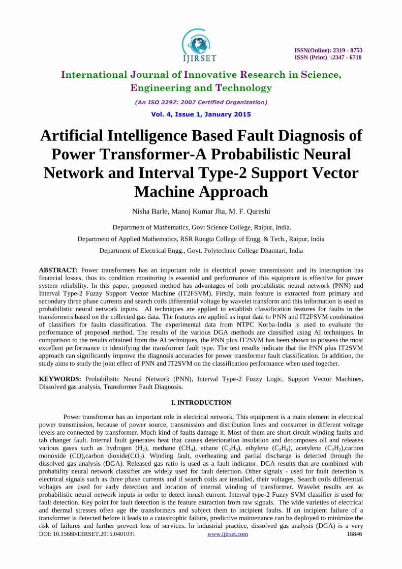
The probabilistic Neural Network used in this paper is shown in Fig.1. The first (leftmost) layer contains one
input node for each input attribute in an application. All connections in the network have a weight of 1, which means
that the input vector is passed directly to each hidden node. In PNN, there is one hidden node for each training instance
i in the training set. Each hidden node hi has a center point yi associated with it, which is the input vector of instance i.
A hidden node also has a spread factor, si, which determines the size of its respective field. There are a variety of ways
to set this parameter. si is equal to the fraction f of the distance to the nearest neighbor of each instance i. The value of f
begins at 0.5 and a binary search is performed to fine tune this value. At each of five steps, the value of f that results in
the highest average confidence of classification is chosen (HongYu et al. 2010). A hidden node receives an input vector
x and outputs an activation given by the Gaussian function g, which returns a value of 1 if x and yi are equal and drops
to an insignificant value as the distance grows (HongYu et al. 2010):
𝑔 𝑥, 𝑦𝑖 , 𝑠𝑖 = exp(−𝐷2(𝑥, 𝑦𝑖)/2𝑠𝑖2)
The distance function D determines how far apart the two vectors are. By far the most common distance
function used in PNNs is Euclidean distance. However, in order to appropriately handle applications that have both
linear and nominal attributes, a heterogeneous distance function HVDM is used to normalize Euclidean distance for
linear attributes and the Value Difference Metric (VDM) for nominal attributes. It is defined as:
𝐻𝐷𝑉𝑀 𝑥, 𝑦 = 𝑑𝑎2
𝑚
𝑖=1
(𝑥𝑎 , 𝑦𝑎)
Where m is the number of attributes. The function da (x, y) returns a distance between the two values x and y
for attribute ‗a‘ and is defined as:
ISSN(Online): 2319 - 8753
ISSN (Print) :2347 - 6710
International Journal of Innovative Research in Science,
Engineering and Technology
(An ISO 3297: 2007 Certified Organization)
Vol. 4, Issue 1, January 2015
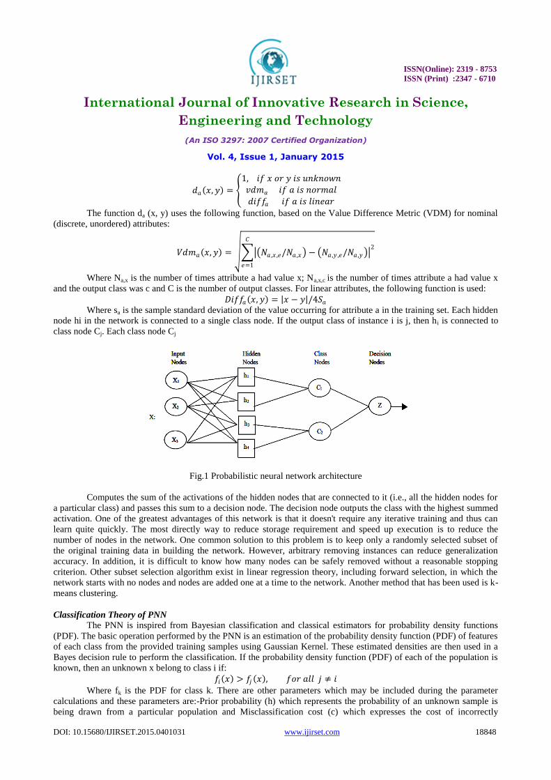
DOI: 10.15680/IJIRSET.2015.0401031 www.ijirset.com 18848
𝑑𝑎 𝑥, 𝑦 =
1, 𝑖𝑓 𝑥 𝑜𝑟 𝑦 𝑖𝑠 𝑢𝑛𝑘𝑛𝑜𝑤𝑛𝑣𝑑𝑚𝑎 𝑖𝑓 𝑎 𝑖𝑠 𝑛𝑜𝑟𝑚𝑎𝑙
𝑑𝑖𝑓𝑓𝑎 𝑖𝑓 𝑎 𝑖𝑠 𝑙𝑖𝑛𝑒𝑎𝑟
The function da (x, y) uses the following function, based on the Value Difference Metric (VDM) for nominal
(discrete, unordered) attributes:
𝑉𝑑𝑚𝑎 𝑥, 𝑦 = 𝑁𝑎 ,𝑥 ,𝑒/𝑁𝑎 ,𝑥 − 𝑁𝑎 ,𝑦 ,𝑒/𝑁𝑎 ,𝑦 2
𝐶
𝑒=1
Where Na,x is the number of times attribute a had value x; Na,x,c is the number of times attribute a had value x
and the output class was c and C is the number of output classes. For linear attributes, the following function is used:
𝐷𝑖𝑓𝑓𝑎 𝑥, 𝑦 = 𝑥 − 𝑦 /4𝑆𝑎
Where sa is the sample standard deviation of the value occurring for attribute a in the training set. Each hidden
node hi in the network is connected to a single class node. If the output class of instance i is j, then hi is connected to
class node Cj. Each class node Cj
Fig.1 Probabilistic neural network architecture
Computes the sum of the activations of the hidden nodes that are connected to it (i.e., all the hidden nodes for
a particular class) and passes this sum to a decision node. The decision node outputs the class with the highest summed
activation. One of the greatest advantages of this network is that it doesn't require any iterative training and thus can
learn quite quickly. The most directly way to reduce storage requirement and speed up execution is to reduce the
number of nodes in the network. One common solution to this problem is to keep only a randomly selected subset of
the original training data in building the network. However, arbitrary removing instances can reduce generalization
accuracy. In addition, it is difficult to know how many nodes can be safely removed without a reasonable stopping
criterion. Other subset selection algorithm exist in linear regression theory, including forward selection, in which the
network starts with no nodes and nodes are added one at a time to the network. Another method that has been used is k-
means clustering.
Classification Theory of PNN
The PNN is inspired from Bayesian classification and classical estimators for probability density functions
(PDF). The basic operation performed by the PNN is an estimation of the probability density function (PDF) of features
of each class from the provided training samples using Gaussian Kernel. These estimated densities are then used in a
Bayes decision rule to perform the classification. If the probability density function (PDF) of each of the population is
known, then an unknown x belong to class i if:
𝑓𝑖 𝑥 > 𝑓𝑗 𝑥 , 𝑓𝑜𝑟 𝑎𝑙𝑙 𝑗 ≠ 𝑖
Where fk is the PDF for class k. There are other parameters which may be included during the parameter
calculations and these parameters are:-Prior probability (h) which represents the probability of an unknown sample is
being drawn from a particular population and Misclassification cost (c) which expresses the cost of incorrectly

ISSN(Online): 2319 - 8753
ISSN (Print) :2347 - 6710
International Journal of Innovative Research in Science,
Engineering and Technology
(An ISO 3297: 2007 Certified Organization)
Vol. 4, Issue 1, January 2015
DOI: 10.15680/IJIRSET.2015.0401031 www.ijirset.com 18849
classifying an unknown. According to the above definition of the PDF and the other parameters that should be
included, the classification decision becomes:-
𝑖𝑐𝑖𝑓𝑖 > 𝑗 𝑐𝑗𝑓𝑗 , 𝑓𝑜𝑟 𝑎𝑙𝑙 𝑗 ≠ 𝑖
This is defined as Bayes optimal decision rule. Estimating the PDF is done using the samples of the
populations (the training set), accordingly: PDF for a single sample (in a population) is calculated from the following
formula:
1/𝑠𝑊 𝑥 − 𝑥𝑘 /𝑠 Where: x: unknown (input), xk: k
th sample, W: weighting function and s: smoothing parameter. So, the PDF
for a single population is calculated from the following formula which is known as Parzen's PDF estimator:
1/𝑛𝜎 𝑤 𝑥 − 𝑥𝑘/𝜎
𝑛
𝑘=1
Which is exactly expresses the average of the PDF‘s for the ―n‖ samples in the population. The estimated PDF
approaches the true PDF as training set size increases as long as the true PDF is smooth. With regards to the weighting
function, we see that it provides a sphere of influence since there is:-large values of small distances between the
unknown and the training samples and it rapidly decreases to zero as the distance increases. The weighting function
commonly use Gaussian function since it behaves well and easily computed and also it isn't related to any assumption
about a normal distribution. When the weighting function use Gaussian function, the estimated PDF is given by:
𝑔 𝑥 = 1/𝑛𝜎 𝑒𝑥𝑝 − 𝑥 − 𝑥𝑘 2/𝜎2
𝑛
𝑘=1
In case of inputting the network a vector, here the PDF for a single sample (in a population) will be given by
the following formula:
1/ 2 𝑝/2
𝑠𝑝𝑒𝑥𝑝 − 𝑥 − 𝑥𝑘 2/2𝑠2
Where x: unknown (input), xk : kth
sample, s : sampling parameter, p : length of vector And in that case of
inputting the network a vector, the PDF for a single population is expressed as:
𝑔 𝑥 = 1/ 2 𝑝/2
𝜎𝑝𝑛, 𝑒𝑥𝑝
𝑛𝑖
𝑘=1
− 𝑥 − 𝑥𝑘 2/2𝜎2
Which is the average of the PDF‘s for the ni samples in the ith
population. The classification criteria in this
case of multivariate input will be expressed as follows:
𝑔𝑖 𝑥 > 𝑔𝑗 𝑥 ,𝑓𝑜𝑟 𝑎𝑙𝑙 𝑗 ≠ 𝑖
𝑔𝑖 𝑥 = 1/𝑛𝑖 𝑒𝑥𝑝 − 𝑥 − 𝑥𝑘 2/2𝜎2
This eliminates common factors and absorbs the ‗2‘ into s.
III. INTERVAL TYPE-2 FUZZY SUPPORT VECTOR MACHINE (IT2SVM)
SVM is a powerful and promising machine learning tool, support vector machines (SVMs) employ Structural
Risk Minimization (SRM) principle to achieve better generalization ability than traditional machine learning
algorithms, such as decision trees and neural networks. SVM classification aims to construct an optimal separating
hyper plane in a higher transformed feature space by maximizing the margin between the separating hyper plane and
classification data. The transformation of feature spaces from input spaces can be made through kernel trick, which
allows every dot-product to be replaced simply by a kernel function. Kernel functions play an essential role in the SVM
classification since they determine feature spaces in which data examples are classified and can directly affect SVM
classification results and performances. A less time-consuming way is to randomly choose several SVMs with different
kernels and construct an ensemble model to combine the different SVM classifiers and generate a hybrid classifier.
This paper proposes an ensemble model to combine multiple SVM classifiers by applying the knowledge of interval
type-2 fuzzy logic system (IT2FLS). Interval type-2 fuzzy sets and IT2FLS can better handle uncertainties and
imprecision in classification data such as noise or outliers. Unlike type-1 FLS, MFs of type-2 fuzzy sets themselves are
fuzzy such that membership grades of type-2 fuzzy sets are fuzzy sets in [0, 1]. This basic characteristic of type-2 fuzzy

ISSN(Online): 2319 - 8753
ISSN (Print) :2347 - 6710
International Journal of Innovative Research in Science,
Engineering and Technology
(An ISO 3297: 2007 Certified Organization)
Vol. 4, Issue 1, January 2015
DOI: 10.15680/IJIRSET.2015.0401031 www.ijirset.com 18850
sets makes type-2 FLS especially useful to handle situations where shapes, positions or other parameters of MFs are
uncertain. The proposed interval type-2 fuzzy ensemble model takes consideration of the classification results of data
examples from different SVMs and generates outputs indicating whether data examples belong to positive or negative
class. For a binary classification problem, assume there is a training data set 𝑆: 𝑥𝑖 , 𝑦𝑖 𝑖=1𝑁 , where each input
m𝑥𝑖 ∈ 𝑅𝑚 and output 𝑦𝑖 ∈ ±1 . The goal of SVMs is to map the input vector x into a feature space 𝑍 = ∅(𝑥) and find
an optimal hyper plane w. z + b = 0 in the feature space to separate the training data into two classes with the maximum
margin,
Where, 𝐼𝑤 = 𝛼𝑖𝑦𝑖𝑧𝑖𝑁𝑖=1
αi is a set of Lagrange multipliers to the following dual problem (J. Mendel et al. 2000)
𝑀𝑎𝑥𝑖𝑚𝑖𝑧𝑒: 𝑤 𝛼 = 𝛼𝑖
𝑁
𝑖=1
−1
2 𝛼𝑖𝛼𝑗𝑦𝑖𝑦𝑗 𝑧𝑖 . 𝑧𝑗
𝑁
𝑖=𝑗=1
𝑆𝑢𝑏𝑗𝑒𝑐𝑡 𝑡𝑜:𝐶 ≥ 𝛼𝑖 ≥ 0, 𝛼𝑖𝑦𝑖
𝑁
𝑖=1
= 0.
Where C is a user-defined regularization parameter, determining the tradeoff between maximizing margin and
minimizing the number of misclassified data examples. It is useful to handle non-separable problems and outliers. The
kernel trick of SVMs allows us to substitute the dot product of data points in (1) with just a kernel function:
𝐾 𝑥𝑖 . 𝑥𝑗 = 𝑧𝑖 . 𝑧𝑗 .
The decision function is made by computing
𝑓 𝑥 = 𝑠𝑖𝑔𝑛 𝑤. 𝑧 + 𝑏 = 𝑠𝑖𝑔𝑛( 𝛼𝑖𝑦𝑖
𝑁
𝑖=1
𝐾 𝑥𝑖 . 𝑥 + 𝑏)
Where f(x) is the distance of a testing data x to the optimal hyper plane. If the distance is less than 0, the
testing data belongs to the negative class. Otherwise, it is in the positive class. Several kernel functions have been used
widely and successfully, such as, polynomial kernel with degree d,
𝐾 𝑥𝑖 . 𝑥𝑗 = 1 + 𝑥𝑖 . 𝑥𝑗 𝑑
Gaussian RBF kernel with tuning parameter σ,
𝐾 𝑥𝑖 . 𝑥𝑗 = 𝑒𝑥𝑝 − 𝑥𝑖 − 𝑥𝑗 2
/ 2𝜎2
and sigmoid kernel with parameter θ,
𝐾 𝑥𝑖 .𝑥𝑗 = tanh 𝑥𝑖 . 𝑥𝑗 − 𝜃 .
Type-2 Fuzzy Sets and Interval Type-2 FLS
A. Type-2 Fuzzy Sets
A type-2 fuzzy set, denoted by 𝐴 , is characterized by a type-2 MF 𝜇𝐴 𝑥,𝑢 , where xϵ X and uϵ J x [0,1] ,
and can be expressed as (T. Joachims 1999):
𝐴 = 𝜇𝐴 𝑢𝜀 𝐽𝑥 𝑥,𝑢 / 𝑥,𝑢
𝑥𝜀𝑋 , 𝐽𝑥 ⊆ 0,1
Where ∫ ∫ denotes union over all admissible x and u. Jx [0,1] is called primary membership of x. The union
of all primary memberships is defined as the footprint of uncertainty (FOU), bounded by the maximum and minimum
type-1 MF called upper MF 𝜇𝐴 (𝑥) and lower MF 𝜇𝐴 (𝑥). When the uncertainties of MFs disappear, type-2 fuzzy sets
reduce to type-1 fuzzy sets whose MFs can be precisely determined. Corresponding to each primary membership, there
is a secondary membership that defines the possibilities of the primary membership. General type-2 FLS is
computationally intensive. However, when secondary MFs are interval fuzzy sets, the computation of type-2 FLS can
be simplified a lot. Therefore, in the paper, we only consider interval type-2 fuzzy sets and FLS. The secondary
memberships of interval type-2 fuzzy sets are either zero or one (𝑓𝑥 𝑢 = 1,∀ 𝑢 𝜀 𝐽𝑥 ⊆ 0,1 ). They reflect a uniform
uncertainty at the primary memberships. A type-2 FLS, similar to a type-1 FLS, includes four components in general:
fuzzifier, fuzzy rule base, fuzzy inference engine, and output processor. One significant difference between type-1 and
type-2 FLS is that the output processor of type-2 FLS needs one additional step: type-reducer just before defuzzifier,

ISSN(Online): 2319 - 8753
ISSN (Print) :2347 - 6710
International Journal of Innovative Research in Science,
Engineering and Technology
(An ISO 3297: 2007 Certified Organization)
Vol. 4, Issue 1, January 2015
DOI: 10.15680/IJIRSET.2015.0401031 www.ijirset.com 18851
which is used to reduce type-2 output fuzzy sets to type-1 output fuzzy sets. After the type reduction, defuzzifier further
reduces type-1 output fuzzy sets into crisp values.
B. Fuzzy Inference of Interval Type-2 FLS
Fuzzy inference engine combines the fired fuzzy rules and maps crisp inputs into type-2 output fuzzy sets. In
our interval type-2 FLS, we use the meet operation under product t-norm, so the firing strength is an interval type-1 set:
𝑓𝑖 𝑥 = 𝑓 𝑖 𝑥 , 𝑓𝑖 𝑥
Where 𝑓𝑖 𝑥 and 𝑓𝑖 𝑥 can be written in (8b) and (8c), where * denotes the product operation:
𝑓𝑖 𝑥 = 𝜇𝐹 1𝑖 𝑥1 ∗ ……∗ 𝜇𝐹 𝑝𝑖 𝑥𝑝
𝑓𝑖 𝑥 = 𝜇𝐹 1𝑖
𝑥1 ∗ …… ∗ 𝜇𝐹 𝑝𝑖 𝑥𝑝
C. Type Reduction of Interval Type-2 FLS
The outputs from the inference engine are type-2 fuzzy sets which must be reduced to type-1 fuzzy sets before
defuzzifier can be applied to generate crisp outputs. In this study, center-of-sets type reducer is used since it requires
reasonable computational complexity comparing with expensive centroid type reducer. Center-of-sets type reducer can
be divided into two phases. The first phase is to calculate the centroids of all type-2 consequence fuzzy sets. The
second phase is to calculate the reduced fuzzy sets.
● Computing the Centroids of Rule Consequences:
Suppose the output of an interval type-2 FLS is represented by interval type-2 fuzzy sets𝐺 𝑡 , where t = 1, … T,
T is the number of output fuzzy sets. The centroid of ith
output fuzzy set 𝑦𝑡 = 𝑦𝑙𝑡 , 𝑦𝑟
𝑡 is a type-1 interval set with
leftmost point 𝑦𝑙𝑡 and rightmost point 𝑦𝑟
𝑡 respectively. Karnik-Mendel iterative algorithm is used to compute the
rightmost point 𝑦𝑟𝑡 for each of T type-2 output fuzzy sets, where Z is the number of discretised points for each output
fuzzy set, 𝐽𝑦𝑧 = 𝐿𝑧 ,𝑅𝑧 , 𝑧 = 𝐿𝑧 + 𝑅𝑧 /2 and ∆𝑧= 𝑅𝑧 + 𝐿𝑧 /2 , z = 1…..Z. Fig.2 shows how to calculate hz , Lz ,
Rz and Δz needed by the algorithm. The leftmost point 𝑦𝑙𝑡 can be calculated in the similar way, set 𝜃𝑧 = 𝑧 + ∆𝑧 for z
≤ e and 𝜃𝑧 = 𝑧 − ∆𝑧 for z > e+1. It has been proved that this iterative procedure can converge in at most Z iterations
to find 𝑦𝑙𝑡or 𝑦𝑟
𝑡 .
●Computing Reduced Type-1 Fuzzy Sets: To compute a type-reduced set, it is sufficient to compute its upper and lower bounds yl and yr, which can be
expressed as follows:
𝑦𝑙 = 𝑓𝑙
𝑖𝑦𝑙𝑖𝑀
𝑖=1
𝑓𝑙𝑖𝑀
𝑖=1
, 𝑦𝑟 = 𝑓𝑟
𝑖𝑦𝑟𝑖𝑀
𝑖=1
𝑓𝑟𝑖𝑀
𝑖=1
where 𝑓𝑙𝑖 and 𝑦𝑙
𝑖 are the firing strength and the centroid of the output fuzzy set of ith
rule (i = 1, …, M)
associated with yl; 𝑓𝑟𝑖 and 𝑦𝑟
𝑖 are the firing strength and the centroid of the output fuzzy set of ith
rule (i = 1, …, M)
associated with yr. To compute yr, we use the iterative procedure, yl can be computed in the similar way by setting
𝑓𝑟𝑖 = 𝑓
𝑖for i ≤ R and 𝑓𝑟
𝑖 = 𝑓 𝑖for i > R. The iterative procedure is proved to converge in no more than M iterations to
compute yr and yl respectively.
Fig.2 Calculation of the parameters needed by each yz.

ISSN(Online): 2319 - 8753
ISSN (Print) :2347 - 6710
International Journal of Innovative Research in Science,
Engineering and Technology
(An ISO 3297: 2007 Certified Organization)
Vol. 4, Issue 1, January 2015
DOI: 10.15680/IJIRSET.2015.0401031 www.ijirset.com 18852
D. Defuzzification
The final output of type-2 FLS is set to the average of yr and yl:
IV. PROBABILISTIC NEURAL NETWORK PLUS INTERVAL TYPE-2 FUZZY SVM FUSION MODEL
A Probabilistic Neural Network plus Interval Type-2 Fuzzy SVM Fusion Model as shown in Fig.3 is
constructed to combine classification results from multiple IT2SVMs. The system can be divided into two phases. In
Phase I, different SVMs are trained and classified to obtain individual SVM accuracies,
Fig.3 PNN plus Interval Type-2 fuzzy SVM fusion system.
and distances of data examples to SVM hyper planes. In Phase II, an interval type-2 FLS is constructed to combine
classification results from multiple SVM classifiers. The type-2 FLS takes SVM accuracies and distances of data
examples in Phase I as the system inputs and produces outputs to indicate whether data examples belong to positive or
negative class. To explain the FLS in detail, in the following sections, we will take three IT2SVM classifiers as an
example to demonstrate how to combine SVM classifiers using the type-2 FLS. This process can be easily extended to
combine arbitrary number of SVM classifiers in general.
A. Input and Output Interval Type-2 Fuzzy MFs
The interval type-2 FLS has three accuracy inputs (one for each SVM classifier), three distance inputs (one
from each SVM) and one output. All the inputs and the output are defined as interval type-2 fuzzy sets as shown in
Fig.4. Each accuracy input is represented by two fuzzy sets: high and low, and each distance input is described by two
fuzzy sets: positive and negative. The output is represented by seven fuzzy sets. The domain of the accuracy MFs is set
to between the minimum and maximum accuracies.
a. b. c.
Fig.4. Input and output interval type-2 fuzzy MFs. (a). Accuracy,(b). Distance,(c). Output

ISSN(Online): 2319 - 8753
ISSN (Print) :2347 - 6710
International Journal of Innovative Research in Science,
Engineering and Technology
(An ISO 3297: 2007 Certified Organization)
Vol. 4, Issue 1, January 2015
DOI: 10.15680/IJIRSET.2015.0401031 www.ijirset.com 18853
The admissible ranges of the interval type-2 MFs for accuracy inputs are set to around 2%. Considering the
SVM classification results, the domain of negative distance MF is set to between the minimum distance and 0.5 and the
domain of positive distance MF is set to between -0.5 and the maximum distance. The admissible ranges of the interval
type-2 MFs for distance inputs are set to 0.1~0.3. The admissible range of the type-2 MFs for the output is set to around
0.1.
B. Fuzzy Rule Base
Since the system has six inputs in total and each input contains two fuzzy sets, there are 2 ^ 6 = 64 fuzzy rules.
The ith rule is defined as follows (i = 1...64):
𝐼𝐹 𝑎1 𝑖𝑠 𝐴 1𝑖 𝑎𝑛𝑑 𝑎2 𝑖𝑠 𝐴 2
𝑖 𝑎𝑛𝑑 𝑎3 𝑖𝑠 𝐴 3𝑖 𝑎𝑛𝑑 𝑑1 𝑖𝑠 𝐷 1
𝑖 𝑎𝑛𝑑 𝑑2 𝑖𝑠 𝐷 2𝑖𝑎𝑛𝑑 𝑑3 𝑖𝑠 𝐷 3
𝑖 .𝑇𝐻𝐸𝑁 𝑔𝑖 𝑖𝑠 𝑂 𝑖
Where𝐴 1𝑖 , 𝐴 2
𝑖 and 𝐴 3𝑖 in {low, high}, 𝐷 1
𝑖 , 𝐷 2𝑖 and 𝐷 3
𝑖 in {negative, positive},and 𝑂 𝑖 in 𝑂 1 ,… . ,𝑂 7 . We assign one of the seven output fuzzy sets to the consequence of each fuzzy rule by considering both the
accuracy and distance information of three SVMs. For example, if all the accuracies of three SVM are high and they all
classify one data example in positive class; the consequence of the corresponding rule is set to 𝑂 7 , indicating the data
example is more likely in the positive class. On the other hand, if all three accuracies are high and all three distances
are negative, the consequence of that rule is set to 𝑂 1 , indicating the data example is more likely in the negative class.
C. Fuzzy Inference and Output Processing
In the inference engine of the type-2 fuzzy SVM fusion model, we use the meet under the product t-norm and
the join under the maximum operation and the extended sup-star composition. Center-of-sets type-reducer (Karnik-
Mendel iterative procedure) is used to reduce the type-2 output fuzzy sets into the type-1 sets. The discrete level is set
to 50 points (Z = 50). After the type-reduction, the reduced type-1 fuzzy sets will be defuzzified to produce a crisp
value in [-1, 1]. If the crisp output is less than zero, we consider the data example is in the negative class. Otherwise, it
belongs to the positive class.
V. SIMULATION OF TRANSFORMERS FAULTS CLASSIFICATION
Transformer Fault Types: IEC Publication 60599 provides a coded list of faults detectable by dissolved gas
analysis (DGA):
• Partial discharge (PD): PD occurs in the gas phase of voids or gas bubbles. It is usually easily detectable by DGA,
however, because it is produced over very long periods of time and within large volumes of paper insulation. It often
generates large amounts of hydrogen.
• Low energy discharge (D1): D1 such as tracking, small arcs, and uninterrupted sparking discharges are usually easily
detectable by DGA, because gas formation is large enough.
• High energy discharge (D2): D2 is evidenced by extensive carbonization, metal fusion and possible tripping of the
equipment.
• Thermal faults T <300 ° C (T1): T1 evidenced by paper turned brownish.
• Thermal faults 300 <T< 700 ºC (T2): T2 evidenced when paper carbonizes.
• Thermal faults T > 700 ºC (T3): T3 evidenced by oil carbonization, metal coloration or fusion.
Diagnosis and Interpretation Methods:
The DGA methods have been widely used by the utilities to interpret the dissolved gas. According to the
pattern of the gases composition, their types and quantities, the interpretation approaches below for dissolved gas are
extensively followed: Key gas method; Ratios method; The graphical representation method. In this key gas method,
we need five key gas concentrations H2, CH4, C2H2, C2H4 and C2H6 available for consistent interpretation of the fault.
Table 1 shows the diagnostic interpretations applying various key gas concentrations. The results are mainly adjectives
and provide a basis for further investigation.

ISSN(Online): 2319 - 8753
ISSN (Print) :2347 - 6710
International Journal of Innovative Research in Science,
Engineering and Technology
(An ISO 3297: 2007 Certified Organization)
Vol. 4, Issue 1, January 2015
DOI: 10.15680/IJIRSET.2015.0401031 www.ijirset.com 18854
Table1. Interpretation gas dissolved in the oil Table.2. Concentration typical values
observed in transformers
The ppm concentration typical values range observed in power transformers according to IEC 60599 are given
in Table 2. In Ratios method, we employ the relationships between gas contents. The key gas ppm values are used in
these methods to generate the ratios between them. The IEC method uses gas ratios that are combinations of key-gas
ratios C2H2/C2H4, CH4/H2 and C2H4/C2H6. Table 3 shows the IEC standard for interpreting fault types and gives the
values for the three key-gas ratios corresponding to the suggested fault diagnosis. When key-gas ratios exceed specific
limits, incipient faults can be expected in the transformer. The graphical representation method is used to visualize the
different cases and facilitate their comparison. The coordinates and limits of the discharge and thermal fault zones of
the Triangle are indicated in Fig.5. Zone DT in Fig.5 corresponds to mixtures of thermal and electrical faults. The
Triangle coordinates corresponding to DGA results in ppm can be calculated as follows: % C2H2 = 100 x / (x + y + z),
% C2H4 = 100y / (x + y + z) and % CH4=100z / (x + y + z), where x = (C2H2), y = (C2H4) and z = (CH4). You can
translate the previous figure in a painting that gives the limits of each fault which are summarized in Table 4.
Training and Testing Data This study employs dissolved gas content data in power transformer oil from chemistry laboratory of the
NTPC Korba-India and Gas (STEG). The data is divided into two data sets: the training data sets (97 samples) and the
testing data sets (35 samples). The extracted DGA data contain not only the five concentrations of key gas, three
relatives‘ percentages and three ratios but also the diagnosis results from on-site inspections. The training data sets have
been evaluated using various methods DGA and the corresponding judgments related to seven classes have been
provided: normal unit (51 samples), Partial Discharge (3 samples), low energy discharge (5 samples), high energy
discharge (19 samples), low temperature overheating (7 samples), middle temperature overheating (11 samples) and
high temperature overheating (18 samples).
Table.3. Diagnosis using the ratio method (IEC 599)
Fig.5 Coordinates and fault zones of the Triangle

ISSN(Online): 2319 - 8753
ISSN (Print) :2347 - 6710
International Journal of Innovative Research in Science,
Engineering and Technology
(An ISO 3297: 2007 Certified Organization)
Vol. 4, Issue 1, January 2015
DOI: 10.15680/IJIRSET.2015.0401031 www.ijirset.com 18855
Table 4. Graphical representation method zone limits
Classification by Interval Type-2 Fuzzy Logic For The fuzzy logic faults classification is performed using several DGA methods as gas signature.
Fuzzy key gas: Firstly, we will classify the faults using key gas as input data with: •5 linguistic variables are the 5 gas:
H2, CH4, C2H2, C2H4 and C2H6; •3 linguistic values: small, medium and high; •5 sets of reference: U = [0, 650] for
H2, U = [0, 550] for CH4, U = [0, 450] for C2H2, U = [0, 750] for C2H4 and U = [0, 370] for C2H6; •7 outputs, the
reference sets are : U = [0, 1] for the non-fault, U = [0, 2] for the PD, U = [1, 3] for the D1, U = [2, 5] for the D2, U =
[3, 6] pour for the T1, U = [4, 7] for the T2 and U = [5, 8] for the T3 ; •3 membership functions: triangular, trapezoidal
and Gaussian; •35 = 251 fuzzy rules; •Defuzzification by the centroid method.
Classification by SVM As shown in Fig.6, the diagnostic model includes six IT2FSVM classifiers which are used to identify the
seven states: normal state and the six faults (PD, D1, D2, T1, T2 and T3). With all the training samples of the states,
IT2FSVM1 is trained to separate the normal state from the fault state. When input of IT2FSVM1 is a sample
representing the normal state, output of IT2FSVM1 is set to +1; otherwise -1. With the samples of single fault,
IT2FSVM2 is trained to separate the discharge fault from the overheating fault. When the input of IT2FSVM2 is a
sample representing discharge fault, the output of IT2FSVM2 is set to +1; otherwise-1. With the samples of discharge
fault, IT2FSVM3 is trained to separate the high-energy discharge (D2) fault from the partial discharge (PD) and low
energy discharge (D1) fault. When the input of IT2FSVM3 is a sample representing the D2 fault, the output of
IT2FSVM3 is set to +1; otherwise -1. With the samples of overheating fault, IT2FSVM4 is trained to separate the high
temperature overheating (T3) fault from the low and middle
Fig.6 Diagnostic model of power transformer based on IT2FSVM classifier

ISSN(Online): 2319 - 8753
ISSN (Print) :2347 - 6710
International Journal of Innovative Research in Science,
Engineering and Technology
(An ISO 3297: 2007 Certified Organization)
Vol. 4, Issue 1, January 2015
DOI: 10.15680/IJIRSET.2015.0401031 www.ijirset.com 18856
Temperature overheating (T1 and T2) fault. When the input of IT2FSVM4 is a sample representing the T3 fault, the
output of IT2FSVM5 is set to +1; otherwise -1. IT2FSVM5 is trained to separate the middle temperature overheating
(T2) fault from the low temperature overheating (T1) fault. When the input of IT2FSVM5 is a sample representing the
T2 fault, the output of IT2FSVM5 is set to +1; otherwise -1. IT2FSVM6 is trained to separate the partial discharge
(PD) fault from the low energy discharge (D1) fault. When the input of IT2FSVM6 is a sample representing the D1
fault, the output of IT2FSVM6 is set to +1; otherwise -1.
The PNN provides a general solution to pattern classification problems based on Bayesian theory. It is chosen
because of its ability to classify a new sample with the maximum probability of success given a large training set using
prior knowledge. The PNN combines the simplicity, speed and transparency of traditional statistical classification
models and the computational power and flexibility of back-propagated neural networks. On the other hand, IT2FSVM
are expressed in the form of a hyper plane that discriminates between positive and negative instances. This is achieved
by maximizing the distance between the two classes (positive and negative instances) and the hyper-plane. The
IT2FSVM are applied in this study since they can avoid local minima and have superior generalization capability.
VI. SIMULATION RESULTS
The performance of key gas method is analyzed in terms false alarm rate and non-detection rate for triangular,
trapezoidal and Gaussian membership functions as shown in Table 5. According to the results, we find that the
triangular membership function is more efficient for system fault diagnosis, but this method does not give excellent
results. So, we must propose an alternative method. All the six IT2FSVMs adopt polynomial and Gaussian as their
kernel function. In IT2FSVM, the parameters σ and C of IT2FSVM model are optimized by the cross validation
method. The adjusted parameters with maximal classification accuracy are selected as the most appropriate parameters.
Then, the optimal parameters are utilized to train the IT2FSVM model. So the output codification is presented in Table
6.
Firstly, we will classify the faults by SVM with the polynomial kernel. To select more efficient kernel between
the two cores used (polynomial and Gaussian), we compare the false alarm rate and non-detection rate given in Table 7.
The results in Table 7 show that the Gaussian kernel gives the best performance for the test. This is aided by a proper
choice of the kernel parameter σ by the cross validation method, because this parameter determines the hyper sphere
radius which encloses the data in multidimensional space. So, for comparison with other classification techniques, we
adopt the SVM with Gaussian kernel SVM as the most efficient.
Table.5.The key gas method classification
performance Table 6. Codification output of SVM
Table.7. False alarm and non-detection rates of SVM for different kernels

ISSN(Online): 2319 - 8753
ISSN (Print) :2347 - 6710
International Journal of Innovative Research in Science,
Engineering and Technology
(An ISO 3297: 2007 Certified Organization)
Vol. 4, Issue 1, January 2015
DOI: 10.15680/IJIRSET.2015.0401031 www.ijirset.com 18857
VII. CONCLUSION
In this paper, the artificial intelligence techniques are implemented for the faults classification using the
dissolved gas analysis for power transformers. The DGA methods studied are key gas, graphical representation and
ratios method. The fault diagnosis models performance was analyzed with interval type-2 fuzzy logic (using Gaussian,
trapezoidal and triangular membership functions), probabilistic neural network (PNN) and Support Vector Machine
(with polynomial and Gaussian kernel functions). The real data sets are used to investigate the performance of the DGA
methods in power transformer oil. In this paper, we propose an interval type-2 SVM fusion model to combine multiple
individual SVM classifiers. The experimental results show that interval type-2 FLS is a suitable and feasible way to
implement ensemble approaches in terms of performance and computational complexity. The proposed type-2 SVM
fusion system demonstrates more stable and more robust generalization ability than individual SVMs. The
experimental results show that the interval type-2 fuzzy logic classifier with triangular membership presents the best
result in comparison with the other two membership functions. The classification accuracies of PNN are superior to
RBF, MLP NN and the SVM with Gaussian kernel function has more excellent diagnostic performance than the SVM
with polynomial kernel function. According to test results, it is found that the ratios method is more suitable as a gas
signature. The IT2SVM with the Gaussian kernel function has a better performance than the other AI methods in
diagnosis accuracy. The proposed method can be applied to online diagnosis of incipient faults in transformers.
Proposed approach for fault classification is presented. IT2SVM combined with PNN has a good efficiency in
transformer fault classification.
REFERENCES
1. HongYu & Jie Wei & Jin Li (2010) ―Transformer Fault Diagnosis Based on Improved Artificial Fish Swarm Optimization Algorithm and BP
Network‖ 2nd International Conference on Industrial Mechatronics and Automation , 99 - 104, Wuhan, China, 30-31 May 2010
2. KeMeng, Zhao Yang Dong , Dian Hui Wang and Kit Po Wong, (Aug. 2010) ―A Self-Adaptive RBF Neural Network Classifier for Transformer Fault Analysis‖ IEEE Transactions on Power Systems delivery ,Vol. 25, No.3, pp. 1350 - 1360.
3. Sy-Ruen Huang, Member, IEEE, Hong-Tai Chen, Student Member, IEEE, Chueh-Cheng Wu, Chau-Yu Guan, and Chiang Cheng (April 2012)
―Distinguishing Internal Winding Faults From Inrush Power Transformers Using Jiles- Atherton Model Parameters Based on Correlation Coefficient‖ IEEE Transactions on Power Systems Delivery, Vol. 27, No. 2, pp. 548 - 553.
4. J. Mendel and R. John (2002) ―Type-2 fuzzy sets made simple,‖ IEEE Transactions on Fuzzy Systems, Vol.10, No.2, pp. 117–127.
5. Q. Liang and J. Mendel (2000) ―Interval type-2 fuzzy logic systems: Theory and design,‖ IEEE Transactions on Fuzzy Systems, Vol. 8, No.5, pp. 535–550.
6. A. Shintemirov, W. Tang and Q.H. Wu, (January 2009) "Power Transformer Fault Classification Based on Dissolved Gas Analysis by
Implementing Bootstrap and Genetic Programming", IEEE transactions on systems, man, and cybernetics—part c: applications and reviews, Vol. 39, No. 1, pp. 69-79.
7. W.H. Tang, J.Y. Goulermas, Q.H.Wu, Z.J. Richardson, and J. Fitch, (April 2008) ―A Probabilistic Classifier for Transformer Dissolved Gas
Analysis With a Particle Swarm Optimizer‖, IEEE transactions on power delivery, Vol. 23, No. 2, pp. 751-759. 8. Chin-Pao Hung, Mang-Hui Wang, (2004) ―Diagnosis of incipient faults in power transformers using CMAC neural network approach‖, Electric
Power Systems Research 71, 235–244.
9. Michel Duval, (June 2002) ―A Review of Faults Detectable by Gas-in-Oil Analysis in Transformers‖. IEEE Electrical Insulation Magazine, Vol.18, No. 3, 8-17.
10. R. Naresh, Veena Sharma and Manisha Vashisth, (October 2008) ―An Integrated Neural Fuzzy Approach for Fault Diagnosis of Transformers‖,
IEEE transactions on power delivery, Vol. 23, No. 4, pp.2017-2024. 11. V. Miranda, A. Rosa Garcez Castro, (October 2005) ―Improving the IEC Table for Transformer Failure Diagnosis With Knowledge Extraction
From Neural Networks‖, IEEE transactions on power delivery, Vol. 20, No. 4, pp. 2509- 2516.
12. Hong-Tzer Yang, Chiung-Chou Liao, (October 1999) ―Adaptive Fuzzy Diagnosis System for Dissolved Gas Analysis of Power Transformers‖,
IEEE Transactions on Power Delivery, Vol.14, No.4, pp. 1342-1350.
13. Mang-Hui Wang, (January 2003) ―A Novel Extension Method for Transformer Fault Diagnosis‖, IEEE transactions on power delivery, Vol.18,
No.1, pp. 164-169.