Artificial IntelligenceArtificial Intelligence

Universitatea Politehnica Bucuresti2008-2009

Adina Magda Florea

http://turing.cs.pub.ro/aifils_08

Lecture no. 7

Uncertain knowledge and reasoning Probability theory Bayesian networks Certainty factors

2

1. Probability theory

1.1 Uncertain knowledgep symptom(p, Toothache) disease(p,cavity)p sympt(p,Toothache)

disease(p,cavity) disease(p,gum_disease) … PL- laziness- theoretical ignorance- practical ignorance Probability theory degree of belief or plausibility

of a statement – a numerical measure in [0,1] Degree of truth – fuzzy logic degree of belief

3

1.2 Definitions

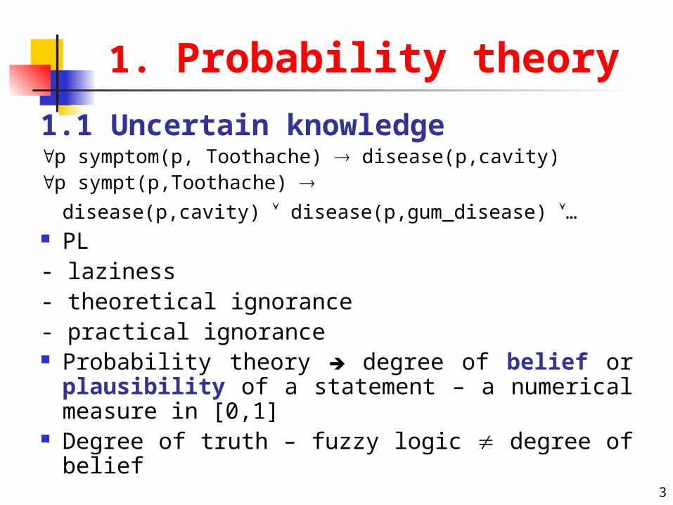
Unconditional or prior probability of A – the degree of belief in A in the absence of any other information – P(A)

A – random variable Probability distribution – P(A), P(A,B)Example

P(Weather = Sunny) = 0.1P(Weather = Rain) = 0.7P(Weather = Snow) = 0.2

Weather – random variable P(Weather) = (0.1, 0.7, 0.2) – probability dsitribution Conditional probability – posterior – once the agent has

obtained some evidence B for A - P(A|B) P(Cavity | Toothache) = 0.8

4

Definitions - cont

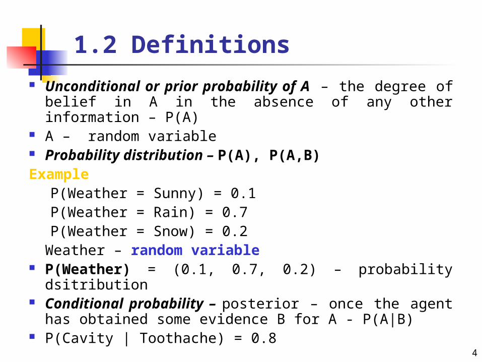
Axioms of probability The measure of the occurrence of an event

(random variable) A – a function P:S R satisfying the axioms:

0 P(A) 1 P(S) = 1 ( or P(true) = 1 and P(false) = 0) P(A B) = P(A) + P(B) - P(A B)

P(A ~A) = P(A)+P(~A) –P(false) = P(true)P(~A) = 1 – P(A)

5

Definitions - cont

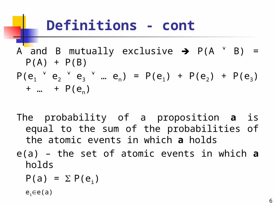
A and B mutually exclusive P(A B) = P(A) + P(B)

P(e1 e2 e3 … en) = P(e1) + P(e2) + P(e3) + … + P(en)

The probability of a proposition a is equal to the sum of the probabilities of the atomic events in which a holds

e(a) – the set of atomic events in which a holds

P(a) = P(ei)eie(a)

6

1.3 Product rule

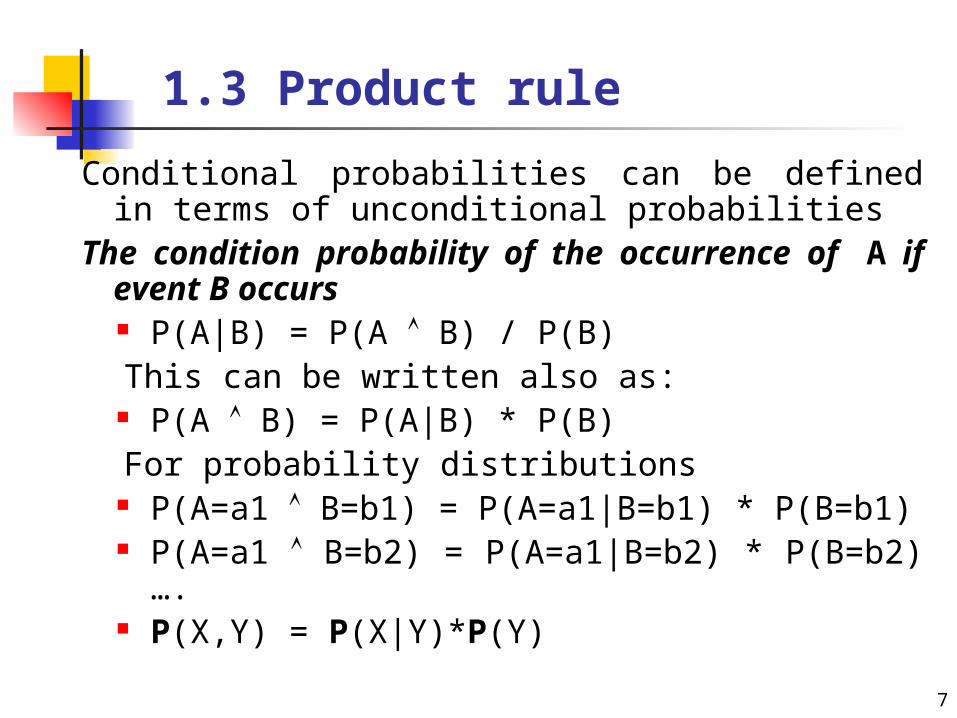
Conditional probabilities can be defined in terms of unconditional probabilities

The condition probability of the occurrence of A if event B occurs P(A|B) = P(A B) / P(B)This can be written also as: P(A B) = P(A|B) * P(B)For probability distributions P(A=a1 B=b1) = P(A=a1|B=b1) * P(B=b1) P(A=a1 B=b2) = P(A=a1|B=b2) * P(B=b2) …. P(X,Y) = P(X|Y)*P(Y)

7

1.4 Bayes’ rule and its use

P(A B) = P(A|B) *P(B)

P(A B) = P(B|A) *P(A)

Bays’ rule (theorem) P(B|A) = P(A | B) * P(B) / P(A)

P(B|A) = P(A | B) * P(B) / P(A)

Bayes Theorem

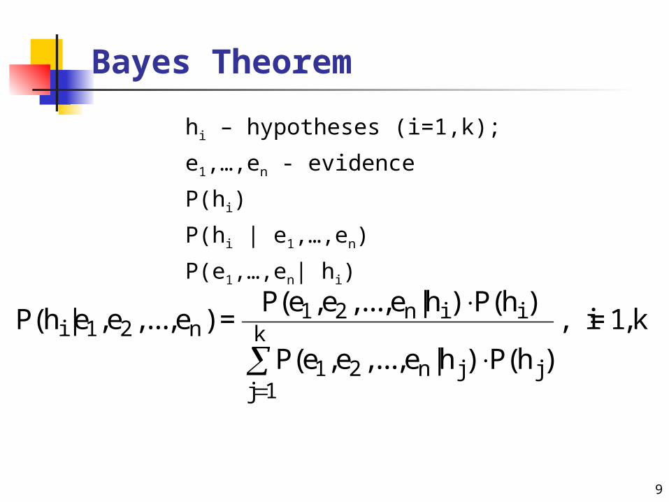
hi – hypotheses (i=1,k);

e1,…,en - evidence

P(hi)

P(hi | e1,…,en)

P(e1,…,en| hi)

9

P(h |e ,e ,...,e ) =P(e ,e ,...,e |h ) P(h )

P(e ,e ,...,e |h ) P(h )

, i = 1,ki 1 2 n1 2 n i i

1 2 n j jj 1

k

Bayes’ Theorem - cont

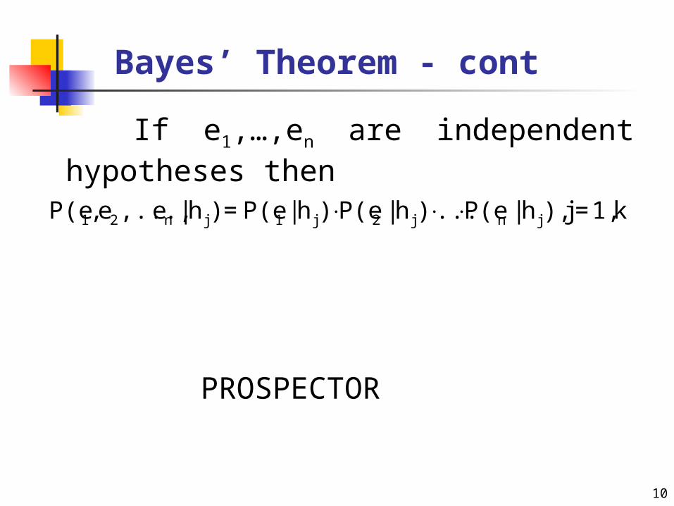
If e1,…,en are independent hypotheses then

PROSPECTOR

10

k1,=j ),h|P(e...)h|P(e)h|P(e=)h|e,...,e,P(e jnj2j1jn21

1.5 Inferences

Probability distribution P(Cavity, Tooth)

Tooth Tooth

Cavity 0.04 0.06

Cavity 0.01 0.89

P(Cavity) = 0.04 + 0.06 = 0.1

P(Cavity Tooth) = 0.04 + 0.01 + 0.06 = 0.11

P(Cavity | Tooth) = P(Cavity Tooth) / P(Tooth) = 0.04 / 0.05

11

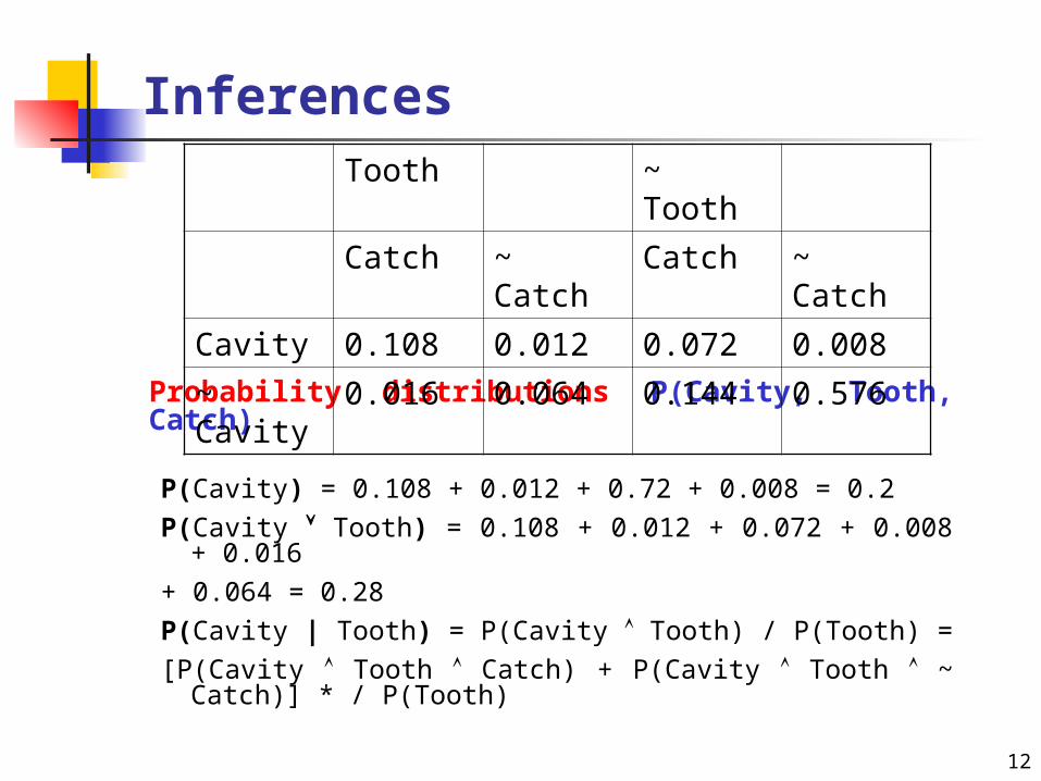
Inferences

Probability distributions P(Cavity, Tooth, Catch)

P(Cavity) = 0.108 + 0.012 + 0.72 + 0.008 = 0.2

P(Cavity Tooth) = 0.108 + 0.012 + 0.072 + 0.008 + 0.016

+ 0.064 = 0.28

P(Cavity | Tooth) = P(Cavity Tooth) / P(Tooth) =

[P(Cavity Tooth Catch) + P(Cavity Tooth ~ Catch)] * / P(Tooth)

12

Tooth ~ Tooth

Catch ~ Catch Catch ~ Catch

Cavity 0.108 0.012 0.072 0.008

~ Cavity 0.016 0.064 0.144 0.576

2 Bayesian networks

Represent dependencies among random variables Give a short specification of conditional probability

distribution Many random variables are conditionally independent Simplifies computations Graphical representation DAG – causal relationships among random variables Allows inferences based on the network structure

13

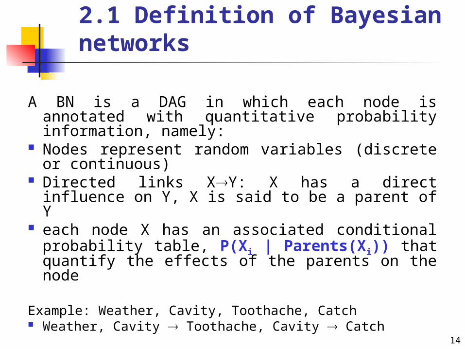
2.1 Definition of Bayesian networks

A BN is a DAG in which each node is annotated with quantitative probability information, namely:

Nodes represent random variables (discrete or continuous)

Directed links XY: X has a direct influence on Y, X is said to be a parent of Y

each node X has an associated conditional probability table, P(Xi | Parents(Xi)) that quantify the effects of the parents on the node

Example: Weather, Cavity, Toothache, Catch Weather, Cavity Toothache, Cavity Catch

14

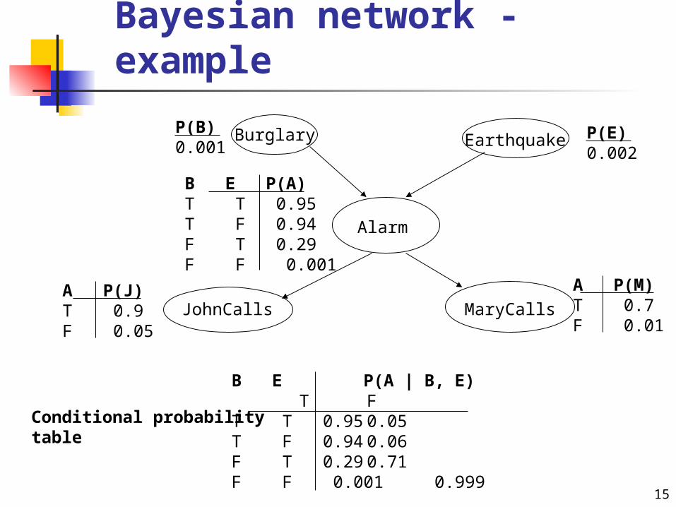
Bayesian network - example

15

Earthquake

Alarm

JohnCalls MaryCalls

BurglaryP(B)0.001

P(E)0.002

B E P(A)T T 0.95T F 0.94F T 0.29F F 0.001

A P(J)T 0.9F 0.05

A P(M)T 0.7F 0.01

B E P(A | B, E)T F

T T 0.95 0.05T F 0.94 0.06F T 0.29 0.71F F 0.001 0.999

Conditional probabilitytable

2.2 Bayesian network semantics

A) Represent a probability distribution

B) Specify conditional independence – build the network

A) each value of the probability distribution can be computed as:

P(X1=x1 … Xn=xn) = P(x1,…, xn) =

i=1,n P(xi | Parents(xi))

where Parents(xi) represent the specific values of Parents(Xi)

16

2.3 Building the network

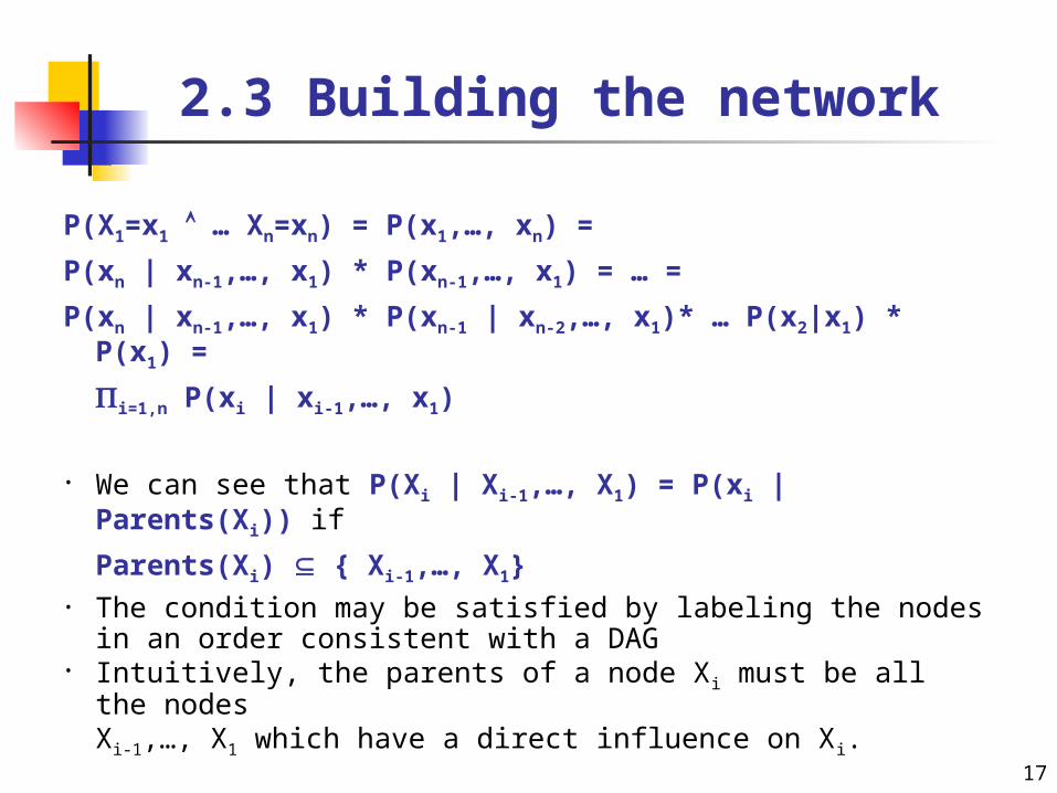
P(X1=x1 … Xn=xn) = P(x1,…, xn) =

P(xn | xn-1,…, x1) * P(xn-1,…, x1) = … =

P(xn | xn-1,…, x1) * P(xn-1 | xn-2,…, x1)* … P(x2|x1) * P(x1) =

i=1,n P(xi | xi-1,…, x1)

• We can see that P(Xi | Xi-1,…, X1) = P(xi | Parents(Xi)) if

Parents(Xi) { Xi-1,…, X1}• The condition may be satisfied by labeling the nodes in an

order consistent with a DAG• Intuitively, the parents of a node Xi must be all the nodes

Xi-1,…, X1 which have a direct influence on Xi.17

Building the network - cont

• Pick a set of random variables that describe the problem• Pick an ordering of those variables• while there are still variables repeat

(a) choose a variable Xi and add a node associated to Xi

(b) assign Parents(Xi) a minimal set of nodes that already exists in the network such that the conditional independence property is satisfied

(c) define the conditional probability table for Xi

• Because each node is linked only to previous nodes DAG• P(MaryCalls | JohnCals, Alarm, Burglary, Earthquake) =

P(MaryCalls | Alarm)18

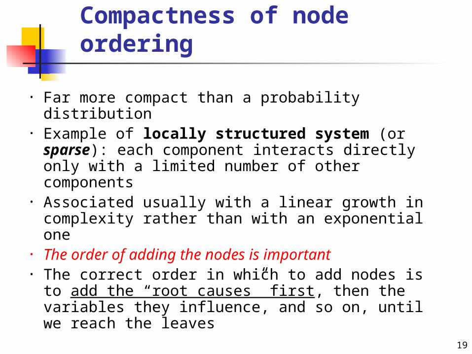
Compactness of node ordering

• Far more compact than a probability distribution• Example of locally structured system (or sparse):

each component interacts directly only with a limited number of other components

• Associated usually with a linear growth in complexity rather than with an exponential one

• The order of adding the nodes is important• The correct order in which to add nodes is to add the

“root causes” first, then the variables they influence, and so on, until we reach the leaves

19

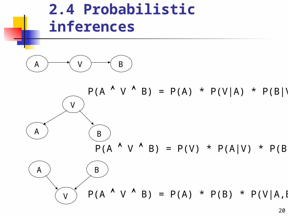
2.4 Probabilistic inferences

20

P(A V B) = P(A) * P(V|A) * P(B|V)V

A

B

B

V

A

A V B

P(A V B) = P(V) * P(A|V) * P(B|V)

P(A V B) = P(A) * P(B) * P(V|A,B)

Probabilistic inferences

21

Earthquake

Alarm

JohnCalls MaryCalls

BurglaryP(B)0.001

P(E)0.002

B E P(A)T T 0.95T F 0.94F T 0.29F F 0.001

A P(J)T 0.9F 0.05

A P(M)T 0.7F 0.01

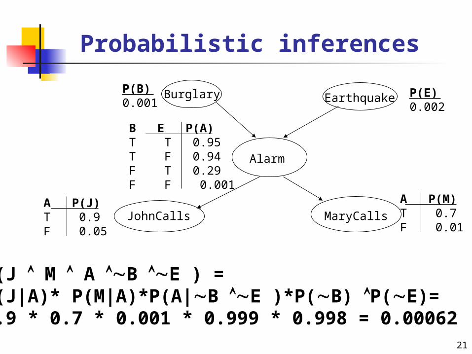
P(J M A B E ) =P(J|A)* P(M|A)*P(A|B E )*P(B) P(E)=0.9 * 0.7 * 0.001 * 0.999 * 0.998 = 0.00062

Probabilistic inferences

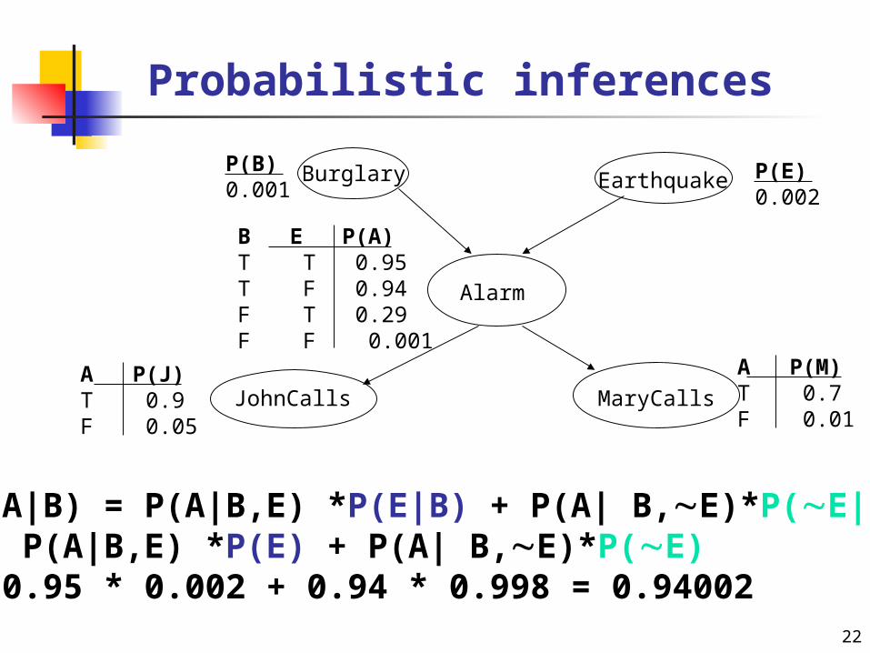
22

Earthquake

Alarm

JohnCalls MaryCalls

BurglaryP(B)0.001

P(E)0.002

B E P(A)T T 0.95T F 0.94F T 0.29F F 0.001

A P(J)T 0.9F 0.05

A P(M)T 0.7F 0.01

P(A|B) = P(A|B,E) *P(E|B) + P(A| B,E)*P(E|B)= P(A|B,E) *P(E) + P(A| B,E)*P(E)= 0.95 * 0.002 + 0.94 * 0.998 = 0.94002

2.5 Different types of inferences

23

Alarm

Intercausal inferences (between cause and common effects)P(Burglary | Alarm Earthquake)

Mixed inferencesP(Alarm | JohnCalls Earthquake) diag + causalP(Burglary | JohnCalls Earthquake) diag + intercausal

Diagnosis inferences (effect cause)P(Burglary | JohnCalls)

Causal inferences (cause effect) P(JohnCalls |Burglary),

P(MaryCalls | Burgalry)

Earthquake

JohnCalls MaryCalls

Burglary

3. Certainty factors

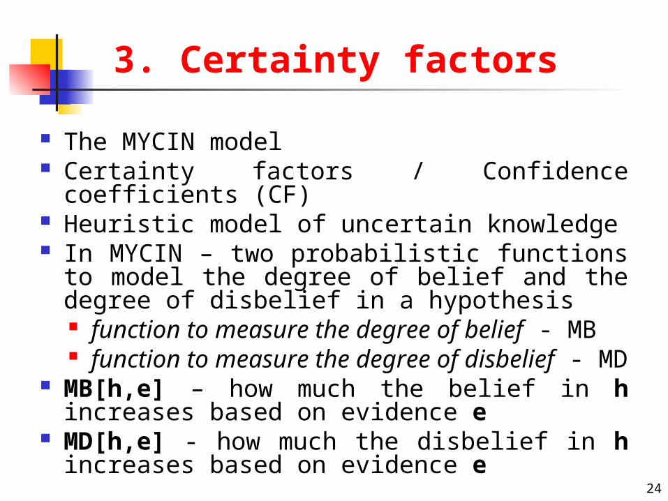
The MYCIN model Certainty factors / Confidence coefficients (CF) Heuristic model of uncertain knowledge In MYCIN – two probabilistic functions to model the

degree of belief and the degree of disbelief in a hypothesis function to measure the degree of belief - MB function to measure the degree of disbelief - MD

MB[h,e] – how much the belief in h increases based on evidence e

MD[h,e] - how much the disbelief in h increases based on evidence e

24

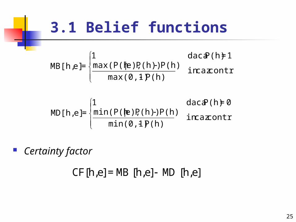
3.1 Belief functions

Certainty factor

25

contrar cazin P(h)max(0,1)

P(h)P(h))e),|max(P(h1=P(h) daca 1

=e]MB[h,

contrar cazin P(h)min(0,1)

P(h)P(h))e),|min(P(h0=P(h) daca 1

=e]MD[h,

CF[h,e] = MB[h,e] MD[h,e]

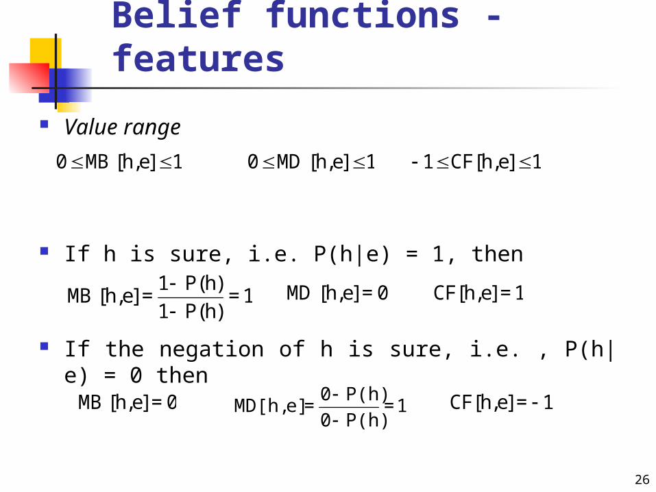
Belief functions - features

Value range

If h is sure, i.e. P(h|e) = 1, then

If the negation of h is sure, i.e. , P(h|e) = 0 then

26

0 MB[h,e] 1 0 MD[h,e] 1 1 CF[h,e] 1

MB[h,e] =1 P(h)

1 P(h)= 1

MD[h,e] = 0 CF[h,e] = 1

MB[h,e] = 0 1=P(h)0

P(h)0=e]MD[h,

CF[h,e] = 1

Example in MYCIN

if (1) the type of the organism is gram-positive, and (2) the morphology of the organism is coccus, and (3) the growth of the organism is chain then there is a strong evidence (0.7) that the identity of the

organism is streptococcus

Example of facts in MYCIN : (identity organism-1 pseudomonas 0.8) (identity organism-2 e.coli 0.15) (morphology organism-2 coccus 1.0)

27

3.2 Combining belief functions

28

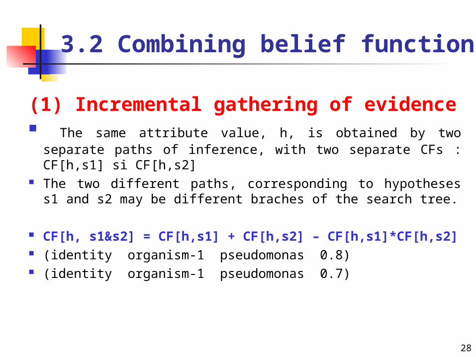
(1) Incremental gathering of evidence The same attribute value, h, is obtained by two separate paths of

inference, with two separate CFs : CF[h,s1] si CF[h,s2] The two different paths, corresponding to hypotheses s1 and s2

may be different braches of the search tree.

CF[h, s1&s2] = CF[h,s1] + CF[h,s2] – CF[h,s1]*CF[h,s2] (identity organism-1 pseudomonas 0.8) (identity organism-1 pseudomonas 0.7)

Combining belief functions

29

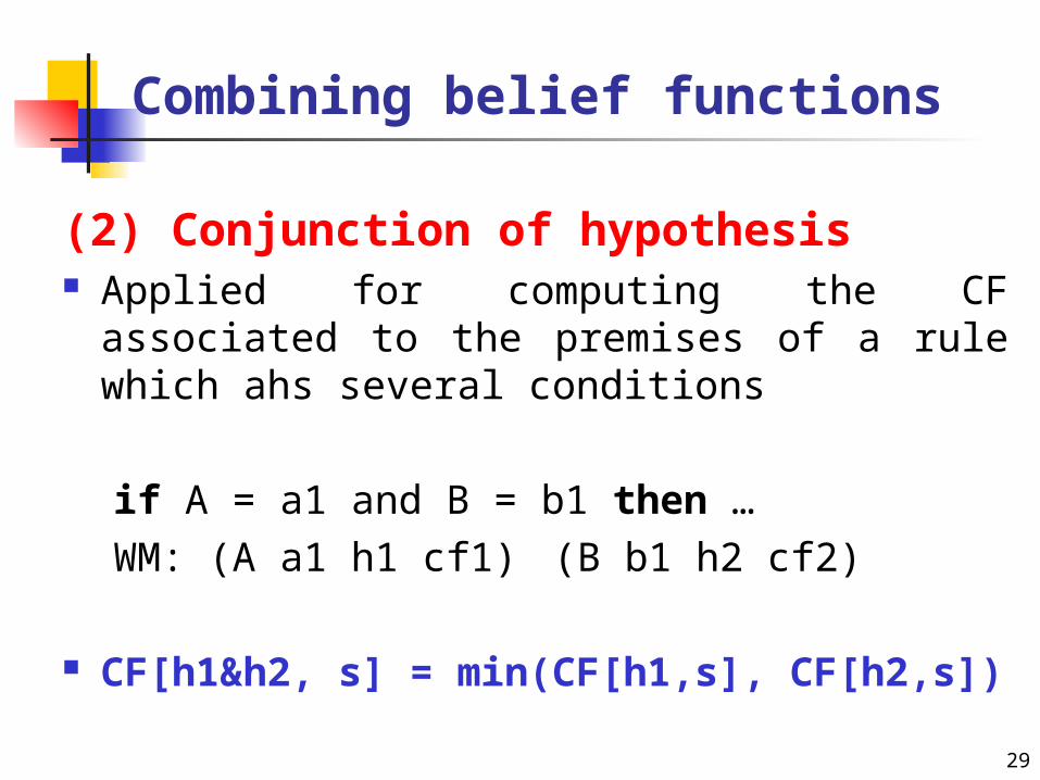
(2) Conjunction of hypothesis Applied for computing the CF associated to the

premises of a rule which ahs several conditions

if A = a1 and B = b1 then …

WM: (A a1 h1 cf1) (B b1 h2 cf2)

CF[h1&h2, s] = min(CF[h1,s], CF[h2,s])

Combining belief functions

30

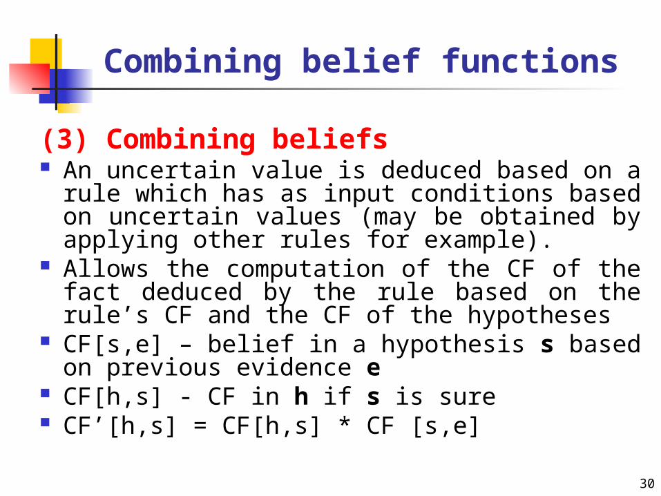
(3) Combining beliefs An uncertain value is deduced based on a rule which

has as input conditions based on uncertain values (may be obtained by applying other rules for example).

Allows the computation of the CF of the fact deduced by the rule based on the rule’s CF and the CF of the hypotheses

CF[s,e] – belief in a hypothesis s based on previous evidence e

CF[h,s] - CF in h if s is sure CF’[h,s] = CF[h,s] * CF [s,e]

Combining belief functions

31

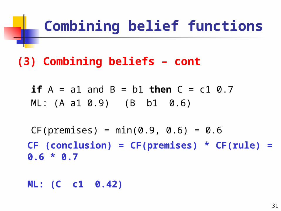
(3) Combining beliefs – cont

if A = a1 and B = b1 then C = c1 0.7

ML: (A a1 0.9) (B b1 0.6)

CF(premises) = min(0.9, 0.6) = 0.6

CF (conclusion) = CF(premises) * CF(rule) = 0.6 * 0.7

ML: (C c1 0.42)

3.3 Limits of CF

32

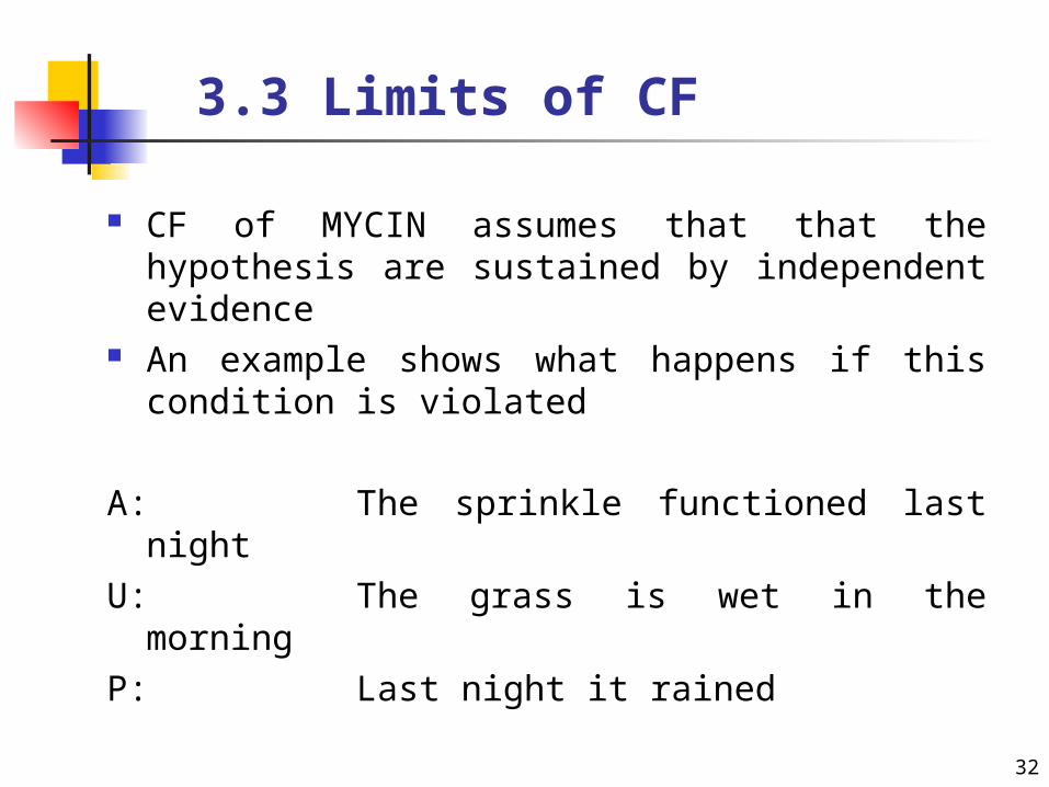
CF of MYCIN assumes that that the hypothesis are sustained by independent evidence

An example shows what happens if this condition is violated

A: The sprinkle functioned last night

U: The grass is wet in the morning

P: Last night it rained

33

R1:if the sprinkle functioned last nightthen there is a strong evidence (0.9) that the grass is wet in the

morningR2:if the grass is wet in the morning

then there is a strong evidence (0.8) that it rained last night CF[U,A] = 0.9 therefore the evidence sprinkle sustains the hypothesis wet grass with

CF = 0.9

CF[P,U] = 0.8 therefore the evidence wet grass sustains the hypothesis rain with CF

= 0.8

CF[P,A] = 0.8 * 0.9 = 0.72 therefore the evidence sprinkle sustains the hypothesis rain with CF =

0.72

Solutions