1

Electrical Engineering Department

Undergraduate Project #2 Final Report

Artificial Neural Networks

And Their Applications To Microwave Problems

Instructor Dr. Nihad Dib

Done by Hadi Matar 982024060 Mahmoud Al-Zu’bi 20000024080

2nd Sem. 2005

2

Table of Contents Abstract ………………………………………………………………………………..1 Chapter One: Introduction ………………………………………………………2 Chapter Two: General Background …..…………………………………….3 2.1 Definition…………………………………………………………………...3

2.2 General Architecture ...........................................................................…...4 2.3 Why ANN?....................................................................................................5 2.4 Implementation, Hardware vs. Software Simulations .......................6 2.5 The Neuron ………………………………………………………………...7 2.6 Learning and Generalization………………………………………….....9 2.7 Back Propagation Learning ………………………………………...….10 2.8 General Considerations ……………………………………………........13 2.9 Applications ……………………………………………………………...14 Chapter Three: Simulations and Applications.…………………..……....15 3.1 Matlab NN Toolbox …………………………………….........................15 3.2 Applications to Microwave Problems ……...………..………………20 Chapter Four: Conclusions.……………………………………….……………30 Appendix ‘1’………………………………………………………………………...32 Appendix ‘2’………………………………………………………………………...34 References……………………………………………………………………………36

3

Abstract

This project describes neural networks theory and addresses three

applications to microwave problems of two different structures; one is

analyzed only, while the other is analyzed and synthesized. Three CAD

models are proposed using the neural networks toolbox in the Matlab

software. The obtained results are in good agreement with those obtained

using conformal mapping technique (CMT).

4

Chapter One

Introduction

Humans have always been trying to imitate nature and God’s creations because they are

so perfect and function efficiently serving their intended purpose. The human brain and

its mysteries have always fascinated us because it enables us to think and control our

body in order to perform tasks which might seem simple and come naturally to us, but are

very hard and difficult to execute by any computer or machine ever invented by us. This

fascination has been evident in different scientific scripts that go back as far as

Hippocrates up to the present time.

Attempts were first made at describing the anatomy of the brain and how its different

parts work. These attempts and others eventually led computer scientists, after many

phases of development, to try and benefit from them in developing computer systems that

function in a way similar to the brain, hence hoping to be able to make these systems

perform or simulate tasks unthought-of in the computer world previously. Part of these

efforts led to artificial intelligence, another part led to artificial neural networks (ANN).

Coplanar striplines (CPS) and coplanar waveguides (CPW) have been used widely in

microwave and millimeter-wave integrated circuits as well as monolithic microwave

integrated circuits (MMIC). They have been used because of the several advantages they

offer such as flexibility in designing complex planar microwave and millimeter-wave

circuitry and simplification of the fabrication process to name a few.

Conventional methods used to obtain characteristic parameters of CPS and CPW have

certain disadvantages: they are mathematically complex, require computational efforts

that are time consuming and are based on a variety of different limited conditions. Neural

networks have been used because they offer a fast and fairly accurate alternative.

5

Chapter two

General Background

2.1 Definition:

ANN have been defined in many ways. In relation to their biological origins, they are

said to be crude electronic models based on the neural structure of the brain, or simple

mathematical constructs that loosely model biological nervous systems, or even highly

simplistic abstractions of the human brain. From a more technical perspective, they are

defined as parallel computing devices consisting of many interconnected simple

processors, or equivalently as an interconnected assembly of simple processing elements.

Another way to describe them is as an information processing paradigm composed of a

large number of highly interconnected processing elements (neurons) working in unison

to solve specific problems. And finally, in relation to their specific function they have

been termed as data classifiers, associators, predictors, conceptualizers and filters.

One important note that must be stated here before moving on is the importance of the

interconnectivity mentioned in all the technical definitions above, because it is the dense

interconnectivity of the brain that interested scientists and it has an important role in the

way the brain functions and reaches its conclusions.

6

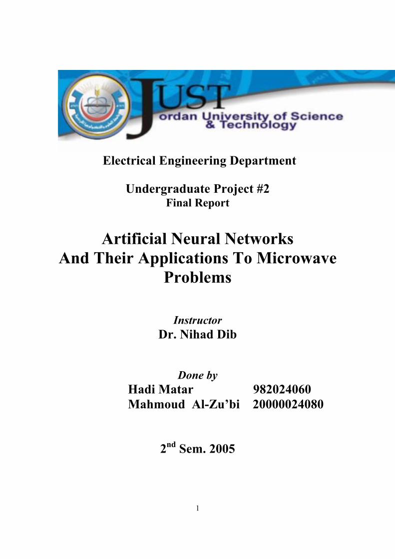
2.2 General architecture:

ANN are formed from interconnected layers of interconnected processing elements

(PE’s). We always have the input and output layers, but what normally varies is the

hidden layer(s), where a hidden layer is simply any layer other than the input and output

layers. What varies inside the layers is the number of PE’s and the connectivity patterns

inside each single layer and between the layers, the general architecture is shown in

Figure 2.1.

Figure 2.1 General Architecture of an ANN

The architecture of a particular network is specified in terms of the number of neurons

per layer, the number of layers and the general connectivity pattern between the different

PE’s in the different layers. The number of input and output PE’s depends on those of the

corresponding system that is being implemented. Hidden layers are needed when the

input/output relation is not quite simple or clear so as to re-modify the inputs in the

hidden layer(s) to give the desired output values. Sometimes increasing the number of

hidden layers will have no tangible improvement on the output values, but increasing the

number of PE’s in the existing hidden layers is what will do the trick. The connectivity

pattern is generally specified by the network model in use; some models have very few

connections while others are densely connected.

7

2.3 Why ANN?

Now that we have given a basic idea about ANN, we can talk about the reasons that

drove scientists towards using them. The parallelism described in the definition and

shown in the architecture is one of the most important reasons; sequential processing has

faced the problems of speed and what is called the whole-picture problem. The speed

problem can be understood by using the analogy of a single door as opposed to many.

There is a limit to the number of people entering a single door at once while you can

allow multiples of that number to enter using many doors (parallel processing).

Supercomputers might have a solution to the speed problem but parallel processing can

take in more factors at one time giving them the ability to look at any problem as a

whole-picture and not only small pieces.

Artificial intelligence has had its limitations and shortcomings in certain areas. Its

representations must be formal which can not be said about humans who have common

sense and use it. Rule-based computers are limited in their abilities to accommodate

inaccurate information and logic machines are not good at dealing with images and

making analogies.

Having described some of the problems facing other technologies, we now mention the

virtues of ANN. They have a rigorous mathematical basis as opposed to other expert

systems, but one can understand and use ANN without being a mathematician.

Knowledge is stored in the network as a whole and not in specific locations. Having the

knowledge distributed allows the network to be associative in the sense that it associates

any new input pattern with a past one just as the brain does. This association property has

the advantages of enabling the network to store large numbers of complex patterns and to

classify new patterns to stored ones quickly. The fact that knowledge is distributed allows

the network to be fault tolerant in the sense that it can make a correct decision concerning

incomplete input data because the network correlates the existing parts with its memory

without the need for the missing parts.

The adaptability of ANN incorporates the PE’s modifying their weights individually, then

in groups, according to the learning scheme of course, and then finally the ability of ANN

8

to respond to new inputs which they have not seen before; this adaptability is a valuable

quality of ANN.

2.4 Implementation, hardware vs. software simulations:

Having known the general architecture and before going into the specifics of operation,

we shall consider the implementation methods of ANN. They have been implemented

both in hardware and software. Implementation in hardware has been in the form of

chips, boards and standalone PC’s called neurocomputers. The choice is actually

application-dependent, applications requiring very high speeds are better hardware

implemented than software implemented because the inherent parallelism of ANN is only

fully utilized when implemented using special ANN hardware and not on the sequentially

running PC’s. But, certain factors have to be taken into consideration when considering

hardware implementation; the increased cost of buying the special hardware and the

software that run on it and the time required to learn how to use the hardware and its

software skillfully. The size of the network in terms of the number of PE’s and

connections has to be predetermined as well as the network model. The speed which is

defined as the number of interconnections processed per second is another deciding

factor.

It has been noted that most applications that require a single net can be implemented

using software with no substantial delay in time except in the training phase which could

be done overnight at the most. Most applications used by scientists require a single net,

whereas larger scale applications, such as optical character recognition, traffic monitoring

and voice recognition, require more than one net, thus requiring the special purpose

hardware for increased speed of processing.

It is worth mentioning that software simulations give us an error margin in terms of

network and parameters choice when planning to build the circuits for the chips. We can

test using software before making the critical decision of building the circuitry; choice

errors might be costly if we were to change an already built chip, board or

neurocomputer.

9

A practical note is that although there are companies manufacturing the ANN hardware,

the ANN hardware market that was expected to boom in the 1980’s did not do so mainly

because only few sophisticated applications require more than a single net and so there is

a limited demand on the hardware.

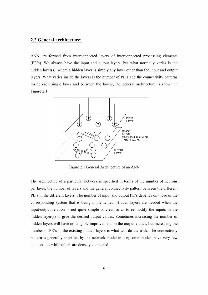
2.5 The neuron:

The most basic component is the processing element, known as the neuron. It has a

limited computational ability as compared to regular computers. This limitation is in its

ability to only add input values and decide what the output value is according to a certain

transfer function.

Figure 2.2 A processing element

As one can see from Figure 2.2, a single PE can have more than one input and each is

multiplied by a weight before being summed at the PE. There might be a bias term which

is summed with the product of the weights and inputs; this term is an attempt at modeling

the fact that biological neurons are affected by external factors. Both the weights and the

bias value are normally initialized at some random state between -0.5 and 0.5. The result

10

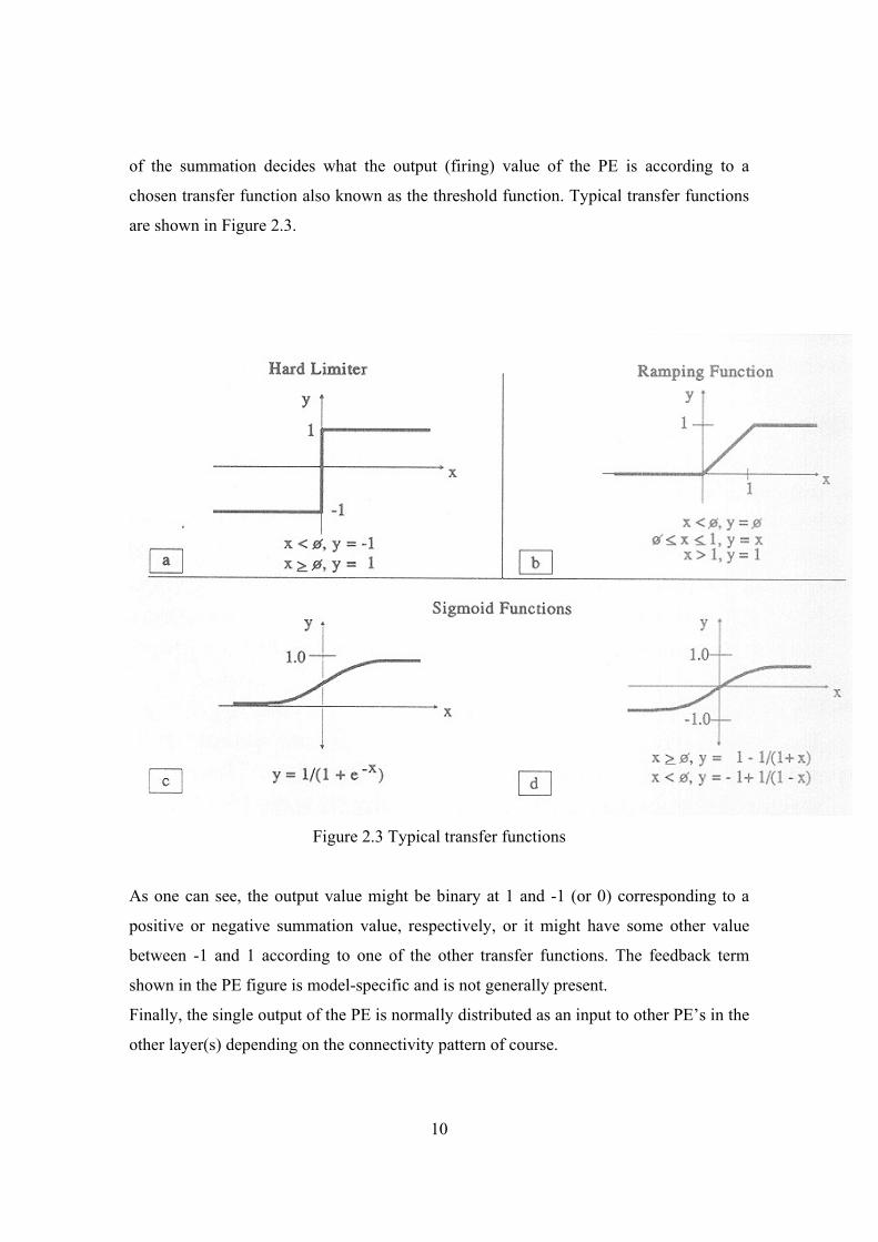
of the summation decides what the output (firing) value of the PE is according to a

chosen transfer function also known as the threshold function. Typical transfer functions

are shown in Figure 2.3.

Figure 2.3 Typical transfer functions

As one can see, the output value might be binary at 1 and -1 (or 0) corresponding to a

positive or negative summation value, respectively, or it might have some other value

between -1 and 1 according to one of the other transfer functions. The feedback term

shown in the PE figure is model-specific and is not generally present.

Finally, the single output of the PE is normally distributed as an input to other PE’s in the

other layer(s) depending on the connectivity pattern of course.

11

2.6 Learning and generalization:

The most desirable feature that ANN have is the ability to learn through training.

Learning is defined as the ability of ANN to change their weights. There are two main

learning modes; supervised and unsupervised learning. As indicated by its name,

supervised learning is one that has a supervisor either in the form of a human supervisor

(which is not practical) or in the form of a given output set corresponding to the input set

provided. The weights are then modified until the output values produced by the network

match those of the given set. Unsupervised learning is that which does not have a human

supervisor or an output set to compare its outputs with. Here the network looks for

regularities or trends in the input set and makes adaptations according to the function of

the network. The network clusters patterns together because they have something in

common and are thus similar, and similar clusters are close to each other.

Generalization is the ability of the network to respond correctly to new inputs after it has

been exposed to many input/output sets (i.e., after learning); a network is of no use if it

can not generalize in the sense described above, and hence we realize the importance of

the network’s ability to generalize.

12

2.7 Back propagation learning:

Many ANN models use supervised learning for which there are many learning laws. The

one that is going to be described next is the one most widely used because it fits the

criteria set by most applications; it is called back propagation learning.

Back propagation is an associating technique in the sense that it associates input patterns

with output patterns; it is a classifying technique in the sense that it classifies inputs

according to their outputs as either belonging to one class or the other (using the transfer

functions), (the two definitions are intertwined).

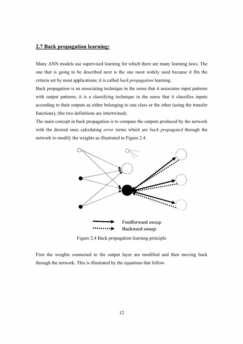
The main concept in back propagation is to compare the outputs produced by the network

with the desired ones calculating error terms which are back propagated through the

network to modify the weights as illustrated in Figure 2.4.

Figure 2.4 Back propagation learning principle

First the weights connected to the output layer are modified and then moving back

through the network. This is illustrated by the equations that follow.

13

The basic equation for a single PE output (disregarding the transfer function for

simplicity) is:

O = θ+∑ ii

i Xw 2.1

where:

iw are the weights connecting to unit i

iX are the inputs to unit i

θ is the bias term

At the output the error term is calculated:

Err = T – O 2.2

where:

T is the true output

The modification to the weights ijw∆ is as follows:

( ) ijij OErrw ×=∆ 2.3

Err=∆θ 2.4

where:

ijw is the weight connecting unit i to unit j

The new weights and biases are the summations of each weight, or bias, and its

calculated modification as follows:

( ) ( ) ijijij wnwnw ∆+=+1 2.5

( ) ( ) θθθ ∆+=+ nn 1 2.6

14

An epoch is defined as a complete cycle through an input set (i.e., all inputs are presented

to the network once and the modifications are made). Now, one of the stopping criteria

used is reaching a certain minimum error value which is equivalent to the outputs

reaching a certain tolerance value with respect to the desired outputs. The stopping

criterion is, more specifically, that all outputs for a certain input pattern are within this

tolerance value during a single epoch

The process of propagating the inputs through the network, then back propagating the

error values and modifying the weights and biases according to the equations given

above, is repeated until the tolerance stopping criterion is met.

But certain problems may arise and one of them is the speed of convergence of the

network (to the minimum error value). Back propagation as a method can be slow; and

this problem is tackled by using a term called the learning rate” η” which speeds up the

network.

The error term calculated at the output is multiplied by this learning rate and then the

weights and biases are modified accordingly as follows:

ijij OErrw ××=∆ η 2.7

jErr×=∆ ηθ 2.8

Another problem is reaching local minima in the error curve, that means that the network

might get stuck at a certain error value which is not the global minimum. This problem

can be solved by increasing the learning rate which might lead to the network not

converging to the global minimum. So, another term called the momentum “mom” is

introduced, it modifies the equations as follows:

( ) ( )nwmomOErrnw ijijij ∆×+××=+∆ η1 2.9

( ) ( )nmomErrn j θηθ ∆×+×=+∆ 1 2.10

It should speed up convergence while helping to avoid local minima at the same time by

making nonradical revisions to the weights thus ensuring that the weight changes do not

oscillate.

Both η and mom have values between 0 and 1, typically 0.5 and 0.9, respectively.

15

Few things need to be pointed out before moving on. Theoretical derivation of back

propagation learning stated that the weights are to be revised after each epoch and that

the error for a certain PE is the sum of all errors resulting from a certain input set, but

experimentation has shown that revision of the weights after each single input yielded

superior results. Another matter is that of repeated presentation of inputs throughout

training, it is preferred that the inputs are not presented in the same order during each

epoch of the repeated runs. The random initial states (of the weights, bias, learning rate

and the momentum term) could lengthen the training period and sometimes give different

results for each training session. The last matter that needs to be discussed is the stopping

criteria, sometimes repeated runs during training cease yielding smaller error terms; in

which case the stopping criterion could be a pre-specified number of epochs, or the error

terms can be averaged over a certain number of epochs and compared for consecutive

groups of epochs, and training should halt if the error term for the last group is not better

than that of the previous one.

2.8 General considerations:

ANN, as all technologies, have their drawbacks. You can not use them for problems that

require precise or exact answers such as keeping one’s finances. The advantage of seeing

the whole-picture is sometimes a disadvantage when you want to see the specifics. ANN

can not count because of their parallelism since counting is done serially; they can not do

operations on numbers the way regular computers do. The problem of errors being

propagated along the network is solved by back propagation though limitations may

exist.

Learning is not that easy, one has to experiment with choosing the model, architecture

with its PE’s and layers, many parameters that may cause oscillation in addition to the

many training sessions that might be needed; it can be a lengthy and difficult process in

which experience is a great advantage.

Answers can not be justified because there is no algorithm or rule that ANN use or

follow. We can not know the output of a certain PE at a certain time or what is going on

inside the network at that instant of time. We have to trust the end results.

16

The quality of training data is of great importance, the inputs have to give an idea about

the whole system so that the networks’ solution is also appropriate for the whole system,

and they have to be accurate enough so that training does lead to the network being able

to solve the problem addressed. The format of the input data is another issue, inputs like

voice or images have to be converted so that the network can accept them as inputs.

2.9 Applications:

We have chosen to mention the applications at the end after having known all aspects

concerning ANN because they enable the reader to better understand and appreciate what

ANN do and how they do it. The scope of applications includes those in biological,

business, financial, environmental, manufacturing, medical and military fields. Some of

these applications are: bomb sniffer, mortgage risk evaluator, speech and pattern

recognition, data compression, weather prediction, adaptive antenna arrays, sonar

classification, adaptive noise canceling, microwave applications which we shall describe

further in the text.

17

Chapter Three

Simulations and Applications

We have used in our project the neural networks toolbox in the Matlab software; it is user

friendly and has many attractive features.

3.1 Matlab’s NN toolbox:

Figure 3.1 NN toolbox general window

Figure 3.1 shows the NN toolbox GUI which consists of three main parts; the first one

shows the inputs, targets, input delay states, networks, outputs, errors and layer delay

states. The second part labeled “Networks and Data” is the one we use to import data

18

from the workspace or to generate new data, create new networks and manage all these

parameters. The third part labeled “Networks only” is used to administer the networks

available in the first part.

When you desire to solve a certain problem using neural networks; the following

procedure should be followed:

1. Training data:

Training data include inputs and targets (desired outputs) for the network.

This data could be generated using two methods:

a. Using the “new data” button in the toolbox in which desired values are

typed in by the user.

b. Using the “import” button which imports previously generated data from

the Matlab workspace.

2. Create network:

To create a new network; pushing the “new network” button will make the

window shown in Figure 3.2 appear.

Figure 3.2 NN toolbox “Create New Network” window

19

The window is used to set the parameters making them most suitable for the problem at

hand:

a. Network Type: there are many types from which one can choose depending

on the type of application, the most suitable type for the problems we will be

addressing is feed-forward back propagation type.

b. Input ranges: They are specified according to one of the sets of values present

in the “inputs” window in the GUI.

c. Training function: One is chosen which best adjusts the weights of the

neurons allowing the network to achieve the desired overall behavior.

d. Adaptation learning function: The function used to specify the value of the

weight change.

e. Performance function: The function used to calculate the error in the network

with respect to the targets.

f. Number of layers: Specified experimentally depending on the complexity of

the problem.

g. Properties for layers:

i. Number of neurons: Specified experimentally to best suit the

problem.

ii. Transfer function: The same as the one described in the previous

chapter, chosen experimentally to best suit the problem.

20

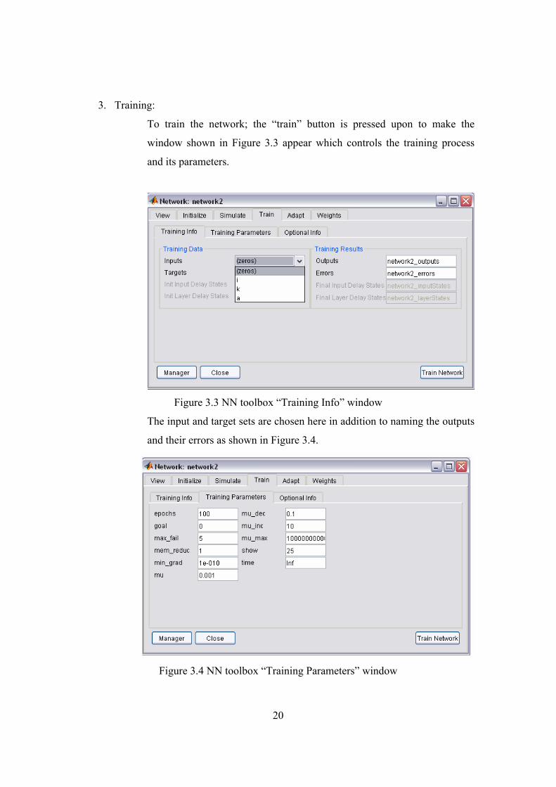
3. Training:

To train the network; the “train” button is pressed upon to make the

window shown in Figure 3.3 appear which controls the training process

and its parameters.

Figure 3.3 NN toolbox “Training Info” window

The input and target sets are chosen here in addition to naming the outputs

and their errors as shown in Figure 3.4.

Figure 3.4 NN toolbox “Training Parameters” window

21

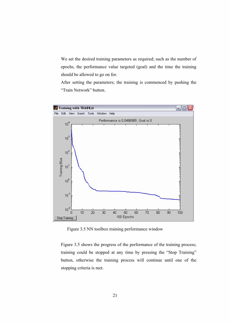
We set the desired training parameters as required; such as the number of

epochs, the performance value targeted (goal) and the time the training

should be allowed to go on for.

After setting the parameters; the training is commenced by pushing the

“Train Network” button.

Figure 3.5 NN toolbox training performance window

Figure 3.5 shows the progress of the performance of the training process;

training could be stopped at any time by pressing the “Stop Training”

button, otherwise the training process will continue until one of the

stopping criteria is met.

22

4. Testing:

The network is tested by pressing the “Simulate” button in the GUI. A

testing set and output name are chosen, the output of the simulation is then

used to verify the network performance.

3.2 Applications to microwave problems:

We have applied NN to microwave problems in two ways yielding two solutions; we first

used them to obtain the characteristic parameters given the dimensions and relative

permittivity, this is called the analysis solution. The second solution known as the design

or synthesis solution is the one in which one of the characteristic parameters switches

roles with one of the dimensions in the input/output relationship; and that dimension is

obtained using the NN.

The analysis solution method was used in the first and second applications while the

design solution method was used in the second application only.

1. Neural model for coplanar waveguide sandwiched between two dielectric

substrates:

a. The structure and characteristic parameters:

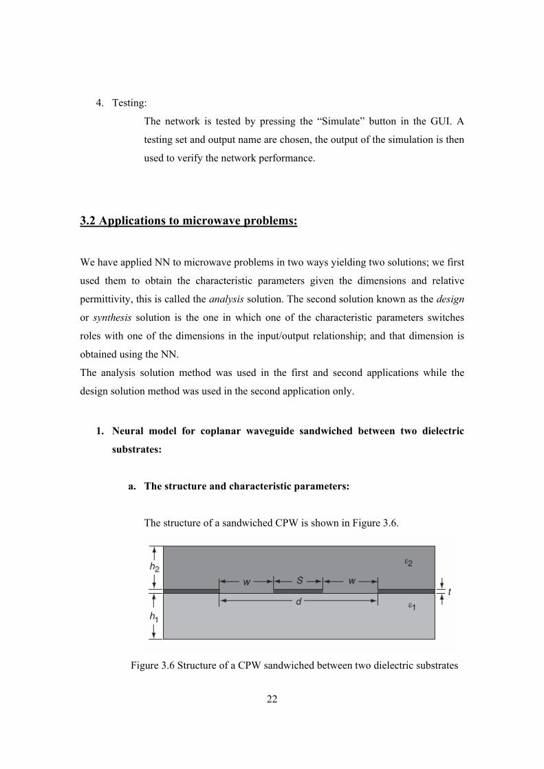
The structure of a sandwiched CPW is shown in Figure 3.6.

Figure 3.6 Structure of a CPW sandwiched between two dielectric substrates

23

1ε and 2ε are the relative permittivities of the lower and upper dielectric

materials with thicknesses 1h and 2h , respectively. S is the center strip

width, W is the slot width and d is the separation between the two semi-

infinite ground planes (d = S+2W).

Quasi static approximations are used to calculate the effective permittivity

( effε ) and characteristic impedance ( 0Z ) of the sandwiched CPW which

are:

0CC

eff =ε 3.1

00 Cv

Z effε= 3.2

where 0v is the speed of light in free space, C is the total capacitance of

the transmission line, and 0C is the capacitance of the corresponding line

with all dielectrics replaced by air.

After using several conformal mapping steps; the equations above are

reduced to [4]:

)1()1(1 2211 −+−+= εεε qqeff 3.3

where 1q and 2q are the partial filling factors given as:

( )( )

( )( )0

'0

'1

11 2

1kKkK

kKkK

q = 3.4

( )( )

( )( )0

'0

'2

22 2

1kKkK

kKkKq = 3.5

24

where ( )ikK and ( )'ikK are the complete elliptic integrals of the first kind

with the modulus given as:

WSSk

20 += 3.6

( )

( )[ ]{ }1

11 42sinh

4sinhhWS

hSk

+=

ππ

3.7

( )

( )[ ]{ }2

22 42sinh

4sinhhWS

hSk+

=π

π 3.8

2' 1 ii kk −= 3.9

The characteristic impedance can be computed as:

( )( )0

'0

030

kKkK

Zeffεπ

= 3.10

b. ANN solution:

We were successful in obtaining the effective permittivity and

characteristic impedance using NN after many trials, the inputs used were

in the ranges 211 1 ≤≤ ε , 131 2 ≤≤ ε , 9.01.0 ≤≤ dS , 35.631 21 ≤≤ hh

and 5.101.0 1 ≤≤ hd . The NN used was of the feed-forward

backpropagation type and consisted of two hidden layers, in addition to

the input and output layers of course, with the configuration

241155 ××× , i.e. 5 neurons in the input layer, 15 and 41 in the first and

second hidden layers, respectively, and 2 neurons in the output layer. The

tangential sigmoid activation function was used in the hidden layers, and

the linear activation function in the input and output layers. Over 7000

25

data sets were used for training and 300 were used for simulation, all were

scaled between 1 and -1 before being applied to the NN. These data sets

were calculated using Matlab as shown in appendix 1.

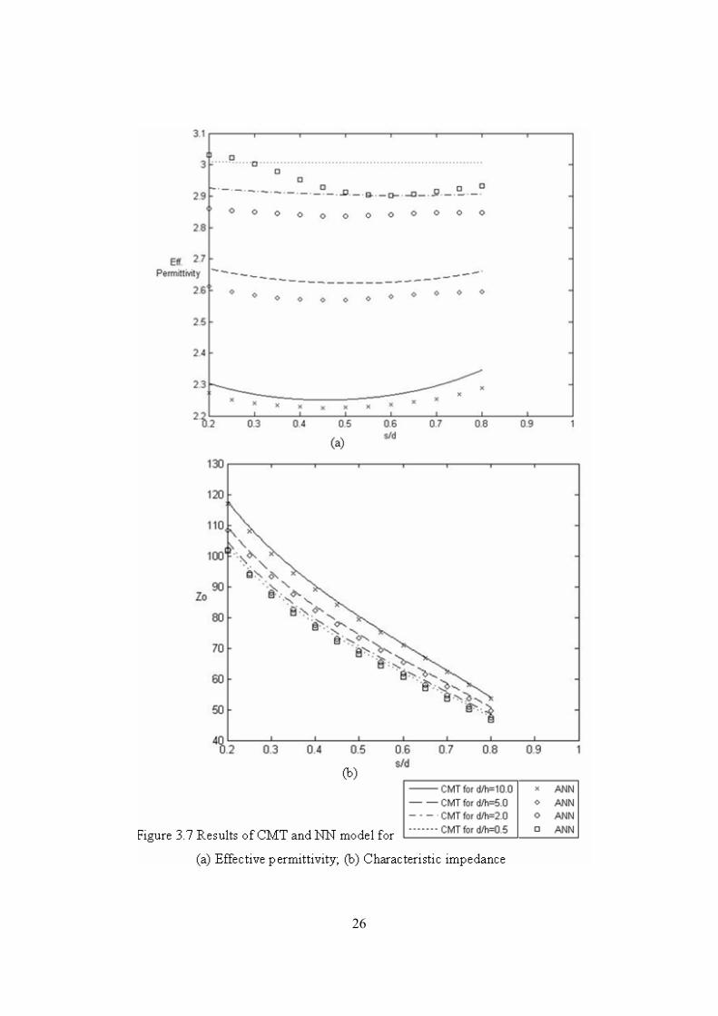
The results obtained from the neural network were then compared with

those calculated using the closed form expressions. Figure 3.7 shows effε

and 0Z versus S/d for mh µ2001 = , mh µ6002 = , 25.21 =ε and

78.32 =ε .

26

27

It can be seen that the NN results for effε are acceptable but not very

accurate which is because of two reasons, the first being that the training

resulted in weights that were more adapted to 0Z and the second is that the

denormalization process might result in such errors. 0Z results on the

other hand are in better agreement with those obtained using CMT and the

error value is small for most cases validating the use of NN instead of the

analytical method.

2. Asymmetric coplanar stripline with an infinitely wide strip:

a. The structure and characteristic parameters:

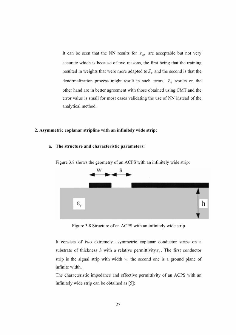
Figure 3.8 shows the geometry of an ACPS with an infinitely wide strip:

Figure 3.8 Structure of an ACPS with an infinitely wide strip

It consists of two extremely asymmetric coplanar conductor strips on a

substrate of thickness h with a relative permittivity rε . The first conductor

strip is the signal strip with width w; the second one is a ground plane of

infinite width.

The characteristic impedance and effective permittivity of an ACPS with an

infinitely wide strip can be obtained as [5]:

28

( )( )'0

60kKkKZ

effεπ

= 3.11

( )( )

( )( )kKkK

kKkKr

eff

'

'211

ε

εεε −+= 3.12

ws

sk+

= 3.13

( )( )( )( )( )( ) ( )( )( )wshhs

hsk24sinh4sinh

4sinh2++

=ππ

πε 3.14

b. ANN solution:

i. Analysis:

We were able to obtain the characteristic impedance and effective

permittivity of the ACPS with infinitely wide strip by using NN with input

ranges 5.133 << rε , 208.0 << hs and 5.1009.0 << sw .

A feed-forward backpropagation network was used with one hidden layer

and the configuration 2303 ×× . The tangential sigmoid activation function

was used in the hidden layer and the linear activation function was used in

the input and output layers.

300 data sets were used to train the network while 100 data sets were used

to test it; these data sets were calculated using Matlab as shown in

appendix 2. The testing outputs were plotted along with the quasi static

equations as shown in Figure 3.9.

29

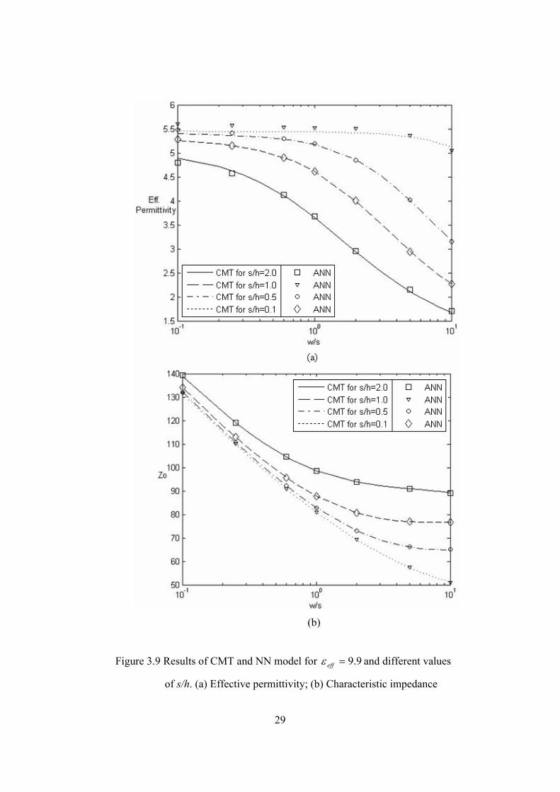
(b)

Figure 3.9 Results of CMT and NN model for 9.9=effε and different values

of s/h. (a) Effective permittivity; (b) Characteristic impedance

30

The effε results in this application are better than those we saw in the

previous one, the inaccuracy in the graph corresponding to 1.0=hs is

due to the weights being more adapted to the other higher ranges. The 0Z

results here are again in good agreement hence also justifying the use of

NN for this application as well instead of CMT if desired.

ii. Design:

The conductor strip width w was obtained successfully using NN. The

same input ranges were used as those in the analysis solution with the

addition of the corresponding characteristic impedance 14050 0 ≤≤ Z .

A feed-forward backpropagation network was used with two hidden layers

and the configuration 142153 ××× . The tangential sigmoid activation

function was used in the hidden layers and the linear activation function

was used in the input and output layers. 2100 data sets were used to train

the network while 100 data sets were used to test it.

The testing outputs were plotted along with the CMT results as shown in

Figure 3.10.

31

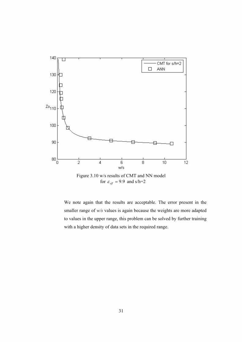
Figure 3.10 w/s results of CMT and NN model

for 9.9=effε and s/h=2

We note again that the results are acceptable. The error present in the

smaller range of w/s values is again because the weights are more adapted

to values in the upper range, this problem can be solved by further training

with a higher density of data sets in the required range.

32

Chapter Four Conclusions

This report should give the reader a background on ANN; it does not cover the whole

subject but serves to cover the basics to say the least. What one can conclude after

reading it, is that ANN are simple to understand and have great potential, but at the same

time are not that easy to deal with nor are they the perfect solution to all problems; they

have a wide range of applications and can be used by practically anyone who has a PC.

We have used Matlab’s NN toolbox in our work because in addition to the fact that we

are familiar with using Matlab itself, the toolbox has many of the known architectures

and paradigms offering the user a wide variety of options to choose from optimizing the

performance, through its user friendly GUI one can manipulate the parameters of the

network with great ease allowing for fine tuning.

Neural networks applications are quite new in the microwave field and have strong

potential for future research and advancement. In this project, the ANN have been used to

find 0Z and effε for CPW and CPS transmission lines. Conventional analytical methods

used for analysis and synthesis of these lines, such as full wave methods and quasi static

methods, have many drawbacks. Deriving solutions for characteristic parameters using

these methods is difficult, time consuming, requires computational efforts and the

solutions themselves are not that easy to implement. Moreover, deriving solutions for

design problems is much more difficult to the degree it becomes impractical to attempt.

Hence, neural networks come in as a practical and fairly accurate alternative.

Our work dealt with two analysis problems and a design problem. The analysis problems

were previously addressed in [4] and [5], however, the design problem has not been

addressed before and hence our solution comes in as a new one.

33

Although neural networks and their Matlab toolbox might seem easy to implement our

work showed that it is a challenging task with many variables to consider. We have faced

many difficulties throughout our work starting with choosing the appropriate architecture

in terms of the number of layers, number of neurons and the activation functions which is

a matter of trial and error where experience and familiarity with neural networks helped

minimize time and effort. The number of data sets used to train a network had to be

carefully chosen to avoid the problems of false convergence when local minima are

reached, and over fitting where weights became to well adapted to the training data sets

and the network lost its ability to generalize, over fitting was also caused by increasing

the number of training epochs more than necessary. The choice of normalization was case

dependant; and resorting to it was done when deemed appropriate. Finally the training

process was time consuming and there were no algorithms or sequence of steps which

could be followed.

We conclude by pointing out the fact that our project and similar work serve as the

foundation for more utilization of neural networks in this field which is not sufficiently

explored.

34

Appendix ‘1’

This appendix shows the Matlab code used for generating the training and test data sets in

the first analysis problem

e1 = 1 + rand(1,3200)*(21-1);

e2 = 1 + rand(1,3200)*(13-1);

h12 = 1/3 + rand(1,3200)*(6.35-1/3);

dh1 = .1 + rand(1,3200)*(10.5-.1);

sd = .1 + rand(1,3200)*(.9-.1);

ko = sd;

kop = sqrt(1-ko.^2);

k1 = sinh(pi.*sd.*dh1./4)./sinh(pi.*dh1./4);

k1p = sqrt(1-k1.^2);

k2 = sinh(pi.*h12.*sd.*dh1./4)./sinh(pi.*dh1.*h12./4);

k2p = sqrt(1-k2.^2);

q1 = .5.*ellipke(k1.^2).*ellipke(kop.^2)./(ellipke(ko.^2).*ellipke(k1p.^2));

q2 = .5.*ellipke(k2.^2).*ellipke(kop.^2)./(ellipke(ko.^2).*ellipke(k2p.^2));

eff = 1+q1.*(e1-1)+q2.*(e2-1);

zo = 30.*pi.*ellipke(kop.^2)./(sqrt(eff).*ellipke(ko.^2));

i = [e1 ; e2 ; h12 ; dh1 ; sd];

[i, minp, maxp, t, mint, maxt] = premnmx(i, t);

t = [eff ; zo];

35

sd = .2:.002:.8;

dh1 = 5*ones(1,301);

e1 = 2.25*ones(1,301);

e2 = 3.78*ones(1,301);

h12 = 1/3*ones(1,301);

ii = [e1 ; e2 ; h12 ; dh1 ; sd];

[ii] = tramnmx(ii, mint, maxt);

36

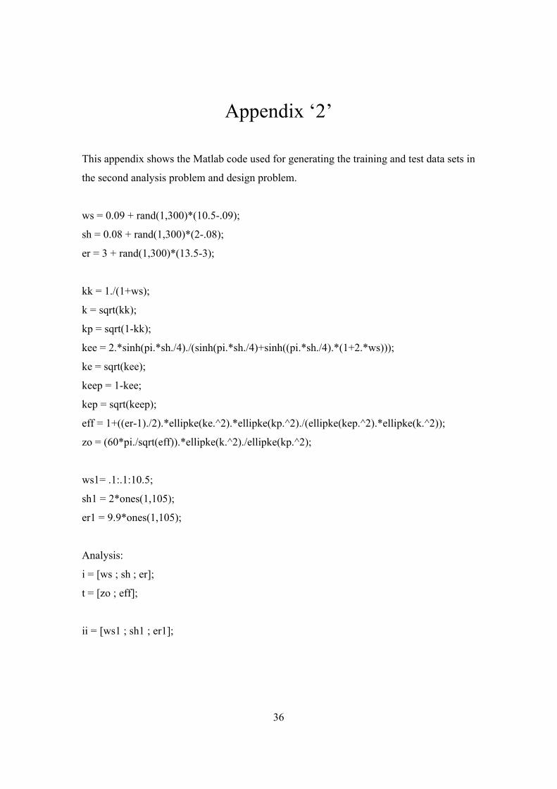
Appendix ‘2’

This appendix shows the Matlab code used for generating the training and test data sets in

the second analysis problem and design problem.

ws = 0.09 + rand(1,300)*(10.5-.09);

sh = 0.08 + rand(1,300)*(2-.08);

er = 3 + rand(1,300)*(13.5-3);

kk = 1./(1+ws);

k = sqrt(kk);

kp = sqrt(1-kk);

kee = 2.*sinh(pi.*sh./4)./(sinh(pi.*sh./4)+sinh((pi.*sh./4).*(1+2.*ws)));

ke = sqrt(kee);

keep = 1-kee;

kep = sqrt(keep);

eff = 1+((er-1)./2).*ellipke(ke.^2).*ellipke(kp.^2)./(ellipke(kep.^2).*ellipke(k.^2));

zo = (60*pi./sqrt(eff)).*ellipke(k.^2)./ellipke(kp.^2);

ws1= .1:.1:10.5;

sh1 = 2*ones(1,105);

er1 = 9.9*ones(1,105);

Analysis:

i = [ws ; sh ; er];

t = [zo ; eff];

ii = [ws1 ; sh1 ; er1];

37

Design:

i = [sh ; zo ; er];

t = [ws];

ii = [sh1 ; zo1 ; er1];

38

References:

[1] Marilyn McCord Nelson - W. T. Illingworth, A Practical Guide to Neural Nets.

Addison-Wesley publishing company, Inc. 1991.

[2] Robert Callan, The Essence of Neural Networks. Prentice Hall Europe, 1999.

[3] Sholom M. Weiss - Casimir A. Kulikowski, Computer Systems That Learn.

Morgan Kaufmann Publishers, Inc. 1991.

[4] C. Yildiz, S. Sagiroglu and M. Turkmen , “Neural model for coplanar waveguide

sandwiched between two dielectric substrates,” IEE Proc.-Microw. Antanna

Propag., vol. 151, No.1, February 2004.

[5] C. Yildiz, S. Sagirgolu and M. Turkman, “Neural models for an asymmetric

coplanar stripline with an infinitely wide strip,” Int. J. Electronics, vol. 90, no 8,

pp. 509-516, 2003.

[6] C. Yildiz and M. Turkmen, “A CAD approach based on artificial neural networks

for shielded multilayered coplanar waveguides,” Int. J. Electron. Commun.,

pp. 1-9, 2004.

[7] C. Yildiz and M. Turkmen, “Very accurate and simple CAD models based on

neural networks for coplanar waveguides synthesis,” Int. J. RF and Microwave,

CAE 15, pp. 218-224, 2005.

[8] Rainee N. Simons, Coplanar Waveguide Circuits, Components and Systems. John

Wiley and Sons., Inc. 2001.

[9] S. Haykin, Neural Networks: A Comprehensive Foundation. Macmillan College

Publishing Comp., New York, 1994.

[10] http://www.dacs.dtic.mil/techs/neural/neural_ToC.html

[11] http://www.doc.ic.ac.uk/~nd/surprise_96/journal/vol4/cs11/report.html

[12] http://www.cs.stir.ac.uk/~lss/NNIntro/InvSlides.html

[13] http://www.shef.ac.uk/psychology/gurney/notes/contents.html

[14] http://www.kcl.ac.uk/neuronet/intro/index.html

[15] http://www.particle.kth.se/~lindsey/HardwareNNWCourse/home.html