arX

iv:a

stro

-ph/

0007

211v

1 1

4 Ju

l 200

0

The Astronomical Journal, in press

The Shapley Supercluster. III. Collapse dynamics and mass of the central

concentration

Andreas Reisenegger1, H. Quintana1, Eleazar R. Carrasco2, and Jeronimo Maze1

areisene@astro.puc.cl

ABSTRACT

We present the first application of a spherical collapse model to a supercluster of

galaxies. Positions and redshifts of ∼ 3000 galaxies in the Shapley Supercluster (SSC)

are used to define velocity caustics that limit the gravitationally collapsing structure in

its central part. This is found to extend at least to 8h−1 Mpc of the central cluster,

A 3558, enclosing 11 ACO clusters. Infall velocities reach ∼ 2000 km s−1. Dynamical

models of the collapsing region are used to estimate its mass profile. An upper bound

on the mass, based on a pure spherical infall model, gives M(< 8h−1Mpc)<∼ 1.3 ×

1016h−1M⊙ for an Einstein-de Sitter (critical) Universe and M(< 8h−1Mpc)<∼ 8.5 ×

1015h−1M⊙ for an empty Universe. The model of Diaferio & Geller (1997), based on

estimating the escape velocity, gives a significantly lower value, M(< 8h−1Mpc) ≈

2.1× 1015h−1M⊙, very similar to the mass found around the Coma cluster by the same

method (Geller et al. 1999), and comparable to or slightly lower than the dynamical

mass in the virialized regions of clusters enclosed in the same region of the SSC. In both

models, the overdensity in this region is substantial, but far from the value required to

account for the peculiar motion of the Local Group with respect to the cosmic microwave

background.

Subject headings: galaxies: clusters: individual (A 3558) — cosmology: observations —

dark matter — large-scale structure — methods: analytical — methods: statistical

1. Introduction

This is the third in a series of papers analyzing the structure and physical parameters of

the Shapley Supercluster (SSC), based on galaxy redshifts. The first (Quintana et al. 1995;

1Departamento de Astronomıa y Astrofısica, Facultad de Fısica, Pontificia Universidad Catolica de Chile, Casilla

306, Santiago 22, Chile

2Instituto Astronomico e Geofısico, Universidade de Sao Paulo, Caixa Postal 3386, 01060-970, Sao Paulo, Brazil

– 2 –

hereafter Paper I) presents and gives an initial analysis of the results of spectroscopic observations

of the central region. The second (Quintana, Carrasco, & Reisenegger 2000, hereafter Paper II)

presents a much extended sample of galaxy redshifts and gives a qualitative discussion of the SSC’s

morphology. Here, we use dynamical collapse models applied to this sample, in order to obtain the

mass of the central region of the SSC. An upcoming paper (Carrasco, Quintana, & Reisenegger

2000, hereafter Paper IV) will analyze the individual clusters of galaxies contained in the sample,

to obtain their physical parameters (velocity dispersion, size, mass), search for substructures within

the clusters, and determine the total mass contained within the virialized regions of clusters in the

whole Shapley area.

The Shapley concentration (Shapley 1930) is the richest supercluster in the local Universe

(Zucca et al. 1993, Einasto et al. 1997, but see also Batuski et al. 1999). This makes its study

important for three main reasons. First, its high density of mass and of clusters of galaxies provides

an extreme environment in which to study galaxy and cluster evolution. Second, its existence and

the fact that it is the richest supercluster in a given volume constrain theories of structure forma-

tion, and particularly the cosmological parameters and power spectrum in the standard model of

hierarchical structure formation by gravitational instability (e.g., Ettori, Fabian, & White 1997;

Bardelli et al. 2000). Finally, it is located near the apex of the motion of the Local Group with

respect to the cosmic microwave background. Thus it is intriguing whether the SSC’s gravitational

pull may contribute significantly to this motion, although most mass estimates (e.g., Raychaud-

hury 1989; Raychaudhury et al. 1991; Paper I; Ettori et al. 1997; Bardelli et al. 2000) make a

contribution beyond a 10 % level very unlikely.

Galaxy counts in redshift space (Bardelli et al. 2000) suggest that most of the supercluster has

a density several times the cosmic average, while the two complexes within ∼ 5h−1 Mpc of clusters

A 3558 and A 3528 have overdensities ∼ 50 and ∼ 20, respectively. These regions are therefore

far outside the “linear regime” of small density perturbations, but still far from being virialized

after full gravitational collapse. The same conclusions are easily reached by even a casual glance

at the redshift structure presented in Paper II. The density of these complexes indicates that they

should be presently collapsing (e.g., Bardelli et al. 2000), and in the present paper we study this

hypothesis for the main complex, around A 3558, where substantially more data, with better areal

coverage, are available (see Paper II).

It should be pointed out that within each of these complexes we expect very large peculiar

velocities, which dominate by far over their Hubble expansion. In this case, redshift differences

among objects within each complex can give information about its dynamics, which we will ana-

lyze below, but essentially no information about relative positions along the line of sight (except,

perhaps, non-trivial information within a given dynamical model). While this is generally acknowl-

edged to be true within clusters of galaxies, where galaxy motions have been randomized by the

collapse, it is sometimes overlooked on somewhat larger, but still nonlinear scales. For instance,

Ettori et al. (1997) calculate three-dimensional distances between clusters in the Shapley region

on the basis of their angular separations and redshifts, and conclude that the group SC 1327-312

– 3 –

and the cluster A 3562, at projected distances ∼ 1 and 3h−1 Mpc from the central cluster A 3558,

are between 5 and 10h−1 Mpc from it in three-dimensional space, because of moderate differences

in redshift. However, there is evidence for interactions between these clusters and groups (Venturi

et al. 1999), suggesting true distances much closer to the projected distances. The discrepancy is

naturally explained by quite modest peculiar velocities of several hundreds of km s−1, easily caused

by the large mass concentration.

In the present paper, we analyze the region around A 3558 in terms of an idealized, spherical

collapse model, which is used both in its pristine, but undoubtedly oversimplified, original form

(Regos & Geller 1989), seen from a slightly different point of view, and in its less appealing,

but possibly more accurate, modern fine-tuning calibrated by simulations (Diaferio & Geller 1997;

Diaferio 1999). Section 2 explains the models, argues for the presence of velocity caustics, and gives

the equations relating the caustics position to the mass distribution. (Some mathematical remarks

regarding this relation are given in the Appendix.) In §3 we present the data, argue that velocity

caustics are indeed present, and explain how we locate their position quantitatively. Section 4

presents and discusses our results, and §5 contains our main conclusions.

2. The models

2.1. Pure spherical collapse

In this approach, we consider a spherical structure in which matter at any radius r moves

radially, with its acceleration determined by the enclosed mass M(r). At a given time t1 of ob-

servation, the infall velocity u(r) = −r(r) (traced by galaxies participating in the mass inflow)

can give direct information about the mass profile (Kaiser 1987; Regos & Geller 1989). Of course,

u(r) is not directly observable. Instead, for each galaxy we only observe its position on the sky,

which translates into a projected distance from the assumed center of the structure, r⊥ ≤ r, and

its redshift, which can be translated into a line-of-sight velocity v with respect to the same center.

The “fundamental” variables r and u and the “observed” variables r⊥ and v (with the line-of-sight

velocity of the structure’s center already subtracted) are related by

v = ±

[

1−(r⊥

r

)2]

12

u(r). (1)

Contrary to the Hubble flow observed on large scales, v is negative (approaching) for the more

distant galaxies on the back side of each shell, and positive (receding) for the closer galaxies on

the front side. At any given projected distance r⊥, one observes galaxies at many different true

distances r from the center. The infall velocity u(r) decreases at large enough distances r, reaching

zero at a finite (“turnaround”) radius rt, and matching onto the Hubble flow, u(r) = −Hr, for

r ≫ rt. The projection factor increases from zero at r = r⊥ (galaxies moving perpendicularly to

– 4 –

the line of sight), asymptotically approaching unity for r ≫ r⊥. Therefore, there will be some

maximum projected velocity

A(r⊥) ≡ maxr≥r⊥

|v(r⊥, r)| = maxr≥r⊥

[

1−(r⊥

r

)2]

1

2

u(r), (2)

which is a monotonically decreasing function of r⊥ (see Appendix), giving rise to caustics in the

(r⊥, v) diagram with the characteristic “trumpet shape” described by Kaiser (1987) and by Regos

& Geller (1989).

In order to obtain the infall velocity u(r) from the galaxy redshifts, we first identify the caustics

amplitude A(r⊥) from the (r⊥, v) diagram by the procedure outlined in §3. Given this relation, we

can invert eq. (2) to obtain

u(r) ≤ ub(r) ≡ minr⊥<r

A(r⊥)

[1− (r⊥/r)2]1

2

. (3)

This is an inequality rather than an equality because for an arbitrary shape of u(r) it is not

guaranteed that the shells at every r will correspond to a maximum amplitude for some r⊥ (see

Appendix for a detailed mathematical discussion).

If the mass density decreases outwards, then the collapse occurs from the inside out, with

innermost mass shells first reaching turnaround and recontraction, and outer shells following in

succession. Any given shell will enclose the same mass M at all times until it starts encountering

matter that has already passed through the center of the structure and is again moving outwards.

The latter is only expected to happen in the very central, nearly virialized, part of the supercluster.

Elsewhere, the dynamics of any given shell is described by the well-known parameterized solution

r = A(1− cos η); t = B(η − sin η); A3 = GMB2 (4)

(e.g., Peebles 1993, chapter 20). Here, A and B are constants for any given shell (related to each

other by the enclosed mass M), and η labels the “phase” of the shell’s evolution (initial “explosion”

at η = 0, maximum radius or “turnaround” at η = π, collapse at η = 2π). As we are observing

many shells at one given cosmic time t1 (measured from the Big Bang, at which all shells started

expanding, to the moment at which the structure emitted the light currently being observed), for

each shell we can write

t1r

r= −H0t1

u

H0r=

sin η(η − sin η)

(1− cos η)2, (5)

where H0 is the current value of the Hubble parameter.

– 5 –

We can determine an upper bound on u(H0r), and therefore on u/(H0r), by the procedure

described above (note that r itself depends on the uncertainty in the cosmic distance scale). The

combination H0t1 is a dimensionless constant, dependent on the cosmological model (identified by

dimensionless constants such as the density parameters Ω). At the redshift of the SSC (z ≈ 0.048),

it is likely to lie in the range 0.62 ≤ H0t1 ≤ 0.95, with the lower limit corresponding to an Einstein-

de Sitter Universe (with critical matter density, Ωm = 1, and no other ingredients), and the upper

limit corresponding to an empty Universe (Ωm = 0 = ΩΛ) or a flat, low-density, Λ-dominated

Universe (Ωm = 1 − ΩΛ ≈ 0.27) (e.g., Peebles 1993, chapter 13). For an assumed value of this

parameter, the left-hand side becomes fully determined, and the equation can be solved for the

value of η for each shell. The equations can also be combined to yield

H0M(r) =(H0r)

3

G(H0t1)2(η − sin η)2

(1− cos η)3, (6)

the mass enclosed within the shell (of current radius r).

For two reasons, a mass estimate obtained by applying this model to real data should be regarded

as an upper bound on the true mass. First, the model gives ub(r), an upper bound on u(r), and

this upper bound is used to derive the mass. Second, the caustics amplitude A(r⊥) is amplified

through random motions due to substructure within the infalling matter (Diaferio & Geller 1997).

Keeping this in mind, we will use the model to put a bound on the mass of the collapsing region

around A 3558.

2.2. Diaferio’s prescription

On the other hand, Diaferio & Geller (1997; see also Diaferio 1999) have shown that the mass

profile of structures forming in numerical simulations can be recovered to good precision from the

formula

M(r) =Fβ

G

∫ r

0

A2(r⊥)dr⊥. (7)

There is no rigorous derivation for this result, although it can be justified heuristically by

assuming that A reflects the escape velocity at different radii, i.e., that all galaxies within the

caustics are gravitationally bound to the structure. One has to assume further that the radial

density profile lies between ρ ∝ r−3 and ρ ∝ r−2 (Diaferio & Geller 1997; Diaferio 1999), as in the

outskirts of simulated clusters of galaxies (e.g., Navarro, Frenk, & White 1997). This mass estimate

is independent of the parameter H0t1, since no dynamical evolution is involved. It has already been

applied to the Coma cluster (Geller, Diaferio, & Kurtz 1999).

– 6 –

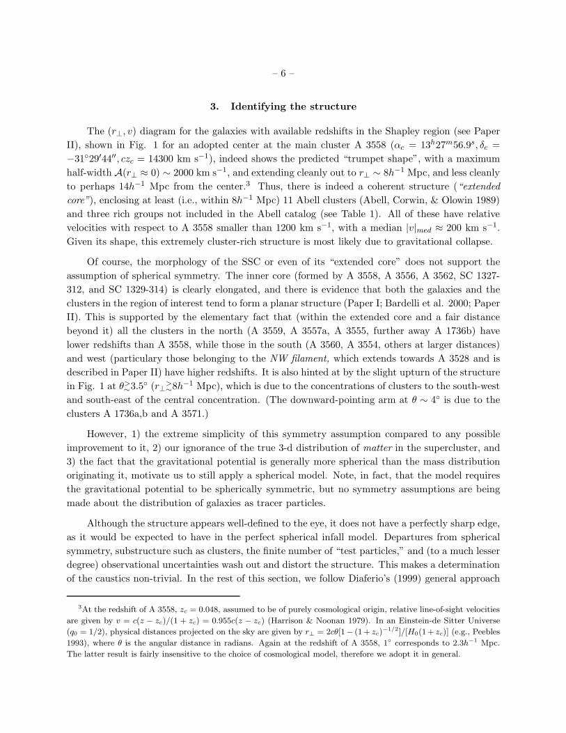
3. Identifying the structure

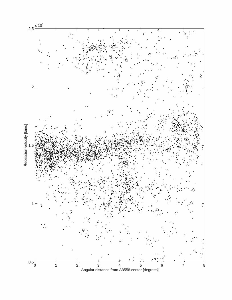
The (r⊥, v) diagram for the galaxies with available redshifts in the Shapley region (see Paper

II), shown in Fig. 1 for an adopted center at the main cluster A 3558 (αc = 13h27m56.9s, δc =

−3129′44′′, czc = 14300 km s−1), indeed shows the predicted “trumpet shape”, with a maximum

half-width A(r⊥ ≈ 0) ∼ 2000 km s−1, and extending cleanly out to r⊥ ∼ 8h−1 Mpc, and less cleanly

to perhaps 14h−1 Mpc from the center.3 Thus, there is indeed a coherent structure (“extended

core”), enclosing at least (i.e., within 8h−1 Mpc) 11 Abell clusters (Abell, Corwin, & Olowin 1989)

and three rich groups not included in the Abell catalog (see Table 1). All of these have relative

velocities with respect to A 3558 smaller than 1200 km s−1, with a median |v|med ≈ 200 km s−1.

Given its shape, this extremely cluster-rich structure is most likely due to gravitational collapse.

Of course, the morphology of the SSC or even of its “extended core” does not support the

assumption of spherical symmetry. The inner core (formed by A 3558, A 3556, A 3562, SC 1327-

312, and SC 1329-314) is clearly elongated, and there is evidence that both the galaxies and the

clusters in the region of interest tend to form a planar structure (Paper I; Bardelli et al. 2000; Paper

II). This is supported by the elementary fact that (within the extended core and a fair distance

beyond it) all the clusters in the north (A 3559, A 3557a, A 3555, further away A 1736b) have

lower redshifts than A 3558, while those in the south (A 3560, A 3554, others at larger distances)

and west (particulary those belonging to the NW filament, which extends towards A 3528 and is

described in Paper II) have higher redshifts. It is also hinted at by the slight upturn of the structure

in Fig. 1 at θ>∼3.5 (r⊥

>∼8h

−1 Mpc), which is due to the concentrations of clusters to the south-west

and south-east of the central concentration. (The downward-pointing arm at θ ∼ 4 is due to the

clusters A 1736a,b and A 3571.)

However, 1) the extreme simplicity of this symmetry assumption compared to any possible

improvement to it, 2) our ignorance of the true 3-d distribution of matter in the supercluster, and

3) the fact that the gravitational potential is generally more spherical than the mass distribution

originating it, motivate us to still apply a spherical model. Note, in fact, that the model requires

the gravitational potential to be spherically symmetric, but no symmetry assumptions are being

made about the distribution of galaxies as tracer particles.

Although the structure appears well-defined to the eye, it does not have a perfectly sharp edge,

as it would be expected to have in the perfect spherical infall model. Departures from spherical

symmetry, substructure such as clusters, the finite number of “test particles,” and (to a much lesser

degree) observational uncertainties wash out and distort the structure. This makes a determination

of the caustics non-trivial. In the rest of this section, we follow Diaferio’s (1999) general approach

3At the redshift of A 3558, zc = 0.048, assumed to be of purely cosmological origin, relative line-of-sight velocities

are given by v = c(z − zc)/(1 + zc) = 0.955c(z − zc) (Harrison & Noonan 1979). In an Einstein-de Sitter Universe

(q0 = 1/2), physical distances projected on the sky are given by r⊥ = 2cθ[1− (1+ zc)−1/2]/[H0(1+ zc)] (e.g., Peebles

1993), where θ is the angular distance in radians. Again at the redshift of A 3558, 1 corresponds to 2.3h−1 Mpc.

The latter result is fairly insensitive to the choice of cosmological model, therefore we adopt it in general.

– 7 –

in first smoothing the data, i.e., obtaining a smooth estimate f(r⊥, v) for the density of observed

galaxies on the (r⊥, v) plane, and then applying a cut at some density contour which is taken to

correspond to the caustics. The details of how each of these steps is carried out differ slightly from

Diaferio’s approach, and are discussed in the rest of this section.

3.1. Density estimation in the (r⊥, v) diagram

For a global analysis of the central (collapsing) region of the SSC, we need to obtain a smooth

estimate f(r⊥, v) of the density of galaxies in the (r⊥, v) diagram. Density estimation has been

discussed by many authors, such as Silverman (1986), and in the astronomical context Pisani (1993;

1996) and Merritt & Tremblay (1994).

Diaferio (1999) applied density estimation to the particular problem of interest here. For N

data points (galaxies) with coordinates (ri⊥, vi), he adopts the estimate

f(r⊥, v) =1

N

N∑

i=1

1

hirhiv

K

(

r⊥ − ri⊥hir

,v − vi

hiv

)

, (8)

where

K(~t) =

4π−1(1− |~t|2)3 if |~t| < 1,

0, otherwise,

is a smooth, but centrally peaked, kernel function. The ratio of smoothing lengths, q = hiv/hir is

fixed, approximately equal to the ratio of observational uncertainties (q = 50km s−1/0.02h−1Mpc =

25H0), and the individual values of, say, hir, are chosen by an adaptive algorithm.

Any choice of smoothing lengths is a compromise between keeping as much structure as possible

(favoring small smoothing lengths) while eliminating as much noise as possible (favoring large

values). The ideal compromise, though quite subjective in any case, depends on the density of data

points, which generally varies over the volume being studied, motivating the choice of a different

smoothing length for each data point. For our particular application, the density of points does

not vary enormously over the area of interest, and we are only interested in the overall envelope

of the structure, not in fine details. Therefore, we consider the additional computational effort

of adaptive smoothing with different local smoothing lengths unjustified. We apply fixed, overall

smoothing lengths hr = 1h−1 Mpc, hv = 500 km s−1 (giving q = 5H0), chosen by eye to preserve

the overall shape while minimizing the noise, and each corresponding to about 1/8 of the total

extension of the structure studied. Changing either of the two lengths by a factor of 2 either way

does not substantially change our results. We note also that the chosen lengths are much larger

than the respective uncertainties in the data, which therefore become irrelevant in determining the

detected structures.

– 8 –

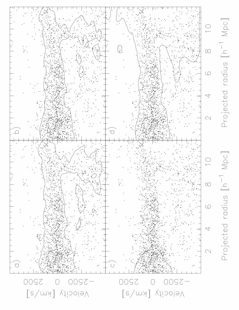
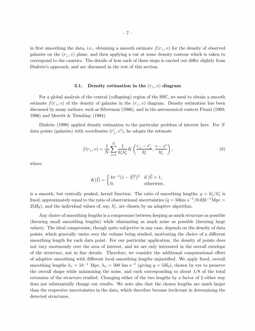
One problem with the smoothing kernel given above is that the data have a natural cutoff at

r⊥ = 0, where they go abruptly from a fairly high (near maximum) density (at r⊥ > 0) to zero (at

r⊥ < 0). When applied to points of small (positive) r⊥, the smoothing kernel extends to negative

values (where there are no data points), producing a decrease in f(r⊥, v) when approaching r⊥ = 0

from above. This causes isodensity contours to narrow as r⊥ → 0+, as seen, e.g., in Fig. 1 of Geller,

Diaferio, & Kurtz (1999), in Figs. 4 and 5 of Diaferio (1999), and in Fig. 2a of the present paper.

This can be cured, e.g., by making a mirror image of the data at r⊥ < 0 and letting the

smoothing kernel integrate over both the real data and their image (Fig. 2b). Aside from correcting

for the “misbehavior” at r⊥ = 0, this procedure gives results very similar to that of Diaferio (1999).

A more rigorous approach is suggested by Merritt & Tremblay (1994), who deal with density

estimation in circularly symmetric structures. They focus on the surface density Σ(r⊥) (number per

unit area) rather than the radial density N(r⊥) = 2πr⊥Σ(r⊥) (number per unit radial coordinate),

and estimate Σ(r⊥) with a circularly averaged kernel. In our case (with one additional coordinate

v, which is not affected by this problem), we can define a number density per unit (projected)

area per unit line-of-sight velocity as Σ(r⊥, v) = f(r⊥, v)/(2πr⊥), and estimate it through a kernel

which is a product of a standard, one-dimensional kernel for v and a circularly averaged kernel for

r⊥. In particularly, Fig. 2c shows the results of applying to our data a one-dimensional quadratic

(Epanechnikov) kernel for v, and an annularly averaged, two-dimensional quadratic kernel for r⊥.

(See Merritt & Tremblay 1994, eqs. 9a and 28a for explicit formulae.) The density Σ obtained from

this procedure is well-behaved in all respects, decreasing from r⊥ = 0 outwards. Indeed, it decreases

so quickly that the density contours tend to close at fairly small radii, contrary to the visual

impression from the data. Therefore, these contours are unlikely to be realistic representations of

the velocity caustics.

A final alternative (with the added virtue of reducing biases due to non-uniform spatial sam-

pling) is to normalize f(r⊥, v) at each given r⊥ with respect to the value at v = 0, i.e., take a

density estimate

f(r⊥, v) ≡f(r⊥, v)

f(r⊥, 0), (9)

with the “original” f(r⊥, v) determined by any of the other methods (the case shown in Fig. 2d is

based on Diaferio’s estimator). This estimator gives results very similar to the first two.

Overall, we consider that the second procedure (the “mirror image” density estimate) is the

one that most closely represents the visual appearance of the data, while at the same time having

mathematically desirable properties (smooth density contours slowly narrowing with increasing r⊥),

and being close enough to Diaferio’s to permit a direct comparison of results. Therefore, we use the

“mirror image” density estimation for the analysis that follows. However, we stress that it is a very

arbitrary choice, and that other choices may give quite different final results. However, discarding

the very different result based on the “surface density” scheme, the other procedures discussed

– 9 –

above give masses that, at any given radius, differ by less than 10 % from the one obtained by the

“mirror image” procedure.

3.2. Finding the caustics

Given the estimated density f(r⊥, v), we now turn to finding the caustics which separate the

collapsing structure from the galaxies in the foreground and background. We are again inspired

by Diaferio (1999), who uses a fixed density cutoff, f(r⊥, v) = κ, with the value of κ fixed by

virial arguments applied to the most central region. In principle, taking a fixed value is somewhat

arbitrary. By plotting in (r⊥, v) space, we are summing galaxies over annuli, and therefore a

uniform background of galaxies would result in a density increasing ∝ r⊥, and therefore a fixed

cutoff might include more and more of the background as r⊥ increases. The problem is worsened by

the non-uniformly sampled data in our particular case. Therefore, a more natural and in principle

better way to distinguish the structure from the background might be to fix on maxima of ∂f∂v for

each r⊥. However, taking and maximizing a derivative of the numerically determined function is

much noisier than just imposing a fixed cutoff. Therefore, we follow Diaferio in adopting the latter

approach.

In order to choose the value of the cutoff, Diaferio (1999) uses the virial theorem to relate the

escape velocity (in his interpretation represented by the velocity amplitude A) and the velocity

dispersion σ of the central cluster, therefore writing 〈A2〉κ,R = 4σ2, where the average is a galaxy

number-weighted average over the region enclosed by the virial radius R of the central cluster,

for a given density cutoff κ. For A 3558, the velocity dispersion is a relatively robust number

(σ ≈ 928 km s−1), not sensitive to the radius of the sphere to be averaged over, and in the central

region A (determined with any reasonable cutoff) is also fairly radius-independent. Therefore,

the dependence on the (poorly determined) virial radius is weak, and we arbitrarily choose it as

R = 1h−1 Mpc, and do a straight radial average (not number-weighted) to calculate 〈A2〉κ,R and

determine κ by Diaferio’s condition.

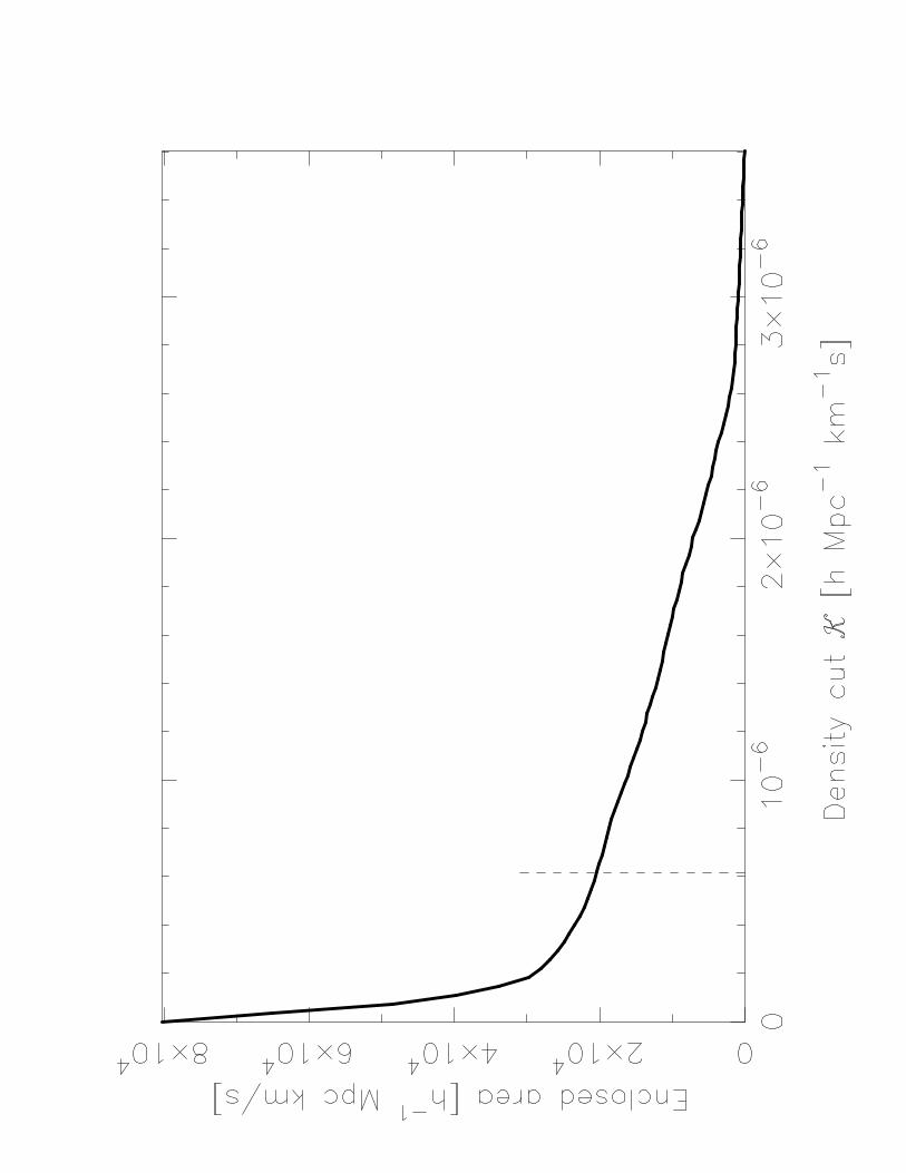
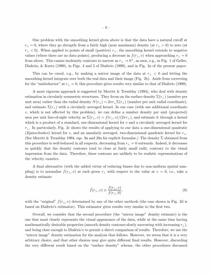
We tested the validity of Diaferio’s condition by the following procedure. Figure 3 shows the

area of the (r⊥, v) diagram enclosed by contour levels with different κ. We clearly distinguish 3

regimes:

(a) At very low densities, the enclosed area is most of the diagram, therefore enclosing much of

the background, not belonging to the structure. The area rapidly decreases as the threshold

density is increased.

(b) At intermediate densities, the decreasing curve becomes much flatter (dA/dκ ≈ constant),

and we interpret this as having most of the background excluded and probing progressively

denser parts of the structure. This is confirmed by watching the contour plots, which indeed

trace the boundaries of the structure, and become progressively tighter.

– 10 –

(c) Finally, at high values of κ, only a few isolated peaks in the structure are left enclosed, and

these finally disappear when κ reaches the maximum density present.

This analysis suggests choosing the threshold at the transition between regimes (a) and (b).

This falls close to the threshold value chosen by Diaferio’s (1999) condition as outlined above,

marked by the vertical line. This strengthens the argument for Diaferio’s choice of cutoff, already

used to choose the contours in Fig. 2, and adopted hereafter.

The chosen density contour of course gives two values of v (one positive, vu, and one negative,

vd) for each value of r⊥. In the SSC, it turns out that the upper contour is much “cleaner”

(separating a dense region from a nearly empty one), therefore we simply adopt A(r⊥) = vu(r⊥)

rather than Diaferio’s prescription A(r⊥) = min|vu(r⊥)|, |vd(r⊥)|.

4. Results and Discussion

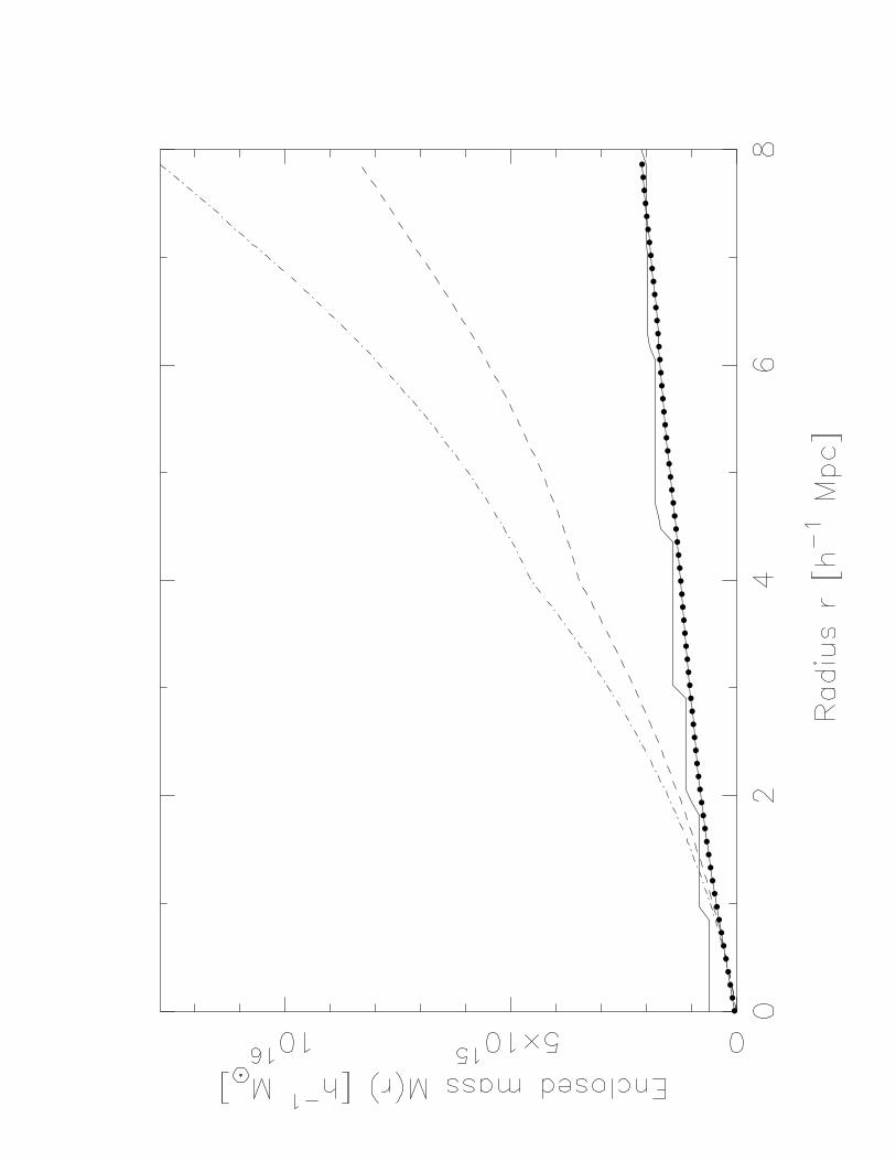
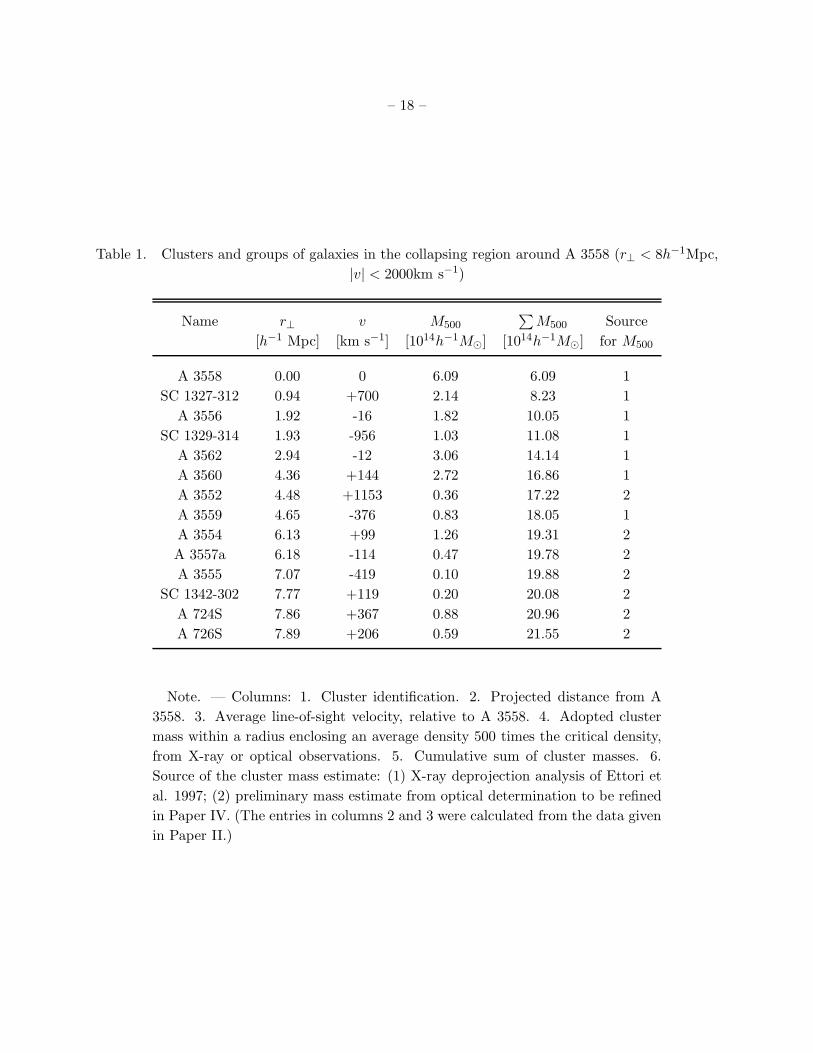
Fig. 4 shows the enclosed mass as a function of radius,M(r), as determined by the two methods

discussed in §2, together with a third determination, namely the cumulative mass of the clusters

enclosed in the given radius, given in Table 1. Note that the mass estimates M500, taken from

Ettori et al. (1997) for the most important clusters, are masses within a radius enclosing an average

density 500 times the critical density ρc. This is substantially higher than the standard “virialization

density” of ∼ 200ρc, and therefore gives a conservative lower limit to the total virialized mass, which

may be increased by a factor ∼ (500/200)1/2 ≈ 1.58 for a more realistic estimate.

Several comments are in order:

1) As discussed above, the pure spherical infall model is highly idealized and, even if correct,

can only give an upper bound on the mass within any given radius. Therefore, the upper (dot-

dashed) curve, corresponding to pure spherical collapse in a cosmological model with H0t1 = 0.62

should be regarded as a fairly robust upper limit to the mass within any given radius.

2) The model of Diaferio & Geller (1997) has been calibrated against simulations. Applied to

the infall regions around clusters of galaxies, it should in principle give the correct mass to within

about 25% (Geller et al. 1999). However, it assumes a density profile decreasing at least as fast as

ρ(r) ∝ r−2, which may not apply to the very noisy region around A 3558, which contains a number

of other, fairly rich clusters. It appears surprising that the mass profile it gives for this region is

quite similar (both in shape and in amplitude) to that obtained by Geller et al. (1997), considering

that Coma is a quite massive cluster (as massive or perhaps even more massive than A 3558), but

is not surrounded by any other massive clusters.

3) The mass estimate based on individual cluster masses is uncertain for two reasons. First, of

course it does not consider the mass in the non-virialized outskirts of the clusters or not associated

with clusters at all, and therefore it would be expected to underestimate the total mass. On the

– 11 –

other hand, in the absence of information on the three-dimensional distance r of each cluster to A

3558, and given that the velocity does not give reliable distance information within the collapsing

structure, each cluster was put at its projected radius r⊥ ≤ r, and therefore contributes to the

enclosed mass already at radii smaller than its true position. Therefore, the mass in virialized

clusters within any given radius M(r) is overestimated by the projection into radius r of clusters

actually at larger radii.

Given these caveats, there seems to be fair agreement among the different mass determinations,

and it seems safe to say that the mass enclosed by radius r = 8h−1 Mpc lies between 2× 1015 and

1.3 × 1016h−1M⊙. It is interesting, nevertheless, that Diaferio’s method gives results that differ

so little from the lower limit to the virialized mass in clusters. Therefore, if Diaferio’s method is

applicable to the SSC, the either there would be very little mass outside the inner, virialized parts

of clusters of galaxies in this region, or the cluster mass estimates would have to be systematically

high.

For comparison, Ettori et al. (1997) used three different mass estimates, namely: 1) the sum

of the gravitational masses of clusters as obtained from their X-ray emission profile, Mgrav, 2) the

total mass expected to be associated with the baryons observed in clusters, MPN , and 3) the mass

obtained from applying the virial theorem to the enclosed clusters, used as test particles, Mvir.

They applied these methods to four progressively larger structures, each enclosing the previous

one. The one most similar to our 8h−1 Mpc sphere appears to be the second, enclosing 12 clusters,

and with a nominal 3-d radius of 13.9h−1 Mpc, obtained by treating redshift as a third coordinate,

which we have argued to give an overestimated depth in the collapsing region. For this region, they

find Mgrav = 2.15, MPN = 5.2Ωm and Mvir = 1.75, all in units of 1015h−1M⊙. The first two are

likely underestimates (as they consider only the matter in the virialized regions of clusters observed

in X-rays), and the third is completely uncertain, given the uncertain distances along the line of

sight and the fact that the SSC is not virialized (but see Small et al. 1998 for a modern, more

careful application of the virial theorem to the Corona Borealis supercluster). Thus, it is reasonable

that we find a somewhat higher mass for the (optically observed) clusters, and a possibly much

higher total dynamical mass, as suggested by the spherical collapse model.

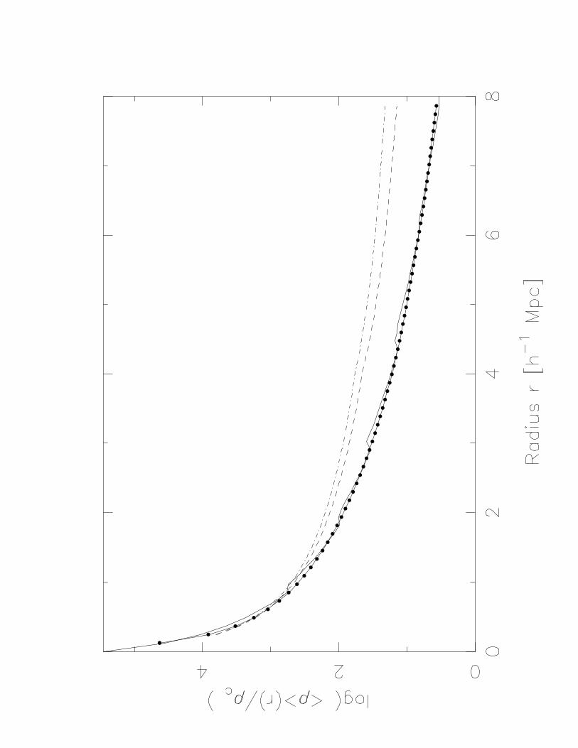
The average enclosed density (see Fig. 5) drops from a value 400 – 500 times the critical

density within 1h−1 Mpc (consistent with the presence of a massive, already collapsed and virialized

cluster) to a value still several times critical (∼ 3.7 to 23 times, depending on the model) within

our outermost radius, 8h−1 Mpc. From galaxy counts in redshift space, Bardelli et al. (2000) find

an overdensity N/N = 11.3 ± 0.4 within a region of equivalent radius 10.1h−1 Mpc. Assuming

that galaxies trace mass, this might in principle allow us to determine the universal matter density

parameter Ωm = ρ/ρcrit = (ρ(r)/ρcrit)/(N(r)/N ). In practice, however, the uncertainty in this

estimate is still much too large to put a useful constraint on Ωm.

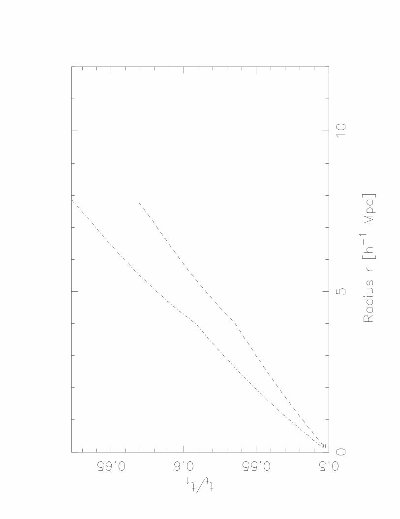
Fig. 6 shows that, in the spherical collapse model, the whole structure within 8h−1 Mpc

has already been contracting for more than 1/3 of its lifetime, and the inner regions are in the

– 12 –

final stages of collapse, consistent with the presence of a massive cluster. Even if there were no

additional mass beyond 8h−1 Mpc, the current turnaround radius would be at ∼ 14h−1 Mpc,

and the bound region (to collapse eventually) would extend to ∼ 20h−1 Mpc, enclosing essentially

the whole supercluster, including the strong concentration around A 3528, A 3530, and A 3532.

However, the much lower enclosed densities in the Diaferio & Geller model would imply that the

8h−1 region around A 3558 is (at best) only now reaching turnaround, and has another Hubble

time to go for final collapse.

As discussed in Paper I, the mass required at the distance of the SSC to produce the observed

motion of the Local Group with respect to the cosmic microwave background is given by

Mdipole ≈ 4.5× 1017Ω0.4m h−1M⊙.

The mass within 8h−1 Mpc can therefore produce at most 3Ω−0.4m % of the observed Local Group

motion, which makes it unlikely that even the whole SSC would dominate its gravitational accel-

eration.

Unfortunately, not much can be said about the regions beyond a radius of ∼ 8h−1 Mpc

from the center. It seems safe to assert, though, that the collapsing region does not extend far

beyond, say, 14h−1 Mpc. This gives an upper bound on the average density enclosed in larger radii,

ρ < 3π/(32Gt21). Thus, in order to produce the peculiar velocity of the Local Group, one would

need a region of radius

r > 55h−1Ω0.13m (H0t1)

2/3Mpc,

which, for the range of cosmological values considered before, corresponds to a lower limit ∼ 40h−1

Mpc. Therefore, in the unlikely case that the whole SSC (characterized in Paper II) were on the

verge of gravitational collapse, it would be able to produce on its own the observed peculiar velocity

of the Local Group. This statement ignores, of course, that the apex of the Local Motion does not

point exactly at the SSC, and therefore some additional contribution is necessary in any case.

5. Conclusions

We have presented the (to our knowledge) first application of a plausible dynamical model to a

supercluster of galaxies, containing a substantial number of clusters. The central 8h−1 Mpc region

of the Shapley spercluster (and probably a much more extended region surrounding it) is argued

to be currently collapsing under the effect of its own gravity. Its mass, although uncertain due to

idealizations in the model, indicates a large enhancement over the average density of the Universe,

although still far from that required to produce the Local Group’s observed motion with respect

to the cosmic microwave background.

– 13 –

The authors thank A. Diaferio for interesting discussions at the First Princeton-U. Catolica

Astrophysics Workshop, The Cosmological Parameters Ω, held in Pucon, Chile, in January 1999,

and for extensive e-mail exchanges thereafter. A previous version of the kernel smoothing program

used here was due to A. Meza. We also thank him and R. Benguria for useful discussions. This work

was financially supported by FONDECYT grant 8970009 (Proyecto de Lıneas Complementarias),

and by a Presidential Chair in Science awarded to H. Quintana. E.R.C. was funded by FAPESP

Ph.D. fellowship 96/04246-7.

A. Geometric interpretation and mathematical properties of the line-of-sight

velocity amplitude A(r⊥) and the infall velocity u(r)

In order to derive and understand intuitively the properties of the observed velocity amplitude

A(r⊥) and the infall velocity u(r) producing it in the spherical model, it is convenient to define

new variables P = r2⊥, R = r2, V = A2, and U = u2. Then,

V (P ) = maxR>P

F (P,R), with F (P,R) ≡

(

1−P

R

)

U(R). (A1)

(We consider only the interval in which u(r) = −r ≥ 0, corresponding to infall.)

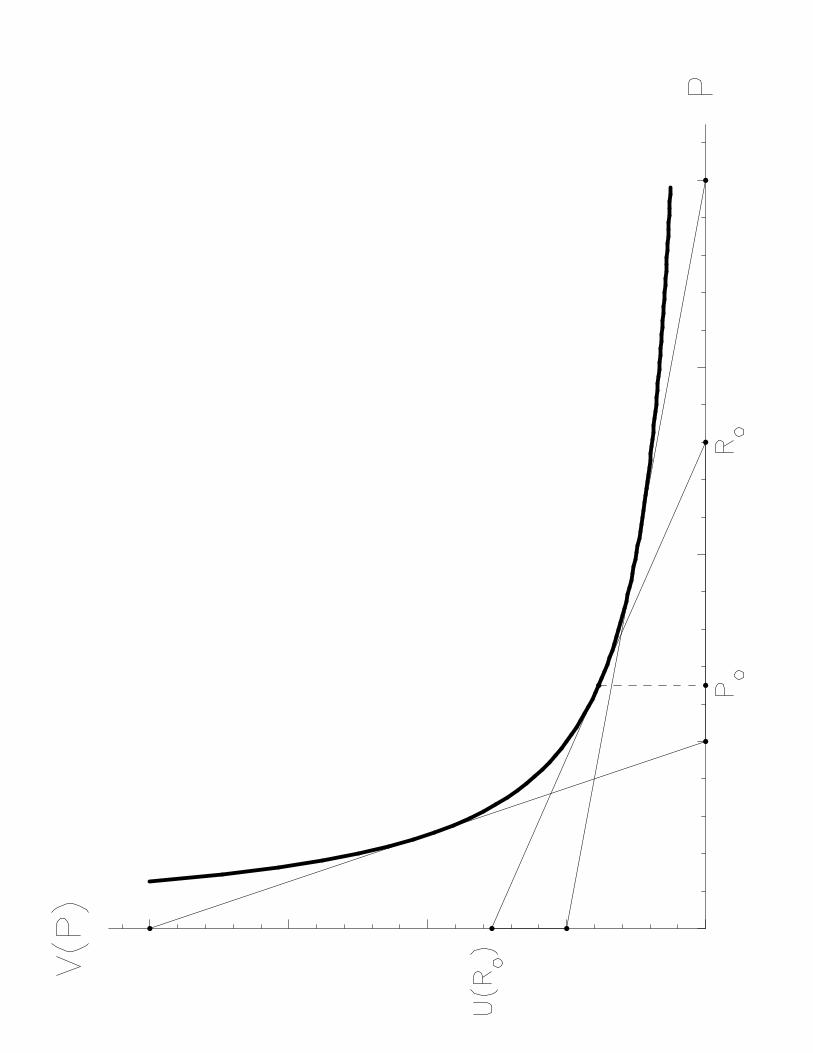
Note that, seen as a function of P for given R, F (P,R) is a straight line intersecting the

horizontal axis at P = R and the vertical axis at F (0, R) = U(R). Therefore, the function U(R)

defines a set of straight lines whose upper envelope gives the function V (P ) (see Fig. 7). The

relation between the functions U(R) and V (P ) is very similar to the Legendre transformation (e.g.,

Courant & Hilbert 1989, §I.6), and shares many of its properties.

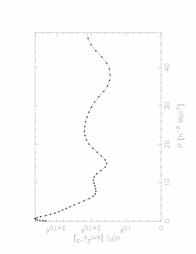
Since U(R) ≥ 0 for all R, V (P ) is positive (V ≥ 0), monotonically decreasing (V ′ ≤ 0),

and convex (V ′′ ≥ 0). Fig. 8 shows the function V (P ) obtained from the data in the way described

in this paper. It is clear that it does not strictly satisfy the conditions of monotonicity and convexity,

indicating that, as expected, the pure spherical infall model does not exactly represent the data.

We can establish a relation R(P ) in the sense that, for any given P = P0, R0 ≡ R(P0) is (are)

the value(s) of R for which the maximum of F (P0, R) occurs, so that

V (P0) = F (P0, R0) =

(

1−P0

R0

)

U(R0) (A2)

(see Fig. 7). In addition, the linear function F (P,R0) is the tangent to V (P ) at P0, so

V ′(P0) =∂F

∂P(P0, R0) = −

U(R0)

R0

. (A3)

– 14 –

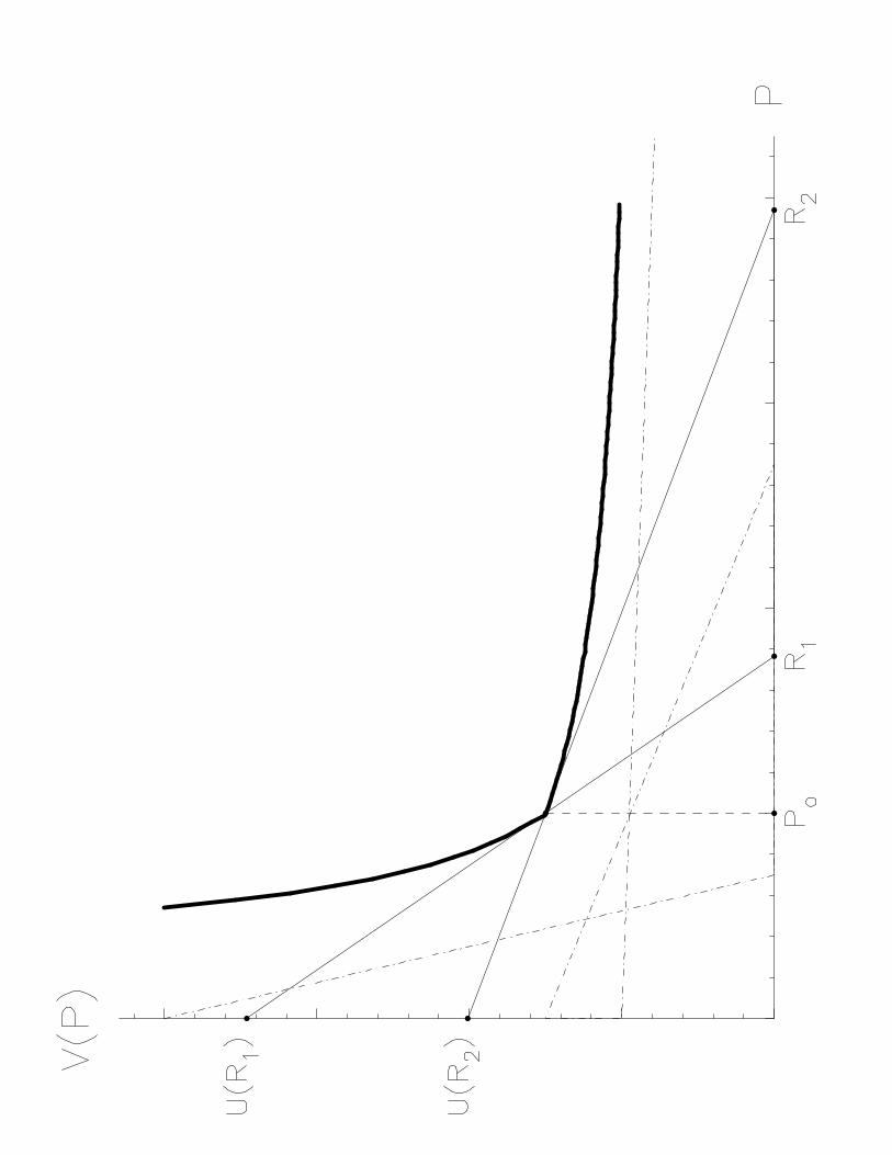
R(P ) is a strictly increasing function, but it is not necessarily continuous. For example, it

can happen that, for some point P0, the maximum occurs at the intersection of two straight lines

labeled by R = R1 and R = R2 > R1 (see Fig. 9), with the lines corresponding to all other values

of R lying below it, i.e.,

V (P0) =

(

1−P0

R1

)

U(R1) =

(

1−P0

R2

)

U(R2) ≥

(

1−P0

R

)

U(R) ∀R ∈ (R1, R2). (A4)

The values of U(R) in the open interval (R1, R2) do not affect the function V (P ) and therefore

cannot be recovered from it. In general, it can only be said that

U(R) ≤ Ub(R) ≡ minP<R

V (P )

1− P/R. (A5)

This is an equality for those R which correspond to a maximum F (P,R) for some P , and a strict

inequality in all other cases. The latter can in principle be diagnosed by realizing that, in the case

discussed above,

limP→P−

0

V ′(P ) = −U(R1)

R1

< limP→P+

0

V ′(P ) = −U(R2)

R2

, (A6)

so both R(P ) and V ′(P ) are discontinuous at P = P0. In practice, with noisy data, a discontinuity

in V ′(P ) is difficult to detect, and the inequality, eq. (A5), has to be used as such. It is interesting

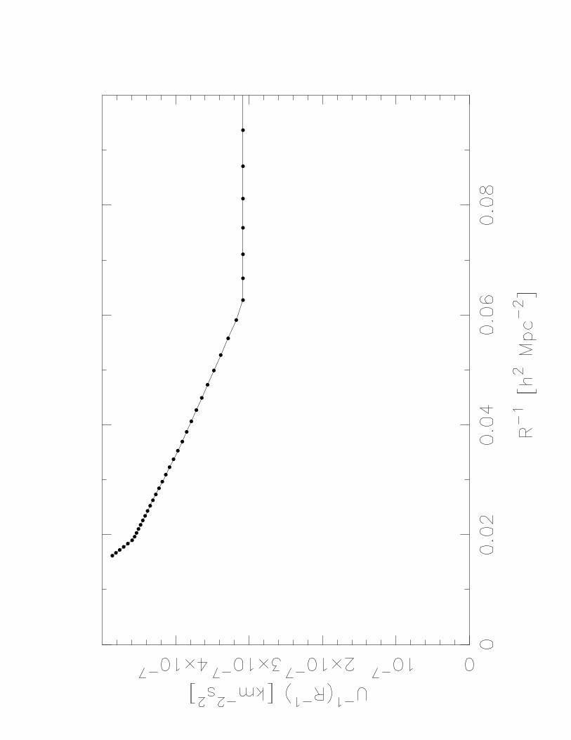
to note that, taking the reciprocal value of all variables, one can write

U−1(R−1) ≥ U−1

b (R−1) = maxP−1>R−1

(

1−R−1

P−1

)

V −1(P−1). (A7)

This has the same form as eq. (A1). We can conclude that U−1

b (R−1) has the same properties as

V (P ), being positive, monotonically decreasing, and convex, in fact, it is the convex and decreasing

lower envelope of U−1(R−1). As long as the latter is itself convex and decreasing, then Ub(R) =

U(R), while in general Ub(R) ≥ U(R). Fig. 10 shows U−1

b (R−1) as obtained from the data. Its

curved parts (here absent) and “corners” are expected (within the pure spherical collapse model)

to correctly estimate U−1(R−1), while the straight segments are lower bounds.

REFERENCES

Abell, G. O., Corwin, H. G. & Olowin, R. P. 1989, ApJS, 70, 1

Bardelli, S., Zucca, E., Zamorani, G., Moscardini, L., & Scaramella, R. 2000, MNRAS, 312, 540

– 15 –

Batuski, D. J., Miller, C. J., Slinglend, K. A., Balkowski, C., Maurogordato, S., Cayatte, V.,

Felenbok, P., & Olowin, R. 1999, ApJ, 520, 491

Carrasco, E. R., Quintana, H., & Reisenegger, A. 2000, in preparation: Paper IV

Courant, R., & Hilbert, D. 1989, Methods of Mathematical Physics, vol. 2 (New York: John Wiley

& Sons)

Diaferio, A. & Geller, M.J. 1997, ApJ, 481, 633

Diaferio, A. 1999, MNRAS, 309, 610

Einasto, M., Tago, E., Jaaniste, J., Einasto, J., & Andernach, H. 1997, A&AS, 123, 119

Ettori, S., Fabian, A. C., & White, D. A. 1997, MNRAS, 289, 787

Geller, M. J., Diaferio, A., & Kurtz, M. J. 1999, ApJ, 517, L23

Harrison, E. R., & Noonan, T. W. 1979, ApJ, 232, 18

Kaiser, N. 1987, MNRAS, 227, 1

Merritt, D., & Tremblay, B. 1994, AJ, 108, 514

Navarro, J. F., Frenk, C. S., & White, S. D. M. 1997, ApJ, 490, 493

Peebles, P. J. E. 1993, Principles of Physical Cosmology (Princeton: Princeton University Press)

Pisani A. 1993, MNRAS, 265, 706

Pisani A. 1996, MNRAS, 278, 697

Quintana, H., Ramırez, A., Melnick, J., Raychaudhury, S. & Slezak, E. 1995, AJ, 110, 463: Paper

I

Quintana, H., Carrasco, E. R., & Reisenegger, A. 2000, AJ, submitted: Paper II

Raychaudhury, S. 1989, Nature, 342, 251

Raychaudhury, S., Fabian, A. C., Edge, A. C., Jones, C., & Forman, W. 1991, MNRAS, 248, 101

Regos, E., & Geller, M.J. 1989, AJ, 98, 755

Shapley, H. 1930, Harvard Coll. Obs. Bull. 874, 9

Silverman, B. W. 1986, Density Estimation for Statistics and Data Analysis (London: Chapman

& Hill)

Small, T. A., Ma, C.-P., Sargent, W. L., & Hamilton, D. 1998, ApJ, 492, 45

– 16 –

Venturi, T., Morganti, R., Bardelli, S., Dallacasa, D., & Hunstead, R. W. 1999, in Observational

Cosmology: The Development of Galaxy Systems, G. Giuricin, M. Mezzetti, and P. Salucci,

eds., Astronomical Society of the Pacific, vol. 176, p. 256

Zucca, E., Zamorani, G., Scaramella, R. & Vettolani, G. 1993, ApJ, 407, 470

This preprint was prepared with the AAS LATEX macros v5.0.

– 17 –

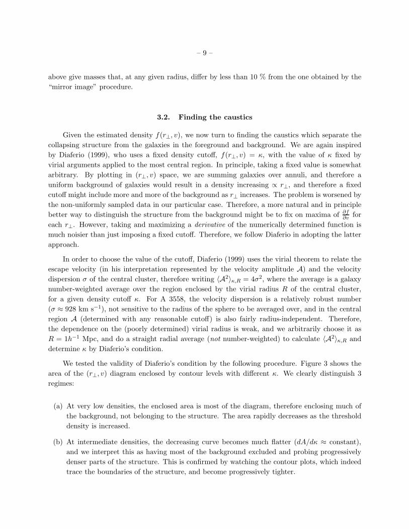
Fig. 1.— Distribution of galaxies and clusters of galaxies in the Shapley Supercluster, with reference

to the central cluster A 3558. The abscissa represents the angular distance θ of each object to the

center of A 3558 (at αc = 13h27m56.9s, δc = −3129′44′′). The vertical axis is the line-of-sight

velocity, cz, where c is the speed of light and z is the redshift. Dots are individual galaxies, circles

represent the centers of clusters and groups of galaxies (see Papers II and IV). Note the dense,

“trumpet shaped” region extending horizontally from the location of A 3558 (circle at θ = 0,

v ≈ 14300 km s−1), which is interpreted as the collapsing structure.

Fig. 2.— The four panels show the central part of the diagram in Fig. 1, with line-of-sight

velocities expressed with respect to A 3558, with the projected radius r⊥ as the abscissa, and

with an isodensity contour superimposed. Each panel corresponds to a different density estimation

scheme. In panel (a), the density estimate is a standard two-dimensional (fixed) kernel smoothing;

in (b) it is modified by considering a “mirror image” of the data to the left-hand side of the

vertical axis; in (c) the estimate is the circularly averaged “surface density” estimate based on

Merritt & Tremblay (1994); in (d) the estimate is the same as in (c), normalized to the values on

the horizontal axis. More details on each of these are given in §3.1, and the choice of isodensity

contours is discussed in §3.2.

Fig. 3.— Area of the (r⊥, v) diagram enclosed by isodensity contours f(r⊥, v) = κ, as a function of

the density cut κ. The vertical line marks the density cut chosen as suggested by Diaferio (1999)

and adopted in the present paper.

Fig. 4.— Enclosed mass as a function of radius around A 3558, given by different methods. The

solid line is is the sum of masses of clusters and groups within the given radius, taking their projected

distance as the true distance to A 3558. The dashed and dot-dashed lines are upper bounds to the

total mass based on the pure spherical infall model, for H0t1 = 0.95 and H0t1 = 0.62, respectively.

The solid-dotted line is the estimate from Diaferio & Geller’s (1997) escape-velocity model.

Fig. 5.— Logarithm of the average enclosed density in units of the critical density, as a function of

radius. The symbols indicate the models, as in Fig. 4.

Fig. 6.— Turnaround time in units of the current age of the Universe, as a function of radius. The

symbols indicate the models, as in Fig. 4.

Fig. 7.— Schematic illustration of the transformation relating V (P ) = A(r2⊥) to U(R) = u2(r2).

See Appendix for an explanation.

Fig. 8.— The function V (P ) = A(r2⊥) determined from the data.

Fig. 9.— Schematic illustration of the transformation relating V (P ) = A2(r2⊥) to U(R) = u2(r2),

when there is a discontinuity in the relation R(P ). See Appendix for an explanation.

Fig. 10.— The function U−1(R−1) = u−2(r−2) determined from the data.

– 18 –

Table 1. Clusters and groups of galaxies in the collapsing region around A 3558 (r⊥ < 8h−1Mpc,

|v| < 2000km s−1)

Name r⊥ v M500

∑

M500 Source

[h−1 Mpc] [km s−1] [1014h−1M⊙] [1014h−1M⊙] for M500

A 3558 0.00 0 6.09 6.09 1

SC 1327-312 0.94 +700 2.14 8.23 1

A 3556 1.92 -16 1.82 10.05 1

SC 1329-314 1.93 -956 1.03 11.08 1

A 3562 2.94 -12 3.06 14.14 1

A 3560 4.36 +144 2.72 16.86 1

A 3552 4.48 +1153 0.36 17.22 2

A 3559 4.65 -376 0.83 18.05 1

A 3554 6.13 +99 1.26 19.31 2

A 3557a 6.18 -114 0.47 19.78 2

A 3555 7.07 -419 0.10 19.88 2

SC 1342-302 7.77 +119 0.20 20.08 2

A 724S 7.86 +367 0.88 20.96 2

A 726S 7.89 +206 0.59 21.55 2

Note. — Columns: 1. Cluster identification. 2. Projected distance from A

3558. 3. Average line-of-sight velocity, relative to A 3558. 4. Adopted cluster

mass within a radius enclosing an average density 500 times the critical density,

from X-ray or optical observations. 5. Cumulative sum of cluster masses. 6.

Source of the cluster mass estimate: (1) X-ray deprojection analysis of Ettori et

al. 1997; (2) preliminary mass estimate from optical determination to be refined

in Paper IV. (The entries in columns 2 and 3 were calculated from the data given

in Paper II.)

0 1 2 3 4 5 6 7 80.5

1

1.5

2

2.5x 10

4

Angular distance from A3558 center [degrees]

Rec

essi

on v

eloc

ity [k

m/s

]