arX

iv:c

s.D

B/0

6070

13 v

1 5

Jul

200

6

Noname manuscript No.(will be inserted by the editor)

Jan Chomicki

Database Querying under ChangingPreferences

Received: date / Accepted: date

Abstract We present here a formal foundation for an iterative and incrementalapproach to constructing and evaluating preference queries. Our main focus ison query modification: a query transformation approach which works by revisingthe preference relation in the query. We provide a detailed analysis of the caseswhere the order-theoretic properties of the preference relation are preserved by therevision. We consider a number of different revision operators: union, prioritizedand Pareto composition. We also formulate algebraic laws that enable incrementalevaluation of preference queries. Finally, we consider twovariations of the basicframework: finite restrictions of preference relations andweak-order extensionsof strict partial order preference relations.

Keywords preference queries· preference revision· query evaluation· strictpartial orders· weak orders

1 Introduction

The notion ofpreferenceis common in various contexts involving decision orchoice. Classical utility theory (Fis70) views preferences asbinary relations. Thisview has recently been adopted in database research (Cho02;Cho03; Kie02; KK02),where preference relations are used in formulatingpreference queries. In AI,various approaches to compact specification of preferenceshave been explored(BBD+04). The semantics underlying such approaches typically relies on prefer-ence relations between worlds.

Research supported by NSF grant IIS-0307434. This paper is an expanded version of (Cho06).

Jan ChomickiDept. of Computer Science and Engineering, University at Buffalo, Buffalo, NY 14260-2000Tel.: +716-645-3180 x103Fax: +716-645-3464E-mail: chomicki@cse.buffalo.edu

2

Preferences can be embedded into database query languages in several dif-ferent ways. First, (Cho02; Cho03; Kie02; KK02) propose to introduce a specialoperator“find all the most preferred tuples according to a given preference rela-tion.” This operator is calledwinnow in (Cho02; Cho03). A special case of win-now is calledskyline(BKS01) and has been recently extensively studied (PTFS03;BGZ04). Second, (AW00; HP04) assume that preference relations are defined us-ing numeric utility functions and queries return tuples ordered by the values ofa supplied utility function. It is well-known that numeric utility functions cannotrepresent all strict partial orders (Fis70), not even thosethat occur in database ap-plications in a natural way (Cho03). For example, utility functions cannot captureskylines. Also, ordered relations go beyond the classical relational model of data.The evaluation and optimization of queries over such relations requires significantchanges to relational query processors and optimizers (ISWGA04). On the otherhand, winnow can be seamlessly combined with any relationaloperators.

We adopt here the first approach, based on winnow, within the preferencequery framework of (Cho03) (a similar model was described in(Kie02)). In thisframework, preference relations between tuples are definedby first-order logicalformulas.

Example 1Consider the relationCar(Make,Year) and the following preferencerelation≻C1 betweenCar tuples:

within each make, prefer a more recent car,

which can be defined as follows:

(m,y)≻C1 (m′,y′)≡m= m′∧y > y′.

The winnow operatorωC1 returns for every make the most recent car available.Consider the instancer1 of Car in Figure 1a. The set of tuplesωC1(r1) is shownin Figure 1b.

Make Year

t1 VW 2002

t2 VW 1997

t3 Kia 1997

(a)

Make Year

t1 VW 2002

t3 Kia 1997

(b)

Fig. 1 (a) The Car relation; (b) Winnow result

In this paper, we focus on preference queries of the formω≻(R), consisting ofa single occurrence of winnow. Here≻ is a preference relation (typically definedby a formula), andR is a database relation. The relationR represents the space ofpossible choices. We also briefly discuss how our results canbe applied to moregeneral preference queries.

3

Past work on preference queries has made the assumption thatpreferences arestatic. However, this assumption is often not satisfied. User preferences change,sometimes as a direct consequence of evaluating a preference query. Therefore,we view preference querying as adynamic, iterative process. The user submits aquery and inspects the result. The result may be satisfactory, in which case thequerying process terminates. Or, the result may be too largeor too small, containunexpected answers, or fail to contain expected answers. Byinspecting the queryanswer, the user may realize some previously unnoticed aspects of her preferences.It is also possible that not all the relevant data was included in the database overwhich the preference query is evaluated.

So if the user is not satisfied with the preference query result, she has severalfurther options:

Modify and resubmitthe query. This is appropriate if the user decides to refineor change her preferences. For example, the user may have started with a partial orvague concept of her preferences (PFT03). We consider here query modificationconsisting ofrevisingthe preference relation≻, although, of course, more generaltransformations may also be envisioned.

Updatethe database. This is appropriate if the user discovers thatthere aremore (or fewer) possible choices than originally envisioned. For example, in com-parison shopping the user may have discovered a new source ofrelevant data.

In this context we pursue the following research challenges:Defining a repertoire of suitable preference relation revisions. In this work,

we consider revisions obtained bycomposingthe original preference relation witha new preference relation, andtransitively closingthe result (to guarantee tran-sitivity). We study different composition operators: union, and prioritized andPareto composition. Those operators represent several basic ways of combiningpreferences and have already been incorporated into preference query languages(Cho03; Kie02). The operators reflect different user attitudes towardspreferenceconflicts. (A conflict is, intuitively, a situation in which two preference relationsorder the same pair of tuples differently.) Union ignores conflicts (and thus suchconflicts need to be prevented if we want to obtain a preference relation whichis a strict partial order). Prioritized composition resolves preference conflicts byconsistently giving priority to one of the preference relations. Pareto compositionresolves conflicts in a symmetric way. We emphasize that revision is done usingcomposition because we want the revised preference relation to be uniquely de-fined in the same first-order language as the original preference relation. Clearly,the revision repertoire that we study in this paper does not exhaust all meaningfulscenarios. One can also imagine approaches where axiomaticproperties of pref-erence revisions are studied, as in belief revision (GR95).

Identifying essential properties of preference revisions. We claim that revisionsshould preserve the order-theoretic properties of the original preference relations.For example, if we start with a preference relation which is astrict partial order, therevised relation should also have those properties. This motivates, among others,transitively closing preference relations to guarantee transitivity. Preserving order-theoretic properties of preference relations is particularly important in view of theiterative construction of preference queries where the output of a revision canserve as the input to another one. We study both necessary andsufficient condi-tions on the original and revising preference relations that yield the preservation of

4

their order-theoretic properties. Necessary conditions are connected with the ab-sence of preference conflicts. However, such conditions aretypically not sufficientand stronger assumptions about the preference relations need to be made. Some-what surprisingly, a special class of strict partial orders, interval orders, plays animportant role in this context. The conditional preservation results we establishin this paper supplement those in (Cho03; Kie02) and may be used in other con-texts where preference relations are composed, for examplein the implementationof preference query languages. Another desirable propertyof revisions is mini-mality in some well-defined sense. We define minimality in terms of symmetricdifference of preference relations but there are clearly other possibilities.

Incremental evaluation of preference queries.At each point of the interactionwith the user, the results of evaluatingpreviousversions of the given preferencequery are available. Therefore, they can be used to make the evaluation of thecurrent query more efficient. For both the preference revision and database up-date scenarios, we formulate algebraic laws that validate new query evaluationplans that use materialized results of past query evaluations. The laws use order-theoretic properties of preference relations in an essential way.

Example 2Consider Example 1. Seeing the result of the queryωC1(r1), a usermay realize that the preference relation≻C1 is not quite what she had in mind.The result of the query may contain some unexpected or unwanted tuples, forexamplet3. Thus the preference relation needs to be modified, for example byrevising it with the following preference relation≻C2:

(m,y)≻C2 (m′,y′)≡m= ′′VW′′∧m′ 6= ′′VW′′∧y = y′.

As there are no conflicts between≻C1 and≻C2, the user chooses union as thecomposition operator. However, to guarantee transitivityof the resulting prefer-ence relation,≻C1 ∪ ≻C2 has to be transitively closed. So the revised relation is≻C∗≡ TC(≻C1 ∪≻C2). (The explicit definition of≻C∗ is given in Example 6.) Thetuplet3 is now dominated byt2 (i.e.,t2≻C∗ t3) and will not be returned to the user.

The plan of the paper is as follows. In Section 2, we define the basic notions. InSection 3, we introduce preference revision. In Section 4, we discuss query modifi-cation and the preservation by revisions of order-theoretic properties of preferencerelations. In Section 5, we discuss incremental evaluationof preference queries inthe context of query modification and database updates. Subsequently, we considertwo variations of our basic framework: (finite) restrictions of preference relations(Section 6) and weak-order extensions of strict partial order preference relations(Section 7). We briefly discuss related work in Section 8 and conclude in Section9.

2 Basic notions

We are working in the context of the relational model of data.Relation schemasconsist of finite sets of attributes. For concreteness, we consider two infinite,countable domains:D (uninterpreted constants, for readability shown as strings)andQ (rational numbers), but our results, except where explicitly indicated, holdalso for finite domains. We assume that database instances are finite sets of tuples.Additionally, we have the standard built-in predicates.

5

2.1 Preference relations

We adopt here the framework of (Cho03).

Definition 1 Given a relation schemaR(A1 · · ·Ak) such thatUi , 1≤ i ≤ k, is thedomain (eitherD or Q) of the attributeAi , a relation≻ is a preference relationover Rif it is a subset of(U1×·· ·×Uk)× (U1×·· ·×Uk).

Although we assume that database instances are finite, in thepresence of infi-nite domains preference relations can be infinite.

Typical properties of a preference relation≻ include (Fis70):

– irreflexivity: ∀x. x 6≻ x;– transitivity: ∀x,y,z. (x≻ y∧y≻ z)⇒ x≻ z;– negative transitivity: ∀x,y,z. (x 6≻ y∧y 6≻ z)⇒ x 6≻ z;– connectivity: ∀x,y. x≻ y∨y≻ x∨x = y;– strict partial order(SPO) if≻ is irreflexive and transitive;– interval order(IO) (Fis85) if≻ is an SPO and satisfies the condition

∀x,y,z,w. (x≻ y∧z≻w)⇒ (x≻ w∨z≻ y);

– weak order(WO) if ≻ is a negatively transitive SPO;– total order if ≻ is a connected SPO.

Every total order is a WO; every WO is an IO.

Definition 2 A preference formula (pf) C(t1, t2) is a first-order formula defining apreference relation≻C in the standard sense, namely

t1≻C t2 iff C(t1, t2).

An intrinsic preference formula (ipf)is a preference formula that uses only built-inpredicates.

By using the notation≻C for a preference relation, we assume that there is anunderlying pfC. Occasionally, we will limit our attention to ipfs consisting of thefollowing two kinds of atomic formulas (assuming we have twokinds of variables:D-variables andQ-variables):

– equality constraints: x = y, x 6= y, x = c, or x 6= c, wherex and y are D-variables, andc is an uninterpreted constant;

– rational-order constraints: xλy or xλc, whereλ ∈ {=, 6=,<,>,≤,≥}, x andy areQ-variables, andc is a rational number.

An ipf all of whose atomic formulas are equality (resp. rational-order) constraintswill be called anequality(resp.rational-order) ipf. If both equality and rational-order constraints are allowed in a formula, the formula willbe calledERO. Clearly,ipfs are a special case of general constraints (KLP00; KKR95), and definefixed,although possibly infinite, relations.

Proposition 1 Satisfiability of quantifier-free ERO formulas is in NP.

6

Proof Satisfiability of conjunctions of atomic ERO constraints can be checked inlinear time (GSW96). In an arbitrary quantifier-free ERO formula negation can beeliminated. Then in every disjunction one needs to nondeterministically select onedisjunct, ultimately obtaining a conjunction of atomic constraints. ⊓⊔

Proposition 1 implies that all the properties that can be polynomially reducedto validity of ERO formulas, for example all the order-theoretic properties listedabove, can be decided in co-NP.

Every preference relation≻ generates an indifference relation∼: two tuplest1 andt2 areindifferent(t1∼ t2) if neither is preferred to the other one, i.e.,t1 6≻ t2andt2 6≻ t1. We denote by∼C the indifference relation generated by≻C.

Composite preference relations are defined from simpler ones using logicalconnectives. We focus on the following basic ways of composing preference rela-tions over the same schema:

– union: t1 (≻1∪≻2) t2 iff t1≻1 t2∨ t1≻2 t2;– prioritized composition: t1 (≻1 �≻2) t2 iff t1≻1 t2∨ (t2 6≻1 t1∧ t1≻2 t2);– Pareto composition:

t1 (≻1⊗≻2) t2 iff (t1≻1 t2∧ t2 6≻2 t1)∨ (t1≻2 t2∧ t2 6≻1 t1).

We will use the above composition operators to construct revisions of given pref-erence relations. We also consider transitive closure:

Definition 3 The transitive closureof a preference relation≻ over a relationschemaR is a preference relationTC(≻) overRdefined as:

(t1, t2) ∈ TC(≻) iff t1≻n t2 for somen > 0,

where:

t1≻1 t2≡ t1≻ t2

t1≻n+1 t2≡ ∃t3. t1≻ t3∧ t3≻n t2.

Clearly, in general Definition 3 leads to infinite formulas. However, in thecases that we consider in this paper the preference relation≻TC(≻) will in fact bedefined by a finite formula.

Proposition 2 Transitive closure of every preference relation defined by an EROipf is definable using an ERO ipf of at most exponential size, which can be com-puted in exponential time.

Proof This is because transitive closure can be expressed in Datalog and the eval-uation of Datalog programs over equality and rational-order constraints terminatesin exponential time (combined complexity) (KKR95). ⊓⊔

In the cases mentioned above, the transitive closure of a given preference rela-tion is a relation definable in the signature of the preference formula. But clearlytransitive closure, unlike union and prioritized or Paretocomposition, is itself nota first-order definable operator.

7

2.2 Winnow

We define now an algebraic operator that picks from a given relation the set of themost preferred tuples, according to a given preference relation.

Definition 4 (Cho03) IfR is a relation schema and≻ a preference relation overR, then thewinnow operatoris written asω≻(R), and for every instancer of R:

ω≻(r) = {t ∈ r | ¬∃t ′ ∈ r. t ′ ≻ t}.

If a preference relation is defined using a pfC, we write simplyωC instead ofω≻C.A preference queryis a relational algebra query containing at least one occurrenceof the winnow operator.

3 Preference revisions

The basic setting is as follows: We have anoriginal preference relation≻ and re-vise it with arevisingpreference relation≻0 to obtain arevisedpreference relation≻′. We also call≻′ a revisionof ≻. We assume that≻,≻0, and≻′ are preferencerelations over the same schema, and that all of them satisfy at least the propertiesof SPOs.

In our setting, a revision is obtained by composing≻ with ≻0 using union,prioritized or Pareto composition, and transitively closing the result (if necessaryto obtain transitivity). However, we formulate some properties, like minimality orcompatibility, in more general terms.

To define minimality, we order revisions using the symmetricdifference (△).

Definition 5 Assume≻1 and≻2 are two revisions of a preference relation≻ witha preference relation≻0. We say that≻1 is closer than≻2 to ≻ if ≻1△≻ ⊂≻2△≻.

To further describe the behavior of revisions, we define several kinds ofpref-erence conflicts. The intuition here is to characterize those conflicts that,wheneliminated by prioritized or Pareto composition, reappearif the resulting prefer-ence relation is closed by transitivity.

Definition 6 A 0-conflict between a preference relation≻ and a preference re-lation ≻0 is a pair(t1, t2) such thatt1≻0 t2 andt2≻ t1. A 1-conflict between≻and ≻0 is a pair(t1, t2) such thatt1≻0 t2 and there exists1, . . .sk, k≥ 1, such thatt2≻ s1≻ ·· · ≻ sk≻ t1 andt1 6≻0 sk 6≻0 · · · 6≻0 s1 6≻0 t2. A 2-conflictbetween≻ and≻0 is a pair(t1, t2) such that there exists1, . . . ,sk, k≥1 andw1, . . . ,wm, m≥1, suchthatt2≻ s1≻ ·· · ≻ sk≻ t1, t1 6≻0 sk 6≻0 · · · 6≻0 s1 6≻0 t2, t1≻0 w1≻0 · · · ≻0 wm≻ t2,andt2 6≻ wm 6≻ · · · 6≻ w1 6≻ t1

A 1-conflict is a 0-conflict if≻ is an SPO, but not necessarily vice versa. A 2-conflict is a 1-conflict if≻0 is an SPO. The different kinds of conflicts are picturedin Figures 2 and 3 (≻ denotes the complement of≻).

8

bt1 b t2

≻0

≺

(a)

bt1 b t2b

sk

b

s1

. . .

≻0

≺,≻0 ≺,≻0

(b)

Fig. 2 (a) 0-conflict; (b) 1-conflict

bt1 b t2

b

w1b

wm. . .

b

sk

b

s1

. . .

≻0,≺ ≻0,≺

≺,≻0 ≺,≻0

Fig. 3 2-conflict

Example 3If ≻0= {(a,b)} and≻= {(b,a)}, then(a,b) is a 0-conflict which isnot a 1-conflict. If we add(b,c) and(c,a) to ≻, then the conflict becomes a 1-conflict (s1 = c). If we further add(c,b) or (a,c) to≻0, then the conflict is not a1-conflict anymore. On the other hand, if we add(a,d) and(d,b) to ≻0 instead,then we obtain a 2-conflict.

We assume here that the preference relations≻ and≻0 are SPOs. If≻′=TC(≻∪≻0), then for every 0-conflict between≻ and≻0, we still obviously havet1 ≻′ t2 andt2 ≻′ t1. Therefore, we say that the union does not resolve any con-flicts. On the other hand, if≻′= TC(≻0 �≻), then for each 0-conflict(t1, t2),t1 ≻0 �≻ t2 and¬(t2 ≻0 �≻ t1). In the case of 1-conflicts, we get againt1 ≻′ t2and t2 ≻′ t1. But in the case where a 0-conflict is not a 1-conflict, we get onlyt1 ≻′ t2. Thus we say that prioritized composition resolves those 0-conflicts thatare not 1-conflicts. Finally, if≻′= TC(≻⊗≻0), then for each 1-conflict(t1, t2),¬(t1 ≻⊗≻0 t2) and¬(t2 ≻⊗≻0 t1). We gett1 ≻′ t2 andt2 ≻′ t1 if the conflictis a 2-conflict, but if it is not, we obtain onlyt2 ≻′ t1. Thus we say that Paretocomposition resolves those 1-conflicts that are not 2-conflicts. (Pareto composi-tion resolves also conflicts that are symmetric versions of 1-conflicts, with≻0 and≻ interchanged, which are not 2-conflicts.)

9

We now characterize those combinations of≻ and≻0 that avoid differentkinds of conflicts.

Definition 7 A preference relation≻ is i-compatible(i = 0,1,2) with a preferencerelation≻0 if there are noi-conflicts between≻ and≻0.

0- and 2-compatibility are symmetric. 1-compatibility is not necessarily symmet-ric. For SPOs, 0-compatibility implies 1-compatibility and 1-compatibility im-plies 2-compatibility. Examples 1 and 2 show a pair of 0-compatible relations.0-compatibility of≻ and≻0 does not requirethe acyclicity of≻∪≻0 or that oneof the following hold:≻ ⊆ ≻0,≻0 ⊆ ≻, or ≻∩≻0 = /0.

Propositions 1 and 2 imply that all the variants of compatibility defined aboveare decidable for ERO ipfs. For example, 1-compatibility isexpressed by the con-dition ≻−1

0 ∩TC(≻−≻−10 ) = /0 where≻−1

0 is the inverse of the preference rela-tion≻0.

0-compatibility of≻ and≻0 is a necessarycondition forTC(≻∪≻0) to beirreflexive, and thus an SPO. Similar considerations apply to TC(≻0 �≻) and 1-compatibility, andTC(≻⊗≻0) and 2-compatibility. In the next section, we willsee that those conditions are notsufficient: further restrictions on the preferencerelations will be introduced.

We conclude by noting the relationships between the three notions of prefer-ence composition introduced above.

Lemma 1 For every preference relations≻ and≻0

≻0⊗≻⊆≻0 �≻⊆≻0∪≻,

and if ≻0 and≻ are 0-compatible

≻0⊗≻=≻0 �≻=≻0∪≻.

4 Query modification

In this section, we study preference query modification1. A given preferencequeryω≻(R) is transformed to the queryω≻′(R) where≻′ is obtained by com-posing the original preference relation≻ with the revising preference relation≻0,and transitively closing the result. (The last step is clearly unnecessary if the ob-tained preference relation is already transitive.) We want≻′ to satisfy the sameorder-theoretic properties as≻ and≻0, and to be minimally different from≻. Toachieve those goals, we impose additional conditions on≻ and≻0.

For everyθ ∈{∪,�,⊗}, we consider the order-theoretic properties of the pref-erence relation≻′ = ≻0 θ ≻, or≻′ = TC(≻0 θ ≻) if ≻0 θ ≻ is not guaranteedto be transitive. To ensure that this preference relation isan SPO, only irreflexivityhas to be guaranteed; for weak orders one has also to establish negative transitivity.

1 The termquery modificationwas used in early relational systems like INGRES to denotea technique that produced a changed version of a query submitted by a user. The changes weremeant to incorporate view definitions, integrity constraints and security specifications. We feelthat it is justified to use the same term in the context of composition of a preference relation ina query with some other preference relation, to produce a newquery.

10

4.1 Strict partial orders

SPOs have several important properties from the user’s point of view, and thustheir preservation is desirable. For instance, all the preference relations definedin (Kie02) and in the language Preference SQL (KK02) are SPOs. Moreover, if≻ is an SPO, then the winnowω≻(r) is nonempty if (a finite)r is nonempty. Thefundamental algorithms for computing winnow require that the preference relationbe an SPO (Cho03). Also, in that case incremental evaluationof preference queriesbecomes possible (Proposition 5 and Theorem 7).

Theorem 1 For every0-compatible preference relations≻ and≻0 such that oneis an interval order (IO) and the other an SPO, the preferencerelation TC(≻0 θ ≻),whereθ ∈ {∪,�,⊗}, is an SPO. If the IO is a WO, then TC(≻0 θ ≻) =≻0 θ ≻.

Proof By Lemma 1, 0-compatibility implies that≻0∪≻ = ≻0 �≻ = ≻0⊗≻.Thus, WLOG we consider only union. Assume≻0 is an IO. If TC(≻∪≻0) is notirreflexive, then≻∪≻0 has a cycle. Consider such cycle of minimum length. Itconsists of edges that are alternately labeled≻0 (only) and≻ (only). (Otherwisethe cycle can be shortened). If there is more than one non-consecutive≻0-edgein the cycle, then≻0 being an IO implies that the cycle can be shortened. So thecycle consists of two edges:t1 ≻0 t2 andt2 ≻ t1. But this is a 0-conflict violating0-compatibility of≻ and≻0. ⊓⊔

It is easy to see that there is no preference relation which isan SPO, contains≻ ∪≻0, and is closer (in the sense of Definition 5) to≻ thanTC(≻∪≻0).

As can be seen from the above proof, the fact that one of the preference re-lations is an interval order makes it possible to eliminate those paths (and thusalso cycles) inTC(≻∪≻0) that interleave≻ and≻0 more than once. In this wayacyclicity reduces to the lack of 0-conflicts.

It seems that the interval order (IO) requirement in Theorem1 cannot be weak-ened without needing to strengthen the remaining assumptions. If neither of≻ and≻0 is an IO, then we can find such elementsx1, y1, z1, w1, x2, y2, z2, w2 that

x1≻ y1,z1≻ w1,x1 6≻ w1,z1 6≻ y1,x2≻0 y2,z2≻0 w2,x2 6≻0 w2,

andz2 6≻0 y2. If we choosey1 = x2, z1 = y2, w1 = z2, andx1 = w2, then we get acycle in≻∪≻0. Note that in this case≻ and≻0 are still 0-compatible. Also, thereis no SPO preference relation which contains≻∪≻0 because each such relationhas to containTC(≻∪≻0). This situation is pictured in Figure 4.

Example 4Consider again the preference relation≻C1:

(m,y)≻C1 (m′,y′)≡m= m′∧y > y′.

Suppose that the new preference information is captured as≻C3 which is an IObut not a WO:

(m,y)≻C3 (m′,y′)≡m= ′′VW′′∧y = 1999∧m′ = ′′Kia′′∧y′ = 1999.

11

bx1 = w2

b

y1 = x2

b z1 = y2

b

w1 = z2

≻≻

0

≺≺0

Fig. 4 A cycle for 0-compatible relations that are not IOs.

ThenTC(≻C1∪≻C3), which properly contains≻C1 ∪≻C3, is defined as the SPO≻C4:

(m,y)≻C4 (m′,y′) ≡ m= m′∧y > y′∨

m= ′′VW′′∧y≥ 1999∧m′ = ′′Kia′′∧y′ ≤ 1999.

Theorem 1 implies that if≻ and≻0 are 0-compatible and one of them containsonly one pair, thenTC(≻∪≻0) is an SPO. So what will happen if we break upthe preference relation≻0 from Figure 4 into two one-element relations≻1 and≻2 and attempt to apply Theorem 1 twice? Unfortunately, such a “strategy” doesnot work. The second step is not possible because the preference relation≻2 isnot 0-compatible with the revision of≻ with ≻1.

For dealing withprioritized composition, 0-compatibility can be replaced by aless restrictive condition, 1-compatibility, because prioritized composition alreadyprovides a way of resolving some conflicts.

Theorem 2 For every preference relations≻ and≻0 such that≻0 is an IO,≻ isan SPO and≻ is 1-compatible with≻0, the preference relation TC(≻0 �≻) is anSPO.

Proof We assume thatTC(≻0 �≻) is not irreflexive and consider a cycle of min-imum length in≻0 �≻. If the cycle has two non-consecutive edges labeled (notnecessarily exclusively) by≻0, then it can be shortened, because≻0 is an IO. Thecycle has to consist of an edget1 ≻0 t2 and a sequence of edges (labeled only by≻): t2 ≻ t3, . . . , tn−1 ≻ tn, tn ≻ t1 such thatn > 2. andt1 6≻0 tn 6≻0 . . . 6≻0 t3 6≻0 t2.(We cannot shorten sequences of consecutive≻-edges because≻ is not necessar-ily preserved in≻0 �≻.) Thus(t1, t2) is a 1-conflict violating 1-compatibility of≻ with ≻0. ⊓⊔

Clearly, there is no SPO preference relation which contains≻0 �≻, and iscloser to≻ thanTC(≻0 �≻). Violating any of the conditions of Theorem 2 maylead to a situation in which no SPO preference relation whichcontains≻0 �≻exists.

If ≻0 is a WO, the requirement of 1-compatibility and the computation oftransitive closure are unnecessary. We first recall some basic properties of weakorders.

12

Proposition 3 Let ≻ be a WO preference relation over a schema R and∼ theindifference relation generated by≻. If x≻ y, y∼ z and z≻w, then also x≻ z andy≻ w.

Theorem 3 For every preference relations≻0 and≻ such that≻0 is a WO and≻ an SPO, the preference relation≻0 �≻ is an SPO.

Proof Clearly,≻′= ≻0 �≻, as a subset of≻0∪≻, is irreflexive. To show tran-sitivity, considert1 ≻′ t2 andt2 ≻′ t3. There are four possibilities: (1) Ift1 ≻0 t2and t2 ≻0 t3, thent1 ≻0 t3 and t1 ≻′ t3. (2) If t1 ≻0 t2, t3 6≻0 t2 andt2 ≻ t3, thenalsot2≻0 t3 or t2∼0 t3 (where∼0 is the indifference relation generated by≻0). Ineither case,t1≻0 t3 andt1≻′ t3 (the second case requires using Proposition 3). (3)t2 6≻0 t1, t1 ≻ t2 andt2 ≻0 t3: symmetric to (2). (4) Ift2 6≻0 t1, t1 ≻ t2, t3 6≻0 t2 andt2≻ t3, thent3 6≻0 t1 (by the negative transitivity of≻0) andt1≻ t3. Thust1≻′ t3.

⊓⊔

Let’s turn now toPareto composition. There does not seem to be any simpleway toweakenthe assumptions in Theorem 1 using the notion of 2-compatibility.Assuming that≻,≻0, or even both are IOs does not sufficiently restrict the possi-ble interleavings of≻ and≻0 in TC(≻0⊗≻) because neither of those two pref-erence relations is guaranteed to be preserved inTC(≻0⊗≻). However, we canestablish a weaker version of Theorem 3.

Theorem 4 For every preference relations≻0 and≻ such that both are WOs, thepreference relation≻0⊗≻ is an SPO.

Proof Similar to the proof of Theorem 3.

Proposition 2 implies that for all preference relations defined using ERO ipfs,the computation of the preference relationsTC(≻∪≻0), TC(≻0 �≻), as wellas TC(≻⊗≻0) terminates. The computation of transitive closure is done in acompletely database-independent way.

Example 5Consider Examples 1 and 4. We can infer that

t1 = (′′VW′′,2002) ≻C4 (′′Kia′′,1997) = t3,

because(′′VW′′,2002)≻C1 (′′VW′′,1999), (′′VW′′,1999)≻C3 (′′Kia′′,1999), and(′′Kia′′,1999)≻C1 (′′Kia′′,1997). The tuples(′′VW′′,1999) and(′′Kia′′,1999) arenot in the database.

If the conditions of Theorems 1 and 2 do not apply, Proposition 2 impliesthat for ERO ipfs the computation ofTC(≻∪≻0), TC(≻0 �≻) andTC(≻⊗≻0)yields some finite ipfC(t1, t2). Thus the irreflexivity of the resulting preferencerelation reduces to the unsatisfiability ofC(t, t), which by Proposition 1 is a de-cidable problem for ERO ipfs. Of course, the relation, beinga transitive closure,is already transitive.

13

Example 6Consider Examples 1 and 2. Neither of the preference relations≻C1and≻C2 is an interval order. Therefore, the results established earlier in this sec-tion do not apply. The preference relation≻C∗= TC(≻C1∪≻C2) is defined as fol-lows (this definition is obtained using Constraint Datalog computation):

(m,y)≻C∗ (m′,y′) ≡ m= m′∧y > y′∨

m= ′′VW′′∧m′ 6= ′′VW′′∧y≥ y′.

The preference relation≻C∗ is irreflexive (this can be effectively checked). Italso properly contains≻C1∪≻C2, becauset1≻C∗ t3 butt1 6≻C1 t3 andt1 6≻C2 t3. ThequeryωC∗(Car) evaluated in the instancer1 (Figure 1) returns only the tuplet1.

4.2 Weak orders

Weak orders are practically important because they capturethe situation where thedomain can be decomposed into layers such that the layers aretotally ordered andall the elements in one layer are mutually indifferent. Thisis the case, for exam-ple, if a preference relation can be represented using a numeric utility function.If a preference relation is a WO, a particularly efficient (essentially single pass)algorithm for computing winnow is applicable (Cho04).

We will see that for weak orders the transitive closure computation is unnec-essary and minimal revisions are directly definable in termsof the preference re-lations involved.

Theorem 5 For every0-compatible WO preference relations≻ and≻0, the pref-erence relations≻∪≻0 and≻⊗≻0 are WO.

Proof In view of Lemma 1, we can consider only≻′=≻∪≻0.Irreflexivity is obvious. For transitivity, assumet1 ≻′ t2 and t2 ≻′ t3. If t1 ≻

t2 ≻ t3 (resp.t1 ≻0 t2 ≻0 t3), thent1 ≻ t3 (resp.t1 ≻0 t3) andt1 ≻′ t3. If t1 ≻0 t2andt2≻ t3, we need 0-compatibility to infer thatt2 6≻ t1 and thust1≻ t2 or t1∼ t2(where∼ is the indifference relation generated by≻). In both cases, we can infert1≻ t3 and thust1≻′ t3. The last case is symmetric to the previous one.

For negative transitivity, considert1 6≻′ t2 andt2 6≻′ t3. Thent1 6≻0 t2, t2 6≻0 t3,t1 6≻ t2, andt2 6≻ t3. Consequently,t1 6≻0 t3, t1 6≻ t3, and thust1 6≻′ t3. ⊓⊔

Note that without the 0-compatibility assumption, WOs are not closed withrespect to union and Pareto composition (Cho03).

For prioritized composition, we can relax the 0-compatibility assumption. Thisimmediately follows from the fact that WOs are closed with respect to prioritizedcomposition (Cho03).

Proposition 4 For every WO preference relations≻ and≻0, the preference rela-tion≻0 �≻ is a WO.

A basic notion in utility theory is that ofrepresentabilityof preference rela-tions using numeric utility functions:

14

Definition 8 A real-valued functionu over a schemaR representsa preferencerelation≻ overR iff

∀t1, t2 [t1≻ t2 iff u(t1) > u(t2)].

Such a preference relation is calledutility-based.

Being a WO is a necessary condition for the existence of a numeric represen-tation for a preference relation. However, it is not sufficient for uncountable orders(Fis70). It is natural to ask whether the existence of numeric representations forthe preference relations≻ and≻0 implies the existence of such a representationfor the preference relation≻′= (≻0 θ ≻) whereθ ∈ {∪,�,⊗}. This is indeed thecase.

Theorem 6 Assume that≻ and≻0 are WO preference relations such that

1. ≻ and≻0 are 0-compatible,2. ≻ can be represented using a real-valued function u,3. ≻0 can be represented using a real-valued function u0.

Then≻′=≻0 θ ≻, whereθ ∈ {∪,�,⊗}, is a WO preference relation that can berepresented using any real-valued function u′ such that for all x

u′(x) = a·u(x)+b·u0(x)+c

where a and b are arbitrary positive real numbers.

Proof Assumex≻′ y. Thusx≻0 y or x≻ y. If x≻0 y, thenu0(x) > u0(y). Also, inthis casey 6≻ xbecause of 0-compatibility. This impliesu(x)≥u(y). Consequently,u′(x) > u′(y). The other case is symmetric.

Assumeu′(x) > u′(y). Thusu0(x) > u0(y) or u(x) > u(y). In the first case, wegetx≻0 y; in the second,x≻ y. Consequently,x≻′ y. ⊓⊔

Surprisingly, the 0-compatibility requirement cannot in general be replaced by1-compatibility if we replace∪ by � in Theorem 6.

Example 7Consider the Euclidean spaceR×R, and the following orders:

(x,y)≻1 (x′,y′)≡ x > x′,

(x,y)≻2 (x′,y′)≡ y > y′,

The orders≻1 and≻2 are 1-compatible (but not 0-compatible) WOs. It is wellknown that their prioritized (also calledlexicographic) composition is not repre-sentable using a utility function (Fis70).

Thus, preservation ofrepresentabilityis possible only under 0-compatibility,in which case≻0∪≻=≻0�≻=≻0⊗≻ (Lemma 1). (The results (Fis70) indicatethat for countable domains considered in this paper, the prioritized composition ofWOs, being a WO, is representable using a utility function. However, that utilityfunction is not definable in terms of the utility functions representing the givenorders.)

15

We conclude this section by showing a general scenario in which the union oforders occurs in a natural way. Assume that we have a numeric utility function urepresenting a (WO) preference relation≻. The indifference relation∼ generatedby≻ is defined as:

x∼ y ≡ u(x) = u(y).

Suppose that the user discovers that∼ is too coarse and needs to be further refined.This may occur, for example, whenx andy are tuples and the functionu takes intoaccount only some of their components. Another functionu0 may be defined totake into account other components ofx andy (such components are calledhiddenattributes(PFT03)). The revising preference relation≻0 is now:

x≻0 y ≡ u(x) = u(y)∧u0(x) > u0(y).

It is easy to see that≻0 is an SPO 0-compatible with≻ (but not necessarily aWO). Therefore, by Theorem 1 the preference relation≻∪≻0 is an SPO.

5 Incremental evaluation

5.1 Query modification

We show here how the already computed result of the original preference querycan be reused to make the evaluation of the modified query moreefficient. We willuse the following result.

Proposition 5 (Cho03) If ≻1 and ≻2 are preference relations over a relationschema R and≻1⊆≻2, then for all instances r of R:

– ω≻2(r) ⊆ ω≻1(r);– ω≻2(ω≻1(r)) = ω≻2(r) if ≻1 and≻2 are SPOs.

Consider the scenario in which we iteratively modify a givenpreference queryby revising the preference relation using only union in sucha way that the revisedpreference relation is an SPO (for example, if the assumptions of Theorem 1 aresatisfied). We obtain a sequence of preference relations≻1, . . . ,≻n such that≻1⊆·· · ⊆≻n.

In this scenario, the sequence of query results is:

r0 = r, r1 = ω≻1(r), r2 = ω≻2(r), . . . , rn = ω≻n(r).

Proposition 5 implies that the sequencer0, r1, . . . , rn is decreasing:

r0⊇ r1⊇ ·· · ⊇ rn

and that it can be computed incrementally:

r1 = ω≻1(r0), r2 = ω≻2(r1), . . . , rn = ω≻n(rn−1).

To computer i , there is no need to look at the tuples inr− r i−1, nor to recomputewinnow from scratch. The sets of tuplesr1, . . . , rn are likely to have much smallercardinality thanr0 = r.

16

It is easy to see that the above comments apply to all cases where the revisedpreference relation is a superset of the original preference relation. Unfortunately,this is not the case for revisions that use prioritized or Pareto composition. How-ever, given a specific pair of preference relations≻ and≻0, one can still effec-tively check whetherTC(≻0 �≻) or TC(≻0⊗≻) contains≻ if the validity ofpreference formulas is decidable, as is the case for ERO formulas (Proposition 1).

5.2 Database update

In the previous section we studied query modification: the query is modified, whilethe database remains unchanged. Here we reverse the situation: the query remainsthe same and the database is updated.

We consider first updates that are insertions of sets of tuples. For a databaserelationr, we denote by∆+r the set of inserted tuples. We show how the previousresult of a given preference query can be reused to make the evaluation of thesame query in an updated database more efficient.

We first establish the following result.

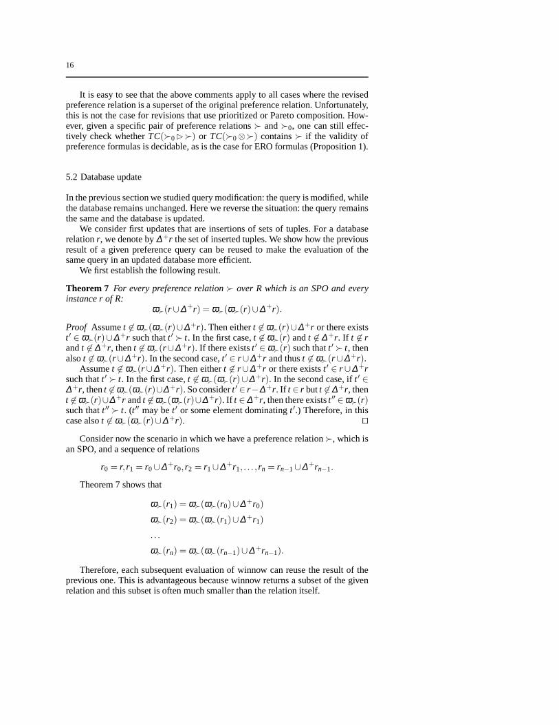
Theorem 7 For every preference relation≻ over R which is an SPO and everyinstance r of R:

ω≻(r ∪∆+r) = ω≻(ω≻(r)∪∆+r).

Proof Assumet 6∈ ω≻(ω≻(r)∪∆+r). Then eithert 6∈ ω≻(r)∪∆+r or there existst ′ ∈ ω≻(r)∪∆+r such thatt ′ ≻ t. In the first case,t 6∈ ω≻(r) andt 6∈ ∆+r. If t 6∈ randt 6∈ ∆+r, thent 6∈ ω≻(r ∪∆+r). If there existst ′ ∈ ω≻(r) such thatt ′ ≻ t, thenalsot 6∈ ω≻(r ∪∆+r). In the second case,t ′ ∈ r ∪∆+r and thust 6∈ ω≻(r ∪∆+r).

Assumet 6∈ ω≻(r ∪∆+r). Then eithert 6∈ r ∪∆+r or there existst ′ ∈ r ∪∆+rsuch thatt ′ ≻ t. In the first case,t 6∈ ω≻(ω≻(r)∪∆+r). In the second case, ift ′ ∈∆+r, thent 6∈ω≻(ω≻(r)∪∆+r). So considert ′ ∈ r−∆+r. If t ∈ r butt 6∈∆+r, thent 6∈ω≻(r)∪∆+r andt 6∈ω≻(ω≻(r)∪∆+r). If t ∈∆+r, then there existst ′′ ∈ω≻(r)such thatt ′′ ≻ t. (t ′′ may bet ′ or some element dominatingt ′.) Therefore, in thiscase alsot 6∈ ω≻(ω≻(r)∪∆+r). ⊓⊔

Consider now the scenario in which we have a preference relation≻, which isan SPO, and a sequence of relations

r0 = r, r1 = r0∪∆+r0, r2 = r1∪∆+r1, . . . , rn = rn−1∪∆+rn−1.

Theorem 7 shows that

ω≻(r1) = ω≻(ω≻(r0)∪∆+r0)

ω≻(r2) = ω≻(ω≻(r1)∪∆+r1)

. . .

ω≻(rn) = ω≻(ω≻(rn−1)∪∆+rn−1).

Therefore, each subsequent evaluation of winnow can reuse the result of theprevious one. This is advantageous because winnow returns asubset of the givenrelation and this subset is often much smaller than the relation itself.

17

Clearly, the algebraic law, stated in Theorem 7, can be used together with other,well-known laws of relational algebra and the laws specific to preference queries(Cho03; KH03) to produce a variety of rewritings of a given preference query. Tosee how a more complex preference query can be handled, let’sconsider the queryconsisting of winnow and selection,ω≻(σα(R)). We have

ω≻(σα(r ∪∆+r)) = ω≻(σα(r)∪σα(∆+r)) = ω≻(ω≻(σα(r))∪σα(∆+r))

for every instancer of R. Here again, one can use the previous result of the query,ω≻(σα(r)), to make its current evaluation more efficient. Other operators thatdistribute through union, for example projection and join,can be handled in thesame way.

Next, we consider updates that are deletions of sets of tuples. For a databaserelationr, we denote by∆−r the set of deleted tuples.

Theorem 8 For every preference relation≻ over R and every instance r of R:

ω≻(r)−∆−r ⊆ ω≻(r−∆−r).

Theorem 8 gives an incremental way to compute an approximation of winnowfrom below. It seems that in the case of deletion there cannotbe an exact lawalong the lines of Theorem 7. This is because the deletion of some tuples from theoriginal database may promote some originally dominated (and discarded) tuplesinto the result of winnow over the updated database.

Example 8Consider the following preference relation≻= {(a,b1), . . . ,(a,bn)}and the databaser = {a,b1, . . . ,bn}. Thenω≻(r) = {a} but

ω≻(r−{a}) = {b1, . . . ,bn}.

6 Finite restrictions of preference relations

6.1 Restriction

It is natural to considerrestrictionsof preference relations to given database in-stances (TC02).

Definition 9 Let r be an instance of a relation schemaR and≻ a preference rela-tion overR. Therestriction[≻]r of≻ to r is a preference relation overR, definedas

[≻]r = ≻ ∩ r× r.

We write(x,y) ∈ [≻]r instead ofx[≻]ry for greater readability.The advantage of using[≻]r instead of≻ comes from the fact that the for-

mer depends on the database contents and can have stronger properties than thelatter. For example,[≻]r may be an SPO, while≻ is not. Similarly,[≻]r may bei-compatible with[≻0]r , while≻ is not i-compatible with≻0. Therefore, restric-tions could be used instead of preference relations in the revision process.

The following is a basic property of restriction. It says that the restriction toan instance does not affect the result of winnowover the same instance, so therestriction can be used in place of the original preference relation.

18

Theorem 9 Let r be an instance of a relation schema R and≻ a preference rela-tion over R. Then

ω[≻]r (r) = ω≻(r).

Proof We have[≻]r ⊆ r and thusω≻(r)⊆ω[≻]r (r). In the other direction, assumet 6∈ ω≻(r). If t 6∈ r, t 6∈ ω[≻]r (r). If t ∈ r and there existst ′ ∈ r such thatt ′ ≻ t, thenalso(t ′, t) ∈ [≻]r andt 6∈ ω[≻]r (r). ⊓⊔

We also establish that restriction distributes over the preference compositionoperators.

Theorem 10 If r is an instance of a relation schema R,θ ∈ {∪,�,⊗}, and≻ and≻0 are preference relations over R, then

[≻0 θ ≻]r = [≻0]rθ [≻]r .

Proof We prove this result forθ = �. The other cases are similar.We have the following equivalences:

(x,y) ∈ [≻0]r � [≻]r ≡

(x,y) ∈ [≻0]r ∨ (y,x) 6∈ [≻0]r ∧ (x,y) ∈ [≻]r ≡

x≻0 y∧x∈ r ∧y∈ r ∨ (y 6≻0 x∨x 6∈ r ∨y 6∈ r)∧x≻ y∧x∈ r ∧y∈ r ≡

x≻0 y∧x∈ r ∧y∈ r ∨y 6≻0 x∧x≻ y∧x∈ r ∧y∈ r ≡

(x≻0 y∨y 6≻0 x∧x≻ y)∧x∈ r ∧y∈ r ≡

(x,y) ∈ [≻0 �≻]r .

The preference revision studied earlier in this paper typically involved thecomputation of the of the revised preference relation defined as the transitive clo-sureTC(≻0 θ ≻), whereθ ∈ {∪,�,⊗},≻ is the original preference relation, and≻0 is the revising preference relation. We study several different ways of impos-ing the restriction of preferences to a relation instance. We consider the followingpreference relations:

≻1 = TC(≻0 θ ≻),

≻2 = [TC(≻0 θ ≻)]r ,

≻3 = TC([≻0 θ ≻]r),

≻4 = TC([≻0]rθ [≻]r).

We establish now some fundamental relationships between the preference re-lations≻1,≻2,≻3, and≻4.

Theorem 11 Let θ ∈ {∪,�,⊗}, and≻ and≻0 be preference relations over aschema R. Then for every instance r of R:

≻4 = ≻3 ⊆ ≻2 ⊆ ≻1,

and there are relation instances for which the containmentsare strict.

19

Proof The equality of≻4 and≻3 follows from Theorem 10. For≻3 ⊆ ≻2, wehave that

[≻0 θ ≻]r ⊆ ≻0 θ ≻,

and[≻0 θ ≻]r ⊆ r× r.

Thus≻3= TC([≻0 θ ≻]r)⊆ r× r,

and≻3⊆ TC(≻0 θ ≻)∩ r× r =≻2 .

The containment≻2 ⊆ ≻1 follows from the definition of the restriction.An example where≻3 ⊂ ≻2 ⊂ ≻1 is as follows. Let≻= {(a,b)}, ≻0=

{(b,c)}, r = {a,c}. Then[≻]r = [≻0]r = /0. Thus also[≻0 θ ≻]r = [≻0]r θ [≻]r =/0, and≻3= /0. On the other hand,≻1= {(a,b),(b,c),(a,c)} and≻2= {(a,c)}.

⊓⊔

Corollary 1 Let θ ∈ {∪,�,⊗}, and≻ and≻0 be preference relations over aschema R. Then for every instance r of a R:

ω≻1(r) = ω≻2(r)⊆ ω≻3(r) = ω≻4(r),

and for some cases the containment is strict.

Proof Follows from Theorem 9 and Theorem 11. In the example given intheproof of Theorem 11, we obtainω≻2(r) = {a} andω≻3(r) = {a,c}. ⊓⊔

We study now the order-theoretic properties of restriction.

Theorem 12 Let θ ∈ {∪,�,⊗}, and≻ and≻0 be preference relations over aschema R. Then for every instance r of R,≻1 is an SPO implies that≻2 is an SPO,which implies that≻3 is an SPO. There are cases in which the reverse implicationdoes not hold.

Proof Because≻2 ⊆ ≻1, ≻2 is irreflexive. Assume thatx≻2 y andy≻2 z. Thenx≻1 y, y≻1 z, x∈ r, y∈ r, andz∈ r. Therefore,x≻1 z∧x∈ r ∧z∈ r, andx≻2 z.

The preference relation≻1= {(a,a)} is not an SPO (and can be obtained fromsome preference relations≻0 and≻ using any composition operator). However,its restriction≻2= [≻1]r for r = {b} is empty, and thus an SPO.

Assume now≻0= {(a,b)} and≻= {(b,a)}. Considerθ = ∪ and r = {b}.Thus,≻1= {(a,b),(b,a),(a,a),(b,b)} and≻2= {(b,b)} (so it is not an SPO).On the other hand,[≻0 ∪ ≻]r = /0 and≻3= /0, too. Similar examples can be con-structed for the other composition operators. ⊓⊔

Unfortunately, for weak orders there is no property analogous to Theorem 12.Subsequently, we examine the impact of restriction on compatibility.

Theorem 13 Let ≻ and≻0 be preference relations over a schema R. Then forevery instance r of a relation schema R and every i= 0,1,2 if ≻ is i-compatiblewith≻0, then[≻]r is i-compatible with[≻0]r . There are cases in which the reverseimplications do not hold.

20

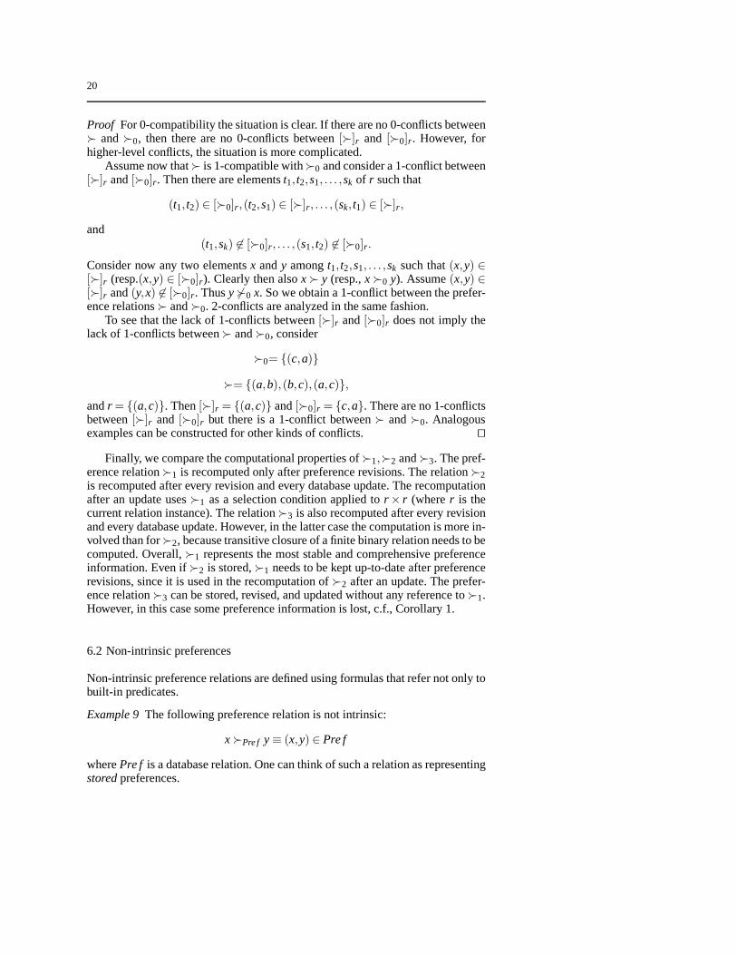
Proof For 0-compatibility the situation is clear. If there are no 0-conflicts between≻ and≻0, then there are no 0-conflicts between[≻]r and [≻0]r . However, forhigher-level conflicts, the situation is more complicated.

Assume now that≻ is 1-compatible with≻0 and consider a 1-conflict between[≻]r and[≻0]r . Then there are elementst1, t2,s1, . . . ,sk of r such that

(t1, t2) ∈ [≻0]r ,(t2,s1) ∈ [≻]r , . . . ,(sk, t1) ∈ [≻]r ,

and(t1,sk) 6∈ [≻0]r , . . . ,(s1, t2) 6∈ [≻0]r .

Consider now any two elementsx andy amongt1, t2,s1, . . . ,sk such that(x,y) ∈[≻]r (resp.(x,y) ∈ [≻0]r). Clearly then alsox≻ y (resp.,x≻0 y). Assume(x,y) ∈[≻]r and(y,x) 6∈ [≻0]r . Thusy 6≻0 x. So we obtain a 1-conflict between the prefer-ence relations≻ and≻0. 2-conflicts are analyzed in the same fashion.

To see that the lack of 1-conflicts between[≻]r and[≻0]r does not imply thelack of 1-conflicts between≻ and≻0, consider

≻0= {(c,a)}

≻= {(a,b),(b,c),(a,c)},

andr = {(a,c)}. Then[≻]r = {(a,c)} and[≻0]r = {c,a}. There are no 1-conflictsbetween[≻]r and [≻0]r but there is a 1-conflict between≻ and≻0. Analogousexamples can be constructed for other kinds of conflicts. ⊓⊔

Finally, we compare the computational properties of≻1,≻2 and≻3. The pref-erence relation≻1 is recomputed only after preference revisions. The relation≻2is recomputed after every revision and every database update. The recomputationafter an update uses≻1 as a selection condition applied tor × r (wherer is thecurrent relation instance). The relation≻3 is also recomputed after every revisionand every database update. However, in the latter case the computation is more in-volved than for≻2, because transitive closure of a finite binary relation needs to becomputed. Overall,≻1 represents the most stable and comprehensive preferenceinformation. Even if≻2 is stored,≻1 needs to be kept up-to-date after preferencerevisions, since it is used in the recomputation of≻2 after an update. The prefer-ence relation≻3 can be stored, revised, and updated without any reference to≻1.However, in this case some preference information is lost, c.f., Corollary 1.

6.2 Non-intrinsic preferences

Non-intrinsic preference relations are defined using formulas that refer not only tobuilt-in predicates.

Example 9The following preference relation is not intrinsic:

x≻Pre f y≡ (x,y) ∈ Pre f

wherePre f is a database relation. One can think of such a relation as representingstoredpreferences.

21

Revising non-intrinsic preference relations looks problematic. First, it is typ-ically not possible to establish the simplest order-theoretic properties of such re-lations. For instance, in Example 9 it is not possible to determine the irreflexivityor transitivity of≻Pre f on the basis of its definition. Whether such properties aresatisfied depends on the contents of the database relationPre f. Second, the tran-sitive closure of a non-intrinsic preference relation may fail to be expressed as afinite formula. Again, Example 9 can be used to illustrate this point.

However, it seems that restriction may be able to alleviate the above problems.Suppose≻ is the original and≻0 the revising preference relations. ComputingTC(≻0 ∪ ≻) may be infeasible, as indicated above. But computingTC([≻0 ∪ ≻]r)is not difficult, as[≻0 ∪ ≻]r is computed by the first-order query

(x≻0 y∨x≻ y)∧x∈ R∧y∈ R.

For other composition operators, the same approach also works because they are,like union, defined in a first-order way.

7 Weak-order extensions

Theorems 3 and 5, and Proposition 4 demonstrate that for weakorders one canprove stronger properties about revisions than for generalpartial orders. The 0-compatibility or the interval order requirements may be relaxed, and the transitiveclosure computation may no longer be necessary.

So it would be advantageous to work with weak orders. Such orders can, forexample, be obtained asextensionsof the given SPOs. We show here how to ex-press the construction of weak order extensions using Datalog¬ rules (AHV95)and the Rule Algebra (IN88). Although not much can be shown inthat frameworkabout WO extensions of arbitrary SPOs, the construction of WO extensions ofinterval orders (IOs) can be guaranteed to terminate.

7.1 Rules

We define theapplication r(X) of a ruler to an input set of factsX in the standardway.

Definition 10 Assumer is of the form

A← B1, . . . ,Bn,¬C1, . . . ,¬Cm.

Then r(X) consists of all the factsτ(A) such thatτ(Bi) ∈ X, i = 1, . . . ,n, andτ(Cj ) 6∈ X, j = 1, . . . ,m, whereτ is a ground substitution. In aninflationaryappli-cationr(X) is added toX.

In this paper, we are dealing with infinite sets of facts represented by con-straints. However, the above definition of rule applicationstill applies. From thisdefinition, we can obtain a more operational definition that will tell us how toconstruct the constraints in the head of the ruler from the constraints in the body(KLP00).

22

Assume that each goalBi , i = 1, . . . ,n is described by a constraintβi and eachgoalCj , j = 1, . . . ,m by a constraintγ j . Also denote byV the set of variables thatoccur only in the body ofr. ThenA is described by the formula

∃V. β1∧·· ·∧βn∧¬γ1∧·· ·∧¬γm.

from which negation and quantifiers have been eliminated.(IN88) present a language called Rule Algebra (RA) which allows rule com-

position. The syntax of RA expressions is defined as follows:

Expr ::= r |Expr; Expr|Expr∪ Expr|Expr+,

wherer is a single rule. The symbol “;” denotes sequential and “∪”, parallel com-position. The superscript “+” denotes unbounded iteration.

The application of RA expressions is defined as follows (IN88):

– for a single rule it is defined as in Definition 10,– (F1;F2)(X)

.= F2(F1(X)),

– (F1∪F2)(X).= F1(X)∪F2(X),

– F+(X).=

⋃i>0F i(X).

Like rule application, the application of RA expressions comes in two differentvariants: inflationary and non-inflationary.

Rule Algebra can be implemented directly. However, (IN88) show also howto map Rule Algebra expressions to a class oflocally-stratifiedlogic programs(Prz88). This class requires a limited use of function symbols to implement coun-ters.

7.2 Strict partial orders

(Fis85) presents a construction of a WO extension of a finite SPO. It is based on avery simple intuition.

Assume we are given thatx ≻ y and y∼ z, or x∼ y and y≻ z. In a weakorder one needs to be able to have alsox≻ z in both cases (see Proposition 3).Therefore, one could produce a WO extension≻′ of a given SPO≻ by supportingthederivationof the implied order relationships. Clearly, such derivation shouldavoid contradiction (x≻′ y andy≻′ x).

Example 10Consider the following order≻= {(a,c),(b,d)}. Thus a ∼ d andb∼ c. So w could derivea≻′ b andb≻′ a, a contradiction.

We construct an extension≻′ of a given SPO≻ using a set of rules. Unfortu-nately, for infinite orders the construction does not alwaysproduce a weak order.The input preference relation≻ is described using a set of facts of the relationTof arity 2n wheren is the arity of the database relation over which≻ is defined.The output preference relation≻′ is also described as a set of facts of the relationT but those facts are computed using rule application.

First, we have two rulesP11 andP12 for deriving new order relationships:

P11 : T(x,z)← T(x,y)∧¬T(z,y)∧¬T(y,z).

23

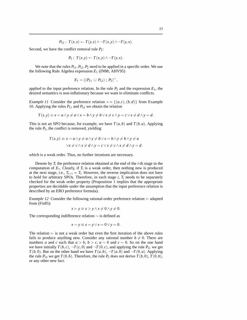
P12 : T(x,z)← T(y,z)∧¬T(x,y)∧¬T(y,x).

Second, we have the conflict removal ruleP2:

P2 : T(x,y)← T(x,y)∧¬T(y,x).

We note that the rulesP11,P12,P2 need to be applied in a specific order. We usethe following Rule Algebra expressionE1 (IN88; AHV95)

E1 = ((P11 ∪ P12) ; P2)+,

applied to the input preference relation. In the ruleP2 and the expressionE1, thedesired semantics is non-inflationary because we want to eliminate conflicts.

Example 11Consider the preference relation≻= {(a,c),(b,d)} from Example10. Applying the rulesP11 andP12 we obtain the relation

T(x,y)≡ x = a∧y 6= a∨x = b∧y 6= b∨x 6= c∧y = c∨x 6= d∧y = d.

This is not an SPO because, for example, we haveT(a,b) andT(b,a). Applyingthe ruleP2, the conflict is removed, yielding

T(x,y) ≡ x = a∧y 6= a∧y 6= b∨x = b∧y 6= b∧y 6= a

∨x 6= c∧x 6= d∧y = c∨x 6= c∧x 6= d∧y = d.

which is a weak order. Thus, no further iterations are necessary.

Denote byTi the preference relation obtained at the end of thei-th stage in thecomputation ofE1. Clearly, if Ti is a weak order, then nothing new is producedat the next stage, i.e.,Ti+1 = Ti . However, the reverse implication does not haveto hold for arbitrary SPOs. Therefore, in each stagei, Ti needs to be separatelychecked for the weak order property (Proposition 1 implies that the appropriateproperties are decidable under the assumption that the input preference relation isdescribed by an ERO preference formula).

Example 12Consider the following rational-order preference relation≻ adaptedfrom (Fis85):

x≻ y≡ x > y∧x 6= 0∧y 6= 0.

The corresponding indifference relation∼ is defined as

x∼ y≡ x = y∨x = 0∨y = 0.

The relation≻ is not a weak order but even the first iteration of the above rulesfails to produce anything new. Consider any rational numberb 6= 0. There arenumbersa andc such thata > b, b > c, a∼ 0 andc∼ 0. So on the one handwe have initiallyT(b,c), ¬T(c,0) and¬T(0,c), and applying the ruleP11 we getT(b,0). But on the other hand we haveT(a,b), ¬T(a,0) and¬T(0,a). Applyingthe ruleP12 we getT(0,b). Therefore, the ruleP2 does not deriveT(b,0), T(0,b),or any other new fact.

24

It is an open question what kind of properties a preference relation should sat-isfy so that the conditionTi+1 = Ti implies the weak order property. (Fis85) showsthat such an implication holds for SPOs over finite domains. Therefore, it alsoholds for finite restrictions of arbitrary SPOs (Section 6).For a finite restriction[≻]r a different way for constructing a weak order extension of[≻]r is availablethrough the use ofranking(Cho03). The “best” tuples – those inω≻(r) – receiverank 1, the “second-best” rank 2 etc. Then the weak order extension≻′ is definedas

x≻′ y≡ rank(x) < rank(y).

7.3 Interval orders

For interval orders, we can show stronger results about constructing WO exten-sions. We still use the Datalog¬/Rule Algebra framework but instead of the ex-pressionE1 we use the following expressionE2:

E2 = (P11 ; P12)+.

We will see that forE2 the inflationary and non-inflationary semantics coin-cide.

For simplicity, we identify here a preference relation withthe set of facts oftheT predicate describing it.

Example 13Consider Example 12. Applying the ruleP11 to the preference rela-tion≻ from this example (which is an interval order) yields the following prefer-ence relation≻′:

x≻′ y≡ x > y∧x 6= 0∧y 6= 0∨x 6= 0∧y = 0.

This relation is a total order, and thus also a weak order.

Lemma 2 For every irreflexive preference relation X, X⊆ P11(X), X ⊆ P12(X),and X⊆ P12(P11(X)).

Lemma 3 Assume X is an interval order preference relation. Then P11(X) andP12(X) are interval order preference relations.

Proof WLOG, considerY = P11(X). Clearly,Y is irreflexive. For transitivity, con-siderT(x,y)∈Y andT(y,z)∈Y. Then there is az′ such thatT(x,z′)∈X, T(z′,y) 6∈X, andT(y,z′) 6∈X. Similarly, there is az′′ such thatT(y,z′′)∈X, T(z′′,z) 6∈X, andT(z,z′′) 6∈ X. BecauseX is an interval order, we haveT(x,z′′) ∈ X or T(y,z′) ∈ X.Assume the former. ThenT(x,z) ∈Y. The preservation of the interval order con-dition can be shown in a similar way. ⊓⊔

Lemma 4 Let F = (P11;P12) and Y be an SPO. Then F(Y)⊆Y iff Y is a WO.

Proof If Y is a WO, then

Y = P11(Y) = P12(P11(Y)).

If Y is not a WO but an SPO, then there arex, y and z such thatT(x,y) ∈ Y,T(x,z) 6∈Y, T(z,x) 6∈Y, T(y,z) 6∈Y andT(z,y) 6∈Y. ThusT(x,z) ∈ P11(Y) and byLemma 2,T(x,z) ∈ P12(P11(Y)). ThusP12(P11(Y)) 6⊆Y. ⊓⊔

25

The following theorem shows that finite termination of the evaluation ofE2 isequivalent to the weak order property.

Theorem 14 Let X be an IO. For every i> 0, E2(X) = (P11;P12)+(X) equals

(P11;P12)i(X) iff (P11;P12)

i(X) is a WO.

Proof Follows from Lemmas 2, 3, and 4. Note that forj < i, (P11;P12)j(X) ⊆

(P11;P12)i(X). It is essential that the given preference relation be an IO.Otherwise,

an application ofP11;P12 may produce preference relations which are not SPOsand the equivalence in Lemma 4 may stop to hold. ⊓⊔

To explore the possible implementations of the Rule AlgebraexpressionE2,we note first that Lemma 2 implies that for the rulesP11 andP12 inflationary andnon-inflationary semantics coincide. Therefore, we can useinflationary or non-inflationary languages for the implementation ofE2. (AHV95) indicate that RuleAlgebra expressions can be translated to Inflationary Datalog¬ (GS86), a variantof Datalog that allows unstratified negation (necessary here because of the rulesP11 andP12) at the price of having inflationary semantics. It is clear that Inflation-ary Datalog¬ programs terminate on finite inputs. However, preference relationsare typically infinite. Still, they are finitely representable using preference for-mulas, and thus we are dealing with the problem of termination of InflationaryConstraint Datalog¬ programs. Fortunately, there are positive results establishedin this area in (KKR95), which, together with Theorem 14, imply the following:

Theorem 15 Every interval order preference relation≻, defined using an EROformula, has a weak order extension≻′, defined using an ERO formula. The for-mula defining≻′ can be computed in exponential time.

8 Related work

8.1 Preference change

(Han95) presents a general framework for modeling change inpreferences. Prefer-ences are represented syntactically using sets of ground preference formulas, andtheir semantics is captured using sets of preference relations. Thanks to the syntac-tic representation preference revision is treated similarly, though not identically,to belief revision (GR95), and some axiomatic properties ofpreference revisionsare identified. The result of a revision is supposed to be minimally different fromthe original preference relation (using a notion of minimality based on symmetricdifference) and satisfy some additional background postulates, for example spe-cific order axioms. (Han95) does not address the issue of constructing or definingrevised relations, nor does it study the properties of specific classes of preferencerelations. On the other hand, (Han95) discusses also preference contraction, anddomain expansion and shrinking.

In our opinion, there are several fundamental differences between belief andpreference revision. In belief revision, propositional theories are revised with propo-sitional formulas, yielding new theories. In preference revision, binary preferencerelations are revised with other preference relations, yielding new preference re-lations. Preference relations are single, finitely representable (though possibly in-finite) first-order structures, satisfying order axioms. Belief revision focuses on

26

axiomatic properties of belief revision operators and various notions of revisionminimality. Preference revision focuses on axiomatic, order-theoretic propertiesof revised preference relations and the definability of suchrelations (though stilltaking revision minimality into account).

(Wil97) considers revising a ranking (a WO) of a finite set of tuples with newinformation, and shows that a new ranking, satisfying the AGM belief revisionpostulates (GR95), can be computed in a simple way. (Rev97) describes a numberof different revision operators for constraint databases.However, the emphasisis on the axiomatic properties of the operators, not on the definability of reviseddatabases. (PFT03) formulates various scenarios of preference revision and doesnot contain any formal framework. (Won94) studies revisionand contraction offinite WO preference relations by single pairst1≻0 t2. (Fre04) describes minimalchange revision ofrational preference relations between propositional formulas.

8.2 Preference queries

Two different approaches to preference queries have been pursued in the literature:qualitative and quantitative. In thequalitativeapproach, preferences are specifiedusing binarypreference relations(LL87; GJM00; Cho02; Cho03; Kie02; KK02).In the quantitativeutility-based approach, preferences are represented using nu-meric utility functions(AW00; HP04), as shown in Section 4. The qualitative ap-proach is strictly more general than the quantitative one, since one can definepreference relations in terms of utility functions. However, only WO preferencerelations can be represented by numeric utility functions (Fis70). Preferences thatare not WOs are common in database applications, c.f., Example 1.

Example 14There is no utility function that captures the preference relation de-scribed in Example 1. Since there is no preference defined betweent1 andt3 or t2andt3, the score oft3 should be equal to the scores of botht1 andt2. But this im-plies that the scores oft1 andt2 are equal which is not possible sincet1 is preferredovert2.

This lack of expressiveness of the quantitative approach iswell known in utilitytheory (Fis70). The paper (Cho03) contains an extensive discussion of the prefer-ence query literature.

In the earlier work on preference queries (Cho03; Kie02), one can find positiveand negative results about closure of different classes of orders, including SPOsand WOs, under various composition operators. The results in the present paperare, however, new. Restricting the relations≻ and≻0 (for example, assuming theinterval order property and compatibility) and applying transitive closure wherenecessary make it possible to come up with positive counterparts of the negativeresults in (Cho03). For example, (Cho03) shows that SPOs andWOs are in generalnot closed w.r.t. union, which should be contrasted with Theorems 1 and 5. In(Kie02), Pareto and prioritized composition are defined somewhat differently fromthe present paper. The operators combine two preference relations, each definedover some database relation. The resulting preference relation is defined over theCartesian product of the database relations. So such operators are not useful in thecontext of revision of preference relations. On the other hand, the careful design

27

of the language guarantees that every preference relation that can be defined is anSPO.

Probably the most thoroughly studied class of qualitative preference queriesis the class ofskylinequeries. A skyline query partitions all the attributes of arelation into DIFF, MAX, and MIN attributes. Only tuples with identical valuesof all DIFF attributes are comparable; among those, MAX attribute values aremaximized and MIN values are minimized. The query in Example1 is a verysimple skyline query (BKS01), withMakeas a DIFF andYearas a MAX attribute.Without DIFF attributes, a skyline is a special case ofn-ary Pareto composition.

Various algorithms for evaluating qualitative preferencequeries are describedin (Cho03; TC02), and for evaluating skyline queries, in (BKS01; PTFS03; BGZ04).(BG04) describes how to implement preference queries that use Pareto compo-sitions of utility-based preference relations. In Preference SQL (KK02) generalpreference queries are implemented by a translation to SQL.(HP04) describeshow materialized results of utility-based preference queries can be used to answerother queries of the same kind.

8.3 CP-nets

CP-nets (BBD+04) are an influential recent formalism for reasoning with condi-tional preference statements underceteris paribussemantics (such semantics isalso adopted in other work (MD04; WD91)). We conjecture thatCP-nets can beexpressed in the framework of preference relations of (Cho03), used in the presentpaper, by making the semantics explicit. If the conjecture is true, the results of thepresent paper will be relevant to revision of CP-nets.

Example 15The CP-netM = {a≻ a,a : b≻ b, a : b≻ b} wherea andb are Boo-lean variables, captures the following preferences: (1) prefera to a, all else beingequal; (2) ifa, preferb to b; (3) if a, prefer b to b. We construct a preferencerelation≻CM between worlds, i.e., Boolean valuations ofa andb:

(a,b)≻CM (a′,b′) ≡ a = 1∧a′ = 0∧b = b′

∨ a = 1∧a′ = 1∧b = 1∧b′ = 0

∨ a = 0∧a′ = 0∧b = 0∧b′ = 1.

Finally, the semantics of the CP-net is fully captured as thetransitive closureTC(≻CM). Such closure can be computed using Constraint Datalog withBooleanconstraints (KLP00).

CP-nets and related formalisms cannot express preference relations over infinitedomains which are essential in database applications.

9 Conclusions and future work

We have presented a formal foundation for an iterative and incremental approachto constructing ans evaluating preference queries. Our main focus is onquery

28

modification, a query transformation approach which works by revising the pref-erence relation in the query. We have provided a detailed analysis of the caseswhere the order-theoretic properties of the preference relation are preserved bythe revision. We have considered a number of different revision operators: union,prioritized and Pareto composition. We have also formulated algebraic laws thatenable incremental evaluation of preference queries. Finally, we have studied thestrengthening of the properties of preference relations through finite restrictionand weak-order extension.

Tables 1 and 2 summarize the closure properties of preference revision underunion and prioritized composition. There is no separate table for Pareto composi-tion, because there are only few results specific to this kindof composition.

≻ SPO ≻ IO ≻WO

≻0 SPO not closed TC SPO if 0-compat. SPO if 0-compat.

≻0 IO TC SPO if 0-compat. TC SPO if 0-compat. SPO if 0-compat.

≻0 WO SPO if 0-compat. SPO if 0-compat. WO if 0-compat.

Table 1 Revision using union

≻ SPO ≻ IO ≻WO

≻0 SPO not closed TC SPO if 0-compat. SPO if 0-compat.

≻0 IO TC SPO if 1-compat. TC SPO if 1-compat. TC SPO if 1-compat.

≻0 WO SPO SPO WO

Table 2 Revision using prioritized composition

Future work includes the integration of our results with standard query opti-mization techniques, both rewriting- and cost-based. Semantic query optimizationtechniques for preference queries (Cho04) can also be applied in this context. An-other possible direction could lead to the design of arevision languagein whichricher classes of preference revisions can be specified (GMR97).

One should also consider possible courses of action if the original preferencerelation≻ and≻0 lack the property of compatibility, for example if≻ and≻0 arenot 0-compatible in the case of revision by union. Then the target of the revisionis an SPO which is the closest to the preference relation≻ ∪ ≻0. Such an SPOwill not be unique. Moreover, it is not clear how to obtain ipfs defining the revi-sions. Similarly, one could studycontractionof preference relations. The need forcontraction arises, for example, when a user realizes that the result of a preferencequery does not contain some expected tuples.

Finally, one can consider preference query transformations which go beyondpreference revision, as well as more general classes of preference queries thatinvolve, for example, ranking (Cho03).

29

References

AHV95. S. Abiteboul, R. Hull, and V. Vianu. Foundations of Databases.Addison-Wesley, 1995.

AW00. R. Agrawal and E. L. Wimmers. A Framework for Expressing andCombining Preferences. InACM SIGMOD International Conferenceon Management of Data, pages 297–306, 2000.

BBD+04. C. Boutilier, R. I. Brafman, C. Domshlak, H. H. Hoos, and D. Poole.CP-nets: A Tool for Representing and Reasoning with ConditionalCeteris Paribus Preference Statements.Journal of Artificial Intelli-gence Research, 21:135–191, 2004.

BG04. W-T. Balke and U. Guntzer. Multi-objective Query Processing forDatabase Systems. InInternational Conference on Very Large DataBases (VLDB), pages 936–947, 2004.

BGZ04. W-T. Balke, U. Guntzer, and J. X. Zhang. Efficient DistributedSkylining for Web Information Systems. InInternational Conferenceon Extending Database Technology (EDBT), pages 256–273, 2004.

BKS01. S. Borzsonyi, D. Kossmann, and K. Stocker. The Skyline Operator. InIEEE International Conference on Data Engineering (ICDE), pages421–430, 2001.

Cho02. J. Chomicki. Querying with Intrinsic Preferences. In InternationalConference on Extending Database Technology (EDBT), pages 34–51. Springer-Verlag, LNCS 2287, 2002.

Cho03. J. Chomicki. Preference Formulas in Relational Queries.ACM Trans-actions on Database Systems, 28(4):427–466, December 2003.

Cho04. J. Chomicki. Semantic Optimization of Preference Queries. InInter-national Symposium on Constraint Databases, pages 133–148, Paris,France, June 2004. Springer-Verlag, LNCS 3074.

Cho06. J. Chomicki. Iterative Modification and IncrementalEvaluationof Preference Queries. InInternational Symposium on Founda-tions of Information and Knowledge Systems (FOIKS), pages 63–82.Springer, LNCS 3861, 2006.

Fis70. P. C. Fishburn.Utility Theory for Decision Making. Wiley & Sons,1970.

Fis85. P. C. Fishburn.Interval Orders and Interval Graphs. Wiley & Sons,1985.

Fre04. M. Freund. On the Revision of Preferences and Rational InferenceProcesses.Artificial Intelligence, 152:105–137, 2004.

GJM00. K. Govindarajan, B. Jayaraman, and S. Mantha. Preference Queriesin Deductive Databases.New Generation Computing, 19(1):57–86,2000.

GMR97. G. Grahne, A. O. Mendelzon, and P. Z. Revesz. Knowledge-base Transformations.Journal of Computer and System Sciences,54(1):98–112, 1997.

GR95. P. Gardenfors and H. Rott. Belief Revision. In D. M. Gabbay, J. Hog-ger, C, and J. A. Robinson, editors,Handbook of Logic in ArtificialIntelligence and Logic Programming, volume 4, pages 35–132. Ox-ford University Press, 1995.

30

GS86. Y. Gurevich and S. Shelah. Fixed-Point Extensions of First-OrderLogic. Annals of Pure and Applied Logic, 32:265–280, 1986.

GSW96. S. Guo, W. Sun, and M.A. Weiss. Solving Satisfiabilityand Implica-tion Problems in Database Systems.ACM Transactions on DatabaseSystems, 21(2):270–293, 1996.

Han95. S. O. Hansson. Changes in Preference.Theory and Decision, 38:1–28, 1995.

HP04. V. Hristidis and Y. Papakonstantinou. Algorithms andApplicationsfor Answering Ranked Queries using Ranked Views.VLDB Journal,13(1):49–70, 2004.

IN88. T. Imielinski and S. Naqvi. Explicit Control of LogicProgramsthrough Rule Algebra. InACM Symposium on Principles of DatabaseSystems (PODS), Austin, Texas, 1988.

ISWGA04. I. F. Ilyas, R. Shah, and A. K. Elmagarmid W. G. Aref,J. S. Vitter.Rank-aware Query Optimization. InACM SIGMOD InternationalConference on Management of Data, pages 203–214, 2004.

KH03. W. Kießling and B. Hafenrichter. Algebraic Optimization of Rela-tional Preference Queries. Technical Report 2003-1, Institut fur In-formatik, Universitat Augsburg, 2003.

Kie02. W. Kießling. Foundations of Preferences in DatabaseSystems. InInternational Conference on Very Large Data Bases (VLDB), pages311–322, 2002.

KK02. W. Kießling and G. Kostler. Preference SQL - Design, Implemen-tation, Experience. InInternational Conference on Very Large DataBases (VLDB), pages 990–1001, 2002.

KKR95. P. C. Kanellakis, G. M. Kuper, and P. Z. Revesz. Constraint QueryLanguages.Journal of Computer and System Sciences, 51(1):26–52,August 1995.

KLP00. G. Kuper, L. Libkin, and J. Paredaens, editors.Constraint Databases.Springer-Verlag, 2000.

LL87. M. Lacroix and P. Lavency. Preferences: Putting More KnowledgeInto Queries. InInternational Conference on Very Large Data Bases(VLDB), pages 217–225, 1987.

MD04. M. McGeachie and J. Doyle. Utility Functions for Ceteris ParibusPreferences.Computational Intelligence, 20(2), 2004.

PFT03. P. Pu, B. Faltings, and M. Torrens. User-Involved Preference Elicita-tion. In IJCAI Workshop on Configuration, 2003.

Prz88. T. C. Przymusinski. On the Declarative Semantics of DeductiveDatabases and Logic Programs. In J. Minker, editor,Foundations ofDeductive Databases and Logic Programming, pages 193–216. Mor-gan Kaufmann Publishers, 1988.

PTFS03. D. Papadias, Y. Tao, G. Fu, and B. Seeger:. An Optimaland Progres-sive Algorithm for Skyline Queries. InACM SIGMOD InternationalConference on Management of Data, pages 467–478, 2003.

Rev97. P. Z. Revesz. Model-Theoretic Minimal Change Operators for Con-straint Databases. InInternational Conference on Database Theory(ICDT), pages 447–460. Springer-Verlag, LNCS 1186, 1997.

31

TC02. R. Torlone and P. Ciaccia. Which Are My Preferred Items? In Work-shop on Recommendation and Personalization in E-Commerce, May2002.

WD91. M. P. Wellman and J. Doyle. Preferential Semantics forGoals. InNational Conference on Artificial Intelligence, pages 698–703, 1991.

Wil97. Mary-Anne Williams. Belief Revision via Database Update. InIn-ternational Intelligent Information Systems Conference, 1997.

Won94. S. T. C. Wong. Preference-Based Decision Making for CooperativeKnowledge-Based Systems.ACM Transactions on Information Sys-tems, 12(4):407–435, 1994.