arX

iv:h

ep-p

h/02

1037

9v1

28

Oct

200

2

Improved Model-Independent Analysis of Semileptonicand Radiative Rare B Decays

Enrico Lunghi∗†

Insitut fur Theoretische Physik, Univeritat Zurich, 8057 Zurich, Switzerland

Abstract

We study the impact of recent B-factories measurements and upper limit of ra-

diative and semileptonic rare B-decays. We present model independent constraints

on the relevant Wilson coefficients and show the impact on the parameter space of

some concrete realizations of the Minimal Supersymmetric Standard Model.

1 Experimental inputs

In this talk we use the most recent experimental results on inclusive and exclusive b→ sγand b → sℓ+ℓ− decays to update the analysis presented in Ref. [1]. The experimentalresults that we use in the analysis are

B(B → Xsγ) = (3.40+0.42−0.37)× 10−4 [2, 3, 4, 5], (1)

B(B → Kℓ+ℓ−) = (0.63+0.14−0.13)× 10−6 [6, 7], (2)

B(B → K∗µ+µ−) ≤ 3.0× 10−6 at 90% C.L. [6, 7], (3)

B(B → K∗e+e−) = (1.68+0.68−0.58 ± 0.28)× 10−6 [6], (4)

B(B → Xsµ+µ−) = (7.9± 2.1+2.0

−1.5)× 10−6 [8], (5)

B(B → Xse+e−) = (5.0± 2.3+1.2

−1.1)× 10−6 [8], (6)

B(B → Xsℓ+ℓ−) = (6.1± 1.4+1.3

−1.1)× 10−6 [8]. (7)

The B → Xsγ branching ratio is given with a cut on the photon energy (Eγ > mb/20)and the value presented is the weighted average of the four available measurements. Thebranching ratios for the semileptonic modes (2–7) refer to the non–resonant branchingratios integrated over the dilepton invariant mass spectrum. On the theoretical side,this amounts to consider only the perturbative part of the amplitude and to leave outall the resonant contributions (that are usually shaped using Breit-Wigner ansatze). Onthe experimental one, judicious cuts are used to remove the dominant resonant contribu-tions arising from intermediate cc resonances (J/ψ, ψ′, ...); SM-based theoretical distribu-tions [9] are then used to correct the data for the experimental acceptance. Finally, let usstress that the B → Xse

+e− branching ratio is given with a cut on the di-lepton invariantmass, Mee ≡ √

s > 0.2 GeV, in order to remove virtual photon contributions and theπ0 → eeγ photon conversion background. The B → Xse

+e− rate increases steeply fors → 0 (because of the almost real photon pole) and is extremely sensitive to the Wilsoncoefficient of the magnetic moment operator (that controls the b → sγ transition). The

∗E-mail address: lunghi@mail.desy.de† This work is supported by the Swiss National Fond

use of the branching ratio without extrapolation to the full s spectrum, allows to reducethe uncertainties in the comparison with the Standard Model (SM) prediction and toproperly analyze models with an enhanced magnetic moment Wilson coefficient.

2 Theoretical framework and SM predictions

The effective Hamiltonian in the SM inducing the b → sℓ+ℓ− and b → sγ transitions is(up to negligible contributions proportional to V ∗

usVub)

Heff = −4GF√2V ∗tsVtb

10∑

i=1

Ci(µ)Oi(µ) , (8)

where GF is the Fermi constant and Vij are the CKM matrix elements. Oi(µ) aredimension-six operators at the scale µ and Ci(µ) are the corresponding Wilson coeffi-cients. The most relevant operators are (the complete list can be found, for instance,in Ref. [1])

O7 =e

g2smb(sLσ

µνbR)Fµν , (9)

O8 =1

gsmb(sLσ

µνT abR)Gaµν , (10)

O9 =e2

g2s(sLγµbL)

∑

ℓ

(ℓγµℓ) , (11)

O10 =e2

g2s(sLγµbL)

∑

ℓ

(ℓγµγ5ℓ) , (12)

where the subscripts L and R refer to left- and right- handed components of the fermionfields.

The differential decay width for the inclusive decay B → Xsℓ+ℓ− is given by the parton

level result supplement by calculable power corrections. In the NNLO approximation, thenon–resonant decay width can be written as

dΓ(b→ sℓ+ℓ−)

ds=(αem

4π

)2 G2Fm

5b,pole |V ∗

tsVtb|2

48π3(1− s)2

[(1 + 2s)

(∣∣∣∣Ceff9

∣∣∣∣2

+

∣∣∣∣Ceff10

∣∣∣∣2)G1(s)

+ 4 (1 + 2/s)∣∣∣∣C

eff7

∣∣∣∣2

G2(s) + 12Re(Ceff7 Ceff∗

9

)G3(s) +Gc(s)

], (13)

where s ≡ s/m2b and the functions Gi(s) (i = 1, 2, 3) and Gc(s) encode respectively the

1/m2b and 1/m2

c corrections. Ceffi are effective Wilson coefficients (whose explicit formis given in Ref. [1]) that are functions of the dilepton mass squared and incorporate

part of the operator matrix elements. In particular, Ceff9 contains contributions due toperturbative cc rescattering and develops an imaginary part for s > 4m2

c . Performing the

s integration and constraining see > (0.2 GeV)2, the decay widths in electrons and muonsare essentially equal and are given by the following numerical formula:

B(B → Xsℓ+ℓ−) =

[4.534 + 8.665 |Ctot

7 |2 + .119 (|CNP9 |2 + |CNP

10 |2) + .996 ReCtot7 CNP∗

9

+4.130 ReCtot7 + 0.171 ImCtot

7 + 1.068 ReCNP9 + .064 ImCNP

9 − 1.011 ReCNP10

]× 10−6 ,

where CNP9 and CNP

10 are the new physics contributions to C9(µW ) and C10(µW ) evaluatedat µW ≃ mW and Ctot

7 is the sum of the SM (CSM7 (µb)) and new physics (CNP

7 (µb))contributions evaluated at µb ≃ 2.5 GeV. A detailed discussion of all the assumptionsthat enter this formula can be found in Ref. [1]. In the SM we find

B(B → Xsℓ+ℓ−) = (4.15± 0.27± 0.21± 0.62)× 10−6 = (4.15± 0.70)× 10−6 (14)

where the errors correspond to variations of µb, mt,pole and mc/mb. Comparing thisestimate with the experimental measurements (5)–(7) we see that there is agreementwith the SM at the 1 σ level. Note that Previous experimental data on the di-electronchannel were extrapolated using SM-based distributions and that the branching ratio forB → Xse

+e− integrated over the whole dilepton invariant mass spectrum is [1] (6.89 ±1.01)× 10−6 (i.e. the see < (0.2 GeV)2 region enhances (14) by 66%). This clearly showsto what extent the choice to give branching ratios not extrapolated allows for a cleaneridentification of new physics effects.

For what concerns the exclusive decays B → K(∗)ℓ+ℓ−, we implement the NNLOcorrections calculated by Bobeth et al. in Ref. [10] and by Asatrian et al. in Ref. [11] forthe short-distance contribution. Then, we use the form factors calculated with the helpof the QCD sum rules in Ref. [12]. For lack of space we can not describe some subtletiesrelated to the treatment of the so–called hard spectator interactions and to the value ofthe magnetic moment form factor at s = 0 (see Ref. [1] for a complete discussion). TheSM NNLO predictions that we obtain are

B(B → Kℓ+ℓ−) = (0.35± 0.12)× 10−6 (δBKℓℓ = ±34%) , (15)

B(B → K∗e+e−) = (1.58± 0.49)× 10−6 (δBK∗ee = ±31%) , (16)

B(B → K∗µ+µ−) = (1.19± 0.39)× 10−6 (δBK∗µµ = ±33%) . (17)

From the comparison with Eqs. (2)–(3) we see that in the B → Kℓ+ℓ− channel there isa 1.6 σ discrepancy with the SM expectation while in the K∗ channels there is a perfectagreement.

3 Model independent analysis

The first step consists in extracting the bounds that the measurement (1) implies forCtot

7 (2.5 GeV). The main difficulty arises from the treatment of the mc dependence of theB → Xsγ branching ratio. In Ref. [13], it was noted that, in this decay, the charm quarkmass enters the matrix elements at the two-loop level only and that it would be moreappropriate to use the running charm mass evaluated at the µb ≃ O(mb) scale, leading

-6 -4 -2 0 2R (M ) 7 W

-10

-5

0

5

10R (M )

8 W

(a)

-1 -0.5 0 0.5 1R (2.5 GeV) 7

-2

0

2

4

R (2.5 GeV)

8

(b)

Figure 1: 90% C.L. bounds in the [R7(µ), R8(µ)] plane following from the world averageB → Xsγ branching ratio for µ = mW (left-hand plot) and µ = 2.5 GeV (right-hand plot).Theoretical uncertainties are taken into account. The solid and dashed lines correspondto the mc = mc,pole and mc = mMS

c (µb) cases respectively. The scatter points correspondto the expectation in MFV models.

to mc/mb ≃ 0.22 ± 0.04, compared to mc,pole/mb ≃ 0.29 ± 0.02. This is a reasonablechoice since the charm quark enters only as virtual particle running inside loops; formally,on the other hand, it is also clear that the difference between the results obtained byinterpreting mc as the pole mass or the running mass is formally a NNLO effect. In whatconcerns b→ sℓ+ℓ−, the situation is somewhat different, as the charm quark mass entersin this case also in some one-loop matrix elements. In these one-loop contributions, mc

has the meaning of the pole mass when using the expressions derived in Ref. [11]. Sincethe bounds on the C7 do not depend dramatically on mc, we just derive them using bothvalues of the charm mass and taking the union of the allowed ranges. We present theresults of this analysis in Figs. 1a and 1b, where we show the allowed regions in the R7

and R8 plane obtained using the 90% C.L. B → Xsγ bound (here R7,8 ≡ Ctot7,8/C

SM7,8 ).

We take |R8(µW )| ≤ 10 in order to satisfy the constraints from the decays b → sg andB → Xc/ [14].The regions in Fig. 1b translate in the following allowed constraints:

{mc/mb = 0.29 : Ctot

7 (2.5 GeV) ∈ [−0.37,−0.18] & [0.21, 0.40] ,mc/mb = 0.22 : Ctot

7 (2.5 GeV) ∈ [−0.35,−0.17] & [0.25, 0.43] .(18)

In the subsequent numerical analysis we impose the union of the above allowed ranges

− 0.37 ≤ Ctot,<07 (2.5 GeV) ≤ −0.17 & 0.21 ≤ Ctot,>0

7 (2.5 GeV) ≤ 0.43 (19)

calling them Ctot7 –positive and Ctot

7 –negative solutions.

We present the results of the model independent analysis of b→ sℓ+ℓ− decays in Fig. 2.Within each plot we vary Ctot

7 inside the allowed ranges (19) and plot the 90% C.L.

-15 -10 -5 0 5 NPC (M ) 9 W

-5

0

5

10

15

NP

C 10

totA < 0 7

12

3

-15 -10 -5 0 5 NPC (M ) 9 W

-5

0

5

10

15

NP

C 10

totA > 0 7

Figure 2: NNLO Case. Constraints on new physics contributions to the Wilson co-efficients C9 and C10 implied by b → sℓ+ℓ− decays. The plots correspond to theCtot

7 (2.5 GeV) < 0 and Ctot7 (2.5 GeV) > 0 case, respectively. The points are obtained

by means of a scanning over the EMFV parameter space and requiring the experimentalbound from B → Xsγ to be satisfied.

constraints implied by Eqs. (2)–(7) in the [CNP9 (µW ), CNP

10 ] plane. The SM correspondto the point (0,0). In each plot the inner and outer contours are determined by themeasurements of the decays B → Kℓ+ℓ− and B → Xsℓ

+ℓ− respectively.

4 Analysis in supersymmetry

In this section we analyze the impact that the measurements (1)–(7) have on three vari-ants of the minimal supersymmetric standard model (MSSM), namely minimal flavourviolation (MFV), gluino mediated contributions and extended minimal flavour violation(EMFV).

MFV. As already known from the existing literature (see for instance Ref. [15]),minimal flavour violating contributions are generally too small to produce sizable effectson the Wilson coefficients C9 and C10. Indeed, scanning over the MFV parameter spaceand imposing the lower bounds on the sparticle masses we obtain

Ctot7 < 0 :

{CMFV

9 (µW ) ∈ [−0.2, 0.4]CMFV

10 ∈ [−1.0, 0.7], Ctot

7 > 0 :

{CMFV

9 (µW ) ∈ [−0.2, 0.3] ,CMFV

10 ∈ [−0.8, 0.5]. (20)

From the comparison of the size of these contributions with the allowed regions depictedin Fig. 2 we see that the current experimental results on b→ sℓ+ℓ− decays are not preciseenough to constraint the MFV parameter space. The situation is completely different forwhat concerns b→ sγ. The scatter plot presented in Fig. 1 is obtained varying the MFVSUSY parameters and shows the strong correlation between the values of the Wilson

100 200 300 400 500 600

0.2

0.3

0.4

0.5

R7H+ −

+−HM

tanβ= 2.3

> 5−tanβ

200 400 600 800 1000−0.8

−0.6

−0.4

−0.2

0

t~si

n

tan

θβ

R7χ

tM~2

M χ1= 100 GeV

M χ1= 200 GeV

M χ1= 300 GeV

M χ1= 400 GeV

M χ1= 500 GeV

2

3

45

1

1:

2:3:4:

5:

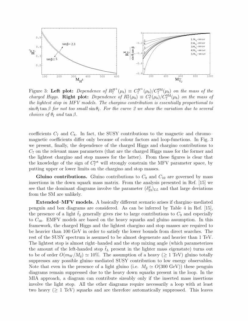
Figure 3: Left plot: Dependence of RH±

7 (µb) ≡ CH±

7 (µb)/CSM7 (µb) on the mass of the

charged Higgs. Right plot: Dependence of Rχ7 (µb) ≡ Cχ

7 (µb)/CSM7 (µb) on the mass of

the lightest stop in MFV models. The chargino contribution is essentially proportional tosin θt tan β for not too small sin θt. For the curve 2 we show the variation due to severalchoices of θt and tanβ.

coefficients C7 and C8. In fact, the SUSY contributions to the magnetic and chromo–magnetic coefficients differ only because of colour factors and loop-functions. In Fig. 3we present, finally, the dependence of the charged Higgs and chargino contributions toC7 on the relevant mass parameters (that are the charged Higgs mass for the former andthe lightest chargino and stop masses for the latter). From these figures is clear thatthe knowledge of the sign of Ctot

7 will strongly constrain the MFV parameter space, byputting upper or lower limits on the chargino and stop masses.

Gluino contributions. Gluino contributions to C9 and C10 are governed by massinsertions in the down squark mass matrix. From the analysis presented in Ref. [15] wesee that the dominant diagrams involve the parameter (δd23)LL and that large deviationsfrom the SM are unlikely.

Extended–MFV models. A basically different scenario arises if chargino–mediatedpenguin and box diagrams are considered. As can be inferred by Table 4 in Ref. [15],the presence of a light t2 generally gives rise to large contributions to C9 and especiallyto C10. EMFV models are based on the heavy squarks and gluino assumption. In thisframework, the charged Higgs and the lightest chargino and stop masses are required tobe heavier than 100 GeV in order to satisfy the lower bounds from direct searches. Therest of the SUSY spectrum is assumed to be almost degenerate and heavier than 1 TeV.The lightest stop is almost right–handed and the stop mixing angle (which parameterizesthe amount of the left-handed stop tL present in the lighter mass eigenstate) turns outto be of order O(mW/Mq) ≃ 10%. The assumption of a heavy (≥ 1 TeV) gluino totallysuppresses any possible gluino–mediated SUSY contribution to low energy observables.Note that even in the presence of a light gluino (i.e. Mg ≃ O(300 GeV)) these penguindiagrams remain suppressed due to the heavy down squarks present in the loop. In theMIA approach, a diagram can contribute sizeably only if the inserted mass insertionsinvolve the light stop. All the other diagrams require necessarily a loop with at leasttwo heavy (≥ 1 TeV) squarks and are therefore automatically suppressed. This leaves

us with only two unsuppressed flavour changing sources other than the CKM matrix,namely the mixings uL − t2 (denoted by δuL t2) and cL − t2 (denoted by δcL t2). We notethat δuL t2

and δcL t2 are mass insertions extracted from the up–squarks mass matrix afterthe diagonalization of the stop system and are therefore linear combinations of (δ13)

ULR,

(δ13)ULL and of (δ23)

ULR, (δ23)

ULL, respectively. In Fig. 2 we present the results of an high

statistic scanning over the EMFV parameter space requiring each point to survive theconstraints coming from the sparticle masses lower bounds and b → sγ. Note that theseSUSY models can account only for a small part of the region allowed by the modelindependent analysis of current data. In the numerical analysis reported here, we haveused the integrated branching ratios alone to put constraints on the effective coefficients.This procedure allows multiple solutions, which can be disentangled from each other onlywith the help of both the dilepton mass spectra and the forward-backward asymmetries.Only such measurements would allow us to determine the exact values and signs of theWilson coefficients C7, C9 and C10.

References

[1] A. Ali, C, Greub, G, Hiller, E. Lunghi, Phys. Rev. D66 (2002) 034002.

[2] R. Barate et al. (ALEPH Collaboration), Phys. Lett. B421 (1998) 169.

[3] D. Chen et al. (CLEO Collaboration), Phys. Rev. Lett. 87 (2001) 251807.

[4] B. Aubert et al. (BABAR Collaboration), hep-ex/0207076.

[5] K. Abe et al. (BELLE Collaboration), Phys. Lett B511 (2001) 151.

[6] B. Aubert et al. (BABAR Collaboration), hep-ex/0207082.

[7] K. Abe et al. (BELLE Collaboration), BELLE-CONF-0241.

[8] J. Kaneko et al. [Belle Collaboration], hep-ex/0208029.

[9] A. Ali, G. Hiller, L. T. Handoko and T. Morozumi, Phys. Rev. D55 (1997) 4105;A. Ali, P. Ball, L. T. Handoko and G. Hiller, Phys. Rev. D61 (2000) 074024.

[10] C. Bobeth, M. Misiak and J. Urban, Nucl. Phys. B574 (2000) 291.

[11] H. H. Asatrian, H. M. Asatrian, C. Greub, M. Walker, Phys. Lett B507 (2001) 162;H. H. Asatryan, H. M. Asatrian, C. Greub, M. Walker, Phys. Rev. D65 (2002)074004.

[12] A. Ali, P. Ball, L. T. Handoko and G. Hiller, Phys. Rev. D61 (2000) 074024.

[13] P. Gambino and M. Misiak, Nucl. Phys. B611 (2001) 338.

[14] C. Greub and P. Liniger, Phys. Rev. D63 (2001) 054025.

[15] E. Lunghi, A. Masiero, I. Scimemi and L. Silvestrini, Nucl. Phys. B568 (2000) 120.