arXiv:hep-th/9701069v1 14 Jan 1997 - arXiv.org e-Print … · arXiv:hep-th/9701069v1 14 Jan 1997 CERN-TH/96-371 hep-th/9701069 Introduction to S-Duality in N= 2 Supersymmetric Gauge

arX

iv:h

ep-t

h/97

0106

9v1

14

Jan

1997

CERN-TH/96-371hep-th/9701069

Introduction to S-Duality in N = 2 Supersymmetric

Gauge Theories

(A Pedagogical Review of the Work of Seiberg and Witten)

Luis Alvarez-Gaume1 and S. F. Hassan2

Theoretical Physics Division, CERNCH - 1211 Geneva 23

Abstract

In these notes we attempt to give a pedagogical introduction to the work of Seibergand Witten on S-duality and the exact results of N = 2 supersymmetric gaugetheories with and without matter. The first half is devoted to a review of monopolesin gauge theories and the construction of supersymmetric gauge theories. In thesecond half, we describe the work of Seiberg and Witten.

CERN-TH/96-371December 1996

1e-mail: [email protected]

2e-mail: [email protected]

http://arXiv.org/abs/hep-th/9701069v1

http://arXiv.org/abs/hep-th/9701069

Introduction

These notes are the very late written version of a series of lectures given at the TriesteSummer School in 1995. The aim was to provide an elementary introduction to the work ofSeiberg and Witten on exact results concerning N = 2 supersymmetric extensions of QuantumChromodynamics. We wanted to provide, in a single place, all the background material neces-sary to study their work in detail. We had in mind graduate students who have already gonethrough their Quantum Field Theory course, but we do not expect much more backgroundto follow these lectures. We have done our best to make the treatment pedagogical. In somesections, we have heavily drawn on previous reviews, for instance in the treatment of supersym-metry we have followed Bagger and Wess [22], and in the theory of monopoles we have used thereviews by Goddard and Olive [1] and by S. Coleman [2, 3]. These sources provide excellentpresentations of these topics, and we had no compelling reason to try to make improvements ontheir presentation. It is also quite obvious that we have drawn heavily on the original papersof Seiberg and Witten [31, 32], but we have tried to provide the necessary tools to make theirreading more accessible to interested students and/or researchers. Recently there have beenother lecture notes published at a more advanced level, where one can find more details and alsothe connection with String Theory (see, for instance, the notes by W. Lerche [40]). We wouldalso like to mention that we have not tried to be exhaustive in quoting all the literature onthe subject. A more complete reference list can be found in [40]. The reference list is intentedto provide a guidance to enter the vastly growing literature on duality in String Theory andField Theory. We apologize to those authors who may be offended by not finding their worksreferenced.

These notes are divided into four sections, with each section further subdivided into severalsubsections. Section 1 is devoted to an introduction to monopoles in gauge theories. We startwith a discussion of the Dirac monopole and the idea of charge quantization, and then describethe ’t Hooft-Polyakov monopole in gauge theories with spontaneous symmetry breaking. Thenwe introduce the notion of Bogomol’nyi bound and the BPS states. After this, we describethe topological classification of monopoles and then describe the Montonen-Olive conjecture ofelectric-magnetic duality. We end this section with a description of how, in the presence of aθ-term in the Lagrangian, the electric charge of a monopole is shifted by its magnetic charge.Section 2 is devoted to an introduction to supersymmetric gauge theories. First we describe thesupersymmetry algebra and its representations without and with central charges and discussits local realizations in terms of superfields. Then we construct N = 1 Lagrangians and finally,N = 2 supersymmetric Lagrangians with both gauge multiplets and matter multiplets (hyper-multiplets). At the end, we calculate the N = 2 central charge both in the pure gauge theory,as well as in the theory with matter and establish its relation to the BPS bound. Having builtthe foundations in the first two sections, in section 3 we describe the Seiberg-Witten analysis ofthe N = 2 pure gauge theory with gauge group SU(2). In the first two subsections, we discussthe parametrization of the moduli space and the breaking of R-symmetries. Then we describehow the chiral U(1) anomaly of the theory can be used to obtain the one-loop form of thelow-energy effective action. The rest of the section is devoted to finding the exact low-energyeffective action by using duality and the singularity structure on the moduli space of the theory.We express the exact solution in terms of complete elliptic integrals. In section 4, we briefly

1

describe the Seiberg-Witten analysis of N = 2 SU(2) gauge theory with Nf matter fields. Aftera discussion of the general features of these theories, we describe how the duality group is nolonger pure SL(2, Z). Then we describe the singularity structure on the moduli space of thesetheories and sketch the procedure for obtaining the exact solutions. Our aim in section 4 isto give a flavour of the analysis of theories with matter and, for a deeper understanding, theinterested reader is referred to the original work of Seiberg and Witten.

1 Magnetic Monopoles in Gauge Theories

In this section, we begin by reviewing the proporties of the Dirac monopole and the ideaof charge quantization. Then we describe the magnetic monopoles and dyons which arise innon-Abelian gauge theories with spontaneous symmetry breaking and discuss their generalproperties. We also introduce the notion of the Bogomol’nyi bound and BPS states. In thelast two subsections, we describe the Montonen-Olive conjecture of electric-magnetic dualityand Witten’s argument about how the presence of the θ-term in the Lagrangian modifies themonopole and dyon electric charges. For a more detailed discussion of most of the material inthis section, the reader is referred to the review article by Goddard and Olive [1], and to thelecture notes by Coleman [2, 3].

1.1 Conventions and Preliminaries

Let us start by stating our conventions: we always take c = 1, and almost always h = 1, exceptwhen it is important to make a distinction between classical and quantum effects. For indexmanipulations, we use the flat Minkowsky metric η of signature +,−,−,−. Moreover, wechoose units in which Maxwell’s equations take the form:

~∇ · ~E = ρ , ~∇× ~B − ∂ ~E/∂t = ~j ,~∇ · ~B = 0 , ~∇× ~E + ∂ ~B/∂t = 0 .

(1)

In these units, a factor of (4π)−1 appears in Coulomb’s law: For a static point-like charge q atthe origin, we have ρ = qδ3(~r). Integrating the first Maxwell equation over a sphere of radius

r and using spherical symmetry, we get∫S2~E · d~s = 4πr2E(r) = q. Hence, ~E = q~r/4πr3, as

stated. The electrostatic potential φ defined by ~E = −~∇φ is given by φ = q/4πr.

In relativistic notation, one introduces the four-potential Aµ = φ, ~A. The electric andmagnetic fields are defined as components of the corresponding field strength tensor Fµν asfollows:

Fµν = ∂µAν − ∂νAµ ,

F0i = ∂0Ai − ∂iA0 = −∂0Ai − ∂iA

0 = Ei ,

Fij = ∂iAj − ∂jAi = −(∂iAj − ∂jAi) = −ǫijkBk , (2)

2

so that Bi = −12ǫijkFjk = −1

2ǫoiµνFµν . The dual field strength tensor is given by

F µν =1

2εµναβFαβ ,

with ε0123 = +1. In component notation, we have

F µν =

0 −Ex −Ey −Ez

Ex 0 −Bz By

Ey Bz 0 −Bx

Ez −Bx By 0

, F µν =

0 −Bx −By −Bz

Bx 0 Ez −Ey

By −Ez 0 Ex

Bz Ey −Ex 0

. (3)

In terms of the electric four-current jµ = ρ,~j, the Maxwell’s equations take the compactform

∂νFµν = −jµ , ∂ν F

µν = 0 . (4)

Note that when jµ = 0, the above equations are invariant under the replacement ~E → ~B, ~B →−~E. This is referred to as the electric-magnetic duality transformation. In the presence ofelectric sources, this transformation is no longer a symmetry of Maxwell’s equations. In orderto restore the duality invariance of these equations for non-zero jµ, Dirac [4] introduced the

magnetic four-current kµ = σ,~k and modified Maxwell’s equations to

∂νFµν = −jµ , ∂ν F

µν = −kµ . (5)

The above equations are now invariant under a combined duality transformation of the fieldsand the currents which can be written as

F → F , F → −F ; jµ → kµ , kµ → −jµ . (6)

Note that the full invariance group of the equations (5) is larger than this discrete duality. Infact, they are invariant under a continuous SO(2) group which rotates the electric and magneticquantities into each other.

For point-like electric and magnetic sources, the current densities can be written as

jµ(x) =∑

a

qa

∫dxµ

aδ4(x− xa) ,

kµ(x) =∑

a

ga

∫dxµ

aδ4(x− xa) .

A particle of electric charge q and magnetic charge g experiences a Lorentz force given by

md2xµ

dτ 2= (qF µν + g F µν)

dxν

dτ.

Although, at the level of quations of motion, Dirac’s modification of Maxwell’s theoryseems trivial, it has highly non-trivial consequences in quantum theory. One way of realizing

3

the problem is to note that the vector potential ~A is indispensable in the quantum formulationof the theory. On the other hand, equations ~B = ~∇ × ~A and ~∇ · ~B 6= 0 are not compatibleunless the vector potential ~A has singularities and, hence, is not globally well-defined. Itturns out that these singularities are gauge dependent and, therefore, their presence shouldnot be experimentally detectable. In the classical theory, which can be formulated in termsof ~B alone, this requirement is trivially satisfied. However, in quantum theory, it leads to theimportant phenomenon of the quantization of electric charge. In the following, we will firstgive a semiclassical derivation of this effect and then describe a derivation based on the notionof the Dirac string.

1.2 A Semiclassical Derivation of Charge Quantization

Consider a non-relativistic charge q in the vicinity of a magnetic monopole of strength g,situated at the origin. The charge q experiences a force m~r = q~r× ~B, where ~B is the monopolefield given by ~B = g~r/4πr3. The change in the orbital angular momentum of the electric chargeunder the effect of this force is given by

d

dt

(m~r × ~r

)= m~r × ~r =

qg

4πr3~r ×

(~r × ~r

)=

d

dt

(qg

4π

~r

r

).

Hence, the total conserved angular momentum of the system is

~J = ~r ×m~r − qg

4π

~r

r. (7)

The second term on the right hand side (henceforth denoted by ~Jem) is the contribution comingfrom the elecromagnetic field. This term can be directly computed by using the fact that themomentum density of an electromagnetic field is given by its Poynting vector, ~E× ~B, and henceits contribution to the angular momentum is given by

~Jem =∫d3x~r × ( ~E × ~B) =

g

4π

∫d3x~r ×

(~E × ~r

r3

).

In components,

J iem =

g

4π

∫d3xEj

(δij −

xixj

r2

)1

r=

g

4π

∫d3xEj∂j(x

i)

=g

4π

∫

S2

xi ~E · ~ds− g

4π

∫d3x~∇ · ~Exi . (8)

When the separation between the electric and magnetic charges is negligible compared to theirdistance from the boundary S2, the contribution of the first integral to ~Jem vanishes by sphericalsymmetry. We are therefore left with

~Jem = − gq

4πr . (9)

4

Returning to equation (7), if we assume that orbital angular momentum is quantized. Thenit follows that

qg

4π=

1

2nh , (10)

where n is an integer. Note that in the above we have assumed the total angular momentum ofthe charge-monopole system to be quantized in half-integral units. This is a strange assumptionconsidering that we did not have to treat the electrically charged particle or the monopole asfermios. both of the components are bosonic. However, it turns out that this actually is thecase and that the situation does not contradict the spin-statistics theorem [5, 6]. We will notdiscuss this issue further but remark that the derivation of the same equation presented in thenext subsection does not depend on this assumption.

Equation (10) is the Dirac charge quantization condition. It implies that if there exists amagnetic monopole of charge g somewhere in the universe, then all electric charges are quantizedin units of 2πh/g. If we have a number of purely electric charges qi and purely magnetic chargesgj, then any pair of them will satisfy a quantization condition:

qigj

4πh=

1

2nij (11)

Thus, any electric charge is an integral multiple of 2πh/gj. For a given gj, let these chargeshave n0j as the highest common factor. Then, all the electric charges are multiples of q0 =n0j2πh/gj. Note that q0 itself may not exist in the spectrum. Similar considerations apply tothe quantization of magnetic charge.

Till now, we have only dealt with particles that carry either an electric or a magneticcharge. Let us now consider dyons, i.e., particles that carry both electric and magnetic charges.Consider two dyons of charges (q1, g1) and (q2, g2). For this system, we can repeat the calculation

of ~Jem by following the steps in (8) where now the electromagnetic fields are split as ~E = ~E1+ ~E2

and ~B = ~B1 + ~B2. The answer is easily found to be

~Jem = − 1

4π(q1g2 − q2g1) r (12)

The charge quantization condition is thus generalized to

q1g2 − q2g1

4πh=

1

2n12 (13)

This is referred to as the Dirac-Schwinger-Zwanziger condition [7, 8]. This condition is invariantunder the SO(2) transformation (q + ig) → eiφ(q + ig) which is also a symmetry of (5).

1.3 The Dirac String

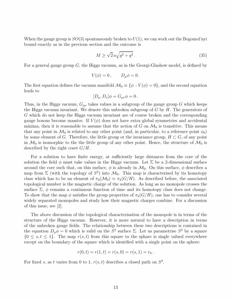
In the following, we present a more rigorous derivation of the Dirac quantization conditionwhich is based on the notion of a Dirac string. Let ~Bmon denote the magnetic field around a

5

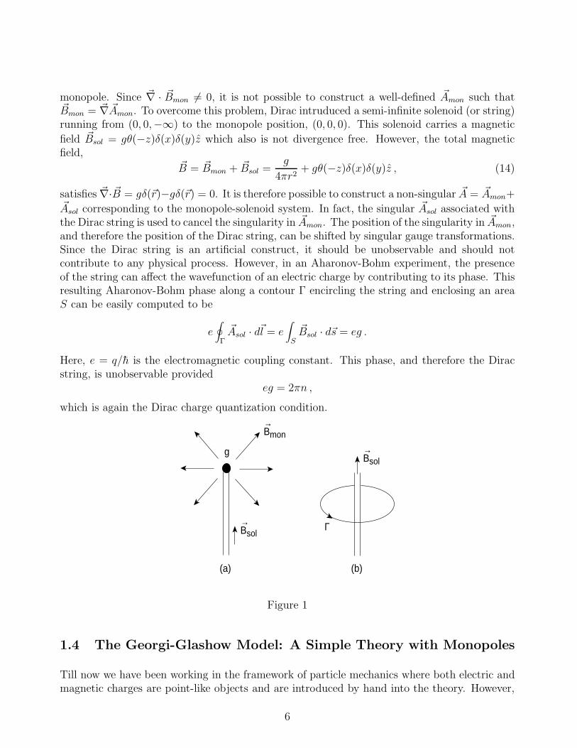
monopole. Since ~∇ · ~Bmon 6= 0, it is not possible to construct a well-defined ~Amon such that~Bmon = ~∇ ~Amon. To overcome this problem, Dirac intruduced a semi-infinite solenoid (or string)running from (0, 0,−∞) to the monopole position, (0, 0, 0). This solenoid carries a magnetic

field ~Bsol = gθ(−z)δ(x)δ(y)z which also is not divergence free. However, the total magneticfield,

~B = ~Bmon + ~Bsol =g

4πr2+ gθ(−z)δ(x)δ(y)z , (14)

satisfies ~∇· ~B = gδ(~r)−gδ(~r) = 0. It is therefore possible to construct a non-singular ~A = ~Amon+~Asol corresponding to the monopole-solenoid system. In fact, the singular ~Asol associated withthe Dirac string is used to cancel the singularity in ~Amon. The position of the singularity in ~Amon,and therefore the position of the Dirac string, can be shifted by singular gauge transformations.Since the Dirac string is an artificial construct, it should be unobservable and should notcontribute to any physical process. However, in an Aharonov-Bohm experiment, the presenceof the string can affect the wavefunction of an electric charge by contributing to its phase. Thisresulting Aharonov-Bohm phase along a contour Γ encircling the string and enclosing an areaS can be easily computed to be

e∮

Γ

~Asol · d~l = e∫

S

~Bsol · d~s = eg .

Here, e = q/h is the electromagnetic coupling constant. This phase, and therefore the Diracstring, is unobservable provided

eg = 2πn ,

which is again the Dirac charge quantization condition.

g

(a) (b)

Bsol→

Bsol→

Bmon→

Γ

Figure 1

1.4 The Georgi-Glashow Model: A Simple Theory with Monopoles

Till now we have been working in the framework of particle mechanics where both electric andmagnetic charges are point-like objects and are introduced by hand into the theory. However,

6

in field theory, these objects can also arise as solitons which are non-trivial solutions of thefield equations with localized energy density. If the gauge field configuration associated with asoliton solution has a magnetic character, the soliton can be identified as a magnetic monopole.The simplest solitons are found in the Sine-Gordon theory, which is a scalar field theory in 1+1dimensions. However, by Derrick’s theorem, a scalar field theory in more than two dimensionscannot support static finite energy solutions. This is basically due to the fact that because ofthe non-trivial structure of the soliton at large distances, the total energy of the configurationdiverges. This situation can be cured by the addition of gauge fields to the theory. Thus, ascalar theory with gauge interactions in four dimensions can admit static finite energy fieldconfigurations. The stability of such solitonic configurations are often related to the fact thatthey are characterized by conserved topological charges. For a more detailed discussion of theseissues, the reader is referred to [1, 2, 3]. In the following, we describe the Georgi-Glashow modelwhich is a simple theory in 3 + 1 dimensions with monopole solutions.

The Georgi-Glashow model is a Yang-Mills-Higgs system which contains a Higgs multipletφa (a = 1, 2, 3) transforming as a vector in the adjoint representation of the gauge group SO(3),and the gauge fields Wµ = W a

µTa. Here, T a are the hermitian generators of SO(3) satifying

[T a, T b] = ifabcT c. In the adjoint representaion, we have (T a)bc = −ifabc and, for SO(3),

fabc = ǫabc. The field strength of Wµ and the cavariant derivative on φa are defined by

Gµν = ∂µWν − ∂νWµ + ie[Wµ,Wν ] ,

Dµφa = ∂µφ

a − eǫabcW bµφ

c . (15)

The minimal Lagrangian is then given by

L = −1

4Ga

µνGaµν +

1

2DµφaDµφ

a − V (φ) , (16)

where,

V (φ) =λ

4

(φ2 − a2

)2. (17)

The equations of motion following from this Lagrangian are

(DνGµν)a = −e ǫabc φb (Dµφ)c, DµDµφ

a = −λφa(φ2 − a2) . (18)

The field strength also satifies the Bianchi identity

Dν Gµνa = 0 . (19)

Let us find the vacuum configurations in this theory. Using the notations G0ia = −E i

a andGij

a = −ǫijkBka , the energy density is written as

θ00 =1

2

((E i

a)2 + (Bi

a)2 + (D0φa)

2 + (Diφa)2)

+ V (φ) . (20)

Note that θ00 ≥ 0, and it vanishes only if

Gµνa = 0, Dµφ = 0, V (φ) = 0 . (21)

7

The first equation implies that in the vacuum, W aµ is pure gauge and the last two equations

define the Higgs vacuum. The structure of the space of vacua is determined by V (φ) = 0 whichsolves to φa = φa

vac such that |φvac| = a. The space of Higgs vacua is therefore a two-sphere(S2) of radius a in the field space. To formulate a perturbation theory, we have to choose oneof these vacua and hence, break the gauge symmetry spontaneously (this is the usual Higgsmechanism). The part of the symmetry which keeps this vacuum invariant, still survives and thecorresponding unbroken generator is φc

vacTc/a. The gauge boson associated with this generator

is Aµ = φcvacW

cµ/a and the electric charge operator for this surviving U(1) is given by

Q = heφc

vacTc

a. (22)

If the group is compact, this charge is quantized. The perturbative spectrum of the theory canbe found by expanding φa around the chosen vacuum as

φa = φavac + φ′a .

A convenient choice is φcvac = δc3a. The perturbative spectrum (which becomes manifest after

choosing an appropriate gauge) consists of a massive Higgs (H), a massless photon (γ) and twocharged massive bosons (W±):

Mass Spin Charge

H a(2λ)1

2 h 0 0γ 0 h 0W± aeh = aq h ±q = ±eh

In the next section, we investigate the existence of monopoles (non-perturbative states) in theGeorgi-Glashow model.

1.5 The ’t Hooft - Polyakov Monopole

Let us look for time-independent, finite energy solutions in the Georgi-Glashow model. Finite-ness of energy requires that as r → ∞, the energy density θ00 given by (20) must approachzero faster than 1/r3. This means that as r → ∞, our solution must go over to a Higgs vac-uum defined by (21). In the following, we will first assume that such a finite energy solutionexists and show that it can have a monopole charge related to its soliton number which is, inturn, determined by the associated Higgs vacuum. This result is proven without having to dealwith any particular solution explicitly. Next, we will describe the ’t Hooft-Polyakov ansatz forexplicitly constructing one such monopole solution. We will also comment on the existence ofDyonic solutions. For convenience, in this section we will use the vector notation for the SO(3)gauge group indices and not for the spatial indices.

The Topological Nature of Magnetic Charge: Let ~φvac denote the field ~φ in a Higgs vacuum. Itthen satisfies the equations

~φvac · ~φvac = a2 ,

∂µ~φvac − e ~Wµ × ~φvac = 0 , (23)

8

which can be solved for ~Wµ. The most general solution is given by

~Wµ =1

ea2~φvac × ∂µ

~φvac +1

a~φvacAµ . (24)

To see that this actually solves (23), note that ∂µ~φvac · ~φvac = 0, so that

1

ea2(~φvac × ∂µ

~φvac) × ~φvac =1

ea2

(∂µ~φvaca

2 − ~φvac(~φvac · ∂µφvac))

=1

e∂µ~φvac .

The first term on the right-hand side of Eq. (24) is the particular solution, and ~φvacAµ is thegeneral solution to the homogeneous equation. Using this solution, we can now compute thefield strength tensor ~Gµν . The field strength Fµν corresponding to the unbroken part of thegauge group can be identified as

Fµν =1

a~φvac · ~Gµν

= ∂µAν − ∂νAµ +1

a3e~φvac · (∂µ

~φvac × ∂ν~φvac) . (25)

Using the equations of motion in the Higgs vacuum it follows that

∂µFµν = 0 , ∂µ F

µν = 0 .

This confirms that Fµν is a valid U(1) field strength tensor. The magnetic field is given byBi = −1

2ǫijkFjk. Let us now consider a static, finite energy solution and a surface Σ enclosing

the core of the solution. We take Σ to be far enough so that, on it, the solution is already inthe Higgs vacuum. We can now use the magnetic field in the Higgs vacuum to calculate themagnetic charge gΣ associated with our solution:

gΣ =∫

ΣBidsi = − 1

2ea3

∫

Σǫijk ~φvac ·

(∂j~φvac × ∂k~φvac

)dsi . (26)

It turns out that the expression on the right hand side is a topological quantity as we explainbelow: Since φ2 = a; the manifold of Higgs vacua (M0) has the topology of S2. The field ~φvac

defines a map from Σ into M0. Since Σ is also an S2, the map φvac : Σ → M0 is characterizedby its homotopy group π2(S

2). In other words, φvac is characterized by an integer ν (the windingnumber) which counts the number of times it wraps Σ around M0. In terms of the map φvac,this integer is given by

ν =1

4πa3

∫

Σ

1

2ǫijk~φvac ·

(∂j~φvac × ∂k~φvac

)dsi . (27)

Comparing this with the expression for magnetic charge, we get the important result

gΣ = −4πν

e. (28)

Hence, the winding number of the soliton determines its monopole charge. Note that the aboveequation differs from the Dirac quantization condition by a factor of 2. This is because the

9

smallest electric charge which could exist in our model is q0 = eh/2 in terms of which, (28)reduces to the Dirac condition.

An Ansatz for Monopoles: Now we describe an ansatz proposed by ’t Hooft [9] and Polyakov[10] for constructing a monopole solution in the Georgi-Glashow model. For a sphericallysymmetric, parity-invariant, static solution of finite energy, they proposed:

φa =xa

er2H(aer) ,

W ai = −ǫaij

xj

er2(1 −K(aer)) , W a

0 = 0 . (29)

For the non-trivial Higgs vacuum at r → ∞, they chose φcvac = axc/r = axc. Note that this maps

an S2 at spatial infinity onto the vacuum manifold with a unit winding number. The asymptoticbehaviour of the functions H(aer) and K(aer) are determined by the Higgs vacuum as r → ∞and regularity at r = 0. Explicitly, defining ξ = aer, we have: as ξ → ∞, H ∼ ξ, K → 0 andas ξ → 0, H ∼ ξ, (K − 1) ∼ ξ. The mass of this solution can be parametrized as

M =4πa

ef (λ/e2)

For this ansatz, the equations of motion reduce to two coupled equations for K and H whichhave been solved exactly only in certain limits. For r → 0, one gets H → ec1r

2 and K =1 + ec2r

2 which shows that the fields are non-singular at r = 0. For r → ∞, we get H →ξ + c3exp(−a

√2λr) and K → c4ξexp(−ξ) which leads to W a

i ≈ −ǫaijxj/er2. Once again,defining Fij = φcGc

ij/a, the magnetic field turns out to be Bi = −xi/er3. The associatedmonopole charge is g = −4π/e, as expected from the unit winding number of the solution. Itshould be mentioned that ’t Hooft’s definition of the Abelian field strength tensor is slightlydifferent but, at large distances, it reduces to the form given above.

Note that in the above monopole solution, the presence of the Dirac string is not obvious.To extract the Dirac string, we have to perform a singular gauge transformation on this solutionwhich rotates the non-trivial Higgs vacuum φc

vac = axc into the trivial vacuum φcvac = aδc3. In

the process,the gauge field develops a Dirac string singularity which now serves as the sourceof the magnetic charge [9].

The Julia-Zee Dyons:

The ’t Hooft-Polyakov monopole carries one unit of magnetic charge and no electric charge.The Georgi-Glashow model also admits solutions which carry both magnetic as well as electriccharges. An ansatz for constructing such a solution was proposed by Julia and Zee [11]. Inthis ansatz, φa and W a

i have exactly the same form as in the ’t Hooft-Polyakov ansatz, but W a0

is no longer zero: W a0 = xaJ(aer)/er2. This serves as the source for the electric charge of the

dyon. It turns out that the dyon electric charge depends of a continuous parameter and, at theclassical level, does not satisfy the quantization condition. However, semiclassical arguments[12, 13] show that, in CP invariant theories, and at the quantum level, the dyon electric chargeis quantized as q = nhe. This can be easiy understood if we recognize that a monopole is notinvariant under a guage transformation which is, of course, a symmetry of the equations of

10

motion. To treate the associated zero-mode properly, the gauge degree of freedom should beregarded as a collective coordinate. Upon quantization, this collective coordinate leads to theexistence of electrically charged states for the monopole with discrete charges. In the presenceof a CP violating term in the Lagrangian, the situation is more subtle as we will discuss later.In the next subsection, we describe a limit in which the equations of motion can be solvedexactly for the ’tHooft-Polyakov and the Julia-Zee ansatz. This is the limit in which the solitonmass saturates the Bogomol’nyi bound.

1.6 The Bogomol’nyi Bound and the BPS States

In this subsection, we derive the Bogomol’nyi bound [14] on the mass of a dyon in term of its

electric and magnetic charges which are the sources for F µν = ~φ · ~Gµν/a. Using the Bianchiidentity (19) and the first equation in (18), we can write the charges as

g ≡∫

S2∞

BidSi =

1

a

∫Ba

i φadSi =

1

a

∫Ba

i (Diφ)ad3x ,

q ≡∫

S2∞

EidSi =

1

a

∫Ea

i φadSi =

1

a

∫Ea

i (Diφ)ad3x . (30)

Now, in the center of mass frame, the dyon mass is given by

M ≡∫d3xθ00 =

∫d3x

(1

2

[(Ea

k )2 + (Bak)

2 + (Dkφa)2 + (D0φ

a)2]+ V (φ)

),

where, θµν is the energy momentum tensor. After a little manipulation, and using the expres-sions for the electric and magnetic charges given in (30), this can be written as

M =∫d3x

(1

2

[(Ea

k −Dkφa sin θ)2 + (Ba

k −Dkφa cos θ)2 + (D0φ

a)2]+ V (φ)

)

+ a(q sin θ + g cos θ) , (31)

where θ is an arbitrary angle. Since the terms in the first line are positive, we can writeM ≥ (q sin θ+ g cos θ). This bound is maximum for tan θ = q/g. Thus we get the Bogomol’nyibound on the dyon mass as

M ≥ a√g2 + q2 .

For the ’t Hooft-Polyakov solution, we have q = 0, and thus, M ≥ a|g|. But |g| = 4π/e andMW = aeh = aq, so that

M ≥ a4π

e=

4π

e2hMW =

4πh

q2MW =

ν

αMW .

Here, α is the fine structure constant and ν = 1 or 1/4, depending on whether the electroncharge is q or q/2. Since α is a very small number (∼ 1/137 for electromagnetism), the aboverelation implies that the monopole is much heavier than the W-bosons associated with thesymmetry breaking.

11

From (31) it is clear that the bound is not saturated unless λ→ 0, so that V (φ) = 0. Thisis the Bogomol’nyi-Prasad-Sommerfield (BPS) limit of the theory [14, 15]. Note that in thislimit, φ2

vac = a2 is no longer determined by the theory and, therefore, has to be imposed asa boundary condition on the Higgs field. Moreover, in this limit, the Higgs scalar becomesmassless. Now, to saturate the bound we have to set

D0φa = 0 , Ea

k = (Dkφ)a sin θ , Bak = (Dkφ)a cos θ , (32)

where, tan θ = q/g. In the BPS limit, one can use the ’t Hooft-Polyakov (or the Julia-Zee)ansatz either in (18), or in (32) to obtain the exact monopole (or dyon) solutions [14, 15].These solutions automatically saturate the Bogomol’nyi bound and are referred to as the BPSstates. Also, note that in the BPS limit, all the perturbative excitations of the theory saturatethis bound and, therefore, belong to the BPS spectrum. As we will see later, the BPS boundappears in a very natural way in theories with N = 2 supersymmetry.

1.7 Monopoles from a Distance

Till now, we have described the monopoles arising in the Georgi-Glashow model in terms ofthe structure of the Higgs vacuum of the theory. In this section, we will consider monopolesin a general Yang-Mills-Higgs system and relate the Higgs vacuum description to a descriptionin terms of the unbroken gauge fields. These are the gauge fields which remain massless andare relevant for the study of monopoles at large distances. This formulation is convenient fordescribing non-abelian monopoles.

Let φ transform as a vector in a given representation of a gauge group G. For convenienceof notation, in the following we do not distinguish between the group element g and a givenrealization of it. Writing the gauge fields as Wµ = T aW a

µ , we can construct the covariantderivative of φ and the curvature tensor of Wµ as

Dµφ = ∂µφ+ ieWµφ ,

Gµν = ∂µWν − ∂νWµ + ie[Wµ,Wν ] .

The Lagrangian density L, the stress-energy tensor θµν and the gauge current jaµ are then given

by

L = −1

4(Ga

µν)2 + (Dµφ)†Dµφ− V (φ) ,

θµν = −GaµλG

aλν + (Dµφ)†(Dνφ) + (Dνφ)†(Dµφ) − gµνL ,

θ00 =1

2E iaEa

i +1

2BiaBa

i +D0φ†D0φ+Diφ

†Diφ+ V (φ) ,

jaµ = ieφ†T aDµφ− ie(Dµφ)†T aφ . (33)

Here, the Higgs potential is gauge invariant: V (gφ) = V (φ). The equations of motion followingfrom the above Lagrangian are

DµDµφa = − ∂V

∂φa, DνGa

µν = −jaµ . (34)

12

When the gauge group is SO(3) spontaneously broken to U(1), we can work out the Bogomol’nyibound exactly as in the previous section and the outcome is

M ≥√

2 a√g2 + q2 . (35)

For a general gauge group G, the Higgs vacuum, as in the Georgi-Glashow model, is defined by

V (φ) = 0 , Dµφ = 0 .

The first equation defines the vacuum manifold M0 ≡ φ : V (φ) = 0, and the second equationleads to

[Dµ, Dν ]φ = Gµνφ = 0 .

Thus, in the Higgs vacuum, Gµν takes values in a subgroup of the gauge group G which keepsthe Higgs vacuum invariant. We denote this unbroken subgroup of G by H . The generators ofG which do not keep the Higgs vacuum invariant are of course broken and the correspondinggauge bosons become massive. If V (φ) does not have extra global symmetries and accidentalminima, then it is reasonable to assume that the action of G on M0 is transitive. This meansthat any point in M0 is related to any other point (and, in particular, to a reference point φ0)by some element of G. Therefore, the little group or the invariance group, H ⊂ G, of any pointin M0 is isomorphic to the the little group of any other point. Hence, the structure of M0 isdescribed by the right coset G/H .

For a solution to have finite energy, at sufficiently large distances from the core of thesolution the field φ must take values in the Higgs vacuum. Let Σ be a 2-dimensional surfacearound the core such that, on this surface, φ is already in M0. On this surface, φ describes amap from Σ (with the topology of S2) into M0. This map is characterised by its homotopyclass which has to be an element of π2(M0) ≃ π2(G/H). As described before, the associatedtopological number is the magnetic charge of the solution. As long as no monopole crosses thesurface Σ, φ remains a continuous function of time and its homotopy class does not change.To show that the map φ satisfies the group properties of π2(G/H), one has to consider severalwidely separated monopoles and study how their magnetic charges combine. For a discussionof this issue, see [2].

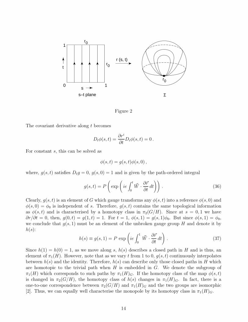
The above discussion of the topological characterisation of the monopole is in terms of thestructure of the Higgs vacuum. However, it is more natural to have a description in termsof the unbroken gauge fields. The relationship between these two descriptions is contained inthe equation Dµφ = 0 which is valid on the S2 surface Σ. Let us parametrise S2 by a square0 ≤ s, t ≤ 1. The map r(s, t) from this square to the sphare is single valued everywhereexcept on the boundary of the square which is identified with a single point on the sphere:

r(0, t) = r(1, t) = r(s, 0) = r(s, 1) = r0 .

For fixed s, as t varies from 0 to 1, r(s, t) describes a closed path on S2.

13

1

0 1

Σ

t

s

s–t plane

r0

r0

r0r (s, t)

Figure 2

The covariant derivative along t becomes

Dtφ(s, t) =∂ri

∂tDiφ(s, t) = 0 .

For constant s, this can be solved as

φ(s, t) = g(s, t)φ(s, 0) ,

where, g(s, t) satisfies Dtg = 0, g(s, 0) = 1 and is given by the path-ordered integral

g(s, t) = P

(exp

(ie∫ t

0

~W · ∂~r∂tdt

)). (36)

Clearly, g(s, t) is an element of G which gauge transforms any φ(s, t) into a reference φ(s, 0) andφ(s, 0) = φ0 is independent of s. Therefore, g(s, t) contains the same topological informationas φ(s, t) and is characterised by a homotopy class in π2(G/H). Since at s = 0, 1 we have∂r/∂t = 0, then, g(0, t) = g(1, t) = 1. For t = 1, φ(s, 1) = g(s, 1)φ0. But since φ(s, 1) = φ0,we conclude that g(s, 1) must be an element of the unbroken gauge group H and denote it byh(s):

h(s) ≡ g(s, 1) = P exp

(ie∫ 1

0

~W · ∂~r∂tdt

). (37)

Since h(1) = h(0) = 1, as we move along s, h(s) describes a closed path in H and is thus, anelement of π1(H). However, note that as we vary t from 1 to 0, g(s, t) continuously interpolatesbetween h(s) and the identity. Therefore, h(s) can describe only those closed paths in H whichare homotopic to the trivial path when H is embedded in G. We denote the subgroup ofπ1(H) which corresponds to such paths by π1(H)G. If the homotopy class of the map φ(s, t)is changed in π2(G/H), the homotopy class of h(s) changes in π1(H)G. In fact, there is aone-to-one correspondence between π2(G/H) and π1(H)G and the two groups are isomorphic[2]. Thus, we can equally well characterise the monopole by its homotopy class in π1(H)G.

14

Let us discuss this in some more detail. Since any closed path in H is also a closed path inG, there is a natural homomorphism from π1(H) into π1(G). As the discussion above shows,π1(H)G is in the kernel of this homomorphism. Moreover, for a compact connected group G,π2(G) = 0, which implies that π2(G) can be embedded in π2(G/H) as its identity element.What we have done above, basically, is to construct part of the following exact sequence:

π2(G) → π2(G/H) → π1(H) → π1(G) → π1(G/H) → π0(H)

Note that if G is simply connected then, π1(G) = 0 and π1(H)G = π1(H). So that the full π1(H)enters the physical description of the monopole. For non-simply connected G, this possibilitycan be realised in the presence of a Dirac string. Such a string appears as a singular point onthe (s, t) plane, in the presence of which, it is no longer possible to continuously deform h(s)to the identity map. Therefore, the homotopy class of h(s) is no longer restricted to π1(H)G.However, for non-simply connected G, it is still possible to have a description in terms of anunrestricted π1 group provided we embed G in its universal covering group G. Let us denote thelittle group of φ by H. Since G is necessarily connected, π1(G) = 0 and π1(H) = π1(H)G. As anexample, let us consider the Georgi-Glashow model. Here, G = SO(3) (with (Ta)ij = −iǫaij)

and G = SU(2) (with Ta = 12σa). The homotopically distinct paths in H (or H) are:

h(t) = exp(it ~φ · ~T 4πN/a), for 0 ≤ t ≤ 1 .

The integer N , which characterises the elements of π1, is determined as follows:

G = SU(2), H = U(1), ~φ · ~T ∈ 12Z, ⇒ N ∈ Z ,

G = SO(3), H = SO(2), ~φ · ~T ∈ Z, ⇒ N ∈ 12Z .

Since SO(3) ∼ S2/Z2, only paths with integer N contribute in both cases. Later we show thatg = 4πN/e. For SU(2), q0 = eh/2 and gq0/4πh = N/2. For SO(3), q0 = eh and gq0/4πh = N .

For Glashow-Weinberg-Salam model, G = SU(2) × U(1) and H = U(1) is a linear combi-nation of SU(2) and U(1). Although π1(H) = Z, π1(H)G = 0. Therefore, in this model, anynon-trivial monopole must have a Dirac string.

We set out to describe the monopole in terms of the unbroken gauge fields (the H-fields).Although, we have obtained a description in terms of π1(H)G, it is not manifest that h(s),as given by (37), involves only the H-fields. We show this in the following: The quantityg−1(s, t)Dsg(s, t) is invariant under a t-dependent gauge transformation. Moreover, by con-struction, Dtg(s, t) = 0. Hence, we can write

∂t(g−1Dsg) = Dt(g

−1Dsg) = g−1[Dt, Ds]g = ieg−1Gijg∂ri

∂t

∂rj

∂s. (38)

Let us integrate the first and the last terms above from t = 0 to t = 1. Since g−1Dsg = 0 att = 0 and g−1Dsg = h−1dh/ds at t = 1, we get

h−1 dh

ds= ie

∫ 1

0dt g−1Gij g

∂ri

∂t

∂rj

∂s. (39)

15

Since Gij was calculated on Σ, it involves only the H-gauge fields. The conjugation by g doesnot bring in a dependence on the massive gauge fields as is evident from the left-hand side ofthe equation. Hence the map is given entirely in terms of the H-fields without any referenceto the Higgs field. As a simple application, consider the Dirac monopole. Integrating (39)

from s = 0 to s = 1, we get h(1) = exp(ie∫ ~B · ~ds). Since h(1) = 1, this leads to the Dirac

quantization condition eg = 2πn or qg/4πh = n/2. Another interesting consequence of (39) isa possible explanation for the fractional charges of quarks. We describe this in the next section.

1.8 The Monopole and Fractional Charges

So far, we have seen how the existence of a monopole can quantize the electric charge in integerunits. In the physical world, however, we also come across fractionally charged quarks. In thefollowing, we see how the existence of a monopole can also account for these fractional charges[16, 1].

Let us represent our adjoint Higgs by φ = φaT a, where T a are the fundamental represen-tation matrices. Moreover, we only consider φ on the surface Σ as described in the previoussubsection. With φ in the Higgs vacuum, a generator T a belongs to the unbroken subgroup Hof G provided [T a, φ] = 0. This implies that φ itself is a generator of H and commutes withits other generators. Thus the Lie Algebra of H is of the form L(H) = u(1) ⊕ L(K) and wechoose L(K) to be orthogonal to u(1): Tr(φKa) = 0 for Ka ∈ K. Locally, H has the structureU(1) × K, though, this is not necessarily the global structure. We refer to K as the colourgroup and identify the U(1) as corresponding to electromagnetism. The gauge fields in H canbe decomposed as W µ = Aµφ/a+Xµ, with Tr(φXµ) = 0. Expanding the covariant derivative∂µ + ieWµ we can identify the electric charge operator which couples to Aµ as Q = (eh/a)φ.

Since h−1dh/ds is a generator of H , we may write

h−1dh

ds= ieα(s)

φ0

a+ iβaK

a . (40)

Using Tr(TaTb) = δab, φ(r) = gφ0g−1 and equation (39), we get

α(s) = − i

aeTr

(φ0h

−1dh

ds

)

=1

a

∫ 1

0Tr (ϕ(r)Gij)

∂ri

∂t

∂rj

∂sdt .

Identifying the electromagnetic field strength tensor as F µν = Tr (φGµν/a), we get α(s) =dΩ/ds, where, Ω(s) is the magnetic flux in a solid angle subtended at the origin by the path0 ≤ t ≤ 1 at fixed s on S2. Substituting this back in (40) and integrating from s = 0 to s, gives

h(s) = k(s)eiQΩ(s)/h .

Since h(1) = 1 and Ω(1) = g (where g is the total magnetic charge inside Σ), the quantizationcondition is replaced by

eigQ/h = k(1)−1 = k ∈ K .

16

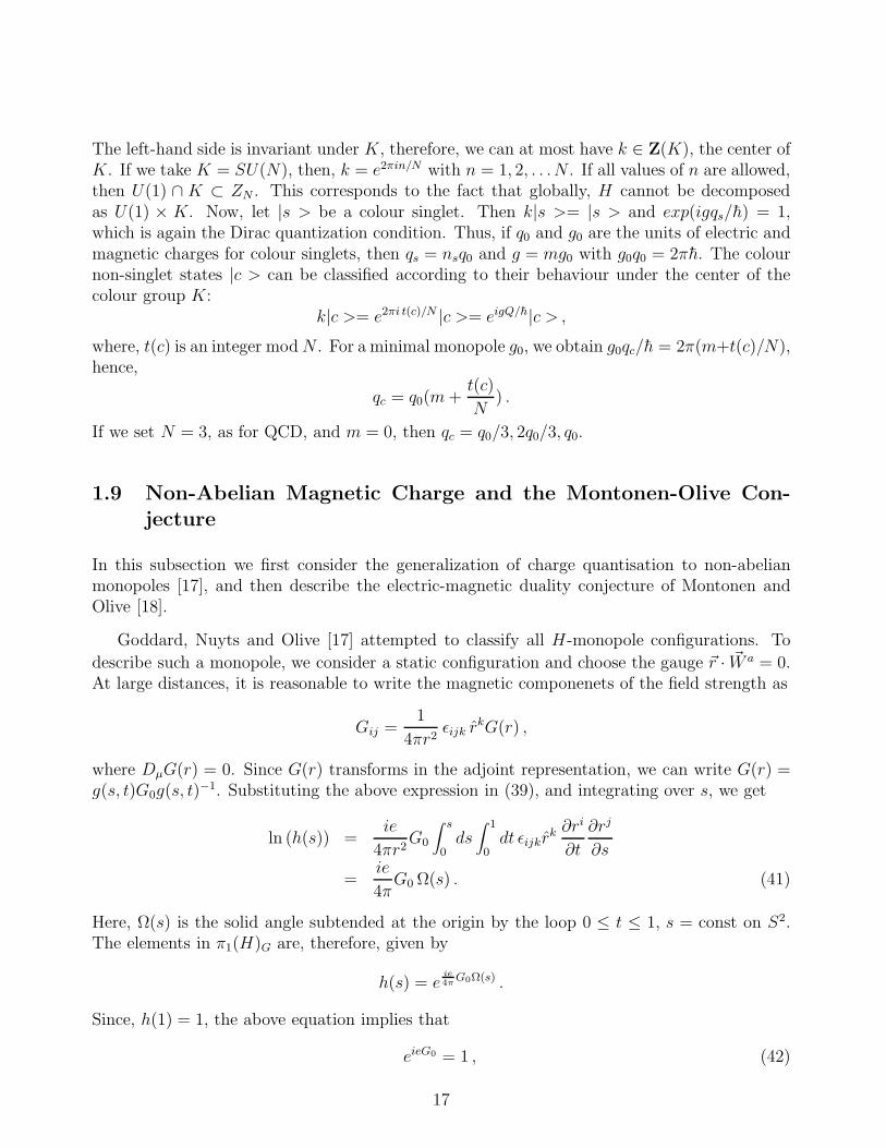
The left-hand side is invariant under K, therefore, we can at most have k ∈ Z(K), the center ofK. If we take K = SU(N), then, k = e2πin/N with n = 1, 2, . . .N . If all values of n are allowed,then U(1) ∩ K ⊂ ZN . This corresponds to the fact that globally, H cannot be decomposedas U(1) × K. Now, let |s > be a colour singlet. Then k|s >= |s > and exp(igqs/h) = 1,which is again the Dirac quantization condition. Thus, if q0 and g0 are the units of electric andmagnetic charges for colour singlets, then qs = nsq0 and g = mg0 with g0q0 = 2πh. The colournon-singlet states |c > can be classified according to their behaviour under the center of thecolour group K:

k|c >= e2πi t(c)/N |c >= eigQ/h|c > ,where, t(c) is an integer modN . For a minimal monopole g0, we obtain g0qc/h = 2π(m+t(c)/N),hence,

qc = q0(m+t(c)

N) .

If we set N = 3, as for QCD, and m = 0, then qc = q0/3, 2q0/3, q0.

1.9 Non-Abelian Magnetic Charge and the Montonen-Olive Con-

jecture

In this subsection we first consider the generalization of charge quantisation to non-abelianmonopoles [17], and then describe the electric-magnetic duality conjecture of Montonen andOlive [18].

Goddard, Nuyts and Olive [17] attempted to classify all H-monopole configurations. To

describe such a monopole, we consider a static configuration and choose the gauge ~r · ~W a = 0.At large distances, it is reasonable to write the magnetic componenets of the field strength as

Gij =1

4πr2ǫijk r

kG(r) ,

where DµG(r) = 0. Since G(r) transforms in the adjoint representation, we can write G(r) =g(s, t)G0g(s, t)

−1. Substituting the above expression in (39), and integrating over s, we get

ln (h(s)) =ie

4πr2G0

∫ s

0ds∫ 1

0dt ǫijkr

k ∂ri

∂t

∂rj

∂s

=ie

4πG0 Ω(s) . (41)

Here, Ω(s) is the solid angle subtended at the origin by the loop 0 ≤ t ≤ 1, s = const on S2.The elements in π1(H)G are, therefore, given by

h(s) = eie4π

G0Ω(s) .

Since, h(1) = 1, the above equation implies that

eieG0 = 1 , (42)

17

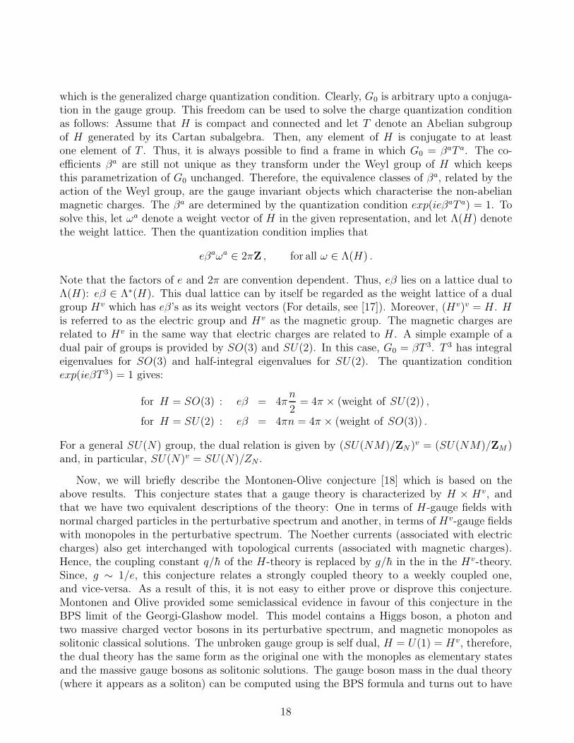
which is the generalized charge quantization condition. Clearly, G0 is arbitrary upto a conjuga-tion in the gauge group. This freedom can be used to solve the charge quantization conditionas follows: Assume that H is compact and connected and let T denote an Abelian subgroupof H generated by its Cartan subalgebra. Then, any element of H is conjugate to at leastone element of T . Thus, it is always possible to find a frame in which G0 = βaT a. The co-efficients βa are still not unique as they transform under the Weyl group of H which keepsthis parametrization of G0 unchanged. Therefore, the equivalence classes of βa, related by theaction of the Weyl group, are the gauge invariant objects which characterise the non-abelianmagnetic charges. The βa are determined by the quantization condition exp(ieβaT a) = 1. Tosolve this, let ωa denote a weight vector of H in the given representation, and let Λ(H) denotethe weight lattice. Then the quantization condition implies that

eβaωa ∈ 2πZ , for all ω ∈ Λ(H) .

Note that the factors of e and 2π are convention dependent. Thus, eβ lies on a lattice dual toΛ(H): eβ ∈ Λ∗(H). This dual lattice can by itself be regarded as the weight lattice of a dualgroup Hv which has eβ’s as its weight vectors (For details, see [17]). Moreover, (Hv)v = H . His referred to as the electric group and Hv as the magnetic group. The magnetic charges arerelated to Hv in the same way that electric charges are related to H . A simple example of adual pair of groups is provided by SO(3) and SU(2). In this case, G0 = βT 3. T 3 has integraleigenvalues for SO(3) and half-integral eigenvalues for SU(2). The quantization conditionexp(ieβT 3) = 1 gives:

for H = SO(3) : eβ = 4πn

2= 4π × (weight of SU(2)) ,

for H = SU(2) : eβ = 4πn = 4π × (weight of SO(3)) .

For a general SU(N) group, the dual relation is given by (SU(NM)/ZN )v = (SU(NM)/ZM )and, in particular, SU(N)v = SU(N)/ZN .

Now, we will briefly describe the Montonen-Olive conjecture [18] which is based on theabove results. This conjecture states that a gauge theory is characterized by H × Hv, andthat we have two equivalent descriptions of the theory: One in terms of H-gauge fields withnormal charged particles in the perturbative spectrum and another, in terms of Hv-gauge fieldswith monopoles in the perturbative spectrum. The Noether currents (associated with electriccharges) also get interchanged with topological currents (associated with magnetic charges).Hence, the coupling constant q/h of the H-theory is replaced by g/h in the in the Hv-theory.Since, g ∼ 1/e, this conjecture relates a strongly coupled theory to a weekly coupled one,and vice-versa. As a result of this, it is not easy to either prove or disprove this conjecture.Montonen and Olive provided some semiclassical evidence in favour of this conjecture in theBPS limit of the Georgi-Glashow model. This model contains a Higgs boson, a photon andtwo massive charged vector bosons in its perturbative spectrum, and magnetic monopoles assolitonic classical solutions. The unbroken gauge group is self dual, H = U(1) = Hv, therefore,the dual theory has the same form as the original one with the monoples as elementary statesand the massive gauge bosons as solitonic solutions. The gauge boson mass in the dual theory(where it appears as a soliton) can be computed using the BPS formula and turns out to have

18

the right value. Moreover, the long-range force between two monopoles as obtained by Manton[19], can be obtained by calculating the potential between W -bosons in the dual theory andturns out to be the same.

Since the Montonen-Olive duality is non-perturbative in nature, it cannot be verified in aperturbative framework unless we have some kind of control over the perturbative and non-perturbative aspects of the theory. Such a control is provided by superysymmetry. In fact,in the N = 4 super Yang-Mills theory, some very non-trivial predictions of this duality wereverified in [20]. In later parts, we will consider in detail the analogue of the Montonen-Oliveduality in N = 2 supersymmetric gauge theories. A prerequisite for this, however, is theintroduction of the θ-term in the Yang-Mills action which affects the electric charges of dyons.

1.10 The θ-Parameter and the Monopole Charge

In this section we will show, following Witten [21], that in the presence of a θ-term in theLagrangian, the magnetic charge of a particle always contributes to its electric charge.

As shown by Schwinger and Zwanziger, for two dyons of charges (q1, g1) and (q2, g2), thequantization condition takes the form

q1g2 − q2g1 = 2πnh (43)

For an electric charge q0 and a dyon (qn, gn), this gives q0gn = 2πnh. Thus, the smallestmagnetic charge the dyon can have is g0 = 2πh/q0. For two dyons of the same magneticcharge g0 and electric charges q1 and q2, the quantization condition implies q1 − q2 = nq0.Therefore, although the difference of electric charges is quantized, the individual charges arestill arbitrary. This arbitrariness in the electric charge of dyons can be fixed if the theory isCP invariant as follows: Under a CP transformation (q, g) → (−q, g). If the theory is CPinvariant, the existence of a state (q, g0) necessarily leads to the existence of (−q, g0). Applyingthe quantization condition to this pair, we get 2q = q0 × integer. This implies that q = nq0or q = (n + 1

2)q0, though at a time we can either have dyons of integral or half-odd integral

charge, and not both together.

In the above argument, it was essential to assume CP invariance to obtain integral or half-odd inegral values for the electric charges of dyons. However, in the real world, CP invariance isviolated and there is no reason to expect that the electric charge should be quantized as above.To study the effect of CP violation, we consider the Georgi-Glashow model with an additionalθ-term which is the source of CP violation:

L = −1

4F a

µνFaµν +

1

2(Dµ

~φ)2 − λ(φ2 − a2)2 +θe2

32π2F a

µνFaµν . (44)

Here, F aµν = 12ǫµνρσF a

ρσ and the vector notation is used to represent indices in the gauge space.The presence of the θ-term does not affect the equations of motion but changes the physicssince the theory is no longer CP invariant. We want to construct the electric charge operatorin this theory. The theory has an SO(3) gauge symmetry but the electric charge is associated

19

with an unbroken U(1) which keeps the Higgs vacuum invariant. Hence, we define an operatorN which implements a gauge rotation around the φ direction with gauge parameter Λa = φa/a.These transformations correspond to the electric charge. Under N , a vector ~v and the gaugefields ~Aµ transform as

δ~v =1

a~φ× ~v , δ ~Aµ =

1

eaDµ

~φ .

Clearly, ~φ is kept invariant. At large distances where |φ| = a, the operator e2πiN is a 2π-rotationabout φ and therefore exp (2πiN) = 1. Elsewhere, the rotation angle is 2π|φ|/a. However, byGauss’ law, if the gauge transformation is 1 at ∞, it leaves the physical states invariant. Thus,it is only the large distance behaviour of the transformation which matters and the eigenvaluesof N are quantized in integer units. Now, we use Noether’s formula to compute N :

N =∫d3x

(δL

δ∂0Aai

δAai +

δLδ∂0φa

δφa

).

Since δ~φ = 0, only the gauge part (which also includes the θ-term) contributes:

δ

δ∂0Aai

(F a

µνFaµν)

= 4F aoi = −4Eai ,

δ

δ∂0Aai

(F a

µνFaµν)

= 2ǫijkF ajk = −4Bai .

Thus, we get

N =1

ae

∫d3xDi

~φ · ~E i − θe

8π2a

∫d3xDi

~φ · ~Bi

=1

eQ− θe

8π2M ,

where, we have used equations (30). Here, Q and M are the electric and magnetic chargeoperators with eigenvalues q and g, respectivly, and N is quantized in integer units. This leadsto the following formula for the electric charge

q = ne+θe2

8π2g .

For the ’t Hooft-Polyakov monopole, n = 1, g = −4π/e, and therefore, q = e(1 − θ/2π). For ageneral dyonic solution we get

g =4π

em, q = ne+

θe

2πm . (45)

Thus, in the presence of a θ-term, a magnetic monopole always carries an electric charge whichis not an integral multiple of some basic unit.

It is very useful to represent the charged states as points on the complex plane, with electriccharges along the real axis and magnetic charges along the imaginary axis. A state can thusbe represented as

q + ig = e(n+mτ) , (46)

20

where,

τ =θ

2π+

4πi

e2(47)

In this parametrisation, the Bogomol’nyi bound (35) takes the form

M ≥√

2|ae(n +mτ)| . (48)

Note that (46) implies that all states lie on a two-dimensional lattice with lattice parameter τand (48) implies that the BPS bound for a state is proportional to the distance of its latticepoint from the origin. These equations play a very important role in the subsequent discussions.

2 Supersymmetric Gauge Theories

In this section we will explain some aspects of supersymmetry and supersymmetric field theorieswhich are relevant to the work of Witten and Seiberg. We start by explaining our conventionsand then briefly describe the representations of supersymmetry algebra with and without centralcharges. We then discuss the representations of N = 1 supersymmetry in terms of quantumfields and construct Lagrangians with N = 1 and N = 2 supersymmetry. Most of the materialin this section is by now standard and can be found in [22, 23, 24]. Towards the end of thissection, we will explicitly calculate the central charges in N = 2 theories with and withoutmatter.

2.1 Conventions

We start by descrbing our conventions. We use the flat metric ηab = diag (1,−1,−1,−1).The spinors of the Lorentz group SL(2, C) ∼ SU(2)L × SU(2)R are written with dotted andundotted components and, under SL(2, C), transform as

ψ′α = M β

α ψβ , ψ′α = M∗ β

α ψβ .

Spinor indices are raised or lowered with the ǫ-tensor,

ǫαβ = ǫαβ =

(0 1−1 0

)= (iσ2) .

By definition, this tensor is invariant under a SL(2, C) transformation: ǫαβ = Mαγǫ

γδM βδ . This

can be written as MTσ2M = σ2 which implies σ2M = (MT )−1σ2 Using this, we can write thetransformations of the spinors with raised indices as

ψ′α = ψβ(M−1) αβ , ψ′α = ψβ(M∗)−1 α

β.

Now, let us define(σµ)αα ≡ (1, ~σ) ,

21

then,

σµPµ =

(P 0 − P 3 −P 1 + iP 2

−P 1 − iP 2 P 0 + P 3

),

and det(σµPµ) = PµPµ. We can raise the indices on σµ using the ǫ-tensor and define σ as

(σµ)αα = −(σµ)αα = ǫαβǫαβ(σµ)ββ .

Numerically, this gives,

(σµ) = (iσ2)(σµ)T (iσ2)

T = σ2(σµ)Tσ2 = (1,−~σ) .

With these conventions, Lorentz transformations are generated by

(σµν) βα =

1

4[σµ

αβσνββ − (µ ↔ ν)] ,

(σµν)αβ

=1

4[σµαβσν

ββ− (µ↔ ν)] .

For the scalar product of spinors, we use the following conventions

ψχ = ψαχα = −ψαχα = χαψα = χψ ,

ψχ = ψαχα = χψ ,

(ψχ)† = χαψα = χψ = ψχ .

We list some more spinor identities

χσµψ = −ψσµχ ,(χσµψ)† = ψσµχ ,χσµσνψ = ψσν σµχ ,

(χσµσνψ)† = ψσνσµχ .

In the above basis, the Dirac matrices and Dirac and Majorana spinors are given by

γµ =

(0 σµ

σµ 0

), ψD =

(ψα

χα

), ψM =

(ψα

ψα

). (49)

As usual, one defines γ5 = −iγ0γ1γ2γ3. Consider a massless fermion moving in the z-direction.Then, P µ = E(1, 0, 0, 1), and the Dirac equation gives (γ0 − γ3)ψ = 0. Since the helicityoperator is now J3 = i

2γ1γ2, one gets, J3ψ = i

2(γ0)2γ1γ2ψ = i

2γ0γ1γ2γ3ψ = −1

2γ5ψ. Hence,

γ5 = +1 ⇒ −ve helicity , γ5 = −1 ⇒ +ve helicity .

2.2 Supersymmetry Algebra without Central Charges

In the absence of central charges, the supersymmetry algebra is written as

QIα, QαJ = 2σµ

ααPµδIJ ,

QIα, Q

Jβ = 0 , QαI , QβJ = 0 . (50)

22

Here, Q and Q are the supersymmetry generators and transform as spin-half operators underthe angular momentum algebra. The indices I, J run from 1 to N , where N is the total numberof supersymmetries. Moreover, the supersymmetry generators commute with the momentumoperator Pµ and hence, with P 2. Therefore, all states in a given representation of the algebrahave the same mass. For a theory to be supersymmetric, it is necessary that its particle contentform a representation of the above algebra. The supersymmetry algebra can be embeddedin the super-Poincare algebra and its representations can be obtained systematically usingWigner’s method. In the following, we will give a brief description of the representations ofsupersymmetry algebra.

Massless Irreducible Representations: For massless states, we can always go to a frame whereP µ = M(1, 0, 0, 1). Then the supersymmetry algebra becomes

QIα, QαJ =

(0 00 4M

)δIJ .

Now, in a unitary theory the norm of a state is always positive definite. Since Qα and Qα areconjugate to each other, and Q1, Q1 = 0, it follows that Q1|phys >= Q1|phys >= 0. As forthe other generators, it is convenient to rescale them as

aI =1

2√MQI

2 , (aI)† =1

2√MQI

2 .

Then, the supersymmetry algebra takes the form

aI , (aJ)† = δIJ , aI , aJ = 0 , (aI)†, (aJ)† = 0 .

This is a Clifford algebra with 2N generators and has a 2N -dimensional representation. Fromthe point of view of the angular momentum algebra, aI is a rising operator and (aI)† is a loweringoperator for the helicity of massless states. We choose the vacuum such that J3|Ωλ >= λ|Ωλ >and aI |Ωλ >= 0 for all I. Other states are generated by the action of (aI)†’s on the vacuumstate. From anti-symmetry it follows that a state with m (aI)†’s, and hence with helicityλ−m/2, will have a degeneracy of NCm. The helicity of all states so constructed will span therange λ to λ−N/2. Some examples are:

N = 1 : |λ >, |λ− 1/2 >N = 2 : |λ >, 2 |λ− 1/2 >, |λ− 1 >N = 4 : |λ >, 4 |λ− 1/2 >, 6 |λ− 1 >, 4 |λ− 3/2 >, |λ− 2 >

The irreducible representations are not necessarily CPT invariant. Therefore, if we want toassign physical states to these representations, we have to suplement them with their CPTconjugates. If a representation is CPT self-conjugate, it is left unchanged. Below, we list therepresentations after the addition of the CPT conjugates and indicate the particle spectra whichcan be assiged to them:

N = 1, λ = 1/2 : |1/2 > , |0 > , | − 1/2 > , |0 >λ = 1 : |1 > , |1/2 > , | − 1 > , | − 1/2 >

N = 2, λ = 1/2 : |1/2 > , 2|0 > , | − 1/2 > , | − 1/2 > , 2|0 > , |1/2 >λ = 1 : |1 > , 2|1/2 > , |0 > , | − 1 > , 2| − 1/2 > , |0 >

N = 4, λ = 1 : |1 > , 4|1/2 > , 6|0 > , 4| − 1/2 > , | − 1 >

23

Thus, for N = 1, the representation contains a Majorana spinor and a complex scalar if λ = 1/2(scalar multiplet), or a massless vector and a Majorana spinor if λ = 1 (vector multiplet). ForN = 2 and λ = 1/2, we have two Majorana spinors (or one Dirac spinor) with two complexscalars. This representation has the same particle content as two copies of the N = 1, λ = 1/2multiplet. For N = 2 and λ = 1, we have a massless vector, two Majorana spinors and acomplex scalar. Note that this multiplet has the same particle content as the two N = 1multiplets for λ = 1/2 and λ = 1 put together. For N = 4, the representation is self-conjugateand accommodates a massless vector, two Dirac fermions and three complex scalars.

Massive Irreducible Representations: For massive states, we can always go to the rest framewhere Pµ = (M, 0, 0, 0) and define

aIα = QI

α/√

2M , (aIα)† = QαI/

√2M .

Then the supersymmetry algebra reduces to

aI1, (a

J1 )† = δIJ , aI

2, (aJ2 )† = δIJ ,

with all other anti-commutators vanishing. The Clifford vacuum is defined by aIα|Ω >= 0

and the representation is constructed by applying (aIα)†’s on Ω. Let |Ω > be a spin singlet.

Then there are 2NCm states at level m and the dimension of the the representation is given by∑2Nm=0

2NCm = 22N . The maximum spin which can be reached is N/2 and not N as one mightnaively expect. This is because (aI

1)†(aI

2)† = 1

2ǫαβ(aI

α)†(aIβ)† is a scalar. Thus the state with

m = 2N has spin zero, as the vacuum. The degeneracy of states with a given spin is labelled bythe irreducible representations of the group USp(2N) which we will not discuss here. Instead,let us consider the simplest example. For N = 1, the massive representation contains 22 = 4states,

|Ω >, a†α|Ω >,1√2ǫαβa†αa

†β|Ω > ,

with spin content (0) ⊕ (1/2) ⊕ (0). Here, (j) denotes a state of total spin j and degeneracy2j + 1. Thus, in the above example, we have a Weyl (or Majorana) spinor and a complexscalar (λ, φ). For N = 2, the representation contains 24 = 16 states which, under the SU(2)of angular momentum, decompose as 5(0) ⊕ 4(1/2) ⊕ 1(1). The N = 4 massive multiplet has28 = 256 states and inclueds a spin 2 state.

Till now we have considered representations based on a singlet vacuum. Let us considera vacuum |Ωj > of spin j which is 2j + 1-fold degenerate. The representation now contains(2j + 1)22N states. The spectrum is worked out by combining the j = 0 representation of theClifford algebra and a spin j, using the angular momentum addition rules. For example, toobtain the N = 1 representation based on |Ωj >, we combine (0) ⊕ (1/2) ⊕ (0) with (j) toobtain (j) ⊕ (j + 1/2) ⊕ (j − 1/2) ⊕ (j). For j = 1/2, we get (1/2) ⊕ (1) ⊕ (0) ⊕ (1/2) whichcorresponds to a gauge field, a Dirac fermion and a scalar field, all of the same mass. Note thatin all cases we get the same number of bosonic and fermionic degrees of freedom.

24

2.3 Supersymmetry Algebra with Central Charges

As shown by Haag, Lapuszanski and Sohnius [25], the supersymmetry algebra (50) admits acentral extension and can be generalised to

QIα, QβJ = 2σµ

αβPµδ

IJ ,

QIα, Q

Jβ = 2

√2ǫαβZ

IJ ,

QαI , QβJ = 2√

2ǫαβZ∗IJ , (51)

where, Z and Z∗ are the central charge metrices which are antisymmetric in I and J . Letus focus on the case of even N . Using a unitary transformation, we can skew-diagonalize Z:ZIJ = U I

AUJBZ

AB, so that it takes the form Z = ǫ⊗D, where D is an N/2-dimensional diagonalmatrix. Thus, the index I which counts the number of supersymmetries can be decomposedinto (a,m), with a = 1, 2 coming from the antisymmetric tensor ǫ, and m = 1, ..., N/2 comingfrom the diagonal matrix D. By a further chiral rotation, we may choose the eigenvalues ofD to be real. Once we have skew-diagonalized, it is sufficient to consider just the N = 2supersymmetry, for which the algebra takes the form

Qaα, Qβb = 2(σµ)αβPµδ

ab ,

Qaα, Q

bβ = 2

√2ǫαβǫ

abZ ,

Qαa, Qβb = 2√

2ǫαβǫabZ . (52)

Since Z commutes with all the generators, we can fix it to be the eigenvalue for the givenrepresentation. Now, let us define:

aα =1

2Q1

α + ǫαβ(Q2β)† , bα =

1

2Q1

α − ǫαβ(Q2β)† .

Then, the algebra (51) reduces to

aα, a†β = δαβ(M +

√2Z) , bα, b†β = δαβ(M −

√2Z) , (53)

with all other anticommutators vanishing. Since all physical states have positive definite norm,it follows that for massless states, the central charge is trivially realised (i.e.,Z = 0). Formassive states, this leads to a bound on the mass M ≥

√2|Z|. When M =

√2|Z|, one set

of operators in (53) is trivially realized and the algebra resembles the massless case and thedimension of representation is greatly reduced. For example, a reduced massive N = 2 multiplethas the same number of states as a massless N = 2 multiplet. Thus the representations ofthe N = 2 algebra with a central charge can be classified as either long multiplets (whenM >

√2|Z|) or short multiplets (when M =

√2|Z|).

The mass boundM ≥√

2|Z| is reminiscent of the Bogomol’nyi bound in the Georgi-Glashowmodel. In fact, it turns out that in the supersymmetric version of the Georgi-Glashow model(which is based on the algebra without central charges) the solitonic solutions do give rise to acentral extension term in the supersymmetry algebra, thus realizing (51)[26]. The origin of the

25

central charge is easy to understand: The supersymmetry charges Q and Q are space integralsof local expressions in the fields (the time component of the super-currents). In calculatingtheir anticommutators, one encounters surface terms which are normally neglected. However,in the presence of electric and magnetic charges, these surface terms are non-zero and give riseto a central charge. As we will explicitly show towards the end of this section, it is found that

Z = a(q + ig) = ae(n +mτ) , (54)

so that M ≥√

2|Z| coincides with the Bogomol’nyi bound (35). From (53) it is clear that theBPS states (which saturate the bound) are annihilated by half of the supersymmetry generatorsand thus belong to reduced representations of (51). An important consequence of this is that,for BPS states, the relationship between their charges and masses is dictated by supersymmetryand does not receive perturbative or non-perturbative corrections in quantum theory. This isso because a modification of this relation implies that the states no longer belong to a shortmultiplet. On the other hand, quantum correction are not expected to generate the extradegrees of freedom needed to convert a short multiplet into a long multiplet. Since there is noother possibility, we conclude that for short multiplets the relation M =

√2|Z| is not modified

either perturbatively or non-perturbatively.

2.4 Local Representations of N=1 Supersymmetry

In this subsection we describe the action of supersymmetry on the local fields in a quantum fieldtheory. It is well known that the Poincare group naturally acts on the space-time coordinates.All other objects transform as components of tensors or spinors defined on the space-timemanifold. Similarly, the supersymmetry transformations naturally act on an extension of thespace-time, called the “superspace”. The quantum fields then transform as components of a“superfield” defined on the superspace. In the following, we first describe these notions andthen introduce the chiral and vector superfields.

Superspace : The superspace is obtained by adding four spinor degrees of freedom θα, θα tothe space-time coordinates xµ. The spinor index is raised and lowered with the ǫ-tensor andθθ = θαθα = −2θ1θ2. Similarly, θθ = θαθ

α = 2θ1θ2. We also have

θαθβ =1

2ǫαβθθ , θαθβ = −1

2ǫαβ θθ , θσµθθσν θ =

1

2θθθθηµν .

These formulae are the basis for Fierz rearrangements.

Under the supersymmetry transformations (50) with N = 1 and transformation parametersξ and ξ, the superspace coordinates are taken to transform as

xµ → x′µ = xµ + iθσµξ − iξσµθ ,

θ → θ′ = θ + ξ ,

θ → θ′ = θ + ξ . (55)

26

Since these transformations are implemented by the operator ξαQα+ ξαQα, we can easily obtain

the representation of the supercharges acting on the superspace as

Qα =∂

∂θα− iσµ

ααθα ∂µ , Qα = − ∂

∂θα+ iθασµ

αα ∂µ . (56)

These satisfy Qα, Qα = 2iσµαα ∂µ. Moreover, using the chain rule, it is easy to see that ∂/∂xµ

is invariant under (55) but not ∂/∂θ and ∂/∂θ. Therefore, we introduce the super-covariantderivatives

Dα =∂

∂θα+ iσµ

αα ∂µ , Dα = − ∂

∂θα− iσµ

ααθα ∂µ . (57)

They satisfy Dα, Dα = −2iσµαα ∂µ and commute with Q and Q.

Superfields: A superfield is a function on the superspace, say, F (x, θ, θ). Since the θ-coordinatesare anti-commuting, the most general N = 1 superfield can always be expanded as

F (x, θ, θ) = f(x) + θφ(x) + θχ(x) + θθm(x) + θθn(x) + θσµθvµ(x)

+ θθθλ(x) + θθθψ(x) + θθθθd(x) . (58)

Clearly, any function of superfields is, by itself, a superfield. Under supersymmetry, the su-perfield transforms as δF = (ξQ + ξQ)F , from which, the transformation of the componentfields can be obtained. Note that since d(x) is the component of highest dimension in themultiplet, its variation under supersymmetry is always a total derivative of other components.Thus, ignoring surface terms, the space-time integral of this component is invariant under su-persymmetry. This tells us that a supersymmetric Lagrangian density may be constructed asthe highest dimension component of an appropriate superfield. To describe physical systems,we do not need all components of the superfield. The relevant components are selected byimposing appropriate constraints on the superfield.

Chiral Multiplets: The N = 1 scalar multiplet is represented by a superfield with one constraint:

DαΦ = 0 .

This is referred to as the chiral superfield. Note that for yµ = xµ + iθσµθ, we have

Dαyµ = 0, Dαθ

β = 0 .

Therefore, any function of (y, θ) is a chiral superfield. It can be shown that this also is anecessary condition. Hence, any chiral superfield can be expanded as

Φ(y, θ) = A(y) +√

2θψ(y) + θθF (y) . (59)

Here, A and ψ are the fermionic and scalar components respectively and F is an auxiliary fieldrequired for the off-shell closure of the algebra. Similarly, an anti-chiral superfield is defined byDαΦ† = 0 and can be expanded as

Φ†(y†, θ) = A†(y†) +√

2θψ(y†) + θθF †(y†) , (60)

27

where, yµ† = xµ − iθσµθ. The product of chiral superfields is a chiral superfield. In general,any arbitrary function of chiral superfields is a chiral superfield:

W(Φi) = W(Ai +√

2θψi + θθFi)

= W(Ai) +∂W∂Ai

√2θψi + θθ

(∂W∂Ai

Fi −1

2

∂2W∂AiAj

ψiψj

). (61)

W is referred to as the superpotential. In terms of the original variables, Φ and Φ† take theform

Φ(x, θ, θ) = A(x) + iθσµθ∂µA− 1

4θ2θ2

2A

+√

2θψ(x) − i√2θθ∂µψσ

µθ + θθF (x) , (62)

Φ†(x, θ, θ) = A†(x) − iθσµθ∂µA† − 1

4θ2θ2

2A†

+√

2θψ(x) +i√2θθ θσµ ∂µψ + θθF †(x) . (63)

Vector Multiplet: This multiplet is represented by a real superfield satifying V = V †. Incomponents, it takes the form

V (x, θ, θ) = C + iθχ− iθχ+ i2θ2(M + iN) − i

2θ2(M − iN)

−θσµθAµ + iθ2θ(λ+ i2σµ∂µχ)

−iθ2θ(λ+ i2σµ∂µχ) + 1

2θ2θ2(D − 1

22C) .

Many of these components can be gauged away using the abelian gauge transformation V →V + Λ + Λ†, where Λ (Λ†) are chiral (antichiral) superfields. In the so called Wess-Zuminogauge, we set C = M = N = χ = 0, so that

V = −θσµθAµ + iθ2θλ− iθ2θλ+1

2θ2θ2D .

In this gauge, V 2 = 12AµA

µθ2θ2 and V 3 = 0. The Wess-Zumino gauge breaks supersymmetry,but not the gauge symmetry of the abelian gauge field Aµ. The Abelian field strength is definedby

Wα = −1

4D2DαV , Wα = −1

4D2DαV .

Wα is a chiral superfield. Since it is gauge invariant, it can be computed in the Wess-Zuminogauge and takes the form

Wα = −iλα(y) + θαD − i

2(σµσνθ)α Fµν + θ2(σµ∂µλ)α , (64)

where, Fµν = ∂µAν − ∂νAµ is the familiar abelian field strength tensor.

In the non-Abelian case, V belongs to the adjoint representation of the gauge group: V =VAT

A, where, TA† = TA. The gauge transformations are now implemented by

e−2V → e−iΛ†

e−2V eiΛ where, Λ = ΛATA

28

The non-Abelian gauge field strength is defined by

Wα =1

8D2e2VDαe

−2V

and transforms asWα →W ′

α = e−iΛWαeiΛ .

In components, it takes the form

Wα = T a(−iλa

α + θαDa − i

2(σµσνθ)αF

aµν + θ2σµDµλ

a), (65)

where,F a

µν = ∂µAaν − ∂νA

aµ + fabcAb

µAcν , Dµλ

a = ∂µλa + fabcAb

µλc .

In the next section, we will construct supersymmetric Lagrangians in terms of superfields.

2.5 Construction of N=1 Lagrangians

In this section we will construct the N = 1 Lagrangians for the scalar and the vector multiplets.These serve as the building blocks for the N = 2 Lagrangian which is our real interest. Asstated before, a supersymmetric Lagrangian can be constructed as the highest component of asuperfield. Thus the problem reduces to that of finding appropriate superfields.

Lagrangian for the Scalar Multiplet: Let us first consider the product of a chiral and an anti-

chiral superfield Φ†iΦj . This is a general superfield and its highest component can be computed

using (62) and (63) as

Φ†iΦj |θ2θ2 = − 1

4A†

i2Aj −1

42A†

iAj + F †i Fj +

1

2∂µA

†i∂

µAj

− i

2ψjσ

µ∂µψi +i

2∂µψjσ

µψi .

Dropping some total derivatives and summing over i = j, we get the free field Lagrangian

L = Φ†iΦi |θ2θ2= ∂µA

†i∂

µAi + F †i Fi − iψiσ

µ∂µψi .

This is the free Lagrangian for a massless scalar and a massless fermion with an auxiliary fieldwhich can be eliminated by its equation of motion. Supersymmetric interaction terms canbe constructed in terms of the superpotential (61) and its conjugate, which are holomorphicfunctions of Φ and Φ†, respectively. Moreover, note that the space of the fields Φ may havea non-trivial metric gij in which case the scalar kinetic term, for example, takes the formgij∂µA

†i∂

µAj , with appropriate modifications for other terms. In such cases, the free fieldLagrangian above has to be replaced by a non-linear σ-model. Thus, the most general N = 1supersymmetric Lagrangian for the scalar multiplet (including the interaction terms) is givenby

L =∫d4θ K(Φ,Φ†) +

∫d2θW(Φ) +

∫d2θW(Φ†) .

29

Note that the θ-integrals pick up the highest component of the superfield and in our conventions,∫d2θθ2 = 1 and

∫d2θθ2 = 1. In terms of the non-holomorphic function K(A,A†), the metric

on the field space is given by gij = ∂2K/∂Ai∂A†j . For this reason, the function K(Φ,Φ†) is

referred to as the Kahler potential.

For a renormalizable theory, the forms of K and W are not arbitrary and are constrainedby R-symmetry. This symmetry acts on the chiral superfields as follows

RΦ(x, θ) = Φ′(x, θ) = e2inαΦ(x, e−iαθ) ,

RΦ†(x, θ) = Φ′†(x, θ) = e−2inαΦ†(x, eiαθ) .

Under this, the component fields transform as

A → e2inαA ,ψ → e2i(n−1/2)αψ ,F → e2i(n−1)αF .

We refer to n as the R-character. Since θ → e+iαθ, or d2θ → e−2iαd2θ, The R-character of thesuperfields in each term of W must add up to one. Similarly, K should be R-neutral. Thevector multiplet is real and it has no natural R-symmetry. This symmetry plays an importantrole in the study of supersymmetric gauge theories and we will come back to it in the nextsection.

Lagrangians for the Vector Multiplet: As mentioned in the previous section, the Abelian fieldstrength W , given by (64), is a chiral superfield. Using the expansion there, one can easilycompute that

W αWα |θθ= −2iλσµ∂µλ+D2 − 1

2F µνFµν +

i

4ǫµνρσFµνFρσ .

Hence, the usual abelian supersymmetric Lagrangian (which does not contain the FF term) isgiven by

L =1

4g2

(∫d2θW αWα +

∫d2θ WαW

α).

Similarly, in the non-Abelian case, using the normalization TrT aT b = δab, we have

Tr(W αWα |θθ) = −2iλaσµDµλa +DaDa − 1

2F aµνF a

µν +i

4ǫµνρσF a

µνFaρσ , (66)

and, hence, the usual non-Abelian supersymmetric Lagrangian (without the FF -term) is givenby

L =1

4g2Tr(∫

d2θW αWα +∫d2θ WαW

α).

However, we are interesed in the supersymmetric analogue of the Lagrangian (44) which alsocontains a θ-term. From (66), it is obvious that the super Yang-Mills Lagrangian with a θ-termcan be written as

L =1

8πIm

(τ Tr

∫d2θW αWα

)

= − 1

4g2F a

µνFaµν +

θ

32π2F a

µνFaµν +

1

g2(1

2DaDa − iλaσµDµλ

a) , (67)

30

where, τ = θ/2π + 4πi/g2. Note that τ can be regarded as a constant chiral superfield.

Interaction Terms and the General N = 1 Lagrangian: Let the chiral superfields Φi belong toa given representation of the gauge group in which the generators are the matrices T a

ij . The

kinetic energy term Φ†iΦi is invariant under global gauge transformations Φ′ = e−iΛΦ. In the

local case, to insure that Φ′ remains a chiral superfield, Λ has to be a chiral superfield. Thesupersymmetric gauge invariant kinetic energy term is then given by Φ†e−2V Φ. We are now ina position to write down the full N=1 supersymmetric Lagrangian as

L =1

8πIm

(τTr

∫dθ W αWα

)+∫d2θd2θΦ†e−2V Φ +

∫d2θW +

∫d2θ W . (68)

Note that since each term is separately invariant, the relative normalisation between the scalarpart and the Yang-Mills part is not fixed by N = 1 supersymmetry. In the above, we haveset the normalization of the scalar part to one, but later, we will change this by rescaling thescalar multiplet Φ. In terms of component fields, the above Lagrangian takes the form

L = − 1

4g2F a

µνFaµν +

θ

32π2F a

µνFaµν − i

g2λaσµDµλ

a +1

2g2DaDa

+ (∂µA− iAaµT

aA)†(∂µA− iAaµT aA) − i ψσµ(∂µψ − iAaµT

aψ)

− DaA†T aA− i√

2A†T aλaψ + i√

2 ψT aAλa + F †i Fi

+∂W∂Ai

Fi +∂W∂A†

i

F †i − 1

2

∂2W∂Ai∂Aj

ψiψj −1

2

∂2W∂A†

i∂A†j

ψiψj . (69)

Here, W denotes the scalar component of the superpotential. The auxiliary fields F and Da

can be eliminated by using their equations of motion. The terms involving these fields, thus,give rise to the scalar potential

V =∑

i

∣∣∣∣∣∂W∂Ai

∣∣∣∣∣

2

− 1

2g2(A†T aA)2 . (70)

2.6 The N = 2 Supersymmetric Lagrangian for Gauge Fields

The on-shell N = 1 scalar multiplet (A,ψ) and vector multiplet (Aµ, λ), put together, havethe same field content as the on-shell N = 2 vector multiplet (A,ψ, λ, Aµ). The Lagrangian(69) contains all these fields but as such is not N = 2 supersymmetric. We now assume that(A,ψ, λ, Aµ) form an N = 2 vector multiplet and discuss the restrictions which this assumtionimposes on the N = 1 Lagrangian in (69). First, since Aa

µ and λa belong to the adjointrepresentation of the gauge group, Ai and ψi should also belong to the same representation ifthey are to be part of the same multiplet. Hence, T a

ij = −ifaij and the sets of indices i and

a coincide. Second, since the two supersymmetry generators in the N = 2 algebra appear onthe same footing, the same must be the case with the fermions ψa and λa in (69). To satisfythis condition, we set the superpotential W to zero since it couples only to ψa. This conditionalso fixes the arbitrary relative normalization between the Yang-Mills part and the scalar part

31

of the Lagrangian since it requires that the kinetic energy terms for both fermions should havethe same normalization. This is achieved by scaling Φ → Φ/g in (69). It turns out that ifthe Lagrangian (69) satisfies these conditions, then it has N = 2 supersymmetry. The termscontaining the auxiliary fields now take the form

1

g2Tr(

1

2DD +D [A† , A] + F †F

),

where, we have used the notation Φ = ΦaT a, with T a in the fundamental representation. Oneliminating D and F , we get the scalar potential

V = − 1

2g2Tr([A† , A]2

). (71)

The full Lagrangian with N = 2 supersymmetry can now be written as

L =1

8πIm Tr

[τ(∫

d2θW αWα + 2∫d2θd2θΦ†e−2V Φ

)]

=1

g2Tr(− 1

4FµνF

µν + g2 θ

32π2FµνF

µν + (DµA)†DµA− 1

2[A† , A]2

− i λσµDµλ− i ψσµDµψ − i√

2 [λ, ψ]A† − i√

2 [λ, ψ]A), (72)

where, in the component expansion, the auxiliary fields have been eliminated. Note that (72)is the supersymmetric generalization of the Yang-Mills-Higgs theories described in section 1,with the Higgs potential V given by (71), and with a θ-term. Therefore, the discussion insection 1 also applies to our N = 2 supersymmetric theory. In particular, the Higgs vacuumis defined by DµA = 0, V = 0, and the potential vanishes for non-zero field configurationsprovided A commutes with A†. Thus the model admits monopole and dyonic solutions andcontains massive gauge bosons. For example, if the gauge group is SU(2) or SO(3), it is brokendown to U(1) and two of the gauge bosons become massive.

Now, suppose that we are interested in the behaviour of this model at energies lower thansome cutoff Λ which is smaller than the mass of the lightest massive state in the theory.At such energies, we will not encounter any on-shell massive states and the physics can bedescribed by the Wilsonian low-energy effective action. This effective action is obtained bycompletely integrating out all massive states as well as integrating out all massless excitationsabove the scale Λ [36, 37]. This, in general, is a complicated procedure and cannot be carriedout explicitly. Fortunately, in our model, the general form of the Wilsonian effective action isseverely constrained by N = 2 supersymmetry. This is easiest to see when the theory (72) isformulated in term of N = 2 superfields as described below.

The N = 2 Superspace Formulation: The N = 2 superspace is obtained by adding four more

fermionic degrees of freedom, say, θ and ¯θ, to the N = 1 superspace. Thus, a generic N = 2

superfield can be written as F (x, θ, θ, θ,¯θ). We need a superfield which has the same components

as the N = 2 vector multiplet. This is obtained by imposing the constraints of chirality andreality on a general N = 2 superfield [27]. We briefly describe this following the approach of

32

[28]. An N = 2 chiral superfield Ψ is defined by the constraints DαΨ = 0 and ¯DαΨ = 0, where,

the supercovariant derivative ¯Dα is defined in the same way as Dα with θ replaced by θ. Theexpansion of Ψ can be arranged in powers of θ and can be written as

Ψ = Ψ(1)(y, θ) +√

2θαΨ(2)α (y, θ) + θαθαΨ(3)(y, θ) ,

where, yµ = xµ + iθσµθ + iθσµ¯θ. This expansion helps us relate the N = 2 formalism to theN = 1 language we have been using so far. Clearly, the component Ψ(1) has the same formas the N = 1 chiral superfield Φ. The remaining two components are constrained by a realitycondition. The outcome is that Ψ(2)

α = Wα(y, θ) as given in (65), and Ψ(3) is given by

Ψ(3)(y, θ) = Φ†(y − iθσθ, θ, θ)exp[2gV (y − iθσθ, θ, θ

]|θθ .

Here, Φ(y − iθσθ, θ, θ) is to be understood as the expansion in (62). Clearly, Ψ has the samefield content as the N = 2 vector multiplet. One can verify that in terms of the N = 2 superfieldΨ, the N = 2 Lagrangian (72) is given by the compact expression

L =1

4πIm Tr

∫d2θd2θ

1

2τΨ2 . (73)

Using the N = 2 chiral superfield Ψ (also referred to as the N = 2 vector superfield), wecan now construct the most general N = 2 Lagrangian for the gauge fields: Corresponding toany function F(Ψ), we can construct a Lagrangian

L =1

4πIm Tr

∫d2θd2θF(Ψ)

=1

8πIm

(∫d2θFab(Φ)W aαW b

α + 2∫d2θd2θ (Φ†e2gV )aFa(Φ)

). (74)

Here, Fa(Φ) = ∂F/∂Φa, Fab(Φ) = ∂2F/∂Φa∂Φb and F is referred to as the N = 2 prepotential.From the above, we can easily read off the Kahler potential as Im(Φ†aFa(Φ). This gives rise toa metric gab = Im(∂a∂bF) on the space of fields. A metric of this form is called a special Kahlermetric. If we demand renormalisability, then F has to be quadratic in Ψ as in (73). However,if we want to write a low-energy effective action, then renormalisability is not a criterion andF can have a more complicated form. In particular, we can start from the microscopic theory(72), corresponding to a quadratic prepotential, and try to construct the modified F for thelow-energy Wilsonian effective action. The exact determination of this function is the subjectof the work of Seiberg and Witten.

2.7 The N = 2 Supersymmetric Lagrangian for Matter Fields

Since matter fields and gauge fields transform under different representations of the gaugegroup, they cannot be part of the same multiplet. TheN = 2 matter supermultiplet is called thehypermultiplet and contains one pair of complex scalars and one pair of two-component spinors,

33

all transforming under the same representation of the gauge group. From our discussion of therepresentations of the supersymmetry algebra it follows that if a hypermultiplet is massive, thenits mass should appear as a central extension in the supersymmetry algera. This is so becauseotherwise N = 2 supersymmetry requires a larger number of components than is containedin a hypermultiplet. In N = 1 notation, a hypermultiplet contains a chiral superfield Q andan anti-chiral superfield Q†, both transforming under the same representatin Nc of the gaugegroup SU(Nc) We denote the components of Q and Q by (q, ψq, Fq) and (q, ψq, Fq) respectively.The form of the Lagrangian for Nf hypermultiplets (labelled by an index i), interacting with aN = 2 vector multiplet, can be partly inferred from the N = 1 theories and is given by

L =∫dθ4

(Q†

ie−2VQi + Qie

2V Q†i

)+∫dθ2

(√2QiΦQi +miQiQi

)+ h.c.

+ · · · (75)

Here, the dots represent the Lagrangian for the pure N = 2 vector multiplet and we havesupressed the gauge group indices. The term

√2QiΦQi is related, by N = 2 supersymmetry,

to the coupling of the hypermultiplet with the N = 1 vector multiplet V . The presence of thisterm is not required in an N = 1 Lagrangian. As in normal QCD, when all masses mi areequal, the theory is invariant under the global flavour group SU(Nf).

Eliminating the auxiliary fields Fq and Fq, which appear in the hypermultiplet, results in acontribution to the scalar potential given by (compare with (70))

V =1

2g2∑

a

DaDa ,

with

Da =Nf∑

i=1

(q†iλ

aqi − qiλaq†i). (76)

Here, λa are the gauge group generators in the fundamental representaion. This term is referredto as the D-term. It must be mentioned that the N = 2 algebra has a global SU(2)R symmetrywhich should also be a symmetry of the Lagrangian. However, in our decomposition of thehypermultiplet in terms of Q and Q†, this symmetry is not manifest since it rotates the scalarcomponents q and q† as a doublet. It is not difficult to write an N = 2 Lagrangian with manifestSU(2)R symmetry [23].

Minimization of the D-term: To find the vacuum of the theory, now we also have to minimizethe D-term contribution and the hypermultiplet mass term contribution to the scalar potential[29, 30]. For non-zero quark masses, the only solution is q = q = 0. Thus, only the scalar Acan have a non-zero vacuum expectation value. But when mi = 0, then the D-term can beminimized for a set of non-vanishing q and q (the potential has flat directions). However, theQΦQ term in the Lagrangian now requires Avac = 0. In the following, we determine these flatdirections.

The minimum of the D-term corresponds to Da = 0. To solve this, note that q(i)α (where α

denotes a colour index) can be regarded as a set of Nc vectors in CNf . Thus, we can construct

34

the matrix of scalar products,

∑

i

q(i)α q

†(i)β = qα · q†β = (qq†)αβ .

In terms of this, ∑

i

q†iλaqi = Tr

(qq†λa

).

Similarly, we construct the matrix q†α · qβ = (q†q)αβ . Hence, Da = 0 can be written as

Da = Tr[(qq† − q†q

)λa]

= 0 .

Since λa are in an irreducible representation of SU(Nc), the above condition is solved by

(qq†) − (q†q) = c21Nc. (77)

Here, we can distinguish two cases: Nf < Nc and Nf ≥ Nc.

1) Nf < Nc: In this case, the matrix (qq†) has rank Nf and thus it has N−Nf zero eigenvalues.The same applies to the matrix (q†q). By using SU(Nc) × SU(Nf) × U(1)R rotations, (qq†)can be diagonalized and condition (77) then implies that (q†q) must also be diagonal. Hence,in this basis, we can solve for q and q as

q =

v(1)1 0 · · · 0

0 v(2)2

.... . .

v(Nf )Nf

0 0 · · · 0...

......

, q =

v(1)1 0 · · · 0 · · ·0 v

(2)2 0 · · ·

.... . .

0 v(Nf )Nf

0 · · ·

.

The presence of zero eigenvalues imply that c = 0 and therefore, v(i)i = v

(i)i . In this case, the

gauge symmetry is broken down to SU(Nc − Nf) except for Nc = Nf − 1, where it is totallybroken. 2NfNc −N2

f quark superfields become heavy and the remaining N2f quark superfields

remain massless and correspond to the Goldstone bosons of broken global symmetries.

2) Nf ≤ N : In this case (qq†) has rank Nc and, generically, its eigenvalues are not zero. As aresult, c 6= 0. Arguing as above, in this case the vacuum values of q and q can be written as

q =

v(1)1 0 · · · 0 · · ·0 v

(2)2 0 · · ·

.... . .

0 v(Nc)Nc

0 · · ·

, q =

v(1)1 0 · · · 0

0 v(2)2

.... . .

v(Nc)Nc

0 0 · · · 0...

......

.

35

and

v(i)i =

√|v(i)

i |2 − c2 .

In this case, the gauge group is completely broken, and depending on the values of v(i)i , the

pattern of chiral symmetry breaking quite complicated with many possibilities. For Nf > N ,there are surviving R-symmetries.

2.8 Central Charges in the N = 2 Pure Gauge Theory

We have seen that the N = 2 supersymmetry algebra with central charge Z implies the boundM ≥

√2|Z| on the particle masses. It was also stated that this bound is the same as the BPS

bound on the masses which is determined in terms of the electric and magnetic charges. In thissection, we prove the above statement by explicitly calculating Z following [26].

In the supersymmetry algebra, The central charge Z appears in the commutator of thesupercharges QI

α which, in turn, are space integrals of SI0α (Here, SIµ

α denotes the supercurrent).Thus, we first have to compute SI0’s in terms of the basic fields, and then evaluate theircommutators. The central charge is related to a surface term in the space integral of thiscommutator which is non-zero if the field configuration corresponds to electric and magneticcharges.

As a warm up exercise, we start with the theory forN = 1 chiral superfields. The Lagrangianis given by

L =∫d4θΦ†Φ +

∫d2θ W(Φ) +

∫d2θW(Φ†) .

Defining yµ = xµ + iθσµθ, the superfield can be expanded as Φ = A(y) +√

2 θψ(y) + θθF (y).In this basis, Qα = ∂/∂θα, Qα = −∂/∂θα +2i(θσµ)α ∂/∂y

µ, and the supersymmetry variations,δǫ = ǫαQα + ǫαQ

α, of the fields are given by

δA =√

2ǫψ , δA =√

2ǫψ ,

δψ =√

2ǫF + i√

2σµǫ∂µA , δψ = −i√

2ǫσµ∂µA+√

2F ǫ ,

δF = i√

2ǫσµ∂µψ , δF = i√

2ǫσµ∂µψ .

Using these transformations, we can compute the variation of the terms involving the superpo-tential W as

δ(W ′F − 1

2

∂2W∂A2

ψψ) = W ′′δAF + W ′δF − 1

2W ′′′δAψψ + W ′′ψδψ

= W ′′√2ǫψF + i√

2W ′ǫσµ∂µψ +√

2W ′′ψ(iσµǫ∂µA + ǫF )

= ∂µ

(i√

2∂W∂A

ǫσµψ

).

Note that we have used W ′′′δAψψ = W ′′′√2(ǫψ)ψψ = 0. Since W ′′′ is totally symmetric, thisstatement is also true in the presence of many fields ψi. Thus, we have,

δ(∫d2θW +

∫d2θW) = i

√2∂µ

(∂W∂Aj

ǫσµψj − ∂W∂Aj

ψjσµǫ

).

36

Next we calculate the variation of the kinetic terms,

LD = ∂µA†∂µA+ F †F − i

2ψσµ∂µψ +

i

2∂µψσ

µψ .

A slightly lengthy computation yields:

δLD = − i√2∂µ(Fψσµǫ) +

i√2∂µ(ǫψ∂µA† − ǫσνµψ∂νA

†)

+i√2∂µ(F †ǫσµψ) +

i√2∂µ(ǫψ∂µA− ψσµν ǫ∂νA) .

Adding the variations of the superpotential and the kinetic terms, and using the definitions

σµν =1

2(σµσν − σν σµ) , σµν =

1

2(σµσν − σνσµ) ,

we get the supercurrent as

Sρmatter =

√2ǫσν σρψ∂νA

† + i√

2∂W∂A† ψσ

ρǫ+√

2ψσρσν ǫ∂νA− i√

2∂W∂A

ǫσρψ . (78)

Note that for convenience, we have included the supersymmetry transformation parameters ǫ, ǫin the definition of the supercurrent. So, expanding in components, we actually have:

Sρ = ǫαSρα + ǫαS

ρα . (79)

Next we consider the inclusion of gauge fields which are described by a vector multiplet.The supersymmetry variations of the fields in this multiplet are given by

δAaµ = −iǫσµλ

a + iλaσµǫ ,δDa = ǫσµDµλ

a +Dµλaσµǫ ,

δλa = 12σµνǫF a

µν + iǫDa ,δλa = 1

2ǫσνµF a

µν − iǫDa .

(80)

Furthermore, in the presence of the gauge interactions, the matter field transformations needsome modification:

δA =√

2ǫψ ,

δψ =√

2ǫF + i√

2σµǫDµA ,

δψ =√

2ǫF † − i√

2ǫσµDµA† ,

δF = i√

2ǫσµDµψ − 2iT aAǫλa .

(81)

The last term in δF is needed to cancel part of the variation of ψ in the term A†T aλaψ inthe Lagrangian (69). The part of the Lagrangian describing the pure vector superfieled can bewritten as

L =1

g2

(−1

4F a

µνFaµν − i

2λaσµDµλ

a +i

2Dµλ

aσµλa +1

2D2)

+θ

32π2F a

µνFaµν .

37

If we ignore the θF F term, then the supercurrent obtained from this part of the Lagrangiantakes the form

Sρgauge = − i

2g2

(λaσρσµνǫF a

µν + ǫσµν σρλaF aµν

).

For the theory coupled to matter, the supercurrent is not just the sum of the above, plusthe gauge-covariantized version of Sρ

matter . We also expect some contribution from the termsDaA†T aA and iA†T aλaψ + h.c.. Taking this into account, the supercurrent for the interactingN = 1 Lagrangian (69) is given by

Sρ = − i

2g2

(λaσρσµνǫ+ ǫσµν σρλa

)F a

µν −(ǫσρλa + λaσρǫ

)A†T aA

+√

2ǫσµσρψDµA† +

√2ψσρσµǫDµA+ i

√2∂W∂A† ψσ

ρǫ− i√

2∂W∂A

ǫσρψ . (82)

Now, let us turn our attention to the pure N = 2 gauge theory. As discussed in section 1,this is obtained from theN = 1 theory (69) by setting W = 0 and by scaling the chiral superfieldΦ to Φ/g. Furthermore, Φ is now a vector in the adjoint representation of the gauge group.Thus, relabelling (λ, ψ) as (λ1, λ2), we can easily write down one of the N = 2 supercurrents as

g2Sρ(1) = − i

2

(λa

1σρσµνǫ+ ǫσµν σρλa

1

)F a

µν −(ǫσρλa

1 + λa1σ

ρǫ)A†T aA

+√

2 ǫσµσρλa2 DµA

a† +√

2 λa2σ

ρσµǫ DµAa .

The N = 2 theory is also invariant under a second set of supersymmetry transformations(with parameter ǫ′) which is obtained from (80) and (81) by the replacement λ→ ψ, ψ → −λ.This corresponds to a transformation of the (λ, ψ) doublet by an element of SU(2)R, which isa symmetry group of the N = 2 algebra. The associated conserved current is then obtainedfrom Sρ

(1) by the replacement λ1 → λ2, λ2 → −λ1:

g2Sρ(2) = − i

2

(λa

2σρσµνǫ′ + ǫ′σµν σρλa

2

)F a

µν −(ǫ′σρλa

2 + λa2σ

ρǫ′)A†T aA

−√

2 ǫ′σµσρλa1 DµA

a† −√

2 λa1σ

ρσµǫ′DµAa .

Let us first concentrate on Sµ(1). Using the identities

σaσbσc = ηabσc − ηacσb + ηbcσa + iǫabcdσd ,

σaσbσc = ηabσc − ηacσb + ηbcσa − iǫabcdσd ,

along with χσµψ = −ψσµχ, this supercurrent can be rewritten as

g2Sµ(1) = − ǫσν λ

a1(iF

aµν + F aµν) +√

2 ǫσν σµλa2 DνA

†a + ǫσµλa1A

†T aA

+ (ǫ dependent terms) .

From the above, we can easily read off the components Sµ(1)α (see eq. (79)) as

g2Sµ(1)α = σνααλ

aα1 (iF aµν + F aµν) +

√2(σν σµλa

2)αDνA†a + σµ

ααλaα1 A†T aA .

38

After lowering the spinor index using

λα1 = ǫαβλ1β = i(σyλ

†1)

α , (Note that λβ = λ†β)

and using vector notation for spatial components of vectors, The µ = 0 component of thecurrent takes the form

g2S0(1)α = − i(~σσyλ

†a1 )α · (i ~F a + ~F )a

+√

2λa2αD0A

†a +√

2(~σ · ~DA†aλa2)α + i(σyλ

†a1 )αA

†T aA ,

where,

~F a = F a0i ,~F

a

= F a0i .

As before, the expression for S0(2)α is obtained from the above by the replacements λ1 → λ2,

λ2 → −λ1.

To evaluate the central charge, we are interested in the anti-commutator

Q(1)α , Q(2)β =∫

d3xS0(1)α(~x, 0) ,

∫d3y S0

(2)β(~y, 0).

As noticed by Olive and Witten [26], a non-zero contribution to this comes from certain bound-ary terms which measure electric and magnetic charges. To check this result, we have to look,in the anti-commutator, for terms of the form

∫d3x∂i(A

†aF aoi + A†aF aoi). For this, we needonly retain the relevant terms in the supercurrents:

g2S0(1)α = −i(~σσyλ

†a1 )α · (i ~F a + ~F )a +

√2 (~σ · ~DA†aλa

2)α + · · · ,

g2S0(2)α = −i(~σσyλ

†a2 )α · (i ~F a + ~F )a −

√2 (~σ · ~DA†aλa

1)α + · · · . (83)

Using this, we get

Q(1)α , Q(2)β =1

g4

∫d3x

∫d3y [i

√2(σiσy)αγσ

jβλλ†a1γ , λ

b1λ(iF a

0i + F a0i)DjA

†b

−i√

2(σj)αγ(σiσy)βλλ†a2γ, λ

b2λ(iF a

0i + F a0i)DjA

†b]

=1

g2

∫d3x i

√2[(σiσyσ

j T )αβ − (σiσyσj T )βα

](iF a

0i + F a0i)DjA

†a.

The term within the square brackets, involving the σ matrices, can be simplified if we useσiσy = −σyσ

i T , so that

(σiσyσj T )αβ = −(σyσ

i Tσj T )αβ = −[σy(δij − iǫijkσT

k )]αβ .

Subtracting from this a similar equation with α and β interchanged, we get the term withinthe square brackets as equal to −2(σy)αβδ

ij = 2iǫαβδij . Thus the commutator takes the form

Q(1)α, Q(2)β = −2√

2

g2ǫαβ

∫d3x(iF a0i + F a0i)DiA

†a .

39

Using the Bianchi identity for the magnetic part, and the equation of motion for the electricpart, one can easily show that this is the same as

Q(1)α, Q(2)β = −2√

2

g2ǫαβ

∫d3x ∂i

[(iF a0i + F a0i)A†a

].

Similarly,

Q(1)α, Q(2)β = −2√

2

g2ǫαβ

∫d3x ∂i

[(−iF a0i + F a0i)Aa

].

Thus, in the commutator of the supercurrents, we have recovered the total derivatives whichare nothing but the electric and magnetic charge densities:

Qele = − 1

ag

∫d3x∂i(F

a0iAa) = gne , Qmag = − 1

ag

∫d3x∂i(F

a0iAa) =4π

gnm .

Here, a is the value of A in the Higgs vacuum. The charge quantization condition used abovecorresponds to integral fundamantal charges as in SU(2) breaking to U(1) with fileds in theadjoint representation. Now, comparing with (52), we can easily read off the N = 2 centralcharge as Z = −ia(ne + (4πi/g2)nm). Recall that the phase of Z is convention dependent andwe are mainly interested in its magnitude.

To find the effect of the θ-parameter, we can either modify the calculation by adding thecontribution from θF F , or simply use the Witten effect described in section (1.10). As we learntthere, the effect of the θ parameter is to shift the electric charge to Qele = gne +(θg2/8π2)Qmag.Using this (and ignoring an overall factor of −i), we get the central charge as

Z = a (ne + τclnm) , where, τcl =θ

2π+

4πi

g2.

Using supersymmetry algebra this implies a mass bound

M ≥√

2 |Z| =√

2 | a (ne + τclnm) | ,

which is the BPS bound. So far, we have considered the microscopic N = 2 action (72). Atthe level of the effective action (74) specified by a prepotential F , the central charge takes theform

Z = ane + aDnm ,

where aD = ∂F/∂a. This formula can be motivated as follows: As we will see in the nextsection, the theory (74) has a dual description in which the magnetic monopoles, and not theelectric charges, appear as fundamental objects. In this description, ne and nm are interchangedand also a is replaced by aD. Thus, in the dual theory, one can easily infer the contribution ofthe monopole to the BPS bound to be aDnm. The full duality group, as we will see in the nextsection, is SL(2, Z) under which a and aD transform as a doublet. Combining these facts leadsto the central extension formula given above. Similar constructions apply to arbitrary groupsSU(N) with adjoint matter.

40

2.9 Central Charge in N=2 Gauge Theory with Matter

When matter in the fundamental representation is added to the N = 2 pure gauge theorydescribed above, there is an important change: the central charge also receives contributionsfrom the masses of the matter fields. In N = 2 supersymmetry, matter fields are part ofhypermultiplets. A hypermultiplet can be most easily described in the N = 1 notation asconsisting of a chiral superfield Q and an anti-chiral superfield Q†. Q (Q) contains componentsq, ψq (q, ψq) and transforms in the N (N) representation of the gauge group SU(N). Under the

SU(2)R symmetry of the N = 2 algebra, q, q† form a doublet while ψq and ψ†q are singlets. Since

the fields in a hypermultiplet have spin ≤ 1/2, they belong to a short representation of theN = 2 algebra and, therefore, must satify the relation M =

√2Z. The fact that Z, as derived in

the previous section, does not satisfy this relation in the presence of bare hypermultiplet masses,indicates that the central charge must receive further contributions from the hypermultiplets.We will calculate this contribution below.

Beside the standard kinetic terms and gauge couplings for the chiral fields Q and Q, theN = 2 Lagrangian in the presence of matter also contains the N = 1 superpotential given by

Nf∑

i=1

√2QiΦQi +

Nf∑

i=1

miQiQi + h.c.

Here, the index i runs over the Nf quark flavours and Φ is the chiral superfield of the vectormultiplet in the adjoint representation. The first term is related to the gauge coupling of thematter fields by N = 2 and the second term is an N = 2 invariant mass term. When all massesare equal, the theory also has a SU(Nf ) flavour symmetry which is broken down to smallersubgroups when the masses are not equal. For all masses unequal, it breaks down to U(1)Nf .

The contribution of Q and Q to the supercurrents can be easily calculated using (78), withthe superpotential W as given above. Thus, as the contribution to Sµ

(1)α, we get (supressingboth colour and flavour indices):

ǫαSµ(1)α = · · · +

√2 ǫσν σµψqDνq

† + i√

2m q†ψqσµǫ

+√

2 ǫσν σµψqDν q† + i

√2mq†ψqσ

µǫ+ · · · .

To obtain the corresponding terms in the second supercurrent, we have to make the replace-ments q → q†, q† → −q,

ǫαSµ(2)α = · · · +

√2 ǫσν σµψqDν q − i

√2mqψqσ

µǫ

−√

2 ǫσν σµψqDνq + i√

2m qψqσµǫ+ · · · .

Using the standard canonical commutation relations and following a procedure similar to theprevious section, we can calculate the contribution of these extra terms to the anti-commutatorof the supercharges. The additional term is of the form 2iǫαβ

∑imiSi, with

Si =∫d3x

(D0q

†i qi + qiD0q

†i −

i

2ψ†

qiψqi +i

2ψqiψ

†qi − (q → q, ψq → ψq)

),

41

where, the index i is not summed over. Clearly, this is a conserved charge associated with aglobal U(1) symmetry under which Qi and Qi carry charges +1 and −1,respectively. These arethe U(1) factors of the broken flavour group. Taking this extra term into account, the formulafor the central charge takes the form

Z = nea+ nmaD +∑

i

1√2miSi . (84)

This formula is crucial in the Seiberg-Witten analysis of N = 2 SU(2) gauge theory with quarkhypermultiplets.

3 The Seiberg-Witten Analysis of N = 2 Supersymmet-

ric Yang-Mills Theory

In this section, we analyze the N = 2 pure SU(2) theory following Seiberg and Witten [31].N = 2 has powerful Ward identities which, together with some physical input, lead to interestingconclusions like monopole condensation and - after N = 2 is softly broken to N = 1 - toconfinement due to condensation of the massless monopoles. The chain of reasoning is longand elaborate. For the theories under consideration, when the θ-angle is set to zero, the BPSbound is given by

M ≥√

2 |Z| ,

Z = a (ne +i

αnm) , with α =

g2

4π.

The form of Z is invariant under ne ↔ nm accompanied by α ↔ 1/α and a ↔ a/α. This maybe regarded as some evidence for the Montonen-Olive conjecture of electromagnetic duality,although we have seen that Z gets an interesting renormalization in N = 2 theories. Whilethe conjecture in its original form makes sense in N = 4 theories, for N = 2, we can stillhave an SL(2, Z) transformation acting on the parameter τ = θ/2π + i4π/g2 which embodiesa weaker form of Montonen-Olive conjecture. By combining these transformations with globalsymmetries and the requirement of positivity of kinetic energy, Seiberg and Witten were ableto formulate a procedure for determining the exact form of the low-energy theory as will bedescribed below.

3.1 Parametrization of the Moduli Space

The classical action for the N = 2 supersymmetric Yang-Mills theory (72) containts the scalarpotential

V =1

2g2Tr([φ†, φ]2

).

42

Therefore, the Higgs vacuum is defined by [φ, φ†] = 0, which implies that φ takes values inthe Cartan subalgebra of the gauge group: φ = φiH

i. Thus, generically, the gauge groupG is broken to the subgroup H which is generated by elements from the Cartan subalgebra.Elements in G/H do not leave the Higgs vacuum invariant, but being gauge transformations,they relate physically equivalent vacua. On the other hand, once a given basis for the Cartansubalgebra is chosen, then different vacuum values of φ, within this subalgebra, correspond todifferent physical theories. Thus these degrees of freedom in φ (i.e., the φi’s) parametrize thespace of physically inequivalent vacua, or the moduli space of the theory. The dimension of thismoduli space is equal to the rank r of the gauge group G. However, this parametrization of themoduli space is not the desired one as there is still some residual gauge invariance: The cosetG/H contains elements which, while not leaving the vacuum invariant, do not take φ out of theCartan subalgebra. These transformations are precisely the Weyl reflections. Therefore, thecorrect parametrization of the moduli space is given not by φ, but by Weyl invariant functionsconstructed out of it.

The Weyl invariants are obtained from the characteristic equation,

det(λ− φ) = 0 .

Since Weyl reflections act on φ by conjugation, det(λ−φ) is invariant. Hence, if we expand thisquantity as a polynomial in powers of λ, then the coefficients are Weyl invariant quantities. Inthe following, we express these coefficients as simple functions of φ. Let a1, · · · , aN denote theroots of the characteristic equation, or the eigenvalues of φ. If the gauge group is SU(N) (orSO(N)), we have Trφ =

∑ai = 0. For generic values of ai, the gauge group is broken to U(1)r.

When some of the eigenvalues coincide, the unbroken group jumps from U(1)r to something atleast as big as U(1)r−1 × SU(2). In terms of ai, the characteristic polynomial takes the form:

λN + λN−2∑

i<j

aiaj − λN−3∑

i<j<k

aiajak + · · ·+ (−1)NN∏

i=1

ai = 0 .

For SU(2), φ = 12aσ3 and it can be easily checked that the desired Weyl invariant is u =

Tr(φ2) = 12a2. For SU(3), the coefficients in the characteristic polynomial are a1a2 +a1a3 +a2a3

and a1a2a3, where a1, a2, a3 are the eigenvalues of φ. Using (Trφ)2 = 0, and (Trφ)3 = 0, onecan easily write the Weyl invariants as

u = 12Tr(φ2) = −(a1a2 + a1a3 + a2a3) ,

v = −13Tr(φ3) = a1a2a3 .

In general, for SU(N) similar formulae can be worked out. The coefficients of the characteristicpolynomial are the “Chern” classes of φ,

det(λ− φ) = λN − λN−1c1(φ) + λN−2c2(φ) + · · · + (−1)jλN−jcj(φ) + · · · + (−1)NcN(φ) = 0 .

The coefficients cj(φ) can be easily determined from the following formal expansion,

det(λ− φ) = λN det(1 − φ/λ) = λNeTr ln(1−φ/λ) = λNexp

(−

∞∑

n=1

Tr (φn)

nλn

)

= λN − 1

2Tr(φ2)λN−2 − 1

3Tr(φ3)λN−3 + · · · .

43

Note that the series expansion for ln(1 − φ/λ) makes sense only for λ >> φ. Therefore, inthe above expansion only terms with positive powers of λ are relevant and they provide all theWeyl invariant quantities we need for a gauge invariant parametrization of the moduli space.

In the above, we have treated φ classically. In quantum field theory, we parametrize themoduli space by the vacuum expectation values of the corresponding classical Weyl invariants.For example, the moduli space of the SU(2) N = 2 supersymmetric Yang-Mills theory isparametrized by u =< Tr(φ2) >, which at the classical limit, reduces to a2/2.

3.2 R-Symmetry and its Breaking

The N -extended supersymmetry algebra (50) is invariant under global U(N) rotations of the Nsupercharges. Therefore, a supersymmetric theory should also exhibit such a global symmetry,usually referred to as R-symmetry. The action of this global symmetry on the superchargescan be easily translated into a transformation of the superspace variables. For example, forN = 1, the U(1) R-symmetry acts on the supercharge as Q → e−iαQ. From this we canobtain its action on the superspace coordinates as θ → eiαθ and θ → e−iαθ (see (56)). ForN = 2, we have a U(1) which acts as above on the N = 2 superspace coordinates θI , θI ,along with an SU(2) R-symmetry which rotates the index I of the supercharges. In order tokeep the supersymmetric Lagrangian invariant under these transformations, we have to assignappropriate transformation properties to various superfields. From this, we can easily obtainthe behaviour of the component fields under R-symmetry. Below, we will describe this in alittle more detail.

Action on the N = 2 Vector Multiplet: As discussed in the previous section, the N = 2 vectormultiplet contains a vector field Aµ, two Weyl spinors λ, ψ and a scalar φ, all transforming inthe adjoint representation of the gauge group G. These components can be arranged as

Aµ

λ ψφ

.

The SU(2)R transformation acts on the rows in the above diagram and rotates the fermions(λ, ψ) into each other while keeping Aµ and φ invariant. In the N = 1 formalism, this multipletdecomposes into a vector superfield V (Aµ, λ), and a chiral superfield Φ(φ, ψ). Therefore, theonly part of SU(2)R which remains manifest in the N = 1 language is a U(1)J subgroup whichdoes not mix λ and ψ. This subgroup is generated by σ3 and acts as (λ, ψ) → (eiαλ, e−iαψ).The action of the U(1)R on the N = 1 superfields was discussed in the previous section. Below,we summarize these transformations:

U(1)R : Φ → e2iαΦ(e−iαθ), V → V (e−iαθ) ,

U(1)J : Φ → Φ(e−iαθ), V → V (e−iαθ) .(85)

Action on the N = 2 Hypermultiplet: In N = 2, the matter fields appear in hypermultiplets,

each containing two complex scalars (q, q†) and two Weyl fermions (ψq, ψ†q). All these compo-

44

nents transform in the same (usually the fundamental) representation of the gauge group. Thecomponents of a hypermultiplet can be arranged as

ψq

q q†

ψ†q

.

Again, SU(2)R acts on the rows and thus rotates q, q†. In the N = 1 language, the hypermulti-plet is decomposed in terms of chiral multiplets Q(q, ψq), and Q(q, ψq), which carry dual gaugequantum numbers. In this decomposition, only the U(1)J subgroup of SU(2)R is manifest.Moreover, in the N = 1 decomposition, a hypermultiplet interacting with a vector multipletgives rise to a superpotential term

W =√

2QΦQ.

Since W should carry two units of U(1)R charge, Q and Q are neutral. We summarize thesetransformations below:

U(1)R : Q→ Q(e−iαθ) , Q→ Q(e−iαθ) ,

U(1)J : Q→ eiαQ(e−iαθ) , Q→ eiαQ(e−iαθ) .

(86)

For later convenience, we list below the transformations of all component fields under U(1)Rand U(1)J :

U(1)R : φ → e2iαφ ,(ψ, λ) → eiα(ψ, λ) ,

(ψq, ψq) → e−iα(ψq, ψq) ,(Aµ, q, q) → (Aµ, q, q) .

U(1)J : (λ, q) → eiα(λ, q) ,(ψ, q†) → e−iα(ψ, q†) ,

(φ,Aµ, ψq, ψ†q) → (φ,Aµ, ψq, ψ

†q) .

Note that we can combine the two-component spinors λ and ψ into a four-component Diracspinor ψD (see (49)). The spinor ψD transforms as eiαψD under U(1)J and as eiαγ5ψD underU(1)R. Similarly, U(1)R acts as a chiral U(1) on the Dirac spinor constructed out of ψq and

ψ†q , though now with the opposite charge. Thus U(1)R is a chiral symmetry and is, therefore,

broken by a chiral anomaly as will be discussed below.

Breaking of R-Symmetries: Classically, our theory has the full global SU(2)R × U(1)R as asymmetry group. However, quantum mechanically, U(1)R is broken to a discrete subgroup dueto anomalies. This subgroup can be easily determined from elementary instanton considerations(the more direct method will be described in the next subsection). To compute the anomalyfor the gauge group SU(Nc), note that by the index theorem, in the presence of an instanton,there is one zero-mode for each left moving fermion in the fundamental or antifundamentalrepresentaion and 2Nc zero-modes for each left-handed fermion in the adjoint representation. Acorrelation function in this theory involves integrations over the fermionic collective coordinatescorresponding to these zero-modes. For a correlator to be non-zero, it should contain enough

45

fermion insertions to soak the zero-modes. Hence, in the presence of Nf flavours, the firstnon-vanishing correlator is

G = 〈λ(x1) · · ·λ(x2Nc)ψ(y1) · · ·ψ(y2Nc

)ψq(z1) · · ·ψq(zNf)ψq(u1) · · · ψq(uNf

)〉 . (87)

Under the U(1)R, G transforms as

G→ eiα(4Nc−2Nf )G .

Hence U(1)R is broken to the discrete group Z4Nc−2Nf. In the following, we focus on the

pure Yang-Mills theory so that Nf = 0. In this case, U(1)R → Z4Ncand is represented by

e2πiα, where α = n/4Nc , n = 1, · · ·4Nc. Thus the global symmetry group is SU(2)R × Z4Nc.

However, note that the centre of SU(2)R, which acts as (λ, ψ) → eiπ(λ, ψ), is also contained inZ4Nc

(corresponding to n = 2Nc). Hence, the true symmetry group is

(SU(2)R × Z4Nc) /Z2 .

This surviving R-symmetry is broken further by the Higgs vacuum. The field φ2 has charge4 under Z4Nc

and transforms to e2πin/Ncφ2, which is invariant only for n = Nc, 2Nc, 3Nc, 4Nc.Therefore, if the vacuum is characterized by non-zero φ2, then Z4Nc

is broken down to Z4. Thisis the situation for the SU(2) gauge theory (Nc = 2). In this case, all elements which do notkeep φ2 invariant, act as a Z2 : φ2 → −φ2. Therefore, the final R-symmetry group for theSU(2) gauge theory is (SU(2)R × Z4)/Z2.

For the gauge group SU(3), we have Z4Nc= Z12. The vacuum is parametrized by φ2 and

φ3, which, under Z4Nc, transform to e2πin/Ncφ2 and e3πin/Ncφ3 respectively. Invariance of φ2

requires n = Nc, 2Nc, 3Nc, 4Nc, breaking Z12 to Z4. Invariance of φ3 picks n = 2Nc, 4Nc. Thus,for the SU(3) gauge theory, Z12 is broken to Z2. The broken Z6 subgroup acts non-tivially onthe moduli space. For SU(4) and higher gauge groups, no subgroup of Z4Nc

survives.

3.3 Low-Energy Effective Action for N = 2 Gauge Theory

Let us consider the N = 2 supersymmetric Yang Mills theory based on a group G of rank rwhich is spontaneously broken by a non-zero 〈φ〉. Far from the points where two eigenvaluesof 〈φ〉 coincide, the only massless fields are the vector supermultiplets associated with theunbroken subgroup U(1)r of G. At sufficiently low energies, non of the massive states willappear as physical states and an effective description of the theory can be given in terms of themassless fields alone. In principle, this low-energy theory can be obtained by integrating outall the massive modes as well as massless modes above a low-energy cutoff. In practice, thisprocedure is not easy to implement. Seiberg and Witten formulated an indirect procedure fordetermining the exact low-energy theory as we will in the remaining part of this section.

As discussed in the previous section, the effective action (the part with at most two deriva-tives) is fully determined by a prepotential F which is only a function of r massless vector

46

supermultiplets. In the N = 1 language, the corresponding Lagrangian takes the form (withAi denoting chiral superfields):

1

4πIm

[∫d4θ

∂F∂Ai

Ai +∫d2θ

1

2

∂2F∂Ai∂Aj

W αiW jα

].

In terms of F(A), the Kahler potential is given by K = Im(Ai∂F(A)/∂Ai

). If ai denotes

the scalar component of the chiral superfield Ai, then the metric on the space of fields, andtherefore, the one on the space of Higgs vacuua, is given by

ds2 = gij daidaj = Im

d2F∂ai∂aj

daidaj .

Note that, by virtue of N = 2 supersymmetry, this metric is the same as the generalized gaugecoupling which appears in front of the F i

µνFµνi term in the above Lagrangian. This relationship

is not modified in the quantum theory.

In the following, we will be mainly interested in the SU(2) gauge group spontaneouslybroken to U(1). In this case the effective low-energy Lagrangian takes the form

Leff =1

4πIm

[∫d4θ

∂F(A)

∂AA+

∫d2θ

1

2

∂2F∂A2

W αWα

], (88)

and the metric on the field space is given by

ds2 = Im(τ) dada , where, τ(a) =∂2F∂a2

. (89)

Our aim in this subsection is to determine the perturbative form of F following [33]. Thedetermination of the exact form of the prepotential, including non-perturbative corrections, isthe subject of the later subsections.

To determine the one-loop perturbative correction to F , we start from the exact microscopictheory (72) with gauge group SU(2). This theory is asymptotically free and therefore athigh energies one can perform reliable perturbative calculations. As indicated in the previoussubsection, the U(1)R symmetry of this theory is broken by the standard chiral anomaly. Thuswe have

∂µJµ5 = − Nc

8π2FµνF

µν .

This implies that, to one-loop, under a U(1)R transformation, the effective Lagrangian changesby

δLeff = −αNc

8π2FF . (90)

If the theory also contains Nf fermions in the fundamental representation, then in the aboveexpression, Nc has to be replaced by Nc−Nf/2. Note that since (32π2)−1

∫FF is an integer, the

anomaly breaks U(1)R to Z4Nc(or to Z4Nc−2Nf

in the presence of matter). The same result wasobtained in the previous subsection from a consideration of fermion zero modes in an instanton

47

background. Moreover, the anomaly can be regarded as causing a shift in the θ-angle. In thefollowing, we use this freedom to set θ to zero by an appropriate chiral rotation of the fermions.

The one-loop form of F can be determined from the requirement that under a U(1)Rtransformation, the low-energy effective action (88) change as in (90). The variation δLeff

could come only from terms in Leff which are quadratic in Fµν . Writing only the releventterms from the Lagrangian (88), this means

1

16πIm

[F ′′(e2iαA)(−FF + iF F )

]=

1

16πIm

[F ′′(A)(−FF + iF F )

]− αNc

8π2FF .

The form of the prepotential is therefore restricted by

F ′′(e2iαA) = F ′′(A) − 2αNc

π,

or, for infinitesimal α, by∂3F∂A3

=Nc

π

i

A.

The above equation can be easily integrated to give the one-loop expression for the prepotentialas

F1−loop(A) =i

2πA2ln

A2

Λ2. (91)

Here, Λ is a fixed dynamically generated scale like ΛQCD. It is known that, due to N = 2supersymmetry, the above one-loop expression for the prepotential does not receive higherorder perturbative corrections. This is related to the fact that in this theory the perturbativeβ-function is only a one-loop effect. Thus, in this theory, the one-loop nature of the perturbativeβ-function is consistent with the well known one-loop nature of the anomaly. This is not thecase in N = 1 theories where the anomaly is, of course, still a one-loop effect but not theβ-function (see, for example, [36, 37]).

Although, the prepotential, as given in (91), is exact in perturbation theory, it does receivenon-perturbative corrections due to instanton effects as argued in [33]. The general form ofthese corrections can be fixed as follows: First, it is clear that a correction to F comingfrom a configuration of instanton number k should be proportional to the k-instanton factorexp(−8π2k/g2) (since the prepotential is a holomorphic function, it cannot receive correctionsfrom anti-instanton configurations). Using the one-loop β-function of the theory given byβ(g) = −g3/4π2, the k-instanton factor can be written as

e−8π2k/g2

=(

Λ

a

)4k

.

Furthermore, following the approach of Seiberg in [38, 39], we note that the broken U(1)Rsymmetry is restored if we assign a charge of 2 to Λ. With this modification, the prepoten-tial should transform under U(1)R as a field of charge 4, without a non-homogeneous term.This implies that the k-instanton correction should also be proportional to A2. Putting thesetogether, the prepotential including generic non-perturbative corrections can be written as

F =i

2πA2ln

A2

Λ2+

∞∑

k=1

Fk

(Λ

A

)4k

A2 .

48

The coefficients Fk are not field dependent due to the fact that in a supersymmetric theory,instantons contribute to the path integral only through zero-modes[34]. The coefficient F1 wascalculated in [33] and found to be non-zero. The determination of the exact form of F is thesubject of the work of Seiberg and Witten.

The one-loop expression for F can also be obtained from integrating the expression for theβ-function, choosing A as one of the integration limits: In the classical low-energy theory, whichis obtained by simply dropping the massive fields from the microscopic Lagrangian (and notintegrating over them), the prepotential is given by F(A) = 1

2τclA

2, where, τcl = θ2π

+i4πg2 . In the

quantum theory, for large a (which is the vev of the scalar somponent of A), asymptotic freedomtakes over and the theory is weakly coupled. Therefore, in this limit, a good approximationto the quantum behaviour of the theory can be obtained by replacing g by the correspondingrunning couplings g(a) (we have set θ to zero by a chiral redefinition of the fermion fields). Inthe limit of large a, g(a) and hence F(a) can be obtained in perturbation theory by integratingthe β-function.

For other gauge groups we note that for every root α, (α > 0), we have massive fieldsW α,W−α. For simply-laced groups, α2 = 2, and

F =i

4π

∑

α>0

(~α · ~a)2 ln(~α · ~a)2

Λ2.

The coefficient of the logarithm follows from the one-loop β-function and it also leads to theunbroken global U(1)R-symmetry.

The one-loop expression for F , coupled with the fact that a well defined theory should havea positive kinetic energy term, leads to very interesting consequences. For large |a|, using (91),we can calculate τ(a) = i

π(ln a2

Λ2 + 3). This is a multi-valued function, though the metric onthe field space given by Imτ is single valued. However, since Imτ(a) is a harmonic function, itcannot have a global minimum. Thus, if it is globally defined, it cannot be positive everywhere.Therefore, the positivity of the kinetic energy requires that τ(a) is defined only locally. Thismeans that in the region of the complex plane where τ(a) becomes negative, one needs adifferent description of the theory. In the next subsection we describe how these equivalentdescriptions could be obtained.

3.4 Duality

To find the duality transformations which relate different descriptions of the same theory, weconsider the gauge field terms in the bosonic part of the action. Working in the Minkowski

space with conventions (Fµν)2 = −(Fµν)

2 and˜F = −F , these terms can be written as

1

32πIm

∫τ(a)(F + iF )2 =

1

16πIm

∫τ(a)(F 2 + iFF ) .

Now we regard F as an independent field and implement the Bianchi identity dF = 0 byintroducing a Lagrange multiplier vector field VD. To fix the Lagrange multiplier term, U(1) ⊂

49

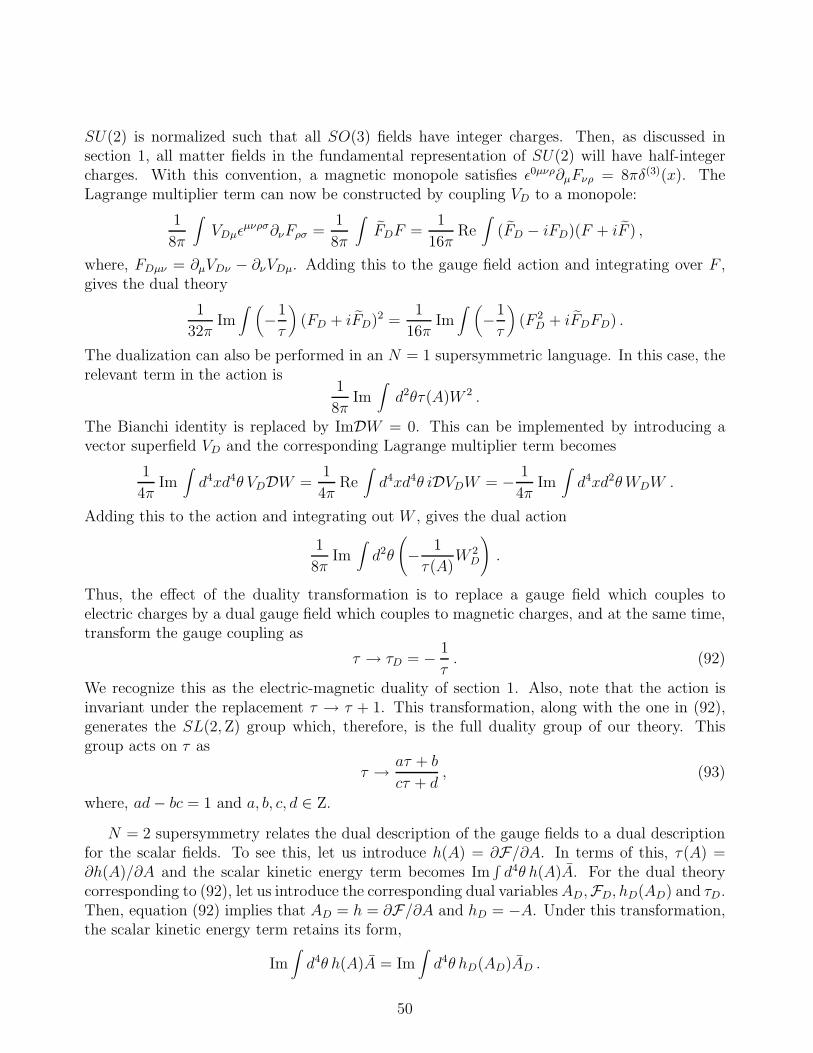
SU(2) is normalized such that all SO(3) fields have integer charges. Then, as discussed insection 1, all matter fields in the fundamental representation of SU(2) will have half-integercharges. With this convention, a magnetic monopole satisfies ǫ0µνρ∂µFνρ = 8πδ(3)(x). TheLagrange multiplier term can now be constructed by coupling VD to a monopole:

1

8π

∫VDµǫ

µνρσ∂νFρσ =1

8π

∫FDF =

1

16πRe

∫(FD − iFD)(F + iF ) ,

where, FDµν = ∂µVDν − ∂νVDµ. Adding this to the gauge field action and integrating over F ,gives the dual theory

1

32πIm

∫ (−1

τ

)(FD + iFD)2 =

1

16πIm

∫ (−1

τ

)(F 2

D + iFDFD) .

The dualization can also be performed in an N = 1 supersymmetric language. In this case, therelevant term in the action is

1

8πIm

∫d2θτ(A)W 2 .

The Bianchi identity is replaced by ImDW = 0. This can be implemented by introducing avector superfield VD and the corresponding Lagrange multiplier term becomes

1

4πIm

∫d4xd4θ VDDW =

1

4πRe

∫d4xd4θ iDVDW = − 1

4πIm

∫d4xd2θWDW .

Adding this to the action and integrating out W , gives the dual action

1

8πIm

∫d2θ

(− 1

τ(A)W 2

D

).

Thus, the effect of the duality transformation is to replace a gauge field which couples toelectric charges by a dual gauge field which couples to magnetic charges, and at the same time,transform the gauge coupling as

τ → τD = − 1

τ. (92)

We recognize this as the electric-magnetic duality of section 1. Also, note that the action isinvariant under the replacement τ → τ + 1. This transformation, along with the one in (92),generates the SL(2,Z) group which, therefore, is the full duality group of our theory. Thisgroup acts on τ as

τ → aτ + b

cτ + d, (93)

where, ad− bc = 1 and a, b, c, d ∈ Z.

N = 2 supersymmetry relates the dual description of the gauge fields to a dual descriptionfor the scalar fields. To see this, let us introduce h(A) = ∂F/∂A. In terms of this, τ(A) =∂h(A)/∂A and the scalar kinetic energy term becomes Im

∫d4θ h(A)A. For the dual theory

corresponding to (92), let us introduce the corresponding dual variablesAD,FD, hD(AD) and τD.Then, equation (92) implies that AD = h = ∂F/∂A and hD = −A. Under this transformation,the scalar kinetic energy term retains its form,

Im∫d4θ h(A)A = Im

∫d4θ hD(AD)AD .

50

In the following, we use the notations AD and h(A) interchangeably.

We now consider the effect of the full SL(2, Z) group on A and F , or equivalently on A andAD = ∂F/∂A. The transformation (93) implies that

(AD

A

)→(a bc d

) (AD

A

). (94)

Note that, in general, we could also add a constant column matrix C to the right-hand sideof the above equation. However, for non-zero C, the BPS mass formula for the theory in theabsence of matter is not invariant under the above transformation. Thus in this case we shouldset C = 0. However, in the presence of matter fields, the BPS mass formula is modified anda non-zero C is allowed. This case will be discussed in the last section. On the space of thescalar fields, the transformations τ → −1/τ and τ → τ + 1 are implemented by the matrices

S =

(0 1−1 0

), T =

(1 10 1

). (95)

These matrices generate the SL(2,Z) group.

The transformation of F can be easily obtained from (94), or equivanlently from

A′D = aAD + bA ,

A′ = cAD + dA .

The first equation can be integrated with respect to A′ by using the second equation and theresult is

F ′ =1

2βδA2 +

1

2αγA2

D + βγAAD + F .

Let us now come back to the metric on the moduli space as given by (89). In terms of thevariable aD, this takes the form

ds2 = Im daDda = − i

2(daDda− dadaD) ,

which is invariant under the SL(2,Z) transformations. To make the description more precise,note that the moduli space M is a complex one dimensional manifold and let u be a holomorphiccoordinate on this manifold. Finally, we will identify u as 〈Trφ2〉. Let a and aD be thecoordinates on a space X ∼= C2 on which we can choose a symplectic form ω = Im daD ∧ da.The functions (aD(u), a(u)) give a map f from M to X. In other words, they determine asection of X regarded as an SL(2,Z) bundle over M. In terms of the coordinate u, the metricon the moduli space takes the form

ds2 = ImdaD

du

da

dududu = − i

2

(daD

du

da

du− daD

du

da

du

)dudu .

This is the pull-back of the Kahler metric associated with the symplectic form ω and is, there-fore, manifestly SL(2,Z) invariant. Choosing u = a, we get back to the original formula. Note

51

that for arbitrary (aD(u), a(u)), the metric is not positive. However, the solution we will obtainlater determines these functions such that the metric is always positive.

Higher Dimensions: For a group of rank r, the metric takes the form

ds2 = Im∂2F∂ai∂aj

daidaj .

Introduce a space X ≃ C2r with coordinates ai, aDj = ∂F/∂aj . Endow X with the symplecticform ω = i

2

∑i(da

i∧daDi−daDi∧dai) and the holomorphic 2-form ωh =∑

i dai∧daDi. Choose

us (s = 1, ..., r) as coordinates on the moduli space M. Then, ai(u), aDj(u) give a map f fromM to X such that f ∗(ωh) = 0 (this condition ensures that aDj = ∂F/∂aj). Thus, the metrictakes the form

ds2 = Im∂aDi

∂ur

∂ai

∂usdurdus .

This is the metric associated with f ∗(ω) and is therefore invariant under Sp(2r,R): If we writevT = (aD, a), then the metric is invariant under v → Mv + c, where, M ∈ Sp(2r,R). In theabsence of matter, c = 0 and moreover, only the Sp(2r,Z) part survives.

If the moduli space M has a non-trivial structure, then, on being taken around a closeloop, the vector vT = (aD, a) will get transformed by an element of the monodromy group. Aswill be shown later, the monodromy group is a subgroup of SL(2,Z), and its determination isessential for solving the problem.

3.5 Dyon Masses

As described in sections 1 and 2, for the microspcopic SU(2) theory, the BPS bound is givenby M ≥

√2|Z|, where,

Z = a(ne + τcl nm) ,

and τcl = θ2π

+ i 4πg2 . All states that saturate this bound fall in a short multiplet of the N =

2 algebra. In a more general N = 2 theory, like the low-energy effective action we havebeen studying, this formula is slightly modified. Suppose, the theory contains matter fields inhypermultiplets. When a 6= 0, these fields, which in the N = 1 formalism are described bychiral fields M, M , become massive. If a hypermultiplet carries charge ne, then its coupling tothe chiral field A is uniquely fixed by N = 2 supersymmetry as

√2neAMM .

From this we can easily see that for such a state, Z = a ne. On the other hand, if we considera magnetic monopole carrying nm units of magnetic charge, then a manipulation very similarto the one in subsection 1.6 leads to the BPS bound

√2|nm aD| or, equivalently, Z = nm aD.

In general, one can compute this formula for dyons and obtain

Z = ane + aDnm . (96)

52

If the gauge group is of rank r, then we have

Z = aine,i + hi(a)nim = a · ne + aD · nm .

Since masses are physically observable, the mass formula should be invariant under the mon-odromies on the moduli space. Therefore, if v = (aD, a)

T transforms to Mv (with M ∈Sp(2r,Z)), then the vector w = (nm, ne) should transform to wM−1. Note that this once againrequires M to be an integral matrix.

Under the action of the monodromy, the coupling matrix τij = ∂aDi/∂aj transforms to

(Aτ + B)(cτ + D)−1, where, M =

(A BC D

). This is very similar to the transformation of

the period matrix of a genus r Riemann surface under the action of the monodromy groupon the moduli space of genus r surfaces. This makes it reasonably appealing to identify ourr-dimensional moduli space of vacua M with the moduli space of genus r Riemann surfaces.The variables ai, aDj are then related to the periods of these surfaces and can be calculated.Moreover, Im τ is always positive definite, which resolves the problem of geting a negativekinetic term. To check this hypothesis for our SU(2) theory, we first have to determine themonodromy structure on the moduli space M. This is the subject of the next subsection.

3.6 Monodromies on the Moduli Space of the SU(2) Theory:

We have discussed the possibility of the existence of monodromies on the moduli space andpointed out that understanding the monodromy structure may help us solve the theory, i.e.,to determine the exact non-perturbative prepotential for the effective low-energy theory. Thisis equivalent to determining the functions aD(u) and a(u). In this subsection, we set out toidentify the singularities on the moduli space M and calculate the associalted monodromies.

Monodromy at large u: At large |a|, the theory is asymptotically free and u = 12a2. To a good

approximation, the prepotential is given by the one-loop formula F(a) = (i/2π)a2 ln (a2/Λ2),from which we obtain

aD =∂F∂a

=2ia

πln (

a

Λ) +

ia

π.

If we make a close loop on the u-plane around u = 0, we get ln u → ln u + 2πi, and ln a →ln a+ iπ, hence,

aD → −aD + 2a ,a → −a .

This is implemented by the monodromy matrix

M∞ = PT−2 =

(−1 20 −1

), (97)

acting on (aD, a)T . Here, P is the negative of the identity element in SL(2,Z) and T is as defined

in (95). Under the action of this monodromy, the magnetic and electric quantum numbers ofBPS states change as (nm, ne) → (−nm,−ne − 2nm) so that the mass formula is unchanged.

53

Monodromies at finite u: The monodromy at u = ∞ implies that there exist other monodromiessomewhere else on the u-plane. If these monodromies commute with M∞, then a2 is a goodglobal coordinate. However, this cannot be the case as then the positivity of the kinetic energyis violated. To get a non-abelian monodromy group, we need at least two singularities on theu-plane, and at finite u, with non-trivial monodromies around them. These singularities will berelated by the broken discrete symmetry u → −u. We make this minimal assumption on thenumber of extra singularities. Then a loop enclosing both these singularities should reproducethe monodromy M∞

What is the origin of these singularities on the moduli space? To obtain the Wilsonian low-energy effective action, we have integrated out all massive states in the theory. The massiveparticle loops then give rise to a non-trivial metric on the moduli space. The values of themasses, however, depend on the modulus u, and it may so happen that for certain values ofu, some of the masses become zero. Then, at these points, we end up integrating out masslessstates and thus create singularities on the moduli space. The nature of a singularity, i.e.,the monodromy associated with it, depends on the properties of the particle which becomesmassless at the singularity. Since, for finite u (the non-perturbative regime), the mass spectrumas a function of u is not known, the singularities cannot be found in a straightforward way.The way to proceed is to assume that some generic states become massless at certain values ofu (say u = 1 and u = −1) and find the corresponding monodromies (say M1 and M−1). Themassless states are then specified by the condition M1M−1 = M∞.

Naively, one may expect that the massive gauge boson multiplets contribute to the sin-gularity when they become massless. Classically, this happens at the point u = 0, which, inquantum theory, may get shifted to a non-zero u. However, as argued in [31], a spin-1 multipletbecoming massless does not lead to a consistent picture. We will not repeat this argument here.

The only other massive states in the theory with spin ≤ 1/2 are monopoles and dyons,which, due to the spin condition, belong to short N = 2 multiplets and, therefore, are BPSstates. These states are described by hypermultiplets. Seiberg and Witten suggested that thesingularities arise when some of these non-perturbative states become massless. The problemnow is to calculate the associated monodromies. Note that the hypermultiplets for monopolesand dyons cannot be coupled to the fundamental fields of our theory in a local way. However, inthe subsection on duality it was seen that it is possible to go to a dual description of the theoryin which some dual gauge fields couple to the monopoles or dyons in exactly the same way thatthe usual gauge fields couple to a particle of unit electric charge. Thus we only have to calculatethe monodromy when a massive electrically charged hypermultiplet becomes massless and then,using the duality transformation, find the monodromy for a generic monopole or dyon. Let usconsider a dual description of the theory in which a certain monopole or dyon appears as anelementary state, and let us label this description by a letter, say q. Near the point where thisstate is massless, all massive fields can be integrated out and the theory is essentially a U(1)theory coupled to a hypermultiplet. If we denote the vev of the scalar field in this descriptionof the theory by a(q), then the mass of a BPS state of unit electric charge goes to zero whena(q) = 0 at some u = uq. Thus, near this point, a(q) is a good local coordinate and can beexpanded as a(q) ≈ cq (u−uq). Moreover, near this point, the one-loop U(1) β-function implies

54

(see the next subsection):

τ(a(q)) = − i

πlna(q)

Λ,

from which we obtain

aD(q) = − i

πa(q) ln

a(q)

Λ+i

π.

Moving on a closed loop around uq so that (u− uq) → e2πi(u− uq), we get the monodromy

aD(q) → aD(q) + 2a(q) ,a(q) → a(q) .

(98)

Let us now calculate the monodromy when a (nm, ne) dyon becomes massless (the dyon isstable or marginally stable if nm and ne are coprime). The first step is to find a dual descriptionof the theory in which this dyon appears as an elementary stat of charge (0, 1). Under a genericSL(2,Z) transformation we get a (nm(q), ne(q)) dyon with

(aD(q)a(q)

)=

(αaD + βaγaD + δa

),

(nm(q)ne(q)

)=

(nmδ − neγ−nmβ + neα

), (99)

so that Z = nmaD +nea is invariant. In the above, αδ−βγ = 1. Now we choose the parameterssuch that nm(q) = 0, ne(q) = 1. With this choice, (aD(q), a(q)) become the variables in terms ofwhich the dyon couples to the SL(2,Z) transformed gauge field in the same way that the unitelectric charge couples to usual gauge fields. In particular, when the dyon becomes massless atsome point on the moduli space, the associated monodromy, in this description, is given by (98).Inverting the first equation in (99), we get aD = −βa(q) + neaD(q) and a = αa(q) − nmaD(q).Thus we can easily find the action of the monodromy on the original variables as

(aD

a

)→(

1 + 2nenm 2n2e

−2n2m 1 − 2nenm

) (aD

a

). (100)

Denoting the monodromy matrix as M(nm, ne), we note that TrM(nm, ne) = 2. Thus themonodromy always belongs to the parabolic subgroup of SL(2,Z).

Now we calculate the monodromies at u = ±1. Let us assume that a (m,n) dyon becomesmassless at u = 1 and a (m′, n′) dyon becomes massless at u = −1. The the associatedmonodromies should satisfy

M1(m,n)M−1(m′, n′) = M(∞) . (101)

Using (97) and (100), this can be written as(

1 + 2mn 2n2

−2m2 1 − 2mn

)=

(−1 20 −1

)(1 − 2m′n′ −2n′2

2m′2 1 + 2m′n′

),

leading to the equations1 +mn = m′n′ + 2m′2 ,

m2 = m′2 ,n2 = n′2 + 1 + 2m′n′ ,

1 −mn = −m′n′ .

55

These imply that m = ±1 and m′ = ±1. For each combination of (m,m′), we can easilydetermine n′ in terms of n and get the following possible sets of solutions

(m,n) : (1, n) , (−1, n) , (−1, n) , (1, n) ,(m′, n′) : (1, n− 1) , (1,−n− 1) , (−1, n+ 1) , (−1,−n+ 1) .

There do not seem to be any solutions where M∞ is factorized into a product of more than twosuch parabolic M(m,n). Moreover, note that the solution allows only dyons of unit magneticcharge to contribute to the monodromy. This is consistent with the result that, semiclassically,only these dyons are stable.

Let us consider another consistency check: In general, under the action of the monodromy,the quantum numbers of dyons will change. However, we expect that the particular dyonwhich becomes massless and is the source of the singularity should remain invariant under themonodromy (as it is the properties of this dyon which determine the monodromy matrix). Thiscan be easily checked. The eigenvalue equation

(qm, qe)

(1 + 2mn 2n2

−2m2 1 − 2mn

)= (qm, qe) , (102)

leads to nqm−mqe = 0, providedm and n do not vanish simultaneously. Clearly, qm = m, qn = nis a solution of this equation. If we restrict ourselves to stable dyons, then this is the onlysolution. Thus, knowing the monodromy, we can find the dyon which gives rise to it.

The simplest solution to the equation (101) corresponds to m = m′ = 1, n = 0, n′ = −1.The monodromy matrices are then given by

M1 =

(1 0−2 1

), M−1 =

(−1 2−2 3

). (103)

A comparison with (102) implies that M1 arises due to a monopole becoming massless at u = 1and M−1 arises when a (1,−1) dyon becomes massless at u = −1. At the point where themonopoles become massless, we have aD = 0 and where the (1,−1) dyon becomes massless, wehave a − aD = 0 as is evident from Z = nmaD + nea. Note that the monodromy at infinity,M∞, shifts the electric charge by 2 units. Hence, at the points where condensation takes place,the electric charge is really defined modulo 2. We can conjugate the representation of thefundamental group by Mn

∞.

3.7 U(1) β-function

To construct the monodromies in the previous subsection, we have used the β-function for aU(1) theory interacting with a hypermultiplet. Let us look at this in some more detail. If wehave Weyl fermions with charge Qf and complex scalars with charge Qs, then their contributionto the U(1)β-functions is

β(g) ≡ µd

dµg =

g3

16π2

∑

f

2

3Q2

f +∑

s

1

3Q2

s

.

56

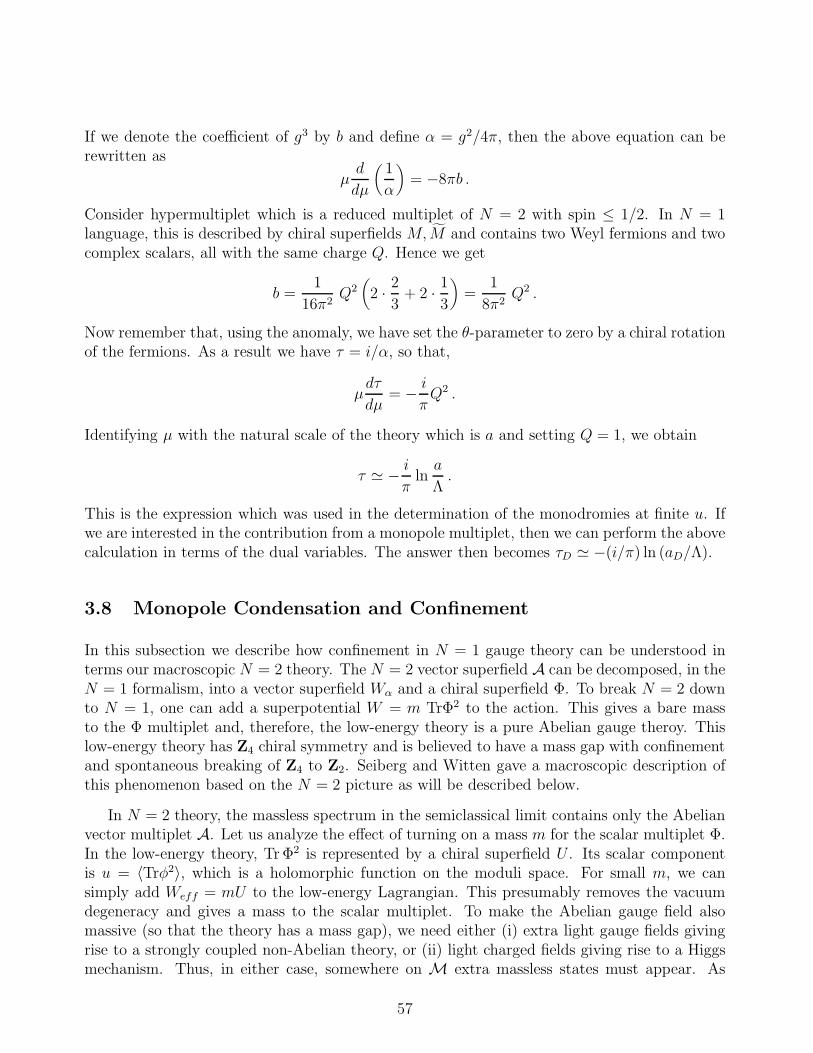
If we denote the coefficient of g3 by b and define α = g2/4π, then the above equation can berewritten as

µd

dµ

(1

α

)= −8πb .

Consider hypermultiplet which is a reduced multiplet of N = 2 with spin ≤ 1/2. In N = 1language, this is described by chiral superfields M, M and contains two Weyl fermions and twocomplex scalars, all with the same charge Q. Hence we get

b =1

16π2Q2

(2 · 2

3+ 2 · 1

3

)=

1

8π2Q2 .

Now remember that, using the anomaly, we have set the θ-parameter to zero by a chiral rotationof the fermions. As a result we have τ = i/α, so that,

µdτ

dµ= − i

πQ2 .

Identifying µ with the natural scale of the theory which is a and setting Q = 1, we obtain

τ ≃ − i

πlna

Λ.

This is the expression which was used in the determination of the monodromies at finite u. Ifwe are interested in the contribution from a monopole multiplet, then we can perform the abovecalculation in terms of the dual variables. The answer then becomes τD ≃ −(i/π) ln (aD/Λ).

3.8 Monopole Condensation and Confinement

In this subsection we describe how confinement in N = 1 gauge theory can be understood interms our macroscopic N = 2 theory. The N = 2 vector superfield A can be decomposed, in theN = 1 formalism, into a vector superfield Wα and a chiral superfield Φ. To break N = 2 downto N = 1, one can add a superpotential W = m TrΦ2 to the action. This gives a bare massto the Φ multiplet and, therefore, the low-energy theory is a pure Abelian gauge theroy. Thislow-energy theory has Z4 chiral symmetry and is believed to have a mass gap with confinementand spontaneous breaking of Z4 to Z2. Seiberg and Witten gave a macroscopic description ofthis phenomenon based on the N = 2 picture as will be described below.

In N = 2 theory, the massless spectrum in the semiclassical limit contains only the Abelianvector multiplet A. Let us analyze the effect of turning on a mass m for the scalar multiplet Φ.In the low-energy theory, Tr Φ2 is represented by a chiral superfield U . Its scalar componentis u = 〈Trφ2〉, which is a holomorphic function on the moduli space. For small m, we cansimply add Weff = mU to the low-energy Lagrangian. This presumably removes the vacuumdegeneracy and gives a mass to the scalar multiplet. To make the Abelian gauge field alsomassive (so that the theory has a mass gap), we need either (i) extra light gauge fields givingrise to a strongly coupled non-Abelian theory, or (ii) light charged fields giving rise to a Higgsmechanism. Thus, in either case, somewhere on M extra massless states must appear. As

57

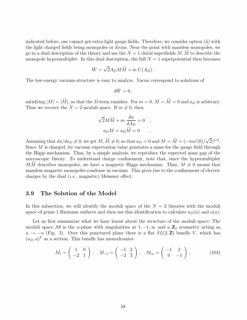
indicated before, one cannot get extra light gauge fields. Therefore, we consider option (ii) withthe light charged fields being monopoles or dyons. Near the point with massless monopoles, wego to a dual description of the theory and use the N = 1 chiral superfields M, M to describe themonopole hypermultiplet. In this dual description, the full N = 1 superpotential then becomes

W =√

2ADMM +m U(AD) .

The low-energy vacuum structure is easy to analyze. Vacua correspond to solutions of

dW = 0 ,

satisfying |M | = |M |, so that the D-term vanishes. For m = 0, M = M = 0 and aD is arbitrary.Thus we recover the N = 2 moduli space. If m 6= 0, then

√2MM +m

du

dAD= 0 ,

aDM = aDM = 0 .

Assuming that du/daD 6= 0, we get M, M 6= 0, so that aD = 0 andM = M = (−mu′(0)/√

2)1/2.Since M is charged, its vacuum expectation value generates a mass for the gauge field throughthe Higgs mechanism. Thus, by a simple analysis, we reproduce the expected mass gap of themicroscopic theory. To understand charge confinement, note that, since the hypermultipletMM describes monopoles, we have a magnetic Higgs mechanism. Thus, M 6= 0 means thatmassless magnetic monopoles condense in vacuum. This gives rise to the confinement of electriccharges by the dual (i.e., magnetic) Meissner effect.

3.9 The Solution of the Model

In this subsection, we will identify the moduli space of the N = 2 theories with the modulispace of genus 1 Riemann surfaces and then use this identification to calculate aD(u) and a(u).

Let us first summarize what we have learnt about the structure of the moduli space: Themoduli space M is the u-plane with singularities at 1,−1,∞ and a Z2 symmetry acting asu → −u (Fig. 3). Over this punctured plane there is a flat SL(2,Z) bundle V , which has(aD, a)

T as a section. This bundle has monodromies

M1 =

(1 0−2 1

), M−1 =

(−1 2−2 3

), M∞ =

(−1 20 −1

), (104)

58

around the singularities.

M∞= M1M–1

M–1

u = –1 u = +1

M1

The u - plane

Figure 3

To be more precise, the quantities (aD(u), a(u)) form a holomorphic section of the bundleV ⊗C, and have the following asymptotic behaviour

u ≈ ∞ :

a ∼=

√2u

aD ≈ i√

2uπ

ln u,

u = 1 :

aD ≈ c0(u− 1)a ≈ a0 + i

πaDln aD

.

where, a0 and c0 are constants. For u = −1 we get a behaviour similar to u = 1 but with aD

replaced by a− aD. The metric on the moduli space is ds2 = Im(τ) |da|2 with

τ =daD/du

da/du. (105)

To insure positivity of kinetic energy, Im(τ) should be positive definite. The monodromiesgenerate a subgroup Γ(2) of SL(2,Z) and, in fact, the u-plane with its singularities is thequotient of the upper half plane H by Γ(2). This quotient has three cusps corresponding tothe three singularites.

The space H/Γ(2), which is the u-plane, also parametrizes the family of curves Eu describedby the equation

y2 = (x− 1)(x+ 1)(x− u) , (106)

where x is a complex variable. First, note that this equation is invariant under the transfor-mations

w : u→ −u , x→ −x , y → ±iy ,that generate a Z4 symmetry, out of which only a Z2 subgroup acts on u. This is the sameas the symmetry structure on M. Now, let us describe the curve which the above equation

59

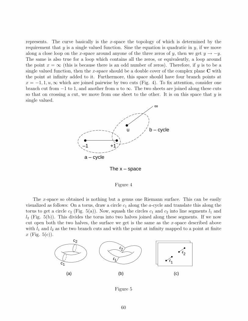
represents. The curve basically is the x-space the topology of which is determined by therequirement that y is a single valued function. Sine the equation is quadratic in y, if we movealong a close loop on the x-space around anyone of the three zeros of y, then we get y → −y.The same is also true for a loop which contains all the zeros, or equivalently, a loop aroundthe point x = ∞ (this is because there is an odd number of zeros). Therefore, if y is to be asingle valued function, then the x-space should be a double cover of the complex plane C withthe point at infinity added to it. Furthermore, this space should have four branch points atx = −1, 1, u,∞ which are joined pairwise by two cuts (Fig. 4). To fix attention, consider onebranch cut from −1 to 1, and another from u to ∞. The two sheets are joined along these cutsso that on crossing a cut, we move from one sheet to the other. It is on this space that y issingle valued.

+1–1

u b – cycle

a – cycle

∞

The x – space

Figure 4

The x-space so obtained is nothing but a genus one Riemann surface. This can be easilyvisualized as follows: On a torus, draw a circle c1 along the a-cycle and translate this along thetorus to get a circle c2 (Fig. 5(a)). Now, squash the circles c1 and c2 into line segments l1 andl2 (Fig. 5(b)). This divides the torus into two halves joined along these segments. If we nowcut open both the two halves, the surface we get is the same as the x-space described abovewith l1 and l2 as the two branch cuts and with the point at infinity mapped to a point at finitex (Fig. 5(c)).

(a)

c2

c1

(b) (c)

11

22

Figure 5

60

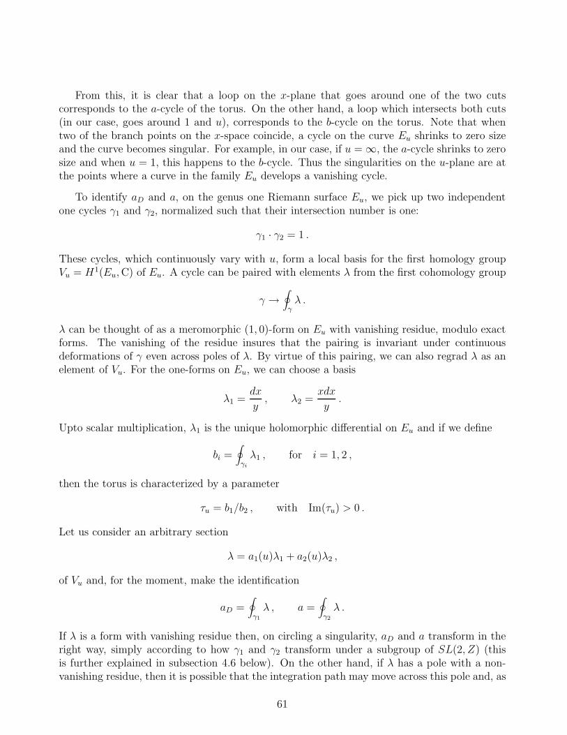
From this, it is clear that a loop on the x-plane that goes around one of the two cutscorresponds to the a-cycle of the torus. On the other hand, a loop which intersects both cuts(in our case, goes around 1 and u), corresponds to the b-cycle on the torus. Note that whentwo of the branch points on the x-space coincide, a cycle on the curve Eu shrinks to zero sizeand the curve becomes singular. For example, in our case, if u = ∞, the a-cycle shrinks to zerosize and when u = 1, this happens to the b-cycle. Thus the singularities on the u-plane are atthe points where a curve in the family Eu develops a vanishing cycle.

To identify aD and a, on the genus one Riemann surface Eu, we pick up two independentone cycles γ1 and γ2, normalized such that their intersection number is one:

γ1 · γ2 = 1 .

These cycles, which continuously vary with u, form a local basis for the first homology groupVu = H1(Eu,C) of Eu. A cycle can be paired with elements λ from the first cohomology group

γ →∮

γλ .

λ can be thought of as a meromorphic (1, 0)-form on Eu with vanishing residue, modulo exactforms. The vanishing of the residue insures that the pairing is invariant under continuousdeformations of γ even across poles of λ. By virtue of this pairing, we can also regrad λ as anelement of Vu. For the one-forms on Eu, we can choose a basis

λ1 =dx

y, λ2 =

xdx

y.

Upto scalar multiplication, λ1 is the unique holomorphic differential on Eu and if we define

bi =∮

γi

λ1 , for i = 1, 2 ,

then the torus is characterized by a parameter

τu = b1/b2 , with Im(τu) > 0 .

Let us consider an arbitrary section

λ = a1(u)λ1 + a2(u)λ2 ,

of Vu and, for the moment, make the identification

aD =∮

γ1

λ , a =∮

γ2

λ .

If λ is a form with vanishing residue then, on circling a singularity, aD and a transform in theright way, simply according to how γ1 and γ2 transform under a subgroup of SL(2, Z) (thisis further explained in subsection 4.6 below). On the other hand, if λ has a pole with a non-vanishing residue, then it is possible that the integration path may move across this pole and, as

61

a result, aD and a may no longer transform under a pure SL(2, Z). This second possibility is ofcourse not consistent with the symmetries of the BPS mass formula in the absence of fermionswith non-zero bare masses, as we already discussed in a previous subsection. Therefore, λshould not have a pole with a non-vanishing residue (In the presence of fermions with non-zerobare masses, the situation is different and will be discussed at the end of the next section). Theabove identification of aD and a implies that

daD

du=∮

γ1

dλ

du,

da

du=∮

γ2

dλ

du.

To fix the arbitrariness in λ, we use the condition Imτ > 0 for the metric on M as defined in(105). First, suppose that

dλ

du= f(u)λ1 = f(u)

dx

y.

Then,daD

du= f(u) b1 ,

da

du= f(u) b2 ,

so that

τ =b1b2

= τu .

Since Im τu > 0, we get Im τ > 0. As argued by Seiberg and Witten, the converse is also true,so dλ/du does not depend on λ2. The function f(u) is fixed by the asymptotic behaviour ofthe theory near the singularities on the u plane and is given by f(u) = −

√2/4π. With this,

we can obtain λ as

λ =

√2

2π

dx√x− u√

x2 − 1=

√2

2π

dxy

x2 − 1=

√2

2π

dx

y(x− u) .

To calculate a and aD, we have to choose a specific basis of one-cycles on Eu. We identify γ2

with the a-cycle on the torus, or equivalently, with a curve which loops around the points −1and 1 on the x plane. We can deform this curve so that it lies entirely along the cut from −1to 1 and back. Thus, a(u) is given by

a(u) =

√2

π

∫ 1

−1

dx√x− u√

x2 − 1. (107)

For γ1, we choose the curve which loops around the points 1 and u and get

aD(u) =

√2

π

∫ u

1

dx√x− u√

x2 − 1. (108)

It can be checked that with this choice of the one-cycles, a and aD have the desired behaviournear the singularities [31].

Explicit Formulae for a(u) and aD(u): One can easily find explicit formulae for the a and aD

in terms complete elliptic integrals E(k) and K(k) by using the integral representation of

62

hypergeometric functions F (α, β, γ; z) [35]. The hypergeometric functions are given by

F (α, β, γ; z) =Γ(γ)

Γ(β)Γ(γ − β)

∫ 1

0dx xβ−1(1 − x)γ−β−1(1 − zx)−α

=Γ(γ)

Γ(α)Γ(β)

∑

n≥0

Γ(α + n)Γ(β + n)

Γ(γ + n)

zn

n!.

Comparing this with the integral representation of a in (107), we can easily see that

a(u) =√

2(1 + u)F (−1/2, 1/2, 1; 2/(1 + u)) .

As for aD, let us first make the substitution x = (u− 1)t+ 1 in (108). This gives

aD(u) =i

π(u− 1)

∫ 1

0dt t−

1

2 (1 − t)1

2 (1 − 1 − u

2t)−

1

2 .

Comparing this with the expression for the hypergeometirc functions, we get

aD(u) =i

2(u− 1)F (1/2, 1/2, 2; (1− u)/2) .

In terms of the hypergeometric functions, the complete elliptic integrals are given by

K(k) =π

2F(1/2, 1/2, 1; k2

),

E(k) =π

2F(−1/2, 1/2, 1; k2

).

Further, we define k′2 = 1 − k2 and set

E ′(k) ≡ E(k′) , K ′(k) ≡ K(k′) .

Now, using the identity

c(1 − z)F (a, b, c; z) − cF (a, b− 1, c; z) + (c− a)zF (a, b, c + 1; z) = 0 ,

with c = 1, a = b = 1/2 and z = (1 − u)/2, in the expression for aD, we get

a(u) =4

πkE(k) ,

aD(u) =4

iπE(i

k′

k) +

4i

πk2K(i

k′

k) .

Here, k2 = 2/(1 + u) and (1 − u)/2 = −k′2/k2. These expressions can be further simplified ifwe note that

F (a, b, c; z) = (1 − z)−aF (a, c− b, c; z/(z − 1)) = (1 − z)−bF (b, c− a, c; z/(z − 1)) .

63

This implies that K(ik′/k) = kK(k′) = kK ′(k) and E(ik′/k) = k−1E(k′) = k−1E ′(k), so that

a(u) =4

πkE(k) ,

aD(u) =4

πi

E ′ −K ′

k.

The generalized coupling τ can be calculated by using

dE

dk=

E −K

k,

dK

dk=

1

kk′2(E − k′2K) ,

dE ′

dk= − k

k′2(E ′ −K ′) ,

dK ′

dk= − 1

kk′2(E ′ − k2K ′) ,

and is given by

τ =∂aD

∂a=daD/dk

da/dk=iK ′

K.

4 The Seiberg-Witten Analysis of N = 2 Gauge Theory

With Matter

In this section, we consider the N = 2 supersymmetric gauge theory, with gauge group SU(2),coupled to Nf matter multiplets. The analysis involves many technical issues and the propertiesof the theory depend on the value of Nf . As in usual QCD, matter fields (fermions) and gaugebosons contribute to the β-function with opposite signs. Thus, to insure asymptotic freedom,we require Nf ≤ 4. The theory with Nf = 4 is finite to all orders in perturbation theoryand, when the quarks are massless, it is very likely conformally invariant non-perturbatively.Seiberg and Witten provided evidence that this theory is an example of an SL(2, Z) invarianttheory. The only other SL(2, Z) invariant theory known in four dimensions is the N = 4supersymmetric gauge theory which also has a vanishing β-function. However, in the following,we will mainly concentrate on Nf ≤ 3. For the Nf = 4 case, the reader is referred to originalwork of Seiberg and Witten [32].

In the presence of matter, it is convenient to choose a charge normalization different from theprevious sections. In N = 2 pure gauge theory all fields transform in the adjoint representationand the charges of particles and monopoles are integers. Hence, in the formula Z = ane+aDnm,ne and nm are integers. With this normalization, when quarks are present, ne could be half-integral. In this section we choose a slightly different convention: To ensure that ne is alwaysintegral, we multiply it by 2 and divide a by 2 to keep the mass formula unchanged. Since aD

is kept unchanged, it is now given by 2aD = ∂F/∂a. In terms of the gauge invariant quantityu = Trφ2, as |u| → ∞, the asymptotic behaviour of a and aD with this normalization becomes

a ∼= 1

2

√2u , aD ≃ i

4

πa log a .

64

Furthermore, the effective coupling is also rescaled to τ = ∂aD/∂a = θπ

+ 8πig2 . This rescaling

of the charge affects the form of the curve which determines the solution of the model, keepingthe physics unchanged.

In this section we are going to study the theory with gauge group SU(2). In this case, themost interesting dynamics appear in the Coulomb branch of the moduli space, where SU(2)breaks down to U(1). It is, therefore, instructive to first study N = 2 supersymmetric QED.

4.1 N = 2 Supersymmetric QED

The N = 2 supersymmetric QED contains the photon vector multiplet and k quark hypermul-tiplets. The photon multiplet consists of the N = 1 chiral superfields (Wα, A) and each quarkhypermultiplet consists of two N = 1 chiral superfields M i and Mi, with U(1) charges +1 and−1, respectively. The only renormalizable N = 2 compatible superpotential is:

W =√

2AM iMi +∑

i

miMiMi .

When mi = 0, the theory has a global symmetry group SU(k) × SU(2)R × U(1)R. SU(k)is a flavour symmetry group acting on the k hypermultiplets, while SU(2)R rotates the twosupersymmetries and U(1)R is the usual R-symmetry which is afflicted by an anomaly. As inthe case without matter, the strategy is to first determine the classical moduli space and thento see whether the quantum moduli space is qualitatively different. The symmetries of thetheory are very useful in determining the structure of these moduli spaces.

In general, the classical moduli space has a Higgs branch and a Coulomb branch. The Higgsbranch is defined by some of the M i’s acquiring vacuum expectation values. In this case, bothin QED and in QCD with gauge group SU(2), the gauge group is completely broken. Fork = 1, there is no Higgs phase. When k ≥ 2, and mi = 0, then, using the global symmetriestogether with the the vanishing condition for the D-term, it is possible to rotate M and Mto the form M = (B, 0, 0, ...) and M = (0, B, 0, ...). From this one can read off the differentpatterns of symmetry breaking as a function of the number of flavours k. A theory on theHiggs branch does not contain monopoles or dyons and hence, the dynamical possibilities arenot as rich as on the Coulomb branch. The classical moduli space is a hyperKahler manifoldand the symmetries of the theory lead to a unique hyperKahler metric on it. As a result ofthis uniqueness, the metric does not receive quantum mechanical corrections. Therefore, onthe Higgs branch, the classical and the quantum moduli spaces are the same.

In the case at hand, if all mi = 0, then the Coulomb branch is defined by < A > 6= 0which, in turn, implies that < M i >=< Mi >= 0. The U(1) gauge group remains unbrokenwhile all the M ’s become massive. At a generic point on the moduli space, the effective low-energy threory (which involves only the massless modes) is a pure N = 2 gauge theory and theKahler potential is of the special geometry type : K = ImaD(a)a. This is related by N = 2supersymmetry to the the gauge kinetic term,

∫d2θ

∂aD

∂aW αWα .

65

The Kahler potential (and thus the metric) receive quantum corrections, but the one-loopapproximation to K is exact and also there are no non-perturbative corrections since this theorydoes not contain instantons. Using the one-loop β-function for QED with k hypermultiplets,we obtain

aD = − ik

2πa ln(a/Λ) . (109)

To reproduce this formula one should be careful about the extra factors of 2 in the super-symmetric way of defining g and the normalization convention mentioned earlier. The metricIm(τ) obtained from this is zero at |a| = Λ/e and thus the effective coupling constant is singu-lar. Because of this Landau pole singularity, the theory does not make sense in the ultra-violetregion unless embedded in a larger theory which is asymptotically free. If fermion mass termsare added, the singularities on the Coulomb branch can move. Since, when a = − 1√

2mi one

electron becomes massless, we have

aD = − i

2π

∑

i

(a+mi/√

2) ln(a +mi/

√2)

Λ.

To each bare mass is now associated a singularity on the moduli space where the particlebecomes massless. Depending on the possible equality of two or more masses, one can haveHiggs and Coulomb branches touching, leading to an intricate structure.

Here, we also see a manifestation of the modified form of the central charge of the N = 2algebra discussed in section 2. For pure N = 2, we have Z = nea + nmaD. However, now theelectron masses are not just

√2|a|, rather the i-th multiplet has mass |

√2a+mi|. As shown in

section 2, this is consistent with the fact that the U(1) charges Si of the massive hypermultipletsappears in the formula for the central charge Z as

Z = nea+ nmaD +∑

i

Simi/√

2 .

4.2 N = 2 Supersymmetric QCD with Matter

The N = 2 supersymmetric QCD coupled to Nf matter hypermultiplets contains the N = 1superpotential

W =Nf∑

i=1

(√

2QiΦQi +miQiQ

i) .

In general, whenmi = 0, this theory has a global symmetry group SU(Nf )×SU(2)R×U(1)R. Inthe special case, when the gauge group is SU(2), the flavour group is enlarged toO(2Nf). This isdue to the fact that for SU(2) the fundamental representation and its conjugate are isomorphicand, therefore, Qi and Qi can be combined into a 2Nf -dimensional vector transforming underO(2Nf). Thus, for the special case of the SU(2) gauge group, the theory also has a paritysymmetry group Z2 ⊂ O(2Nf) acting as

ρ : Q1 ↔ Q1 , (110)

66

with all other fields remaining unchanged. This parity plays an important role in the analysisof the theory. The global symmetry group of the theory is actually a quotient of O(2Nf) ×SU(2)R × U(1)R. The quotient is to be taken because a Z2 ⊂ U(1)R is the same as (−1)F

contained in the Lorentz group. This, combined with the center of SU(2)R, is the same as theZ2 in the center of O(2Nf).

For Nf = 0, 1, the theory has only a Coulomb branch with (< φ >6= 0). On this branchSU(2) is broken to U(1) and all quarks are massive. Moreover, U(1)R is spontaneously brokenbecause Φ has U(1)R charge 2. For Nf ≥ 2 we can either have a Coulomb branch or Higgsbranches. On a Higgs branch, the gauge symmetry is fully broken and the dynamics is not veryrich. We will not analyse this branch in detail, but will only mention that, as in the QED case,the metric on the moduli space is uniquely determined by the symmetries and does not receivequantum correction.

Some Properties of the Quantum Theory: The perturbative β-function of our theory (which,due to supersymmetry, is only a one-loop effect) is given by

β(g) = −4 −Nf

16π2g3. (111)

Therefore, to insure asymptotic freedom, we consider only Nf = 0, 1, 2, 3, 4.

In the previous section, from the counting of fermion zero-modes in an instanton background,we found that U(1)R is broken to a discrete subgroup Z4Nc−2Nf

. This was obtained by requiringthe invariance of the correlation function G given by (87) under U(1)R. For Nc = 2, we havean extra discrete symmetry group (110) which permutes the fermion zero-modes ψq1

and ψq1.

This group is anomalous as it changes G to −G. Therefore, now we can also allow U(1)Rtransformations which do not keep G invariant, but change it by a sign. This sign can becompensated for by an anomalous Z2 transformation. Thus, for Nc = 2, U(1)R is broken tothe discrete subgroup Z2(4Nc−2Nf ) = Z4(4−Nf ). This can be combined with the anomalous Z2 toget a discrete Z4(4−Nf ) anomaly-free subgroup with the action (see (85) and (86)):

Wα → ωWα(ω−1θ)Φ → ω2Φ(ω−1θ)

Q1 → Q1(ω−1θ)

Q1 → Q1(ω−1θ)Qi → Qi(ω−1θ)

Qi → Qi(ω−1θ)

i 6= 1 ,

where, ω = exp(2iπ/4(4 −Nf )). For Nf = 0 we do not have the quarks to cancel the anomalyand only the square of the above transformations is anomaly free. This case was discussedin the previous section. Furthermore, it can be seen that a subgroup Z2 ⊂ Z4(4−Nf ) is thesame as (−1)F in the Lorentz group. Combining the above transformations with the U(1)J

subgroup of SU(2)R (see (85) and (86)), we find a Z4(4−Nf ) symmetry which commutes N = 1

67

supersymmetryΦ → ω2Φ(θ)

Q1 → ω−1Q1(θ)

Q1 → ω−1Q1(θ)Qi → ω−1Qi(θ)

Q1 → ω−1Qi(θ)

i 6= 1 .

(112)

Under this transformation, the gauge invariant order parameter u = Trφ2 has charge 4 andtransforms as u→ exp 2πi/(4−Nf)u. This further breaks Z4(4−Nf ) down to Z4. The remainingZ4−Nf

acts non-trivially on the u-plane. Note that for Nf = 0, the subgroup which does notkeep u invariant is only a Z2.

As in the Nf = 0 case, the large u-behaviour of aD(u) is determined by the one-loopβ-function (111):

a ∼= 1

2

√2u+ · · · ,

aD ≃ i4 −Nf

2πa(u) ln

u

Λ2Nf

+ · · · . (113)

Here, the dots represent non-perturbative instanton corrections. The generic form of thesecorrections can be obtained by arguments similar to the ones used for the Nf = 0 case in theprevious section. First, a correction coming from a k-instanton configuration is proportional tothe k-instanton factor, which, using the β-function (111), can be written as

e−8π2k/g2

=

(ΛNf

a

)k(4−Nf )

. (114)

Following Seiberg [38, 39], we can restore the broken part of the U(1)R × Z2(ρ) symmetryby assigning appropriate charges to u and ΛNf

. Thus we assign charge 4 and even ρ-parity

to u and charge 2(4 − Nf ) and odd ρ-parity to Λ4−Nf

Nf. Note that with this assignment, the

one-instanton factor exp(−8π2/g2) will have an odd ρ-parity which compensates for the oddparity under Z2(ρ) of the correlation function G in (87), thus keeping it invariant . For thespecial case of Nf = 4, U(1)R is non-anomalous and u has charge 4. Z2(ρ) in O(8) is stillanomalous, but again, it can be treated as unbroken by assigning odd parity to the instantonfactor exp(−8π2/g2). Invariance under U(1)R with the above charge assignments implies thateach correction term should contain a factor of

√u. Moreover, since the metric on the u-plane

is invariant under the ρ-parity, configurations with odd instanton numbers cannot contributeto a and aD. Putting these facts together, we can write the generic form of the corrected a andaD as

a =1

2

√2u

1 +

∞∑

n=1

an(Nf)

(Λ2

Nf

u

)n(4−Nf ) ,

aD = i4 −Nf

2πa(u) ln

u

Λ2Nf

+√u

∞∑

n=0

aDn(Nf )

(Λ2

Nf

u

)n(4−Nf )

.

68

The difficult part is to compute the coefficients an and aDn.

Since the gauge group SU(2) breaks to U(1), the theory will have massive charged statesand we want to know how the unbroken global symmetry acts on them. The unbroken partof the global symmetry, which is the part that keeps u invariant, is obtained by raising thetransformations (112) to the power 4 − Nf . This unbroken transformation changes the signof φ and therefore acts as charge conjugation on the charged fields. For Nf = 1, 3; 4 − Nf

is odd and the unbroken transformation contains odd powers of ρ. It, therefore, acts as theparity in O(2Nf). Hence, in this case, the parity (110) is realized on the spectrum but itreverses the signs of electric and magnetic charges. States of given charge belong to SO(2) (forNf = 1) or SO(6) (for Nf = 3) multiplets. For Nf = 2, 4; 4 − Nf is even and the unbrokentransformation contains only even powers of ρ. All the odd powers of ρ, which amount to theparity transformation, are part of the broken transformations. Thus, in this case, the paritysymmetry is broken and the states are only in SO(4) (for Nf = 2) or SO(8) (for Nf = 4)representations.

4.3 BPS Saturated States

On the Higgs branch SU(2), is completely broken and there are no electric or magnetic charges.Thus the central charge of the N = 2 algebra only contains contributions from the U(1) chargesof the hypermultiplets. We will not discuss this in any detail.

On the Coulomb branch, the simplest BPS saturated states are the quarks with zero baremass and which acquire masses M =

√2|a| after the spontaneous breaking of the gauge sym-

metry. These form a set of BPS states which transform as a vector of SO(2Nf). Besides these,there are BPS states which transform as a spinor of SO(2Nf) arising as follows: Since the gaugesymmetry is broken to U(1), the theory contains monopoles. In the presence of a monopoleeach SU(2) doublet of fermions has one zero-mode. Since there are Nf hypermultiplets, thereare 2Nf fermion doublets and, therefore, 2Nf fermion zero-modes. After quantization, thesezero-modes give rise to a 2Nf -dimensional Dirac algebra which provides a spinor representationof SO(2Nf). Thus the fermion zero-modes turn the monopole into a spinor of SO(2Nf). Thisis very similar to the quantization of the Ramond sector of the Superstring theory. The pres-ence of spinors indicate that, at the quantum level, the symmetry group is a universal cover ofSO(2Nf), or Spin(2Nf ).

One of the monopole’s collective coordinates is a charge rotation. Upon quantization thisleads to a spectrum of electrically charged states for the monopole. A 2π rotation by the electriccharge operator, however, is not the identity. Using the Witten effect, such a rotation gives atopologically non-trivial gauge transformation with eigenvalue eiθ(−1)H for a monopole withnm = 1. Here, (−1)H is the centre of SU(2) which is odd for states in the hypermultiplet andeven for states in the vector multipler. In this section we normalize the charge operator sothat elementary quarks have charges ±1 and massive gauge bosons have charges ±2. With thisnormalization, the above mentioned gauge rotation can be written as an operator statement

eiπQ = eiθnm(−1)H .

69

where, Q = ne + nmθ/π. Since, ne ∈ Z, this relation implies that states of even ne have(−1)H = 1 and states of odd ne have (−1)H = −1. The factor (−1)H can be identified with thechirality operator for the spinor representation of SO(2Nf). For Nf = 1, 3, the SO(2Nf) paritytransformation acts on the spectrum and it guarantees that a dyon transforming as a positivechirality spinor of SO(2Nf) is degenerate with a particle of opposite electric and magneticcharges and opposite SO(2Nf) chirality. No such relation exists for Nf = 2, 4.

For Nf > 0 we will see that the spectrum contains states with nm > 1. A convenient wayof labelling states is in terms of their behaviour under the centre of Spin(2Nf ).

• Nf = 2: Spin(4) = SU(2) × SU(2) with centre Z2 × Z2. The representations of thecenter can be labeled by (ǫ, ǫ′), where ǫ = 0 for vector-like irreducible representationand ǫ = 1 for spinor-like irreducible representations. An elementary quark transformsas (ǫ, ǫ′) = (1, 1). Multiple quark states then transform as (ne mod 2, ne mod 2). Sincemonopoles behave like spinors, we have

(ǫ, ǫ′) = ((ne + nm) mod 2, ne mod 2) for Nf = 2 .

• Nf = 3: Spin(6) = SU(4) with centre Z4. The elementary quarks are in the 6 ofSpin(6), thus they have charge 2 with respect to the centre. Since monopoles behave likespinors, we conclude that Z4 acts as:

expiπ

4(nm + 2ne) for Nf = 3 .

• Nf = 4: Spin(8) has centre Z2 × Z2. Hence, using similar arguments as above, we get,(ǫ, ǫ′)=(nm mod 2, ne mod 2). The four representations of the center are labeled by therepresentations of of Spin(8) which realize them: (0, 1) ≡ v, (1, 0) ≡ s, (1, 1) ≡ c and(0, 0) ≡ o. Here, v refers to the vector representation, s and c to two spinor representatiosand o to the trivial representation. Spin(8) has a triality group of outer automorphismswhich is isomorphic to the permutation group S3 acting on v, s and c.

If an N = 2 invariant mass is turned on, say mNf6= 0, then SO(2Nf) explicitly breaks to

SO(2Nf − 2) × SO(2), and the global Abelian charge associated with SO(2) appears in thecentral charge

Z = nea+ nmaD + SNf

mNf√2, M =

√2|Z| .

Hence for a = ±mNf/√

2 one of the elementary quarks becomes massless. This will be cruciallater in determining the global structure of the quantum moduli space on the Coulomb branch.

4.4 Duality

As in the Nf = 0 case, there is an SL(2, Z) duality group which acts on the fields and thecouplings. In the presence of matter, some new issues appear which will be discussed below.

70

As before, we can compute the monodromy matrices for (aD, a) around the singular pointson the moduli space. The simplest case corresponds to having a single quark with non-zerobare mass, and investigating what happens as a ≈ a0 ≡ mNf

/√

2. From the QED analysis weknow that there is a logarithmic singularity at a0 where this quark becomes massless. Near thesingularity we have

a ≈ a0 ,aD ≈ − i

2π(a− a0) ln(a− a0) + c .

The monodromy can now be easily computed to be

a → a ,

aD → aD + a− mNf√2.

Unlike the Nf = 0 case, now we have an inhomogeneous transformation as the column vector(aD, a)

T picks up a shift under the monodromy (besides the usual SL(2, Z) transformation).The possibility of such a shift was also noticed for the pure gauge theory case in the previoussection. There, however, the shift was not part of the monodromy group and, furthermore, itwas not compatible with the symmetries of the BPS mass formula. In the presence of matter,this shift is allowed since the BPS mass formula is modified. Moreover, now the shift naturallyappears as a part of the monodromy group. To write a monodromy matrix, we construct acolumn vector (m/

√2, aD, a)

T . The monodromy can now be written as

m/

√2

aD

a

→ M

m/

√2

aD

a

,

with the monodromy matrix M given by

M =

1 0 0−1 1 10 0 1

, M−1 =

1 0 01 1 −10 1 1

.

If we arrange the charges as a row vector W = (S, nm, ne), then invariance of Z (or of M)implies that, under the monodromy, W → WM−1. In general the matrix M can be of theform

M =

1 0 0r k lq n p

, M−1 =

1 0 0lq − pr p −lnr − kq −n k

,

with detM = 1.

Note that under the monodromy, the electric and magnetic charges can mix with each otherbut will not pick up contributions proportional to S which is a global symmetry charge. Onthe other hand, S can pick up contributions proportional to ne and nm which are related tothe local gauge symmetry. For the example considered above,

(S, nm, ne) → (S + nm, nm,−nm + ne) .

71

This leads once again to issues of marginal stability: For large values ofmNf, the singularity is in

the weak-coupling region of large u where a semi-classical treatment of monopole is reliable. Inthe semi-classical quantization, the global U(1) charge is carried only by fermionic zero-modes.Since there is only a finite number of these modes, one cannot construct states with arbitrarilylarge values of S. This means that, although, by acting with M−1 we can increase the valueof S at will, what might have started as a one-particle state comes back as a multiparticlestate. This is possible if at some point, when going around the singularity, the single-particlestate becomes unstable and decays into a multi-particle state. Thus, although the formalism isSL(2, Z) covariant, the spectrum is not.

Seiberg and Witten provide many compelling arguments to suggest that the theory withNf = 4, like the theory with N = 4, is SL(2, Z) invariant, though the details are quite dif-ferent. In the Nf = 4 theory, the global symmetry group is Spin(8) which is the universalcover of SO(8). The states (nm, ne) = (0, 1) are the elementary hypermultiplets in the vectorrepresentation v of Spin(8). The states (nm, ne) = (1, 0) are in a spinor representaion s, and(nm, ne) = (1, 1) are in a spinor representation c of Spin(8). While SL(2, Z) alone cannot keepthis spectrum unchanged, a combination of SL(2, Z) and the Spin(8) triality group (which per-mutes the representations v, s and c) could do so. This is provided one is willing to assume thatthere are monopole bound states for every pair of relatively prime integers (p, q), analoguous tothe situation discussed by Sen for the N = 4 theory [20]. For each such pair, there should existeight states transforming in a representation 8v, 8s or 8c of Spin(8), depending on the mod 2reduction of (p, q). SL(2, Z) mixed with triality will then keep the spectrum invariant. Thesolution Seiberg and Witten provided for this model gives strong support to this possibility.The global symmetry group is then a semi-direct product of Spin(8) and SL(2, Z).

4.5 A First Look at Singularities

As in the pure N = 2, we first try to locate the singularities on the moduli space beforecomputing their monodromies. We recall that, with the standard normalization of the gaugecoupling constant g, the one-loop β-function which is given by (111), can be integrated to give

1

αNf(µ)

=4 −Nf

2πln

µ

ΛNf

,

where, α = 4π/g2. Now, if some (say Nf − N ′f ) of the quarks have masses mi = m, and we

are looking at the theory at some scale µ < m, then the low energy theory contains only N ′f

hypermultiplets as the degrees of freedom. The coupling α(N ′f) is then given by an expression

similar to the above one with Nf and ΛNfreplaced by N ′

f and ΛN ′f. The scales of the theories

can be related by the matching condition αNf(m) = αN ′

f(m), which implies

Λ4−N ′

f

N ′f

= mNf−N ′f Λ

4−Nf

Nf.

For instance,Nf = 3 , N ′

f = 0 ⇒ Λ40 = m3Λ3 ,

Nf = 1 , N ′f = 0 ⇒ Λ4

0 = mΛ31 .

72

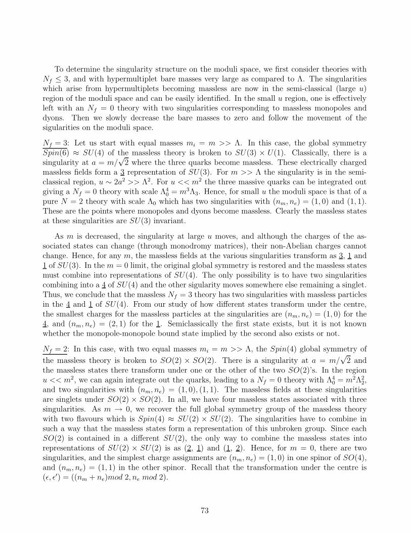
To determine the singularity structure on the moduli space, we first consider theories withNf ≤ 3, and with hypermultiplet bare masses very large as compared to Λ. The singularitieswhich arise from hypermultiplets becoming massless are now in the semi-classical (large u)region of the moduli space and can be easily identified. In the small u region, one is effectivelyleft with an Nf = 0 theory with two singularities corresponding to massless monopoles anddyons. Then we slowly decrease the bare masses to zero and follow the movement of thesigularities on the moduli space.

Nf = 3: Let us start with equal masses mi = m >> Λ. In this case, the global symmetrySpin(6) ≈ SU(4) of the massless theory is broken to SU(3) × U(1). Classically, there is asingularity at a = m/

√2 where the three quarks become massless. These electrically charged

massless fields form a 3 representation of SU(3). For m >> Λ the singularity is in the semi-classical region, u ∼ 2a2 >> Λ2. For u << m2 the three massive quarks can be integrated outgiving a Nf = 0 theory with scale Λ4

0 = m3Λ3. Hence, for small u the moduli space is that of apure N = 2 theory with scale Λ0 which has two singularities with (nm, ne) = (1, 0) and (1, 1).These are the points where monopoles and dyons become massless. Clearly the massless statesat these singularities are SU(3) invariant.

As m is decreased, the singularity at large u moves, and although the charges of the as-sociated states can change (through monodromy matrices), their non-Abelian charges cannotchange. Hence, for any m, the massless fields at the various singularities transform as 3, 1 and1 of SU(3). In the m = 0 limit, the original global symmetry is restored and the massless statesmust combine into representations of SU(4). The only possibility is to have two singularitiescombining into a 4 of SU(4) and the other sigularity moves somewhere else remaining a singlet.Thus, we conclude that the massless Nf = 3 theory has two singularities with massless particlesin the 4 and 1 of SU(4). From our study of how different states transform under the centre,the smallest charges for the massless particles at the singularities are (nm, ne) = (1, 0) for the4, and (nm, ne) = (2, 1) for the 1. Semiclassically the first state exists, but it is not knownwhether the monopole-monopole bound state implied by the second also exists or not.

Nf = 2: In this case, with two equal masses mi = m >> Λ, the Spin(4) global symmetry of

the massless theory is broken to SO(2) × SO(2). There is a singularity at a = m/√

2 andthe massless states there transform under one or the other of the two SO(2)’s. In the regionu << m2, we can again integrate out the quarks, leading to a Nf = 0 theory with Λ4

0 = m2Λ22,

and two singularities with (nm, ne) = (1, 0), (1, 1). The massless fields at these singularitiesare singlets under SO(2) × SO(2). In all, we have four massless states associated with threesingularities. As m → 0, we recover the full global symmetry group of the massless theorywith two flavours which is Spin(4) ≈ SU(2) × SU(2). The singularities have to combine insuch a way that the massless states form a representation of this unbroken group. Since eachSO(2) is contained in a different SU(2), the only way to combine the massless states intorepresentations of SU(2) × SU(2) is as (2, 1) and (1, 2). Hence, for m = 0, there are twosingularities, and the simplest charge assignments are (nm, ne) = (1, 0) in one spinor of SO(4),and (nm, ne) = (1, 1) in the other spinor. Recall that the transformation under the centre is(ǫ, ǫ′) = ((nm + ne)mod 2, ne mod 2).

73

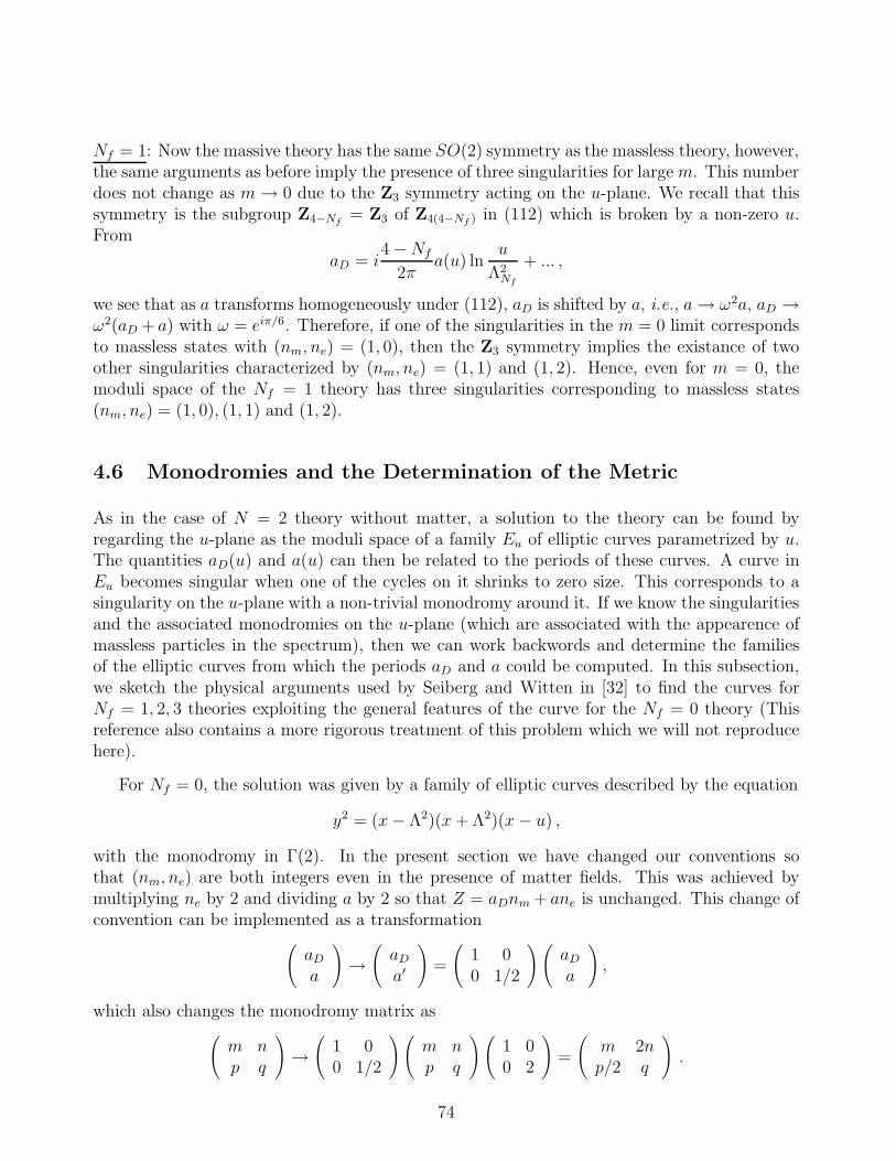
Nf = 1: Now the massive theory has the same SO(2) symmetry as the massless theory, however,the same arguments as before imply the presence of three singularities for large m. This numberdoes not change as m → 0 due to the Z3 symmetry acting on the u-plane. We recall that thissymmetry is the subgroup Z4−Nf

= Z3 of Z4(4−Nf ) in (112) which is broken by a non-zero u.From

aD = i4 −Nf

2πa(u) ln

u

Λ2Nf

+ ... ,

we see that as a transforms homogeneously under (112), aD is shifted by a, i.e., a→ ω2a, aD →ω2(aD + a) with ω = eiπ/6. Therefore, if one of the singularities in the m = 0 limit correspondsto massless states with (nm, ne) = (1, 0), then the Z3 symmetry implies the existance of twoother singularities characterized by (nm, ne) = (1, 1) and (1, 2). Hence, even for m = 0, themoduli space of the Nf = 1 theory has three singularities corresponding to massless states(nm, ne) = (1, 0), (1, 1) and (1, 2).

4.6 Monodromies and the Determination of the Metric

As in the case of N = 2 theory without matter, a solution to the theory can be found byregarding the u-plane as the moduli space of a family Eu of elliptic curves parametrized by u.The quantities aD(u) and a(u) can then be related to the periods of these curves. A curve inEu becomes singular when one of the cycles on it shrinks to zero size. This corresponds to asingularity on the u-plane with a non-trivial monodromy around it. If we know the singularitiesand the associated monodromies on the u-plane (which are associated with the appearence ofmassless particles in the spectrum), then we can work backwords and determine the familiesof the elliptic curves from which the periods aD and a could be computed. In this subsection,we sketch the physical arguments used by Seiberg and Witten in [32] to find the curves forNf = 1, 2, 3 theories exploiting the general features of the curve for the Nf = 0 theory (Thisreference also contains a more rigorous treatment of this problem which we will not reproducehere).

For Nf = 0, the solution was given by a family of elliptic curves described by the equation

y2 = (x− Λ2)(x+ Λ2)(x− u) ,

with the monodromy in Γ(2). In the present section we have changed our conventions sothat (nm, ne) are both integers even in the presence of matter fields. This was achieved bymultiplying ne by 2 and dividing a by 2 so that Z = aDnm + ane is unchanged. This change ofconvention can be implemented as a transformation

(aD

a

)→(aD

a′

)=

(1 00 1/2

)(aD

a

),

which also changes the monodromy matrix as(m np q

)→(

1 00 1/2

)(m np q

)(1 00 2

)=

(m 2np/2 q

).

74

Since p and n are integers modulo 2, the new monodromy matrix contains the entry 2n whichis an integer modulo 4, while all other entries are integers. These martices form the subgroupΓ0(4) of SL(2, Z). In the new convention, the monodromies in (104) take the form

M∞ =

(−1 40 −1

), M1 =

(1 0−1 1

), M−1 =

(−1 4−1 3

), (115)

and the solution is given by a family of curves described by

y2 = x3 − ux2 +1

4Λ4x . (116)

As discussed in the previous section, any genus-one curve can be represented by a cubic

y2 = F (x) = (x− e1)(x− e2)(x− e3) .

This describes a space x as a double cover of the complex plane branched over e1, e2, e3 and ∞.The curve becomes singular when two branch points coincide (e.g., e1 = e2 6= e3 or e3 → ∞).In this case the singularity is called stable. If more than two branch points coincide, then thesingularity is not stable, but a u-dependent reparametrization of x and y can always convertthis into a stable singularity. For the curve (116) the branch points are at

x = 0,1

2(u±

√u2 − Λ4), ∞ .

For u = ±Λ2 we have two stable singularities, but the u→ ∞ singularity is not stable.

To understand the properties of this curve better, let us first consider a generic situation:For a stable singularity at, for instance, u = 0, the family of curves near u = 0 can be writtenin the form

y2 = (x− 1)(x2 − un) ,

for some integer n. The monodromy around u = 0 is then conjugate to T n where the matrixT is defined in (95). This can be understood as follows: Consider the holomorphic Abeliandifferential ω = dx/y on a curve y2 = (x − 1)(x2 − λ), where λ = un. The periods can bewritten as

ω1 =∫

Γ1

dx

y, ω2 =

∫

Γ2

dx

y,

where Γ1 is a path from u = −λ1/2 to u = λ1/2, and Γ2 is a path from u = λ1/2 to u = 1(Fig. 6(a)). As λ → e2πiλ, λ1/2 → −λ1/2 and the cut Γ1 moves as in Fig. 6(b). This simplyexchanges the branches of the integrand and therefore ω1 → ω1.

As for ω2, the path Γ2 is transformed as in Fig. 7.

Thus, ω2 → ω2 + ω1. Since λ = un, when u → e2πiu, λ makes n turns and we obtain the n-thpower of the monodromy. Thus, in terms of λ, the monodromy is conjugate to T while in termsof u, it is conjugate to T n as we wanted to show.

75

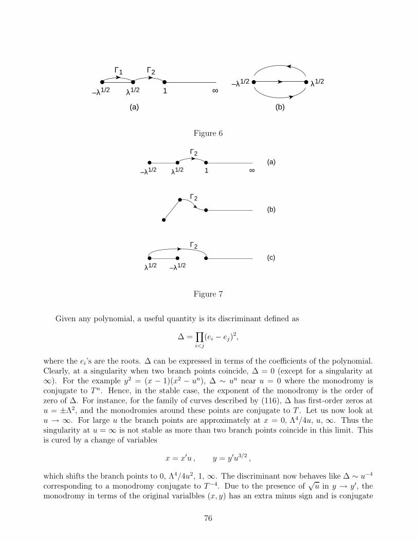
(a)

1 ∞

(b)

–λ1/2–λ1/2 λ1/2

λ1/2

Γ1 Γ2

Figure 6

(a)1 ∞–λ1/2 λ1/2

Γ2

(b)

Γ2

(c)

–λ1/2λ1/2

Γ2

Figure 7

Given any polynomial, a useful quantity is its discriminant defined as

∆ =∏

i<j

(ei − ej)2,

where the ei’s are the roots. ∆ can be expressed in terms of the coefficients of the polynomial.Clearly, at a singularity when two branch points coincide, ∆ = 0 (except for a singularity at∞). For the example y2 = (x − 1)(x2 − un), ∆ ∼ un near u = 0 where the monodromy isconjugate to T n. Hence, in the stable case, the exponent of the monodromy is the order ofzero of ∆. For instance, for the family of curves described by (116), ∆ has first-order zeros atu = ±Λ2, and the monodromies around these points are conjugate to T . Let us now look atu → ∞. For large u the branch points are approximately at x = 0, Λ4/4u, u, ∞. Thus thesingularity at u = ∞ is not stable as more than two branch points coincide in this limit. Thisis cured by a change of variables

x = x′u , y = y′u3/2 ,

which shifts the branch points to 0, Λ4/4u2, 1, ∞. The discriminant now behaves like ∆ ∼ u−4

corresponding to a monodromy conjugate to T−4. Due to the presence of√u in y → y′, the

monodromy in terms of the original varialbles (x, y) has an extra minus sign and is conjugate

76

to PT−4. Thus we see that the curve (116) produces the correct monodromies of the Nf = 0theory.

To obtain the curves for theories with non-zero Nf , we should know the monodromies whicharise in these theories. This can be easily worked out (as in the Nf = 0 case) since we alreadyknow the charge spectrum of the particles which become massless at the singularities on theu-plane. First note that, as in the Nf = 0 theory, the monodromy at u = ∞ can be obtainedform the perturbative β-function (111), or equivalently (113), and is given by

M∞ = PTNf−4.

The singularities at finite points in the u-plane, in general, correspond to massless magneticmonopoles with one unit of magnetic charge and ne units of magnetic charge. To calculatethe corresponding monodromy, we have to go to a dual description of the theory in whichthe monopole couples to the dual gauge field the way an electron couples to the usual gaugefield. In this frame, the monodromy is determined by the one-loop QED β-function (109) withk hypermultiplets and is given by T k. This has to be conjugated with T neS which convertsa hypermultiplet of charge (0, 1) into a monopole of charge (1, ne). Hence the monodromyaround a point with k magnetic monopoles with (nm = 1, ne) is (T neS)T k(T neS)−1. Similararguments can be applied to calculate the monodromy for the (2, 1) state in the Nf = 3 theory.In the following we list all the monodromies around the singularities described in the previoussubsection:

Nf = 0 : STS−1, (T 2S)T (T 2S)−1 →M∞ = PT−4 ,Nf = 1 : STS−1, (TS)T (TS)−1, (T 2S)T (T 2S)−1 →M∞ = PT−3 ,Nf = 2 : ST 2S−1, (TS)T 2(TS)−1 →M∞ = PT−2 ,Nf = 3 : (ST 2S)T (ST 2S)−1, ST 4S−1 →M∞ = PT−1 .

Using S2 = −1 and (ST )3 = 1, it is easy to check that, for each Nf , the product of themonodromy matrices at finite u yields M∞. Note that in the first three cases (Nf = 0, 1, 2) theelectric charges assigned to the singularities differ in sign from those determined by our previousarguments. This is consistent with the inherent ambiguities in relating the universal chargeswith the transformation properties under the centre of the group. Based on the knowledgeobtained so far, in the following we sketch the arguments of Seiberg and Witten to obtain theexplicit form of the curves for theories with non-zero Nf .

Properties of the Nf = 0 Curve: Before proceeding further, it is very useful to enumerate someproperties of the Nf = 0 curve which are expected to remain valid even for non-zero Nf :

1. The equation describing the family of curves is of the generic form y2 = F (x, u,Λ), whereF is a polynomial at most cubic in x and u.

2. The part of F cubic in x and u is F0 = x2(x− u).

3. If we assign U(1)R charge 4 to u and x and charge 2 to Λ, then F has charge 12. If y isassigned charge 6, then the curve is invariant under U(1)R transformations.

77

4. F can be written as F = F0 + Λ4F1 where F1 = x/4.

The property (1) remains an ansatz for Nf > 0. It will lead to the correct monodromymatrices, and it can also be justified in part when considering the Nf = 4 theory. Property(2) is a consequence of the fact that as u → ∞, we must obtain the monodromy at infinityassociated with a logarithm in aD coming from the one-loop β-function. This means that one ofthe branch points at finite x should move to infinity as u→ ∞. For large u, the cubic part canbe written as (x− e1u)(x− e2u)(x− e3u). Then the desired behaviour can be obtained if twoei’s coincide and the other is different, say e1 = e2 6= e3. In this case, by a redefinition of x, wecan bring F0 to the form x2(x− u). Property (4) in the Nf = 0 theory is a consequence of theU(1)R charge assignments. Note that F has only a classical contribution plus a one-instantonterm : Λ4x/4. Now we use these properties to determine the curves for Nf = 1, 2, 3.

The Curves for Massless Nf = 1 Theory: In this theory, from equation (114), the instanton

amplitude is proportional to Λ31. However, for Nf ≥ 1, the instanton factor is odd under the

ρ parity and, therefore, only even powers of it can appear in F . Since Λ1 has U(1)R charge 2and F has charge 12, the only possibility is

y2 = x2(x− u) + tΛ61 .

The constant t can be absorbed in a redefinition of Λ1: tΛ61 = Λ6. The discriminant of this

family of curves is∆ = Λ6

1(4u3 − 27Λ6

1) .

This has three zeros which are interchanged under the Z3 transformation acting on the u-planeand the associated monodromies are conjugate to T . Similarly, the monodromy at large u canbe worked out to be PT−3. This is consistent with what we should have for the Nf = 1 theory.

The Curves for Massless Nf = 2 Theory: In this case the instanton factor is Λ22 and, again, in

the absence of bare masses, only even powers of it can appear in F . Since Λ2 has U(1)R charge2, the general form of the curve is

y2 = x2(x− u) + (ax+ bu)Λ42 .

From our discussion of the Nf = 2 theory, we expect two singularities, each with two masslessmonopoles. Hence the monodromy at each singularity is conjugate to T 2 which means that thediscriminant at each finite singularity should have a double zero. This condition determines aand b. After a rescaling of Λ2, the family of Nf = 2 curves can be written as

y2 = (x2 − Λ42)(x− u) ,

which has the expected Z2 symmetry.

The curves for Massless Nf = 3 Theory: In this case, there are two singularities on the u-plane

with monodromies conjugate to T 4 and T respectively, and there is no symmetry acting on theu-plane. Take the T 4 singularity to be at u = 0. The discriminant then should have a fourth-order zero at u = 0. This, together with the usual U(1)R charge and ρ parity assignments,leads to

F = aΛ23x

2 + bu2x+ cux2 + x3 .

78

Here, b 6= 0 since otherwise the curve is singular for all u. Requiring that the cubic part of Fhave the expected classical behaviour, and after some rescaling, one gets

y2 = x2(x− u) + Λ23(x− u)2 .

Note that in the above we have only considered theories without a bare mass term. Since amass term has odd ρ-parity, in a theory with non-zero bare masses, odd powers of the instantonfactor can also contribute to the equation for the curve. We will not discuss these cases here,but for the sake of completeness, will simply reproduce the final results:

Nf = 1 : y2 = x2(x− u) +1

4mΛ3

1x−1

64Λ6

1 ,

Nf = 2 : y2 = (x2 − 1

64Λ4

2)(x− u) +m1m2Λ22x−

1

64(m2

1 +m22)Λ

42 ,

Nf = 3 : y2 = x2(x− u) − 1

64Λ2

3(x− u)2 − 1

64(m2

1 +m22 +m2

3)Λ23(x− u)

+1

4m1m2m3Λ3x−

1

64(m2

1m22 +m2

2m23 +m2

1m23)Λ

23 .

For more details and discussions (including the Nf = 4 case), as well as a more rigorous methodof obtaining the equations for the curves, the reader is referred to the original work of Seibergand Witten [32].

Once the curves are determined, the rest of the procedure is very similar to the Nf = 0case. We define the quantities a and aD by the contour integrals

a =∫

γ1

λ , aD =∫

γ2

λ ,

and the metric is given by Im(τ) with τ = daD

du/ da

du. Here λ is a holomorphic one-form such that

dλ

du=

√2

8π

dx

y.

The difference with the Nf = 0 case is that now λ can have poles with non-zero residue,however, the residues should be u independent. If this is the case, then τ still undergoes anSL(2, Z) transformation while (aD, a) undergoes an SL(2, Z) transformation plus a shift. Aswe saw in the case of QED with quarks of non-zero bare masses, this shift is actually neededand is consistent with the modified form of the BPS mass formula (84). From this it followsthat the residues of λ, which are responsible for the shifts, should be proportional to the barequark masses. This was checked in [32] for the Nf = 2 curve and found to be the case. Infact, the existence of residues is very restrictive and this information was used by Seiberg andWitten to drive the curve for the Nf = 4 theory in a rigorous way. The curves for other theoriescan then be determined by renormalization group flow and the results agree with what is listedabove.

Acknowledgments

79

We have benefited from numerous conversations with our colleagues on the subjects coveredin these lectures. We would like to thank in particular E. Alvarez, S. Randjbar-Daemi, W.Lerche, A. Klemm, S. Yankielowicz, C. Gomez, K. Kounnas, M. Marino, J. Distler, E. Verlinde,A. Giveon, E. Rabinovici and G. L. Cardoso for discussions. We would also like to thank theTrieste Theory Group for the opportunity to present this material in a stimulating environment.

References

[1] P. Goddard and D. I. Olive, Rep. Prog. Phys. 41 (1978) 1357.

[2] S. Coleman, Classical Lumps and Their Quantum Descendants, In the Proc. of the 1975Int. School of Subnuclear Physics, Erice; Ed. A. Zichichi, Plenum Press (1977).

[3] S. Coleman, The Magnetic Monopole Fifty Years Later, In the Proc. of the 1981 Int.School of Subnuclear Physic, Erice; Ed. A. Zichichi, Plenum Press (1983).

[4] P. A. M. Dirac, Phys. Rev. 74 (1948) 817.

[5] A. S. Goldhaber, Phys. Rev. Lett. 36 (1976) 1122.

[6] F. Wilczek, Phys. Rev. Lett. 48 (1982) 1146.

[7] J. Schwinger, Phys. Rev. 144 (1966) 1087; 173 (1968) 1536.

[8] D. Zwanziger, Phys. Rev. 176 (1968) 1480.

[9] G. ’t Hooft, Nucl. Phys. B79 (1974) 276.

[10] A. M. Polyakov, JETP Lett. 20 (1974) 194.

[11] B. Julia and A. Zee, Phys. Rev. D11 (1975) 2227.

[12] E. Tomboulis and G. Woo, Nucl. Phys. B107 (1976) 221.

[13] J. L. Gervais, B. Sakita and S. Wadia, Phys. Lett. 63B (1976) 55.

[14] E. B. Bogomol’nyi, Sov. J. Nucl. Phys. 24 (1976) 449.

[15] M. K. Prasad and C. M. Sommerfield, Phys. Rev. Lett. 35 (1975) 760.

[16] E. Corrigan and D. Olive, Nucl. Phys. B110 (1976) 237.

[17] P. Goddard, J. Nuyts and D. Olive, Nucl. Phys. B125 (1977) 1.

[18] C. Montonen and D. Olive, Phys. Lett. 72B (1977) 117.

[19] N. S. Manton, Nucl. Phys. B126 (1977) 525.

[20] A. Sen, Phys. Lett. 329B (1994) 217.

80

[21] E. Witten, Phys. Lett. 86B (1979) 283.

[22] J. Wess and J. Bagger, Supersymmetry and Supergravity, Princeton University Press(1983).

[23] P. West, Introduction to Supersymmetry and Supergravity, World Scientific, Singapore(1990).

[24] M. Sohnius, Phys. Rep. 128 (1985) 39.

[25] R. Haag, J. T. Lopuszanski and M. Sohnius, Nucl. Phys. B88 (1975) 257.

[26] E. Witten and D. Olive, Phys. Lett. 78B (1978) 97.

[27] R. Grimm, M. Sohnius and J. Wess, Nucl. Phys. B133 (1978) 275.

[28] A. Bilal, Duality in N=2 SUSY SU(2) Yang-Mills Theory: A Pedagogical Introduction tothe Work of Seiberg and Witten, hep-th/9601007.

[29] A. C. Davis, M. Dine and N. Seiberg, Phys. Lett. 125B (1983) 487.

[30] I. Affleck, M. Dine and N. Seiberg, Nucl. Phys. B241 (1984) 493.

[31] N. Seiberg and E. Witten, Nucl. Phys. B426 (1994) 19.

[32] N. Seiberg and E. Witten, Nucl. Phys. B431 (1994) 484.

[33] N. Seiberg, Phys. Lett. 206B (1988) 75.

[34] A. D’adda and P. DiVecchia, Phys. Lett. 73B (1978) 162.

[35] I. S. Gradshteyn and I. M. Ryzhik, Table of Integrals, Series and Products, AcademicPress (1980).

[36] M. A. Shifman, A. I. Vainshtein, Nucl. Phys. B277 (1986) 456.

[37] M. A. Shifman and A. I. Vainshtein, Nucl. Phys. B359 (1991) 571.

[38] N. Seiberg, Phys. Lett. 318B (1993) 469.

[39] N. Seiberg, Power of Holomorphy - Exact Results in 4-D Supersymmetric Gauge Theories,hep-th/9408013.

[40] W. Lerche, Introduction to Seiberg-Witten Theory and its Stringy Origin, In the proceed-ings of the 1996 Trieste spring school on String Theor, hep-th/9611190.

81




Documents

arXiv:hep-th/9701069v1 14 Jan 1997 - arXiv.org e-Print … · arXiv:hep-th/9701069v1 14 Jan 1997 CERN-TH/96-371 hep-th/9701069 Introduction to S-Duality in N= 2 Supersymmetric Gauge