June 1'993

A SCHOOL MATH·EMATICS MAGAZINE

Ft1N(;tIpN·•••is.·.~"~fhelna1ics11)~g~e~tldfe~~~~·~.~c1~tsiilifhe .. upperforms ofseconQarY'$9lto<>Js. . .' . ·d···:" . ,"':: •. ,:: ,.. ' .

It i~ a ... 'sp~ial .. i~tere~t' :.~oP111.al fottbose .who~eintere$ted in . mathematics.WindS1.Ufers, chess-pl~yersancl'g~d~n~i;S ·.anbavemagaz~~s\that·ca.ter l()their· interests.FUNCTION is a~ounteJ'Part of these~ .

Covera:ge. is wide;. - pureIIla~¢Illatics,statistics, computer science and applicationsof mathematics are .. all included. '.' .~ecent issues have carried articles on 'advances inmathematics, news items ·oil. :lIlathematics .·and .. its .applications, special interest matters,such as computer chess, problems and solutions, discussions, cover diagrams, evencartoons.

* * * * *

Articles, correspondence, problems (with or without solutions) and other material forpublication are invited. Address them to:

The ~itors,

FUNCTION,D~p~entofMathematics,MQnash' .University,Clayton, .Victoria, 3168.

Alternatively correspondence may 'be addressed individually to any of the editors atthe mathematics departments of the institUtions ·listed on the inside front cover.

FUNCfION is .published five tin)es a year,appeariJlg in February, April, June, August,October. Pri~e'or five "issu~s(inc.uding.pos~e):~~7..00*; single issqes $4.00.Paymen~s should be sent to the .Business Manager .·at the above address: <cheques and moneyorders should be made payable to Monash University-. Enquiries about advertising. should bedirected to the business .manager.

*$8.50 for bona fide secondary or tertiary students.

* * * * *

65

FUNCTION

Volunze 17

The Front Cover

Winning Tattslotto - Twice!

Trigonometric Solutions toQuadratic Equations

Computers and Computing

History of Mathematics

Problems and Solutions

(Founder editor: G.B. Preston

CONTENTS

Michael A.B. Deakin

Malcolm Clark

Richard Whitaker

* * * * *

Part 3

66

68

74

76

83

89

Note: . A news update on the Monash University Sundial has had to be held over becauseof lack of space. We apologize to those readers who had hoped to see this itemin the present issue.

66

THE 'FRONT COVER

Michael A.B. Deakin, Monash University

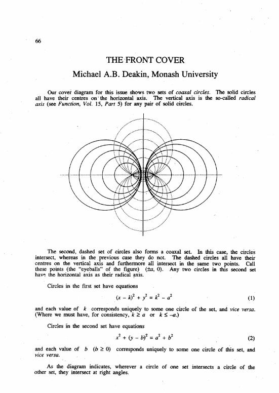
Our cover diagram for this issue shows two sets of coaxal circles. The solid circlesali have their centres on' the horizontal axis. The vertical axis is the so-called radicalaxis (see Function, Vol. 15, Part 5) for any pair of solid circles.

- #<'

...................-.......-

• ••• fi

The second, dashed set of circles also forms a coaxal set. In this case, the circlesintersect, whereas in the. previous case they do not. The dashed circles all have theircentres on the vertical axis and furthennore all intersect in the same two points. Callthese points (the ueyeballs" of the figure) (±a, 0). Any two circles in this second sethav~ the. horizontal axis as their radical ~xis.

Circles in the frrst ~t have equations

(x _ k)2 + y2 =k2 _ a2(1)

and each" value of k corresponds uniquely to some one circle of the set, and vice versa.(Where we must have, for consistency, k ~ a or k ~ -0.)

Circles in the second set have equations

(2)

and each value of b (b ~ 0) corresponds uniquely to some one circle of this set, andvice versa.

As the diagram indicates, wherever a circle of one set intersects .a circle of theother set, they intersect at right angles.

(3)

67

- This underlies an important physical application. Suppose,. e.g., a bar magnet is soplaced that its poles occupy the points (±a, 0). Then a magnetic .field is set up, and thetwo lots of circles give two different ways of visualising this. The dashed circles showthe lines of force, 'the paths along which a minute magnetic monopOle would travel.Commonly, and you may well have seen this in your science· class, they are m~de visible·bymeans of iron filings. .

The solid circles show the contours of magnetic potential (similar to the morefamiliar electric potential). Lines of force are indeed always perpendicular to contoursof potential, and vice versa.

As the radii of the 'solid circles get larger and larger, the value of k increasesand the circles get flatter. It is usual to include as a member of· the family th<.limiting case, which is the vertical axis, and to say that this corresponds to k =00.

Similarly with the dashed circles, where the horizontal axis corresponds, byconvention, to b = 00.

Weare now in a position to notice an interesting fact~ Every point of the planecorresponds, u~iquely to an intersection of a solid .circle and a dashed circle (or almostevery point;. the special cases (±G, 0) will be, dealt with later). Each intersection of.a .solid with a dashed circle, however, corresponds to two points in the plane.

Let us see how this works. First suppose we are given a point (x, y). ThenEquations (1), (2) both hold.

We thus have two equations in the unknowns b, k, given that we are supposing thatx, y are known. We find, easily enough: .

222k - x +Y +a

- 2x

b _ x2+y

2-a

2

- 2y

and thus, given (x, y), we may determine (k, b). The only difficulty. arises when eitherx or Y = 0 and th~s is usually solved by putting k = 00 when x = 0, and' b = 00 whenY = 0, in accordance with the convention outlined above.

Now consider the case in which k, b are known and we wailt to detennine x, y. Thismeans solving Equations (1), (2) as simultaneous quadratics. The result is:

x = (a2+b

2)k2 + b2(k

2-a2) ± b Mb(k

2-a2)

k(b2+k2) .

(4)

y =2b(e-a2) ± khb(k2

-a2

)

b2+k 2

and as we have b ~ 0 imd k2~a2, the square roots exist. Notice that in most cases,

there are indeed two values for (x, y) given b, k.

We now come back to the troublesome points x= ±a, y =O. Here Equations (3) y~eld

k = ±a, b = 0/0. Now % is undefmed - it ·may have" any value (not necessarily 00).

68

This correspond~ to the fact that all. the dashed circles, whatever the relevant value ofb, pass through these points. Conversely, put k =±a into Equation (4) to find the sameresult.

The correspondence between (x, y) on the on~ hand and (b, k) on the other may beused to construct an exotic coordinate system based on (b, k) rather than on (x, y).(Our cover diagram for. Vol. 10, Part· 5 was based on another, different, such exoticcoordinate system.) Such -coordinate systems can be useful for special purposes, givingsimple forms to otherwise quite complicated expressions. For example, the complicatedcubic expression

has, in these new coordinates, the· simple equation

k = b.

You may care to see what curve this represents.

WINNING TATTSLOTTO - TWICE!

Malcol~ Clark, Monash University

. Introduction

In February 1991, Mr Ray Williams of Albury became the first person to win the topprize in Tattslotto twice. He won the First Division prize, by correctly choosing all sixwinning numbers out of the 45 numbers. He had the same success back in 1984.

Most people would regard winning Tattslotto twice as a one-in-a-billion chance.There are 8,145,060 ways of selecting 6 numbers from 45, and so the chance of winning

Tattslotto just once in a single game is 1/8,145,060 ~ 1.22 x 10-7• Since succ~ssive

Tattslotto draws are presumably independent in the probability Sense, the chance of

winning Tattslotto twice ,must surely be "the above number squared, that is, 1.51 x 10-14 orabout 1 in 66 million million. .

This naive intuitive calculation is fundamentally flawed, on three grounds. First,many Tattslotto players have multiple entries or system entries, so that their chance of

winning once is considerably higher than 1.22 x 10-7• Secondly and more importantly, itis not valid here to multiply probabilities, as when finding the probability of two ormore independent events. Such multiplication would only be valid if you wanted to findthe probability that a particular person, specified in advance, will win twice.

Thirdly, we would be ~ven more amazed to find several two-time winners, or even aperson who had won more than twice. So it is more appropriate to consider the probabilitythat at least one person will win more than once, over a given number of Tattslotto draws.

69

The Birthday Problem

Before answering this question, we consider the related and well-known uBirthday

Pr:oblem".t Suppose that N people are selected at random; what is the probability thattwo people in this group have the same birthday (day and month, ignoring year)?

Once again, we need to be more precise. Presumably, if'we found, say, five people inour group of N with the same birthday, we would be even more surprised than if we foundjust two. Hence what is of interest is the probability that at least two out of the Nrandomly selected people have the saine birthday.

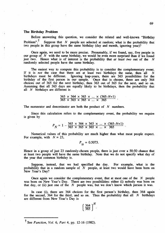
The easiest way to compute this probability. is to consider the complementary event.If it is not the case that there are at least two birthdays the same, then all IVbirthdays must be different. Ignoring leap-years, there are' 365 possibilities for the,birthday of the fIrst person in our sample. Once· that is chosen,there are only 364choices out of 365 for the next birthday, then 363 out of 365 for the next, and so on.Assuming that all 365 days are equally likely to be birthdays, then the probability thatall N birthdays are different is

365 x 364 x 363 x x (365-N+l)365 x 365 x 365 x x 365

The numerator and denominator are both the product of N numbers.

Since this calculation refers to the complementary event, the probability we requireis given by

P _ l' 365 x 364 x 363 x x (365-N+l)N. - - 365 x 365 x 365 x x 365 .

Numerical values of this probability are much higher than what most people expect.For example, with N_= 23,

P23 =0.5073.

Hence in a group of just 23 randomly-chosen people, there is just over a 50:50 chance thatat least two people will have the same birthday. .Note that we do not specify what day ofthe year that common birthday is.

Suppose, instead, that we had specified the day. For example, what is theprobability that iIi a random sample of N people, at least two would have· been born onNew .Year's Day?

Once·again we consider the complementary event, that at most ..one, of the N peoplewas born on New Year's Day. There are two possibilities: either (i). nobody ~as "born onthat day, or (ii) just one of the N pe<?ple was, but we don't know which person it was.

In case (i), there are 364 choices for thefrrst person's birthday, then 364 againfor the second, 364 for "the third, and so on. Thus the probability that all N birthdaysare different from New Year's Day is

t See Function, Vol. 6, Part 4, pp. 12-16 (1982).

70

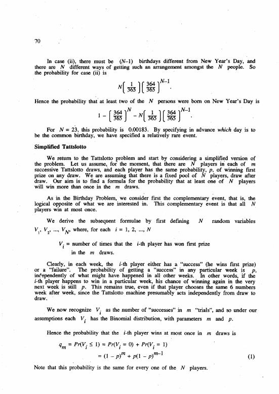
In case (ii), there must be (N-1) birthdays different from New Year's Day, andthere are N different ways of getting such an arrangement amongst the N people. So"the probability for case (ii) is "

N( ~)(m(-1.Hence the probability that" at least two of the N persons were born on New Year's Day is

[364 ]N (1] (364 ]"N-l1- 305 -N 303 :J05 .

For N = 23, this probability. is 0.00183. By specifying in advance which day is tobe the common birthday, we have specified a relatively rare event.

Simplified Tattslotto

We return to. the Tattslotto problem and start by considering a simplified. version ofthe problem. Let us assume, for' the moment, that there are N players in each of msuccessive Tattslotto draws, and each player has the same probability, p, of. winning fIrstprize on any draw. We are assuming that there is a fixed pool of N players, draw afterdraw. Our aim is to find a fonnula for the probability that at least one of N playerswill win more than once in the m draws.

As in the Birthday Problem, we consider fust the complementary event, that is, thelogical opposite of what we are interested in. This complementary event is that all Nplayers- win at most once. "

We derive the subsequent .fonnulae by first defming N random variables

VI' V2

, ..., VN , where, for each i = 1,2, ..., N

Vi = number of times that the i-th player has won fIrst prize

in the m draws.

Clearly, in each week, the i-th player either has a "success" (he wins fust prize)or a "failure". The probability of getting a "success" in any particular week is p,in~ependently of what might have happened in all other weeks. In other words, if thei-th player happens to win in a particular week, his chance of winning again in the verynext week is still p. This remains true, even if that player chooses the same 6 numbersweek after week, since the Tattslotto machine presumably acts independently from draw todraw.

We now recognize V. as the number of "successes" in m "trials", and so under our" 1...

assumptions each Vi has the Binomial distribution, with parameters m and p.

Hence the. probability that the i-th player wins at most once in m draws is

qJn =Pr(Vi ~ 1) ::: Pr(Vi =0) + Pr(Vi = 1)

In m-1= (~ - p) + p(1 - p)

Note that this probability is the same for every one of the N players.

(1)

(2)

11

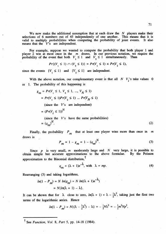
We now make. the additional assumption that at each draw the N players make. theirselections of 6 numbers out of 45 independently of one another~ This means that it isvalid to multiply probabilities when computing the probability of joint events. It alsomeans that the V's are independent.

For example, suppose we wanted to compute the probability that both player 1 andplayer 2 win at most once in the m draws. In our previous notation, we require theprobability of the event that both Vi ~ 1 and V

2~ 1 simultaneously. Then

Pr( (Vi ~ 1) (l (V2

.~ I)} = Pr(Vl~ 1) X Pr(V

2~ 1),

since the events (VI ~ I) and {V2'~ -1} are independent.

With the above notation, our complementary event is that all N Vi's take values 0

or 1. The probability of this happening is

8m =Pr(V1~ 1, V

2~ 1, ..., VN ~ 1)

=Pr(Vt~ I)Pr(V

2~ 1) ... Pr(VN ~ 1)

(since the V's are independent)

=(Pr(V. ~ l»N1

(since the V's have the same probabilities)N=(qI11) •

Finally, the probability Pm that at least one player wins more than once in ·m

draws isN

Pm =1-8m =1-(qm) . (3)

Since p is very small, m moderately large and N very large, it is possible toobtain simple but accurate approximations to the above formulae. By the Poisson

approximation to the Binomial distribution,t

q ~ (A + l)e-A, with A= lnp. (4)n1.

Rearranging (3) and taking logarithms,

In(1 - Pm) =N In(q,n) ~ N In«A + l)e-A)

= N(ln(A, + 1) - Al.

It can be shown that for A close to zero, In(A + 1) ~ A - ~A2, taking just the frrst two

terms of the logarithmic. series. Hence

.In(1 - P ) ~ N{(A - .!.A?) - A} =- .!.m} =- .!.m2Np2m 2 2 2'

t See Function, Vol. 8, Part 5, pp. 14-18 (1984).

72

leading to

(5)

Some Numerical Values

What are reasonable values of N and p to use in the above fonnulae? Forsimplicity, we will consider only Saturday draws of Tattslotto, in which typically 2.3million tickets are sold, comprising ·a totaltumover of about $7.8 million. To enterTattslotto, a player must make at least four selections of 6 numbers (and at most 12selections) per ticket. Thus the chance that any regular Tattslotto ticket will be awinning ticket is a~ least 4 times the much-quoted 1 in 8,145,060.

Roughly 45% of Saturday' Tattslotto entries are "regular" entries (in which the playermakes up to 12 selections of 6 numbers), 330/0 are "Quick-Pick" entries (12 selectionsgenerated by computer), and 22% are "system" entries. The majority of regular entriescontain 12 "games".

To get· some idea of the order of magnitude of P , let us ignore system entries form .'the time being, and assume that there are 2.3 million players, each entering one regular

entry of 12 "games'" per week. So N = 2.3 x 1(f, p =12/(8,145,060), and let us setm = 260, corresponding to five years of Saturday draws. With these very crudeassumptions, we fmd

A. = 3.8305 X 10-4

and

Pun = 0.1557.

So with these assumed values of N and p, there is about a 1 in 6 chance that atleast one person will win ·frrst prize in Saturday Tattslotto more than once in the nextfive years.

The following graph shows how the probability Pm depends on m, the number of weeks

considered, anq N, the number of players.

0.35

0.30

Number of Players (Millions)

Number of

Years

- - - - SIX---- FIVE--- FOUR--- THREE-,- -TWO--ONE

73

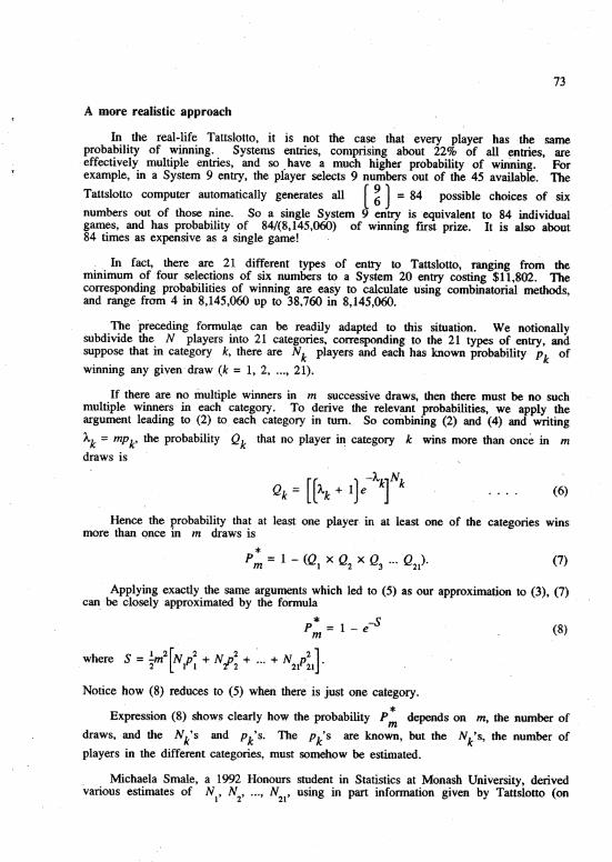
A more realistic a~proach

In the real-life Tattslotto, it is not the case that every player has the sameprobability of winning. Systems entries, conlprising about 22% of all ~ntries, are"effectively multiple entries, and so _have a much higher probability of· winning. Forexample, in a System 9 entry, the player selects 9 numbers out of the 45 available. The

Tattslotto computer automatically generates all ( ~) = 84 possible choices of six

numbers out of those nine. So a single System 9 entry is "equivalent to 84 individualgames, and has probability of 84/(8,145,060) of winning fIrst prize. It is also about84 times as expensive as a single game!

" In fact, there are 21 different types of entry to Tattslotto, ranging from theminimum of four selections of six numbers to a System 20 entry costing $11,802. Thecorresponding, probabilities of winning are easy to calculate u"sing combinatorial methods,and range from 4 in 8,145,060 up to 38,760 in '8,145,060.

The preceding .formul~e can be readily adapted to this situation. We notionallysubdivide the N players into 21 categories, corresponding ~o the 21 types of entry, andsuppose that in category k, there are Nk players and each has known probability Pk of

winning any given' draw (k = 1, 2, ..., 21).

If there are no multiple- winners in m successive draws, then there must be no suchmultiple winners in each category. To derive the relev~t probabilities, we apply theargument leading to (2) to each category in tum. So combining (2) and (4) and writing

Ak = mpk' the probability Qk that no player i~ category k wins more than once in m

draws is

(6)

Hence the probability that at least one player in at least one of the categories winsmore than once in In draws is

(7)

Applying exactly the same arguments which led to (5) as our approximatipn to (3), (7)can, be closely approximated by the formula

* -SPm = 1 - e (8)

Notice how (8) reduces to (5) when there is just one category.

*Expression (8) shows clearly how the probability Pm depends on m, the number of

draws, and the Nk's and Pk's. The Pk's are known, but the Nk's, the number of

players in the different categories, must somehow be estimated.

Michaela Smale, a 1992 Honours student in Statistics at Monash University, derivedvarious estimates of Nt' N

2, ..., N

21, using in part information given by Tattslotto (on

Let

74

.I the numbers of winners in different categories in 1990-91 and ,numbers of transactions indifferent groups). By allowing in this way for different categories of player, theprobability of there being a multiple winner increased dramatically. Fot example,.Michaela estimated that the probability of at least one person winning more than once in 5years of Saturday Tattslotto draws was 0.95!

Formula (8) is still a simplification, in that its derivation assumed that eachplayer only made one entry per draw. Clearly, many people make multiple entries,' possiblyof "different types, and do not do the same every week. Nevertheless, the probabilitygiven by (8) is likely to be of the right order of magnitude.

Coincidences (such as Mr Williams' double win) are not as remarkable as most peoplethink. In .fact; they will happen to someone, somewhere, some time. But if you expect tobe the one to win Tattslotto twice, then the ·originally-given. odds are more realistic.Don't hold your breath while you are waiting!

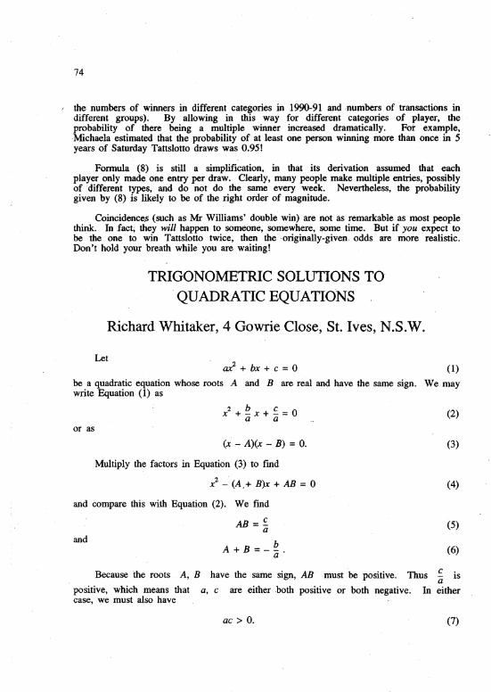
TRIGONOMETRIC SOLUTIONS TO'QUADRATIC EQUATIONS

Richard Whitaker, 4 Gowrie Close, St. Ives, N.S.W.

ax2 + bx + c =0 (1)

be a quadratic equation whose roots A and B are real and have the same sign. We maywrite Equation (1) as

x2 +£x+£.=Oa aor as

(x - A)(x - B) = O.

Multiply the factors in Equation (3) to fmd

x2 -"(A.+ B)x + AB = 0

and compare this with Equation (2). We find

AB =£.a

(2)

(3)

(4)

(5)

andA+B=-£.

a (6)

Because the roots A, B have the same sign, AB must be positive. Thus £. isa

positive, which means that a, C are either -both positive or both negative. In eithercase, we must also have

ac > O. (7)

75

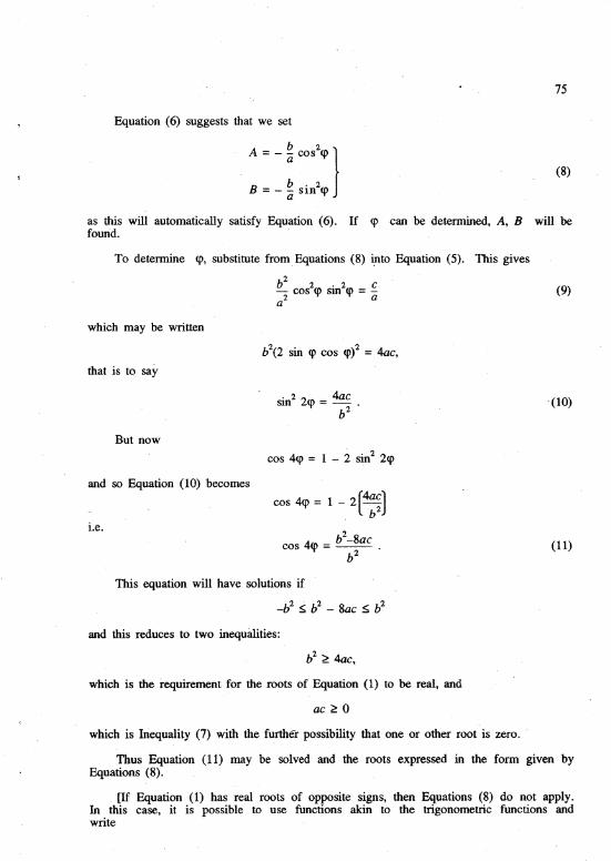
Equation (6) suggests that we set

(8)

as this will automatically satisfy Equation (6). If <p can be determined, A, B will befound. .

To detennine <p, substitute from. Equations (8) ~to Equation (5). This gives

b2. 2 • 2 C- cos <p sm cp =- (9)

a2 a

which may be written

b\2 sin <p cos cp)2 = 4ac,

that is to say• 2 2 4ac

SIn cp =- .b2

But now

cos 4cp = 1 - 2 sin2 2cp

-(10)

and so Equation (10) becomes

i.e.

cos 4cp = 1- 2[~~J

. b2-8accos 4<p = _.-2- .

b(11)

This equation will have solutions if

_b2 ~ b2_ 8ac ~ b2

and this reduces to two inequalities:

which is the requirement for the roots of Equation (1) to be real, and

ac ~ 0

which is Iriequality (7) with the further possibility that one or other root is zero.

Thus Equation (11) may be solved and the roots expressed in the form given byEquations (8).

. [If Equation (1) has real roots of opposite signs, then Equations (8) do not apply.In this case, it is possible to use functions akin to the trigonometric functions andwrite

76

A =- ~ cosh2

<P }(12)

B = + ~ sinh2

<p

where cosh and sinh. are so-called hyperbolic 'functions. This, however, lies outsidethe scope of Function.]

Consider as an example

x2- 4x + 3 = O.

Here a = 1, b = -4, c = 3. Equation (11) has a solution <p = ~ and this gives (check as

an exercise!) the roots A = 3, B = 1.

COMPUTERS AND COMPUTING

EDITOR: CRISTINA VARSAVSKY

Solving Mathematical Problems with a Spreadsheet

Computers are becoming more and more accessible th.ese days. If you do not own acomputer you certainly have access to a PC in your school. Perhaps you find themattractive because of the many interesting games you can play (some of them verychallenging indeed). Of many other computer applications you have most certainly seen aspreadsheet. It would have been one of the many available in the market: LOTUS 123,EXCEL, QUATTRO, VP-PLANNER, VC_CALC AND OTHERS.

A spreadsheet is like a big electronic table which is used for presenting andmanipulating data. In one sense, it is a programming language. It is usually considereda business tool because it is very useful for the manipulation of numbers organised in atable: adding colunms or tows of numbers, working out the average, combining contents oftwo or more colu!JlI1s, graphs, etc.

I have noticed that too few students (and teachers) appreciate its potential as atool to explore mathematics. Spreadsheets are very useful when· solving some mathematicalproblems, specially those involving a repetitive task. This article will show someproblems that could be solved smartly and quickly with a spreadsheet. .

Let us fust have a short introduction to spreadsheets' (or revision) because you needto be able to use them effectively before you actually start solving problems with them.

As I mentioned "before, a spreadsheet is a big electronic·· table consisting of manycells (many more than we usually use). The address of each cell is detennined by a letter(or two) followed by a number, indicating the column and the row respectively. . Text, anumber, or a formula can be stored in each cell. To enter or change the content of a cellyou need to move the cursor to. that cell -<using either the mouse or the arrow keys), typethe content, and hit the ENTER key..For example, enter the number 234.5 in Al and thenumber 672.1 in A2. In A3, enter

+ Al + 3* A2

77

(the "+" sign at the front means that what follows is a formula, not text). Yourspreadsheet should look like Figure 1.

! A 8 C1 234.52 672.13 2250.8456

Figure 1

A 8 C1 234.5 232 672.1 103 2250.8 53456.

Figure 2

, Notice that if you now change 178.45 to 234.5 in Al the content of the cell A3changes accordingly.

One of the most powerful features of a spreadsheet is the .copying of formulaecontaining references to other cells, like the formula we stored in A3 which adds to thecontent in A1 three times the content of A3. This fonnula is actually interpreted asfollows:

add to the content of the cell two rows above three times the contentof the cell immediately above. .

Before actually copying the formula, let us store the number 23 in Cl and the numberlOin C~. 'Now copy the formula you have in A3 to the cell C3~ ,

from.the main menu select COPY, then highlight the cell A3 (range to becopied) and hit ENTER; move the cursor to C3 (range to be copied to)and press 'ENTER.

What happened? The cell C3 now contains 53, which is the content of CI (two rows above)added to the ,triple of the number in C2 (immediately above). See Figure 2. This is whythe references to Al and A2 in the fonnula we have in A3 are called relative references.If we wanted to copy that formula to keep the references to Al and A2 regardless of theposition' to be stored to, we would have used the dollar sign ($) in front of the columnand the row, meaning absolute reference to that cell. '

Let us now go to some examples where we 'use tI,lis. concept of copying formulaecontaining relative references to other cells.

Generating sequences

Do you remember the Fibonacci sequence? The fIrst two terms are 1, and then thesubsequent terms are generated by adding the two previous terms:

1st term =12nd term =13rd term =1st term + 2nd term = 24th tenn =2nd term + 3rd term = 35th term =3rd term + 4th term = 7etc....

78

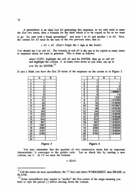
A spreadsheet is an ideal tool for generating this sequence, as we only need to enterthe fust two terms, then a fonnula for the third which is to be copied as far as we want

to go. So, start with a blank spreadsheett and store I in Al and another 1 in A2. Now,the content for A3 must be the sum of the two previous ones, that is:

+ Al ~ A2 (Don't forget the + sign at the front!)

You should see 2 in cell A3. The formula in cell A3 is the one to be copied· as many timesas sequence tenns we want to generate. This is done as follows:

select COPY, highlight the cell A3 and hit ENTER, then go to cell A4and highlight the column A as many rows down as you want, say up to

row 20; hit ENTER.tt

In just a blink you have the fust 20 terms of the sequence on the screen as in Figure 3.

A B1 12 13 24 35 56 87 138 219 34

10 55.11 8912 14413 23314 37715 61016 98717 159718 2584:19 418120 67652122

Figure 3 .

A B C1 12 1 13 2 24 3 1.55 5 1.6666676 8 1.67 13 1.6258 21 1.6153859 34 1.619048

10 55 1.61764711 89 1.61'818212 144 1.61797813 233 1.61805614 377 1.61802615 61.0 1.61803716 987 1.61803317 1597 1.61803418 .2584 1.61803419 4t81 1.61803420 6765 1.6180342122

Figure 4

You may remember that the quotient of two consecutive terms had an importantcharacteristic: it converges to ~e golden. ratio. Let lis check this by startiqg a newcolumn, say C. In C2 we enter the fonnula

+ A2/AI

t Call the menu (in most spreadsheets, the "f' key) and select WORKSHEET, then ERASE, orBLANK. .

tt Some spreadsheets may require to "anchor" the first corner of the range meaning youneed to type the period (.) before moving down the column.

79

Copy that fonnula from column C down to row 20. What do you see? Two consecutive tennsof the 'new sequence are closer as we move down the column C, indicating that ~e sequenceof consecutive quotients converges approximately to 1.618034, known as the golden ratio.(See Figure 4.) Although this is not a rigorous proof, it certainly gives a goodapproximation to the answer.

Here you have' two exercises along the same lines:

Exercise 1: Change the values for the' two frrst terms of the Fibonacci sequence. Whathappens to the sequence of the quotients?

Exercise 2: Generate some terms of the sequence defmed as follows:

1 2Xl = 1 ; X2 =2" ; Xn+I =Xn·

Make a co~jecture about its convergence.

Finding limits

Spreadsh~ets are also very useful to investigate the limiting values of functions.

Take for example lim. ~n' sin x. The function y = sin x cannot be evaluated at x =0x~ x x .

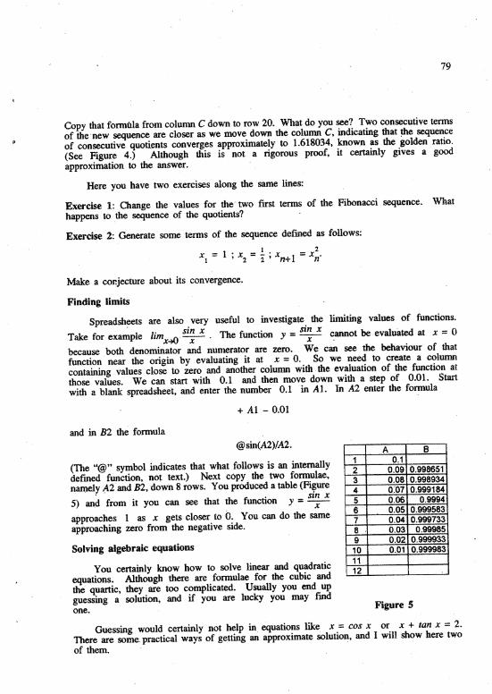
because both denominator and numerator are zero. We can see the behaviour of thatfunction near the origin by evaluating it at x = O. SO we need to create a columncontaining values close to zero and another column with· the evaluation of the function atthose values. We can start with 0.1 and .then move down with a step of 0.01. Startwith a blank spreadsheet, and enter the number 0.1 in At. In A2 enter the formula

+ Al - 0.01

and in B2 the formula

@sin(A2)/A2.

(The "@" symbol indicates that what follows is an internallydefmed function, no~ text.) Next copy the two formulae~

namely ~2' and B2, down 8 rows. You produced a table (Figure

5) and from it you can see that the function y = si~ x

approaches 1 as x gets closer to O. You can do the sameapproaching zero from the negative side.

Solving algebraic equations

You certainly know how to solve linear and quadraticequations. Although there are fonnulae for the cubic andthe- quartic,tbey are too complicated. Usually you end upguessing a solution, and if you are lucky you may fmdone.

A 81 0.12 0.09 0.9986513 0.08 0.9989344 0:07 0.9991845 0.06 0.9994a' 0.05 0.9995837 0.04' 0.9997338 0.03 0.999859 0.02 0.999933

10 0.01 0.9999831112

Figure 5

Guessing would certainly not help in, equations like, x::: cos x or x + tan x =2.There are some" practical ways of getting an approximate solution, and I will show here twoof them.

80

Tabulating the function

Solving an equation means fmding the value of the variable such that both sides areequal, or where the left-hand side minus the right-hand side is zero. The idea is then toproduce a table with two columns: in the fIrst one we list values for ~e variable, and inthe second we - evaluate the difference between the left- and right-hand sides at thosevalues to identify where it is close to zero. Usually we can get some bounds for thesolution, for example by looking at the graphs of y =cos x and y =x we can see thatthe solution is somewhere between 0 and 1. So let us create the table: start with ablank spreadsheet and enter 0 in AI. Move to A2 and enter the formula

+ Al + 0.1.

In B2 enter the function

@cos(A2) - A2.

Then copy the fonnulae in A2 and B2 down to· row 10. If .you investigate the table -(Figure6, columns A and B) you can conclude that cos x - x is equal to 0 somewhere between0.7 and 0.8. If we need more precision we can create another. table, but taking asmaller step: start with 0.7, and go up to 0.8 wi~ the step 0.01. (Figure 6, columns Dand E.) By doing that we can now see that the solution lies between 0.73 and 0.74. Ifwe want "mOre' accuracy for the solution we should look closer at the values between 0.73and 0.74 by using a smaller step, say- O.OCH.

A B C 0 E1 0 0.72 0.1 0.895004 0.71 0.0483623 0.2 0.780067 0.72 0.0318064 0.3 :0.655336 0.73 0:0151745 0.4 0.521061 0.74 -0.001536 0.5 0.377583 0.75 -0.018317 0.6 0.225336 0.76 -0.035168 0.7 0.064842 0.77 -0.052099 0~8 -0.10329 0.78 -0.0690910 0.9 -0.27839 . 0.79 -0.086151112

Figure 6

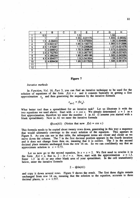
. A similar procedure may be followed to solve the equation In x + x = 2 which couldbe rewritten as In x + x - 2 =O. Again, we tabulate the function In x + x - 2 insteps of 0.5 between 0.5 and 5 (logarithm is· not defmed at O!). This is done inFigure 7: the fust column is for the values of the variable~ the second column containsthe fonnula. In Al we enter-the value 0.5. In A2, we have the fonnula 4- Al + 0.5 andin 82 the fonnula @In(A2) + A2 - 2. We can see that the values jump from positive tonegative between 1.5 and 2, so this is the· range blown up in the third column. Fromthe fourth column we can conclude that the solution is between 1.55 and 1.6 and wegain .one decimal in the precision. You can. complete the spreadsheet to increase theaccuracy (columns G and H).

81

A 8 C 0 E F G H1 0.5 1.5 1.552 1 -1 1.55 -0.01175 . 1.555 -0.003523 1.5 -0.09453 1.6 0.070004 1.56 0~OO4686·

4 2 0.693147 1.65 0.150775 1.565 0.012886·s 2.5 1.416291 1.7 0.230628 1.57 0.0210766 3 2.098612 1.75 0.309616 1.575 0.0292557 3.5· 2.752763 1.8 0.387787 1.58 0.0374258 4.3.386294 1'.85 0.465186 1.585 0~045584

9 4.5 4.004077 1.9 0.541854 1.59 0.053734-10 5 4.609438 . 1.95 0.617829 1.595 0.0618741112

Figure 7

Iterative methods

In Function, Vol. 16, Part 3., you. can fmd an iterative technique to be 'used for thesolution of equations of. the form J(x) =x and it consists' basically in. getting a frrstapproximation x0 and then generating the sequence by the iterative formula

xn+1 = j(xn)·

What better· tool than a spreadsheet for an iterative task? Let us illustrate it with thetwo equations we used above. Start with x = cos x. We already determined x = 1 as afIrst approximation, therefore we enter the number 1 in Al .(I assume you started with ablank spreadsheet). Now in A2 we enter the iterative formula

@cos(Al) (Notice that now .f(x) = cos x.)

This formula needs to be copied about twenty rows down, generating in this way a sequencethat would ultimately~onverge to the exact solution of the equation. This appears inFigure 8. As you can see in that table, the subsequent terms are closer and closer as wemove down the colunm. The 7 in the fIrst decimal position appears in the fourth iterationand it does not change from then on, meaning that it is correct. The 3 in the seconddecimal place remains unchanged from· the row 16 on. So we c'an confidently say that anapproximate solution is x =0.73.

Let us now go. to the second equation, In x + x =2. We fIrst need to rewrite it inthe form j(x) =x, that is, 2 - In x =x. Now, start with the approximation .x = 1.5.Enter 1.5 in Al or any other blank area of your spreadsheet. In the cell immediatelybelow, enter the iterative formula

2 - @In(Al)

and copy it down several rows. Figure 9 shows the result. The frrst three digits remainunchanged from row 14 on, meaning that. the solution to the equation, accurate to threedecimal places, is x = 1-.557..

82

A1 1.2' 0.5403023 '0.857553·4 0.65429-5 0.79348

. ',,6:. 0.701369:7,:,:,: 0.76396

,:8' 0.722102',:9·.:.0.750418·to:·:,:j 0.731404

.. '12:,·;:: 0.735&05

. '16 ';:: 0.738369f7': 0.739567

"'1'8"::: 0.738761.9:::~·: 0.73930420 :: 0.738938'21,

Figure 8

8 A1 1.52 1.594535.3 1.53341,84 1.572501.5 1.547333·6 1.5634677 . 1.5530948 ' 1.5597519 1.555474

1:0:: _1.55822--1-1 1.556456:-12: 1.5575891.'3. 1.556861'14- -:: 1.557328"f5"~: r.557028

,:.1·:1.:-;~ 1.557097'(11::8·6: 1.557177

'.20·;' 1.55715821· .

Figure 9

B

Although this is not _the best technique to solve equations iterativelyt- , it is a goodexample to show that spreadsheets are' not only good for business, bu.t also to solve a widerange of mathematical problems, specially those involving iterative fonnulae.

There are many other possible _applications but it is impossible to show them in justa few pages. I hope this small sample is enough to encourage you to think of thespreadsheet as a useful tool when solvirig problems. .

To conclude, I suggest you investigate the iteration

Start with the constant C:: 1 and Xl = 0.5. Generate a sequence using the -iterative

formula (use at l~ast 200 iterations). Then fwd out what happens when you systematicallyincrease C from 1 to 4. You may also use graphs the better to understand it. Bydoing this exercise you are entering in the field of chaos. Good luck!

t The Newton-Raphson method converges much more rapidly. This may be a topic for anotherFunction article!·.

83

HISTORY OF" MATHEMATICS

EDITOR: M.A.B. DEAKIN

The Wonderful Deduction

Mathematics has, as one of its most important components, . the concept of proof. Itis necessary in .Mathematics, not only that one's assertion be true, but that one also beable to demonstrate their truth. [See, for example, the article by Jim Mackenzie inFunction, Vol. 17, Part 1.] Proofs may take many different fonns, but some followstandard patterns, and this article will examine one of the least-known of these.

But before we get to that, let us begin with another: the so-called reductio adabsurdum. Suppose we want to prove a proposition P to be false. We begin by supposingit to be true. That is to say, we wish to prove .the negative of 'P, nonnally writtennot-P,· or - P, and to this end, we entertain the possibility P.

The proof then proceeds by showing that P implies some false proposition, Q sa~.

This we write asP => Q.

Deduction (1) is known to be equivalent to

- Q => - P,

and, since Q is false, - Q is true and thus, by Deduction (2), - P is established.

Consider as an example the theorem:

(1)

(2)

If two angles of a triangle are equal to one another, then the sides which areopposite to the equal angles are equal to one another.

This is Proposition 6 of Book. I of Euclid's Elements. It is· theconv.erset of Propo~ition5 of Book I: the theorel11 -known as the pons asitiorum, stating that the angles at the baseof an isosceles triangle are equal. (For more on this, see Function, Vol. 3, Part 3.)

A

The proof of 1.6 makes use of Figure 1 at right.Weare told that

L ABC =L ACB

. and must prove that, in consequence, AB = AC.

e'-----.... c

Figure 1

t Many theorems are themselves statements of the form P => Q. The converse of such atheorem is the statement Q => P. The converse may be true (as in this case) or false. Anexample of the latter: If the series a1 + a2 + ... + an + ... converges, then an ~ 0 as

n ~ 00. The converse (if .' an ~ 0, then the series converges) is false. See Peter

Grossman's article in Function, Vol. 17, Part 2.

A

84

To do this, sUppose AB ¢ AC; then one or other of these lengths, AB say, will be thegreater. On AB then, measure off DB such _that DB =AC. Then join CD as shown.

Now consider the triangles DBC and ACB. We have: '

(1) DB =AC, by our hypothesis and construction,(2) BC =CB, obviou.sly,(3) L DBC =L ACB, also by hypothesis.

Thus these triangles are congruent and so have equal areas, which is, of course, anonsense.

Thus our hypothesis of different lengths has led to an absurdity and so we-mustabandon it. Let P represent the statement AB ~ AC and let Q be the statement thatthe' whole is equal to· one of its· parts. We have found

P=>Q

and as -Q is false, - P is established, Le. P is false, and so AB = AC.

An even starker form of reductio ad absurdum is to be found in the event thatQ =- P. That is ~o say, we assume P and fmd that

p => - P. (3)

(If P is true, then it is also false!) Clearly P is then false, i.e. - P is true.Logicians write this fonn of the reductio ad absurdum argument as

(P ==> - P) ==> - P (4)

(a proposition that implies its own falsehood must be false).

An example of this mode of argument is to be found in the proof of 1.19 of Euclid'sElements. This states:

If one angle of a triangle is greater than anotherp then the side oppo$ite thegreater angle is greater than the side' opposite the less.

This theorem is. the converse of the preceding theorem (I. 1'8) in the Elements:

1/ one side of a triangle is rgreater than another, then the angle opposite thegreater side is greater than the angle opposite the less.

The proof of 1.19 runs as follows.

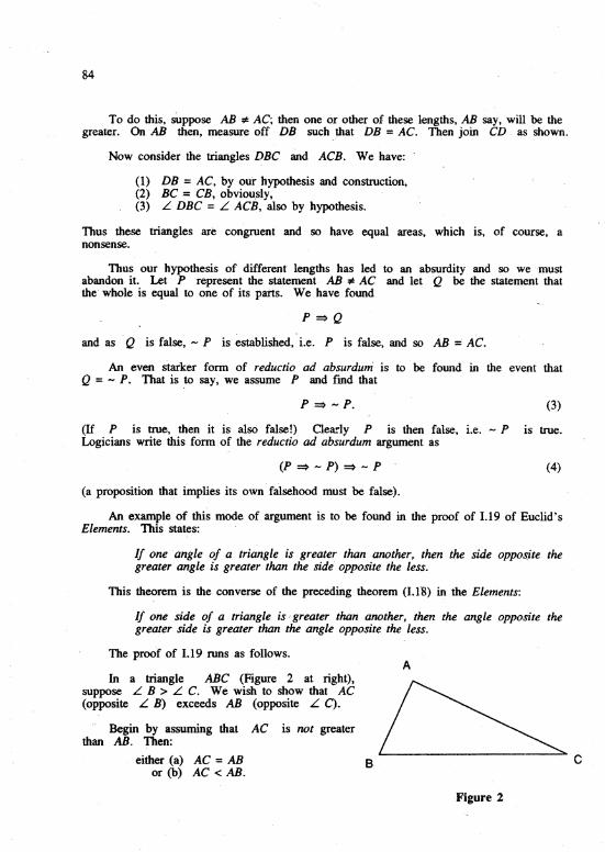
In a triangle ABC (Figure 2 at right),suppose L B > L C. We wish to show that AC(opposite L B) exceeds AB (opposite L C).

Begin by assuming that AC is not greaterthan AB. Then:

either(a) AC = AB Bor (b) AC< AB.

Figure 2

c

85

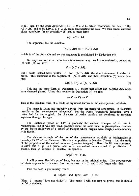
If (a), then by the pons asinorum (1.5) L B =L C, which contradicts the data; if (b),AB > AC and so by 1.19 L C > L. B, again contradicting the data. We thus cannot entertaineither possibility (a) or possibility (b) and so must·have

(c) AC > AB.

The argument has the structure

(AC ~ AB) ~ - (AC ~ AB) (5)

which is of the fonn (3) and so our argument is established by Deduction (4).

We may however write Deduction (5) in another way. As I have outlined it, comparing(3) with (5), we have

P = (AC ~ .4B).

But 1 could. instead have written P for (AC > AB), the direct statement I wished toprove. This statement is the negation of (AC ~ AB) and then Deduction (5) would haveread

-(AC > AB) ~ (AC > AB). (6)

This has the same fonn as' Deduction (3), except that direct and negated statementshave changed places. Using this notation in Deduction (4) we fmd

(- p => P) => P. (7)

This is the standard fonn of a· mode of argument known as the consequentia mirabilis.

The name is Latin and probably derives from the medieval schoolmen. It translatesliterally as the "consequence miraculous", but the words "wonderful deduction" give abetter feel for the original. Its character of quaint paradox has continued to fascinatelogicians through the ages.

The Euclidean· proof of 1.19 is probably" the earliest example of its use inMathematics, but it· was also used, probably about the same time, in philosophical contextsby the Stoics (followers of a school of thought whose origins were roughly. contemporarywith Euclid).

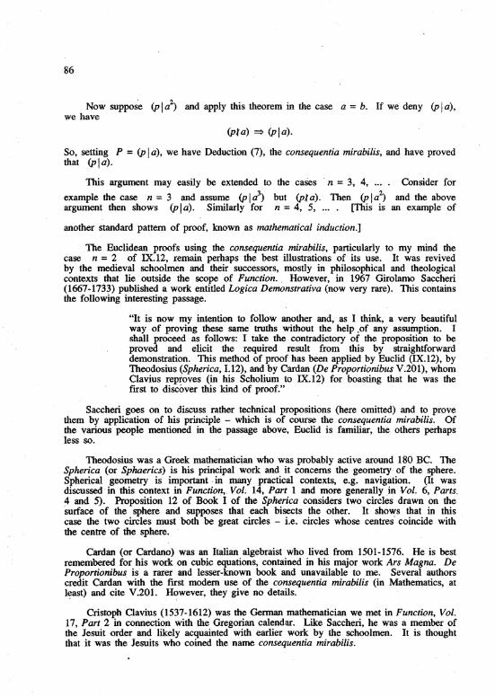
The clearest example of the use of the consequentia nzirabilis in Mathematics isprobably IX.12 of the Elenlenls. This is a proposition· in Number Theory - Le. the studyof the properties of the natural numbers (positive integers). Here, Euclid was concernedto show that if p is a prime and a, n are natural numbers and if p divides anexactly, then p divides a exactly. In symbols,

1 will present Euclid's proof 'here, but not in its 9riginal order. The consequentiamirabilis appears in its starkest form in the case n = 2 and 1 will begin with that.

First we need a preliminary result:

If (p lab) and (Pk a), then (p Ib).

(Here k means "does not divide".) This result 1 will not stop to prove, but it shouldbe fairly obvious.

86

Now suppose (p Ia2) and apply this theorem in the case a =b. If we deny (P Ia),

we have

(Pi a) => (p Ia).

So, setting P = (P Ia), we have Deduction (7), the consequentia mirabilis, and have provedthat (PIa).

This argument may easily be extended to the caSes . n =3, 4, .... Consider for

example the case n =3 and assume (p Ia3) but (Pi a). Then (p Ia2

) and the aboveargument then shows (P Ia). Similarly for n =4, 5, .... [This is an example of

another standard pattern of proof, known as rnq.thematical induction.]

The Euclidean proofs using the consequentia mirabilis, particularly to my mind thecase n = 2 of IX.12, remain perhaps the best illustrations of its use. It was revivedby the medieval schoolmen and their successors, mostly in philosophical and theologicalcontexts that lie outside the scope of Function.. However, in 1967 Girolamo Saccheri(1667-173~) published a work entitled Logica Demonstrativa (now very rare). This containsthe following interesting passage.

"It is now my intention to follow another and, as I think, a very beautifulway ·of proving these same truths without the help .of any assumption. Ishall proceed as follows: I take the contradictory of the proposition to beproved and elicit the required result from this by straightforwarddemonstration. This method of proof has been applied by Euclid (IX.12), byTheodosius (Spherica, 1.12), and by Cardan (De Proportionibus V.201), whomClavius reproves (in his. Scholium to IX.12) for boasting that he was thefirst to discover this kind of proof." . ,

Saccheri goes on to discuss rather technical propositions (here omitted) and to provethem by application of his principle - which is of course the consequentia mirabilis. Ofthe various· people mentioned in the passage above, Euclid· is familiar, the others perhapsless so.

Theodosius was a Greek mathematician who was probably active around 180 BC. TheSpherica (or Sphaerics) is his principal work and it concerns the geometry· of the sphere.Spherical geometry is important -in many practical contexts, e.g. navigation. (It wasdiscussed in this context in Function,. Vol~ 14, Part 1 and more generally in ,Vol. 6, Parts.4 and 5). Proposition 12 of Book I of the Spherica considers two circles drawn··on the'surface of the sphere and supposes that each bisects the other. It shows that in thiscase the two circles must both ·be great circles - i.e. circles whose centres' coincide withthe centre of the sphere. .

Cardan (or Cardano) was an Italian algebraist who lived from 1501-1576. He is bestremembered for his work on cubic. equations, contained in his major work Ars Magna. DeProportionibu8, is' a rarer and lesser-known book and unavailable to me. Several authorscredit Cardan with the frrst modem use of the consequentia mirabilis (in Mathematics, atl~ast) and cite V.20t. H~wever, they give no details.

Cristopb Clavius (1537-1612) was the Gennan mathematician we met in Function, Vol.17, Part 2 in connection with· the Gregorian calendar. Like Saccheri, he was a member ofthe Jesuit order and likely acquainted with earlier work by the schoolmen. It is thoughtthat it was the Jesuits who coined the name consequentia mirabilis.

Figure 3

87

Clavius wrote commentaries on both Euclid's Ele.ments and Theodosius' Spherica.Regrettably neither of these nor any edition of the Spherica has .~en available tome.The use of the consequentia mirabilis in the proof of 1.12 has been variously attributedto Theodosius himself (as in the passage quoted above). or· to Oavius as edit,?r. Neitheroriginal is available to me,' bu~ I have seen a summary of Oavius' version. ,This summarywould seem to show that the proof is inadequate (though the theorem itself is .true).

Saccheri· himself went on to use the consequentia mirabilis in a context that was muchmore interesting - though his .proof was also flawed. Saccheri was one of a number ofm,athematicians who sought to prove Euclid's "Fifth Postulate" and, it is in this contextthat he is best remembered. The postulates in Euclid, with ·the· exception...of the Fifth,are basic assumptions whose truth we may readily accept. For example, the Third Postulatestates that we may construct a circle about any centre .and with arbitrary radius.

The Fifth, however conceinsparallels and, in essence, states that, in Figure 3, thelines 11 and 1

2are parallel if and only if

a + p= 180°. This postulate seems much lessobvious than the others and it strock many people,from Euclid's· time till quite recently, that it wasthe sort of thing that really should be proved.

The suspicion arose, that this postulate couldin fact be deduced from the others. [In the caseof the Fourth Postulate (All rightangles areequal) such proof is possible.] It is now knownthat the Fifth Postulate cannot be so proved, forwe may assert its opposite and reach .consistentnon-Euclidean geometries (see Function, Vol. 3,Parts 2 and 4, and Vol. 12, Part 4).

However, before this was known, there were many attempts to prove the FifthPostulate. One of the best-known and most thorough was Saccheri's. He began by denying

the Postulate - by supposing that there were cases in which a + P* 180°, . butnevertheless I} and /2 were parallel. This is the geometry later invented by .Gauss,

Bolyai and Lobachevsky and referred to nowadays as Lobachevskian geometry. Theconsistency of Lobachevskian geometry, the fact that no contradictions may arise in it,was. later proved by Poincare.

Saccheri investigated the consequences of denying the Fifth Postulate and did so ingreat detail. In the course of this work, ,he discovered many of the theorems ofLobachevskian geometry. But ultimately he made a mistake and, working from this incorrectbasis, he deduced that, after all, ,the Fifth Postulate was true. What he thought he hadwas' (with P representing the Fifth Postulate):

-P=:!iP

and so, using the consequentia mirabilis (7), he argued

(-P~P)~P

and therefore P. So, Euclid was viridicated -his' Fifth Postulate was proved..

In a sense, it's sad that he was wrong; it was a genuinely heroic effort, marred by asingle, but critical, mistake.

88

The non-mathematical 'uses of the consequentia mirabilis lie' mainly outside the scopeof Function, but perhaps one deserves mention. ' This is the proof of the statement (P):

SOl1ze proposition is true.

To prove this, consider the negation of P (- P):

No proposition is true.

But if P is false, then -'P is true and - P is a proposition! So at least oneproposition· (- P) is true and so p. is true after all. We may put things thus: P istrue, because its negation, - P, is self-contradictory.

[This form of the example .has been attributed to the Belgian Arnold Geulincx(1624.;1669), but its roots are much older. The Stoics, mentioned briefly above, were atodds with the Sceptics, those who denied the.possibility of knowledge.· The Sceptics then"knew" that you could know nothing. The· irnitionality of universal doubt also played amajor role in the philosophical thought of Descartes (1596-1650) after 'whom cartesian(co-ordinate) geometry is named.]

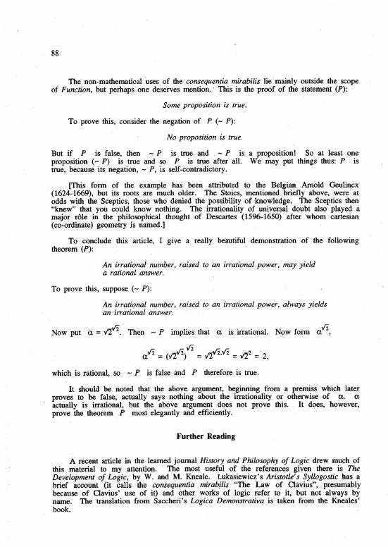
To conclude this article, I give a really beautiful demonstration of the followingtheorem (P): .

An irrational nurnber, raised to an irrational power, may yielda rational anSl1-'er.

To prove this, suppose (- P):

An irrational nU111ber, raised to an irrational power, aI-ways yieldsan irrational answer. .

Now put a = V'1,V2. Then - P implies that a is irrational. NQw fonn a12,

which is ration~l, so - P is false and P therefore is true.

It should be noted that the above argument, beginning from a premiss which laterproves to be false, actually says nothing about the irrationality or otherwise of a. aactually is irrational, but the above argument does not prove this. It does, however,prove the theorem P most elegantly and efficiently.

Further Reading

A recent article in the learned journal History and Philosophy of Logic drew much ofthis material to my attention. The most useful of the references given there is TheDevelopment of Logic, by· W. and M. Kneale. Lukasiewicz's Aristotle's Syllogostic has abrief account (it calls theconsequentia mirabjlis "The Law of' Clavius", presumablybecause of Clavius' use of it) and other works· of logic refer to it, but not always byname. The translation from Saccheri's Logica Demonstrativa is taken from the Kneales'book.

89

PROBLEMS AND SOLUTIONS

We continue in this issue to publish solutions to long-outstanding problems.

SOLUTION TO PROBLEM 14.1.6f

E

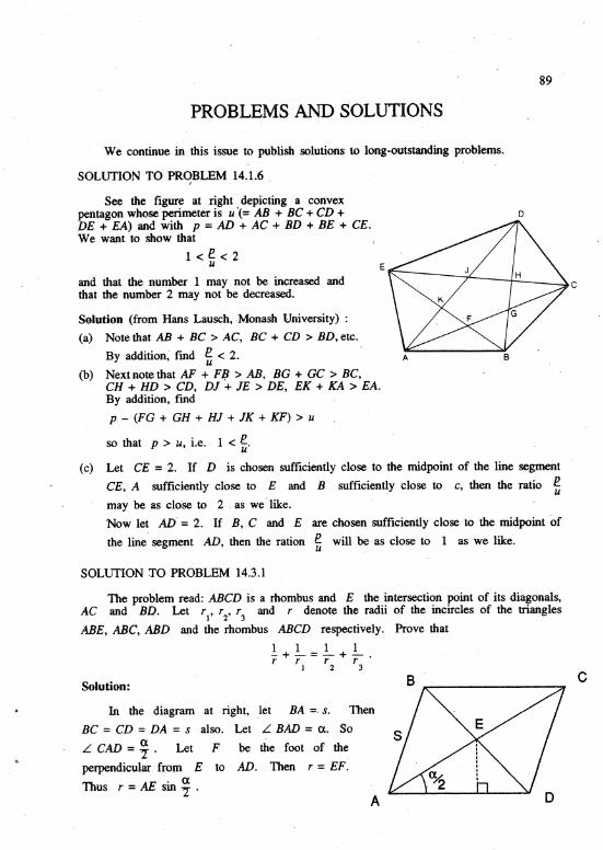
See the figure at right depicting a convexpentagon whose perimeter is u '(= AB + BC +CD +DE + EA)and with p = AD + AC + BD + BE + CEoWe want to show that

1<l!.<2u

and that the number 1 may not be increased andthat the number 2 may not be decreased.

Solution (from Hans Lausch, .Monash University) :

(a) Note that AB + BC > AC, BC + CD > BD, etc.

By addition, fmd t < 2. A

(b) Next note that AF + FB > AB, BO + GC > BC,eH + HD > CD, DJ 4. JE > DE, EK + KA > EA.By addition,. fmd

p - (FG + GH + Hi + JK + KF) > u

B

o

c

so that p > u, Le. 1 < ~.

(c) Let CE =2. If D is chosen .sufficiently close to the midpoint of the line segment

CE, A sufficiently close to E and B sufficiently close to c, then the ratio e- umay be as close to 2. as we J like.

"Now let AD' = 2. liB, C and E are chosen sufficiently close to the midpoint of

the line segment AD, then the ration l!. will be as close to 1 as we like.u

SOLUTION TO PROBLEM 14.3.1

c

A

In the diagram at right, let .BA =, s. Then

BC= CD =DA = s also. Let L BAD =a.. SoaL CAD = "T' Let F be the foot of the

perpendicular from E to AD. Then r =EF.

Thus r = AE sin -! .

Solution:

The problem read: ABeD is a rhombus and E the intersection point ·of its diagonals,AC and BD. Letr

l, r

2, r

3and r denote the radii of the incircles of the triangles

ABE, ABC, ABD and the rhombus ABeD respectively. Prove that

!+l.=.!-+.!-.r r r r

1 2 3

90

But now it is a theorem that L AED is a right angle. Thereforea . a

AE =AD cos "'! =8 COS "T. Thus

~ a a. 1 . (1), ::: 8 sm "! cos "I =1.8 sm a.

To fmd r1, '2"3 we need to kn~w a formula. The in-radius of a triangle is equal

to its area divided by its semi-perimeter. As BE =8 sin ~, we readily fmd

'1 = Z(sin 0.)/(1 + sin ~ +~ cos ~) (2)

'2 = ! (sin 0.)/(1 + cos t) (3)

'3 =! (sin 0.)/(1 + sin ~)~ (4)

The required result now follows, after a little algebra, from Equations (1), (2), (3)and (4). (

SOLUTION TO PROBLEM 14.3.2

The problem read: ABC is a triangle right-angled at A, and .D is the foot of thealtitude from .A. Let X and Y be the incentres of triangles ABD and ADCrespectively. Detennine the angles of triangle AXY in terms of triangle ABC.

Solution: ,_ Consult the diagram at right. Thedotted lines bisect 'the angles at A, B, C, D asshown. Thus if L ABC = ~ and L ACB =1, then

~ + "( =~. L BAD =1 and L CAD = 13. Thus

'L XAY =~~ + 1) =~ . '. Let AB =b. Then

AC =b tan ~.

Apply the sine rule to the triangle ABX.

Note that L AXB =1t - ( ~].= ~. Thus

. AX =(sin ~)b/(sin ~) = V'l b sin ~ .

Similarly,

c

\. Y 0" ..

A . B

AY =..;'l b tan ~ sin 1.Put L AXY =9. ThenL AYX ::; 1t - 9 - ~ =~ - 9. Now apply the sine rule to the

triangle AYX.

VI b tan p sin y/2 _ IZ b sin 13/2SIn 9 - sin(~ - 9) .

After a large number of somewhat tedious manipulations (here omitted in the interestof brevity), this equation redu~es to

. (1t~]tan 9 = tan 1+1

so 9=;+~ and ~-e=~-~.

The angles are thus ~, 2- + ~ , ~ - ~ .

91

SOLlITION TO PROBLEM 14.3.3

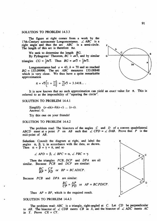
The figure at right comes from a work by the17th-Century astronomer Longomontanus. L ABC is arightangle and thus the arc ABC is a semi-circle.The length of this arc is therefore . 1ta.

We seek to determine· the l~ngthBG.

By Pythagoras' Theorem, Be =aI'J, and by similar

triangles CG =~. Thus BG' =aI'J + ~.

Longomontanus had .a =43, b =70 and so reachedBG =135.09996. 'The arc ABC measures 135.08848which is- very close. We thus have a quite remarkableapproximation

1t Q! Y3(1 +~] = !!"3" = 3.1418....43 43

F

G

2a

A

It is now. known that no such approximation can yield an exact value for 1t. This isreferred to as the impossibility of "squaring the circle".

SOLUTION TO PROBLEM 14.4.1

Simplify (x-a)(x-b)(x-c) ... (x-z).Answer: O.

Try this one on your friends!

SOLUTION TO PROBLEM 14.4.2

The problem read: The bisectors of the angles C and D of a convex quadrilateralABCD meet at a point P on AB such that L CPD = L DAB. Prove that P is thet:IDd-point of AB.

Solution: Consult the diagram at right, and label the~gles (l,~, 'Y, in accordance with the data, as shown.Then (l + ~ + 'Y =1t, an~ so

L APD = ~, L BPC =(l, L PBC ='Y.

Then the triangles PCB, DCP and' DPA are allsimilar. Because PCB and DCP are similar:

BC CP1IP = P1J or BP =BC.AD/CP.

Because. PCB and DPA are similar:

~ =~ or AP =BC.PD/CP.

Thus AP ='BP, which is the required result.

SOLUTION TO PROBLEM 14.4.3

B

~c

~

p y

aa 0

y

A

The problem read: ABC is a triangle, right-angled at C. ,Let CD be perpendicularto AB. The bisector ofL CDB meets CB in X, and the bisector of L ADC meets ACin Y. Prove CX =CY.

92

Solution: A coordinate geometry approach works well. Let C be (O,O)~ A be (O,a)and B be (b,O).' Let L BCD be a, where tan a =bla. [This last is readily proved.]D is the point

(ab2 a

2b]" a2+b2

' a2+b2

and ,DX makes an angle in radianst of· (~+ a) with CB. Thus DX has slope

tan(~ + a.) and this is (b+a)/(b--a). We may thus obtain the equation of the line DX

and so fmd the x-coordinate of x' to be ab/(d+b). I.e.

CX =ab/(a+b).

The symmetry of this expression now allows us to conclude that CY also equalsab/(a+b). Hence the result.

SOLUTION TO PROBLEM 14..4.4

The problem read: L BAe is an obtuse angle. A -circle through A cuts AB at, Pand AC at Q. The bisectors of angles L QPB and L PQC cut the circle at X and Yrespectively. Prove that XY is perpendicular to the bisector of L BAC.

Solution: Let AZ bisect L BAC and meet XY at Z. (See'diagram.) Extend PX andAZ to meet at D. Let AZ, PQ clit at E.

A

Bc

o

t In elementary geometry, it matters little what angular units are used. However, in acalculus context, one 'must employ radians, so it is a good idea to get into the habitearly.

93

Forsimplicity, put L QPA ,= a., L PQA = ~. Then, working in radians, L BPQ =1t - aand so L XPQ = tTt - a). SimiladyL YQP =~1t - P). But. L- PAQ =1t - a - P, so

. L PAZ = ~1t - a - J3).

Now L PEZ = L QPA + L PAZ =~1t + a- ~) and similarly L QEZ (= L PEA) =¥1t - a + (}). But· now .

L PDA =L PEA - L XPQ = ~J3.

Furthermore, PQYX is a quadrilateral inscribed in a circle, so L PXY =1t - L YQP =¥1t + fJ). So L DXZ =~1t - 13).

Now L'AZX = L DXZ + L PDA1 A 1 A 1t=i<1t - p) + -i<1t + p) ="Z

as required. )

SOLUTION TO PROBLEM 14.4.5

The problem stated: ABeD is a square and P a point on the circumcircle and ·lyingbetween A and B. The distances from P to A, B, C and D are denoted by a, b, cand d respectively. Show (v'2+1)(a+b) =" + C and that a - b =("2+ l)(d-c) ..

Solution. The diagram below illustrates the situation.

94

Let L f AB' = a, L PBA = <p; let s be the length of the side of the square and R bethe radius of the circle. Let 0 be the centre of the. circle.

Apply the sine role to the triangle ABC. Then

a = 2R sin <p, b = 2R 'sin a, s = 2R· sin(9+<p). (1)

Further L COP (the reflex angle indicated) is twice L CBP; i.e. 1t + 2<p. Thus theangle COP (the one in the triangle COP) is 1t - 2<p. Now apply the cosine role to the

triangle COP. c2 =R2 + R2- 2R2cos(1t-2<p) = 2R

2[1 + cos 2<p] = 4R2coS2<p.

Thus

c = 2Rcos <po

Similarly

d = 2R cos a.Now'

2 (9+<p) (~)c+d _ cos <p + cos a _ cos -2- cos 2 _ 1a+o - SID <p + sin 6 - 2sin(9+4J)cos(6-q» - .-ta-n~(6""'+-<p-) .

2 2 2

. But s =RI'Z and so, by (1),

(2)

(3)

(4)

and

Thus

and

sin(9 + <p) ,= 1/,;'1

1t9+<P=4'

9+<p _ 1t-r --g

tan(9+<P) =_1_ ~2 12+1

[The reader may prove this as· an exercise.]

The first part of the problem is thus proved. The second follows likewise.

SOLUTION TO PROBLEM 14.4.10

The problem asked for a proof that 2x + 3y and 9x + 5y are divisible by 17 forthe same set of integral values of x and y.

Solution: Suppose2x + 3y is divisible by 17. Then 2x + 3y = 17m for some integer m.Then, multiplying by 9, we find

18x + 27y =9 x 17m

or

18x + lOy = 9 x 17m - 17y.

The right-hand side is clearly divisible by 17 and so

1&x + lOy = 17n

95

for some integer n, which also clearly must be even. Therefore 9x + 5y is divisible by17.

A similar' argument shows that if 9x + 5y· is divisible by 17, then so is . 2x + 3y.

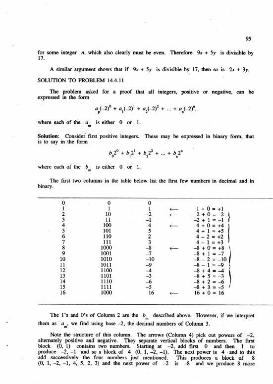
SOLUTION TO PROBLEM 14.4.11

The problem asked for a proof that all integers, positive or negative, can beexpressed in the fonn

a (_2)0 + a (_2)1 + a (_2)2 + ..~ + a (_2)D,p 1 2 n

where each of the a is either 0 or. 1.m

Solution: Consider ftrst positive integers. These may be expressed in binary fonn, thatis to say in the form

b 20 + b 21 + b 22 + ... + b 2n

012 n

where each of the b is either 0 ~ or 1.m

The fIrst two columns in the table below. list the fIrst few numbers in decimal and inbinary.

of23456789

10111213141516

o1

1011

100101110111

100010011010101111001101111011111000

o1

-2-14523

-8-7-10-9-4-3-6-5

16

1 + 0 =+1~2 + 0 = -2 }-2 + 1 =-14+0=+414 + 1 =+54 - 2 =+24 - 1 = +3

-8 + 0 =+8-8 + 1 =-7-8 - 2 = -10-8 - 1 =-9-8+4=-4-8 + 5 =-3-8+2=-6-8 +3 = ~516 + 0 = 16

The l's and .o's of Column 2 are the bm described above. However, if we interpret

them as " am' we find using base -2, the decimal numbers of Column 3.

Note th~ structure of this column. The arrows (Column 4) pick out powers of -2,alternately positive .and negative.. They separate vertical blocks· of numbers. The ftrstblock (0, 1) contains two numbers. Starting at -2, add frrst 0 and then 1 toproduce -2, -1 and so a. block of 4 (0, 1, -2, -1). The next power is 4· and to thisadd successively the four numbers just mentioned. This produces a block of 8(0, 1, -2, -1, 4, 5, 2, 3) and the next power of -2 is -8 and we produce 8 more

96

entries in the table. After this we will have 16 entries and so on.

Before 4, we have generated the integers -2, -1, 0, 1.Before -8, we have generated the integers -2, , 5.Before 16, we have generated the integers -10, , 5.

Continuing this pattern, we see that before 32, we will have generated a ron of 32integers starting with ...;.10, i.e~ -10, ..., 21; before 64, a run of 64 integers endingwith 21, i.e. -42, ..., 2L

Thus all positive and all negative integers are eventually generated.

This analysis also answers PROBLEM 14.5.1 for if the number of digits is even, thenumber is negative, and yes, the representations are clearly unique.

SOLUfION TO PROBLEM 14.4.12

The problem is historically based and may be stated in tenns of the diagram below.DBL is the diameter of a circle and BZ is a radius perpendicular to it. We are told

that ST =BD and are asked to prove that L TBL = ;'L DBE.

L

B

o

1tSolution: Let L TBL = 9. Then L TBS ='! - 9 and since ST = DB = BT,

~ TSB = L TBS = ~ - 9. Thus L BTS =29. But now in the triangle TBE, TB =E!J and so

L TEB = 29 also. Thus L TBE =1t - 49, whence L LBE =1t - 39' and so L DBE = 39.

The problem raises the question as to whether we have successfully trisected theangle DBE. We have, but it ,is not possible to construct the point T' with ruler andcompass alone. No such constroction is possible.

For more on angle trisection, see Function, Vol. 3, Part 3.

* * * * *

M.A.B. Deakin (Chairman)R.J. ArianrhodR.M. ClarkL.R. EvansP.A. GrossmanC..T. Varsavsky

BOARD OF EDITORS

Monash University

J.B. HenryP.E. Kloeden

K. MeR. EvansD. Easdown

}- Deakin University

fonnerly of Scotch CollegeUniversity of Sydney, N.S.W.

* * * * *

BUSINESS MANAGER:

TEXT PRODUCfION:

ART WORK:

Mary Beal (03) 565-4445

Anne-Marie Vandenberg

Jean Sheldon

* * * * *

SPECIALIST EDITORS

}Monash University,Qayton

Computers and Computing: C.T. Varsavsky

History of Mathematics: M.A.B. Deakin

Problems and Solutions:

Special Correspondent onCompetitions and Olympiads: H. Lausch

* * * * *

Registered for posting. as a periodical - "Category B"ISSN 0313 - 6825

* * * * *Published by Monash University. Mathematics Department