ASD and LRFD Methods Codes and Economics of Dynamic Testing

ASTM D4945

Load Testing .

Static Load Testing

ASTM D1143

Deadload Testing

React. Piles/Anchors

Static Load Tests are the “standard”

Costly: Need 100% load + long time

Static Analysis Methods are not accurate

3

International Prediction Event “Behaviour of Bored, CFA, and

Driven Piles in Residual Soil”, ISC’2 Experimental Site, 2003,

by Viana da Fonseca and Jamie Santos 3

CAPWAP - Results

CAPWAP

SLT

4

+20%

-20%

•Allowable Stress Design (ASD)

Ru > Qd * F.S. (F.S. = Factor of Safety)

Design Concepts - Factors of Safety

5

ASDAASHTO: F.S. Gates 3.50Wave Eqn 2.75DLT 2.25

SLT 2.00SLT + DLT 1.90

SLT or DLT 2.00 IBC

6

PDCA LRFD - 2000

Application: 2000 ton total structure load,

200 ton ultimate capacity piles

design load piles

F.S. per pile needed

3.50 200/3.50 = 57 t 35 dyn. formula

2.75 200/2.75 = 72 t 28 wave equation

2.25 200/2.25 = 89 t 23 dynamic test

2.00 200/2.00 = 100 t 20 Static (SLT)

1.90 200/1.90 = 105 t 19 SLT + dynamic

Lower F.S. fewer piles less cost

AASHTO standard specifications (ASD)(15th Ed. 1992) – code for bridges

Ru >(F.S.) Qd

•Allowable Stress Design (ASD)

Ru > Qd * F.S. (F.S. = Factor of Safety)

•Load and Resistance Factor Design (LRFD)

φ Ru > fDLD + fLLL + fiLi + …

ASD “Factor of Safety” split into Load and

Resistance factors F.S. ~ favg / φ)

Design Concepts - Factors of Safety

9

(1.25D + 1.75L)φ (D + L)

FS =

(1.25D + 1.75L)φ (D + L)

FS =

10

Get resistance factors (φ) from conversion of ASD “Factors of Safety”

Equate Ru and solve for FS

If D/L = 2

(1.25*2 + 1.75)FS (2 + 1)

φ =

1.4167FS

φ =

ASD LRFD AASHTOAASHTO: F.S. f f

Gates 3.50 0.41 0.40Wave Eqn 2.75 0.52 0.50DLT (>2%) 2.25 0.63 0.65

DLT (100%) 0.75SLT 2.00 0.71 0.75SLT + DLT 1.90 0.75 0.80

SLT or DLT 2.00 0.71IBC

From ASD conversion (D/L = 2)11

F.S.3.542.832.181.891.891.77

PDCA LRFD - 2000

Application:

2000 ton structure load 2750 ton “factored load”

200 ton ult capacity piles ( “nominal resistance” )

“factored resistance” piles

phi per pile needed

0.40 200*0.40 = 80 t 35 Gates formula

0.50 200*0.50 = 100 t 28 wave equation

0.65 200*0.65 = 130 t 22 2%, 2# dynamic

0.75 200*0.75 = 150 t 19 SLT or 100% dyn

0.80 200*0.80 = 160 t 18 SLT and 2%,# dyn

AASHTO ( LRFD 2010) 1.25D + 1.75L

look at D/L = 3 D = 1500: L = 500

1500 x 1.25 + 500 x 1.75 = 2750

AASHTO Comparison ASD vs LRFD

Gates 35 35

Wave Equation 28 28

Dynamic testing 23 22 (20 ODOT)

Static testing 20 19

100% Dyn testing x 19

Static + Dynamic 19 18

# piles in example

ASD LRFD

14

Statistical analysis methods

Mean (bias) = λAverage of results

Standard Deviation = σ68% of data fall within one σ of mean95% of data fall within two σ of mean

Coefficient of Variation (COV) = σ / λ

15

g = R – Q

Probability density of g

Reliability index b

[ ]E g

b

b

0

Probability of failure Pf

= shaded area

Reliability Index β Probability of failure pf

β = 2.00 2.28%β = 2.33 1.00%β = 2.50 0.62%β = 3.00 0.10%

Geotechnical use for piles (β = 2.33) because failure of group is 1 to 4 orders of magnitude smaller than for single pile

𝜷 =𝝀

𝝈

LRFD is based on Reliability

𝝀 g = R - Qg > 0 is satisfactoryg < 0 is unsatisfactory

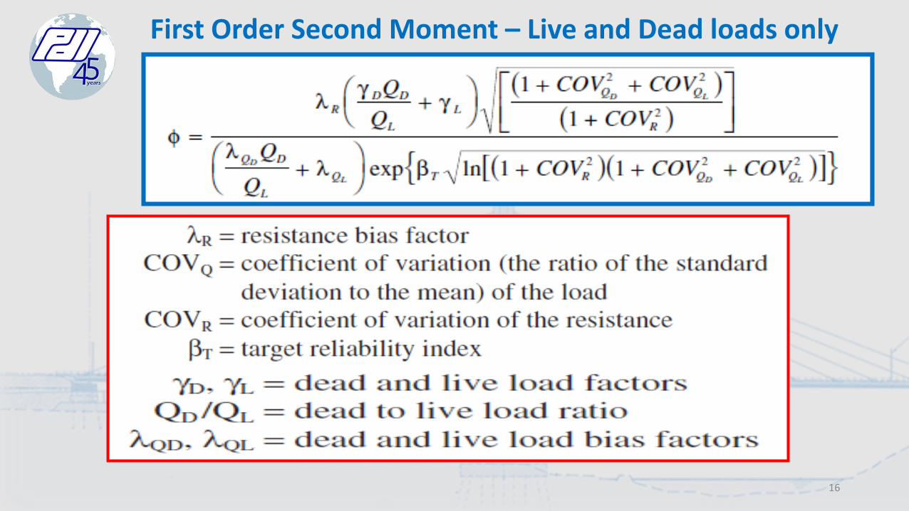
First Order Second Moment – Live and Dead loads only

16

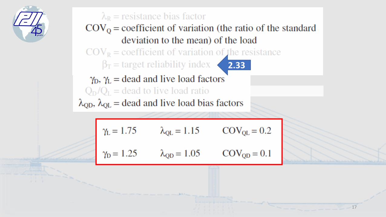
17

2.33

First Order Second Moment – Live and Dead loads only

Two factors from correlation of measured vs predicted.( measured / predicted )

18

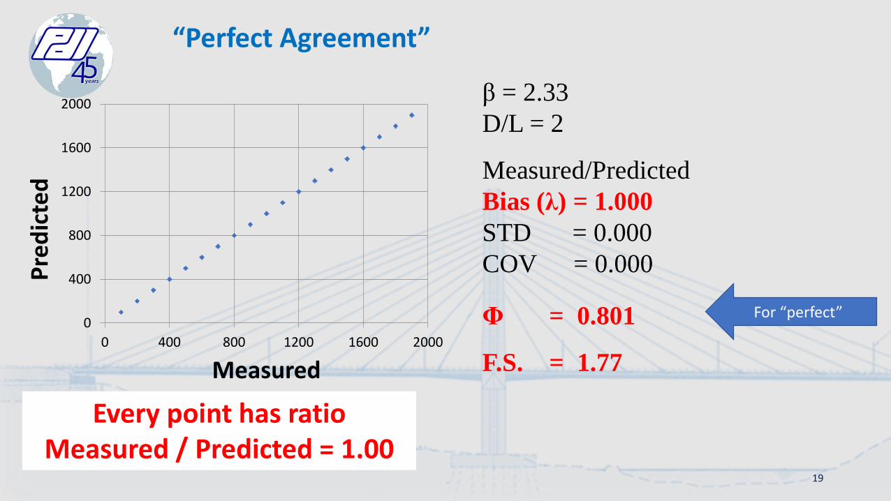
β = 2.33

D/L = 2

Measured/Predicted

Bias (λ) = 1.000

STD = 0.000

COV = 0.000

Φ = 0.801

F.S. = 1.77

0

400

800

1200

1600

2000

0 400 800 1200 1600 2000

Pre

dic

ted

Measured

“Perfect Agreement”

Every point has ratio Measured / Predicted = 1.00

19

For “perfect”

β = 2.33

D/L = 2

Measured/Predicted

Bias (λ) = 2.000

STD = 0.000

COV = 0.000

Φ = 1.602

F.S. = 0.88

F.S.*λ= 1.77

“Perfect Agreement”

20

Example: DL = 1000; LL = 500Total load = 1500Measured RU = 2656Predicted RU = 1328

Predicted RU is half real RU

YES

ASD: FS=1.77

Example (D/L = 2):Factored resistance ≥ factored load (Predicted RU *φ) ≥ (1.25D + 1.75L)

(1328*1.6) ≥ (1000*1.25 + 500*1.75)

2125 ≥ 2125

In application, Bias λ is already accounted for in

φ

YES

21

UnderpredictOverpredict

High

er C

OV

Low

er φ

Obviously, low COV is highly beneficial

22

0

10,000

20,000

30,000

40,000

0 10,000 20,000 30,000 40,000

CW

[k

N]

SLT [kN]

CW vs SLT combined (N=303)

CAPWAP – Combined: 1980, 1996, 2004

β = 2.33

D/L = 2

Measured/Predicted

Bias (λ) = 1.0278

STD= 0.170

COV= 0.165

Φ = 0.715

F.S. = 2.04

N = 303

23

▪ Monte Carlo Simulation (MCS)

• Monte Carlo Simulation is a more “rigorous” method for thecalculation of the resistance factors, in terms of providing anexact solution (to any degree of precision, given sufficientsimulation size/time)

• MCS method can be applied to random samples withdistributions that are neither normal nor lognormal or whenthe limit state equation is not linear.

Another statistics approach ….

▪ Monte Carlo Simulation (MCS) overview:

• Describe a performance function g(x) (e.g. g = R – Q)

• Compute g(x) for very large number of sets of randomlygenerated independent parameters (from mean λ andstandard deviation σ) and trial φ

• Number of events when g(x) is unsatisfactory divided bynumber of simulation sets is Probability of Failure p(f)

• Compare p(f) to a Target Probability of Failure P(f)

• Adjust φ and repeat until p(f) < P(f)

▪ Monte Carlo Simulation (MCS) results

Monte Carlo

Method

B=2.33 B=3.0

bias p(f)=1.0% p(f)=0.1% p(f)=0.01% p(f)=0

λ COV-R max φ max φ max φ φCAPWAP N=303

60,000 simulations 1.028 0.165 0.846 0.838 0.78 0.739

CAPWAP N=3031,000,000

simulations 1.028 0.165 0.851 0.845 0.744

27

Compare FOSM with Monte Carlo with AASHTO

AASHTO testing 2% φ = 0.65 2.18

testing 100% φ = 0.75 1.89testing 2% plus a SLT φ = 0.80 1.77

IBC F.S. = 2.00

Monte Carlo

Method

B=2.33

bias p(f)=1.0% p(f)=0

λ COV-R max φ φ

CAPWAP N=303 1.028 0.165 0.851 0.744

D/L=2 F.S. = 1.71 1.96

FOSM N λ COV φ F.S.

CAPWAP 303 1.028 0.165 0.715 2.04

from 2004 published correlation paper

Dynamic Pile Testing

For each blow determine

– Capacity at time of testing

DRIVEN PILESCurrent Situation:

Inefficient use of materials (design < 20% Fy)

Proof Tests to { 2x Design } F.S. = 2 “Tradition”

Conditions Favorable to Higher Capacities:

Soft Rock, Till

Hard Rock

Soil Setup

Allowable Compression Capacities (tons)

using IBC max allowable stresses (PPC Piles)

20th

Cent.

loads

Pile

size

f’c (psi) assume prestress 700 psi

Increase factor over

20th Century loads

Inch 5000 6000 7000 5000 6000 7000

90 14 143 176 208 1.59 1.95 2.31

Karl Higgins “Competitive Advantages of High Capacity, Prestressed Precast Concrete Piles”

PDCA DICEP conference, Sept. 2007

76 inch dia Drilled Shaft Vs. 14" PPC Pile (160 tons)

7660

$32.6714

50

$16.57

$350/ cu. Yds.

$35/lf

0

50

100

150

200

250

300

350

400

Diameter/Width Length (lf) Cost/unit Cost Per Ton

76-inch Shaft

PPC-14

Final

Design

by IBC

Savings:

50%Potomac

Yard

Pile Cap Costs

Included for

comparison driven

piles are

least cost

IBC safety factor is 2.0 for

either static or dynamic test

Most Sites Have “Set-up” (defined as capacity gain with time)

• Caused by reduced effective stresses

in soil during pile driving (temporary)

– Pore pressure effects - clay

– Arching (lateral motions) - sand

– Soil structure (e.g. chemical bonds)

– “Cookie cutters”

• Measure it by Dynamic Tests

on Both End of Drive and Restrike

152 bpf @

twice the

Energy

Aug 11, 1999

Sept 16

24 x 0.5 inch c.e.pipe, ICE 120S

St. John’s River Bridge – test program

25 bpf

ST Johns River BridgePDA test program $650,000

increased loads by 33%

with substantially shorter piles

(set-up considered)

Total project (6 bridges):

• $130 million (estimate)

• $110 million (actual)

• $20 million (savings)

Ref: Scales & Wolcott, FDOT, presentation at PDCA Roundtable Orlando 2004

Caution…

Sometimes the pile can

lose capacity with time…

Soils with relaxation potential• Weathered bedrock formations

➢ Weathered shale is most susceptible

➢ Rule of thumb: more weathered bedrock = more relaxation

➢ Seeping water effectively softens bedrock surface

➢ High normal force after driving plastically creeps away with time; reduces friction

➢ Rock fracturing from driving adjacent piles

• Saturated dense to v.dense sands & sandy silts➢ Due to negative pore water pressure during driving increases effective

stresses of end bearing➢ Pore water pressure equalizes after wait causing reduced soil strength

Dynamic Pile Monitoring

– Pile integrity

– Pile stresses

– Hammer performance

Last three items detect or prevent problems for driven piles

For each blow determine

– Capacity at time of testing

Consequences of no redundancy, site variability, and only

minimal testing, caused disastrous sudden failure.

TAMPA Tribune – Nov 23, 2004 – “Almost half of the foundations

supporting the new elevated portion of the Lee Roy Selmon

Expressway need major repairs, and the cost of fixing

them has grown to $78 million.”

(eventual total cost was $120 M)

April 2004

Large Projects• Pre-bid special test program optimizes design

• Pile length and size, pile type• Establish design load (ultimate capacity)• Evaluate set-up or relaxation

(multi-day restikes)• Early production pile tests (different hammer?)

• Establish driving criteria• Evaluate hammer and procedures• Confirm set-up or relaxation trends

• Periodic production pile tests• Monitors hammer consistency• Evaluate site variability

• Evaluate “problem piles”

Dynamic Testing – save $$, reduce risk

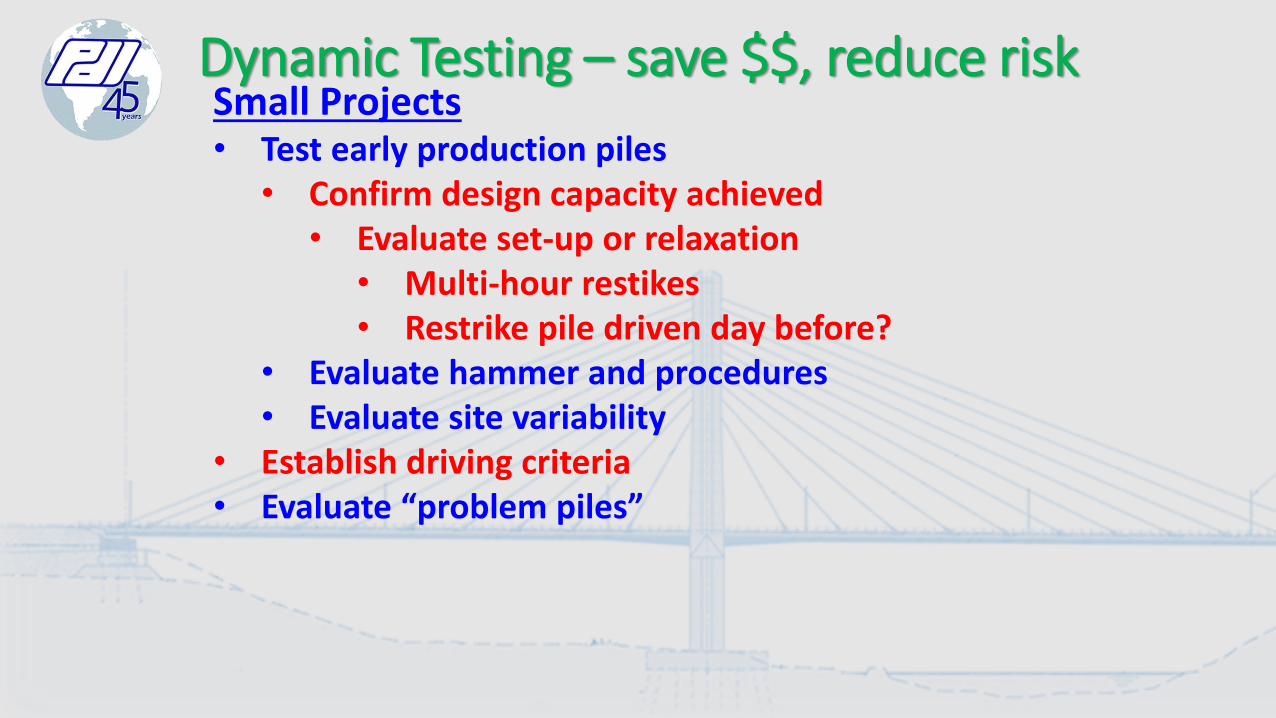
Small Projects• Test early production piles

• Confirm design capacity achieved• Evaluate set-up or relaxation

• Multi-hour restikes• Restrike pile driven day before?

• Evaluate hammer and procedures• Evaluate site variability

• Establish driving criteria• Evaluate “problem piles”

Dynamic Testing – save $$, reduce risk

Authors: Van Komurka, & Adam Theiss,

16 inch x 0.5 inch x 61 ft steel pipes -concrete filled. Costs include cap

soils - silty sands to silt with sand, some lean clay in upper layers

To be presented at IFCEE 2018, Orlando, March 2018

SAVINGS FROM TESTING THE DRIVEN-PILE FOUNDATION FOR A HIGH-RISE BUILDING

Construction Control Method (CCM)

Safety Factor

Design Load (kips) # piles Total Cost

Foundation Cost

Testing Cost

Cost Penalty

WE, DLT, SLT 2.0 600 456 2,513,762 2,277,502 236,260 0

WE & DLT 2.5 480 572 2,983,308 2,795,349 187,959 469,546

WE 3.0 400 684 3,307,287 3,305,287 2,000 793,525

formula 3.5 343 806 3,835,023 3,834,523 500 1,321,261

Above: Taking advantage of Set-up

Below: Ignoring Set-up

WE, DLT, SLT 2.0 400 684 3,477,927 3,305,287 172,640 964,165

WE & DLT 2.5 320 885 4,361,508 4,231,169 130,339 1,847,746

WE 3.0 267 1050 4,992,764 4,990,764 2,000 2,479,002

formula 3.5 229 1222 5,814,673 5,814,173 500 3,300,911

SAVINGS FROM TESTING THE DRIVEN-PILE FOUNDATION FOR A HIGH-RISE BUILDING

Construction Control Method (CCM)

Safety Factor

Design Load (kips)

# piles Total CostCost

PenaltyConstruction

days

Time Penalty (days)

WE, DLT, SLT 2.0 600 456 2,513,762 0 85 0WE & DLT 2.5 480 572 2,983,308 469,546 107 22

WE 3.0 400 684 3,307,287 793,525 127 42formula 3.5 343 806 3,835,023 1,321,261 150 65

Above: Taking advantage of Set-up

Below: Ignoring Set-upWE, DLT, SLT 2.0 400 684 3,477,927 964,165 127 42

WE & DLT 2.5 320 885 4,361,508 1,847,746 165 80WE 3.0 267 1050 4,992,764 2,479,002 196 111

formula 3.5 229 1222 5,814,673 3,300,911 228 143

SAVINGS FROM TESTING THE DRIVEN-PILE FOUNDATION FOR A HIGH-RISE BUILDING

PDCA project of the year award (marine greater than $5 million)Ref: PDCA PILEDRIVER Issue 4, 2017

South Carolina Ports Authority Wando Terminal ImprovementsBy Cape Romain Contractors

“In-situ dynamic testing carried an initial cost of $275,000, only 0.4 percent of the overall program budget. Ultimately, spending this 0.4 percent initially ended up saving SCPA 15 percent in construction costs.”

Year Driven Pile Cost Testing Cost

2005 $10,705,041 $305,921

2006 $18,836,927 $313,315

2007 $15,948,151 $379,750

2008 $26,591,945 $587,882

2009 $25,308,605 $450,863

2010 $26,211,622 $518,557

Total $123,602,290 $2,556,288

$2.5M / $123.6 M = 2%

Test / driven pile cost

Peter Narsavage

Ohio Dept of Transportation

2011 PDCA seminar, Orlando

Method AASHTO PHI(LRFD)

Relative cost of piles Savings

Formula (Gates) 0.40 1.00 0%

Wave Equation 0.50 0.80 20%

2% PDA 0.65 0.62 38%

2 # PDA Ohio DOT 0.70 0.57 43%100%PDA or SLT 0.75 0.53 47%

PDA + SLT 0.80 0.50 50%

Savings $92,700,000

Advantages of Dynamic Testing• More information faster and at lower cost

• Supplement or replace static tests• Optimize foundation design• Capacity & distribution from CAPWAP• 40 years experience; large database

• Detect bad hammers• Know driving stresses (compression-tension)

• Develop better installation procedures• Detect pile damage• Lowers risk of foundation failures

• Lower overall foundation costs

•Main cost is the foundation and its installation,

not the testing cost. The benefit to cost ratio for

dynamic testing is very favorable for the

contractor, engineer, and the owner.

•Testing needed to get most benefit (low F.S. or high PHI),

Significant set-up allows significant savings

•Dynamic Testing is highly beneficial (lowers total costs),

particularly to design build or value engineering.

Lowest project cost results from more testing

•Need to guard against relaxation in some soils

fortunately fairly rare and soils generally known.

• Lack of adequate testing can cause failures, and the

remediation can be very expensive.

Testing reduces risk

Conclusions www.pile.com

Unknowns = Risk = Liability

Actual testing removes unknowns and therefore reduces risks and liability

State-of-Practice includes testing

“One test result is worth a thousand expert opinions”

Werner Von Braun

Father of the Saturn V rocket

Measurements are better than Guesses