Asemi-supervisedMachineLearningsearchfornever-seen

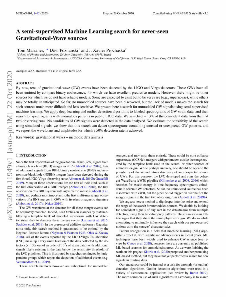
MNRAS 000, 1–12 (2020) Preprint 26 October 2020 Compiled using MNRAS LATEX style file v3.0

A semi-supervised Machine Learning search for never-seenGravitational-Wave sources

Tom Marianer,1★ Dovi Poznanski1 and J. Xavier Prochaska21School of Physics and Astronomy, Tel-Aviv University, Tel-Aviv 69978, Israel2Department of Astronomy & Astrophysics, UCO/Lick Observatory, University of California, 1156 High Street, Santa Cruz, CA 95064, USA

Accepted XXX. Received YYY; in original form ZZZ

ABSTRACTBy now, tens of gravitational-wave (GW) events have been detected by the LIGO and Virgo detectors. These GWs have allbeen emitted by compact binary coalescence, for which we have excellent predictive models. However, there might be othersources for which we do not have reliable models. Some are expected to exist but to be very rare (e.g., supernovae), while othersmay be totally unanticipated. So far, no unmodeled sources have been discovered, but the lack of models makes the search forsuch sources much more difficult and less sensitive. We present here a search for unmodeled GW signals using semi-supervisedmachine learning. We apply deep learning and outlier detection algorithms to labeled spectrograms of GW strain data, and thensearch for spectrograms with anomalous patterns in public LIGO data. We searched ∼ 13% of the coincident data from the firsttwo observing runs. No candidates of GW signals were detected in the data analyzed. We evaluate the sensitivity of the searchusing simulated signals, we show that this search can detect spectrograms containing unusual or unexpected GW patterns, andwe report the waveforms and amplitudes for which a 50% detection rate is achieved.

Key words: gravitational waves – methods: data analysis

1 INTRODUCTION

Since the first observation of the gravitational wave (GW) signal froma binary black hole (BBH) merger in 2015 (Abbott et al. 2016), tensof additional signals from BBH, binary neutron star (BNS) and neu-tron star-black hole (NSBH) mergers have been detected during thefirst three LIGO-Virgo observing runs (Abbott et al. 2019b; GraceDB2019). Many of these observations are the first of their kind, such asthe first observation of a BBH merger (Abbott et al. 2016), the firstobservation of a BBH system with asymmetric masses (Abbott et al.2020), and perhapsmost importantly, the firstmulti-messenger obser-vations of a BNS merger in GWs with its electromagnetic signature(Abbott et al. 2017b; Nakar 2019).The GW waveform at the detector for all these merger events can

be accurately modeled. Indeed, LIGO relies on searches by matched-filtering a template bank of modeled waveforms with GW detec-tor strain data to discover these merger events (Usman et al. 2016;Sachdev et al. 2019). In the presence of additive stationary Gaussiannoise only, this search method is guaranteed to be optimal by theNeyman-Pearson lemma (Neyman & Pearson 1933; Ofek & Zackay2018). All of the events reported by the LIGO-Virgo Collaboration(LVC) make up a very small fraction of the data collected by the de-tectors (< 100s out of an order of 107s of strain data), with additionalsignals likely existing in the data below the sensitivity threshold ofthe LVC pipelines. This is illustrated by searches conducted by inde-pendent groups which report the detection of additional events (e.g.Venumadhav et al. 2019).These search methods however are suboptimal for unmodeled

★ E-mail: [email protected]

sources, and may miss them entirely. These could be core collapsesupernovae (CCSNe), mergers with parameters ouside the range cov-ered by the template bank used in the search, or other sources ofunknown origin. While perhaps unlikely, one should be open to thepossibility of the serendipitous discovery of an unexpected sourceof GWs. For this purpose, the LVC developed and runs the coher-ent WaveBurst (cWB) pipeline (Klimenko et al. 2008, 2016) whichsearches for excess energy in time-frequency spectrograms coinci-dent in several GW detectors. So far, no unmodeled source has beendiscovered with cWB, but the pipeline did trigger on over half of themerger signals in the first two observing runs (Abbott et al. 2019b).We suggest here a method to dig deeper into the noise and extend

the range of the search for unmodeled sources. We do this by lookingfor coincident signals of any sort in the datastreams from multipledetectors, using their time-freqency patterns. These can serve as tell-tale signs that they share the same physical origin. We do so whileattempting to minimally influence the search with our preconceivednotions as to the sources’ characteristics.Pattern recognition is a field that machine learning (ML) algo-

rithms excel at, with significant advancements in recent years. MLtechniques have been widely used to enhance GW science (see re-view by Cuoco et al. 2020), however there are currently no publishedML-based searches for unmodeled sources. As we were finishing thework on this project, Skliris et al. (2020) proposed another promisingML-based method, but they have not yet performed a search for newsignals in existing data.Our endeavour could be framed as a task for anomaly (or outlier)

detection algorithms. Outlier detection algorithms were used in avariety of astronomical applications (see review by Baron 2019).The more common use of such algorithms in astronomy is to search

© 2020 The Authors

arX

iv:2

010.

1194

9v1

[as

tro-

ph.I

M]

22

Oct

202

0

2 T. Marianer et al.

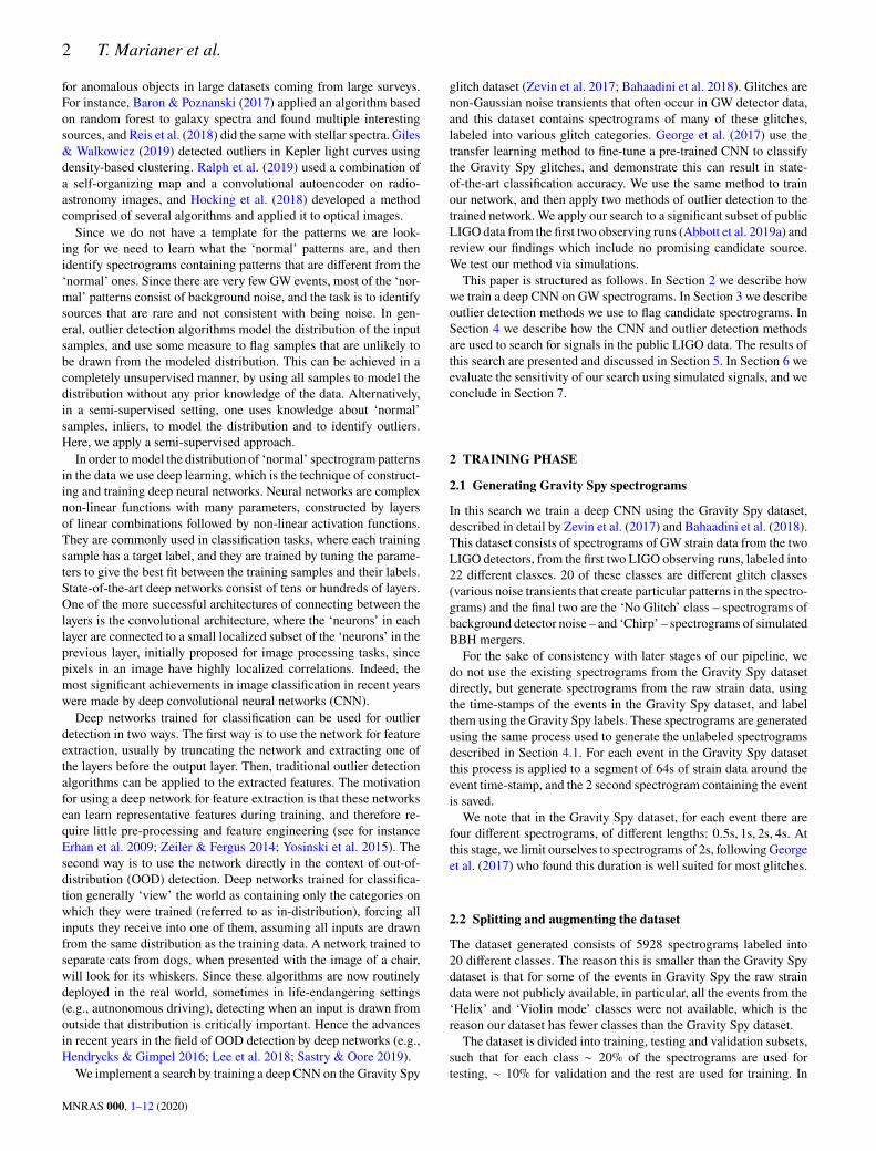
for anomalous objects in large datasets coming from large surveys.For instance, Baron & Poznanski (2017) applied an algorithm basedon random forest to galaxy spectra and found multiple interestingsources, and Reis et al. (2018) did the same with stellar spectra. Giles& Walkowicz (2019) detected outliers in Kepler light curves usingdensity-based clustering. Ralph et al. (2019) used a combination ofa self-organizing map and a convolutional autoencoder on radio-astronomy images, and Hocking et al. (2018) developed a methodcomprised of several algorithms and applied it to optical images.Since we do not have a template for the patterns we are look-

ing for we need to learn what the ‘normal’ patterns are, and thenidentify spectrograms containing patterns that are different from the‘normal’ ones. Since there are very few GW events, most of the ‘nor-mal’ patterns consist of background noise, and the task is to identifysources that are rare and not consistent with being noise. In gen-eral, outlier detection algorithms model the distribution of the inputsamples, and use some measure to flag samples that are unlikely tobe drawn from the modeled distribution. This can be achieved in acompletely unsupervised manner, by using all samples to model thedistribution without any prior knowledge of the data. Alternatively,in a semi-supervised setting, one uses knowledge about ‘normal’samples, inliers, to model the distribution and to identify outliers.Here, we apply a semi-supervised approach.In order tomodel the distribution of ‘normal’ spectrogram patterns

in the data we use deep learning, which is the technique of construct-ing and training deep neural networks. Neural networks are complexnon-linear functions with many parameters, constructed by layersof linear combinations followed by non-linear activation functions.They are commonly used in classification tasks, where each trainingsample has a target label, and they are trained by tuning the parame-ters to give the best fit between the training samples and their labels.State-of-the-art deep networks consist of tens or hundreds of layers.One of the more successful architectures of connecting between thelayers is the convolutional architecture, where the ‘neurons’ in eachlayer are connected to a small localized subset of the ‘neurons’ in theprevious layer, initially proposed for image processing tasks, sincepixels in an image have highly localized correlations. Indeed, themost significant achievements in image classification in recent yearswere made by deep convolutional neural networks (CNN).Deep networks trained for classification can be used for outlier

detection in two ways. The first way is to use the network for featureextraction, usually by truncating the network and extracting one ofthe layers before the output layer. Then, traditional outlier detectionalgorithms can be applied to the extracted features. The motivationfor using a deep network for feature extraction is that these networkscan learn representative features during training, and therefore re-quire little pre-processing and feature engineering (see for instanceErhan et al. 2009; Zeiler & Fergus 2014; Yosinski et al. 2015). Thesecond way is to use the network directly in the context of out-of-distribution (OOD) detection. Deep networks trained for classifica-tion generally ‘view’ the world as containing only the categories onwhich they were trained (referred to as in-distribution), forcing allinputs they receive into one of them, assuming all inputs are drawnfrom the same distribution as the training data. A network trained toseparate cats from dogs, when presented with the image of a chair,will look for its whiskers. Since these algorithms are now routinelydeployed in the real world, sometimes in life-endangering settings(e.g., autnonomous driving), detecting when an input is drawn fromoutside that distribution is critically important. Hence the advancesin recent years in the field of OOD detection by deep networks (e.g.,Hendrycks & Gimpel 2016; Lee et al. 2018; Sastry & Oore 2019).We implement a search by training a deep CNN on the Gravity Spy

glitch dataset (Zevin et al. 2017; Bahaadini et al. 2018). Glitches arenon-Gaussian noise transients that often occur in GW detector data,and this dataset contains spectrograms of many of these glitches,labeled into various glitch categories. George et al. (2017) use thetransfer learning method to fine-tune a pre-trained CNN to classifythe Gravity Spy glitches, and demonstrate this can result in state-of-the-art classification accuracy. We use the same method to trainour network, and then apply two methods of outlier detection to thetrained network. We apply our search to a significant subset of publicLIGO data from the first two observing runs (Abbott et al. 2019a) andreview our findings which include no promising candidate source.We test our method via simulations.This paper is structured as follows. In Section 2 we describe how

we train a deep CNN on GW spectrograms. In Section 3 we describeoutlier detection methods we use to flag candidate spectrograms. InSection 4 we describe how the CNN and outlier detection methodsare used to search for signals in the public LIGO data. The results ofthis search are presented and discussed in Section 5. In Section 6 weevaluate the sensitivity of our search using simulated signals, and weconclude in Section 7.

2 TRAINING PHASE

2.1 Generating Gravity Spy spectrograms

In this search we train a deep CNN using the Gravity Spy dataset,described in detail by Zevin et al. (2017) and Bahaadini et al. (2018).This dataset consists of spectrograms of GW strain data from the twoLIGO detectors, from the first two LIGO observing runs, labeled into22 different classes. 20 of these classes are different glitch classes(various noise transients that create particular patterns in the spectro-grams) and the final two are the ‘No Glitch’ class – spectrograms ofbackground detector noise – and ‘Chirp’ – spectrograms of simulatedBBH mergers.For the sake of consistency with later stages of our pipeline, we

do not use the existing spectrograms from the Gravity Spy datasetdirectly, but generate spectrograms from the raw strain data, usingthe time-stamps of the events in the Gravity Spy dataset, and labelthem using the Gravity Spy labels. These spectrograms are generatedusing the same process used to generate the unlabeled spectrogramsdescribed in Section 4.1. For each event in the Gravity Spy datasetthis process is applied to a segment of 64s of strain data around theevent time-stamp, and the 2 second spectrogram containing the eventis saved.We note that in the Gravity Spy dataset, for each event there are

four different spectrograms, of different lengths: 0.5s, 1s, 2s, 4s. Atthis stage, we limit ourselves to spectrograms of 2s, following Georgeet al. (2017) who found this duration is well suited for most glitches.

2.2 Splitting and augmenting the dataset

The dataset generated consists of 5928 spectrograms labeled into20 different classes. The reason this is smaller than the Gravity Spydataset is that for some of the events in Gravity Spy the raw straindata were not publicly available, in particular, all the events from the‘Helix’ and ‘Violin mode’ classes were not available, which is thereason our dataset has fewer classes than the Gravity Spy dataset.The dataset is divided into training, testing and validation subsets,

such that for each class ∼ 20% of the spectrograms are used fortesting, ∼ 10% for validation and the rest are used for training. In

MNRAS 000, 1–12 (2020)

ML search for never-seen GW sources 3

total this results in training, test and validation sets consisting of4249, 1197 and 482 spectrograms, respectively.When training the network we use data augmentation to increase

the size of the training set. The spectrogram images are randomlyshifted by up to 50% of the image size in the horizontal (time) di-rection (149 pixels, which are 1s). Aside from increasing the sizeof the training set, which is necessary for training a deep network,the horizontal shift may be useful in training the network to identifyspectrograms of signals which are not centered in the spectrogram(since we do not know in advance the timing of an event relativeto the center of the spectrogram it appears in). To reduce class im-balance, for classes with more than 1000 spectrograms, we augmenteach spectrogram once (one spectrogram with the random shifts de-scribed above is created), for classes with between 200 and 1000spectrograms we augment each spectrogram 4 times, and for classeswith fewer than 200 spectrograms we augment each spectrogram10 times. In total the augmented training set, including the originaltraining set, consists of 24641 spectrograms.

2.3 Training the network

We train our CNNusing the transfer learningmethod, used byGeorgeet al. (2017). We take a CNN that was pre-trained on ImageNet – alarge dataset of over 1 million images in 1000 different classes – andfine-tune its weights by re-training it on the dataset described above.The pre-trained network we use is ResNet152V2 proposed by Heet al. (2016a). This network is a refined version of the original resid-ual network presented in He et al. (2016b), known as ResNet, whichbecame one of the most popular architectures in the field of imageprocessing using neural networks since it won the ILSVRC imageclassification competition in 2015. The advantage of residual archi-tectures is that they allow training very deep networks by addressingthe vanishing gradient problem. The problem is that when using back-propagation to compute gradients in deep networks, the gradients ofthe initial layers become very small, effectively preventing training(see for instance (Glorot & Bengio 2010)). The ResNet architecturedeals with this problem by using ‘shortcut connections’, which areconnections that skip one or more layers. The basic building block ofthe ResNet architecture is a block of two or three convolution layerswith ReLU activations and a ‘shortcut connection’ connecting theinput of the block to its output, before the output activation (skippingthe convolution layers). The refinement presented in He et al. (2016a)is to use ‘pre-activation’ instead of ‘post-activation’, meaning addinga ReLU activation layer at the input of the block and removing theone at its output. ResNet152V2 contains 50 such blocks containing3 convolution layers each, plus an additional convolution layer at thenetwork’s input, and a fully connected layer of 1000 neurons withsoftmax activation at its output, totalling in 152 trainable layers.We adapt ResNet152V2 for our task by removing the output layer

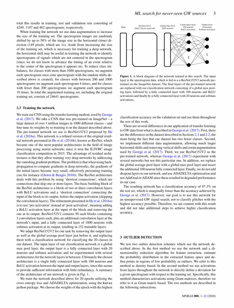
as well as the global average pool layer just before it, and replacingthem with a classification network for classifying the 20 classes inour dataset. The input layer of our classification network is a globalmax pool layer, the output layer is a fully connected layer with 20neurons and softmax activation, and we experimented with severalarchitectures for the network layers in between. Ultimately the chosenarchitecture is a single fully connected layer with 100 neurons andReLU activation between the input and output layers, since this seemsto provide sufficient information with little redundancy. A summaryof the architecture of our network is given in Fig. 1.We train the network described above for 20 epochs utilizing the

cross entropy loss and ADADELTA optimization, using the keraspython package. We choose the weights of the epoch with the highest

Input ResNet152V2(final2layersremoved)

GlobalMaxPool2048neurons

Latentspacelayer100neurons

ReLUactivation

Outputlayer20neurons

Softmaxactivation

Figure 1. A block diagram of the network trained in this search. The inputlayer is the spectrogram data, which is fed to a a ResNet152V2 network pre-trained on the ImageNet dataset. The final layers of the pre-trained networkare replaced with our classification network consisting of a global max pool-ing layer, followed by a fully connected layer with 100 neurons and ReLUactivations and finally by a fully connected layer with 20 neurons and softmaxactivations.

classification accuracy on the validation set and use them throughoutthe rest of this work.There are several differences in our application of transfer learning

to GWdata fromwhat is described in George et al. (2017). First, thereare the differences in the dataset described in Sections 2.1 and 2.2, themain being the fact that our dataset has two fewer classes. Second,we implement different data augmentation, allowing much largerhorizontal shifts and removing vertical shifts and zoom augmentationused by George et al. (2017). Third, we use ResNet152V2 as thepre-trained network, whereas George et al. (2017) experiment withseveral networks but not this particular one. In addition, we replacethe global average pool layer with a global max pool layer and insertthe additional 100 neuron fully connected layer. Finally,we do not adddropout layers to our network, and useADADELTAoptimization andnot AdaGrad or ADAM since these resulted in degraded performancein our case.The resulting network has a classification accuracy of 97.3% on

the test set, which is marginally lower than the accuracy achieved byGeorge et al. (2017). However, our goal is to use this network foran unsupervised GW signal search, not to classify glitches with thehighest accuracy possible. Therefore, we are content with this resultand did not take additional steps to achieve higher classificationaccuracy.

3 OUTLIER DETECTION

We test two outlier detection schemes which use the network de-scribed above. In the first method we use the network and a di-mensionality reduction algorithm for feature extraction, estimatethe probability distribution in the extracted feature space and de-fine points in regions of low probability as outliers. We refer to thismethod as density based. In the second method we use activationsfrom layers throughout the network to directly define a deviation fora given spectrogram with respect to the training set. Specifically, thismethod characterizes activations using Gram matrices, therefore werefer to it as Gram matrix based. The two methods are described inthe following subsections.

MNRAS 000, 1–12 (2020)


3.1 Density based method

Each spectrogram in our dataset is fed through the network, andthe latent layer just before the output layer is extracted as a featurerepresentation for the spectrogram in the 100D latent space. Next,we perform dimensionality reduction using the UMAP algorithm(McInnes et al. 2018), which can compute a mapping between the100D latent space and a lower dimensional space. We compute sucha mapping to a 2D space (which we refer to as the map space) bytraining the UMAP algorithm on the latent features of the trainingexamples in our dataset. The key in this step is to reduce the dimen-sionality of the data, to something manageable by a human, whilepreserving as much as possible the structure of the manifold in whichthe data reside.There are many existing dimensionality reduction algorithms that

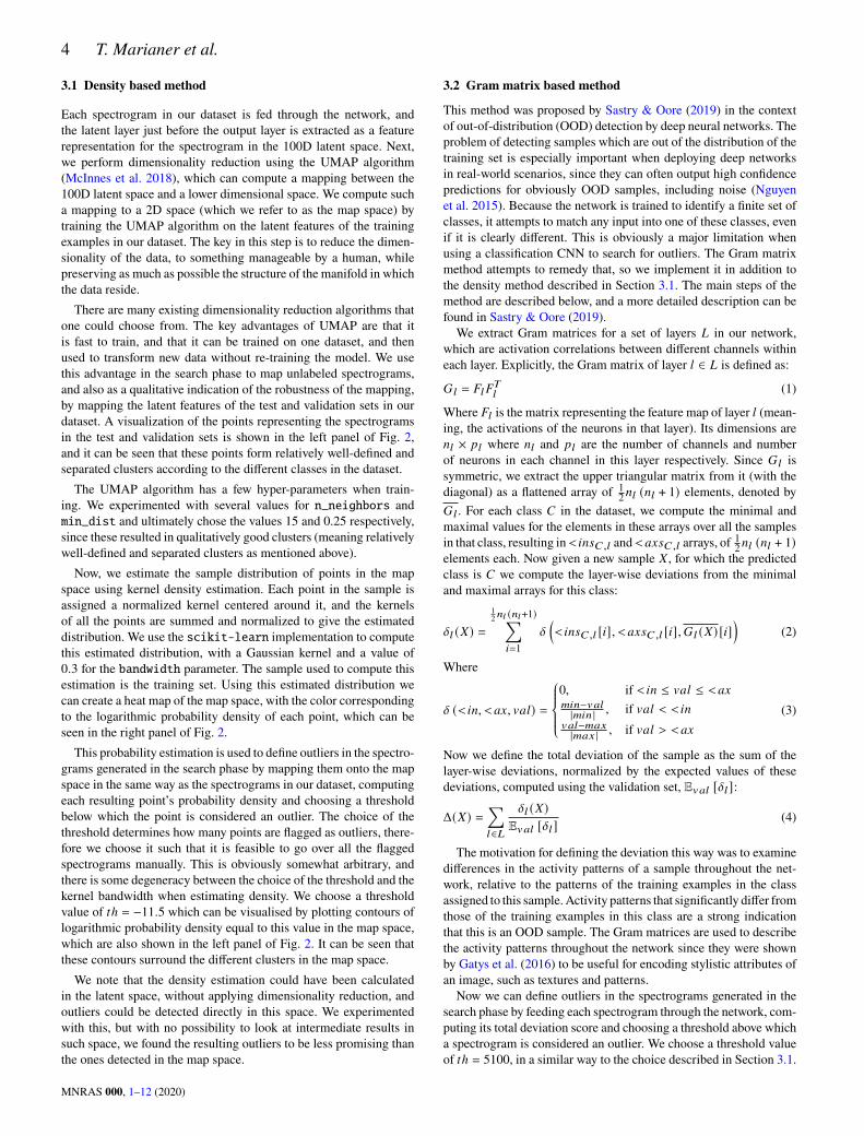
one could choose from. The key advantages of UMAP are that itis fast to train, and that it can be trained on one dataset, and thenused to transform new data without re-training the model. We usethis advantage in the search phase to map unlabeled spectrograms,and also as a qualitative indication of the robustness of the mapping,by mapping the latent features of the test and validation sets in ourdataset. A visualization of the points representing the spectrogramsin the test and validation sets is shown in the left panel of Fig. 2,and it can be seen that these points form relatively well-defined andseparated clusters according to the different classes in the dataset.The UMAP algorithm has a few hyper-parameters when train-

ing. We experimented with several values for n_neighbors andmin_dist and ultimately chose the values 15 and 0.25 respectively,since these resulted in qualitatively good clusters (meaning relativelywell-defined and separated clusters as mentioned above).Now, we estimate the sample distribution of points in the map

space using kernel density estimation. Each point in the sample isassigned a normalized kernel centered around it, and the kernelsof all the points are summed and normalized to give the estimateddistribution. We use the scikit-learn implementation to computethis estimated distribution, with a Gaussian kernel and a value of0.3 for the bandwidth parameter. The sample used to compute thisestimation is the training set. Using this estimated distribution wecan create a heat map of the map space, with the color correspondingto the logarithmic probability density of each point, which can beseen in the right panel of Fig. 2.This probability estimation is used to define outliers in the spectro-

grams generated in the search phase by mapping them onto the mapspace in the same way as the spectrograms in our dataset, computingeach resulting point’s probability density and choosing a thresholdbelow which the point is considered an outlier. The choice of thethreshold determines how many points are flagged as outliers, there-fore we choose it such that it is feasible to go over all the flaggedspectrograms manually. This is obviously somewhat arbitrary, andthere is some degeneracy between the choice of the threshold and thekernel bandwidth when estimating density. We choose a thresholdvalue of 𝑡ℎ = −11.5 which can be visualised by plotting contours oflogarithmic probability density equal to this value in the map space,which are also shown in the left panel of Fig. 2. It can be seen thatthese contours surround the different clusters in the map space.We note that the density estimation could have been calculated

in the latent space, without applying dimensionality reduction, andoutliers could be detected directly in this space. We experimentedwith this, but with no possibility to look at intermediate results insuch space, we found the resulting outliers to be less promising thanthe ones detected in the map space.

3.2 Gram matrix based method

This method was proposed by Sastry & Oore (2019) in the contextof out-of-distribution (OOD) detection by deep neural networks. Theproblem of detecting samples which are out of the distribution of thetraining set is especially important when deploying deep networksin real-world scenarios, since they can often output high confidencepredictions for obviously OOD samples, including noise (Nguyenet al. 2015). Because the network is trained to identify a finite set ofclasses, it attempts to match any input into one of these classes, evenif it is clearly different. This is obviously a major limitation whenusing a classification CNN to search for outliers. The Gram matrixmethod attempts to remedy that, so we implement it in addition tothe density method described in Section 3.1. The main steps of themethod are described below, and a more detailed description can befound in Sastry & Oore (2019).We extract Gram matrices for a set of layers 𝐿 in our network,

which are activation correlations between different channels withineach layer. Explicitly, the Gram matrix of layer 𝑙 ∈ 𝐿 is defined as:

𝐺𝑙 = 𝐹𝑙𝐹𝑇𝑙

(1)

Where 𝐹𝑙 is the matrix representing the feature map of layer 𝑙 (mean-ing, the activations of the neurons in that layer). Its dimensions are𝑛𝑙 × 𝑝𝑙 where 𝑛𝑙 and 𝑝𝑙 are the number of channels and numberof neurons in each channel in this layer respectively. Since 𝐺𝑙 issymmetric, we extract the upper triangular matrix from it (with thediagonal) as a flattened array of 12𝑛𝑙 (𝑛𝑙 + 1) elements, denoted by𝐺𝑙 . For each class 𝐶 in the dataset, we compute the minimal andmaximal values for the elements in these arrays over all the samplesin that class, resulting in𝑚𝑖𝑛𝑠𝐶,𝑙 and𝑚𝑎𝑥𝑠𝐶,𝑙 arrays, of 12𝑛𝑙 (𝑛𝑙 + 1)elements each. Now given a new sample 𝑋 , for which the predictedclass is 𝐶 we compute the layer-wise deviations from the minimaland maximal arrays for this class:

𝛿𝑙 (𝑋) =12 𝑛𝑙 (𝑛𝑙+1)∑︁

𝑖=1𝛿

(𝑚𝑖𝑛𝑠𝐶,𝑙 [𝑖], 𝑚𝑎𝑥𝑠𝐶,𝑙 [𝑖], 𝐺𝑙 (𝑋) [𝑖]

)(2)

Where

𝛿 (𝑚𝑖𝑛, 𝑚𝑎𝑥, 𝑣𝑎𝑙) =

0, if 𝑚𝑖𝑛 ≤ 𝑣𝑎𝑙 ≤ 𝑚𝑎𝑥𝑚𝑖𝑛−𝑣𝑎𝑙|𝑚𝑖𝑛 | , if 𝑣𝑎𝑙 < 𝑚𝑖𝑛

𝑣𝑎𝑙−𝑚𝑎𝑥|𝑚𝑎𝑥 | , if 𝑣𝑎𝑙 > 𝑚𝑎𝑥

(3)

Now we define the total deviation of the sample as the sum of thelayer-wise deviations, normalized by the expected values of thesedeviations, computed using the validation set, E𝑣𝑎𝑙 [𝛿𝑙]:

Δ(𝑋) =∑︁𝑙∈𝐿

𝛿𝑙 (𝑋)E𝑣𝑎𝑙 [𝛿𝑙]

(4)

The motivation for defining the deviation this way was to examinedifferences in the activity patterns of a sample throughout the net-work, relative to the patterns of the training examples in the classassigned to this sample.Activity patterns that significantly differ fromthose of the training examples in this class are a strong indicationthat this is an OOD sample. The Gram matrices are used to describethe activity patterns throughout the network since they were shownby Gatys et al. (2016) to be useful for encoding stylistic attributes ofan image, such as textures and patterns.Now we can define outliers in the spectrograms generated in the

search phase by feeding each spectrogram through the network, com-puting its total deviation score and choosing a threshold above whicha spectrogram is considered an outlier. We choose a threshold valueof 𝑡ℎ = 5100, in a similar way to the choice described in Section 3.1.

MNRAS 000, 1–12 (2020)


1080Lines1400RipplesAir_CompressorBlipChirpExtremely_LoudKoi_FishLight_ModulationLow_Frequency_BurstLow_Frequency_LinesNo_GlitchNone_of_the_AbovePaired_DovesPower_LineRepeating_BlipsScattered_LightScratchyTomteWandering_LineWhistle

11

10

9

8

7

6

5

loga

rithm

ic pr

obab

ility

dens

ity

Figure 2. Plots illustrating the map space which is the result of training the UMAP algorithm on the latent space features of the training set. The axes of theseplots are the two abstract dimensions of the map space. The left panel is a plot of the map space representation of the spectrograms in the test and validationsets. Each point represents a spectrogram from the dataset, and their shapes and colors are determined according to the corresponding label. It can be seen thatvarious classes cluster quite well. The contours are contours of logarithmic probability density equal to 𝑡ℎ = −11.5 in this space. The right panel is a heat mapof the estimated distribution of points in the map space. The color corresponds to the logarithmic probability density.

We note a few differences between our implementation of thismethod and the original proposed by Sastry & Oore (2019). First,Sastry & Oore (2019) compute the Gram matrices and the layer-wise deviations for all the layers in their network. We compute thesematrices and deviations for a subset of layers 𝐿. The layers we useare the output layers of the odd numbered residual blocks, 26 layersin total (not 25 because the layer numbering is not continuous).Second, Sastry & Oore (2019) define higher-order Gram matrices,while we only use the first order matrix defined above. The reasonfor both differences is reduction in the time required to process eachspectrogram, since the network we use is larger than the one usedin Sastry & Oore (2019) (they used ResNet34, which consists of 34layers).Due to the importance of OOD detection, there are quite a few

more methods being proposed in the literature. The advantages ofthe one we chose to implement here are that it can be used withpre-trained networks, i.e., we can use the same network we trainedin Section 2.3. Furthermore, it only has a few hyperparameters andcan work without the need for fine-tuning using OOD examples,something we prefer not to bias ourselves with. In addition, thismethod is reported by Sastry & Oore (2019) to have a performancecomparable to the state-of-the-art.

4 SEARCH PHASE

4.1 Generating spectrograms

We generate unlabeled spectrograms from bulk strain data using aprocess similar to the one described by Robinet (2016). First, thedata are divided into segments for which data are continuously avail-able (data are not publicly available for the entire duration of theobserving runs), then we divide each segment into chunks of length𝑇𝑐 = 64s. Each chunk is conditioned by subtracting its mean, apply-ing a high-pass filter with a cut-off frequency of 20Hz, and finally itis multiplied by a Tukey window (using the SciPy implementation)which insures a smooth transition to 0 at both chunk ends, in order

to avoid edge artifacts when generating the time-frequency spectro-grams. In order to avoid data loss because of the windowing, there isan overlap of𝑇𝑜 = 2s between consecutive chunks, which determinesthe parameter of the window to be 𝛼 = 𝑇𝑜/𝑇𝑐 = 2/64.After conditioning, the data in each chunk are whitened: The noise

power spectral density during the chunk is estimated and then a filteris applied to the chunk which yields a white (meaning constant) noisespectral density for the filtered data.Next, the multi-Q transform, which is a modification of the

constant-Q transform is applied to the whitened data. The constant-Qtransform is a time-frequency transform similar to the standard short-time Fourier transform, which computes a time-dependant frequencyrepresentation of the data by computing windowed Fourier trans-forms with window lengths determining the frequency resolution,and the overlap between windows determining the time resolution.In the constant-Q transform the frequency axis is logarithmicallyspaced, and instead of using a constant window for all frequencies,the window length is inversely proportional to the frequency whichresults in a constant 𝑄 value, which is the ratio of the frequency ofeach bin to its bandwidth. The multi-Q transform applies multipleconstant-Q transforms for a range of 𝑄 values and then chooses theone which has highest peak energy. More detailed descriptions ofthese transforms and the way they are used for GW searches can befound in Blankertz (2001), Chatterji et al. (2004) and Robinet (2016).The multi-Q transform is computed using the GWpy methodq_transform, which also implements the data whitening. The func-tion parameters we use in this work are the same as the ones that wereused to generate the Gravity Spy dataset, except for the gps param-eter. This parameter, when passed to the method, determines thetime-stamp to focus on for choosing the 𝑄 value with highest peakenergy, and when the Gravity Spy spectrograms were generated thisparameter was equal to the event time-stamp each spectrogram rep-resents. We do not use this parameter, therefore the entire chunk isused for choosing the 𝑄 value.Finally, the resulting multi-Q transform is cropped by 𝑇𝑜/2 = 1s

at each end to get rid of data affected by the windowing, and the

MNRAS 000, 1–12 (2020)


remaining 62s are divided into 31 non-overlapping spectrograms of2s each.The fact that our spectrograms do not overlap suggests we might

miss signals that occur during the transition from one spectrogramto the next. One can overcome this issue by adding overlap betweenspectrograms, at a small computational cost. In this work we chosenot to add this overlap, as the probability of missing signals is rel-atively small. The reason for this is that short signals have a smallprobability of occurring precisely during the transition between spec-trograms, and we expect longer signals to create a significant patternin at least one of the spectrograms even if they are truncated, suchthat they may still be detected as outliers by our search.

4.2 Flagging spectrograms of interest

Weprocess the spectrograms using the network trained in Section 2.3,and flag outliers using the two methods described in Section 3.In addition to outlier detection, we also utilize the network predic-

tions, and flag spectrograms that are classified as ‘Chirp’ (the classof binary mergers). We also note that the ‘None of the Above’ class ismeant to be a ‘catch-all’ class in the Gravity Spy dataset, containingall the glitches in the dataset that do not resemble any of the otherclasses. However, it would be false to assume that all outliers shouldbe classified by the network as ‘None of the Above’. Rather, it willclassify as ‘None of the Above’ spectrograms which resemble the ex-amples it was trained on, and there is no way of knowing in advancethe prediction of an outlier with a spectrogram that is sufficiently dif-ferent than all the spectrograms in the dataset (including the ‘Noneof the Above’ examples). Indeed, when examining the spectrogramsclassified as ‘None of the Above’ we found them less interesting thanthe outliers flagged by the methods described above. However, sincethe ‘None of the Above’ should be a rare class, it is interesting toexamine time-stamps for which the spectrograms from both detectorsare classified as such.

5 RESULTS

We apply the methods described in Section 3 to a subset of the publicLIGO data from the first two observing runs – O1 and O2 (Abbottet al. 2019a). We focus on times where data are available from bothLIGO detectors and process about 2 million seconds of data, whichare about 13% of those times. We generate spectrograms using theprocess described in Section 4.1 for the data from each detector,resulting in about 1 million spectrograms and corresponding 2Drepresentations for each detector.We examine the spectrograms flagged as outliers by the two meth-

ods, and divide them into 14 categories, summarized in Table 1 anddescribed in detail in the following subsections.

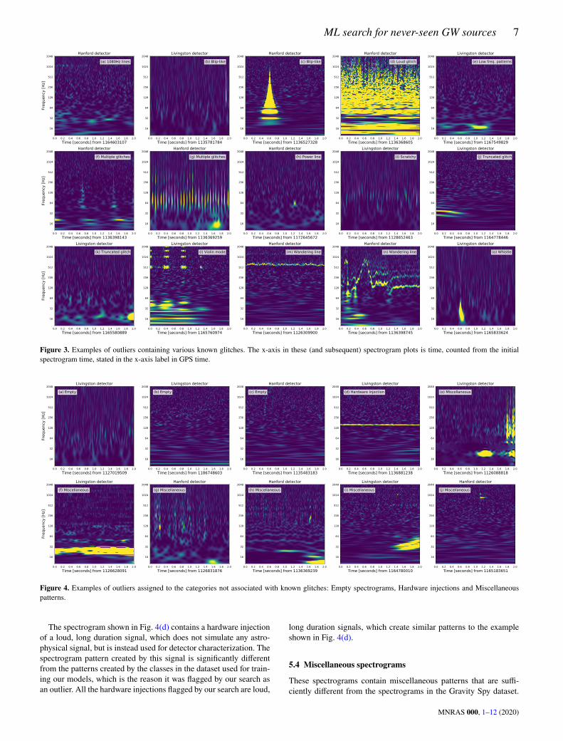
5.1 Known glitches

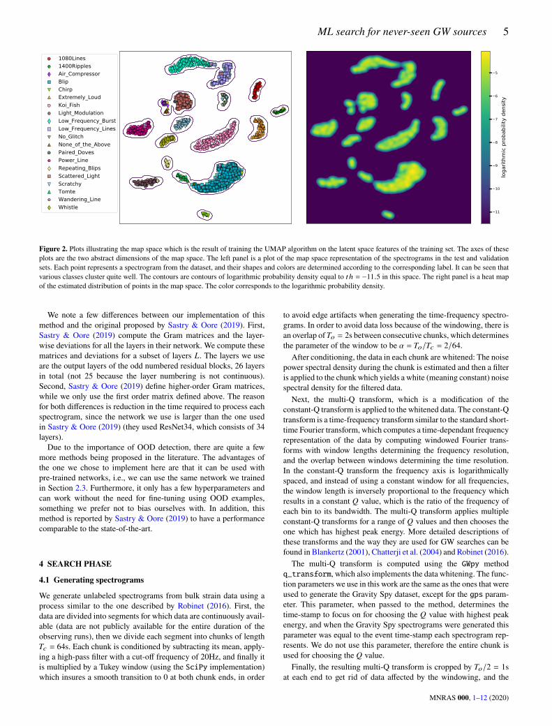
These spectrograms contain known types of glitches that are alsopresent in the Gravity Spy dataset. These outliers, examples of whichare shown in Fig. 3, make up about half of the total outliers flaggedby each method (163 and 176 by the density method and the Grammatrix method respectively), however, for many of them we canfind a reasonable explanation for what might have caused them tobe flagged as outliers. Many of them contain relatively faint sig-nals, fainter than the typical glitches in the dataset. For instance, thespectrogram in Fig. 3(a) contains a faint ‘1080Hz lines’ glitch, thespectrogram in Fig. 3(h) contains a faint ‘Power line’ glitch, and the

Table 1. Breakdown of the outliers detected by each method into differentspectrogram categories.

Density Gram matrix

Known glitches

‘1080Hz lines’ 2 2‘Blip’-like 8 3Loud glitch 2 6Low freq. patterns 77 83Multiple glitches 13 36‘Power line’ 7 0‘Scratchy’ 2 2Truncated glitch 41 12‘Violin mode’ 3 2‘Wandering line’ 3 13‘Whistle’ 5 17Empty spectrogram 183 122Hardware injection 0 25Miscellaneous 40 55Total 386 378

spectrogram in Fig. 3(i) contains a faint ‘Scratchy’ glitch. The factthese faint signals are flagged suggests that our search can detectthese faint signals and identify that they are somewhat different fromtheir louder counterparts, which is a desirable property of a searchfor unmodeled signals. The spectrograms assigned to the multipleglitches category contain multiple glitches in a single spectrogram,like the ones shown in Figs. 3(f) and 3(g). The spectrograms assignedto the truncated glitch category contain glitches that overlap two con-secutive spectrograms, and therefore the pattern in each one appearstruncated, examples of which can be seen in Figs. 3(j) and 3(k).In addition, there are glitches which belong to classes which areunder-represented in our dataset. For instance, the ‘Violin mode’glitch shown in Fig. 3(l) belongs to one of the classes mentionedin Section 2.2 which are not present in our training dataset, and the‘Wandering line’ glitches shown in Figs. 3(m) and 3(n) belong tothe smallest class in our dataset (containing only 3 examples in thetraining set). Finally, the ‘Whistle’ glitch shown in Fig. 3(o) presentsa somewhat different pattern than the glitches belonging to the sameclass in our dataset – the low frequency part of the signal is quitestrong while the higher frequency pattern is much fainter.

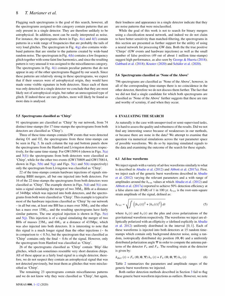
5.2 ‘Empty’ spectrograms

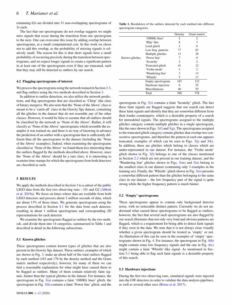
These spectrograms appear to contain only background detectornoise, with no noticeable distinct pattern. Currently we do not un-derstand what caused these spectrograms to be flagged as outliers,however, the fact that several such spectrograms are also flagged byour search illustrates that not only very loud and obvious patterns areflagged, which is a requirement for being able to detect faint signalsif they exist in the data. We note that it is not always clear visuallywhether a given spectrogram should be treated as ‘empty’ or not.An illustration of this can be seen in the examples of ‘empty’ spec-trograms shown in Fig. 4. For instance, the spectrogram in Fig. 4(b)might contain some low frequency signals and the one in Fig. 4(c)might contain a faint ‘Whistle’-like signal. As mentioned in Sec-tion 5.1 being able to flag such faint signals is a desirable propertyof this search.

5.3 Hardware injections

During the first two observing runs, simulated signals were injectedinto the GW detectors in order to validate the data analysis pipelines,as well as several other uses (Biwer et al. 2017).

MNRAS 000, 1–12 (2020)


0.0 0.2 0.4 0.6 0.8 1.0 1.2 1.4 1.6 1.8 2.0Time [seconds] from 1164603107

2048

1024

512

256

128

64

32

16

Freq

uenc

y [H

z]

(a) 1080Hz lines

Hanford detector


2048

1024

512

256

128

64

32

16

(b) Blip-like

Livingston detector


2048

1024

512

256

128

64

32

16

(c) Blip-like

Hanford detector


2048

1024

512

256

128

64

32

16

(d) Loud glitch

Hanford detector


2048

1024

512

256

128

64

32

16

(e) Low freq. patterns

Livingston detector


2048

1024

512

256

128

64

32

16

Freq

uenc

y [H

z]

(f) Multiple glitches

Hanford detector


2048

1024

512

256

128

64

32

16

(g) Multiple glitches

Hanford detector


2048

1024

512

256

128

64

32

16

(h) Power line

Hanford detector


2048

1024

512

256

128

64

32

16

(i) Scratchy

Livingston detector


2048

1024

512

256

128

64

32

16

(j) Truncated glitch

Livingston detector


2048

1024

512

256

128

64

32

16

Freq

uenc

y [H

z]

(k) Truncated glitch

Livingston detector


2048

1024

512

256

128

64

32

16

(l) Violin mode

Livingston detector


2048

1024

512

256

128

64

32

16

(m) Wandering line

Hanford detector


2048

1024

512

256

128

64

32

16

(n) Wandering line

Hanford detector


2048

1024

512

256

128

64

32

16

(o) Whistle

Livingston detector

Figure 3. Examples of outliers containing various known glitches. The x-axis in these (and subsequent) spectrogram plots is time, counted from the initialspectrogram time, stated in the x-axis label in GPS time.


2048

1024

512

256

128

64

32

16

Freq

uenc

y [H

z]

(a) Empty

Livingston detector


2048

1024

512

256

128

64

32

16

(b) Empty

Livingston detector


2048

1024

512

256

128

64

32

16

(c) Empty

Hanford detector


2048

1024

512

256

128

64

32

16

(d) Hardware injection

Livingston detector


2048

1024

512

256

128

64

32

16

(e) Miscellaneous

Livingston detector


2048

1024

512

256

128

64

32

16

Freq

uenc

y [H

z]

(f) Miscellaneous

Livingston detector


2048

1024

512

256

128

64

32

16

(g) Miscellaneous

Hanford detector


2048

1024

512

256

128

64

32

16

(h) Miscellaneous

Hanford detector


2048

1024

512

256

128

64

32

16

(i) Miscellaneous

Livingston detector


2048

1024

512

256

128

64

32

16

(j) Miscellaneous

Hanford detector

Figure 4. Examples of outliers assigned to the categories not associated with known glitches: Empty spectrograms, Hardware injections and Miscellaneouspatterns.

The spectrogram shown in Fig. 4(d) contains a hardware injectionof a loud, long duration signal, which does not simulate any astro-physical signal, but is instead used for detector characterization. Thespectrogram pattern created by this signal is significantly differentfrom the patterns created by the classes in the dataset used for train-ing our models, which is the reason it was flagged by our search asan outlier. All the hardware injections flagged by our search are loud,

long duration signals, which create similar patterns to the exampleshown in Fig. 4(d).

5.4 Miscellaneous spectrograms

These spectrograms contain miscellaneous patterns that are suffi-ciently different from the spectrograms in the Gravity Spy dataset.

MNRAS 000, 1–12 (2020)


Flagging such spectrograms is the goal of this search, however, allthe spectrograms assigned to this category contain patterns that areonly present in a single detector. They are therefore unlikely to beastrophysical. In addition, most can be easily interpreted as noise.For instance, the spectrograms shown in Figs. 4(e) and 4(f) containpatterns in a wide range of frequencies that are probably the tails ofvery loud glitches. The spectrogram in Fig. 4(g) also contains wide-band patterns that are similar to the patterns created by wide-bandrandom noise. The spectrogram in Fig. 4(h) contains a low frequencyglitch together with some faint line harmonics, and since the resultingpattern is very unusual it was assigned to the miscellaneous category.The spectrograms in Fig. 4(i) contain peculiar patterns that do notappear in any of the other spectrograms flagged by our search. Sincethese patterns are relatively strong in these spectrograms, we expectthat if their sources were of astrophysical origin, they would havemade some visible signature in both detectors. Since each of themwas only detected in a single detector we conclude that they are mostlikely not of astrophysical origin, but rather an unrecognized type ofglitch. If indeed these are rare glitches, more will likely be found asmore data is analysed.

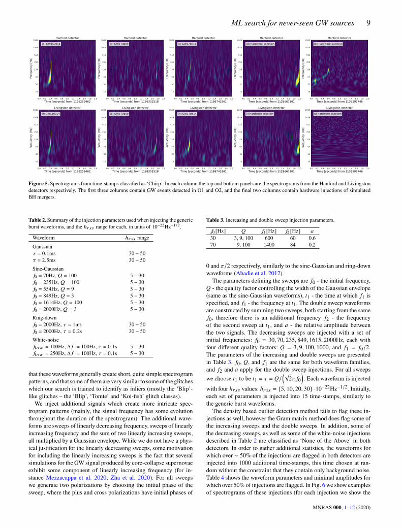
5.5 Spectrograms classified as ‘Chirp’

91 spectrograms are classified as ‘Chirp’ by our network, from 74distinct time-stamps (for 17 time-stamps the spectrograms from bothdetectors are classified as ‘Chirp’).Three of these time-stamps contain GW events that were detected

during O1 and O2, the spectrograms from these time-stamps canbe seen in Fig. 5. In each column the top and bottom panels showthe spectrograms from the Hanford and Livingston detectors respec-tively, for the same time-stamp. For GW150914 (shown in Figs. 5(a)and 5(f)) the spectrograms from both detectors were classified as‘Chirp’, while for the other two events (GW170809 and GW170814,shown in Figs. 5(b) and 5(g) and Figs. 5(c) and 5(h) respectively)only the spectrogram from Livingston was classified as ‘Chirp’.22 of the time-stamps contain hardware injections of signals sim-

ulating BBH mergers, all but one injected into both detectors. For16 of the 22 time-stamps the spectrograms from both detectors wereclassified as ‘Chirp’. The example shown in Figs. 5(d) and 5(i) con-tains a signal simulating the merger of two 38M� BHs at a distanceof 344Mpc which was injected into both detectors, and the spectro-grams from both were classified as ‘Chirp’. This example is typical tomost of the hardware injections classified as ‘Chirp’ by our network– in all but one, at least one BH has a mass over 30M� and the otherhas a mass over 15M� , and the resulting spectrograms have fairlysimilar patterns. The one atypical injection is shown in Figs. 5(e)and 5(j). This injection is of a signal simulating the merger of twoBHs of masses 23M� and 6M� at a distance of 433Mpc, whichwas also injected into both detectors. It is interesting to note thatthis signal is a much longer signal than the other injections (∼ 6sin comparison to < 0.5s), but the spectrogram that was classified as‘Chirp’ contains only the final ∼ 0.6s of the signal. However, onlythe spectrogram from Hanford was classified as ‘Chirp’.26 of the spectrograms classified as ‘Chirp’ contain ‘Blip’-like

glitches, which can sometimes resemble very short duration chirps.All of these appear as a fairly loud signal in a single detector, there-fore, we do not suspect they contain an astrophysical signal that wasnot detected previously, but treat them as glitches that were misclas-sified as ‘Chirp’.The remaining 23 spectrograms contain miscellaneous patterns

and we do not know why they were classified as ‘Chirp’, but again,

their loudness and appearance in a single detector indicate that theyare noise patterns that were misclassified.While the goal of this work is not to search for binary mergers

using a classification neural network, and indeed we do not claimto have better sensitivity than matched-filtering, the spectrograms inthis section are presented as further support for the utility of usinga neural network for processing GW data. Both the the true positive‘Chirps’ (GW events and hardware injections) as well as the smallnumber of false positives (49 out of about 1 million time-stamps)suggest high performance, as also seen by George & Huerta (2018);Gabbard et al. (2018); Krastev (2020) and Schäfer et al. (2020).

5.6 Spectrograms classified as ‘None of the Above’

796 spectrograms are classified as ‘None of the Above’, however, inall of the corresponding time-stamps there is no coincidence in theother detector, therefore we do not discuss them further. The fact thatwe did not find a single candidate for which both spectrograms areclassified as ‘None of the Above’ further suggests that these are rareand worthy of scrutiny, if and when they occur.

6 EVALUATING THE SEARCH

As naturally is the case with unsupervised or semi-supervised tasks,it is hard to assess the quality and robustness of the results. Didwe notfind any interesting source because of weaknesses in our methods,or because there are none in the data? We attempt to examine thatquestion via numerical simulations across the vast parameter spaceof possible waveforms. We do so by injecting simulated signals tothe data and examining the outcome of the search for these signals.

6.1 Ad-hoc waveforms

We inject signalswith a variety of ad-hocwaveforms similarly towhatis described in Abadie et al. (2012) and Abbott et al. (2017a). First,we inject each of the generic burst waveforms described in Abadieet al. (2012) varying the relevant parameters and a with range ofamplitudes around the ℎ𝑟𝑠𝑠 values at which Abadie et al. (2012) andAbbott et al. (2017a) reported to achieve 50% detection efficiency ata false alarm rate (FAR) of 1 in 100 yr. ℎ𝑟𝑠𝑠 is the root-sum-squarestrain amplitude of the signal, defined as:

ℎ𝑟𝑠𝑠 =

√︄∫ (|ℎ+ (𝑡) |2 + |ℎ× (𝑡) |2

)𝑑𝑡 (5)

where ℎ+ (𝑡) and ℎ× (𝑡) are the plus and cross polarizations of thegravitational waveform respectively. The waveforms we inject are el-liptically polarized with an ellipticity 𝛼 (defined explicitly in Abadieet al. 2012) uniformly distributed in the interval [0, 1]. Each ofthese waveforms is injected into both detectors at 15 random time-stamps which contain only background detector noise, using a ran-dom, isotropically distributed sky position (Θ,Φ) and a uniformlydistributed polarization angleΨ in order to compute the antenna pat-terns of the detector 𝐹+ and 𝐹×. The resulting strain at the detectoris given by:

ℎ𝑑𝑒𝑡 (𝑡) = 𝐹+ (Θ,Φ,Ψ) ℎ+ (𝑡) + 𝐹× (Θ,Φ,Ψ) ℎ× (𝑡) (6)

Table 2 summarizes the parameters and amplitude ranges of thegeneric burst waveforms we injected.Both outlier detection methods described in Section 3 fail to flag

these generic burst waveform injections as outliers. However, we note

MNRAS 000, 1–12 (2020)



2048

1024

512

256

128

64

32

16

Freq

uenc

y [H

z]

(a) GW150914

Hanford detector


2048

1024

512

256

128

64

32

16

Freq

uenc

y [H

z]

(f) GW150914

Livingston detector


2048

1024

512

256

128

64

32

16

Freq

uenc

y [H

z]

(b) GW170809

Hanford detector


2048

1024

512

256

128

64

32

16

Freq

uenc

y [H

z]

(g) GW170809

Livingston detector


2048

1024

512

256

128

64

32

16

Freq

uenc

y [H

z]

(c) GW170814

Hanford detector


2048

1024

512

256

128

64

32

16

Freq

uenc

y [H

z]

(h) GW170814

Livingston detector


2048

1024

512

256

128

64

32

16

Freq

uenc

y [H

z]

(d) Hardware injection

Hanford detector


2048

1024

512

256

128

64

32

16

Freq

uenc

y [H

z]

(i) Hardware injection

Livingston detector


2048

1024

512

256

128

64

32

16

Freq

uenc

y [H

z]

(e) Hardware injection

Hanford detector


2048

1024

512

256

128

64

32

16

Freq

uenc

y [H

z]

(j) Hardware injection

Livingston detector

Figure 5. Spectrograms from time-stamps classified as ‘Chirp’. In each column the top and bottom panels are the spectrograms from the Hanford and Livingstondetectors respectively. The first three columns contain GW events detected in O1 and O2, and the final two columns contain hardware injections of simulatedBH mergers.

Table 2. Summary of the injection parameters usedwhen injecting the genericburst waveforms, and the ℎ𝑟𝑠𝑠 range for each, in units of 10−22Hz−1/2.

Waveform ℎ𝑟𝑠𝑠 range

Gaussian𝜏 = 0.1ms 30 − 50𝜏 = 2.5ms 30 − 50Sine-Gaussian𝑓0 = 70Hz, 𝑄 = 100 5 − 30𝑓0 = 235Hz, 𝑄 = 100 5 − 30𝑓0 = 554Hz, 𝑄 = 9 5 − 30𝑓0 = 849Hz, 𝑄 = 3 5 − 30𝑓0 = 1614Hz, 𝑄 = 100 5 − 30𝑓0 = 2000Hz, 𝑄 = 3 5 − 30Ring-down𝑓0 = 2000Hz, 𝜏 = 1ms 30 − 50𝑓0 = 2000Hz, 𝜏 = 0.2s 30 − 50White-noise𝑓𝑙𝑜𝑤 = 100Hz, Δ 𝑓 = 100Hz, 𝜏 = 0.1s 5 − 30𝑓𝑙𝑜𝑤 = 250Hz, Δ 𝑓 = 100Hz, 𝜏 = 0.1s 5 − 30

that thesewaveforms generally create short, quite simple spectrogrampatterns, and that someof themare very similar to someof the glitcheswhich our search is trained to identify as inliers (mostly the ‘Blip’-like glitches – the ‘Blip’, ‘Tomte’ and ‘Koi-fish’ glitch classes).We inject additional signals which create more intricate spec-

trogram patterns (mainly, the signal frequency has some evolutionthroughout the duration of the spectrogram). The additional wave-forms are sweeps of linearly decreasing frequency, sweeps of linearlyincreasing frequency and the sum of two linearly increasing sweeps,all multiplied by a Gaussian envelope. While we do not have a phys-ical justification for the linearly decreasing sweeps, some motivationfor including the linearly increasing sweeps is the fact that severalsimulations for the GW signal produced by core-collapse supernovaeexhibit some component of linearly increasing frequency (for in-stance Mezzacappa et al. 2020; Zha et al. 2020). For all sweepswe generate two polarizations by choosing the initial phase of thesweep, where the plus and cross polarizations have initial phases of

Table 3. Increasing and double sweep injection parameters.

𝑓0 [Hz] 𝑄 𝑓1 [Hz] 𝑓2 [Hz] 𝑎

30 3, 9, 100 600 60 0.670 9, 100 1400 84 0.2

0 and 𝜋/2 respectively, similarly to the sine-Gaussian and ring-downwaveforms (Abadie et al. 2012).The parameters defining the sweeps are 𝑓0 - the initial frequency,

𝑄 - the quality factor controlling the width of the Gaussian envelope(same as the sine-Gaussian waveforms), 𝑡1 - the time at which 𝑓1 isspecified, and 𝑓1 - the frequency at 𝑡1. The double sweep waveformsare constructed by summing two sweeps, both starting from the same𝑓0, therefore there is an additional frequency 𝑓2 - the frequencyof the second sweep at 𝑡1, and 𝑎 - the relative amplitude betweenthe two signals. The decreasing sweeps are injected with a set ofinitial frequencies: 𝑓0 = 30, 70, 235, 849, 1615, 2000Hz, each withfour different quality factors: 𝑄 = 3, 9, 100, 1000, and 𝑓1 = 𝑓0/2.The parameters of the increasing and double sweeps are presentedin Table 3. 𝑓0, 𝑄, and 𝑓1 are the same for both waveform families,and 𝑓2 and 𝑎 apply for the double sweep injections. For all sweepswe choose 𝑡1 to be 𝑡1 = 𝜏 = 𝑄/

(√2𝜋 𝑓0

). Each waveform is injected

with four ℎ𝑟𝑠𝑠 values: ℎ𝑟𝑠𝑠 = {5, 10, 20, 30} ·10−22Hz−1/2. Initially,each set of parameters is injected into 15 time-stamps, similarly tothe generic burst waveforms.The density based outlier detection method fails to flag these in-

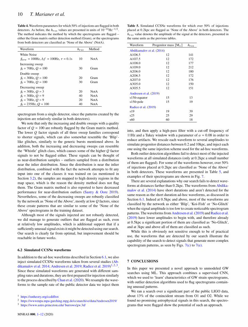
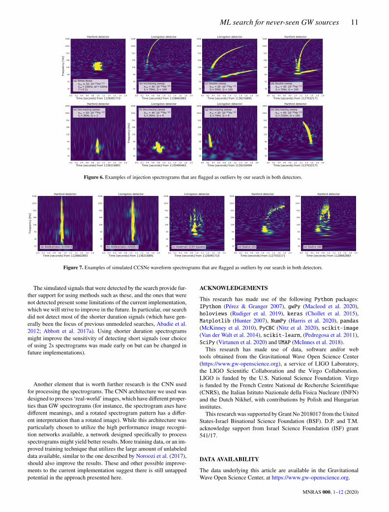
jections as well, however the Gram matrix method does flag some ofthe increasing sweeps and the double sweeps. In addition, some ofthe decreasing sweeps, as well as some of the white-noise injectionsdescribed in Table 2 are classified as ‘None of the Above’ in bothdetectors. In order to gather additional statistics, the waveforms forwhich over ∼ 50% of the injections are flagged in both detectors areinjected into 1000 additional time-stamps, this time chosen at ran-dom without the constraint that they contain only background noise.Table 4 shows the waveform parameters and minimal amplitudes forwhich over 50% of injections are flagged. In Fig. 6 we show examplesof spectrograms of these injections (for each injection we show the

MNRAS 000, 1–12 (2020)


Table 4.Waveform parameters for which 50% of injections are flagged in bothdetectors. As before, the ℎ𝑟𝑠𝑠 values are presented in units of 10−22Hz−1/2.The method indicates the method by which the spectrograms are flagged –either the Gram matrix outlier detection method (Gram), or the spectrogramsfrom both detectors are classified as ‘None of the Above’ (NotA).

Waveform ℎ𝑟𝑠𝑠 Method

White Noise𝑓𝑙𝑜𝑤 = 100Hz, Δ 𝑓 = 100Hz, 𝜏 = 0.1s 10 NotAIncreasing sweep𝑓0 = 70Hz, 𝑄 = 100 30 GramDouble sweep𝑓0 = 30Hz, 𝑄 = 100 20 Gram𝑓0 = 70Hz, 𝑄 = 100 30 GramDecreasing sweep𝑓0 = 30Hz, 𝑄 = 3 20 NotA𝑓0 = 30Hz, 𝑄 = 9 40 NotA𝑓0 = 70Hz, 𝑄 = 9 20 NotA𝑓0 = 235Hz, 𝑄 = 100 40 NotA

spectrogram from a single detector, since the patterns created by theinjection are relatively similar in both detectors).We note that only the increasing and double sweeps with a quality

factor of 𝑄 = 100 are robustly flagged by the Gram matrix method.The lower 𝑄 factor signals of all three sweep families correspondto shorter signals, which can also somewhat resemble the ‘Blip’-like glitches, similarly to the generic bursts mentioned above. Inaddition, both the increasing and decreasing sweeps can resemblethe ‘Whistle’ glitch class, which causes some of the higher 𝑄 factorsignals to not be flagged either. These signals can be thought ofas near-distribution samples – outliers sampled from a distributionnear the inlier distribution. Since the distribution is near the inlierdistribution, combined with the fact the network attempts to fit anyinput into one of the classes it was trained on (as mentioned inSection 3.2), the samples are mapped to high density regions in themap space, which is the reason the density method does not flagthem. The Gram matrix method is also reported to have decreasedperformance for near-distribution outliers (Sastry & Oore 2019).Nevertheless, some of the decreasing sweeps are robustly classifiedby the network as ‘None of the Above’, mostly at low𝑄 factors, sincethese create patterns that are similar to some of the ‘None of theAbove’ spectrograms in the training dataset.Although most of the signals injected are not robustly detected,

we did manage to generate outliers that are flagged as such, evenat relatively low amplitudes, which is additional support that if asufficiently unusual signal exists itmight be detected using our search.Our search is clearly far from optimal, but improvement should bereachable in future works.

6.2 Simulated CCSNe waveforms

In addition to the ad-hoc waveforms described in Section 6.1, we alsoinject simulated CCSNe waveforms taken from several studies (Ab-dikamalov et al. 2014; Andresen et al. 2019; Radice et al. 2019)1,2,3.Since these simulated waveforms are generated with different sam-pling rates and durations, they are first prepared for injection similarlyto the process described byChan et al. (2020).We resample thewave-forms to the sample rate of the public detector data we inject them

1 https://sntheory.org/ccdiffrot2 https://wwwmpa.mpa-garching.mpg.de/ccsnarchive/data/Andresen2019/3 https://www.astro.princeton.edu/ burrows/gw.3d/

Table 5. Simulated CCSNe waveforms for which over 50% of injectionsplaced at 0.2kpc are flagged as ‘None of the Above’ in both detectors. Theℎ𝑟𝑠𝑠 value denotes the amplitude of the signal at the detectors, presented inthe same units as the previous tables.

Waveform Progenitor mass [M� ] ℎ𝑟𝑠𝑠

Abdikamalov et al. (2014)A1O6.5 12 141A1O7.5 12 172A1O8.0 12 177A1O9.0 12 212A2O6.0 12 180A2O6.5 12 172A2O7.0 12 176A3O5.0 12 150A3O5.5 12 151Andresen et al. (2019)s15fr-equator 15 13s15fr-pole 15 19Radice et al. (2019)s19 19 39s25 25 29s60 60 18

into, and then apply a high-pass filter with a cut-off frequency of11Hz and a Tukey window with a parameter of 𝛼 = 0.08 in order toreduce artifacts. We rescale each waveform to several amplitudes tosimulate progenitor distances between 0.2 and 10kpc, and inject eachone using the same injection scheme used for the ad-hoc waveforms.Both outlier detection algorithms fail to detect most of the injected

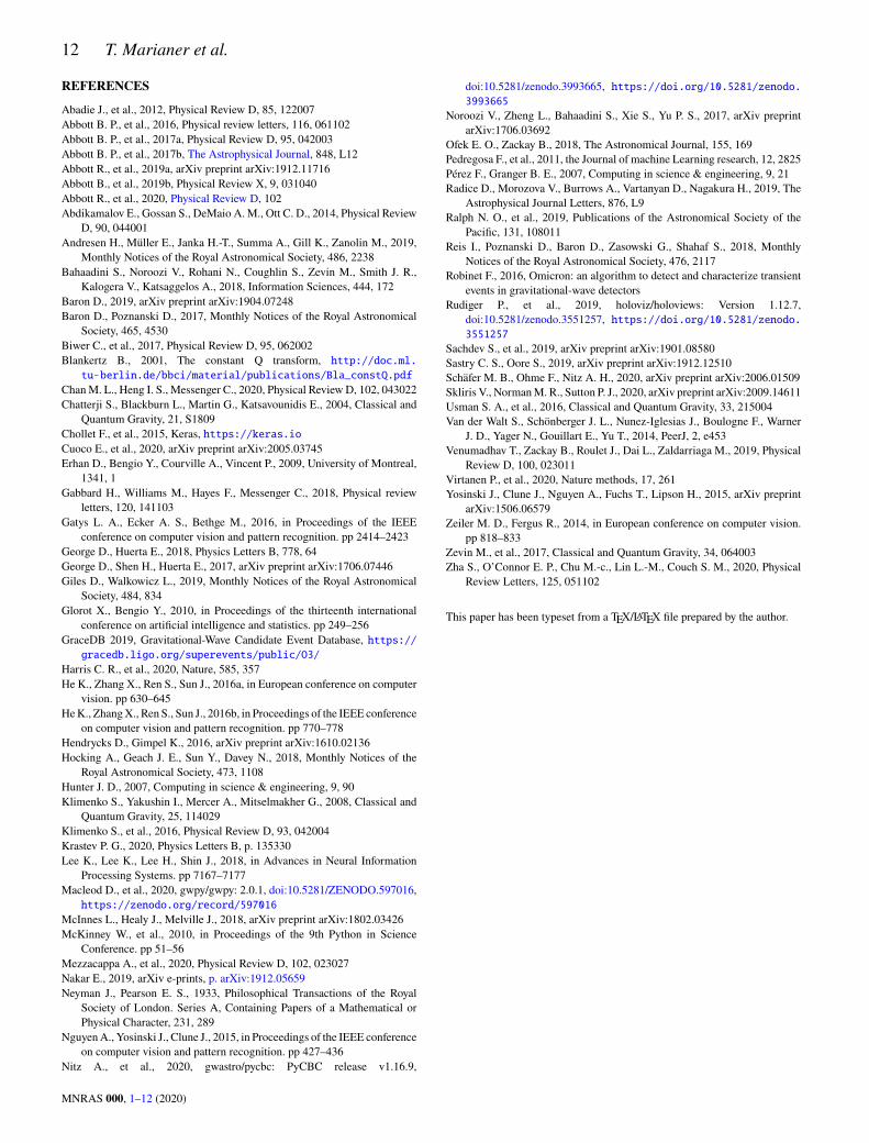
waveforms at all simulated distances (only at 0.2kpc a small numberof them are flagged). For some of the waveforms however, over 50%of injections placed at 0.2kpc are classified as ‘None of the Above’in both detectors. These waveforms are presented in Table 5, andexamples of their spectrograms are shown in Fig. 7.There are several explanations why our search fails to detect wave-

forms at distances farther than 0.2kpc. The waveforms from Abdika-malov et al. (2014) have short durations and aren’t detected for thesame reason as the short duration ad-hoc waveforms, as discussed inSection 6.1. Indeed at 0.5kpc and above, most of the waveforms areclassified by the network as either ‘Blip’, ‘Koi-Fish’ or ‘No-Glitch’when the signal amplitude is too low to create noticeable spectrogrampatterns. Thewaveforms fromAndresen et al. (2019) andRadice et al.(2019) have lower amplitudes to begin with, and therefore alreadyat 0.5kpc a significant portion of them are classified as ‘No-Glitch’,and at 3kpc and above all of them are classified as such.While this is obviously not sensitive enough to be of practical

use, the waveforms that are detected by our search illustrate thecapability of the search to detect signals that generate more complexspectrogram patterns, as seen by Figs. 7(c) to 7(e).

7 CONCLUSIONS

In this paper we presented a novel approach to unmodeled GWsearches using ML. This approach combines a supervised CNN,which we used to ‘learn’ characteristics of GW strain spectrograms,with outlier detection algorithms used to flag spectrograms contain-ing unusual patterns.We ran a search over a significant part of the public LIGO data,

about 13% of the conincident stream from O1 and O2. While wefound no promising astrophysical signals in this search, the spectro-grams that were flagged show the potential of such an approach.

MNRAS 000, 1–12 (2020)

https://sntheory.org/ccdiffrot

https://wwwmpa.mpa-garching.mpg.de/ccsnarchive/data/Andresen2019/

https://www.astro.princeton.edu/~burrows/gw.3d/



2048

1024

512

256

128

64

32

16

Freq

uenc

y [H

z]

(a) White Noise hrss = 10 10 22Hz 1/2

flow = 100Hz, f = 100Hz = 0.1s

Hanford detector


2048

1024

512

256

128

64

32

16

(b) Increasing sweep hrss = 30 10 22Hz 1/2

f0 = 70Hz, Q = 100

Livingston detector


2048

1024

512

256

128

64

32

16

(c) Double sweep hrss = 20 10 22Hz 1/2

f0 = 30Hz, Q = 100

Livingston detector


2048

1024

512

256

128

64

32

16

(d) Double sweep hrss = 30 10 22Hz 1/2

f0 = 70Hz, Q = 100

Hanford detector


2048

1024

512

256

128

64

32

16

(e) Decreasing sweep hrss = 20 10 22Hz 1/2

f0 = 30Hz, Q = 3

Hanford detector


2048

1024

512

256

128

64

32

16

Freq

uenc

y [H

z]

(f) Decreasing sweep hrss = 40 10 22Hz 1/2

f0 = 30Hz, Q = 9

Livingston detector


2048

1024

512

256

128

64

32

16

(g) Decreasing sweep hrss = 20 10 22Hz 1/2

f0 = 70Hz, Q = 9

Livingston detector


2048

1024

512

256

128

64

32

16

(h) Decreasing sweep hrss = 40 10 22Hz 1/2

f0 = 235Hz, Q = 100

Hanford detector

Figure 6. Examples of injection spectrograms that are flagged as outliers by our search in both detectors.


2048

1024

512

256

128

64

32

16

Freq

uenc

y [H

z]

(a) Abdikamalov A1O08.0

Hanford detector


2048

1024

512

256

128

64

32

16 (b) Abdikamalov A3O05.5

Livingston detector


2048

1024

512

256

128

64

32

16 (c) Andersen s15fr-equator

Livingston detector


2048

1024

512

256

128

64

32

16 (d) Radice s25

Hanford detector


2048

1024

512

256

128

64

32

16 (e) Radice s60

Hanford detector

Figure 7. Examples of simulated CCSNe waveform spectrograms that are flagged as outliers by our search in both detectors.

The simulated signals that were detected by the search provide fur-ther support for using methods such as these, and the ones that werenot detected present some limitations of the current implementation,which we will strive to improve in the future. In particular, our searchdid not detect most of the shorter duration signals (which have gen-erally been the focus of previous unmodeled searches, Abadie et al.2012; Abbott et al. 2017a). Using shorter duration spectrogramsmight improve the sensitivity of detecting short signals (our choiceof using 2s spectrograms was made early on but can be changed infuture implementations).

Another element that is worth further research is the CNN usedfor processing the spectrograms. The CNN architecture we used wasdesigned to process ‘real-world’ images, which have different proper-ties than GW spectrograms (for instance, the spectrogram axes havedifferent meanings, and a rotated spectrogram pattern has a differ-ent interpretation than a rotated image). While this architecture wasparticularly chosen to utilize the high performance image recogni-tion networks available, a network designed specifically to processspectrograms might yield better results. More training data, or an im-proved training technique that utilizes the large amount of unlabeleddata available, similar to the one described by Noroozi et al. (2017),should also improve the results. These and other possible improve-ments to the current implementation suggest there is still untappedpotential in the approach presented here.

ACKNOWLEDGEMENTS

This research has made use of the following Python packages:IPython (Pérez & Granger 2007), gwPy (Macleod et al. 2020),holoviews (Rudiger et al. 2019), keras (Chollet et al. 2015),Matplotlib (Hunter 2007), NumPy (Harris et al. 2020), pandas(McKinney et al. 2010), PyCBC (Nitz et al. 2020), scikit-image(Van der Walt et al. 2014), scikit-learn, (Pedregosa et al. 2011),SciPy (Virtanen et al. 2020) and UMAP (McInnes et al. 2018).This research has made use of data, software and/or web

tools obtained from the Gravitational Wave Open Science Center(https://www.gw-openscience.org), a service of LIGO Laboratory,the LIGO Scientific Collaboration and the Virgo Collaboration.LIGO is funded by the U.S. National Science Foundation. Virgois funded by the French Centre National de Recherche Scientifique(CNRS), the Italian Istituto Nazionale della Fisica Nucleare (INFN)and the Dutch Nikhef, with contributions by Polish and Hungarianinstitutes.This researchwas supported byGrant No 2018017 from theUnited

States-Israel Binational Science Foundation (BSF). D.P. and T.M.acknowledge support from Israel Science Foundation (ISF) grant541/17.

DATA AVAILABILITY

The data underlying this article are available in the GravitationalWave Open Science Center, at https://www.gw-openscience.org.

MNRAS 000, 1–12 (2020)

https://www.gw-openscience.org

https://www.gw-openscience.org


REFERENCES

Abadie J., et al., 2012, Physical Review D, 85, 122007Abbott B. P., et al., 2016, Physical review letters, 116, 061102Abbott B. P., et al., 2017a, Physical Review D, 95, 042003Abbott B. P., et al., 2017b, The Astrophysical Journal, 848, L12Abbott R., et al., 2019a, arXiv preprint arXiv:1912.11716Abbott B., et al., 2019b, Physical Review X, 9, 031040Abbott R., et al., 2020, Physical Review D, 102Abdikamalov E., Gossan S., DeMaio A. M., Ott C. D., 2014, Physical ReviewD, 90, 044001

Andresen H., Müller E., Janka H.-T., Summa A., Gill K., Zanolin M., 2019,Monthly Notices of the Royal Astronomical Society, 486, 2238

Bahaadini S., Noroozi V., Rohani N., Coughlin S., Zevin M., Smith J. R.,Kalogera V., Katsaggelos A., 2018, Information Sciences, 444, 172

Baron D., 2019, arXiv preprint arXiv:1904.07248Baron D., Poznanski D., 2017, Monthly Notices of the Royal AstronomicalSociety, 465, 4530

Biwer C., et al., 2017, Physical Review D, 95, 062002Blankertz B., 2001, The constant Q transform, http://doc.ml.tu-berlin.de/bbci/material/publications/Bla_constQ.pdf

ChanM. L., Heng I. S., Messenger C., 2020, Physical Review D, 102, 043022Chatterji S., Blackburn L., Martin G., Katsavounidis E., 2004, Classical andQuantum Gravity, 21, S1809

Chollet F., et al., 2015, Keras, https://keras.ioCuoco E., et al., 2020, arXiv preprint arXiv:2005.03745Erhan D., Bengio Y., Courville A., Vincent P., 2009, University of Montreal,1341, 1

Gabbard H., Williams M., Hayes F., Messenger C., 2018, Physical reviewletters, 120, 141103

Gatys L. A., Ecker A. S., Bethge M., 2016, in Proceedings of the IEEEconference on computer vision and pattern recognition. pp 2414–2423

George D., Huerta E., 2018, Physics Letters B, 778, 64George D., Shen H., Huerta E., 2017, arXiv preprint arXiv:1706.07446Giles D., Walkowicz L., 2019, Monthly Notices of the Royal AstronomicalSociety, 484, 834

Glorot X., Bengio Y., 2010, in Proceedings of the thirteenth internationalconference on artificial intelligence and statistics. pp 249–256

GraceDB 2019, Gravitational-Wave Candidate Event Database, https://gracedb.ligo.org/superevents/public/O3/

Harris C. R., et al., 2020, Nature, 585, 357He K., Zhang X., Ren S., Sun J., 2016a, in European conference on computervision. pp 630–645

HeK., ZhangX., Ren S., Sun J., 2016b, in Proceedings of the IEEE conferenceon computer vision and pattern recognition. pp 770–778

Hendrycks D., Gimpel K., 2016, arXiv preprint arXiv:1610.02136Hocking A., Geach J. E., Sun Y., Davey N., 2018, Monthly Notices of theRoyal Astronomical Society, 473, 1108

Hunter J. D., 2007, Computing in science & engineering, 9, 90Klimenko S., Yakushin I., Mercer A., Mitselmakher G., 2008, Classical andQuantum Gravity, 25, 114029

Klimenko S., et al., 2016, Physical Review D, 93, 042004Krastev P. G., 2020, Physics Letters B, p. 135330Lee K., Lee K., Lee H., Shin J., 2018, in Advances in Neural InformationProcessing Systems. pp 7167–7177

Macleod D., et al., 2020, gwpy/gwpy: 2.0.1, doi:10.5281/ZENODO.597016,https://zenodo.org/record/597016

McInnes L., Healy J., Melville J., 2018, arXiv preprint arXiv:1802.03426McKinney W., et al., 2010, in Proceedings of the 9th Python in ScienceConference. pp 51–56

Mezzacappa A., et al., 2020, Physical Review D, 102, 023027Nakar E., 2019, arXiv e-prints, p. arXiv:1912.05659Neyman J., Pearson E. S., 1933, Philosophical Transactions of the RoyalSociety of London. Series A, Containing Papers of a Mathematical orPhysical Character, 231, 289

NguyenA., Yosinski J., Clune J., 2015, in Proceedings of the IEEE conferenceon computer vision and pattern recognition. pp 427–436

Nitz A., et al., 2020, gwastro/pycbc: PyCBC release v1.16.9,

doi:10.5281/zenodo.3993665, https://doi.org/10.5281/zenodo.3993665

Noroozi V., Zheng L., Bahaadini S., Xie S., Yu P. S., 2017, arXiv preprintarXiv:1706.03692

Ofek E. O., Zackay B., 2018, The Astronomical Journal, 155, 169Pedregosa F., et al., 2011, the Journal of machine Learning research, 12, 2825Pérez F., Granger B. E., 2007, Computing in science & engineering, 9, 21Radice D., Morozova V., Burrows A., Vartanyan D., Nagakura H., 2019, TheAstrophysical Journal Letters, 876, L9

Ralph N. O., et al., 2019, Publications of the Astronomical Society of thePacific, 131, 108011

Reis I., Poznanski D., Baron D., Zasowski G., Shahaf S., 2018, MonthlyNotices of the Royal Astronomical Society, 476, 2117

Robinet F., 2016, Omicron: an algorithm to detect and characterize transientevents in gravitational-wave detectors

Rudiger P., et al., 2019, holoviz/holoviews: Version 1.12.7,doi:10.5281/zenodo.3551257, https://doi.org/10.5281/zenodo.3551257

Sachdev S., et al., 2019, arXiv preprint arXiv:1901.08580Sastry C. S., Oore S., 2019, arXiv preprint arXiv:1912.12510Schäfer M. B., Ohme F., Nitz A. H., 2020, arXiv preprint arXiv:2006.01509Skliris V., NormanM. R., Sutton P. J., 2020, arXiv preprint arXiv:2009.14611Usman S. A., et al., 2016, Classical and Quantum Gravity, 33, 215004Van der Walt S., Schönberger J. L., Nunez-Iglesias J., Boulogne F., WarnerJ. D., Yager N., Gouillart E., Yu T., 2014, PeerJ, 2, e453

Venumadhav T., Zackay B., Roulet J., Dai L., Zaldarriaga M., 2019, PhysicalReview D, 100, 023011

Virtanen P., et al., 2020, Nature methods, 17, 261Yosinski J., Clune J., Nguyen A., Fuchs T., Lipson H., 2015, arXiv preprintarXiv:1506.06579

Zeiler M. D., Fergus R., 2014, in European conference on computer vision.pp 818–833

Zevin M., et al., 2017, Classical and Quantum Gravity, 34, 064003Zha S., O’Connor E. P., Chu M.-c., Lin L.-M., Couch S. M., 2020, PhysicalReview Letters, 125, 051102

This paper has been typeset from a TEX/LATEX file prepared by the author.

MNRAS 000, 1–12 (2020)

http://dx.doi.org/10.3847/2041-8213/aa91c9

http://dx.doi.org/10.1103/physrevd.102.043015

http://doc.ml.tu-berlin.de/bbci/material/publications/Bla_constQ.pdf

http://doc.ml.tu-berlin.de/bbci/material/publications/Bla_constQ.pdf

https://keras.io

https://gracedb.ligo.org/superevents/public/O3/

https://gracedb.ligo.org/superevents/public/O3/

http://dx.doi.org/10.5281/ZENODO.597016

https://zenodo.org/record/597016

https://ui.adsabs.harvard.edu/abs/2019arXiv191205659N

http://dx.doi.org/10.5281/zenodo.3993665

https://doi.org/10.5281/zenodo.3993665


http://dx.doi.org/10.5281/zenodo.3551257



Documents

Asemi-supervisedMachineLearningsearchfornever-seen