Embed Size (px)
Citation preview
ADBI Working Paper Series
GLOBALIZATION, STRUCTURAL CHANGE AND INTERREGIONAL PRODUCTIVITY GROWTH IN THE EMERGING COUNTRIES
Jagannath Mallick
No. 774 August 2017
Asian Development Bank Institute
The Working Paper series is a continuation of the formerly named Discussion Paper series; the numbering of the papers continued without interruption or change. ADBI’s working papers reflect initial ideas on a topic and are posted online for discussion. ADBI encourages readers to post their comments on the main page for each working paper (given in the citation below). Some working papers may develop into other forms of publication.
Suggested citation:
Mallick, J. 2017. Globalization, Structural Change and Interregional Productivity Growth in the Emerging Countries. ADBI Working Paper 774. Tokyo: Asian Development Bank Institute. Available: https://www.adb.org/publications/globalization-structural-change-interregional-productivity Please contact the authors for information about this paper.
Email: [email protected]
This work was done at the University of Hyogo, Japan, under the International Research Fellowship of the Japan Society for the Promotion of Science (JSPS). Currently, Jagannath Mallick is assistant professor at BIMTECH, Greater Noida, India. The views expressed in this paper are the views of the author and do not necessarily reflect the views or policies of ADBI, ADB, its Board of Directors, or the governments they represent. ADBI does not guarantee the accuracy of the data included in this paper and accepts no responsibility for any consequences of their use. Terminology used may not necessarily be consistent with ADB official terms. Working papers are subject to formal revision and correction before they are finalized and considered published.
Asian Development Bank Institute Kasumigaseki Building, 8th Floor 3-2-5 Kasumigaseki, Chiyoda-ku Tokyo 100-6008, Japan Tel: +81-3-3593-5500 Fax: +81-3-3593-5571 URL: www.adbi.org E-mail: [email protected] © 2017 Asian Development Bank Institute
ADBI Working Paper 774 J. Mallick
Abstract The aim of this paper is to contribute to the debate on the structural change effects or labor reallocation effects on the regional disparity in productivity growth in India and the People’s Republic of China (PRC). The paper uses secondary data at the state level in India and provinces in the PRC between 1993 and 2010. This paper uses the generalized method of moment (GMM) system estimator in a dynamic spatial panel data framework for the empirical analysis. The empirical investigations draw four results. First, the shift-share analysis suggests that the low-income regions have a higher structural change effect on labor productivity growth (LPG) than the high-income and middle-income regions. Second, the structural change has played an important role in boosting LPG. Third, the neighborhood effects also contribute positively to LPG. Fourth, human capital, investment in fixed assets, and FDI have boosted LPG. Finally, I suggest that policymakers should consider the role of structural change effects along with the neighborhood relationship, human capital, physical investment, and FDI for designing policies in order to reduce disparities in productivity growth, and hence economic growth, which will in turn help to avoid the middle-income trap. Keywords: globalization, structural change, regional productivity growth, dynamic spatial panel JEL Classification: F02, F43, R11, L1
ADBI Working Paper 774 J. Mallick
Contents
1. INTRODUCTION ....................................................................................................... 1
2. DATA AND EMPIRICAL APPROACHES ................................................................... 2
2.1 Data ............................................................................................................... 2 2.2 Decomposition of Employment Growth .......................................................... 3 2.3 Decomposition of Labor Productivity Growth .................................................. 4 2.4 Empirical Specifications ................................................................................. 5
3. STRUCTURAL CHANGE IN INDIA AND PRC ........................................................... 7
4. DECOMPOSITION OF INTERREGIONAL EMPLOYMENT GROWTH .................... 10
5. STRUCTURAL CHANGE AND INTERREGIONAL PRODUCTIVITY GROWTH ...... 12
6. EMPIRICAL RESULTS ............................................................................................ 13
7. CONCLUSIONS AND POLICY IMPLICATIONS ...................................................... 18
REFERENCES ................................................................................................................... 20
APPENDIX A ...................................................................................................................... 25
ADBI Working Paper 774 J. Mallick
1. INTRODUCTION There is a burning debate among academics and policymakers on the issue of the middle-income trap (MIT) of an economy. Economic structure and income inequality at the regional and individual levels are established as two of the factors of the middle-income trap of an economy (Aiyar et al. 2013; Egawa 2013; Islam 2015). Globalization and economic integration have affected emerging countries in various ways. They have facilitated the transfer of technology, contributed to the efficiencies in production, and also substantially increased foreign direct investment (FDI) inflows and trade. The inflow of FDI brings advanced technology and modern management skills to host economies, which enhances labor productivity directly as input to the production function. In addition, it may affect the human capital, infrastructure, domestic firms, etc., which in turn contribute to the productivity growth also (Hale and Long 2007). Further, certain studies establish the fact that globalization increases income inequalities within countries through interregional competition (Candelaria, Daly and Hale 2013; Ezcurra and Rodríquez-Pose 2013; Wan, Lu and Chen 2007).1 Furthermore, FDI is also expected to have an endogenous relationship with productivity growth (Li and Liu 2005). The disproportionate nature of the economic structure is one of the reasons for an MIT. For instance, there is a significant concentration of employment in the agriculture sector, a low-productivity sector in emerging and developing countries. The agriculture sector’s share of income is substantially low compared to that of employment. This has led to highly heterogeneous labor productivity across various activities, which results in low aggregate labor productivity in these countries. The differences in factor returns across various activities may lead to a reallocation of factors or structural change, which may boost overall productivity growth (Lewis 1954; Kuznets 1979; Syrquin 1984). The reallocation of labor from low- to high-productivity activities benefits growth (Lewis 1954), which is referred to as the ‘growth bonus’ (Temple 2001). Therefore, structural change should be seen as a major source of labor productivity growth (LPG) and hence economic growth. Further, there is a high variation in labor productivity across the regions in the emerging countries. There is also high variation in labor productivity across the sectors in the low-income regions in the emerging countries. Such a productivity gap may cause the reallocation of labor from the low- to the high-productivity sector within the region. Therefore, the underdeveloped or low-income regions should gain more from the structural change than the developed regions, which helps to reduce the imbalances. This reallocation may cause convergence, assuming poor regions have relatively more labor in low-productivity sectors such as agriculture (Abramovitz 1986). The relevance of the issues of structural change and interregional productivity growth in the emerging economies is largely due to (i) these countries’ rising international trade and FDI inflows; (ii) advancement of technologies that have reduced production costs; (iii) the changing federalism structure from co-operative to competitive; and (iv) the persistence of interregional income inequalities within a country. The importance of the issue of regional income disparities in a country is highlighted in Ezcurra and Rodríquez-Pose (2013). However, the existing studies on this issue such as McMillan and Rodrik (2011), Havlik (2005), Mallick (2017), Mallick (2015a), Fukao and Yuan (2012), and Brandt, Hsieh and Zhu (2008) are mainly focused on the national
1 The persistence of regional imbalances in economic growth and development in the context of the People’s Republic of China (PRC) and India is a hot debate (Li and Wei 2010; Mallick2015b, 2014, 2013a, 2013b).
1
ADBI Working Paper 774 J. Mallick
level. The structural transformation occurs not only across the broad sectors, but also across the subsectors. Nevertheless, more disaggregated-level study at the regional level is a challenging task in the context of the emerging countries, due to unavailability of data. This is an empirical question as to whether structural change has been important for disparity in LPG. The main purpose of this paper is to examine the patterns of economic structure between three broad sectors, and to measure the effects of structural change on the disparity in LPG across regions in India and the People’s Republic of China (PRC). It is important to know whether, and to what extent, the reallocation of employment from relatively low- to high-productivity sectors has an effect on interregional LPG. If poor regions benefit more, then the policies targeted at facilitating structural change may help to reduce regional disparities and to reduce poverty. As India and the PRC are middle-income countries (MICs), it is important to reduce the regional disparity to avoid the middle-income trap (Egawa 2013; ADB 2011; Eichengreen, Park and Shin2011). The issue is crucial for countries like India and the PRC due to its wider policy implications. The patterns of employment structure will help us to understand the process of structural change. The decomposition of LPG will suggest the role of structural change in the disparity of LPG and hence economic growth. However, there is a dearth of studies that compare the issues of structural change and interregional productivity growth at the regional level in India and the PRC. These are the two largest emerging economies and they have been broadly following similar patterns of growth and interregional disparity since the initiation of substantial economic reform measures. Further, the structural changes are expected to play a larger role in reducing imbalances in interregional productivity growth and economic growth. Hence, a comparative study of the experience of India and the PRC during the period of globalization will be useful for policymakers for framing policies to achieve higher national economic growth and development, by reducing interregional inequalities and poverty (Hasan, Lamba and Gupta 2013). Therefore, the present study attempts to strengthen the existing literature from several points of view in the context of regions in India and the PRC. First, the study decomposes the employment growth to understand the process of structural change. Second, the study measures the contribution of the effect of structural change to overall LPG. Third, the study empirically evaluates the effect of same on LPG by controlling the effects of economic globalization represented by FDI, and by taking into account the spatial interactions. Fourth, the study examines the interaction effect of FDI with physical investment and human capital. Finally, the study provides policy implications for reducing regional disparities in productivity growth and achieving higher regional and national economic growth.
2. DATA AND EMPIRICAL APPROACHES
2.1 Data
The study uses annual data at the state level for India and provincial level in the PRC from 1993 to 2010. The study follows a three-sector classification of economy: primary, secondary, and tertiary sectors. There are no ready-made data on state-level sectoral employment in India. The study uses the quinquennial surveys of the National Sample Survey (NSS) to estimate the sectoral-level employment data. The estimation of state-wise employment is described in Appendix A. The gross state domestic product (GSDP) at the base year of 2004–05 is taken from the Central Statistical Organization (CSO) for India. The sectoral-level provincial data on labor and income in the PRC are
2
ADBI Working Paper 774 J. Mallick
taken from the National Bureau of Statistics of China (NBSC). The estimates of labor at the regional level in both countries are controlled by the national aggregate data from World KLEMS, which is a reliable and internationally comparable data source. The data on other variables used in the empirical analysis are mainly sourced from the NBSC (for the PRC) and the CSO, annual reports of the University Grant Commission, and Secretariat of Industrial Assistance (SIA) (for India). The data on investment at the state level are not available in India; their detailed limitations are discussed in Mallick (2012; 2013a; 2013b; 2014). This paper estimates the same based on the conventional theoretical propositions by using national-level sectoral investment data, which are explained in Appendix A. The detailed variables, measurement, and data sources of the variables included in the empirical analysis are described in Table A1.
2.2 Decomposition of Employment Growth
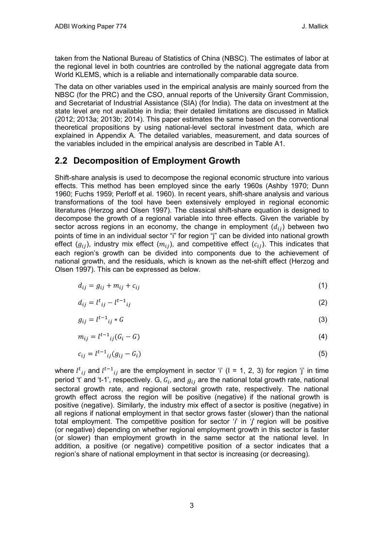
Shift-share analysis is used to decompose the regional economic structure into various effects. This method has been employed since the early 1960s (Ashby 1970; Dunn 1960; Fuchs 1959; Perloff et al. 1960). In recent years, shift-share analysis and various transformations of the tool have been extensively employed in regional economic literatures (Herzog and Olsen 1997). The classical shift-share equation is designed to decompose the growth of a regional variable into three effects. Given the variable by sector across regions in an economy, the change in employment (𝑑𝑖𝑗) between two points of time in an individual sector “i” for region “j” can be divided into national growth effect (𝑔𝑖𝑗), industry mix effect (𝑚𝑖𝑗), and competitive effect (𝑐𝑖𝑗). This indicates that each region’s growth can be divided into components due to the achievement of national growth, and the residuals, which is known as the net-shift effect (Herzog and Olsen 1997). This can be expressed as below.
𝑑𝑖𝑗 = 𝑔𝑖𝑗 + 𝑚𝑖𝑗 + 𝑐𝑖𝑗 (1)
𝑑𝑖𝑗 = 𝑙𝑡𝑖𝑗 − 𝑙𝑡−1𝑖𝑗 (2)
𝑔𝑖𝑗 = 𝑙𝑡−1𝑖𝑗 ∗ 𝐺 (3)
𝑚𝑖𝑗 = 𝑙𝑡−1𝑖𝑗(𝐺𝑖 − 𝐺) (4)
𝑐𝑖𝑗 = 𝑙𝑡−1𝑖𝑗(𝑔𝑖𝑗 − 𝐺𝑖) (5)
where 𝑙𝑡𝑖𝑗 and 𝑙𝑡−1𝑖𝑗 are the employment in sector ‘i’ (I = 1, 2, 3) for region ‘j’ in time period ‘t’ and ‘t-1’, respectively. G, 𝐺𝑖, and 𝑔𝑖𝑗 are the national total growth rate, national sectoral growth rate, and regional sectoral growth rate, respectively. The national growth effect across the region will be positive (negative) if the national growth is positive (negative). Similarly, the industry mix effect of a sector is positive (negative) in all regions if national employment in that sector grows faster (slower) than the national total employment. The competitive position for sector ‘i’ in ‘j’ region will be positive (or negative) depending on whether regional employment growth in this sector is faster (or slower) than employment growth in the same sector at the national level. In addition, a positive (or negative) competitive position of a sector indicates that a region’s share of national employment in that sector is increasing (or decreasing).
3
ADBI Working Paper 774 J. Mallick
2.3 Decomposition of Labor Productivity Growth
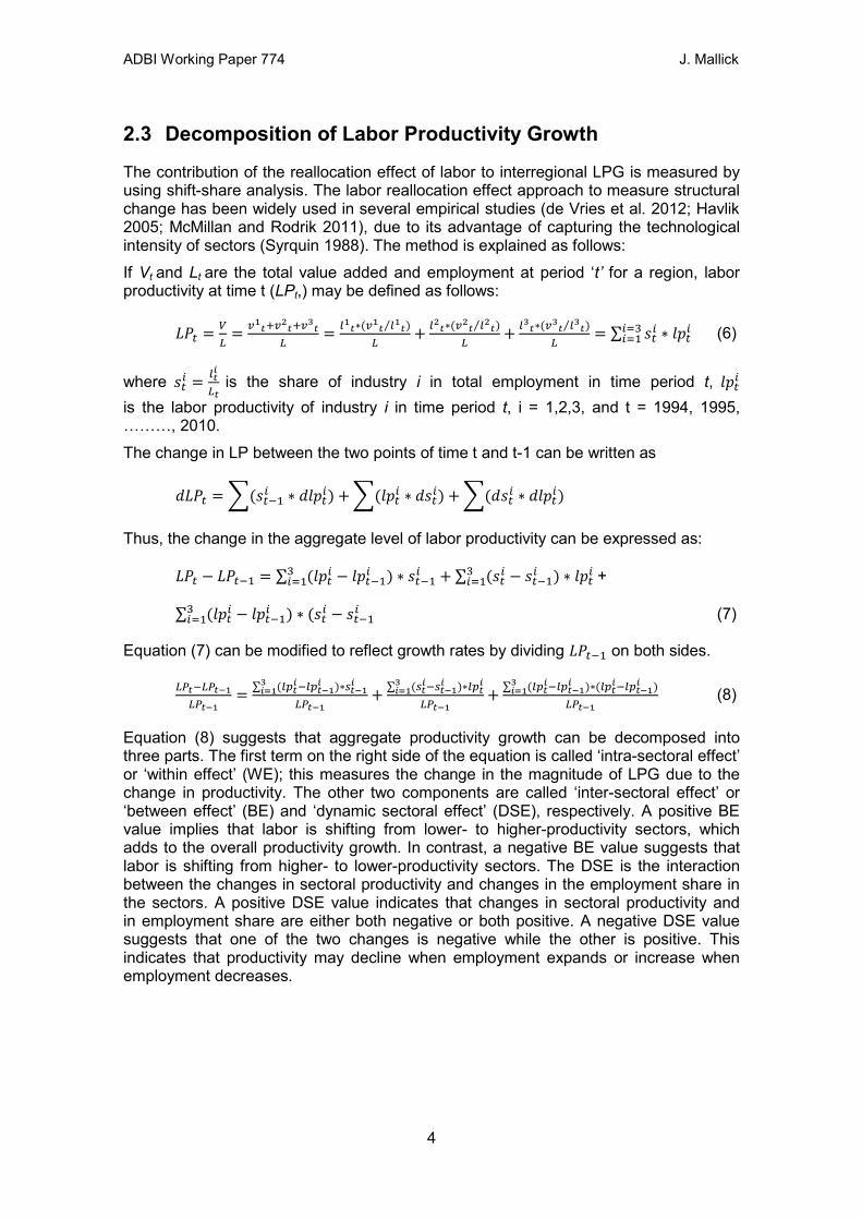
The contribution of the reallocation effect of labor to interregional LPG is measured by using shift-share analysis. The labor reallocation effect approach to measure structural change has been widely used in several empirical studies (de Vries et al. 2012; Havlik 2005; McMillan and Rodrik 2011), due to its advantage of capturing the technological intensity of sectors (Syrquin 1988). The method is explained as follows: If Vt and Lt are the total value added and employment at period ‘t’ for a region, labor productivity at time t (LPt,) may be defined as follows:
𝐿𝑃𝑡 = 𝑉𝐿
= 𝑣1𝑡+𝑣2𝑡+𝑣3𝑡𝐿
= 𝑙1𝑡∗(𝑣1𝑡 𝑙1𝑡)⁄𝐿
+ 𝑙2𝑡∗(𝑣2𝑡 𝑙2𝑡)⁄𝐿
+ 𝑙3𝑡∗(𝑣3𝑡 𝑙3𝑡)⁄𝐿
= ∑ 𝑠𝑡𝑖𝑖=3𝑖=1 ∗ 𝑙𝑝𝑡𝑖 (6)
where 𝑠𝑡𝑖 = 𝑙𝑡𝑖
𝐿𝑡 is the share of industry i in total employment in time period t, 𝑙𝑝𝑡𝑖
is the labor productivity of industry i in time period t, i = 1,2,3, and t = 1994, 1995, ………, 2010. The change in LP between the two points of time t and t-1 can be written as
𝑑𝐿𝑃𝑡 = �(𝑠𝑡−1𝑖 ∗ 𝑑𝑙𝑝𝑡𝑖) +�(𝑙𝑝𝑡𝑖 ∗ 𝑑𝑠𝑡𝑖) + �(𝑑𝑠𝑡𝑖 ∗ 𝑑𝑙𝑝𝑡𝑖)
Thus, the change in the aggregate level of labor productivity can be expressed as:
𝐿𝑃𝑡 − 𝐿𝑃𝑡−1 = ∑ (𝑙𝑝𝑡𝑖3𝑖=1 − 𝑙𝑝𝑡−1𝑖 ) ∗ 𝑠𝑡−1𝑖 + ∑ (𝑠𝑡𝑖3
𝑖=1 − 𝑠𝑡−1𝑖 ) ∗ 𝑙𝑝𝑡𝑖 +
∑ (𝑙𝑝𝑡𝑖3𝑖=1 − 𝑙𝑝𝑡−1𝑖 ) ∗ (𝑠𝑡𝑖 − 𝑠𝑡−1𝑖 (7)
Equation (7) can be modified to reflect growth rates by dividing 𝐿𝑃𝑡−1 on both sides.
𝐿𝑃𝑡−𝐿𝑃𝑡−1𝐿𝑃𝑡−1
= ∑ (𝑙𝑝𝑡𝑖3
𝑖=1 −𝑙𝑝𝑡−1𝑖 )∗𝑠𝑡−1
𝑖
𝐿𝑃𝑡−1+ ∑ (𝑠𝑡
𝑖3𝑖=1 −𝑠𝑡−1
𝑖 )∗𝑙𝑝𝑡𝑖
𝐿𝑃𝑡−1+ ∑ (𝑙𝑝𝑡
𝑖3𝑖=1 −𝑙𝑝𝑡−1
𝑖 )∗(𝑙𝑝𝑡𝑖−𝑙𝑝𝑡−1
𝑖 )𝐿𝑃𝑡−1
(8)
Equation (8) suggests that aggregate productivity growth can be decomposed into three parts. The first term on the right side of the equation is called ‘intra-sectoral effect’ or ‘within effect’ (WE); this measures the change in the magnitude of LPG due to the change in productivity. The other two components are called ‘inter-sectoral effect’ or ‘between effect’ (BE) and ‘dynamic sectoral effect’ (DSE), respectively. A positive BE value implies that labor is shifting from lower- to higher-productivity sectors, which adds to the overall productivity growth. In contrast, a negative BE value suggests that labor is shifting from higher- to lower-productivity sectors. The DSE is the interaction between the changes in sectoral productivity and changes in the employment share in the sectors. A positive DSE value indicates that changes in sectoral productivity and in employment share are either both negative or both positive. A negative DSE value suggests that one of the two changes is negative while the other is positive. This indicates that productivity may decline when employment expands or increase when employment decreases.
4
ADBI Working Paper 774 J. Mallick
2.4 Empirical Specifications
The study focuses on the impact of structural change on interregional LPG by taking into account the spatial correlation among the regions in India and the PRC. The control variables in the empirical analysis have been selected on the basis of existing studies on the determinants of productivity growth, and include FDI to represent economic globalization (Blomstrom and Kokko 1998; Globerman and Ries 1994; Baldwin and Dhaliwal 2001; Rao and Tang 2005; Baldwin and Gu 2005; Driffield and Munday 2002), human capital (Schultz 1975; Welch 1970; Romer 1990; Benhabib and Speigel 1992; Apergis, Economidou and Filippidis 2008; Lucas 1988; Kremer and Thompson 1993), and physical capital formation (Zhang 2002; Biggeri 2003; Zhang and Zhang 2003). The empirical analysis includes 20 major states and 30 provinces for India and the PRC, respectively, over the period from 1993–94 to 2010–11. The study analyzes in a panel data framework, as it controls the individual heterogeneity of the regions and has a greater degree of freedom and efficiency (Baltagi 2001). A panel data equation can be written as follows:
𝑌𝑖𝑡 = ∂ + 𝛽 ∗ 𝐸𝑋𝑖𝑡 + 𝜇𝑖 + 𝜀𝑖𝑡 (9)
where i = 1, 2, .. n (n = 20 for India and n = 30 for the PRC) and t = 1994–95, 1995–96, .., 2010–11. 𝑌𝑖𝑡 is the LPG and EXit is the vector of explanatory variables. In the panel data method, the error term is a composite residual consisting of time-invariant individual-specific (states/provinces) components µi that capture various characteristics of the region, which are not observable, but have a significant impact on the LPG, and a disturbance term 𝜀𝑖𝑡 , which satisfies the classical linear regression model assumptions. In other words, Ɛit and μi are independent for each i over all t, and there is no autocorrelation in the Ɛit. Some of the explanatory variables such as FDI, structural change, and investment may be endogenously related to the LPG. These problems can be tackled through a dynamic panel model by adopting the approach of the generalized method of moments (GMM) estimator. The dynamic panel GMM has been widely employed in the empirical literature on development economics due to its advantages. 2 This methodology is designed to take into account the following: i) the time series dimension of the data, ii) unobserved individual specific effects, iii) inclusion of the lagged dependent variables as the explanatory variables, and iv) the endogenous relationship of explanatory variables. The dynamic representation of the panel data equation (10) is as follows:
𝑌𝑖𝑡 = 𝛼𝑌𝑖𝑡−1 + 𝛿𝑋𝑖𝑡 + 𝜆𝑍𝑖𝑡 + µ𝑖 + 𝜀𝑖𝑡 (10)
where Yit-1 is a one-year lag of LPG, Xit is the vector of strictly exogenous variables, and Zit is the vector of predetermined and endogenous variables,3 and where α, 𝛿, and λ are the parameters. The presence of the lagged dependent variable as one of the explanatory variables makes the relationship dynamic. There are two approaches to estimating the dynamic panel data: difference GMM and system GMM. In difference
2 The GMM estimator is good at exploiting the time series variation in the data, accounting for unobserved individual specific effects, and therefore providing better control for endogeneity of all the explanatory variables (Beck et al. 2000).
3 Predetermined variables and endogenous variables are assumed to be correlated with only past errors, and both past and present errors, respectively.
5
ADBI Working Paper 774 J. Mallick
GMM, the lagged values of the explanatory variables are used as the instruments. There are statistical problems in the difference GMM when the first differences of the regressors are persistent, which makes the lagged levels of Z and X weak instruments. The use of weak instruments increases the variance of the coefficient, which becomes biased in small samples. To reduce the potential bias and inaccuracy associated with the use of t h e DIFF-GMM estimator, Arellano and Bover (1995) and Blundell and Bond (1998) developed a system of regressions in differences and levels. 4 The lagged levels of the explanatory variables are the instruments in the regression in differences, and the lagged differences of explanatory variables are the instruments in the regression in levels. However, the validity of the moment conditions decides the consistency of the GMM estimator. There are two specification tests based on Arellano and Bond (1991), Arellano and Bover (1995), and Blundell and Bond (1998) to judge the validity of the instruments, and hence the consistency of the GMM estimator: first, Hansen’s test of overidentifying restrictions, which verifies the joint null hypothesis, that the instruments are valid instruments; second, the Arellano-Bond test, which tests the hypothesis of no second-order serial correlation in the error term.
Spatial Effects in Dynamic Panel Data The panel data do not capture the spatial interaction or correlation among the regions. The sign of spatial correlation is issue-specific. For instance, in the context of productivity growth or overall economic growth, the spatial correlation is expected to have a positive effect. However, in some cases, for instance the location of investment, the correlation could be negative or positive. The location of investment in one region may affect its neighboring regions positively due to the effects of the agglomeration effect or spillover. This relation may be negative, on the other hand, because the relatively strong business environment of a region reduces the location of investment in its neighboring regions. These kinds of relations (or spatial interaction effects) can be controlled through spatial dependence models. According to Anselin and Bera (1998), the spatial dependence can be taken into account by the spatial autoregressive (SAR) model, where a spatial lag of the dependent variable is included as one of the explanatory variables on the right-hand side of the equation. The panel representation of the spatial lag model can be specified as follows:
𝑌𝑖𝑡 = α + 𝜌∑ 𝑤𝑖𝑗𝑛𝑗=1 𝑌𝑖𝑡 + 𝛽𝑋𝑖𝑡 + 𝜇𝑖 + 𝜀𝑖𝑡 (11)
where ∑ 𝑤𝑖𝑗𝑛𝑗=1 is the classical weight matrix,5 which is a row-standardized matrix of
spatial weights describing the structure and intensity of spatial effects. 𝞺 is the spatial autoregressive coefficient, which is the parameter of the spatially lagged dependent variable that captures the spatial interaction effect. This indicates the extent to which the LPG in one region is determined by the behavior of its neighborhood, after controlling for the important factors of LPG. The sign of the value of the 𝞺 parameter indicates the sign of the spatial autocorrelation. The error term 𝜀𝑖𝑡 is again assumed to be normally distributed and independent of the explanatory variables and spatially lagged dependent variable, under the assumption that all spatial dependence effects are captured by the lagged term. In other words, 𝜀𝑖𝑡 is the classical zero mean error
4 For a detailed explanation of the GMM estimator, see Green (2000, Chapter 11), Wooldridge (2002, Chapter 8 and Chapter 14), and Roodman (2009).
5 In this paper, the weight matrix is based on the classical binary connectivity matrix, which assumes a value of 1 if the two regions share a common border and zero otherwise.
6
ADBI Working Paper 774 J. Mallick
term assumed to be independent under the hypothesis that all spatial dependence effects are captured by the spatially lagged variable term. Equation (11) is known as the ‘fixed-effect lag model.’ Corresponding to the dynamic panel GMM estimator in equation (10), the dynamic spatial panel lag model can be specified as follows (Baltagi, Fingleton and Pirotte2014):
𝑌𝑖𝑡 = 𝛼𝑌𝑖𝑡−1 + 𝜌∑ 𝑤𝑖𝑗𝑛𝑗=1 𝑌𝑖𝑡 + 𝛿𝑋𝑖𝑡 + 𝜆𝑍𝑖𝑡 + µ𝑖 + 𝜀𝑖𝑡 (12)
This model can also be estimated by the difference GMM and system GMM approaches like the nonspatial dynamic panel data model.
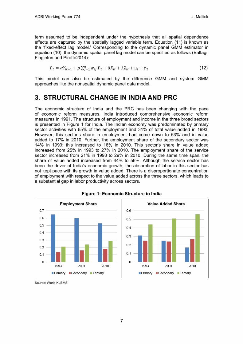
3. STRUCTURAL CHANGE IN INDIA AND PRC The economic structure of India and the PRC has been changing with the pace of economic reform measures. India introduced comprehensive economic reform measures in 1991. The structure of employment and income in the three broad sectors is presented in Figure 1 for India. The Indian economy was predominated by primary sector activities with 65% of the employment and 31% of total value added in 1993. However, this sector’s share in employment had come down to 53% and in value added to 17% in 2010. Further, the employment share of the secondary sector was 14% in 1993; this increased to 18% in 2010. This sector’s share in value added increased from 25% in 1993 to 27% in 2010. The employment share of the service sector increased from 21% in 1993 to 29% in 2010. During the same time span, the share of value added increased from 44% to 56%. Although the service sector has been the driver of India’s economic growth, the absorption of labor in this sector has not kept pace with its growth in value added. There is a disproportionate concentration of employment with respect to the value added across the three sectors, which leads to a substantial gap in labor productivity across sectors.
Figure 1: Economic Structure in India
Source: World KLEMS.
7
ADBI Working Paper 774 J. Mallick
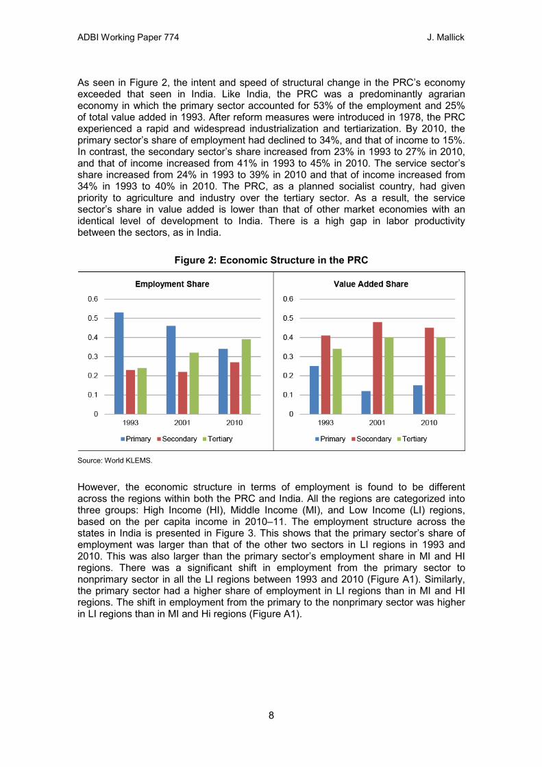
As seen in Figure 2, the intent and speed of structural change in the PRC’s economy exceeded that seen in India. Like India, the PRC was a predominantly agrarian economy in which the primary sector accounted for 53% of the employment and 25% of total value added in 1993. After reform measures were introduced in 1978, the PRC experienced a rapid and widespread industrialization and tertiarization. By 2010, the primary sector’s share of employment had declined to 34%, and that of income to 15%. In contrast, the secondary sector’s share increased from 23% in 1993 to 27% in 2010, and that of income increased from 41% in 1993 to 45% in 2010. The service sector’s share increased from 24% in 1993 to 39% in 2010 and that of income increased from 34% in 1993 to 40% in 2010. The PRC, as a planned socialist country, had given priority to agriculture and industry over the tertiary sector. As a result, the service sector’s share in value added is lower than that of other market economies with an identical level of development to India. There is a high gap in labor productivity between the sectors, as in India.
Figure 2: Economic Structure in the PRC
Source: World KLEMS.
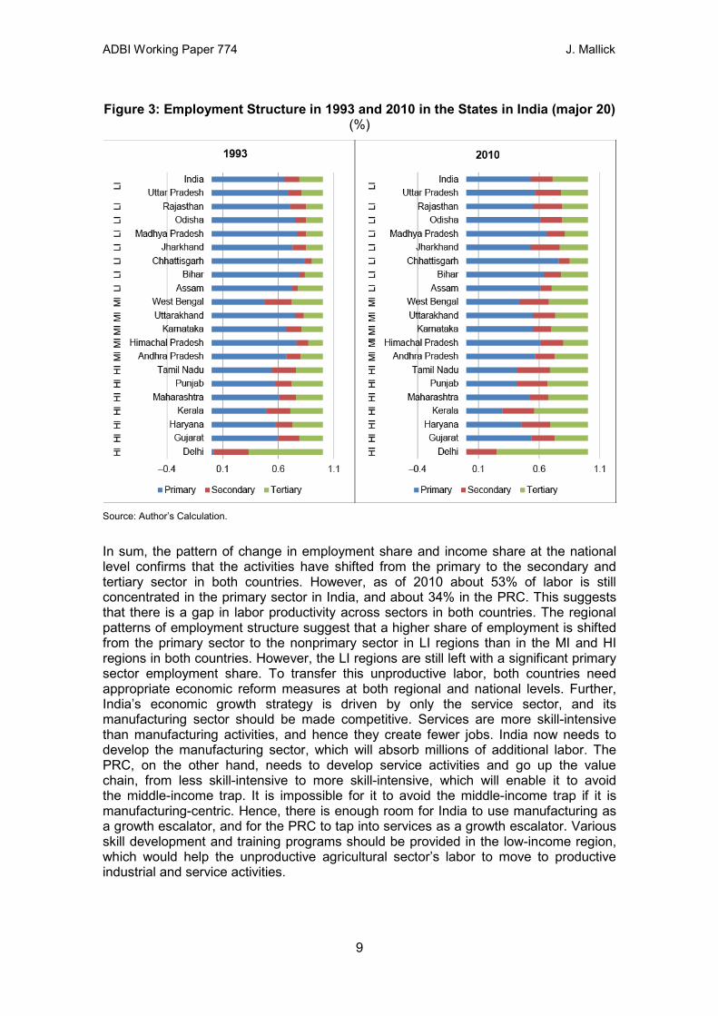
However, the economic structure in terms of employment is found to be different across the regions within both the PRC and India. All the regions are categorized into three groups: High Income (HI), Middle Income (MI), and Low Income (LI) regions, based on the per capita income in 2010–11. The employment structure across the states in India is presented in Figure 3. This shows that the primary sector’s share of employment was larger than that of the other two sectors in LI regions in 1993 and 2010. This was also larger than the primary sector’s employment share in MI and HI regions. There was a significant shift in employment from the primary sector to nonprimary sector in all the LI regions between 1993 and 2010 (Figure A1). Similarly, the primary sector had a higher share of employment in LI regions than in MI and HI regions. The shift in employment from the primary to the nonprimary sector was higher in LI regions than in MI and Hi regions (Figure A1).
8
ADBI Working Paper 774 J. Mallick
Figure 3: Employment Structure in 1993 and 2010 in the States in India (major 20) (%)
Source: Author’s Calculation.
In sum, the pattern of change in employment share and income share at the national level confirms that the activities have shifted from the primary to the secondary and tertiary sector in both countries. However, as of 2010 about 53% of labor is still concentrated in the primary sector in India, and about 34% in the PRC. This suggests that there is a gap in labor productivity across sectors in both countries. The regional patterns of employment structure suggest that a higher share of employment is shifted from the primary sector to the nonprimary sector in LI regions than in the MI and HI regions in both countries. However, the LI regions are still left with a significant primary sector employment share. To transfer this unproductive labor, both countries need appropriate economic reform measures at both regional and national levels. Further, India’s economic growth strategy is driven by only the service sector, and its manufacturing sector should be made competitive. Services are more skill-intensive than manufacturing activities, and hence they create fewer jobs. India now needs to develop the manufacturing sector, which will absorb millions of additional labor. The PRC, on the other hand, needs to develop service activities and go up the value chain, from less skill-intensive to more skill-intensive, which will enable it to avoid the middle-income trap. It is impossible for it to avoid the middle-income trap if it is manufacturing-centric. Hence, there is enough room for India to use manufacturing as a growth escalator, and for the PRC to tap into services as a growth escalator. Various skill development and training programs should be provided in the low-income region, which would help the unproductive agricultural sector’s labor to move to productive industrial and service activities.
9
ADBI Working Paper 774 J. Mallick
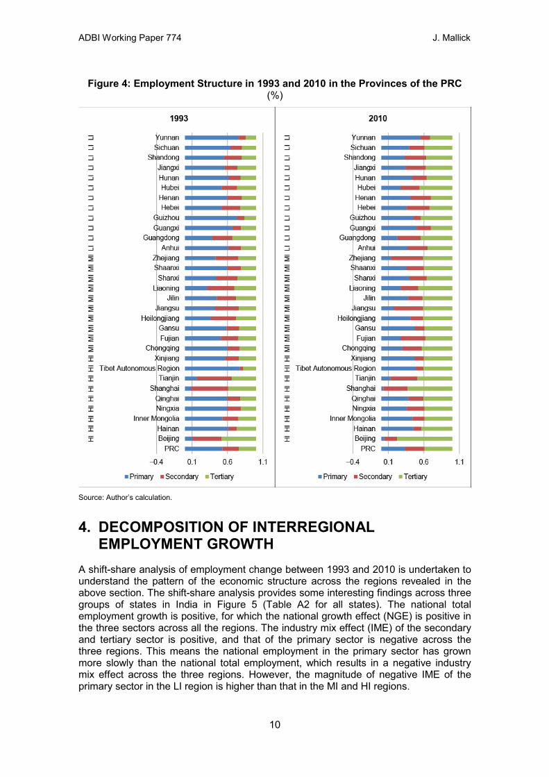
Figure 4: Employment Structure in 1993 and 2010 in the Provinces of the PRC (%)
Source: Author’s calculation.
4. DECOMPOSITION OF INTERREGIONAL EMPLOYMENT GROWTH
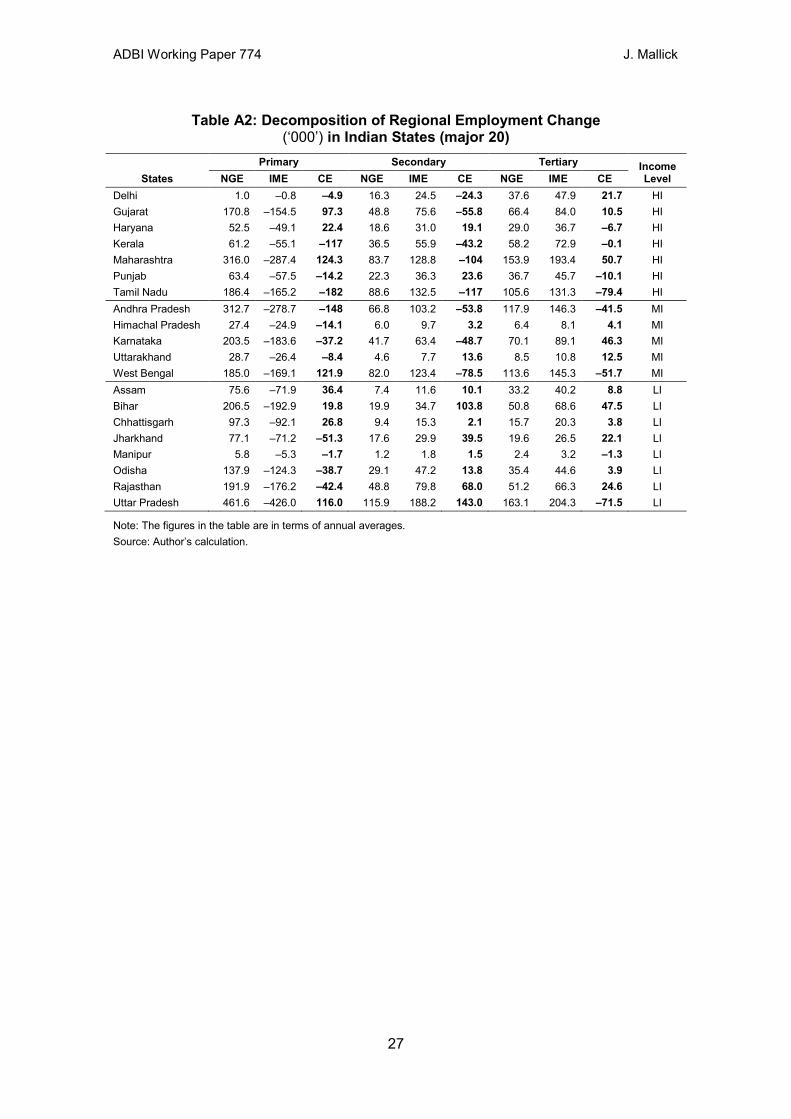
A shift-share analysis of employment change between 1993 and 2010 is undertaken to understand the pattern of the economic structure across the regions revealed in the above section. The shift-share analysis provides some interesting findings across three groups of states in India in Figure 5 (Table A2 for all states). The national total employment growth is positive, for which the national growth effect (NGE) is positive in the three sectors across all the regions. The industry mix effect (IME) of the secondary and tertiary sector is positive, and that of the primary sector is negative across the three regions. This means the national employment in the primary sector has grown more slowly than the national total employment, which results in a negative industry mix effect across the three regions. However, the magnitude of negative IME of the primary sector in the LI region is higher than that in the MI and HI regions.
10
ADBI Working Paper 774 J. Mallick
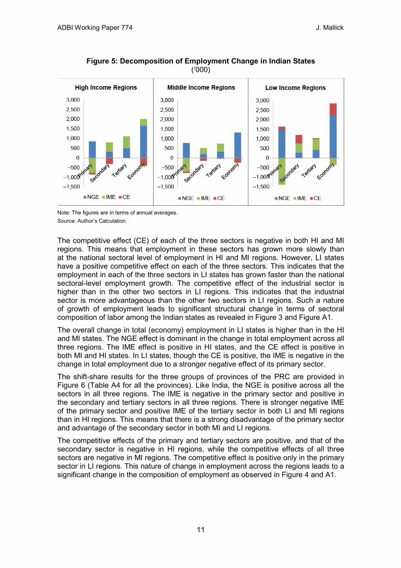
Figure 5: Decomposition of Employment Change in Indian States (‘000)
Note: The figures are in terms of annual averages. Source: Author’s Calculation.
The competitive effect (CE) of each of the three sectors is negative in both HI and MI regions. This means that employment in these sectors has grown more slowly than at the national sectoral level of employment in HI and MI regions. However, LI states have a positive competitive effect on each of the three sectors. This indicates that the employment in each of the three sectors in LI states has grown faster than the national sectoral-level employment growth. The competitive effect of the industrial sector is higher than in the other two sectors in LI regions. This indicates that the industrial sector is more advantageous than the other two sectors in LI regions. Such a nature of growth of employment leads to significant structural change in terms of sectoral composition of labor among the Indian states as revealed in Figure 3 and Figure A1. The overall change in total (economy) employment in LI states is higher than in the HI and MI states. The NGE effect is dominant in the change in total employment across all three regions. The IME effect is positive in HI states, and the CE effect is positive in both MI and HI states. In LI states, though the CE is positive, the IME is negative in the change in total employment due to a stronger negative effect of its primary sector. The shift-share results for the three groups of provinces of the PRC are provided in Figure 6 (Table A4 for all the provinces). Like India, the NGE is positive across all the sectors in all three regions. The IME is negative in the primary sector and positive in the secondary and tertiary sectors in all three regions. There is stronger negative IME of the primary sector and positive IME of the tertiary sector in both LI and MI regions than in HI regions. This means that there is a strong disadvantage of the primary sector and advantage of the secondary sector in both MI and LI regions. The competitive effects of the primary and tertiary sectors are positive, and that of the secondary sector is negative in HI regions, while the competitive effects of all three sectors are negative in MI regions. The competitive effect is positive only in the primary sector in LI regions. This nature of change in employment across the regions leads to a significant change in the composition of employment as observed in Figure 4 and A1.
11
ADBI Working Paper 774 J. Mallick
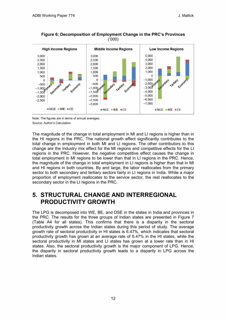
Figure 6: Decomposition of Employment Change in the PRC’s Provinces (‘000)
Note: The figures are in terms of annual averages. Source: Author’s Calculation.
The magnitude of the change in total employment in MI and LI regions is higher than in the HI regions in the PRC. The national growth effect significantly contributes to the total change in employment in both MI and LI regions. The other contributors to this change are the industry mix effect for the MI regions and competitive effects for the LI regions in the PRC. However, the negative competitive effect causes the change in total employment in MI regions to be lower than that in LI regions in the PRC. Hence, the magnitude of the change in total employment in LI regions is higher than that in MI and HI regions in both countries. By and large, the labor reallocates from the primary sector to both secondary and tertiary sectors fairly in LI regions in India. While a major proportion of employment reallocates to the service sector, the rest reallocates to the secondary sector in the LI regions in the PRC.
5. STRUCTURAL CHANGE AND INTERREGIONAL PRODUCTIVITY GROWTH
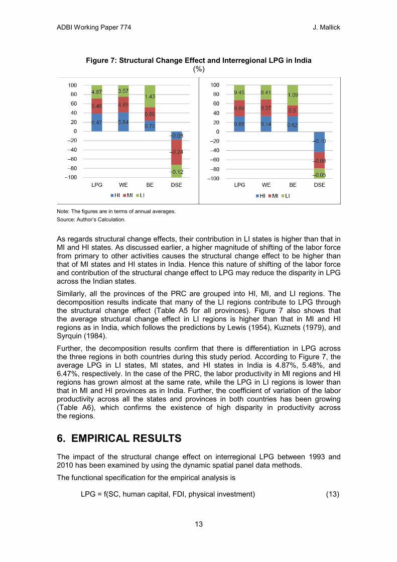
The LPG is decomposed into WE, BE, and DSE in the states in India and provinces in the PRC. The results for the three groups of Indian states are presented in Figure 7 (Table A4 for all states). This confirms that there is a disparity in the sectoral productivity growth across the Indian states during this period of study. The average growth rate of sectoral productivity in HI states is 6.47%, which indicates that sectoral productivity growth has grown at an average rate of 6.47% in the HI states, while the sectoral productivity in MI states and LI states has grown at a lower rate than in HI states. Also, the sectoral productivity growth is the major component of LPG. Hence, the disparity in sectoral productivity growth leads to a disparity in LPG across the Indian states.
12
ADBI Working Paper 774 J. Mallick
Figure 7: Structural Change Effect and Interregional LPG in India (%)
Note: The figures are in terms of annual averages. Source: Author’s Calculation.
As regards structural change effects, their contribution in LI states is higher than that in MI and HI states. As discussed earlier, a higher magnitude of shifting of the labor force from primary to other activities causes the structural change effect to be higher than that of MI states and HI states in India. Hence this nature of shifting of the labor force and contribution of the structural change effect to LPG may reduce the disparity in LPG across the Indian states. Similarly, all the provinces of the PRC are grouped into HI, MI, and LI regions. The decomposition results indicate that many of the LI regions contribute to LPG through the structural change effect (Table A5 for all provinces). Figure 7 also shows that the average structural change effect in LI regions is higher than that in MI and HI regions as in India, which follows the predictions by Lewis (1954), Kuznets (1979), and Syrquin (1984). Further, the decomposition results confirm that there is differentiation in LPG across the three regions in both countries during this study period. According to Figure 7, the average LPG in LI states, MI states, and HI states in India is 4.87%, 5.48%, and 6.47%, respectively. In the case of the PRC, the labor productivity in MI regions and HI regions has grown almost at the same rate, while the LPG in LI regions is lower than that in MI and HI provinces as in India. Further, the coefficient of variation of the labor productivity across all the states and provinces in both countries has been growing (Table A6), which confirms the existence of high disparity in productivity across the regions.
6. EMPIRICAL RESULTS The impact of the structural change effect on interregional LPG between 1993 and 2010 has been examined by using the dynamic spatial panel data methods. The functional specification for the empirical analysis is
LPG = f(SC, human capital, FDI, physical investment) (13)
13
ADBI Working Paper 774 J. Mallick
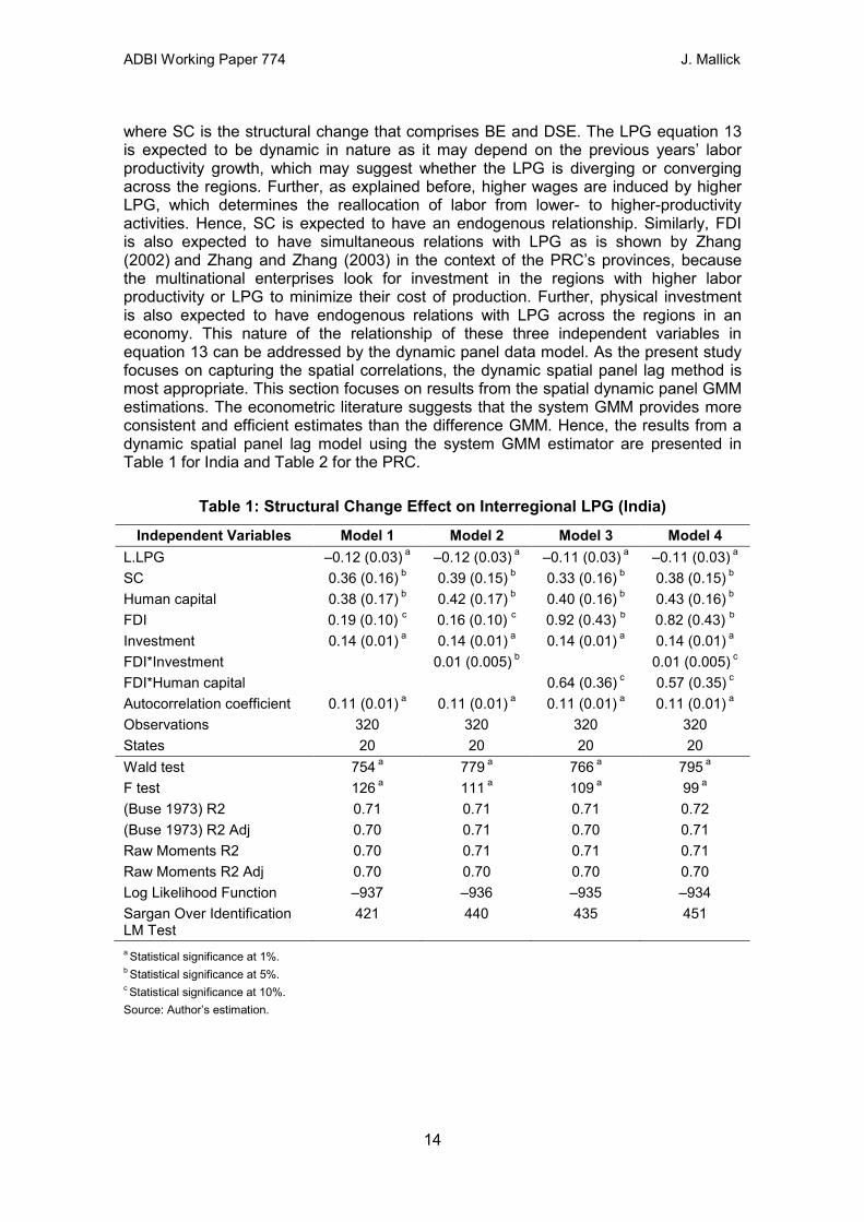
where SC is the structural change that comprises BE and DSE. The LPG equation 13 is expected to be dynamic in nature as it may depend on the previous years’ labor productivity growth, which may suggest whether the LPG is diverging or converging across the regions. Further, as explained before, higher wages are induced by higher LPG, which determines the reallocation of labor from lower- to higher-productivity activities. Hence, SC is expected to have an endogenous relationship. Similarly, FDI is also expected to have simultaneous relations with LPG as is shown by Zhang (2002) and Zhang and Zhang (2003) in the context of the PRC’s provinces, because the multinational enterprises look for investment in the regions with higher labor productivity or LPG to minimize their cost of production. Further, physical investment is also expected to have endogenous relations with LPG across the regions in an economy. This nature of the relationship of these three independent variables in equation 13 can be addressed by the dynamic panel data model. As the present study focuses on capturing the spatial correlations, the dynamic spatial panel lag method is most appropriate. This section focuses on results from the spatial dynamic panel GMM estimations. The econometric literature suggests that the system GMM provides more consistent and efficient estimates than the difference GMM. Hence, the results from a dynamic spatial panel lag model using the system GMM estimator are presented in Table 1 for India and Table 2 for the PRC.
Table 1: Structural Change Effect on Interregional LPG (India) Independent Variables Model 1 Model 2 Model 3 Model 4
L.LPG –0.12 (0.03) a –0.12 (0.03) a –0.11 (0.03) a –0.11 (0.03) a SC 0.36 (0.16) b 0.39 (0.15) b 0.33 (0.16) b 0.38 (0.15) b Human capital 0.38 (0.17) b 0.42 (0.17) b 0.40 (0.16) b 0.43 (0.16) b FDI 0.19 (0.10) c 0.16 (0.10) c 0.92 (0.43) b 0.82 (0.43) b Investment 0.14 (0.01) a 0.14 (0.01) a 0.14 (0.01) a 0.14 (0.01) a FDI*Investment 0.01 (0.005) b 0.01 (0.005) c FDI*Human capital 0.64 (0.36) c 0.57 (0.35) c Autocorrelation coefficient 0.11 (0.01) a 0.11 (0.01) a 0.11 (0.01) a 0.11 (0.01) a Observations 320 320 320 320 States 20 20 20 20 Wald test 754 a 779 a 766 a 795 a F test 126 a 111 a 109 a 99 a (Buse 1973) R2 0.71 0.71 0.71 0.72 (Buse 1973) R2 Adj 0.70 0.71 0.70 0.71 Raw Moments R2 0.70 0.71 0.71 0.71 Raw Moments R2 Adj 0.70 0.70 0.70 0.70 Log Likelihood Function –937 –936 –935 –934 Sargan Over Identification LM Test
421 440 435 451
a Statistical significance at 1%. b Statistical significance at 5%. c Statistical significance at 10%. Source: Author’s estimation.
14
ADBI Working Paper 774 J. Mallick
The results of four sets of regressions for each of the countries are provided. The first specification uses structural change and three control variables as in equation 13. The second, third, and fourth specifications use the first interaction term, the second interaction term, and both interaction terms, respectively. The first interaction term is the interaction between FDI and domestic physical investment. There could be correlation between them. If the correlation is positive (negative), it suggests a crowding-in (crowding-out) relation between FDI and the domestic physical investment. The impact of FDI is more than the domestic investment in the developing countries as argued by Graham and Krugman (1991). It is expected that a foreign firm will enjoy lower costs and higher productive efficiency than its domestic counterparts in the host country. The higher efficiency of FDI would be the result of the combination of advanced management skills and modern technologies, where the advanced technologies are transferred to developing countries mainly through FDI. The second term is the interaction between the FDI and human capital. As argued in the literature, human capital is a crucial factor of inflows of FDI across the regions within an economy. Hence, to avoid multicollinearity problems the inclusion of these interaction effects is necessary. As can be seen, the inclusion of these interaction effects has contributed to explaining the variation in LPG as reflected by the value of the log likelihood function in both countries. The results in Table 1 provide interesting findings regarding India. First, the autocorrelation coefficients for the spatial effects are found to be significant for all four models. This indicates that the states surrounded by higher-productivity growth regions are influenced positively. This is due to the spillover effect of knowledge, technological diffusion, interregional trade, migration, and capital movement etc., which are not captured in this specification. Second, the structural change effect is found to be significant in all the models with a positive sign. This indicates the significance of the structural change effect for boosting interregional LPG. Third, the study includes FDI, human capital, and physical investment as the possible factors in explaining productivity growth. The coefficients of all these control variables are statistically significant with a positive sign in all four models. This suggests that FDI, human capital, and physical investment are the important factors for the variation in LPG across the Indian states during this study period. The findings of this study corroborate several earlier findings in the context of India (Goldar, Renganathan and Banga, 2004; Kathuria, Raj and Sen 2013; Siddharthan and Lal 2004) that FDI positively affects interregional productivity growth. The inflow of FDI has boosted productivity growth by bringing new advanced technologies and management skills to India. Further, Kathuria, Raj and Sen (2013) also provide evidence to show that human capital is a crucial factor for productivity growth in the context of India. Productivity growth has a significant relationship with the quality of human capital, through the technological competence of the workforce. One and the same technology can be applied in two different firms, but the output would vary with respect to the skill or human capital of the labor force employed in these firms. Hence the nature of human capital is also crucial to productivity growth (Apergis, Economidou and Filippidid 2008; Benhabib and Speigel 1992; Romer 1990; Schultz 1975; Welch 1970). Further, other studies – with a somewhat different focus – have also found that FDI, human capital, and physical capital are crucial for the variation in economic growth across the Indian states (Mallick 2012, 2014).
15
ADBI Working Paper 774 J. Mallick
Although both FDI and physical investment are statistically significant in all the models, the differences that are found in the value of coefficients constitute one of the crucial findings of this study. For instance, the values of coefficients of FDI and investment in Model 4 are 0.82 and 0.14, respectively. This indicates that a 1% increase in the share of FDI in GDP leads to a 0.82% increase in LPG, and a 1% increase in the share of physical investment in GDP leads to an increase in LPG of 0.14%. It can be inferred, therefore, that FDI encourages the boosting of productivity growth more than physical investment. This could be due to the direct role that multinational enterprises have in the production process of local firms through both forward and backward linkage effects. Multinationals try to increase their profit by increasing the efficiency of local firms through importing their capital, advanced technologies, marketing, and managerial skills (Baldwin and Dhaliwal 2001; Baldwin and Gu 2005; Blomstrom and Kokko 1998; Globerman and Ries 1994; Rao and Tang 2005). The findings corroborate those of Mallick (2012) in the Indian states. Fourth, it is important to note that the one-year lag of labor productivity growth is statistically significant, and negative for India. This suggests that LPG is converging across the Indian states with conditioning of the spatial correlations, structural change effects, FDI, physical investment, and human capital during this study period. Fifth, the interaction effects are also statistically significant in all the models in the context of India. The coefficient of the interaction effect between FDI and investment is positive, which shows that FDI is also contributing to productivity growth indirectly by crowding in the domestic investment across the Indian states during this study period.6 The positive coefficient of the interaction effect of FDI and human capital indicates that they have positive relationships during the study period. It is worth noting that Borenzstein, Gregorio and Lee (1995) provide evidence to confirm that the interaction effects of FDI with domestic investment and human capital on the national economic growth are positive in the context of developing countries. Further, other studies with a somewhat different focus have also found an interaction effect between foreign financing and the level of human capital on economic growth. Cohen (1992) finds a positive interaction between human capital and the overall access to foreign financing of developing countries. The findings of this study may in fact provide a rationale for his finding, at least as far as the FDI component of foreign financing is concerned. Romer (1993) finds a positive effect of the interaction between secondary school enrollment and machinery imports on economic growth. While imports of machinery and equipment may be one channel for the international transmission of technological advances, FDI probably has an even larger role, as it also allows the transmission of knowledge on business practices, management techniques, etc. There are some different stories to tell about the disparity in productivity growth across the PRC’s provinces from the results in Table 2. The results do not suggest the presence of conditional convergence or divergence of LPG across the provinces, unlike India. FDI is found to be significant after controlling for interaction effect with the human capital in Model 7 and Model 8. The inflow of FDI has boosted productivity growth by bringing new advanced technologies and managerial skills to the PRC’s provinces. This finding is consistent with Biggeri (2003), Zhang and Zhang (2003), Li and Wei (2010), and Xu, Lai and Qi (2008) for the PRC in establishing a positive impact of FDI on productivity growth across provinces. The coefficients of human capital are found to be strongly statistically significant in all the models. Studies such as Zhang (2002), Xu, Lai and Qi (2008), and Wei and Hao (2011) at the provincial level in the PRC also
6 FDI can influence an economy through four channels: job creation, trade expansion, technology improvement, and economic growth promotion through capital accumulation and factors of production.
16
ADBI Working Paper 774 J. Mallick
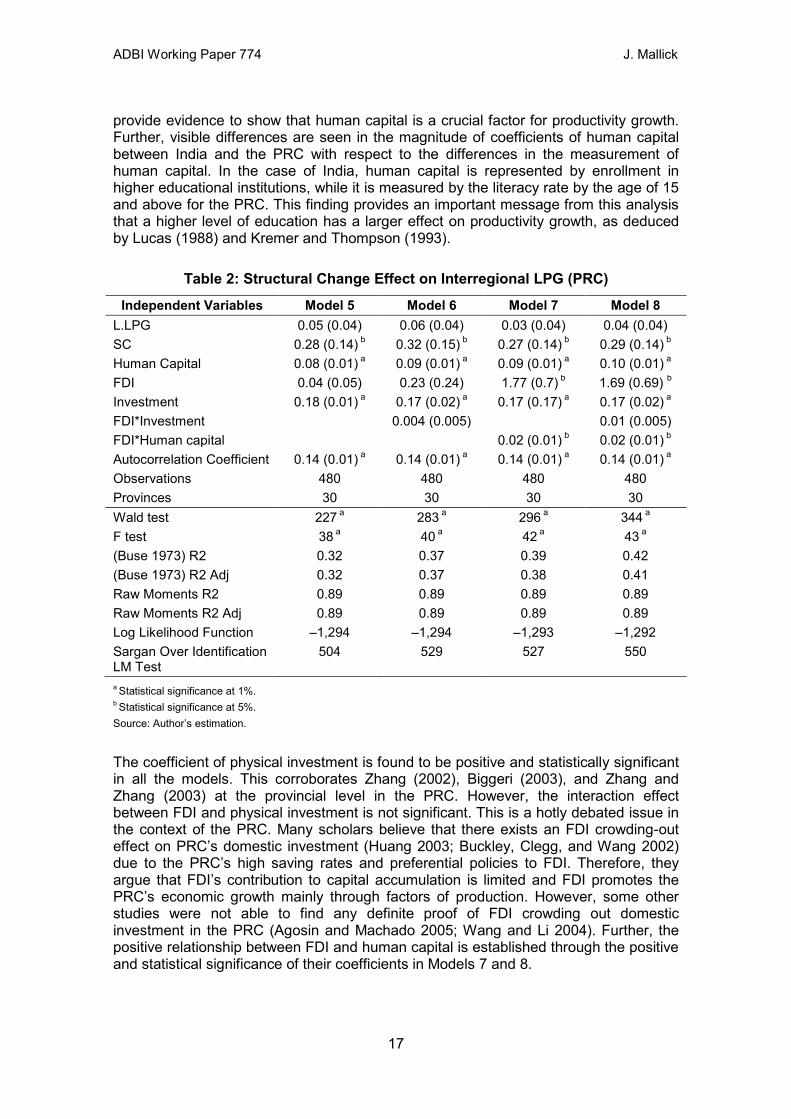
provide evidence to show that human capital is a crucial factor for productivity growth. Further, visible differences are seen in the magnitude of coefficients of human capital between India and the PRC with respect to the differences in the measurement of human capital. In the case of India, human capital is represented by enrollment in higher educational institutions, while it is measured by the literacy rate by the age of 15 and above for the PRC. This finding provides an important message from this analysis that a higher level of education has a larger effect on productivity growth, as deduced by Lucas (1988) and Kremer and Thompson (1993).
Table 2: Structural Change Effect on Interregional LPG (PRC) Independent Variables Model 5 Model 6 Model 7 Model 8
L.LPG 0.05 (0.04) 0.06 (0.04) 0.03 (0.04) 0.04 (0.04) SC 0.28 (0.14) b 0.32 (0.15) b 0.27 (0.14) b 0.29 (0.14) b Human Capital 0.08 (0.01) a 0.09 (0.01) a 0.09 (0.01) a 0.10 (0.01) a FDI 0.04 (0.05) 0.23 (0.24) 1.77 (0.7) b 1.69 (0.69) b Investment 0.18 (0.01) a 0.17 (0.02) a 0.17 (0.17) a 0.17 (0.02) a FDI*Investment 0.004 (0.005) 0.01 (0.005) FDI*Human capital 0.02 (0.01) b 0.02 (0.01) b Autocorrelation Coefficient 0.14 (0.01) a 0.14 (0.01) a 0.14 (0.01) a 0.14 (0.01) a Observations 480 480 480 480 Provinces 30 30 30 30 Wald test 227 a 283 a 296 a 344 a F test 38 a 40 a 42 a 43 a (Buse 1973) R2 0.32 0.37 0.39 0.42 (Buse 1973) R2 Adj 0.32 0.37 0.38 0.41 Raw Moments R2 0.89 0.89 0.89 0.89 Raw Moments R2 Adj 0.89 0.89 0.89 0.89 Log Likelihood Function –1,294 –1,294 –1,293 –1,292 Sargan Over Identification LM Test
504 529 527 550
a Statistical significance at 1%. b Statistical significance at 5%.
Source: Author’s estimation.
The coefficient of physical investment is found to be positive and statistically significant in all the models. This corroborates Zhang (2002), Biggeri (2003), and Zhang and Zhang (2003) at the provincial level in the PRC. However, the interaction effect between FDI and physical investment is not significant. This is a hotly debated issue in the context of the PRC. Many scholars believe that there exists an FDI crowding-out effect on PRC’s domestic investment (Huang 2003; Buckley, Clegg, and Wang 2002) due to the PRC’s high saving rates and preferential policies to FDI. Therefore, they argue that FDI’s contribution to capital accumulation is limited and FDI promotes the PRC’s economic growth mainly through factors of production. However, some other studies were not able to find any definite proof of FDI crowding out domestic investment in the PRC (Agosin and Machado 2005; Wang and Li 2004). Further, the positive relationship between FDI and human capital is established through the positive and statistical significance of their coefficients in Models 7 and 8.
17
ADBI Working Paper 774 J. Mallick
7. CONCLUSIONS AND POLICY IMPLICATIONS This paper provides an explanation for the growing regional income inequality in emerging countries, with special emphasis on the impact of the structural change effect on LPG by using a recently developed methodology in the context of India and the PRC during the period 1993–2010. I have taken into account the spatial interaction effects among the regions, which has not been considered in previous studies of the related topics. This allows me to take into consideration the role played by a number of dimensions that flow or spill over from one region to its neighbors within a country. The descriptive analysis shows that the economy as a whole and the activities in terms of reallocation of labor are shifting away from the primary sector to the secondary and service sectors in both countries. Although a higher proportion of unproductive labor force is concentrated in the LI region’s primary sector, a substantially greater number of employment reallocates from the primary sector to the nonprimary sector in the LI region than in the HI and MI regions in both countries, which results in a higher contribution of the structural change effect to LPG in the low-income regions than in the MI and HI regions. This trend is helpful for reducing regional imbalances in LPG and hence income inequalities, which in turn helps in avoiding the middle-income trap (Egawa 2013). The GMM system results from the dynamic spatial panel data show a positive association between the structural change effect and the interregional LPG in each country by controlling for physical investment, human capital, and FDI as representative of the degree of economic globalization in both countries. This conclusion still holds when the interaction terms are used as additional control variables to avoid the possible multicollinearity relations of FDI with physical investment and with human capital in the estimation. Hence, the structural change effect is crucial in reducing the regional imbalances, as it significantly explains the interregional LPG, where a higher contribution is achieved by the LI regions than the MI and HI regions. Further, the findings show that neighborhood relations are significant in explaining the interregional LPG in both countries. That means a higher LPG in one region drives LPG in its neighboring regions. The empirical analysis establishes that FDI is significant, where FDI broadly represents the degree of economic globalization. Based on the results of the study, regions with a greater degree of economic globalization or integration with the rest of the world, everything else being equal, have higher LPG. This is potentially important, since the level of international market integration in many emerging countries still has large potential to grow. The results of this paper provide an additional contribution to the debate by emphasizing the impact of economic globalization and integration on interregional LPG, and hence income inequality within a country. However, one of the limitations of the study is that only FDI is used to represent the degree of economic globalization without considering international trade.7 The rising regional inequality in LPG leads to regional income inequalities and presents huge challenges to social and economic stability, which may push India and the PRC into the middle-income trap. The empirical results of the study provide the following policy implications for reducing regional disparities:
7 Due to the unavailability of data on trade at the state level in India, the study is restricted to the use of only FDI to represent the degree of economic globalization and integration.
18
ADBI Working Paper 774 J. Mallick
• The findings show that human capital is significant in explaining the interregional LPG in both countries. Hence, to ensure and achieve higher labor productivity, the relevant policies related to knowledge must be pursued with a view to providing incentive and encouraging investments in human capital, technology, and innovations in the entire country. A special consideration should be given to encouraging and promoting them in the lagging regions.
• Further, globalization will lead to higher regional inequality in India and the PRC unless concerted efforts are devoted to promoting FDI flows and trade in the lagging regions. The FDI inflow brings advanced technology and expertise from the country of origin, and helps in enhancing labor productivity in the hosting regions. The formulation of more and more outward-oriented policies would further enhance productivity. Hence, special promotional policies should be designed to encourage FDI flows and trade in the lagging regions as they are in a disadvantageous position with respect to market potential and location considerations. A converging trend in these will help in reducing regional inequalities.
• With regard to the lagging regions, the incentive policies for the promotion of FDI and human capital should be redesigned by coordinating governments at both local and national levels.
• Also, the equalization of domestic capital across regions will reduce regional inequality. To narrow down the gaps in capital possession, it is necessary, though difficult, to break the vicious circle existing in capital formation. This calls for the development of a financial market, especially in poor rural areas. Again, policy support for investment in poorer regions is needed in terms of tax concessions and bank lending.
• In addition to the direct policy measures aimed at boosting LPG, further policy measures should be taken to increase the contributions due to the reallocation of the labor effect. A larger proportion of the unproductive labor force of the lagging regions is concentrated in the agricultural sector, which is mainly in rural areas. However, there are certain restrictions on migration in some of the emerging countries, for instance the hukou system in the PRC. Hence, restrictions on migration with regard to both location and sector should be lifted and rural-urban migration encouraged, which will transfer the labor force from low- to high-productivity activities. Labor mobility can be facilitated through the establishment of various labor market institutions.
Structural change not only increases productivity growth, it also reduces poverty by pushing up the wage rate in the agricultural sector (Hasan, Lamba and Gupta 2013). A huge proportion of workers is concentrated mainly in the agricultural sector in the low-income regions. The reallocation of labor from agriculture to nonagriculture increases the wage rate of the laborers who move to the nonagricultural sector, and also those who remain working in the agricultural sector. International trade and infrastructure are also crucial for promoting both domestic and foreign investment, and hence LPG. Therefore, integrated domestic markets should be promoted by removing interregional trade barriers in the lagging regions. Further, financial assistance and administrative help should be provided to develop public infrastructure such as highways and telecommunication networks in the lagging regions.
19
ADBI Working Paper 774 J. Mallick
REFERENCES Abramovitz, M. (1986). Catching up, forging ahead and falling behind. Journal of
Economic History, 46(2): 385–406. Agosin, M.R., and R. Machado. (2005). Foreign investment in developing countries:
Does it crowd in domestic investment? Oxford Development Studies, 33(2): 149–162.
Aiyar, S., R. Duval, D. Puy, Y. Wu, and L. Zhang (2013). Growth slowdowns and the middle-income trap. IMF Working Paper 13/71. International Monetary Fund, Washington, D.C.
Anselin L., and Bera A.K. (1998). Spatial dependence in linear regression models with an introduction to spatial econometrics. In: Hullah, A. and Gelis, D.E.A. (eds). Handbook of Applied Economic Statistics, Marcel Deker, New York, pp. 237–290.
Apergis, N., C. Economidou, and I. Filippidis. (2008). Innovation technology transfer and labor productivity linkages: Evidence from a panel of manufacturing industries. Review of World Economics, 144(3): 491–508.
Arellano, M., and S. Bond. (1991). Some tests of specification for panel data: Monte Carlo evidence and an application to employment equations. Review of Economic Studies, 58(2): 277–297.
Arellano M., and O. Bover, (1995). Another look at the instrumental-variable estimation of error: Components models. Journal of Econometrics, 68(1): 29–51.
Asian Development Bank (ADB). (2011). Asia 2050: Realizing the Asian Century. Manila.
Ashby, L. D. (1970). Changes in regional industrial structure: A comment. Urban Studies, l(3): 298–304.
Baldwin, J. R., and N. Dhaliwal. (2001). Heterogeneity in Labour Productivity Growth in Manufacturing: Differences between Domestic and Foreign-Controlled Establishments. Productivity Growth in Canada. Statistics Canada, Ottawa.
Baldwin, J. R., and W. Gu. (2005). Global Links: Multinationals, Foreign Ownership and Productivity Growth in Canadian Manufacturing. Statistics Canada, Micro Economic Studies and Analysis Division, Ottawa, Canada.
Baltagi, B. H. (2001). Econometric Analysis of Panel Data. West Sussex PO191UD, John Wiley & Sons, Ltd., England.
Baltagi, B. H., B. Fingleton, and A. Pirotte. (2014). Estimating and forecasting with a dynamic spatial panel data model. Oxford Bulletin of Economics and Statistics, 76(1): 112–138.
Beck, T., R. Levine, and N. Loayza. (2000). Financial development and the sources of growth. Journal of Financial Economics, 58 (1-2): 261-300
Benhabib, J., and M. M. Speigel (1992). The Role of Human Capital in Economic Development: Evidence from Aggregate Cross-Country and Regional US Data. Department of Economics, New York University.
Biggeri, Mario. (2003). Key factors of recent Chinese provincial economic growth. Journal of Chinese Economics and Business Studies, 1: 159–183.
20
ADBI Working Paper 774 J. Mallick
Blomstrom, M., and A. Kokko. (1998). Multinational corporations and spillovers. Journal of Economic Surveys, 12(3): 247–277.
Blundell, R., and S. Bond. (1998). Initial conditions and moment restrictions in dynamic panel data models. Journal of Econometrics, 87(1): 115–43.
Borenzstein, E., J. Gregorio, and J. Lee. (1995). How does foreign direct investment affect economic growth? NBER Working Paper, No. 5057.
Brandt, L., C. Hsieh, X. Zhu. (2008). Growth and structural transformation in China. In Brandt, L. and Rawski, T. (eds). China’s Great Economic Transformation. Cambridge University Press, pp. 569–632.
Buckley, P. J., J. Clegg, and C. Wang (2002). The impact of inward of FDI on the performance of Chinese manufacturing firms. Journal of International Business Studies, 33(4): 637–655.
Candelaria, C., M. Daly, and G. Hale. (2013). Persistence of regional inequality in China. Working Paper 2013-06, Federal Reserve Bank of San Francisco.
Cohen, D. (1992). Foreign finance and economic growth: An empirical analysis. In Leiderman and Razin (eds). Capital Mobility. CEPR and Cambridge University Press.
de Vries, G. J., A. A. Erumban, M. P. Timmer, I. Voskoboynikov, and H. X. Wu. (2012). Deconstructing the BRICs: Structural transformation and aggregate productivity growth. Journal of Comparative Economics, 40, 211–227.
Driffield, N., and M. Munday. (2002). Foreign direct investment, transactions linkages and the performance of the domestic sector. International Journal of the Economics of Business, 9(3): 335–351.
Dunn, E. S., Jr. (1960). A Statistical and Analytical Technique for Regional Analysis. Papers and Proceedings of the Regional Science Association, 97–112.
Egawa, A. (2013). Will income inequality cause a middle-income trap in Asia? Bruegel Working Paper 2013/06, October 9, 2013, Brussels, Belgium.
Eichengreen, B, P. D. Park and K. Shin (2011). When fast growing economies slow down: International evidence and implication for China. NBER Working Paper, 16919.
Ezcurra, R., and A. Rodríquez-Pose. (2013). Does economic globalization affect regional inequality? A cross-country analysis. World Development, 52: 92–103.
Fuchs, V. R. (1959). Changes in the location of US manufacturing since 1929. Journal of Regional Science, 1(2): 1–17.
Fukao K., and T. Yuan (2012). China’s economic growth, structural change and the Lewisian turning point. Hitotsubashi Journal of Economics, 53(2): 147–176.
Globerman, S., and J. Ries, (1994). The economic performance of foreign affiliates in Canada. Canadian Journal of Economics, 27: 143–156.
Goldar, B. N., V. S. Renganathan, and Rashmi Banga. (2004). Ownership and efficiency in engineering firms: 1990–91 to 1999–2000. Economic and Political Weekly, January 31: 441–447.
Graham, E., and P. Krugman. (1991). Foreign Direct Investment in the United States, Institute for International Economics, Washington DC.
Greene, W. H. (2006). Econometric Analysis, 5th ed., Dorling Kindersley (India) Pvt Ltd.
21
ADBI Working Paper 774 J. Mallick
Hale, G., and C. Long. (2007). Is there evidence of FDI spillover on Chinese firms’ productivity and innovation? Yale University Economic Growth Center Discussion Paper No. 934.
Hasan, R., S. Lamba, and A. S. Gupta. (2013). Growth, structural change, and poverty reduction: Evidence from India. ADB South Asia Working Paper Series, No. 22, November.
Havlik, P. (2005). Structural change, productivity and employment in the new EU member states. WIIW Research Report, No. 313, Vienna Institute for International Economic Studies.
Herzog, H., Jr., and Olsen, R. (1997). Shift-share analysis revisited: The allocation effect and the stability of regional structure. Journal of Regional Science, 17(December): 441–454.
Huang, Y., ed. (2003). Selling China: Foreign Direct Investment During the Reform Era. Cambridge University Press, New York.
Islam, S. N. (2015). Will inequality lead China to the middle income trap? DESA Working Paper No. 142.
Kathuria, V., S. R. Raj, and K. Sen. (2013). Impact of human capital on manufacturing productivity growth in India. In Siddharthan N. and Narayanan K. (eds). Human Capital and Development: The Indian Experience, 2nd ed., pp. 23–37. Springer, New Delhi.
Kremer, M., and J. Thompson. (1993). Why Isn’t Convergence Instantaneous? Mimeo, Harvard University.
Kuznets, S. (1979). “Growth and Structural Shifts.” In http://catalogue.nla.gov.au/ Record/999370 edited by W. Galenson. Ithaca, New York: Cornell University Press.
Lewis, W. A. (1954). Economic Development with Unlimited Supplies of Labour. The Manchester School, 22, 139–191.
Li, Xiaoying and X. Liu. (2005). Foreign direct investment and economic growth: An increasingly endogenous relationship. World Development, 33(3): 393-407.
Li, Y., and Y. H. D. Wei. (2010). The Spatial-Temporal Hierarchy of Regional Inequality of China. Applied Geography. 30: 303–316.
Lucas, R. (1988). On the mechanics of economic development. Journal of Monetary Economics, 22: 3–42.
Mallick, J. (2012). Private investment in ICT sector of Indian States. Indian Economic Review, 47(1): 33–56.
———. (2013a). Private investment in India: Regional patterns and determinant. Annals of Regional Science, 51(2): 515–536.
———. (2013b), Public expenditure, private investment and States income in India. Journal of Developing Areas, 47(1): 181–205.
———. (2014). Regional convergence of economic growth during post-reform period in India. The Singapore Economic Review, 59(2): 1450012-1-1450012-18
———. (2015a) Globalisation, structural change and productivity growth in the emerging countries. Indian Economic Review, 50(2): 181-216.
22
ADBI Working Paper 774 J. Mallick
———. (2015b). Private investment and income disparity across Indian states: Ideas for India. London School of Economics, International Growth Center, http://www.ideasforindia.in/article. aspx?article_id=1459, June 3.
———. (2017). Structural change and productivity growth in the emerging countries. ADBI Working Paper No.656, Asia Development Bank Institute (ADBI), Tokyo.
McMillan, M., and D. Rodrik. (2011). Globalization, structural change, and productivity growth. NBER Working Paper 17143, NBER, Cambridge.
Perloff, H. S., E. S. Dunn, Jr., R. E. Lampanl, and R. F. Muth. (1960). Regions, Resources and Economic Growth. The Johns Hopkins Press, Baltimore.
Rao, S., and J. Tang. (2005). Foreign ownership and total factor productivity. In L. Eden and W. Dobson (eds), Governance, Multinationals and Growth, Cheltenham, UK and Northampton, MA, US: Edward Elgar, pp. 100–124
Romer, P. (1993). Idea gaps and object gaps in economic development. Journal of Monetary Economics, 32: 543–573.
Romer, P. M. (1990). Endogenous technical change. Journal of Political Economy, 98(2), Part 2: S71–102.
Schultz, T. W. (1975). The value of the ability to deal with disequilibrium. Journal of Economic Literature, 13: 827–846.
Siddharthan, N. S., and K. Lal. (2004). Liberalisation, MNE and productivity of Indian enterprises. Economic and Political Weekly, January 31: 448–52.
Sivasubramonian, S. (2004). The Sources of Economic Growth in India. 1950–51 to 1999–2000. Oxford University Press, New Delhi.
Syrquin, M. (1984). Resource reallocation and productivity growth. In Syrquin M., Taylor L. and. Westphal L. E. (eds). Economic Structure and Performance, Academic Press, New York.
———. (1988). Patterns of structural change. In Chenery Hollis B. and Srinivasan T. N. (eds). Handbook of Development Economics, Vol. I, pp. 203–273, Elsevier, Amsterdam, North-Holland.
Temple J. (2001). Structural change and Europe’s golden age. Centre for Economic Policy Research, Discussion Paper No. 2861, June.
Visaria, P. (2002). Workforce and employment in India, 1961–94. In Minhas B.S. (ed.). National Income Accounts and Data Systems, Oxford University Press, New Delhi.
Wan, G. H., M. Lu, and Z. Chen. (2007). Globalization and regional inequality: Evidence from within China. Review of Income and Wealth, 53(1): 35–59.
Wang, Z., and Z. Li. (2004). Re-examine the crowd in or crowd out effects of FDI on domestic investment. Statistical Research, July: 37–43.
Wei, Z., and R. Hao. (2011). The role of human capital in China’s total factor productivity growth: A cross-province analysis. The Developing Economies, 49(1): 1–35.
Welch, F. (1970). Education and production. Journal of Political Economy, 7(8): 35–59. Xu, H., M. Lai, and P. Qi. (2008). Openness, human capital and total factor productivity
evidence from China. Journal of Chinese Economic and Business Studies, 6(3): 279–289.
23

ADBI Working Paper 774 J. Mallick
Zhang, X., and K. Zhang. (2003). How does globalization affect regional inequality within a developing country? Evidence from China. The Journal of Development Studies, 39: 47–67.
Zhang, Z. Y. (2002). Productivity and economic growth: An empirical assessment of the contribution of FDI to the Chinese economy. Journal of Economic Development, 27(2): 81–94.
24
ADBI Working Paper 774 J. Mallick
APPENDIX A Measurement of State-wise Employment in India
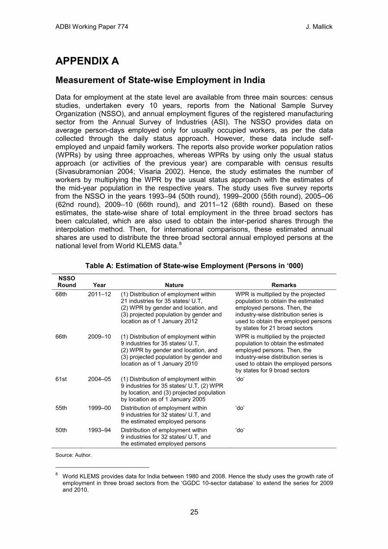
Data for employment at the state level are available from three main sources: census studies, undertaken every 10 years, reports from the National Sample Survey Organization (NSSO), and annual employment figures of the registered manufacturing sector from the Annual Survey of Industries (ASI). The NSSO provides data on average person-days employed only for usually occupied workers, as per the data collected through the daily status approach. However, these data include self-employed and unpaid family workers. The reports also provide worker population ratios (WPRs) by using three approaches, whereas WPRs by using only the usual status approach (or activities of the previous year) are comparable with census results (Sivasubramonian 2004; Visaria 2002). Hence, the study estimates the number of workers by multiplying the WPR by the usual status approach with the estimates of the mid-year population in the respective years. The study uses five survey reports from the NSSO in the years 1993–94 (50th round), 1999–2000 (55th round), 2005–06 (62nd round), 2009–10 (66th round), and 2011–12 (68th round). Based on these estimates, the state-wise share of total employment in the three broad sectors has been calculated, which are also used to obtain the inter-period shares through the interpolation method. Then, for international comparisons, these estimated annual shares are used to distribute the three broad sectoral annual employed persons at the national level from World KLEMS data.8
Table A: Estimation of State-wise Employment (Persons in ‘000) NSSO Round Year Nature Remarks
68th 2011–12 (1) Distribution of employment within 21 industries for 35 states/ U.T, (2) WPR by gender and location, and (3) projected population by gender and location as of 1 January 2012
WPR is multiplied by the projected population to obtain the estimated employed persons. Then, the industry-wise distribution series is used to obtain the employed persons by states for 21 broad sectors
66th 2009–10 (1) Distribution of employment within 9 industries for 35 states/ U.T, (2) WPR by gender and location, and (3) projected population by gender and location as of 1 January 2010
WPR is multiplied by the projected population to obtain the estimated employed persons. Then, the industry-wise distribution series is used to obtain the employed persons by states for 9 broad sectors
61st 2004–05 (1) Distribution of employment within 9 industries for 35 states/ U.T, (2) WPR by location, and (3) projected population by location as of 1 January 2005
‘do’
55th 1999–00 Distribution of employment within 9 industries for 32 states/ U.T, and the estimated employed persons
‘do’
50th 1993–94 Distribution of employment within 9 industries for 32 states/ U.T, and the estimated employed persons
‘do’
Source: Author.
8 World KLEMS provides data for India between 1980 and 2008. Hence the study uses the growth rate of employment in three broad sectors from the ‘GGDC 10-sector database’ to extend the series for 2009 and 2010.
25
ADBI Working Paper 774 J. Mallick
Measurement of State-wise Capital Stock in India
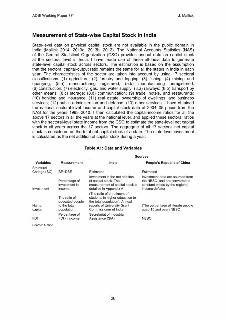
State-level data on physical capital stock are not available in the public domain in India (Mallick 2014, 2013a, 2013b, 2012). The National Accounts Statistics (NAS) of the Central Statistical Organization (CSO) provides annual data on capital stock at the sectoral level in India. I have made use of these all-India data to generate state-level capital stock across sectors. The estimation is based on the assumption that the sectoral capital-output ratio remains the same for all the states in India in each year. The characteristics of the sector are taken into account by using 17 sectoral classifications: (1) agriculture; (2) forestry and logging; (3) fishing; (4) mining and quarrying; (5.a) manufacturing registered; (5.b) manufacturing unregistered; (6) construction; (7) electricity, gas, and water supply; (8.a) railways; (8.b) transport by other means; (8.c) storage; (8.d) communication; (9) trade, hotels, and restaurants; (10) banking and insurance; (11) real estate, ownership of dwellings, and business services; (12) public administration and defense; (13) other services. I have obtained the national sectoral-level income and capital stock data at 2004–05 prices from the NAS for the years 1993–2010. I then calculated the capital-income ratios for all the above 17 sectors in all the years at the national level, and applied these sectoral ratios with the sectoral-level state income from the CSO to estimate the state-level net capital stock in all years across the 17 sectors. The aggregate of all 17 sectors’ net capital stock is considered as the total net capital stock of a state. The state-level investment is calculated as the net addition of capital stock during a year.
Table A1: Data and Variables
Variables Measurement
Sources
India People’s Republic of China Structural Change (SC) BE+DSE Estimated Estimated
Investment
Percentage of investment in income
Investment is the net addition of capital stock. The measurement of capital stock is detailed in Appendix A
Investment data are sourced from the NBSC, and are converted to constant prices by the regional income deflator
Human capital
The ratio of educated people to the total population
(The ratio of enrollment of students in higher education to the total population). Annual reports of University Grant Commissioner of India
(The percentage of literate people aged 15 and over) NBSC
FDI Percentage of FDI in income
Secretariat of Industrial Assistance (SIA) NBSC
Source: Author.
26
ADBI Working Paper 774 J. Mallick
Table A2: Decomposition of Regional Employment Change (‘000’) in Indian States (major 20)
States Primary Secondary Tertiary Income
Level NGE IME CE NGE IME CE NGE IME CE Delhi 1.0 –0.8 –4.9 16.3 24.5 –24.3 37.6 47.9 21.7 HI Gujarat 170.8 –154.5 97.3 48.8 75.6 –55.8 66.4 84.0 10.5 HI Haryana 52.5 –49.1 22.4 18.6 31.0 19.1 29.0 36.7 –6.7 HI Kerala 61.2 –55.1 –117 36.5 55.9 –43.2 58.2 72.9 –0.1 HI Maharashtra 316.0 –287.4 124.3 83.7 128.8 –104 153.9 193.4 50.7 HI Punjab 63.4 –57.5 –14.2 22.3 36.3 23.6 36.7 45.7 –10.1 HI Tamil Nadu 186.4 –165.2 –182 88.6 132.5 –117 105.6 131.3 –79.4 HI Andhra Pradesh 312.7 –278.7 –148 66.8 103.2 –53.8 117.9 146.3 –41.5 MI Himachal Pradesh 27.4 –24.9 –14.1 6.0 9.7 3.2 6.4 8.1 4.1 MI Karnataka 203.5 –183.6 –37.2 41.7 63.4 –48.7 70.1 89.1 46.3 MI Uttarakhand 28.7 –26.4 –8.4 4.6 7.7 13.6 8.5 10.8 12.5 MI West Bengal 185.0 –169.1 121.9 82.0 123.4 –78.5 113.6 145.3 –51.7 MI Assam 75.6 –71.9 36.4 7.4 11.6 10.1 33.2 40.2 8.8 LI Bihar 206.5 –192.9 19.8 19.9 34.7 103.8 50.8 68.6 47.5 LI Chhattisgarh 97.3 –92.1 26.8 9.4 15.3 2.1 15.7 20.3 3.8 LI Jharkhand 77.1 –71.2 –51.3 17.6 29.9 39.5 19.6 26.5 22.1 LI Manipur 5.8 –5.3 –1.7 1.2 1.8 1.5 2.4 3.2 –1.3 LI Odisha 137.9 –124.3 –38.7 29.1 47.2 13.8 35.4 44.6 3.9 LI Rajasthan 191.9 –176.2 –42.4 48.8 79.8 68.0 51.2 66.3 24.6 LI Uttar Pradesh 461.6 –426.0 116.0 115.9 188.2 143.0 163.1 204.3 –71.5 LI
Note: The figures in the table are in terms of annual averages. Source: Author’s calculation.
27
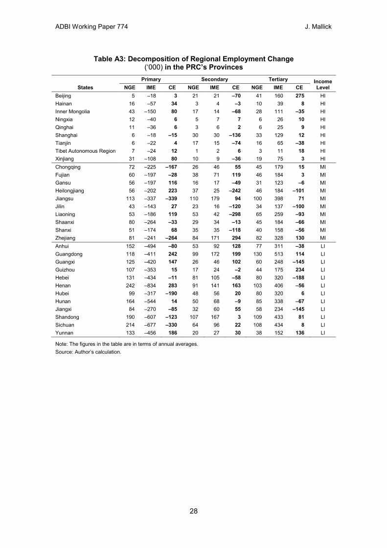
ADBI Working Paper 774 J. Mallick
Table A3: Decomposition of Regional Employment Change (‘000) in the PRC’s Provinces
States Primary Secondary Tertiary Income
Level NGE IME CE NGE IME CE NGE IME CE Beijing 5 –18 3 21 21 –70 41 160 275 HI Hainan 16 –57 34 3 4 –3 10 39 8 HI Inner Mongolia 43 –150 80 17 14 –68 28 111 –35 HI Ningxia 12 –40 6 5 7 7 6 26 10 HI Qinghai 11 –36 6 3 6 2 6 25 9 HI Shanghai 6 –18 –15 30 30 –136 33 129 12 HI Tianjin 6 –22 4 17 15 –74 16 65 –38 HI Tibet Autonomous Region 7 –24 12 1 2 6 3 11 18 HI Xinjiang 31 –108 80 10 9 –36 19 75 3 HI Chongqing 72 –225 –167 26 46 55 45 179 15 MI Fujian 60 –197 –28 38 71 119 46 184 3 MI Gansu 56 –197 116 16 17 –49 31 123 –6 MI Heilongjiang 56 –202 223 37 25 –242 46 184 –101 MI Jiangsu 113 –337 –339 110 179 94 100 398 71 MI Jilin 43 –143 27 23 16 –120 34 137 –100 MI Liaoning 53 –186 119 53 42 –298 65 259 –93 MI Shaanxi 80 –264 –33 29 34 –13 45 184 –66 MI Shanxi 51 –174 68 35 35 –118 40 158 –56 MI Zhejiang 81 –241 –264 84 171 294 82 328 130 MI Anhui 152 –494 –80 53 92 128 77 311 –38 LI Guangdong 118 –411 242 99 172 199 130 513 114 LI Guangxi 125 –420 147 26 46 102 60 248 –145 LI Guizhou 107 –353 15 17 24 –2 44 175 234 LI Hebei 131 –434 –11 81 105 –58 80 320 –188 LI Henan 242 –834 283 91 141 163 103 406 –56 LI Hubei 99 –317 –190 48 56 20 80 320 6 LI Hunan 164 –544 14 50 68 –9 85 338 –67 LI Jiangxi 84 –270 –85 32 60 55 58 234 –145 LI Shandong 190 –607 –123 107 167 3 109 433 81 LI Sichuan 214 –677 –330 64 96 22 108 434 8 LI Yunnan 133 –456 186 20 27 30 38 152 136 LI
Note: The figures in the table are in terms of annual averages. Source: Author’s calculation.
28
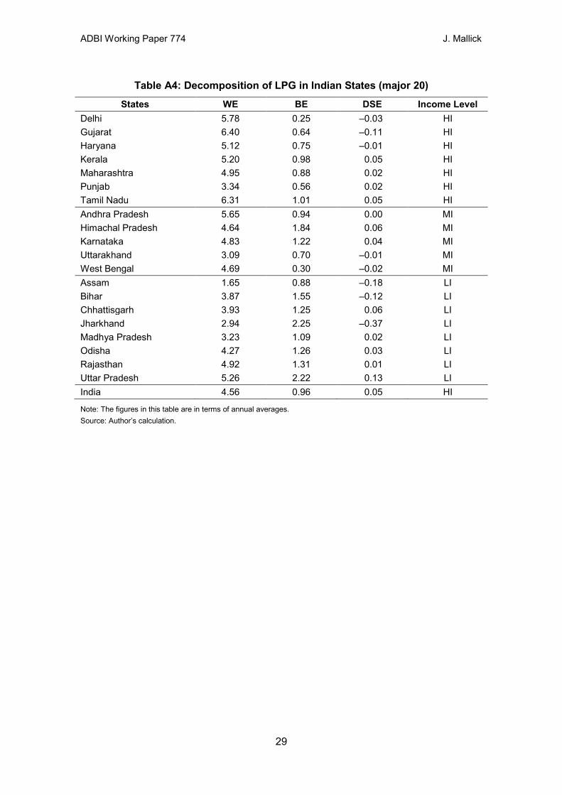
ADBI Working Paper 774 J. Mallick
Table A4: Decomposition of LPG in Indian States (major 20) States WE BE DSE Income Level
Delhi 5.78 0.25 –0.03 HI Gujarat 6.40 0.64 –0.11 HI Haryana 5.12 0.75 –0.01 HI Kerala 5.20 0.98 0.05 HI Maharashtra 4.95 0.88 0.02 HI Punjab 3.34 0.56 0.02 HI Tamil Nadu 6.31 1.01 0.05 HI Andhra Pradesh 5.65 0.94 0.00 MI Himachal Pradesh 4.64 1.84 0.06 MI Karnataka 4.83 1.22 0.04 MI Uttarakhand 3.09 0.70 –0.01 MI West Bengal 4.69 0.30 –0.02 MI Assam 1.65 0.88 –0.18 LI Bihar 3.87 1.55 –0.12 LI Chhattisgarh 3.93 1.25 0.06 LI Jharkhand 2.94 2.25 –0.37 LI Madhya Pradesh 3.23 1.09 0.02 LI Odisha 4.27 1.26 0.03 LI Rajasthan 4.92 1.31 0.01 LI Uttar Pradesh 5.26 2.22 0.13 LI India 4.56 0.96 0.05 HI Note: The figures in this table are in terms of annual averages. Source: Author’s calculation.
29

ADBI Working Paper 774 J. Mallick
Table A5: Decomposition of Interregional LPG in the PRC’s Provinces Provinces WE BE DSE Income Level
Beijing 8.77 0.45 –0.16 HI Hainan 5.98 0.12 –0.02 HI Inner Mongolia 10.27 0.18 –0.11 HI Ningxia 9.97 1.52 –0.02 HI Qinghai 8.65 1.30 –0.01 HI Shanghai 9.74 0.23 –0.18 HI Tianjin 11.58 0.03 –0.07 HI Tibet Autonomous Region 4.31 2.70 –0.13 HI Xinjiang 9.82 0.17 –0.12 HI Anhui 7.97 1.19 0.02 LI Guangdong 7.20 0.73 –0.03 LI Guangxi 7.51 1.17 –0.33 LI Guizhou 7.83 1.47 –0.12 LI Hebei 9.47 0.79 –0.06 LI Henan 8.59 1.09 –0.01 LI Hubei 9.09 0.72 –0.11 LI Hunan 9.38 0.89 0.02 LI Jiangxi 9.80 0.82 –0.04 LI Shandong 8.65 1.16 0.03 LI Sichuan 8.57 1.17 0.03 LI Yunnan 6.82 1.87 0.00 LI Chongqing 8.63 1.59 0.05 MI Fujian 7.48 1.10 –0.16 MI Gansu 9.36 0.41 –0.03 MI Heilongjiang 10.72 –0.86 –0.35 MI Jiangsu 8.45 0.98 –0.01 MI Jilin 10.84 –0.02 –0.16 MI Liaoning 9.79 –0.25 –0.19 MI Shaanxi 9.75 1.35 0.00 MI Shanxi 11.03 0.40 –0.03 MI Zhejiang 7.69 1.26 0.04 MI All 8.59 0.98 0.04
Note: The figures are in terms of annual averages. Source: Author’s calculation.
30
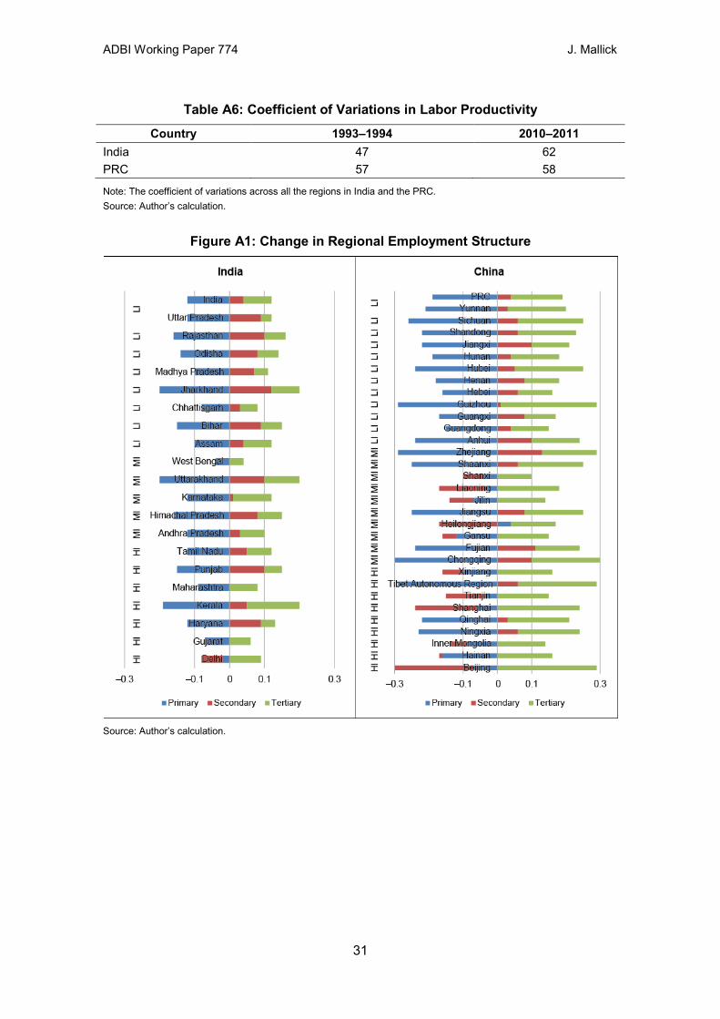
ADBI Working Paper 774 J. Mallick
Table A6: Coefficient of Variations in Labor Productivity Country 1993–1994 2010–2011
India 47 62 PRC 57 58
Note: The coefficient of variations across all the regions in India and the PRC. Source: Author’s calculation.
Figure A1: Change in Regional Employment Structure
Source: Author’s calculation.
31