ASK THE MUTANTSMUTATING FAULTY PROGRAMS FOR FAULT LOCALISATION

Shin Yoo, University College London Seokhyun Mun, KAIST

Yunho Kim, KAIST Moonzoo Kim, KAIST

OUTLINE

• MUSE: Mutation-based Fault Localisation Engine

• Locality Information Loss: a new evaluation metric

• Ongoing work (post ICST 2014)

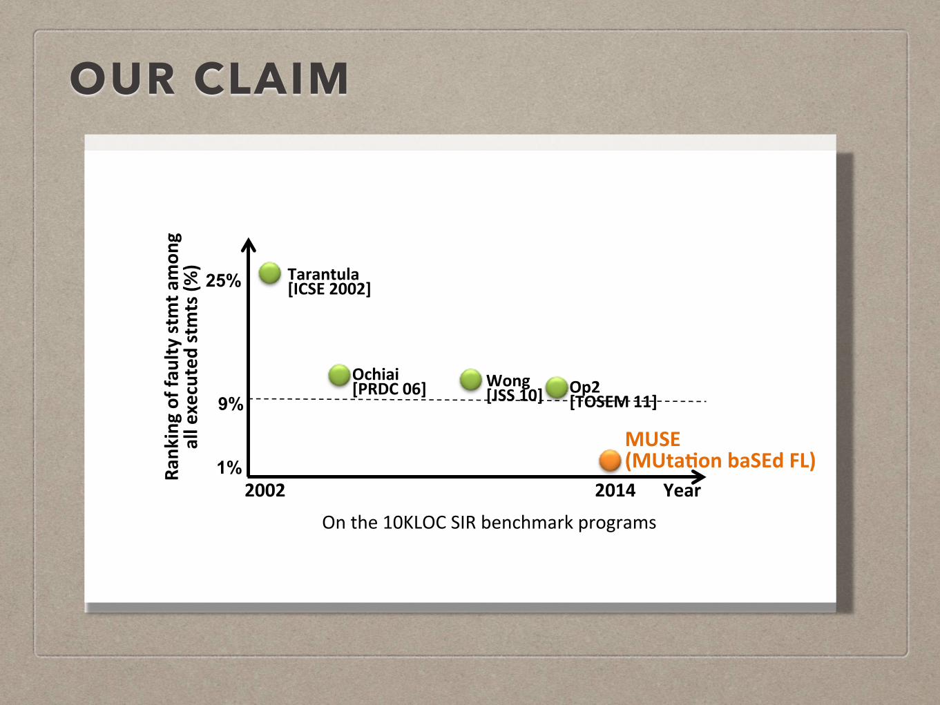
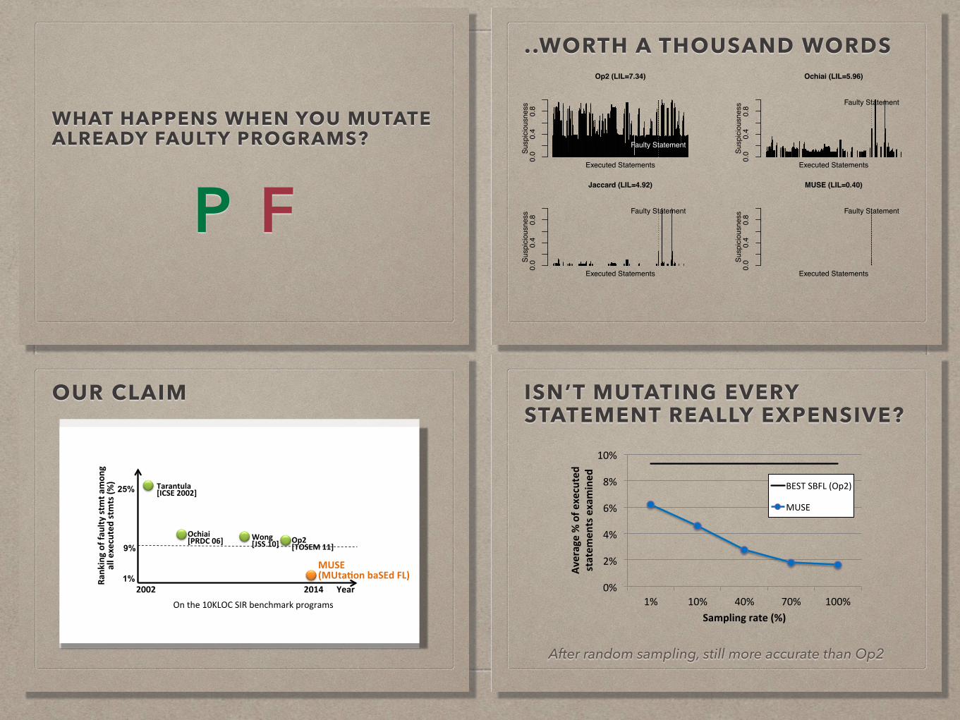
OUR CLAIM

Tarantula([ICSE(2002]

Ochiai([PRDC(06](((( Wong(

[JSS(10]

MUSE((MUtaAon(baSEd(FL)((

2014((((((Year

Ran

king(of(fau

lty(stmt(am

ong(

all(executed(stmts((%

)

Op2([TOSEM(11]

25%

1% 2002(

9%

On#the#10KLOC#SIR#benchmark#programs

MOTIVATION

• We have hit the ceiling of Spectrum-based Fault Localisation

• Not accurate enough, effectiveness varies significantly depending on test suites, inherently limited by block-level granularity

• Can we use mutation testing in a pre-emptive manner?

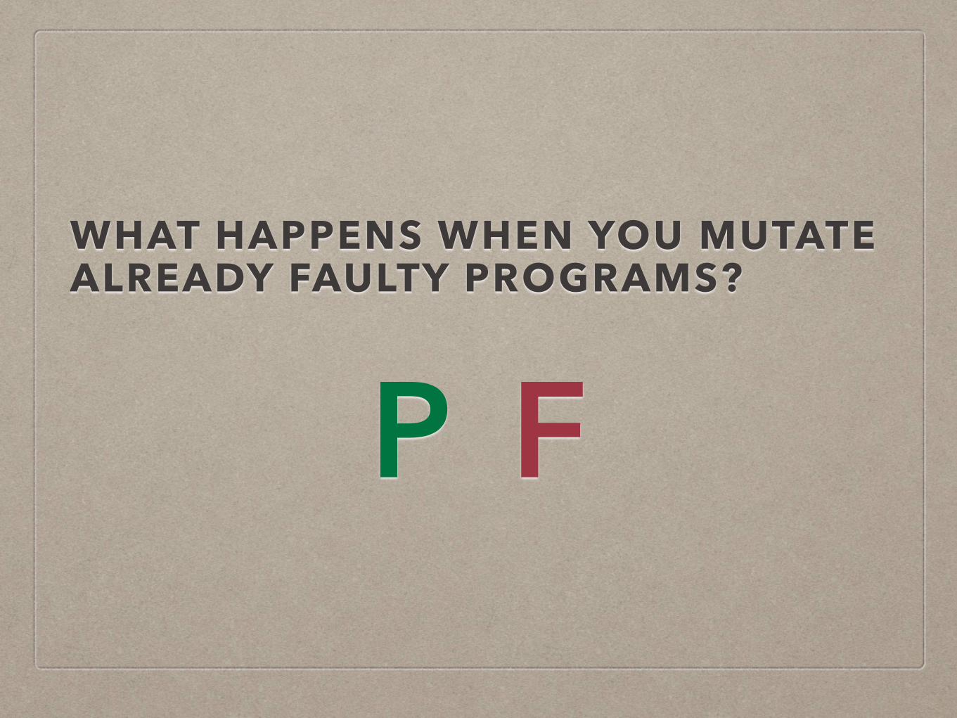
WHAT HAPPENS WHEN YOU MUTATE ALREADY FAULTY PROGRAMS?

P F

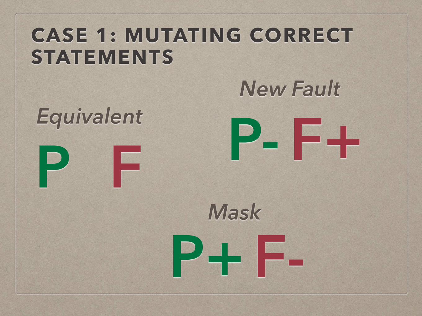
CASE 1: MUTATING CORRECT STATEMENTS

P FEquivalent P- F+

New Fault

P+F-Mask

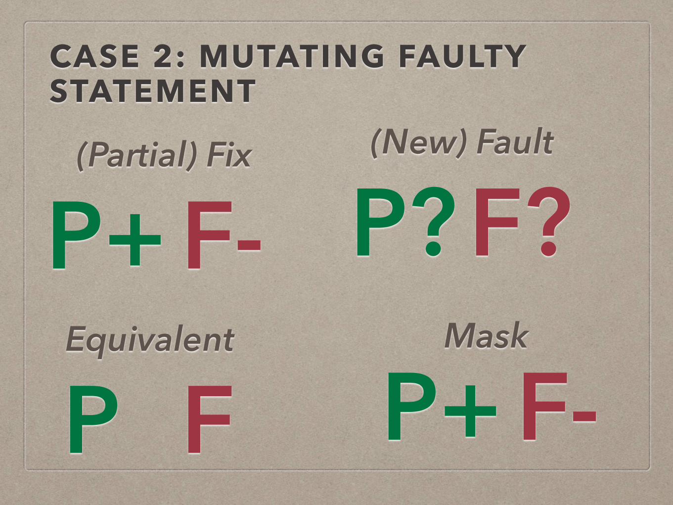
CASE 2: MUTATING FAULTY STATEMENT

P+F-(Partial) Fix

P?F?(New) Fault

P+F-Mask

P FEquivalent

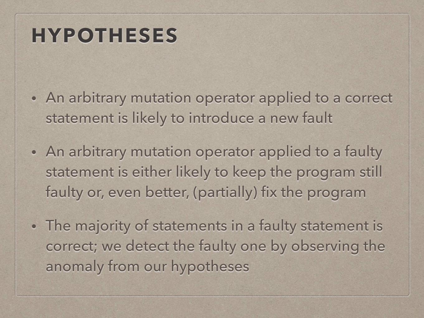
HYPOTHESES

• An arbitrary mutation operator applied to a correct statement is likely to introduce a new fault

• An arbitrary mutation operator applied to a faulty statement is either likely to keep the program still faulty or, even better, (partially) fix the program

• The majority of statements in a faulty statement is correct; we detect the faulty one by observing the anomaly from our hypotheses

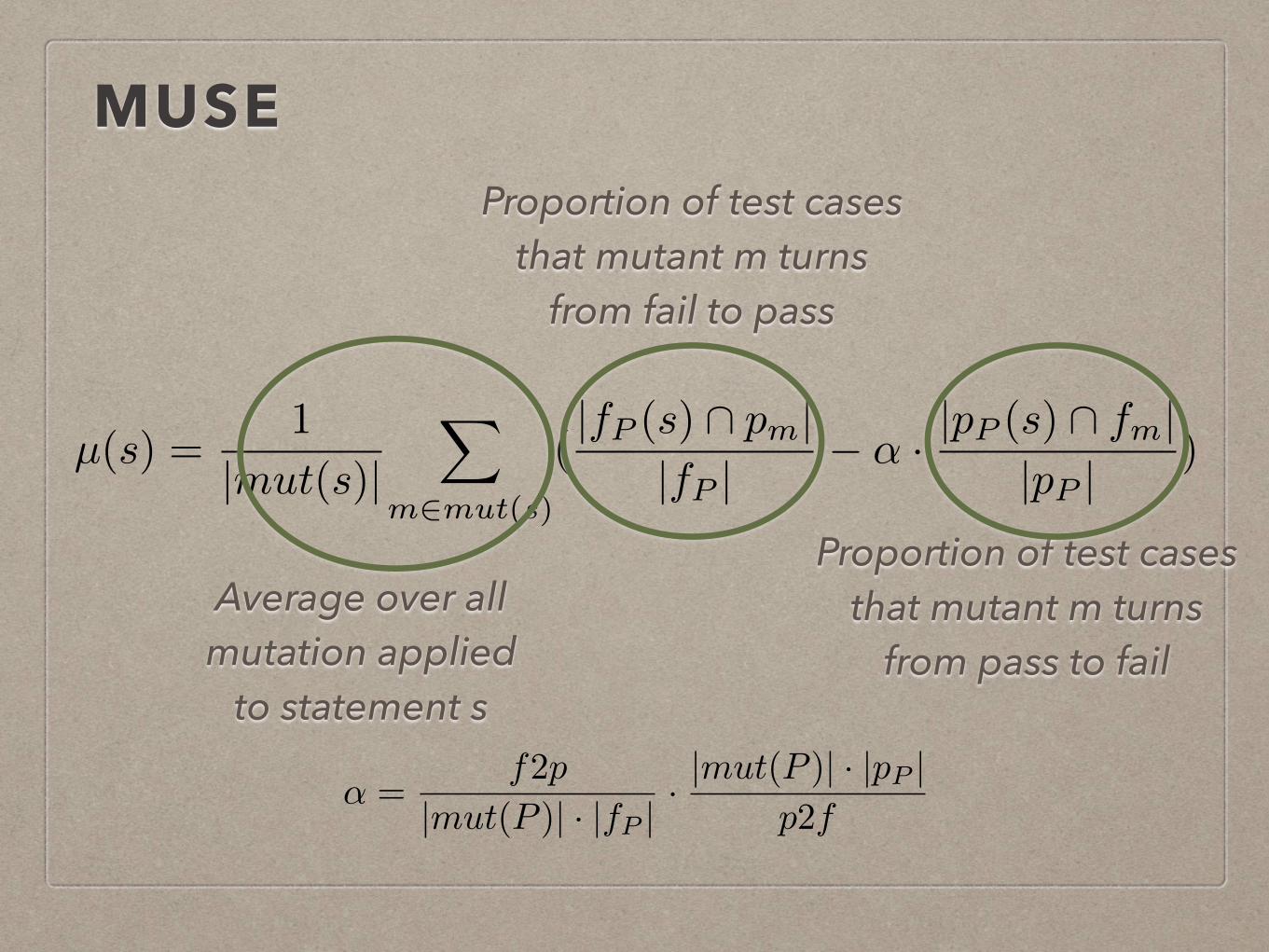
MUSE

µ(s) =1

|mut(s)|X

m2mut(s)

(|fP (s) \ pm|

|fP |� ↵ · |pP (s) \ fm|

|pP |)

Proportion of test cases that mutant m turns

from fail to pass

Proportion of test cases that mutant m turns

from pass to failAverage over all mutation applied

to statement s

↵ =f2p

|mut(P )| · |fP |· |mut(P )| · |pP |

p2f

EMPIRICAL EVALUATIONTable IV: Precision of Jaccard, Ochiai, Op2, and MUtation-baSEd fault localization technique (MUSE)

Subject % of executed stmts examined Rank of a faulty stmt Locality Information LossProgram Jaccard Ochiai Op2 MUSE Jaccard Ochiai Op2 MUSE Jaccard Ochiai Op2 MUSE

flex v1 49.48 45.04 32.01 0.04 1,371 1,248 887 1 8.33 7.89 7.68 1.28flex v7 3.60 3.60 3.60 0.07 100 100 100 2 5.72 6.52 7.45 1.22flex v11 19.76 19.54 13.51 0.04 547 541 374 1 7.39 7.49 7.40 1.59grep v3 1.06 1.01 0.71 1.87 21 20 14 37 5.25 5.68 6.21 5.92grep v11 3.44 3.44 3.44 1.60 58 58 58 27 5.43 6.20 5.46 7.19gzip v2 2.14 2.14 2.14 0.07 31 31 31 1 5.18 4.62 6.24 1.66gzip v5 1.83 1.83 1.83 0.07 26 26 26 1 4.45 4.73 5.27 1.88gzip v13 1.03 1.03 1.03 0.07 15 15 15 1 3.12 3.65 5.71 0.70sed v1 0.54 0.54 0.54 0.90 12 12 12 20 4.24 5.02 5.80 6.72sed v3 2.56 2.56 2.56 0.13 57 57 57 3 6.14 5.92 6.40 2.66sed v5 37.84 37.84 37.15 0.28 814 814 799 6 7.34 7.42 7.34 4.80space v19 0.03 0.03 0.03 0.06 1 1 1 2 5.27 5.93 6.64 2.15space v21 0.45 0.45 0.45 0.03 15 15 15 1 4.92 5.96 7.34 0.40space v28 11.57 10.66 6.89 0.04 329 303 196 1 7.33 7.40 7.24 1.96

Average 9.67 9.27 7.56 0.38 242.64 231.50 184.64 7.43 5.72 6.03 6.58 2.87

Table III: The average numbers of the test cases whose resultschange on the mutants

# of Failing Tests that # of passing tests thatSubject Pass after Mutating: fail after mutating:programs Correct Faulty (B)/(A) Correct Faulty (C)/(D) ↵

Stmts. Stmts. Stmts. Stmts.(A) (B) (C) (D)

flex v1 0.0002 1.2727 6155.6 15.7270 8.8182 1.8 0.0009flex v7 0.0002 0.6667 2721.1 16.3644 0.0000 N/A 0.0007flex v11 0.0026 14.2857 5421.3 5.1064 3.5714 1.4 0.0013grep v3 0.1299 0.4792 3.7 30.7825 8.0625 3.8 0.1490grep v11 8.9740 85.8181 9.6 0.1942 0.0000 N/A 5.7939gzip v2 0.0095 0.5625 59.1 113.3410 1.0000 113.3 0.0322gzip v5 0.0611 15.1111 247.2 64.7306 0.1111 582.6 0.0227gzip v13 0.0000 2.7000 N/A 109.2140 0.0000 N/A 0.0141sed v1 0.0095 0.0000 0.0 189.3610 6.1111 31.0 0.0004sed v3 0.0040 0.2500 63.0 238.7950 91.5000 2.6 0.0062sed v5 0.3556 31.8333 89.5 12.6217 12.0690 1.0 0.0365space v19 0.0105 4.6667 444.5 45.7808 13.1667 3.5 0.0057space v21 0.0000 0.3333 N/A 65.6796 1.0000 65.7 0.0002space v28 0.0114 23.0000 2016.5 31.2257 26.5000 1.2 0.0016

Average 0.6835 12.9271 1435.9 67.0660 12.2793 73.4 0.4332

0.0611 and 15.1111 failing test cases on gzip v5 pass onmc and mf respectively.

Table III provides supporting evidence for the conjecturesof MUSE. The number of the failing test cases on P thatpass on mf is 1435.9 times greater than the number on mc

on average, which supports the first conjecture. Similarly,the number of the passing test cases on P that fail on mc

is 73.4 times greater than the number on mf on average,which supports the second conjecture. Based on the results,we claim that both conjectures are true.

C. Regarding RQ2: Precision of MUSE in terms of the %of executed statements examined to localize a fault

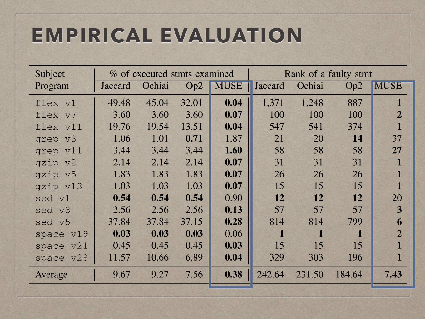
Table IV presents the precision evaluation of Jaccard,Ochiai, Op2, and MUSE with the proportion of executedstatements required to be examined before localizing thefault (i.e. the Expense metric). The most precise resultsare marked in bold. Following the ranking produced by

MUSE, one can localize a fault after examining 0.38% ofthe executed statements on average. The average precisionof MUSE is 25.68 (=9.67/0.38), 24.61 (=9.27/0.38), and20.09 (=7.56/0.38) times higher than that of Jaccard, Ochiai,and Op2, respectively. In addition, MUSE produces themost precise results for 11 out of the 14 studied faultyversions. This provides quantitative answer to RQ2: MUSEcan outperform the state-of-the-art SBFL techniques over theExpense metric.

In response to Parnin and Orso [22], we also reportthe absolute rankings produced by MUSE, i.e. the actualnumber of statements that need to be inspected beforeencountering the faulty statement. MUSE ranks the faultystatements of the seven faulty versions (flex v1,v11,gzip v2,v5,v13, and space v21,v28) at the topand ranks the faulty statement of another three versions(flex v7, sed v3, and space v19) among the topthree. On average, MUSE ranks the faulty statement amongthe top 7.43 places, which is 24.86 (=184.64/7.43) timesmore precise than the best performing SBFL technique, Op2.We believe MUSE is precise enough that its results can beused by a human developer in practice.

D. Regarding RQ3: Precision of MUSE in terms of theLocality Information Loss

The Locality Information Loss column of Table IV showsthe precision of Jaccard, Ochiai, Op2, and MUSE in termsof the LIL metric, calculated with ✏ = 10�17. The bestresults (i.e. the lowest values) are marked in bold. The LILmetric value of MUSE is 2.87 on average, which is 1.99(=5.72/2.87), 2.10 (=6.03/2.87), and 2.29 (=6.58/2.87) timesmore precise than those of Jaccard, Ochiai, and Op2. Inaddition, the LIL metric values of MUSE are the smallestones on the eleven out of the 14 subject program versions.

MOTIVATION

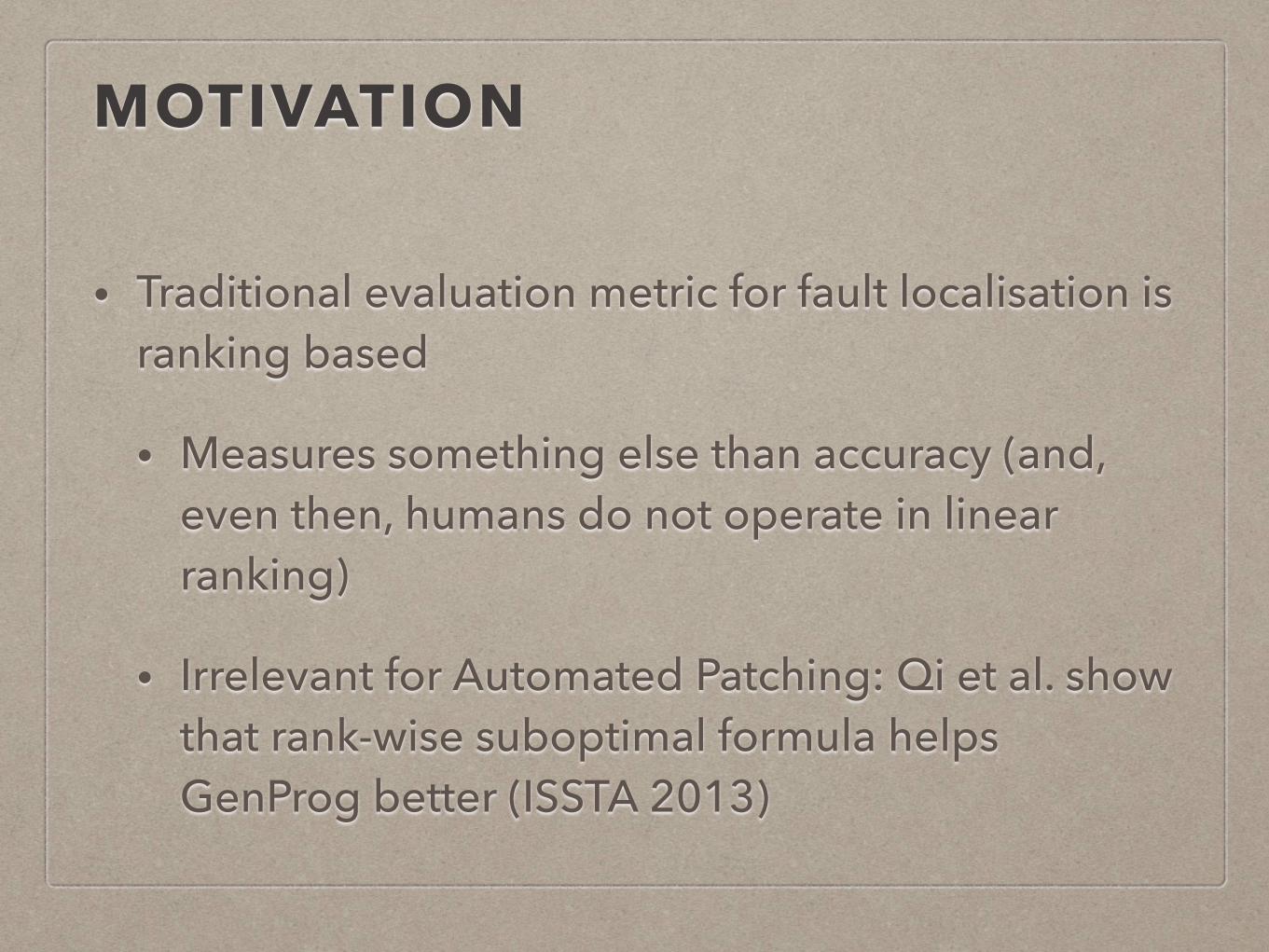
• Traditional evaluation metric for fault localisation is ranking based

• Measures something else than accuracy (and, even then, humans do not operate in linear ranking)

• Irrelevant for Automated Patching: Qi et al. show that rank-wise suboptimal formula helps GenProg better (ISSTA 2013)

LIL(LOCALITY INFORMATION LOSS)

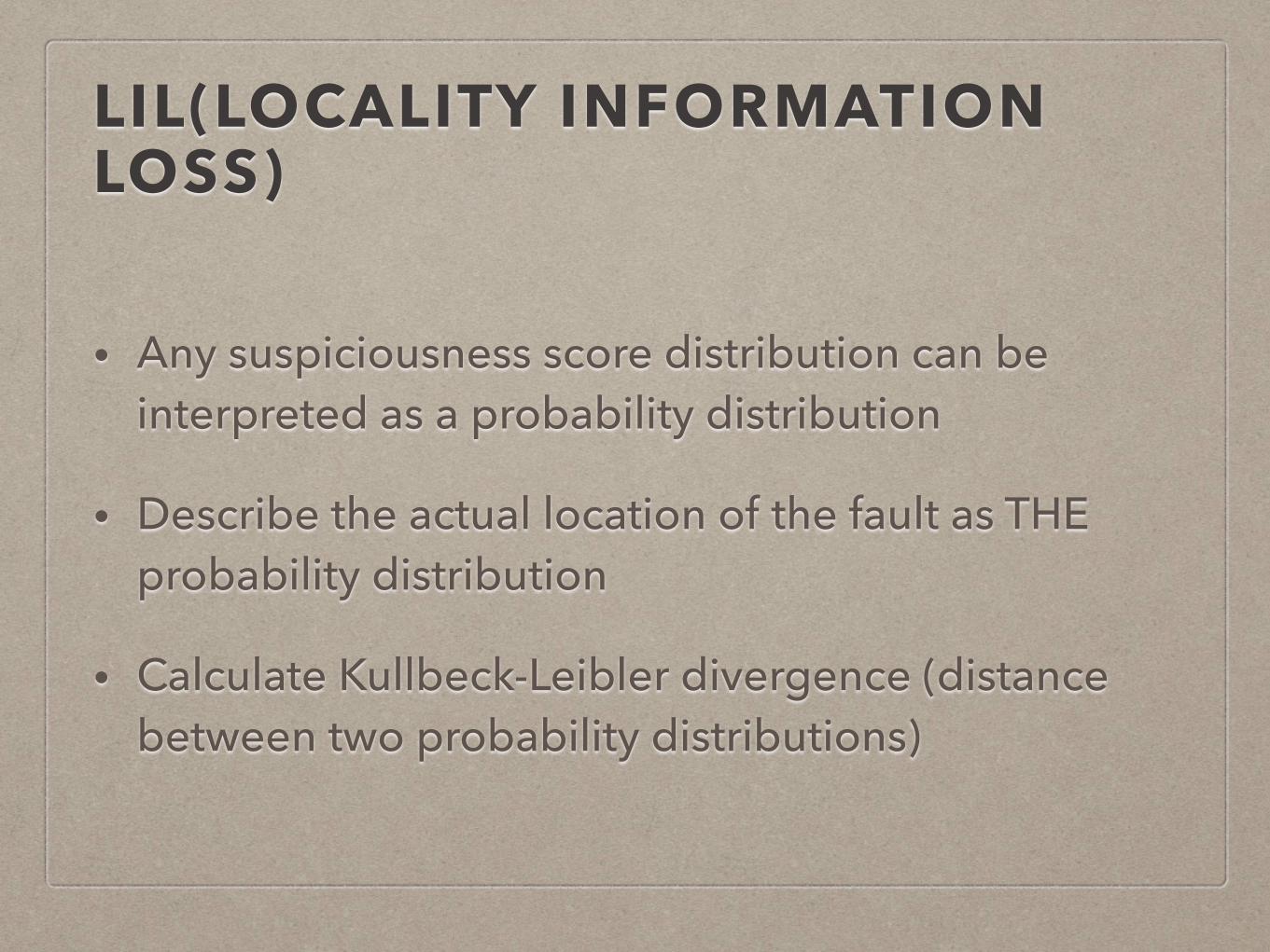
• Any suspiciousness score distribution can be interpreted as a probability distribution

• Describe the actual location of the fault as THE probability distribution

• Calculate Kullbeck-Leibler divergence (distance between two probability distributions)

LIL

to the likelihood of the statement containing the fault, weconvert the suspiciousness score given by an FL technique,⌧ : S ! [0, 1], into the probability of any member of Scontaining the fault, P⌧ (s), as follows:

P⌧ (si) =⌧(si)Pni=1 ⌧(si)

, (1 i n) (3)

This converts suspiciousness scores given by any ⌧ (includ-ing L) into a probability distribution, P⌧ . The metric wepropose is the Kullback-Leibler divergence [16] of P⌧ fromPL, denoted as DKL(PL||P⌧ ): it measures the informationloss that happens when using P⌧ instead of PL and iscalculated as follows:

DKL(PL||P⌧ ) =X

i

lnPL(si)

P⌧ (si)PL(si) (4)

We call this as Locality Information Loss (LIL). Kullback-Leibler divergence between two given probability distribu-tion P and Q requires the following: both P and Q shouldsum to 1, and Q(si) = 0 implies P (si) = 0. We satisfy theformer by the normalization in Equation 3 and the latter byalways substituting 0 with ✏ after normalizing ⌧ 2 (becausewe cannot guarantee the implication in our application).When these properties are satisfied, DKL(PL||P⌧ ) becomes0 when PL and P⌧ are identical. As with the Expensemetric, the lower the LIL value is the more accurate theFL technique is. Based on Information Theory, LIL has thefollowing strengths compared to the Expense metric:

• Expressiveness: unlike the Expense metric that onlyconcerns the actual faulty statement, LIL also reflectshow well the suspiciousness of non-faulty statementshave been supressed by an FL technique. That is, LILcan be used to explain the results of Qi et al. [23]quantitatively.

• Flexibility: unlike the Expense metric that only con-cerns a single faulty statement, LIL can handle multiplelocations of faults. For m faults (or for a fault thatconsists of m different locations), the distribution PLwill simply show not one but m spikes, each with 1

mas height.

• Applicability: Expense metric is tied to FL techniquesthat produce rankings, whereas LIL can be applied toany FL technique. If a technique assigns suspiciousnessscores to statements, it can be converted into P⌧ ; if atechnique simply presents one or more statements ascandidate fault location, P⌧ can be formulated to havecorresponding peaks.

IV. EXPERIMENTAL SETUP

We have designed the following three research questionsto evaluate the effectiveness of MUSE in terms of the

2✏ should be smaller than the smallest normalized non-zero suspicious-

ness score by ⌧ .

Expense metric [18] and the LIL metric (Section III):

RQ1. Foundation: How many test results change fromfailure to pass and vice versa between before and after on amutant generated by mutating a faulty statement, comparedwith a mutant generated by mutating a correct one?

RQ1 is to validate the conjectures in Section II-A, onwhich MUSE depends. If these conjectures are valid (i.e.,more failing test cases become passing after mutating thefaulty statement than a correct one, and more passing testcases become failing after mutating a correct statement thanthe faulty one), we can expect that MUSE will localize afault precisely.

RQ2. Precision: How precise is MUSE, compared withJaccard, Ochiai, and Op2 in terms of the % of executedstatements examined to localize a first fault?

Precision in terms of the % of program statements to beexamined is the traditional evaluation criteria for fault local-ization techniques. RQ2 evaluates MUSE with the Expensemetric against the three widely studied SBFL techniques –Jaccard, Ochiai, and Op2. Op2 [19] is proven to performwell in Expense metric; Ochiai [20] performs closely to Op2,while Jaccard [10] shows good performance when used withautomated program repair [23].

RQ3. Information Loss: How precise is MUSE, comparedwith Jaccard, Ochiai, and Op2 in terms of the LocalityInformation Loss (LIL) metric?

RQ3 evaluates the precision of MUSE with the LIL metricintroduced in Section III against the three SBFL techniques(Jaccard, Ochiai, and Op2). The smaller the LIL value is,the more precise the FL technique is.

To answer the research questions, we performed a se-ries of experiments by applying Jaccard, Ochiai, Op2, andMUSE to the 14 faulty versions in five real world Cprograms. The following subsections describe the details ofthe experiments.

A. Subject Programs

For the experiments, we used five non-trivial real-worldprograms including flex version 2.4.7, grep version 2.2,gzip version 1.1.2, sed version 1.18, and space, all ofwhich are from the SIR benchmark suite [4].

Table I describes the target programs including theirsizes in Lines of Code, the faulty versions used, and thenumbers of failing and passing test cases for each programversion/fault pair. From the base versions listed above, werandomly selected three faulty versions from each programexcept grep where a failure is detected only in two faultyversions by the used test suite. grep v3 and spacev19 have multiple faults and the other versions have onefault per each version. The fault ID of each version ispresented in Table I (For the rest of the paper, we refer to

Program P

Execution Test

result Coverage analysis

Stmts. covered by failing tests

Mutation

m1

mn Exec.

Test result1

Test resultn

Calc. Susp.

Susp. & Rank

Exec. Test

suite T

Step 1: selecting target statements to mutate Step 2: testing mutants Step 3: calculating

suspiciousness

Figure 2: Framework of MUtation-baSEd fault localization technique (MUSE)D. MUSE Framework

Figure 2 shows the framework of MUtation-baSEd faultlocalization technique (MUSE). There are three majorstages: selection of statements to mutate, testing of themutants, and calculation of the suspiciousness scores.Step 1: MUSE receives a target program P and a testsuite T . After executing T on P , MUSE selects the targetstatements, i.e. the statements of P that are executed by atleast one failing test case in T . We focus on only thesestatements as those not covered by any failing tests, can beconsidered not faulty with respect to T .Step 2: MUSE generates mutant versions of P by mutatingeach of the statements selected at Step 1. MUSE maygenerate multiple mutants from a single statement since onestatement may contain multiple mutation points [8]. MUSEtests all generated mutants with T and records the results.Step 3: MUSE compares the test results of T on P with thetest results of T on all mutants. This produces the weight↵, based on which MUSE calculates the suspiciousness ofthe target statements of P .

III. LIL: LOCALITY INFORMATION LOSS

The output of fault localization techniques can be con-sumed by either human developers or automated program re-pair techniques. Expense [18] metric measures the portion ofprogram statements that need to be inspected by developersuntil the localization of the fault. It has been widely adoptedas an evaluation metric for FL techniques [13, 19, 31] as wellas a theoretical framework that showed hierarchies betweenSBFL techniques [28, 29]. However, the Expense metric hasbeen criticised for being unrealistic to be used by a humandeveloper directly [22].

In an attempt to evaluate the precision of SBFL tech-niques, Qi et al. [23] compared SBFL techniques by mea-suring the Number of Candidate Patches (NCP) generatedby GenProg [25] automated program repair tool, with thegiven localization information.1 Automated program repairtechniques tend to bypass the ranking and directly use the

1Essentially this measures the number of fitness evaluation for theGenetic Programming part of GenProg; hence the lower the NCP scoreis, the more efficient GenProg becomes, and in turn the more effective thegiven localization technique is.

suspiciousness scores of each statement as the probabilityof mutating the statement (expecting that mutating a highlysuspicious statement is more likely to result in a potentialfix) [6, 25]. An interesting empirical observation by Qiet al. [23] is that Jaccard [10] produced lower NCP thanOp2 [19], despite having been proven to always producea lower ranking for the faulty statement than Op2 [28].This is due to the actual distribution of the suspiciousnessscore: while Op2 produced higher ranking for the faultystatement than Jaccard, it assigned almost equally high sus-piciousness scores to some correct statements. On the otherhand, Jaccard assigned much lower suspiciousness scoresto correct statements, despite ranking the faulty statementslightly lower than Op2.

This illustrates that evaluation and theoretical analysisbased on the linear ranking model is not applicable toautomated program repair techniques. LIL metric can mea-sure the aptitude of FL techniques for automated repairtechniques as it measures the effectiveness of localizationin terms of information loss rather than the behavioural costof inspecting a ranking of statements. LIL metric essentiallycaptures the essence of the entropy-based formulation offault localization [32] in the form of an evaluation metric.

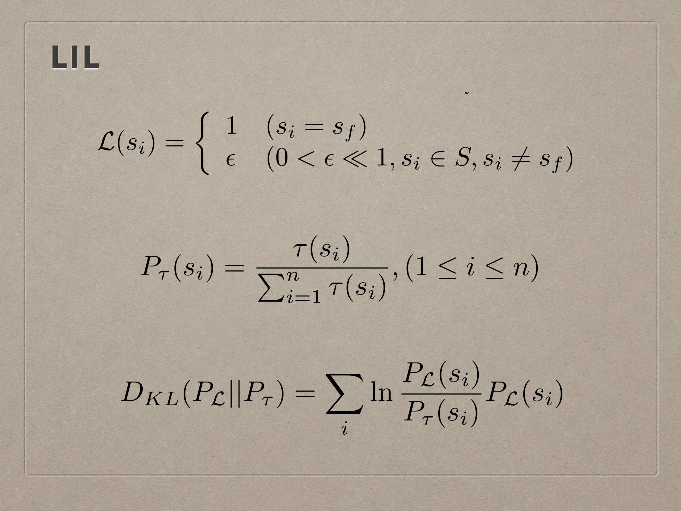
We propose a new evaluation metric that does not sufferfrom this discrepancy between two consumption models.Let S be the set of n statements of the Program UnderTest, {s1, . . . , sn}, sf , (1 f n) being the single faultystatement. Without losing generality, we assume that outputof any fault localization technique ⌧ can be normalized to [0,1]. Now suppose that there exists an ideal fault localizationtechnique, L, that can always pinpoint sf as follows:

L(si) =⇢

1 (si = sf )✏ (0 < ✏ ⌧ 1, si 2 S, si 6= sf )

(2)

Note that we can convert outputs of FL techniques that donot use suspiciousness scores in a similar way: if a technique⌧ simply reports a set C of m statements as candidate faultystatements, we can set ⌧(si) = 1

m when si 2 C and ⌧(si) =✏ when si 2 S \ C.

We now cast the fault localization problem in a proba-bilistic framework as in the previous work [32]. Since thesuspiciousness score of a statement is supposed to correlate

to the likelihood of the statement containing the fault, weconvert the suspiciousness score given by an FL technique,⌧ : S ! [0, 1], into the probability of any member of Scontaining the fault, P⌧ (s), as follows:

P⌧ (si) =⌧(si)Pni=1 ⌧(si)

, (1 i n) (3)

This converts suspiciousness scores given by any ⌧ (includ-ing L) into a probability distribution, P⌧ . The metric wepropose is the Kullback-Leibler divergence [16] of P⌧ fromPL, denoted as DKL(PL||P⌧ ): it measures the informationloss that happens when using P⌧ instead of PL and iscalculated as follows:

DKL(PL||P⌧ ) =X

i

lnPL(si)

P⌧ (si)PL(si) (4)

We call this as Locality Information Loss (LIL). Kullback-Leibler divergence between two given probability distribu-tion P and Q requires the following: both P and Q shouldsum to 1, and Q(si) = 0 implies P (si) = 0. We satisfy theformer by the normalization in Equation 3 and the latter byalways substituting 0 with ✏ after normalizing ⌧ 2 (becausewe cannot guarantee the implication in our application).When these properties are satisfied, DKL(PL||P⌧ ) becomes0 when PL and P⌧ are identical. As with the Expensemetric, the lower the LIL value is the more accurate theFL technique is. Based on Information Theory, LIL has thefollowing strengths compared to the Expense metric:

• Expressiveness: unlike the Expense metric that onlyconcerns the actual faulty statement, LIL also reflectshow well the suspiciousness of non-faulty statementshave been supressed by an FL technique. That is, LILcan be used to explain the results of Qi et al. [23]quantitatively.

• Flexibility: unlike the Expense metric that only con-cerns a single faulty statement, LIL can handle multiplelocations of faults. For m faults (or for a fault thatconsists of m different locations), the distribution PLwill simply show not one but m spikes, each with 1

mas height.

• Applicability: Expense metric is tied to FL techniquesthat produce rankings, whereas LIL can be applied toany FL technique. If a technique assigns suspiciousnessscores to statements, it can be converted into P⌧ ; if atechnique simply presents one or more statements ascandidate fault location, P⌧ can be formulated to havecorresponding peaks.

IV. EXPERIMENTAL SETUP

We have designed the following three research questionsto evaluate the effectiveness of MUSE in terms of the

2✏ should be smaller than the smallest normalized non-zero suspicious-

ness score by ⌧ .

Expense metric [18] and the LIL metric (Section III):

RQ1. Foundation: How many test results change fromfailure to pass and vice versa between before and after on amutant generated by mutating a faulty statement, comparedwith a mutant generated by mutating a correct one?

RQ1 is to validate the conjectures in Section II-A, onwhich MUSE depends. If these conjectures are valid (i.e.,more failing test cases become passing after mutating thefaulty statement than a correct one, and more passing testcases become failing after mutating a correct statement thanthe faulty one), we can expect that MUSE will localize afault precisely.

RQ2. Precision: How precise is MUSE, compared withJaccard, Ochiai, and Op2 in terms of the % of executedstatements examined to localize a first fault?

Precision in terms of the % of program statements to beexamined is the traditional evaluation criteria for fault local-ization techniques. RQ2 evaluates MUSE with the Expensemetric against the three widely studied SBFL techniques –Jaccard, Ochiai, and Op2. Op2 [19] is proven to performwell in Expense metric; Ochiai [20] performs closely to Op2,while Jaccard [10] shows good performance when used withautomated program repair [23].

RQ3. Information Loss: How precise is MUSE, comparedwith Jaccard, Ochiai, and Op2 in terms of the LocalityInformation Loss (LIL) metric?

RQ3 evaluates the precision of MUSE with the LIL metricintroduced in Section III against the three SBFL techniques(Jaccard, Ochiai, and Op2). The smaller the LIL value is,the more precise the FL technique is.

To answer the research questions, we performed a se-ries of experiments by applying Jaccard, Ochiai, Op2, andMUSE to the 14 faulty versions in five real world Cprograms. The following subsections describe the details ofthe experiments.

A. Subject Programs

For the experiments, we used five non-trivial real-worldprograms including flex version 2.4.7, grep version 2.2,gzip version 1.1.2, sed version 1.18, and space, all ofwhich are from the SIR benchmark suite [4].

Table I describes the target programs including theirsizes in Lines of Code, the faulty versions used, and thenumbers of failing and passing test cases for each programversion/fault pair. From the base versions listed above, werandomly selected three faulty versions from each programexcept grep where a failure is detected only in two faultyversions by the used test suite. grep v3 and spacev19 have multiple faults and the other versions have onefault per each version. The fault ID of each version ispresented in Table I (For the rest of the paper, we refer to

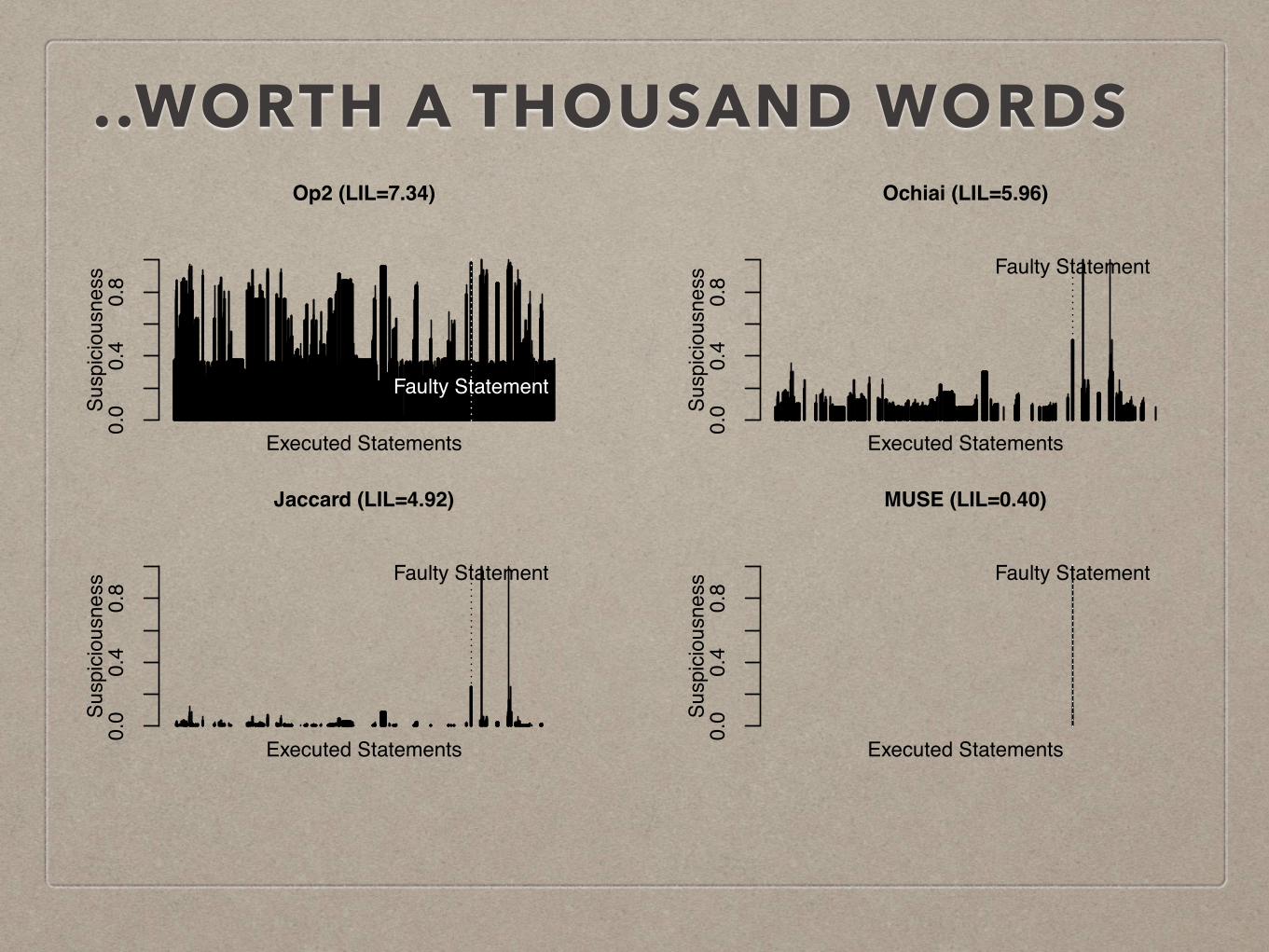
..WORTH A THOUSAND WORDS

Jaccard (LIL=4.92)

Executed Statements

0.0

0.4

0.8

Faulty Statement

Susp

icio

usne

ss

MUSE (LIL=0.40)

Executed Statements0.

00.

40.

8

Faulty Statement

Susp

icio

usne

ss

Ochiai (LIL=5.96)

Executed Statements

0.0

0.4

0.8

Faulty Statement

Susp

icio

usne

ss

Op2 (LIL=7.34)

Executed Statements

0.0

0.4

0.8

Faulty Statement

Susp

icio

usne

ss

ONGOING WORK

• With actual progress

• Mutant Sampling

• Hybridisation

• More adventurous

• Multiple Faults

• Pre-emptive localisation

• Learning mutation

• Genetic Programming for MUSE

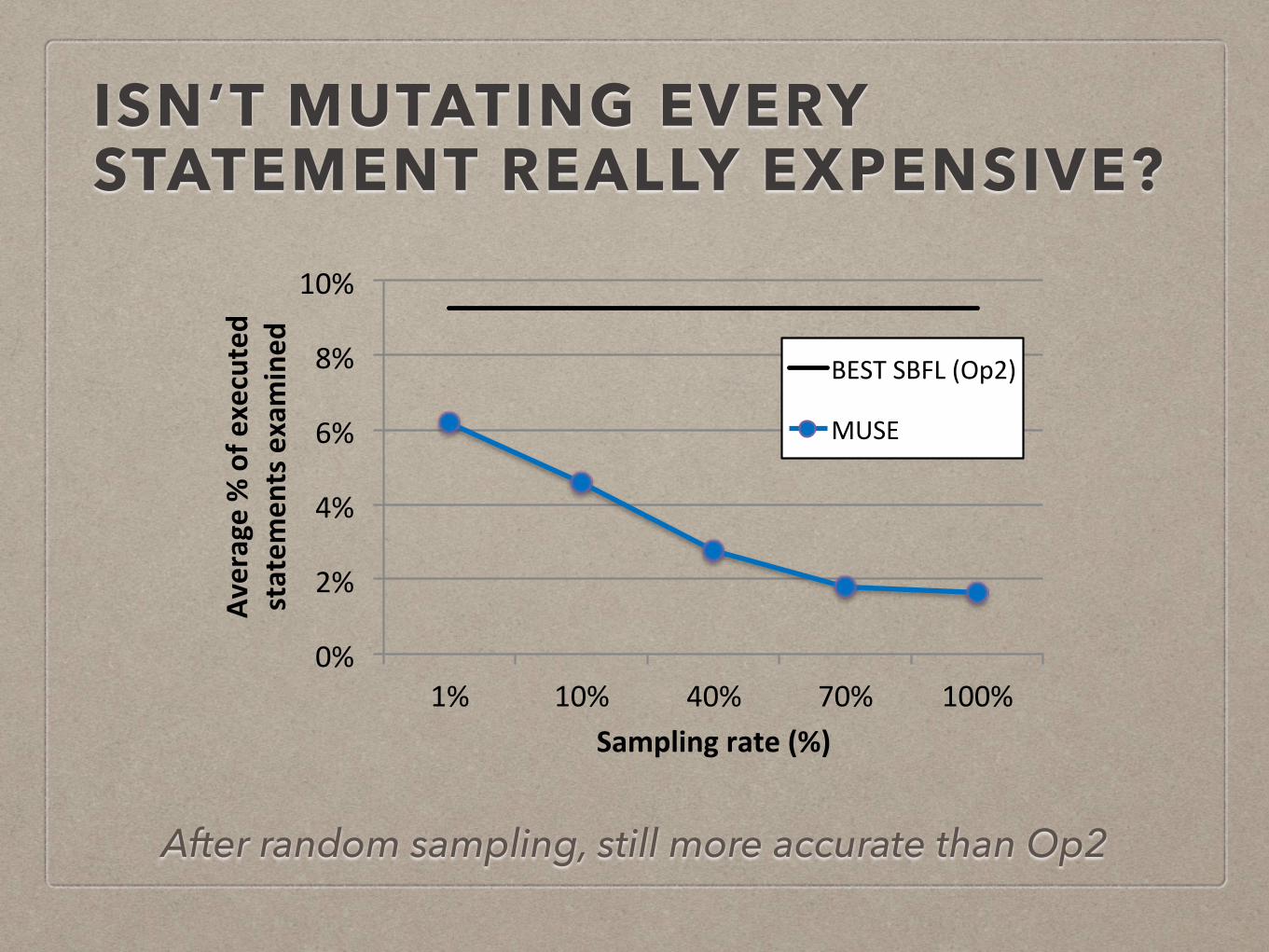
ISN’T MUTATING EVERY STATEMENT REALLY EXPENSIVE?

0%#

2%#

4%#

6%#

8%#

10%#

1%# 10%# 40%# 70%# 100%#

Average'%'of'e

xecuted'

statem

ents'examined

Sampling'rate'(%)

BEST#SBFL#(Op2)#

MUSE#

After random sampling, still more accurate than Op2

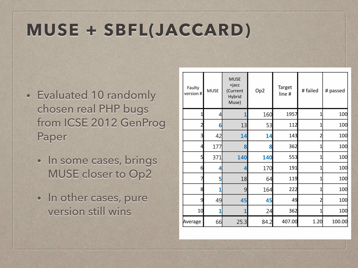
MUSE + SBFL(JACCARD)

• Evaluated 10 randomly chosen real PHP bugs from ICSE 2012 GenProg Paper

• In some cases, brings MUSE closer to Op2

• In other cases, pure version still wins

Faulty Stmt Rank

10

Faulty version # MUSE

MUSE +jacc

(Current Hybrid Muse)

MUSE +Ochiai

MUSE_op2 +jacc

MUSE_ochi +ochi

MUSE_taran +ochi

MUSE_ampl +ochiai

MUSE_jacc +jacc Op2 Target

line # # failed # passed

1 4 1 1 1 1 1 1 1 160 1957 1 100

2 6 13 13 13 6 6 13 13 53 112 1 100

3 42 14 14 14 14 14 14 14 14 143 2 100

4 177 8 8 8 8 8 8 8 8 362 1 100

5 371 140 140 140 140 140 140 140 140 553 1 100

6 4 4 4 4 4 4 4 4 170 191 1 100

7 5 18 5 18 5 5 5 18 64 119 1 100

8 1 9 9 9 9 9 9 9 164 222 1 100

9 49 45 45 45 45 45 45 45 45 49 2 100

10 1 1 1 1 1 1 1 1 24 362 1 100

Average 66 25.3 24 25.3 23.3 23.3 24 25.3 84.2 407.00 1.20 100.00

Faulty Stmt Rank

10

Faulty version # MUSE

MUSE +jacc

(Current Hybrid Muse)

MUSE +Ochiai

MUSE_op2 +jacc

MUSE_ochi +ochi

MUSE_taran +ochi

MUSE_ampl +ochiai

MUSE_jacc +jacc Op2 Target

line # # failed # passed

1 4 1 1 1 1 1 1 1 160 1957 1 100

2 6 13 13 13 6 6 13 13 53 112 1 100

3 42 14 14 14 14 14 14 14 14 143 2 100

4 177 8 8 8 8 8 8 8 8 362 1 100

5 371 140 140 140 140 140 140 140 140 553 1 100

6 4 4 4 4 4 4 4 4 170 191 1 100

7 5 18 5 18 5 5 5 18 64 119 1 100

8 1 9 9 9 9 9 9 9 164 222 1 100

9 49 45 45 45 45 45 45 45 45 49 2 100

10 1 1 1 1 1 1 1 1 24 362 1 100

Average 66 25.3 24 25.3 23.3 23.3 24 25.3 84.2 407.00 1.20 100.00

MULTIPLE FAULTS CONJECTURE

• For independent faults that results in disjoint failures, MUSE is not affected at all

• For faults that interact with each other, test suite design/composition will play a key role

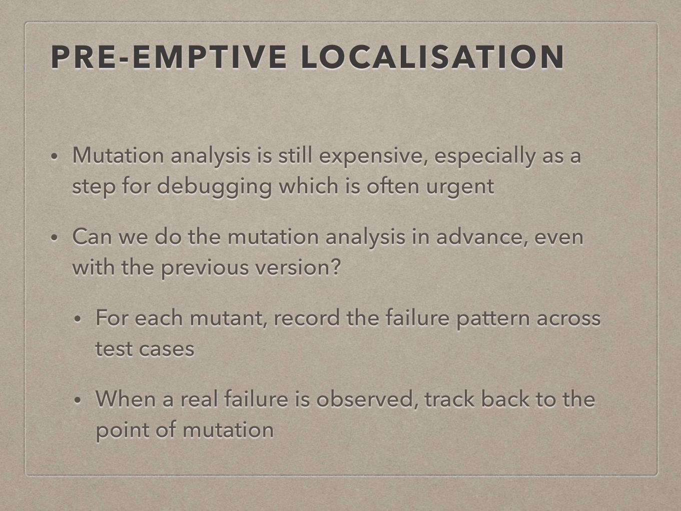
PRE-EMPTIVE LOCALISATION

• Mutation analysis is still expensive, especially as a step for debugging which is often urgent

• Can we do the mutation analysis in advance, even with the previous version?

• For each mutant, record the failure pattern across test cases

• When a real failure is observed, track back to the point of mutation

GP FOR MUSE

• GP worked for SBFL; does it work for MUSE?

• More variables, which means a larger search space

WHAT HAPPENS WHEN YOU MUTATE ALREADY FAULTY PROGRAMS?

P F

..WORTH A THOUSAND WORDS

Jaccard (LIL=4.92)

Executed Statements

0.0

0.4

0.8

Faulty Statement

Susp

icio

usne

ss

MUSE (LIL=0.40)

Executed Statements

0.0

0.4

0.8

Faulty Statement

Susp

icio

usne

ss

Ochiai (LIL=5.96)

Executed Statements

0.0

0.4

0.8

Faulty Statement

Susp

icio

usne

ss

Op2 (LIL=7.34)

Executed Statements

0.0

0.4

0.8

Faulty Statement

Susp

icio

usne

ss

OUR CLAIM

Tarantula([ICSE(2002]

Ochiai([PRDC(06](((( Wong(

[JSS(10]

MUSE((MUtaAon(baSEd(FL)((

2014((((((Year

Ran

king(of(fau

lty(stmt(am

ong(

all(executed(stmts((%

)

Op2([TOSEM(11]

25%

1% 2002(

9%

On#the#10KLOC#SIR#benchmark#programs

ISN’T MUTATING EVERY STATEMENT REALLY EXPENSIVE?

0%#

2%#

4%#

6%#

8%#

10%#

1%# 10%# 40%# 70%# 100%#

Average'%'of'e

xecuted'

statem

ents'examined

Sampling'rate'(%)

BEST#SBFL#(Op2)#

MUSE#

After random sampling, still more accurate than Op2