Embed Size (px)
Citation preview
1Tartu 2016
ISSN 1406-0299ISBN 978-9949-77-133-2
DISSERTATIONES CHIMICAE
UNIVERSITATIS TARTUENSIS
153
A
SKO
LAA
NISTE
Com
parison and optimisation of novel m
ass spectrometry ionisation sources
ASKO LAANISTE
Comparison and optimisation of novelmass spectrometry ionisation sources

DISSERTATIONES CHIMICAE UNIVERSITATIS TARTUENSIS 153
DISSERTATIONES CHIMICAE UNIVERSITATIS TARTUENSIS 153
ASKO LAANISTE
Comparison and optimisation of novel mass spectrometry ionisation sources
Institute of Chemistry, Faculty of Science and Technology. University of Tartu. Estonia. Dissertation was accepted for the commencement of the degree of Doctor philosophiae in Chemistry at the University of Tartu on May 27th, 2016, by the Council of Institute of Chemistry, Faculty of Science and Technology, Uni-versity of Tartu. Supervisor: Anneli Kruve, PhD, Institute of Chemistry, University of
Tartu, Estonia Professor Ivo Leito, Institute of Chemistry, University of
Tartu, Estonia Opponent: Prof. Risto Kostiainen, PhD, University of Helsinki, Finland Commencement: Room 1021, Chemicum, 14A Ravila street, Tartu, on the 31st
of August in 2016, at 12:00. This work has been partially supported by Graduate School Functional materials and technologies receiving funding from the European Reginal Development Fund under project in University of Tartu, Estonia
ISSN 1406-0299 ISBN 978-9949-77-133-2 (print) ISBN 978-9949-77-134-9 (pdf) Copyright: Asko Laaniste, 2016 University of Tartu Press www.tyk.ee
Hiiele, kes on mind alati vankumatult toetanud, kuid piisavalt arvustanud.

7
TABLE OF CONTENTS
LIST OF ORIGINAL PUBLICATIONS ....................................................... 9
ABBREVATIONS ......................................................................................... 10
INTRODUCTION .......................................................................................... 11
1. REVIEW OF LITERATURE .................................................................... 12 1.1. Liquid chromatography/mass spectrometry ...................................... 12 1.2. Ionisation sources in LC/MS ............................................................. 12
1.2.1. ESI and HESI ........................................................................... 13 1.2.2. APCI and APPI ........................................................................ 14 1.2.3. Multimode sources .................................................................. 15 1.2.4. Other sources ........................................................................... 17
1.3. Advantages and limitations of different sources ............................... 17 1.3.1. Linearity ................................................................................... 18 1.3.2. Matrix effects ........................................................................... 18 1.3.3. Limit of detection, signal-to-noise ratio and sensitivity .......... 18
1.4. Novel developments in ESI sources .................................................. 19 2. EXPERIMENTAL .................................................................................... 21
2.1. Chemicals .......................................................................................... 21 2.2. Instrumentation .................................................................................. 21 2.3. Selectivity .......................................................................................... 23 2.4. Samples for Paper II .......................................................................... 24 2.5. Sample pretreatments ........................................................................ 25
2.5.1. QuEChERS in the comparison of nebulisers in Paper I .......... 25 2.5.2. QuEChERS for honey samples pretreatment in Paper II ......... 25 2.5.3. QuEChERS for garlic and tomato samples in comparison
of ionisation modes in Paper III ............................................... 25 2.6. Data analysis in experiments ............................................................. 26
2.6.1. Calculation of validation parameters ....................................... 26 2.6.2. Proportions analysis ................................................................. 27 2.6.3. Principal component analysis (PCA) ....................................... 28 2.6.4. Full factorial design for the optimisation of 3R nebuliser ....... 28
2.7. Design of experiment for ionisation modes comparison ................... 30 3. RESULTS AND DISCUSSION ............................................................... 31
3.1. Comparison of ionisation sources ...................................................... 31 3.1.1. Comparison of chromatogram profiles .................................... 31 3.1.2. Repeatability ............................................................................ 33 3.1.3. Matrix effects ........................................................................... 34 3.1.4. Linearity ................................................................................... 37 3.1.5. Limit of detection, signal-to-noise ratio and sensitivity .......... 41 3.1.6. Principal Component Analysis of LoD results ........................ 43 3.1.7. Conclusions of comparison ...................................................... 44
8
3.2. Novel 3R nebuliser for ESI source .................................................... 44 3.3. 3R nebuliser optimisation .................................................................. 45
3.3.1. Testing different nebuliser parameters .................................... 46 3.3.2. Finding optimal nebuliser parameters and creating
a model describing effects of different parameters .................. 47 3.3.3. Influence of eluent flow rate on the ionisation ........................ 48 3.3.4. Universality of 3R nebuliser .................................................... 50
3.4. Practical applications of the novel 3R ESI source: neonicotinoids in honey ............................................................................................. 53 3.4.1. Results of nebulisers comparison ............................................ 54
SUMMARY ................................................................................................... 58 SUMMARY IN ESTONIAN ......................................................................... 59 REFERENCES ............................................................................................... 60 ACKNOWLEDGEMENTS ........................................................................... 65 APPENDICES ................................................................................................ 66
CURRICULUM VITAE IN ENGLISH ......................................................... 143
CURRICULUM VITAE IN ESTONIAN ...................................................... 14
PUBLICATIONS ........................................................................................... 77
6
9
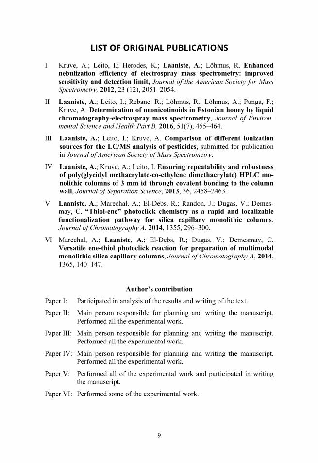
Author’s contribution
Paper I: Participated in analysis of the results and writing of the text.
Paper II: Main person responsible for planning and writing the manuscript. Performed all the experimental work.
Paper III: Main person responsible for planning and writing the manuscript. Performed all the experimental work.
Paper IV: Main person responsible for planning and writing the manuscript. Performed all the experimental work.
Paper V: Performed all of the experimental work and participated in writing the manuscript.
Paper VI: Performed some of the experimental work.
LIST OF ORIGINAL PUBLICATIONS
I Kruve, A.; Leito, I.; Herodes, K.; Laaniste, A.; Lõhmus, R. Enhanced nebulization efficiency of electrospray mass spectrometry: improved sensitivity and detection limit, Journal of the American Society for Mass Spectrometry, 2012, 23 (12), 2051–2054.
II Laaniste, A.; Leito, I.; Rebane, R.; Lõhmus, R.; Lõhmus, A.; Punga, F.; Kruve, A. Determination of neonicotinoids in Estonian honey by liquid chromatography-electrospray mass spectrometry, Journal of Environ-mental Science and Health Part B, 2016, 51(7), 455–464.
III Laaniste, A.; Leito, I.; Kruve, A. Comparison of different ionization sources for the LC/MS analysis of pesticides, submitted for publication in Journal of American Society of Mass Spectrometry.
IV Laaniste, A.; Kruve, A.; Leito, I. Ensuring repeatability and robustness of poly(glycidyl methacrylate-co-ethylene dimethacrylate) HPLC mo-nolithic columns of 3 mm id through covalent bonding to the column wall, Journal of Separation Science, 2013, 36, 2458–2463.
V Laaniste, A.; Marechal, A.; El-Debs, R.; Randon, J.; Dugas, V.; Demes-may, C. “Thiol-ene” photoclick chemistry as a rapid and localizable functionalization pathway for silica capillary monolithic columns, Journal of Chromatography A, 2014, 1355, 296–300.
VI Marechal, A.; Laaniste, A.; El-Debs, R.; Dugas, V.; Demesmay, C. Versatile ene-thiol photoclick reaction for preparation of multimodal monolithic silica capillary columns, Journal of Chromatography A, 2014, 1365, 140–147.
10
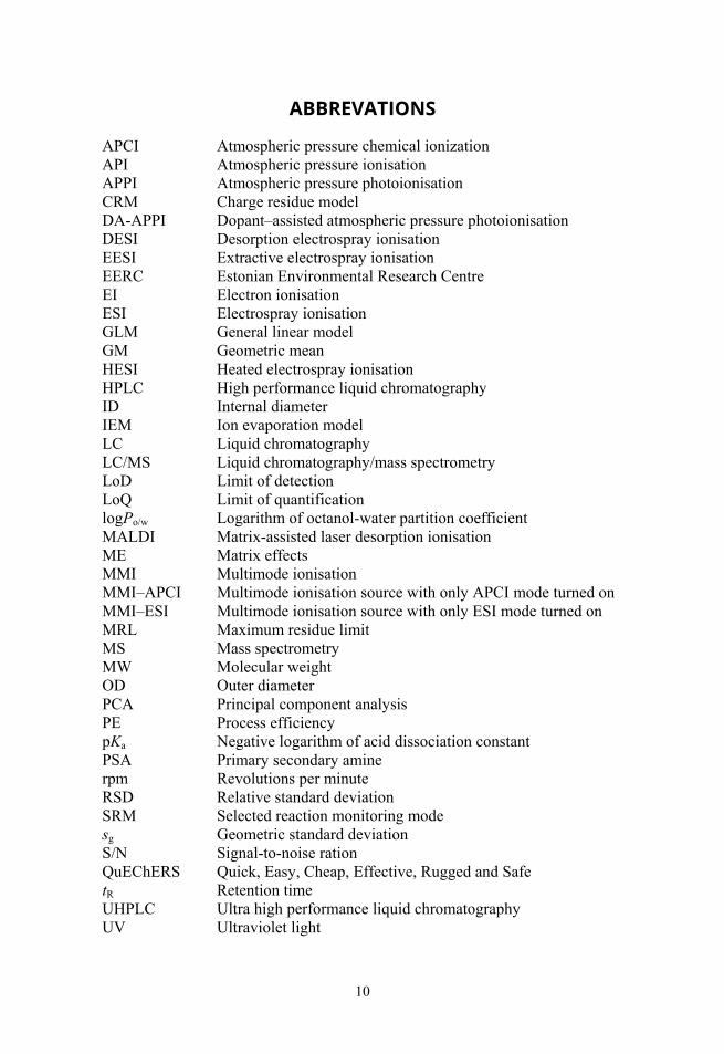
ABBREVATIONS
APCI Atmospheric pressure chemical ionization API Atmospheric pressure ionisation APPI Atmospheric pressure photoionisation CRM Charge residue model DA-APPI Dopant–assisted atmospheric pressure photoionisation DESI Desorption electrospray ionisation EESI Extractive electrospray ionisation EERC Estonian Environmental Research Centre EI Electron ionisation ESI Electrospray ionisation GLM General linear model GM Geometric mean HESI Heated electrospray ionisation HPLC High performance liquid chromatography ID Internal diameter IEM Ion evaporation model LC Liquid chromatography LC/MS Liquid chromatography/mass spectrometry LoD Limit of detection LoQ Limit of quantification logPo/w Logarithm of octanol-water partition coefficient MALDI Matrix-assisted laser desorption ionisation ME Matrix effects MMI Multimode ionisation MMI–APCI Multimode ionisation source with only APCI mode turned on MMI–ESI Multimode ionisation source with only ESI mode turned on MRL Maximum residue limit MS Mass spectrometry MW Molecular weight OD Outer diameter PCA Principal component analysis PE Process efficiency pKa Negative logarithm of acid dissociation constant PSA Primary secondary amine rpm Revolutions per minute RSD Relative standard deviation SRM Selected reaction monitoring mode sg Geometric standard deviation S/N Signal-to-noise ration QuEChERS Quick, Easy, Cheap, Effective, Rugged and Safe tR Retention time UHPLC Ultra high performance liquid chromatography UV Ultraviolet light
11
INTRODUCTION Coupling of liquid chromatography (LC) and mass spectrometry (MS) has given a powerful and selective analytical tool for various applications ranging from routine monitoring of contaminants in environmental samples to the identification of novel synthesis products. This coupling became possible due to the invention of electrospray ionisation source. Liquid chromatography/mass spectrometry (LC/MS) has ever since developed rapidly, both in LC part and MS part. An important component from the sensitivity perspective is the ionisation source of MS, which is generating ions from the LC effluent. Ionisation is affected by many different factors, such as the properties of analytes, matrix components, source parameters, eluent composition etc. One way for obtaining the best results is having several different sources operating with different principles and choosing the optimal source for a specific analysis. Today there are many novel ion sources introduced in the literature and several of them are also available commercially. In order for analyst to be able to choose among them, a lot of work needs to be done to compare different sources.
Electrospray ionisation (ESI) source is most used source for generating ions in MS. Some other popular sources are atmospheric pressure chemical ionisation (APCI) and atmospheric pressure photoionisation (APPI) sources. While they enable analysis of many different compounds, none of these sources is universal. Several novel sources are designed to give even better performance by lowering limits of detection and reducing matrix effects, such as heated ESI (HESI) sources, and to be able to analyse wider range of analytes, such as multimode (MMI) sources, which combine different ionisation modes in one source.
A novel nebuliser developed in our group for ESI has been characterised in this study as part of an effort to further enhance the ESI method (Paper I). Its novelty resides in the addition of nebuliser gas capillary inside the liquid capil-lary. This enhances the nebulisation process by generating finer droplets of effluent. However it needed optimisation and comparison with other sources.
During the thesis studies another possibility for enhancement of LC/MS method was researched: monolithic chromatographic columns (Papers IV–VI). Since monolithic columns are not as accessible as ionisation sources, we discuss the effect of ionisation sources in detail.
The aim of the thesis was two-fold: the comparison of different ionisation methods and secondly the optimisation of novel nebuliser. Also one of the aims was to compare the optimised novel ESI nebuliser with commercially available ESI nebuliser, in order to see which one has advantage in practical analysis (Paper II).
Different ionisation sources were compared to the performance of conven-tional ESI source under practical analysis conditions (Paper III). The comparison was performed on the basis of analysis of pesticides commonly analysed with LC/MS and having highly varying properties from the point of view of ionisation and compared with relevant statistical tests. It was also important to fulfil the aims of this work in the context of practical samples, such as garlic, honey, tomato etc., using relevant analytes (pesticides, drugs).
12
1. REVIEW OF LITERATURE
1.1. Liquid chromatography/mass spectrometry LC/MS is widely used method for the determination of many different analytes, such as pesticides,1–4 lipids,5 amino acids,6 pharmaceuticals,7 polymers and their additives,8,9 metabolites, etc.10 in different matrices such as fruits and vege-tables,2 blood plasma,1,5 bees,11,12 human body fluids10 etc. LC/MS is very diverse in its instrumentation, employing different stationary phases, pressures (HPLC vs UHPLC) and eluents in the LC part as well as a number of ionisation sources13,14 (ESI, APCI, APPI, MALDI, EI etc.) and mass analysers (ion trap, triple quadrupole etc.) in the MS part. Since it has such a variety of instru-mentation and its uses, there is a need to investigate the advantages and disadvantages of the different parts of LC/MS instrumentation and compare them with each other in order to find the best combinations for different applications. This study focuses on the MS ionisation sources part of LC/MS in order to choose between different sources on the basis of their advantages and disadvantages.
1.2. Ionisation sources in LC/MS Since the introduction of electrospray ionisation (ESI) source by Dole et al.15 and Fenn et al.16 several new ionisation sources for generating gas phase ions from solution phase have been introduced and commercialised. The two main principles for atmospheric pressure ionisation (API) are based on liquid phase ionisation processes (ESI, HESI, DESI, EESI etc.) or gas phase ionisation processes (APCI, APPI).
The most popular sources in addition to ESI are the atmospheric pressure chemical ionisation (APCI)13,17 and atmospheric pressure photoionisation (APPI) sources, which can be seen as adaption of the APCI concept.18 Some of the new developments have offered additional capabilities to the 2 main ionisa-tion processes. Heated electrospray ionisation (HESI) is a modification of the ESI source with additional sheath gas to further assist the nebulisation of effluent.19,20 Among other new sources the multimode ionisation (MMI) source is of great interest.13 In the MMI source the advantages of different ionisation techniques are combined such as ESI-APCI,21–23 ESI-APPI23 or APCI-APPI.24 With MMI it is possible to analyse a wider range of analytes with different hydrophobicity, polarity, volatility, etc. than with the individual sources.25
With increasing number of ion sources available it is of growing interest for researchers and chromatography practitioners to find the optimal ionisation source for a given LC/MS analysis task – one that gives highest sensitivity and lowest limits of detection, is least prone to matrix effects, etc. ESI is commonly seen as the default LC/MS ionisation source for analysing many different com-pounds, but due to a number of recent developments in ionisation sources, it is
13
important to compare the performance of ESI source with the novel sources, to determine the most suitable ionisation mode for a given analytical task.
1.2.1. ESI and HESI
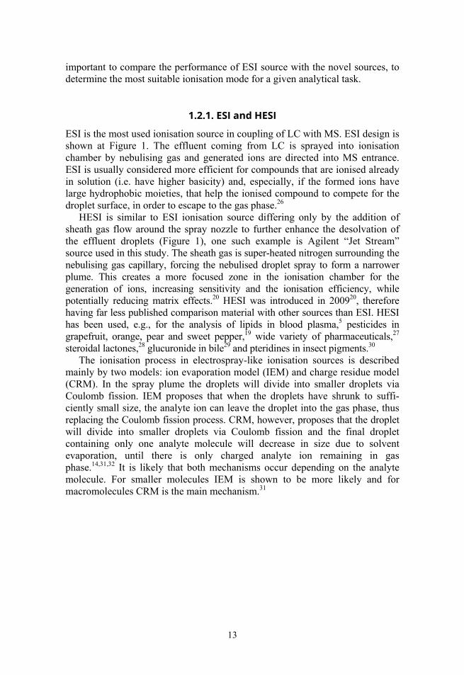
ESI is the most used ionisation source in coupling of LC with MS. ESI design is shown at Figure 1. The effluent coming from LC is sprayed into ionisation chamber by nebulising gas and generated ions are directed into MS entrance. ESI is usually considered more efficient for compounds that are ionised already in solution (i.e. have higher basicity) and, especially, if the formed ions have large hydrophobic moieties, that help the ionised compound to compete for the droplet surface, in order to escape to the gas phase.26
HESI is similar to ESI ionisation source differing only by the addition of sheath gas flow around the spray nozzle to further enhance the desolvation of the effluent droplets (Figure 1), one such example is Agilent “Jet Stream” source used in this study. The sheath gas is super-heated nitrogen surrounding the nebulising gas capillary, forcing the nebulised droplet spray to form a narrower plume. This creates a more focused zone in the ionisation chamber for the generation of ions, increasing sensitivity and the ionisation efficiency, while potentially reducing matrix effects.20 HESI was introduced in 200920, therefore having far less published comparison material with other sources than ESI. HESI has been used, e.g., for the analysis of lipids in blood plasma,5 pesticides in grapefruit, orange, pear and sweet pepper,19 wide variety of pharmaceuticals,27 steroidal lactones,28 glucuronide in bile29 and pteridines in insect pigments.30
The ionisation process in electrospray-like ionisation sources is described mainly by two models: ion evaporation model (IEM) and charge residue model (CRM). In the spray plume the droplets will divide into smaller droplets via Coulomb fission. IEM proposes that when the droplets have shrunk to suffi-ciently small size, the analyte ion can leave the droplet into the gas phase, thus replacing the Coulomb fission process. CRM, however, proposes that the droplet will divide into smaller droplets via Coulomb fission and the final droplet containing only one analyte molecule will decrease in size due to solvent evaporation, until there is only charged analyte ion remaining in gas phase.14,31,32 It is likely that both mechanisms occur depending on the analyte molecule. For smaller molecules IEM is shown to be more likely and for macromolecules CRM is the main mechanism.31
14
Figure 1. Instrumental principles of ESI and HESI.
1.2.2. APCI and APPI
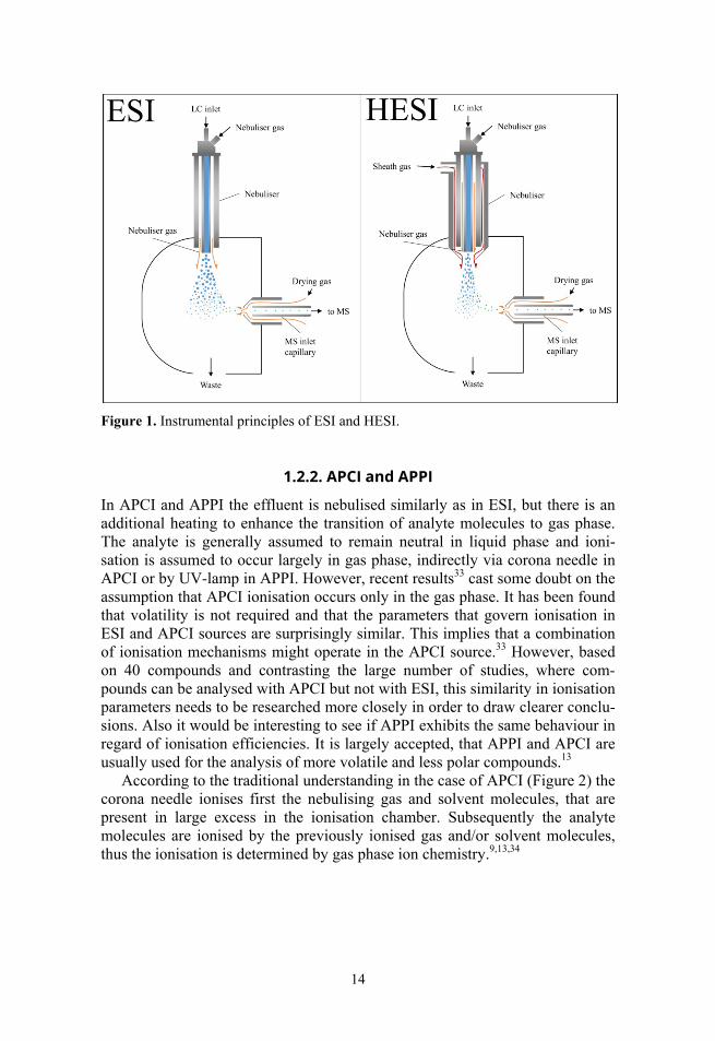
In APCI and APPI the effluent is nebulised similarly as in ESI, but there is an additional heating to enhance the transition of analyte molecules to gas phase. The analyte is generally assumed to remain neutral in liquid phase and ioni-sation is assumed to occur largely in gas phase, indirectly via corona needle in APCI or by UV-lamp in APPI. However, recent results33 cast some doubt on the assumption that APCI ionisation occurs only in the gas phase. It has been found that volatility is not required and that the parameters that govern ionisation in ESI and APCI sources are surprisingly similar. This implies that a combination of ionisation mechanisms might operate in the APCI source.33 However, based on 40 compounds and contrasting the large number of studies, where com-pounds can be analysed with APCI but not with ESI, this similarity in ionisation parameters needs to be researched more closely in order to draw clearer conclu-sions. Also it would be interesting to see if APPI exhibits the same behaviour in regard of ionisation efficiencies. It is largely accepted, that APPI and APCI are usually used for the analysis of more volatile and less polar compounds.13
According to the traditional understanding in the case of APCI (Figure 2) the corona needle ionises first the nebulising gas and solvent molecules, that are present in large excess in the ionisation chamber. Subsequently the analyte molecules are ionised by the previously ionised gas and/or solvent molecules, thus the ionisation is determined by gas phase ion chemistry.9,13,34
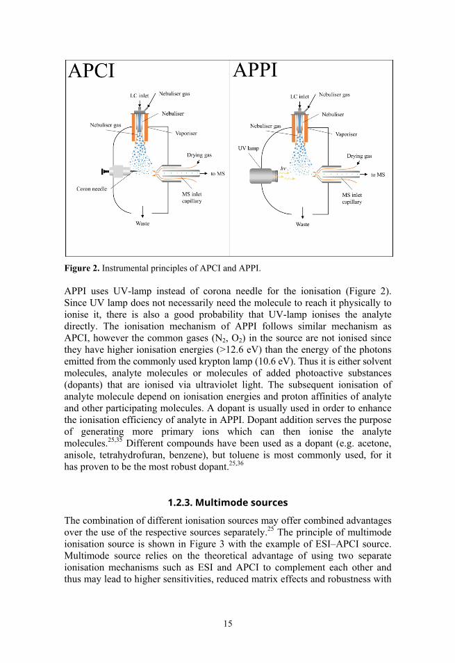
15
Figure 2. Instrumental principles of APCI and APPI.
APPI uses UV-lamp instead of corona needle for the ionisation (Figure 2). Since UV lamp does not necessarily need the molecule to reach it physically to ionise it, there is also a good probability that UV-lamp ionises the analyte directly. The ionisation mechanism of APPI follows similar mechanism as APCI, however the common gases (N2, O2) in the source are not ionised since they have higher ionisation energies (>12.6 eV) than the energy of the photons emitted from the commonly used krypton lamp (10.6 eV). Thus it is either solvent molecules, analyte molecules or molecules of added photoactive substances (dopants) that are ionised via ultraviolet light. The subsequent ionisation of analyte molecule depend on ionisation energies and proton affinities of analyte and other participating molecules. A dopant is usually used in order to enhance the ionisation efficiency of analyte in APPI. Dopant addition serves the purpose of generating more primary ions which can then ionise the analyte molecules.25,35 Different compounds have been used as a dopant (e.g. acetone, anisole, tetrahydrofuran, benzene), but toluene is most commonly used, for it has proven to be the most robust dopant.25,36
1.2.3. Multimode sources
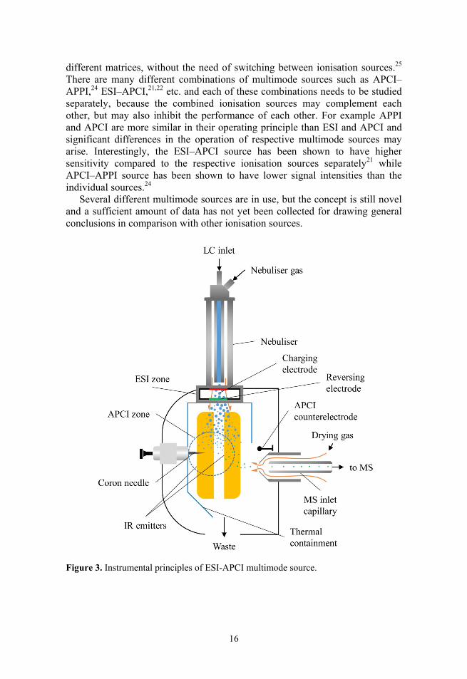
The combination of different ionisation sources may offer combined advantages over the use of the respective sources separately.25 The principle of multimode ionisation source is shown in Figure 3 with the example of ESI–APCI source. Multimode source relies on the theoretical advantage of using two separate ionisation mechanisms such as ESI and APCI to complement each other and thus may lead to higher sensitivities, reduced matrix effects and robustness with
16
different matrices, without the need of switching between ionisation sources.25 There are many different combinations of multimode sources such as APCI–APPI,24 ESI–APCI,21,22 etc. and each of these combinations needs to be studied separately, because the combined ionisation sources may complement each other, but may also inhibit the performance of each other. For example APPI and APCI are more similar in their operating principle than ESI and APCI and significant differences in the operation of respective multimode sources may arise. Interestingly, the ESI–APCI source has been shown to have higher sensitivity compared to the respective ionisation sources separately21 while APCI–APPI source has been shown to have lower signal intensities than the individual sources.24
Several different multimode sources are in use, but the concept is still novel and a sufficient amount of data has not yet been collected for drawing general conclusions in comparison with other ionisation sources.
Figure 3. Instrumental principles of ESI-APCI multimode source.
17
1.2.4. Other sources
Many other ionisation sources exist, which differ from the previous ones, such as electron ionisation (EI), where gaseous neutral analyte molecules are ionised in collision with high-energy electrons in order to produce radical cations.37 EI produces a lot of fragments and is not suitable when molecular ions are desired. Traditionally EI has been the standard ion source in gas chromatography-mass spectrometry, but lately has found uses in coupling with LC also.38 A softer ionisation method compared to EI is the matrix-assisted laser desorption ionisation (MALDI), where the sample is mixed with organic matrix for assisting the desorption and is then irradiated with a short laser pulse to produce a plume of ionised analyte that is subsequently analysed by MS. MALDI has become an especially powerful imaging tool for tissues.39 However, the coupling of online LC with MALDI is problematic.40
In desorption electrospray ionisation (DESI)41 a spray from ESI source is directed at the surface of solid sample, thus desorbing and ionising the analyte molecules from the surface. MS inlet is positioned at an angle of the bouncing droplets from the surface containing ionised analyte. This allows for direct analysis of analytes from surfaces. Extractive electrospray ionisation (EESI)42 is also a variant of ESI where the effluent containing neutral analyte is sprayed at an angle with another ESI nebuliser spraying a solvent solution. In collision of the two sprays the analyte molecules are ionised. EESI allows for direct analysis of liquid matrices such as water and urine. DESI and EESI, as variants of ESI, can also be used for the analysis of wide variety of analytes.
These are only a selection of the vast number of available ionisation sources. There is a lot more diversity and variations within each ionisation method and also with combinations of different sources.37
1.3. Advantages and limitations of different sources Mostly the traditional ESI source has been compared with APCI and/or APPI sources. HESI and MMI ionisation sources have received much less attention, partly because they are novel sources. The most important comparison para-meters have been the limit of detection (LoD),7,8,43–57 signal-to-noise ratio (S/N)7,48,50,53,56,58 and matrix effects (ME).19,46–48,50,55,56,59–61 Linearity47,48,53,56,57 and sensitivity (as calibration graph slope)44,48,51,53 have also been considered. The results published in the literature agree only in very general terms. Signi-ficant differences are evident in more specific aspects. The results are affected by the analytes used, matrix, solvent composition, ionisation source parameters, chromatographic separation etc.31

18
1.3.1. Linearity
Linear range can be an important characteristic in comparison of different ionisation sources. For the analysis of estradiol ESI, APCI and APPI have been used, both in negative and positive mode. ESI in positive mode yielded narrower linear range than APCI or APPI. For negative mode the linear ranges for ESI, APCI and APPI were comparable.48 Cai and Syage53 compared ESI, APCI and APPI in positive mode and also found the narrowest linear range for the ESI source. Titato et al.57 found comparable linear ranges for pesticides in comparison of ESI with APCI.
1.3.2. Matrix effects
One crucial parameter of an ionisation source is the matrix effect – ionisation suppression or enhancement caused by co-eluting matrix components. Matrix effect results usually in decreased (less often enhanced) analyte signal therefore causing underestimation (less often overestimation) of analyte quantity in the sample. Matrix effect can be influenced by the matrix type, chemical properties of the analyte, sample pretreatment, separation, instrumentation used etc.62–64 Therefore matrix effect can be very troublesome to eliminate. It would be preferable to use an ionisation source that is less prone to matrix effect. There-fore this parameter has been often used for comparison of ionisation sources. APCI and APPI have been often compared to ESI in terms of matrix effect. In general more matrix effect has been observed for ESI,46,48,56,59–61 however, in some cases ESI has performed better than APCI or APPI.47,50,55 For example Hanold et al.65 observed that APPI was much less susceptible to ion suppression than ESI and APCI. The differences in the extent of matrix effect have been related to the different ionisation mechanisms of ESI and APCI/APPI,62 but as the factors contributing to matrix effect are diverse, the conflicting results in the literature are not surprising. Also variations between different varieties of electrospray sources have been observed. Stahnke et al.19 have shown that ESI was less prone to matrix effects than HESI, although the opposite would be expected due to HESI’s improved ion desolvation and confinement of the spray by thermal gradient.20
1.3.3. Limit of detection, signal-to-noise ratio and sensitivity
LoD is among the most often used comparison parameters for ionisation sources. A number of authors have observed comparable or lower LoD values for ESI compared to APCI or APPI when analysing pharmaceuticals,50 pesticides,44,47,56 anabolic steroids,45 phytoestrogens,51 triazines, phenylureas,46 aflatoxin M156 and flavonoids.43 But the opposite has been observed for lipids,53 sulfonate esters,49 polymer additives,8 estradiol48 and pyrene derivatives52. It can be concluded that ESI and APCI/APPI are compound-dependent, as Thurman
19
et al.44 also concluded in case of pesticides. Comparing the compounds in the previous studies reveals that finding compound-property dependence patterns is complicated. It does seem, however, that compounds lacking ionic functional groups are performing better in APCI or APPI, in agreement with the classical ionisation models.
In several papers ionisation sources have been compared on the basis of S/N at a given concentration. S/N can be improved greatly if noise levels could be reduced, thus leading to potentially lower LoDs. Higher noise levels can origi-nate from matrix components, solvent clusters and contaminants.66,67 Thus different ionisation sources can have significantly different S/N ratios, as also observed in literature. It has usually been observed that APCI gives higher S/N values than ESI48,53 and APPI comparable or higher S/N values than APCI.7,48,53,58,65 However, Garcia-Ac et al.50 have shown the opposite: higher S/N for ESI than for APCI and APPI.
Sensitivity can be measured as the calibration graph slope. Based on the data obtained by Keski-Rahkonen et al.48 and Cai and Syage53 it can be concluded that the best sensitivity in these studies was observed for APPI, followed by APCI. The lowest sensitivity was observed for ESI. A gain in analyte peak areas (up to 4 times) has been reported for HESI compared to ESI,5 therefore it can be expected that HESI should have at least comparable if not better sensitivity compared to conventional ESI.
1.4. Novel developments in ESI sources There have been a number of novel developments for ESI sources. Some of the examples include modifying the nebuliser capillary tip68, implementing a wire into the liquid capillary69 and also the previously mentioned HESI with adding a super-heated desolvation gas capillary20, which has been commercialised by Agilent and is called “Jet Stream” ESI source.
Maxwell et al.68 showed that an asymmetrically cut ESI emitter tip offers increased sensitivity (approximately two times) compared to the conventional emitter tip geometry. Additionally, Reschke et al.69 compared emitters with different internal diameters (ID) in the range of 5 μm to 360 μm and found that larger ID results in higher signals even though the reverse is generally accepted from both theory and practice70. However, both of these studies were carried out for nano-ESI emitters and their conclusions cannot be automatically transferred to the pneumatically assisted nebulisers implemented in the conventional high flow rate ESI sources.
Bajic et al.71 have described the addition of a wire (preferably from a conducting material) into the liquid capillary. According to the results presented in ref 71 this addition improves ESI sensitivity by up to 3 times (for Reserpine) depending on the flow rate of the liquid. The sensitivity improvement due to the additional wire may result from two factors. First, the additional wire reduces the effective cross-sectional area of the liquid capillary. Secondly, more surface
20
is available in the nebuliser tip where electrochemical reactions – producing charge excess for the droplets – can take place.
Among other novel nebuliser designs we have recently introduced (Paper I) a novel concept of nebuliser design. An additional capillary – carrying the nebuliser gas – was installed inside the liquid capillary. The advantages of the prototype – lowering of LoD values by up to 250 times – were shown for four analytes even without optimisation of the nebuliser design.72 This nebuliser design is called 3R nebuliser.
It has also been described in the literature64 that different analytes as well as standards and samples may have somewhat different optimal ionisation and mass-spectrometer parameters. This indicates that samples with different complexity may result in somewhat different optima and also nebuliser design suitable for one analyte may be less beneficial for another analyte. Therefore it is very important to test the newly developed ESI nebuliser under different conditions (e.g. standards vs samples, different analytes).
21
2. EXPERIMENTAL
2.1. Chemicals Standards of carbendazim (99.0%), thiabendazole (98.5%), pymetrozine (99.0%), thiamethoxam (99.0%), vamidothion (99.0%), methiocarb sulfoxide (96.0%), chloridazon (98.0%), imidacloprid (99.5%), acetamiprid (98.5%), methiocarb sulfone (99.0%), thiacloprid (98.0%), imazalil (97.5%), thiophanate-methyl (97.5%), metribuzin (99.0%), pyrimethanil (99.0%), fenpropimorph (97.0%), spiroxamine (97.5%), propoxur (99.5%), triasulfuron (97.5%), bupirimate (98.0%), paclobutrazol (98.5%), methiocarb (98.5%), azoxystrobin (99.5%), epoxiconazole (98.5%), myclobutanil (97.5%), fenhexamid (99.0%), fluquin-conazole (98.5%), flusilazole (99.5%), mepanipyrim (99.0%), bitertanol (98.0%), propiconazole (97.5%), triazophos (81.0%), methoxychlor (98.5%), ditalimfos (99.5%), tebufenozide (99.0%), benalaxyl (99.5%), pyrazophos (97.0%), buprofezin (99.0%), indoxacarb (99.5%), trifloxystrobin (99.5%), quinoxyfen (99.0%), pirimiphos-ethyl (98.5%) and hexythiazox (99.3%) were obtained from Dr. Erhenstorfer (Augsburg, Germany). Acetonitrile (HPLC grade) for sample pretreatment and chromatographic separation was acquired from Sigma-Aldrich (St. Louis, United States). Methanol (HPLC grade) for chromatographic separation was acquired from J. T. Baker (Deventer, Netherlands). Toluene (99.9%) was acquired from Sigma-Aldrich (St. Louis, United States). Ultra-pure water was obtained with a Millipore Milli-Q Advantage A10 setup (Millipore, USA). For sample pretreatment anhydrous MgSO4 (99.2%) and glacial acetic acid, for acidification of acetonitrile, were acquired from Lach-Ner (Neratovice, Czech Republic), NaCl and sodium acetate from Reakhim (Leningrad, former Soviet Union) and primary-secondary amine (PSA) sorbent from Supelco (Bellefonte, USA). The aqueous mobile phase component (0.1% formic acid) for UHPLC were prepared from formic acid (98.0%, Riedel-de Haёn, Switzerland) and dissolved in ultra-pure water. The buffer (pH = 2.8) for HPLC was prepared from formic acid,1 mM ammonium acetate (99.0%, Fluka Chemie AG, Buchs, Germany) dissolved in ultra-pure water.
2.2. Instrumentation In Papers I and II measurements were performed on an Agilent Series 1100 LC/MSD Trap XCT (Agilent Technologies, Santa-Clara, USA). The instrument was equipped with a binary pump, an autosampler and a thermostatted column compartment. The injection volume was 5 or 10 μL, depending on analysis. For the separation, a 250 mm long Zorbax Eclipse XDB-C18 column with an Eclipse XDB-C18 12.5 mm pre-column (both with an internal diameter of 4.6 mm and particle size of 5 μm) was used. The mass spectrometer uses a quadrupole ion trap mass analyser. For instrument control, an Agilent ChemStation for LC Rev. A. 10.02 and MSD Trap Control version 5.2 were used. The ion transportation
22
parameters were optimised for each analyte at a chromatographic flow rate via MSD Trap Control software.64 All of the analyses were carried out in positive mode. The mass spectrometer was operated in the selected reaction monitoring mode (SRM). Full MS2 spectra were recorded.
In this study the dimensions and parameters of the novel nebuliser developed in our group were optimised. The optimised novel nebuliser was compared with a commercial nebuliser (with also optimised parameters according to procedure described by Kruve et al.64). Observed MS2 were independent of the nebuliser used.
In Paper I for the analysis of carbendazim, thiabendazole, imazalil and methiocarb72 gradient elution with methanol and buffer solution (pH = 2.8) was used. The linear gradient started at 20% methanol and was raised to 100% within 15 min, then the column was eluted for 7 min with methanol. After that the methanol content was lowered to 20% in 3 min. Stabilisation time of 7 min was used between injections. Eluent flow rate was 0.8 ml/min.
In Paper II for the analysis of honey samples gradient elution (flow rate 0.8 mL/min) was used with acetate buffer and methanol. The methanol percentage (v/v) was raised from 40 to 100% in 17 min, maintained at 100% for 5 min and lowered back to 40% in 3 min. The stabilisation time between runs was 7 min.
In Paper III, for the comparison of different ionisation modes, an Agilent 6495 Triple Quad LC/MS/MS instrument (Agilent Technologies, Santa-Clara, USA) was used. The UHPLC instrument was Agilent Infinity 1290, equipped with binary pump, an autosampler, a thermostatted column compartment. An Agilent Zorbax RRHD SB-C18 2.1×50 mm column with 1.8 μm particles was used for analyte separation. The injection volume was 1 μl. The mass spectro-meter uses a triple quadrupole mass analyser and has exchangeable ion sources. 7 different ionisation modes were used: ESI source, HESI source, APPI source with and without dopant and MMI source with simultaneous ESI and APCI ionisation, as well as both ESI and APCI separately. In the context of this work the term ionisation mode means both different sources as well different ionisation approaches within the same source (APPI with and without dopant; MMI source with simultaneous ESI and APCI, as well as ESI and APCI sepa-rately). For instrument control Agilent MassHunter Workstation version B.07.00 was used. The fragmentation voltages were optimised using the MassHunter Optimizer software. Sequential injections were made while changing collision energy in steps to find the values where most intense fragments were formed. After automatic fragmentation optimisation it was confirmed and fine-tuned manually. Manufacturer’s default source parameters were used for the analysis in the case of all sources.
In Paper III UHPLC analysis of 41 pesticides in the comparison of different ionisation modes gradient elution was used with formic acid aqueous solution and acetonitrile at 0.3 ml/min flow rate. Acetonitrile percentage (v/v) was raised from 10 to 100% in 6 min, maintained at 100% for 1 min and returned to 10% in 1 min. The stabilisation time between runs was 0.5 min.
23
For DA-APPI the dopant (toluene) was infused after column with infusion pump from KD Scientific (Holliston, United States). The flow rate of dopant was optimised within 0–1.75 ml/h range for all 41 pesticides. The lowest flow rate that gave the best peak areas for the largest number of compounds was chosen. 0.5 ml/h proved to be optimal for that.
For sample pretreatment, a centrifuge (Centrifuge 5430R) and stirrer (Mix-Mate from Eppendorf (Hamburg, Germany)) were used.
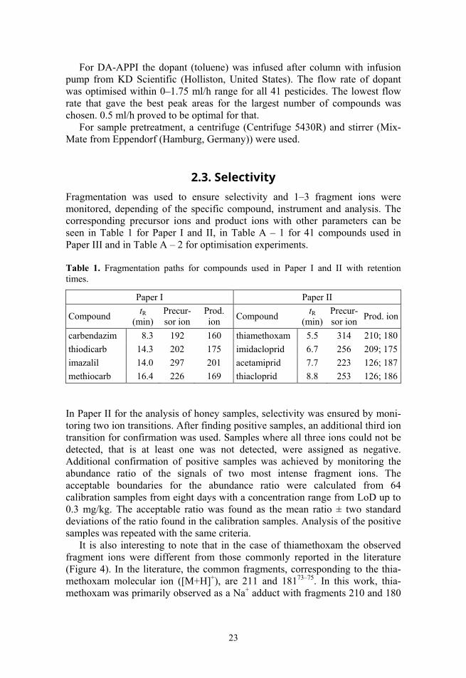
2.3. Selectivity Fragmentation was used to ensure selectivity and 1–3 fragment ions were monitored, depending of the specific compound, instrument and analysis. The corresponding precursor ions and product ions with other parameters can be seen in Table 1 for Paper I and II, in Table A – 1 for 41 compounds used in Paper III and in Table A – 2 for optimisation experiments.
Table 1. Fragmentation paths for compounds used in Paper I and II with retention times.
Paper I Paper II
Compound tR (min)
Precur-sor ion
Prod. ion Compound tR
(min)Precur-sor ion Prod. ion
carbendazim 8.3 192 160 thiamethoxam 5.5 314 210; 180 thiodicarb 14.3 202 175 imidacloprid 6.7 256 209; 175 imazalil 14.0 297 201 acetamiprid 7.7 223 126; 187 methiocarb 16.4 226 169 thiacloprid 8.8 253 126; 186
In Paper II for the analysis of honey samples, selectivity was ensured by moni-toring two ion transitions. After finding positive samples, an additional third ion transition for confirmation was used. Samples where all three ions could not be detected, that is at least one was not detected, were assigned as negative. Additional confirmation of positive samples was achieved by monitoring the abundance ratio of the signals of two most intense fragment ions. The acceptable boundaries for the abundance ratio were calculated from 64 calibration samples from eight days with a concentration range from LoD up to 0.3 mg/kg. The acceptable ratio was found as the mean ratio ± two standard deviations of the ratio found in the calibration samples. Analysis of the positive samples was repeated with the same criteria.
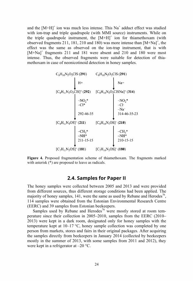
It is also interesting to note that in the case of thiamethoxam the observed fragment ions were different from those commonly reported in the literature (Figure 4). In the literature, the common fragments, corresponding to the thia-methoxam molecular ion ([M+H]+), are 211 and 18173–75. In this work, thia-methoxam was primarily observed as a Na+ adduct with fragments 210 and 180
24
and the [M+H]+ ion was much less intense. This Na+ adduct effect was studied with ion-trap and triple quadrupole (with MMI source) instruments. While on the triple quadrupole instrument, the [M+H]+ ion for thiamethoxam (with observed fragments 211, 181, 210 and 180) was more intense than [M+Na]+, the effect was the same as observed on the ion-trap instrument, that is with [M+Na]+ fragments 211 and 181 were absent and 210 and 180 were most intense. Thus, the observed fragments were suitable for detection of thia-methoxam in case of neonicotinoid detection in honey samples.
Figure 4. Proposed fragmentation scheme of thiamethoxam. The fragments marked with asterisk (*) are proposed to leave as radicals.
2.4. Samples for Paper II The honey samples were collected between 2005 and 2013 and were provided from different sources, thus different storage conditions had been applied. The majority of honey samples, 141, were the same as used by Rebane and Herodes76, 114 samples were obtained from the Estonian Environmental Research Centre (EERC) and 39 samples from Estonian beekeepers.
Samples used by Rebane and Herodes76 were mostly stored at room tem-perature since their collection in 2005–2010, samples from the EERC (2010–2013) were kept in a dark room, designated only for honey samples with the temperature kept at 10–17 °C, honey sample collection was completed by one person from markets, stores and fairs in their original packages. After acquiring the samples directly from beekeepers in January 2014 (collected by beekeepers mostly in the summer of 2013, with some samples from 2011 and 2012), they were kept in a refrigerator at –20 °C.
25
2.5. Sample pretreatments 2.5.1. QuEChERS in the comparison of nebulisers in Paper I
15 ml of 1% acetic acid in acetonitrile, 6 g MgSO4 and 1.5 g anhydrous sodium acetate was added to 15 g of homogenised sample. Shaken vigorously for 1 min and centrifuged at 5000 rpm for 1 min. The extract was transferred to tube containing 50 mg PSA + 150 mg anhydrous MgSO4 per 1 ml of extract. It was shaken again and centrifuged at 5000 rpm for 1 min.77
2.5.2. QuEChERS for honey samples pretreatment in Paper II
For sample pretreatment, the modified QuEChERS method77 was used. 1 g of honey was dissolved in 10 ml of purified water and 10 ml of acetonitrile. 4 g of MgSO4 and 1 g of NaCl were added and shaken for 1 min, followed by centri-fugation for 3 min at 4400 rpm. An acetonitrile fraction of 1 ml was pipetted into a 2 ml centrifuge tube with 150 mg of MgSO4 and 25 mg of PSA for clean-up, followed by stirring for 1 min. Tubes were centrifuged for 1 min at 5000 rpm and the supernatant was taken for analysis. For every honey sample, sample pretreatment was performed, followed by subsequent analysis on the same day.
2.5.3. QuEChERS for garlic and tomato samples in comparison of ionisation modes in Paper III
For sample pretreatment modified QuEChERS (Quick, Easy, Cheap, Effective, Rugged and Safe) method was used.78 15 ml of 1% acetic acid in acetonitrile was added to 15 g of tomato or 5 g of garlic homogenised sample. In the case of garlic, 10 ml of ultrapure water was also added, because the water content is much lower in garlic matrix. Subsequently 6 g of MgSO4 and 1.5 g of sodium acetate were added. The mixture was stirred and centrifuged for 7 min at 5000 rpm. 3.33 ml of the acetonitrile fraction was pipetted into 15 ml centrifuge tube with 500 mg of MgSO4 and 170 mg of primary secondary amine (PSA) for clean-up, followed by stirring and centrifugation for 7 min at 5000 rpm. The supernatant was taken for analysis. Samples were analysed in both extract and clean-up steps for the calculation of matrix effects with spiking of the blank sample, blank extract and blank extract clean-up steps.
26
2.6. Data analysis in experiments 2.6.1. Calculation of validation parameters
Upper limit of linear range was evaluated via visual inspection of residuals graph. The lower limit of linear range was determined by relative residuals. The limit of relative residuals was set to 20% as suggested in the SANCO guidelines (SANCO/12571/2013).79
LoD was determined either by S/N or by standard deviation of residuals. S/N was used for the preliminary characterisation of novel 3R nebuliser, because it is often used as one of the comparison parameters in case of novel develop-ments in ion sources. In the S/N approach the lowest concentration that gave S/N value of at least 3 was assigned as LoD. In the residuals approach the LoD was calculated according to the ICH validation guidelines:80,81
LoD = 3.3 × (1)
Both standard deviation of residuals and slope were determined in the LoD region, covering concentrations over approximately an order of magnitude. If it was not possible to confirm the calculated LoD with another fragment ion, then the lowest concentration where the peak of confirmatory ion was seen, was taken as LoD. The LoQ was determined by
LoQ = 10 × . (2)
S/N values from triple quadrupole mass spectrometer were obtained with the MassHunter software with signal definition as area and noise definition as Auto-RMS (root-mean-square of the baseline over time window). S/N values from ion-trap mass spectrometer for the comparison of nebulisers were obtained with Data Analysis software version 5.2, which calculates noise over the whole chromatogram except the peaks.
Sensitivities of the ion sources were compared on the basis of calibration graph slopes in the linear range. As the slope values ranged over several orders of magnitude ratios of slopes were compared instead.
For the comparison of sensitivity, S/N and LoD values, geometric mean (GM) as well as geometric standard deviation (sg) were used according to formulas,
GM = × × ⋯ (3) where an is the compound-wise ratio value of sensitivity, S/N or LoD values between two ionisation modes and n is the sum of all product ions over the 41 compounds detected. Formula for geometric standard deviation is defined as follows,
27
= exp ∑ ( )
(4)
where n is the same as in GM formula, ai is the same as an in GM formula, μg is the geometric mean of the ratio values of sensitivity, S/N or LoD values between two ionisation modes. The comparison of geometric means of the LoD, S/N and sensitivity ratios was done with HESI, because it gave the best results for these 3 parameters.
Matrix effect was calculated as follows: ME = ( )( ) × 100% (5)
where c(found) is the analyte concentration calculated from the analysis results and c(spiked) is the theoretical analyte concentration in the spiked sample. Matrix effect determinations were performed over a time period of 6 months in 4 dif-ferent series. Within series the extraction step of the sample pretreatment was performed with blank samples and 3 replicates of spiked matrix samples. Part of the blank extract was spiked and samples for analysis were taken from each solution in this step. The sample clean-up step was then performed with the 3 spiked matrix samples, blank extract and 3 replicates of the spiked extract. After the clean-up the blank sample was spiked and again samples for analysis were taken from each solution. Analysis of the samples was done in duplicate.
In Paper III for repeatability determination 9 replicates in garlic matrix were used. Repeatabilities obtained with the different ionisation sources were com-pared using the F-test and relative standard deviation of the signals of spiked garlic extracts (see Table A – 5). At first the statistical differences in variances of signals were established with comparison of the best performing source (ESI) with others using the F-test. Then the relative standard deviation was used to estimate if the statistical difference is of practical significance. If the relative standard deviation was over 10% for the source with higher repeatability stan-dard deviation, then the difference was considered significant in practice.
ANOVA, GLM and PCA analysis, as well as preparation of figures was per-formed with the R free software environment for statistical computing and graphics version 3.2.0 with packages pca3d and rgl (for PCA). Data were scaled and centred before analysis.
2.6.2. Proportions analysis
In Paper II neonicotinoids in honey samples were analysed for the comparison of novel nebuliser with commercial nebuliser. Honey samples were acquired from different years and for positive honey samples confidence intervals (the borders where in case of normal distribution the true value of the observed
28
parameter is with given condifence probability) were calculated. Proportions with 95% confidence intervals were calculated on a year-wise basis using the following formula:
= + 2+ 4 ; = 2 × (1 − )+ 4 (6)
where p is proportion, npos is the number of positive samples, n is the overall number of samples and W is the error margin at a 95% confidence level.82
2.6.3. Principal component analysis (PCA)
In Paper III PCA was performed for analytes with molecular parameters: retention time (tR), acidity of the conjugate acid (i.e. pKa of protonated analyte), octanol-water partition coefficient (logPo/w), molecular weight (MW) (values and additional information in Table A – 4) and separately for LoD and matrix effect data.
Three principal components were used for the analysis of molecular para-meters, describing 97% of variance in data. Then the data points on the 3D plot of the 4 molecular parameters were analysed in the context of LoD and ME values. Separately for each ionisation mode the LoD and ME values were divided into 4 groups of equal size, where each group had 25% of the data points. Then the PCA plot was analysed in order to see if the LoD and ME values were in an observable correlation with the PCA.
Another PCA was done to compare ionisation modes using only LoD or ME data, in order to see the profile differences of the different ionisation modes. Three principal components were used for LoD and ME, describing 84% and 67% of variance, respectively.
If one point of data was missing for a compound the whole compound was omitted because of the requirement of PCA that the data matrix is complete. Thus, altogether 36 compounds were used for LoD and 40 compounds were used for ME profile analysis. In the analysis of LoD PCA plot myclobutanil was deliberately omitted from the dataset, because it had LoD results that were heavily influenced by existence and detection concentration levels of qualitative fragmentation ions.
2.6.4. Full factorial design for the optimisation of 3R nebuliser
Full factorial design83 was used to plan the nebuliser optimisation experiments for both pesticides (standard solution and spiked garlic sample, both 1 mg/kg) and pharmaceuticals. For specifying most crucial parameters a two level design was used for 5 parameters (for instrumentation details see Figure 11):
29
1. Capillary B ID (B_ID): 0.25 mm and 0.50 mm; 2. Capillary C (C) presence: Yes (value 1 in GLM model) or No (value 0 in
GLM model); 3. Capillary C ID (C_ID): 90 μm and 175 μm (corresponding OD were 230 and
360 μm, therefore both could be implemented only if Capillary B ID was 0.5 mm);
4. Capillary C pressure (Cp): if present: 8 bar and 14 bar; 5. Capillary A pressure (CA): 5 and 12 psi; 6. Capillary Voltage (CapV): 2500 V and 4000 V.
The parameter levels were chosen according to both previous experiences and to cover a wide range of possible parameter values (for gas pressures and capillary voltages). For example the approximate dimensions of commercial ESI nebuliser are 150 μm ID and 250 μm OD for liquid capillary, 575 μm ID and 1700 μm OD for gas capillary.
Due to the technical reasons – mainly the limited long-term stability of the MS and the analytes – it was impossible to include more parameter levels into the parameter effect study, though more information on the nebulisation mecha-nism could be gathered this way. In order to detect parameters significantly influencing the ESI/MS sensitivity a two level data analysis was performed. First, the parameters statistically significantly influencing the ESI/MS signal were detected with ANOVA. Thereafter, the parameters, previously found to be statistically significant, were implemented into a GLM. GLM was used to estimate the physical impact (how large signal increase/decrease occurs due to a change of a parameter value) of each parameter and all possible two-parameter interactions. This two-stage data treatment is necessary as some parameters being statistically significant may have considerably lower influence on the ESI/MS signal than other parameters also being statistically significant. Before data treatment both parameter levels and obtained peak areas were scaled in order to obtain comparable results. The GLM model was obtained in the form:
= ∑ × + ∑ ∑ × (7) where only two parameter interactions were considered as follows: = × (8) The aim of the GLM model is not a full and accurate description of the electro-spray ionisation process, but revealing nebuliser design elements and working parameters that have significant impact on ESI/MS signal. The impact of each parameter or parameter interaction can be estimated from the absolute value of the coefficients – the larger the absolute coefficient the larger is the impact of the parameter-parameter interaction.
30
2.7. Design of experiment for ionisation modes comparison
A high concentration was selected for matrix effect and repeatability de-termination in order to avoid the loss of signal due to ionisation suppression with sources that give higher LoD values. This concentration was mostly at the upper part or near the upper limit of linear ranges, corresponding to the concentration range where the maximum residue limits (MRLs) of most of the compounds are in garlic and tomato (0.01–0.5 mg/kg). The concentration in matrices was approximately 0.1 mg/kg in garlic and in tomato. The corres-ponding solvent concentrations of the pesticides in the analysed samples were approximately 0.05 mg/kg and 0.16 mg/kg.
Manufacturers’ default source parameters were used for all ionisation sources. It was impractical to use individual source parameters for each compound in a study like this, as the gas flow rates and temperatures take a lot of time for stabilisation and therefore cannot be reasonably varied within a run. Additionally, different solvent compositions are expected to have somewhat different optimal source parameters. At the same time this study includes a large number of analytes, with very different retention times, and therefore eluting in very different solvent compositions. The average optimal parameter set is therefore expected not to deviate significantly from the default values.
SRM was used instead of full scan mode. For the absolute comparison of ionisation efficiencies in the sources full scan monitoring would be more proper. However, full scan would be impractical (especially keeping in mind selectivity), since SRM is mainly used in regular analysis of complex samples in order to ensure selectivity.
Besides the ionisation mode the results depend on compounds and elution conditions as well as on the MS system and ion source design and in order to obtain general conclusions these need to be cancelled out or accounted for. The compound dependence is accounted for by including compounds with varying properties. Dependence on the elution conditions and MS system is cancelled out by using all the MS sources on the same MS and with the same chromato-graphic method.
Dependence on the ion source design cannot be directly addressed in this experimental design, so that rigorously speaking, the results are applicable only to the sources used in this work. However, it has been demonstrated recently84 that the relative order of the compounds by ionisation efficiency largely follow the same trend across different mass analysers, indicating that the main processes responsible for ionisation are the same in different instruments regardless of different source design. Also, since all manufacturers of ion sources adhere to the same general goals – trying to produce as robust and sen-sitive ion sources as possible – it is expected that the general conclusions are valid for the same source types from different manufacturers.
31
3. RESULTS AND DISCUSSION
3.1. Comparison of ionisation sources Due to the large amount of different ionisation sources and the constant development of novel sources, it is important to compare different sources in order to find the optimal source for different applications. The aim of the comparison of different ionisation modes was to determine the ionisation source providing highest sensitivity and robustness for the analysis of pesticides. Thurman et al.44 showed that for different pesticide classes different ionisation sources (ESI or APCI) were optimal. Therefore it is interesting to see if the novel MMI source offers useful properties of combined sources and therefore minimising the need to use different sources. 7 different ionisation modes – ESI, HESI, direct APPI, DA-APPI and MMI with ESI and APCI mode simultaneously and separately, were used for the analysis of pesticides in tomato and garlic.
Pesticides are widely used for crop protection and the large number of different pesticides demands strict control over the MRLs established by EU and other authorised organisations3,85,86. Pesticides differ widely by polarity, acid/base properties, hydrophobicity etc. thus several ionisation sources have been used for their analysis including ESI, APCI and HESI19,44,47,86.
3.1.1. Comparison of chromatogram profiles
The peak profiles of different ionisation modes can give useful information about the general picture of ionisation efficiencies. As can be seen in Figure 5 relative peak areas of the compounds depend strongly on ionisation mode. For example, pirimiphos-ethyl gives large peaks in HESI and ESI modes (orange peak at 5.9 min in Figure 5), while for other ionisation modes the peak area of pirimiphos-ethyl is comparable to other compounds. Also much smaller (or absent) peaks of MMI-APCI are noticeable compared with other ionisation modes at the same concentrations. It is interesting that for both APPI modes the peak areas of different compounds are much closer to each other than for other ionisation modes (but at the same time, generally lower than with other modes). From data in Figure 5 both APPI modes seem to be less discriminating between compounds based on peak areas.
It has been shown that ionisation efficiency of compounds in ESI is affected by the ionisation in the solution phase and by competition for the surface of the droplets14,87. Recently it has been demonstrated that the relative order of com-pounds in ionisation efficiency scales is similar between ESI and APCI33. From Figure 5 also the similar profiles of chromatograms obtained with ESI and APCI can be observed. However, the chromatograms in Figure 5 seem to show similar profiles of MMI-APCI with ESI and HESI, but MMI-ESI leads to a
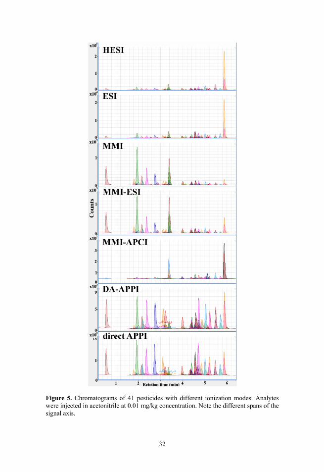
32
Figure 5. Chromatograms of 41 pesticides with different ionization modes. Analytes were injected in acetonitrile at 0.01 mg/kg concentration. Note the different spans of the signal axis.
33
surprisingly different peak profile. The peak profiles of the 3 MMI modes are inconsistent across different data series acquired on different time, giving sometimes the profile of MMI-APCI in Figure 5 and sometimes the profile of MMI-ESI in Figure 5 for all 3 modes. It can be concluded that MMI source itself is not very robust in its performance between series. For other ionisation sources the profiles matched throughout the experiments carried out over a period of one year.
A possible explanation for the less discriminating peak profiles of APPI is the direct ionisation mechanism. In the case of APPI the analyte molecule can be ionised both directly and indirectly.14,18,88 This potential reason needs to be researched more closely, in order to draw clearer conclusions. To the best of our knowledge there have been no studies relating the APPI ionisation efficiency with molecular parameters.
3.1.2. Repeatability
ESI and HESI displayed the best repeatability standard deviations pooled over all studied compounds: 3.1% and 3.4% respectively (Table A – 5), which can be considered acceptable. For both direct APPI and DA-APPI the average relative repeatability standard deviations were higher: 11.6% and 12.2%, respectively. The MMI ionisation modes display still worse repeatability: the average relative standard deviations were 18.3%, 34.3% and 23.0% for MMI, MMI-APCI and MMI-ESI, respectively, over the 41 compounds. The worst individual repeat-abilities for ESI and HESI were 8.2% and 9.0%, for fenhezamid and tebufenozide, respectively. For direct APPI, DA-APPI, MMI, MMI-APCI and MMI-ESI the worst repeatabilities were 43.4% (methiocarb sulfone), 52.9% (ditalimfos), 37.8% (benalaxyl), 267.7% (pyrimethanil) and 38.4% (quinoxyfen), respectively.
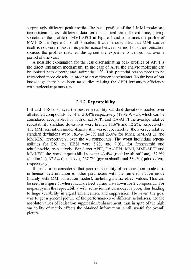
It needs to be considered that poor repeatability of an ionisation mode also influences determination of other parameters with the same ionisation mode (mainly with MMI ionisation modes), including matrix effect values. This can be seen in Figure 6, where matrix effect values are shown for 2 compounds. For mepanipyrim the repeatability with some ionisation modes is poor, thus leading to huge variability in signal enhancement and suppression. However, the goal was to get a general picture of the performances of different nebulisers, not the absolute values of ionisation suppression/enhancement, thus in spite of the high variability of matrix effects the obtained information is still useful for overall picture.
34
Figure 6. Example of matrix effect values over all series of data for chloridazon and mepanipyrim with all 7 ionization modes presented on a beeswarm plot. The high scatter of mepanipyrim matrix effect values in the case of MMI-APCI and MMI-ESI modes is caused by overall poor repeatability of mepanipyrim response with the MMI ion source.
3.1.3. Matrix effects
Matrix effect values were first analysed with t-test (95% confidence), com-paring the values with 100%. If matrix effects were not present then no signifi-cant difference from 100% should be observed over the data of 4 different series. Analysis showed that out of the 41 compounds there were no significant diffe-rences from 100% for 9, 9, 18, 12, 7, 3 and 19 compounds in case of ESI, MMI, MMI-APCI, MMI-ESI, HESI, direct APPI and DA-APPI respectively in garlic and in tomato 36, 27, 16, 28, 36, 34 and 40 compounds in case of ESI, MMI, MMI-APCI, MMI-ESI, HESI, direct APPI and DA-APPI respectively. It can be seen that matrix effect values in case of MMI-APCI and DA-APPI were not significantly different for close to half of the compounds in garlic and for most of the compounds in case tomato (except MMI-APCI). The t-test results are influenced by both average matrix effect and the repeatability observed with the respective source. MMI-APCI showed high variability (see section 1.12.2) of the results, which therefore may mask some important deviations from 100%. Additionally statistical differences may be insignificant in practice. Thus matrix effect values were also compared with the limits (70–120%) established by the SANCO/12571/2013 guideline, which considers trueness (process efficiency) values between 70 and 120% as acceptable. Though process efficiency incor-porates both matrix effect and recoveries from sample pretreatment, the matrix effect has to be at least in the same range to provide acceptable results.
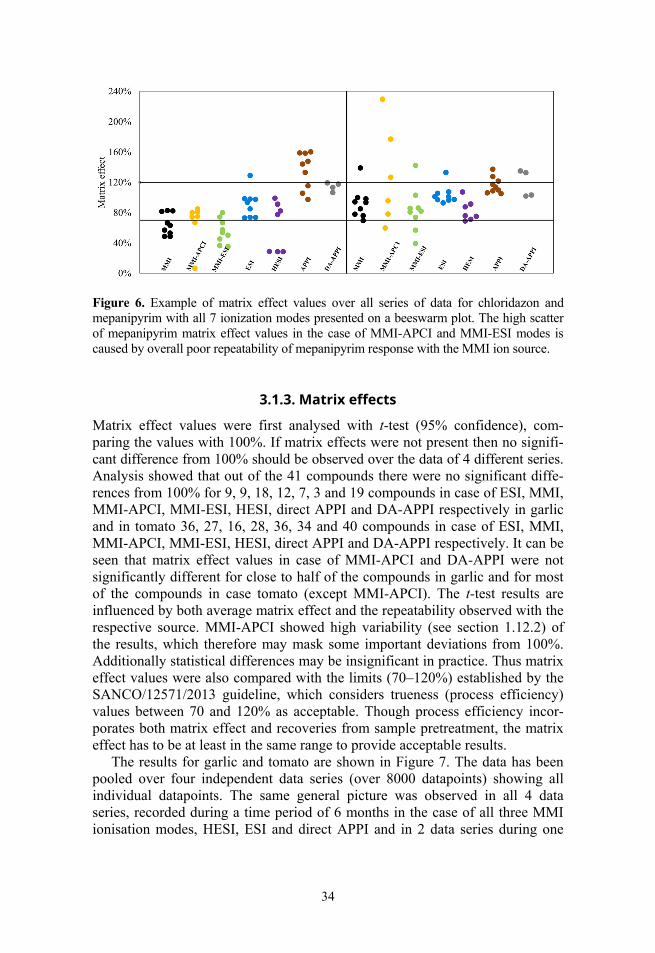
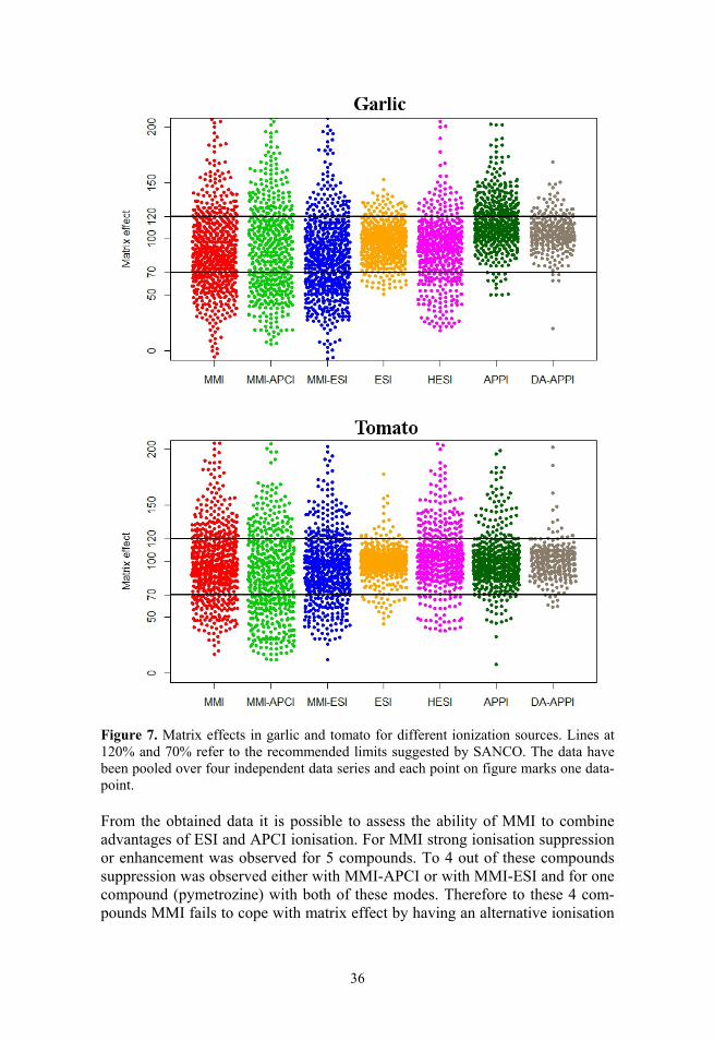
The results for garlic and tomato are shown in Figure 7. The data has been pooled over four independent data series (over 8000 datapoints) showing all individual datapoints. The same general picture was observed in all 4 data series, recorded during a time period of 6 months in the case of all three MMI ionisation modes, HESI, ESI and direct APPI and in 2 data series during one
35
month in the case of DA-APPI. Figure 7 reveals that all three MMI ionisation modes and HESI suffer from ionisation suppression or enhancement for a significant number of compounds (although, as mentioned above in a number of cases the poor repeatability can be the cause of large difference from 100%). HESI performs better than the three MMI ionisation modes but in the case of HESI there are still only 65% and 70% of the compounds (in garlic and tomato matrix, respectively) within the acceptable matrix effect limits as suggested by SANCO. These results for HESI are in agreement with those observed by Stahnke et al.19 Direct APPI has significant ionisation enhancement for garlic, with only 57% of the compounds within the limits, but shows better results for tomato, with 82% within limits. ESI and DA-APPI exhibit the least ionisation enhancement or suppression: 89% and 83% of the compounds, respectively, were within the acceptable limits in garlic and 93% and 91%, respectively, in tomato. It can be concluded that ESI and DA-APPI have least matrix effects in the case of tomato and garlic samples.
As would be expected, all ionisation modes have stronger ionisation enhancement or suppression in garlic samples than in tomato samples. Garlic is considered one of the worst matrices from the LC/MS matrix effect perspective, whereas tomato is a relatively simple matrix.89 The three MMI ionisation modes and HESI still display significant ionisation suppression or enhancement in tomato matrix. Only direct APPI, DA-APPI and ESI have over 80% of the data points within the acceptable limits for tomato samples.
The results on matrix effect published in literature are conflicting. Some studies show ESI to be less prone to matrix effect compared to APCI or APPI,46,48,56,59–61 but other studies show the opposite.47,50,55 This is most probably due to the variability of compounds and matrices analysed and elution conditions used. Since APPI/APCI have different mechanisms of ionisation compared to ESI, it is not unexpected that depending on the analyte and the co-eluting matrix components the results may vary. Based on the results of this study it can be concluded that for a large variety of small neutral molecules (containing both nitrogen and oxygen bases with very different ionisation sites) ESI seems to have from the point of view of matrix effect advantage over APPI, 3 MMI modes and HESI.
Comparing the ionisation modes compound-wise gave interesting results. Compounds that had statistically significant difference from 100% and gave consistently out of limits matrix effect values in all series after complete sample pretreatment were identified. Ionisation of pymetrozine was suppressed in all 4 measurement series in all ionisation modes except for ESI (in garlic and tomato) and DA-APPI (in tomato). The most probable reason is that pymetrozine is the first eluting compound with retention time tR = 0.57 min (dead time 0.50 min), while all other compounds have retention time over 1.7 minutes. With this retention time pymetrozine co-elutes with early-eluting matrix components as well as possible salt residues from the sample pretreatment. In spite of this the matrix effect of pymetrozine in the ESI source is within the acceptable limits even under such conditions.
36
Figure 7. Matrix effects in garlic and tomato for different ionization sources. Lines at 120% and 70% refer to the recommended limits suggested by SANCO. The data have been pooled over four independent data series and each point on figure marks one data-point.
From the obtained data it is possible to assess the ability of MMI to combine advantages of ESI and APCI ionisation. For MMI strong ionisation suppression or enhancement was observed for 5 compounds. To 4 out of these compounds suppression was observed either with MMI-APCI or with MMI-ESI and for one compound (pymetrozine) with both of these modes. Therefore to these 4 com-pounds MMI fails to cope with matrix effect by having an alternative ionisation
37
mechanism. On the other hand for 7 compounds MMI-APCI produced strong ionisation suppression or enhancement and for 2 compounds strong ionisation suppression with MMI-ESI in garlic samples, but MMI did not show ionisation suppression or enhancement. Similar trends were also observed for tomato matrix. Therefore the advantages of MMI tend to be strongly compound-dependent. Data in Figure 7 indicates that MMI is by matrix effect comparable with MMI-ESI and inferior to ESI, thus offering no real advantage.
The general trend of the ionisation enhancement and suppression across the chromatogram reveals more ionisation suppression than enhancement in the first half of the chromatogram and more enhancement in the second half of the chromatogram for all three MMI modes. The observed ionisation suppression may be caused by polar or ionic compounds in the extract and eluting in the beginning of the chromatogram. No other significant trends were observed.
PCA analysis of matrix effects within a series and also in the context of molecular parameters showed no correlations. That is to be expected, since matrix effect is also dependent on the matrix components and concentrations of the components among other variables. Thus it was not expected that ME could be explained by analytes molecular parameters alone.
3.1.4. Linearity
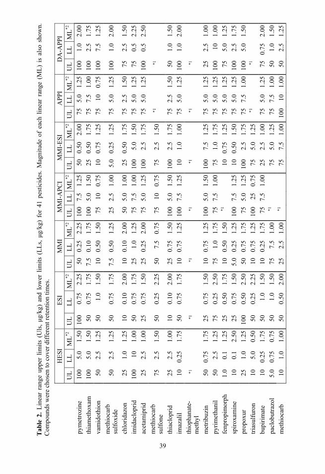
The linear ranges for ESI (Figure 8 and Table 2) are in general wide and extend to low concentrations. ESI is closely followed by HESI, DA-APPI and MMI. All three have on average narrower linear ranges than ESI. The MMI-ESI source has slightly wider linear ranges that extend to lower concentrations com-pared to direct APPI and MMI-APCI ionisation modes. However, for MMI-ESI and especially for MMI-APCI the linear range for many compounds could not be determined, because for these compounds no linearity was observed (MMI-ESI and MMI-APCI) or the number of data points with significant signal was too small for linearity determination (MMI-APCI).
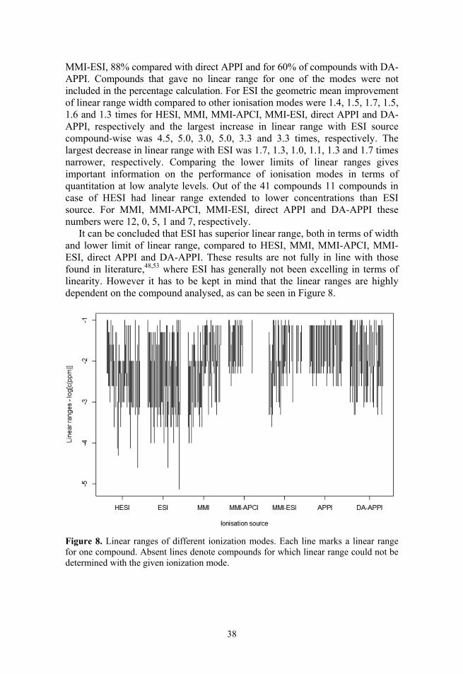
In the case of ESI the linear ranges could be determined for all compounds except for thiophanate-methyl (signals were obtained for concentrations range of less than 1 order of magnitude). Three compounds did not have a linear range with HESI, 2 compound with MMI, 24 with MMI-APCI, 10 with MMI-ESI, 7 with APPI and 6 with DA-APPI, because there were either not enough points for the given compound or linearity was not observed in the analysed range. In the case of 8 compounds (fenhexamid, mepanipyrim, bitertanol, methoxychlor, ditalimfos, tebufenozide, benalaxyl and quinoxyfen) the linear ranges could not be determined neither with MMI-ESI nor with MMI-APCI, but could be determined in with MMI. For trifloxystrobin linear range could not be determined with any arrangement of the MMI source.
When comparing the linear ranges compound-wise it was observed that ESI gave wider linear ranges for 68% of compounds compared to HESI, 72% compared with MMI, 94% compared with MMI-APCI, 84% compared with
38
MMI-ESI, 88% compared with direct APPI and for 60% of compounds with DA-APPI. Compounds that gave no linear range for one of the modes were not included in the percentage calculation. For ESI the geometric mean improvement of linear range width compared to other ionisation modes were 1.4, 1.5, 1.7, 1.5, 1.6 and 1.3 times for HESI, MMI, MMI-APCI, MMI-ESI, direct APPI and DA-APPI, respectively and the largest increase in linear range with ESI source compound-wise was 4.5, 5.0, 3.0, 5.0, 3.3 and 3.3 times, respectively. The largest decrease in linear range with ESI was 1.7, 1.3, 1.0, 1.1, 1.3 and 1.7 times narrower, respectively. Comparing the lower limits of linear ranges gives important information on the performance of ionisation modes in terms of quantitation at low analyte levels. Out of the 41 compounds 11 compounds in case of HESI had linear range extended to lower concentrations than ESI source. For MMI, MMI-APCI, MMI-ESI, direct APPI and DA-APPI these numbers were 12, 0, 5, 1 and 7, respectively.
It can be concluded that ESI has superior linear range, both in terms of width and lower limit of linear range, compared to HESI, MMI, MMI-APCI, MMI-ESI, direct APPI and DA-APPI. These results are not fully in line with those found in literature,48,53 where ESI has generally not been excelling in terms of linearity. However it has to be kept in mind that the linear ranges are highly dependent on the compound analysed, as can be seen in Figure 8.
Figure 8. Linear ranges of different ionization modes. Each line marks a linear range for one compound. Absent lines denote compounds for which linear range could not be determined with the given ionization mode.
39
Tab
le 2
. L
inea
r ra
nge
uppe
r li
mit
s (U
ls, μg
/kg)
and
low
er l
imits
(L
Ls,
μg/
kg)
for
41 p
estic
ides
. M
agni
tude
of
each
lin
ear
rang
e (M
L)
is a
lso
show
n.
Com
poun
ds w
ere
chos
en to
cov
er d
iffe
rent
ret
entio
n tim
es.
HE
SI
ES
I M
MI
MM
I-A
PC
I M
MI-
ESI
A
PPI
D
A-A
PPI
UL
LL
M
L*2
UL
LL
M
L*2
UL
LL
M
L*2
UL
LL
ML
*2U
LL
L
ML
*2U
LL
LM
L*2
UL
LL
M
L*2
pym
etro
zine
10
05.
01.
5010
00.
752.
2550
0.25
2.
2510
07.
51.
2550
0.50
2.00
755.
01.
2510
01.
0 2.
00
thia
met
hoxa
m
100
5.0
1.50
500.
751.
757.
50.
10
1.75
100
5.0
1.50
250.
501.
7575
7.5
1.00
100
2.5
1.75
vam
idot
hion
50
2.5
1.25
501.
01.
5010
0.50
1.
5075
100.
7510
0.75
1.25
7510
0.75
100
7.5
1.25
met
hioc
arb
sulf
oxid
e 50
2.5
1.25
500.
751.
757.
50.
50
1.25
252.
51.
005.
00.
251.
2575
5.0
1.25
100
1.0
2.00
chlo
rida
zon
251.
01.
2510
0.10
2.00
100.
10
2.00
505.
01.
0025
0.50
1.75
752.
51.
5075
2.5
1.50
imid
aclo
prid
10
010
1.00
500.
751.
7525
1.0
1.25
757.
51.
0010
05.
01.
5075
5.0
1.25
750.
5 2.
25
acet
amip
rid
252.
51.
0025
0.75
1.50
250.
25
2.00
755.
01.
2510
02.
51.
7575
5.0
1.25
100
0.5
2.50
met
hioc
arb
sulf
one
752.
51.
5050
0.25
2.25
507.
5 0.
7575
100.
7575
2.5
1.50
*1*1
thia
clop
rid
252.
51.
0010
0.10
2.00
250.
75
1.50
100
5.0
1.50
100
2.5
1.75
752.
51.
5050
1.0
1.50
imaz
alil
10
0.25
1.75
500.
751.
7510
0.75
1.
2510
07.
51.
2510
1.0
1.00
755.
01.
2510
01.
0 2.
00
thio
phan
ate-
met
hyl
*1*1
*1
*1
*1*1
*1
met
ribu
zin
500.
751.
7525
0.75
1.50
100.
75
1.25
100
5.0
1.50
100
7.5
1.25
755.
01.
2525
2.5
1.00
pyri
met
hani
l 50
2.5
1.25
750.
252.
5075
1.0
1.75
757.
51.
0075
1.0
1.75
755.
01.
2510
010
1.
00
fenp
ropi
mor
ph
1.0
0.1
1.25
250.
501.
7510
0.50
1.
50*1
100.
751.
2575
5.0
1.25
755.
0 1.
25
spir
oxam
ine
100.
12.
5025
0.75
1.50
5.0
0.25
1.
2510
07.
51.
2510
0.50
1.50
755.
01.
2510
02.
5 1.
75
prop
oxur
25
1.0
1.25
100
0.50
2.50
500.
75
1.75
755.
01.
2510
02.
51.
7575
7.5
1.00
100
5.0
1.50
tria
sulf
uron
10
5.0
0.50
500.
252.
2510
0.75
1.
2510
025
0.75
755.
01.
25*1
*1
bupi
rim
ate
100.
251.
7550
1.0
1.50
100.
25
1.75
757.
51.
0025
2.5
1.00
755.
01.
2575
0.75
2.
00
pacl
obut
razo
l 5.
00.
750.
7550
1.0
1.50
757.
5 1.
00*1
755.
01.
2575
7.5
1.00
501.
0 1.
50
met
hioc
arb
101.
01.
0050
0.50
2.00
252.
5 1.
00*1
757.
51.
0010
010
1.00
502.
5 1.
25
39
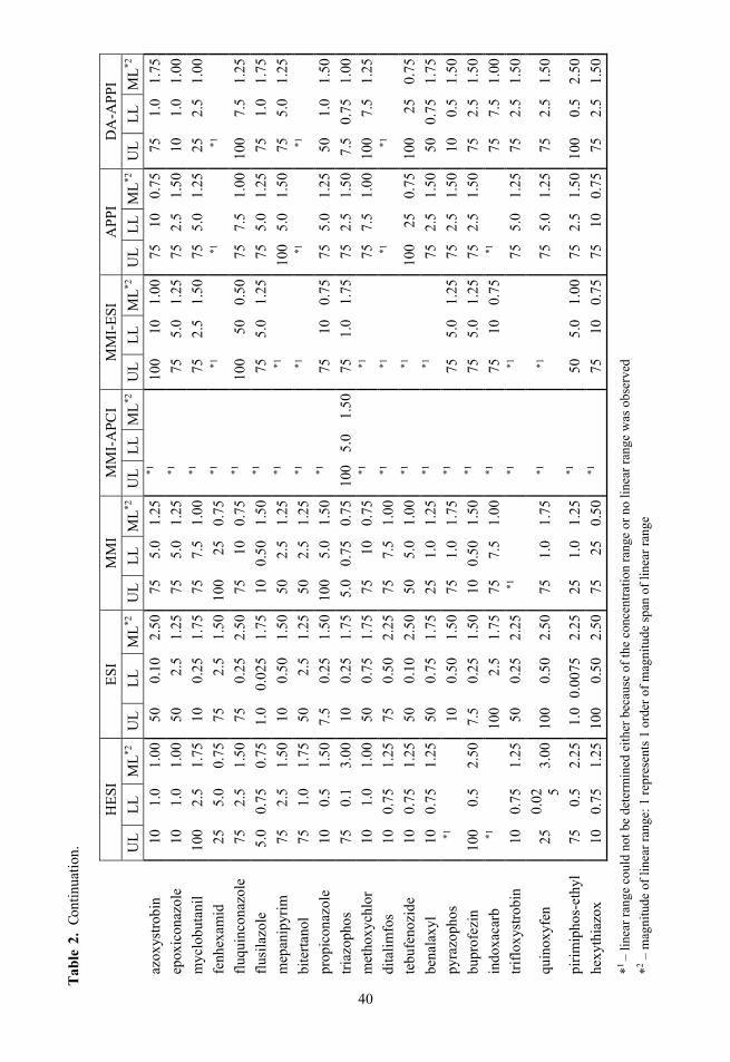
40
HE
SI
ES
I M
MI
MM
I-A
PC
I M
MI-
ESI
A
PPI
D
A-A
PPI
UL
LL
M
L*2
UL
LL
M
L*2
UL
LL
M
L*2
UL
LL
ML
*2U
LL
L
ML
*2U
LL
LM
L*2
UL
LL
M
L*2
azox
ystr
obin
10
1.0
1.00
500.
102.
5075
5.0
1.25
*110
010
1.00
7510
0.75
751.
0 1.
75
epox
icon
azol
e 10
1.0
1.00
502.
51.
2575
5.0
1.25
*175
5.0
1.25
752.
51.
5010
1.0
1.00
myc
lobu
tani
l 10
02.
51.
7510
0.25
1.75
757.
5 1.
00*1
752.
51.
5075
5.0
1.25
252.
5 1.
00
fenh
exam
id
255.
00.
7575
2.5
1.50
100
25
0.75
*1*1
*1*1
fluq
uinc
onaz
ole
752.
51.
5075
0.25
2.50
7510
0.
75*1
100
500.
5075
7.5
1.00
100
7.5
1.25
flus
ilazo
le
5.0
0.75
0.75
1.0
0.02
51.
7510
0.50
1.
50*1
755.
01.
2575
5.0
1.25
751.
0 1.
75
mep
anip
yrim
75
2.5
1.50
100.
501.
5050
2.5
1.25
*1*1
100
5.0
1.50
755.
0 1.
25
bite
rtan
ol
751.
01.
7550
2.5
1.25
502.
5 1.
25*1
*1*1
*1
prop
icon
azol
e 10
0.5
1.50
7.5
0.25
1.50
100
5.0
1.50
*175
100.
7575
5.0
1.25
501.
0 1.
50
tria
zoph
os
750.
13.
0010
0.25
1.75
5.0
0.75
0.
7510
05.
01.
5075
1.0
1.75
752.
51.
507.
50.
75
1.00
met
hoxy
chlo
r 10
1.0
1.00
500.
751.
7575
10
0.75
*1*1
757.
51.
0010
07.
5 1.
25
dita
lim
fos
100.
751.
2575
0.50
2.25
757.
5 1.
00*1
*1*1
*1
tebu
feno
zide
10
0.75
1.25
500.
102.
5050
5.0
1.00
*1*1
100
250.
7510
025
0.
75
bena
laxy
l 10
0.75
1.25
500.
751.
7525
1.0
1.25
*1*1
752.
51.
5050
0.75
1.
75
pyra
zoph
os
*110
0.50
1.50
751.
0 1.
75*1
755.
01.
2575
2.5
1.50
100.
5 1.
50
bupr
ofez
in
100
0.5
2.50
7.5
0.25
1.50
100.
50
1.50
*175
5.0
1.25
752.
51.
5075
2.5
1.50
indo
xaca
rb
*110
02.
51.
7575
7.5
1.00
*175
100.
75*1
757.
5 1.
00
trif
loxy
stro
bin
100.
751.
2550
0.25
2.25
*1*1
*175
5.0
1.25
752.
5 1.
50
quin
oxyf
en
250.
02 53.
0010
00.
502.
5075
1.0
1.75
*1*1
755.
01.
2575
2.5
1.50
piri
mip
hos-
ethy
l 75
0.5
2.25
1.0
0.00
752.
2525
1.0
1.25
*150
5.0
1.00
752.
51.
5010
00.
5 2.
50
hexy
thia
zox
100.
751.
2510
00.
502.
5075
25
0.50
*175
100.
7575
100.
7575
2.5
1.50
*1 –
line
ar r
ange
cou
ld n
ot b
e de
term
ined
eit
her
beca
use
of th
e co
ncen
trat
ion
rang
e or
no
line
ar r
ange
was
obs
erve
d
*2 – m
agni
tude
of
line
ar r
ange
: 1 r
epre
sent
s 1
orde
r of
mag
nitu
de s
pan
of li
near
ran
ge
Tab
le 2
. Co
ntin
uati
on.
40
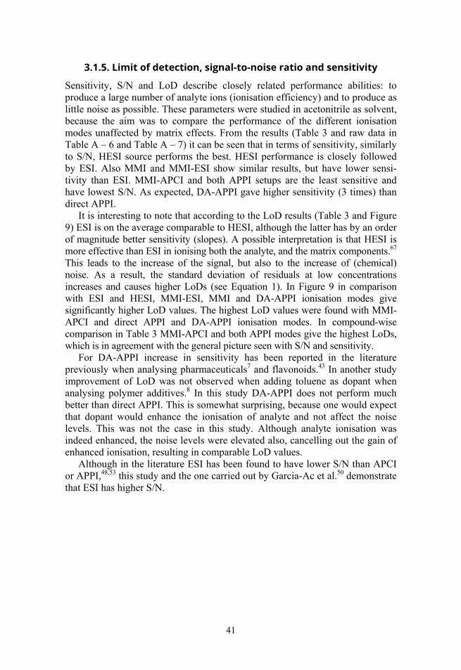
41
3.1.5. Limit of detection, signal-to-noise ratio and sensitivity
Sensitivity, S/N and LoD describe closely related performance abilities: to produce a large number of analyte ions (ionisation efficiency) and to produce as little noise as possible. These parameters were studied in acetonitrile as solvent, because the aim was to compare the performance of the different ionisation modes unaffected by matrix effects. From the results (Table 3 and raw data in Table A – 6 and Table A – 7) it can be seen that in terms of sensitivity, similarly to S/N, HESI source performs the best. HESI performance is closely followed by ESI. Also MMI and MMI-ESI show similar results, but have lower sensi-tivity than ESI. MMI-APCI and both APPI setups are the least sensitive and have lowest S/N. As expected, DA-APPI gave higher sensitivity (3 times) than direct APPI.
It is interesting to note that according to the LoD results (Table 3 and Figure 9) ESI is on the average comparable to HESI, although the latter has by an order of magnitude better sensitivity (slopes). A possible interpretation is that HESI is more effective than ESI in ionising both the analyte, and the matrix components.67 This leads to the increase of the signal, but also to the increase of (chemical) noise. As a result, the standard deviation of residuals at low concentrations increases and causes higher LoDs (see Equation 1). In Figure 9 in comparison with ESI and HESI, MMI-ESI, MMI and DA-APPI ionisation modes give significantly higher LoD values. The highest LoD values were found with MMI-APCI and direct APPI and DA-APPI ionisation modes. In compound-wise comparison in Table 3 MMI-APCI and both APPI modes give the highest LoDs, which is in agreement with the general picture seen with S/N and sensitivity.
For DA-APPI increase in sensitivity has been reported in the literature previously when analysing pharmaceuticals7 and flavonoids.43 In another study improvement of LoD was not observed when adding toluene as dopant when analysing polymer additives.8 In this study DA-APPI does not perform much better than direct APPI. This is somewhat surprising, because one would expect that dopant would enhance the ionisation of analyte and not affect the noise levels. This was not the case in this study. Although analyte ionisation was indeed enhanced, the noise levels were elevated also, cancelling out the gain of enhanced ionisation, resulting in comparable LoD values.
Although in the literature ESI has been found to have lower S/N than APCI or APPI,48,53 this study and the one carried out by Garcia-Ac et al.50 demonstrate that ESI has higher S/N.
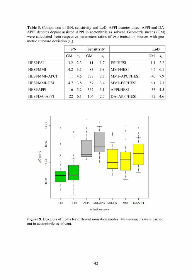
42
Table 3. Comparison of S/N, sensitivity and LoD. APPI denotes direct APPI and DA-APPI denotes dopant assisted APPI in acetonitrile as solvent. Geometric means (GM) were calculated from respective parameters ratios of two ionisation sources with geo-metric standard deviation (sg).
S/N Sensitivity LoD GM sg GM sg GM sg
HESI/ESI 3.2 2.3 11 1.7 ESI/HESI 1.1 2.2
HESI/MMI 4.2 3.1 83 3.8 MMI/HESI 4.5 6.1
HESI/MMI–APCI 11 4.5 378 2.8 MMI–APCI/HESI 40 7.9
HESI/MMI–ESI 4.7 3.8 57 3.4 MMI–ESI/HESI 6.1 7.3
HESI/APPI 16 5.2 362 3.1 APPI/HESI 33 4.5
HESI/DA–APPI 22 6.1 104 2.7 DA–APPI/HESI 32 4.6
Figure 9. Boxplots of LoDs for different ionisation modes. Measurements were carried out in acetonitrile as solvent.
43
3.1.6. Principal Component Analysis of LoD results
PCA was used in order to gain better understanding on which properties facili-tate low LoD values on one or another ionisation source. The LoD PCA plot for 3 principal components explaining 84% of data variance is presented in Figure 10. From the PCA plot the ionisation modes grouped into 3 distinct groups. First group shows that HESI and ESI have similar profiles, with the fluctuations in the LoD values follow similar logic (not the same values). The correlation of the LoD values of ESI and HESI was high (R2=0.87). APPI and DA-APPI also follow similar logic in LoD values and the 3 MMI modes form a third group. The correlation of the LoD values were not as high as ESI and HESI had shown: APPI and DA-APPI had R2=0.56 and others were even worse. These groups seem to be formed based on ionisation mechanisms. However, MMI-ESI would be expected to be more similar to ESI, but this is not the case. It seems that there is some other process affecting the 3 MMI modes that seems to be sufficiently different from the ESI ionisation mechanism. One of the reasons could be that MMI-ESI has distinctly different geometry than HESI and ESI.
Figure 10. PCA plot for LoDs of different ionization modes. 84% of data variance is explained by first 3 principal components. PCA was also carried out on the basis of the molecular parameters shown in Table A – 4 in Appendices. It was attempted to group the data points on the 3D plot according to LoD results, i.e. the LoD results did not affect the plot. However there were no clear correlations between the molecular parameters and LoD results. It can be because too few compounds were analysed for such analysis.
44
3.1.7. Conclusions of comparison
The ionisation mechanism in different ionisation modes is an active research field.14,31,35,63 Nevertheless, some general trends are evident. Interestingly, the MMI source underperformed in comparison to the traditional ESI, although in theory it should have performed better,21,25 because of the addition of APCI. It is the opinion of the authors that at least part of the reason is that the geometry of the MMI ionisation chamber is optimal neither for ESI nor for APCI. The nebuliser capillary tip of the MMI source is situated at a much larger distance from the MS inlet than in the conventional ESI source. Also there is a small separating wall perpendicular to MS inlet functioning as separator of the ESI and APCI regions in the source. Because of this separating wall some part of the nebulised effluent is directed further away from MS inlet, causing decreased sensitivities and increased LoDs. This design of the ionisation chamber can be the reason why MMI-ESI performs better than MMI-APCI when the respective traditional APCI has in some cases shown to perform better than traditional ESI.43–45,48,49,51,57
The unexpected underperformance of HESI may also be caused by the source design. HESI uses additional sheath gas to confine the spray plume for enhanced desolvation of droplets.20 However, the addition of sheath gas seems to increase matrix effects both in this study and in the report by Stahnke et al.19 HESI is significantly more prone to chemical noise, which is the generation of ions from matrix components other than the analyte.67 Thus the advantage in sensitivity, achieved by more efficient ionisation of the analyte is partially offset by the increase in chemical noise.
The poor sensitivity and high LoD values of direct APPI can be explained by the compounds properties used for the comparison. Although the pesticides vary significantly in polarity (logP between –0.2 to 5), they are still small molecules having ionisable functional groups (all have at least one nitrogen or oxygen atom in molecule), thus the poor performance might be caused by the com-pounds that are not APPI specific. DA-APPI showed a significant improvement compared with direct APPI in the case of matrix effects and linear range. However, as the overall conclusion, the sensitivity and LoD values of DA-APPI are still much inferior to ESI.
3.2. Novel 3R nebuliser for ESI source Novel 3R nebuliser offers a new concept of the ESI source introduced by Kruve et al.72. While the commercial nebuliser has spraying gas around the effluent only, the novel nebuliser introduces additional gas inside the effluent as is shown in Figure 11. It is hypothesised that the inner nebuliser gas gives addi-tional nebulising power to generate smaller droplets and enhanced ionisation of analytes.
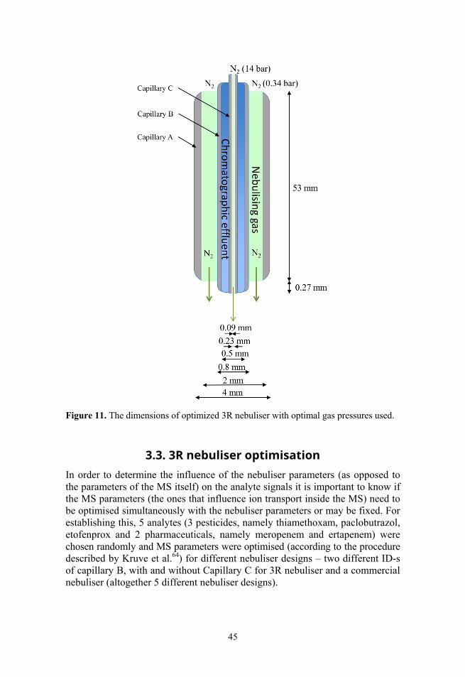
45
Figure 11. The dimensions of optimized 3R nebuliser with optimal gas pressures used.
3.3. 3R nebuliser optimisation In order to determine the influence of the nebuliser parameters (as opposed to the parameters of the MS itself) on the analyte signals it is important to know if the MS parameters (the ones that influence ion transport inside the MS) need to be optimised simultaneously with the nebuliser parameters or may be fixed. For establishing this, 5 analytes (3 pesticides, namely thiamethoxam, paclobutrazol, etofenprox and 2 pharmaceuticals, namely meropenem and ertapenem) were chosen randomly and MS parameters were optimised (according to the procedure described by Kruve et al.64) for different nebuliser designs – two different ID-s of capillary B, with and without Capillary C for 3R nebuliser and a commercial nebuliser (altogether 5 different nebuliser designs).
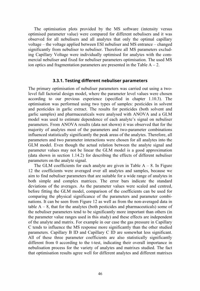
46
The optimisation plots provided by the MS software (intensity versus optimised parameter value) were compared for different nebulisers and it was observed for all nebulisers and all analytes that only the optimal capillary voltage – the voltage applied between ESI nebuliser and MS entrance – changed significantly from nebuliser to nebuliser. Therefore all MS parameters exclud-ing Capillary Voltage were individually optimised for analytes with the com-mercial nebuliser and fixed for nebuliser parameters optimisation. The used MS ion optics and fragmentation parameters are presented in the Table A – 2.
3.3.1. Testing different nebuliser parameters
The primary optimisation of nebuliser parameters was carried out using a two-level full factorial design model, where the parameter level values were chosen according to our previous experience (specified in chapter 1.10.3). The optimisation was performed using two types of samples: pesticides in solvent and pesticides in garlic extract. The results for pesticides (both solvent and garlic samples) and pharmaceuticals were analysed with ANOVA and a GLM model was used to estimate dependence of each analyte’s signal on nebuliser parameters. From ANOVA results (data not shown) it was observed that for the majority of analytes most of the parameters and two-parameter combinations influenced statistically significantly the peak areas of the analytes. Therefore, all parameters and two parameter interactions were chosen for all analytes into the GLM model. Even though the actual relation between the analyte signal and parameter values may not be linear the GLM model is a good approximation (data shown in section 1.14.2) for describing the effects of different nebuliser parameters on the analyte signal.
The GLM coefficients for each analyte are given in Table A – 8. In Figure 12 the coefficients were averaged over all analytes and samples, because we aim to find nebuliser parameters that are suitable for a wide range of analytes in both simple and complex matrices. The error bars indicate the standard deviations of the averages. As the parameter values were scaled and centred, before fitting the GLM model, comparison of the coefficients can be used for comparing the physical significance of the parameters and parameter combi-nations. It can be seen from Figure 12 as well as from the non-averaged data in table A – 8, that for the analytes (both pesticides and pharmaceuticals) some of the nebuliser parameters tend to be significantly more important than others (in the parameter value ranges used in this study) and these effects are independent of the analyte and matrix. For example in our case the gas pressure in Capillary C tends to influence the MS response more significantly than the other studied parameters. Capillary B ID and Capillary C ID are somewhat less significant. All of these three parameter coefficients are also statistically significantly different from 0 according to the t-test, indicating their overall importance in nebulisation process for the variety of analytes and matrixes studied. The fact that optimisation results agree well for different analytes and different matrixes
47
(as indicated by the t-test) confirms that the 3R nebuliser with optimal parameters can be universally used for analytes of wide polarity range and matrixes of different complexity.
Figure 12. GLM coefficient values for different parameters and parameter combinations (abbreviations described in section 1.10.3). The values are given as averages over all pesticides and error bars represent standard deviations of the average coefficients. Similar results were also observed for pharmaceuticals (see Appendices Table A – 8).
3.3.2. Finding optimal nebuliser parameters and creating
a model describing effects of different parameters
The coefficients averaged over all analytes and matrices for the 3 most signi-ficant parameters were used to predict the analytes signals:
S = (0.37 ± 0.04) × B − (0.22 ± 0.05) × C + (0.95 ± 0.06) × Cp (9) where Sanalyte is the scaled predicted analyte signal, B_IDs, C_IDs and Cps are the scaled values of Capillary B ID, Capillary C ID and gas pressure in Capillary C. Standard deviation of the obtained coefficients is presented as ±. Correlations between the predicted signals and measured signals (scaled within one analyte and sample type e.g. solvent or garlic extract) was studied for all analytes. For the majority of the compounds 60 to 80% of the signal variation (i.e. R2 between 0.6 and 0.8) can be explained by the variation of only these three nebuliser parameters (Capillary B ID, Capillary C ID and gas pressure in Capillary C). The GLM model in our approximation is used as an indicative tool, therefore the descriptive properties of this model are sufficient according to the observed R2 values. Importantly, the correlation analysis for standard solutions and samples was carried out separately as our model only aims to account for signal variation due to nebuliser and not for signal variation due to matrices.
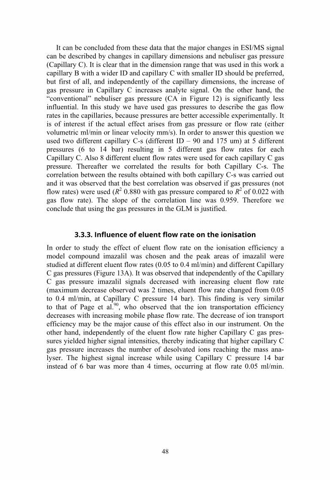
48
It can be concluded from these data that the major changes in ESI/MS signal can be described by changes in capillary dimensions and nebuliser gas pressure (Capillary C). It is clear that in the dimension range that was used in this work a capillary B with a wider ID and capillary C with smaller ID should be preferred, but first of all, and independently of the capillary dimensions, the increase of gas pressure in Capillary C increases analyte signal. On the other hand, the “conventional” nebuliser gas pressure (CA in Figure 12) is significantly less influential. In this study we have used gas pressures to describe the gas flow rates in the capillaries, because pressures are better accessible experimentally. It is of interest if the actual effect arises from gas pressure or flow rate (either volumetric ml/min or linear velocity mm/s). In order to answer this question we used two different capillary C-s (different ID – 90 and 175 um) at 5 different pressures (6 to 14 bar) resulting in 5 different gas flow rates for each Capillary C. Also 8 different eluent flow rates were used for each capillary C gas pressure. Thereafter we correlated the results for both Capillary C-s. The correlation between the results obtained with both capillary C-s was carried out and it was observed that the best correlation was observed if gas pressures (not flow rates) were used (R2 0.880 with gas pressure compared to R2 of 0.022 with gas flow rate). The slope of the correlation line was 0.959. Therefore we conclude that using the gas pressures in the GLM is justified.
3.3.3. Influence of eluent flow rate on the ionisation
In order to study the effect of eluent flow rate on the ionisation efficiency a model compound imazalil was chosen and the peak areas of imazalil were studied at different eluent flow rates (0.05 to 0.4 ml/min) and different Capillary C gas pressures (Figure 13A). It was observed that independently of the Capillary C gas pressure imazalil signals decreased with increasing eluent flow rate (maximum decrease observed was 2 times, eluent flow rate changed from 0.05 to 0.4 ml/min, at Capillary C pressure 14 bar). This finding is very similar to that of Page et al.90, who observed that the ion transportation efficiency decreases with increasing mobile phase flow rate. The decrease of ion transport efficiency may be the major cause of this effect also in our instrument. On the other hand, independently of the eluent flow rate higher Capillary C gas pres-sures yielded higher signal intensities, thereby indicating that higher capillary C gas pressure increases the number of desolvated ions reaching the mass ana-lyser. The highest signal increase while using Capillary C pressure 14 bar instead of 6 bar was more than 4 times, occurring at flow rate 0.05 ml/min.
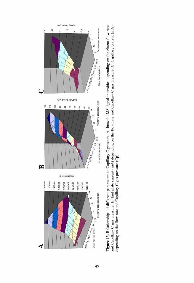
Fi
gure
13.
Rel
atio
nshi
ps o
f diff
eren
t par
amet
ers
to C
apill
ary
C pr
essu
re. A
: Im
azal
il M
S sig
nal i
nten
sitie
s de
pend
ing
on th
e el
uent
flow
rate
an
d Ca
pilla
ry C
gas
pre
ssur
e. B
: End
pla
te c
urre
nt (m
A) d
epen
ding
on
the
flow
rate
and
Cap
illar
y C
gas
pres
sure
. C: C
apill
ary
curre
nt (m
A)
depe
ndin
g on
the
flow
rate
and
Cap
illar
y C
gas p
ress
ure
(Cp)
.
49
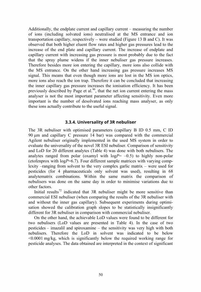
50
Additionally, the endplate current and capillary current – measuring the number of ions (including solvated ions) neutralised at the MS entrance and ion transportation capillary, respectively – were studied (Figure 13 B and C). It was observed that both higher eluent flow rates and higher gas pressures lead to the increase of the end plate and capillary current. The increase of endplate and capillary current with increasing gas pressure is most probably due to the fact that the spray plume widens if the inner nebuliser gas pressure increases. Therefore besides more ion entering the capillary, more ions also collide with the MS entrance. On the other hand increasing gas pressure increases MS signal. This means that even though more ions are lost in the MS ion optics, more ions also reach the ion trap. Therefore it can be concluded that increasing the inner capillary gas pressure increases the ionisation efficiency. It has been previously described by Page et al.90, that the net ion current entering the mass analyser is not the most important parameter affecting sensitivity. Even more important is the number of desolvated ions reaching mass analyser, as only these ions actually contribute to the useful signal.
3.3.4. Universality of 3R nebuliser
The 3R nebuliser with optimised parameters (capillary B ID 0.5 mm, C ID 90 μm and capillary C pressure 14 bar) was compared with the commercial Agilent nebuliser originally implemented in the used MS system in order to evaluate the universality of the novel 3R ESI nebuliser. Comparison of sensitivity and LoD for 20 different analytes (Table 4) was done with both nebulisers. The analytes ranged from polar (oxamyl with logP= –0.5) to highly non-polar (etofenprox with logP=6.7). Four different sample matrices with varying comp-lexity –ranging from solvent to the very complex garlic matrix – were used for pesticides (for 4 pharmaceuticals only solvent was used), resulting in 68 analytematrix combinations. Within the same matrix the comparison of nebulisers was done on the same day in order to minimise variations due to other factors.
Initial results72 indicated that 3R nebuliser might be more sensitive than commercial ESI nebuliser (when comparing the results of the 3R nebuliser with and without the inner gas capillary). Subsequent experiments during optimi-sation showed the calibration graph slopes to be statistically insignificantly different for 3R nebuliser in comparison with commercial nebuliser.
On the other hand, the achievable LoD values were found to be different for two nebulisers (LoD values are presented in Table 4). In the case of two pesticides – imazalil and spiroxamine – the sensitivity was very high with both nebulisers. Therefore the LoD in solvent was indicated to be below <0.0001 mg/kg, which is significantly below the required working range for pesticide analyses. The data obtained are interpreted in the context of significant
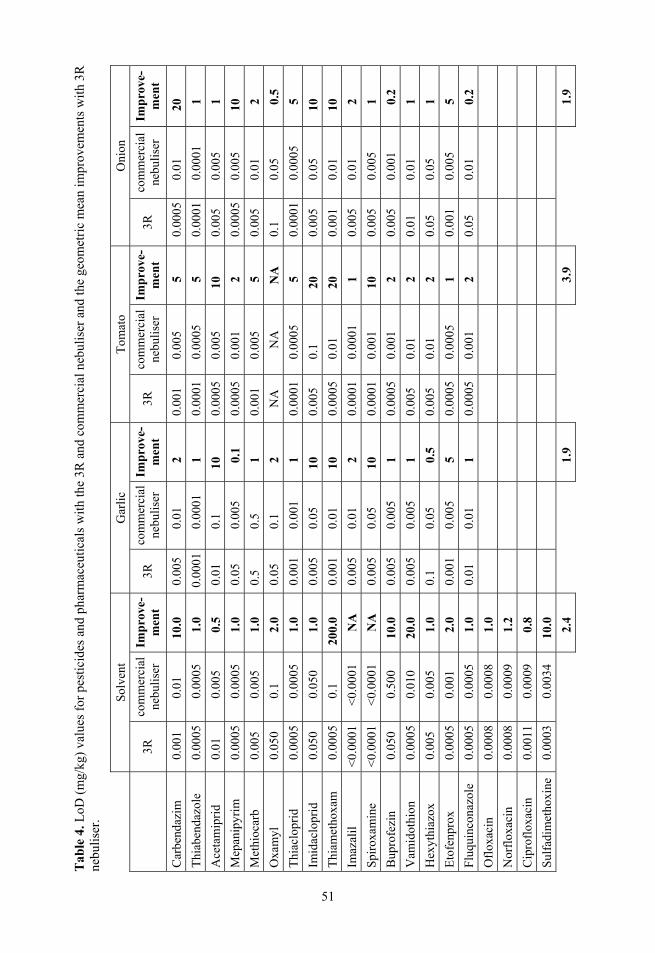
51
Tab
le 4
. LoD
(m
g/kg
) va
lues
for
pes
tici
des
and
phar
mac
euti
cals
wit
h th
e 3R
and
com
mer
cial
neb
ulis
er a
nd th
e ge
omet
ric
mea
n im
prov
emen
ts w
ith 3
R
nebu
liser
.
S
olve
nt
Gar
lic
Tom
ato
Oni
on
3R
co
mm
erci
al
nebu
lise
r Im
pro
ve-
men
t 3R
co
mm
erci
al
nebu
lise
r Im
pro
ve-
men
t 3R
co
mm
erci
al
nebu
lise
r Im
pro
ve-
men
t 3R
co
mm
erci
al
nebu
lise
r Im
pro
ve-
men
t
Car
bend
azim
0.
001
0.01
10
.0
0.00
5 0.
01
2 0.
001
0.00
5 5
0.00
050.
01
20
Thi
aben
dazo
le
0.00
050.
0005
1.
0 0.
0001
0.00
01
1 0.
0001
0.
0005
5
0.00
010.
0001
1
Ace
tam
ipri
d 0.
01
0.00
5 0.
5 0.
01
0.1
10
0.00
05
0.00
5 10
0.
005
0.00
5 1
Mep
anip
yrim
0.
0005
0.00
05
1.0
0.05
0.
005
0.1
0.00
05
0.00
1 2
0.00
050.
005
10
Met
hioc
arb
0.00
5 0.
005
1.0
0.5
0.5
1 0.
001
0.00
5 5
0.00
5 0.
01
2
Oxa
myl
0.
050
0.1
2.0
0.05
0.
1 2
NA
N
A
NA
0.
1 0.
05
0.5
Thi
aclo
prid
0.
0005
0.00
05
1.0
0.00
1 0.
001
1 0.
0001
0.
0005
5
0.00
010.
0005
5
Imid
aclo
prid
0.
050
0.05
0 1.
0 0.
005
0.05
10
0.
005
0.1
20
0.00
5 0.
05
10
Thi
amet
hoxa
m
0.00
050.
1 20
0.0
0.00
1 0.
01
10
0.00
05
0.01
20
0.
001
0.01
10
Imaz
alil
<
0.00
01<
0.00
01
NA
0.
005
0.01
2
0.00
01
0.00
01
1 0.
005
0.01
2
Spi
roxa
min
e <
0.00
01<
0.00
01
NA
0.
005
0.05
10
0.
0001
0.
001
10
0.00
5 0.
005
1
Bup
rofe
zin
0.05
0 0.
500
10.0
0.
005
0.00
5 1
0.00
05
0.00
1 2
0.00
5 0.
001
0.2
Vam
idot
hion
0.
0005
0.01
0 20
.0
0.00
5 0.
005
1 0.
005
0.01
2
0.01
0.
01
1
Hex
ythi
azox
0.
005
0.00
5 1.
0 0.
1 0.
05
0.5
0.00
5 0.
01
2 0.
05
0.05
1
Eto
fenp
rox
0.00
050.
001
2.0
0.00
1 0.
005
5 0.
0005
0.
0005
1
0.00
1 0.
005
5
Flu
quin
cona
zole
0.
0005
0.00
05
1.0
0.01
0.
01
1 0.
0005
0.
001
2 0.
05
0.01
0.
2
Ofl
oxac
in
0.00
080.
0008
1.
0
Nor
flox
acin
0.
0008
0.00
09
1.2
Cip
rofl
oxac
in
0.00
110.
0009
0.
8
Sul
fadi
met
hoxi
ne0.
0003
0.00
34
10.0
2.
4
1.
9
3.
9
1.
9
51
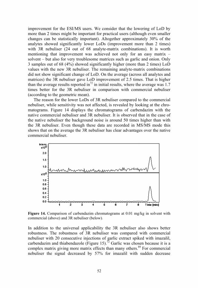
52
improvement for the ESI/MS users. We consider that the lowering of LoD by more than 2 times might be important for practical users (although even smaller changes can be statistically important). Altogether approximately 30% of the analytes showed significantly lower LoDs (improvement more than 2 times) with 3R nebuliser (24 out of 68 analyte-matrix combinations). It is worth mentioning that improvement was achieved not only for an easy matrix – solvent – but also for very troublesome matrices such as garlic and onion. Only 3 samples out of 68 (4%) showed significantly higher (more than 2 times) LoD values with the new 3R nebuliser. The remaining analyte-matrix combinations did not show significant change of LoD. On the average (across all analytes and matrices) the 3R nebuliser gave LoD improvement of 2.5 times. That is higher than the average results reported in72 in initial results, where the average was 1.7 times better for the 3R nebuliser in comparison with commercial nebuliser (according to the geometric mean).
The reason for the lower LoDs of 3R nebuliser compared to the commercial nebuliser, while sensitivity was not affected, is revealed by looking at the chro-matograms. Figure 14 displays the chromatograms of carbendazim with the native commercial nebuliser and 3R nebuliser. It is observed that in the case of the native nebuliser the background noise is around 50 times higher than with the 3R nebuliser. Even though these data are recorded in MS/MS mode this shows that on the average the 3R nebuliser has clear advantages over the native commercial nebuliser.
Figure 14. Comparison of carbendazim chromatograms at 0.01 mg/kg in solvent with commercial (above) and 3R nebuliser (below).
In addition to the universal applicability the 3R nebuliser also shows better robustness. The robustness of 3R nebuliser was compared with commercial nebuliser with 20 consecutive injections of garlic extract spiked with imazalil, carbendazim and thiabendazole (Figure 15).72 Garlic was chosen because it is a complex matrix giving more matrix effects than many others.89 For commercial nebuliser the signal decreased by 57% for imazalil with sudden decrease
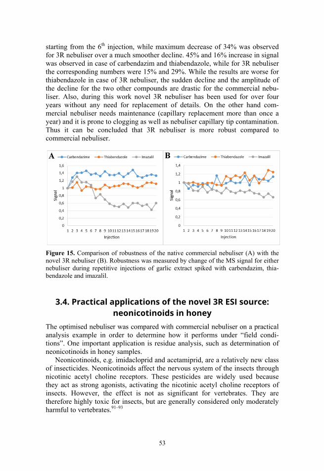
53
starting from the 6th injection, while maximum decrease of 34% was observed for 3R nebuliser over a much smoother decline. 45% and 16% increase in signal was observed in case of carbendazim and thiabendazole, while for 3R nebuliser the corresponding numbers were 15% and 29%. While the results are worse for thiabendazole in case of 3R nebuliser, the sudden decline and the amplitude of the decline for the two other compounds are drastic for the commercial nebu-liser. Also, during this work novel 3R nebuliser has been used for over four years without any need for replacement of details. On the other hand com-mercial nebuliser needs maintenance (capillary replacement more than once a year) and it is prone to clogging as well as nebuliser capillary tip contamination. Thus it can be concluded that 3R nebuliser is more robust compared to commercial nebuliser.
Figure 15. Comparison of robustness of the native commercial nebuliser (A) with the novel 3R nebuliser (B). Robustness was measured by change of the MS signal for either nebuliser during repetitive injections of garlic extract spiked with carbendazim, thia-bendazole and imazalil.
3.4. Practical applications of the novel 3R ESI source: neonicotinoids in honey
The optimised nebuliser was compared with commercial nebuliser on a practical analysis example in order to determine how it performs under “field condi-tions”. One important application is residue analysis, such as determination of neonicotinoids in honey samples.
Neonicotinoids, e.g. imidacloprid and acetamiprid, are a relatively new class of insecticides. Neonicotinoids affect the nervous system of the insects through nicotinic acetyl choline receptors. These pesticides are widely used because they act as strong agonists, activating the nicotinic acetyl choline receptors of insects. However, the effect is not as significant for vertebrates. They are therefore highly toxic for insects, but are generally considered only moderately harmful to vertebrates.91–93
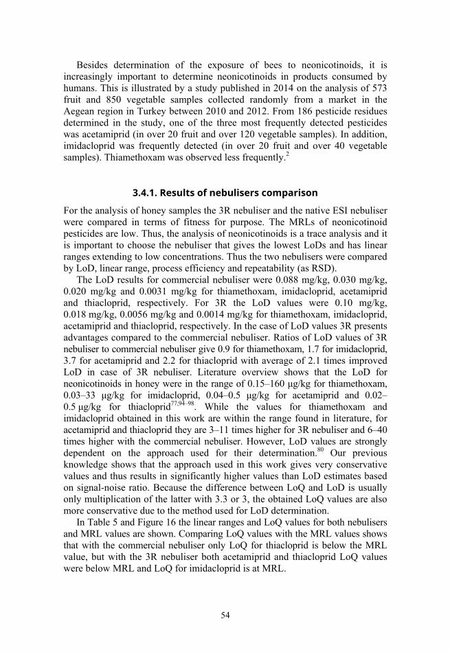
54
Besides determination of the exposure of bees to neonicotinoids, it is increasingly important to determine neonicotinoids in products consumed by humans. This is illustrated by a study published in 2014 on the analysis of 573 fruit and 850 vegetable samples collected randomly from a market in the Aegean region in Turkey between 2010 and 2012. From 186 pesticide residues determined in the study, one of the three most frequently detected pesticides was acetamiprid (in over 20 fruit and over 120 vegetable samples). In addition, imidacloprid was frequently detected (in over 20 fruit and over 40 vegetable samples). Thiamethoxam was observed less frequently.2
3.4.1. Results of nebulisers comparison
For the analysis of honey samples the 3R nebuliser and the native ESI nebuliser were compared in terms of fitness for purpose. The MRLs of neonicotinoid pesticides are low. Thus, the analysis of neonicotinoids is a trace analysis and it is important to choose the nebuliser that gives the lowest LoDs and has linear ranges extending to low concentrations. Thus the two nebulisers were compared by LoD, linear range, process efficiency and repeatability (as RSD).
The LoD results for commercial nebuliser were 0.088 mg/kg, 0.030 mg/kg, 0.020 mg/kg and 0.0031 mg/kg for thiamethoxam, imidacloprid, acetamiprid and thiacloprid, respectively. For 3R the LoD values were 0.10 mg/kg, 0.018 mg/kg, 0.0056 mg/kg and 0.0014 mg/kg for thiamethoxam, imidacloprid, acetamiprid and thiacloprid, respectively. In the case of LoD values 3R presents advantages compared to the commercial nebuliser. Ratios of LoD values of 3R nebuliser to commercial nebuliser give 0.9 for thiamethoxam, 1.7 for imidacloprid, 3.7 for acetamiprid and 2.2 for thiacloprid with average of 2.1 times improved LoD in case of 3R nebuliser. Literature overview shows that the LoD for neonicotinoids in honey were in the range of 0.15–160 μg/kg for thiamethoxam, 0.03–33 μg/kg for imidacloprid, 0.04–0.5 μg/kg for acetamiprid and 0.02–0.5 μg/kg for thiacloprid77,94–98. While the values for thiamethoxam and imidacloprid obtained in this work are within the range found in literature, for acetamiprid and thiacloprid they are 3–11 times higher for 3R nebuliser and 6–40 times higher with the commercial nebuliser. However, LoD values are strongly dependent on the approach used for their determination.80 Our previous knowledge shows that the approach used in this work gives very conservative values and thus results in significantly higher values than LoD estimates based on signal-noise ratio. Because the difference between LoQ and LoD is usually only multiplication of the latter with 3.3 or 3, the obtained LoQ values are also more conservative due to the method used for LoD determination.
In Table 5 and Figure 16 the linear ranges and LoQ values for both nebulisers and MRL values are shown. Comparing LoQ values with the MRL values shows that with the commercial nebuliser only LoQ for thiacloprid is below the MRL value, but with the 3R nebuliser both acetamiprid and thiacloprid LoQ values were below MRL and LoQ for imidacloprid is at MRL.
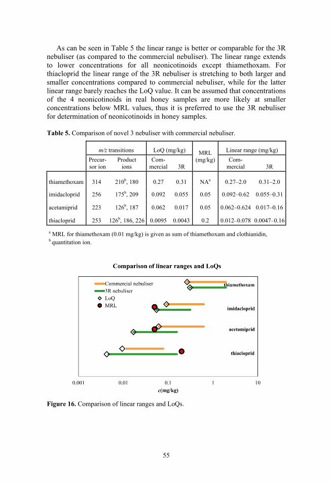
55
As can be seen in Table 5 the linear range is better or comparable for the 3R nebuliser (as compared to the commercial nebuliser). The linear range extends to lower concentrations for all neonicotinoids except thiamethoxam. For thiacloprid the linear range of the 3R nebuliser is stretching to both larger and smaller concentrations compared to commercial nebuliser, while for the latter linear range barely reaches the LoQ value. It can be assumed that concentrations of the 4 neonicotinoids in real honey samples are more likely at smaller concentrations below MRL values, thus it is preferred to use the 3R nebuliser for determination of neonicotinoids in honey samples.
Figure 16. Comparison of linear ranges and LoQs.
Table 5. Comparison of novel 3 nebuliser with commercial nebuliser.
m/z transitions LoQ (mg/kg) MRL (mg/kg)
Linear range (mg/kg)
Precur-sor ion
Product ions
Com-mercial 3R
Com-mercial 3R
thiamethoxam 314 210b, 180 0.27 0.31 NAa 0.27–2.0 0.31–2.0
imidacloprid 256 175b, 209 0.092 0.055 0.05 0.092–0.62 0.055–0.31
acetamiprid 223 126b, 187 0.062 0.017 0.05 0.062–0.624 0.017–0.16
thiacloprid 253 126b, 186, 226 0.0095 0.0043 0.2 0.012–0.078 0.0047–0.16
a MRL for thiamethoxam (0.01 mg/kg) is given as sum of thiamethoxam and clothianidin, b quantitation ion.
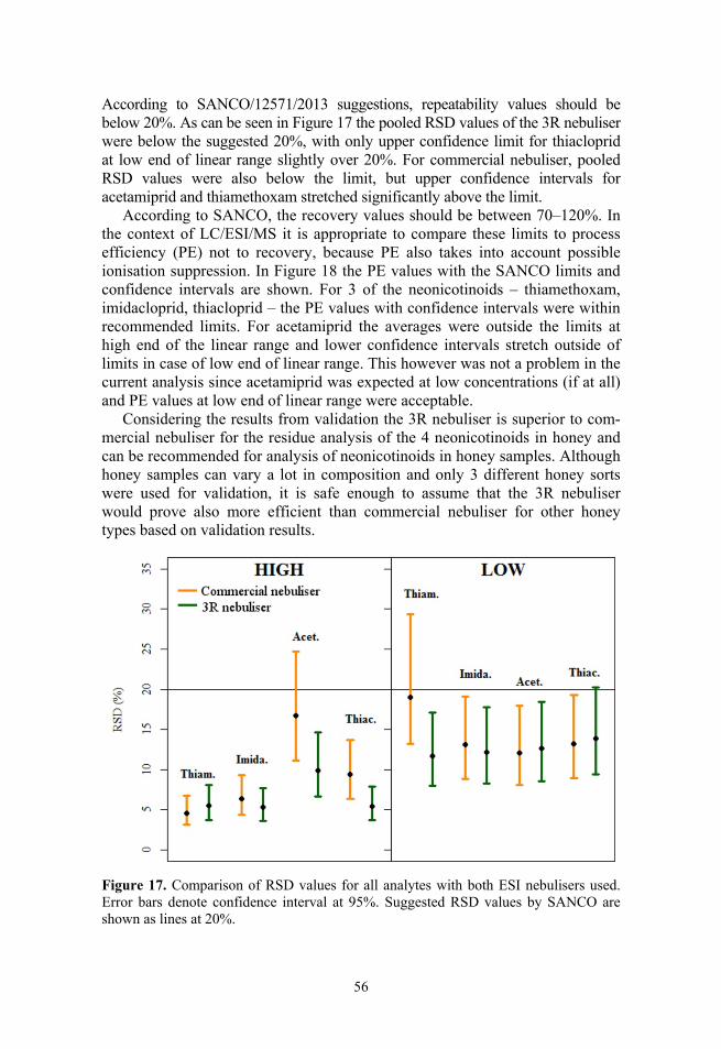
56
According to SANCO/12571/2013 suggestions, repeatability values should be below 20%. As can be seen in Figure 17 the pooled RSD values of the 3R nebuliser were below the suggested 20%, with only upper confidence limit for thiacloprid at low end of linear range slightly over 20%. For commercial nebuliser, pooled RSD values were also below the limit, but upper confidence intervals for acetamiprid and thiamethoxam stretched significantly above the limit.
According to SANCO, the recovery values should be between 70–120%. In the context of LC/ESI/MS it is appropriate to compare these limits to process efficiency (PE) not to recovery, because PE also takes into account possible ionisation suppression. In Figure 18 the PE values with the SANCO limits and confidence intervals are shown. For 3 of the neonicotinoids – thiamethoxam, imidacloprid, thiacloprid – the PE values with confidence intervals were within recommended limits. For acetamiprid the averages were outside the limits at high end of the linear range and lower confidence intervals stretch outside of limits in case of low end of linear range. This however was not a problem in the current analysis since acetamiprid was expected at low concentrations (if at all) and PE values at low end of linear range were acceptable.
Considering the results from validation the 3R nebuliser is superior to com-mercial nebuliser for the residue analysis of the 4 neonicotinoids in honey and can be recommended for analysis of neonicotinoids in honey samples. Although honey samples can vary a lot in composition and only 3 different honey sorts were used for validation, it is safe enough to assume that the 3R nebuliser would prove also more efficient than commercial nebuliser for other honey types based on validation results.
Figure 17. Comparison of RSD values for all analytes with both ESI nebulisers used. Error bars denote confidence interval at 95%. Suggested RSD values by SANCO are shown as lines at 20%.
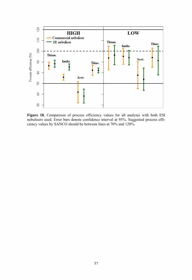
57
Figure 18. Comparison of process efficiency values for all analytes with both ESI nebulisers used. Error bars denote confidence interval at 95%. Suggested process effi-ciency values by SANCO should be between lines at 70% and 120%.
58
SUMMARY
There are numerous novel developments aiming to improve the interface between LC and MS. Novel commercial ion sources need to be compared with each other in order to evaluate their advantages. For some novel ion sources the comparison has been done in this study, occasionally with surprising results.
Comparison of the conventional ESI source with some of the newer develop-ments in commercial ionisation sources, such as HESI, MMI (ESI-APCI) and APPI sources demonstrated that the ESI source is on an average the most robust and sensitive method for generating ions in the interface of LC and MS. While HESI proved to be superior in sensitivity and LoD over most other sources used in comparison and DA-APPI was robust when considering matrix effects, only ESI was among the leaders in all comparison parameters. The LoD values of ESI were comparable to HESI and the best matrix effects were observed with ESI source. ESI source also proved to be comparable or better in repeatability, linear ranges and sensitivity with respect to other sources.
The novel 3R nebuliser for ESI source recently developed in our group was compared to the conventional ESI source. Optimization of nebuliser parameters was successfully concluded during the study. Analysis of the main nebuliser parameters affecting the ionisation showed that the inner gas capillary pressure and internal diameter as well as the liquid capillary internal diameter had the strongest influence on the results. The importance of the outer gas capillary pressure, responsible of the nebulisation in the conventional ESI nebuliser, proved to be much less important than the gas pressure in the inner gas capillary, showing the advantage of the novel approach to ESI nebuliser.
The 3R nebuliser was demonstrated to give on the average 2.5 times (up to 200 times) lower limits of detection and less noise than the native commercial ESI source. After the optimisation of the novel nebuliser the advantage of lower LoDs became even more pronounced. It was also shown that the 3R nebuliser is more robust than the conventional one. The advantages of the 3R nebuliser were put to test with a practical analysis of neonicotinoids in honey. It is a trace analysis and thus is demanding of the ionisation source to give good results with as low LoD as possible. In the comparison with the native commercial nebuliser the 3R nebuliser proved to be comparable or better.
The aims of the thesis were fulfilled successfully, but many more novel ion source developments need to be evaluated and the work on improving the LC/MS method as such is far from done. This study is expected to add valuable information for the improvement of the LC/MS method and proposes a new direction for the improvement of ESI source.

59
SUMMARY IN ESTONIAN
“Uudsete massispektromeetria ionisatsiooniallikate võrdlemine ja optimeerimine”
Vedelikkromatograafia-massispektromeetria (LC/MS) on laialt kasutatav meetod väga mitmekesiste analüüside teostamiseks nii rutiin- kui teaduslaborites. Ioni-satsiooniallikas on kahe meetodi (vedelikkromatograafia ja massispektromeet-ria) ühendamiseks oluline liides, mille abil tekitatakse kromatograafist tulevast vedelikust analüüdimolekulide ioonid, mida analüüsitakse massispektromeetriga. Erinevaid ionisatsiooniallikaid on mitmeid ning pidevalt täiendatakse olemas-olevaid ja leiutatakse uusi. Seetõttu on vajalik võrrelda erinevaid uusi ionisat-siooniallikaid, et leida millised on spetsiifilise töö jaoks parimad.
Antud töö käigus võrreldi mitmeid uusi ionisatsiooniallikaid kommertsiaal-selt levinud elektropihustus-ionisatsiooni allikaga (ESI). Võrdluses kasutati atmosfäärirõhulist fotoionisatsiooni allikat (APPI), kuumutatud elektropihustus-ionisatsiooni (HESI) ja mitmikmeetoditega (MMI) allikat. Võrdluseks kasu-tatavad parameetrid olid avastamispiir (LoD), tundlikkus, maatriksefektid (ME), lineaarne ala ja korduvus. Parimaid tulemusi saadi kommertsiaalse ESI allikaga. Samuti häid tulemusi näitas HESI allikas tundlikkuse osas, kuid jäi märkimis-väärselt alla ME tulemuste poolest ESI ja dopandiga abistatud APPI allikatele. Kehvimad tulemused olid MMI allikatega.
Samuti oli töö eesmärgiks meie töögrupis eelnevalt väljatöötatud uudse ESI allika pihusti (3R) optimeerimine, mis viidi edukalt lõpule. Optimeerimise tule-mused näitavad, et ionisatsiooni mõjutab oluliselt enam vedelikukapillaari sees asuv pihustusgaasi kapillaar võrreldes kommertisaalsel allika välimise pihustus-gaasi kapillaariga. Uudse 3R pihusti eelised seisnevad peamiselt madalamates avastamispiirides ja robustsuses võrreldes kommertsiaalse allikaga.
Samuti täideti edukalt uudse pihustiga seotud teine eesmärk: võrreldi kom-mertsiaalse pihustiga praktilise analüüsi näitel. Selleks oli jälgede määramine neonikotinoidide analüüsil meeproovidest. 3R pihustile leiti madalamale ula-tuvad lineaarsed alad, madalamad või samaväärsed avastamispiirid ja parem korduvus võrreldes kommertsiaalse allikaga.
Antud töös leitud erinevate ionisatsiooniallikate võrdlusandmed ning uudse ESI pihusti iseloomustamisel leitud eelised lisavad olulist informatsiooni väga mitmekesisele MS ionisatsiooniallikate temaatikale. Teadlased püüdlevad ühest küljest aina universaalsemate allikate poole, kuid samas otsitakse allikaid väga spetsiifiliste analüüside teostamiseks, mis annaksid parimaid tulemusi. Selleks on vajalik aina uuesti võrrelda praeguseid parimaid allikaid uudsete leiutistega, et leida effektiivseim liides LC/MS meetodile.
60
REFERENCES
(1) Kocaman, A. Y.; Rencüzoğulları, E.; Topaktaş, M. Environ. Toxicol. 2014, 29 (6), 631–641.
(2) Bakırcı, G. T.; Yaman Acay, D. B.; Bakırcı, F.; Ötleş, S. Food Chem. 2014, 160, 379–392.
(3) Andreu, V.; Picó, Y. Anal. Bioanal. Chem. 2012, 404, 2659–2681. (4) Grimalt, S.; Dehouck, P. J. Chromatogr. A 2016, 1433, 1–23. (5) Sandra, K.; Pereira, A. dos S.; Vanhoenacker, G.; David, F.; Sandra, P. J.
Chromatogr. A 2010, 1217 (25), 4087–4099. (6) Rebane, R.; Herodes, K. Anal. Chim. Acta 2010, 672 (1–2), 79–84. (7) Cai, S.-S.; Hanold, K. A.; Syage, J. A. Anal. Chem. 2007, 79 (6), 2491–2498. (8) Himmelsbach, M.; Buchberger, W.; Reingruber, E. Polym. Degrad. Stab. 2009,
94 (8), 1213–1219. (9) Terrier, P.; Desmazières, B.; Tortajada, J.; Buchmann, W. Mass Spectrom. Rev.
2011, 30, 854–874. (10) Znaleziona, J.; Ginterová, P.; Petr, J.; Ondra, P.; Válka, I.; Ševčík, J.; Chrastina, J.;
Maier, V. Anal. Chim. Acta 2015, 874, 11–25. (11) Rancan, M.; Rossi, S.; Sabatini, A. G. J. Chromatogr. A 2006, 1123 (1), 60–65. (12) Kasiotis, K. M.; Anagnostopoulos, C.; Anastasiadou, P.; Machera, K. Sci. Total
Environ. 2014, 485–486, 633–642. (13) Covey, T. R.; Thomson, B. A.; Schneider, B. B. Mass Spectrom. Rev. 2009, 28
(6), 870–897. (14) Awad, H.; Khamis, M. M.; El-Aneed, A. Appl. Spectrosc. Rev. 2015, 50 (2),
158–175. (15) Dole, M. J. Chem. Phys. 1968, 49 (5), 2240–2249. (16) Whitehouse, C. M.; Dreyer, R. N.; Yamashita, M.; Fenn, J. B. Anal. Chem.
1985, 57 (3), 675–679. (17) Gross, J. H. Mass Spectrometry, 2nd ed.; Springer: Heidelberg, 2011. (18) Robb, D. B.; Covey, T. R.; Bruins, A. P. Anal. Chem. 2000, 72 (15), 3653–3659. (19) Stahnke, H.; Kittlaus, S.; Kempe, G.; Hemmerling, C.; Alder, L. J. Mass
Spectrom. 2012, 47 (7), 875–884. (20) Mordehai, A.; Fjeldsted, J. Agil. Technol. Tech. Note Publ. Number 5990 2009,
3494. (21) Galaon, T.; Vacaresteanu, C.; Anghel, D.-F.; David, V. Drug Test. Anal. 2013, 6,
439–450. (22) Tölgyesi, Á.; Kunsági, Z. Microchem. J. 2013, 106, 300–306. (23) Short, L. C.; Hanold, K. A.; Cai, S.-S.; Syage, J. A. Rapid Commun. Mass
Spectrom. 2007, 21 (10), 1561–1566. (24) Lien, G.-W.; Chen, C.-Y.; Wang, G.-S. J. Chromatogr. A 2009, 1216 (6), 956–
966. (25) Marchi, I.; Rudaz, S.; Veuthey, J. Talanta 2009, 78 (1), 1–18. (26) Liigand, J.; Kruve, A.; Leito, I.; Girod, M.; Antoine, R. J. Am. Soc. Mass
Spectrom. 2014, 25 (11), 1853–1861. (27) Periat, A.; Kohler, I.; Bugey, A.; Bieri, S.; Versace, F.; Staub, C.; Guillarme, D.
J. Chromatogr. A 2014, 1356, 211–220. (28) Ali, A.; Maher, S.; Khan, S. A.; Chaudhary, M. I.; Musharraf, S. G. Steroids
2015, 104, 176–181.
61
(29) Amarasinghe, K.; Chu, P.-S.; Evans, E.; Reimschuessel, R.; Hasbrouck, N.; Jayasuriya, H. J. Agric. Food Chem. 2012, 60 (20), 5084–5088.
(30) Kozlík, P.; Krajíček, J.; Kalíková, K.; Tesařová, E.; Čabala, R.; Exnerová, A.; Štys, P.; Bosáková, Z. J. Chromatogr. B 2013, 930, 82–89.
(31) Kebarle, P.; Verkerk, U. H. Mass Spectrom. Rev. 2009, 28 (6), 898–917. (32) Konermann, L.; Ahadi, E.; Rodriguez, A. D.; Vahidi, S. Anal. Chem. 2013, 85
(1), 2–9. (33) Rebane, R.; Kruve, A.; Liigand, P.; Liigand, J.; Herodes, K.; Leito, I. Anal. Chem.
2016. (34) Herrera, L.; Grossert, J.; Ramaley, L. J. Am. Soc. Mass Spectrom. 2008, 19 (12),
1926–1941. (35) Kauppila, T. J.; Kersten, H.; Benter, T. J. Am. Soc. Mass Spectrom. 2014, 25
(11), 1870–1881. (36) Cai, Y.; McConnell, O.; Bach, A. C. Rapid Commun. Mass Spectrom. 2009, 23
(15), 2283–2291. (37) Bhardwaj, C.; Hanley, L. Nat. Prod. Rep. 2014, 31 (6), 756–767. (38) Cappiello, A.; Famiglini, G.; Palma, P.; Pierini, E.; Termopoli, V.; Trufelli, H.
Mass Spectrom. Rev. 2011, 30 (6), 1242–1255. (39) Crecelius, A. C.; Schubert, U. S.; von Eggeling, F. The Analyst 2015, 140 (17),
5806–5820. (40) Cole, R. B. Electrospray and MALDI Mass Spectrometry: Fundamentals,
Instrumentation, Practicalities, and Biological Applications, 2nd edition.; Wiley: Hoboken, New Jersey, 2010.
(41) Cooks, R. G.; Ouyang, Z.; Takats, Z.; Wiseman, J. M. Science 2006, 311 (5767), 1566–1570.
(42) Chen, H.; Venter, A.; Cooks, R. G. Chem. Commun. 2006, No. 19, 2042–2044. (43) Rauha, J.-P.; Vuorela, H.; Kostiainen, R. J. Mass Spectrom. 2001, 36 (12),
1269–1280. (44) Thurman, E. M.; Ferrer, I.; Barceló, D. Anal. Chem. 2001, 73 (22), 5441–5449. (45) Leinonen, A.; Kuuranne, T.; Kostiainen, R. J. Mass Spectrom. 2002, 37 (7),
693–698. (46) Maragou, N. C.; Thomaidis, N. S.; Koupparis, M. A. J. Am. Soc. Mass
Spectrom. 2011, 22 (10), 1826–1838. (47) Gilbert-López, B.; Geltenpoth, H.; Meyer, C.; Michels, A.; Hayen, H.; Molina-
Díaz, A.; García-Reyes, J. F.; Franzke, J. Rapid Commun. Mass Spectrom. 2013, 27 (3), 419–429.
(48) Keski-Rahkonen, P.; Huhtinen, K.; Desai, R.; Tim Harwood, D.; Handelsman, D. J.; Poutanen, M.; Auriola, S. J. Mass Spectrom. 2013, 48 (9), 1050–1058.
(49) Guo, T.; Shi, Y.; Zheng, L.; Feng, F.; Zheng, F.; Liu, W. J. Chromatogr. A 2014, 1355, 73–79.
(50) Garcia-Ac, A.; Segura, P. A.; Viglino, L.; Gagnon, C.; Sauvé, S. J. Mass Spectrom. 2011, 46 (4), 383–390.
(51) Rybak, M. E.; Parker, D. L.; Pfeiffer, C. M. J. Chromatogr. B 2008, 861 (1), 145–150.
(52) Straube, E. A.; Dekant, W.; Völkel, W. J. Am. Soc. Mass Spectrom. 2004, 15 (12), 1853–1862.
(53) Cai, S.-S.; Syage, J. A. Anal. Chem. 2006, 78 (4), 1191–1199. (54) Kauppila, T. J.; Nikkola, T.; Ketola, R. A.; Kostiainen, R. J. Mass Spectrom.
2006, 41 (6), 781–789.
62
(55) Wang, I.-T.; Feng, Y.-T.; Chen, C.-Y. J. Chromatogr. B 2010, 878 (30), 3095–3105.
(56) Cavaliere, C.; Foglia, P.; Pastorini, E.; Samperi, R.; Laganà, A. J. Chromatogr. A 2006, 1101 (1–2), 69–78.
(57) Titato, G. M.; Bicudo, R. C.; Lanças, F. M. J. Mass Spectrom. 2007, 42 (10), 1348–1357.
(58) Fredenhagen, A.; Kühnöl, J. J. Mass Spectrom. 2014, 49 (8), 727–736. (59) Xu, X.; Mei, H.; Wang, S.; Zhou, Q.; Wang, G.; Broske, L.; Pena, A.; Korf-
macher, W. A. Rapid Commun. Mass Spectrom. 2005, 19 (18), 2643–2650. (60) Ross, M. S.; Wong, C. S. J. Chromatogr. A 2010, 1217 (50), 7855–7863. (61) Souverain, S.; Rudaz, S.; Veuthey, J.-L. J. Chromatogr. A 2004, 1058 (1–2),
61–66. (62) Gosetti, F.; Mazzucco, E.; Zampieri, D.; Gennaro, M. C. J. Chromatogr. A
2010, 1217 (25), 3929–3937. (63) Ghosh, C.; Shinde, C. P.; Chakraborty, B. S. J. Chromatogr. B 2012, 893–894,
193–200. (64) Kruve, A.; Herodes, K.; Leito, I. Rapid Commun. Mass Spectrom. 2010, 24 (7),
919–926. (65) Hanold, K. A.; Fischer, S. M.; Cormia, P. H.; Miller, C. E.; Syage, J. A. Anal.
Chem. 2004, 76 (10), 2842–2851. (66) Guo, X.; Bruins, A. P.; Covey, T. R. Rapid Commun. Mass Spectrom. 2006, 20
(20), 3145–3150. (67) Busch, K. L. Spectroscopy 2002, 17 (10), 32–37. (68) Maxwell, E. J.; Zhong, X.; Chen, D. D. Y. Anal. Chem. 2010, 82 (20), 8377–
8381. (69) Reschke, B. R.; Timperman, A. T. J. Am. Soc. Mass Spectrom. 2011, 22 (12),
2115–2124. (70) Tang, L.; Kebarle, P. Anal. Chem. 1991, 63 (23), 2709–2715. (71) Bajic, S. Mass spectrometer. US2009/0242749A 1, October 1, 2009. (72) Kruve, A.; Leito, I.; Herodes, K.; Laaniste, A.; Lõhmus, R. J. Am. Soc. Mass
Spectrom. 2012, 23 (12), 2051–2054. (73) Dankyi, E.; Gordon, C.; Carboo, D.; Fomsgaard, I. S. Sci. Total Environ. 2014,
499, 276–283. (74) Rahman, M. M.; Farha, W.; Abd El-Aty, A. M.; Kabir, M. H.; Im, S. J.; Jung,
D.-I.; Choi, J.-H.; Kim, S.-W.; Son, Y. W.; Kwon, C.-H.; Shin, H.-C.; Shim, J.-H. Food Chem. 2015, 174, 248–255.
(75) Yang, A.; Park, J.-H.; Abd El-Aty, A. M.; Choi, J.-H.; Oh, J.-H.; Do, J.-A.; Kwon, K.; Shim, K.-H.; Choi, O.-J.; Shim, J.-H. Food Control 2012, 28 (1), 99–105.
(76) Rebane, R.; Herodes, K. J. Agric. Food Chem. 2008, 56 (22), 10716–10720. (77) Bargańska, Ż.; Ślebioda, M.; Namieśnik, J. Food Control 2013, 31 (1), 196–
201. (78) Lehotay, S. J.; Mastovska, K.; Lightfield, A. R. 2 2005, 88, 615–629. (79) European Commission: Health & Consumer Protection Directorate-General
November 19, 2013. (80) Kruve, A.; Rebane, R.; Kipper, K.; Oldekop, M.-L.; Evard, H.; Herodes, K.;
Ravio, P.; Leito, I. Anal. Chim. Acta 2015, 870, 29–44. (81) ICH Harmonised Tripartite Guideline. 2005.
63
(82) Motulsky, H. In Intuitive biostatistics: A nonmathematical guide to statistical thinking; Oxford University Press: New York, 2010; pp 32–36.
(83) Miller, J. N.; Miller, J. C. Pearson/Prentice Hall: Harlow, 2005. (84) Liigand, J.; Kruve, A.; Liigand, P.; Laaniste, A.; Girod, M.; Antoine, R.; Leito,
I. J. Am. Soc. Mass Spectrom. 2015, 26 (11), 1923–1930. (85) Aktar, W.; Sengupta, D.; Chowdhury, A. Interdiscip. Toxicol. 2009, 2 (1), 1–12. (86) Picó, Y.; Blasco, C.; Font, G. Mass Spectrom. Rev. 2004, 23 (1), 45–85. (87) Oss, M.; Kruve, A.; Herodes, K.; Leito, I. Anal. Chem. 2010, 82 (7), 2865–
2872. (88) Marotta, E.; Seraglia, R.; Fabris, F.; Traldi, P. Int. J. Mass Spectrom. 2003, 228
(2–3), 841–849. (89) Kruve, A.; Herodes, K.; Leito, I. J. AOAC Int. 2010, 93 (1), 306–314. (90) Page, J. S.; Kelly, R. T.; Tang, K.; Smith, R. D. J. Am. Soc. Mass Spectrom.
2007, 18 (9), 1582–1590. (91) European Food Safety Authority Panel on Plant Protection Products and their
Residues (PPR). EFSA Journal 2013, No. 11, 3471–3517. (92) Tomizawa, M.; Casida, J. E. Annu. Rev. Pharmacol. Toxicol. 2005, 45 (1), 247–
268. (93) van der Sluijs, J. P.; Simon-Delso, N.; Goulson, D.; Maxim, L.; Bonmatin, J.-M.;
Belzunces, L. P. Curr. Opin. Environ. Sustain. 2013, 5 (3–4), 293–305. (94) Campillo, N.; Viñas, P.; Férez-Melgarejo, G.; Hernández-Córdoba, M. J. Agric.
Food Chem. 2013, 61 (20), 4799–4805. (95) Jovanov, P.; Guzsvány, V.; Franko, M.; Lazić, S.; Sakač, M.; Šarić, B.; Banjac,
V. Talanta 2013, 111, 125–133. (96) Kamel, A. J. Agric. Food Chem. 2010, 58 (10), 5926–5931. (97) Proietto Galeano, M.; Scordino, M.; Sabatino, L.; Pantò, V.; Morabito, G.;
Chiappara, E.; Traulo, P.; Gagliano, G. Int. J. Food Sci. 2013, 2013, 1–7. (98) Tomasini, D.; Sampaio, M. R. F.; Caldas, S. S.; Buffon, J. G.; Duarte, F. A.;
Primel, E. G. Talanta 2012, 99, 380–386. (99) University of Hertfordshire Pesticide Properties DataBase Home Page,
http://sitem.herts.ac.uk/aeru/ppdb/en/search.htm, last accessed 31.03.16. (100) The Toxin and Toxin Target Database Home Page, http://www.t3db.ca/, last
accessed 31.03.16. (101) Tomlin, C. D. S. British Crop Protection Council: Surrey, England, 1997; p
1045/1668. (102) EFSA (European Food Safety Authority). EFSA J. 2014, 12 (9), 3817. (103) MacBean, C. The e-Pesticide Manual, 15th ed. Version 5.0.1.; British Crop
Protection Council: Surrey, England, 2010. (104) Advanced Chemistry Development (ACD/Labs) Software V11.02, 1994–2016
ACD/Labs. (105) US Environmental Protection Agency Home Page; Estimation Program Interface
(EPI) Suite. Ver.3.12., http://www.epa.gov/oppt/exposure/pubs/episuitedl.htm, last accessed 31.03.16 November 30, 2004.
(106) Braumann, T.; Grimme, L. H. J Chrom A 1981, 7. (107) Benfenati, E.; Gini, G.; Piclin, N.; Roncaglioni, A.; Varı̀, M. R. Chemosphere
2003, 53 (9), 1155–1164. (108) ACE and JChem acidity and basicity calculator,
http://epoch.uky.edu/ace/public/pKa.jsp, last accessed 31.03.16.
64
(109) US Environmental Protection Agency Home Page, Pesticide Fact Sheet: Acetamiprid, https://www3.epa.gov/pesticides/chem_search/reg_actions/registration/fs_PC-099050_15-Mar-02.pdf, last accessed 31.03.16 2002.
(110) US Environmental Protection Agency Home Page; Pesticide Fact Sheet: Thiacloprid, http://www.epa.gov/opprd001/factsheets/thiacloprid.pdf, last accessed 31.03.16 2003.
(111) Tomlin, C. D. S. British Crop Protection Council: Surrey, England. (112) Hansch, C.; Leo, A.; Hoekman, D. Exploring QSAR – Hydrophobic, Electronic,
and Steric Constants; American Chemical Society, 1995. (113) Albro, P. W.; Parker, C. A.; Abusteit, E. O.; Mester, T. C.; Hass, J. R.; Sheldon,
Y. S.; Corbin, F. T. J Agric Food Chem 1984, 32, 212–217. (114) ChemSpider Home Page, http://www.chemspider.com/Chemical-Structure.84290.html, last accessed
31.03.16. (115) Koh, M.; Brown, C. D. Earth Sciences, The University of York 2007. (116) http://www.chinese-pesticide.com/fungicides/spiroxamine.html, last accessed
31.03.16. (117) EFSA (European Food Safety Authority). EFSA J. 2010, 8 (10), 1719. (118) EFSA (European Food Safety Authority). EFSA J. 2010, 8 (10), 1786. (119) Pesticide Management Education Program Home Page,
http://pmep.cce.cornell.edu/profiles/herb-growthreg/naa-rimsulfuron/paclobutrazol/herb-prof-paclobutrazol.html, last accessed 31.03.16.
(120) MacBean, C. The e-Pesticide Manual, 15th ed. Version 5.1.; British Crop Pro-tection Council: Alton, England, 2008.
(121) Drug Future Home Page, http://www.drugfuture.com/chemdata/fluquinconazole.html, last accessed 31.03.16.
(122) Molbase Home Page, http://www.molbase.com/en/85509-19-9-moldata-28531.html, last accessed 31.03.16.
(123) Food and Agriculture Organization of the United Nations Hope Page, http://www.fao.org/fileadmin/templates/agphome/documents/Pests_Pesticides/ Specs/Flusilazole08.pdf, last accessed 31.03.16.
(124) Nagai, Y.; Shimba, K.; Yusa, Y.; Yagi, A. J. Pestic. Sci. 1999, 24, 280–286. (125) LookChem Home Page, http://www.lookchem.com/Bitertanol/, last accessed
31.03.16. (126) SPARC – pKa/property server. Ver 3.; 2006.
65
ACKNOWLEDGEMENTS
I would like to thank University of Tartu and Institute of Chemistry for making it possible for having this journey in science. I thank my advisor Anneli Kruve for guiding me on this journey since bachelor´s studies and always answering my questions (both science and life related). I thank my advisor Ivo Leito for guiding me during my doctoral studies and giving me constructive feedback. I also thank my wife Hiie, for the support she has shown to me during my studies. I thank my mother and little brother who have supported me on my path to and in the university. I wish to thank the countless number of people who have given me insightful conversations about science and innumerable aspects of life itself, especially Alina, Andi, Arno, Gerli, Hanno, Indrek, Jaanus, Joosep, Karin, Karl, Koit, Liina, Maarja-Liisa, Martin, Ott, Piia, Riin and Roger.
I also wish to thank Lyon 1st university and prof. Randon for an opportunity to conduct research in an environment that was different. I thank Amelie, Audrey, Claire, Jose, Josiane, Nestor, Rasha and Vincent for the support they showed me during my time in Lyon.
This work was supported by the Personal Research Funding Project 34 from the Estonian Research Council and by the European Union through the Euro-pean Regional Development Fund (Centre of Excellence ‘‘Mesosystems: Theory and Applications’’, TK114). This work was also supported by the Esto-nian Ministry of Education and Research through the institutional research funding IUT14-20 (TLOKT14014I). The authors also acknowledge support for this work by grants 8572 and 9007 from the Estonian Science Foundation, by the target financing projects SF0180061s08, and SF0180058s07 from the Esto-nian ministry of education and science, by Graduate School on Functional Materials and Technologies (GSFMT), University of Tartu and Tallinn Uni-versity of Technology project 1.2.0401.09-0079, and by European Union through the European Regional Development Fund. The work was also partly supported by Estonian Nanotechnology Competence Centre (EU29996).
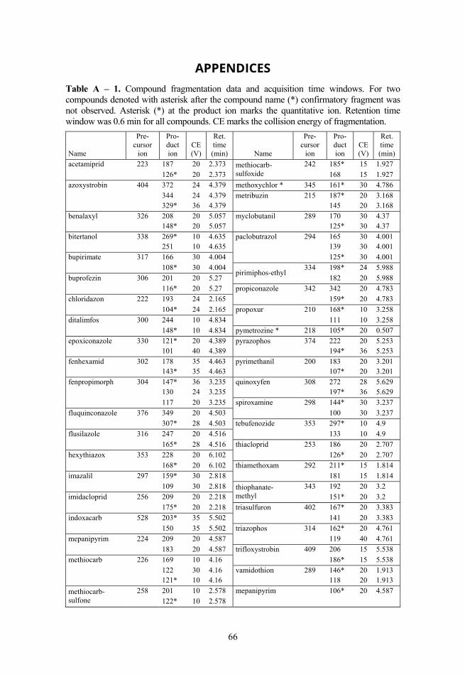
66
APPENDICES Table A – 1. Compound fragmentation data and acquisition time windows. For two compounds denoted with asterisk after the compound name (*) confirmatory fragment was not observed. Asterisk (*) at the product ion marks the quantitative ion. Retention time window was 0.6 min for all compounds. CE marks the collision energy of fragmentation.
Name
Pre-cursor
ion
Pro-duct ion
CE (V)
Ret. time (min) Name
Pre- cursor
ion
Pro-duct ion
CE (V)
Ret. time (min)
acetamiprid 223 187 20 2.373 methiocarb-sulfoxide
242 185* 15 1.927
126* 20 2.373 168 15 1.927
azoxystrobin 404 372 24 4.379 methoxychlor * 345 161* 30 4.786
344 24 4.379 metribuzin 215 187* 20 3.168 329* 36 4.379 145 20 3.168
benalaxyl 326 208 20 5.057 myclobutanil 289 170 30 4.37 148* 20 5.057 125* 30 4.37
bitertanol 338 269* 10 4.635 paclobutrazol 294 165 30 4.001 251 10 4.635 139 30 4.001
bupirimate 317 166 30 4.004 125* 30 4.001
108* 30 4.004 pirimiphos-ethyl
334 198* 24 5.988
buprofezin 306 201 20 5.27 182 20 5.988
116* 20 5.27 propiconazole 342 342 20 4.783
chloridazon 222 193 24 2.165 159* 20 4.783
104* 24 2.165 propoxur 210 168* 10 3.258
ditalimfos 300 244 10 4.834 111 10 3.258
148* 10 4.834 pymetrozine * 218 105* 20 0.507
epoxiconazole 330 121* 20 4.389 pyrazophos 374 222 20 5.253 101 40 4.389 194* 36 5.253
fenhexamid 302 178 35 4.463 pyrimethanil 200 183 20 3.201 143* 35 4.463 107* 20 3.201
fenpropimorph 304 147* 36 3.235 quinoxyfen 308 272 28 5.629 130 24 3.235 197* 36 5.629
117 20 3.235 spiroxamine 298 144* 30 3.237
fluquinconazole 376 349 20 4.503 100 30 3.237
307* 28 4.503 tebufenozide 353 297* 10 4.9
flusilazole 316 247 20 4.516 133 10 4.9
165* 28 4.516 thiacloprid 253 186 20 2.707
hexythiazox 353 228 20 6.102 126* 20 2.707
168* 20 6.102 thiamethoxam 292 211* 15 1.814
imazalil 297 159* 30 2.818 181 15 1.814
109 30 2.818 thiophanate-methyl
343 192 20 3.2
imidacloprid 256 209 20 2.218 151* 20 3.2
175* 20 2.218 triasulfuron 402 167* 20 3.383
indoxacarb 528 203* 35 5.502 141 20 3.383
150 35 5.502 triazophos 314 162* 20 4.761
mepanipyrim 224 209 20 4.587 119 40 4.761
183 20 4.587 trifloxystrobin 409 206 15 5.538
methiocarb 226 169 10 4.16 186* 15 5.538
122 30 4.16 vamidothion 289 146* 20 1.913 121* 10 4.16 118 20 1.913
methiocarb-sulfone
258 201 10 2.578 mepanipyrim 106* 20 4.587
122* 10 2.578
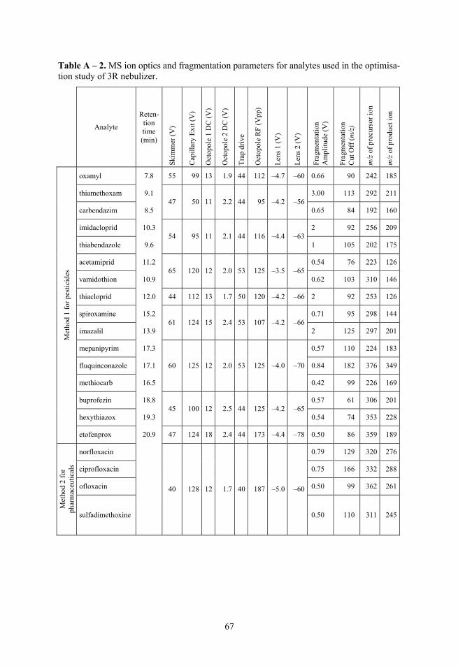
67
Table A – 2. MS ion optics and fragmentation parameters for analytes used in the optimisa-tion study of 3R nebulizer.
Analyte
Reten-tion time (min)
Ski
mm
er (
V)
Cap
illa
ry E
xit (
V)
Oct
opol
e 1
DC
(V
)
Oct
opol
e 2
DC
(V
)
Tra
p dr
ive
Oct
opol
e R
F (
Vpp
)
Len
s 1
(V)
Len
s 2
(V)
Fra
gmen
tati
on
Am
plit
ude
(V)
Fra
gmen
tati
on
Cut
Off
(m
/z)
m/z
of
prec
urso
r io
n
m/z
of
prod
uct i
on
Met
hod
1 fo
r pe
stic
ides
oxamyl 7.8 55 99 13 1.9 44 112 –4.7 –60 0.66 90 242 185
thiamethoxam 9.1 47 50 11 2.2 44 95 –4.2 –56
3.00 113 292 211
carbendazim 8.5 0.65 84 192 160
imidacloprid 10.3 54 95 11 2.1 44 116 –4.4 –63
2 92 256 209
thiabendazole 9.6 1 105 202 175
acetamiprid 11.2 65 120 12 2.0 53 125 –3.5 –65
0.54 76 223 126
vamidothion 10.9 0.62 103 310 146
thiacloprid 12.0 44 112 13 1.7 50 120 –4.2 –66 2 92 253 126
spiroxamine 15.2 61 124 15 2.4 53 107 –4.2 –66
0.71 95 298 144
imazalil 13.9 2 125 297 201
mepanipyrim 17.3
60 125 12 2.0 53 125 –4.0 –70
0.57 110 224 183
fluquinconazole 17.1 0.84 182 376 349
methiocarb 16.5 0.42 99 226 169
buprofezin 18.8 45 100 12 2.5 44 125 –4.2 –65
0.57 61 306 201
hexythiazox 19.3 0.54 74 353 228
etofenprox 20.9 47 124 18 2.4 44 173 –4.4 –78 0.50 86 359 189
Met
hod
2 fo
r ph
arm
aceu
tica
ls
norfloxacin
40 128 12 1.7 40 187 –5.0 –60
0.79 129 320 276
ciprofloxacin
0.75 166 332 288
ofloxacin
0.50 99 362 261
sulfadimethoxine
0.50 110 311 245
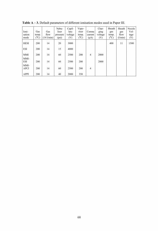
68
Table A – 3. Default parameters of different ionisation modes used in Paper III.
Ioni-sation mode
Gas temp. (⁰C)
Gas flow
(14 l/min)
Nebu-liser
pressure (psi)
Capil-lary
voltage (V)
Vapo-riser temp. (⁰C)
Corona current (μA)
Char-ging
voltage (V)
Sheath gas
temp. (⁰C)
Sheath gas
flow (l/min)
Nozzle Vol-tage (V)
HESI 200 14 20 3000 400 11 1500
ESI 200 14 15 4000
MMI 200 14 60 2500 200 4 2000
MMI-ESI 200 14 60 2500 200 2000
MMI-APCI 200 14 60 2500 200 4
APPI 200 14 40 2000 350
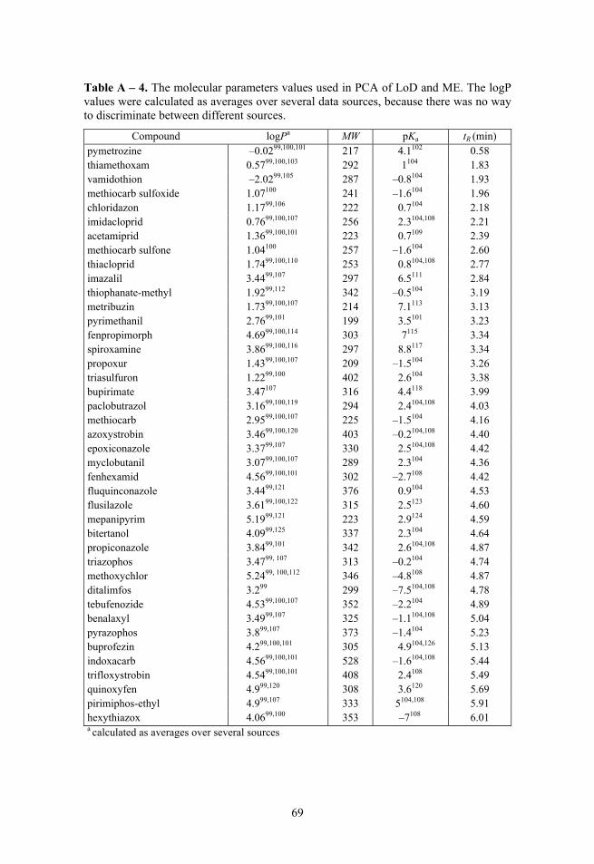
69
Table A – 4. The molecular parameters values used in PCA of LoD and ME. The logP values were calculated as averages over several data sources, because there was no way to discriminate between different sources.
Compound logPa MW pKa tR (min) pymetrozine –0.0299,100,101 217 4.1102 0.58 thiamethoxam 0.5799,100,103 292 1104 1.83 vamidothion –2.0299,105 287 –0.8104 1.93 methiocarb sulfoxide 1.07100 241 –1.6104 1.96 chloridazon 1.1799,106 222 0.7104 2.18 imidacloprid 0.7699,100,107 256 2.3104,108 2.21 acetamiprid 1.3699,100,101 223 0.7109 2.39 methiocarb sulfone 1.04100 257 –1.6104 2.60 thiacloprid 1.7499,100,110 253 0.8104,108 2.77 imazalil 3.4499,107 297 6.5111 2.84 thiophanate-methyl 1.9299,112 342 –0.5104 3.19 metribuzin 1.7399,100,107 214 7.1113 3.13 pyrimethanil 2.7699,101 199 3.5101 3.23 fenpropimorph 4.6999,100,114 303 7115 3.34 spiroxamine 3.8699,100,116 297 8.8117 3.34 propoxur 1.4399,100,107 209 –1.5104 3.26 triasulfuron 1.2299,100 402 2.6104 3.38 bupirimate 3.47107 316 4.4118 3.99 paclobutrazol 3.1699,100,119 294 2.4104,108 4.03 methiocarb 2.9599,100,107 225 –1.5104 4.16 azoxystrobin 3.4699,100,120 403 –0.2104,108 4.40 epoxiconazole 3.3799,107 330 2.5104,108 4.42 myclobutanil 3.0799,100,107 289 2.3104 4.36 fenhexamid 4.5699,100,101 302 –2.7108 4.42 fluquinconazole 3.4499,121 376 0.9104 4.53 flusilazole 3.6199,100,122 315 2.5123 4.60 mepanipyrim 5.1999,121 223 2.9124 4.59 bitertanol 4.0999,125 337 2.3104 4.64 propiconazole 3.8499,101 342 2.6104,108 4.87 triazophos 3.4799, 107 313 –0.2104 4.74 methoxychlor 5.2499, 100,112 346 –4.8108 4.87 ditalimfos 3.299 299 –7.5104,108 4.78 tebufenozide 4.5399,100,107 352 –2.2104 4.89 benalaxyl 3.4999,107 325 –1.1104,108 5.04 pyrazophos 3.899,107 373 –1.4104 5.23 buprofezin 4.299,100,101 305 4.9104,126 5.13 indoxacarb 4.5699,100,101 528 –1.6104,108 5.44 trifloxystrobin 4.5499,100,101 408 2.4108 5.49 quinoxyfen 4.999,120 308 3.6120 5.69 pirimiphos-ethyl 4.999,107 333 5104,108 5.91 hexythiazox 4.0699,100 353 –7108 6.01 a calculated as averages over several sources
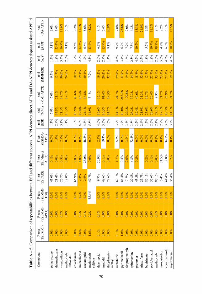
70
Tab
le A
– 5
. Com
pari
son
of r
epea
tabi
liti
es b
etw
een
ES
I an
d di
ffer
ent s
ourc
es. A
PPI
deno
tes
dire
ct A
PP
I an
d D
A-A
PP
I de
note
s do
pant
ass
iste
d A
PPI.
d
Com
poun
d F
-tes
t (E
SI/
MM
I)F
-tes
t (E
SI/
MM
I-A
PC
I)
F-t
est
(ES
I/M
MI-
ES
I)
F-t
est
(ES
I/A
JS)
F-t
est
(ES
I/ d
irec
t A
PP
I)
F-t
est
(ES
I/D
A-
AP
PI)
rstd
(E
SI)
rs
td
(MM
I)rs
td
(MM
I-A
PC
I)rs
td
(MM
I-E
SI)
rs
td
(AJS
) rs
td
(AP
PI)
rs
td
(DA
-AP
PI)
pym
etro
zine
0.
0%
0.0%
0.
0%
43.0
%
0.1%
0.
0%
1.3%
7.
9%
7.0%
9.
5%
1.7%
5.
1%
6.0%
thia
met
hoxa
m
0.0%
0.
0%
0.0%
21
.4%
0.
0%
1.4%
2.
9%
13.8
%21
.1%
12
.7%
1.
8%
23.4
%
7.4%
vam
idot
hion
0.
0%
0.2%
0.
0%
26.7
%
0.3%
2.
7%
5.1%
21
.5%
17.7
%
36.0
%
3.3%
16
.9%
11
.6%
met
hioc
arb
sulf
oxid
e 0.
0%
0.0%
0.
0%
12.0
%
0.0%
0.
0%
1.4%
15
.5%
17.1
%
24.6
%
2.6%
8.
1%
6.1%
chlo
rida
zon
0.0%
0.
0%
0.0%
65
.9%
0.
0%
0.0%
1.
6%
18.9
%40
.6%
10
.5%
1.
9%
9.5%
9.
2%
imid
aclo
prid
3.
8%
0.3%
0.
2%
2.3%
4.
0%
0.3%
5.
6%
12.4
%18
.3%
19
.1%
2.
2%
12.3
%
17.7
%
acet
amip
rid
0.0%
0.
1%
0.0%
2.
6%
23.0
%
48.5
%
4.3%
24
.1%
16.8
%
20.1
%
1.7%
6.
8%
5.6%
met
hioc
arb
sulf
one
1.6%
9.
2%
55.6
%
49.7
%
0.0%
0.
0%
5.8%
14
.9%
3.1%
7.
2%
4.5%
43
.4%
43
.2%
thia
clop
rid
0.1%
0.
1%
0.0%
9.
7%
20.9
%
2.7%
4.
0%
15.6
%15
.1%
19
.2%
2.
0%
6.3%
9.
1%
imaz
alil
0.
0%
0.0%
0.
0%
48.6
%
0.1%
10
.3%
3.
5%
15.5
%91
.4%
26
.2%
2.
7%
13.9
%
6.4%
thio
phan
ate-
met
hyl
0.0%
0.
0%
0.0%
77
.6%
0.
0%
0.0%
1.
6%
14.7
%19
.3%
32
.2%
1.
4%
8.1%
20
.9%
met
ribu
zin
0.1%
0.
0%
0.0%
69
.1%
1.
7%
5.5%
3.
9%
14.1
%24
.7%
29
.9%
4.
5%
9.7%
7.
8%
pyri
met
hani
l 1.
0%
0.0%
0.
0%
86.4
%
9.4%
0.
0%
3.7%
10
.0%
267.
7%
31.9
%
3.4%
6.
9%
25.8
%
fenp
ropi
mor
ph
0.0%
0.
0%
0.0%
7.
7%
2.6%
3.
7%
3.3%
27
.3%
170.
8%
19.4
%
1.6%
7.
7%
7.0%
spir
oxam
ine
0.0%
0.
0%
0.0%
29
.8%
6.
8%
72.3
%
3.8%
26
.2%
37.3
%
34.7
%
2.5%
7.
5%
4.3%
prop
oxur
0.
0%
0.0%
0.
0%
43.5
%
0.2%
0.
0%
3.2%
19
.4%
40.6
%
18.8
%
4.2%
10
.7%
13
.1%
tria
sulf
uron
0.
0%
0.0%
0.
0%
25.7
%
0.
0%
2.4%
21
.9%
31.3
%
32.6
%
3.7%
21.0
%
bupi
rim
ate
0.0%
0.
0%
0.0%
80
.1%
0.
2%
0.0%
1.
7%
27.6
%16
.7%
12
.5%
1.
8%
5.7%
6.
8%
pacl
obut
razo
l 0.
0%
0.0%
0.
0%
35.6
%
0.1%
0.
0%
2.6%
26
.6%
20.4
%
22.7
%
1.8%
10
.4%
11
.2%
met
hioc
arb
0.0%
0.
1%
0.0%
80
.1%
0.
0%
0.2%
2.
4%
27.1
%9.
3%
33.5
%
2.6%
39
.7%
8.
1%
azox
ystr
obin
0.
0%
0.0%
0.
0%
5.4%
21
.5%
0.
4%
2.7%
17
.1%
21.7
%
23.3
%
5.6%
4.
2%
8.2%
epox
icon
azol
e 0.
0%
0.0%
0.
0%
64.4
%
12.0
%
34.1
%
3.6%
18
.3%
26.9
%
22.3
%
4.3%
6.
5%
5.1%
myc
lobu
tani
l 0.
0%
0.0%
0.
0%
35.4
%
0.2%
0.
1%
3.2%
14
.1%
24.7
%
19.5
%
4.5%
10
.8%
12
.5%
70
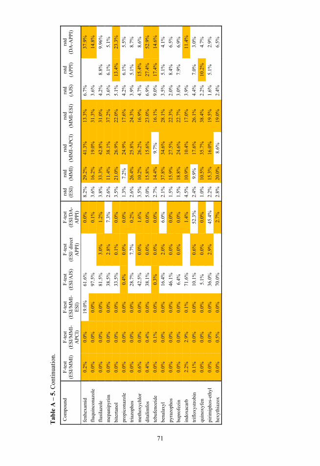
71
Com
poun
d F
-tes
t (E
SI/
MM
I)F
-tes
t (E
SI/
MM
I-A
PC
I)
F-t
est
(ES
I/M
MI-
ES
I)
F-t
est
(ES
I/A
JS)
F-t
est
(ES
I/ d
irec
t A
PP
I)
F-t
est
(ES
I/D
A-
AP
PI)
rstd
(E
SI)
rs
td
(MM
I)rs
td
(MM
I-A
PC
I)rs
td
(MM
I-E
SI)
rs
td
(AJS
) rs
td
(AP
PI)
rs
td
(DA
-AP
PI)
fenh
exam
id
0.2%
0.
0%
19.0
%
61.6
%
0.
0%
8.2%
29
.2%
41.3
%
13.3
%
6.7%
37.9
%
fluq
uinc
onaz
ole
0.0%
0.
0%
0.0%
97
.5%
0.1%
3.
6%
16.2
%19
.0%
31
.3%
3.
6%
14
.8%
flus
ilaz
ole
0.0%
0.
0%
0.0%
81
.5%
3.
0%
1.2%
3.
8%
33.3
%42
.8%
31
.0%
4.
2%
8.8%
9.
96%
mep
anip
yrim
0.
0%
0.0%
0.
0%
38.5
%
2.8%
7.
3%
2.6%
11
.4%
38.1
%
37.2
%
3.6%
6.
1%
5.1%
bite
rtan
ol
0.0%
0.
0%
0.0%
33
.5%
0.
1%
0.0%
3.
5%
21.0
%26
.9%
22
.0%
5.
1%
13.4
%
23.3
%
prop
icon
azol
e 0.
0%
0.0%
0.
0%
0.4%
0.
0%
0.0%
1.
3%
7.2%
24
.9%
17
.6%
4.
2%
6.1%
5.
5%
tria
zoph
os
0.0%
0.
0%
0.0%
28
.7%
7.
7%
0.2%
2.
6%
26.4
%25
.8%
24
.3%
3.
9%
5.1%
8.
7%
met
hoxy
chlo
r 0.
6%
0.0%
0.
0%
42.5
%
0.0%
1.
6%
3.5%
10
.2%
26.2
%
16.9
%
4.7%
15
.4%
8.
6%
dita
lim
fos
0.4%
0.
4%
0.0%
38
.1%
0.
0%
0.0%
5.
0%
15.8
%15
.6%
23
.0%
6.
9%
27.4
%
52.9
%
tebu
feno
zide
0.
0%
0.1%
0.
0%
0.3%
0.
0%
0.0%
2.
7%
14.4
%9.
7%
16.1
%
9.0%
17
.4%
14
.6%
bena
laxy
l 0.
0%
0.0%
0.
0%
16.4
%
2.0%
6.
0%
2.1%
37
.8%
34.6
%
28.1
%
3.5%
5.
1%
4.1%
pyra
zoph
os
0.0%
0.
0%
0.0%
46
.1%
0.
0%
0.0%
1.
5%
15.9
%27
.5%
22
.3%
2.
0%
8.4%
6.
5%
bupr
ofez
in
0.0%
0.
0%
0.0%
6.
4%
0.0%
0.
0%
1.5%
18
.8%
24.6
%
22.7
%
3.0%
7.
9%
6.9%
indo
xaca
rb
2.2%
2.
9%
0.1%
71
.6%
1.4%
4.
5%
10.9
%10
.4%
17
.0%
3.
9%
11
.4%
trif
loxy
stro
bin
0.1%
0.
0%
0.0%
10
.1%
0.
6%
52.3
%
2.4%
9.
9%
17.6
%
26.1
%
4.4%
7.
0%
3.0%
quin
oxyf
en
0.0%
0.
0%
0.0%
5.
1%
0.0%
0.
0%
1.0%
10
.5%
35.7
%
38.4
%
2.2%
10
.2%
4.
7%
piri
mip
hos-
ethy
l 0.
0%
0.0%
0.
0%
36.0
%
2.9%
45
.4%
2.
2%
15.3
%16
.0%
19
.5%
1.
6%
5.1%
2.
9%
hexy
thia
zox
0.
0%
0.5%
0.
0%
70.0
%
2.
7%
2.8%
20
.0%
8.6%
19
.0%
2.
4%
6.
5%
71
Tab
le A
– 5
. Con
tinu
atio
n.
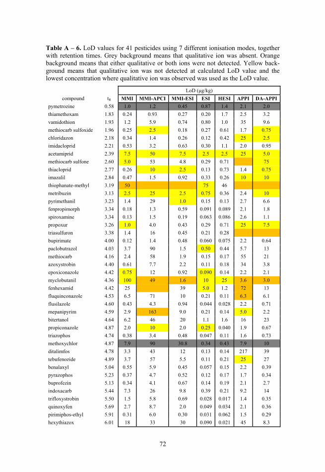
72
Table A – 6. LoD values for 41 pesticides using 7 different ionisation modes, together with retention times. Grey background means that qualitative ion was absent. Orange background means that either qualitative or both ions were not detected. Yellow back-ground means that qualitative ion was not detected at calculated LoD value and the lowest concentration where qualitative ion was observed was used as the LoD value.
LoD (μg/kg)
compound tR MMI MMI-APCI MMI-ESI ESI HESI APPI DA-APPI
pymetrozine 0.58 1.0 1.2 0.45 0.87 1.4 2.1 2.0
thiamethoxam 1.83 0.24 0.93 0.27 0.20 1.7 2.5 3.2
vamidothion 1.93 1.2 5.9 0.74 0.80 1.0 35 9.6
methiocarb sulfoxide 1.96 0.25 2.5 0.18 0.27 0.61 1.7 0.75
chloridazon 2.18 0.34 1.4 0.26 0.12 0.42 25 2.5
imidacloprid 2.21 0.53 3.2 0.63 0.30 1.1 2.0 0.95
acetamiprid 2.39 7.5 50 7.5 2.5 2.5 25 5.0
methiocarb sulfone 2.60 5.0 53 4.8 0.29 0.71 75
thiacloprid 2.77 0.26 10 2.5 0.13 0.73 1.4 0.75
imazalil 2.84 0.47 1.5 0.92 0.33 0.26 10 10
thiophanate-methyl 3.19 50 75 46
metribuzin 3.13 2.5 25 2.5 0.75 0.36 2.4 10
pyrimethanil 3.23 1.4 29 1.0 0.15 0.13 2.7 6.6
fenpropimorph 3.34 0.18 1.3 0.59 0.091 0.089 2.1 1.8
spiroxamine 3.34 0.13 1.5 0.19 0.063 0.086 2.6 1.1
propoxur 3.26 1.0 4.0 0.43 0.29 0.71 25 7.5
triasulfuron 3.38 1.4 16 0.45 0.21 0.28
bupirimate 4.00 0.12 1.4 0.48 0.060 0.075 2.2 0.64
paclobutrazol 4.03 3.7 90 1.5 0.50 0.44 5.7 13
methiocarb 4.16 2.4 58 1.9 0.15 0.17 55 21
azoxystrobin 4.40 0.61 7.7 2.2 0.11 0.18 34 3.8
epoxiconazole 4.42 0.75 12 0.92 0.090 0.14 2.2 2.1
myclobutanil 4.36 100 49 1.6 10 25 3.6 3.0
fenhexamid 4.42 25 39 5.0 1.2 72 13
fluquinconazole 4.53 6.5 71 10 0.21 0.11 6.3 6.1
flusilazole 4.60 0.43 4.3 0.94 0.044 0.028 2.2 0.71
mepanipyrim 4.59 2.9 163 9.0 0.21 0.14 5.0 2.2
bitertanol 4.64 6.2 46 20 1.1 1.6 16 23
propiconazole 4.87 2.0 10 2.0 0.25 0.040 1.9 0.67
triazophos 4.74 0.38 3.4 0.48 0.047 0.11 1.6 0.73
methoxychlor 4.87 7.9 90 30.8 0.34 0.43 7.9 10
ditalimfos 4.78 3.3 43 12 0.13 0.14 217 39
tebufenozide 4.89 3.7 57 5.5 0.11 0.21 25 27
benalaxyl 5.04 0.55 5.9 0.45 0.057 0.15 2.2 0.39
pyrazophos 5.23 0.37 4.7 0.52 0.12 0.17 1.7 0.34
buprofezin 5.13 0.34 4.1 0.67 0.14 0.19 2.1 2.7
indoxacarb 5.44 7.3 26 9.8 0.39 0.21 9.2 14
trifloxystrobin 5.50 1.5 5.8 0.69 0.028 0.017 1.4 0.35
quinoxyfen 5.69 2.7 8.7 2.0 0.049 0.034 2.1 0.36
pirimiphos-ethyl 5.91 0.31 6.0 0.30 0.031 0.062 1.5 0.29
hexythiazox 6.01 18 33 30 0.090 0.021 45 8.3
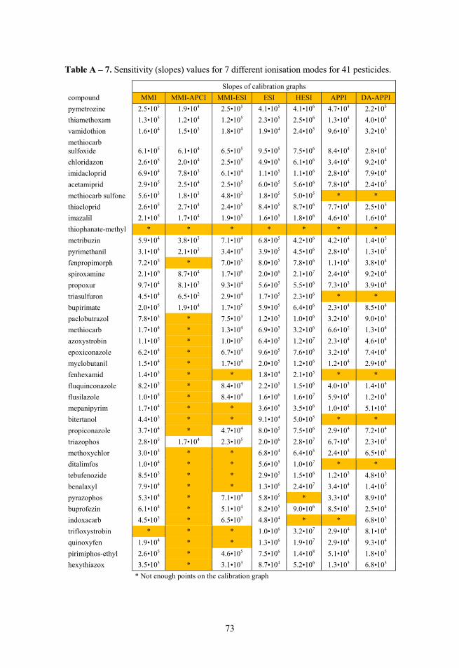
73
Table A – 7. Sensitivity (slopes) values for 7 different ionisation modes for 41 pesticides.
Slopes of calibration graphs
compound MMI MMI-APCI MMI-ESI ESI HESI APPI DA-APPI
pymetrozine 2.5•105 1.9•104 2.5•105 4.1•105 4.1•106 4.7•104 2.2•105
thiamethoxam 1.3•105 1.2•104 1.2•105 2.3•105 2.5•106 1.3•104 4.0•104
vamidothion 1.6•104 1.5•103 1.8•104 1.9•104 2.4•105 9.6•102 3.2•103
methiocarb sulfoxide 6.1•105 6.1•104 6.5•105 9.5•105 7.5•106 8.4•104 2.8•105
chloridazon 2.6•105 2.0•104 2.5•105 4.9•105 6.1•106 3.4•104 9.2•104
imidacloprid 6.9•104 7.8•103 6.1•104 1.1•105 1.1•106 2.8•104 7.9•104
acetamiprid 2.9•105 2.5•104 2.5•105 6.0•105 5.6•106 7.8•104 2.4•105
methiocarb sulfone 5.6•103 1.8•103 4.8•103 1.8•105 5.0•105 * *
thiacloprid 2.6•105 2.7•104 2.4•105 8.4•105 8.7•106 7.7•104 2.5•105
imazalil 2.1•105 1.7•104 1.9•105 1.6•105 1.8•106 4.6•103 1.6•104
thiophanate-methyl * * * * * * *
metribuzin 5.9•104 3.8•103 7.1•104 6.8•105 4.2•106 4.2•104 1.4•105
pyrimethanil 3.1•104 2.1•103 3.4•104 3.9•105 4.5•106 2.8•104 1.3•105
fenpropimorph 7.2•105 * 7.0•105 8.0•105 7.8•106 1.1•104 3.8•104
spiroxamine 2.1•106 8.7•104 1.7•106 2.0•106 2.1•107 2.4•104 9.2•104
propoxur 9.7•104 8.1•103 9.3•104 5.6•105 5.5•106 7.3•103 3.9•104
triasulfuron 4.5•104 6.5•102 2.9•104 1.7•105 2.3•106 * *
bupirimate 2.0•105 1.9•104 1.7•105 5.9•105 6.4•106 2.3•104 8.5•104
paclobutrazol 7.8•103 * 7.5•103 1.2•105 1.0•106 3.2•103 9.0•103
methiocarb 1.7•104 * 1.3•104 6.9•105 3.2•106 6.6•102 1.3•104
azoxystrobin 1.1•105 * 1.0•105 6.4•105 1.2•107 2.3•104 4.6•104
epoxiconazole 6.2•104 * 6.7•104 9.6•105 7.6•106 3.2•104 7.4•104
myclobutanil 1.5•104 * 1.7•104 2.0•105 1.2•106 1.2•104 2.9•104
fenhexamid 1.4•103 * * 1.8•104 2.1•105 * *
fluquinconazole 8.2•103 * 8.4•104 2.2•105 1.5•106 4.0•103 1.4•104
flusilazole 1.0•105 * 8.4•104 1.6•106 1.6•107 5.9•104 1.2•105
mepanipyrim 1.7•104 * * 3.6•105 3.5•106 1.0•104 5.1•104
bitertanol 4.4•103 * * 9.1•104 5.0•105 * *
propiconazole 3.7•104 * 4.7•104 8.0•105 7.5•106 2.9•104 7.2•104
triazophos 2.8•105 1.7•104 2.3•105 2.0•106 2.8•107 6.7•104 2.3•105
methoxychlor 3.0•103 * * 6.8•104 6.4•105 2.4•103 6.5•103
ditalimfos 1.0•104 * * 5.6•105 1.0•107 * *
tebufenozide 8.5•103 * * 2.9•105 1.5•106 1.2•103 4.8•103
benalaxyl 7.9•104 * * 1.3•106 2.4•107 3.4•104 1.4•105
pyrazophos 5.3•104 * 7.1•104 5.8•105 * 3.3•104 8.9•104
buprofezin 6.1•104 * 5.1•104 8.2•105 9.0•106 8.5•103 2.5•104
indoxacarb 4.5•103 * 6.5•103 4.8•104 * * 6.8•103
trifloxystrobin * * * 1.0•106 3.2•107 2.9•104 8.1•104
quinoxyfen 1.9•104 * * 1.3•106 1.9•107 2.9•104 9.3•104
pirimiphos-ethyl 2.6•105 * 4.6•105 7.5•106 1.4•108 5.1•104 1.8•105
hexythiazox 3.5•103 * 3.1•103 8.7•104 5.2•106 1.3•103 6.8•103
* Not enough points on the calibration graph
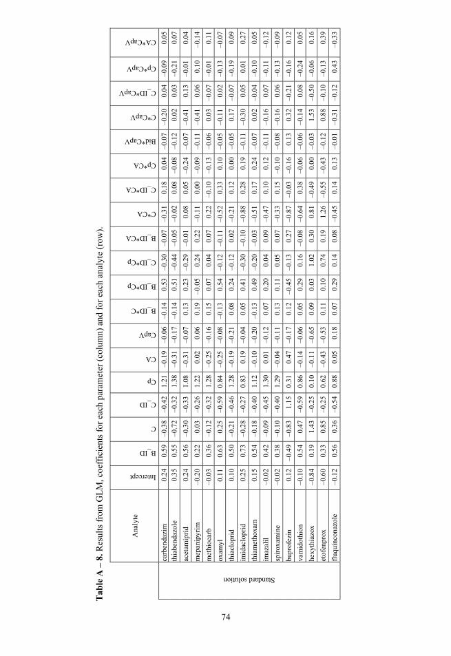
74
74
Tab
le A
– 8
. Res
ults
fro
m G
LM
, coe
ffic
ient
s fo
r ea
ch p
aram
eter
(co
lum
n) a
nd f
or e
ach
anal
yte
(row
).
A
naly
te
Intercept
B_ID
C
C_ID
Cp
CA
CapV
B_ID*C
B_ID*Cp
C_ID*Cp
B_ID*CA
C*CA
C_ID*CA
Cp*CA
Bid*CapV
C*CapV
C_ID*CapV
Cp*CapV
CA*CapV
Standard solution
carb
enda
zim
0.
240.
59–0
.38
–0.4
21.
21–0
.19
–0.0
6–0
.14
0.53
–0.3
0–0
.07
–0.3
10.
180.
04–0
.07
–0.2
00.
04
–0.0
9 0.
05
thia
bend
azol
e 0.
350.
55–0
.72
–0.3
21.
38–0
.31
–0.1
7–0
.14
0.51
–0.4
4–0
.05
–0.0
20.
08–0
.08
–0.1
20.
020.
03
–0.2
1 0.
07
acet
amip
rid
0.24
0.56
–0.3
0–0
.33
1.08
–0.3
1 –0
.07
0.13
0.23
–0.2
9–0
.01
0.08
0.05
–0.2
4–0
.07
–0.4
10.
13
–0.0
1 0.
04
mep
anip
yrim
–0
.20
0.22
0.03
–0.2
61.
220.
02
0.06
0.19
–0.0
50.
240.
22–0
.11
0.00
–0.0
9–0
.11
–0.4
10.
06
0.10
–0
.14
met
hioc
arb
–0.0
30.
36–0
.12
–0.3
21.
28–0
.25
–0.1
60.
150.
070.
040.
070.
22–0
.10
–0.1
3–0
.06
0.03
–0.0
7 –0
.01
0.11
oxam
yl
0.11
0.63
0.25
–0.5
90.
84–0
.25
–0.0
8–0
.13
0.54
–0.1
2–0
.11
–0.5
20.
330.
10–0
.05
–0.1
10.
02
–0.1
3 –0
.07
thia
clop
rid
0.10
0.50
–0.2
1–0
.46
1.28
–0.1
9 –0
.21
0.08
0.24
–0.1
20.
02–0
.21
0.12
0.00
–0.0
50.
17–0
.07
–0.1
9 0.
09
imid
aclo
prid
0.
250.
73–0
.28
–0.2
70.
830.
19
–0.0
40.
050.
41–0
.30
–0.1
0–0
.88
0.28
0.19
–0.1
1–0
.30
0.05
0.
01
0.27
thia
met
hoxa
m
0.15
0.54
–0.1
8–0
.40
1.12
–0.1
0 –0
.20
–0.1
30.
49–0
.20
–0.0
3–0
.51
0.17
0.24
–0.0
70.
02–0
.04
–0.1
0 0.
05
imaz
alil
–0
.02
0.42
–0.0
9–0
.45
1.30
0.01
–0
.12
0.07
0.20
0.04
0.09
–0.4
70.
100.
12–0
.11
–0.1
60.
07
–0.1
1 –0
.12
spir
oxam
ine
–0.0
20.
38–0
.10
–0.4
01.
29–0
.04
–0.1
10.
130.
110.
050.
07–0
.33
0.15
–0.1
0–0
.08
–0.1
60.
06
–0.1
3 –0
.09
bupr
ofez
in
0.12
–0.4
9–0
.83
1.15
0.31
0.47
–0
.17
0.12
–0.4
5–0
.13
0.27
–0.8
7–0
.03
–0.1
60.
130.
32–0
.21
–0.1
6 0.
12
vam
idot
hion
–0
.10
0.54
0.47
–0.5
90.
86–0
.14
–0.0
60.
050.
290.
16–0
.08
–0.6
40.
38–0
.06
–0.0
6–0
.14
0.08
–0
.24
0.05
hexy
thia
zox
–0.8
40.
191.
43–0
.25
0.10
–0.1
1 –0
.65
0.09
0.03
1.02
0.30
0.81
–0.4
90.
00–0
.03
1.53
–0.5
0 –0
.06
0.16
etof
enpr
ox
–0.6
00.
330.
85–0
.25
0.62
–0.4
3 –0
.53
0.11
0.10
0.74
0.19
1.26
–0.5
5–0
.43
–0.1
20.
88–0
.10
–0.1
3 0.
39
fluq
uinc
onaz
ole
–0.1
20.
560.
36–0
.54
0.88
0.05
0.
180.
070.
290.
140.
08–0
.45
0.14
0.13
–0.0
1–0
.31
–0.1
2 0.
43
–0.3
3
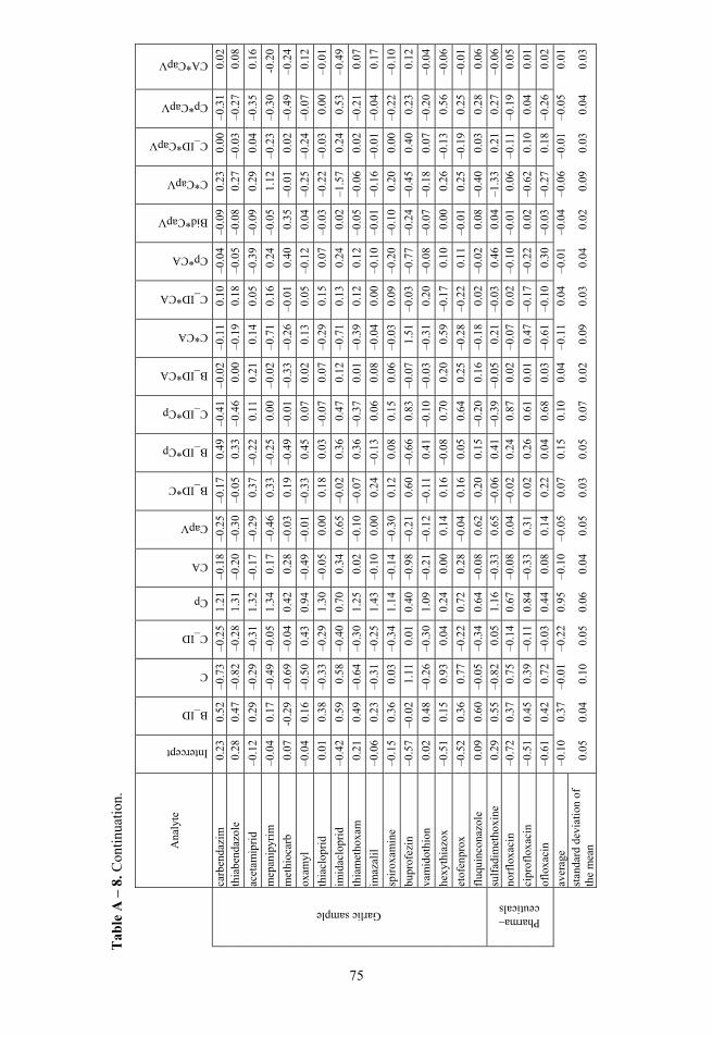
75
75
A
naly
te
Intercept
B_ID
C
C_ID
Cp
CA
CapV
B_ID*C
B_ID*Cp
C_ID*Cp
B_ID*CA
C*CA
C_ID*CA
Cp*CA
Bid*CapV
C*CapV
C_ID*CapV
Cp*CapV
CA*CapV
Garlic sample
carb
enda
zim
0.
230.
52–0
.73
–0.2
51.
21–0
.18
–0.2
5–0
.17
0.49
–0.4
1–0
.02
–0.1
10.
10–0
.04
–0.0
90.
230.
00
–0.3
1 0.
02
thia
bend
azol
e 0.
280.
47–0
.82
–0.2
81.
31–0
.20
–0.3
0–0
.05
0.33
–0.4
60.
00–0
.19
0.18
–0.0
5–0
.08
0.27
–0.0
3 –0
.27
0.08
acet
amip
rid
–0.1
20.
29–0
.29
–0.3
11.
32–0
.17
–0.2
90.
37–0
.22
0.11
0.21
0.14
0.05
–0.3
9–0
.09
0.29
0.04
–0
.35
0.16
mep
anip
yrim
–0
.04
0.17
–0.4
9–0
.05
1.34
0.17
–0
.46
0.33
–0.2
50.
00–0
.02
–0.7
10.
160.
24–0
.05
1.12
–0.2
3 –0
.30
-0.2
0
met
hioc
arb
0.07
-0.2
9–0
.69
–0.0
40.
420.
28
–0.0
30.
19–0
.49
–0.0
1–0
.33
–0.2
6–0
.01
0.40
0.35
–0.0
10.
02
–0.4
9 –0
.24
oxam
yl
–0.0
40.
16–0
.50
0.43
0.94
–0.4
9 –0
.01
–0.3
30.
450.
070.
020.
130.
05–0
.12
0.04
–0.2
5–0
.24
–0.0
7 0.
12
thia
clop
rid
0.01
0.38
–0.3
3–0
.29
1.30
–0.0
5 0.
000.
180.
03–0
.07
0.07
–0.2
90.
150.
07–0
.03
–0.2
2–0
.03
0.00
–0
.01
imid
aclo
prid
–0
.42
0.59
0.58
–0.4
00.
700.
34
0.65
–0.0
20.
360.
470.
12–0
.71
0.13
0.24
0.02
–1.5
70.
24
0.53
–0
.49
thia
met
hoxa
m
0.21
0.49
–0.6
4–0
.30
1.25
0.02
–0
.10
–0.0
70.
36–0
.37
0.01
–0.3
90.
120.
12–0
.05
–0.0
60.
02
–0.2
1 0.
07
imaz
alil
–0
.06
0.23
–0.3
1–0
.25
1.43
–0.1
0 0.
000.
24–0
.13
0.06
0.08
–0.0
40.
00–0
.10
–0.0
1–0
.16
–0.0
1 –0
.04
0.17
spir
oxam
ine
–0.1
50.
360.
03–0
.34
1.14
–0.1
4 –0
.30
0.12
0.08
0.15
0.06
–0.0
30.
09–0
.20
–0.1
00.
200.
00
–0.2
2 –0
.10
bupr
ofez
in
–0.5
7–0
.02
1.11
0.01
0.40
–0.9
8 –0
.21
0.60
–0.6
60.
83–0
.07
1.51
–0.0
3–0
.77
–0.2
4–0
.45
0.40
0.
23
0.12
vam
idot
hion
0.
020.
48–0
.26
–0.3
01.
09–0
.21
–0.1
2–0
.11
0.41
–0.1
0–0
.03
–0.3
10.
20–0
.08
–0.0
7–0
.18
0.07
–0
.20
–0.0
4
hexy
thia
zox
–0.5
10.
150.
930.
040.
240.
00
0.14
0.16
–0.0
80.
700.
200.
59–0
.17
0.10
0.00
0.26
–0.1
3 0.
56
–0.0
6
etof
enpr
ox
–0.5
20.
360.
77–0
.22
0.72
0.28
–0
.04
0.16
0.05
0.64
0.25
–0.2
8–0
.22
0.11
–0.0
10.
25–0
.19
0.25
–0
.01
fluq
uinc
onaz
ole
0.09
0.60
–0.0
5–0
.34
0.64
–0.0
8 0.
620.
200.
15–0
.20
0.16
–0.1
80.
02–0
.02
0.08
–0.4
00.
03
0.28
0.
06
Pharma–ceuticals
sulf
adim
etho
xine
0.
290.
55–0
.82
0.05
1.16
–0.3
3 0.
65–0
.06
0.41
–0.3
9–0
.05
0.21
–0.0
30.
460.
04–1
.33
0.21
0.
27
–0.0
6 no
rflo
xaci
n –0
.72
0.37
0.75
–0.1
40.
67–0
.08
0.04
–0.0
20.
240.
870.
02–0
.07
0.02
–0.1
0–0
.01
0.06
–0.1
1 –0
.19
0.05
cipr
oflo
xaci
n –0
.51
0.45
0.39
–0.1
10.
84–0
.33
0.31
0.02
0.26
0.61
0.01
0.47
–0.1
7–0
.22
0.02
–0.6
20.
10
0.04
0.
01
oflo
xaci
n –0
.61
0.42
0.72
–0.0
30.
440.
08
0.14
0.22
0.04
0.68
0.03
–0.6
1–0
.10
0.30
–0.0
3–0
.27
0.18
–0
.26
0.02
aver
age
–0.1
00.
37–0
.01
–0.2
20.
95–0
.10
–0.0
50.
070.
150.
100.
04–0
.11
0.04
–0.0
1–0
.04
–0.0
6–0
.01
–0.0
5 0.
01
stan
dard
dev
iati
on o
f th
e m
ean
0.05
0.04
0.10
0.05
0.06
0.04
0.
050.
030.
050.
070.
020.
090.
030.
040.
020.
090.
03
0.04
0.
03
Tab
le A
– 8
. Con
tinu
atio
n.

PUBLICATIONS
143
Curriculum Vitae in English
I Personal information 1. Name: Asko Laaniste 2. Date of birth: 21st of September, 1987 3. Citizenship: estonian 4. Address: Tiigi 57–10, Tartu Phone, e-mail: 58313727 [email protected] 5. Current position: University of Tartu, chemist 6. Education: 2012–…, University of Tartu, doctoral studies 2010–2012, University of Tartu, master’s studies, MSc 2007–2010, University of Tartu, bachelor’s studies, BSc 7. Language skills: estonian mother tongue english fluent in speech and writing japanese basic understanding of speech 8. Professional career: 01.2014 – … University of Tartu, chemist II Research and development work 1. Main fields of research:
LC/MS, method validation, sample pretreatment, pesticides, HPLC, mono-lithic columns
2. Publications: Anneli Kruve, Ivo Leito, Koit Herodes, Asko Laaniste, Rünno Lõhmus,
Enhanced Nebulization Efficiency of Electrospray Mass Spectrometry: Improved Sensitivity and Detection Limit, J. Am. Soc. Mass Spectrom. 2012, 23, 2051–2054
Asko Laaniste, Anneli Kruve, Ivo Leito, Ensuring repeatability and robustness of poly(glycidyl methacrylate-co-ethylene dimethacrylate) HPLC monolithic columns of 3 mm id through covalent bonding to the column wall, J. Sep. Sci., 2013, 36, 2458–2463
Asko Laaniste, Audrey Marechal, Racha El-Debs, Jerome Randon, Vincent Dugas, Claire Demesmay, “Thiol-ene” photoclick chemistry as a rapid and localizable functionalization pathway for silica capillary monolithic columns, J. Chromatogr. A, 2014, 1355, 296–300
Audrey Marechal, Asko Laaniste, Racha El-Debs, Vincent Dugas, Claire Demesmay Versatile ene-thiol photoclick reaction for preparation of multi-modal monolithic silica capillary columns, J. Chromatogr. A. 2014, 1365, 140–147
Jaanus Liigand, Anneli Kruve, Piia Liigand, Asko Laaniste, Marion Girod, Rodolphe Antoine, Ivo Leito, Transferability of the electrospray ionization efficiency scale between different instruments, J. Am. Soc. Mass Spectrom., 2015, 26, 1923–30.
144
Asko Laaniste, Anneli Kruve, Ivo Leito, Riin Rebane, Rünno Lõhmus, Ants Lõhmus, Fredrik Punga, Determination of neonicotinoids in Estonian honey by LC/ESI/MS with novel nebulizer, Journal of Environmental Science and Health, Part B, accepted for publication.
Asko Laaniste, Ivo Leito, Anneli Kruve, Comparison of different ionization sources for the LC/MS analysis of pesticides, submitted to Rapid Commu-nications in Mass Spectrometry.
3. Research grants and scholarships: 2013 – Kristjan Jaak Scholarships for part-time studies in Lyon, France. 2014 – Doctoral school scholarship for participation in 38th ISEAC. 2015 – Estonian Students Fund in USA for financial support to worthy Esto-
nian candidates, who demonstrate through academic excellence and community leadership their capacity for, and commitment to, making a contribution to Estonian society.
2015 – Kristjan Jaak Scholarships for participation in HPLC 2016 conference. 4. Other administrative and professional activities: ValChrom project “Development of software for validation of chromatographic
methods” (with registration number 3.2.1201.13-0020) under the sub-measure “Supporting the development of R&D of info and communication technology” funded by the EU Regional Development Fund.
Roles in the project (10.2015 – end of project in 08.2015): one of the software testers and developers for correspondence with validation guidelines (ICH, AOAC, EuraChem, IUPAC, EMA, FDA, NordVal); programming of the ValChrom software on QureDesign platform, overview of the progress of testing, promoting the program at HPLC 2015.
III Teaching activities Analüütilise keemia praktikum I Since 2007 actively participated in popularization of science amongst elementary
and high school students. Had a leading role in development and organization of chemistry workshop for “Teaduslaager” 2009–2014 (science camp for ele-mentary school students on summers) and chemistry workshop for “Õpikojad” since 2010 (year-long practical workshops for elementary and high school students).
Also part of Estonian Olympiad committee since 2012, responsible for organization of the olympiad, generation of the exercises for the participants and training of Estonian students for International Chemistry Olympiad. Also a volunteer for European Science Olympiad in 2016.
IV Professional self-improvement and conferences 30.11.2013 – Training for teaching assistants, Tartu, Eesti. 02.–07.2013 – Visited the 1st University in Lyon for 5 months, studying
functionalization of monolithic silica columns in prof. J. Randon’s group.
145
11. October 2013 – Eesti XXXIII Keemiapäevad (Estonian XXXIII Chemistry Days).
04.–05. March 2014 – TÜ and TTÜ collaborative doctoral school’s conference “FMTDK Teaduskonverents 2014”.
16.–20. June 2014 – The 38th International Symposium on Environmental Ana-lytical Chemistry.
Spring 2015. – Estimation of measurement uncertainty in chemical analysis, MOOC, Tartu, Eesti.
21.06.2015. – SFC – Principles, Instrumentation, Method Development, and Appli-cations, Geneva, Switzerland.
21.–25. June 2015 – 42nd Symposium on high performance liquid phase separations and related techniques (HPLC 2015).
09.–10.06.2016. – 16th International Chromatography School, Zagreb. 19.–24.06.2016. – 44th International Symposium on high performance liquid phase
separations and related techniques (HPLC 2016), San Francisco, USA.
146
Curriculum Vitae in Estonian
I Üldandmed 1. Nimi: Asko Laaniste 2. Sünniaeg: 21.09.1987 3. Kodakondsus: eestlane 4. Aadress Tiigi 57–10, Tartu Telefon, E-mail: 58313727 [email protected] 5. Praegune töökoht: Tartu Ülikool, keemik 6. Haridus: 2012 …, Tartu Ülikool, doktoriõpe 2010 2012, Tartu Ülikool, magistriõpe, MSc 2007 2010, Tartu Ülikool, bakalaureuseõpe, BSc 7. Keelteoskus: eesti keel emakeel inglise keel sujuv nii kõnes kui kirjas jaapani keel arusaamine lihtsamast kõnest 8. Teenistuskäik: 01.2014 – … aastaTartu Ülikool, keemik II Teaduslik ja arendustegevus 1. Peamised uurimisvaldkonnad:
LC/MS, metoodikate valideerimine, proovi eeltöötlus, pestitsiidid, HPLC, monoliitsed kolonnid
2. Publikatsioonide loetelu: Anneli Kruve, Ivo Leito, Koit Herodes, Asko Laaniste, Rünno Lõhmus,
Enhanced Nebulization Efficiency of Electrospray Mass Spectrometry: Improved Sensitivity and Detection Limit, J. Am. Soc. Mass Spectrom. 2012, 23, 2051–2054
Asko Laaniste, Anneli Kruve, Ivo Leito, Ensuring repeatability and robustness of poly(glycidyl methacrylate-co-ethylene dimethacrylate) HPLC monolithic columns of 3 mm id through covalent bonding to the column wall, J. Sep. Sci., 2013, 36, 2458–2463
Asko Laaniste, Audrey Marechal, Racha El-Debs, Jerome Randon, Vincent Dugas, Claire Demesmay, “Thiol-ene” photoclick chemistry as a rapid and localizable functionalization pathway for silica capillary monolithic columns, J. Chromatogr. A, 2014, 1355, 296–300
Audrey Marechal, Asko Laaniste, Racha El-Debs, Vincent Dugas, Claire Demesmay Versatile ene-thiol photoclick reaction for preparation of multi-modal monolithic silica capillary columns, J. Chromatogr. A. 2014, 1365, 140–147
Jaanus Liigand, Anneli Kruve, Piia Liigand, Asko Laaniste, Marion Girod, Rodolphe Antoine, Ivo Leito, Transferability of the electrospray ionization efficiency scale between different instruments, J. Am. Soc. Mass Spectrom., 2015, 26, 1923–30
147
Asko Laaniste, Anneli Kruve, Ivo Leito, Riin Rebane, Rünno Lõhmus, Ants Lõhmus, Fredrik Punga, Determination of neonicotinoids in Estonian honey by LC/ESI/MS with novel nebulizer, Journal of Environmental Science and Health, Part B, accepted for publication.
Asko Laaniste, Ivo Leito, Anneli Kruve, Comparison of different ionization sources for the LC/MS analysis of pesticides, submitted to Rapid Commu-nications in Mass Spectrometry.
3. Saadud uurimistoetused ja stipendiumid: 2013 – Kristjan Jaagu osalise õppe stipendium teadustööks Lyonis, Prantsus-
maal. 2014 – Doktorikooli stipendium osalemaks 38.. ISEAC konverentsil. 2015 – Eesti Üliõpilaste Toetusfond USAs stipendium toetamaks finantsiliselt
silmapaistvaid üliõpilasi. 2015 – Kristjan Jaagu stipendium osalemiseks HPLC 2016 konverentsil. 4. Muu teaduslik organisatsiooniline ja erialane tegevus: ValChrom projekt “Development of software for validation of chromatographic
methods” (registreerimisnumbriga 3.2.1201.13-0020) alamüksuse “Sup-porting the development of R&D of info and communication technology” toetatud EU Regional Development Fund poolt.
Roll projektis (10.2015 – end of project in 08.2015): valideerimisalase tark-vara testimine ja arendamine vastavusse peamiste valideerimisjuhenditega (ICH, AOAC, EuraChem, IUPAC, EMA, FDA, NordVal); ValChrom tarkvara programmeerimine, ülevaade testimistest.
III Õppetöö Analüütilise keemia praktikum I Alates 2007. aastast olen olnud teaduse populariseerija põhikooli ja gümnaa-
siumiastme õpilaste seas. Olen omanud juhtivat rolli “Teaduslaager” 2009–2014 ja “Õpikojad” 2010–2016 väljatöötamisel ja läbiviimisel.
Samuti olen Eesti keemiaolümpiaadi organiseeriva komitee liige alates 2012. aastast, viies läbi treeninglaagreid, koostades ülesandeid ning valmistades Eesti õpilasi ette rahvusvaheliseks olümpiaadiks. Lisaks võtan vabataht-likuna osa Euroopa Teadusolümpiaadi EUSO 2016 organiseerimisest.
IV Erialane enesetäiendus ja konverentsid 30.11.2013 – Õppeassistentide koolitus, Tartu, Eesti. 2013 – Tegin teadustööd Lyoni 1. Ülikoolis 5 kuud, prof. J. Randoni grupis, mis
tegeleb monoliitsete kolonnide valmistamise ja funktrionaliseerimisega. 11.10.2013. – Eesti XXXIII Keemiapäevad 04.–05.03.2014. – TÜ ja TTÜ doktorikooli konverents “FMTDK Teaduskonve-
rents 2014”. 16.–20.06.2014. – The 38th International Symposium on Environmental Analytical
Chemistry

148
Kevad 2015. – Mõõtemääramatuse hindamine keemilises analüüsis, Tartu, Eesti. 21.06.2015. – SFC – Principles, Instrumentation, Method Development, and Appli-
cations, Genf, Šveits. 21.–25.06.2015. – 42nd International Symposium on high performance liquid phase
separations and related techniques (HPLC 2015). 09.–10.06.2016. – 16th International Chromatography School, Zagreb. 19.–24.06.2016. – 44 International Symposium on high performance liquid phase th
separations and related techniques (HPLC 2016), San Francisco, USA.
149
DISSERTATIONES CHIMICAE UNIVERSITATIS TARTUENSIS
1. Toomas Tamm. Quantum-chemical simulation of solvent effects. Tartu, 1993, 110 p.
2. Peeter Burk. Theoretical study of gas-phase acid-base equilibria. Tartu, 1994, 96 p.
3. Victor Lobanov. Quantitative structure-property relationships in large descriptor spaces. Tartu, 1995, 135 p.
4. Vahur Mäemets. The 17O and 1H nuclear magnetic resonance study of H2O in individual solvents and its charged clusters in aqueous solutions of electrolytes. Tartu, 1997, 140 p.
5. Andrus Metsala. Microcanonical rate constant in nonequilibrium distribu-tion of vibrational energy and in restricted intramolecular vibrational energy redistribution on the basis of slater’s theory of unimolecular re-actions. Tartu, 1997, 150 p.
6. Uko Maran. Quantum-mechanical study of potential energy surfaces in different environments. Tartu, 1997, 137 p.
7. Alar Jänes. Adsorption of organic compounds on antimony, bismuth and cadmium electrodes. Tartu, 1998, 219 p.
8. Kaido Tammeveski. Oxygen electroreduction on thin platinum films and the electrochemical detection of superoxide anion. Tartu, 1998, 139 p.
9. Ivo Leito. Studies of Brønsted acid-base equilibria in water and non-aqueous media. Tartu, 1998, 101 p.
10. Jaan Leis. Conformational dynamics and equilibria in amides. Tartu, 1998, 131 p.
11. Toonika Rinken. The modelling of amperometric biosensors based on oxi-doreductases. Tartu, 2000, 108 p.
12. Dmitri Panov. Partially solvated Grignard reagents. Tartu, 2000, 64 p. 13. Kaja Orupõld. Treatment and analysis of phenolic wastewater with micro-
organisms. Tartu, 2000, 123 p. 14. Jüri Ivask. Ion Chromatographic determination of major anions and
cations in polar ice core. Tartu, 2000, 85 p. 15. Lauri Vares. Stereoselective Synthesis of Tetrahydrofuran and Tetra-
hydropyran Derivatives by Use of Asymmetric Horner-Wadsworth- Emmons and Ring Closure Reactions. Tartu, 2000, 184 p.
16. Martin Lepiku. Kinetic aspects of dopamine D2 receptor interactions with specific ligands. Tartu, 2000, 81 p.
17. Katrin Sak. Some aspects of ligand specificity of P2Y receptors. Tartu, 2000, 106 p.
18. Vello Pällin. The role of solvation in the formation of iotsitch complexes. Tartu, 2001, 95 p.
19. Katrin Kollist. Interactions between polycyclic aromatic compounds and humic substances. Tartu, 2001, 93 p.
150
20. Ivar Koppel. Quantum chemical study of acidity of strong and superstrong Brønsted acids. Tartu, 2001, 104 p.
21. Viljar Pihl. The study of the substituent and solvent effects on the acidity of OH and CH acids. Tartu, 2001, 132 p.
22. Natalia Palm. Specification of the minimum, sufficient and significant set of descriptors for general description of solvent effects. Tartu, 2001, 134 p.
23. Sulev Sild. QSPR/QSAR approaches for complex molecular systems. Tartu, 2001, 134 p.
24. Ruslan Petrukhin. Industrial applications of the quantitative structure-property relationships. Tartu, 2001, 162 p.
25. Boris V. Rogovoy. Synthesis of (benzotriazolyl)carboximidamides and their application in relations with N- and S-nucleophyles. Tartu, 2002, 84 p.
26. Koit Herodes. Solvent effects on UV-vis absorption spectra of some solvatochromic substances in binary solvent mixtures: the preferential solvation model. Tartu, 2002, 102 p.
27. Anti Perkson. Synthesis and characterisation of nanostructured carbon. Tartu, 2002, 152 p.
28. Ivari Kaljurand. Self-consistent acidity scales of neutral and cationic Brønsted acids in acetonitrile and tetrahydrofuran. Tartu, 2003, 108 p.
29. Karmen Lust. Adsorption of anions on bismuth single crystal electrodes. Tartu, 2003, 128 p.
30. Mare Piirsalu. Substituent, temperature and solvent effects on the alkaline hydrolysis of substituted phenyl and alkyl esters of benzoic acid. Tartu, 2003, 156 p.
31. Meeri Sassian. Reactions of partially solvated Grignard reagents. Tartu, 2003, 78 p.
32. Tarmo Tamm. Quantum chemical modelling of polypyrrole. Tartu, 2003. 100 p.
33. Erik Teinemaa. The environmental fate of the particulate matter and organic pollutants from an oil shale power plant. Tartu, 2003. 102 p.
34. Jaana Tammiku-Taul. Quantum chemical study of the properties of Grignard reagents. Tartu, 2003. 120 p.
35. Andre Lomaka. Biomedical applications of predictive computational chemistry. Tartu, 2003. 132 p.
36. Kostyantyn Kirichenko. Benzotriazole – Mediated Carbon–Carbon Bond Formation. Tartu, 2003. 132 p.
37. Gunnar Nurk. Adsorption kinetics of some organic compounds on bis-muth single crystal electrodes. Tartu, 2003, 170 p.
38. Mati Arulepp. Electrochemical characteristics of porous carbon materials and electrical double layer capacitors. Tartu, 2003, 196 p.
39. Dan Cornel Fara. QSPR modeling of complexation and distribution of organic compounds. Tartu, 2004, 126 p.
40. Riina Mahlapuu. Signalling of galanin and amyloid precursor protein through adenylate cyclase. Tartu, 2004, 124 p.
151
41. Mihkel Kerikmäe. Some luminescent materials for dosimetric applications and physical research. Tartu, 2004, 143 p.
42. Jaanus Kruusma. Determination of some important trace metal ions in human blood. Tartu, 2004, 115 p.
43. Urmas Johanson. Investigations of the electrochemical properties of poly-pyrrole modified electrodes. Tartu, 2004, 91 p.
44. Kaido Sillar. Computational study of the acid sites in zeolite ZSM-5. Tartu, 2004, 80 p.
45. Aldo Oras. Kinetic aspects of dATPαS interaction with P2Y1 receptor. Tartu, 2004, 75 p.
46. Erik Mölder. Measurement of the oxygen mass transfer through the air-water interface. Tartu, 2005, 73 p.
47. Thomas Thomberg. The kinetics of electroreduction of peroxodisulfate anion on cadmium (0001) single crystal electrode. Tartu, 2005, 95 p.
48. Olavi Loog. Aspects of condensations of carbonyl compounds and their imine analogues. Tartu, 2005, 83 p.
49. Siim Salmar. Effect of ultrasound on ester hydrolysis in aqueous ethanol. Tartu, 2006, 73 p.
50. Ain Uustare. Modulation of signal transduction of heptahelical receptors by other receptors and G proteins. Tartu, 2006, 121 p.
51. Sergei Yurchenko. Determination of some carcinogenic contaminants in food. Tartu, 2006, 143 p.
52. Kaido Tämm. QSPR modeling of some properties of organic compounds. Tartu, 2006, 67 p.
53. Olga Tšubrik. New methods in the synthesis of multisubstituted hydra-zines. Tartu. 2006, 183 p.
54. Lilli Sooväli. Spectrophotometric measurements and their uncertainty in chemical analysis and dissociation constant measurements. Tartu, 2006, 125 p.
55. Eve Koort. Uncertainty estimation of potentiometrically measured ph and pKa values. Tartu, 2006, 139 p.
56. Sergei Kopanchuk. Regulation of ligand binding to melanocortin receptor subtypes. Tartu, 2006, 119 p.
57. Silvar Kallip. Surface structure of some bismuth and antimony single crystal electrodes. Tartu, 2006, 107 p.
58. Kristjan Saal. Surface silanization and its application in biomolecule coupling. Tartu, 2006, 77 p.
59. Tanel Tätte. High viscosity Sn(OBu)4 oligomeric concentrates and their applications in technology. Tartu, 2006, 91 p.
60. Dimitar Atanasov Dobchev. Robust QSAR methods for the prediction of properties from molecular structure. Tartu, 2006, 118 p.
61. Hannes Hagu. Impact of ultrasound on hydrophobic interactions in solutions. Tartu, 2007, 81 p.
152
62. Rutha Jäger. Electroreduction of peroxodisulfate anion on bismuth electrodes. Tartu, 2007, 142 p.
63. Kaido Viht. Immobilizable bisubstrate-analogue inhibitors of basophilic protein kinases: development and application in biosensors. Tartu, 2007, 88 p.
64. Eva-Ingrid Rõõm. Acid-base equilibria in nonpolar media. Tartu, 2007, 156 p.
65. Sven Tamp. DFT study of the cesium cation containing complexes relevant to the cesium cation binding by the humic acids. Tartu, 2007, 102 p.
66. Jaak Nerut. Electroreduction of hexacyanoferrate(III) anion on Cadmium (0001) single crystal electrode. Tartu, 2007, 180 p.
67. Lauri Jalukse. Measurement uncertainty estimation in amperometric dissolved oxygen concentration measurement. Tartu, 2007, 112 p.
68. Aime Lust. Charge state of dopants and ordered clusters formation in CaF2:Mn and CaF2:Eu luminophors. Tartu, 2007, 100 p.
69. Iiris Kahn. Quantitative Structure-Activity Relationships of environ-mentally relevant properties. Tartu, 2007, 98 p.
70. Mari Reinik. Nitrates, nitrites, N-nitrosamines and polycyclic aromatic hydrocarbons in food: analytical methods, occurrence and dietary intake. Tartu, 2007, 172 p.
71. Heili Kasuk. Thermodynamic parameters and adsorption kinetics of orga-nic compounds forming the compact adsorption layer at Bi single crystal electrodes. Tartu, 2007, 212 p.
72. Erki Enkvist. Synthesis of adenosine-peptide conjugates for biological applications. Tartu, 2007, 114 p.
73. Svetoslav Hristov Slavov. Biomedical applications of the QSAR approach. Tartu, 2007, 146 p.
74. Eneli Härk. Electroreduction of complex cations on electrochemically polished Bi(hkl) single crystal electrodes. Tartu, 2008, 158 p.
75. Priit Möller. Electrochemical characteristics of some cathodes for medium temperature solid oxide fuel cells, synthesized by solid state reaction technique. Tartu, 2008, 90 p.
76. Signe Viggor. Impact of biochemical parameters of genetically different pseudomonads at the degradation of phenolic compounds. Tartu, 2008, 122 p.
77. Ave Sarapuu. Electrochemical reduction of oxygen on quinone-modified carbon electrodes and on thin films of platinum and gold. Tartu, 2008, 134 p.
78. Agnes Kütt. Studies of acid-base equilibria in non-aqueous media. Tartu, 2008, 198 p.
79. Rouvim Kadis. Evaluation of measurement uncertainty in analytical che-mistry: related concepts and some points of misinterpretation. Tartu, 2008, 118 p.
80. Valter Reedo. Elaboration of IVB group metal oxide structures and their possible applications. Tartu, 2008, 98 p.
153
81. Aleksei Kuznetsov. Allosteric effects in reactions catalyzed by the cAMP-dependent protein kinase catalytic subunit. Tartu, 2009, 133 p.
82. Aleksei Bredihhin. Use of mono- and polyanions in the synthesis of multisubstituted hydrazine derivatives. Tartu, 2009, 105 p.
83. Anu Ploom. Quantitative structure-reactivity analysis in organosilicon chemistry. Tartu, 2009, 99 p.
84. Argo Vonk. Determination of adenosine A2A- and dopamine D1 receptor-specific modulation of adenylate cyclase activity in rat striatum. Tartu, 2009, 129 p.
85. Indrek Kivi. Synthesis and electrochemical characterization of porous cathode materials for intermediate temperature solid oxide fuel cells. Tartu, 2009, 177 p.
86. Jaanus Eskusson. Synthesis and characterisation of diamond-like carbon thin films prepared by pulsed laser deposition method. Tartu, 2009, 117 p.
87. Marko Lätt. Carbide derived microporous carbon and electrical double layer capacitors. Tartu, 2009, 107 p.
88. Vladimir Stepanov. Slow conformational changes in dopamine transporter interaction with its ligands. Tartu, 2009, 103 p.
89. Aleksander Trummal. Computational Study of Structural and Solvent Effects on Acidities of Some Brønsted Acids. Tartu, 2009, 103 p.
90. Eerold Vellemäe. Applications of mischmetal in organic synthesis. Tartu, 2009, 93 p.
91. Sven Parkel. Ligand binding to 5-HT1A receptors and its regulation by Mg2+ and Mn2+. Tartu, 2010, 99 p.
92. Signe Vahur. Expanding the possibilities of ATR-FT-IR spectroscopy in determination of inorganic pigments. Tartu, 2010, 184 p.
93. Tavo Romann. Preparation and surface modification of bismuth thin film, porous, and microelectrodes. Tartu, 2010, 155 p.
94. Nadežda Aleksejeva. Electrocatalytic reduction of oxygen on carbon nanotube-based nanocomposite materials. Tartu, 2010, 147 p.
95. Marko Kullapere. Electrochemical properties of glassy carbon, nickel and gold electrodes modified with aryl groups. Tartu, 2010, 233 p.
96. Liis Siinor. Adsorption kinetics of ions at Bi single crystal planes from aqueous electrolyte solutions and room-temperature ionic liquids. Tartu, 2010, 101 p.
97. Angela Vaasa. Development of fluorescence-based kinetic and binding assays for characterization of protein kinases and their inhibitors. Tartu 2010, 101 p.
98. Indrek Tulp. Multivariate analysis of chemical and biological properties. Tartu 2010, 105 p.
99. Aare Selberg. Evaluation of environmental quality in Northern Estonia by the analysis of leachate. Tartu 2010, 117 p.
100. Darja Lavõgina. Development of protein kinase inhibitors based on adenosine analogue-oligoarginine conjugates. Tartu 2010, 248 p.
154
101. Laura Herm. Biochemistry of dopamine D2 receptors and its association with motivated behaviour. Tartu 2010, 156 p.
102. Terje Raudsepp. Influence of dopant anions on the electrochemical pro-perties of polypyrrole films. Tartu 2010, 112 p.
103. Margus Marandi. Electroformation of Polypyrrole Films: In-situ AFM and STM Study. Tartu 2011, 116 p.
104. Kairi Kivirand. Diamine oxidase-based biosensors: construction and working principles. Tartu, 2011, 140 p.
105. Anneli Kruve. Matrix effects in liquid-chromatography electrospray mass-spectrometry. Tartu, 2011, 156 p.
106. Gary Urb. Assessment of environmental impact of oil shale fly ash from PF and CFB combustion. Tartu, 2011, 108 p.
107. Nikita Oskolkov. A novel strategy for peptide-mediated cellular delivery and induction of endosomal escape. Tartu, 2011, 106 p.
108. Dana Martin. The QSPR/QSAR approach for the prediction of properties of fullerene derivatives. Tartu, 2011, 98 p.
109. Säde Viirlaid. Novel glutathione analogues and their antioxidant activity. Tartu, 2011, 106 p.
110. Ülis Sõukand. Simultaneous adsorption of Cd2+, Ni2+, and Pb2+ on peat. Tartu, 2011, 124 p.
111. Lauri Lipping. The acidity of strong and superstrong Brønsted acids, an outreach for the “limits of growth”: a quantum chemical study. Tartu, 2011, 124 p.
112. Heisi Kurig. Electrical double-layer capacitors based on ionic liquids as electrolytes. Tartu, 2011, 146 p.
113. Marje Kasari. Bisubstrate luminescent probes, optical sensors and affinity adsorbents for measurement of active protein kinases in biological samples. Tartu, 2012, 126 p.
114. Kalev Takkis. Virtual screening of chemical databases for bioactive mole-cules. Tartu, 2012, 122 p.
115. Ksenija Kisseljova. Synthesis of aza-β3-amino acid containing peptides and kinetic study of their phosphorylation by protein kinase A. Tartu, 2012, 104 p.
116. Riin Rebane. Advanced method development strategy for derivatization LC/ESI/MS. Tartu, 2012, 184 p.
117. Vladislav Ivaništšev. Double layer structure and adsorption kinetics of ions at metal electrodes in room temperature ionic liquids. Tartu, 2012, 128 p.
118. Irja Helm. High accuracy gravimetric Winkler method for determination of dissolved oxygen. Tartu, 2012, 139 p.
119. Karin Kipper. Fluoroalcohols as Components of LC-ESI-MS Eluents: Usage and Applications. Tartu, 2012, 164 p.
120. Arno Ratas. Energy storage and transfer in dosimetric luminescent materials. Tartu, 2012, 163 p.
121. Reet Reinart-Okugbeni. Assay systems for characterisation of subtype-selective binding and functional activity of ligands on dopamine recep-tors. Tartu, 2012, 159 p.
122. Lauri Sikk. Computational study of the Sonogashira cross-coupling reaction. Tartu, 2012, 81 p.
123. Karita Raudkivi. Neurochemical studies on inter-individual differences in affect-related behaviour of the laboratory rat. Tartu, 2012, 161 p.
124. Indrek Saar. Design of GalR2 subtype specific ligands: their role in depression-like behavior and feeding regulation. Tartu, 2013, 126 p.
125. Ann Laheäär. Electrochemical characterization of alkali metal salt based non-aqueous electrolytes for supercapacitors. Tartu, 2013, 127 p.
126. Kerli Tõnurist. Influence of electrospun separator materials properties on electrochemical performance of electrical double-layer capacitors. Tartu, 2013, 147 p.
127. Kaija Põhako-Esko. Novel organic and inorganic ionogels: preparation and characterization. Tartu, 2013, 124 p.
128. Ivar Kruusenberg. Electroreduction of oxygen on carbon nanomaterial-based catalysts. Tartu, 2013, 191 p.
129. Sander Piiskop. Kinetic effects of ultrasound in aqueous acetonitrile solutions. Tartu, 2013, 95 p.
130. Ilona Faustova. Regulatory role of L-type pyruvate kinase N-terminal domain. Tartu, 2013, 109 p.
131. Kadi Tamm. Synthesis and characterization of the micro-mesoporous anode materials and testing of the medium temperature solid oxide fuel cell single cells. Tartu, 2013, 138 p.
132. Iva Bozhidarova Stoyanova-Slavova. Validation of QSAR/QSPR for regulatory purposes. Tartu, 2013, 109 p.
133. Vitali Grozovski. Adsorption of organic molecules at single crystal electrodes studied by in situ STM method. Tartu, 2014, 146 p.
134. Santa Veikšina. Development of assay systems for characterisation of ligand binding properties to melanocortin 4 receptors. Tartu, 2014, 151 p.
135. Jüri Liiv. PVDF (polyvinylidene difluoride) as material for active element of twisting-ball displays. Tartu, 2014, 111 p.
136. Kersti Vaarmets. Electrochemical and physical characterization of pristine and activated molybdenum carbide-derived carbon electrodes for the oxygen electroreduction reaction. Tartu, 2014, 131 p.
137. Lauri Tõntson. Regulation of G-protein subtypes by receptors, guanine nucleotides and Mn2+. Tartu, 2014, 105 p.
138. Aiko Adamson. Properties of amine-boranes and phosphorus analogues in the gas phase. Tartu, 2014, 78 p.
139. Elo Kibena. Electrochemical grafting of glassy carbon, gold, highly oriented pyrolytic graphite and chemical vapour deposition-grown graphene electrodes by diazonium reduction method. Tartu, 2014, 184 p.
155
140. Teemu Näykki. Novel Tools for Water Quality Monitoring – From Field to Laboratory. Tartu, 2014, 202 p.
141. Karl Kaupmees. Acidity and basicity in non-aqueous media: importance of solvent properties and purity. Tartu, 2014, 128 p.
142. Oleg Lebedev. Hydrazine polyanions: different strategies in the synthesis of heterocycles. Tartu, 2015, 118 p.
143. Geven Piir. Environmental risk assessment of chemicals using QSAR methods. Tartu, 2015, 123 p.
144. Olga Mazina. Development and application of the biosensor assay for measurements of cyclic adenosine monophosphate in studies of G protein-coupled receptor signalinga. Tartu, 2015, 116 p.
145. Sandip Ashokrao Kadam. Anion receptors: synthesis and accurate binding measurements. Tartu, 2015, 116 p.
146. Indrek Tallo. Synthesis and characterization of new micro-mesoporous carbide derived carbon materials for high energy and power density electrical double layer capacitors. Tartu, 2015, 148 p.
147. Heiki Erikson. Electrochemical reduction of oxygen on nanostructured palladium and gold catalysts. Tartu, 2015, 204 p.
148. Erik Anderson. In situ Scanning Tunnelling Microscopy studies of the interfacial structure between Bi(111) electrode and a room temperature ionic liquid. Tartu, 2015, 118 p.
149. Girinath G. Pillai. Computational Modelling of Diverse Chemical, Bio-chemical and Biomedical Properties. Tartu, 2015, 140 p.
150. Piret Pikma. Interfacial structure and adsorption of organic compounds at Cd(0001) and Sb(111) electrodes from ionic liquid and aqueous electrolytes: an in situ STM study. Tartu, 2015, 126 p.
151. Ganesh babu Manoharan. Combining chemical and genetic approaches for photoluminescence assays of protein kinases. Tartu, 2016, 126 p.
152. Carolin Siimenson. Electrochemical characterization of halide ion adsorption from liquid mixtures at Bi(111) and pyrolytic graphite electrode surface. Tartu, 2016, 110 p.