Embed Size (px)
Citation preview

ASlib: A Benchmark Library for Algorithm Selection
Bernd Bischla, Pascal Kerschkeb, Lars Kotthoffd, Marius Lindauerc,Yuri Malitskyg, Alexandre Frechetted, Holger Hoosd, Frank Hutterc,
Kevin Leyton-Brownd, Kevin Tierneye, Joaquin Vanschorenf
aLMU Munich, GermanybUniversity of Munster, GermanycUniversity of Freiburg, Germany
dUniversity of British Columbia, Vancouver, CanadaeUniversity of Paderborn, Germany
fEindhoven Institute of Technology, NetherlandsgIBM Research, United States
Abstract
The task of algorithm selection involves choosing an algorithm from a set ofalgorithms on a per-instance basis in order to exploit the varying performance ofalgorithms over a set of instances. The algorithm selection problem is attractingincreasing attention from researchers and practitioners in AI. Years of fruitfulapplications in a number of domains have resulted in a large amount of data,but the community lacks a standard format or repository for this data. Thissituation makes it difficult to share and compare different approaches effectively,as is done in other, more established fields. It also unnecessarily hinders newresearchers who want to work in this area. To address this problem, we introducea standardized format for representing algorithm selection scenarios and arepository that contains a growing number of data sets from the literature.Our format has been designed to be able to express a wide variety of differentscenarios. To demonstrate the breadth and power of our platform, we describe astudy that builds and evaluates algorithm selection models through a commoninterface. The results display the potential of algorithm selection to achievesignificant performance improvements across a broad range of problems andalgorithms.
Keywords: algorithm selection, machine learning, empirical performanceestimation
Email addresses: [email protected] (Bernd Bischl),[email protected] (Pascal Kerschke), [email protected] (Lars Kotthoff),[email protected] (Marius Lindauer), [email protected](Yuri Malitsky), [email protected] (Alexandre Frechette), [email protected] (Holger Hoos),[email protected] (Frank Hutter), [email protected] (Kevin Leyton-Brown),[email protected] (Kevin Tierney), [email protected] (Joaquin Vanschoren)
Preprint submitted to Elsevier April 7, 2016
arX
iv:1
506.
0246
5v3
[cs
.AI]
6 A
pr 2
016
1. Introduction
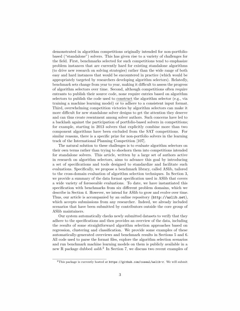
Although NP-complete problems are widely believed to be intractable inthe worst case, it is often possible to solve even very large instances of suchproblems that arise in practice. This is fortunate, because such problems areubiquitous in Artificial Intelligence applications. There has thus emerged a largesubfield of AI devoted to the advancement and analysis of heuristic algorithms forattacking hard computational problems. Indeed, quite surprisingly, this subfieldhas made consistent and substantial progress over the past few decades, withthe newest algorithms quickly solving benchmark problems that were beyondreach until recently. The results of the international SAT competitions providea paradigmatic example of this phenomenon. Indeed, the importance of thiscompetition series has gone far beyond documenting the progress achieved bythe SAT community in solving difficult and application-relevant SAT instances—it has been instrumental in driving research itself, helping the community tocoalesce around a shared set of benchmark instances and providing an impartialbasis for determining which new ideas yield the biggest performance gains.
The central premise of events like the SAT competitions is that the researchcommunity ought to build, identify and reward single solvers that achieve strongacross-the-board performance. However, this quest appears quixotic: most hardcomputational problems admit multiple solution approaches, none of whichdominates all alternatives across multiple problem instances. In particular, thisfact has been observed to hold across a wide variety of AI applications, includingpropositional satisfiability (SAT) [120], constraint satisfaction (CSP) [79], plan-ning [42, 45], and supervised machine learning [26, 104, 112]. An alternative is toaccept that no single algorithm will offer the best performance on all instances,and instead aim to identify a portfolio of complementary algorithms and astrategy for choosing between them [85]. To see the appeal of this idea, considerthe results of the sequential application (SAT+UNSAT) track of the 2014 SATCompetition.1 The best of the 35 submitted solvers, Lingeling ayv [9], solved77% of the 300 instances. However, if we could somehow choose the best amongthese 35 solvers on a per-instance basis, we would be able to solve 92% of theinstances.
Research on this algorithm selection problem [85] has demonstrated the prac-tical feasibility of using machine learning for this task. In fact, although practicalalgorithm selectors occasionally choose suboptimal algorithms, their performancecan get close to that of an oracle that always makes the best choice. Thearea began to attract considerable attention when methods based on algorithmselection began to outperform standalone solvers in SAT competitions [118].Algorithm selectors have since come to dominate the state of the art on manyother problems, including CSP [79], planning [42], Max-SAT [71], QBF [83], andASP [31].
To date, much of the progress in research on algorithm selection has been
1http://www.satcompetition.org/2014/results.shtml
2
demonstrated in algorithm competitions originally intended for non-portfolio-based (“standalone”) solvers. This has given rise to a variety of challenges forthe field. First, benchmarks selected for such competitions tend to emphasizeproblem instances that are currently hard for existing standalone algorithms(to drive new research on solving strategies) rather than the wide range of botheasy and hard instances that would be encountered in practice (which would beappropriately targeted by researchers developing algorithm selectors). Relatedly,benchmark sets change from year to year, making it difficult to assess the progressof algorithm selectors over time. Second, although competitions often requireentrants to publish their source code, none require entries based on algorithmselectors to publish the code used to construct the algorithm selector (e.g., viatraining a machine learning model) or to adhere to a consistent input format.Third, overwhelming competition victories by algorithm selectors can make itmore difficult for new standalone solver designs to get the attention they deserveand can thus create resentment among solver authors. Such concerns have led toa backlash against the participation of portfolio-based solvers in competitions;for example, starting in 2013 solvers that explicitly combine more than twocomponent algorithms have been excluded from the SAT competitions. Forsimilar reasons, there is a specific prize for non-portfolio solvers in the learningtrack of the International Planning Competition [107].
The natural solution to these challenges is to evaluate algorithm selectors ontheir own terms rather than trying to shoehorn them into competitions intendedfor standalone solvers. This article, written by a large set of authors activein research on algorithm selectors, aims to advance this goal by introducinga set of specifications and tools designed to standardize and facilitate suchevaluations. Specifically, we propose a benchmark library, called ASlib, tailoredto the cross-domain evaluation of algorithm selection techniques. In Section 3,we provide a summary of the data format specification used in ASlib that coversa wide variety of foreseeable evaluations. To date, we have instantiated thisspecification with benchmarks from six different problem domains, which wedescribe in Section 4. However, we intend for ASlib to grow and evolve over time.Thus, our article is accompanied by an online repository (http://aslib.net),which accepts submissions from any researcher. Indeed, we already includedscenarios that have been submitted by contributors outside the core group ofASlib maintainers.
Our system automatically checks newly submitted datasets to verify that theyadhere to the specifications and then provides an overview of the data, includingthe results of some straightforward algorithm selection approaches based onregression, clustering and classification. We provide some examples of theseautomatically-generated overviews and benchmark results in Sections 5 and 6.All code used to parse the format files, explore the algorithm selection scenariosand run benchmark machine learning models on them is publicly available in anew R package dubbed aslib.2 In Section 7, we discuss two recent examples of
2This package is currently hosted at https://github.com/coseal/aslib-r. We will submit
3
competition settings using ASlib, along with their advantages and disadvantages.Overall, our main objective in creating ASlib is the same as that of an
algorithm competition: to allow researchers to compare their algorithms sys-tematically and fairly, without having to replicate someone else’s system orto personally collect raw data. We hope that it will help the community toobtain an unbiased understanding of the strengths and weaknesses of differentmethodologies and thus to improve the current state of the art in per-instancealgorithm selection.
2. Background
Rice [85] was the first to formalize the idea of selecting among differentalgorithms on a per-instance basis. While he referred to the problem simplyas algorithm selection, we prefer the more precise term per-instance algorithmselection, to avoid confusion with the (simpler) task of selecting one of severalgiven algorithms to optimize performance on a given set or distribution ofinstances.
Definition 1 (Per-instance algorithm selection problem). Given
• a set I of problem instances drawn from a distribution D,
• a space of algorithms A, and
• a performance measure m : I × A → R,
the per-instance algorithm selection problem is to find a mapping s : I → A thatoptimizes Ei∼Dm(i, s(i)), i.e., the expected performance measure for instances idistributed according to D, achieved by running the selected algorithm s(i) forinstance i.
In practice, the mapping s is often implemented by using so-called instancefeatures, i.e., characterizations of the instances i ∈ I. These instance featuresare then mapped to an algorithm using machine learning techniques. However,the computation of instance features incurs additional costs, which have to beconsidered in the performance measure m.
There are many ways of tackling per-instance algorithm selection and relatedproblems. Almost all contemporary approaches use machine learning to buildpredictors of the behaviour of given algorithms as a function of instance features.This general strategy may involve a single learned model or a complex combina-tion of several, which, given a new problem instance to solve, is used to decidewhich algorithm or which combination of algorithms to choose.
it to the official R package server CRAN alongside the final version of this article.
4
2.1. What to select and when
It is perhaps most natural to select a single algorithm for solving a givenproblem instance. This approach is, e.g., used in the SATzilla [77, 118], ArgoS-mArT [75], SALSA [22] and Eureka [19] systems. Its main disadvantage isthat there is no way of mitigating a poor selection—the system cannot recover ifthe algorithm it chose for a problem instance exhibits poor performance.
Alternatively, we can seek a schedule that determines an ordering and timebudget according to which we run all or a subset of the algorithms in theportfolio; usually, this schedule is chosen in a way that reflects the expectedperformance of the given algorithms (see, e.g., [44, 45, 56, 79, 83]). Under some ofthese approaches, the computation of the schedule is treated as an optimizationproblem that aims to maximize, e.g., the number of problem instances solvedwithin a timeout. For stochastic algorithms, the further question of whether andwhen to restart an algorithm arises, opening the possibility of schedules thatcontain only a single algorithm, restarted several times (see, e.g., [18, 28, 37, 99]).Instead of performing algorithm selection only once before starting to solve aproblem, selection can also be carried out repeatedly while the instance is beingsolved, taking into account information revealed during the algorithm run. Suchmethods monitor the execution of the chosen algorithm(s) and take remedialaction if performance deviates from what is expected [29, 67, 72], or performselection repeatedly for subproblems of the given instance [5, 64, 65, 90].
2.2. How to select
The kinds of decisions the selection process is asked to produce drive thechoice of machine learning models that perform the selection. If only a singlealgorithm should be run, we can train a classification model that makes exactlythat prediction. This renders algorithm selection conceptually quite simple—onlya single machine learning model needs to be trained and run to determine whichalgorithm to choose (see, e.g., [33, 39, 73]).
There are alternatives to using a classification model to select a singlealgorithm to be run on a given instance, such as using regression models topredict the performance of each algorithm in the portfolio. This regressionapproach was adopted by several systems [74, 77, 87, 92, 118]. Other approachesinclude the use of clustering techniques to partition problem instances in featurespace and make decisions for each partition separately [57, 97], hierarchicalmodels that make a series of decisions [46, 116], cost-sensitive support vectormachines [15] and cost-sensitive decision forests [119].
2.3. Selection enablers
In order to make their decisions, algorithm selection systems need informationabout the problem instance to solve and the performance of the algorithms inthe given portfolio. The extraction of this information—the features used by themachine learning techniques used for selection—incurs overhead not requiredwhen only a single algorithm is used for all instances regardless of instancecharacteristics. It is therefore desirable to extract information as cheaply as
5
possible, thus ensuring that the performance benefits of using algorithm selectionare not outweighed by this overhead.
Some approaches use only past performance of the algorithms in the portfolioas a basis for selecting the one(s) to be run on a given problem instance [29, 92, 98].This approach has the benefit that the required data can be collected withminimal overhead as algorithms are executed. It can work well if the performanceof the algorithms is similar on broad ranges of problem instances. However,when this assumption is not satisfied (as is often the case), more informativefeatures are needed.
Turning to richer instance-specific features, commonly used features includethe number of variables of a problem instance and properties of the variabledomains (e.g., the list of possible assignments in constraint problems, the numberof clauses in SAT, the number of goals in planning). Deeper analysis can involveproperties of graph representations derived from the input instance (such asthe constraint graph [33, 68]) or properties of encodings into different problems(such as SAT features for SAT-encoded planning problems [25]).
In addition, features can be extracted from short runs of one or more solverson the given problem instance. Examples of such probing features includethe number of search nodes explored within a certain time, the fraction ofpartial solutions that are disallowed by a certain constraint or clause, theaverage depth reached before backtracking is required, or characteristics of localminima found quickly using local search. Probing features are usually moreexpensive to compute than the features that can be obtained from shallowanalysis of the instance specification, but they can also be more powerful andhave thus been used by many authors (see, e.g., [54, 78, 79, 82, 118]). Forcontinuous blackbox optimization, algorithm selection can be performed basedon Exploratory Landscape Analysis [15, 60, 74]. The approach defines a setof numerical features (of different complexities and computational costs) todescribe the landscapes of such optimization problems. Examples range fromsimple features that describe the distribution of sampled objective values tomore expensive probing features based on local search.
Finally, in the area of meta-learning (learning about the performance ofmachine learning algorithms; for an overview, see, e.g, [17]), these features areknown as meta-features. They include statistical and information-theoreticalmeasures (e.g., variable entropy), landmarkers (measurements of the performanceof fast algorithms [80]), sampling landmarkers (similar to probing features) andmodel-based meta-features [111]. These meta-features, and the past performancemeasurements of many machine learning algorithms, are available from theonline machine learning platform OpenML [113]. In contrast to ASlib, however,OpenML is not designed to allow cross-domain evaluation of algorithm selectiontechniques.
2.4. Algorithm Selection and Algorithm Configuration
A problem closely related to algorithm selection is the algorithm configura-tion problem: given a parameterized algorithm A, a set of problem instancesI and a performance measure m, find a parameter setting of A that optimizes
6
m on I (see [52] for a formal definition). While algorithm selection operates onfinite (usually small) sets of algorithms, algorithm configuration operates on thecombinatorial space of an algorithm’s parameter settings. General algorithmconfiguration methods, such as ParamILS [52], GGA [4], I/F-Race [11], andSMAC [50], have yielded substantial performance improvements (sometimes or-ders of magnitude speedups) of state-of-the-art algorithms for several benchmarks,including SAT-based formal verification [47], mixed integer programming [49],AI planning [88, 109], the combined selection and hyperparameter optimizationof machine learning algorithms [104], and joint architecture and hyperparametersearch in deep learning [23]. Algorithm configuration and selection are com-plementary since configuration can identify algorithms with peak performancefor homogeneous benchmarks and selection can then choose from among thesespecialized algorithms. Consequently, several possibilities exist for combiningalgorithm configuration and selection [3, 27, 48, 57, 71, 89, 117, 119]. The algo-rithm configuration counterpart of ASlib is AClib [53] (http://aclib.net). Incontrast to ASlib, it is infeasible in AClib to store performance data for all pos-sible parameter configurations, which often number more than 1050. Therefore,an experiment on AClib includes new (expensive) runs of the target algorithmswith different configurations and hence, experiments on AClib are a lot morecostly than experiments on ASlib, where no new algorithm runs are necessary.3
Furthermore, in contrast to AClib, ASlib does not include the actual instancesand binaries of the algorithms. Therefore, ASlib does not provide a way togenerate new performance data, as is required in AClib as a consequence of theneed to assess the performance of new target algorithm configurations arisingwithin the configuration process. However, ASlib and AClib can be combined bygenerating actual performance data based on the resources in AClib and thencreating an ASlib scenario which selects between different solver configurationson a per-instance basis.
A full coverage of the wide literature on algorithm selection is beyond thescope of this article, but we refer the interested reader to recent survey articleson the topic [63, 91, 93, 108].
3. Summary of Format Specification
We propose a data format specification for algorithm selection scenarios, i.e.,instances of the per-instance algorithm selection problem. This format and theresulting data repository allow a fair and convenient scientific evaluation andcomparison of algorithm selectors.
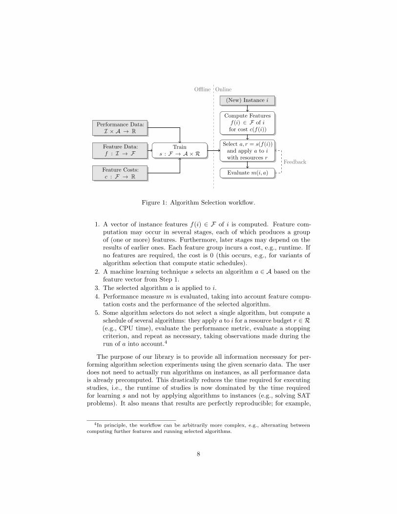
The format specification assumes a generic approach to algorithm selection,depicted in Figure 1. The general approach is as follows.
3In algorithm configuration, this need for expensive runs indeed causes a problem for research.One way of mitigating it is offered by fast-to-evaluate surrogate algorithm configurationbenchmarks [24].
7
Performance Data:I × A → R
Feature Data:f : I → F
Feature Costs:c : F → R
Trains : F → A × R
Select a, r = s(f(i))and apply a to iwith resources r
Compute Featuresf(i) ∈ F of ifor cost c(f(i))
(New) Instance i
Evaluate m(i, a)
Feedback
Offline Online
Figure 1: Algorithm Selection workflow.
1. A vector of instance features f(i) ∈ F of i is computed. Feature com-putation may occur in several stages, each of which produces a groupof (one or more) features. Furthermore, later stages may depend on theresults of earlier ones. Each feature group incurs a cost, e.g., runtime. Ifno features are required, the cost is 0 (this occurs, e.g., for variants ofalgorithm selection that compute static schedules).
2. A machine learning technique s selects an algorithm a ∈ A based on thefeature vector from Step 1.
3. The selected algorithm a is applied to i.
4. Performance measure m is evaluated, taking into account feature compu-tation costs and the performance of the selected algorithm.
5. Some algorithm selectors do not select a single algorithm, but compute aschedule of several algorithms: they apply a to i for a resource budget r ∈ R(e.g., CPU time), evaluate the performance metric, evaluate a stoppingcriterion, and repeat as necessary, taking observations made during therun of a into account.4
The purpose of our library is to provide all information necessary for per-forming algorithm selection experiments using the given scenario data. The userdoes not need to actually run algorithms on instances, as all performance datais already precomputed. This drastically reduces the time required for executingstudies, i.e., the runtime of studies is now dominated by the time requiredfor learning s and not by applying algorithms to instances (e.g., solving SATproblems). It also means that results are perfectly reproducible; for example,
4In principle, the workflow can be arbitrarily more complex, e.g., alternating betweencomputing further features and running selected algorithms.
8
the runtimes of algorithms do not depend on the hardware used; rather, theycan be simply looked up in the performance data for a scenario.
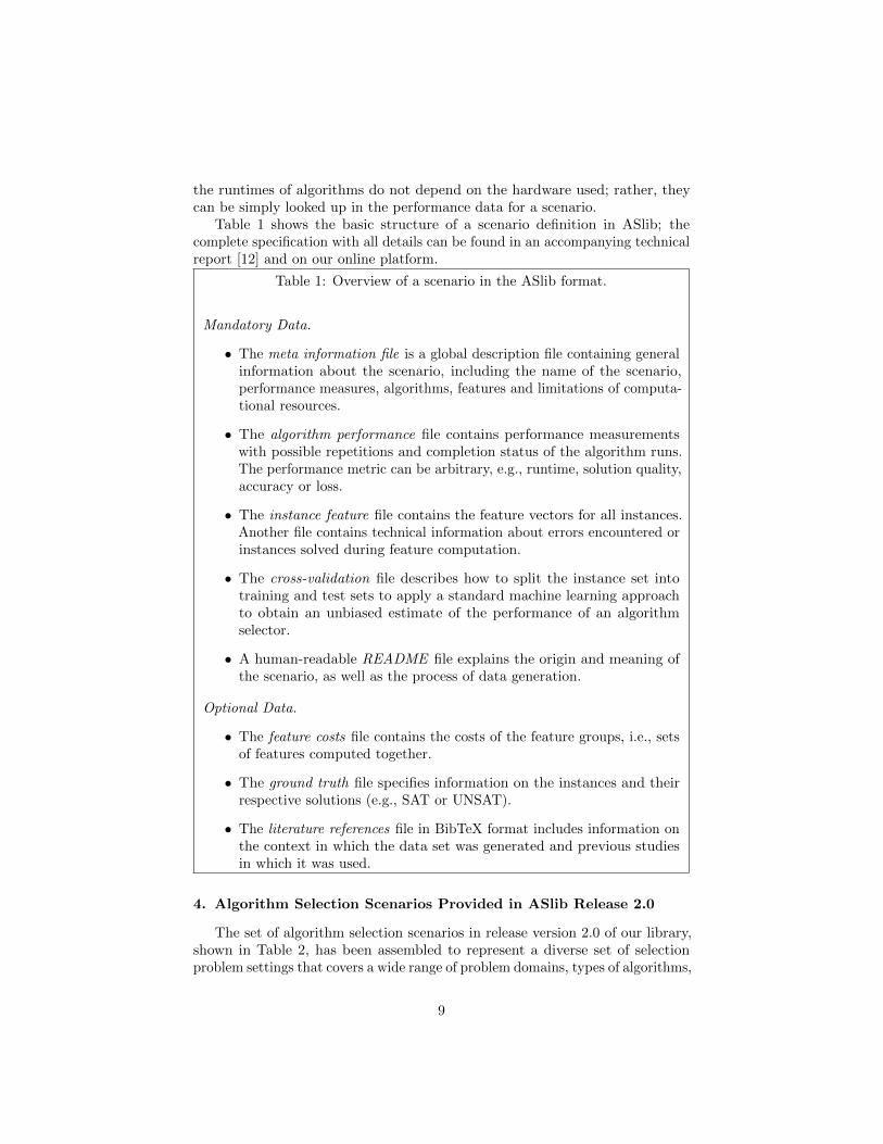
Table 1 shows the basic structure of a scenario definition in ASlib; thecomplete specification with all details can be found in an accompanying technicalreport [12] and on our online platform.
Table 1: Overview of a scenario in the ASlib format.
Mandatory Data.
• The meta information file is a global description file containing generalinformation about the scenario, including the name of the scenario,performance measures, algorithms, features and limitations of computa-tional resources.
• The algorithm performance file contains performance measurementswith possible repetitions and completion status of the algorithm runs.The performance metric can be arbitrary, e.g., runtime, solution quality,accuracy or loss.
• The instance feature file contains the feature vectors for all instances.Another file contains technical information about errors encountered orinstances solved during feature computation.
• The cross-validation file describes how to split the instance set intotraining and test sets to apply a standard machine learning approachto obtain an unbiased estimate of the performance of an algorithmselector.
• A human-readable README file explains the origin and meaning ofthe scenario, as well as the process of data generation.
Optional Data.
• The feature costs file contains the costs of the feature groups, i.e., setsof features computed together.
• The ground truth file specifies information on the instances and theirrespective solutions (e.g., SAT or UNSAT).
• The literature references file in BibTeX format includes information onthe context in which the data set was generated and previous studiesin which it was used.
4. Algorithm Selection Scenarios Provided in ASlib Release 2.0
The set of algorithm selection scenarios in release version 2.0 of our library,shown in Table 2, has been assembled to represent a diverse set of selectionproblem settings that covers a wide range of problem domains, types of algorithms,
9
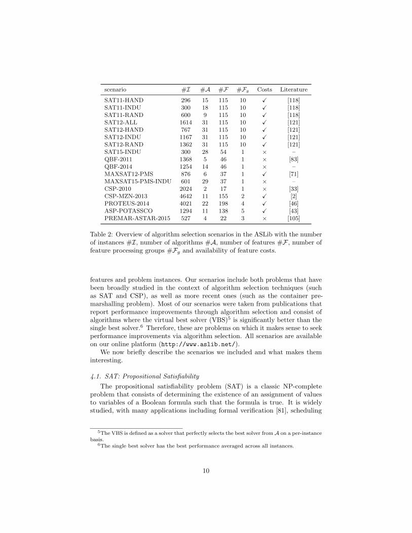
scenario #I #A #F #Fg Costs Literature
SAT11-HAND 296 15 115 10 X [118]SAT11-INDU 300 18 115 10 X [118]SAT11-RAND 600 9 115 10 X [118]SAT12-ALL 1614 31 115 10 X [121]SAT12-HAND 767 31 115 10 X [121]SAT12-INDU 1167 31 115 10 X [121]SAT12-RAND 1362 31 115 10 X [121]SAT15-INDU 300 28 54 1 × –QBF-2011 1368 5 46 1 × [83]QBF-2014 1254 14 46 1 × –MAXSAT12-PMS 876 6 37 1 X [71]MAXSAT15-PMS-INDU 601 29 37 1 × –CSP-2010 2024 2 17 1 × [33]CSP-MZN-2013 4642 11 155 2 X [2]PROTEUS-2014 4021 22 198 4 X [46]ASP-POTASSCO 1294 11 138 5 X [43]PREMAR-ASTAR-2015 527 4 22 3 × [105]
Table 2: Overview of algorithm selection scenarios in the ASLib with the numberof instances #I, number of algorithms #A, number of features #F , number offeature processing groups #Fg and availability of feature costs.
features and problem instances. Our scenarios include both problems that havebeen broadly studied in the context of algorithm selection techniques (suchas SAT and CSP), as well as more recent ones (such as the container pre-marshalling problem). Most of our scenarios were taken from publications thatreport performance improvements through algorithm selection and consist ofalgorithms where the virtual best solver (VBS)5 is significantly better than thesingle best solver.6 Therefore, these are problems on which it makes sense to seekperformance improvements via algorithm selection. All scenarios are availableon our online platform (http://www.aslib.net/).
We now briefly describe the scenarios we included and what makes theminteresting.
4.1. SAT: Propositional Satisfiability
The propositional satisfiability problem (SAT) is a classic NP-completeproblem that consists of determining the existence of an assignment of valuesto variables of a Boolean formula such that the formula is true. It is widelystudied, with many applications including formal verification [81], scheduling
5The VBS is defined as a solver that perfectly selects the best solver from A on a per-instancebasis.
6The single best solver has the best performance averaged across all instances.
10
[20], planning [59] and graph coloring [110]. Our SAT data mainly stems fromdifferent iterations of the SAT competition,7 which is split into three tracks:industrial (INDU), crafted (HAND), and random (RAND).
The SAT scenarios are characterized by a high level of maturity and diversityin terms of their solvers, features and instances. Each SAT scenario involvesa highly diverse set of solvers, many of which have been developed for severalyears. In addition, the set of SAT features is probably the best-studied featureset among our scenarios; it includes both static and probing features that areorganized into as many as ten different feature groups. The instance sets usedin our various SAT scenarios range from randomly-generated ones to real-worldinstances submitted by industry.
4.2. QBF: Quantified Boolean Formula
A quantified Boolean formula (QBF) is a formula in propositional logic withuniversal or existential quantifiers on each variable in the formula. A QBF solverfinds a set of variable assignments that makes the formula true or proves thatno such set can exist. This is a PSPACE-complete problem for which solversexhibit a wide range of performance characteristics. Our QBF-2011 data setcomes from the QBF Solver Evaluation 20108 and consists of instances from themain, small hard, 2QBF and random tracks. Our QBF-2014 data set comesfrom the application track of the QBF Gallery 20149. The instance featureswere computed using the AQME system and are described in more detail byPulina et al. [83]. The solvers for QBF-2011 come from the AQME system aswell, whereas the solvers for QBF-2014 are the ones submitted to the applicationtrack of the QBF Gallery.
4.3. MAXSAT: Maximum Satisfiability
MaxSAT is the optimization version of the previously introduced SAT prob-lem, and aims to find a variable assignment that maximizes the number ofsatisfied clauses. The MaxSAT problem representation can be used to effectivelyencode a number of real-world problems, such as FPGA routing [115], andsoftware package installation [6], among others, as it permits reasoning aboutboth optimality and feasibility. The particular scenarios focus on the partialMaxSAT (PMS) problem [10].
The MAXSAT12-PMS scenario is composed of a collection of random, craftedand industrial instances from the 2012 MaxSAT Evaluation [7]. The techniquesused to solve the various instances in this scenario are very complementary toeach other, leading to a substantial performance gap between the single bestand the virtual best solver. Furthermore, because there are only six solvers withvery different performance characteristics, algorithm selection approaches mustbe very accurate in their choices, as any mistake is heavily penalized.
7http://www.satcompetition.org/8http://www.qbflib.org/index_eval.php9http://qbf.satisfiability.org/gallery/
11
The more recent MAXSAT15-PMS-INDU was built on the performance dataof the industrial track on partial MAXSAT problems from the 2015 MAXSATEvaluation.10 With 29 algorithms, it provides a larger set of solvers thanMAXSAT12-PMS. However, there are different parameterizations of the samesolvers, e.g., four different variants of ahms, such that there are some subsetsof strongly correlated solvers. The performance gap between the single bestand virtual best solver is larger in MAXSAT12-PMS than in MAXSAT15-PMS-INDU.
4.4. CSP: Constraint solving
Constraint Satisfaction Problem (CSP; [100]) is concerned with finding solu-tions to constraint satisfaction problems—a task that is NP-complete. Learningin the context of constraint solving is a technique by which previously unknownconstraints that are implied by the problem specification are uncovered duringsearch and subsequently used to speed up the solving process.
The scenario CSP-2010 contains only two solvers: one that employs lazylearning [33, 35] and one that does not [34]. The data set is heavily biasedtowards the non-learning solver, such that the baseline (the single best solver)is very good already. Improving on this is a challenging task and harder thanin many of the other scenarios. Furthermore, both solvers share a commoncore, which results in a scenario that directly evaluates the efficacy of a specifictechnique in different contexts.
The more recent scenario CSP-MZN-2013 provides a larger set of instances,algorithms and instance features. Instances and algorithms come from theMiniZinc challenge 2012 and the International Constraint Solver Competitions(ICSC) in 2009. Specifically, the instances come from the MiniZinc 1.6 benchmarksuite and the algorithms in the scenario participated in the MiniZinc Challenge2012. Algorithms, instances and instance features are described in more detailin [1, 2].
Our final CSP scenario PROTEUS comes from [46] and includes an extremelydiverse mix of well-known CSP solvers alongside competition-winning SAT solversthat have to solve (converted) XCSP instances11. The SAT solvers can acceptdifferent conversions of the CSP problem into SAT (see, e.g., [66, 101, 102]),which in our format are provided as separate algorithms. This scenario is theonly one in which solvers are tested with varying “views” of the same problem.The features of this scenario are also unique in that they include both the SATand CSP features for a given instance. This potentially provides additionalinformation to the selection approach that would normally not be availablefor solving CSPs. An algorithm selection system has a very high degree offlexibility here and may choose to perform only part of the possible conversions,thereby reducing the set of solvers and features, but also reducing the overhead
10http://www.maxsat.udl.cat/15/results/index.html11The XCSP instances are taken from http://www.cril.univ-artois.fr/~lecoutre/
benchmarks.html as described in [46].
12
of performing the conversions and feature computations. There are also synergiesbetween feature computation and algorithm runs that can be exploited, e.g.,if the same conversion is used for feature computation and to run the chosenalgorithm then the cost of performing the conversion is only incurred once. Inother cases, where features are computed on one representation and another oneis solved, conversion costs are incurred both during feature computation and therunning of the algorithm.
4.5. ASP: Answer Set Programming
Answer Set Programming (ASP, [8, 30]) is a form of declarative programmingwith roots in knowledge representation, non-monotonic reasoning and constraintsolving. In contrast to many other constraint solving domains (e.g., the satisfia-bility problem), ASP provides a rich yet simple declarative modeling language inwhich problems up to ∆p
3 (disjunctive optimization problems) can be expressed.ASP has proven to be efficiently applicable to many real-world applications, e.g.,product configuration [95], decision support for NASA shuttle controllers [76],synthesis of multiprocessor systems [55] and industrial team building [38].
In contrast to the other scenarios, the algorithms in the scenario ASP-POTASSCO were automatically constructed by an adapted version of Hydra [117],i.e., the set of algorithms consists of complementary configurations of the solverclasp [32]. The instance features were generated by a light-weight version ofclasp, including static and probing features organized into feature groups; theywere previously used in the algorithm selector claspfolio [31, 43].
4.6. PREMAR-ASTAR-2015: Container pre-marshalling
The container pre-marshalling problem (CPMP) is an NP-hard containerstacking problem from the container terminals literature [96]. We constructedan algorithm selection scenario from two recent A* and IDA* approaches forsolving the CPMP presented in [106], using instances from the literature. Thescenario is described in detail in [105].
The pre-marshalling scenario differs from other scenarios in that the set ofalgorithms is highly homogeneous. All of the algorithms are parameterizationsof a single symmetry breaking heuristic, either using the A* or IDA* searchtechniques, which stands in sharp contrast to the diversity of solvers present inmost other scenarios. The scenario represents a real-world, time-sensitive problemfrom the operations research literature, where algorithm selection techniquescan have a large impact.
5. Automated Exploratory Data Analysis
The online platform for our benchmark repository offers not only the scenariodata files themselves. It also provides many tables and figures that summarizethem. These pages are automatically generated and currently consist (amongothers) of the following parts:
13
• an overview table that lists, for example, the number of instances, algo-rithms and features for all available scenarios, similar to Table 2;
• a summary of the algorithms’ performance and run status data;
• a summary of the feature values, as well as the run status and costs of thefeature groups;
• benchmark results for standard machine learning models for each scenario;see Section 6.
Presenting this additional data offers the following advantages:
• Researchers can quickly understand which scenarios are available and selectthose best suited to their needs.
• Data can quickly be sanity-checked. It is common that data collectionerrors occur when scenario data is gathered and submitted for the firsttime.
• Interesting or challenging properties of the data sets become visible, pro-viding the researcher with a quick and informative first impression.
The platform’s summary page for the algorithms starts with a tablelisting summary statistics regarding their performance (e.g., mean values andstandard variations) and run status (e.g., how many runs were successful). Wealso indicate whether one algorithm is dominated by another, i.e., an algorithm a1dominates another algorithm a2 if and only if a1 has performance at least equalto that of a2 on all instances, and a1 outperforms a2 on at least one instance.This is useful, because there is no reason to include a dominated algorithmin a portfolio. Various visualizations, such as box plots, scatter plot matrices,correlation plots and density plots enable further inspection of the performancedistribution and correlation between algorithms, allowing the reader to betterunderstand the strengths and weaknesses of each algorithm. All of our plotscan be configured to use log scales, which often improves visual understandingof heavy-tailed distributions (e.g., runtime distributions of hard combinatorialsolvers [36]).
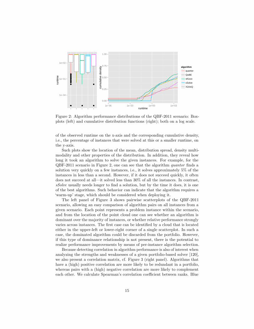
Figure 2 shows boxplots and cumulative distribution functions for the algo-rithms in the QBF-2011 scenario as an example. The boxplots summarize theruntimes of an algorithm by drawing a box between the 25%- and 75%-quantile ofthe sample, i.e., the smallest values that are greater or equal to 25% and 75% ofthe runtimes. In addition, each box contains a line showing the median runtime,as well as so-called whiskers, i.e., lines that connect the box with runtimes thatare within 150% of the interquartile range (the length of the box) below the25%- or above the 75%-quantile, respectively. Observations with even moreextreme runtimes are considered to be outliers and are depicted by a single pointper outlier. The cumulative distribution function plots on the other hand showruntimes on all instances for the algorithm. Each point within the plot consists
14
●●
●●●
●
●
●●●
●●●
●
●
●
●
●
●
●
●
●
●
●
●
●
●●
●●●●
●●
●
●●●
●
●
●
●
●
●●●●
●
●
●
●
●●
●●●
●
●
●●●●●●
●●
●
●
●●
●
●●
●●●●●●●●●●●●●●●●●●
●●●●
●●
●●●●●
●
●●●●●●●●●●●●
●
●
●
●●●●
●
●●
●
●
●●●
●
●●●●●●
●
●
●●
●
●●●●●
●●
●
●●●●●
●
●
●
●
●●●
●
●
●
●
●
●●●●
●●●●●● ●●●●●●●●●●●●●●●●●●●●●●●●●●●●●●●●●●●●●●●●●●●●●●●
●●●
●●
●●●●●●●
●●
●●●
●
●●●●
●●●●●●●●●●●●
●●
●●●●●●●●
●
●●●●●
1e−04
1e−01
1e+02
runt
ime
0.00
0.25
0.50
0.75
1.00
1e−06 1e−03 1e+00 1e+03runtime
cum
ulat
ive
dens
ity algorithm
quantor
QuBE
sKizzo
sSolve
X2clsQ
Figure 2: Algorithm performance distributions of the QBF-2011 scenario: Box-plots (left) and cumulative distribution functions (right); both on a log scale.
of the observed runtime on the x-axis and the corresponding cumulative density,i.e., the percentage of instances that were solved at this or a smaller runtime, onthe y-axis.
Such plots show the location of the mean, distribution spread, density multi-modality and other properties of the distribution. In addition, they reveal howlong it took an algorithm to solve the given instances. For example, for theQBF-2011 scenario in Figure 2, one can see that the algorithm quantor finds asolution very quickly on a few instances, i.e., it solves approximately 5% of theinstances in less than a second. However, if it does not succeed quickly, it oftendoes not succeed at all—it solved less than 30% of all the instances. In contrast,sSolve usually needs longer to find a solution, but by the time it does, it is oneof the best algorithms. Such behavior can indicate that the algorithm requires a‘warm-up’ stage, which should be considered when deploying it.
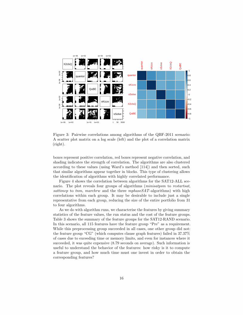
The left panel of Figure 3 shows pairwise scatterplots of the QBF-2011scenario, allowing an easy comparison of algorithm pairs on all instances from agiven scenario. Each point represents a problem instance within the scenario,and from the location of the point cloud one can see whether an algorithm isdominant over the majority of instances, or whether relative performance stronglyvaries across instances. The first case can be identified by a cloud that is locatedeither in the upper-left or lower-right corner of a single scatterplot. In such acase, the dominated algorithm could be discarded from the portfolio. However,if this type of dominance relationship is not present, there is the potential torealize performance improvements by means of per-instance algorithm selection.
Because detecting correlation in algorithm performance is also of interest whenanalyzing the strengths and weaknesses of a given portfolio-based solver [120],we also present a correlation matrix, cf. Figure 3 (right panel). Algorithms thathave a (high) positive correlation are more likely to be redundant in a portfolio,whereas pairs with a (high) negative correlation are more likely to complementeach other. We calculate Spearman’s correlation coefficient between ranks. Blue
15
X2clsQ
1e−06 1e+02
●●●●●●●●● ●●● ● ●●
●●●●●
●●●●●
●●
●
●●●
●●
●● ●● ●●●
●●
●●● ●
●
●●●●●●
●
●● ●●
●
●●●●●●●●●●●● ●●●
●●
●●
●
●●● ●●●●●●●●●●●●●●●
●
●●●●●●
●●
●●● ●●●●● ●●●●
●
●●●
●
●
●●●
●
●
●●
●
● ●●●●●●●
●
●
●
● ●●●●●
●●
●● ●●●●●●
●
● ●●●●● ●●
●●
●
●●
●●
●●●
●
●●
●●●●●●●●●
●●●●
●●●●●
●
●●●●●●●●●●●●●●●●
●●
●●●●●●●●●●●
●●●●
●
●
●●●●●●●●●
●●● ●● ●● ●●
●
●●● ●●
●
●●●●●●●●●●●●● ● ●●●●●●
●
●●
●
●●●●
●
●●●●●
●
●
●●
●
●
●●●●
●
●
●
●
●●
●
●
●
●
●
● ●●●●●●●●●●●●●●●●●●●●●●●●●●●●● ●● ● ●● ● ●
●
●●●●●●●
●●
●●●●
●
●
●●●●●●●●●●
●●●●
●●
●●
●
●●●●●●● ●●●● ●●●●
●
●
●●
●
●●
●
●
●
●
●
●●●●● ●●●● ●●●●●● ●●●● ●●●●●●●●●●●●●●●●●●●●●
●
●
●
●●
●
●
●
●
●
●
●
●
●●
●
●
●
●
●
●
●
●
●●
●
●
●
●
●
●
●
●
●●
●
●
●
●
●●●●●●●●●●●●●●●
●
●
●●●
●
● ●
●●●●●●●●●●●●●●●●●●●●●●●●●●●●●●●●●●●●●●●●●●●●●●●●●●●●●●●●●●●●●●●●●●●●●●●●●●●●●●●●●●●●●●●●●●
●●●●●●●●●●●●●●●●●●●●
●●●●●●●●●●●●●●●●●●●●●●●●●●●●●●●●●
●●●●●●●
●●●●●
●●●●●
●●●●●
●●●●●
●●●
●
●●●●●●
●●●●●●●●●●●●●●● ●●●
● ●●●●●●●●●●●●●●●●●●●●●●●●●●●●●●●●●●●●●●●●●●●●●●●●●●●●●●●●●●●●●●●●●●●●●●●
●
●
●● ● ● ●●●●●●●●●●●●●●●●●●●●●●●●●●●●● ●●●●●●●●●●●●●● ●●●● ●●●●●●●●●●●●●
●
●●●●
●●●●
●●●●
●● ●
●●●●●
●●●●●●
●●
●●●●●
●●●●●●●●
●●●
●
●●●
●●●●●
●●●●
●
●● ●●●
●
●●●●
●
●●●●
●●
●●●●
●
●
●●●●
●
●
●●●●●●
●
●●●●●●
●● ●
●
●
●●
●
●●
●
●
●● ●●●
●●●●
●
●●●● ●● ● ●●●●●● ●●●●●●●●●●●
●●
●
●
●
●
●●●●●●●●●●
●●●●●
●
●●●
●
●
●
●
●●●●● ●●●● ●●●●●
● ●●●
●
●
●
●
●
●●
●
●●●●●
●●●●●
●
●●●●●●●●●●●● ●●●●●● ●●●●●●●●●●●●●● ●●●●●●● ●●
●
●●
●
●●●●●●●●●●●●
●
●●●●●●●●●●●
●●
●●● ●●●●●●● ●●
●
●●●● ●●●●●
●
●●●●●
●●
●
●
●
●
●●●●●●●●●●
●
●●
●●●●●●●●●●●●●
●
●● ●●
●
●
●●●
● ●●
●
●●
●●●●●
●●
●
●●●● ●
●
●
●●
●
●●●●●
●●●●
●●●
●
●
●
●
●
●●
●●
●●●●●●●●●●●●●●●●●●●●●●●
● ●●●●●●
●
●●●●●●●●●●●
●
●●●●●●●●
●●●●●●
●●
●●●●●●●●●●●●●
●
●●●●●
●
●●●●●●●●●●●●●●●●●
●●●●●●●●●●
●
●
●●●●●
●
●
●
●
●●●●●●●●●●●●●●●
●●●●●
●●●●●
●●
●
●●●
●●
●●●●●●●●●
●●● ●
●
● ●●● ●●
●
●● ● ●
●
●●● ●● ● ●●●●● ●●●●
●●
●●
●
●● ●●●● ● ●●●●● ●● ●● ● ●
●
● ●● ● ●●
●●
●●●●●●●●●●●●
●
●●●
●
●
●●●
●
●
●●
●
●●●●●●●●
●
●
●
●●●●●●
●●
●●●●●●●●
●
●●●●●●●●
●●
●
●●
● ●
●●●
●
●●
●●●● ●●●●●
●●●●
●●●●●
●
●●●●●●●●●● ●●● ●●●
●●
●●●●● ●●●●●●
●●●●
●
●
●●●●●●●●●
●●● ●●●●●●
●
●●● ●●
●
●●●●●●●●●●●●●●●●●●●●
●
●●
●
●●●●
●
●●●●●
●
●
● ●
●
●
●● ●●
●
●
●
●
●●
●
●
●
●
●
●●●●●●●●●●●●●●●●●●●●●●●●●●●●●●●●●●●●●
●
●●●●●●●●●
●●●
●
●
●
●●● ●●●●●●●
●●●
●
●●
●●
●
●●●●●●●●●●●●●●●●
●
●●
●
●●
●
●
●
●
●
●●●●●●●●●●●●●●●●●●●●●●●● ●●●●●●●●●● ●●●●●●
●
●
●
●●
●
●
●
●
●
●
●
●
●●
●
●
●
●
●
●
●
●
●●
●
●
●
●
●
●
●
●
●●
●
●
●
●
● ●●●●● ●●●●●●●●●
●
●
●●●
●
●●
●●●●●●●●●●●●●●●●●●●●●●●●●●●●●●●●●●●●●●●●●●●●●●●●●●●●●●●●●●●●●●●●●●●●●●●●●●●●●●●●●●●●●●●●●●
●●●●●●●●●● ●●●●●●●●●●
●●●●●●●●●● ●●●● ●●●●●●● ●●●●●●●●●●●●●●
●● ●●●
●●
●●
●
●●
● ●●
●●●
●●
●●
●● ●
●●●
●
●●●●●●
●●●●●●●●●●●● ●●● ●●●
●● ●●●●●●●●●●●●●●●●●●●●●●●●●●●●●●●●●●●●●●●●●●●●●●●●●●●●●●●●●●●●●●●●●●●●●●
●
●
●●●●●●●●●●●●●●●●●●●●●●●●●●●●●●●●●●●●●●●●●●●●●●●●●●●●●●●●●●●●●●●●
●
●●●●
● ●●●● ●●●
●●●
● ●●●●
●● ●● ●●
●●
●●
●●●●
●●●
●●●●●●
●
●
●●●
●●●●●
●●●●
●
●● ●●●
●
●●●●
●
●●
●●
●●
●●
●●
●
●
●●●●
●
●
●●● ●●
●
●
●●●●●●
●●●
●
●
●●
●
●●
●
●
●●●●●
●●●
●
●
● ●●●●●●●●●●●●●●●●●●●●●●●
●●
●
●
●
●
●●●●●●●●●●
●●●●●
●
●●●
●
●
●
●
●●●● ●●● ●●● ●●●●
● ●●●
●
●
●
●
●
●●
●
●●●●●●●●●●
●
●●●●●●●●●●●●●●●●●●●●●●●●●●●●●●●●●●●●●●●●●
●
●●
●
●●●●●●●●●●●●
●
●●●●●●●●●●●
●●
●●●●●●●●●●●●
●
●●●●●●●●●
●
●●●●●
●●
●
●
●
●
●●●●●●●●●●
●
● ●
●●●●●●●●●●●●●
●
●●●●
●
●
●●●
●●●
●
●●
●●●●●
●●
●
●●●●●
●
●
●●
●
●●●●●
●●●●
●●●
●
●
●
●
●
●●
●●
●● ●●
●● ●●●●●
●●●
●●●●●●●
●●
●●●●●●●
●
●●●●● ●●● ●●
●
●
●●●●●●●●
●●●●
●●
●●
●●● ●● ●●●●
●●●●
●
●●●● ●
●
● ●● ●●●● ●●●●●●●●●●
●●
●●●
●●●●●
●
●
●●
● ●●
●
●
●
●
1e−06 1e+02
● ●● ●●●●●● ●●●●● ●
●●●●●
●●●●●
●●
●
●●●
●●
●●●●●●●●●
●●● ●
●
●● ●●●●
●
●● ●●
●
●●● ●● ●● ●●●●● ●●●
●●
●●
●
●●●● ●● ● ●●● ●● ●● ●●●●
●
● ●● ●●●
●●
●●● ●●●●● ●●●●
●
●●●
●
●
●●●
●
●
●●
●
● ●●● ●●●●
●
●
●
● ●●●●●
●●
●● ●●●●●●
●
● ●●●●● ● ●
●●
●
●●
●●
●●●
●
●●
●●●● ●● ●●●
●●●●
●●●●●
●
●●●●●●●●●●●●●●●●
●●
●●●●●●●●●●●
●●● ●
●
●
● ●●●●●● ●●
● ●● ●● ●● ●●
●
● ●●●●
●
●●●●●●●●●●●●●● ●●●●●●
●
● ●
●
●●●●
●
●●● ●●
●
●
● ●
●
●
●●●●
●
●
●
●
●●
●
●
●
●
●
● ●● ●●
●●●●● ●●●●●● ●●●●●●●●●●●●●●●●●●●●●
●
● ●● ●● ●●●●
●●●●
●
●
●●● ●●●●●●●
●●●●
●●
●●
●
●●●●●●●●●●●●●●
●●
●
●●
●
●●
●
●
●
●
●
●●●● ●●●●● ●●●●● ●●●●● ●●●●●●●●●●●●●●●●●●●●●
●
●
●
●●
●
●
●
●
●
●
●
●
●●
●
●
●
●
●
●
●
●
●●
●
●
●
●
●
●
●
●
●●
●
●
●
●
●●●●● ●●●●● ●●●● ●
●
●
●●●
●
●●
●●●●●●●●●●●●●●●●●●●●●●●●●●●●●●●●●●●●●●●●●●●●●●●●●●●●●●●●●●●●●●●●●●●●● ●●●●●●●●●●●●●●●●●●●●●
●●●● ●● ●●
●● ●●●●●●●● ●●●●●●●●●●●●●●●●●●●●●●●●●●●●●●●●●●●●●●●●●●
●●●●●
●●●●●
●●●●●
●●●●●
● ●●
●
●●● ●●●
●●●●●●●●●●●● ● ●● ●●●
● ● ●●●●●●●●●●●●●●●●●●●●●●●●●●●●●●●●●●●●●●●●●●●●●●●●●●●●●●●●●●●●●●●●●●●●●●
●
●
●●●● ●●●●●●● ●●●● ●● ●●●●●●● ●●● ●●●●● ●●●● ●●●●●●●● ●●● ●● ●● ● ●●●●●● ●● ●●●●
●
●●●●
● ●●●●●
●●●
●●● ●●
●●●●●●●
●● ●
●●
● ●●●
● ●●
●●●●●●
●
●
●●
●●●
● ●●●
●● ●
●
●● ●●●
●
●●●●
●
●●
●●
●●
●●
●●
●
●
●●●●
●
●
●●●●
●●
●
● ●●● ●●
●●●
●
●
●●
●
● ●
●
●
●●●●●
●●●
●
●
●●●● ●● ●●●●●●● ●●●●●●●●●●●
●●
●
●
●
●
●●●● ●● ●●●●
●●●● ●
●
●●●
●
●
●
●
●●●●● ●●●● ●●●●●
● ●●●
●
●
●
●
●
●●
●
●●●●●
●●●●●
●
●●●●●● ●●● ●● ●●●●●●●● ●●●●● ●●●● ●●●●● ●●● ●●●● ●
●
●●
●
●●●●●●●●● ●● ●
●
●● ● ●●●●● ●●●
●●
● ●●●●●●● ●●●●
●
●●●●●●●●●
●
●●●●●
●●
●
●
●
●
●●●●●●●●●●
●
●●
●●●●●●●●●●●●●
●
●●●●
●
●
● ●●
●●●
●
●●
●● ●● ●
●●
●
●●●●●
●
●
●●
●
●●●●●
●●●●
●●●
●
●
●
●
●
●●
●●
●● ●●●●●●●●●
●●●
●●●●●●●●
●
●●●●●●●
●
●●●●●●●● ●●
●
●
●●●●●●●●
●●●●●
●
●●
●●●●●●●●●●●●●
●
●●●●●
●
●●●●●●●●●●●●●●●●●
●●●●●●●●●●
●
●
●●●●●
●
●
●
●
1e−
061e
+02●●●●●●●●●●●●●●●
●●● ●●
●●●●●
●●
●
●●●
●●
●● ●●●●●
● ●
●●● ●
●
●● ●●●●
●
●● ●●
●
●●●●●●● ●●●●● ●●●
●●
● ●
●
● ●● ●●●●●●●●●●●●● ●●
●
●●●●●●
●●
●●●●●● ●● ●●●●
●
●●●
●
●
●●●
●
●
●●
●
● ●●●●●●●
●
●
●
●●●●● ●
●●
●● ●●●●●●
●
● ●●●●●●●
● ●
●
●●
● ●
●●●
●
●●
●●●●●●●●●
●●●●
●●●●●
●
●●●●●●●●●●●●●●●●
●●
●●●●●●●●●●●
●●●●
●
●
●●●●●●●●●●●●●●●●●●
●
●●● ●●
●
● ● ●●●●●●●●●●●●●●●●●●
●
●●
●
●●●●
●
●●●●●
●
●
● ●
●
●
● ●●●
●
●
●
●
● ●
●
●
●
●
●
●●●●●
● ● ●●●●●●●
●●●●●●●●●●●●●● ●●●● ●●●●●
●
●●●●●●
●●●
● ●●●
●
●
●●● ● ●●● ●●●
●●●●
●●
●●
●
●●●●●●● ●●●● ● ●●
●●
●
●●
●
●●
●
●
●
●
●
●● ●●● ●●●●●●● ●●● ●●● ●●●● ●●● ●●● ●●●● ●●● ●●● ●●
●
●
●
●●
●
●
●
●
●
●
●
●
●●
●
●
●
●
●
●
●
●
●●
●
●
●
●
●
●
●
●
●●
●
●
●
●
● ●●●●●●●●● ●●●●●
●
●
●● ●
●
● ●
●●●●●●●●●●●●●●●●●●●●●●●●●●●●●●●●●●●●●●●●●●●●●●●●●●● ●●●●●●● ● ●●●●●●●●●●● ●●●● ●●●●● ● ●●●●●●●●●●
●●●●●●●●●●●●●●●●●●●●●●●●●●●●●●●●●●●●●●●●●●●●●●●●●●●●
●●●●●●●●
●●●●●
●●●●●
●●●●●
●●●●●
●●●
●
●●●●●●
●● ●●●●●●● ●●●●●●●●●●●●●●●●●●●●● ●●●● ● ●●●●● ●●●● ●●●●●● ●●●●●●●●●●●●●●●●●●●●●●●●●●●●●●●● ●● ●●●● ● ●
●
●
●●● ● ●●●●●●●●●●●●●●●●●●●●●●●●●●●●●●●●●●●●●●●●●●●●●●●●●●●●●●●●●●●●
●
●●●●
● ●●●
● ●●●
●●●
● ●●●●
●●●●●●
● ●
●●
●●●●
● ●●
●●●●●●
●
●
●●
●●●
● ●●●
●● ●
●
●● ● ●●
●
●● ●●
●
●●
●●
●●
●●
●●
●
●
●●●●
●
●
●●● ●
●●
●
● ●●● ●●
●●●
●
●
●●
●
● ●
●
●
●●● ●●
●●● ●
●
●●●● ●●●●●●●●●●●●●●●●●●●●
●●
●
●
●
●
●●●●●●●●●●
●●●●●
●
●●●
●
●
●
●
●●●●● ●●●●●●●●●
● ●●●
●
●
●
●
●
●●
●
●●●●●
●●●●●
●
● ●●●●●● ●●●●●●●●●●●●●●●●●●●●●●●●●●●●●●●●●●
●
● ●
●
●●●●●● ●●●●●●
●
●●● ●●●●
●●●●
●●
● ●●●●●●●●●●●
●
● ●●●● ●●● ●
●
●●●●●
●●
●
●
●
●
●●●●●●●●●●
●
● ●
●●●●●●●●●●●● ●
●
●●●●
●
●
●●●
●●●
●
●●
●●●●●
●●
●
●●●●●
●
●
●●
●
●●●●●
●●●●
●●●
●
●
●
●
●
●●
●●
●●●●●●●●●●●●●●●●●●●●●●●
●●●●●●●
●
●●●●● ●●●●●●
●
●●●●●●●●
●●●●●
●
●●
●●●●●●●●●●●●●
●
●●●●●
●
●●●●●●●●●●●●●●●●●
●●
●●●
●●● ●●
●
●
●●
● ●●
●
●
●
●
1e−
061e
+02 ●●●●●●●●
●
●
●
●
●
●●●●●●● ●●●●● ●●●●●●●● ●
●
●●●
●●●●
●●
●
●
●
●●●●●●
●
●
●
●●
●
●●●●●●●●●●●
●
●●●
●
●
●●
●
●●
●
●●●●●●●●●●●●●●●
●
●●●●●
●●●
●●
●
●●●●●
●●●●●
●●●
●●
●●●
●●
● ●●
●
●●●●●●●
● ●
●
●
●●●●
●
●●
●
●
●●●●●●
●
●
●●●●
●
●●
●
●
●
●●
●●
●●●
●
●●
●●●●●●●●●●●●● ●●●●●● ●●●●●●●●●●●●●●●●●● ●●●●●●●●●●●●●●● ●● ●●●●●●●●●
●●
●
●
●
●
●
●●
●
●●
●
●●
●
●●●●●●●●●●●
●●
●●●●●●●
●●●● ●●●●● ●●●●●● ● ●●● ●●●●
●
●● ●
●
●●● ●●
●
●
●
●●●● ●●●●●●●●●●●●●●●●●●●●●●●●
●
●
●
●●●●
●
●
●●
●●●●
●●●
●●●●
●
●●●
●●●●●●●●
●
●●●
●●
●●
●
●
●●●●●●
●●●
●
●●●
●
●
●
●●
●
●●
●
●
●
●
●
●●●●
●
●●●
●
●●●●●
●
●●●
●
●●●●●●●●●●●●●●●●●●●●●
● ●●
●●
● ●
●
●
●
● ●●
●●
● ●
●
●
●
●
●
●
●●
●
● ●● ●
●
●
●
●●
●
● ●● ●●●●●●●●●●●●●●●
●●
●●●
●
●
●
●●●●●●●●●●●●●●●●●●●●●●●●●●●●●●●●●●●●●●●●●●●●●●●●●●●●●●●●●●●●●●●●●●●●●●●●●●●●●●●●●●●●●●●●●●
●●●●●●●●●●
●●●●●●●●●●●●●●●●●●●●●●●●●●●●●●●●●●●●●●●●●●●●●●●●●●● ●●●● ●●●●●●●●●● ●● ●●●
●●●● ●●●●●●
●●●●●●●●●●
●●●●●
●●
●
●
●●●●●●●●●●●●●●●●●●●●●●●●●●●●●●●●●●●●●●●●●●●●●●●●●●●●●●●●●●●●●●●●●●●●●●●
● ●
●●●
●
●●●●●●●●●●●●●●●●●●●●●●●●●●●●
●
●●●●●●●●●●●●●
●
●●●●●●●●●●●●●●●●●
●
●●●
●
●●
●●
●●
●●
●
●
●●●●
●●
●●●●●
●
●●
●
● ●●●
●
●●●●●●●
●●
●
●
●●●
●●
●●●
●
●●●
●
●
●
●●
●●
●●●●
●
●●●●
●●
●●●●
●
●
●●●●
●
●
●●●●●●
●
●●●●●●
●●
●●
●
●●
●
●●
●
●
●●
●●
●
●●●●
●
●●●
●
●
●
●
●●●●●
●
●●●●●●●●●●●●● ●●● ●●●●●●●●●●● ●●●●
●
● ●●●
●
● ●
●
●●●●
●
●●●
●
●●●●
●
●
● ●●
●
●
●
●
●
●●
●
●●●
●●
●●●●●●
●●●●●●●●●●●
●
●●●●
●●●●●●●●●●●●●●●
●
●●●●●●
●
●●
●
●●
●
●●●●●●●●●●●
●
●
●●●●●●●●●●
●
●●
●●
●
●●●●●●
●
●●
●
●●●
●
●●●●●● ●●●●●●● ●●● ●●●●●●●●●●● ●
●
●
●●●●●●●●●●●●●
●
●
●●
●●
●●●● ●
● ●
●●●
●●●●●
●
●
●
●
●●●
●
●
●
●
●
●
●●●●
●●●●●
●●●● ●● ●● ●●●● ●●●●●●●●●●●●●●●●●●●●●●●
●
●●●●●●● ●●●●●●●●●●●● ●●●●●●●●●●●●●●●● ● ●●●●●●
●●
●●●●● ●●●●●● ●●●●●●●●●●●●●●●●●
● ●●●●●●●●●
●● ●●●●● ●● ●
●
quantor
●●●●●●●●
●
●
●
●
●
●●●●●●●●●●●●●●●●●●●●●
●
●●●
●●●●
●●
●
●
●
● ●●● ●●
●
●
●
● ●
●
●●● ●● ● ●●●●●
●
●●●
●
●
●●
●
●●
●
●●● ● ●●●●● ●● ●● ● ●
●
● ●● ● ●
●●●
●●
●
●●●●●
●●
●●●
●●●
●●
●●●
●●●●●●
●●●●●●●
●●
●
●
●●●●
●
●●
●
●
●●●●●●
●
●
●●●●
●
●●
●
●
●
●●
● ●
●●●
●
●●
●●●● ●●●●●●●●● ●●●●●● ●●●●●●●●●● ●●● ●●●●● ●●●●● ●●●●●●●●●● ●● ●●●●●●●●●
●●
●
●
●
●
●
●●
●
●●
●
●●
●
●●●●●●●●●●●
●●
●●●●●●●
●●●● ●●●●● ●●●●●● ● ● ●●●●● ●
●
●● ●
●
●●●●●
●
●
●
●●●●●●●●●●●●●●●●●●●●●●●●●●●●
●
●
●
●●●●
●
●
●●
●●●●
●●●
●●● ●
●
●●●
●●●●●●●●
●
●●●
●●
●●
●
●
●●●●●●
●●●
●
●●●
●
●
●
●●
●
●●
●
●
●
●
●
●●●●
●
●●●
●
●●●●●
●
●●●
●
●●●●● ●●●●●●●●●● ●●●●●●
●●●
●●
● ●
●
●
●
● ●●
●●
● ●
●
●
●
●
●
●
●●
●
● ●● ●
●
●
●
●●
●
● ●● ● ●●●●● ●●●●●●●●●
●●
●●●
●
●
●
●●●●●●●●●●●●●●●●●●●●●●●●●●●●●●●●●●●●●●●●●●●●●●●●●●●●●●●●●●●●●●●●●●●●●●●●●●●●●●●●●●●●●●●●●●
●●●●●●●●●●
●●●●●●●●●●
●●●●●●●●●●●●●● ●●●●●●● ●●●●●●●●●●
●●●● ●●●●
●●●● ●●●● ● ●●●●● ●● ●● ●● ●
●●●●●●●●●●
●●●●●●●●●●
●●
●●●
●●
●
●
● ●●●●●●●●●●●●●●●●●●●●●●●●●●●●●●●●●●●●●●●●●●●●●●●●●●●●●●●●●●●●●●●●●●●●●●
● ●
●●●
●
●●●●●●●●●●●●●●●●●●●●●●●●●●●●
●
●●●●●●●●●●●●●
●
●●●●●●●●●●●●●●●●●
●
●●●
●
● ●
●●
● ●
●●
●
●
● ● ●●
●●
●● ●● ●
●
●●
●
● ●●●
●
●●● ●●●●
●●
●
●
● ●●
●●
●●●
●
●●●
●
●
●
●●
●●
●●●●
●
●●●●
●●
● ●●●
●
●
●●●●
●
●
●●● ●●●
●
●●●●●●
●●
●●
●
●●
●
●●
●
●
●●
●●
●
●●●●
●
● ●●
●
●
●
●
●●●●●
●
●●●●●●●●●●●●●●●●●●●●●●●●●●● ●●●●
●
●●●●
●
● ●
●
● ●●●
●
●● ●
●
● ●●●
●
●
●●●
●
●
●
●
●
●●
●
●●●
●●
●●●●●●
●●●●●●●●●●●
●
●●●●
●●●●●●●●●●●●●●●
●
●●●●●●
●
●●
●
●●
●
●●●●●●●●●●●
●
●
●●●●●●●●●●
●
●●
●●
●
●●●●●●
●
●●
●
●●●
●
●●●●●● ●●●●●●●●●●●●●●●●●●●●● ●
●
●
●●●●●●●●●●●●●
●
●
●●
●●
●●●●●
●●
●● ●
●●●●●
●
●
●
●
●●●
●
●
●
●
●
●
●●●●
●●●●●
●●●● ●● ●● ●●●● ●● ●●● ● ●●●●● ●●●● ●●●●●●● ●
●
●●● ●●●● ●●●●● ●●● ●●●● ●●●●●●●●●●● ● ●●●● ●●● ●● ●●
●●
●● ●●● ●●●● ●●● ●● ●●●● ●●●●●●●●●●
●●● ●●●●●●●
●● ●●● ●●●●●
●
● ●● ●●●●●
●
●
●
●
●
● ●●●●●●●●●●●●●●●●●●●●
●
●●●
●●●
●
●●
●
●
●
●● ●●●●
●
●
●
●●
●
●●● ●● ●● ●●●●
●
●●●
●
●
●●
●
●●
●
● ●● ● ●●● ●● ●● ●●●●
●
● ●● ●●
●●●
●●
●
●●●
●●
●●
●●●
●●●
●●
●●●
●●
●●●●
●●●●●●●
●●
●
●
●●●●
●
●●
●
●
●●●●●●
●
●
●●●●
●
● ●
●
●
●
●●
●●
●●●
●
●●
●●●● ●● ●●●●●●●●●●●● ●●●●●●●●●●● ●●●●●●●● ●●●●●●●●●●●●●● ●● ●● ●●●●●● ●●
● ●
●
●
●
●
●
●●
●
●●
●
●●
●
●●●●●●●●●●●
●●
●●●●●●●
●● ●●●●●●● ●●● ●●●● ● ●●●●●●
●
●●●
●
●● ●●●●
●
●
●●
●● ●●●●● ●●●●●● ●●●●●●●●●●●●●
●
●
●
●●●●
●
●
● ●
●●● ●
●●●
●●●●
●
●●●
●●●●●●●●
●
●●●
●●
●●
●
●
●●●●●●
●●●
●
●●●
●
●
●
●●
●
●●
●
●
●
●
●
●●●●
●
●●●
●
●●●●●
●
●●●
●
●●●●●●●●●●●●●●●●●●●●●
●● ●
●●
●●
●
●
●
●● ●
●●
●●
●
●
●
●
●
●
●●
●
● ●● ●
●
●
●
●●
●
● ●● ●●●●● ●●●●● ●●●● ●
●●
●●●
●
●
●
●●●●●●●●●●●●●●●●●●●●●●●●●●●●●●●●●●●●●●●●●●●●●●●●●●●●●●●●●●●●●●●●●●●●● ●●●●●●●●●●●●●●●●●●●●●
●●●● ●● ●●●●
●●●●●●●●●●●●●●●●●●●●●●●●●●●●●●
●●●●●●●●●●●●●●●●●●●●●●●●●●●●●●●●●●●●●●●●
● ●●●●●● ●●●
●●●●●●●●●●
●●
● ●●
●●
●
●
● ●●●●●●●●●●●●●●●●●●●●●●●●●●●●●●●●●●●●●●●●●●●●●●●●●●●●●●●●●●●●●●●●●●●●●●
●●
●●
●
●
●●●●●●● ●●●● ●● ●●●●●●● ●●● ●●●●●
●
●●● ●●●●●●●● ●●
●
●● ●●
● ●●●●●● ●● ●●●●
●
●●●
●
● ●
●●
●●
●●
●
●
●● ●●
●●
●●●●●
●
● ●
●
● ● ●●
●
● ●● ●●●●
●●
●
●
●● ●
●●
● ●●
●
●● ●
●
●
●
●●
●●
● ●●●
●
● ●●●
●●
● ●●●
●
●
●●●●
●
●
●● ●●● ●
●
● ●●● ●●
●●
●●
●
●●
●
● ●
●
●
●●
●●
●
●●● ●
●
●●●
●
●
●
●
●●●●●
●
●●●●●●●●●●●●● ●●●●●●●● ●● ●●●● ●●●●
●
● ●●●
●
●●
●
●●●●
●
●●●
●
●●●●
●
●
●●●
●
●
●
●
●
●●
●
●●●
●●
●●●●●●
●●●●●● ●●● ●●
●
●●●●
●●● ●●●●● ●●●● ●●●
●
● ●●● ●●
●
● ●
●
●●
●
●●●●●●●●● ●●
●
●
●● ● ●●●●● ●●
●
●●
● ●
●
●●●●● ●
●
●●
●
●●●
●
●●●●●●●●●●●●●●●●●●●●●●●●●●● ●
●
●
●●●●●●●●●●●●●
●
●
●●
●●
●● ●● ●
●●
●●●
●● ●● ●
●
●
●
●
●●●
●
●
●
●
●
●
●●●●
●●●●●
●●●●●●● ●●●●●●● ●●●●●●●●● ●●● ●●●●●●●●●
●
●●● ●●●●●●●●●●●● ●●●●●●●●●●●●●●● ●●●●● ●●●●●●●
●●
●●●●●●●●●●●●●●●●●●●●●●●●●●●●
●●●●●●●●●●
●●●●●●●●●●
●
●●●●●●●●
●
●
●
●
●
●●●●● ●●●●●●●●●●●●●●●●
●
●●●
●●●
●
●●
●
●
●
●● ●●●●
●
●
●
●●
●
●●●●●●● ●●●●
●
●●●
●
●
● ●
●
● ●
●
●●●●●●●●●●●●● ●●
●
●●●●●
●●●
●●
●
●●●
●●
●●
●●●
●●●
●●
●●●
●●
●●●
●
●●●●●●●
●●
●
●
●●●●
●
●●
●
●
●●●●●●
●
●
●●●●
●
●●
●
●
●
●●
● ●
●●●
●
●●
●●●●●●●●●●●●● ●●●●●● ●●●●●●●●●●●●●●●●●● ●●●●●●●●●●●●●●● ●● ●●●●●●●●●●●
●
●
●
●
●
●●
●
●●
●
●●
●
● ● ●●●●●●●●●
●●
●●●●●●●
●●●● ●●●●● ●●●●●● ● ● ●●●● ●●
●
●●●
●
● ● ●●●
●
●
●
●●●● ● ● ●●●●●●● ●●●●●●●●●●●●●● ●
●
●
●
●●●
●
●
●
●●
●●●●
●●●
● ●● ●
●
●●●
●● ●●● ●●●
●
●●●
●●
●●
●
●
●●●●●●
●●●
●
● ●●
●
●
●
●●
●
●●
●
●
●
●
●
●● ●●
●
●●●
●
●●● ●●
●
●●●
●
●●● ●●● ●●● ●●●● ●●● ●●● ●●
●●●
●●
●●
●
●
●
●●●
●●
●●
●
●
●
●
●
●
●●
●
●●● ●
●
●
●
●●
●
●●● ● ●●●●●●●●● ●●●●●
●●
●●●
●
●
●
●●●●●●●●●●●●●●●●●●●●●●●●●●●●●●●●●●●●●●●●●●●●●●●●●●● ●●●●●●● ● ●●●●●●●●●●● ●●●● ●●●●● ● ●●●●●●●●●●
●●●●●●●●●●●●●●●●●●●●●●●●●●●●●●●●●●●●●●●●●●●●●●●●●●●●●●●●●●●
●●●●●●●●●●●●●●●●●●●●●
●●●●●●●●●●
●● ●●●●●●● ●
●●●●●
●●●
●
●●●●●●●●●●● ●●●● ● ●●●●● ●●●● ●●●●●● ●●●●●●●●●●●●●●●●●●●●●●●●●●●●●●●● ●● ●●●● ● ●
●●
●●●
●
●●●●●●●●●●●●●●●●●●●●●●●●●●●●
●
●●●●●●●●●●●●●
●
●●●●●●●●●●●●●●●●●
●
●●●
●
● ●
●●
● ●
●●
●
●
● ● ●●
●●
●●●●●
●
● ●
●
● ●●●
●
● ●● ●●●●
●●
●
●
●● ●
●●
● ●●
●
●● ●
●
●
●
● ●
●●
● ● ●●
●
● ●●●
●●
● ●●●
●
●
●●●●
●
●
●● ● ●● ●
●
● ●●● ●●
●●
●●
●
●●
●
● ●
●
●
●●
● ●
●
●●● ●
●
●●●
●
●
●
●
●●●●●
●
●●●●●●●●●●●●●●●●●●●●●●●●●●● ●●●●
●
● ●●●
●
●●
●
●●●●
●
●●●
●
●●●●
●
●
●●●
●
●
●
●
●
●●
●
●●●
●●
●●●●●●
● ●●●●●● ●●●●
●
●●●●
●●●●●●●●●●●●●●●
●
●●●●●●
●
●●
●
● ●
●
●●●●●● ●●●●●
●
●
●●● ●●●● ●●●
●
●●
● ●
●
●●●●●●
●
●●
●
● ●●
●
● ●●● ●● ●●●●●●●●●●●●●●●●●●●●● ●
●
●
●●●●●●●●●●●● ●
●
●
●●
●●
●●●●●
●●
●●●
●●●●●
●
●
●
●
●●●
●
●
●
●
●
●
●●●●
●●●●●
●●●● ●● ●● ●●●● ●●●●●●●●●●●●●●●●●●●●●●●
●
●●●●●●● ●●●●● ●●●●●●●●●●●●●●● ●●●●●● ●●● ●●●●●●
●●
●●●●●●●●●●●●●●●●●●●●●●●●●●●●
●●● ●●●●● ●●
●●●●● ●●●●●
●
●●●●●●●●●●●●●●●
●●●●●●●●●● ●●
●●●●●
●●●●●●●●●●
●●
●
●
●
●
●●
●
●●
●
●
●
●
●
●
●
●●
●
●
●
●●●●
●
●●●
●
●●
●
●●
●●
●●
●
●
●●●●●●
●
●
●●
●
●●
●
●
●
●
●
●
●●
●●●●●●●●●●
●●
●
●●●●
●
●●●
●
●● ●●
●●●●●●●●● ●
●
●●●●●●●● ●●●●●●●●● ●●●●●●●●
●●
●
●●
●
●
●●●
●
●●
●
●●●
●
●●●●
●●●●
●●●
●●
●
●●●●●●●
●●●
●
●●
●●●
●●
●
●●●●
●●●●●
●
●●●●
●
●
●●●●●●●●
●
●●
●
●●●●●●
●
●●
●
●●
●
●●●●●●●●●●●●●●●●●●●●
●
●●
●
●●●●
●
●●●●●
●
●●
●●
●●●
●
●
●
●
●
●
●●
●●
●●●
●●●●● ●●●●●●●●●●●●●●●●●●●●●●●●●●●●●●●●
●
●●●●●●●●●
●●●
●
●
●●●
●
●●●●●●●
●
●●●
●●
●●●
●●●●●●●●●●●●●●●●
●
●●
●
●●
●
●
●
●
●
●●●●●●●●●●●●●●●●●●●●●●●
●
●●●●●●●●●
●
●●●●●●
●●
●
●
●
●
●●
●
●
●
●
●
●●
●●
●
●
●
● ●●
●
●
● ●
●
●
●
●●
●
●
●
● ●
●
●
●
●●●●
●
●●●●●●●●
●
●
●
●●●
●
●●
●●●●●●●●●●●●●●●●●●●●●●●●●●●●●●●●●●●●●●●●●●●●●●●●●●●●●●●●●●●●●●●●●●●●●●●●●●●●●●●●●●●●●●●●●●
●●●●●●●●●●●●●●●●●●●●
●●●●●●●●●●●●●●●●●●●●●●●●●●●●●●●●
●●
●
●
●
●●●
● ●
●
●
●●
●
●
●
●●●●
●
●●
●
●
●
●
●●●● ●●●●●●
●●●●●●●●●●
●
●
●●●
●
●●
●●
●●●●●●●●●●●●●●●●●●●●●●●●●●●●●●●●●●●●●●●●●●●●●●●●●●●●●●●●●●●●●●●●●●●●●●
●
● ●●●●●●●●●●●●●●●●●●●●●●●●●●●●●●●●●●●●●●●●●●●●●●●●●●●●●●●●●●●●●●●●
●
●●●
●
●
●
●● ●
●
●●
●
●●
●
●
●
●●
●
●
●
●●
●
●●
●●
●
●●
●
●●
●
●
●●●
●●
●
● ●●●
●●
●●●
●
●●●
●
●
●●●
●●
●●●●
●
●●
●●●●
●
●
●●
●●
●●●●
●
●
●●●
●
●●
●
●●●●●●
●●●
●
●●●
●
●●
●
●
●●●●●
●●●●
●
●
●●●●●●●●●●●●●●●●●●●
●●●●●● ●●● ●●●●●●●●●●●
●●●●●
●●●●
●
●
●●●
●
●●
●●
●
●●
●
●●●●
●
● ●●
●
●
●
●
●
●●
●
●●●●● ●●●●●
●
●●●●●●●●●●●●●●●●●●●●●●●●●●●●●●●●●●●●●●●●●
●
●●
●
●●●●●●●●●●●●
●
●●●●●●●●●●●
●●
●●●●●●●●●●●●
●
●●●●●●●●●
●
●
●●●●●● ●●● ●●●●●●●●●●●
●
●
●
●●●●●●●●●●●●●
●
●
●●
●
● ●●●● ●●●
●
●
●
●●●●●
●
●●●●●●●●
●
●
●●●●●●●
●●●●
●●●
●
●
●
●
●
●●
●●
●
●
●●
●●
●
●●●●
●●●
●
●●●●●●
●
●
●●●●
●●●
●
●●
●●●
●●
●
●●
●
●
●●●●●●●●
●●●
●
●●
●●
●
●●
●
●
●●
●●●●
●
●●
●●●
●
●
●●
●
●
●●●●
●●●●●●●●●●
● ●●●●
●●●●●
●●●
●●
●● ●●
●
●
●●●●●●●●● ●●● ● ●●
●●●●●●●●●●●●●●●●●●●
● ●● ●●●●●
●●
●
●
●
●
●●
●
●●
●
●
●
●
●
●
●
●●
●
●
●
●●●●
●
● ●●
●
●●
●
●●
●●
● ●
●
●
●●●●●●
●
●
●●
●
●●
●
●
●
●
●
●
●●
●●● ●●●●● ●●
●●
●
●●●●
●
●●●
●
●●●●
● ●●●●●●●●●
●
● ●●●●●●● ●● ●●●●●●●● ●●●●● ●●
●●
●
●●
●
●
●●●
●
●●
●
●●●
●
●●●●
●●●●
●●●
●●
●
●●●●●●●
●●●
●
●●
●●●
●●
●
●●●●
●●●●●
●
●●●●
●
●
●●●●●●●●
●
●●
●
●● ●● ●●
●
●●
●
●●
●
●●●●●●●●●●●●● ● ●●●●●●
●
●●
●
●●●●
●
●●●●●
●
●●
●●
●●●
●
●
●
●
●
●
●●
●●
●●●
● ●●●●●●●●●●●●●●●●●●●●●●●●●●●●● ●● ● ●● ● ●
●
●●●●●●● ●●
●●●
●
●
●●●
●
●●●●●●●
●
●●●
●●
●●●
●●●●●●● ●●●● ●●●● ●
●
●●
●
●●
●
●
●
●
●
●●●●● ●●●● ●●●●●● ●●●● ●●●●
●
●●●●●●●●●
●
●●●●●●
●●
●
●
●
●
●●
●
●
●
●
●
●●
●●
●
●
●
● ●●
●
●
● ●
●
●
●
●●
●
●
●
● ●
●
●
●
●●●●
●
●●●●●●●●
●
●
●
●●●
●
● ●
●●●●●●●●●●●●●●●●●●●●●●●●●●●●●●●●●●●●●●●●●●●●●●●●●●●●●●●●●●●●●●●●●●●●●●●●●●●●●●●●●●●●●●●●●●
●●●●●●●●●●
●●●●●●●●●●
●●●●●●●●●●
●●●●●●●●●●●●●●●●●●●●●●●
●
●
●
●
●●●
●●
●
●
●●
●
●
●
●●●●
●
●●
●
●
●
●
●●●●●●●●●●
●●●●●●●●●●
●
●
●●●
●
●●
●●
●●●●●●●●●●●●●●●●●●●●●●●●●●●●●●●●●●●●●●●●●●●●●●●●●●●●●●●●●●●●●●●●●●●●●●
●
● ●● ● ● ●●●●●●●●●●●●●●●●●●●●●●●●●●●●● ●●●●●●●●●●●●●● ●●●● ●●●●●●●●●●●●●
●
●●●
●
●
●
●● ●
●
●●
●
● ●
●
●
●
●●
●
●
●
●●
●
●●
●●
●
●●
●
●●●
●
●●●
●●
●
● ●●●
●●
●●●
●
●●●
●
●
●●●
●●
●●●●
●
●●●●
●●
●
●
●●
●●
●●●●
●
●
●●●
●
●●
●
●●●●●●
●●
●
●
●●●
●
●●
●
●
●● ●●
●
●●●●
●
●
●●● ●● ● ●●●●●● ●●●●●●●
●●●●●●●●●●●●●●●●●●●●
●●●●●
●●●●
●
●
●●●
●
●●
● ●
●
●●
●
●●●●
●
●●●
●
●
●
●
●
●●
●
●●●●● ●●●●●
●
●●●●●●●●●●●● ●●●●●● ●●●●●●●●●●●●●● ●●●●●●● ●●
●
●●
●
●●●●●●●●●●●●
●
●●●●●●●●●●●
●●
●●● ●●●●●●● ●●
●
●●●● ●●●●●
●
●
●●●●●●●●●●●●●●●●●●●●
●
●
●
●●●●●●●●●●●●●
●
●
●●
●
●●●●●● ●●
●
●
●
●●●●●
●
●●●●●● ●●●
●
●●●●●●●
●●●●
●●●
●
●
●
●
●
●●
●●
●
●
●●
●●
●
●●●●
●●●
●
●●●●●●
●
●
●●●●
●●●
●
●●
●●●
●●
●
●●
●
●
●●●●●●●●
●●●
●
●●
●●
●
●●
●
●
●●
●●●●
●
●●
●●●
●
●
●●
●
●
●●●●
●●●●●●●●●●
●●●●●●●●●●
●●●●●
●●●●●
●
QuBE
● ●● ●●●●●● ●●●●● ●
●●●●●●●●●●●●●
●●●●●●●●●●●●●●
●●
●
●
●
●
● ●
●
●●
●
●
●
●
●
●
●
●●
●
●
●
● ●●●
●
● ●●
●
●●
●
●●
●●
●●
●
●
●●●
●●
●
●
●
●●
●
●●
●
●
●
●
●
●
●●
●●● ●●●●● ●●
●●
●
●●●●
●
●●●
●
● ●●●
● ●●● ●●●●●●
●
● ●●●●●●● ●● ●●●●●●●● ●●●●● ● ●
●●
●
●●
●
●
●●●
●
●●
●
●●●
●
● ●●●
●●●●
●●●
●●
●
●●●●●●●
●●●
●
●●
●●●
●●
●
●●●●
●●●●●
●
●●● ●
●
●
● ●●●●●● ●
●
● ●
●
●● ●● ●●
●
● ●
●
●●
●
●●●●●●●●●●●●●● ●●●●●●
●
● ●
●
●●●●
●
●●● ●●
●
●●
●●
●●●
●
●
●
●
●
●
●●
●●●●●
● ●● ●● ●●●●● ●●●●●● ●●●●●●●●●●●●●●●●●●●●●
●
● ●● ●● ●●●●
●●●
●
●
●●●
●
●●●●●●●
●
●●●
●●
●●●
●●●●●●●●●●●●●●●●
●
●●
●
●●
●
●
●
●
●
●●●● ●●●●● ●●●●● ●●●●● ●●●●
●
●●●●●●●●●
●
●●●●●●
●●
●
●
●
●
●●
●
●
●
●
●
●●
●●
●
●
●
● ●●
●
●
● ●
●
●
●
●●
●
●
●
● ●
●
●
●
●●●●
●
●●●● ●●●●
●
●
●
●●●
●
●●
●●●●●●●●●●●●●●●●●●●●●●●●●●●●●●●●●●●●●●●●●●●●●●●●●●●●●●●●●●●●●●●●●●●●● ●●●●●●●●●●●●●●●●●●●●●
●●●● ●● ●●●●●●●
●●●●● ●●
●●●●●●●●●●●●●
●●●●●●●●●●
●●●●●●●●●●●
●
●
●
●●●
●●
●
●
●●
●
●
●
●●●●
●
●●
●
●
●
●
● ●●●●●● ●●●
●●●●●●●●●●
●
●
● ●●
●
●●
●●
●●●●●●●●●●●●●●●●●●●●●●●●●●●●●●●●●●●●●●●●●●●●●●●●●●●●●●●●●●●●●●●●●●●●●●
●
● ●●●● ●●●●●●● ●●●● ●● ●●●●●●● ●●● ●●●●● ●●●● ●●●●●●●● ●●● ●● ●● ● ●●●●●● ●● ●●●●
●
●●●
●
●
●
●●●
●
●●
●
●●
●
●
●
●●
●
●
●
●●
●
● ●
●●
●
●●
●
●●
●
●
●●●
●●
●
● ●● ●
●●
● ●●
●
●● ●
●
●
●●●
●●
● ●●●
●
●●
●●●●
●
●
●●
●●
●●●●
●
●
●● ●
●
●●
●
● ●●●●
●
●●●
●
●●●
●
●●
●
●
●●●●
●
●●●●
●
●
●●● ●● ●●●●●●● ●●●●●●●
●●●●●● ●●●●●●●● ●● ●●●●
●●●● ●
●●●●
●
●
●●●
●
●●
● ●
●
●●
●
●●●●
●
●●●
●
●
●
●
●
●●
●
●●●●● ●●●●●
●
●●●●●● ●●● ●● ●●●●●●●● ●●●●● ●●●● ●●●●● ●●● ●●●● ●
●
●●
●
●●●●●●●●● ●● ●
●
●● ● ●●●●● ●●●
●●
● ●●●●●●● ●●●●
●
●●●●●●●●●
●
●
●●●●●●●●●●●●●●●●●●●●
●
●
●
●●●●●●●●●●●●●
●
●
●●
●
●●● ●● ●●●
●
●
●
●● ●● ●
●
●●●●●●●●●
●
●●●●●●●
●●●●
●●●
●
●
●
●
●
●●
●●
●
●
●●
●●
●
●●●●
●●●
●
●●●●●●
●
●
●●●●
●●●
●
●●
●●●
●●
●
●●
●
●
●●●●●●●●
●●●
●
●●
●●
●
●●
●
●
●●
●●●●
●
●●
●●●
●
●
●●
●
●
●●●●
●●●●●●●●●●
●●●●●●●●●●
●●●●●
●●●●●
●
1e−
011e
+03●●●●●●●●●●●●●●●
●●● ●●●●●●●●●●
●●●●●●● ●●● ●●● ●
●●
●
●
●
●
● ●
●
●●
●
●
●
●
●
●
●
●●
●
●
●
● ●●●
●
● ●●
●
●●
●
●●● ●
● ●
●
●
●●●
●●●
●
●
●●
●
●●
●
●
●
●
●
●
●●
●●●●●● ●● ●●
●●
●
●●●●
●
●●●
●
●●●●
● ●●●●●●●●●
●
●●●●● ●●● ●● ●●●●●●●● ●●●●●●●
● ●
●
●●
●
●
●●●
●
●●
●
●●●
●
●●●●
●●●●
●●●
●●
●
●●●●●●●
●●●
●
●●
●●●
●●
●
●●●●
●●●●●
●
●●●●
●
●
●●●●●●●●
●
●●
●
●●●●●●
●
●●
●
●●
●
● ● ●●●●●●●●●●●●●●●●●●
●
●●
●
●●●●
●
●●●●●
●
●●
●●
●● ●
●
●
●
●
●
●
● ●
●●
●●●
●●●●● ● ● ●●●●●●● ●●●●●●●●●●●●●● ●●●● ●●●●●
●
●●●●●●●●●
● ●●
●
●
●●●
●
● ●●● ●●●
●
●●●
●●
●●●
●●●●●●● ●●●● ● ●●● ●
●
●●
●
●●
●
●
●
●
●
●● ●●● ●●●●●●● ●●● ●●● ●●●● ●
●
● ●●● ●●●● ●
●
● ●●● ●●
●●
●
●
●
●
●●
●
●
●
●
●
●●
●●
●
●
●
●●●
●
●
●●
●
●
●
●●●
●
●
●●
●
●
●
●●●●
●
●●●● ●●●●
●
●
●
●● ●
●
● ●
●●●●●●●●●●●●●●●●●●●●●●●●●●●●●●●●●●●●●●●●●●●●●●●●●●● ●●●●●●● ● ●●●●●●●●●●● ●●●● ●●●●● ● ●●●●●●●●●●
●●●●●●●●●●●●●●●●●●●●
●●●●●●●●●●●●●●●●●●●●●●●●●●●●●●●●
●●
●
●
●
●●●
●●
●
●
●●
●
●
●
●●●●
●
●●
●
●
●
●
●●●●●●●●●●
●● ●●●●●●● ●
●
●
●●●
●
●●●●
●●●●●●●●●● ●●●● ● ●●●●● ●●●● ●●●●●● ●●●●●●●●●●●●●●●●●●●●●●●●●●●●●●●● ●● ●●●● ● ●
●
●●●● ● ●●●●●●●●●●●●●●●●●●●●●●●●●●●●●●●●●●●●●●●●●●●●●●●●●●●●●●●●●●●●
●
●●●
●
●
●
●●●
●
●●
●
●●
●
●
●
●●
●
●
●
●●
●
● ●
●●
●
●●
●
●●
●
●
●●●
●●
●
● ●● ●
●●
● ●●
●
●● ●
●
●
●●
●
●●
● ●●●
●
●●
●●●●
●
●
●●
●●
●●●●
●
●
●● ●
●
●●
●
● ●●●●●
●●●
●
●●●
●
●●
●
●
●●●●
●
●●● ●
●
●
●●● ●●●●●●●●●●●●●●●●
●●●●●●●●●●●●●●●●●●●●
●●●●●
●●●●
●
●
●●●
●
●●
● ●
●
●●
●
●●●●
●
●●●
●
●
●
●
●
●●
●
●●●●● ●●●●●
●
● ●●●●●● ●●●●●●●●●●●●●●●●●●●●●●●●●●●●●●●●●●
●
● ●
●
●●●●●● ●●●●●●
●
●●● ●●●● ●●●●
●●
● ●●●●●●●●●●●
●
● ●●●● ●●● ●
●
●
●●●●●●●●●●●●●●●●●●●●
●
●
●
●●●●●●●●●●●● ●
●
●
●●
●
●●●●●●●●
●
●
●
●●●●●
●
●●●●●●●●●
●
●●●●●●●
●●●●
●●●
●
●
●
●
●
●●
●●
●
●
●●
●●
●
●●●
●
●●●
●
●●●●●●
●
●
●●●●
●●●
●
●●
●●●
●●
●
●●
●
●
●●●●●●●●
●●●
●
●●
●●
●
●●
●
●
●●
●●●●
●
●●
●●●
●
●
●●
●
●
●●●●
●●●●●●●●●●
●●●
●●●●
●●●
●●●●
●
●●●●●
●
1e−
061e
+02
●
●
●
●●●●
●
●
●
●●●●
●
●●●●●
●●●●● ●●●
●●●●● ●●●●●●●●●
●●
●
●
●
●●
●●●●
●
●
●
●●
●
●
●●
●
●
●●●●●●
●
●●●
●
●
●
●
●
●●●●
●
●
●
●●
●
●
●
●
●
●●●●
●
●
●
●
●●
●●●
●●
●
●●●●●
●●
●●●
●●●
●●
●●●
● ●
● ●●
●
●●●
●●●●
● ●●
●
●●●●●
●
●●
●
●●●●●●●
●
●●●●
●●
●
●●
●
●●
●●
●●●
●
●●
●
●●●
●
●
●
●●●●●● ●●●●●
● ●●●●●●●●●●●●●
●●●●●
●●●●●●●●●●●●●
●
●
●● ●
●●●
●●●
●●
●
●
●
●
●
●
●
●●
●
●●●●●
●
●●●●●●●●●●●●
●●
●●●●●●
●●
●● ●●●●
●
●●
●
●●
● ●
●●● ●●●●
●
●● ●
●
●●● ●● ●
●●
●
●
●
●
●●●●
●●●●
●●●
●●●●●●●●●
●●●●
●●●●●●●●●
●
●
●●●
●
●●●
●●●●●
● ●●●
●●●●●●●
●●●●●
●
●●
●●
●●●●●●●●●●●●●
●●
● ●
●●
●●
●
●
●
●
●
●●●
●
●●●●
●
●●●●
●
●●●●
●
●●●●●●●●●●●●●●●●●●●●●
● ●
●
●
●
●●
●
●
●
● ●
●
●
●
●●
●
●
●
●
●
●
●●
●
●
●
●
●
●
●
●
●●
●
●
●
●
●●●
●●
●●●●
●
●●●
●
●
●
●
●●●
●
●●
●●●●●●●●●●●●●●●●●●●●●●●●●●●●●●●●●●●●●●●●●●●●●●●●●●●●●●●●●●●●●●●●●●●●
●
●●●●●●●●●●●●●●●●●●●●●
●●
●●
●●
●
●●●
●●●●●●●●
●●
●●●●●●●●●●●●●●●●●●●●●●●●●●●●●●●●●●●●●●●●● ●●●● ●●●●●●●●●● ●● ●●●
●
●●● ●
●●
●
●●
●●●●●●●●●●●
●
●
●
●
●●
●●
●
●●●●●●●●●●●●●●●●●●●●●●●●●●●●●●●●●●●●●●●●●●●●●●●●●●●●●●●●●●●●●●●●●●●●●●
● ●
●●●●
●
●●●●●●
●
●●●
●
●
●●
●●●●●
●
●●●●●●●
●●
●●
●
●●●●●●●
●●
●
●●
●
●
●
●●●●
●●
●
●
●
●●●●
●●●
●●
●
●●●●●●
●
●●
●
●
●●●
●●●
●●●
●
●
●●
●
●
●●●
●
●
●
●●●●●
●
●●●
●
●●●
●
●●
●
●
●
●●
●
●●
●●●
●●●
●●
●
●●●●
●
●
●●●
●
●●●●
●
●●●
●●
●
●
●●
●●
●
●●
●●● ●●
●
●●
●
●
●
●
●●●●●
●●●
●
●
●●●
●
●
●
●●●●●●
●
●●●●●●●●●●●
●●
●●●
●●
●●●●
●
●●●●
●●●●●
●
●●●
●
● ●
●
●●●●
●
●●●
●
●●●●
●
●
● ●●
●
●
●
●
●
●●
●
●●●
●●
●●●●●
●
●
●●●●●
●
●●
●
●
●●●●●●●
●
●●●
●●
●
●●●
●●●●
●
●●
●
●●●
●
●
●
●●
●
●●●●●●●●
●
●
●
●
●
●●
●
●●●
●●
●●●
●●
●●●●
●●●●
●●●●
●
●●●●●●●●●● ●
●●●●●● ●●● ●●●●●●●●●●●
●●
●
●●●●●●●●●●●●●
●
●
●●
●●
●●
●
●
●● ●●●●
●●
●
●
●●●●
●●●●●● ●
●
●
●
●●●●●
●●●●
●●
●●●● ●
●●●●● ●
●
●
●●●●●●●●
●●●
●●●●●●●●●
●●●●
●●●● ●●●●●●●●
●●●
●
●●●●●●●●
●●●
●●
●●
●
● ●●●●●●
●●
●●●●●
●●●●●● ●●●●●●●●●●●●●●●●●
● ●●●●●●●●●
●● ●●●●● ●● ●
●
●
●
●
●●●●
●
●
●
●●● ●
●
●●●●●
●●●●●●●●●●●●●●● ●● ●●●
●●
●●
●
●
●
●●
●●●●
●
●
●
●●
●
●
●●
●
●
●●●●●●
●
●●●
●
●
●
●
●
●●● ●
●
●
●
●●
●
●
●
●
●
●●●●
●
●
●
●
●●
●●●
●●
●
●●●
●●
●●
●●●
●●●
●●
●●●
●●
●●●
●
●●●
●●●●
●●●
●
●●●●●
●
●●
●
●●●●●●●
●
●●●●
●●
●
●●
●
●●
●●
●●●
●
●●
●
●●●
●
●
●
●●●●●●●●●●●
●●●●●●●●●●●●●●
●●●●●
●●●●●●●●●●●●●
●
●
●●●
●●●
●●●
●●
●
●
●
●
●
●
●
●●
●
●●● ●●
●
●●●●●●●●●●●●
●●
●●●●●●
●●
●●●●●●
●
●●
●
●●
●●
●●●●●●●
●
●●●
●
●●●●● ●
●●
●
●
●
●
●●●●
●●●●
●●●
●●●●●●●●●
●●●●
● ●● ●●● ● ●●
●
●
●●●
●
● ●●
●●●●●
●●●●
●●●●●●●
●●●●●
●
●●
●●
●●●●●● ●●
●● ●●●●
●
●●
●●
●●
●
●
●
●
●
●●●
●
● ●●●
●
●●●●
●
● ●●●
●
●●●●●●●●●●●●●●●●●●●●●
●●
●
●
●
●●
●
●
●
●●
●
●
●
●●
●
●
●
●
●
●
●●
●
●
●
●
●
●
●
●
●●
●
●
●
●
●●●
●●
●●●●
●
●●●
●
●
●
●
●●●
●
●●
●●●●●●●●●●●●●●●●●●●●●●●●●●●●●●●●●●●●●●●●●●●●●●●●●●●●●●●●●●●●●●●●●●●●
●
●●●●●●●●●●●●●●●●●●●●●
●●
●●
●●
●
●●●
●●●●●●●●
●●
●●●●●●●●●●●●●●
●●●●●●●●●●●●●●●●●●●●●●●●●●●●●●●●●●●●
●●●●●●●●●●
●
●●●●
●●
●
●●
●●●●●●●●●●●
●
●
●
●
●●
●●
●
●●●●●●●●●●●●●●●●●●●●●●●●●●●●●●●●●●●●●●●●●●●●●●●●●●●●●●●●●●●●●●●●●●●●●●
●●
●●
●●
●
●●●●●●
●
●●●
●
●
●●
●●●●●
●
●●●●●●●
● ●
●●
●
●●●●●●●
●●
●
●●
●
●
●
●●●●
●●
●
●
●
●●●●
●●●
●●
●
●●●●●●
●
●●●
●
●●●
●●●
●●●
●
●
●●
●
●
●●
●
●
●
●
●●●●●
●
●●●
●
●●●
●
●●
●
●
●
●●
●
●●
●●●
●●●
●●
●
●●●●
●
●
●●●
●
●●●●
●
●●●
●●
●
●
●●
●●
●
●●
●●● ●
●
●
●●
●
●
●
●
●●●●
●●●●
●
●
●●●
●
●
●
● ●●●●●
●
●●●●●●●●●●●
●●
●●●●●
●●●●
●
●●●●●●●●
●
●
●●●
●
●●
●
●●●●
●
●●●
●
●●●●
●
●
●●●
●
●
●
●
●
●●
●
●●●
●●
●●●●●
●
●
●●●●●
●
●●
●
●
● ●●●●●●
●
●●●
●●
●
●●●
●●●●
●
●●
●
●●●
●
●
●
●●
●
●●●●●●●●
●
●
●
●
●
●●
●
●●●
●●
●●●
●●
●●● ●
●●●●
●● ●●
●
●●●● ●●●●●●●
●●●●●●●●●●●●●●●●●●●●
●●
●
●●●●●●●●●●●●●
●
●
●●
●●
●●
●
●
● ●●●●●
●●
●
●
●●
●●●●●● ●
● ●
●
●
●
●●●●●
●●●●
●●
●●●●●●●●●●●●
●
●●●●●●●●
●●●●●●●●●●●●
●●●●
●●●●●●●●●●●●●●●●
●●●●●●●●
●●●
●●
●●
●
●●●●●●●
●●
●●●●●●●●●●●●●●●●●●●●●●●●●●●●
●●●●●●●●●●
●●●●●●●●●●
●
●
●
●
●●●●
●
●
●
●●●●
●
●●●●●●●●●●●●●
●●●●●●●●●●●●●●
●●
●
●
●
● ●
●● ●●
●
●
●
● ●
●
●
●●
●
●
●●●●●●
●
●●●
●
●
●
●
●
●● ●●
●
●
●
●●
●
●
●
●
●
●● ● ●
●
●
●
●
● ●
●●●
●●
●
●●●●●
●●
●●●
●●●
●●
●●●
● ●
●●●
●
●●●
●●●●
●●●
●
●●●●●
●
●●
●
●●●●●●●
●
●●●●
●●
●
●●
●
●●
● ●
●●●
●
●●
●
●●●
●
●
●
●●●●●● ●●●●●
● ●●●●●●●●●●●●●
●●●●●
●●●●● ●●
●●●●●●
●
●
●● ●
●●●
●●●
●●
●
●
●
●
●
●
●
●●
●
●●● ●●
●
●●●●●●●●●●●●
●●
●●●●●●
●●
●● ●●●●
●
●●
●
●●
● ●
●●●●●● ●
●
●● ●
●
●●●●●●
●●
●
●
●
●
●●●●
●●●●
●●●
●●●●●●●●●
●●●●●●●●●●●●●
●
●
●●●
●
●●●
●●● ●●
●●●●
●●●●●●●
●●●●●
●
●●
●●
●●●●●●●●●●●●●●●
● ●
●●
●●
●
●
●
●
●
●●●
●
●●●●
●
●●●●
●
●●●●
●
●●●●● ●●●●●●●●●● ●●●●●●
●●
●
●
●
●●
●
●
●
● ●
●
●
●
●●
●
●
●
●
●
●
●●
●
●
●
●
●
●
●
●
●●
●
●
●
●
● ●●
●●
● ●●●
●
●●●
●
●
●
●
●●●
●
●●
●●●●●●●●●●●●●●●●●●●●●●●●●●●●●●●●●●●●●●●●●●●●●●●●●●●●●●●●●●●●●●●●●●●●
●
●●●●●●●●●●●●●●●●●●●●●
●●
●●
●●
●
●●●
●●●●●●●●
●●
●●●●●●●●●● ●●●●
●●●●●●● ●●●
●●●●●●●●●●● ●● ●●●●●● ●●●● ● ●●●●● ●● ●● ●● ●
●
●●●●
●●
●
●●
●●●●●●●●●●●
●
●
●
●
●●
●●
●
●●●●●●●●●●●●●●●●●●●●●●●●●●●●●●●●●●●●●●●●●●●●●●●●●●●●●●●●●●●●●●●●●●●●●●
● ●
●●●●
●
●●●●●●
●
●●●
●
●
●●
●●●●●
●
●●●●●●●
●●
●●
●
●●●●●●●
●●
●
●●
●
●
●
●●●●
●●
●
●
●
●●●●
●●●
●●
●
●●● ●●●
●
●●
●
●
●●●
●● ●
● ●●
●
●
●●
●
●
●●
●
●
●
●
●●●●●
●
●● ●
●
●●●
●
●●
●
●
●
●●
●
●●
●●●
●●●
●●
●
●●●●
●
●
●●●
●
●●●●
●
●●●
● ●
●
●
●●
●●
●
●●
●●● ●●
●
●●
●
●
●
●
●●●
●●
●●●
●
●
● ●●
●
●
●
●●●●●●
●
●●●●●●●●●●●
●●
●●●●●
●●●●
●
●●●●
●●●●●
●
●●●
●
● ●
●
● ●●●
●
●● ●
●
● ●●●
●
●
●●●
●
●
●
●
●
●●
●
●●●
●●
●●●●●
●
●
●●●●●
●
●●
●
●
●●●●●●●
●
●●●
●●
●
●●●
●●●●
●
●●
●
●●●
●
●
●
●●
●
●●●●●●●●
●
●
●
●
●
●●
●
●●●
●●
●●●
●●
●●●●
●●●●
●●●●
●
●●●●●●●●●● ●
●●●●●●●●●●●●●●●●●●●●
●●
●
●●●●●●●●●●●●●
●
●
●●
●●
●●
●
●
●●●●● ●
●●
●
●
●●
●●●●●●●●●
●
●
●
●●●●●
●●●●
●●
●●●● ●
●●●●● ●
●
●
●● ● ●●●●●
●●●
●●●●●●●● ●
●●●●
●●●● ●●●●● ●●●
●●●
●
●●●●●●●●
●●●
● ●
●●
●
●●● ●● ●●
●●
●● ●●●
●●●● ●●● ●● ●●●● ●●●●●●●●●●
●●● ●●●●●●●
●● ●●● ●●●●●
● sKizzo●
●
●
●●●●
●
●
●
●●●●
●
●●● ●
●●●●●●●●●
●●●●●●●●●● ●●
●●
●●
●
●
●
●●
●●●●
●
●
●
●●
●
●
●●
●
●
●●
●●●●
●
●●●
●
●
●
●
●
● ●● ●
●
●
●
●●
●
●
●
●
●
●● ●●
●
●
●
●
●●
●●●
●●
●
●●●
●●
●●
●●●
●●●
●●
●●●
●●
●●●
●
●●●
●●●●
●●●
●
●●●●●
●
●●
●
●●●●●●●
●
●●●●
●●
●
●●
●
●●
● ●
●●●
●
●●
●
●●●
●
●
●
●●●●●● ●●●●●
● ●●●●●●●●●●●●●
●●●●●
●●●●●●●●●●●●●
●
●
●● ●
●●●
●●●
●●●
●
●
●
●
●
●
●●
●
●●● ●●
●
● ● ●●●●●●●●●●
●●
●●●●●●
●●
●● ●●●●
●
●●
●
●●
● ●
●●●●● ●●
●
●●●
●
● ●●●● ●
●●
●
●
●
●
●● ●●
●●●●
●●●
●●●●●●●●●
●●●
●●●●
●●●●●●
●
●
●●●
●
●●●
● ●● ●●
● ●●●
● ●●● ●●●
●●●●●
●
●●
●●
●●●●●● ●●●
● ● ●●●
●
● ●
●●●●
●
●
●
●
●
●● ●
●
● ●●●
●
●●● ●
●
● ●●●
●
●●● ●●● ●●● ●●●● ●●● ●●● ●●
●●
●
●
●
●●
●
●
●
●●
●
●
●
●●
●
●
●
●
●
●
●●
●
●
●
●
●
●
●
●
●●
●
●
●
●
● ●●
●●
●●●●
●
●●●
●
●
●
●
●● ●
●
●●
●●●●●●●●●●●●●●●●●●●●●●●●●●●●●●●●●●●●●●●●●●●●●●●●●●● ●●●●●●● ● ●●●●●●●●●
●
● ●●●● ●●●●● ● ●●●●●●●●●●
●●
●●
●●
●
●●●
●●●●●●●●
●●●●●●●●●●●●●●●●●●●●●●●●●●●●●●●●●●●●●●●●●●●●●●●●●●●●
●●●●●●●●●●
●
●●●●
●●
●
●●
●● ●●●●●●● ●●
●
●
●
●
●●
●●
●
●●●●●●●●●● ●●●● ● ●●●●● ●●●● ●●●●●● ●●●●●●●●●●●●●●●●●●●●●●●●●●●●●●●● ●● ●●●● ● ●
●●
●●●
●
●
●●●●●●
●
●●●
●
●
●●
●●●●●
●
●●●●●●●
●●
●●
●
●●●●●●●
●●
●
●●
●
●
●
●●●●
●●
●
●
●
●●●●
●●●
●●
●
●●● ●
●●
●
●●
●
●
●●●
●●●
●●●
●
●
●●
●
●
●●
●
●
●
●
●●●●●
●
●●●
●
●●●
●
●●
●
●
●
●●
●
● ●
●●●
● ●●
●●
●
●●●●
●
●
●●●
●
●●●●
●
●●●
● ●
●
●
●●
●●
●
●●
●●● ●
●
●
●●
●
●
●
●
●●●
●●
●●●
●
●
●●●
●
●
●
●●●●●●
●
●●●●●●●●●●●
●●
●●●●●
●●●●
●
●●●●
●●●●●
●
●●●
●
●●
●
●●●●
●
●●●
●
●●●●
●
●
●●●
●
●
●
●
●
●●
●
●●●
●●
●●●●●
●
●
●●●●●
●
●●
●
●
●●●●●●●
●
●●●
●●
●
●●●
●●●●
●
●●
●
●●●
●
●
●
● ●
●
●●●●●● ●●
●
●
●
●
●
●●
●
●●●
●●
●●●
●●
●●●●
●●●●
●●●●
●
● ●●●● ●●● ●● ●
●●●●●●●●●●●●●●●●●●●●
●●
●
●●●●●●●●●●●● ●
●
●
●●
●●
●●
●
●
●●●●●●
●●
●
●
●●
●●●●●●●●●
●
●
●
●●●●●
●●●●
●●
●●●● ●
●●●●● ●●
●
●●●●●●●●
●●●●●●●●●●●●●●●●
●●●● ●●●●● ●●●
●●●●
●●●●●●●●
●●●
●●
● ●
●
● ●●●●●●
●●
●●●●●●●●●●●●●●●●●●●●●●●●●●●●
●●● ●●●●● ●●
●●●●● ●●●●●
●
1e−06 1e+02
●●●●●●●●●●●●●●●●
●
●
●● ●●●●● ●●●
●●●●● ●●
●●●
●●
●
●
●●
●
●
●
●
●
●●●●
●
●
●
●●
●
●●●●●●
●
●●●●
●
●●●
●●●
●
● ●
●
●
●●
●●●●●●●●●●●●●
●
●●●●●●
●
●
●●●●●
●
●
●
●●
●●
●
●●●
●
●
●●●● ●
●●
●●
●●●●●●●● ●
●
●●●
●
●
●●
●
●
●
●●●●●●
●
●
●●●●●●●
●
●
●
●●
●
●
●●●
●
●●
●●●●●●●●●●●
●●
●●●●●
●
●●●●●●●●●●●●●●●●
●●
●●●●●●●●●●●
●●
●●
●
●
●●●●●●●●● ●●●●●●●●●
●
●●
●●●
●
●
●
●●●●●●●●●●●●●●●●●●
●
●●
●
●●●●
●
●●●●●
●
●
●●
●●
●
●
●●
●● ●
●
●
●
● ●
●
●● ●●●●
●
●
●
●●●●●●
●
●●
●●●●●●●●●
●
●●
●
●●●●●●●●
●
●●●●●●●●●
●●●
●
●
●
●●
●●●●
●●●
●
●
●●●
●●
●●
●
●
●●●●●●
●●●
●
●●●
●
●●
●
●
● ●●● ●● ●●
●
●
●
●
●
●●●●●●
●
●
●●
●
●●
●●●
●
●
●
●
●
●●
●●●
●
●
●●
●
●●
●●
●
●●
●
●● ●●
●
●
●
●●
●
●● ●
●●
●
●
●●
●
●● ● ●●
●
●
●●
●
●● ●
●●
●
●●●●●●●●
●
●●●●●
●
●
●●
●
●
●
●
●●●●●●●●●●●●●●●●●●●●●●●●●●●●●●●●●●●●●●●●●●●●●●●●●●●●●
●●●●
●
●
●
●●●●●●●●●●
●●●●
●●
●●
●
●
●●●●●●●●●●
●●●●●●●●●●●●●●●●●●●●●●●●●●●●●●●●●●●●●●●●●●●●●●●●●●●●
●●●●●●●●● ●●●● ●●●●●●●●●● ●● ●●●●●●● ●●●●●●●●●●
●●●●●
●
●●●●●●●●●●●●●●●●●●●●
●●●●●●●●●●
●●●●●●●●●●
●●●●●●●●●●●●●●●●●●●●●●●●●●●●●●
●
●
●
●●●
●●
●
●
● ● ●●●
●
●●●●●●●●●●●●●●●●●●●●●●●●●●●●●●●●●●●●●●●●●●●●●●●●●●●●●●●●●●●●
●
●●●
●
●
●
●●●
●
●●
●
●●
●
●
●
●●
●●●
●
●
●
●
●
●●
●●
●
●
●
●
●
●
●●●
●●
●
●
●
●
●
●●
●
●
●
●
●
●
●
●
●
●
●
●
●●
●
●
●●
●
●
●
●●
●●
●
●
●●
●
●
●●●●
●
●
●●
●●
●
●
●
●
●●
●
●●
●●●
●
●
●
●
●
●
●
●
●
●●●
●
●
●●●
●
●
●●●
●
●●●●●●●●●●●●●●●●
●●●●●● ●●● ●
●●●●●●●●●●
●●●●●
●
●●●
●
●●
●
●●●●
●
●●●●●●●●●
●
● ●●
●
●
●
●
●
●
●
●
●●
●
●●
●●●●●
●
●
●●●●●
●
●●●●●●●●●●●●●●●●●●●●●●●●●●●●●●●●●●
●
●
●
●
●●●●●
●
●●●●●●
●
●●
●
●●●
●
●●●●
●●
●
●●●●●●●●●●
●
●
●
●●
●●
●●
●
●
●
●
●●●●●● ●●● ●●●●●●●●●●●
●
●
●
●●●●●●●●●●●
●
●● ●
●●
●
● ●●●● ●● ●
●
●●
●●●●●
●
●● ●●●●●●●
●
●●●●
●●●●●●●
●●●
●
●
●
●
●
●●
●●●●●●●●●●●●
●●●●●●●●●●●●●●●●●●●●
●
●●●●
●
●●●●●●● ●●●
●●●●
●
●●●●●
●
●●
●
●●●●●●
●●
●●●●● ●●●●●● ●●●●●●●●●●●●●●●●●
● ●
●
●●●●
●
●●
●● ●●
●
●● ●● ●
●
●●●●●●●●● ●●● ● ●●●
●
●
●●●●●●●●●●
●●●●●●●
●●
●
●●
●
●
●●
●
●
●
●
●
●●●●
●
●
●
●●
●
●●●●●●
●
●●●●
●
●●●
●●●
●
● ●
●
●
●●
●●●●●●●●●●●●●
●
●●●●●●
●
●
●●● ●●
●
●
●
●●
●●
●
●●●
●
●
●●●●●
●●
●●
●●●●●●●●●
●
●●●
●
●
●●
●
●
●
●●●●●●
●
●
●●●●● ●●
●
●
●
●●
●
●
●●●
●
●●
●●●●●●●●●●●
●●
●●●●●
●
●●●●●●●●●●●●●●●●
●●
●●●●●●●●●●●
●●
●●
●
●
●●●●●●●●● ●●● ●● ●● ●●
●
●●
●●●
●
●
●
●●●●●●●●●●● ● ●●●●●●
●
●●
●
●●●●
●
●●●●●
●
●
●●
●●
●
●
●●
●●●
●
●
●
●●
●
●● ● ●●●
●
●
●
●●●●●●
●
●●
●●●●●●●●●
●
●●
●
● ●●●
●● ●
●
●
●●●●●●●
●●
●●●
●
●
●
●●
●●●●
●●●
●
●
●●●
●●
●●
●
●
●●●●●●
●●●
●
●●●
●
●●
●
●
● ●●● ●● ●●
●
●
●
●
●
●●●
● ●●
●
●
●●
●
●●
● ●●
●
●
●
●
●
●●
●●●
●
●
●●
●
●●
●●
●
●●
●
●●●●
●
●
●
●●
●
●●●
●●
●
●
●●
●
●● ●●●
●
●
●●
●
●● ●
●●
●
●●●●●●●●
●
●●●●●
●
●
●●
●
●
●
●
●●●●●●●●●●●●●●●●●●●●●●●●●●●●●●●●●●●●●●●●●●●●●●●●●●●●●
●●●●
●
●
●
●●●●●●●●●●
●●●●
●●
●●
●
●
●●●●●●●●●●
●●●●●●●●●●●●●●●●●●●●●●●●●●●●●●●●●●●●●●●●●●●●●●●●●●●●●●●●●●●
●●●●●●●●●●●●●●●●●●●●●●●●●●●●●●●●●●●
●●●●●
●
●●●●● ●● ●● ●●●●●●●●●●●
●●●●●●●●●●
●●●●●●●●●●
●●●●●●●●●●●●●●●●●●●●●●●●●●●●●●
●
●
●
●●●
●●
●
●
●● ●●●
●
●●●●●●●●●●●●●●●●●●●●●●●●●●●●● ●●●●●●●●●●●●●● ●●●● ●●●●●●●●●●●●●
●
●●●
●
●
●
●●●
●
●●
●
●●
●
●
●
●●
●●●
●
●
●
●
●
●●
●●
●
●
●
●
●
●
●●●
●●
●
●
●
●
●
●●
●
●
●
●
●
●
●
●
●
●
●
●
●●
●
●
●●
●
●
●
●●
●●
●
●
●●
●
●
●●●●
●
●
●●
●●
●
●
●
●
●●
●
●●
●●●
●
●
●
●
●
●
●
●
●
●● ●
●
●
●●●
●
●
●●●
●
●● ● ●●●●●● ●●●●●●●
●●●●●●●●●●
●●●●●●●●●●
●●●●●
●
●●●
●
●●
●
●●●●
●
●●●● ●●●●●
●
●●●
●
●
●
●
●
●
●
●
●●
●
●●
●●●●●
●
●
●●●●●
●
●●●●● ●●●●●● ●●●●●●●●●●●●●● ●●●●●●● ●●
●
●
●
●
●●●●●
●
●●●●●●
●
●●
●
●●●
●
●●●●
●●
●
●● ●●●●●●● ●
●
●
●
●●
●●
●●
●
●
●
●
●●●●●●●●●●●●●●●●●●●●
●
●
●
●●●●●●●●●●●
●
●● ●
●●
●
●●●●●● ●●
●
●●
●●●●●
●
●● ●●●● ●●●
●
●●●●●●●●●●●
●●●
●
●
●
●
●
●●
●●●●●●●●●●●●●●●●●●●●●●●●●● ●●●●●●
●
●●●●
●
●●●●●●●●●●
●●●●
●
●●●●●
●
●●
●
●●●●●●
●●
●●●●●●●●●●●●●●●●●●●●●●●●●●●●
●●
●
●●●●
●
●●
●●●●
●
●●●●●
●
1e−01 1e+03
●●●●●●●●●●●●●●●●
●
●
●●●●●●●●●●
●●●●●●●
●●●
●●
●
●
●●
●
●
●
●
●
●● ●●
●
●
●
● ●
●
●●● ●● ●
●
●●●●
●
●●●
●●●
●
● ●
●
●
●●
● ● ●●●●● ●●
●●●
●●
● ●● ● ●●
●
●
●●●●●
●
●
●
●●
●●
●
●●●
●
●
●●●● ●
●●
●●
●●●●●●●●●
●
●●●
●
●
●●
●
●
●
●●●●●●
●
●
●●●●●●●
●
●
●
●●
●
●
●●●
●
●●
●●●● ●●●●●●●
●●
●●●●●
●
●●●●●●●●●● ●●● ●●●
●●
●●●●● ●●●●●●
●●
●●
●
●
●●●●●●●●● ●●● ●●●●●●
●
●●
●●●
●
●
●
●●●●●●●●●●●●●●●●●●
●
●●
●
●●●●
●
●●●●●
●
●
●●
●●
●
●
●●
●● ●
●
●
●
●●
●
●● ●●●●
●
●
●
●●●●●●
●
●●
●●●●●●●●●
●
●●
●
●●●●●●●●
●
●●●●●●●●●
●●●
●
●
●
●●
●●●●
●●●
●
●
●●●
●●
●●
●
●
●●●●●●
●●●
●
●●●
●
●●
●
●
● ●●● ●● ●●
●
●
●
●
●
●●●●●●
●
●
●●
●
●●
●●●
●
●
●
●
●
●●
●●●
●
●
● ●
●
●●
●●
●
●●
●
●● ●●
●
●
●
●●
●
●● ●
●●
●
●
●●
●
●●● ●●
●
●
●●
●
●●●
●●
●
●●●●● ●●●
●
●●●●●
●
●
●●
●
●
●
●
●●●●●●●●●●●●●●●●●●●●●●●●●●●●●●●●●●●●●●●●●●●●●●●●●●●●●
●●●●
●
●
●
●●●●●●●●●●
●●●●
●●
●●
●
●
●●●●●●●●●●
●●●●●●●●●● ●●●●●●●●●● ●●●●●●●●●● ●●●● ●●●●●●● ●●●●●●●●●●●●●● ●● ●●●●●● ●●●● ● ●●●●● ●● ●● ●● ●●●●●●●●●●●
●●●●
●●●●●
●
●● ●●● ●●●●● ●●●●●●●●●●
●●●●●●●●●●
●●●●●●●●●●
●●●●●●●●●●●●●●●●●●●●●●●●●●●●●●
●
●
●
●●●
●●
●
●
● ●●●●
●
●●●●●●●●●●●●●●●●●●●●●●●●●●●●●●●●●●●●●●●●●●●●●●●●●●●●●●●●●●●●
●
●●●
●
●
●
●●●
●
●●
●
●●
●
●
●
●●
●● ●
●
●
●
●
●
●●
●●
●
●
●
●
●
●
●●●
●●
●
●
●
●
●
●●
●
●
●
●
●
●
●
●
●
●
●
●
●●
●
●
●●
●
●
●
●●
●●
●
●
●●
●
●
●●●●
●
●
●●
●●
●
●
●
●
●●
●
●●
●●●
●
●
●
●
●
●
●
●
●
●●●
●
●
●●●
●
●
● ●●
●
●●●●●●●●●●●●●●●●
●●●●●●●●●●
●●●●●●●●●●
●●●●●
●
●●●
●
●●
●
● ●●●
●
●● ●●● ●●●●
●
●●●
●
●
●
●
●
●
●
●
●●
●
●●
●●●●●
●
●
●●●●●
●
●●●●●●●●●●●●●●●●●●●●●●●●●●●●●●●●●●
●
●
●
●
●●●●●
●
●●●●●●
●
●●
●
●●●
●
●●●●
●●
●
●●●●●●●●●●
●
●
●
●●
●●
●●
●
●
●
●
●●●●●●●●●●●●●●●●●●●●
●
●
●
●●●●●●●●●●●
●
●● ●
●●
●
●●●●●●●●
●
●●
●●●●●
●
●●●●●●●●●
●
●●●●
●●●●●●●
●●●
●
●
●
●
●
●●
●●●● ●●● ● ●●●●
●●●●● ●●●●●●● ●●●●● ●●●
●
●●●●
●
●●● ●●●● ●●●
●●●●
●
●●●● ●
●
●●
●
●● ●● ●●
●●
●● ●●● ●●●● ●●● ●● ●●●● ●●●●●●●●●●
●●
●
●●●●
●
●●
●● ●●
●
●●●●●
●
● ●● ●●●●●● ●●●●● ●●
●
●
●●●●●●●●●●
●●●●●●●
●●●
●●
●
●
●●
●
●
●
●
●
●●●●
●
●
●
●●
●
●●● ●● ●
●
●●●●
●
●●●
●●●
●
● ●
●
●
● ●
● ● ●●●●● ●●●●●●
●
● ●● ●●●
●
●
●●● ●●
●
●
●
●●
●●
●
●●●
●
●
●●●●●
●●
●●
●●● ●●●●●●
●
●●●
●
●
●●
●
●
●
●●●●●●
●
●
●●●●● ● ●
●
●
●
●●
●
●
●●●
●
●●
●●●● ●● ●●●●●
●●
●●●●●
●
●●●●●●●●●● ●●●●●●
●●
●●●●●●●●●●●
●●
● ●
●
●
● ●●●●●● ●●● ●● ●● ●● ●●
●
● ●
●●●
●
●
●
●●●●●●●●●●●● ●●●●●●
●
● ●
●
●●●●
●
●●● ●●
●
●
●●
●●
●
●
●●
●●●
●
●
●
●●
●
●● ● ●● ●
●
●
●
●●● ●●●
●
●●
●●●●●●●●●
●
●●
●
●●●●
●●●●
●
● ●● ●● ●●●●
●●●
●
●
●
●●
●●●●
●●●
●
●
●●●
●●
●●
●
●
●●●●●●
●●●
●
●●●
●
●●●
●
● ●●● ●● ●●
●
●
●
●
●
●●●
● ●●
●
●
● ●
●
●●
● ●●
●
●
●
●
●
●●
●●●
●
●
●●
●
●●
●●
●
● ●
●
● ●●●
●
●
●
● ●
●
●●●
●●
●
●
●●
●
●● ● ●●
●
●
●●
●
●● ●
●●
●
●●●● ●●●●
●
●●●● ●
●
●
●●
●
●
●
●
●●●●●●●●●●●●●●●●●●●●●●●●●●●●●●●●●●●●●●●●●●●●●●●●●●●●●
●●●●
●
●
●
●●●●●●●●● ●
●●●●
●●
●●
●
●
●●●●●●●●●●
●●●● ●● ●●●● ●●●●●●●● ●● ●●●●●●●●●●●●●●●●●●●●●●●●●●●●●●●●●●●●●●●●●●●●●●●●●●●●●●●●●●●●● ●●●●●● ●●●
●●●●
●●●●●
●
●● ● ●● ●●●● ● ●●●●●●●●●●
●●●●●●●●●●
●●●●●●●●●●
●●●●●●●●●●●●●●●●●●●●●●●●●●●●●●
●
●
●
●●●
●●
●
●
●● ●●●
●
●●●●●●● ●●●● ●● ●●●●●●● ●●● ●●●●● ●●●● ●●●●●●●● ●●● ●● ●● ● ●●●●●● ●● ●●●●
●
●●●
●
●
●
●●●
●
●●
●
●●
●
●
●
●●
●●●
●
●
●
●
●
●●
● ●
●
●
●
●
●
●
●●●
●●
●
●
●
●
●
●●
●
●
●
●
●
●
●
●
●
●
●
●
●●
●
●
●●
●
●
●
●●
●●
●
●
●●
●
●
●●●●
●
●
●●
●●
●
●
●
●
●●
●
●●
●●●
●
●
●
●
●
●
●
●
●
●●●
●
●
●●●
●
●
●●●
●
●● ●●●●●●● ●●●●●●●
●●●●●● ●●●●
●●●● ●● ●●●●
●●●● ●
●
●●●
●
●●
●
●●●●
●
●●●● ●●●●●
●
●●●
●
●
●
●
●
●
●
●
●●
●
●●
●●●●●
●
●
●●●●●
●
●● ●● ●●●●●●●● ●●●●● ●●●● ●●●●● ●●● ●●●● ●
●
●
●
●
●●●●●
●
●●● ●● ●
●
●●
●
●●●
●
● ●●●
●●
●
●●●●●●● ●●●
●
●
●
●●
●●
●●
●
●
●
●
●●●●●●●●●●●●●●●●●●●●
●
●
●
●●●●●●●●●●●
●
●● ●
●●
●
●●● ●● ●●●
●
●●
●● ●●●
●
●●●●●●●●●
●
●●●●●●●●●●●
●●●
●
●
●
●
●
●●
●●●● ●●●●●●●●
●●●● ●●●●●●●●●●●●● ●●●
●
●●●●
●
●●● ●●●●●●●
●●●●
●
●●●●●
●
●●
●
●●●●●●
●●
●●●●●●●●●●●●●●●●●●●●●●●●●●●●
●●
●
●●●●
●
●●
●●●●
●
●●●●●
●
1 50 5000
150
5000
sSolve
−1
−0.8
−0.6
−0.4
−0.2
0
0.2
0.4
0.6
0.8
1
quan
tor
sKiz
zo
sSol
ve
X2c
lsQ
QuB
E
quantor
sKizzo
sSolve
X2clsQ
QuBE
Figure 3: Pairwise correlations among algorithms of the QBF-2011 scenario:A scatter plot matrix on a log scale (left) and the plot of a correlation matrix(right).
boxes represent positive correlation, red boxes represent negative correlation, andshading indicates the strength of correlation. The algorithms are also clusteredaccording to these values (using Ward’s method [114]) and then sorted, suchthat similar algorithms appear together in blocks. This type of clustering allowsthe identification of algorithms with highly correlated performance.
Figure 4 shows the correlation between algorithms for the SAT12-ALL sce-nario. The plot reveals four groups of algorithms (minisatpsm to restartsat,sattimep to tnm, marchrw and the three mphaseSAT -algorithms) with highcorrelations within each group. It may be desirable to include just a singlerepresentative from each group, reducing the size of the entire portfolio from 31to four algorithms.
As we do with algorithm runs, we characterise the features by giving summarystatistics of the feature values, the run status and the cost of the feature groups.Table 3 shows the summary of the feature groups for the SAT12-RAND scenario.In this scenario, all 115 features have the feature group “Pre” as a requirement.While this preprocessing group succeeded in all cases, one other group did not:the feature group “CG” (which computes clause graph features) failed in 37.37%of cases due to exceeding time or memory limits, and even for instances where itsucceeded, it was quite expensive (8.79 seconds on average). Such information isuseful to understand the behavior of the features: how risky is it to computea feature group, and how much time must one invest in order to obtain thecorresponding features?
16
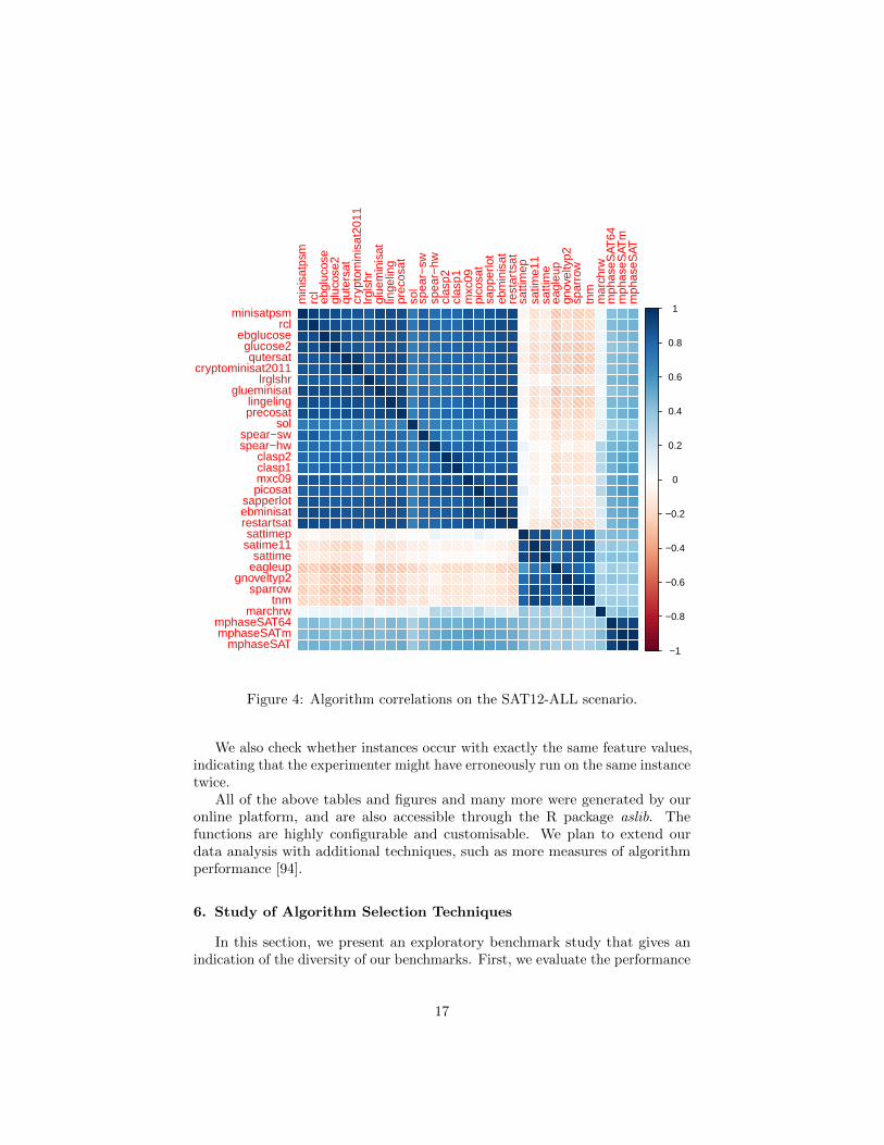
−1
−0.8
−0.6
−0.4
−0.2
0
0.2
0.4
0.6
0.8
1m
inis
atps
mrc
leb
gluc
ose
gluc
ose2
qute
rsat
cryp
tom
inis
at20
11lrg
lshr
glue
min
isat
linge
ling
prec
osat
sol
spea
r−sw
spea
r−hw
clas
p2cl
asp1
mxc
09pi
cosa
tsa
pper
lot
ebm
inis
atre
star
tsat
satti
mep
satim
e11
satti
me
eagl
eup
gnov
elty
p2sp
arro
wtn
mm
arch
rwm
phas
eSAT
64m
phas
eSAT
mm
phas
eSAT
minisatpsmrcl
ebglucoseglucose2qutersat
cryptominisat2011lrglshr
glueminisatlingelingprecosat
solspear−swspear−hw
clasp2clasp1mxc09picosat
sapperlotebminisatrestartsatsattimepsatime11
sattimeeagleup
gnoveltyp2sparrow
tnmmarchrw
mphaseSAT64mphaseSATm
mphaseSAT
Figure 4: Algorithm correlations on the SAT12-ALL scenario.
We also check whether instances occur with exactly the same feature values,indicating that the experimenter might have erroneously run on the same instancetwice.
All of the above tables and figures and many more were generated by ouronline platform, and are also accessible through the R package aslib. Thefunctions are highly configurable and customisable. We plan to extend ourdata analysis with additional techniques, such as more measures of algorithmperformance [94].
6. Study of Algorithm Selection Techniques
In this section, we present an exploratory benchmark study that gives anindication of the diversity of our benchmarks. First, we evaluate the performance
17
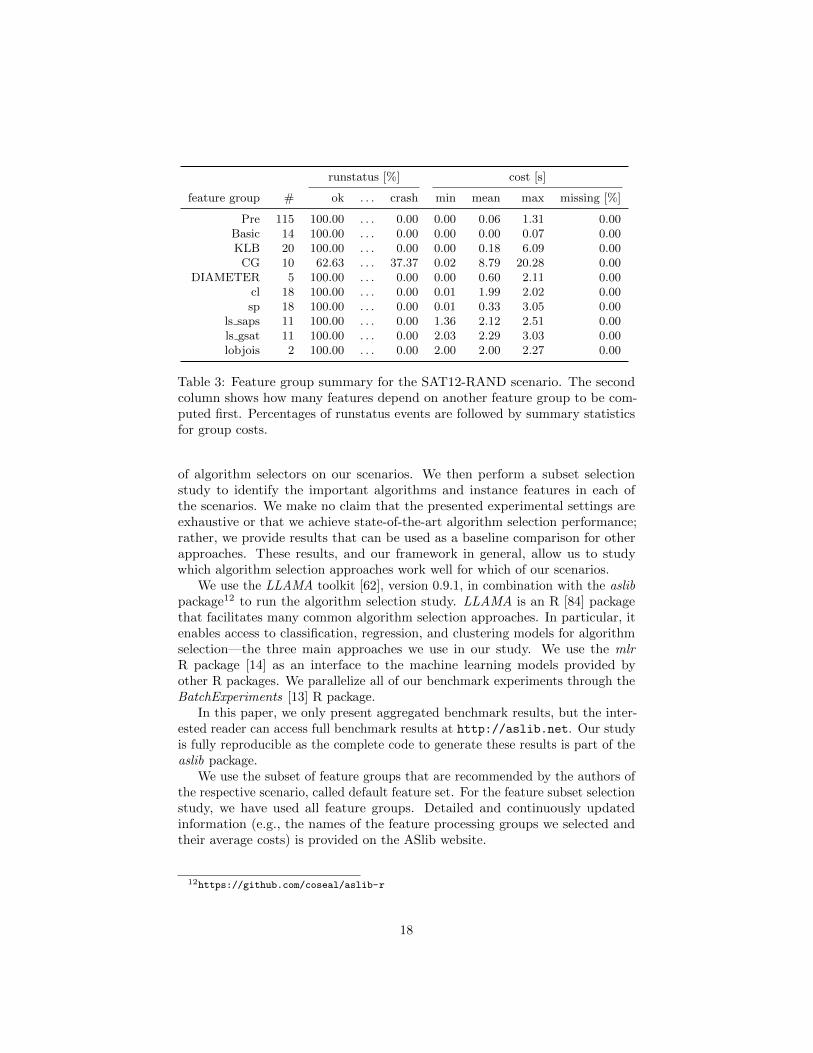
runstatus [%] cost [s]
feature group # ok . . . crash min mean max missing [%]
Pre 115 100.00 . . . 0.00 0.00 0.06 1.31 0.00Basic 14 100.00 . . . 0.00 0.00 0.00 0.07 0.00KLB 20 100.00 . . . 0.00 0.00 0.18 6.09 0.00
CG 10 62.63 . . . 37.37 0.02 8.79 20.28 0.00DIAMETER 5 100.00 . . . 0.00 0.00 0.60 2.11 0.00
cl 18 100.00 . . . 0.00 0.01 1.99 2.02 0.00sp 18 100.00 . . . 0.00 0.01 0.33 3.05 0.00
ls saps 11 100.00 . . . 0.00 1.36 2.12 2.51 0.00ls gsat 11 100.00 . . . 0.00 2.03 2.29 3.03 0.00lobjois 2 100.00 . . . 0.00 2.00 2.00 2.27 0.00
Table 3: Feature group summary for the SAT12-RAND scenario. The secondcolumn shows how many features depend on another feature group to be com-puted first. Percentages of runstatus events are followed by summary statisticsfor group costs.
of algorithm selectors on our scenarios. We then perform a subset selectionstudy to identify the important algorithms and instance features in each ofthe scenarios. We make no claim that the presented experimental settings areexhaustive or that we achieve state-of-the-art algorithm selection performance;rather, we provide results that can be used as a baseline comparison for otherapproaches. These results, and our framework in general, allow us to studywhich algorithm selection approaches work well for which of our scenarios.
We use the LLAMA toolkit [62], version 0.9.1, in combination with the aslibpackage12 to run the algorithm selection study. LLAMA is an R [84] packagethat facilitates many common algorithm selection approaches. In particular, itenables access to classification, regression, and clustering models for algorithmselection—the three main approaches we use in our study. We use the mlrR package [14] as an interface to the machine learning models provided byother R packages. We parallelize all of our benchmark experiments through theBatchExperiments [13] R package.
In this paper, we only present aggregated benchmark results, but the inter-ested reader can access full benchmark results at http://aslib.net. Our studyis fully reproducible as the complete code to generate these results is part of theaslib package.
We use the subset of feature groups that are recommended by the authors ofthe respective scenario, called default feature set. For the feature subset selectionstudy, we have used all feature groups. Detailed and continuously updatedinformation (e.g., the names of the feature processing groups we selected andtheir average costs) is provided on the ASlib website.
12https://github.com/coseal/aslib-r
18
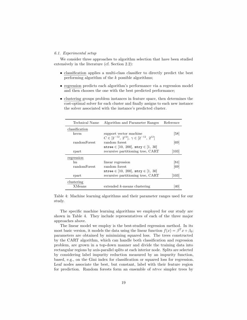
6.1. Experimental setup
We consider three approaches to algorithm selection that have been studiedextensively in the literature (cf. Section 2.2):
• classification applies a multi-class classifier to directly predict the bestperforming algorithm of the k possible algorithms;
• regression predicts each algorithm’s performance via a regression modeland then chooses the one with the best predicted performance;
• clustering groups problem instances in feature space, then determines thecost-optimal solver for each cluster and finally assigns to each new instancethe solver associated with the instance’s predicted cluster.
Technical Name Algorithm and Parameter Ranges Reference
classificationksvm support vector machine [58]
C ∈ [2−12, 212], γ ∈ [2−12, 212]randomForest random forest [69]
ntree ∈ [10, 200], mtry ∈ [1, 30]rpart recursive partitioning tree, CART [103]
regressionlm linear regression [84]randomForest random forest [69]
ntree ∈ [10, 200], mtry ∈ [1, 30]rpart recursive partitioning tree, CART [103]
clusteringXMeans extended k-means clustering [40]
Table 4: Machine learning algorithms and their parameter ranges used for ourstudy.
The specific machine learning algorithms we employed for our study areshown in Table 4. They include representatives of each of the three majorapproaches above.
The linear model we employ is the best-studied regression method. In itsmost basic version, it models the data using the linear function f(x) = βTx+β0;parameters are obtained by minimizing squared loss. The trees constructedby the CART algorithm, which can handle both classification and regressionproblem, are grown in a top-down manner and divide the training data intorectangular regions by axis-parallel splits at each interior node. Splits are selectedby considering label impurity reduction measured by an impurity function,based, e.g., on the Gini index for classification or squared loss for regression.Leaf nodes associate the best, but constant, label with their feature regionfor prediction. Random forests form an ensemble of ntree simpler trees by
19
bootstrapping multiple data sets from the original one and then fitting a treefor each. Predictions are made through majority voting for classification andaveraging for regression. Furthermore, ensemble members are decorrelated byrandomly selecting only a few candidate features for each split point (controlledby parameter mtry) in a tree and maximally growing trees without any earlystopping or pruning. Support Vector Machines perform linear classification in atransformed feature space by maximizing the margin between the positive andnegative examples. Parameter C controls the trade-off between the size of themargin and classification loss. The feature mapping is implicitly built into thealgorithm by substituting the regular inner product of the Euclidean space witha so-called kernel. Parameter γ is a property of the radial basis function kernelused here. The XMeans clustering algorithm is the only unsupervised learningalgorithm we study. It is an extension of the well known k-means methodto adaptively select the number of clusters. k-means starts with k randomcluster centroids, assigns each point to the nearest centroid, and then iterativelyrecomputes the cluster centroids and cluster assignments until convergence. Forfurther details on all methods the reader is referred to the standard literature [41]and for XMeans to [21].
We tuned the hyperparameters of ksvm and randomForest (classificationand regression) within the listed parameter ranges, using random search with250 iterations and a nested cross validation (with three internal folds) to ensureunbiased performance results. All other parameters were left at their defaultvalues. For the clustering algorithm, we set the (maximum) number of clusters to30 after some preliminary experiments; the exact number of clusters is determinedinternally by XMeans.
6.2. Data preprocessing
We preprocessed the data as follows. We removed constant-valued (andtherefore irrelevant) features and imputed missing feature values as the mean overall non-missing values of the feature.13 For the clustering methods, we normalizedthe range of each feature to the interval [−1, 1]. The scenarios we consider in thisarticle contain only continuous features. The other machine learning methodsthat require normalized data perform this internally (for example the SVMs).Missing performance values were imputed using the timeout value of the scenario.
For each problem instance, we calculated the total feature computationcost as the sum of the costs of all feature groups, in the order specified in thedefinition of the scenario. If the problem instance was solved during featurecomputation (e.g., using SLS-probing features [118]), we only considered thecost of the feature groups up to the one that solved it. Furthermore, we set theruntime for all algorithms to zero for instances solved during feature computation.If the instance was not solved during feature computation, we added the featurecosts computed in this way to the runtimes of the individual algorithms on
13For the CSP-MZN-2013 scenario, we also removed the gc circuit feature, which is almostconstant.
20
the respective instances (c(fi) + t(i, a)). Given these new runtimes, we checkedwhether the specified timeout was now exceeded and set the run status of anycorresponding algorithm accordingly. Preprocessing runtimes to include featurecomputation time in this way allows us to focus on an algorithm selectionsystem’s overall performance, and avoids overstating the fraction of instancesthat would be solved within a time budget in cases where features are expensiveto compute.
Each scenario specifies a partition into 10 folds for cross-validation to ensureconsistent evaluation across different methods. We used this partition in ourstudy.
6.3. Evaluation
We evaluated different algorithm selection models using three different measures:
• the fraction of all instances solved within the timeout;
• the penalized average runtime with a penalty factor of 10, i.e., a timeoutcounts as 10 times the timeout;
• the average misclassification penalty, which, for a given instance, is thedifference between the performance of the selected algorithm and theperformance of the best algorithm.
The performance of each algorithm selection model was compared to thevirtual best solver (VBS) and the single best solver. The virtual best solverselects the best solver from A for each instance (∀i ∈ I : arg maxa∈Am(i, a)).Note that the misclassification penalty for VBS is zero by definition. The singlebest solver is the actual solver that has the overall best performance on the dataset (arg maxa∈A
∑i∈Im(i, a)). Specifically, we consider the solver with the best
PAR10 score over all problem instances in a scenario.
6.4. Results
Figure 5 presents a summary of the results of our study. In most cases, thealgorithm selection approaches performed better than the single best solver. Weexpected this, as most of our data sets come from publications that advocatealgorithm selection systems.
Nevertheless, there were significant differences between the scenarios. Whilealmost all algorithm selection approaches outperformed the single best algorithm,there are some scenarios that seem to be much harder for algorithm selection.In particular, on the SAT12-INDU scenario, three approaches were not able toachieve a performance improvement.
Random regression forests stood out quite clearly as the best overall approach,achieving the best performance on 13 of the 17 datasets. This is in line withrecent results showing the strong performance of this model for algorithm runtimeprediction [54]. The results are also consistent with those of the original papersintroducing the datasets.
21
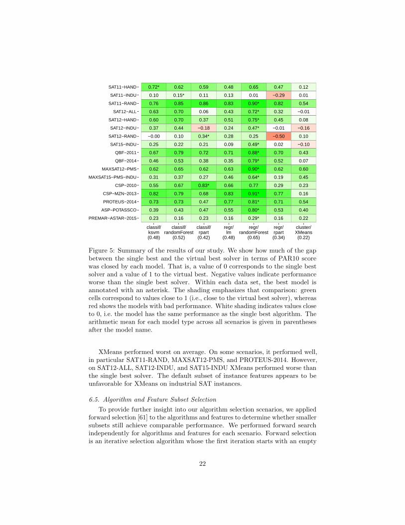
0.590.620.72* 0.48 0.470.65 0.12
0.110.15*0.10 0.13 −0.290.01 0.01
0.860.850.76 0.83 0.820.90* 0.54
0.060.700.63 0.43 0.320.72* −0.01
0.370.700.60 0.51 0.450.75* 0.08
−0.180.440.37 0.24 −0.010.47* −0.16
0.34*0.10−0.00 0.28 −0.500.25 0.10
0.210.220.25 0.09 0.020.49* −0.10
0.720.790.67 0.71 0.700.88* 0.43
0.380.530.46 0.35 0.520.79* 0.07
0.620.650.62 0.63 0.620.90* 0.60
0.270.370.31 0.46 0.190.64* 0.45
0.83*0.670.55 0.66 0.290.77 0.23
0.680.79 0.83 0.770.91* 0.160.82
0.470.730.73 0.77 0.710.81* 0.54
0.470.430.39 0.55 0.530.80* 0.40
0.230.160.23 0.16 0.160.29* 0.22PREMAR−ASTAR−2015
ASP−POTASSCO
PROTEUS−2014
CSP−MZN−2013
CSP−2010
MAXSAT15−PMS−INDU
MAXSAT12−PMS
QBF−2014
QBF−2011
SAT15−INDU
SAT12−RAND
SAT12−INDU
SAT12−HAND
SAT12−ALL
SAT11−RAND
SAT11−INDU
SAT11−HAND
classif/ksvm(0.48)
classif/randomForest
(0.52)
classif/rpart(0.42)
regr/lm
(0.48)
regr/randomForest
(0.65)
regr/rpart(0.34)
cluster/XMeans(0.22)
Figure 5: Summary of the results of our study. We show how much of the gapbetween the single best and the virtual best solver in terms of PAR10 scorewas closed by each model. That is, a value of 0 corresponds to the single bestsolver and a value of 1 to the virtual best. Negative values indicate performanceworse than the single best solver. Within each data set, the best model isannotated with an asterisk. The shading emphasizes that comparison: greencells correspond to values close to 1 (i.e., close to the virtual best solver), whereasred shows the models with bad performance. White shading indicates values closeto 0, i.e. the model has the same performance as the single best algorithm. Thearithmetic mean for each model type across all scenarios is given in parenthesesafter the model name.
XMeans performed worst on average. On some scenarios, it performed well,in particular SAT11-RAND, MAXSAT12-PMS, and PROTEUS-2014. However,on SAT12-ALL, SAT12-INDU, and SAT15-INDU XMeans performed worse thanthe single best solver. The default subset of instance features appears to beunfavorable for XMeans on industrial SAT instances.
6.5. Algorithm and Feature Subset Selection
To provide further insight into our algorithm selection scenarios, we appliedforward selection [61] to the algorithms and features to determine whether smallersubsets still achieve comparable performance. We performed forward searchindependently for algorithms and features for each scenario. Forward selectionis an iterative selection algorithm whose the first iteration starts with an empty
22
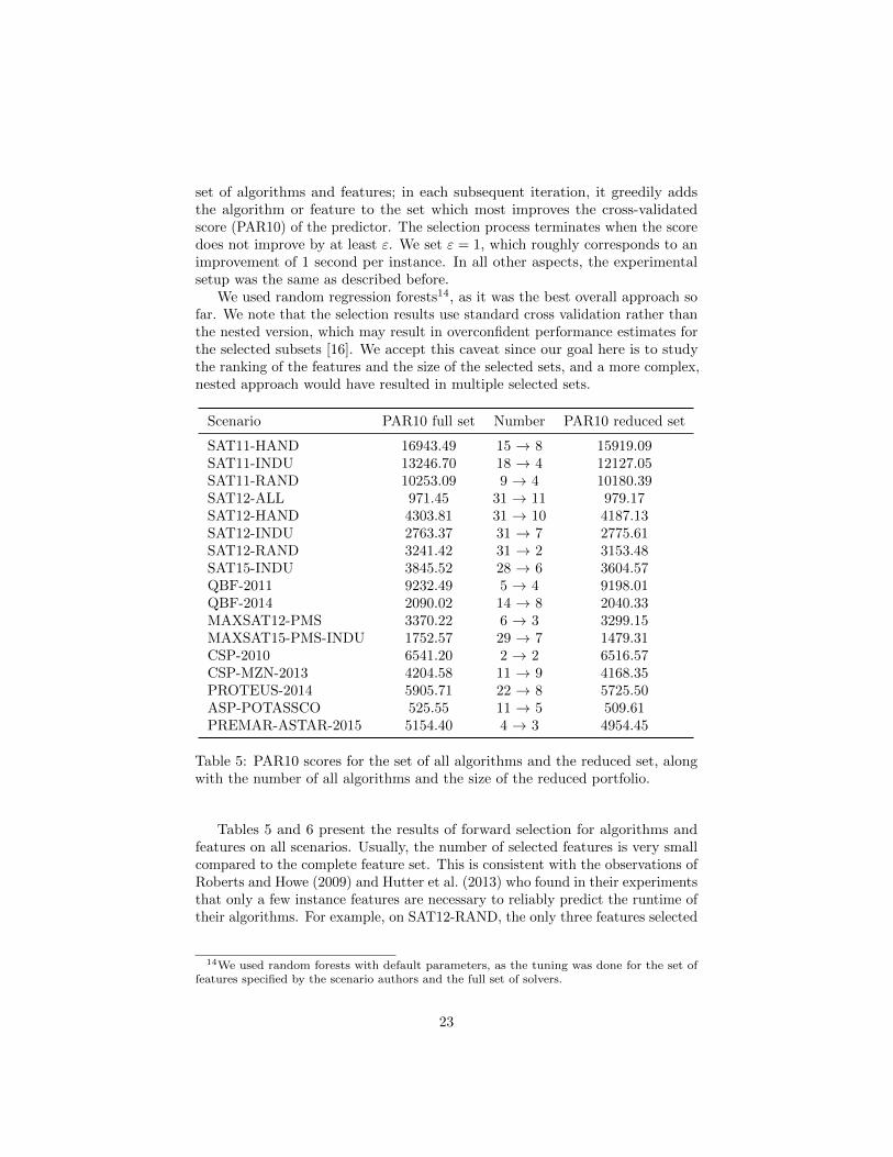
set of algorithms and features; in each subsequent iteration, it greedily addsthe algorithm or feature to the set which most improves the cross-validatedscore (PAR10) of the predictor. The selection process terminates when the scoredoes not improve by at least ε. We set ε = 1, which roughly corresponds to animprovement of 1 second per instance. In all other aspects, the experimentalsetup was the same as described before.
We used random regression forests14, as it was the best overall approach sofar. We note that the selection results use standard cross validation rather thanthe nested version, which may result in overconfident performance estimates forthe selected subsets [16]. We accept this caveat since our goal here is to studythe ranking of the features and the size of the selected sets, and a more complex,nested approach would have resulted in multiple selected sets.
Scenario PAR10 full set Number PAR10 reduced set
SAT11-HAND 16943.49 15 → 8 15919.09SAT11-INDU 13246.70 18 → 4 12127.05SAT11-RAND 10253.09 9 → 4 10180.39SAT12-ALL 971.45 31 → 11 979.17SAT12-HAND 4303.81 31 → 10 4187.13SAT12-INDU 2763.37 31 → 7 2775.61SAT12-RAND 3241.42 31 → 2 3153.48SAT15-INDU 3845.52 28 → 6 3604.57QBF-2011 9232.49 5 → 4 9198.01QBF-2014 2090.02 14 → 8 2040.33MAXSAT12-PMS 3370.22 6 → 3 3299.15MAXSAT15-PMS-INDU 1752.57 29 → 7 1479.31CSP-2010 6541.20 2 → 2 6516.57CSP-MZN-2013 4204.58 11 → 9 4168.35PROTEUS-2014 5905.71 22 → 8 5725.50ASP-POTASSCO 525.55 11 → 5 509.61PREMAR-ASTAR-2015 5154.40 4 → 3 4954.45
Table 5: PAR10 scores for the set of all algorithms and the reduced set, alongwith the number of all algorithms and the size of the reduced portfolio.
Tables 5 and 6 present the results of forward selection for algorithms andfeatures on all scenarios. Usually, the number of selected features is very smallcompared to the complete feature set. This is consistent with the observations ofRoberts and Howe (2009) and Hutter et al. (2013) who found in their experimentsthat only a few instance features are necessary to reliably predict the runtime oftheir algorithms. For example, on SAT12-RAND, the only three features selected
14We used random forests with default parameters, as the tuning was done for the set offeatures specified by the scenario authors and the full set of solvers.
23
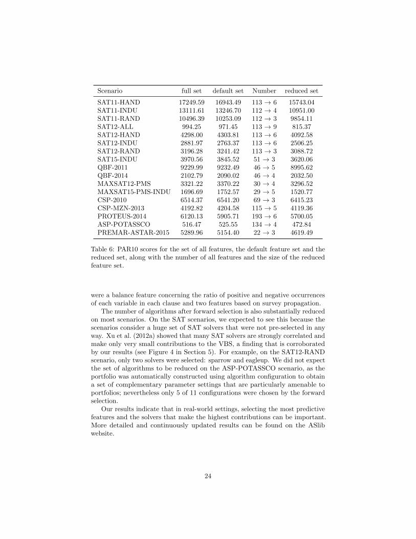
Scenario full set default set Number reduced set
SAT11-HAND 17249.59 16943.49 113 → 6 15743.04SAT11-INDU 13111.61 13246.70 112 → 4 10951.00SAT11-RAND 10496.39 10253.09 112 → 3 9854.11SAT12-ALL 994.25 971.45 113 → 9 815.37SAT12-HAND 4298.00 4303.81 113 → 6 4092.58SAT12-INDU 2881.97 2763.37 113 → 6 2506.25SAT12-RAND 3196.28 3241.42 113 → 3 3088.72SAT15-INDU 3970.56 3845.52 51 → 3 3620.06QBF-2011 9229.99 9232.49 46 → 5 8995.62QBF-2014 2102.79 2090.02 46 → 4 2032.50MAXSAT12-PMS 3321.22 3370.22 30 → 4 3296.52MAXSAT15-PMS-INDU 1696.69 1752.57 29 → 5 1520.77CSP-2010 6514.37 6541.20 69 → 3 6415.23CSP-MZN-2013 4192.82 4204.58 115 → 5 4119.36PROTEUS-2014 6120.13 5905.71 193 → 6 5700.05ASP-POTASSCO 516.47 525.55 134 → 4 472.84PREMAR-ASTAR-2015 5289.96 5154.40 22 → 3 4619.49
Table 6: PAR10 scores for the set of all features, the default feature set and thereduced set, along with the number of all features and the size of the reducedfeature set.
were a balance feature concerning the ratio of positive and negative occurrencesof each variable in each clause and two features based on survey propagation.
The number of algorithms after forward selection is also substantially reducedon most scenarios. On the SAT scenarios, we expected to see this because thescenarios consider a huge set of SAT solvers that were not pre-selected in anyway. Xu et al. (2012a) showed that many SAT solvers are strongly correlated andmake only very small contributions to the VBS, a finding that is corroboratedby our results (see Figure 4 in Section 5). For example, on the SAT12-RANDscenario, only two solvers were selected: sparrow and eagleup. We did not expectthe set of algorithms to be reduced on the ASP-POTASSCO scenario, as theportfolio was automatically constructed using algorithm configuration to obtaina set of complementary parameter settings that are particularly amenable toportfolios; nevertheless only 5 of 11 configurations were chosen by the forwardselection.
Our results indicate that in real-world settings, selecting the most predictivefeatures and the solvers that make the highest contributions can be important.More detailed and continuously updated results can be found on the ASlibwebsite.
24
7. Competitions on ASlib
As described before and illustrated in Section 6, we designed ASlib to enableeasy and fair comparison of different algorithm selection approaches. Thenext step to get unbiased performance comparisons of algorithm selectors is toorganize competitions based on ASlib. In this section, we will briefly describetwo exemplary competition settings based on ASlib.
On-going Evaluation on ASlib. In the on-going evaluation on ASlib15, everyparticipant can simply submit his/her performance for each scenario (using theprovided cross validation splits) and the source code of their algorithm selector.The latter will only be used to verify the results in case of doubt. The results(i.e., (penalized) average performance on each scenario) will be added in anoverview table and the system will be linked.
In this setting, every system that can read the ASlib format can easilyparticipate and no deadlines for submission are required. Therefore, the newestsystems and results can always be added on-the-fly such that the on-goingevaluation always reflects the most recent known state-of-the-art systems andtheir performances. Disadvantages of this setting are:
1. the different participants use different amounts of computational resourcesto compute the results – for example, two well-performing systems in theon-going evaluation are SATzilla [118] and AutoFolio [70] but it is alsowell-known that these two systems use a lot more computation resources(several CPU days) than other systems;
2. since the test and training data are published, the system will tend tooverfit the scenarios if we will not regularly provide new scenarios to revealsuch overfitting.
ICON Challenge on Algorithm Selection. The ICON Challenge on AlgorithmSelection16 provided a comparative evaluation of state-of-the-art algorithmselection systems. The winner of the challenge was the zilla system [121]. Inthis competition, the algorithm selectors needed to be submitted before a fixeddeadline and each system was executed on the organizers’ hardware with somelimitations (e.g., at most 12 CPU hours for training on one scenario). Althoughthe used scenarios were also already published before (i.e., ASlib version 1.0.1),the organizers did not reveal the training-test splits to avoid overly strongoverfitting on these scenarios. Furthermore, the ICON challenge assessed theperformance of the algorithm selectors based on 3 different performance metrics(i.e., average number of solved instances, PAR10, and misclassification penalty(MCP)) which revealed some strengths and weaknesses of algorithm selectors,e.g., systems that used an algorithm schedule had better performance on solvedinstances and PAR10, but wasted some time with respect to MCP.
15The most recent results of the on-going evaluation can be found on the ASlib homepageaslib.net.
16http://challenge.icon-fet.eu/
25
8. Summary
We have introduced ASlib, a benchmark library for algorithm selection,a rapidly growing field of research with substantial impact on various sub-communities in artificial intelligence. ASlib facilitates research on algorithmselection methods by providing a common set of benchmarks and tools for workingwith these. Similar to solver competitions, it enables principled comparativeempirical performance assessment. It also considerably lowers the otherwiserather high barrier for researchers to work on algorithm selection, since anyoneusing the benchmark scenarios we provide does not have to perform actualruns of the solvers contained in them. Since our library provides performancedata for the solvers and problem instances included in each selection scenario,using ASlib also substantially reduces the computational burden of performanceassessments. Otherwise, these data would have to be produced, at considerablecomputational cost, by anyone working with that scenario. We carefully selectedthe set of scenarios included in release version 2.0 of ASlib to challenge algorithmselection methods in various ways and thus provide a solid basis for developingand assessing such methods.
Release version 2.0 of the library contains 17 algorithm selection scenarios fromsix different areas with a focus on (but not a limitation to) constraint satisfactionproblems. We discussed the format of new algorithm selection scenarios andshowed examples of the automated exploratory data analysis that will run foreach new scenario submitted to our online platform http://aslib.net/. Finally,exploratory studies with various algorithm selection approaches demonstratedthe performance that algorithm selection systems can achieve on our scenarios.
Acknowledgements
We thank the creators of the algorithms and instance distributions usedin our various algorithm selection scenarios. The performance of algorithmselection systems depends critically upon the ingenuity and tireless efforts ofdomain experts who continue to invent novel solver strategies.
FH and ML are supported by the DFG (German Research Foundation) underEmmy Noether grant HU 1900/2-1. KLB, AF and LK were supported by anNSERC E.W.R. Steacie Fellowship; in addition, all of these, along with HH, weresupported under the NSERC Discovery Grant Program. Part of this researchwas supported by an Azure for Research grant.
References
[1] Amadini, R., Gabbrielli, M., Mauro, J., 2014a. An enhanced featuresextractor for a portfolio of constraint solvers, in: Symposium on AppliedComputing, SAC 2014, Gyeongju, Republic of Korea - March 24 - 28, 2014,pp. 1357–1359.
[2] Amadini, R., Gabbrielli, M., Mauro, J., 2014b. SUNNY: a lazy portfolioapproach for constraint solving. TPLP 14, 509–524.
26
[3] Ansotegui, C., Malitsky, Y., Sellmann, M., 2014. MaxSAT by ImprovedInstance-Specific Algorithm Configuration, in: Proceedings of the Twenty-Eighth National Conference on Artificial Intelligence, pp. 2594–260.
[4] Ansotegui, C., Sellmann, M., Tierney, K., 2009. A gender-based geneticalgorithm for the automatic configuration of algorithms, in: Proceedingsof the Fifteenth International Conference on Principles and Practice ofConstraint Programming (CP’09), pp. 142–157.
[5] Arbelaez, A., Hamadi, Y., Sebag, M., 2010. Continuous search in constraintprogramming, in: Proceedings of the Twenty-Second IEEE InternationalConference on Tools with Artificial Intelligence, pp. 53–60.
[6] Argelich, J., Berre, D.L., Lynce, I., Marques-Silva, J., Rapicault, P.,2010. Solving linux upgradeability problems using boolean optimization,in: Proceedings of the International Workshop on Logics for ComponentConfiguration, pp. 11–22.
[7] Argelich, J., Li, C., Manya, F., Planes, J., 2012. Seventh MaxSAT Evalua-tion. http://www.maxsat.udl.cat/12/.
[8] Baral, C., 2003. Knowledge Representation, Reasoning and DeclarativeProblem Solving. Cambridge University Press.
[9] Biere, A., 2014. Yet another local search solver and Lingeling and friendsentering the SAT competition 2014, in: Proceedings of SAT Competition2014: Solver and Benchmark Descriptions, pp. 39–40.
[10] Biere, A., Heule, M., van Maaren, H., Walsh, T. (Eds.), 2009. Handbookof Satisfiability. volume 185 of Frontiers in Artificial Intelligence andApplications. IOS Press.
[11] Birattari, M., Yuan, Z., Balaprakash, P., Stutzle, T., 2010. in: EmpiricalMethods for the Analysis of Optimization Algorithms. Springer. chapterF-race and iterated F-race: An overview.
[12] Bischl, B., Kotthoff, L., Lindauer, M., Malitsky, Y., Frechette, A., Hoos,H., Hutter, F., Kerschke, P., Leyton-Brown, K., Vanschoren, J., 2014.Algorithm Selection Format Specification. Technical Report. Available athttp://www.aslib.net/.
[13] Bischl, B., Lang, M., Mersmann, O., Rahnenfuhrer, J., Weihs, C., 2015a.BatchJobs and BatchExperiments: Abstraction mechanisms for using R inbatch environments. Journal of Statistical Software 64, 1–25.
[14] Bischl, B., Lang, M., Richter, J., Bossek, J., Judt, L., Kuehn, T., Studerus,E., Kotthoff, L., Jones, Z., 2015b. mlr: Machine Learning in R. R packageversion 2.7. https://github.com/mlr-org/mlr.
27
[15] Bischl, B., Mersmann, O., Trautmann, H., Preuss, M., 2012a. Algorithmselection based on exploratory landscape analysis and cost-sensitive learn-ing, in: Proceedings of the Fourteenth Annual Conference on Genetic andEvolutionary Computation, pp. 313–320.
[16] Bischl, B., Mersmann, O., Trautmann, H., Weihs, C., 2012b. Resamplingmethods for meta-model validation with recommendations for evolutionarycomputation. Evolutionary Computation 20, 249–275.
[17] Brazdil, P., Giraud-Carrier, C., Soares, C., Vilalta, R., 2008. Metalearning:Applications to Data Mining. 1st ed., Springer.
[18] Cicirello, V.A., Smith, S.F., 2005. The max k-armed bandit: A new modelof exploration applied to search heuristic selection, in: Proceedings of theTwentieth National Conference on Artificial Intelligence, AAAI Press. pp.1355–1361.
[19] Cook, D.J., Varnell, R.C., 1997. Maximizing the benefits of parallelsearch using machine learning, in: Proceedings of the Fourteenth NationalConference on Artificial Intelligence, AAAI Press. pp. 559–564.
[20] Crawford, J.M., Baker, A.B., 1994. Experimental results on the applicationof satisfiability algorithms to scheduling problems, in: In Proceedings ofthe Twelfth National Conference on Artificial Intelligence, pp. 1092–1097.
[21] Dan Pelleg, A.M., 2000. X-means: Extending k-means with efficientestimation of the number of clusters, in: Proceedings of the SeventeenthInternational Conference on Machine Learning, Morgan Kaufmann, SanFrancisco. pp. 727–734.
[22] Demmel, J., Dongarra, J., Eijkhout, V., Fuentes, E., Petitet, A., Vuduc,R., Whaley, R.C., Yelick, K., 2005. Self-Adapting linear algebra algorithmsand software. Proceedings of the IEEE 93, 293–312.
[23] Domhan, T., Springenberg, J.T., Hutter, F., 2015. Speeding up automatichyperparameter optimization of deep neural networks by extrapolation oflearning curves, in: Proceedings of the 24th International Joint Conferenceon Artificial Intelligence (IJCAI).
[24] Eggensperger, K., Hutter, F., Hoos, H.H., Leyton-Brown, K., 2015. Efficientbenchmarking of hyperparameter optimizers via surrogates, in: Proceedingsof the Twenty-Ninth AAAI Conference on Artificial Intelligence.
[25] Fawcett, C., Vallati, M., Hutter, F., Hoffmann, J., Hoos, H., Leyton-Brown,K., 2014. Improved features for runtime prediction of domain-independentplanners, in: Proceedings of the International Conference on AutomatedPlanning and Scheduling.
28
[26] Feurer, M., Klein, A., Eggensperger, K., Springenberg, J., Blum, M.,Hutter, F., 2015a. Efficient and robust automated machine leraning, in:Advances in Neural Information Processing Systems 28, pp. 2944–2952.
[27] Feurer, M., Springenberg, J.T., Hutter, F., 2015b. Initializing Bayesianhyperparameter optimization via meta-learning, in: Bonet, B., Koenig, S.(Eds.), Proceedings of the Twenty-Ninth AAAI Conference on ArtificialIntelligence, January 25-30, 2015, Austin, Texas, USA., AAAI Press. pp.1128–1135.
[28] Gagliolo, M., Schmidhuber, J., 2007. Learning restart strategies, in:Proceedings of the Twentieth International Joint Conference on ArtificialIntelligence (IJCAI), pp. 792–797.
[29] Gagliolo, M., Zhumatiy, V., Schmidhuber, J., 2004. Adaptive online timeallocation to search algorithms, in: Proceedings of European Conferenceon Machine Learning, Springer. pp. 134–143.
[30] Gebser, M., Kaminski, R., Kaufmann, B., Schaub, T., 2012a. AnswerSet Solving in Practice. Synthesis Lectures on Artificial Intelligence andMachine Learning, Morgan and Claypool Publishers.
[31] Gebser, M., Kaminski, R., Kaufmann, B., Schaub, T., Schneider, M.T.,Ziller, S., 2011. A portfolio solver for answer set programming: preliminaryreport, in: Eleventh International Conference on Logic Programming andNonmonotonic Reasoning, Springer. pp. 352–357.
[32] Gebser, M., Kaufmann, B., Schaub, T., 2012b. Multi-threaded ASP solvingwith clasp. Theory and Practice of Logic Programming 12, 525–545.
[33] Gent, I., Jefferson, C., Kotthoff, L., Miguel, I., Moore, N., Nightingale, P.,Petrie, K., 2010a. Learning when to use lazy learning in constraint solving,in: Proceedings of the Nineteenth European Conference on ArtificialIntelligence, IOS Press. pp. 873–878.
[34] Gent, I.P., Jefferson, C.A., Miguel, I., 2006. MINION: A fast, scalable,constraint solver, in: Proceedings of the European Conference on ArtificialIntelligence, pp. 98–102.
[35] Gent, I.P., Miguel, I., Moore, N.C.A., 2010b. Lazy explanations forconstraint propagators, in: Proceedings of the Twelfth International Sym-posium on Practical Aspects of Declarative Languages, pp. 217–233.
[36] Gomes, C., Selman, B., Crato, N., Kautz, H., 2000. Heavy-tailed phe-nomena in satisfiability and constraint satisfaction problems. Journal ofAutomated Reasoning 24, 67–100.
[37] Gomes, C.P., Selman, B., 2001. Algorithm portfolios. Artificial Intelligence126, 43–62.
29
[38] Grasso, G., Iiritano, S., Leone, N., Lio, V., Ricca, F., Scalise, F., 2010.An ASP-based system for team-building in the Gioia-Tauro seaport, in:Proceedings of the Twelfth International Symposium on Practical Aspectsof Declarative Languages, pp. 40–42.
[39] Guerri, A., Milano, M., 2004. Learning techniques for automatic algorithmportfolio selection, in: Proceedings of the Sixteenth Eureopean Conferenceon Artificial Intelligence, IOS Press. pp. 475–479.
[40] Hall, M., Frank, E., Holmes, G., Pfahringer, B., Reutemann, P., Witten,I.H., 2009. The WEKA data mining software: An update. SIGKDDExplorations 11, 10–18.
[41] Hastie, T.J., Tibshirani, R.J., Friedman, J.H., 2009. The elements ofstatistical learning : data mining, inference, and prediction. Springer seriesin statistics, Springer, New York.
[42] Helmert, M., Roger, G., Karpas, E., 2011. Fast downward stone soup: Abaseline for building planner portfolios, in: Proceedings of the Workshopon Planning and Learning at the Twenty-First International Conferenceon Automated Planning and Scheduling, pp. 28–35.
[43] Hoos, H., Lindauer, M., Schaub, T., 2014a. claspfolio 2: Advances inalgorithm selection for answer set programming. Theory and Practice ofLogic Programming , 569–585.
[44] Hoos, H.H., Kaminski, R., Lindauer, M., Schaub, T., 2014b. aspeed: Solverscheduling via answer set programming. Theory and Practice of LogicProgramming , 1–26.
[45] Howe, A.E., Dahlman, E., Hansen, C., Scheetz, M., von Mayrhauser, A.,1999. Exploiting competitive planner performance, in: Proceedings of theFifth European Conference on Planning, Springer. pp. 62–72.
[46] Hurley, B., Kotthoff, L., Malitsky, Y., O’Sullivan, B., 2014. Proteus: Ahierarchical portfolio of solvers and transformations, in: Proceedings of theEleventh International Conference on Integration of AI and OR Techniquesin Constraint Programming for Combinatorial Optimization Problems, pp.301–317.
[47] Hutter, F., Babic, D., Hoos, H.H., Hu, A.J., 2007. Boosting Verificationby Automatic Tuning of Decision Procedures, in: Formal Methods inComputer Aided Design, IEEE Computer Society. pp. 27–34.
[48] Hutter, F., Hamadi, Y., Hoos, H.H., Leyton-Brown, K., 2006. Performanceprediction and automated tuning of randomized and parametric algorithms,in: Proceedings of the Twelfth International Conference on Principles andPractice of Constraint Programming, pp. 213–228.
30
[49] Hutter, F., Hoos, H.H., Leyton-Brown, K., 2010. Automated configurationof mixed integer programming solvers, in: Integration of AI and ORTechniques in Constraint Programming for Combinatorial OptimizationProblems, pp. 186–202.
[50] Hutter, F., Hoos, H.H., Leyton-Brown, K., 2011. Sequential model-basedoptimization for general algorithm configuration, in: Proceedings of theInternational Conference on Learning and Intelligent Optimization, pp.507–523.
[51] Hutter, F., Hoos, H.H., Leyton-Brown, K., 2013. Identifying key algorithmparameters and instance features using forward selection, in: LION 7.
[52] Hutter, F., Hoos, H.H., Leyton-Brown, K., Stutzle, T., 2009. ParamILS:an automatic algorithm configuration framework. Journal of ArtificialIntelligence Research (JAIR) 36, 267–306.
[53] Hutter, F., Lopez-Ibanez, M., Fawcett, C., Lindauer, M., Hoos, H., Leyton-Brown, K., Stutzle, T., 2014a. Aclib: a benchmark library for algorithmconfiguration, in: Proceedings of the International Conference on Learningand Intelligent Optimization, pp. 36–40.
[54] Hutter, F., Xu, L., Hoos, H.H., Leyton-Brown, K., 2014b. Algorithmruntime prediction: Methods & evaluation. Artificial Intelligence 206,79–111.
[55] Ishebabi, H., Mahr, P., Bobda, C., Gebser, M., Schaub, T., 2009. Answerset vs. integer linear programming for automatic synthesis of multiproces-sor systems from real-time parallel programs. Journal of ReconfigurableComputing .
[56] Kadioglu, S., Malitsky, Y., Sabharwal, A., Samulowitz, H., Sellmann, M.,2011. Algorithm selection and scheduling, in: Proceedings of the Interna-tional Conference on Principles and Practice of Constraint Programming.Springer. volume 6876 of Lecture Notes in Computer Science, pp. 454–469.
[57] Kadioglu, S., Malitsky, Y., Sellmann, M., Tierney, K., 2010. ISAC Instance-Specific Algorithm Configuration, in: Proceedings of Nineteenth EuropeanConference on Artificial Intelligence, IOS Press. pp. 751–756.
[58] Karatzoglou, A., Smola, A., Hornik, K., Zeileis, A., 2004. kernlab – an S4package for kernel methods in R. Journal of Statistical Software 11, 1–20.
[59] Kautz, H., Selman, B., 1999. Unifying SAT-based and graph-based plan-ning, in: Proceedings of the Sixteenth International Joint Conference onArtifical Intelligence, Morgan Kaufmann. pp. 318–325.
[60] Kerschke, P., Preuss, M., Hernandez, C., Schutze, O., Sun, J.Q., Grimme,C., Rudolph, G., Bischl, B., Trautmann, H., 2014. Cell mapping techniquesfor exploratory landscape analysis, in: Proceedings of the EVOLVE 2014:
31
A Bridge between Probability, Set Oriented Numerics, and EvolutionaryComputation, Springer. pp. 115–131.
[61] Kohavi, R., John, G.H., 1997. Wrappers for feature subset selection.Artificial Intelligence 97, 273–324.
[62] Kotthoff, L., 2013. LLAMA: Leveraging Learning to Automatically ManageAlgorithms. Technical Report arXiv:1306.1031. arXiv. http://arxiv.org/abs/1306.1031.
[63] Kotthoff, L., 2014. Algorithm selection for combinatorial search problems:A survey. AI Magazine 35, 48–60.
[64] Lagoudakis, M., Littman, M., 2000. Algorithm selection using reinforce-ment learning, in: Proceedings of the Seventeenth International Conferenceon Machine Learning, pp. 511–518.
[65] Lagoudakis, M., Littman, M., 2001. Learning to select branching rules inthe DPLL procedure for satisfiability, in: Proceedings of the InternationalConference on Satisfiability, pp. 344–359.
[66] Le Berre, D., Lynce, I., 2008. CSP2SAT4J: A simple CSP to SAT translator,in: Proceedings of the Second International CSP Solver Competition, pp.43–54.
[67] Leite, R., Brazdil, P., Vanschoren, J., 2012. Selecting classification al-gorithms with active testing, in: Machine Learning and Data Mining inPattern Recognition, Springer. pp. 117–131.
[68] Leyton-Brown, K., Nudelman, E., Andrew, G., McFadden, J., Shoham,Y., 2003. A portfolio approach to algorithm selection, in: Proceedings ofthe Eighteenth International Joint Conference on Artificial Intelligence,Morgan Kaufmann. pp. 1542–1543.
[69] Liaw, A., Wiener, M., 2002. Classification and regression by randomForest.R News 2, 18–22.
[70] Lindauer, M., Hoos, H., Hutter, F., Schaub, T., 2015. Autofolio: An auto-matically configured algorithm selector. Journal of Artificial Intelligence53, 745–778.
[71] Malitsky, Y., Mehta, D., O’Sullivan, B., 2013. Evolving instance specific al-gorithm configuration, in: The Sixth Annual Symposium on CombinatorialSearch.
[72] Malitsky, Y., O’Sullivan, B., Previti, A., Marques-Silva, J., 2014. A port-folio approach to enumerating minimal correction subsets for satisfiabilityproblems, in: Proceedings of the Eleventh International Conference onIntegration of Artificical Intelligence and Operations Research Techniquesin Constraint Programming.
32
[73] Malitsky, Y., Sabharwal, A., Samulowitz, H., Sellmann, M., 2011. Non-model-based algorithm portfolios for SAT, in: Proceedings of the Four-teenth International Conference on Theory and Applications of SatisfiabilityTesting, Springer. pp. 369–370.
[74] Mersmann, O., Bischl, B., Trautmann, H., Wagner, M., Bossek, J., Neu-mann, F., 2013. A novel feature-based approach to characterize algorithmperformance for the traveling salesperson problem. Annals of Mathematicsand Artificial Intelligence , 1–32.
[75] Nikolic, M., Maric, F., Janicic, P., 2009. Instance-based selection of policiesfor SAT solvers, in: Proceedings of the Twelfth International Conferenceon Theory and Applications of Satisfiability Testing, Springer. pp. 326–340.
[76] Nogueira, M., Balduccini, M., Gelfond, M., Watson, R., Barry, M., 2001.An A-prolog decision support system for the space shuttle, in: Proceedingsof the Third International Symposium on Practical Aspects of DeclarativeLanguages, Springer. pp. 169–183.
[77] Nudelman, E., Leyton-Brown, K., Andrew, G., Gomes, C., McFadden, J.,Selman, B., Shoham, Y., 2003. Satzilla 0.9.
[78] Nudelman, E., Leyton-Brown, K., Hoos, H.H., Devkar, A., Shoham, Y.,2004. Understanding random SAT: beyond the Clauses-to-Variables ratio,in: Principles and Practice of Constraint Programming CP 2004, Springer.pp. 438–452.
[79] O’Mahony, E., Hebrard, E., Holland, A., Nugent, C., O’Sullivan, B., 2008.Using case-based reasoning in an algorithm portfolio for constraint solving,in: Proceedings of the Nineteenth Irish Conference on Artificial Intelligenceand Cognitive Science.
[80] Pfahringer, B., Bensusan, H., Giraud-Carrier, C., 2000. Meta-learning bylandmarking various learning algorithms. Proceedings of the SeventeenthInternational Conference on Machine Learning , 743–750.
[81] Prasad, M.R., Biere, A., Gupta, A., 2005. A survey of recent advances inSAT-based formal verification. International Journal on Software Toolsfor Technology Transfer 7, 156–173.
[82] Pulina, L., Tacchella, A., 2007. A multi-engine solver for quantified booleanformulas, in: Proceedings of the Thirteenth International Conference onPrinciples and Practice of Constraint Programming, Springer. pp. 574–589.
[83] Pulina, L., Tacchella, A., 2009. A self-adaptive multi-engine solver forquantified boolean formulas. Constraints 14, 80–116.
[84] R Core Team, 2014. R: A Language and Environment for StatisticalComputing. R Foundation for Statistical Computing. Vienna, Austria.URL: http://www.R-project.org/.
33
[85] Rice, J.R., 1976. The algorithm selection problem. Advances in Computers15, 65–118.
[86] Roberts, M., Howe, A., 2009. Learning from planner performance. ArtificialIntelligence Journal 173, 536–561.
[87] Roberts, M., Howe, A.E., 2007. Learned models of performance for manyplanners, in: Proceedings of the Workshop on AI Planning and Learningat the Seventeenth International Conference on Automated Planning andScheduling.
[88] Roberts, M., Howe, A.E., Wilson, B., desJardins, M., 2008. What makesplanners predictable?, in: ICAPS, pp. 288–295.
[89] Sabharwal, A., Samulowitz, H., Sellmann, M., Malitsky, Y., 2013. Boostingsequential solver portfolios: Knowledge sharing and accuracy prediction,in: LION 7.
[90] Samulowitz, H., Memisevic, R., 2007. Learning to solve QBF, in: Proceed-ings of the Twenty-Second National Conference on Artificial Intelligence,AAAI Press. pp. 255–260.
[91] Serban, F., Vanschoren, J., Kietz, J.U., Bernstein, A., 2013. A survey ofintelligent assistants for data analysis. ACM Comput. Surv. 45, 1–35.
[92] Silverthorn, B., Miikkulainen, R., 2010. Latent class models for algorithmportfolio methods., in: Proceedings of the Twenty-Fourth AAAI Conferenceon Artificial Intelligence, pp. 167–172.
[93] Smith-Miles, K.A., 2008. Cross-disciplinary perspectives on meta-learningfor algorithm selection. ACM Computing Surveys 41, 6:1–6:25.
[94] Smith-Miles, K.A., Baatar, D., Wreford, B.J., Lewis, R., 2014. Towardsobjective measures of algorithm performance across instance space. Com-puters & Operations Research 45, 12–24.
[95] Soininen, T., Niemela, I., 1999. Developing a declarative rule languagefor applications in product configuration, in: Proceedings of the FirstInternational Workshop on Practical Aspects of Declarative Languages,Springer. pp. 305–319.
[96] Stahlbock, R., Voß, S., 2008. Operations research at container terminals:a literature update. OR Spectrum 30, 1–52.
[97] Stergiou, K., 2009. Heuristics for dynamically adapting propagation inconstraint satisfaction problems. AI Communications 22, 125–141.
[98] Streeter, M.J., Golovin, D., Smith, S.F., 2007a. Combining multiple heuris-tics online, in: Proceedings of the Twenty-Second National Conference onArtificial Intelligence, AAAI Press. pp. 1197–1203.
34
[99] Streeter, M.J., Golovin, D., Smith, S.F., 2007b. Restart schedules forensembles of problem instances, in: Proceedings of the Twenty-SecondNational Conference on Artificial Intelligence, AAAI Press. pp. 1204–1210.
[100] Stuckey, P.J., Feydy, T., Schutt, A., Tack, G., Fischer, J., 2014. TheMiniZinc challenge 2008-2013. AI Magazine 35, 55–60.
[101] Tamura, N., Tanjo, T., Banbara, M., 2008. System description of a SAT-based CSP solver sugar, in: Proceedings of the Third International CSPSolver Competition, pp. 71–75.
[102] Tanjo, T., Tamura, N., Banbara, M., 2012. Azucar: a SAT-based CSPsolver using compact order encoding, in: Theory and Applications ofSatisfiability Testing – SAT 2012. Springer, pp. 456–462.
[103] Therneau, T., Atkinson, B., Ripley, B., 2014. rpart: Recursive Partition-ing and Regression Trees. URL: http://CRAN.R-project.org/package=rpart. r package version 4.1-8.
[104] Thornton, C., Hutter, F., Hoos, H., Leyton-Brown, K., 2013. Auto-WEKA:Combined selection and hyperparameter optimization of classificationalgorithms, in: Proceedings of the Nineteenth ACM SIGKDD InternationalConference on Knowledge Discovery and Data Mining, ACM. pp. 847–855.
[105] Tierney, K., Malitsky, Y., 2015. An algorithm selection benchmark ofthe container pre-marshalling problem, in: Dhaenens, C., Jourdan, L.,Marmion, M.E. (Eds.), Learning and Intelligent Optimization, SpringerInternational Publishing. pp. 17–22.
[106] Tierney, K., Pacino, D., Voß, S., 2014. Solving the Pre-Marshalling Problemto Optimality with A* and IDA*. Technical Report Working Paper #1401.Decision Support & Optimization Lab, University of Paderborn.
[107] Vallati, M., Chrpa, L., Grzes, M., McCluskey, T.L., Roberts, M., Sanner,S., 2015a. The 2014 international planning competition: Progress andtrends. AI Magazine 36, 90–98.
[108] Vallati, M., Chrpa, L., Kitchin, D., 2015b. Portfolio-based planning: Stateof the art, common practice and open challenges. AI Communincations28, 717–733.
[109] Vallati, M., Fawcett, C., Gerevini, A., Hoos, H.H., Saetti, A., 2013. Au-tomatic generation of efficient domain-optimized planners from genericparametrized planners, in: International Symposium on CombinatorialSearch (SoCS).
[110] Van Gelder, A., 2008. Another look at graph coloring via propositionalsatisfiability. Discrete Applied Mathematics 156, 230–243.
35
[111] Vanschoren, J., 2010. Understanding Machine Learning Performance withExperiment Databases. Ph.D. thesis. University of Leuven.
[112] Vanschoren, J., Blockeel, H., Pfahringer, B., Holmes, G., 2012. Experimentdatabases. A new way to share, organize and learn from experiments.Machine Learning 87, 127–158.
[113] Vanschoren, J., van Rijn, J.N., Bischl, B., Torgo, L., 2013. OpenML:Networked science in machine learning. SIGKDD Explorations 15, 49–60.
[114] Ward, J., 1963. Hierarchical grouping to optimize an objective function.Journal of the American Statistical Association 22, 236–244.
[115] Xu, H., Rutenbar, R., Sakallah, K., 2003. Sub-SAT: A formulation forrelaxed boolean satisfiability with applications in routing, in: IEEE Trans-actions on Computer-Aided Design of Integrated Circuits and Systems, pp.814–820.
[116] Xu, L., Hoos, H.H., Leyton-Brown, K., 2007. Hierarchical hardness modelsfor SAT, in: Proceedings of the Thirteenth International Conference onPrinciples and Practice of Constraint Programming, Springer. pp. 696–711.
[117] Xu, L., Hoos, H.H., Leyton-Brown, K., 2010. Hydra: Automaticallyconfiguring algorithms for Portfolio-Based selection, in: Proceedings of theTwenty-Fourth AAAI Conference on Artificial Intelligence, AAAI Press.pp. 210–216.
[118] Xu, L., Hutter, F., Hoos, H.H., Leyton-Brown, K., 2008. SATzilla:portfolio-based algorithm selection for SAT. Journal of Artificial Intelli-gence Research 32, 565–606.
[119] Xu, L., Hutter, F., Hoos, H.H., Leyton-Brown, K., 2011. Hydra-MIP:automated algorithm configuration and selection for mixed integer program-ming, in: Proceedings of the RCRA Workshop on Experimental Evaluationof Algorithms for Solving Problems with Combinatorial Explosion at theTwenty-Second International Joint Conference on Artificial Intelligence.
[120] Xu, L., Hutter, F., Hoos, H.H., Leyton-Brown, K., 2012a. Evaluatingcomponent solver contributions to Portfolio-Based algorithm selectors,in: Proceedings of the Fifteenth International Conference on Theory andApplications of Satisfiability Testing, Springer. pp. 228–241.
[121] Xu, L., Hutter, F., Shen, J., Hoos, H.H., Leyton-Brown, K., 2012b.Satzilla2012: Improved algorithm selection based on cost-sensitive clas-sification models, in: Proceedings of SAT Challenge 2012: Solver andBenchmark Descriptions, pp. 57–58.
36