Asme Ptc 11-2008 Fans

Fans

A N A M E R I C A N N A T I O N A L S T A N D A R D

ASME PTC 11-2008

Performance Test Codes

(Revision of ASME PTC 11-1984)

Copyright ASME International Provided by IHS under license with ASME No reproduction or networking permitted without license from IHS

Fans

ASME PTC 11-2008(Revision of ASME PTC 11-1984)

A N A M E R I C A N N A T I O N A L S T A N D A R D

Performance Test Codes


Date of Issuance: December 8, 2008

This Code will be revised when the Society approves the issuance of a new edition. There will be no addenda issued to PTC 11-2008.

ASME issues written replies to inquiries concerning interpretations of technical aspects of this document. Periodically certain actions of the ASME PTC Committee may be published as Code Cases. Code Cases and interpretations are published on the ASME Web site under the Committee Pages at http://cstools.asme.org as they are issued.

ASME is the registered trademark of The American Society of Mechanical Engineers.

This code or standard was developed under procedures accredited as meeting the criteria for American National Standards. The Standards Committee that approved the code or standard was balanced to assure that individuals from competent and concerned interests have had an opportunity to participate. The proposed code or standard was made available for public review and comment that provides an opportunity for additional public input from industry, academia, regulatory agencies, and the public-at-large.

ASME does not “approve,” “rate,” or “endorse” any item, construction, proprietary device, or activity.

ASME does not take any position with respect to the validity of any patent rights asserted in connection with any items mentioned in this document, and does not undertake to insure anyone utilizing a standard against liability for infringement of any applicable letters patent, nor assumes any such liability. Users of a code or standard are expressly advised that determination of the validity of any such patent rights, and the risk of infringement of such rights, is entirely their own responsibility.

Participation by federal agency representative(s) or person(s) affiliated with industry is not to be interpreted as government or industry endorsement of this code or standard.

ASME accepts responsibility for only those interpretations of this document issued in accordance with the established ASME procedures and policies, which precludes the issuance of interpretations by individuals.

No part of this document may be reproduced in any form, in an electronic retrieval system or otherwise,

without the prior written permission of the publisher.

The American Society of Mechanical Engineers Three Park Avenue, New York, NY 10016-5990

Copyright © 2008 by THE AMERICAN SOCIETY OF MECHANICAL ENGINEERS

All rights reserved Printed in U.S.A.


iii

CONTENTS

Notice......................................................................................................................................................... vi Foreword ................................................................................................................................................... vii Committee Roster ....................................................................................................................................... ix Correspondence With the PTC 11 Committee ............................................................................................ xi

1 Object and Scope ....................................................................................................................... 1 1-1 Object.......................................................................................................................................... 1 1-2 Scope........................................................................................................................................... 1 1-3 Applicability................................................................................................................................ 2 1-4 Uncertainty.................................................................................................................................. 2

2 Definitions of Terms, Symbols, and Their Descriptions ........................................................... 3 2-1 Symbols ...................................................................................................................................... 3 2-2 Definitions................................................................................................................................... 8

3 Guiding Principles ................................................................................................................... 15 3-1 Introduction ............................................................................................................................... 15 3-2 Prior Agreements....................................................................................................................... 15 3-3 Code Philosophy........................................................................................................................ 15 3-4 System Design Considerations ................................................................................................... 18 3-5 Internal Inspection and Measurement of Cross Section............................................................... 18 3-6 Test Personnel ........................................................................................................................... 19 3-7 Point of Operation ..................................................................................................................... 19 3-8 Method of Operation During Test .............................................................................................. 19 3-9 Inspection, Alterations, and Adjustments ................................................................................... 19 3-10 Inconsistencies........................................................................................................................... 20 3-11 Multiple Inlets or Ducts ............................................................................................................. 20 3-12 Preliminary Test ........................................................................................................................ 20 3-13 Reference Measurements ........................................................................................................... 20

4 Instruments and Methods of Measurement ............................................................................ 22 4-1 General Considerations .............................................................................................................. 22 4-2 Traverse Specifications .............................................................................................................. 22 4-3 Barometric Pressure................................................................................................................... 29 4-4 Temperature .............................................................................................................................. 30 4-5 Moisture .................................................................................................................................... 30 4-6 Gas Composition ....................................................................................................................... 31 4-7 Pressure Sensing........................................................................................................................ 31 4-8 Pressure Indicating .................................................................................................................... 40 4-9 Yaw and Pitch ........................................................................................................................... 41 4-10 Rotational Speed........................................................................................................................ 44 4-11 Input Power ............................................................................................................................... 44

5 Computation of Results ........................................................................................................... 47 5-1 General Considerations .............................................................................................................. 47 5-2 Correction of Traverse Data ....................................................................................................... 47 5-3 Gas Composition ....................................................................................................................... 49 5-4 Density ...................................................................................................................................... 52


iv

5-5 Fluid Velocity ............................................................................................................................52 5-6 Mass Flow Rate..........................................................................................................................53 5-7 Flow-Weighted Averages ...........................................................................................................54 5-8 Fan Input Power .........................................................................................................................55 5-9 Fan Speed (Slip Method) ............................................................................................................55 5-10 Mass Flow Rate: Specific Energy Approach ...............................................................................55 5-11 Volume Flow Rate: Pressure Approach ......................................................................................57 5-12 Inlet Flow Distortion ..................................................................................................................59 5-13 Uncertainties ..............................................................................................................................62

6 Report of Results ......................................................................................................................68 6-1 General Requirements ................................................................................................................68 6-2 Executive Summary ...................................................................................................................68 6-3 Introduction................................................................................................................................68 6-4 Calculations and Results.............................................................................................................68 6-5 Instrumentation ..........................................................................................................................69 6-6 Conclusions................................................................................................................................69 6-7 Appendices ................................................................................................................................69

7 Uncertainty Analysis ................................................................................................................70 7-1 Introduction................................................................................................................................70 7-2 Uncertainty Propagation Equations.............................................................................................70 7-3 Assigning Values to Primary Uncertainties .................................................................................71 7-4 Fan Mass Flow and Uncertainty for Multiple Traverse Planes.....................................................74

Figures 2-2.4-1 Typical Input and Outlet Boundaries ..........................................................................................10 2-2.4-2 Typical Input Power Boundaries ................................................................................................11 4-2.2-1 Fan Room Pressure.....................................................................................................................24 4-2.4-1 Sampling Point Details (Rectangular Duct).................................................................................25 4-2.4-2 Sampling Point Details (Circular Duct).......................................................................................26 4-2.4-3 Number of Traverse Points ........................................................................................................27 4-2.5-1 Probe Orientation: Centrifugal Fans............................................................................................28 4-2.5-2 Probe Orientation: Axial Fans.....................................................................................................29 4-7-1 Fechheimer Probe.......................................................................................................................32 4-7-2 Five-Hole Probe .........................................................................................................................33 4-7-3 Yaw and Pitch Planes .................................................................................................................34 4-7-4 Yaw and Pitch Convention .........................................................................................................34 4-7.1-1 Five-Hole Probe Photos .............................................................................................................35 4-7.1-2 Prism Probe Cut-Away...............................................................................................................36 4-7.3-1 Free Stream Nozzle Jet ...............................................................................................................37 4-7.3-2 Wind Tunnel .............................................................................................................................37 4-7.3-3 Free Stream ...............................................................................................................................38 4-9.3-1 Pitch Angle, φ, Versus Pitch Coefficient, Cφ ...............................................................................42 4-9.3-2 Velocity Pressure Coefficient, Kv, Versus Pitch Pressure Coefficient, Cφ ....................................43 4-9.3-3 Total Pressure Coefficient, Kt, Versus Pitch Pressure Coefficient, Cφ ..........................................43 5-12.7-1 Traverse Point Geometry............................................................................................................61


v

Tables 4-11.5-1 Summary of Instrumentation Requirements................................................................................ 46 7-3.2.2-1 Typical Values for Primary Systematic Uncertainty ................................................................... 73

Mandatory Appendix............................................................................................................................... 75 I Reduced Load Fan Input Power Determination .......................................................................... 75

Nonmandatory Appendices ..................................................................................................................... 77 A Data Sheets................................................................................................................................ 77 B Sample Calculations .................................................................................................................. 82 C Method of Approaching a Specified Point of Operation............................................................ 124 D Derivations of Uncertainties Equations ................................................................................... 128 E References and Further Reading............................................................................................... 163


vi

NOTICE

All Performance Test Codes must adhere to the requirements of ASME PTC 1, General Instructions. The following information is based on that document and is included here for emphasis and for the convenience of the user of the Code. It is expected that the Code user is fully cognizant of Sections 1 and 3 of ASME PTC 1 and has read them prior to applying this Code.

ASME Performance Test Codes provide test procedures that yield results of the highest level of accuracy consistent with the best engineering knowledge and practice currently available. They were developed by balanced committees representing all concerned interests and specify procedures, instrumentation, equipment-operating requirements, calculation methods, and uncertainty analysis.

When tests are run in accordance with a code, the test results themselves, without adjustment for uncertainty, yield the best available indication of the actual performance of the tested equipment. ASME Performance Test Codes do not specify means to compare those results with contractual guarantees. Therefore, it is recommended that the parties to a commercial test agree before starting the test and preferably before signing the contract on the method to be used for comparing the test results with the contractual guarantees. It is beyond the scope of any code to determine or interpret how such comparisons shall be made.


vii

FOREWORD

PTC 11-1946, entitled Test Code for Fans, was published by the Society in 1946. As noted in its Foreword, the personnel of the committee that developed the Code consisted of members of the American Society of Heating and Ventilating Engineers, the National Association of Fan Manufacturers, and the American Society of Mechanical Engineers. The Code, as written, was a laboratory test standard in that it provided instructions for arrangement of test equipment, such as ducts, plenum chamber, and flow straighteners, as well as instruments. It even stated that the test could be conducted in the manufacturer’s shops, the customer’s premises, or elsewhere.

Most ASME Power Test Codes (later called Performance Test Codes) provided instructions for testing equipment after it was installed. Since PTC 11-1946 was a laboratory standard, it was allowed to go out of print with the expectation that a revised code would be written that would provide directions for site testing of fans.

In July of 1961, a new PTC 11 Committee was formed. Several drafts were prepared, but all of them essentially provided laboratory directions. This Committee still considered field or site testing to be impractical unless laboratory conditions could be duplicated.

The PTC 11 Committee was reorganized in 1971. It initially attempted to resolve the difficulties of site testing by resorting to model testing. This was not acceptable to the Society. Ultimately, procedures were developed that could be used in the field without the need to modify the installation so as to condition the flow for measurement. The Committee performed tests to determine the acceptability of these procedures. These tests included full-scale field tests of two large mechanical-draft fans, as well as various laboratory tests of various probes for measuring flow angles and pressures. Subsequent tests [3] performed independently of the Committee have demonstrated the practicability of this Code with regard to both manpower and equipment in a large power-plant situation.

The Committee also monitored the progress of an International Committee that was writing test codes for fans. While this Committee, ISO 117, had not completed its work, it was obvious that several things they were doing should be incorporated in PTC 11. The major item contributed by ISO 117 is the concept of specific energy (also called work per unit mass), which, when combined with mass flow rate, provides an approach to fan performance that can be used instead of the volume flow rate/pressure approach. ISO also recognizes the distributionality of velocity across the measuring plane, and PTC 11 incorporates provisions to account for this. This resulted in the second edition, published in 1984.

Work on the current revision began on January 17, 2002. The goal for this effort was to revise and update several sections to make the Code more universally accepted and user friendly. For example, additional points of agreement between parties to the test were developed. The number and geometry of the traverse grid elements were changed to allow greater variation in the aspect parameter. A statistical procedure was developed to guide the user in selection of traverse planes for defining fan flow. Greater emphasis was placed on the use of five-hole (three-dimensional) probes to completely characterize flow at the traverse plane(s). Guidance was included for establishing fan operation at test conditions so that it would be near specified conditions after all corrections have been applied. A procedure was developed to correct fan power from test conditions to specified conditions.

Historically, fan performance was typically based on design, or test block, conditions that represent the fan’s ability to move a specific amount of gas at a specific system resistance. It is generally taken to be the fan’s maximum performance capability. More recently, however, there has been increased emphasis in demonstrating fan performance at a power guarantee point usually corresponding to part load on a fan. This presents some unique testing challenges.


viii

There have also been significant advancements in electronic technology. Readily available portable computers are now able to support off-the-shelf data acquisition systems to monitor key parameters and provide real-time trends of operational steadiness during a test. This capability extends to traverse data as well, where key pressures are electronically monitored to determine the alignment of directionally sensitive probes with flow, to average all pressures, and to archive all information. Repeatability of results is greatly improved because mental averaging and manual data logging are eliminated. Finally, data reduction turnaround time is greatly shortened, which increases the productivity of test personnel when multiple test runs are required or where test time may be limited.

While some installations may not meet ideal inlet and/or outlet conditions for flow distribution or geometry, the objective of this test code is to determine a fan’s installed performance without listing any criteria for disqualification of this test procedure. The subcommittee has made every effort to include test and data reduction methods that will lead to results that will be acceptable to all parties to the test.

This Code was approved by the Council as a Standard practice of the Society by action of the Board on Standardization and Testing on April 7, 2008. It was also approved as an American National Standard by the ANSI Board of Standards Review on July 15, 2008.


ix

ASME PTC COMMITTEE PERFORMANCE TEST CODES

(The following is the roster of the Committee at the time of approval of this Code.)

STANDARDS COMMITTEE OFFICERS M. P. McHale, Chair

J. R. Friedman, Vice Chair J. H. Karian, Secretary

STANDARDS COMMITTEE PERSONNEL

P.G. Albert, General Electric Co.

R. P. Allen, Consultant

J. M. Burns, Burns Engineering

W. C. Campbell, Southern Company Services

M. J. Dooley, Alstom Power

A. J. Egli, Alstom Power

J. R. Friedman, Siemens Power Generation, Inc.

G. J. Gerber, Consultant

P. M. Gerhart, University of Evansville

T. C. Heil, The Babcock & Wilcox Co.

R. A. Johnson, Safe Harbor Water Power Corp.

J. H. Karian, The American Society of Mechanical Engineers

D. R. Keyser, Survice Engineering

S. J. Korellis, Dynegy Generation

M. P. McHale, McHale & Associates, Inc.

P. M. McHale, McHale & Associates, Inc.

J. W. Milton, Reliant Energy

S. P. Nuspl, The Babcock & Wilcox Co.

A. L. Plumley, Plumley Associates

R. R. Priestley, General Electric

J. A. Rabensteine, Environmental Systems Corp.

J. A. Silvaggio, Jr., Turbomachinery, Inc.

W. G. Steele, Jr., Mississippi State University

J. C. Westcott, Mustan Corp.

W. C. Wood, Duke Power Co.

J. G. Yost, Airtricity, Inc.


x

PTC 11 COMMITTEE — FANS

S. P. Nuspl, Chair, The Babcock & Wilcox Co. P. M. Gerhart, Vice Chair, University of Evansville J. H. Karian, Secretary, The American Society of Mechanical Engineers C. W. Carr, Southern Company Services J. T. Greenzweig, FlaktWoods R. E. Henry, Sargent & Lundy LLC R. Jorgensen, Consultant M. J. Magill, Howden Buffalo, Inc. R. A. Moczadlo, TLT-Babcock, Inc. R. T. Noble, Southern Company Services


xi

CORRESPONDENCE WITH THE PTC 11 COMMITTEE

General. ASME Codes are developed and maintained with the intent to represent the consensus of concerned interests. As such, users of this Code may interact with the Committee by requesting interpretations, proposing revisions, and attending Committee meetings. Correspondence should be addressed to:

Secretary, PTC 11 Standards Committee The American Society of Mechanical Engineers Three Park Avenue New York, NY 10016-5990

Proposing Revisions. Revisions are made periodically to the Code to incorporate changes that appear necessary or desirable, as demonstrated by the experience gained from the application of the Code. Approved revisions will be published periodically.

The Committee welcomes proposals for revisions to this Code. Such proposals should be as specific as possible, citing the paragraph number(s), the proposed wording, and a detailed description of the reasons for the proposal, including any pertinent documentation.

Proposing a Case. Cases may be issued for the purpose of providing alternative rules when justified, to permit early implementation of an approved revision when the need is urgent, or to provide rules not covered by existing provisions. Cases are effective immediately upon ASME approval and shall be posted on the ASME Committee Web page.

Requests for Cases shall provide a Statement of Need and Background Information. The request should identify the Code, the paragraph, figure or table number(s), and be written as a Question and Reply in the same format as existing Cases. Requests for Cases should also indicate the applicable edition(s) of the Code to which the proposed Case applies.

Interpretations. Upon request, the PTC 11 Committee will render an interpretation of any requirement of the Code. Interpretations can only be rendered in response to a written request sent to the Secretary of the PTC 11 Standards Committee.

The request for interpretation should be clear and unambiguous. It is further recommended that the inquirer submit his request in the following format:

Subject: Cite the applicable paragraph number(s) and a concise description. Edition: Cite the applicable edition of the Code for which the interpretation is being requested. Question: Phrase the question as a request for an interpretation of a specific requirement suitable for

general understanding and use, not as a request for an approval of a proprietary design or situation. The inquirer may also include any plans or drawings that are necessary to explain the question; however, they should not contain proprietary names or information.

Requests that are not in this format will be rewritten in this format by the Committee prior to being answered, which may inadvertently change the intent of the original request.

ASME procedures provide for reconsideration of any interpretation when or if additional information that might affect an interpretation is available. Further, persons aggrieved by an interpretation may appeal to the cognizant ASME Committee. ASME does not “approve,” “certify,” “rate,” or “endorse” any item, construction, proprietary device, or activity.

Attending Committee Meetings. The PTC 11 Standards Committee holds meetings or telephone conferences, which are open to the public. Persons wishing to attend any meeting or telephone conference should contact the Secretary of the PTC 11 Standards Committee or check our Web site at http://cstools.asme.org.


xii

INTENTIONALLY LEFT BLANK


ASME PTC 11-2008

1

FANS

Section 1 Object and Scope

1-1 OBJECT

This Code provides standard procedures for conducting and reporting tests on fans, including those of the centrifugal, axial, and mixed flow types.

1-1.1 Objectives

The objectives of this Code are to provide:

(a) the rules for testing fans to determine performance under actual operating conditions

(b) additional rules for converting measured performance to that which would prevail under specified operating conditions

(c) methods for comparing measured or converted performance with specified performance

1-1.2 Principal Quantities

The principal quantities that can be determined are

(a) fan mass flow rate or, alternatively, fan volume flow rate

(b) fan specific energy or, alternatively, fan pressure

(c) fan input power

Henceforth, these parameters shall be inclusively covered by the term “performance.”

1-1.3 Additional Quantities

Additional quantities that can be determined are

(a) gas properties at the fan inlet

(b) fan speed

Henceforth, these parameters shall be inclusively covered by the term “operating conditions.”

1-1.4 Other Quantities

Various other quantities can be determined, including

(a) fan output power

(b) compressibility coefficient

(c) fan efficiency

(d) inlet flow conditions

1-2 SCOPE

The scope of this Code is limited to the testing of fans after they have been installed in the systems for which they were intended. However, the same directions can be followed in a laboratory test. (The laboratory test performance may not be duplicated by a test after installation because of system effects.) The term “fan” implies that the machine is used primarily for moving air or gas rather than compression. The distinction between fans, blowers, exhausters, and compressors in common practice is rather vague; accordingly, machines that bear any of these names may be tested under the provisions of this Code. (It is conceivable that these machines can also be tested under the provisions of PTC 10, Compressors and Exhausters.)


ASME PTC 11-2008

2

This Code does not include procedures for determining fan mechanical and acoustical characteristics.

1-3 APPLICABILITY

A fan test is considered an ASME Code test only if the test procedures comply with procedures and allowed variations specified by this Code.

1-4 UNCERTAINTY

The uncertainties of fan test results depend on features of the fan installation, such as duct configuration, and on parameters of the performance test, such as instruments selected, their locations, and number and frequency of readings. This Code requires a post-test uncertainty analysis as described herein and in accordance with PTC 19.1. The pretest uncertainty analysis, although nonmandatory, may be used to develop specific test procedures that result in meeting an agreed upon uncertainty. For a typical fan installation and performance test in accordance with this Code, the following uncertainties can be realized:

(a) fan flow rate, 2%

(b) fan specific energy/fan pressure, 1%

(c) fan input power, 1½%


ASME PTC 11-2008

3

Section 2 Definitions of Terms, Symbols, and Their Descriptions

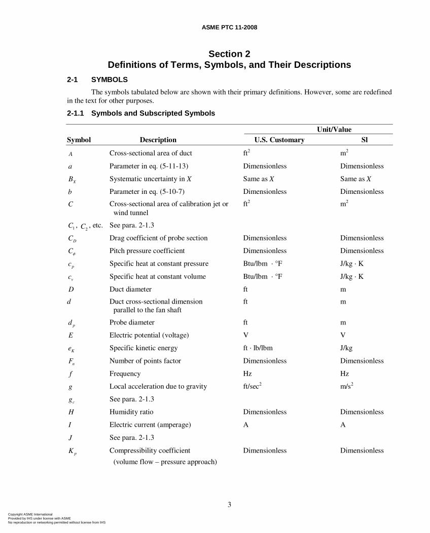
2-1 SYMBOLS

The symbols tabulated below are shown with their primary definitions. However, some are redefined in the text for other purposes.

2-1.1 Symbols and Subscripted Symbols

Unit/Value

Symbol Description U.S. Customary Sl

A Cross-sectional area of duct ft2 m2

a Parameter in eq. (5-11-13) Dimensionless Dimensionless

XB Systematic uncertainty in X Same as X Same as X

b Parameter in eq. (5-10-7) Dimensionless Dimensionless

C Cross-sectional area of calibration jet or ft2 m2

wind tunnel

1C , 2C , etc. See para. 2-1.3

DC Drag coefficient of probe section Dimensionless Dimensionless

Cφ Pitch pressure coefficient Dimensionless Dimensionless

pc Specific heat at constant pressure Btu/lbm ⋅ °F J/kg ⋅ K

vc Specific heat at constant volume Btu/lbm ⋅ °F J/kg ⋅ K

D Duct diameter ft m

d Duct cross-sectional dimension ft m parallel to the fan shaft

pd Probe diameter ft m

E Electric potential (voltage) V V

Ke Specific kinetic energy ft ⋅ lb/lbm J/kg

nF Number of points factor Dimensionless Dimensionless

f Frequency Hz Hz

g Local acceleration due to gravity ft/sec2 m/s2

cg See para. 2-1.3

H Humidity ratio Dimensionless Dimensionless

I Electric current (amperage) A A

J See para. 2-1.3

pK Compressibility coefficient Dimensionless Dimensionless

(volume flow – pressure approach)


ASME PTC 11-2008

4

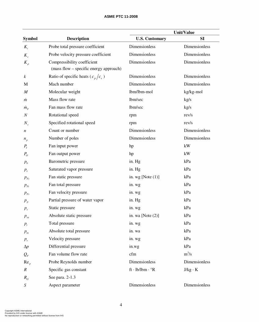
Unit/Value

Symbol Description U.S. Customary SI

tK Probe total pressure coefficient Dimensionless Dimensionless

vK Probe velocity pressure coefficient Dimensionless Dimensionless

Kρ Compressibility coefficient Dimensionless Dimensionless

(mass flow – specific energy approach)

k Ratio of specific heats ( p vc c ) Dimensionless Dimensionless

M Mach number Dimensionless Dimensionless

M Molecular weight lbm/lbm-mol kg/kg-mol

m Mass flow rate lbm/sec kg/s

Fm Fan mass flow rate lbm/sec kg/s

N Rotational speed rpm rev/s

sN Specified rotational speed rpm rev/s

n Count or number Dimensionless Dimensionless

pn Number of poles Dimensionless Dimensionless

IP Fan input power hp kW

OP Fan output power hp kW

bp Barometric pressure in. Hg kPa

ep Saturated vapor pressure in. Hg kPa

Fsp Fan static pressure in. wg [Note (1)] kPa

Ftp Fan total pressure in. wg kPa

Fvp Fan velocity pressure in. wg kPa

pp Partial pressure of water vapor in. Hg kPa

sp Static pressure in. wg kPa

sap Absolute static pressure in. wa [Note (2)] kPa

tp Total pressure in. wg kPa

tap Absolute total pressure in. wa kPa

vp Velocity pressure in. wg kPa

pΔ Differential pressure in.wg kPa

FQ Fan volume flow rate cfm m3/s

Re p Probe Reynolds number Dimensionless Dimensionless

R Specific gas constant ft ⋅ lb/lbm ⋅ °R J/kg ⋅ K

OR See para. 2-1.3

S Aspect parameter Dimensionless Dimensionless


ASME PTC 11-2008

5

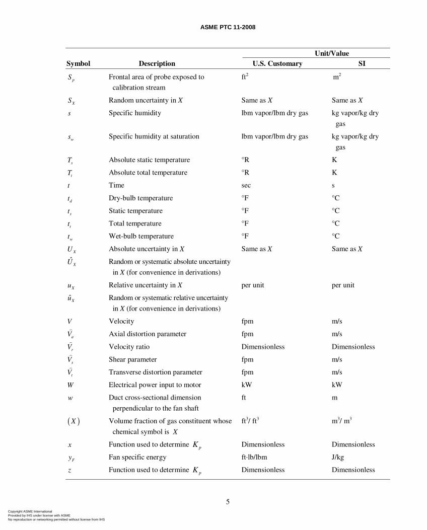
Unit/Value


pS Frontal area of probe exposed to ft2 m2

calibration stream

XS Random uncertainty in X Same as X Same as X

s Specific humidity lbm vapor/lbm dry gas kg vapor/kg dry

gas

ws Specific humidity at saturation lbm vapor/lbm dry gas kg vapor/kg dry

gas

sT Absolute static temperature °R K

tT Absolute total temperature °R K

t Time sec s

dt Dry-bulb temperature °F °C

st Static temperature °F °C

tt Total temperature °F °C

wt Wet-bulb temperature °F °C

XU Absolute uncertainty in X Same as X Same as X

ˆXU Random or systematic absolute uncertainty

in X (for convenience in derivations)

Xu Relative uncertainty in X per unit per unit

ˆXu Random or systematic relative uncertainty

in X (for convenience in derivations)

V Velocity fpm m/s

aV Axial distortion parameter fpm m/s

rV Velocity ratio Dimensionless Dimensionless

sV Shear parameter fpm m/s

tV Transverse distortion parameter fpm m/s

W Electrical power input to motor kW kW

w Duct cross-sectional dimension ft m

perpendicular to the fan shaft

( )X Volume fraction of gas constituent whose ft3/ ft3 m3/ m3

chemical symbol is X

x Function used to determine pK Dimensionless Dimensionless

Fy Fan specific energy ft⋅lb/lbm J/kg

z Function used to determine pK Dimensionless Dimensionless


ASME PTC 11-2008

6

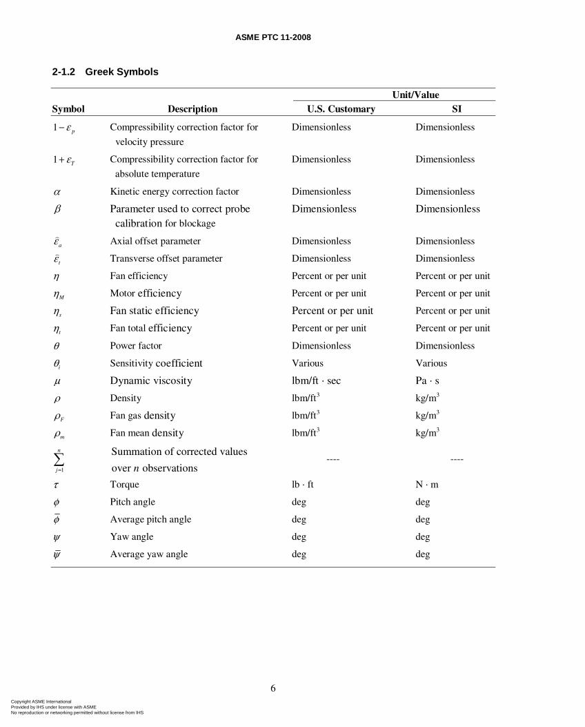
2-1.2 Greek Symbols

Unit/Value


1 pε− Compressibility correction factor for Dimensionless Dimensionless

velocity pressure

1 Tε+ Compressibility correction factor for Dimensionless Dimensionless

absolute temperature

α Kinetic energy correction factor Dimensionless Dimensionless

β Parameter used to correct probe Dimensionless Dimensionless calibration for blockage

aε Axial offset parameter Dimensionless Dimensionless

tε Transverse offset parameter Dimensionless Dimensionless

η Fan efficiency Percent or per unit Percent or per unit

Mη Motor efficiency Percent or per unit Percent or per unit

sη Fan static efficiency Percent or per unit Percent or per unit

tη Fan total efficiency Percent or per unit Percent or per unit

θ Power factor Dimensionless Dimensionless

iθ Sensitivity coefficient Various Various

μ Dynamic viscosity lbm/ft ⋅ sec Pa ⋅ s

ρ Density lbm/ft3 kg/m3

Fρ Fan gas density lbm/ft3 kg/m3

mρ Fan mean density lbm/ft3 kg/m3

1

n

j=∑

Summation of corrected values

over observationsn ---- ----

τ Torque lb ⋅ ft N ⋅ m

φ Pitch angle deg deg

φ Average pitch angle deg deg

ψ Yaw angle deg deg

ψ Average yaw angle deg deg


ASME PTC 11-2008

7

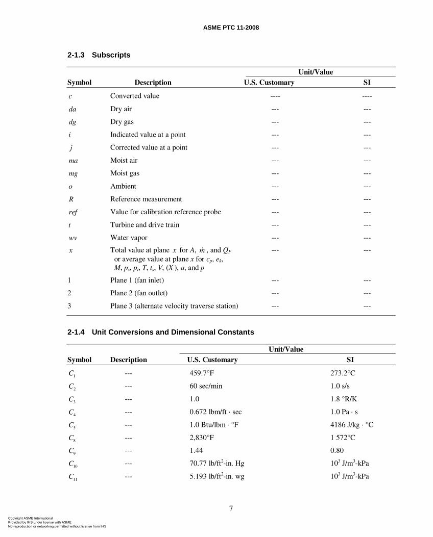
2-1.3 Subscripts

Unit/Value


c Converted value ---- ----

da Dry air --- ---

dg Dry gas --- ---

i Indicated value at a point --- ---

j Corrected value at a point --- ---

ma Moist air --- ---

mg Moist gas --- ---

o Ambient --- ---

R Reference measurement --- ---

ref Value for calibration reference probe --- ---

t Turbine and drive train --- ---

wv Water vapor --- ---

x Total value at plane x for A, m , and QF --- --- or average value at plane x for cp, ek, M, ps, pt, T, ts, V, (X ), a, and p

1 Plane 1 (fan inlet) --- ---

2 Plane 2 (fan outlet) --- ---

3 Plane 3 (alternate velocity traverse station) --- ---

2-1.4 Unit Conversions and Dimensional Constants

Unit/Value


1C --- 459.7°F 273.2°C

2C --- 60 sec/min 1.0 s/s

3C --- 1.0 1.8 °R/K

4C --- 0.672 lbm/ft ⋅ sec 1.0 Pa ⋅ s

5C --- 1.0 Btu/lbm ⋅ °F 4186 J/kg ⋅ °C

8C --- 2,830°F 1 572°C

9C --- 1.44 0.80

10C --- 70.77 lb/ft2-in. Hg 103 J/m3-kPa

11C --- 5.193 lb/ft2-in. wg 103 J/m3-kPa


ASME PTC 11-2008

8

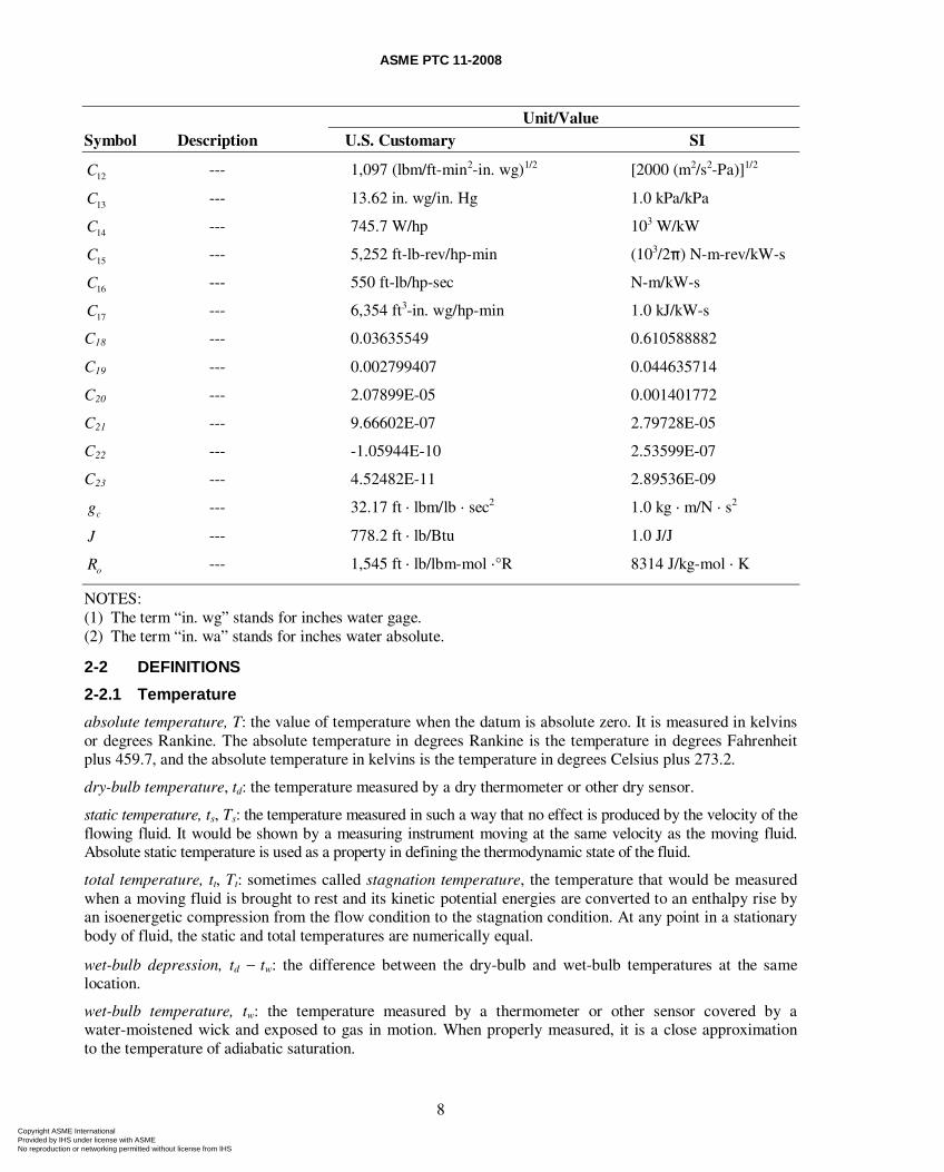
Unit/Value


12C --- 1,097 (lbm/ft-min2-in. wg)1/2 [2000 (m2/s2-Pa)]1/2

13C --- 13.62 in. wg/in. Hg 1.0 kPa/kPa

14C --- 745.7 W/hp 103 W/kW

15C --- 5,252 ft-lb-rev/hp-min (103/2π) N-m-rev/kW-s

16C --- 550 ft-lb/hp-sec N-m/kW-s

17C --- 6,354 ft3-in. wg/hp-min 1.0 kJ/kW-s

C18 --- 0.03635549 0.610588882

C19 --- 0.002799407 0.044635714

C20 --- 2.07899E-05 0.001401772

C21 --- 9.66602E-07 2.79728E-05

C22 --- -1.05944E-10 2.53599E-07

C23 --- 4.52482E-11 2.89536E-09

cg --- 32.17 ft ⋅ lbm/lb ⋅ sec2 1.0 kg ⋅ m/N ⋅ s2

J --- 778.2 ft ⋅ lb/Btu 1.0 J/J

oR --- 1,545 ft ⋅ lb/lbm-mol ⋅°R 8314 J/kg-mol ⋅ K

NOTES: (1) The term “in. wg” stands for inches water gage. (2) The term “in. wa” stands for inches water absolute.

2-2 DEFINITIONS

2-2.1 Temperature

absolute temperature, T: the value of temperature when the datum is absolute zero. It is measured in kelvins or degrees Rankine. The absolute temperature in degrees Rankine is the temperature in degrees Fahrenheit plus 459.7, and the absolute temperature in kelvins is the temperature in degrees Celsius plus 273.2.

dry-bulb temperature, td: the temperature measured by a dry thermometer or other dry sensor.

static temperature, ts, Ts: the temperature measured in such a way that no effect is produced by the velocity of the flowing fluid. It would be shown by a measuring instrument moving at the same velocity as the moving fluid. Absolute static temperature is used as a property in defining the thermodynamic state of the fluid.

total temperature, tt, Tt: sometimes called stagnation temperature, the temperature that would be measured when a moving fluid is brought to rest and its kinetic potential energies are converted to an enthalpy rise by an isoenergetic compression from the flow condition to the stagnation condition. At any point in a stationary body of fluid, the static and total temperatures are numerically equal.

wet-bulb depression, td − tw: the difference between the dry-bulb and wet-bulb temperatures at the same location.

wet-bulb temperature, tw: the temperature measured by a thermometer or other sensor covered by a water-moistened wick and exposed to gas in motion. When properly measured, it is a close approximation to the temperature of adiabatic saturation.


ASME PTC 11-2008

9

2-2.2 Specific Energy and Pressure

absolute pressure, pa: the value of a pressure when the datum is absolute zero. It is always positive.

barometric pressure, pb: the absolute pressure exerted by the atmosphere.

differential pressure, Δp: the difference between any two pressures.

gage pressure, p: the value of a pressure when the datum is the barometric pressure at the point of measurement. It is the difference between the absolute pressure at a point and the pressure of the ambient atmosphere in which the measuring gage is located. It may be positive or negative.

pressure, p: normal force per unit area. Since pressure divided by density may appear in energy balance equations, it is sometimes convenient to consider pressure as a type of energy per unit volume.

specific energy, y: energy per unit mass. Specific kinetic energy is kinetic energy per unit mass and is equal to one-half the square of the fluid velocity. Specific potential energy is potential energy per unit mass and is equal to the gravitational acceleration multiplied by the elevation above a specified datum. Fluid pressure divided by density is sometimes called “specific pressure energy” and is considered a type of specific energy; however, this term is more properly called specific flow work.

static pressure, ps, psa: the pressure measured in such a manner that no effect is produced by the velocity of the flowing fluid. Similar to the static temperature, it would be sensed by a measuring instrument moving at the same velocity as the fluid. Static pressure may be expressed as either an absolute or gage pressure. Absolute static pressure is used as a property in defining the thermodynamic state of the fluid.

total pressure, pt, pta: sometimes called the stagnation pressure, would be measured when a moving fluid is brought to rest and its kinetic and potential energies are converted to an enthalpy rise by an isentropic compression from the flow condition to the stagnation condition. It is the pressure sensed by an impact tube or by the impact hole of a Pitot-static tube when the tube is aligned with the local velocity vector. Total pressure may be expressed as either an absolute or gage pressure. In a stationary body of fluid, the static and total pressures are numerically equal.

velocity pressure, pv: sometimes called “dynamic pressure,” is defined as the product of fluid density and specific kinetic energy. Hence, velocity pressure is kinetic energy per unit volume. If compressibility can be neglected, it is equal to the difference of the total pressure and the static pressure at the same point in a fluid and is the differential pressure, which would be sensed by a properly aligned Pitot-static tube. In this Code, the indicated velocity pressure, pvi, shall be corrected for probe calibration, probe blockage, and compressibility before it can be called velocity pressure.

2-2.3 Density and Specific Humidity

density, ρ: mass per unit volume of a fluid. The density can be given static and total values in a fashion similar to pressure and temperature. If the gas is at rest, static and total densities are equal.

specific humidity, s: the mass of water vapor per unit mass of dry gas.

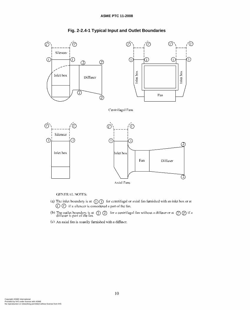
2-2.4 Fan Boundaries

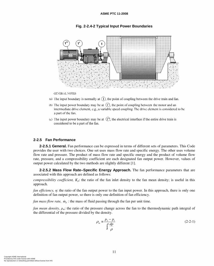
The fan boundaries are defined as the interface between the fan and the remainder of the system. These boundaries may differ slightly from fan to fan. The fan accepts power at its input power boundary and moves a quantity of gas from its inlet boundary to its outlet boundary and in the process increases the specific energy and pressure of this gas. The inlet boundary may be specified to include inlet boxes, silencers, rain hoods, or debris screens as a part of the fan. The outlet boundary may be specified to include dampers or a diffuser as a part of the fan. The input power boundary may be specified to include the fan-to-motor coupling or a speed reducer as part of the fan. See Figs. 2-2.4-1 and 2-2.4-2.


ASME PTC 11-2008

10

Fig. 2-2.4-1 Typical Input and Outlet Boundaries


ASME PTC 11-2008

11

Fig. 2-2.4-2 Typical Input Power Boundaries

2-2.5 Fan Performance

2-2.5.1 General. Fan performance can be expressed in terms of different sets of parameters. This Code provides the user with two choices. One set uses mass flow rate and specific energy. The other uses volume flow rate and pressure. The product of mass flow rate and specific energy and the product of volume flow rate, pressure, and a compressibility coefficient are each designated fan output power. However, values of output power calculated by the two methods are slightly different [1].

2-2.5.2 Mass Flow Rate–Specific Energy Approach. The fan performance parameters that are associated with this approach are defined as follows:

compressibility coefficient, Kρ: the ratio of the fan inlet density to the fan mean density; is useful in this approach.

fan efficiency, η: the ratio of the fan output power to the fan input power. In this approach, there is only one definition of fan output power, so there is only one definition of fan efficiency.

fan mass flow rate, Fm : the mass of fluid passing through the fan per unit time.

fan mean density, ρm: the ratio of the pressure change across the fan to the thermodynamic path integral of the differential of the pressure divided by the density.

2 1

2

1

m

p pdp

ρ

ρ

−≡

∫ (2-2-1)


ASME PTC 11-2008

12

In this approach, mean density is approximated by the arithmetic mean of inlet and outlet densities.

1 2

2m

ρ ρρ +⎛ ⎞≈ ⎜ ⎟⎝ ⎠

(2-2-2)

fan output power, Po: the product of fan mass flow rate and fan specific energy. Since mass flow rate equals the product of volume flow rate and density at a particular plane, fan output power can also be expressed as the product of fan inlet density, fan inlet volume flow rate, and fan specific energy.

fan specific energy, yF: the work per unit mass that would be done on the gas in an ideal (frictionless) transition between the actual inlet and outlet states. The ideal work done on a unit mass of fluid is equal to the integral of the static pressure differential divided by the fluid density for the fan flow process plus changes of specific kinetic energy and specific potential energy across the fan. The fan specific energy is the average of the ideal work for all fluid particles passing through the fan. Refer to subsection 5-7 for appropriate averages.

Only the component of velocity in the nominal direction of flow shall be taken into account when determining the specific kinetic energy. It is customary to assume that changes in potential energy are negligible in fans.

2

2 11F K K

dpy e e

ρ= + −∫ (2-2-3)

For an incompressible flow process, the product of fan specific energy and fluid density is equal to the fan total pressure. For a nonconstant density process, fan specific energy can be approximated by assuming some thermodynamic process within the fan in order to perform the pressure-density integration.

kinetic energy correction factor, α: a dimensionless factor used to account for the difference between the true average kinetic energy of the fluid and the kinetic energy calculated as one half the square of the average velocity.

2-2.5.3 Volume Flow Rate–Pressure Approach. The fan performance parameters associated with this approach are defined as follows.

compressibility coefficient, Kp: a dimensionless coefficient used to account for compressibility effects [2] and is calculated according to the procedure given in para. 5-11.4 [3].

fan efficiency, η: In this approach, fan efficiency is expressed as either fan total efficiency or fan static efficiency.

fan static efficiency, ηs: the ratio of fan output power to fan input power, in which the fan output power is modified by deleting the fan velocity pressure. This may also be called total-to-static efficiency.

fan total efficiency, ηt: the ratio of fan output power to fan input power. This may also be called total-to-total efficiency.

fan gas density, ρF: the total density of the gas at fan inlet conditions.

fan output power, Po: the product of fan volume flow rate, fan total pressure, and compressibility coefficient Kp.

fan pressure: in this approach, three fan pressures are defined as follows:

fan static pressure, pFs: the difference between the fan total pressure and the fan velocity pressure. Therefore, fan static pressure is the difference between the average static pressure at the fan outlet and the average total pressure at the fan inlet. Refer to subsection 5-7 for appropriate averages.


ASME PTC 11-2008

13

fan total pressure, pFt: the difference between the average total pressure at the fan outlet and the average total pressure at the fan inlet. Only the component of velocity in the nominal direction of flow shall be taken into account when determining fan total pressure. Refer to subsection 5-7 for appropriate averages. It is customary to assume that pressure changes due to elevation changes are negligible in fans.

fan velocity pressure, pFv: the product of the average density and average specific kinetic energy at the fan outlet. Refer to subsection 5-7 for the appropriate averages. This corresponds to the velocity pressure corresponding to the average velocity at the fan outlet as defined in the ASHRAE Standard 51 and AMCA Standard 210 [2].

fan volume flow rate, QF: the fan mass flow rate divided by the fan gas density.

2-2.5.4 Fan Input Power. PI, fan input power, is the power required to drive the fan and any elements in the drive train that are considered to be within the fan boundaries.

2-2.6 Fan Operating Conditions

Fan operating conditions are specified by the speed of rotation of the fan and sufficient information to determine the average gas properties, including pressure, temperature, density, viscosity, gas constants, and specific heats at the fan inlet.

2-2.7 Errors and Uncertainties

confidence level, Lc: a percentage value such that if a very large number of determinations of a variable are made, there is an Lc percent probability that the true value will fall within the interval defined by the mean plus or minus the uncertainty. A value for uncertainty is meaningful only if it is associated with a specific confidence level. As used in this Code, all uncertainties are assumed to be at the 95% confidence level. If the number of determinations of a variable is large and if the values are normally distributed, the uncertainty at the 95% confidence level is approximately twice the standard deviation of the mean of the values.

error: the difference between the true value of a quantity and the measured value. The true value of an error cannot be determined.

random uncertainty, XS , /XS X : uncertainty due to numerous small independent influences that prevent a

measurement system from delivering the same reading when supplied with the same input. Random uncertainties can be reduced by replication and averaging [4]. Random uncertainty is often calculated as the standard deviation of the mean for a particular set of measurements. Hence, the symbol used for random uncertainty is the same as that typically used for standard deviation of the mean.

sensitivity coefficient, θi: also called “sensitivity factor,” the ratio of the change in a result to a unit change in a parameter. Influence coefficients have been utilized in the derivations of the uncertainties equations in this Code.

systematic uncertainty, BX, BX / X: uncertainty due to such things as instrument and operator bias and changes in ambient conditions for the instruments. Systematic uncertainty is essentially “frozen” in the measurement system and cannot be reduced by increasing the number of measurements if the equipment and conditions of measurements remain unchanged [4].

total uncertainty, UX, UX/ X: of a result is obtained by combining the random and systematic uncertainties of that result in a manner that reflects the confidence level. In this Code, random and systematic uncertainties are combined using a “root sum square (RSS) model.” See eqs. (5-13-1) and (5-13-2).

uncertainty: a possible value for the error [5]. It is also the interval within which the true value can be expected to lie with a stated probability [4]. The uncertainty is used to estimate the error.

absolute uncertainty (U): has the same units as the variable in question.

relative uncertainty (u): absolute uncertainty divided by the magnitude of the variable and is dimensionless; also called “per unit uncertainty.”


ASME PTC 11-2008

14

2-2.8 General Definitions

acceptance test: the evaluating action(s) to determine if a new or modified piece of equipment satisfactorily meets its performance criteria, permitting the purchaser to “accept” it from the supplier.

calibration: the process of comparing the response of an instrument or measurement system with a standard instrument or measurement system over some measurement range and adjusting the instrument or measurement system to match the standard if appropriate.

instrument: a tool or device used to measure the physical value of a variable. These values can include size, weight, pressure, temperature, velocity, fluid flow, voltage, electric current, density, viscosity, gas composition, and power. Sensors are included that may not, by themselves, incorporate a display but transmit signals to remote computer type devices for display, processing, or process control. Also included are items of ancillary equipment directly affecting the display of the primary instrument (e.g., ammeter shunt). Also included are tools or fixtures used as the basis for determining part acceptability.

parties to a test: those persons and companies interested in the results.

serialize: to permanently mark an instrument so that it can be identified and tracked.

test boundary: see Fan Boundaries, Figs. 2-2.4-1 and 2-2.4-2.

test reading: one recording of all required test instrumentation.

test run: a group of test readings.

traceable: records are available demonstrating that the instrument can be traced through a series of calibrations to an appropriate ultimate reference, such as National Institute for Standards and Technology (NIST).


ASME PTC 11-2008

15

Section 3 Guiding Principles

3-1 INTRODUCTION

In applying this Code to a specific fan test, various decisions must be made. This Section explains what decisions shall be made and gives general guidelines for performing a Code test.

Any test shall be performed only after the fan has been found by inspection to be in a satisfactory condition to undergo the test. The parties to the test shall mutually decide when the test is to be performed and shall be entitled to have present such representatives as are required for them to be assured that the test is conducted in accordance with this Code and with any written agreements made prior to the test.

3-2 PRIOR AGREEMENTS

Prior to conducting a Code test, written agreement shall be reached by the parties to the test on the following items:

(a) object of test

(b) duration of operation under test conditions

(c) test personnel and assignments

(d) person in charge of test

(e) test methods to be used

(f) test instrumentation and methods of calibration

(g) locations for taking measurements and orientation of traverse ports

(h) number and frequency of observations, including reference measurements

(i) method of computing results

(j) values or methods for calculation of primary uncertainties

(k) arbitrator to be used if one becomes necessary

(l) applicable performance curves and/or the specified performance and operating conditions

(m) fan boundaries

(n) number of test runs

(o) pretest uncertainty analysis

(p) uncertainty targets

(q) permissible limits of inlet flow distortion

3-3 CODE PHILOSOPHY

3-3.1 Fan Performance

This Code offers the user the choice of expressing fan performance in terms of mass flow rate and specific energy or volume flow rate and pressure. After reviewing both methods, the parties to the test shall decide which method they intend to use. Once a method is selected, then the principles and procedures for only that method shall be adhered to throughout the test, rather than commingling the various aspects of the two methods [1].

3-3.2 Methods for Determining Fan Performance

The methods of this Code are based on the assumption that fan pressures or specific energies are measured sufficiently close to the fan boundaries that corrections for losses between the measurement planes and fan boundaries are not required. It is not feasible to include methods for such corrections in this Code; therefore, if such corrections are necessary, the test cannot be a Code test.


ASME PTC 11-2008

16

For the purpose of determining proper average values of pressure, temperature, and density, it is always necessary to measure point velocities at the fan boundaries. However, only the point velocities measured at traverse planes conforming to the requirements of this Code (see para. 4-2.3) shall be used for fan flow rate. If the conditions at the fan boundaries do not meet the criteria given in this Code for a suitable flow traverse, then point velocity measurements made at the fan boundaries shall be used only for determining average values of pressure, temperature, density, and specific kinetic energy and not for fan flow rate. If this condition exists, then the fan flow rate may be determined at a plane other than the fan boundary, provided that no fluid enters or leaves the duct between the fan boundary and measurement plane. Although the point velocities measured at the fan boundaries may not conform to the requirements for a valid flow traverse, they can provide a useful statistical basis for substantiating the fan flow rate.

3-3.3 Flow Measurement Methods

For large ducts handling gas flows, often the only practicable method of gas flow measurement is the velocity traverse method. This method shall be considered the primary method for measuring flows of the type addressed by this Code. Other methods of determining flow, including but not limited to stoichiometric methods (where applicable), ultrasonic methods, and methods using such devices as flow nozzles, may be permitted if it can be shown that the accuracy of the proposed method is at least equal to that of the primary method.

In the velocity traverse method, the duct is subdivided into a number of elemental areas and, using a suitable probe, the velocity is measured at a point in each elemental area. The total flow is then obtained by summing the contributions of each elemental area (some methods use different weighting factors for different areas). Within the framework of the velocity traverse method, many different techniques have been proposed for selecting the number of points at which velocity is measured, for establishing the size and geometry of the elemental areas, and for summing (theoretically integrating) the contributions of each elemental area. Options that have been proposed include the placing of points based on an assumed (log-linear, Legendre polynomial, or Chebyschev polynomial) velocity distribution [2, 6], the use of graphical or numerical techniques to integrate the velocity distribution over the duct cross section [6, 7], the use of equal elemental areas with simple arithmetic summing of the contribution of each area to the total flow [6, 8, 9], and the use of boundary layer corrections to account for the thin layer of slow-moving fluid near a wall. As a general rule, accuracy of flow measurement can be increased by either increasing the number of points in the traverse plane or by using more sophisticated mathematical techniques (e.g., interpolation polynomials, boundary layer corrections) [6, 8]. PTC 19.5 recommends either a Gaussian or Chebyschev integration scheme. Investigations performed by the PTC 11 committee using different velocity distributions similar to those that actually occur in the field have shown that no particular technique is always more accurate.

Considering the requirements of field testing and the varied velocity distributions that may occur in the field, this Code specifies flow measurements at a relatively large number of points in lieu of assuming velocity distributions or using corrections for boundary layer effects. It is usually desirable to have a large number of points (elemental areas) so that the complete velocity profile can be characterized. Accordingly, this Code adopts the equal-area method with measurement at a relatively large number of points. Investigations of flow measurement under conditions similar to those expected in application of this Code have demonstrated the validity of this approach [8–10]. In some circumstances, it may be desirable to use Gaussian or Chebyschev schemes because they require a smaller number of measurement points. PTC 19.5 may be consulted for details on these methods.

3-3.4 Flow at the Fan Boundaries

Due to the highly disturbed flow at the fan boundaries and the errors obtained when making measurements with probes unable to distinguish directionality, probes capable of indicating gas direction and speed, hereinafter referred to as directional probes, are generally required. Only the component of velocity normal to the elemental area is pertinent to the calculation of flow. Measurement of this component cannot be accomplished by simply aligning a nondirectional probe parallel to the duct axis, since such probes only


ASME PTC 11-2008

17

indicate the correct velocity pressure when aligned with the velocity vector. Errors are generally due to undeterminable effects on the static (and, to a lesser degree, total) pressure-sensing holes. Therefore, adequate flow measurements in a highly disturbed region can only be made by measuring speed and direction at each point and then calculating the component of velocity parallel to the duct axis. Only in some circumstances (see subsection 4-7) may nondirectional probes be used.

3-3.5 Averaging Methods

Various methods of averaging are required to calculate the appropriate values of the parameters that determine fan performance. These methods, along with the large number of traverse points, the directional probe, and requirements for measurements at the fan boundaries, make it possible to conduct an accurate field test for most fan installations.

3-3.6 Compressibility Effects

The instruments and methods of measurement specified in this Code are selected on the premise that only mild compressibility effects are present in the flow. The velocity, pressure, and temperature determinations provided for in this Code are limited to situations in which the gas is moving with a Mach number less than 0.4. This corresponds to a value of (Kvjpvi / psai) of approximately 0.1 (see para. 5-2.2).

3-3.7 Test Speed Versus Specified Speed

Although this Code provides methods for conversion of measured fan performance variables to specified operating conditions, such conversions shall not be permitted if the test speed differs by more than 10% from the specified speed or if the test values of the fan inlet density, ρ1, or fan gas density, ρF, differ by more than 20% from specified values.

3-3.8 Accuracy of Results

A question that invariably arises in connection with any test is, “How accurate are the results?” [5]. This question is addressed in this Code by the inclusion of a complete procedure for the evaluation of uncertainties. It is believed that all significant sources of error in a fan test have been identified and addressed in this procedure. Since in fact any results based on measurements are of little value without an accompanying statement of their expected accuracy, uncertainty evaluation is made a mandatory part of this Code.

3-3.9 Inlet Flow Distortion

Fan performance is typically predicted assuming that a uniform flow velocity profile at the fan inlet plane and equal flow at each inlet, in the case of double inlet fans, will be present. Laboratory test conditions ensure that such a uniform profile exists. When a fan is installed in a system, the fan may be subjected to a distorted inlet profile because of upstream ductwork geometry or, for open inlet fans, the geometry of the space in which the fan is installed. Experience shows that inlet flow distortion or imbalance can exist and can often affect fan performance. Wright et al. [11, 12] have measured the effects of inlet flow distortion on a single-inlet centrifugal fan. This is the only published information on distortion known to the PTC 11 Committee.

Inlet flow distortion can be quantified by various velocity profile parameters: velocity ratio, transverse distortion, axial distortion, transverse shear, transverse offset, axial offset, average yaw, and average pitch. The term “transverse” refers to the direction perpendicular to the fan shaft, and the term “axial” refers to the direction parallel to the fan shaft. This Code provides equations for computing these parameters. Specification of acceptable levels for these parameters or methods for accounting for the effects of distortion on fan performance is beyond the scope of this Code.

3-3.10 Laboratory Versus In Situ Tests

Commercially quoted fan performance is usually based on measurements made under laboratory conditions. In a laboratory test, a fan is operated in a system specifically designed to facilitate accurate


ASME PTC 11-2008

18

measurement of fan performance parameters and to minimize those system effects that can degrade fan performance [2, 13]. Comparative fan tests conducted according to a laboratory standard [2] and procedures of this Code have demonstrated that similar performance ratings can be obtained if the fan is operated under laboratory conditions [14].

The user of this Code should be aware that application of the procedures contained herein will reveal the performance of the test fan as it is affected by the system in which it is installed. These in situ performance ratings and ratings of the same fan based on laboratory tests or ratings of a model fan based on laboratory tests may not be the same due to various effects generally called “system effects” [13]. Any methods for reconciliation of in situ performance ratings and laboratory-based ratings are beyond the scope of this Code.

3-4 SYSTEM DESIGN CONSIDERATIONS

There are field situations where it is not possible to obtain sufficiently accurate measurements to conform with this Code. Consideration of a few simple concepts when a new system is designed will facilitate fan testing as well as improve the fan system performance.

3-4.1 Fan Flow Rate

Generally, the most difficult parameter to determine during a field test is the fan flow rate. If the following considerations can be made during the design of the fan and duct system, fan flow rates will be easier to determine:

(a) Design of inlet and outlet ducts should avoid internal stiffeners for three equivalent diameters both upstream and downstream of the fan boundaries.

(b) Abrupt changes in direction should not be located at the fan boundaries.

(c) All transitions in duct size should be smooth.

(d) A duct length of approximately 3 ft (1 m) should be allowed at the fan boundaries for inserting probes. This section should be free of internal obstructions that would affect the flow measurement and external obstructions that would impede probe maneuverability, such as structural steel, walkways, handrails, etc. Ideally, the area of the measuring section, A2duct, should be the same as that of the fan, A2fan. If not, the fan velocity pressure shall be corrected as indicated below. Differences in density may be ignored.

3-4.2 Fan Input Power

Considerations to be observed that will aid the determination of fan input power are

(a) installing a calibrated drive train or

(b) allowing sufficient shaft length at the fan for the installation of a torque meter

3-5 INTERNAL INSPECTION AND MEASUREMENT OF CROSS SECTION

An internal inspection of the ductwork, at planes where velocity and/or pressure measurements are to be made, shall be conducted by the parties to the test to ensure that no obstructions will affect the measurements. Areas where there is an accumulation of dust such that the duct area is significantly reduced shall be avoided as this indicates that the velocities are inadequate to prevent entrained dust from settling. This dust settlement will in effect cause the duct cross-sectional area to decrease during the test. Where this situation exists, it is recommended that velocity measurements be made in vertical runs.

The internal cross-sectional area shall be based on the average of at least four equally spaced measurements across each duct dimension for nominally rectangular ducts and on the basis of the average of at least four equally spaced diametral measurements for nominally circular ducts. Sufficient equally spaced measurements shall be used to limit the uncertainty in the area to 0.3%. If the duct area is measured under conditions different from operating conditions, suitable expansion or contraction corrections for temperature and pressure shall be made.


ASME PTC 11-2008

19

3-6 TEST PERSONNEL

3-6.1 Test Team

A test team shall be selected that includes a sufficient number of test personnel to record the various readings in the allotted time. Test personnel shall have the experience and training necessary to obtain accurate and reliable records. All data sheets shall be signed by the observers. The use of automatic data recording systems can reduce the number of people required.

3-6.2 Person-in-Charge

The person in charge of the test shall direct the test and shall exercise authority over all observers. This person shall certify that the test is conducted in accordance with this Code and with all written agreements made prior to the test. This person may be required to be a registered professional engineer.

3-7 POINT OF OPERATION

This Code describes a method for determining the performance of a fan at a single point of operation. If more than one point of operation is required, a test shall be made for each. The parties to the test must agree prior to the tests on the method of varying the system resistance to obtain the various points of operation. If performance curves are desired, then the parties to the test shall agree beforehand as to the number and location of points required to construct the curves.

3-8 METHOD OF OPERATION DURING TEST

3-8.1 Manual Mode Operation

When a system contains fans operating in parallel, the fan to be tested shall be operated in the manual mode during the test and the remaining fans in the system used to follow load variations. The fan to be tested shall be operated at a constant speed with constant damper and vane positions. Various positions may be required for part-load tests.

3-8.2 Constant Conditions

The system shall be operated to maintain conditions at constant gas flows and other operating conditions. For example, for draft fans, the boiler load should be steady. Soot blowers should not be cycled on and off during the test. If soot blowing is necessary, it should be used throughout the test. The operation of pulverizers, stokers, baghouses, scrubbers, air heaters, etc., shall not be allowed to affect the results of the test.

3-8.3 Records

Adequate records of the position of variable vanes, variable blades, dampers, or other control devices shall be maintained.

3-9 INSPECTION, ALTERATIONS, AND ADJUSTMENTS

Prior to the test, the manufacturer or supplier shall have reasonable opportunity to inspect the fan and appurtenances for correction of noted defects, for normal adjustments to meet specifications and contract agreements, and to otherwise place the equipment in condition to undergo further operation and testing. The parties to the test shall not alter or change the equipment or appurtenances in such a manner as to modify or void specifications or contract agreements or prevent continuous and reliable operation of the equipment at all capacities and outputs under all specified operating conditions. Adjustments to the fan that may affect test results are not permitted once the test has started. Should such adjustments be deemed necessary, prior test runs shall be voided and the test restarted. Any readjustments and reruns shall be agreed to by the parties to the test.


ASME PTC 11-2008

20

3-10 INCONSISTENCIES

If inconsistencies in the measurements are observed during the conduct of the test, the person in charge of the test shall be permitted to take steps to remedy the inconsistency and continue the test. Any actions in this regard must be noted and are subject to approval by the parties to the test. Any such action shall be fully documented in the test report.

3-11 MULTIPLE INLETS OR DUCTS

If there is more than one fan inlet, measurements shall be obtained at each inlet or in each inlet duct. It is not permissible to measure the conditions at one inlet and assume the conditions are the same for all the inlets. Similarly, if the discharge duct from a fan splits into two or more ducts and it is more practical to measure the conditions downstream of the split, then the conditions in each branch of the duct shall be measured to determine the total flow.

3-12 PRELIMINARY TEST

Prior to performing a Code test, a preliminary test shall be made. The purpose of the preliminary test is to train the observers, determine if all instruments are functioning properly, and verify that the system and fan are in proper order to permit a valid Code test. The preliminary test can be considered a Code test if agreed to by the parties to the test and all requirements of this Code are met.

In fans with multiple inlets or ducts, it may be desirable to calculate parameters such as flow rate, density, gas composition, and parameters used to describe inlet flow distortion separately for each inlet or duct. If this is done, then the total mass flow rate shall be calculated as the sum of the separate inlet or duct mass flow rates, and the inlet static pressure, temperature, specific kinetic energy, and gas composition shall be calculated as the mass flow-weighted average of the values determined in the separate inlets or ducts.

3-13 REFERENCE MEASUREMENTS

For the purposes of determining that the system has reached steady state, verifying the constancy of operating conditions, and verifying that the fan performs at a constant point of operation during the test, the following reference measurements shall be made:

(a) speed, NR

(b) driver power, or some quantity proportional to driver power (e.g., IR, τR, WR, etc.)

(c) fan inlet static pressure, 1sRp

(d) fan outlet static pressure, 2sRp

(e) static pressure at traverse plane (if used), 3sRp

(f) fan inlet temperature, 1RT

(g) fan outlet temperature, 2RT

(h) temperature at traverse plane (if used), 3RT

(i) total pressure rise across the fan, tRp

(j) velocity pressure in either inlet or outlet or traverse plane, vRp


ASME PTC 11-2008

21

The measurement of speed and power made in accordance with the requirements of Section 4 for determining fan performance shall be used for reference purposes. The reference measurements for pressure and temperature shall be in accordance with Section 4 except a single point measurement shall be used for each parameter instead of the sampling grid. For purposes of reference measurements, probes capable of sensing total pressure, static pressure, velocity pressure, and temperature connected to appropriate indicators shall be permanently fixed at central locations in the inlet and outlet planes. These need not be directional probes nor do they have to be calibrated, since measurements taken from these probes are for reference purposes only. To facilitate uncertainty analysis, at least 30 sets of reference measurements shall be taken during a test run. Reference measurements shall be taken at regular intervals and shall be averaged over a time period of at least 15 sec. For example, for a 1-hr test, reference measurements would be made at 2-min intervals and recorded as averages over 15-sec periods. This may be done manually or automatically. It would be useful to record the trend on a graph.

The following test shall be used to determine if the test conditions are sufficiently steady. For each reference measurement, a test parameter equal to twice the standard deviation of the mean divided by the

mean of the measurements ( )2 XS X is calculated. If the value of the test parameter exceeds 0.01 (1%) for

any reference measurement, the test shall be invalidated because of unsteadiness.

The person in charge of the test shall be solely responsible for deciding when operating conditions are sufficiently constant to begin and continue the test.


ASME PTC 11-2008

22

Section 4 Instruments and Methods of Measurement

4-1 GENERAL CONSIDERATIONS

4-1.1 Accuracy

The specifications for selection and calibration of instruments that follow include accuracy requirements. Unless otherwise stated, specified accuracies are expressed in terms of the maximum uncertainty in any reading due to the instrument based on a minimum confidence level of 95%.

It is a requirement of this Code that the parties to the test agree in advance on the limits of possible measurement errors and test uncertainties. The parties should base their judgments of possible error on the references cited for each instrument, any records pertaining to the instrument to be used, and their collective experience with similar measurements.

Certain instruments are specified in this Code. However, it should be understood that other instruments for the same purpose may be used, provided their accuracies are equal to or better than those of the specified instruments.

4-1.2 Instrument Calibration

All instruments used in a Code test shall be calibrated. It is not necessary to calibrate all instruments specifically for the test if the parties to the test agree on the validity of previous calibrations.

The calibration data for an instrument shall be represented as a continuous function that may be determined by graphically fairing a smooth curve among the calibration points or by fitting, using the least squares methods, a mathematical curve that has a number of fitting parameters less than or equal to one-half of the number of calibration points. In a polynomial, the fitting parameters are the undetermined coefficients. In a power law equation, e.g., y = axb, where a and b are the fitting parameters. The fitting parameters for other cases may be determined in a similar manner.

Where the physical facts dictate, the calibration function may be extrapolated to the origin. Calibration data should cover the entire range of instrument readings, except where extrapolation to zero is indicated. Any other extrapolation requires agreement among the parties.

4-1.3 Monitoring Operational Steadiness

It is a requirement of this Code (see subsection 3-13) that operating conditions and point of operation be held steady during the test. Readings for some of the test parameters, such as rotational speed and input power, can be monitored for operational steadiness. Other test variables, such as velocity and pressure, are not uniformly distributed; therefore, test readings should not be used to monitor operational steadiness. Separate instruments shall, therefore, be used. Such monitoring instruments shall be held in a fixed position rather than used to traverse the plane.

Monitoring instruments shall be sensitive to changes in the monitored variables that would affect results. However, the accuracy and calibration requirements for the measuring instruments that follow can be relaxed or eliminated for instruments used only for monitoring purposes. It may even be desirable to use instruments with appreciably more damping than would be acceptable for measuring instruments as long as the response is fast enough to adequately indicate departures from operational steadiness.

4-2 TRAVERSE SPECIFICATIONS

4-2.1 Quantities Measured by Traverse

Because the distributions of velocity, pressure, temperature, gas composition, and moisture across the duct cross section are nonuniform, each quantity shall be measured at a sufficient number of points to facilitate the calculation of a proper average value. Point values of all of these quantities are theoretically


ASME PTC 11-2008

23

required at every traverse plane, but this Code recognizes that the distributions of gas composition and moisture are generally much more uniform than the distributions of velocity, pressure, and temperature. Accordingly, the Code does not require that gas composition and moisture be measured at every point in a traverse plane. Similarly, the Code does not require that these quantities be measured at all traverse planes if there are sound reasons to believe that there will be no change between planes. There may also be cases where the distribution of temperature is quite uniform. The parties may, therefore, agree to relax the requirement for temperature measurements if they are convinced this will have a negligible effect on the results.

4-2.2 Number of Traverse Planes

Two traverse planes are required to determine specific output (fan pressure or fan specific energy), except for the case mentioned below. The preferred locations for the traverse planes are at the fan inlet and outlet boundaries. However, a slight offset, upstream or downstream, is usually required so that heavy flanges or stiffeners do not have to be penetrated. Similarly, when dampers are located at the fan boundaries, it is more desirable to traverse slightly upstream of these dampers than downstream of them.

Only one traverse plane is required to determine flow rate, but if both the inlet plane and outlet plane qualify, each should be used. If neither the inlet plane nor outlet plane qualifies, a third plane will be required for the velocity traverse to determine flow rate.

If at its inlet boundary the fan draws gas from an essentially quiescent region of large volume and the inlet flow path is free from obstructions (e.g., a fan drawing air from the atmosphere or a fan located inside a large room), it is not necessary to traverse the inlet to determine specific output. The inlet total pressure, inlet static pressure, and inlet velocity pressure are all zero if the inlet region pressure is selected as the datum. If the inlet region pressure is not the datum, then the inlet velocity pressure is zero, and the inlet total and inlet static pressures are each equal to the inlet region pressure (see Fig. 4-2.2-1). However, if such fans are equipped with inlet boxes, the flow can be expected to be quite uniform at the entrance to the inlet box, particularly if equipped with an inlet bell, and this may be the optimum location for a velocity traverse to determine the flow rate.

4-2.3 Qualified Velocity Traverse Planes

To qualify for a velocity traverse for purposes of determining fan flow rate (see para. 3-3.2), a plane shall meet the following specifications:

(a) There shall be no internal stiffeners or other internal obstructions.

(b) There shall be no accumulation of dust or debris.

(c) The traverse plane shall be at least one damper blade width upstream or ten damper blade widths downstream of a damper.

(d) A preliminary velocity traverse shall show that the flow is reversed or essentially stagnant at no more than 15% (preferably 0%) of the elemental areas.

(e) There shall be no sudden change in either cross-sectional area or duct direction.

4-2.4 Determination of Sampling Grid

Measurements shall be taken at centroids of equal elemental areas. However, allowing for probe stem droop and the need to avoid duct bracing, the probe tip shall be located within a central area the sides of which are no more than 30% of the corresponding dimensions of the elemental area. Similarly, the probe tip may be outside the traverse plane by no more than 30% of the largest elemental area dimension and then only if the duct area is the same as at the traverse plane. Refer to Figs. 4-2.4-1 and 4-2.4-2. The minimum number of test points shall be per Fig. 4-2.4-3.


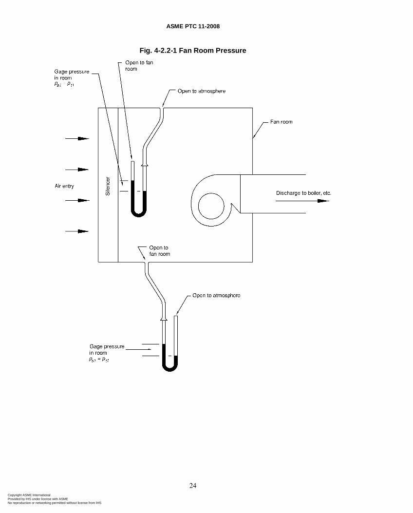
ASME PTC 11-2008

24

Fig. 4-2.2-1 Fan Room Pressure


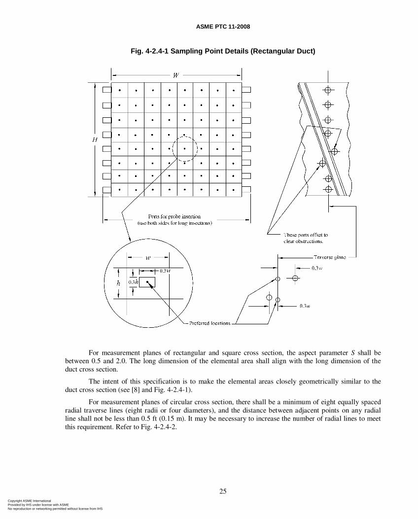
ASME PTC 11-2008

25

Fig. 4-2.4-1 Sampling Point Details (Rectangular Duct)

For measurement planes of rectangular and square cross section, the aspect parameter S shall be between 0.5 and 2.0. The long dimension of the elemental area shall align with the long dimension of the duct cross section.

The intent of this specification is to make the elemental areas closely geometrically similar to the duct cross section (see [8] and Fig. 4-2.4-1).

For measurement planes of circular cross section, there shall be a minimum of eight equally spaced radial traverse lines (eight radii or four diameters), and the distance between adjacent points on any radial line shall not be less than 0.5 ft (0.15 m). It may be necessary to increase the number of radial lines to meet this requirement. Refer to Fig. 4-2.4-2.


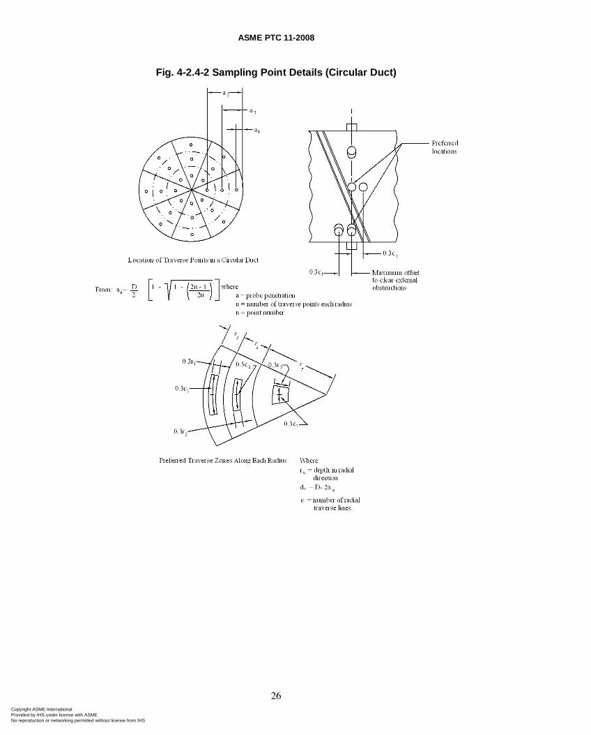
ASME PTC 11-2008

26

Fig. 4-2.4-2 Sampling Point Details (Circular Duct)


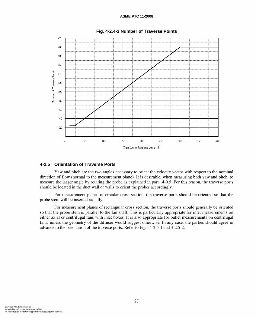
ASME PTC 11-2008

27

Fig. 4-2.4-3 Number of Traverse Points

4-2.5 Orientation of Traverse Ports

Yaw and pitch are the two angles necessary to orient the velocity vector with respect to the nominal direction of flow (normal to the measurement plane). It is desirable, when measuring both yaw and pitch, to measure the larger angle by rotating the probe as explained in para. 4-9.5. For this reason, the traverse ports should be located in the duct wall or walls to orient the probes accordingly.

For measurement planes of circular cross section, the traverse ports should be oriented so that the probe stem will be inserted radially.

For measurement planes of rectangular cross section, the traverse ports should generally be oriented so that the probe stem is parallel to the fan shaft. This is particularly appropriate for inlet measurements on either axial or centrifugal fans with inlet boxes. It is also appropriate for outlet measurements on centrifugal fans, unless the geometry of the diffuser would suggest otherwise. In any case, the parties should agree in advance to the orientation of the traverse ports. Refer to Figs. 4-2.5-1 and 4-2.5-2.


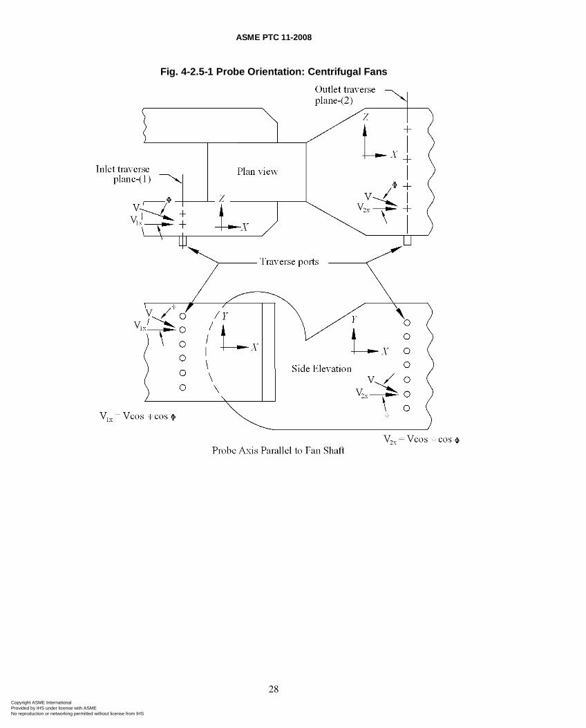
ASME PTC 11-2008

28

Fig. 4-2.5-1 Probe Orientation: Centrifugal Fans


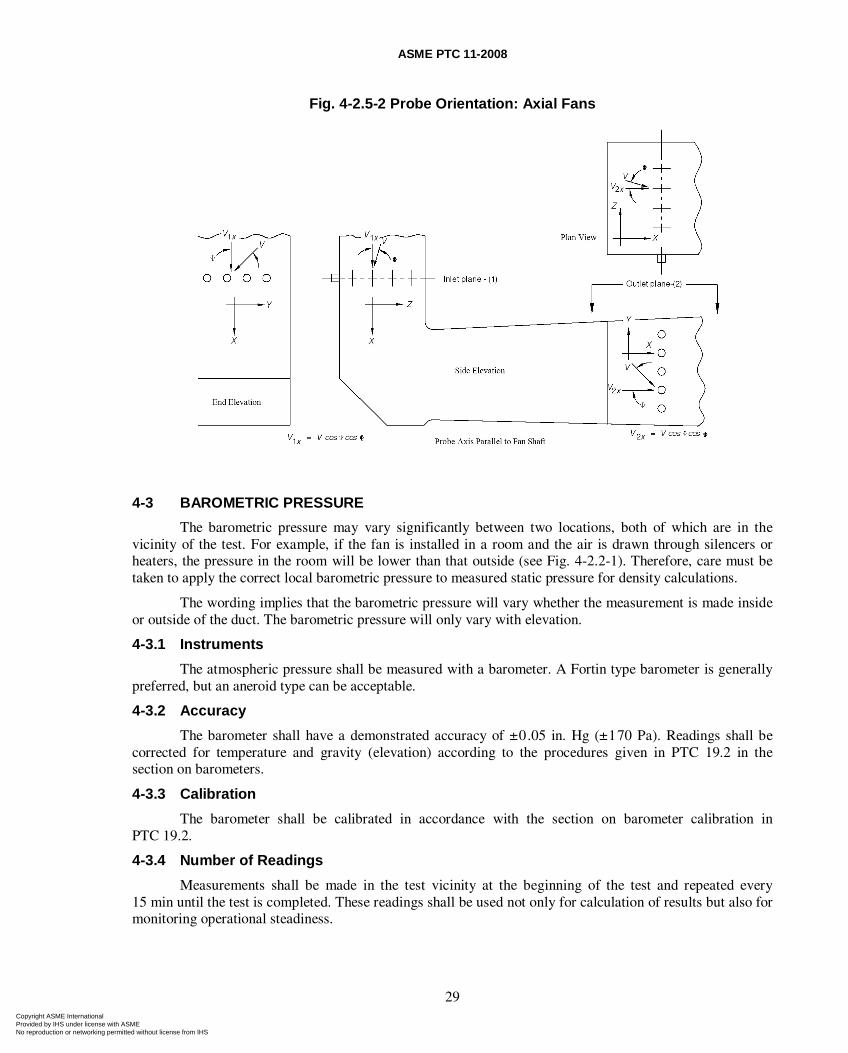
ASME PTC 11-2008

29

Fig. 4-2.5-2 Probe Orientation: Axial Fans

4-3 BAROMETRIC PRESSURE

The barometric pressure may vary significantly between two locations, both of which are in the vicinity of the test. For example, if the fan is installed in a room and the air is drawn through silencers or heaters, the pressure in the room will be lower than that outside (see Fig. 4-2.2-1). Therefore, care must be taken to apply the correct local barometric pressure to measured static pressure for density calculations.

The wording implies that the barometric pressure will vary whether the measurement is made inside or outside of the duct. The barometric pressure will only vary with elevation.

4-3.1 Instruments

The atmospheric pressure shall be measured with a barometer. A Fortin type barometer is generally preferred, but an aneroid type can be acceptable.

4-3.2 Accuracy

The barometer shall have a demonstrated accuracy of ±0.05 in. Hg (±170 Pa). Readings shall be corrected for temperature and gravity (elevation) according to the procedures given in PTC 19.2 in the section on barometers.

4-3.3 Calibration

The barometer shall be calibrated in accordance with the section on barometer calibration in PTC 19.2.

4-3.4 Number of Readings

Measurements shall be made in the test vicinity at the beginning of the test and repeated every 15 min until the test is completed. These readings shall be used not only for calculation of results but also for monitoring operational steadiness.


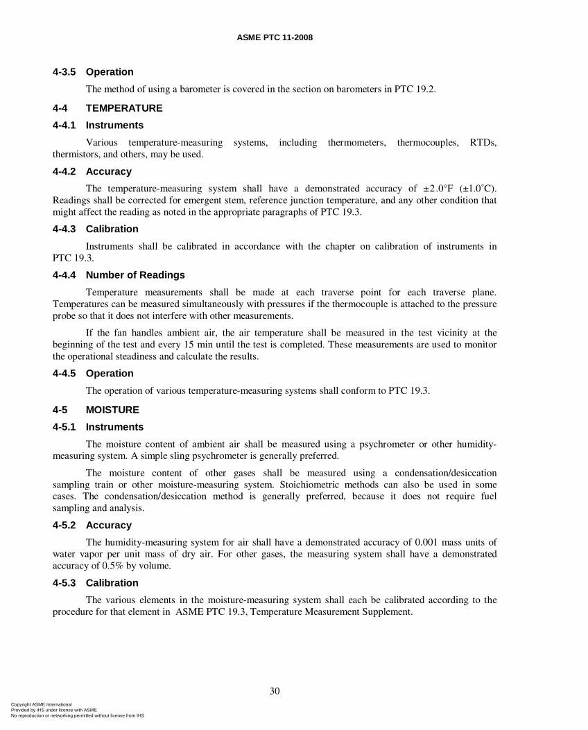
ASME PTC 11-2008

30

4-3.5 Operation

The method of using a barometer is covered in the section on barometers in PTC 19.2.

4-4 TEMPERATURE

4-4.1 Instruments

Various temperature-measuring systems, including thermometers, thermocouples, RTDs, thermistors, and others, may be used.

4-4.2 Accuracy

The temperature-measuring system shall have a demonstrated accuracy of ±2.0°F (±l.0˚C). Readings shall be corrected for emergent stem, reference junction temperature, and any other condition that might affect the reading as noted in the appropriate paragraphs of PTC 19.3.

4-4.3 Calibration

Instruments shall be calibrated in accordance with the chapter on calibration of instruments in PTC 19.3.


Temperature measurements shall be made at each traverse point for each traverse plane. Temperatures can be measured simultaneously with pressures if the thermocouple is attached to the pressure probe so that it does not interfere with other measurements.

If the fan handles ambient air, the air temperature shall be measured in the test vicinity at the beginning of the test and every 15 min until the test is completed. These measurements are used to monitor the operational steadiness and calculate the results.

4-4.5 Operation

The operation of various temperature-measuring systems shall conform to PTC 19.3.

4-5 MOISTURE

4-5.1 Instruments

The moisture content of ambient air shall be measured using a psychrometer or other humidity-measuring system. A simple sling psychrometer is generally preferred.

The moisture content of other gases shall be measured using a condensation/desiccation sampling train or other moisture-measuring system. Stoichiometric methods can also be used in some cases. The condensation/desiccation method is generally preferred, because it does not require fuel sampling and analysis.

4-5.2 Accuracy

The humidity-measuring system for air shall have a demonstrated accuracy of 0.001 mass units of water vapor per unit mass of dry air. For other gases, the measuring system shall have a demonstrated accuracy of 0.5% by volume.

4-5.3 Calibration

The various elements in the moisture-measuring system shall each be calibrated according to the procedure for that element in ASME PTC 19.3, Temperature Measurement Supplement.


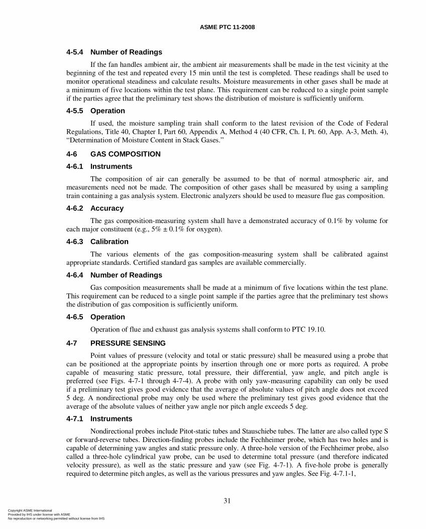
ASME PTC 11-2008

31


If the fan handles ambient air, the ambient air measurements shall be made in the test vicinity at the beginning of the test and repeated every 15 min until the test is completed. These readings shall be used to monitor operational steadiness and calculate results. Moisture measurements in other gases shall be made at a minimum of five locations within the test plane. This requirement can be reduced to a single point sample if the parties agree that the preliminary test shows the distribution of moisture is sufficiently uniform.

4-5.5 Operation

If used, the moisture sampling train shall conform to the latest revision of the Code of Federal Regulations, Title 40, Chapter I, Part 60, Appendix A, Method 4 (40 CFR, Ch. I, Pt. 60, App. A-3, Meth. 4), “Determination of Moisture Content in Stack Gases.”

4-6 GAS COMPOSITION

4-6.1 Instruments

The composition of air can generally be assumed to be that of normal atmospheric air, and measurements need not be made. The composition of other gases shall be measured by using a sampling train containing a gas analysis system. Electronic analyzers should be used to measure flue gas composition.

4-6.2 Accuracy

The gas composition-measuring system shall have a demonstrated accuracy of 0.1% by volume for each major constituent (e.g., 5% ± 0.1% for oxygen).

4-6.3 Calibration

The various elements of the gas composition-measuring system shall be calibrated against appropriate standards. Certified standard gas samples are available commercially.


Gas composition measurements shall be made at a minimum of five locations within the test plane. This requirement can be reduced to a single point sample if the parties agree that the preliminary test shows the distribution of gas composition is sufficiently uniform.

4-6.5 Operation

Operation of flue and exhaust gas analysis systems shall conform to PTC 19.10.

4-7 PRESSURE SENSING

Point values of pressure (velocity and total or static pressure) shall be measured using a probe that can be positioned at the appropriate points by insertion through one or more ports as required. A probe capable of measuring static pressure, total pressure, their differential, yaw angle, and pitch angle is preferred (see Figs. 4-7-1 through 4-7-4). A probe with only yaw-measuring capability can only be used if a preliminary test gives good evidence that the average of absolute values of pitch angle does not exceed 5 deg. A nondirectional probe may only be used where the preliminary test gives good evidence that the average of the absolute values of neither yaw angle nor pitch angle exceeds 5 deg.

4-7.1 Instruments

Nondirectional probes include Pitot-static tubes and Stauschiebe tubes. The latter are also called type S or forward-reverse tubes. Direction-finding probes include the Fechheimer probe, which has two holes and is capable of determining yaw angles and static pressure only. A three-hole version of the Fechheimer probe, also called a three-hole cylindrical yaw probe, can be used to determine total pressure (and therefore indicated velocity pressure), as well as the static pressure and yaw (see Fig. 4-7-1). A five-hole probe is generally required to determine pitch angles, as well as the various pressures and yaw angles. See Fig. 4-7.1-1,


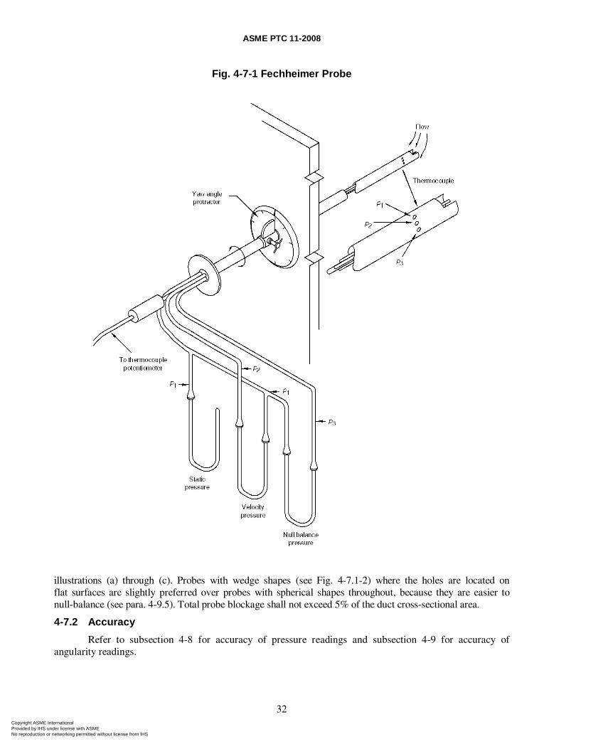
ASME PTC 11-2008

32

Fig. 4-7-1 Fechheimer Probe

illustrations (a) through (c). Probes with wedge shapes (see Fig. 4-7.1-2) where the holes are located on flat surfaces are slightly preferred over probes with spherical shapes throughout, because they are easier to null-balance (see para. 4-9.5). Total probe blockage shall not exceed 5% of the duct cross-sectional area.

4-7.2 Accuracy

Refer to subsection 4-8 for accuracy of pressure readings and subsection 4-9 for accuracy of angularity readings.


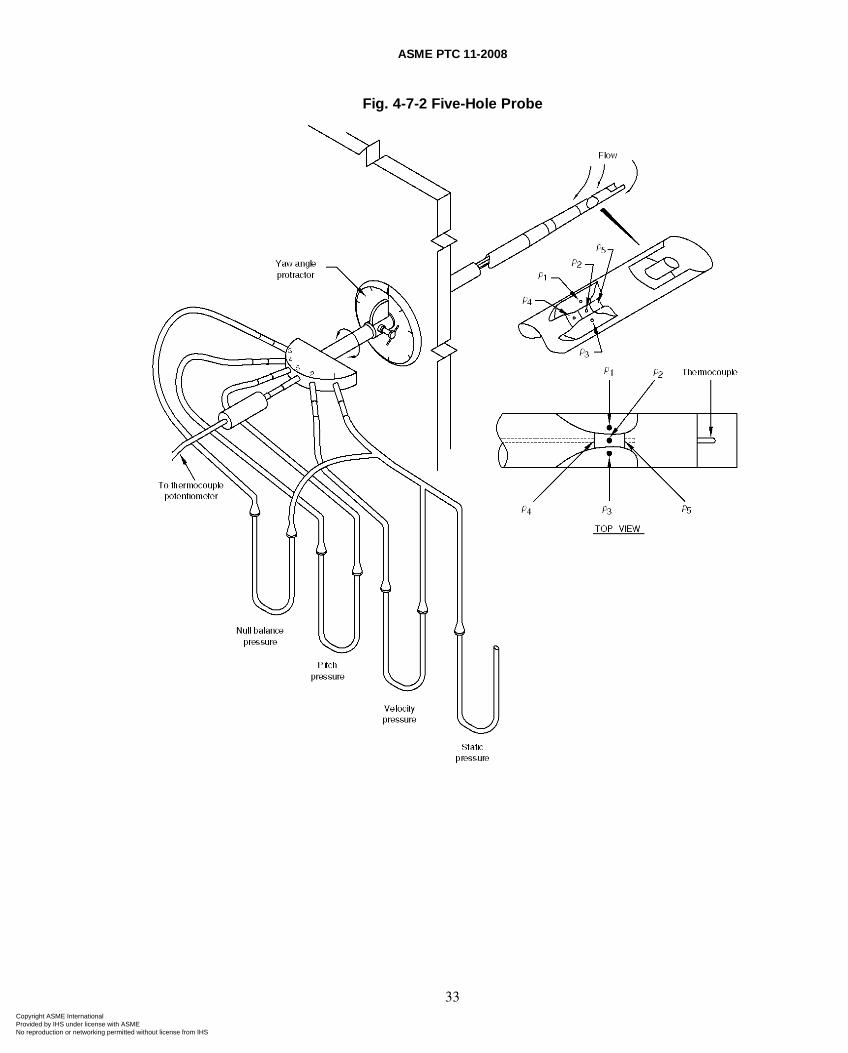
ASME PTC 11-2008

33

Fig. 4-7-2 Five-Hole Probe


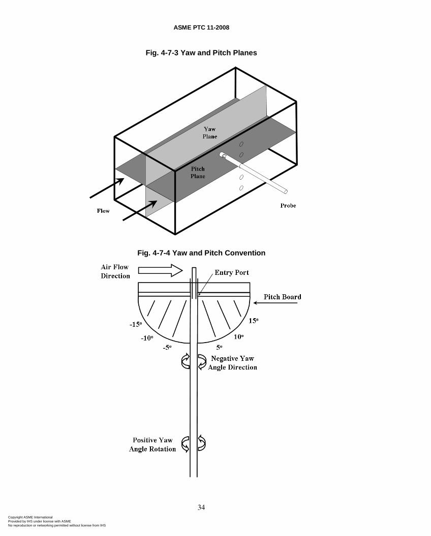
ASME PTC 11-2008

34

Fig. 4-7-3 Yaw and Pitch Planes

Fig. 4-7-4 Yaw and Pitch Convention


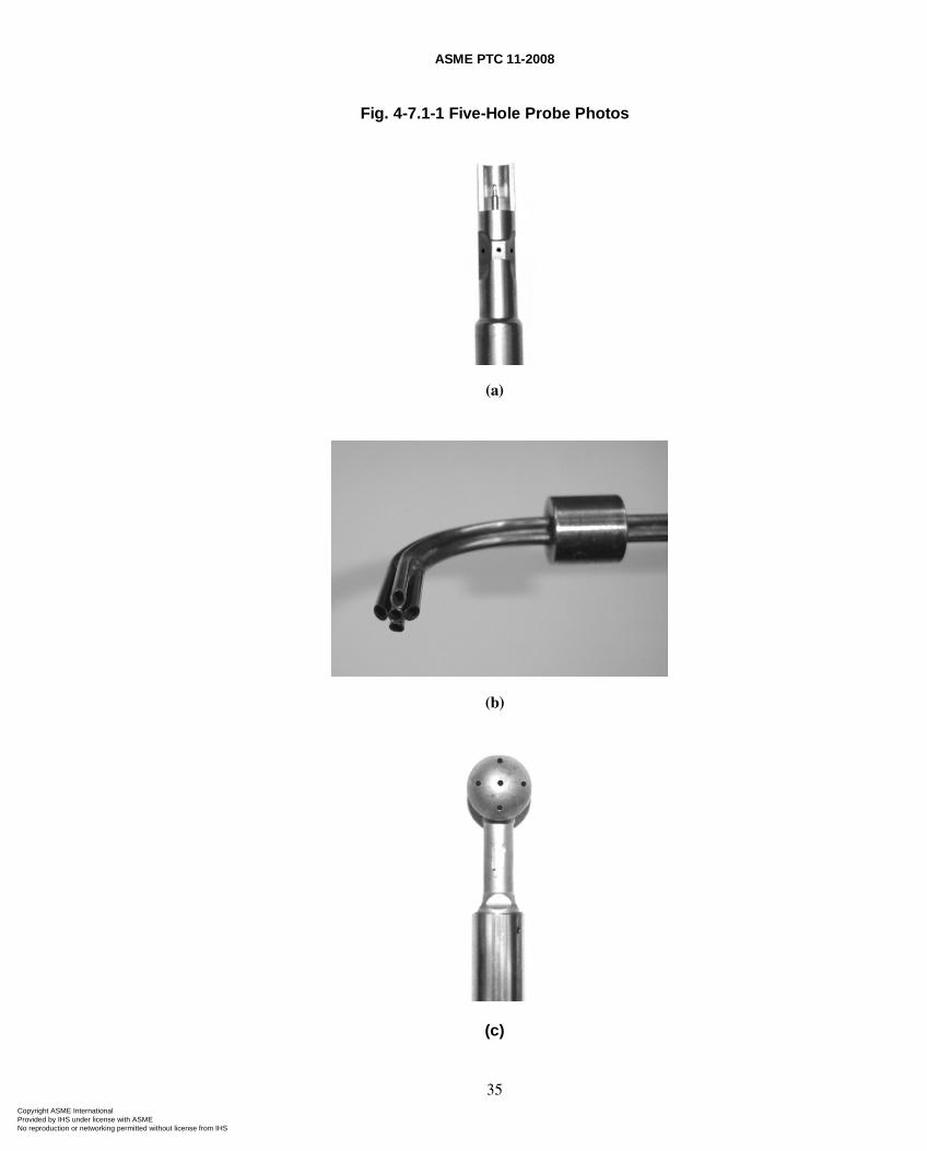
ASME PTC 11-2008

35

Fig. 4-7.1-1 Five-Hole Probe Photos

(a)

(b)

(c)


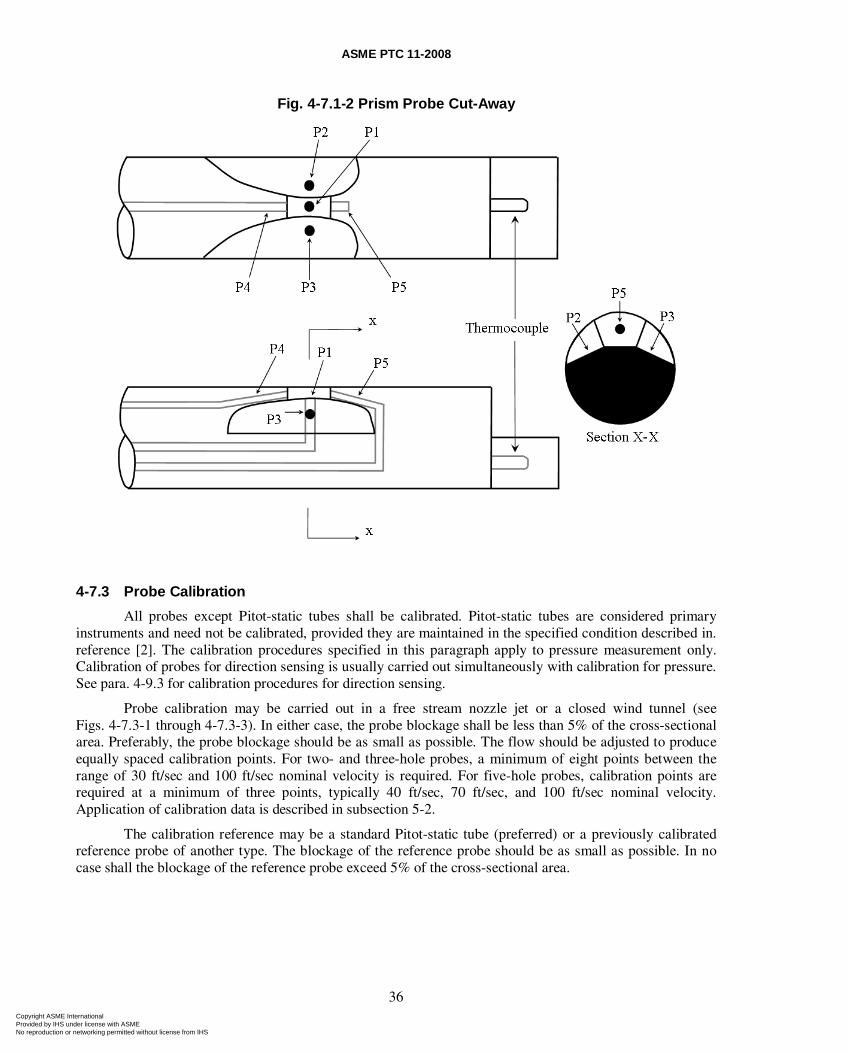
ASME PTC 11-2008

36

Fig. 4-7.1-2 Prism Probe Cut-Away

4-7.3 Probe Calibration

All probes except Pitot-static tubes shall be calibrated. Pitot-static tubes are considered primary instruments and need not be calibrated, provided they are maintained in the specified condition described in. reference [2]. The calibration procedures specified in this paragraph apply to pressure measurement only. Calibration of probes for direction sensing is usually carried out simultaneously with calibration for pressure. See para. 4-9.3 for calibration procedures for direction sensing.

Probe calibration may be carried out in a free stream nozzle jet or a closed wind tunnel (see Figs. 4-7.3-1 through 4-7.3-3). In either case, the probe blockage shall be less than 5% of the cross-sectional area. Preferably, the probe blockage should be as small as possible. The flow should be adjusted to produce equally spaced calibration points. For two- and three-hole probes, a minimum of eight points between the range of 30 ft/sec and 100 ft/sec nominal velocity is required. For five-hole probes, calibration points are required at a minimum of three points, typically 40 ft/sec, 70 ft/sec, and 100 ft/sec nominal velocity. Application of calibration data is described in subsection 5-2.

The calibration reference may be a standard Pitot-static tube (preferred) or a previously calibrated reference probe of another type. The blockage of the reference probe should be as small as possible. In no case shall the blockage of the reference probe exceed 5% of the cross-sectional area.


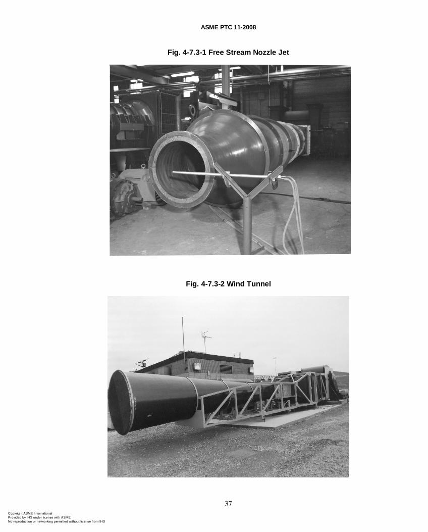
ASME PTC 11-2008

37

Fig. 4-7.3-1 Free Stream Nozzle Jet

Fig. 4-7.3-2 Wind Tunnel


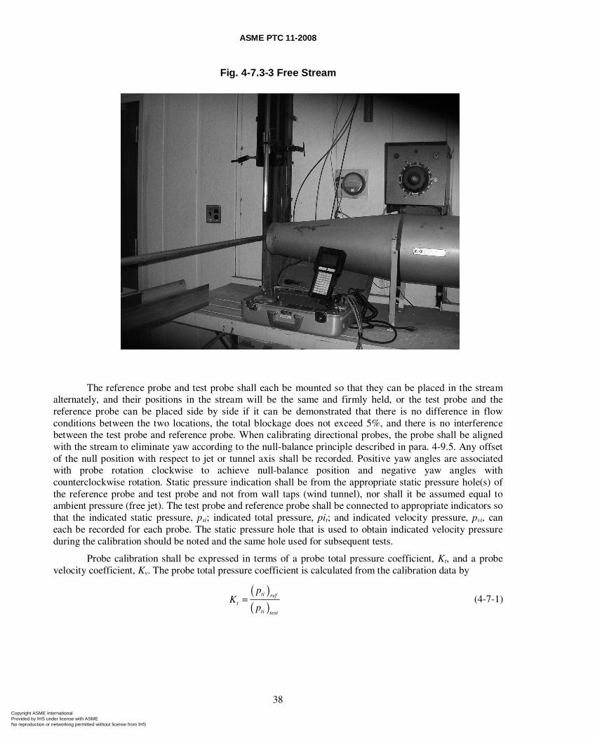
ASME PTC 11-2008

38

Fig. 4-7.3-3 Free Stream

The reference probe and test probe shall each be mounted so that they can be placed in the stream alternately, and their positions in the stream will be the same and firmly held, or the test probe and the reference probe can be placed side by side if it can be demonstrated that there is no difference in flow conditions between the two locations, the total blockage does not exceed 5%, and there is no interference between the test probe and reference probe. When calibrating directional probes, the probe shall be aligned with the stream to eliminate yaw according to the null-balance principle described in para. 4-9.5. Any offset of the null position with respect to jet or tunnel axis shall be recorded. Positive yaw angles are associated with probe rotation clockwise to achieve null-balance position and negative yaw angles with counterclockwise rotation. Static pressure indication shall be from the appropriate static pressure hole(s) of the reference probe and test probe and not from wall taps (wind tunnel), nor shall it be assumed equal to ambient pressure (free jet). The test probe and reference probe shall be connected to appropriate indicators so that the indicated static pressure, psi; indicated total pressure, pit; and indicated velocity pressure, pvi, can each be recorded for each probe. The static pressure hole that is used to obtain indicated velocity pressure during the calibration should be noted and the same hole used for subsequent tests.

Probe calibration shall be expressed in terms of a probe total pressure coefficient, Kt, and a probe velocity coefficient, Kv. The probe total pressure coefficient is calculated from the calibration data by

( )( )

ti reft

ti test

pK

p= (4-7-1)


ASME PTC 11-2008

39

The probe velocity pressure coefficient is calculated from the test data by

( )( )

( )( )

( )( )

( )( )

1

1

1

1

1

11

v vref ref

v ref vref test

v

test v vref ref

v ref vref test

K p

K pK

K p

K p

β

ββ

⎛ ⎞⎛ ⎞⎜ ⎟⎜ ⎟⎜ ⎟⎜ ⎟+ ⎝ ⎠⎝ ⎠=⎛ ⎞⎛ ⎞

− ⎜ ⎟⎜ ⎟⎜ ⎟⎜ ⎟+ ⎝ ⎠⎝ ⎠

(4-7-2)

where

( )( )( )

1

4 1 3D p p

p

C S

C

εβ

ε− ⎛ ⎞

= ± ⎜ ⎟− − ⎝ ⎠ (4-7-3)

and

( )( ) ( )

( )1 1

2

v viref refp

sa ref

K p

k pε

⎡ ⎤ ⎡ ⎤− = − ⎢ ⎥ ⎢ ⎥

⎣ ⎦ ⎢ ⎥⎣ ⎦ (4-7-4)

NOTE: It is recognized that CD is usually not known to a high degree of accuracy. Lacking specific information, CD ≈ 1.2 for probes of cylindrical shape. For a closed wind tunnel, β will be positive; for a free jet, β will be negative.

The equation for Kv includes a correction for probe blockage derived from the analysis presented in references [15] and [16]. If the reference probe is a Pitot-static tube Kv,ref = 1.0 and the blockage of both the reference probe and test probe is negligible (Sp/C<0.005), the equation for vK assumes the simplified form

( )( )

vi refv

vi test

pK

p= (4-7-5)

Generally, the probe total pressure coefficient and probe velocity pressure coefficient are functions of Reynolds number, Rep, for nondirectional and three-hole probes and functions of pitch pressure coefficient, Cφ, and Reynolds number for five-hole probes. For probes of highly angular shape, such as the prismatic five-hole probe shown in Fig. 4-7.1-2, the coefficients may be expected to be independent of Reynolds number for values of Reynolds number above roughly 104. For such probes, Reynolds number effects on the coefficients may be ignored. See para. 4-1.2 regarding calibration function.

Calibrated probes should be handled with care because large scratches or nicks near the pressure taps will invalidate the calibration. Probe recalibration should be performed on a regular basis but shall be performed if damage near the sensing holes is noted.


Pressure measurements shall be made at each traverse point for each traverse plane. The indicated velocity pressure and either the total pressure or static pressure shall be measured. The remaining pressure can be determined arithmetically.

Pressures can be obtained at two or more locations, simultaneously, by using two or more probes as appropriate. It may be desirable to traverse both inlet boxes of a double inlet fan and to traverse from both sides of the outlet, all simultaneously. This would require four probes and four probe crews, but it would significantly reduce the total elapsed time required for a test.


ASME PTC 11-2008

40

4-7.5 Operation

Refer to paras. 4-8.5 and 4-9.5.

4-8 PRESSURE INDICATING

4-8.1 Instruments

Manometers or other pressure-indicating systems shall be connected to the appropriate taps of the pressure-sensing probes to measure point values of pressure. A five-hole probe requires one indicator for velocity pressure, one indicator for static pressure or total pressure, and additional indicators for nulling and pitch determination (see subsection 4-9 for the latter). A three-hole probe requires the same indicators, except for pitch determination. A nondirectional probe requires indicators only for velocity pressure and either static or total pressure. Pressure transducers are generally preferred, but inclined manometers, U-tube manometers, and other indicators are acceptable if they meet the following specifications.

4-8.2 Accuracy

Pressure-measuring systems including the sensor and indicator shall have a demonstrated accuracy of ±1% of the reading or 0.01 in. wg (2.5 Pa), whichever is larger. Readings shall be corrected for any difference from calibration conditions in specific weight of manometer fluid, gas column balancing effect, or any change in length of the graduated scale due to temperature. However, corrections may be omitted for temperature changes less than 10ºF (5ºC) from calibration and elevation changes less than 5,000 ft (1 500 m).

4-8.3 Calibration

Pressure-indicating instruments shall be calibrated against a suitable standard for pressures from 0 in. wg to 10 in. wg (0 kPa to 2.5 kPa), gage of the micrometer type, or a precision micromanometer. When the pressure is above 10 in. wg (2.5 kPa), calibration shall be against a water-filled hook gage of the micrometer type, a precision micromanometer, or water-filled U-tube. Pressure-indicating instruments should preferably be calibrated in place, but the parties may agree to a remote calibration in a more suitable laboratory environment. In the latter case, extreme care should be taken to mount the pressure-indicating instrument in exactly the same manner for calibration as it is mounted for the test. Calibration points shall be selected to fall at both ends of the expected range and at sufficient intermediate points so that no reading will be more than 0.25 in. wg (60 Pa) removed from a calibration point for pressures from 0 in. wg to 10 in. wg (0 kPa to 2.5 kPa) or more than 1 in. wg (250 Pa) removed for pressures above 10 in. wg (2.5 kPa).

4-8.4 Averaging Fluctuating Readings

Pressure-measuring instruments shall be read at each position of the probe as outlined in para. 4-7.4. Since pressures are seldom strictly steady, the pressure indicated on any instrument will fluctuate with time. To obtain a reading, either the instrument shall be damped or the readings shall be averaged in a suitable manner. Averaging can be accomplished mentally, if the fluctuations are small and regular. If the fluctuations are large and irregular, more sophisticated methods shall be used. It is possible to obtain a temporal average electronically when an electrical pressure transducer is the primary element. Even though the spatial average velocity is obtained from the square roots of the temporal average velocity pressures, it is not proper to take the square root of the raw data before temporal averaging, as this may introduce a bias into the average values [10].

4-8.5 Operation

For many of the principles of operation, refer to PTC 19.2. Refer to Figs. 4-7-1 and 4-7-2 for the proper hose connecting arrangements for probes and indicators. Precautions should be taken to protect the indicator from the effects of wind, sun, and radiant heat. Periodically during the test, probes, hoses, and indicators should be checked for leaks or plugging. Plugging can result from either particulate buildup in the probe or condensation in a portion of the system.


ASME PTC 11-2008

41

Indicators used for static or total pressure measurement have one tap open to atmosphere. If the indicator is not located in the same atmosphere as the barometer, an additional measurement to determine the difference in pressure is required.

4-9 YAW AND PITCH

4-9.1 Instruments

Yaw angle shall be measured using a directional probe equipped with a suitable indicating device. Pitch shall be determined from directional probe calibration. A five-hole probe is preferred as noted in para. 4-7.1. A three-hole probe may be suitable in some cases (see Figs.4-7-1 and 4-7-2).

4-9.2 Accuracy

The yaw- and pitch-measuring systems shall have demonstrated accuracies of ±2 deg.

4-9.3 Calibration

A reference line shall be scribed along the probe axis prior to calibration for pressure response. This reference line is typically aligned with, or 180 deg from, the total pressure-sensing hole. The scribe is used as a reference position for installation of a yaw angle-measuring device. The relationship of the reference line to null-balance position shall be known as determined in para. 4-7.3. The probe is then equipped with a protractor scale that can be checked against any high-quality protractor used as a reference. As noted below, the protractor arrangement is only used to measure yaw.

Calibration for pitch can be performed in a free stream nozzle jet or in a wind tunnel and is usually completed during calibrations outlined in para. 4-7.3. The facility should be equipped to allow the test probe to be positioned at various pitch angles. The mounting apparatus should firmly hold the test probe at each location along the pitch arc. Probe sensing head location should remain in the same position within the flow stream as the probe pitch angle is varied.

The probe shall be precision aligned at various pitch angles, null-balanced, and the pressure difference across the taps for the fourth and fifth holes recorded along with pressures and pressure differences required in para. 4-7.3 and any null-balance offset. Pressure data shall be recorded at pitch angles from –30 deg to +30 deg in 5-deg increments at each of three nominal velocities as described in para. 4-7.3. The calibration facility flow should be set at one nominal velocity and data recorded at each required pitch angle before proceeding to subsequent nominal velocities and repeating. Alternatively, the nominal velocity can be set at required values for each probe pitch position to develop the data set.

Calibration functions, which represent pitch angle and probe coefficient(s) as a function of pitch pressure coefficient, CΦ ( ≡ pitch pressure difference/indicated velocity pressure), and Reynolds number may be derived. For probes of highly angular shape, such as the prismatic five-hole probe, the pitch angle-pitch pressure coefficient relationship may be expected to be independent of Reynolds number for values of Reynolds number above roughly 104. For such probes, Reynolds number effects may be ignored (see Figs. 4-9.3-1 through 4-9.3-3).


Yaw and pitch angles shall be determined at each traverse point for each traverse plane. This is the same requirement as for pressures that should be measured simultaneously.

4-9.5 Operation

In operation, a five-hole probe is inserted in the proper port to the proper depth for each traverse point. The probe should be rigid enough over its inserted length to avoid any droop beyond the permissible amount as noted in para. 4-2.4. The reference line on the probe should be used to orient the probe in such a way that when the total pressure hole is pointing upstream perpendicular to the measuring plane, the indicated yaw angle is zero. The probe is then rotated about its own axis until a null balance is obtained


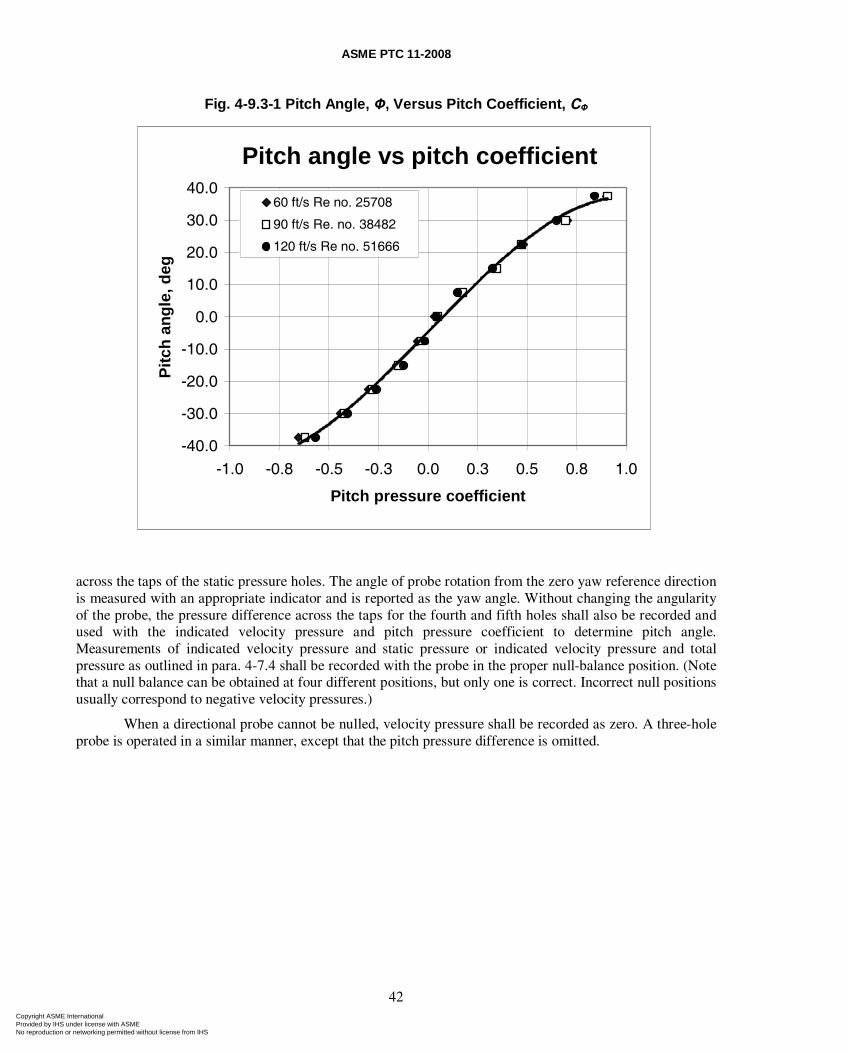
ASME PTC 11-2008

42

Fig. 4-9.3-1 Pitch Angle, Ф, Versus Pitch Coefficient, CФ

Pitch angle vs pitch coefficient

-40.0

-30.0

-20.0

-10.0

0.0

10.0

20.0

30.0

40.0

-1.0 -0.8 -0.5 -0.3 0.0 0.3 0.5 0.8 1.0

Pitch pressure coefficient

Pit

ch a

ng

le, d

eg

60 ft/s Re no. 25708

90 ft/s Re. no. 38482

120 ft/s Re no. 51666

across the taps of the static pressure holes. The angle of probe rotation from the zero yaw reference direction is measured with an appropriate indicator and is reported as the yaw angle. Without changing the angularity of the probe, the pressure difference across the taps for the fourth and fifth holes shall also be recorded and used with the indicated velocity pressure and pitch pressure coefficient to determine pitch angle. Measurements of indicated velocity pressure and static pressure or indicated velocity pressure and total pressure as outlined in para. 4-7.4 shall be recorded with the probe in the proper null-balance position. (Note that a null balance can be obtained at four different positions, but only one is correct. Incorrect null positions usually correspond to negative velocity pressures.)

When a directional probe cannot be nulled, velocity pressure shall be recorded as zero. A three-hole probe is operated in a similar manner, except that the pitch pressure difference is omitted.


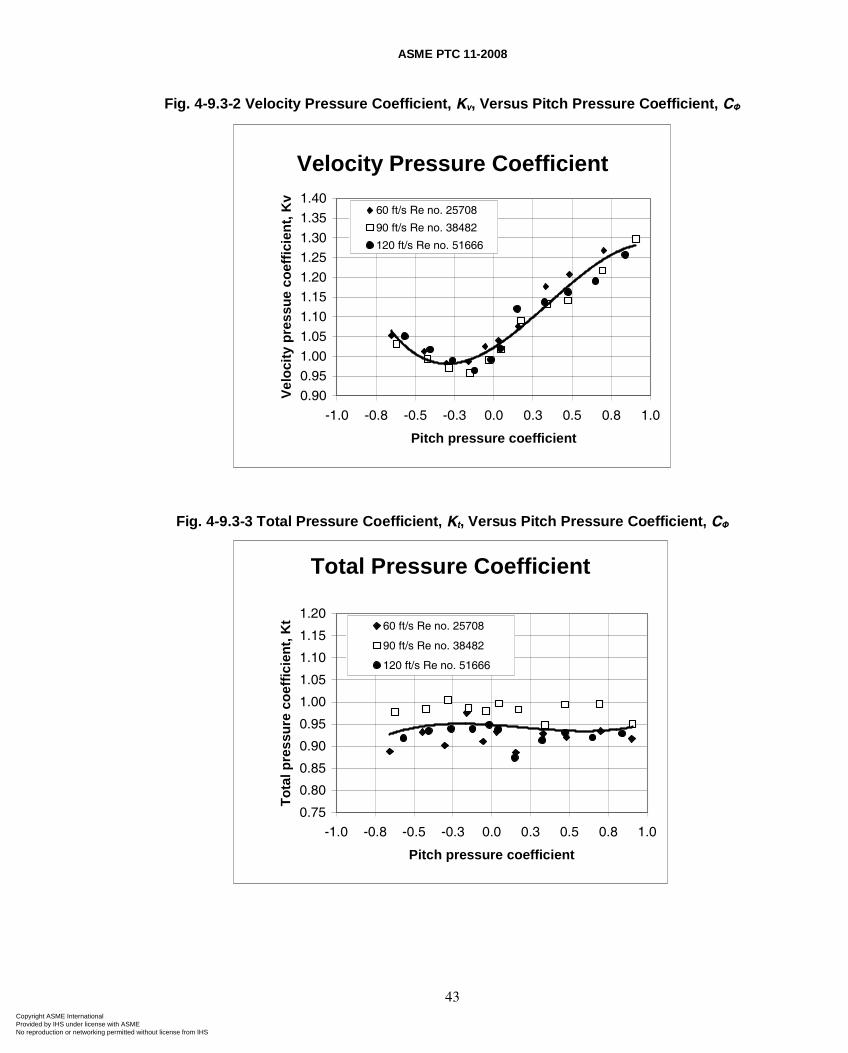
ASME PTC 11-2008

43

Fig. 4-9.3-2 Velocity Pressure Coefficient, Kv, Versus Pitch Pressure Coefficient, CФ

Velocity Pressure Coefficient

0.90

0.95

1.00

1.05

1.10

1.15

1.20

1.25

1.30

1.35

1.40

-1.0 -0.8 -0.5 -0.3 0.0 0.3 0.5 0.8 1.0


Vel

oci

ty p

ress

ue

coef

fici

ent,

Kv

60 ft/s Re no. 25708

90 ft/s Re no. 38482

120 ft/s Re no. 51666

Fig. 4-9.3-3 Total Pressure Coefficient, Kt, Versus Pitch Pressure Coefficient, CФ

Total Pressure Coefficient

0.75

0.80

0.85

0.90

0.95

1.00

1.05

1.10

1.15

1.20

-1.0 -0.8 -0.5 -0.3 0.0 0.3 0.5 0.8 1.0


To

tal p

ress

ure

co

effi

cien

t, K

t 60 ft/s Re no. 25708

90 ft/s Re no. 38482

120 ft/s Re no. 51666


ASME PTC 11-2008

44

4-10 ROTATIONAL SPEED

4-10.1 Instruments

The speed of the fan shall be measured with a speed-measuring system. An electronic counter actuated by a magnetic pulse generator or photoelectric pickup is preferred. Slip counting with stroboscopic light may be acceptable for speeds close to line frequency synchronous speeds. Hand tachometers, mechanical revolution counters, and vibrating-reed tachometers are unacceptable.

4-10.2 Accuracy

Speed-measuring instruments shall be calibrated against the line frequency of a suitable major power circuit or other frequency standard.


Fan speed shall be measured at the beginning of the test and every 15 min until the conclusion of the test. These readings shall be used to monitor operational steadiness as well as for calculations.

4-10.4 Operation

The electronic counter should be equipped with a digital readout and may be equipped with a recorder and an automatic average.

With the slip method, the shaft must be marked with a reference line or other mark that is easily visible under stroboscopic light flashing at line frequency. The mark will appear to slowly rotate opposite shaft rotation and permit visual observation of the slip frequency. A stopwatch shall be used to measure the time for at least ten rotations of the mark. Average slip frequency is derived by dividing the total number of mark rotations by the measured time interval for which the counts were made.

See PTC 19.13 for further information on the measurement of rotary speed.

4-11 INPUT POWER

4-11.1 Instruments

The fan input power shall be derived from measurements of torque with a torque meter, measurements of electrical input when a calibrated electric motor is used, or other suitable measurements if the fan is driven by some other calibrated prime mover and drive train. Both the torque meter and calibrated prime mover measurements qualify as preferred methods. If a torque meter cannot be used and if the drive train is not calibrated prior to installation, the parties to the test must agree upon a method of estimating the drive train losses. Also, it must be noted that various methods and procedures for calibrating the drive train may result in accuracies that are unacceptable for this Code. The parties to the test and party responsible for the calibration must agree beforehand to the method of calibration and expected accuracy. (PTC 19.7-1980 and relevant IEEE standards, such as IEEE 112, may offer some insight.)

Since the temperature rise through a fan is generally not large enough to permit accurate measurement and heat transfer losses through the casing are indeterminate, the heat balance method is not acceptable for determining fan input power.

4-11.2 Accuracy

The input power-measuring system shall have a demonstrated accuracy of ±1%.

4-11.3 Calibration

A torque meter shall be calibrated in accordance with the provisions of PTC 19.7. The drive train in the context of this Code includes the driver, whether it is an electric motor, steam turbine, or other prime mover, and any in intermediate elements, such as gear boxes and variable speed drives. The drive train may


ASME PTC 11-2008

45

be calibrated as a unit, or the driver and any intermediate elements may be separately calibrated. Calibration procedures as given in ASME PTC 19.7 and the following IEEE standards should be followed.

Designator Title IEEE 112 Test procedure for polyphase induction motors and generators IEEE 113 Test procedure for DC machines IEEE 114 Standard test procedures for single-phase induction motors IEEE 115 Test procedure for synchronous machines

Calibration shall be performed under specified operating conditions and a range of loads sufficient to cover the anticipated test conditions.


Torque or electrical input shall be measured at the start of the test and at least every 15 min until the conclusion of the test. These readings shall be used to monitor operational steadiness, as well as for calculations.

4-11.5 Operation

Operation of prime movers is covered in the various Standards listed in para. 4-11.3. Operation of the instruments for measuring the output of these prime movers is covered in various supplements on instruments and apparatuses. Electrical instruments shall conform to ASME PTC 19.22. A wattmeter and voltmeter or an ammeter, voltmeter, and power factor meter may be used together with the necessary instrument transformers. Of the above-mentioned devices, a wattmeter with appropriate current and voltage transformers is preferred. Refer to PTC 19.6, Electrical Power Measurements, for instructions. Meter ranges and transformer ratio shall be such as to produce readings above one-third full scale. Instruments shall have full-scale accuracy of 0.5% or better. They shall be used in the same position as rated (usually horizontal). Care should be taken to maintain instruments at a uniform and constant temperature near the calibration temperature; otherwise, corrections shall be made according to manufacturer’s instructions regarding lead wires, waveform, etc.

The preferred location for taking electrical measurement is at the terminals of the motor. If this is not possible, then allowance shall be made for the drop in potential between the point of measurement and the motor terminals. Care shall be taken to measure motor power only and not include any auxiliary’s power.

When fan speed is controlled by a variable frequency drive or a hydraulic coupling, accurate determination of fan input power by electrical means is impractical, and a torque meter is the preferred method of power measurement.

For fans driven by steam or gas turbines, or other nonelectric means, the torque meter is again the preferred method of power measurement.

For a summary of instrumentation requirements, see Table 4-11.5-1.


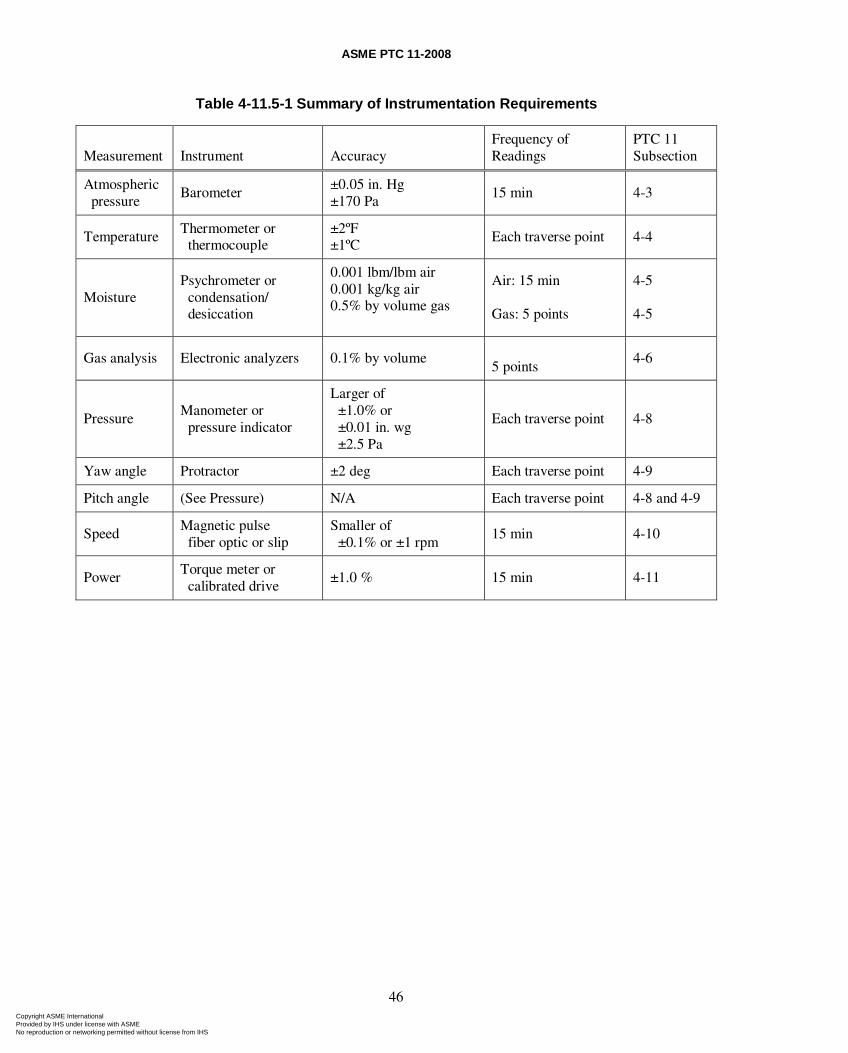
ASME PTC 11-2008

46

Table 4-11.5-1 Summary of Instrumentation Requirements

Measurement

Instrument

Accuracy

Frequency of Readings

PTC 11 Subsection

Atmospheric pressure

Barometer ±0.05 in. Hg ±170 Pa

15 min 4-3

Temperature Thermometer or thermocouple

±2ºF ±1ºC

Each traverse point 4-4

Moisture Psychrometer or condensation/ desiccation

0.001 lbm/lbm air 0.001 kg/kg air 0.5% by volume gas

Air: 15 min Gas: 5 points

4-5 4-5

Gas analysis Electronic analyzers 0.1% by volume 5 points

4-6

Pressure Manometer or pressure indicator

Larger of ±1.0% or ±0.01 in. wg ±2.5 Pa

Each traverse point 4-8

Yaw angle Protractor ±2 deg Each traverse point 4-9

Pitch angle (See Pressure) N/A Each traverse point 4-8 and 4-9

Speed Magnetic pulse fiber optic or slip

Smaller of ±0.1% or ±1 rpm

15 min 4-10

Power Torque meter or calibrated drive

±1.0 % 15 min 4-11


ASME PTC 11-2008

47

Section 5 Computation of Results

5-1 GENERAL CONSIDERATIONS

The results of the test shall be calculated in accordance with the appropriate paragraphs of this Section and any prior agreement reached by the parties regarding computation of results. The following paragraphs are intended to cover all possible cases, but it is not necessary to use every paragraph for any particular case (i.e., it is not necessary to refer to the paragraphs on products of combustion if the test gas is air). Similarly, only the paragraphs on computing power that correspond to the method of power measurement shall be used. Various other calculations may be omitted depending on whether mass flow rate and specific energy or volume flow rate and fan total pressure are used to express fan performance. The data to be used in the calculations are the measured values of pressure and temperature at various planes, the fan input power measurements, various geometric information (primarily duct areas at measurement planes), and information used to determine gas composition.

This Section provides the equations for calculating test results and uncertainty. These equations can be used directly; however, incorporating them into a spreadsheet or other computer program together with the test data is recommended because of the complexity involved.

5-1.1 Calibration Corrections

Temporal averaging shall be performed prior to correcting for calibrations. Calibration corrections shall be applied to individual readings before spatial averaging or other calculations.

5-1.2 Average Values

Nonuniform velocity distribution and temperature or composition stratification are normal on large fans. Therefore, the appropriate volume-flow-weighted or mass-flow-weighted average values at the traverse planes must be used for determination of fan performance. [17]

5-2 CORRECTION OF TRAVERSE DATA

Difficulties arise in using traverse data in calculations as these data usually must be corrected for probe calibration and possibly for blockage and compressibility as well. The probe calibration coefficients

tK and vK are sometimes functions of the probe Reynolds number Rep, which is determined by actual gas

velocity V, density ρ, and viscosity μ at the probe location. They are also slightly dependent upon specific heat ratio k. As these four quantities are determined only from the measurements themselves, an iteration procedure may be necessary. Such a procedure would be as follows:

(a) Select provisional values of Ktj, Kvj, and k (see para. 5-2.1).

(b) Correct the traverse readings for calibration, and, if necessary, probe blockage and compressibility (see para. 5-2.2)

(c) Proceed with calculations.

(d) After determining gas composition (see subsection 5-3), densities (see subsection 5-4), and velocities (see para. 5-5.1) at all points in a traverse plane, calculate Reynolds number (see para. 5-2.2) at all points, and determine new values of Ktj and Kvj.

(e) If new values of Ktj and Kvj are significantly different from the old values, the process must be repeated.

The probe calibration coefficients are also a function of pitch pressure coefficient, Cφ; however, this dependency does not affect the iteration process.


ASME PTC 11-2008

48

5-2.1 Guideline for Initial Estimation of Probe Coefficient

To begin calculations, initial values of t jK and v jK must be selected. The selection of an appropriate

value makes the calculation procedure converge more rapidly, often making iteration unnecessary. The following are guidelines to help the initial selection of Ktj and Kvj:

(a) For Pitot-static probe, Ktj and Kvj = 1.0 and need not be changed.

(b) For other probes, the Ktj and Kvj versus Rep curves should be relatively flat in the range of interest; hence, any reasonable first estimates of Ktj and Kvj should produce satisfactory results. The following ideas are suggested:

(1) Select the values of Ktj and Kvj at the middle of the range of calibration data

(2) Use an average Ktj and Kvj value based on the calibration data

(3) Estimate Rep from specified fan conditions, and use corresponding Ktj and Kvj values, or

(4) Estimate Rep from a typical point in the traverse data, and use the corresponding Ktj and Kvj values

5-2.2 Correction for Probe Coefficient and Probe Blockage

Measured values from traverse are ti, pvi, and psi or pti. The remaining pressures can be calculated from ti si vip p p= + . Corrected values (subscript j ) at each point shall be obtained from the measured values (subscript i) at that point and probe coefficients Ktj and Kvj using

t j t j t ip K p= (5-2-1)

1

vjvjc

j vj

KK

Kβ=

+ (5-2-2)

sj tj ti vjc vip K p K p= − or

( )s j v jc si v jc t j tip K p K K p= − − (5-2-3)

13sa j s j bp p C p= + (5-2-4)

(1 )v j v jc p vip K pε= − (5-2-5)

(1 )s j i TT T ε= +

where

1i iT t C= + (5-2-6)

βj is used to correct for probe blockage and is calculated by

(1 )

4(1 ) 3D p pj

jp

C S

A

εβ

ε−

=− −

(5-2-7)

In these equations, ( )1 pε− and ( )1 tε+ are compressibility corrections and are calculated by

1

(1 ) 12

v jc vip

sa j

K P

k Pε

⎛ ⎞− = − ⎜ ⎟⎜ ⎟

⎝ ⎠ (5-2-8)


ASME PTC 11-2008

49

and

1

(1 ) 1 0.85 v jc viT

sa j

K Pk

k pε

⎛ ⎞−+ = + ⎜ ⎟⎜ ⎟⎝ ⎠

(5-2-9)

provided that ( /v jc vi sa jK p p ) does not exceed 0.1 (see para. 3-3.6).

NOTE: The recovery factor of the temperature sensor is assumed to be 0.85 [18].

5-3 GAS COMPOSITION

For the purpose of this Code, it is sufficient to use a uniform gas composition and uniform values of molecular weight, specific heats, and viscosity to characterize any particular plane. These values shall be determined by arithmetic averages of gas composition data and the use of arithmetic averages of measured temperatures in the plane in question where temperatures are needed to determine the appropriate gas properties.

5-3.1 Arithmetic Average of Composition and Property Data

The average volume fraction of constituent (X)x at plane x shall be calculated from the point values (X)j using

1

1( ) ( )

n

x jj

X Xn =

= ∑ (5-3-1)

The average temperature xt at plane x (to be used only for purposes of defining gas composition and

properties) shall be calculated from point values jt using

1

1 n

x jj

t tn =

= ∑ (5-3-2)

5-3.2 Molecular Weight and Humidity Ratio

The molecular weight of air is 28.965. The molecular weight of any dry gas, including flue gas Mdg, shall be calculated from the average volume fractions (X)x using

( ) ( ) ( ) ( )2 2 2 44.01 CO 28.01 CO 32 O 28.02 N dgM = + + + + (5-3-3)

The molecular weight of moist gas mgM shall be calculated from

1

118.02

mg

dg

HM

H

M

+=

+ (5-3-4)

The humidity ratio H shall be calculated from the following equations unless a condensation/ desiccation method is used to measure moisture content. In that event, calculations appropriate to the method shall be used.

Saturation vapor pressure ( ewp ) at wt for tw between 32°F and 140°F (0°C to 60°C)

2 3 4 518 19 20 21 22 23 ew w w w w wp C C t C t C t C t C t= + + + + + (5-3-5)


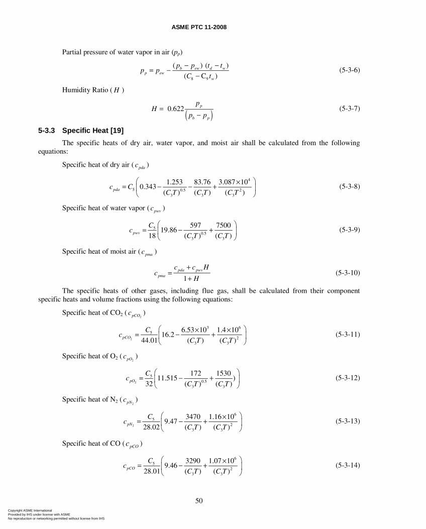
ASME PTC 11-2008

50

Partial pressure of water vapor in air (pp)

8 9

( ) ( )

( C )b ew d w

p eww

p p t tp p

C t

− −= −

− (5-3-6)

Humidity Ratio ( H )

( ) 0.622 p

b p

pH

p p=

− (5-3-7)

5-3.3 Specific Heat [19]

The specific heats of dry air, water vapor, and moist air shall be calculated from the following equations:

Specific heat of dry air ( pdac )

4

5 0.5 23 3 3

1.253 83.76 3.087 100.343

( ) ( ) ( )pdac CC T C T C T

⎛ ⎞×= − − +⎜ ⎟⎝ ⎠

(5-3-8)

Specific heat of water vapor ( pwvc )

50.5

3 3

597 750019.86

18 ( ) ( )pwv

Cc

C T C T

⎛ ⎞= − +⎜ ⎟

⎝ ⎠ (5-3-9)

Specific heat of moist air ( pmac )

1

pda pwvpma

c c Hc

H

+=

+ (5-3-10)

The specific heats of other gases, including flue gas, shall be calculated from their component specific heats and volume fractions using the following equations:

Specific heat of CO2 (2pCOc )

2

3 65

23 3

6.53 10 1.4 1016.2

44.01 ( ) ( )pCO

Cc

C T C T

⎛ ⎞× ×= − +⎜ ⎟⎝ ⎠

(5-3-11)

Specific heat of O2 (2pOc )

2

50.5

3 3

172 153011.515 )

32 ( ) ( )pO

Cc

C T C T

⎛ ⎞= − +⎜ ⎟

⎝ ⎠ (5-3-12)

Specific heat of N2 (2pNc )

2

65

23 3

3470 1.16 109.47

28.02 ( ) ( )pN

Cc

C T C T

⎛ ⎞×= − +⎜ ⎟⎝ ⎠

(5-3-13)

Specific heat of CO ( pCOc )

6

52

3 3

3290 1.07 109.46

28.01 ( ) ( )pCO

Cc

C T C T

⎛ ⎞×= − +⎜ ⎟⎝ ⎠

(5-3-14)


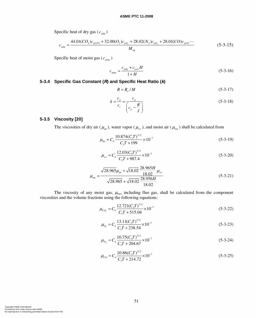
ASME PTC 11-2008

51

Specific heat of dry gas ( pdgc )

2 22 2 2 244.01( ) 32.00( ) 28.02( ) 28.01( )pCO pO pN pCO

pdgdg

CO c O c N c CO cc

M

+ + += (5-3-15)

Specific heat of moist gas ( pmgc )

1

pdg pwvpmg

c c Hc

H

+=

+ (5-3-16)

5-3.4 Specific Gas Constant (R) and Specific Heat Ratio (k)

/oR R M= (5-3-17)

p p

vp

c ck

Rcc

J

= =⎛ ⎞−⎜ ⎟⎝ ⎠

(5-3-18)

5-3.5 Viscosity [20]

The viscosities of dry air ( daμ ), water vapor ( wvμ ), and moist air ( maμ ) shall be calculated from

3/ 2

734

3

10.874( )10

199da

C TC

C Tμ −= ×

+ (5-3-19)

3/ 2

734

3

12.03( )10

987.4wv

C TC

C Tμ −= ×

+ (5-3-20)

28.96528.965 18.02

18.0228.956

28.965 18.0218.02

da wv

ma

H

H

μ μμ

+=

+ (5-3-21)

The viscosity of any moist gas, μmg, including flue gas, shall be calculated from the component viscosities and the volume fractions using the following equations:

2

3/ 273

43

12.721( )10

515.04CO

C TC

C Tμ −= ×

+ (5-3-22)

2

3/ 273

43

13.11( )10

238.54O

C TC

C Tμ −= ×

+ (5-3-23)

2

3/ 273

43

10.75( )10

204.67N

C TC

C Tμ −= ×

+ (5-3-24)

3/ 2

734

3

10.86( )10

214.72CO

C TC

C Tμ −= ×

+ (5-3-25)


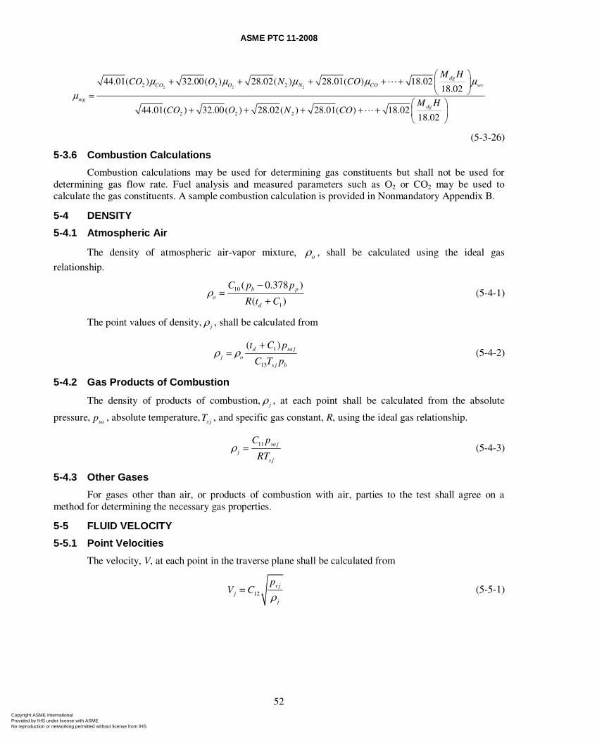
ASME PTC 11-2008

52

2 2 22 2 2

2 2 2

44.01( ) 32.00( ) 28.02( ) 28.01( ) 18.0218.02

44.01( ) 32.00( ) 28.02( ) 28.01( ) 18.0218.02

dgCO O N CO wv

mgdg

M HCO O N CO

M HCO O N CO

μ μ μ μ μμ

⎛ ⎞+ + + + + ⎜ ⎟

⎝ ⎠=⎛ ⎞

+ + + + + ⎜ ⎟⎝ ⎠

(5-3-26)

5-3.6 Combustion Calculations

Combustion calculations may be used for determining gas constituents but shall not be used for determining gas flow rate. Fuel analysis and measured parameters such as O2 or CO2 may be used to calculate the gas constituents. A sample combustion calculation is provided in Nonmandatory Appendix B.

5-4 DENSITY

5-4.1 Atmospheric Air

The density of atmospheric air-vapor mixture, oρ , shall be calculated using the ideal gas

relationship.

10

1

( 0.378 )

( )b p

od

C p p

R t Cρ

−=

+ (5-4-1)

The point values of density, jρ , shall be calculated from

1

13

( )d sa jj o

s j b

t C p

C T pρ ρ

+= (5-4-2)

5-4.2 Gas Products of Combustion

The density of products of combustion, jρ , at each point shall be calculated from the absolute

pressure, sap , absolute temperature, s jT , and specific gas constant, R, using the ideal gas relationship.

11 sa jj

s j

C p

RTρ = (5-4-3)

5-4.3 Other Gases

For gases other than air, or products of combustion with air, parties to the test shall agree on a method for determining the necessary gas properties.

5-5 FLUID VELOCITY

5-5.1 Point Velocities

The velocity, V, at each point in the traverse plane shall be calculated from

12v j

jj

pV C

ρ= (5-5-1)


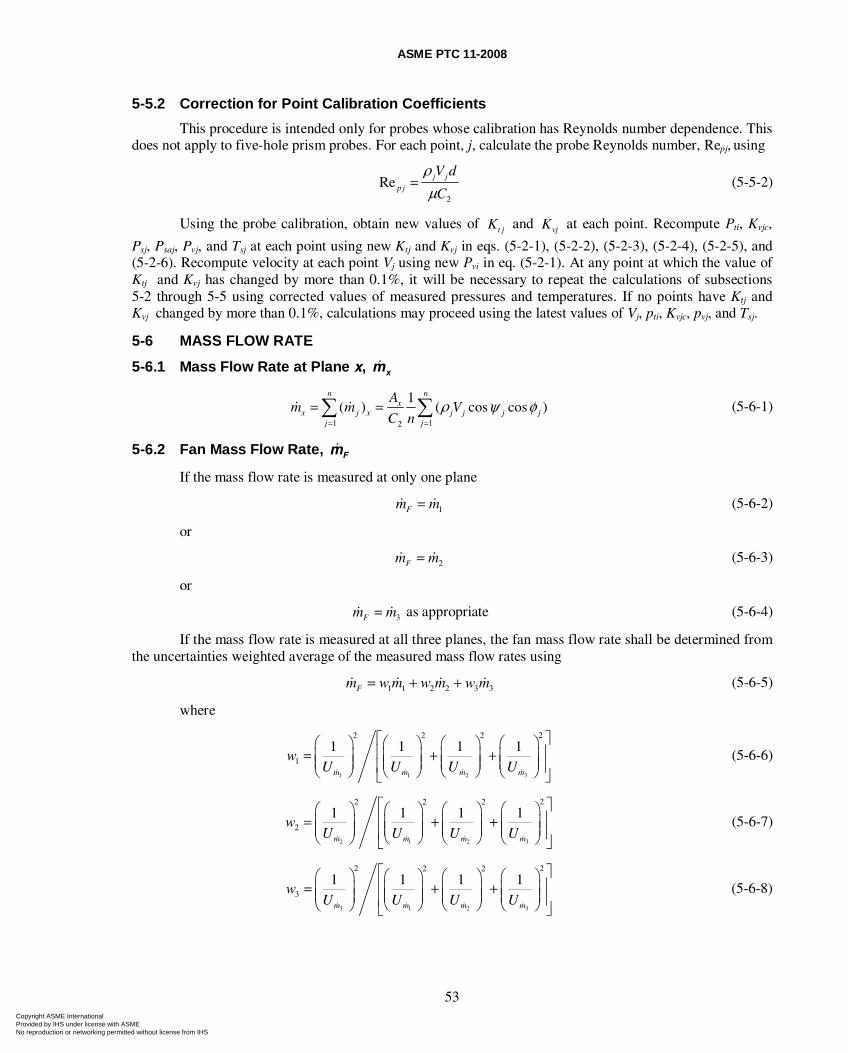
ASME PTC 11-2008

53

5-5.2 Correction for Point Calibration Coefficients

This procedure is intended only for probes whose calibration has Reynolds number dependence. This does not apply to five-hole prism probes. For each point, j, calculate the probe Reynolds number, Repj, using

2

Re j jp j

V d

C

ρμ

= (5-5-2)

Using the probe calibration, obtain new values of t jK and vjK at each point. Recompute Pti, Kvjc,

Psj, Psaj, Pvj, and Tsj at each point using new Ktj and Kvj in eqs. (5-2-1), (5-2-2), (5-2-3), (5-2-4), (5-2-5), and (5-2-6). Recompute velocity at each point Vj using new Pvi in eq. (5-2-1). At any point at which the value of Ktj and Kvj has changed by more than 0.1%, it will be necessary to repeat the calculations of subsections 5-2 through 5-5 using corrected values of measured pressures and temperatures. If no points have Ktj and Kvj changed by more than 0.1%, calculations may proceed using the latest values of Vj, pti, Kvjc, pvj, and Tsj.

5-6 MASS FLOW RATE

5-6.1 Mass Flow Rate at Plane x, xm

1 12

1( ) ( cos cos )

n nx

x j x j j j jj j

Am m V

C nρ ψ φ

= =

= =∑ ∑ (5-6-1)

5-6.2 Fan Mass Flow Rate, Fm

If the mass flow rate is measured at only one plane

1Fm m= (5-6-2)

or

2Fm m= (5-6-3)

or

3Fm m= as appropriate (5-6-4)

If the mass flow rate is measured at all three planes, the fan mass flow rate shall be determined from the uncertainties weighted average of the measured mass flow rates using

1 1 2 2 3 3Fm w m w m w m= + + (5-6-5)

where

1 1 2 3

22 2 2

1

1 1 1 1

m m m m

wU U U U

⎡ ⎤⎛ ⎞⎛ ⎞ ⎛ ⎞ ⎛ ⎞⎢ ⎥= + + ⎜ ⎟⎜ ⎟ ⎜ ⎟ ⎜ ⎟⎜ ⎟ ⎜ ⎟ ⎜ ⎟ ⎜ ⎟⎢ ⎥⎝ ⎠ ⎝ ⎠ ⎝ ⎠ ⎝ ⎠⎣ ⎦

(5-6-6)

2 1 2 3

22 2 2

2

1 1 1 1

m m m m

wU U U U

⎡ ⎤⎛ ⎞⎛ ⎞ ⎛ ⎞ ⎛ ⎞⎢ ⎥= + + ⎜ ⎟⎜ ⎟ ⎜ ⎟ ⎜ ⎟⎜ ⎟ ⎜ ⎟ ⎜ ⎟ ⎜ ⎟⎢ ⎥⎝ ⎠ ⎝ ⎠ ⎝ ⎠ ⎝ ⎠⎣ ⎦

(5-6-7)

3 1 2 3

2 22 2

3

1 1 1 1

m m m m

wU U U U

⎡ ⎤⎛ ⎞ ⎛ ⎞⎛ ⎞ ⎛ ⎞⎢ ⎥= + +⎜ ⎟ ⎜ ⎟⎜ ⎟ ⎜ ⎟⎜ ⎟ ⎜ ⎟⎜ ⎟ ⎜ ⎟⎢ ⎥⎝ ⎠ ⎝ ⎠⎝ ⎠ ⎝ ⎠⎣ ⎦

(5-6-8)


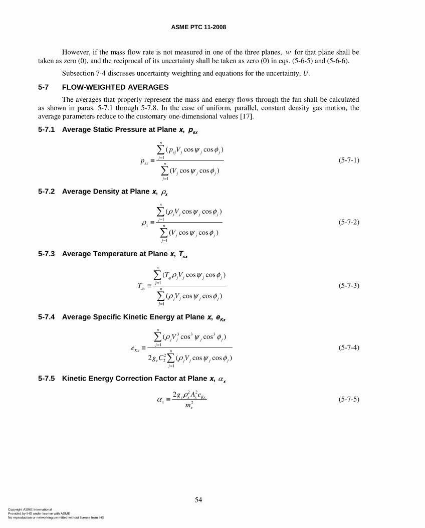
ASME PTC 11-2008

54

However, if the mass flow rate is not measured in one of the three planes, w for that plane shall be taken as zero (0), and the reciprocal of its uncertainty shall be taken as zero (0) in eqs. (5-6-5) and (5-6-6).

Subsection 7-4 discusses uncertainty weighting and equations for the uncertainty, U.

5-7 FLOW-WEIGHTED AVERAGES

The averages that properly represent the mass and energy flows through the fan shall be calculated as shown in paras. 5-7.1 through 5-7.8. In the case of uniform, parallel, constant density gas motion, the average parameters reduce to the customary one-dimensional values [17].

5-7.1 Average Static Pressure at Plane x, sxp

1

1

( cos cos )

( cos cos )

n

sj j j jj

sx n

j j jj

p V

p

V

ψ φ

ψ φ

=

=

≡∑

∑ (5-7-1)

5-7.2 Average Density at Plane x, xρ

1

1

( cos cos )

( cos cos )

n

j j j jj

x n

j j jj

V

V

ρ ψ φρ

ψ φ

=

=

≡∑

∑ (5-7-2)

5-7.3 Average Temperature at Plane x, sxT

1

1

( cos cos )

( cos cos )

n

sj j j j jj

sx n

j j j jj

T V

T

V

ρ ψ φ

ρ ψ φ

=

=

≡∑

∑ (5-7-3)

5-7.4 Average Specific Kinetic Energy at Plane x, Kxe

3 3 3

1

22

1

( cos cos )

2 ( cos cos )

n

j j j jj

Kx n

c j j j jj

V

eg C V

ρ ψ φ

ρ ψ φ

=

=

≡∑

∑ (5-7-4)

5-7.5 Kinetic Energy Correction Factor at Plane x, xα

2 2

2

2 c x x Kxx

x

g A e

m

ρα ≡ (5-7-5)


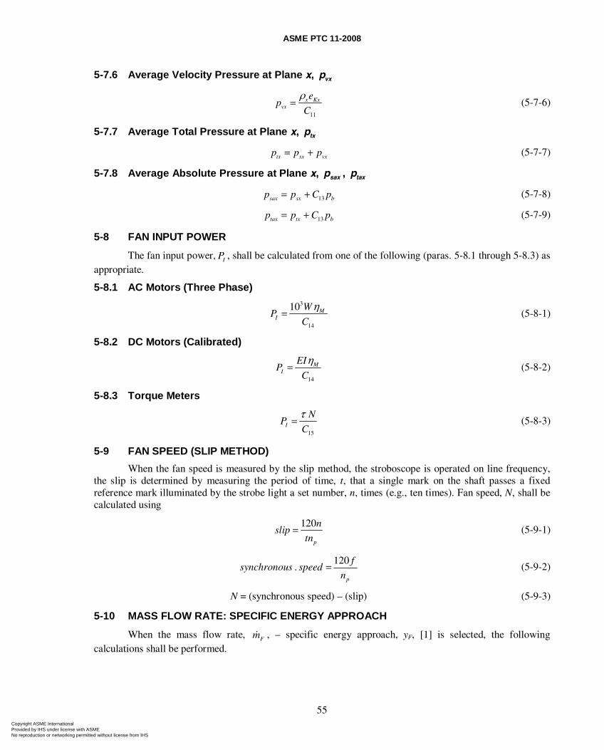
ASME PTC 11-2008

55

5-7.6 Average Velocity Pressure at Plane x, vxp

11

x Kxvx

ep

C

ρ= (5-7-6)

5-7.7 Average Total Pressure at Plane x, txp

tx sx vxp p p= + (5-7-7)

5-7.8 Average Absolute Pressure at Plane x, saxp , taxp

13sax sx bp p C p= + (5-7-8)

13tax tx bp p C p= + (5-7-9)

5-8 FAN INPUT POWER

The fan input power, IP , shall be calculated from one of the following (paras. 5-8.1 through 5-8.3) as appropriate.

5-8.1 AC Motors (Three Phase)

3

14

10 MI

WP

C

η= (5-8-1)

5-8.2 DC Motors (Calibrated)

14

MI

EIP

C

η= (5-8-2)

5-8.3 Torque Meters

15

I

NP

C

τ= (5-8-3)

5-9 FAN SPEED (SLIP METHOD)

When the fan speed is measured by the slip method, the stroboscope is operated on line frequency, the slip is determined by measuring the period of time, t, that a single mark on the shaft passes a fixed reference mark illuminated by the strobe light a set number, n, times (e.g., ten times). Fan speed, N, shall be calculated using

120

p

nslip

tn= (5-9-1)

120

.p

fsynchronous speed

n= (5-9-2)

N = (synchronous speed) – (slip) (5-9-3)

5-10 MASS FLOW RATE: SPECIFIC ENERGY APPROACH

When the mass flow rate, Fm , – specific energy approach, yF, [1] is selected, the following calculations shall be performed.


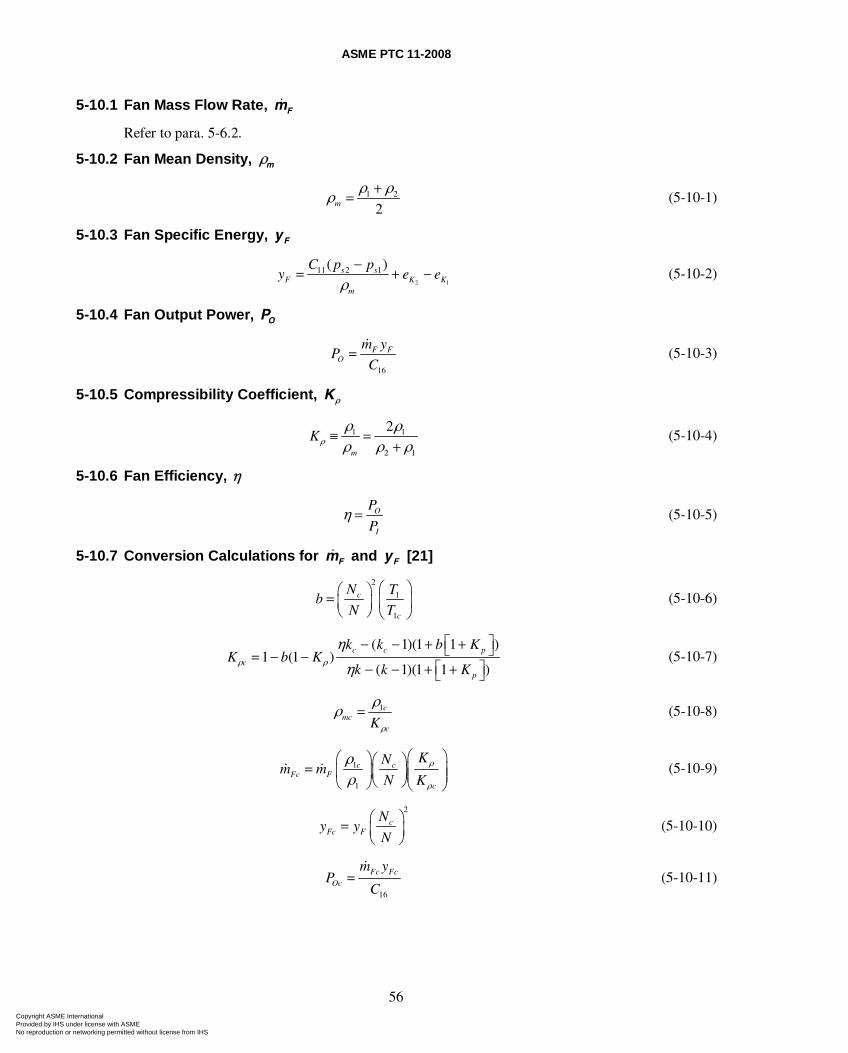
ASME PTC 11-2008

56


Refer to para. 5-6.2.

5-10.2 Fan Mean Density, mρ

1 2

2m

ρ ρρ += (5-10-1)

5-10.3 Fan Specific Energy, Fy

2 1

11 2 1( )s sF K K

m

C p py e e

ρ−

= + − (5-10-2)

5-10.4 Fan Output Power, OP

16

F FO

m yP

C= (5-10-3)

5-10.5 Compressibility Coefficient, Kρ

1 1

2 1

2

m

Kρρ ρρ ρ ρ

≡ =+

(5-10-4)

5-10.6 Fan Efficiency, η

O

I

P

Pη = (5-10-5)

5-10.7 Conversion Calculations for Fm and Fy [21]

2

1

1

c

c

N Tb

N T

⎛ ⎞⎛ ⎞= ⎜ ⎟⎜ ⎟⎝ ⎠ ⎝ ⎠

(5-10-6)

( 1)(1 1 )

1 (1 )( 1)(1 1 )

c c p

c

p

k k b KK b K

k k Kρ ρ

ηη

⎡ ⎤− − + +⎣ ⎦= − −⎡ ⎤− − + +⎣ ⎦

(5-10-7)

1cmc

cKρ

ρρ = (5-10-8)

1

1

c cFc F

c

KNm m

N Kρ

ρ

ρρ

⎛ ⎞⎛ ⎞⎛ ⎞= ⎜ ⎟⎜ ⎟⎜ ⎟⎜ ⎟⎝ ⎠⎝ ⎠ ⎝ ⎠ (5-10-9)

2

cFc F

Ny y

N⎛ ⎞= ⎜ ⎟⎝ ⎠

(5-10-10)

16

Fc FcOc

m yP

C= (5-10-11)


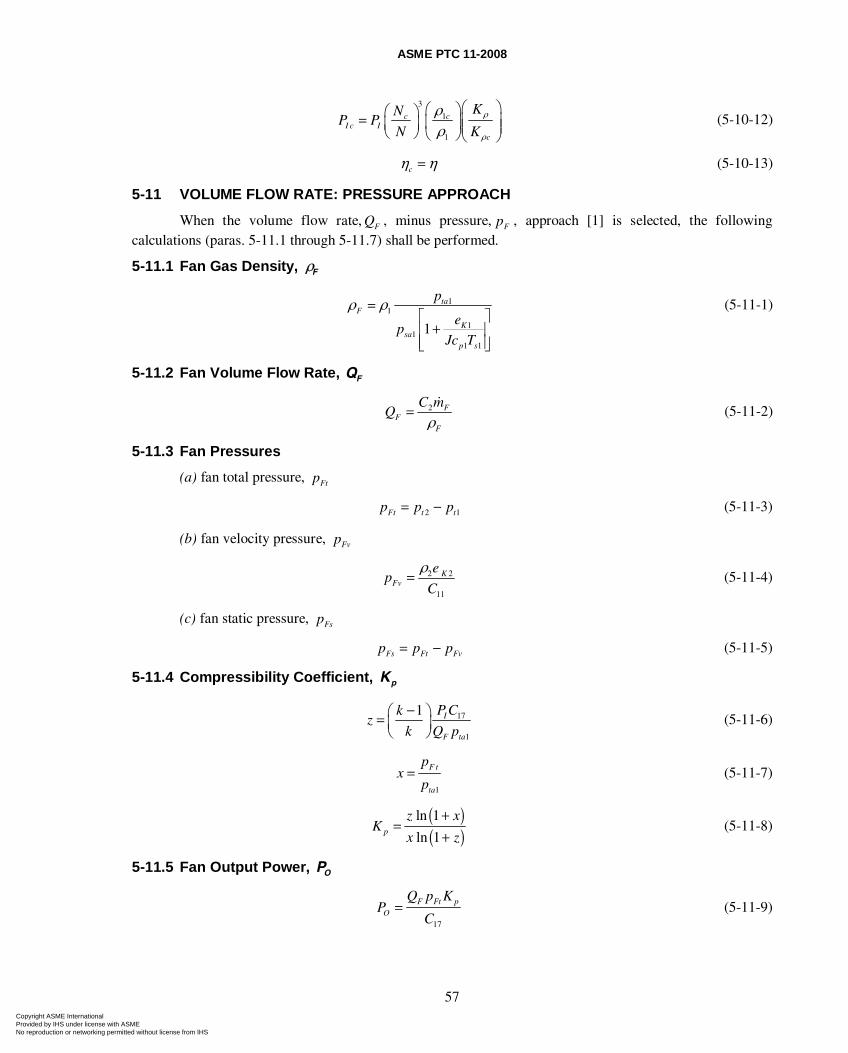
ASME PTC 11-2008

57

3

1

1

c cI c I

c

KNP P

N Kρ

ρ

ρρ

⎛ ⎞⎛ ⎞⎛ ⎞= ⎜ ⎟⎜ ⎟⎜ ⎟ ⎜ ⎟⎝ ⎠ ⎝ ⎠⎝ ⎠ (5-10-12)

cη η= (5-10-13)

5-11 VOLUME FLOW RATE: PRESSURE APPROACH

When the volume flow rate, FQ , minus pressure, Fp , approach [1] is selected, the following calculations (paras. 5-11.1 through 5-11.7) shall be performed.

5-11.1 Fan Gas Density, Fρ

11

11

1 1

1

taF

Ksa

p s

p

ep

Jc T

ρ ρ=⎡ ⎤+⎢ ⎥

⎢ ⎥⎣ ⎦

(5-11-1)

5-11.2 Fan Volume Flow Rate, FQ

2 FF

F

C mQ

ρ= (5-11-2)

5-11.3 Fan Pressures

(a) fan total pressure, Ftp

2 1Ft t tp p p= − (5-11-3)

(b) fan velocity pressure, Fvp

2 2

11

KFv

ep

C

ρ= (5-11-4)

(c) fan static pressure, Fsp

Fs Ft Fvp p p= − (5-11-5)

5-11.4 Compressibility Coefficient, pK

17

1

1 I

F ta

P Ckz

k Q p

−⎛ ⎞= ⎜ ⎟⎝ ⎠

(5-11-6)

1

F t

ta

px

p= (5-11-7)

( )( )

ln 1

ln 1p

z xK

x z

+=

+ (5-11-8)


17

F Ft pO

Q p KP

C= (5-11-9)


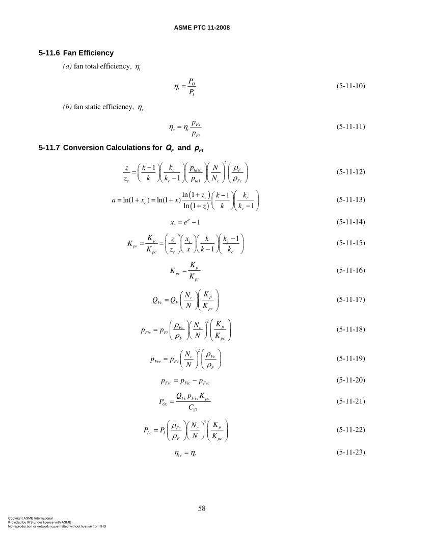
ASME PTC 11-2008

58

5-11.6 Fan Efficiency

(a) fan total efficiency, tη

Ot

I

P

Pη = (5-11-10)

(b) fan static efficiency, sη

Fss t

Ft

p

pη η= (5-11-11)

5-11.7 Conversion Calculations for FQ and Ftp

2

1

1

1

1c ta c F

c c ta c Fc

k pz k N

z k k p N

ρρ

⎛ ⎞⎛ ⎞⎛ ⎞ ⎛ ⎞−⎛ ⎞= ⎜ ⎟⎜ ⎟⎜ ⎟ ⎜ ⎟⎜ ⎟ −⎝ ⎠⎝ ⎠⎝ ⎠⎝ ⎠ ⎝ ⎠ (5-11-12)

( )( )

ln 1 1ln(1 ) ln(1 )

ln 1 1c c

cc

z kka x x

z k k

+ ⎛ ⎞−⎛ ⎞= + = + ⎜ ⎟⎜ ⎟+ −⎝ ⎠⎝ ⎠ (5-11-13)

1acx e= − (5-11-14)

1

1p c c

prpc c c

K x kz kK

K z x k k

⎛ ⎞ ⎛ ⎞−⎛ ⎞⎛ ⎞= = ⎜ ⎟ ⎜ ⎟⎜ ⎟⎜ ⎟ −⎝ ⎠⎝ ⎠⎝ ⎠ ⎝ ⎠ (5-11-15)

ppc

pr

KK

K= (5-11-16)

pcFc F

pc

KNQ Q

N K

⎛ ⎞⎛ ⎞= ⎜ ⎟⎜ ⎟⎜ ⎟⎝ ⎠⎝ ⎠ (5-11-17)

2

pFc cFtc Ft

F pc

KNp p

N K

ρρ

⎛ ⎞⎛ ⎞⎛ ⎞= ⎜ ⎟⎜ ⎟⎜ ⎟ ⎜ ⎟⎝ ⎠⎝ ⎠ ⎝ ⎠ (5-11-18)

2

c FcFvc Fv

F

Np p

N

ρρ

⎛ ⎞⎛ ⎞= ⎜ ⎟⎜ ⎟⎝ ⎠ ⎝ ⎠

(5-11-19)

Fsc Ftc Fvcp p p= − (5-11-20)

17

Fc F t c pcOc

Q p KP

C= (5-11-21)

3

pFc cI c I

F pc

KNP P

N K

ρρ

⎛ ⎞⎛ ⎞⎛ ⎞= ⎜ ⎟⎜ ⎟⎜ ⎟ ⎜ ⎟⎝ ⎠⎝ ⎠ ⎝ ⎠ (5-11-22)

t c tη η= (5-11-23)


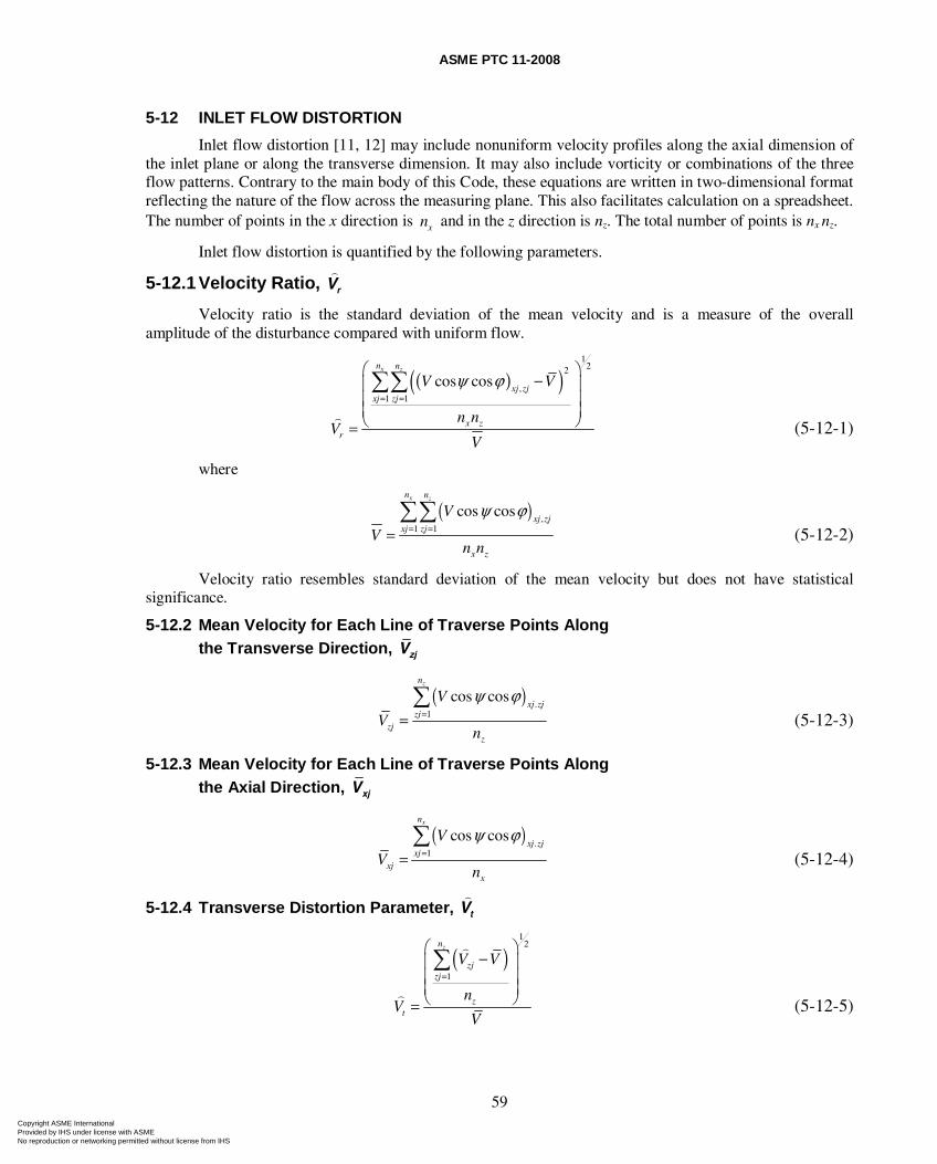
ASME PTC 11-2008

59

5-12 INLET FLOW DISTORTION

Inlet flow distortion [11, 12] may include nonuniform velocity profiles along the axial dimension of the inlet plane or along the transverse dimension. It may also include vorticity or combinations of the three flow patterns. Contrary to the main body of this Code, these equations are written in two-dimensional format reflecting the nature of the flow across the measuring plane. This also facilitates calculation on a spreadsheet. The number of points in the x direction is xn and in the z direction is nz. The total number of points is nx nz.

Inlet flow distortion is quantified by the following parameters.

5-12.1 Velocity Ratio, rV

Velocity ratio is the standard deviation of the mean velocity and is a measure of the overall amplitude of the disturbance compared with uniform flow.

( )( )1

22

,1 1

cos cosx zn n

xj zjxj zj

x zr

V V

n nV

V

ψ ϕ= =

⎛ ⎞−⎜ ⎟

⎜ ⎟⎜ ⎟⎝ ⎠=

∑∑

(5-12-1)

where

( ) ,

1 1

cos cosx zn n

xj zjxj zj

x z

V

Vn n

ψ ϕ= ==∑∑

(5-12-2)

Velocity ratio resembles standard deviation of the mean velocity but does not have statistical significance.

5-12.2 Mean Velocity for Each Line of Traverse Points Along the Transverse Direction, zjV

( ) .

1

cos coszn

xj zjzj

zjz

V

Vn

ψ ϕ==∑

(5-12-3)

5-12.3 Mean Velocity for Each Line of Traverse Points Along the Axial Direction, xjV

( ) .

1

cos cosxn

xj zjxj

xjx

V

Vn

ψ ϕ==∑

(5-12-4)

5-12.4 Transverse Distortion Parameter, tV

( )1

2

1

zn

zjzj

zt

V V

nV

V

=

⎛ ⎞−⎜ ⎟

⎜ ⎟⎜ ⎟⎝ ⎠=

∑

(5-12-5)


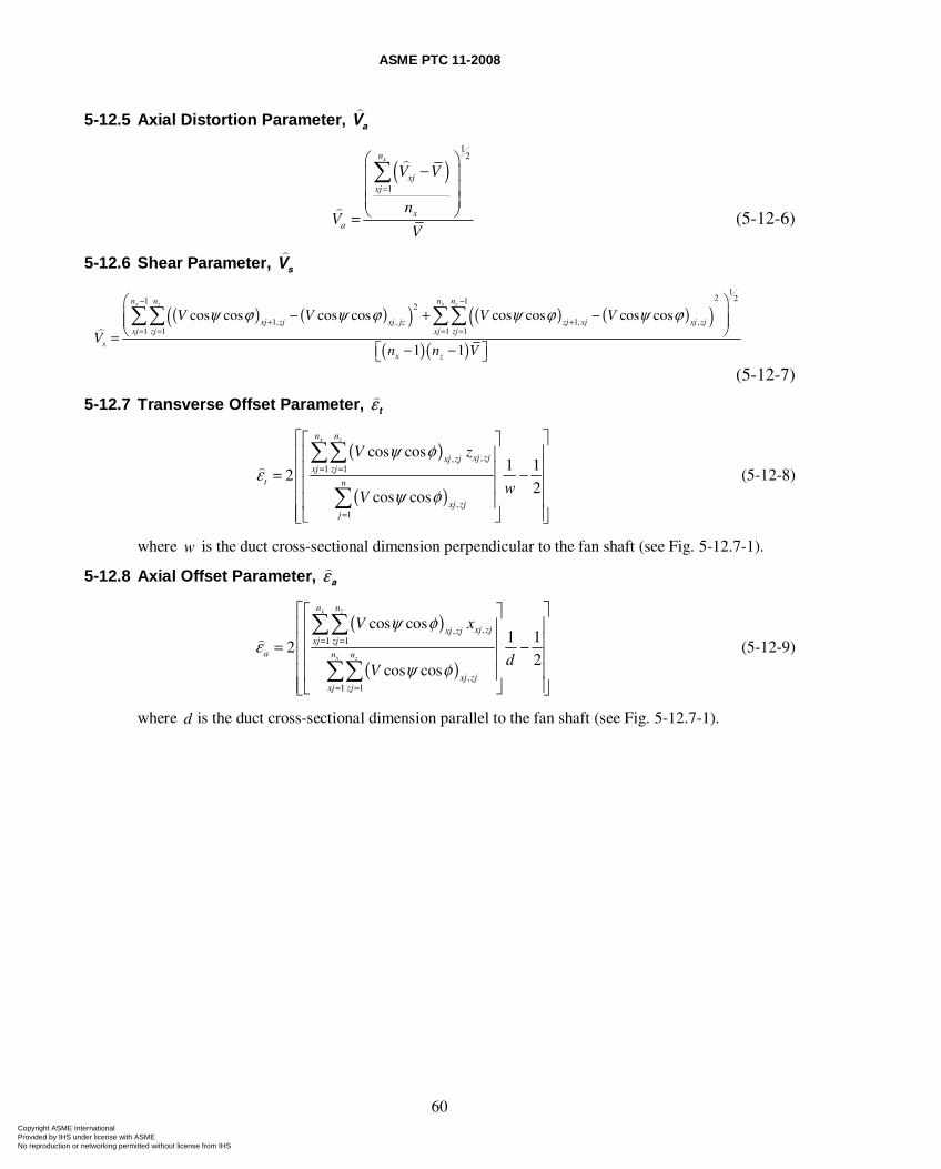
ASME PTC 11-2008

60

5-12.5 Axial Distortion Parameter, aV

( )1

2

1

xn

xjxj

xa

V V

nV

V

=

⎛ ⎞−⎜ ⎟

⎜ ⎟⎜ ⎟⎝ ⎠=

∑

(5-12-6)

5-12.6 Shear Parameter, sV

( ) ( )( ) ( ) ( )( )

( )( )

12 21 1

2

1, , 1, ,1 1 1 1

cos cos cos cos cos cos cos cos

1 1

x xz zn nn n

xj zj xj jz zj xj xj zjxj zj xj zj

s

x z

V V V V

Vn n V

ψ ϕ ψ ϕ ψ ϕ ψ ϕ− −

+ += = = =

⎛ ⎞− + −⎜ ⎟⎜ ⎟

⎝ ⎠=⎡ ⎤− −⎣ ⎦

∑∑ ∑∑

(5-12-7)

5-12.7 Transverse Offset Parameter, tε

( )

( )

,,1 1

,1

cos cos1 1

22cos cos

x zn n

xj zjxj zjxj zj

t n

xj zjj

V z

wV

ψ φε

ψ φ

= =

=

⎡ ⎤⎡ ⎤⎢ ⎥⎢ ⎥⎢ ⎥⎢ ⎥= −⎢ ⎥⎢ ⎥⎢ ⎥⎢ ⎥⎢ ⎥⎣ ⎦⎣ ⎦

∑∑

∑ (5-12-8)

where w is the duct cross-sectional dimension perpendicular to the fan shaft (see Fig. 5-12.7-1).

5-12.8 Axial Offset Parameter, aε

( )

( )

,,1 1

,1 1

cos cos1 1

22

cos cos

x z

x z

n n

xj zjxj zjxj zj

a n n

xj zjxj zj

V x

dV

ψ φε

ψ φ

= =

= =

⎡ ⎤⎡ ⎤⎢ ⎥⎢ ⎥⎢ ⎥⎢ ⎥= −⎢ ⎥⎢ ⎥⎢ ⎥⎢ ⎥⎢ ⎥⎣ ⎦⎣ ⎦

∑∑

∑∑ (5-12-9)

where d is the duct cross-sectional dimension parallel to the fan shaft (see Fig. 5-12.7-1).


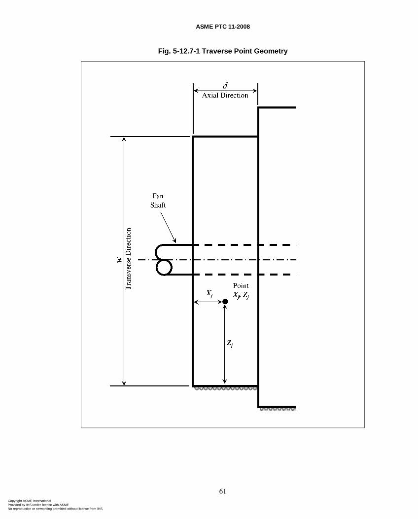
ASME PTC 11-2008

61

Fig. 5-12.7-1 Traverse Point Geometry


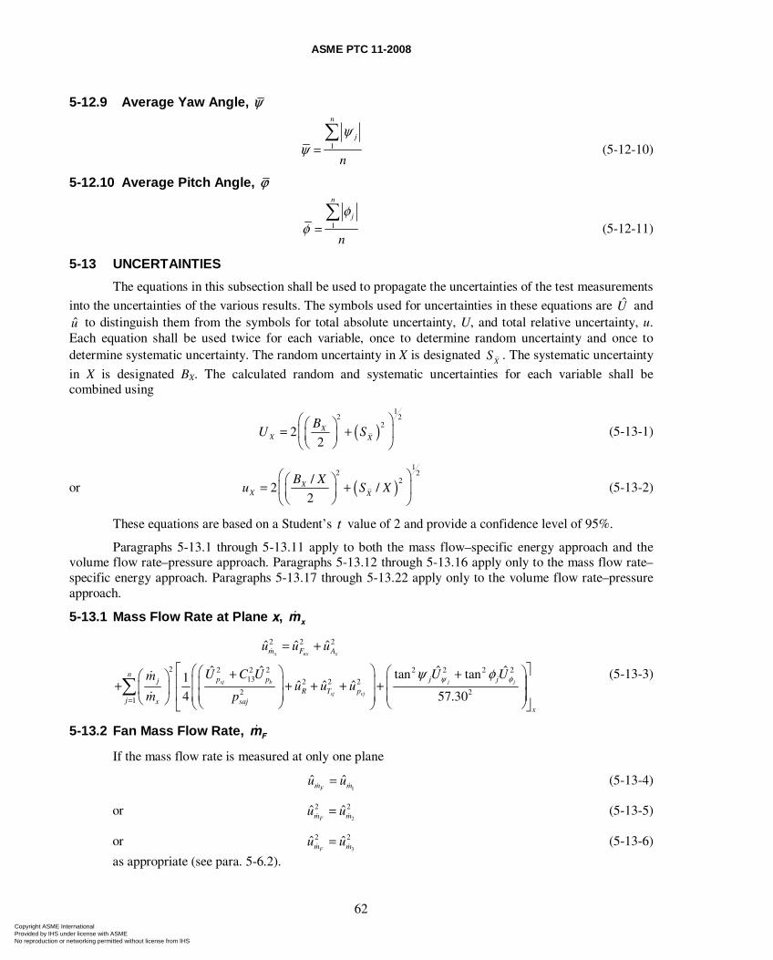
ASME PTC 11-2008

62

5-12.9 Average Yaw Angle, ψ

1

n

j

n

ψψ =

∑ (5-12-10)

5-12.10 Average Pitch Angle, ϕ

1

n

j

n

φφ =

∑ (5-12-11)

5-13 UNCERTAINTIES

The equations in this subsection shall be used to propagate the uncertainties of the test measurements

into the uncertainties of the various results. The symbols used for uncertainties in these equations are U and u to distinguish them from the symbols for total absolute uncertainty, U, and total relative uncertainty, u. Each equation shall be used twice for each variable, once to determine random uncertainty and once to determine systematic uncertainty. The random uncertainty in X is designated

XS . The systematic uncertainty

in X is designated BX. The calculated random and systematic uncertainties for each variable shall be combined using

( )1

2 22

22X

X X

BU S

⎛ ⎞⎛ ⎞= +⎜ ⎟⎜ ⎟⎝ ⎠⎝ ⎠

(5-13-1)

or ( )1

2 22/

2 /2

XX X

B Xu S X

⎛ ⎞⎛ ⎞= +⎜ ⎟⎜ ⎟⎝ ⎠⎝ ⎠

(5-13-2)

These equations are based on a Student’s t value of 2 and provide a confidence level of 95%.

Paragraphs 5-13.1 through 5-13.11 apply to both the mass flow–specific energy approach and the volume flow rate–pressure approach. Paragraphs 5-13.12 through 5-13.16 apply only to the mass flow rate–specific energy approach. Paragraphs 5-13.17 through 5-13.22 apply only to the volume flow rate–pressure approach.

5-13.1 Mass Flow Rate at Plane x, xm

2 2 2

2 2 2 2 2 2 2 213 2 2 2

2 21

ˆ ˆ ˆ

ˆ ˆ ˆ ˆtan tan1ˆ ˆ ˆ

4 57.30

x nx x

sj b j j

sj vj

m F A

np p j jj

R T pj x saj

x

u u u

U C U U Umu u u

m p

ψ φψ φ

=

= +

⎡ ⎤⎛ ⎞⎛ ⎞ ⎛ ⎞+ +⎛ ⎞ ⎢ ⎥⎜ ⎟⎜ ⎟ ⎜ ⎟+ + + + +⎜ ⎟ ⎜ ⎟ ⎜ ⎟⎢ ⎥⎜ ⎟⎝ ⎠ ⎝ ⎠ ⎝ ⎠⎝ ⎠⎣ ⎦∑

(5-13-3)


If the mass flow rate is measured at only one plane

1

ˆ ˆFm mu u= (5-13-4)

or 2

2 2ˆ ˆFm mu u= (5-13-5)

or 3

2 2ˆ ˆFm mu u= (5-13-6)

as appropriate (see para. 5-6.2).


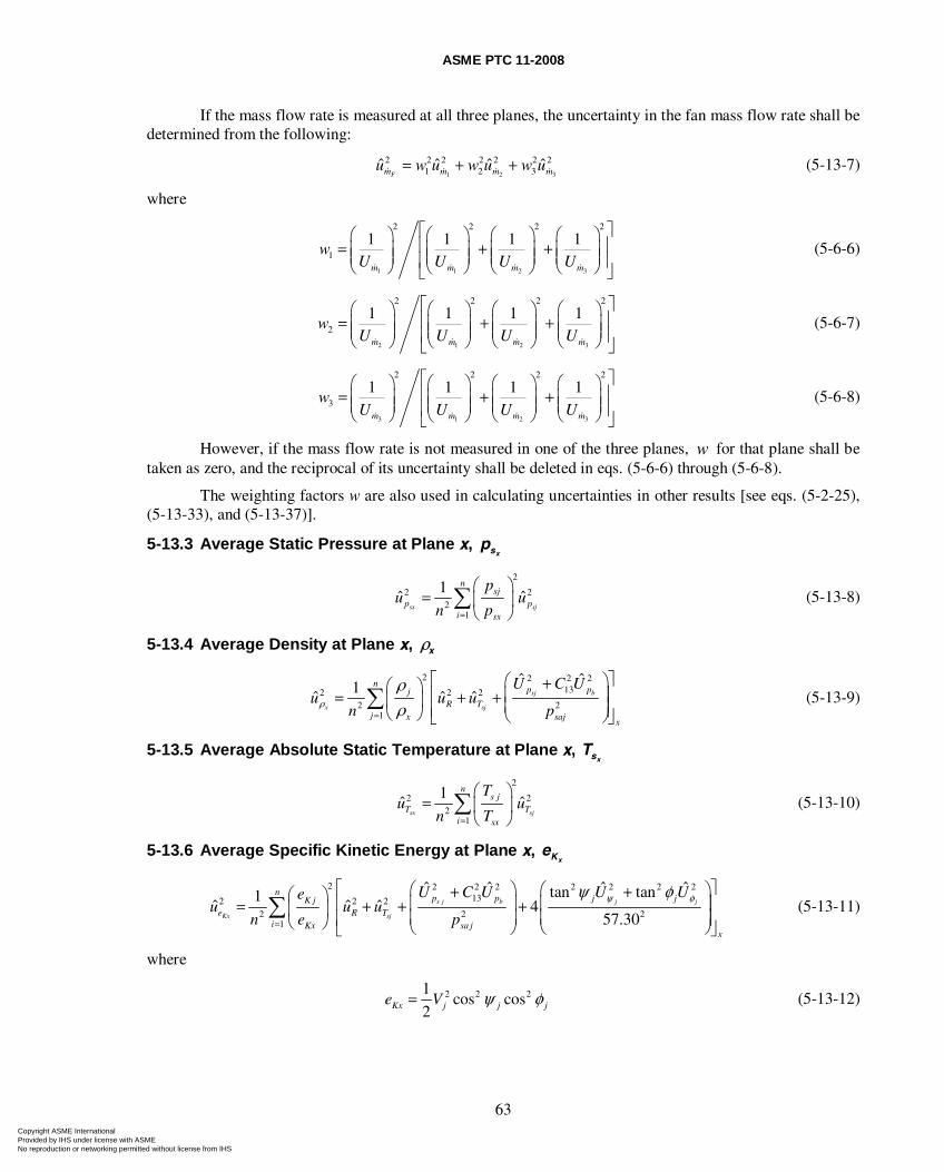
ASME PTC 11-2008

63

If the mass flow rate is measured at all three planes, the uncertainty in the fan mass flow rate shall be determined from the following:

1 2 3

2 2 2 2 2 2 21 2 3ˆ ˆ ˆ ˆ

Fm m m mu w u w u w u= + + (5-13-7)

where

1 1 2 3

22 2 2

1

1 1 1 1

m m m m

wU U U U

⎡ ⎤⎛ ⎞⎛ ⎞ ⎛ ⎞ ⎛ ⎞⎢ ⎥= + + ⎜ ⎟⎜ ⎟ ⎜ ⎟ ⎜ ⎟⎜ ⎟ ⎜ ⎟ ⎜ ⎟ ⎜ ⎟⎢ ⎥⎝ ⎠ ⎝ ⎠ ⎝ ⎠ ⎝ ⎠⎣ ⎦

(5-6-6)

2 1 2 3

22 2 2

2

1 1 1 1

m m m m

wU U U U

⎡ ⎤⎛ ⎞⎛ ⎞ ⎛ ⎞ ⎛ ⎞⎢ ⎥= + + ⎜ ⎟⎜ ⎟ ⎜ ⎟ ⎜ ⎟⎜ ⎟ ⎜ ⎟ ⎜ ⎟ ⎜ ⎟⎢ ⎥⎝ ⎠ ⎝ ⎠ ⎝ ⎠ ⎝ ⎠⎣ ⎦

(5-6-7)

3 1 2 3

2 22 2

3

1 1 1 1

m m m m

wU U U U

⎡ ⎤⎛ ⎞ ⎛ ⎞⎛ ⎞ ⎛ ⎞⎢ ⎥= + +⎜ ⎟ ⎜ ⎟⎜ ⎟ ⎜ ⎟⎜ ⎟ ⎜ ⎟⎜ ⎟ ⎜ ⎟⎢ ⎥⎝ ⎠ ⎝ ⎠⎝ ⎠ ⎝ ⎠⎣ ⎦

(5-6-8)

However, if the mass flow rate is not measured in one of the three planes, w for that plane shall be taken as zero, and the reciprocal of its uncertainty shall be deleted in eqs. (5-6-6) through (5-6-8).

The weighting factors w are also used in calculating uncertainties in other results [see eqs. (5-2-25), (5-13-33), and (5-13-37)].

5-13.3 Average Static Pressure at Plane x, xsp

2

2 22

1

1ˆ ˆ

sx sj

nsj

p pi sx

pu u

n p=

⎛ ⎞= ⎜ ⎟

⎝ ⎠∑ (5-13-8)

5-13.4 Average Density at Plane x, xρ

2 2 2 2

132 2 22 2

1

ˆ ˆ1ˆ ˆ ˆ sj b

x sj

np pj

R Tj x saj

x

U C Uu u u

n pρ

ρρ=

⎡ ⎤⎛ ⎞+⎛ ⎞ ⎢ ⎥⎜ ⎟= + +⎜ ⎟ ⎜ ⎟⎢ ⎥⎝ ⎠ ⎝ ⎠⎣ ⎦∑ (5-13-9)

5-13.5 Average Absolute Static Temperature at Plane x, xsT

2

2 22

1

1ˆ ˆ

sx sj

ns j

T Ti sx

Tu u

n T=

⎛ ⎞= ⎜ ⎟

⎝ ⎠∑ (5-13-10)

5-13.6 Average Specific Kinetic Energy at Plane x, xKe

2 2 2 2 2 2 2 2

132 2 22 2 2

1

ˆ ˆ ˆ ˆtan tan1ˆ ˆ ˆ 4

57.30s j b j j

Kx sj

np p j jK j

e R Ti Kx sa j

x

U C U U Ueu u u

n e p

ψ φψ φ

=

⎡ ⎤⎛ ⎞ ⎛ ⎞+ +⎛ ⎞ ⎢ ⎥⎜ ⎟ ⎜ ⎟= + + +⎜ ⎟ ⎜ ⎟⎜ ⎟⎢ ⎥⎝ ⎠ ⎝ ⎠⎝ ⎠⎣ ⎦∑ (5-13-11)

where

2 2 21cos cos

2Kx j j je V ψ φ= (5-13-12)


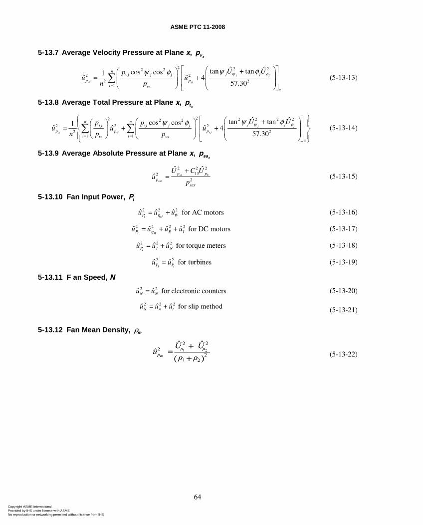
ASME PTC 11-2008

64

5-13.7 Average Velocity Pressure at Plane x, xvp

2 2 22 22 2

2 21

ˆ ˆtan tancos cos1ˆ ˆ 4

57.30j j

vx vj

nj jv j j j

p pi vx

x

U Upu u

n p

ψ φψ φψ φ

=

⎡ ⎤⎛ ⎞+⎛ ⎞⎢ ⎥⎜ ⎟= +⎜ ⎟⎜ ⎟ ⎜ ⎟⎢ ⎥⎝ ⎠ ⎝ ⎠⎣ ⎦

∑ (5-13-13)

5-13.8 Average Total Pressure at Plane x, xtp

22 2 2 2 22 22 2 2

2 21 1

ˆ ˆtan tancos cos1ˆ ˆ ˆ 4

57.30j j

tx vj v j

n nj js j vj j j

p p pi itx vx

x

U Up pu u u

n p p

ψ φψ φψ φ= =

⎧ ⎫⎡ ⎤⎛ ⎞+⎛ ⎞⎛ ⎞⎪ ⎪⎢ ⎥⎜ ⎟= + +⎜ ⎟⎨ ⎬⎜ ⎟ ⎜ ⎟ ⎜ ⎟⎢ ⎥⎝ ⎠⎪ ⎪⎝ ⎠ ⎝ ⎠⎣ ⎦⎩ ⎭∑ ∑ (5-13-14)

5-13.9 Average Absolute Pressure at Plane x, xsap

2 2 2

1322

ˆ ˆˆ sx b

sax

p p

psax

U C Uu

p

+= (5-13-15)

5-13.10 Fan Input Power, IP

2 2 2ˆ ˆ ˆ for AC motorsI MP Wu u uη= + (5-13-16)

2 2 2 2ˆ ˆ ˆ ˆ for DC motorsI MP E Iu u u uη= + + (5-13-17)

2 2 2ˆ ˆ ˆ for torque metersIP Nu u uτ= + (5-13-18)

2 2ˆ Î tP Pu u= for turbines (5-13-19)

5-13.11 F an Speed, N

2 2ˆ ˆ for electronic countersN Nu u= (5-13-20)

2 2 2ˆ ˆ ˆ for slip methodN n tu u u= + (5-13-21)

5-13.12 Fan Mean Density, mρ

(5-13-22)


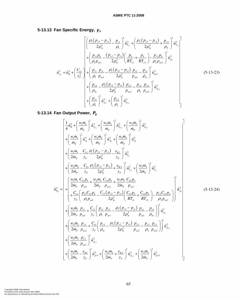
ASME PTC 11-2008

65

5-13.13 Fan Specific Energy, Fy

( ) ( )

( )

( )

1 2

2 2

1 2 1 2 2 12 21 22 2

1 2

2

2 1 21 22

1 1 1 2 2 2

1 2 12 2 1 1 1 1112 2

1 1 1

ˆ ˆ2 2

ˆ2

ˆ ˆ2

s s

b

F

s s s sv vT T

m m

s sv b b b v bp

sa m s s sa

s sv s s sy R

F sa m sa m

p p p pp pu u

p pp p p p p pu

p RT RT p

p pp p p pCu u

y p p

ρ ρρ ρ ρ ρ

ρ ρ ρ

ρρ ρ ρ

⎛ − ⎞ ⎛ − ⎞− + +⎜ ⎟ ⎜ ⎟

⎝ ⎠ ⎝ ⎠

⎛ − ⎞⎛ ⎞+ − + −⎜ ⎟⎜ ⎟⎝ ⎠⎝ ⎠

⎛ − ⎞⎛ ⎞= + + − −⎜⎜ ⎟⎝ ⎠ ⎝ ⎠

( )2

1 2

2

21

2

2 2 1 22 2 2 22

2 2 2

2 22 21 2

1 1

ˆ

ˆ2

ˆ ˆ

s

v v

ps

s ss s v sp

m m sa sa

v vp p

u

p pp p p pu

p p

p pu u

ρρ ρ ρ

ρ ρ

⎡ ⎤⎢ ⎥⎢ ⎥⎢ ⎥⎢ ⎥⎢ ⎥⎢ ⎥⎢ ⎥⎢ ⎥⎟⎢ ⎥⎢ ⎥⎢ ⎥⎛ − ⎞⎢ ⎥+ − −⎜ ⎟⎢ ⎥⎝ ⎠⎢ ⎥⎛ ⎞ ⎛ ⎞⎢ ⎥+ +⎜ ⎟ ⎜ ⎟⎢ ⎥⎝ ⎠ ⎝ ⎠⎣ ⎦

(5-13-23)


( )

1 2 3

1 2 3

1

22 22 2 2 23 31 1 2 2

22 22 2 23 31 1 2 2

2

1 2 1 21 1 11 12

2 2 1

2

1ˆ ˆ ˆ ˆ

4

ˆ ˆ ˆ

ˆ2 2

2

ˆ

n n n

s

O

R F F FF F F

A A AF F F

s s KT

F F m F

F

P

w mw m w mu u u u

m m m

w mw m w mu u u

m m m

p pw m C eu

m y y

w m C

m

u

ρρ

⎛ ⎞⎛ ⎞ ⎛ ⎞+ + + ⎜ ⎟⎜ ⎟ ⎜ ⎟⎝ ⎠ ⎝ ⎠ ⎝ ⎠

⎛ ⎞⎛ ⎞ ⎛ ⎞+ + + ⎜ ⎟⎜ ⎟ ⎜ ⎟⎝ ⎠ ⎝ ⎠ ⎝ ⎠

⎛ − ⎞+ − −⎜ ⎟⎝ ⎠

+ −

=

( )

( )

2 3

2 22 2 1 2 23 31 2

2

13 13 3 3 131 1 2 2

1 2 3

11 2 11 13 13 13 2 13112

1 1 1 2 2 2

ˆ ˆ2 2

2 2 2

2

s s

s s KT T

F m F F

b b b

F sa F sa F sa

s sv b b b v b

F sa m s s sa

p p w meu u

y y m

C p C p w m C pw m w m

m p m p m p

C p pp C p C p C p p C pC

y p RT RT p

ρρ

ρ ρ ρ

⎛ − ⎞ ⎛ ⎞+ +⎜ ⎟ ⎜ ⎟⎝ ⎠⎝ ⎠

⎛ ⎞+ +⎜⎜+⎜ ⎛ − ⎞⎛ ⎞⎜+ − + −⎜ ⎟⎜ ⎟⎜ ⎝ ⎠⎝ ⎠⎝

( )

( )

1

2

2

2

2

1 2 1 21 1 1 1 11 1 112

1 1 1 1

2

2 2 1 22 2 2 2 22 2 112

2 2 2 2

3 3 3

3

ˆ

ˆ2 2

ˆ2 2

2

b

s

s

p

s ss v s s sp

F sa F sa m sa m

s ss s s v sp

F sa F m m sa sa

s

F sa

u

p pp p p p pw m Cu

m p y p p

p pp p p p pw m Cu

m p y p p

w m p

m p

ρρ ρ ρ

ρρ ρ ρ

⎟⎟⎟⎟⎟⎠

⎛ ⎞⎛ − ⎞+ + − −⎜ ⎟⎜ ⎟⎜ ⎟⎝ ⎠⎝ ⎠

⎛ ⎞⎛ − ⎞+ + − −⎜ ⎟⎜ ⎟⎜ ⎟⎝ ⎠⎝ ⎠

⎛ ⎞+⎜⎝ ⎠

3

2

22

22 22 2 23 31 1 1 2 2 2

1 3

ˆ

ˆ ˆ ˆ2 2 2

s

v

p

K Kpv p pv

F F F F F

u

w mw m e w m eu u u

m y m y m

⎡ ⎤⎢ ⎥⎢ ⎥⎢ ⎥⎢ ⎥⎢ ⎥⎢ ⎥⎢ ⎥⎢ ⎥⎢ ⎥⎢ ⎥⎢ ⎥⎢ ⎥⎢ ⎥⎢ ⎥⎢ ⎥⎢ ⎥⎢ ⎥⎢ ⎥⎢ ⎥⎢ ⎥⎢ ⎥⎢ ⎥⎢ ⎥⎢ ⎥⎢ ⎥⎢ ⎥⎢ ⎥⎢ ⎥⎢ ⎥⎢ ⎥⎟⎢ ⎥⎢ ⎥

⎛ ⎞⎛ ⎞ ⎛ ⎞⎢ ⎥+ − + + + ⎜ ⎟⎜ ⎟ ⎜ ⎟⎢ ⎥⎝ ⎠ ⎝ ⎠ ⎝ ⎠⎣ ⎦

(5-13-24)


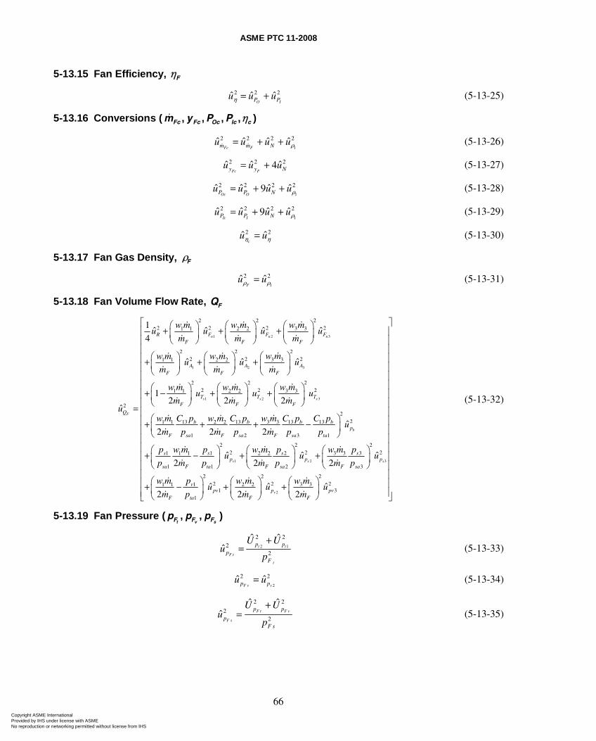
ASME PTC 11-2008

66

5-13.15 Fan Efficiency, Fη

2 2 2ˆ ˆ Ô IP Pu u uη = + (5-13-25)

5-13.16 Conversions ( Fc Fc Oc Ic cm y P P η, , , , )

1

2 2 2 2ˆ ˆ ˆ ˆFc Fm m Nu u u uρ= + + (5-13-26)

2 2 2ˆ ˆ ˆ4Fc Fy y Nu u u= + (5-13-27)

1

2 2 2 2ˆ ˆ ˆ ˆ9Oc OP P Nu u u uρ= + + (5-13-28)

1

2 2 2 2ˆ ˆ ˆ ˆ9Ic IP P Nu u u uρ= + + (5-13-29)

2 2ˆ ˆc

u uη η= (5-13-30)

5-13.17 Fan Gas Density, Fρ

1

2 2ˆ ˆF

u uρ ρ= (5-13-31)

5-13.18 Fan Volume Flow Rate, FQ

1 2 3

1 2 3

1 2

22 22 2 2 23 31 1 2 2

22 22 2 23 31 1 2 2

2 22 2 3 31 1 2 2

2

1ˆ ˆ ˆ ˆ

4

ˆ ˆ ˆ

12 2 2

ˆ

n n n

s s

F

R F F FF F F

A A AF F F

T TF F F

Q

w mw m w mu u u u

m m m

w mw m w mu u u

m m m

w mw m w mu u

m m mu

⎛ ⎞⎛ ⎞ ⎛ ⎞+ + + ⎜ ⎟⎜ ⎟ ⎜ ⎟⎝ ⎠ ⎝ ⎠ ⎝ ⎠

⎛ ⎞⎛ ⎞ ⎛ ⎞+ + + ⎜ ⎟⎜ ⎟ ⎜ ⎟⎝ ⎠ ⎝ ⎠ ⎝ ⎠

⎛⎛ ⎞ ⎛ ⎞+ − + + ⎜⎜ ⎟ ⎜ ⎟⎝ ⎠ ⎝ ⎠ ⎝=

3

1 2 3

22

2213 13 3 3 13 131 1 2 2

1 2 3 1

2 2 22 2 21 1 2 3 3 31 1 2 2

1 1 2 3

11 1

ˆ2 2 2

ˆ ˆ ˆ2 2 2

2

s

b

s s s

T

b b b bp

F sa F sa F sa ta

s s s sp p p

sa F ta F sa F sa

v

F

u

C p C p w m C p C pw m w mu

m p m p m p p

p p p w m pw m w mu u u

p m p m p m p

pw m

m

⎞⎟⎠

⎛ ⎞+ + + −⎜ ⎟⎝ ⎠

⎛ ⎞ ⎛ ⎞ ⎛ ⎞+ − + +⎜ ⎟ ⎜ ⎟ ⎜ ⎟⎝ ⎠ ⎝ ⎠ ⎝ ⎠

+ −2

2 222 2 23 32 2

1 31

ˆ ˆ ˆ2 2vpv p pv

ta F F

w mw mu u u

p m m

⎡ ⎤⎢ ⎥⎢ ⎥⎢ ⎥⎢ ⎥⎢ ⎥⎢ ⎥⎢ ⎥⎢ ⎥⎢ ⎥⎢ ⎥⎢ ⎥⎢ ⎥⎢ ⎥⎢ ⎥⎢ ⎥⎢ ⎥⎢ ⎥⎛ ⎞ ⎛ ⎞⎛ ⎞⎢ ⎥+ +⎜ ⎟ ⎜ ⎟⎜ ⎟⎢ ⎥⎝ ⎠ ⎝ ⎠⎝ ⎠⎣ ⎦

(5-13-32)

5-13.19 Fan Pressure (t v sF F Fp p p, , )

2 1

2 2

22

ˆ ˆˆ t t

F t

t

p p

pF

U Uu

p

+= (5-13-33)

2

2 2ˆ ˆF v vp pu u= (5-13-34)

2 2

22

ˆ ˆˆ F t F v

F s

p p

pF s

U Uu

p

+= (5-13-35)


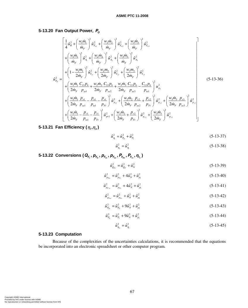
ASME PTC 11-2008

67


1 2 3

1 2 3

1 2

22 22 2 2 23 31 1 2 2

22 22 2 23 31 1 2 2

2 22 2 3 31 1 2 2

2

1ˆ ˆ ˆ ˆ

4

ˆ ˆ ˆ

ˆ ˆ12 2 2

ˆ

n n n

s s

O

R F F FF F F

A A AF F F

T TF F F

P

w mw m w mu u u u

m m m

w mw m w mu u u

m m m

w mw m w mu u

m m mu

⎛ ⎞⎛ ⎞ ⎛ ⎞+ + + ⎜ ⎟⎜ ⎟ ⎜ ⎟⎝ ⎠ ⎝ ⎠ ⎝ ⎠

⎛ ⎞⎛ ⎞ ⎛ ⎞+ + + ⎜ ⎟⎜ ⎟ ⎜ ⎟⎝ ⎠ ⎝ ⎠ ⎝ ⎠

⎛ ⎞⎛ ⎞ ⎛ ⎞+ − + + ⎜⎜ ⎟ ⎜ ⎟⎝ ⎠ ⎝ ⎠ ⎝=

3

1 2 3

22

2213 13 3 3 13 131 1 2 2

1 2 3 1

2 2 22 2 21 1 1 2 2 3 3 31 1 2 2

1 1 2 3

ˆ

2 2 2

ˆ ˆ ˆ2 2 2

s

b

s s s

T

b b b bp

F sa F sa F sa ta

s s s s s sp p p

F sa ta Ft F sa Ft F sa

u


m p m p m p p

p p p p p w m pw m w mu u u

m p p p m p p m p

⎟⎠

⎛ ⎞+ + + −⎜ ⎟⎝ ⎠

⎛ ⎞ ⎛ ⎞ ⎛ ⎞+ − − + + +⎜ ⎟ ⎜ ⎟ ⎜ ⎟⎝ ⎠ ⎝ ⎠ ⎝ ⎠

+2 3

2 2 22 2 21 1 2 3 31 1 2 2

11

ˆ ˆ ˆ2 2 2v v

v v vpv p p

F ta Ft F Ft F

p p p w mw m w mu u u

m p p m p m

⎡ ⎤⎢ ⎥⎢ ⎥⎢ ⎥⎢ ⎥⎢ ⎥⎢ ⎥⎢ ⎥⎢ ⎥⎢ ⎥⎢ ⎥⎢ ⎥⎢ ⎥⎢ ⎥⎢ ⎥⎢ ⎥⎢ ⎥⎢ ⎥⎛ ⎞ ⎛ ⎞ ⎛ ⎞⎢ ⎥− − + + +⎜ ⎟ ⎜ ⎟ ⎜ ⎟⎢ ⎥⎝ ⎠⎝ ⎠ ⎝ ⎠⎣ ⎦

(5-13-36)

5-13.21 Fan Efficiency ( t sη η, )

2 2 2ˆ ˆ ˆt O IP Pu u uη = + (5-13-37)

2 2ˆ ˆs t

u uη η= (5-13-38)

5-13.22 Conversions (c tc vc sc Oc I c cF F F F F F tQ p p p P P η, , , , , , )

2 2 2ˆ ˆ ˆFc FQ Q Nu u u= + (5-13-39)

1

2 2 2 2ˆ ˆ ˆ ˆ4Ftc Ftp p Nu u u uρ= + + (5-13-40)

1

2 2 2 2ˆ ˆ ˆ ˆ4F vc Fvp p Nu u u uρ= + + (5-13-41)

1

2 2 2 2ˆ ˆ ˆ ˆFsc Fsp p Nu u u uρ= + + (5-13-42)

1

2 2 2 2ˆ ˆ ˆ ˆ9Oc OP P Nu u u uρ= + + (5-13-43)

1

2 2 2 2ˆ ˆ ˆ ˆ9Ic IP P Nu u u uρ= + + (5-13-44)

2 2ˆ ˆtc t

u uη η= (5-13-45)

5-13.23 Computation

Because of the complexities of the uncertainties calculations, it is recommended that the equations be incorporated into an electronic spreadsheet or other computer program.


ASME PTC 11-2008

68

Section 6 Report of Results

6-1 GENERAL REQUIREMENTS

The results of the test shall be presented in a written report. The preparation of the report shall be the responsibility of the person in charge of the test who shall certify its correctness.

Prior to writing the report, the parties shall decide whether to use SI units, U.S. Customary units, or both. This selection will generally depend upon the units in which the fan performance is specified.

The Test Report shall include the information specified in subsections 6-2 through 6-7.

6-2 EXECUTIVE SUMMARY

The following information is to be included in the executive summary:

(a) general information about the fan and the test, such as the fan type and operating configuration, and the test objective

(b) date and time of the test

(c) summary of the results of the test, including uncertainty and conclusions reached

(d) comparison with the specified performance, if any

(e) any agreements among the parties to the test to allow any deviations from the test requirements

6-3 INTRODUCTION

The following information is to be included in the introduction:

(a) authorization for the tests, their object, specified performance, stipulated agreements, by whom the test is directed, and the representative parties to the test

(b) any additional general information about the fan and the test not included in the executive summary, such as

(1) a historical perspective, if appropriate

(2) an equipment diagram showing the test boundary

(3) description of the equipment tested and any other auxiliary apparatus, the operation of which may influence the test result

(c) a listing of the representatives of the parties to the test

(d) any pretest agreements that were not tabulated in the executive summary

(e) the organization of the test personnel

(f) test goal per Sections 3 and 5 of this Code

6-4 CALCULATIONS AND RESULTS

The following information is to be included in the calculations and results:

(a) method of the test and operating conditions

(b) tabular summary of measurements and observations, including the reduced data necessary to calculate the results and a summary of additional operating conditions not part of such reduced data

(c) step-by-step calculation of test results from the reduced data, including the uncertainty analysis

(d) any calculations showing elimination of data for outlier reason or for any other reason

(e) comparison of repeatability of test runs


ASME PTC 11-2008

69

(f) correction factors to be applied because of deviations, if any, of test conditions from those specified

(g) primary measurement uncertainties, including method of application

(h) the test performances stated under the following headings:

(1) test results computed on the basis of the test operating conditions, instrument calibrations only having been applied

(2) test results corrected to specified conditions if test operating conditions have deviated from those specified

(i) tabular and graphical presentation of the test results

(j) discussion and details of the test results uncertainties

(k) discussion of the test and its results

A copy of the computer program used to determine results will be included as an appendix to the report.

6-5 INSTRUMENTATION

The following information is to be included in the instrumentation:

(a) tabulation of instrumentation used, including make, model number, etc.

(b) description of the instrumentation location

(c) means of data collection for each data point, such as temporary data acquisition system printout, plant control computer printout, or manual data sheet, and any identifying tag number and/or address of each

(d) identification of the instrument that was used as backup

(e) description of data acquisition system(s) used

(f) summary of pretest and post-test calibration

6-6 CONCLUSIONS

The following information is to be included in the conclusions:

(a) A statement as to whether the test met the test objectives. If it does not meet the test objectives, the reasons shall be stated.

(b) A statement as to whether the test met the requirements of PTC 11. If it does not meet the requirements of PTC 11, the reasons shall be stated.

(c) A statement as to whether the fan met the specified performance (if applicable).

6-7 APPENDICES

The following information is to be included in the appendices:

(a) copies of original data sheets and/or data acquisition system(s) printouts

(b) copies of operator logs or other recording of operating activity during each test

(c) instrumentation calibration results from laboratories, certification from manufacturers

(d) copies of fuel analysis (if applicable)


ASME PTC 11-2008

70

Section 7 Uncertainty Analysis

7-1 INTRODUCTION

Uncertainty analysis is a procedure by which the accuracy of test results can be quantified. Because it is required that the parties to the test agree to the quality of the test (measured by test uncertainty), pretest and post-test uncertainty analyses are an indispensable part of a meaningful performance test.

In planning a test, a pretest uncertainty analysis allows corrective action to be taken prior to the test, either to decrease the uncertainty to a level consistent with the overall objective of the test or to reduce the cost of the test while still attaining the objective. An uncertainty analysis is useful to determine the number of observations.

A post-test uncertainty analysis determines the uncertainty intervals for the actual test. This analysis should confirm the pretest systematic and random uncertainty estimates. It serves to validate the quality of the test results or to expose problems.

PTC 19.1, Test Uncertainty, is the primary reference for uncertainty calculations, and any uncertainty analysis method that conforms to PTC 19.1 is acceptable.

Before an uncertainties analysis can be performed, both the random uncertainty,XS , and the

systematic uncertainty, BX, in each of the test measurements X must be established. For this Code, the random and systematic uncertainties for an additional factor must also be determined. This is called the number-of-points factor, Fn. Next, the appropriate test measurement uncertainties must be combined appropriately for each test result, a process called propagating the test uncertainties into the uncertainty of the results. The random and systematic uncertainties must be propagated individually for each result. Finally, these random and systematic uncertainties are combined to yield the total absolute uncertainty, UX, or the total relative uncertainty, uX, in each of the results. See eq. (5-13-1) or (5-13-2).

The confidence level for uncertainties calculated in this manner will be 95%. Subsection 7-2 explains how this Code propagates the test uncertainties into the results. Subsection 7-3 describes how to determine the random and systematic uncertainties in the basic measured parameters and number of points factor. Subsection 7-4 discusses the uncertainty when mass flow is determined at multiple traverse planes. Subsection 5-13 of this Code provides the equations for calculating the uncertainty in each result. These equations can be used directly; however, incorporating them into a spreadsheet or other computer program together with the test data is recommended because of the complexity involved.

An alternative to the use of the equations of subsection 5-13 is to use numerical evaluation of sensitivity coefficients, as described in PTC 19.1 This method is sometimes called “dithering” or “jittering.” This method is especially useful when a computer code or spreadsheet is being used to calculate test results because the computer can be easily used to calculate the results that would occur with a small perturbation of the input (test) data.

7-2 UNCERTAINTY PROPAGATION EQUATIONS

The uncertainty propagation equations are given in subsection 5-13. These equations are derived in Nonmandatory Appendix E. All the derivations follow the approach suggested by Kline and McClintock [5]. This approach is equivalent to the “Taylor Series” method described in PTC 19.1.

The uncertainty propagation equations derived and used in this Code assume that there are no correlations between systematic uncertainties. This would be the case when different measuring systems, calibrated against different standards, are used at each point in each traverse plane. This approach is taken because it is not possible to identify in general all cases wherein correlated systematic uncertainties may occur. For example, in one test, the same instrument system may be used to traverse both the inlet and outlet


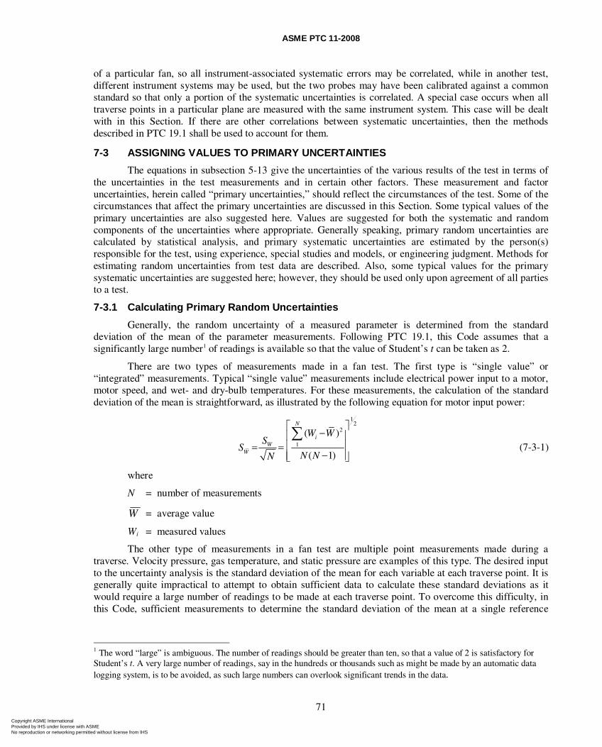
ASME PTC 11-2008

71

of a particular fan, so all instrument-associated systematic errors may be correlated, while in another test, different instrument systems may be used, but the two probes may have been calibrated against a common standard so that only a portion of the systematic uncertainties is correlated. A special case occurs when all traverse points in a particular plane are measured with the same instrument system. This case will be dealt with in this Section. If there are other correlations between systematic uncertainties, then the methods described in PTC 19.1 shall be used to account for them.

7-3 ASSIGNING VALUES TO PRIMARY UNCERTAINTIES

The equations in subsection 5-13 give the uncertainties of the various results of the test in terms of the uncertainties in the test measurements and in certain other factors. These measurement and factor uncertainties, herein called “primary uncertainties,” should reflect the circumstances of the test. Some of the circumstances that affect the primary uncertainties are discussed in this Section. Some typical values of the primary uncertainties are also suggested here. Values are suggested for both the systematic and random components of the uncertainties where appropriate. Generally speaking, primary random uncertainties are calculated by statistical analysis, and primary systematic uncertainties are estimated by the person(s) responsible for the test, using experience, special studies and models, or engineering judgment. Methods for estimating random uncertainties from test data are described. Also, some typical values for the primary systematic uncertainties are suggested here; however, they should be used only upon agreement of all parties to a test.

7-3.1 Calculating Primary Random Uncertainties

Generally, the random uncertainty of a measured parameter is determined from the standard deviation of the mean of the parameter measurements. Following PTC 19.1, this Code assumes that a significantly large number1 of readings is available so that the value of Student’s t can be taken as 2.

There are two types of measurements made in a fan test. The first type is “single value” or “integrated” measurements. Typical “single value” measurements include electrical power input to a motor, motor speed, and wet- and dry-bulb temperatures. For these measurements, the calculation of the standard deviation of the mean is straightforward, as illustrated by the following equation for motor input power:

12

2

1

( )

( 1)

N

iW

W

W WS

SN NN

⎡ ⎤−⎢ ⎥

⎢ ⎥= =−⎢ ⎥⎣ ⎦

∑ (7-3-1)

where

N = number of measurements

W = average value

Wi = measured values

The other type of measurements in a fan test are multiple point measurements made during a traverse. Velocity pressure, gas temperature, and static pressure are examples of this type. The desired input to the uncertainty analysis is the standard deviation of the mean for each variable at each traverse point. It is generally quite impractical to attempt to obtain sufficient data to calculate these standard deviations as it would require a large number of readings to be made at each traverse point. To overcome this difficulty, in this Code, sufficient measurements to determine the standard deviation of the mean at a single reference

1 The word “large” is ambiguous. The number of readings should be greater than ten, so that a value of 2 is satisfactory for Student’s t. A very large number of readings, say in the hundreds or thousands such as might be made by an automatic data logging system, is to be avoided, as such large numbers can overlook significant trends in the data.


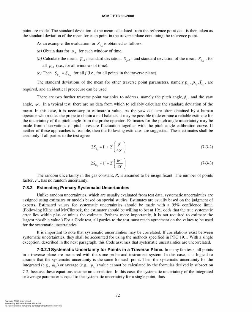
ASME PTC 11-2008

72

point are made. The standard deviation of the mean calculated from the reference point data is then taken as the standard deviation of the mean for each point in the traverse plane containing the reference point.

As an example, the evaluation for vjpS is obtained as follows:

(a) Obtain data for vRp for each window of time.

(b) Calculate the mean, vRp ; standard deviation, pvRS ; and standard deviation of the mean, vRpS , for

all vRp (i.e., for all windows of time).

(c) Then vRvj

p pS S= for all j (i.e., for all points in the traverse plane).

The standard deviations of the mean for other traverse point parameters, namely p p Ts t sj j j, , , are

required, and an identical procedure can be used.

There are two further traverse point variables to address, namely the pitch angle, jφ , and the yaw

angle, jψ . In a typical test, there are no data from which to reliably calculate the standard deviation of the

mean. In this case, it is necessary to estimate a value. As the yaw data are often obtained by a human operator who rotates the probe to obtain a null balance, it may be possible to determine a reliable estimate for the uncertainty of the pitch angle from the probe operator. Estimates for the pitch angle uncertainty may be made from observations of pitch pressure fluctuation together with the pitch angle calibration curve. If neither of these approaches is feasible, then the following estimates are suggested. These estimates shall be used only if all parties to the test agree.

2 1 245j

Sφφ° ° ⎛ ⎞

≈ + ⎜ ⎟⎝ ⎠

(7-3-2)

2 1 245j

Sψψ° ° ⎛ ⎞

≈ + ⎜ ⎟⎝ ⎠

(7-3-3)

The random uncertainty in the gas constant, R, is assumed to be insignificant. The number of points factor, Fn, has no random uncertainty.

7-3.2 Estimating Primary Systematic Uncertainties

Unlike random uncertainties, which are usually evaluated from test data, systematic uncertainties are assigned using estimates or models based on special studies. Estimates are usually based on the judgment of experts. Estimated values for systematic uncertainties should be made with a 95% confidence limit. (Following Kline and McClintock, the estimator should be willing to bet at 19:1 odds that the true systematic error lies within plus or minus the estimate. Perhaps more importantly, it is not required to estimate the largest possible value.) For a Code test, all parties to the test must reach agreement on the values to be used for the systematic uncertainties.

It is important to note that systematic uncertainties may be correlated. If correlations exist between systematic uncertainties, they shall be accounted for using the methods specified in PTC 19.1. With a single exception, described in the next paragraph, this Code assumes that systematic uncertainties are uncorrelated.

7-3.2.1 Systematic Uncertainty for Points in a Traverse Plane. In many fan tests, all points in a traverse plane are measured with the same probe and instrument system. In this case, it is logical to assume that the systematic uncertainty is the same for each point. Then the systematic uncertainty for the integrated (e.g., xm ) or average (e.g.,

xsp ) value cannot be calculated by the formulas derived in subsection

7-2, because these equations assume no correlation. In this case, the systematic uncertainty of the integrated or average parameter is equal to the systematic uncertainty for a single point, thus


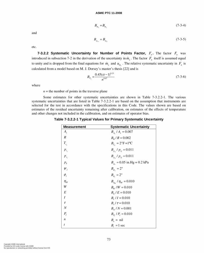
ASME PTC 11-2008

73

x jm mB B= (7-3-4)

and

sx sjp pB B= (7-3-5)

etc.

7-3.2.2 Systematic Uncertainty for Number of Points Factor, Fn . The factor Fn was

introduced in subsection 7-2 in the derivation of the uncertainty in mx . The factor Fn itself is assumed equal

to unity and is dropped from the final equations for mx and umx. The relative systematic uncertainty in Fn is

calculated from a model based on M. J. Dorsey’s master’s thesis [22] and is

0.33

0.67

0.45( 1)nFB

n

α −= (7-3-6)

where

n = the number of points in the traverse plane

Some estimates for other systematic uncertainties are shown in Table 7-3.2.2-1. The various systematic uncertainties that are listed in Table 7-3.2.2-1 are based on the assumption that instruments are selected for the test in accordance with the specifications in this Code. The values shown are based on estimates of the residual uncertainty remaining after calibration, on estimates of the effects of temperature and other changes not included in the calibration, and on estimates of operator bias.

Table 7-3.2.2-1 Typical Values for Primary Systematic Uncertainty

Measurement Systematic Uncertainty

xA / 0.007xA xB A =

R / 0.002RB R =

jsT 2 FsjTB = ° =1ºC

jvp / 0.011vjp vjB p =

jsp / 0.011sjp sjB p =

bp 0.05 in.HgbpB = = 0.2 kPa

jψ 2j

Bψ = °

jφ 2j

Bφ = °

Mη / 0.010M MBη η =

W / 0.010WB W =

E / 0.010EB E =

I / 0.010IB I = τ / 0.010Bτ τ = N / 0.001NB N =

IP / 0.010IP IB P =

n nilnB = t 1 sectB =


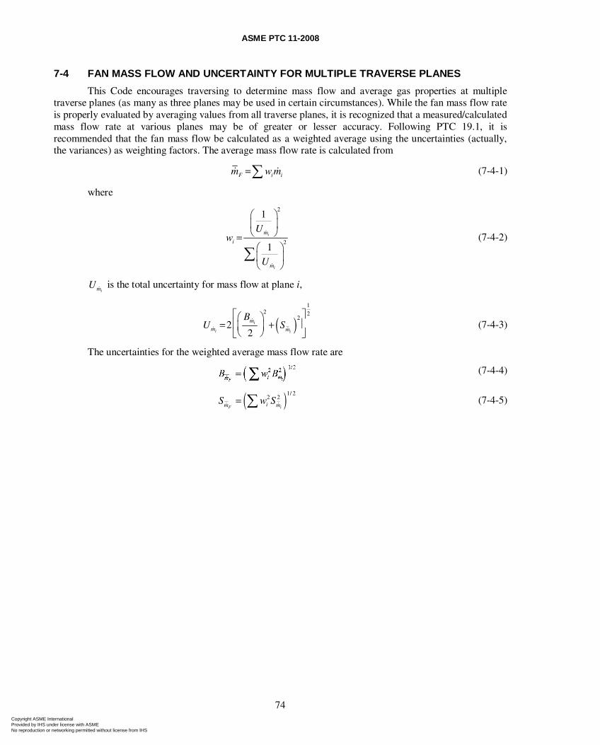
ASME PTC 11-2008

74

7-4 FAN MASS FLOW AND UNCERTAINTY FOR MULTIPLE TRAVERSE PLANES

This Code encourages traversing to determine mass flow and average gas properties at multiple traverse planes (as many as three planes may be used in certain circumstances). While the fan mass flow rate is properly evaluated by averaging values from all traverse planes, it is recognized that a measured/calculated mass flow rate at various planes may be of greater or lesser accuracy. Following PTC 19.1, it is recommended that the fan mass flow be calculated as a weighted average using the uncertainties (actually, the variances) as weighting factors. The average mass flow rate is calculated from

F i im w m=∑ (7-4-1)

where

2

2

1

1

i

i

m

i

m

Uw

U

⎛ ⎞⎜ ⎟⎝ ⎠=⎛ ⎞⎜ ⎟⎝ ⎠

∑ (7-4-2)

imU is the total uncertainty for mass flow at plane i,

( )1

2 22

22

i

i i

m

m m

BU S

⎡ ⎤⎛ ⎞⎢ ⎥= +⎜ ⎟⎝ ⎠⎣ ⎦

(7-4-3)

The uncertainties for the weighted average mass flow rate are

(7-4-4)

( )1/ 22 2

F iim mS w S= ∑ (7-4-5)


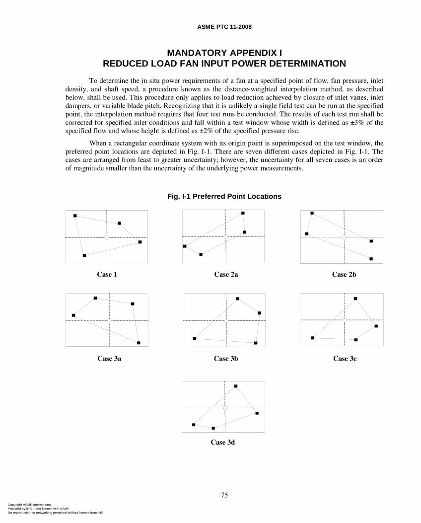
ASME PTC 11-2008

75

MANDATORY APPENDIX I REDUCED LOAD FAN INPUT POWER DETERMINATION

To determine the in situ power requirements of a fan at a specified point of flow, fan pressure, inlet density, and shaft speed, a procedure known as the distance-weighted interpolation method, as described below, shall be used. This procedure only applies to load reduction achieved by closure of inlet vanes, inlet dampers, or variable blade pitch. Recognizing that it is unlikely a single field test can be run at the specified point, the interpolation method requires that four test runs be conducted. The results of each test run shall be corrected for specified inlet conditions and fall within a test window whose width is defined as ±3% of the specified flow and whose height is defined as ±2% of the specified pressure rise.

When a rectangular coordinate system with its origin point is superimposed on the test window, the preferred point locations are depicted in Fig. I-1. There are seven different cases depicted in Fig. I-1. The cases are arranged from least to greater uncertainty; however, the uncertainty for all seven cases is an order of magnitude smaller than the uncertainty of the underlying power measurements.

Fig. I-1 Preferred Point Locations

Case 3a Case 3b Case 3c

Case 1 Case 2a Case 2b

Case 3d


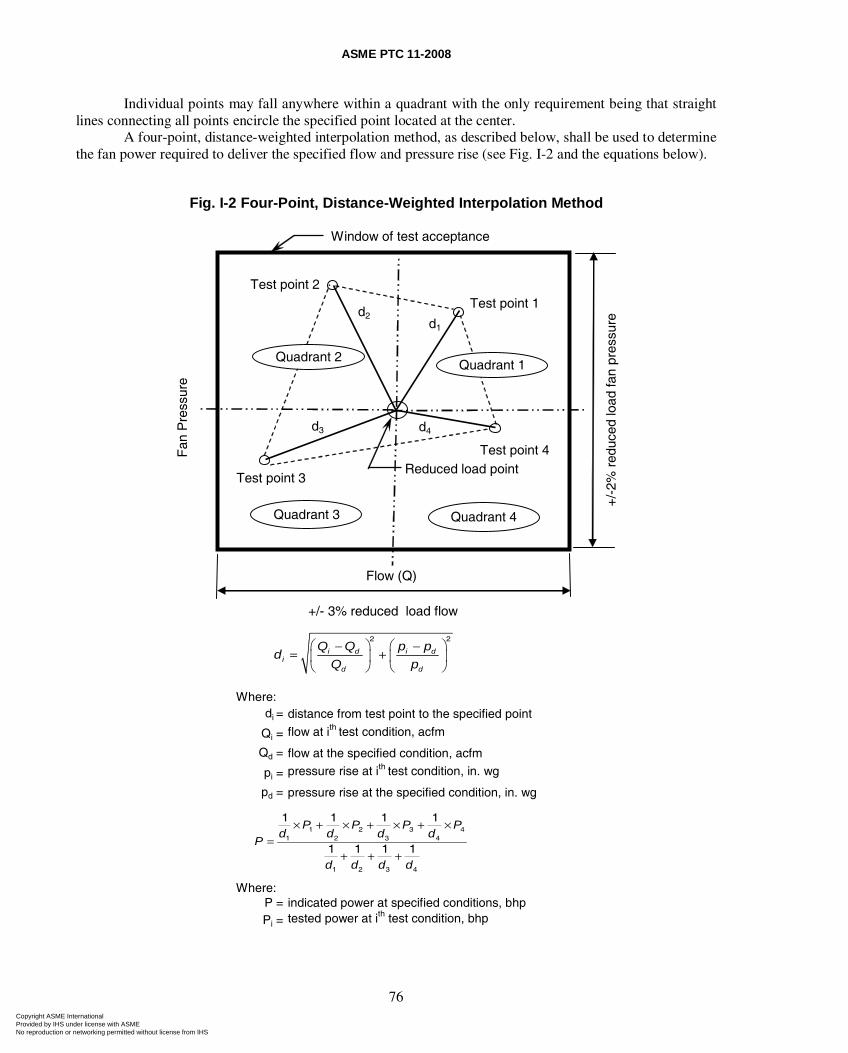
ASME PTC 11-2008

76

Individual points may fall anywhere within a quadrant with the only requirement being that straight lines connecting all points encircle the specified point located at the center.

A four-point, distance-weighted interpolation method, as described below, shall be used to determine the fan power required to deliver the specified flow and pressure rise (see Fig. I-2 and the equations below).

Fig. I-2 Four-Point, Distance-Weighted Interpolation Method

d1

d2

d3 d4

Reduced load point

Window of test acceptance

Test point 1Test point 2

Test point 3

Test point 4Fan

Pre

ssur

e

Quadrant 3 Quadrant 4

Quadrant 2Quadrant 1

Flow (Q)

+/- 3% reduced load flow+

/-2%

red

uced

load

fan

pres

sure

Where:di = distance from test point to the specified point

Qi = flow at ith test condition, acfm

Qd = flow at the specified condition, acfm

pi = pressure rise at ith test condition, in. wg

pd = pressure rise at the specified condition, in. wg

Where:P = indicated power at specified conditions, bhpPi = tested power at ith test condition, bhp

1 2 3 41 2 3 4

1 2 3 4

1 1 1 1

1 1 1 1

P P P Pd d d d

P

d d d d

× + × + × + ×=

+ + +

2 2

i d i di

d d

Q Q p pd

Q p

⎛ ⎞ ⎛ ⎞− −= +⎜ ⎟ ⎜ ⎟

⎝ ⎠ ⎝ ⎠


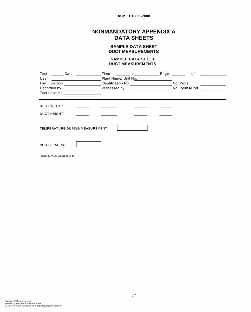
ASME PTC 11-2008

77

NONMANDATORY APPENDIX A DATA SHEETS

SAMPLE DATA SHEET DUCT MEASUREMENTS

Test Date Time to Page ofUser Plant Name/ Unit No.Fan: Function Identification No. No. PortsRecorded by No. Points/PortTest Location

DUCT W IDTH*

DUCT HEIGHT*

TEMPERATURE DURING MEASUREMENT

PORT SPACING

· Identify measurement units

SAMPLE DATA SHEET

Witnessed by

DUCT MEASUREMENTS


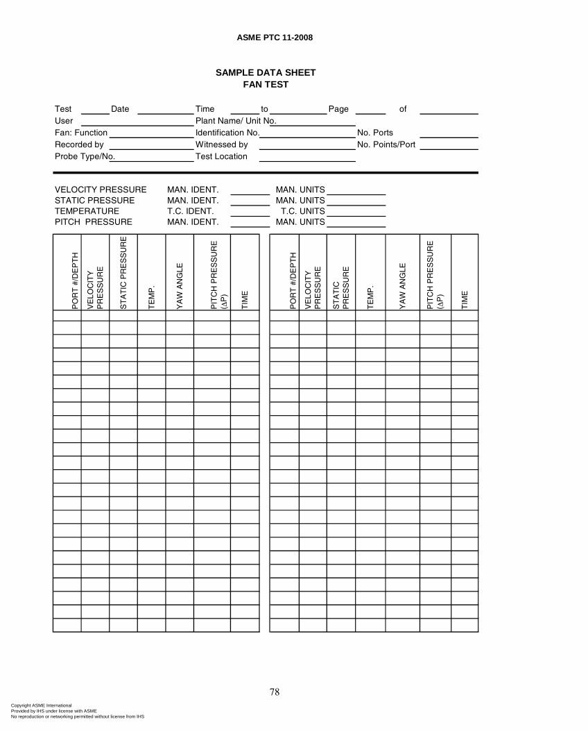
ASME PTC 11-2008

78

Test Date Time to Page ofUser Plant Name/ Unit No.Fan: Function Identification No. No. PortsRecorded by No. Points/PortProbe Type/No. Test Location

VELOCITY PRESSURE MAN. IDENT. MAN. UNITSSTATIC PRESSURE MAN. IDENT. MAN. UNITSTEMPERATURE T.C. IDENT. T.C. UNITSPITCH PRESSURE MAN. IDENT. MAN. UNITS

PO

RT

#/D

EP

TH

VE

LOC

ITY

P

RE

SS

UR

E

ST

AT

IC P

RE

SS

UR

E

TE

MP

.

YA

W A

NG

LE

PIT

CH

PR

ES

SU

RE

( ∆

P)

TIM

E

PO

RT

#/D

EP

TH

VE

LOC

ITY

P

RE

SS

UR

E

ST

AT

IC

PR

ES

SU

RE

TE

MP

.

YA

W A

NG

LE

PIT

CH

PR

ES

SU

RE

( ∆

P)

TIM

E

SAMPLE DATA SHEET

Witnessed by

FAN TEST


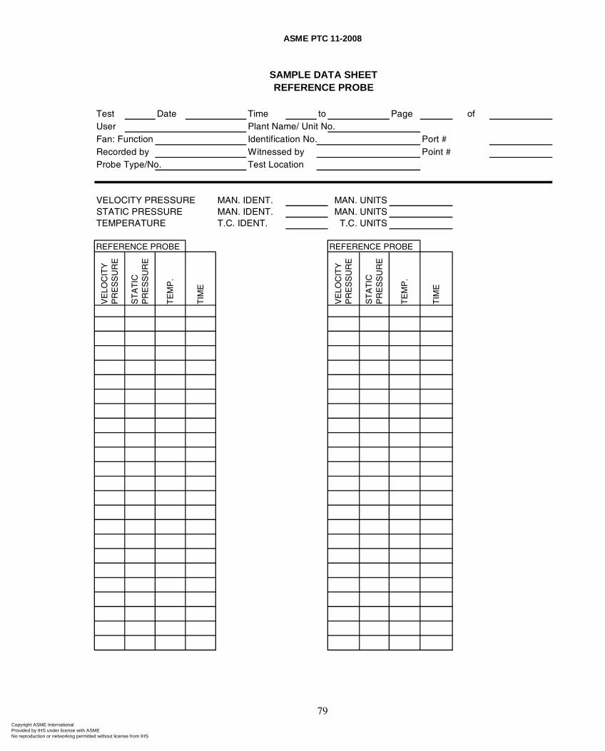
ASME PTC 11-2008

79

Test Date Time to Page ofUser Plant Name/ Unit No.Fan: Function Identification No. Port #Recorded by Point #Probe Type/No. Test Location

VELOCITY PRESSURE MAN. IDENT. MAN. UNITSSTATIC PRESSURE MAN. IDENT. MAN. UNITSTEMPERATURE T.C. IDENT. T.C. UNITS

REFERENCE PROBE REFERENCE PROBE

VE

LOC

ITY

P

RE

SS

UR

E

ST

AT

IC

PR

ES

SU

RE

TE

MP

.

TIM

E

VE

LOC

ITY

P

RE

SS

UR

E

ST

AT

IC

PR

ES

SU

RE

TE

MP

.

TIM

E

SAMPLE DATA SHEET

Witnessed by

REFERENCE PROBE


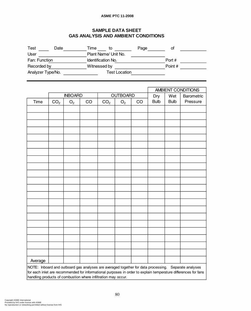
ASME PTC 11-2008

80

Test Date Time to Page ofUser Plant Name/ Unit No.Fan: Function Identification No. Port #Recorded by Witnessed by Point #Analyzer Type/No. Test Location

CO2 O2 O2 COCO2

Average

OUTBOARD

NOTE: Inboard and outboard gas analyses are averaged together for data processing. Separate analyses for each inlet are recommended for informational purposes in order to explain temperature differences for fans handling products of combustion where infiltration may occur.

Barometric Pressure

SAMPLE DATA SHEETGAS ANALYSIS AND AMBIENT CONDITIONS

AMBIENT CONDITIONSDry Bulb

Wet BulbTime CO

INBOARD


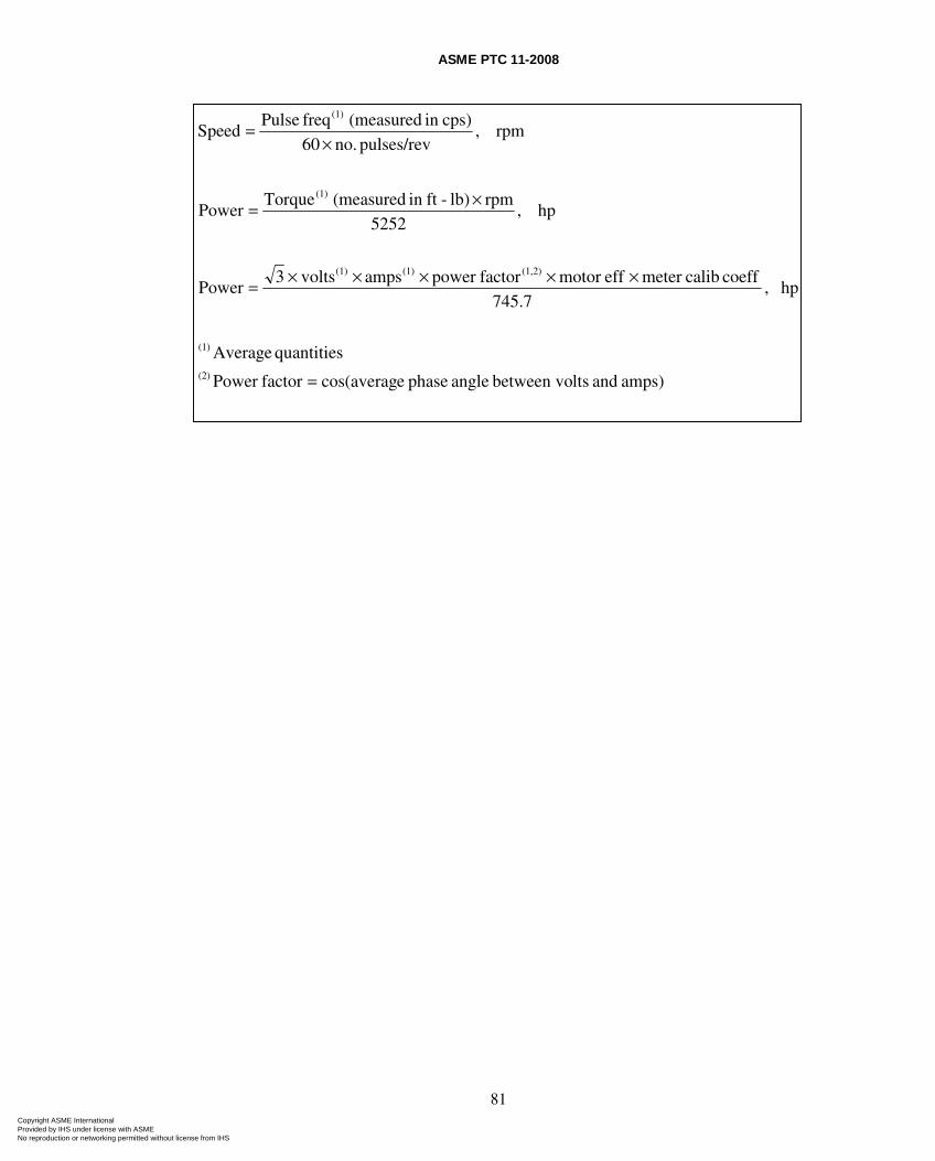
ASME PTC 11-2008

81

amps) and ltsbetween vo angle phase ecos(averagfactorPower

quantities Average

hp ,745.7

coeff calibmeter effmotor factorpower ampsvolts3Power

hp ,5252

rpmlb)-ftin (measured TorquePower

rpm ,pulses/rev no.60

cps)in (measured freq PulseSpeed

(2)

(1)

(1,2)(1)(1)

(1)

(1)

=

×××××=

×=

×=


ASME PTC 11-2008

82

NONMANDATORY APPENDIX B SAMPLE CALCULATIONS

The code recommends that a spreadsheet or other computer program be used for the calculations of results and uncertainties. The following tables are extracted from a spreadsheet program.

These tables are of two types. The first type shows what data have been entered, as well as the results of the calculations. Data entry cells are shaded; results cells are not. The second type of table, designated by an F after the table number, shows the formulas for the various results in the corresponding first type of table.

The tables with the formulas show the variable names, values for constants and input, formulas for calculations, and names of the cell or range. Each cell or range has a name that is as close to the symbols used in this Code, with the limits of EXCEL. If the formulas are entered as shown, and the cells and ranges are named as indicated, the results should be the same as the sample.

To minimize the number of pages devoted to this example, neither the input data nor the calculations are complete. Traverse data and traverse point calculations are shown for only a limited number of points at Plane 1A and completely omitted for Planes 1B and 2. The results are given for all three planes.

This example uses U.S. Customary units and simulates a test of a double inlet-induced draft fan using five-hole probes in rectangular ducts. Power is measured by wattmeter.


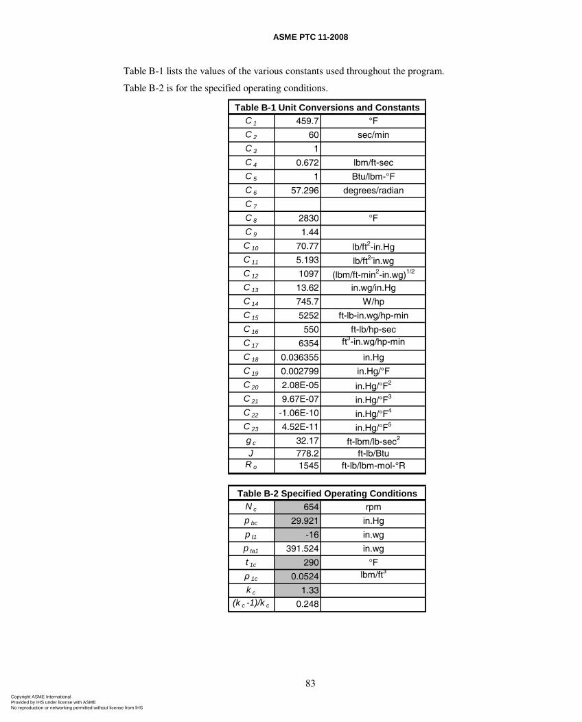
ASME PTC 11-2008

83

Table B-1 lists the values of the various constants used throughout the program.

Table B-2 is for the specified operating conditions.

C 1 459.7 °F

C 2 60 sec/min

C 3 1

C 4 0.672 lbm/ft-sec

C 5 1 Btu/lbm-°F

C 6 57.296 degrees/radian

C 7

C 8 2830 °F

C 9 1.44

C 10 70.77 lb/ft2-in.HgC 11 5.193 lb/ft2-in.wgC 12 1097 (lbm/ft-min2-in.wg)1/2

C 13 13.62 in.wg/in.Hg

C 14 745.7 W/hp

C 15 5252 ft-lb-in.wg/hp-min

C 16 550 ft-lb/hp-sec

C 17 6354 ft3-in.wg/hp-min

C 18 0.036355 in.Hg

C 19 0.002799 in.Hg/°F

C 20 2.08E-05 in.Hg/°F2

C 21 9.67E-07 in.Hg/°F3

C 22 -1.06E-10 in.Hg/°F4

C 23 4.52E-11 in.Hg/°F5

g c 32.17 ft-lbm/lb-sec2

J 778.2 ft-lb/BtuR o 1545 ft-lb/lbm-mol-°R

N c 654 rpm

p bc 29.921 in.Hg

p t1 -16 in.wg

p ta1 391.524 in.wg

t 1c 290 °F

ρ 1c 0.0524 lbm/ft3

k c 1.33(k c -1)/k c 0.248

Table B-1 Unit Conversions and Constants

Table B-2 Specified Operating Conditions


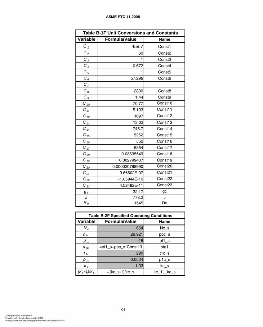
ASME PTC 11-2008

84

Variable Formula/Value Name

C 1 459.7 Const1

C 2 60 Const2

C 3 1 Const3

C 4 0.672 Const4

C 5 1 Const5

C 6 57.296 Const6

C 7

C 8 2830 Const8

C 9 1.44 Const9

C 10 70.77 Const10

C 11 5.193 Const11

C 12 1097 Const12

C 13 13.62 Const13

C 14 745.7 Const14

C 15 5252 Const15

C 16 550 Const16

C 17 6354 Const17

C 18 0.03635549 Const18

C 19 0.002799407 Const19

C 20 0.000020788990 Const20

C 21 9.66602E-07 Const21

C 22 -1.05944E-10 Const22

C 23 4.52482E-11 Const23

g c 32.17 gc

J 778.2 JR o 1545 Ro

Variable Formula/Value Name

N c 654 Nc_s

p bc 29.921 pbc_s

p t1 -16 pt1_s

p ta1 =pt1_s+pbc_s*Const13 pta1

t 1c 290 t1c_s

ρ 1c 0.0524 ρ1c_s

k c 1.33 kc_s(k c -1)/k c =(kc_s-1)/kc_s kc_1__kc_s

Table B-1F Unit Conversions and Constants

Table B-2F Specified Operating Conditions


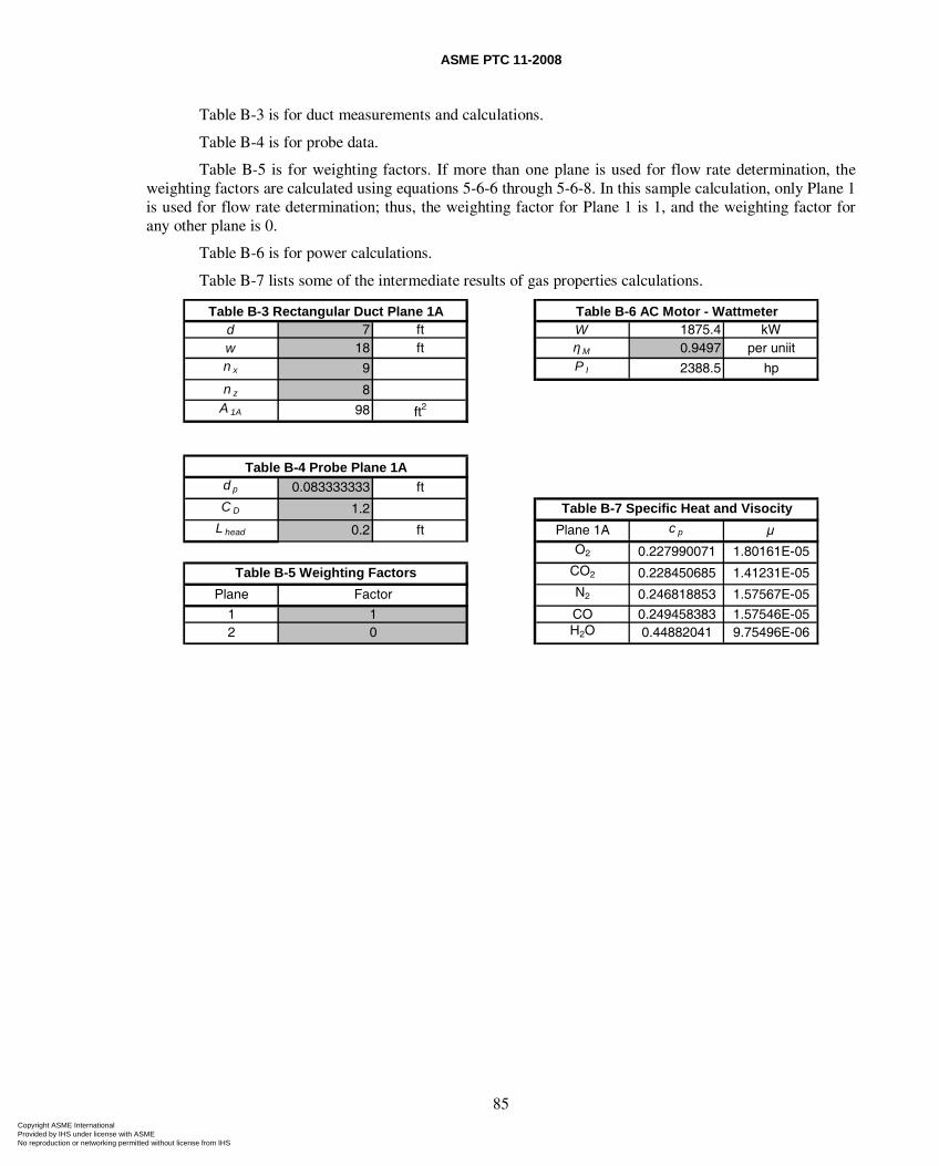
ASME PTC 11-2008

85

Table B-3 is for duct measurements and calculations.

Table B-4 is for probe data.

Table B-5 is for weighting factors. If more than one plane is used for flow rate determination, the weighting factors are calculated using equations 5-6-6 through 5-6-8. In this sample calculation, only Plane 1 is used for flow rate determination; thus, the weighting factor for Plane 1 is 1, and the weighting factor for any other plane is 0.

Table B-6 is for power calculations.

Table B-7 lists some of the intermediate results of gas properties calculations.

d 7 ft W 1875.4 kWw 18 ft ηM 0.9497 per uniitn x 9 P I 2388.5 hp

n z 8A 1A 98 ft2

d p 0.083333333 ft

C D 1.2

L head 0.2 ft Plane 1A c p μO2 0.227990071 1.80161E-05

CO2 0.228450685 1.41231E-05

Plane N2 0.246818853 1.57567E-05

1 CO 0.249458383 1.57546E-052 H2O 0.44882041 9.75496E-06

Table B-3 Rectangular Duct Plane 1A Table B-6 AC Motor - Wattmeter

Table B-4 Probe Plane 1A

Table B-7 Specific Heat and Visocity

Factor

10

Table B-5 Weighting Factors


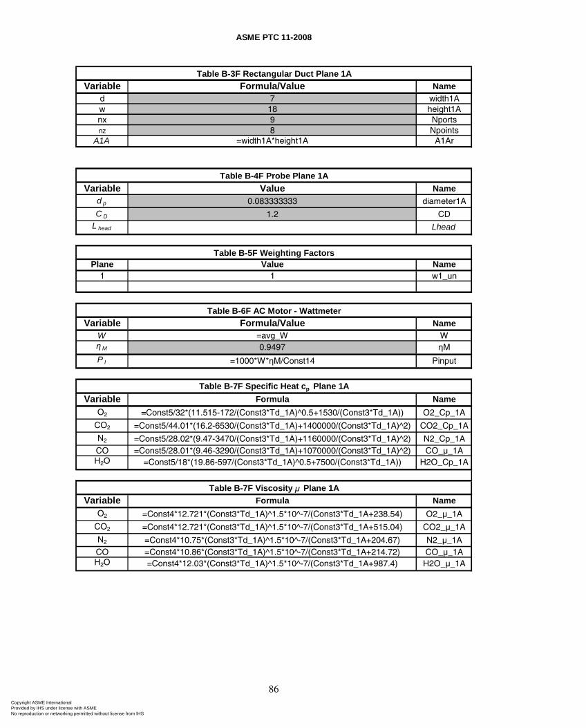
ASME PTC 11-2008

86

Variable Formula/Value Named 7 width1Aw 18 height1Anx 9 Nportsnz 8 Npoints

A1A =width1A*height1A A1Ar

Variable Value Named p 0.083333333 diameter1A

C D 1.2 CDL head Lhead

Plane Value Name1 1 w1_un

Variable Formula/Value NameW =avg_W Wη M 0.9497 ηM

P I =1000*W*ηM/Const14 Pinput

Variable Formula Name

O2 =Const5/32*(11.515-172/(Const3*Td_1A)^0.5+1530/(Const3*Td_1A)) O2_Cp_1A

CO2 =Const5/44.01*(16.2-6530/(Const3*Td_1A)+1400000/(Const3*Td_1A)^2) CO2_Cp_1A

N2 =Const5/28.02*(9.47-3470/(Const3*Td_1A)+1160000/(Const3*Td_1A)^2) N2_Cp_1ACO =Const5/28.01*(9.46-3290/(Const3*Td_1A)+1070000/(Const3*Td_1A)^2) CO_μ_1AH2O =Const5/18*(19.86-597/(Const3*Td_1A)^0.5+7500/(Const3*Td_1A)) H2O_Cp_1A


O2 =Const4*12.721*(Const3*Td_1A)^1.5*10^-7/(Const3*Td_1A+238.54) O2_μ_1A

CO2 =Const4*12.721*(Const3*Td_1A)^1.5*10^-7/(Const3*Td_1A+515.04) CO2_μ_1A

N2 =Const4*10.75*(Const3*Td_1A)^1.5*10^-7/(Const3*Td_1A+204.67) N2_μ_1ACO =Const4*10.86*(Const3*Td_1A)^1.5*10^-7/(Const3*Td_1A+214.72) CO_μ_1AH2O =Const4*12.03*(Const3*Td_1A)^1.5*10^-7/(Const3*Td_1A+987.4) H2O_μ_1A

Table B-7F Specific Heat cp Plane 1A

Table B-7F Viscosity μ Plane 1A

Table B-3F Rectangular Duct Plane 1A

Table B-4F Probe Plane 1A

Table B-5F Weighting Factors

Table B-6F AC Motor - Wattmeter


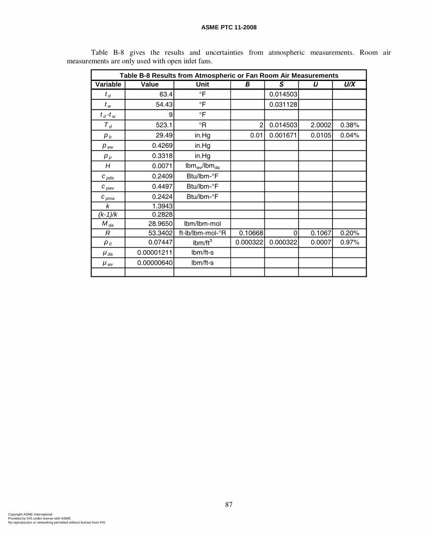
ASME PTC 11-2008

87

Table B-8 gives the results and uncertainties from atmospheric measurements. Room air measurements are only used with open inlet fans.

Variable Value Unit B S U U/Xt d 63.4 °F 0.014503

t w 54.43 °F 0.031128

t d -t w 9 °F

T d 523.1 °R 2 0.014503 2.0002 0.38%

p b 29.49 in.Hg 0.01 0.001671 0.0105 0.04%

p ew 0.4269 in.Hg

p p 0.3318 in.Hg

H 0.0071 lbmwv/lbmda

c pda 0.2409 Btu/lbm-°F

c pwv 0.4497 Btu/lbm-°F

c pma 0.2424 Btu/lbm-°Fk 1.3943

(k-1)/k 0.2828M da 28.9650 lbm/lbm-molR 53.3402 ft-lb/lbm-mol-°R 0.10668 0 0.1067 0.20%ρ 0 0.07447 lbm/ft3 0.000322 0.000322 0.0007 0.97%

μ da 0.00001211 lbm/ft-s

μ wv 0.00000640 lbm/ft-s

Table B-8 Results from Atmospheric or Fan Room Air Measurements


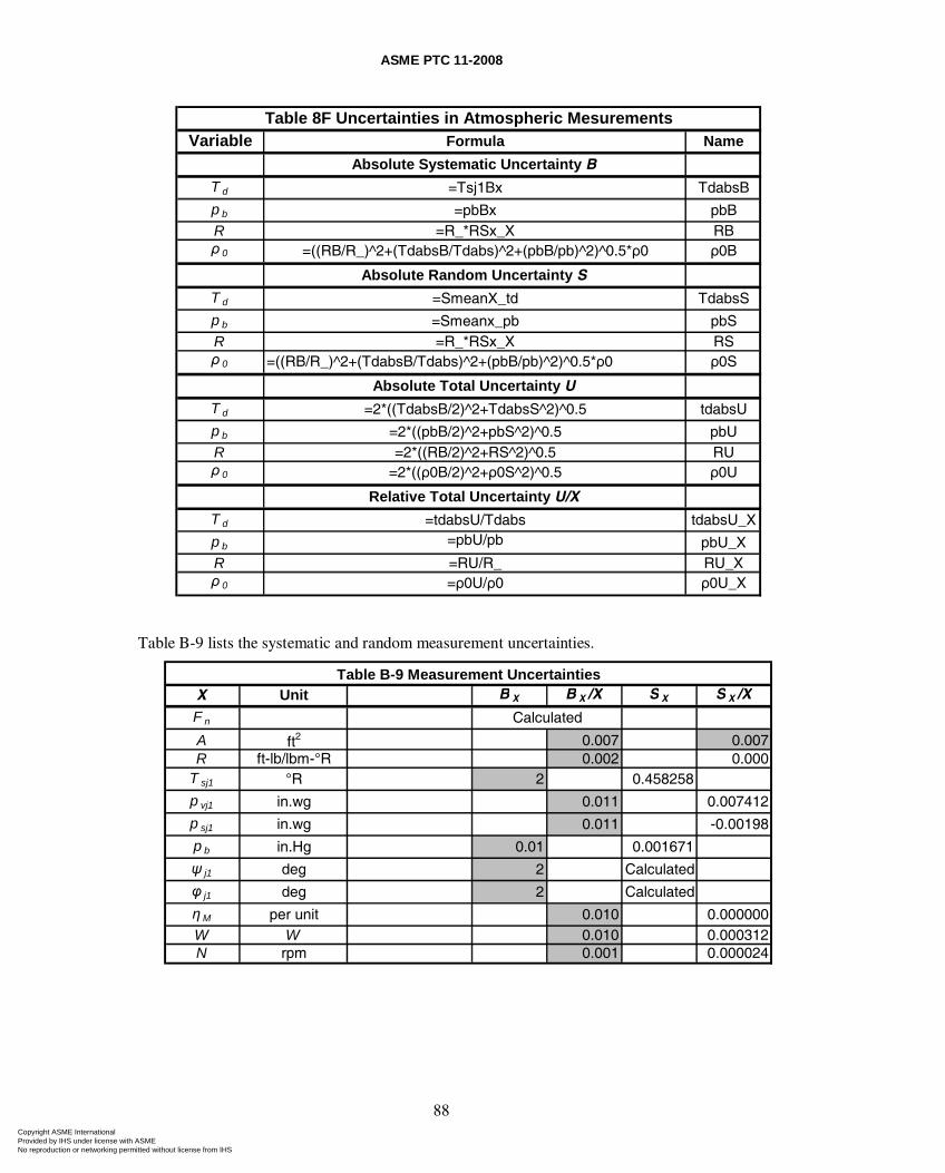
ASME PTC 11-2008

88


Absolute Systematic Uncertainty B

T d =Tsj1Bx TdabsB

p b =pbBx pbBR =R_*RSx_X RBρ 0 =((RB/R_)^2+(TdabsB/Tdabs)^2+(pbB/pb)^2)^0.5*ρ0 ρ0B

Absolute Random Uncertainty S

T d =SmeanX_td TdabsS

p b =Smeanx_pb pbSR =R_*RSx_X RSρ 0 =((RB/R_)^2+(TdabsB/Tdabs)^2+(pbB/pb)^2)^0.5*ρ0 ρ0S

Absolute Total Uncertainty U

T d =2*((TdabsB/2)^2+TdabsS^2)^0.5 tdabsU

p b =2*((pbB/2)^2+pbS^2)^0.5 pbUR =2*((RB/2)^2+RS^2)^0.5 RUρ 0 =2*((ρ0B/2)^2+ρ0S^2)^0.5 ρ0U

Relative Total Uncertainty U/X

T d =tdabsU/Tdabs tdabsU_X

p b =pbU/pb pbU_XR =RU/R_ RU_Xρ 0 =ρ0U/ρ0 ρ0U_X

Table 8F Uncertainties in Atmospheric Mesurements

Table B-9 lists the systematic and random measurement uncertainties.

X Unit B X B X /X S X S X /X

F n

A ft2 0.007 0.007R ft-lb/lbm-°R 0.002 0.000

T sj1 °R 2 0.458258

p vj1 in.wg 0.011 0.007412

p sj1 in.wg 0.011 -0.00198

p b in.Hg 0.01 0.001671

ψ j1 deg 2 Calculated

φ j1 deg 2 Calculated

η M per unit 0.010 0.000000W W 0.010 0.000312N rpm 0.001 0.000024

Table B-9 Measurement Uncertainties

Calculated


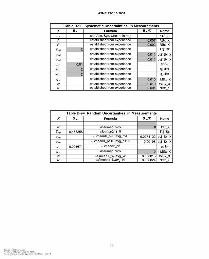
ASME PTC 11-2008

89

X B X Formula B X /X Name

F n see Abs. Sys. Uncert. in n 1A n1A_BA established from experience 0.007 ABx_XR established from experience 0.002 RBx_X

T sj1 2 established from experience Tsj1Bx

p vj1 established from experience 0.011 pvj1Bx_X

p sj1 established from experience 0.011 psj1Bx_X

p b 0.01 established from experience pbBx

ψ j1 2 established from experience ψj1Bx

φ j1 2 established from experience φj1Bx

η M established from experience 0.010 ηMBx_XW established from experience 0.010 WBx_XN established from experience 0.001 NBx_X

X S X Formula S X /X Name

R assumed zero 0 RSx_XT sj1 0.458258 =SmeanX_t1R Tsj1Sx

p vj1 =SmeanX_pvR/avg_pvR 0.0074122 pvj1Sx_X

p sj1 =SmeanX_ps1R/avg_ps1R -0.00198 psj1Sx_X

p b 0.001671 =Smeanx_pb pbSx

η M assumed zero 0 ηMSx_XW =SmeanX_W/avg_W 0.000015 WSx_XN =Smeanx_N/avg_N 0.000024 NSx_X

Table B-9F Systematic Uncertainties in Measurements

Table B-9F Random Uncertainties in Measurements


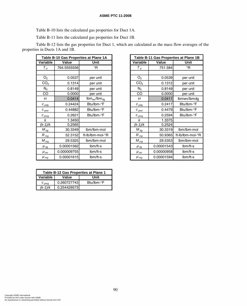
ASME PTC 11-2008

90

Table B-10 lists the calculated gas properties for Duct 1A.

Table B-11 lists the calculated gas properties for Duct 1B.

Table B-12 lists the gas properties for Duct 1, which are calculated as the mass flow averages of the properties in Ducts 1A and 1B.

Variable Value Unit Variable Value UnitT d 764.5555556 °R T d 751.584 °R

O2 0.0537 per unit O2 0.0539 per unit

CO2 0.1314 per unit CO2 0.1312 per unit

N2 0.8149 per unit N2 0.8149 per unitCO 0.0000 per unit CO 0.0000 per unitH 0.0414 lbmwv/lbmdg H 0.0411 lbmwv/lbmdg

c pdg 0.24424 Btu/lbm-°F c pdg 0.2417 Btu/lbm-°F

c pwv 0.44882 Btu/lbm-°F c pwv 0.4479 Btu/lbm-°F

c pmg 0.2621 Btu/lbm-°F c pmg 0.2594 Btu/lbm-°Fk 1.3450 k 1.3375

(k-1)/k 0.2565 (k-1)/k 0.2524M dg 30.3349 lbm/lbm-mol M dg 30.3319 lbm/lbm-mol

R mg 52.3152 ft-lb/lbm-mol-°R R mg 50.9365 ft-lb/lbm-mol-°R

M mg 29.5325 lbm/lbm-mol M mg 29.5353 lbm/lbm-mol

μ dg 0.00001562 lbm/ft-s μ dg 0.00001543 lbm/ft-s

μ wv 0.000009755 lbm/ft-s μ wv 0.00000958 lbm/ft-sμmg 0.00001615 lbm/ft-s μmg 0.00001594 lbm/ft-s

Variable Value Unitc pmg 0.260727743 Btu/lbm-°F

(k-1)/k 0.254429573

Table B-10 Gas Properties at Plane 1A

Table B-12 Gas Properties at Plane 1

Table B-11 Gas Properties at Plane 1B


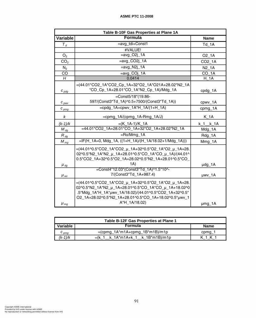
ASME PTC 11-2008

91


T d =avg_tdi+Const1 Td_1A #VALUE!

O2 =avg_O2j_1A O2_1A

CO2 =avg_CO2j_1A CO2_1A

N2 =avg_N2j_1A N2_1ACO =avg_COj_1A CO_1AH 0.0414 H_1A

c pdg

=(44.01*CO2_1A*CO2_Cp_1A+32*O2_1A*O21A+28.02*N2_1A*CO_Cp_1A+28.01*CO_1A*N2_Cp_1A)/Mdg_1A cpdg_1A

c pwv

=Const5/18*(19.86-597/(Const3*Td_1A)^0.5+7500/(Const3*Td_1A)) cpwv_1A

c pmg =cpdg_1A+cpwv_1A*H_1A/(1+H_1A) cpmg_1A

k =cpmg_1A/(cpmg_1A-Rmg_1A/J) K_1A

(k-1)/k =(K_1A-1)/K_1A k_1__k_1AM dg =44.01*CO2_1A+28.01*CO_1A+32*O2_1A+28.02*N2_1A Mdg_1A

R dg =Ro/Mmg_1A Rdg_1A

M mg =IF(H_1A=0, Mdg_1A, ((1+H_1A)/(H_1A/18.02+1/Mdg_1A))) Mmg_1A

μ dg

=(44.01^0.5*CO2_1A*CO2_μ_1A+32^0.5*O2_1A*O2_μ_1A+28.02^0.5*N2_1A*N2_μ_1A+28.01^0.5*CO_1A*CO_μ_1A)/(44.01^0.5*CO2_1A+32^0.5*O2_1A+28.02^0.5*N2_1A+28.01^0.5*CO_

1A) μdg_1A

μ wv

=Const4*12.03*(Const3*Td_1A)^1.5*10^-7/(Const3*Td_1A+987.4) μwv_1A

μmg

=(44.01^0.5*CO2_1A*CO2_μ_1A+32^0.5*O2_1A*O2_μ_1A+28.02^0.5*N2_1A*N2_μ_1A+28.01^0.5*CO_1A*CO_μ_1A+18.02^0.5*Mdg_1A*H_1A*μwv_1A/18.02)/(44.01^0.5*CO2_1A+32^0.5*O2_1A+28.02^0.5*N2_1A+28.01^0.5*CO_1A+18.02^0.5*μwv_1

A*H_1A/18.02) μmg_1A

Variable Formula Namec pmg =(cpmg_1A*m1A+cpmg_1B*m1B)/m1p cpmg_1

(k-1)/k =(k_1__k_1A*m1A+k_1__k_1B*m1B)/m1p K_1_K_1

Table B-10F Gas Properties at Plane 1A

Table B-12F Gas Properties at Plane 1


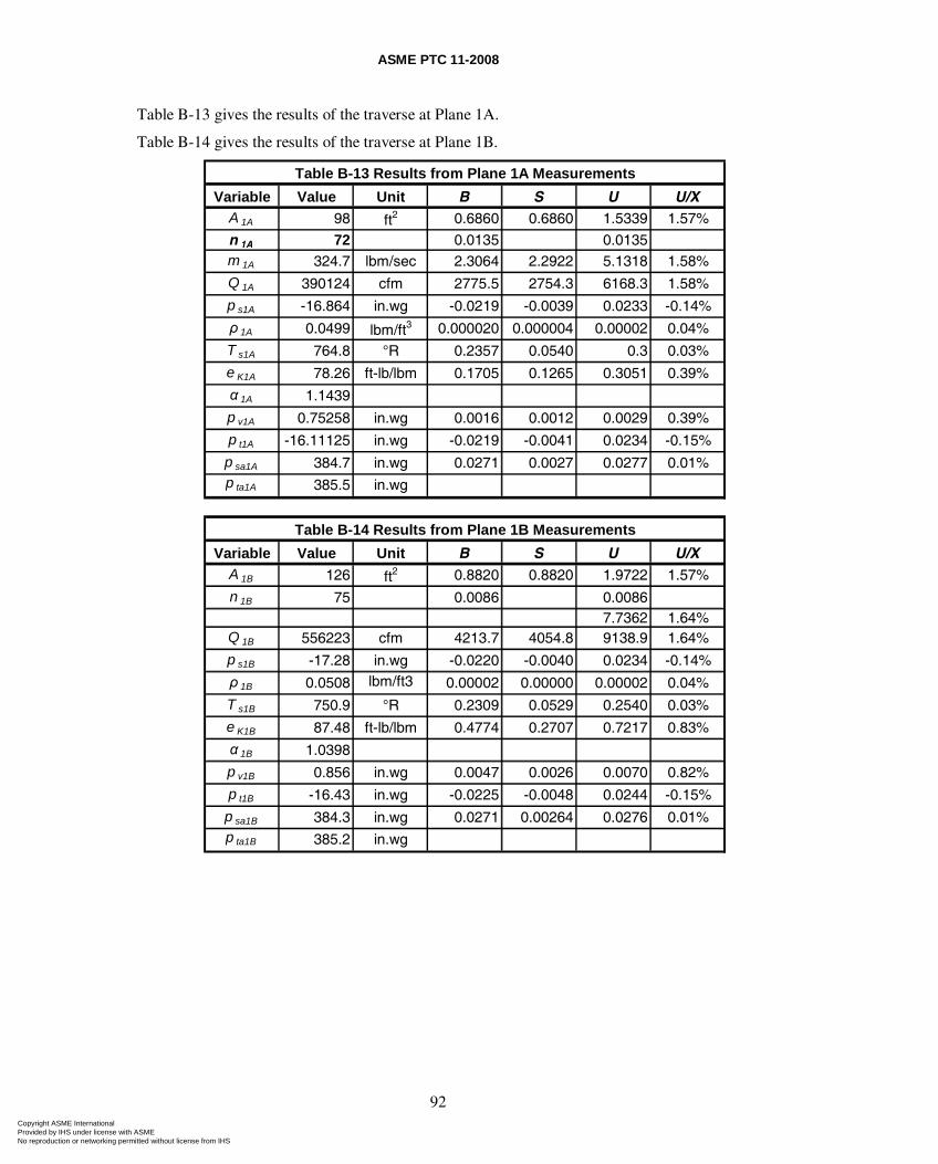
ASME PTC 11-2008

92

Table B-13 gives the results of the traverse at Plane 1A.

Table B-14 gives the results of the traverse at Plane 1B.

Variable Value Unit B S U U/XA 1A 98 ft2 0.6860 0.6860 1.5339 1.57%

n 1A 72 0.0135 0.0135 m 1A 324.7 lbm/sec 2.3064 2.2922 5.1318 1.58%

Q 1A 390124 cfm 2775.5 2754.3 6168.3 1.58%

p s1A -16.864 in.wg -0.0219 -0.0039 0.0233 -0.14%

ρ 1A 0.0499 lbm/ft3 0.000020 0.000004 0.00002 0.04%

T s1A 764.8 °R 0.2357 0.0540 0.3 0.03%

e K1A 78.26 ft-lb/lbm 0.1705 0.1265 0.3051 0.39%

α 1A 1.1439

p v1A 0.75258 in.wg 0.0016 0.0012 0.0029 0.39%

p t1A -16.11125 in.wg -0.0219 -0.0041 0.0234 -0.15%

p sa1A 384.7 in.wg 0.0271 0.0027 0.0277 0.01%p ta1A 385.5 in.wg

Variable Value Unit B S U U/XA 1B 126 ft2 0.8820 0.8820 1.9722 1.57%

n 1B 75 0.0086 0.0086 7.7362 1.64%

Q 1B 556223 cfm 4213.7 4054.8 9138.9 1.64%

p s1B -17.28 in.wg -0.0220 -0.0040 0.0234 -0.14%

ρ 1B 0.0508 lbm/ft3 0.00002 0.00000 0.00002 0.04%

T s1B 750.9 °R 0.2309 0.0529 0.2540 0.03%

e K1B 87.48 ft-lb/lbm 0.4774 0.2707 0.7217 0.83%

α 1B 1.0398

p v1B 0.856 in.wg 0.0047 0.0026 0.0070 0.82%

p t1B -16.43 in.wg -0.0225 -0.0048 0.0244 -0.15%

p sa1B 384.3 in.wg 0.0271 0.00264 0.0276 0.01%p ta1B 385.2 in.wg

Table B-13 Results from Plane 1A Measurements

Table B-14 Results from Plane 1B Measurements


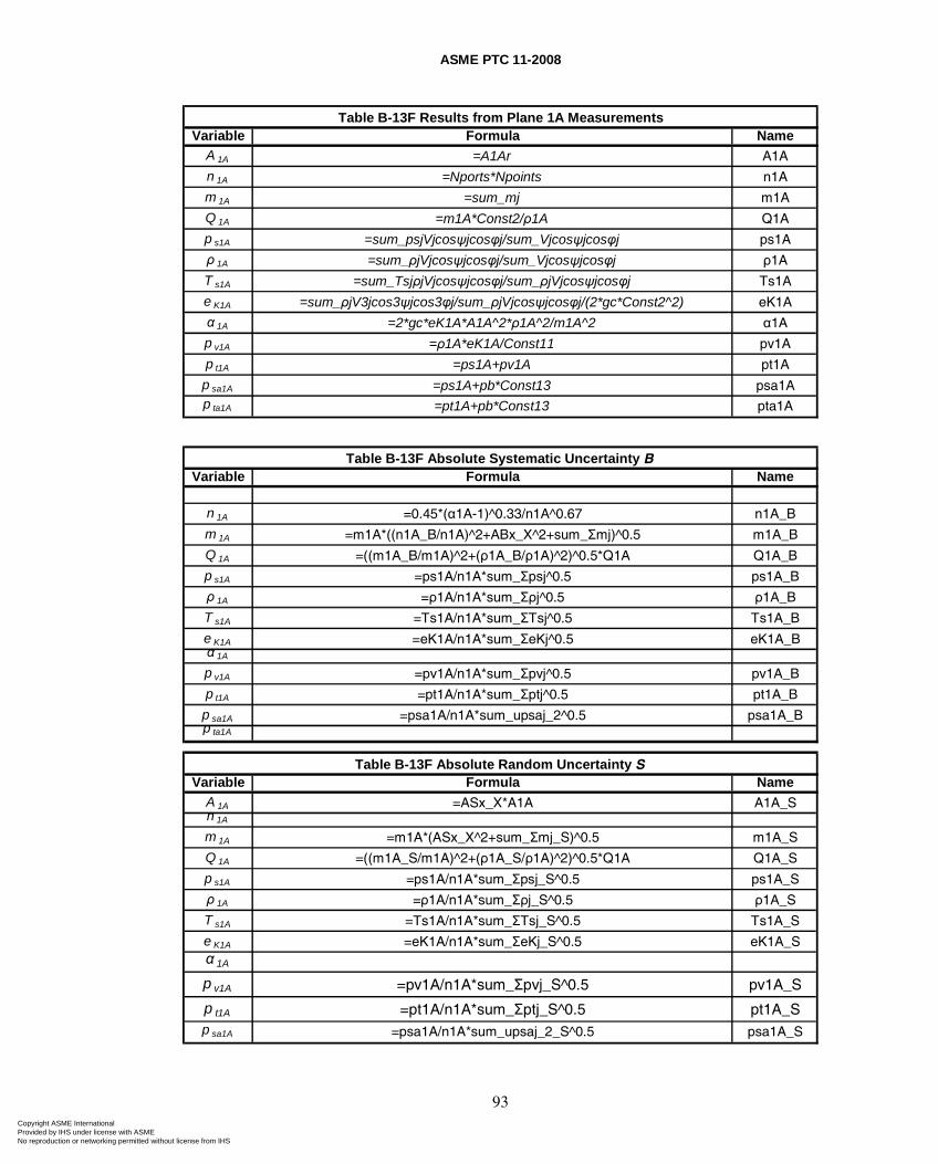
ASME PTC 11-2008

93

Variable Formula NameA 1A =A1Ar A1A

n 1A =Nports*Npoints n1A

m 1A =sum_mj m1A

Q 1A =m1A*Const2/ρ1A Q1A

p s1A =sum_psjVjcosψjcosφj/sum_Vjcosψjcosφj ps1A

ρ 1A =sum_ρjVjcosψjcosφj/sum_Vjcosψjcosφj ρ1A

T s1A =sum_TsjρjVjcosψjcosφj/sum_ρjVjcosψjcosφj Ts1A

e K1A =sum_ρjV3jcos3ψjcos3φj/sum_ρjVjcosψjcosφj/(2*gc*Const2^2) eK1A

α 1A =2*gc*eK1A*A1A^2*ρ1A^2/m1A^2 α1A

p v1A =ρ1A*eK1A/Const11 pv1A

p t1A =ps1A+pv1A pt1A

p sa1A =ps1A+pb*Const13 psa1Ap ta1A =pt1A+pb*Const13 pta1A

Table B-13F Results from Plane 1A Measurements


n 1A =0.45*(α1A-1)^0.33/n1A^0.67 n1A_B

m 1A =m1A*((n1A_B/n1A)^2+ABx_X^2+sum_Σmj)^0.5 m1A_B

Q 1A =((m1A_B/m1A)^2+(ρ1A_B/ρ1A)^2)^0.5*Q1A Q1A_B

p s1A =ps1A/n1A*sum_Σpsj^0.5 ps1A_B

ρ 1A =ρ1A/n1A*sum_Σρj^0.5 ρ1A_B

T s1A =Ts1A/n1A*sum_ΣTsj^0.5 Ts1A_B

e K1A =eK1A/n1A*sum_ΣeKj^0.5 eK1A_Bα 1A

p v1A =pv1A/n1A*sum_Σpvj^0.5 pv1A_B

p t1A =pt1A/n1A*sum_Σptj^0.5 pt1A_B

p sa1A =psa1A/n1A*sum_upsaj_2^0.5 psa1A_Bp ta1A

Variable Formula NameA 1A =ASx_X*A1A A1A_Sn 1A

m 1A =m1A*(ASx_X^2+sum_Σmj_S)^0.5 m1A_S

Q 1A =((m1A_S/m1A)^2+(ρ1A_S/ρ1A)^2)^0.5*Q1A Q1A_S

p s1A =ps1A/n1A*sum_Σpsj_S^0.5 ps1A_S

ρ 1A =ρ1A/n1A*sum_Σρj_S^0.5 ρ1A_S

T s1A =Ts1A/n1A*sum_ΣTsj_S^0.5 Ts1A_S

e K1A =eK1A/n1A*sum_ΣeKj_S^0.5 eK1A_Sα 1A

p v1A =pv1A/n1A*sum_Σpvj_S^0.5 pv1A_S

p t1A =pt1A/n1A*sum_Σptj_S^0.5 pt1A_Sp sa1A =psa1A/n1A*sum_upsaj_2_S^0.5 psa1A_S

Table B-13F Absolute Systematic Uncertainty B

Table B-13F Absolute Random Uncertainty S


ASME PTC 11-2008

94

Variable Formula NameA 1A =2*((A1A_B/2)^2+A1A_S^2)^0.5 A1A_U

n 1A =2*((n1A_B/2)^2+AI5^2)^0.5 n1A_U

m 1A =2*((m1A_B/2)^2+m1A_S^2)^0.5 m1A_U

Q 1A =2*((Q1A_B/2)^2+Q1A_S^2)^0.5 Q1A_U

p s1A =2*((ps1A_B/2)^2+ps1A_S^2)^0.5 ps1A_U

ρ 1A =2*((ρ1A_B/2)^2+ρ1A_S^2)^0.5 ρ1A_U

T s1A =2*((Ts1A_B/2)^2+Ts1A_S^2)^0.5 Ts1A_U

e K1A =2*((eK1A_B/2)^2+eK1A_S^2)^0.5 eK1A_U

α 1A

p v1A =2*((pv1A_B/2)^2+pv1A_S^2)^0.5 pv1A_U

p t1A =2*((pt1A_B/2)^2+pt1A_S^2)^0.5 pt1A_U

p sa1A =2*((psa1A_B/2)^2+psa1A_S^2)^0.5 psa1A_Up ta1A

Variable Formula NameA 1A =A1A_U/A1A A1A_U_X

n 1A

m 1A =m1A_U/m1A m1A_U_X

Q 1A =Q1A_U/Q1A Q1A_U_X

p s1A =ps1A_U/ps1A ps1A_U_X

ρ 1A =ρ1A_U/ρ1A ρ1A_U_X

T s1A =Ts1A_U/Ts1A Ts1A_U_X

e K1A =eK1A_U/eK1A eK1A_U_X

α 1A

p v1A =pv1A_U/pv1A pv1A_U_X

p t1A =pt1A_U/pt1A pt1A_U_X

p sa1A =psa1A_U/psa1A psa1A_U_Xp ta1A

Table B-13F Relative Total Uncertainty U/X

Table B-13F Absolute Total Uncertainty U


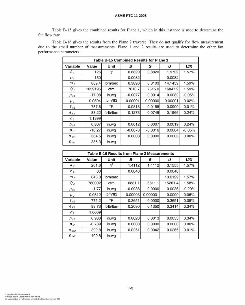
ASME PTC 11-2008

95

Table B-15 gives the combined results for Plane 1, which in this instance is used to determine the fan flow rate.

Table B-16 gives the results from the Plane 2 traverse. They do not qualify for flow measurement due to the small number of measurements. Plane 1 and 2 results are used to determine the other fan performance parameters.

Variable Value Unit B S U U/XA 1 126 ft2 0.8820 0.8820 1.9722 1.57%

n 1 150 0.0082 0.0082 m 1 889.4 lbm/sec 6.3896 6.3103 14.1459 1.59%

Q 1 1059196 cfm 7610.7 7515.0 16847.2 1.59%

p s1 -17.08 in.wg -0.0077 -0.0014 0.0082 -0.05%

ρ 1 0.0504 lbm/ft3 0.00001 0.00000 0.00001 0.02%

T s1 757.6 °R 0.0818 0.0188 0.0900 0.01%

e K1 83.22 ft-lb/lbm 0.1273 0.0749 0.1966 0.24%

α 1 1.1399

p v1 0.807 in.wg 0.0012 0.0007 0.0019 0.24%

p t1 -16.27 in.wg -0.0078 -0.0016 0.0084 -0.05%

p sa1 384.5 in.wg 0.0003 0.0000 0.0003 0.00%p ta1 385.3 in.wg

Variable Value Unit B S U U/XA 2 201.6 ft2 1.4112 1.4112 3.1555 1.57%

n 2 30 0.0046 0.0046

m 1 648.0 lbm/sec 13.0129 1.57%

Q 2 780002 cfm 6881.1 6811.1 15261.4 1.58%

p s2 -1.77 in.wg -0.0036 0.0000 0.0036 -0.20%

ρ 2 0.0512 lbm/ft3 0.00003 0.000001 0.0000 0.06%

T s2 775.2 °R 0.3651 0.0000 0.3651 0.05%

e K2 99.73 ft-lb/lbm 0.2090 0.1350 0.3414 0.34%

α 2 1.0009

p v2 0.983 in.wg 0.0020 0.0013 0.0033 0.34%

p t2 -0.789 in.wg 0.0000 0.0000 0.0000 0.00%

p sa2 399.8 in.wg 0.0251 0.0042 0.0265 0.01%p ta2 400.8 in.wg

Table B-15 Combined Results for Plane 1

Table B-16 Results from Plane 2 Measurements


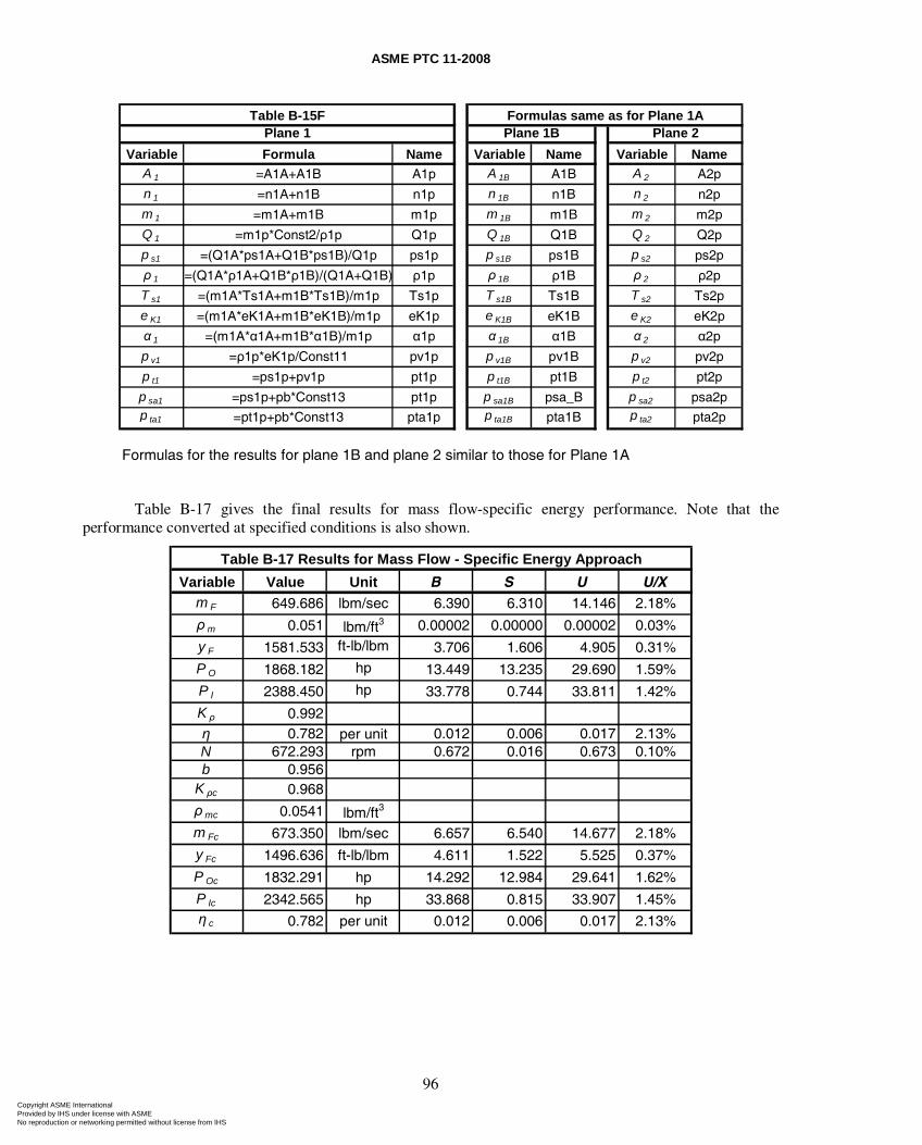
ASME PTC 11-2008

96

Variable Formula Name Variable Name Variable NameA 1 =A1A+A1B A1p A 1B A1B A 2 A2p

n 1 =n1A+n1B n1p n 1B n1B n 2 n2p

m 1 =m1A+m1B m1p m 1B m1B m 2 m2p

Q 1 =m1p*Const2/ρ1p Q1p Q 1B Q1B Q 2 Q2p

p s1 =(Q1A*ps1A+Q1B*ps1B)/Q1p ps1p p s1B ps1B p s2 ps2p

ρ 1 =(Q1A*ρ1A+Q1B*ρ1B)/(Q1A+Q1B) ρ1p ρ 1B ρ1B ρ 2 ρ2p

T s1 =(m1A*Ts1A+m1B*Ts1B)/m1p Ts1p T s1B Ts1B T s2 Ts2p

e K1 =(m1A*eK1A+m1B*eK1B)/m1p eK1p e K1B eK1B e K2 eK2p

α 1 =(m1A*α1A+m1B*α1B)/m1p α1p α 1B α1B α 2 α2p

p v1 =ρ1p*eK1p/Const11 pv1p p v1B pv1B p v2 pv2p

p t1 =ps1p+pv1p pt1p p t1B pt1B p t2 pt2p

p sa1 =ps1p+pb*Const13 pt1p p sa1B psa_B p sa2 psa2pp ta1 =pt1p+pb*Const13 pta1p p ta1B pta1B p ta2 pta2p

Formulas for the results for plane 1B and plane 2 similar to those for Plane 1A

Plane 2Formulas same as for Plane 1ATable B-15F

Plane 1 Plane 1B

Table B-17 gives the final results for mass flow-specific energy performance. Note that the performance converted at specified conditions is also shown.

Variable Value Unit B S U U/Xm F 649.686 lbm/sec 6.390 6.310 14.146 2.18%

ρ m 0.051 lbm/ft3 0.00002 0.00000 0.00002 0.03%

y F 1581.533 ft-lb/lbm 3.706 1.606 4.905 0.31%

P O 1868.182 hp 13.449 13.235 29.690 1.59%

P I 2388.450 hp 33.778 0.744 33.811 1.42%

K ρ 0.992η 0.782 per unit 0.012 0.006 0.017 2.13%N 672.293 rpm 0.672 0.016 0.673 0.10%b 0.956

K ρc 0.968

ρ mc 0.0541 lbm/ft3

m Fc 673.350 lbm/sec 6.657 6.540 14.677 2.18%

y Fc 1496.636 ft-lb/lbm 4.611 1.522 5.525 0.37%

P Oc 1832.291 hp 14.292 12.984 29.641 1.62%

P Ic 2342.565 hp 33.868 0.815 33.907 1.45%η c 0.782 per unit 0.012 0.006 0.017 2.13%

Table B-17 Results for Mass Flow - Specific Energy Approach


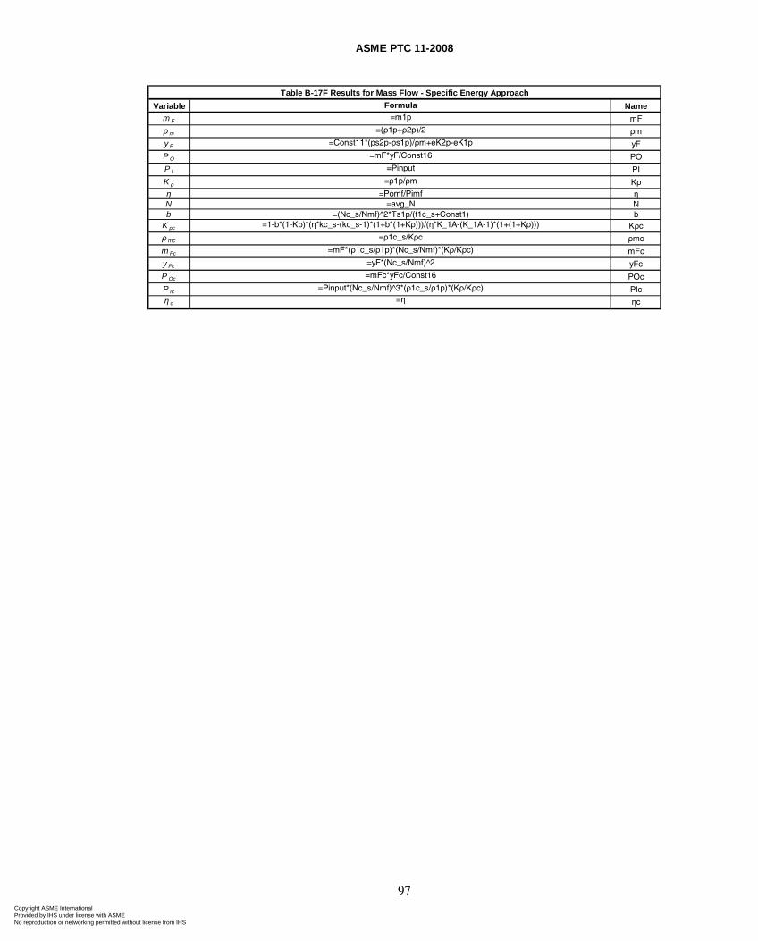
ASME PTC 11-2008

97

Variable Formula Namem F =m1p mF

ρ m =(ρ1p+ρ2p)/2 ρm

y F =Const11*(ps2p-ps1p)/ρm+eK2p-eK1p yF

P O =mF*yF/Const16 PO

P I =Pinput PI

K ρ =ρ1p/ρm Kρη =Pomf/Pimf ηN =avg_N Nb =(Nc_s/Nmf)^2*Ts1p/(t1c_s+Const1) b

K ρc =1-b*(1-Kρ)*(η*kc_s-(kc_s-1)*(1+b*(1+Kρ)))/(η*K_1A-(K_1A-1)*(1+(1+Kρ))) Kρc

ρ mc =ρ1c_s/Kρc ρmc

m Fc =mF*(ρ1c_s/ρ1p)*(Nc_s/Nmf)*(Kρ/Kρc) mFc

y Fc =yF*(Nc_s/Nmf)^2 yFc

P Oc =mFc*yFc/Const16 POc

P Ic =Pinput*(Nc_s/Nmf)^3*(ρ1c_s/ρ1p)*(Kρ/Kρc) PIcη c =η ηc

Table B-17F Results for Mass Flow - Specific Energy Approach


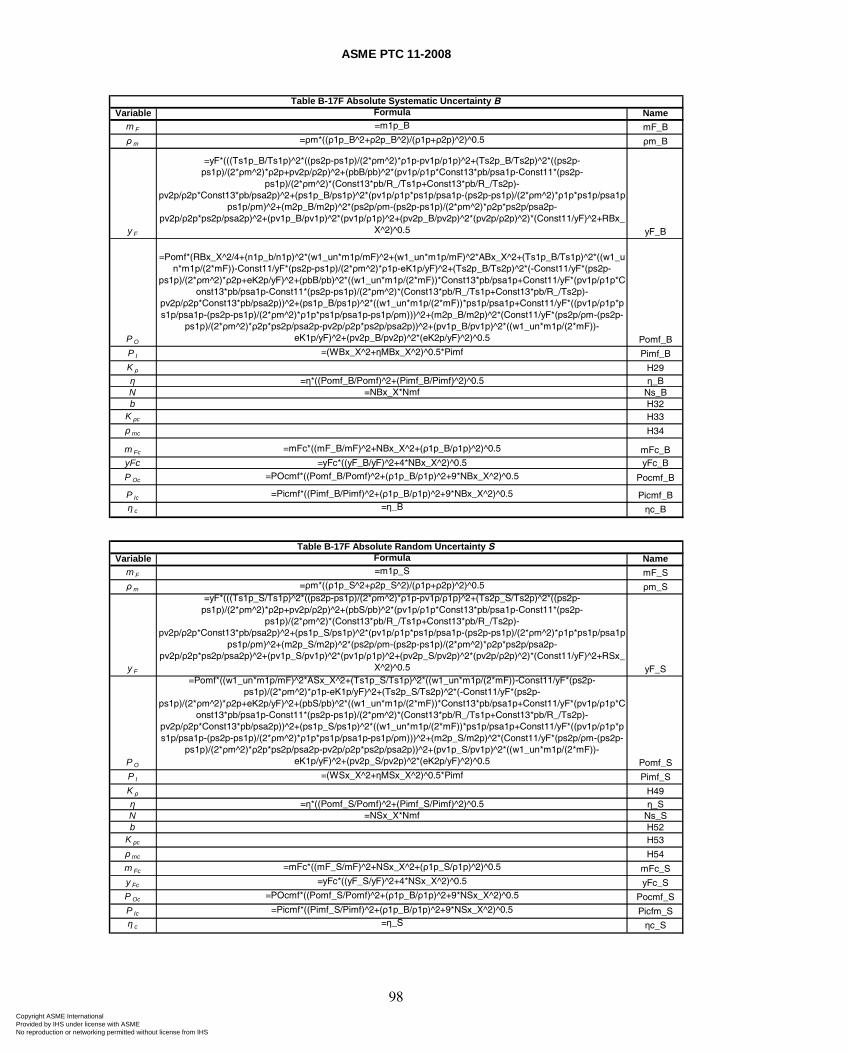
ASME PTC 11-2008

98

Variable Formula Namem F =m1p_B mF_B

ρ m =ρm*((ρ1p_B^2+ρ2p_B^2)/(ρ1p+ρ2p)^2)^0.5 ρm_B

y F

=yF*(((Ts1p_B/Ts1p)^2*((ps2p-ps1p)/(2*ρm^2)*ρ1p-pv1p/ρ1p)^2+(Ts2p_B/Ts2p)^2*((ps2p-ps1p)/(2*ρm^2)*ρ2p+pv2p/ρ2p)^2+(pbB/pb)^2*(pv1p/ρ1p*Const13*pb/psa1p-Const11*(ps2p-

ps1p)/(2*ρm^2)*(Const13*pb/R_/Ts1p+Const13*pb/R_/Ts2p)-pv2p/ρ2p*Const13*pb/psa2p)^2+(ps1p_B/ps1p)^2*(pv1p/ρ1p*ps1p/psa1p-(ps2p-ps1p)/(2*ρm^2)*ρ1p*ps1p/psa1p-

ps1p/ρm)^2+(m2p_B/m2p)^2*(ps2p/ρm-(ps2p-ps1p)/(2*ρm^2)*ρ2p*ps2p/psa2p-pv2p/ρ2p*ps2p/psa2p)^2+(pv1p_B/pv1p)^2*(pv1p/ρ1p)^2+(pv2p_B/pv2p)^2*(pv2p/ρ2p)^2)*(Const11/yF)^2+RBx_

X^2)^0.5 yF_B

P O

=Pomf*(RBx_X^2/4+(n1p_b/n1p)^2*(w1_un*m1p/mF)^2+(w1_un*m1p/mF)^2*ABx_X^2+(Ts1p_B/Ts1p)^2*((w1_un*m1p/(2*mF))-Const11/yF*(ps2p-ps1p)/(2*ρm^2)*ρ1p-eK1p/yF)^2+(Ts2p_B/Ts2p)^2*(-Const11/yF*(ps2p-

ps1p)/(2*ρm^2)*ρ2p+eK2p/yF)^2+(pbB/pb)^2*((w1_un*m1p/(2*mF))*Const13*pb/psa1p+Const11/yF*(pv1p/ρ1p*Const13*pb/psa1p-Const11*(ps2p-ps1p)/(2*ρm^2)*(Const13*pb/R_/Ts1p+Const13*pb/R_/Ts2p)-

pv2p/ρ2p*Const13*pb/psa2p))^2+(ps1p_B/ps1p)^2*((w1_un*m1p/(2*mF))*ps1p/psa1p+Const11/yF*((pv1p/ρ1p*ps1p/psa1p-(ps2p-ps1p)/(2*ρm^2)*ρ1p*ps1p/psa1p-ps1p/ρm)))^2+(m2p_B/m2p)^2*(Const11/yF*(ps2p/ρm-(ps2p-

ps1p)/(2*ρm^2)*ρ2p*ps2p/psa2p-pv2p/ρ2p*ps2p/psa2p))^2+(pv1p_B/pv1p)^2*((w1_un*m1p/(2*mF))-eK1p/yF)^2+(pv2p_B/pv2p)^2*(eK2p/yF)^2)^0.5 Pomf_B

P I =(WBx_X^2+ηMBx_X^2)^0.5*Pimf Pimf_B

K ρ H29η =η*((Pomf_B/Pomf)^2+(Pimf_B/Pimf)^2)^0.5 η_BN =NBx_X*Nmf Ns_Bb H32

K ρc H33

ρ mc H34

m Fc =mFc*((mF_B/mF)^2+NBx_X^2+(ρ1p_B/ρ1p)^2)^0.5 mFc_ByFc =yFc*((yF_B/yF)^2+4*NBx_X^2)^0.5 yFc_B

P Oc =POcmf*((Pomf_B/Pomf)^2+(ρ1p_B/ρ1p)^2+9*NBx_X^2)^0.5 Pocmf_B

P Ic =Picmf*((Pimf_B/Pimf)^2+(ρ1p_B/ρ1p)^2+9*NBx_X^2)^0.5 Picmf_Bη c =η_B ηc_B

Variable Formula Namem F =m1p_S mF_S

ρ m =ρm*((ρ1p_S^2+ρ2p_S^2)/(ρ1p+ρ2p)^2)^0.5 ρm_S

y F

=yF*(((Ts1p_S/Ts1p)^2*((ps2p-ps1p)/(2*ρm^2)*ρ1p-pv1p/ρ1p)^2+(Ts2p_S/Ts2p)^2*((ps2p-ps1p)/(2*ρm^2)*ρ2p+pv2p/ρ2p)^2+(pbS/pb)^2*(pv1p/ρ1p*Const13*pb/psa1p-Const11*(ps2p-

ps1p)/(2*ρm^2)*(Const13*pb/R_/Ts1p+Const13*pb/R_/Ts2p)-pv2p/ρ2p*Const13*pb/psa2p)^2+(ps1p_S/ps1p)^2*(pv1p/ρ1p*ps1p/psa1p-(ps2p-ps1p)/(2*ρm^2)*ρ1p*ps1p/psa1p-

ps1p/ρm)^2+(m2p_S/m2p)^2*(ps2p/ρm-(ps2p-ps1p)/(2*ρm^2)*ρ2p*ps2p/psa2p-pv2p/ρ2p*ps2p/psa2p)^2+(pv1p_S/pv1p)^2*(pv1p/ρ1p)^2+(pv2p_S/pv2p)^2*(pv2p/ρ2p)^2)*(Const11/yF)^2+RSx_

X^2)^0.5 yF_S

P O

=Pomf*((w1_un*m1p/mF)^2*ASx_X^2+(Ts1p_S/Ts1p)^2*((w1_un*m1p/(2*mF))-Const11/yF*(ps2p-ps1p)/(2*ρm^2)*ρ1p-eK1p/yF)^2+(Ts2p_S/Ts2p)^2*(-Const11/yF*(ps2p-

ps1p)/(2*ρm^2)*ρ2p+eK2p/yF)^2+(pbS/pb)^2*((w1_un*m1p/(2*mF))*Const13*pb/psa1p+Const11/yF*(pv1p/ρ1p*Const13*pb/psa1p-Const11*(ps2p-ps1p)/(2*ρm^2)*(Const13*pb/R_/Ts1p+Const13*pb/R_/Ts2p)-

pv2p/ρ2p*Const13*pb/psa2p))^2+(ps1p_S/ps1p)^2*((w1_un*m1p/(2*mF))*ps1p/psa1p+Const11/yF*((pv1p/ρ1p*ps1p/psa1p-(ps2p-ps1p)/(2*ρm^2)*ρ1p*ps1p/psa1p-ps1p/ρm)))^2+(m2p_S/m2p)^2*(Const11/yF*(ps2p/ρm-(ps2p-

ps1p)/(2*ρm^2)*ρ2p*ps2p/psa2p-pv2p/ρ2p*ps2p/psa2p))^2+(pv1p_S/pv1p)^2*((w1_un*m1p/(2*mF))-eK1p/yF)^2+(pv2p_S/pv2p)^2*(eK2p/yF)^2)^0.5 Pomf_S

P I =(WSx_X^2+ηMSx_X^2)^0.5*Pimf Pimf_S

K ρ H49η =η*((Pomf_S/Pomf)^2+(Pimf_S/Pimf)^2)^0.5 η_SN =NSx_X*Nmf Ns_Sb H52

K ρc H53

ρ mc H54

m Fc =mFc*((mF_S/mF)^2+NSx_X^2+(ρ1p_S/ρ1p)^2)^0.5 mFc_S

y Fc =yFc*((yF_S/yF)^2+4*NSx_X^2)^0.5 yFc_S

P Oc =POcmf*((Pomf_S/Pomf)^2+(ρ1p_B/ρ1p)^2+9*NSx_X^2)^0.5 Pocmf_S

P Ic =Picmf*((Pimf_S/Pimf)^2+(ρ1p_B/ρ1p)^2+9*NSx_X^2)^0.5 Picfm_Sη c =η_S ηc_S

Table B-17F Absolute Systematic Uncertainty B

Table B-17F Absolute Random Uncertainty S


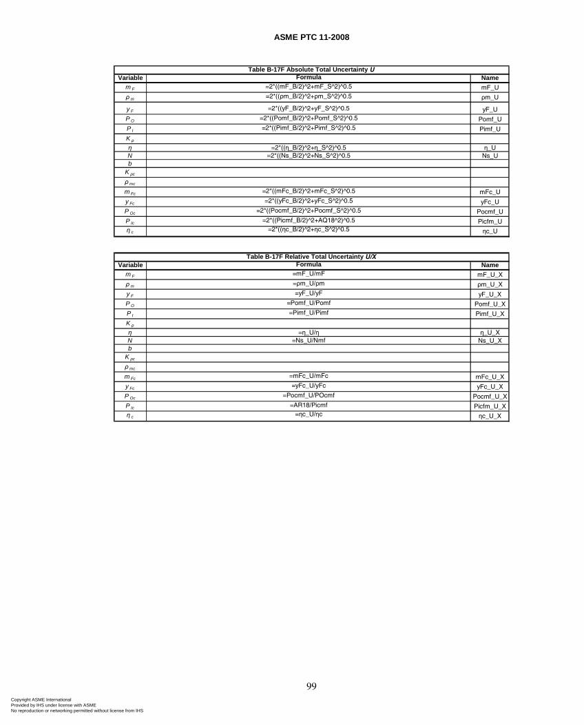
ASME PTC 11-2008

99

Variable Formula Namem F =2*((mF_B/2)^2+mF_S^2)^0.5 mF_U

ρ m =2*((ρm_B/2)^2+ρm_S^2)^0.5 ρm_U

y F =2*((yF_B/2)^2+yF_S^2)^0.5 yF_U

P O =2*((Pomf_B/2)^2+Pomf_S^2)^0.5 Pomf_U

P I =2*((Pimf_B/2)^2+Pimf_S^2)^0.5 Pimf_U

K ρ

η =2*((η_B/2)^2+η_S^2)^0.5 η_UN =2*((Ns_B/2)^2+Ns_S^2)^0.5 Ns_Ub

K ρc

ρ mc

m Fc =2*((mFc_B/2)^2+mFc_S^2)^0.5 mFc_U

y Fc =2*((yFc_B/2)^2+yFc_S^2)^0.5 yFc_U

P Oc =2*((Pocmf_B/2)^2+Pocmf_S^2)^0.5 Pocmf_U

P Ic =2*((Picmf_B/2)^2+AQ18^2)^0.5 Picfm_Uη c =2*((ηc_B/2)^2+ηc_S^2)^0.5 ηc_U

Variable Formula Namem F =mF_U/mF mF_U_X

ρ m =ρm_U/ρm ρm_U_X

y F =yF_U/yF yF_U_X

P O =Pomf_U/Pomf Pomf_U_X

P I =Pimf_U/Pimf Pimf_U_X

K ρ

η =η_U/η η_U_XN =Ns_U/Nmf Ns_U_Xb

K ρc

ρ mc

m Fc =mFc_U/mFc mFc_U_X

y Fc =yFc_U/yFc yFc_U_X

P Oc =Pocmf_U/POcmf Pocmf_U_X

P Ic =AR18/Picmf Picfm_U_Xη c =ηc_U/ηc ηc_U_X




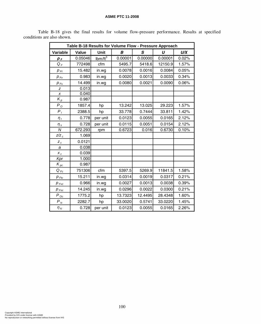
ASME PTC 11-2008

100

Table B-18 gives the final results for volume flow-pressure performance. Results at specified conditions are also shown.

Variable Value Unit B S U U/Xρ F 0.05046 lbm/ft3 0.00001 0.00000 0.00001 0.02%Q F 772498 cfm 5495.7 5418.6 12150.9 1.57%

p Ft 15.482 in.wg 0.0078 0.0016 0.0084 0.05%

p Fv 0.983 in.wg 0.0020 0.0013 0.0033 0.34%

p Fs 14.499 in.wg 0.0080 0.0021 0.0090 0.06%z 0.013x 0.040

K p 0.987

P O 1857.4 hp 13.242 13.025 29.223 1.57%

P I 2388.5 hp 33.778 0.7444 33.811 1.42%

η t 0.778 per unit 0.0123 0.0055 0.0165 2.12%

η s 0.728 per unit 0.0115 0.0051 0.0154 2.12%N 672.293 rpm 0.6723 0.016 0.6730 0.10%

z/z c 1.069

z c 0.0121a 0.038x c 0.039Kpr 1.000K pc 0.987

Q Fc 751306 cfm 5397.5 5269.9 11841.5 1.58%

p Ftc 15.211 in.wg 0.0314 0.0019 0.0317 0.21%

p Fvc 0.966 in.wg 0.0027 0.0013 0.0038 0.39%

p Fsc 14.245 in.wg 0.0296 0.0022 0.0300 0.21%

P Oc 1775.2 hp 13.7323 12.4495 28.4348 1.60%

P Ic 2282.7 hp 33.0020 0.5741 33.0220 1.45%η tc 0.728 per unit 0.0123 0.0055 0.0165 2.26%

Table B-18 Results for Volume Flow - Pressure Approach


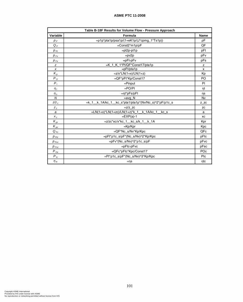
ASME PTC 11-2008

101

Variable Formula Nameρ F =ρ1p*pta1p/psa1p/(1+eK1p/(J*cpmg_1*Ts1p)) ρF

Q F =Const2*m1p/ρF QF

p Ft =pt2p-pt1p pFt

p Fv =pv2p pFv

p Fs =pFt-pFv pFsz =K_1_K_1*PI/QF*Const17/pta1p zx =pFt/pta1p x

K p =z/x*LN(1+x)/LN(1+z) Kp

P O =QF*pFt*Kp/Const17 PO

P I =Pinput PI

η t =PO/PI ηt

η s =ηt*pFs/pFt ηsN =avg_N Nv

z/z c =k_1__k_1A/kc_1__kc_s*pta1/pta1p*(Nv/Nc_s)^2*ρF/ρ1c_s z_zc

z c =z/z_zc zca =LN(1+x)*LN(1+zc)/LN(1+z)*k_1__k_1A/kc_1__kc_s ax c =EXP(a)-1 xc

K pr =z/zc*xc/x*kc_1__kc_s/k_1__k_1A Kpr

K pc =Kp/Kpr Kpc

Q Fc =QF*Nc_s/Nv*Kp/Kpc QFc

p Ftc =pFt*ρ1c_s/ρF*(Nc_s/Nv)^2*Kp/Kpc pFtc

p Fvc =pFv*(Nc_s/Nv)^2*ρ1c_s/ρF pFvc

p Fsc =pFtc-pFvc pFsc

P Oc =QFc*pFtc*Kpc/Const17 POc

P Ic =PI*ρ1c_s/ρF*(Nc_s/Nv)^3*Kp/Kpc PIcη tc =ηs ηtc

Table B-18F Results for Volume Flow - Pressure Approach


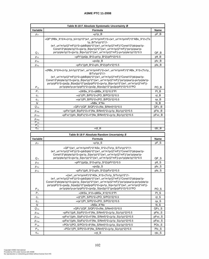
ASME PTC 11-2008

102

Variable Formula Nameρ F =ρ1p_B ρF_B

Q F

=QF*(RBx_X^2/4+(n1p_b/n1p)^2*(w1_un*m1p/mF)^2+(w1_un*m1p/mF)^2*ABx_X^2+(Ts1p_B/Ts1p)^2*(1-

(w1_un*m1p/(2*mF)))^2+(pbB/pb)^2*((w1_un*m1p/(2*mF))*Const13*pb/psa1p-Const13*pb/pta1p)^2+(ps1p_B/ps1p)^2*((w1_un*m1p/(2*mF))*ps1p/psa1p-ps1p/pta1p)^2+(pv1p_B/pv1p)^2*((w1_un*m1p/(2*mF))-pv1p/pta1p)^2)^0.5 QF_B

p Ft =pFt*((pt2p_B^2+pt1p_B^2)/pFt^2)^0.5 pft_B

p Fv =pv2p_B pfv_B

p Fs =pFs*((pft_B^2+pfv_B^2)/pFs^2)^0.5 pfs_B

P O

=(RBx_X^2/4+(n1p_b/n1p)^2*(w1_un*m1p/mF)^2+(w1_un*m1p/mF)^2*ABx_X^2+(Ts1p_B/Ts1p)^2*(1-

(w1_un*m1p/(2*mF)))^2+(pbB/pb)^2*((w1_un*m1p/(2*mF))*Const13*pb/psa1p-Const13*pb/pta1p)^2+(ps1p_B/ps1p)^2*((w1_un*m1p/(2*mF))*ps1p/psa1p-ps1p/pta1p-ps1p/pFt)^2+(ps2p_B/ps2p)^2*(ps2p/pFt)^2+(pv1p_B/pv1p)^2*((w1_un*m1p/(2*mF))-

pv1p/pta1p-pv1p/pFt)^2+(pv2p_B/pv2p)^2*(pv2p/pFt)^2)^0.5*PO PO_B

P I =(WBx_X^2+ηMBx_X^2)^0.5*PI PI_B

η t =ηt*((PI_B/PI)^2+(PO_B/PO)^2)^0.5 ηt_B

η s =ηs*((PI_B/PI)^2+(PO_B/PO)^2)^0.5 ηs_BN =NBx_X*Nv N_B

Q Fc =QFc*((QF_B/QF)^2+(Ns_B/Nmf)^2)^0.5 QFc_B

p Ftc =pFtc*((pft_B/pFt)^2+4*(Ns_B/Nmf)^2+(ρ1p_B/ρ1p)^2)^0.5 pFtc_B

p Fvc =pFvc*((pfv_B/pFv)^2+4*(Ns_B/Nmf)^2+(ρ1p_B/ρ1p)^2)^0.5 pFvc_B

p Fsc

P Oc

P Icη tc =ηt_B ηtc_B

Variable Formula Nameρ F =ρ1p_S ρF_S

Q F

=QF*((w1_un*m1p/mF)^2*ASx_X^2+(Ts1p_S/Ts1p)^2*(1-(w1_un*m1p/(2*mF)))^2+(pbS/pb)^2*((w1_un*m1p/(2*mF))*Const13*pb/psa1p-

Const13*pb/pta1p)^2+(ps1p_S/ps1p)^2*((w1_un*m1p/(2*mF))*ps1p/psa1p-ps1p/pta1p)^2+(pv1p_S/pv1p)^2*((w1_un*m1p/(2*mF))-pv1p/pta1p)^2)^0.5 QF_S

p Ft =pFt*((pt2p_S^2+pt1p_S^2)/pFt^2)^0.5 pft_S

p Fv =pv2p_S pfv_S

p Fs =pFs*((pft_S^2+pfv_S^2)/pFs^2)^0.5 pfs_S

P O

=((w1_un*m1p/mF)^2*ASx_X^2+(Ts1p_S/Ts1p)^2*(1-(w1_un*m1p/(2*mF)))^2+(pbS/pb)^2*((w1_un*m1p/(2*mF))*Const13*pb/psa1p-

Const13*pb/pta1p)^2+(ps1p_S/ps1p)^2*((w1_un*m1p/(2*mF))*ps1p/psa1p-ps1p/pta1p-ps1p/pFt)^2+(ps2p_S/ps2p)^2*(ps2p/pFt)^2+(pv1p_S/pv1p)^2*((w1_un*m1p/(2*mF))-

pv1p/pta1p-pv1p/pFt)^2+(pv2p_S/pv2p)^2*(pv2p/pFt)^2)^0.5*PO PO_S

P I =(WSx_X^2+ηMSx_X^2)^0.5*PI PI_S

η t =ηt*((PI_S/PI)^2+(PO_S/PO)^2)^0.5 ηt_S

η s =ηs*((PI_S/PI)^2+(PO_S/PO)^2)^0.5 ηs_SN =NSx_X*Nv N_S

Q Fc =QFc*((QF_S/QF)^2+(Ns_S/Nmf)^2)^0.5 QFc_S

p Ftc =pFtc*((pft_S/pFt)^2+4*(Ns_S/Nmf)^2+(ρ1p_S/ρ1p)^2)^0.5 pFtc_S

p Fvc =pFvc*((pfv_S/pFv)^2+4*(Ns_S/Nmf)^2+(ρ1p_S/ρ1p)^2)^0.5 pFvc_S

p Fsc =pFsc*((pfs_S/pFs)^2+4*(Ns_S/Nmf)^2+(ρ1p_S/ρ1p)^2)^0.5 pFsc_S

P Oc =POc*((PO_S/PO)^2+9*(Ns_S/Nmf)^2+(ρ1p_S/ρ1p)^2)^0.5 POc_S

P Ic =POc*((PI_S/PI)^2+9*(Ns_S/Nmf)^2+(ρ1p_S/ρ1p)^2)^0.5 PIc_Sη tc =ηt_S ηtc_S

Table B-18 F Absolute Systematic Uncertainty B

Table B-18 F Absolute Random Uncertainty S


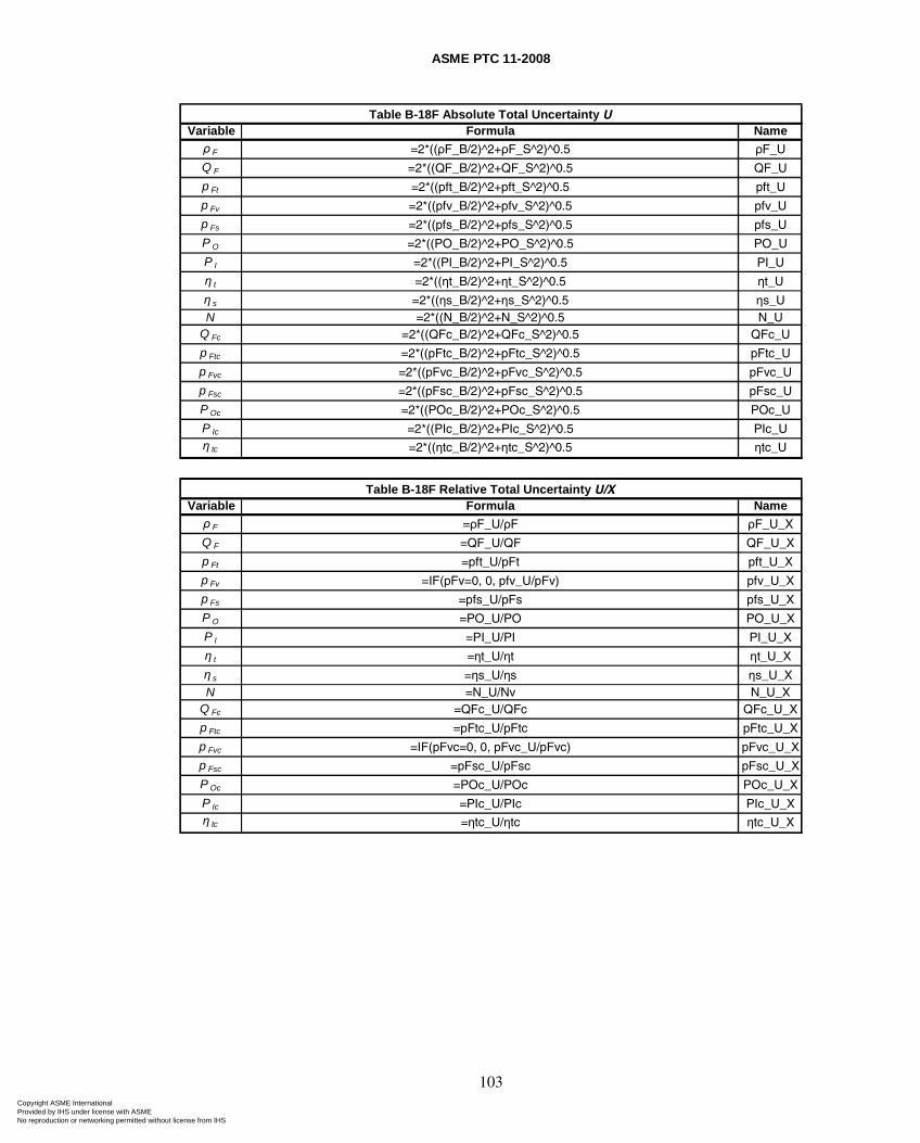
ASME PTC 11-2008

103

Variable Formula Nameρ F =2*((ρF_B/2)^2+ρF_S^2)^0.5 ρF_U

Q F =2*((QF_B/2)^2+QF_S^2)^0.5 QF_U

p Ft =2*((pft_B/2)^2+pft_S^2)^0.5 pft_U

p Fv =2*((pfv_B/2)^2+pfv_S^2)^0.5 pfv_U

p Fs =2*((pfs_B/2)^2+pfs_S^2)^0.5 pfs_U

P O =2*((PO_B/2)^2+PO_S^2)^0.5 PO_U

P I =2*((PI_B/2)^2+PI_S^2)^0.5 PI_U

η t =2*((ηt_B/2)^2+ηt_S^2)^0.5 ηt_U

η s =2*((ηs_B/2)^2+ηs_S^2)^0.5 ηs_UN =2*((N_B/2)^2+N_S^2)^0.5 N_U

Q Fc =2*((QFc_B/2)^2+QFc_S^2)^0.5 QFc_U

p Ftc =2*((pFtc_B/2)^2+pFtc_S^2)^0.5 pFtc_U

p Fvc =2*((pFvc_B/2)^2+pFvc_S^2)^0.5 pFvc_U

p Fsc =2*((pFsc_B/2)^2+pFsc_S^2)^0.5 pFsc_U

P Oc =2*((POc_B/2)^2+POc_S^2)^0.5 POc_U

P Ic =2*((PIc_B/2)^2+PIc_S^2)^0.5 PIc_Uη tc =2*((ηtc_B/2)^2+ηtc_S^2)^0.5 ηtc_U

Variable Formula Nameρ F =ρF_U/ρF ρF_U_X

Q F =QF_U/QF QF_U_X

p Ft =pft_U/pFt pft_U_X

p Fv =IF(pFv=0, 0, pfv_U/pFv) pfv_U_X

p Fs =pfs_U/pFs pfs_U_X

P O =PO_U/PO PO_U_X

P I =PI_U/PI PI_U_X

η t =ηt_U/ηt ηt_U_X

η s =ηs_U/ηs ηs_U_XN =N_U/Nv N_U_X

Q Fc =QFc_U/QFc QFc_U_X

p Ftc =pFtc_U/pFtc pFtc_U_X

p Fvc =IF(pFvc=0, 0, pFvc_U/pFvc) pFvc_U_X

p Fsc =pFsc_U/pFsc pFsc_U_X

P Oc =POc_U/POc POc_U_X

P Ic =PIc_U/PIc PIc_U_Xη tc =ηtc_U/ηtc ηtc_U_X




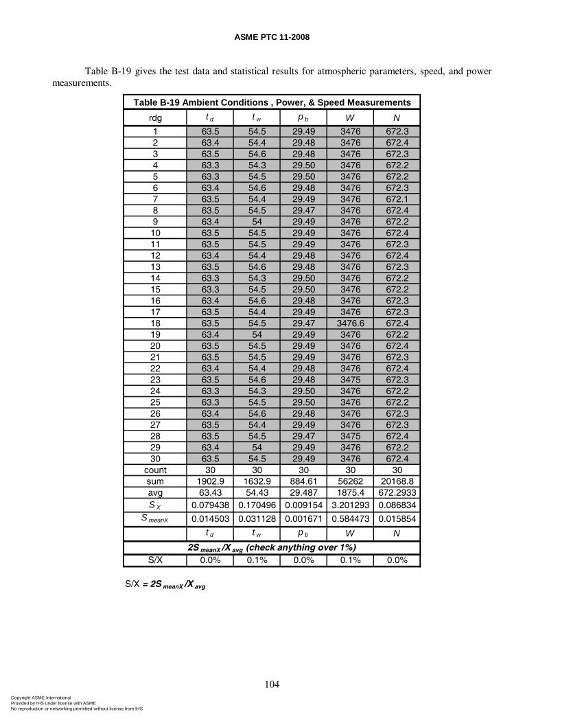
ASME PTC 11-2008

104

Table B-19 gives the test data and statistical results for atmospheric parameters, speed, and power measurements.

rdg t d t w p b W N

1 63.5 54.5 29.49 3476 672.32 63.4 54.4 29.48 3476 672.43 63.5 54.6 29.48 3476 672.34 63.3 54.3 29.50 3476 672.25 63.3 54.5 29.50 3476 672.26 63.4 54.6 29.48 3476 672.37 63.5 54.4 29.49 3476 672.18 63.5 54.5 29.47 3476 672.49 63.4 54 29.49 3476 672.210 63.5 54.5 29.49 3476 672.411 63.5 54.5 29.49 3476 672.312 63.4 54.4 29.48 3476 672.413 63.5 54.6 29.48 3476 672.314 63.3 54.3 29.50 3476 672.215 63.3 54.5 29.50 3476 672.216 63.4 54.6 29.48 3476 672.317 63.5 54.4 29.49 3476 672.318 63.5 54.5 29.47 3476.6 672.419 63.4 54 29.49 3476 672.220 63.5 54.5 29.49 3476 672.421 63.5 54.5 29.49 3476 672.322 63.4 54.4 29.48 3476 672.423 63.5 54.6 29.48 3475 672.324 63.3 54.3 29.50 3476 672.225 63.3 54.5 29.50 3476 672.226 63.4 54.6 29.48 3476 672.327 63.5 54.4 29.49 3476 672.328 63.5 54.5 29.47 3475 672.429 63.4 54 29.49 3476 672.230 63.5 54.5 29.49 3476 672.4

count 30 30 30 30 30sum 1902.9 1632.9 884.61 56262 20168.8avg 63.43 54.43 29.487 1875.4 672.2933S X 0.079438 0.170496 0.009154 3.201293 0.086834

S meanX 0.014503 0.031128 0.001671 0.584473 0.015854

t d t w p b W N

S/X 0.0% 0.1% 0.0% 0.1% 0.0%

Table B-19 Ambient Conditions , Power, & Speed Measurements

2S meanX /X avg (check anything over 1%)

S/X = 2S meanX /X avg


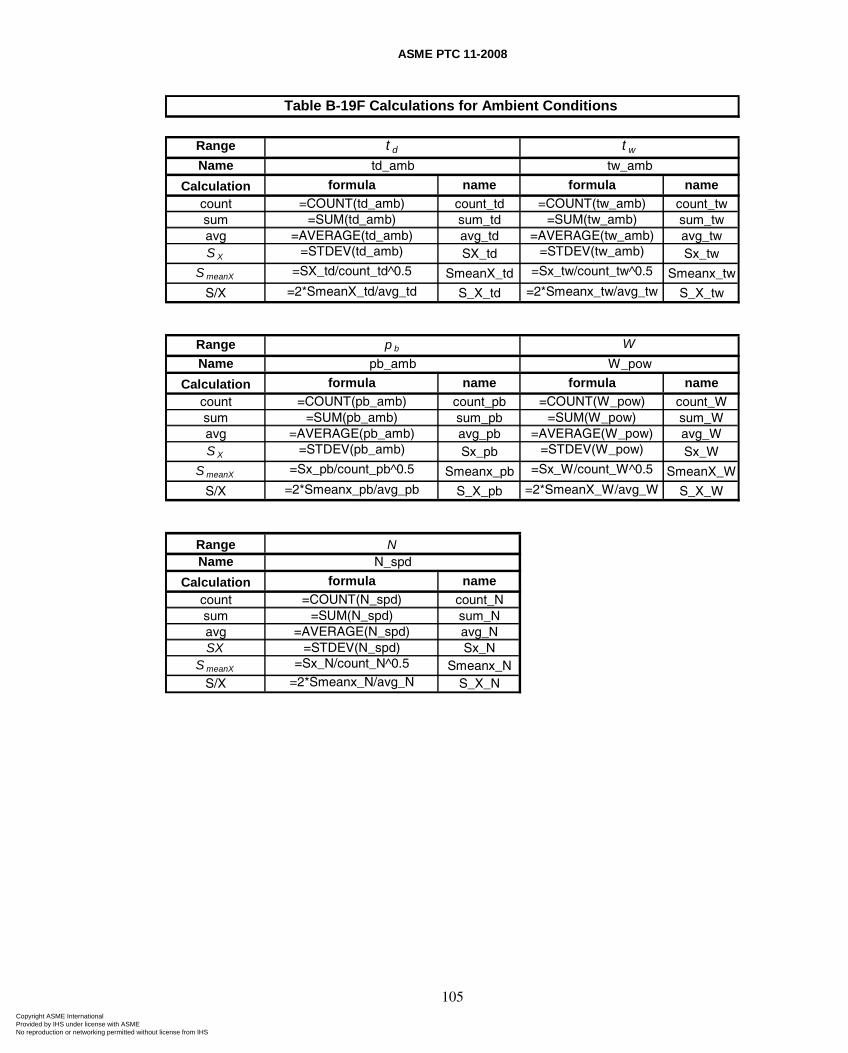
ASME PTC 11-2008

105

Range

Name

Calculation formula name formula namecount =COUNT(td_amb) count_td =COUNT(tw_amb) count_twsum =SUM(td_amb) sum_td =SUM(tw_amb) sum_twavg =AVERAGE(td_amb) avg_td =AVERAGE(tw_amb) avg_twS X =STDEV(td_amb) SX_td =STDEV(tw_amb) Sx_tw

S meanX =SX_td/count_td^0.5 SmeanX_td =Sx_tw/count_tw^0.5 Smeanx_tw

S/X =2*SmeanX_td/avg_td S_X_td =2*Smeanx_tw/avg_tw S_X_tw

RangeName

Calculation formula name formula namecount =COUNT(pb_amb) count_pb =COUNT(W_pow) count_Wsum =SUM(pb_amb) sum_pb =SUM(W_pow) sum_Wavg =AVERAGE(pb_amb) avg_pb =AVERAGE(W_pow) avg_WS X =STDEV(pb_amb) Sx_pb =STDEV(W_pow) Sx_W

S meanX =Sx_pb/count_pb^0.5 Smeanx_pb =Sx_W/count_W^0.5 SmeanX_W

S/X =2*Smeanx_pb/avg_pb S_X_pb =2*SmeanX_W/avg_W S_X_W

RangeName

Calculation formula namecount =COUNT(N_spd) count_Nsum =SUM(N_spd) sum_Navg =AVERAGE(N_spd) avg_NSX =STDEV(N_spd) Sx_N

S meanX =Sx_N/count_N^0.5 Smeanx_NS/X =2*Smeanx_N/avg_N S_X_N

NN_spd

Table B-19F Calculations for Ambient Conditions

t d

td_amb

t w

tw_amb

p b

pb_amb

W

W_pow


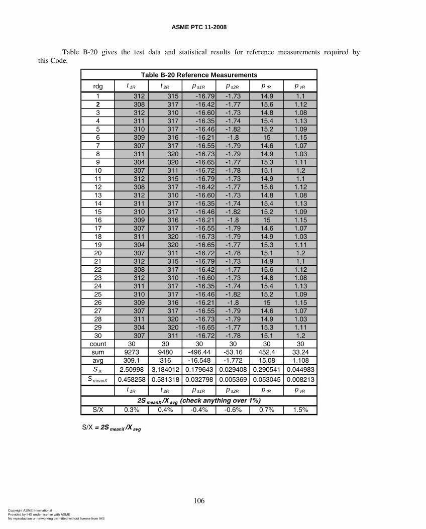
ASME PTC 11-2008

106

Table B-20 gives the test data and statistical results for reference measurements required by this Code.

rdg t 1R t 2R p s1R p s2R p tR p vR

1 312 315 -16.79 -1.73 14.9 1.12 308 317 -16.42 -1.77 15.6 1.123 312 310 -16.60 -1.73 14.8 1.084 311 317 -16.35 -1.74 15.4 1.135 310 317 -16.46 -1.82 15.2 1.096 309 316 -16.21 -1.8 15 1.157 307 317 -16.55 -1.79 14.6 1.078 311 320 -16.73 -1.79 14.9 1.039 304 320 -16.65 -1.77 15.3 1.1110 307 311 -16.72 -1.78 15.1 1.211 312 315 -16.79 -1.73 14.9 1.112 308 317 -16.42 -1.77 15.6 1.1213 312 310 -16.60 -1.73 14.8 1.0814 311 317 -16.35 -1.74 15.4 1.1315 310 317 -16.46 -1.82 15.2 1.0916 309 316 -16.21 -1.8 15 1.1517 307 317 -16.55 -1.79 14.6 1.0718 311 320 -16.73 -1.79 14.9 1.0319 304 320 -16.65 -1.77 15.3 1.1120 307 311 -16.72 -1.78 15.1 1.221 312 315 -16.79 -1.73 14.9 1.122 308 317 -16.42 -1.77 15.6 1.1223 312 310 -16.60 -1.73 14.8 1.0824 311 317 -16.35 -1.74 15.4 1.1325 310 317 -16.46 -1.82 15.2 1.0926 309 316 -16.21 -1.8 15 1.1527 307 317 -16.55 -1.79 14.6 1.0728 311 320 -16.73 -1.79 14.9 1.0329 304 320 -16.65 -1.77 15.3 1.1130 307 311 -16.72 -1.78 15.1 1.2

count 30 30 30 30 30 30sum 9273 9480 -496.44 -53.16 452.4 33.24avg 309.1 316 -16.548 -1.772 15.08 1.108S X 2.50998 3.184012 0.179643 0.029408 0.290541 0.044983

S meanX 0.458258 0.581318 0.032798 0.005369 0.053045 0.008213

t 1R t 2R p s1R p s2R p tR p vR

S/X 0.3% 0.4% -0.4% -0.6% 0.7% 1.5%

Table B-20 Reference Measurements

2S meanX /X avg (check anything over 1%)

S/X = 2S meanX /X avg


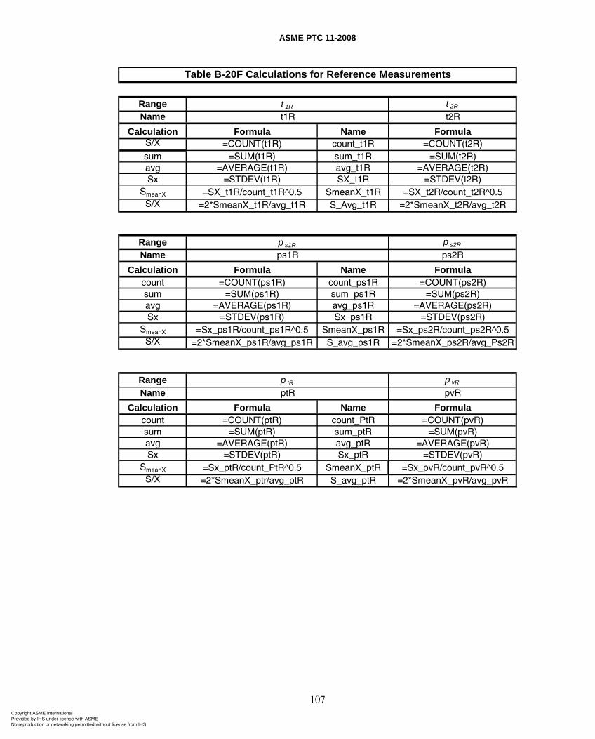
ASME PTC 11-2008

107

Range t 2R

Name t2R

Calculation Formula Name FormulaS/X =COUNT(t1R) count_t1R =COUNT(t2R)sum =SUM(t1R) sum_t1R =SUM(t2R)avg =AVERAGE(t1R) avg_t1R =AVERAGE(t2R)Sx =STDEV(t1R) SX_t1R =STDEV(t2R)

SmeanX =SX_t1R/count_t1R^0.5 SmeanX_t1R =SX_t2R/count_t2R^0.5S/X =2*SmeanX_t1R/avg_t1R S_Avg_t1R =2*SmeanX_t2R/avg_t2R

Range p s2R

Name ps2R

Calculation Formula Name Formulacount =COUNT(ps1R) count_ps1R =COUNT(ps2R)sum =SUM(ps1R) sum_ps1R =SUM(ps2R)avg =AVERAGE(ps1R) avg_ps1R =AVERAGE(ps2R)Sx =STDEV(ps1R) Sx_ps1R =STDEV(ps2R)

SmeanX =Sx_ps1R/count_ps1R^0.5 SmeanX_ps1R =Sx_ps2R/count_ps2R^0.5S/X =2*SmeanX_ps1R/avg_ps1R S_avg_ps1R =2*SmeanX_ps2R/avg_Ps2R

Range p vR

Name pvR

Calculation Formula Name Formulacount =COUNT(ptR) count_PtR =COUNT(pvR)sum =SUM(ptR) sum_ptR =SUM(pvR)avg =AVERAGE(ptR) avg_ptR =AVERAGE(pvR)Sx =STDEV(ptR) Sx_ptR =STDEV(pvR)

SmeanX =Sx_ptR/count_PtR^0.5 SmeanX_ptR =Sx_pvR/count_pvR^0.5S/X =2*SmeanX_ptr/avg_ptR S_avg_ptR =2*SmeanX_pvR/avg_pvR

p tR

ptR

Table B-20F Calculations for Reference Measurements

p s1R

ps1R

t 1R

t1R


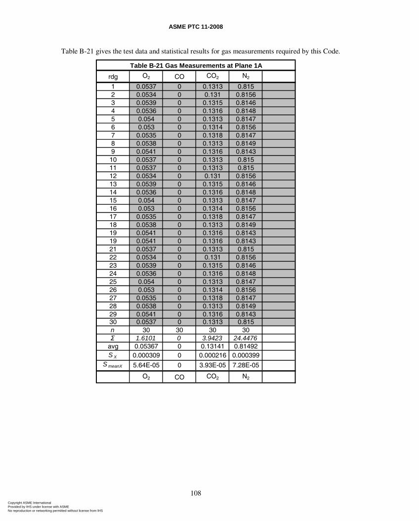
ASME PTC 11-2008

108

Table B-21 gives the test data and statistical results for gas measurements required by this Code.

rdg O2 CO CO2 N2

1 0.0537 0 0.1313 0.8152 0.0534 0 0.131 0.81563 0.0539 0 0.1315 0.81464 0.0536 0 0.1316 0.81485 0.054 0 0.1313 0.81476 0.053 0 0.1314 0.81567 0.0535 0 0.1318 0.81478 0.0538 0 0.1313 0.81499 0.0541 0 0.1316 0.814310 0.0537 0 0.1313 0.81511 0.0537 0 0.1313 0.81512 0.0534 0 0.131 0.815613 0.0539 0 0.1315 0.814614 0.0536 0 0.1316 0.814815 0.054 0 0.1313 0.814716 0.053 0 0.1314 0.815617 0.0535 0 0.1318 0.814718 0.0538 0 0.1313 0.814919 0.0541 0 0.1316 0.814319 0.0541 0 0.1316 0.814321 0.0537 0 0.1313 0.81522 0.0534 0 0.131 0.815623 0.0539 0 0.1315 0.814624 0.0536 0 0.1316 0.814825 0.054 0 0.1313 0.814726 0.053 0 0.1314 0.815627 0.0535 0 0.1318 0.814728 0.0538 0 0.1313 0.814929 0.0541 0 0.1316 0.814330 0.0537 0 0.1313 0.815n 30 30 30 30Σ 1.6101 0 3.9423 24.4476

avg 0.05367 0 0.13141 0.81492S X 0.000309 0 0.000216 0.000399

S meanX 5.64E-05 0 3.93E-05 7.28E-05

O2 CO CO2 N2

Table B-21 Gas Measurements at Plane 1A


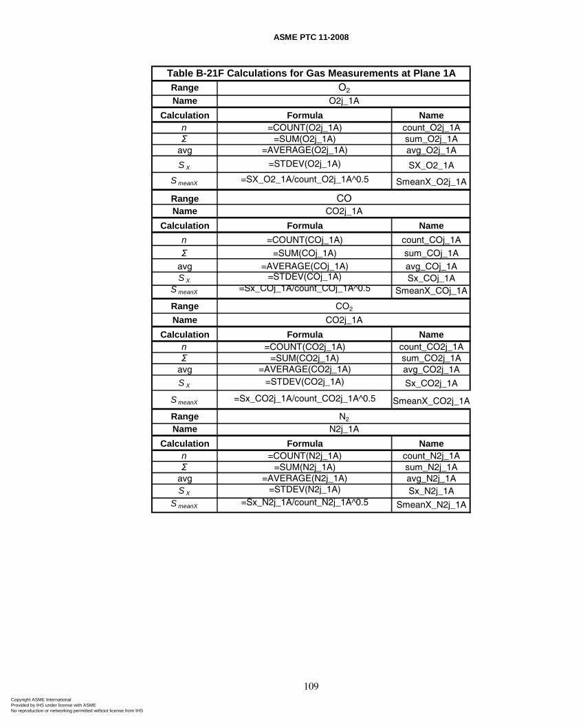
ASME PTC 11-2008

109

RangeName

Calculation Formula Namen =COUNT(O2j_1A) count_O2j_1AΣ =SUM(O2j_1A) sum_O2j_1A

avg =AVERAGE(O2j_1A) avg_O2j_1A

S X =STDEV(O2j_1A) SX_O2_1A

S meanX =SX_O2_1A/count_O2j_1A^0.5 SmeanX_O2j_1A

RangeName

Calculation Formula Name

n =COUNT(COj_1A) count_COj_1A

Σ =SUM(COj_1A) sum_COj_1A

avg =AVERAGE(COj_1A) avg_COj_1AS X =STDEV(COj_1A) Sx_COj_1A

S meanX =Sx_COj_1A/count_COj_1A^0.5 SmeanX_COj_1A

Range

Name

Calculation Formula Namen =COUNT(CO2j_1A) count_CO2j_1AΣ =SUM(CO2j_1A) sum_CO2j_1A

avg =AVERAGE(CO2j_1A) avg_CO2j_1A

S X =STDEV(CO2j_1A) Sx_CO2j_1A

S meanX =Sx_CO2j_1A/count_CO2j_1A^0.5 SmeanX_CO2j_1A

RangeName

Calculation Formula Namen =COUNT(N2j_1A) count_N2j_1AΣ =SUM(N2j_1A) sum_N2j_1A

avg =AVERAGE(N2j_1A) avg_N2j_1AS X =STDEV(N2j_1A) Sx_N2j_1A

S meanX =Sx_N2j_1A/count_N2j_1A^0.5 SmeanX_N2j_1A

N2j_1A

CO2j_1A

CO2

CO2j_1A

N2

Table B-21F Calculations for Gas Measurements at Plane 1AO2

O2j_1A

CO


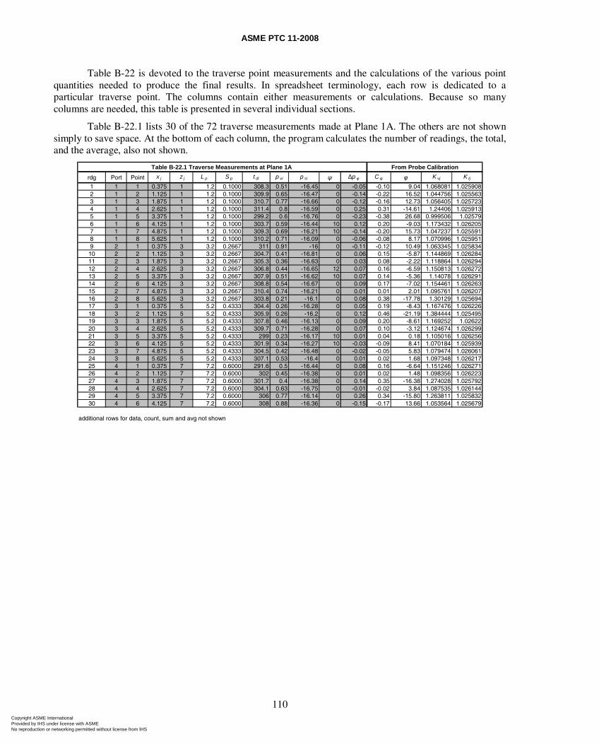
ASME PTC 11-2008

110

Table B-22 is devoted to the traverse point measurements and the calculations of the various point quantities needed to produce the final results. In spreadsheet terminology, each row is dedicated to a particular traverse point. The columns contain either measurements or calculations. Because so many columns are needed, this table is presented in several individual sections.

Table B-22.1 lists 30 of the 72 traverse measurements made at Plane 1A. The others are not shown simply to save space. At the bottom of each column, the program calculates the number of readings, the total, and the average, also not shown.

rdg Port Point x j z j L p S p t di p vi p si ψ Δp φ C φ φ K vj K tj

1 1 1 0.375 1 1.2 0.1000 308.3 0.51 -16.45 0 -0.05 -0.10 9.04 1.068081 1.0259082 1 2 1.125 1 1.2 0.1000 309.9 0.65 -16.47 0 -0.14 -0.22 16.52 1.044756 1.0255633 1 3 1.875 1 1.2 0.1000 310.7 0.77 -16.66 0 -0.12 -0.16 12.73 1.056405 1.0257234 1 4 2.625 1 1.2 0.1000 311.4 0.8 -16.59 0 0.25 0.31 -14.61 1.24406 1.0259135 1 5 3.375 1 1.2 0.1000 299.2 0.6 -16.76 0 -0.23 -0.38 26.68 0.999506 1.025796 1 6 4.125 1 1.2 0.1000 303.7 0.59 -16.44 10 0.12 0.20 -9.03 1.173432 1.0262057 1 7 4.875 1 1.2 0.1000 309.3 0.69 -16.21 10 -0.14 -0.20 15.73 1.047237 1.0255918 1 8 5.625 1 1.2 0.1000 310.2 0.71 -16.09 0 -0.06 -0.08 8.17 1.070996 1.0259519 2 1 0.375 3 3.2 0.2667 311 0.91 -16 0 -0.11 -0.12 10.49 1.063345 1.02583410 2 2 1.125 3 3.2 0.2667 304.7 0.41 -16.81 0 0.06 0.15 -5.87 1.144869 1.02628411 2 3 1.875 3 3.2 0.2667 305.3 0.36 -16.63 0 0.03 0.08 -2.22 1.118864 1.02629412 2 4 2.625 3 3.2 0.2667 306.8 0.44 -16.65 12 0.07 0.16 -6.59 1.150813 1.02627213 2 5 3.375 3 3.2 0.2667 307.9 0.51 -16.62 10 0.07 0.14 -5.36 1.14078 1.02629114 2 6 4.125 3 3.2 0.2667 308.8 0.54 -16.67 0 0.09 0.17 -7.02 1.154461 1.02626315 2 7 4.875 3 3.2 0.2667 310.4 0.74 -16.21 0 0.01 0.01 2.01 1.095761 1.02620716 2 8 5.625 3 3.2 0.2667 303.8 0.21 -16.1 0 0.08 0.38 -17.78 1.30129 1.02569417 3 1 0.375 5 5.2 0.4333 304.4 0.26 -16.28 0 0.05 0.19 -8.43 1.167476 1.02622618 3 2 1.125 5 5.2 0.4333 305.9 0.26 -16.2 0 0.12 0.46 -21.19 1.384444 1.02549519 3 3 1.875 5 5.2 0.4333 307.8 0.46 -16.13 0 0.09 0.20 -8.61 1.169252 1.0262220 3 4 2.625 5 5.2 0.4333 309.7 0.71 -16.28 0 0.07 0.10 -3.12 1.124674 1.02629921 3 5 3.375 5 5.2 0.4333 299 0.23 -16.17 10 0.01 0.04 0.18 1.105016 1.02625622 3 6 4.125 5 5.2 0.4333 301.9 0.34 -16.27 10 -0.03 -0.09 8.41 1.070184 1.02593923 3 7 4.875 5 5.2 0.4333 304.5 0.42 -16.48 0 -0.02 -0.05 5.83 1.079474 1.02606124 3 8 5.625 5 5.2 0.4333 307.1 0.53 -16.4 0 0.01 0.02 1.68 1.097348 1.02621725 4 1 0.375 7 7.2 0.6000 291.6 0.5 -16.44 0 0.08 0.16 -6.64 1.151246 1.02627126 4 2 1.125 7 7.2 0.6000 302 0.45 -16.38 0 0.01 0.02 1.48 1.098356 1.02622327 4 3 1.875 7 7.2 0.6000 301.7 0.4 -16.38 0 0.14 0.35 -16.38 1.274028 1.02579228 4 4 2.625 7 7.2 0.6000 304.1 0.63 -16.75 0 -0.01 -0.02 3.84 1.087535 1.02614429 4 5 3.375 7 7.2 0.6000 306 0.77 -16.14 0 0.26 0.34 -15.80 1.263811 1.02583230 4 6 4.125 7 7.2 0.6000 308 0.88 -16.36 0 -0.15 -0.17 13.66 1.053564 1.025679

additional rows for data, count, sum and avg not shown

Table B-22.1 Traverse Measurements at Plane 1A From Probe Calibration


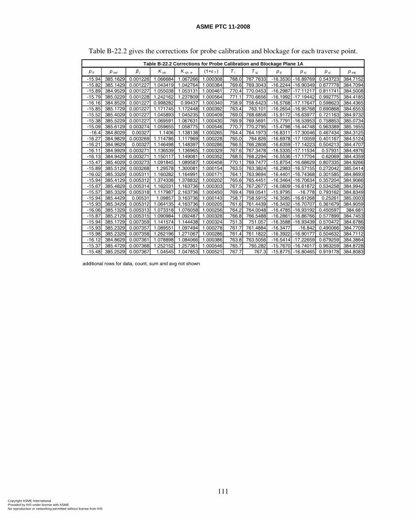
ASME PTC 11-2008

111

Table B-22.2 gives the corrections for probe calibration and blockage for each traverse point.

p ti p sai β j K vjc K vjc_e (1+ε T ) T i T sj p tj p sj p vj p saj

-15.94 385.1629 0.001226 1.066684 1.067266 1.000308 768.0 767.7633 -16.3530 -16.89769 0.543723 384.7152-15.82 385.1429 0.001227 1.043419 1.042764 1.000384 769.6 769.3043 -16.2244 -16.90349 0.677778 384.7094-15.89 384.9529 0.001227 1.055038 1.053131 1.000461 770.4 770.0453 -16.2987 -17.11217 0.811741 384.5008-15.79 385.0229 0.001228 1.242162 1.237809 1.000564 771.1 770.6656 -16.1992 -17.19442 0.992775 384.4185-16.16 384.8529 0.001227 0.998282 0.99437 1.000340 758.9 758.6423 -16.5768 -17.17647 0.598623 384.4365-15.85 385.1729 0.001227 1.171745 1.172448 1.000392 763.4 763.101 -16.2654 -16.95768 0.690868 384.6553-15.52 385.4029 0.001227 1.045893 1.045235 1.000409 769.0 768.6858 -15.9172 -16.63977 0.721163 384.9732-15.38 385.5229 0.001227 1.069591 1.067631 1.000430 769.9 769.5691 -15.7791 -16.53953 0.758853 385.0734-15.09 385.6129 0.003274 1.059655 1.058775 1.000546 770.7 770.2795 -15.4798 -16.44748 0.963389 385.1655

-16.4 384.8029 0.00327 1.1406 1.138138 1.000265 764.4 764.1973 -16.8311 -17.30046 0.467434 384.3125-16.27 384.9829 0.003269 1.114786 1.117969 1.000228 765.0 764.826 -16.6978 -17.10059 0.401167 384.5124-16.21 384.9629 0.00327 1.146498 1.148397 1.000286 766.5 766.2808 -16.6359 -17.14223 0.504213 384.4707-16.11 384.9929 0.003271 1.136539 1.136965 1.000329 767.6 767.3478 -16.5335 -17.11534 0.57931 384.4976-16.13 384.9429 0.003271 1.150117 1.149081 1.000352 768.5 768.2294 -16.5536 -17.17704 0.62069 384.4359-15.47 385.4029 0.003273 1.091845 1.089587 1.000458 770.1 769.7477 -15.8754 -16.68629 0.807335 384.9266-15.89 385.5129 0.003268 1.29578 1.300081 1.000154 763.5 763.3824 -16.2983 -16.57155 0.272042 385.0414-16.02 385.3329 0.005311 1.160282 1.164991 1.000171 764.1 763.9694 -16.4401 -16.74368 0.301585 384.8693-15.94 385.4129 0.005312 1.374338 1.378832 1.000202 765.6 765.4451 -16.3464 -16.70634 0.357204 384.9066-15.67 385.4829 0.005314 1.162031 1.163736 1.000303 767.5 767.2677 -16.0809 -16.61872 0.534258 384.9942-15.57 385.3329 0.005318 1.117987 2.163736 1.000450 769.4 769.0541 -15.9795 -16.778 0.793162 384.8349-15.94 385.4429 0.00531 1.09857 3.163736 1.000143 758.7 758.5915 -16.3585 -16.61268 0.25261 385.0003-15.93 385.3429 0.005312 1.064135 4.163736 1.000205 761.6 761.4439 -16.3432 -16.70707 0.361679 384.9059-16.06 385.1329 0.005313 1.073318 1.076058 1.000256 764.2 764.0048 -16.4785 -16.93192 0.450597 384.681-15.87 385.2129 0.005315 1.090984 1.092487 1.000328 766.8 766.5488 -16.2861 -16.86766 0.577899 384.7453-15.94 385.1729 0.007359 1.141574 1.144438 1.000324 751.3 751.057 -16.3588 -16.93439 0.570472 384.6786-15.93 385.2329 0.007357 1.089551 1.097494 1.000278 761.7 761.4884 -16.3477 -16.842 0.490066 384.7709-15.98 385.2329 0.007358 1.262196 1.271067 1.000286 761.4 761.1822 -16.3922 -16.90177 0.504632 384.7112-16.12 384.8629 0.007361 1.078898 1.084066 1.000386 763.8 763.5056 -16.5414 -17.22659 0.679259 384.3864-15.37 385.4729 0.007368 1.252152 1.257361 1.000546 765.7 765.282 -15.7670 -16.74017 0.963259 384.8728-15.48 385.2529 0.007367 1.04545 1.047853 1.000521 767.7 767.3 -15.8775 -16.80465 0.919178 384.8083


Table B-22.2 Corrections for Probe Calibration and Blockage Plane 1A


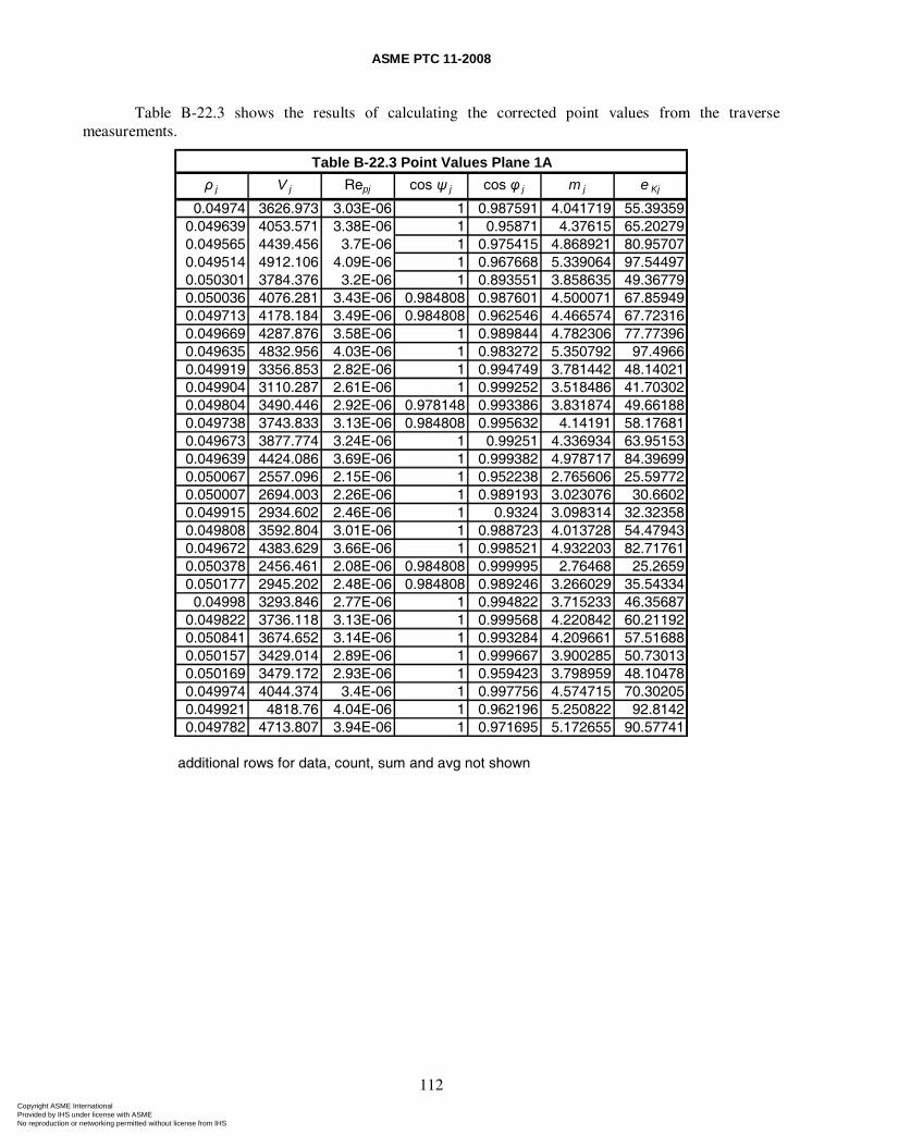
ASME PTC 11-2008

112

Table B-22.3 shows the results of calculating the corrected point values from the traverse measurements.

ρ j V j Repj cos ψ j cos φ j m j e Kj

0.04974 3626.973 3.03E-06 1 0.987591 4.041719 55.393590.049639 4053.571 3.38E-06 1 0.95871 4.37615 65.202790.049565 4439.456 3.7E-06 1 0.975415 4.868921 80.957070.049514 4912.106 4.09E-06 1 0.967668 5.339064 97.544970.050301 3784.376 3.2E-06 1 0.893551 3.858635 49.367790.050036 4076.281 3.43E-06 0.984808 0.987601 4.500071 67.859490.049713 4178.184 3.49E-06 0.984808 0.962546 4.466574 67.723160.049669 4287.876 3.58E-06 1 0.989844 4.782306 77.773960.049635 4832.956 4.03E-06 1 0.983272 5.350792 97.49660.049919 3356.853 2.82E-06 1 0.994749 3.781442 48.140210.049904 3110.287 2.61E-06 1 0.999252 3.518486 41.703020.049804 3490.446 2.92E-06 0.978148 0.993386 3.831874 49.661880.049738 3743.833 3.13E-06 0.984808 0.995632 4.14191 58.176810.049673 3877.774 3.24E-06 1 0.99251 4.336934 63.951530.049639 4424.086 3.69E-06 1 0.999382 4.978717 84.396990.050067 2557.096 2.15E-06 1 0.952238 2.765606 25.597720.050007 2694.003 2.26E-06 1 0.989193 3.023076 30.66020.049915 2934.602 2.46E-06 1 0.9324 3.098314 32.323580.049808 3592.804 3.01E-06 1 0.988723 4.013728 54.479430.049672 4383.629 3.66E-06 1 0.998521 4.932203 82.717610.050378 2456.461 2.08E-06 0.984808 0.999995 2.76468 25.26590.050177 2945.202 2.48E-06 0.984808 0.989246 3.266029 35.543340.04998 3293.846 2.77E-06 1 0.994822 3.715233 46.35687

0.049822 3736.118 3.13E-06 1 0.999568 4.220842 60.211920.050841 3674.652 3.14E-06 1 0.993284 4.209661 57.516880.050157 3429.014 2.89E-06 1 0.999667 3.900285 50.730130.050169 3479.172 2.93E-06 1 0.959423 3.798959 48.104780.049974 4044.374 3.4E-06 1 0.997756 4.574715 70.302050.049921 4818.76 4.04E-06 1 0.962196 5.250822 92.81420.049782 4713.807 3.94E-06 1 0.971695 5.172655 90.57741


Table B-22.3 Point Values Plane 1A


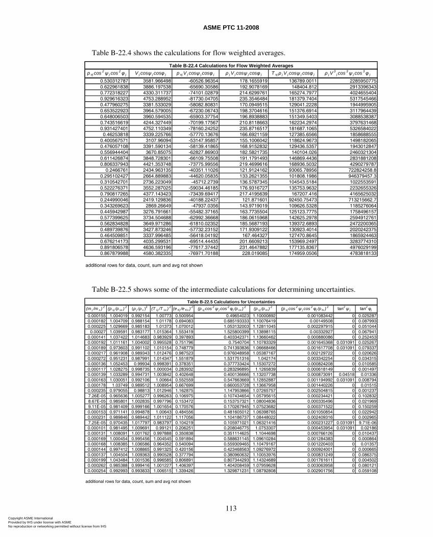
ASME PTC 11-2008

113

Table B-22.4 shows the calculations for flow weighted averages.

p vj cos 2ψ j cos 2φ j V j cosψ j cosφ j p sj V j cosψ j cosφ j ρ j V j cosψ j cosφ j T sjρ j V j cosψ j cosφ j ρ j V3

j cos 3ψ j cos 3φ j

0.530312787 3581.966498 -60526.96354 178.1655919 136789.0011 22859507750.622961838 3886.197538 -65690.30586 192.9078169 148404.812 29133963430.772318227 4330.311737 -74101.02879 214.6299761 165274.7977 40246554040.929616323 4753.288952 -81730.04705 235.3546484 181379.7404 53175454660.477960275 3381.533029 -58082.80831 170.0949515 129041.2228 19449959050.653522923 3964.579005 -67230.06743 198.3704616 151376.6914 31179644390.648006503 3960.594535 -65903.37754 196.8938883 151349.5403 30885383870.743516619 4244.327449 -70199.17567 210.8118663 162234.2974 37976314680.931427401 4752.110349 -78160.24252 235.8716517 181687.1065 5326584022

0.46253818 3339.225766 -57770.13676 166.6921159 127385.6566 18586885550.400567571 3107.96094 -53147.95857 155.1006042 118624.9673 14981820650.476057108 3391.590134 -58139.41865 168.9152832 129436.5357 19430128470.556944404 3670.85075 -62827.86903 182.5821735 140104.026 24603213040.611426874 3848.728301 -66109.75508 191.1791493 146869.4436 28318812080.806337943 4421.353748 -73775.99556 219.4699616 168936.5032 4290279787

0.2466761 2434.963135 -40351.11026 121.9124162 93065.78956 722824258.80.295102427 2664.889883 -44620.05835 133.2621355 101808.1986 946379457.30.310542701 2736.223049 -45712.2739 136.5787345 104543.5184 10225535910.522276371 3552.287025 -59034.46185 176.9316727 135753.9632 22326553260.790817265 4377.143423 -73439.69417 217.4195639 167207.416 41656250320.244990046 2419.129836 -40188.22437 121.871601 92450.75473 713215662.70.343269623 2869.26649 -47937.0356 143.9719019 109626.5328 11852760640.445942987 3276.791661 -55482.37165 163.7735504 125123.7775 17584961570.577399625 3734.504688 -62992.36668 186.0615968 142625.2978 25949127610.562834828 3649.971286 -61810.02352 185.5687193 139372.6893 24722003650.489739876 3427.873246 -57732.23152 171.9309122 130923.4014 20202423750.464509851 3337.996485 -56418.04192 167.464327 127470.8645 18659244630.676214173 4035.299531 -69514.44435 201.6609213 153969.2497 32837743100.891806578 4636.593196 -77617.37442 231.4647882 177135.8367 49760291990.867879988 4580.382335 -76971.70188 228.019085 174959.0506 4783818133


Table B-22.4 Calculations for Flow Weighted Averages

Table B-22.5 shows some of the intermediate calculations for determining uncertainties.

(m j /m x ) 2 (p sj /p sx ) 2 (ρ j /ρ x )2 (T sj /T sx ) 2 (e Kj /e Kx ) 2 (p vj cos 2ψ j cos 2φj /p vx ) 2 (p sj /p tx ) 2 (p vj cos 2ψ j cos 2φj /p tx ) 2 tan2ψ j tan2φj

0.000155 1.004019 0.992154 1.00773 0.500954 0.49654023 1.10000892 0.001083442 0 0.0252870.000182 1.004709 0.988154 1.01178 0.694083 0.685193333 1.10076419 0.00149508 0 0.0879930.000225 1.029669 0.985183 1.01373 1.070012 1.053132003 1.12811045 0.002297915 0 0.0510440.00027 1.039591 0.983177 1.015364 1.553419 1.525800399 1.13898115 0.00332927 0 0.067941

0.000141 1.037422 1.014683 0.983929 0.397893 0.403342371 1.13660462 0.000880086 0 0.2524530.000192 1.011161 1.004002 0.995528 0.751796 0.7540704 1.10783329 0.001645368 0.031091 0.0252670.000189 0.973603 0.991102 1.010154 0.748779 0.741393836 1.06668466 0.001617708 0.031091 0.0793370.000217 0.961908 0.989343 1.012476 0.987523 0.976048958 1.05387167 0.002129722 0 0.0206260.000272 0.951231 0.987991 1.014347 1.551879 1.531751316 1.042174 0.003342254 0 0.0343150.000136 1.052453 0.99934 0.998391 0.378351 0.377733424 1.15307272 0.000824208 0 0.0105850.000117 1.028275 0.998735 1.000034 0.283932 0.283296895 1.1265839 0.000618149 0 0.0014970.000139 1.033289 0.994731 1.003842 0.402648 0.400136666 1.13207738 0.000873091 0.04518 0.013360.000163 1.030051 0.992106 1.00664 0.552559 0.547663669 1.12852887 0.001194992 0.031091 0.0087940.000178 1.03749 0.989512 1.008954 0.667699 0.660053728 1.13667958 0.001440226 0 0.015150.000235 0.979055 0.98813 1.012946 1.162875 1.147953866 1.07265757 0.002504815 0 0.0012377.26E-05 0.965636 1.005277 0.996263 0.106975 0.107434654 1.05795615 0.000234421 0 0.1028328.67E-05 0.985801 1.002835 0.997796 0.153472 0.153757321 1.08004836 0.000335496 0 0.0219699.11E-05 0.981409 0.999166 1.001654 0.170576 0.170267945 1.07523682 0.000371522 0 0.1502590.000153 0.971141 0.994878 1.00643 0.484556 0.481605012 1.06398765 0.001050854 0 0.0229420.000231 0.989846 0.989442 1.011122 1.117056 1.104186737 1.08448022 0.002409316 0 0.0029657.25E-05 0.970435 1.017797 0.983797 0.104219 0.105971021 1.06321416 0.000231227 0.031091 9.71E-060.000101 0.981495 1.009691 0.99121 0.206251 0.208046775 1.0753307 0.000453954 0.031091 0.021860.000131 1.008091 1.001762 0.997888 0.350838 0.351114625 1.1044698 0.000766126 0 0.0104370.000169 1.000454 0.995456 1.004545 0.591894 0.588631145 1.09610284 0.001284383 0 0.0008640.000168 1.008385 1.036586 0.964352 0.540094 0.559309465 1.10479167 0.001220403 0 0.013570.000144 0.997412 1.008865 0.991325 0.420156 0.423468563 1.09276972 0.000924001 0 0.0006650.000137 1.004504 1.009363 0.990528 0.377794 0.380960632 1.10053976 0.000831249 0 0.0863750.000199 1.043484 1.001536 0.996585 0.806891 0.807344293 1.14324689 0.001761611 0 0.0045020.000262 0.985388 0.999416 1.001227 1.406397 1.404208459 1.07959628 0.003063958 0 0.0801210.000254 0.992993 0.993833 1.006515 1.339426 1.329871231 1.08792808 0.002901756 0 0.059108


Table B-22.5 Calculations for Uncertainties


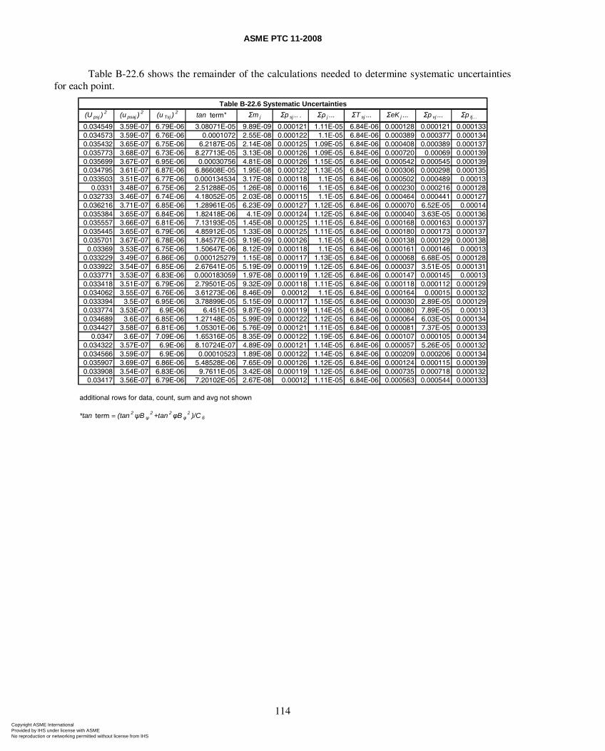
ASME PTC 11-2008

114

Table B-22.6 shows the remainder of the calculations needed to determine systematic uncertainties for each point.

(U psj )2 (u psaj )

2 (u Tsj )2 tan term* Σm j Σp sj .. . Σρ j ... ΣT sj ... ΣeK j ... Σp vj ... Σp tj…

0.034549 3.59E-07 6.79E-06 3.08071E-05 9.89E-09 0.000121 1.11E-05 6.84E-06 0.000128 0.000121 0.0001330.034573 3.59E-07 6.76E-06 0.0001072 2.55E-08 0.000122 1.1E-05 6.84E-06 0.000389 0.000377 0.0001340.035432 3.65E-07 6.75E-06 6.2187E-05 2.14E-08 0.000125 1.09E-05 6.84E-06 0.000408 0.000389 0.0001370.035773 3.68E-07 6.73E-06 8.27713E-05 3.13E-08 0.000126 1.09E-05 6.84E-06 0.000720 0.00069 0.0001390.035699 3.67E-07 6.95E-06 0.00030756 4.81E-08 0.000126 1.15E-05 6.84E-06 0.000542 0.000545 0.0001390.034795 3.61E-07 6.87E-06 6.86608E-05 1.95E-08 0.000122 1.13E-05 6.84E-06 0.000306 0.000298 0.0001350.033503 3.51E-07 6.77E-06 0.000134534 3.17E-08 0.000118 1.1E-05 6.84E-06 0.000502 0.000489 0.00013

0.0331 3.48E-07 6.75E-06 2.51288E-05 1.26E-08 0.000116 1.1E-05 6.84E-06 0.000230 0.000216 0.0001280.032733 3.46E-07 6.74E-06 4.18052E-05 2.03E-08 0.000115 1.1E-05 6.84E-06 0.000464 0.000441 0.0001270.036216 3.71E-07 6.85E-06 1.28961E-05 6.23E-09 0.000127 1.12E-05 6.84E-06 0.000070 6.52E-05 0.000140.035384 3.65E-07 6.84E-06 1.82418E-06 4.1E-09 0.000124 1.12E-05 6.84E-06 0.000040 3.63E-05 0.0001360.035557 3.66E-07 6.81E-06 7.13193E-05 1.45E-08 0.000125 1.11E-05 6.84E-06 0.000168 0.000163 0.0001370.035445 3.65E-07 6.79E-06 4.85912E-05 1.33E-08 0.000125 1.11E-05 6.84E-06 0.000180 0.000173 0.0001370.035701 3.67E-07 6.78E-06 1.84577E-05 9.19E-09 0.000126 1.1E-05 6.84E-06 0.000138 0.000129 0.0001380.03369 3.53E-07 6.75E-06 1.50647E-06 8.12E-09 0.000118 1.1E-05 6.84E-06 0.000161 0.000146 0.00013

0.033229 3.49E-07 6.86E-06 0.000125279 1.15E-08 0.000117 1.13E-05 6.84E-06 0.000068 6.68E-05 0.0001280.033922 3.54E-07 6.85E-06 2.67641E-05 5.19E-09 0.000119 1.12E-05 6.84E-06 0.000037 3.51E-05 0.0001310.033771 3.53E-07 6.83E-06 0.000183059 1.97E-08 0.000119 1.12E-05 6.84E-06 0.000147 0.000145 0.000130.033418 3.51E-07 6.79E-06 2.79501E-05 9.32E-09 0.000118 1.11E-05 6.84E-06 0.000118 0.000112 0.0001290.034062 3.55E-07 6.76E-06 3.61273E-06 8.46E-09 0.00012 1.1E-05 6.84E-06 0.000164 0.00015 0.0001320.033394 3.5E-07 6.95E-06 3.78899E-05 5.15E-09 0.000117 1.15E-05 6.84E-06 0.000030 2.89E-05 0.0001290.033774 3.53E-07 6.9E-06 6.451E-05 9.87E-09 0.000119 1.14E-05 6.84E-06 0.000080 7.89E-05 0.000130.034689 3.6E-07 6.85E-06 1.27148E-05 5.99E-09 0.000122 1.12E-05 6.84E-06 0.000064 6.03E-05 0.0001340.034427 3.58E-07 6.81E-06 1.05301E-06 5.76E-09 0.000121 1.11E-05 6.84E-06 0.000081 7.37E-05 0.000133

0.0347 3.6E-07 7.09E-06 1.65316E-05 8.35E-09 0.000122 1.19E-05 6.84E-06 0.000107 0.000105 0.0001340.034322 3.57E-07 6.9E-06 8.10724E-07 4.89E-09 0.000121 1.14E-05 6.84E-06 0.000057 5.26E-05 0.0001320.034566 3.59E-07 6.9E-06 0.00010523 1.89E-08 0.000122 1.14E-05 6.84E-06 0.000209 0.000206 0.0001340.035907 3.69E-07 6.86E-06 5.48528E-06 7.65E-09 0.000126 1.12E-05 6.84E-06 0.000124 0.000115 0.0001390.033908 3.54E-07 6.83E-06 9.7611E-05 3.42E-08 0.000119 1.12E-05 6.84E-06 0.000735 0.000718 0.0001320.03417 3.56E-07 6.79E-06 7.20102E-05 2.67E-08 0.00012 1.11E-05 6.84E-06 0.000563 0.000544 0.000133


*tan term = (tan 2ψB ψ2 +tan 2φB φ

2 )/C 6

Table B-22.6 Systematic Uncertainties


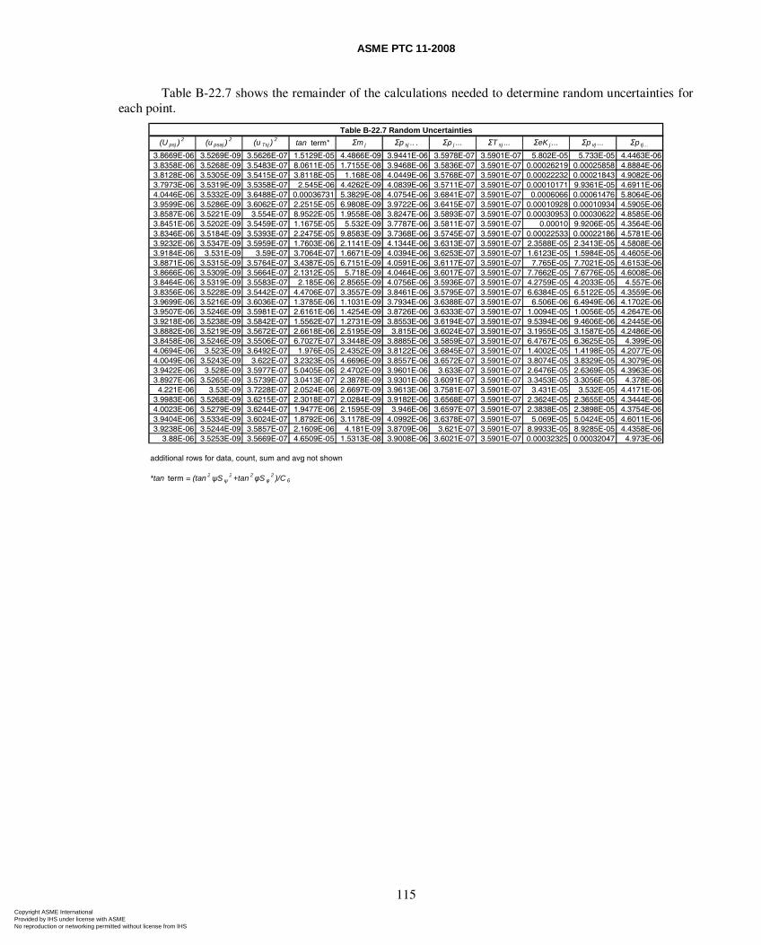
ASME PTC 11-2008

115

Table B-22.7 shows the remainder of the calculations needed to determine random uncertainties for each point.

(U psj )2 (u psaj )

2 (u Tsj )2 tan term* Σm j Σp sj .. . Σρ j ... ΣT sj ... ΣeK j ... Σp vj ... Σp tj…

3.8669E-06 3.5269E-09 3.5626E-07 1.5129E-05 4.4866E-09 3.9441E-06 3.5978E-07 3.5901E-07 5.802E-05 5.733E-05 4.4463E-063.8358E-06 3.5268E-09 3.5483E-07 8.0611E-05 1.7155E-08 3.9468E-06 3.5836E-07 3.5901E-07 0.00026219 0.00025858 4.8884E-063.8128E-06 3.5305E-09 3.5415E-07 3.8118E-05 1.168E-08 4.0449E-06 3.5768E-07 3.5901E-07 0.00022232 0.00021843 4.9082E-063.7973E-06 3.5319E-09 3.5358E-07 2.545E-06 4.4262E-09 4.0839E-06 3.5711E-07 3.5901E-07 0.00010171 9.9361E-05 4.6911E-064.0446E-06 3.5332E-09 3.6488E-07 0.00036731 5.3829E-08 4.0754E-06 3.6841E-07 3.5901E-07 0.0006066 0.00061476 5.8064E-063.9599E-06 3.5286E-09 3.6062E-07 2.2515E-05 6.9808E-09 3.9722E-06 3.6415E-07 3.5901E-07 0.00010928 0.00010934 4.5905E-063.8587E-06 3.5221E-09 3.554E-07 8.9522E-05 1.9558E-08 3.8247E-06 3.5893E-07 3.5901E-07 0.00030953 0.00030622 4.8585E-063.8451E-06 3.5202E-09 3.5459E-07 1.1675E-05 5.532E-09 3.7787E-06 3.5811E-07 3.5901E-07 0.00010 9.9206E-05 4.3564E-063.8346E-06 3.5184E-09 3.5393E-07 2.2475E-05 9.8583E-09 3.7368E-06 3.5745E-07 3.5901E-07 0.00022533 0.00022186 4.5781E-063.9232E-06 3.5347E-09 3.5959E-07 1.7603E-06 2.1141E-09 4.1344E-06 3.6313E-07 3.5901E-07 2.3588E-05 2.3413E-05 4.5808E-063.9184E-06 3.531E-09 3.59E-07 3.7064E-07 1.6671E-09 4.0394E-06 3.6253E-07 3.5901E-07 1.6123E-05 1.5984E-05 4.4605E-063.8871E-06 3.5315E-09 3.5764E-07 3.4387E-05 6.7151E-09 4.0591E-06 3.6117E-07 3.5901E-07 7.765E-05 7.7021E-05 4.6153E-063.8666E-06 3.5309E-09 3.5664E-07 2.1312E-05 5.718E-09 4.0464E-06 3.6017E-07 3.5901E-07 7.7662E-05 7.6776E-05 4.6008E-063.8464E-06 3.5319E-09 3.5583E-07 2.185E-06 2.8565E-09 4.0756E-06 3.5936E-07 3.5901E-07 4.2759E-05 4.2033E-05 4.557E-063.8356E-06 3.5228E-09 3.5442E-07 4.4706E-07 3.3557E-09 3.8461E-06 3.5795E-07 3.5901E-07 6.6384E-05 6.5122E-05 4.3559E-063.9699E-06 3.5216E-09 3.6036E-07 1.3785E-06 1.1031E-09 3.7934E-06 3.6388E-07 3.5901E-07 6.506E-06 6.4949E-06 4.1702E-063.9507E-06 3.5246E-09 3.5981E-07 2.6161E-06 1.4254E-09 3.8726E-06 3.6333E-07 3.5901E-07 1.0094E-05 1.0056E-05 4.2647E-063.9218E-06 3.5238E-09 3.5842E-07 1.5562E-07 1.2731E-09 3.8553E-06 3.6194E-07 3.5901E-07 9.5394E-06 9.4606E-06 4.2445E-063.8882E-06 3.5219E-09 3.5672E-07 2.6618E-06 2.5195E-09 3.815E-06 3.6024E-07 3.5901E-07 3.1955E-05 3.1587E-05 4.2486E-063.8458E-06 3.5246E-09 3.5506E-07 6.7027E-07 3.3448E-09 3.8885E-06 3.5859E-07 3.5901E-07 6.4767E-05 6.3625E-05 4.399E-064.0694E-06 3.523E-09 3.6492E-07 1.976E-05 2.4352E-09 3.8122E-06 3.6845E-07 3.5901E-07 1.4002E-05 1.4198E-05 4.2077E-064.0049E-06 3.5243E-09 3.622E-07 3.2323E-05 4.6696E-09 3.8557E-06 3.6572E-07 3.5901E-07 3.8074E-05 3.8329E-05 4.3079E-063.9422E-06 3.528E-09 3.5977E-07 5.0405E-06 2.4702E-09 3.9601E-06 3.633E-07 3.5901E-07 2.6476E-05 2.6369E-05 4.3963E-063.8927E-06 3.5265E-09 3.5739E-07 3.0413E-07 2.3878E-09 3.9301E-06 3.6091E-07 3.5901E-07 3.3453E-05 3.3056E-05 4.378E-06

4.221E-06 3.53E-09 3.7228E-07 2.0524E-06 2.6697E-09 3.9613E-06 3.7581E-07 3.5901E-07 3.431E-05 3.532E-05 4.4171E-063.9983E-06 3.5268E-09 3.6215E-07 2.3018E-07 2.0284E-09 3.9182E-06 3.6568E-07 3.5901E-07 2.3624E-05 2.3655E-05 4.3444E-064.0023E-06 3.5279E-09 3.6244E-07 1.9477E-06 2.1595E-09 3.946E-06 3.6597E-07 3.5901E-07 2.3838E-05 2.3898E-05 4.3754E-063.9404E-06 3.5334E-09 3.6024E-07 1.8792E-06 3.1178E-09 4.0992E-06 3.6378E-07 3.5901E-07 5.069E-05 5.0424E-05 4.6011E-063.9238E-06 3.5244E-09 3.5857E-07 2.1609E-06 4.181E-09 3.8709E-06 3.621E-07 3.5901E-07 8.9933E-05 8.9285E-05 4.4358E-06

3.88E-06 3.5253E-09 3.5669E-07 4.6509E-05 1.5313E-08 3.9008E-06 3.6021E-07 3.5901E-07 0.00032325 0.00032047 4.973E-06


*tan term = (tan 2ψS ψ2 +tan 2φS φ

2 )/C 6

Table B-22.7 Random Uncertainties


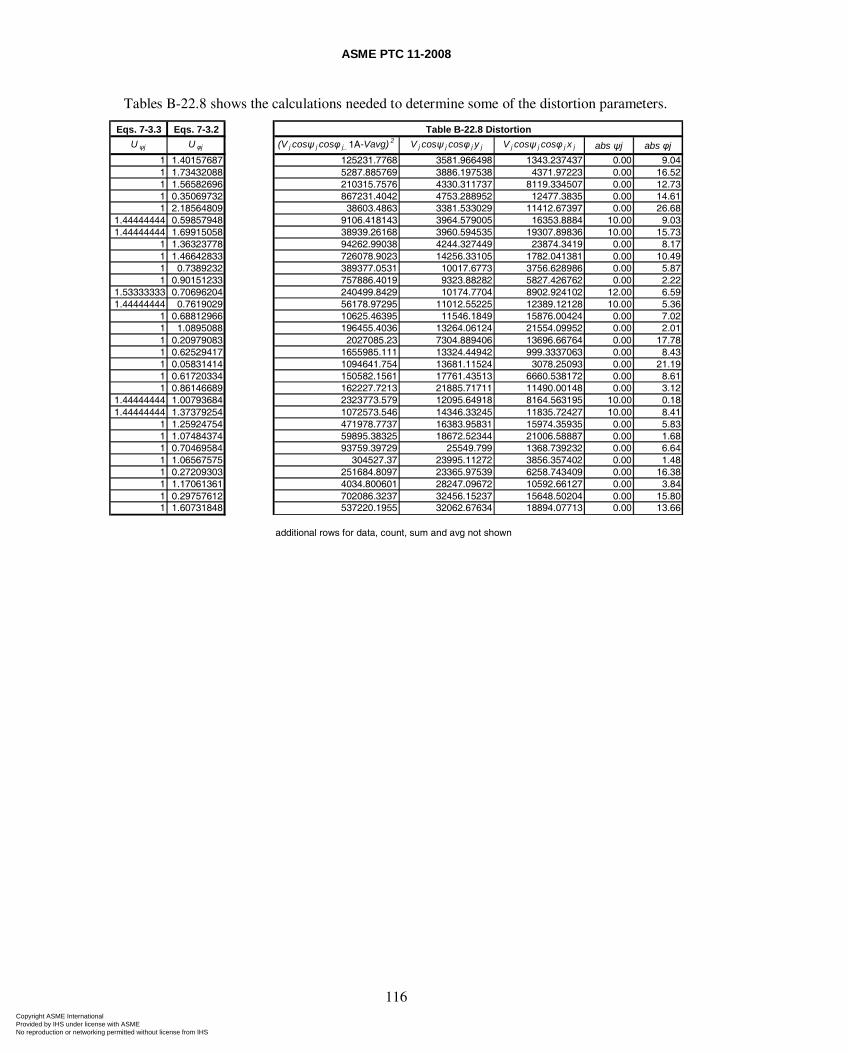
ASME PTC 11-2008

116

Tables B-22.8 shows the calculations needed to determine some of the distortion parameters.

Eqs. 7-3.3 Eqs. 7-3.2

U ψj U φj (V j cosψ j cosφ j_ 1A-Vavg) 2 V j cosψ j cosφ j y j V j cosψ j cosφ j x j abs ψj abs φj

1 1.40157687 125231.7768 3581.966498 1343.237437 0.00 9.041 1.73432088 5287.885769 3886.197538 4371.97223 0.00 16.521 1.56582696 210315.7576 4330.311737 8119.334507 0.00 12.731 0.35069732 867231.4042 4753.288952 12477.3835 0.00 14.611 2.18564809 38603.4863 3381.533029 11412.67397 0.00 26.68

1.44444444 0.59857948 9106.418143 3964.579005 16353.8884 10.00 9.031.44444444 1.69915058 38939.26168 3960.594535 19307.89836 10.00 15.73

1 1.36323778 94262.99038 4244.327449 23874.3419 0.00 8.171 1.46642833 726078.9023 14256.33105 1782.041381 0.00 10.491 0.7389232 389377.0531 10017.6773 3756.628986 0.00 5.871 0.90151233 757886.4019 9323.88282 5827.426762 0.00 2.22

1.53333333 0.70696204 240499.8429 10174.7704 8902.924102 12.00 6.591.44444444 0.7619029 56178.97295 11012.55225 12389.12128 10.00 5.36

1 0.68812966 10625.46395 11546.1849 15876.00424 0.00 7.021 1.0895088 196455.4036 13264.06124 21554.09952 0.00 2.011 0.20979083 2027085.23 7304.889406 13696.66764 0.00 17.781 0.62529417 1655985.111 13324.44942 999.3337063 0.00 8.431 0.05831414 1094641.754 13681.11524 3078.25093 0.00 21.191 0.61720334 150582.1561 17761.43513 6660.538172 0.00 8.611 0.86146689 162227.7213 21885.71711 11490.00148 0.00 3.12

1.44444444 1.00793684 2323773.579 12095.64918 8164.563195 10.00 0.181.44444444 1.37379254 1072573.546 14346.33245 11835.72427 10.00 8.41

1 1.25924754 471978.7737 16383.95831 15974.35935 0.00 5.831 1.07484374 59895.38325 18672.52344 21006.58887 0.00 1.681 0.70469584 93759.39729 25549.799 1368.739232 0.00 6.641 1.06567575 304527.37 23995.11272 3856.357402 0.00 1.481 0.27209303 251684.8097 23365.97539 6258.743409 0.00 16.381 1.17061361 4034.800601 28247.09672 10592.66127 0.00 3.841 0.29757612 702086.3237 32456.15237 15648.50204 0.00 15.801 1.60731848 537220.1955 32062.67634 18894.07713 0.00 13.66


Table B-22.8 Distortion


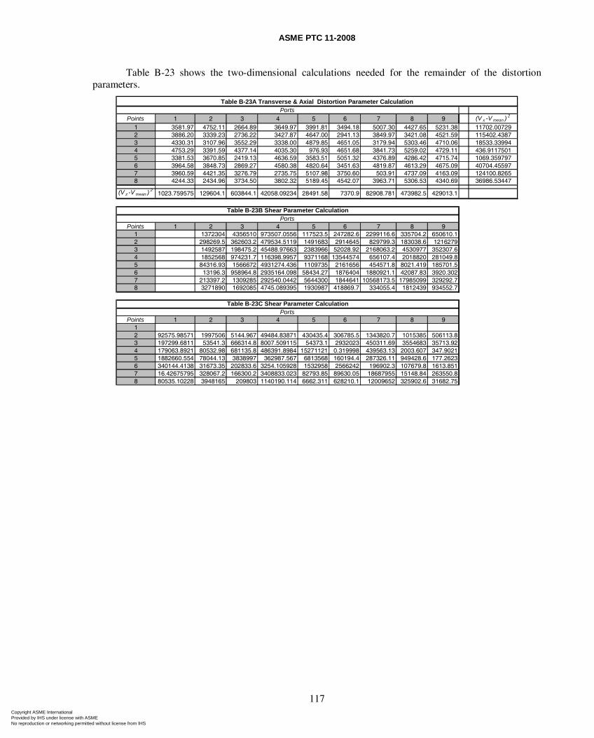
ASME PTC 11-2008

117

Table B-23 shows the two-dimensional calculations needed for the remainder of the distortion parameters.

Points 1 2 3 4 5 6 7 8 9 (V x -V mean ) 2

1 3581.97 4752.11 2664.89 3649.97 3991.81 3494.18 5007.30 4427.65 5231.38 11702.007292 3886.20 3339.23 2736.22 3427.87 4647.00 2941.13 3849.97 3421.08 4521.59 115402.43873 4330.31 3107.96 3552.29 3338.00 4879.85 4651.05 3179.94 5303.46 4710.06 18533.339944 4753.29 3391.59 4377.14 4035.30 976.93 4651.68 3841.73 5259.02 4729.11 436.91175015 3381.53 3670.85 2419.13 4636.59 3583.51 5051.32 4376.89 4286.42 4715.74 1069.3597976 3964.58 3848.73 2869.27 4580.38 4820.64 3451.63 4819.87 4613.29 4675.09 40704.455977 3960.59 4421.35 3276.79 2735.75 5107.98 3750.60 503.91 4737.09 4163.09 124100.82658 4244.33 2434.96 3734.50 3802.32 5189.45 4542.07 3963.71 5306.53 4340.69 36986.53447

(V z -V mean ) 21023.759575 129604.1 603844.1 42058.09234 28491.58 7370.9 82908.781 473982.5 429013.1

Points 1 2 3 4 5 6 7 8 91 1372304 4356510 973507.0556 117523.5 247282.6 2299116.6 335704.2 650610.12 298269.5 362603.2 479534.5119 1491683 2914645 829799.3 183038.6 12162793 1492587 198475.2 45488.97663 2383966 52028.92 2168063.2 4530977 352307.64 1852568 974231.7 116398.9957 9371168 13544574 656107.4 2018820 281049.85 84316.93 1566672 4931274.436 1109735 2161656 454571.8 8021.419 185701.56 13196.3 958964.8 2935164.098 58434.27 1876404 1880921.1 42087.83 3920.3027 213397.2 1309285 292540.0442 5644300 1844641 10568173.5 17985099 329292.78 3271890 1692085 4745.089395 1930987 418869.7 334055.4 1812439 934552.7

Points 1 2 3 4 5 6 7 8 912 92575.98571 1997506 5144.967 49484.83871 430435.4 306785.5 1343820.7 1015385 506113.83 197299.6811 53541.3 666314.8 8007.509115 54373.1 2932023 450311.69 3554683 35713.924 179063.8921 80532.98 681135.8 486391.8984 15271121 0.319998 439563.13 2003.607 347.90215 1882660.554 78044.13 3838997 362987.567 6813568 160194.4 287326.11 949428.6 177.26236 340144.4138 31673.35 202833.6 3254.105928 1532958 2566242 196902.3 107679.8 1613.8517 16.42675795 328067.2 166300.2 3408833.023 82793.85 89630.05 18687955 15148.84 263550.88 80535.10228 3948165 209803 1140190.114 6662.311 628210.1 12009652 325902.6 31682.75

PortsTable B-23A Transverse & Axial Distortion Parameter Calculation

Table B-23C Shear Parameter CalculationPorts

Table B-23B Shear Parameter CalculationPorts


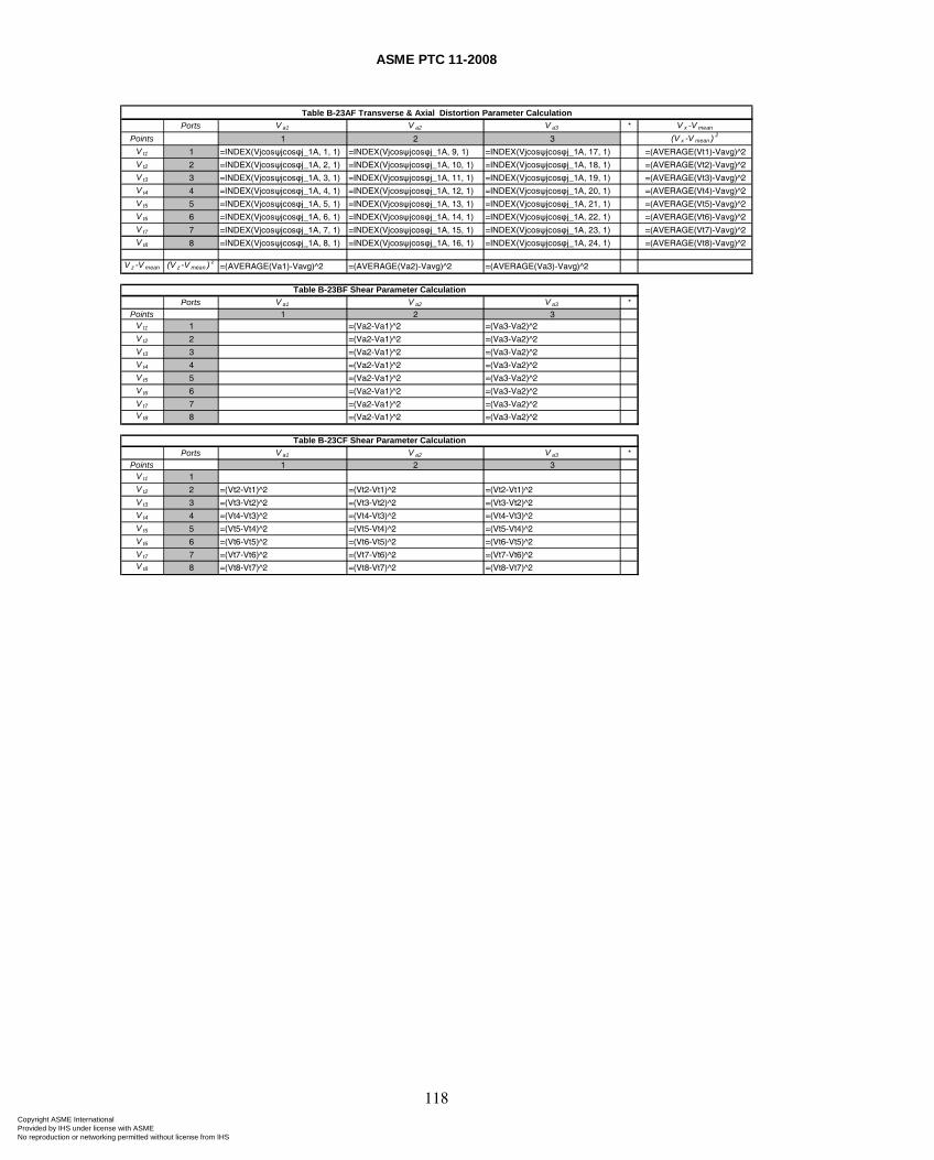
ASME PTC 11-2008

118

Ports V a1 V a2 V a3 * V x -V mean

Points 1 2 3 (V x -V mean ) 2

V t1 1 =INDEX(Vjcosψjcosφj_1A, 1, 1) =INDEX(Vjcosψjcosφj_1A, 9, 1) =INDEX(Vjcosψjcosφj_1A, 17, 1) =(AVERAGE(Vt1)-Vavg)^2








V z -V mean (V z -V mean ) 2=(AVERAGE(Va1)-Vavg)^2 =(AVERAGE(Va2)-Vavg)^2 =(AVERAGE(Va3)-Vavg)^2

Ports V a1 V a2 V a3 *Points 1 2 3

V t1 1 =(Va2-Va1)^2 =(Va3-Va2)^2

V t2 2 =(Va2-Va1)^2 =(Va3-Va2)^2

V t3 3 =(Va2-Va1)^2 =(Va3-Va2)^2

V t4 4 =(Va2-Va1)^2 =(Va3-Va2)^2

V t5 5 =(Va2-Va1)^2 =(Va3-Va2)^2

V t6 6 =(Va2-Va1)^2 =(Va3-Va2)^2

V t7 7 =(Va2-Va1)^2 =(Va3-Va2)^2V t8 8 =(Va2-Va1)^2 =(Va3-Va2)^2

Ports V a1 V a2 V a3 *Points 1 2 3

V t1 1

V t2 2 =(Vt2-Vt1)^2 =(Vt2-Vt1)^2 =(Vt2-Vt1)^2

V t3 3 =(Vt3-Vt2)^2 =(Vt3-Vt2)^2 =(Vt3-Vt2)^2

V t4 4 =(Vt4-Vt3)^2 =(Vt4-Vt3)^2 =(Vt4-Vt3)^2

V t5 5 =(Vt5-Vt4)^2 =(Vt5-Vt4)^2 =(Vt5-Vt4)^2

V t6 6 =(Vt6-Vt5)^2 =(Vt6-Vt5)^2 =(Vt6-Vt5)^2

V t7 7 =(Vt7-Vt6)^2 =(Vt7-Vt6)^2 =(Vt7-Vt6)^2V t8 8 =(Vt8-Vt7)^2 =(Vt8-Vt7)^2 =(Vt8-Vt7)^2

Table B-23AF Transverse & Axial Distortion Parameter Calculation

Table B-23CF Shear Parameter Calculation

Table B-23BF Shear Parameter Calculation


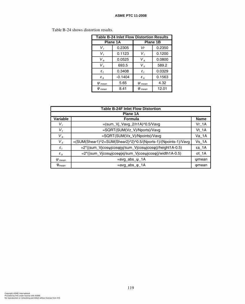
ASME PTC 11-2008

119

Table B-24 shows distortion results.

V r 0.2305 Vr 0.2350

V t 0.1123 V t 0.1200

V a 0.0525 V a 0.0800

V s 693.5 V s 589.2

ε t 0.3408 ε t 0.0329

ε a -0.1404 ε a 0.1563

ψ mean 5.65 ψ mean 4.32φ mean 8.41 φ mean 12.01

Variable NameV r Vr_1A

V t Vt_1A

V a Va_1A

V s Vs_1A

ε t εa_1A

ε a σt_1A

ψ mean ψmeanφmean φmean

Formula

Table B-24 Inlet Flow Distortion Results

=2*((sum_Vjcosψjcosφjyj/sum_Vjcosψjcosφj)/height1A-0.5)

=2*((sum_Vjcosψjcosφjxj/sum_Vjcosψjcosφj)/width1A-0.5)

Table B-24F Inlet Flow DistortionPlane 1A

Plane 1A Plane 1B

=avg_abs_ψ_1A

=avg_abs_φ_1A

=(sum_Vj_Vavg_2/n1A)^0.5/Vavg

=SQRT(SUM(Vz_V)/Nports)/Vavg

=SQRT(SUM(Vx_V)/Npoints)/Vavg

=(SUM(Shear1)^2+SUM(Shear2)^2)^0.5/(Nports-1)/(Npoints-1)/Vavg


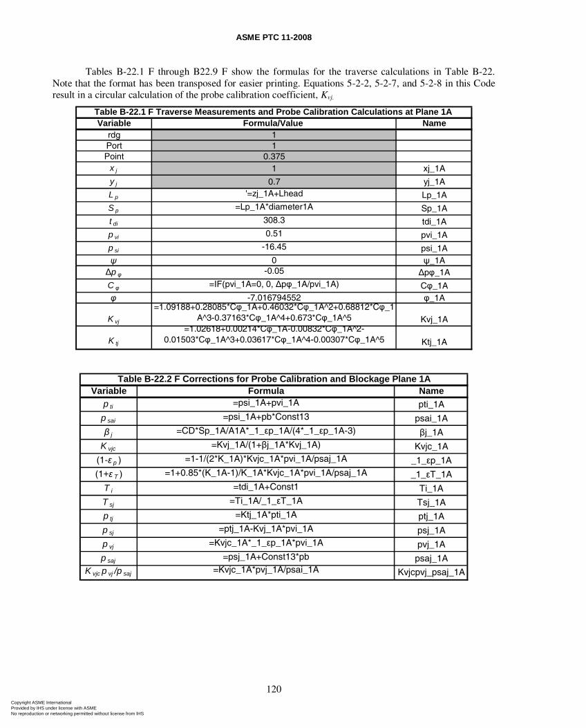
ASME PTC 11-2008

120

Tables B-22.1 F through B22.9 F show the formulas for the traverse calculations in Table B-22. Note that the format has been transposed for easier printing. Equations 5-2-2, 5-2-7, and 5-2-8 in this Code result in a circular calculation of the probe calibration coefficient, Kvj.

Variable Formula/Value Namerdg 1Port 1Point 0.375

x j 1 xj_1A

y j 0.7 yj_1A

L p '=zj_1A+Lhead Lp_1A

S p =Lp_1A*diameter1A Sp_1A

t di 308.3 tdi_1A

p vi 0.51 pvi_1A

p si -16.45 psi_1Aψ 0 ψ_1AΔp φ -0.05 Δpφ_1A

C φ =IF(pvi_1A=0, 0, Δpφ_1A/pvi_1A) Cφ_1Aφ -7.016794552 φ_1A

K vj

=1.09188+0.28085*Cφ_1A+0.46032*Cφ_1A^2+0.68812*Cφ_1A^3-0.37163*Cφ_1A^4+0.673*Cφ_1A^5 Kvj_1A

K tj

=1.02618+0.00214*Cφ_1A-0.00832*Cφ_1A^2-0.01503*Cφ_1A^3+0.03617*Cφ_1A^4-0.00307*Cφ_1A^5 Ktj_1A

Table B-22.1 F Traverse Measurements and Probe Calibration Calculations at Plane 1A

Variable Formula Namep ti =psi_1A+pvi_1A pti_1A

p sai =psi_1A+pb*Const13 psai_1A

β j =CD*Sp_1A/A1A*_1_εp_1A/(4*_1_εp_1A-3) βj_1A

K vjc =Kvj_1A/(1+βj_1A*Kvj_1A) Kvjc_1A

(1-ε p ) =1-1/(2*K_1A)*Kvjc_1A*pvi_1A/psaj_1A _1_εp_1A

(1+ε T ) =1+0.85*(K_1A-1)/K_1A*Kvjc_1A*pvi_1A/psaj_1A _1_εT_1A

T i =tdi_1A+Const1 Ti_1A

T sj =Ti_1A/_1_εT_1A Tsj_1A

p tj =Ktj_1A*pti_1A ptj_1A

p sj =ptj_1A-Kvj_1A*pvi_1A psj_1A

p vj =Kvjc_1A*_1_εp_1A*pvi_1A pvj_1A

p saj =psj_1A+Const13*pb psaj_1AK vjc p vj /p saj =Kvjc_1A*pvj_1A/psai_1A Kvjcpvj_psaj_1A

Table B-22.2 F Corrections for Probe Calibration and Blockage Plane 1A


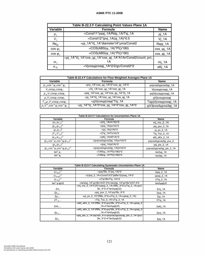
ASME PTC 11-2008

121

Variable Formula Nameρ j =Const11*psaj_1A/Rdg_1A/Tsj_1A ρj_1A

V j =Const12*(pvj_1A/ρj_1A)^0.5 Vj_1A

Repj =ρj_1A*Vj_1A*diameter1A*μma/Const2 Repj_1A

cos ψ j =COS(ABS(ψ_1A)*PI()/180) cos_ψj_1A

cos φ j =COS(ABS(φ_1A)*PI()/180) cos_φj_1A

m j

=ρj_1A*Vj_1A*cos_ψj_1A*cos_φj_1A*A1Ar/Const2/count_pvi_1A mj_1A

e Kj =Vjcosψjcosφj_1A^2/2/gc/Const2^2 eKj_1A

Table B-22.3 F Calculating Point Values Plane 1A

Variable Formula Namep vj cos 2ψ j cos 2φ j =pvj_1A*cos_ψj_1A^2*cos_φj_1A^2 pvjcos2ψjcos2φj_1A

V j cosψ j cosφ j =Vj_1A*cos_ψj_1A*cos_φj_1A Vjcosψjcosφj_1A

p sj V j cosψ j cosφ j =psj_1A*cos_ψj_1A*cos_φj_1A*Vj_1A psjVjcosψjcosφj_1A

ρ j V j cosψ j cosφ j =ρj_1A*Vj_1A*cos_ψj_1A*cos_φj_1A ρjVjcosψjcosφj

T sjρ j V j cosψ j cosφ j =ρjVjcosψjcosφj*Tsj_1A TsjρjVjcosψjcosφj_1Aρ j V

3j cos 3ψ j cos 3φ j =ρj_1A*Vj_1A^3*cos_ψj_1A^3*cos_φj_1A^3 ρjV3jcos3ψjcos3φj_1A

Table B-22.4 F Calculations for Flow Weighted Averages Plane 1A

Variable Formula Name(m j /m x ) 2 =(mj_1A/m1A)^2 mj_mx_2_1A(p sj /p sx ) 2 =(psj_1A/ps1A)^2 psj_psx_2_1A

(ρ j /ρ x )2 =(ρj_1A/ρ1A)^2 ρj_ρx_2_1A

(T sj /T sx ) 2 =(Tsj_1A/Ts1A)^2 Tsj_Tsx_2_1A

(e Kj /e Kx ) 2 =(eKj_1A/eK1A)^2 eKj_eKx_2_1A

(p vj cos 2ψ j cos 2φj /p vx ) 2 =(pvjcos2ψjcos2φj_1A/pv1A)^2 pvjcos2ψjcos2φj_pvx_2

(p sj /p tx ) 2 =(psj_1A/pt1A)^2 psj_ptx_2_1A

(p vj cos 2ψ j cos 2φj /p tx ) 2 =(pvjcos2ψjcos2φj_1A/pt1A)^2 pvjcos2ψjcos2φj_ptx_2_1A

tan2ψ j =TAN(ψ_1A*PI()/180)^2 tan2ψj_1Atan2φj =TAN(φ_1A*PI()/180)^2 tan2φj_1A

Table B-22.5 F Calculations for Uncertainties Plane 1A

Variable Formula Name(U psj )

2 =(psj1Bx_X*psj_1A)^2 Upsj_2_1A

(u psaj )2 =(Upsj_2_1A+Const13^2*pbBx^2)/psaj_1A^2 upsaj_2_1A

(u Tsj )2 =(Tsj1Bx/Tsj_1A)^2 uTsj_2_1A

tan2ψφjU2 =tan2ψj_1A*ψj1Bx^2/57.3^2+tan2φj_1A*φj1Bx^2/57.3^2 tan2ψφjU2

Σm j

=mj_mx_2_1A*0.25*(upsaj_2_1A+RBx_X^2+uTsj_2_1A+pvj1Bx_X^2+4*tan2ψφjU2) Σmj_1A

Σp sj .. . =psj_psx_2_1A*psj1Bx_X^2 Σpsj_1A

Σρ j ... =ρj_ρx_2_1A*(RBx_X^2+uTsj_2_1A+upsaj_2_1A) Σρj_1A

ΣT sj ... =Tsj_Tsx_2_1A*uTsj_2_1A ΣTsj_1A

ΣeK j ...=eKj_eKx_2_1A*(RBx_X^2+pvj1Bx_X^2+uTsj_2_1A+upsaj_2

_1A+4*tan2ψφjU2) ΣeKj_1A

Σp vj ...=eKj_eKx_2_1A*(RBx_X^2+pvj1Bx_X^2+uTsj_2_1A+upsaj_2

_1A+4*tan2ψφjU2) Σpvj_1A

Σp tj…

=psj_ptx_2_1A*psj1Bx_X^2+pvjcos2ψjcos2φj_ptx_2_1A*(pvj1Bx_X^2+4*tan2ψφjU2) Σptj_1A

Table B-22.6 F Calculating Systematic Uncertainties Plane 1A


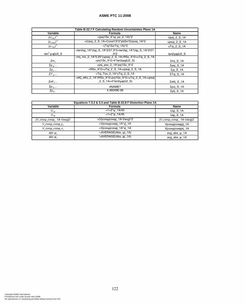
ASME PTC 11-2008

122

Variable Formula Name(U psj )

2 =(psj1Sx_X*ρj_ρx_2_1A)^2 Upsj_2_S_1A

(u psaj )2 =(Upsj_2_S_1A+Const13^2*pbSx^2)/psaj_1A^2 upsaj_2_S_1A

(u Tsj )2 =(Tsj1Sx/Tsj_1A)^2 uTsj_2_S_1A

tan2ψφjU2_S=tan2ψj_1A*Uψj_S_1A^2/57.3^2+tan2φj_1A*Uφj_S_1A^2/57.

3^2 tan2ψφjU2_S

Σm j

=mj_mx_2_1A*0.25*(upsaj_2_S_1A+RSx_X^2+uTsj_2_S_1A+pvj1Sx_X^2+4*tan2ψφjU2_S) Σmj_S_1A

Σp sj .. . =psj_psx_2_1A*psj1Sx_X^2 Σpsj_S_1A

Σρ j ... =RSx_X^2+uTsj_2_S_1A+upsaj_2_S_1A Σρj_S_1A

ΣT sj ... =Tsj_Tsx_2_1A*uTsj_2_S_1A ΣTsj_S_1A

ΣeK j ...=eKj_eKx_2_1A*(RSx_X^2+pvj1Sx_X^2+uTsj_2_S_1A+upsaj

_2_S_1A+4*tan2ψφjU2_S) ΣeKj_S_1A

Σp vj ... #NAME? Σpvj_S_1AΣp tj… 4.46049E-06 Σptj_S_1A

Table B-22.7 F Calculating Random Uncertainties Plane 1A

Variable Formula NameU ψj =1+2*ψ_1A/45 Uψj_S_1AU φj =1+2*φ_1A/45 Uφj_S_1A

(V j cosψ j cosφ j_ 1A-Vavg)2 =(Vjcosψjcosφj_1A-Vavg)^2 (V j cosψ j cosφ j_ 1A-Vavg)2

V j cosψ j cosφ j y j =Vjcosψjcosφj_1A*yj_1A Vjcosψjcosφjyj_1A

V j cosψ j cosφ j x j =Vjcosψjcosφj_1A*xj_1A Vjcosψjcosφjxj_1A

abs ψ j '=AVERAGE(Abs_ψj_1A) avg_abs_ψ_1Aabs φ j '=AVERAGE(Abs_φj_1A) avg_abs_φ_1A

Equations 7-3.2 & 3.3 and Table B-22.8 F Distortion Plane 1A


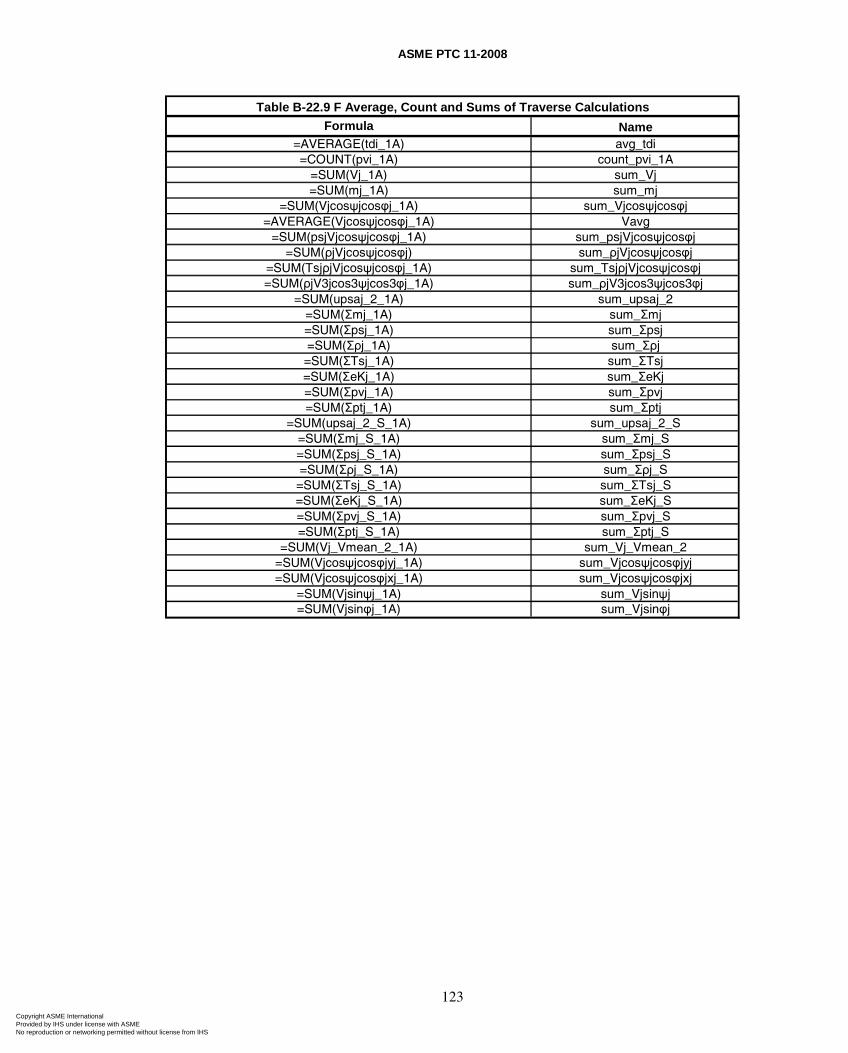
ASME PTC 11-2008

123

Formula Name=AVERAGE(tdi_1A) avg_tdi=COUNT(pvi_1A) count_pvi_1A

=SUM(Vj_1A) sum_Vj=SUM(mj_1A) sum_mj

=SUM(Vjcosψjcosφj_1A) sum_Vjcosψjcosφj=AVERAGE(Vjcosψjcosφj_1A) Vavg

=SUM(psjVjcosψjcosφj_1A) sum_psjVjcosψjcosφj=SUM(ρjVjcosψjcosφj) sum_ρjVjcosψjcosφj

=SUM(TsjρjVjcosψjcosφj_1A) sum_TsjρjVjcosψjcosφj=SUM(ρjV3jcos3ψjcos3φj_1A) sum_ρjV3jcos3ψjcos3φj

=SUM(upsaj_2_1A) sum_upsaj_2=SUM(Σmj_1A) sum_Σmj=SUM(Σpsj_1A) sum_Σpsj=SUM(Σρj_1A) sum_Σρj=SUM(ΣTsj_1A) sum_ΣTsj=SUM(ΣeKj_1A) sum_ΣeKj=SUM(Σpvj_1A) sum_Σpvj=SUM(Σptj_1A) sum_Σptj

=SUM(upsaj_2_S_1A) sum_upsaj_2_S=SUM(Σmj_S_1A) sum_Σmj_S=SUM(Σpsj_S_1A) sum_Σpsj_S=SUM(Σρj_S_1A) sum_Σρj_S

=SUM(ΣTsj_S_1A) sum_ΣTsj_S=SUM(ΣeKj_S_1A) sum_ΣeKj_S=SUM(Σpvj_S_1A) sum_Σpvj_S=SUM(Σptj_S_1A) sum_Σptj_S

=SUM(Vj_Vmean_2_1A) sum_Vj_Vmean_2=SUM(Vjcosψjcosφjyj_1A) sum_Vjcosψjcosφjyj=SUM(Vjcosψjcosφjxj_1A) sum_Vjcosψjcosφjxj

=SUM(Vjsinψj_1A) sum_Vjsinψj=SUM(Vjsinφj_1A) sum_Vjsinφj

Table B-22.9 F Average, Count and Sums of Traverse Calculations


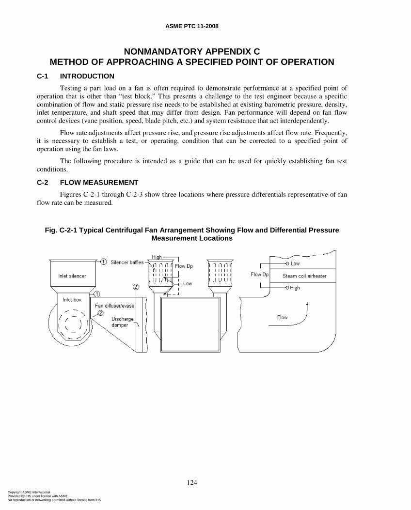
ASME PTC 11-2008

124

NONMANDATORY APPENDIX C METHOD OF APPROACHING A SPECIFIED POINT OF OPERATION

C-1 INTRODUCTION

Testing a part load on a fan is often required to demonstrate performance at a specified point of operation that is other than “test block.” This presents a challenge to the test engineer because a specific combination of flow and static pressure rise needs to be established at existing barometric pressure, density, inlet temperature, and shaft speed that may differ from design. Fan performance will depend on fan flow control devices (vane position, speed, blade pitch, etc.) and system resistance that act interdependently.

Flow rate adjustments affect pressure rise, and pressure rise adjustments affect flow rate. Frequently, it is necessary to establish a test, or operating, condition that can be corrected to a specified point of operation using the fan laws.

The following procedure is intended as a guide that can be used for quickly establishing fan test conditions.

C-2 FLOW MEASUREMENT

Figures C-2-1 through C-2-3 show three locations where pressure differentials representative of fan flow rate can be measured.

Fig. C-2-1 Typical Centrifugal Fan Arrangement Showing Flow and Differential Pressure Measurement Locations


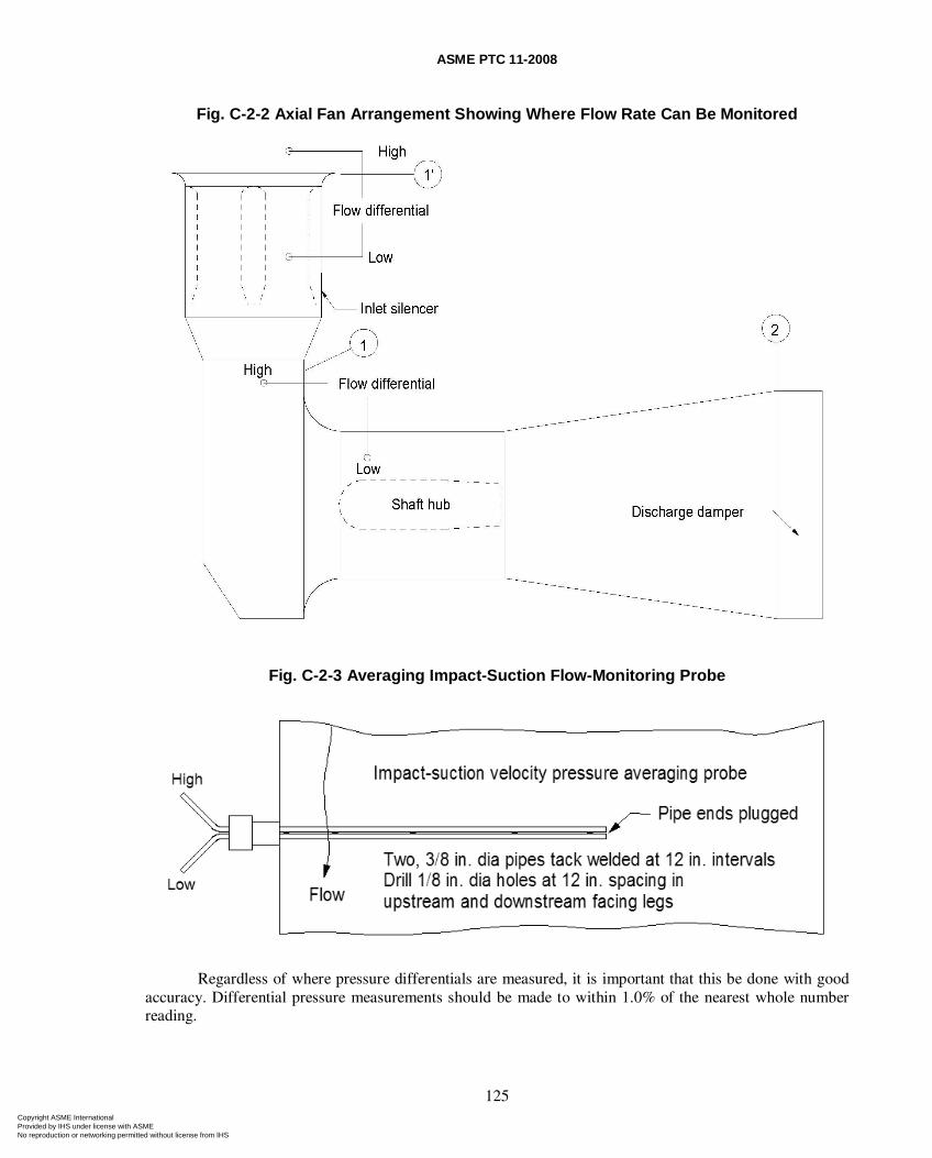
ASME PTC 11-2008

125

Fig. C-2-2 Axial Fan Arrangement Showing Where Flow Rate Can Be Monitored

Fig. C-2-3 Averaging Impact-Suction Flow-Monitoring Probe

Regardless of where pressure differentials are measured, it is important that this be done with good accuracy. Differential pressure measurements should be made to within 1.0% of the nearest whole number reading.


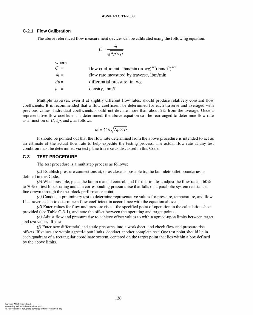
ASME PTC 11-2008

126

C-2.1 Flow Calibration

The above referenced flow measurement devices can be calibrated using the following equation:

m

Cp ρ

=Δ ×

where C = flow coefficient, -0.5 3 -0.5lbm/min (in. wg) (lbm/ft ) m = flow rate measured by traverse, lbm/min

Δp = differential pressure, in. wg

ρ = density, lbm/ft3

Multiple traverses, even if at slightly different flow rates, should produce relatively constant flow coefficients. It is recommended that a flow coefficient be determined for each traverse and averaged with previous values. Individual coefficients should not deviate more than about 2% from the average. Once a representative flow coefficient is determined, the above equation can be rearranged to determine flow rate as a function of C, Δp, and ρ as follows:

m C p ρ= × Δ ×

It should be pointed out that the flow rate determined from the above procedure is intended to act as an estimate of the actual flow rate to help expedite the testing process. The actual flow rate at any test condition must be determined via test plane traverse as discussed in this Code.

C-3 TEST PROCEDURE

The test procedure is a multistep process as follows:

(a) Establish pressure connections at, or as close as possible to, the fan inlet/outlet boundaries as defined in this Code.

(b) When possible, place the fan in manual control, and for the first test, adjust the flow rate at 60% to 70% of test block rating and at a corresponding pressure rise that falls on a parabolic system resistance line drawn through the test block performance point.

(c) Conduct a preliminary test to determine representative values for pressure, temperature, and flow. Use traverse data to determine a flow coefficient in accordance with the equation above.

(d) Enter values for flow and pressure rise at the specified point of operation in the calculation sheet provided (see Table C-3-1), and note the offset between the operating and target points.

(e) Adjust flow and pressure rise to achieve offset values to within agreed-upon limits between target and test values. Retest.

(f) Enter new differential and static pressures into a worksheet, and check flow and pressure rise offsets. If values are within agreed-upon limits, conduct another complete test. One test point should lie in each quadrant of a rectangular coordinate system, centered on the target point that lies within a box defined by the above limits.


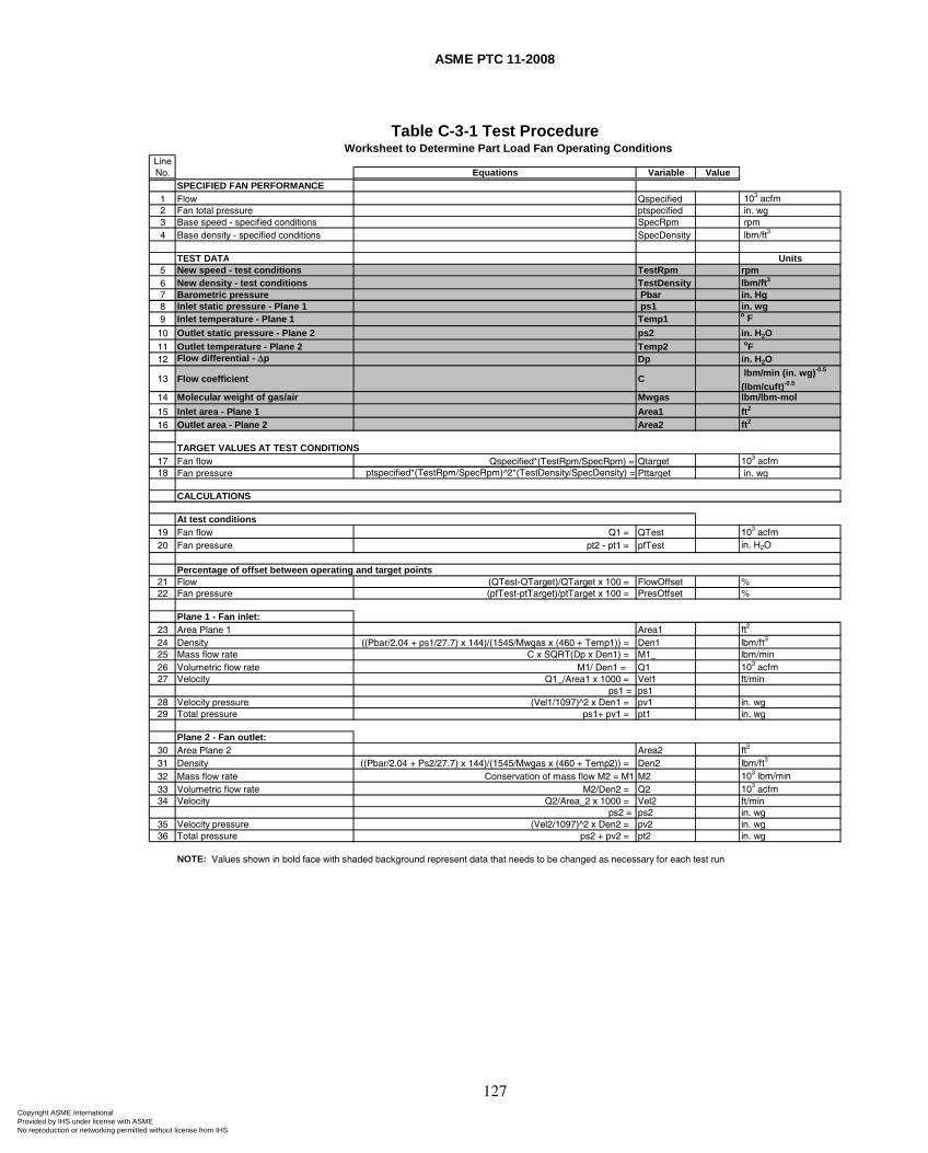
ASME PTC 11-2008

127

Table C-3-1 Test Procedure

LineNo. Equations Variable Value

SPECIFIED FAN PERFORMANCE1 Flow Qspecified 103 acfm2 Fan total pressure ptspecified in. wg3 Base speed - specified conditions SpecRpm rpm4 Base density - specified conditions SpecDensity lbm/ft3

TEST DATA Units5 New speed - test conditions TestRpm rpm6 New density - test conditions TestDensity lbm/ft3

7 Barometric pressure Pbar in. Hg8 Inlet static pressure - Plane 1 ps1 in. wg9 Inlet temperature - Plane 1 Temp1 o F

10 Outlet static pressure - Plane 2 ps2 in. H2O11 Outlet temperature - Plane 2 Temp2 oF12 Flow differential - Δp Dp in. H2O

13 Flow coefficient C lbm/min (in. wg)-0.5

(lbm/cuft)-0.5

14 Molecular weight of gas/air Mwgas lbm/lbm-mol

15 Inlet area - Plane 1 Area1 ft2

16 Outlet area - Plane 2 Area2 ft2

TARGET VALUES AT TEST CONDITIONS17 Fan flow Qspecified*(TestRpm/SpecRpm) = Qtarget 103 acfm18 Fan pressure ptspecified*(TestRpm/SpecRpm)^2*(TestDensity/SpecDensity) = Pttarget in. wg

At test conditions19 Fan flow Q1 = QTest 103 acfm20 Fan pressure pt2 - pt1 = pfTest in. H2O

Percentage of offset between operating and target points21 Flow (QTest-QTarget)/QTarget x 100 = FlowOffset %22 Fan pressure (pfTest-ptTarget)/ptTarget x 100 = PresOffset %

Plane 1 - Fan inlet: 23 Area Plane 1 Area1 ft2

24 Density ((Pbar/2.04 + ps1/27.7) x 144)/(1545/Mwgas x (460 + Temp1)) = Den1 lbm/ft3

25 Mass flow rate C x SQRT(Dp x Den1) = M1_ lbm/min26 Volumetric flow rate M1/ Den1 = Q1 103 acfm27 Velocity Q1_/Area1 x 1000 = Vel1 ft/min

ps1 = ps128 Velocity pressure (Vel1/1097)^2 x Den1 = pv1 in. wg29 Total pressure ps1+ pv1 = pt1 in. wg

Plane 2 - Fan outlet:30 Area Plane 2 Area2 ft2

31 Density ((Pbar/2.04 + Ps2/27.7) x 144)/(1545/Mwgas x (460 + Temp2)) = Den2 lbm/ft3

32 Mass flow rate Conservation of mass flow M2 = M1 M2 103 lbm/min33 Volumetric flow rate M2/Den2 = Q2 103 acfm34 Velocity Q2/Area_2 x 1000 = Vel2 ft/min

ps2 = ps2 in. wg35 Velocity pressure (Vel2/1097)^2 x Den2 = pv2 in. wg36 Total pressure ps2 + pv2 = pt2 in. wg

NOTE: Values shown in bold face with shaded background represent data that needs to be changed as necessary for each test run

CALCULATIONS

Worksheet to Determine Part Load Fan Operating Conditions


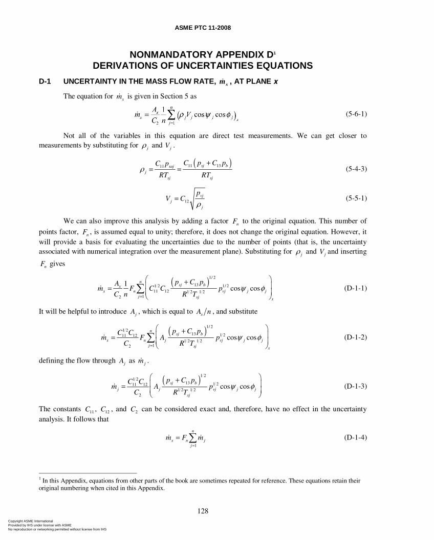
ASME PTC 11-2008

128

NONMANDATORY APPENDIX D1 DERIVATIONS OF UNCERTAINTIES EQUATIONS

D-1 UNCERTAINTY IN THE MASS FLOW RATE, xm , AT PLANE x

The equation for xm is given in Section 5 as

(5-6-1)

Not all of the variables in this equation are direct test measurements. We can get closer to

measurements by substituting for jρ and jV .

( )11 1311 sj bsaj

jsj sj

C p C pC p

RT RTρ

+= = (5-4-3)

12vj

jj

pV C

ρ= (5-5-1)

We can also improve this analysis by adding a factor nF to the original equation. This number of

points factor, nF , is assumed equal to unity; therefore, it does not change the original equation. However, it will provide a basis for evaluating the uncertainties due to the number of points (that is, the uncertainty associated with numerical integration over the measurement plane). Substituting for jρ and jV and inserting

nF gives

( )1/ 2

131 2 1/ 211 12 1 2 1 2

12

1cos cos

nsj bx

x n vj j jj sj x

p C pAm F C C p

C n R Tψ φ

=

⎛ ⎞+⎜ ⎟= ⎜ ⎟⎝ ⎠

∑ (D-1-1)

It will be helpful to introduce jA , which is equal to xA n , and substitute

( )1/ 2

1 213 1 211 12

1 2 1 212

cos cosn

sj b

x n j vj j jj sj x

p C pC Cm F A p

C R Tψ φ

=

⎛ ⎞+⎜ ⎟= ⎜ ⎟⎝ ⎠

∑ (D-1-2)

defining the flow through jA as jm .

( )1 2

1 213 1 211 12

1 2 1 22

cos cossj b

j j vj j jsj

p C pC Cm A p

C R Tψ φ

⎛ ⎞+⎜ ⎟= ⎜ ⎟⎝ ⎠

(D-1-3)

The constants 11C , 12C , and 2C can be considered exact and, therefore, have no effect in the uncertainty analysis. It follows that

1

n

x n jj

m F m=

= ∑ (D-1-4)

1 In this Appendix, equations from other parts of the book are sometimes repeated for reference. These equations retain their original numbering when cited in this Appendix.


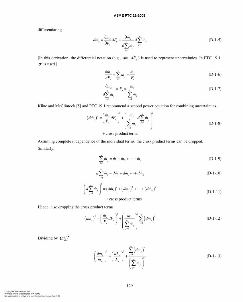
ASME PTC 11-2008

129

differentiating

1

1

nx x

x n jnjn

jj

m mdm dF d m

Fm =

=

∂ ∂= +∂ ∂

∑∑

(D-1-5)

[In this derivation, the differential notation (e.g., ndF,md ) is used to represent uncertainties. In PTC 19.1,

σ is used.]

1

nx x

jjn n

m mm

F F=

∂= =

∂ ∑ (D-1-6)

1 1

x xnn n

j jj j

m mF

m m= =

∂ = =∂∑ ∑

(D-1-7)

Kline and McClintock [5] and PTC 19.1 recommend a second power equation for combining uncertainties.

( )

222

1

1

cross product terms

nx x

x n jnjn

jj

m mdm dF d m

Fm =

=

⎛ ⎞⎛ ⎞= + ⎜ ⎟⎜ ⎟⎝ ⎠ ⎜ ⎟⎜ ⎟

⎝ ⎠+

∑∑ (D-1-8)

Assuming complete independence of the individual terms, the cross product terms can be dropped.

Similarly,

1 21

n

j nj

m m m m=

= + + +∑ (D-1-9)

1 21

n

j nj

d m dm dm dm=

= + +∑ (D-1-10)

( ) ( ) ( )

22 2 2

1 21

cross product terms

n

j nj

d m dm dm dm=

⎛ ⎞ = + + +⎜ ⎟⎝ ⎠

+

∑ (D-1-11)

Hence, also dropping the cross product terms,

( ) ( )2 2

22

1

1

nx x

x n jnjn

jj

m mdm dF dm

Fm =

=

⎛ ⎞ ⎛ ⎞= +⎜ ⎟ ⎜ ⎟⎝ ⎠ ⎜ ⎟⎜ ⎟

⎝ ⎠

∑∑

(D-1-12)

Dividing by

( )2

2 21

2

1

n

jjx n

nx n

jj

dmdm dF

m Fm

=

=

⎛ ⎞ ⎛ ⎞= +⎜ ⎟ ⎜ ⎟⎛ ⎞⎝ ⎠ ⎝ ⎠⎜ ⎟⎝ ⎠

∑

∑ (D-1-13)


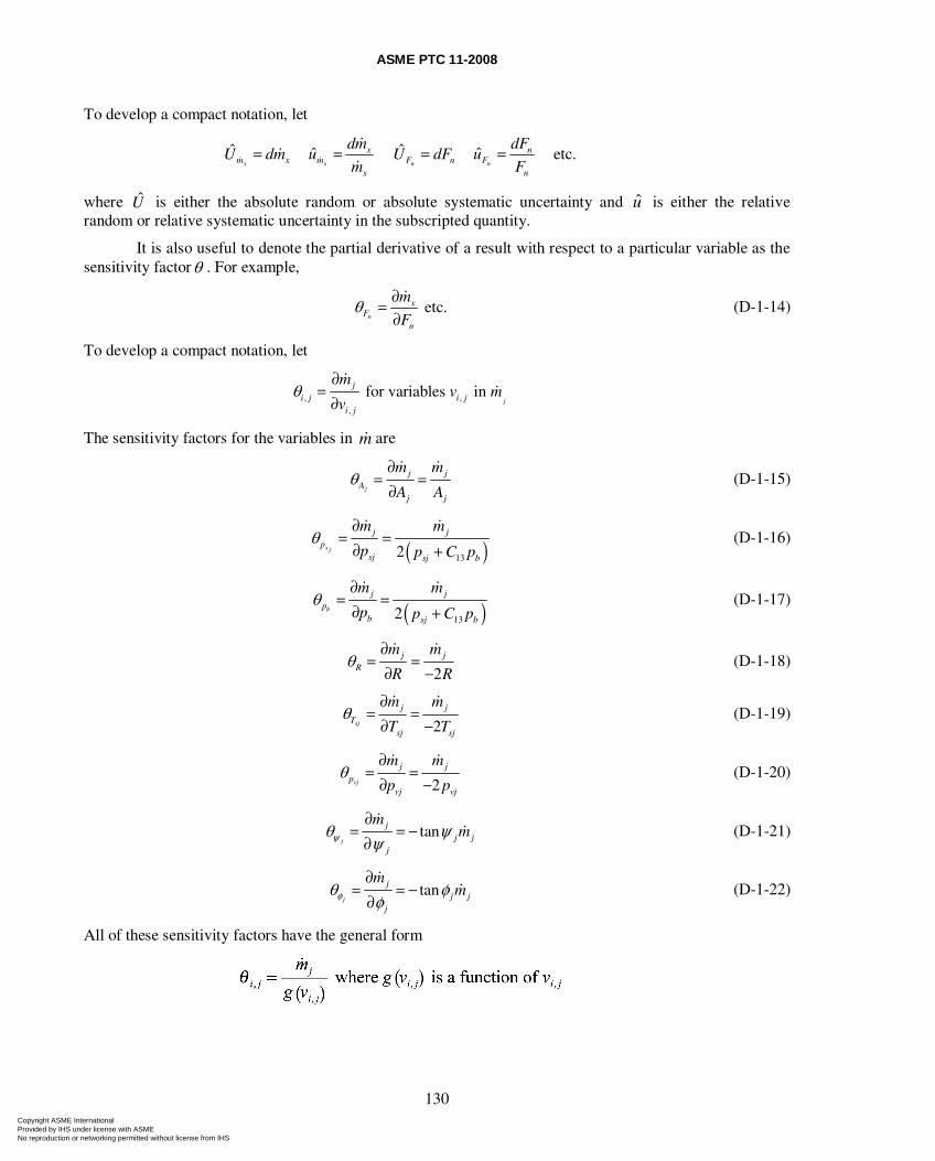
ASME PTC 11-2008

130

To develop a compact notation, let

ˆ ˆˆ ˆ etc.x x n n

x nm x m F n F

x n

dm dFU dm u U dF u

m F= = = =

where U is either the absolute random or absolute systematic uncertainty and u is either the relative random or relative systematic uncertainty in the subscripted quantity.

It is also useful to denote the partial derivative of a result with respect to a particular variable as the sensitivity factorθ . For example,

etc.n

xF

n

m

Fθ ∂

=∂

(D-1-14)

To develop a compact notation, let

, ,,

for variables in j

ji j i j

i j

mv m

vθ

∂=∂

The sensitivity factors for the variables in m are

j

j jA

j j

m m

A Aθ

∂= =∂

(D-1-15)

( )132s j

j jp

sj sj b

m m

p p C pθ

∂= =∂ +

(D-1-16)

( )132b

j jp

b sj b

m m

p p C pθ

∂= =∂ +

(D-1-17)

2

j jR

m m

R Rθ

∂= =∂ −

(D-1-18)

2sj

j jT

sj sj

m m

T Tθ

∂= =∂ −

(D-1-19)

2vj

j jp

vj vj

m m

p pθ

∂= =∂ −

(D-1-20)

tanj

jj j

j

mmψθ ψ

ψ∂

= = −∂

(D-1-21)

tanj

jj j

j

mmφθ φ

φ∂

= = −∂

(D-1-22)

All of these sensitivity factors have the general form


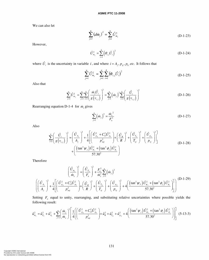
ASME PTC 11-2008

131

We can also let

(D-1-23)

However,

( )22

,1

ˆ ˆj

k

m i j ii

U Uθ=

=∑ (D-1-24)

where îU is the uncertainty in variable i , and where , , , .j sj bi A p p etc= It follows that

(D-1-25)

Also that

( ) ( ) ( )2 2

22

1 1 1 1 1, ,

ˆ ˆˆ

j

n n k n kj i i

m jj j i j ii j i j

m U UU m

g v g v= = = = =

⎛ ⎞ ⎛ ⎞= =⎜ ⎟ ⎜ ⎟⎜ ⎟ ⎜ ⎟

⎝ ⎠ ⎝ ⎠∑ ∑∑ ∑ ∑ (D-1-26)

Rearranging equation D-1-4 for xm gives

( )2

2

21

nx

jj n

mm

F=

=∑ (D-1-27)

Also

( )( ) ( )

2 2 22 22 2 213

21 ,

2 2 2 2

2

ˆ ˆ ˆ ˆ ˆˆ ˆ1

4

ˆ ˆtan tan

57.30

j sj b sj vj

j j

kA p p T pi R

i j saj sj vji j

j j

U U C U U UU U

A p R T pg v

U Uψ φψ φ

=

⎡ ⎤⎛ ⎞ ⎛ ⎞ ⎛ ⎞ ⎛ ⎞+⎛ ⎞ ⎛ ⎞⎢ ⎥⎜ ⎟ ⎜ ⎟ ⎜ ⎟ ⎜ ⎟= + + + +⎜ ⎟ ⎜ ⎟⎜ ⎟ ⎜ ⎟ ⎜ ⎟ ⎜ ⎟⎢ ⎥⎜ ⎟ ⎝ ⎠⎝ ⎠ ⎝ ⎠ ⎝ ⎠ ⎝ ⎠⎣ ⎦⎝ ⎠⎛ ⎞+⎜ ⎟+⎝ ⎠

∑ (D-1-28)

Therefore

( )

( ) ( )

2 22

2

21

2 2 222 2 2 2 2 213

2

ˆ ˆ

ˆ ˆ ˆ ˆ ˆ ˆˆ tan tan14

4

x n

j sj b sj vj j

nm F n

jjx n x

A p p T p J jR

j saj sj vj

U U Fm

m F m

U U C U U U UU

A p R T p

ψψ φ

=

⎛ ⎞ ⎛ ⎞⎜ ⎟ ⎜ ⎟= +⎜ ⎟ ⎜ ⎟⎝ ⎠ ⎝ ⎠

⎛ ⎞ ⎛ ⎞ ⎛ ⎞ ⎛ ⎞+ +⎛ ⎞⎜ ⎟ ⎜ ⎟ ⎜ ⎟ ⎜ ⎟+ + + + +⎜ ⎟⎜ ⎟ ⎜ ⎟ ⎜ ⎟ ⎜ ⎟⎝ ⎠⎝ ⎠ ⎝ ⎠ ⎝ ⎠ ⎝ ⎠

∑

2

2

ˆ

57.30j

Uφ⎛ ⎞⎡ ⎤⎛ ⎞⎜ ⎟⎢ ⎥⎜ ⎟⎜ ⎟⎢ ⎥⎝ ⎠⎣ ⎦⎝ ⎠

(D-1-29)

Setting nF equal to unity, rearranging, and substituting relative uncertainties where possible yields the following result:

( ) ( )2 2 2 2 2 2 2 2132 2 2 2 2 2

2 21

ˆ ˆ ˆ ˆtan tan1ˆ ˆ ˆ ˆ ˆ ˆ 4

4 57.30sj b j j

x n x sj vj

np p j jj

m F A R T pj x saj

U C U U Umu u u u u u

m p

ψ φψ φ

=

⎡ ⎤⎛ ⎞⎛ ⎞⎛ ⎞+ +⎛ ⎞ ⎢ ⎥⎜ ⎟⎜ ⎟⎜ ⎟= + + + + + +⎜ ⎟ ⎜ ⎟⎜ ⎟⎢ ⎥⎝ ⎠⎝ ⎠ ⎝ ⎠⎝ ⎠⎣ ⎦∑ (5-13-3)


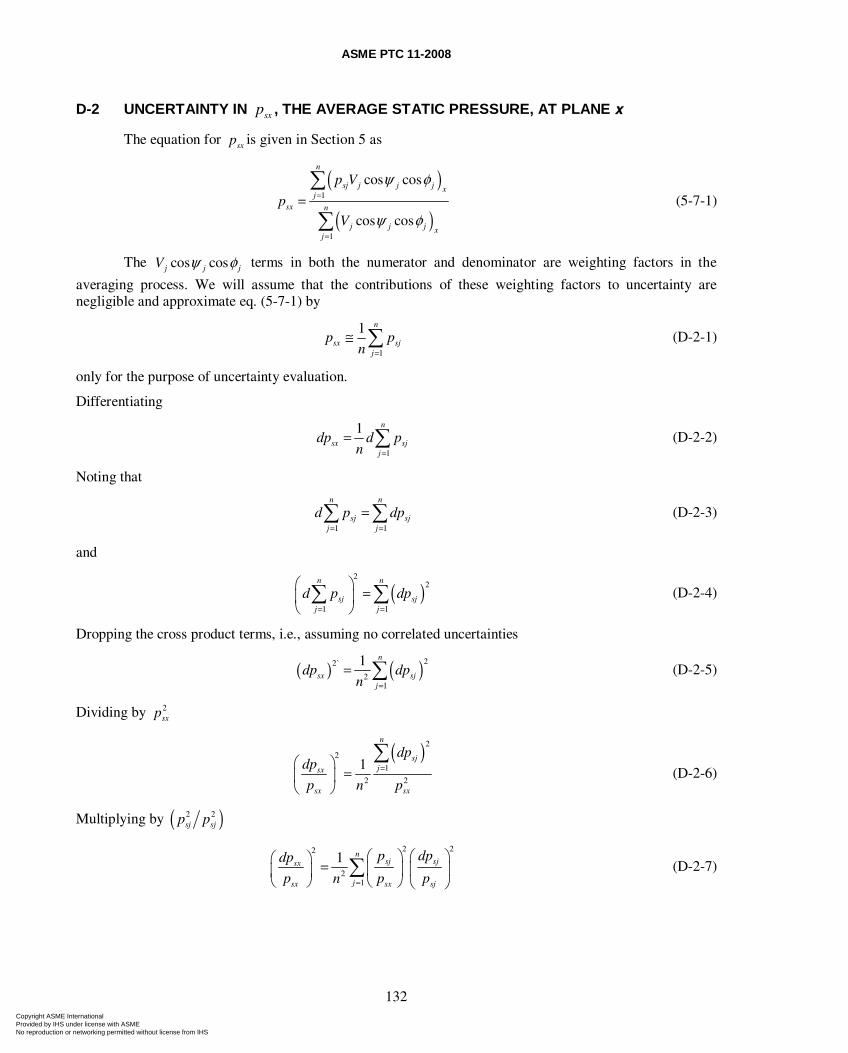
ASME PTC 11-2008

132

D-2 UNCERTAINTY IN sxp , THE AVERAGE STATIC PRESSURE, AT PLANE x

The equation for sxp is given in Section 5 as

( )

( )1

1

cos cos

cos cos

n

sj j j j xj

sx n

j j j xj

p V

pV

ψ φ

ψ φ

=

=

=∑

∑ (5-7-1)

The cos cosj j jV ψ φ terms in both the numerator and denominator are weighting factors in the

averaging process. We will assume that the contributions of these weighting factors to uncertainty are negligible and approximate eq. (5-7-1) by

1

1 n

sx sjj

p pn =

≅ ∑ (D-2-1)

only for the purpose of uncertainty evaluation.

Differentiating

1

1 n

sx sjj

dp d pn =

= ∑ (D-2-2)

Noting that

1 1

n n

sj sjj j

d p dp= =

=∑ ∑ (D-2-3)

and

( )2

2

1 1

n n

sj sjj j

d p dp= =

⎛ ⎞ =⎜ ⎟⎝ ⎠∑ ∑ (D-2-4)

Dropping the cross product terms, i.e., assuming no correlated uncertainties

( ) ( )22`

21

1 n

sx sjj

dp dpn =

= ∑ (D-2-5)

Dividing by 2sxp

( )2

2

1

2 2

1

n

sjjsx

sx sx

dpdp

p n p=⎛ ⎞

=⎜ ⎟⎝ ⎠

∑ (D-2-6)

Multiplying by ( )2 2sj sjp p

2 22

21

1 nsj sjsx

jsx sx sj

p dpdp

p n p p=

⎛ ⎞ ⎛ ⎞⎛ ⎞ = ⎜ ⎟ ⎜ ⎟⎜ ⎟⎝ ⎠ ⎝ ⎠ ⎝ ⎠

∑ (D-2-7)


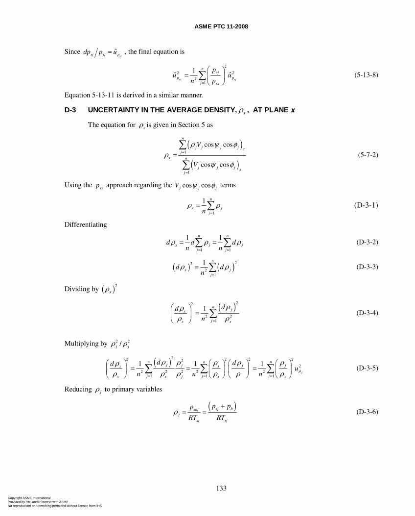
ASME PTC 11-2008

133

Since ˆsjsj sj pdp p u= , the final equation is

2

2 22

1

1ˆ ˆ

sx sj

nsj

p pj sx

pu u

n p=

⎛ ⎞= ⎜ ⎟

⎝ ⎠∑ (5-13-8)

Equation 5-13-11 is derived in a similar manner.

D-3 UNCERTAINTY IN THE AVERAGE DENSITY, xρ , AT PLANE x

The equation for xρ is given in Section 5 as

( )

( )1

1

cos cos

cos cos

n

j j j j xj

x n

j j j xj

V

V

ρ ψ φρ

ψ φ

=

=

=∑

∑ (5-7-2)

Using the sxp approach regarding the cos cosj j jV ψ φ terms

1

1 n

x jjn

ρ ρ=

= ∑ (D-3-1)

Differentiating

1 1

1 1n n

x j jj j

d d dn n

ρ ρ ρ= =

= =∑ ∑ (D-3-2)

( ) ( )22

21

1 n

x jj

d dn

ρ ρ=

= ∑ (D-3-3)

Dividing by ( )2

xρ

( )22

2 21

1 njx

jx x

dd

n

ρρρ ρ=

⎛ ⎞=⎜ ⎟

⎝ ⎠∑ (D-3-4)

Multiplying by 2 2/j jρ ρ

( )22 2 222

22 2 2 2 2

1 1 1

1 1 1j

n n nj j j j jx

j j jx x j x x

d ddu

n n n ρ

ρ ρ ρ ρ ρρρ ρ ρ ρ ρ ρ= = =

⎛ ⎞ ⎛ ⎞ ⎛ ⎞⎛ ⎞= = =⎜ ⎟ ⎜ ⎟ ⎜ ⎟⎜ ⎟

⎝ ⎠⎝ ⎠ ⎝ ⎠ ⎝ ⎠∑ ∑ ∑ (D-3-5)

Reducing jρ to primary variables

( )sj bsaj

jsj sj

p pp

RT RTρ

+= = (D-3-6)


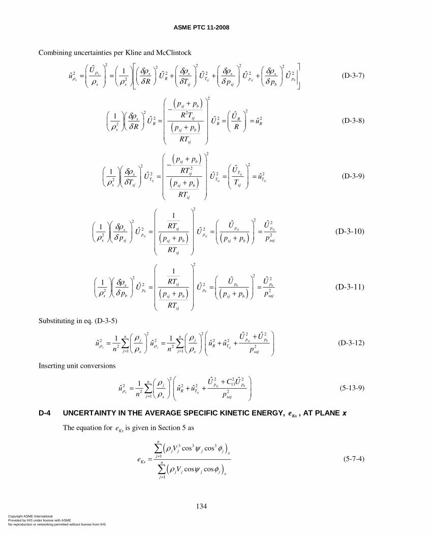
ASME PTC 11-2008

134

Combining uncertainties per Kline and McClintock

2 2 2 222 2 2 2 2

2

ˆ 1 ˆ ˆ ˆ ˆˆ x

x sj sj b

x x x xR T p p

x x sj sj b

Uu U U U U

R T p pρ

ρδρ δρ δρ δρ

ρ ρ δ δ δ δ

⎡ ⎤⎛ ⎞ ⎛ ⎞ ⎛ ⎞⎛ ⎞ ⎛ ⎞⎛ ⎞⎢ ⎥⎜ ⎟= = + + +⎜ ⎟ ⎜ ⎟⎜ ⎟ ⎜ ⎟⎜ ⎟ ⎜ ⎟ ⎜ ⎟⎜ ⎟ ⎢ ⎥⎝ ⎠⎝ ⎠ ⎝ ⎠⎝ ⎠ ⎝ ⎠⎝ ⎠ ⎣ ⎦ (D-3-7)

( )

( )

2

22 22 2 2

2

ˆ1 ˆ ˆ ˆ

sj b

sjx RR R R

x sj b

sj

p p

R T UU U u

R Rp p

RT

δρρ δ

⎛ ⎞+⎜ ⎟−

⎛ ⎞⎛ ⎞ ⎜ ⎟⎛ ⎞ = = =⎜ ⎟⎜ ⎟⎜ ⎟ ⎜ ⎟ ⎜ ⎟+⎝ ⎠⎝ ⎠ ⎝ ⎠⎜ ⎟⎜ ⎟⎝ ⎠

(D-3-8)

( )

( )

2

22 22 2 2

2

ˆ1 ˆ ˆ ˆsj

sj sj sj

sj b

TsjxT T T

x sj sjsj b

sj

p p

URTU U u

T Tp p

RT

δρρ δ

⎛ ⎞+⎜ ⎟− ⎛ ⎞⎛ ⎞⎛ ⎞ ⎜ ⎟ ⎜ ⎟= = =⎜ ⎟⎜ ⎟ ⎜ ⎟⎜ ⎟ ⎜ ⎟+⎝ ⎠⎝ ⎠ ⎜ ⎟ ⎝ ⎠⎜ ⎟⎝ ⎠

(D-3-9)

( ) ( )

2

22 2

2 22 2

1ˆ ˆ1 ˆ ˆ sj sj

sj sj

p psjxp p

x sj sajsj b sj b

sj

U URTU U

p pp p p p

RT

δρρ δ

⎛ ⎞⎜ ⎟ ⎛ ⎞⎛ ⎞⎛ ⎞ ⎜ ⎟ ⎜ ⎟= = =⎜ ⎟⎜ ⎟ ⎜ ⎟⎜ ⎟ ⎜ ⎟+ +⎝ ⎠⎝ ⎠ ⎜ ⎟ ⎝ ⎠⎜ ⎟⎝ ⎠

(D-3-10)

( ) ( )

2

22 22 2

2 2

1ˆ ˆ1 ˆ ˆ b b

b b

p psjxp p

x b sajsj b sj b

sj

U URTU U

p pp p p p

RT

δρρ δ

⎛ ⎞⎜ ⎟ ⎛ ⎞⎛ ⎞⎛ ⎞ ⎜ ⎟ ⎜ ⎟= = =⎜ ⎟⎜ ⎟ ⎜ ⎟ ⎜ ⎟+ +⎝ ⎠⎝ ⎠ ⎜ ⎟ ⎝ ⎠⎜ ⎟⎝ ⎠

(D-3-11)

Substituting in eq. (D-3-5)

2 2 2 2

2 2 2 22 2 2

1 1

ˆ ˆ1 1ˆ ˆ ˆ ˆ sj b

x j sj

n np pj j

R Tj jx x saj

U Uu u u u

n n pρ ρ

ρ ρρ ρ= =

⎛ ⎞+⎛ ⎞ ⎛ ⎞ ⎜ ⎟= = + +⎜ ⎟ ⎜ ⎟ ⎜ ⎟⎝ ⎠ ⎝ ⎠ ⎝ ⎠∑ ∑ (D-3-12)

Inserting unit conversions

2 2 2 2

132 2 22 2

1

ˆ ˆ1ˆ ˆ ˆ sj b

x sj

np pj

R Tj x saj

U C Uu u u

n pρ

ρρ=

⎛ ⎞+⎛ ⎞ ⎜ ⎟= + +⎜ ⎟ ⎜ ⎟⎝ ⎠ ⎝ ⎠∑ (5-13-9)

D-4 UNCERTAINTY IN THE AVERAGE SPECIFIC KINETIC ENERGY, Kxe , AT PLANE x

The equation for Kxe is given in Section 5 as

( )

( )

3 3 3

1

1

cos cos

cos cos

n

j j j j xj

Kx n

j j j j xj

V

eV

ρ ψ φ

ρ ψ φ

=

=

=∑

∑ (5-7-4)


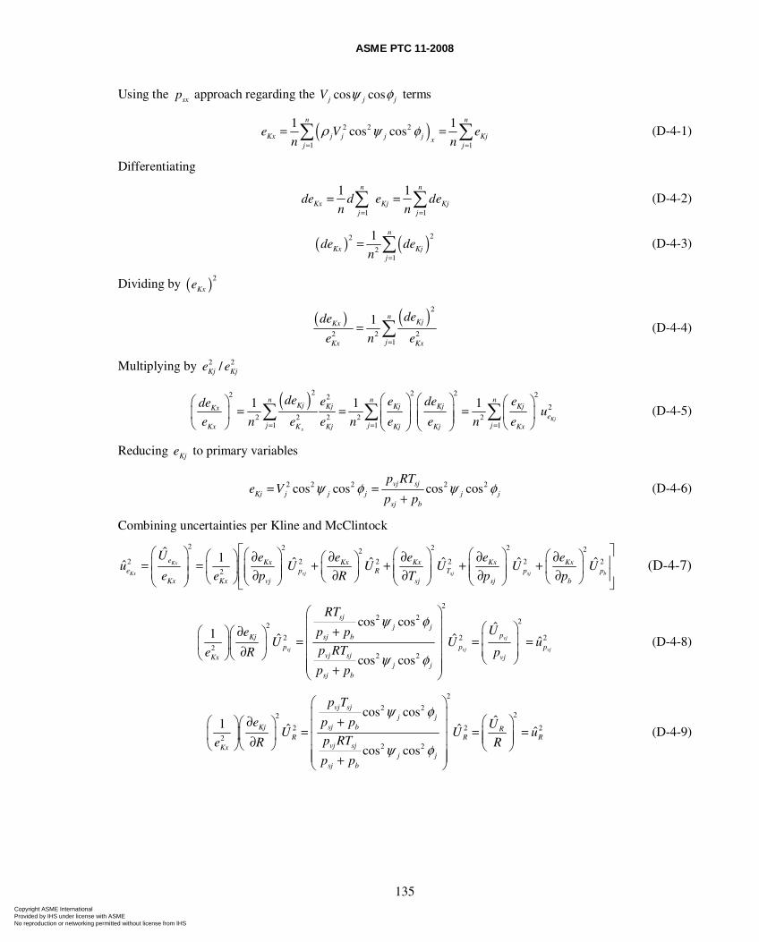
ASME PTC 11-2008

135


( )2 2 2

1 1

1 1cos cos

n n

Kx j j j j Kjxj j

e V en n

ρ ψ φ= =

= =∑ ∑ (D-4-1)

Differentiating

1 1

1 1n n

Kx Kj Kjj j

de d e den n= =

= =∑ ∑ (D-4-2)

( ) ( )22

21

1 n

Kx Kjj

de den =

= ∑ (D-4-3)

Dividing by ( )2

Kxe

( ) ( )2

2 2 21

1 nKjKx

jKx Kx

dede

e n e=

= ∑ (D-4-4)

Multiplying by 2 2/Kj Kje e

( )2 2 22 22

22 2 2 2 2

1 1 1

1 1 1Kj

x

n n nKj Kj Kj Kj KjKx

ej j jKx K Kj Kj Kj Kx

de e e de edeu

e n e e n e e n e= = =

⎛ ⎞ ⎛ ⎞⎛ ⎞ ⎛ ⎞= = =⎜ ⎟ ⎜ ⎟⎜ ⎟ ⎜ ⎟⎜ ⎟ ⎜ ⎟⎝ ⎠ ⎝ ⎠⎝ ⎠ ⎝ ⎠

∑ ∑ ∑ (D-4-5)

Reducing Kje to primary variables

2 2 2 2 2cos cos cos cosvj sjKj j j j j j

sj b

p RTe V

p pψ φ ψ φ= =

+ (D-4-6)


2 2 2 2 22

2 2 2 2 2 22

ˆ 1 ˆ ˆ ˆ ˆ ˆˆ Kx

Kx vj sj sj b

e Kx Kx Kx Kx Kxe p R T p p

Kx Kx vj sj sj b

U e e e e eu U U U U U

e e p R T p p

⎡ ⎤⎛ ⎞ ⎛ ⎞ ⎛ ⎞ ⎛ ⎞⎛ ⎞ ⎛ ⎞∂ ∂ ∂ ∂ ∂⎛ ⎞⎢ ⎥⎜ ⎟= = + + + +⎜ ⎟ ⎜ ⎟ ⎜ ⎟⎜ ⎟ ⎜ ⎟⎜ ⎟⎜ ⎟ ⎜ ⎟ ⎜ ⎟⎜ ⎟ ∂ ∂ ∂ ∂ ∂⎢ ⎥⎝ ⎠⎝ ⎠ ⎝ ⎠⎝ ⎠ ⎝ ⎠ ⎝ ⎠⎝ ⎠ ⎣ ⎦ (D-4-7)

2

2 2 22

2 2 22

2 2

cos cos ˆ1 ˆ ˆ ˆ

cos cos

vj

vj vj vj

sjj j

pKj sj bp p p

vj sjKx vjj j

sj b

RT

Ue p pU U u

p RTe R p

p p

ψ φ

ψ φ

⎛ ⎞⎜ ⎟ ⎛ ⎞∂ +⎛ ⎞⎛ ⎞ ⎜ ⎟ ⎜ ⎟= = =⎜ ⎟⎜ ⎟ ⎜ ⎟ ⎜ ⎟∂⎝ ⎠⎝ ⎠ ⎝ ⎠⎜ ⎟⎜ ⎟+⎝ ⎠

(D-4-8)

2

2 222

2 2 22

2 2

cos cosˆ1 ˆ ˆ ˆ

cos cos

vj sjj j

Kj sj b RR R R

vj sjKxj j

sj b

p T

e p p UU U u

p RTe R R

p p

ψ φ

ψ φ

⎛ ⎞⎜ ⎟∂ + ⎛ ⎞⎛ ⎞⎛ ⎞ ⎜ ⎟= = =⎜ ⎟⎜ ⎟⎜ ⎟ ⎜ ⎟⎜ ⎟∂⎝ ⎠⎝ ⎠ ⎝ ⎠⎜ ⎟⎜ ⎟+⎝ ⎠

(D-4-9)


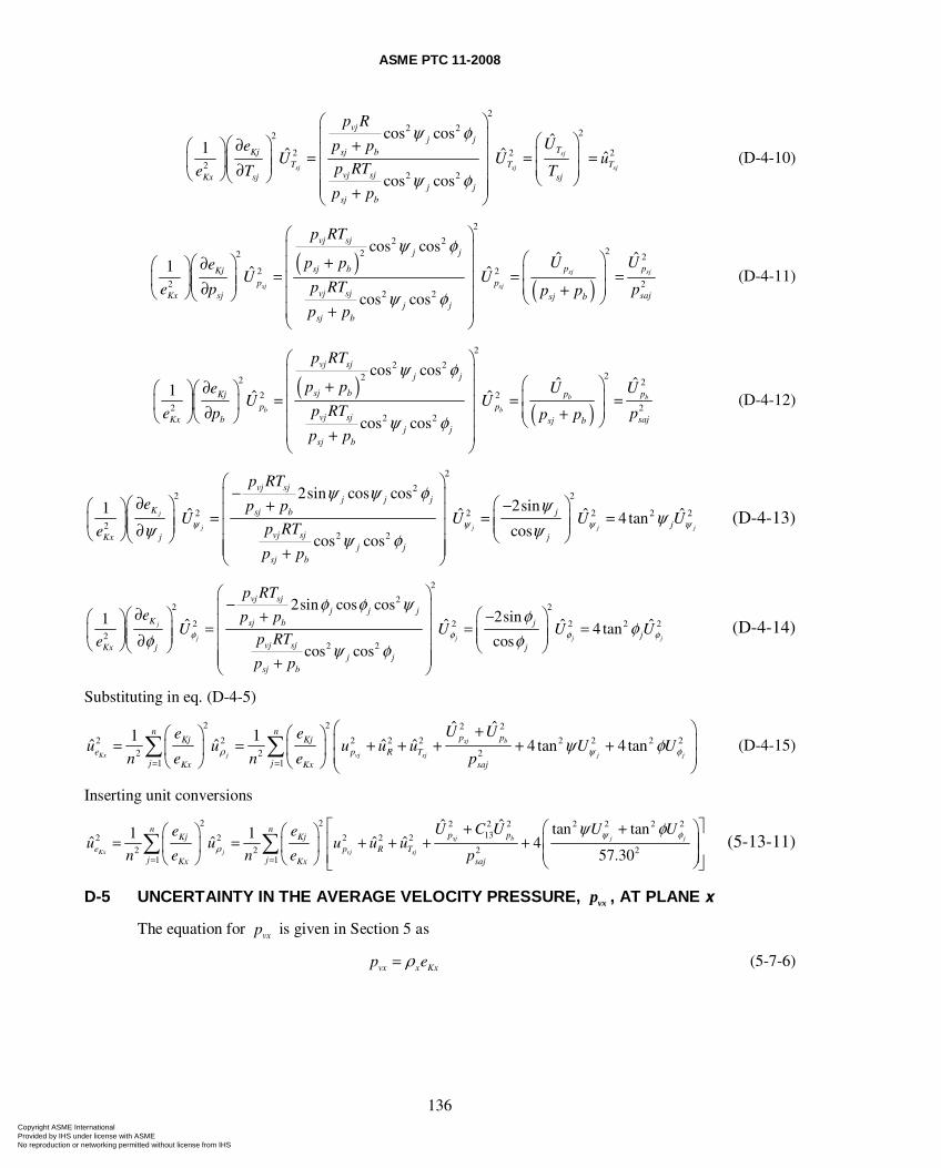
ASME PTC 11-2008

136

2

2 2 22

2 2 22

2 2

cos cos ˆ1 ˆ ˆ ˆ

cos cos

sj

sj sj sj

vjj j

TKj sj bT T T

vj sjKx sj sjj j

sj b

p R

Ue p pU U u

p RTe T T

p p

ψ φ

ψ φ

⎛ ⎞⎜ ⎟ ⎛ ⎞⎛ ⎞∂ +⎛ ⎞ ⎜ ⎟ ⎜ ⎟= = =⎜ ⎟⎜ ⎟⎜ ⎟ ⎜ ⎟ ⎜ ⎟∂⎝ ⎠⎝ ⎠ ⎝ ⎠⎜ ⎟⎜ ⎟+⎝ ⎠

(D-4-10)

( )

( )

2

2 2222 2

2 22 2

2 2

cos cosˆ ˆ1 ˆ ˆ

cos cos

sj sj

sj sj

vj sjj j

p psj bKjp p

vj sjKx sj sajsj bj j

sj b

p RT

U Up peU U

p RTe p pp pp p

ψ φ

ψ φ

⎛ ⎞⎜ ⎟

⎛ ⎞+⎛ ⎞∂⎛ ⎞ ⎜ ⎟ ⎜ ⎟= = =⎜ ⎟⎜ ⎟ ⎜ ⎟⎜ ⎟ ⎜ ⎟∂ +⎝ ⎠⎝ ⎠ ⎜ ⎟ ⎝ ⎠⎜ + ⎟⎝ ⎠

(D-4-11)

( )

( )

2

2 2222 2

2 22 2

2 2

cos cosˆ ˆ1 ˆ ˆ

cos cos

b b

b b

vj sjj j

sj b p pKjp p

vj sjKx b sajsj bj j

sj b

p RT

p p U UeU U

p RTe p pp pp p

ψ φ

ψ φ

⎛ ⎞⎜ ⎟

⎛ ⎞+∂⎛ ⎞⎛ ⎞ ⎜ ⎟⎜ ⎟= = =⎜ ⎟⎜ ⎟ ⎜ ⎟ ⎜ ⎟∂ +⎝ ⎠⎝ ⎠ ⎜ ⎟ ⎝ ⎠

⎜ + ⎟⎝ ⎠

(D-4-12)

2

22 2

2 2 2 2 22

2 2

2sin cos cos2sin1 ˆ ˆ ˆ ˆ4 tancos

cos cos

j

j j j j

vj sjj j j

K sj b jj

vj sjKx j jj j

sj b

p RT

e p pU U U U

p RTe

p p

ψ ψ ψ ψ

ψ ψ φψ

ψψ ψψ φ

⎛ ⎞−⎜ ⎟∂⎛ ⎞ ⎛ ⎞+ −⎛ ⎞ ⎜ ⎟= = =⎜ ⎟ ⎜ ⎟⎜ ⎟⎜ ⎟ ⎜ ⎟⎜ ⎟∂⎝ ⎠⎝ ⎠ ⎝ ⎠⎜ ⎟⎜ ⎟+⎝ ⎠

(D-4-13)

2

22 2

2 2 2 2 22

2 2

2sin cos cos2sin1 ˆ ˆ ˆ ˆ4 tancos

cos cos

j

j j j j

vj sjj j j

K sj b jj

vj sjKx j jj j

sj b

p RT

e p pU U U U

p RTe

p p

φ φ φ φ

φ φ ψφ

φφ φψ φ

⎛ ⎞−⎜ ⎟∂⎛ ⎞ ⎛ ⎞+ −⎛ ⎞ ⎜ ⎟= = =⎜ ⎟ ⎜ ⎟⎜ ⎟⎜ ⎟ ⎜ ⎟⎜ ⎟∂⎝ ⎠⎝ ⎠ ⎝ ⎠⎜ ⎟⎜ ⎟+⎝ ⎠

(D-4-14)

Substituting in eq. (D-4-5)

2 2 2 2

2 2 2 2 2 2 2 2 22 2 2

1 1

ˆ ˆ1 1ˆ ˆ ˆ ˆ 4 tan 4 tansj b

Kx j vj sj j j

n np pKj Kj

e p R Tj jKx Kx saj

U Ue eu u u u u U U

n e n e pρ ψ φψ φ= =

⎛ ⎞+⎛ ⎞ ⎛ ⎞ ⎜ ⎟= = + + + + +⎜ ⎟ ⎜ ⎟ ⎜ ⎟⎝ ⎠ ⎝ ⎠ ⎝ ⎠∑ ∑ (D-4-15)


2 2 2 2 2 2 2 2 2132 2 2 2 2

2 2 2 21 1

ˆ ˆ tan tan1 1ˆ ˆ ˆ ˆ 4

57.30sj b j j

Kx j vj sj

n np pKj Kj

e p R Tj jKx Kx saj

U C U U Ue eu u u u u

n e n e p

ψ φρ

ψ φ

= =

⎡ ⎤⎛ ⎞+ +⎛ ⎞ ⎛ ⎞⎢ ⎥⎜ ⎟= = + + + +⎜ ⎟ ⎜ ⎟ ⎜ ⎟⎢ ⎥⎝ ⎠ ⎝ ⎠ ⎝ ⎠⎣ ⎦

∑ ∑ (5-13-11)

D-5 UNCERTAINTY IN THE AVERAGE VELOCITY PRESSURE, vxp , AT PLANE x

The equation for vxp is given in Section 5 as

vx x Kxp eρ= (5-7-6)


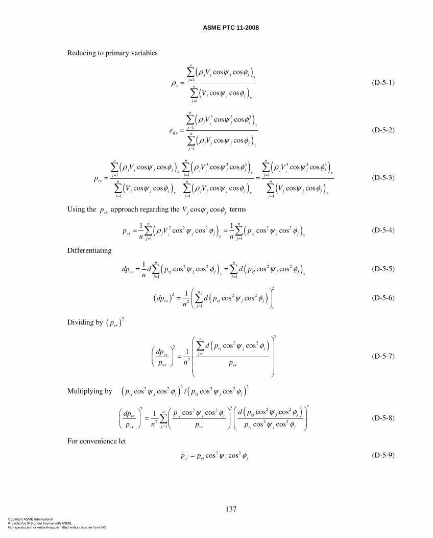
ASME PTC 11-2008

137

Reducing to primary variables

( )

( )1

1

cos cos

cos cos

n

j j j j xj

x n

j j j xj

V

V

ρ ψ φρ

ψ φ

=

=

=∑

∑ (D-5-1)

( )( )

3 3 3

1

1

cos cos

cos cos

j

n

j j jxj

Kx n

j j j j xj

V

eV

ρ ψ φ

ρ ψ φ

=

=

=∑

∑ (D-5-2)

( )

( )

( )( )

( )( )

3 3 3 3 3 3

1 1 1

1 1 1

cos cos cos cos cos cos

cos cos cos cos cos cos

j j

n n n

j j j j j j j j j jx x xj j jvx n n n

j j j j j j j j j jx x xj j j

V V V

pV V V

ρ ψ φ ρ ψ φ ρ ψ φ

ψ φ ρ ψ φ ψ φ

= = =

= = =

= =∑ ∑ ∑

∑ ∑ ∑ (D-5-3)


( ) ( )2 2 2 2 2

1 1

1 1cos cos cos cos

j

n n

vx j j j vj j j xxj j

p V pn n

ρ ψ φ ψ φ= =

= =∑ ∑ (D-5-4)

Differentiating

( ) ( )2 2 2 2

1 1

1cos cos cos cos

n n

vx vj j j vj j jx xj j

dp d p d pn

ψ φ ψ φ= =

= =∑ ∑ (D-5-5)

( ) ( )2

2 2 22

1

1cos cos

n

vx vj j jj x

dp d pn

ψ φ=

⎛ ⎞= ⎜ ⎟

⎝ ⎠∑ (D-5-6)

Dividing by ( )2

vxp

( )

2

2 22

1

2

cos cos1

n

vj j jjvx

vx vx

d pdp

p n p

ψ φ=

⎛ ⎞⎜ ⎟⎛ ⎞ ⎜ ⎟=⎜ ⎟ ⎜ ⎟⎝ ⎠⎜ ⎟⎝ ⎠

∑ (D-5-7)

Multiplying by ( )22 2cos cosvj j jp ψ φ / ( )22 2cos cosvj j jp ψ φ

( ) 222 2 22 2

2 2 21

cos coscos cos1

cos cos

nvj j jvj j jvx

jvx vx vj j j

d ppdp

p n p p

ψ φψ φψ φ=

⎛ ⎞⎛ ⎞⎛ ⎞⎜ ⎟= ⎜ ⎟⎜ ⎟ ⎜ ⎟ ⎜ ⎟⎝ ⎠ ⎝ ⎠ ⎝ ⎠

∑ (D-5-8)

For convenience let

2 2cos cosvj vj j jp p ψ φ= (D-5-9)


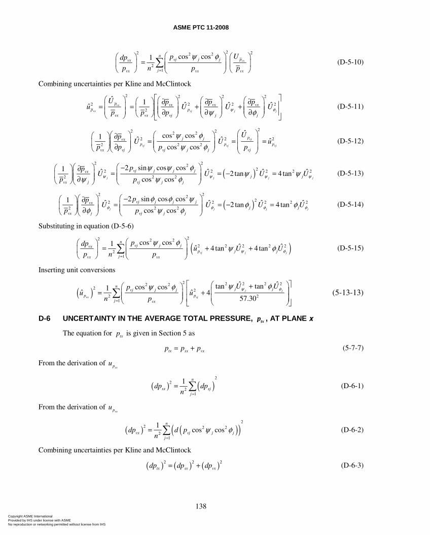
ASME PTC 11-2008

138

2 22 2 2

21

cos cos1vx

npvj j jvx

jvx vx vx

Updp

p n p p

ψ φ=

⎛ ⎞ ⎛ ⎞⎛ ⎞= ⎜ ⎟ ⎜ ⎟⎜ ⎟ ⎜ ⎟⎝ ⎠ ⎝ ⎠⎝ ⎠

∑ (D-5-10)


2 2 2 2

2 2 2 22

ˆ 1 ˆ ˆ ˆˆ vx

vx vj j j

p vx vx vxp p

vx vx vj j j

U p p pu U U U

p p p ψ φψ φ

⎡ ⎤⎛ ⎞ ⎛ ⎞ ⎛ ⎞ ⎛ ⎞⎛ ⎞ ∂ ∂ ∂⎢ ⎥⎜ ⎟= = + +⎜ ⎟ ⎜ ⎟ ⎜ ⎟⎜ ⎟ ⎜ ⎟ ⎜ ⎟ ⎜ ⎟⎜ ⎟ ∂ ∂ ∂⎢ ⎥⎝ ⎠ ⎝ ⎠ ⎝ ⎠ ⎝ ⎠⎝ ⎠ ⎣ ⎦ (D-5-11)

22 22 22 2 2

2 2 2

ˆcos cos1 ˆ ˆ ˆcos cos

vj

vj vj vj

pj jvxp p p

vx vj vj j j vj

UpU U u

p p p p

ψ φψ φ

⎛ ⎞⎛ ⎞ ⎛ ⎞⎛ ⎞ ∂ ⎜ ⎟= = =⎜ ⎟ ⎜ ⎟⎜ ⎟⎜ ⎟ ⎜ ⎟ ⎜ ⎟∂⎝ ⎠⎝ ⎠ ⎝ ⎠ ⎝ ⎠ (D-5-12)

( )2 22

22 2 2 2 22 2 2

2 sin cos cos1 ˆ ˆ ˆ ˆ2 tan 4 tancos cosj j j j

vj j j jvxj j

vx j vj j j

ppU U U U

p pψ ψ ψ ψ

ψ ψ φψ ψ

ψ ψ φ⎛ ⎞ ⎛ ⎞−⎛ ⎞ ∂

= = − =⎜ ⎟ ⎜ ⎟⎜ ⎟⎜ ⎟ ⎜ ⎟∂⎝ ⎠⎝ ⎠ ⎝ ⎠ (D-5-13)

( )2 22

22 2 2 2 22 2 2

2 sin cos cos1 ˆ ˆ ˆ ˆ2 tan 4 tancos cosj j j j

vj j j jvxj j

vx j vj j j

ppU U U U

p pφ φ φ φ

φ φ ψφ φ

φ ψ φ⎛ ⎞ ⎛ ⎞−⎛ ⎞ ∂

= = − =⎜ ⎟ ⎜ ⎟⎜ ⎟⎜ ⎟ ⎜ ⎟∂⎝ ⎠⎝ ⎠ ⎝ ⎠ (D-5-14)

Substituting in equation (D-5-6)

( )22 2 2

2 2 2 2 22

1

cos cos1 ˆ ˆˆ 4 tan 4 tanvj j j

nvj j jvx

p j jjvx vx

pdpu U U

p n p ψ φ

ψ φψ φ

=

⎛ ⎞⎛ ⎞= + +⎜ ⎟⎜ ⎟ ⎜ ⎟⎝ ⎠ ⎝ ⎠

∑ (D-5-15)


( )2 2 2 2 22 2

2 22 2

1

ˆ ˆtan tancos cos1ˆ ˆ 4

57.30j j

vx vj

nj jvj j j

p pj vx

U Upu u

n p

ψ φψ φψ φ=

⎡ ⎤⎛ ⎞+⎛ ⎞⎢ ⎥⎜ ⎟= +⎜ ⎟⎜ ⎟ ⎜ ⎟⎢ ⎥⎝ ⎠ ⎝ ⎠⎣ ⎦

∑ (5-13-13)

D-6 UNCERTAINTY IN THE AVERAGE TOTAL PRESSURE, txp , AT PLANE x

The equation for txp is given in Section 5 as

tx sx vxp p p= + (5-7-7)

From the derivation of sxpu

( ) ( )2

2

21

1 n

sx sjj

dp dpn =

= ∑ (D-6-1)

From the derivation of vxpu

( ) ( )( )2

2 2 22

1

1cos cos

n

vx vj j jj

dp d pn

ψ φ=

= ∑ (D-6-2)


( ) ( ) ( )2 2 2

tx sx vxdp dp dp= + (D-6-3)


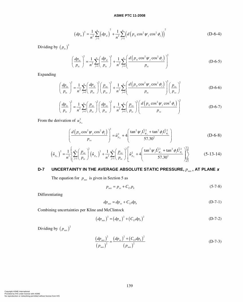
ASME PTC 11-2008

139

( ) ( ) ( )( )2 2

2 2 22 2

1 1

1 1cos cos

n n

tx sj vj j jj j

dp dp d pn n

ψ φ= =

= +∑ ∑ (D-6-4)

Dividing by ( )2

txp

( ) 22 2 2 2

2 21 1

cos cos1 1n nvj j jsjtx

j jtx tx tx

d pdpdp

p n p n p

ψ φ

= =

⎛ ⎞⎛ ⎞ ⎛ ⎞⎜ ⎟= +⎜ ⎟ ⎜ ⎟ ⎜ ⎟⎝ ⎠ ⎝ ⎠ ⎝ ⎠

∑ ∑ (D-6-5)

Expanding

( ) 22 2 2 22 2

2 21 1

cos cos1 1n nvj j jsjtx sx vx

j jtx tx sx tx vx

d pdpdp p p

p n p p n p p

ψ φ

= =

⎛ ⎞⎛ ⎞ ⎛ ⎞ ⎛ ⎞ ⎛ ⎞⎜ ⎟= +⎜ ⎟ ⎜ ⎟ ⎜ ⎟ ⎜ ⎟⎜ ⎟⎝ ⎠ ⎝ ⎠ ⎝ ⎠ ⎝ ⎠⎝ ⎠

∑ ∑ (D-6-6)

( ) 22 2 2 2 2 2

2 21 1

cos cos1 1n nvj j jtx sx sx vx

j jtx tx sx tx vx

d pdp p dp p

p n p p n p p

ψ φ

= =

⎛ ⎞⎛ ⎞ ⎛ ⎞ ⎛ ⎞ ⎛ ⎞⎜ ⎟= +⎜ ⎟ ⎜ ⎟ ⎜ ⎟ ⎜ ⎟ ⎜ ⎟⎝ ⎠ ⎝ ⎠ ⎝ ⎠ ⎝ ⎠ ⎝ ⎠

∑ ∑ (D-6-7)

From the derivation of 2

vxpu

( ) 2

2 2 2 22 2

22

ˆ ˆtan tancos cosˆ 4

57.30j j

vj

j jvj j j

pvx

U Ud pu

p

ψ φψ φψ φ ⎛ ⎞⎛ ⎞ +⎜ ⎟⎜ ⎟ = +

⎜ ⎟ ⎜ ⎟⎝ ⎠ ⎝ ⎠ (D-6-8)

( ) ( )2 2 2 2 2 2

2 2 22 2 2

1 1

ˆ ˆtan tan1 1ˆ ˆ ˆ 4

57.30j j

tx sx vj

n nj jsx vx

p p pj jtx tx

U Up pu u u

n p n p

ψ φψ φ

= =

⎧ ⎫⎡ ⎤⎛ ⎞+⎛ ⎞ ⎛ ⎞⎪ ⎪⎢ ⎥⎜ ⎟= + +⎨ ⎬⎜ ⎟ ⎜ ⎟ ⎜ ⎟⎢ ⎥⎝ ⎠ ⎝ ⎠⎪ ⎪⎝ ⎠⎣ ⎦⎩ ⎭∑ ∑ (5-13-14)

D-7 UNCERTAINTY IN THE AVERAGE ABSOLUTE STATIC PRESSURE, saxp , AT PLANE x

The equation for saxp is given in Section 5 as

13sax sx bp p C p= + (5-7-8)

Differentiating

13sax sx bdp dp C dp= + (D-7-1)


( ) ( ) ( )2 2 2

13sax sx bdp dp C dp= + (D-7-2)

Dividing by ( )2

saxp

( )( )

( ) ( )( )

2 2 2

132 2

sax sx b

sax sax

dp dp C dp

p p

+= (D-7-3)


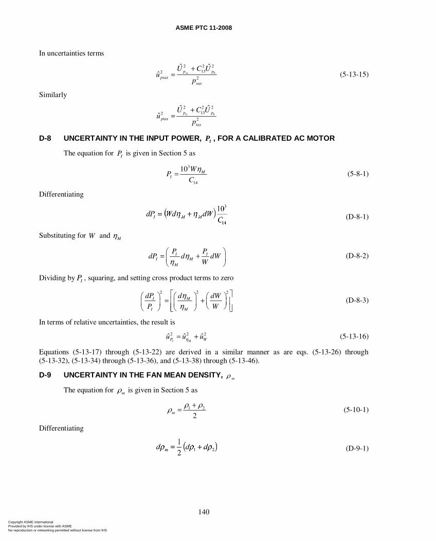
ASME PTC 11-2008

140

In uncertainties terms

2 2 2

1322

ˆ ˆˆ sx bp p

psaxsax

U C Uu

p

+= (5-13-15)

Similarly

2 2 2

1322

ˆ ˆˆ tx bp p

ptaxtax

U C Uu

p

+=

D-8 UNCERTAINTY IN THE INPUT POWER, IP , FOR A CALIBRATED AC MOTOR

The equation for IP is given in Section 5 as

3

14

10 MI

WP

C

η= (5-8-1)

Differentiating

(D-8-1)

Substituting for W and Mη

I II M

M

P PdP d dW

Wη

η⎛ ⎞= +⎜ ⎟⎝ ⎠

(D-8-2)

Dividing by PI , squaring, and setting cross product terms to zero

2 2 2

I M

I M

dP d dW

P W

ηη

⎡ ⎤⎛ ⎞ ⎛ ⎞ ⎛ ⎞= +⎢ ⎥⎜ ⎟⎜ ⎟ ⎜ ⎟ ⎝ ⎠⎢ ⎥⎝ ⎠ ⎝ ⎠⎣ ⎦ (D-8-3)

In terms of relative uncertainties, the result is

2 2 2ˆ ˆ Î MP Wu u uη= + (5-13-16)

Equations (5-13-17) through (5-13-22) are derived in a similar manner as are eqs. (5-13-26) through (5-13-32), (5-13-34) through (5-13-36), and (5-13-38) through (5-13-46).

D-9 UNCERTAINTY IN THE FAN MEAN DENSITY, ρ m

The equation for mρ is given in Section 5 as

1 2

2m

ρ ρρ += (5-10-1)

Differentiating

(D-9-1)


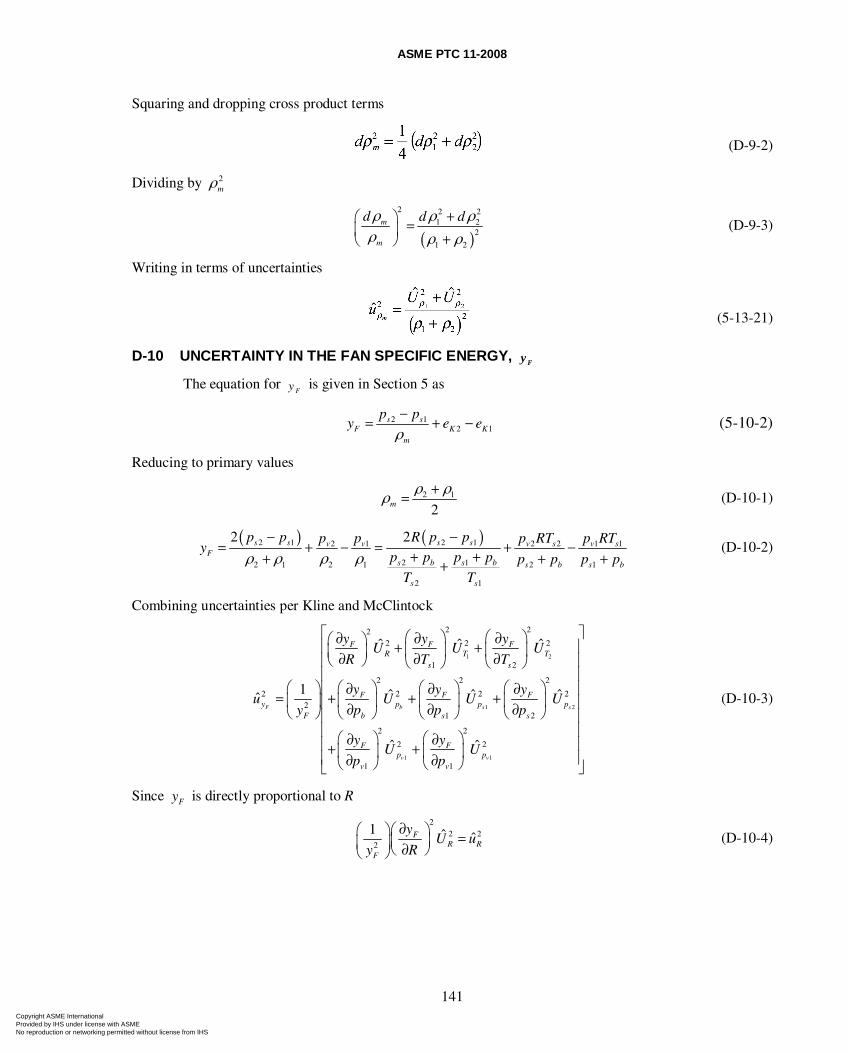
ASME PTC 11-2008

141

Squaring and dropping cross product terms

(D-9-2)

Dividing by 2mρ

( )

2 2 21 2

2

1 2

m

m

d d dρ ρ ρρ ρ ρ

+⎛ ⎞ =⎜ ⎟ +⎝ ⎠ (D-9-3)

Writing in terms of uncertainties

(5-13-21)

D-10 UNCERTAINTY IN THE FAN SPECIFIC ENERGY, Fy

The equation for Fy is given in Section 5 as

2 12 1

s sF K K

m

p py e e

ρ−= + − (5-10-2)

Reducing to primary values

2 1

2m

ρ ρρ += (D-10-1)

( ) ( )2 1 2 12 1 2 2 1 1

2 12 1 2 1 2 1

2 1

2 2s s s sv v v s v sF

s b s b s b s b

s s

p p R p pp p p RT p RTy

p p p p p p p pT T

ρ ρ ρ ρ− −

= + − = + −+ ++ + ++

(D-10-2)


1 2

1 2

1 1

2 222 2 2

1 2

2 2 2

2 2 2 22

1 2

2 2

2 2

1 1

ˆ ˆ ˆ

1 ˆ ˆ ˆˆ

ˆ ˆ

F b s s

v v

F F FR T T

s s

F F Fy p p p

F b s s

F Fp p

v v

y y yU U U

R T T

y y yu U U U

y p p p

y yU U

p p

⎡ ⎤⎛ ⎞ ⎛ ⎞∂ ∂ ∂⎛ ⎞⎢ ⎥+ +⎜ ⎟ ⎜ ⎟⎜ ⎟∂ ∂ ∂⎝ ⎠⎢ ⎥⎝ ⎠ ⎝ ⎠⎢ ⎥⎛ ⎞ ⎛ ⎞ ⎛ ⎞⎛ ⎞ ∂ ∂ ∂⎢ ⎥= + + +⎜ ⎟ ⎜ ⎟ ⎜ ⎟⎜ ⎟ ⎢ ⎥∂ ∂ ∂⎝ ⎠ ⎝ ⎠ ⎝ ⎠ ⎝ ⎠⎢ ⎥

⎢ ⎥⎛ ⎞ ⎛ ⎞∂ ∂⎢ ⎥+ +⎜ ⎟ ⎜ ⎟⎢ ⎥∂ ∂⎝ ⎠ ⎝ ⎠⎣ ⎦

(D-10-3)

Since Fy is directly proportional to R

2

2 22

1 ˆ ˆFR R

F

yU u

y R

∂⎛ ⎞⎛ ⎞ =⎜ ⎟⎜ ⎟ ∂⎝ ⎠⎝ ⎠ (D-10-4)


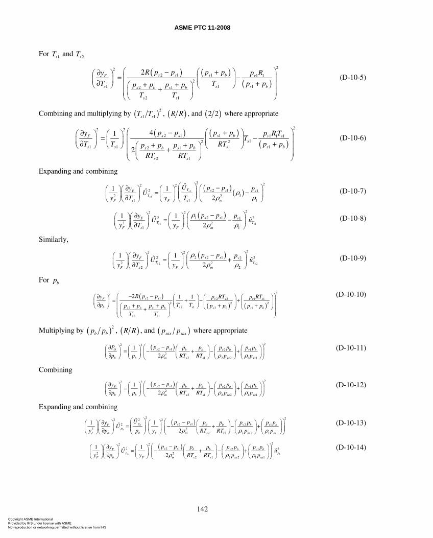
ASME PTC 11-2008

142

For 1sT and 2sT

( ) ( )

( )

222 1 1 1 1

21 1 12 1

2 1

2 s s s b vF

s s s bs b s b

s s

R p p p p p Ry

T T p pp p p p

T T

⎛ ⎞− ⎛ + ⎞∂⎛ ⎞ = −⎜ ⎟⎜ ⎟⎜ ⎟∂ ++ +⎛ ⎞⎝ ⎠ ⎜ ⎟⎝ ⎠+⎜ ⎟⎜ ⎟⎝ ⎠⎝ ⎠

(D-10-5)

Combining and multiplying by ( )2

1 1s sT T , ( )R R , and ( )2 2 where appropriate

( ) ( )

( )

22 22 1 1 1 1 1

12 21 1 1 12 1

2 1

41

2

s s s b v sFs

s s s s bs b s b

s s

p p p p p R TyT

T T RT p pp p p p

RT RT

⎛ ⎞− ⎛ + ⎞∂⎛ ⎞ ⎛ ⎞= −⎜ ⎟⎜ ⎟⎜ ⎟ ⎜ ⎟∂ ++ +⎛ ⎞⎝ ⎠ ⎝ ⎠ ⎝ ⎠⎜ ⎟+⎜ ⎟⎜ ⎟⎝ ⎠⎝ ⎠

(D-10-6)

Expanding and combining

( ) ( )1

1

2 22 22 12 1

12 21 1 1

ˆ1 1ˆ2

s

s

T s s vFT

F s F s m

U p p pyU

y T y Tρ

ρ ρ⎛ ⎞ ⎛ − ⎞∂⎛ ⎞⎛ ⎞ ⎛ ⎞ ⎜ ⎟= −⎜ ⎟⎜ ⎟⎜ ⎟ ⎜ ⎟ ⎜ ⎟∂⎝ ⎠ ⎝ ⎠⎝ ⎠ ⎝ ⎠ ⎝ ⎠

(D-10-7)

( )1 1

22 21 2 12 21

2 21 1

1 1ˆ ˆ2s s

s s vFT T

F s F m

p p pyU u

y T y

ρρ ρ

⎛ − ⎞∂⎛ ⎞⎛ ⎞ ⎛ ⎞= −⎜ ⎟⎜ ⎟⎜ ⎟ ⎜ ⎟∂⎝ ⎠ ⎝ ⎠⎝ ⎠ ⎝ ⎠ (D-10-8)

Similarly,

( )2 2

22 22 2 12 22

2 22 2

1 1ˆ ˆ2s s

s s vFT T

F s F m

p p pyU u

y T y

ρρ ρ

⎛ − ⎞∂⎛ ⎞⎛ ⎞ ⎛ ⎞= +⎜ ⎟⎜ ⎟⎜ ⎟ ⎜ ⎟∂⎝ ⎠ ⎝ ⎠⎝ ⎠ ⎝ ⎠ (D-10-9)

For bp

( )( ) ( )

222 1 2 2 1 1

2 2 22 1 2 12 1

2 1

2 1 1s s v s v sF

b s s s b s bs b s b

s s

R p p p RT p RTy

p T T p p p pp p p p

T T

⎛ − − ⎞∂ ⎛ ⎞ ⎛ ⎞⎛ ⎞ ⎛ ⎞= + − +⎜ ⎟⎜ ⎟ ⎜ ⎟⎜ ⎟ ⎜ ⎟∂ + ++ +⎛ ⎞⎝ ⎠ ⎝ ⎠⎜ ⎟⎝ ⎠ ⎝ ⎠+⎜ ⎟⎜ ⎟⎝ ⎠⎝ ⎠

(D-10-10)

Multiplying by ( )2

b bp p , ( )R R , and ( )sax saxp p where appropriate

( ) 22 22 1 2 1

22 1 2 2 1 1

1

2s sO b b v b v b

b b m s s sa sa

p pP p p p p p p

p p RT RT p pρ ρ ρ⎛ − ⎞∂⎛ ⎞ ⎛ ⎞ ⎛ ⎞ ⎛ ⎞⎛ ⎞= − + − +⎜ ⎟⎜ ⎟ ⎜ ⎟ ⎜ ⎟ ⎜ ⎟⎜ ⎟∂⎝ ⎠ ⎝ ⎠ ⎝ ⎠ ⎝ ⎠ ⎝ ⎠⎝ ⎠

(D-10-11)

Combining

( ) 22 22 1 2 1

22 1 2 2 1 1

1

2s s b b v b v bF

b b m s s sa sa

p p p p p p p py

p p RT RT p pρ ρ ρ⎛ − ⎞∂ ⎛ ⎞ ⎛ ⎞ ⎛ ⎞⎛ ⎞ ⎛ ⎞= − + − +⎜ ⎟⎜ ⎟ ⎜ ⎟ ⎜ ⎟⎜ ⎟ ⎜ ⎟∂⎝ ⎠ ⎝ ⎠ ⎝ ⎠ ⎝ ⎠ ⎝ ⎠⎝ ⎠

(D-10-12)


( )2 222 2

2 12 2 12 2

2 1 2 2 1 1

ˆ1 1ˆ2

b

b

p s s b b v b v bFp

F b b F m s s sa sa

U p p p p p p p pyU

y p p y RT RT p pρ ρ ρ⎛ ⎞ ⎛ ⎞− ⎛ ⎞∂ ⎛ ⎞ ⎛ ⎞⎛ ⎞⎛ ⎞ ⎛ ⎞⎜ ⎟= − + − +⎜ ⎟⎜ ⎟⎜ ⎟ ⎜ ⎟⎜ ⎟⎜ ⎟ ⎜ ⎟⎜ ⎟ ⎜ ⎟∂⎝ ⎠ ⎝ ⎠⎝ ⎠ ⎝ ⎠ ⎝ ⎠ ⎝ ⎠ ⎝ ⎠⎝ ⎠

(D-10-13)

( ) 22 22 12 22 1

2 22 1 2 2 1 1

1 1ˆ ˆ2b b

s s b b v b v bFp p

F b F m s s sa sa

p p p p p p p pyU u

y p y RT RT p pρ ρ ρ⎛ − ⎞∂ ⎛ ⎞ ⎛ ⎞ ⎛ ⎞⎛ ⎞⎛ ⎞ ⎛ ⎞= − + − +⎜ ⎟⎜ ⎟ ⎜ ⎟ ⎜ ⎟⎜ ⎟⎜ ⎟ ⎜ ⎟∂⎝ ⎠ ⎝ ⎠⎝ ⎠ ⎝ ⎠ ⎝ ⎠ ⎝ ⎠⎝ ⎠

(D-10-14)


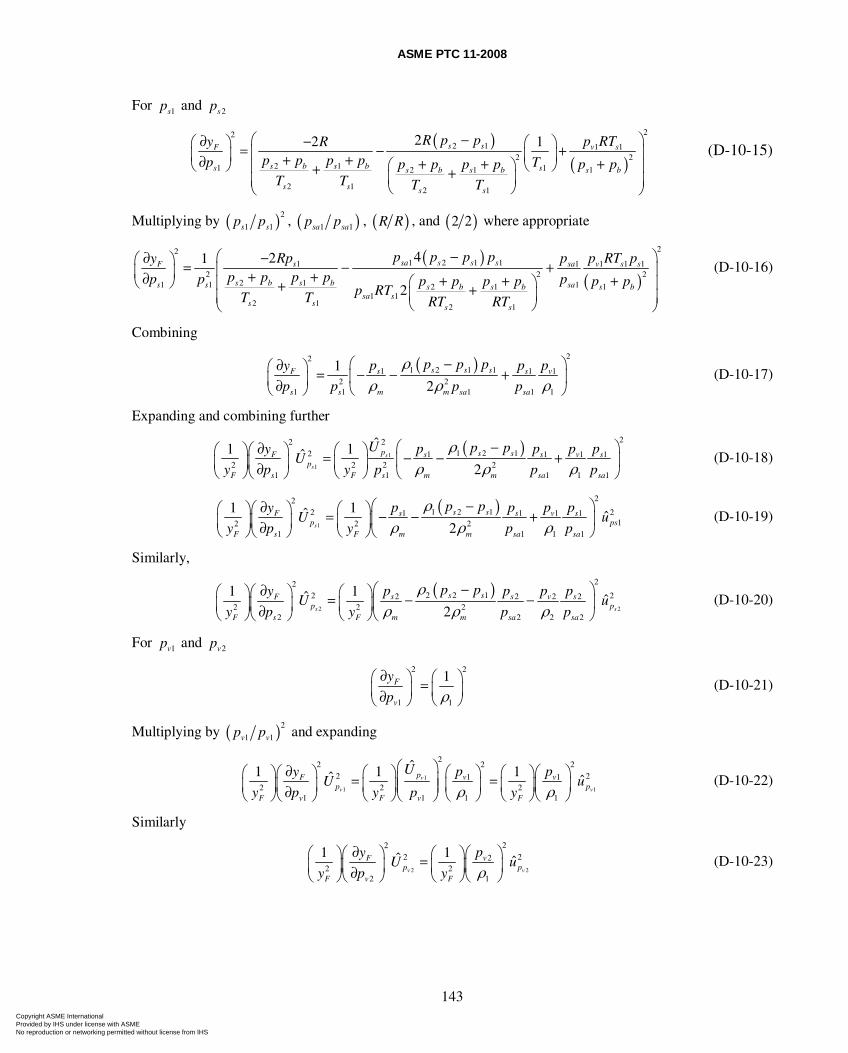
ASME PTC 11-2008

143

For 1sp and 2sp

( )

( )

222 1 1 1

2 22 11 1 12 1

2 1 2 1

22 1s s v sF

s b s bs s s bs b s b

s s s s

R p p p RTy Rp p p pp T p pp p p p

T T T T

⎛ − ⎞∂ −⎛ ⎞ ⎛ ⎞= − +⎜ ⎟⎜ ⎟ ⎜ ⎟+ +∂ ++ +⎛ ⎞⎝ ⎠ ⎝ ⎠⎜ ⎟+ +⎜ ⎟⎜ ⎟⎝ ⎠⎝ ⎠

(D-10-15)

Multiplying by ( )2

1 1s sp p , ( )1 1sa sap p , ( )R R , and ( )2 2 where appropriate

( )( )

221 2 1 11 1 1 1 1

2 222 11 1 1 12 1

1 12 1 2 1

421

2

sa s s ss sa v s sF

s b s bs s sa s bs b s bsa s

s s s s

p p p pRp p p RT pyp p p pp p p p pp p p p

p RTT T RT RT

⎛ − ⎞−∂⎛ ⎞ = − +⎜ ⎟⎜ ⎟ + +∂ ++ +⎛ ⎞⎝ ⎠ ⎜ ⎟+ +⎜ ⎟⎜ ⎟⎝ ⎠⎝ ⎠

(D-10-16)

Combining

( ) 22

1 2 1 11 1 12 2

1 1 1 1 1

1

2s s ss s vF

s s m m sa sa

p p pp p py

p p p p

ρρ ρ ρ

⎛ − ⎞∂⎛ ⎞ = − − +⎜ ⎟⎜ ⎟∂⎝ ⎠ ⎝ ⎠ (D-10-17)

Expanding and combining further

( )

1

1

2221 2 12 1 1 1 1

2 2 2 21 1 1 1 1

ˆ1 1ˆ2

s

s

p s ss s v sFp

F s F s m m sa sa

U p pp p p pyU

y p y p p p

ρρ ρ ρ

⎛ − ⎞∂⎛ ⎞⎛ ⎞ ⎛ ⎞= − − +⎜ ⎟⎜ ⎟⎜ ⎟ ⎜ ⎟∂⎝ ⎠ ⎝ ⎠⎝ ⎠ ⎝ ⎠ (D-10-18)

( )

1

221 2 12 21 1 1 1

12 2 21 1 1 1

1 1ˆ ˆ2s

s ss s v sFp ps

F s F m m sa sa

p pp p p pyU u

y p y p p

ρρ ρ ρ

⎛ − ⎞∂⎛ ⎞⎛ ⎞ ⎛ ⎞= − − +⎜ ⎟⎜ ⎟⎜ ⎟ ⎜ ⎟∂⎝ ⎠ ⎝ ⎠⎝ ⎠ ⎝ ⎠ (D-10-19)

Similarly,

( )

2 2

222 2 12 22 2 2 2

2 2 22 2 2 2

1 1ˆ ˆ2s s

s ss s v sFp p

F s F m m sa sa

p pp p p pyU u

y p y p p

ρρ ρ ρ

⎛ − ⎞∂⎛ ⎞⎛ ⎞ ⎛ ⎞= − −⎜ ⎟⎜ ⎟⎜ ⎟ ⎜ ⎟∂⎝ ⎠ ⎝ ⎠⎝ ⎠ ⎝ ⎠ (D-10-20)

For 1vp and 2vp

2 2

1 1

1F

v

y

p ρ∂⎛ ⎞ ⎛ ⎞=⎜ ⎟ ⎜ ⎟∂ ⎝ ⎠⎝ ⎠

(D-10-21)

Multiplying by ( )2

1 1v vp p and expanding

1

1 1

22 22

2 21 12 2 2

1 1 1 1

ˆ1 1 1ˆ ˆv

v v

p v vFp p

F v F v F

U p pyU u

y p y p yρ ρ⎛ ⎞∂ ⎛ ⎞ ⎛ ⎞⎛ ⎞⎛ ⎞ ⎛ ⎞ ⎛ ⎞⎜ ⎟= =⎜ ⎟ ⎜ ⎟⎜ ⎟⎜ ⎟ ⎜ ⎟ ⎜ ⎟⎜ ⎟∂⎝ ⎠ ⎝ ⎠ ⎝ ⎠ ⎝ ⎠⎝ ⎠⎝ ⎠ ⎝ ⎠

(D-10-22)

Similarly

2 2

222 22

2 22 1

1 1ˆ ˆv v

vFp p

F v F

pyU u

y p y ρ∂ ⎛ ⎞⎛ ⎞⎛ ⎞ ⎛ ⎞= ⎜ ⎟⎜ ⎟⎜ ⎟ ⎜ ⎟∂⎝ ⎠ ⎝ ⎠⎝ ⎠⎝ ⎠

(D-10-23)


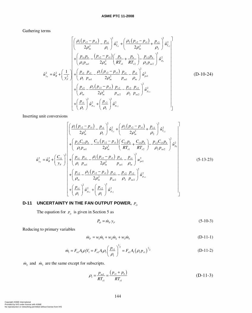
ASME PTC 11-2008

144

Gathering terms

( ) ( )

( )

( )

1 2

2 2

1 2 1 2 2 12 21 22 2

1 2

2

2 1 21 22

1 1 1 2 2 2

2

1 2 12 2 1 1 1 12 2

1 1 1

ˆ ˆ2 2

ˆ2

1ˆ ˆ

2

s s

b

F

s s s sv vT T

m m

s sv b b b v bp

sa m s s sa

s sv s s sy R

F sa m sa m

p p p pp pu u

p pp p p p p pu

p RT RT p

p pp p p pu u

y p p

ρ ρρ ρ ρ ρ

ρ ρ ρ

ρρ ρ ρ

⎛ − ⎞ ⎛ − ⎞− + +⎜ ⎟ ⎜ ⎟

⎝ ⎠ ⎝ ⎠

⎛ − ⎞⎛ ⎞+ − + −⎜ ⎟⎜ ⎟⎝ ⎠⎝ ⎠

⎛ − ⎞⎛ ⎞= + + − −⎜ ⎟⎜ ⎟⎝ ⎠ ⎝ ⎠

( )2

1 2

21

2

2 2 1 22 2 2 22

2 2 2

2 22 21 2

1 1

ˆ

ˆ2

ˆ ˆ

s

v v

ps

s ss s v sp

m m sa sa

v vp p

u

p pp p p pu

p p

p pu u

ρρ ρ ρ

ρ ρ

⎡ ⎤⎢ ⎥⎢ ⎥⎢ ⎥⎢ ⎥⎢ ⎥⎢ ⎥⎢ ⎥⎢ ⎥⎢ ⎥⎢ ⎥⎢ ⎥⎛ − ⎞⎢ ⎥+ − −⎜ ⎟⎢ ⎥⎝ ⎠⎢ ⎥⎛ ⎞ ⎛ ⎞⎢ ⎥+ +⎜ ⎟ ⎜ ⎟⎢ ⎥⎝ ⎠ ⎝ ⎠⎣ ⎦

(D-10-24)


( ) ( )

( )

( )

1 2

2 2

1 2 1 2 2 12 21 22 2

1 2

2

11 2 1 21 13 13 13 2 132

1 1 1 2 2 2

21 2 12 2 1 1 111

21 1

ˆ ˆ2 2

ˆ2

ˆ ˆ2

s s

b

F

s s s sv vT T

m m

s sv b b b v bp

sa m s s sa

s sv s sy R

F sa m

p p p pp pu u

C p pp C p C p C p p C pu

p RT RT p

p pp p pCu u

y p

ρ ρρ ρ ρ ρ

ρ ρ ρ

ρρ ρ

⎛ − ⎞ ⎛ − ⎞− + +⎜ ⎟ ⎜ ⎟

⎝ ⎠ ⎝ ⎠

⎛ − ⎞⎛ ⎞+ − + −⎜ ⎟⎜ ⎟⎝ ⎠⎝ ⎠

−⎛ ⎞= + + −⎜ ⎟⎝ ⎠

( )2

1 2

2

211

1

2

2 2 1 22 2 2 22

2 2 2

222 21 2

1 1

ˆ2

ˆ ˆ

s

v v

sps

sa m

s ss s v sp

m m sa sa

v vp p

pu

p

p pp p p pu

p p

p pu u

ρ

ρρ ρ ρ

ρ ρ

⎡ ⎤⎢ ⎥⎢ ⎥⎢ ⎥⎢ ⎥⎢ ⎥⎢ ⎥⎢ ⎥⎛ ⎞⎢ ⎥−⎜ ⎟⎢ ⎥⎝ ⎠⎢ ⎥

⎢ ⎥⎛ − ⎞⎢ ⎥+ − −⎜ ⎟⎢ ⎥⎝ ⎠⎢ ⎥

⎛ ⎞⎢ ⎥⎛ ⎞+ + ⎜ ⎟⎢ ⎥⎜ ⎟⎝ ⎠ ⎝ ⎠⎣ ⎦

(5-13-23)

D-11 UNCERTAINTY IN THE FAN OUTPUT POWER, OP

The equation for OP is given in Section 5 as

O F FP m y= (5-10-3)


1 1 2 2 3 3Fm w m w m w m= + + (D-11-1)

( )1

2 11 2

1 1 1 1 1 1 1 1 1 1 1 11

vn n n v

pm F A V F A F A pρ ρ ρ

ρ⎛ ⎞= = =⎜ ⎟⎝ ⎠

(D-11-2)

2m and 3m are the same except for subscripts.

( )11

11 1

s bsa

s s

p pp

RT RTρ

+= = (D-11-3)


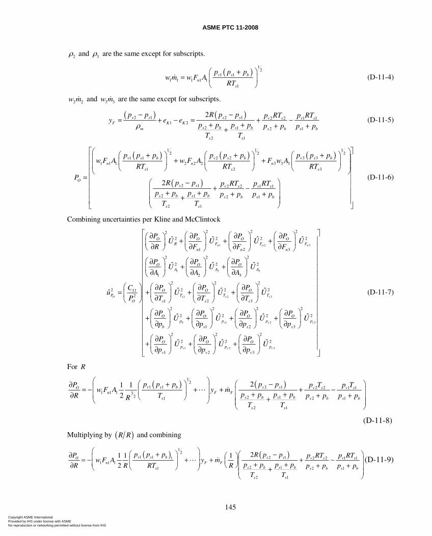
ASME PTC 11-2008

145

2ρ and 3ρ are the same except for subscripts.

( )

12

1 11 1 1 1 1

1

v s bn

s

p p pw m w F A

RT

⎛ + ⎞= ⎜ ⎟

⎝ ⎠ (D-11-4)

2 2w m and 3 3w m are the same except for subscripts.

( ) ( )2 1 2 1 2 2 1 1

1 22 1 2 1

2 1

2s s s s v s v sF K K

s b s bm s b s b

s s

p p R p p p RT p RTy e e

p p p p p p p pT T

ρ− −

= + − = + −+ + + ++

(D-11-5)

( ) ( ) ( )

( )

1 1 12 2 2

1 1 2 2 3 31 1 1 2 2 2 3 3 3

1 2 3

2 1 2 2 1 1

2 1 2 1

2 1

2

v s b v s b v s bn n n

s s s

Os s v s v s

s b s b s b s b

s s

p p p p p p p p pw F A w F A F w A

RT RT RT

PR p p p RT p RT

p p p p p p p pT T

⎡⎛ ⎞⎛ + ⎞ ⎛ + ⎞ ⎛ + ⎞⎢⎜ ⎟+ +⎜ ⎟ ⎜ ⎟ ⎜ ⎟⎢⎜ ⎟⎝ ⎠ ⎝ ⎠ ⎝ ⎠⎝ ⎠⎢= ⎢ ⎛ − ⎞⎢ + −⎜ ⎟+ + + +⎜ ⎟+⎜ ⎟⎝ ⎠⎣

⎤⎥⎥⎥⎥⎥

⎢ ⎥⎢ ⎥

⎦

(D-11-6)


1 2 3

1 2 3

1 2

2 2 222 2 2 2

1 2 3

22 2

2 2 2

1 2 3

2 2

2 2 2112

1 2

ˆ ˆ ˆ ˆ

ˆ ˆ ˆ

ˆ ˆˆ

n n n

O s s

O O O OR F F F

n n n

O O OA A A

O O OP T T

O s s

P P P PU U U U

R F F F

P P PU U U

A A A

P P PCu U U

P T T

⎛ ⎞ ⎛ ⎞ ⎛ ⎞∂ ∂ ∂ ∂⎛ ⎞ + + +⎜ ⎟ ⎜ ⎟ ⎜ ⎟⎜ ⎟∂ ∂ ∂ ∂⎝ ⎠ ⎝ ⎠ ⎝ ⎠ ⎝ ⎠

⎛ ⎞⎛ ⎞ ⎛ ⎞∂ ∂ ∂+ + ⎜ ⎟⎜ ⎟ ⎜ ⎟∂ ∂ ∂⎝ ⎠ ⎝ ⎠ ⎝ ⎠

⎛ ⎞ ⎛ ⎞ ⎛ ⎞∂ ∂ ∂= + + +⎜ ⎟ ⎜ ⎟ ⎜ ⎟∂ ∂ ∂⎝ ⎠ ⎝ ⎠ ⎝ ⎠3

1 2 3

1 2 3

2

2

3

2 2 2 2

2 2 2 2

1 2 3

2 2 2

2 2 2

1 2 3

ˆ

ˆ ˆ ˆ ˆ

ˆ ˆ ˆ

s

b s s s

v v v

Ts

O O O Op p p p

b s s s

O O Op p p

v v v

UT

P P P PU U U U

p p p p

P P PU U U

p p p

⎡ ⎤⎢ ⎥⎢ ⎥⎢ ⎥⎢ ⎥⎢ ⎥⎢ ⎥⎢ ⎥⎛ ⎞⎢ ⎥⎜ ⎟⎢ ⎥⎝ ⎠⎢ ⎥⎢ ⎥⎛ ⎞ ⎛ ⎞ ⎛ ⎞ ⎛ ⎞∂ ∂ ∂ ∂+ + + +⎢ ⎥⎜ ⎟ ⎜ ⎟ ⎜ ⎟ ⎜ ⎟∂ ∂ ∂ ∂⎢ ⎥⎝ ⎠ ⎝ ⎠ ⎝ ⎠ ⎝ ⎠⎢ ⎥⎛ ⎞ ⎛ ⎞ ⎛ ⎞∂ ∂ ∂⎢ ⎥+ + +⎜ ⎟ ⎜ ⎟ ⎜ ⎟⎢ ⎥∂ ∂ ∂⎝ ⎠ ⎝ ⎠ ⎝ ⎠⎣ ⎦

(D-11-7)

For R

( ) ( )1

21 1 2 1 2 2 1 1

1 1 1 32 2 11 2 1

2 1

21 1

2v s b s sO v s v s

n F Fs b s bs s b s b

s s

p p p p pP p T p Tw F A y m

p p p pR T p p p pRT T

⎛ ⎞⎛ + ⎞ ⎛ − ⎞∂ ⎜ ⎟= − + + + −⎜ ⎟ ⎜ ⎟+ +⎜ ⎟∂ + +⎝ ⎠ ⎜ ⎟+⎝ ⎠ ⎜ ⎟⎝ ⎠

(D-11-8)

Multiplying by ( )R R and combining

( ) ( )1

21 1 2 1 2 2 1 11

1 1 12 11 2 1

2 1

21 1 1

2v s b s sO v s v s

n F Fs b s bs s b s b

s s

p p p R p pP p RT p RTw F A y m

p p p pR R RT R p p p pT T

⎛ ⎞⎛ ⎞+ ⎛ ⎞−∂ ⎛ ⎞⎜ ⎟= − + + + −⎜ ⎟ ⎜ ⎟⎜ ⎟⎜ ⎟ + +∂ ⎝ ⎠ + +⎝ ⎠ ⎜ ⎟⎝ ⎠ +⎜ ⎟⎝ ⎠

(D-11-9)


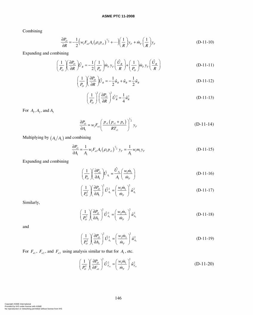
ASME PTC 11-2008

146

Combining

( )( )12

1 1 1 1 1

1 1 1

2O

n v F F F

Pw F A p y m y

R R Rρ∂ ⎛ ⎞ ⎛ ⎞= − + +⎜ ⎟ ⎜ ⎟∂ ⎝ ⎠ ⎝ ⎠

(D-11-10)


ˆ ˆ1 1 1 1ˆ

2O R R

R F F F FO O O

P U UU m y m y

P R P R P R

⎛ ⎞ ⎛ ⎞∂⎛ ⎞⎛ ⎞ ⎛ ⎞ ⎛ ⎞= − +⎜ ⎟ ⎜ ⎟⎜ ⎟⎜ ⎟ ⎜ ⎟ ⎜ ⎟∂ ⎝ ⎠ ⎝ ⎠⎝ ⎠⎝ ⎠ ⎝ ⎠ ⎝ ⎠ (D-11-11)

1 1 1ˆ ˆ ˆ ˆ

2 2O

R R R RO

PU u u u

P R

∂⎛ ⎞⎛ ⎞ = − + =⎜ ⎟⎜ ⎟ ∂⎝ ⎠⎝ ⎠ (D-11-12)

22

2 21 1ˆ ˆ4

OR R

O

PU u

P R

∂⎛ ⎞⎛ ⎞ =⎜ ⎟⎜ ⎟ ∂⎝ ⎠⎝ ⎠ (D-11-13)

For 1 2 3, , and A A A

( )

12

1 11 1

1 1

v s bOn F

s

p p pPw F y

A RT

⎛ + ⎞∂= ⎜ ⎟∂ ⎝ ⎠

(D-11-14)

Multiplying by ( )1 1A A and combining

( ) 12

1 1 1 1 1 1 11 1 1

1 1On v F F

Pw F A p y w m y

A A Aρ∂ = =

∂ (D-11-15)


1

1

1 1

1 1

ˆ1 ˆ AOA

O F

UP w mU

P A A m

∂⎛ ⎞ ⎛ ⎞⎛ ⎞ =⎜ ⎟ ⎜ ⎟⎜ ⎟ ∂⎝ ⎠ ⎝ ⎠⎝ ⎠ (D-11-16)

1 1

2 22 21 1

21

1 ˆ ÔA A

O F

P w mU u

P A m

∂⎛ ⎞ ⎛ ⎞⎛ ⎞ =⎜ ⎟ ⎜ ⎟⎜ ⎟ ∂⎝ ⎠ ⎝ ⎠⎝ ⎠ (D-11-17)

Similarly,

2 2

2 22 22 2

22

1 ˆ ÔA A

O F

P w mU u

P A m

∂⎛ ⎞ ⎛ ⎞⎛ ⎞ =⎜ ⎟ ⎜ ⎟⎜ ⎟ ∂⎝ ⎠ ⎝ ⎠⎝ ⎠ (D-11-18)

and

3 3

2 22 23 3

23

1 ˆ ÔA A

O F

P w mU u

P A m

∂⎛ ⎞ ⎛ ⎞⎛ ⎞ =⎜ ⎟ ⎜ ⎟⎜ ⎟ ∂ ⎝ ⎠⎝ ⎠⎝ ⎠ (D-11-19)

For 1nF , 2nF , and 3nF using analysis similar to that for 1A , etc.

1 1

2 22 21 1

21

1 ˆ ˆn n

OF F

O n F

P w mU u

P F m

∂⎛ ⎞ ⎛ ⎞⎛ ⎞ =⎜ ⎟ ⎜ ⎟⎜ ⎟ ∂ ⎝ ⎠⎝ ⎠⎝ ⎠ (D-11-20)


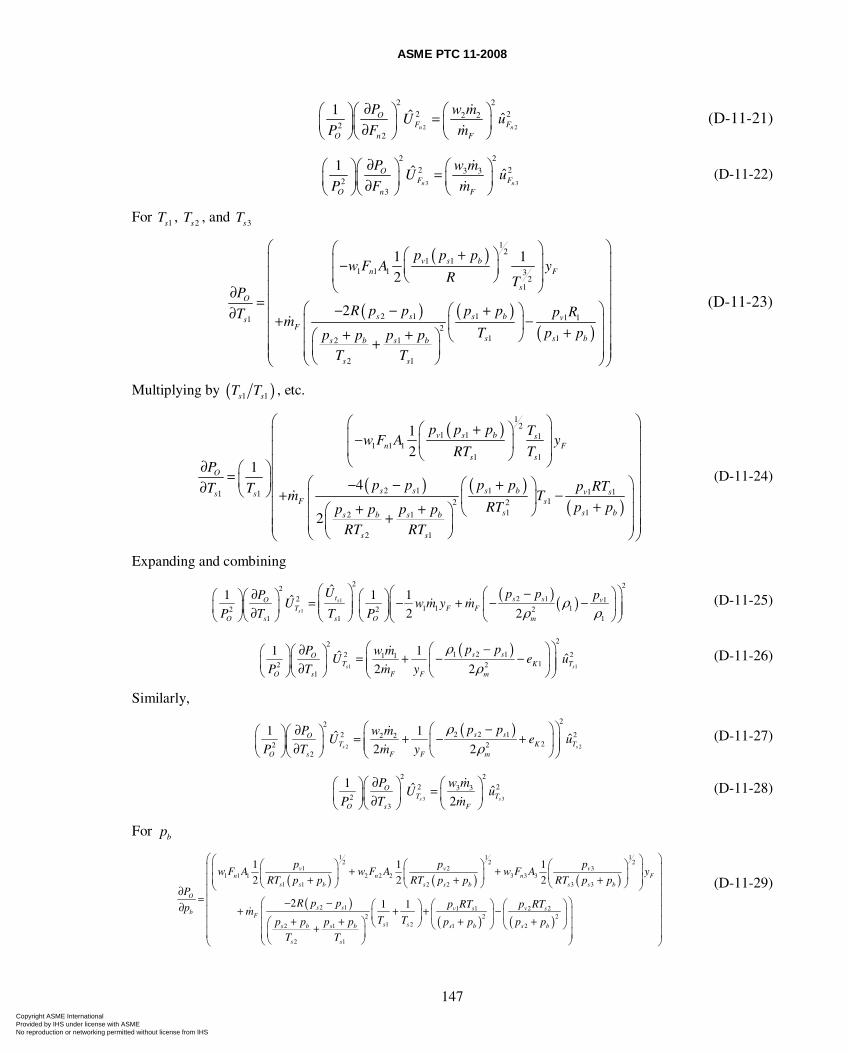
ASME PTC 11-2008

147

2 2

2 22 22 2

22

1 ˆ ˆn n

OF F

O n F

P w mU u

P F m

∂⎛ ⎞ ⎛ ⎞⎛ ⎞ =⎜ ⎟ ⎜ ⎟⎜ ⎟ ∂ ⎝ ⎠⎝ ⎠⎝ ⎠ (D-11-21)

3 3

2 22 23 3

23

1 ˆ ˆn n

OF F

O n F

P w mU u

P F m

∂⎛ ⎞ ⎛ ⎞⎛ ⎞ =⎜ ⎟ ⎜ ⎟⎜ ⎟ ∂ ⎝ ⎠⎝ ⎠⎝ ⎠ (D-11-22)

For 1sT , 2sT , and 3sT

( )

( ) ( )( )

12

1 11 1 1 3

21

2 1 1 1 112

1 12 1

2 1

1 1

2

2

v s bn F

sO

s s s b vsF

s s bs b s b

s s

p p pw F A y

R TP

R p p p p p RT mT p pp p p p

T T

⎛ ⎞⎛ ⎞⎛ + ⎞⎜ ⎟⎜ ⎟− ⎜ ⎟⎜ ⎟⎜ ⎟⎝ ⎠⎝ ⎠⎜ ⎟∂ = ⎜ ⎟⎛ ⎞− − ⎛ + ⎞∂ ⎜ ⎟+ −⎜ ⎟⎜ ⎟⎜ ⎟++ +⎛ ⎞ ⎝ ⎠⎜ ⎟+⎜ ⎟⎜ ⎟⎜ ⎟⎜ ⎟⎝ ⎠⎝ ⎠⎝ ⎠

(D-11-23)

Multiplying by ( )1 1s sT T , etc.

( )

( ) ( )( )

12

1 1 11 1 1

1 1

2 1 1 1 11 112 2

1 12 1

2 1

1

21

4

2

v s b sn F

s s

O

s s s b v ss sF s

s s bs b s b

s s

p p p Tw F A y

RT TP

p p p p p RTT T m TRT p pp p p p

RT RT

⎛ ⎞⎛ ⎞⎛ + ⎞⎜ ⎟⎜ ⎟− ⎜ ⎟⎜ ⎟⎜ ⎟⎝ ⎠⎝ ⎠⎜ ⎟∂ ⎛ ⎞= ⎜ ⎟⎜ ⎟ ⎛ ⎞− − ⎛ + ⎞∂ ⎜ ⎟⎝ ⎠ + −⎜ ⎟⎜ ⎟⎜ ⎟++ +⎛ ⎞ ⎝ ⎠⎜ ⎟+⎜ ⎟⎜ ⎟⎜ ⎟⎜ ⎟⎝ ⎠⎝ ⎠⎝ ⎠

(D-11-24)


( ) ( )1

1

2 222 12 1

1 1 12 2 21 1 1

ˆ1 1 1ˆ2 2

s

s

t s sO vT F F

O s s O m

U p pP pU w m y m

P T T Pρ

ρ ρ⎛ ⎞ ⎛ ⎞⎛ − ⎞∂⎛ ⎞⎛ ⎞ ⎛ ⎞⎜ ⎟= − + − −⎜ ⎟⎜ ⎟⎜ ⎟⎜ ⎟ ⎜ ⎟⎜ ⎟ ⎜ ⎟∂⎝ ⎠⎝ ⎠ ⎝ ⎠ ⎝ ⎠ ⎝ ⎠⎝ ⎠

(D-11-25)

( )1 1

221 2 12 21 1

12 21

1 1ˆ ˆ2 2s s

s sOT K T

O s F F m

p pP w mU e u

P T m y

ρρ

⎛ ⎞⎛ − ⎞∂⎛ ⎞⎛ ⎞ = + − −⎜ ⎟⎜ ⎟⎜ ⎟⎜ ⎟ ⎜ ⎟∂⎝ ⎠⎝ ⎠ ⎝ ⎠⎝ ⎠ (D-11-26)

Similarly,

( )2 2

222 2 12 22 2

22 22

1 1ˆ ˆ2 2s s

s sOT K T

O s F F m

p pP w mU e u

P T m y

ρρ

⎛ ⎞⎛ − ⎞∂⎛ ⎞⎛ ⎞ = + − +⎜ ⎟⎜ ⎟⎜ ⎟⎜ ⎟ ⎜ ⎟∂⎝ ⎠⎝ ⎠ ⎝ ⎠⎝ ⎠ (D-11-27)

3 3

2 22 23 3

23

1 ˆ ˆ2s s

OT T

O s F

P w mU u

P T m

∂⎛ ⎞ ⎛ ⎞⎛ ⎞ =⎜ ⎟ ⎜ ⎟⎜ ⎟ ∂ ⎝ ⎠⎝ ⎠⎝ ⎠ (D-11-28)

For bp

( ) ( ) ( )( )

( )

1 1 12 2 2

1 2 31 1 1 2 2 2 3 3 3

1 1 2 2 3 3

2 1 1 1 22 2

1 2 12 1

2 1

1 1 1

2 2 2

2 1 1

v v vn n n F

s s b s s b s s b

O

s s v s v sb

Fs s s bs b s b

s s

p p pw F A w F A w F A y

RT p p RT p p RT p pP

R p p p RT p RTp mT T p pp p p p

T T

⎛ ⎞⎛ ⎞ ⎛ ⎞ ⎛ ⎞⎜ ⎟+ +⎜ ⎟ ⎜ ⎟ ⎜ ⎟⎜ ⎟+ + +⎝ ⎠ ⎝ ⎠ ⎝ ⎠⎝ ⎠∂= − − ⎛ ⎞⎛ ⎞∂ + + + −⎜ ⎟⎜ ⎟ ++ +⎛ ⎞ ⎝ ⎠ ⎝ ⎠+⎜ ⎟

⎝ ⎠

( )2

2

2s bp p

⎛ ⎞⎜ ⎟⎜ ⎟⎜ ⎟⎜ ⎟⎛ ⎞⎛ ⎞⎜ ⎟⎜ ⎟⎜ ⎟+⎜ ⎟⎜ ⎟⎝ ⎠⎜ ⎟⎜ ⎟

⎝ ⎠⎝ ⎠

(D-11-29)


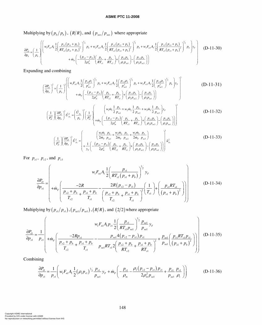
ASME PTC 11-2008

148

Multiplying by ( )b bp p , ( )R R , and ( )sax saxp p where appropriate

( )( )

( )( )

( )( )

( )

1 1 12 2 2

1 1 2 2 3 31 1 1 2 2 2 3 3 32 2 2

1 1 2 2 3 3

2 1

2

1 1 1

2 2 21

2

v s b v s b v s bn b n b n b F

s s b s s b s s bO

b bs s b

Fm

p p p p p p p p pw F A p w F A p w F A p y


p p p p pm

RTρ

⎛ ⎞⎛ + ⎞ ⎛ + ⎞ ⎛ + ⎞⎜ ⎟+ +⎜ ⎟ ⎜ ⎟ ⎜ ⎟⎜ ⎟ ⎜ ⎟ ⎜ ⎟⎜ ⎟+ + +∂ ⎛ ⎞ ⎝ ⎠ ⎝ ⎠ ⎝ ⎠⎝ ⎠= ⎜ ⎟∂ ⎝ ⎠ −+ − 1 2

1 2 1 1 2 2

b v b v b

s s sa sa

p p p p p

RT p pρ ρ

⎛ ⎞⎜ ⎟⎜ ⎟⎜ ⎟⎜ ⎟⎛ ⎞⎛ ⎞ ⎛ ⎞ ⎛ ⎞⎜ ⎟+ + −⎜ ⎟⎜ ⎟ ⎜ ⎟ ⎜ ⎟⎜ ⎟⎝ ⎠ ⎝ ⎠ ⎝ ⎠⎝ ⎠⎝ ⎠

(D-11-30)


( )

1 1 12 2 2

1 1 2 2 3 31 1 1 2 2 2 3 3 32 2 2 22

1 2 3

2 1 2 12

2 1 2 2 1 1

1 1 1

2 2 21

2

v v vn b n b n b F

sa sa saO

b b s s b b v b v bF

m s s sa sa

p p pw F A p w F A p w F A p y

p p pP

p p p p p p p p p pm

RT RT p p

ρ ρ ρ

ρ ρ ρ

⎛ ⎞⎛ ⎞ ⎛ ⎞ ⎛ ⎞⎜ ⎟+ +⎜ ⎟ ⎜ ⎟ ⎜ ⎟⎜ ⎟∂⎛ ⎞ ⎛ ⎞ ⎝ ⎠ ⎝ ⎠ ⎝ ⎠⎝ ⎠=⎜ ⎟ ⎜ ⎟∂⎝ ⎠ ⎝ ⎠ − ⎛ ⎞ ⎛ ⎞ ⎛ ⎞+ − + + −⎜ ⎟ ⎜ ⎟ ⎜⎝ ⎠ ⎝ ⎠ ⎝

2⎛ ⎞⎜ ⎟⎜ ⎟⎜ ⎟

⎛ ⎞⎜ ⎟⎜ ⎟⎜ ⎟⎟

⎠⎝ ⎠⎝ ⎠

(D-11-31)

( )

2 1 1 2 2 3 321 2 32

2 22 1 2 1

22 1 2 2 1 1

1 1 1

ˆ 2 2 21 1ˆ

2

b

b

b b bF

sa sa sapOp

O b b O s s b b v b v bF

m s s sa sa

p p pw m w m w m y

p p pUPU

P p p P p p p p p p p pm

RT RT p pρ ρ ρ

⎛ ⎞⎛ ⎞+ +⎜ ⎟⎜ ⎟⎛ ⎞ ⎝ ⎠∂⎛ ⎞⎛ ⎞ ⎛ ⎞⎜⎜ ⎟=⎜ ⎟⎜ ⎟ ⎜ ⎟⎜⎜ ⎟∂ ⎛ − ⎞⎛ ⎞ ⎛ ⎞ ⎛ ⎞⎝ ⎠⎝ ⎠ ⎝ ⎠ ⎝ ⎠⎜+ − + + −⎜ ⎟⎜ ⎟ ⎜ ⎟ ⎜ ⎟⎜ ⎝ ⎠ ⎝ ⎠ ⎝ ⎠⎝ ⎠⎝ ⎠

2

⎟⎟⎟⎟

(D-11-32)

( )

2

3 31 1 2 2

21 2 32 2

22 1 2 1

22 1 2 2 1 1

2 2 21 ˆ ˆ

1

2

b b

b b b

F sa F sa F saOp p

O b s s b b v b v b

F m s s sa sa

p p w m pw m w m

m p m p m pPU u

P p p p p p p p p p

y RT RT p pρ ρ ρ

⎛ ⎞⎛ ⎞+ +⎜ ⎟⎜ ⎟⎝ ⎠∂⎛ ⎞⎛ ⎞ ⎜ ⎟=⎜ ⎟⎜ ⎟ ⎜ ⎟∂ ⎛ − ⎞⎛ ⎞ ⎛ ⎞ ⎛ ⎞⎝ ⎠⎝ ⎠ ⎜ ⎟+ − + + −⎜ ⎟⎜ ⎟ ⎜ ⎟ ⎜ ⎟⎜ ⎟⎝ ⎠ ⎝ ⎠ ⎝ ⎠⎝ ⎠⎝ ⎠

(D-11-33)

For 1sp , 2sp , and 3sp

( )( )

( )

12

11 1 1

1 1

2 1 1 11

2 22 1 1 12 1

2 1 2 1

1

2

22 1

vn F

s s b

O

s s v ss F

s b s b s s bs b s b

s s s s

pw F A y

RT p pP

R p p p RTRp mp p p p T p pp p p p

T T T T

⎛ ⎞⎛ ⎞⎜ ⎟⎜ ⎟+⎜ ⎟⎝ ⎠⎜ ⎟∂ = ⎛ ⎞⎛ ⎞⎜ ⎟− ⎛ ⎞−∂ ⎜ ⎟⎜ ⎟+ − +⎜ ⎟⎜ ⎟ ⎜ ⎟+ +⎜ ⎟++ +⎛ ⎞⎜ ⎟⎝ ⎠ ⎝ ⎠+ +⎜ ⎟⎜ ⎟⎜ ⎟⎝ ⎠⎝ ⎠⎝ ⎠

(D-11-34)

Multiplying by ( )1 1s sp p , ( )1 1sa sap p , ( )R R , and ( )2 2 where appropriate

( )

12

1 11 1 1 1

1 1 1

1 2 1 11 1 1 1 11 1 2

2 1 1 12 11 1

2 1 2 1

1

21

42

2

v san s F

s sa sa

O

sa s s ss sa v s ss s F

s b s b sa ss b s bsa s

s s s s

p pw F A p y

RT p pP

p p p pRp p p RT pp p mp p p p p pp p p p

p RTT T RT RT

⎛ ⎞⎜ ⎟⎝ ⎠∂

= −−∂ + − ++ + ++ +⎛ ⎞+ +⎜ ⎟

⎝ ⎠

( )2

bp

⎛ ⎞⎜ ⎟⎜ ⎟⎜ ⎟

⎛ ⎞⎛ ⎞⎜ ⎟⎜ ⎟⎜ ⎟⎜ ⎟⎜ ⎟⎝ ⎠⎜ ⎟⎜ ⎟⎜ ⎟⎝ ⎠⎝ ⎠

(D-11-35)

Combining

( ) ( )1 1 2 1 11 1 1 121 1 1 1 1 2

1 1 1 1 1 1

1 1

2 2s s sO s s s v

n v F Fs s sa m m sa sa

p p pP p p p pw F A p y m

p p p p p

ρρ

ρ ρ ρ⎛ ⎞⎛ − ⎞∂

= + − − +⎜ ⎟⎜ ⎟⎜ ⎟∂ ⎝ ⎠⎝ ⎠ (D-11-36)


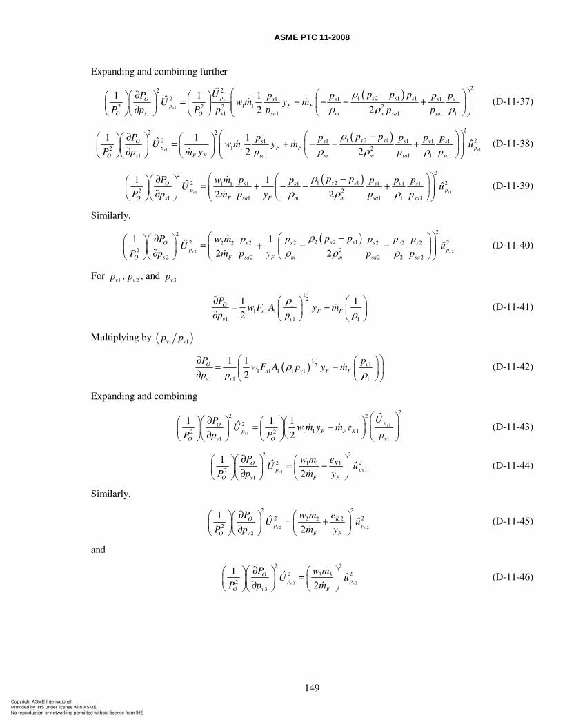
ASME PTC 11-2008

149


( )

1

1

22 21 2 1 12 1 1 1 1

1 12 2 2 21 1 1 1 1 1

ˆ1 1 1ˆ2 2

s

s

p s s sO s s s vp F F

O s O s sa m m sa sa

U p p pP p p p pU w m y m

P p P p p p p

ρρ ρ ρ

⎛ ⎞⎛ − ⎞∂⎛ ⎞⎛ ⎞ ⎛ ⎞= + − − +⎜ ⎟⎜ ⎟⎜ ⎟⎜ ⎟ ⎜ ⎟ ⎜ ⎟∂⎝ ⎠⎝ ⎠ ⎝ ⎠ ⎝ ⎠⎝ ⎠ (D-11-37)

( )

1 1

22 21 2 12 21 1 1 1 1

1 12 21 1 1 1 1

1 1 1ˆ ˆ2 2s s

s sO s s s v sp F F p

O s F F sa m m sa sa

p pP p p p p pU w m y m u

P p m y p p p

ρρ ρ ρ

⎛ ⎞⎛ − ⎞∂⎛ ⎞⎛ ⎞ ⎛ ⎞= + − − +⎜ ⎟⎜ ⎟⎜ ⎟⎜ ⎟ ⎜ ⎟ ⎜ ⎟∂ ⎝ ⎠⎝ ⎠⎝ ⎠ ⎝ ⎠⎝ ⎠ (D-11-38)

( )

1 1

221 2 12 21 1 1 1 11 1

2 21 1 1 1 1

1 1ˆ ˆ2 2s s

s sO s s s v sp p

O s F sa F m m sa sa

p pP p p p p pw mU u

P p m p y p p

ρρ ρ ρ

⎛ ⎞⎛ − ⎞∂⎛ ⎞⎛ ⎞ = + − − +⎜ ⎟⎜ ⎟⎜ ⎟⎜ ⎟ ⎜ ⎟∂⎝ ⎠⎝ ⎠ ⎝ ⎠⎝ ⎠ (D-11-39)

Similarly,

( )

2 2

222 2 12 22 2 2 2 22 2

2 22 2 2 2 2

1 1ˆ ˆ2 2s s

s sO s s s v sp p

O s F sa F m m sa sa

p pP p p p p pw mU u

P p m p y p p

ρρ ρ ρ

⎛ ⎞⎛ − ⎞∂⎛ ⎞⎛ ⎞ = + − −⎜ ⎟⎜ ⎟⎜ ⎟⎜ ⎟ ⎜ ⎟∂⎝ ⎠⎝ ⎠ ⎝ ⎠⎝ ⎠ (D-11-40)

For 1vp , 2vp , and 3vp

1

21

1 1 11 1 1

1 1

2O

n F Fv v

Pw F A y m

p p

ρρ

∂ ⎛ ⎞ ⎛ ⎞= −⎜ ⎟ ⎜ ⎟∂ ⎝ ⎠⎝ ⎠ (D-11-41)

Multiplying by ( )1 1v vp p

( )112

1 1 1 1 11 1 1

1 1

2O v

n v F Fv v

P pw F A p y m

p pρ

ρ⎛ ⎞∂ ⎛ ⎞= −⎜ ⎟⎜ ⎟∂ ⎝ ⎠⎝ ⎠

(D-11-42)


1

1

22 2

21 1 12 2

1 1

ˆ1 1 1ˆ2

v

v

pOp F F K

O v O v

UPU w m y m e

P p P p

⎛ ⎞∂⎛ ⎞⎛ ⎞ ⎛ ⎞⎛ ⎞ ⎜ ⎟= −⎜ ⎟⎜ ⎟⎜ ⎟ ⎜ ⎟ ⎜ ⎟∂ ⎝ ⎠⎝ ⎠⎝ ⎠ ⎝ ⎠ ⎝ ⎠ (D-11-43)

1

2 22 21 1 1

121

1 ˆ ˆ2v

O Kp pv

O v F F

P w m eU u

P p m y

∂⎛ ⎞ ⎛ ⎞⎛ ⎞ = −⎜ ⎟ ⎜ ⎟⎜ ⎟ ∂ ⎝ ⎠⎝ ⎠⎝ ⎠ (D-11-44)

Similarly,

2 2

2 22 22 2 2

22

1 ˆ ˆ2v v

O Kp p

O v F F

P w m eU u

P p m y

∂⎛ ⎞ ⎛ ⎞⎛ ⎞ = +⎜ ⎟ ⎜ ⎟⎜ ⎟ ∂ ⎝ ⎠⎝ ⎠⎝ ⎠ (D-11-45)

and

3 3

2 22 23 3

23

1 ˆ ˆ2v v

Op p

O v F

P w mU u

P p m

∂⎛ ⎞ ⎛ ⎞⎛ ⎞ =⎜ ⎟ ⎜ ⎟⎜ ⎟ ∂ ⎝ ⎠⎝ ⎠⎝ ⎠ (D-11-46)


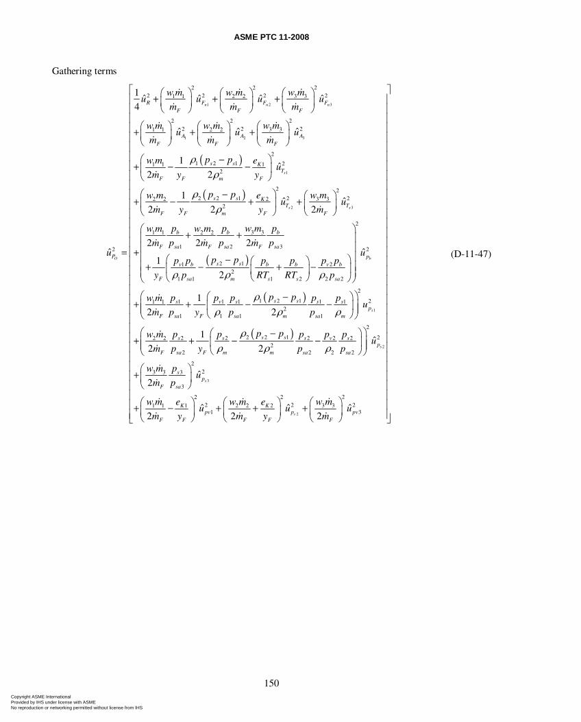
ASME PTC 11-2008

150

Gathering terms

( )

1 2 3

1 2 3

1

22 22 2 2 23 31 1 2 2

22 22 2 23 31 1 2 2

2

1 2 1 21 1 12

2 2

2

1ˆ ˆ ˆ ˆ

4

ˆ ˆ ˆ

1ˆ

2 2

1

2

ˆ

n n n

s

O

R F F FF F F

A A AF F F

s s KT

F F m F

F F

P

w mw m w mu u u u

m m m

w mw m w mu u u

m m m

p pw m eu

m y y

w m

m y

u

ρρ

ρ

⎛ ⎞⎛ ⎞ ⎛ ⎞+ + + ⎜ ⎟⎜ ⎟ ⎜ ⎟⎝ ⎠ ⎝ ⎠ ⎝ ⎠

⎛ ⎞⎛ ⎞ ⎛ ⎞+ + + ⎜ ⎟⎜ ⎟ ⎜ ⎟⎝ ⎠ ⎝ ⎠ ⎝ ⎠

⎛ − ⎞+ − −⎜ ⎟⎝ ⎠

+ −

=

( )

( )

2 3

2 22 2 1 2 23 32

2

2

3 31 1 2 2

1 2 3 2

2 11 22

1 1 1 2 2 2

11 1

1

ˆ ˆ2 2

2 2 2ˆ

1

2

2

s s

b

s s KT T

m F F

b b b

F sa F sa F sa

ps sv b b b v b

F sa m s s sa

s

F sa

p p w meu u

y m

p p w m pw m w m

m p m p m pu

p pp p p p p p

y p RT RT p

pw m

m p

ρ

ρ ρ ρ

⎛ − ⎞ ⎛ ⎞+ +⎜ ⎟ ⎜ ⎟⎝ ⎠⎝ ⎠

⎛ ⎞+ +⎜ ⎟⎜ ⎟+⎜ ⎟⎛ − ⎞⎛ ⎞⎜ ⎟+ − + −⎜ ⎟⎜ ⎟⎜ ⎟⎝ ⎠⎝ ⎠⎝ ⎠

+ +( )

( )

1

2

3

2

1 2 1 21 1 1 12

1 1 1

2

2 2 1 22 2 2 2 22 22

2 2 2 2

223 3 3

3

2

1 1 1

1

2

1ˆ

2 2

ˆ2

ˆ2

s

s

s

s sv s s sp

F sa m sa m

s ss s s v sp

F sa F m m sa sa

sp

F sa

Kpv

F F

p pp p p pu

y p p

p pp p p p pw mu

m p y p p

w m pu

m p

w m eu

m y

ρρ ρ ρ

ρρ ρ ρ

⎛ ⎞⎛ − ⎞− −⎜ ⎟⎜ ⎟⎜ ⎟⎝ ⎠⎝ ⎠

⎛ ⎞⎛ − ⎞+ + − −⎜ ⎟⎜ ⎟⎜ ⎟⎝ ⎠⎝ ⎠

⎛ ⎞+⎜ ⎟⎝ ⎠

⎛ ⎞+ −⎜ ⎟⎝ ⎠

2

222 2 23 32 2 2

1 3ˆ ˆ2 2v

Kp pv

F F F

w mw m eu u

m y m

⎡ ⎤⎢ ⎥⎢ ⎥⎢ ⎥⎢ ⎥⎢ ⎥⎢ ⎥⎢ ⎥⎢ ⎥⎢ ⎥⎢ ⎥⎢ ⎥⎢ ⎥⎢ ⎥⎢ ⎥⎢ ⎥⎢ ⎥⎢ ⎥⎢ ⎥⎢ ⎥⎢ ⎥⎢ ⎥⎢ ⎥⎢ ⎥⎢ ⎥⎢ ⎥⎢ ⎥⎢ ⎥⎢ ⎥⎢ ⎥⎢ ⎥⎢ ⎥⎢ ⎥

⎛ ⎞⎛ ⎞⎢ ⎥+ + + ⎜ ⎟⎜ ⎟⎢ ⎥⎝ ⎠ ⎝ ⎠⎣ ⎦

(D-11-47)


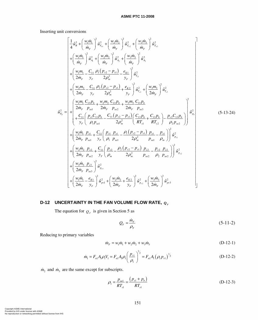
ASME PTC 11-2008

151


( )

1 2 3

1 2 3

1

22 22 2 2 23 31 1 2 2

22 22 2 23 31 1 2 2

2

1 2 1 21 1 11 12

2 2 1

2

1ˆ ˆ ˆ ˆ

4

ˆ ˆ ˆ

ˆ2 2

2

ˆ

n n n

s

O

R F F FF F F

A A AF F F

s s KT

F F m F

F

P

w mw m w mu u u u

m m m

w mw m w mu u u

m m m

p pw m C eu

m y y

w m C

m

u

ρρ

⎛ ⎞⎛ ⎞ ⎛ ⎞+ + + ⎜ ⎟⎜ ⎟ ⎜ ⎟⎝ ⎠ ⎝ ⎠ ⎝ ⎠

⎛ ⎞⎛ ⎞ ⎛ ⎞+ + + ⎜ ⎟⎜ ⎟ ⎜ ⎟⎝ ⎠ ⎝ ⎠ ⎝ ⎠

⎛ − ⎞+ − −⎜ ⎟⎝ ⎠

+ −

=

( )

( )

2 3

2 22 2 1 2 23 31 2

2

13 13 3 3 131 1 2 2

1 2 3

11 2 11 13 13 13 2 13112

1 1 1 2 2 2

ˆ ˆ2 2

2 2 2

2

s s

s s KT T

F m F F

b b b

F sa F sa F sa

s sv b b b v b

F sa m s s sa

p p w meu u

y y m

C p C p w m C pw m w m

m p m p m p

C p pp C p C p C p p C pC

y p RT RT p

ρρ

ρ ρ ρ

⎛ − ⎞ ⎛ ⎞+ +⎜ ⎟ ⎜ ⎟⎝ ⎠⎝ ⎠

⎛ ⎞+ +⎜⎜+⎜ ⎛ − ⎞⎛ ⎞⎜+ − + −⎜ ⎟⎜ ⎟⎜ ⎝ ⎠⎝ ⎠⎝

( )

( )

1

2

2

2

2

1 2 1 21 1 1 1 11 1 112

1 1 1 1

2

2 2 1 22 2 2 2 22 2 112

2 2 2 2

3 3 3

3

ˆ

ˆ2 2

ˆ2 2

2

b

s

s

p

s ss v s s sp

F sa F sa m sa m

s ss s s v sp

F sa F m m sa sa

s

F sa

u

p pp p p p pw m Cu

m p y p p

p pp p p p pw m Cu

m p y p p

w m p

m p

ρρ ρ ρ

ρρ ρ ρ

⎟⎟⎟⎟⎟⎠

⎛ ⎞⎛ − ⎞+ + − −⎜ ⎟⎜ ⎟⎜ ⎟⎝ ⎠⎝ ⎠

⎛ ⎞⎛ − ⎞+ + − −⎜ ⎟⎜ ⎟⎜ ⎟⎝ ⎠⎝ ⎠

⎛ ⎞+⎜⎝ ⎠

3

2

22

22 22 2 23 31 1 1 2 2 2

1 3

ˆ

ˆ ˆ ˆ2 2 2

s

v

p

K Kpv p pv

F F F F F

u

w mw m e w m eu u u

m y m y m

⎡ ⎤⎢ ⎥⎢ ⎥⎢ ⎥⎢ ⎥⎢ ⎥⎢ ⎥⎢ ⎥⎢ ⎥⎢ ⎥⎢ ⎥⎢ ⎥⎢ ⎥⎢ ⎥⎢ ⎥⎢ ⎥⎢ ⎥⎢ ⎥⎢ ⎥⎢ ⎥⎢ ⎥⎢ ⎥⎢ ⎥⎢ ⎥⎢ ⎥⎢ ⎥⎢ ⎥⎢ ⎥⎢ ⎥⎢ ⎥⎢ ⎥⎟⎢ ⎥⎢ ⎥

⎛ ⎞⎛ ⎞ ⎛ ⎞⎢ ⎥+ − + + + ⎜ ⎟⎜ ⎟ ⎜ ⎟⎢ ⎥⎝ ⎠ ⎝ ⎠ ⎝ ⎠⎣ ⎦

(5-13-24)

D-12 UNCERTAINTY IN THE FAN VOLUME FLOW RATE, FQ

The equation for FQ is given in Section 5 as

FF

F

mQ

ρ= (5-11-2)


1 1 2 2 3 3Fm w m w m w m= + + (D-12-1)

( )1

2 11 2

1 1 1 1 1 1 1 1 1 1 1 11

vn n n v


ρ⎛ ⎞= = =⎜ ⎟⎝ ⎠

(D-12-2)


( )11

11 1

s bsa

s s

p pp

RT RTρ

+= = (D-12-3)


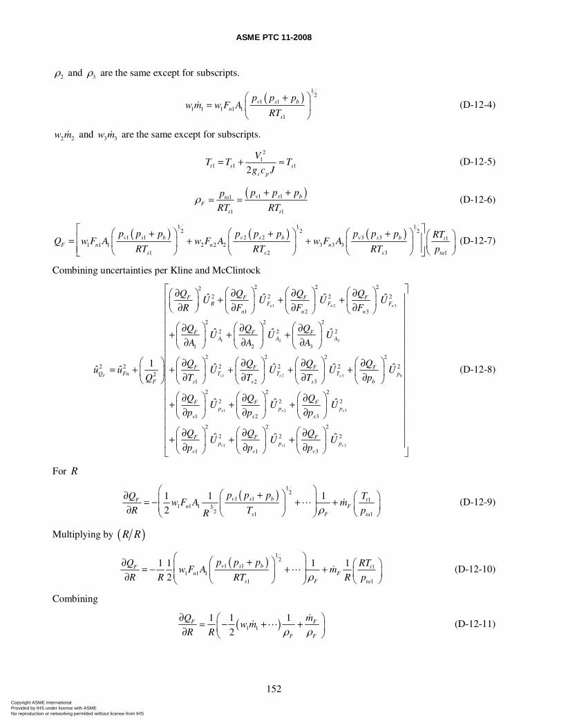
ASME PTC 11-2008

152


( )

12

1 11 1 1 1 1

1

v s bn

s

p p pw m w F A

RT

⎛ + ⎞= ⎜ ⎟

⎝ ⎠ (D-12-4)


2

11 1 12t s s

c p

VT T T

g c J= + ≈ (D-12-5)

( )1 11

1 1

v s btaF

t t

p p pp

RT RTρ

+ += = (D-12-6)

( ) ( ) ( )1 1 1

2 2 21 1 2 2 3 3 1

1 1 1 2 2 2 3 3 31 2 3 1

v s b v s b v s b tF n n n

s s s ta

p p p p p p p p p RTQ w F A w F A w F A

RT RT RT p

⎡ ⎤⎛ + ⎞ ⎛ + ⎞ ⎛ + ⎞ ⎛ ⎞⎢ ⎥= + +⎜ ⎟ ⎜ ⎟ ⎜ ⎟ ⎜ ⎟⎢ ⎥⎝ ⎠ ⎝ ⎠ ⎝ ⎠ ⎝ ⎠⎣ ⎦ (D-12-7)


1 2 3

1 2 3

1 2

2 2 222 2 2 2

1 2 3

22 2

2 2 2

1 2 3

2 2

2 2 2 22

1 2

ˆ ˆ ˆ ˆ

ˆ ˆ ˆ

1 ˆ ˆˆ ˆ

n n n

F s s

F F F FR F F F

n n n

F F FA A A

F FQ Fn T T

F s s

Q Q Q QU U U U

R F F F

Q Q QU U U

A A A

Q Qu u U U

Q T T

⎛ ⎞ ⎛ ⎞ ⎛ ⎞∂ ∂ ∂ ∂⎛ ⎞ + + +⎜ ⎟ ⎜ ⎟ ⎜ ⎟⎜ ⎟∂ ∂ ∂ ∂⎝ ⎠ ⎝ ⎠ ⎝ ⎠ ⎝ ⎠

⎛ ⎞⎛ ⎞ ⎛ ⎞∂ ∂ ∂+ + + ⎜ ⎟⎜ ⎟ ⎜ ⎟∂ ∂ ∂⎝ ⎠ ⎝ ⎠ ⎝ ⎠

⎛ ⎞ ⎛ ⎞⎛ ⎞ ∂ ∂= + + +⎜ ⎟ ⎜ ⎟⎜ ⎟ ∂ ∂⎝ ⎠ ⎝ ⎠ ⎝ ⎠3

1 2 3

1 1 3

2 2

2 2

3

2 2 2

2 2 2

1 2 3

2 2 2

2 2 2

1 1 3

ˆ ˆ

ˆ ˆ ˆ

ˆ ˆ ˆ

s b

s s s

v v v

F FT p

s b

F F Fp p p

s s s

F F Fp p p

v v v

Q QU U

T p

Q Q QU U U

p p p

Q Q QU U U

p p p

⎡ ⎤⎢ ⎥⎢ ⎥⎢ ⎥⎢ ⎥⎢ ⎥⎢ ⎥⎢ ⎥⎛ ⎞ ⎛ ⎞∂ ∂⎢ ⎥+ +⎜ ⎟ ⎜ ⎟⎢ ⎥∂ ∂⎝ ⎠ ⎝ ⎠⎢ ⎥⎢ ⎥⎛ ⎞ ⎛ ⎞ ⎛ ⎞∂ ∂ ∂+ + +⎢ ⎥⎜ ⎟ ⎜ ⎟ ⎜ ⎟∂ ∂ ∂⎢ ⎥⎝ ⎠ ⎝ ⎠ ⎝ ⎠⎢ ⎥⎛ ⎞ ⎛ ⎞ ⎛ ⎞∂ ∂ ∂⎢+ + +⎜ ⎟ ⎜ ⎟ ⎜ ⎟⎢ ∂ ∂ ∂⎝ ⎠ ⎝ ⎠ ⎝ ⎠⎣ ⎦

⎥⎥

(D-12-8)

For R

( )

12

1 1 11 1 1 3

2 1 1

1 1 1

2v s b tF

n Fs F ta

p p p TQw F A m

R T pR ρ

⎛ ⎞⎛ + ⎞∂ ⎛ ⎞⎜ ⎟= − + +⎜ ⎟ ⎜ ⎟⎜ ⎟∂ ⎝ ⎠ ⎝ ⎠⎝ ⎠ (D-12-9)

Multiplying by ( )R R

( )

12

1 1 11 1 1

1 1

1 1 1 1

2v s b tF

n Fs F ta

p p p RTQw F A m

R R RT R pρ

⎛ ⎞⎛ + ⎞∂ ⎛ ⎞⎜ ⎟= − + +⎜ ⎟ ⎜ ⎟⎜ ⎟∂ ⎝ ⎠ ⎝ ⎠⎝ ⎠ (D-12-10)

Combining

( )1 1

1 1 1

2F F

F F

Q mw m

R R ρ ρ∂ ⎛ ⎞= − + +⎜ ⎟∂ ⎝ ⎠

(D-12-11)


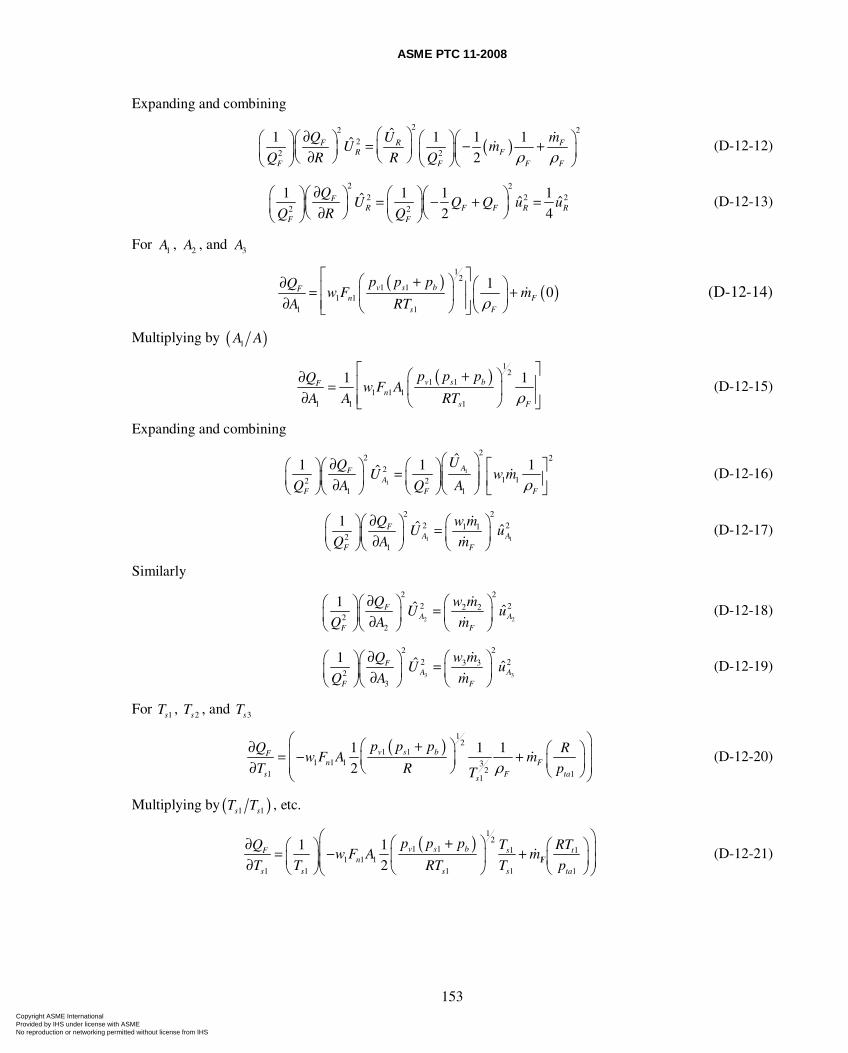
ASME PTC 11-2008

153


( )22 2

22 2

ˆ1 1 1 1ˆ2

F R FR F

F F F F

Q U mU m

Q R R Q ρ ρ⎛ ⎞∂⎛ ⎞ ⎛ ⎞⎛ ⎞ ⎛ ⎞= − +⎜ ⎟⎜ ⎟ ⎜ ⎟⎜ ⎟ ⎜ ⎟∂ ⎝ ⎠⎝ ⎠⎝ ⎠ ⎝ ⎠⎝ ⎠

(D-12-12)

2 2

2 2 22 2

1 1 1 1ˆ ˆ ˆ2 4

FR F F R R

F F

QU Q Q u u

Q R Q

∂⎛ ⎞⎛ ⎞ ⎛ ⎞⎛ ⎞= − + =⎜ ⎟⎜ ⎟⎜ ⎟ ⎜ ⎟∂ ⎝ ⎠⎝ ⎠⎝ ⎠ ⎝ ⎠ (D-12-13)

For 1A , 2A , and 3A

( ) ( )

12

1 11 1

1 1

10v s bF

n Fs F

p p pQw F m

A RT ρ

⎡ ⎤⎛ + ⎞∂ ⎛ ⎞⎢ ⎥= +⎜ ⎟ ⎜ ⎟⎢ ⎥∂ ⎝ ⎠⎝ ⎠⎣ ⎦ (D-12-14)

Multiplying by ( )1A A

( )

12

1 11 1 1

1 1 1

1 1v s bFn

s F

p p pQw F A

A A RT ρ

⎡ ⎤⎛ + ⎞∂ ⎢ ⎥= ⎜ ⎟⎢ ⎥∂ ⎝ ⎠⎣ ⎦ (D-12-15)


1

1

22 2

21 12 2

1 1

ˆ1 1 1ˆ AFA

F F F

UQU w m

Q A Q A ρ⎛ ⎞∂⎛ ⎞⎛ ⎞ ⎛ ⎞ ⎡ ⎤⎜ ⎟=⎜ ⎟⎜ ⎟ ⎜ ⎟ ⎢ ⎥⎜ ⎟∂⎝ ⎠⎝ ⎠ ⎝ ⎠⎝ ⎠ ⎣ ⎦

(D-12-16)

1 1

2 22 21 1

21

1 ˆ ˆFA A

F F

Q w mU u

Q A m

∂⎛ ⎞ ⎛ ⎞⎛ ⎞ =⎜ ⎟ ⎜ ⎟⎜ ⎟ ∂⎝ ⎠⎝ ⎠ ⎝ ⎠ (D-12-17)

Similarly

2 2

2 22 22 2

22

1 ˆ ˆFA A

F F

Q w mU u

Q A m

∂⎛ ⎞ ⎛ ⎞⎛ ⎞ =⎜ ⎟ ⎜ ⎟⎜ ⎟ ∂⎝ ⎠⎝ ⎠ ⎝ ⎠ (D-12-18)

3 3

222 23 3

23

1 ˆ ˆFA A

F F

w mQU u

Q A m

∂ ⎛ ⎞⎛ ⎞⎛ ⎞ = ⎜ ⎟⎜ ⎟⎜ ⎟ ∂⎝ ⎠ ⎝ ⎠⎝ ⎠ (D-12-19)


( )

12

1 11 1 1 3

21 11

1 1 1

2v s bF

n Fs F tas

p p pQ Rw F A m

T R pT ρ

⎛ ⎞⎛ + ⎞∂ ⎛ ⎞⎜ ⎟= − +⎜ ⎟ ⎜ ⎟⎜ ⎟∂ ⎝ ⎠ ⎝ ⎠⎝ ⎠ (D-12-20)


( )

12

1 1 1 11 1 1 1

1 1 1 1 1

1 1

2v s b s tF

n Fs s s s ta

p p p T RTQw F A m

T T RT T p

⎛ ⎞⎛ + ⎞∂ ⎛ ⎞⎛ ⎞⎜ ⎟= − +⎜ ⎟ ⎜ ⎟⎜ ⎟⎜ ⎟∂ ⎝ ⎠ ⎝ ⎠ ⎝ ⎠⎝ ⎠ (D-12-21)


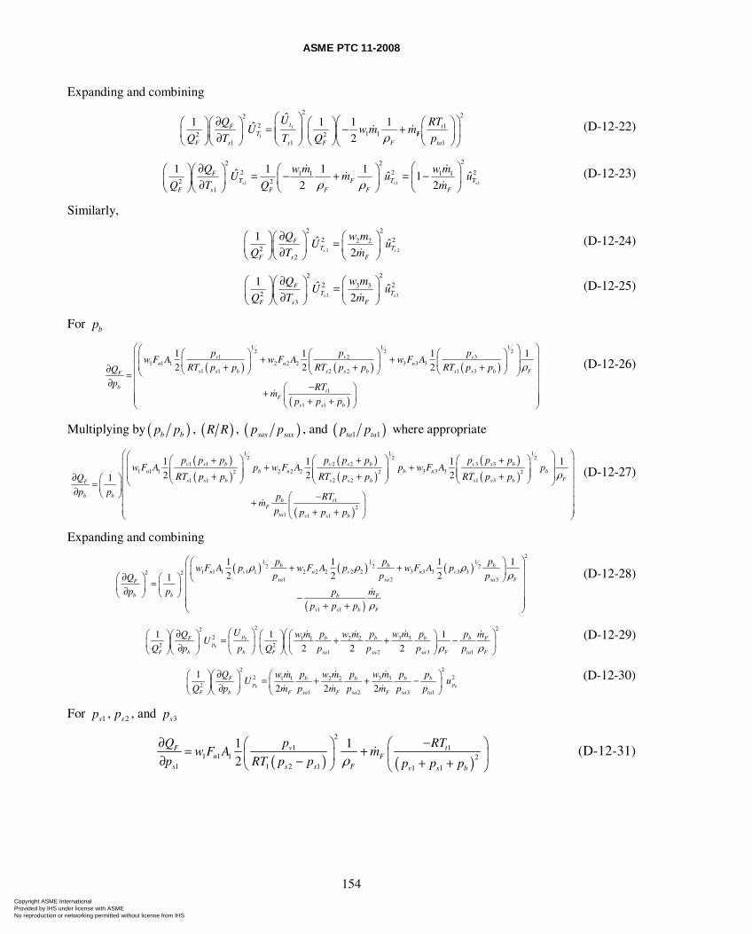
ASME PTC 11-2008

154


1

1

2 222 1

1 1 12 21 1 1

ˆ1 1 1 1ˆ2

t tFT F

F s s F F ta

U RTQU w m m

Q T T Q pρ⎛ ⎞ ⎛ ⎞∂ ⎛ ⎞⎛ ⎞⎛ ⎞ ⎛ ⎞⎜ ⎟= − +⎜ ⎟⎜ ⎟⎜ ⎟⎜ ⎟ ⎜ ⎟⎜ ⎟∂⎝ ⎠ ⎝ ⎠⎝ ⎠ ⎝ ⎠ ⎝ ⎠⎝ ⎠

(D-12-22)

1 1 1

22 22 2 21 1 1 1

2 21

1 1 1 1ˆ ˆ ˆ12 2s s s

FT F T T

F s F F F F

Q w m w mU m u u

Q T Q mρ ρ⎛ ⎞∂⎛ ⎞ ⎛ ⎞⎛ ⎞ = − + = −⎜ ⎟⎜ ⎟ ⎜ ⎟⎜ ⎟ ∂⎝ ⎠ ⎝ ⎠ ⎝ ⎠⎝ ⎠

(D-12-23)

Similarly,

2 2

2 22 22 2

22

1 ˆ ˆ2s s

FT T

F s F

Q w mU u

Q T m

∂⎛ ⎞ ⎛ ⎞⎛ ⎞ =⎜ ⎟ ⎜ ⎟⎜ ⎟ ∂⎝ ⎠ ⎝ ⎠⎝ ⎠ (D-12-24)

3 3

222 23 3

23

1 ˆ ˆ2s s

FT T

F s F

w mQU u

Q T m

∂ ⎛ ⎞⎛ ⎞⎛ ⎞ = ⎜ ⎟⎜ ⎟⎜ ⎟ ∂⎝ ⎠ ⎝ ⎠⎝ ⎠ (D-12-25)

For bp

( ) ( ) ( )

( )

1 1 12 2 2

1 2 31 1 1 2 2 2 3 3 3

1 1 2 2 1 3

1

1 1

1 1 1 1

2 2 2

v v vn n n

s s b s s b s s b FF

bt

Fv s b

p p pw F A w F A w F A

RT p p RT p p RT p pQ

p RTm

p p p

ρ

⎛ ⎞⎛ ⎞⎛ ⎞ ⎛ ⎞ ⎛ ⎞⎜ ⎟⎜ ⎟+ +⎜ ⎟ ⎜ ⎟ ⎜ ⎟⎜ ⎟⎜ + + + ⎟∂ ⎝ ⎠ ⎝ ⎠ ⎝ ⎠⎝ ⎠= ⎜ ⎟∂ ⎜ ⎟−⎛ ⎞+⎜ ⎟⎜ ⎟⎜ ⎟+ +⎝ ⎠⎝ ⎠

(D-12-26)

Multiplying by ( )b bp p , ( )R R , ( )sax saxp p , and ( )1 1ta tap p where appropriate

( )( )

( )( )

( )( )

1 1 12 2 2

1 1 2 2 3 31 1 1 2 2 2 3 3 32 2 2

1 1 2 2 1 3

1 1 1 1

2 2 21

v s b v s b v s bn b n b n b

Fs s b s s b s s bF

b b

p p p p p p p p pw F A p w F A p w F A p

RT p p RT p p RT p pQ

p p

ρ

⎛ ⎞⎛ + ⎞ ⎛ + ⎞ ⎛ + ⎞⎜ ⎟+ +⎜ ⎟ ⎜ ⎟ ⎜ ⎟⎜ ⎟ ⎜ ⎟ ⎜ ⎟⎜ ⎟+ + +∂ ⎛ ⎞ ⎝ ⎠ ⎝ ⎠ ⎝ ⎠⎝ ⎠= ⎜ ⎟∂ ⎝ ⎠

( )1

21 1 1

b tF

ta v s b

p RTm

p p p p

⎛ ⎞⎜ ⎟⎜ ⎟⎜ ⎟⎜ ⎟−⎛ ⎞⎜ ⎟+ ⎜ ⎟⎜ ⎟+ +⎝ ⎠⎝ ⎠

(D-12-27)


( ) ( ) ( )

( )

21 1 1

2 2 21 1 1 1 1 2 2 2 2 2 3 3 3 3 32 2

1 2 3

1 1

1 1 1 1

2 2 21

b b bn v n v n v

sa sa sa FF

b b b F

v s b F

p p pw F A p w F A p w F A p

p p pQ

p p p m

p p p

ρ ρ ρρ

ρ

⎛ ⎞⎛ ⎞+ +⎜ ⎟⎜ ⎟∂⎛ ⎞ ⎛ ⎞ ⎝ ⎠⎜ ⎟=⎜ ⎟ ⎜ ⎟ ⎜ ⎟∂⎝ ⎠ ⎝ ⎠ −⎜ ⎟⎜ ⎟+ +⎝ ⎠

(D-12-28)

2 22

2 3 31 1 2 22 2

1 2 3 1

1 1 1

2 2 2b

b

p b b b bF Fp

F b b F sa sa sa F ta F

U p p w m p pQ w m w m mU

Q p p Q p p p pρ ρ⎛ ⎞ ⎛ ⎞∂ ⎛ ⎞⎛ ⎞⎛ ⎞ ⎛ ⎞= + + −⎜ ⎟ ⎜ ⎟⎜ ⎟⎜ ⎟⎜ ⎟ ⎜ ⎟∂⎝ ⎠ ⎝ ⎠⎝ ⎠ ⎝ ⎠ ⎝ ⎠⎝ ⎠

(D-12-29)

22

2 23 31 1 2 22

1 2 3 1

1

2 2 2b b

b b b bFp p

F b F sa F sa F sa ta

p p w m p pQ w m w mU u

Q p m p m p m p p

∂ ⎛ ⎞⎛ ⎞⎛ ⎞ = + + −⎜ ⎟⎜ ⎟⎜ ⎟ ∂⎝ ⎠⎝ ⎠ ⎝ ⎠ (D-12-30)

For 1sp , 2sp , and 3sp

( ) ( )

2

1 11 1 1 2

1 1 2 1 1 1

1 1

2v tF

n Fs s s F v s b

p RTQw F A m

p RT p p p p pρ−∂ ⎛ ⎞ ⎛ ⎞= +⎜ ⎟ ⎜ ⎟∂ − + +⎝ ⎠ ⎝ ⎠

(D-12-31)


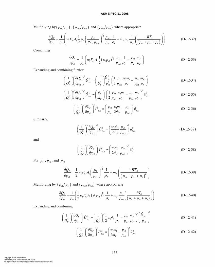
ASME PTC 11-2008

155

Multiplying by ( )1 1s sp p , ( )1 1sa sap p and ( )1 1ta tap p where appropriate

( )

12

1 1 11 1 1 1 1

1 1 1 1 1 1 1 1

1 1 1 1

2v sa tF

n s F ss s s sa sa F ta v s b

p p RTQw F A p m p

p p RT p p p p p pρ

⎛ ⎞−∂ ⎛ ⎞ ⎛ ⎞⎜ ⎟= +⎜ ⎟ ⎜ ⎟⎜ ⎟∂ + +⎝ ⎠ ⎝ ⎠⎝ ⎠ (D-12-32)

Combining

( )11 12

1 1 1 1 11 1 1 1

1 1 1

2s sF F

n vs s sa F ta F

p pQ mw F A p

p p p pρ

ρ ρ∂ ⎛ ⎞= −⎜ ⎟∂ ⎝ ⎠

(D-12-33)


1

1

2222 1 11 1

2 2 21 1 1 1

ˆ1 1 1ˆ2

s

s

p s sF Fp

F s F s sa F ta F

U p pQ w m mU

Q p Q p p pρ ρ∂ ⎛ ⎞⎛ ⎞⎛ ⎞ ⎛ ⎞= −⎜ ⎟⎜ ⎟⎜ ⎟ ⎜ ⎟∂⎝ ⎠ ⎝ ⎠⎝ ⎠ ⎝ ⎠

(D-12-34)

1 1

22 22 21 11 1

21 1 1

1 1ˆ ˆ2s s

s sF F Fp p

F s F sa F ta F

p pQ w m mU u

Q p m p p

ρρ ρ

∂ ⎛ ⎞⎛ ⎞ ⎛ ⎞⎛ ⎞ = −⎜ ⎟⎜ ⎟ ⎜ ⎟⎜ ⎟ ∂⎝ ⎠ ⎝ ⎠⎝ ⎠ ⎝ ⎠ (D-12-35)

1 1

222 21 11 1

21 1 1

1 ˆ ˆ2s s

s sFp p

F s sa F ta

p pQ w mU u

Q p p m p

∂ ⎛ ⎞⎛ ⎞⎛ ⎞ = −⎜ ⎟⎜ ⎟⎜ ⎟ ∂⎝ ⎠⎝ ⎠ ⎝ ⎠ (D-12-36)

Similarly,

2 2

222 222 2

22 2

1 ˆ ˆ2s s

sFp p

F s F sa

pQ w mU u

Q p m p

∂ ⎛ ⎞⎛ ⎞⎛ ⎞ = ⎜ ⎟⎜ ⎟⎜ ⎟ ∂⎝ ⎠⎝ ⎠ ⎝ ⎠ (D-12-37)

and

3 3

222 23 3 3

23 3

1 ˆ ˆ2s s

sFp p

F s F sa

w m pQU u

Q p m p

∂ ⎛ ⎞⎛ ⎞⎛ ⎞ = ⎜ ⎟⎜ ⎟⎜ ⎟ ∂⎝ ⎠⎝ ⎠ ⎝ ⎠ (D-12-38)


( )

12

111 1 1 2

1 1 1 1

1 1

2tF

n Fv v F v s b

RTQw F A m

p p p p p

ρρ

−∂ ⎛ ⎞⎛ ⎞= + ⎜ ⎟⎜ ⎟∂ + +⎝ ⎠ ⎝ ⎠ (D-12-39)

Multiplying by ( )1 1v vp p and ( )1 1ta tap p where appropriate

( ) ( )1

1 121 1 1 1 1

1 1 1 1 1

1 1 1

2v tF

n v Fv v F ta v s b

p RTQw F A p m

p p p p p pρ

ρ⎛ ⎞−∂ ⎛ ⎞= +⎜ ⎟⎜ ⎟∂ + +⎝ ⎠⎝ ⎠

(D-12-40)


1

1

222

2 11 12 2

1 1 1

ˆ1 1 1 1ˆ2

v

v

pvF Fp

F v F F ta F v

UpQ mU w m

Q p Q p pρ ρ⎛ ⎞∂ ⎛ ⎞⎛ ⎞⎛ ⎞ ⎛ ⎞ ⎜ ⎟= −⎜ ⎟⎜ ⎟⎜ ⎟ ⎜ ⎟ ⎜ ⎟∂⎝ ⎠ ⎝ ⎠⎝ ⎠ ⎝ ⎠ ⎝ ⎠

(D-12-41)

1

222 211 1

121 1

1 ˆ ˆ2v

vFp pv

F v F ta

pQ w mU u

Q p m p

∂ ⎛ ⎞⎛ ⎞⎛ ⎞ = −⎜ ⎟⎜ ⎟⎜ ⎟ ∂⎝ ⎠⎝ ⎠ ⎝ ⎠ (D-12-42)


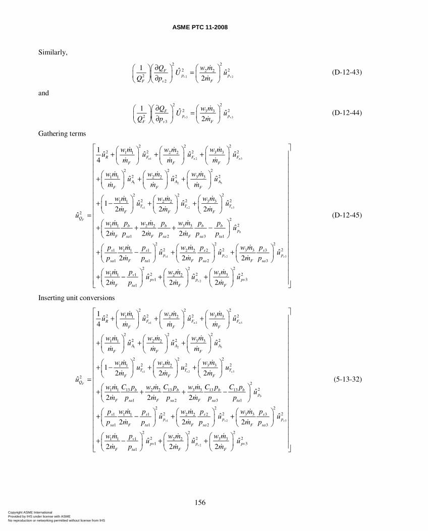
ASME PTC 11-2008

156

Similarly,

2 2

2 22 22 2

22

1 ˆ ˆ2v v

Fp p

F v F

Q w mU u

Q p m

∂⎛ ⎞ ⎛ ⎞⎛ ⎞ =⎜ ⎟ ⎜ ⎟⎜ ⎟ ∂⎝ ⎠ ⎝ ⎠⎝ ⎠ (D-12-43)

and

3 3

222 23 3

23

1 ˆ ˆ2v v

Fp p

F v F

w mQU u

Q p m

∂ ⎛ ⎞⎛ ⎞⎛ ⎞ = ⎜ ⎟⎜ ⎟⎜ ⎟ ∂⎝ ⎠ ⎝ ⎠⎝ ⎠ (D-12-44)

Gathering terms

1 2 3

1 2 3

1 2

22 22 2 2 23 31 1 2 2

22 22 2 23 31 1 2 2

2 22 2 3 31 1 2 2

2

1ˆ ˆ ˆ ˆ

4

ˆ ˆ ˆ

ˆ ˆ12 2 2

ˆ

n n n

s s

F

R F F FF F F

A A AF F F

T TF F F

Q

w mw m w mu u u u

m m m

w mw m w mu u u

m m m

w mw m w mu u

m m mu

⎛ ⎞⎛ ⎞ ⎛ ⎞+ + + ⎜ ⎟⎜ ⎟ ⎜ ⎟⎝ ⎠ ⎝ ⎠ ⎝ ⎠

⎛ ⎞⎛ ⎞ ⎛ ⎞+ + + ⎜ ⎟⎜ ⎟ ⎜ ⎟⎝ ⎠ ⎝ ⎠ ⎝ ⎠

⎛⎛ ⎞ ⎛ ⎞+ − + +⎜ ⎟ ⎜ ⎟⎝ ⎠ ⎝ ⎠=

3

1 2 3

22

223 31 1 2 2

1 2 3 1

2 2 22 2 21 1 2 3 3 31 1 2 2

1 1 2 3

11 1

1

ˆ

ˆ2 2 2

ˆ ˆ ˆ2 2 2

2

s

b

s s s

T

b b b bp

F sa F sa F sa ta

s s s sp p p

sa F ta F sa F sa

v

F ta

u

p p w m p pw m w mu

m p m p m p p


p m p m p m p

pw m

m p

⎞⎜ ⎟⎝ ⎠

⎛ ⎞+ + + −⎜ ⎟⎝ ⎠

⎛ ⎞ ⎛ ⎞ ⎛ ⎞+ − + +⎜ ⎟ ⎜ ⎟ ⎜ ⎟⎝ ⎠ ⎝ ⎠ ⎝ ⎠

⎛ ⎞+ −⎜⎝ ⎠

2

2 222 2 23 32 2

1 3ˆ ˆ ˆ2 2vpv p pv

F F

w mw mu u u

m m

⎡ ⎤⎢ ⎥⎢ ⎥⎢ ⎥⎢ ⎥⎢ ⎥⎢ ⎥⎢ ⎥⎢ ⎥⎢ ⎥⎢ ⎥⎢ ⎥⎢ ⎥⎢ ⎥⎢ ⎥⎢ ⎥⎢ ⎥⎢ ⎥

⎛ ⎞⎛ ⎞⎢ ⎥+ +⎟ ⎜ ⎟⎜ ⎟⎢ ⎥⎝ ⎠ ⎝ ⎠⎣ ⎦

(D-12-45)


1 2 3

1 2 3

1 2

22 22 2 2 23 31 1 2 2

22 22 2 23 31 1 2 2

2 22 2 3 31 1 2 2

2

1ˆ ˆ ˆ ˆ

4

ˆ ˆ ˆ

12 2 2

ˆ

n n n

s s

F

R F F FF F F

A A AF F F

T TF F F

Q

w mw m w mu u u u

m m m

w mw m w mu u u

m m m

w mw m w mu u

m m mu

⎛ ⎞⎛ ⎞ ⎛ ⎞+ + + ⎜ ⎟⎜ ⎟ ⎜ ⎟⎝ ⎠ ⎝ ⎠ ⎝ ⎠

⎛ ⎞⎛ ⎞ ⎛ ⎞+ + + ⎜ ⎟⎜ ⎟ ⎜ ⎟⎝ ⎠ ⎝ ⎠ ⎝ ⎠

⎛⎛ ⎞ ⎛ ⎞+ − + + ⎜⎜ ⎟ ⎜ ⎟⎝ ⎠ ⎝ ⎠ ⎝=

3

1 2 3

22

2213 13 3 3 13 131 1 2 2

1 2 3 1

2 2 22 2 21 1 2 3 3 31 1 2 2

1 1 2 3

11 1

ˆ2 2 2

ˆ ˆ ˆ2 2 2

2

s

b

s s s

T

b b b bp

F sa F sa F sa ta

s s s sp p p

sa F ta F sa F sa

v

F

u


m p m p m p p


p m p m p m p

pw m

m

⎞⎟⎠

⎛ ⎞+ + + −⎜ ⎟⎝ ⎠

⎛ ⎞ ⎛ ⎞ ⎛ ⎞+ − + +⎜ ⎟ ⎜ ⎟ ⎜ ⎟⎝ ⎠ ⎝ ⎠ ⎝ ⎠

+ −2

2 222 2 23 32 2

1 31

ˆ ˆ ˆ2 2vpv p pv

ta F F

w mw mu u u

p m m

⎡ ⎤⎢ ⎥⎢ ⎥⎢ ⎥⎢ ⎥⎢ ⎥⎢ ⎥⎢ ⎥⎢ ⎥⎢ ⎥⎢ ⎥⎢ ⎥⎢ ⎥⎢ ⎥⎢ ⎥⎢ ⎥⎢ ⎥⎢ ⎥⎛ ⎞ ⎛ ⎞⎛ ⎞⎢ ⎥+ +⎜ ⎟ ⎜ ⎟⎜ ⎟⎢ ⎥⎝ ⎠ ⎝ ⎠⎝ ⎠⎣ ⎦

(5-13-32)


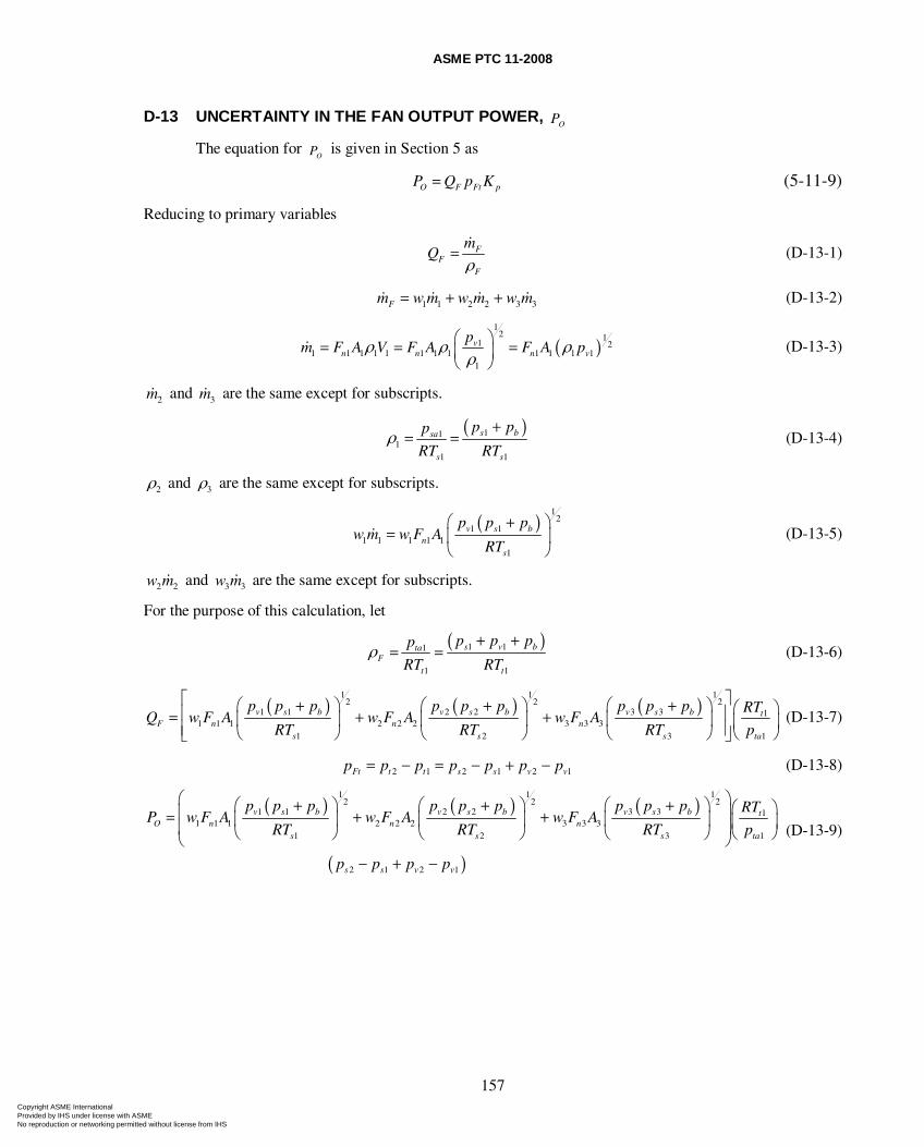
ASME PTC 11-2008

157

D-13 UNCERTAINTY IN THE FAN OUTPUT POWER, OP

The equation for OP is given in Section 5 as

O F Ft pP Q p K= (5-11-9)


FF

F

mQ

ρ= (D-13-1)

1 1 2 2 3 3Fm w m w m w m= + + (D-13-2)

( )1

2 11 2

1 1 1 1 1 1 1 1 1 1 1 11

vn n n v


ρ⎛ ⎞= = =⎜ ⎟⎝ ⎠

(D-13-3)


( )11

11 1

s bsa

s s

p pp

RT RTρ

+= = (D-13-4)


( )

12

1 11 1 1 1 1

1

v s bn

s

p p pw m w F A

RT

⎛ + ⎞= ⎜ ⎟

⎝ ⎠ (D-13-5)


For the purpose of this calculation, let

( )1 11

1 1

s v btaF

t t

p p pp

RT RTρ

+ += = (D-13-6)

( ) ( ) ( )1 1 1

2 2 21 1 2 2 3 3 1

1 1 1 2 2 2 3 3 31 2 3 1

v s b v s b v s b tF n n n

s s s ta

p p p p p p p p p RTQ w F A w F A w F A

RT RT RT p

⎡ ⎤⎛ + ⎞ ⎛ + ⎞ ⎛ + ⎞ ⎛ ⎞⎢ ⎥= + +⎜ ⎟ ⎜ ⎟ ⎜ ⎟ ⎜ ⎟⎢ ⎥⎝ ⎠ ⎝ ⎠ ⎝ ⎠ ⎝ ⎠⎣ ⎦ (D-13-7)

2 1 2 1 2 1Ft t t s s v vp p p p p p p= − = − + − (D-13-8)

( ) ( ) ( )

( )

1 1 12 2 2

1 1 2 2 3 3 11 1 1 2 2 2 3 3 3

1 2 3 1

2 1 2 1

v s b v s b v s b tO n n n

s s s ta

s s v v

p p p p p p p p p RTP w F A w F A w F A

RT RT RT p

p p p p

⎛ ⎞⎛ + ⎞ ⎛ + ⎞ ⎛ + ⎞ ⎛ ⎞⎜ ⎟= + +⎜ ⎟ ⎜ ⎟ ⎜ ⎟ ⎜ ⎟⎜ ⎟⎝ ⎠ ⎝ ⎠ ⎝ ⎠ ⎝ ⎠⎝ ⎠− + −

(D-13-9)


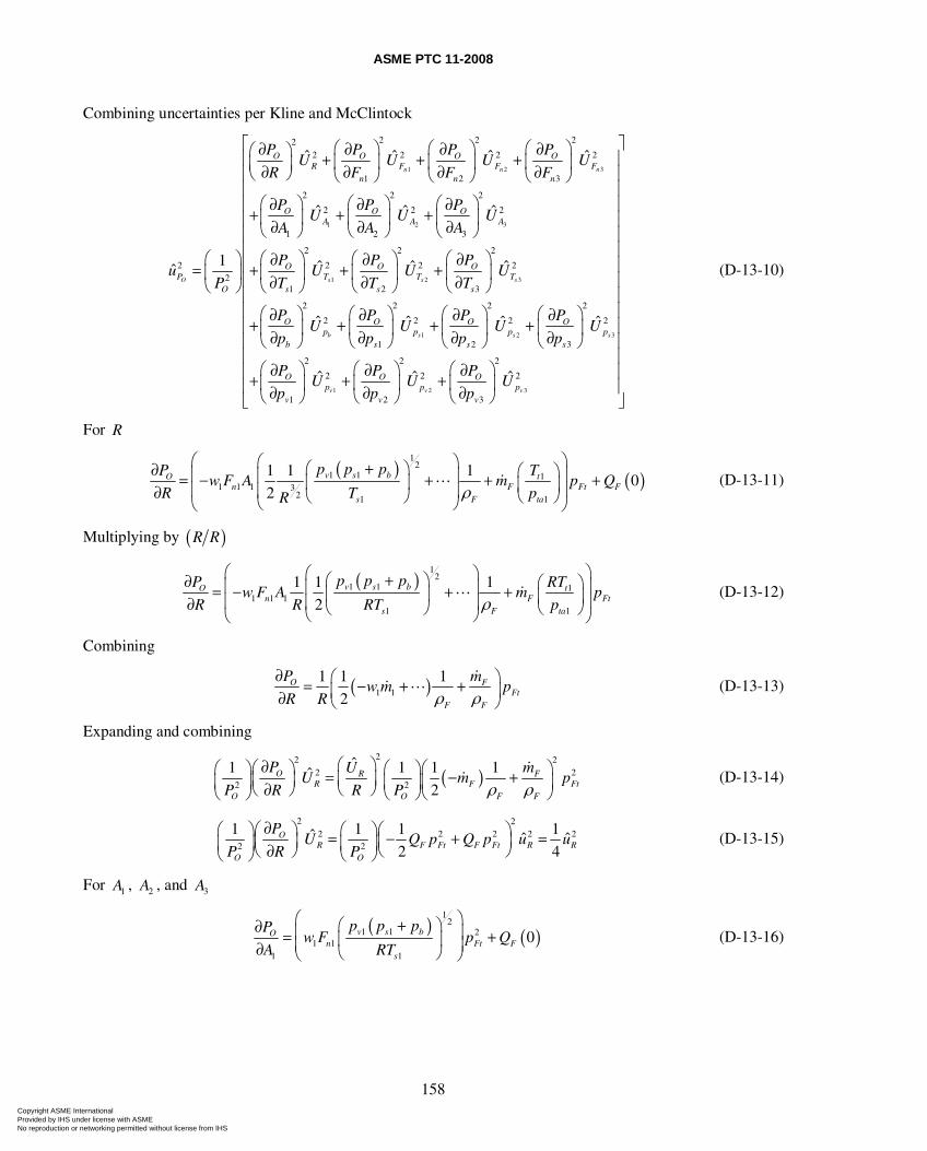
ASME PTC 11-2008

158


1 2 3

1 2 3

1 2

2 2 222 2 2 2

1 2 3

22 2

2 2 2

1 2 3

2 2

2 2 22

1 2

ˆ ˆ ˆ ˆ

ˆ ˆ ˆ

1 ˆ ˆˆ

n n n

O s s

O O O OR F F F

n n n

O O OA A A

O O OP T T

O s s

P P P PU U U U

R F F F

P P PU U U

A A A

P P Pu U U

P T T T

⎛ ⎞ ⎛ ⎞ ⎛ ⎞∂ ∂ ∂ ∂⎛ ⎞ + + +⎜ ⎟ ⎜ ⎟ ⎜ ⎟⎜ ⎟∂ ∂ ∂ ∂⎝ ⎠ ⎝ ⎠ ⎝ ⎠ ⎝ ⎠

⎛ ⎞⎛ ⎞ ⎛ ⎞∂ ∂ ∂+ + + ⎜ ⎟⎜ ⎟ ⎜ ⎟∂ ∂ ∂⎝ ⎠ ⎝ ⎠ ⎝ ⎠

⎛ ⎞ ⎛ ⎞ ⎛ ⎞∂ ∂ ∂= + + +⎜ ⎟ ⎜ ⎟ ⎜ ⎟∂ ∂ ∂⎝ ⎠ ⎝ ⎠ ⎝ ⎠

3

1 2 3

1 2 3

2

2

3

2 2 2 2

2 2 2 2

1 2 3

2 2 2

2 2 2

1 2 3

ˆ

ˆ ˆ ˆ ˆ

ˆ ˆ ˆ

s

b s s s

v v v

Ts

O O O Op p p p

b s s s

O O Op p p

v v v

U

P P P PU U U U

p p p p

P P PU U U

p p p

⎡ ⎤⎢ ⎥⎢ ⎥⎢ ⎥⎢ ⎥⎢ ⎥⎢ ⎥⎢ ⎥⎛ ⎞⎢ ⎥⎜ ⎟⎢ ⎥⎝ ⎠⎢ ⎥⎢ ⎥⎛ ⎞ ⎛ ⎞ ⎛ ⎞ ⎛ ⎞∂ ∂ ∂ ∂+ + + +⎢ ⎥⎜ ⎟ ⎜ ⎟ ⎜ ⎟ ⎜ ⎟∂ ∂ ∂ ∂⎢ ⎥⎝ ⎠ ⎝ ⎠ ⎝ ⎠ ⎝ ⎠⎢ ⎥⎛ ⎞ ⎛ ⎞ ⎛ ⎞∂ ∂ ∂⎢ ⎥+ + +⎜ ⎟ ⎜ ⎟ ⎜ ⎟⎢ ⎥∂ ∂ ∂⎝ ⎠ ⎝ ⎠ ⎝ ⎠⎣ ⎦

(D-13-10)

For R

( ) ( )

12

1 1 11 1 1 3

2 1 1

1 1 10

2v s bO t

n F Ft Fs F ta

p p pP Tw F A m p Q

R T pR ρ

⎛ ⎞⎛ ⎞⎛ + ⎞∂ ⎛ ⎞⎜ ⎟⎜ ⎟= − + + +⎜ ⎟ ⎜ ⎟⎜ ⎟⎜ ⎟∂ ⎝ ⎠ ⎝ ⎠⎝ ⎠⎝ ⎠

(D-13-11)

Multiplying by ( )R R

( )

12

1 1 11 1 1

1 1

1 1 1

2v s bO t

n F Fts F ta

p p pP RTw F A m p

R R RT pρ

⎛ ⎞⎛ ⎞⎛ + ⎞∂ ⎛ ⎞⎜ ⎟⎜ ⎟= − + +⎜ ⎟ ⎜ ⎟⎜ ⎟⎜ ⎟∂ ⎝ ⎠⎝ ⎠⎝ ⎠⎝ ⎠

(D-13-12)

Combining

( )1 1

1 1 1

2O F

FtF F

P mw m p

R R ρ ρ∂ ⎛ ⎞= − + +⎜ ⎟∂ ⎝ ⎠

(D-13-13)


( )22 2

2 22 2

ˆ1 1 1 1ˆ2

O R FR F Ft

O O F F

P U mU m p

P R R P ρ ρ⎛ ⎞∂⎛ ⎞ ⎛ ⎞⎛ ⎞ ⎛ ⎞= − +⎜ ⎟⎜ ⎟ ⎜ ⎟⎜ ⎟ ⎜ ⎟∂ ⎝ ⎠⎝ ⎠ ⎝ ⎠⎝ ⎠ ⎝ ⎠

(D-13-14)

2 2

2 2 2 2 22 2

1 1 1 1ˆ ˆ ˆ2 4

OR F Ft F Ft R R

O O

PU Q p Q p u u

P R P

∂⎛ ⎞⎛ ⎞ ⎛ ⎞⎛ ⎞= − + =⎜ ⎟⎜ ⎟⎜ ⎟ ⎜ ⎟∂ ⎝ ⎠⎝ ⎠⎝ ⎠ ⎝ ⎠ (D-13-15)

For 1A , 2A , and 3A

( ) ( )

12

1 1 21 1

1 1

0v s bOn Ft F

s

p p pPw F p Q

A RT

⎛ ⎞⎛ + ⎞∂ ⎜ ⎟= +⎜ ⎟⎜ ⎟∂ ⎝ ⎠⎝ ⎠ (D-13-16)


ASME PTC 11-2008

159

Multiplying by ( )1A A

( )

12

1 1 21 1 1

1 1 1

1 v s bOn Ft

s

p p pPw F A p

A A RT

⎛ ⎞⎛ + ⎞∂ ⎜ ⎟= ⎜ ⎟⎜ ⎟∂ ⎝ ⎠⎝ ⎠ (D-13-17)


( )1

1

22

22 21 12 2

1 1

ˆ1 1ˆ AOA Ft

O O

UPU w m p

P A P A

⎛ ⎞∂⎛ ⎞⎛ ⎞ ⎛ ⎞⎜ ⎟=⎜ ⎟⎜ ⎟ ⎜ ⎟⎜ ⎟∂⎝ ⎠ ⎝ ⎠⎝ ⎠ ⎝ ⎠ (D-13-18)

1 1

2 22 21 1

21

1 ˆ ÔA A

O F

P w mU u

P A m

∂⎛ ⎞ ⎛ ⎞⎛ ⎞ =⎜ ⎟ ⎜ ⎟⎜ ⎟ ∂⎝ ⎠ ⎝ ⎠⎝ ⎠ (D-13-19)

Similarly

2 2

2 22 22 2

22

1 ˆ ÔA A

O F

P w mU u

P A m

∂⎛ ⎞ ⎛ ⎞⎛ ⎞ =⎜ ⎟ ⎜ ⎟⎜ ⎟ ∂⎝ ⎠ ⎝ ⎠⎝ ⎠ (D-13-20)

3 3

2 22 23 3

23

1 ˆ ÔA A

O F

P w mU u

P A m

∂⎛ ⎞ ⎛ ⎞⎛ ⎞ =⎜ ⎟ ⎜ ⎟⎜ ⎟ ∂ ⎝ ⎠⎝ ⎠⎝ ⎠ (D-13-21)


( ) ( )

12

1 11 1 1 3

21 11

1 1 10

2v s bO

n F Ft FF tas

p p pP Rw F A m p Q

T R pT ρ

⎛ ⎞⎛ + ⎞∂ ⎜ ⎟= − + +⎜ ⎟⎜ ⎟∂ ⎝ ⎠⎝ ⎠ (D-13-22)


( )

12

1 1 1 11 1 1 1

1 1 1 1 1

1 1 1

2v s bO s t

n F Fts s s F ta

p p pP T RTw F A m p

T T RT T pρ

⎛ ⎞⎛ + ⎞∂ ⎛ ⎞⎜ ⎟= − +⎜ ⎟⎜ ⎟⎜ ⎟∂ ⎝ ⎠ ⎝ ⎠⎝ ⎠ (D-13-23)


1

1

22 22

21 1 12

1 1

ˆ1 1 1 1ˆ2

s

s

TO FtT F Ft

O s s O F F

UP pU w m m p

P T T P ρ ρ⎛ ⎞∂⎛ ⎞ ⎛ ⎞⎛ ⎞ ⎛ ⎞⎜ ⎟= − +⎜ ⎟ ⎜ ⎟⎜ ⎟ ⎜ ⎟⎜ ⎟∂ ⎝ ⎠⎝ ⎠⎝ ⎠ ⎝ ⎠ ⎝ ⎠

(D-13-24)

1

1

22 2

21 12

1 1

ˆ1 1 1ˆ 12

s

s

TOT

O s s F

UPU w m

P T T m

⎛ ⎞∂⎛ ⎞⎛ ⎞ ⎛ ⎞⎜ ⎟= − +⎜ ⎟⎜ ⎟ ⎜ ⎟⎜ ⎟∂ ⎝ ⎠⎝ ⎠⎝ ⎠ ⎝ ⎠ (D-13-25)

1 1

2 22 21 1

21

1 ˆ ˆ12s s

OT T

O s F

P w mU u

P T m

∂⎛ ⎞ ⎛ ⎞⎛ ⎞ = −⎜ ⎟ ⎜ ⎟⎜ ⎟ ∂ ⎝ ⎠⎝ ⎠⎝ ⎠ (D-13-26)

Similarly,

2 2

2 22 22 2

22

1 ˆ ˆ2s s

OT T

O s F

P w mU u

P T m

∂⎛ ⎞ ⎛ ⎞⎛ ⎞ =⎜ ⎟ ⎜ ⎟⎜ ⎟ ∂ ⎝ ⎠⎝ ⎠⎝ ⎠ (D-13-27)


ASME PTC 11-2008

160

3 3

2 22 23 3

23

1 ˆ ˆ2s s

OT T

O s F

P w mU u

P T m

∂⎛ ⎞ ⎛ ⎞⎛ ⎞ =⎜ ⎟ ⎜ ⎟⎜ ⎟ ∂ ⎝ ⎠⎝ ⎠⎝ ⎠ (D-13-28)

For bp

( ) ( ) ( )

( )

1 1 12 2 2

1 2 31 1 1 2 2 2 3 3 3

1 1 2 2 3 3

12

1 1

1 1 1 1

2 2 2

v v vn n n

s s b s s b s s b FO

b tF

s v b

p p pw F A w F A w F A


p RTm

p p p

ρ

⎛ ⎞⎛ ⎞⎛ ⎞ ⎛ ⎞ ⎛ ⎞⎜ ⎟⎜ ⎟+ +⎜ ⎟ ⎜ ⎟ ⎜ ⎟⎜ ⎟⎜ + + +∂ ⎝ ⎠ ⎝ ⎠ ⎝ ⎠⎝ ⎠= ⎜∂ ⎜ −⎛ ⎞+⎜ ⎜ ⎟⎜ + +⎝ ⎠⎝ ⎠

( )0Ft Fp Q⎟

+⎟⎟⎟⎟

(D-13-29)

Multiplying by ( )b bp p , ( )R R , ( )sax saxp p , and ( )1 1ta tap p where appropriate

( )( )

( )( )

( )( )

1 1 12 2 2

1 1 2 2 3 31 1 1 2 2 2 3 3 32 2 2

1 1 2 2 3 3

1 1 1

2 2 21

v s b v s b v s b Ftn b n b n b

Fs s b s s b s s bO

b b

p p p p p p p p p pw F A p w F A p w F A p


p p

ρ

⎛ ⎞⎛ + ⎞ ⎛ + ⎞ ⎛ + ⎞⎜ ⎟+ +⎜ ⎟ ⎜ ⎟ ⎜ ⎟⎜ ⎟ ⎜ ⎟ ⎜ ⎟⎜ ⎟+ + +∂ ⎛ ⎞ ⎝ ⎠ ⎝ ⎠ ⎝ ⎠⎝ ⎠= ⎜ ⎟∂ ⎝ ⎠

( )1

1 1 1

b tF Ft

ta s v b

p RTm p

p p p p

⎛ ⎞⎜ ⎟⎜ ⎟⎜ ⎟⎜ ⎟−⎛ ⎞⎜ ⎟+ ⎜ ⎟⎜ ⎟+ +⎝ ⎠⎝ ⎠

(D-13-30)


( ) ( ) ( )22 2

1 1 1 22 2 21 1 1 1 1 2 2 2 2 2 3 3 3 3 3

1 2 3 1

1 1 1 1 1

2 2 2O b b b b F

n v n v n v Ftb b sa sa sa F ta F

P p p p p mw F A p w F A p w F A p p

p p p p p pρ ρ ρ

ρ ρ⎛ ⎞⎛ ⎞ ⎛ ⎞∂ ⎛ ⎞= + + −⎜ ⎟⎜ ⎟ ⎜ ⎟ ⎜ ⎟⎜ ⎟∂⎝ ⎠ ⎝ ⎠ ⎝ ⎠⎝ ⎠

(D-13-31)

2 2 22

2 3 31 1 2 22

1 2 3 1

1 1

2 2 2b

b

pO b b b Ft b Fp Ft

O b b F Ft sa sa sa F ta F

UP p p w m p p pw m w m mU p

P p p Q p p p p pρ ρ⎛ ⎞⎛ ⎞ ⎛ ⎞ ⎛ ⎞∂⎛ ⎞ ⎛ ⎞= + + −⎜ ⎟⎜ ⎟ ⎜ ⎟ ⎜ ⎟⎜ ⎟ ⎜ ⎟∂⎝ ⎠⎝ ⎠ ⎝ ⎠ ⎝ ⎠ ⎝ ⎠⎝ ⎠

(D-13-32)

2 2

2 23 31 1 2 22

1 2 3 1

1

2 2 2b b

O b b b bp p

O b F sa F sa F sa ta

P p p w m p pw m w mU u

P p m p m p m p p

∂⎛ ⎞ ⎛ ⎞⎛ ⎞ = + + −⎜ ⎟ ⎜ ⎟⎜ ⎟ ∂⎝ ⎠⎝ ⎠ ⎝ ⎠ (D-13-33)

For 1sp and 2sp

( ) ( )

( )2

1 11 1 1 2

1 1 2 1 1 1

1 11

2O v t

n F Ft Fs s s s F s b

P p RTw F A m p Q

p RT p p p p pρ

⎛ ⎞⎛ ⎞∂ −⎜ ⎟= + + −⎜ ⎟⎜ ⎟⎜ ⎟∂ − + +⎝ ⎠⎝ ⎠ (D-13-34)

Multiplying by ( )1 1s sp p , ( )1 1sa sap p , and ( )1 1ta tap p where appropriate

( )

12

1 1 11 1 1 1 1 1

1 1 1 1 1 1 1 1

1 1 1 1

2O v sa t

n s F s Ft s Fs s s sa sa F ta s b

P p p RTw F A p m p p p Q

p p RT p p p p p pρ

⎛ ⎞⎛ ⎞⎛ ⎞∂ −⎜ ⎟⎜ ⎟= + −⎜ ⎟⎜ ⎟⎜ ⎟∂ + +⎝ ⎠⎝ ⎠⎝ ⎠ (D-13-35)

Combining

( )11 12

1 1 1 1 1 11 1 1 1

1 1 1

2O s s F

n v Ft s Fs s sa F ta F

P p p mw F A p p p Q

p p p pρ

ρ ρ∂ ⎛ ⎞= − −⎜ ⎟∂ ⎝ ⎠

(D-13-36)


ASME PTC 11-2008

161


1

1

22 22 1 11 1

12 2 21 1 1 1

ˆ1 1 1ˆ2

s

s

pO s sp F Ft s F

O s O s sa F ta

UP p pw mU Q p p Q

P p P p p pρ⎛ ⎞∂⎛ ⎞ ⎛ ⎞⎛ ⎞ ⎛ ⎞= − −⎜ ⎟⎜ ⎟ ⎜ ⎟⎜ ⎟ ⎜ ⎟∂⎝ ⎠⎝ ⎠ ⎝ ⎠ ⎝ ⎠⎝ ⎠

(D-13-37)

1 1

22 22 21 11 1

121 1 1

1 1ˆ ˆ2s s

O s Ft sp F Ft s F p

O s F Ft sa F ta

P p p pw mU Q p p Q u

P p Q p p pρ⎛ ⎞∂⎛ ⎞ ⎛ ⎞⎛ ⎞ ⎛ ⎞= − −⎜ ⎟⎜ ⎟ ⎜ ⎟⎜ ⎟ ⎜ ⎟∂⎝ ⎠⎝ ⎠ ⎝ ⎠ ⎝ ⎠⎝ ⎠

(D-13-38)

1 1

2 22 21 1 11 1

21 1 1

1 ˆ ˆ2s s

O s s sp p

O s F sa ta Ft

P p p pw mU u

P p m p p p

∂⎛ ⎞ ⎛ ⎞⎛ ⎞ = − −⎜ ⎟ ⎜ ⎟⎜ ⎟ ∂⎝ ⎠⎝ ⎠ ⎝ ⎠ (D-13-39)

Similarly,

2 2

2 22 22 22 2

22 2

1 ˆ ˆ2s s

O s sp p

O s F sa Ft

P p pw mU u

P p m p p

∂⎛ ⎞ ⎛ ⎞⎛ ⎞ = +⎜ ⎟ ⎜ ⎟⎜ ⎟ ∂⎝ ⎠⎝ ⎠ ⎝ ⎠ (D-13-40)

and

3 3

2 22 23 3 3

23 3

1 ˆ ˆ2s s

O sp p

O s F sa

P w m pU u

P p m p

∂⎛ ⎞ ⎛ ⎞⎛ ⎞ =⎜ ⎟ ⎜ ⎟⎜ ⎟ ∂⎝ ⎠⎝ ⎠ ⎝ ⎠ (D-13-41)


( )

( )1

211

1 1 1 21 1 1 1

1 11

2O t

n F Ft Fv v F s v b

P Tw F A m p Q

p p p p p

ρρ

⎛ ⎞∂ −⎛ ⎞⎜ ⎟= + + −⎜ ⎟⎜ ⎟∂ + +⎝ ⎠⎝ ⎠ (D-13-42)

Multiplying by ( )1 1v vp p and ( )1 1ta tap p where appropriate

( ) ( )1

1 121 1 1 1 1 1

1 1 1 1 1

1 1 1

2O v t

n v F Ft v Fv v F ta v s b

P p RTw F A p m p p Q

p p p p p pρ

ρ⎛ ⎞∂ −⎛ ⎞= + −⎜ ⎟⎜ ⎟∂ + +⎝ ⎠⎝ ⎠

(D-13-43)


1

1

22 22

2 11 1 12

1 1 1

ˆ1 1 1 1ˆ2

v

v

pO v Fp v F

O v O F ta F v

UP p mU w m p Q

P p P p pρ ρ⎛ ⎞⎛ ⎞ ∂⎛ ⎞ ⎛ ⎞⎛ ⎞ ⎜ ⎟= − −⎜ ⎟⎜ ⎟ ⎜ ⎟⎜ ⎟ ⎜ ⎟∂⎝ ⎠⎝ ⎠ ⎝ ⎠ ⎝ ⎠ ⎝ ⎠

(D-13-44)

1

2 22 21 11 1

121 1

1 ˆ ˆ2v

O v vp pv

O v F ta Ft

P p pw mU u

P p m p p

∂⎛ ⎞ ⎛ ⎞⎛ ⎞ = − −⎜ ⎟ ⎜ ⎟⎜ ⎟ ∂⎝ ⎠⎝ ⎠ ⎝ ⎠ (D-13-45)

Similarly,

2 2

2 22 222 2

22

1 ˆ ˆ2v v

O vp p

O v F Ft

P pw mU u

P p m p

∂⎛ ⎞ ⎛ ⎞⎛ ⎞ = +⎜ ⎟ ⎜ ⎟⎜ ⎟ ∂⎝ ⎠⎝ ⎠ ⎝ ⎠ (D-13-46)

and

3 3

2 22 23 3

23

1 ˆ ˆ2v v

Op p

O v F

P w mU u

P p m

∂⎛ ⎞ ⎛ ⎞⎛ ⎞ =⎜ ⎟ ⎜ ⎟⎜ ⎟ ∂ ⎝ ⎠⎝ ⎠⎝ ⎠ (D-13-47)


ASME PTC 11-2008

162

Gathering terms

1 2 3

1 2 3

1 2

22 22 2 2 23 31 1 2 2

22 22 2 23 31 1 2 2

2 22 2 3 31 1 2 2

2

1ˆ ˆ ˆ

4

ˆ ˆ ˆ

ˆ ˆ12 2 2

ˆ

n n n

s s

O

R F F FF F F

A A AF F F

T TF F F

P

w mw m w mu u u u

m m m

w mw m w mu u u

m m m

w mw m w mu u

m m mu

⎛ ⎞⎛ ⎞ ⎛ ⎞+ + + ⎜ ⎟⎜ ⎟ ⎜ ⎟⎝ ⎠ ⎝ ⎠ ⎝ ⎠

⎛ ⎞⎛ ⎞ ⎛ ⎞+ + + ⎜ ⎟⎜ ⎟ ⎜ ⎟⎝ ⎠ ⎝ ⎠ ⎝ ⎠

⎛ ⎞⎛ ⎞ ⎛ ⎞+ − + + ⎜⎜ ⎟ ⎜ ⎟⎝ ⎠ ⎝ ⎠ ⎝ ⎠=

3

1 2 3

22

223 31 1 2 2

1 2 3 1

2 2 22 2 21 1 1 2 2 3 3 31 1 2 2

1 1 2 3

1 1

ˆ

ˆ2 2 2

ˆ ˆ ˆ2 2 2

2

s

b

s s s

T

b b b bp

F sa F sa F sa ta

s s s s s sp p p


v

F

u

p p w m p pw m w mu

m p m p m p p


m p p p m p p m p

pw m

m

⎟

⎛ ⎞+ + + −⎜ ⎟⎝ ⎠

⎛ ⎞ ⎛ ⎞ ⎛ ⎞+ − − + + +⎜ ⎟ ⎜ ⎟ ⎜ ⎟⎝ ⎠ ⎝ ⎠ ⎝ ⎠

+ −2 3

2 2 22 2 21 1 2 3 32 2

11

ˆ ˆ ˆ2 2v v

v vpv p p

ta Ft F Ft F

p p w mw mu u u

p p m p m

⎡ ⎤⎢ ⎥⎢ ⎥⎢ ⎥⎢ ⎥⎢ ⎥⎢ ⎥⎢ ⎥⎢ ⎥⎢ ⎥⎢ ⎥⎢ ⎥⎢ ⎥⎢ ⎥⎢ ⎥⎢ ⎥⎢ ⎥⎢ ⎥⎛ ⎞ ⎛ ⎞ ⎛ ⎞⎢ ⎥− + + +⎜ ⎟ ⎜ ⎟ ⎜ ⎟⎢ ⎥⎝ ⎠⎝ ⎠ ⎝ ⎠⎣ ⎦

(D-13-48)


1 2 3

1 2 3

1 2

22 22 2 2 23 31 1 2 2

22 22 2 23 31 1 2 2

2 22 2 3 31 1 2 2

2

1ˆ ˆ ˆ ˆ

4

ˆ ˆ ˆ

ˆ ˆ12 2 2

ˆ

n n n

s s

O

R F F FF F F

A A AF F F

T TF F F

P

w mw m w mu u u u

m m m

w mw m w mu u u

m m m

w mw m w mu u

m m mu

⎛ ⎞⎛ ⎞ ⎛ ⎞+ + + ⎜ ⎟⎜ ⎟ ⎜ ⎟⎝ ⎠ ⎝ ⎠ ⎝ ⎠

⎛ ⎞⎛ ⎞ ⎛ ⎞+ + + ⎜ ⎟⎜ ⎟ ⎜ ⎟⎝ ⎠ ⎝ ⎠ ⎝ ⎠

⎛ ⎞⎛ ⎞ ⎛ ⎞+ − + + ⎜⎜ ⎟ ⎜ ⎟⎝ ⎠ ⎝ ⎠ ⎝=

3

1 2 3

22

2213 13 3 3 13 131 1 2 2

1 2 3 1

2 2 22 2 21 1 1 2 2 3 3 31 1 2 2

1 1 2 3

ˆ

2 2 2

ˆ ˆ ˆ2 2 2

s

b

s s s

T

b b b bp

F sa F sa F sa ta

s s s s s sp p p


u


m p m p m p p


m p p p m p p m p

⎟⎠

⎛ ⎞+ + + −⎜ ⎟⎝ ⎠

⎛ ⎞ ⎛ ⎞ ⎛ ⎞+ − − + + +⎜ ⎟ ⎜ ⎟ ⎜ ⎟⎝ ⎠ ⎝ ⎠ ⎝ ⎠

+2 3

2 2 22 2 21 1 2 3 31 1 2 2

11

ˆ ˆ ˆ2 2 2v v

v v vpv p p

F ta Ft F Ft F

p p p w mw m w mu u u

m p p m p m

⎡ ⎤⎢ ⎥⎢ ⎥⎢ ⎥⎢ ⎥⎢ ⎥⎢ ⎥⎢ ⎥⎢ ⎥⎢ ⎥⎢ ⎥⎢ ⎥⎢ ⎥⎢ ⎥⎢ ⎥⎢ ⎥⎢ ⎥⎢ ⎥⎛ ⎞ ⎛ ⎞ ⎛ ⎞⎢ ⎥− − + + +⎜ ⎟ ⎜ ⎟ ⎜ ⎟⎢ ⎥⎝ ⎠⎝ ⎠ ⎝ ⎠⎣ ⎦

(5-13-36)


ASME PTC 11-2008

163

NONMANDATORY APPENDIX E REFERENCES AND FURTHER READING

E-1 REFERENCES

[1] Gerhart, P. M., Jorgensen, R., and Kroll, J. “A Comparison of Two Alternative Methods for Defining Fan Performance,” Journal of Engineering for Power, January 1982.

[2] ASHRAE Standard 51-75/AMCA Standard 210-74, “Laboratory Methods of Testing Fans for Rating.”

[3] Yost, John G. “Field Performance Testing of Large Power Plant Fans,” MSME Thesis, University of Akron, Akron, Ohio.

[4] ISO Standard 5168, “Measurement of Fluid Flow-Estimation of Uncertainty of a Flow-Rate Measurement.”

[5] Kline, S. J., and McClintock, F. A. “Describing Uncertainties in Single-Sample Experiments,” Mechanical Engineering, January 1953.

[6] Brown, N. “A Mathematical Evaluation of Pitot Tube Traverse Methods,” ASHRAE Paper 2325, 1975.

[7] “Draft Proposal for an ISO Standard: Measurement of Fluid Flow in Closed Conduits by the Velocity Area Method Using Pitot-Static Tubes,” ISO/TC-30/SC-3, February 1974.

[8] “Particulate Sampling Strategies for Large Power Plants Including Non-uniform Flow,” EPA Report PB-257-090, June 1976.

[9] Gerhart, P. M., Nuspl, S., Wood, C., and Lovejoy, S. “An Evaluation of Velocity Probes for Measuring Non-uniform Gas Flow in Large Ducts,” Journal of Engineering for Power, October 1979.

[10] Gerhart, P. M., and Dorsey, M. J. “Investigation of Field Test Procedures for Large Fans,” EPRI Report CS 1651, December 1980.

[11] Madhaven, S., DiRe, J., and Wright, T. “Inlet Flow Distortion in Centrifugal Fans,” ASME Paper 84-JPGC-GT-4.

[12] Wright, T., Madhaven, S., and DiRe, J. “Centrifugal Fan Performance With Disturbed Inflows,” ASME Paper 83-JPGC-GT-5.

[13] AMCA Publication 201, Fans and Systems.

[14] Clarke, M. S. “The Implementation and Analysis of a PTC 11 Test Program,” 1982 AMCA Engineering Conference.

[15] Wyler, J. S. “Probe Blockage Effects in Free Jets and Closed Tunnels,” Journal of Engineering for Power, October 1975.

[16] Benedict, R. P. Fundamentals of Temperature, Pressure, and Flow Measurements, 2nd Edition, Wiley-lnterscience, 1977, pp. 356–359.

[17] Gerhart, P. M. “Averaging Methods for Determining the Performance of Large Fans from Field Measurements,” Journal of Engineering for Power, April 1981.

[18] Dean, R. C. (ed.) Aerodynamic Measurements, MIT Gas Turbine Lab Report, 1953.

[19] Obert, E., and Gaggoli, R. Thermodynamics, 2nd Edition, McGraw-Hill Book Co., 1963.

[20] Perry and Chilton. Chemical Engineers Handbook, 5th Edition, McGraw-Hill Book Co., 1973, pp. 3–248.


ASME PTC 11-2008

164

[21] “Compressibility Effects for Industrial Fans,” ISO/TC 117/SC-1, January 1982.

[22] Dorsey, M. J. “Minimizing and Estimation of Uncertainty in Numerical Integration by Controlling the Number and Location of Integration Data Points,” MSME Thesis, August 1986, University of Akron.

E-2 FURTHER READING

Henry, R., Jorgensen, R., and Gerhart, P.M. Uncertainty Analysis in Fan Testing, POWER 2007-22099.

Kaufman, S., and Falk, M. Fan Performance Test and Evaluation Methodology: Addressing the Difficulties of Full and Partial Capacity Testing When the Specified and Site Conditions Don’t Match, POWER 2007-22110.

Nuspl, S., and Gerhart, P. M. Reduced Load Fan Performance Testing for Input Power Determination, POWER 2007-22087.


ASME PTC 11-2008

C05208


Documents

Asme Ptc 11-2008 Fans