Embed Size (px)
Citation preview

ASPECT Hackathon 2019 Preliminary report
ASPECT Hackathon 2019 Preliminary report 1
Introduction 3
Timeline 3
Participants and areas of interest 4
Resources 8 Git Tutorial: 8
Report on projects the participants worked on 9 Update ASPECT to the new deal.II Version 9 Correct the viscosity in global_melt material model 9 SUPG implementation 9 Create the “advection in annulus” benchmark and test it with SUPG 9 Stabilization benchmarks 11 Implement the ability to visualize data only on the surface 12 Convert pieces of code to C++11 12 Add a rigid shear benchmark with an analytical Stokes solution 13 Add a particle plugin that tracks plastic, viscous, or total strain 13 Add an initial temperature model that accounts for anelasticity when converting shear wave velocity to temperature 14 Applications and benchmarks for imposing boundary tractions to a free surface 15 Initial topography function 16 Steady-state continental geotherm initial temperature condition 16 Initial topography for the chunk geometry model 17 Mesh deformation 17 Initial temperature model that sets a constant temperature within a 3D lithosphere 18 Material model that sets a constant viscosity within a 3D lithosphere 19 Viscosity grooves benchmark 20 Polydiapirs 21 Slab detachment 21 A geometric multigrid preconditioner for the Stokes solve 22 A material model that uses density and viscosity inputs constrained by anelastic shear wave velocity to temperature conversion 23 Add some python routines in contrib/ folder 24 Author Networks 24 Anisotropic viscous layer in Rayleigh-Taylor instability cookbook 26 Custom meshes for the spherical shell geometry 27 A numerical model of brittle thrust wedges 29
1

Choi & Petersen 2015 plasticity 31 Isotherm mesh refinement plugin 33 Tester coverage testing 34 Change nonlinear Picard solver to defect correction 34 Refactoring of material models 34 Move the material lookup namespace to material model utilities 34 Add an unstructured table lookup class 34 Create plugin for Frank-Kamenetskii rheology 35 New cookbook for the 2D rigid "punch" indentation benchmark 36 New CRUST1.0 plugin 37
List of hackathon related ASPECT animations 41
Statistics about ASPECT’s growth during the hackathon 44
2

Introduction To further develop the mantle convection code ASPECT and to grow and foster its user community, 24 users and developers of ASPECT worked side-by-side over a 9 day period close to Heber City, Utah in May and June 2019. Below is the timeline and a description of the individual contributions.
Timeline Day Scheduled items
Tuesday, 05/21 Arrival 8 pm: Welcome, Introduction, House rules, Reiterating technical prerequisites
Wednesday, 05/22 9 am: Individual topic introductions, create teams 9:30 am: Git Pull Requests (Rene) 10:30 am: Mesh deformation / Surface processes
Thursday, 05/23 9 am: Morning rounds 11 am: Advection-Diffusion Stabilization 2 pm: IDEs (Timo, Wolfgang) 7 pm: Material Model reorganization
Friday, 05/24 9 am: Morning rounds 9:30 am: Public pull request review (Rene) 10 am: GMG/BFBT Solver improvements 8 pm: Using XSEDE resources
Saturday, 05/25 9 am: Morning rounds Afternoon: Half-day off, Dinner on your own
Sunday, 05/26 9 am: Morning rounds 9:30 am: Showcase ASPECT parameters website 1 pm: Gravity postprocessor
Monday, 05/27 9 am: Morning rounds 1 pm: World builder presentation
Tuesday, 05/28 Day off
Wednesday, 05/29 9 am: Morning rounds 10 am: Q1Q1
3

1 pm: Newton Solver
Thursday, 05/30 9 am: Morning rounds
Friday, 05/31 9 am: Morning rounds 3 pm: FastScape intro / TTLEM
Saturday, 06/01 Check-out and departure before 10am
Participants and areas of interest
Name, affiliation, email Goals and interests for this hackathon
Rene Gassmoeller, UC Davis, [email protected]
1. Help others achieve their goals 2. Review pull requests 3. Add rigid shear benchmark 4. Work on mesh deformation handler 5. Cleanup duty
Lorraine Hwang UC Davis [email protected]
1. Logistics 2. Reporting 3. Baking 4. ASPECT Networks 5. Logistics
Wolfgang Bangerth Colorado State University [email protected]
1. Review pull requests 2. Help others 3. Write documentation 4. Deal with the reference viscosity mess 5. Finish the Q1-Q1 implementation with Cedric
Juliane Dannberg UC Davis [email protected]
1. Help others 2. Review pull requests 3. Make operator splitting faster 4. If there is time, extend melt transport models
Timo Heister University of Utah [email protected]
1. Review pull requests 2. Help others 3. Infrastructure work (testing, cmake, etc.) 4. Linear solvers (multigrid, Schur complement) 5. Geometry representation 6. Stabilization schemes
Cedric Thieulot 1. Polydiapirs cookbook 2. ‘Groovy’ benchmark 3. Work on crust1.0/litho1.0 interface 4. Work on Q1xQ1 paper 5. Work on plasticity
4

Menno Fraters Utrecht University [email protected]
1. Add Newton benchmarks to repository 2. Merge core structure of world generator plugin 3. Review pull requests 4. Help others
John Naliboff UC Davis [email protected]
1. Help others achieve their goals 2. Review pull requests 3. Free surface processes 4. Improve two-phase flow + plasticity
implementation
Anne Glerum 1. Improve free surface normal/vertical projection?
2. Free surface diffusion 3. Coupling to FASTSCAPE 4. Add some initial conditions for continental
rifting (steady-state continental geotherm, crustal and mantle lithosphere layers, strain)
5. Help and review
Paul Bremner University of Florida [email protected]
1. Add function to format a PerpleX table for use in ASPECT
2. Implement the ability to lookup material properties from PerpleX tables on the fly
3. Complete and implement functions to calculate properties of mineral grain size
4. Help anyone working on converting seismic velocities to temperature
Marie Kajan University of Florida [email protected]
1. Work on new mesh plugin for 3-D spherical shell geometry
2. Implement log-space interpolation of viscosity (for ASCII input)
3. (At least start to) work on self-gravity
Grant Euen Virginia Tech [email protected]
1. Compare/contrast points of order for low Rayleigh number spherical shell convection
2. Create benchmark to test advection stabilization
3. Contribute notes back to manual 4. Look into SUPG etc, and determine the status
of higher Rayleigh number cases 5. If all else goes well, begin implementation of
impact modeling into modern code
Marine Lasbleis Université de Nantes [email protected]
1. Check and use 2-phase flow in spherical geometry, with fluid going through the boundary
2. Change the melting/freezing in 2-phase flow to not use peridotite in the core
3. Look into surface deformation/mesh
5

deformation to “grow” the inner core 4. See if/how we can share jupyter
notebooks/python codes for processing data.
Stephanie Sparks Arizona State University [email protected]
1. Surface boundary condition/mesh deformation 2. Coupling ASPECT to landscape evolution
models 3. Simplified lithospheric-scale material models
Derek Neuharth GFZ Potsdam [email protected]
1. Mesh deformation and coupling with surface processes.
2. Free surface and particles
Agnes Kiraly CEED, University of Oslo [email protected]
Anisotropic viscosity 1. Cookbook with Rayleigh Taylor instability
(after Lev and Hager and Perry-Houts) 2. Include olivine slip system parameters 3. Include olivine texture development model
Sibiao Liu University of Illinois at Urbana-Champaign [email protected]
1. Benchmark of sandbox shortening model 2. Include composition fields all-in-one output
parameter in visualization 3. Top boundary condition 4. Regional subduction model with chunk 3D
geometry and velocity BC from CitcomS
Conrad Clevenger Clemson University [email protected]
1. Create/merge pull request for initial GMG Stokes solver
2. Add no-normal flux BCs to Stokes solve 3. BFBT for Schur complement
Fred Richards Harvard University [email protected]
1. Initial temperature condition that reads absolute Vs file and converts to temperature using various anelasticity parameterisations.
2. Link anelasticity parameterisations to material model to self-consistently initialise viscosity and density.
3. LAB plugin to treat lithosphere differently from convecting interior.
Sophie Coulson Harvard University [email protected]
1. Initial temperature condition that has constant temperature in lithosphere - applied on top of any other initial temperature model
2. Material model that also reads in 3D LAB 3. Learn more about relevant material models
Fiona Clerc MIT/WHOI [email protected]
1. Normal forces on free surface 2. Benchmarks of post-glacial rebound 3. Benchmarks with melt production (Iceland)
Bob Myhill 1. Integration of thermodynamic data (with Paul)
6

University of Bristol [email protected]
2. Add cookbook/longer section in the manual for thermodynamically consistent material models, update these models to the new structure.
3. Relaxation of topography (on Mars, with John) a. Check/fix initial topography for
chunk/ellipsoidal chunk/spherical shell b. Implement topo model from MOLA.
4. Extend ULVZ melt model (with Juliane)
Ludovic Jeanniot Utrecht University [email protected]
1. Crust1.0 plugin (with John and Cedric) 2. Cookbook Crust1.0 with gravity postprocessor 3. Custom Spherical shell mesh generation (with
Marie and Wolfgang) 4. Initial topography on spherical shell (same as
for the chunk geometry - Anne)
Jeroen van Hunen Durham University, UK [email protected]
1. Converting melt_global material model into a (de)hydration model
2. Apply to slab dehydration.
7

Resources
Git Tutorial: - Git commands cheat sheet: https://education.github.com/git-cheat-sheet-education.pdf - Github workflow: https://guides.github.com/introduction/flow/ - Git tutorial: https://swcarpentry.github.io/git-novice/
1. Explain and set up Git:
a. https://swcarpentry.github.io/git-novice/01-basics/index.html b. https://swcarpentry.github.io/git-novice/02-setup/index.html
2. Explain Github Workflow: a. https://guides.github.com/introduction/flow/ b. Ensure forked repositories c. Ensure proper remotes
3. Walkthrough a. Create Branch
i. ‘git checkout master’ ii. ‘git pull upstream master’ iii. ‘git checkout -b remove_dealii_compatibility_fix’
b. Make changes for DEAL_II_VERSION_GTE in one of: i. source/postprocess/heat_flux_map.cc ii. source/postprocess/depth_average.cc iii. source/postprocess/stokes_residual.cc iv. source/simulator/melt.cc v. source/simulator/helper_functions.cc vi. source/simulator/core.cc vii. source/simulator/solver.cc viii. source/simulator/assemblers/advection.cc ix. source/utilities.cc
c. Create commit i. ‘git add FILE’ ii. ‘git commit -m ‘Removed a now unnecessary compatibility fix’
d. Push and open PR i. ‘git push origin remove_dealii_compatibility_fix’ ii. Open PR on github (CTRL-Click on shown link)
e. Wait for review f. Address review (repeat steps b,c,d) g. Success!
4. Now repeat the steps in 3. on your own. Pick a section of the manual that interests you. Find a sentence or description or formula to improve. Then repeat 3. and make your changes to the file doc/manual/manual.tex.
8

Report on projects the participants worked on
Update ASPECT to the new deal.II Version (Timo Heister, Rene Gassmöller, Fred Richards, Grant Euen, Stephanie Sparks, and others) We removed support for deal.II 8.5 and removed the remaining compatibility code in ASPECT.
Correct the viscosity in global_melt material model (Marine Lasbleis) The global melt material model was set up so that without melting/freezing, the system would not be modified by existing melts (in particular, the viscosity was not modified by porosity). This would be OK if the only way to get a non-zero porosity would be through freezing/melting. However, it’s also possible to have non-zero porosity from initial conditions or boundary conditions.
SUPG implementation (Timo Heister, Thomas C. Clevenger) ASPECT has used the “entropy viscosity” (EV) stabilization method by Guermond et al. for the temperature and compositional equations since the very beginning. However, recent benchmarking has shown that it is, despite its sophistication, actually quite diffusive and requires a rather fine mesh to reproduce certain benchmarks. As a consequence, we have now also implemented the Streamline Upwind/Petrov Galerkin (SUPG) method for stabilization, a rather old method that nevertheless is widely used and has shown very positive properties in other codes. The following sections demonstrate its qualities in comparison to the EV method on several test cases.
Create the “advection in annulus” benchmark and test it with SUPG (Grant Euen, Rene Gassmoeller, Timo Heister) In order to figure out what parameters have an effect on the amount of cooling out of the model, the 2d annulus benchmark was modified. The advection_in_annulus benchmark runs a very simple annulus with prescribed Stokes flow creating four convection cells. Various parameters were tested, including temperature polynomial degree, thermal conductivity, and the stabilization parameters beta and cR. Using this benchmark to test EV (the “entropy viscosity”, currently used in ASPECT as the stabilization method) and the newly-implemented SUPG shows that fine resolutions are indistinguishable. However, coarse resolutions show that EV
9

results in a much larger amount of diffusion. Convergence testing of average and maximum temperature versus mesh refinement and the stabilization parameters show that smaller stabilization parameters can be used for higher order temperature elements. The following pictures show the EV approach on the left and SUPG on the right. The top row is on a fine mesh where the two methods yield essentially the same solution; the bottom is on a coarse mesh, where EV clearly is too diffusive.
10
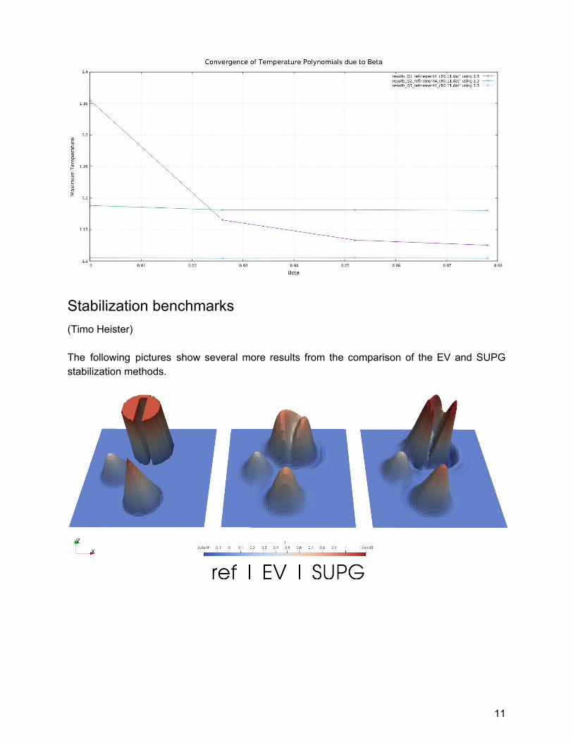
Stabilization benchmarks (Timo Heister) The following pictures show several more results from the comparison of the EV and SUPG stabilization methods.
11

Implement the ability to visualize data only on the surface (Wolfgang Bangerth) Some data lives only on the surface of the model. Examples are heat flux densities, dynamic topography, etc. In those cases, we have always output the relevant data as volume data (i.e., on every cell of the mesh). For purposes of visualization, this is sufficient since one then just visualizes the surface of this bulk data. But it is wasteful in terms of disk space and inefficient regarding the time necessary to visualize large data sets. During the hackathon, I have started a revamp of the system that created graphical output. The end result will be a system in which a visualization postprocessor can say whether it wants to produce volume or surface data, and in the latter case its output will be directed through channels that only visualize data on faces of the mesh located at the surface. The data will then end up in a separate set of output files.
Convert pieces of code to C++11 (Wolfgang Bangerth) The most recent ASPECT version was the first one that required the compiler to understand the C++11 language standard. This has allowed the use of certain (new) language features, and these new features were frequently used in new pieces of code. But there was little effort to convert existing pieces of code to the new standard to improve correctness and readability. To address this in at least one regard, all places where we used the std::shared_ptr class in a way that didn’t actually require sharing the pointer were converted to std::unique_ptr. This makes the code safer since it avoids the inadvertent sharing of objects, for example in compiler-generated
12

copy constructors. It has also allowed us to identify several places in the code that happened to work more by accident than by design.
Add a rigid shear benchmark with an analytical Stokes solution (Rene Gassmoeller) I added a new “rigid shear” benchmark case that I developed for a publication. It features a manufactured solution for the Stokes equation that is stationary in time. Therefore it can be used to test different advection methods, and how their accuracy influences the accuracy of the Stokes equation. It features a box with tangential velocities at each side, and shear and rotational velocity components in the interior. The following picture shows how particles (colored for better visibility) are transported along with the flow field defined by this benchmark.
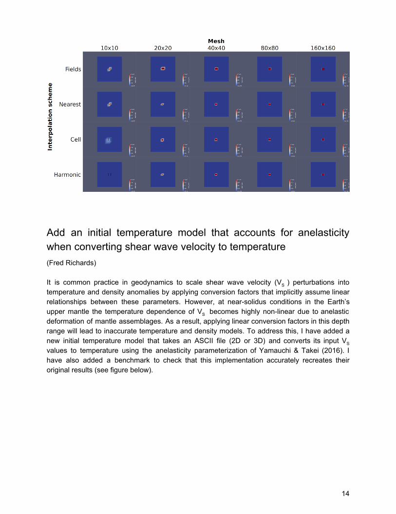
Add a particle plugin that tracks plastic, viscous, or total strain (Derek Neuharth and Anne Glerum) We added a new plugin which works in combination with the viscoplastic material model to track the plastic and/or viscous, or total strain with particles. The below figure shows a comparison of the visco_plastic_yield_plastic_strain_weakening test at a variety of resolutions and with compositional fields, and the cell/harmonic average and nearest neighbor particle interpolation schemes. The black box (if even visible) shows the defined seed location.
13
Add an initial temperature model that accounts for anelasticity when converting shear wave velocity to temperature (Fred Richards) It is common practice in geodynamics to scale shear wave velocity (VS ) perturbations into temperature and density anomalies by applying conversion factors that implicitly assume linear relationships between these parameters. However, at near-solidus conditions in the Earth’s upper mantle the temperature dependence of VS becomes highly non-linear due to anelastic deformation of mantle assemblages. As a result, applying linear conversion factors in this depth range will lead to inaccurate temperature and density models. To address this, I have added a new initial temperature model that takes an ASCII file (2D or 3D) and converts its input VS values to temperature using the anelasticity parameterization of Yamauchi & Takei (2016). I have also added a benchmark to check that this implementation accurately recreates their original results (see figure below).
14

Applications and benchmarks for imposing boundary tractions to a free surface (Fiona Clerc, John Naliboff, Cedric Thieulot) This project involves adapting ASPECT to allow non-zero boundary tractions on the free surface and benchmarking the implementation against analytical solutions and other codes (ELEFANT). This is useful when, for example, modeling a heavy overburden that is not considered a part of the domain – e.g., an ice sheet.
15
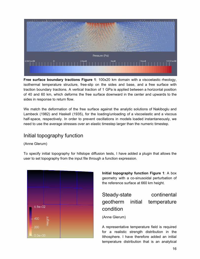
Free surface boundary tractions Figure 1: 100x20 km domain with a viscoelastic rheology, isothermal temperature structure, free-slip on the sides and base, and a free surface with traction boundary tractions. A vertical traction of 1 GPa is applied between a horizontal position of 40 and 60 km, which deforms the free surface downward in the center and upwards to the sides in response to return flow. We match the deformation of the free surface against the analytic solutions of Nakiboglu and Lambeck (1982) and Haskell (1935), for the loading/unloading of a viscoelastic and a viscous half-space, respectively. In order to prevent oscillations in models loaded instantaneously, we need to use the average stresses over an elastic timestep larger than the numeric timestep.
Initial topography function (Anne Glerum) To specify initial topography for hillslope diffusion tests, I have added a plugin that allows the user to set topography from the input file through a function expression.
Initial topography function Figure 1: A box geometry with a co-sinusoidal perturbation of the reference surface at 660 km height.
Steady-state continental geotherm initial temperature condition (Anne Glerum) A representative temperature field is required for a realistic strength distribution in the lithosphere. I have therefore added an initial temperature distribution that is an analytical
16

solution of the 1D conductive heat equation. It takes into account a three-layer lithospheric system with layer-constant radioactive heating rates, densities and thermal conductivities that are read from the heating and material model input directly to avoid duplication of parameters. The initial temperature condition can be combined with other temperature plugins that specify the temperature below the lithosphere-asthenosphere boundary.
Steady-state continental geotherm Figure 1. The initial temperature distribution for the continental extension cookbook as obtained with the lengthy function expression in the parameter file (upper left) and with the new plugin (lower left). Both methods give the same 1D temperature profile (right), but the plugin only requires a surface and LAB temperature from the user.
Initial topography for the chunk geometry model (Anne Glerum and Bob Myhill) When including crustal and lithospheric thickness models for the initial composition conditions or to investigate the response to topographic loads, it is useful to also include data on the topography by perturbing the initial mesh. With the new plugin such perturbations can now be prescribed to the chunk geometry model after being read from Ascii data. We have used this on an example describing the Martian surface.
Mesh deformation (Rene Gassmoeller, Anne Glerum, Derek Neuharth, Marine Lasbleis) We continued Rene’s work to move the free surface code into a framework for any kind of mesh deformation, like a prescribed function on a boundary or diffusion of the surface. An example of a 2D sphere growing with a linear function is shown below, using a model of the growth of Earth’s inner core:
17

Initial temperature model that sets a constant temperature within a 3D lithosphere (Sophie Coulson) Shear wave velocity variations in the lithosphere are often generated by compositional variations rather than temperature induced density variations. This means that Vs-to-temperature scalings used in the initial temperature plug-ins for whole mantle models are often not valid in the lithosphere, and therefore give unphysical temperatures at shallow depths. I have added an initial temperature plugin (to be used in conjunction with the “replace if valid” operator) which reads in an ASCII file specifying the depth of the lithosphere at each lat/long point. The temperature within the lithosphere is set to a constant and the temperature beneath the lithosphere-asthenosphere boundary is taken from any other initial temperature plug-in. The figure below shows the temperature in the lithosphere set to 1600 K, with temperature perturbation below calculated from SL2013 and S40RTS (using the “Patch on S40RTS” initial temperature model).
18
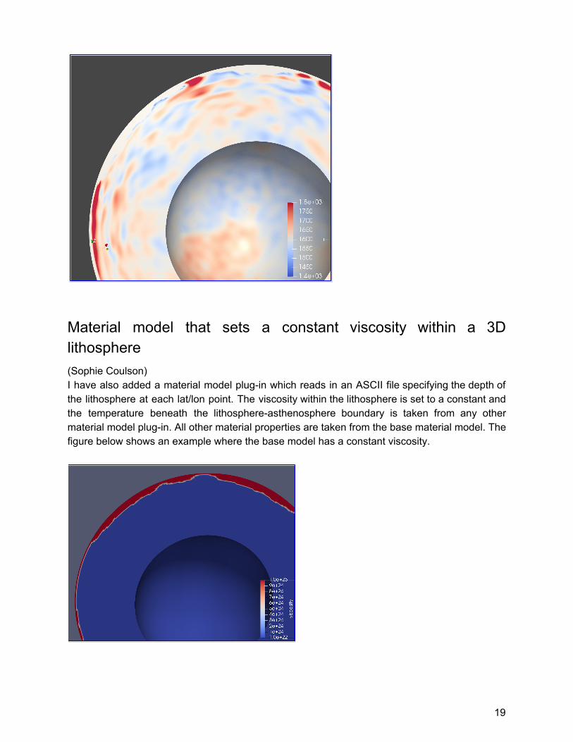
Material model that sets a constant viscosity within a 3D lithosphere (Sophie Coulson) I have also added a material model plug-in which reads in an ASCII file specifying the depth of the lithosphere at each lat/lon point. The viscosity within the lithosphere is set to a constant and the temperature beneath the lithosphere-asthenosphere boundary is taken from any other material model plug-in. All other material properties are taken from the base material model. The figure below shows an example where the base model has a constant viscosity.
19

Viscosity grooves benchmark (Cedric Thieulot) Following a private communication with Dave May a few years back I have implemented his benchmark which showcases a (potentially) large number of low viscosity grooves. Although the velocity and the pressure fields are smooth functions, the presence of large viscosity contrasts in the domain which do not align with the mesh makes this benchmark particularly challenging for the solver(s).
20

Polydiapirs (Cedric Thieulot) I have added a benchmark which models the time evolution of a polydiapiric system composed of 3 layers with different densities and viscosities. This will be used in a publication currently in preparation.
Slab detachment (Cedric Thieulot and Anne Glerum) Schmalholtz presents in his 2011 paper a simplified setup for slab necking/detachment. That setup was used by A. Glerum in her 2018 paper, although with a proprietary visco-plastic material model. I have updated Anne’s input file so that it uses the visco-plastic material model that is now available in the code.
21

A geometric multigrid preconditioner for the Stokes solve (Conrad Clevenger) We merged a version of our GMG preconditioner for the Stokes solve. It is currently usable only for prescribed velocity boundary values or free-slip boundary in a box. The parts of a complete implementation that are still needed are:
22

● Free-slip BC for spherical shell ● Compressible flow ● Projecting coefficients into higher order elements for better transfer to coarser cells ● Free surface ● Melt Transport
The following is a weak scaling comparison between GMG and AMG for the N-sinker benchmark (3D cube, 18.5M to 2.2B degrees of freedom):
A material model that uses density and viscosity inputs constrained by anelastic shear wave velocity to temperature conversion (Fred Richards) The anelastic shear wave velocity (VS) to temperature conversion of Yamauchi & Takei 2016 includes a parameterization of density and viscosity. In order to generate fully self-consistent models of temperature, density and viscosity based on this anelasticity parameterization, I have written a material model that incorporates these calculations. The resulting predictions for the average temperature, density, and viscosity structure of the oceanic upper mantle, between 0-400 km depth, are shown below. The VS input model is derived by stacking Pacific VSV from the PM2012 model as a function of lithospheric age (Priestley & McKenzie, 2013). Note that no input data exists above 50 km depth so values in this depth range should be taken with a pinch of salt. In these plots, distance from the ridge axis is calculated assuming a constant plate velocity of 10 mm/year. White lines represent isotherms plotted every 100 K.
23

Add some python routines in contrib/ folder (Marine Lasbleis) I added a file with python routines based on the packages pandas and numpy to read the output files from ASPECT in a general way (it automatically reads the headers and provides a database with column names which are from the header) . So far, the script reads statistics files, the .prm files, and gnuplot output in 1D or 2D (it should also work in 3D, but then I think paraview is easier for plotting). I also added a jupyter notebook with an example on how to use these routines for the different files. The notebook is already populated with the figures from my own repo, to see which kind of figures can be done.
Author Networks (Lorraine J. Hwang)
24

I cleaned-up and modified a R script created by Dr. Jane Carlen (DSI, UC Davis) which creates author network diagrams for the ASPECT project. The file uses the citing_aspect.bib file which must be located in the same working directory as the R script. The R script will need maintenance if a new bibtex entry is added for an established author but the author name is different. Else, every unique name will get a separate entry. The current plan is to upload the script into my own github repo and published plots somewhere in geodynamics.org. Caution: Currently, this script does not understand the bibtex entry type @techreport.
The figure above shows a network diagram of hackathon attendees from 2014-2018. The figure below shows a network diagram of co-authors of all known ASPECT publications.
25

Anisotropic viscous layer in Rayleigh-Taylor instability cookbook (Ágnes Király) I combined the anisotropic viscosity test and the material model form Perry-Houts and Karlstrom (2019), to represent layers with transverse isotropy (with one easy shear direction). The viscosity in the anisotropic layer is defined by a normal and a shear viscosity, while the easy slip direction is tracked by a set of director vectors (n[ni,nj] unit vector). In the material model, the orientation of the directors is updated based on the velocity gradient, and the rank4 viscosity tensor is calculated from the orientation of the directors (for more details see Mühlhaus et al., 2002). The 2D setup consists of a dense, anisotropic layer on the top and an isotropic viscous layer below (the opposite of the van keken cookbook). Depending on the initial orientation and the strength of anisotropy (the ratio between the shear and normal viscosity) the growth/rate and the number of drips changes:
26

The figures above show the end points of three models starting from the same geometry with different AV parameters. Two videos showing 45deg dipping anisotropy and Horizontal anisotropy have also been produced.
Custom meshes for the spherical shell geometry (Ludovic Jeanniot, Marie Kajan, and Wolfgang Bangerth) This update to the “Spherical shell” geometry plugin gives more flexibility in creating a 2d or 3d spherical shell following a custom mesh scheme: it allows for a list of radial values, or a number of slices. This is particularly useful for thin spherical shell geometries where the cell aspect ratio can become skewed using the default mesh, which is generated assuming an Earth-like maximal depth for the model domain. A surface mesh is first generated and refined as desired, before it is extruded radially according to the specified scheme. The ‘list of radial values’ scheme subdivides the spherical shell at
27
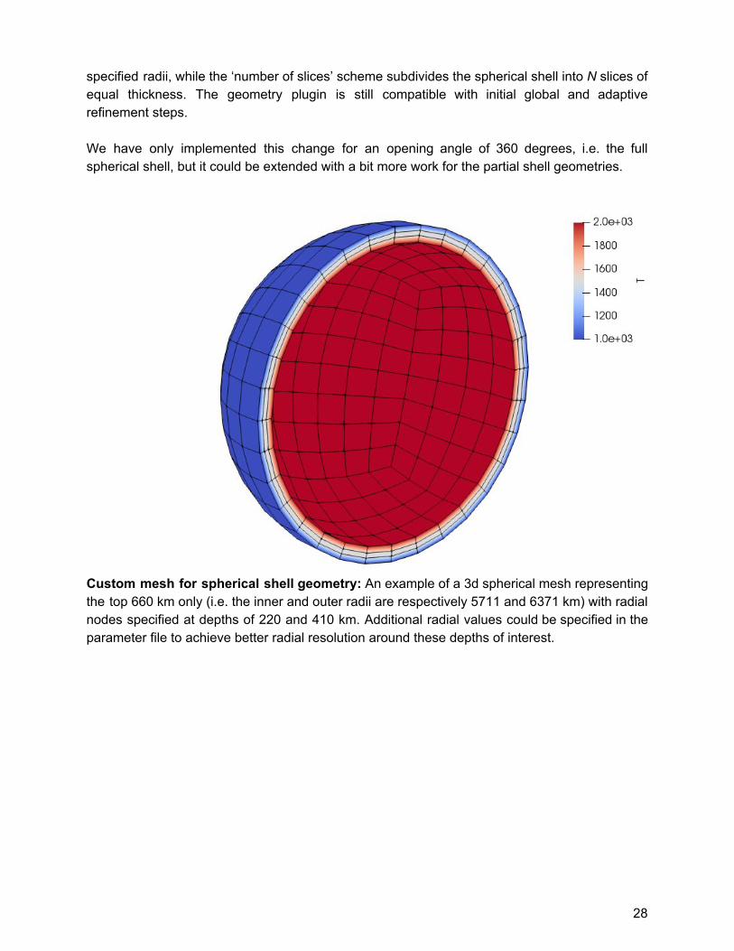
specified radii, while the ‘number of slices’ scheme subdivides the spherical shell into N slices of equal thickness. The geometry plugin is still compatible with initial global and adaptive refinement steps. We have only implemented this change for an opening angle of 360 degrees, i.e. the full spherical shell, but it could be extended with a bit more work for the partial shell geometries.
Custom mesh for spherical shell geometry: An example of a 3d spherical mesh representing the top 660 km only (i.e. the inner and outer radii are respectively 5711 and 6371 km) with radial nodes specified at depths of 220 and 410 km. Additional radial values could be specified in the parameter file to achieve better radial resolution around these depths of interest.
28

Custom mesh for spherical shell geometry: A 2d spherical shell with R0 = 5771 km, R1 = 6371 km, list of radial values = [6231 km, 6331 km], and initial lateral refinement = 5.
A numerical model of brittle thrust wedges (Sibiao Liu, Stephanie Sparks, John Naliboff, Cedric Thieulot) Buiter et al. (2016) organized new comparison experiments with analogue and numerical models to investigate brittle thrust wedge behavior. Here we developed the benchmark 2D models of the thrust wedge. More specifically, we reproduced the numerical simulations of stable wedge experiment 1 and unstable wedge experiment 2 in this paper. Experiment 1 tests whether model wedges in the stable domain of critical taper theory remain stable when translated horizontally. A quartz sand wedge with a horizontal base and a surface slope of 20 degrees is pushed a minimum of 4 cm horizontally by inward movement of a mobile wall at the right boundary with a velocity of 2.5 cm/hour (Figure S1). The basal angle is zero (horizontal), a thin layer separates the sand and boundary to ensure minimum coupling between the wedge and bounding box during translation, and a sticky air layer is used above the wedge. Further, the purely plastic material should not undergo any deformation during translation. Experiment 2 tests how an unstable subcritical wedge deforms to reach the critical taper solution. In this experiment, horizontal layers of sand suffer 10 cm shortening by inward
29

movement of a mobile wall with a velocity of 2.5 cm/hour (Figure S2 a-b). It builds thrust wedges near the mobile wall through a combination of mainly in-sequence forward and backward thrusting (Figure S2 b-d). The strain field (Figure S2c) highlights several incipient shear zones that do not always accumulate enough offset to become visible in the material field (Figure S2b). The pressure field of the model remains more or less lithostatic, with lower pressure values in (incipient) shear zones (Figure S2d).
Figure S1: Numerical model of a stable sand wedge. a) material field after 4 cm of translation b) viscosity field and c) pressure field.
30

Figure S2: The numerical model of an unstable subcritical wedge. a) Initial model setup. b) The material field of the sands after 10 cm shortening. c) The strain field and d) the pressure field.
Choi & Petersen 2015 plasticity (John Naliboff, Cedric Thieulot, Timo Heister) Following a suggestion by John, we looked at a modified set of equations for associative plasticity following the paper by Choi & Petersen (2015). The implementation is rather simple and guarantees a resolution-independent plastic shear band angle. At the time of writing a proof of concept has been carried out in a standalone python code and debugging is needed in the ASPECT implementation. Preliminary results are very encouraging:
31
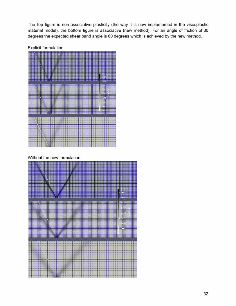
The top figure is non-associative plasticity (the way it is now implemented in the viscoplastic material model), the bottom figure is associative (new method). For an angle of friction of 30 degrees the expected shear band angle is 60 degrees which is achieved by the new method. Explicit formulation:
Without the new formulation:
32

Convergence:
Isotherm mesh refinement plugin (Menno Fraters) I worked on finishing a plugin which allows to refine based on absolute temperature through defining isotherms and the range of refinement levels allowed within those isotherms. It also allows to exclude a specific composition from this criterion which can be useful with, for example, a sticky air layer.
33

Tester coverage testing (Menno Fraters) I started implementing tester coverage testing for ASPECT. When implemented, we will know how well the ASPECT test suite covers the code and how each pull request changes the coverage. This will also allow to track the tester coverage over time.
Change nonlinear Picard solver to defect correction (Menno Fraters) I started implementing the change from a normal Picard iteration to a defect correction Picard iteration in ASPECT. This is supposed to be more stable and accurate than solving the full linear system every nonlinear iteration.
Refactoring of material models (Juliane Dannberg, Rene Gassmoeller) Some material models had become very long, complicated and difficult to read. In addition, it turned out that it would be useful to be able to combine parts of different material models in a new way. To allow this, we restructured the material models in a way that allows the equation of state and the rheology model to be located in a separate class and file that read all of the input parameters and fills all of the outputs. This has allowed us to make material models shorter and easier to read, and will allow it to combine the features of different models more easily in the future.
Move the material lookup namespace to material model utilities (Paul Bremner) We relocated the Material Model Lookup namespace from the grain_size material model to the material model utilities files. This change makes the functions contained within Lookup available for all material models, rather than material models needing to depend upon another material model (for example, the Steinberger model depended on the grain_size model). The functions included in Lookup namespace include the PerpleX and HeFESTo readers, and their associated components. This change also supports the material model refactoring (see above).
Add an unstructured table lookup class (Paul Bremner)
34
Added a new class that reads in an unstructured (not gridded) table of values. This new class is located in the main ASPECT utilities files, and the user format is modeled off of the ASCII data reader. The ASCII data reader assumes a gridded table of values. The purpose of this new functionality is to allow unstructured values to be read in. The original purpose in mind was to enable reading in unstructured material properties files, but the class is not restricted to this. An example is the following: Reading in multiple compositional files from PerpleX that have been processed to eliminate pressure/temperature values that are unphysical, or that have variable increments in pressure/temperature in order to capture phase transitions more completely. The new class is intended to be built on, and the current implementation has the following functionality: (1) read in multiple compositional files, (2) store all coordinate values in an easily searchable object for all the compositional files read in, (3) store a set of data complementary to the coordinate object. Data properties (such as material properties) for a set of coordinates (such as pressure/temperature conditions) can be looked up in order to update model simulations on-the-fly. File format is similar to the ASCII data reader requirements. There are any number of comment lines (denoted with a “#” character at the beginning of the line) at the top of the file. One of those comment lines needs to have "#POINTS: A B C”, where A = the total number of data lines in the file, B = the number of coordinate columns, and C = the number of data columns. From left to right, all the coordinate columns are expected to be first, followed by the data columns. Again, similar to the ASCII data reader, if a column descriptor header is present immediately above the data lines, it will be read and parsed. The parsed column descriptors are searchable.
Create plugin for Frank-Kamenetskii rheology (Grant Euen) Created a plugin that modifies the material model Simple to allow for a different temperature-dependent viscosity law based on the Frank-Kamenetskii approximation. The plugin allows the user to specify a few new parameters in the Simple model subsection, the main difference being that there are two reference temperatures: one for the density and one for the viscosity. See Stein and Hansen, 2013, and Zhong et al., 2008 for more information on this rheology. This plugin is still a work-in-progress.
35

The figure above illustrates isotherms showing 4 upwelling plumes surrounded by downwelling valleys.
New cookbook for the 2D rigid "punch" indentation benchmark (Stephanie Sparks and Cedric Thieulot) We created a new cookbook that simulates a rigid indentation in a rigid plastic half-space that can be compared with an analytical solution. The plane strain formulation of the equations and the detailed solution to the problem were derived in the Appendix of Thieulot et al., 2008 and are also presented in Gerbault et al., 1998. The results shown in the figure below are obtained with an adaptively refined mesh beginning with a global mesh refinement level 6 and increasing by 3 levels. For both the 'rough' and 'smooth' indenter setup we see that the obtained shear bands follow the expected distribution of slip lines and the measured angles are indeed pi/4.
36

Figure S1: Results from rough (left) and smooth (right) punch numerical experiments. The pressure solution at y=L_y is shown in Figure S2. The pressure under the smooth punch (right panel of Figure S2) is measured at p ~ 4.16, i.e. approx. 0.5% error and the velocity of the rigid blocks is measured at 0.70, i.e. approx. 1% error (see also Glerum et al., 2018). However, in the case of the rough punch, the pressure is found to be approx. 4.96, i.e. an error of about 20% (left panel of Figure S2). Figure S2: Pressure along the surface for rough and smooth punch benchmark results and analytical solution (1 + pi).
New CRUST1.0 plugin (John Naliboff, Cédric Thieulot, Ludovic Jeanniot and Marie Kajan) Crust1.0 is a density model composed of 9 layers from surface topography to the Moho. Densities are read in a new material model “crust1” as an initial composition. For each point composing the mesh, their position coordinates and depth are tracked through the crust1.0 dataset and allocated the adequate density. Below some gravity plot for testing the new crust1.0 plugin.
For top to bottom:
37

1/ GRAVITY - from gravity postprocessor using new crust1.0 plugin
2/ GRAVITY - from gravity postprocessor using crust1.0 density from an ascii file. This model has the same resolution as above (GMR 7 - 25 000 000 cells and ~800m).
3/ GRAVITY - from spherical harmonic software
Figure 1a: gravity using new crust1.0 plugin
Figure 1b: gravity using ascii file
38

Figure 1c: gravity from spherical harmonics
39

In terms of gravity magnitude, gravity from the new crust1.0 plugin is the closest to the gravity obtained with the SH software. But in terms of pattern, gravity from loading density ascii file is the closest to the gravity obtained with the SH software.
40

List of hackathon related ASPECT animations A number of movies and animations were produced at the hackathon. They can be found at the following locations: https://www.youtube.com/playlist?list=PLob40YrYSCoZ6ZtwHFERX7dWINAM31Hkq (anisotropy cookbook models) https://www.youtube.com/watch?v=7fmSfNetG3c&feature=youtu.be (brittle thrust wedge exp2) https://www.youtube.com/watch?v=KSk7zA--_ZQ&feature=youtu.be SUPG / diffusion benchmark https://www.youtube.com/watch?v=cXix0dvACS0 Microplate formation https://www.youtube.com/watch?v=DmUqSfRHmHA pulsing plume (fixed!) https://youtu.be/lPtjUYpo_dE polydiapirs benchmark https://www.youtube.com/watch?v=vPy9WEGJqHY&feature=youtu.be brick satellite https://www.youtube.com/watch?v=YzNTubNG83Q jellyfish Inner core growth: see next page Free surface rebound: see next page. https://youtu.be/jYmQy6HEdgw 3d subduction https://youtu.be/oqDhayMt7Ew https://durhamuniversity.app.box.com/file/467900970855
41

42

43

Statistics about ASPECT’s growth during the hackathon The following contains a number of statistics about how much ASPECT has grown during the hackathon:
● Number of source files in ASPECT before/after: 520 -> 540 + 20 ● Lines of code in ASPECT before/after: 128,121 -> 134,857 + 6,300 ● Number of merged pull requests before/after: 2067 -> 2206 + 139 ● Commits in github before/after: 6638 -> 7011 + 373 ● Number of tests before/after: 681 -> 707 + 26
These numbers are a significant increase over the previous hackathon. For comparison, these were the statistics for last year’s (2018) hackathon:
● Number of source files in ASPECT before/after: 497 -> 509 +12 ● Lines of code in ASPECT before/after: 120,058 -> 124,162 +4,104 ● Number of merged pull requests before/after: 1595 -> 1771 +176 ● Commits in github before/after: 5705 -> 6012 +307 ● Number of tests before/after: 583 -> 608 +25
The difference between the second number here (at the end of the 2018 hackathon) and the first number in each column of the table above it (at the start of the 2019 hackathon) illustrates the level of development that happened over the course of the year between the hackathons. These statistics were generated through the following commands:
● find include/ source/ | egrep '\.(h|cc)$' | wc -l ● cat `find include/ source/ | egrep '\.(h|cc)$'` | wc -l ● git log --format=oneline | grep "Merge pull request" | wc -l ● git log --format=oneline | grep -v "Merge pull request" | wc -l ● ls -l tests/*prm | wc -l
44