Embed Size (px)
Citation preview

1
Aspects of Holographic Induced Gravities
ByRohan Rahgava Poojary
PHYS10200904001
The Institute of Mathematical Sciences, Chennai
A thesis submitted to the
Board of Studies in Physical Sciences
In partial fulfilment of requirements
For the Degree of
DOCTOR OF PHILOSOPHY
of
HOMI BHABHA NATIONAL INSTITUTE
26th October, 2015

2
Homi Bhabha National InstituteRecommendations of the Viva Voce Board
As members of the Viva Voce Board, we certify that we have read the dissertation pre-pared by Rohan Raghava Poojary entitled "Aspects of Holographic Induced Gravities"and recommend that it maybe accepted as fulfilling the dissertation requirement for theDegree of Doctor of Philosophy.
Date:
Chair - Balachandran Sathiapalan
Date:
Guide/Convener - Nemani Venkata Suryanarayana
Date:
Member 1 - Sujay K. Ashok
Date:
Member 2 - Syed R. Hassan
Date:
External Examiner
Final approval and acceptance of this dissertation is contingent upon the candidate’ssubmission of the final copies of the dissertation to HBNI.
I hereby certify that I have read this dissertation prepared under my direction andrecommend that it may be accepted as fulfilling the dissertation requirement.
Date:
Place: Guide

3
STATEMENT BY AUTHOR
This dissertation has been submitted in partial fulfilment of requirements for an advanced
degree at Homi Bhabha National Institute (HBNI) and is deposited in the Library to be
made available to borrowers under rules of the HBNI.
Brief quotations from this dissertation are allowable without special permission, provided
that accurate acknowledgement of source is made. Requests for permission for extended
quotation from or reproduction of this manuscript in whole or in part may be granted by
the Competent Authority of HBNI when in his or her judgement the proposed use of the
material is in the interests of scholarship. In all other instances, however, permission must
be obtained from the author.
Rohan Raghava Poojary

4
DECLARATION
I, hereby declare that the investigation presented in the thesis has been carried out by me.
The work is original and has not been submitted earlier as a whole or in part for a degree
/ diploma at this or any other Institution / University.
Rohan Raghava Poojary

5
Dedicated To,
Mom.

6
ACKNOWLEDGEMENTS
I owe a great deal of debt and gratitude to Nemani Suryanarayana who guided me through
the course of my Phd. in IMSc. I would also like to thank him for his continued moti-
vations despite my shortcomings, and for having shared his unique insights into physics
time and again; which have always been good food for thought. I have also benefited
substantially from discussions with Sujay Ashok, who also motivated me tremendously
during my stay in IMSc; to which I find myself forever indebted. I would also like to
acknowledge the collaboration with Steven Avery on my first paper and for sharing his
useful insights in physics and Mathematica. I would also like to thank my doctoral com-
mittee members for having given useful suggestions throughout the course of my PhD.
I would further like to thank Alok Laddha, Sudipta Sarkar, Partha Mukhopadhyay, Prof.
Balachandran Sathiapalan, Prof. Kalyana Rama and Prof. Suresh Govindarajan for useful
discussions; primarily during the weekly string theory journal clubs, which have always
furthered my understanding and made me aware of current topics of interest in physics.
I am obliged to my colleagues I. Karthik, Sudipto, Swastik, Renjan, Pinaki, Nirmalya,
Madhu, Debangshu, Attanu and Arnab for useful discussions on related topics of interest,
in a warm and friendly atmosphere.
My stay in IMSc has been made memorable by the warmth and care of my dear friends
whom I met here. I would like to thank Alok, Soumyajit, Ramu, Belli, Madhushree,
Neha, Prem, Rajeev and Somdeb who have been an integral part of my stay in IMSc. I
would also like to thank Dude Karteek, Yadu, Gaurav and Tiger; and also Vinu, K.K.,
Ramanatha, Nitin, Meesum, Anup, Sreejith, Mubeena, Narayanan, Swaroop, Baskar,
Pranabendu, Raja, Joydeep, Vasan, Renjan, Madhu, Soumyadeep, Prathyush, Prateek,
Prashanth and Tanmoy who made my stay pleasant and memorable. I would be remiss if
I didn’t mention Abhra, Archana, Arya, Tanmay, Dibya, Sriluksmy, Subhadeep, Rajesh,
Kamil & family, Bahubali, Sudhir, Tanumoy, Panchu, Prateep, Sarbeswar, Drhiti, Samrat,
Arghya, Chandan, Nikhil, Suratno and Debangshu for making me feel at ease in Chen-

7
nai. I would also like to thank Jaya, Saumia and Arama for the wonderful memories. I
find myself specially obliged to the friendship of Prof. S. R. Hassan for making me truly
appreciate the science of simple cooking and for providing me with endless dawats at his
place, which I know I would certainly come to miss. I would also like to thank Arijit-da
and Jayeeta-di for the wonderful dinners at their place.
Lastly I would like to thank the mess and canteen workers who work the hardest to provide
timely nourishment and refreshment without whom I cannot imagine my stay in MatSci.

8

Contents
Synopsis 12
0.1 Overview . . . . . . . . . . . . . . . . . . . . . . . . . . . . . . . . . . 13
0.2 Boundary condition analysis of AlAdS 3 in second order formalism . . . . 16
0.3 Analysis of AlAdS 3 as Chern-Simons theory . . . . . . . . . . . . . . . . 19
0.4 Chiral boundary conditions for supergravity . . . . . . . . . . . . . . . . 24
0.5 Conclusion . . . . . . . . . . . . . . . . . . . . . . . . . . . . . . . . . 25
1 Introduction 27
1.0.1 Brown-Henneaux analysis . . . . . . . . . . . . . . . . . . . . . 28
1.0.2 Generalizing the Brown-Henneaux analysis . . . . . . . . . . . . 31
1.0.3 Deviations from the Brown-Henneaux type boundary conditions . 35
1.1 Induced gravity . . . . . . . . . . . . . . . . . . . . . . . . . . . . . . . 39
2 New boundary conditions in AdS 3 gravity 45
2.1 Chiral boundary conditions . . . . . . . . . . . . . . . . . . . . . . . . . 48
2.1.1 The non-linear solution . . . . . . . . . . . . . . . . . . . . . . . 50
2.1.2 Charges, algebra and central charges . . . . . . . . . . . . . . . . 52
9

10 CONTENTS
2.2 Boundary conditions as a result of gauge fixing linearised fluctuations . . 57
2.3 Holographic Liouville theory . . . . . . . . . . . . . . . . . . . . . . . . 58
2.3.1 Classical Solutions and asymptotic symmetries . . . . . . . . . . 61
2.4 Holographic CIG in first order formalism . . . . . . . . . . . . . . . . . 64
2.4.1 Residual gauge transformations . . . . . . . . . . . . . . . . . . 66
2.5 Liouville boundary conditions in CS formulation . . . . . . . . . . . . . 68
2.5.1 Asypmtotic symmetry analysis in the first order formalism . . . . 70
3 Holographic induced supergravities 73
3.1 N = (1, 1) super-gravity in AdS 3 . . . . . . . . . . . . . . . . . . . . . 74
3.1.1 Action . . . . . . . . . . . . . . . . . . . . . . . . . . . . . . . . 75
3.1.2 Boundary conditions . . . . . . . . . . . . . . . . . . . . . . . . 75
3.1.3 Charges and asymptotic symmetry . . . . . . . . . . . . . . . . . 78
3.2 Generalization to extended AdS 3 super-gravity . . . . . . . . . . . . . . 83
3.2.1 Action . . . . . . . . . . . . . . . . . . . . . . . . . . . . . . . . 84
3.2.2 Boundary conditions . . . . . . . . . . . . . . . . . . . . . . . . 85
3.2.3 Charges and symmetries . . . . . . . . . . . . . . . . . . . . . . 87
3.3 Boundary conditions for holographic induced super-Liouville theory . . . 90
4 Holographic chiral induced W-gravities 95
4.1 Chiral boundary conditions for S L(3,R) higher spin theory . . . . . . . . 96
4.2 Solutions of W3 Ward identities . . . . . . . . . . . . . . . . . . . . . . . 101

CONTENTS 11
4.3 Asymptotic symmetries, charges and Poisson brackets . . . . . . . . . . . 102
4.3.1 The left sector symmetry algebra . . . . . . . . . . . . . . . . . . 103
4.3.2 κ0 = 0 and ω0 = 0 . . . . . . . . . . . . . . . . . . . . . . . . . . 104
4.3.3 κ0 = −14 and ω0 = 0 . . . . . . . . . . . . . . . . . . . . . . . . . 105
4.3.4 κ0 , 0, ω0 , 0, ∂− f (−1) = ∂−g(−2) = 0 . . . . . . . . . . . . . . . . 106
5 Conclusion and discussions 111
5.1 Conclusion . . . . . . . . . . . . . . . . . . . . . . . . . . . . . . . . . 111
5.2 Discussions . . . . . . . . . . . . . . . . . . . . . . . . . . . . . . . . . 112
6 Appendix 119
6.1 Gauge fixing linearised AdS 3 gravity . . . . . . . . . . . . . . . . . . . . 119
6.1.1 Solutions to residual gauge vector equation in AdS 3: . . . . . . . 123
6.1.2 Gauge fixing in the Chern-Simons formalism . . . . . . . . . . . 130
6.1.3 Gauge fixing the the Fefferman-Graham gauge . . . . . . . . . . 132
6.2 Review of the asymptotic covariant charge formalism . . . . . . . . . . . 136
6.2.1 Introduction . . . . . . . . . . . . . . . . . . . . . . . . . . . . . 136
6.2.2 Definitions and result . . . . . . . . . . . . . . . . . . . . . . . . 138
6.2.3 Some examples . . . . . . . . . . . . . . . . . . . . . . . . . . . 144
6.3 AdS 3 gravity in first order formulation . . . . . . . . . . . . . . . . . . . 148
6.4 Generalization to extended AdS 3 super-gravity . . . . . . . . . . . . . . 150
6.4.1 Conventions . . . . . . . . . . . . . . . . . . . . . . . . . . . . 150
12 CONTENTS
6.4.2 Action . . . . . . . . . . . . . . . . . . . . . . . . . . . . . . . . 152
6.4.3 Boundary conditions . . . . . . . . . . . . . . . . . . . . . . . . 154
6.4.4 Charges and symmetries . . . . . . . . . . . . . . . . . . . . . . 156
6.5 sl(3,R) conventions . . . . . . . . . . . . . . . . . . . . . . . . . . . . . 162

Synopsis
0.1 Overview
The AdS/CFT correspondence has emerged as one of the most powerful tools in theoreti-
cal physics in the past few years. In its simplest and most concrete form it is a statement
of equivalence (a duality) between a d-dimensional conformal field theory (CFTd) and a
string theory in a background with a (d + 1)-dimensional Anti-de Sitter (AdS d+1) factor.
The set of well studied examples of this correspondence include
• N = 4, d = 4 S U(N) Yang-Mills theory↔ type IIB string theory on AdS 5 × S 5,
• N = (4, 4), d = 2 D1-D5 CFT↔ type IIB string theory on AdS 3 × S 3 × T 4,
and various generalizations there of.
The symmetries of the vacuum of the CFTd get mapped to the isometries of the AdS d+1
space, while the symmetries of the CFT are isomorphic to the appropriately defined
asymptotic symmetries of the string/gravity theory in such a background. A famous
illustration of this aspect of the duality is the seminal work of Brown and Henneaux
[1] that was a precursor to the AdS/CFT conjecture. This involved exhibiting that the
asymptotic symmetry algebra of a (d + 1)-dimensional gravity with negative cosmologi-
cal constant (AdS d+1 gravity) is isomorphic to the algebra of conformal transformations
of the d-dimensional CFT. Brown and Henneaux were concerned with finding asymptotic
symmetries which included in them the set of global conformal transformations of the
13

14 CONTENTS
CFTd while demanding that the metric at the boundary of AdS d+1 is held fixed (Dirichlet
condition). Their boundary conditions provided a definition of the so called asymptoti-
cally locally AdS (AlAdS ) spaces. In more recent times the Brown-Henneaux analysis
has been generalised to AdS 3 supergravities [2] and AdS 3 higher spin gauge theories as
well.
In particular, when d = 2 the asymptotic symmetry algebra of AdS 3 gravity with Brown-
Henneaux boundary conditions is the sum of two commuting copies of the Virasoro alge-
bra with central charges of both the Virasoros given by c = 3l2G , where G is the Newton’s
constant and l is the radius of the AdS 3 space in AdS 3 gravity. The CFT2 in this case
is thus expected to be a standard 2d conformal field theory with the left and right mov-
ing sectors treated symmetrically. Similarly in the AdS 3 higher spin context (containing
gauge fields with spins upto N) the asymptotic symmetry algebra is a sum of two com-
muting copies of WN algebra with Brown-Henneaux central charges, again, with perfect
parity between their left and right sectors.
However, there have been 2d CFTs which do not maintain such parity between their left
and right sectors. Perhaps the simplest way to break this parity is to consider cases where
the central charges appearing in the left and right Virasoro algebras are different. More
dramatic breaking of the left-right parity would be when the symmetry algebra either on
the left sector or the right sector is not a Virasoro/WN algebra. In fact there have been
such 2d CFTs in the literature and they are generically termed as chiral CFTs. Thus a
natural question is how to generalise the Brown-Henneaux type computation to allow for
asymptotic symmetry algebras of chiral CFTs.
This thesis concerns itself with studying different boundary conditions imposed on 3d
AdS spaces and thus uncovering new asymptotic symmetry algebras. We do this in differ-
ent settings, first involving pure AdS 3 gravity [3], then the 3d higher-spin gauge theories
[4] and finally some AdS 3 supergravities. It turns out that we need to consider boundary
conditions that are not the Dirichlet type, i.e. the fields and the metric at the AdS boundary

0.1. OVERVIEW 15
can fluctuate. For the generalization to higher spin and supergravity it becomes necessary
to work in the first order formalism of AdS 3 gravity/3d higher-spin theories. Our investi-
gations fall into two different cases depending on whether or not the asymptotic symmetry
algebra contains fully the global part of the 2d conformal/higher-spin algebra.
There have appeared some works in the literature that provide examples of generaliza-
tions of Brown-Henneaux that belong to both these categories. In [5] Troessaert provided
boundary conditions that allow the conformal factor of the boundary metric to fluctuate
with the boundary metric having zero scalar curvature. In this case the asymptotic algebra
contains fully 2d conformal symmetry. In [6] Compère, Song and Strominger provided
boundary conditions with a symmetry algebra being one copy of Virasoro and one copy
of a U(1) Kac-Moody algebra. Our investigations presented in this thesis will provide
results that are complementary to the results of [5], [6] and various generalizations.
The thesis contains the following results summarized in the next sections:
• Chiral boundary condition: Generalizations of Brown-Henneaux boundary con-
ditions for AdS 3 gravity in the second order (metric) formulation, with asymptotic
symmetry algebra equal to one copy of Virasoro algebra with Brown-Henneaux
central charge and one copy of sl(2,R) current algebra with level k = c/6 [3].
• Liouville boundary condition: Generalization of [5] where the conformal factor
of the boundary metric satisfies the Liouville equation both in second order and first
order formulations of AdS 3 gravity.
• Duals to chiral induced W gravities: Generalizations of the boundary conditions
of [7] pertaining to 3d spin-3 gravity with symmetry algebra equal to one copy of W3
algebra with Brown-Henneaux central charge and one copy of sl(3,R) algebra with
level k = c/6. Generalization of [6] to the 3d spin-3 gravity where the symmetry
algebra is a copy of W3 and two u(1) Kac-Moody algebras [4].
• Chiral boundary condition for supergravities: We generalize these boundary
16 CONTENTS
conditions to minimal AdS 3 supergravities.
In what follows we give a brief summary of these results and juxtapose them with previous
works studying 2d CFTs and their AdS 3 duals.
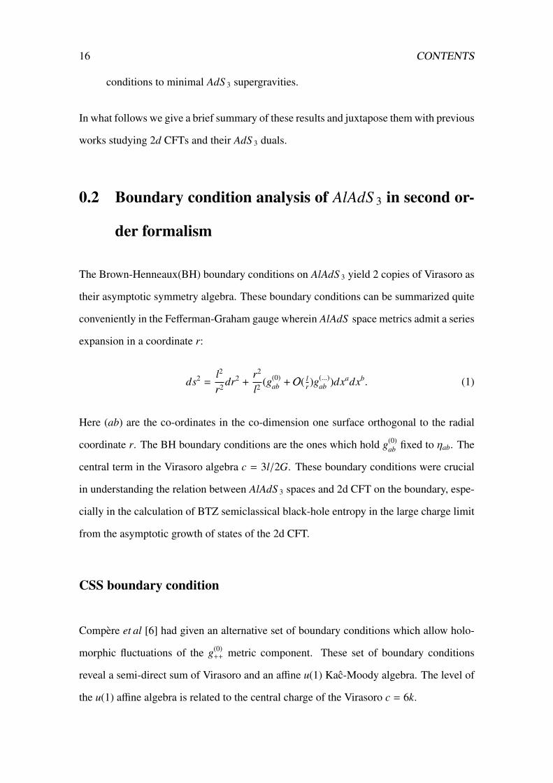
0.2 Boundary condition analysis of AlAdS 3 in second or-
der formalism
The Brown-Henneaux(BH) boundary conditions on AlAdS 3 yield 2 copies of Virasoro as
their asymptotic symmetry algebra. These boundary conditions can be summarized quite
conveniently in the Fefferman-Graham gauge wherein AlAdS space metrics admit a series
expansion in a coordinate r:
ds2 =l2
r2 dr2 +r2
l2 (g(0)ab + O( l
r )g(...)ab )dxadxb. (1)
Here (ab) are the co-ordinates in the co-dimension one surface orthogonal to the radial
coordinate r. The BH boundary conditions are the ones which hold g(0)ab fixed to ηab. The
central term in the Virasoro algebra c = 3l/2G. These boundary conditions were crucial
in understanding the relation between AlAdS 3 spaces and 2d CFT on the boundary, espe-
cially in the calculation of BTZ semiclassical black-hole entropy in the large charge limit
from the asymptotic growth of states of the 2d CFT.
CSS boundary condition
Compère et al [6] had given an alternative set of boundary conditions which allow holo-
morphic fluctuations of the g(0)++ metric component. These set of boundary conditions
reveal a semi-direct sum of Virasoro and an affine u(1) Kac-Moody algebra. The level of
the u(1) affine algebra is related to the central charge of the Virasoro c = 6k.

0.2. BOUNDARY CONDITION ANALYSIS OF ALADS 3 IN SECOND ORDER FORMALISM17
Chiral boundary condition
In [3], we generalized the CSS[6] boundary conditions to allow for a priori generic
fluctuations of g(0)++, which when constrained by Einstein’s eom restrict it to be of the
form,
g(0)++ = F = f (x+) + g(x+)eix− + g(x+)e−ix− . (2)
For the theory in the bulk to be consistent with the variational principle, one is required
to add a boundary term of the form:
S bndy = −18πG
∫∂M
d2x√−γ 1
2Tabγab,
where T µν = −12r4 l2δ
µ+δ
ν−. (3)
This term in turn fixes the T−− component of the Brown-York stress tensor for the bulk ge-
ometries. Such boundary term basically minimizes the on-shell bulk action only for those
configurations which are allowed by the proposed boundary conditions. The Gibbons-
Hawking term alone is enough to define the Brown-Henneaux (Dirichlet) type boundary
condition. It is apparent that allowing any boundary metric component to fluctuate re-
quires holding requisite component of the Brown-York stress tensor fixed.
δS total =
∫∂M
d2x√−γ 1
2T µνδγµν. (4)
A case where the boundary metric is completely free was considered in [8]. We would
here be describing cases where only certain components of the boundary metric are al-
lowed to fluctuate, thus corresponding to mixed (Robin) boundary conditions. For the
CSS case, the boundary term is chosen to allow for fluctuations of the type δg(0)++ = F(x+).
The above boundary term similarly is chosen to allow for the fluctuations of the boundary
metric component g(0)++ in accordance with (2).

18 CONTENTS
The asymptotic symmetry algebra we obtained is a semi-direct product of a Virasoro
with an affine Kac-Moody sl(2,R) algebra with level k = c6 = l
4G . Similar analysis is done
in Poincaré AdS 3[9] where the boundary is spatially non-compact. The Ward identities
thus derived from the bulk eom are seen to correspond to the chiral induced gravity theory
first written down by Polyakov[10].
Troessaert’s boundary condition
On the heels of [6] was a paper by Troessaert[5] which proposed boundary conditions
which freed up the conformal factor of the boundary metric. This conformal factor was
written as a product of holomorphic and anti-holomorphic components, thus restricting
the boundary metric to be conformally flat. The asymptotic symmetry algebra that re-
sulted from such considerations yielded left and right moving affine u(1)s along with two
copies of Virasoro with the central charge c = 3l2G = 6k.

0.3. ANALYSIS OF ALADS 3 AS CHERN-SIMONS THEORY 19
Liouville boundary condition
The Liouville theory eom is ∂+∂− log F = 2χF. One can ask what possibly could be
a required set of boundary conditions on AlAdS 3 such that the conformal factor of the
boundary metric is this Liouville field? To this end we find that one needs to add an
appropriate boundary term of the form,
S bndy =5χl4πG
∫∂M
d2x√−γ. (5)
apart from allowing the boundary metric to have an a priori arbitrary conformal factor
F(x+, x−). Upon imposing the variational principle on shell, F would obey the eom of the
Liouville theory.
One finds that the asymptotic symmetry algebra in this case would be two copies of
Virasoro corresponding to the Brown-Henneaux deformations, plus two copies of Vira-
soro corresponding to the holomorphic and anti-holomorphic components of the Liouville
stress-tensor. One also finds that the Liouville central charge is cLiouville = −cBH = − 3l2G .
Therefore the total central charge of such a theory is zero.
0.3 Analysis of AlAdS 3 as Chern-Simons theory
The second order formalism described previously is not amenable to analysis if one wants
to generalize such mixed boundary conditions to higher-spins(hs) and supergravities in
AdS 3. The second order action for hs in AdS 3 is not completely known and the compu-
tation of the asymptotic algebra for the boundary conditions of interest is difficult in the
case of supergravity. 3d gravity with negative cosmological constant can be expressed as
a difference of two Chern-Simons theories with gauge group S L(2,R)[11]. The left and
right gauge fields are then given in terms of A = ω + el and A = ω − e
l , with torsionless

20 CONTENTS
condition and Einstein’s equations being imposed by flatness of gauge connections for the
2 gauge fields.
S CS [A] = k4π
∫dA ∧ A + 2
3 A ∧ A ∧ A,
S AdS 3 = S CS [A] − S CS [A]. (6)
The analysis of the previous sub-section can then be repeated in this first order formalism
by imposing different gauge field fall-off conditions.
AdS 3 gravity described thus was used to study the asymptotic dynamics by analysing
WZNW in 2d [12, 13]. It was found that the suitable constraints on the WZNW con-
served currents corresponded to the Brown-Henneaux boundary conditions. The CSS
boundary conditions were also translated into the WZNW theory by the same authors.
This formalism is particularly suitable to analyse supergravity with negative cosmologi-
cal constant in 3d [2], where the asymptotic symmetry algebra now consists of two copies
of super-Virasoro algebra i.e. the extended super conformal algebra with quadratic non-
linearities in the current.
The first order formalism is the only way one can analyze the higher-spins in AdS 3. Here
since sl(3,R) ⊂ hs[λ], one can analyze CS-CS theory with S L(3,R) gauge group as a
consistent truncation of the full hs[λ] theory. The asymptotic symmetry algebra for such
theory was studied in [7] and was found to be 2-copies of W3 algebra, which are the hs
analogues of Virasoro.
Chiral boundary conditions
The gauge fields corresponding to the metric configurations restricted by chiral bound-

0.3. ANALYSIS OF ALADS 3 AS CHERN-SIMONS THEORY 21
ary conditions are [4]:
A = b−1∂rbdr + b−1[(L1 + a(−)+ L−1 + a(0)
+ L0)dx+(a(−)− L−1)dx−]b,
A = b∂rb−1dr + b[(a(+)+ L+ + a(0)
+ L0 + a(−)+ L−)dx+ + (−L− + a(+)
− L+)dx−]b−1,
where b = elog rl L0 . (7)
The A gauge field obeys the Brown-Henneaux type boundary condition but A has mode
a(−)+ which survives at boundary . The metric obtained from A and A does relate g(0)
++ = a(−)+ .
The Ward identity is given by the remaining eom for A:
(∂+ + 2∂−a(−)+ + a(−)
+ ∂−)a(+)− = 1
2∂3−a
(−)+ . (8)
Suitable boundary terms have to be added to make the theory variationally well defined:
S bdy = −k4π
∫dx2tr(L0[a+, a−]) − k
4π
∫dx2tr(L0[a+, a−] − 2κ0L+a+),
=⇒ δS total = k2π
∫dx2(a(+)
− − κ0)δa(−)+ . (9)
For a(+)− = κ0 = −1
4 one gets the desired asymptotic symmetries as in the second order
formalism.
Liouville boundary condition
The Liouville theory obtained in the previous section, can also be cast in a first order
form. The gauge fields corresponding to configurations in [5] are:
a = (a(+)+ (x+)L1 −
κ(x+)a(+)
+
L−1)dx+, A = b−1ab + b−1db,
a = (a(−)− (x−)L−1 −
κ(x−)a(−)−
L1)dx−, A = bab−1 + bdb−1,
b = elog rl L0 . (10)

22 CONTENTS
If one needs the generic Liouville type of eom for the conformal factor F = −a(+)+ a(−)
−
of the boundary metric, then one would be forced to choose (a)a which is not (anti-
)holomorphic.
a = (a(+)+ L1 − ∂+(log a(−)
− )L0 −κ(x+)a(+)
+
L−1)dx+ + (∂−(log a(+)+ )L0 − a(−)
− L−1)dx−,
a = (a(−)− L−1 + ∂−(log a(+)
+ )L0 −κ(x−)a(−)−
L1)dx− + (−∂+(log a(−)− )L0 − a(+)
+ L1)dx+.
(11)
Duals to chiral induced W gravities
Massless higher-spin excitations can also be studied in a similar light in AdS 3 where
the bulk action is written as CS-CS with the gauge group being S L(3,R)1. Here we pro-
pose a new set of boundary conditions which allow for either an su(1, 2) or sl(3,R) or a
u(1)×u(1) affine Kac-Moody algebra along with a W3 as an asymptotic symmetry algebra
[4].
The gauge fields are2
a = (L1 − κL−1 − ωW−2)dx+,
a = (−L−1 + κL1 + ωW−2)dx− + (1∑
a=−1
f (a)La +
2∑i=−2
g(i)Wi)dx+. (12)
The gauge algebra sl(3,R) is in the principle embedding with the Las denoting the sl(2,R).
The eom on the gauge fields yield a to be of the holomorphic form, while the components
of a can be solved in terms of each other yielding chiral W3 induced gravity Ward identi-
ties. On the left gauge field we impose the usual constraints prevalent in literature [7, 14]
which would yield a copy of W3 algebra. The boundary term needed for the right gauge
1We restrict ourselves to the case of spins=2,3 although these can be generalized in a similar fashion toinclude arbitrary higher spins.
2The small case a and a have their radial dependence gauged away as in (10).

0.3. ANALYSIS OF ALADS 3 AS CHERN-SIMONS THEORY 23
field is:
S bndy = k4π
∫d2x tr(−L0[a+, a−] + 2κ0L1a+ + 1
2αW0{a+, a−}) + 13 a+a− + 2ω0W2a+),
=⇒ δS total = − k2π
∫d2x [(κ − κ0)δ f (−1) + 4α2(ω − ω0)δg(−2)] (13)
We impose κ = κ0 and ω = ω0 thus allowing for fluctuations of f (−1) and g(−2) which are
the most leading order components in the radial co-ordinate r. Along with the left copy
of W3 algebra we get different affine Kac-Moody algebras depending on the choice of
parameters κ0 and ω0:
• κ0 = 0 , ω0 = 0:
This choice of the parameters yields an affine Kac-Moody of sl(3,R) at level k = c6
and describes a field theory on a boundary with a non-compact spatial direction.
• κ0 = −14 , ω0 = 0:
This choice of the parameters yields an affine Kac-Moody of su(1, 2) at level k =
c6 with the boundary having a spatial circle. Both sl(3,R) and su(1, 2) are non-
compact real forms of sl(3,C)3.
• κ0 , 0 , ω0 , 0:
In this case one can make a choice of currents such that one gets a u(1)× u(1) affine
Kac-Moody as an asymptotic symmetry algebra. This generalizes results of [6] to
the case of hs.
The asymptotic symmetries and the Ward identities make it apparent that a suitable candi-
date for the duals of such bulk configurations are chiral induced W3 gravities. W-gravity
is the higher-spin analogue of gravity in 2d based on the underlying W-algebra[15, 16].
Here, W-algebra plays a similar role as that of Virasoro algebra in pure 2d gravity4. We
3This ambiguity doesn’t arise in pure gravity since the non-compact real forms of sl(2,C) are sl(2,R) ≡su(1, 1)
4It is worthwhile to point out that although 2d gravity admits a higher-spin extension with an underlyingW-algebra, this is not a Lie algebra in the usual sense; the commutator of 2 generators generally consists

24 CONTENTS
will concern ourselves to W3 gravity in this text.
The induced (effective) action for pure 2d gravity in chiral gauge was shown to be de-
rived from a constrained sl(2,R) WZNW system[17, 18, 19, 20]. It was then derived to
all orders in c. This approach made the hidden sl(2,R) symmetry in the induced gravity
manifest. An identical approach was used to find the induced W3 gravity action to all
orders in the chiral gauge [21]. It was obtained by constraining the sl(3,R) WZNW field
theory which can be further regarded as a reduced sl(3,R) Chern-Simons theory in 3d.
0.4 Chiral boundary conditions for supergravity
It would be useful to see whether the boundary conditions in (0.2) can be extended to in-
clude minimal supergravity in AlAdS 3 spaces. This would ba a first step in realising such
boundary conditions in the context of string theory. Analogues work was done for the
case of Brown-Henneaux boundary conditions in [22, 23]. Extended AlAdS 3 supergrav-
ity were considered in [2] and their corresponding duals were proposed along the lines of
[12]. Since the number of fields increases in supergravity, it would also be worthwhile to
find the most general minimal supergravity extension which admits a bosonic truncation
down to the chiral case.
N = (1, 0) and higher supergravity in AdS3
The superalgebra for supergravity in locally AdS 3 with N = (1, 0) is osp(1|2) × sl(2,R).
Here we show that there exists a unique extension of the chiral boundary condition to in-
clude fluctuations of the Rarita-Schwinger field on the boundary. The analysis in second
order formalism is quite cumbersome as mentioned previously and we therefore analyse
of composites of generators. The restriction to W3 gravity on the other hand has only linear and quadraticterms.

0.5. CONCLUSION 25
it in the first order formalism. A large part of the analysis done in section (0.3) in the
first order formalism can be repeated, including the boundary terms to be added, since the
only difference here would be the change in the gauge algebra from sl(2,R) to osp(1|2).
We show here that the asymptotic symmetry algebra consists of a Virasoro and an affine
osp(1|2) Kac-Moody algebra with level k = c6 . The above generalizations of chiral bound-
ary condition can be easily extended to the N = (1, 1) and more generally to the N = (p, q)
case in the first order formalism. When Dirichlet boundary conditions were imposed on
these theories [22, 23], two copies of the super-Virasoro were found as the asymptotic
symmetry algebra. It turns out that for the bosonic sector to be containing configurations
corresponding to chiral boundary conditions of (0.2), it is enough to change one of the
gauge fields (A for ex.) to obey conditions similar to (0.3), while imposing Dirichlet (BH
generalizations) boundary condition on the other (A). Then, the asymptotic symmetry
algebra of A turns out to be the super extension of Virasoro while that obtained from A
gives rise to an affine Kac-Moody algebra of the relevant super algebra under consid-
eration. These boundary conditions on N = (1, 0) supergravity must correspond to the
minimal supersymmetric extension of Polyakov’s induced gravity in 2d analysed by [24].
The case for 2d chiral induced N = (1, 1) and generic N = (p, q) supergravity was ad-
dressed in [25].
0.5 Conclusion
The above analysis shows that relaxing boundary conditions on AlAdS 3 in a systematic
way does enrichen the AdS /CFT holography in relating it to different possible CFTs. It
is known in AdS d for d > 3, the Dirichlet(BH) boundary conditions only yield the global
conformal transformations of the d − 1 boundary. Infinite dimensional symmetries are
know to exist in 3d and 4d asymptotically flat Minkowski spaces, known as the BMS

26 CONTENTS
group. The above analysis can be used as an indication that relaxing boundary conditions
in these cases might yield new asymptotic symmetries and corresponding dual CFTs on
the AdS boundary. This in turn may shed light on certain hidden infinite dimensional
symmetries of these CFTs − previously known or otherwise, of the kind envisaged by
Bershadsy and Ooguri [20, 26]. In a similar spirit it would be interesting to see how these
considerations are realized in the context of string theory on AdS sapces, where infinite
dimensional symmetries - like the Yangian, are know to occur in the CFTs.
The thesis would be organized as follows:
1. The first chapter would comprise of a brief review of 2d induced gravity theories.
2. The second chapter would summarize results in the second order formulation.
3. The third chapter would analyze the implications of different boundary conditions
in the first order formalism and would include results in hs and supergravity.
4. The fourth chapter would discuss possible implications of the results stated and
open problems.

Chapter 1
Introduction
The AdS /CFT correspondence has emerged as one of the most powerful tools from string
theory in the past one and a half decades. In its strongest form, it proposes a duality
between string theory (supergravity) on a product of (d + 1) dimensional Anti-de Sitter
space times a compact manifold (AdS d+1 × Σcompact) and the large N limit of certain CFTd
living on its boundary. The well studied examples of this duality include
• N = 4, d = 4 S U(N) Yang-Mills theory↔ type IIB string theory on AdS 5 × S 5,
• N = 6, d = 3 U(N)×U(N) ABJM theory↔ type IIA string theory on AdS 4×CP3,
• N = (4, 4), d = 2 D1-D5 CFT↔ type IIB string theory on AdS 3 × S 3 × T 4,
and other various generalizations.
This duality maps the symmetries of the two theories to each other. The symmetries
vacuum of the CFTd gets mapped to the symmetries of the maximally symmetric global
AdS d+1 space, whereas, the global symmetries of the CFTd are mapped to the appropri-
ately defined asymptotic symmetries of the theory in Asdd+1 × Σ space. Much of the
richness of this duality stems from some interesting properties of the AdS space itself.
The first statement can be understood from the fact that the Killing symmetries of AdS d+1
- SO(2, d), are exactly the conformal symmetries of the boundary - R × S d−1 where the
27

28 CHAPTER 1. INTRODUCTION
CFT lives.
According to the AdS /CFT correspondence, there exists an operator OΦ on boundary
CFT for every field Φ in the bulk supergravity. The boundary value Φ(0), of the bulk field,
Φ can be identified as a source which couples to the operator OΦ. The bulk partition func-
tion is then a functional of the boundary values {Φ(0)} of the bulk fields {Φ}. Under this
duality, the bulk supergravity partition function is equal to the generating function of the
correlation functions in the conformal field theory at spatial infinity ∂AdS [27].
Zsugra[{Φ[0]}] ' 〈exp
−∫∂AdS
∑{Φ}
Φ(0)OΦ
〉CFT = ZCFT[{Φ(0)}] (1.1)
When the bulk theory is weakly coupled, the lhs in the above equation can be approxi-
mated by the leading contribution from the on-shell bulk configurations {Φ}cl, which solve
the classical equations of motion with the boundary values being {Φ(0)}, yielding
− S sugra[{Φ}cl]∣∣∣{Φ(0)}' WCFT[{Φ(0)}] = − log ZCFT[{Φ(0)}]. (1.2)
The conformal dimension of the operators {OΦ} in the CFT are given in terms of the
masses and spins of the fields {Φ} in the supergravity in AdS 1. Boundary conditions
imposed on the bulk gravity theory play an important role as the duality requires one to
specify boundary conditions at the spatial infinity of the AdS space, which in particular
fixes the CFT to which its is dual to.
1.0.1 Brown-Henneaux analysis
A famous illustration of the relation between the boundary conditions on AdS d+1 space
and global symmetries of the CFTd was carried out in d = 3 by Brown and Henneaux [1].
Here although the Killing isometeries of AdS 3 form an SO(2,2), the conformal isome-1We use the phrases (super)gravity with negative cosmological constant and (super)gravity in AdS space
interchangeably.

29
tries of the boundary metric ηab are given by two copies of the infinite dimensional Witt
algebra.
ds2 = ηabdxadxb = −dx+dx− = −dτ2 + dφ2,
[Lm, Ln] = (m − n)Lm+n [Lm, Ln] = (m − n)Lm+n,
where, Ln = einx+
∂+ Ln = einx−∂−, (1.3)
where x± = τ ± φ. They were interested in finding the space of solutions to AdS 3 gravity
which would include the maximally symmetric global AdS 3
ds2 =`2
r2 dr2 + r2[−dx+dx− − `2
4r2 (dx+2 + dx−2) − `4
32r4 dx+dx−], (1.4)
of AdS radius ` and reproduce the above algebra from the bulk as an asymptotic symmetry
algebra. To this end they demanded that all solutions to Einstein’s equation with negative
cosmological constant in the bulk have the same induced metric at spatial infinity. This
amounted to imposing a Dirichlet boundary condition on the bulk geometries. The on-
shell variation of the bulk Einstein-Hilbert action reads:
S = −1
16πG
∫M
d3x√−g
(R +
2`2
)−
18πG
∫∂M
d2x√−γΘ +
18πG
S ct(γµν),
δS =
∫∂M
d2x√−γT abδγab, (1.5)
where T ab is the Brown-York stress tensor defined on the co-dimension one time-like
surface orthogonal to the radial direction r and γab is the induced metric on the bound-
ary. Here, S ct contains counter terms that make the on-shell action finite and are deter-
mined through a procedure of holographic renormalization first outlined in [28]. Impos-
ing Dirichlet boundary condition implied δγab = 0 on the space of allowed solutions. The

30 CHAPTER 1. INTRODUCTION
boundary fall-off conditions thus obtained are:
grr =`2
r2 + O(1r4 )
gra ≈ O(1r3 )
gab = r2ηab + O(r0), (1.6)
since termed as the Brown-Henneaux boundary conditions2. The space of diffeomor-
phisms which respects these fall-off conditions are generated by:
ξr = r R(τ, φ) +`2
rR(τ, φ) + O(
1r3 ),
ξτ = T (τ, φ) −`2
2r2∂τR(τ, φ) + O(1r4 ),
ξφ = Φ(τ, φ) +`2
2r2∂φR(τ, φ) + O(1r4 ), (1.7)
where R = ∂tT = ∂φΦ, ∂tΦ = ∂φT . These are termed as asymptotic Killing vectors since
they leave the boundary metric unchanged. These of course are unique only upto those
vector fields which are sub-leading in r i.e. begin at O(1/r). The commutator defined via
Lie derivative action of these vector fields obeys the Witt algebra. Brown and Henneaux
computed the central extension to this algebra by computing the change in the asymptotic
charge under such diffeomorphisms and uncovered two copies of Virasoro algebra:
[Lm, Ln] = (m − n)Lm+n +c
12m(m2 − 1)δm+n,0,
[Lm, Ln] = (m − n)Lm+n +c
12m(m2 − 1)δm+n,0, (1.8)
with c = 3`2G . Here ` is the AdS length and G is the three dimensional Newton’s constant.
Conserved currents of a two dimensional CFT are generally expected to obey the above
algebra where the central extension c is the central charge of the CFT. This was used
to derive the Bekenstein-Hawking entropy for the BTZ black hole by using the Cardy
2Here we denote the indices corresponding to the boundary directions by lower case Roman alphabetsa, b. The boundary metric γab is taken to be the flat space metric ηab

31
formula for the asymptotic growth of states in a CFT in the large central charge limit.
Which in turn implies that the size of AdS 3 is much larger than the three dimensional
Newton’s constant; ` >> G.
1.0.2 Generalizing the Brown-Henneaux analysis
The Brown-Henneaux boundary conditions have since been adapted to different settings
in the context of AdS /CFT. Most notable works being the ones studying supergravity with
negative cosmological constant in three dimensions [22, 23, 2], and more recently in the
study of higher-spin gauge fields in AdS 3, which are conjectured to be duals to the coset
models proposed by Gaberdiel and Gopakuamar [29]. In these cases, generalizations of
the Virasoro have been obtained as the asymptotic symmetry algebra in d=3 dimensions.
The above works rely heavily on the fact that three dimensional AdS gravity can be cast
as a difference of two Chern-Simons theories at level k = `4G ,
S AdS 3 = S CS [A]∣∣∣k− S CS [A]
∣∣∣k,
S CS [A]∣∣∣k
=k
4π
∫tr(A ∧ A +
23
A ∧ A ∧ A), (1.9)
defined over a manifold Σdisk × R, where R is the time co-ordinate. Here, the fields in the
bulk are a derived concept as the vielbein and the spin connections are given in terms of
the gauge fields as
ω =12
(A + A) & e =`
2(A − A). (1.10)
For the case of pure gravity, the gauge fields are valued in the adjoint of sl(2,R). The
equations of motion in this first order formalism translate to flatness of gauge connections
for the two gauge fields. The Brown-Henneaux analysis can be done in this formalism
too. Here, one imposes boundary fall-off conditions on the gauge fields such that the

32 CHAPTER 1. INTRODUCTION
metric obeys the fall-off conditions of Brown-Henneaux,
a =[L1 − κ(x+) L−1
]dx+, a =
[−L1 + κ(x−) L1
]dx−,
A = b−1(d + a)b, A = b(d + a)b−1,
where, b = eL0 ln( r`
)[Lm, Ln] = (m − n)Lm+n, m, n ∈ {−1, 0, 1}. (1.11)
The two copies of Virasoro algebra manifests themselves in the modes of κ(x+) and κ(x−)
with the same central extension. In terms of the Poisson brackets fro the right-moving
Virasoro look like
{κ(x+), κ(x+)
}= −κ′(x+) δ(x+ − x+) − 2 κ (x+) δ′(x+ − x+) − k
4π δ′′′(x+ − x+). (1.12)
The first order formalism is useful in that allowing the gauge algebra to contain sl(2,R)
as a subset of a bigger algebra leads to theories with other gauge fields coupled to gravity
in d = 3 dimensions. As an example, supergravities in AdS 3 were studied to generalize
Brown-Henneaux boundary conditions by Henneaux et al [2]. This was done by replacing
the sl(2,R) gauge group with a Z2 graded algebra for the sl(2,R) ⊕ G bosonic algebra,
where G is the internal bosonic symmetry.
The guiding principle in the analysis of Henneaux et al [2] was to impose similar Dirich-
let type boundary conditions on the supergravity fields such that the bulk metric is still
asymptotically locally AdS 3 (AlAdS 3). This was done by demanding that the gauge fields
obey the following fall of conditions3
Γ = bdb−1 + bab−1, Γ = b−1db + b−1ab,
where b = eσ0 ln(r/`),
a =[σ− + L(x+)σ+ + ψ+α+(x+)R+α + Ba+(x+)T a] dx+,
3The conventions and notations are taken from chapter 3.

33
a =[σ+ + L(x−)σ− + ψ−α−(x−)R−α + Ba−(x−)T a
]dx−. (1.13)
These boundary conditions, which were extensions of the Brown-Henneaux boundary
conditions to the supergravity case, uncovered two copies of super-Virasoro i.e. the ex-
tended super-conformal algebra as the asymptotic symmetry algebra4. This algebra, un-
like the Virasoro, contains quadratic non-linearities in currents. There were other works
which had reproduced special cases of the above result [22, 23].
In a similar light, one can obtain a bulk theory of higher-spin gauge fields coupled to
gravity in AdS 3 by demanding that the two Chern-Simons gauge fields be valued in the
adjoint of sl(N,R). Here, one would end up with a bulk theory for gauge fields with spins
ranging from 2, ...N, with the spin-2 gauge field being the graviton.
The asymptotic symmetry of higher-spin gauge fields coupled to gravity in d = 3 dimen-
sions was first done by Campoleoni et al [7], where they restricted to spin 3 fields coupled
to gravity yielding 2-copies of classical W3 algebra first written down by Zamalodchikov
[15]. Here too, the authors were concerned only with finding the asymptotic symmetry
algebra such that all the solutions admitted by the boundary conditions have a metric
(spin-2 field) which is AlAdS 3. The boundary conditions are given as fall-off conditions
on the gauge fields, as before
A = b−1ab + b−1db A = bab−1 + bdb−1,
a = (L1 − κL−1 − ωW−2)dx+ a = (−L−1 + κL1 + ωW2)dx−,
b = eL0ln rl , (1.14)
where the gauge fields are valued in the adjoint of sl(3,R) listed in the appendix 6.5. Here
one finds that the gauge field a only depends on x+ and as a 1-form has a component only
along the same coordinate. The same is true for a and its x− dependence. The analysis
4This analysis is contained in part in chapter 3.

34 CHAPTER 1. INTRODUCTION
is the same for either of the gauge fields. The spin fields are recovered from these gauge
fields as
gµν =12
Tr(eµeν) ϕµνρ =13!
Tr(e(µeνeρ)),
e =`
2(A − A) ω =
12
(A + A). (1.15)
Here, they uncovered two copies of the classical W3 algebra as the asymptotic symmetry
algebra, one each for the two gauge fields A and A. This algebra is represented by Poisson
brackets between the functions parametrizing the phase-space of solutions i.e. for instance
κ and ω for the gauge field A
− k2π
{κ(x+), κ(x+)
}= −κ′(x+) δ(x+ − x+) − 2 κ (x+) δ′(x+ − x+) + 1
2 δ′′′(x+ − x+),
− k2π
{κ(x+), ω(x+)
}= −2ω′(x+) δ(x+ − x+) − 3ω(x+) δ′(x+ − x+),
−2kα2
π
{ω(x+), ω(x+)
}= 8
3 [κ2(x+) δ′(x+ − x+) + κ(x+) κ′(x+)δ(x+ − x+)]
−16 [5κ(x+)δ′′′(x+ − x+) + κ′′′(x+)δ(x+ − x+)]
−14 [3κ′′(x+)δ′(x+ − x+) + 5κ′(x+)δ′′(x+ − x+)] + 1
24δ(5)(x+ − x+)
(1.16)
Here, the Virasoro is a part of the above algebra. Also the W3 algebra is not a Lie algebra
in the conventional sense since the rhs does contain quadratic non-linearities. The proce-
dure for obtaining the above algebra from the boundary conditions imposed is outlined in
detail in chapter 4. As mentioned earlier, these boundary conditions are generalizations
of the ones imposed by Brown and Henneaux in that for the above fall-off conditions on
the gauge fields 1.14, the bulk solutions are AlAdS 3. In other words, the spin-3 field ϕµνρ
doesn’t survive till the boundary of AdS 3 while gµν contains all the configurations allowed
by the Brown-Henneaux boundary condition.

35
The case of the higher-spin (hs) theory with spins ranging from 2....N with N → ∞
in AdS 3 was dealt by Henneaux and Rey [14] where 2-copies ofW∞ were uncovered as
the asymptotic symmetry algebra. The gauge group in the bulk is hs[λ]×hs[λ], which for
suitable values of λ is equivalent to an S L(N,R) × S L(N,R).5 This as mentioned earlier,
describes fields with spins ranging from 2 to N. The asymptotic symmetry group in such
cases was shown to be two copies of WN algebra [7, 14]. These are the generalizations
of Virasoros to the higher-spin case with a similar peculiarity of having non-linearities in
the right hand sides of the algebra for finite N. Although, these analyses were similar in
spirit to the ones done by Brown and Henneaux [1], since they always demanded AlAdS 3
configurations; they differed in that they used the Chern-Simons formulation of gravity
coupled to higher-spin fields in three dimensions as the second order formulation of the
action is not yet completely known.
1.0.3 Deviations from the Brown-Henneaux type boundary condi-
tions
We would now like to summarize some works which have required deviations from the
Brown-Henneaux type boundary conditions in their analysis. Since- as already mentioned
at the very beginning, boundary conditions play a major role in the AdS /CFT correspon-
dence, it is worthwhile to see what kind of duality one unearths when one tries to impose
different boundary conditions from that of Brown and Henneaux’s.
In all the cases mentioned above, there is always a symmetry between the left and the
right sectors. But there have been interesting examples of CFTs where this symmetry
is broken, and further under the AdS /CFT correspondence these have been dual to in-
teresting geometries in the bulk. There have been several works relating the statistical
degeneracy of an extremal black hole to a thermal ensemble of a 1+1 dimensional chiral
CFT [30, 31, 32, 33, 34, 35, 36, 37, 38, 39]. It was observed that the near horizon ge-
5This requires moding the gauge algebra in the bulk by a suitable ideal.

36 CHAPTER 1. INTRODUCTION
ometry of many extremal black holes in many dimensions, in both flat and AdS spaces,
contains an AdS 2 factor with a constant electric field [40]. A consistent application of the
AdS /CFT conjecture leads to a dual theory in 1+1 dimensions which is a Discrete Light
Cone Quantized (DLCQ) CFT [34, 35, 36, 37][41]. This is a chiral CFT with only one
copy of Virasoro, where the states in the CFT are not charged with respect to the other Vi-
rasoro. Here, three dimensional extremal BTZ plays a crucial role since it appears in the
near-horizon metric of many extremal black holes in asymptotically flat and AdS spaces,
`−2ds2BTZ =
dr2
r2 − r2dx+dx− +(`M + J)
2k(dx+)2 +
(`M − J)2k
(dx−)2
−(`2M2 − J2)
4k2r2 dx+dx−,
where k =`
4G, ds2
BTZ−extremal = ds2BTZ
∣∣∣`M=J
. (1.17)
The DLCQ CFT mentioned above is obtained by applying a dimensional reduction on
the CFT dual to this BTZ [41]. The dual to this would be an AdS 2 with an electric flux
[35] obtained from an AdS 3 as a U(1) fibration over an AdS 2 base. The Virasoro of the
chiral CFT was then obtained by showing that a consistent set of boundary conditions ex-
isted which enhanced this U(1) isometery to a Virasoro [41]. Here, a chiral version of the
Brown-Henneaux boundary conditions were imposed breaking the left-right symmetry.
These analyses established that the DLCQ chiral CFTs are a feature of the extremal black
holes since non-extremal black holes do not have an AdS 2 throat.
There have been some works analysing from the bulk perspective what happens when one
tries to leave the domain of boundary conditions described by Brown and Henneaux. A
work by Compère and Marolf [8] analysed the effect of allowing the boundary metric of
the AdS space to fluctuate. The effect of completely freeing the boundary metric would
require holding the Brown-York stress tensor fixed to T ab = 0, as can be seen from the
variation of the bulk action (1.5). This would correspond to imposing completely Neu-
mann boundary conditions on the bulk gravitational dynamics in stead of the completely

37
Dirichlet ones, as done by Brown and Henneaux. The CFT on the boundary would be a
theory of "induced gravity" where the boundary CFT partition function involves integrat-
ing over all possible fluctuations of the boundary metric.
Zinduced :=∫Dg(0)ZCFT [g(0)], (1.18)
where lnZCFT [g(0)] defines the effective action for g(0)ab after integrating out all the fields in
the CFT. They further showed that such corresponding geometries in the bulk, described
by T ab = 0, are normalizable with respect to a simplectic structure defined by the full
bulk action. Here, the contribution from the appropriate boundary counter term S ct is
included. The additional S ct is added to make the variational principle well defined. This
term plays a crucial role in that it minimises the on-shell bulk action for those bulk con-
figurations which are allowed by the boundary conditions imposed. The authors of [8]
reached to similar conclusions when a mix of Dirichlet and Neumann boundary condi-
tions, also termed as Robin boundary conditions were imposed on the boundary metric.
This allowed for certain components of the boundary metric g(0) to be held fixed while
allowing the others to fluctuate. Again, this was achieved after suitable S ct was added in
accordance with the variational principle.
In [6], Compère et al introduced new boundary conditions for AdS 3 where they uncovered
a copy of Virasoro with a central charge c = 3`/2G along with an affine u(1) Kac-Moody
algebra.6 These boundary conditions are chiral in nature, in that they do not respect the
left-right symmetry by allowing a component of the boundary metric g(0)++ to fluctuate
along the x+ boundary direction.
grr =l2
r2 + O(r−4), gr± = O(r−3),
g+− = −r2
2+ O(r0), g++ = r2 f (x+) + O(r0), g−− = −
l2
4N2 + O(r−1),
(1.19)
6Since it is affine u(1) current, the value of its level can always be absorbed by scaling the currents withreal constants, but its sign remains unchanged.

38 CHAPTER 1. INTRODUCTION
A suitable boundary term was added to the bulk Einstein-Hilbert action so as to allow for
the bulk solutions with such fall-of conditions be variationally consistent. They further
construct the CFT dual to their boundary conditions by writing the AdS 3 gravity action
in terms of difference of two Chern-Simons theories valued in sl(2,R) (6.3) and interpret-
ing their boundary conditions as constraints on WZNW theory dual to the Chern-Simon
theory. This analysis is similar to the work done by Coussaert et al [12] in the context
of Brown-Henneaux boundary conditions. Here they found a Liouville theory obtained
from a constrained WZNW theory. On the heels of [6] was a paper by Troessaert [5]
which allowed the boundary metric to fluctuate upto a conformal factor but restricted the
boundary metric to be conformally flat.
ds2 = −eΦ(x+,x−)dx+dx−,
where, Φ(x+, x−) = φ(x+) + φ(x−). (1.20)
The asymptotic analysis of this theory revealed two copies of affine u(1) Kac-Moody
×Virasoro as the asymptotic algebra. Here the central extension of the Virasoro sector
from both halves is c = 3`/2G, while the two affine u(1) currents have a level k = −c/6,
implying that the total central charge vanishes. Although as pointed out earlier6 that the
affine u(1) levels can be scaled by scaling the u(1) currents.
In both the cases mentioned above there were boundary terms added to the bulk gravi-
tational action so as to allow the required boundary metric component to fluctuate. The
resultant dual CFT2 theory would be an induced gravity theory as mentioned in [8] and
the boundary terms are useful in defining a normalizable theory in the bulk. The induced
gravity theory is an effective theory of these fluctuating boundary gravity modes which
are obtained by first coupling them to a boundary CFT2 and then integrating out the fields
of the original CFT2. The concept of induced gravity was first introduced in 1967 by An-
drei Sakharov [42]. Here a psuedo-Riemannian manifold is considered as a background

1.1. INDUCED GRAVITY 39
in which there are matter fields. The gravitational dynamics is not imposed but emerges
at one loop order when the matter fields are integrated over. This procedure was shown to
produce the Einstein-Hilbert term with a large cosmological constant along with higher
derivative terms. The induced gravity action that arises in the context of AdS 3/CFT2
would be the ones in which the original matter theory is a CFT. We would refer to this as
induced gravity in this thesis.
Next, we give a brief summary of works that were carried out more than two decades ago
when the subject of induced gravity was in vogue.
1.1 Induced gravity
A conformal field theory (CFT) in a background space-time with flat metric ηab admits a
spin-2 current namely the energy-momentum tensor Tab which is symmetric, traceless and
conserved (∂aTab = 0). In two dimensions it has two independent components T++(x+)
and T−−(x−) where x± = t±x are the null coordinates. Classically one can couple the CFT
to an arbitrary background metric making it a gravitational theory as well. Such a gravity
coupled to matter in two dimensions plays an important role as the world-sheet theory
of string theories. Classically this theory would be diffeomorphism and Weyl invariant
though quantum mechanically these symmetries may become anomalous. Demanding
that the Weyl symmetry is not anomalous constrains the matter content or the possible
metric backgrounds. For instance, for a string propagating in the flat n-dimensional space-
time the world-sheet theory being Weyl invariant at the quantum level means that the
string should propagate in critical dimensions (n = 26) and one can gauge fix the world-
sheet metric completely. Gauge fixing the world-sheet metric to the flat metric leaves
one with a 2d CFT in flat background whose symmetries are two commuting copies of
Virasoro algebra generated by the modes of the conserved stress-energy tensor of the

40 CHAPTER 1. INTRODUCTION
CFT. However, away from the critical dimension the 2d metric cannot be gauged away
because of the Weyl anomaly - leaving one degree of freedom in the metric. Long ago, in
a seminal paper [10], Polyakov addressed the problem of quantizing this theory.
When one integrates over the matter sector one obtains a non-local theory [43] of the
metric referred to as the induced gravity theory. The covariant manifestation of such an
effective action for the now dynamical metric (induced gravity action) is non-local as is
made explicit in the expression for induced gravity in 2d arising in the quantization of
string world sheet [10, 43],
Γ =c
96π
∫d2x√
g(R1∇2 R + Λ). (1.21)
The induced gravity theory is diffeomorphism invariant but not Weyl invariant as ex-
pected. One can use the diffeomorphisms to gauge fix the metric down to one independent
component. There are two standard gauge choices used in the literature:
• the conformal gauge: ds2 = −eφ(x+,x)dx+dx−
• the light-cone gauge: ds2 = −dx+dx + F(x+, x)(dx+)2
The induced gravity theory becomes local in either of these gauge choices7. In the con-
formal gauge it is known to reduce to the Liouville theory.
S Liou =
∫d2x
(∂aΦ∂
aΦ + e2χΦ). (1.22)
In the light-cone gauge the induced gravity theory is called the chiral induced gravity
(CIG) theory. Polyakov examined the CIG and uncovered an sl(2, R) current algebra
worth of symmetries of it which in turn led to the determination of all correlation functions
in that theory [10]. This was achieved by studying the Ward identity of the stress-tensor
component in the chiral gauge. Subsequently people extended this analysis to the case7In the light-cone gauge a further change of variables is required to make the action take a local form.
These were termed as Polyakov’s variables in the literature.

1.1. INDUCED GRAVITY 41
of N = (1, 0),N = (1, 1) and N = (p, q) super-gravities in 2d [25, 44]. Here for the
chiral gauge8 analysis of what one may call 2d chiral induced supergravity, the conserved
currents obeyed the relevant super-Kac-Moody current algebra.
On the other hand holography through the AdS /CFT correspondence has been a powerful
tool to study CFTs. Since global isometries of a 2d CFT are identical to the asymptotic
symmetry algebra of Brown-Henneaux, a natural question is whether one can generalize
AdS /CFT to include gravity on the CFT side. To generalize the CFT to include gravity
one requires to consider boundary conditions that are not Dirichlet type. We provide a
solution to this question in chapter 2 where we make explicit the boundary conditions
on gravity in AdS 3 which admits an sl(2,R) Kac-Moody current algebra as one of the
asymptotic symmetries.
2d Chiral Induced W-gravity
A given conformal field theory in 2d flat space-time can admit more conserved currents
than the energy-momentum tensor Tab. The corresponding symmetry algebra should in-
clude the two commuting copies of Virasoro algebra. One such enhancement of symmetry
algebra involves extending each copy of the Virasoro algebra to a WN algebra first discov-
ered by Zamolodchikov [15]. It is worthwhile to point out that although 2d gravity admits
a higher-spin extension with an underlying W-algebra, this is not a Lie algebra in the usual
sense; the commutator of 2 generators generally consists of composites of generators. A
CFT with WN⊕WN symmetry (referred to as a WCFT) will have conserved currents given
by completely symmetric and traceless rank-s tensorsWa1...as with the spin s ranging from
2 to N (here Wab = Tab ). The two independent components of such a traceless spin-s
current areW+···+(x+) andW−···−(x−) in light-cone coordinates.
One can again couple such a CFT to background given by spin-s gauge fields. One then
writes a W−covariant action thus promoting the global W−symmetries of the original
8Also termed as light-cone gauge.

42 CHAPTER 1. INTRODUCTION
theory to a local one; resulting in a higher spin extension of the 2d gravity referred to as the
W-gravity theory (see [45] for a review). Therefore, along with the usual diffeomorphism,
Weyl and Lorentz symmetries, W-gravity is supplemented with the WN analogues of the
above symmetries. But these symmetries are only obeyed classically, and at the quantum
level some of these symmetries become anomalous; just as seen in the previous section.
Again integrating out the WCFT field content will generically induce a dynamical theory
for these higher spin fields which is the induced W-gravity9.
Following Polyakov’s work [10] and the discovery of W-symmetries (see [16, 45] for a
review) people studied the induced W-gravity theories in a particular light-cone gauge.
In this gauge the background spin-s gauge field is coupled only to one of the two inde-
pendent components of the corresponding W-current, sayW−···−(x−). This is achieved by
considering the action
S W−gravity = S WCFT +
∫d2x
N∑s=2
µ(s)+···+W
(s)−···− (1.23)
before integrating out the WCFT fields, where S WCFT denotes the action of the WCFT in
2d flat space-time. After integrating out the WCFT field content the resulting theory of
µ(s)+···+ fields is dubbed the chiral induced W-gravity (CIWG). This can be done purturba-
tively in 1/c expansion where c was the central charge of the original matter system. It was
shown in [20] that these CIWG theories are expected to have sl(n,R)-type current algebra
symmetries generalizing the sl(2,R) current algebra symmetry of the CIG of Polyakov.
The Ward identities are then obtained as the functional differential equation obeyed by
the variation of the induced gravity action. These generalize the Virasoro Ward identities
of 2d CIG and are also known for quite some time. For details of how these symmetries
and Ward identities emerge see, for instance, [20, 21]. It is an interesting question to ask
if CIWG theories also admit holographic descriptions.
In this thesis we also generalize the results of chapter 2 and [9] towards describing chiral9This induced gravity action can be written in a covariant manner for the case of pure gravity, as seen in
the previous section. But no such W-covariant action is known for the case of induced W-gravity.

1.1. INDUCED GRAVITY 43
induced W-gravities (CIWG) holographically. It is natural to expect that the bulk theory
should be a higher spin theory with one higher spin gauge field corresponding to each
higher spin field in the induced W-gravity theory of interest. As mentioned before, such
3d theories have a description in terms of Chern-Simons theories with gauge algebra
sl(n,R) ⊕ sl(n,R) [46]. We therefore expect that the 3d higher spin gauge theory based
on sl(n,R) ⊕ sl(n,R) Chern-Simons action admits a set of boundary conditions that can
describe a suitable chiral induced W-gravity with spins ranging from 2 to n.
We, in particular, provide and study a set of boundary conditions for the case of n = 3 and
compute their asymptotic symmetry algebras. We verify that these boundary conditions
give rise to the W3 -Ward identities of the CIWG. We find that, in this case, the higher
spin theory with our boundary conditions admits one copy of classical W3 algebra and
an sl(3,R) (or an su(1, 2)) current algebra as its asymptotic symmetry algebra. As a by-
product we also provide a generalization of the boundary conditions of [6] to this higher
spin theory and compute the corresponding symmetry algebra.

44 CHAPTER 1. INTRODUCTION

Chapter 2
New boundary conditions in AdS 3
gravity
In his seminal 1987 paper [10], Polyakov provides a solution to the two-dimensional
induced gravity theory (such as the one on a bosonic string worldsheet) [43],
S =c
96π
∫d2x√−g R
1∇2 R, (2.1)
by working in a light-cone gauge. The gauge choice puts the metric into the form
ds2 = −dx+dx− + F(x+, x−)(dx+)2. (2.2)
Polyakov shows that the quantum theory for the dynamical field F(x+, x−) admits an
sl(2,R) current algebra symmetry with level k = c/6. We would like to find the AdS 3
duals which would exhibit essential features of such an induced gravity on the boundary.
As espoused in the introduction, we seek this by allowing the (dx+)2 boundary term to
fluctuate.
The action of three-dimensional gravity with negative cosmological constant [47] is given
45

46 CHAPTER 2. NEW BOUNDARY CONDITIONS IN ADS 3 GRAVITY
by
S = −1
16πG
∫d3x√−g
(R +
2l2
)−
18πG
∫∂M
d2x√−γΘ +
18πG
S ct(γµν), (2.3)
where γµν is the induced metric and Θ is trace of the extrinsic curvature of the boundary.
Varying the action yields
δS =
∫∂M
d2x√−γ
12
T µνδγµν , (2.4)
where
T µν =1
8πG
[Θµν − Θγµν +
2√−γ
δS ct
δγµν
]. (2.5)
The variational principle is made well-defined by imposing δγµν = 0 (Dirichlet) or T µν = 0
(Neumann) at the boundary (see [8] for a recent discussion).
Recently Compère, Song and Strominger (CSS) [48, 6] and Troessaert [5] proposed new
sets of boundary conditions for three-dimensional gravity, which differ from the well-
known Dirichlet-type Brown–Henneaux boundary conditions [1].1 Before delving into
specifics, let us discuss the general strategy employed by [6]. One begins by adding a
term of the type
S ′ = −1
8πG
∫∂M
d2x√−γ
12T µνγµν (2.6)
for a fixed (γµν-independent) symmetric boundary tensor T µν. The variation of this term
is
δS ′ = −1
8πG
∫∂M
d2x√−γT µνδγµν, (2.7)
1In fact, the boundary conditions of [5] subsume those of [1].

47
where T µν = T µν − 12 (T αβγαβ) γµν. The variation of the total action then gives
δS + δS ′ =1
8πG
∫∂M
d2x√−γ(T µν − T µν)δγµν. (2.8)
Now the boundary conditions consistent with the variational principle depend on T µν.
Generically, this leads to “mixed” type boundary conditions. If for a given class of bound-
ary conditions some particular component of Tαβ − T αβ vanishes sufficiently fast in the
boundary limit such that its contribution to the integrand in (2.8) vanishes, then the cor-
responding component of γαβ can be allowed to fluctuate. Since we want the boundary
metric to match (2.2), we would like Neumann boundary conditions for γ++. Therefore
we choose T µν such that the leading term of T ++ equals T ++ in the boundary limit.
This condition has been imposed in [6], with the addition of an extra boundary term with2
T µν = −1
2r4 N2lδµ+δν+, (2.9)
and the following boundary conditions are imposed on the metric:
grr =l2
r2 + O(r−4), gr± = O(r−3),
g+− = −r2
2+ O(r0), g++ = r2 f (x+) + O(r0), g−− = −
l2
4N2 + O(r−1),
(2.10)
where f (x+) is a dynamical field and N2 is fixed constant.3 These boundary conditions
give rise to an asymptotic symmetry algebra: a chiral U(1) current algebra with level
determined by N. They also ensure that T−− is held fixed in the variational problem,
whereas g++ is allowed to fluctuate as long as its boundary value is independent of x−.
In what follows, we show that (2.10) are not the most general boundary conditions con-
sistent with the variational principle and the extra boundary term given by (2.9). For this,
we introduce a weaker set of consistent boundary conditions that enhance the asymptotic
2The induced metric γµν differs from g(0)µν of [6] by a factor of r2.
3To relate to the notation in [6], set N2 = − 16G∆l and f (x+) = l2∂+P(x+).

48 CHAPTER 2. NEW BOUNDARY CONDITIONS IN ADS 3 GRAVITY
symmetry algebra to an sl(2,R) current algebra whose level is independent of N.
2.1 Chiral boundary conditions
In the new boundary conditions, the class of allowed boundary metrics coincides with that
of (2.2). Since we want to allow γ++ to fluctuate, we keep T−− fixed in our asymptotically
locally AdS 3 metrics. Therefore, we propose the following boundary conditions:
grr =l2
r2 + O( 1r4 ), gr+ = O( 1
r ), gr− = O( 1r3 ),
g+− = −r2
2+ O(r0), g−− = l2κ + O(1
r ),
g++ = r2F(x+, x−) + O(r0),
(2.11)
where, as above, we take F(x+, x−) to be a dynamical field and κ(x+, x−) fixed. We were
motivated to study this boundary condition after an analysis of the residual diffeomor-
phisms of linearised fluctuations of the metric in the covariant gauge (2.2, 6.1). The
crucial difference between these boundary conditions and those in (2.10) is the different
fall-off condition for gr+ which allows for the boundary component of g++ to depend on x−
as well. One must, of course, check the consistency of these conditions with the equations
of motion. This involves constructing the non-linear solution in an expansion in inverse
powers of r. Working to the first non-trivial order, one finds the following condition on
F(x+, x−):
2 (∂+ + 2 ∂−F + F ∂−) κ = ∂3−F . (2.12)
The above equation may be recognised as the Virasoro Ward identity of Polyakov[10]
expected from the 2d CIG. This Ward identity is integrable. To find the solution, inspired
by Polyakov, let us parametrize F = −∂+ f∂− f . With this parametrization one can show that

2.1. CHIRAL BOUNDARY CONDITIONS 49
the above constraint (2.12) can be cast into the following form:
(∂− f ∂+ − ∂+ f ∂−)[4 (∂− f )−2 κ − (∂− f )−4 [3 (∂2
− f )2 − 2 ∂− f (∂3− f )]
]= 0 (2.13)
For an arbitrary f (x+, x−) the general solution to this equation is
κ(x+, x−) =14
G[ f ](∂− f )2 +14
(∂− f )−2 [3 (∂2− f )2 − 2 ∂− f (∂3
− f )] (2.14)
where G[ f ] is an arbitrary functional of f (x+, x−). The second term in the solution may
be recognized as the Schwarzian derivative of f with respect to x−.
Along with this solution (2.14) for κ the configurations in (2.34, 2.35, 2.36) provide the
most general solutions consistent with the boundary conditions in (2.11).
The AdS 3 gravity with the boundary conditions (2.11) should provide a holographic de-
scription of the 2d CIG with F playing the role of its dynamical field. However, the
classical solutions of the 2d CIG should correspond to bulk solutions with κ either van-
ishing or an appropriate non-zero constant. In the latter case one needs to add additional
boundary terms to the action (2.3), see [6, 3]. When κ = 0 one gets the solutions appro-
priate to asymptotically Poincare AdS 3, where as κ = −1/4 correspond to the solutions
considered in [3].4
Now, the boundary term added to the action holds the value of the g−− component to be
fixed at −l2/4, i.e. κ = −1/4. This implies
∂−F(x+, x−) + ∂3−F(x+, x−) = 0, (2.15)
which forces F(x+, x−) to take the form
F(x+, x−) = f (x+) + g(x+)eix− + g(x+)e−ix− (2.16)
4Let us note that these solutions also include those of [6] when one takes κ = ∆ and ∂−F = 0.

50 CHAPTER 2. NEW BOUNDARY CONDITIONS IN ADS 3 GRAVITY
where f (x+) is a real function and g(x+) is the complex conjugate of g(x+).
Let us note that this is directly analogous to the form of F(x+, x−) derived in [10]. Through-
out our discussion we think of φ = x+−x−2 as 2π-periodic (and τ = x++x−
2 as the time coordi-
nate), and therefore we restrict our consideration to κ < 0. Similarly, we impose periodic
boundary conditions on f (x+) and g(x+). If one takes the spatial part of the boundary to
be instead of S 1, there are no such restrictions and one may even consider κ > 0 like in [6].
The form of eq.(2.12) is exactly the same as the Ward identity obtained in Polyakov’s
chiral induced gravity. It is interesting to note that this appears as an equation of motion in
the bulk and therefore satisfing this Ward identity doesn’t imply that one is on-shell with
respect to the boundary theory. In stead, it implies that on-shell bulk configurations as
described above, are dual to the space of solutions in the boundary theory which satisfy its
quantum symmetries. Further, when the required boundary term is added so as to impose
the variational principle on this space of solutions, the full bulk action is minimized for
only a subset of these bulk on-shell geometries specified by (2.15). Thus reducing the
space of solutions, which would now be dual to the boundary on-shell solutions with
respect to the induced gravity theory.
2.1.1 The non-linear solution
One can write a general non-linear solution of AdS 3 gravity in Fefferman–Graham coor-
dinates [49] as:
ds2 =dr2
r2 + r2[g(0)
ab +l2
r2 g(2)ab +
l4
r4 g(4)ab
]dxadxb. (2.17)

2.1. CHIRAL BOUNDARY CONDITIONS 51
Therefore, the full set of non-linear solutions consistent with our boundary conditions is
obtained when
g(0)++ = F(x+, x−), g(0)
+− = −12, g(0)
−− = 0,
g(2)++ = κ(x+, x−), g(2)
+− = σ(x+, x−), g(2)−− = κ(x+, x−),
g(4)ab =
14
g(2)ac gcd
(0)g(2)db ,
(2.18)
where in the last line gcd(0) is g(0)
cd inverse. Imposing the equations of motion Rµν −12R gµν −
1l2 gµν = 0 one finds that these equations are satisfied for µ, ν = +,−. Then the remaining
three equations coming from (µ, ν) = (r, r), (r,+), (r,−) impose the following relations:
σ(x+, x−) =12
[∂2−F − 2 κ F]
κ(x+, x−) = κ0(x+) +12
[∂+∂−F + 2 κ F2 − F ∂2−F − 1
2 (∂−F)2] (2.19)
and
2 (∂+ + 2 ∂−F + F ∂−) κ = ∂3−F , (2.20)
with the general solution for κ given in the last section 2.14. This solution reduces to
the one given in [6] when g(x+) = g(x+) = 0, f (x+) → l2∂+P(x+) and κ → −16G∆`
. To
demonstrate the asymptotic symmetry of the simplest case we will confine ourselves to
holding κ(x+, x−) fixed at −14 ; this would imply that global AdS 3 would be part of the
solution space. The metric then takes the form
g(0)++ = f (x+) + g(x+) eix− + g(x+) e−ix− , g(0)
+− = −12, g(0)
−− = 0,
g(2)++ = κ(x+) +
12
[g2(x+) e2ix− + g2(x+) e−2ix−
]+
i2
[g′(x+)eix− − g′(x+)e−ix−
],
g(2)+− =
14
[f (x+) − g(x+) eix− − g(x+) e−ix−
], g(2)
−− = −14,
g(4)ab =
14
g(2)ac gcd
(0)g(2)db ,
(2.21)

52 CHAPTER 2. NEW BOUNDARY CONDITIONS IN ADS 3 GRAVITY
where in the last line gcd(0) is g(0)
cd inverse. As above, demanding that the solution respects
the periodicity of φ-direction the functions f (x+), g(x+) and κ(x+) to be periodic.
Finally note that the global AdS 3 metric can be recovered by setting f = g = g = 0 and
κ = −14 . Our solutions do not include the regular BTZ solutions. However by setting
f = g = g = 0 and κ = −14 +∆ one can recover an extremal BTZ (with the horizon located
at r2 = ∆ − 1/4) solution.
As mentioned in the previous subsection one can take κ > 0 implying that the boundary
spatial coordinate is not periodic. In this case too one can easily work out the the non-
linear solution of the form (2.21) with g(x+) and g(x+) treated as two real and independent
functions. However, we will not consider this case further here.
2.1.2 Charges, algebra and central charges
It is easy to see that vectors of the form
ξr = −12
[B′(x+) + iA(x+)eix− − iA(x+)eix−
]r + O(r0)
ξ+ = B(x+) −l2
2r2
[A(x+)eix− + A(x+)e−ix−
]+ O( 1
r3 )
ξ− = A0(x+) + A(x+)eix− + A(x+)e−ix− + O( 1r )
(2.22)
satisfy the criteria of [50], which allow us to construct corresponding asymptotic charges.
If, on the other hand, one demands that the asymptotic symmetry generators ξ leave the
space of boundary conditions invariant, one finds the same vectors but with the first sub-
leading terms appearing at one higher order for each component. For either set of vectors,
the Lie bracket algebra closes to the same order as one has defined the vectors.
Here, B(x+) and A0(x+) are real and A(x+) is complex; therefore, there are four real,
periodic functions of x+ that specify this asymptotic vector. We take the following basis

2.1. CHIRAL BOUNDARY CONDITIONS 53
for the modes of the vector fields:
Ln = iei n x+
[∂+ −i2
n r∂r] + · · ·
T (0)n = iei n x+
∂− + · · ·
T (+)n = iei(n x++ x−)[∂− −
i2
r∂r −1
2r2∂+] + · · ·
T (−)n = iei(n x+− x−)[∂− +
i2
r∂r −1
2r2∂+] + · · · ,
(2.23)
which satisfy the Lie bracket algebra
[Lm, Ln] = (m − n) Lm+n, [Lm,T (a)n ] = −n T (a)
m+n,
[T (0)m ,T (±)
n ] = ∓T (±)m+n, [T (+)
m ,T (−)n ] = 2 T (0)
m+n .
(2.24)
Thus, the classical asymptotic symmetry algebra is a Witt algebra and an sl(2,R) current
algebra.
The variation of the parameters labelling the space of solutions under the diffeomorphisms
generated by the above vector fields can be summarized as
δξJa = ∂+λa − i f a
bcJb λc + ∂+(Ja λ)
= ∂+(λa + Ja λ) − i f abcJb (λc + Jc λ), (2.25)
where {J(−1), J(0), J(1)} = {g, f , g} and {λ(−1), λ(0), λ(1)} = {A, A0, A} and λ = B. Here f abcs are
the structure constants in sl(2,R) written as [Lm, Ln] = (m − n)Lm+n for m, n ∈ {−1, 0, 1}.
One can note that the fluctuations of the currents can be cast in a form reminiscent of
transformation of gauge field Ja under gauge transformation parameter
Λa = λa + λ. (2.26)
This is should not be surprise since as mentioned earlier 3d pure gravity can be written as
a Chern-Simons theory. We will return to this point after computing the central terms for
the above algebra.

54 CHAPTER 2. NEW BOUNDARY CONDITIONS IN ADS 3 GRAVITY
Since a boundary metric component varies for different solutions in the space of allowed
geometries in the bulk, the determination of the conserved asymptotic charge is subtle.
Were this not the case we could have read the change in the asymptotic charge from the
holographically renormalized Brown-York stress tensor, first written down by Balasub-
ramanian and Kraus in [47]. Fortunately there does exist a generalized prescription for
computing asymptotic charges for gauge transformations given a set of boundary condi-
tions developed by Barnich and Brandt in [50] and further studied in [51]. We have review
it in the Appendix (6.2) were in some relevant examples have also been worked out.
Using this formalism for computing the corresponding charges of our geometry requires
computing charge via (6.99) after computing the super-potential (6.98) for pure AdS 3
gravity. We find that the charges are integrable over the solution with
δ/Qξ =1
8πGδ
∫dφ
{B(x+)
[κ(x+) + (
12
f 2(x+) − g(x+)g(x+))
+12
(eix−g(x+) + e−ix− g(x+))
+i2∂+[B(x+) (eix−g(x+) − e−ix− g(x+))]
]}−
18πG
δ
∫dφ
[12
A0(x+) f (x+) − (g(x+)A(x+) + g(x+)A(x+))].
(2.27)
These can be integrated between the configurations trivially in the solution space from
f (x+) = g(x+) = κ(x+) = 0 to general values of these fields to write down the charges
QB =1
8πG
∫ 2π
0dφ
[B(x+)
(κ(x+) +
12
( f 2(x+) − 2 g(x+)g(x+)))
+12
(∂+ − ∂−)∂−[eix−g(x+) + e−ix− g(x+)]]
=1
8πG
∫ 2π
0dφ
[B(x+)[κ(x+) +
12
( f 2(x+) − 2 g(x+)g(x+))]
+1
32πG∂−[eix−g(x+) + e−ix− g(x+)]
∣∣∣∣φ=2π
φ=0,
(2.28)

2.1. CHIRAL BOUNDARY CONDITIONS 55
QA = −1
8πG
∫ 2π
0dφ
[12
A0(x+) f (x+) − (g(x+)A(x+) + g(x+)A(x+))]. (2.29)
The boundary term in (2.28) vanishes as we assumed g(x+) to be periodic. It is important
to point out that these boundary conditions yield an expression asymptotic charge which
on the space of solutions is finite. In other words, the change in the asymptotic charge
while moving from one allowed solution to any other solution on the solution-space (via
suitable residual diffeomorphism generated by (2.22) ) is finite. Were this not true, then
it would imply that the boundary conditions are weak in that they relate the space of
bulk configurations to two or more phase spaces in the boundary separated by infinite
conserved charges; which belong to different boundary theories.
Next we compute possible central extensions for the charges computed above. We find
that the central term in the commutation relation between charges corresponding to two
asymptotic symmetry vectors ξ and ξ is given by
(−i)l
32πG
∫ 2π
0dφ
[B′(x+)B′′(x+) − B(x+)B′′′(x+)
+ 2 A0(x+)A′0(x+) − 4(A(x+) ¯A′(x+) + A(x+)A′(x+)
)]. (2.30)
These give rise to the following algebra for the charges5
[Lm, Ln] = (m − n) Lm+n +c
12m3 δm+n,0 ,
[Lm,T an ] = −n T a
m+n ,
[T am,T
bn ] = f ab
cTcm+n +
k2ηab m δm+n,0 (2.31)
with
c =3l2G
, k =c6, f 0+
+ = −1, f 0−− = 1, f +−
0 = 2, η00 = −1, η+− = 2.
(2.32)
5The bracket in (2.31) is i times the Dirac bracket.
56 CHAPTER 2. NEW BOUNDARY CONDITIONS IN ADS 3 GRAVITY
This is precisely the sl(2,R) current algebra found in [10].
We would like to mention here that the algebra (2.31) which consists of a semi direct prod-
uct of the Virasoro modes; Lms and the the sl(2,R) current modes; T (a)m s can be decoupled
by redefining the Virasoro upto a suitable Sugawara stress tensor constructed from the
sl(2,R) Kac-Moody currents. This procedure does not change the central extensions of
the the algebra but merely has the effect of putting the commutator between [Lm,T an ] = 0,
where L = L+Lsug(T a). The fact that the cross commutators can be put to zero by suitable
redefinitions without effecting the central extensions can be mimicked at by redefining the
residual gauge transformation parameters as in (2.26). It would turn out that the analysis
done in the Chern-Simons formalism naturally produces an asymptotic symmetry algebra
for the boundary conditions of this section where the commutators between the Virasoro
and the Kac-Moody current algebra are zero.
It should be pointed out that although the boundary conditions imposed above seem to
generalize the ones given in [6], the space of allowed solutions in the bulk are very differ-
ent. The only solution common between the space of solutions in [6] and those allowed
by the above boundary conditions is the extremal BTZ. In fact, the boundary conditions
in [6] allow for non-extremal BTZs but do not allow for global AdS 3 to be in the space
of solutions; therefore they do not realize the full set of isometries of the global AdS 3 as
a subset of the resulting asymptotic symmetry algebra. The Brown-Henneaux boundary
conditions are one such boundary conditions which do realize the full global AdS 3 isome-
teries as a subset of the asymptotic symmetry algebra; however they contain all the BTZ
black-hole solutions too. The boundary conditions studied in this chapter on the other
hand do allow for global AdS 3 but contain only the extremal BTZ as the allowed black
hole solution.
Since the boundary metric in these boundary conditions is fixed to be in the light-cone
gauge; the boundary CFT must be an induced gravity theory similar to the one studied by
Polyakov in [10]. This is further lend credence to by the fact that the asymptotic sym-

2.2. BOUNDARY CONDITIONS AS A RESULT OF GAUGE FIXING LINEARISED FLUCTUATIONS57
metry algebra contains an sl(2,R) Kac-Moody current algebra spanned by the modes of
chiral component of the boundary metric, just as in Polyakov’s analysis of Chiral induced
gravity in [10].
Next we analyse the result of holding the boundary metric fixed in the conformal gauge,
and what happens when the conformal factor obeys the generic Liouville equation of
motion.
2.2 Boundary conditions as a result of gauge fixing lin-
earised fluctuations
There is an interesting way in which one can perceive how the chiral boundary conditions
and the Dirichlet boundary conditions imposed by Brown and Henneaux, naturally arise
as a result of gauge fixing linearised solutions to Einstein’s equation. This is covered in
the Appendix (6.1).
One begins with gauge fixing in de Donder gauge (6.15) (also called the covariant gauge)
the gravitational fluctuations about global AdS 3. The residual gauge transformations
would be those diffeomorphisms which respect this gauge choice. The vector fields gen-
erating these diffeomorphisms solve a either of the two first order linear differential equa-
tions (6.26) in the case of the background being globally AdS 36. Of the solutions to these
differential equations, interesting ones are those which survive till the boundary and these
can be given exactly in terms of hyperbolic functions everywhere in the bulk of global
AdS 3. These solutions can be categorized as to how they effect the boundary metric un-
der the Lie action, and as a whole they yield a Diff×Weyl action on the boundary metric.
In them one can find two copies of Witt algebra which commute with each other only
asymptotically. Interestingly, the asymptotic values of the components of the solutions
yield a semi-direct product of left moving Witt with left moving sl(2,R) Kac-Moody cur-
6These are identical to the left and right Maurer-Cartan equations obeyed by vector fields on S 3.

58 CHAPTER 2. NEW BOUNDARY CONDITIONS IN ADS 3 GRAVITY
rent and a semi-direct product of right moving Witt with right moving sl(2,R) Kac-Moody
current.
This gauge condition can be readily cast in the Chern-Simons formalism (6.1) which
therefore would admit ready generalisation to the cases of super-gravity and higher-spins
in AdS 3.
2.3 Holographic Liouville theory
The analysis of the previous section can be carried out for a different set of boundary con-
ditions which is such that the fluctuating field on the AdS 3 boundary obeys the Liouville
equation ∂+∂− log F = 2χF. Here we would choose F to be the conformal factor of the
metric on the AdS boundary. This is primarily motivated by the induced gravity obtained
after fixing the boundary metric in the conformal gauge in (2.1). Therefore we propose
the following boundary conditions on AlAdS 3:
grr =l2
r2 + O(r−4), gr+ = O(r−1), gr− = O(r−3),
g+− = −r2
2F(x+, x−) + O(r0), g−− = O(r0),
g++ = O(r0),
(2.33)
where x+, x− are treated to be the boundary coordinates and r is the radial coordinate with
the asymptotic boundary at r−1 = 0. One can write a general non-linear solution of AdS 3
gravity in Fefferman–Graham coordinates [49] as:
ds2 = l2 dr2
r2 + r2[g(0)
ab +l2
r2 g(2)ab +
l4
r4 g(4)ab
]dxadxb. (2.34)

2.3. HOLOGRAPHIC LIOUVILLE THEORY 59
Therefore, the full set of non-linear solutions consistent with our boundary conditions is
obtained when
g(0)++ = 0, g(0)
+− = −12
F(x+, x−), g(0)−− = 0,
g(2)++ = κ(x+, x−), g(2)
+− = σ(x+, x−), g(2)−− = κ(x+, x−),
g(4)ab =
14
g(2)ac gcd
(0)g(2)db ,
(2.35)
where in the last line gcd(0) is g(0)
cd inverse. Imposing the equations of motion Rµν −12R gµν −
1l2 gµν = 0 one finds that these equations are satisfied for µ, ν = +,−. Then the remaining
three equations coming from (µ, ν) = (r, r), (r,+), (r,−) impose the following relations:
σ(x+, x−) −12∂+∂− log F = 0,
∂−κ = F ∂+
(σ
F
), ∂+κ = F ∂−
(σ
F
)(2.36)
In general the equations can be solved for κ and κ in terms of F as follows:
κ(x+, x−) = κ0(x+) +12∂2
+ log F −14
(∂+ log F)2
κ(x+, x−) = κ0(x−) +12∂2− log F −
14
(∂− log F)2 (2.37)
We now have to specialise to some subset of solutions such that we have Liouville equa-
tion satisfied by F. For this observe that when ∂−κ = ∂+κ = 0 we have σ = χ F for some
constant χ. Then the ward identity σ = 12∂+∂− log F reads:
12∂+∂− log F = χ F (2.38)
which is the famous Liouville’s equation. So if we add boundary terms such that we keep
σ = χ F then it follows that ∂−κ = ∂+κ = 0. For this, it is useful to note that the boundary

60 CHAPTER 2. NEW BOUNDARY CONDITIONS IN ADS 3 GRAVITY
(holographic) stress tensor Ti j for the class of metrics we have is proportional to
g(2)µν − R(0) g(0)
µν =
κ 5σ
5σ κ
(2.39)
Taking the trace with respect to the boundary metric gives
gµν(0)(g(2)µν − R(0) g(0)
µν ) = −20σ
F(2.40)
Therefore the constraint σ = χ F simply translates into demanding gµν(0)(g(2)µν − R(0) g(0)
µν ) =
−20 χ. The variation of the action along the solution space is
δS =12
∫bdy.
d2x√|g(0)| T i jδg(0)
i j = −l
8πG
∫bdy
d2x5σFδF. (2.41)
So we add the boundary term:
l8πG
∫bdy.
d2x 10χ√|g(0)| =
l8πG
∫bdy
d2x 5χ F (2.42)
such that the total variation of the action is
δS total = −l
8πG
∫bdy
d2x 5 (σ
F− χ) δF. (2.43)
Now we could choose either δF = 0 (Dirichlet) or σ = χ F (Neumann). Choosing the
latter gives rise to the Liouville equation as we desire.

2.3. HOLOGRAPHIC LIOUVILLE THEORY 61
2.3.1 Classical Solutions and asymptotic symmetries
It is well known that the general solution of the Liouville equation ∂+∂− log F = 2χ F is
given by
F = χ−1 ∂+ f (x+) ∂− f (x−)[1 + f (x+) f (x−)]2
for χ , 0, F = f (x+) f (x−) for χ = 0. (2.44)
The latter case was considered by [5]. It will be interesting to work out the asymptotic
symmetry algebra in the former case. We now proceed to get the asymptotic symmetries
for the above boundary conditions. The residual diffeomorphisms that the leave the metric
in the above form are:
ξ = rξr∂r + (ξ+ + (O)(1r ))∂+ + (ξ− + O( 1
r ))∂−,
where ∂−ξ+ = ∂+ξ
− = 0 , ∂+∂−ξr = 2ξrF, (2.45)
the subleading functions in r are all determined from the boundary values of components.
For convenience of calculation, let us introduce a field Φ = log(χF). The equation for Φ
then is:
∂+∂−Φ = 2eΦ. (2.46)
The first order variation of the above differential equation satisfies:
∂+∂−δΦ = 2eΦδΦ, (2.47)
therefore δΦ satisfies the same equation as ξr. Reading off δΦ from the general solution
of F and labelling δ f = g f ′ and δ f = g f ′, the expression for ξr reads:
ξr = g′ + g′ + g∂+Φ + g∂−Φ,
where ∂−g = ∂+g = 0. (2.48)

62 CHAPTER 2. NEW BOUNDARY CONDITIONS IN ADS 3 GRAVITY
The infinitesimal change in the asymptotic charge under such diffeomorphisms is given
by:
/δQ = −l
8πG
∫∂M
dφ{
2(ξ+(0)δκ + ξ−(0)δκ) +
δFF2 ξ
r(∂+ + ∂−)F −ξr
F(∂+ + ∂−)δF +
δFF
(∂+ + ∂−)ξr
}(2.49)
Which can be simplified to be brought to an integrable form after throwing away terms
which are total derivatives of φ:
/δQ = −l
8πG
∫∂M
dφ{2(ξ+
(0)δκ + ξ−(0)δκ) + δΦ(∂+ + ∂−)ξr − ξr(∂+ + ∂−)δΦ}. (2.50)
One has to show that the above charge is integrable. The total integrated charge can be
written again (after similarly throwing away total derivatives in φ):
Q = −l
4πG
∫∂M
dφ{ξ+
(0)κ + ξ−(0)κ + g(∂2+Φ − 1
2 (∂+Φ)2) + g(∂2−Φ −
12 (∂−Φ)2)
}. (2.51)
The factors multiplying g and g can be recognized as the stress-tensor modes of the Li-
ouville theory. One can proceed to construct the classical Poisson brackets by demanding
that the above charge gives rise to the fluctuations of the metric components F , κ and
κ produced by the residual diffeomorphisms (2.45). The change in the parameters under
such boundary condition preserving gauge transformations are:
δF = 2Fξr + ∂+(Fξ+(0)) + ∂−(Fξ−(0)),
δ f = (g + 12ξ
+(0)) f ′,
δ f = (g + 12ξ−(0)) f ′,
δκ = ξ+(0)κ′ + 2κξ+
(0)′+ g′′′ + g′ f + 1
2g∂+ f ,
δκ = ξ−(0)κ′ + 2κξ−(0)
′+ g′′′ + g′ ˆf + 1
2 g∂− ˆf . (2.52)

2.3. HOLOGRAPHIC LIOUVILLE THEORY 63
Where f = 2∂2+Φ − (∂+Φ)2 and ˆf = 2∂2
−Φ − (∂−Φ)2. The variation in F can be cast in
terms of f and ˆf as:
12δ f = (2g + ξ+
(0))′′′ + (2g + ξ+
(0))′ f + 1
2 (2g + ξ+(0))∂+ f ,
12δ
ˆf = (2g + ξ−(0))′′′ + (2g + ξ−(0))
′ ˆf + 12 (2g + ξ−(0))∂−
ˆf . (2.53)
Therefore the space of classical solutions allowed by the proposed boundary condition(2.33)
are parametrized by the functions ( f , ˆf , κ, κ), where as the diffeomorphisms that would
keep the metric under Lie derivative in this form are parametrized by (g, g, ξ+(0), ξ
−(0)). Re-
defining functions as:
f → 12 f , ˆf → 1
2ˆf ,
κ → (κ − 12 f ), κ → (κ − 1
2ˆf ),
g→ (g + 12ξ
+(0)), g→ (g + 1
2ξ−(0)), (2.54)
the Poisson algebra reads:
− k2π
{κ(x+′), κ(x+)
}= −[κ(x+) + κ(x+′)]δ′(x+′ − x+) + δ′′′(x+′ − x+),
− k2π
{f (x+′), f (x+)
}= −[ f (x+) + f (x+′)]δ′(x+′ − x+) − δ′′′(x+′ − x+),{
f (x+′, κ(x+))}
= 0. (2.55)
Similarly for the left sector, which commutes with the right sector. This shows that cen-
tral charge associated with the Virasoros of the Liouville theory to be negative of the
central charge of the Virasoros obtained from the Brown-Henneaux boundary conditions.
The space of bulk geometries allowed by the Brown-Henneaux boundary conditions is
contained in the space of solutions allowed by the above boundary condition.

64 CHAPTER 2. NEW BOUNDARY CONDITIONS IN ADS 3 GRAVITY
If one begins with a generic 3d asymptotically locally AdS 3 metric in the Fefferman
and Graham gauge then the residual diffeomorphisms are the ones which would gener-
ate the Diff×Weyl7 for the boundary metric. Restricting the boundary metric to have the
form as the one in (2.11) restricts the residual diffeomorphisms further to have an algebra
chiral-Diff×Witt to the leading order. Sub-leading order corrections to the residual dif-
feomorphisms further restrict it to an sl(2,R)×Virasoro. Similarly, if on the other hand
one imposed the boundary conditions of section (2.3), then the Diff×Weyl reduces to two
copies of left-right Virasoro with opposite central charges.
The analyses of the previous two sections were done in the second order formalism of
gravity using the Einstein-Hilbert action. As mentioned in the Introduction of this thesis,
generalizing these analyses to include super-gravity and higher-spin gauge fields in AdS 3
would require one to have the bulk action analysed in the first order formulation were the
bulk theory can be written as a difference of two Chern-Simons gauge fields. Therefore,
as a prelude to this we formulate the analyses of the previous two sections in the Chern-
Simons formulation of pure gravity in AdS 3.
2.4 Holographic CIG in first order formalism
It is well-known [11, 52] that the AdS 3 gravity in the Hilbert-Palatini formulation can be
recast as a Chern-Simons (CS) gauge theory with action8
S [A, A] =k
4π
∫tr(A ∧ A +
23
A ∧ A ∧ A) −k
4π
∫tr(A ∧ A +
23
A ∧ A ∧ A) (2.56)
up to boundary terms, where the gauge group is S L(2,R). These are related to veilbein
and spin connection through A = ωa + 1l ea and A = ωa − 1
l ea. The equations of motion are
F = dA + A ∧ A = 0 and F := dA + A ∧ A = 0. See appendix A for details on the most
7This is actually a semi-direct product where the commutator of Diff with Weyl is a Weyl.8As is standard the symbol tr is understood to be 1
2TrL20Tr where Tr is the ordinary matrix trace.

2.4. HOLOGRAPHIC CIG IN FIRST ORDER FORMALISM 65
general solutions to these flatness conditions.
Next we will write the solutions of AdS 3 gravity consistent with (2.11) in CS language.
For this we simply specialize the flat connections given in appendix A to
A = b−1∂rb dr + b−1[(L1 + a(−)+ L−1 + a(0)
+ L0) dx+ + (a(−)− L−1) dx−] b
A = b ∂rb−1 dr + b [(a(0)+ L0 + a(+)
+ L1 + a(−)+ L−1) dx+ + (a(+)
− L1 − L−1) dx−] b−1(2.57)
where b = eL0 ln rl and all the functions are taken to be functions of both the boundary
coordinates (x+, x−). The equations of motion impose the following conditions:
a(−)− =
12∂−a
(0)+ , a(−)
+ = −κ0(x+) +14
(a(0)+ )2 +
12∂+a(0)
+
a(0)+ = −∂−a
(−)+ , a(+)
+ = −a(−)+ a(+)
− −12∂−a
(0)+ , (2.58)
and
(∂+ + 2 ∂−a(−)+ + a(−)
+ ∂−) a(+)− =
12∂3−a
(−)+ (2.59)
The last equation is a Virasoro Ward identity and it can be solved as before. To obtain
metric in the FG gauge we need to impose a(0)+ = a(0)
+ . With this choice it is easy to see
that the metric obtained matches exactly with the solution given above in (2.34 - 2.36)
with F = a(−)+ and κ = a(+)
− .
To be able to define a variational principle that admits a fluctuating F, we add the follow-
ing boundary action:
S bdy. = −k
4π
∫d2x tr(L0 [A+, A−]) −
k4π
∫d2x tr(L0 [A+, A−] − 2 κ0 L1 A+) (2.60)
where κ0 is some constant. Then it is easy to see that the variation of the full action gives
δS total =k
2π
∫d2x (κ − κ0) δF. (2.61)

66 CHAPTER 2. NEW BOUNDARY CONDITIONS IN ADS 3 GRAVITY
In showing this we have to use all the constraints in (2.58) coming from the equations of
motion except the Virasoro Ward identity. Therefore, we again have two ways to impose
the variational principle δS = 0: (i) δF = 0 and (ii) κ = κ0. The former is the usual
Brown-Henneaux [1] type Dirichlet boundary condition. We therefore consider the latter.
2.4.1 Residual gauge transformations
To analyze the asymptotic symmetries in the CS language we seek the residual gauge
transformations that leave κ fixed, and the above flat connections form-invariant.
The gauge transformations act as δΛA = dΛ+ [A,Λ] which in turn act as δλa = dλ+ [a,Λ]
where A = b−1 a b + b−1 db with Λ = b−1 λ b (and similarly on the right sector gauge fields
a with parameters labeled λ). The resulting gauge parameters are
λ = λ(−)(x+, x−) L−1 + [a(0)+ λ(+)(x+) − ∂+λ
(+)(x+)] L0 + λ(+)(x+) L1
λ = λ(−) L−1 − ∂−λ(−) L0 − [a(+)
− λ(−) −12∂2−λ
(−)] L1, (2.62)
that induce the variations
δλa(0)+ = 2 [λ(−) − a(−)
+ λ(+)] − ∂+[∂+λ(+) − a(0)
+ λ(+)]
δλa(−)+ = ∂+λ
(−) + a(0)+ λ(−) + a(−)
+ [∂+λ(+) − a(0)
+ λ(+) ] (2.63)
and
δλa(−)+ = (∂+ + a(−)
+ ∂− − ∂−a(−)+ ) λ(−)
δλa(+)− = −λ(−) ∂−a
(+)− − 2 a(+)
− ∂−λ(−) +
12∂3−λ
(−) (2.64)
respectively. In the global case when we hold a(+)− fixed at −1/4 we find that λ(−) =
λ f + ei x−λg + e−i x− λg. When we make a gauge transformation to ensure that we remain

2.4. HOLOGRAPHIC CIG IN FIRST ORDER FORMALISM 67
the FG coordinates for the metric we need to impose
(δλa(0)+ − δλa
(0)+ )
∣∣∣∣a(0)
+ =a(0)+
= 0 (2.65)
We find that this condition drastically reduces the number of independent residual gauge
parameters down to four functions of x+. In particular, the function λ(−)(x+, x−) is deter-
mined to be
λ(−)(x+, x−) = −14λ(+)(g e−i x− − g ei x−)2 − κ0 λ
(+) +12∂2
+λ(+) +
i2
(g ei x− − g e−i x−)∂+λ(+)
+12
[(λg ei x− + λg e−i x−) f − (g ei x− + g e−i x−) λ f − i(∂+λg ei x− − ∂+λg e−i x−)] (2.66)
These induce the following transformations:
δλ f = λ′f + 2i (g λg − λg g), δλg = λ′g + i ( f λg − g λ f ), δλg = λ′g − i ( f λg − g λ f ),
δκ0 = λ(+) κ′0 + 2κ0 ∂+λ(+) −
12∂3
+λ(+) (2.67)
We could have obtained this result starting with the left sector a to be a = [L1−κ0(x+) L−1] dx+.
Now, comparing this result with (2.25) one finds that {λ f , λg, λg, λ(+)} are not quite the
parameters in (2.25) that correspond to the asymptotic symmetry vector fields of [3]. For
this it turns out that we have to redefine the gauge parameters
{λ f , λg, λg, λ} → {λ f + f λ, λg + g λ, λg + g λ, λ} (2.68)
Then the transformations read
δλ f = λ′f + 2i (g λg − λg g) + ( fλ(+))′, δλg = λ′g + i ( f λg − g λ f ) + (gλ(+))′,
δλg = λ′g − i ( f λg − g λ f ) + (gλ(+))′, δκ0 = λ(+) κ′0 + 2κ0 ∂+λ(+) −
12∂3
+λ(+) (2.69)
which match exactly with those in (2.25).

68 CHAPTER 2. NEW BOUNDARY CONDITIONS IN ADS 3 GRAVITY
A method for computing the charges corresponding to residual gauge transformations is
provided by the Barnich et al [50, 51]. Using their method one can show that the change
in the charge /δQ along the space of solutions of one copy of the Chern-Simons theory to
be:
/δQ = − k2π
∫ 2π
0dφ tr[Λ δAφ]. (2.70)
where Λ is the gauge transformation parameter. We will see that these charges are inte-
grable for all the residual gauge transformations considered below.
Now, demanding that the charge (corresponding to a given residual gauge transformation)
generates the right variations of the functions parametrizing the solutions via
δλ f (x) = {Q, f (x)}, (2.71)
allows one to read out the Poisson brackets between those functions.
If we compute the charges and the algebra of these symmetries it can be seen that they
match with those of (2.28) and (2.31) in the second order formalism. We do not show this
explicitly here since the above analyses in the first order formulation generalizing these
boundary conditions to supergravity and higher-spins in AdS 3 would be thoroughly dealt
with in the following chapters, and all these admit a consistent truncation to pure gravity
in AdS 3.
2.5 Liouville boundary conditions in CS formulation
The starting point here - as in the previous section, is to first find the gauge fields which
yield the metric proposed in (2.33). As before, one mods out the radial r dependence with

2.5. LIOUVILLE BOUNDARY CONDITIONS IN CS FORMULATION 69
a finite gauge transformation,
A = b−1ab + b−1db,
A = bab−1 + bdb−1,
b = elog rl L0 . (2.72)
Since the equations of motion for A and A are flatness of their connections, one can
equivalently work with a and a for the rest of the analysis. Let us specialise the solution
in the Appendix (6.105) to:
a = (a(+)+ L1 − a(−)
+ L−1 + a(0)+ L0) dx+ + (−a(−)
− L−1 + a(0)− L0) dx− (2.73)
Assuming that a(+)+ does not vanish, the flatness conditions imply:
a(0)− =
1
a(+)+
∂−a(+)+ , a(+)
+ a(−)− = −
12
(∂−a(0)+ − ∂+a(0)
− ) (2.74)
a(+)+ a(−)
+ = κ0(x+) −14
(a(0)+ )2 −
12∂+a(0)
+ +12
a(0)+ ∂+ ln a(+)
+ +12∂2
+ ln a(+)+ −
14
(∂+ ln a(+)+ )2
Similarly if we consider the 1-form
a = (a(+)+ L1 + a(0)
+ L0) dx+ + (−a(+)− L1 + a(−)
− L−1 + a(0)− L0) dx− (2.75)
Then, assuming now that a(−)− does not vanish, the flatness conditions read
a(−)− a(+)
+ = −12
(∂−a(0)+ − ∂+a(0)
− ), a(0)+ = −
1
a(−)−
∂+a(−)− (2.76)
a(−)− a(+)
− = κ0(x−) −14
(a(0)− )2 +
12∂−a
(0)− −
12
a(0)− ∂− ln a(−)
− +12∂2− ln a(−)
− −14
(∂− ln a(−)− )2
The corresponding analysis in the second order formulation made us of the Fefferman
and Graham (FG) gauge for the metric. One may impose this gauge on the above gauge
fields by demanding that the metric corresponding to them be in the FG gauge. This is not
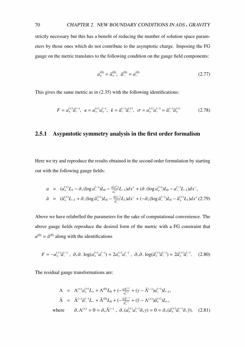
70 CHAPTER 2. NEW BOUNDARY CONDITIONS IN ADS 3 GRAVITY
strictly necessary but this has a benefit of reducing the number of solution space param-
eters by those ones which do not contribute to the asymptotic charge. Imposing the FG
gauge on the metric translates to the following condition on the gauge field components:
a(0)+ = a(0)
+ , a(0)− = a(0)
− (2.77)
This gives the same metric as in (2.35) with the following identifications:
F = a(+)+ a(−)
− , κ = a(+)+ a(−)
+ , κ = a(−)− a(+)
− , σ = a(+)+ a(−)
− = a(−)− a(+)
+ (2.78)
2.5.1 Asypmtotic symmetry analysis in the first order formalism
Here we try and reproduce the results obtained in the second order formulation by starting
out with the following gauge fields:
a = (a(+)+ L1 − ∂+(log a(−)
− )L0 −κ(x+)a(+)
+
L−1)dx+ + (∂−(log a(+)+ )L0 − a(−)
− L−1)dx−,
a = (a(+)+ L−1 + ∂−(log a(+)
+ )L0 −κ(x−)a(−)−
L1)dx− + (−∂+(log a(−)− )L0 − a(+)
+ L1)dx+.(2.79)
Above we have relabelled the parameters for the sake of computational convenience. The
above gauge fields reproduce the desired form of the metric with a FG constraint that
a(0) = a(0) along with the identifications
F = −a(+)+ a(−)
− , ∂+∂− log(a(+)+ a(−)
− ) = 2a(+)+ a(−)
− , ∂+∂− log(a(+)+ a(−)
− ) = 2a(+)+ a(−)
− . (2.80)
The residual gauge transformations are:
Λ = Λ(+)a(+)+ L+ + Λ(0)L0 + (− κΛ
(+)
a(+)+
+ (y − Λ(−))a(−)− )L−1,
Λ = Λ(−)a(−)− L− + Λ(0)L0 + (− κΛ
(−)
a(−)−
+ (y − Λ(+))a(+)+ )L+,
where ∂−Λ(+) = 0 = ∂+Λ(−) , ∂−(a
(+)+ a(−)
− ∂+y) = 0 = ∂+(a(+)+ a(−)
− ∂−y). (2.81)

2.5. LIOUVILLE BOUNDARY CONDITIONS IN CS FORMULATION 71
The solutions to y and y can be given in terms of ξr (2.48):
y = −∂+ξ
r
a(+)+ a(−)
−
, y = −∂−ξ
r
a(+)+ a(−)
−
. (2.82)
The FG constraint on the fluctuations yield the condition:
Λ(0) − Λ(0) = ∂−y + y∂− log(a(+)+ a(−)
− ) = ∂+y + y∂+ log(a(+)+ a(−)
− ). (2.83)
Therefore the residual gauge transformation parameters are labelled by {g, g,Λ(+),Λ(−)}.
After imposing the FG gauge the on can write
F = 1χa(+)
+ a(−)− , a(+)
+ = − 1χa(+)
+ , a(−)− = −χa(−)
− . (2.84)
It turns out that the fluctuations of the gauge field components yield the same result for
the metric components{F, κ, κ} as in the second order formalism with Λ(+) = ξ+(0) and
Λ(−) = ξ−(0); explicitly given in (2.52). The asymptotic charge for such configurations can
then be written as:
/δQ = − k2π
∫dφ (Tr[Λ.Aφ] − Tr[Λ.Aφ]),
= `8πG
∫dφ [Λ(+)δκ + Λ(−)δκ]
+(Λ(0)−Λ(0))
2 ∂−δ log a(+)+ − δa
(+)+ a(−)
− y +(Λ(0)−Λ(0))
2 ∂+δ log a(−)− − δa
(−)− a(+)
+ y,
= `16πG
∫dφ
{2(ξ+
(0)δκ + ξ−(0)δκ) + δΦ(∂+ + ∂−)ξr − ξr(∂+ + ∂−)δΦ}. (2.85)
The above expression for charge turns out to be the same as (2.50), as that in the second
order formalism. Since the expressions for the fluctuations and the charges are the same
in both the formalisms, we get the same asymptotic symmetry algebra as expected.
We are now ready to study the effects of generalizing boundary conditions studied in this
chapter to the case of supergravity and higher-spins in AdS 3. Since pure gravity in AdS 3
can be obtained as a consistent truncation of both supergravity and higher-spin gauge

72 CHAPTER 2. NEW BOUNDARY CONDITIONS IN ADS 3 GRAVITY
fields in AdS 3, demanding that the generalizations of the boundary conditions contain all
the configurations allowed by the boundary conditions studied in pure gravity may not be
enough. Tentatively one may consistently impose Dirichlet type boundary conditions on
all additional fields in the supergravity and higher-spin settings in AdS 3, while imposing
the boundary conditions studied in this chapter on the 3d metric components alone. We
would not be interested in such generalizations in this thesis.
In the pure gravity case studied here, the dynamical fields on the boundary are the bound-
ary metric(gauge field) components. In a similar spirit, we will demand that there be ad-
ditional supergravity and higher-spin gauge field components on the boundary of AdS 3,
apart from the metric(gauge field) components allowed by the boundary conditions stud-
ied in this chapter. In doing so we would be able study the properties of holographic duals
to induced supergravities and induced W-gravities.

Chapter 3
Holographic induced supergravities
We would now like to generalize the chiral and conformal boundary conditions pro-
posed for pure gravity in AdS 3 to a supersymmetric setting. This would primarily be a
first step in understanding how these boundary conditions arise in supersymmetric string
theories in AdS d×Σcompact spaces. Here, we would like to have configurations which allow
the additional supergravity fields to fluctuate along the boundary of AdS . We first analyse
this in a minimal set-up ofN = (1, 1) supergarvity with negative cosmological constant in
(2+1) dimensions, before commenting about generalizations to other more generic cases.
Here we uncover a relevant graded version of the sl(2,R) Kac-Moody current algebra
along with a super-Virasoro as the asymptotic symmetry algebra. This exercise was done
to generalize the Brown-Henneaux boundary conditions in [22] for the case ofN = (1, 1),
while the boundary conditions for extended sugra in AdS 3 was done in [2]. Here, the
authors were concerned with imposing boundary conditions consistent with the Brown-
Henneaux result in the pure gravity sector while imposing similar Dirichlet conditions on
the other superfields. In [2], the authors made full use of the Chern-Simons formulation of
AdS 3 supergravity and showed that the asymptotic symmetry algebra is composed of two
copies of super-Virasoros, i.e. supersymmetric generalization of two dimensional local
conformal transformations (Witt algebras) with central extension c = 3l/2G. Although
a supersymmetric extension of the Virasoro, these contained quadratic non-linearities on
73

74 CHAPTER 3. HOLOGRAPHIC INDUCED SUPERGRAVITIES
their right-hand sides, just like the W3 algebra. We would also study in the last section
of this chapter boundary conditions which generalize the the analysis of [5] to extended
super-gravities in AdS 3. This boundary condition allowed for the boundary metric to have
a dynamical conformal factor with flat curvature. The asymptotic algebra consists in this
case two copies of a Virasoro with an algebra of what one may term as supersymmetrized
harmonic Weyl transformations.
The contents of this chapter may be found in future in a paper yet to appear in [53].
3.1 N = (1, 1) super-gravity in AdS 3
We first begin with a simple set up where we would like to see whether one can generalize
the chiral boundary conditions of chapter 2. We will work in the Chern-Simons formula-
tion as we would see that the calculations are easier in this formulation of super-gravity
in AdS 3. The graded Lie algebra of interest for us is osp(1|2) which contains in it the
bosonic sl(2,R). The commutation relations are as follows:
σ0 = 12σ
3,[σ0,R±
]= ±1
2R±,[σ0, σ±
]= ±σ±,
[σ±,R±
]= 0,[
σ+, σ−]
= 2σ0,[σ±,R∓
]= R±,{
R±,R±}
= ±σ±,{R±,R∓
}= −σ0. (3.1)
The gauge-invariant, bi-linear, non-degenerate metric on the algebra is:
Tr(σaσb) = hab =14
2 0 0
0 0 4
0 4 0
, S Tr(R−R+) = −S Tr
(R+R−
)= 1. (3.2)

3.1. N = (1, 1) SUPER-GRAVITY IN ADS 3 75
3.1.1 Action
The N = (1, 1) supergravity action can be written as a difference to two Chern-Simons
actions,
S sugra−AdS 3 = S CS [Γ]∣∣∣k− S CS [Γ]
∣∣∣k,
S CS [Γ] =k
4π
∫S Tr(Γ ∧ dΓ + 2
3Γ ∧ Γ ∧ Γ),
where Γ =[Aaµσ
a + ψ+µR+ + ψ−µR−]
dxµ (3.3)
where the gauge algebra for the two CS terms is osp(1|2)1. One can rewrite the the above
Chern-Simons action in an explicit form for As and ψs as [23]
S CS [Γ] =k
4π
∫ [Tr(A ∧ dA + 2
3 A ∧ A ∧ A) + iψ ∧ Dψ],
ψ = ψTγ0, where γ0 =
0 1
−1 0
, γ1 =
1 0
0 −1
, γ2 =
0 1
1 0
,ψ =
ψ+
ψ−
, Dψ = dψ + 12 Aa ∧ γaψ. (3.4)
Note that the above definition for ψ would not be used from here on in this thesis. The
analysis can equivalently be carried out in the above form of the action and. We would
prefer to use the former form with the osp(1|2) algebra listed in the previous section. The
equation of motion- as mentioned earlier, is implied by the flatness condition imposed on
the two gauge fields valued in the adjoint of osp(1|2).
3.1.2 Boundary conditions
In order to obtain the required generalization, we first notice the form of the gauge fields
corresponding to the chiral boundary conditions written down in chapter 2. Referring back
1The product of two fermions differs by a factor of i from the standard Grasmann product ((ab)∗ = b∗a∗);this amounts to using S Tr (R−R+) = −S Tr (R+R−) = −i and {R±,R±} = ∓iσ±, {R±,R∓} = iσ0.

76 CHAPTER 3. HOLOGRAPHIC INDUCED SUPERGRAVITIES
to the analysis in section 2.3 we notice that the Virasoro Ward identity can be obtained
even when the components a(0) and a(−)− are put to zero. Therefore for ease of analysis, we
write the following gauge fields which also yields the same chiral boundary conditions on
the metric but the metric will no longer be in Fefferman-Graham gauge.
a = [L1 − κL−1] dx+,
a = [−L−1 + κL1] dx− + f (a)Ladx+,
A = b−1(d + a)b,
A = b(d + a)b−1, (3.5)
where we have used the notations and conventions of Appendix(6.3). The same conclu-
sions of section 2.3 can be reached by working with the above ansatz for the gauge fields
and they would indeed correspond to the chiral boundary conditions studied in sections
(2.3) and (2.2).
Here we note that the fluctuating field at the boundary comes from the f (−1) component of
a+ in (3.5). The components of a− play the role of sources i.e. functions that need to spec-
ified like a chemical potential. We further notice that all the a+ components are a priori
turned on and are determined in terms of f (−1). On the other hand, the a− component with
leading r dependence is fixed to be −1, while only the sub-leading component, L1 of a− is
allowed to have functional dependence.
Therefore taking a cue from the above observation, we propose the following fall-off
conditions:
Γ = bdb−1 + bab−1,
Γ = b−1db + b−1ab,
where b = eσ0 ln(r/`),
a =[σ− + Lσ+ + ψ+R+] dx+,

3.1. N = (1, 1) SUPER-GRAVITY IN ADS 3 77
a =[σ+ + Lσ− + ψ−R−
]dx− +
[Aa+σ
a + ψ+R+ + ψ−R−]
dx+.
(3.6)
Here the dx− component of the gauge field a one form is that of a super-gauge field
corresponding to Dirichlet boundary condition as given in [23, 22]. All functions above
are a priori functions of both the boundary coordinates. The equations of motion imply
∂+Γ− − ∂−Γ+ + [Γ+,Γ−] = 0,
∂+Γ− − ∂−Γ+ + [Γ+, Γ−] = 0. (3.7)
For the left gauge field this implies that the functions are independent of the x− co-
ordinate. i.e. ∂−a = 0.
∂−L = ∂−ψ+ = 0. (3.8)
While for the right gauge field components, equation of motion allows one to express the
sub-leading components of a+ in r in terms of its leading ones i.e. A++, ψ+,
A0+ = ∂−A++,
A−+ = A++L − 12∂
2−A++ + i
2 ψ+ψ−,
ψ− = A++ψ− − ∂−ψ+. (3.9)
The remaining relations imposed by equations of motion are differential equations relat-
ing components of a− and leading r components of a−. These are interpreted as Ward
identities for the boundary theory:
∂+L + 12∂
3−A++ − 2L∂−A++ − A++∂−L + iψ−
(A++ψ− + ∂−ψ+
)+ i∂−(ψ−ψ+) = 0,
∂+ψ− − ∂−[A++ψ− − ∂−ψ+] − 12∂−A++ψ− − Lψ+ = 0. (3.10)
Here, conventionally (according to Brown-Henneaux analysis) the () functions; A++, ψ+,
are sources i.e. chemical potentials coupling to conserved currents labelled by L, ψ− re-

78 CHAPTER 3. HOLOGRAPHIC INDUCED SUPERGRAVITIES
spectively. But our boundary conditions would require that the currents L, ψ− play the
role of sources. We will later choose these sources such that global AdS 3 is a part of the
moduli space of bulk solutions, i.e. L = −14 and ψ = 0.
The boundary terms required to make the set of solutions considered above variationally
well defined are:
S bndy =k
8π
∫∂M
d2x S Tr(−σ0[a+, a−]) − 2L0σ−a+ −
12 (ψ0)−R−a+). (3.11)
The variation of the total action therefore reads:
δS total =k
8π
∫M
d2x 2(L − L0)δA++ + i2 (ψ− − (ψ0)−)δψ+ (3.12)
Here, choosing the fluctuations δA++ and δψ+ to vanish would be similar to imposing
Dirichlet type boundary condition, where as allowing for their fluctuations demands that
the variational principal is satisfied when L = L0 and ψ− = ψ0. We choose the later case
as this would precisely imply fields fluctuating on the AdS boundary.
One may try and generalize the boundary conditions of Compère et al [6] by choosing
only x+ dependence for the fields fluctuating on the boundary -A++ and ψ+, for arbitrary
values of the sources L0 and ψ0−; but when one solves the above Ward identities then
one sees that ψ+ cannot just be a function of x+ unless L = 0. Therefore extending the
boundary conditions of [6] to the super-gravity case yields no super-symmetrization of
the asymptotic symmetries of their boundary conditions in the pure gravity case.
3.1.3 Charges and asymptotic symmetry
We first solve the equation of motion (3.10) for a particular value of L = −14 and ψ− = 0.
This choice of L allows for global AdS 3 to be one of the allowed solutions. This implies

3.1. N = (1, 1) SUPER-GRAVITY IN ADS 3 79
that the boundary fields A++ and ψ+ take the following form:
A++ = f (x+) + g(x+)eix− + g(x+)e−ix− ,
ψ+ = χ(x+)eix−/2 + χ(x+)e−ix−/2. (3.13)
The residual gauge transformations that leave a form invariant are thus:
Λ = ξaσa + ε±R±,
δa− = dΛ + [a−, Λ],
=⇒ ξ0 = ∂−ξ+,
ξ− = −14 (1 + 2∂2
−)ξ+,
ε− = −∂−ε+,
∂−(1 + ∂2−)ξ+ = 0 = (∂2
− + 14 )ε+. (3.14)
One can solve for the residual gauge transformation parameters:
ξ+ = λ f (x+) + λg(x+)eix− + λg(x+)e−ix− ,
ε+ = ε(x+)eix−/2 + ε(x+)e−ix−/2. (3.15)
The left gauge field components are independent of x− and the corresponding residual
gauge transformation are parametrized by:
Λ = ζaσa + ε±R±,
δa = dΛ + [a,Λ] ,
ζ0 = −∂+ζ−,
ζ+ = −12∂
2+ζ− + ζ−L − iψ+ε−,
ε+ = −∂+ε− + ζ−ψ+.,
0 = ∂−ζ− = ∂−ε−, (3.16)

80 CHAPTER 3. HOLOGRAPHIC INDUCED SUPERGRAVITIES
where all the parameters are determined in terms of ζ−(x+) and ε−(x+). We observe that the
arbitrary functions specifying the space of gauge fields a and a and the space of residual
gauge transformations are specified by functions of x+ alone. Therefore the x+ depen-
dence of the functions will be suppressed further. The variation of the above parameters
under the residual gauge transformations for the right sector are:
δ f = λ′f + 2i(gλg − gλg) + i(χε + χε),
δg = λ′g + i(gλ f − λg f ) + iχε,
δg = λ′g − i(gλ f − λg f ) + iχε,
δχ = ε′ + i[gε − f2ε − λgχ +
λ f
2 χ],
δχ = ε′ − i[gε − f2 ε − λgχ +
λ f
2 χ] (3.17)
Similar those for the left sector are:
δL = −12ζ′′′− +
[(ζ−L)′ + ζ′−L
]− i
[12 (ψ+ε−)′ + ψ+ε
′−
]δψ+ = −ε′′− +
[(ζ−ψ+)′ + 1
2ζ′−ψ+
]+ Lε−. (3.18)
The charges corresponding to these transformation is given by:
/δQ[Λ, Λ] = k2π
∫dφ
{S tr[Λ, δaφ] − S tr[Λ, δaφ]
}. (3.19)
The above charge can be integrated and is finite. The charges for the two gauge fields
decouple:
Q[Λ] = − k2π
∫dφ[− f
2λ f + gλg + gλg + χε − χε],
Q [Λ] = k2π
∫dφ (ζ−L + iε−δψ+) . (3.20)

3.1. N = (1, 1) SUPER-GRAVITY IN ADS 3 81
This charge is the generator of canonical transformations on the space of solutions parametrized
by set of functions F via the Poisson bracket.
δΛF = {Q[Λ], F} (3.21)
Therefore the Poisson bracket algebra for the right sector is:
{ f (x+′), f (x+)} = −2αQδ′(x+′ − x+), {χ(x+′), f (x+)} = −iαQδ(x+′ − x+)χ,
{g(x+′), f (x+)} = −2iαQg(x+)δ(x+′ − x+), {χ(x+′), f (x+)} = iαQδ(x+′ − x+)χ,
{g(x+′), f (x+)} = 2iαQg(x+)δ(x+′ − x+), {χ(x+′), g(x+)} = iαQδ(x+′ − x+)χ,
{g(x+′), g(x+)} = iαQ f (x+)δ(x+′ − x+), {χ(x+′), g(x+)} = −iαQδ(x+′ − x+)χ.
+αQδ′(x+′ − x+) (3.22)
While the fermionic Poisson brackets are:
{χ(x+′), χ(x+)} =iαQ
2 f (x+)δ(x+′ − x+) + αQδ′(x+′ − x+),
{χ(x+′), χ(x+)} = iαQg(x+)δ(x+′ − x+),
{χ(x+′), χ(x+)} = iαQg(x+)δ(x+′ − x+). (3.23)
where αQ = 2πk . Rescaling the above currents to:
f → k4π f , g→ k
2πg, g→ k2π g, χα →
k2πχα, χα →
k2π χα, (3.24)
and expanding them in the Fourier modes in x+ yields the following commutators:
[ fm, fn] = m k2δm+n, [χm, fn] = 1
2χm+n,
[gm, fn] = gm+n, [χm, fn] = −12 χm+n,
[gm, fn] = −gm+n, [χm, gn] = −χm+n,
[gm, gn] = −2 fm+n − mkδm+n,0, [χm, gn] = χm+n, (3.25)

82 CHAPTER 3. HOLOGRAPHIC INDUCED SUPERGRAVITIES
and anti-commutators:
{χm, χn} = −gm+n, {χm, χn} = −gm+n,
{χm, χn} = − fm+n − kmδm+n,0. (3.26)
This yields the familiar affine sl(2,R) current algebra at level k = c/6 with two additional
fermionic current parametrized by χ, χ. These fermionic currents form a semi-direct sum
with the sl(2,R) current algebra elements with their anti-commutators yielding the later.
Similarly the left sector yields the familiar Brown-Henneaux result. We first redefine the
currents by suitable scaling:
L→ k2πL , ψ+ →
k2πψ+. (3.27)
After these redefinitions one gets the following Poisson algebra:
{L(x′+), L(x+)
}=
k4πδ′′′(x′+ − x+) −
(L(x′+−) + L(x+)
)δ′(x′+ − x+),
i{ψ+(x′+), ψ+(x+)
}= − k
πδ′′(x′+ − x+) + 2L(x′+)δ(x′+ − x+),{
L(x′+), ψ+(x+)}
= −[ψ+(x′+) + 1
2ψ+(x+)]δ′(x′+ − x+). (3.28)
The Fourier modes for the above algebra satisfy the following Dirac brackets:
[Lm, Ln] = (m − n)Lm+n + k2m3δm+n,0,
{ψ+m, ψ+n} = 2Lm+n + 2km2δm+n,0,[Lm, ψ+n
]= (m
2 − n)ψ+(m+n). (3.29)
This is the Virasoro algebra with an affine super-current parametrized by ψ+.
The above result may also be obtained by working in the Hilbert-Palatini action for
super-gravity where the gauge transformations are recognized as diffeomorphisms and
local Lorentz transformations. This exercise was done for the Brown-Henneaux case in
3.2. GENERALIZATION TO EXTENDED ADS 3 SUPER-GRAVITY 83
[54]. The bulk diffeomorphisms that respect the super-gravity generalization of Brown-
Henneaux boundary condition would be generated by asymptotic Killing vectors and
asymptotic Killing spinors. The spinor bi-linears of the later are again asymptotic Killing
vectors. For the case of chiral boundary conditions dealt with in this chapter, it is difficult
to define asymptotic charges via the formalism of Barnich, Brandt and Compère is one
uses the approach of [54]. However one would essentially reach at the same set of asymp-
totic symmetries. Here too, one finds that bulk diffeomorphisms are generated by a set
of generalized Killing spinors whose bi-linears are the vector fields generating residual
diffeomorphisms found in chapter 2.
3.2 Generalization to extended AdS 3 super-gravity
Next, we will generalize the analysis of the last section to a extended super-gravity setting
with negative cosmological constant. Since the number for gauge field components would
now increase to include the once corresponding to the internal bosonic directions, it would
be interesting to see whether the chiral boundary conditions proposed admit a unique non-
trivial generalization. That is, we would seek boundary fall-off conditions for the gauge
field components such that all of them admit a fluctuating mode at the AdS 3 boundary
with the solutions elucidated in the pure gravity case being a subset. The N(4, 4) case
which would be of interest for realizing these boundary conditions in a string theoretic
setting would therefore be a special case of this analysis.
One first begins by classifying the super algebras possible in AdS 3 [55, 2]. Let G denote
the graded Lie algebra, such that G = G0 ⊕ G1, where G0 denotes the even part where
as G1 denotes the odd part. The even part, G0 must contain a direct sum of sl(2,R)
and an internal symmetry algebra denoted by G. The fermions must transform in the 2-
dimensional spinor representation of sl(2,R). The dimension of the internal algebra G is
denoted by D while the fermions transform under a representation ρ (dim ρ = d) of G

84 CHAPTER 3. HOLOGRAPHIC INDUCED SUPERGRAVITIES
which is real but not necessarily unitary. This is possible in the seven cases listed below:
G G D ρ
osp(N |2,R) so(N) N(N − 1)/2 N
su(1, 1|N)N,2 su(N) + u(1) N2 N + N
su(1, 1|2)/u(1) su(2) 3 2 + 2
osp(4∗|2M) su(2) + usp(2M) M(2M+1)+3 (2M, 2)
D1(2, 1;α) su(2) + su(2) 6 (2, 2)
G(3) G2 14 7
F(4) spin(7) 21 8s
The super-traces defined above are consistent, invariant and non-degenerate with respect
to the super-algebra defined above and would be used in defining the action and the
charges. The detailed analysis is given in in Appendix (6.4).
3.2.1 Action
The gauge field is then written as a super gauge field valued in the adjoint of the above
(graded Lie) super-algebra.:
Γ =[Aaµσ
a + BaµT a + ψ+αµR+α + ψ−αµR−α]
dxµ,
= ΓaµJadxµ. (3.30)
The gauge field as written above, separates as a sum of sl(2,R), G and fermionic one
forms. The parameters Aa and Ba commute2, while ψ±αs are anti-commuting Grasmann
parameters. The gauge field Γ is a G valued one-form.
The super-gravity action is then given as the difference of two Chern-Simons action at2It is understood in the above context that since Aa parametrizes the gauge one-form along the sl(2,R),
its index a runs from {0,+,−}. While the index a for the parameter Ba runs from {1..D} along the internalG basis.

3.2. GENERALIZATION TO EXTENDED ADS 3 SUPER-GRAVITY 85
level k written for two such gauge fields Γ and Γ.
S [Γ, Γ] = S CS [Γ] − S CS [Γ]. (3.31)
We will concern ourselves with the case where both Γ and Γ are valued in the same G.
The cases where this is not so leads to chiral action and can be regarded as one of the ways
to generate chiral asymptotic symmetries3. The detailed action is written out explicitly in
terms of the specific super-gauge field components in Appendix (6.4.2).
3.2.2 Boundary conditions
Now, we would like to impose boundary conditions on the gauge fields- just as in the
higher-spin case, which generalize the chiral boundary conditions on pure AdS 3 of chap-
ter 2. Here we would allow one of the super-gauge fields- Γ, to obey the boundary condi-
tions of [2] i.e. consistent with Brown-Henneaux, while proposing new boundary condi-
tions on Γ. The review of Brown-Henneaux type boundary conditions would be done in
the following analysis of Γ while the chiral boundary conditions generalized to extended
super-gravity would be analysed in Γ.
The fall-off conditions in terms of the gauge fields are:
Γ = bdb−1 + bab−1,
Γ = b−1db + b−1ab,
where b = eσ0 ln(r/`),
a =[σ− + Lσ+ + ψ+α+R+α + Ba+T a] dx+,
3At the level of the action there is no reason to suspect that the left and the right gauge fields representleft and right chiralities. A comment of such a nature can only be made in the light of suitable boundary con-ditions, which we know are necessary to be supplemented with a Chern-Simons theory on a non-compactgauge group. It so happens, that for the Brown-Henneaux boundary conditions the left and the right gaugefields do represent left and right chiralities, and it is with this understanding that we refer to them as twochiral sectors.

86 CHAPTER 3. HOLOGRAPHIC INDUCED SUPERGRAVITIES
a =[σ+ + Lσ− + ψ−α−R−α + Ba−T a
]dx− +
[Aa+σ
a + Ba+T a + ψ±α+R±α]
dx+.
(3.32)
Refer to Appendix (6.4.3) for more details. Provided they satisfy the following set of
differential equations:
∂+L + 12∂
3−A++ − 2L∂−A++ − A++∂−L
+iηαβψ−β−(A++ψ−α− + (λa)βαBa−ψ+β+ + ∂−ψ+α+
)+ iηαβ∂−(ψ−β−ψ+α+) = 0,
∂+Ba− − ∂−Ba+ + f bcaBb+Bc− + id−1
2Cρ(λa)αβψ+α+ψ−β− = 0,
∂+ψ−α− − ∂−[A++ψ−α− − ∂−ψ+α+ + (λa)βαBa−ψ+β+] − 12∂−A++ψ−α−
+(λa)βαBa−[A++ψ−β− − ∂−ψ+β+ + (λa)γβBb−ψ+γ+] − (λa)βαBa+ψ−β− − Lψ+α+ = 0.
(3.33)
These are the Ward identities expected to be satisfied by the induced gravity theory on the
boundary. Here, conventionally, the () functions A++, Ba+, ψ+α+, are sources coupling to
conserved currents L, Ba−, ψ−α−, respectively. Since it is the sources which are the ones
which survive on the boundary- as can be seen if one plugs back the r dependence, we
would like to solve these differential equations for particular value of the currents. There-
fore, as expected yielding an effective theory of of fluctuating sources on the boundary.
We will later choose the () functions such that global AdS 3 is a part of the moduli space
of bulk solutions.i.e. L = −14 and B = 0 = ψ.
The boundary term to be added so as to make the right sector ansatz variationally well
defined is given by:
S bndy =k
8π
∫∂M
d2x S Tr(−σ0[a+, a−]) − 2L0σ−a+ + (d−1
2Cρ)2T aT bS Tr(a+Ta)S Tr(a−Tb)
−2(d−12Cρ
)B0aT aT bS Tr(a+T b) − 12 (ψ0)−αR−αa+). (3.34)

3.2. GENERALIZATION TO EXTENDED ADS 3 SUPER-GRAVITY 87
This implies the following desired variation of the total action:
δS total =k
8π
∫M
d2x 2(L − L0)δA++ + 2( 2Cρ
d−1 )(Ba− − B0a)δBa+ + i2 (ψ−α− − (ψ0)−α)δψ+α+η
αβ
(3.35)
Here, one has an option of choosing δ() functions to vanish at the AdS asymptote, imply-
ing a Brown-Henneaux type boundary condition where A++, Ba+, ψ+α+ act as chemical po-
tentials. Or, alternatively, treat L, B0a, (ψ0)−α as chemical potentials allowing A++, Ba+, ψ+α+
to fluctuate. Thus describing a theory of induced gravity on the boundary. In our present
case, we would be choosing the later by fixing L = −1/4, B0a = 0 = (ψ0)−α. Thus the
variational principle is satisfied for configurations with L = −14 and Ba− = 0 = ψ−α− which
describes global AdS 3.
It turns out that one can choose the global AdS 3 configuration as the one with the zero
asymptotic charge i.e. the vacuum for the above boundary condition. If on the other hand
one chooses L = 0 - which corresponds to an extremal BTZ blackhole, then one gets
the generalization of Compère et al’s [48] to minimal supergravity. Here the vacuum
can be chosen to be extremal BTZ with global AdS 3 configuration not being a part of
the allowed space of solution. It is however interesting to note that allowing for global
AdS 3 to be part of the solution space allows extremal BTZ to be in the space of solutions
while disallowing non-extremal BTZ solutions. In other words, the only BTZ black-hole
configuration allowed by the above boundary condition is an extremal one.
3.2.3 Charges and symmetries
Just as in the previous chapters, one needs to find the space of gauge transformations
that maintains the above form of the gauge fields, thus inducing transformations on the
functions Aa+, Ba+, ψ+α+, L, Ba, ψ+α+ which parametrize the space of solutions. Once this
is achieved, one can define asymptotic conserved charge associated with the change in-

88 CHAPTER 3. HOLOGRAPHIC INDUCED SUPERGRAVITIES
duced by such residual gauge transformations on the space of solutions. For the boundary
conditions to be well defined, this asymptotic charge must be finite and be integrable on
the space of solutions.
Left sector
The analysis of the left sector is exactly as in [2] and is covered in the Appendix (6.4.4).
One basically gets the super-Virasoro with quadratic non-linearities as the asymptotic
algebra for the modes of parameters labelling the left sector gauge filed Γ.
[Lm, Ln] = (m − n)Lm+n + k2m3δm+n,0,[
Bam, B
bn
]= − f abcBc
m+n +2kCρ
d−1 mδabδm+n,0,[Lm, Ba
n]
= −nBam+n,{
(ψ+α)m, (ψ+β)n
}= 2ηαβLm+n − 2id−1
2Cρ(m − n)(λa)αβ(Ba)m+n
+ 2kηαβm2δm+n,0
− k( d−12kCρ
)2[{λa, λb
}αβ
+2Cρ
d−1ηαβδab]
(BaBb)m+n,[Lm, (ψ+α)n
]= (m
2 − n)(ψ+α)m+n,[Ba
m, (ψ+α)n]
= i(λa)βα(ψ+β)m+n. (3.36)
This is the non-linear super-conformal algebra or the super-Virosoro algebra. The central
extension is k = c/6, and is the same for all the seven cases listed in the table previously.
This algebra, although a supersymmetric extension of the Virasoro algebra, is not a graded
Lie algebra in the sense that the right-hand sides of the fermionic (Rarita-Schwinger)
anti-commutators contains quadratic non-linearities in currents for the internal symmetry
directions.

3.2. GENERALIZATION TO EXTENDED ADS 3 SUPER-GRAVITY 89
Right sector
The analysis of the right sector is similar to the one covered in the N = (1, 1) case and
is covered in the Appendix (6.4.4). Here we choose L = −14 , B = 0 = ψ as the values
for the chemical potential as it would allow for global AdS 3 as one of the solutions. The
asymptotic symmetry algebra in Fourier modes of the parameters labelling the right gauge
field Γ is
[ fm, fn] = m k2δm+n,0, [(χα)m, fn] = 1
2 (χα)(m+n),
[gm, fn] = gm+n, [(χα)m, fn] = −12 (χα)(m+n),
[gm, fn] = −gm+n, [(χα)m, gn] = −(χα)m+n,
[gm, gn] = −2 fm+n − mkδm+n,0, [(χα)m, gn] = (χα)m+n,
{(χα)m, (χβ)n} = −ηαβgm+n, {(χα)m, (χβ)n} = −ηαβgm+n,
[(Ba+)m, (χβ)n] = −(d−12Cρ
)(λa)αβ(χα)(m+n), [(Ba+)m, (χβ)n] = −(d−12Cρ
)(λa)αβ(χα)(m+n),
[(Ba+)m, (Bb+)n] = −i( d−12Cρ
) f cab (Bc+)(m+n) − (d−1
2Cρ)kmδabδm+n,0,
{(χα)m, (χβ)n} = −ηαβ f(m+n) + i(λa)αβ(Bc+)(m+n) − kmηαβδm+n,0. (3.37)
This is the affine Kac-Moody super-algebra. Here, it is evident that the central extension
to the sl(2,R)current sub-algebra spanned by ( f , g, g) is k = c/6. The quadratic non-
linearities that occur in the super-Virasoro are not present here.
Thus demanding that one considers all types of fields (A, B, ψ) have fluctuating compo-
nents on the boundary of asymptotic AdS 3, we have constructed a unique generalization
of the boundary condition studied in chapter 2 to extended super-gravity in asymptoti-
cally AdS 3 spaces. In doing so we uncovered the expected super-Virasoro algebra with
quadratic non-linearities for the left sector and a Kac-Moody super-current algebra at

90 CHAPTER 3. HOLOGRAPHIC INDUCED SUPERGRAVITIES
level k = c/6 for the right sector. Here, we have demanded as before that the global AdS 3
remain in the space of allowed solutions.
3.3 Boundary conditions for holographic induced super-
Liouville theory
We now turn to generalizing boundary conditions proposed by [5] to extended super-
gravity in AdS 3 The boundary conditions proposed by [5] allow the boundary metric to
fluctuate upto a conformal factor; demanding that the boundary metric have vanishing
Ricci curvature. This corresponds to the χ = 0 case in chapter 2, in (2.44). The nota-
tions and conventions below are taken from Henneaux et al [2] and are summarized in
Appendix (6.4.1).
We would like to carry out this analysis in the Chern-Simons formulation of gravity in
d = 3, as the supergravity fields can be conveniently encapsulated as components of the
gauge fields along the graded gauge algebra which comprise the super-gravity algebra.
Like in the case for boundary conditions for induced Liouville theory in chapter 2, the
analysis for the two gauge fields are identical; hence we will give the details of only one
of the gauge fields - A. One begins with an ansatz,
A = bab−1 + bdb−1,
a =[e−Φκσ− + eΦσ+ + Ba−T a + ψ+α−R+α + ψ−α−R−α
]dx−,
∂+a = 0, b = eσ0 ln(r/`). (3.38)
The equation of motion, ∂+a− − ∂−a+ + [a+, a−] = 0 is readily satisfied. The above form
of the gauge field ansatz doesn’t need extra boundary terms added to the Chern-Simons
action to make it variationally consistent. This is made apparent due to the fact that
the gauge field a as an 1-form only has a dx− component along the boundary while the

3.3. BOUNDARY CONDITIONS FOR HOLOGRAPHIC INDUCED SUPER-LIOUVILLE THEORY91
fluctuation of the action yields,
δS CS [A] = k2π
∫∂M
S tr[a ∧ δa]. (3.39)
We now look for the space of gauge transformations which keep the above 1−form a form
invariant.
δΛa = dΛ + [a, Λ] =⇒ δΛa∣∣∣σ0 = 0, ∂+Λ = 0 (3.40)
where
Λ = ξaσa + baT a + ε±αR±α. (3.41)
Solving these constraints on Λ, we get
δΛa∣∣∣σ0 = 0,
=⇒ ξ− = −12e−Φ∂−ξ0 + e−2Φκξ+ −
12e−Φηαβ(ψ+α−ε−β + ψ−α−ε+β). (3.42)
The variations these induce on the functions parametrizing the 1−form a are
δΛΦ = e−Φ∂−ξ+ − ξ0 + ie−Φηαβψ+α−ε+β,
δΛκ = −12∂
2−ξ0 + 1
2∂−Φ∂−ξ0 − 2∂−Φe−Φκξ+e−Φ + ∂−(κξ+),
− i2
[∂−Φ − ∂−
]ηαβ(ψ+α−ε−β + ψ−α−ε+β) + e−Φκ∂−ξ+
−iηαβ[eΦψ−α−ε−β − e−Φκψ+α− ˜ε+β
],
δΛBa− = ∂−ba + f bca Bb−bc − id−1
2Cρ(λa)αβ(ψ−α−ε+β − ψ+α−ε−β),
δΛψ+α− = ∂−ε+α −12 ψ+α−ξ0 + (eΦε−α − ψ−α−ξ+) − (λa)βα(Ba−ε+β − baψ+β−),
δΛψ−α− = ∂−ε−α + 12 ψ−α−ξ0 + eΦκε+α − (λa)βα(Ba−ε−β − baψ−β−)
−ψ+α+
[−1
2e−Φ∂−ξ0 + e−2Φκξ+ + i2e−Φηαβ(ψ+α−ε−β − ψ−α−ε+β)
]. (3.43)
Associated to the above fluctuations that keeps the gauge field a in the same form, are

92 CHAPTER 3. HOLOGRAPHIC INDUCED SUPERGRAVITIES
infinitesimal variations of a well defined asymptotic charge.
/δQ = − k2π
∫dφ S tr[Λδaφ],
= − k2π
∫dφ
{ξ−δeΦ + ξ+δ(e−Φκ) − iηαβ(δψ+α−ε−β − δψ−α−ε+β) +
2Cρ
d−1δBa−ba}.(3.44)
The next step is to be able to write the above change in the charge such that it is a total
variation δQ so that δ can be taken out of the integral and (the charge) can be integrated
from a suitable point (vacuum) on the solution space to any arbitrary point. Therefore, it
is important to recognize field independent parameters parametrizing the gauge transfor-
mations and accordingly functions of the fields parametrizing the space of solutions on
whom a phase space can be defined via the Poisson brackets induced by the integrated
charge.
The above expression for /δQ can be simplified if one redefines
ψ±α− = Ψ±α−e±Φ, ε±α = ε±αe±Φ, ξ+ = Ξ+eΦ. (3.45)
δQ = − k2π
∫dφ
{12δΦ
′ξ0 + Ξ+δκ +2Cρ
d−1δBa−ba − iηαβ[δΨ+α−ε−β − δΨ−α−ε+β
]}(3.46)
Therefore the total integrated charge is
Q = − k2π
∫dφ
{12Φ′ξ0 + Ξ+κ +
2Cρ
d−1 Ba−ba − iηαβ[Ψ+α−ε−β − Ψ−α−ε+β
]}(3.47)
The redefined gauge transformation parameters in (3.45) are therefore to be considered
field independent. Also, one sees that it is Φ′ and not Φ which is appropriate for defining
the phase space structure on the space of solutions. The variations of the redefined fields
in terms of the field independent gauge parameters are,
δΛΦ′ = ∂−(Φ′Ξ+) + ∂2−Ξ+ − ∂−ξ0 + iηαβ(∂−Ψ+α−ε+β + Ψ+α−∂−ε+β),
δΛκ = 2κ∂−Ξ+ + ∂−κΞ+ −12∂
2−ξ0 + 1
2Φ′∂−ξ0
− i2η
αβ[(Φ′Ψ+α− − ∂−Ψ+α− − Ψ+α−∂− + 2Ψ−α−)ε−β

3.3. BOUNDARY CONDITIONS FOR HOLOGRAPHIC INDUCED SUPER-LIOUVILLE THEORY93
+(Φ′Ψ−α− − ∂−Ψ−α− − 2κΨ+α− − Ψ−α−∂−)ε+β
],
δΛΨ+α− = −12Ψ+α−
[Φ′Ξ+ + iηρσΨ+ρ−ε+σ
]+ ∂−ε+α + 1
2Φ′ε+α + ε−α − Ψ−α−Ξ+
−(λa)βα(Ba−ε+β − baΨ+α−),
δΛΨ−α− = ∂−ε−α −12Φ′ε−α + κε+α − (λa)βα(Ba−ε−β − baΨ−β−)
−Ψ+α−
[−1
2∂−ξ0 + κΞ+ + iηαβ(Ψ+α−ε−β − Ψ−α−ε+β)]
+12Ψ−α−
[Ψ′Ξ+ + ∂−Ξ+ + iηαβΨ+α−ε+β
],
δΛBa− = ∂−ba + f bca Ba−ba − i d−1
2Cρ (λa)αβ(Ψ−α−ε+β − Ψ+α−ε−β). (3.48)
This leads to the following Poisson brackets amongst the solution space variables
−k2π
{κ(x−′), κ(x−)
}= −2κ(x−)δ′(x−′ − x−) + κ′(x−)δ(x−′ − x−),
−k2π
{Φ′(x−′), κ(x−)
}= −Φ′(x−)δ′(x−′ − x−) − δ′′(x−′ − x−),
−k2π
{Ψ+α−(x−′), κ(x−)
}=
[12Φ′Ψ+α− −
12∂−Ψ+α− + Ψ−α−
](x−)δ(x−′ − x−)
+12Ψ+α−(x−)δ′(x−′ − x−),
−k2π
{Ψ−α−(x−′), κ(x−)
}=
[−1
2Φ′Ψ−α− + 12∂−Ψ−α− − κΨ+α−
](x−)δ(x−′ − x−)
−12Ψ−α−δ
′(x−′ − x−),
−k2π
{Φ′(x−′), Φ′(x−)
}= 2δ′(x−′ − x−),
−k2π
{Ψ−α−(x−′), Φ′(x−)
}= −Ψ+α−(x−′)δ′(x−′ − x−),
−k2π
{Ψ+α−(x−′), Ψ+β−(x−)
}= −iηαβδ(x−′ − x−),
−k2π
{Ψ−α−(x−′), Ψ+β−(x−)
}= −iηαβδ′(x−′ − x−)
+[
i2ηαβΦ
′ − i(λa)αβBa− + 12Ψ+β−Ψ+α−
](x−)δ(x−′ − x−),
−k2π
{Ψ−α−(x−′), Ψ−β−(x−)
}=
[iκηαβ − Ψ+β−Ψ−α− −
12Ψ−β−Ψ+α−
](x−)δ(x−′ − x−),
−k2π
{Ba−(x−′), Ψ+α−(x−)
}= d−1
2Cρ (λa)βαΨ+β−(x−)δ(x−′ − x−),
−k2π
{Ba−(x−′), Ψ−α−(x−)
}= d−1
2Cρ(λa)βαΨ−β−(x−)δ(x−′ − x−),
−k2π
{Ba−(x−′), Bb−(x−)
}= −d−1
2Cρ
[δabδ
′(x−′ − x−) − f cab Bc−δ(x−′ − x−)
]. (3.49)
The first Possion bracket among κs can be easily recognized as that of the Witt algebra

94 CHAPTER 3. HOLOGRAPHIC INDUCED SUPERGRAVITIES
i.e. Virasoro without the central extension. The phase-space variable Φ′ can be used to
generate the central term in the Witt algebra of κ by redefining
ˆκ = κ + αcΦ′′. (3.50)
After further rescaling ˆκ → k2π one can show the central term in the Virasoro of ˆκ to be
2αc(αc + 1)k/(2π); which for αc = −12 ±
1√
2yields the central extension of the Virasoro
found in Brown-Henneaux analysis.
We conclude this chapter mentioning some salient points. The Brown-Henneaux type
boundary conditions adapted to super-gravity in AdS 3 [2] yield the super-Virasoro alge-
bra which has quadratic non-linearities, while the current algebra obtained as a result of
imposing chiral boundary conditions yielding the super-Kac-Moody current algebra do
not have such non-linearities on the rhs. We will see that this seems to be a recurrent
feature of the chiral boundary conditions imposed on gauge theories on AdS 3. We further
shown that the super-symmetrizing the boundary conditions of [5] yields a super exten-
sion of the harmonic Weyl transformations as the asymptotic algebra. Thus we see that
the Virosoro can be a sub-algebra of a new infinite dimensional super-algebra apart from
the super-Virasoro uncovered in [2].

Chapter 4
Holographic chiral induced W-gravities
In this chapter we turn to generalization of chiral boundary conditions studied in chapter
2 to the case of higher-spin gauge fields in AdS 3. We expect these boundary conditions
on such gauge fields in AdS 3 to be dual to a dynamical theory of higher-spin currents i.e.
induced theory of W-gravity, since according to the AdS /CFT prescription it is the gauge
fields in the bulk which couple to the boundary conserved currents. We study the case of
higher-spin fields with spin-2 and spin-3 fields are turned on; spin-2 field being the usual
metric or the graviton. As mentioned in the introduction, the only known complete action
for such theories when spins greater than 2 are included is in the Chern-Simons formalism
of gauge fields in AdS 3. For the higher spin theory based on sl(3,R)⊕ sl(3,R) algebra, our
boundary conditions give rise to one copy of classical W3 and a copy of sl(3,R) or su(1, 2)
Kac-Moody as the asymptotic symmetry algebra. We propose that the higher spin theories
with these boundary conditions describe appropriate chiral induced W-gravity theories on
the boundary. We also consider boundary conditions of spin-3 higher spin gravity that
admit a u(1) ⊕ u(1) current algebra.
95

96 CHAPTER 4. HOLOGRAPHIC CHIRAL INDUCED W-GRAVITIES
4.1 Chiral boundary conditions for S L(3,R) higher spin
theory
We are interested in proposing boundary conditions for higher spin theories such that they
holographically describe appropriate chiral induced W-gravity theories. In the first order
formalism the theory is formulated on the same lines as AdS 3 gravity but with the gauge
group replaced by S L(3,R) [46, 56]. The Dirichlet boundary conditions of this theory
were considered by Campoleoni et al [56] and they showed that the asymptotic symmetry
algebra is two commuting copies of classical W3 algebra with central charges.
We now turn to generalising the boundary conditions of the section (2.1) to the 3-dimensional
higher spin theory based on two copies of sl(3,R) or su(1, 2) algebra [46, 56]. Motivated
by the CIG boundary conditions of chapter 2 we write the connections again as deforma-
tions of AdS 3 solution. We work in the principal embedding basis for the gauge algebra.
Our conventions very closely follow those of [56] and may be found in Appendix (6.5).
The action is given as difference of two chern-Simons theories valued with gauge fields -
A and A, valued in the adjoint of sl(3,R). The generalized dribein and spin connections
are still given by the same relation,
e =`
2(A − A) ω =
12
(A + A), (4.1)
with the spin fields given by,
gµν =12
Tr(eµeν) ϕµνρ =13!
Tr(e(µeνeρ)). (4.2)
We make use of the same observation; as in the super-gravity analysis, to propose bound-
ary fall-off conditions on the higher-spin gauge fields. The gauge fields given below
a = [L1 − κL−1] dx+,

4.1. CHIRAL BOUNDARY CONDITIONS FOR S L(3,R) HIGHER SPIN THEORY97
a = [−L−1 + κL1] dx− + f (a)Ladx+,
A = b−1(d + a)b,
A = b(d + a)b−1, b = eL0 ln( r` ), (4.3)
reproduce the same Ward identity as in (2.59) and asymptotic symmetry algebra as in the
case of chiral induced gravity boundary conditions of chapter 2. They can be constructed
as follows:
Begin with the generic solution corresponding to the Brown-Henneaux boundary condi-
tions; which after getting rid of their radial dependence have 1-form components in either
x+ or x− directions. Then add to one of the gauge fields; a in the above case, a generic
adjoint valued component in the other direction; in this case f (a)Ladx+. Solving eom
with a priori generic functional dependence would subsequently yield the required Ward
identity.
Therefore we start with the following ansatz for the gauge connections:
A = b−1∂rb dr + b−1 [(L1 − κ L−1 − ωW−2) dx+] b (4.4)
A = b ∂rb−1 dr + b
(−L−1 + κ L1 + ωW2) dx− +
1∑a=−1
f (a)La +
2∑i=−2
g(i)Wi
dx+
b−1
where b is again eL0 ln rl . Note that, as in sl(2,R) case, our ansatz is the Dirichlet one
of [56] for the left sector. Similarly, the right sector includes the right sector ansatz of
previous section as a special case.1 All the coefficients of the algebra generators above
are understood to be functions of x+ and x−.
Imposing flatness conditions on A and A demand
∂−κ = 0, ∂−ω = 0, (4.5)
1A similar ansatz has been considered in [57].

98 CHAPTER 4. HOLOGRAPHIC CHIRAL INDUCED W-GRAVITIES
∂− f (−1) + f (0) = 0,
∂− f (0) + 2 f (1) + 2 κ f (−1) − 16α2 ω g(−2) = 0,
−∂+κ + ∂− f (1) + κ f (0) − 4α2 ω g(−1) = 0
∂−g(−2) + g(−1) = 0,
∂−g(−1) + 2 g(0) + 4 κ g(−2) = 0,
∂−g(0) + 3 g(1) + 3 κ g(−1) = 0,
∂−g(1) + 4 g(2) + 2 κ g(0) + 4 ω f (−1) = 0,
−∂+ω + ∂−g(2) + κ g(1) + 2 ω f (0) = 0. (4.6)
These equations enable one to solve for { f (0), f (1), g(−1), g(0), g(1), g(2)} in terms of {κ,
ω, f (−1), g(−2)} and their derivatives, provided the functions {κ, ω, f (−1), g(−2)} satisfy the
constraints coming from the 3rd and the 8th equations:
(∂+ + 2 ∂− f (−1) + f (−1) ∂−) κ − α2 (12 ∂−g(−2) + 8 g(−2)∂−) ω =12∂3− f (−1), (4.7)
12 (∂+ + 3 ∂− f (−1) + f (−1)∂−) ω + (10 ∂3−g
(−2) + 15 ∂2−g
(−2) ∂−+ 9 ∂−g(−2)∂2−+ 2 g(−2)∂3
−) κ
− 16 (2 ∂−g(−2)+ g(−2) ∂−) κ2 =12∂5−g
(−2). (4.8)
We point out that these are the Ward identities that the induced W3 gravity action is ex-
pected to satisfy. See Ooguri et al [21] for a comparison. These have also appeared
recently in [57] in a related context.
Next, we seek the residual gauge transformations of our solutions. Defining the gauge
parameter to be λ = λ(a)La + η(i) Wi and imposing the conditions that the gauge field
configuration a = (L1 − κ L−1 − ωW−2) dx+ is left form-invariant leads to the following
conditions [56]:
∂−λ(a) = ∂−η
(i) = 0,

4.1. CHIRAL BOUNDARY CONDITIONS FOR S L(3,R) HIGHER SPIN THEORY99
∂+λ(0) + 2 λ(−1) + 2 κ λ(1) − 16α2 ωη(2) = 0,
∂+λ(1) + λ(0) = 0,
∂+η(−1) + 4 η(−2) + 2 κ η(0) + 4ωλ(1) = 0,
∂+η(0) + 3 η(−1) + 3 κ η(1) = 0,
∂+η(1) + 2 η(0) + 4 κ η(2) = 0,
∂+η(2) + η(1) = 0. (4.9)
Under these we have
δκ = λ κ′ + 2 λ′ κ −12λ′′′ − 8α2 ηω′ − 12α2 ωη′ (4.10)
δω = λω′ + 3ωλ′ −83κ (κ η′ + η κ′) +
14
(5 κ′ η′′ + 3 η′ κ′′) +16
(5 κ η′′′ + η κ′′′) −1
24η′′′′′
(4.11)
We parametrize the residual gauge transformations of a by the gauge parameters λ =
λ(a)La + η(i) Wi. The constraints on this parameter are
λ0 + ∂−λ(−1) = 0,
∂−λ0 + 2 λ(1) + 2 κ λ(−1) − 16α2 ω η(−2) = 0,
∂−η(−2) + η(−1) = 0,
∂−η(−1) + 2 η(0) + 4 η(−2) κ = 0,
∂−η(0) + 3 η(1) + 3 η(−1) κ = 0,
∂−η(1) + 4 η(2) + 2 η(0) κ + 4 λ(−1) ω = 0. (4.12)
These induce the following variations:
δκ = −2 κ ∂−λ(−1) − λ(−1)∂−κ + 8α2 η(−2) ∂−ω + 12α2 ω ∂−η(−2) +
12∂3−λ
(−1) (4.13)

100 CHAPTER 4. HOLOGRAPHIC CHIRAL INDUCED W-GRAVITIES
δω = −λ(−1) ∂−ω − 3 ω ∂−λ(−1) +83κ (κ ∂−η(−2) + η(−2) ∂−κ)
−14
(5 ∂−κ ∂2−η
(−2) + 3 ∂−η(−2) ∂2−κ) −
16
(5 κ ∂3−η
(−2) + η(−2) ∂3−κ) +
124∂5−η
(−2)
(4.14)
δ f (−1) = ∂+λ(−1) + f (−1) ∂−λ
(−1) − λ(−1) ∂− f (−1) +323α2 κ (g(−2) ∂−η
(−2) − η(−2) ∂−g(−2))
+α2(∂−g(−2) ∂2−η
(−2) − ∂−η(−2) ∂2
−g(−2)) −
23α2 (g(−2) ∂3
−η(−2) − η(−2) ∂3
−g(−2)) (4.15)
δg(−2) = ∂+η(−2) + f (−1) ∂−η
(−2) − λ(−1) ∂−g(−2) + 2 (g(−2) ∂−λ(−1) − η(−2) ∂− f (−1)) (4.16)
For the residual gauge transformations to be global symmetries of the boundary theory
one needs to impose the variational principle δS = 0 as well. We add the following
boundary action:
S bdy.
=k
4π
∫d2x tr (−L0[A+, A−] + 2 κ0 L1 A+ +
12α
W0{A+, A−} +13
A+ A− + 2 ω0 W2A+)
(4.17)
With this the variation of the total action can be seen to be:
δS total = −k
2π
∫d2x [(κ − κ0) δ f (−1) + 4α2 (ω − ω0) δg(−2)] (4.18)
where κ0 and ω0 are some real numbers. Again we have several ways to satisfy δS = 0:
1. δ f (−1) = 0 and δg(−2) = 0.
This is the Dirichlet condition again (has been considered by [57] recently for con-
stant f (−1) and g(−2)) and leads to W3 as the asymptotic symmetry algebra.
2. κ = κ0 (ω = ω0 ) and δg(−2) = 0 (δ f (−1) = 0).

4.2. SOLUTIONS OF W3 WARD IDENTITIES 101
These are the other mixed boundary conditions – we will not consider them further
here.
3. κ = κ0 and ω = ω0 are the free boundary conditions we will consider below.
4.2 Solutions of W3 Ward identities
The W3 Ward identities (4.7, 4.8) are also expected to be integrable (just as the Vira-
soro one in section 2 was) and general solutions can be written down by appropriate
reparametrization of f (−1) and g(−2).
However, we restrict to the case of κ = κ0 and ω = ω0 for constant κ0 and ω0, and holding
them fixed. This allows for classical solutions with fluctuating f (−1) and g(−2). Let us solve
the W3 Ward identities in this case. These read
∂3− f (−1) + 24α2 ω0 ∂−g(−2) − 4 κ0 ∂− f (−1) = 0
∂5−g
(−2) − 20 κ0 ∂3−g
(−2) + 64 κ20 ∂−g
(−2) − 72 ω0 ∂− f (−1) = 0 (4.19)
There are two distinct cases: ω0 = 0 and ω0 , 0. When ω0 = 0 there are further two
distinct cases:
1. ω0 = 0 and κ0 = 0 gives:
f (−1) = f−1(x+) + x− f0(x+) + (x−)2 f1(x+), (4.20)
g(−2) = g−2(x+) + x− g−1(x+) + (x−)2 g0(x+) + (x−)3 g1(x+) + (x−)4 g2(x+)
This solution is suitable for non-compact x+ and x− (such as the boundary of Poincare
or Euclidean AdS 3)

102 CHAPTER 4. HOLOGRAPHIC CHIRAL INDUCED W-GRAVITIES
2. ω0 = 0 and κ0 , 0:
f (−1) = fκ(x+) + gκ(x+) e2√κ0 x− + gκ(x+) e−2
√κ0 x− , (4.21)
g(−2) = fω(x+) + gω(x+) e2√κ0 x−+ gω(x+) e−2
√κ0 x−+ hω(x+) e4
√κ0 x−+ hω(x+) e−4
√κ0 x−
Again any positive value for κ0 is suitable for non-compact boundary coordinates.
Among the negative values κ0 = −14 (times square of any integer) is suitable for
compact boundary coordinates (such as the boundary of global AdS 3).
3. When κ0 , 0 and ω0 , 0, again the Ward identities can be solved. The general
solutions involve eight arbitrary functions of x+ (just as in the cases with ω0 = 0).
Here we will only consider the special case where the solutions do not depend on
x−:
f (−1) = f (x+), g(−2) = g(x+). (4.22)
This case is the analogue of [6] in the higher spin context.
Next we analyse these cases one by one and find the asymptotic symmetries.
4.3 Asymptotic symmetries, charges and Poisson brack-
ets
To find the asymptotic symmetries to which we can associate charges one needs to look
for the residual gauge transformations of the solutions of interest. Just as in the sl(2,R)
case we can look at the residual gauge transformations of a and a and translate the corre-
sponding gauge parameters λ and λ using Λ = b−1λ b and Λ = b λ b−1. After finding these
one can compute the corresponding charges.
We are now ready to carry out this exercise for left sector and each of the cases (4.20,

4.3. ASYMPTOTIC SYMMETRIES, CHARGES AND POISSON BRACKETS 103
4.21, 4.22) in the right sector one by one.
4.3.1 The left sector symmetry algebra
The left sector is common for all of the cases we consider in this paper. The corresponding
/δQ is
/δQλ = − k2π
∫ 2π
0dφ (λ δκ − 4α2 η δω) (4.23)
This when integrated between (κ = 0, ω = 0) and generic (κ, ω) gives
Q(λ,η) = − k2π
∫ 2π
0dφ [λ κ − 4α2 ηω] (4.24)
This charge generates the variations (4.10, 4.11) provided we take the Poisson brackets
amongst the κ and ω to be:
− k2π
{κ(x+), κ(x+)
}= −κ′(x+) δ(x+ − x+) − 2 κ (x+) δ′(x+ − x+) + 1
2 δ′′′(x+ − x+),
− k2π
{κ(x+), ω(x+)
}= −2ω′(x+) δ(x+ − x+) − 3ω(x+) δ′(x+ − x+),
−2kα2
π
{ω(x+), ω(x+)
}= 8
3 [κ2(x+) δ′(x+ − x+) + κ(x+) κ′(x+)δ(x+ − x+)]
−16 [5κ(x+)δ′′′(x+ − x+) + κ′′′(x+)δ(x+ − x+)]
−14 [3κ′′(x+)δ′(x+ − x+) + 5κ′(x+)δ′′(x+ − x+)] + 1
24δ(5)(x+ − x+)
(4.25)
These brackets were computed by Campoleoni et al. [7]. To compare with their answers
one has to take κ → −2πk κ, ω→
π2kα2ω, α2 → −σ in the expressions here.
Next we turn to computing the charges and Poisson brackets on the right sector for all the
cases of interest.

104 CHAPTER 4. HOLOGRAPHIC CHIRAL INDUCED W-GRAVITIES
4.3.2 κ0 = 0 and ω0 = 0
In this case the residual gauge transformation parameters are
λ(−1) = λ−1(x+) + x− λ0(x+) + (x−)2 λ1(x+)
η(−2) = η−2(x+) + x− η−1(x+) + (x−)2 η0(x+) + (x−)3 η1(x+) + (x−)4 η2(x+) (4.26)
The corresponding action on the fields gives
δ f0 = λ′0 + 2 ( f−1 λ1 − λ−1 f1) − 2α2 (η−1 g1 − η1 g−1) − 16α2 (η2 g−2 − η−2 g2)
δ f1 = λ′1 + (λ1 f0 − λ0 f1) − 2α2 (η0 g1 − η1 g0) − 4α2 (η2 g−1 − η−1 g2)
δ f−1 = λ′−1 + (λ0 f−1 − λ−1 f0) − 2α2 (η−1 g0 − η0 g−1) − 4α2 (η1 g−2 − η−2 g1)
δg0 = η′0 + 3 (η1 f−1 − η−1 f1) + 3 (λ1 g−1 − λ−1g1)
δg1 = η′1 + (η1 f0 − λ0 g1) + 2 (λ1 g0 − η0 f1) + 4 (η2 f−1 − λ−1 g2)
δg−1 = η′−1 + (λ0 g−1 − η−1 f0) + 2 (η0 f−1 − λ−1 g0) + 4 (λ1 g−2 − η−2 f1)
δg2 = η′2 + (λ1 g1 − η1 f1) + 2 (η2 f0 − λ0 g2)
δg−2 = η′−2 + (η−1 f−1 − λ−1 g−1) + 2 (λ0 g−2 − η−2 f0) (4.27)
Defining
{Ja, a = 1, · · · , 8} = { f−1, f0, f1, g−2, g−1, g0, g1, g2}
{λa, a = 1, · · · , 8} = {λ−1, λ0, λ1, η−2, η−1, η0, η1, η2} (4.28)
these expressions can also be written in a compact form:
δJa = ∂+λa − f a
bcJbλc (4.29)

4.3. ASYMPTOTIC SYMMETRIES, CHARGES AND POISSON BRACKETS 105
where f abc are structure constants of our gauge algebra. The charge in this case is inte-
grable and has the expression:
Q[λ] = k4π
∫dx+ ηabJaλb (4.30)
The Poisson brackets can be read out and we find:
{Ja(x+), Jb(x+)} = f abc Jc(x+) δ(x+ − x+) − k
4π ηab δ′(x+ − x+) (4.31)
where we have redefined: Ja → − 4πk Ja. This may be recognized as level −k Kac-Moody
extension of the algebra used in defining the higher spin theory.
4.3.3 κ0 = −14 and ω0 = 0
In this case the residual gauge transformation parameters are
λ(−1) = λ f (x+) + λg(x+) ei x− + λg(x+) e−i x−
η(−2) = η f (x+) + ηg(x+) ei x− + ηg(x+) e−i x− + ηh(x+) e2i x− + ηh(x+) e−2i x− (4.32)
The symmetry transformations are:
δ fκ = λ′f + 2 i (gκ λg − λg gκ) + 2 iα2 (ηg gω − ηg gω) + 16 iα2 (ηh hω − ηh hω)
δgκ = λ′g + i (λg fκ − λ f gκ) + 2 iα2 (η f gω − ηg fω) + 4 iα2 (ηh gω − ηg hω)
δgκ = λ′g + i (λ f gκ − λg fκ) + 2 iα2 (ηg fω − η f gω) + 4 iα2 (ηg hω − ηh gω)
δ fω = η′f + 3i (ηg gκ − ηg gκ) + 3i (λg gω − λggω)
δgω = η′g + i (ηg fκ − λ f gω) + 2i (λg fω − η f gκ) + 4i (ηh gκ − λg hω)
δgω = η′g + i (λ f gω − ηg fκ) + 2i (η f gκ − λg fω) + 4i (λg hω − ηh gκ)
δhω = η′h + i(λg gω − ηg gκ) + 2i (ηh fκ − λ f hω)
δhω = η′h + i (ηg gκ − λg gω) + 2i (λ f hω − ηh fκ) (4.33)

106 CHAPTER 4. HOLOGRAPHIC CHIRAL INDUCED W-GRAVITIES
Defining the currents Ja and parameters λa as
{Ja, a = 1, · · · , 8} = {gκ, fκ, gκ, hω, gω, fω, gω, hω}
{λa, a = 1, · · · , 8} = {λg, λ f , λg, ηh, ηg, η f , ηg, ηh} (4.34)
these expressions can also be written in a compact form:
δJa = ∂+λa − i f a
bcJbλc (4.35)
where (some what surprisingly) f abc are obtained from the structure constants f a
bc by
replacing α2 → −α2. In this case the charge is:
Q[λa] = − k4π
∫ 2π
0dφ ηab λ
aJb (4.36)
where ηab is the one obtained from ηab by replacing α2 by −α2. The corresponding Poisson
brackets are
{Ja(x+), Jb(x+)} = i f abc Jc(x+) δ(x+ − x+) +
k4π
habδ′(x+ − x+). (4.37)
where again we have redefined: Ja → 4πk Ja. This again is a level-k Kac-Moody algebra,
but for the difference that it is obtained from the gauge algebra by α2 → −α2 replacement.
4.3.4 κ0 , 0, ω0 , 0, ∂− f (−1) = ∂−g(−2) = 0
In this case the residual gauge transformation parameters are
λ(−1) = λ(x+), η(−2) = η(x+). (4.38)

4.3. ASYMPTOTIC SYMMETRIES, CHARGES AND POISSON BRACKETS 107
Under these gauge transformations the fields transform as
δ f (−1) = ∂+λ, δg(−2) = ∂+η. (4.39)
Thus the residual gauge symmetries generate two commuting copies of U(1) classically.
Restricted to the sl(2,R) sub-sector this case corresponds to [6]. The charge is
Qa = k2π
∫ 2π
0dφ 2 [λ (κ0 f − 6α2 ω0 g) + η 2α2 (8
3 κ20 g − 3 ω0 f )] (4.40)
This leads to Poisson brackets:
{κ0 f (x+) − 6α2 ω0 g(x+), f (x+)} = −πkδ′(x+ − x+′), {83 κ
20 g(x+) − 3 ω0 f (x+), f (x+)} = 0
{κ0 f (x+) − 6α2 ω0 g(x+), g(x+)} = 0, { 83 κ20 g(x+) − 3 ω0 f (x+), g(x+)} = − π
2kα2 δ′(x+ − x+)
(4.41)
These four relations are solved by the following three equations:
{ f (x+), f (x+)} = −πkκ2
0∆δ′(x+ − x+), {g(x+), g(x+)} = −πk
3 κ016 ∆α2 δ
′(x+ − x+),
{ f (x+), g(x+)} = −πk9 ω08 ∆δ′(x+ − x+) (4.42)
where ∆ = κ30 −
274 α
2 ω20 which we have to assume not to vanish.2
The diagonal embedding of sl(2,R) in sl(3,R) gives rise to an asymptotic symmetry al-
gebra consisting of two copies ofW(2)3 also known as the Polyakov-Bershadsky algebra
when one generalizes Brown-Henneaux boundary condition to this case [58]. The central
2Taking linear combinations f + χ g and f − χ g (for some constant χ) as the currents one can decouplethese two u(1) Kac-Moody algebras.

108 CHAPTER 4. HOLOGRAPHIC CHIRAL INDUCED W-GRAVITIES
charge for the algebra turns out to be c/4. The gauge field choosen in [58] is of the type
A = eL0 ln(r/`)(W2 − T W−2 + jW0 + g1L−1 + g2W−1)e−L0 ln(r/`)dx+ + L0dr`,
where, W±2 = ±14W±2, L0 = 1
2 L0. (4.43)
Here the equations of motion forces the gauge field parameters to be a function of of
x+ alone. One can propose chiral boundary conditions in a manner similar to the one
illustrated in this chapter; one considers a gauge field of the type
A = eL0 ln(r/`)(a)e−L0 ln(r/`) + L0dr`,
where a = (W2 − T W−2 + jW0 + g1L−1 + g2W−1)dx+ + f (a)Jadx−,
& Ja ∈ {W−2,W−1, L−1, L0,W0, L1,W1, W2}. (4.44)
Here as before, the parameters are a priori functions of both the boundary co-ordinates.
The equation of motion can be used to to solve for f (a)s yielding differential equations
which are interpreted as Ward identities. The parameters {T , g1, g2, j} can be fixed to a
specific values by choosing boundary terms to be added to the Chern-Simons action fro
the gauge field A. One again expects to get an sl(3,R) and su(1, 2) current algebra for
certain values of these parameters {T , g1, g2, j}.
Thus the chiral boundary conditions studied in this chapter can be adapted to various
known W-algebras [45] yielding Ward identities for the corresponding chiral induced W-
gravities.
In this chapter, generalizing the results of chiral boundary conditions studied in chapter
2 and [9], we proposed boundary conditions for higher spin gauge theories in 3d in their
first order formalism that are different from the usual Dirichlet boundary conditions.3 The
left sector is treated with the usual Dirichlet boundary conditions where as in the right
3It should be noted that the ansatz for the right sector gauge field (4.4) studied here also appearedrecently in [59, 57] where the authors were still interested in generalizations of Dirichlet type boundaryconditions.

4.3. ASYMPTOTIC SYMMETRIES, CHARGES AND POISSON BRACKETS 109
sector we chose free boundary conditions. We restricted our attention to the spin-3 case
for calculational convenience. The Dirichlet boundary conditions for general higher spin
theory based on sl(n,R) Chern-Simons was discussed in [56] and for hs[λ] case in [14].
One should be able to generalize our considerations to these other higher spin theories as
well.
The boundary conditions considered here give one copy of W3 and a copy of sl(3,R) (or
su(1, 2) or u(1) ⊕ u(1)) Kac-Moody algebra. This matches with the symmetry algebra
expected of the 2d chiral induced W-gravity with an appropriate field content.
Let us emphasize that there appears to be a surprising difference between the asymptotic
symmetry algebras of section (4.3.2) and section (4.3.3) namely the maximal finite sub-
algebra of (4.31) is isomorphic to the gauge algebra of the higher spin theory where as
for that in (4.37) differs from the gauge algbra by α2 → −α2 (this interchanges sl(3,R)
and su(1, 2)). It will be interesting to understand the source of this possibility of getting a
different real-form of the complexified gauge algebra out of our boundary conditions.
The Poisson brackets between κ or ω of the left sector and any of the right sector currents
vanish. Recall that in the sl(2,R) case, motivated by how the asymptotic vector fields in
the second order formalism [3] acted on the fields, we made (current dependent) redef-
initions of the residual gauge parameters. Here too one can do such a redefinition. For
instance, if we change variables
λa → λa + α1Ja λ + α2 dabcJb Jc η + · · · (4.45)
where λa are the parameters defined in (4.28) and λ and η are the gauge parameters of the
left sector, dabc ∼ Tr(Ta{Tb,Tc}), then one finds that
κ → κ + #ηabJaJb + · · · , ω→ ω + #dabcJaJbJc + · · · , (4.46)
where the dots in these redefinitions represent possible terms of higher orders in Jas or

110 CHAPTER 4. HOLOGRAPHIC CHIRAL INDUCED W-GRAVITIES
terms involving derivatives of currents. The additional terms here may be recognized
as the (classical analogues) of Sugawara constructions of spin-2 and spin-3 currents out
of the Kac-Moody currents. After such redefinitions the generators of the asymptotic
symmetry algebras of the left and the right sectors will not commute any longer.

Chapter 5
Conclusion and discussions
5.1 Conclusion
In this thesis we uncovered the effect of imposing a novel set of boundary conditions on
gravity in AdS 3 which allow the boundary metric - and other fields if present, to fluctuate
along the boundary of AdS 3. This we further divide into two cases; one when the fluctu-
ating component of the boundary metric is chiral; another when it is a conformal factor
of the boundary metric.
• For the chiral boundary conditions imposed on pure gravity in AdS 3, we uncov-
ered a Virasoro with c = 3`2G times an sl(2,R) Kac-Moody current algebra with
level k = c/6 as the asymptotic symmetry algebra. We proposed that such chiral
boundary conditions make the bulk theory dual to a chiral induced gravity in 2d
first studied by Polyakov [10]. This is also born out by the Ward identity one ob-
tains as the bulk equations of motion for generic configurations obeying the chiral
boundary conditions. We generalized the chiral boundary conditions to extended
super-gravities and higher-spin gauge fields in AdS 3.
• In the super-gravity case we found a copy of super-Virasoro along with a Kac-
Moody super-current algebra with level k = c/6 as the asymptotic symmetry alge-
111

112 CHAPTER 5. CONCLUSION AND DISCUSSIONS
bra corresponding to super-symmetric extension of chiral induced gravity. Here we
also obtained the Ward identities obeyed by the Kac-Moody super-current algebra.
• In the higher-spin case we restricted the analysis to spins= 2, 3 and uncovered a
classical W3 algebra along with an su(1, 2) Kac-Moody current algebra with level
k = c/6 when the solution space contains global AdS 3; and an sl(3,R) Kac-Moody
current algebra with k = −c/6 when Poincaré AdS 3 is in the solution-space.
• We also generalized the boundary conditions of Compère et al [6] to the higher-
spin case and uncover a u(1) × u(1) along with a W3 as the asymptotic symmetry
algebra.
• For the case of conformal boundary conditions, we first provide a set of boundary
conditions for pure gravity in AdS 3 such that the boundary metric has non van-
ishing curvature and the boundary conformal factor satisfies the Liouville equa-
tions of motion. Here we uncovered 2-copies of Virasoro corresponding to the
Brown-Henneaux analysis with c = 3`2G and 2-copies of Virasoro corresponding to
the Liouville field stress tensor with c = − 3`2G . The conformal boundary conditions
with vanishing boundary curvature was studied by Troessaert [5] were 2-copies of
Virasoronu(1) were uncovered. We generalized these to extended super-gravity and
uncovered 2-copies of super-Virasoronsuper-current which is a super-symmetric
extension of the harmonic Weyl current obtained in [5].
5.2 Discussions
The chiral boundary conditions for pure gravity studied in this thesis have global AdS 3 in
the space of allowed solutions, implying that the asymptotic symmetry algebra contains
the sl(2,R) × sl(2,R) algebra; the symmetries of the maximally symmetric geometry in
3d with negative cosmological constant. This is not true for the boundary conditions
of Compère et al [6]. In this sense it is a solution to the question as to what boundary

5.2. DISCUSSIONS 113
conditions allow for asymptotic symmetries which admit an sl(2,R) × sl(2,R); to which
Brown-Henneaux [1], Troessaert’s boundary condition [5] and the conformal boundary
condition studied in chapter 2 are other answers.
Since the Ward identity uncovered for the chiral boundary conditions are exactly the same
as those of the chiral induced gravity in 2d [10], it would be interesting to know how one
can recover the correlation functions of the boundary currents from the bulk analysis. The
chiral boundary conditions studied here are peculiar in having a non-vanishing boundary
curvature and therefore a Weyl anomaly. This is also true for chiral induced gravity whose
effective action is usually interpreted as ‘integrated anomaly’1. The action for the 2d
induced gravity can be seen as an effective action for the boundary currents [45, 21, 60]
and can be obtained from the bulk on-shell action after the addition of suitable boundary
terms as written down in chapter 2.
The Chern-Simons formalism of 3d gravity gives a better understanding of this as one
can write the boundary conditions imposed as constraints on the conserved currents of a
WZNW action derived from the Chern-Simons theory on the group S L(2,R) [61]. There-
fore one may view the different boundary conditions on gravity in AdS 3 being dual to dif-
ferent constrained WZNW theories on the boundary. Similarly, induced gravities can be
obtained from constraining WZNW field theories with an appropriate level. For ordinary
gravity this was first studied in [62] and was generalized to W−gravity in [21]. These
comments also apply for the generalization of chiral boundary conditions to the case of
super-gravities and higher-spin gauge fields in AdS 3 with appropriate gauge groups.
An interesting exercise would be generalizing the conformal boundary conditions to in-
clude the higher-spin gauge fields in AdS 3 which would correspond to the conformal
factors of the higher-spin fields obeying Toda equations of motion. Since the case studied
in [5] corresponds to vanishing of the boundary Ricci scalar, generalizing to higher-spin
gauge fields in AdS 3 would require the knowledge of higher-spin curvature tensors, a
1See chapter 8 of the review on ‘W-symmetry in conformal field theory’ - Bouwknegt and Schoutens[16].

114 CHAPTER 5. CONCLUSION AND DISCUSSIONS
form of which was proposed in [63]. It is worthwhile to point out that the Liouville action
and similarly the Toda action can be derived from a constrained WZNW action on appro-
priate gauge group2, where in suitable constraints are placed on the conserved currents of
the latter action; this was first demonstrated by Balog et al [64] and Forgacs et al [65].
It would also be of interest to work out the case of super-higher-spin gauge fields in
AdS 3 in a similar light; generalizing both, the chiral and conformal boundary conditions.
The work generalizing Brown-Henneaux boundary conditions to super-higher-spins in
AdS 3 was done by Henneaux et al [66] where they discovered two copies of a non-linear
(N,M) extended super-W∞ algebra when the Chern-Simons theory defining the super-
higher-spin theory in the bulk is based on an infinite dimensional super-higher-spin alge-
bra shsE(N|2,R) × shsE(M|2,R). Further investigations of higher-spin theories in AdS 3
super-gravities and their CFT duals were considered in [67],[68].
It would be interesting to see how the considerations of the boundary conditions studied
in this thesis can be adapted when the bulk dimensions is d > 3 with negative cosmolog-
ical constant. Here if one tries to use the Dirichlet type boundary conditions and repeat
the Brown-Henneaux analysis, one simply uncovers the conformal Killing algebra of the
boundary which is finite dimensional so(2, d − 1) algebra when the boundary has dimen-
sions greater than two. As was seen in the chiral boundary conditions studied in this
thesis, bulk equations of motions on generic bulk configurations obeying a certain chiral
boundary condition may yield Ward identities for induced gravities defined on the dim>2
boundary. As mentioned in the introduction, these would be the Ward identities obeyed
by the generating function of the stress-tensor correlators of the boundary CFT.
The Ward identities and asymptotic symmetry analysis done in the bulk corresponds to
the large central charge limit. This central charge must correspond to the original CFT on
the boundary which was integrated out after coupling to gauge fields yielding an effective
theory of the these fields which is the induced gravity action on the boundary. People
2S L(2,R) for Liouville and S L(N,R) higher-spins ranging from 2, ...,N corresponding to N − 1 fieldsof the Toda theory.

5.2. DISCUSSIONS 115
have found a 1/c expansion for this effective action, and in the chiral induced gravities an
exact action in all orders of c on the boundary was found by Ooguri et al [21]. It would
be interesting to get a perturbative or if possible exact in c Ward identities and asymptotic
symmetries from the bulk analysis.
The notion of small and large gauge transformations or equivalently diffeomorphisms de-
pends on the boundary conditions imposed on the theory in question. When considering
Brown-Henneaux type boundary conditions; in vogue for over two decades, large diffeo-
morphisms where those which changed the boundary metric. When one uses boundary
conditions studied in this thesis and in [6, 5], large diffeomorphisms would be those which
would change the fall-off behaviour of the bulk configurations such that the change in the
asymptotic charge computed by the Barnich and Brandt’s approach [50] is infinite3.
It has been known for a long time that 2d unitary, Poincare and rigid scale invariant
QFT with a discrete non-negative spectrum of scaling dimensions has an extended global
symmetry of left and right semi-local conformal symmetry [69]. It was shown by Hofman
and Strominger [70] that if one began with 2D translations and just scale invariance in the
left sector i.e. x− → λx−, then one finds that the left sector scale symmetry gets enhanced
to an infinite dimensional left conformal symmetry, whereas the right translations either
can be enhanced to a right conformal symmetry or a U(1) Kac-Mood symmetry. This
seems to suggest the existence of 2d CFTs with infinite dimensional symmetries which
are not only of the left and right conformal symmetries i.e. the Virasoros. Given the fact
that 2d induced pure gravity has an S L(2,R) Kac-Moody symmetry it should be possible
to generalize the considerations in [70] to see the rigid right translations get enhanced
to either of an U(1) or an S L(2,R) or a right conformal symmetry. Moreover one could
also find minimum symmetries to be demanded by a unitary, Poincare and scale invariant
2D super-symmetric QFT and higher-spin QFT so that one can generalize the results of
[69] and [70] and further seek minimal conditions on these 2d QFTs to have relevant
super-symmetric and higher-spin Kac-Moody currents obtained in chapters 3 and 4.
3See Appendix (6.2) for a brief review.

116 CHAPTER 5. CONCLUSION AND DISCUSSIONS
The asymptotic symmetries of flat space pure gravity and super gravity have been com-
puted using techniques similar to the ones employed in this thesis4. For pure gravity in 3d
asymptotically flat space-times the BMS3 algebra emerges as the asymptotic symmetry
algebra, its supergravity extension was studied in [71] where in a super-symmetric ex-
tension of BMS3 was uncovered. The BMS algebra in 4d asymptotically flat space times
is closely related to Weinberg’s soft theorems and was studied by Strominger [72, 73]
and by Laddha and Campiglia [74]. The implications of BMS group in critical bosonic
string theory was studied by Avery and Burkhard [75] were they showed that the gener-
alized Ward identity for the action of this group yields the Weinberg’s soft theorem. The
BMS3 algebra and its super-symmetric extension was shown to be related to the flat-space
limit of gravity and similarly super-gravity in AdS 3 with Dirichlet boundary conditions.
It would be interesting to work out the possible flat-space limits of for the chiral and
conformal boundary conditions studied here for gravity and super-gravity in AdS 3.
It would be interesting to investigate as to where in the world-sheet formulation of string
theory in space times with AdS factors does one have the information about the boundary
conditions imposed. For the case of string theories on AdS 3 there have been works were
operators corresponding to the boundary Virasoro and super-Virasoro algebra have been
constructed in the world-sheet theory [76, 77, 78, 79]. It would be exciting to investi-
gate how such analysis can be carried out in the string world-sheet when the boundary
conditions studied in this thesis are considered.
The boundary conditions of [6] pick a certain class of BTZ configurations in the bulk
with the vacuum being the extremal BTZ solution. While the chiral boundary conditions
of chapter 2 have the global AdS 3 as the vacuum and the only black-hole solution allowed
is the extremal BTZ. The bulk theory of gravity in AdS 3 with boundary conditions of [6]
were interpreted as an effective theory on AdS 2 after dimensional reduction describing
the near horizon geometry of a (near)extremal black-hole. It would be interesting to see
whether the chiral boundary conditions studied here can have any application in such
4Various other approaches also exist.
5.2. DISCUSSIONS 117
a regard, especially since the boundary conditions of [8] do not yield a super-current
when generalized to super-gravities in AdS 3 but the chiral boundary conditions studied in
chapter 3 do.
It would in general be interesting to see how this duality between induced gravities on the
boundary with boundary condition similar to the ones proposed here on locally asymptotic
AdS spaces furthers our understanding of AdS/CFT and how it may give new insights into
quantities such as entanglement entropy, black-hole entropy etc.

118 CHAPTER 5. CONCLUSION AND DISCUSSIONS

Chapter 6
Appendix
6.1 Gauge fixing linearised AdS 3 gravity
In this section we linearise n-dimensional gravity1 with negative cosmological constant
around its global AdS n vacuum. Our conventions are
Γλµν =12
gλσ(∂µgσν + ∂νgµσ − ∂σgµν), Rλµσν = ∂σΓλµν − ∂νΓ
λµσ + ΓλδσΓδµν − ΓλδνΓ
δµσ
Rµν = Rλµλν, R = Rµνgµν . (6.1)
Then the variations of various terms are
δ(√−g) =
12√−g gµν δgµν = −
12√−g gµν δgµν, (6.2)
One useful variation is to find the physical fluctuations around any given background one
needs to consider the linearisation of GR:
gµν = gµν + hµν (6.3)
1We later fix n = 3.
119

120 CHAPTER 6. APPENDIX
and hµν = −gµλgνσhλσ. The background metric gµν is taken to satisfy the Einstein equation
Rµν = x gµν. This leads to the following variation of the Christoffel connections
δΓρµν =12
gρσ(∇µhσν + ∇νhµσ − ∇σhµν), (6.4)
for Riemann tensor
δRλµσν = 2∇[σδΓ
λν]µ, (6.5)
and for Ricci tensor
δRµν = ∇σδΓσµν − ∇νδΓ
σµσ
= ∇λ∇(µhν)λ −12
(∇2hµν + ∇µ∇νh) := RLµν
δRµν = hµσRσν + gµσRL
σν, (6.6)
where h = gµνhµν. The variation of the Ricci scalar is
δR = hµνRµν + gµνδRµν
= hµνRµν + ∇λ∇σhλσ − ∇2h := RL (6.7)
To simplify this further let us note the identity
[∇µ,∇ν]Tσκ···αβ··· = Rσ
λµνT λκ···αβ··· + Rκ
λµνTσλ···αβ··· + · · · − Rλ
αµνTσκ···λβ··· − Rλ
βµνTσκ···αλ··· − · · ·(6.8)
The equation that we would like to linearlize is
Rµν −12
R gµν =(n − 1)(n − 2)
2l2 gµν (6.9)
which is equivalent to
Rµν = −(n − 1)
l2 gµν. (6.10)
6.1. GAUGE FIXING LINEARISED ADS 3 GRAVITY 121
We assume that the background solution is a locally AdS n space with R = −n(n − 1)/l2.
Then we can write the Riemann tensor as
Rαβµν = −
1l2 (δαµ gβν − δαν gβµ) (6.11)
and we have
[∇µ, ∇ν] Tαβ = −gµαTνβ − gµβTαν + gνβTαµ + gναTµβ . (6.12)
Then the linearized equation is
−12
(∇2hµν + ∇µ∇νh) + ∇λ∇(µhν)λ = −n − 1
l2 hµν . (6.13)
Contracting this equation with gµν gives
∇λ∇σhλσ − ∇2h = −n − 1
l2 h . (6.14)
We try the gauge ∇λhλσ = κ ∇σh. The most popular choices are κ = 0 and κ = 1. We
choose the latter
∇λhλσ = ∇σh (6.15)
which when contracted by ∇σ gives
∇λ∇σhλσ = ∇2h
Substituting this into the linearized equation gives h = 0 (for n ≥ 2). Then we use (6.12)
to write
gλσ∇λ∇µhνσ = −n hµν + gµν h .

122 CHAPTER 6. APPENDIX
Finally we have
(2l2 + ∇2)hµν = 0, ∇µhµν = 0, gµνhµν = 0. (6.16)
Let us note that the gauge condition: ∇µhµν = 0 does not fix the diffeomorphism gauge
completely. If we perform a diffeomorphism by a vector ξ: hi j → hi j + gik∇ jξk + g jk∇iξ
k
then if ξk satisfies ∇kξk = 0, ∇2 ξi + gikRk jξ
j = 0. On the AdS n background we have
∇kξk = ∇2 ξi −
n − 1l2 ξi = 0. (6.17)
The former comes from demanding that h = 0 is preserved and the second follows from
requiring that the gauge condition is respected.2
From here on we restrict to n = 3 case and will solve these equations completely. The
equations (∇2 + 2l2 )hi j = g jk∇ jhki = h = 0 are implied by the first order equations:
1lhi j + εi
mn∇mhn j = 0 or1lhi j − εi
mn∇mhn j = 0 (6.18)
In fact as noted by Li et al [80] one can write (∇2 + 2l2 )hi j = 0 as DLDRhi j = 0 where
DL/Rhi j = 0 are the first order equations above. Therefore the most general solution for
hi j can be written as a linear combination of solutions to these first order equations.
Now, every solution to the fluctuation equations of AdS 3 gravity should be locally a pure
gauge - diffeomorphic to the background. This is true also of any solution to the above
first order equations where the diffeomorphism is generated by one of the solutions to the
residual gauge transformation equations. To see this one can show easily that gi j = gi j+hi j
where hi j is taken to be a solution of either of the first order equations has
δRλµσν = −
1l2 (δλσhµν − δλνhµσ) . (6.19)
2These equations are precisely that satisfied by any Killing vector, but not necessary that ξi is Killing.

6.1. GAUGE FIXING LINEARISED ADS 3 GRAVITY 123
This in turn implies that the Riemann tensor of gi j takes the form expected of a locally
AdS 3 metric up to higher order terms. But the background metric gi j is already that of
AdS 3. Therefore hi j should be writable locally as hi j = Lξgi j for some vector field ξi.
However, there are some diffeos that act non-trivially in the asymptotes and others don’t.
To discern which diffeomorphisms take one solution to a physically different solution,
one would have to take into account the boundary condition one imposes on the theory.
It is with regards to the boundary condition imposed that one would be able to determine
whether finite, infinite or zero charges are associated with these gauge transformations
rendering them as allowed, not allowed or trivial respectively. This would be dealt in the
next chapter of this Appendix.
Since we are working in a gauge we first look for all solutions to the residual gauge
transformation equations.
6.1.1 Solutions to residual gauge vector equation in AdS 3:
We work with the global coordinates for AdS 3:
ds2AdS 3
= l2(dρ2 − cosh2ρ dτ2 + sinh2ρ dφ2). (6.20)
The Killing vectors of this metric are:
L30 = −∂τ, L12 = ∂φ
(L31 + iη1L32) + iη2(L01 + iη1L02) = −ei(η1φ+η2τ)[∂ρ + i(η1 coth ρ ∂φ + η2 tanh ρ ∂τ)]
(6.21)
where η1, η2 are ±1. Here the algebra involved is:
[Lmn, Lpq] = ηmqLnp + ηnpLmq − ηmpLnq − ηnqLmp (6.22)

124 CHAPTER 6. APPENDIX
where m, n ∈ {3, 0, 1, 2} and ηmn = diag{−1,−1, 1, 1}. We also have for any Killing vector:
∇i∇ jξk = Rk
i jmξm, ∇2ξi = −gikRkmξ
m . (6.23)
The isometry algebra S O(2, 2) can be separated into sl(2,R) ⊕ sl(2,R):
L0 =i2
(∂τ + ∂φ), L±1 = ±12
e±i(τ+φ)(∂ρ ± i(tanh ρ ∂τ + coth ρ ∂φ) ,
L0 =i2
(∂τ − ∂φ), L±1 = ±12
e±i(τ−φ)(∂ρ ± i(tanh ρ ∂τ − coth ρ ∂φ) . (6.24)
The equations satisfied by the vector fields that generate residual gauge transformations
are:
∇kξk = 0, ∇2ξk =
2l2 ξ
k . (6.25)
One can in principle solve the above second order equation for ξk by solving for the
Green’s function3 for a massive vector field and using the vanishing divergence condition
in AdS 3, but we choose a different approach below. These can be decomposed into two
first order equations on ξi:
εmni ∇mξn = −
1lξi, εmn
i ∇mξn =1lξi (6.26)
Where ετρφ = l3 cosh ρ sinh ρ; we call these left and right movers respectively. Since these
are each a set of three coupled linear differential equations in ρ, the independent data
must comprise of three arbitrary functions of the boundary co-ordinate. This is exactly
the number of parameters which are required to parametrize a Diff×Weyl action on the
boundary metric. We consider the following ansatz for vector fields and decompose each
of the above equations to a second order ODE in one of the components.
ξi = ei(E0τ+Sφ)V i(ρ) (6.27)
3This would correspond to a bulk to bulk propagator for the massive vector field in AdS 3.

6.1. GAUGE FIXING LINEARISED ADS 3 GRAVITY 125
The left equation reduces to:
−iS Vρ − 2 sinh ρ cosh ρ(Vτ − Vφ
)+ sinh2 ρ ∂ρVφ = 0,
2Vτ + i(E0 tanh ρVφ + S coth ρVτ
)= 0,
iE0 Vτ + 2 sinh ρ cosh ρ(Vφ + Vτ
)+ cosh2 ρ ∂ρVτ = 0,
(6.28)
Eliminating Vρ and Vτ we get :
2(3E20 − E0S + 4S 2 − E2
0S 2 − S 4 + (E20 − S 2)(−4 + S 2) cosh 2ρ
+E0(E0 + S ) cosh 4ρ)Vφ + (sinh 2ρ cosh 2ρ(−4 + 6S 2)
+4 sinh 2ρ(S 2 + cosh 4ρ))∂ρVφ(ρ) + sinh2 2ρ(−2 + S 2 + 2 cosh 2ρ) ∂2ρV
φ = 0
(6.29)
The above differential equation has the boundary ρ→ ∞ as a regular singular point, hence
the solutions can be expanded in a series about the boundary. There are two solutions, one
which dies out at the boundary and one which doesn’t. Further we find that asymptotically
finite solutions exist when certain conditions between S and E0 hold true (6.31). We try
an ansatz for Vφ of the type:
Vφ(ρ) = sech2ρ tanhm ρ(a + cosh2 ρ). (6.30)

126 CHAPTER 6. APPENDIX
It turns out that the solution of this form implies the same conditions on E0 and S for
which it is asymptotically finite. Values of a and m for these solutions are:
E0 = S =⇒{m = −2 + S , a = 1/2(−2 + S + S 2)
}&
{m = −2 − S , a = 1/2(−2 − S + S 2)
},
E0 = −S =⇒ {m = −2 + S , a = 1/2(−2 + S )}
& {m = −2 − S , a = 1/2(−2 − S )} ,
E0 = 2 − S =⇒ {m = −2 + S , a = 0}
& {m = −4 + S , a = −1} ,
E0 = −2 − S =⇒ {m = −2 − S , a = 0}
& {m = −4 − S , a = −1} . (6.31)
Similar conditions are implied by the existence of asymptotic solutions of the right mov-
ing equation:
E0 = −S =⇒{m = −2 + S , a = 1/2(−2 + S + S 2)
}&
{m = −2 − S , a = 1/2(−2 − S + S 2)
},
E0 = S =⇒ {m = −2 + S , a = 1/2(−2 + S )}
& {m = −2 − S , a = 1/2(−2 − S )} ,
E0 = −2 + S =⇒ {m = −2 + S , a = 0}
& {m = −4 + S , a = −1} ,
E0 = 2 + S =⇒ {m = −4 − S , a = −1}
& {m = −2 − S , a = 0} . (6.32)
The first of the conditions in (6.31) and (6.32) give the left and right Virasoros in the bulk.
The 3rd and 4th conditions give only one solution instead of two, therefore there exist
more solutions linearly independent from those above for E0 = 2 − S , E0 = −2 − S for

6.1. GAUGE FIXING LINEARISED ADS 3 GRAVITY 127
left movers and E0 = −2 + S , E0 = 2 + S for right movers. Also (6.29) has a symmetry of
E0 → −E0 , S → −S which enables us to write down solutions for condition 4 (in (6.31)
& (6.32)) interms of solution for condition 3. The 4 copies of Virasoros are:
Ln =14
ieni(τ+φ)(1 + n + n2 + cosh 2ρ)sech2ρ tanhn ρ ∂τ
+12
eni(τ+φ)n(n + cosh 2ρ)csch2ρ tanhn ρ ∂ρ
+14
ieni(τ+φ)(−1 + n + n2 + cosh 2ρ)csch2ρ tanhn ρ ∂φ, & L†n
Ln = −14
iein(τ−φ)(−1 + n + n2 − cosh 2ρ)sech2ρ cothn ρ ∂τ+
12
ein(τ−φ)n(−n + cosh 2ρ)csch2ρ cothn ρ ∂ρ
−14
ieni(τ−φ)(−1 − n + n2 + cosh 2ρ)csch2ρ cothn ρ ∂φ, & L†n (6.33)
Ln and L†n correspond to the left moving Virasoro with E0 = S and Ln and L†n correspond
to the right moving Virasoro with E0 = −S . The remaining solutions to the left moving
equations are:
Tn = eni(τ−φ)[14
i(1 − n + cosh 2ρ)sech2ρ cothn ρ∂τ −12
n csch2ρ cothn ρ ∂ρ
+14
i(−1 − n + cosh 2ρ) csch2ρ cothn ρ ∂φ] &
T †n for E0 = −S .
Bn =12
ei(τ(2−n)+nφ)[i tanhn ρ ∂τ + tanh(n−1) ρ ∂ρ + i tanh(n−2) ρ ∂φ]
for E0 = 2 − S &
B†n for E0 = −2 − S ;
[L−1,Tn−1] = Dn
= 116ei(τ(n−2)−φn)
[−i(11 − 10n + 2n2 − 2(n − 3) cosh 2ρ + cosh 4ρ)sech4ρ cothn ρ ∂τ
+(−3 + 4n − 2n2 − 4(n − 1) cosh 2ρ + cosh 4ρ)cschρ sech3ρ cothn ρ ∂ρ
−i(−5 + 2n + 2n2 − 2(n − 1) cosh 2ρ + cosh 4ρ)
csch22ρ sech22ρ cothn ρ ∂φ]
for E0 = 2 − S &

128 CHAPTER 6. APPENDIX
[L−1,Tn−1]† = [T †n−1, L1] = D†n for E0 = −2 − S .
Similarly the ones for the right moving equation are:
Tn = ein(τ+φ)[i4
(1 + n + cosh 2ρ)sech2ρ tanhn ρ ∂τ −12
n csch2ρ tanhn ρ ∂ρ
−i4
(−1 + n + cosh 2ρ) csch2ρ tanhn ρ ∂φ] &
T †n for E0 = S
Bn =12
ei(τ(2+n)+φn)[i cothn ρ ∂τ + coth1+n ρ ∂ρ − i coth2+n ρ ∂φ],
for E0 = 2 + S &
B†n for E0 = −2 + S
[L1, Tn] = Dn
=18
(1 + n)ei((n+2)τ+nφ)
[i(5 + 2n + cosh 2ρ + cosh 4ρ) cschρ sech3ρ tanhn ρ ∂τ
(−3 − 2n + cosh 2ρ cosh 4ρ) csch22ρ tanhn ρ ∂ρ
+i(1 + 2n + cosh ρ) csch3ρ sechρ tanhn ρ ∂φ]
for E0 = 2 + S
[L1, Tn]† = [T †n , L−1] = D†n for E0 = −2 + S .
Their commutation relations with the killing vectors are(to be read along with their her-
mitian conjugates):
[Tn,Tm] = 0 [Tn, Tm] = 0
[L0,Tn] = 0 [L0, Tn] = 0
[L0,Tn] = −nTn [L0, Tn] = −nTn
[L1,Tn] = B1−n [L−1, Tn] = −B†−n−1
[L1,Tn] = −nTn+1 [L1, Tn] = −nTn+1
[L−1,Tn] = −nTn−1 [L−1, Tn] = −nTn−1
(6.34)

6.1. GAUGE FIXING LINEARISED ADS 3 GRAVITY 129
[Bn, Bm] = 0 [Bn, Bm] = 0
[L0, Bn] = −Bn [L0, Bn] = −Bn
[L0, Bn] = (n − 1)Bn [L0, Bn] = −(n + 1)Bn
[L1, Bn] = 0 [L1, Bn] = 0
[L−1, Bn] = −2T1−n [L−1, Bn] = −2T †−n−1
[L1, Bn] = (n − 1)Bn−1 [L1, Bn] = −(n + 1)Bn+1
[L−1, Bn] = (n − 1)Bn+1 [L−1, Bn] = −(n + 1)Bn−1
(6.35)
Also note that B1 = L1 & B−1 = L1.
Using these vector fields one can generate solutions to the metric fluctuation equation:
hi j = ∇iξ j + ∇ jξi. From Ln and Ln we find that the behaviour of hi j near the asymptotes is
hρρ ≈ O(e−4ρ), hρτ ≈ O(e−2ρ) ≈ hρφ, hττ ≈ hτφ ≈ hφφ ≈ O(1) . (6.36)
Note these are consistent with Brown-Henneaux boundary conditions (in fact hrr ∼ 1/r6
seems to fall faster then BH requirement). Whereas for Tn and Tn they are:
hρρ ≈ O(e−2ρ), hρτ ≈ O(e−2ρ) ≈ hρφ, hττ ≈ hτφ ≈ hφφ ≈ O(e2ρ) . (6.37)
and for Bn,Dn and their Bn, Dn they are:
hρρ ≈ O(e−2ρ), hρτ ≈ O(1) ≈ hρφ, hττ ≈ hτφ ≈ hφφ ≈ O(e2ρ) . (6.38)
If one tries to categorize these vector fields as to how they act on the boundary metric
then one can see that except for the Virasoros Ln, Ln, all other vectors effect the boundary
metric. {Tn, Bn, B†n} and {Tn, Bn, B
†n} change the dx+2 and dx−2 components while Dn, Dn
change the boundary metric by a mix of chiral Diff and Weyl transformation. Therefore,

130 CHAPTER 6. APPENDIX
the residual gauge transformations in the covariant gauge have an action of Diff×Weyl
on the boundary metric, as was also expected from the analysis done in the Fefferman-
Graham gauge.
The asymptotic values of the components of {Tn, Bn, B†n} match exactly in form to the
asymptotic values of {T (0)n ,T (+)
n ,T (−)n }
4 in (2.23). The essential data defining these vector
fields is their most leading asymptotic value, the subleading terms into the bulk away from
the boundary are basically an artefact of which gauge one tries to work in.
Therefore in the covariant gauge we do obtain close form expressions for the vector fields
which comprise the two copies of Witt algebra and the two copies of of the sl(2,R) Kac-
Moody current algebra. Which of these get choosen as the asymptotic algebra depends on
the boundary conditions and the boundary terms one adds to make the variational problem
well defined as discussed in all the chapters.
As was mentioned in chapter (2), one may have proceeded to work in the Fefferman-
Graham gauge where the residual gauge transformations generate a Diff×Weyl transfor-
mations of the boundary metric.
6.1.2 Gauge fixing in the Chern-Simons formalism
Since the the first order formalism for AdS 3 written as a difference of two Chern-Simons
theories can be a very useful, and in some cases the only construction, it would be inter-
esting to present the covariant gauge fixing approach outlined above in this formalism.
To this end it simply becomes necessary to write down the equivalent equations to (6.26)
on the gauge parameters Λ and Λ. The first order formalism is reviewed in the Appendix
(6.3) for details.
4The exact values of n might be different for either sides.

6.1. GAUGE FIXING LINEARISED ADS 3 GRAVITY 131
The equations (6.26) on the vector fields is equivalent to
ea[µDν]Λa = 0 & ea
[µDν]Λa = 0, (6.39)
where
eaµ = (A − A)a
µ,
Dµ and Dν are the respective gauge covariant derivatives. Since the Chern-Simons for-
malism admits natural generalisations to super-gravity and higher-spins in AdS 3, the
above gauge fixing condition generalises as it stands to these cases. One may read out
what the above condition translates to the non-sl(2,R) components of the gauge transfor-
mation parameters in these cases. For example, in the case of N = (1, 1) super-gravity in
AdS 3, the above condition translates to
γµDµε = 0.
ε = e−ργ2/2(ε0(x±) + e−ρε1(x±) + e−2ρε2(x±) . . . ).
where :
ε−0 = ε−0+(x+)eix−/2 + ε−0 (x+)e−ix−/2 + ε−00(x−),
ε+0 = −2∂−ε−0 ,
ε1.3.5... = 0,
ε−2 = −4∂−∂+ε−0 ,
ε−4 = 12ε−0 + 4∂−ε−0 + 2∂+ε
+2 (x±),
ε+4 = ∂−ε
−00 + 4i(eix−/2∂2
+ε−0+ − e−ix−/2∂2
+ε−0−) + 4∂3
−ε−00 + 2∂+∂−ε
+2 . (6.40)
Where
Dµε = (∂µ +14ωµ
a.b.Γa.b.)ε +
η
2lγµε, (6.41)
and the frames are
e0 = l cosh ρ dτ, e1 = l sinh ρ dφ, e2 = l dρ. (6.42)

132 CHAPTER 6. APPENDIX
Here we work with the following gamma matrices:
Γ0.
=
0 −1
1 0
, Γ1.
=
0 1
1 0
, Γ2.
=
−1 0
0 1
, (6.43)
Above, the ± index denotes 2 dimensional chirality w.r.t. γ2. The spinor bi-linears con-
structed out of these residual gauge spinors - χγµε are:
ξµ∂µ = −12∂− f (x±)∂ρ + f (x±)∂− + O(e−ρ).
where :
− f (x±) l4 = χ−00ε
−00 + χ−0−ε
−0+ + χ−0+ε
−0− + e−ix−χ−0 ε
−0− + eix−χ−0+ε
−0+ + e−ix−/2(χ−0−ε
−00 + χ−00ε
−0−)
+e−ix−/2(χ−0+ε−00 + χ−00ε
−0+). (6.44)
The above expression for the vector field coincides with the vector fields (2.23) if the
spinor parameters χ−00 and ε−00 are put to zero. Therefore:
− f (x±) l4 = χ−00ε
−00 + χ−0−ε
−0+ + χ−0+ε
−0− + e−ix−χ−0−ε
−0− + eix−χ−0+ε
−0+. (6.45)
6.1.3 Gauge fixing the the Fefferman-Graham gauge
The considerations of the previous sub-sections are easily reflected if the analysis were
carried out in the Fefferman-Graham gauge. Since we already know that the fluctuation
hµν will be given by a Lie derivative of the background metric gµν we can start with the
ansatz
hµν = −∇µξν − ∇νξµ (6.46)
and impose the gauge fixing conditions to find ξ. We write the background metric of
global AdS 3 as
ds2AdS 3
= l2[− cosh2ρ dτ2 + dρ2 + sinh2ρ dφ2
](6.47)

6.1. GAUGE FIXING LINEARISED ADS 3 GRAVITY 133
Then the gauge conditions hρρ = hρτ = hρφ = 0 give the following equations:
∂ρξρ = 0, − cosh2ρ ∂ρξ
τ + ∂τξρ = 0, sinh2ρ ∂ρξ
φ + ∂φξρ = 0. (6.48)
The general solution to these equations is given by the vector
ξ =[aτ(τ, φ) + (tanh ρ − 1) ∂τσ(τ, φ)
]∂τ+
[aφ(τ, φ) + (coth ρ − 1) ∂φσ(τ, φ)
]∂φ+σ(τ, φ) ∂ρ .
(6.49)
The corresponding hµν is
hττ = 2 cosh ρ[
sinh ρ (σ + ∂2τσ) + cosh ρ ∂τ(aτ − ∂τσ)
]hτφ = cosh2ρ ∂φ(aτ − ∂τσ) − sinh2ρ ∂τ(aφ − ∂φσ)
hφφ = −2 sinh ρ[
cosh ρ (σ + ∂2φσ) + sinh ρ ∂φ(aφ − ∂φσ)
](6.50)
The physical fluctuations therefore are characterized by a boundary scalar σ and a bound-
ary vector aµ. We have done the fluctuation analysis around the global AdS 3. The new
boundary metric changes and is given by
g(0)ττ = −
14
+12
(∂τaτ + σ), g(0)τφ =
14
(∂φaτ − ∂τaφ), g(0)φφ =
14−
12
(∂φaφ + σ) (6.51)
It turns out that the physical fluctuations around asymptotically locally AdS 3 space are
also characterized by a boundary scalar and a boundary vector. To see this we start with a
asymptotically locally AdS 3 space in Fefferman-Graham expansion:
ds2 = l2 dr2
r2 + r2[g(0)
ab +l2
r2 g(2)ab + · · ·
]dxadxb (6.52)
where xa are the boundary coordinates with boundary metric g(0). Then the gauge condi-
tions hrr = hra = 0 give rise to the residual gauge vector
ξ = σ(x) r∂r + aa(x) ∂a +1
2r2 gab(0)(x)∂bσ(x)∂a + O( 1
r4 ) (6.53)

134 CHAPTER 6. APPENDIX
with
hab = −r2[Lag(0)
ab + 2σ g(0)ab + O( 1
r2 )]
(6.54)
Therefore the residual diffeomorphisms in the Fefferman-Graham gauge have an action of
Diff×Weyl on the boundary metric g(0). The Diff×Weyl algebra in terms of the parameters
aa(x) and σ(x) is
[(aa
(1)∂a, σ1), (aa(2)∂a, σ2)
]=
((ac
(2)∂caa(1) − ac
(1)∂caa(2)) ∂a, ac
(1)∂cσ2 − ac(2)∂cσ1
), (6.55)
where aa(x) parametrises the vector fields generating infinitesimal diffeomorphisms and
σ(x) denotes the Weyl transformation parameter.
The 2d Lorentzian boundary metric is conformally flat and can always be locally written
as
ds2 = eϕ′(x+,x−)dx+dx−. (6.56)
The Lorentzian version of the Beltrami transform on (x+, x−) to (z(x, x+), z(x+, x−)) such
that
∂zx+ = µ∂zx+, ∂zx− = µ∂zx−, (6.57)
brings the boundary metric in the form
ds2 = eϕ(dz + µdz)(dz + µdz). (6.58)
Here the parameters µ and µ are such that |µ| < 1 and |µ| < 1. When the boundary has
just one spatial periodic direction, this parametrization captures arbitrary metric on the
boundary with fixed co-ordinates (z, z). For the case when µ = 0 = µ one recovers
the conformal metric. While for the case of chiral or light-cone gauge corresponds to
µ = 0 = φ. For either of these gauge choices one can recover the induced gravity action
on the boundary by considering appropriate boundary terms added to the bulk action. A

6.1. GAUGE FIXING LINEARISED ADS 3 GRAVITY 135
similar exercise was done by Bañados et al in [13].

136 CHAPTER 6. APPENDIX
6.2 Review of the asymptotic covariant charge formalism
6.2.1 Introduction
Noether’s first theorem gives a systematic way of associating conserved charges to con-
tinuous global symmetries of a theory. By global we mean that the parameters of these
symmetries are constants and have no space-time dependence. Gauge theories on the
other hand posses gauge symmetries which are parametrized by local functions of space-
time, and are a commonplace in physics. If one tries to associate conserved currents to
gauge symmetries following the usual procedure then one runs into a problem; the asso-
ciated current vanishes on-shell. This was first noticed by Noether herself and addressed
in Noether’s second theorem. We briefly outline the consequence of this theorem eluci-
dating the problem.
Consider a Lagrangian L(φi) which is function of fields φi and it’s space time deriva-
tives at a point in n dimensions. We denote by Xi the character of a symmetry of the
Lagrangian L i.e. Xi = δXφi. By definition a symmetry of the Lagrangian L satisfies
Xi δL
δφi = ∂µ jµX. (6.59)
The current jµX is conserved when Euler-Lagrange equations (eom) hold i.e. δLδφi = 0. Con-
sider now a gauge symmetry of the same Lagrangian L whose character we denote by
δ fφ = Riα( f α), where Ri
α =∑
k=0 Ri(µ1µ2...µk)α ∂µ1 ...∂µk and f α are some arbitrary (possibly
field dependent) local functions. Since this is a symmetry therefore
Riα( f α)
δL
δφi = ∂µ jµf . (6.60)

6.2. REVIEW OF THE ASYMPTOTIC COVARIANT CHARGE FORMALISM 137
Now, since the gauge transformation character Riα(.) is linear in its argument, one can shift
derivatives from the later onto δLδφi
Riα( f α)
δL
δφi = f αR+iα (δL
δφi ) + ∂µS µiα (δL
δφi , f α) = ∂µ jµf ,
=⇒ f αR+iα (δL
δφi ) = ∂µ
[jµf − S µi
α (δL
δφi , f α)]. (6.61)
The last equation implies that the r.h.s. is a total divergence for arbitrary local function
f α multiplying the l.h.s, implying
R+iα
(δL
δφi
)= 0. (6.62)
Therefore, in the presence of gauge symmetries there exists associated identities among
the Euler-Lagrange equations of motion. It is easily seen that the Euler-Lagrange equa-
tions satisfy a system of equations which are same in number to the independent gauge
parameters, and of same order in derivatives as is the character of gauge transformations.
This is Noether’s second theorem. Therefore for any conserved current jµf associated with
gauge transformations,
∂µ( jµf − S µiα (δL
δφi , f α)) = 0 (6.63)
holds true off-shell. The current S µiα ( δL
δφi , f α) depends linearly on the Euler-Lagrange equa-
tions of motion and the gauge transformation parameters. Using the algebraic Poincaré
lemma one concludes that the conserved current can be improved on-shell by a divergence
of a super-potential k[µν]f
jµf = S µiα (δL
δφi , f α) − ∂νk[µν]f (6.64)
for space-time dimensions greater than one. The form of the super potential is chosen
such that it drops out when the divergence of jµf is computed. The associated Noether
charge is then given by
Q f [φ] =
∫Σ
j f |φ =
∫∂Σ
k f |φ (6.65)

138 CHAPTER 6. APPENDIX
evaluated on-shell. Here, Σ is a n − 1 dimensional space-like surface with a boundary
∂Σ. This implies that the Noether charge associated with gauge transformation may be
given by some seemingly arbitrary super-potential thus giving rise to the fore mentioned
problem.
The work by Barnich and Brandt allows one to associate a certain equivalence class of
conserved n − 2 forms k[µν] to an equivalence class of gauge transformations respecting a
given set of boundary conditions. They further give conditions enabling one to associate
finite charges with such conserved n − 2 forms. Their analysis applies to quite a gen-
eral set of Lagrangian field theories as it is carried out independent of the specific details
Lagrangian in question. Prior to this work, prescriptions for computing finite conserved
charges associated to gauge theories prescribed with a particular set of boundary con-
ditions have been worked out for some specific Lagrangians, such as the Chern-Simons
theory defined on a non-compact gauge group and Einstein-Hilbert action for gravity in
2 + 1 dimensions. These results are readily reproduced from the general prescription
outlined in their work.
6.2.2 Definitions and result
We begin with a summary of definitions and notations required to state the result.
Let φi denote a solution to the Euler-Lagrange equations near the boundary. We denote
a field configuration by φi = φi + ϕi, where ϕi → O(χi) as one approaches the bound-
ary. Here, χi denote a set of functions which prescribes a desired fall-off condition, for
instance χi = 1/rmi, where the boundary is reached by taking the limit r → ∞ and mis
being some integers. Therefore {χi} describe a set of boundary conditions.
We further assume that the theory is "asymptotically linear". More precisely the leading

6.2. REVIEW OF THE ASYMPTOTIC COVARIANT CHARGE FORMALISM 139
order contribution to the Euler-Lagrange equations as one approaches the boundary comes
from the Euler-Lagrange equations linearised around a background solution. Let the be-
haviour of the linearised Euler-Lagrange equations evaluated on arbitrary ϕi → O(χi) be
denoted by O(χi) i.e.
∀ϕi → O(χi) :δL f ree
δϕi
∣∣∣∣∣ϕ(x)
dxn → O(χi), (6.66)
where L f ree is the Lagrangian L linearised about a background solution φi. Further, any
ϕi would be termed as an asymptotic solution if
δL f ree
δϕi
∣∣∣∣∣ϕ(x)
dxn → o(χi), (6.67)
where o(χi) denotes asymptotic behaviour of a lower degree than that of χi. The theory
being asymptotically linear would imply
∀ϕi −→ O(χi) :[δL
δφi −δL f ree
δϕi
]∣∣∣∣∣ϕ(x)
dxn → o(χi). (6.68)
We call those gauge transformation parameters as reducibility parameters which vanish
when the Euler-Lagrange equations hold and denote them by f α i.e.
Riα( f α) ≈ 0 (6.69)
Just like the Lagrangian, both Riα(.) and f α can be expanded in a power series in ϕi about
a particular background solution φi. We denote with a superscript as to how many powers
of ϕi they contain i.e.
Riα = Ri0
α + Ri1α + ... ,
f α = f α0 + f α1 + ... . (6.70)

140 CHAPTER 6. APPENDIX
Since δ fφi = Ri
α( f α) is a gauge symmetry of the full theory therefore we have
Riα( f α)
δL
δφi = ∂µS µiα (δL
δφi , f α). (6.71)
Expanding the above equation in powers of ϕi about φi one can show that R+i0α ( f α) gener-
ates gauge symmetries of L f ree. Further if f α = f α(x) is a field independent reducibility
parameter of the free theory, then the defining equation (6.69) for reducibility parameter
yields
Ri0α ( f α) = 05 (6.72)
and Ri1α ( f α) generates symmetries of the free theory.
As shown in the previous section, the Noether operators R+iα can be obtained from the
generating set of gauge transformations Riα by integration by parts and ignoring the total
derivative term that vanishes on-shell. These operators too furnish an asymptotic expan-
sion. Let R+iα denote the generating set of all Noether identities for the full theory i.e.
R+iα (δL
δφi ) = 0. (6.73)
Then, the generating set of Noether identities for the linearised theory is given by R+i0α
such that
R+i0α (
δL f ree
δφi )dxn −→ 0. (6.74)
Here as before, R+i0α is the ϕi independent term in the linearisation of R+i
α . Further we
define χα as
∀ψi −→ O(χi) : R+i0α (ψi) −→ O(χα). (6.75)
5Here the equality is evaluated while being on-shell w.r.t. the background field φi but being off shellw.r.t. to the linearised Lagrangian L f ree for ϕi

6.2. REVIEW OF THE ASYMPTOTIC COVARIANT CHARGE FORMALISM 141
Since the theory linearises as we approach the boundary therefore we assume
∀ψi −→ O(χi) : [R+iα (ψi) − R+i0
α (ψi)] −→ o(χα). (6.76)
The operators R+iα and R+i0
α are termed as the Noether operators of the full and the lin-
earised (free) theory respectively and act upon the left-hand sides of the respective Euler-
Lagrange equations of motion. The above statements on the linearisation of the full the-
ory implies that the linearised Euler-Lagrange equations and the corresponding linearised
Noether operators capture the leading order behaviour of the corresponding quantities of
the full theory as one approaches the boundary.
As explained in the previous section, a conserved current jµf defined in the usual manner
for any gauge transformation vanishes on-shell and can only be improved by a super-
potential k[µν]f , the origin of which seems arbitrary. But one can systematically associate
equivalence class of conserved n − 2 forms k[µν]f for equivalence class of asymptotic re-
ducibility parameters f α.
Let us now define what one means by an asymptotic reducibility parameter in the context
of a linearisable theory. We begin by expanding the definition for a reducibility parameter
(6.69) about a background solution φi in powers of the fluctuation ϕi.
Riα( f α) = M+i j(
δL
δφ j ),
φi = φi + ϕi,
δL
δφi
∣∣∣∣∣φi
= 0 (6.77)
and the operator M+i j(.) is linear and homogeneous in its arguments. Here we assume in
all generality that the operators Riα, M+i j and parameters f α depend on φi. At the zeroth

142 CHAPTER 6. APPENDIX
order in ϕi we find that the r.h.s. vanishes giving
Ri0α ( f α0) = 0 (6.78)
Further, if f α were field independent i.e. independent of ϕi6 then this would imply Ri0α ( f α) =
0. This should be seen as a condition defining a field independent reducibility parameter
of the full theory linearised about a background solution. Therefore, in a sense this would
be similar to finding Killing vectors of a background solution in general relativity about
which a theory is linearised.
Since we are interested in studying the symmetries of the linearised theory as it ap-
proaches a boundary, we therefore relax this condition and define asymptotic reducibility
parameters as a field independent parameters f α s.t.
∀ψi −→ O(χi) : ψiRi0α ( f α) −→ 0. (6.79)
Since R+i0α (ψi) −→ O(χα) and assuming integration by parts does not change the asymp-
totic degree, the above condition holds trivially for
f α −→ o(χα) ⇐⇒ f α ∼ 0, (6.80)
where |χα| = −|χα|. Therefore, non-trivial asymptotic reducibility parameters: f α −→
O(χα) - are defined upto asymptotic reducibility parameters with the above fall-off be-
haviour.
An asymptotically conserved n − 2 form is defined as
∀ϕi(x) : dH k|ϕ(x) −→ si(δL
δϕi )|ϕ(x), (6.81)
6Since we have linearised the theory about a background solution, field independence would refer to notdepending upon the fluctuation ϕi.

6.2. REVIEW OF THE ASYMPTOTIC COVARIANT CHARGE FORMALISM 143
where si(.) is an n − 1 form which depends linearly and homogeneously on its argument
and its derivatives. A conserved n − 2 form is trivial if
∀ϕi(x) : k|ϕ(x) −→ ti(δL f ree
δϕi )∣∣∣∣∣ϕ(x)
+ dH l|ϕ(x) (6.82)
where ti(.) is an n − 2 form which depends linearly and homogeneously on its argument
and its derivatives.
We use the above definitions to state the following bijective correspondence. An n − 1
form siα can be defined for a set of functions Qi as
∀Qi : dnx QiRi0α ( f α) = dnx R+i0
α (Qi) f α + dH siα(Qi, f α) (6.83)
For the case of Qi = δL f ree
δϕi the above equation reduces to
dH si(δL f ree
δϕi , f α) = dnxδL f ree
δϕi Ri0α ( f α). (6.84)
Further if f α is an asymptotic reducibility parameter as defined above then
∀ϕi : dH s f |ϕ(x) −→ 0,
=⇒ ∀ϕi : s f |ϕ(x) −→ −dH k f |ϕ(x). (6.85)
As s f is linear and homogeneous in the linearised field equations, k f is therefore an asymp-
totically conserved n − 2 form. The explicit expression for k f can be obtained from ap-
plying the contracting homotopy of the algebraic Poincaré lemma to s f .
k[µν]f
=12ϕi∂S sν
f
∂ϕiµ
+
(23ϕiλ −
13ϕi∂λ
) ∂S sνf
∂ϕiλµ
− (µ↔ ν), (6.86)
where ϕiλ = ∂µϕ
i and ∂Sϕiµ1µ2...µk
/∂ϕjν1ν2...νk = δi
jδν1ν2...νk(µ1µ2...µk), where indices are symmetrised
with weight one.
144 CHAPTER 6. APPENDIX
6.2.3 Some examples
As mentioned in the last section, the above result - which applies for a generic Lagrangian
systems that admits linearisation, yields the same expression for asymptotic charges as
was known in the case of certain gauge theories. We illustrate this in the case of Chern-
Simons theory defined on non-compact gauge group S l(2,R). Next, the prescription can
be used to define an asymptotically conserved D−2 current for the case of Einstein-Hilbert
gravity with arbitrary cosmological constant and boundary fall-off conditions.
Chern-Simons theory for a non-compact gauge group
We illustrate this in the case of Chern-Simons theory with a non-compact gauge group
S l(2,R) and level k
S cs =k
4π
∫A ∧ dA +
23
A ∧ A ∧ A. (6.87)
The theory is defined on a disk times a time coordinate Σ × R parametrized by (r, φ, t).
The asymptotic charge in this case was derived from Hamiltonian constraint analysis to
be
Qλ = −k
2π
∫dφ tr(λ aφ). (6.88)
Where A = A + a with A being flat F = dA + A ∧ A = 0 satisfies the Euler-Lagrange
equations. The gauge transformations and the linearised equation of motion for a are
described by
δλa = dλ + [A, λ] = ∇λ,
εσµν∇µaν = 0, (6.89)
respectively. Therefore, the analogue of Riα( f α) δL
δφi is
Riα( f α)
δL
δφi ∼ (∇σλa)εσµν∇µaaν. (6.90)

6.2. REVIEW OF THE ASYMPTOTIC COVARIANT CHARGE FORMALISM 145
One can show the existence of Noether’s identities by shifting the gauge covariant deriva-
tive from the gauge transformation parameter λ to the rest of the expression:
(∇σλa)εσµν∇µaaν = λaε
σµν∇σ∇µaaν + ∇σ(λaε
σµν∇µaaν),
= 2λaεσµν[Fσµ, aa
ν] + ∇σ(λaεσµν∇µaa
ν). (6.91)
The first term on the r.h.s. vanishes off-shell for arbitrary aν, therefore εσµν[Fσµ, aaν] = 0
is the Noether’s identity. The remaining term is interpreted as the divergence of
sµλ = −k
2πεµρσλa∇µaa
ν (6.92)
which is the required n − 1 form. Using (6.86) one gets
k[µν]λ = −
k2πεµνσλaaa
σ,
,
Qλ = −k
2π
∫dφ tr(λ aφ) (6.93)
as the super-potential and the conserved charge respectively.
Einstein-Hilbert gravity
We would now like to apply this technique to the case of classical gravity as defined by
the Einstein-Hilbert action in D space-time dimensions.
L =1
16π√−g(R − 2Λ) +Lmatter. (6.94)
Here the field is the metric gµν and the gauge transformations on it are the diffeomor-
phisms generated infinitesimally by vector fields via the Lie derivative i.e. δgµν = ∇(µξν).
We will work with configurations where the matter fields do not survive till the boundary.
In this case only the asymptotic dynamics of the theory is not governed by Lmatter.

146 CHAPTER 6. APPENDIX
The equation of motion linearised about a solution gµν for hµν = gµν − gµν reads as:
Hµν[h, g] =
√−g
32π
(2Λ
D − 2(2hµν‘ − gµνh) + DµDνh + DλDλhµν
−2DλD(µhν)λ − gµν(DλDλh − DλDρhρλ))
(6.95)
where h = hµνgµν and hµν = gµαgνβhαβ7. The gauge transformations are given by δξhµν =
gρ(ν∇µ)ξρ. Therefore
Riα( f α)
δL
δφi ←→ ∇(µξν)Hµν (6.96)
Thus the Noether identities which are obeyed for arbitrary fluctuations over the back-
ground hµν are given by ∇µHµν = 0, which can be easily verified by using equations of
motion Rµν = 2Λ(D − 2)−1gµν satisfied by gµν and general properties of the Riemann cur-
vature tensor.
The asymptotic reducibility parameters are vector fields such that
∀hµν → O(χµν) : dDx∇µξνHµν −→ 0. (6.97)
Applying the general formula (6.86) to the D − 1 form conserved current ξνHµν we get
k[νµ]ξ [h, g] = −
√−g
16π[∇ν(hξµ) + ∇σ(hµσξν) + ∇µ(hνσξσ)
+32h∇µξν + 3
2hσµ∇νξσ + 32hνσ∇σξµ − (µ↔ ν)
](6.98)
as the asymptotically conserved D − 2 form. The asymptotic conserved charge is accord-
ingly given by the integral of the above current over the D − 2 space-like surface at the
asymptote.
The above charges yield the expected charges (mass, angular momenta etc.) for the global
7Here () indicates quantities computed w.r.t. the background metric gµν.

6.2. REVIEW OF THE ASYMPTOTIC COVARIANT CHARGE FORMALISM 147
Killing vectors of the space-time w.r.t. a background metric (typically chosen to be the
maximally symmetric solution.).
/δQξ =
∫∂Σ
dD−2x kξ[h = δg, g] (6.99)
hµν consists of infinitesimal parameters hµν[δ f1, δ f2 . . . ] = δgµν that takes one away from
the background metric gµν. For the boundary conditions implied on hµν to be consistent the
expression for the infinitesimal variation of the asymptotic charge, /δQξ must be integrable,
i.e. /δQξ must have an expression as δ(Qξ).
148 CHAPTER 6. APPENDIX
6.3 AdS 3 gravity in first order formulation
The AdS 3 gravity in the Hilbert-Palatini formulation can be recast as a gauge theory with
action
S [A, A] =k
4π
∫tr(A ∧ A +
23
A ∧ A ∧ A) −k
4π
∫tr(A ∧ A +
23
A ∧ A ∧ A) (6.100)
up to boundary terms, where the gauge group is S L(2,R). These are related to vielbein
and spin connection through A = ωa + 1l ea and A = ωa − 1
l ea. The equations of motion
are F = dA + A ∧ A = 0 and F := dA + A ∧ A = 0. We work with the following defining
representation of the sl(2,R) algebra.
L−1 =
0 −1
0 0
, L0 =12
1 0
0 −1
, L1 =
0 0
1 0
, , (6.101)
Satisfying [Lm, Ln] = (m − n)Lm+n. The metric defined by Tr(Ta,Tb) = 12hab is
hab =
0 0 −2
0 1 0
−2 0 0
(6.102)
It is known that the connections
A = b−1∂rb dr + b−1(L1 − κ(x+) L−1) b dx+
A = b ∂rb−1 dr + b (κ(x−) L1 − L−1) b−1 dx− (6.103)
represent all the solutions of AdS 3 gravity satisfying Brown-Henneaux (Dirichlet) bound-
ary conditions (in FG coordinates) where b = eL0 ln rl . In fact, any solution of the Chern-
Simons theory (locally) can be written as
A = b−1∂rb dr + b−1 a b, A = b ∂rb−1 dr + b a b−1 (6.104)

6.3. ADS 3 GRAVITY IN FIRST ORDER FORMULATION 149
where a and a are flat connections in two dimensions with coordinates (x+, x−). The
general solution can be written as a = g−1 dg and a = g dg−1 where g and g are S L(2,R)
group elements that depend on (x+, x−). We now present general solution to this flatness
condition in a different parametrization that will be useful to us. Consider the most general
sl(2,R) 1-form on the boundary
a = (a(+)+ L1 + a(−)
+ L−1 + a(0)+ L0) dx+ + (a(+)
− L1 + a(−)− L−1 + a(0)
− L0) dx− (6.105)
Assuming that a(+)+ does not vanish, the flatness conditions imply:
a(0)− =
1
a(+)+
(a(+)− a(0)
+ + ∂−a(+)+ − ∂+a(+)
−
), a(−)
− =1
2a(+)+
(2 a(+)− a(−)
+ + ∂−a(0)+ − ∂+a(0)
−
)12∂3
+ f = ∂−κ − 2 κ ∂+ f − f ∂+κ (6.106)
where κ = a(+)+ a(−)
+ −14 (a(0)
+ )2 − 12∂+a(0)
+ + 12a(0)
+ ∂+ ln a(+)+ + 1
2∂2+ ln a(+)
+ −14 (∂+ ln a(+)
+ )2 and
f =a(+)−
a(+)+
. Similarly if we consider the 1-form
a = (a(+)+ L1 + a(−)
+ L−1 + a(0)+ L0) dx+ + (a(+)
− L1 + a(−)− L−1 + a(0)
− L0) dx− (6.107)
Then, assuming now that a(−)− does not vanish, the flatness conditions read
a(+)+ =
1
2 a(−)−
(2 a(+)− a(−)
+ + ∂−a(0)+ − ∂+a(0)
− ), a(0)+ =
1
a(−)−
(a(0)− a(−)
+ + ∂−a(−)+ − ∂+a(−)
− )
12∂3− f = ∂+κ − 2 κ ∂− f − f ∂−κ (6.108)
where f =a(−)
+
a(−)−
and κ = a(−)− a(+)
− −14 (a(0)− )2 + 1
2∂−a(0)− −
12 a(0)− ∂− ln a(−)
− + 12∂
2− ln a(−)
− −
14 (∂− ln a(−)
− )2. The last equation is again the famous Virasoro Ward identity that can be
solved explicitly as in section 2. Some special cases of the above formulae have appeared
before, for instance, in [61].

150 CHAPTER 6. APPENDIX
6.4 Generalization to extended AdS 3 super-gravity
We give the detail analysis of generalizing the chiral induced boundary conditions in-
troduced in chapter 2 to extended super-gravity in AdS 3. Here, the left moving gauge
field Γ obeys the boundary conditions of the Dirichlet type studied in [2] and we repeat
their analysis as it is for the left sector while imposing generalization of chiral boundary
condition on the right moving gauge field Γ. The conventions are taken as it is from [2].
6.4.1 Conventions
We follow the conventions of [2]. The structure constants for the G are fabc which are
completely anti-symmetric. The representation ρ has the basis (λa)αβ where a counts the
dimension of G i.e. D. Therefore, [λa, λb] = f abcλ
c. the Killing metric on G is denoted
by gab = − f acd f bcd = −Cνδab, where Cν is the eigenvalue of the second Casimir in the
adjoint representation of G. Similarly tr(λaλb) = − dDCρδ
ab, where Cρ is the eigenvalue of
the second Casimir in the representation ρ. We denote by ηαβ the G−invariant symmetric
metric on the representation ρ which is orthogonal. Its inverse is ηαβ, this is used to raise
and lower the supersymmetric (Greek) indices.
The list of all possible super-gravities in AdS 3 is given in section (3.2); we consider any
such generic extended sugra in AdS 3. Below we list all the super-algebra generators:
• The sl(2,R) generators are denoted as before by (σ0, σ±)
σ0 = 12σ
3,[σ0, σ±
]= ±σ±,[
σ+, σ−]
= 2σ0. (6.109)

6.4. GENERALIZATION TO EXTENDED ADS 3 SUPER-GRAVITY 151
The Killing form on sl(2,R) is:
Tr(σaσb) = hab =14
2 0 0
0 0 4
0 4 0
(6.110)
• The generators of G which commute with σas are8:
[T a,T b
]= f ab
c T c, where aε {1,D} ,[T a, σb
]= 0, where bε {+,−, 0} ,
S Tr(T aT b
)=
2Cρ
d−1δab. (6.111)
• The fermionic generators are denoted by R±α, where ± denotes the spinor indices
with respect to the sl(2,R) and α (Greek indices) denotes the vector index in the
representation ρ of G.
[σ0,R±α
]= ±1
2R±α, whereαε {1, d} ,[σ±,R±α
]= 0,[
σ±,R∓α]
= R±α,[T a,R±α
]= −(λa)αβR
±β,{R±α,R±β
}= ±ηαβσ±,{
R±α,R∓β}
= −ηαβσ0 ± d−12Cρ
(λa)αβT a,
S Tr(R−αR+β
)= −S Tr
(R+αR−β
)= ηαβ. (6.112)
Since the underlining algebra is now promoted to a graded Lie algebra, its genera-
tors satisfy the generalized Jacobi identity. The three fermion Jacobi identity thus
8The indices on σ always run over (0,+,−) while those on T run from (1...D), this is to be understoodfrom the context.

152 CHAPTER 6. APPENDIX
yields an identity for the matrices in the representation ρ of the internal algebra G:
(λa)αβ(λa)γδ + (λa)γβ(λa)αδ =Cρ
d − 1(2ηαγηβδ − ηαβηγδ − ηγβηαδ) (6.113)
The super-traces defined above are consistent, invariant and non-degenerate with respect
to the super-algebra defined above and would be used in defining the action and the
charges.
6.4.2 Action
The super Chern-Simons action is defined as:
S CS [Γ] =k
2π
∫M
S tr[Γ ∧ dΓ +23
Γ ∧ Γ ∧ Γ]. (6.114)
The above integration is over a three manifoldM = D × R, where D has a topology of
a disk. The level k of the Chern-Simons action is related to the Newton’s constant G in
three dimension and the AdS length ` through k = `/(4G). The product of two fermions
differs by a factor of i from the standard Grasmann product ((ab)∗ = b∗a∗).This basically
requires one the multiply a factor of −i where ever ηαβ occurs, and where ever d−12Cρ (λa)αβ
occurs while evaluating anti-commutator between fermionic generators in the calculations
below9.
In the Chern-Simons formulation of (super-)gravity, the metric (and other fields) which
occur in Einstein-Hilbert (Hilbert-Palatini) action are a derived concept. The equations of
motion for the Chern-Simons action can for example be satisfied by gauge field configu-9This basically so because the product of two real Grasmann fields is imaginary. This is equivalent to
using {R±α,R±β
}= ∓iηαβσ±,{
R±α,R∓β}
= iηαβσ0 ∓ i d−12Cρ
(λa)αβT a,
S Tr(R−αR+β
)= −S Tr
(R+αR−β
)= −iηαβ, (6.115)
instead of the one stated in the commutation relations of the extended super-algebra.

6.4. GENERALIZATION TO EXTENDED ADS 3 SUPER-GRAVITY 153
rations which may yield a non-singular metric. There fore one has to make sure that such
configurations are not considered in the analysis.
The super-gravity action for the above super-algebra can be written in full detail yielding
the action in the Hilbert-Palatini form:
S [Γ, Γ] = 18πG
∫M
d3x{12eR +e`2 +
−i`2εi jk(ψi)D
µνj (ψk)ν +
i`2εi jk(ψi)D
µνj (ψk)ν}
+Cρ
d − 1`εi jk(Ba
i ∂ jBak + 1
3 fabcBai Bb
j Bck)
−Cρ
d − 1`εi jk(Ba
i ∂ jBak + 1
3 fabcBai Bb
j Bck)
−i2εi jkηαβea
i ([ψ j]αta[ψk]β − [ ˜ψ j]αta[ψk]β)} (6.116)
The square brackets denote the two-component sl(2,R) spinor representations. The spin
covariant operatorsD and D are:
Dµνj =
2(ηαβ∂ j + (λa)αβBa
j)δµ+αδ
ν−β+
−ηαβ( 1
2ω3j[δ
µ+αδ
ν−β + δ
µ−αδ
ν+β] + ω+
j δµ−αδ
ν−β − ω
−j δ
µ+αδ
ν+β
) ,
Dµνj =
2(ηαβ∂ j + (λa)αβBa
j)δµ+αδ
ν−β+
−ηαβ( 1
2ω3j[δ
µ+αδ
ν−β + δ
µ−αδ
ν+β] + ω+
j δµ−αδ
ν−β − ω
−j δ
µ+αδ
ν+β
) (6.117)
From the form of the above action it is quite evident that the analysis done in the Hilbert-
Palatini formulation of super-gravity would be quite cumbersome if not difficult. Further,
it was found that computation of the asymptotic charge associated with gauge transfor-
mations which vary the super-gauge field at the AdS asymptote10 via the prescription of
Barnich et al [50] for the above form of the action is too difficult. The same prescription
of computing asymptotic charges in the Chern-Simons formalism yields a know expres-
sion for asymptotic charge in Chern-Simons theory. Therefore we proceed as before with
the analysis in the Chern-Simons prescription.
10By this we mean the boundary of the disk D

154 CHAPTER 6. APPENDIX
6.4.3 Boundary conditions
The fall-off conditions in terms of the gauge fields are:
Γ = bdb−1 + bab−1,
Γ = b−1db + b−1ab,
where b = eσ0 ln(r/`),
a =[σ− + Lσ+ + ψ+α+R+α + Ba+T a] dx+,
a =[σ+ + Lσ− + ψ−α−R−α + Ba−T a
]dx−
+[Aa+σ
a + Ba+T a + ψ+α+R+α + ψ−α+R−α]
dx+. (6.118)
Here the dx− component of the gauge field a one form is that of a super-gauge field corre-
sponding to Dirichlet boundary condition as given in [2]. All functions above are a priori
functions of both the boundary coordinates. The equation of motion- as mentioned earlier,
is implied by the flatness condition imposed on the two gauge fields. For the right gauge
field this implies that the functions are independent of the x− co-ordinate. i.e. ∂−a = 0.
∂−L = ∂−ψ+α+ = ∂−Ba+ = 0 (6.119)
For the left gauge field we would like to use the equations of motion to solve for the
a+ components. This gives the a+ components in terms of A++, Ba+, ψ+α+ and the a−
components:
A0+ = ∂−A++,
A−+ = A++L − 12∂
2−A++ + i η
αβ
2 ψ+α+ψ−β−,
ψ−α+ = A++ψ−α− − ∂−ψ+α+ + (λa)βαBaψ+β+. (6.120)
Provided they satisfy the following set of differential equations:
∂+L + 12∂
3−A++ − 2L∂−A++ − A++∂−L

6.4. GENERALIZATION TO EXTENDED ADS 3 SUPER-GRAVITY 155
+iηαβψ−β−(A++ψ−α− + (λa)βαBa−ψ+β+ + ∂−ψ+α+
)+ iηαβ∂−(ψ−β−ψ+α+) = 0,
∂+Ba− − ∂−Ba+ + f bcaBb+Bc− + id−1
2Cρ(λa)αβψ+α+ψ−β− = 0,
∂+ψ−α− − ∂−[A++ψ−α− − ∂−ψ+α+ + (λa)βαBa−ψ+β+] − 12∂−A++ψ−α−
+(λa)βαBa−[A++ψ−β− − ∂−ψ+β+ + (λa)γβBb−ψ+γ+] − (λa)βαBa+ψ−β− − Lψ+α+ = 0.
(6.121)
These are the Ward identities expected to be satisfied by the induced gravity theory on
the boundary. We will later choose the () functions such that global AdS 3 is a part of the
moduli space of bulk solutions.i.e. L = −14 and B = 0 = ψ.
In the following analysis we will consider the sources i.e. the bared functions as constants
along the boundary directions. There is no need to assume this, and we have done so only
for simplicity in the expressions for change in the moduli space parameters. Either ways,
demanding that the bared functions- L, B, ψ, be treated as sources which determine aspects
of the theory requires adding of specific boundary term to the bulk action. As explained
previously, this is done so that the required set of bulk solutions obey the variational
principle.
The boundary term to be added is given by:
S bndy =k
8π
∫∂M
d2x S Tr(−σ0[a+, a−]) − 2L0σ−a+ + (d−1
2Cρ)2T aT bS Tr(a+Ta)S Tr(a−Tb)
−2(d−12Cρ
)B0aT aT bS Tr(a+T b) − 12 (ψ0)−αR−αa+). (6.122)
This implies the following desired variation of the total action:
δS total =k
8π
∫M
d2x 2(L − L0)δA++ + 2( 2Cρ
d−1 )(Ba− − B0a)δBa+ + i2 (ψ−α− − (ψ0)−α)δψ+α+η
αβ
(6.123)
In our present case, we would be choosing the later by fixing L = −1/4, B0a = 0 = (ψ0)−α.
Thus the variational principle is satisfied for configurations with L = −14 and Ba− = 0 =

156 CHAPTER 6. APPENDIX
ψ−α− which describes global AdS 3.
6.4.4 Charges and symmetries
Just as in the previous chapters, one needs to find the space of gauge transformations
that maintains the above form of the gauge fields, thus inducing transformations on the
functions Aa+, Ba+, ψ+α+, L, Ba, ψ+α+ which parametrize the space of solutions. Once this
is achieved, one can define asymptotic conserved charge associated with the change in-
duced by such residual gauge transformations on the space of solutions. For the boundary
conditions to be well defined, this asymptotic charge must be finite and be integrable on
the space of solutions.
Left sector
The analysis of the left sector i.e. on the gauge field Γ is exactly the one done in [2]. We
first find the space of residual gauge transformations that maintain the form of Γ. The
residual gauge transformations acting on a are parametrized as Λ = ζaσa +ωaT a +ε±αR±α
where there is no explicit radial dependence. The radial dependence can be introduced
just as for the gauge fields b−1Λb. The variation of a under such gauge transformation is:
δa− = 0,
=⇒ ∂−Λ = 0,
δa+ = ∂+Λ + [a+,Λ],
=(∂+ζ0 + 2Lζ− − 2ζ+ − iηαβψ+αε−β
)σ0
+(∂+ζ+ − Lζ0 + iηαβψ+αε+β
)σ+
+ (∂+ζ− + ζ0)σ−
+(∂+ωc + f abcBaωb + id−1
2Cρ(λc)αβψ+αε−β
)T c
+(∂+ε+β + Lε−β − (λa)αβε+αBa − ζ0ψ+β + (λa)αβωaψ+α
)R+β
+(∂+ε−β + ε+β − (λa)αβε−αBa − ζ−ψ+β
)R−β (6.124)

6.4. GENERALIZATION TO EXTENDED ADS 3 SUPER-GRAVITY 157
The above change in a under gauge transformation must preserve the form of a. This
allows for three independent gauge transformation parameters in terms of which the rest
of the gauge transformation parameters are determined.
ζ0 = −∂+ζ−,
ζ+ = −12∂
2+ζ− + ζ−L − iηαβψ+αε−β,
ε+α = −∂+ε−α + ζ−ψ+α + (λa)βαε−βBa. (6.125)
Here, all the residual gauge parameters are independent of x−, just like the solution space
parameters for the gauge field Γ. The gauge transformation parameter Λ with the above
substitution parametrizes the space of residual gauge transformations for Γ. The corre-
sponding changes in the solution space parameters are:
δL = −12ζ′′′− +
[(ζ−L)′ + ζ′−L
]− iηαβ
[12 (ψ+αε−β)′ + ψ+αε
′−β
]−(λa)αβψ+αBaε−β,
δBa = ω′a + f bca Bbωc + id−1
Cρ(λa)αβψ+αε−β,
δψ+α = −ε′′−α +[(ζ−ψ+α)′ + 1
2ζ′−ψ+α
]+ Lε−α + (λa)βα
[(ε−βBa)′ + ε′−βBa
]+
+ (λa)βαωaψ+β − ζ−(λa)βαψ+βBa −12
{λa, λb
}γαε−γBaBb. (6.126)
The asymptotic charge associated with the full bulk geometry splits as difference for the
ones corresponding to the left and the right sector, just like the action. The asymptotic
charge associated with the left sector is given by:
/δQ =k
2π
∫dφS Tr[Λδaφ],
δQ =k
2π
∫dφ
(ζ−δL + d−1
2CρωaδBa + iηαβε−αδψ+β
). (6.127)
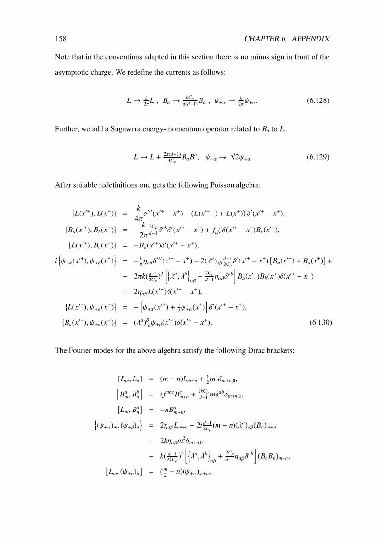
158 CHAPTER 6. APPENDIX
Note that in the conventions adapted in this section there is no minus sign in front of the
asymptotic charge. We redefine the currents as follows:
L→ k2πL , Ba →
kCρ
π(d−1) Ba , ψ+α →k
2πψ+α. (6.128)
Further, we add a Sugawara energy-momentum operator related to Ba to L.
L→ L +2π(d−1)
4CρBaBa, ψ+α →
√2ψ+α (6.129)
After suitable redefinitions one gets the following Poisson algebra:
{L(x′+), L(x+)
}=
k4πδ′′′(x′+ − x+) −
(L(x′+−) + L(x+)
)δ′(x′+ − x+),{
Ba(x′+), Bb(x+)}
= −k
2π2Cρ
d−1δabδ′(x′+ − x+) + f c
ab δ(x′+ − x+)Bc(x′+),{L(x′+), Ba(x+)
}= −Ba(x′+)δ′(x′+ − x+),
i{ψ+α(x′+), ψ+β(x+)
}= − k
πηαβδ
′′′(x′+ − x+) − 2(λa)αβ d−12Cρδ′(x′+ − x+)
[Ba(x′+) + Ba(x+)
]+
− 2πk(d−12Cρ
)2[{λa, λb
}αβ
+2Cρ
d−1ηαβδab]
Ba(x′+)Bb(x+)δ(x′+ − x+)
+ 2ηαβL(x′+)δ(x′+ − x+),{L(x′+), ψ+α(x+)
}= −
[ψ+α(x′+) + 1
2ψ+α(x+)]δ′(x′+ − x+),{
Ba(x′+), ψ+α(x+)}
= (λa)βαψ+β(x′+)δ(x′+ − x+). (6.130)
The Fourier modes for the above algebra satisfy the following Dirac brackets:
[Lm, Ln] = (m − n)Lm+n + k2m3δm+n,0,[
Bam, B
bn
]= i f abcBc
m+n +2kCρ
d−1 mδabδm+n,0,[Lm, Ba
n]
= −nBam+n,{
(ψ+α)m, (ψ+β)n
}= 2ηαβLm+n − 2id−1
2Cρ(m − n)(λa)αβ(Ba)m+n
+ 2kηαβm2δm+n,0
− k( d−12kCρ
)2[{λa, λb
}αβ
+2Cρ
d−1ηαβδab]
(BaBb)m+n,[Lm, (ψ+α)n
]= (m
2 − n)(ψ+α)m+n,

6.4. GENERALIZATION TO EXTENDED ADS 3 SUPER-GRAVITY 159[Ba
m, (ψ+α)n]
= i(λa)βα(ψ+β)m+n. (6.131)
This is the non-linear super-conformal algebra or the super-Virosoro algebra. The central
extension is k = c/6, and is the same for all the seven cases listed in the table chapter 3.
This algebra, although a supersymmetric extension of the Virasoro algebra, is not a graded
Lie algebra in the sense that the right-hand sides of the fermionic (Rarita-Schwinger)
anti-commutators contains quadratic non-linearities in currents for the internal symmetry
directions.
Right sector
For the choice of L = −14 , B = 0 = ψ the eom can be solved and the solutions can be
parametrized as below:
A++ = f (x+) + g(x+)eix− + g(x+)e−ix− ,
Ba+ � Ba+(x+),
ψ+α+ = χα(x+)eix−/2 + χα(x+)e−ix−/2. (6.132)
We would now seek the residual gauge tranformation parameters that would keep the
above form of the gauge field Γ form invariant. The residual gauge transformations are
generated by Λ = ξaσa + baT a + ε+αR+α + ε−αR−α with the constraint that δa− = 0:
δa− = dΛ + [a−, Λ],
=⇒ ξ0 = ∂−ξ+,
ξ− = −14 (1 + 2∂2
−)ξ+,
ε−α = −∂−ε+α,
∂−(1 + ∂2−)ξ+ = 0,
∂−ba = 0 = (∂2− + 1
4 )ε+α. (6.133)
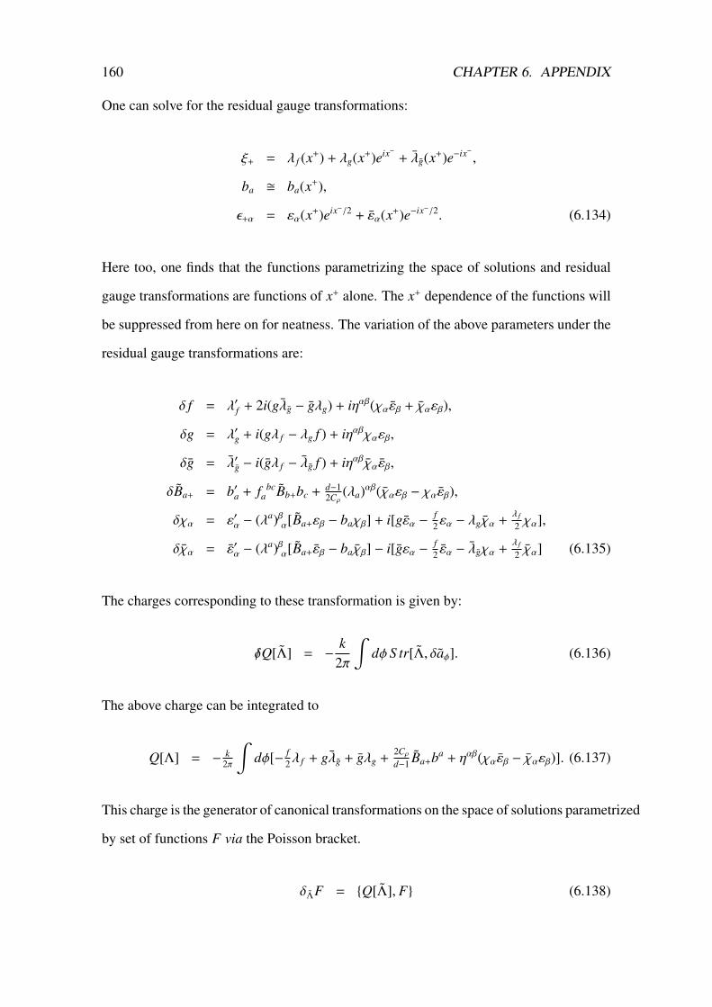
160 CHAPTER 6. APPENDIX
One can solve for the residual gauge transformations:
ξ+ = λ f (x+) + λg(x+)eix− + λg(x+)e−ix− ,
ba � ba(x+),
ε+α = εα(x+)eix−/2 + εα(x+)e−ix−/2. (6.134)
Here too, one finds that the functions parametrizing the space of solutions and residual
gauge transformations are functions of x+ alone. The x+ dependence of the functions will
be suppressed from here on for neatness. The variation of the above parameters under the
residual gauge transformations are:
δ f = λ′f + 2i(gλg − gλg) + iηαβ(χαεβ + χαεβ),
δg = λ′g + i(gλ f − λg f ) + iηαβχαεβ,
δg = λ′g − i(gλ f − λg f ) + iηαβχαεβ,
δBa+ = b′a + f bca Bb+bc + d−1
2Cρ(λa)αβ(χαεβ − χαεβ),
δχα = ε′α − (λa)βα[Ba+εβ − baχβ] + i[gεα −f2εα − λgχα +
λ f
2 χα],
δχα = ε′α − (λa)βα[Ba+εβ − baχβ] − i[gεα −f2 εα − λgχα +
λ f
2 χα] (6.135)
The charges corresponding to these transformation is given by:
/δQ[Λ] = −k
2π
∫dφ S tr[Λ, δaφ]. (6.136)
The above charge can be integrated to
Q[Λ] = − k2π
∫dφ[− f
2λ f + gλg + gλg +2Cρ
d−1 Ba+ba + ηαβ(χαεβ − χαεβ)]. (6.137)
This charge is the generator of canonical transformations on the space of solutions parametrized
by set of functions F via the Poisson bracket.
δΛF = {Q[Λ], F} (6.138)
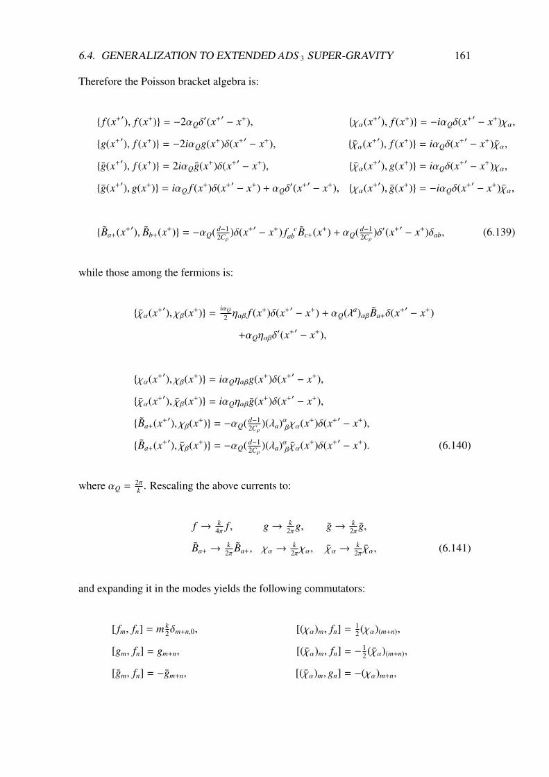
6.4. GENERALIZATION TO EXTENDED ADS 3 SUPER-GRAVITY 161
Therefore the Poisson bracket algebra is:
{ f (x+′), f (x+)} = −2αQδ′(x+′ − x+), {χα(x+′), f (x+)} = −iαQδ(x+′ − x+)χα,
{g(x+′), f (x+)} = −2iαQg(x+)δ(x+′ − x+), {χα(x+′), f (x+)} = iαQδ(x+′ − x+)χα,
{g(x+′), f (x+)} = 2iαQg(x+)δ(x+′ − x+), {χα(x+′), g(x+)} = iαQδ(x+′ − x+)χα,
{g(x+′), g(x+)} = iαQ f (x+)δ(x+′ − x+) + αQδ′(x+′ − x+), {χα(x+′), g(x+)} = −iαQδ(x+′ − x+)χα,
{Ba+(x+′), Bb+(x+)} = −αQ( d−12Cρ
)δ(x+′ − x+) f cab Bc+(x+) + αQ( d−1
2Cρ)δ′(x+′ − x+)δab, (6.139)
while those among the fermions is:
{χα(x+′), χβ(x+)} =iαQ
2 ηαβ f (x+)δ(x+′ − x+) + αQ(λa)αβBa+δ(x+′ − x+)
+αQηαβδ′(x+′ − x+),
{χα(x+′), χβ(x+)} = iαQηαβg(x+)δ(x+′ − x+),
{χα(x+′), χβ(x+)} = iαQηαβg(x+)δ(x+′ − x+),
{Ba+(x+′), χβ(x+)} = −αQ( d−12Cρ
)(λa)αβχα(x+)δ(x+′ − x+),
{Ba+(x+′), χβ(x+)} = −αQ( d−12Cρ
)(λa)αβχα(x+)δ(x+′ − x+). (6.140)
where αQ = 2πk . Rescaling the above currents to:
f → k4π f , g→ k
2πg, g→ k2π g,
Ba+ →k
2π Ba+, χα →k
2πχα, χα →k
2π χα, (6.141)
and expanding it in the modes yields the following commutators:
[ fm, fn] = m k2δm+n,0, [(χα)m, fn] = 1
2 (χα)(m+n),
[gm, fn] = gm+n, [(χα)m, fn] = −12 (χα)(m+n),
[gm, fn] = −gm+n, [(χα)m, gn] = −(χα)m+n,

162 CHAPTER 6. APPENDIX
[gm, gn] = −2 fm+n − mkδm+n,0, [(χα)m, gn] = (χα)m+n,
{(χα)m, (χβ)n} = −ηαβgm+n, {(χα)m, (χβ)n} = −ηαβgm+n,
[(Ba+)m, (χβ)n] = i(d−12Cρ
)(λa)αβ(χα)(m+n), [(Ba+)m, (χβ)n] = i(d−12Cρ
)(λa)αβ(χα)(m+n),
[(Ba+)m, (Bb+)n] = −i(d−12Cρ
) f cab (Bc+)(m+n) − (d−1
2Cρ)kmδabδm+n,0,
{(χα)m, (χβ)n} = −ηαβ f(m+n) + i(λa)αβ(Bc+)(m+n) − kmηαβδm+n,0. (6.142)
This is the affine Kac-Moody super-algebra. Here, it is evident that the central extension
to the sl(2,R)current sub-algebra spanned by ( f , g, g) is k = c/6. The quadratic non-
linearities that occur in the super-Virasoro are not present here.
6.5 sl(3,R) conventions
We work with the following basis of 3 × 3 matrices (see [7]) for the fundamental repre-
sentation of the gauge group used in the definition of the higher spin theory:
L−1 =
0 −2 0
0 0 −2
0 0 0
, L0 =
1 0 0
0 0 0
0 0 −1
, L1 =
0 0 0
1 0 0
0 1 0
, W−2 = α
0 0 8
0 0 0
0 0 0
,
W−1 = α
0 −2 0
0 0 2
0 0 0
, W0 = α 23
1 0 0
0 −2 0
0 0 1
, W1 = α
0 0 0
1 0 0
0 −1 0
, W2 = α
0 0 0
0 0 0
2 0 0
.(6.143)
The algebra satisfied by these matrices is
[Lm, Ln] = (m − n) Lm+n, [Lm,Wn] = (2m − n) wm+n,
[Wm,Wn] = −α2
3(m − n)(2m2 + 2n2 − mn − 8) Lm+n (6.144)

6.5. S L(3,R) CONVENTIONS 163
For α2 = −1 this is the su(1, 2) algebra and for α2 = 1 this is the sl(3,R) algebra. We
take the Killing metric as ηab = 12 Tr(TaTb) where Ta are the above matrices. The
structure constants are fabc = 12Tr(Ta [Tb,Tc]).

164 CHAPTER 6. APPENDIX

Bibliography
[1] J. D. Brown and M. Henneaux, “Central Charges in the Canonical Realization of
Asymptotic Symmetries: An Example from Three-Dimensional Gravity,”
Commun.Math.Phys. 104 (1986) 207–226. 0.1, 1.0.1, 1.0.2, 2, 1, 2.4, 5.2
[2] M. Henneaux, L. Maoz, and A. Schwimmer, “Asymptotic dynamics and
asymptotic symmetries of three-dimensional extended AdS supergravity,” Annals
Phys. 282 (2000) 31–66, arXiv:hep-th/9910013 [hep-th]. 0.1, 0.3, 0.4, 1.0.2,
1.0.2, 3, 3.2, 3.2.2, 3.2.3, 3.3, 3.3, 6.4, 6.4.1, 6.4.3, 6.4.4
[3] S. G. Avery, R. R. Poojary, and N. V. Suryanarayana, “An sl(2,R) current algebra
from AdS 3 gravity,” JHEP 1401 (2014) 144, arXiv:1304.4252 [hep-th]. 0.1,
0.2, 2.1, 2.4.1, 4.3.4
[4] R. R. Poojary and N. V. Suryanarayana, “Holographic chiral induced W-gravities,”
arXiv:1412.2510 [hep-th]. 0.1, 0.3, 0.3
[5] C. Troessaert, “Enhanced asymptotic symmetry algebra of AdS 3,” JHEP 1308
(2013) 044, arXiv:1303.3296 [hep-th]. 0.1, 0.2, 0.3, 1.0.3, 2, 1, 2.3.1, 3, 3.3,
3.3, 5.1, 5.2
[6] G. Compère, W. Song, and A. Strominger, “New Boundary Conditions for AdS3,”
JHEP 1305 (2013) 152, arXiv:1303.2662 [hep-th]. 0.1, 0.2, 0.2, 0.3, 1.0.3,
1.0.3, 1.1, 2, 2, 3, 2.1, 4, 2.1, 2.1.1, 2.1.2, 3.1.2, 3, 4.3.4, 5.1, 5.2
165

166 BIBLIOGRAPHY
[7] A. Campoleoni, S. Fredenhagen, S. Pfenninger, and S. Theisen, “Asymptotic
symmetries of three-dimensional gravity coupled to higher-spin fields,” JHEP 1011
(2010) 007, arXiv:1008.4744 [hep-th]. 0.1, 0.3, 0.3, 1.0.2, 1.0.2, 4.3.1, 6.5
[8] G. Compère and D. Marolf, “Setting the boundary free in AdS/CFT,”
Class.Quant.Grav. 25 (2008) 195014, arXiv:0805.1902 [hep-th]. 0.2, 1.0.3,
1.0.3, 1.0.3, 2, 5.2
[9] L. Apolo and M. Porrati, “Free boundary conditions and the AdS3/CFT2
correspondence,” JHEP 1403 (2014) 116, arXiv:1401.1197 [hep-th]. 0.2, 1.1,
4.3.4
[10] A. M. Polyakov, “Quantum Gravity in Two-Dimensions,” Mod.Phys.Lett. A2
(1987) 893. 0.2, 1.1, 1.1, 1.1, 2, 2.1, 2.1, 2.1.2, 5.1, 5.2
[11] A. Achucarro and P. Townsend, “A Chern-Simons Action for Three-Dimensional
anti-De Sitter Supergravity Theories,” Phys.Lett. B180 (1986) 89. 0.3, 2.4
[12] O. Coussaert, M. Henneaux, and P. van Driel, “The Asymptotic dynamics of
three-dimensional Einstein gravity with a negative cosmological constant,”
Class.Quant.Grav. 12 (1995) 2961–2966, arXiv:gr-qc/9506019 [gr-qc]. 0.3,
0.4, 1.0.3
[13] M. Bañados, O. Chandia, and A. Ritz, “Holography and the Polyakov action,”
Phys.Rev. D65 (2002) 126008, arXiv:hep-th/0203021 [hep-th]. 0.3, 6.1.3
[14] M. Henneaux and S.-J. Rey, “Nonlinear Win f inity as Asymptotic Symmetry of
Three-Dimensional Higher Spin Anti-de Sitter Gravity,” JHEP 1012 (2010) 007,
arXiv:1008.4579 [hep-th]. 0.3, 1.0.2, 4.3.4
[15] A. Zamolodchikov, “Infinite Additional Symmetries in Two-Dimensional
Conformal Quantum Field Theory,” Theor.Math.Phys. 65 (1985) 1205–1213. 0.3,
1.0.2, 1.1

BIBLIOGRAPHY 167
[16] P. Bouwknegt and K. Schoutens, “W symmetry in conformal field theory,”
Phys.Rept. 223 (1993) 183–276, arXiv:hep-th/9210010 [hep-th]. 0.3, 1.1, 1
[17] E. Witten, “Nonabelian Bosonization in Two-Dimensions,” Commun.Math.Phys.
92 (1984) 455–472. 0.3
[18] A. M. Polyakov and P. Wiegmann, “Theory of Nonabelian Goldstone Bosons,”
Phys.Lett. B131 (1983) 121–126. 0.3
[19] A. Alekseev and S. L. Shatashvili, “Path Integral Quantization of the Coadjoint
Orbits of the Virasoro Group and 2D Gravity,” Nucl.Phys. B323 (1989) 719. 0.3
[20] M. Bershadsky and H. Ooguri, “Hidden SL(n) Symmetry in Conformal Field
Theories,” Commun.Math.Phys. 126 (1989) 49. 0.3, 0.5, 1.1
[21] H. Ooguri, K. Schoutens, A. Sevrin, and P. van Nieuwenhuizen, “The Induced
action of W(3) gravity,” Commun.Math.Phys. 145 (1992) 515–540. 0.3, 1.1, 4.1,
5.2
[22] K. Bautier, “AdS(3) asymptotic (super)symmetries,” arXiv:hep-th/9909097
[hep-th]. 0.4, 1.0.2, 1.0.2, 3, 3.1.2
[23] M. Banados, K. Bautier, O. Coussaert, M. Henneaux, and M. Ortiz, “Anti-de Sitter
/ CFT correspondence in three-dimensional supergravity,” Phys.Rev. D58 (1998)
085020, arXiv:hep-th/9805165 [hep-th]. 0.4, 1.0.2, 1.0.2, 3.1.1, 3.1.2
[24] N. Hari Dass and R. Sumitra, “Symmetry Reorganization in Exactly Solvable
Two-dimensional Quantized Supergravity,” Int.J.Mod.Phys. A4 (1989) 2245. 0.4
[25] M. T. Grisaru and R.-M. Xu, “Quantum Supergravities in Two-dimensions,”
Phys.Lett. B205 (1988) 486. 0.4, 1.1
[26] M. Bershadsky and H. Ooguri, “Hidden Osp(N,2) Symmetries in Superconformal
Field Theories,” Phys.Lett. B229 (1989) 374. 0.5

168 BIBLIOGRAPHY
[27] E. Witten, “Anti-de Sitter space and holography,” Adv.Theor.Math.Phys. 2 (1998)
253–291, arXiv:hep-th/9802150 [hep-th]. 1
[28] M. Henningson and K. Skenderis, “Weyl anomaly for Wilson surfaces,” JHEP 06
(1999) 012, arXiv:hep-th/9905163 [hep-th]. 1.0.1
[29] M. R. Gaberdiel and R. Gopakumar, “An AdS 3 Dual for Minimal Model CFTs,”
Phys.Rev. D83 (2011) 066007, arXiv:1011.2986 [hep-th]. 1.0.2
[30] J. M. Maldacena, “The large n limit of superconformal field theories and
supergravity,” arXiv:hep-th/9711200v3 [hep-th].
http://arxiv.org/abs/hep-th/9711200v3.
Adv.Theor.Math.Phys.2:231-252,1998. 1.0.3
[31] O. Aharony, S. S. Gubser, J. Maldacena, H. Ooguri, and Y. Oz, “Large n field
theories, string theory and gravity,” arXiv:hep-th/9905111v3 [hep-th].
http://arxiv.org/abs/hep-th/9905111v3. Phys.Rept.323:183-386,2000.
1.0.3
[32] D. Gaiotto, A. Strominger, and X. Yin, “Superconformal black hole quantum
mechanics,” arXiv:hep-th/0412322v1 [hep-th].
http://arxiv.org/abs/hep-th/0412322v1. JHEP 0511:017,2005. 1.0.3
[33] R. K. Gupta and A. Sen, “Ads(3)/cft(2) to ads(2)/cft(1),” arXiv:0806.0053v4
[hep-th]. http://arxiv.org/abs/0806.0053v4. 1.0.3
[34] T. Azeyanagi, T. Nishioka, and T. Takayanagi, “Near extremal black hole entropy
as entanglement entropy via ads2/cft1,” arXiv:0710.2956v4 [hep-th].
http://arxiv.org/abs/0710.2956v4. Phys.Rev.D77:064005,2008. 1.0.3
[35] A. Strominger, “Ads2 quantum gravity and string theory,”
arXiv:hep-th/9809027v2 [hep-th].
http://arxiv.org/abs/hep-th/9809027v2. JHEP 9901:007,1999. 1.0.3,
1.0.3

BIBLIOGRAPHY 169
[36] V. Balasubramanian, A. Naqvi, and J. Simon, “A multi-boundary ads orbifold and
dlcq holography: A universal holographic description of extremal black hole
horizons,” arXiv:hep-th/0311237v3 [hep-th].
http://arxiv.org/abs/hep-th/0311237v3. JHEP0408:023,2004. 1.0.3
[37] J.-H. Cho, T. Lee, and G. Semenoff, “Two dimensional anti-de sitter space and
discrete light cone quantization,” arXiv:hep-th/9906078v2 [hep-th].
http://arxiv.org/abs/hep-th/9906078v2. Phys.Lett. B468 (1999) 52-57.
1.0.3
[38] D. Gaiotto, M. Guica, L. Huang, A. Simons, A. Strominger, et al., “D4-D0 branes
on the quintic,” JHEP 0603 (2006) 019, arXiv:hep-th/0509168 [hep-th].
1.0.3
[39] M. Spradlin and A. Strominger, “Vacuum states for AdS(2) black holes,” JHEP
9911 (1999) 021, arXiv:hep-th/9904143 [hep-th]. 1.0.3
[40] H. K. Kunduri, J. Lucietti, and H. S. Reall, “Near-horizon symmetries of extremal
black holes,” Class.Quant.Grav. 24 (2007) 4169–4190, arXiv:0705.4214
[hep-th]. 1.0.3
[41] V. Balasubramanian, J. de Boer, M. Sheikh-Jabbari, and J. Simon, “What is a chiral
2d CFT? And what does it have to do with extremal black holes?,” JHEP 1002
(2010) 017, arXiv:0906.3272 [hep-th]. 1.0.3, 1.0.3
[42] A. Sakharov, “Vacuum quantum fluctuations in curved space and the theory of
gravitation,” Sov.Phys.Dokl. 12 (1968) 1040–1041. 1.0.3
[43] A. M. Polyakov, “Quantum Geometry of Bosonic Strings,” Phys.Lett. B103 (1981)
207–210. 1.1, 2
[44] J. Grundberg and R. Nakayama, “On 2-D (Super)gravity in the Light Cone Gauge,”
Mod. Phys. Lett. A4 (1989) 55. 1.1

170 BIBLIOGRAPHY
[45] C. Hull, “Classical and quantum W gravity,” Conf.Proc. C9115201 (1991)
495–539, arXiv:hep-th/9201057 [hep-th]. 1.1, 4.3.4, 5.2
[46] M. Blencowe, “A Consistent Interacting Massless Higher Spin Field Theory in D =
(2+1),” Class.Quant.Grav. 6 (1989) 443. 1.1, 4.1
[47] V. Balasubramanian and P. Kraus, “A Stress tensor for Anti-de Sitter gravity,”
Commun.Math.Phys. 208 (1999) 413–428, arXiv:hep-th/9902121 [hep-th].
2, 2.1.2
[48] G. Compère, W. Song, and A. Strominger, “Chiral Liouville Gravity,” JHEP 1305
(2013) 154, arXiv:1303.2660 [hep-th]. 2, 3.2.2
[49] K. Skenderis and S. N. Solodukhin, “Quantum effective action from the AdS / CFT
correspondence,” Phys.Lett. B472 (2000) 316–322, arXiv:hep-th/9910023
[hep-th]. 2.1.1, 2.3
[50] G. Barnich and F. Brandt, “Covariant theory of asymptotic symmetries,
conservation laws and central charges,” Nucl.Phys. B633 (2002) 3–82,
arXiv:hep-th/0111246 [hep-th]. 2.1.2, 2.1.2, 2.4.1, 5.2, 6.4.2
[51] G. Barnich and G. Compere, “Surface charge algebra in gauge theories and
thermodynamic integrability,” J.Math.Phys. 49 (2008) 042901, arXiv:0708.2378
[gr-qc]. 2.1.2, 2.4.1
[52] E. Witten, “(2+1)-Dimensional Gravity as an Exactly Soluble System,” Nucl.Phys.
B311 (1988) 46. 2.4
[53] R. Poojary and N. Suryanarayana, “Holographic induced supergravities,”
arXiv:(to appear soon) [hep-th]. 3
[54] Y. Hyakutake, “Super Virasoro Algebra From Supergravity,” Phys.Rev. D87 no. 4,
(2013) 045028, arXiv:1211.3547 [hep-th]. 3.1.3

BIBLIOGRAPHY 171
[55] W. Nahm, “Supersymmetries and their Representations,” Nucl. Phys. B135 (1978)
149. 3.2
[56] A. Campoleoni, S. Fredenhagen, and S. Pfenninger, “Asymptotic W-symmetries in
three-dimensional higher-spin gauge theories,” JHEP 1109 (2011) 113,
arXiv:1107.0290 [hep-th]. 4.1, 4.1, 4.1, 4.3.4
[57] J. de Boer and J. I. Jottar, “Boundary Conditions and Partition Functions in Higher
Spin AdS3/CFT2,” arXiv:1407.3844 [hep-th]. 1, 4.1, 1, 3
[58] M. Ammon, M. Gutperle, P. Kraus, and E. Perlmutter, “Spacetime Geometry in
Higher Spin Gravity,” JHEP 10 (2011) 053, arXiv:1106.4788 [hep-th]. 4.3.4
[59] G. Compère and W. Song, “W symmetry and integrability of higher spin black
holes,” JHEP 1309 (2013) 144, arXiv:1306.0014 [hep-th]. 3
[60] K. Schoutens, A. Sevrin, and P. van Nieuwenhuizen, “Induced gauge theories and
W gravity,”. 5.2
[61] M. Banados and R. Caro, “Holographic ward identities: Examples from 2+1
gravity,” JHEP 0412 (2004) 036, arXiv:hep-th/0411060 [hep-th]. 5.2, 6.3
[62] V. G. Knizhnik, A. M. Polyakov, and A. B. Zamolodchikov, “Fractal Structure of
2D Quantum Gravity,” Mod. Phys. Lett. A3 (1988) 819. 5.2
[63] W. Li and S. Theisen, “Some Aspects of Holographic W-Gravity,” JHEP 08 (2015)
035, arXiv:1504.07799 [hep-th]. 5.2
[64] J. Balog, L. Feher, L. O’Raifeartaigh, P. Forgacs, and A. Wipf, “Toda Theory and
W Algebra From a Gauged WZNW Point of View,” Annals Phys. 203 (1990)
76–136. 5.2
[65] P. Forgacs, A. Wipf, J. Balog, L. Feher, and L. O’Raifeartaigh, “Liouville and Toda
Theories as Conformally Reduced WZNW Theories,” Phys. Lett. B227 (1989) 214.
5.2

172 BIBLIOGRAPHY
[66] M. Henneaux, G. Lucena Gómez, J. Park, and S.-J. Rey, “Super- W(infinity)
Asymptotic Symmetry of Higher-Spin AdS 3 Supergravity,” JHEP 06 (2012) 037,
arXiv:1203.5152 [hep-th]. 5.2
[67] T. Creutzig, Y. Hikida, and P. B. Ronne, “Higher spin AdS3 supergravity and its
dual CFT,” JHEP 02 (2012) 109, arXiv:1111.2139 [hep-th]. 5.2
[68] C. Candu, C. Peng, and C. Vollenweider, “Extended supersymmetry in AdS3 higher
spin theories,” JHEP 12 (2014) 113, arXiv:1408.5144 [hep-th]. 5.2
[69] J. Polchinski, “Scale and Conformal Invariance in Quantum Field Theory,” Nucl.
Phys. B303 (1988) 226. 5.2
[70] D. M. Hofman and A. Strominger, “Chiral Scale and Conformal Invariance in 2D
Quantum Field Theory,” Phys.Rev.Lett. 107 (2011) 161601, arXiv:1107.2917
[hep-th]. 5.2
[71] G. Barnich, L. Donnay, J. Matulich, and R. Troncoso, “Asymptotic symmetries and
dynamics of three-dimensional flat supergravity,” JHEP 08 (2014) 071,
arXiv:1407.4275 [hep-th]. 5.2
[72] A. Strominger, “Asymptotic Symmetries of Yang-Mills Theory,” JHEP 07 (2014)
151, arXiv:1308.0589 [hep-th]. 5.2
[73] A. Strominger, “On BMS Invariance of Gravitational Scattering,” JHEP 07 (2014)
152, arXiv:1312.2229 [hep-th]. 5.2
[74] M. Campiglia and A. Laddha, “Asymptotic symmetries of QED and Weinberg’s
soft photon theorem,” JHEP 07 (2015) 115, arXiv:1505.05346 [hep-th]. 5.2
[75] S. G. Avery and B. U. W. Schwab, “BMS, String Theory, and Soft Theorems,”
arXiv:1506.05789 [hep-th]. 5.2

BIBLIOGRAPHY 173
[76] S. K. Ashok, R. Benichou, and J. Troost, “Asymptotic Symmetries of String
Theory on AdS(3) x S**3 with Ramond-Ramond Fluxes,” JHEP 10 (2009) 051,
arXiv:0907.1242 [hep-th]. 5.2
[77] A. Giveon, D. Kutasov, and N. Seiberg, “Comments on string theory on AdS(3),”
Adv. Theor. Math. Phys. 2 (1998) 733–780, arXiv:hep-th/9806194 [hep-th].
5.2
[78] J. de Boer, H. Ooguri, H. Robins, and J. Tannenhauser, “String theory on AdS(3),”
JHEP 12 (1998) 026, arXiv:hep-th/9812046 [hep-th]. 5.2
[79] D. Kutasov and N. Seiberg, “More comments on string theory on AdS(3),” JHEP
04 (1999) 008, arXiv:hep-th/9903219 [hep-th]. 5.2
[80] W. Li, W. Song, and A. Strominger, “Chiral Gravity in Three Dimensions,” JHEP
0804 (2008) 082, arXiv:0801.4566 [hep-th]. 6.1