Embed Size (px)
Citation preview
9HSTFMG*agefib+
ISBN 978-952-60-6458-1 (printed) ISBN 978-952-60-6459-8 (pdf) ISSN-L 1799-4934 ISSN 1799-4934 (printed) ISSN 1799-4942 (pdf) Aalto University School of Engineering Department of Real Estate, Planning and Geoinformatics www.aalto.fi
BUSINESS + ECONOMY ART + DESIGN + ARCHITECTURE SCIENCE + TECHNOLOGY CROSSOVER DOCTORAL DISSERTATIONS
Aalto-D
D 172
/2015
We studied various aspects of modelling geographical information from the geodetic and geodynamic points of view. The data for our studies were acquired by a variety of methods: laser scanning, levelling and satellite positioning. The major subject of this dissertation is quality and its measures. We study various modelling approaches on geodetic data aimed at use cases in the fields of geodesy, geodynamics and geographic information science. The dissertation discusses internal and external quality aspects of the modelling and the data used. The main objectives of the research are related to the data modelling aspects and fitness for use within the fields of study as expressed quantitatively in various quality measures. The novelty of the dissertation is in the application of appropriate quality measures, like precision or accuracy from the viewpoint of fitness for use, which for the various models depends on the input data precision as well as on the envisaged applications of the model product.
Karin K
ollo A
spects of Modelling G
eographic Information in G
eodesy and Geodynam
ics A
alto U
nive
rsity
2015
Department of Real Estate, Planning and Geoinformatics
Aspects of Modelling Geographic Information in Geodesy and Geodynamics
Karin Kollo
DOCTORAL DISSERTATIONS
Aalto University publication series DOCTORAL DISSERTATIONS 172/2015
Aspects of Modelling Geographic Information in Geodesy and Geodynamics
Karin Kollo
A doctoral dissertation completed for the degree of Doctor of Science (Technology) to be defended, with the permission of the Aalto University School of Engineering, at a public examination held in lecture hall M1, Otakaari 1 on 13 November 2015 at 12.
Aalto University School of Engineering Department of Real Estate, Planning and Geoinformatics

Supervising professor Professor Martin Vermeer, Aalto University, Finland Thesis advisor Professor Martin Vermeer, Aalto University, Finland Preliminary examiners Associate Professor Eimuntas Paršeliūnas, Vilnius Gediminas Technical University, Lithuania DSc Arzu Cöltekin, University of Zurich, Switzerland Opponents DSc Arzu Cöltekin, University of Zurich, Switzerland DSc Jānis Kaminskis, Riga Technical University, Latvia
Aalto University publication series DOCTORAL DISSERTATIONS 172/2015 © Karin Kollo ISBN 978-952-60-6458-1 (printed) ISBN 978-952-60-6459-8 (pdf) ISSN-L 1799-4934 ISSN 1799-4934 (printed) ISSN 1799-4942 (pdf) http://urn.fi/URN:ISBN:978-952-60-6459-8 Unigrafia Oy Helsinki 2015 Finland
Abstract Aalto University, P.O. Box 11000, FI-00076 Aalto www.aalto.fi
Author Karin Kollo Name of the doctoral dissertation Aspects of Modelling Geographic Information in Geodesy and Geodynamics Publisher School of Engineering Unit Department of Real Estate, Planning and Geoinformatics
Series Aalto University publication series DOCTORAL DISSERTATIONS 172/2015
Field of research Geodesy
Manuscript submitted 2 June 2015 Date of the defence 13 November 2015
Permission to publish granted (date) 1 September 2015 Language English
Monograph Article dissertation (summary + original articles)
Abstract We studied aspects of modelling geographical information from the geodetic and geodynamic viewpoints. The data for our studies were acquired by a variety of methods: laser scanning, levelling and satellite positioning.
The major subject of this dissertation is quality and its measures. We study various modelling approaches on geodetic data aimed at use cases in the fields of geodesy, geodynamics and geographic information science. The dissertation discusses internal and external quality aspects of the modelling and the data used. The main objectives of the research are related to data modelling aspects and fitness for use within the fields of study as expressed quantitatively in various quality measures. The novelty of the dissertation is in the application of appropriate quality measures, like precision or accuracy, in these fields of research from the viewpoint of fitness for use, which for the various models depend on input data precision as well as on the envisaged applications of the model product.
This dissertation has three main topics. Firstly, the modelling of gravity based heights was studied. Three different modelling methods were used: kriging, fuzzy modelling and bilinear affine transformation. We studied the use of geostatistical and geodetic methods for the construction of digital elevation models and height transformation surfaces. Within these methods also quality measures were formulated showing their applicability in height modelling. We found that the quality of the results is dependent on the data point distribution and the availability of precise geoid heights. Secondly, precision measures for gravimetric geoid determination were derived for two test areas. For this study three error sources were investigated: the error of omission, the aliasing error and the out-of-area error. We showed that error sources were dependent on the spatial extent and accuracy of the gravimetric measurements. Thirdly, the modelling of post-glacial land uplift was investigated, using two methods: land uplift prediction by least-squares collocation, and Glacial Isostatic Adjustment (GIA) modelling using two different ice models and fitting the Earth model parameter values. In the land uplift recovery study, possibilities were investigated for projecting the land uplift forward in time. From this study a statistical model for predicting land uplift rate from point velocity rates using a relatively simple formulation was derived by the least squares collocation technique, with error propagation into the predicted land uplift. The GIA modelling study gave us experience in building land uplift models. We found that the two methods, land uplift rate prediction and physical GIA modelling, though being very different, are giving similar accuracy measures for the derived land uplift values.
Keywords bilinear affine transformation, digital elevation model, fuzzy modelling, geoid precision, glacial isostatic adjustment, kriging, least squares collocation
ISBN (printed) 978-952-60-6458-1 ISBN (pdf) 978-952-60-6459-8
ISSN-L 1799-4934 ISSN (printed) 1799-4934 ISSN (pdf) 1799-4942
Location of publisher Helsinki Location of printing Helsinki Year 2015
Pages 120 urn http://urn.fi/URN:ISBN:978-952-60-6459-8

Acknowledgements
The process of my postgraduate studies has been interesting and chal-
lenging. The journey has been long - altogether 12 years. During this
time I have had the opportunity to extend my knowledge and get to know
persons who have introduced me to the world of science.
First, I cordially thank my supervisor Professor Martin Vermeer for en-
couraging me, for inspiring me and believing in me. I am grateful to pro-
fessor Kirsi Virrantaus, who helped me to find out my way, and being
supportive throughout my studies at the Aalto University. I am grateful
to my co-authors Rangsima Sunila, Martin Vermeer and Giorgio Spada.
I would like to thank my colleagues from the Aalto University (former
Helsinki University of Technology) and from the Estonian Land Board.
My special thanks go to Mr Priit Pihlak and Mr Raivo Vallner from the
Estonian Land Board for their understanding, encouragement and sup-
port. Many thanks to Maila Marka for proofreading the thesis and for her
valuable remarks.
I am grateful for financial support provided by the following institutions
and scholarship foundations: Helsinki University of Technology schol-
arship; Kristjan Jaak Scholarship Foundation; the Academy of Finland,
Finnish Academy Award No. 123113: “Regional Crustal Deformation and
Lithosphere Thickness Observed with Geodetic Techniques (RCD-LITO)”;
funding from the Finnish Ministry of Agriculture and Forestry, Project
No. 310 838 (Dnro 5000/416/2005); part of this work was supported by
COST Action ES0701 "Improved constraints on models of Glacial Isostatic
Adjustment"; grant from Estonian Science Academy No ETF8749; Aalto
University Doctoral Programme RYM-TO; Estonian Land Board.
I would like to thank the following persons for their assistance with the
data used in case studies: Mr Priit Pihlak from the Estonian Land Board
(data for Paper A); Mr Mathias Hurme from the Department of Real Es-
1

Acknowledgements
tate, Division of City Mapping, Helsinki City (data for the paper B); Mr
Tõnis Oja from the Estonian Land Board (data for Paper C); Mr Veikko
Saaranen from the Finnish Geodetic Institute (data for Paper D); Dr Gio-
vanni Sella from the National Oceanic and Atmospheric Administration
(NOAA), National Geodetic Survey (data for Paper E); Dr Martin Lidberg
from Lantmäteriet (data for Paper D and E). Sincere acknowledgements
to Professor Giorgio Spada from Dipartimento di Scienze di base e Fon-
damenti (DiSBeF), Università degli Studi di Urbino for providing support
for learning to use the SELEN program for the case study of Paper E.
I wish to thank the pre-examiners of my thesis, Dr Arzu Cöltekin from
University of Zurich and professor Eimuntas Paršeliunas from Vilnius
Gediminas University for their valuable remarks that helped to improve
the final thesis.
Last but not least, I would like to thank my family: my dad, husband
Karmo and especially Johanna, Aleksander and Helerin.
Helsinki, October 2015
Karin Kollo
2
Contents
Contents 3
1. Introduction 13
1.1 Motivation and aim of the dissertation . . . . . . . . . . . . . 15
1.2 Structure of the dissertation . . . . . . . . . . . . . . . . . . . 16
1.3 Key concepts . . . . . . . . . . . . . . . . . . . . . . . . . . . . 16
1.4 Objectives and research topics . . . . . . . . . . . . . . . . . . 16
2. Theoretical background 19
2.1 Spatial framework . . . . . . . . . . . . . . . . . . . . . . . . 19
2.1.1 Reference frames . . . . . . . . . . . . . . . . . . . . . 19
2.1.2 Height systems . . . . . . . . . . . . . . . . . . . . . . 21
2.1.3 Transformation methods for heights . . . . . . . . . . 21
2.2 Geostatistical methods . . . . . . . . . . . . . . . . . . . . . . 22
2.2.1 Fuzzy modelling . . . . . . . . . . . . . . . . . . . . . . 22
2.2.2 Kriging . . . . . . . . . . . . . . . . . . . . . . . . . . . 23
2.3 Glacial isostatic adjustment . . . . . . . . . . . . . . . . . . . 24
2.3.1 Overview . . . . . . . . . . . . . . . . . . . . . . . . . . 24
2.3.2 Regions of land uplift . . . . . . . . . . . . . . . . . . . 25
2.3.2.1 Fennoscandia . . . . . . . . . . . . . . . . . . 26
2.3.2.2 North America . . . . . . . . . . . . . . . . . 27
2.3.3 GIA models . . . . . . . . . . . . . . . . . . . . . . . . . 27
2.3.4 Earth models . . . . . . . . . . . . . . . . . . . . . . . 29
2.3.5 Ice models . . . . . . . . . . . . . . . . . . . . . . . . . 29
2.3.6 Sea level . . . . . . . . . . . . . . . . . . . . . . . . . . 31
2.3.7 The sea-level equation . . . . . . . . . . . . . . . . . . 32
3. Research methods and materials 35
3.1 Publication A . . . . . . . . . . . . . . . . . . . . . . . . . . . . 35
3
Contents
3.2 Publication B . . . . . . . . . . . . . . . . . . . . . . . . . . . . 36
3.3 Publication C . . . . . . . . . . . . . . . . . . . . . . . . . . . . 37
3.4 Publication D . . . . . . . . . . . . . . . . . . . . . . . . . . . 38
3.5 Publication E . . . . . . . . . . . . . . . . . . . . . . . . . . . . 39
4. Discussion of research results 41
4.1 Transformation surface and DEM . . . . . . . . . . . . . . . . 41
4.1.1 Obtaining height values by means of a transforma-
tion surface (Publication A) . . . . . . . . . . . . . . . 41
4.1.2 Obtaining DEM by means of a transformation sur-
face (Publication B) . . . . . . . . . . . . . . . . . . . . 43
4.1.3 Quality measures for height transformation surface
models (Publications A and B) . . . . . . . . . . . . . . 43
4.2 Quality measures for the geoid model (Publication C) . . . . 44
4.3 Land uplift rate recovery and GIA . . . . . . . . . . . . . . . 45
4.3.1 Land uplift rate model (Publication D) . . . . . . . . . 46
4.3.2 GIA modelling (Publication E) . . . . . . . . . . . . . 46
4.3.3 Quality measures for the land uplift models (Publi-
cations D and E) . . . . . . . . . . . . . . . . . . . . . . 47
4.4 Outline . . . . . . . . . . . . . . . . . . . . . . . . . . . . . . . 48
5. Conclusions 51
Bibliography 55
4
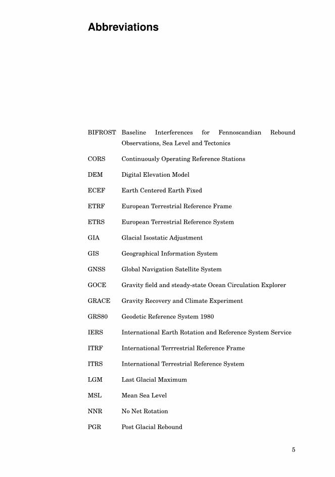
Abbreviations
BIFROST Baseline Interferences for Fennoscandian Rebound
Observations, Sea Level and Tectonics
CORS Continuously Operating Reference Stations
DEM Digital Elevation Model
ECEF Earth Centered Earth Fixed
ETRF European Terrestrial Reference Frame
ETRS European Terrestrial Reference System
GIA Glacial Isostatic Adjustment
GIS Geographical Information System
GNSS Global Navigation Satellite System
GOCE Gravity field and steady-state Ocean Circulation Explorer
GRACE Gravity Recovery and Climate Experiment
GRS80 Geodetic Reference System 1980
IERS International Earth Rotation and Reference System Service
ITRF International Terrrestrial Reference Frame
ITRS International Terrestrial Reference System
LGM Last Glacial Maximum
MSL Mean Sea Level
NNR No Net Rotation
PGR Post Glacial Rebound
5

Abbreviations
PREM Preliminary Earth Model
RMS Root Mean Square
SLE Sea Level Equation
SNARF Stable North American Reference Frame
TIN Triangulated Irregular Network
6
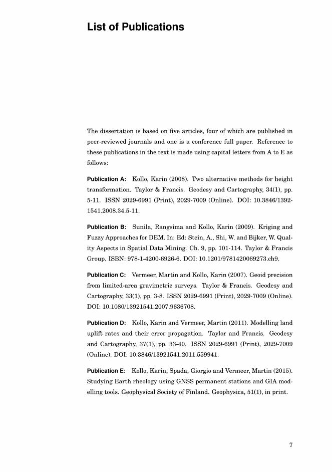
List of Publications
The dissertation is based on five articles, four of which are published in
peer-reviewed journals and one is a conference full paper. Reference to
these publications in the text is made using capital letters from A to E as
follows:
Publication A: Kollo, Karin (2008). Two alternative methods for height
transformation. Taylor & Francis. Geodesy and Cartography, 34(1), pp.
5-11. ISSN 2029-6991 (Print), 2029-7009 (Online). DOI: 10.3846/1392-
1541.2008.34.5-11.
Publication B: Sunila, Rangsima and Kollo, Karin (2009). Kriging and
Fuzzy Approaches for DEM. In: Ed: Stein, A., Shi, W. and Bijker, W. Qual-
ity Aspects in Spatial Data Mining. Ch. 9, pp. 101-114. Taylor & Francis
Group. ISBN: 978-1-4200-6926-6. DOI: 10.1201/9781420069273.ch9.
Publication C: Vermeer, Martin and Kollo, Karin (2007). Geoid precision
from limited-area gravimetric surveys. Taylor & Francis. Geodesy and
Cartography, 33(1), pp. 3-8. ISSN 2029-6991 (Print), 2029-7009 (Online).
DOI: 10.1080/13921541.2007.9636708.
Publication D: Kollo, Karin and Vermeer, Martin (2011). Modelling land
uplift rates and their error propagation. Taylor and Francis. Geodesy
and Cartography, 37(1), pp. 33-40. ISSN 2029-6991 (Print), 2029-7009
(Online). DOI: 10.3846/13921541.2011.559941.
Publication E: Kollo, Karin, Spada, Giorgio and Vermeer, Martin (2015).
Studying Earth rheology using GNSS permanent stations and GIA mod-
elling tools. Geophysical Society of Finland. Geophysica, 51(1), in print.
7

List of Publications
8
Author’s contribution
Publication A: The author was responsible for the entirety of the work
described in the paper.
Publication B: The second author was responsible for computations of
fuzzy model construction for DEM, analysing and summarising corre-
sponding parts of the paper and the paper was written by both authors
together. The research idea originated in discussions between the au-
thors.
Publication C: The second author was responsible for acquiring and pro-
cessing Estonian gravity survey data and wrote the corresponding chapter
in the paper. The original idea came from the first author.
Publication D: The first author was partly responsible for designing and
writing the code and analyzing and summarizing the results and drawing
of figures; she was fully responsible for calculations, both authors together
wrote the paper. The research idea was developed jointly by the authors.
Publication E: The first author had the main responsibility for writing
the article with minor assistance from second and third authors, all com-
putations and figures. The research idea was proposed by the first author.
9

Author’s contribution
10
Summary of Publications
Publication A: This article introduces two different methods for height
transformation: the bilinear affine transformation approach and fuzzy
modelling, and applies them to the territory of Estonia. We showed that
using these methods, a transformation surface can be determined and its
accuracy in computing the heights of arbitrary points can be evaluated.
Precision estimates for the individual case studies are presented.
Publication B: This article discusses the construction of digital elevation
models (DEM) using the kriging and fuzzy modelling approaches. As in-
put data height data from a laser scanning survey for a sub-urban area
of Helsinki were used. We demonstrated the construction of digital eleva-
tion models with their quality measures. Additionally, a comparison with
an independently constructed TIN model was made.
Publication C: In the article rough theoretical estimates for the preci-
sion of a gravimetric geoid model and the structure of the uncertainty
budget computed from discrete data points were presented. We presented
calculations for two case studies, Estonia and Finland.
Publication D: In the article a statistical model for predicting the uplift
rates from the existing point uplift rates was derived with its empirical
signal covariance function for the Fennoscandian land uplift area. We
showed how the model uplift rate can be calculated for an arbitrary point.
If one knows uplift rates, heights of points in the terrain, and GNSS posi-
tioning together with a precise geoid model, then one may project geodetic
heights forward in time.
Publication E: In the article we found best fitting Earth model param-
eters with their uncertainties for ice models ICE-5G and KL05 in the
North-American and Fennoscandian uplift areas and compared them with
results from other published studies.
11

Summary of Publications
12
1. Introduction
Nowadays geographical information plays a central role in society. Almost
everything is based on geographical information, the geographical infor-
mation itself is based on position information acquired by, or tied in with,
for example, though not only, geodetic measurements.
Geographical information stands for “geographical knowledge from in-
vestigation of geographical features”, whatever kind of geographical fea-
tures are studied (Peuquet, 2002). More often terrain based features
are described – spatial information, boundaries, heights, etc. Within the
spatial information, one also needs spatial framework information, i.e.,
geodetic datum and reference systems. These are based on precise geode-
tic control points, which help to make the link to a real physical location.
The dissertation interconnects geodesy, geodynamics and geographical
modelling. Geodesy is the science of measuring the Earth and its size and
shape; geodynamics is the discipline for studying the Earth’s size, shape
and orientation change over time. Geographical modelling studies phe-
nomena on, above or below the surface of the Earth. A central question in
geographic information is: how geographic information can be presented
and used (Peuquet, 2002).
Within the fields of geographic information presentation and usage, the
term quality is often used. Data quality is an overall term for various
concepts, like precision, accuracy, consistency, completeness, validity, un-
certainty, timeliness, etc. As it is not possible to make a perfect represen-
tation of real world phenomena in GIS, some deficiency in the quality of
the final products is inevitable (Longley et al., 2001).
Generally, different geographic models are used to represent reality. The
model is always simpler than the reality it represents and, therefore, dif-
ferent types and magnitudes of errors are always present. It should be
realised that there is no such thing as the correct geographic data model
13
Introduction
(Longley et al., 2001).
For modelling purposes, the geographical information can be collected
by measurements as objects (e.g., in geodesy, in photogrammetry, or ob-
tained by digitizing from pre-existing sources) or as fields (e.g., remote
sensing) (Devillers and Jeansoulin, 2006). Furthermore, from geodetic
measurements, the results are given in the form of discrete objects. From
geodynamical studies, it is possible to obtain the change in coordinates,
i.e., the rates or velocities, which are given as continuous objects, i.e.,
time series. With the help of geographic information and its modelling
tools, we may gain a better understanding of the Earth system. Also, al-
though this is not an objective of this study, it is possible to make these
results visually attractive and useful to public understanding.
In connection with geographic information systems we used two terms:
data and information, which do not mean the same thing. Data means
just numerical values, but information, on the other hand, means data
plus metadata, i.e., interpreted data.
The practice of modelling itself includes the acquisition of input data,
methods for analysing the input data, choice of study area, modelling
techniques, computational methods and programs, etc. Each of these as-
pects needs to be considered in designing geographical information sys-
tems (GIS); the most crucial one is the precision and spatial distribution
of input data. From the dissertation, additional value in geographical
modelling was acquired and its results are applicable to further studies
and may be used by cartographers, geodesists and other geoscientists.
Quality can be expressed by internal or external measures. Internal
quality measures are, e.g., precision and completeness. An external qual-
ity measure is, e.g., accuracy. Accuracy shows the measurement error
against a reference dataset, e.g., the difference from ground truth. Preci-
sion describes the consistency of repeated measurements, i.e., how close
repeated measurements are to each other. Collectively, accuracy and pre-
cision can be referred to as uncertainty (JCGM/WG 1, 2008).
Applications of relevance to this dissertation include determination of
height models, geoid models and land uplift rate models. The quality of
these models will vary, e.g., height models used in, e.g., large scale urban
mapping, have to be centimetre precision, whereas for mapping of remote
areas on small scale they may be decimetre or even metre precision. Sim-
ilar considerations apply to the other model types.
As input data, many different datasets can be used for modelling. For
14
Introduction
example, in a Digital Elevation Model (DEM) point height data from lev-
elling or laser scanning can be used. In this case, the model is composed of
crisp data and the result can be visualised as a field or a surface. Another
possibility is to incorporate into the model different physical parameters
together with the evaluation data sets. In this case, one can see the model
as an object (Devillers and Jeansoulin, 2006). Besides input data, there
is usually some kind of computation strategy involved in model computa-
tion. The computation strategy should be in accordance with the model’s
suitability for purpose and intended use (Zhang and Goodchild, 2002).
For example, for DEM, geostatistical methods can be used. In geody-
namics, various types of advanced mathematical and physical approaches
are used, e.g., the sea-level equation used in Glacial Isostatic Adjustment
(GIA) modelling.
In building models, proper reference systems have to be used: the spa-
tial framework includes the reference systems tied to the Earth. It must
be considered that the Earth moves – both around its own axis and around
the Sun, movements that have to be taken into account. There are two ba-
sic aspects of reference systems – the geometrical aspect and the physical
aspect. The geometrical aspect refers to the International Terrestrial Ref-
erence System (ITRS) and its realisations. Coordinates are geocentric and
may be presented either in rectangular form or as geodetic coordinates on
the reference ellipsoid. The physical aspect includes the height system
and the figure of the Earth – the geoid. The geoid corresponds, not to the
actual surface of the Earth, but to a surface defined by the gravity field of
the Earth, which is known as the physical figure of the Earth.
1.1 Motivation and aim of the dissertation
The motivation for the dissertation is to study various modelling approach-
es on geodetic data, to be used in the fields of geodesy, geodynamics and
geographic information science. The dissertation discusses issues of inter-
nal and external quality aspects of both the modelling techniques and the
data used. The models in geodesy, geodynamics and geoinformatics can
be thought of as approximations to reality, in which the key element is un-
certainty. Modelling can be based on treating reality either as objects or
as fields. Both modelling approaches have been used within the disserta-
tion. Geodesy deals with point measurements on the millimetre accuracy
level, i.e., the accuracy characteristics are well measured and well known.
15
Introduction
However, users sometimes do not need as accurate results, their applica-
tions can accept precisions on the centimetre or decimetre level. Also,
techniques from geographic information science and geostatistics can be
used to generalise results obtained into lower resolution, lower precision
results that better match actual user requirements.
The novelty of the dissertation is in the application of appropriate pre-
cision measures in the various fields of research. The fitness for use of
the different models depends on the input data precision as well as on the
envisaged applications of the model product. E.g., in geodesy an appro-
priate precision can be from millimetres to centimetres, but in geographic
information science the precision may vary within larger bounds.
1.2 Structure of the dissertation
The summary part of the dissertation comprises five chapters. The first
chapter introduces the subject and presents the motivation and research
questions addressed. The second chapter gives an overview of the the-
oretical background and related research. An overview of the research
methods, input data and other materials used are presented in the third
chapter. Chapter four presents our main findings and discusses them,
while chapter five presents conclusions.
1.3 Key concepts
The key concept of the dissertation is finding criteria for judging the
fitness for use of models in geodesy, geodynamics and geoinformatics.
Within the different modelling approaches, different quality measures are
considered. These quality measures are usually stated in the negative;
they include imprecision, uncertainty, standard error, standard deviation,
variance and the root mean square (RMS) error.
1.4 Objectives and research topics
The main objectives of the research are the data modelling aspects related
to the fitness for use as expressed quantitatively in various quality mea-
sures within the fields of geodesy, geodynamics and geoinformatics. In
the dissertation, different models for these disciplines with their quality
16
Introduction
measures are developed. From this the main research question can be
formulated:
Which measures for model quality (such as accuracy or precision) can be used
to judge the fitness for use in various use cases?
The research topics for this dissertation are the following (see Table 1.1):
1. constructing height transformation surfaces, i.e., models, using various
techniques
2. deriving empirical land uplift models for GIA affected areas
3. identifying quality measures for modelling appropriate to each model’s
use case.
Table 1.1. Research topics addressed by each publication
Publication Research topic
Two alternative methods for height
transformation(1), (3)
Kriging and Fuzzy Approaches for DEM (1), (3)
Geoid precision from limited-area gravimetric
surveys(3)
Modelling land uplift rates and their error
propagation(2), (3)
Studying Earth rheology using GNSS
permanent stations and GIA modelling tools(2), (3)
The practical study of these research topics was done as follows:
I. The main characteristics for building empirical models for use in geodesy,
geodynamics and geoinformatics. The dissertation discusses model con-
struction for DEM, for transformation approaches and for geodynamic
studies. For DEM construction, the issues with height modelling together
17
Introduction
with DEM compilation are addressed. The main idea was to present alter-
native ways to model heights in a geographical area. Two problems were
addressed in this context: one related to DEM modelling and the other
to height transformation techniques. Three approaches were used: fuzzy
modelling, kriging and the bilinear transformation approach. By using
these methods, different surfaces were constructed with their precision
measures. Also, more complex models were used, e.g., for GIA modelling.
As the GIA has an impact both on vertical and horizontal crustal move-
ments, various Earth model parameters have to be incorporated into the
models. To study the land uplift, two methods were used. Firstly, a func-
tional land uplift model was derived with its signal covariance function.
For this, point coordinates and their rates of change were used, obtained
from GNSS and high-precision levelling. Secondly, physical GIA models
were constructed using the sea-level equation (SLE) and SELEN software
(Spada and Stocchi, 2007), and validated with the crustal motion values
for the land uplift areas (Fennoscandia and North-America) obtained from
GNSS time series.
II. The main characteristics defining quality measures for models. Qual-
ity, e.g., accuracy or precision, or more generally, uncertainty, plays an
important role in model construction. Numerically expressed uncertainty
is the first measure for users – does this model with this accuracy or pre-
cision, meet user needs? There are different quality concepts in use –
internal quality, e.g., precision, and external quality, e.g., accuracy. Also,
there exist other qualitative and quantitative measures of quality. In the
dissertation, various quality measures, associated with different models
are used to describe the uncertainty or quality of the models.
18
2. Theoretical background
Theoretical quality estimates allow us to judge in a numerical fashion
whether the quality of a model is sufficient for a particular application.
Specifying what quality requirement any particular application has, be-
longs to the domain of study of that application. For example, the qual-
ity, e.g., the accuracy or precision, required for a digital elevation model
will depend on which kind of area will be mapped and on which scale.
From this requirement one can infer which modelling techniques and in-
put datasets will be fit for purpose.
There are many other theoretical concepts of direct relevance for this
dissertation, which will be discussed below.
2.1 Spatial framework
2.1.1 Reference frames
One of the main tasks of modern geodesy is to define and maintain a
global terrestrial reference frame in order to measure and map the Earth’s
surface. A geodetic reference frame may be considered as a consistent
set of geodetic stations with assigned coordinate values, velocities, and an
epoch of validity (Altamimi et al., 2007). The reference frame connects
observations in space and time, and also defines the framework for global
and regional observations (Blewitt et al., 2010).
In geodesy, a datum is a reference point or surface to refer geodetic coor-
dinates or heights to. A horizontal datum is used to describe the location
of a point on the Earth’s surface in a certain coordinate system, a vertical
datum is used to describe an elevation in a certain height system. Nowa-
days datums are three-dimensional, having, e.g., rectangular coordinates
(X,Y, Z), or geographic coordinates (ϕ,λ,h) based on a reference ellipsoid,
19
Theoretical background
e.g., GRS80.
An Earth-fixed (i.e. co-rotating with the Earth) and Earth-centered
(ECEF) system of spatial coordinates is used as the fundamental terres-
trial coordinate system (Torge, 2001). The International Terrestrial Ref-
erence System (ITRS) is realised by the International Earth Rotation and
Reference System Service (IERS) through a global set of space geodetic ob-
serving sites. The geocentric Cartesian coordinates and velocities of the
observing sites comprise the International Terrestrial Reference Frame
(ITRF) (Torge, 2001).
The European Terrestrial Reference System (ETRS) is a regional coor-
dinate reference system for Europe, based on the ITRS, but is fixed to
(co-moves with) the stable part of Eurasian tectonic plate, coinciding with
ITRS for the epoch 1989.0, and called ETRS89 (Torge, 2001).
The Stable North American Reference Frame (SNARF) is a regional co-
ordinate reference system used in North America. SNARF defines a refer-
ence frame that represents the stable interior of North America in order
to interpret intra-plate (relative) motions, which are affected by Glacial
Isostatic Adjustment (GIA) (Blewitt et al., 2006).
In geodesy, the three-dimensional motion of the reference frame is con-
strained by assuming that sites do not move in the radial direction, i.e.,
they move laterally only, as a rotation around the geocentre with a specific
“pole” and rotation rate. One commonly used model to describe plate tec-
tonic motion is the NNR-NUVEL 1A (DeMets et al., 1994). It takes into
account the general drift of a plate, but in the areas of intra-plate defor-
mation the model cannot be applied, as it accounts only for the horizontal
plate motion (Koivula et al., 2006).
If one wishes to use Global Navigation Satellite System (GNSS) posi-
tioning techniques to provide the height information, one has to have de-
tailed information on the form of the Earth’s gravity field (Vermeer, 1988).
The reason for this is that the GNSS satellites provide coordinates in a
system which is near-geocentric and has no direct connection with the
Earth’s figure (Vermeer, 1988; Ekman, 1995).
Networks of continuously operating reference stations (CORS) provide
an accurate method for determining present-day crustal 3-D deforma-
tions. Both horizontal and vertical motions can be measured simulta-
neously. From time series of decadal length, the horizontal velocities can
be measured at the mm/a level and vertical rates about 2 times less accu-
rately (Koivula et al., 2006). Nowadays GNSS measurements are used for
20
Theoretical background
providing constraints to GIA modelling (Steffen et al., 2006).
2.1.2 Height systems
In common usage, elevations are often cited as heights above mean sea
level, also called gravity based heights. Mean Sea Level (MSL) is a tidal
datum which is described as the arithmetic mean of the hourly water ele-
vation taken over an 18.6 years Lunar cycle (Ekman, 1995).
The geoid, introduced by Gauss in 1828, is usually defined as the equipo-
tential surface (level surface) of the Earth‘s gravity field which is closest to
the mean sea level of the oceans (Ekman, 1995). Postglacial rebound has
an impact on heights through the uplift of the crust, but due to the asso-
ciated inflow of mantle material below the crust it also affects the gravity
field, and therefore, one has to specify an epoch for which the geoid is valid
(Ekman, 1995).
A vertical datum is used for measuring the elevations of points on the
Earth’s surface. Vertical datums are either tidal (based on sea levels),
gravimetric (based on a geoid) or geodetic (based on reference ellipsoid
models). The heights are needed within the local gravity field, therefore
one has to have information about the precise shape of the geoid (Vermeer,
1988).
2.1.3 Transformation methods for heights
The height information is always connected to geoid modelling and its
error propagation. Height data are usually obtained by levelling, a tech-
nique which is very labour intensive and costly. Nowadays GNSS mea-
surements can be used, which are much faster and cheaper, but in order
to use GNSS measurements for height determination, one needs a precise
geoid model to transform GNSS heights to heights above sea level.
For height transformation, locally (e.g., within one triangle of a Delau-
nay triangulation) a bilinear or affine transformation can be used (Publi-
cation A):
H = h+ c0 + c1x+ c2y, (2.1)
where H is the orthometric or normal height, h is the ellipsoidal height,
x and y are map projection coordinates and c0, c1, c2 are transformation
parameters. Note that in Publication A all height units (in tables and
histograms) are cm.
21
Theoretical background
In this one-dimensional case, the model reduces to a TIN (Triangulated
Irregular Network) representation.
Another way to look at this is to use barycentric coordinates as a way to
describe the bilinear transformation as follows (Publication A):
Hi = hi + pAi (HA − hA) + pBi (HB − hB) + pCi (HC − hC) , (2.2)
where pAi , pBi and pCi are the barycentric coordinates of point i relative
to the triangle corners A, B and C. (Note that this formula differs from
that given in Publication A, which has the sign of the height differences
reversed. Eq. 2.2 is the one actually used in the computations.)
2.2 Geostatistical methods
Modelling procedures are usually accompanied by some kind of statistical
measures. For example, geostatistical methods are by nature mathemati-
cal methods to produce interpolative data (Longley et al., 2001).
2.2.1 Fuzzy modelling
Fuzzy set theory was invented by Lofti Zadeh in the 1960’s. It provides
an rational basis for handling imprecise entities (Niskanen, 2003).
Fuzzy logic can be understood as a many-valued logic. In traditional
logic theory a two-valued logic (true or false) is used, in fuzzy logic the
concept of partial truth can be used, where the logic value may range be-
tween completely true and completely false (Niskanen, 2003). Fuzziness
is an approximation and it is derived from characteristics of the real world
and human knowledge (Peuquet, 2002). In the real world, objects are not
always defined by sharp boundaries, they are changing in space and in
time (Stein et al., 2009).
In fuzzy logic, objects can have partial degrees to belong to the classes
(Longley et al., 2001). Fuzzy modelling can be thought as approximate
rather than accurate. One of the most important characteristics of fuzzy
sets is that the approach can be used for datasets where the boundaries
are not defined precisely, and it is impossible to establish clearly the mem-
bership function (Longley et al., 2001). By using given input values, the
fuzzy approach is fitted by using neural network programming to the cho-
sen function for the given values.
One of the most used fuzzy systems is the Takagi-Sugeno-Kang model,
22
Theoretical background
where the consequent part uses a linear combination of the input vari-
ables and the antecedent part uses linguistic variables (Niskanen, 2003).
For linear fuzzy sets, the formula can be presented as (The MathWorks,
Inc., 2015):
IF x isA and y isB THEN z = f (x, y) , (2.3)
where A and B are fuzzy sets in the antecendent part and z = f (x, y) is
a crisp function in the consequent part. Usually f (x, y) is the function
containing input variables x and y.
A typical rule for the Takagi-Sugeno-Kang model is expressed as (The
MathWorks, Inc., 2015):
IF input 1 = x and input 2 = y, THEN output is z = ax+ by + c, (2.4)
where x and y are the input values and a, b, and c are constants.
The algorithm for using fuzzy modelling includes the following steps
(The MathWorks, Inc., 2015):
1. Fuzzification, i.e, choosing the membership functions to be used and
mapping input values to membership values.
2. Weighting of the each rule (using, e.g., the multiplying or minimising
techniques).
3. Generating consequents (either fuzzy or crisp) for each rule.
4. Defuzzification, i.e. computing crisp values from fuzzy sets.
2.2.2 Kriging
Geostatistical methods for interpolation are often based on the fact that
the spatial variation of continuous attributes is too irregular to be mod-
elled by a simple mathematical function, additionally they provide qual-
ity measures for the interpolation (Burrough and McDonnell, 1998). One
interpolation method using geostatistics is known as kriging, after D. G.
Krige (Burrough and McDonnell, 1998). It uses a statistical model for spa-
tial continuity in the interpolation of unknown values, based on values at
neighbouring points (Sunila et al., 2004).
23
Theoretical background
The variogram is an important tool to determine the optimal weight
for interpolation (Burrough and McDonnell, 1998). In kringing, the vari-
ogram is used to investigate the spatial continuity and how this continuity
changes as a function of distance and direction.
Ordinary kriging is a variation of the weighted interpolation technique,
the basic equation used is (Burrough and McDonnell, 1998):
Z (x0) =n∑
i=1
λiz (xi), (2.5)
where n is the number of sample points; λi is the weight of each sample
point and z (xi) is the value at each of the points.
Ordinary kriging can be thought of as a true interpolator, e.g., the sur-
face for interpolation coincides with the values at the data points (Bur-
rough and McDonnell, 1998).
2.3 Glacial isostatic adjustment
2.3.1 Overview
Land uplift, also called post-glacial rebound (PGR) or glacial isostatic ad-
justment (GIA), is caused by changes in the continental ice sheet loading
in high-latitude areas. GIA has an impact on horizontal and vertical coor-
dinates, specifically in the regions where the phenomenon is still ongoing.
GIA is described as the rise of land masses that were depressed by the
weight of glaciers during the last glacial period (Peltier, 1990; Fjeldskaar,
1991). During the last glacial maximum, the ice was up to two-three kilo-
metres thick in Fennoscandia and North-America, and water from the
oceans was tied up in these large ice sheets (Sella et al., 2007). The weight
of the ice caused a depression of the Earth surface. At the end of the ice
age, when the glaciers melted, the removal of the weight of the ice caused
land uplift, and the meltwater caused global sea level rise. Because of the
high mantle viscosity, thousands of years will pass for the Earth to regain
its equilibrium state (Steffen and Wu, 2011)
The Earth is influenced by the time-dependent behaviour of ice sheets.
With the main periodicity of the 100 ka period, the ice caps have regularly
grown and decayed (Le Meur, 1996; Johansson et al., 2002). This influ-
ence is described as a “memory effect”, meaning that ice loads in the past
continue to have an effect today, i.e., the Earth has not yet recovered the
24
Theoretical background
equilibrium state corresponding to the present-day load (Le Meur, 1996;
Johansson et al., 2002).
Ice loading generates both elastic and viscous deformation. After un-
loading, the elastic deformation is recovered instantaneously while vis-
cous deformation recovers according to the relaxation time of the specific
deformation mode. Practically, this relaxation is stopped by the start of
another ice age and the deformation that is observable today is the result
of a series of glacial cycles (Whitehouse, 2009).
GIA is a slow process which decays exponentially and is determined
by the mantle viscosity (Douglas and Peltier, 2002). Glacial isostatic ad-
justment is affected by the global history of the deglaciations, constraints
for it are obtained from geomorphology and sea level data (Whitehouse,
2009).
To study the GIA process, several data sources are in use, including time
series of sea level data and tide gauges, high-precision levelling and grav-
ity measurements (Johansson et al., 2002). High precision measurements
of crustal deformations in three dimensions were not possible before the
appearance of space geodetic techniques (Koivula et al., 2006).
2.3.2 Regions of land uplift
The uplift of the crust has influenced the Earth mostly, but not only, on
the northern hemisphere. For GIA studies the Fennoscandian uplift area
is very well investigated and may be considered a best of breed. But the
same changes can be seen also in, e.g., North America, Antarctica and
Australia. In the following, the land uplift in two areas – Fennoscandia
and North America will be described.
The land uplift regions in Fennoscandia and North America (Lauren-
tide) are similar in many ways (Walcott, 1973):
• In both regions, the shield merges with a continental platform one side
and with heavily glaciated mountains that border the adjacent ocean at
the other side.
• Both regions have an elliptical shape, the major axis of the Laurentide
uplift region is directed north-west, for the Fennoscandian uplift region
it is directed north-east.
• To the north of the major uplift region, there is a smaller region of re-
25
Theoretical background
bound.
The difference between the Fennoscandian and North American uplift re-
gions is in their horizontal extent, in which they differ by a factor of about
two (Walcott, 1973).
2.3.2.1 Fennoscandia
In recent decades, the Fennoscandian region has offered a great potential
for post-glacial rebound studies (Le Meur, 1996). The main reason is the
fact that the Earth still experiences the influence of the past ice-loading
events (Le Meur, 1996). A small contribution also comes from the reload-
ing of sea water due to the land uplift itself (Ekman, 1988).
In Fennoscandia, the uplift is well determined by geodetic observations.
In 1992, the project called BIFROST (Baseline Inferences for Fennoscan-
dian Rebound Observations, Sea Level and Tectonics) was created (Jo-
hansson et al., 2002). One of the primary goals of BIFROST was to use the
three-dimensional measurements from the GNSS network to constrain
models of the GIA process in Fennoscandia (Johansson et al., 2002; Lid-
berg et al., 2010).
For Fennoscandia, the maximum absolute land uplift is about 1 cm/a, in
very good agreement with results from the BIFROST project, which gives
the absolute land uplift value as 11 mm/a (Ekman, 2009; Mäkinen, 2000;
Scherneck et al., 2001; Lidberg, 2007).
The vertical motion is usually accompanied with a horizontal motion.
The horizontal motion is relatively slow where the radial motion is large
(as in the uplift centre). The horizontal motion increases within distances
from the uplift centre and can reach about 1 to 2 mm/a (Milne et al.,
2001). The motion is everywhere radially away from the centre of the up-
lift area (Ekman, 2009; Mäkinen, 2000; Scherneck et al., 2001; Lidberg,
2007; Milne et al., 2001). In Fennoscandia the horizontal rebound com-
ponent has a unique property – the deformation is dominated by surface
extension throughout the uplift area (Scherneck et al., 2001).
For Fennoscandia, several land uplift models have been obtained over
the last decades, e.g., Ekman (1996), Lambeck et al. (1998a) and Vestøl
(2006). These models are based on different data types: sea level records,
lake level records, repeated high-precision levelling, and time series from
continuous GNSS stations. In these models different modelling techniques
were used, nevertheless, they all agree about the maximum uplift rate in
26
Theoretical background
Fennoscandia (about 10 mm/a) (Ekman, 1996; Staudt et al., 2004; Lam-
beck et al., 1998a; Vestøl, 2006; Müller et al., 2005).
2.3.2.2 North America
Besides the uplift in Fennoscandia, similar patterns are visible in North
America. The North American uplift area is two-three times larger than
the Fennoscandian one, but the Fennoscandian uplift is well determined
by geodetic observations. The reason is that the distribution of GNSS
stations in North America is not as good as in Fennoscandia, mostly due
to the inaccessibility of large parts of Canada and North America.
In North America, the present-day uplift rates are about 1 cm/a near
Hudson Bay (Latychev et al., 2005; Sella et al., 2007). To the south of the
Great Lakes, the predicted subsidence is about 1-2 mm/a, higher rates
(3 mm/a) are found to the northwest of Laurentia, in locations on the
periphery of more than one glaciation centre (Latychev et al., 2005).
The horizontal velocities are scattered and they show a spoke-like pat-
tern of motions directed outward and increasing in amplitude away from
the area of maximum uplift (Latychev et al., 2005; Sella et al., 2007). This
trend turns around in the far-field area of the deglaciation, where the mo-
tions are directed towards Hudson Bay (Latychev et al., 2005; Sella et al.,
2007). There is no radial pattern visible as it is in Fennoscandia (Sella
et al., 2007). The predicted horizontal motions are about 1-2 mm/a in the
near field and close to 1 mm/a in the far field of Hudson Bay (Latychev
et al., 2005). Some of the horizontal motion is a combination of local site
effects and intraplate tectonic signal (Sella et al., 2007).
2.3.3 GIA models
The deformation of the solid Earth is a key process of GIA. Nowadays
it may be observed using GNSS technology to measure horizontal and
vertical deformation rates relative to the centre of the Earth (Scherneck
et al., 2001; Johansson et al., 2002; Lidberg et al., 2010). Accompanying
this deformation is sea level change. Present-day rates of relative sea
level change are measured using tide gauges. A third observable relates
to changes in the gravity field. This signal is the observable in the rate of
change of the present-day gravity field measured by the Gravity Recovery
and Climate Experiment (GRACE) satellite mission or terrestrial gravity
surveys. (Whitehouse, 2009)
The glacial and post-glacial readjustment process of the Earth depends
27
Theoretical background
on the space-time history of the large ice sheets and the rheology of the
Earth’s lithosphere and mantle (Wu et al., 1998). The first input to the
GIA model is the ice loading history, it determines the ocean loading his-
tory via the sea-level equation (Lambeck et al., 1998b). Thereafter the
combined loading (ice and water) is applied to the chosen Earth model,
which is the second input to the GIA model. Once the solid Earth de-
formation is calculated, the resulting change in relative sea level can be
determined. (Whitehouse, 2009)
With the help of GIA an overview of three major Earth processes can
be obtained (Sella et al., 2007): first, the delayed response to deglaciation
helps to constrain the viscosity structure of the mantle; second, GIA sig-
nals provide constraints on the distribution and thickness of ice; third,
GIA causes a deformation of continental plates and possibly causes seis-
mic events.
And vice versa, GIA produces the following measurable effects (Ekman,
2009): vertical crustal motion, global sea level change, horizontal crustal
motion, gravity field change, the Earth’s rotational motion change, and a
state of stress leading to multiple small earthquakes.
In GIA modelling, a description of the Earth structure consists of pa-
rameters for lithosphere thickness and mantle viscosity. The method for
solving the sea-level equation depends on the choice of Earth structure.
(Whitehouse, 2009)
Earth models used in GIA studies apply spherical geometry to repre-
sent the whole Earth. These models consist of an elastic lithosphere of
constant thickness and viscoelastic mantle layers. The mantle is divided
usually into the upper and lower mantle or a multi-layer structure is used,
each layer has usually a single viscosity value. (Whitehouse, 2009)
Space geodetic techniques have the sensitivity to recover horizontal de-
formation due to GIA, they add important information on the viscosity
structure of the Earth mantle and lithosphere thickness, thus helping to
place tighter bounds on ice shield parameters (Scherneck et al., 2001). As
the horizontal movements are generally smaller than the vertical move-
ments, their detection is a more difficult (Vanícek and Krakiwsky, 1986).
Moreover, the horizontal motions are sensitive to the gradient of the ra-
dial motions, i.e., they are small in regions where the radial velocities are
at a maximum (Mitrovica et al., 2001).
28
Theoretical background
2.3.4 Earth models
The solid Earth deforms due to the variable loads on its surface. The
deformation can be divided into an instantaneous and a time-dependent
component. The instantaneous component is modelled by the Hooke or
elastic deformation model, which describes reversible deformations that
will revert instantly when the load vanishes. The time-dependent compo-
nent is modelled by the Newton or plastic deformation model, which will
not revert in this way.
In all models which use spherical geometry, the spherically layered Earth
model (Preliminary Reference Earth Mode or PREM) from Dziewonski
and Anderson (1981) is used to determine the Earth’s radial elastic and
density structure (Whitehouse, 2009). Viscosity values can be obtained
by inversion or can be estimated from independent geophysical studies.
In different studies different Earth model parameters are used, but the
range of mantle layer viscosities is for upper mantle 2× 10²⁰ < ηum < 1021
Pa s and lower mantle 2 × 10²¹ < ηlm < 1023 Pa s respectively (see as
well Lambeck et al. 1998b; Steffen and Kaufmann 2006; Milne et al. 2001;
Lambeck et al. 1998a; Tushingham and Peltier 1991; Thatcher and Pollitz
2008; Moisio and Mäkinen 2006; Wieczerkowski et al. 1999; Lidberg et al.
2010; Kaufmann and Lambeck 2000; Milne et al. 2004; Whitehouse 2009
and references therein). For the lower mantle the value of 8 × 10²² Pa s
was given already by Walcott (1973). The viscous structure is represented
by a simple three-layer model defined by an elastic lithosphere and uni-
form upper and lower mantle viscosities, where the boundary between the
viscous layers coincides with the seismic discontinuity at a depth of 670
km (PREM). The uplift data require continental lithospheric thickness to
be about 70-200 km (Whitehouse, 2009). There is a viscosity difference
between the upper and lower mantle of approximately 1-2 orders of mag-
nitude (Walcott, 1973).
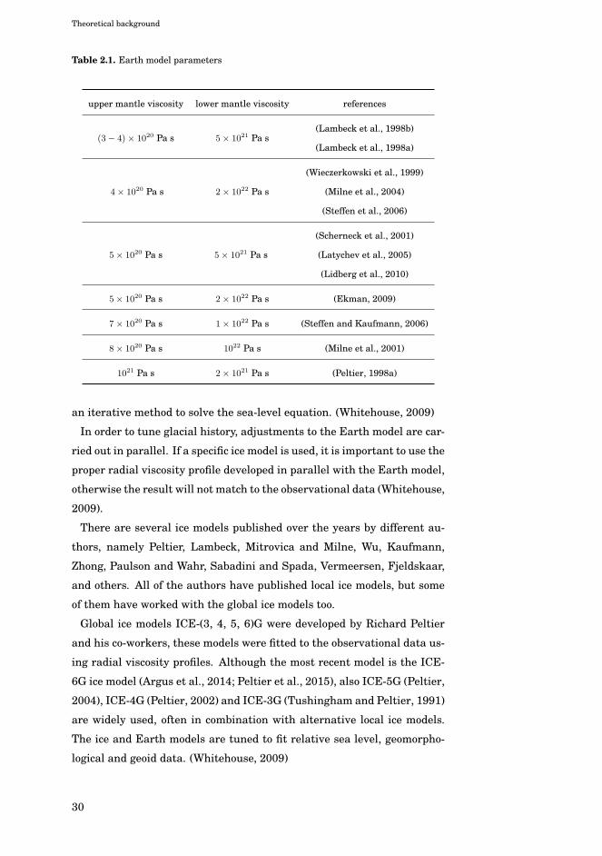
Different sets of viscosity values are used throughout different studies,
an overview is given in Table 2.1.
2.3.5 Ice models
For the ice model three types of data can be used: ice margin data, ice
loading data and global sea level data. There are two ways of constraining
ice models: the first is using the relative sea-level history. The second uses
29
Theoretical background
Table 2.1. Earth model parameters
upper mantle viscosity lower mantle viscosity references
(3− 4)× 1020 Pa s 5× 10²¹ Pa s(Lambeck et al., 1998b)
(Lambeck et al., 1998a)
4× 10²⁰ Pa s 2× 10²² Pa s
(Wieczerkowski et al., 1999)
(Milne et al., 2004)
(Steffen et al., 2006)
5× 10²⁰ Pa s 5× 10²¹ Pa s
(Scherneck et al., 2001)
(Latychev et al., 2005)
(Lidberg et al., 2010)
5× 10²⁰ Pa s 2× 10²² Pa s (Ekman, 2009)
7× 10²⁰ Pa s 1× 10²² Pa s (Steffen and Kaufmann, 2006)
8× 10²⁰ Pa s 1022 Pa s (Milne et al., 2001)
1021 Pa s 2× 10²¹ Pa s (Peltier, 1998a)
an iterative method to solve the sea-level equation. (Whitehouse, 2009)
In order to tune glacial history, adjustments to the Earth model are car-
ried out in parallel. If a specific ice model is used, it is important to use the
proper radial viscosity profile developed in parallel with the Earth model,
otherwise the result will not match to the observational data (Whitehouse,
2009).
There are several ice models published over the years by different au-
thors, namely Peltier, Lambeck, Mitrovica and Milne, Wu, Kaufmann,
Zhong, Paulson and Wahr, Sabadini and Spada, Vermeersen, Fjeldskaar,
and others. All of the authors have published local ice models, but some
of them have worked with the global ice models too.
Global ice models ICE-(3, 4, 5, 6)G were developed by Richard Peltier
and his co-workers, these models were fitted to the observational data us-
ing radial viscosity profiles. Although the most recent model is the ICE-
6G ice model (Argus et al., 2014; Peltier et al., 2015), also ICE-5G (Peltier,
2004), ICE-4G (Peltier, 2002) and ICE-3G (Tushingham and Peltier, 1991)
are widely used, often in combination with alternative local ice models.
The ice and Earth models are tuned to fit relative sea level, geomorpho-
logical and geoid data. (Whitehouse, 2009)
30
Theoretical background
ICE-5G is an updated version of ICE-4G, for the ice model new obser-
vational data were added, e.g., historical sea level data, ice margin data,
GIA data as well as geodetic and gravimetric measurements from differ-
ent regions (Whitehouse, 2009). ICE-5G ice model should be used together
with the VM2 Earth Model (Peltier, 2004).
Global ice models KL05 (or ANU05) were developed by Kurt Lambeck
and his co-workers, these models are based on observational data from ice
sheet history, Earth structure, and the records of climate, glacial cycles,
and sea-level change (Whitehouse, 2009). The model KL05 has been as-
sembled from several regional ice models (Whitehouse, 2009): the Fenno-
scandian part, which covers also the Barents Sea, FBK8 from Lambeck
et al. (1998b), Laurentide and Greenland parts of ICE-1 from (Peltier and
Andrews, 1976), the British Isles ice model from (Lambeck, 1993) and the
ANT3 Antarctic model from (Nakada and Lambeck, 1998).
Models ICE-5G and KL05 differ in several aspects, including the man-
tle viscosity profile, the ice distribution and the history of equivalent sea-
level measurements (Spada and Galassi, 2012). But the spatial scale of
these models at the Last Glacial Maximum is similar, although ice thick-
ness is counted differently in the areas of deglaciation (Whitehouse, 2009).
Because of the mentioned differences, both ice models will give different
output when used in conjunction with a GIA model (Whitehouse, 2009).
2.3.6 Sea level
The GIA component of sea-level change is evaluated solving the sea-level
equation (SLE), all terms of the SLE are dependent on the history of ice
thickness variation (Spada and Galassi, 2012). During the LGM global
sea level was reduced due to the large volume of water retained in con-
tinental ice sheets (Rittenour, 2015). During deglaciation the meltwater
returns to the oceans and sea level rises. Sea level has varied by more
than 120 m during glacial/interglacial cycles (Church et al., 2008). Ge-
ological records of sea level changes show that the redistribution of the
meltwater is not the same everywhere in the oceans, this is due to the
gravitational attraction change and the change in centrifugal potential
due to the Earth’s variable rotation (Whitehouse, 2009).
The uplift of the crust relative to mean sea level can be detected from
long time measurements of sea and lake levels. The geocentric uplift (de-
noted by h) can be obtained from (Ekman, 1988):
31
Theoretical background
h = Ha + He + Hg, (2.6)
where Ha is the apparent land uplift (i.e., the relative motion of land and
sea surface), He is the eustatic sea-level rise and Hg is the geoid uplift.
The absolute, i.e., geocentric land uplift is needed when dealing with
gravity decrease due to the land uplift as well as determining the uplift
component from GNSS time series. The latter is used to study apparent
and absolute land uplift differences and gives the possibility to study sea-
level changes (Ekman, 1988).
The prediction of relative sea-level variations is a complicated process:
the ocean redistribution is directed by the gravitational field and defor-
mations of the solid Earth, the gravitational field itself is perturbed by
the direct gravitational effect of the ocean redistribution and the solid
Earth deformation (Mitrovica et al., 2010). This circularity is solved by
the sea-level equation (Farrell and Clark, 1976).
2.3.7 The sea-level equation
The theory of glacial isostatic adjustment can predict the history of rel-
ative sea level variations, given as function of S (ϕ, λ, t), which is known
as the sea-level equation (Peltier, 1998b). The sea-level equation shows
the spatial and temporal change in ocean bathymetry, where the grav-
ity potential over the sea surface shall be spatially constant for a specific
deglaciation chronology and viscoelastic Earth model (Spada and Stocchi,
2005).
The sea-level equation has been discussed already in many publications
(see Whitehouse (2009) and references therein). One can write (Lambeck
et al., 1998b):
Δζ (ϕ, t) = Δζe (t) + ΔζI (ϕ, t) + ΔζT (ϕ, t) , (2.7)
where Δζ (ϕ, t) is the mean sea level at location ϕ and time t, measured
with respect to present sea level; Δζe (t) is the eustatic sea-level change,
which is defined as: Δζe (t) = change in ocean volume / ocean surface area;
ΔζI (ϕ, t) is the additional change that results from the isostatic adjust-
ment of the crust to the changing ice-water surface load; ΔζT (ϕ, t) is any
additional tectonic contribution resulting from geophysical factors (Lam-
beck et al., 1998b).
To solve the sea-level equation, the solution shall include the whole
32
Theoretical background
Earth. This ensures that water produced by the melting of ice sheets
is consistently redistributed throughout the oceans. (Whitehouse, 2009)
A simple algorithm to solve the sea-level equation can be described as
follows (Whitehouse, 2009):
• Using initial predictions for the global distribution of the change in
ocean height for a given time step (Δζ (ϕ, t)), the resulting global dis-
tribution of the change in sea level in the spectral domain is calculated;
• This solution is transformed to the spatial domain, and projected to the
ocean function (a function that has the value of 1 on the oceans and 0 on
land);
• The solution is transformed back to the spectral domain for a next esti-
mate for ocean height change (Δζ (ϕ, t)). The process is repeated until
convergence is achieved for the ocean height change for that time step.
33

Theoretical background
34
3. Research methods and materials
The main research idea was to investigate a variety of modelling ap-
proaches, their various precision measures and their suitability for differ-
ent use cases. The choices made in modelling included modelling strate-
gies and precision estimation methods. The main research question was:
Which measures for model quality (such as accuracy or precision) can be used
to judge the fitness for use in various use cases?
In this research, the common elements of modelling approaches in the
field of geodesy, geodynamics and geoinformatics were discussed from this
viewpoint.
3.1 Publication A
Publication A introduces two different methods for height transformation:
the bilinear affine transformation approach and fuzzy modelling.
In geodesy, in general, transformation methods are used to find missing
information by means of various mathematical approaches. By its nature,
the height transformation can be thought of as a linear approach, but, be-
cause it is dependent on the geoid, this would require a more complicated
approximating function. The main assumption of this research was the
geoid piecewise linearity over the study area in Estonia. For input data,
data from the Estonian geodetic network were used.
Firstly, the affine bilinear transformation technique was applied to a
triangulated network covering the study area. Within every triangle,
barycentric coordinates were used in order to calculate normal heights
for points. In the triangle nodes known rectangular map projection co-
35
Research methods and materials
ordinates (x, y) as well as ellipsoidal (h) and normal heights (H∗) were
used.
Secondly, the fuzzy method was used, taking advantage of multi-valued
reasoning. The fuzzy membership functions were fitted to the input data
and the transformation surface was formed. In order to find a suitable
fuzzy algorithm, different models with different membership functions
were created. The most suitable for the elevation surface construction
were triangular and Gaussian models with different numbers of member-
ship functions. Thereafter height values for data points were derived from
the transformation surface.
For both the bilinear affine transformation and fuzzy modelling approach-
es, the transformation surfaces were determined and the heights of the
points were computed with their error measures.
3.2 Publication B
Publication B discusses the possibility for DEM construction and quality
measures when using kriging and fuzzy approaches.
A Digital Elevation Model (DEM) was used to present topographic infor-
mation. For DEM construction, several different methods can be used. In
this article two of these were studied: fuzzy modelling and kriging. The
input data were height data from a laser scanning survey, altogether 2000
laser-scanning points, which were situated in the area of about 2 km2 in
the Rastila area in Helsinki. The data used were rectangular point co-
ordinates in the map projection plane and heights above sea level in the
range of 0 to 18 m.
For constructing a DEM by the fuzzy modelling method, the Matlab
Fuzzy Toolbox was used. Two methods of fuzzy modelling were chosen
for the study – grid partition and subclustering. Altogether 20 models
were computed, from which three models were chosen by the smallest
RMS value.
Kriging is a geostatistical method based on least-squares interpolation
producing optimal field predictions from discrete data points. For the con-
struction of the kriging DEM, first the candidate variograms were com-
puted. For the selection the RMS value was used, which shows how well
the model is fitted to the empirical variogram. From the RMS analysis the
exponential variogram was chosen as the most suitable one. Thereafter
the ordinary kriging method was implemented to estimate and interpo-
36
Research methods and materials
late the data and the kriging DEM map was produced.
As the result, two DEM models with their quality measures were com-
puted.
3.3 Publication C
Publication C discusses theoretical estimates for the gravimetric geoid
precision as well as the structure of the uncertainty – i.e., the uncertainty
budget. In this context the sources of uncertainty and their relative con-
tributions as well as data coverage (i.e., how lacking data outside the bor-
der and the limited resolution of global models affect the precision) were
studied. The example calculations are given for two case study areas –
Finland and Estonia.
In the study three geoid error sources were considered:
• The error of omission. This error represents geoid error directly caused
by the finite spatial density of the gravity survey.
• The aliasing error. This error represents geoid error due to finite spatial
density of the gravity survey, the part of the field above the truncation
degree. For this error two approaches were given, one of them used the
concept of white noise and the other used the Stokes integral. For the
aliasing error the accuracy was computed for the different grid spac-
ings. These calculations assumed an infinite extent of the gravitational
survey data.
• The out-of-area error. This error acknowledges the fact that gravimetric
data may not be available for neighbouring areas.
The input data needed for the calculation of the geoid errors were the
mean separation of gravimetric measurement points and the average “er-
ror of prediction” of the gravimetric survey for two test regions (see Table
3.1).
37
Research methods and materials
Table 3.1. Input data for geoid precision study (Publication C)
Indicator Finland Estonia
Average “error of prediction” [mGal] ± 2 ± 3
Mean separation of gravimetric points [km] 4 5
3.4 Publication D
Publication D introduces a statistical model for predicting the uplift rates
from the existing point uplift rates with its empirical signal covariance
function.
In this study we investigated, given the precision of the land uplift val-
ues obtained from GNSS time series, how precise the land uplift value
predicted at an arbitrary point would be. In order to find the solution,
firstly, one should know the functional behaviour of the land uplift model,
and secondly, the general stochastic behaviour of local uplift deviations
from this functional model. These deviations can be characterised by a
signal covariance function estimated empirically by least-squares colloca-
tion.
The derived model allows the prediction of point height values above sea
level if the following are given:
• point coordinates allowing to extract the uplift rates from the model;
• current point height as measured by GNSS;
• a geoid model for extracting the point geoid height using point coordi-
nates.
Two different datasets for obtaining uplift values for Fennoscandia were
used: data from the BIFROST project (Johansson et al., 2002) and data
from the last Finnish precise levellings, jointly adjusted with the previ-
ous levelling campaigns. From the BIFROST project, uplift values for the
whole Fennoscandian uplift area and uplift values for the Fennoscandian
central area were used. One has to be aware that the BIFROST project
38
Research methods and materials
provides geocentric land uplift values; the dataset from the Finnish pre-
cise levelling, on the other hand, provides land uplift values relative to
mean sea level.
Firstly, a functional model for uplift rate prediction was derived based
on a 2D elliptical geometry. Thereafter plausible initial values for the
model parameters were chosen. The computation iteratively improved the
model parameter values. It showed the quality of the functional model for
predicting land uplift at an arbitrary point. After parameter estimation,
an uncertainty model over the Fennoscandian area was derived by using
the least-squares collocation method. As a result, an empirical covariance
function for residuals relative to the functional model from the previous
stage was derived for quality assessment.
3.5 Publication E
Publication E describes the modelling of GIA in the North American and
Fennoscandian uplift areas, deriving fitted Earth model parameters and
their uncertainties, using the ice models ICE-5G and KL05 as input.
In this article the focus was on GIA processes in North America and
Fennoscandia. For these areas GIA modelling was carried out using the
free software SELEN for the visco-elastic modelling (Spada and Stocchi,
2007). For the reference dataset GNSS data from CORS were used. For
North America the dataset from Sella et al. (2007) and for Fennoscandia
the BIFROST dataset from Lidberg et al. (2010) were used.
The study was performed in different stages. Firstly, the sensitivity of
the results to the maximum harmonic degree included in the model was
tested. As a result, a maximum harmonic degree of 72 was chosen, as
including higher degree numbers did not significantly change the results
obtained. Secondly, the GIA computation was carried out in order to find
the Earth model parameters yielding the best fit with the GNSS-based
velocity field. With both ice models the following Earth model parameters
were included in the estimation process: upper mantle viscosity, lower
mantle viscosity and lithosphere thickness. In addition, an alternative,
two-step method (the “2D+1D approach”) was tested against the more ex-
act 3D approach. For this 2D+1D approach we considered the estimation
of Earth model parameters in two steps: firstly, mantle viscosity values
were fitted and thereafter the lithosphere thickness was estimated.
For optimal fitting the χ2 goodness of fit measure was used (Milne et al.,
39

Research methods and materials
2001) to test the GIA induced velocity against the velocity values from the
GNSS time series. In the computations the Fennoscandian dataset was
used for testing the methodology, and afterwards the same computations
were performed for the North American uplift area. As the result, the
optimum Earth model parameters were found for both ice models having
the smallest χ2 misfit with the GNSS data.
40
4. Discussion of research results
4.1 Transformation surface and DEM
Height modelling, as discussed in this dissertation, covers transformation
surface modelling and DEM modelling methods. Transformation methods
are always used within the context of some reference frame, relations be-
tween coordinate systems are described by coordinate transformations.
4.1.1 Obtaining height values by means of a transformationsurface (Publication A)
Among coordinate transformation methods, the height transformation is
the easiest one, as it has only one dimension. In this study different in-
terpolation methods for finding correct gravity based, i.e., orthometric or
normal heights (in the absence of a precise geoid model) were tested by
using plane coordinates and ellipsoidal heights from GNSS as input data.
The purpose was to construct a height transformation surface covering
the Estonian territory by using two different methods.
Table 4.1 presents an overview of the used methods, using standard de-
viation as a quality measure. All three models were based on the triangu-
lation of the area of study. The difference between the three models was
in triangle size, i.e., the distance between triangle nodes.
41
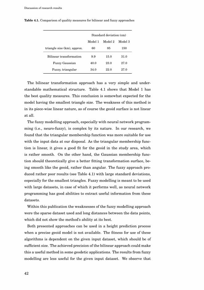
Discussion of research results
Table 4.1. Comparison of quality measures for bilinear and fuzzy approaches
Standard deviation (cm)
Model 1 Model 2 Model 3
triangle size (km), approx. 60 85 150
Bilinear transformation 9.9 15.0 31.0
Fuzzy Gaussian 40.0 23.0 27.0
Fuzzy, triangular 34.0 22.0 27.0
The bilinear transformation approach has a very simple and under-
standable mathematical structure. Table 4.1 shows that Model 1 has
the best quality measures. This conclusion is somewhat expected for the
model having the smallest triangle size. The weakness of this method is
in its piece-wise linear nature, as of course the geoid surface is not linear
at all.
The fuzzy modelling approach, especially with neural network program-
ming (i.e., neuro-fuzzy), is complex by its nature. In our research, we
found that the triangular membership function was more suitable for use
with the input data at our disposal. As the triangular membership func-
tion is linear, it gives a good fit for the geoid in the study area, which
is rather smooth. On the other hand, the Gaussian membership func-
tion should theoretically give a better fitting transformation surface, be-
ing smooth like the geoid, rather than angular. The fuzzy approach pro-
duced rather poor results (see Table 4.1) with large standard deviations,
especially for the smallest triangles. Fuzzy modelling is meant to be used
with large datasets, in case of which it performs well, as neural network
programming has good abilities to extract useful information from these
datasets.
Within this publication the weaknesses of the fuzzy modelling approach
were the sparse dataset used and long distances between the data points,
which did not show the method’s ability at its best.
Both presented approaches can be used in a height prediction process
when a precise geoid model is not available. The fitness for use of these
algorithms is dependent on the given input dataset, which should be of
sufficient size. The achieved precision of the bilinear approach could make
this a useful method in some geodetic applications. The results from fuzzy
modelling are less useful for the given input dataset. We observe that
42
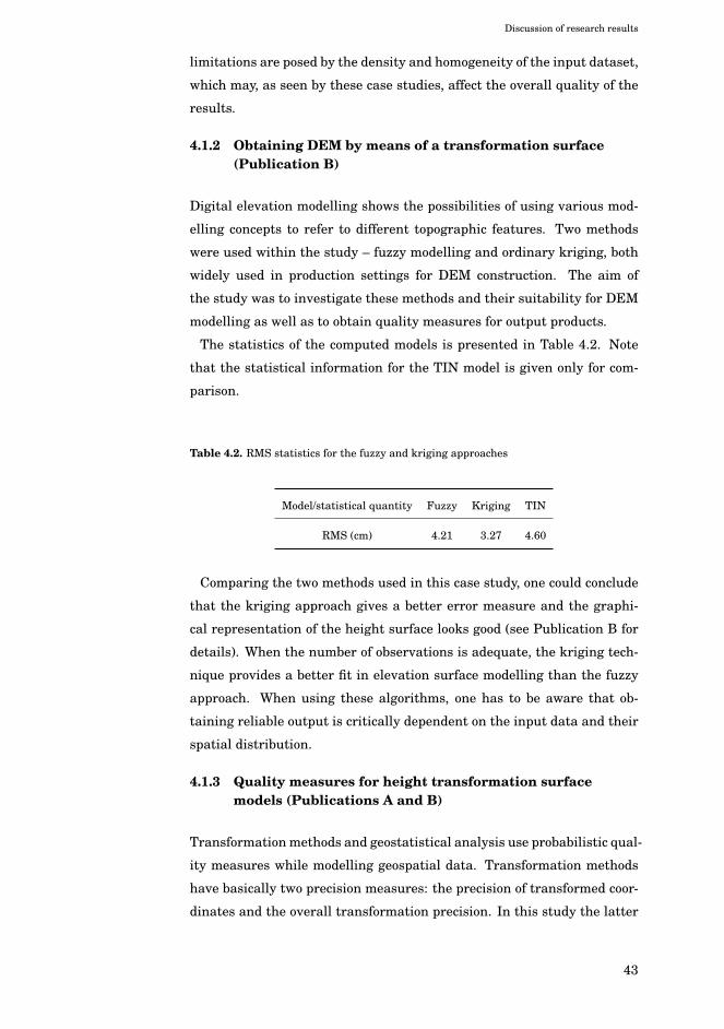
Discussion of research results
limitations are posed by the density and homogeneity of the input dataset,
which may, as seen by these case studies, affect the overall quality of the
results.
4.1.2 Obtaining DEM by means of a transformation surface(Publication B)
Digital elevation modelling shows the possibilities of using various mod-
elling concepts to refer to different topographic features. Two methods
were used within the study – fuzzy modelling and ordinary kriging, both
widely used in production settings for DEM construction. The aim of
the study was to investigate these methods and their suitability for DEM
modelling as well as to obtain quality measures for output products.
The statistics of the computed models is presented in Table 4.2. Note
that the statistical information for the TIN model is given only for com-
parison.
Table 4.2. RMS statistics for the fuzzy and kriging approaches
Model/statistical quantity Fuzzy Kriging TIN
RMS (cm) 4.21 3.27 4.60
Comparing the two methods used in this case study, one could conclude
that the kriging approach gives a better error measure and the graphi-
cal representation of the height surface looks good (see Publication B for
details). When the number of observations is adequate, the kriging tech-
nique provides a better fit in elevation surface modelling than the fuzzy
approach. When using these algorithms, one has to be aware that ob-
taining reliable output is critically dependent on the input data and their
spatial distribution.
4.1.3 Quality measures for height transformation surfacemodels (Publications A and B)
Transformation methods and geostatistical analysis use probabilistic qual-
ity measures while modelling geospatial data. Transformation methods
have basically two precision measures: the precision of transformed coor-
dinates and the overall transformation precision. In this study the latter
43
Discussion of research results
was used for comparison. For geostatistical analysis continuous variables
are usually tested against reference data using RMS or similar accuracy
measures.
In Publications A and B, the quality measures were computed for DEM
models and transformation surfaces. For Publication A the achieved qual-
ity measures are presented in Table 4.1. The input data density was also
very sparse, being about 1 point for 2000 km2. For the given data density,
the methods used can not be applied for high-precision geodetic applica-
tions, but may be sufficient for cartographic or GIS purposes. For Publi-
cation B two different methods were used for DEM construction and error
estimation. The quality measures for DEM models are presented in Table
4.2. The input point density for this study was about 2000 points for the
area of 2 km2. These quality measures suggest that these methods can
also be used in some geodetic applications.
These two studies indicated (Table 4.1 and Table 4.2) that the quality
measures improved when the data point density increased. This sug-
gests that the results of the first study would have been better if a denser
dataset could have been used (see Publication A). Unfortunately, this was
not available at the time.
The results for height modelling showed that both the transformation
(traditional application) and DEM (non-traditional application) methods
were suitable for geodetic or GIS applications. The most important factors
to affect the quality measures were the precision and spatial distribution
of input data.
4.2 Quality measures for the geoid model (Publication C)
For geoid models different quality measures as well as the structure of
the uncertainty were investigated and evaluated for the two test areas,
Finland and Estonia, see paragraph 3.3 and Table 3.1.
44
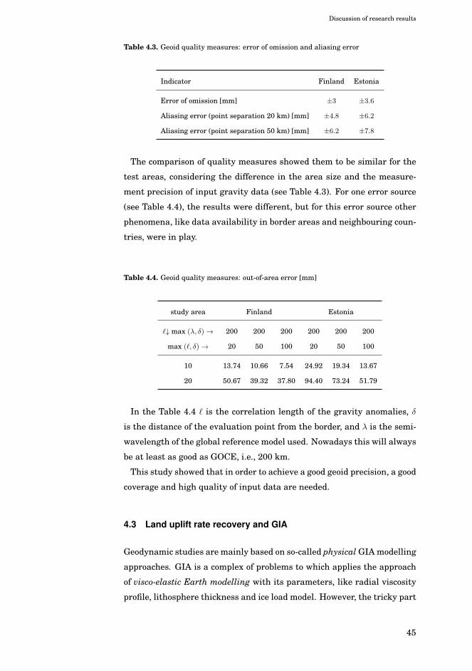
Discussion of research results
Table 4.3. Geoid quality measures: error of omission and aliasing error
Indicator Finland Estonia
Error of omission [mm] ±3 ±3.6
Aliasing error (point separation 20 km) [mm] ±4.8 ±6.2
Aliasing error (point separation 50 km) [mm] ±6.2 ±7.8
The comparison of quality measures showed them to be similar for the
test areas, considering the difference in the area size and the measure-
ment precision of input gravity data (see Table 4.3). For one error source
(see Table 4.4), the results were different, but for this error source other
phenomena, like data availability in border areas and neighbouring coun-
tries, were in play.
Table 4.4. Geoid quality measures: out-of-area error [mm]
study area Finland Estonia
�↓ max (λ, δ) → 200 200 200 200 200 200
max (�, δ) → 20 50 100 20 50 100
10 13.74 10.66 7.54 24.92 19.34 13.67
20 50.67 39.32 37.80 94.40 73.24 51.79
In the Table 4.4 � is the correlation length of the gravity anomalies, δ
is the distance of the evaluation point from the border, and λ is the semi-
wavelength of the global reference model used. Nowadays this will always
be at least as good as GOCE, i.e., 200 km.
This study showed that in order to achieve a good geoid precision, a good
coverage and high quality of input data are needed.
4.3 Land uplift rate recovery and GIA
Geodynamic studies are mainly based on so-called physical GIA modelling
approaches. GIA is a complex of problems to which applies the approach
of visco-elastic Earth modelling with its parameters, like radial viscosity
profile, lithosphere thickness and ice load model. However, the tricky part
45
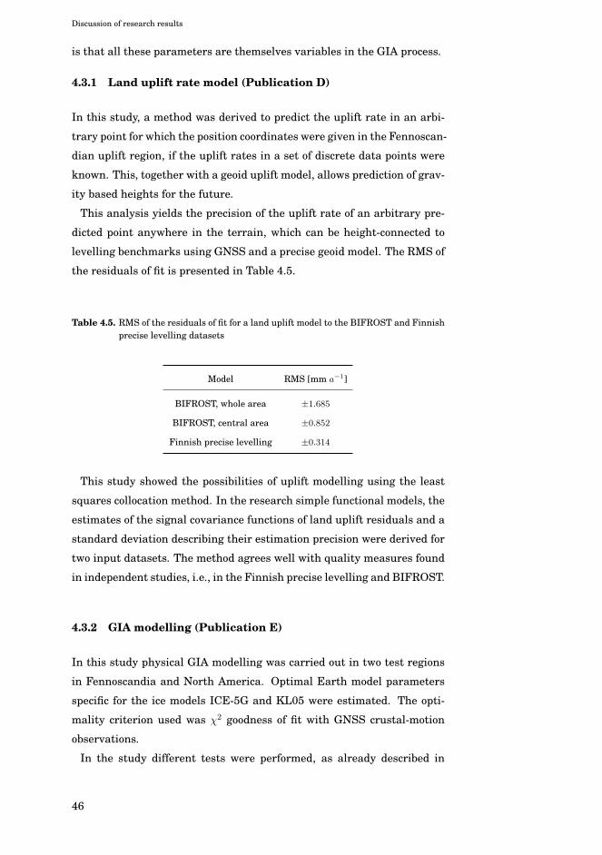
Discussion of research results
is that all these parameters are themselves variables in the GIA process.
4.3.1 Land uplift rate model (Publication D)
In this study, a method was derived to predict the uplift rate in an arbi-
trary point for which the position coordinates were given in the Fennoscan-
dian uplift region, if the uplift rates in a set of discrete data points were
known. This, together with a geoid uplift model, allows prediction of grav-
ity based heights for the future.
This analysis yields the precision of the uplift rate of an arbitrary pre-
dicted point anywhere in the terrain, which can be height-connected to
levelling benchmarks using GNSS and a precise geoid model. The RMS of
the residuals of fit is presented in Table 4.5.
Table 4.5. RMS of the residuals of fit for a land uplift model to the BIFROST and Finnishprecise levelling datasets
Model RMS [mm a−1]
BIFROST, whole area ±1.685
BIFROST, central area ±0.852
Finnish precise levelling ±0.314
This study showed the possibilities of uplift modelling using the least
squares collocation method. In the research simple functional models, the
estimates of the signal covariance functions of land uplift residuals and a
standard deviation describing their estimation precision were derived for
two input datasets. The method agrees well with quality measures found
in independent studies, i.e., in the Finnish precise levelling and BIFROST.
4.3.2 GIA modelling (Publication E)
In this study physical GIA modelling was carried out in two test regions
in Fennoscandia and North America. Optimal Earth model parameters
specific for the ice models ICE-5G and KL05 were estimated. The opti-
mality criterion used was χ2 goodness of fit with GNSS crustal-motion
observations.
In the study different tests were performed, as already described in
46
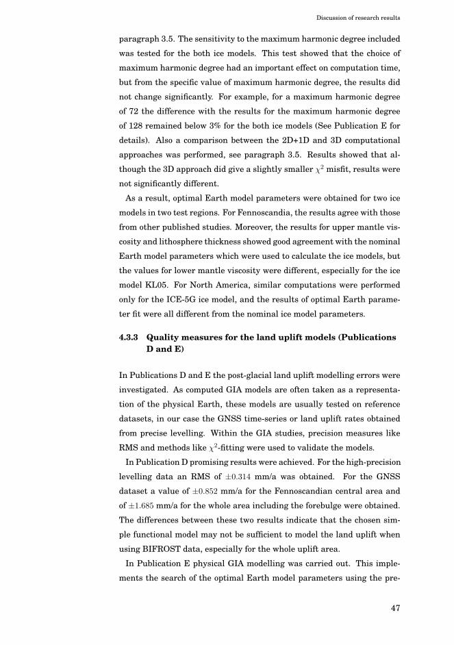
Discussion of research results
paragraph 3.5. The sensitivity to the maximum harmonic degree included
was tested for the both ice models. This test showed that the choice of
maximum harmonic degree had an important effect on computation time,
but from the specific value of maximum harmonic degree, the results did
not change significantly. For example, for a maximum harmonic degree
of 72 the difference with the results for the maximum harmonic degree
of 128 remained below 3% for the both ice models (See Publication E for
details). Also a comparison between the 2D+1D and 3D computational
approaches was performed, see paragraph 3.5. Results showed that al-
though the 3D approach did give a slightly smaller χ2 misfit, results were
not significantly different.
As a result, optimal Earth model parameters were obtained for two ice
models in two test regions. For Fennoscandia, the results agree with those
from other published studies. Moreover, the results for upper mantle vis-
cosity and lithosphere thickness showed good agreement with the nominal
Earth model parameters which were used to calculate the ice models, but
the values for lower mantle viscosity were different, especially for the ice
model KL05. For North America, similar computations were performed
only for the ICE-5G ice model, and the results of optimal Earth parame-
ter fit were all different from the nominal ice model parameters.
4.3.3 Quality measures for the land uplift models (PublicationsD and E)
In Publications D and E the post-glacial land uplift modelling errors were
investigated. As computed GIA models are often taken as a representa-
tion of the physical Earth, these models are usually tested on reference
datasets, in our case the GNSS time-series or land uplift rates obtained
from precise levelling. Within the GIA studies, precision measures like
RMS and methods like χ2-fitting were used to validate the models.
In Publication D promising results were achieved. For the high-precision
levelling data an RMS of ±0.314 mm/a was obtained. For the GNSS
dataset a value of ±0.852 mm/a for the Fennoscandian central area and
of ±1.685 mm/a for the whole area including the forebulge were obtained.
The differences between these two results indicate that the chosen sim-
ple functional model may not be sufficient to model the land uplift when
using BIFROST data, especially for the whole uplift area.
In Publication E physical GIA modelling was carried out. This imple-
ments the search of the optimal Earth model parameters using the pre-
47
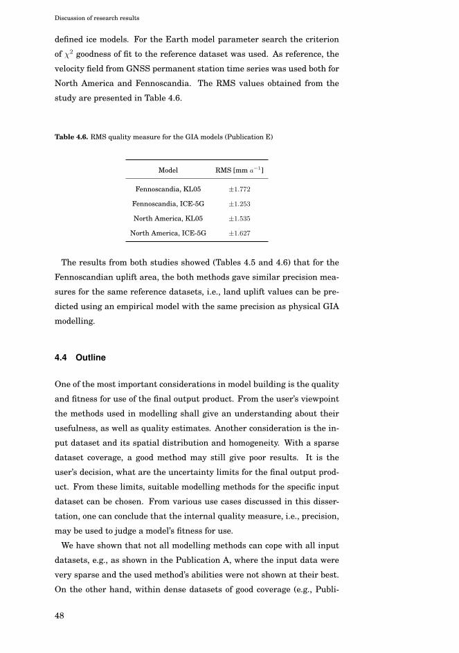
Discussion of research results
defined ice models. For the Earth model parameter search the criterion
of χ2 goodness of fit to the reference dataset was used. As reference, the
velocity field from GNSS permanent station time series was used both for
North America and Fennoscandia. The RMS values obtained from the
study are presented in Table 4.6.
Table 4.6. RMS quality measure for the GIA models (Publication E)
Model RMS [mm a−1]
Fennoscandia, KL05 ±1.772
Fennoscandia, ICE-5G ±1.253
North America, KL05 ±1.535
North America, ICE-5G ±1.627
The results from both studies showed (Tables 4.5 and 4.6) that for the
Fennoscandian uplift area, the both methods gave similar precision mea-
sures for the same reference datasets, i.e., land uplift values can be pre-
dicted using an empirical model with the same precision as physical GIA
modelling.
4.4 Outline
One of the most important considerations in model building is the quality
and fitness for use of the final output product. From the user’s viewpoint
the methods used in modelling shall give an understanding about their
usefulness, as well as quality estimates. Another consideration is the in-
put dataset and its spatial distribution and homogeneity. With a sparse
dataset coverage, a good method may still give poor results. It is the
user’s decision, what are the uncertainty limits for the final output prod-
uct. From these limits, suitable modelling methods for the specific input
dataset can be chosen. From various use cases discussed in this disser-
tation, one can conclude that the internal quality measure, i.e., precision,
may be used to judge a model’s fitness for use.
We have shown that not all modelling methods can cope with all input
datasets, e.g., as shown in the Publication A, where the input data were
very sparse and the used method’s abilities were not shown at their best.
On the other hand, within dense datasets of good coverage (e.g., Publi-
48
Discussion of research results
cation B), the method’s behaviour was indeed impressive. The same was
shown in Publication C, i.e., input data density and coverage has an effect
on the theoretical uncertainty estimates, as we compared there the var-
ious geoid uncertainty contributions for two case study areas. Although
the one area was about seven times larger then the other, the data den-
sity and coverage for it was much better, which has an influence on the
computed uncertainties. In the Publications D and E we showed that
two different independent modelling methods can give similar precision
estimates for land uplift rates for the same study area using these two
approaches.
49

Discussion of research results
50
5. Conclusions
In this dissertation a variety of modelling approaches of a spatial nature
were investigated. These were demonstrated to be able to model geo-
graphical information from different perspectives. All methods used were
formulated in mathematical terms and could offer added value to geodetic
and geoinformatics studies.
In the geosciences different features are often modelled as spatially cor-
related random variables and they usually are location dependent (Zhang
and Goodchild, 2002). Within modelling one has the possibility to choose
the precision measures. Besides the different quality concepts, the preci-
sion of modelling depends also on the input data and their spatial distri-
bution.
In the dissertation, modelling aspects in geodesy, geoinformatics and
geodynamics were investigated. In relation to geodesy, transformation
methods as well as quality measures for geoid models were discussed.
In relation to geoinformatics, fuzzy modelling and kriging methods to be
used in height transformation surface modelling and DEM were investi-
gated. In relation to geodynamics, land uplift rate prediction computation
and GIA modelling were performed.
The following conclusions can be drawn according to the research topics:
1. Several different mathematical and geostatistical methods were used
in height modelling. These include the affine bilinear method, and the
fuzzy and kriging modelling methods. The study showed that the trans-
formation approach using either traditional or non-traditional methods
can be used in various geodetic and GIS applications. In both studies,
quality measures were evaluated for DEM models and transformation
surfaces.
(a) In the first study on transformation surfaces, the achieved quality in
51
Conclusions
terms of standard deviations was about 10 cm for the traditional (bi-
linear affine) transformation approach, and 20 cm for non-traditional
fuzzy modelling.
(b) In the second study on digital elevation modelling, the achieved ac-
curacy was about 3 to 5 cm. Although the size of the area and the
number of input data points as well as the point distribution were very
different from the earlier case study, the results showed the suitability
of these modelling approaches to be used in this kind of research.
One can conclude that the quality measures improve when the data point
density increases, thus, results can even be better while using a still denser
input dataset, especially when using the traditional transformation method.
As a result, we showed that these modelling techniques could be used in
constructing terrain height models (DEM) to be used in GIS, but to some
extent also in geodesy, e.g., for the prediction of heights when no geoid model
is available.
2. In the geoid uncertainty study we showed that the uncertainty was de-
pendent both on gravity data coverage and on the precision of gravity
measurements, as well as on the availability of gravity data from neigh-
bouring countries in border areas. Also the underlying global geopoten-
tial model that was used had an effect.
3. In GIA modelling, we investigated two methods for predicting land up-
lift rates. These include land uplift modelling by least squares colloca-
tion and GIA model computations by visco-elastic modelling.
(a) Firstly, an empirical model for predicting the land uplift rate was de-
rived. Achieved quality measures were following: for the high-precision
levelling data an RMS of ±0.314 mm/a; for the GNSS dataset an RMS
of ±0.852 mm/a for the Fennoscandian central area and of ±1.685 mm/a
for the whole area including the forebulge were obtained.
(b) Secondly, physical GIA modelling was performed. The quality mea-
sures were very promising, for the Fennoscandian uplift area an RMS
of ±1.772 mm/a and of ±1.253 mm/a were obtained for ice models KL05
and ICE-5G respectively. For the North American uplift area an RMS
52
Conclusions
of ±1.535 mm/a and of ±1.627 mm/a were obtained for ice models KL05
and ICE-5G respectively.
For both studies, reference datasets from GNSS time series were used to val-
idate the constructed models. As a result, we showed that land uplift values
can be predicted empirically with similar accuracy as the physics based GIA
modelling, as RMS was about 1.2 to 1.5 mm/a for both studies as shown in
the case study of the Fennoscandian region.
The dissertation showed different use cases in the field of geodesy, geody-
namics and geoinformatics. We constructed various models using various
modelling methodologies and input datasets. The models were studied
and discussed from the viewpont of fitness for use, i.e., suitable qual-
ity measures for these models were evaluated. The quality measures
achieved for the various models showed their applicability in the fields
of geodesy, geodynamics and geoinformation science.
In this dissertation a large amount of numerical results were obtained
and some conclusions drawn. The purpose of such research shall always
be insight, not only numerical results. Indeed, this provided an oppor-
tunity to compare the chosen methods and to understand the theories
behind them. The obtained understanding pertains not only to the mod-
elling itself and its use in different applications, but also to the choice of
parameters used in the modelling. They all together serve as the basis for
decision making on different levels.
53

Conclusions
54
Bibliography
Altamimi, Z., Collilieux, X., Legrand, J., Garayt, B., and Boucher, C. (2007).ITRF2005: A New Release of the International Terrestrial Reference Framebased on time series of station positions and Earth Orientation Parameters. J.Geophys. Res.
Argus, D. F., Peltier, W. R., Drummond, R., and Moore, A. W. (2014). The Antarc-tica component of postglacial rebound model ICE-6G_C (VM5a) based uponGPS positioning, exposure age dating of ice thicknesses, and relative sea levelhistories. Geophys. J. Int., (198(1)):537–563.
Blewitt, G., Altamini, Z., Davis, J., Gross, R., Kuo, C.-Y., Lemoine, G. F., Moor,A. W., Neilan, R. E., Plag, H.-P., Rotacher, M., Schum, C. K., Sideris, M. G.,Schöne, T., Tregoning, P., and Zerbini, S. (2010). Geodetic Observations andGlobal Reference Frame Contributions to Understanding Sea-Level Rise andVariability. In Church, J. A., Woodworth, P. L., Aarup, T., and Wilson, W. S.,editors, Understanding Sea-level Rise and Variability. Wiley-Blackwell Pub-lishing Ltd.
Blewitt, G., Larson, K., Davis, J., Argus, D., Bennett, R., Bock, Y., Calais, E.,Craymer, M. ., Dixon, T., Freymueller, J. Herring, T., Johnson, D., Miller, M.,Sella, G., Snay, R., and Tamisiea, M. (2006). SNARF 1.0 A Regional ReferenceFrame for North America. In Geodetic Reference Frames, GRF2006, Interna-tional IAG/FIG Symposium, Munich, October 9-14, 2006.
Burrough, P. A. and McDonnell, R. A. (1998). Principles of Geographical Infor-mation Systems. Oxford University Press.
Church, J. A., White, N. J., Aarup, T., Wilson, W. S., Woodworth, P. L., Domingues,C. M., Hunter, R., and Lambeck, K. (2008). Understanding global sea levels:past, present and future. Sustainability Science, 3:9–22.
DeMets, C., Gordon, R. G., Argus, D. F., and Stein, S. (1994). Effect of recentrevisions to the geomagnetic reversal time scale on estimates of current platemotions. Geophysical Research Letters, 21(20):2191–2194.
Devillers, R. and Jeansoulin, R. (2006). Fundamentals of Spatial Data Quality.ISTE Ltd.
Douglas, B. C. and Peltier, W. R. (2002). The puzzle of global sea-level rise.Physics Today, pages 35–40.
Dziewonski, A. and Anderson, D. (1981). Preliminary reference earth model.Phys. Earth Planet. Inter., pages 297–356.
55
Bibliography
Ekman, M. (1988). The impact of geodynamic phenomena on systems for heightand gravity. In Nordic Geodetic Commission, 2nd Research School, pages 109–167. Ebeltoft, Denmark.
Ekman, M. (1995). What is the geoid? In Vermeer, M., editor, Coordinate systems,GPS, and the geoid. Proceedings, NorFA Urgency Seminar held at Hanasaari,Espoo, Finland, June 27-29, 1994, number 4 in Reports of the Finnish GeodeticInstitute, pages 49–51.
Ekman, M. (1996). A consistent map of the postglacial uplift of Fennoscandia.Terra Nova, 8(2):158–165.
Ekman, M. (2009). The Changing Level of the Baltic Sea during 300 Years: AClue to Understanding the Earth. Summer Institute for Historical Geophysics,Åland Islands.
Farrell, W. E. and Clark, J. A. (1976). On Postglacial Sea Level. Geophys. J. R.Astr. Soc., 46:647–667.
Fjeldskaar, W. (1991). Geoidal-eustatic changes induced by the deglaciation ofFennoscandia. Quaternary International, 9:1–6.
JCGM/WG 1 (2008). Evaluation of measurement data - Guide to the expressionof uncertainty in measurement. Technical Report 2008:100, BIPM.
Johansson, J. M., Davis, J. L., Scherneck, H.-G., Milne, G. A., Vermeer, M., Mitro-vica, J. X., Bennet, R. A., Jonsson, B., Elgered, G., Elosegui, P., Koivula, H.,Poutanen, M., Rönnäng, B. O., and Shapiro, I. I. (2002). Continuous GPSmeasurements of postglacial adjustment in Fennoscandia 1. Geodetic results.Journal of Geophysical Research, 107(B8).
Kaufmann, G. and Lambeck, K. (2000). Mantle dynamics, postglacial reboundand the radial viscosity profile. Physics of the Earth Planetary Interiors,121:301–324.
Koivula, H., Tervo, M., and Poutanen, M. (2006). Contemporary crustal mo-tion in Fennoscandia observed with continuous GPS networks. In Kukkonen,I. T., Eklund, O., Korja, A., Korja, T., Pesonen, L. J., and Poutanen, M., edi-tors, Lithosphere 2006, Fourth Symposium on the structure, composition andevolution of the lithosphere in Finland, November 9-10, 2006, Espoo, Finland.Report S-46. Geological Survey of Finland, pages 59–65.
Lambeck, K. (1993). Glacial rebound of the British Isles. I. A high-resolution,high-precision model. Geophysical Journal International, 115(3):960–990.
Lambeck, K., Smither, C., and Ekman, M. (1998a). Tests of glacial rebound mod-els for Fennoscandia based on instrumented sea- and lake-level records. Geo-phys. J. Int., 135:375–387.
Lambeck, K., Smither, C., and Johnston, P. (1998b). Sea-level change, glacialrebound and mantle viscosity for Northern Europe. Geophys. J. Int., 134:102–144.
Latychev, K., Mitrovica, J. X., Tamisiea, M. E., Tromp, J., and Moucha, R. (2005).Influence of lithospheric thickness variations on 3-D crustal velocities due toglacial isostatic adjustment. Geophysical Research Letters, 32:L01304.
56
Bibliography
Le Meur, E. (1996). Isostatic postglacial rebound over Fennoscandia with a self-gravitating spherical visco-elastic Earth model. Annals of Glaciology, 23:318–327.
Lidberg, M. (2007). Geodetic Reference Frames in Presence of Crustal Deforma-tions. PhD thesis, Departement of Radio and Space Science, Chalmers Univer-sity of Technology, Gothenborg, Sweden .
Lidberg, M., Johannson, J. M., Scherneck, H.-G., and Milne, G. A. (2010). Re-cent results based on continuous GPS observations of the GIA process inFennoscandia from BIFROST. Journal of Geodynamics.
Longley, P. A., Goodchild, M. F., Maguire, D. J., and Rhind, D. W. (2001). Geo-graphic Information Systems and Science. John Wiley & Sons Ltd., Chichester,New York, Weinheim, Brisbane, Singapore, Toronto.
Milne, G., Mitrovica, J., Davis, J., Scherneck, H., Johansson, J., Koivula, H., andVermeer, M. (2004). Continuous GPS Measurements of Postglacial Adjustmentin Fennoscandia 2. Modeling Results. Journal of Geophysical Research: SolidEarth, 109(B2):B02412.
Milne, G. A., Davis, J. L., Mitrovica, J. X., Scherneck, H.-G., Johansson, J. M.,Vermeer, M., and Koivula, H. (2001). Space-geodetic constraints on glacialisostatic adjustment in Fennoscandia. Science, 291:2381–2385.
Mitrovica, J. X., Tamisiea, M. E., Ivins, E. R., Vermeersen, L. L. A., Milne, G. A.,and Lambeck, K. (2010). Surface Mass Loading on a Dynamic Earth: Complex-ity and Contamination in the Geodetic Analysis of Global Sea-Level Trends. InChurch, J. A., Woodworth, P. L., Aarup, T., and Wilson, W. S., editors, Under-standing Sea-level Rise and Variability. Wiley-Blackwell Publishing Ltd.
Mitrovica, J., X., Milne, G., A., , and Davis, J. L. (2001). Glacial isostatic adjust-ment on a rotating Earth. Geophysical Journal International, 147:562–578.
Mäkinen, J. (2000). Geodynamical studies using gravimetry and levelling. PhDthesis, Faculty of Science, University of Helsinki, Helsinki.
Müller, J., Neumann-Redlin, M., Jarecki, F., Timmen, L., Denker, H., and Gitlein,O. (2005). Gravity Change in Fennoscandian Land Uplift Area as Observed byGRACE. Geophysical Research Abstracts, 7:04900.
Moisio, K. and Mäkinen, J. (2006). Rheology of the lithosphere and models ofpostglacial rebound. In Kukkonen, I. T., Eklund, O., Korja, A., Korja, T., Peso-nen, L. J., and Poutanen, M., editors, Lithosphere 2006, Fourth Symposium onthe structure, composition and evolution of the lithosphere in Finland, Novem-ber 9-10, 2006, Espoo, Finland. Report S-46. Geological Survey of Finland.
Nakada, M. and Lambeck, K. (1998). The melting history of the Late PleistoceneAntarctic ice sheet. Nature, (333):36–40.
Niskanen, V. A. (2003). Soft Computing Methods in Human Sciences. Springer.
Peltier, W. R. (1990). Glacial Isostatic Adjustment and Relative Sea-LevelChange. In Studies in Geophysics, Sea-Level Change, pages 73–87. NationalAcademy Press, Washington, D. C.
57
Bibliography
Peltier, W. R. (1998a). Lithospheric thickness, Antarctic deglaciation history,and ocean basin discretization effects in global model of postglacial sea levelchange: a summary of some sources of nonuniqueness. Quaternary Research,29:93–112.
Peltier, W. R. (1998b). A space geodetic target for mantle viscosity discrimina-tion: Horizontal motions induced by glacial isostatic adjustment. GeophysicalResearch Letters, 25(4):543–546.
Peltier, W. R. (2002). Global glacial isostatic adjustment: palaeogeodetic andspace-geodetic tests of the ICE-4G (VM2) model. Journal of Quaternary Sci-ence, 17(5-6):491–510.
Peltier, W. R. (2004). Global glacial isostasy and the surface of the ice-age Earth:The Ice-5G (VM2) model and GRACE. Annu. Rev. Earth Planet. Sci., 32:111–149.
Peltier, W. R. and Andrews, J. T. (1976). Glacial-isostatic adjustment - 1. Theforward problem. Geophys. J. R. Astron. Soc., (46):605–646.
Peltier, W. R., Argus, D. F., and Drummond, R. (2015). Space geodesy constrainsice-age terminal deglaciation: The global ICE-6G_C (VM5a) model. J. Geophys.Res. Solid Earth, (120):450–487.
Peuquet, D. J. (2002). Representations of Space and Time. The Guilford Press.New York, London.
Rittenour, T. M. (2015). Ice Ages in New England.http://www.bio.umass.edu/biology/conn.river/iceages.html. Last visited24.05.2015.
Scherneck, H.-G., Johansson, J. M., Vermeer, M., Davis, J. L., Milne, G. A., andMitrovica, J. X. (2001). BIFROST project: 3-D crustal deformation rates de-rived from GPS confirm postglacial rebound in Fennoscandia. Earth PlanetSpace, 53:703–708.
Sella, G. F., Stein, S., Dixon, T. H., Craymer, M., James, T. S., Mazotti, S., andDokka, R. K. (2007). Observations of glacial isostatic adjustment in "stable"North America with GPS. Geophysical Research Letters, 34:L02306.
Spada, G. and Galassi, G. (2012). New estimates of a secular sea-level rise fromtide gauge data and GIA modelling. Geophysical Journal International, (191(3)):1067–1094.
Spada, G. and Stocchi, P. (2005). Solving the "Sea Level Equation". Part 1-Theory.Samizdat Press.
Spada, G. and Stocchi, P. (2007). SELEN: A Fortran 90 program for solving the"sea-level equation". Computers & Geosciences, 33:538–562.
Staudt, M., Kallio, H., and Schnidt-Thorne, P. (2004). Modelling a future sea levelchange scenario affecting the spatial development in the Baltic Sea Region -First results of the SEAREG project. In Löser, G. S. N., editor, Managing theBaltic Sea. Coastline Reports 2, pages 195–199.
Steffen, H. and Kaufmann, G. (2006). Glacial isostatic adjustment of Scandinaviaand north-western Europe and the radial viscosity structure of the Earth’smantle. Geophys. J. Int., 163/2:801–812.
58
Bibliography
Steffen, H., Kaufmann, G., and Wu, P. (2006). Three-dimensional finite-elementmodel of the glacial isostatic adjustment in Fennoscandia. Earth Planet Sci.Lett., 250:358–375.
Steffen, H. and Wu, P. (2011). Glacial isostatic adjustment in Fennoscandia - Areview of data and modeling. Journal of Geodynamics, (52 (3-4)):169–204.
Stein, A., Shi, W., and Bijker, W. (2009). Quality Aspects in Spatial Data Mining.CRC Press, Taylor & Francis Group, Boca Raton, London, New York.
Sunila, R., Laine, E., and Kremenova, O. (2004). Fuzzy Modelling and Krig-ing for Imprecise Soil Polygon Boundaries. In Proceedings 12th InternationalConference on Geoinformatics - Geospatial Information Research: Bridging thePacific and Atlantic, Gävle, pages 489–495.
Thatcher, W. and Pollitz, F. F. (2008). Temporal evolution of continental litho-spheric strength in actively deforming regions. GSA Today, 18(4/5).
The MathWorks, Inc. (2015). Fuzzy Logic Toolbox. User’s Guide. The MathWorksInc.
Torge, W. (2001). Geodesy. Walter de Gruyter, Berlin, New York.
Tushingham, A. M. and Peltier, W. R. (1991). Ice-3G: A new global model of LatePleistocene deglaciation based upon geophysical predictions of post-glacial rel-ative sea level change. Journal of Geophysical Research, 96(B3).
Vanícek, P. and Krakiwsky, E. J. (1986). Geodesy: the concepts. Elsevier SciencePublishers B. V., North Holland, Amsterdam, New York, Oxford, Tokyo.
Vermeer, M. (1988). The Role of the Geoid in GPS positioning. In Nordic GeodeticCommission, 2nd Research School, Ebeltoft, Denmark, pages 413–436.
Vestøl, O. (2006). Determination of Postglacial Land Uplift in Fennoscandia fromLevelling, Tide-gauges and Continuous GPS Stations using Least Squares Col-location. Journal of Geodesy, 80(5):248–258.
Walcott, R. I. (1973). Structure of the Earth from glacio-isostatic rebound. An-nual Reviews Inc., pages 15–37.
Whitehouse, P. (2009). Glacial isostatic adjustment and sea-level change. State ofart report. Technical report TR-09-11. Technical report, Svensk Kärnbränsle-hantering AB.
Wieczerkowski, K., Mitrovica, J. X., and Wolf, D. (1999). A revised relaxation-time spectrum for Fennoscandia. Geophys. J. Int., 139:69–86.
Wu, P., Ni, Z., and Kaufmann, G. (1998). Postglacial rebound with lateral hetero-geneities: from 2D to 3D modelling. In Wu, P., editor, Dynamics of the Ice AgeEarth: A Modern Perspective, pages 557–582. Trans Tech Publ, Switzerland.
Zhang, J. and Goodchild, M. (2002). Uncertainty in Geographical Information.Taylor & Francis.
59
9HSTFMG*agefib+
ISBN 978-952-60-6458-1 (printed) ISBN 978-952-60-6459-8 (pdf) ISSN-L 1799-4934 ISSN 1799-4934 (printed) ISSN 1799-4942 (pdf) Aalto University School of Engineering Department of Real Estate, Planning and Geoinformatics www.aalto.fi
BUSINESS + ECONOMY ART + DESIGN + ARCHITECTURE SCIENCE + TECHNOLOGY CROSSOVER DOCTORAL DISSERTATIONS
Aalto-D
D 172
/2015
We studied various aspects of modelling geographical information from the geodetic and geodynamic points of view. The data for our studies were acquired by a variety of methods: laser scanning, levelling and satellite positioning. The major subject of this dissertation is quality and its measures. We study various modelling approaches on geodetic data aimed at use cases in the fields of geodesy, geodynamics and geographic information science. The dissertation discusses internal and external quality aspects of the modelling and the data used. The main objectives of the research are related to the data modelling aspects and fitness for use within the fields of study as expressed quantitatively in various quality measures. The novelty of the dissertation is in the application of appropriate quality measures, like precision or accuracy from the viewpoint of fitness for use, which for the various models depends on the input data precision as well as on the envisaged applications of the model product.
Karin K
ollo A
spects of Modelling G
eographic Information in G
eodesy and Geodynam
ics A
alto U
nive
rsity
2015
Department of Real Estate, Planning and Geoinformatics
Aspects of Modelling Geographic Information in Geodesy and Geodynamics
Karin Kollo
DOCTORAL DISSERTATIONS