Embed Size (px)
Citation preview
Unit Operations and Reaction Models
Aspen Polymers
Version Number: V8.2May 2013
Copyright (c) 1981-2013 by Aspen Technology, Inc. All rights reserved.
Aspen Polymers™, Aspen Custom Modeler®, Aspen Dynamics®, Aspen Plus®, Aspen Properties®, aspenONE, theaspen leaf logo and Plantelligence and Enterprise Optimization are trademarks or registered trademarks of AspenTechnology, Inc., Burlington, MA.
All other brand and product names are trademarks or registered trademarks of their respective companies.This software includes NIST Standard Reference Database 103b: NIST Thermodata Engine Version 7.1This document is intended as a guide to using AspenTech's software. This documentation contains AspenTechproprietary and confidential information and may not be disclosed, used, or copied without the prior consent ofAspenTech or as set forth in the applicable license agreement. Users are solely responsible for the proper use ofthe software and the application of the results obtained.
Although AspenTech has tested the software and reviewed the documentation, the sole warranty for the softwaremay be found in the applicable license agreement between AspenTech and the user. ASPENTECH MAKES NOWARRANTY OR REPRESENTATION, EITHER EXPRESSED OR IMPLIED, WITH RESPECT TO THIS DOCUMENTATION,ITS QUALITY, PERFORMANCE, MERCHANTABILITY, OR FITNESS FOR A PARTICULAR PURPOSE.
Aspen Technology, Inc.200 Wheeler RoadBurlington, MA 01803-5501USAPhone: (1) (781) 221-6400Toll Free: (1) (888) 996-7100URL: http://www.aspentech.com
Contents iii
Contents
Introducing Aspen Polymers ...................................................................................1
About This Documentation Set ...........................................................................1Related Documentation.....................................................................................2Technical Support ............................................................................................3
1 Polymer Manufacturing Process Overview...........................................................5
About Aspen Polymers ......................................................................................5Overview of Polymerization Processes.................................................................6
Polymer Manufacturing Process Steps .......................................................6Issues of Concern in Polymer Process Modeling....................................................7
Monomer Synthesis and Purification .........................................................8Polymerization .......................................................................................8Recovery / Separation ............................................................................9Polymer Processing ................................................................................9Summary ..............................................................................................9
Aspen Polymers Tools .......................................................................................9Component Characterization.................................................................. 10Polymer Physical Properties ................................................................... 10Polymerization Kinetics ......................................................................... 10Modeling Data...................................................................................... 11Process Flowsheeting............................................................................ 11
Defining a Model in Aspen Polymers ................................................................. 12References .................................................................................................... 14
2 Polymer Structural Characterization .................................................................15
Polymer Structure .......................................................................................... 15Polymer Structural Properties .......................................................................... 19Characterization Approach............................................................................... 19
Component Attributes........................................................................... 20References .................................................................................................... 20
3 Component Classification ..................................................................................21
Component Categories.................................................................................... 21Conventional Components ..................................................................... 22Polymers............................................................................................. 22Oligomers ........................................................................................... 23Segments............................................................................................ 24Site-Based .......................................................................................... 24
Component Databanks.................................................................................... 25Pure Component Databank.................................................................... 25PC-SAFT Databank ............................................................................... 26POLYPCSF Databank ............................................................................. 26
iv Contents
INITIATO Databank .............................................................................. 26Segment Databank............................................................................... 26Polymer Databank................................................................................ 27
Segment Methodology .................................................................................... 27Specifying Components................................................................................... 28
Selecting Databanks ............................................................................. 28Defining Component Names and Types ................................................... 28Specifying Segments ............................................................................ 29Specifying Polymers ............................................................................. 29Specifying Oligomers ............................................................................ 30Specifying Site-Based Components......................................................... 30
References .................................................................................................... 31
4 Polymer Structural Properties ...........................................................................33
Structural Properties as Component Attributes................................................... 33Component Attribute Classes ........................................................................... 34Component Attribute Categories ...................................................................... 35
Polymer Component Attributes............................................................... 35Site-Based Species Attributes ................................................................ 44User Attributes .................................................................................... 45
Component Attribute Initialization .................................................................... 46Attribute Initialization Scheme ............................................................... 47
Component Attribute Scale Factors................................................................... 50Specifying Component Attributes ..................................................................... 51
Specifying Polymer Component Attributes ............................................... 51Specifying Site-Based Component Attributes ........................................... 51Specifying Conventional Component Attributes ........................................ 52Initializing Component Attributes in Streams or Blocks.............................. 52Specifying Component Attribute Scaling Factors....................................... 53
References .................................................................................................... 53
5 Structural Property Distributions ......................................................................55
Property Distribution Types ............................................................................. 55Distribution Functions ..................................................................................... 56
Schulz-Flory Most Probable Distribution................................................... 56Stockmayer Bivariate Distribution .......................................................... 58
Distributions in Process Models ........................................................................ 58Average Properties and Moments ........................................................... 58Method of Instantaneous Properties........................................................ 60Copolymerization ................................................................................. 64
Mechanism for Tracking Distributions................................................................ 65Distributions in Kinetic Reactors ............................................................. 65Distributions in Process Streams ............................................................ 67Verifying the Accuracy of Distribution Calculations.................................... 68
Requesting Distribution Calculations ................................................................. 69Selecting Distribution Characteristics ...................................................... 69Displaying Distribution Data for a Reactor ............................................... 70Displaying Distribution Data for Streams ................................................. 70
References .................................................................................................... 71
Contents v
6 End-Use Properties............................................................................................73
Polymer Properties ......................................................................................... 73Prop-Set Properties ........................................................................................ 73End-Use Properties......................................................................................... 74
Relationship to Molecular Structure ........................................................ 75Method for Calculating End-Use Properties ........................................................ 76
Intrinsic Viscosity ................................................................................. 77Zero-Shear Viscosity ............................................................................ 77Density of Copolymer ........................................................................... 78Melt Index........................................................................................... 78Melt Index Ratio................................................................................... 79
Calculating End-Use Properties ........................................................................ 79Selecting an End-Use Property ............................................................... 79Adding an End-Use Property Prop-Set ..................................................... 79
References .................................................................................................... 79
7 Polymerization Reactions ..................................................................................81
Polymerization Reaction Categories .................................................................. 81Step-Growth Polymerization .................................................................. 83Chain-Growth Polymerization................................................................. 83
Polymerization Process Types .......................................................................... 84Aspen Polymers Reaction Models...................................................................... 85
Built-in Models..................................................................................... 85User Models......................................................................................... 86
References .................................................................................................... 86
8 Step-Growth Polymerization Model ...................................................................89
Summary of Applications................................................................................. 89Step-Growth Processes ................................................................................... 90
Polyesters ........................................................................................... 90Nylon-6............................................................................................... 96Nylon-6,6............................................................................................ 98Polycarbonate.................................................................................... 100
Reaction Kinetic Scheme ............................................................................... 101Nucleophilic Reactions ........................................................................ 101Polyester Reaction Kinetics .................................................................. 105Nylon-6 Reaction Kinetics.................................................................... 111Nylon-6,6 Reaction Kinetics ................................................................. 115Melt Polycarbonate Reaction Kinetics .................................................... 122
Model Features and Assumptions ................................................................... 124Model Predictions ............................................................................... 124Phase Equilibria ................................................................................. 126Reaction Mechanism ........................................................................... 126
Model Structure ........................................................................................... 127Reacting Groups and Species............................................................... 127Reaction Stoichiometry Generation....................................................... 132Model-Generated Reactions ................................................................. 133User Reactions................................................................................... 138User Subroutines ............................................................................... 140
Specifying Step-Growth Polymerization Kinetics ............................................... 155Accessing the Step-Growth Model......................................................... 155
vi Contents
Specifying the Step-Growth Model........................................................ 156Specifying Reacting Components.......................................................... 156Listing Built-In Reactions..................................................................... 157Specifying Built-In Reaction Rate Constants........................................... 157Assigning Rate Constants to Reactions.................................................. 158Including User Reactions ..................................................................... 158Adding or Editing User Reactions.......................................................... 159Specifying Rate Constants for User Reactions ........................................ 159Assigning Rate Constants to User Reactions........................................... 159Selecting Report Options..................................................................... 160Selecting the Reacting Phase ............................................................... 160Specifying Units of Measurement for Pre-Exponential Factors................... 160Including a User Kinetic Subroutine ...................................................... 161Including a User Rate Constant Subroutine............................................ 161Including a User Basis Subroutine ........................................................ 161
References .................................................................................................. 161
9 Free-Radical Bulk Polymerization Model..........................................................163
Summary of Applications............................................................................... 163Free-Radical Bulk/Solution Processes.............................................................. 164Reaction Kinetic Scheme ............................................................................... 165
Initiation ........................................................................................... 171Propagation....................................................................................... 176Chain Transfer to Small Molecules ........................................................ 178Termination....................................................................................... 179Long Chain Branching ......................................................................... 181Short Chain Branching ........................................................................ 182Beta-Scission..................................................................................... 183Reactions Involving Diene Monomers.................................................... 183
Model Features and Assumptions ................................................................... 185Calculation Method ............................................................................. 185Quasi-Steady-State Approximation (QSSA) ........................................... 188Phase Equilibrium............................................................................... 188Gel Effect .......................................................................................... 188
Polymer Properties Calculated........................................................................ 190Specifying Free-Radical Polymerization Kinetics................................................ 193
Accessing the Free-Radical Model ......................................................... 193Specifying the Free-Radical Model ........................................................ 193Specifying Reacting Species................................................................. 194Listing Reactions ................................................................................ 194Adding Reactions ............................................................................... 194Editing Reactions ............................................................................... 195Assigning Rate Constants to Reactions.................................................. 195Adding Gel-Effect ............................................................................... 196Selecting Calculation Options............................................................... 196Specifying User Profiles....................................................................... 197
References .................................................................................................. 197
10 Emulsion Polymerization Model.....................................................................199
Summary of Applications............................................................................... 199Emulsion Polymerization Processes................................................................. 200Reaction Kinetic Scheme ............................................................................... 200
Contents vii
Micellar Nucleation ............................................................................. 201Homogeneous Nucleation .................................................................... 204Particle Growth .................................................................................. 206Radical Balance.................................................................................. 207Kinetics of Emulsion Polymerization ...................................................... 211
Model Features and Assumptions ................................................................... 215Model Assumptions............................................................................. 215Thermodynamics of Monomer Partitioning ............................................. 215Polymer Particle Size Distribution ......................................................... 216
Polymer Particle Properties Calculated ............................................................ 218User Profiles ...................................................................................... 218
Specifying Emulsion Polymerization Kinetics .................................................... 219Accessing the Emulsion Model.............................................................. 219Specifying the Emulsion Model ............................................................. 219Specifying Reacting Species................................................................. 220Listing Reactions ................................................................................ 220Adding Reactions ............................................................................... 221Editing Reactions ............................................................................... 221Assigning Rate Constants to Reactions.................................................. 221Selecting Calculation Options............................................................... 222Adding Gel-Effect ............................................................................... 222Specifying Phase Partitioning ............................................................... 222Specifying Particle Growth Parameters .................................................. 223
References .................................................................................................. 223
11 Ziegler-Natta Polymerization Model ..............................................................225
Summary of Applications............................................................................... 225Ziegler-Natta Processes ................................................................................ 226
Catalyst Types ................................................................................... 226Ethylene Process Types....................................................................... 227Propylene Process Types ..................................................................... 228
Reaction Kinetic Scheme ............................................................................... 230Catalyst Pre-Activation........................................................................ 237Catalyst Site Activation ....................................................................... 237Chain Initiation .................................................................................. 237Propagation....................................................................................... 238Chain Transfer to Small Molecules ........................................................ 239Site Deactivation................................................................................ 239Site Inhibition.................................................................................... 240Cocatalyst Poisoning........................................................................... 240Terminal Double Bond Polymerization ................................................... 240
Model Features and Assumptions ................................................................... 243Phase Equilibria ................................................................................. 243Rate Calculations ............................................................................... 243
Polymer Properties Calculated........................................................................ 243Specifying Ziegler-Natta Polymerization Kinetics .............................................. 244
Accessing the Ziegler-Natta Model ........................................................ 244Specifying the Ziegler-Natta Model ....................................................... 244Specifying Reacting Species................................................................. 245Listing Reactions ................................................................................ 245Adding Reactions ............................................................................... 246Editing Reactions ............................................................................... 246
viii Contents
Assigning Rate Constants to Reactions.................................................. 246References .................................................................................................. 247
12 Ionic Polymerization Model ...........................................................................249
Summary of Applications............................................................................... 249Ionic Processes ............................................................................................ 250Reaction Kinetic Scheme ............................................................................... 250
Formation of Active Species................................................................. 254Chain Initiation .................................................................................. 255Propagation....................................................................................... 255Association or Aggregation .................................................................. 256Exchange .......................................................................................... 256Equilibrium with Counter-Ion ............................................................... 256Chain Transfer ................................................................................... 257Chain Termination.............................................................................. 257Coupling ........................................................................................... 258
Model Features and Assumptions ................................................................... 258Phase Equilibria ................................................................................. 258Rate Calculations ............................................................................... 258
Polymer Properties Calculated........................................................................ 259Specifying Ionic Polymerization Kinetics .......................................................... 260
Accessing the Ionic Model ................................................................... 260Specifying the Ionic Model................................................................... 260Specifying Reacting Species................................................................. 260Listing Reactions ................................................................................ 261Adding Reactions ............................................................................... 261Editing Reactions ............................................................................... 261Assigning Rate Constants to Reactions.................................................. 262
References .................................................................................................. 262
13 Segment-Based Reaction Model ....................................................................265
Summary of Applications............................................................................... 265Step-Growth Addition Processes........................................................... 266Polymer Modification Processes ............................................................ 266
Segment-Based Model Allowed Reactions ........................................................ 267Conventional Species.......................................................................... 268Side Group or Backbone Modifications................................................... 269Chain Scission ................................................................................... 269Depolymerization ............................................................................... 269Propagation....................................................................................... 270Combination ...................................................................................... 270Branch Formation............................................................................... 270Cross Linking..................................................................................... 270Kinetic Rate Expression....................................................................... 270
Model Features and Assumptions ................................................................... 272Polymer Properties Calculated........................................................................ 273
User Subroutines ............................................................................... 274Specifying Segment-Based Kinetics ................................................................ 285
Accessing the Segment-Based Model .................................................... 285Specifying the Segment-Based Model ................................................... 285Specifying Reaction Settings................................................................ 285Building A Reaction Scheme ................................................................ 287
Contents ix
Adding or Editing Reactions ................................................................. 287Specifying Reaction Rate Constants ...................................................... 288Assigning Rate Constants to Reactions.................................................. 288Including a User Rate Constant Subroutine............................................ 289Including a User Basis Subroutine ........................................................ 289
References .................................................................................................. 289
14 Steady-State Flowsheeting............................................................................291
Polymer Manufacturing Flowsheets ................................................................. 291Monomer Synthesis ............................................................................ 292Polymerization ................................................................................... 293Recovery / Separations ....................................................................... 293Polymer Processing ............................................................................ 293
Modeling Polymer Process Flowsheets ............................................................. 293Steady-State Modeling Features..................................................................... 294
Unit Operations Modeling Features ....................................................... 294Plant Data Fitting Features .................................................................. 294Process Model Application Tools ........................................................... 294
References .................................................................................................. 294
15 Steady-State Unit Operation Models..............................................................295
Summary of Aspen Plus Unit Operation Models ................................................ 295Dupl ................................................................................................. 296Flash2............................................................................................... 298Flash3............................................................................................... 298FSplit................................................................................................ 299Heater .............................................................................................. 299Mixer ................................................................................................ 299Mult.................................................................................................. 299Pump................................................................................................ 300Pipe.................................................................................................. 300Sep .................................................................................................. 301Sep2 ................................................................................................ 301
Distillation Models ........................................................................................ 301RadFrac ............................................................................................ 301
Reactor Models ............................................................................................ 302Mass-Balance Reactor Models ........................................................................ 302
RStoic............................................................................................... 302RYield ............................................................................................... 303
Equilibrium Reactor Models............................................................................ 304REquil ............................................................................................... 304RGibbs.............................................................................................. 304
Kinetic Reactor Models .................................................................................. 304RCSTR .............................................................................................. 304RPlug................................................................................................ 317RBatch.............................................................................................. 327
Treatment of Component Attributes in Unit Operation Models ............................ 335References .................................................................................................. 338
16 Plant Data Fitting ..........................................................................................339
Data Fitting Applications ............................................................................... 339
x Contents
Data Fitting For Polymer Models..................................................................... 340Data Collection and Verification............................................................ 341Literature Review ............................................................................... 341Preliminary Parameter Fitting............................................................... 342Preliminary Model Development ........................................................... 343Trend Analysis ................................................................................... 343Model Refinement .............................................................................. 344
Steps for Using the Data Regression Tool ........................................................ 345Identifying Flowsheet Variables............................................................ 346Manipulating Variables Indirectly.......................................................... 347Entering Point Data ............................................................................ 349Entering Profile Data........................................................................... 350Entering Standard Deviations .............................................................. 351Defining Data Regression Cases ........................................................... 352Sequencing Data Regression Cases ...................................................... 352Interpreting Data Regression Results .................................................... 352Troubleshooting Convergence Problems ................................................ 353
17 User Models...................................................................................................359
User Unit Operation Models ........................................................................... 359User Unit Operation Models Structure ................................................... 359User Unit Operation Model Calculations ................................................. 360User Unit Operation Report Writing....................................................... 365
User Kinetic Models ...................................................................................... 365User Physical Property Models........................................................................ 370References .................................................................................................. 373
18 Application Tools ...........................................................................................375
Example Applications for a Simulation Model ................................................... 375Application Tools Available in Aspen Polymers.................................................. 376
CALCULATOR..................................................................................... 376DESIGN-SPEC.................................................................................... 377SENSITIVITY ..................................................................................... 377OPTIMIZATION .................................................................................. 377
Model Variable Accessing .............................................................................. 378References .................................................................................................. 380
19 Run-Time Environment..................................................................................381
Aspen Polymers Architecture ......................................................................... 381Installation Issues ........................................................................................ 382
Hardware Requirements...................................................................... 382Installation Procedure ......................................................................... 382
Configuration Tips ........................................................................................ 382Startup Files ...................................................................................... 382Simulation Templates ......................................................................... 382
User Fortran ................................................................................................ 383User Fortran Templates....................................................................... 383User Fortran Linking ........................................................................... 383
Troubleshooting Guide .................................................................................. 383User Interface Problems...................................................................... 383Simulation Engine Run-Time Problems ................................................. 385
Contents xi
References .................................................................................................. 386
A Component Databanks ....................................................................................387
Pure Component Databank............................................................................ 387POLYMER Databank ...................................................................................... 387
POLYMER Property Parameters............................................................. 387POLYMER Databank Components.......................................................... 388
SEGMENT Databank ..................................................................................... 391SEGMENT Property Parameters ............................................................ 391SEGMENT Databank Components ......................................................... 392
B Kinetic Rate Constant Parameters...................................................................431
Initiator Decomposition Rate Parameters......................................................... 431Solvent Dependency ........................................................................... 431Concentration Dependency.................................................................. 432Temperature Dependency ................................................................... 432Pressure Dependency ......................................................................... 433
References .................................................................................................. 444
C Fortran Utilities ...............................................................................................445
D Input Language Reference..............................................................................447
Specifying Components................................................................................. 447Naming Components .......................................................................... 447Specifying Component Characterization Inputs........................................ 448
Specifying Component Attributes ................................................................... 451Specifying Characterization Attributes................................................... 451Specifying Conventional Component Attributes ...................................... 451Initializing Attributes in Streams .......................................................... 451
Specifying Attribute Scaling Factors................................................................ 453Specifying Component Attribute Scale Factors ....................................... 453
Requesting Distribution Calculations ............................................................... 454Calculating End Use Properties....................................................................... 454Specifying Physical Property Inputs ................................................................ 456
Specifying Property Methods................................................................ 456Specifying Property Data..................................................................... 458Estimating Property Parameters ........................................................... 459
Specifying Step-Growth Polymerization Kinetics ............................................... 460Specifying Free-Radical Polymerization Kinetics................................................ 467Specifying Emulsion Polymerization Kinetics .................................................... 477Specifying Ziegler-Natta Polymerization Kinetics .............................................. 484Specifying Ionic Polymerization Kinetics .......................................................... 494Specifying Segment-Based Polymer Modification Reactions................................ 501References .................................................................................................. 505
Index ..................................................................................................................507

xii Contents
Introducing Aspen Polymers 1
Introducing Aspen Polymers
Aspen Polymers (formerly known as Aspen Polymers Plus) is a general-purpose process modeling system for the simulation of polymermanufacturing processes. The modeling system includes modules for theestimation of thermophysical properties, and for performing polymerizationkinetic calculations and associated mass and energy balances.
Also included in Aspen Polymers are modules for:
Characterizing polymer molecular structure
Calculating rheological and mechanical properties
Tracking these properties throughout a flowsheet
There are also many additional features that permit the simulation of theentire manufacturing processes.
About This Documentation SetThe Aspen Polymers User Guide is divided into two volumes. Each volumedocuments features unique to Aspen Polymers. This User Guide assumes priorknowledge of basic Aspen Plus capabilities or user access to the Aspen Plusdocumentation set. If you are using Aspen Polymers with Aspen Dynamics,please refer to the Aspen Dynamics documentation set.
Volume 1 provides an introduction to the use of modeling for polymerprocesses and discusses specific Aspen Polymers capabilities. Topics include:
Polymer manufacturing process overview - describes the basics ofpolymer process modeling and the steps involved in defining a model inAspen Polymers.
Polymer structural characterization - describes the methods used forcharacterizing components. Included are the methodologies for calculatingdistributions and features for tracking end-use properties.
Polymerization reactions - describes the polymerization kinetic models,including: step-growth, free-radical, emulsion, Ziegler-Natta, ionic, andsegment based. An overview of the various categories of polymerizationkinetic schemes is given.
Steady-state flowsheeting - provides an overview of capabilities usedin constructing a polymer process flowsheet model. For example, the unit
2 Introducing Aspen Polymers
operation models, data fitting tools, and analysis tools, such as sensitivitystudies.
Run-time environment - covers issues concerning the run-timeenvironment including configuration and troubleshooting tips.
Volume 2 describes methodologies for tracking chemical componentproperties, physical properties, and phase equilibria. It covers the physicalproperty methods and models available in Aspen Polymers. Topics include:
Thermodynamic properties of polymer systems – describes polymerthermodynamic properties, their importance to process modeling, andavailable property methods and models.
Equation-of-state (EOS) models – provides an overview of theproperties calculated from EOS models and describes available models,including: Sanchez-Lacombe, polymer SRK, SAFT, and PC-SAFT.
Activity coefficient models – provides an overview of the propertiescalculated from activity coefficient models and describes available models,including: Flory-Huggins, polymer NRTL, electrolyte-polymer NRTL,polymer UNIFAC.
Thermophysical properties of polymers – provides and overview ofthe thermophysical properties exhibited by polymers and describesavailable models, including: Aspen ideal gas, Tait liquid molar volume,pure component liquid enthalpy, and Van Krevelen liquid and solid, meltand glass transition temperature correlations, and group contributionmethods.
Polymer viscosity models – describes polymer viscosity modelimplementation and available models, including: modified Mark-Houwink/van Krevelen, Aspen polymer mixture, and van Krevelen polymersolution.
Polymer thermal conductivity models - describes thermal conductivitymodel implementation and available models, including: modified vanKrevelen and Aspen polymer mixture.
Related DocumentationA volume devoted to simulation and application examples for Aspen Polymersis provided as a complement to this User Guide. These examples are designedto give you an overall understanding of the steps involved in using AspenPolymers to model specific systems. In addition to this document, a numberof other documents are provided to help you learn and use Aspen Polymers,Aspen Plus, and Aspen Dynamics applications. The documentation set consistsof the following:
Installation Guides
Aspen Engineering Suite Installation Guide
Aspen Polymers Guides
Aspen Polymers User Guide, Volume 1
Introducing Aspen Polymers 3
Aspen Polymers User Guide, Volume 2(Physical Property Methods & Models)
Aspen Polymers Examples & Applications Case Book
Aspen Plus Guides
Aspen Plus User Guide
Aspen Plus Getting Started Guides
Aspen Physical Property System Guides
Aspen Physical Property System Physical Property Methods and Models
Aspen Physical Property System Physical Property Data
Aspen Dynamics Guides
Aspen Dynamics Examples
Aspen Dynamics User Guide
Aspen Dynamics Reference Guide
Help
Aspen Polymers has a complete system of online help and context-sensitiveprompts. The help system contains both context-sensitive help and referenceinformation. For more information about using Aspen Polymers help, see theAspen Plus User Guide.
Third-Party
More detailed examples are available in Step-Growth Polymerization ProcessModeling and Product Design by Kevin Seavey and Y. A. Liu, ISBN: 978-0-470-23823-3, Wiley, 2008.
Technical SupportAspenTech customers with a valid license and software maintenanceagreement can register to access the online AspenTech Support Center at:
http://support.aspentech.com
This Web support site allows you to:
Access current product documentation
Search for tech tips, solutions and frequently asked questions (FAQs)
Search for and download application examples
Search for and download service packs and product updates
Submit and track technical issues
Send suggestions
Report product defects

4 Introducing Aspen Polymers
Review lists of known deficiencies and defects
Registered users can also subscribe to our Technical Support e-Bulletins.These e-Bulletins are used to alert users to important technical supportinformation such as:
Technical advisories
Product updates and releases
Customer support is also available by phone, fax, and email. The most up-to-date contact information is available at the AspenTech Support Center athttp://support.aspentech.com.
1 Polymer Manufacturing Process Overview 5
1 Polymer ManufacturingProcess Overview
This chapter provides an overview of the issues related to polymermanufacturing process modeling and their handling in Aspen Polymers(formerly known as Aspen Polymers Plus).
Topics covered include:
About Aspen Polymers, 5
Overview of Polymerization Processes, 6
Issues of Concern in Polymer Process Modeling, 7
Aspen Polymers Tools, 9
Defining a Model in Aspen Polymers, 12
About Aspen PolymersAspen Polymers is a general-purpose process modeling system for thesimulation of polymer manufacturing processes. The modeling systemincludes modules for the estimation of thermophysical properties, and forperforming polymerization kinetic calculations and associated mass andenergy balances.
Also included in Aspen Polymers are modules for:
Characterizing polymer molecular structure
Calculating rheological and mechanical properties
Tracking these properties throughout a flowsheet
There are also many additional features that permit the simulation of theentire manufacturing processes.
6 1 Polymer Manufacturing Process Overview
Overview of PolymerizationProcesses
Polymer Definition
A polymer is a macromolecule made up of many smaller repeating unitsproviding linear and branched chain structures. Although a wide variety ofpolymers are produced naturally, synthetic or man-made polymers can betailored to satisfy specific needs in the market place, and affect our daily livesat an ever-increasing rate. The worldwide production of synthetic polymers,estimated at approximately 100 million tons annually, provides products suchas plastics, rubber, fibers, paints, and adhesives used in the manufacture ofconstruction and packaging materials, tires, clothing, and decorative andprotective products.
Polymer MolecularBonds
Polymer molecules involve the same chemical bonds and intermolecularforces as other smaller chemical species. However, the interactions aremagnified due to the molecular size of the polymers. Also important inpolymer production are production rate optimization, waste minimization andcompliance to environmental constraints, yield increases and product quality.In addition to these considerations, end-product processing characteristicsand properties must be taken into account in the production of polymers(Dotson, 1996).
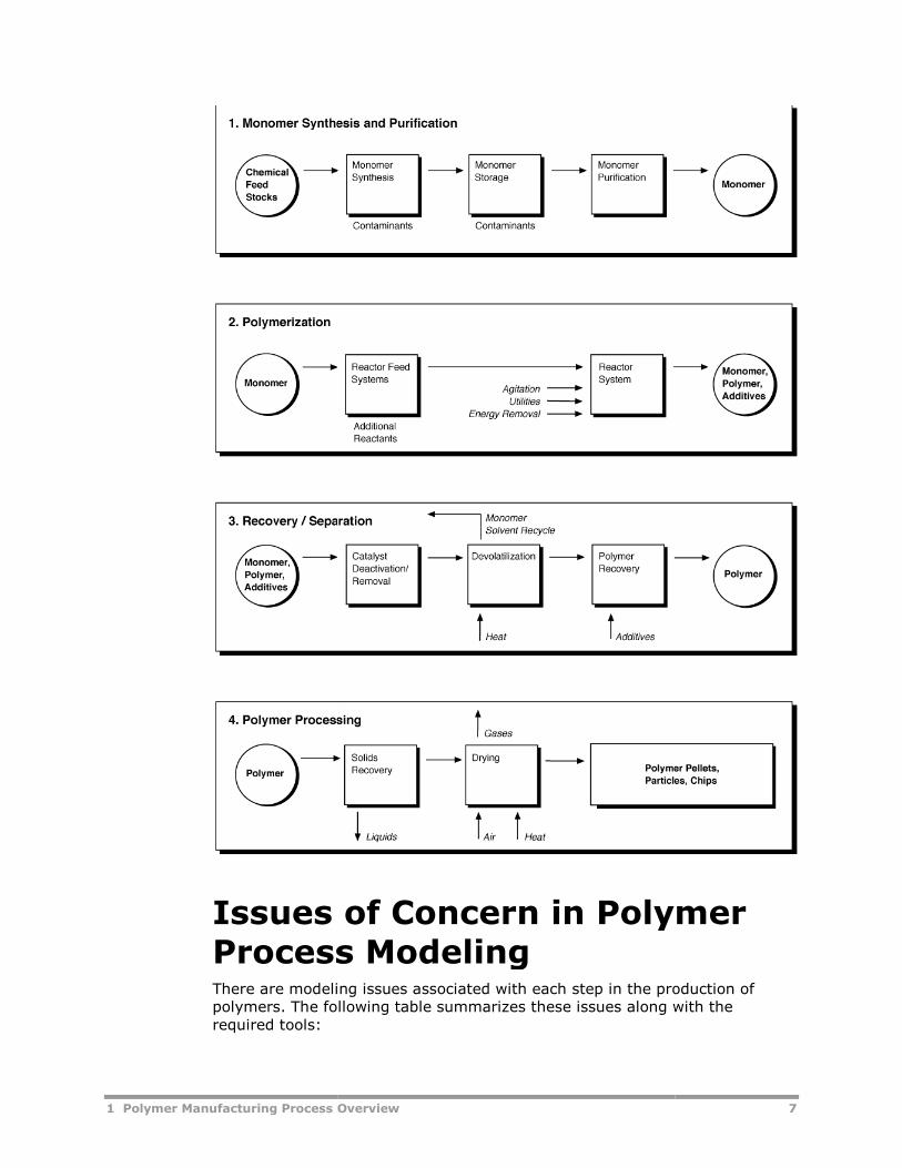
Polymer Manufacturing Process StepsPolymer manufacturing processes are usually divided into the following majorsteps:
1 Monomer Synthesis and Purification
2 Polymerization
3 Recovery / Separation
4 Polymer Processing
The four steps may be carried out by the same manufacturer within a singleintegrated plant, or specific companies may focus on one or more of thesesteps (Grulke, 1994).
The four steps may be carried out by the same manufacturer within a singleintegrated plant, or specific companies may focus on one or more of thesesteps (Grulke, 1994).
The following figure illustrates the important stages for each of the fourpolymer production steps. The main issues of concern for each of these stepsare described next.
1 Polymer Manufacturing Process Overview
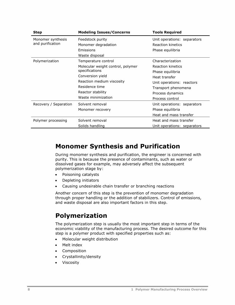
Issues of Concern in PolymerProcess ModelingThere are modeling issues associated with each step in the production ofpolymers. The following table summarizes these issues along with therequired tools:
Manufacturing Process Overview
Issues of Concern in PolymerProcess ModelingThere are modeling issues associated with each step in the production ofpolymers. The following table summarizes these issues along with the
7
Issues of Concern in Polymer
There are modeling issues associated with each step in the production ofpolymers. The following table summarizes these issues along with the
8 1 Polymer Manufacturing Process Overview
Step Modeling Issues/Concerns Tools Required
Monomer synthesisand purification
Feedstock purity
Monomer degradation
Emissions
Waste disposal
Unit operations: separators
Reaction kinetics
Phase equilibria
Polymerization Temperature control
Molecular weight control, polymerspecifications
Conversion yield
Reaction medium viscosity
Residence time
Reactor stability
Waste minimization
Characterization
Reaction kinetics
Phase equilibria
Heat transfer
Unit operations: reactors
Transport phenomena
Process dynamics
Process control
Recovery / Separation Solvent removal
Monomer recovery
Unit operations: separators
Phase equilibria
Heat and mass transfer
Polymer processing Solvent removal
Solids handling
Heat and mass transfer
Unit operations: separators
Monomer Synthesis and PurificationDuring monomer synthesis and purification, the engineer is concerned withpurity. This is because the presence of contaminants, such as water ordissolved gases for example, may adversely affect the subsequentpolymerization stage by:
Poisoning catalysts
Depleting initiators
Causing undesirable chain transfer or branching reactions
Another concern of this step is the prevention of monomer degradationthrough proper handling or the addition of stabilizers. Control of emissions,and waste disposal are also important factors in this step.
PolymerizationThe polymerization step is usually the most important step in terms of theeconomic viability of the manufacturing process. The desired outcome for thisstep is a polymer product with specified properties such as:
Molecular weight distribution
Melt index
Composition
Crystallinity/density
Viscosity
1 Polymer Manufacturing Process Overview 9
The obstacles that must be overcome to reach this goal depend on both themechanism of polymer synthesis (chain growth or step growth), and on thepolymerization process used.
Polymerization processes may be batch, semi-batch or continuous. Inaddition, they may be carried out in bulk, solution, slurry, gas-phase,suspension or emulsion. Batch and semi-batch processes are preferred forspecialty grade polymers. Continuous processes are usually used tomanufacture large volume commodity polymers. Productivity depends on heatremoval rates and monomer conversion levels achieved. Viscosity of polymersolutions, and polymer particle suspensions and mixing are importantconsiderations. These factors influence the choice of, for example, bulk versussolution versus slurry polymerization. Another example is the choice ofemulsion polymerization that is often dictated by the form of the end-useproduct, water-based coating or adhesive. Other important considerationsmay include health, safety and environmental impact.
Most polymerizations are highly exothermic, some involve monomers that areknown carcinogens and others may have to deal with contaminated water.
In summary, for the polymerization step, the reactions which occur usuallycause dramatic changes in the reaction medium (e.g. significant viscosityincreases may occur), which in turn make high conversion kinetics, residence-time distribution, agitation and heat transfer the most important issues forthe majority of process types.
Recovery / SeparationThe recovery/separation step can be considered the step where the desiredpolymer produced is further purified or isolated from by-products or residualreactants. In this step, monomers and solvents are separated and purified forrecycle or resale. The important concerns for this step are heat and masstransfer.
Polymer ProcessingThe last step, polymer processing, can also be considered a recovery step. Inthis step, the polymer slurry is turned into solid pellets or chips. Heat ofvaporization is an important factor in this step (Grulke, 1994).
SummaryIn summary, production rate optimization, waste minimization andcompliance to environmental constraints, yield increase, and product qualityare also important issues in the production of polymers. In addition, processdynamics and stability constitute important factors primarily for reactors.
Aspen Polymers ToolsAspen Polymers provides the tools that allow polymer manufacturers tocapture the benefits of process modeling.
10 1 Polymer Manufacturing Process Overview
Aspen Polymers can be used to build models for representing processes intwo modes: with Aspen Plus for steady-state models, and with AspenDynamics or Aspen Custom Modeler™ for dynamic models. In both cases, thetools used specifically for representing polymer systems fall into fourcategories:
Polymer characterization
Physical properties
Reaction kinetics
Data
Through Aspen Plus, Aspen Dynamics and Aspen Custom Modeler, AspenPolymers provides robust and efficient algorithms for handling:
Flowsheet convergence and optimization
Complex separation and reaction problems
User customization through an open architecture
Component CharacterizationCharacterization of a polymer component poses some unique challenges. Forexample, the polymer component is not a single species but a mixture ofmany species. Properties such as molecular weight and copolymercomposition are not necessarily constant and may vary throughout theflowsheet and with time. Aspen Polymers provides a flexible methodology forcharacterizing polymer components (U.S. Patent No. 5,687,090).
Each polymer is considered to be made up of a series of segments. Segmentshave a fixed structure. The changing nature of the polymer is accounted forby the specification of the number and type of segments it contains at a givenprocessing step.
Each polymer component has associated attributes used to store informationon molecular structure and distributions, product properties, and particle sizewhen necessary. The polymer attributes are solved/integrated together withthe material and energy balances in the unit operation models.
Polymer Physical PropertiesCorrelative and predictive models are available in Aspen Polymers forrepresenting the thermophysical properties of a polymer system, the phaseequilibrium, and the transport phenomena. Several physical property methodscombining these models are available. In addition to the built-inthermodynamic models, the open architecture design allows users to overridethe existing models with their own in-house models.
Polymerization KineticsThe polymerization step represents the most important stage in polymerprocesses. In this step, kinetics play a crucial role. Aspen Polymers providesbuilt-in kinetic mechanisms for several chain-growth and step-growth typepolymerization processes. The mechanisms are based on well-establishedsources from the open literature, and have been extensively used and
1 Polymer Manufacturing Process Overview 11
validated against data during modeling projects of industrial polymerizationreactors.
There are also models for representing polymer modification reactions, andfor modeling standard chemical kinetics. In addition to the built-in kineticmechanisms, the open-architecture design allows users to specify additionalreactions, or to override the built-in mechanisms.
Modeling DataA key factor in the development of a successful simulation model is the use ofaccurate thermodynamic data for representing the physical properties of thesystem, and of kinetic rate constant data which provide a good match againstobserved trends.
In order to provide the physical property models with the parametersnecessary for property calculations, Aspen Polymers has property parameterdatabanks available. These include:
Polymer databank containing parameters independent of chain length
Segment databank containing parameters to which composition and chainlength are applied for polymer property calculations
Functional group databank containing parameters for models using agroup contribution approach is also included
This User Guide contains several tabulated parameters which may be used asstarting values for specific property models. Property data packages are alsobeing compiled for some polymerization processes and will be made availablein future versions.
In addition to physical property data, Aspen Polymers provides users withways of estimating missing reaction rate constant data. For example, the dataregression tool can be used to fit rate constants against molecular weightdata.
Process FlowsheetingAspen Polymers provides unit operation models, flowsheeting options, andanalysis tools for a complete representation of a process.
Models for batch, semi-batch and continuous reactors with mixing extremesof plug flow to backmix are available. In addition, other unit operation modelsessential for flowsheet modeling are available such as:
Mixers
Flow splitters
Flash tanks
Devolatilization units
Flowsheet connectivity and sequencing is handled in a straightforwardmanner.
Several analysis tools are available for applying the simulation modelsdeveloped. These include tools for:
Process optimization
12 1 Polymer Manufacturing Process Overview
Examining process alternatives
Analyzing the sensitivities of key process variables on polymer productproperties
Fitting process variables to meet design specifications
Defining a Model in AspenPolymersIn order to build a model of a polymer process you must already be familiarwith Aspen Plus. Therefore, only the steps specific to polymer systems will bedescribed in detail later in this User Guide. The steps for defining a model inAspen Polymers are as follows:
Step 1. Specifying Global Simulation Options
The first step in defining the model is the specification of:
Global simulation options, i.e. simulation type
Units to be used for simulation inputs and results
Basis for flowrates
Maximum simulation times
Diagnostic options
Step 2. Defining the Flowsheet
For a full flowsheet model, the next step is the flowsheet definition. Here youwould specify the unit operation models contained in the flowsheet and definetheir connectivity.
Chapter 4 describes the unit operation models available for building aflowsheet.
Step 3. Defining Components
Most simulation types require a definition of the component system. You mustcorrectly identify polymers, polymer segments, and oligomers as such. Allother components are considered conventional by default.
Chapter 2 provides information on defining components.
Step 4. Characterizing Components
Conventional components in the system are categorized by type. Additionalcharacterization information is required for other than conventionalcomponents. You must specify the:
Component attributes to be tracked for polymers
Type of segments present
Structure of oligomers
Type and activity of catalysts
In addition, you may wish to request tracking of molecular weightdistribution.
Component characterization is discussed in Chapter 2.
1 Polymer Manufacturing Process Overview 13
Step 5. Specifying Property Models
You must select the models to be used to represent the physical properties ofyour system.
The Aspen Polymers User Guide, Volume 2, Aspen Polymers Physical PropertyMethods and Models, describes the options available for specifying physicalproperty models.
Step 6. Defining Polymerization Kinetics
Once you have made selections out of the built-in polymerization kineticmodels to represent your reaction system, you need to choose specificreactions from the sets available and enter rate constant parameters for thesereactions.
Chapter 3 describes the models available and provides descriptions of theinput options.
Step 7. Defining Feed Streams
For flowsheet simulations, you must enter the conditions of the process feedstreams. If the feed streams contain polymers, you must initialize thepolymer attributes.
Polymer attribute definition in streams is discussed in a separate section ofChapter 2.
Step 8. Specifying UOS Model Operating Conditions
You must specify the configuration and operating condition for unit operationmodels contained in the flowsheet. In the case of reactors, you have theoption of assigning kinetic models defined in step 6 to specific reactors.
Chapter 4 provides some general information regarding the use of unitoperation models.
Step 9. Specifying Additional Simulation Options
For a basic simulation the input information you are required to enter in steps1-8 is sufficient. However, there are many more advanced simulation optionsyou may wish to add in order to refine or apply your model. These includesetting up the model for plant data fitting, sensitivity analyses, etc.
Many of these options are described in a separate section of Chapter 4.
Information for building dynamic models is given in the Aspen Dynamics andAspen Custom Modeler documentation sets. Note that for building dynamicmodels, users must first build a steady-state model containing:
Definition of the polymer system in terms of components present
Physical property models
Polymerization kinetic models
Note: Aspen Polymers setup and configuration instructions are given inChapter 5.
14 1 Polymer Manufacturing Process Overview
ReferencesDotson, N. A., Galván, R., Laurence, R. L., & Tirrell, M. (1996). PolymerizationProcess Modeling. New York: VCH Publishers.
Grulke, E. A. (1994). Polymer Process Engineering. Englewood Cliffs, NJ:Prentice Hall.
Odian, George. (1991). Principles of Polymerization (3rd Ed.). New York: JohnWiley and Sons.
2 Polymer Structural Characterization 15
2 Polymer StructuralCharacterization
One of the fundamental aspects of modeling polymer systems is the handlingof the molecular structure information of polymers. This chapter discusses theapproaches used to address this issue in Aspen Polymers (formerly known asAspen Polymers Plus).
Topics covered include:
Polymer Structure, 15
Polymer Structural Properties, 19
Characterization Approach, 19
Included in this manual are several sections devoted to the specification ofpolymer structural characterization information.
3 Component Classification, 21
Polymer Structural Properties, 33
Structural Property Distributions, 55
End-Use Properties, 73
Polymer StructurePolymers can be defined as large molecules or macromolecules where asmaller constituting structure repeats itself along a chain. For this reason,polymers tend to exhibit different physical behavior than small molecules alsocalled monomers. Synthetic polymers are produced when monomers bondtogether through polymerization and become the repeating structure orsegment within a chain. When two or more monomers bond together, apolymer is formed. Small polymer chains containing 20 or less repeating unitsare usually called oligomers.
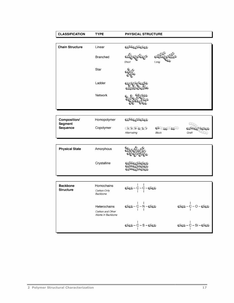
The fact that identifiable segments are found repeatedly along a polymerchain, provides convenient ways to categorize polymers. Polymers can beclassified based on segment composition or sequence:
Homopolymers - containing one type of repeating unit which can bemapped into one segment
16 2 Polymer Structural Characterization
Copolymers - which have two or more repeating units. Copolymers can bein a random, alternating, block, or graft configuration
If we consider the arrangement of a given chain, another classification arises.Polymers may be:
Linear
Branched (with short or long chains)
Star
Ladder
Network
Another classification that results from polymer structure has to do withphysical state. A solid polymer may be:
Amorphous - when the chains are not arranged in a particular pattern
Crystalline - when the chains are arranged in a regular pattern
A related classification divides polymers by thermal and mechanical propertiesinto:
Thermoplastics (may go from solid to melt and vice versa)
Thermosets (remain solid through heating)
Elastomers (which have elastic properties)
Finally, polymers can be categorized based on the form they aremanufactured into: plastics, fibers, film, coatings, adhesives, foams, andcomposites.
Polymer Types by Physical Structure
The following figure illustrates the various polymer types based on chainstructure:
2 Polymer Structural Characterization2 Polymer Structural Characterization 17
18 2 Polymer Structural Characterization
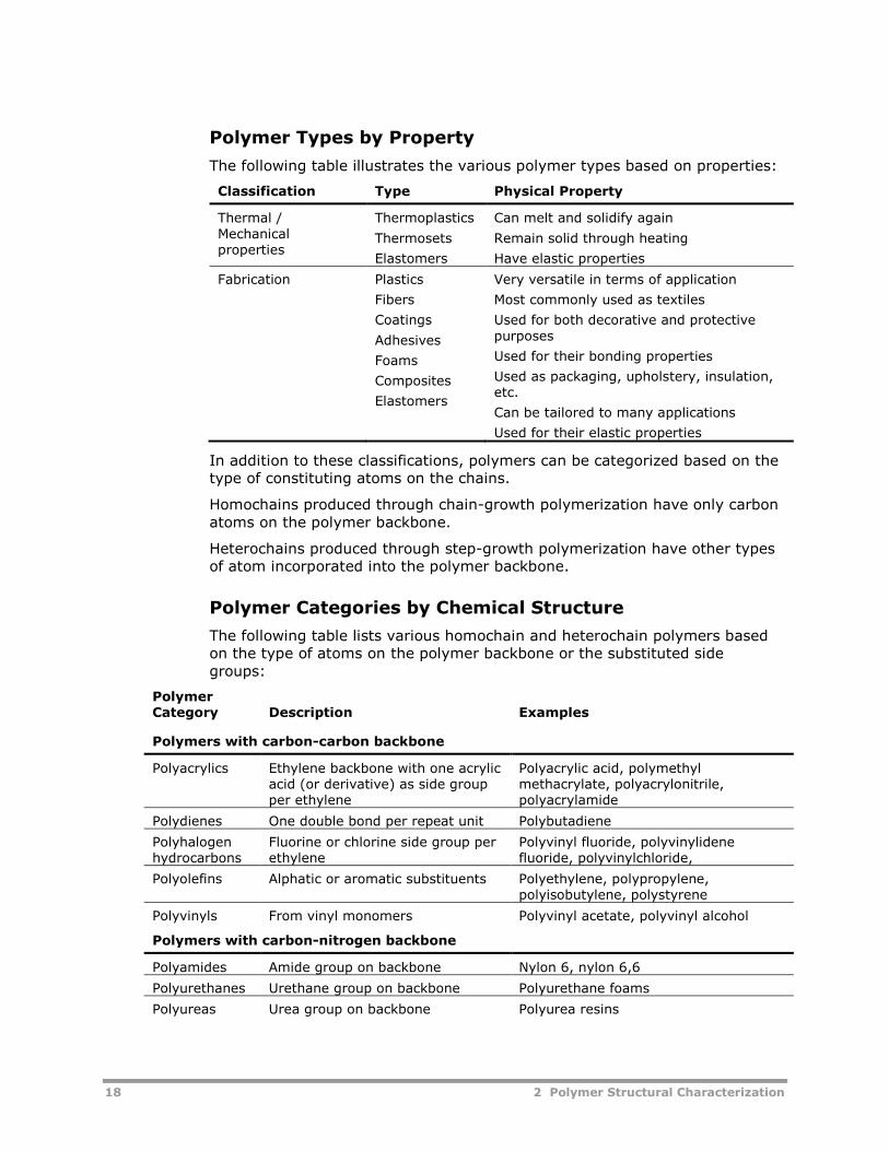
Polymer Types by Property
The following table illustrates the various polymer types based on properties:
Classification Type Physical Property
Thermal /Mechanicalproperties
Thermoplastics
Thermosets
Elastomers
Can melt and solidify again
Remain solid through heating
Have elastic properties
Fabrication Plastics
Fibers
Coatings
Adhesives
Foams
Composites
Elastomers
Very versatile in terms of application
Most commonly used as textiles
Used for both decorative and protectivepurposes
Used for their bonding properties
Used as packaging, upholstery, insulation,etc.
Can be tailored to many applications
Used for their elastic properties
In addition to these classifications, polymers can be categorized based on thetype of constituting atoms on the chains.
Homochains produced through chain-growth polymerization have only carbonatoms on the polymer backbone.
Heterochains produced through step-growth polymerization have other typesof atom incorporated into the polymer backbone.
Polymer Categories by Chemical Structure
The following table lists various homochain and heterochain polymers basedon the type of atoms on the polymer backbone or the substituted sidegroups:
PolymerCategory Description Examples
Polymers with carbon-carbon backbone
Polyacrylics Ethylene backbone with one acrylicacid (or derivative) as side groupper ethylene
Polyacrylic acid, polymethylmethacrylate, polyacrylonitrile,polyacrylamide
Polydienes One double bond per repeat unit Polybutadiene
Polyhalogenhydrocarbons
Fluorine or chlorine side group perethylene
Polyvinyl fluoride, polyvinylidenefluoride, polyvinylchloride,
Polyolefins Alphatic or aromatic substituents Polyethylene, polypropylene,polyisobutylene, polystyrene
Polyvinyls From vinyl monomers Polyvinyl acetate, polyvinyl alcohol
Polymers with carbon-nitrogen backbone
Polyamides Amide group on backbone Nylon 6, nylon 6,6
Polyurethanes Urethane group on backbone Polyurethane foams
Polyureas Urea group on backbone Polyurea resins
2 Polymer Structural Characterization 19
PolymerCategory Description Examples
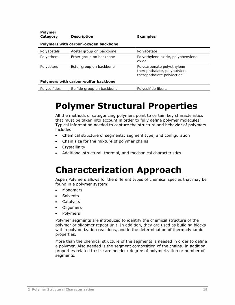
Polymers with carbon-oxygen backbone
Polyacetals Acetal group on backbone Polyacetate
Polyethers Ether group on backbone Polyethylene oxide, polyphenyleneoxide
Polyesters Ester group on backbone Polycarbonate polyethylenetherephthalate, polybutylenetherephthalate polylactide
Polymers with carbon-sulfur backbone
Polysulfides Sulfide group on backbone Polysulfide fibers
Polymer Structural PropertiesAll the methods of categorizing polymers point to certain key characteristicsthat must be taken into account in order to fully define polymer molecules.Typical information needed to capture the structure and behavior of polymersincludes:
Chemical structure of segments: segment type, and configuration
Chain size for the mixture of polymer chains
Crystallinity
Additional structural, thermal, and mechanical characteristics
Characterization ApproachAspen Polymers allows for the different types of chemical species that may befound in a polymer system:
Monomers
Solvents
Catalysts
Oligomers
Polymers
Polymer segments are introduced to identify the chemical structure of thepolymer or oligomer repeat unit. In addition, they are used as building blockswithin polymerization reactions, and in the determination of thermodynamicproperties.
More than the chemical structure of the segments is needed in order to definea polymer. Also needed is the segment composition of the chains. In addition,properties related to size are needed: degree of polymerization or number ofsegments.
20 2 Polymer Structural Characterization
Component AttributesWithin Aspen Polymers, component attributes are used to define thesestructural characteristics. Component attributes are available to tracksegment composition, degree of polymerization, molecular weight, etc.Because the polymer is a mixture of chains, there is normally a distribution ofthese structural characteristics. The component attributes are used to trackthe averages.
There are additional attributes used to track information about thedistribution of chain sizes. These are the moments of chain lengthdistribution. For detailed information about component attributes, seePolymer Structural Properties on page 33.
In addition to the component attributes, users have the option within AspenPolymers to examine polymer molecular weight distribution. This feature isbased on a method of instantaneous properties. For more information, seeMethod of Instantaneous Properties on page 60.
ReferencesGrulke, E. A. (1994). Polymer Process Engineering. Englewood Cliffs, NJ:Prentice Hall.
Munk, P. (1989). Introduction to Macromolecular Science. New York: JohnWiley and Sons.
Odian, G. (1991). Principles of Polymerization (3rd Ed.). New York: JohnWiley and Sons.
Rudin, A. (1982). The Elements of Polymer Science and Engineering. Orlando:Academic Press.
3 Component Classification 21
3 Component Classification
This section discusses the specification of components in a simulation model.
Topics covered include:
Component Categories, 21
Component Databanks, 25
Segment Methodology, 27
Specifying Components, 28
Component CategoriesWhen developing a simulation model in Aspen Polymers (formerly known asAspen Polymers Plus), users must assign components present in process flowstreams to one of the following categories:
Conventional
Polymer
Oligomer
Segment
Site-based
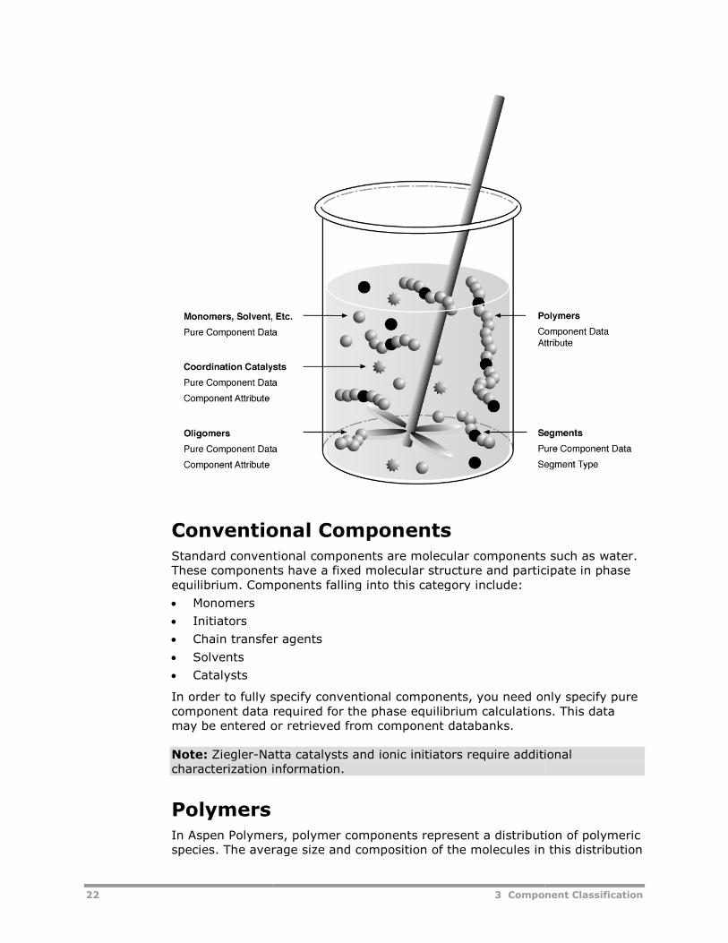
The following figure illustrates the different categories of components andtheir input requirements:
22
Conventional ComponentsStandard conventional components are molecular components such as water.These components have a fixed molecular structure and participate in phaseequilibrium. Components falling into this category include:
Monomers
Initiators
Chain transfer agents
Solvents
Catalysts
In order to fully specify conventional ccomponent data required for the phase equilibrium calculations. This datamay be entered or retrieved from component databanks.
Note: Ziegler-Natta catalysts and ionic initiators require additionalcharacterization inf
PolymersIn Aspen Polymers, polymer components represent a distribution of polymericspecies. The average size and composition of the molecules in this distribution
3 Component Classification
Conventional ComponentsStandard conventional components are molecular components such as water.These components have a fixed molecular structure and participate in phasequilibrium. Components falling into this category include:
Chain transfer agents
In order to fully specify conventional components, you need only specify purecomponent data required for the phase equilibrium calculations. This datamay be entered or retrieved from component databanks.
Natta catalysts and ionic initiators require additionalcharacterization information.
In Aspen Polymers, polymer components represent a distribution of polymericspecies. The average size and composition of the molecules in this distribution
3 Component Classification
Standard conventional components are molecular components such as water.These components have a fixed molecular structure and participate in phase
omponents, you need only specify purecomponent data required for the phase equilibrium calculations. This data
Natta catalysts and ionic initiators require additional
In Aspen Polymers, polymer components represent a distribution of polymericspecies. The average size and composition of the molecules in this distribution
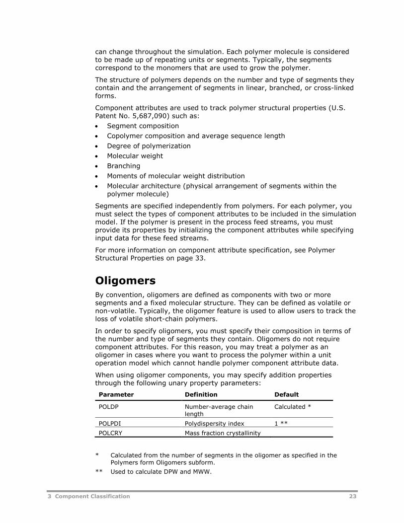
3 Component Classification 23
can change throughout the simulation. Each polymer molecule is consideredto be made up of repeating units or segments. Typically, the segmentscorrespond to the monomers that are used to grow the polymer.
The structure of polymers depends on the number and type of segments theycontain and the arrangement of segments in linear, branched, or cross-linkedforms.
Component attributes are used to track polymer structural properties (U.S.Patent No. 5,687,090) such as:
Segment composition
Copolymer composition and average sequence length
Degree of polymerization
Molecular weight
Branching
Moments of molecular weight distribution
Molecular architecture (physical arrangement of segments within thepolymer molecule)
Segments are specified independently from polymers. For each polymer, youmust select the types of component attributes to be included in the simulationmodel. If the polymer is present in the process feed streams, you mustprovide its properties by initializing the component attributes while specifyinginput data for these feed streams.
For more information on component attribute specification, see PolymerStructural Properties on page 33.
OligomersBy convention, oligomers are defined as components with two or moresegments and a fixed molecular structure. They can be defined as volatile ornon-volatile. Typically, the oligomer feature is used to allow users to track theloss of volatile short-chain polymers.
In order to specify oligomers, you must specify their composition in terms ofthe number and type of segments they contain. Oligomers do not requirecomponent attributes. For this reason, you may treat a polymer as anoligomer in cases where you want to process the polymer within a unitoperation model which cannot handle polymer component attribute data.
When using oligomer components, you may specify addition propertiesthrough the following unary property parameters:
Parameter Definition Default
POLDP Number-average chainlength
Calculated *
POLPDI Polydispersity index 1 **
POLCRY Mass fraction crystallinity
* Calculated from the number of segments in the oligomer as specified in thePolymers form Oligomers subform.
** Used to calculate DPW and MWW.
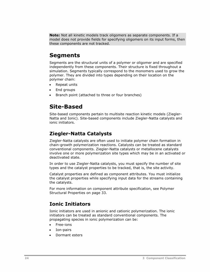
24 3 Component Classification
Note: Not all kinetic models track oligomers as separate components. If amodel does not provide fields for specifying oligomers on its input forms, thenthese components are not tracked.
SegmentsSegments are the structural units of a polymer or oligomer and are specifiedindependently from these components. Their structure is fixed throughout asimulation. Segments typically correspond to the monomers used to grow thepolymer. They are divided into types depending on their location on thepolymer chain:
Repeat units
End groups
Branch point (attached to three or four branches)
Site-BasedSite-based components pertain to multisite reaction kinetic models (Ziegler-Natta and Ionic). Site-based components include Ziegler-Natta catalysts andionic initiators.
Ziegler-Natta Catalysts
Ziegler-Natta catalysts are often used to initiate polymer chain formation inchain-growth polymerization reactions. Catalysts can be treated as standardconventional components. Ziegler-Natta catalysts or metallocene catalystsinvolve one or more polymerization site types which may be in an activated ordeactivated state.
In order to use Ziegler-Natta catalysts, you must specify the number of sitetypes and the catalyst properties to be tracked, that is, the site activity.
Catalyst properties are defined as component attributes. You must initializethe catalyst properties while specifying input data for the streams containingthe catalysts.
For more information on component attribute specification, see PolymerStructural Properties on page 33.
Ionic Initiators
Ionic initiators are used in anionic and cationic polymerization. The ionicinitiators can be treated as standard conventional components. Thepropagating species in ionic polymerization can be:
Free-ions
Ion-pairs
Dormant esters
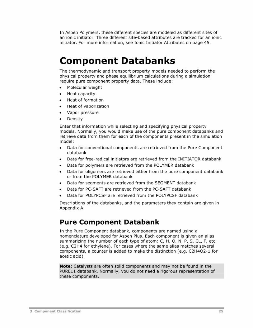
3 Component Classification 25
In Aspen Polymers, these different species are modeled as different sites ofan ionic initiator. Three different site-based attributes are tracked for an ionicinitiator. For more information, see Ionic Initiator Attributes on page 45.
Component DatabanksThe thermodynamic and transport property models needed to perform thephysical property and phase equilibrium calculations during a simulationrequire pure component property data. These include:
Molecular weight
Heat capacity
Heat of formation
Heat of vaporization
Vapor pressure
Density
Enter that information while selecting and specifying physical propertymodels. Normally, you would make use of the pure component databanks andretrieve data from them for each of the components present in the simulationmodel:
Data for conventional components are retrieved from the Pure Componentdatabank
Data for free-radical initiators are retrieved from the INITIATOR databank
Data for polymers are retrieved from the POLYMER databank
Data for oligomers are retrieved either from the pure component databankor from the POLYMER databank
Data for segments are retrieved from the SEGMENT databank
Data for PC-SAFT are retrieved from the PC-SAFT databank
Data for POLYPCSF are retrieved from the POLYPCSF databank
Descriptions of the databanks, and the parameters they contain are given inAppendix A.
Pure Component DatabankIn the Pure Component databank, components are named using anomenclature developed for Aspen Plus. Each component is given an aliassummarizing the number of each type of atom: C, H, O, N, P, S, CL, F, etc.(e.g. C2H4 for ethylene). For cases where the same alias matches severalcomponents, a counter is added to make the distinction (e.g. C2H4O2-1 foracetic acid).
Note: Catalysts are often solid components and may not be found in thePURE11 databank. Normally, you do not need a rigorous representation ofthese components.
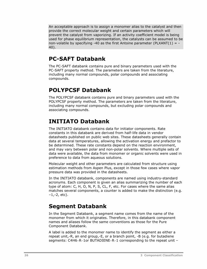
26 3 Component Classification
An acceptable approach is to assign a monomer alias to the catalyst and thenprovide the correct molecular weight and certain parameters which willprevent the catalyst from vaporizing. If an activity coefficient model is beingused for phase equilibrium representation, the catalysts can be assumed to benon-volatile by specifying -40 as the first Antoine parameter (PLXANT(1) = -40).
PC-SAFT DatabankThe PC-SAFT databank contains pure and binary parameters used with thePC-SAFT property method. The parameters are taken from the literature,including many normal compounds, polar compounds and associatingcompounds.
POLYPCSF DatabankThe POLYPCSF databank contains pure and binary parameters used with thePOLYPCSF property method. The parameters are taken from the literature,including many normal compounds, but excluding polar compounds andassociating compounds.
INITIATO DatabankThe INITIATO databank contains data for initiator components. Rateconstants in this databank are derived from half-life data in vendordatasheets published on public web sites. These datasheets generally containdata at several temperatures, allowing the activation energy and prefactor tobe determined. These rate constants depend on the reaction environment,and may vary between polar and non-polar solvents. Where multiple sets ofdata were available, the data from monomer or organic solvents were used inpreference to data from aqueous solutions.
Molecular weight and other parameters are calculated from structure usingestimation methods from Aspen Plus, except in those few cases where vaporpressure data was provided in the datasheets.
In the INITIATO databank, components are named using industry-standardacronyms. Each component is given an alias summarizing the number of eachtype of atom: C, H, O, N, P, S, CL, F, etc. For cases where the same aliasmatches several components, a counter is added to make the distinction (e.g.–1,-2, etc).
Segment DatabankIn the Segment Databank, a segment name comes from the name of themonomer from which it originates. Therefore, in this databank componentnames and aliases follow the same conventions as those for the PureComponent Databank.
A label is added to the monomer name to identify the segment as either arepeat unit,-R, an end group,-E, or a branch point, -B (e.g. for butadienesegments: C4H6R1or BUTADIENER1 corresponding to the repeat unit –
3 Component Classification 27
CH2–CH=CH–CH2, C4H5E1 or BUTADIENEE1 corresponding to the endgroup –CH=CH–CH=CH2 and C4H5B or BUTADIENEB corresponding to the
branch segment CH2 CH CH CH ).
Polymer DatabankThe Polymer Databank does not follow the conventional nomenclature. Thepolymer aliases are the typical acronyms used in industry or academia, andthe polymer names consist of the repeat unit name enclosed in parenthesesand preceded by the prefix Poly (e.g. PS or POLY(STYRENE) for polystyrene).
Note: The MW property parameter used to store molecular weights in thecomponent databanks is the true molecular weight for all component typesexcept polymers. For polymers, the true polymer molecular weight is normallytracked as a component attribute only. The molecular weight stored in thedatabank is the apparent molecular weight calculated as the average segmentmolecular weight (See Appendix A).
Segment MethodologyThe segment approach to characterizing components is a fundamentalmethodology which affects almost every functionality within Aspen Polymers.Segments are used as the building blocks for polymers. Once you havespecified the types of segments in the polymer, the segment composition anddegree of polymerization defined as component attributes may be used todefine the size and composition of the polymer.
For oligomers, although component attributes are not used, the number ofeach segment must be specified directly.
Most of the Aspen Polymers physical property models calculate polymer andoligomer properties from segment properties. This is done by taking intoaccount the degree of polymerization and the segment composition. Thecalculated properties should be the same for both oligomers and polymers,assuming that the oligomer structure and molecular weight were specifiedcorrectly. Note that this is true for mass-based properties only. Mole-basedproperties will be different between polymer and oligomer if their apparentmolecular weights are different.
Within the polymerization reaction models, segments also play a key role. Aspolymerization progresses, the models map the reacting monomers into thecorresponding segments and return rates of change for the segmentcomposition.
28 3 Component Classification
Specifying ComponentsTo specify components within your model you need to know the following:
Item For
Component types All the species in your system
Property parameter databankselections
The species in the system
IUPAC names All conventional components or you need theirphysical properties (molecular weight, boiling point,Antoine constants, etc.)
Segment structure All polymers and oligomers (define whether you wantto include any end groups or branch points)
Polymer properties to betracked
All polymers, that is, degree of polymerization,segment composition
Additional characteristics All additional characteristics for catalysts, or ionicinitiators
Selecting DatabanksFor an Aspen Polymers simulation, you generally retrieve physical propertydata from the following databanks:
Pure component databank (PURE12)
Polymer databank (POLYMER)
Polymer segment databank (SEGMENT)
Initiator databank (INITIATOR)
You can also use other Aspen Plus databanks, user databanks, or in-housedatabanks. Appendix A provides descriptions of the polymer and segmentdatabanks and the parameters they contain.
If you selected a polymer template to start your simulation, the correctdatabanks are already specified.
If you did not select a polymer template, or if you want to modify thedatabank selection:
1 From the Data Browser, click Components.
2 From the Components folder, click Specifications.
3 On the Selection sheet, click the Databanks tab to open the databankselection form.
Defining Component Names and TypesYou must specify a:
Name and a type for each component in the simulation
Component name or identifier
Databank name or alias that sets the pure component properties for thecomponent
3 Component Classification 29
Component type that sets the category to which the component belongsand determines the treatment of that component
To access the components specifications input sheet:
1 From the Data Browser, click Components.
2 From the Components folder, click Specifications.
3 On the Selection sheet, click the Databanks tab to set the databanks tobe searched for pure component properties.
To define component names and types:
1 On the Selection sheet, in the Component ID field, specify an ID foreach component.
This ID is used to refer to the component in all subsequent input, and isalso used to identify the component in the simulation report.
2 For polymers, oligomers, and segments, specify the component type inthe Type field.
By default, all components are assumed to be standard conventionalcomponents. For Aspen Polymers simulation you must correctly identifythe component types:
Use For
Conventional Standard conventional components
Polymer Homo and copolymers
Oligomer Short chain polymer molecules
Segment Polymer or oligomer repeat units
3 If component property data is being retrieved from databanks, you mustalso supply either the databank alias in the Alias field, or the databankname in the Component name field.
Specifying SegmentsThe Type of each polymer or oligomer segment must be specified on thePolymer Characterization Segments sheet. Segments can be repeat units,end groups or branch points attached to three or four branches.
To access the segments definition input form:
1 From the Data Browser, click Components.
2 From the Components folder, click Polymers.
3 From the Polymers folder, click Characterization.
To define segments:
On the Segments sheet, assign a type to the segments from the Typefield.
Specifying PolymersFor each polymer you must define the component attributes to be tracked. Allcomponents specified Polymer in the Components Specifications folderrequire component attributes.
30 3 Component Classification
To access the polymer input specifications:
1 From the Data Browser, click Components.
2 From the Components folder, click Polymers.
3 From the Polymers folder, click Characterization.
4 From the Characterization form, click the Polymers tab.
To specify component attributes for the polymers in your simulation:
1 In the Polymer ID field, select the polymer.
2 If you want to retrieve a predefined set of component attributes, in Built-in attribute group select a grouping. The attribute summary table isfilled in.
For a complete discussion of Aspen Polymers component attributes, seePolymer Structural Properties on page 33.
or
If you do not want to use a predefined set of attributes, or if you want tochange the attribute selection for a given group, click the attribute tableor click Edit to open the attribute list.
3 Click specific attributes to add or remove them from the list.
Repeat these steps for each polymer.
Specifying OligomersFor each oligomer you must specify an ID and a structure in terms of numberand name of contained segments.
To access the oligomers definition input form:
1 From the Data Browser, click Components.
2 From the Components folder, click Polymers.
3 From the Polymers folder, click Characterization.
4 From the Characterization form, click the Oligomers tab.
To define oligomers:
1 In the Oligomer field, select the oligomer.
2 In the Segment field, enter the name of a segment contained in theoligomer.
3 Repeat these steps for each oligomer.
You can define as many segments as needed for an oligomer.
Specifying Site-Based ComponentsSpecify the structure and activity of site-based catalytic species such asZiegler-Natta catalysts and ionic initiators.
To access the site-based species definition form:
1 From the Data Browser, click Components.
2 From the Components folder, click Polymers.
3 From the Polymers folder, click Characterization.
4 From the Characterization form, click the Site-Based Species tab.
3 Component Classification 31
To specify site-based species characteristics:
1 Select the component type: Ziegler-Natta catalyst, ionic initiator, etc.
2 In the Comp ID field, specify the component name.
3 Specify the number of site types in Number of sites for the component.For Ziegler-Natta catalysts, you must also specify the moles of sites pergram of catalyst.
4 Select the list of properties or component attributes to be tracked for thatcomponent. Click the attribute list table or Edit to open the attribute list.
5 Click specific attributes to add or remove them from the list for thecomponent.
ReferencesBailey, J., & Ollis, D. F. (1986) Biochemical Engineering Fundamentals (2ndEd.). New York: McGraw-Hill.
Brandrup, J., & Immergut, E. H. (Eds.). (1989). Polymer Handbook (3rd Ed.).New York: John Wiley & Sons.
Danner R. P., & High, M. S. (1992). Handbook of Polymer SolutionThermodynamics. New York: American Institute of Chemical Engineers.
Kroschwitz, J. (Ed.). (1990). Concise Encyclopedia of Polymer Science andEngineering. New York: John Wiley and Sons.

32 3 Component Classification
4 Polymer Structural Properties 33
4 Polymer StructuralProperties
This section discusses the use of component attributes for tracking polymerstructural properties in a simulation model.
Topics covered include:
Structural Properties as Component Attributes, 33
Component Attribute Classes, 34
Component Attribute Categories, 35
Component Attribute Initialization, 46
Component Attribute Scale Factors, 50
Specifying Component Attributes, 51
Structural Properties asComponent AttributesComponent attributes provide a convenient framework to associate structuralcharacterization data to components in a flow stream. They are carriedthroughout the flowsheet along with state and composition information, andeffectively extend the stream structure.
Aspen Polymers (formerly known as Aspen Polymers Plus) uses componentattributes as a vehicle for tracking important modeling information forpolymers, ionic initiators and Ziegler-Natta catalysts (U.S. Patent No.5,687,090). For example, there are component attributes to store:
Segment composition (segment fraction or segment flow)
Copolymer composition and average sequence length
Degree of polymerization (number, weight, and z-average)
Molecular weight (number, weight, and z-average)
Degree of branching (long and short)
Degree of cross-linking (cross-link density)
Molecular architecture (physical arrangement of segments within thepolymer molecule)
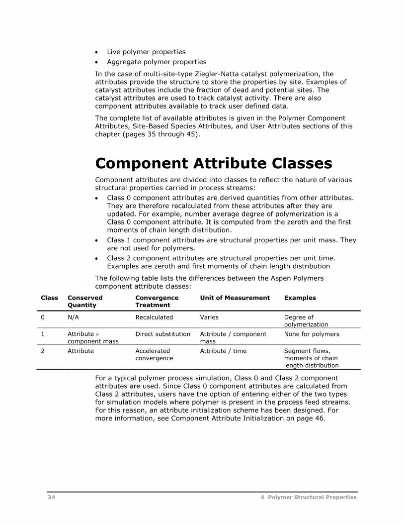
34 4 Polymer Structural Properties
Live polymer properties
Aggregate polymer properties
In the case of multi-site-type Ziegler-Natta catalyst polymerization, theattributes provide the structure to store the properties by site. Examples ofcatalyst attributes include the fraction of dead and potential sites. Thecatalyst attributes are used to track catalyst activity. There are alsocomponent attributes available to track user defined data.
The complete list of available attributes is given in the Polymer ComponentAttributes, Site-Based Species Attributes, and User Attributes sections of thischapter (pages 35 through 45).
Component Attribute ClassesComponent attributes are divided into classes to reflect the nature of variousstructural properties carried in process streams:
Class 0 component attributes are derived quantities from other attributes.They are therefore recalculated from these attributes after they areupdated. For example, number average degree of polymerization is aClass 0 component attribute. It is computed from the zeroth and the firstmoments of chain length distribution.
Class 1 component attributes are structural properties per unit mass. Theyare not used for polymers.
Class 2 component attributes are structural properties per unit time.Examples are zeroth and first moments of chain length distribution
The following table lists the differences between the Aspen Polymerscomponent attribute classes:
Class ConservedQuantity
ConvergenceTreatment
Unit of Measurement Examples
0 N/A Recalculated Varies Degree ofpolymerization
1 Attribute component mass
Direct substitution Attribute / componentmass
None for polymers
2 Attribute Acceleratedconvergence
Attribute / time Segment flows,moments of chainlength distribution
For a typical polymer process simulation, Class 0 and Class 2 componentattributes are used. Since Class 0 component attributes are calculated fromClass 2 attributes, users have the option of entering either of the two typesfor simulation models where polymer is present in the process feed streams.For this reason, an attribute initialization scheme has been designed. Formore information, see Component Attribute Initialization on page 46.
4 Polymer Structural Properties 35
Component AttributeCategoriesThe main categories of component attributes available are:
Polymer attributes
Ziegler-Natta catalyst attributes
Ionic initiator attributes
User attributes
Polymer Component AttributesThe polymer properties tracked as component attributes include:
Segment fraction
Segment flow
Flow and fraction of segment dyads (pairs)
Number-average degree of polymerization and molecular weight
Weight-average degree of polymerization and molecular weight
Z-average degree of polymerization and molecular weight
Zeroth through third moment of chain length distribution
Number of long and short chain branches
Long and short chain branching frequency
Number and frequency of cross-links
Number-average block length (sequence length)
Several aspects of molecular architecture, including tacticity, head-to-head insertions (orienticity)
Flow and fraction of terminal double bonds
Flow and fraction of cis-, trans-, and vinyl- isomers associated with dienesegments (internal and pendent double bonds)
There are component attributes available to track most of these properties fordead polymer, live polymer, and aggregate polymer. You may want to trackinformation for live polymers for cases of free-radical polymerization wherethe quasi-steady-state approximation (QSSA) is not used. Site basedcomponent attributes are also available to accommodate multi-site typeZiegler-Natta catalyst polymerization. Composite attributes are summed overall site types. They represent the average properties of the polymer.
Polymer Attribute Sets
In summary, there are six sets of polymer component attributes.
Composite Polymer Set contains the basic attributes that may be used forany type of polymerization, including the minimum required set for allsimulation models.
Composite Live Polymer Set contains the attributes required to track thecharacteristics of live polymer chains in chain growth polymerization.
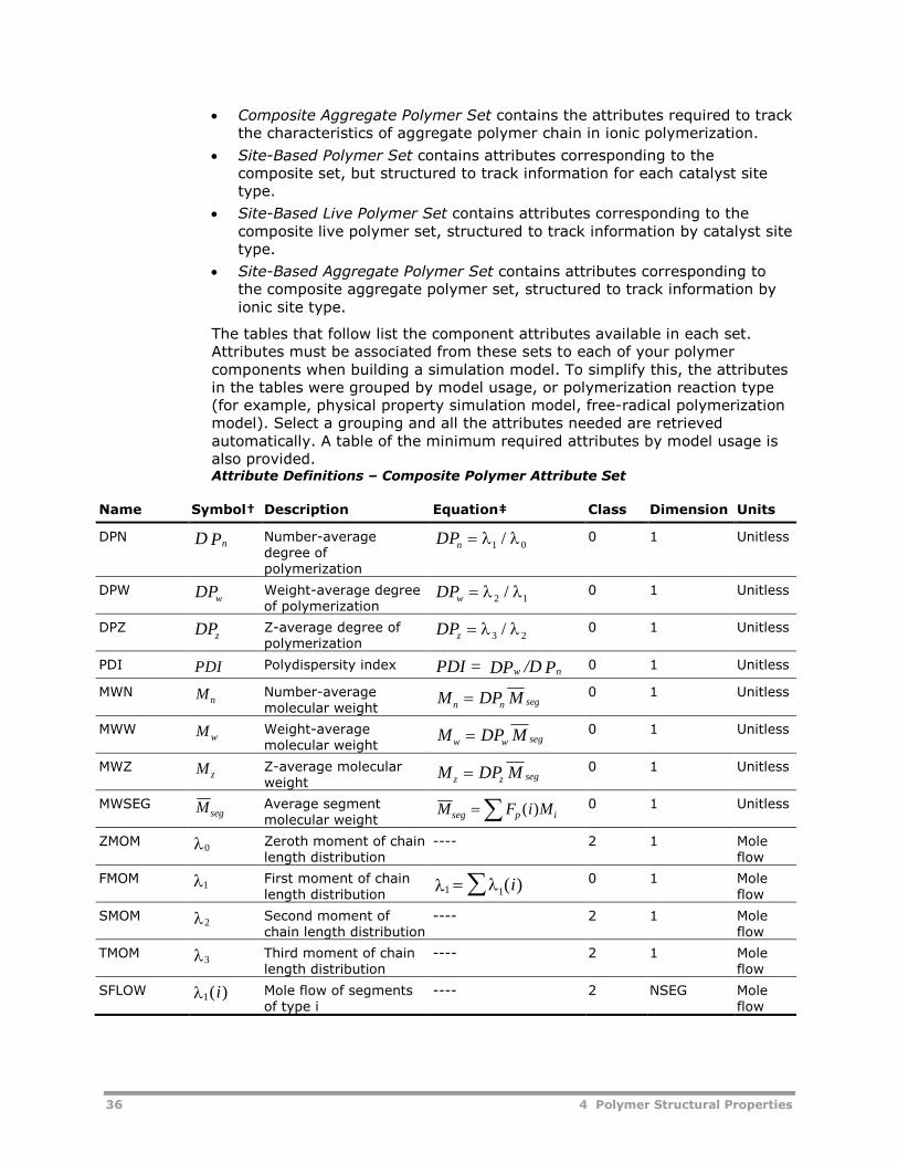
36 4 Polymer Structural Properties
Composite Aggregate Polymer Set contains the attributes required to trackthe characteristics of aggregate polymer chain in ionic polymerization.
Site-Based Polymer Set contains attributes corresponding to thecomposite set, but structured to track information for each catalyst sitetype.
Site-Based Live Polymer Set contains attributes corresponding to thecomposite live polymer set, structured to track information by catalyst sitetype.
Site-Based Aggregate Polymer Set contains attributes corresponding tothe composite aggregate polymer set, structured to track information byionic site type.
The tables that follow list the component attributes available in each set.Attributes must be associated from these sets to each of your polymercomponents when building a simulation model. To simplify this, the attributesin the tables were grouped by model usage, or polymerization reaction type(for example, physical property simulation model, free-radical polymerizationmodel). Select a grouping and all the attributes needed are retrievedautomatically. A table of the minimum required attributes by model usage isalso provided.Attribute Definitions – Composite Polymer Attribute Set
Name Symbol† Description Equation‡ Class Dimension Units
DPN D PnNumber-averagedegree ofpolymerization
DPn 1 0/ 0 1 Unitless
DPW DPwWeight-average degreeof polymerization
DPw 2 1/ 0 1 Unitless
DPZ DPzZ-average degree ofpolymerization
DPz 3 2/ 0 1 Unitless
PDI PDI Polydispersity index PDI = DP /D Pw n0 1 Unitless
MWN MnNumber-averagemolecular weight
M DP Mn n seg 0 1 Unitless
MWW MwWeight-averagemolecular weight
M DP Mw w seg 0 1 Unitless
MWZ M zZ-average molecularweight
M DP Mz z seg 0 1 Unitless
MWSEG MsegAverage segmentmolecular weight
M F i Mseg p i ( ) 0 1 Unitless
ZMOM0 Zeroth moment of chain
length distribution---- 2 1 Mole
flow
FMOM1 First moment of chain
length distribution 1 1 ( )i 0 1 Moleflow
SMOM2 Second moment of
chain length distribution---- 2 1 Mole
flow
TMOM3 Third moment of chain
length distribution---- 2 1 Mole
flow
SFLOW 1( ) i Mole flow of segmentsof type i
---- 2 NSEG Moleflow
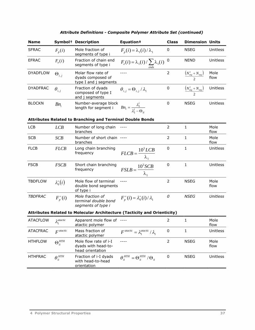
4 Polymer Structural Properties 37
Attribute Definitions - Composite Polymer Attribute Set (continued)
Name Symbol† Description Equation‡ Class Dimension Units
SFRAC F ip( ) Mole fraction ofsegments of type i
F i ip( ) ( ) / 1 10 NSEG Unitless
EFRAC F ie( ) Fraction of chain endsegments of type i
F i i ieends
( ) ( ) / ( ) 1 10 NEND Unitless
DYADFLOWji, Molar flow rate of
dyads composed oftype I and j segments
---- 2 2
2segseg NN Mole
flow
DYADFRACji , Fraction of dyads
composed of type Iand j segments
1,, / jiji 0 2
2segseg NN Unitless
BLOCKNiBn Number-average block
length for segment iii
i
i
iBn
1
1
0 NSEG Unitless
Attributes Related to Branching and Terminal Double Bonds
LCB LCB Number of long chainbranches
---- 2 1 Moleflow
SCB SCB Number of short chainbranches
---- 2 1 Moleflow
FLCB FLCB Long chain branchingfrequency FLCB
LCB
103
1
0 1 Unitless
FSCB FSCB Short chain branchingfrequency FSLB
SCB
103
1
0 1 Unitless
TBDFLOW i0
Mole flow of terminaldouble bond segmentsof type i
---- 2 NSEG Moleflow
TBDFRAC Mole fraction ofterminal double bondsegments of type i
0 NSEG Unitless
Attributes Related to Molecular Architecture (Tacticity and Orienticity)
ATACFLOW atactic1
Apparent mole flow ofatactic polymer
---- 2 1 Moleflow
ATACFRAC atacticF Mass fraction ofatactic polymer 11 /atacticatacticF 0 1 Unitless
HTHFLOW HTHii Mole flow rate of i-I
dyads with head-to-head orientation
---- 2 NSEG Moleflow
HTHFRAC HTHii Fraction of i-I dyads
with head-to-headorientation
iiHTHii
HTHii / 0 NSEG Unitless
)(iFp
10 /)()( iiFp
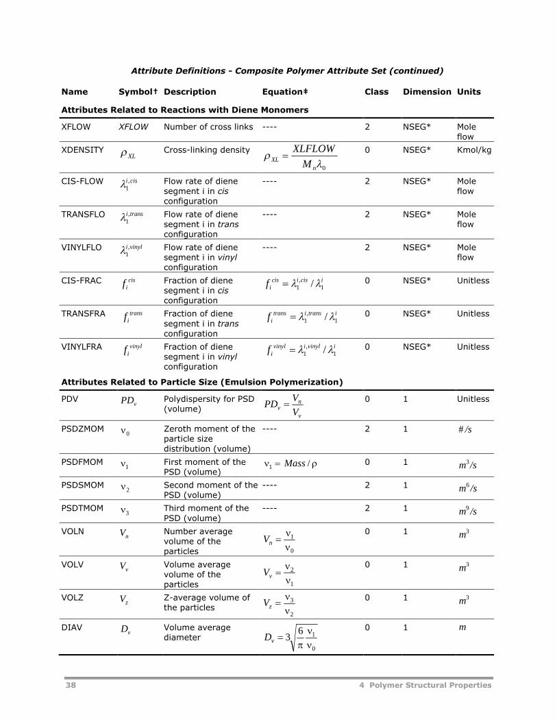
38 4 Polymer Structural Properties
Attribute Definitions - Composite Polymer Attribute Set (continued)
Name Symbol† Description Equation‡ Class Dimension Units
Attributes Related to Reactions with Diene Monomers
XFLOW XFLOW Number of cross links ---- 2 NSEG* Moleflow
XDENSITYXL Cross-linking density
0
n
XLM
XLFLOW
0 NSEG* Kmol/kg
CIS-FLOW cisi ,1
Flow rate of dienesegment i in cisconfiguration
---- 2 NSEG* Moleflow
TRANSFLO transi ,1
Flow rate of dienesegment i in transconfiguration
---- 2 NSEG* Moleflow
VINYLFLO vinyli,1
Flow rate of dienesegment i in vinylconfiguration
---- 2 NSEG* Moleflow
CIS-FRAC cisif
Fraction of dienesegment i in cisconfiguration
icisicisif 1
,1 / 0 NSEG* Unitless
TRANSFRA Fraction of dienesegment i in transconfiguration
0 NSEG* Unitless
VINYLFRA Fraction of dienesegment i in vinylconfiguration
0 NSEG* Unitless
Attributes Related to Particle Size (Emulsion Polymerization)
PDV PDvPolydispersity for PSD(volume)
PDV
Vv
n
v
0 1 Unitless
PSDZMOM 0Zeroth moment of theparticle sizedistribution (volume)
---- 2 1 # /s
PSDFMOM 1First moment of thePSD (volume)
1 Mass / 0 1 m /s3
PSDSMOM 2Second moment of thePSD (volume)
---- 2 1 m /s6
PSDTMOM 3Third moment of thePSD (volume)
---- 2 1 m /s9
VOLN VnNumber averagevolume of theparticles
Vn
1
0
0 1 m3
VOLV VvVolume averagevolume of theparticles
Vv
2
1
0 1 m3
VOLZ VzZ-average volume ofthe particles
Vz
3
2
0 1 m3
DIAV DvVolume averagediameter Dv 3
6 1
0
0 1 m
transif
itransitransif 1
,1 /
vinylif
ivinylivinylif 1
,1 /
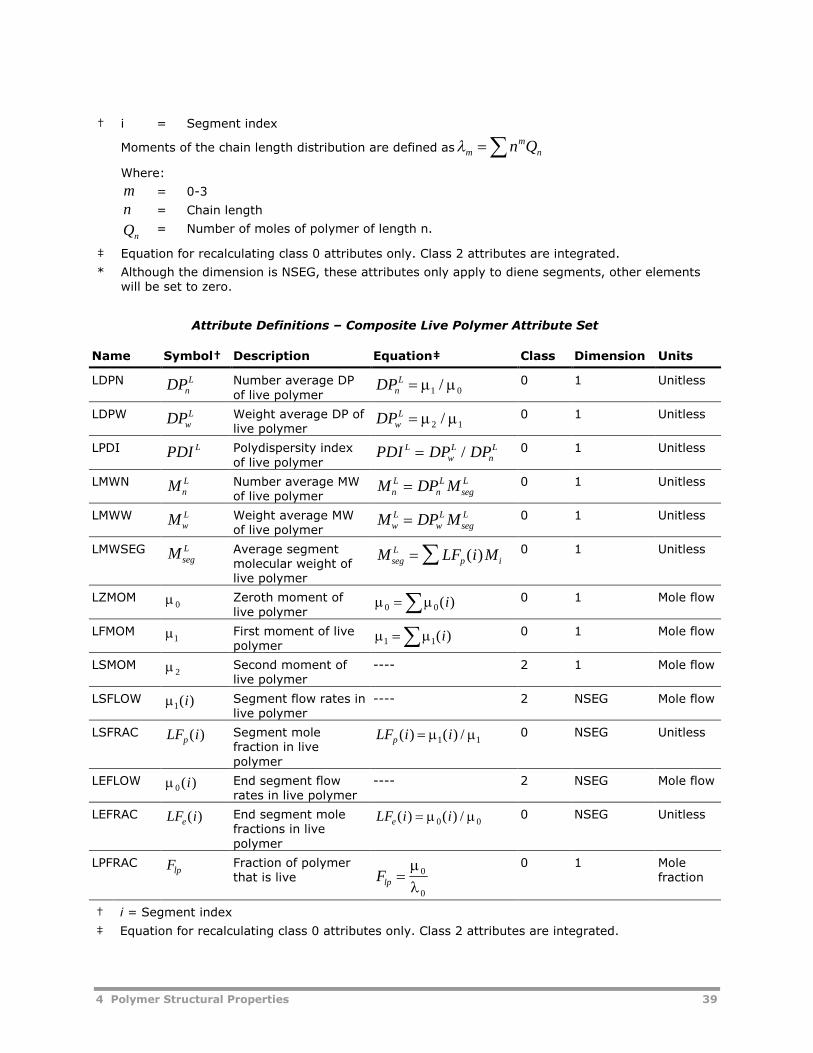
4 Polymer Structural Properties 39
† i = Segment index
Moments of the chain length distribution are defined as nm
m Qn
Where:
m = 0-3
n = Chain length
Qn= Number of moles of polymer of length n.
‡ Equation for recalculating class 0 attributes only. Class 2 attributes are integrated.
* Although the dimension is NSEG, these attributes only apply to diene segments, other elementswill be set to zero.
Attribute Definitions – Composite Live Polymer Attribute Set
Name Symbol† Description Equation‡ Class Dimension Units
LDPN DPnL Number average DP
of live polymerDPn
L 1 0/ 0 1 Unitless
LDPW DPwL Weight average DP of
live polymerDPw
L 2 1/ 0 1 Unitless
LPDI PDI L Polydispersity indexof live polymer
PDI DP DPLwL
nL / 0 1 Unitless
LMWN MnL Number average MW
of live polymerM DP Mn
LnL
segL 0 1 Unitless
LMWW MwL Weight average MW
of live polymerM DP Mw
LwL
segL 0 1 Unitless
LMWSEG MsegL Average segment
molecular weight oflive polymer
M LF i MsegL
p i ( ) 0 1 Unitless
LZMOM 0Zeroth moment oflive polymer
0 0 ( )i 0 1 Mole flow
LFMOM 1First moment of livepolymer
1 1 ( )i 0 1 Mole flow
LSMOM 2Second moment oflive polymer
---- 2 1 Mole flow
LSFLOW 1( )i Segment flow rates inlive polymer
---- 2 NSEG Mole flow
LSFRAC LF ip( ) Segment molefraction in livepolymer
LF i ip ( ) ( ) / 1 10 NSEG Unitless
LEFLOW 0( )i End segment flowrates in live polymer
---- 2 NSEG Mole flow
LEFRAC LF ie( ) End segment molefractions in livepolymer
LF i ie( ) ( ) / 0 00 NSEG Unitless
LPFRAC FlpFraction of polymerthat is live Flp
0
0
0 1 Molefraction
† i = Segment index
‡ Equation for recalculating class 0 attributes only. Class 2 attributes are integrated.
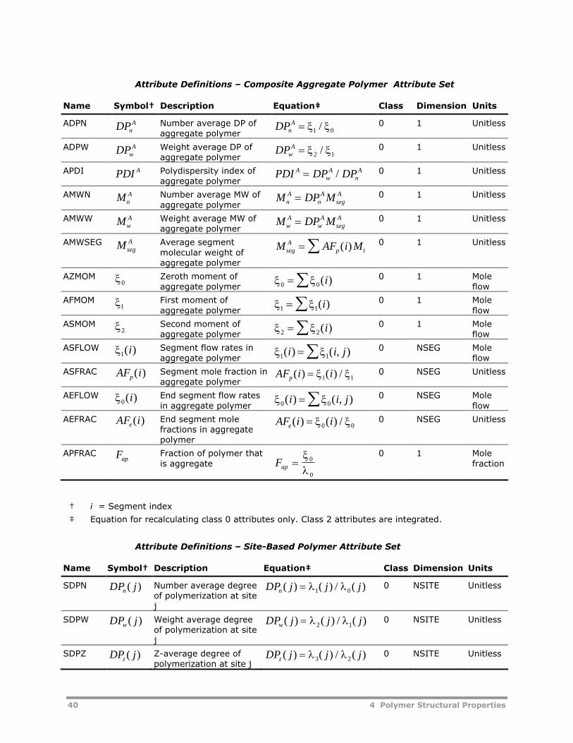
40 4 Polymer Structural Properties
Attribute Definitions – Composite Aggregate Polymer Attribute Set
Name Symbol† Description Equation‡ Class Dimension Units
ADPN DPnA Number average DP of
aggregate polymerDPn
A 1 0/ 0 1 Unitless
ADPW DPwA Weight average DP of
aggregate polymerDPw
A 2 1/ 0 1 Unitless
APDI PDI A Polydispersity index ofaggregate polymer
PDI DP DPAwA
nA / 0 1 Unitless
AMWN MnA Number average MW of
aggregate polymerM DP Mn
AnA
segA 0 1 Unitless
AMWW MwA Weight average MW of
aggregate polymerM DP Mw
AwA
segA 0 1 Unitless
AMWSEG MsegA Average segment
molecular weight ofaggregate polymer
M AF i MsegA
p i ( ) 0 1 Unitless
AZMOM 0Zeroth moment ofaggregate polymer
0 0 ( )i 0 1 Moleflow
AFMOM 1First moment ofaggregate polymer
1 1 ( )i 0 1 Moleflow
ASMOM 2Second moment ofaggregate polymer
2 2 ( )i 0 1 Moleflow
ASFLOW 1( )i Segment flow rates inaggregate polymer
1 1( ) ( , )i i j 0 NSEG Moleflow
ASFRAC AF ip( ) Segment mole fraction inaggregate polymer
AF i ip( ) ( ) / 1 10 NSEG Unitless
AEFLOW 0( )i End segment flow ratesin aggregate polymer
0 0( ) ( , )i i j 0 NSEG Moleflow
AEFRAC End segment molefractions in aggregatepolymer
AF i ie( ) ( ) / 0 00 NSEG Unitless
APFRAC Fraction of polymer thatis aggregate Fap
0
0
0 1 Molefraction
† i = Segment index
‡ Equation for recalculating class 0 attributes only. Class 2 attributes are integrated.
Attribute Definitions – Site-Based Polymer Attribute Set
Name Symbol† Description Equation‡ Class Dimension Units
SDPN DP jn ( ) Number average degreeof polymerization at sitej
DP j j jn ( ) ( ) / ( ) 1 00 NSITE Unitless
SDPW DP jw ( ) Weight average degreeof polymerization at sitej
DP j j jw( ) ( ) / ( ) 2 10 NSITE Unitless
SDPZ DP jz ( ) Z-average degree ofpolymerization at site j
DP j j jz ( ) ( ) / ( ) 3 20 NSITE Unitless
AF ie( )
Fap
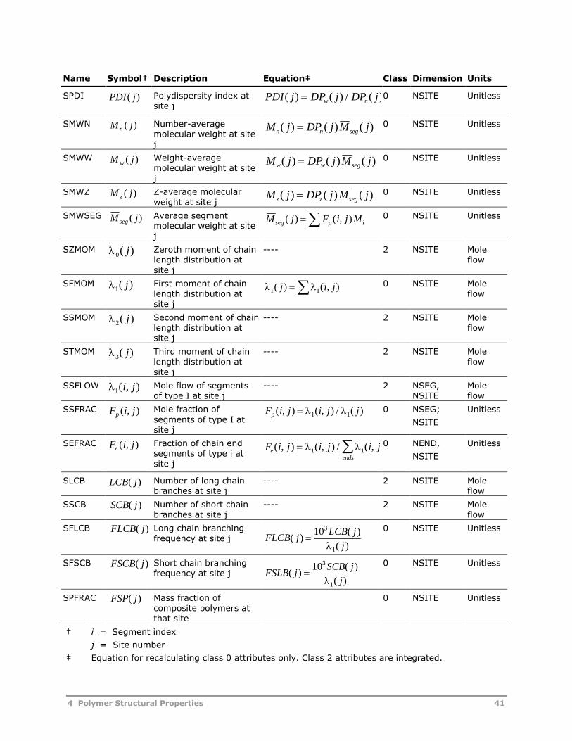
4 Polymer Structural Properties 41
Name Symbol† Description Equation‡ Class Dimension Units
SPDI PDI j( ) Polydispersity index atsite j
PDI j DP j DP jw n( ) ( ) / ( ) 0 NSITE Unitless
SMWN M jn ( ) Number-averagemolecular weight at sitej
M j DP j M jn n seg( ) ( ) ( ) 0 NSITE Unitless
SMWW M jw ( ) Weight-averagemolecular weight at sitej
M j DP j M jw w seg( ) ( ) ( ) 0 NSITE Unitless
SMWZ M jz ( ) Z-average molecularweight at site j
M j DP j M jz z seg( ) ( ) ( ) 0 NSITE Unitless
SMWSEG M jseg ( ) Average segmentmolecular weight at sitej
M j F i j Mseg p i( ) ( , ) 0 NSITE Unitless
SZMOM 0( )j Zeroth moment of chainlength distribution atsite j
---- 2 NSITE Moleflow
SFMOM 1( )j First moment of chainlength distribution atsite j
1 1( ) ( , )j i j 0 NSITE Moleflow
SSMOM 2( )j Second moment of chainlength distribution atsite j
---- 2 NSITE Moleflow
STMOM 3( )j Third moment of chainlength distribution atsite j
---- 2 NSITE Moleflow
SSFLOW 1( , )i j Mole flow of segmentsof type I at site j
---- 2 NSEG,NSITE
Moleflow
SSFRAC F i jp ( , ) Mole fraction ofsegments of type I atsite j
F i j i j jp( , ) ( , ) / ( ) 1 10 NSEG;
NSITE
Unitless
SEFRAC F i je ( , ) Fraction of chain endsegments of type i atsite j
F i j i j i jeends
( , ) ( , ) / ( , 1 10 NEND,
NSITE
Unitless
SLCB LCB j( ) Number of long chainbranches at site j
---- 2 NSITE Moleflow
SSCB Number of short chainbranches at site j
---- 2 NSITE Moleflow
SFLCB Long chain branchingfrequency at site j
0 NSITE Unitless
SFSCB Short chain branchingfrequency at site j
0 NSITE Unitless
SPFRAC Mass fraction ofcomposite polymers atthat site
0 NSITE Unitless
† i = Segment index
j = Site number
‡ Equation for recalculating class 0 attributes only. Class 2 attributes are integrated.
SCB j( )
FLCB j( )FLCB j
LCB j
j( )
( )
( )
103
1
FSCB j( )FSLB j
SCB j
j( )
( )
( )
103
1
FSP j( )
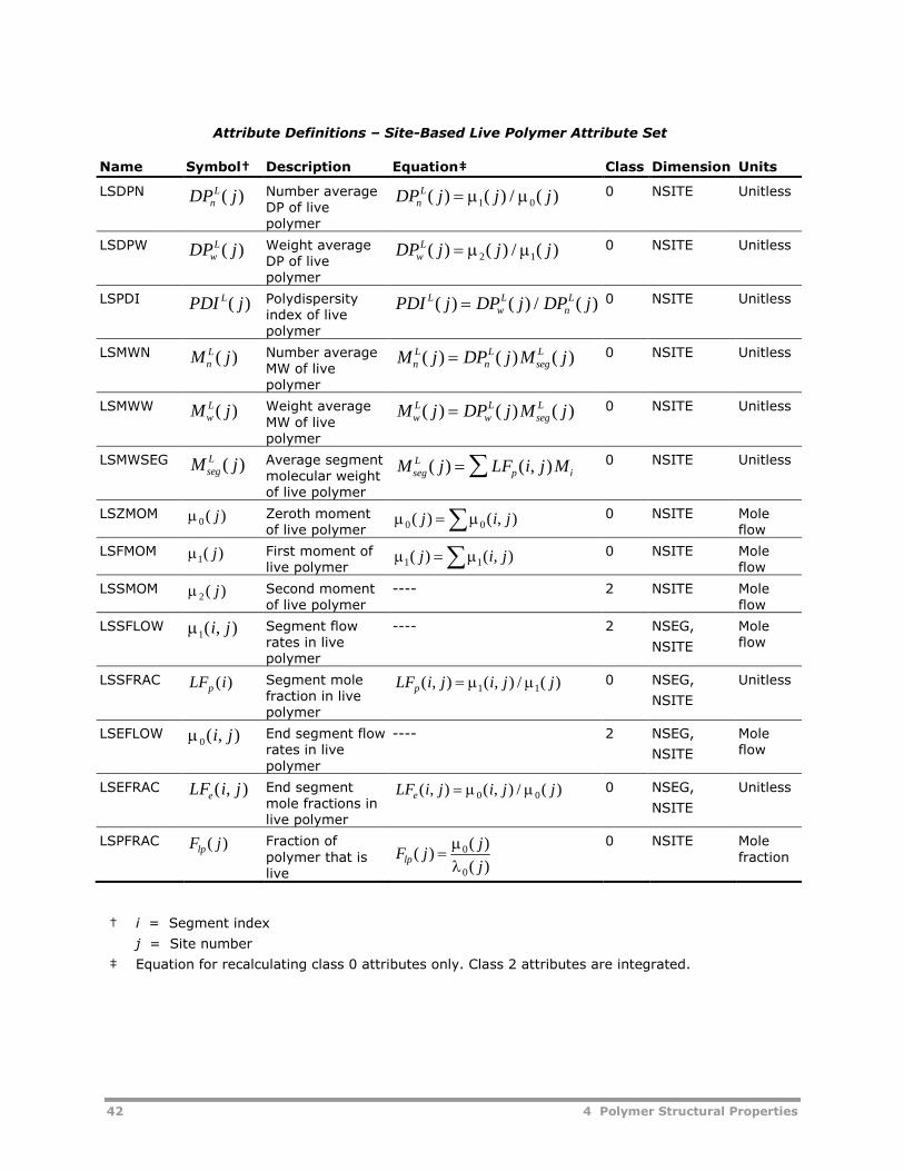
42 4 Polymer Structural Properties
Attribute Definitions – Site-Based Live Polymer Attribute Set
Name Symbol† Description Equation‡ Class Dimension Units
LSDPN DP jnL( ) Number average
DP of livepolymer
DP j j jnL( ) ( ) / 1 0( ) 0 NSITE Unitless
LSDPW DP jwL( ) Weight average
DP of livepolymer
DP j j jwL( ) ( ) / 2 1( ) 0 NSITE Unitless
LSPDI PDI jL( ) Polydispersityindex of livepolymer
PDI j DP j DP jLwL
nL( ) ( ) / ( ) 0 NSITE Unitless
LSMWN M jnL( ) Number average
MW of livepolymer
M j DP j M jnL
nL
segL( ) ( ) ( ) 0 NSITE Unitless
LSMWW M jwL( ) Weight average
MW of livepolymer
M j DP j M jwL
wL
segL( ) ( ) ( ) 0 NSITE Unitless
LSMWSEG M jsegL ( ) Average segment
molecular weightof live polymer
M j LF i j MsegL
p i( ) ( , ) 0 NSITE Unitless
LSZMOM 0( )j Zeroth momentof live polymer
0 0( ) ( , )j i j 0 NSITE Moleflow
LSFMOM 1( )j First moment oflive polymer
1 1( ) ( , )j i j 0 NSITE Moleflow
LSSMOM 2( )j Second momentof live polymer
---- 2 NSITE Moleflow
LSSFLOW 1( , )i j Segment flowrates in livepolymer
---- 2 NSEG,
NSITE
Moleflow
LSSFRAC LF ip ( ) Segment molefraction in livepolymer
LF i j i j jp( , ) ( , ) / ( ) 1 10 NSEG,
NSITE
Unitless
LSEFLOW 0( , )i j End segment flowrates in livepolymer
---- 2 NSEG,
NSITE
Moleflow
LSEFRAC LF i je( , ) End segmentmole fractions inlive polymer
LF i j i j je( , ) ( , ) / ( ) 0 00 NSEG,
NSITE
Unitless
LSPFRAC F jlp( ) Fraction ofpolymer that islive
F jj
jlp( )
( )
( )
0
0
0 NSITE Molefraction
† i = Segment index
j = Site number
‡ Equation for recalculating class 0 attributes only. Class 2 attributes are integrated.
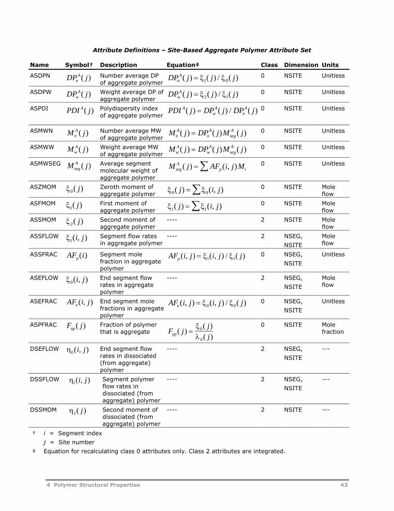
4 Polymer Structural Properties 43
Attribute Definitions – Site-Based Aggregate Polymer Attribute Set
Name Symbol† Description Equation‡ Class Dimension Units
ASDPN DP jnA( ) Number average DP
of aggregate polymerDP j j jn
A( ) ( ) / 1 0( ) 0 NSITE Unitless
ASDPW DP jwA( ) Weight average DP of
aggregate polymerDP j j jw
A( ) ( ) / 2 1( ) 0 NSITE Unitless
ASPDI PDI jA( ) Polydispersity indexof aggregate polymer
PDI j DP j DP jAwA
nA( ) ( ) / ( ) 0 NSITE Unitless
ASMWN M jnA( ) Number average MW
of aggregate polymerM j DP j M jn
AnA
segA( ) ( ) ( ) 0 NSITE Unitless
ASMWW M jwA( ) Weight average MW
of aggregate polymerM j DP j M jw
AwA
segA( ) ( ) ( ) 0 NSITE Unitless
ASMWSEG M jsegA ( ) Average segment
molecular weight ofaggregate polymer
M j AF i j MsegA
p i( ) ( , ) 0 NSITE Unitless
ASZMOM 0( )j Zeroth moment ofaggregate polymer
0 0( ) ( , )j i j 0 NSITE Moleflow
ASFMOM 1( )j First moment ofaggregate polymer
1 1( ) ( , )j i j 0 NSITE Moleflow
ASSMOM 2( )j Second moment ofaggregate polymer
---- 2 NSITE Moleflow
ASSFLOW 1( , )i j Segment flow ratesin aggregate polymer
---- 2 NSEG,
NSITE
Moleflow
ASSFRAC AF ip( ) Segment molefraction in aggregatepolymer
AF i j i j jp ( , ) ( , ) / ( ) 1 10 NSEG,
NSITE
Unitless
ASEFLOW 0( , )i j End segment flowrates in aggregatepolymer
---- 2 NSEG,
NSITE
Moleflow
ASEFRAC AF i je( , ) End segment molefractions in aggregatepolymer
AF i j i j je( , ) ( , ) / ( ) 0 00 NSEG,
NSITE
Unitless
ASPFRAC F jap( ) Fraction of polymerthat is aggregate F j
j
jap( )( )
( )
0
0
0 NSITE Molefraction
DSEFLOW 0( , )i j End segment flowrates in dissociated(from aggregate)polymer
---- 2 NSEG,
NSITE
---
DSSFLOW 1( , )i j Segment polymerflow rates indissociated (fromaggregate) polymer
---- 2 NSEG,
NSITE
---
DSSMOM 2( )j Second moment ofdissociated (fromaggregate) polymer
---- 2 NSITE ---
† i = Segment index
j = Site number
‡ Equation for recalculating class 0 attributes only. Class 2 attributes are integrated.
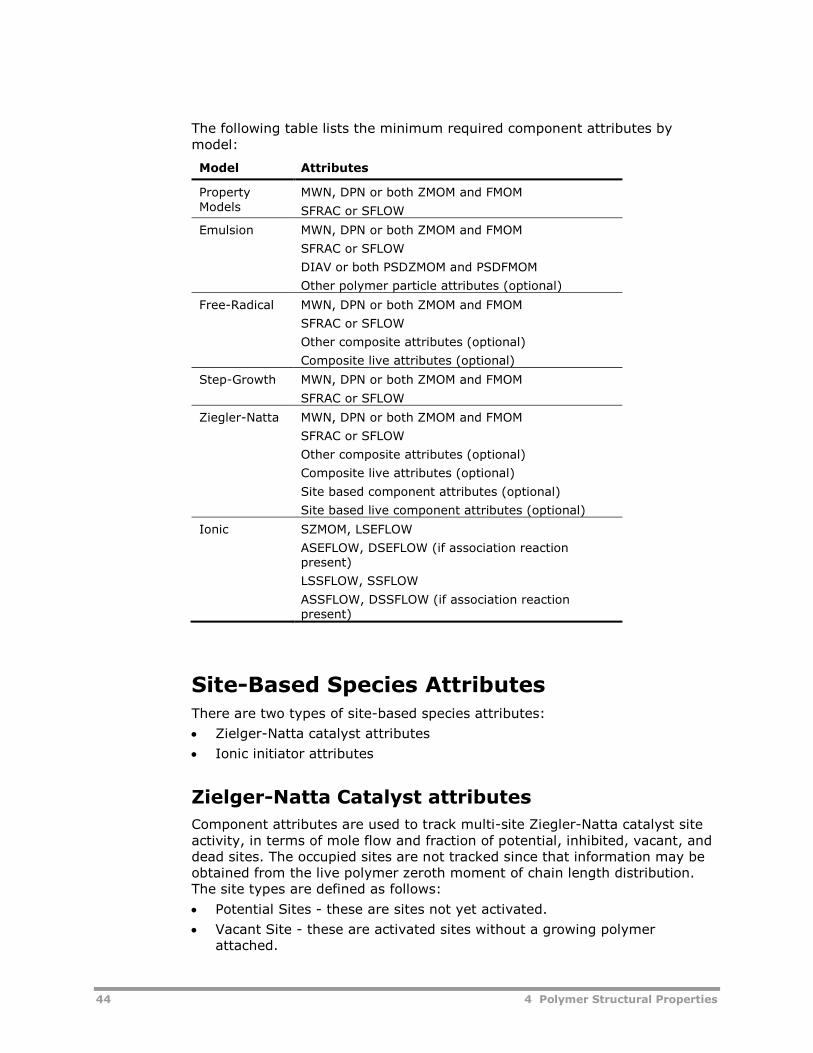
44 4 Polymer Structural Properties
The following table lists the minimum required component attributes bymodel:
Model Attributes
PropertyModels
MWN, DPN or both ZMOM and FMOM
SFRAC or SFLOW
Emulsion MWN, DPN or both ZMOM and FMOM
SFRAC or SFLOW
DIAV or both PSDZMOM and PSDFMOM
Other polymer particle attributes (optional)
Free-Radical MWN, DPN or both ZMOM and FMOM
SFRAC or SFLOW
Other composite attributes (optional)
Composite live attributes (optional)
Step-Growth MWN, DPN or both ZMOM and FMOM
SFRAC or SFLOW
Ziegler-Natta MWN, DPN or both ZMOM and FMOM
SFRAC or SFLOW
Other composite attributes (optional)
Composite live attributes (optional)
Site based component attributes (optional)
Site based live component attributes (optional)
Ionic SZMOM, LSEFLOW
ASEFLOW, DSEFLOW (if association reactionpresent)
LSSFLOW, SSFLOW
ASSFLOW, DSSFLOW (if association reactionpresent)
Site-Based Species AttributesThere are two types of site-based species attributes:
Zielger-Natta catalyst attributes
Ionic initiator attributes
Zielger-Natta Catalyst attributes
Component attributes are used to track multi-site Ziegler-Natta catalyst siteactivity, in terms of mole flow and fraction of potential, inhibited, vacant, anddead sites. The occupied sites are not tracked since that information may beobtained from the live polymer zeroth moment of chain length distribution.The site types are defined as follows:
Potential Sites - these are sites not yet activated.
Vacant Site - these are activated sites without a growing polymerattached.
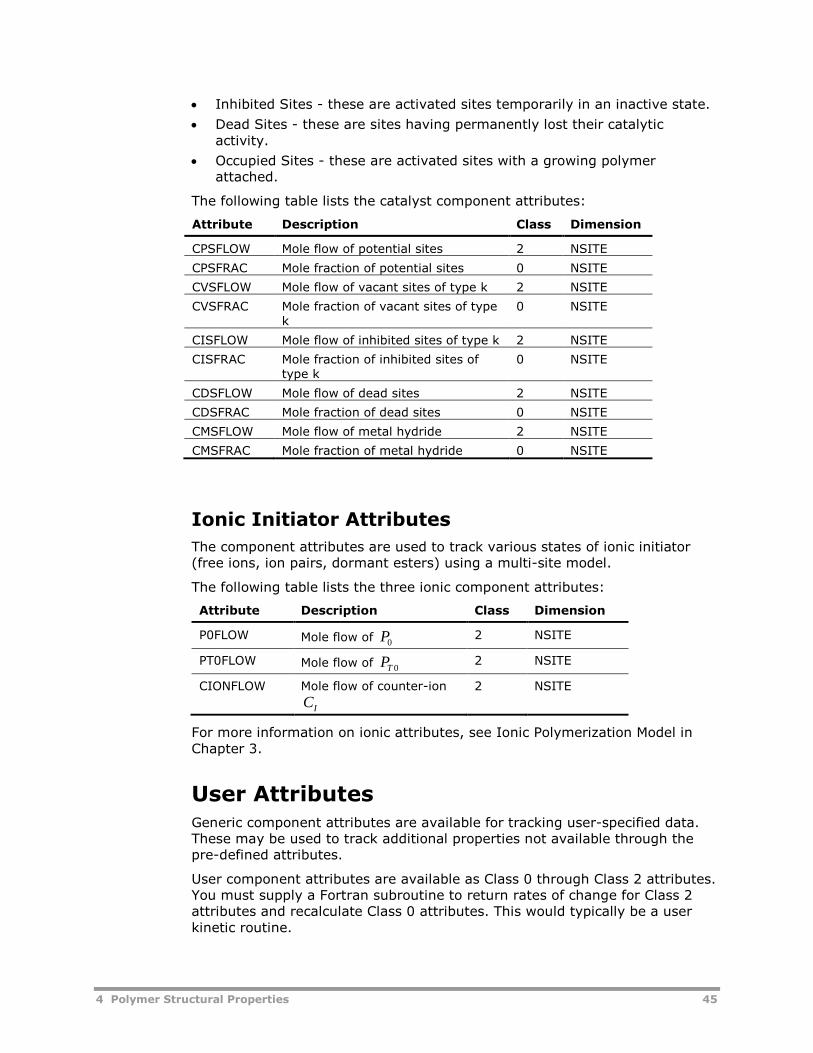
4 Polymer Structural Properties 45
Inhibited Sites - these are activated sites temporarily in an inactive state.
Dead Sites - these are sites having permanently lost their catalyticactivity.
Occupied Sites - these are activated sites with a growing polymerattached.
The following table lists the catalyst component attributes:
Attribute Description Class Dimension
CPSFLOW Mole flow of potential sites 2 NSITE
CPSFRAC Mole fraction of potential sites 0 NSITE
CVSFLOW Mole flow of vacant sites of type k 2 NSITE
CVSFRAC Mole fraction of vacant sites of typek
0 NSITE
CISFLOW Mole flow of inhibited sites of type k 2 NSITE
CISFRAC Mole fraction of inhibited sites oftype k
0 NSITE
CDSFLOW Mole flow of dead sites 2 NSITE
CDSFRAC Mole fraction of dead sites 0 NSITE
CMSFLOW Mole flow of metal hydride 2 NSITE
CMSFRAC Mole fraction of metal hydride 0 NSITE
Ionic Initiator Attributes
The component attributes are used to track various states of ionic initiator(free ions, ion pairs, dormant esters) using a multi-site model.
The following table lists the three ionic component attributes:
Attribute Description Class Dimension
P0FLOW Mole flow of P02 NSITE
PT0FLOW Mole flow of PT 02 NSITE
CIONFLOW Mole flow of counter-ion
CI
2 NSITE
For more information on ionic attributes, see Ionic Polymerization Model inChapter 3.
User AttributesGeneric component attributes are available for tracking user-specified data.These may be used to track additional properties not available through thepre-defined attributes.
User component attributes are available as Class 0 through Class 2 attributes.You must supply a Fortran subroutine to return rates of change for Class 2attributes and recalculate Class 0 attributes. This would typically be a userkinetic routine.
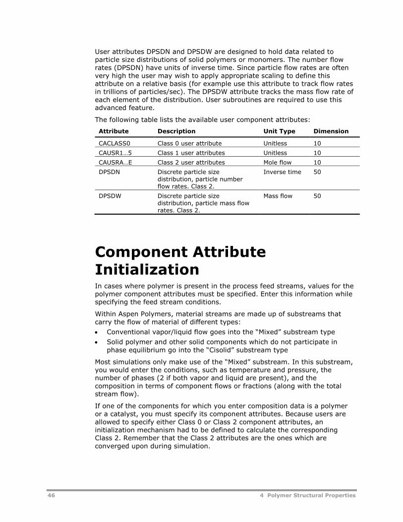
46 4 Polymer Structural Properties
User attributes DPSDN and DPSDW are designed to hold data related toparticle size distributions of solid polymers or monomers. The number flowrates (DPSDN) have units of inverse time. Since particle flow rates are oftenvery high the user may wish to apply appropriate scaling to define thisattribute on a relative basis (for example use this attribute to track flow ratesin trillions of particles/sec). The DPSDW attribute tracks the mass flow rate ofeach element of the distribution. User subroutines are required to use thisadvanced feature.
The following table lists the available user component attributes:
Attribute Description Unit Type Dimension
CACLASS0 Class 0 user attribute Unitless 10
CAUSR1…5 Class 1 user attributes Unitless 10
CAUSRA…E Class 2 user attributes Mole flow 10
DPSDN Discrete particle sizedistribution, particle numberflow rates. Class 2.
Inverse time 50
DPSDW Discrete particle sizedistribution, particle mass flowrates. Class 2.
Mass flow 50
Component AttributeInitializationIn cases where polymer is present in the process feed streams, values for thepolymer component attributes must be specified. Enter this information whilespecifying the feed stream conditions.
Within Aspen Polymers, material streams are made up of substreams thatcarry the flow of material of different types:
Conventional vapor/liquid flow goes into the “Mixed” substream type
Solid polymer and other solid components which do not participate inphase equilibrium go into the “Cisolid” substream type
Most simulations only make use of the “Mixed” substream. In this substream,you would enter the conditions, such as temperature and pressure, thenumber of phases (2 if both vapor and liquid are present), and thecomposition in terms of component flows or fractions (along with the totalstream flow).
If one of the components for which you enter composition data is a polymeror a catalyst, you must specify its component attributes. Because users areallowed to specify either Class 0 or Class 2 component attributes, aninitialization mechanism had to be defined to calculate the correspondingClass 2. Remember that the Class 2 attributes are the ones which areconverged upon during simulation.
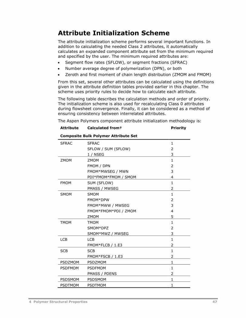
4 Polymer Structural Properties 47
Attribute Initialization SchemeThe attribute initialization scheme performs several important functions. Inaddition to calculating the needed Class 2 attributes, it automaticallycalculates an expanded component attribute set from the minimum requiredand specified by the user. The minimum required attributes are:
Segment flow rates (SFLOW), or segment fractions (SFRAC)
Number average degree of polymerization (DPN), or both
Zeroth and first moment of chain length distribution (ZMOM and FMOM)
From this set, several other attributes can be calculated using the definitionsgiven in the attribute definition tables provided earlier in this chapter. Thescheme uses priority rules to decide how to calculate each attribute.
The following table describes the calculation methods and order of priority.The initialization scheme is also used for recalculating Class 0 attributesduring flowsheet convergence. Finally, it can be considered as a method ofensuring consistency between interrelated attributes.
The Aspen Polymers component attribute initialization methodology is:
Attribute Calculated from† Priority
Composite Bulk Polymer Attribute Set
SFRAC SFRAC
SFLOW / SUM (SFLOW)
1 / NSEG
1
2
3
ZMOM ZMOM
FMOM / DPN
FMOM*MWSEG / MWN
PDI*FMOM*FMOM / SMOM
1
2
3
4
FMOM SUM (SFLOW)
PMASS / MWSEG
1
2
SMOM SMOM
FMOM*DPW
FMOM*MWW / MWSEG
FMOM*FMOM*PDI / ZMOM
ZMOM
1
2
3
4
5
TMOM TMOM
SMOM*DPZ
SMOM*MWZ / MWSEG
1
2
3
LCB LCB
FMOM*FLCB / 1.E3
1
2
SCB SCB
FMOM*FSCB / 1.E3
1
2
PSDZMOM PSDZMOM 1
PSDFMOM PSDFMOM
PMASS / PDENS
1
2
PSDSMOM PSDSMOM 1
PSDTMOM PSDTMOM 1
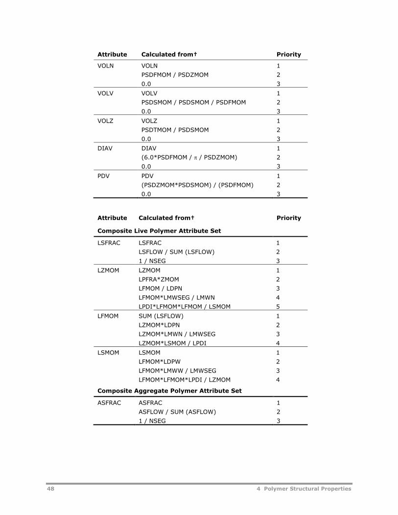
48 4 Polymer Structural Properties
Attribute Calculated from† Priority
VOLN VOLN
PSDFMOM / PSDZMOM
0.0
1
2
3
VOLV VOLV
PSDSMOM / PSDSMOM / PSDFMOM
0.0
1
2
3
VOLZ VOLZ
PSDTMOM / PSDSMOM
0.0
1
2
3
DIAV DIAV
(6.0*PSDFMOM / / PSDZMOM)
0.0
1
2
3
PDV PDV
(PSDZMOM*PSDSMOM) / (PSDFMOM)
0.0
1
2
3
Attribute Calculated from† Priority
Composite Live Polymer Attribute Set
LSFRAC LSFRAC
LSFLOW / SUM (LSFLOW)
1 / NSEG
1
2
3
LZMOM LZMOM
LPFRA*ZMOM
LFMOM / LDPN
LFMOM*LMWSEG / LMWN
LPDI*LFMOM*LFMOM / LSMOM
1
2
3
4
5
LFMOM SUM (LSFLOW)
LZMOM*LDPN
LZMOM*LMWN / LMWSEG
LZMOM*LSMOM / LPDI
1
2
3
4
LSMOM LSMOM
LFMOM*LDPW
LFMOM*LMWW / LMWSEG
LFMOM*LFMOM*LPDI / LZMOM
1
2
3
4
Composite Aggregate Polymer Attribute Set
ASFRAC ASFRAC
ASFLOW / SUM (ASFLOW)
1 / NSEG
1
2
3
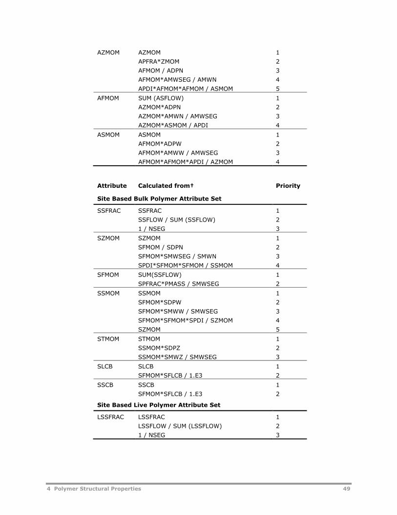
4 Polymer Structural Properties 49
AZMOM AZMOM
APFRA*ZMOM
AFMOM / ADPN
AFMOM*AMWSEG / AMWN
APDI*AFMOM*AFMOM / ASMOM
1
2
3
4
5
AFMOM SUM (ASFLOW)
AZMOM*ADPN
AZMOM*AMWN / AMWSEG
AZMOM*ASMOM / APDI
1
2
3
4
ASMOM ASMOM
AFMOM*ADPW
AFMOM*AMWW / AMWSEG
AFMOM*AFMOM*APDI / AZMOM
1
2
3
4
Attribute Calculated from† Priority
Site Based Bulk Polymer Attribute Set
SSFRAC SSFRAC
SSFLOW / SUM (SSFLOW)
1 / NSEG
1
2
3
SZMOM SZMOM
SFMOM / SDPN
SFMOM*SMWSEG / SMWN
SPDI*SFMOM*SFMOM / SSMOM
1
2
3
4
SFMOM SUM(SSFLOW)
SPFRAC*PMASS / SMWSEG
1
2
SSMOM SSMOM
SFMOM*SDPW
SFMOM*SMWW / SMWSEG
SFMOM*SFMOM*SPDI / SZMOM
SZMOM
1
2
3
4
5
STMOM STMOM
SSMOM*SDPZ
SSMOM*SMWZ / SMWSEG
1
2
3
SLCB SLCB
SFMOM*SFLCB / 1.E3
1
2
SSCB SSCB
SFMOM*SFLCB / 1.E3
1
2
Site Based Live Polymer Attribute Set
LSSFRAC LSSFRAC
LSSFLOW / SUM (LSSFLOW)
1 / NSEG
1
2
3
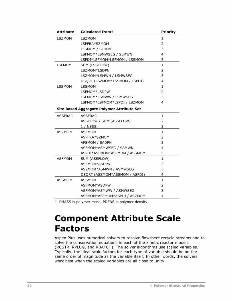
50 4 Polymer Structural Properties
Attribute Calculated from† Priority
LSZMOM LSZMOM
LSPFRA*SZMOM
LFSMOM / SLDPN
LSFMOM*LSMWSEG / SLMWN
LSPDI*LSFMOM*LSFMOM / LSSMOM
1
2
3
4
5
LSFMOM SUM (LSSFLOW)
LSZMOM*LSDPN
LSZMOM*LSMWN / LSMWSEG
DSQRT (LSZMOM*LSSMOM / LSPDI)
1
2
3
4
LSSMOM LSSMOM
LSFMOM*LSDPW
LSFMOM*LSMWW / LSMWSEG
LSFMOM*LSFMOM*LSPDI / LSZMOM
1
2
3
4
Site Based Aggregate Polymer Attribute Set
ASSFRAC ASSFRAC
ASSFLOW / SUM (ASSFLOW)
1 / NSEG
1
2
3
ASZMOM ASZMOM
ASPFRA*SZMOM
AFSMOM / SADPN
ASFMOM*ASMWSEG / SAMWN
ASPDI*ASFMOM*ASFMOM / ASSMOM
1
2
3
4
5
ASFMOM SUM (ASSFLOW)
ASZMOM*ASDPN
ASZMOM*ASMWN / ASMWSEG
DSQRT (ASZMOM*ASSMOM / ASPDI)
1
2
3
4
ASSMOM ASSMOM
ASFMOM*ASDPW
ASFMOM*ASMWW / ASMWSEG
ASFMOM*ASFMOM*ASPDI / ASZMOM
1
2
3
4
† PMASS is polymer mass, PDENS is polymer density
Component Attribute ScaleFactorsAspen Plus uses numerical solvers to resolve flowsheet recycle streams and tosolve the conservation equations in each of the kinetic reactor models(RCSTR, RPLUG, and RBATCH). The solver algorithms use scaled variables.Typically, the ideal scale factors for each type of variable should be on thesame order of magnitude as the variable itself. In other words, the solverswork best when the scaled variables are all close to unity.
4 Polymer Structural Properties 51
In Aspen Polymers, default scaling factors are defined for each type ofcomponent attribute variable. These defaults are designed to address a widerange of problems, however they may not be ideal for any particular problem.The Scaling form lets you view and change the default scaling factors for eachtype of component attribute.
Under some circumstances, you may be able to improve the reactor and/orflowsheet recycle stream convergence by optimizing the attribute scalingfactors. For example, in a Ziegler-Natta polymerization process the live endflow rate (LEFLOW) and the related attributes LZMOM and LSZMOM aresensitive to the catalyst activity. Highly active catalysts result in very low liveend flow rates. Further, the number of vacant and potential sites (CVSFLOWand CPSFLOW) may be very low for the catalyst.
The Scaling form can be used to specify more accurate scaling factors for thecomponent attributes for polymers, catalysts, and other types of attributedcomponents.
Reducing the scaling factors on this form tightens the tolerance on theselected variables. If the scaling factors are set too low, the tolerance will beunreasonably tight, leading to convergence problems or excessive CPU time.If the scaling factors are set too high, the problem may be loosely convergedand the simulation accuracy may suffer.
The reactor models and flowsheet recycle convergence algorithms currentlyignore the attribute upper bound limits that appear on this form.
Specifying ComponentAttributesThere are several categories of components for which you can specifycomponent attributes:
Polymers
Site-based components
Conventional components
Specifying Polymer Component AttributesSee Specifying Polymers on page 29.
Specifying Site-Based ComponentAttributesSee Specifying Site-Based Components on page 30.
52 4 Polymer Structural Properties
Specifying Conventional ComponentAttributesYou can associate attributes to conventional components by selecting userattributes. Typically, you do this if you have a user subroutine to returnvalues for these attributes.
To access the user component attribute selection form:
1 From the Data Browser, click Components.
2 From the Components folder, click Component Attributes.
To associate user attributes to conventional components:
1 On the Selection sheet, specify the component name in the Componentfield.
2 In the Attribute field, specify the attribute name.
3 Continue adding as many attributes as needed.
Initializing Component Attributes inStreams or BlocksIf you have an attributed component present in a feed stream, you mustspecify component attribute values for that component.
To access the component attribute input form for a stream:
1 From the Process Flowsheet window, use the right mouse button to clickthe feed stream.
2 Click Input.
3 From the stream input specifications sheet, click the Component Attr.tab.
4 On the Component Attr. sheet, select the Component ID.
5 For each attribute, select the Attribute ID and enter the values for theattributes.
If you have an attributed component produced within a reactor, you canspecify attribute values (product values or product value estimates) for thatcomponent. This is not available for all reactors.
For a description of the treatment of component attributes in reactors, seeSteady-State Unit Operation Models in Chapter 4.
To access the component attribute input form for a reactor:
1 From the Process Flowsheet window, use the right mouse button to clickthe reactor.
2 Click Input.
3 From the reactor input specifications sheet, click the Component Attr.tab.
4 On the Component Attr. sheet, select the Component ID.
5 For each attribute, select the Attribute ID and enter the values for theattributes.
4 Polymer Structural Properties 53
Specifying Component Attribute ScalingFactorsYou can override default component attribute convergence parameters forpolymer or catalyst components. Adjusting the scaling factor helps youimprove flowsheet convergence and internal convergence in reactor models.Typically, the scaling factor should be the same order as the expected valueof the variable.
To access the component attribute scaling form:
1 From the Data Browser, click Components.
2 From the Components folder, click Scaling.
To adjust the default scaling factor and upper bound of defined attributes:
1 On the Input tab, specify the component name in the Component IDfield.
2 In the Attribute field, specify the attribute name.
3 Continue adding as many attributes as needed.
4 Adjust the Scaling factor and/or Upper bound as needed.
ReferencesAspen Plus User Guide. Burlington, MA: Aspen Technology, Inc.

54 4 Polymer Structural Properties
5 Structural Property Distributions 55
5 Structural PropertyDistributions
This section discusses the mechanism available in Aspen Polymers (formerlyknown as Aspen Polymers Plus) for tracking structural property distributions,in particular chain size distribution, for chain-growth polymerization processes(U.S. Patent No. 6,093,211).
Topics covered include:
Property Distribution Types, 55
Distribution Functions, 56
Distributions in Process Models, 58
Mechanism for Tracking Distributions, 65
Requesting Distribution Calculations, 69
Property Distribution TypesThe common polymer structural properties for which distributions are typicallyconsidered include:
Chain size - molecular weight or chain length
Copolymer composition
Degree of branching
Polymer particle size
In order to accurately characterize a polymer component, and maintaincontrol of polymer product properties, engineers must concern themselveswith these distributions.
From a modeling standpoint, many theoretical and empirical functions havebeen developed to represent distributions. These functions tend to fall intocategories derived from their formulation, or from their graphicalrepresentation.
For example, distributions that consider two dependent parameterssimultaneously (for example, chain size and copolymer composition) aretermed bivariate distributions.
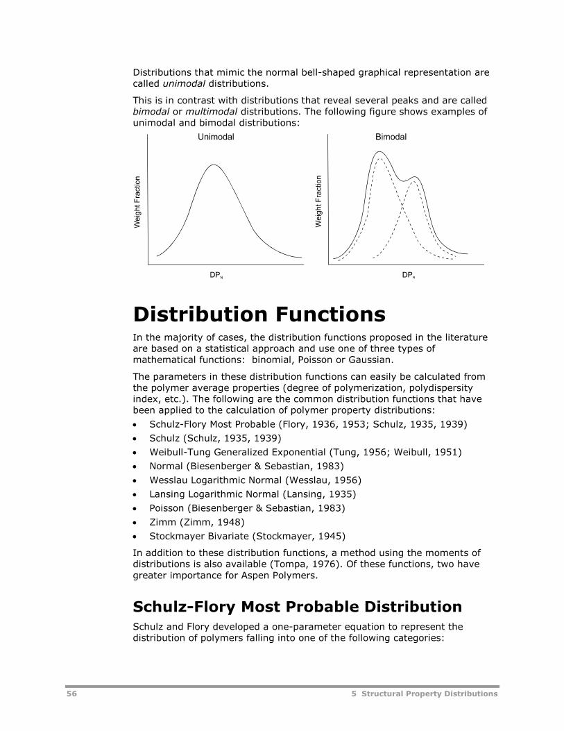
56 5 Structural Property Distributions
Distributions that mimic the normal bell-shaped graphical representation arecalled unimodal distributions.
This is in contrast with distributions that reveal several peaks and are calledbimodal or multimodal distributions. The following figure shows examples ofunimodal and bimodal distributions:
Distribution FunctionsIn the majority of cases, the distribution functions proposed in the literatureare based on a statistical approach and use one of three types ofmathematical functions: binomial, Poisson or Gaussian.
The parameters in these distribution functions can easily be calculated fromthe polymer average properties (degree of polymerization, polydispersityindex, etc.). The following are the common distribution functions that havebeen applied to the calculation of polymer property distributions:
Schulz-Flory Most Probable (Flory, 1936, 1953; Schulz, 1935, 1939)
Schulz (Schulz, 1935, 1939)
Weibull-Tung Generalized Exponential (Tung, 1956; Weibull, 1951)
Normal (Biesenberger & Sebastian, 1983)
Wesslau Logarithmic Normal (Wesslau, 1956)
Lansing Logarithmic Normal (Lansing, 1935)
Poisson (Biesenberger & Sebastian, 1983)
Zimm (Zimm, 1948)
Stockmayer Bivariate (Stockmayer, 1945)
In addition to these distribution functions, a method using the moments ofdistributions is also available (Tompa, 1976). Of these functions, two havegreater importance for Aspen Polymers.
Schulz-Flory Most Probable DistributionSchulz and Flory developed a one-parameter equation to represent thedistribution of polymers falling into one of the following categories:
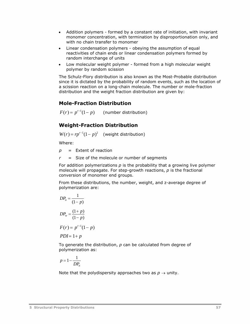
5 Structural Property Distributions 57
Addition polymers - formed by a constant rate of initiation, with invariantmonomer concentration, with termination by disproportionation only, andwith no chain transfer to monomer
Linear condensation polymers - obeying the assumption of equalreactivities of chain ends or linear condensation polymers formed byrandom interchange of units
Low molecular weight polymer - formed from a high molecular weightpolymer by random scission
The Schulz-Flory distribution is also known as the Most-Probable distributionsince it is dictated by the probability of random events, such as the location ofa scission reaction on a long-chain molecule. The number or mole-fractiondistribution and the weight fraction distribution are given by:
Mole-Fraction Distribution
F r p pr( ) ( ) 1 1 (number distribution)
Weight-Fraction Distribution
W r rp pr( ) ( ) 1 21 (weight distribution)
Where:
p = Extent of reaction
r = Size of the molecule or number of segments
For addition polymerizations p is the probability that a growing live polymermolecule will propagate. For step-growth reactions, p is the fractionalconversion of monomer end groups.
From these distributions, the number, weight, and z-average degree ofpolymerization are:
DPp
n
1
1( )
DPp
pw
( )
( )
1
1
F r p pr( ) ( ) 1 1
PDI p 1
To generate the distribution, p can be calculated from degree ofpolymerization as:
pDPn
11
Note that the polydispersity approaches two as p unity.
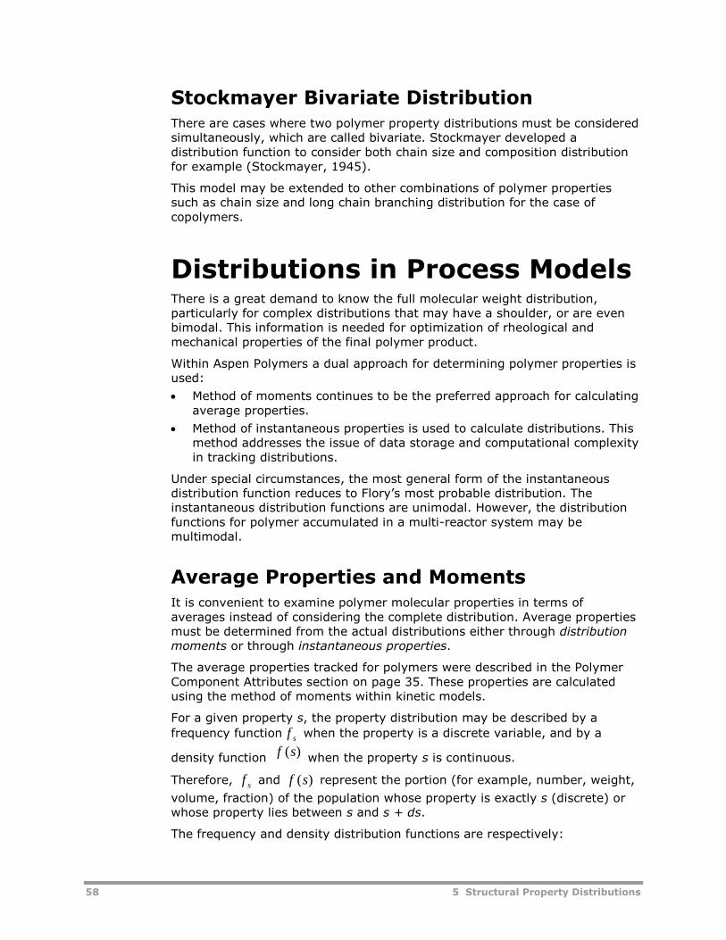
58 5 Structural Property Distributions
Stockmayer Bivariate DistributionThere are cases where two polymer property distributions must be consideredsimultaneously, which are called bivariate. Stockmayer developed adistribution function to consider both chain size and composition distributionfor example (Stockmayer, 1945).
This model may be extended to other combinations of polymer propertiessuch as chain size and long chain branching distribution for the case ofcopolymers.
Distributions in Process ModelsThere is a great demand to know the full molecular weight distribution,particularly for complex distributions that may have a shoulder, or are evenbimodal. This information is needed for optimization of rheological andmechanical properties of the final polymer product.
Within Aspen Polymers a dual approach for determining polymer properties isused:
Method of moments continues to be the preferred approach for calculatingaverage properties.
Method of instantaneous properties is used to calculate distributions. Thismethod addresses the issue of data storage and computational complexityin tracking distributions.
Under special circumstances, the most general form of the instantaneousdistribution function reduces to Flory’s most probable distribution. Theinstantaneous distribution functions are unimodal. However, the distributionfunctions for polymer accumulated in a multi-reactor system may bemultimodal.
Average Properties and MomentsIt is convenient to examine polymer molecular properties in terms ofaverages instead of considering the complete distribution. Average propertiesmust be determined from the actual distributions either through distributionmoments or through instantaneous properties.
The average properties tracked for polymers were described in the PolymerComponent Attributes section on page 35. These properties are calculatedusing the method of moments within kinetic models.
For a given property s, the property distribution may be described by a
frequency function f s when the property is a discrete variable, and by a
density function when the property s is continuous.
Therefore, f s and f s( ) represent the portion (for example, number, weight,
volume, fraction) of the population whose property is exactly s (discrete) orwhose property lies between s and s + ds.
The frequency and density distribution functions are respectively:
f s( )
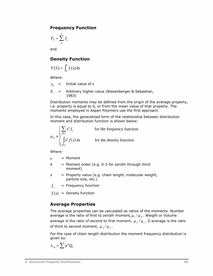
5 Structural Property Distributions 59
Frequency Function
F fS ss
S
0
and
Density Function
F S f s dss
S
( ) ( ) 0
Where:
s0= Initial value of s
S = Arbitrary higher value (Biesenberger & Sebastian,1983)
Distribution moments may be defined from the origin of the average property,i.e. property is equal to 0, or from the mean value of that property. Themoments employed in Aspen Polymers use the first approach.
In this case, the generalized form of the relationship between distributionmoment and distribution function is shown below:
Where:
= Moment
k = Moment order (e.g. 0-3 for zeroth through thirdmoment)
s = Property value (e.g. chain length, molecular weight,particle size, etc.)
f s= Frequency function
f s( ) = Density function
Average Properties
The average properties can be calculated as ratios of the moments. Number
average is the ratio of first to zeroth moment, 1 0/ . Weight or Volume
average is the ratio of second to first moment, 2 1/ . Z-average is the ratio
of third to second moment, 3 2/ .
For the case of chain length distribution the moment frequency distribution isgiven by:
mm
nn Q
k
k
all ss
k
all s
s f
s f s ds
for the frequency function
for the density function
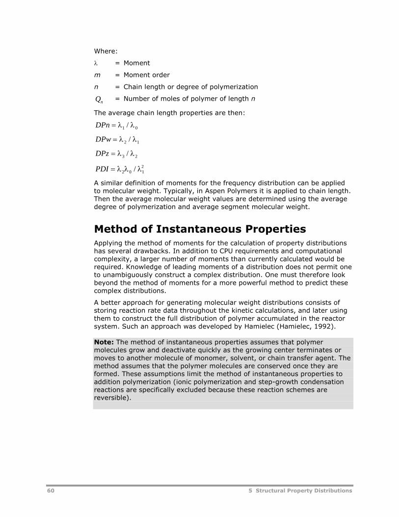
60 5 Structural Property Distributions
Where:
= Moment
m = Moment order
n = Chain length or degree of polymerization
Qn= Number of moles of polymer of length n
The average chain length properties are then:
DPn 1 0/
DPw 2 1/
DPz 3 2/
PDI 2 0 12/
A similar definition of moments for the frequency distribution can be appliedto molecular weight. Typically, in Aspen Polymers it is applied to chain length.Then the average molecular weight values are determined using the averagedegree of polymerization and average segment molecular weight.
Method of Instantaneous PropertiesApplying the method of moments for the calculation of property distributionshas several drawbacks. In addition to CPU requirements and computationalcomplexity, a larger number of moments than currently calculated would berequired. Knowledge of leading moments of a distribution does not permit oneto unambiguously construct a complex distribution. One must therefore lookbeyond the method of moments for a more powerful method to predict thesecomplex distributions.
A better approach for generating molecular weight distributions consists ofstoring reaction rate data throughout the kinetic calculations, and later usingthem to construct the full distribution of polymer accumulated in the reactorsystem. Such an approach was developed by Hamielec (Hamielec, 1992).
Note: The method of instantaneous properties assumes that polymermolecules grow and deactivate quickly as the growing center terminates ormoves to another molecule of monomer, solvent, or chain transfer agent. Themethod assumes that the polymer molecules are conserved once they areformed. These assumptions limit the method of instantaneous properties toaddition polymerization (ionic polymerization and step-growth condensationreactions are specifically excluded because these reaction schemes arereversible).
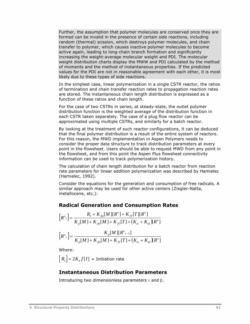
5 Structural Property Distributions 61
Further, the assumption that polymer molecules are conserved once they areformed can be invalid in the presence of certain side reactions, includingrandom (thermal) scission, which destroys polymer molecules, and chaintransfer to polymer, which causes inactive polymer molecules to becomeactive again, leading to long-chain branch formation and significantlyincreasing the weight-average molecular weight and PDI. The molecularweight distribution charts display the MWW and PDI calculated by the methodof moments and the method of instantaneous properties. If the predictedvalues for the PDI are not in reasonable agreement with each other, it is mostlikely due to these types of side reactions.
In the simplest case, linear polymerization in a single CSTR reactor, the ratiosof termination and chain transfer reaction rates to propagation reaction ratesare stored. The instantaneous chain length distribution is expressed as afunction of these ratios and chain length.
For the case of two CSTRs in series, at steady-state, the outlet polymerdistribution function is the weighted average of the distribution function ineach CSTR taken separately. The case of a plug flow reactor can beapproximated using multiple CSTRs, and similarly for a batch reactor.
By looking at the treatment of such reactor configurations, it can be deducedthat the final polymer distribution is a result of the entire system of reactors.For this reason, the MWD implementation in Aspen Polymers needs toconsider the proper data structure to track distribution parameters at everypoint in the flowsheet. Users should be able to request MWD from any point inthe flowsheet, and from this point the Aspen Plus flowsheet connectivityinformation can be used to track polymerization history.
The calculation of chain length distribution for a batch reactor from reactionrate parameters for linear addition polymerization was described by Hamielec(Hamielec, 1992).
Consider the equations for the generation and consumption of free radicals. Asimilar approach may be used for other active centers (Ziegler-Natta,metallocene, etc.):
Radical Generation and Consumption Rates
][][][][
]][[]][[o
tdtcfTfmp
ofT
ofmI
lo
RKKTKMKMK
RTKRMKRR
][][][][
]][[ 1
otdtcfTfmp
ro
pr
o
RKKTKMKMK
RMKR
Where:
R K f II d 2 [ ] = Initiation rate
Instantaneous Distribution Parameters
Introducing two dimensionless parameters and .
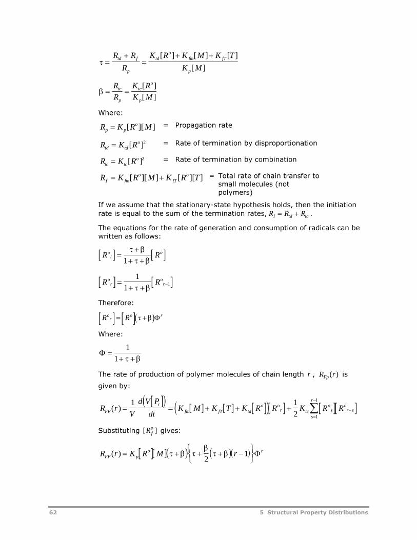
62 5 Structural Property Distributions
R R
R
K R K M K T
K M
td f
p
tdo
fm fT
p
[ ] [ ] [ ]
[ ]
R
R
K R
K Mtc
p
tco
p
[ ]
[ ]
Where:
R K R Mp po [ ][ ] = Propagation rate
R K Rtd tdo [ ]2 = Rate of termination by disproportionation
R K Rtc tco [ ]2 = Rate of termination by combination
R K R M K R Tf fmo
fTo [ ][ ] [ ][ ] = Total rate of chain transfer to
small molecules (notpolymers)
If we assume that the stationary-state hypothesis holds, then the initiation
rate is equal to the sum of the termination rates, R R RI td tc .
The equations for the rate of generation and consumption of radicals can bewritten as follows:
R Rol
o
1
R Ror
or
1
11
Therefore:
R Ror
o r
Where:
1
1
The rate of production of polymer molecules of chain length r , R rFp ( ) is
given by:
R r
V
d V P
dtK M K T K R R K R RFP
r
fm fT tdo o
r tco
s
s
ro
r s( )
1 1
2 1
1
Substituting [ ]R fo
gives:
R r K R M rFP po r( )
2
1
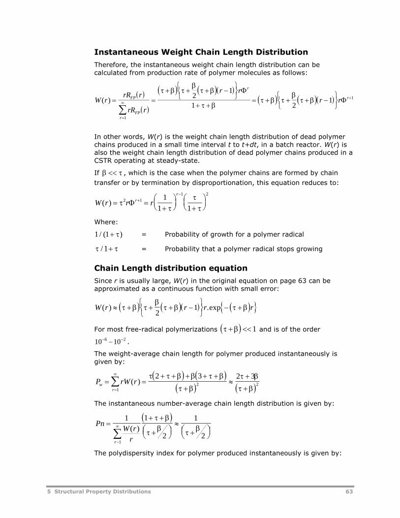
5 Structural Property Distributions 63
Instantaneous Weight Chain Length Distribution
Therefore, the instantaneous weight chain length distribution can becalculated from production rate of polymer molecules as follows:
W r
rR r
rR r
r r
r rFP
FPr
r
r( )
1
121
1 21
In other words, W(r) is the weight chain length distribution of dead polymerchains produced in a small time interval t to t+dt, in a batch reactor. W(r) isalso the weight chain length distribution of dead polymer chains produced in aCSTR operating at steady-state.
If , which is the case when the polymer chains are formed by chain
transfer or by termination by disproportionation, this equation reduces to:
W r r rr
r
( )
2 1
1 21
1 1
Where:
1 1/ ( ) = Probability of growth for a polymer radical
/ 1 = Probability that a polymer radical stops growing
Chain Length distribution equation
Since r is usually large, W(r) in the original equation on page 63 can beapproximated as a continuous function with small error:
W r r r r( ) .exp
2
1
For most free-radical polymerizations 1 and is of the order
10 106 2 .
The weight-average chain length for polymer produced instantaneously isgiven by:
P rW rwr
( )1
2 2
2 3 2 3
The instantaneous number-average chain length distribution is given by:
Pn
W r
rr
1 1
2
1
21
( )
The polydispersity index for polymer produced instantaneously is given by:
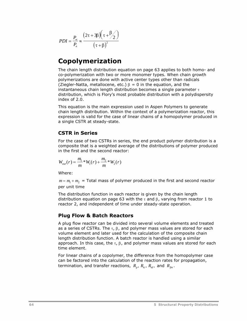
64 5 Structural Property Distributions
PDI
P
Pw
n
2 3 22
CopolymerizationThe chain length distribution equation on page 63 applies to both homo- andco-polymerization with two or more monomer types. When chain growthpolymerizations are done with active center types other than radicals(Ziegler-Natta, metallocene, etc.) = 0 in the equation, and theinstantaneous chain length distribution becomes a single parameter distribution, which is Flory’s most probable distribution with a polydispersityindex of 2.0.
This equation is the main expression used in Aspen Polymers to generatechain length distribution. Within the context of a polymerization reactor, thisexpression is valid for the case of linear chains of a homopolymer produced ina single CSTR at steady-state.
CSTR in Series
For the case of two CSTRs in series, the end product polymer distribution is acomposite that is a weighted average of the distributions of polymer producedin the first and the second reactor:
W rm
mW r
m
mW rout ( ) * ( ) * ( ) 1
12
2
Where:
m m m 1 2 = Total mass of polymer produced in the first and second reactor
per unit time
The distribution function in each reactor is given by the chain lengthdistribution equation on page 63 with the and , varying from reactor 1 toreactor 2, and independent of time under steady-state operation.
Plug Flow & Batch Reactors
A plug flow reactor can be divided into several volume elements and treatedas a series of CSTRs. The , , and polymer mass values are stored for eachvolume element and later used for the calculation of the composite chainlength distribution function. A batch reactor is handled using a similarapproach. In this case, the , , and polymer mass values are stored for eachtime element.
For linear chains of a copolymer, the difference from the homopolymer casecan be factored into the calculation of the reaction rates for propagation,
termination, and transfer reactions, R R Rp tc td, , , and R fm .
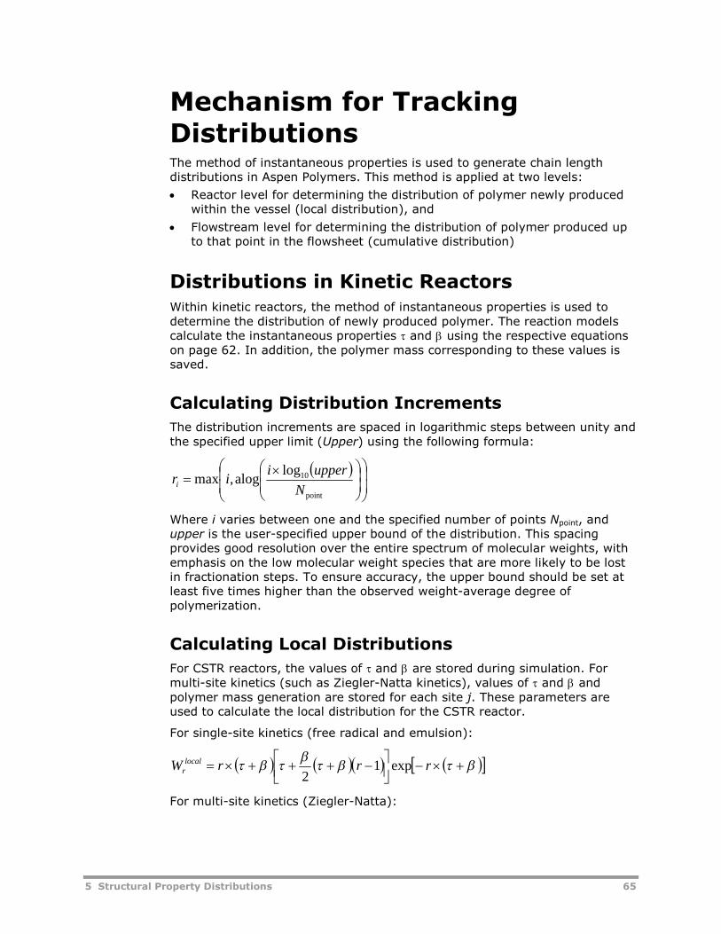
5 Structural Property Distributions 65
Mechanism for TrackingDistributionsThe method of instantaneous properties is used to generate chain lengthdistributions in Aspen Polymers. This method is applied at two levels:
Reactor level for determining the distribution of polymer newly producedwithin the vessel (local distribution), and
Flowstream level for determining the distribution of polymer produced upto that point in the flowsheet (cumulative distribution)
Distributions in Kinetic ReactorsWithin kinetic reactors, the method of instantaneous properties is used todetermine the distribution of newly produced polymer. The reaction modelscalculate the instantaneous properties and using the respective equationson page 62. In addition, the polymer mass corresponding to these values issaved.
Calculating Distribution Increments
The distribution increments are spaced in logarithmic steps between unity andthe specified upper limit (Upper) using the following formula:
point
10logalog,max
N
upperiiri
Where i varies between one and the specified number of points Npoint, andupper is the user-specified upper bound of the distribution. This spacingprovides good resolution over the entire spectrum of molecular weights, withemphasis on the low molecular weight species that are more likely to be lostin fractionation steps. To ensure accuracy, the upper bound should be set atleast five times higher than the observed weight-average degree ofpolymerization.
Calculating Local Distributions
For CSTR reactors, the values of and are stored during simulation. Formulti-site kinetics (such as Ziegler-Natta kinetics), values of and andpolymer mass generation are stored for each site j. These parameters areused to calculate the local distribution for the CSTR reactor.
For single-site kinetics (free radical and emulsion):
rrrW local
r exp12
For multi-site kinetics (Ziegler-Natta):
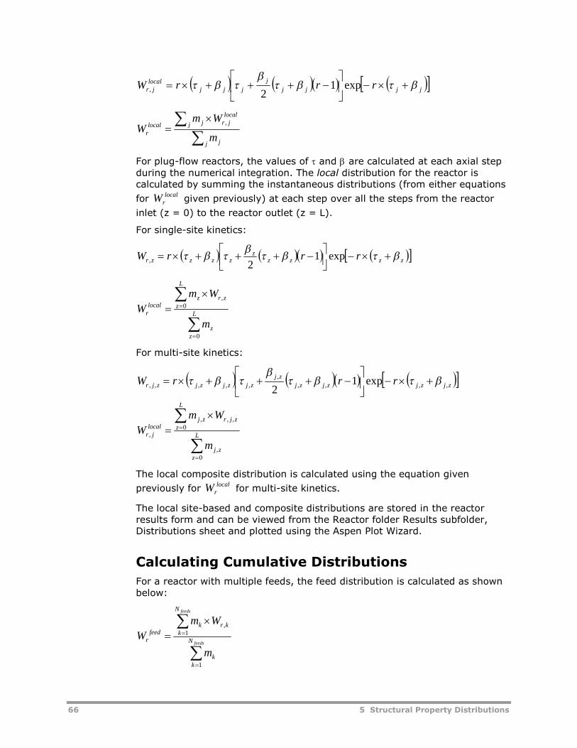
66 5 Structural Property Distributions
jjjj
j
jjjlocal
jr rrrW
exp1
2,
j j
j
localjrjlocal
rm
WmW
,
For plug-flow reactors, the values of and are calculated at each axial stepduring the numerical integration. The local distribution for the reactor iscalculated by summing the instantaneous distributions (from either equations
forlocal
rW given previously) at each step over all the steps from the reactor
inlet (z = 0) to the reactor outlet (z = L).
For single-site kinetics:
zzzzz
zzzzr rrrW
exp1
2,
L
zz
L
zzrz
localr
m
Wm
W
0
0,
For multi-site kinetics:
zjzjzjzj
zj
zjzjzjzjr rrrW ,,,,
,
,,,,, exp12
L
zzj
L
zzjrzj
localjr
m
Wm
W
0,
0,,,
,
The local composite distribution is calculated using the equation given
previously forlocal
rW for multi-site kinetics.
The local site-based and composite distributions are stored in the reactorresults form and can be viewed from the Reactor folder Results subfolder,Distributions sheet and plotted using the Aspen Plot Wizard.
Calculating Cumulative Distributions
For a reactor with multiple feeds, the feed distribution is calculated as shownbelow:
feeds
feeds
N
kk
N
kkrk
feedr
m
Wm
W
1
1,
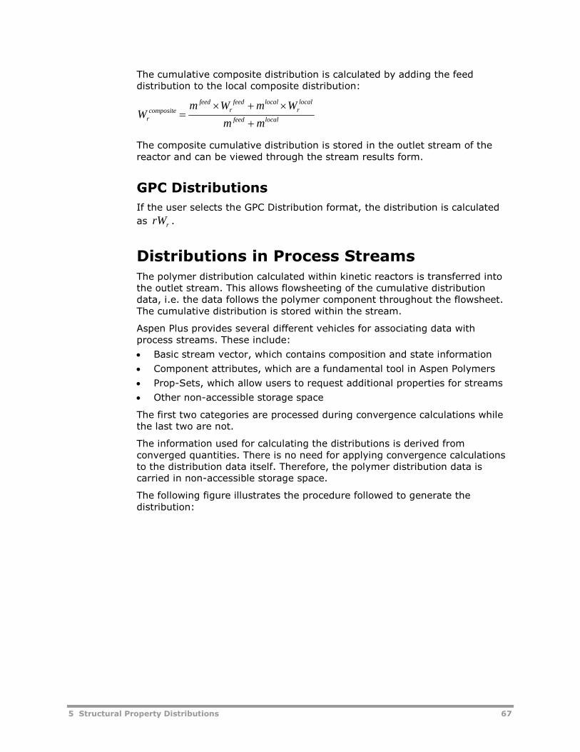
5 Structural Property Distributions 67
The cumulative composite distribution is calculated by adding the feeddistribution to the local composite distribution:
localfeed
localr
localfeedr
feed
compositer
mm
WmWmW
The composite cumulative distribution is stored in the outlet stream of thereactor and can be viewed through the stream results form.
GPC Distributions
If the user selects the GPC Distribution format, the distribution is calculated
as rrW .
Distributions in Process StreamsThe polymer distribution calculated within kinetic reactors is transferred intothe outlet stream. This allows flowsheeting of the cumulative distributiondata, i.e. the data follows the polymer component throughout the flowsheet.The cumulative distribution is stored within the stream.
Aspen Plus provides several different vehicles for associating data withprocess streams. These include:
Basic stream vector, which contains composition and state information
Component attributes, which are a fundamental tool in Aspen Polymers
Prop-Sets, which allow users to request additional properties for streams
Other non-accessible storage space
The first two categories are processed during convergence calculations whilethe last two are not.
The information used for calculating the distributions is derived fromconverged quantities. There is no need for applying convergence calculationsto the distribution data itself. Therefore, the polymer distribution data iscarried in non-accessible storage space.
The following figure illustrates the procedure followed to generate thedistribution:
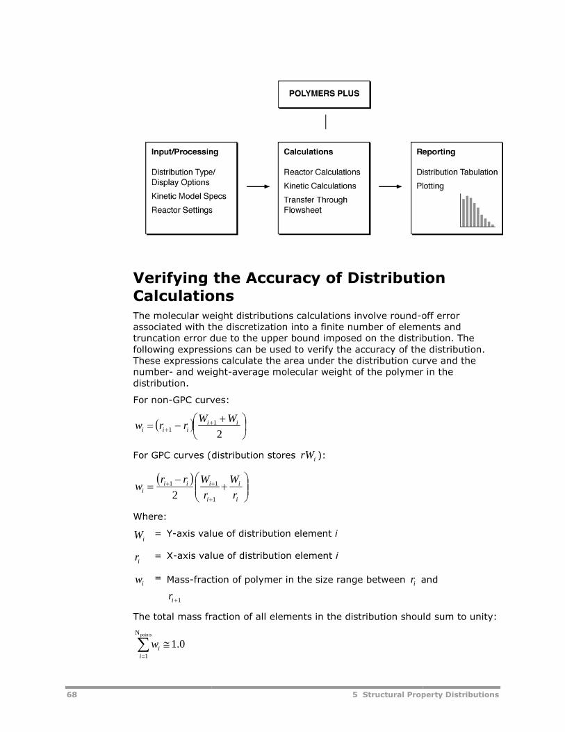
68
Verifying the Accuracy of DistributionCalculationsThe molecular weight distributions calculations involve roundassociated with the discretization into a finite number of elements andtruncation error due to the upper bound imposed on the distributionfollowing expressions can be used to verify the accuracy of the distribution.These expressions calculate the area under the distribution curve and thenumber- and weightdistribution.
For non-GPC curve
1i
iii
Wrrw
For GPC curves (distribution stores
i
iiii
r
Wrrw 1
2
Where:
iW = Y-axis value of distribution element
ir = X-axis value of distribution element
iw = Mass-fraction of polymer in the size range between
1ir
The total mass fraction of all elements in the distribution should sum to unity:
0.1pointsN
1
i
iw
5 Structural Property Distributions
Verifying the Accuracy of DistributionCalculationsThe molecular weight distributions calculations involve round-off errorassociated with the discretization into a finite number of elements andtruncation error due to the upper bound imposed on the distributionfollowing expressions can be used to verify the accuracy of the distribution.These expressions calculate the area under the distribution curve and the
and weight-average molecular weight of the polymer in the
GPC curves:
21 iW
curves (distribution stores irW ):
i
i
r
W
1
1
axis value of distribution element i
axis value of distribution element i
fraction of polymer in the size range between ir and
The total mass fraction of all elements in the distribution should sum to unity:
5 Structural Property Distributions
Verifying the Accuracy of Distribution
off errorassociated with the discretization into a finite number of elements andtruncation error due to the upper bound imposed on the distribution. Thefollowing expressions can be used to verify the accuracy of the distribution.These expressions calculate the area under the distribution curve and the
average molecular weight of the polymer in the
and
The total mass fraction of all elements in the distribution should sum to unity:
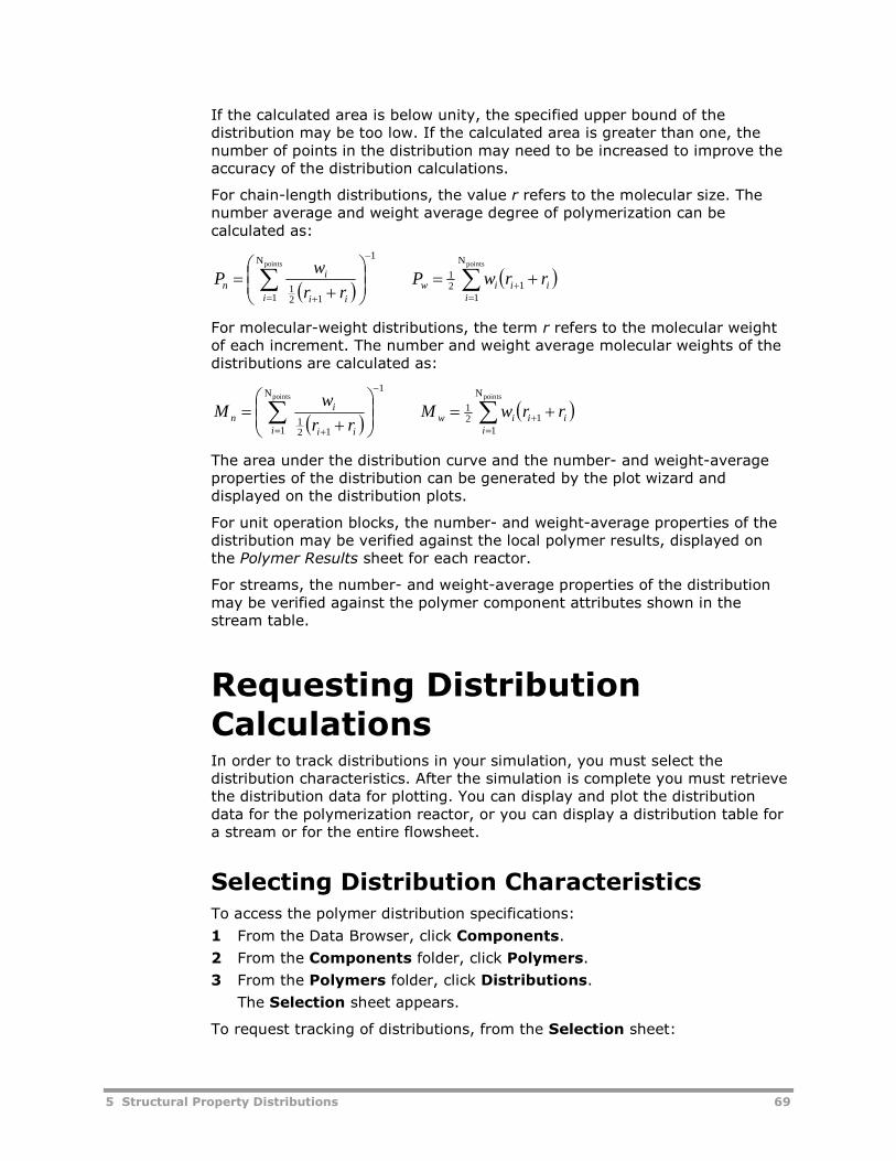
5 Structural Property Distributions 69
If the calculated area is below unity, the specified upper bound of thedistribution may be too low. If the calculated area is greater than one, thenumber of points in the distribution may need to be increased to improve theaccuracy of the distribution calculations.
For chain-length distributions, the value r refers to the molecular size. Thenumber average and weight average degree of polymerization can becalculated as:
1N
1 121
points
i ii
in
rr
wP
pointsN
112
1
iiiiw rrwP
For molecular-weight distributions, the term r refers to the molecular weightof each increment. The number and weight average molecular weights of thedistributions are calculated as:
1N
1 121
points
i ii
in
rr
wM
pointsN
112
1
iiiiw rrwM
The area under the distribution curve and the number- and weight-averageproperties of the distribution can be generated by the plot wizard anddisplayed on the distribution plots.
For unit operation blocks, the number- and weight-average properties of thedistribution may be verified against the local polymer results, displayed onthe Polymer Results sheet for each reactor.
For streams, the number- and weight-average properties of the distributionmay be verified against the polymer component attributes shown in thestream table.
Requesting DistributionCalculationsIn order to track distributions in your simulation, you must select thedistribution characteristics. After the simulation is complete you must retrievethe distribution data for plotting. You can display and plot the distributiondata for the polymerization reactor, or you can display a distribution table fora stream or for the entire flowsheet.
Selecting Distribution CharacteristicsTo access the polymer distribution specifications:
1 From the Data Browser, click Components.
2 From the Components folder, click Polymers.
3 From the Polymers folder, click Distributions.
The Selection sheet appears.
To request tracking of distributions, from the Selection sheet:
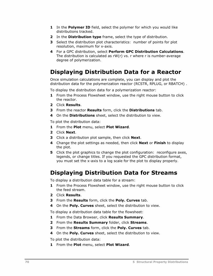
70 5 Structural Property Distributions
1 In the Polymer ID field, select the polymer for which you would likedistributions tracked.
2 In the Distribution type frame, select the type of distribution.
3 Select the distribution plot characteristics: number of points for plotresolution, maximum for x-axis.
4 For a GPC distribution, select Perform GPC Distribution Calculations.The distribution is calculated as rW(r) vs. r where r is number-averagedegree of polymerization.
Displaying Distribution Data for a ReactorOnce simulation calculations are complete, you can display and plot thedistribution data for the polymerization reactor (RCSTR, RPLUG, or RBATCH) .
To display the distribution data for a polymerization reactor:
1 From the Process Flowsheet window, use the right mouse button to clickthe reactor.
2 Click Results.
3 From the reactor Results form, click the Distributions tab.
4 On the Distributions sheet, select the distribution to view.
To plot the distribution data:
1 From the Plot menu, select Plot Wizard.
2 Click Next.
3 Click a distribution plot sample, then click Next.
4 Change the plot settings as needed, then click Next or Finish to displaythe plot.
5 Click the plot graphics to change the plot configuration: reconfigure axes,legends, or change titles. If you requested the GPC distribution format,you must set the x-axis to a log scale for the plot to display properly.
Displaying Distribution Data for StreamsTo display a distribution data table for a stream:
1 From the Process Flowsheet window, use the right mouse button to clickthe feed stream.
2 Click Results.
3 From the Results form, click the Poly. Curves tab.
4 On the Poly. Curves sheet, select the distribution to view.
To display a distribution data table for the flowsheet:
1 From the Data Browser, click Results Summary.
2 From the Results Summary folder, click Streams.
3 From the Streams form, click the Poly. Curves tab.
4 On the Poly. Curves sheet, select the distribution to view.
To plot the distribution data:
1 From the Plot menu, select Plot Wizard.
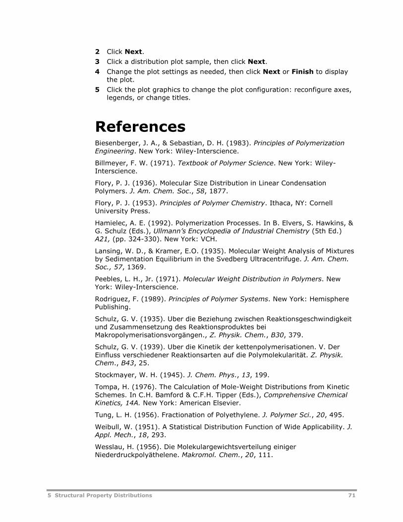
5 Structural Property Distributions 71
2 Click Next.
3 Click a distribution plot sample, then click Next.
4 Change the plot settings as needed, then click Next or Finish to displaythe plot.
5 Click the plot graphics to change the plot configuration: reconfigure axes,legends, or change titles.
ReferencesBiesenberger, J. A., & Sebastian, D. H. (1983). Principles of PolymerizationEngineering. New York: Wiley-Interscience.
Billmeyer, F. W. (1971). Textbook of Polymer Science. New York: Wiley-Interscience.
Flory, P. J. (1936). Molecular Size Distribution in Linear CondensationPolymers. J. Am. Chem. Soc., 58, 1877.
Flory, P. J. (1953). Principles of Polymer Chemistry. Ithaca, NY: CornellUniversity Press.
Hamielec, A. E. (1992). Polymerization Processes. In B. Elvers, S. Hawkins, &G. Schulz (Eds.), Ullmann’s Encyclopedia of Industrial Chemistry (5th Ed.)A21, (pp. 324-330). New York: VCH.
Lansing, W. D., & Kramer, E.O. (1935). Molecular Weight Analysis of Mixturesby Sedimentation Equilibrium in the Svedberg Ultracentrifuge. J. Am. Chem.Soc., 57, 1369.
Peebles, L. H., Jr. (1971). Molecular Weight Distribution in Polymers. NewYork: Wiley-Interscience.
Rodriguez, F. (1989). Principles of Polymer Systems. New York: HemispherePublishing.
Schulz, G. V. (1935). Uber die Beziehung zwischen Reaktionsgeschwindigkeitund Zusammensetzung des Reaktionsproduktes beiMakropolymerisationsvorgängen., Z. Physik. Chem., B30, 379.
Schulz, G. V. (1939). Uber die Kinetik der kettenpolymerisationen. V. DerEinfluss verschiedener Reaktionsarten auf die Polymolekularität. Z. Physik.Chem., B43, 25.
Stockmayer, W. H. (1945). J. Chem. Phys., 13, 199.
Tompa, H. (1976). The Calculation of Mole-Weight Distributions from KineticSchemes. In C.H. Bamford & C.F.H. Tipper (Eds.), Comprehensive ChemicalKinetics, 14A. New York: American Elsevier.
Tung, L. H. (1956). Fractionation of Polyethylene. J. Polymer Sci., 20, 495.
Weibull, W. (1951). A Statistical Distribution Function of Wide Applicability. J.Appl. Mech., 18, 293.
Wesslau, H. (1956). Die Molekulargewichtsverteilung einigerNiederdruckpolyäthelene. Makromol. Chem., 20, 111.
72 5 Structural Property Distributions
Zimm, B. H. (1948). Apparatus and Methods for Measurement andInterpretation of the Angular Variation of Light Scattering; Preliminary Resultson Polystyrene Solutions. J. Chem. Phys., 16, 1099.
6 End-Use Properties 73
6 End-Use Properties
This section describes polymer end-use properties. First, an overview of theproperties of interest for polymers is given, followed by methods available inAspen Polymers (formerly known as Aspen Polymers Plus) for calculatingthese properties.
Topics covered include:
Polymer Properties, 73
Prop-Set Properties, 73
End-Use Properties, 74
Method for Calculating End-Use Properties, 76
Calculating End-Use Properties, 79
Polymer PropertiesPolymer properties fall into many categories:
Structural properties
Thermophysical properties - which provide an indication of thethermodynamic behavior of polymers
Thermochemical properties - which provide information on thermalstability
Transport properties
Processing and end-use properties - which provide information aboutprocessability and performance during end-use
Polymer structural properties do not provide a direct measure of theperformance of the polymer product during processing or during its end use.
However, there is a relationship between polymer structural properties andthe end use properties. For this reason, it is important to account for suchproperties within polymer process simulation models.
Prop-Set PropertiesA property set is a collection of thermodynamic, transport, and otherproperties that you can use in:
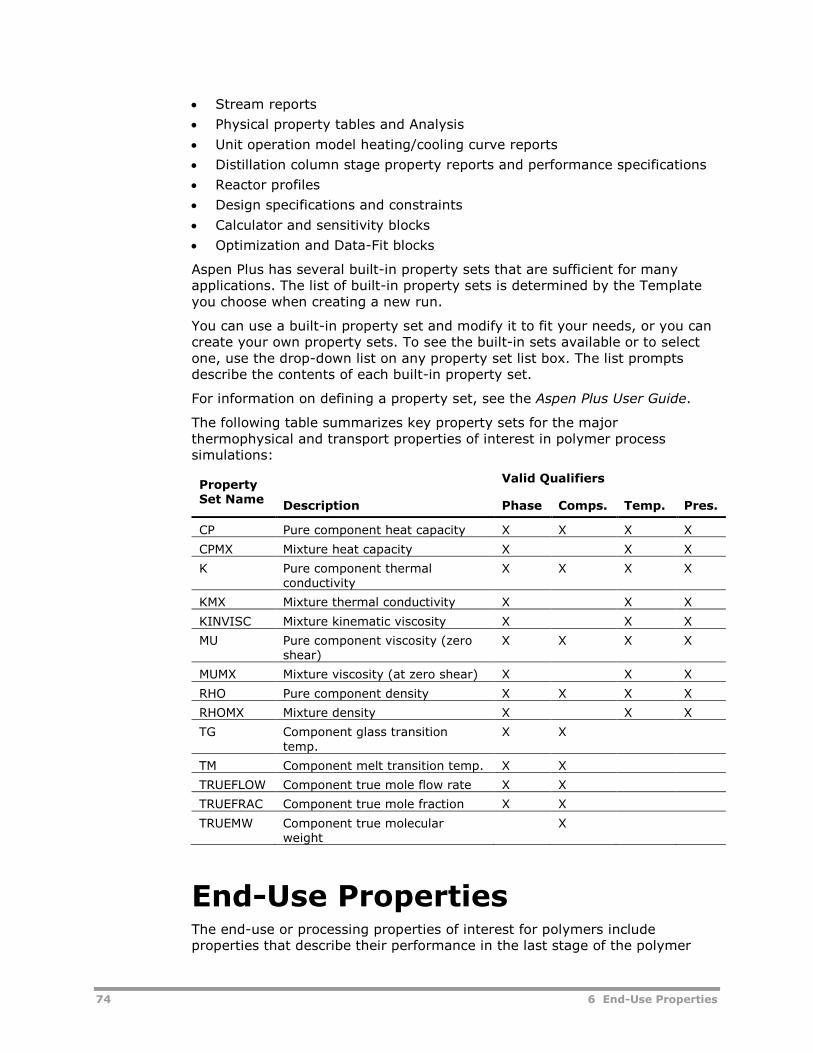
74 6 End-Use Properties
Stream reports
Physical property tables and Analysis
Unit operation model heating/cooling curve reports
Distillation column stage property reports and performance specifications
Reactor profiles
Design specifications and constraints
Calculator and sensitivity blocks
Optimization and Data-Fit blocks
Aspen Plus has several built-in property sets that are sufficient for manyapplications. The list of built-in property sets is determined by the Templateyou choose when creating a new run.
You can use a built-in property set and modify it to fit your needs, or you cancreate your own property sets. To see the built-in sets available or to selectone, use the drop-down list on any property set list box. The list promptsdescribe the contents of each built-in property set.
For information on defining a property set, see the Aspen Plus User Guide.
The following table summarizes key property sets for the majorthermophysical and transport properties of interest in polymer processsimulations:
PropertySet Name
Description
Valid Qualifiers
Phase Comps. Temp. Pres.
CP Pure component heat capacity X X X X
CPMX Mixture heat capacity X X X
K Pure component thermalconductivity
X X X X
KMX Mixture thermal conductivity X X X
KINVISC Mixture kinematic viscosity X X X
MU Pure component viscosity (zeroshear)
X X X X
MUMX Mixture viscosity (at zero shear) X X X
RHO Pure component density X X X X
RHOMX Mixture density X X X
TG Component glass transitiontemp.
X X
TM Component melt transition temp. X X
TRUEFLOW Component true mole flow rate X X
TRUEFRAC Component true mole fraction X X
TRUEMW Component true molecularweight
X
End-Use PropertiesThe end-use or processing properties of interest for polymers includeproperties that describe their performance in the last stage of the polymer
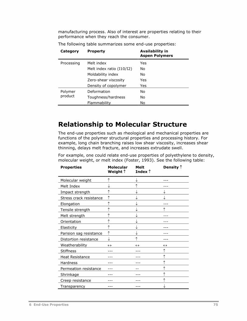
6 End-Use Properties 75
manufacturing process. Also of interest are properties relating to theirperformance when they reach the consumer.
The following table summarizes some end-use properties:
Category Property Availability inAspen Polymers
Processing Melt index
Melt index ratio (I10/I2)
Moldability index
Zero-shear viscosity
Density of copolymer
Yes
No
No
Yes
Yes
Polymerproduct
Deformation
Toughness/hardness
Flammability
No
No
No
Relationship to Molecular StructureThe end-use properties such as rheological and mechanical properties arefunctions of the polymer structural properties and processing history. Forexample, long chain branching raises low shear viscosity, increases shearthinning, delays melt fracture, and increases extrudate swell.
For example, one could relate end-use properties of polyethylene to density,molecular weight, or melt index (Foster, 1993). See the following table:
Properties MolecularWeight
MeltIndex
Density
Molecular weight ---
Melt Index ---
Impact strength
Stress crack resistance
Elongation ---
Tensile strength
Melt strength ---
Orientation ---
Elasticity ---
Parision sag resistance ---
Distortion resistance ---
Weatherability
Stiffness --- ---
Heat Resistance --- ---
Hardness --- ---
Permeation resistance --- --
Shrinkage --- ---
Creep resistance --- ---
Transparency --- ---
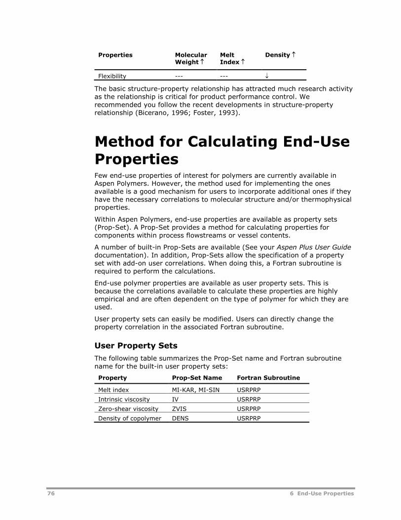
76 6 End-Use Properties
Properties MolecularWeight
MeltIndex
Density
Flexibility --- ---
The basic structure-property relationship has attracted much research activityas the relationship is critical for product performance control. Werecommended you follow the recent developments in structure-propertyrelationship (Bicerano, 1996; Foster, 1993).
Method for Calculating End-UsePropertiesFew end-use properties of interest for polymers are currently available inAspen Polymers. However, the method used for implementing the onesavailable is a good mechanism for users to incorporate additional ones if theyhave the necessary correlations to molecular structure and/or thermophysicalproperties.
Within Aspen Polymers, end-use properties are available as property sets(Prop-Set). A Prop-Set provides a method for calculating properties forcomponents within process flowstreams or vessel contents.
A number of built-in Prop-Sets are available (See your Aspen Plus User Guidedocumentation). In addition, Prop-Sets allow the specification of a propertyset with add-on user correlations. When doing this, a Fortran subroutine isrequired to perform the calculations.
End-use polymer properties are available as user property sets. This isbecause the correlations available to calculate these properties are highlyempirical and are often dependent on the type of polymer for which they areused.
User property sets can easily be modified. Users can directly change theproperty correlation in the associated Fortran subroutine.
User Property Sets
The following table summarizes the Prop-Set name and Fortran subroutinename for the built-in user property sets:
Property Prop-Set Name Fortran Subroutine
Melt index MI-KAR, MI-SIN USRPRP
Intrinsic viscosity IV USRPRP
Zero-shear viscosity ZVIS USRPRP
Density of copolymer DENS USRPRP
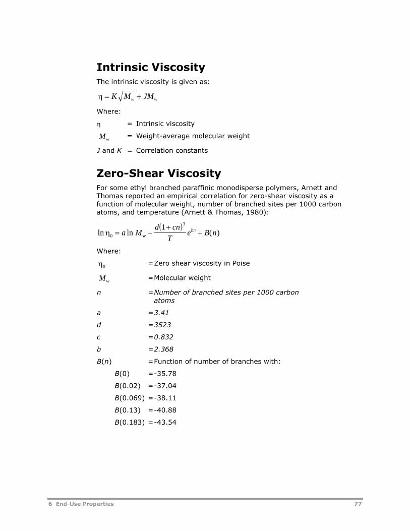
6 End-Use Properties 77
Intrinsic ViscosityThe intrinsic viscosity is given as:
K M JMw w
Where:
= Intrinsic viscosity
Mw= Weight-average molecular weight
J and K = Correlation constants
Zero-Shear ViscosityFor some ethyl branched paraffinic monodisperse polymers, Arnett andThomas reported an empirical correlation for zero-shear viscosity as afunction of molecular weight, number of branched sites per 1000 carbonatoms, and temperature (Arnett & Thomas, 1980):
ln ln ( )0
31
a Md cn
Te B nw
bn
Where:
0=Zero shear viscosity in Poise
Mw=Molecular weight
n =Number of branched sites per 1000 carbonatoms
a =3.41
d =3523
c =0.832
b =2.368
B(n) =Function of number of branches with:
B(0) =-35.78
B(0.02) =-37.04
B(0.069) =-38.11
B(0.13) =-40.88
B(0.183) =-43.54
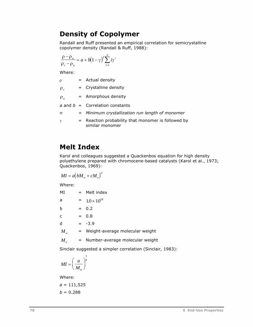
78 6 End-Use Properties
Density of CopolymerRandall and Ruff presented an empirical correlation for semicrystallinecopolymer density (Randall & Ruff, 1988):
Where:
= Actual density
c= Crystalline density
a= Amorphous density
a and b = Correlation constants
n = Minimum crystallization run length of monomer
= Reaction probability that monomer is followed bysimilar monomer
Melt IndexKarol and colleagues suggested a Quackenbos equation for high densitypolyethylene prepared with chromocene-based catalysts (Karol et al., 1973;Quackenbos, 1969):
MI a bM cMw n
d
Where:
MI = Melt index
a = 10 1018.
b = 0.2
c = 0.8
d = -3.9
Mw= Weight-average molecular weight
M n= Number-average molecular weight
Sinclair suggested a simpler correlation (Sinclair, 1983):
MIa
Mw
b
1
Where:
a = 111,525
b = 0.288
a
c a
i
i
n
a b i12
1
6 End-Use Properties 79
Melt Index RatioThe Quackenbos equation can also be used to correlate melt index ratio.
Calculating End-Use PropertiesEnd-use properties are calculated as Prop-Sets. You must first select whichend-use property to include in the simulation, then you must define thisproperty as a Prop-Set.
Selecting an End-Use PropertyTo access end-use property Prop-Sets:
1 From the Data Browser, click Properties.
2 From the Properties folder, click Advanced.
3 From the Advanced folder, click User Properties.
4 From the User Properties object manager, click New.
5 If necessary, change the default ID for the user-property and click OK.
6 From the User Properties Specifications sheet, choose the standardproperty as the type (default), then provide the subroutine name.
Create one User-Property for each end-use property.
Adding an End-Use Property Prop-SetTo access Prop-Sets:
1 From the Data Browser, click Properties.
2 From the Properties folder, click Prop-Sets.
3 From the Prop-Sets object manager, click New.
4 If necessary, change the default ID for the Prop-set and click OK.
5 From the Prop-Set Properties sheet, in the Physical Properties field,select the ID for the end-use property User-Property.
You can have as many User-Properties as needed.
ReferencesArnett, R. L. & Thomas, C. P. (1980). Zero-Shear Viscosity of Some EthylBranched Paraffinic Model Polymers. J. Phys. Chem., 84, 649-652.
Aspen Plus User Guide. Burlington, MA: Aspen Technology, Inc.
Bicerano, J. (1996). Prediction of Polymer Properties. New York: MarcelDekker.
Foster, G.N. (1993). Short Course: Polymer Reaction Engineering. Ontario,Canada: McMaster Institute for Polymer Production Technology.
80 6 End-Use Properties
Grulke, E. A. (1994). Polymer Process Engineering. Englewood Cliffs, NJ:Prentice Hall.
Hamielec, A. E. (1996), Polymer Reactor Modeling Technology (CourseNotes). Cambridge, MA: Aspen Technology, Inc.
Karol, F. J., Brown, G. L., & Davison, J. M. (1973) Chromocene-BasedCatalysts for Ethylene Polymerization: Kinetic Parameters. J. of PolymerScience: Polymer Chemistry Edition, 11, 413-424.
Quackenbos, H. M. (1969). Practical Use of Intrinsic Viscosity forPolyethylenes. J. of Applied Polymer Science, 13, 341-351.
Randall, J. C. & Ruff, C. J. (1988). A New Look at the 'Run Number' Conceptin Copolymer Characterization. Macromolecules, 21, 3446-3454.
Rudin, A. (1982). The Elements of Polymer Science and Engineering. NewYork: Academic Press Inc., Harcourt Brace Jovanovich.
Sinclair, K. B. (1983). Characteristics of Linear LPPE and Description of UCCGas Phase Process, Process Economics Report. Menlo Park, CA: SRIInternational.
7 Polymerization Reactions 81
7 Polymerization Reactions
This chapter discusses polymerization mechanisms and kinetics. Topicsdiscussed in the introductory section include:
Polymerization Reaction Categories, 81
Polymerization Process Types, 84
Aspen Polymers Reaction Models, 85
Following an introduction that provides background information of thesubject, a separate section is devoted to each of the polymerization kineticmodels available in Aspen Polymers (formerly known as Aspen PolymersPlus).
Step-Growth Polymerization Model, 89
Free-Radical Bulk Polymerization Model,
Emulsion Polymerization Model,
Ziegler-Natta Polymerization Model,
Ionic Polymerization Model,
Segment-Based Reaction Model,
Polymerization ReactionCategoriesOver the years, many classifications have been developed for polymerizationreactions. One classification divides them into condensation and additionpolymerization.
Condensation Polymerization
Condensation polymerization results in the elimination of a smaller molecule,water for example, through the reaction of bi- or polyfunctional monomers.
Addition Polymerization
Addition polymerization, on the other hand, does not produce small moleculebyproducts. The repeating units within the polymer have the same structureas the monomers from which they originated.
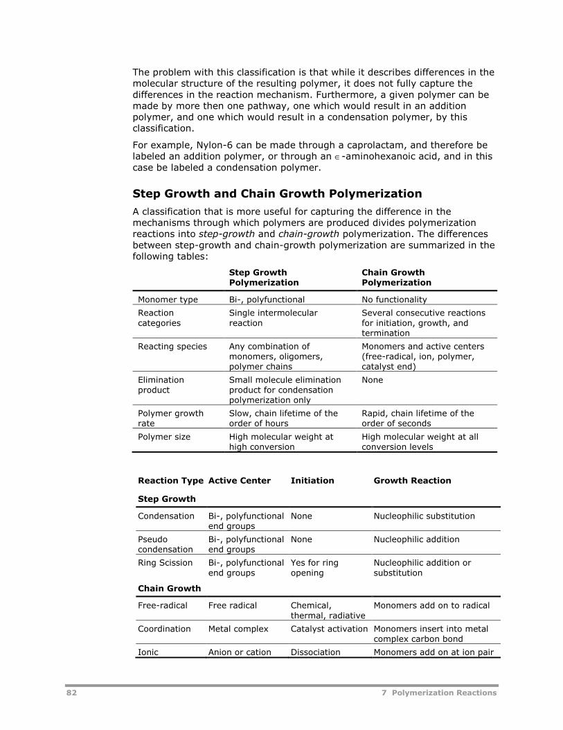
82 7 Polymerization Reactions
The problem with this classification is that while it describes differences in themolecular structure of the resulting polymer, it does not fully capture thedifferences in the reaction mechanism. Furthermore, a given polymer can bemade by more then one pathway, one which would result in an additionpolymer, and one which would result in a condensation polymer, by thisclassification.
For example, Nylon-6 can be made through a caprolactam, and therefore belabeled an addition polymer, or through an -aminohexanoic acid, and in thiscase be labeled a condensation polymer.
Step Growth and Chain Growth Polymerization
A classification that is more useful for capturing the difference in themechanisms through which polymers are produced divides polymerizationreactions into step-growth and chain-growth polymerization. The differencesbetween step-growth and chain-growth polymerization are summarized in thefollowing tables:
Step GrowthPolymerization
Chain GrowthPolymerization
Monomer type Bi-, polyfunctional No functionality
Reactioncategories
Single intermolecularreaction
Several consecutive reactionsfor initiation, growth, andtermination
Reacting species Any combination ofmonomers, oligomers,polymer chains
Monomers and active centers(free-radical, ion, polymer,catalyst end)
Eliminationproduct
Small molecule eliminationproduct for condensationpolymerization only
None
Polymer growthrate
Slow, chain lifetime of theorder of hours
Rapid, chain lifetime of theorder of seconds
Polymer size High molecular weight athigh conversion
High molecular weight at allconversion levels
Reaction Type Active Center Initiation Growth Reaction
Step Growth
Condensation Bi-, polyfunctionalend groups
None Nucleophilic substitution
Pseudocondensation
Bi-, polyfunctionalend groups
None Nucleophilic addition
Ring Scission Bi-, polyfunctionalend groups
Yes for ringopening
Nucleophilic addition orsubstitution
Chain Growth
Free-radical Free radical Chemical,thermal, radiative
Monomers add on to radical
Coordination Metal complex Catalyst activation Monomers insert into metalcomplex carbon bond
Ionic Anion or cation Dissociation Monomers add on at ion pair
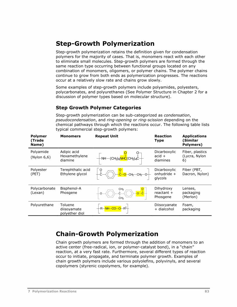
7 Polymerization Reactions 83
Step-Growth PolymerizationStep-growth polymerization retains the definition given for condensationpolymers for the majority of cases. That is, monomers react with each otherto eliminate small molecules. Step-growth polymers are formed through thesame reaction type occurring between functional groups located on anycombination of monomers, oligomers, or polymer chains. The polymer chainscontinue to grow from both ends as polymerization progresses. The reactionsoccur at a relatively slow rate and chains grow slowly.
Some examples of step-growth polymers include polyamides, polyesters,polycarbonates, and polyurethanes (See Polymer Structure in Chapter 2 for adiscussion of polymer types based on molecular structure).
Step Growth Polymer Categories
Step-growth polymerization can be sub-categorized as condensation,pseudocondensation, and ring-opening or ring-scission depending on thechemical pathways through which the reactions occur. The following table liststypical commercial step-growth polymers:
Polymer(TradeName)
Monomers Repeat Unit ReactionType
Applications(SimilarPolymers)
Polyamide
(Nylon 6,6)
Adipic acidHexamethylenediamine
NH (CH2)6NHC(CH2)4C
O O Dicarboxylicacid +diamines
Fiber, plastics(Lycra, Nylon6)
Polyester(PET)
Terephthalic acidEthylene glycol C
O
C O CH2 CH2 O
O Dicarboxyliconhydride +glycols
Fiber (PBT,Dacron, Nylon)
Polycarbonate(Lexan)
Bisphenol-APhosgene O C
CH3
CH3
O C
O Dihydroxyreactant +Phosgene
Lenses,packaging(Merlon)
Polyurethane Toluenediisoyamatepolyether diol
R NH CO O R1Diisocyanate+ dialcohol
Foam,packaging
Chain-Growth PolymerizationChain growth polymers are formed through the addition of monomers to anactive center (free-radical, ion, or polymer-catalyst bond), in a “chain”reaction, at a very fast rate. Furthermore, several different types of reactionoccur to initiate, propagate, and terminate polymer growth. Examples ofchain growth polymers include various polyolefins, polyvinyls, and severalcopolymers (styrenic copolymers, for example).
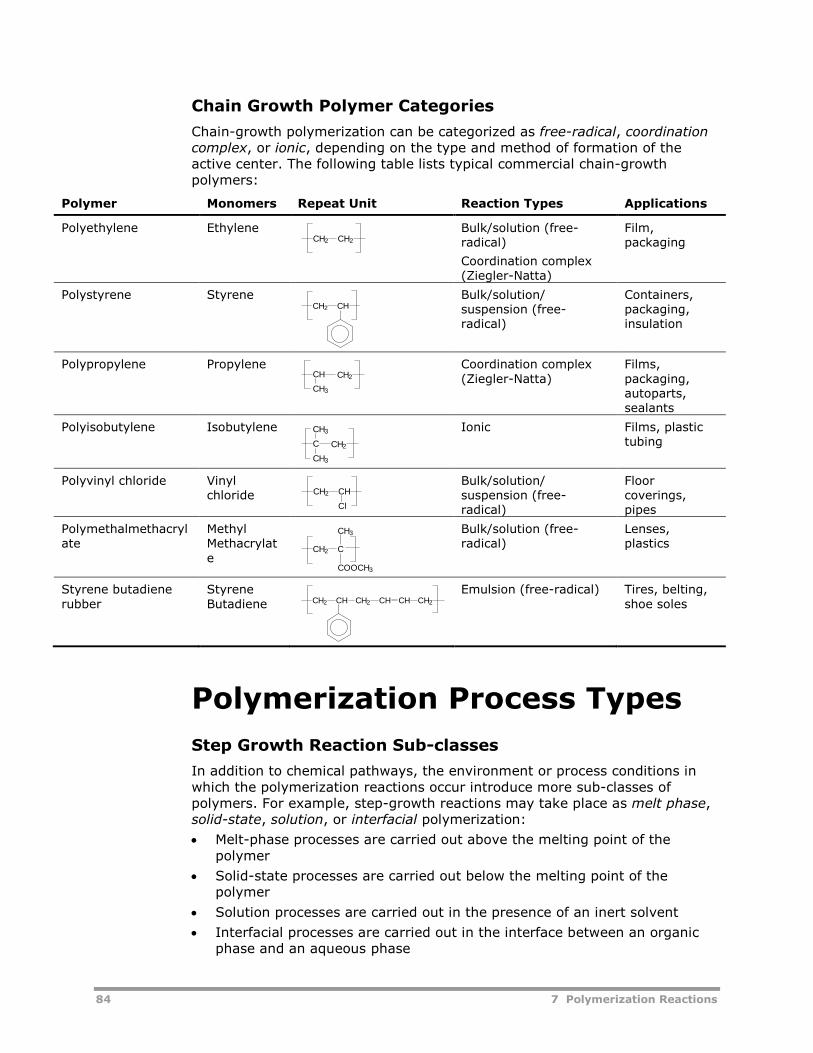
84 7 Polymerization Reactions
Chain Growth Polymer Categories
Chain-growth polymerization can be categorized as free-radical, coordinationcomplex, or ionic, depending on the type and method of formation of theactive center. The following table lists typical commercial chain-growthpolymers:
Polymer Monomers Repeat Unit Reaction Types Applications
Polyethylene Ethylene Bulk/solution (free-radical)
Coordination complex(Ziegler-Natta)
Film,packaging
Polystyrene Styrene Bulk/solution/suspension (free-radical)
Containers,packaging,insulation
Polypropylene Propylene Coordination complex(Ziegler-Natta)
Films,packaging,autoparts,sealants
Polyisobutylene Isobutylene Ionic Films, plastictubing
Polyvinyl chloride Vinylchloride
Bulk/solution/suspension (free-radical)
Floorcoverings,pipes
Polymethalmethacrylate
MethylMethacrylate
Bulk/solution (free-radical)
Lenses,plastics
Styrene butadienerubber
StyreneButadiene
Emulsion (free-radical) Tires, belting,shoe soles
Polymerization Process Types
Step Growth Reaction Sub-classes
In addition to chemical pathways, the environment or process conditions inwhich the polymerization reactions occur introduce more sub-classes ofpolymers. For example, step-growth reactions may take place as melt phase,solid-state, solution, or interfacial polymerization:
Melt-phase processes are carried out above the melting point of thepolymer
Solid-state processes are carried out below the melting point of thepolymer
Solution processes are carried out in the presence of an inert solvent
Interfacial processes are carried out in the interface between an organicphase and an aqueous phase
CH2 CH2
CH2 CH
CH2CH
CH3
CH2C
CH3
CH3
CH2 CH
Cl
CH2 C
COOCH3
CH3
CH2 CH CH2 CH CH CH2
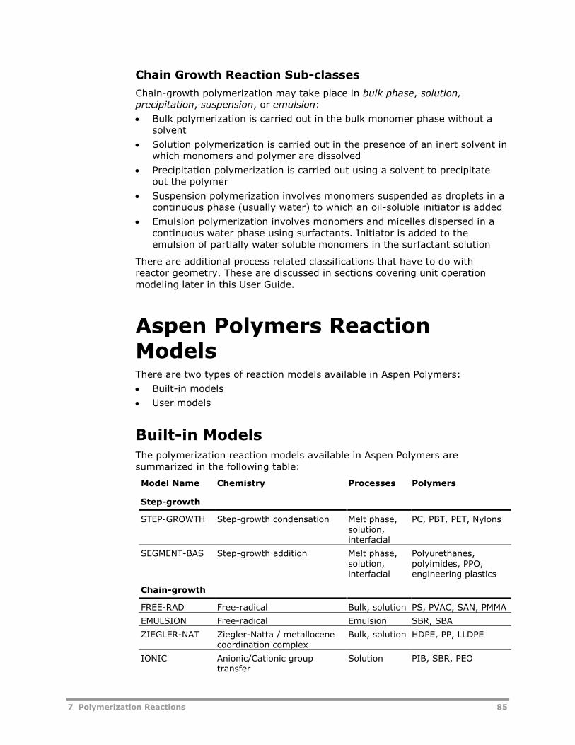
7 Polymerization Reactions 85
Chain Growth Reaction Sub-classes
Chain-growth polymerization may take place in bulk phase, solution,precipitation, suspension, or emulsion:
Bulk polymerization is carried out in the bulk monomer phase without asolvent
Solution polymerization is carried out in the presence of an inert solvent inwhich monomers and polymer are dissolved
Precipitation polymerization is carried out using a solvent to precipitateout the polymer
Suspension polymerization involves monomers suspended as droplets in acontinuous phase (usually water) to which an oil-soluble initiator is added
Emulsion polymerization involves monomers and micelles dispersed in acontinuous water phase using surfactants. Initiator is added to theemulsion of partially water soluble monomers in the surfactant solution
There are additional process related classifications that have to do withreactor geometry. These are discussed in sections covering unit operationmodeling later in this User Guide.
Aspen Polymers ReactionModelsThere are two types of reaction models available in Aspen Polymers:
Built-in models
User models
Built-in ModelsThe polymerization reaction models available in Aspen Polymers aresummarized in the following table:
Model Name Chemistry Processes Polymers
Step-growth
STEP-GROWTH Step-growth condensation Melt phase,solution,interfacial
PC, PBT, PET, Nylons
SEGMENT-BAS Step-growth addition Melt phase,solution,interfacial
Polyurethanes,polyimides, PPO,engineering plastics
Chain-growth
FREE-RAD Free-radical Bulk, solution PS, PVAC, SAN, PMMA
EMULSION Free-radical Emulsion SBR, SBA
ZIEGLER-NAT Ziegler-Natta / metallocenecoordination complex
Bulk, solution HDPE, PP, LLDPE
IONIC Anionic/Cationic grouptransfer
Solution PIB, SBR, PEO
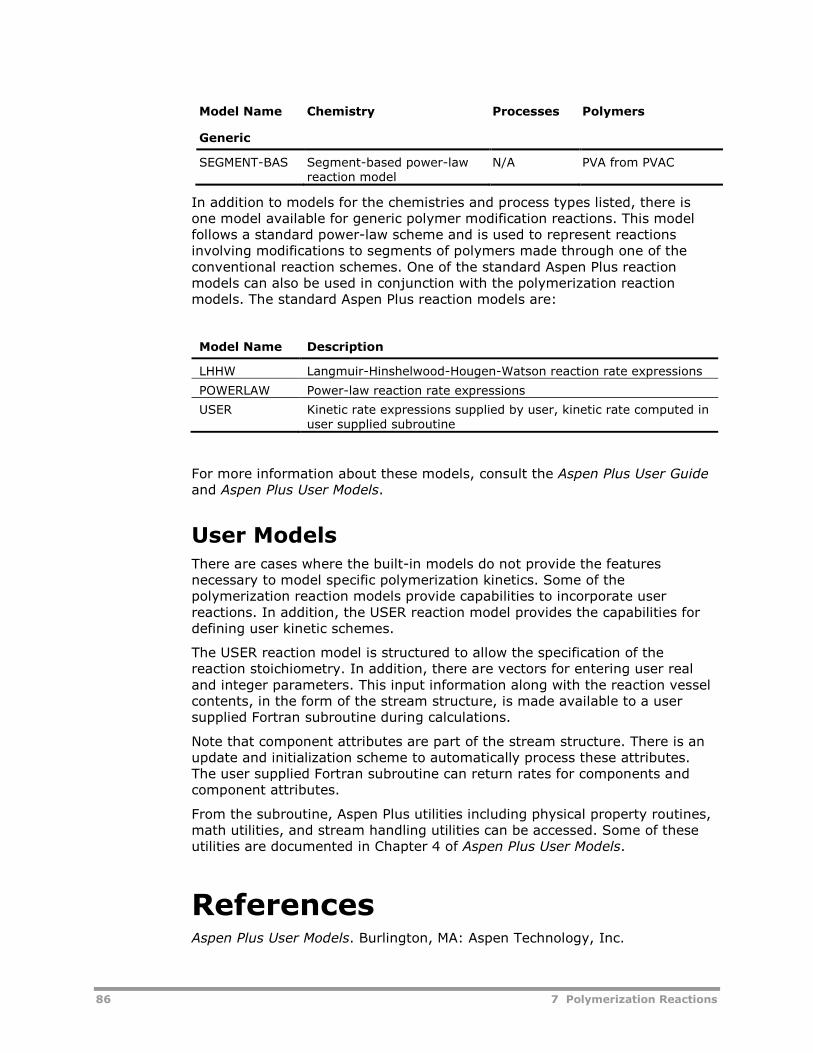
86 7 Polymerization Reactions
Model Name Chemistry Processes Polymers
Generic
SEGMENT-BAS Segment-based power-lawreaction model
N/A PVA from PVAC
In addition to models for the chemistries and process types listed, there isone model available for generic polymer modification reactions. This modelfollows a standard power-law scheme and is used to represent reactionsinvolving modifications to segments of polymers made through one of theconventional reaction schemes. One of the standard Aspen Plus reactionmodels can also be used in conjunction with the polymerization reactionmodels. The standard Aspen Plus reaction models are:
Model Name Description
LHHW Langmuir-Hinshelwood-Hougen-Watson reaction rate expressions
POWERLAW Power-law reaction rate expressions
USER Kinetic rate expressions supplied by user, kinetic rate computed inuser supplied subroutine
For more information about these models, consult the Aspen Plus User Guideand Aspen Plus User Models.
User ModelsThere are cases where the built-in models do not provide the featuresnecessary to model specific polymerization kinetics. Some of thepolymerization reaction models provide capabilities to incorporate userreactions. In addition, the USER reaction model provides the capabilities fordefining user kinetic schemes.
The USER reaction model is structured to allow the specification of thereaction stoichiometry. In addition, there are vectors for entering user realand integer parameters. This input information along with the reaction vesselcontents, in the form of the stream structure, is made available to a usersupplied Fortran subroutine during calculations.
Note that component attributes are part of the stream structure. There is anupdate and initialization scheme to automatically process these attributes.The user supplied Fortran subroutine can return rates for components andcomponent attributes.
From the subroutine, Aspen Plus utilities including physical property routines,math utilities, and stream handling utilities can be accessed. Some of theseutilities are documented in Chapter 4 of Aspen Plus User Models.
ReferencesAspen Plus User Models. Burlington, MA: Aspen Technology, Inc.
7 Polymerization Reactions 87
Aspen Plus User Guide. Burlington, MA: Aspen Technology, Inc.
Dotson, N. A, Galván, R., Laurence, R. L., & Tirrell, M. (1996). PolymerizationProcess Modeling. New York: VCH Publishers.
Grulke, E. A. (1994). Polymer Process Engineering. Englewood Cliffs, NJ:Prentice Hall.
Hamielec, A. E. (1992). Polymerization Processes. In B. Elvers, S. Hawkins, &G. Schulz (Eds.), Ullmann’s Encyclopedia of Industrial Chemistry (5th Ed.)A21, (pp. 324-330). New York: VCH.
Odian, G. (1991). Principles of Polymerization, 3rd Ed. New York: John Wiley& Sons.
Rudin, A. P. (1982). The Elements of Polymer Science and Engineering.Orlando, FL: Academic Press.
Sun, S. F. (1994). Physical Chemistry of Macromolecules. New York: JohnWiley & Sons.

88 7 Polymerization Reactions
8 Step-Growth Polymerization Model 89
8 Step-GrowthPolymerization Model
This section covers the step-growth polymerization model available in AspenPolymers (formerly known as Aspen Polymers Plus). It begins with generalbackground information on step-growth polymerization and covers some ofthe terms associated with these kinetics. Several industrial polymerizationprocesses are examined in detail. A discussion of the model features andusage is also included.
Topics covered include:
Summary of Applications, 89
Step-Growth Processes, 90
Reaction Kinetic Scheme, 101
Model Features and Assumptions, 124
Model Structure, 127
Specifying Step-Growth Polymerization Kinetics, 155
The Aspen Polymers Examples & Applications Case Book illustrates how to usethe step-growth model to simulate nylon-6 polymerization from caprolactam.
More detailed examples are available in Step-Growth Polymerization ProcessModeling and Product Design by Kevin Seavey and Y. A. Liu, ISBN: 978-0-470-23823-3, Wiley, 2008.
Summary of ApplicationsStep-growth polymerization can be used to model various polycondensationand specialty plastic processes. Some of the applicable polymers aredescribed below:
Aliphatic polycarbonates - Transesterification of diols with lower dialkylcarbonates, dioxolanones, or diphenyl carbonate in the presence ofcatalysts such as alkali metal, tin, and titanium compounds.
Aromatic polycarbonates - Reaction product of bisphenols with carbonicacid derivatives. May be prepared by transesterification, solutionpolymerization, and, most often by interfacial polymerization.
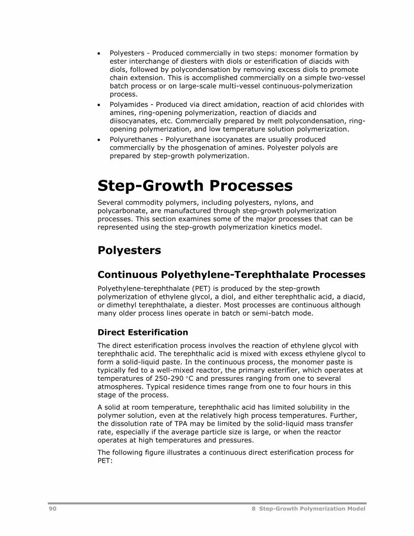
90 8 Step-Growth Polymerization Model
Polyesters - Produced commercially in two steps: monomer formation byester interchange of diesters with diols or esterification of diacids withdiols, followed by polycondensation by removing excess diols to promotechain extension. This is accomplished commercially on a simple two-vesselbatch process or on large-scale multi-vessel continuous-polymerizationprocess.
Polyamides - Produced via direct amidation, reaction of acid chlorides withamines, ring-opening polymerization, reaction of diacids anddiisocyanates, etc. Commercially prepared by melt polycondensation, ring-opening polymerization, and low temperature solution polymerization.
Polyurethanes - Polyurethane isocyanates are usually producedcommercially by the phosgenation of amines. Polyester polyols areprepared by step-growth polymerization.
Step-Growth ProcessesSeveral commodity polymers, including polyesters, nylons, andpolycarbonate, are manufactured through step-growth polymerizationprocesses. This section examines some of the major processes that can berepresented using the step-growth polymerization kinetics model.
Polyesters
Continuous Polyethylene-Terephthalate Processes
Polyethylene-terephthalate (PET) is produced by the step-growthpolymerization of ethylene glycol, a diol, and either terephthalic acid, a diacid,or dimethyl terephthalate, a diester. Most processes are continuous althoughmany older process lines operate in batch or semi-batch mode.
Direct Esterification
The direct esterification process involves the reaction of ethylene glycol withterephthalic acid. The terephthalic acid is mixed with excess ethylene glycol toform a solid-liquid paste. In the continuous process, the monomer paste istypically fed to a well-mixed reactor, the primary esterifier, which operates attemperatures of 250-290 C and pressures ranging from one to severalatmospheres. Typical residence times range from one to four hours in thisstage of the process.
A solid at room temperature, terephthalic acid has limited solubility in thepolymer solution, even at the relatively high process temperatures. Further,the dissolution rate of TPA may be limited by the solid-liquid mass transferrate, especially if the average particle size is large, or when the reactoroperates at high temperatures and pressures.
The following figure illustrates a continuous direct esterification process forPET:
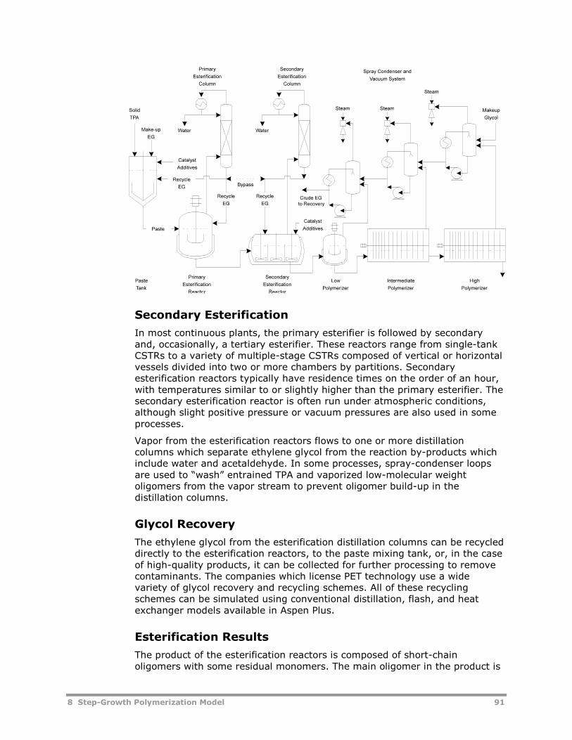
8 Step-Growth Polymerization Model 91
Secondary Esterification
In most continuous plants, the primary esterifier is followed by secondaryand, occasionally, a tertiary esterifier. These reactors range from single-tankCSTRs to a variety of multiple-stage CSTRs composed of vertical or horizontalvessels divided into two or more chambers by partitions. Secondaryesterification reactors typically have residence times on the order of an hour,with temperatures similar to or slightly higher than the primary esterifier. Thesecondary esterification reactor is often run under atmospheric conditions,although slight positive pressure or vacuum pressures are also used in someprocesses.
Vapor from the esterification reactors flows to one or more distillationcolumns which separate ethylene glycol from the reaction by-products whichinclude water and acetaldehyde. In some processes, spray-condenser loopsare used to “wash” entrained TPA and vaporized low-molecular weightoligomers from the vapor stream to prevent oligomer build-up in thedistillation columns.
Glycol Recovery
The ethylene glycol from the esterification distillation columns can be recycleddirectly to the esterification reactors, to the paste mixing tank, or, in the caseof high-quality products, it can be collected for further processing to removecontaminants. The companies which license PET technology use a widevariety of glycol recovery and recycling schemes. All of these recyclingschemes can be simulated using conventional distillation, flash, and heatexchanger models available in Aspen Plus.
Esterification Results
The product of the esterification reactors is composed of short-chainoligomers with some residual monomers. The main oligomer in the product is
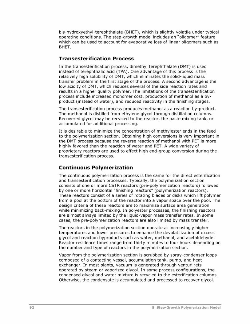
92 8 Step-Growth Polymerization Model
bis-hydroxyethyl-terephthalate (BHET), which is slightly volatile under typicaloperating conditions. The step-growth model includes an “oligomer” featurewhich can be used to account for evaporative loss of linear oligomers such asBHET.
Transesterification Process
In the transesterification process, dimethyl terephthalate (DMT) is usedinstead of terephthalic acid (TPA). One advantage of this process is therelatively high solubility of DMT, which eliminates the solid-liquid masstransfer problem in the first stage of the process. A second advantage is thelow acidity of DMT, which reduces several of the side reaction rates andresults in a higher quality polymer. The limitations of the transesterificationprocess include increased monomer cost, production of methanol as a by-product (instead of water), and reduced reactivity in the finishing stages.
The transesterification process produces methanol as a reaction by-product.The methanol is distilled from ethylene glycol through distillation columns.Recovered glycol may be recycled to the reactor, the paste mixing tank, oraccumulated for additional processing.
It is desirable to minimize the concentration of methylester ends in the feedto the polymerization section. Obtaining high conversions is very important inthe DMT process because the reverse reaction of methanol with PET is morehighly favored than the reaction of water and PET. A wide variety ofproprietary reactors are used to effect high end-group conversion during thetransesterification process.
Continuous Polymerization
The continuous polymerization process is the same for the direct esterificationand transesterification processes. Typically, the polymerization sectionconsists of one or more CSTR reactors (pre-polymerization reactors) followedby one or more horizontal “finishing reactors” (polymerization reactors).These reactors consist of a series of rotating blades or disks which lift polymerfrom a pool at the bottom of the reactor into a vapor space over the pool. Thedesign criteria of these reactors are to maximize surface area generationwhile minimizing back-mixing. In polyester processes, the finishing reactorsare almost always limited by the liquid-vapor mass transfer rates. In somecases, the pre-polymerization reactors are also limited by mass transfer.
The reactors in the polymerization section operate at increasingly highertemperatures and lower pressures to enhance the devolatilization of excessglycol and reaction byproducts such as water, methanol, and acetaldehyde.Reactor residence times range from thirty minutes to four hours depending onthe number and type of reactors in the polymerization section.
Vapor from the polymerization section is scrubbed by spray-condenser loopscomposed of a contacting vessel, accumulation tank, pump, and heatexchanger. In most plants, vacuum is generated through venturi jetsoperated by steam or vaporized glycol. In some process configurations, thecondensed glycol and water mixture is recycled to the esterification columns.Otherwise, the condensate is accumulated and processed to recover glycol.
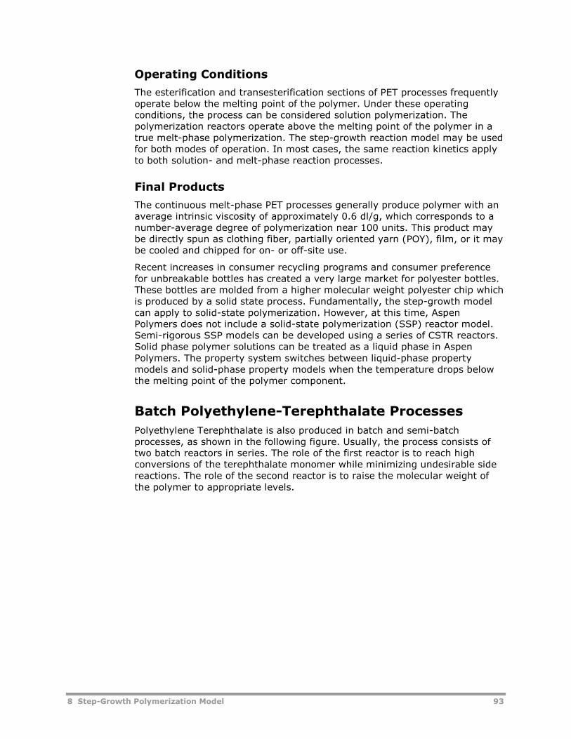
8 Step-Growth Polymerization Model 93
Operating Conditions
The esterification and transesterification sections of PET processes frequentlyoperate below the melting point of the polymer. Under these operatingconditions, the process can be considered solution polymerization. Thepolymerization reactors operate above the melting point of the polymer in atrue melt-phase polymerization. The step-growth reaction model may be usedfor both modes of operation. In most cases, the same reaction kinetics applyto both solution- and melt-phase reaction processes.
Final Products
The continuous melt-phase PET processes generally produce polymer with anaverage intrinsic viscosity of approximately 0.6 dl/g, which corresponds to anumber-average degree of polymerization near 100 units. This product maybe directly spun as clothing fiber, partially oriented yarn (POY), film, or it maybe cooled and chipped for on- or off-site use.
Recent increases in consumer recycling programs and consumer preferencefor unbreakable bottles has created a very large market for polyester bottles.These bottles are molded from a higher molecular weight polyester chip whichis produced by a solid state process. Fundamentally, the step-growth modelcan apply to solid-state polymerization. However, at this time, AspenPolymers does not include a solid-state polymerization (SSP) reactor model.Semi-rigorous SSP models can be developed using a series of CSTR reactors.Solid phase polymer solutions can be treated as a liquid phase in AspenPolymers. The property system switches between liquid-phase propertymodels and solid-phase property models when the temperature drops belowthe melting point of the polymer component.
Batch Polyethylene-Terephthalate Processes
Polyethylene Terephthalate is also produced in batch and semi-batchprocesses, as shown in the following figure. Usually, the process consists oftwo batch reactors in series. The role of the first reactor is to reach highconversions of the terephthalate monomer while minimizing undesirable sidereactions. The role of the second reactor is to raise the molecular weight ofthe polymer to appropriate levels.
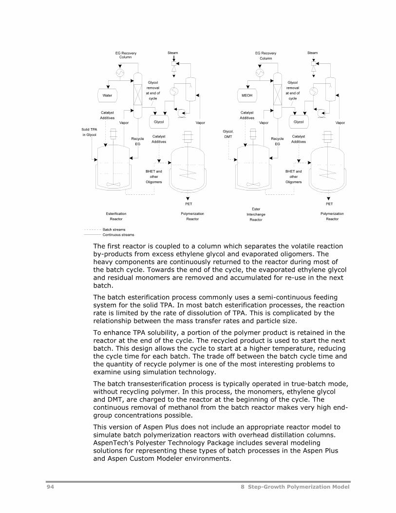
94 8 Step-Growth Polymerization Model
The first reactor is coupled to a column which separates the volatile reactionby-products from excess ethylene glycol and evaporated oligomers. Theheavy components are continuously returned to the reactor during most ofthe batch cycle. Towards the end of the cycle, the evaporated ethylene glycoland residual monomers are removed and accumulated for re-use in the nextbatch.
The batch esterification process commonly uses a semi-continuous feedingsystem for the solid TPA. In most batch esterification processes, the reactionrate is limited by the rate of dissolution of TPA. This is complicated by therelationship between the mass transfer rates and particle size.
To enhance TPA solubility, a portion of the polymer product is retained in thereactor at the end of the cycle. The recycled product is used to start the nextbatch. This design allows the cycle to start at a higher temperature, reducingthe cycle time for each batch. The trade off between the batch cycle time andthe quantity of recycle polymer is one of the most interesting problems toexamine using simulation technology.
The batch transesterification process is typically operated in true-batch mode,without recycling polymer. In this process, the monomers, ethylene glycoland DMT, are charged to the reactor at the beginning of the cycle. Thecontinuous removal of methanol from the batch reactor makes very high end-group concentrations possible.
This version of Aspen Plus does not include an appropriate reactor model tosimulate batch polymerization reactors with overhead distillation columns.AspenTech’s Polyester Technology Package includes several modelingsolutions for representing these types of batch processes in the Aspen Plusand Aspen Custom Modeler environments.
8 Step-Growth Polymerization Model 95
Second Batch Stage
The liquid product from the batch esterification or transesterification ischarged to a second batch stage. In this stage, the reactor is evacuated asthe temperature is increased. These operating profiles enhance the removalof excess ethylene glycol from the reaction mixture, allowing these highlyreversible reactions to proceed.
As the polymer viscosity increases, the reactions become limited by the rateof mass transfer from the liquid phase to the vapor phase due to decreasedsurface renewal rates and reduced agitator speeds.
Other Polyester Processes
Polybutylene-terephthalate (PBT) is an engineering plastic frequently used formachine parts, car body panels, and other applications. Polybutyleneterephthalate is analogous to PET, except butylene glycol is used in place ofethylene glycol. Most PBT is manufactured from DMT through continuoustransesterification processes, although batch processes and directesterification processes are also found in industry.
In the PBT process, tetrahydrofurane, THF, is formed from butylene glycolend groups as an undesirable reaction by-product. The transesterificationprocess is favored over direct esterification because the acid end groups inTPA catalyze the formation of THF.
Polypropylene-terephthalate (PPT) is used for carpet fiber and otherapplications. Like PET and PBT, PPT can be manufactured from terephthalicacid or dimethyl terephthalate. In the PPT process, propylene glycol is used asthe diol monomer.
Polyethylene-naphthalate (PEN) manufacturing processes are underdevelopment by several polyester producers. This new product has a highermelting point than PET, and is aimed at specific demands, such as hot-fillbottles, which are not well satisfied by other polyesters. The dimethyl esternaphthalate monomer is much more expensive than TPA or DMT, so PEN isfrequently produced as a copolymer with PET.
At this time, most PEN is produced in batch processes which are analogous tothe batch PET process. Copolymers of PEN and PET are being used for somebottling applications already. The similarities in the chemical mechanism forPET and PEN make them relatively easy to copolymerize in various ratios,resulting in several product grades with properties intermediate between purePET and pure PEN.
Polyester Technology Package
Aspen Technology offers several solutions for polyester processes. TheAspenTech Polyester Technology Package provides steady-state simulation ofmelt-phase continuous processes and also includes process models for batchpolyester processes. The Polyester Technology Package is designed for PETand PBT, but can be easily modified for analogous polyesters such as PEN,PTT, etc.
96 8 Step-Growth Polymerization Model
Aspen PolyQuestSM, jointly developed with Hosokawa Bepex corporation, is asimulation package covering all varieties of solid-state PET processes. AspenPolyQuest includes detailed and rigorous models for reaction kinetics,diffusion, heat transfer, and crystallization, as well as a library of detailed unitoperation models for solid-state processing equipment. Aspen PolyQuest runson the Aspen Custom Modeler platform. The underlying equation-basedmodels can be used for dynamic or steady-state process simulation.
The models in these packages account for all the major side reactions in theprocess, such as thermal scission, aldehyde formation, DEG formation, andcyclic trimer formation. The reaction kinetic models consider the influence ofseveral common catalysts and additives as well as acid catalysis anduncatalyzed side reactions. The package includes reactor models whichconsider solid-liquid mass transfer for the direct esterification process, andliquid-vapor mass transfer limited kinetics for the polymerization reactors.
The Polyester Technology Package includes models of several commonprocess configurations, including both batch and continuous processes. Themodels predict various quality parameters such as the acid end groupconcentration (acid value), intrinsic viscosity, vinyl end content, DEG content,conversion, etc.
Contact your Aspen Technology sales representative for more informationabout the Polyester Technology Package, Aspen PolyQuest, and advancedconsulting services.
Nylon-6Nylon-6 is produced by ring-opening polymerization of -caprolactam. Waterand caprolactam are fed to a primary reactor where the ring-opening reactiontakes place. The primary reactor may be a single (liquid) phase tubularreactor, CSTR, or one of a variety of proprietary reactors.
The following figure illustrates a continuous melt-phase nylon-6 process:
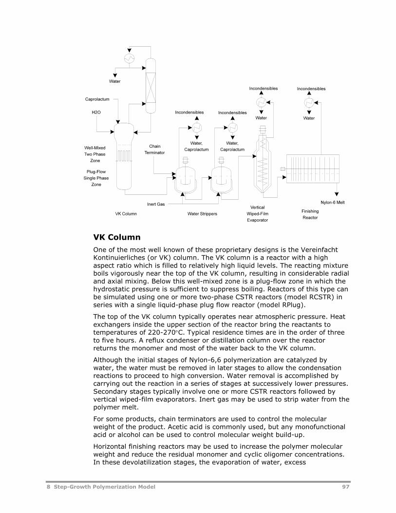
8 Step-Growth Polymerization Model 97
VK Column
One of the most well known of these proprietary designs is the VereinfachtKontinuierliches (or VK) column. The VK column is a reactor with a highaspect ratio which is filled to relatively high liquid levels. The reacting mixtureboils vigorously near the top of the VK column, resulting in considerable radialand axial mixing. Below this well-mixed zone is a plug-flow zone in which thehydrostatic pressure is sufficient to suppress boiling. Reactors of this type canbe simulated using one or more two-phase CSTR reactors (model RCSTR) inseries with a single liquid-phase plug flow reactor (model RPlug).
The top of the VK column typically operates near atmospheric pressure. Heatexchangers inside the upper section of the reactor bring the reactants totemperatures of 220-270C. Typical residence times are in the order of threeto five hours. A reflux condenser or distillation column over the reactorreturns the monomer and most of the water back to the VK column.
Although the initial stages of Nylon-6,6 polymerization are catalyzed bywater, the water must be removed in later stages to allow the condensationreactions to proceed to high conversion. Water removal is accomplished bycarrying out the reaction in a series of stages at successively lower pressures.Secondary stages typically involve one or more CSTR reactors followed byvertical wiped-film evaporators. Inert gas may be used to strip water from thepolymer melt.
For some products, chain terminators are used to control the molecularweight of the product. Acetic acid is commonly used, but any monofunctionalacid or alcohol can be used to control molecular weight build-up.
Horizontal finishing reactors may be used to increase the polymer molecularweight and reduce the residual monomer and cyclic oligomer concentrations.In these devolatilization stages, the evaporation of water, excess
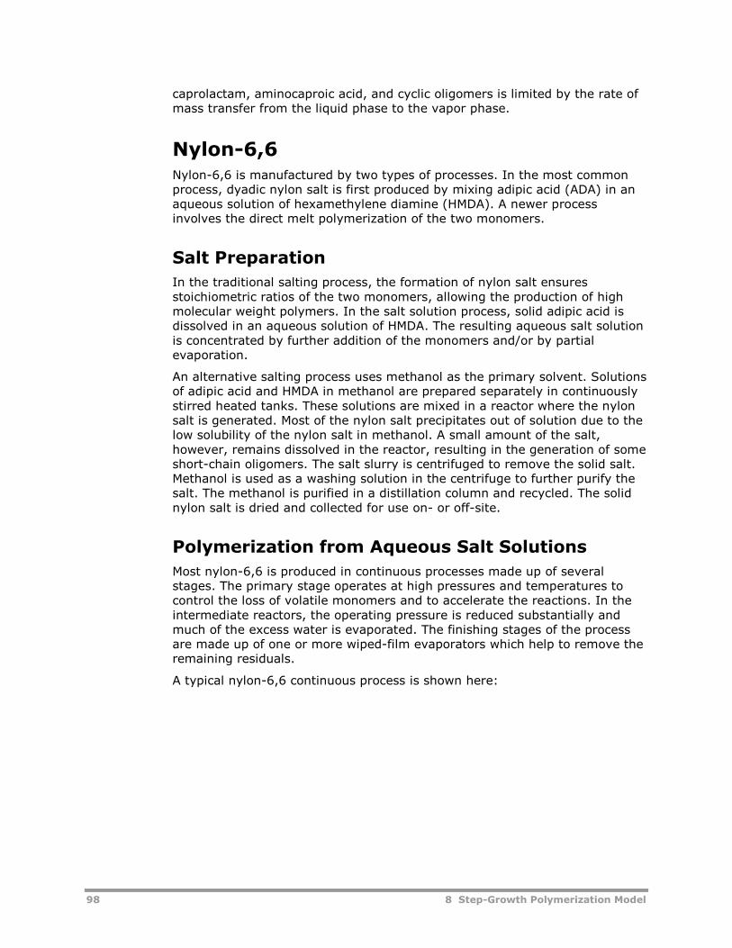
98 8 Step-Growth Polymerization Model
caprolactam, aminocaproic acid, and cyclic oligomers is limited by the rate ofmass transfer from the liquid phase to the vapor phase.
Nylon-6,6Nylon-6,6 is manufactured by two types of processes. In the most commonprocess, dyadic nylon salt is first produced by mixing adipic acid (ADA) in anaqueous solution of hexamethylene diamine (HMDA). A newer processinvolves the direct melt polymerization of the two monomers.
Salt Preparation
In the traditional salting process, the formation of nylon salt ensuresstoichiometric ratios of the two monomers, allowing the production of highmolecular weight polymers. In the salt solution process, solid adipic acid isdissolved in an aqueous solution of HMDA. The resulting aqueous salt solutionis concentrated by further addition of the monomers and/or by partialevaporation.
An alternative salting process uses methanol as the primary solvent. Solutionsof adipic acid and HMDA in methanol are prepared separately in continuouslystirred heated tanks. These solutions are mixed in a reactor where the nylonsalt is generated. Most of the nylon salt precipitates out of solution due to thelow solubility of the nylon salt in methanol. A small amount of the salt,however, remains dissolved in the reactor, resulting in the generation of someshort-chain oligomers. The salt slurry is centrifuged to remove the solid salt.Methanol is used as a washing solution in the centrifuge to further purify thesalt. The methanol is purified in a distillation column and recycled. The solidnylon salt is dried and collected for use on- or off-site.
Polymerization from Aqueous Salt Solutions
Most nylon-6,6 is produced in continuous processes made up of severalstages. The primary stage operates at high pressures and temperatures tocontrol the loss of volatile monomers and to accelerate the reactions. In theintermediate reactors, the operating pressure is reduced substantially andmuch of the excess water is evaporated. The finishing stages of the processare made up of one or more wiped-film evaporators which help to remove theremaining residuals.
A typical nylon-6,6 continuous process is shown here:
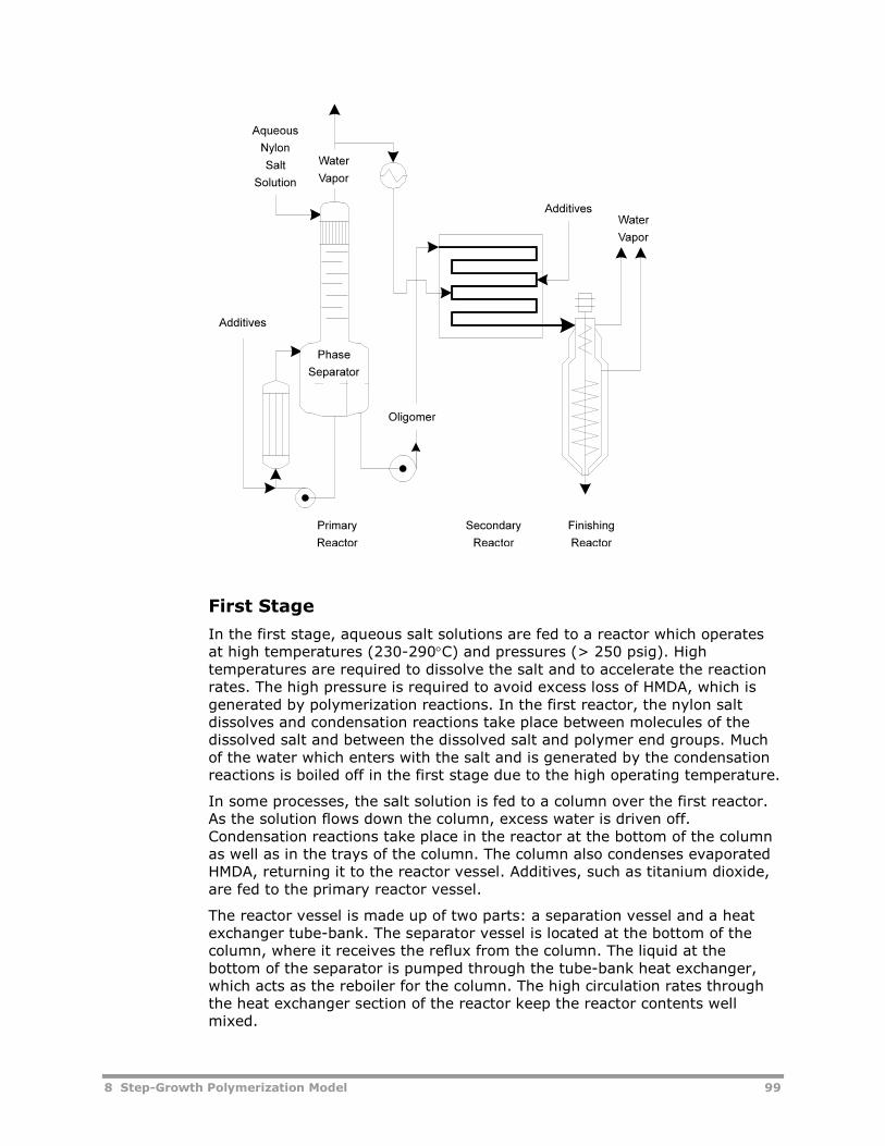
8 Step-Growth Polymerization Model 99
First Stage
In the first stage, aqueous salt solutions are fed to a reactor which operatesat high temperatures (230-290C) and pressures (> 250 psig). Hightemperatures are required to dissolve the salt and to accelerate the reactionrates. The high pressure is required to avoid excess loss of HMDA, which isgenerated by polymerization reactions. In the first reactor, the nylon saltdissolves and condensation reactions take place between molecules of thedissolved salt and between the dissolved salt and polymer end groups. Muchof the water which enters with the salt and is generated by the condensationreactions is boiled off in the first stage due to the high operating temperature.
In some processes, the salt solution is fed to a column over the first reactor.As the solution flows down the column, excess water is driven off.Condensation reactions take place in the reactor at the bottom of the columnas well as in the trays of the column. The column also condenses evaporatedHMDA, returning it to the reactor vessel. Additives, such as titanium dioxide,are fed to the primary reactor vessel.
The reactor vessel is made up of two parts: a separation vessel and a heatexchanger tube-bank. The separator vessel is located at the bottom of thecolumn, where it receives the reflux from the column. The liquid at thebottom of the separator is pumped through the tube-bank heat exchanger,which acts as the reboiler for the column. The high circulation rates throughthe heat exchanger section of the reactor keep the reactor contents wellmixed.
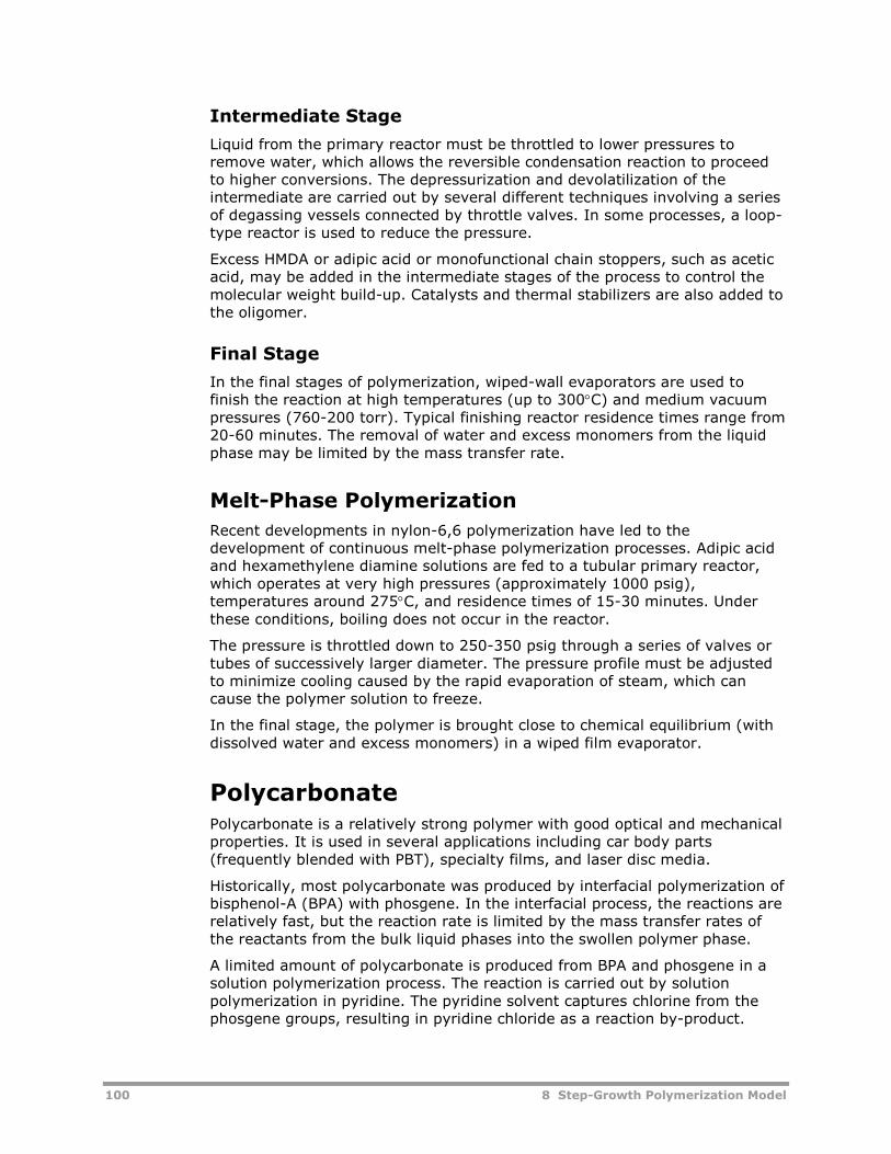
100 8 Step-Growth Polymerization Model
Intermediate Stage
Liquid from the primary reactor must be throttled to lower pressures toremove water, which allows the reversible condensation reaction to proceedto higher conversions. The depressurization and devolatilization of theintermediate are carried out by several different techniques involving a seriesof degassing vessels connected by throttle valves. In some processes, a loop-type reactor is used to reduce the pressure.
Excess HMDA or adipic acid or monofunctional chain stoppers, such as aceticacid, may be added in the intermediate stages of the process to control themolecular weight build-up. Catalysts and thermal stabilizers are also added tothe oligomer.
Final Stage
In the final stages of polymerization, wiped-wall evaporators are used tofinish the reaction at high temperatures (up to 300C) and medium vacuumpressures (760-200 torr). Typical finishing reactor residence times range from20-60 minutes. The removal of water and excess monomers from the liquidphase may be limited by the mass transfer rate.
Melt-Phase Polymerization
Recent developments in nylon-6,6 polymerization have led to thedevelopment of continuous melt-phase polymerization processes. Adipic acidand hexamethylene diamine solutions are fed to a tubular primary reactor,which operates at very high pressures (approximately 1000 psig),temperatures around 275C, and residence times of 15-30 minutes. Underthese conditions, boiling does not occur in the reactor.
The pressure is throttled down to 250-350 psig through a series of valves ortubes of successively larger diameter. The pressure profile must be adjustedto minimize cooling caused by the rapid evaporation of steam, which cancause the polymer solution to freeze.
In the final stage, the polymer is brought close to chemical equilibrium (withdissolved water and excess monomers) in a wiped film evaporator.
PolycarbonatePolycarbonate is a relatively strong polymer with good optical and mechanicalproperties. It is used in several applications including car body parts(frequently blended with PBT), specialty films, and laser disc media.
Historically, most polycarbonate was produced by interfacial polymerization ofbisphenol-A (BPA) with phosgene. In the interfacial process, the reactions arerelatively fast, but the reaction rate is limited by the mass transfer rates ofthe reactants from the bulk liquid phases into the swollen polymer phase.
A limited amount of polycarbonate is produced from BPA and phosgene in asolution polymerization process. The reaction is carried out by solutionpolymerization in pyridine. The pyridine solvent captures chlorine from thephosgene groups, resulting in pyridine chloride as a reaction by-product.
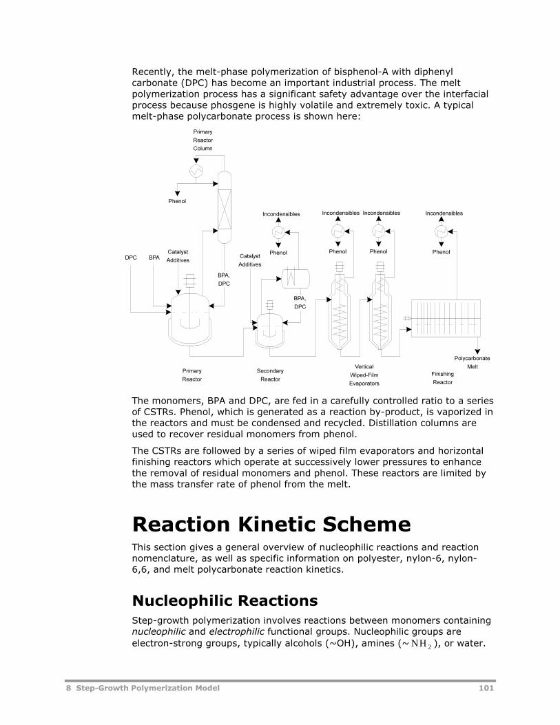
8 Step-Growth Polymerization Model 101
Recently, the melt-phase polymerization of bisphenol-A with diphenylcarbonate (DPC) has become an important industrial process. The meltpolymerization process has a significant safety advantage over the interfacialprocess because phosgene is highly volatile and extremely toxic. A typicalmelt-phase polycarbonate process is shown here:
The monomers, BPA and DPC, are fed in a carefully controlled ratio to a seriesof CSTRs. Phenol, which is generated as a reaction by-product, is vaporized inthe reactors and must be condensed and recycled. Distillation columns areused to recover residual monomers from phenol.
The CSTRs are followed by a series of wiped film evaporators and horizontalfinishing reactors which operate at successively lower pressures to enhancethe removal of residual monomers and phenol. These reactors are limited bythe mass transfer rate of phenol from the melt.
Reaction Kinetic SchemeThis section gives a general overview of nucleophilic reactions and reactionnomenclature, as well as specific information on polyester, nylon-6, nylon-6,6, and melt polycarbonate reaction kinetics.
Nucleophilic ReactionsStep-growth polymerization involves reactions between monomers containingnucleophilic and electrophilic functional groups. Nucleophilic groups are
electron-strong groups, typically alcohols (~OH), amines (~ NH 2 ), or water.
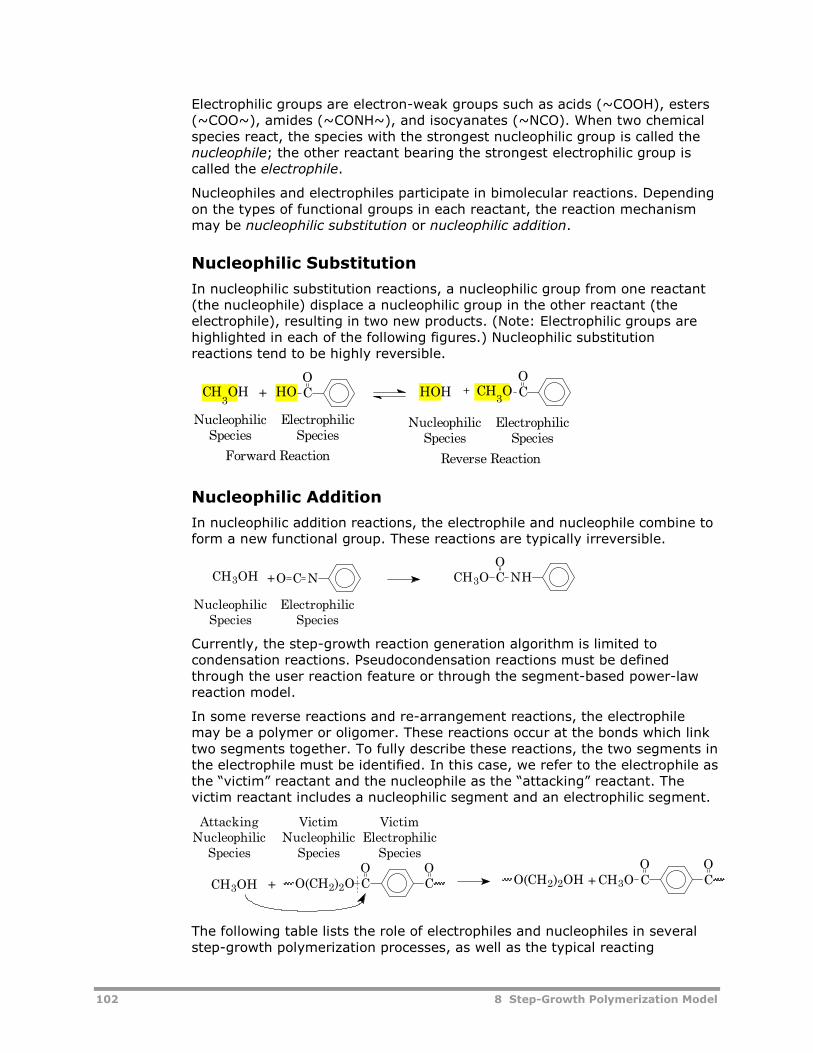
102 8 Step-Growth Polymerization Model
Electrophilic groups are electron-weak groups such as acids (~COOH), esters(~COO~), amides (~CONH~), and isocyanates (~NCO). When two chemicalspecies react, the species with the strongest nucleophilic group is called thenucleophile; the other reactant bearing the strongest electrophilic group iscalled the electrophile.
Nucleophiles and electrophiles participate in bimolecular reactions. Dependingon the types of functional groups in each reactant, the reaction mechanismmay be nucleophilic substitution or nucleophilic addition.
Nucleophilic Substitution
In nucleophilic substitution reactions, a nucleophilic group from one reactant(the nucleophile) displace a nucleophilic group in the other reactant (theelectrophile), resulting in two new products. (Note: Electrophilic groups arehighlighted in each of the following figures.) Nucleophilic substitutionreactions tend to be highly reversible.
Nucleophilic Addition
In nucleophilic addition reactions, the electrophile and nucleophile combine toform a new functional group. These reactions are typically irreversible.
Currently, the step-growth reaction generation algorithm is limited tocondensation reactions. Pseudocondensation reactions must be definedthrough the user reaction feature or through the segment-based power-lawreaction model.
In some reverse reactions and re-arrangement reactions, the electrophilemay be a polymer or oligomer. These reactions occur at the bonds which linktwo segments together. To fully describe these reactions, the two segments inthe electrophile must be identified. In this case, we refer to the electrophile asthe “victim” reactant and the nucleophile as the “attacking” reactant. Thevictim reactant includes a nucleophilic segment and an electrophilic segment.
The following table lists the role of electrophiles and nucleophiles in severalstep-growth polymerization processes, as well as the typical reacting
CH3OH + CHO
OHOH + CCH
3O
O
NucleophilicSpecies
ElectrophilicSpecies
Forward Reaction Reverse Reaction
ElectrophilicSpecies
NucleophilicSpecies
CH3OH + NHCCH3OO
NCO
ElectrophilicSpecies
NucleophilicSpecies
CH3OH + CO
CO(CH2)2OO
AttackingNucleophilic
Species
VictimNucleophilic
Species
VictimElectrophilic
Species
O(CH2)2OH + CCOO
CH3O
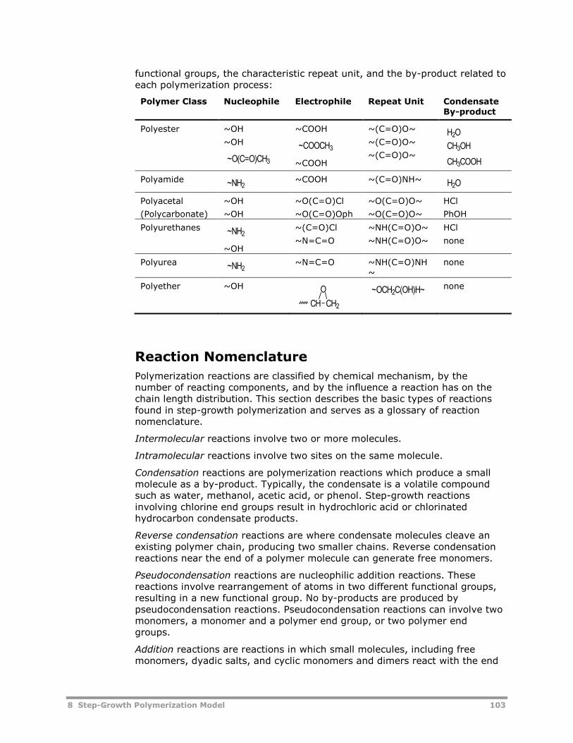
8 Step-Growth Polymerization Model 103
functional groups, the characteristic repeat unit, and the by-product related toeach polymerization process:
Polymer Class Nucleophile Electrophile Repeat Unit CondensateBy-product
Polyester ~OH
~OH
~COOH
~COOH
~(C=O)O~
~(C=O)O~
~(C=O)O~
Polyamide ~COOH ~(C=O)NH~
Polyacetal
(Polycarbonate)
~OH
~OH
~O(C=O)Cl
~O(C=O)Oph
~O(C=O)O~
~O(C=O)O~
HCl
PhOH
Polyurethanes
~OH
~(C=O)Cl
~N=C=O
~NH(C=O)O~
~NH(C=O)O~
HCl
none
Polyurea ~N=C=O ~NH(C=O)NH~
none
Polyether ~OH none
Reaction Nomenclature
Polymerization reactions are classified by chemical mechanism, by thenumber of reacting components, and by the influence a reaction has on thechain length distribution. This section describes the basic types of reactionsfound in step-growth polymerization and serves as a glossary of reactionnomenclature.
Intermolecular reactions involve two or more molecules.
Intramolecular reactions involve two sites on the same molecule.
Condensation reactions are polymerization reactions which produce a smallmolecule as a by-product. Typically, the condensate is a volatile compoundsuch as water, methanol, acetic acid, or phenol. Step-growth reactionsinvolving chlorine end groups result in hydrochloric acid or chlorinatedhydrocarbon condensate products.
Reverse condensation reactions are where condensate molecules cleave anexisting polymer chain, producing two smaller chains. Reverse condensationreactions near the end of a polymer molecule can generate free monomers.
Pseudocondensation reactions are nucleophilic addition reactions. Thesereactions involve rearrangement of atoms in two different functional groups,resulting in a new functional group. No by-products are produced bypseudocondensation reactions. Pseudocondensation reactions can involve twomonomers, a monomer and a polymer end group, or two polymer endgroups.
Addition reactions are reactions in which small molecules, including freemonomers, dyadic salts, and cyclic monomers and dimers react with the end
~O(C=O)CH3
~COOCH3
H2O
CH3OH
CH3COOH
~NH2 H2O
~NH2
~NH2
O
CH CH2
~OCH2C(OH)H~
104 8 Step-Growth Polymerization Model
of a growing polymer molecule. These reactions are responsible for theconversion of the monomers and most of the conversion of functional endgroups.
Combination reactions involve reactions between the end groups of twopolymer molecules. In most systems, combination reactions play animportant role in molecular weight growth.
Rearrangement reactions occur between two polymer molecules, resulting intwo new polymer molecules with different molecular weights. These reactionsmay involve the end group of one molecule and an internal site on anothermolecule, or they may involve internal sites on both molecules.
Ring opening reactions are intermolecular reactions between condensate ormonomer molecules and cyclic monomers or oligomers. Condensatemolecules or monomers react with cyclic compounds, opening the ringstructure to produce linear oligomers or cyclic monomers.
Ring closing reactions are intramolecular reactions which occur between thetwo end groups of a linear molecule. Ring-closing reactions which occurbetween two end groups of a branched or network molecule are referred tohere as intramolecular cyclization to differentiate them from reactions whichform ring-shaped molecules.
Ring addition reactions are intermolecular reactions between polymer endgroups and cyclic monomers or oligomers. The end group of the polymer linksto the cyclic compound, opening the ring and lengthening the chain of thelinear molecule.
Cyclodepolymerization reactions are intramolecular reactions in which apolymer end group reacts with a segment in the same molecule, forming aring. The ring-shaped molecule is lost from the linear parent molecule,reducing the molecular weight of the parent.
Terminal monomer loss involves the loss of a monomer unit at the end of apolymer chain due to thermal degradation mechanisms.
Random scission involves the spontaneous cleavage of a polymer chain due tothermal degradation.
End group reformation reactions are those reactions which convert one typeof end group into another without influencing the chain length.
The following table summarizes the reactions for step-growth polymerization:
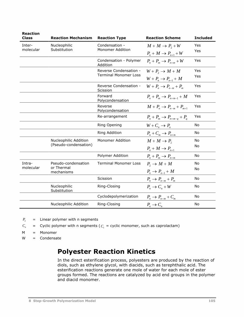
8 Step-Growth Polymerization Model 105
ReactionClass Reaction Mechanism Reaction Type Reaction Scheme Included
Inter-molecular
NucleophilicSubstitution
Condensation -Monomer Addition
M M P W 2
P M P Wn n 1
Yes
Yes
Condensation - PolymerAddition
P P P Wn m n m Yes
Reverse Condensation -Terminal Monomer Loss
W P M M 2
W P P Mn n 1
Yes
Yes
Reverse Condensation -Scission
W P P Pn n m m Yes
ForwardPolycondensation
P P P Mn m n m 1Yes
ReversePolycondensation
M P P Pn n m m 1Yes
Re-arrangement P P P Pn m n m q q Yes
Ring Opening W C Pn n No
Ring Addition P C Pn m n m No
Nucleophilic Addition(Pseudo-condensation)
Monomer Addition M M P 2
P M Pn n 1
No
No
Polymer Addition P P Pn m n m No
Intra-molecular
Pseudo-condensationor Thermalmechanisms
Terminal Monomer Loss P M M2
P P Mn n 1
No
No
Scission P P Pn n m m No
NucleophilicSubstitution
Ring-Closing P C Wn n No
Cyclodepolymerization P P Cn n m m No
Nucleophilic Addition Ring-Closing P Cn n No
Pn = Linear polymer with n segments
Cn = Cyclic polymer with n segments (C1= cyclic monomer, such as caprolactam)
M = Monomer
W = Condensate
Polyester Reaction KineticsIn the direct esterification process, polyesters are produced by the reaction ofdiols, such as ethylene glycol, with diacids, such as terephthalic acid. Theesterification reactions generate one mole of water for each mole of estergroups formed. The reactions are catalyzed by acid end groups in the polymerand diacid monomer.
106 8 Step-Growth Polymerization Model
Side Reactions
Several of the key side reactions are also acid-catalyzed. In the PET process,these reactions include the formation of diethylene glycol, or DEG, fromethylene glycol. The transesterification process does not involve acids, andsubstantially less DEG is produced.
An analogous reaction generates tetrahydrofurane (THF) in the PBT process.Like DEG formation, THF formation is accelerated by acid end groups. SinceTHF poses environmental concerns, the generation of THF should beminimized. For this reason, PBT is usually produced by the transesterificationroute.
Metal acetate catalysts are used to accelerate the reaction rates in the laterstages of the direct esterification process and throughout thetransesterification process. These catalysts accelerate the main reactions andseveral side reactions including thermal scission and aldehyde formation.
In the transesterification process, acid end groups may be formed by thermaldegradation reactions or by exchange reactions with water, which may beformed as a reaction by-product. These acid end groups participate in thereaction scheme, making transesterification kinetics a superset ofesterification kinetics.
Polymerization Stage
The polymerization stage involves chain building reactions. There are twomain growth mechanisms. Condensation reactions occur between twopolymer end groups, releasing water or methanol. Polymerization reactionsoccur between diol end groups in different polymer molecules, generating amolecule of free glycol.
The polymer end group distribution and molecular weight distribution arerandomized by redistribution reactions.
Polyester Production Final Stages
In the final stages of polyester production, high temperatures lead to thermaldegradation reactions. In the PET process, these reactions degrade glycol endgroups, producing acid ends and free acetaldehyde. Thermal scissionreactions generate acid end groups and oxyvinyl end groups. Analogousreactions in the PBT process yield butenol and 1,4-butadiene. Additional sidereactions involving these vinyl groups are the main source of color bodies inpolyesters.
Cyclic compounds are formed by ring-closing and cyclodepolymerizationreactions. Cyclic monomers, and some cyclic dimers do not form interephthalic polyesters because of steric limitations. Trace amounts of largercyclic oligomers, including trimers, tetramers, and pentamers, are commonlyobserved in terephthalate polyesters. These cyclic compounds reduce thequality of the polyester. Cyclic oligomers evaporate from the finishing reactorsand condense in vapor vent lines, causing maintenance problems.
The reaction kinetics of terephthalate polyesters are summarized in the tablesthat follow.
The components involved in the reactions are:
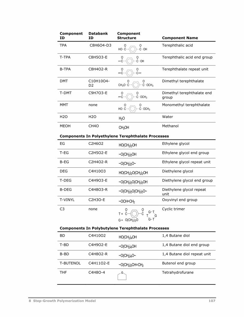
8 Step-Growth Polymerization Model 107
ComponentID
DatabankID
ComponentStructure Component Name
TPA C8H6O4-D3 Terephthalic acid
T-TPA C8H5O3-E Terephthalic acid end group
B-TPA C8H4O2-R Terephthalate repeat unit
DMT C10H10O4-D2
Dimethyl terephthalate
T-DMT C9H7O3-E Dimethyl terephthalate endgroup
MMT none Monomethyl terephthalate
H2O H2O Water
MEOH CH4O Methanol
Components In Polyethylene Terephthalate Processes
EG C2H6O2 Ethylene glycol
T-EG C2H5O2-E Ethylene glycol end group
B-EG C2H4O2-R Ethylene glycol repeat unit
DEG C4H10O3 Diethylene glycol
T-DEG C4H9O3-E Diethylene glycol end group
B-DEG C4H8O3-R Diethylene glycol repeatunit
T-VINYL C2H3O-E Oxyvinyl end group
C3 none Cyclic trimer
Components In Polybutylene Terephthalate Processes
BD C4H10O2 1,4 Butane diol
T-BD C4H9O2-E 1,4 Butane diol end group
B-BD C4H8O2-R 1,4 Butane diol repeat unit
T-BUTENOL C4H11O2-E Butenol end group
THF C4H8O-4 Tetrahydrofurane
CCOO
OHHO
CCOO
OH
CCOO
CCOO
OCH3CH3O
CCOO
OCH3
CCOO
OCH3HO
H2O
CH3OH
HO(CH2)2OH
~O(CH2)2OH
~O(CH2)2O~
HO(CH2)2O(CH2)2OH
~O(CH2)2O(CH2)2OH
~O(CH2)2O(CH2)2O~
~OCH=CH2
TG T
GTG
G = O(CH2)2O
T = CCOO
HO(CH2)4OH
~O(CH2)4OH
~O(CH2)4O~
~O(CH2)2CH=CH2
o
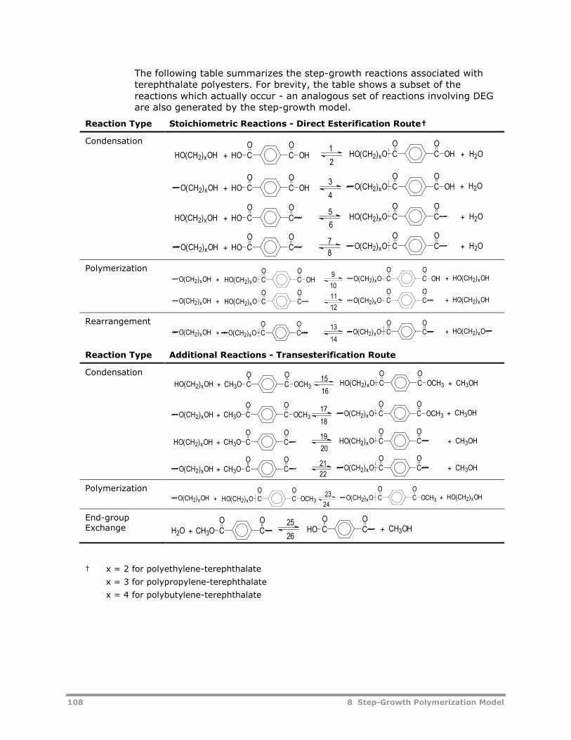
108 8 Step-Growth Polymerization Model
The following table summarizes the step-growth reactions associated withterephthalate polyesters. For brevity, the table shows a subset of thereactions which actually occur - an analogous set of reactions involving DEGare also generated by the step-growth model.
Reaction Type Stoichiometric Reactions - Direct Esterification Route†
Condensation
Polymerization
Rearrangement
Reaction Type Additional Reactions - Transesterification Route
Condensation
Polymerization
End-groupExchange
† x = 2 for polyethylene-terephthalate
x = 3 for polypropylene-terephthalate
x = 4 for polybutylene-terephthalate
CCOO
OHHOHO(CH2)xOH + CCOO
OHHO(CH2)xO + H2O
CCOO
OHO(CH2)xO+O(CH2)xOH CCOO
OHHO + H2O
CCOO
HOHO(CH2)xOH + CCOO
HO(CH2)xO + H2O
CCOO
HOO(CH2)xOH + CCOO
O(CH2)xO + H2O
1
2
3
4
5
6
7
8
CCOO
OHO(CH2)xO+O(CH2)xOH + HO(CH2)xOHCCOO
OHHO(CH2)xO
CCOO
O(CH2)xO+O(CH2)xOH + HO(CH2)xOHCCOO
HO(CH2)xO
9
10
11
12
CCOO
O(CH2)xO+O(CH2)xOH + HO(CH2)xOCCOO
O(CH2)xO13
14
15
16
17
18
19
20
21
22
CCOO
OCH3CH3OHO(CH2)xOH + CCOO
OCH3HO(CH2)xO + CH3OH
CCOO
OCH3O(CH2)xO+O(CH2)xOH CCOO
OCH3CH3O + CH3OH
CCOO
CH3OHO(CH2)xOH + CCOO
HO(CH2)xO + CH3OH
CCOO
CH3OO(CH2)xOH + CCOO
O(CH2)xO + CH3OH
23
24CCOO
OCH3O(CH2)xO+O(CH2)xOH + HO(CH2)xOHCCOO
OCH3HO(CH2)xO
25
26+ CC
OOCH3O + CH3OHCC
OOHOH2O
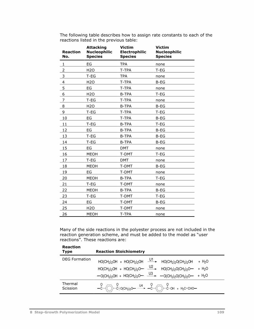
8 Step-Growth Polymerization Model 109
The following table describes how to assign rate constants to each of thereactions listed in the previous table:
ReactionNo.
AttackingNucleophilicSpecies
VictimElectrophilicSpecies
VictimNucleophilicSpecies
1 EG TPA none
2 H2O T-TPA T-EG
3 T-EG TPA none
4 H2O T-TPA B-EG
5 EG T-TPA none
6 H2O B-TPA T-EG
7 T-EG T-TPA none
8 H2O B-TPA B-EG
9 T-EG T-TPA T-EG
10 EG T-TPA B-EG
11 T-EG B-TPA T-EG
12 EG B-TPA B-EG
13 T-EG B-TPA B-EG
14 T-EG B-TPA B-EG
15 EG DMT none
16 MEOH T-DMT T-EG
17 T-EG DMT none
18 MEOH T-DMT B-EG
19 EG T-DMT none
20 MEOH B-TPA T-EG
21 T-EG T-DMT none
22 MEOH B-TPA B-EG
23 T-EG T-DMT T-EG
24 EG T-DMT B-EG
25 H2O T-DMT none
26 MEOH T-TPA none
Many of the side reactions in the polyester process are not included in thereaction generation scheme, and must be added to the model as “userreactions”. These reactions are:
ReactionType Reaction Stoichiometry
DEG Formation
ThermalScission
U1HO(CH2)2OH + + H2OHO(CH2)2OH HO(CH2)2O(CH2)2OH
HO(CH2)2O(CH2)2OHO(CH2)2O + H2O+HO(CH2)2OHU2
U3O(CH2)2OH + + H2OHO(CH2)2O O(CH2)2O(CH2)2O
CCOO
O(CH2)2O CCOO
OH +U4
H2C CHO
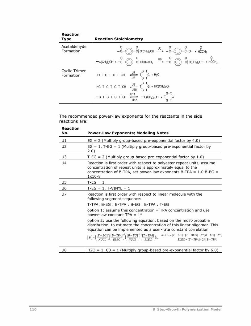
110 8 Step-Growth Polymerization Model
ReactionType Reaction Stoichiometry
AcetaldehydeFormation
Cyclic TrimerFormation
The recommended power-law exponents for the reactants in the sidereactions are:
ReactionNo. Power-Law Exponents; Modeling Notes
U1 EG = 2 (Multiply group-based pre-exponential factor by 4.0)
U2 EG = 1, T-EG = 1 (Multiply group-based pre-exponential factor by2.0)
U3 T-EG = 2 (Multiply group-based pre-exponential factor by 1.0)
U4 Reaction is first order with respect to polyester repeat units, assumeconcentration of repeat units is approximately equal to theconcentration of B-TPA, set power-law exponents B-TPA = 1.0 B-EG =1x10⁻⁸
U5 T-EG = 1
U6 T-EG = 1, T-VINYL = 1
U7 Reaction is first order with respect to linear molecule with thefollowing segment sequence:
T-TPA: B-EG : B-TPA : B-EG : B-TPA : T-EG
option 1: assume this concentration = TPA concentration and usepower-law constant TPA = 1*
option 2: use the following equation, based on the most-probabledistribution, to estimate the concentration of this linear oligomer. Thisequation can be implemented as a user-rate constant correlation
PT EG
NUCL
B TPA
ELEC
B EG
NUCL
T TPA
ELEC
NUCL T EG T DEG B EG
ELEC T TPA B TPA2
2 2
0
2 2
2
[ ] [ ] [ ] [ ] [ ] [ ] *[ ] *[
[ ] *[ ]
U8 H2O = 1, C3 = 1 (Multiply group-based pre-exponential factor by 6.0)
CCOO
O(CH2)2OH CCOO
OH + HCCH3
O
HCCH3
O+CC
OOOCH CH2O(CH2)2OH + CC
OOO(CH2)2O
U5
U6
U7
U8T
G TG
TGG T GHTGHOT + H2O
U9
U10T
G TG
TGG T GHTGTHG + HO(CH2)2OH
U11
U12T
G TG
TGG T GHTGTG +O(CH2)2OH
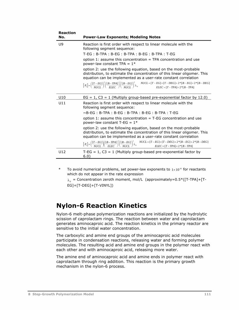
8 Step-Growth Polymerization Model 111
ReactionNo. Power-Law Exponents; Modeling Notes
U9 Reaction is first order with respect to linear molecule with thefollowing segment sequence:
T-EG : B-TPA : B-EG : B-TPA : B-EG : B-TPA : T-EG
option 1: assume this concentration = TPA concentration and usepower-law constant TPA = 1*
option 2: use the following equation, based on the most-probabledistribution, to estimate the concentration of this linear oligomer. Thisequation can be implemented as a user-rate constant correlation
PT EG
NUCL
B TPA
ELEC
B EG
NUCL
NUCL T EG T DEG B EG B DEG
ELEC T TPA B TPA2
2 3 2
0
2 2
2
[ ] [ ] [ ] [ ] [ ] *[ ] *[ ]
[ ] *[ ]
U10 EG = 1, C3 = 1 (Multiply group-based pre-exponential factor by 12.0)
U11 Reaction is first order with respect to linear molecule with thefollowing segment sequence:
~B-EG : B-TPA : B-EG : B-TPA : B-EG : B-TPA : T-EG
option 1: assume this concentration = T-EG concentration and usepower-law constant T-EG = 1*
option 2: use the following equation, based on the most-probabledistribution, to estimate the concentration of this linear oligomer. Thisequation can be implemented as a user-rate constant correlation
PT EG
NUCL
B TPA
ELEC
B EG
NUCL
NUCL T EG T DEG B EG B DEG
ELEC T TPA B TPA2
3 3
0
2 2
2
[ ] [ ] [ ] [ ] [ ] *[ ] *[ ]
[ ] *[ ]
U12 T-EG = 1, C3 = 1 (Multiply group-based pre-exponential factor by6.0)
* To avoid numerical problems, set power-law exponents to 8101 for reactants
which do not appear in the rate expression
0 = Concentration zeroth moment, mol/L (approximately=0.5*([T-TPA]+[T-
EG]+[T-DEG]+[T-VINYL])
Nylon-6 Reaction KineticsNylon-6 melt-phase polymerization reactions are initialized by the hydrolyticscission of caprolactam rings. The reaction between water and caprolactamgenerates aminocaproic acid. The reaction kinetics in the primary reactor aresensitive to the initial water concentration.
The carboxylic and amine end groups of the aminocaproic acid moleculesparticipate in condensation reactions, releasing water and forming polymermolecules. The resulting acid and amine end groups in the polymer react witheach other and with aminocaproic acid, releasing more water.
The amine end of aminocaproic acid and amine ends in polymer react withcaprolactam through ring addition. This reaction is the primary growthmechanism in the nylon-6 process.
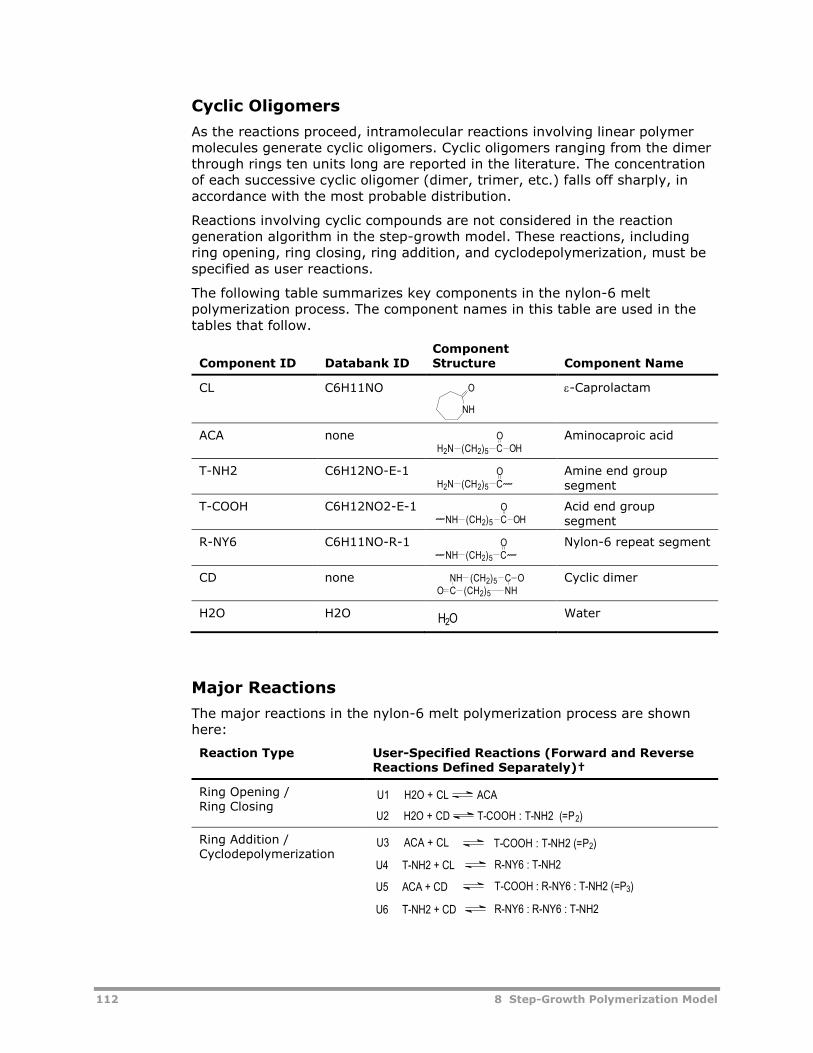
112 8 Step-Growth Polymerization Model
Cyclic Oligomers
As the reactions proceed, intramolecular reactions involving linear polymermolecules generate cyclic oligomers. Cyclic oligomers ranging from the dimerthrough rings ten units long are reported in the literature. The concentrationof each successive cyclic oligomer (dimer, trimer, etc.) falls off sharply, inaccordance with the most probable distribution.
Reactions involving cyclic compounds are not considered in the reactiongeneration algorithm in the step-growth model. These reactions, includingring opening, ring closing, ring addition, and cyclodepolymerization, must bespecified as user reactions.
The following table summarizes key components in the nylon-6 meltpolymerization process. The component names in this table are used in thetables that follow.
Component ID Databank IDComponentStructure Component Name
CL C6H11NO -Caprolactam
ACA none Aminocaproic acid
T-NH2 C6H12NO-E-1 Amine end groupsegment
T-COOH C6H12NO2-E-1 Acid end groupsegment
R-NY6 C6H11NO-R-1 Nylon-6 repeat segment
CD none Cyclic dimer
H2O H2O Water
Major Reactions
The major reactions in the nylon-6 melt polymerization process are shownhere:
Reaction Type User-Specified Reactions (Forward and ReverseReactions Defined Separately)†
Ring Opening /Ring Closing
Ring Addition /Cyclodepolymerization
NH
O
(CH2)5 CH2NO
OH
(CH2)5 CH2NO
(CH2)5 CNHO
OH
(CH2)5 CNHO
(CH2)5 CNHC NH(CH2)5O
O
H2O
U1 H2O + CL ACA
U2 H2O + CD T-COOH : T-NH2 (=P2)
U3 ACA + CL T-COOH : T-NH2 (=P2)
U4 T-NH2 + CL R-NY6 : T-NH2
U5 ACA + CD T-COOH : R-NY6 : T-NH2 (=P3)
R-NY6 : R-NY6 : T-NH2U6 T-NH2 + CD
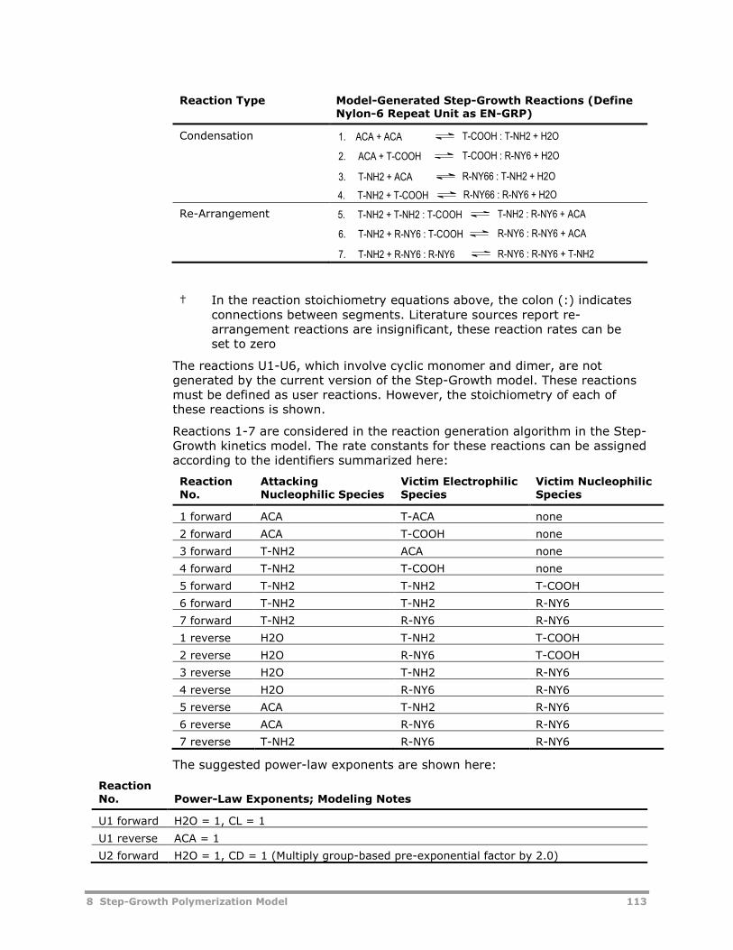
8 Step-Growth Polymerization Model 113
Reaction Type Model-Generated Step-Growth Reactions (DefineNylon-6 Repeat Unit as EN-GRP)
Condensation
Re-Arrangement
† In the reaction stoichiometry equations above, the colon (:) indicatesconnections between segments. Literature sources report re-arrangement reactions are insignificant, these reaction rates can beset to zero
The reactions U1-U6, which involve cyclic monomer and dimer, are notgenerated by the current version of the Step-Growth model. These reactionsmust be defined as user reactions. However, the stoichiometry of each ofthese reactions is shown.
Reactions 1-7 are considered in the reaction generation algorithm in the Step-Growth kinetics model. The rate constants for these reactions can be assignedaccording to the identifiers summarized here:
ReactionNo.
AttackingNucleophilic Species
Victim ElectrophilicSpecies
Victim NucleophilicSpecies
1 forward ACA T-ACA none
2 forward ACA T-COOH none
3 forward T-NH2 ACA none
4 forward T-NH2 T-COOH none
5 forward T-NH2 T-NH2 T-COOH
6 forward T-NH2 T-NH2 R-NY6
7 forward T-NH2 R-NY6 R-NY6
1 reverse H2O T-NH2 T-COOH
2 reverse H2O R-NY6 T-COOH
3 reverse H2O T-NH2 R-NY6
4 reverse H2O R-NY6 R-NY6
5 reverse ACA T-NH2 R-NY6
6 reverse ACA R-NY6 R-NY6
7 reverse T-NH2 R-NY6 R-NY6
The suggested power-law exponents are shown here:
ReactionNo. Power-Law Exponents; Modeling Notes
U1 forward H2O = 1, CL = 1
U1 reverse ACA = 1
U2 forward H2O = 1, CD = 1 (Multiply group-based pre-exponential factor by 2.0)
1. ACA + ACA T-COOH : T-NH2 + H2O
2. ACA + T-COOH T-COOH : R-NY6 + H2O
R-NY66 : T-NH2 + H2O3. T-NH2 + ACA
4. T-NH2 + T-COOH R-NY66 : R-NY6 + H2O
5. T-NH2 + T-NH2 : T-COOH T-NH2 : R-NY6 + ACA
6. T-NH2 + R-NY6 : T-COOH R-NY6 : R-NY6 + ACA
R-NY6 : R-NY6 + T-NH27. T-NH2 + R-NY6 : R-NY6
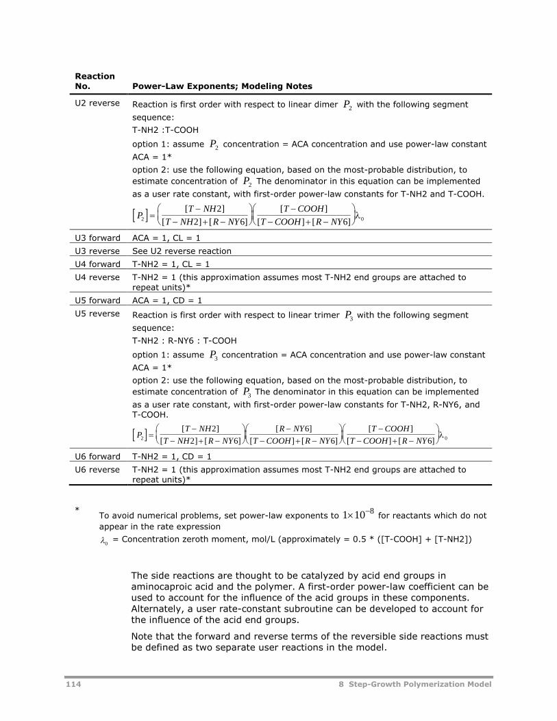
114 8 Step-Growth Polymerization Model
ReactionNo. Power-Law Exponents; Modeling Notes
U2 reverse Reaction is first order with respect to linear dimer P2 with the following segment
sequence:
T-NH2 :T-COOH
option 1: assume P2 concentration = ACA concentration and use power-law constant
ACA = 1*
option 2: use the following equation, based on the most-probable distribution, to
estimate concentration of P2 The denominator in this equation can be implemented
as a user rate constant, with first-order power-law constants for T-NH2 and T-COOH.
PT NH
T NH R NY
T COOH
T COOH R NY2 0
2
2 6 6
[ ]
[ ] [ ]
[ ]
[ ] [ ]
U3 forward ACA = 1, CL = 1
U3 reverse See U2 reverse reaction
U4 forward T-NH2 = 1, CL = 1
U4 reverse T-NH2 = 1 (this approximation assumes most T-NH2 end groups are attached torepeat units)*
U5 forward ACA = 1, CD = 1
U5 reverse Reaction is first order with respect to linear trimer P3 with the following segment
sequence:
T-NH2 : R-NY6 : T-COOH
option 1: assume P3 concentration = ACA concentration and use power-law constant
ACA = 1*
option 2: use the following equation, based on the most-probable distribution, to
estimate concentration of P3 The denominator in this equation can be implemented
as a user rate constant, with first-order power-law constants for T-NH2, R-NY6, andT-COOH.
PT NH
T NH R NY
R NY
T COOH R NY
T COOH
T COOH R NY2 0
2
2 6
6
6 6
[ ]
[ ] [ ]
[ ]
[ ] [ ]
[ ]
[ ] [ ]
U6 forward T-NH2 = 1, CD = 1
U6 reverse T-NH2 = 1 (this approximation assumes most T-NH2 end groups are attached torepeat units)*
*To avoid numerical problems, set power-law exponents to
8101 for reactants which do not
appear in the rate expression
0 = Concentration zeroth moment, mol/L (approximately = 0.5 * ([T-COOH] + [T-NH2])
The side reactions are thought to be catalyzed by acid end groups inaminocaproic acid and the polymer. A first-order power-law coefficient can beused to account for the influence of the acid groups in these components.Alternately, a user rate-constant subroutine can be developed to account forthe influence of the acid end groups.
Note that the forward and reverse terms of the reversible side reactions mustbe defined as two separate user reactions in the model.
8 Step-Growth Polymerization Model 115
Nylon-6,6 Reaction KineticsThe salt process involves a preliminary reaction to form the salt, whichprecipitates from solution. During the salt formation, some of the salt remainsin solution, leading to higher polymers. For a rigorous model, it is a good ideato consider these oligomerization reactions, even in the salt precipitationreactor. Accounting for these reactions is important when using the model tooptimize the temperature, pressure, and water content of the nylon saltcrystallizer.
The model needs to consider three phase equilibrium (solid salt, liquid, andvapor). Three phase equilibrium can be considered in Aspen Plus using theelectrolyte chemistry feature. In version 10.0, however, the CSTR model doesnot allow a component to appear simultaneously in chemistry reactions andkinetic reactions. Another way to represent the solid-liquid equilibrium is todefine an equilibrium reaction between the components representing thedissolved and solid salt. Chemical equilibrium equations can be defined usingthe Power-Law reaction kinetics model in Aspen Plus. Apply the “mole-gamma” option to force the equilibrium equation to use the ratio of the molaractivities as the basis of the equilibrium constant. By using this assumption,the equilibrium constant is the same as the solubility constant of the solidsalt.
To model the reaction kinetics of the salt process, the dissolved salt should beconsidered as a component in the reaction model. The models described inthe open literature do this by considering the salt as an “AB” type monomer.This treatment, however, fails to consider some of the reverse reactionswhich can occur during polymerization. This approach assumes that reversecondensation reactions and re-arrangement reactions always generateproducts with an equal number of adipic acid and HMDA units. In reality,polymer chains with an unequal number of units can be formed because thereactions can occur inside the repeat units which originally came from thereacting salts. Further, the reverse reactions can generate free adipic acid orHMDA when the reaction occurs at the end of a polymer chain.
Reverse Rate Constant
The models in the literature use a reverse rate constant which is twice thereverse rate constant experienced by an individual amine group. This factor oftwo accounts for the fact that each repeat unit has two amine groups. In theapproach described here, the reverse rate constants used in the model shouldbe the rate constant between two functional groups, for example betweenwater and a single amine group.
Considering salt as a component, there are several reversible reactions whichmust be considered in the model. A number of condensation reactions occurincluding those between molecules of dissolved salt, dissolved monomers, andpolymer end groups. These reactions can be implemented in the step-growthmodel through the user reaction feature. The step-growth model will generatethe reactions which do not involve the salt component.
The molecular weight distribution of nylon-6,6 is known to re-equilibratewhen the polymer is exposed to HMDA under pressure. Further, as vacuum isapplied, free HMDA appears to be generated. These facts indicate thatrearrangement reactions are important in this process.
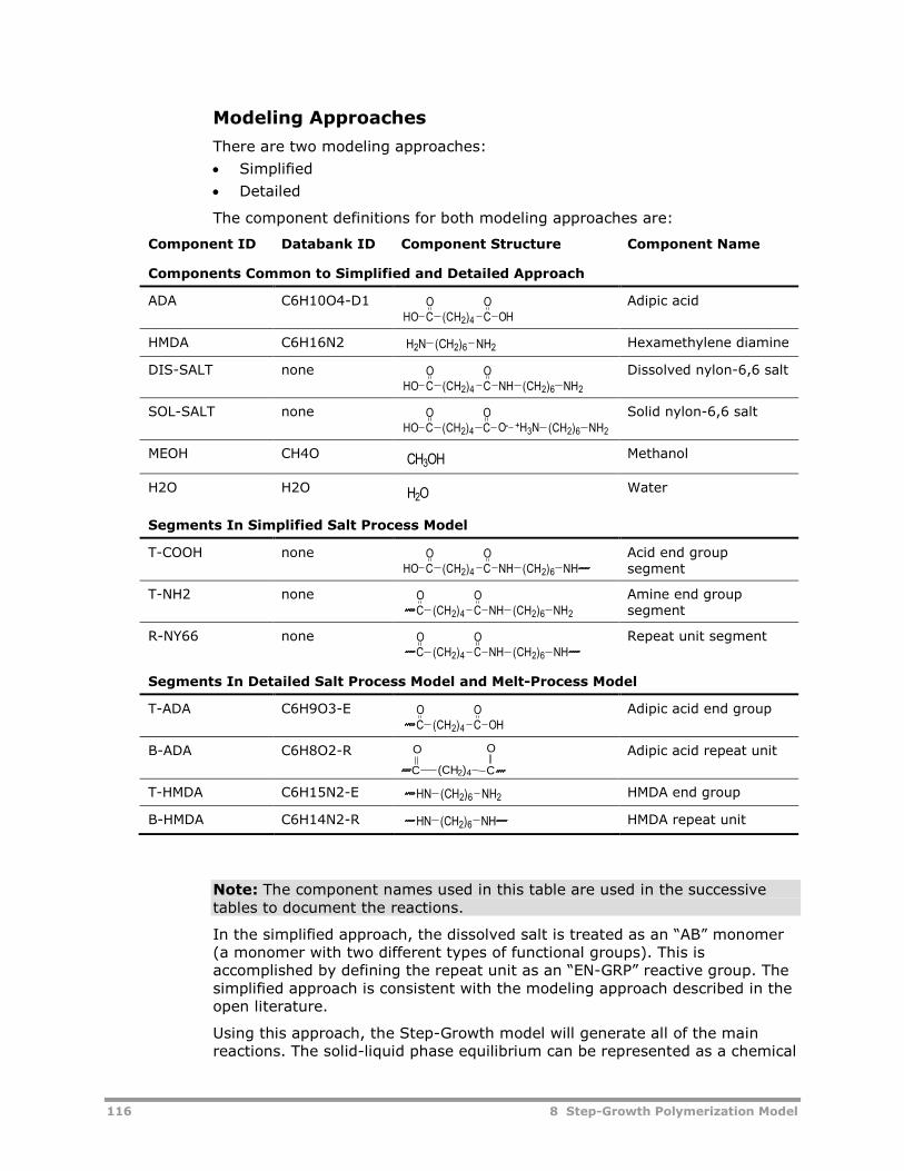
116 8 Step-Growth Polymerization Model
Modeling Approaches
There are two modeling approaches:
Simplified
Detailed
The component definitions for both modeling approaches are:
Component ID Databank ID Component Structure Component Name
Components Common to Simplified and Detailed Approach
ADA C6H10O4-D1 Adipic acid
HMDA C6H16N2 Hexamethylene diamine
DIS-SALT none Dissolved nylon-6,6 salt
SOL-SALT none Solid nylon-6,6 salt
MEOH CH4O Methanol
H2O H2O Water
Segments In Simplified Salt Process Model
T-COOH none Acid end groupsegment
T-NH2 none Amine end groupsegment
R-NY66 none Repeat unit segment
Segments In Detailed Salt Process Model and Melt-Process Model
T-ADA C6H9O3-E Adipic acid end group
B-ADA C6H8O2-R
C (CH2)4 C
OO Adipic acid repeat unit
T-HMDA C6H15N2-E HMDA end group
B-HMDA C6H14N2-R HMDA repeat unit
Note: The component names used in this table are used in the successivetables to document the reactions.
In the simplified approach, the dissolved salt is treated as an “AB” monomer(a monomer with two different types of functional groups). This isaccomplished by defining the repeat unit as an “EN-GRP” reactive group. Thesimplified approach is consistent with the modeling approach described in theopen literature.
Using this approach, the Step-Growth model will generate all of the mainreactions. The solid-liquid phase equilibrium can be represented as a chemical
(CH2)4CO
HO C OHO
(CH2)6 NH2H2N
(CH2)4CO
HO CO
NH (CH2)6 NH2
(CH2)4CO
HO C O-O
+H3N (CH2)6 NH2
CH3OH
H2O
(CH2)4CO
HO CO
NH (CH2)6 NH
(CH2)4CO
CO
NH (CH2)6 NH2
(CH2)4CO
CO
NH (CH2)6 NH
(CH2)4CO
C OHO
(CH2)6 NH2HN
(CH2)6 NHHN
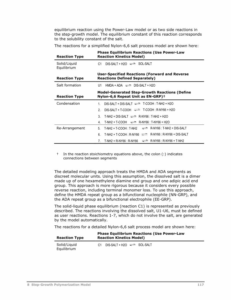
8 Step-Growth Polymerization Model 117
equilibrium reaction using the Power-Law model or as two side reactions inthe step-growth model. The equilibrium constant of this reaction correspondsto the solubility constant of the salt.
The reactions for a simplified Nylon-6,6 salt process model are shown here:
Reaction TypePhase Equilibrium Reactions (Use Power-LawReaction Kinetics Model)
Solid/LiquidEquilibrium
Reaction TypeUser-Specified Reactions (Forward and ReverseReactions Defined Separately)
Salt formation
Reaction TypeModel-Generated Step-Growth Reactions (DefineNylon-6,6 Repeat Unit as EN-GRP)†
Condensation
Re-Arrangement
† In the reaction stoichiometry equations above, the colon (:) indicatesconnections between segments
The detailed modeling approach treats the HMDA and ADA segments asdiscreet molecular units. Using this assumption, the dissolved salt is a dimermade up of one hexamethylene diamine end group and one adipic acid endgroup. This approach is more rigorous because it considers every possiblereverse reaction, including terminal monomer loss. To use this approach,define the HMDA repeat group as a bifunctional nucleophile (NN-GRP), andthe ADA repeat group as a bifunctional electrophile (EE-GRP).
The solid-liquid phase equilibrium (reaction C1) is represented as previouslydescribed. The reactions involving the dissolved salt, U1-U6, must be definedas user reactions. Reactions 1-7, which do not involve the salt, are generatedby the model automatically.
The reactions for a detailed Nylon-6,6 salt process model are shown here:
Reaction TypePhase Equilibrium Reactions (Use Power-LawReaction Kinetics Model)
Solid/LiquidEquilibrium
C1 DIS-SALT + H2O SOL-SALT
U1 HMDA + ADA DIS-SALT + H2O
3. T-NH2 + DIS-SALT R-NY66 : T-NH2 + H2O
T-COOH : R-NY66 + H2O2. DIS-SALT + T-COOH
T-COOH : T-NH2 + H2O1. DIS-SALT + DIS-SALT
R-NY66 : T-NY66 + H2O4. T-NH2 + T-COOH
5. T-NH2 + T-COOH : T-NH2 R-NY66 : T-NH2 + DIS-SALT
6. T-NH2 + T-COOH : R-NY66 R-NY66 : R-NY66 + DIS-SALT
R-NY66 : R-NY66 + T-NH27. T-NH2 + R-NY66 : R-NY66
C1 DIS-SALT + H2O SOL-SALT
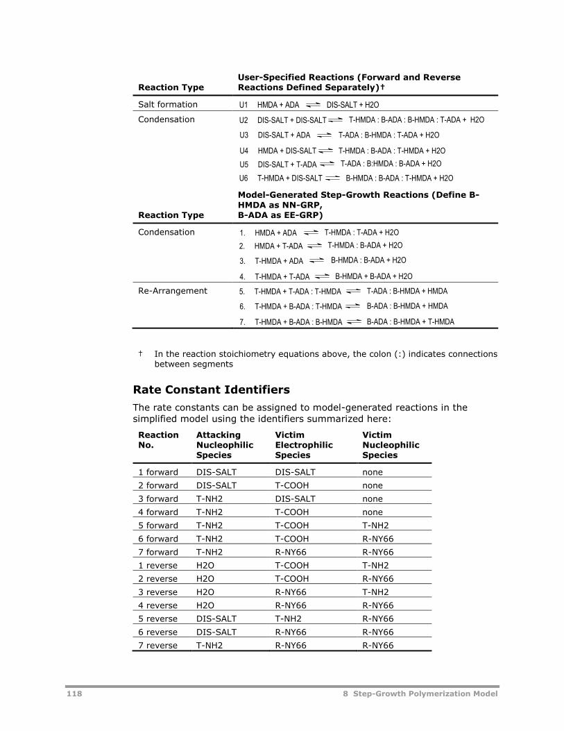
118 8 Step-Growth Polymerization Model
Reaction TypeUser-Specified Reactions (Forward and ReverseReactions Defined Separately)†
Salt formation
Condensation
Reaction Type
Model-Generated Step-Growth Reactions (Define B-HMDA as NN-GRP,B-ADA as EE-GRP)
Condensation
Re-Arrangement
† In the reaction stoichiometry equations above, the colon (:) indicates connectionsbetween segments
Rate Constant Identifiers
The rate constants can be assigned to model-generated reactions in thesimplified model using the identifiers summarized here:
ReactionNo.
AttackingNucleophilicSpecies
VictimElectrophilicSpecies
VictimNucleophilicSpecies
1 forward DIS-SALT DIS-SALT none
2 forward DIS-SALT T-COOH none
3 forward T-NH2 DIS-SALT none
4 forward T-NH2 T-COOH none
5 forward T-NH2 T-COOH T-NH2
6 forward T-NH2 T-COOH R-NY66
7 forward T-NH2 R-NY66 R-NY66
1 reverse H2O T-COOH T-NH2
2 reverse H2O T-COOH R-NY66
3 reverse H2O R-NY66 T-NH2
4 reverse H2O R-NY66 R-NY66
5 reverse DIS-SALT T-NH2 R-NY66
6 reverse DIS-SALT R-NY66 R-NY66
7 reverse T-NH2 R-NY66 R-NY66
U1 HMDA + ADA DIS-SALT + H2O
U4 HMDA + DIS-SALT T-HMDA : B-ADA : T-HMDA + H2O
T-ADA : B-HMDA : T-ADA + H2OU3 DIS-SALT + ADA
T-HMDA : B-ADA : B-HMDA : T-ADA + H2OU2 DIS-SALT + DIS-SALT
T-ADA : B:HMDA : B-ADA + H2OU5 DIS-SALT + T-ADA
U6 T-HMDA + DIS-SALT B-HMDA : B-ADA : T-HMDA + H2O
2. HMDA + T-ADA T-HMDA : B-ADA + H2O
3. T-HMDA + ADA B-HMDA : B-ADA + H2O
B-HMDA + B-ADA + H2O4. T-HMDA + T-ADA
T-HMDA : T-ADA + H2O1. HMDA + ADA
5. T-HMDA + T-ADA : T-HMDA T-ADA : B-HMDA + HMDA
6. T-HMDA + B-ADA : T-HMDA B-ADA : B-HMDA + HMDA
B-ADA : B-HMDA + T-HMDA7. T-HMDA + B-ADA : B-HMDA
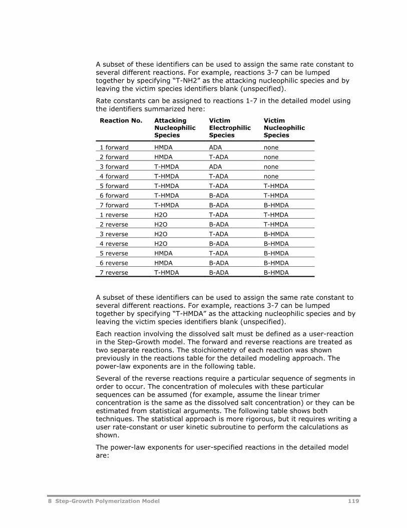
8 Step-Growth Polymerization Model 119
A subset of these identifiers can be used to assign the same rate constant toseveral different reactions. For example, reactions 3-7 can be lumpedtogether by specifying “T-NH2” as the attacking nucleophilic species and byleaving the victim species identifiers blank (unspecified).
Rate constants can be assigned to reactions 1-7 in the detailed model usingthe identifiers summarized here:
Reaction No. AttackingNucleophilicSpecies
VictimElectrophilicSpecies
VictimNucleophilicSpecies
1 forward HMDA ADA none
2 forward HMDA T-ADA none
3 forward T-HMDA ADA none
4 forward T-HMDA T-ADA none
5 forward T-HMDA T-ADA T-HMDA
6 forward T-HMDA B-ADA T-HMDA
7 forward T-HMDA B-ADA B-HMDA
1 reverse H2O T-ADA T-HMDA
2 reverse H2O B-ADA T-HMDA
3 reverse H2O T-ADA B-HMDA
4 reverse H2O B-ADA B-HMDA
5 reverse HMDA T-ADA B-HMDA
6 reverse HMDA B-ADA B-HMDA
7 reverse T-HMDA B-ADA B-HMDA
A subset of these identifiers can be used to assign the same rate constant toseveral different reactions. For example, reactions 3-7 can be lumpedtogether by specifying “T-HMDA” as the attacking nucleophilic species and byleaving the victim species identifiers blank (unspecified).
Each reaction involving the dissolved salt must be defined as a user-reactionin the Step-Growth model. The forward and reverse reactions are treated astwo separate reactions. The stoichiometry of each reaction was shownpreviously in the reactions table for the detailed modeling approach. Thepower-law exponents are in the following table.
Several of the reverse reactions require a particular sequence of segments inorder to occur. The concentration of molecules with these particularsequences can be assumed (for example, assume the linear trimerconcentration is the same as the dissolved salt concentration) or they can beestimated from statistical arguments. The following table shows bothtechniques. The statistical approach is more rigorous, but it requires writing auser rate-constant or user kinetic subroutine to perform the calculations asshown.
The power-law exponents for user-specified reactions in the detailed modelare:
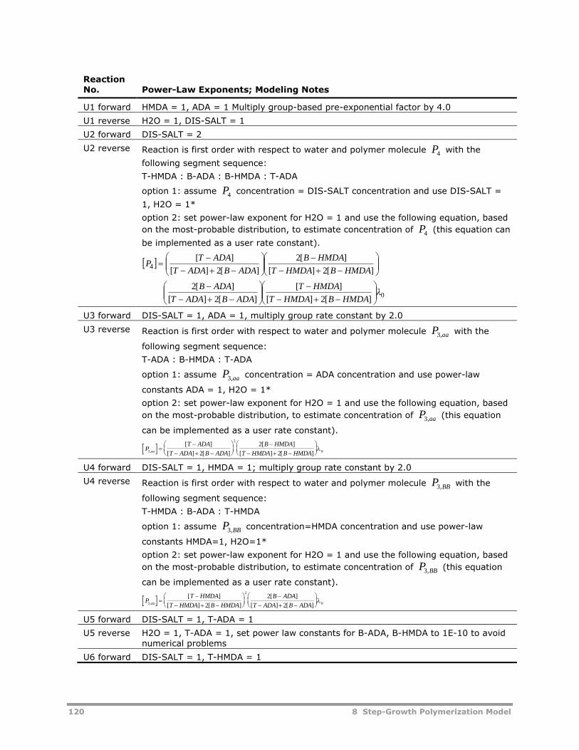
120 8 Step-Growth Polymerization Model
ReactionNo. Power-Law Exponents; Modeling Notes
U1 forward HMDA = 1, ADA = 1 Multiply group-based pre-exponential factor by 4.0
U1 reverse H2O = 1, DIS-SALT = 1
U2 forward DIS-SALT = 2
U2 reverse Reaction is first order with respect to water and polymer molecule P4 with the
following segment sequence:
T-HMDA : B-ADA : B-HMDA : T-ADA
option 1: assume P4 concentration = DIS-SALT concentration and use DIS-SALT =
1, H2O = 1*
option 2: set power-law exponent for H2O = 1 and use the following equation, based
on the most-probable distribution, to estimate concentration of P4 (this equation can
be implemented as a user rate constant).
0
4
][2][
][
][2][
][2
][2][
][2
][2][
][
HMDABHMDAT
HMDAT
ADABADAT
ADAB
HMDABHMDAT
HMDAB
ADABADAT
ADATP
U3 forward DIS-SALT = 1, ADA = 1, multiply group rate constant by 2.0
U3 reverse Reaction is first order with respect to water and polymer molecule P aa3, with the
following segment sequence:
T-ADA : B-HMDA : T-ADA
option 1: assume P aa3, concentration = ADA concentration and use power-law
constants ADA = 1, H2O = 1*
option 2: set power-law exponent for H2O = 1 and use the following equation, based
on the most-probable distribution, to estimate concentration of P aa3, (this equation
can be implemented as a user rate constant).
PT ADA
T ADA B ADA
B HMDA
T HMDA B HMDAaa3
2
02
2
2,
[ ]
[ ] [ ]
[ ]
[ ] [ ]
U4 forward DIS-SALT = 1, HMDA = 1; multiply group rate constant by 2.0
U4 reverse Reaction is first order with respect to water and polymer molecule P BB3, with the
following segment sequence:
T-HMDA : B-ADA : T-HMDA
option 1: assume P BB3, concentration=HMDA concentration and use power-law
constants HMDA=1, H2O=1*
option 2: set power-law exponent for H2O = 1 and use the following equation, based
on the most-probable distribution, to estimate concentration of P BB3, (this equation
can be implemented as a user rate constant).
PT HMDA
T HMDA B HMDA
B ADA
T ADA B ADAaa3
2
02
2
2,
[ ]
[ ] [ ]
[ ]
[ ] [ ]
U5 forward DIS-SALT = 1, T-ADA = 1
U5 reverse H2O = 1, T-ADA = 1, set power law constants for B-ADA, B-HMDA to 1E-10 to avoidnumerical problems
U6 forward DIS-SALT = 1, T-HMDA = 1
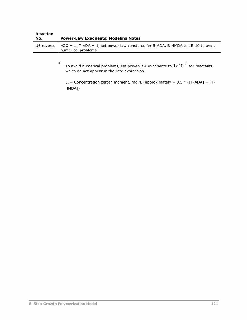
8 Step-Growth Polymerization Model 121
ReactionNo. Power-Law Exponents; Modeling Notes
U6 reverse H2O = 1, T-ADA = 1, set power law constants for B-ADA, B-HMDA to 1E-10 to avoidnumerical problems
*To avoid numerical problems, set power-law exponents to
8101 for reactants
which do not appear in the rate expression
0 = Concentration zeroth moment, mol/L (approximately = 0.5 * ([T-ADA] + [T-
HMDA])
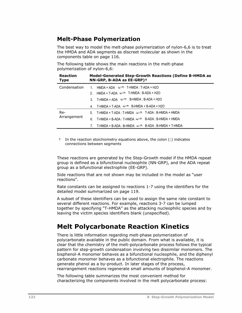
122 8 Step-Growth Polymerization Model
Melt-Phase Polymerization
The best way to model the melt-phase polymerization of nylon-6,6 is to treatthe HMDA and ADA segments as discreet molecular as shown in thecomponents table on page 116.
The following table shows the main reactions in the melt-phasepolymerization of nylon-6,6:
ReactionType
Model-Generated Step-Growth Reactions (Define B-HMDA asNN-GRP, B-ADA as EE-GRP)†
Condensation
Re-Arrangement
† In the reaction stoichiometry equations above, the colon (:) indicatesconnections between segments
These reactions are generated by the Step-Growth model if the HMDA repeatgroup is defined as a bifunctional nucleophile (NN-GRP), and the ADA repeatgroup as a bifunctional electrophile (EE-GRP).
Side reactions that are not shown may be included in the model as “userreactions”.
Rate constants can be assigned to reactions 1-7 using the identifiers for thedetailed model summarized on page 119.
A subset of these identifiers can be used to assign the same rate constant toseveral different reactions. For example, reactions 3-7 can be lumpedtogether by specifying “T-HMDA” as the attacking nucleophilic species and byleaving the victim species identifiers blank (unspecified).
Melt Polycarbonate Reaction KineticsThere is little information regarding melt-phase polymerization ofpolycarbonate available in the public domain. From what is available, it isclear that the chemistry of the melt-polycarbonate process follows the typicalpattern for step-growth condensation involving two dissimilar monomers. Thebisphenol-A monomer behaves as a bifunctional nucleophile, and the diphenylcarbonate monomer behaves as a bifunctional electrophile. The reactionsgenerate phenol as a by-product. In later stages of the process,rearrangement reactions regenerate small amounts of bisphenol-A monomer.
The following table summarizes the most convenient method forcharacterizing the components involved in the melt polycarbonate process:
2. HMDA + T-ADA T-HMDA : B-ADA + H2O
3. T-HMDA + ADA B-HMDA : B-ADA + H2O
B-HMDA + B-ADA + H2O4. T-HMDA + T-ADA
T-HMDA : T-ADA + H2O1. HMDA + ADA
5. T-HMDA + T-ADA : T-HMDA T-ADA : B-HMDA + HMDA
6. T-HMDA + B-ADA : T-HMDA B-ADA : B-HMDA + HMDA
B-ADA : B-HMDA + T-HMDA7. T-HMDA + B-ADA : B-HMDA
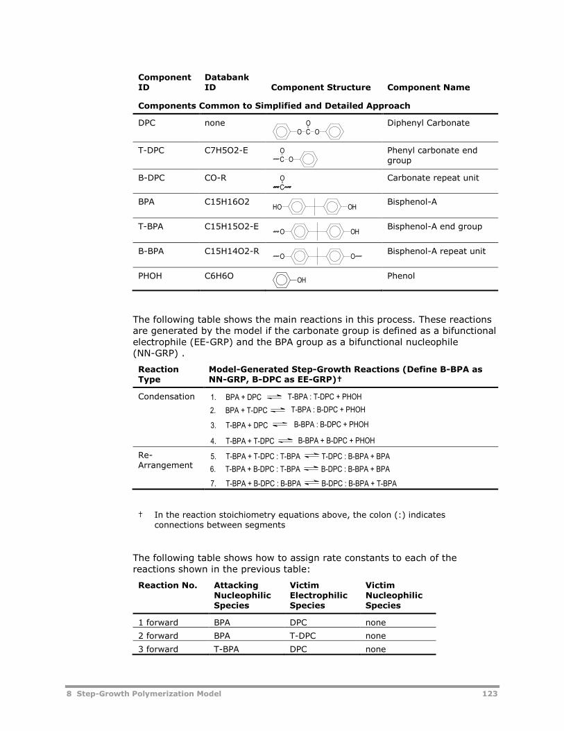
8 Step-Growth Polymerization Model 123
ComponentID
DatabankID Component Structure Component Name
Components Common to Simplified and Detailed Approach
DPC none Diphenyl Carbonate
T-DPC C7H5O2-E Phenyl carbonate endgroup
B-DPC CO-R Carbonate repeat unit
BPA C15H16O2 Bisphenol-A
T-BPA C15H15O2-E Bisphenol-A end group
B-BPA C15H14O2-R Bisphenol-A repeat unit
PHOH C6H6O Phenol
The following table shows the main reactions in this process. These reactionsare generated by the model if the carbonate group is defined as a bifunctionalelectrophile (EE-GRP) and the BPA group as a bifunctional nucleophile(NN-GRP) .
ReactionType
Model-Generated Step-Growth Reactions (Define B-BPA asNN-GRP, B-DPC as EE-GRP)†
Condensation
Re-Arrangement
† In the reaction stoichiometry equations above, the colon (:) indicatesconnections between segments
The following table shows how to assign rate constants to each of thereactions shown in the previous table:
Reaction No. AttackingNucleophilicSpecies
VictimElectrophilicSpecies
VictimNucleophilicSpecies
1 forward BPA DPC none
2 forward BPA T-DPC none
3 forward T-BPA DPC none
CO
OO
CO
O
CO
HO OH
O OH
O O
OH
2. BPA + T-DPC T-BPA : B-DPC + PHOH
3. T-BPA + DPC B-BPA : B-DPC + PHOH
B-BPA + B-DPC + PHOH4. T-BPA + T-DPC
T-BPA : T-DPC + PHOH1. BPA + DPC
T-DPC : B-BPA + BPA5. T-BPA + T-DPC : T-BPA
6. T-BPA + B-DPC : T-BPA B-DPC : B-BPA + BPA
7. T-BPA + B-DPC : B-BPA B-DPC : B-BPA + T-BPA
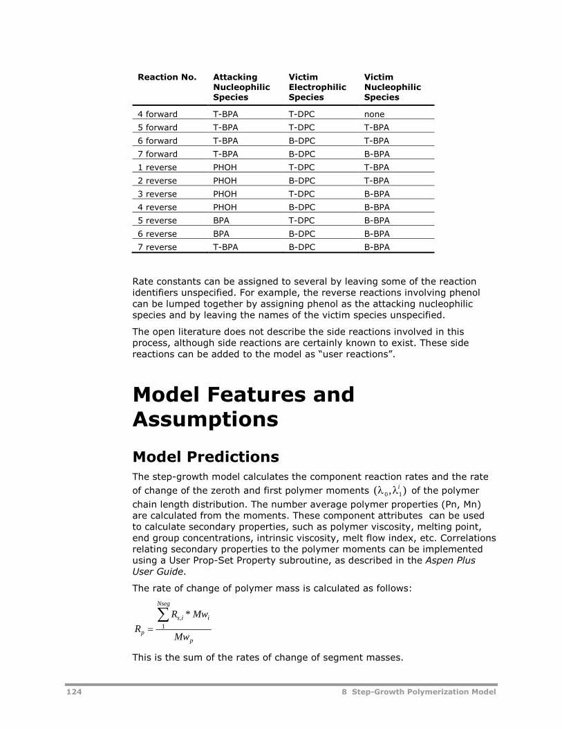
124 8 Step-Growth Polymerization Model
Reaction No. AttackingNucleophilicSpecies
VictimElectrophilicSpecies
VictimNucleophilicSpecies
4 forward T-BPA T-DPC none
5 forward T-BPA T-DPC T-BPA
6 forward T-BPA B-DPC T-BPA
7 forward T-BPA B-DPC B-BPA
1 reverse PHOH T-DPC T-BPA
2 reverse PHOH B-DPC T-BPA
3 reverse PHOH T-DPC B-BPA
4 reverse PHOH B-DPC B-BPA
5 reverse BPA T-DPC B-BPA
6 reverse BPA B-DPC B-BPA
7 reverse T-BPA B-DPC B-BPA
Rate constants can be assigned to several by leaving some of the reactionidentifiers unspecified. For example, the reverse reactions involving phenolcan be lumped together by assigning phenol as the attacking nucleophilicspecies and by leaving the names of the victim species unspecified.
The open literature does not describe the side reactions involved in thisprocess, although side reactions are certainly known to exist. These sidereactions can be added to the model as “user reactions”.
Model Features andAssumptions
Model PredictionsThe step-growth model calculates the component reaction rates and the rate
of change of the zeroth and first polymer moments ( , ) 0 1i
of the polymer
chain length distribution. The number average polymer properties (Pn, Mn)are calculated from the moments. These component attributes can be usedto calculate secondary properties, such as polymer viscosity, melting point,end group concentrations, intrinsic viscosity, melt flow index, etc. Correlationsrelating secondary properties to the polymer moments can be implementedusing a User Prop-Set Property subroutine, as described in the Aspen PlusUser Guide.
The rate of change of polymer mass is calculated as follows:
R
R Mw
Mwp
s i i
Nseg
p
, *
1
This is the sum of the rates of change of segment masses.
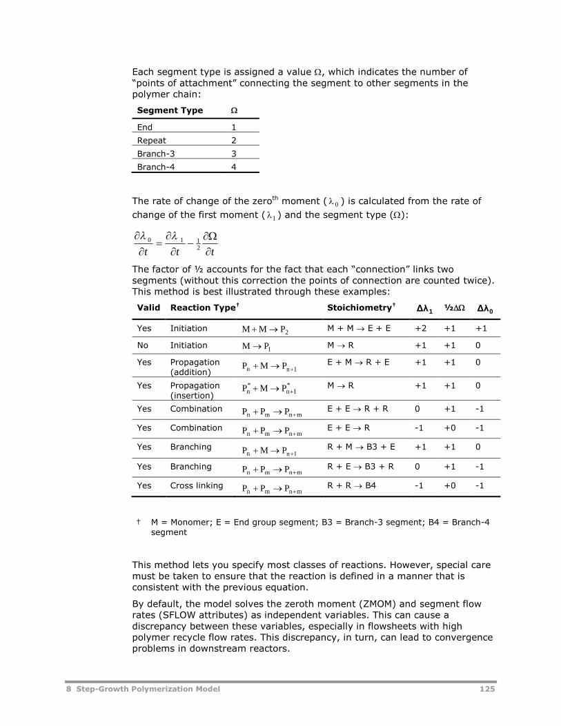
8 Step-Growth Polymerization Model 125
Each segment type is assigned a value , which indicates the number of“points of attachment” connecting the segment to other segments in thepolymer chain:
Segment Type
End 1
Repeat 2
Branch-3 3
Branch-4 4
The rate of change of the zeroth moment ( 0 ) is calculated from the rate of
change of the first moment ( 1 ) and the segment type ():
ttt
2110
The factor of ½ accounts for the fact that each “connection” links twosegments (without this correction the points of connection are counted twice).This method is best illustrated through these examples:
Valid Reaction Type† Stoichiometry†1Δλ ½ 0Δλ
Yes Initiation 2PMM M + M E + E +2 +1 +1
No Initiation 1PM M R +1 +1 0
Yes Propagation(addition) 1nn PMP E + M R + E +1 +1 0
Yes Propagation(insertion)
*1n
*n PMP M R +1 +1 0
Yes Combinationmnmn PPP E + E R + R 0 +1 -1
Yes Combinationmnmn PPP E + E R -1 +0 -1
Yes Branching1nn PMP R + M B3 + E +1 +1 0
Yes Branchingmnmn PPP R + E B3 + R 0 +1 -1
Yes Cross linkingmnmn PPP R + R B4 -1 +0 -1
† M = Monomer; E = End group segment; B3 = Branch-3 segment; B4 = Branch-4segment
This method lets you specify most classes of reactions. However, special caremust be taken to ensure that the reaction is defined in a manner that isconsistent with the previous equation.
By default, the model solves the zeroth moment (ZMOM) and segment flowrates (SFLOW attributes) as independent variables. This can cause adiscrepancy between these variables, especially in flowsheets with highpolymer recycle flow rates. This discrepancy, in turn, can lead to convergenceproblems in downstream reactors.
126 8 Step-Growth Polymerization Model
To avoid this problem, you can force the model to calculate the zerothmoment directly from the segment flow rates by checking the “explicitly solvezeroth moment” option on the step-growth Options form. When this option isselected, the model calculates the zeroth moment as:
21
10
This option cannot be invoked if two or more reaction models are referencedfrom a single reactor block.
Phase EquilibriaThe step-growth model can be used to simulate reactions in single-phase(vapor or liquid), two-phase (VL), or three-phase (VLL) systems. Each step-growth reaction model is associated with a particular reaction phase, specifiedon the Options sheet. The user can consider simultaneous reactions inmultiple phases by referring to two or more reaction models in a reactor.
Typical applications of this model include melt-phase polymerization andsolution polymerization. Slurry, suspension, and emulsion processes involvingstep-growth kinetics can also be simulated with this model.
Interfacial polymerization involves a solvent phase, an organic monomerphase, and a polymer phase. The reaction rate is usually limited by the rateof mass transfer of monomers from the organic phase to the reacting polymerphase. The mass-transfer limits across the liquid-liquid interface are not takeninto account by the standard model. These systems can be simulated bydeveloping a custom reactor model in Aspen Custom Modeler or Aspen Plus,or by writing an appropriate concentration basis subroutine for the step-growth model.
Solid-state polymerization involves crystalline and amorphous solid polymerphases and a vapor phase. The reaction kinetics may be limited by the rate ofmass transfer of volatile reaction by-products from the amorphous solid phaseto the polymer phase. None of the standard reactor models in Aspen Polymersare designed for solid-state polymerization. Solid-state polymerization modelscan be developed in Aspen Custom Modeler and interfaced to the step-growthpolymerization model through the Aspen Custom Modeler / Aspen PolymersInterface.
Mass transfer limitations in thin-film or horizontal finishing reactors can beconsidered by customizing the Step-Growth model using the availableconcentration basis subroutine or by developing an appropriate user reactormodel in Aspen Plus or Aspen Custom Modeler.
Reaction MechanismThe Step-Growth reaction model applies to condensation polymerization. Inthe future the model will be extended to cover pseudocondensation and ring-addition polymerization. The model accounts for any combination ofmonofunctional and bifunctional monomers. Cyclic monomers andmultifunctional monomers, however, are not included in the standard reactionscheme.
8 Step-Growth Polymerization Model 127
User-defined stoichiometric reactions can be added to the model to accountfor reactions which are not included in the standard reaction scheme. Thesereactions use a power-law rate expression which can be extended to morecomplex rate expressions through the application of a user-written Fortransubroutine.
Model StructureThis section outlines the structure of the Step-Growth kinetics model. Itexamines the theoretical framework in detail. The assumptions and limits ofthe algorithms are documented.
Reacting Groups and SpeciesThe first step in the development of any process simulation model is todetermine the list of components. In Aspen Polymers it is also important todecide how to characterize the polymer components. A polymer can bebroken down into segments any number of ways. For example, the nylon-6repeat unit can be treated as a segment, or it can be divided into twosegments corresponding to the portions of the repeat unit which came fromthe diacid and diamine monomers.
Segments
The preferred method of segmenting the polymer component is to definesegments corresponding to the monomers which are used to produce thepolymer. This technique has two distinct advantages. First, the propertymodels in Aspen Polymers use the monomer as a reference point formolecular size. Second, the reaction kinetics usually involve addingmonomers to the end of growing polymer chains. Defining segmentscorresponding to the monomers makes it easy to write reactionscorresponding to monomers and segments, for example monomer “A” segment “A”.
The Step-Growth model assumes that the polymer is segmented in thismanner. For monadic polymers such as nylon-6, this technique isstraightforward. This method of segmenting the polymer is a bit unusual fordyadic polymers, such as PET, because it treats them as alternatingcopolymers. Thus, a molecule of PET with 100 PET units is defined as having adegree of polymerization of 200 in this model (100 terephthalate units and100 glycol units).
Monofunctional monomers, such as benzoic acid, always correspond to anend-group segment in the model. Bifunctional monomers can end up inside alinear polymer chain as a repeat unit, or may be located at the end of thechain as an end group. Each symmetric bifunctional monomer (diacids, diols,diamines, etc.) corresponds to one repeat segment and one end-groupsegment. Asymmetric bifunctional monomers (monomers with two differenttypes of end groups) correspond to one repeat unit and two end-groupsegments. Multifunctional monomers can correspond to several segments, asshown:
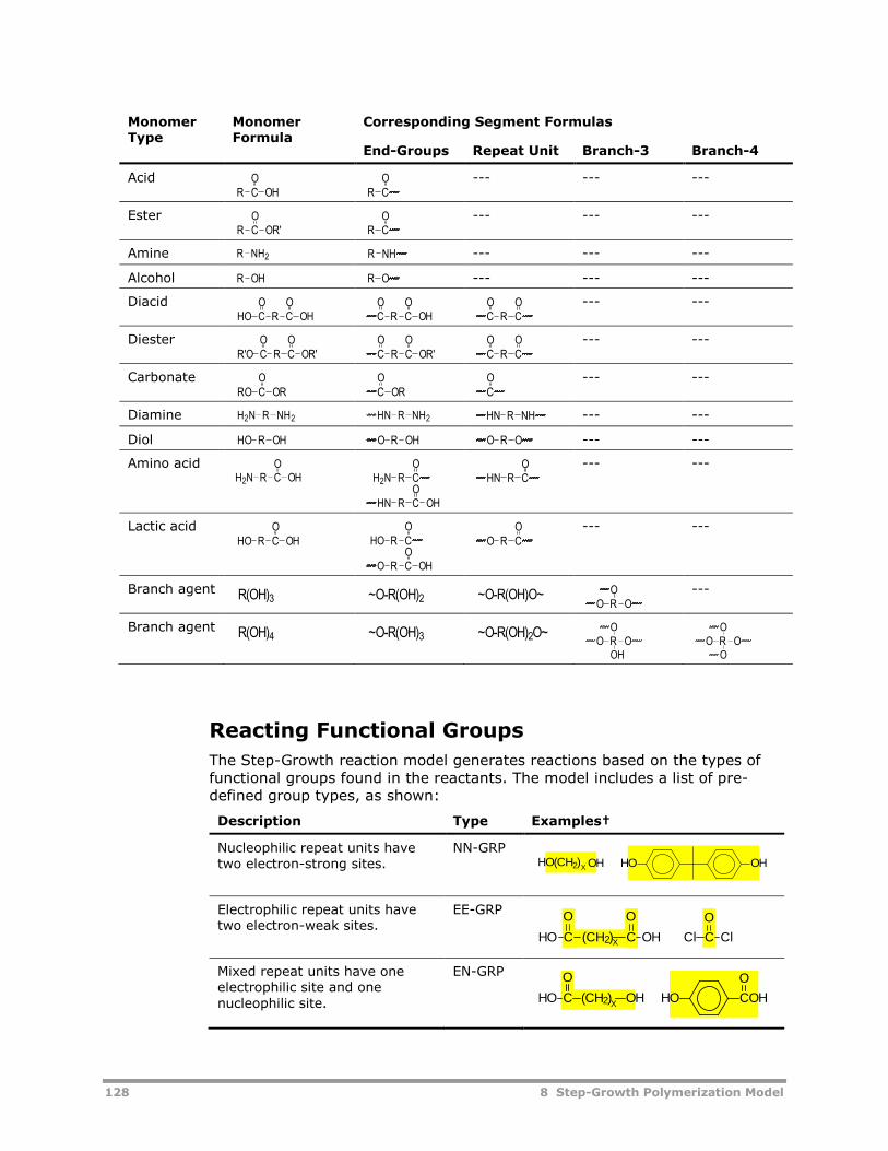
128 8 Step-Growth Polymerization Model
MonomerType
MonomerFormula
Corresponding Segment Formulas
End-Groups Repeat Unit Branch-3 Branch-4
Acid --- --- ---
Ester --- --- ---
Amine --- --- ---
Alcohol --- --- ---
Diacid --- ---
Diester --- ---
Carbonate --- ---
Diamine --- ---
Diol --- ---
Amino acid --- ---
Lactic acid --- ---
Branch agent ---
Branch agent
Reacting Functional Groups
The Step-Growth reaction model generates reactions based on the types offunctional groups found in the reactants. The model includes a list of pre-defined group types, as shown:
Description Type Examples†
Nucleophilic repeat units havetwo electron-strong sites.
NN-GRP
Electrophilic repeat units havetwo electron-weak sites.
EE-GRP
Mixed repeat units have oneelectrophilic site and onenucleophilic site.
EN-GRP
CO
OHR CO
R
CO
OR'R CO
R
R NH2 R NH
R OH R O
CO
OHRCO
HO CO
OHRCO
CO
RCO
CO
OR'RCO
R'O CO
OR'RCO
CO
RCO
CO
ORRO CO
OR CO
R NH2H2N R NH2HN R NHHN
R OHHO R OHO R OO
CO
OHRH2N CO
RH2N
CO
OHRHN
CO
RHN
CO
OHRHO CO
RHO
CO
OHRO
CO
RO
R(OH)3 ~O-R(OH)2 ~O-R(OH)O~RO OO
R(OH)4 ~O-R(OH)3 ~O-R(OH)2O~RO OO
OHRO OO
O
HO(CH2)X OH HO OH
HO C
O
(CH2) C OH
O
X Cl C Cl
O
HO C
O
(CH2) OHX
HO COH
O
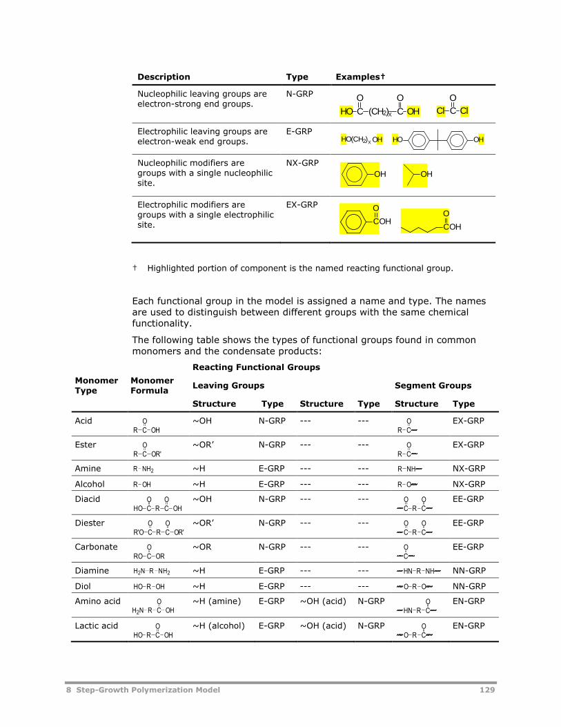
8 Step-Growth Polymerization Model 129
Description Type Examples†
Nucleophilic leaving groups areelectron-strong end groups.
N-GRP
Electrophilic leaving groups areelectron-weak end groups.
E-GRP
Nucleophilic modifiers aregroups with a single nucleophilicsite.
NX-GRP
Electrophilic modifiers aregroups with a single electrophilicsite.
EX-GRP
† Highlighted portion of component is the named reacting functional group.
Each functional group in the model is assigned a name and type. The namesare used to distinguish between different groups with the same chemicalfunctionality.
The following table shows the types of functional groups found in commonmonomers and the condensate products:
MonomerType
MonomerFormula
Reacting Functional Groups
Leaving Groups Segment Groups
Structure Type Structure Type Structure Type
Acid ~OH N-GRP --- --- EX-GRP
Ester ~OR’ N-GRP --- --- EX-GRP
Amine ~H E-GRP --- --- NX-GRP
Alcohol ~H E-GRP --- --- NX-GRP
Diacid ~OH N-GRP --- --- EE-GRP
Diester ~OR’ N-GRP --- --- EE-GRP
Carbonate ~OR N-GRP --- --- EE-GRP
Diamine ~H E-GRP --- --- NN-GRP
Diol ~H E-GRP --- --- NN-GRP
Amino acid ~H (amine) E-GRP ~OH (acid) N-GRP EN-GRP
Lactic acid ~H (alcohol) E-GRP ~OH (acid) N-GRP EN-GRP
XHO C
O
(CH2) C OH
O
Cl C Cl
O
OHXHO(CH2) HO OH
OH OH
COH
O
COH
O
CO
OHR CO
R
CO
OR'R CO
R
R NH2 R NH
R OH R O
CO
OHRCO
HO CO
RCO
CO
OR'RCO
R'O CO
RCO
CO
ORRO CO
R NH2H2N R NHHN
R OHHO R OO
CO
OHRH2N CO
RHN
CO
OHRHO CO
RO
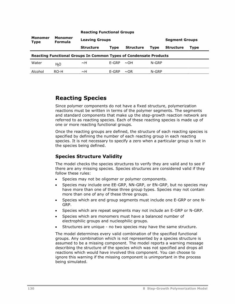
130 8 Step-Growth Polymerization Model
MonomerType
MonomerFormula
Reacting Functional Groups
Leaving Groups Segment Groups
Structure Type Structure Type Structure Type
Reacting Functional Groups In Common Types of Condensate Products
Water ~H E-GRP ~OH N-GRP
Alcohol RO-H ~H E-GRP ~OR N-GRP
Reacting Species
Since polymer components do not have a fixed structure, polymerizationreactions must be written in terms of the polymer segments. The segmentsand standard components that make up the step-growth reaction network arereferred to as reacting species. Each of these reacting species is made up ofone or more reacting functional groups.
Once the reacting groups are defined, the structure of each reacting species isspecified by defining the number of each reacting group in each reactingspecies. It is not necessary to specify a zero when a particular group is not inthe species being defined.
Species Structure Validity
The model checks the species structures to verify they are valid and to see ifthere are any missing species. Species structures are considered valid if theyfollow these rules:
Species may not be oligomer or polymer components.
Species may include one EE-GRP, NN-GRP, or EN-GRP, but no species mayhave more than one of these three group types. Species may not containmore than one of any of these three groups.
Species which are end group segments must include one E-GRP or one N-GRP.
Species which are repeat segments may not include an E-GRP or N-GRP.
Species which are monomers must have a balanced number ofelectrophilic groups and nucleophilic groups.
Structures are unique - no two species may have the same structure.
The model determines every valid combination of the specified functionalgroups. Any combination which is not represented by a species structure isassumed to be a missing component. The model reports a warning messagedescribing the structure of the species which was not specified and drops allreactions which would have involved this component. You can choose toignore this warning if the missing component is unimportant in the processbeing simulated.
H2O
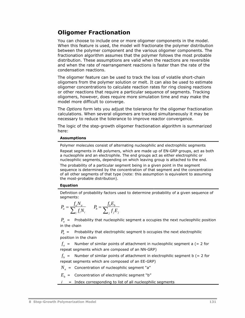
8 Step-Growth Polymerization Model 131
Oligomer Fractionation
You can choose to include one or more oligomer components in the model.When this feature is used, the model will fractionate the polymer distributionbetween the polymer component and the various oligomer components. Thefractionation algorithm assumes that the polymer follows the most probabledistribution. These assumptions are valid when the reactions are reversibleand when the rate of rearrangement reactions is faster than the rate of thecondensation reactions.
The oligomer feature can be used to track the loss of volatile short-chainoligomers from the polymer solution or melt. It can also be used to estimateoligomer concentrations to calculate reaction rates for ring closing reactionsor other reactions that require a particular sequence of segments. Trackingoligomers, however, does require more simulation time and may make themodel more difficult to converge.
The Options form lets you adjust the tolerance for the oligomer fractionationcalculations. When several oligomers are tracked simultaneously it may benecessary to reduce the tolerance to improve reactor convergence.
The logic of the step-growth oligomer fractionation algorithm is summarizedhere:
Assumptions
Polymer molecules consist of alternating nucleophilic and electrophilic segments
Repeat segments in AB polymers, which are made up of EN-GRP groups, act as botha nucleophile and an electrophile. The end groups act as either electrophilic ornucleophilic segments, depending on which leaving group is attached to the end.
The probability of a particular segment being in a given point in the segmentsequence is determined by the concentration of that segment and the concentrationof all other segments of that type (note: this assumption is equivalent to assumingthe most-probable distribution).
Equation
Definition of probability factors used to determine probability of a given sequence ofsegments:
Pf N
f NP
f E
f Eaa a
ii i
bb b
jj j
Pa = Probability that nucleophilic segment a occupies the next nucleophilic position
in the chain
Pb = Probability that electrophilic segment b occupies the next electrophilic
position in the chain
fa = Number of similar points of attachment in nucleophilic segment a (= 2 for
repeat segments which are composed of an NN-GRP)
fb = Number of similar points of attachment in electrophilic segment b (= 2 for
repeat segments which are composed of an EE-GRP)
Na = Concentration of nucleophilic segment “a”
Eb = Concentration of electrophilic segment “b”
i = Index corresponding to list of all nucleophilic segments
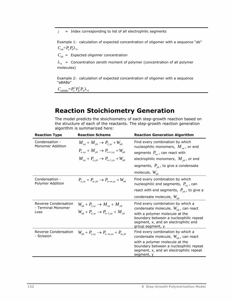
132 8 Step-Growth Polymerization Model
j = Index corresponding to list of all electrophilic segments
Example 1: calculation of expected concentration of oligomer with a sequence “ab”
C =P Pab a b0
Cab = Expected oligomer concentration
0 = Concentration zeroth moment of polymer (concentration of all polymer
molecules)
Example 2: calculation of expected concentration of oligomer with a sequence“aBABa”
C =P P PaBABa a B A2 2
0
Reaction Stoichiometry GenerationThe model predicts the stoichiometry of each step-growth reaction based onthe structure of each of the reactants. The step-growth reaction generationalgorithm is summarized here:
Reaction Type Reaction Scheme Reaction Generation Algorithm
Condensation -Monomer Addition
M M P Wxa yb xy ab 2,
P M P Wn xa yb n xy ab, , 1
M P P Wxa n yb n yx ab , ,1
Find every combination by which
nucleophilic monomers, M xa , or end
segments Pxa , can react with
electrophilic monomers, M yb , or end
segments, Pyb , to give a condensate
molecule, Wab
Condensation -Polymer Addition
P P P Wn xa m yb n m xy ab, , , Find every combination by which
nucleophilic end segments, Pxa , can
react with end segments, Pyb , to give a
condensate molecule, Wab
Reverse Condensation- Terminal MonomerLoss
W P M M
W P P M
ab xy xa yb
ab n xy n xa yb
2
1
,
, ,
Find every combination by which a
condensate molecule, Wab , can react
with a polymer molecule at theboundary between a nucleophilic repeatsegment, x, and an electrophilic endgroup segment, y
Reverse Condensation- Scission
W P P Pab n xy n m xa m yb , , ,Find every combination by which a
condensate molecule, Wab , can react
with a polymer molecule at theboundary between a nucleophilic repeatsegment, x, and an electrophilic repeatsegment, y
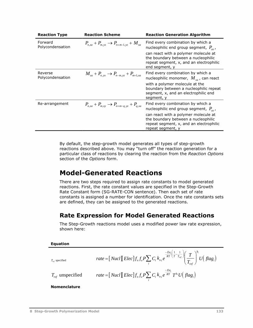
8 Step-Growth Polymerization Model 133
Reaction Type Reaction Scheme Reaction Generation Algorithm
ForwardPolycondensation
P P P Mn za m yx n m yz xa, , , 1Find every combination by which a
nucleophilic end group segment, Pza ,
can react with a polymer molecule atthe boundary between a nucleophilicrepeat segment, x, and an electrophilicend segment, y
ReversePolycondensation
M P P Pza n yx n m yz m xa , , ,1Find every combination by which a
nucleophilic monomer, M xa , can react
with a polymer molecule at theboundary between a nucleophilic repeatsegment, x, and an electrophilic endsegment, y
Re-arrangement P P P Pn za m xy n m q yz q xa, , , , Find every combination by which a
nucleophilic end group segment, Pza ,
can react with a polymer molecule atthe boundary between a nucleophilicrepeat segment, x, and an electrophilicrepeat segment, y
By default, the step-growth model generates all types of step-growthreactions described above. You may “turn off” the reaction generation for aparticular class of reactions by clearing the reaction from the Reaction Optionssection of the Options form.
Model-Generated ReactionsThere are two steps required to assign rate constants to model generatedreactions. First, the rate constant values are specified in the Step-GrowthRate Constant form (SG-RATE-CON sentence). Then each set of rateconstants is assigned a number for identification. Once the rate constants setsare defined, they can be assigned to the generated reactions.
Rate Expression for Model Generated Reactions
The Step-Growth reactions model uses a modified power law rate expression,shown here:
Equation
Tref specified rate Nucl Elec f f P C k eT
TU flagn e i io
Ea
RT T T
ref
b
ii
i
ref
i
1 1
Tref unspecified rate Nucl Elec f f P C k e T U flagn e i io
Ea
RT bi
i
i
i
Nomenclature
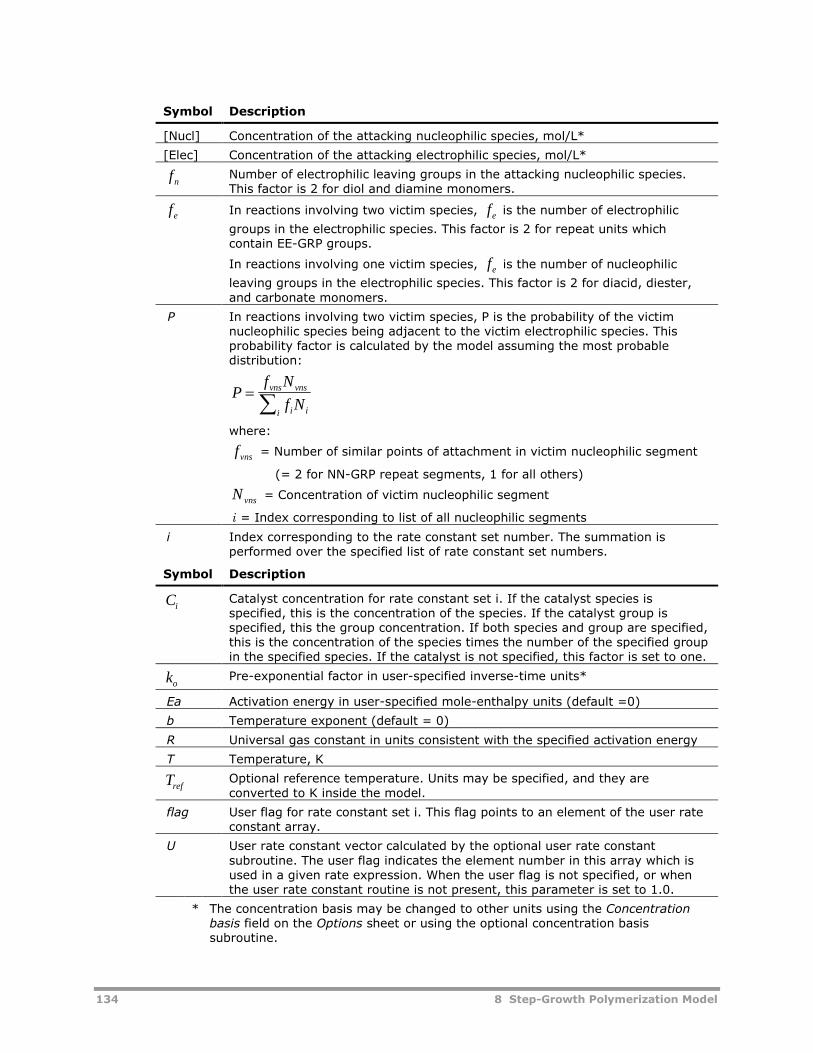
134 8 Step-Growth Polymerization Model
Symbol Description
[Nucl] Concentration of the attacking nucleophilic species, mol/L*
[Elec] Concentration of the attacking electrophilic species, mol/L*
fnNumber of electrophilic leaving groups in the attacking nucleophilic species.This factor is 2 for diol and diamine monomers.
fe In reactions involving two victim species, fe is the number of electrophilic
groups in the electrophilic species. This factor is 2 for repeat units whichcontain EE-GRP groups.
In reactions involving one victim species, fe is the number of nucleophilic
leaving groups in the electrophilic species. This factor is 2 for diacid, diester,and carbonate monomers.
P In reactions involving two victim species, P is the probability of the victimnucleophilic species being adjacent to the victim electrophilic species. Thisprobability factor is calculated by the model assuming the most probabledistribution:
Pf N
f Nvns vns
ii i
where:
fvns = Number of similar points of attachment in victim nucleophilic segment
(= 2 for NN-GRP repeat segments, 1 for all others)
N vns = Concentration of victim nucleophilic segment
i = Index corresponding to list of all nucleophilic segments
i Index corresponding to the rate constant set number. The summation isperformed over the specified list of rate constant set numbers.
Symbol Description
CiCatalyst concentration for rate constant set i. If the catalyst species isspecified, this is the concentration of the species. If the catalyst group isspecified, this the group concentration. If both species and group are specified,this is the concentration of the species times the number of the specified groupin the specified species. If the catalyst is not specified, this factor is set to one.
koPre-exponential factor in user-specified inverse-time units*
Ea Activation energy in user-specified mole-enthalpy units (default =0)
b Temperature exponent (default = 0)
R Universal gas constant in units consistent with the specified activation energy
T Temperature, K
TrefOptional reference temperature. Units may be specified, and they areconverted to K inside the model.
flag User flag for rate constant set i. This flag points to an element of the user rateconstant array.
U User rate constant vector calculated by the optional user rate constantsubroutine. The user flag indicates the element number in this array which isused in a given rate expression. When the user flag is not specified, or whenthe user rate constant routine is not present, this parameter is set to 1.0.
* The concentration basis may be changed to other units using the Concentrationbasis field on the Options sheet or using the optional concentration basissubroutine.
8 Step-Growth Polymerization Model 135
The reactions follow second order kinetics: one order with respect to thenucleophilic reactant and one order with respect to the electrophilic reactant.Catalysts may make the reaction third order (one order with respect tocatalyst).
The rate constants for the model-generated reactions are assumed to be on afunctional group basis. The model applies correction factors to account for thenumber of like functional groups in each of the reactants. For example, in areaction between a diol monomer and a diacid monomer, the specified rateconstant is multiplied by four to account for the two acid groups in the diacidand the two alcohol groups in the diol.
Some reactions occur inside polymer chains at the intersection of twosegments. The model applies a probability factor to estimate theconcentration of the given segment pair. This probability is based on the mostprobable distribution. It assumes that the segments in the polymer alternatebetween nucleophilic segments and electrophilic segments. Repeat segmentscomposed of an EN-GRP functional group behave as both nucleophiles andelectrophiles, so these segments can alternate with themselves.
The standard rate expression is modified using the optional user rate constantfeature. The rate constant form includes a parameter called the “user flag”which identifies an element in an array of user rate constants. This array iscalculated by a user-written Fortran subroutine. The standard rate expressionis multiplied by the user rate constants.
Assignment of Rate Constants to Model-Generated Reactions
Six qualifiers are used to assign each set of rate constants to internally-generated step-growth reactions, the:
Attacking nucleophilic reactant name (A-NUCL-SPEC)
Attacking electrophilic leaving group name (A-ELEC-GRP)
Victim electrophilic reactant name (V-ELEC-SPEC)
Victim nucleophilic group name (V-NUCL-GRP)
Victim electrophilic species name (V-ELEC-SPEC)
Victim electrophilic group name (V-ELEC-GRP)
The following table contains an example illustrating how these identifiers areused to distinguish between reactions. Note that the victim electrophilicspecies is only used for reactions which occur at the intersection of twosegments in a polymer molecule.
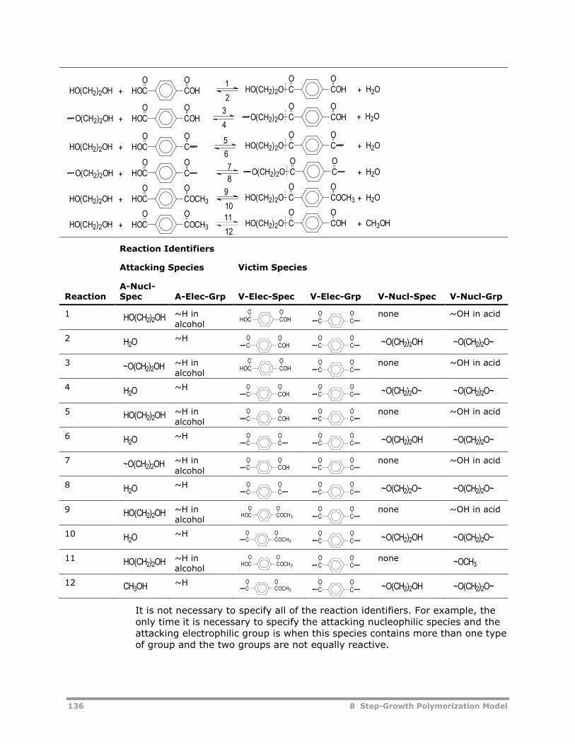
136 8 Step-Growth Polymerization Model
Reaction
Reaction Identifiers
Attacking Species Victim Species
A-Nucl-Spec A-Elec-Grp V-Elec-Spec V-Elec-Grp V-Nucl-Spec V-Nucl-Grp
1 ~H inalcohol
none ~OH in acid
2 ~H
3 ~H inalcohol
none ~OH in acid
4 ~H
5 ~H inalcohol
none ~OH in acid
6 ~H
7 ~H inalcohol
none ~OH in acid
8 ~H
9 ~H inalcohol
none ~OH in acid
10 ~H
11 ~H inalcohol
none
12 ~H
It is not necessary to specify all of the reaction identifiers. For example, theonly time it is necessary to specify the attacking nucleophilic species and theattacking electrophilic group is when this species contains more than one typeof group and the two groups are not equally reactive.
COHCOO
O(CH2)2O+O(CH2)2OH COHHOCOO
+ H2O
CHOCOO
O(CH2)2OH + CCOO
O(CH2)2O + H2O
10
9COCH3HOCOO
HO(CH2)2OH + COCH3COO
HO(CH2)2O + H2O
12
11COCH3HOCOO
HO(CH2)2OH + COHCOO
HO(CH2)2O + CH3OH
3
4
CHOCOO
HO(CH2)2OH + CCOO
HO(CH2)2O + H2O5
6
7
8
1
2COHHOCOO
HO(CH2)2OH + COHCOO
HO(CH2)2O + H2O
HO(CH2)2OH COHHOCOO
CCOO
H2O COHCOO
CCOO
~O(CH2)2OH ~O(CH2)2O~
~O(CH2)2OH COHHOCOO
CCOO
H2O COHCOO
CCOO
~O(CH2)2O~ ~O(CH2)2O~
HO(CH2)2OH COHCOO
CCOO
H2O CCOO
CCOO
~O(CH2)2OH ~O(CH2)2O~
~O(CH2)2OH COHCOO
CCOO
H2O CCOO
CCOO
~O(CH2)2O~ ~O(CH2)2O~
HO(CH2)2OH COCH3HOCOO
CCOO
H2O COCH3COO
CCOO
~O(CH2)2OH ~O(CH2)2O~
HO(CH2)2OH COCH3HOCOO
CCOO
~OCH3
CH3OH COCH3COO
CCOO
~O(CH2)2OH ~O(CH2)2O~
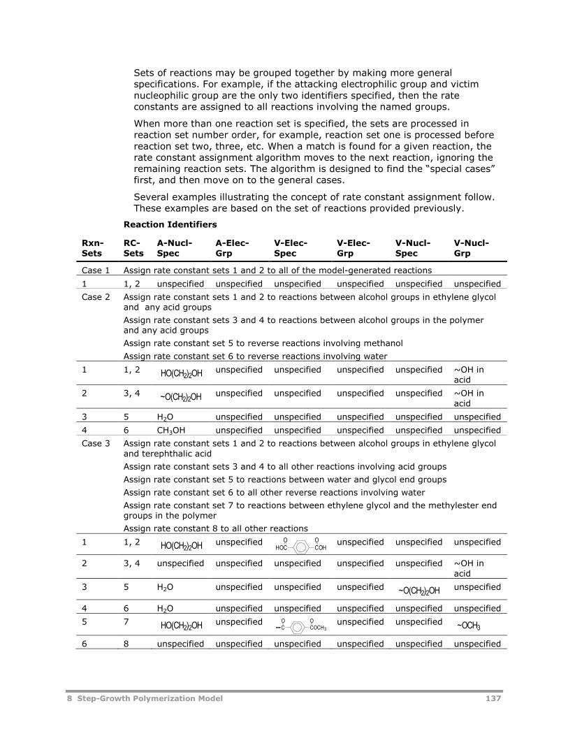
8 Step-Growth Polymerization Model 137
Sets of reactions may be grouped together by making more generalspecifications. For example, if the attacking electrophilic group and victimnucleophilic group are the only two identifiers specified, then the rateconstants are assigned to all reactions involving the named groups.
When more than one reaction set is specified, the sets are processed inreaction set number order, for example, reaction set one is processed beforereaction set two, three, etc. When a match is found for a given reaction, therate constant assignment algorithm moves to the next reaction, ignoring theremaining reaction sets. The algorithm is designed to find the “special cases”first, and then move on to the general cases.
Several examples illustrating the concept of rate constant assignment follow.These examples are based on the set of reactions provided previously.
Rxn-Sets
Reaction Identifiers
RC-Sets
A-Nucl-Spec
A-Elec-Grp
V-Elec-Spec
V-Elec-Grp
V-Nucl-Spec
V-Nucl-Grp
Case 1 Assign rate constant sets 1 and 2 to all of the model-generated reactions
1 1, 2 unspecified unspecified unspecified unspecified unspecified unspecified
Case 2 Assign rate constant sets 1 and 2 to reactions between alcohol groups in ethylene glycoland any acid groups
Assign rate constant sets 3 and 4 to reactions between alcohol groups in the polymerand any acid groups
Assign rate constant set 5 to reverse reactions involving methanol
Assign rate constant set 6 to reverse reactions involving water
1 1, 2 unspecified unspecified unspecified unspecified ~OH inacid
2 3, 4 unspecified unspecified unspecified unspecified ~OH inacid
3 5 H2O unspecified unspecified unspecified unspecified unspecified
4 6 CH3OH unspecified unspecified unspecified unspecified unspecified
Case 3 Assign rate constant sets 1 and 2 to reactions between alcohol groups in ethylene glycoland terephthalic acid
Assign rate constant sets 3 and 4 to all other reactions involving acid groups
Assign rate constant set 5 to reactions between water and glycol end groups
Assign rate constant set 6 to all other reverse reactions involving water
Assign rate constant set 7 to reactions between ethylene glycol and the methylester endgroups in the polymer
Assign rate constant 8 to all other reactions
1 1, 2 unspecified unspecified unspecified unspecified
2 3, 4 unspecified unspecified unspecified unspecified unspecified ~OH inacid
3 5 H2O unspecified unspecified unspecified unspecified
4 6 H2O unspecified unspecified unspecified unspecified unspecified
5 7 unspecified unspecified unspecified
6 8 unspecified unspecified unspecified unspecified unspecified unspecified
HO(CH2)2OH
~O(CH2)2OH
HO(CH2)2OH COHHOCOO
~O(CH2)2OH
HO(CH2)2OH COCH3COO
~OCH3
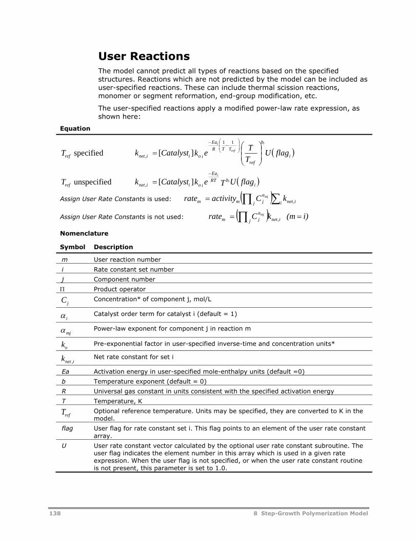
138 8 Step-Growth Polymerization Model
User ReactionsThe model cannot predict all types of reactions based on the specifiedstructures. Reactions which are not predicted by the model can be included asuser-specified reactions. These can include thermal scission reactions,monomer or segment reformation, end-group modification, etc.
The user-specified reactions apply a modified power-law rate expression, asshown here:
Equation
Tref specified i
ref
b
TTR
Ea
o iiinet flagUT
TekCatalystk
i
ref
i
11
, ][
Tref unspecified ibRT
Ea
o iiinet flagUTekCatalystk i
i
][,
Assign User Rate Constants is used: i inetj
a
jmm kCactivityrate mj
,
Assign User Rate Constants is not used: i)(mkCrate inetj
a
jmmj ,
Nomenclature
Symbol Description
m User reaction number
i Rate constant set number
j Component number
Product operator
C jConcentration* of component j, mol/L
i Catalyst order term for catalyst i (default = 1)
mj Power-law exponent for component j in reaction m
koPre-exponential factor in user-specified inverse-time and concentration units*
i,netk Net rate constant for set i
Ea Activation energy in user-specified mole-enthalpy units (default =0)
b Temperature exponent (default = 0)
R Universal gas constant in units consistent with the specified activation energy
T Temperature, K
TrefOptional reference temperature. Units may be specified, they are converted to K in themodel.
flag User flag for rate constant set i. This flag points to an element of the user rate constantarray.
U User rate constant vector calculated by the optional user rate constant subroutine. Theuser flag indicates the element number in this array which is used in a given rateexpression. When the user flag is not specified, or when the user rate constant routineis not present, this parameter is set to 1.0.
8 Step-Growth Polymerization Model 139
* The concentration basis may be changed to other units using the Concentrationbasis field on the Options sheet or using the optional concentration basissubroutine.
You can modify the standard rate expression using the optional user rateconstant feature. The rate constant form includes a parameter called the“user flag” which identifies an element in an array of user rate constants. Thisarray is calculated by a user-written Fortran subroutine. The standard rateexpression is multiplied by the user rate constants as shown.
Assignment of Rate Constants to User SpecifiedReactions There are two options for assigning rate constants to user-specified
reactions. By default, the model assumes there is exactly one set of rateconstants for each reaction (for example, rate constant set “i” is used forreaction “i”).
Alternately, you may use the Assign User Rate Constant sheet to assign oneor more sets of rate constants to each reaction. This feature is convenient intwo situations:
Models with a large number of user side reactions when the rate constantsof the various reactions are equal or are related to each otheralgebraically.
Reactions catalyzed by several catalysts simultaneously.
Conventional and Power-Law Components
Conventional components and segments can appear as reactants or productsin the reaction stoichiometry. Each reaction must be mass balanced (the massof the products must be equal to the mass of the reactants).
The power-law components can include conventional components, segments,or oligomers. Power-law coefficients can be specified for components whichdo not appear in the reaction stoichiometry, such as catalysts or inhibitors.
The model allows the reactants to have power-law constants of zero, but thisis not recommended because it can lead to numerical problems in the reactormodels. For example, if a reaction “AB” is zeroth order with respect tocomponent “A”, the reaction could have a positive rate even when component“A” is not present. This causes “non-negativity violation” integrator errors inRPlug and RBatch and causes convergence errors in RCSTR. To avoid these
problems, specify a very small power-law coefficient, such as 1 10-8 .
A user-specified reaction can be accelerated by several different catalysts. Inthis situation, use the Assign User Rate Constants form to link multiple sets ofrate constants to each reaction. Each set of rate constants may be associatedwith a particular catalyst.
When the side reaction kinetics are complicated, it can be easier to write thekinetics in the context of the available user kinetic subroutine. This subroutineis called from the Step-Growth reaction model. The argument list for thisuser-written Fortran subroutine includes the step-growth rate constants, user
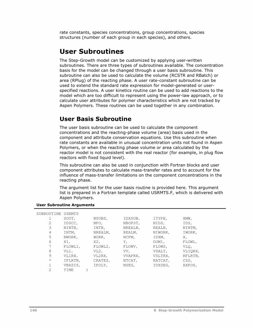
140 8 Step-Growth Polymerization Model
rate constants, species concentrations, group concentrations, speciesstructures (number of each group in each species), and others.
User SubroutinesThe Step-Growth model can be customized by applying user-writtensubroutines. There are three types of subroutines available. The concentrationbasis for the model can be changed through a user basis subroutine. Thissubroutine can also be used to calculate the volume (RCSTR and RBatch) orarea (RPlug) of the reacting phase. A user rate-constant subroutine can beused to extend the standard rate expression for model-generated or user-specified reactions. A user kinetics routine can be used to add reactions to themodel which are too difficult to represent using the power-law approach, or tocalculate user attributes for polymer characteristics which are not tracked byAspen Polymers. These routines can be used together in any combination.
User Basis Subroutine
The user basis subroutine can be used to calculate the componentconcentrations and the reacting-phase volume (area) basis used in thecomponent and attribute conservation equations. Use this subroutine whenrate constants are available in unusual concentration units not found in AspenPolymers, or when the reacting phase volume or area calculated by thereactor model is not consistent with the real reactor (for example, in plug flowreactors with fixed liquid level).
This subroutine can also be used in conjunction with Fortran blocks and usercomponent attributes to calculate mass-transfer rates and to account for theinfluence of mass-transfer limitations on the component concentrations in thereacting phase.
The argument list for the user basis routine is provided here. This argumentlist is prepared in a Fortran template called USRMTS.F, which is delivered withAspen Polymers.
User Subroutine Arguments
SUBROUTINE USRMTS1 SOUT, NSUBS, IDXSUB, ITYPE, XMW,2 IDSCC, NPO, NBOPST, NIDS, IDS,3 NINTB, INTB, NREALB, REALB, NINTM,4 INTM, NREALM, REALM, NIWORK, IWORK,5 NWORK, WORK, NCPM, IDXM, X,6 X1, X2, Y, DUM1, FLOWL,7 FLOWL1, FLOWL2, FLOWV, FLOWS, VLQ,8 VL1, VL2, VV, VSALT, VLIQRX,9 VL1RX, VL2RX, VVAPRX, VSLTRX, RFLRTN,* IFLRTN, CRATES, NTCAT, RATCAT, CSS,1 VBASIS, IPOLY, NSEG, IDXSEG, AXPOS,2 TIME )
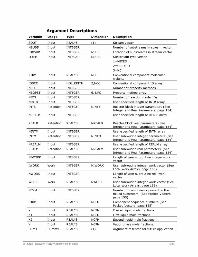
8 Step-Growth Polymerization Model 141
Argument Descriptions
Variable Usage Type Dimension Description
SOUT Input REAL*8 (1) Stream vector
NSUBS Input INTEGER Number of substreams in stream vector
IDXSUB Input INTEGER NSUBS Location of substreams in stream vector
ITYPE Input INTEGER NSUBS Substream type vector
1=MIXED
2=CISOLID
3=NC
XMW Input REAL*8 NCC Conventional component molecularweights
IDSCC Input HOLLERITH 2,NCC Conventional component ID array
NPO Input INTEGER Number of property methods
NBOPST Input INTEGER 6, NPO Property method array
NIDS Input INTEGER Number of reaction model IDs
NINTB Input INTEGER User-specified length of INTB array
INTB Retention INTEGER NINTB Reactor block integer parameters (SeeInteger and Real Parameters, page 154)
NREALB Input INTEGER User-specified length of REALB array
REALB Retention REAL*8 NREALB Reactor block real parameters (SeeInteger and Real Parameters, page 154)
NINTM Input INTEGER User-specified length of INTM array
INTM Retention INTEGER NINTM User subroutine integer parameters (SeeInteger and Real Parameters, page 154)
NREALM Input INTEGER User-specified length of REALM array
REALM Retention REAL*8 NREALM User subroutine real parameters (SeeInteger and Real Parameters, page 154)
NIWORK Input INTEGER Length of user subroutine integer workvector
IWORK Work INTEGER NIWORK User subroutine integer work vector (SeeLocal Work Arrays, page 155)
NWORK Input INTEGER Length of user subroutine real workvector
WORK Work REAL*8 NWORK User subroutine integer work vector (SeeLocal Work Arrays, page 155)
NCPM Input INTEGER Number of components present in themixed substream (See Packed Vectors,page 155)
IDXM Input REAL*8 NCPM Component sequence numbers (SeePacked Vectors, page 155)
X Input REAL*8 NCPM Overall liquid mole fractions
X1 Input REAL*8 NCPM First liquid mole fractions
X2 Input REAL*8 NCPM Second liquid mole fractions
Y Input REAL*8 NCPM Vapor phase mole fractions
Dum1 Dummy REAL*8 (1) Argument reserved for future application
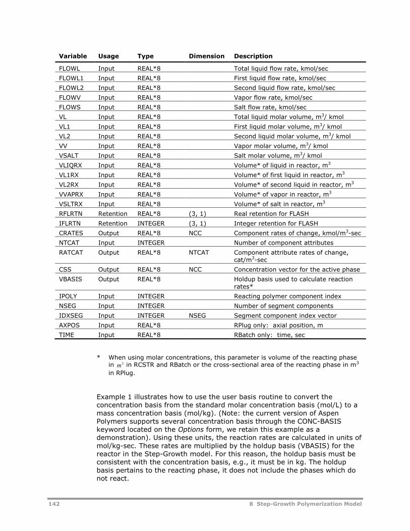
142 8 Step-Growth Polymerization Model
Variable Usage Type Dimension Description
FLOWL Input REAL*8 Total liquid flow rate, kmol/sec
FLOWL1 Input REAL*8 First liquid flow rate, kmol/sec
FLOWL2 Input REAL*8 Second liquid flow rate, kmol/sec
FLOWV Input REAL*8 Vapor flow rate, kmol/sec
FLOWS Input REAL*8 Salt flow rate, kmol/sec
VL Input REAL*8 Total liquid molar volume, m3/ kmol
VL1 Input REAL*8 First liquid molar volume, m3/ kmol
VL2 Input REAL*8 Second liquid molar volume, m3/ kmol
VV Input REAL*8 Vapor molar volume, m3/ kmol
VSALT Input REAL*8 Salt molar volume, m3/ kmol
VLIQRX Input REAL*8 Volume* of liquid in reactor, m3
VL1RX Input REAL*8 Volume* of first liquid in reactor, m3
VL2RX Input REAL*8 Volume* of second liquid in reactor, m3
VVAPRX Input REAL*8 Volume* of vapor in reactor, m3
VSLTRX Input REAL*8 Volume* of salt in reactor, m3
RFLRTN Retention REAL*8 (3, 1) Real retention for FLASH
IFLRTN Retention INTEGER (3, 1) Integer retention for FLASH
CRATES Output REAL*8 NCC Component rates of change, kmol/m3-sec
NTCAT Input INTEGER Number of component attributes
RATCAT Output REAL*8 NTCAT Component attribute rates of change,cat/m3-sec
CSS Output REAL*8 NCC Concentration vector for the active phase
VBASIS Output REAL*8 Holdup basis used to calculate reactionrates*
IPOLY Input INTEGER Reacting polymer component index
NSEG Input INTEGER Number of segment components
IDXSEG Input INTEGER NSEG Segment component index vector
AXPOS Input REAL*8 RPlug only: axial position, m
TIME Input REAL*8 RBatch only: time, sec
* When using molar concentrations, this parameter is volume of the reacting phasein 3m in RCSTR and RBatch or the cross-sectional area of the reacting phase in m3
in RPlug.
Example 1 illustrates how to use the user basis routine to convert theconcentration basis from the standard molar concentration basis (mol/L) to amass concentration basis (mol/kg). (Note: the current version of AspenPolymers supports several concentration basis through the CONC-BASISkeyword located on the Options form, we retain this example as ademonstration). Using these units, the reaction rates are calculated in units ofmol/kg-sec. These rates are multiplied by the holdup basis (VBASIS) for thereactor in the Step-Growth model. For this reason, the holdup basis must beconsistent with the concentration basis, e.g., it must be in kg. The holdupbasis pertains to the reacting phase, it does not include the phases which donot react.
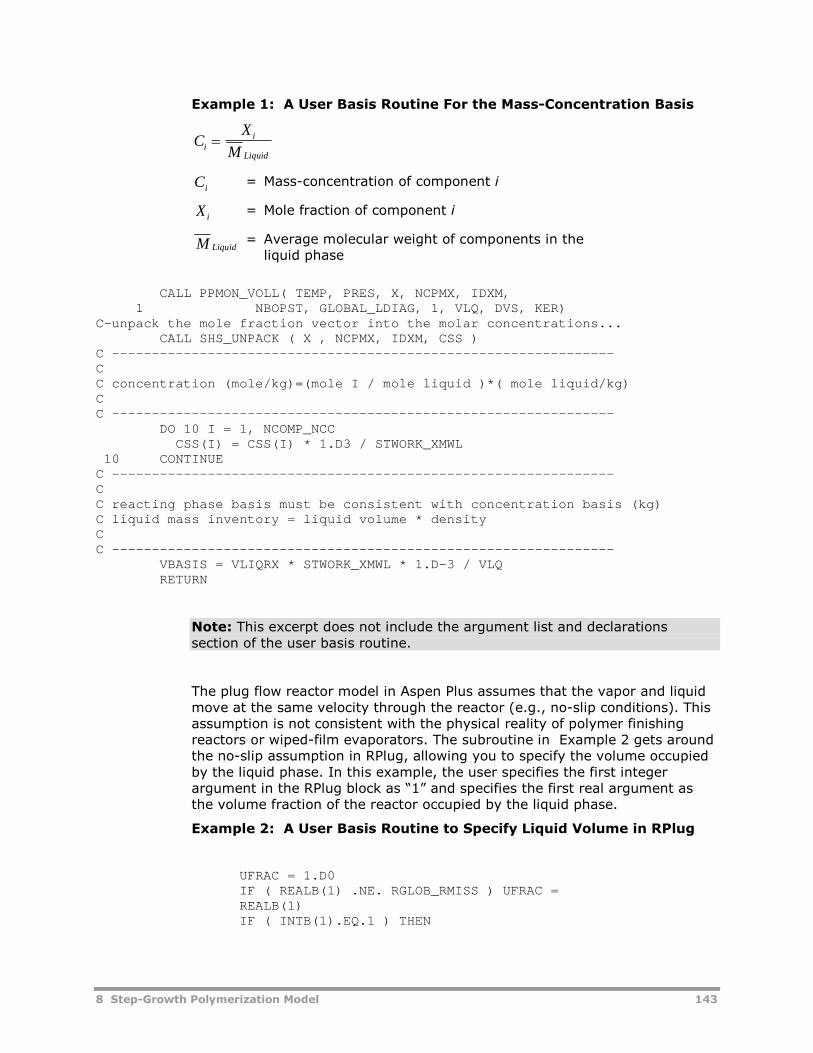
8 Step-Growth Polymerization Model 143
Example 1: A User Basis Routine For the Mass-Concentration Basis
CX
Mii
Liquid
Ci= Mass-concentration of component i
X i= Mole fraction of component i
M Liquid= Average molecular weight of components in the
liquid phase
CALL PPMON_VOLL( TEMP, PRES, X, NCPMX, IDXM,1 NBOPST, GLOBAL_LDIAG, 1, VLQ, DVS, KER)
C-unpack the mole fraction vector into the molar concentrations...CALL SHS_UNPACK ( X , NCPMX, IDXM, CSS )
C ---------------------------------------------------------------CC concentration (mole/kg)=(mole I / mole liquid )*( mole liquid/kg)CC ---------------------------------------------------------------
DO 10 I = 1, NCOMP_NCCCSS(I) = CSS(I) * 1.D3 / STWORK_XMWL
10 CONTINUEC ---------------------------------------------------------------CC reacting phase basis must be consistent with concentration basis (kg)C liquid mass inventory = liquid volume * densityCC ---------------------------------------------------------------
VBASIS = VLIQRX * STWORK_XMWL * 1.D-3 / VLQRETURN
Note: This excerpt does not include the argument list and declarationssection of the user basis routine.
The plug flow reactor model in Aspen Plus assumes that the vapor and liquidmove at the same velocity through the reactor (e.g., no-slip conditions). Thisassumption is not consistent with the physical reality of polymer finishingreactors or wiped-film evaporators. The subroutine in Example 2 gets aroundthe no-slip assumption in RPlug, allowing you to specify the volume occupiedby the liquid phase. In this example, the user specifies the first integerargument in the RPlug block as “1” and specifies the first real argument asthe volume fraction of the reactor occupied by the liquid phase.
Example 2: A User Basis Routine to Specify Liquid Volume in RPlug
UFRAC = 1.D0IF ( REALB(1) .NE. RGLOB_RMISS ) UFRAC =REALB(1)IF ( INTB(1).EQ.1 ) THEN
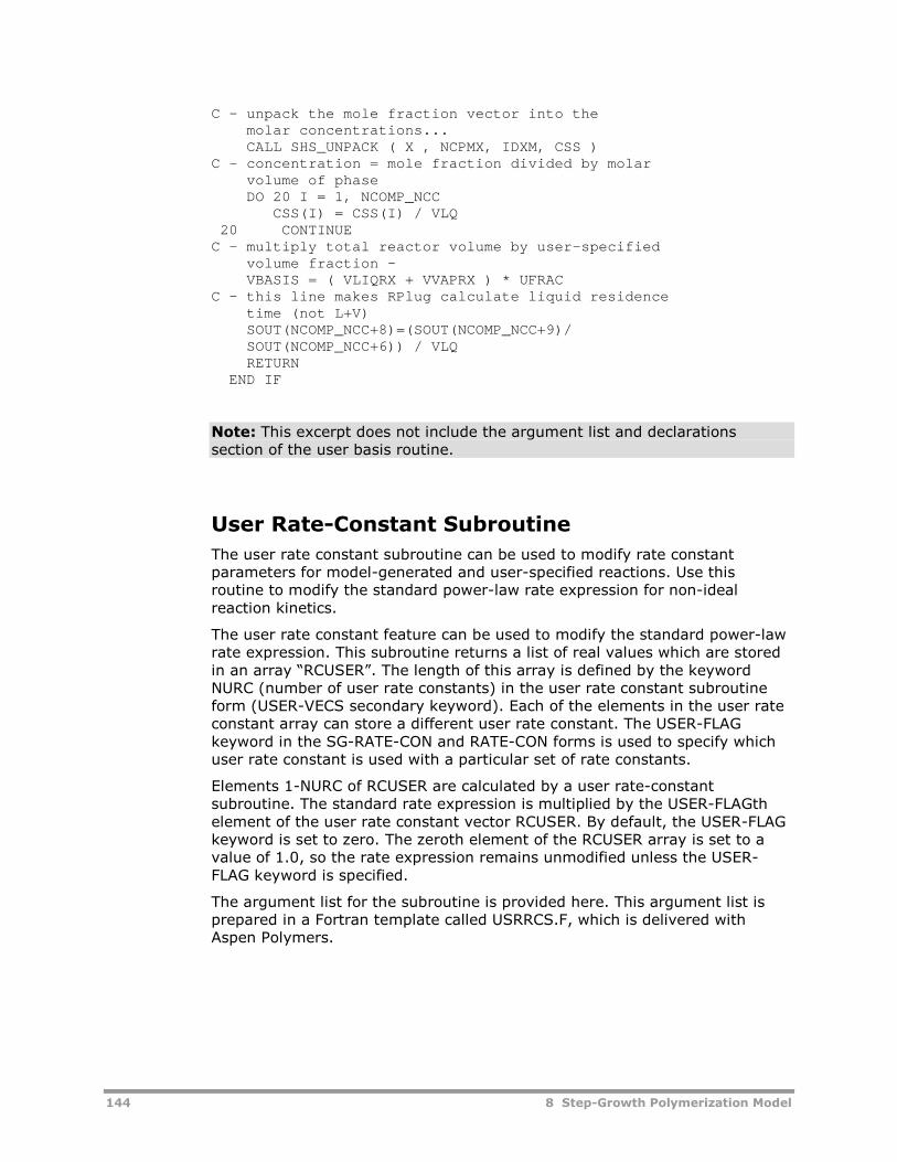
144 8 Step-Growth Polymerization Model
C - unpack the mole fraction vector into themolar concentrations...CALL SHS_UNPACK ( X , NCPMX, IDXM, CSS )
C - concentration = mole fraction divided by molarvolume of phaseDO 20 I = 1, NCOMP_NCC
CSS(I) = CSS(I) / VLQ20 CONTINUE
C - multiply total reactor volume by user-specifiedvolume fraction -VBASIS = ( VLIQRX + VVAPRX ) * UFRAC
C - this line makes RPlug calculate liquid residencetime (not L+V)SOUT(NCOMP_NCC+8)=(SOUT(NCOMP_NCC+9)/SOUT(NCOMP_NCC+6)) / VLQRETURN
END IF
Note: This excerpt does not include the argument list and declarationssection of the user basis routine.
User Rate-Constant Subroutine
The user rate constant subroutine can be used to modify rate constantparameters for model-generated and user-specified reactions. Use thisroutine to modify the standard power-law rate expression for non-idealreaction kinetics.
The user rate constant feature can be used to modify the standard power-lawrate expression. This subroutine returns a list of real values which are storedin an array “RCUSER”. The length of this array is defined by the keywordNURC (number of user rate constants) in the user rate constant subroutineform (USER-VECS secondary keyword). Each of the elements in the user rateconstant array can store a different user rate constant. The USER-FLAGkeyword in the SG-RATE-CON and RATE-CON forms is used to specify whichuser rate constant is used with a particular set of rate constants.
Elements 1-NURC of RCUSER are calculated by a user rate-constantsubroutine. The standard rate expression is multiplied by the USER-FLAGthelement of the user rate constant vector RCUSER. By default, the USER-FLAGkeyword is set to zero. The zeroth element of the RCUSER array is set to avalue of 1.0, so the rate expression remains unmodified unless the USER-FLAG keyword is specified.
The argument list for the subroutine is provided here. This argument list isprepared in a Fortran template called USRRCS.F, which is delivered withAspen Polymers.
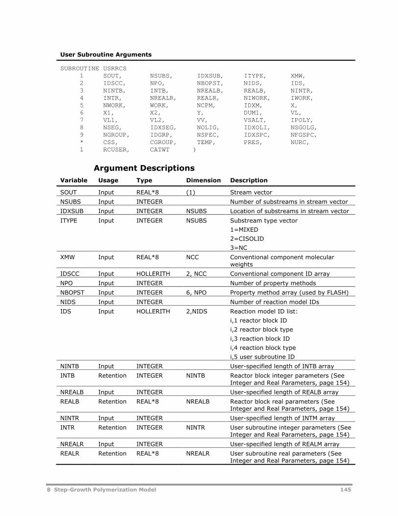
8 Step-Growth Polymerization Model 145
User Subroutine Arguments
SUBROUTINE USRRCS1 SOUT, NSUBS, IDXSUB, ITYPE, XMW,2 IDSCC, NPO, NBOPST, NIDS, IDS,3 NINTB, INTB, NREALB, REALB, NINTR,4 INTR, NREALR, REALR, NIWORK, IWORK,5 NWORK, WORK, NCPM, IDXM, X,6 X1, X2, Y, DUM1, VL,7 VL1, VL2, VV, VSALT, IPOLY,8 NSEG, IDXSEG, NOLIG, IDXOLI, NSGOLG,9 NGROUP, IDGRP, NSPEC, IDXSPC, NFGSPC,* CSS, CGROUP, TEMP, PRES, NURC,1 RCUSER, CATWT )
Argument Descriptions
Variable Usage Type Dimension Description
SOUT Input REAL*8 (1) Stream vector
NSUBS Input INTEGER Number of substreams in stream vector
IDXSUB Input INTEGER NSUBS Location of substreams in stream vector
ITYPE Input INTEGER NSUBS Substream type vector
1=MIXED
2=CISOLID
3=NC
XMW Input REAL*8 NCC Conventional component molecularweights
IDSCC Input HOLLERITH 2, NCC Conventional component ID array
NPO Input INTEGER Number of property methods
NBOPST Input INTEGER 6, NPO Property method array (used by FLASH)
NIDS Input INTEGER Number of reaction model IDs
IDS Input HOLLERITH 2,NIDS Reaction model ID list:
i,1 reactor block ID
i,2 reactor block type
i,3 reaction block ID
i,4 reaction block type
i,5 user subroutine ID
NINTB Input INTEGER User-specified length of INTB array
INTB Retention INTEGER NINTB Reactor block integer parameters (SeeInteger and Real Parameters, page 154)
NREALB Input INTEGER User-specified length of REALB array
REALB Retention REAL*8 NREALB Reactor block real parameters (SeeInteger and Real Parameters, page 154)
NINTR Input INTEGER User-specified length of INTM array
INTR Retention INTEGER NINTR User subroutine integer parameters (SeeInteger and Real Parameters, page 154)
NREALR Input INTEGER User-specified length of REALM array
REALR Retention REAL*8 NREALR User subroutine real parameters (SeeInteger and Real Parameters, page 154)
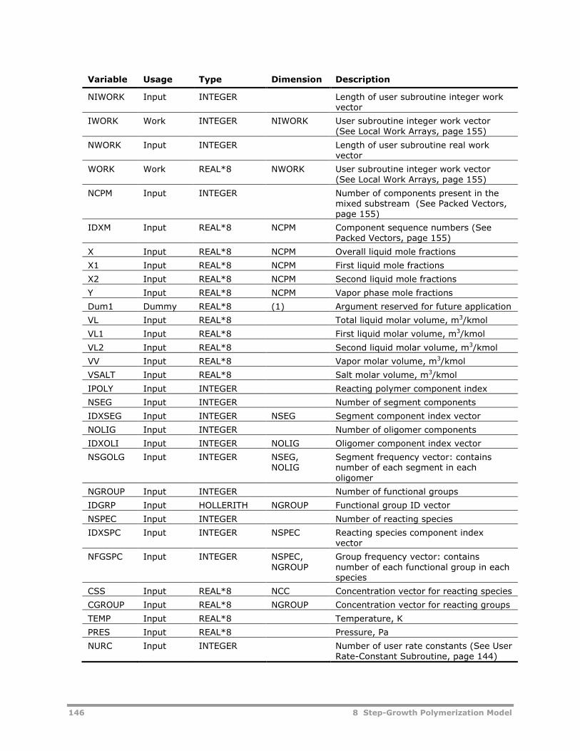
146 8 Step-Growth Polymerization Model
Variable Usage Type Dimension Description
NIWORK Input INTEGER Length of user subroutine integer workvector
IWORK Work INTEGER NIWORK User subroutine integer work vector(See Local Work Arrays, page 155)
NWORK Input INTEGER Length of user subroutine real workvector
WORK Work REAL*8 NWORK User subroutine integer work vector(See Local Work Arrays, page 155)
NCPM Input INTEGER Number of components present in themixed substream (See Packed Vectors,page 155)
IDXM Input REAL*8 NCPM Component sequence numbers (SeePacked Vectors, page 155)
X Input REAL*8 NCPM Overall liquid mole fractions
X1 Input REAL*8 NCPM First liquid mole fractions
X2 Input REAL*8 NCPM Second liquid mole fractions
Y Input REAL*8 NCPM Vapor phase mole fractions
Dum1 Dummy REAL*8 (1) Argument reserved for future application
VL Input REAL*8 Total liquid molar volume, m3/kmol
VL1 Input REAL*8 First liquid molar volume, m3/kmol
VL2 Input REAL*8 Second liquid molar volume, m3/kmol
VV Input REAL*8 Vapor molar volume, m3/kmol
VSALT Input REAL*8 Salt molar volume, m3/kmol
IPOLY Input INTEGER Reacting polymer component index
NSEG Input INTEGER Number of segment components
IDXSEG Input INTEGER NSEG Segment component index vector
NOLIG Input INTEGER Number of oligomer components
IDXOLI Input INTEGER NOLIG Oligomer component index vector
NSGOLG Input INTEGER NSEG,NOLIG
Segment frequency vector: containsnumber of each segment in eacholigomer
NGROUP Input INTEGER Number of functional groups
IDGRP Input HOLLERITH NGROUP Functional group ID vector
NSPEC Input INTEGER Number of reacting species
IDXSPC Input INTEGER NSPEC Reacting species component indexvector
NFGSPC Input INTEGER NSPEC,NGROUP
Group frequency vector: containsnumber of each functional group in eachspecies
CSS Input REAL*8 NCC Concentration vector for reacting species
CGROUP Input REAL*8 NGROUP Concentration vector for reacting groups
TEMP Input REAL*8 Temperature, K
PRES Input REAL*8 Pressure, Pa
NURC Input INTEGER Number of user rate constants (See UserRate-Constant Subroutine, page 144)
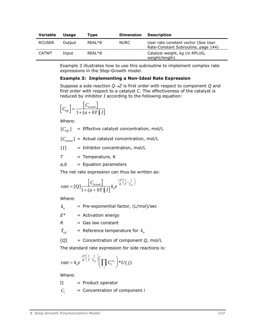
8 Step-Growth Polymerization Model 147
Variable Usage Type Dimension Description
RCUSER Output REAL*8 NURC User rate constant vector (See UserRate-Constant Subroutine, page 144)
CATWT Input REAL*8 Catalyst weight, kg (in RPLUG,weight/length)
Example 3 illustrates how to use this subroutine to implement complex rateexpressions in the Step-Growth model.
Example 3: Implementing a Non-Ideal Rate Expression
Suppose a side reaction QZ is first order with respect to component Q andfirst order with respect to a catalyst C. The effectiveness of the catalyst isreduced by inhibitor I according to the following equation:
CC
a bT Ieff
actual
1 ( )
Where:
[ ]Ceff= Effective catalyst concentration, mol/L
[ ]Cactual= Actual catalyst concentration, mol/L
[ ]I = Inhibitor concentration, mol/L
T = Temperature, K
a,b = Equation parameters
The net rate expression can thus be written as:
rate QC
a bT Ik e
actual
o
E
R T Tref
[ ]( )
*
1
1 1
Where:
ko= Pre-exponential factor, (L/mol)/sec
E* = Activation energy
R = Gas law constant
Tref= Reference temperature for ko
[Q] = Concentration of component Q, mol/L
The standard rate expression for side reactions is:
rate k e C U jo
E
R T T
ii
ref i
*
* ( )
1 1
Where:
= Product operator
Ci= Concentration of component i
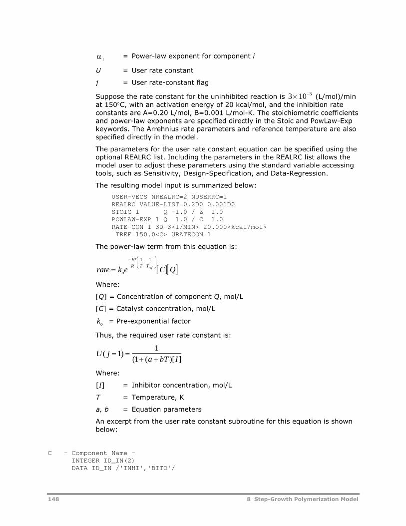
148 8 Step-Growth Polymerization Model
i= Power-law exponent for component i
U = User rate constant
j = User rate-constant flag
Suppose the rate constant for the uninhibited reaction is 3 10 3 (L/mol)/min
at 150C, with an activation energy of 20 kcal/mol, and the inhibition rateconstants are A=0.20 L/mol, B=0.001 L/mol-K. The stoichiometric coefficientsand power-law exponents are specified directly in the Stoic and PowLaw-Expkeywords. The Arrehnius rate parameters and reference temperature are alsospecified directly in the model.
The parameters for the user rate constant equation can be specified using theoptional REALRC list. Including the parameters in the REALRC list allows themodel user to adjust these parameters using the standard variable accessingtools, such as Sensitivity, Design-Specification, and Data-Regression.
The resulting model input is summarized below:
USER-VECS NREALRC=2 NUSERRC=1REALRC VALUE-LIST=0.2D0 0.001D0STOIC 1 Q -1.0 / Z 1.0POWLAW-EXP 1 Q 1.0 / C 1.0RATE-CON 1 3D-3<1/MIN> 20.000<kcal/mol>TREF=150.0<C> URATECON=1
The power-law term from this equation is:
rate k e C Qo
E
R T Tref
* 1 1
Where:
[Q] = Concentration of component Q, mol/L
[C] = Catalyst concentration, mol/L
ko = Pre-exponential factor
Thus, the required user rate constant is:
U ja bT I
( )( ( )[ ]
11
1
Where:
[I] = Inhibitor concentration, mol/L
T = Temperature, K
a, b = Equation parameters
An excerpt from the user rate constant subroutine for this equation is shownbelow:
C - Component Name -INTEGER ID_IN(2)DATA ID_IN /'INHI','BITO'/
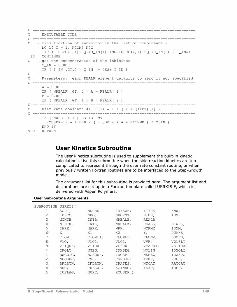
8 Step-Growth Polymerization Model 149
C ======================================================================C EXECUTABLE CODEC ======================================================================C - find location of inhibitor in the list of components -
DO 10 I = 1, NCOMP_NCCIF ( IDSCC(1,I).EQ.ID_IN(1).AND.IDSCC(2,I).EQ.ID_IN(2) ) I_IN=I
10 CONTINUEC - get the concentration of the inhibitor -
C_IN = 0.0D0IF ( I_IN .GT.0 ) C_IN = CSS( I_IN )
C ----------------------------------------------------------------------C Parameters: each REALR element defaults to zero if not specifiedC ----------------------------------------------------------------------
A = 0.0D0IF ( NREALR .GT. 0 ) A = REALR( 1 )B = 0.0D0IF ( NREALR .GT. 1 ) B = REALR( 2 )
C ----------------------------------------------------------------------C User rate constant #1 U(1) = 1 / ( 1 + (A+BT)[I] )C ----------------------------------------------------------------------
IF ( NURC.LT.1 ) GO TO 999RCUSER(1) = 1.0D0 / ( 1.0D0 + ( A + B*TEMP ) * C_IN )
END IF999 RETURN
User Kinetics Subroutine
The user kinetics subroutine is used to supplement the built-in kineticcalculations. Use this subroutine when the side reaction kinetics are toocomplicated to represent through the user rate constant routine, or whenpreviously written Fortran routines are to be interfaced to the Step-Growthmodel.
The argument list for this subroutine is provided here. The argument list anddeclarations are set up in a Fortran template called USRKIS.F, which isdelivered with Aspen Polymers.
User Subroutine Arguments
SUBROUTINE USRKIS(1 SOUT, NSUBS, IDXSUB, ITYPE, XMW,2 IDSCC, NPO, NBOPST, NIDS, IDS,3 NINTB, INTB, NREALB, REALB,4 NINTK, INTK, NREALK, REALK, NIWRK,5 IWRK, NWRK, WRK, NCPMX, IDXM,6 X, X1, X2, Y, DUMXS,7 FLOWL, FLOWL1, FLOWL2, FLOWV, DUMFS,8 VLQ, VLQ1, VLQ2, VVP, VOLSLT,9 VLIQRX, VL1RX, VL2RX, VVAPRX, VSLTRX,* IPOLY, NSEG, IDXSEG, NOLIG, IDXOLI,1 NSGOLG, NGROUP, IDGRP, NSPEC, IDXSPC,2 NFGSPC, CSS, CGROUP, TEMP, PRES,3 RFLRTN, IFLRTN, CRATES, NTCAT, RATCAT,4 NRC, PREEXP, ACTNRG, TEXP, TREF,5 IUFLAG, NURC, RCUSER )
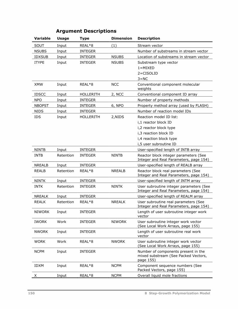
150 8 Step-Growth Polymerization Model
Argument Descriptions
Variable Usage Type Dimension Description
SOUT Input REAL*8 (1) Stream vector
NSUBS Input INTEGER Number of substreams in stream vector
IDXSUB Input INTEGER NSUBS Location of substreams in stream vector
ITYPE Input INTEGER NSUBS Substream type vector
1=MIXED
2=CISOLID
3=NC
XMW Input REAL*8 NCC Conventional component molecularweights
IDSCC Input HOLLERITH 2, NCC Conventional component ID array
NPO Input INTEGER Number of property methods
NBOPST Input INTEGER 6, NPO Property method array (used by FLASH)
NIDS Input INTEGER Number of reaction model IDs
IDS Input HOLLERITH 2,NIDS Reaction model ID list:
i,1 reactor block ID
i,2 reactor block type
i,3 reaction block ID
i,4 reaction block type
i,5 user subroutine ID
NINTB Input INTEGER User-specified length of INTB array
INTB Retention INTEGER NINTB Reactor block integer parameters (SeeInteger and Real Parameters, page 154)
NREALB Input INTEGER User-specified length of REALB array
REALB Retention REAL*8 NREALB Reactor block real parameters (SeeInteger and Real Parameters, page 154)
NINTK Input INTEGER User-specified length of INTM array
INTK Retention INTEGER NINTK User subroutine integer parameters (SeeInteger and Real Parameters, page 154)
NREALK Input INTEGER User-specified length of REALM array
REALK Retention REAL*8 NREALK User subroutine real parameters (SeeInteger and Real Parameters, page 154)
NIWORK Input INTEGER Length of user subroutine integer workvector
IWORK Work INTEGER NIWORK User subroutine integer work vector(See Local Work Arrays, page 155)
NWORK Input INTEGER Length of user subroutine real workvector
WORK Work REAL*8 NWORK User subroutine integer work vector(See Local Work Arrays, page 155)
NCPM Input INTEGER Number of components present in themixed substream (See Packed Vectors,page 155)
IDXM Input REAL*8 NCPM Component sequence numbers (SeePacked Vectors, page 155)
X Input REAL*8 NCPM Overall liquid mole fractions
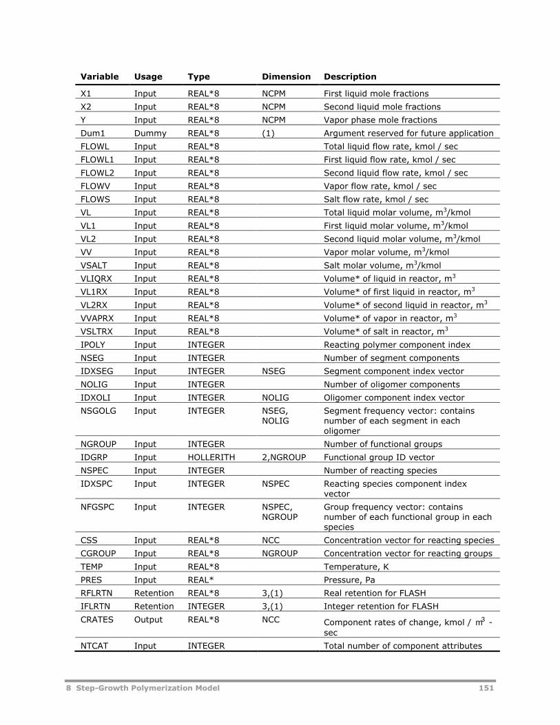
8 Step-Growth Polymerization Model 151
Variable Usage Type Dimension Description
X1 Input REAL*8 NCPM First liquid mole fractions
X2 Input REAL*8 NCPM Second liquid mole fractions
Y Input REAL*8 NCPM Vapor phase mole fractions
Dum1 Dummy REAL*8 (1) Argument reserved for future application
FLOWL Input REAL*8 Total liquid flow rate, kmol / sec
FLOWL1 Input REAL*8 First liquid flow rate, kmol / sec
FLOWL2 Input REAL*8 Second liquid flow rate, kmol / sec
FLOWV Input REAL*8 Vapor flow rate, kmol / sec
FLOWS Input REAL*8 Salt flow rate, kmol / sec
VL Input REAL*8 Total liquid molar volume, m3/kmol
VL1 Input REAL*8 First liquid molar volume, m3/kmol
VL2 Input REAL*8 Second liquid molar volume, m3/kmol
VV Input REAL*8 Vapor molar volume, m3/kmol
VSALT Input REAL*8 Salt molar volume, m3/kmol
VLIQRX Input REAL*8 Volume* of liquid in reactor, m3
VL1RX Input REAL*8 Volume* of first liquid in reactor, m3
VL2RX Input REAL*8 Volume* of second liquid in reactor, m3
VVAPRX Input REAL*8 Volume* of vapor in reactor, m3
VSLTRX Input REAL*8 Volume* of salt in reactor, m3
IPOLY Input INTEGER Reacting polymer component index
NSEG Input INTEGER Number of segment components
IDXSEG Input INTEGER NSEG Segment component index vector
NOLIG Input INTEGER Number of oligomer components
IDXOLI Input INTEGER NOLIG Oligomer component index vector
NSGOLG Input INTEGER NSEG,NOLIG
Segment frequency vector: containsnumber of each segment in eacholigomer
NGROUP Input INTEGER Number of functional groups
IDGRP Input HOLLERITH 2,NGROUP Functional group ID vector
NSPEC Input INTEGER Number of reacting species
IDXSPC Input INTEGER NSPEC Reacting species component indexvector
NFGSPC Input INTEGER NSPEC,NGROUP
Group frequency vector: containsnumber of each functional group in eachspecies
CSS Input REAL*8 NCC Concentration vector for reacting species
CGROUP Input REAL*8 NGROUP Concentration vector for reacting groups
TEMP Input REAL*8 Temperature, K
PRES Input REAL* Pressure, Pa
RFLRTN Retention REAL*8 3,(1) Real retention for FLASH
IFLRTN Retention INTEGER 3,(1) Integer retention for FLASH
CRATES Output REAL*8 NCC Component rates of change, kmol / m3 -
sec
NTCAT Input INTEGER Total number of component attributes
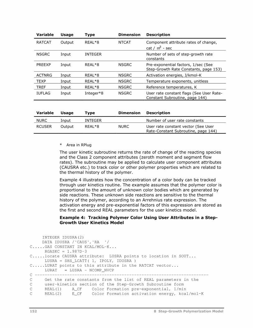
152 8 Step-Growth Polymerization Model
Variable Usage Type Dimension Description
RATCAT Output REAL*8 NTCAT Component attribute rates of change,
cat / m3 - sec
NSGRC Input INTEGER Number of sets of step-growth rateconstants
PREEXP Input REAL*8 NSGRC Pre-exponential factors, 1/sec (SeeStep-Growth Rate Constants, page 153)
ACTNRG Input REAL*8 NSGRC Activation energies, J/kmol-K
TEXP Input REAL*8 NSGRC Temperature exponents, unitless
TREF Input REAL*8 NSGRC Reference temperatures, K
IUFLAG Input Integer*8 NSGRC User rate constant flags (See User Rate-Constant Subroutine, page 144)
Variable Usage Type Dimension Description
NURC Input INTEGER Number of user rate constants
RCUSER Output REAL*8 NURC User rate constant vector (See UserRate-Constant Subroutine, page 144)
* Area in RPlug
The user kinetic subroutine returns the rate of change of the reacting speciesand the Class 2 component attributes (zeroth moment and segment flowrates). The subroutine may be applied to calculate user component attributes(CAUSRA etc.) to track color or other polymer properties which are related tothe thermal history of the polymer.
Example 4 illustrates how the concentration of a color body can be trackedthrough user kinetics routine. The example assumes that the polymer color isproportional to the amount of unknown color bodies which are generated byside reactions. These unknown side reactions are sensitive to the thermalhistory of the polymer, according to an Arrehnius rate expression. Theactivation energy and pre-exponential factors of this expression are stored asthe first and second REAL parameters for the user kinetics model.
Example 4: Tracking Polymer Color Using User Attributes in a Step-Growth User Kinetics Model
INTEGER IDUSRA(2)DATA IDUSRA /'CAUS','RA '/
C.....GAS CONSTANT IN KCAL/MOL-K...RGASKC = 1.987D-3
C.....locate CAUSRA attribute: LUSRA points to location in SOUT...LUSRA = SHS_LCATT( 1, IPOLY, IDUSRA )
C.....LURAT points to this attribute in the RATCAT vector...LURAT = LUSRA - NCOMP_NVCP
C ----------------------------------------------------------------------C Get the rate constants from the list of REAL parameters in theC user-kinetics section of the Step-Growth Subroutine formC REAL(1) A_CF Color Formation pre-exponential, 1/minC REAL(2) E_CF Color Formation activation energy, kcal/mol-K
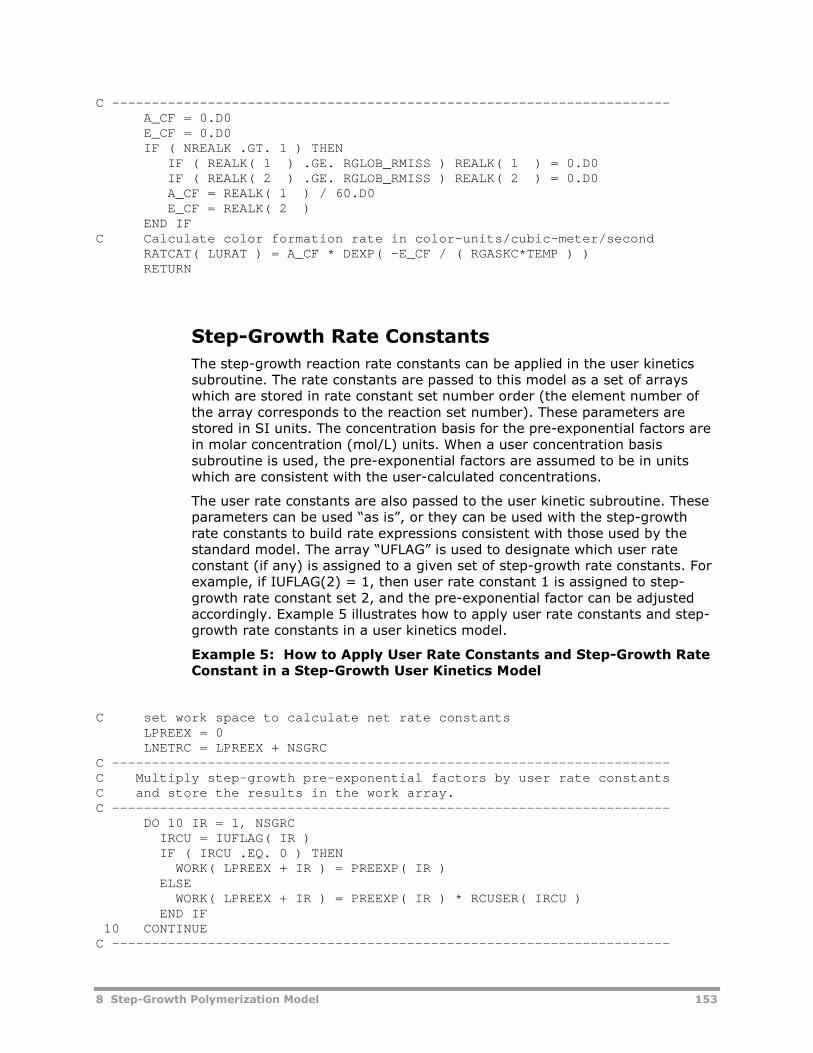
8 Step-Growth Polymerization Model 153
C ----------------------------------------------------------------------A_CF = 0.D0E_CF = 0.D0IF ( NREALK .GT. 1 ) THEN
IF ( REALK( 1 ) .GE. RGLOB_RMISS ) REALK( 1 ) = 0.D0IF ( REALK( 2 ) .GE. RGLOB_RMISS ) REALK( 2 ) = 0.D0A_CF = REALK( 1 ) / 60.D0E_CF = REALK( 2 )
END IFC Calculate color formation rate in color-units/cubic-meter/second
RATCAT( LURAT ) = A_CF * DEXP( -E_CF / ( RGASKC*TEMP ) )RETURN
Step-Growth Rate Constants
The step-growth reaction rate constants can be applied in the user kineticssubroutine. The rate constants are passed to this model as a set of arrayswhich are stored in rate constant set number order (the element number ofthe array corresponds to the reaction set number). These parameters arestored in SI units. The concentration basis for the pre-exponential factors arein molar concentration (mol/L) units. When a user concentration basissubroutine is used, the pre-exponential factors are assumed to be in unitswhich are consistent with the user-calculated concentrations.
The user rate constants are also passed to the user kinetic subroutine. Theseparameters can be used “as is”, or they can be used with the step-growthrate constants to build rate expressions consistent with those used by thestandard model. The array “UFLAG” is used to designate which user rateconstant (if any) is assigned to a given set of step-growth rate constants. Forexample, if IUFLAG(2) = 1, then user rate constant 1 is assigned to step-growth rate constant set 2, and the pre-exponential factor can be adjustedaccordingly. Example 5 illustrates how to apply user rate constants and step-growth rate constants in a user kinetics model.
Example 5: How to Apply User Rate Constants and Step-Growth RateConstant in a Step-Growth User Kinetics Model
C set work space to calculate net rate constantsLPREEX = 0LNETRC = LPREEX + NSGRC
C ----------------------------------------------------------------------C Multiply step-growth pre-exponential factors by user rate constantsC and store the results in the work array.C ----------------------------------------------------------------------
DO 10 IR = 1, NSGRCIRCU = IUFLAG( IR )IF ( IRCU .EQ. 0 ) THEN
WORK( LPREEX + IR ) = PREEXP( IR )ELSE
WORK( LPREEX + IR ) = PREEXP( IR ) * RCUSER( IRCU )END IF
10 CONTINUEC ----------------------------------------------------------------------
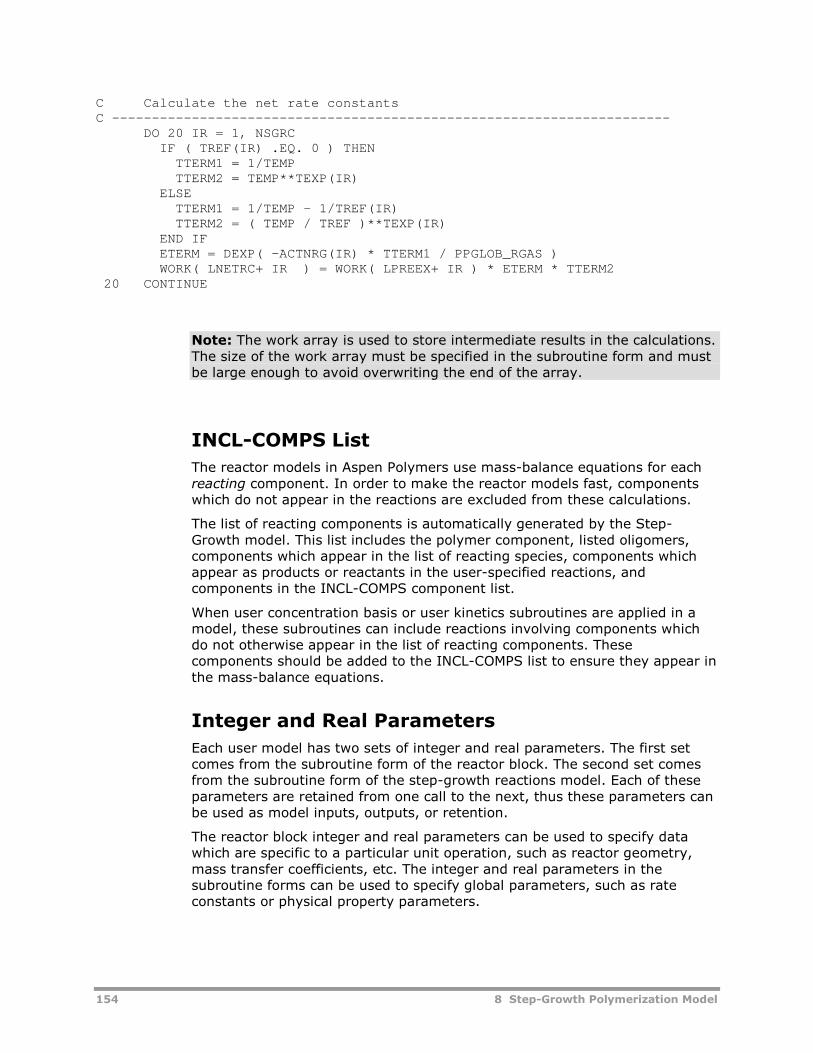
154 8 Step-Growth Polymerization Model
C Calculate the net rate constantsC ----------------------------------------------------------------------
DO 20 IR = 1, NSGRCIF ( TREF(IR) .EQ. 0 ) THEN
TTERM1 = 1/TEMPTTERM2 = TEMP**TEXP(IR)
ELSETTERM1 = 1/TEMP - 1/TREF(IR)TTERM2 = ( TEMP / TREF )**TEXP(IR)
END IFETERM = DEXP( -ACTNRG(IR) * TTERM1 / PPGLOB_RGAS )WORK( LNETRC+ IR ) = WORK( LPREEX+ IR ) * ETERM * TTERM2
20 CONTINUE
Note: The work array is used to store intermediate results in the calculations.The size of the work array must be specified in the subroutine form and mustbe large enough to avoid overwriting the end of the array.
INCL-COMPS List
The reactor models in Aspen Polymers use mass-balance equations for eachreacting component. In order to make the reactor models fast, componentswhich do not appear in the reactions are excluded from these calculations.
The list of reacting components is automatically generated by the Step-Growth model. This list includes the polymer component, listed oligomers,components which appear in the list of reacting species, components whichappear as products or reactants in the user-specified reactions, andcomponents in the INCL-COMPS component list.
When user concentration basis or user kinetics subroutines are applied in amodel, these subroutines can include reactions involving components whichdo not otherwise appear in the list of reacting components. Thesecomponents should be added to the INCL-COMPS list to ensure they appear inthe mass-balance equations.
Integer and Real Parameters
Each user model has two sets of integer and real parameters. The first setcomes from the subroutine form of the reactor block. The second set comesfrom the subroutine form of the step-growth reactions model. Each of theseparameters are retained from one call to the next, thus these parameters canbe used as model inputs, outputs, or retention.
The reactor block integer and real parameters can be used to specify datawhich are specific to a particular unit operation, such as reactor geometry,mass transfer coefficients, etc. The integer and real parameters in thesubroutine forms can be used to specify global parameters, such as rateconstants or physical property parameters.
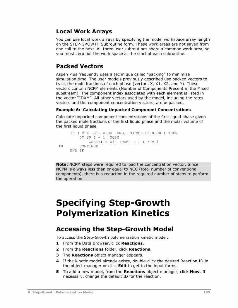
8 Step-Growth Polymerization Model 155
Local Work Arrays
You can use local work arrays by specifying the model workspace array lengthon the STEP-GROWTH Subroutine form. These work areas are not saved fromone call to the next. All three user subroutines share a common work area, soyou must zero out the work space at the start of each subroutine.
Packed Vectors
Aspen Plus frequently uses a technique called “packing” to minimizesimulation time. The user models previously described use packed vectors totrack the mole fractions of each phase (vectors X, X1, X2, and Y). Thesevectors contain NCPM elements (Number of Components Present in the Mixedsubstream). The component index associated with each element is listed inthe vector “IDXM”. All other vectors used by the model, including the ratesvectors and the component concentration vectors, are unpacked.
Example 6: Calculating Unpacked Component Concentrations
Calculate unpacked component concentrations of the first liquid phase giventhe packed mole fractions of the first liquid phase and the molar volume ofthe first liquid phase.
IF ( VL1 .GT. 0.D0 .AND. FLOWL1.GT.0.D0 ) THENDO 10 I = 1, NCPM
CSS(I) = X1( IDXM( I ) ) / VL110 CONTINUE
END IF
Note: NCPM steps were required to load the concentration vector. SinceNCPM is always less than or equal to NCC (total number of conventionalcomponents), there is a reduction in the required number of steps to performthe operation.
Specifying Step-GrowthPolymerization Kinetics
Accessing the Step-Growth ModelTo access the Step-Growth polymerization kinetic model:
1 From the Data Browser, click Reactions.
2 From the Reactions folder, click Reactions.
3 The Reactions object manager appears.
4 If the kinetic model already exists, double-click the desired Reaction ID inthe object manager or click Edit to get to the input forms.
5 To add a new model, from the Reactions object manager, click New. Ifnecessary, change the default ID for the reaction.
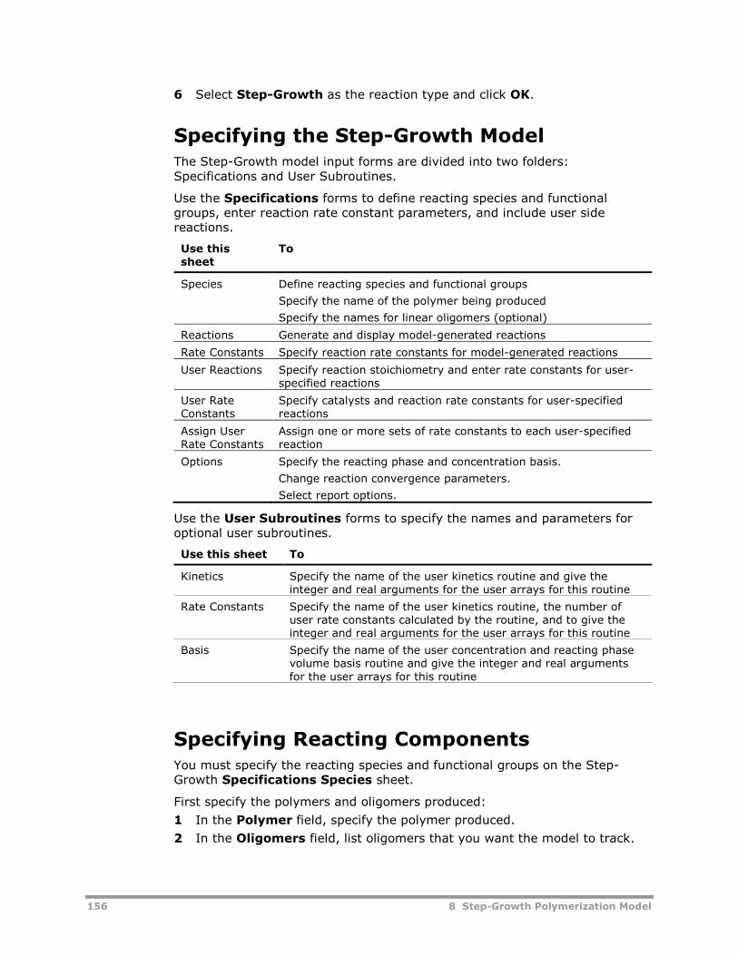
156 8 Step-Growth Polymerization Model
6 Select Step-Growth as the reaction type and click OK.
Specifying the Step-Growth ModelThe Step-Growth model input forms are divided into two folders:Specifications and User Subroutines.
Use the Specifications forms to define reacting species and functionalgroups, enter reaction rate constant parameters, and include user sidereactions.
Use thissheet
To
Species Define reacting species and functional groups
Specify the name of the polymer being produced
Specify the names for linear oligomers (optional)
Reactions Generate and display model-generated reactions
Rate Constants Specify reaction rate constants for model-generated reactions
User Reactions Specify reaction stoichiometry and enter rate constants for user-specified reactions
User RateConstants
Specify catalysts and reaction rate constants for user-specifiedreactions
Assign UserRate Constants
Assign one or more sets of rate constants to each user-specifiedreaction
Options Specify the reacting phase and concentration basis.
Change reaction convergence parameters.
Select report options.
Use the User Subroutines forms to specify the names and parameters foroptional user subroutines.
Use this sheet To
Kinetics Specify the name of the user kinetics routine and give theinteger and real arguments for the user arrays for this routine
Rate Constants Specify the name of the user kinetics routine, the number ofuser rate constants calculated by the routine, and to give theinteger and real arguments for the user arrays for this routine
Basis Specify the name of the user concentration and reacting phasevolume basis routine and give the integer and real argumentsfor the user arrays for this routine
Specifying Reacting ComponentsYou must specify the reacting species and functional groups on the Step-Growth Specifications Species sheet.
First specify the polymers and oligomers produced:
1 In the Polymer field, specify the polymer produced.
2 In the Oligomers field, list oligomers that you want the model to track.
8 Step-Growth Polymerization Model 157
3 In the species definition table, specify the functional groups contained ineach reacting species and define each group type.
The structure of reacting species in terms of the reactive functional groupsthey contain must be defined. To do this:
1 In the Group field specify an ID name for each functional group typepresent in the reacting species.
2 For each group, select a type from the group type field.
3 List the species in the Species field.
These species can be monomers, condensates, or segments.
The resulting form is a spreadsheet, with each column representing afunctional group and each row representing a reacting species. The cells inthe spreadsheet correspond to the number of each functional group ineach species.
4 In the number field for each species, specify the number of each definedfunctional group contained in that species.
Unspecified fields are interpreted as zeros.
Listing Built-In ReactionsThe step-growth model generates reactions based on the functional groupdefinition of reacting species. You can view the system-generated reactions,by clicking the Generate Reactions button on the SpecificationsReactions sheet.
In the Reaction summary listing for each reaction, the first column indicatesthe reaction type. The second column lists the reactants, and the last columnlists the products. The Data Browser window can be resized to better view thereaction listing.
Specifying Built-In Reaction Rate ConstantsYou can define the catalysts and rate constants for system-generatedreactions. The model applies a modified power-law rate expression, which canbe customized through a user-written rate constant subroutine. By default,the model assumes concentrations are in mol/liter. Another concentrationbasis can be applied through a user-written basis subroutine.
To specify rate constants:
1 Go to the Rate constants sheet.
2 In the reaction No. field, assign a unique integer identifier for a set of rateconstant parameters.
3 In the Catalyst Species field, specify the name of a catalyst speciesassociated with the rate constant set.
You can leave this field unspecified if the reaction is uncatalyzed, or if thecatalyst is defined as a functional group.
4 In the Catalyst Group field, specify the name of a catalyst functionalgroup associated with the rate constant set.
You can leave this field unspecified if the reaction is uncatalyzed, or if thecatalyst is defined as a species.
158 8 Step-Growth Polymerization Model
5 Enter the rate constant parameters: ko for Pre-exponential factor, Ea forActivation energy, b for Temperature exponent, Tref for Referencetemperature.
6 Request any user rate constant expression in the User flag field.
7 Repeat these steps as needed to specify the list of rate constantparameters.
Assigning Rate Constants to ReactionsYou can assign rate constants to individual reactions using the reactionstoichiometry, or you can assign rate constants to sets or reactions using theappropriate reaction identifiers.
To assign the rate constants set:
1 Click the Assign Rate Constants button on the Specifications Rateconstants sheet.
2 Click the Global tab to assign rate constants to a set of reactions or usethe Individual sheet to assign rate constants to individual reactions.
3 Go to the Rate Constant Sets field, select from the list of pre-defined rateconstant sets for each reaction.
Including User ReactionsYou can add user reactions to the built-in set. For this you must specify areaction stoichiometry and the associated rate constants. The model applies amodified rate expression, which can be customized through a user-writtenrate constant subroutine.
To add user reactions use the following options found on the SpecificationsUser Reactions sheet:
Click To
New Add new reactions to the scheme
Edit Specify reaction stoichiometry and power-lawexponents
Rate Constants Specify reaction rate constant parameters for thereactions
Click to select a reaction. Click a reaction then Control-Click to includeadditional reactions for multiple selections. Double-click to edit a reaction.
In addition, you can use the following buttons:
Click To
Hide/RevealExclude/Include a reaction from thecalculations
DeletePermanently remove a reaction from the model
8 Step-Growth Polymerization Model 159
Adding or Editing User ReactionsIn the User Reactions sheet, to add a new reaction to the scheme or edit anexisting reaction, open the Edit subform. When you open the Edit subform, aunique number is assigned in the Reaction no. field, to the reaction beingadded.
To add or edit your reaction:
1 On the Edit subform, specify the Component ID and stoichiometricCoefficient for the reactants.
Reactants must have a negative coefficient.
2 Specify the Component ID and stoichiometric Coefficient for theproducts.
Products must have a positive coefficient.
3 Click to check the Completion Status
or
Click Close to return to the reaction summary.
Specifying Rate Constants for UserReactionsAll the rate constants for user-specified reactions are summarized in a grid onthe User Rate Constants tab:
1 In the ko field, enter the pre-exponential factor.
2 In the field, enter the activation energy.
3 In the b field, enter the temperature exponent.
4 In the Tref field, enter the reference temperature.
Note: Use the Catalyst Species field to associate a rate constant with aparticular catalyst. If you leave this field blank the model drops the catalystterm from the rate expression.Use the Catalyst Order field to specify the reaction order with respect to thecatalyst (the model assumes first order by default).
Assigning Rate Constants to User ReactionsBy default, the model assumes one set of rate parameters for each reaction.(For example, rate constants in row 1 apply to user reaction 1). Alternately,you may assign one or more rate constants to each reaction using the AssignUser Rate Constants form.
When several rate constants are assigned to a reaction the model calculates anet rate constant by summing all of the listed rate constants and multiplyingthe sum by a specified activity.
To assign rate constants to user reactions:
1 On the Assign User Rate Constants form, use the Activity field tospecify the activity factor.
Ea
160 8 Step-Growth Polymerization Model
2 In the Rate Constant Sets field, select from the list of pre-defined rateconstant sets for each reaction.
Selecting Report OptionsYou can select which format to use for the step-growth reactions in the reportfile. On the Options sheet, go to the Report frame to request a reactionreport. Then, select a Summary or Detailed format.
Selecting the Reacting PhaseThe Options form lets you specify the phase in which the reactions occur.
Select the appropriate phase from the list in the Reacting Phase field. All ofthe reactions in a particular step-growth object are assumed to take place inthe same phase.
Note: You must specify the Valid Phases keyword for each reactor modelreferencing the kinetics to ensure the specified reacting phase exists.
If the Reacting Phase option is set to Liquid-1 or Liquid-2 the modelassumes two liquid phases exist. When the named phase is not present, themodel prints a warning message and sets the reaction rates to zero. Thereare two options for handling phase collapse:
Select the Use bulk liquid phase option to force the model to apply thespecified reaction kinetics to the bulk phase when the named phasedisappears.
Select the Suppress warnings option to deactivate the warningmessages associated with phase collapse.
These options are especially convenient when modeling simultaneousreactions in two liquid phases using two step-growth models. In this situation,you would typically select the Use bulk liquid option for one phase and notthe other (to avoid double-counting reactions when one phase collapses).
Specifying Units of Measurement for Pre-Exponential FactorsReaction rates are defined on a molar basis (moles per volume per time) .The time units for the pre-exponential factors are specified directly on theRate Constant forms.
By default, the concentration units are presumed to be in SI units (kmole/m3
or mole/L).
You change the concentration basis to other units using the ConcentrationBasis field of the Options sheet. Alternately, you may apply a user basissubroutine.
8 Step-Growth Polymerization Model 161
Including a User Kinetic SubroutineUse the User Subroutines Kinetics form to specify parameters for userkinetics calculations:
1 In subroutine Name, enter the name of the Fortran subroutine.
2 Specify the size of vectors for Integer, Real in Number of parameters,and Length of work arrays.
3 Enter integer and real parameter values in Values for parameterscolumns.
4 Click Include Comps to specify components to be included in materialbalance convergence.
Including a User Rate Constant SubroutineUse the User Subroutines Rate Constants form to specify parameters foruser rate constants calculations:
1 In subroutine Name, enter the name of the Fortran subroutine.
2 Specify the size of vectors for Integer, Real and No. const. in Numberof parameters.
3 Specify the size of vectors of Integer and Real in Length of workarrays.
4 Enter integer and real parameter values in Values for parameterscolumns.
Including a User Basis SubroutineUse the User Subroutines Basis form to specify parameters for basiscalculations:
1 In subroutine Name, enter the name of the Fortran subroutine.
2 Specify the size of vectors for Integer and Real in the Number ofparameters and Length of work arrays.
3 Enter integer and real parameter values in Values for parameterscolumns.
ReferencesBillmeyer, F. W. (1971). Textbook of Polymer Science. New York: Wiley.
Gupta, S. K, & Kumar, A. (1987). Reaction Engineering of Step-GrowthPolymerization. New York: Plenum.
Jacobsen, L. L., & Ray, W. H. (1992). Unified Modeling for PolycondensationKinetics. J. Macromol. Sci.-Rev. Macromol. Chem. Phys.
Kaufman, H. S., & Falcetta, J. J. (Eds). (1977). Introduction to PolymerScience and Technology: An SPE Textbook. New York: Wiley.
McKetta, J. J. (Ed.). (1992). Encyclopedia of Chemical Processing and Design,39 & 40. New York: Marcel Dekker.
162 8 Step-Growth Polymerization Model
Rodriguez, F. (1989). Principles of Polymer Systems. New York: Hemisphere.
9 Free-Radical Bulk Polymerization Model 163
9 Free-Radical BulkPolymerization Model
This section covers the free-radical bulk/solution polymerization modelavailable in Aspen Polymers (formerly known as Aspen Polymers Plus).
Topics covered include:
Summary of Applications, 163
Free-Radical Bulk/Solution Processes, 164
Reaction Kinetic Scheme, 165
Model Features and Assumptions, 183
Polymer Properties Calculated, 190
Specifying Free-Radical Polymerization Kinetics, 193
Several example applications of the free-radical bulk/solution polymerizationmodel are given in the Aspen Polymers Examples & Applications Case Book.
The Examples & Applications Case Book provide process details and thekinetics of polymerization for specific monomer-polymer systems.
Summary of ApplicationsThe free-radical bulk/solution polymerization model is applicable to bulk andsolution polymerization processes. Some examples of applicable polymersare:
General purpose polystyrene - Made by polymerization of styrenemonomer with or without solvent fed continuously to reactor.
High impact polystyrene - Made by polymerization of an unsaturatedrubber dissolved in styrene in a solution process. Also produced in mass-suspension processes.
Poly(vinyl chloride) - Produced in bulk polymerization using monomer-soluble free radical initiators. Most of the homopolymers and copolymersof vinyl chloride, however, are produced by suspension polymerization.
Poly(vinyl acetate) - Produced industrially by the polymerization of vinylacetate in bulk or solution processes. Also produced in suspension andemulsion processes. Both batch and continuous processes are used.
164 9 Free-Radical Bulk Polymerization Model
Poly(vinyl alcohol) - Poly(vinyl acetate) is converted into thecorresponding poly(vinyl alcohol) by direct hydrolysis or catalyzedalcoholysis. The reaction can be catalyzed by strong acids or strong bases.
Poly(methyl methacrylate) - The vast majority of commercially preparedacrylic polymers and methacrylic polymers are copolymers. Commerciallythey are prepared by solution polymerization. They are also produced byemulsion polymerization and suspension polymerization.
Low density polyethylene - Made by high pressure, free radical processesin either a tubular reactor or a stirred autoclave. Typical commercialprocesses include staged compression, initiator injection, partialconversion of ethylene to polymer, separation of ethylene from polymer,extrusion of molten polymer, and cooling of ethylene.
The Free-Radical model may also be used to simulate suspensionpolymerization processes in which the polymer is completely soluble in theorganic (monomer) phase. Two reaction models can be applied togetherto represent reactions in each liquid phase. An example of this process is:
Poly(styrene) - Poly(styrene) may be produced in a continuous suspensionprocess in a series of CSTR type reactors.
Free-Radical Bulk/SolutionProcessesFree-radical polymerization accounts for a large proportion (more than 40%by weight) of the commodity grade polymers. It is employed in the synthesisof countless homo- and copolymers using monomers that are either
monosubstituted ethylenes RHC CH 2 or 1,1-disubstituted ethylenes
R R C CH1 2 2 .
Free-radical polymerization usually takes place with the monomer in the liquidphase. Several types of processes are used. A solvent or suspending mediummay be used, and the polymer formed may be soluble, insoluble, or swelledby the monomer and solvent. Commercially important processes for free-radical polymerization include bulk, solution, suspension, and emulsionpolymerization.
Bulk and Solution Polymerization
Bulk and solution polymerization processes are characterized by the fact thatthe reactions proceed in a single phase. Typically the monomers are fed to areactor with or without a solvent. A small amount of initiator is also fed. Atthe reaction temperature, the initiator decomposes to form radicals thatinitiate the polymerization reactions. The polymer formed is usually soluble inthe monomer/solvent mixture. However, in some systems, such as PVC, thepolymer is insoluble and forms a separate phase.
The most commonly used reactor types include batch, semi-batch, continuousstirred-tank and tubular reactors. Flowsheets consisting of several reactors inseries are common. The main technical challenges with bulk/solutionpolymerization processes are heat removal, handling of the highly viscous
9 Free-Radical Bulk Polymerization Model 165
liquid, and recovery of residual monomer/solvent. Several modes of heatremoval can be employed, including jacket cooling, internal coolingcoils/baffles, external heat exchangers and reflux condensors.
Reaction Kinetic SchemeMost free-radical polymerizations have at least four basic reaction steps:
Initiation
Propagation
Chain transfer to a small molecule (i.e. monomer, solvent or transferagent)
Termination
These reactions occur simultaneously during the polymerization. For branchedpolymers additional reactions for long and short chain branching can also bepresent. A comprehensive kinetic scheme for the free-radical homo- and
copolymerization of up to N m monomers has been built into Aspen Polymers.
The scheme includes most of the reactions commonly used for modeling free-radical polymerization. The model also includes several optional reactions:
Terminal double bond polymerization
Pendent double bond polymerization (for diene monomers)
Head-to-head propagation (for asymmetric monomers)
Cis- and trans- propagation (for diene monomers)
Primary and secondary decomposition of bifunctional initiators
Reactions such as depropagation and random chain scission are not includedin the current model. These reactions may be added to the built-in scheme inthe future.
The main reactions in the current built-in free-radical kinetic scheme is shownhere :

166
Built-in Free-Radical
The nomenclature used in the free
9 Free-Radical Bulk Polymerization Model
Radical Polymerization Kinetic Scheme
The nomenclature used in the free-radical kinetic scheme is shown here
Radical Bulk Polymerization Model
radical kinetic scheme is shown here:
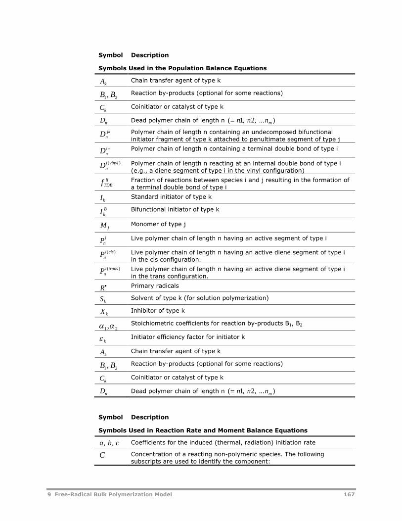
9 Free-Radical Bulk Polymerization Model 167
Symbol Description
Symbols Used in the Population Balance Equations
AkChain transfer agent of type k
21, BB Reaction by-products (optional for some reactions)
CkCoinitiator or catalyst of type k
Dn Dead polymer chain of length n ( , , ... ) n n nm1 2
jknD Polymer chain of length n containing an undecomposed bifunctional
initiator fragment of type k attached to penultimate segment of type j
inD Polymer chain of length n containing a terminal double bond of type i
)(vinylinD Polymer chain of length n reacting at an internal double bond of type i
(e.g., a diene segment of type i in the vinyl configuration)
ijTDBf Fraction of reactions between species i and j resulting in the formation of
a terminal double bond of type i
IkStandard initiator of type k
BkI Bifunctional initiator of type k
M jMonomer of type j
Pni Live polymer chain of length n having an active segment of type i
)(cisinP Live polymer chain of length n having an active diene segment of type i
in the cis configuration.
)(transinP Live polymer chain of length n having an active diene segment of type i
in the trans configuration.
R Primary radicals
SkSolvent of type k (for solution polymerization)
X kInhibitor of type k
21, Stoichiometric coefficients for reaction by-products B1, B2
k Initiator efficiency factor for initiator k
AkChain transfer agent of type k
21, BB Reaction by-products (optional for some reactions)
CkCoinitiator or catalyst of type k
Dn Dead polymer chain of length n ( , , ... ) n n nm1 2
Symbol Description
Symbols Used in Reaction Rate and Moment Balance Equations
a b c, , Coefficients for the induced (thermal, radiation) initiation rate
C Concentration of a reacting non-polymeric species. The followingsubscripts are used to identify the component:
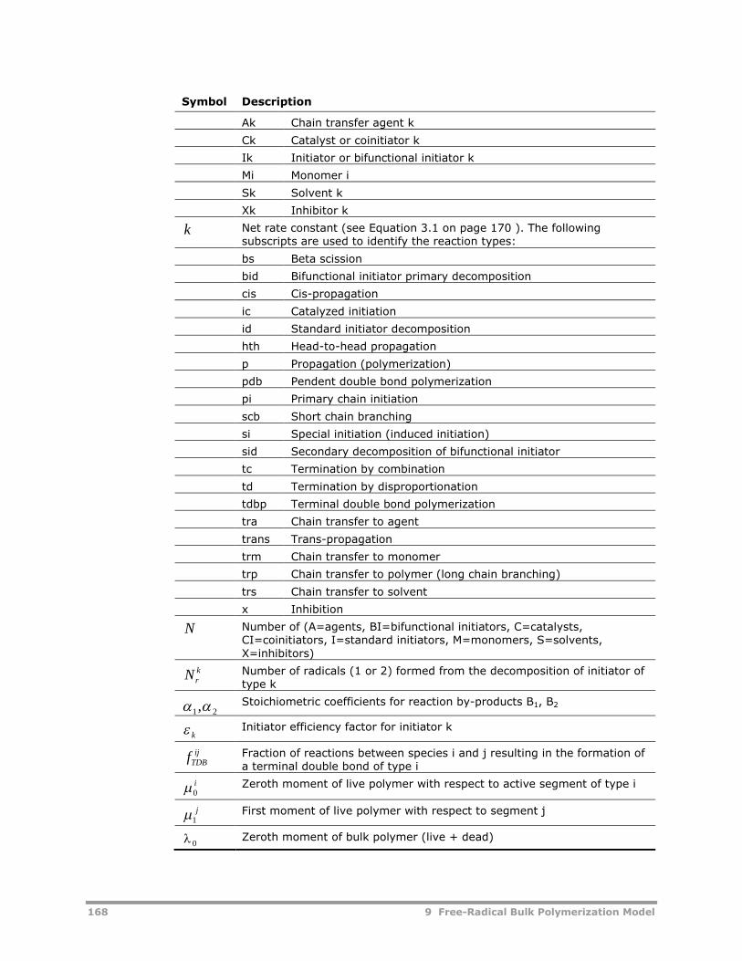
168 9 Free-Radical Bulk Polymerization Model
Symbol Description
Ak Chain transfer agent k
Ck Catalyst or coinitiator k
Ik Initiator or bifunctional initiator k
Mi Monomer i
Sk Solvent k
Xk Inhibitor k
k Net rate constant (see Equation 3.1 on page 170 ). The followingsubscripts are used to identify the reaction types:
bs Beta scission
bid Bifunctional initiator primary decomposition
cis Cis-propagation
ic Catalyzed initiation
id Standard initiator decomposition
hth Head-to-head propagation
p Propagation (polymerization)
pdb Pendent double bond polymerization
pi Primary chain initiation
scb Short chain branching
si Special initiation (induced initiation)
sid Secondary decomposition of bifunctional initiator
tc Termination by combination
td Termination by disproportionation
tdbp Terminal double bond polymerization
tra Chain transfer to agent
trans Trans-propagation
trm Chain transfer to monomer
trp Chain transfer to polymer (long chain branching)
trs Chain transfer to solvent
x Inhibition
N Number of (A=agents, BI=bifunctional initiators, C=catalysts,CI=coinitiators, I=standard initiators, M=monomers, S=solvents,X=inhibitors)
krN Number of radicals (1 or 2) formed from the decomposition of initiator of
type k
21, Stoichiometric coefficients for reaction by-products B1, B2
k Initiator efficiency factor for initiator k
ijTDBf Fraction of reactions between species i and j resulting in the formation of
a terminal double bond of type i
i0
Zeroth moment of live polymer with respect to active segment of type i
j1
First moment of live polymer with respect to segment j
0Zeroth moment of bulk polymer (live + dead)
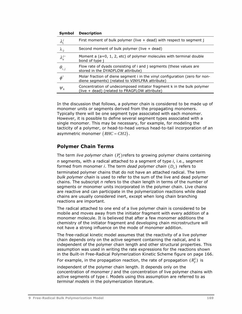
9 Free-Radical Bulk Polymerization Model 169
Symbol Description
j1
First moment of bulk polymer (live + dead) with respect to segment j
2Second moment of bulk polymer (live + dead)
ja
Moment a (a=0, 1, 2, etc) of polymer molecules with terminal doublebond of type j
ji , Flow rate of dyads consisting of i and j segments (these values arestored in the DYADFLOW attribute)
i Molar fraction of diene segment i in the vinyl configuration (zero for non-diene segments) (related to VINYLFRA attribute)
k Concentration of undecomposed initiator fragment k in the bulk polymer(live + dead) (related to FRAGFLOW attribute)
In the discussion that follows, a polymer chain is considered to be made up ofmonomer units or segments derived from the propagating monomers.Typically there will be one segment type associated with each monomer.However, it is possible to define several segment types associated with asingle monomer. This may be necessary, for example, for modeling thetacticity of a polymer, or head-to-head versus head-to-tail incorporation of an
asymmetric monomer RHC CH 2 .
Polymer Chain Terms
The term live polymer chain ( )Pni refers to growing polymer chains containing
n segments, with a radical attached to a segment of type i, i.e., segment
formed from monomer i. The term dead polymer chain ( )Dn refers to
terminated polymer chains that do not have an attached radical. The termbulk polymer chain is used to refer to the sum of the live and dead polymerchains. The subscript n refers to the chain length in terms of the number ofsegments or monomer units incorporated in the polymer chain. Live chainsare reactive and can participate in the polymerization reactions while deadchains are usually considered inert, except when long chain branchingreactions are important.
The radical attached to one end of a live polymer chain is considered to bemobile and moves away from the initiator fragment with every addition of amonomer molecule. It is believed that after a few monomer additions thechemistry of the initiator fragment and developing chain microstructure willnot have a strong influence on the mode of monomer addition.
The free-radical kinetic model assumes that the reactivity of a live polymerchain depends only on the active segment containing the radical, and isindependent of the polymer chain length and other structural properties. Thisassumption was used in writing the rate expressions for the reactions shownin the Built-in Free-Radical Polymerization Kinetic Scheme figure on page 166.
For example, in the propagation reaction, the rate of propagation ( )Rpij
is
independent of the polymer chain length. It depends only on theconcentration of monomer j and the concentration of live polymer chains withactive segments of type i. Models using this assumption are referred to asterminal models in the polymerization literature.
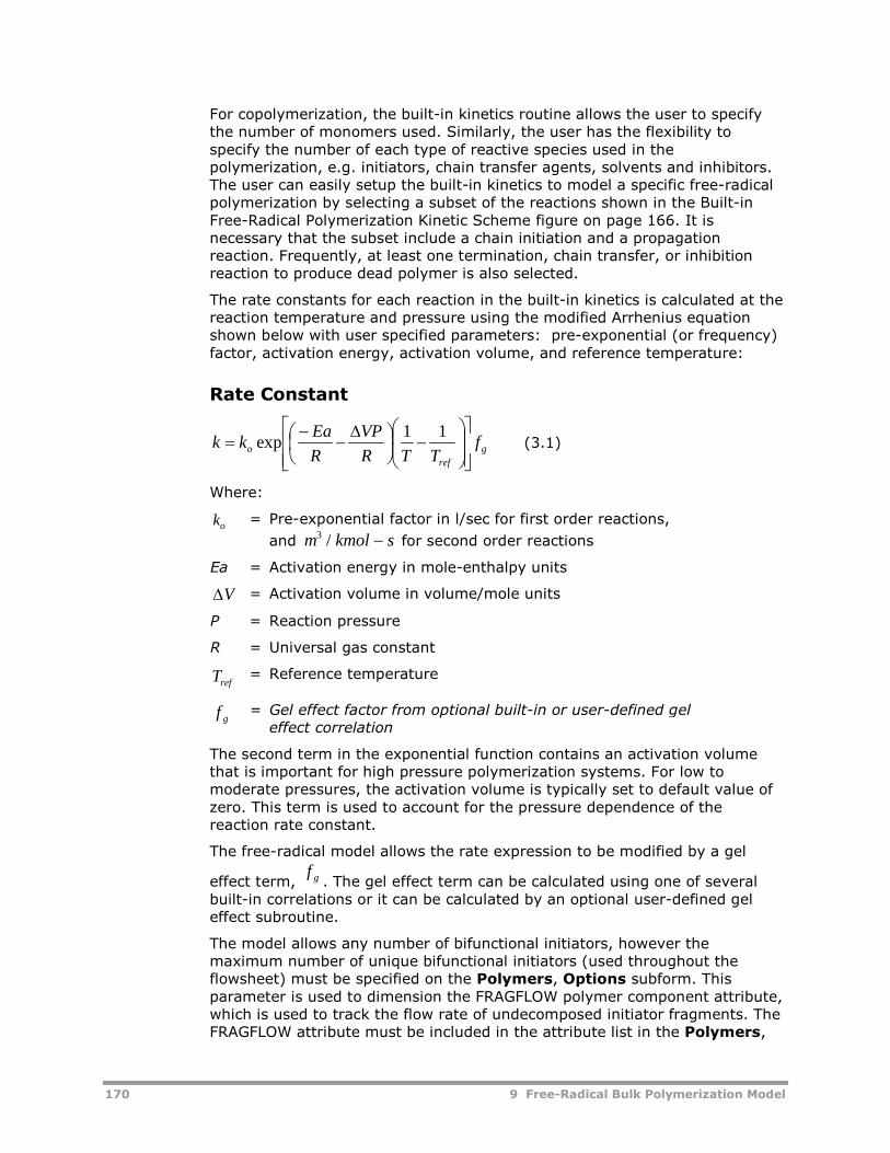
170 9 Free-Radical Bulk Polymerization Model
For copolymerization, the built-in kinetics routine allows the user to specifythe number of monomers used. Similarly, the user has the flexibility tospecify the number of each type of reactive species used in thepolymerization, e.g. initiators, chain transfer agents, solvents and inhibitors.The user can easily setup the built-in kinetics to model a specific free-radicalpolymerization by selecting a subset of the reactions shown in the Built-inFree-Radical Polymerization Kinetic Scheme figure on page 166. It isnecessary that the subset include a chain initiation and a propagationreaction. Frequently, at least one termination, chain transfer, or inhibitionreaction to produce dead polymer is also selected.
The rate constants for each reaction in the built-in kinetics is calculated at thereaction temperature and pressure using the modified Arrhenius equationshown below with user specified parameters: pre-exponential (or frequency)factor, activation energy, activation volume, and reference temperature:
Rate Constant
g
ref
o fTTR
VP
R
Eakk
11exp (3.1)
Where:
ko= Pre-exponential factor in l/sec for first order reactions,
and m kmol s3 / for second order reactions
Ea = Activation energy in mole-enthalpy units
V = Activation volume in volume/mole units
P = Reaction pressure
R = Universal gas constant
refT = Reference temperature
gf = Gel effect factor from optional built-in or user-defined geleffect correlation
The second term in the exponential function contains an activation volumethat is important for high pressure polymerization systems. For low tomoderate pressures, the activation volume is typically set to default value ofzero. This term is used to account for the pressure dependence of thereaction rate constant.
The free-radical model allows the rate expression to be modified by a gel
effect term, gf. The gel effect term can be calculated using one of several
built-in correlations or it can be calculated by an optional user-defined geleffect subroutine.
The model allows any number of bifunctional initiators, however themaximum number of unique bifunctional initiators (used throughout theflowsheet) must be specified on the Polymers, Options subform. Thisparameter is used to dimension the FRAGFLOW polymer component attribute,which is used to track the flow rate of undecomposed initiator fragments. TheFRAGFLOW attribute must be included in the attribute list in the Polymers,
9 Free-Radical Bulk Polymerization Model 171
Polymers subform. Bifunctional and standard initiators can be used in thesame model.
InitiationThe initiation step involves the generation of reactive free-radicals followed bythe addition of a monomer molecule (chain initiation) to form chain radicals of
unit length ( )Pi1 . The non-chain or primary radicals ( )R may be generated by
the thermal decomposition of a chemical initiator, a catalyzed initiationreaction involving electron transfer from ions, or by thermal/radiation inducedmechanisms. Three types of standard initiation reactions are included in thebuilt-in kinetics:
Initiator decomposition reaction
Induced initiation reaction
Catalyzed initiation reaction
The initiator decomposition reaction accounts for primary radical generationfrom the thermal decomposition of chemical initiators.
The induced initiation reaction can be configured to account for the generationof radicals by thermal and radiation induced mechanisms from the monomersthemselves, with or without the use of a coinitiator or promoter.
The catalyzed initiation reaction can be used to account for redox initiation,which has found wide application in aqueous emulsion polymerizationsystems.
The most commonly used radical generation method is the thermaldecomposition of chemical initiators (usually peroxide or azo compounds)which decompose to form radicals when heated to an appropriatetemperature. Only small amounts of the chemical initiator (less than 1 wt. %based on monomer) are needed. However, due to their high activationenergies chemical initiators have a relatively narrow useful temperature range(approx. 30C) over which the decomposition rates are neither too fast nortoo slow.
Some processes, notably bulk polystyrene polymerization, use initiators withtwo active sites. These bifunctional initiators decompose in two stages,providing greater control over the molecular weight distribution of theproduct.
The free-radical model includes two reactions associated with bifunctionalinitiators:
Bifunctional initiator decomposition (primary decomposition)
Secondary initiator decomposition (primary decomposition)
The primary decomposition reaction generates a pair of radicals, anundecomposed initiator fragment, and optional by-products. Theundecomposed fragment is tracked using the FRAGFLOW polymercomponent attribute.
The initiator fragment decomposes in the secondary decompositionreaction, generating a free radical and a polymeric radical.
172 9 Free-Radical Bulk Polymerization Model
Initiator Decomposition Reaction
The initiator decomposition reaction is modeled as a first order thermaldecomposition reaction:
Ikkid
kidkkrkkk CkRBBRNI
2,21,1
This rate expression )( kidR describes the rate for the thermal decomposition of
standard initiator k. The symbols 1B and 2B represent optional user-specified
reaction by-products. This feature lets you track the formation of low-molecular weight decomposition by-products, such as carbon dioxide, whichmay be generated as the initiators decompose. The byproduct formation ratesare determined by:
IkkidkkBIk
kidkkB CkRCkR ,2,,1, 21
For mass balance purposes, the polymer mass generation rate is incrementedby the initiator mass consumption rate, less the mass formation rate of by-products.
The rate expression for the formation of primary radicals from the thermaldecomposition of standard initiators is given by:
IN
kIk
kidk
kr
radid CkNR
1
There are a number of user specifiable parameters associated with thisreaction. The user can specify more than one initiator to model systemswhere multiple initiators with different half-lives are used to control theinitiation rate over the course of the polymerization. Depending on theinitiator, either one or two primary radicals may be formed, hence the
parameter Nrk should be set to 1 or 2. Bifunctional initiators, which can
produce up to four radicals, are handled explicitly using another set ofreactions described below. A fraction of the radicals generated bydecomposition undergo radical recombination in the radical-cage, leading to
stable byproducts. The initiator efficiency factor, k , is used to specify the
fraction of radicals which are not destroyed by the cage effect. The efficiencyfactor can be adjusted using an efficiency gel effect correlation as describedlater in the text.
The rate constantkidk is calculated using a modified Arrhenius equation
(Equation 3.1 on page 170) with three parameters: pre-exponential factor,activation energy and activation volume. As noted previously, the activationvolume accounts for the pressure dependence of the rate constant. Thisparameter is typically non-zero only at high pressures. Appendix B listsinitiator decomposition rate constant parameters (pre-exponential factor andactivation energies) for many commonly used initiators. These rateparameters are included in the INITIATOR databank and are automaticallyloaded into the model each time the reaction network is generated.
The standard rate expression can be modified using an optional built-in oruser-defined gel effect correlation as described later in the text.
9 Free-Radical Bulk Polymerization Model 173
Induced Initiation Reaction
Free-radicals can also be generated from some monomers by thermal,radiative (UV, electron beam or gamma rays) or induced mechanisms. Forexample, styrene at temperatures above 120C has a significant thermalinitiation rate. The thermal initiation mechanism for styrene is believed to be3rd-order in monomer (Hui & Hamielec, 1972). This reaction results in theformation of significant amounts of cyclic dimers and trimers which have to beremoved during devolatilization. Hence, thermal initiation is not favoredcommercially.
Radiation initiation has been used mainly for polymer modification to inducebranching, crosslinking or grafting reactions. The induced initiation reaction,shown below, can be configured to model both these initiation mechanisms:
)(hCCk=RPC+Mcjbj
MajCksisi2211
j1kj j
kjkjkjkj BB
For thermal initiation, the rate should bebjMj
jsi
jsi CkR (set a cj j, to zero).
For radiation initiation, the rate should becjbj
Mjj
sij
si hCkR )( (set ja to zero)
The induced initiation reaction can also account for the effects of using an
initiator or promoter )( kC to increase the rate of radical generation.
The parameters 1 and 2 are optional stoichiometric coefficients related to
by-products 1B and 2B . The byproduct formation rates are determined by:
cjbjMj
ajCk
jsi
kjkjB
cjbjMj
ajCk
jsi
kjkjB hCCkRhCCkR )()( 2211
The molar consumption rate of the monomer is equal tokjsiR . If a promoter is
specified in the reaction, its molar consumption rate is also set tokjsiR . The
mass generation rate of the polymer is set equal to the mass consumption
rate of the monomer ( jM ) and promoter ( kC ).
The special initiation reactions generate live polymer directly, thus thisreaction does not contribute to radical generation.
Catalyzed Initiation Reaction
The catalyzed initiation reaction is similar to the initiator decompositionreaction except that a catalyst concentration term is included in the reactionrate expression:
CjIkkjci
kjcikjkjjrkkjjk CCkRBBCRNCI
2,21,1 This rate
expression )( kjciR describes the rate of consumption of initiator k. The catalyst
rate is set to zero, assuming that the catalyst is not consumed by thisreaction. The corresponding rate expression for the formation of primaryradicals is given by:
I CIN
k
N
jCjIk
kjic
kjrkj
radic CCkNR
1 1
174 9 Free-Radical Bulk Polymerization Model
The parameters 1 and 2 are optional stoichiometric coefficients related to
by-products 1B and 2B . The byproduct formation rates are determined by:
CjIkkjic
kjkjBCjIk
kjic
kjkjB CCkRCCkR 2211 For mass balance purposes, the
polymer mass generation rate is incremented by the initiator massconsumption rate, less the mass formation rate of by-products.
Primary Chain Initiation
To complete the initiation process, the reactive primary radicals ( )R react
with monomer by the primary chain initiation reaction to form polymer chainradicals of unit length. The chain initiation reaction is shown below:
R M P R k C Rjj
pij
pij
Mj 1
The chain radicals grow by successive addition of monomer molecules to formlong chain polymer molecules. It is common practice to set the chain initiationrate constants equal to the propagation rate constant each monomer.
The primary chain initiation reaction consumes primary radicals:
MN
iMi
ipi
radpi RCkR
1
Bifunctional Initiator Primary Decomposition Reaction
The bifunctional initiator decomposition reaction is modeled as a first orderthermal decomposition reaction:
Ikkbid
kbidkkkkk
Bk CkRBBRRI
2,21,1
This rate expression )( kbidR describes the rate for the primary decomposition
of bifunctional initiator k. Each primary decomposition reaction generates anundecomposed fragment. The generation rate of undecomposed fragments isequal to the initiator decomposition rate:
IkkbidkF CkR )(
The symbols 1B and 2B represent optional user-specified reaction by-
products. This feature allows you to track the formation of low-molecularweight decomposition by-products, such as carbon dioxide, which may begenerated as the initiators decompose. The byproduct formation rates aredetermined by:
IkkbidkkBIk
kbidkkB CkRCkR ,2,,1, 21
For mass balance purposes, the polymer mass generation rate is incrementedby the bi-initiator mass consumption rate, less the mass formation rate of by-products.
The rate expression for the formation of primary radicals from the primarythermal decomposition of bifunctional initiators is given by:
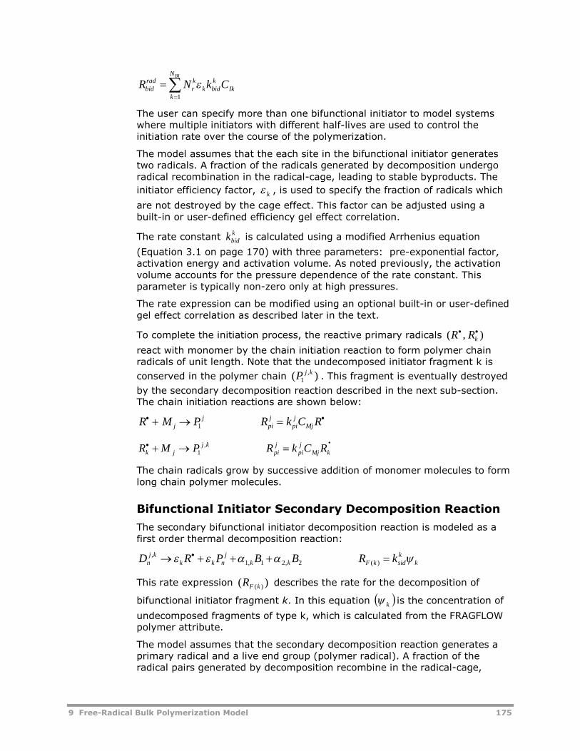
9 Free-Radical Bulk Polymerization Model 175
BIN
kIk
kbidk
kr
radbid CkNR
1
The user can specify more than one bifunctional initiator to model systemswhere multiple initiators with different half-lives are used to control theinitiation rate over the course of the polymerization.
The model assumes that the each site in the bifunctional initiator generatestwo radicals. A fraction of the radicals generated by decomposition undergoradical recombination in the radical-cage, leading to stable byproducts. The
initiator efficiency factor, k , is used to specify the fraction of radicals which
are not destroyed by the cage effect. This factor can be adjusted using abuilt-in or user-defined efficiency gel effect correlation.
The rate constantkbidk is calculated using a modified Arrhenius equation
(Equation 3.1 on page 170) with three parameters: pre-exponential factor,activation energy and activation volume. As noted previously, the activationvolume accounts for the pressure dependence of the rate constant. Thisparameter is typically non-zero only at high pressures.
The rate expression can be modified using an optional built-in or user-definedgel effect correlation as described later in the text.
To complete the initiation process, the reactive primary radicals ),( kRR
react with monomer by the chain initiation reaction to form polymer chainradicals of unit length. Note that the undecomposed initiator fragment k is
conserved in the polymer chain )( ,1
kjP . This fragment is eventually destroyed
by the secondary decomposition reaction described in the next sub-section.The chain initiation reactions are shown below:
R M P R k C Rjj
pij
pij
Mj 1
kMj
jpi
jpi
kjjk RCkRPMR ,
1
The chain radicals grow by successive addition of monomer molecules to formlong chain polymer molecules.
Bifunctional Initiator Secondary Decomposition Reaction
The secondary bifunctional initiator decomposition reaction is modeled as afirst order thermal decomposition reaction:
kksidkFkk
jnkk
kjn kRBBPRD
)(2,21,1,
This rate expression )( )(kFR describes the rate for the decomposition of
bifunctional initiator fragment k. In this equation k is the concentration of
undecomposed fragments of type k, which is calculated from the FRAGFLOWpolymer attribute.
The model assumes that the secondary decomposition reaction generates aprimary radical and a live end group (polymer radical). A fraction of theradical pairs generated by decomposition recombine in the radical-cage,
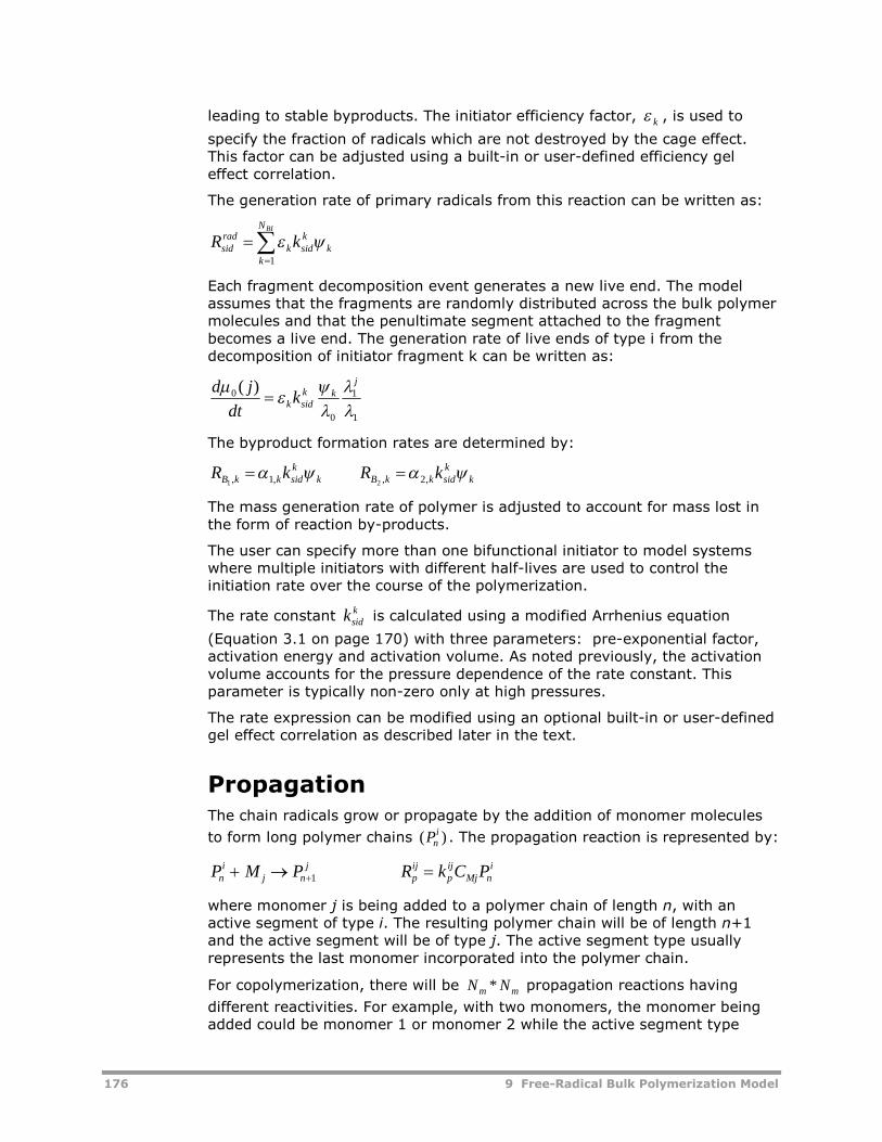
176 9 Free-Radical Bulk Polymerization Model
leading to stable byproducts. The initiator efficiency factor, k , is used to
specify the fraction of radicals which are not destroyed by the cage effect.This factor can be adjusted using a built-in or user-defined efficiency geleffect correlation.
The generation rate of primary radicals from this reaction can be written as:
BIN
kk
ksidk
radsid kR
1
Each fragment decomposition event generates a new live end. The modelassumes that the fragments are randomly distributed across the bulk polymermolecules and that the penultimate segment attached to the fragmentbecomes a live end. The generation rate of live ends of type i from thedecomposition of initiator fragment k can be written as:
1
1
0
0 )(
jkk
sidk kdt
jd
The byproduct formation rates are determined by:
kksidkkBk
ksidkkB kRkR ,2,,1, 21
The mass generation rate of polymer is adjusted to account for mass lost inthe form of reaction by-products.
The user can specify more than one bifunctional initiator to model systemswhere multiple initiators with different half-lives are used to control theinitiation rate over the course of the polymerization.
The rate constantksidk is calculated using a modified Arrhenius equation
(Equation 3.1 on page 170) with three parameters: pre-exponential factor,activation energy and activation volume. As noted previously, the activationvolume accounts for the pressure dependence of the rate constant. Thisparameter is typically non-zero only at high pressures.
The rate expression can be modified using an optional built-in or user-definedgel effect correlation as described later in the text.
PropagationThe chain radicals grow or propagate by the addition of monomer molecules
to form long polymer chains ( )Pni . The propagation reaction is represented by:
P M P R k C Pni
j nj
pij
pij
Mj ni 1
where monomer j is being added to a polymer chain of length n, with anactive segment of type i. The resulting polymer chain will be of length n+1and the active segment will be of type j. The active segment type usuallyrepresents the last monomer incorporated into the polymer chain.
For copolymerization, there will be N Nm m* propagation reactions having
different reactivities. For example, with two monomers, the monomer beingadded could be monomer 1 or monomer 2 while the active segment type
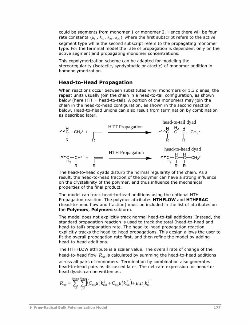
9 Free-Radical Bulk Polymerization Model 177
could be segments from monomer 1 or monomer 2. Hence there will be four
rate constants ( , , , )k k k k11 12 21 22 where the first subscript refers to the active
segment type while the second subscript refers to the propagating monomertype. For the terminal model the rate of propagation is dependent only on theactive segment and propagating monomer concentrations.
This copolymerization scheme can be adapted for modeling thestereoregularity (isotactic, syndyotactic or atactic) of monomer addition inhomopolymerization.
Head-to-Head Propagation
When reactions occur between substituted vinyl monomers or 1,3 dienes, therepeat units usually join the chain in a head-to-tail configuration, as shownbelow (here HTT = head-to-tail). A portion of the monomers may join thechain in the head-to-head configuration, as shown in the second reactionbelow. Head-to-head unions can also result from termination by combinationas described later.
R
HC CH2*
R
+HTT Propagation H
CH2C
R
HC CH2*
R
R
CH2
CH* +HTH Propagation
CH2
HC
HC CH2*
RR R
head-to-tail dyad
head-to-head dyad
The head-to-head dyads disturb the normal regularity of the chain. As aresult, the head-to-head fraction of the polymer can have a strong influenceon the crystallinity of the polymer, and thus influence the mechanicalproperties of the final product.
The model can track head-to-head additions using the optional HTHPropagation reaction. The polymer attributes HTHFLOW and HTHFRAC(head-to-head flow and fraction) must be included in the list of attributes onthe Polymers, Polymers subform.
The model does not explicitly track normal head-to-tail additions. Instead, thestandard propagation reaction is used to track the total (head-to-head andhead-to-tail) propagation rate. The head-to-head propagation reactionexplicitly tracks the head-to-head propagations. This design allows the user tofit the overall propagation rate first, and then refine the model by addinghead-to-head additions.
The HTHFLOW attribute is a scalar value. The overall rate of change of the
head-to-head flow hthR is calculated by summing the head-to-head additions
across all pairs of monomers. Termination by combination also generateshead-to-head pairs as discussed later. The net rate expression for head-to-head dyads can be written as:
Nmon
i
Nmon
j
ijtcji
jihth
iMj
ijhth
jMihth kkCkCR
1 100
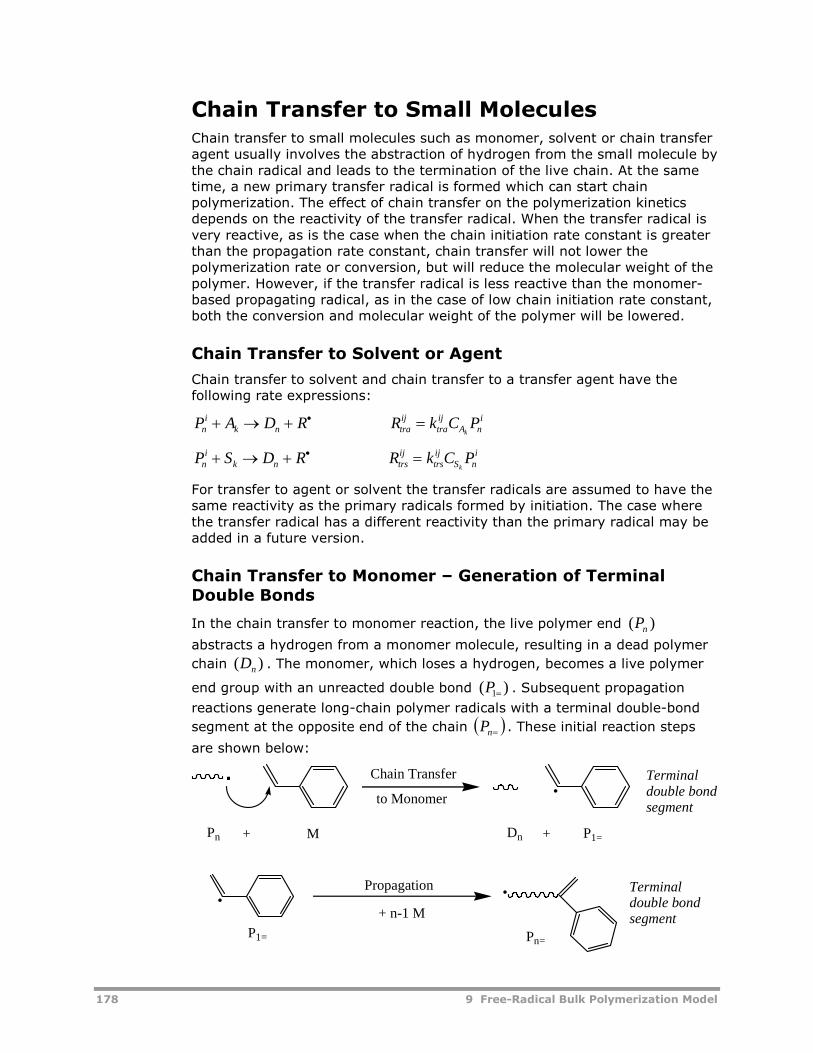
178 9 Free-Radical Bulk Polymerization Model
Chain Transfer to Small MoleculesChain transfer to small molecules such as monomer, solvent or chain transferagent usually involves the abstraction of hydrogen from the small molecule bythe chain radical and leads to the termination of the live chain. At the sametime, a new primary transfer radical is formed which can start chainpolymerization. The effect of chain transfer on the polymerization kineticsdepends on the reactivity of the transfer radical. When the transfer radical isvery reactive, as is the case when the chain initiation rate constant is greaterthan the propagation rate constant, chain transfer will not lower thepolymerization rate or conversion, but will reduce the molecular weight of thepolymer. However, if the transfer radical is less reactive than the monomer-based propagating radical, as in the case of low chain initiation rate constant,both the conversion and molecular weight of the polymer will be lowered.
Chain Transfer to Solvent or Agent
Chain transfer to solvent and chain transfer to a transfer agent have thefollowing rate expressions:
P A D R R k C Pni
k n traij
traij
A ni
k
P S D R R k C Pni
k n trsij
trsij
S ni
k
For transfer to agent or solvent the transfer radicals are assumed to have thesame reactivity as the primary radicals formed by initiation. The case wherethe transfer radical has a different reactivity than the primary radical may beadded in a future version.
Chain Transfer to Monomer – Generation of TerminalDouble Bonds
In the chain transfer to monomer reaction, the live polymer end )( nP
abstracts a hydrogen from a monomer molecule, resulting in a dead polymer
chain )( nD . The monomer, which loses a hydrogen, becomes a live polymer
end group with an unreacted double bond )( 1P . Subsequent propagation
reactions generate long-chain polymer radicals with a terminal double-bond
segment at the opposite end of the chain nP . These initial reaction steps
are shown below:
·
Pn + M Dn + P1=
·
P1=
·Propagation
+ n-1 M
Pn=
Terminaldouble bondsegment
Chain Transfer Terminaldouble bondsegment
to Monomer
·
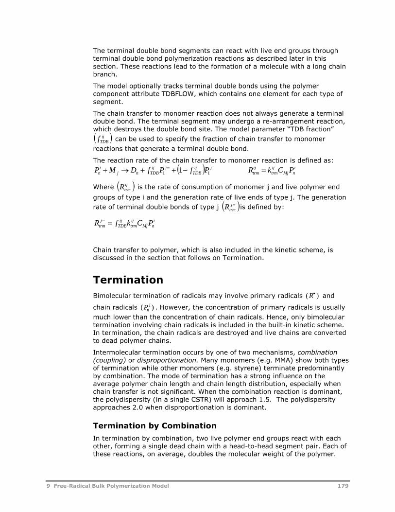
9 Free-Radical Bulk Polymerization Model 179
The terminal double bond segments can react with live end groups throughterminal double bond polymerization reactions as described later in thissection. These reactions lead to the formation of a molecule with a long chainbranch.
The model optionally tracks terminal double bonds using the polymercomponent attribute TDBFLOW, which contains one element for each type ofsegment.
The chain transfer to monomer reaction does not always generate a terminaldouble bond. The terminal segment may undergo a re-arrangement reaction,which destroys the double bond site. The model parameter “TDB fraction”
ijTDBf can be used to specify the fraction of chain transfer to monomer
reactions that generate a terminal double bond.
The reaction rate of the chain transfer to monomer reaction is defined as:
inMj
ijtrm
ijtrm
jijTDB
jijTDBnj
in PCkRPfPfDMP 1 11
Where ijtrmR is the rate of consumption of monomer j and live polymer end
groups of type i and the generation rate of live ends of type j. The generation
rate of terminal double bonds of type j jtrmR is defined by:
inMj
ijtrm
ijTDB
jtrm PCkfR
Chain transfer to polymer, which is also included in the kinetic scheme, isdiscussed in the section that follows on Termination.
Termination
Bimolecular termination of radicals may involve primary radicals ( )R and
chain radicals ( )Pnj . However, the concentration of primary radicals is usually
much lower than the concentration of chain radicals. Hence, only bimoleculartermination involving chain radicals is included in the built-in kinetic scheme.In termination, the chain radicals are destroyed and live chains are convertedto dead polymer chains.
Intermolecular termination occurs by one of two mechanisms, combination(coupling) or disproportionation. Many monomers (e.g. MMA) show both typesof termination while other monomers (e.g. styrene) terminate predominantlyby combination. The mode of termination has a strong influence on theaverage polymer chain length and chain length distribution, especially whenchain transfer is not significant. When the combination reaction is dominant,the polydispersity (in a single CSTR) will approach 1.5. The polydispersityapproaches 2.0 when disproportionation is dominant.
Termination by Combination
In termination by combination, two live polymer end groups react with eachother, forming a single dead chain with a head-to-head segment pair. Each ofthese reactions, on average, doubles the molecular weight of the polymer.
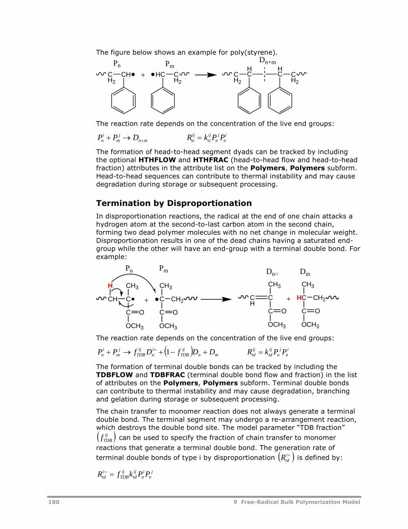
180 9 Free-Radical Bulk Polymerization Model
The figure below shows an example for poly(styrene).
Pn
CH2
CH + CH2
HC CH2
HC C
H2
HC
PmDn+m
The reaction rate depends on the concentration of the live end groups:
P P D R k P Pni
mj
n m tcij
tcij
nj
ni
The formation of head-to-head segment dyads can be tracked by includingthe optional HTHFLOW and HTHFRAC (head-to-head flow and head-to-headfraction) attributes in the attribute list on the Polymers, Polymers subform.Head-to-head sequences can contribute to thermal instability and may causedegradation during storage or subsequent processing.
Termination by Disproportionation
In disproportionation reactions, the radical at the end of one chain attacks ahydrogen atom at the second-to-last carbon atom in the second chain,forming two dead polymer molecules with no net change in molecular weight.Disproportionation results in one of the dead chains having a saturated end-group while the other will have an end-group with a terminal double bond. Forexample:
CH C
CH3
C O
OCH3
H
+ CH2C
CH3
C
OCH3
O
CH
C
CH3
C O
OCH3
+ CH2HC
CH3
C
OCH3
O
Pn Pm Dn= Dm
The reaction rate depends on the concentration of the live end groups:
in
jn
ijtd
ijtdmn
ijTDB
in
ijTDB
jm
in PPkRDDfDfPP 1
The formation of terminal double bonds can be tracked by including theTDBFLOW and TDBFRAC (terminal double bond flow and fraction) in the listof attributes on the Polymers, Polymers subform. Terminal double bondscan contribute to thermal instability and may cause degradation, branchingand gelation during storage or subsequent processing.
The chain transfer to monomer reaction does not always generate a terminaldouble bond. The terminal segment may undergo a re-arrangement reaction,which destroys the double bond site. The model parameter “TDB fraction”
ijTDBf can be used to specify the fraction of chain transfer to monomer
reactions that generate a terminal double bond. The generation rate of
terminal double bonds of type i by disproportionation itdR is defined by:
jn
in
ijtd
ijTDB
itd PPkfR
9 Free-Radical Bulk Polymerization Model 181
Inhibition
Inhibition is included as an additional termination mechanism. This involvesreaction between a chain radical and a small molecule (inhibitor or impurities)to form a dead chain:
inXk
ikx
ikxnk
in PCkRDXP
The model assumes that the inhibitor is consumed by the reaction; thepolymer mass generation rate is adjusted accordingly.
Gel effect in Termination
Bimolecular termination reactions between chain radicals become diffusioncontrolled at high polymer concentration or high conversion. This leads to anincrease in the polymerization rate and molecular weight. This condition isknown as the gel effect or Trommsdorff effect. At high conversions theincreased viscosity of the reaction medium imposes a diffusional limitation onthe polymer chains, leading to lower effective termination rates. Eventually athigh enough conversions, even the propagation, initiation, and chain transferrates may be affected by the diffusional limitation.
The diffusional limitation is modeled by multiplying the low conversionreaction rate coefficients by a gel-effect factor that will lower their effectivevalue with increasing conversion. The free-radical model includes an option tomodify the reaction rate expressions using a built-in or user-defined gel-effectcorrelation, as described later in this chapter.
Long Chain Branching
Chain Transfer to Polymer
The polymer radical in one chain can transfer to a repeat unit in a secondchain. This chain transfer to polymer reaction always generates a long chainbranch, since subsequent propagation from the live site causes the backbonemolecule to grow a new branch.
The chain transfer to polymer reaction can be written as:
P D D P R k m D Pni
m n mj
trpij
trpij
j m ni
Each transfer reaction generates one long chain branch. The optional polymercomponent attributes LCB and FLCB are used to track the molar flow rate oflong chain branches and the long chain branching frequency (branch point perthousand repeat units).
Terminal Double Bond Polymerization
Polymer chains with terminal double bonds are formed by several reactions,including chain transfer to monomer, termination by disproportionation, beta-scission and beta-hydride elimination.
These terminal double bond groups can participate in propagation reactions inmuch the same manner as a monomer molecule. The resulting terminaldouble bond propagation reactions generate a long chain branch since the
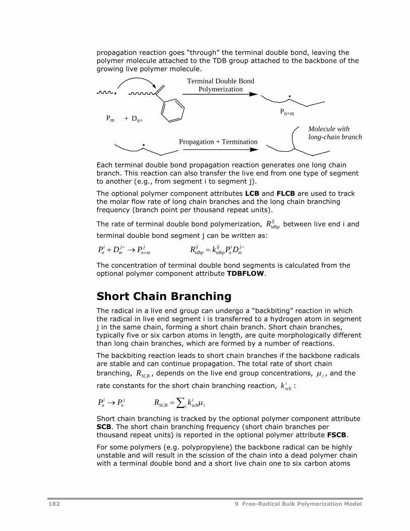
182 9 Free-Radical Bulk Polymerization Model
propagation reaction goes “through” the terminal double bond, leaving thepolymer molecule attached to the TDB group attached to the backbone of thegrowing live polymer molecule.
Dn=
·
+
Terminal Double BondPolymerization
·
· Propagation + Termination
Molecule withlong-chain branch
Pn+mPm
Each terminal double bond propagation reaction generates one long chainbranch. This reaction can also transfer the live end from one type of segmentto another (e.g., from segment i to segment j).
The optional polymer component attributes LCB and FLCB are used to trackthe molar flow rate of long chain branches and the long chain branchingfrequency (branch point per thousand repeat units).
The rate of terminal double bond polymerization,ijtdbpR between live end i and
terminal double bond segment j can be written as:
jm
in
ijtdbp
ijtdbp
jmn
jm
in DPkRPDP
The concentration of terminal double bond segments is calculated from theoptional polymer component attribute TDBFLOW.
Short Chain BranchingThe radical in a live end group can undergo a “backbiting” reaction in whichthe radical in live end segment i is transferred to a hydrogen atom in segmentj in the same chain, forming a short chain branch. Short chain branches,typically five or six carbon atoms in length, are quite morphologically differentthan long chain branches, which are formed by a number of reactions.
The backbiting reaction leads to short chain branches if the backbone radicalsare stable and can continue propagation. The total rate of short chain
branching, SCBR , depends on the live end group concentrations, i , and the
rate constants for the short chain branching reaction,iscbk :
i i
iscbSCB
jn
in kRPP
Short chain branching is tracked by the optional polymer component attributeSCB. The short chain branching frequency (short chain branches perthousand repeat units) is reported in the optional polymer attribute FSCB.
For some polymers (e.g. polypropylene) the backbone radical can be highlyunstable and will result in the scission of the chain into a dead polymer chainwith a terminal double bond and a short live chain one to six carbon atoms

9 Free-Radical Bulk Polymerization Model 183
long. Use the beta scission reaction (see below) to track these types ofreactions.
Beta-ScissionA simplified beta-scission reaction is included in the built-in kinetics. It islimited to reactions where a live chain undergoes scission to form a deadchain of the same length and a primary radical:
in
ibs
ibsn
iTDB
in
iTDB
in PkRRDfDfP )1(
This reaction can be used to simulate backbiting reactions which form short-chain polymer radicals (see Short Chain Branching).
The beta scission reaction usually generates a terminal double bondcorresponding to the live end i. In some special cases, the double bond maynot form or may be unstable. The “terminal double bond fraction” parameter,
iTDBf , can be used to specify the fraction of beta-scission reactions which
generate a terminal double bond (by default, this parameter is unity). Thus,the rate of generation of terminal double bonds from the beta-scission
reaction,i
tdR , can be defined as:
jn
in
ijtd
ijTDB
itd PPkfR
Reactions Involving Diene Monomers
Cis and Trans Propagation
Propagation reactions involving 1,3-diene monomers, such as butadiene orisoprene, can generate three types of repeat segments as shown below.
* +CH2
* +
* +CH2
C C
CH2*
H
H
CH2
C C
H
CH2*
H
Normal Propagation
Cis Propagation
Trans Propagation
CH* Vinyl Configuration
Cis Configuration
Trans Configuration
Although these segments may exhibit different physical properties, it isconvenient to lump them together as a single repeat segment, and track thevarious segment configurations using the optional polymer componentattributes CIS-FLOW and TRANSFLO. Likewise, the three types ofpropagation reactions are lumped together under the standard propagationreaction. Optional Cis-Propagation and Trans-Propagation reactions are usedto specify the rate parameters for reactions that generate segments with thecis- or trans- configurations.
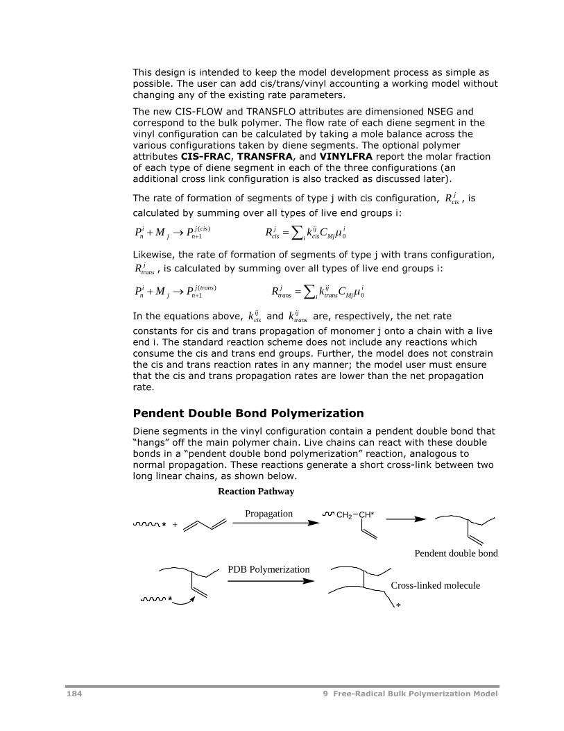
184 9 Free-Radical Bulk Polymerization Model
This design is intended to keep the model development process as simple aspossible. The user can add cis/trans/vinyl accounting a working model withoutchanging any of the existing rate parameters.
The new CIS-FLOW and TRANSFLO attributes are dimensioned NSEG andcorrespond to the bulk polymer. The flow rate of each diene segment in thevinyl configuration can be calculated by taking a mole balance across thevarious configurations taken by diene segments. The optional polymerattributes CIS-FRAC, TRANSFRA, and VINYLFRA report the molar fractionof each type of diene segment in each of the three configurations (anadditional cross link configuration is also tracked as discussed later).
The rate of formation of segments of type j with cis configuration,j
cisR , is
calculated by summing over all types of live end groups i:
i
iMj
ijcis
jcis
cisjnj
in CkRPMP 0
)(1
Likewise, the rate of formation of segments of type j with trans configuration,j
transR , is calculated by summing over all types of live end groups i:
i
iMj
ijtrans
jtrans
transjnj
in CkRPMP 0
)(1
In the equations above,ijcisk and
ijtransk are, respectively, the net rate
constants for cis and trans propagation of monomer j onto a chain with a liveend i. The standard reaction scheme does not include any reactions whichconsume the cis and trans end groups. Further, the model does not constrainthe cis and trans reaction rates in any manner; the model user must ensurethat the cis and trans propagation rates are lower than the net propagationrate.
Pendent Double Bond Polymerization
Diene segments in the vinyl configuration contain a pendent double bond that“hangs” off the main polymer chain. Live chains can react with these doublebonds in a “pendent double bond polymerization” reaction, analogous tonormal propagation. These reactions generate a short cross-link between twolong linear chains, as shown below.
* +CH2Propagation
Reaction Pathway
*
PDB Polymerization
*
Cross-linked molecule
CH*
Pendent double bond
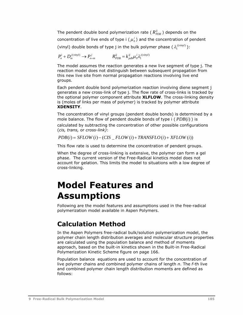
9 Free-Radical Bulk Polymerization Model 185
The pendent double bond polymerization rate (ijPDBR ) depends on the
concentration of live ends of type i (i0 ) and the concentration of pendent
(vinyl) double bonds of type j in the bulk polymer phase ()(
1vinylj ):
)(10
)( vinyljiijpdb
ijPDB
jmn
vinyljm
in kRPDP
The model assumes the reaction generates a new live segment of type j. Thereaction model does not distinguish between subsequent propagation fromthis new live site from normal propagation reactions involving live endgroups.
Each pendent double bond polymerization reaction involving diene segment jgenerates a new cross-link of type j. The flow rate of cross-links is tracked bythe optional polymer component attribute XLFLOW. The cross-linking densityis (moles of links per mass of polymer) is tracked by polymer attributeXDENSITY.
The concentration of vinyl groups (pendent double bonds) is determined by a
mole balance. The flow of pendent double bonds of type i ( )(iPDB ) is
calculated by subtracting the concentration of other possible configurations(cis, trans, or cross-link):
))()()(_()()( iXFLOWiTRANSFLOiFLOWCISiSFLOWiPDB
This flow rate is used to determine the concentration of pendent groups.
When the degree of cross-linking is extensive, the polymer can form a gelphase. The current version of the Free-Radical kinetics model does notaccount for gelation. This limits the model to situations with a low degree ofcross-linking.
Model Features andAssumptionsFollowing are the model features and assumptions used in the free-radicalpolymerization model available in Aspen Polymers.
Calculation MethodIn the Aspen Polymers free-radical bulk/solution polymerization model, thepolymer chain length distribution averages and molecular structure propertiesare calculated using the population balance and method of momentsapproach, based on the built-in kinetics shown in the Built-in Free-RadicalPolymerization Kinetic Scheme figure on page 166.
Population balance equations are used to account for the concentration oflive polymer chains and combined polymer chains of length n. The f-th liveand combined polymer chain length distribution moments are defined asfollows:
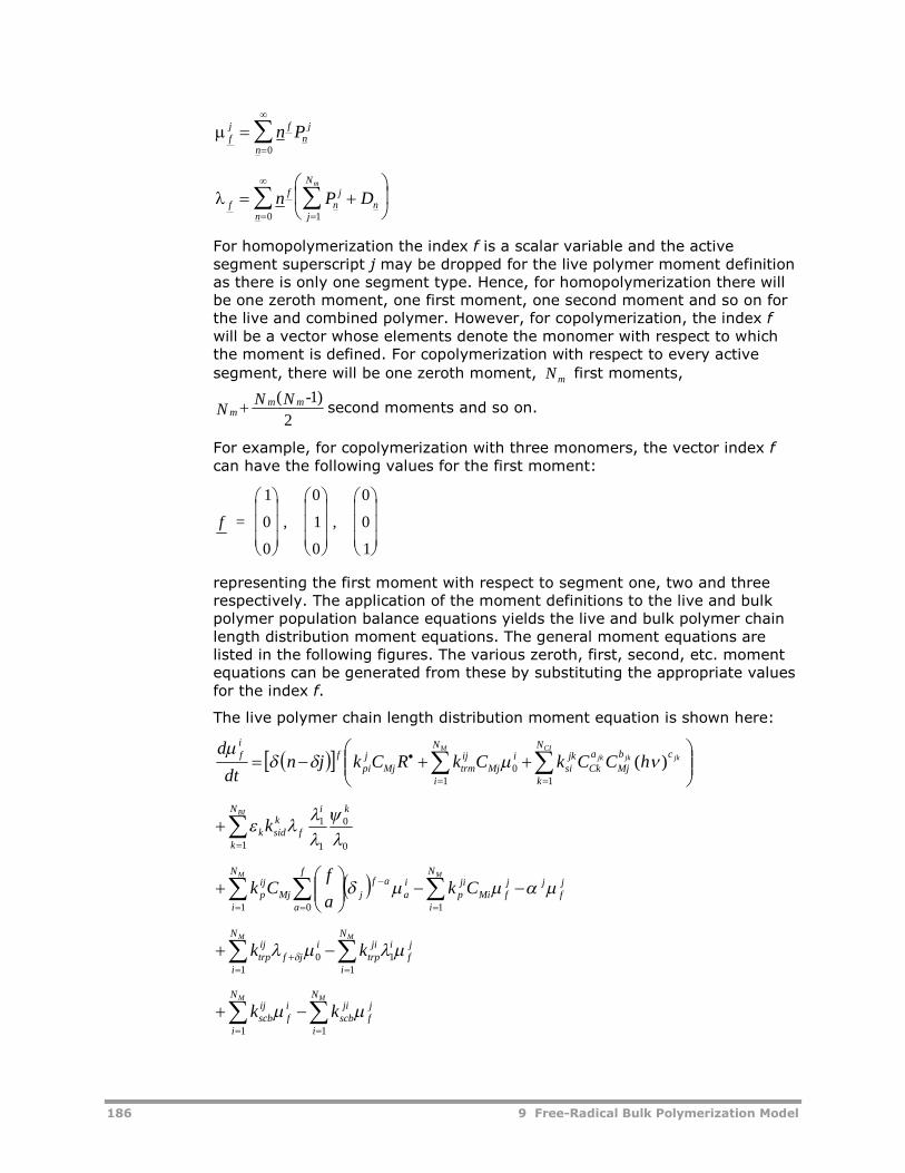
186 9 Free-Radical Bulk Polymerization Model
fj f
nj
n
n P
0
ff
nj
nj
N
n
n P Dm
10
For homopolymerization the index f is a scalar variable and the activesegment superscript j may be dropped for the live polymer moment definitionas there is only one segment type. Hence, for homopolymerization there willbe one zeroth moment, one first moment, one second moment and so on forthe live and combined polymer. However, for copolymerization, the index fwill be a vector whose elements denote the monomer with respect to whichthe moment is defined. For copolymerization with respect to every active
segment, there will be one zeroth moment, Nm first moments,
mm m
NN N -
( )1
2second moments and so on.
For example, for copolymerization with three monomers, the vector index fcan have the following values for the first moment:
f = , ,
1
0
0
0
1
0
0
0
1
representing the first moment with respect to segment one, two and threerespectively. The application of the moment definitions to the live and bulkpolymer population balance equations yields the live and bulk polymer chainlength distribution moment equations. The general moment equations arelisted in the following figures. The various zeroth, first, second, etc. momentequations can be generated from these by substituting the appropriate valuesfor the index f.
The live polymer chain length distribution moment equation is shown here:
CI
jkjkjk
M N
k
cb
Mj
a
Ckjk
si
N
i
iMj
ijtrmMj
jpi
fif
hCCkCkRCkjndt
d
110 )(
BIN
k
ki
fksidk k
1 0
0
1
1
jf
jjf
N
i
N
iMi
jip
f
a
ia
af
jMjijp
M M
Cka
fCk
1 10
MM N
i
jf
ijitrp
N
i
ijf
ijtrp kk
11
10
MM N
i
jf
jiscb
N
i
if
ijscb kk
11
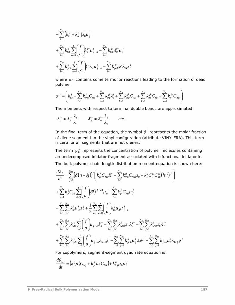
9 Free-Radical Bulk Polymerization Model 187
MN
i
jf
iijtc
ijtd kk
10
MM N
i
jf
ijitdb
N
i
f
a
iaf
ja
ijtdb k
a
fk
10
1 0
MM N
i
jf
ijipdb
N
i
f
a
iafa
jijpdb k
a
fk
11
1 0
where j contains some terms for reactions leading to the formation of dead
polymer
XSAMM N
kXk
jkx
N
kSk
jktrs
N
kAk
jktra
N
i
ijitrp
N
iMi
jitrm
jbs
j CkCkCkkCkk1111
11
The moments with respect to terminal double bonds are approximated:
...0
202
0
101 etciiii
In the final term of the equation, the symboli represents the molar fraction
of diene segment i in the vinyl configuration (attribute VINYLFRA). This termis zero for all segments that are not dienes.
The termk0 represents the concentration of polymer molecules containing
an undecomposed initiator fragment associated with bifunctional initiator k.
The bulk polymer chain length distribution moment equation is shown here:
M MN
j
N
i
cjbjMj
ajC
jsi
iMj
ijtrmMj
jpi
ffhCCkCkRCkjn
dt
d
1 10
MM N
i
jfMi
jip
N
j
f
a
ia
af
Mjijp Ckj
a
fCk
11 0
M MMN
i
N
i
f
a
jaf
ia
ijtc
jf
iN
j
ijtc k
a
fk
1 1 00
1 2
1
M MM MM M N
i
N
j
jf
iijtdb
N
i
N
j
jif
ijtdb
N
i
N
j
f
a
ia
jaf
jitdb kk
a
fk
1 10
1 10
1 1 0
M MM MM M N
i
N
j
jf
iijpdb
N
i
N
j
jif
ijpdb
N
i
N
j
f
a
ia
jaf
jipdb kk
a
fk
1 110
1 11
1 1 01
For copolymers, segment-segment dyad rate equation is:
jitcjiMi
jjipMj
iijp
ji kCkCkdt
d00,00
,
188 9 Free-Radical Bulk Polymerization Model
Quasi-Steady-State Approximation (QSSA)Users may invoke the Quasi-Steady-State Approximation (QSSA) for the livemoment equations. Invoking QSSA converts the live moment differentialequations (ODE) to algebraic equations, which are solved internally in thekinetics routine. Assuming QSSA is equivalent to assuming that the livemoments attain their steady-state values instantaneously. This approximationmakes the system of ODEs much easier to integrate by reducing stiffness.
Comparison of the results with and without QSSA for most free-radicalpolymerization systems, where the chain lifetimes are short compared to theresidence time, show negligible differences. Therefore it is usually reasonableto use the QSSA. However, users should check the validity of thisapproximation by running cases with the QSSA switch set to YES and NO fortheir particular system. By default the QSSA is turned off (QSSA switch is setto NO). Users have the option of invoking the QSSA for all the live polymermoment equations, or selectively for only the zeroth, first, or second momentof live polymer.
Phase EquilibriumThe polymerization model currently considers a single-phase system (vapor orliquid), two-phase system (vapor and liquid), or three-phase (VLL) systemwhen calculating concentrations for the reaction kinetics. For single-phasesystems, the reacting phase may be either vapor or liquid. In multi-phasesystems, reactions can occur in one or more phases simultaneously. Eachreaction object is associated with a single reacting phase, identified on theoptions form.
By default the reacting phase is assumed to be the liquid phase (for VLLsystems, the reacting phase must be specified). Several reaction models canbe referenced from a single reactor block to account for reactions in eachphase.
Gel EffectBimolecular termination reactions between chain radicals become diffusioncontrolled at high polymer concentrations or high conversion leading to aninitial increase in the polymerization rate and molecular weight. This conditionis known as the gel effect or Trommsdorff effect. At high polymerconcentrations, the increased viscosity of the reaction medium imposes adiffusional limitation on the polymer chains, which leads to lower effectivetermination rates. Typically the termination rate coefficients are affected firstby the gel effect because they involve diffusion of two bulky polymer radicals.Eventually at high enough conversions, even the propagation, initiation, chaintransfer reactions, and the initiator efficiency are lowered by the gel effect.Hence, in general it may be necessary to allow gel/glass effects for all thepolymerization reactions in the built-in kinetic scheme.
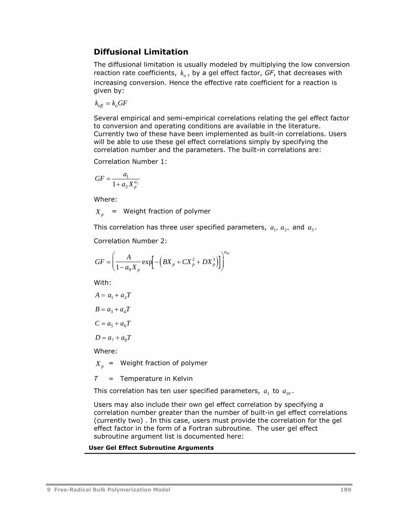
9 Free-Radical Bulk Polymerization Model 189
Diffusional Limitation
The diffusional limitation is usually modeled by multiplying the low conversion
reaction rate coefficients, ko , by a gel effect factor, GF, that decreases with
increasing conversion. Hence the effective rate coefficient for a reaction isgiven by:
k k GFeff o
Several empirical and semi-empirical correlations relating the gel effect factorto conversion and operating conditions are available in the literature.Currently two of these have been implemented as built-in correlations. Userswill be able to use these gel effect correlations simply by specifying thecorrelation number and the parameters. The built-in correlations are:
Correlation Number 1:
GFa
a X pa
1
21 3
Where:
X p= Weight fraction of polymer
This correlation has three user specified parameters, a a1, ,2 and a3 .
Correlation Number 2:
GFA
a XBX CX DX
pp p p
a
1 9
2 3
10
exp
With:
A a a T 1 2
B a a T 3 4
C a a T 5 6
D a a T 7 8
Where:
X p= Weight fraction of polymer
T = Temperature in Kelvin
This correlation has ten user specified parameters, a1 to a10 .
Users may also include their own gel effect correlation by specifying acorrelation number greater than the number of built-in gel effect correlations(currently two) . In this case, users must provide the correlation for the geleffect factor in the form of a Fortran subroutine. The user gel effectsubroutine argument list is documented here:
User Gel Effect Subroutine Arguments
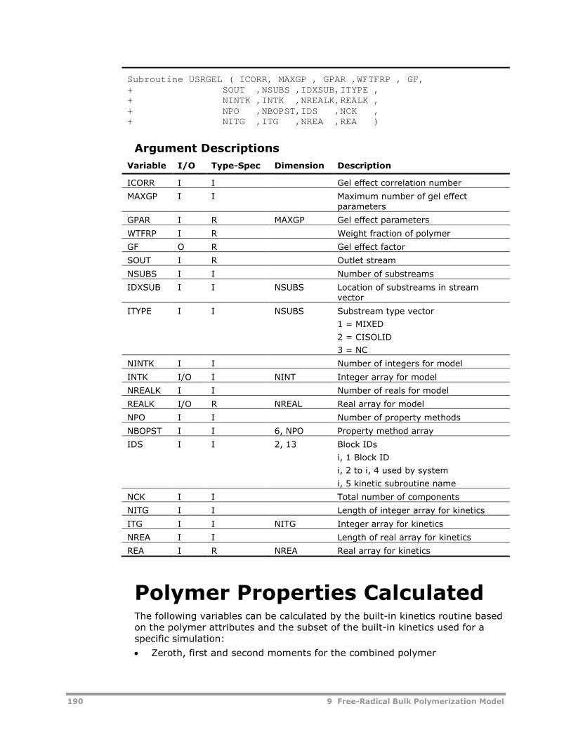
190 9 Free-Radical Bulk Polymerization Model
Subroutine USRGEL ( ICORR, MAXGP , GPAR ,WFTFRP , GF,+ SOUT ,NSUBS ,IDXSUB,ITYPE ,+ NINTK ,INTK ,NREALK,REALK ,+ NPO ,NBOPST,IDS ,NCK ,+ NITG ,ITG ,NREA ,REA )
Argument Descriptions
Variable I/O Type-Spec Dimension Description
ICORR I I Gel effect correlation number
MAXGP I I Maximum number of gel effectparameters
GPAR I R MAXGP Gel effect parameters
WTFRP I R Weight fraction of polymer
GF O R Gel effect factor
SOUT I R Outlet stream
NSUBS I I Number of substreams
IDXSUB I I NSUBS Location of substreams in streamvector
ITYPE I I NSUBS Substream type vector
1 = MIXED
2 = CISOLID
3 = NC
NINTK I I Number of integers for model
INTK I/O I NINT Integer array for model
NREALK I I Number of reals for model
REALK I/O R NREAL Real array for model
NPO I I Number of property methods
NBOPST I I 6, NPO Property method array
IDS I I 2, 13 Block IDs
i, 1 Block ID
i, 2 to i, 4 used by system
i, 5 kinetic subroutine name
NCK I I Total number of components
NITG I I Length of integer array for kinetics
ITG I I NITG Integer array for kinetics
NREA I I Length of real array for kinetics
REA I R NREA Real array for kinetics
Polymer Properties CalculatedThe following variables can be calculated by the built-in kinetics routine basedon the polymer attributes and the subset of the built-in kinetics used for aspecific simulation:
Zeroth, first and second moments for the combined polymer
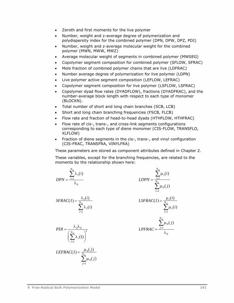
9 Free-Radical Bulk Polymerization Model 191
Zeroth and first moments for the live polymer
Number, weight and z-average degree of polymerization andpolydispersity index for the combined polymer (DPN, DPW, DPZ, PDI)
Number, weight and z-average molecular weight for the combinedpolymer (MWN, MWW, MWZ)
Average molecular weight of segments in combined polymer (MWSEG)
Copolymer segment composition for combined polymer (SFLOW, SFRAC)
Mole fraction of combined polymer chains that are live (LDFRAC)
Number average degree of polymerization for live polymer (LDPN)
Live polymer active segment composition (LEFLOW, LEFRAC)
Copolymer segment composition for live polymer (LSFLOW, LSFRAC)
Copolymer dyad flow rates (DYADFLOW), fractions (DYADFRAC), and thenumber-average block length with respect to each type of monomer(BLOCKN).
Total number of short and long chain branches (SCB, LCB)
Short and long chain branching frequencies (FSCB, FLCB)
Flow rate and fraction of head-to-head dyads (HTHFLOW, HTHFRAC)
Flow rate of cis-, trans-, and cross-link segments configurationscorresponding to each type of diene monomer (CIS-FLOW, TRANSFLO,XLFLOW)
Fraction of diene segments in the cis-, trans-, and vinyl configuration(CIS-FRAC, TRANSFRA, VINYLFRA)
These parameters are stored as component attributes defined in Chapter 2.
These variables, except for the branching frequencies, are related to themoments by the relationship shown here:
DPN
ii
Nm
1
1
0
( )
LDPN
i
j
i
N
i
N
m
m
1
1
0
1
( )
( )
SFRAC Ii
ii
Nm( )
( )
( )
1
1
1
LSFRAC Ii
ii
Nm( )
( )
( )
1
1
1
PDI
i
i
Nm
2 0
1
2
1( )
LPFRAC
jj
Nm
0
1
0
( )
LEFRAC Ij
jj
Nm( )
( )
( )
0
0
1
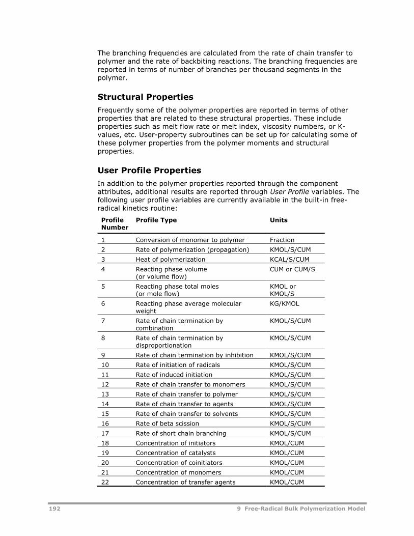
192 9 Free-Radical Bulk Polymerization Model
The branching frequencies are calculated from the rate of chain transfer topolymer and the rate of backbiting reactions. The branching frequencies arereported in terms of number of branches per thousand segments in thepolymer.
Structural Properties
Frequently some of the polymer properties are reported in terms of otherproperties that are related to these structural properties. These includeproperties such as melt flow rate or melt index, viscosity numbers, or K-values, etc. User-property subroutines can be set up for calculating some ofthese polymer properties from the polymer moments and structuralproperties.
User Profile Properties
In addition to the polymer properties reported through the componentattributes, additional results are reported through User Profile variables. Thefollowing user profile variables are currently available in the built-in free-radical kinetics routine:
ProfileNumber
Profile Type Units
1 Conversion of monomer to polymer Fraction
2 Rate of polymerization (propagation) KMOL/S/CUM
3 Heat of polymerization KCAL/S/CUM
4 Reacting phase volume(or volume flow)
CUM or CUM/S
5 Reacting phase total moles(or mole flow)
KMOL orKMOL/S
6 Reacting phase average molecularweight
KG/KMOL
7 Rate of chain termination bycombination
KMOL/S/CUM
8 Rate of chain termination bydisproportionation
KMOL/S/CUM
9 Rate of chain termination by inhibition KMOL/S/CUM
10 Rate of initiation of radicals KMOL/S/CUM
11 Rate of induced initiation KMOL/S/CUM
12 Rate of chain transfer to monomers KMOL/S/CUM
13 Rate of chain transfer to polymer KMOL/S/CUM
14 Rate of chain transfer to agents KMOL/S/CUM
15 Rate of chain transfer to solvents KMOL/S/CUM
16 Rate of beta scission KMOL/S/CUM
17 Rate of short chain branching KMOL/S/CUM
18 Concentration of initiators KMOL/CUM
19 Concentration of catalysts KMOL/CUM
20 Concentration of coinitiators KMOL/CUM
21 Concentration of monomers KMOL/CUM
22 Concentration of transfer agents KMOL/CUM
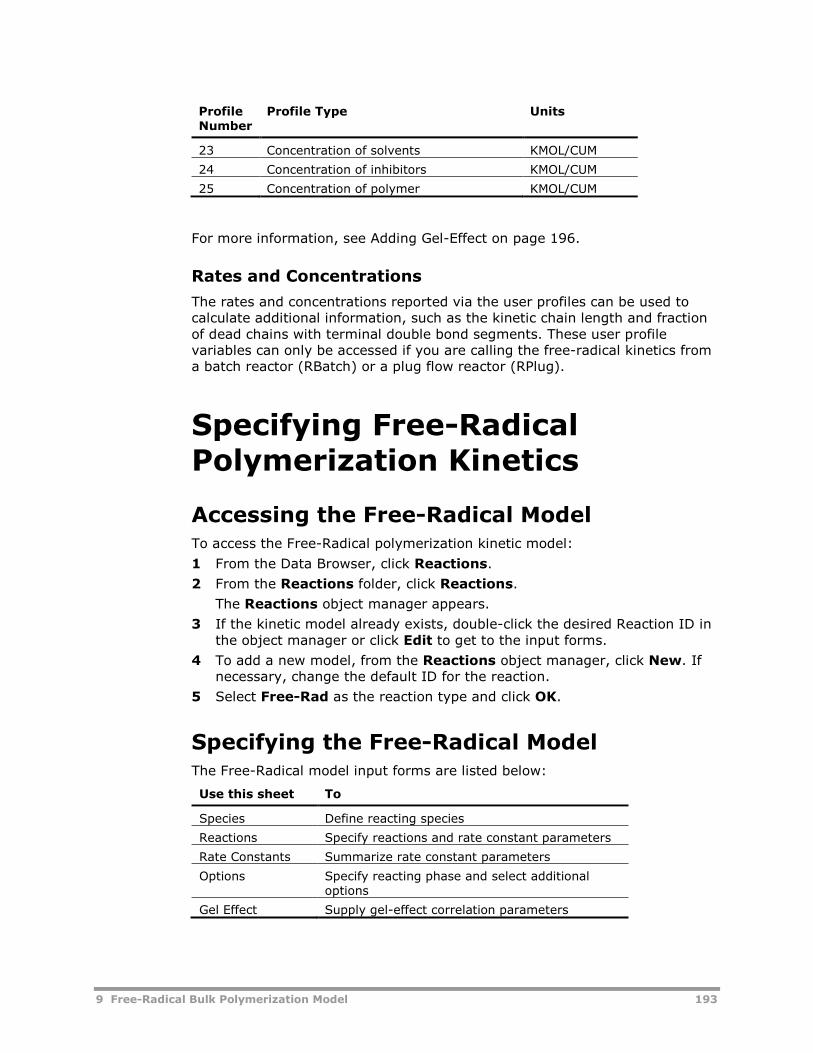
9 Free-Radical Bulk Polymerization Model 193
ProfileNumber
Profile Type Units
23 Concentration of solvents KMOL/CUM
24 Concentration of inhibitors KMOL/CUM
25 Concentration of polymer KMOL/CUM
For more information, see Adding Gel-Effect on page 196.
Rates and Concentrations
The rates and concentrations reported via the user profiles can be used tocalculate additional information, such as the kinetic chain length and fractionof dead chains with terminal double bond segments. These user profilevariables can only be accessed if you are calling the free-radical kinetics froma batch reactor (RBatch) or a plug flow reactor (RPlug).
Specifying Free-RadicalPolymerization Kinetics
Accessing the Free-Radical ModelTo access the Free-Radical polymerization kinetic model:
1 From the Data Browser, click Reactions.
2 From the Reactions folder, click Reactions.
The Reactions object manager appears.
3 If the kinetic model already exists, double-click the desired Reaction ID inthe object manager or click Edit to get to the input forms.
4 To add a new model, from the Reactions object manager, click New. Ifnecessary, change the default ID for the reaction.
5 Select Free-Rad as the reaction type and click OK.
Specifying the Free-Radical ModelThe Free-Radical model input forms are listed below:
Use this sheet To
Species Define reacting species
Reactions Specify reactions and rate constant parameters
Rate Constants Summarize rate constant parameters
Options Specify reacting phase and select additionaloptions
Gel Effect Supply gel-effect correlation parameters
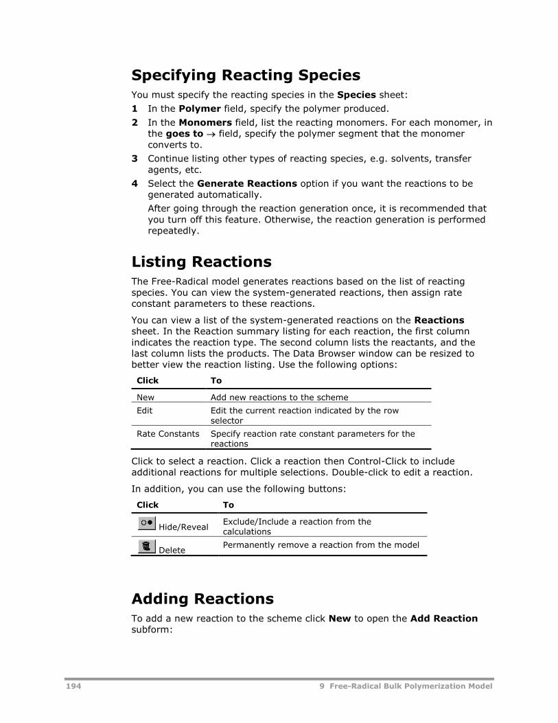
194 9 Free-Radical Bulk Polymerization Model
Specifying Reacting SpeciesYou must specify the reacting species in the Species sheet:
1 In the Polymer field, specify the polymer produced.
2 In the Monomers field, list the reacting monomers. For each monomer, inthe goes to field, specify the polymer segment that the monomerconverts to.
3 Continue listing other types of reacting species, e.g. solvents, transferagents, etc.
4 Select the Generate Reactions option if you want the reactions to begenerated automatically.
After going through the reaction generation once, it is recommended thatyou turn off this feature. Otherwise, the reaction generation is performedrepeatedly.
Listing ReactionsThe Free-Radical model generates reactions based on the list of reactingspecies. You can view the system-generated reactions, then assign rateconstant parameters to these reactions.
You can view a list of the system-generated reactions on the Reactionssheet. In the Reaction summary listing for each reaction, the first columnindicates the reaction type. The second column lists the reactants, and thelast column lists the products. The Data Browser window can be resized tobetter view the reaction listing. Use the following options:
Click To
New Add new reactions to the scheme
Edit Edit the current reaction indicated by the rowselector
Rate Constants Specify reaction rate constant parameters for thereactions
Click to select a reaction. Click a reaction then Control-Click to includeadditional reactions for multiple selections. Double-click to edit a reaction.
In addition, you can use the following buttons:
Click To
Hide/RevealExclude/Include a reaction from thecalculations
DeletePermanently remove a reaction from the model
Adding ReactionsTo add a new reaction to the scheme click New to open the Add Reactionsubform:
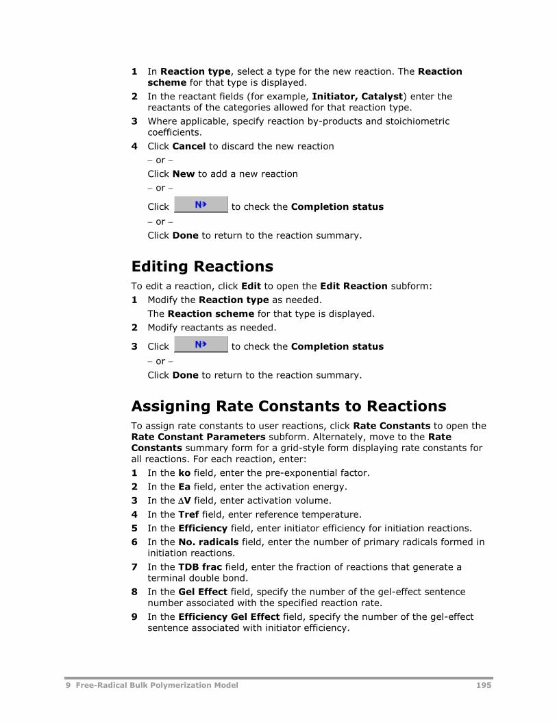
9 Free-Radical Bulk Polymerization Model 195
1 In Reaction type, select a type for the new reaction. The Reactionscheme for that type is displayed.
2 In the reactant fields (for example, Initiator, Catalyst) enter thereactants of the categories allowed for that reaction type.
3 Where applicable, specify reaction by-products and stoichiometriccoefficients.
4 Click Cancel to discard the new reaction
or
Click New to add a new reaction
or
Click to check the Completion status
or
Click Done to return to the reaction summary.
Editing ReactionsTo edit a reaction, click Edit to open the Edit Reaction subform:
1 Modify the Reaction type as needed.
The Reaction scheme for that type is displayed.
2 Modify reactants as needed.
3 Click to check the Completion status
or
Click Done to return to the reaction summary.
Assigning Rate Constants to ReactionsTo assign rate constants to user reactions, click Rate Constants to open theRate Constant Parameters subform. Alternately, move to the RateConstants summary form for a grid-style form displaying rate constants forall reactions. For each reaction, enter:
1 In the ko field, enter the pre-exponential factor.
2 In the Ea field, enter the activation energy.
3 In the V field, enter activation volume.
4 In the Tref field, enter reference temperature.
5 In the Efficiency field, enter initiator efficiency for initiation reactions.
6 In the No. radicals field, enter the number of primary radicals formed ininitiation reactions.
7 In the TDB frac field, enter the fraction of reactions that generate aterminal double bond.
8 In the Gel Effect field, specify the number of the gel-effect sentencenumber associated with the specified reaction rate.
9 In the Efficiency Gel Effect field, specify the number of the gel-effectsentence associated with initiator efficiency.
196 9 Free-Radical Bulk Polymerization Model
10 Click the stoichiometry list and select a new reaction. Enter rate constantsfor the new reaction. You can use the Prev and Next buttons to select theprevious or next reaction in the list (or move to another row when usingthe Rate Constants summary form).
11 Click to check the Completion status
or
Click Close to return to the reaction summary.
Adding Gel-EffectUse the Gel-Effect sheet to add gel effect to reactions:
1 To activate the form, click Use Gel Effect.
2 In Sentence ID, enter a unique integer identifier.
3 In the Corr. No. field, specify a gel effect correlation number (use anumber greater than 100 for user-defined gel effect correlations).
4 In Parameters, list the parameters for the gel effect correlation.
When the specified correlation number is larger than the number of built-in correlations, you must also enter the gel-effect subroutine name in theSubroutine box.
5 To repeat steps 1-4 for additional gel-effect correlations, in the SentenceID field, click New.
Selecting Calculation OptionsYou can select additional simulation options for the model such as QSSA,special initiation options, and gel-effect on the Options sheet.
Option Field Description
QSSA Apply the quasi-steady-state approximation.
This activates additional options in the Apply QSSA to frameon the right side of the form. Inside this frame, select themoments for which you would like to apply the QSSAapproximation.
SpecialInitiation
Activate the Special Initiation Parameters frame at thebottom of the form.
In this frame, list the monomers affected, and enter thespecial initiation coefficients and radiation intensity.
Reacting Phase Specify the phase in which reactions occur.
All of the reactions in the free-radical reaction object areassumed to take place in the same phase. You can use two(or more) free-radical models in the same reactor to accountfor simultaneous reactions in multiple phases (see theSuspensionEPS example).
If the Reacting Phase option is set to Liquid phase 1 or Liquid phase 2the model assumes two liquid phases exist. When the named phase is notpresent, the model prints a warning message and sets the reaction rates tozero. There are two options for handling phase collapse:
9 Free-Radical Bulk Polymerization Model 197
Select the Use bulk liquid phase option to force the model to apply thespecified reaction kinetics to the bulk phase when the named phasedisappears.
Select the Suppress warnings option to deactivate the warningmessages associated with phase collapse.
Note: You must specify the Valid Phases keyword for each reactor modelreferencing the kinetics to ensure the reactor models are consistent with thereaction models.
Specifying User ProfilesUser profiles may be tabulated in RBatch and RPlug reactors. To specify userprofiles, go the reactor’s User Subroutine form User Variables sheet:
1 In the Number of user variables field, enter the number of user variableprofiles to be tabulated.
For a list of user profiles available in the free-radical model, see PolymerProperties Calculated on page 192.
2 In the Variable No. field, list the profile numbers in order.
You must enter the profiles sequentially, without omissions.
3 For each profile, enter a profile Label and a Units Label.
Although these labels are displayed, the reactor model does not performunit conversions on the user profiles. The user profile variables are totals.For example, the reported propagation rate is summed over allpropagation reactions.
4 To view user profile results, go to the User Variables sheet of thereactor’s Profiles form.
ReferencesArriola, D. J. (1989). Modeling of Addition Polymerization Systems, Ph.D.Thesis. University of Wisconsin-Madison, WI.
Biesenberger, J. A., & Sebastian, D. H. (1983). Principles of PolymerizationEngineering. New York: Wiley.
Billmeyer, F. W. (1971). Textbook of Polymer Science. New York: Wiley-Interscience.
Choi, K.Y. & Kim, K.J. (1987). Steady State Behavior of a Continuous StirredTank Reactor for Styrene Polymerization with Bifunctional Initiators. ChemicalEngineering Science.
Choi, K.Y., Liang, W.R., and G.D. Lei (1988). Kinetics of Bulk StyrenePolymerization Catalyzed by Symmetrical Bifunctional Initiators. Journal ofApplied Polymer Science Vol. 35, 1547-1562.
Choi, K.Y., & Lei, G.D. (1987). Modeling of Free-Radical Polymerization ofBifunctional Initiators. AICHE Journal Vol. 33 No. 12, 2067-2076.
Friis, N., & Hamielec, A. E. (1976). Gel-Effect in Emulsion Polymerization ofVinyl Monomers. ACS Symp. Ser., 24.
198 9 Free-Radical Bulk Polymerization Model
Ham, G. E. (Ed.). (1967). Vinyl Polymerization Volume 1. New York: MarcelDekker.
Hui, A. E., & Hamielec, A. E. (1972). Thermal Polymerization of Styrene atHigh Conversion and Temperatures. An Experimental Study. J. of AppliedPolym. Sci., 16, pp. 749-769.
Kim, K.J., and Choi, K.Y. (1989). Modeling of Free Radical Polymerization ofStyrene by Unsymmetrical Bifunctional Initiators. Chemical EngineeringScience, Vol. 44 No. 2, pp. 297-312.
Lenz, R. W. (1968). Organic Chemistry of Synthetic High Polymers. New York:Wiley-Interscience.
Marten, F. L., & Hamielec, A. E. (1979). High Conversion Diffusion ControlledPolymerization. ACS Symp. Ser., 104.
Ray, W. H., & Laurence, R. L. (1977). Polymerization Reaction Engineering. InChemical Reactor Theory. New Jersey: Prentice-Hall.
Villalobos, M.A., Hamielec, A.E., and P.E. Wood (1991). Kinetic Model forShort-Cycle Bulk Styrene Polymerization through Bifunctional Initiators.Journal of Applied Polymer Sciene V 42, 629-641.
10 Emulsion Polymerization Model 199
10 Emulsion PolymerizationModel
This section covers the emulsion polymerization model available in AspenPolymers (formerly known as Aspen Polymers Plus).
Topics covered include:
Summary of Applications, 199
Emulsion Polymerization Processes, 200
Reaction Kinetic Scheme, 200
Model Features and Assumptions, 215
Polymer Particle Properties Calculated, 218
Specifying Emulsion Polymerization Kinetics, 219
The Aspen Polymers Examples & Applications Case Book illustrates how to usethe emulsion model to simulate styrene butadiene copolymerization.
Summary of ApplicationsThe emulsion polymerization model is applicable to emulsion polymerizationprocesses where nucleation occurs by both the micellar and homogeneousmechanisms or to seeded polymerization. Some of the applicable polymersare described below:
Styrene - A component of synthetic rubber and paper coating
Butadiene - Synthetic rubber, impact modifier in ABS and HIPS
Tetrafluroethylene - Polytetrafluroethylene (PTFE), fluoropolymers Viton
Vinylacetate - Polyvinylacetate (PVA) adhesives, paint formulation
Methylmethacrylate - Surface coating applications.
Acrylic Acid - Minor component in paints
2-chloro-1,3-butadiene (chloroprene) - Neoprene rubber
Butyl Acrylate - Surface coatings
Butyl Methacrylate - Comonomer in surface coatings
Vinyl Chloride - PVC used in floor covering and coatings
200 10 Emulsion Polymerization Model
A wide variety of processes are used in emulsion polymerization. Theprocesses that can be modeled using the Aspen Polymers emulsionpolymerization model are those that follow micellar, homogeneous, or seededpolymerization.
An example of a process that follows micellar nucleation and subsequentgrowth is the production of SBR latex in semi-batch reactors for paper coatingapplications. The following lists polymeric products made by emulsionpolymerization:
Emulsion paints, made from a number of monomers (styrene, butadiene,acrylates, etc.) and a variety of other ingredients
Adhesives, from slightly plasticized poly(vinyl acetate) and poly(ethylene-co-vinyl acetate) - a pressure sensitive adhesive
SBR, for carpet backing and for coating paper and card board along withchina clay, thus facilitating printing on surfaces
Non-woven fabrics, which have their fabrics pre-coated with polymer andthen heat pressed (these are termed “thermoformable” felts)
ABS (Acrylonitrile-Butadiene-Styrene), used in high impact strengthmaterial made by swelling of a polybutadiene latex with a mixture ofstyrene and acrylonitrile and polymerizing further. HIPS (High-ImpactPolyStyrene) made from bulk polymerized polystyrene in the presence ofpolybutadiene
Emulsion PolymerizationProcessesEmulsion polymerization is an industrially important process for theproduction of polymers used as synthetic rubber, adhesives, paints, inks,coatings, etc. The polymerization is usually carried out using water as thedispersion medium. This makes emulsion polymerization less detrimental tothe environment than other processes in which volatile organic liquids areused as a medium.
In addition, emulsion polymerization offers distinct processing advantages forthe production of polymers. Unlike in bulk or solution polymerization, theviscosity of the reaction mixture does not increase as dramatically aspolymerization progresses. For this reason, the emulsion polymerizationprocess offers excellent heat transfer and good temperature throughout thecourse of polymer synthesis. This process is always chosen when the polymerproduct is used in latex form.
Reaction Kinetic SchemeIn emulsion polymerization, free-radical propagation reactions take place inparticles isolated from each other by the intervening dispersion medium. Thisreduces termination rates, giving high polymerization rates, andsimultaneously makes it possible to produce high molecular weight polymers.
10 Emulsion Polymerization Model 201
One can increase the rate of polymerization without reducing the molecularweight of the polymer. Emulsion polymerization has more recently becomeimportant for the production of a wide variety of specialty polymers.
Particle Formation
To appreciate the complexities of emulsion polymerization, a basicunderstanding of the fundamentals of particle formation and of the kinetics ofthe subsequent particle growth stage is required. A number of mechanismshave been proposed for particle formation. It is generally accepted that anyone of the mechanisms could be responsible for particle formation dependingon the nature of the monomer and the amount of emulsifier used in therecipe.
The two common mechanisms for particle formation are:
Micellar nucleation
Homogeneous nucleation
With micellar nucleation, micelles, which are aggregates of emulsifiermolecules, act as the site of nucleation.
With homogeneous nucleation, the radicals produced in the aqueous phasepolymerize with dissolved monomer and precipitate out to form precursorparticles. The precipitated precursor particles coagulate with each other untila stable particle is formed.
Micellar NucleationMicellar nucleation is considered to be the primary mechanism for particleformation (Harkins, 1945; Smith & Ewart, 1948) in those emulsionpolymerization systems for which the monomer is very sparingly soluble inwater, and where the concentration of emulsifier is above the critical micelleconcentration (CMC). As the name implies, the micelles, which are formedwhen the emulsifier concentration is above the CMC, act as the site forparticle nucleation.
The reaction mixture consists of water, monomer, emulsifier and a water-soluble initiator. The monomer is dispersed in the form of droplets in thewater by agitation. The droplets formed are stabilized by the emulsifiermolecules which are adsorbed on the droplet surface. In addition to thedroplets, monomer is also found dissolved in the aqueous medium andsolubilized inside the micelles.
Similarly, the emulsifier is found in three locations: in the micelles, dissolvedin the aqueous medium, and adsorbed on the monomer droplets. Since awater soluble initiator is used, the initiator molecules will be mainly founddissolved in the water medium.
When a typical emulsion polymerization recipe is heated, the initiatordissociates in the aqueous medium and produces initiator radicals. Uponpropagating with monomer in the water phase the initiator radicals formoligomeric radicals and enter the micelles, which are aggregates of emulsifiermolecules inside which a small amount of monomer is entrapped. Thecapturing of a radical by micelle and reaction with the entrapped monomersignifies the formation of a particle from a micelle. As the propagation takes
202 10 Emulsion Polymerization Model
place in the newly created particle, a thermodynamic potential difference iscreated for the diffusion of the monomer from the monomer droplets into thegrowing particles.
As the particles grow, some of the micelles disintegrate and cover thegrowing particles to stabilize them. Therefore, the micelles are not onlyconsumed in the formation of polymer particles, but also in the stabilization ofgrowing polymeric particles. In fact, approximately one percent of themicelles are used in the formation of particles. When no micelles remain inthe reaction mixture, micellar nucleation ceases.
Stage I
The time required for particle nucleation to be complete is also called thenucleation time or the nucleation period, and usually lasts 10-15 minutes inconventional polymerization systems. This is commonly referred to as theseed stage, or Stage I, in the emulsion polymerization industry. After thenucleation or seed stage, the number of particles in the reaction mixtureremains constant if particles do not agglomerate.
Stage II
The stage following the seed stage is called the growth stage or Stage II ofthe emulsion polymerization. In Stage II, the polymer particles grow througha steady diffusion of monomer from the monomer droplets to the particles.Since the number of particles remains constant and the particles aresaturated with monomer, this stage is marked by a constant rate ofpolymerization and could easily be observed on a conversion vs. time plot.Stage II is considered complete when the monomer droplets are totallydepleted.
Stage III
In Stage III, the monomer finishing stage, the reaction mixture consists ofthe monomer swollen polymer particles and the aqueous medium. Furtherpolymerization of the monomer in the particles takes place. This results in adecrease of the particle size due to higher density of the polymer compared tothe monomer. During Stage III, the concentration of monomer dissolved inthe aqueous phase falls rapidly, as does the concentration in the polymerparticles. The final product obtained at the end of Stage III is called latex.
The following figure illustrates the stages in a micellar nucleation emulsionpolymerization reaction:
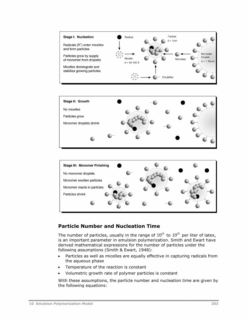
10 Emulsion Polymerization Model
Particle Number and Nucleation Time
The number of particles, usually in the range ofis an important parameter in emulsion polymerization. Smith and Ewart havederived mathematicalfollowing assumptions (Smith & Ewart, 1948):
Particles as well as micelles are equally effective in capturing radicals fromthe aqueous phase
Temperature of the reaction is constant
Volumetric growth rate
With these assumptions, the particle numberthe following equatio
10 Emulsion Polymerization Model
Particle Number and Nucleation Time
mber of particles, usually in the range of 1016to 1018
per liter of latexis an important parameter in emulsion polymerization. Smith and Ewart havederived mathematical expressions for the number of particles under thefollowing assumptions (Smith & Ewart, 1948):
Particles as well as micelles are equally effective in capturing radicals fromthe aqueous phase
Temperature of the reaction is constant
Volumetric growth rate of polymer particles is constant
With these assumptions, the particle number and nucleation timethe following equations:
203
per liter of latex,is an important parameter in emulsion polymerization. Smith and Ewart have
expressions for the number of particles under the
Particles as well as micelles are equally effective in capturing radicals from
and nucleation time are given by
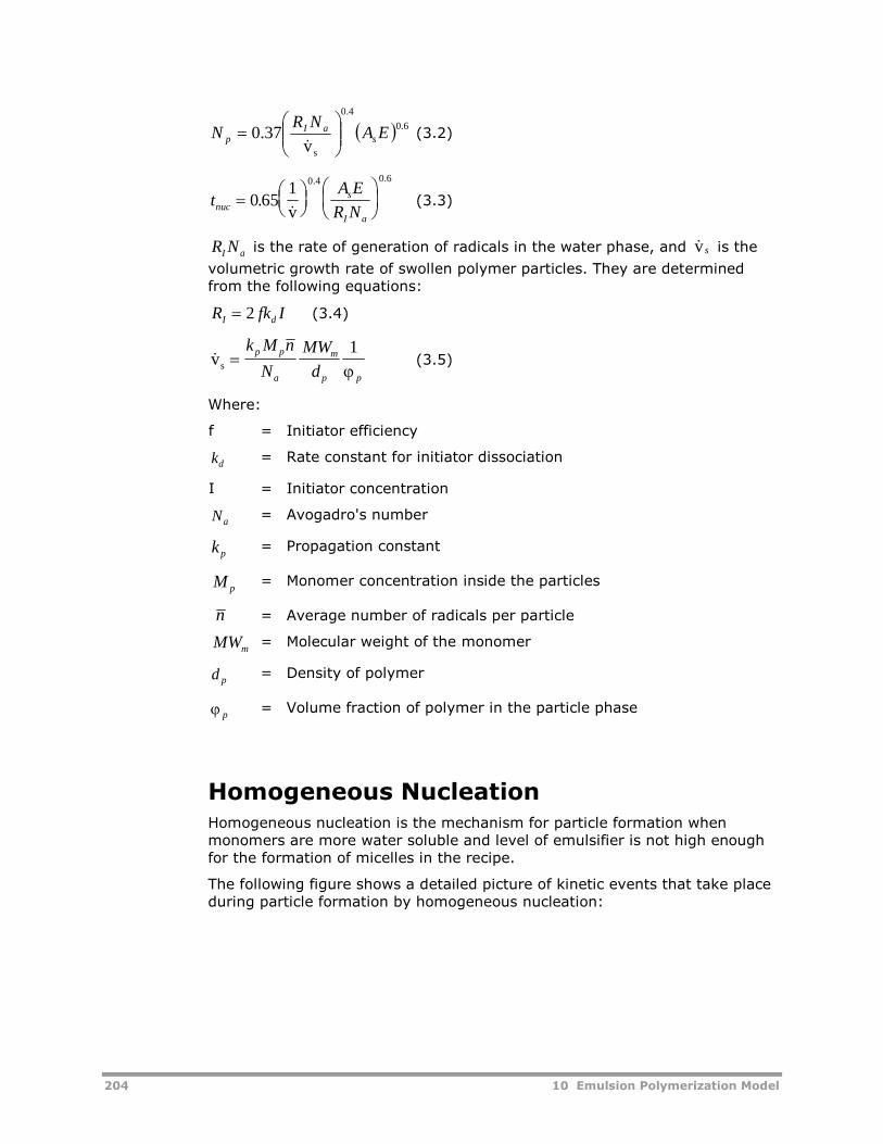
204 10 Emulsion Polymerization Model
6.0
4.0
sv37.0 EA
NRN s
aIp
(3.2)
tA E
R Nnucs
I a
0 65
10 4 0 6
.
. .
v(3.3)
R NI a is the rate of generation of radicals in the water phase, and v s is the
volumetric growth rate of swollen polymer particles. They are determinedfrom the following equations:
R fk II d 2 (3.4)
vs k M n
N
MW
d
p p
a
m
p p
1
(3.5)
Where:
f = Initiator efficiency
kd= Rate constant for initiator dissociation
I = Initiator concentration
Na= Avogadro's number
kp= Propagation constant
M p= Monomer concentration inside the particles
n = Average number of radicals per particle
MWm= Molecular weight of the monomer
d p= Density of polymer
p= Volume fraction of polymer in the particle phase
Homogeneous NucleationHomogeneous nucleation is the mechanism for particle formation whenmonomers are more water soluble and level of emulsifier is not high enoughfor the formation of micelles in the recipe.
The following figure shows a detailed picture of kinetic events that take placeduring particle formation by homogeneous nucleation:
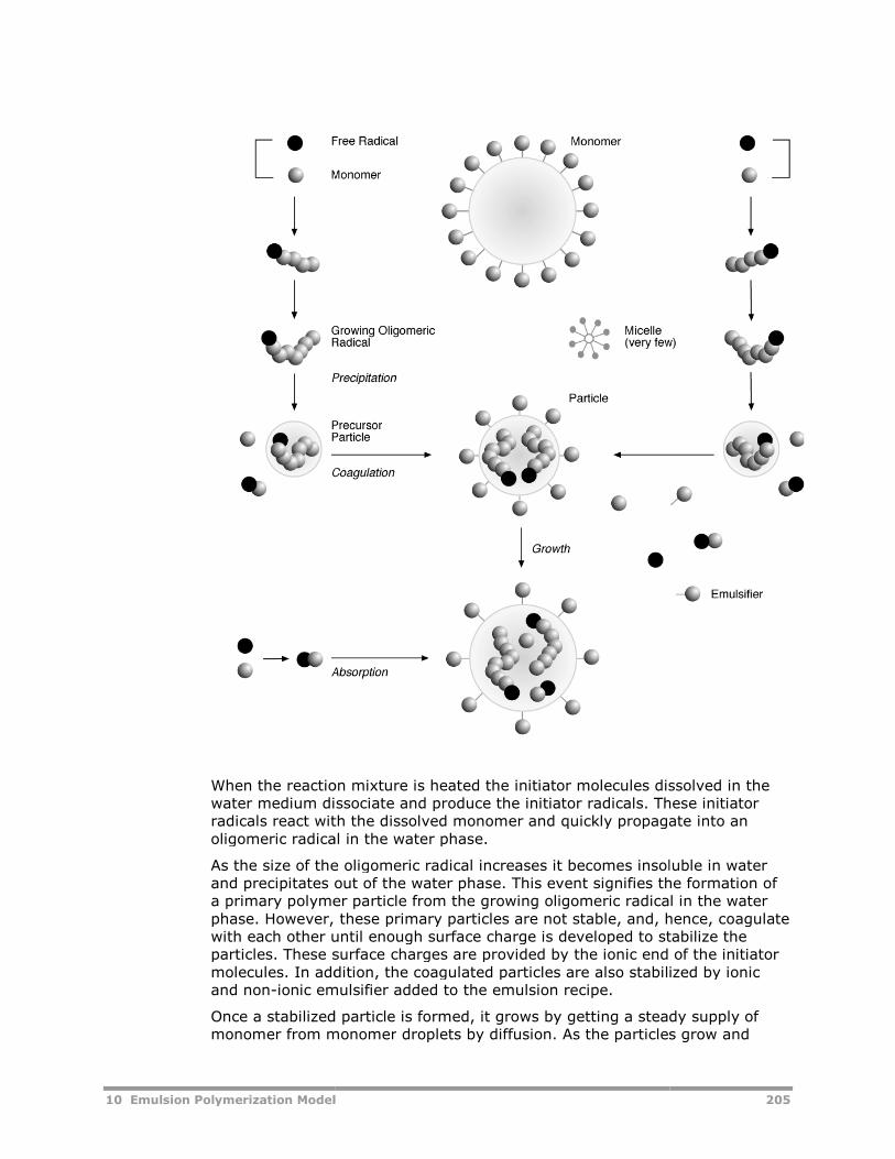
10 Emulsion Polymerization Model
When the reaction mixture is heated the initiator molecules dissolved in thewater medium dissociate and produce the initiator radicals. These initiatorradicals react with the dissolved monooligomeric radical in the water phase.
As the size of the oligomeric radical increases it becomes insoluble in waterand precipitates out of the water phase. This event signifies the formation ofa primary polymer particlephase. However, these primary particles are not stable, and, hence, coagulatewith each other until enough surface charge is developed to stabilize theparticles. These surface charges are provided by the imolecules. In addition, the coagulated particles are also stabilized by ionicand non-ionic emulsifier added to the emulsion recipe.
Once a stabilized particle is formed, it grows by getting a steady supply ofmonomer from monomer
10 Emulsion Polymerization Model
When the reaction mixture is heated the initiator molecules dissolved in thewater medium dissociate and produce the initiator radicals. These initiatorradicals react with the dissolved monomer and quickly propagate into anoligomeric radical in the water phase.
As the size of the oligomeric radical increases it becomes insoluble in waterand precipitates out of the water phase. This event signifies the formation ofa primary polymer particle from the growing oligomeric radical in the waterphase. However, these primary particles are not stable, and, hence, coagulatewith each other until enough surface charge is developed to stabilize theparticles. These surface charges are provided by the ionic end of the initiatormolecules. In addition, the coagulated particles are also stabilized by ionic
ionic emulsifier added to the emulsion recipe.
Once a stabilized particle is formed, it grows by getting a steady supply ofmonomer from monomer droplets by diffusion. As the particles grow and
205
When the reaction mixture is heated the initiator molecules dissolved in thewater medium dissociate and produce the initiator radicals. These initiator
mer and quickly propagate into an
As the size of the oligomeric radical increases it becomes insoluble in waterand precipitates out of the water phase. This event signifies the formation of
from the growing oligomeric radical in the waterphase. However, these primary particles are not stable, and, hence, coagulatewith each other until enough surface charge is developed to stabilize the
onic end of the initiatormolecules. In addition, the coagulated particles are also stabilized by ionic
Once a stabilized particle is formed, it grows by getting a steady supply ofdroplets by diffusion. As the particles grow and
206 10 Emulsion Polymerization Model
become large, the oligomeric radicals that are formed in the water phase aredirectly absorbed by the particles. After sufficient number of particles areformed that are able to absorb all of the radicals in the water phase, no newparticles are formed in the water phase and the number of particles becomesconstant. Also in homogeneous nucleation the particle number reaches aconstant value, as in micellar nucleation. The subsequent growth stage issimilar to the growth stage in the micellar nucleation.
Particle Formation Rate
The rate of particle formation by homogeneous nucleation can be derived byconsidering the water phase kinetics and rate of precipitation of the polymersat an assumed critical chain length (jcr). Assuming the aggregation number
( )Nagg for the formation of stable particles from the precipitated precursor
particles, the rate of particle formation by homogeneous nucleation is givenby:
R
dN
dt
N k nN N
N
k M
k M k R k A k Aa i de a
agg
pw w
pw w tw w ap p am m
jcr
homo
/1
In the above equation Rw
refers to the concentration of live radicals in the
water phase and is given by:
R
k nN N
k M k R k A k Aw
i de a
pw w tw w ap p am m
jcr
/ 1
1
1
Where:
k M
k M k R k A k A
pw w
pw w tw w ap p am m
Refer to the table of page 208 for the explanation of the symbols in the aboveequations.
Particle GrowthStage II, the growth stage, starts after the completion of the seed stage inthe in situ seed process . In the in situ seed process, the micelles are used forthe generation of the seeds. In the case of an external seed process, a wellcharacterized seed is used as the starting material for emulsion production. Ifquality control tests indicate that the particle number and particle sizedistribution of the seed particles will not result in the desired end-productspecifications, the batch is normally terminated. Therefore, in the growthstage it can be assumed that the desired number of particles, with the desiredparticle size distribution has already been formed.
It is generally agreed that the growth process is a well understood processand amenable to control. The growth reaction is responsible for developingmolecular properties (molecular weights, composition, etc.) and morphology(core-shell, particle size distribution). Since the growth reaction lasts about
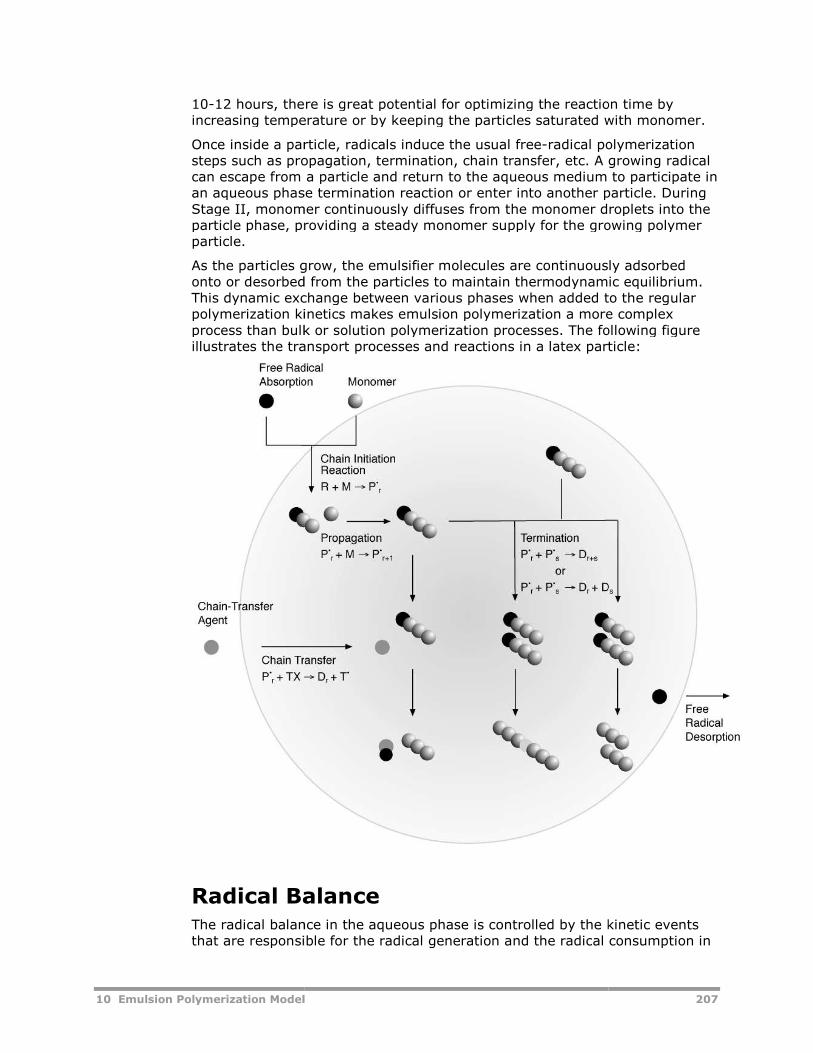
10 Emulsion Polymerization Model
10-12 hours, there is great potential for optimizing the reaction time byincreasing temperature or by keeping the particles saturated with monomer.
Once inside a particle, radicals induce the usual freesteps such as propagation, termination, chain transfer, etc. A growing radicalcan escape from a particle and return to the aqueous medium to participate inan aqueous phase termination reactStage II, monomer continuously diffuses from the monomer droplets into theparticle phase, providing a steady monomer supply for the growing polymerparticle.
As the particles grow, the emulsifier molecules are coonto or desorbed from the particles to maintain thermodynamic equilibrium.This dynamic exchange between various phases when added to the regularpolymerization kinetics makes emulsion polymerization a more complexprocess than bulk orillustrates the transport processes and reactions in a latex particle
Radical BalanceThe radical balancethat are responsible for the radical generation and the radic
10 Emulsion Polymerization Model
12 hours, there is great potential for optimizing the reaction time byincreasing temperature or by keeping the particles saturated with monomer.
particle, radicals induce the usual free-radical polymerizationsteps such as propagation, termination, chain transfer, etc. A growing radicalcan escape from a particle and return to the aqueous medium to participate inan aqueous phase termination reaction or enter into another particle. DuringStage II, monomer continuously diffuses from the monomer droplets into theparticle phase, providing a steady monomer supply for the growing polymer
As the particles grow, the emulsifier molecules are continuously adsorbedonto or desorbed from the particles to maintain thermodynamic equilibrium.This dynamic exchange between various phases when added to the regularpolymerization kinetics makes emulsion polymerization a more complexprocess than bulk or solution polymerization processes. The following figureillustrates the transport processes and reactions in a latex particle
Radical Balancebalance in the aqueous phase is controlled by the kinetic events
that are responsible for the radical generation and the radical consumption in
207
12 hours, there is great potential for optimizing the reaction time byincreasing temperature or by keeping the particles saturated with monomer.
radical polymerizationsteps such as propagation, termination, chain transfer, etc. A growing radicalcan escape from a particle and return to the aqueous medium to participate in
ion or enter into another particle. DuringStage II, monomer continuously diffuses from the monomer droplets into theparticle phase, providing a steady monomer supply for the growing polymer
ntinuously adsorbedonto or desorbed from the particles to maintain thermodynamic equilibrium.This dynamic exchange between various phases when added to the regularpolymerization kinetics makes emulsion polymerization a more complex
solution polymerization processes. The following figureillustrates the transport processes and reactions in a latex particle:
in the aqueous phase is controlled by the kinetic eventsal consumption in
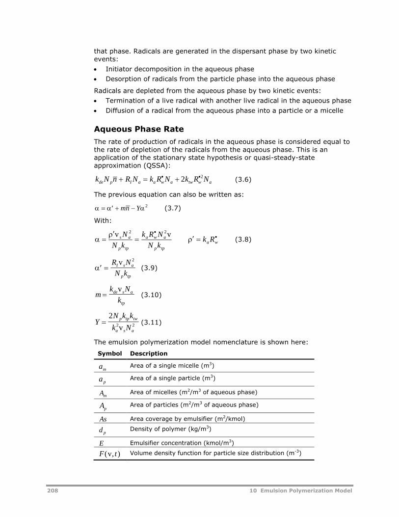
208 10 Emulsion Polymerization Model
that phase. Radicals are generated in the dispersant phase by two kineticevents:
Initiator decomposition in the aqueous phase
Desorption of radicals from the particle phase into the aqueous phase
Radicals are depleted from the aqueous phase by two kinetic events:
Termination of a live radical with another live radical in the aqueous phase
Diffusion of a radical from the aqueous phase into a particle or a micelle
Aqueous Phase Rate
The rate of production of radicals in the aqueous phase is considered equal tothe rate of depletion of the radicals from the aqueous phase. This is anapplication of the stationary state hypothesis or quasi-steady-stateapproximation (QSSA):
k N n R N k R N k R Nde p I a a w a tw w a 2 2(3.6)
The previous equation can also be written as:
mn Y 2 (3.7)
With:
wa
tpp
awa
tpp
as RkkN
NRk
kN
N vv 22
(3.8)
R N
N kI s a
p tp
v 2
(3.9)
mk N
kde s a
tp
v
(3.10)
YN k k
k N
p tp tw
a s a
2
2 2v(3.11)
The emulsion polymerization model nomenclature is shown here:
Symbol Description
amArea of a single micelle (m3)
a pArea of a single particle (m3)
AmArea of micelles (m2/m3 of aqueous phase)
ApArea of particles (m2/m3 of aqueous phase)
As Area coverage by emulsifier (m2/kmol)
d pDensity of polymer (kg/m3)
E Emulsifier concentration (kmol/m3)
F t( , )v Volume density function for particle size distribution (m-3)
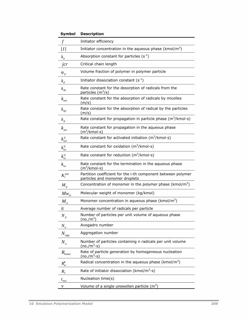
10 Emulsion Polymerization Model 209
Symbol Description
f Initiator efficiency
[ ]I Initiator concentration in the aqueous phase (kmol/m3)
kaAbsorption constant for particles (s-1)
jcr Critical chain length
pVolume fraction of polymer in polymer particle
kdInitiator dissociation constant (s-1)
kdeRate constant for the desorption of radicals from theparticles (m3/s)
kamRate constant for the absorption of radicals by micelles(m/s)
kapRate constant for the absorption of radical by the particles(m/s)
k pRate constant for propagation in particle phase (m3/kmol-s)
kpwRate constant for propagation in the aqueous phase(m3/kmol-s)
kactij Rate constant for activated initiation (m3/kmol-s)
koxij Rate constant for oxidation (m3/kmol-s)
kreij Rate constant for reduction (m3/kmol-s)
ktwRate constant for the termination in the aqueous phase(m3/kmol-s)
Kipm Partition coefficient for the i-th component between polymer
particles and monomer droplets
M pConcentration of monomer in the polymer phase (kmol/m3)
MwmMolecular weight of monomer (kg/kmol)
MwMonomer concentration in aqueous phase (kmol/m3)
n Average number of radicals per particle
N pNumber of particles per unit volume of aqueous phase(no./m3)
NaAvogadro number
NaggAggregation number
N nNumber of particles containing n radicals per unit volume(no./m3-s)
RhomoRate of particle generation by homogeneous nucleation(no./m3-s)
Rw Radical concentration in the aqueous phase (kmol/m3)
RIRate of initiator dissociation (kmol/m3-s)
tnucNucleation time(s)
v Volume of a single unswollen particle (m3)
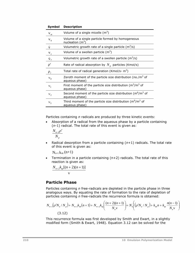
210 10 Emulsion Polymerization Model
Symbol Description
vmVolume of a single micelle (m3)
v hVolume of a single particle formed by homogeneousnucleation (m3)
v Volumetric growth rate of a single particle (m3/s)
v sVolume of a swollen particle (m3)
v s Volumetric growth rate of a swollen particle (m3/s)
Rate of radical absorption by N p particles (Kmol/s)
iTotal rate of radical generation (Kmol/s- m3)
0Zeroth moment of the particle size distribution (no./m3 ofaqueous phase)
1First moment of the particle size distribution (m3/m3 ofaqueous phase)
2Second moment of the particle size distribution (m6/m3 ofaqueous phase)
3Third moment of the particle size distribution (m9/m3 ofaqueous phase)
Particles containing n radicals are produced by three kinetic events:
Absorption of a radical from the aqueous phase by a particle containing(n-1) radical. The total rate of this event is given as:
p
n
N
N 1
Radical desorption from a particle containing (n+1) radicals. The total rateof this event is given as:
1)(n+kN de1n+
Termination in a particle containing (n+2) radicals. The total rate of thisreaction is given as:
v
)]1)(2[(2 nnkN tpn
Particle Phase
Particles containing n free-radicals are depleted in the particle phase in threeanalogous ways. By equating the rate of formation to the rate of depletion ofparticles containing n free-radicals the recurrence formula is obtained:
v
)1(/
v
)1)(2(1/ 211
a
tpdepan
a
tpndenpanN
nnknkNNN
N
nnkNnkNNNN
(3.12)
This recurrence formula was first developed by Smith and Ewart, in a slightlymodified form (Smith & Ewart, 1948). Equation 3.12 can be solved for the
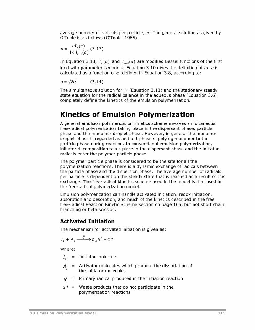
10 Emulsion Polymerization Model 211
average number of radicals per particle, n . The general solution as given byO'Toole is as follows (O'Toole, 1965):
naI a
I am
m
( )
( )4 1
(3.13)
In Equation 3.13, I am( ) and I am1( ) are modified Bessel functions of the first
kind with parameters m and a. Equation 3.10 gives the definition of m. a iscalculated as a function of , defined in Equation 3.8, according to:
a 8 (3.14)
The simultaneous solution for n (Equation 3.13) and the stationary steadystate equation for the radical balance in the aqueous phase (Equation 3.6)completely define the kinetics of the emulsion polymerization.
Kinetics of Emulsion PolymerizationA general emulsion polymerization kinetics scheme involves simultaneousfree-radical polymerization taking place in the dispersant phase, particlephase and the monomer droplet phase. However, in general the monomerdroplet phase is regarded as an inert phase supplying monomer to theparticle phase during reaction. In conventional emulsion polymerization,initiator decomposition takes place in the dispersant phase and the initiatorradicals enter the polymer particle phase.
The polymer particle phase is considered to be the site for all thepolymerization reactions. There is a dynamic exchange of radicals betweenthe particle phase and the dispersion phase. The average number of radicalsper particle is dependent on the steady state that is reached as a result of thisexchange. The free-radical kinetics scheme used in the model is that used inthe free-radical polymerization model.
Emulsion polymerization can handle activated initiation, redox initiation,absorption and desorption, and much of the kinetics described in the freefree-radical Reaction Kinetic Scheme section on page 165, but not short chainbranching or beta scission.
Activated Initiation
The mechanism for activated initiation is given as:
I A n R xk j
k
kjactkj
*
Where:
Ik= Initiator molecule
Aj= Activator molecules which promote the dissociation of
the initiator molecules
R = Primary radical produced in the initiation reaction
x * = Waste products that do not participate in thepolymerization reactions
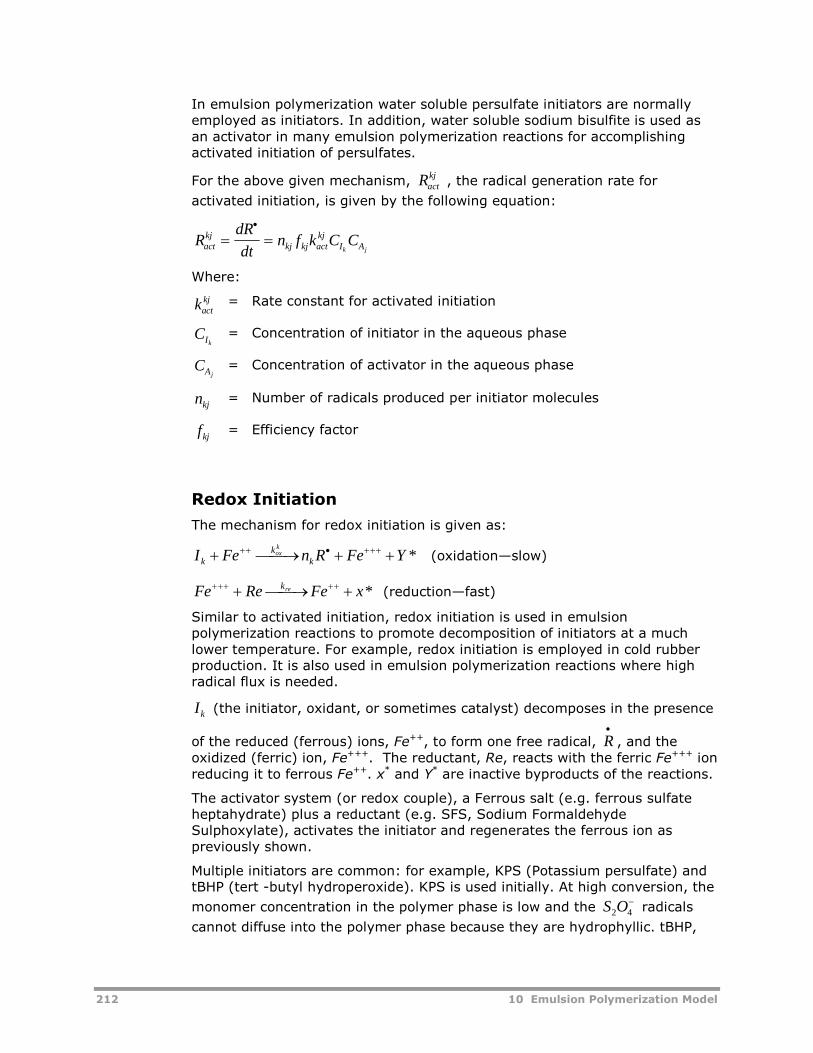
212 10 Emulsion Polymerization Model
In emulsion polymerization water soluble persulfate initiators are normallyemployed as initiators. In addition, water soluble sodium bisulfite is used asan activator in many emulsion polymerization reactions for accomplishingactivated initiation of persulfates.
For the above given mechanism, Ractkj
, the radical generation rate for
activated initiation, is given by the following equation:
RdR
dtn f k C Cact
kjkj kj act
kjI Ak j
Where:
kactkj = Rate constant for activated initiation
CIk= Concentration of initiator in the aqueous phase
CA j= Concentration of activator in the aqueous phase
nkj= Number of radicals produced per initiator molecules
fkj= Efficiency factor
Redox Initiation
The mechanism for redox initiation is given as:
*YFeRnFeI kk
k
kox
(oxidation—slow)
*xFeReFe rek (reduction—fast)
Similar to activated initiation, redox initiation is used in emulsionpolymerization reactions to promote decomposition of initiators at a muchlower temperature. For example, redox initiation is employed in cold rubberproduction. It is also used in emulsion polymerization reactions where highradical flux is needed.
kI (the initiator, oxidant, or sometimes catalyst) decomposes in the presence
of the reduced (ferrous) ions, Fe++, to form one free radical, R
, and theoxidized (ferric) ion, Fe+++. The reductant, Re, reacts with the ferric Fe+++ ionreducing it to ferrous Fe++. x* and Y* are inactive byproducts of the reactions.
The activator system (or redox couple), a Ferrous salt (e.g. ferrous sulfateheptahydrate) plus a reductant (e.g. SFS, Sodium FormaldehydeSulphoxylate), activates the initiator and regenerates the ferrous ion aspreviously shown.
Multiple initiators are common: for example, KPS (Potassium persulfate) andtBHP (tert -butyl hydroperoxide). KPS is used initially. At high conversion, the
monomer concentration in the polymer phase is low and the42OS radicals
cannot diffuse into the polymer phase because they are hydrophyllic. tBHP,
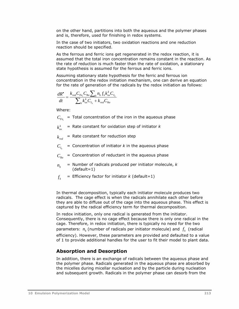
10 Emulsion Polymerization Model 213
on the other hand, partitions into both the aqueous and the polymer phasesand is, therefore, used for finishing in redox systems.
In the case of two initiators, two oxidation reactions and one reductionreaction should be specified.
As the ferrous and ferric ions get regenerated in the redox reaction, it isassumed that the total iron concentration remains constant in the reaction. Asthe rate of reduction is much faster than the rate of oxidation, a stationarystate hypothesis is assumed for the ferrous and ferric ions.
Assuming stationary state hypothesis for the ferric and ferrous ionconcentration in the redox initiation mechanism, one can derive an equationfor the rate of generation of the radicals by the redox initiation as follows:
Re
Re
CkCk
CkfnCCk
dt
dR
redk Ikox
k IkoxkkFered
k
kt
Where:
CFet= Total concentration of the iron in the aqueous phase
koxk = Rate constant for oxidation step of initiator k
redk = Rate constant for reduction step
CIk= Concentration of initiator k in the aqueous phase
ReC = Concentration of reductant in the aqueous phase
kn = Number of radicals produced per initiator molecule, k(default=1)
kf = Efficiency factor for initiator k (default=1)
In thermal decomposition, typically each initiator molecule produces tworadicals. The cage effect is when the radicals annihilate each other beforethey are able to diffuse out of the cage into the aqueous phase. This effect iscaptured by the radical efficiency term for thermal decomposition.
In redox initiation, only one radical is generated from the initiator.Consequently, there is no cage effect because there is only one radical in thecage. Therefore, in redox initiation, there is typically no need for the two
parameters: kn (number of radicals per initiator molecule) and kf (radical
efficiency). However, these parameters are provided and defaulted to a valueof 1 to provide additional handles for the user to fit their model to plant data.
Absorption and Desorption
In addition, there is an exchange of radicals between the aqueous phase andthe polymer phase. Radicals generated in the aqueous phase are absorbed bythe micelles during micellar nucleation and by the particle during nucleationand subsequent growth. Radicals in the polymer phase can desorb from the
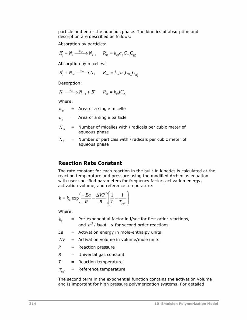
214 10 Emulsion Polymerization Model
particle and enter the aqueous phase. The kinetics of absorption anddesorption are described as follows:
Absorption by particles:
R N Nj i
k
iap
1 R k a C Cap ap p N Ri j
Absorption by micelles:
R N Nj m
kam 1 R k a C Cam am m N Rm j
Desorption:
N N Ri
k
ide
1 R k iCde de N i
Where:
am= Area of a single micelle
a p= Area of a single particle
Nm= Number of micelles with i radicals per cubic meter of
aqueous phase
N i= Number of particles with i radicals per cubic meter of
aqueous phase
Reaction Rate Constant
The rate constant for each reaction in the built-in kinetics is calculated at thereaction temperature and pressure using the modified Arrhenius equationwith user specified parameters for frequency factor, activation energy,activation volume, and reference temperature:
ref
oTTR
VP
R
Eakk
11exp
Where:
ko= Pre-exponential factor in l/sec for first order reactions,
and m kmol s3 / for second order reactions
Ea = Activation energy in mole-enthalpy units
V = Activation volume in volume/mole units
P = Reaction pressure
R = Universal gas constant
T = Reaction temperature
refT = Reference temperature
The second term in the exponential function contains the activation volumeand is important for high pressure polymerization systems. For detailed
10 Emulsion Polymerization Model 215
information of the reactions, see the free-radical Reaction Kinetic Schemesection on page 165.
Rate constants related to absorption by particles, absorption by micelles anddesorption from particles are given by the Arrhenius expression as:
k kEa
RTo
exp
assuming zero activation volume.
Model Features andAssumptionsFollowing are the model features and assumptions used in the emulsionpolymerization model available in Aspen Polymers.
Model AssumptionsThe emulsion polymerization process is extremely complex and involvesphenomena for which a complete theoretical understanding has not beenreached. Important assumptions are made in the emulsion polymerizationmodel:
The reaction mixture is perfectly mixed
Particles are formed by the micellar or the homogeneous mechanism
No agglomeration or breakage of particles occurs
No secondary nucleation occurs
All particles have the same average number of radicals and hence thesame volumetric growth rate
The particle size distribution is unimodal, with moments of PSD sufficientto describe the PSD
There are no mass transfer limitations on the polymerization reactions
Molecular weight is controlled by chain transfer reactions
Thermodynamics of Monomer PartitioningModeling of the kinetics involved in emulsion polymerization is complicated bythe fact that the reaction mixture is multiphase. It is important to account forpartitioning of the components among various phases. Up to four coexistingphases may be present in the reaction mixture. After the consumption of themonomer droplets, only three phases will remain in the system.
A short-cut partition coefficient methodology was used to handle the fourphases. One benefit of using this approach is that NRTL parameters are notrequired for the polymer or its segments. The method assumes the polymersolubility is zero in the monomer, aqueous, and vapor phases and performs arigorous 3-phase flash calculation to yield:
Vapor phase - if present, contains water and monomers
216 10 Emulsion Polymerization Model
Dispersion phase - contains water, initiators, emulsifiers, activators andsome dissolved monomer
Monomer phase - contains monomer and some dissolved water
The user provides a partition coefficient for each component that may bepresent in the polymer phase. Following the rigorous 3-phase flash, aniterative algorithm calculates the amount of each component to transfer fromthe monomer phase, if present, and the aqueous phase to the polymer phasein order to satisfy the partition coefficient constraints. As monomer istransferred to the polymer phase, water is transferred from the monomerphase to the aqueous phase so that its concentration in the monomer phaseis the saturation concentration calculated by the rigorous flash.
The user-supplied partition coefficients are provided as either:
Monomer (L1) basis
iipi xkx 11
Aqueous (L2) basis
iipi xkx 22
In either case, the partition coefficients are on a mass basis.
This scheme works equally well for monomer starved or monomer saturatedsituations. When the monomer phase collapses, the algorithm transfersmonomer from the aqueous phase to the polymer phase. If the user providedpartition coefficients on a monomer basis, the partition coefficient withrespect to the aqueous phase is calculated as:
LLiii kkk /12
LLik values are only available when there is sufficient monomer present in the
swollen polymer particles to form a separate monomer phase if polymer wereremoved. If the 3-phase flash does not detect a separate monomer phase,
LLik values will not be available, and the algorithm will transfer all monomer
from the aqueous phase to the polymer phase.
In addition, there are two rigorous phase equilibrium approaches to handlethe thermodynamics of monomer partitioning. The first rigorous approachassumes the presence of two liquid phases. The distribution of water,monomers, and polymers is determined by isofugacity relationships, and thefugacities of various species are computed by the physical property option setchosen for the system. The second approach performs rigorous four phase(vapor-liquid-liquid-polymer) flash calculations based on a newly availableflash algorithm.
Polymer Particle Size DistributionPolymer particle size and size distribution, among other factors, determinethe rheological properties of the latex . Although actual particle sizedistribution is important, it is often measured in terms of certain averagessuch as number average and weight average diameters. Further, rigoroustracking of the particle size distribution by discrete methods iscomputationally expensive.
10 Emulsion Polymerization Model 217
In conventional emulsion polymerization where unimodal distributions arenormally encountered, the moments of the particle size distribution givesufficient information about the nature of the particle size distribution. Theparticle size distribution can be described in terms of different independentvariables such as diameter or volume of the particle. Since volumetric growthrate of the particle in emulsion polymerization remains almost constant inStage I and Stage II of the process, the population balance equation isformulated in terms of the volume of the particles.
General Population Balance Equation
The general population balance equation for the emulsion polymerization isgiven as follows:
F t
t
F tk A N R Ram m a w m h
v v v
vv v v v
, ,
homo (3.15)
In Equation 3.15 the right-hand side represents the nucleation of particlesfrom miceller and homogeneous nucleation. Refer to the table on page 208
for an explanation of the variables used. The volumetric growth rate is v fora single unswollen particle (Equation 3.5):
v k M n
N
MW
d
p p
a
m
p
(3.16)
The general population balance equation can be converted to the equivalentmoment equations. The j-th moment of the particle size distribution is givenas:
jjF j d
( , )0
(3.17)
Applying moment definition in Equation 3.17 to the general populationbalance equation in Equation 3.15, the first four moments of the particle sizedistribution are given as:
d
dtk A N R Ram m a w
0 [ ] homo (3.18)
d
dtk A N R Rm am m a w h
1
0 [ ]v v v homo (3.19)
d
dtk A N R Rm am m a w h
2
12 22 [ ]v v v homo (3.20)
d
dtk A N R Rm am m a w h
3
23 33 [ ]v v v homo (3.21)
Where:
kam= Kinetic constant for the absorption of the oligomeric
radicals into the micelles
Am= Area of the micelles
218 10 Emulsion Polymerization Model
Rhomo= Rate of particle formation by homogeneous
nucleation
Polymer Particle PropertiesCalculatedThe emulsion model is designed to generate the following results that are ofinterest for the emulsion polymerization process:
Copolymer composition
Number average molecular weight
Particle size distribution averages for unswollen particles
The results are available as component attributes under the names listedhere:
Name Symbol Description Class Units
PSDZMOM 0Zeroth moment of theparticle sizedistribution (volume)
2 no./s
PSDFMOM 1First moment of thePSD (volume)
0 m3/s
PSDSMOM 2Second moment of thePSD (volume)
2 m6/s
PSDTMOM 3Third moment of thePSD (volume)
2 m9/s
VOLN VnNumber averagevolume of the particles
0 m3
VOLV VvVolume averagevolume of the particles
0 m3
VOLZ VzZ-average volume ofthe particles
0 m3
DIAV DvVolume averagediameter
0 m
PDV PDvPolydispersity for PSD(Volume)
0 ---
SFRAC --- Copolymercomposition
0 ---
MWN --- Number averagemolecular weight
0 kg/kmol
User ProfilesIn addition to the polymer properties reported through the componentattributes, other model calculations are reported through User Profilevariables. The following user profile variables may be requested from themodel:
10 Emulsion Polymerization Model 219
Glass transition temperature of the polymer (C)
Average number of radicals per particle
% Soap coverage of the polymer particles
Volume of the monomer droplet phase (m3)
Concentration of monomers in the monomer droplets (kmol/m3)†
Volume of the aqueous phase (m3)
Monomer concentration in the aqueous phase (kmol/m3)†
Volume of the polymer particle phase (m3)
Monomer concentration in the polymer particles (kmol/m3)†
Monomer conversion
† One profile is reported for each monomer.
User profiles are only accessible if the reaction model is called from a batchreactor (RBatch) or a plug flow reactor (RPlug). The user profiles are returnedin the order shown. A label must be provided to differentiate the profilevariables. For the monomer concentrations in the aqueous, monomer, andpolymer phases one profile is returned for each monomer.
Specifying EmulsionPolymerization Kinetics
Accessing the Emulsion ModelTo access the Emulsion polymerization kinetic model:
1 From the Data Browser, click Reactions.
2 From the Reactions folder, click Reactions.
The Reactions object manager appears.
3 If the kinetic model already exists, double-click the desired Reaction ID inthe object manager or click Edit to get to the input forms.
4 To add a new model, from the Reactions object manager, click New. Ifnecessary, change the default ID for the reaction.
5 Select Emulsion as the reaction type and click OK.
Specifying the Emulsion ModelThe Emulsion model input forms are divided into two folders: Specificationsand Phases.
Use the Specifications forms to define reacting species and enter reactionrate constant parameters. Use the following options:
Use this sheet To
Species Define reacting species
Reactions Specify reactions and rate constant parameters
Rate Constants Summarize rate constant parameters
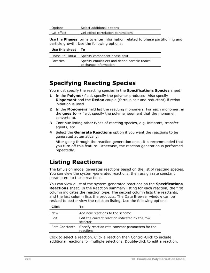
220 10 Emulsion Polymerization Model
Options Select additional options
Gel Effect Gel-effect correlation parameters
Use the Phases forms to enter information related to phase partitioning andparticle growth. Use the following options:
Use this sheet To
Phase Equilibria Specify component phase split
Particles Specify emulsifiers and define particle radicalexchange information
Specifying Reacting SpeciesYou must specify the reacting species in the Specifications Species sheet:
1 In the Polymer field, specify the polymer produced. Also specifyDispersant and the Redox couple (ferrous salt and reductant) if redoxinitiation is used.
2 In the Monomers field list the reacting monomers. For each monomer, inthe goes to field, specify the polymer segment that the monomerconverts to.
3 Continue listing other types of reacting species, e.g. initiators, transferagents, etc.
4 Select the Generate Reactions option if you want the reactions to begenerated automatically.
After going through the reaction generation once, it is recommended thatyou turn off this feature. Otherwise, the reaction generation is performedrepeatedly.
Listing ReactionsThe Emulsion model generates reactions based on the list of reacting species.You can view the system-generated reactions, then assign rate constantparameters to these reactions.
You can view a list of the system-generated reactions on the SpecificationsReactions sheet. In the Reaction summary listing for each reaction, the firstcolumn indicates the reaction type. The second column lists the reactants,and the last column lists the products. The Data Browser window can beresized to better view the reaction listing. Use the following options:
Click To
New Add new reactions to the scheme
Edit Edit the current reaction indicated by the rowselector
Rate Constants Specify reaction rate constant parameters for thereactions
Click to select a reaction. Click a reaction then Control-Click to includeadditional reactions for multiple selections. Double-click to edit a reaction.
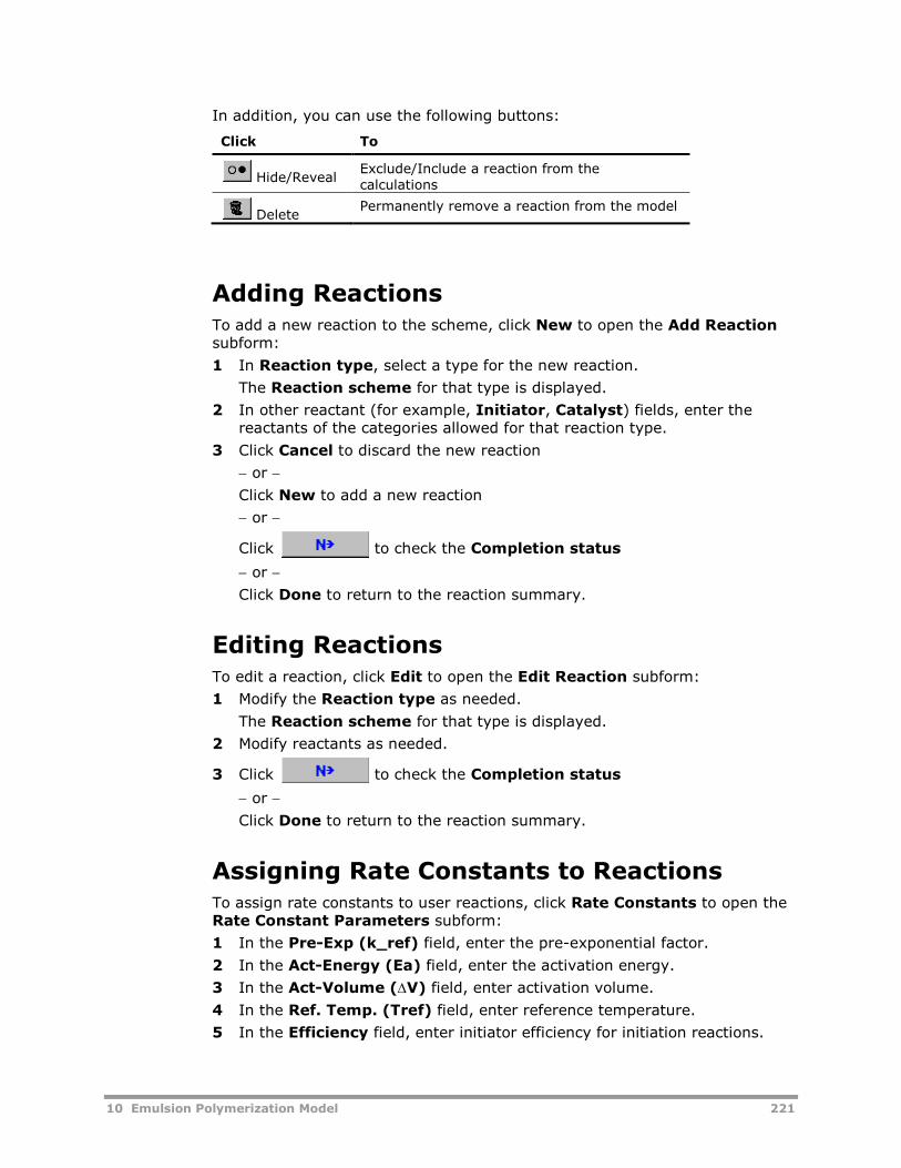
10 Emulsion Polymerization Model 221
In addition, you can use the following buttons:
Click To
Hide/RevealExclude/Include a reaction from thecalculations
DeletePermanently remove a reaction from the model
Adding ReactionsTo add a new reaction to the scheme, click New to open the Add Reactionsubform:
1 In Reaction type, select a type for the new reaction.
The Reaction scheme for that type is displayed.
2 In other reactant (for example, Initiator, Catalyst) fields, enter thereactants of the categories allowed for that reaction type.
3 Click Cancel to discard the new reaction
or
Click New to add a new reaction
or
Click to check the Completion status
or
Click Done to return to the reaction summary.
Editing ReactionsTo edit a reaction, click Edit to open the Edit Reaction subform:
1 Modify the Reaction type as needed.
The Reaction scheme for that type is displayed.
2 Modify reactants as needed.
3 Click to check the Completion status
or
Click Done to return to the reaction summary.
Assigning Rate Constants to ReactionsTo assign rate constants to user reactions, click Rate Constants to open theRate Constant Parameters subform:
1 In the Pre-Exp (k_ref) field, enter the pre-exponential factor.
2 In the Act-Energy (Ea) field, enter the activation energy.
3 In the Act-Volume (V) field, enter activation volume.
4 In the Ref. Temp. (Tref) field, enter reference temperature.
5 In the Efficiency field, enter initiator efficiency for initiation reactions.
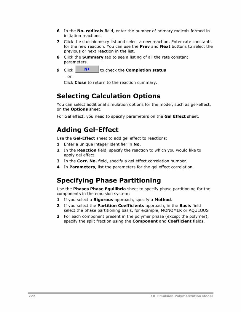
222 10 Emulsion Polymerization Model
6 In the No. radicals field, enter the number of primary radicals formed ininitiation reactions.
7 Click the stoichiometry list and select a new reaction. Enter rate constantsfor the new reaction. You can use the Prev and Next buttons to select theprevious or next reaction in the list.
8 Click the Summary tab to see a listing of all the rate constantparameters.
9 Click to check the Completion status
or
Click Close to return to the reaction summary.
Selecting Calculation OptionsYou can select additional simulation options for the model, such as gel-effect,on the Options sheet.
For Gel effect, you need to specify parameters on the Gel Effect sheet.
Adding Gel-EffectUse the Gel-Effect sheet to add gel effect to reactions:
1 Enter a unique integer identifier in No.
2 In the Reaction field, specify the reaction to which you would like toapply gel effect.
3 In the Corr. No. field, specify a gel effect correlation number.
4 In Parameters, list the parameters for the gel effect correlation.
Specifying Phase PartitioningUse the Phases Phase Equilibria sheet to specify phase partitioning for thecomponents in the emulsion system:
1 If you select a Rigorous approach, specify a Method.
2 If you select the Partition Coefficients approach, in the Basis fieldselect the phase partitioning basis, for example, MONOMER or AQUEOUS
3 For each component present in the polymer phase (except the polymer),specify the split fraction using the Component and Coefficient fields.
10 Emulsion Polymerization Model 223
Specifying Particle Growth ParametersUse the Phases Particles sheet to specify data for particle generation andparticle related events:
1 Define Emulsifier, and specify critical micelle concentration, CMC, andsurfactant Area.
2 For homogeneous nucleation, specify Aggregation number and Criticallength.
You must specify radical absorption and desorption rate constant parametersfor micelles and particles.
ReferencesBarton, J., & Capek, I. (1994). Radical Polymerization in Disperse Systems.New York: Ellis Harwood.
Blackley, D. C. (1975). Emulsion Polymerization: Theory and Practice.London: Applied Science Publishers Ltd.
Gilbert, R. G. (1995). Emulsion Polymerization: A Mechanistic Approach.Boston: Academic Press.
Hamielec, A. E., & Tobita, H. (1992). Polymerization Processes. In UllmansEncyclopedia of Industrial Chemistry, A21, 305. New York: VCH Publishers.
Harkins, W. D. (1945). J. Chem. Phys., 13, 301.
Odian, G. (1991). Principles of Polymerization, 3rd. Ed. New York: John Wiley& Sons.
O’Toole, J. T. (1965). Kinetics of Emulsion Polymerization. J. Appl. Polym.Sci., 9, 1291.
Poehlein, G. W. (1986). Emulsion Polymerization. In H.F. Mark, N. M. Bikales,C. G. Overberger, and G. Menges, (Eds.). Encyclopedia of Polymer Science &Technology, 6, 1. New York: Wiley-Interscience.
Ponnuswamy, S. R., & Hamielec, A. E. (1997). Emulsion Polymerization:Theory and Practice. Lecture notes for intensive short course on polymerreaction engineering held at Burlington, ON, Canada, April 28-30.
Smith, W. V., & Ewart, R. H. (1948). J. Chem. Phys., 16, 592.

224 10 Emulsion Polymerization Model
11 Ziegler-Natta Polymerization Model 225
11 Ziegler-NattaPolymerization Model
This section covers the Ziegler-Natta polymerization kinetic model available inAspen Polymers (formerly known as Aspen Polymers Plus). The term Ziegler-Natta polymerization is used here to describe a variety of stereospecific multi-site and single site catalyzed addition polymerization systems including thetraditional Ziegler-Natta catalyzed systems, chromium based catalyzedsystems (Phillips type) and the more recent metallocene based catalyzedsystems.
Topics covered include:
Summary of Applications, 225
Ziegler-Natta Processes, 226
Reaction Kinetic Scheme, 230
Model Features and Assumptions, 243
Polymer Properties Calculated, 243
Specifying Ziegler-Natta Polymerization Kinetics, 244
Several example applications of the Ziegler-Natta polymerization model aregiven in the Aspen Polymers Examples & Applications Case Book. Additionally,the Examples & Applications Case Book provides process details and thekinetics of polymerization for specific monomer-polymer systems.
Summary of ApplicationsThe Ziegler-Natta polymerization model is applicable to processes utilizingcoordination catalysts for the production of stereospecific polymers.
Some examples of applicable polymers are:
Linear low density polyethylene - Ethylene is copolymerized with an alpha-olefin, such as 1-butene, 1-hexene, or 1-octene. Commercial processesinclude low pressure, slurry-phase processes, solution-phase processes,low pressure, gas phase processes.
High density polyethylene - Ethylene homopolymers or copolymers with
high alpha olefins with density 0.940 g / cm3and higher. Commercial
226 11 Ziegler-Natta Polymerization Model
processes include solution, slurry or suspension, and gas phasepolymerization.
Ethylene-propylene elastomers - Polymerization proceeds by solution orslurry processes. Both are operated continuously in liquid-phase back-mixed reactors.
Polypropylene - Commercial processes include liquid pool, diluent slurry,and gas phase polymerization.
Ziegler-Natta ProcessesZiegler-Natta polymerization accounts for a significant fraction of thepolyethylene polymers and all the polypropylene homopolymers andcopolymers produced commercially. The commercial production of thesepolyolefins is done exclusively by continuous processes using several differentprocesses and reactor types operating over a wide range of conditions.
High density polyethylene (HDPE) and linear low density polyethylene (LLDPE)are produced via catalyzed polymerization processes. The operatingconditions for the catalyzed processes are relatively less severe compared tothe high pressure processes for LDPE production. The pressure generallyranges from 10-80 atm while the temperatures range from 80-110C. Thepressure and temperature may be as high as 200 atm and 250C in some ofthe solution polymerization processes.
Catalyst TypesThere is a variety of catalysts used for ethylene polymerization includingsupported and unsupported heterogeneous catalyst systems andhomogeneous catalyst systems. The Ziegler-Natta transition metal (Ti) basedcatalysts are the most widely used.
However, there are numerous variations of these catalysts. Some vanadiumbased catalysts are also used. Chromic oxide on silica catalysts are used inthe Phillips loop reactor process, while the Union Carbide Unipol process mayuse either Ziegler-Natta (Ti) or chromium compounds on silica catalysts.
More recently, several manufacturers have been developing commercialprocesses using metallocene based catalysts, mainly zirconium and titanium.These catalysts are believed to be single site catalysts that are capable ofproducing high yields, combined with narrow molecular weight and copolymercomposition distributions.
All commercial isotactic polypropylene homopolymer (PP) is manufacturedusing heterogeneous Ziegler-Natta catalyst systems. The catalyst consists of
a solid transition metal halide, usually TiCl3 , with an organoaluminum
compound cocatalysts, such as diethylaluminum chloride (DEAC), or a MgCl2
supported TiCl AlEt4 3. catalyst.
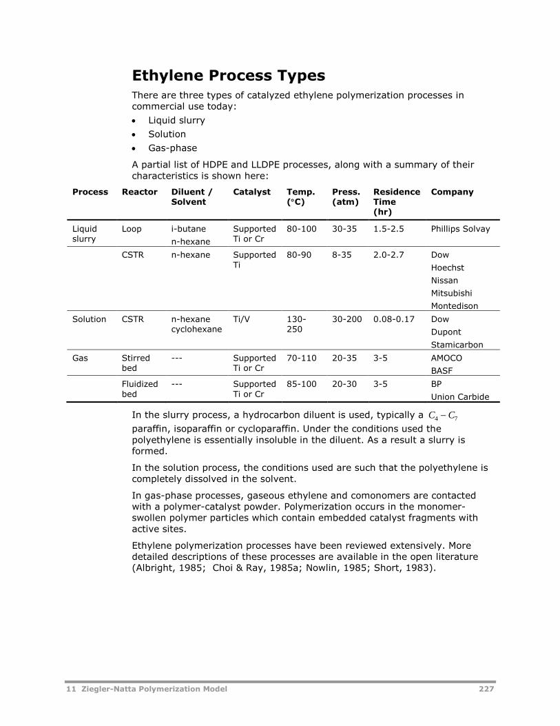
11 Ziegler-Natta Polymerization Model 227
Ethylene Process TypesThere are three types of catalyzed ethylene polymerization processes incommercial use today:
Liquid slurry
Solution
Gas-phase
A partial list of HDPE and LLDPE processes, along with a summary of theircharacteristics is shown here:
Process Reactor Diluent /Solvent
Catalyst Temp.(C)
Press.(atm)
ResidenceTime(hr)
Company
Liquidslurry
Loop i-butane
n-hexane
SupportedTi or Cr
80-100 30-35 1.5-2.5 Phillips Solvay
CSTR n-hexane SupportedTi
80-90 8-35 2.0-2.7 Dow
Hoechst
Nissan
Mitsubishi
Montedison
Solution CSTR n-hexanecyclohexane
Ti/V 130-250
30-200 0.08-0.17 Dow
Dupont
Stamicarbon
Gas Stirredbed
--- SupportedTi or Cr
70-110 20-35 3-5 AMOCO
BASF
Fluidizedbed
--- SupportedTi or Cr
85-100 20-30 3-5 BP
Union Carbide
In the slurry process, a hydrocarbon diluent is used, typically a C C4 7
paraffin, isoparaffin or cycloparaffin. Under the conditions used thepolyethylene is essentially insoluble in the diluent. As a result a slurry isformed.
In the solution process, the conditions used are such that the polyethylene iscompletely dissolved in the solvent.
In gas-phase processes, gaseous ethylene and comonomers are contactedwith a polymer-catalyst powder. Polymerization occurs in the monomer-swollen polymer particles which contain embedded catalyst fragments withactive sites.
Ethylene polymerization processes have been reviewed extensively. Moredetailed descriptions of these processes are available in the open literature(Albright, 1985; Choi & Ray, 1985a; Nowlin, 1985; Short, 1983).
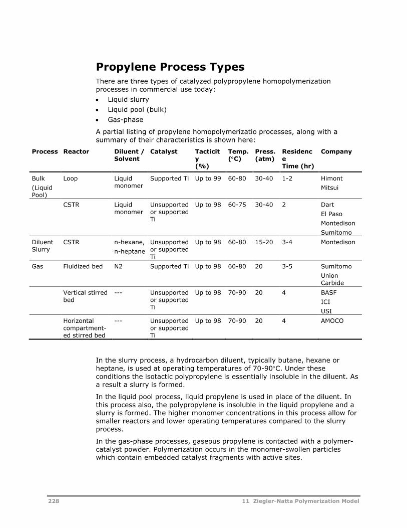
228 11 Ziegler-Natta Polymerization Model
Propylene Process TypesThere are three types of catalyzed polypropylene homopolymerizationprocesses in commercial use today:
Liquid slurry
Liquid pool (bulk)
Gas-phase
A partial listing of propylene homopolymerizatio processes, along with asummary of their characteristics is shown here:
Process Reactor Diluent /Solvent
Catalyst Tacticity(%)
Temp.(C)
Press.(atm)
ResidenceTime (hr)
Company
Bulk
(LiquidPool)
Loop Liquidmonomer
Supported Ti Up to 99 60-80 30-40 1-2 Himont
Mitsui
CSTR Liquidmonomer
Unsupportedor supportedTi
Up to 98 60-75 30-40 2 Dart
El Paso
Montedison
Sumitomo
DiluentSlurry
CSTR n-hexane,
n-heptane
Unsupportedor supportedTi
Up to 98 60-80 15-20 3-4 Montedison
Gas Fluidized bed N2 Supported Ti Up to 98 60-80 20 3-5 Sumitomo
UnionCarbide
Vertical stirredbed
--- Unsupportedor supportedTi
Up to 98 70-90 20 4 BASF
ICI
USI
Horizontalcompartment-ed stirred bed
--- Unsupportedor supportedTi
Up to 98 70-90 20 4 AMOCO
In the slurry process, a hydrocarbon diluent, typically butane, hexane orheptane, is used at operating temperatures of 70-90C. Under theseconditions the isotactic polypropylene is essentially insoluble in the diluent. Asa result a slurry is formed.
In the liquid pool process, liquid propylene is used in place of the diluent. Inthis process also, the polypropylene is insoluble in the liquid propylene and aslurry is formed. The higher monomer concentrations in this process allow forsmaller reactors and lower operating temperatures compared to the slurryprocess.
In the gas-phase processes, gaseous propylene is contacted with a polymer-catalyst powder. Polymerization occurs in the monomer-swollen particleswhich contain embedded catalyst fragments with active sites.
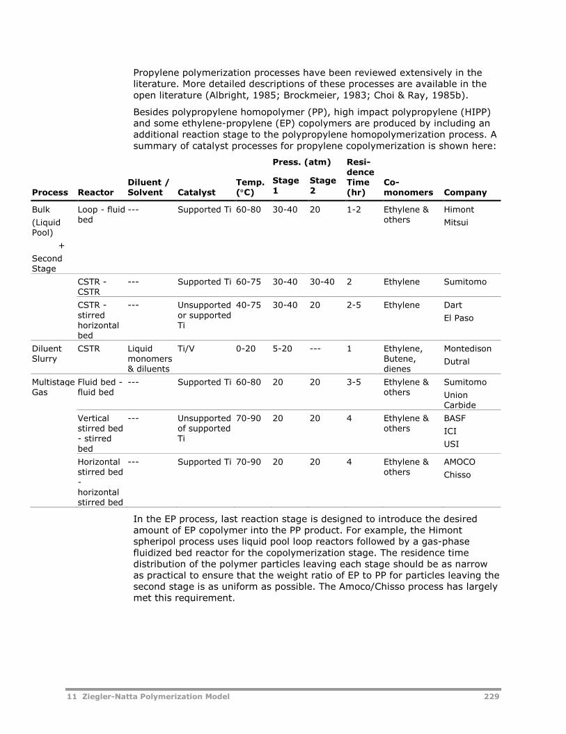
11 Ziegler-Natta Polymerization Model 229
Propylene polymerization processes have been reviewed extensively in theliterature. More detailed descriptions of these processes are available in theopen literature (Albright, 1985; Brockmeier, 1983; Choi & Ray, 1985b).
Besides polypropylene homopolymer (PP), high impact polypropylene (HIPP)and some ethylene-propylene (EP) copolymers are produced by including anadditional reaction stage to the polypropylene homopolymerization process. Asummary of catalyst processes for propylene copolymerization is shown here:
Process ReactorDiluent /Solvent Catalyst
Temp.(C)
Press. (atm) Resi-denceTime(hr)
Co-monomers Company
Stage1
Stage2
Bulk
(LiquidPool)
+
SecondStage
Loop - fluidbed
--- Supported Ti 60-80 30-40 20 1-2 Ethylene &others
Himont
Mitsui
CSTR -CSTR
--- Supported Ti 60-75 30-40 30-40 2 Ethylene Sumitomo
CSTR -stirredhorizontalbed
--- Unsupportedor supportedTi
40-75 30-40 20 2-5 Ethylene Dart
El Paso
DiluentSlurry
CSTR Liquidmonomers& diluents
Ti/V 0-20 5-20 --- 1 Ethylene,Butene,dienes
Montedison
Dutral
MultistageGas
Fluid bed -fluid bed
--- Supported Ti 60-80 20 20 3-5 Ethylene &others
Sumitomo
UnionCarbide
Verticalstirred bed- stirredbed
--- Unsupportedof supportedTi
70-90 20 20 4 Ethylene &others
BASF
ICI
USI
Horizontalstirred bed-horizontalstirred bed
--- Supported Ti 70-90 20 20 4 Ethylene &others
AMOCO
Chisso
In the EP process, last reaction stage is designed to introduce the desiredamount of EP copolymer into the PP product. For example, the Himontspheripol process uses liquid pool loop reactors followed by a gas-phasefluidized bed reactor for the copolymerization stage. The residence timedistribution of the polymer particles leaving each stage should be as narrowas practical to ensure that the weight ratio of EP to PP for particles leaving thesecond stage is as uniform as possible. The Amoco/Chisso process has largelymet this requirement.
230 11 Ziegler-Natta Polymerization Model
Reaction Kinetic SchemeThe built-in catalyst/polymerization kinetic scheme represents the typicalscheme described in the open literature (Xie et al., 1994). Although a numberof reaction mechanisms have been proposed to describe stereospecificZiegler-Natta polymerization, there is still no definitive reaction mechanism tocompletely describe the kinetic behavior of these complexcatalyst/polymerization systems.
Most of the proposed mechanisms include a detailed set of reactions.However, not all of these reactions apply to every catalyst system nor canthey be verified. The kinetic scheme for chromium and metallocene catalyzedsystems can be considered to be a subset of a comprehensive Ziegler-Nattakinetic scheme.
Reaction Steps
There are a few key elementary reactions that apply to almost all catalyzedaddition polymerization systems. These include the three basic reaction steps:
Chain initiation
Propagation
Chain transfer (spontaneous and to small molecules such as monomer,solvent and chain transfer agents)
For chromium and metallocene catalyst systems, additional reactions for longchain branching via terminal double bond polymerization must also beincluded.
In addition to the polymerization reactions, there are reactions affecting thecatalyst active sites on which the polymerization reactions take place. Theseinclude catalyst site activation, inhibition and deactivation. The catalystreactions and the polymerization reactions occur simultaneously during thepolymerization.
A comprehensive kinetic scheme for the catalyzed multi-site homo- andcopolymerization of any number of monomers has been built into AspenPolymers.
Catalyst States
The multi-site catalyst states and the types of reactions affecting them areshown here:
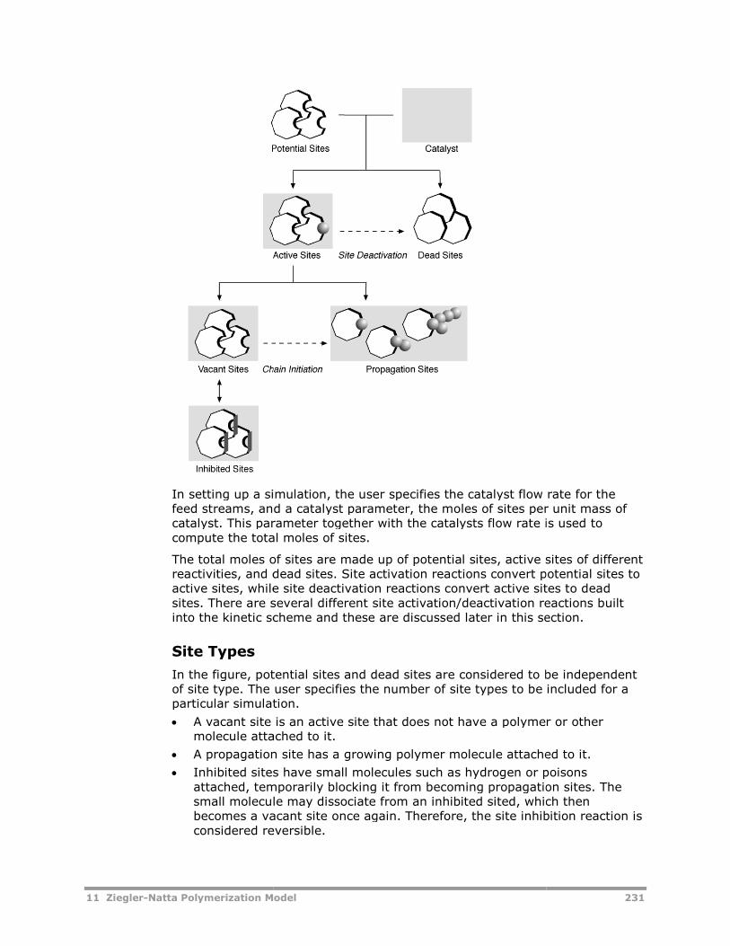
11 Ziegler-Natta Polymerization Model
In setting up a sifeed streams, and a catalyst parameter, the moles of sites per unit mass ofcatalyst. This parameter together with the catalysts flow rate is used tocompute the total moles of sites.
The total moles of sites are made up of potential sites, active sites of differentreactivities, and dead sites. Site activation reactions convert potential sites toactive sites, while site deactivation reactions convert active sites to deadsites. There are severalinto the kinetic scheme and these are discussed later in this section.
Site Types
In the figure, potential sites and dead sites are considered to be independentof site type. The user specifies the number of site types to be included for aparticular simulation.
A vacant sitemolecule attached to it.
A propagation site
Inhibited sitesattached, temporarily blocking it from becoming propagation sites. Thesmall molecule may dissociate from an inhibited sited, which thenbecomes a vacant site once again. Therefore, the site inhibition reaction isconsidered reversible.
Natta Polymerization Model
In setting up a simulation, the user specifies the catalyst flow rate for thefeed streams, and a catalyst parameter, the moles of sites per unit mass ofcatalyst. This parameter together with the catalysts flow rate is used tocompute the total moles of sites.
les of sites are made up of potential sites, active sites of differentreactivities, and dead sites. Site activation reactions convert potential sites toactive sites, while site deactivation reactions convert active sites to deadsites. There are several different site activation/deactivation reactions builtinto the kinetic scheme and these are discussed later in this section.
In the figure, potential sites and dead sites are considered to be independent. The user specifies the number of site types to be included for a
particular simulation.
is an active site that does not have a polymer or othemolecule attached to it.
A propagation site has a growing polymer molecule attached to it.
Inhibited sites have small molecules such as hydrogen or poisonsattached, temporarily blocking it from becoming propagation sites. Thesmall molecule may dissociate from an inhibited sited, which thenbecomes a vacant site once again. Therefore, the site inhibition reaction isconsidered reversible.
231
mulation, the user specifies the catalyst flow rate for thefeed streams, and a catalyst parameter, the moles of sites per unit mass ofcatalyst. This parameter together with the catalysts flow rate is used to
les of sites are made up of potential sites, active sites of differentreactivities, and dead sites. Site activation reactions convert potential sites toactive sites, while site deactivation reactions convert active sites to dead
different site activation/deactivation reactions builtinto the kinetic scheme and these are discussed later in this section.
In the figure, potential sites and dead sites are considered to be independent. The user specifies the number of site types to be included for a
is an active site that does not have a polymer or other
has a growing polymer molecule attached to it.
ogen or poisonsattached, temporarily blocking it from becoming propagation sites. Thesmall molecule may dissociate from an inhibited sited, which thenbecomes a vacant site once again. Therefore, the site inhibition reaction is
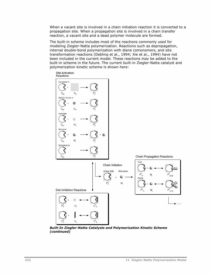
232
When a vacant site is involved in a chain initiation reaction it is converted to apropagation site. When a propagation site is involved in a chain transferreaction, a vacant site and a dead polymer molecule are formed.
The built-in scheme includes most of tmodeling Ziegler-internal double-bond polymerization with diene comonomers, and sitetransformation reactions (Debling et al., 1994; Xie et al., 1994) have notbeen included in the current model. These reactions may be added to thebuilt-in scheme in the future. The current builtpolymerization kinetic scheme is shown here
Built-In Ziegler-Natta Catalysts and Polymerization Kinetic Scheme(continued)
11 Ziegler-Natta Polymerization Model
n a vacant site is involved in a chain initiation reaction it is converted to apropagation site. When a propagation site is involved in a chain transferreaction, a vacant site and a dead polymer molecule are formed.
in scheme includes most of the reactions commonly used for-Natta polymerization. Reactions such as depropagation,
bond polymerization with diene comonomers, and sitetransformation reactions (Debling et al., 1994; Xie et al., 1994) have not
ded in the current model. These reactions may be added to thein scheme in the future. The current built-in Ziegler-Natta catalyst and
polymerization kinetic scheme is shown here:
Natta Catalysts and Polymerization Kinetic Scheme
Natta Polymerization Model
n a vacant site is involved in a chain initiation reaction it is converted to apropagation site. When a propagation site is involved in a chain transferreaction, a vacant site and a dead polymer molecule are formed.
he reactions commonly used forNatta polymerization. Reactions such as depropagation,
bond polymerization with diene comonomers, and sitetransformation reactions (Debling et al., 1994; Xie et al., 1994) have not
ded in the current model. These reactions may be added to theNatta catalyst and
Natta Catalysts and Polymerization Kinetic Scheme
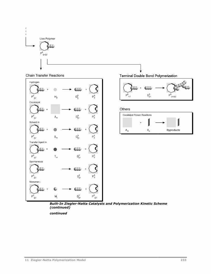
11 Ziegler-Natta Polymerization Model
Built-In Ziegler-Natta Catalysts and Polymerization Kinetic Scheme(continued)
continued
Model
Natta Catalysts and Polymerization Kinetic Scheme
233
Natta Catalysts and Polymerization Kinetic Scheme
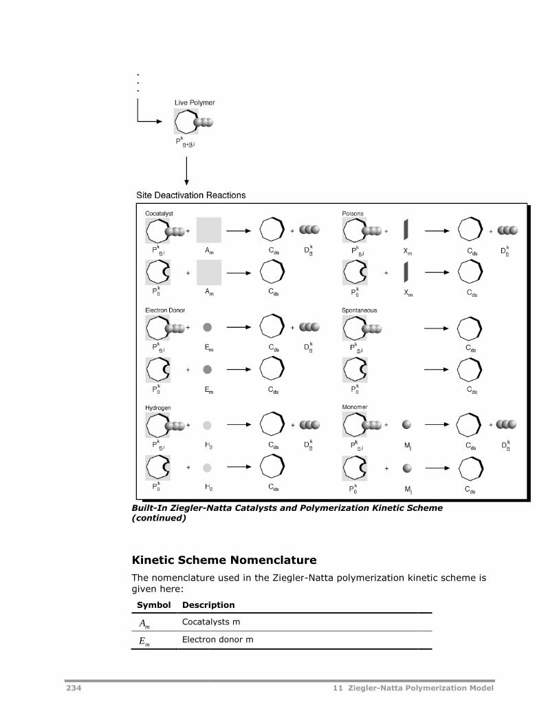
234
Built-In Ziegler-Natta Catalysts and Polymerization Kinetic Scheme(continued)
Kinetic Scheme Nomenclature
The nomenclature used in the Zieglergiven here:
Symbol Description
AmCocatalysts m
EmElectron donor m
11 Ziegler-Natta Polymerization Model
Natta Catalysts and Polymerization Kinetic Scheme
Kinetic Scheme Nomenclature
The nomenclature used in the Ziegler-Natta polymerization kinetic scheme is
Description
Cocatalysts m
Electron donor m
Natta Polymerization Model
Natta Catalysts and Polymerization Kinetic Scheme
Natta polymerization kinetic scheme is
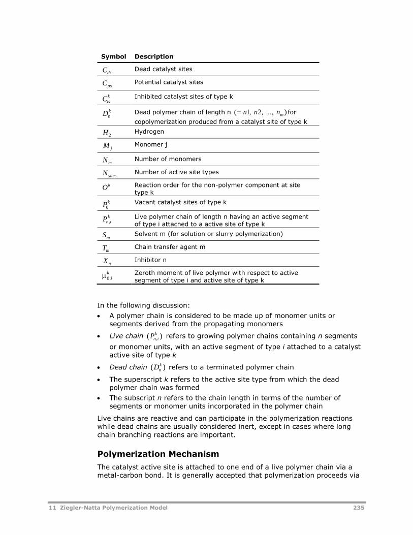
11 Ziegler-Natta Polymerization Model 235
Symbol Description
CdsDead catalyst sites
CpsPotential catalyst sites
Cisk Inhibited catalyst sites of type k
Dnk Dead polymer chain of length n ( , , ..., ) n n nm1 2 for
copolymerization produced from a catalyst site of type k
H2Hydrogen
M jMonomer j
NmNumber of monomers
N sitesNumber of active site types
Ok Reaction order for the non-polymer component at sitetype k
Pk0
Vacant catalyst sites of type k
Pn ik,
Live polymer chain of length n having an active segmentof type i attached to a active site of type k
SmSolvent m (for solution or slurry polymerization)
TmChain transfer agent m
X nInhibitor n
0,ik Zeroth moment of live polymer with respect to active
segment of type i and active site of type k
In the following discussion:
A polymer chain is considered to be made up of monomer units orsegments derived from the propagating monomers
Live chain ( ),Pn ik refers to growing polymer chains containing n segments
or monomer units, with an active segment of type i attached to a catalystactive site of type k
Dead chain ( )Dnk refers to a terminated polymer chain
The superscript k refers to the active site type from which the deadpolymer chain was formed
The subscript n refers to the chain length in terms of the number ofsegments or monomer units incorporated in the polymer chain
Live chains are reactive and can participate in the polymerization reactionswhile dead chains are usually considered inert, except in cases where longchain branching reactions are important.
Polymerization Mechanism
The catalyst active site is attached to one end of a live polymer chain via ametal-carbon bond. It is generally accepted that polymerization proceeds via
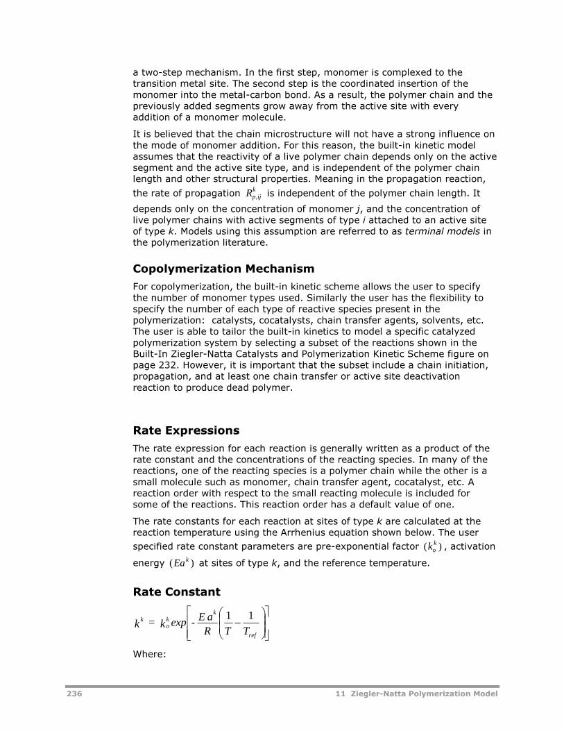
236 11 Ziegler-Natta Polymerization Model
a two-step mechanism. In the first step, monomer is complexed to thetransition metal site. The second step is the coordinated insertion of themonomer into the metal-carbon bond. As a result, the polymer chain and thepreviously added segments grow away from the active site with everyaddition of a monomer molecule.
It is believed that the chain microstructure will not have a strong influence onthe mode of monomer addition. For this reason, the built-in kinetic modelassumes that the reactivity of a live polymer chain depends only on the activesegment and the active site type, and is independent of the polymer chainlength and other structural properties. Meaning in the propagation reaction,
the rate of propagation Rp ijk, is independent of the polymer chain length. It
depends only on the concentration of monomer j, and the concentration oflive polymer chains with active segments of type i attached to an active siteof type k. Models using this assumption are referred to as terminal models inthe polymerization literature.
Copolymerization Mechanism
For copolymerization, the built-in kinetic scheme allows the user to specifythe number of monomer types used. Similarly the user has the flexibility tospecify the number of each type of reactive species present in thepolymerization: catalysts, cocatalysts, chain transfer agents, solvents, etc.The user is able to tailor the built-in kinetics to model a specific catalyzedpolymerization system by selecting a subset of the reactions shown in theBuilt-In Ziegler-Natta Catalysts and Polymerization Kinetic Scheme figure onpage 232. However, it is important that the subset include a chain initiation,propagation, and at least one chain transfer or active site deactivationreaction to produce dead polymer.
Rate Expressions
The rate expression for each reaction is generally written as a product of therate constant and the concentrations of the reacting species. In many of thereactions, one of the reacting species is a polymer chain while the other is asmall molecule such as monomer, chain transfer agent, cocatalyst, etc. Areaction order with respect to the small reacting molecule is included forsome of the reactions. This reaction order has a default value of one.
The rate constants for each reaction at sites of type k are calculated at thereaction temperature using the Arrhenius equation shown below. The user
specified rate constant parameters are pre-exponential factor ( )kok , activation
energy ( )Ea k at sites of type k, and the reference temperature.
Rate Constant
ref
kko
k
TTR
aE-expk=k11
Where:
11 Ziegler-Natta Polymerization Model 237
ko= Pre-exponential factor in 1/sec for first order reactions
and m kmol3 / sec for second order reactions
Ea = Activation energy in mole enthalpy units
R = Universal gas constant
refT = Reference temperature in Kelvin
Catalyst Pre-ActivationSome of the chromium catalysts used in these processes exhibit slowactivation with induction period. This slow activation can be modeled bycatalyst preactivation reaction. The precatalyst goes to catalyst that furtherundergoes site activation, initiation and propagation.
Catalyst Site ActivationThe catalyst site activation step involves the generation of reactive vacantactive sites from potential sites. Depending on the catalysts system, theactivation may be done before the catalyst is fed to the reactor or within thereactor.
There are several different site activation reactions included in the built-inkinetic scheme. They include site activation by cocatalyst, by electron donors,by hydrogen, by monomer, and spontaneous site activation. Different catalystsystems tend to be activated by a different subset of the reactions in this
scheme. For example, TiCl3 catalyst systems are usually activated with an
organoaluminum cocatalyst such as diethylaluminum chloride (DEAC), in thereactor. Chromic oxide catalysts are calcined by heating with air for severalhours at temperatures of 400C to 975C and cooled in dry air. Some of thesecatalysts may be activated with a reducing agent before introduction into thereactor, while others are activated within the reactor.
Site Activation Reactions
Some of the site activation reactions (activation by monomer, electron donor,hydrogen) have been proposed to explain the observed rate enhancementbehavior in different catalyst systems. For example, the activation ofadditional sites by comonomer has been proposed to explain the rateenhancement observed with the addition of a comonomer to ethylene andpropylene homopolymerization reactors.
Chain InitiationChain initiation involves the reaction of a monomer molecule at a vacantactive site to form a live polymer molecule of unit length at that site. Thisreaction converts a vacant active site to a propagation site. The chaininitiation reaction is shown below:
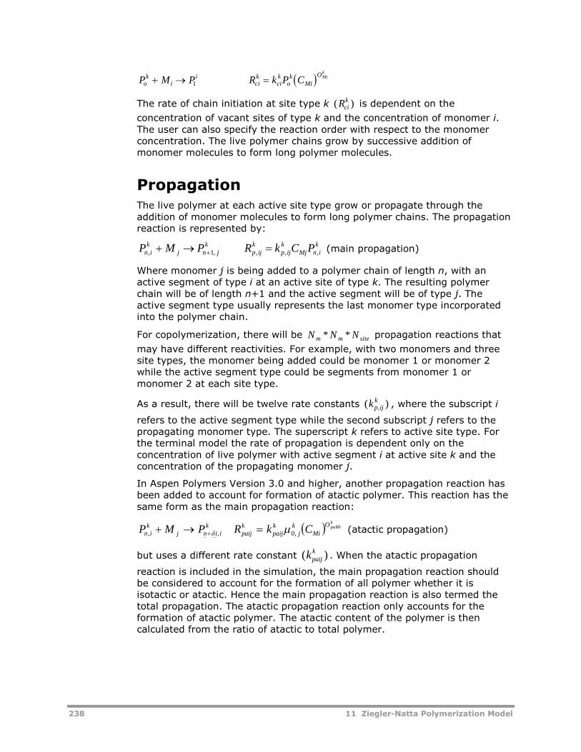
238 11 Ziegler-Natta Polymerization Model
P M P R k P Cok
ii
cik
cik
ok
Mi
OMik
1
The rate of chain initiation at site type k ( )Rcik is dependent on the
concentration of vacant sites of type k and the concentration of monomer i.The user can also specify the reaction order with respect to the monomerconcentration. The live polymer chains grow by successive addition ofmonomer molecules to form long polymer molecules.
PropagationThe live polymer at each active site type grow or propagate through theaddition of monomer molecules to form long polymer chains. The propagationreaction is represented by:
kinMj
kijp
kijp
kjnj
kin PCkRPMP ,,,,1, (main propagation)
Where monomer j is being added to a polymer chain of length n, with anactive segment of type i at an active site of type k. The resulting polymerchain will be of length n+1 and the active segment will be of type j. Theactive segment type usually represents the last monomer type incorporatedinto the polymer chain.
For copolymerization, there will be N N Nm m site* * propagation reactions that
may have different reactivities. For example, with two monomers and threesite types, the monomer being added could be monomer 1 or monomer 2while the active segment type could be segments from monomer 1 ormonomer 2 at each site type.
As a result, there will be twelve rate constants ( ),kp ijk
, where the subscript i
refers to the active segment type while the second subscript j refers to thepropagating monomer type. The superscript k refers to active site type. Forthe terminal model the rate of propagation is dependent only on theconcentration of live polymer with active segment i at active site k and theconcentration of the propagating monomer j.
In Aspen Polymers Version 3.0 and higher, another propagation reaction hasbeen added to account for formation of atactic polymer. This reaction has thesame form as the main propagation reaction:
kpaMiO
Mik
jkpaij
kpaij
kiinj
kin CkRPMP ,0,, (atactic propagation)
but uses a different rate constant ( )kpaijk
. When the atactic propagation
reaction is included in the simulation, the main propagation reaction shouldbe considered to account for the formation of all polymer whether it isisotactic or atactic. Hence the main propagation reaction is also termed thetotal propagation. The atactic propagation reaction only accounts for theformation of atactic polymer. The atactic content of the polymer is thencalculated from the ratio of atactic to total polymer.
11 Ziegler-Natta Polymerization Model 239
Chain Transfer to Small MoleculesChain transfer to small molecules such as monomer, solvent or chain transferagent usually involves the extraction of hydrogen from the small molecule bythe active site and leads to the termination of the live chain. At the sametime, a new vacant site is formed which can undergo chain initiation to startpolymerization. The effect of chain transfer on the polymerization kineticsdepends on the reactivity of the transfer sites.
When the transfer site is very reactive, as is the case when the chain initiationrate constant is greater than the propagation rate constant, chain transfer willnot lower the polymerization rate or conversion, but will reduce the molecularweight of the polymer. However, if the transfer site is less reactive, as in thecase of low chain initiation rate constant, both the conversion and molecularweight of the polymer will be lowered.
In the built-in kinetics, chain transfer to hydrogen, cocatalysts, solvent,transfer agent, electron donor, monomer and spontaneous chain transfer areincluded as shown in the Built-In Ziegler-Natta Catalysts and PolymerizationKinetic Scheme figure on page 232.
Chain Transfer to Monomer
For chain transfer to monomer a new polymer chain of unit length isgenerated while for the other transfer reactions a vacant site of that type isgenerated. The dead polymer chain formed by some of the chain transferreactions will have an end-group with a terminal double bond. In addition tothe rate constant parameters and the reaction order, the user may alsospecify a parameter to track the fraction of dead polymer chains with terminaldouble bonds that are generated from the chain transfer reactions. Thedefault value for this parameter is zero.
Site DeactivationThe catalyst site deactivation step involves the deactivation of active sites,vacant and propagation, to form dead sites. Depending on the catalystsystem and operating conditions, the deactivation rate may be high or low.
There are several different site deactivations reactions included in the built-inkinetic scheme. They include site deactivation by cocatalyst, by electrondonors, by hydrogen, by monomer, by poisons, and spontaneous sitedeactivation. Different catalyst systems tend to be deactivated by a differentsubset of the reactions.
The deactivation rate constants are assumed to be dependent only on the sitetype and not on the polymer segment attached to a site. Therefore, the samerate constant is applied to both vacant and propagation sites of the sametype. Note that deactivation rates shown in the Built-In Ziegler-NattaCatalysts and Polymerization Kinetic Scheme figure on page 232 are per unitof active (vacant and propagation) site concentration.
240 11 Ziegler-Natta Polymerization Model
Site InhibitionInhibited sites have small molecules such as hydrogen or poisons attached.As a result, inhibited sites are temporarily blocked from becomingpropagation sites. The site inhibition reaction is considered reversible.Therefore, the small molecule may dissociate from an inhibited site whichthen becomes a vacant site once again. The user must specify rate constantparameters for both the forward (inhibition) and reverse (dissociation)reactions.
Cocatalyst PoisoningFor some catalyst systems, additional amounts of cocatalysts are fed to thereactor to counteract the effect of any poisons present . This is modeled as acocatalyst poisoning reaction in the built-in kinetics. The product of thisreaction is designated as a byproduct in the list of reactive species. Thebyproduct is considered to be inert and does not participate in any reaction.
Terminal Double Bond PolymerizationFor some catalyst systems, primarily metallocene, polymer chains with longchain branches are formed. However, the long chain branching frequency isusually small. The long chain branches are believed to be due to propagationreactions involving a live chain and a terminal double bond on a dead polymerchain. Polymer chains with terminal double bonds are formed by some of thechain transfer reactions. To form long chain branches, the metal center mustbe open to provide a favorable reactivity ratio for the macromonomer.
The concentration of terminal double bond (TDB) end-groups on the deadpolymer chains are tracked through an additional segment called the TDB-Segment. TDB-Segments are generated through the chain transfer reactionsand are consumed through the TDB polymerization reaction. When the TDBreaction is used, one additional segment needs to be defined in theComponents form for the TDB-Segment. Typically, for a copolymerizationsystem with N monomers, N repeat segments would be defined in theComponents form. However, with the TDB polymerization reaction, N repeatsegments and one end segment should be defined in the Component form.The end segment must be specified as the TDB-Seg species in the Speciesfolder of the Ziegler-Natta kinetics.
Example for Terminal Double Bond Polymerization
This example starts with the delivered example file Polymers\pp.bkp.
1 Include a segment to represent the terminal double bond. The segmentdatabase includes several preconfigured TDB segments (each containingone less hydrogen than the corresponding monomer). Be sure to selectType Segment.
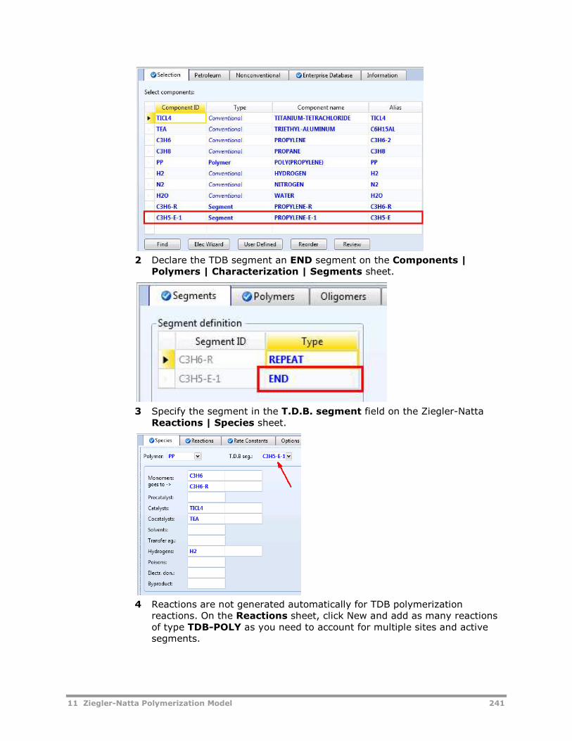
11 Ziegler-Natta Polymerization Model 241
2 Declare the TDB segment an END segment on the Components |Polymers | Characterization | Segments sheet.
3 Specify the segment in the T.D.B. segment field on the Ziegler-NattaReactions | Species sheet.
4 Reactions are not generated automatically for TDB polymerizationreactions. On the Reactions sheet, click New and add as many reactionsof type TDB-POLY as you need to account for multiple sites and activesegments.
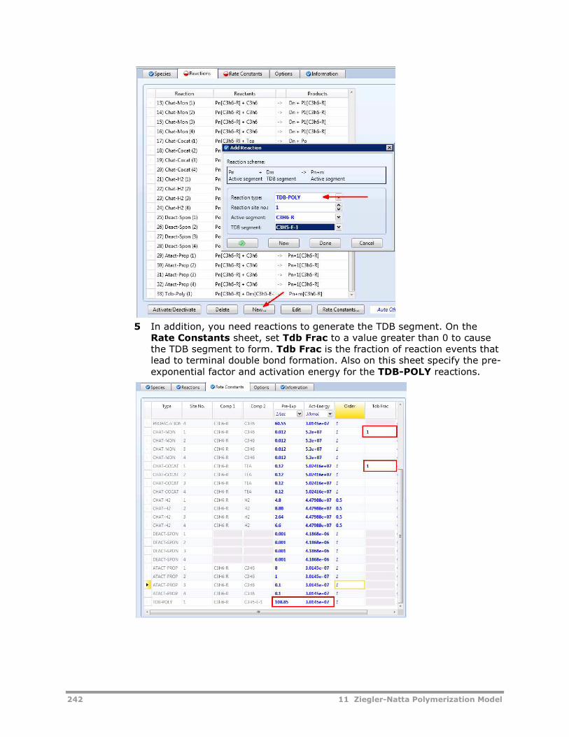
242 11 Ziegler-Natta Polymerization Model
5 In addition, you need reactions to generate the TDB segment. On theRate Constants sheet, set Tdb Frac to a value greater than 0 to causethe TDB segment to form. Tdb Frac is the fraction of reaction events thatlead to terminal double bond formation. Also on this sheet specify the pre-exponential factor and activation energy for the TDB-POLY reactions.
11 Ziegler-Natta Polymerization Model 243
Model Features andAssumptionsFollowing are the model features and assumptions used in the Ziegler-Nattapolymerization model available in Aspen Polymers.
Phase EquilibriaThe polymerization model currently considers a single-phase system (vapor orliquid), two-phase system (vapor and liquid), or three-phase (VLL) systemwhen calculating concentrations for the reaction kinetics. For single-phasesystems, the reacting phase may be either vapor or liquid. In multi-phasesystems, reactions can occur in one or more phases simultaneously. Eachreaction object is associated with a single reacting phase, identified on theoptions form.
By default the reacting phase is assumed to be the liquid phase (for VLLsystems, the reacting phase must be specified). Several reaction models canbe referenced from a single reactor block to account for reactions in eachphase.
Rate CalculationsThe Ziegler-Natta polymerization kinetic model supplies to the reactor modelsthe reaction rates for the components and the rate of change of polymerattributes (e.g. the chain length distribution moments) . The componentreaction rates are computed from the kinetic scheme by summing over allreactions that involve the component. The site based moment rates arederived from a population balance and method of moments approach similarto that described in the Calculation Method section on page 185.
Polymer Properties CalculatedThe following variables can be calculated by the built-in kinetics routine basedon the polymer attributes selected, and the subset of the built-in kinetics usedfor a specific simulation:
Zeroth, first and second moments for the composite and site basedcombined polymer
Zeroth and first moments for the composite and site based live polymer
Number and weight degree of polymerization and polydispersity index forthe composite and site based bulk polymer (DPN, DPW, PDI and SDPN,SDPW, SPDI)
Number and weight average molecular weight for the composite and sitebased bulk polymer (MWN, MWW and SMWN, SMWW)
Copolymer segment composition for composite and site based bulkpolymer (SFRAC and SSFRAC segment mole fractions)
Total number long chain branches (LCB)
244 11 Ziegler-Natta Polymerization Model
Long chain branching frequencies (FLCB)
Mole fraction of live bulk polymer chains (LPFRAC and LSPFRAC)
Number average degree of polymerization for live polymer (LDPN andLSDPN)
Copolymer segment composition for live polymer (LSFRAC and LSSFRAC)
Live polymer active segment composition (LEFRAC and LSEFRAC)
These variables are stored as component attributes (See Chapter 2). It isassumed that attributes needed for the kinetic scheme are selected. Thespecification of the Ziegler-Natta Model is described later in this section.
In many cases, users may need to know polymer product properties relatedto the above structural properties. For example, users may be interested inmelt flow rate or melt index, viscosity, density, etc. These properties can becalculated in user-supplied Fortran subroutines which take the polymermoments and structural information and return the desired property. Anexample use of a user supplied subroutine to return melt index is shown inthe HDPE section of the Aspen Polymers Examples & Applications Case Book.
Specifying Ziegler-NattaPolymerization Kinetics
Accessing the Ziegler-Natta ModelTo access the Ziegler-Natta polymerization kinetic model:
1 From the Data Browser, click Reactions.
2 From the Reactions folder, click Reactions.
The Reactions object manager appears.
3 If the kinetic model already exists, double-click the desired Reaction ID inthe object manager or click Edit to get to the input forms.
4 To add a new model, from the Reactions object manager, click New. Ifnecessary, change the default ID for the reaction.
5 Select Ziegler-Nat as the reaction type and click OK.
Specifying the Ziegler-Natta ModelThe Ziegler-Natta model input forms are as listed below. Use these forms todefine reacting species and enter reaction rate constant parameters.
Use this sheet To
Species Define reacting species
Reactions Specify reactions and rate constant parameters
Rate Constants Summarize rate constant parameters
Options Specify the reacting phase
11 Ziegler-Natta Polymerization Model 245
Specifying Reacting SpeciesYou must specify the reacting species on the Species sheet:
1 In the Polymer field, specify the polymer produced.
2 In the Monomers field list the reacting monomers. For each monomer, inthe goes to field, specify the polymer segment that the monomerconverts to.
3 If you select the terminal double bond polymerization reaction, in theT.D.B.-Seg field, list TDB segment that is formed by the chain transferreactions and is consumed by the terminal double bond polymerizationreaction. Otherwise, go to step 4.
Note: The TDB segment should be of type end segment and should not beused as a repeat segment for a particular monomer (see Step 2).
4 Continue listing other types of reacting species, for example, solvents,transfer agents, etc.
5 Select the Generate Reactions option if you want the reactions to begenerated automatically.
After going through the reaction generation once, it is recommended thatyou turn off this feature. Otherwise, the reaction generation is performedrepeatedly.
Listing ReactionsThe Ziegler-Natta model generates reactions based on the list of reactingspecies. You can view the system-generated reactions, then assign rateconstant parameters to these reactions.
You can view a list of the system-generated reactions on the Reactionssheet. In the Reaction summary listing for each reaction, the first columnindicates the reaction type. The second column lists the reactants, and thelast column lists the products. The Data Browser window can be resized tobetter view the reaction listing. Use the following options:
Click To
New Add new reactions to the scheme
Edit Edit the current reaction indicated by the rowselector
Rate Constants Specify reaction rate constant parameters for thereactions
Click to select a reaction. Click a reaction then Control-Click to includeadditional reactions for multiple selections. Double-click to edit a reaction.
In addition, you can use the following buttons:
Click To
Hide/RevealExclude/Include a reaction from thecalculations
DeletePermanently remove a reaction from themodel
246 11 Ziegler-Natta Polymerization Model
Adding ReactionsTo add a new reaction to the scheme, click New to open the Add Reactionsubform:
1 In Reaction type, select a type for the new reaction.
The Reaction scheme for that type is displayed.
2 In other reactant (for example, Initiator, Catalyst) fields, enter thereactants of the categories allowed for that reaction type.
3 Click Cancel to discard the new reaction
or
Click New to add a new reaction
or
Click to check the Completion status
or
Click Done to return to the reaction summary.
Editing ReactionsTo edit a reaction, click Edit to open the Edit Reaction subform:
1 Modify the Reaction type as needed.
The Reaction scheme for that type is displayed.
2 Modify reactants as needed.
3 Click to check the Completion status
or
Click Done to return to the reaction summary.
Assigning Rate Constants to ReactionsTo assign rate constants to user reactions, click Rate Constants to open theRate Constant Parameters subform:
1 In the Site No. field, enter the site number.
2 In the ko field, enter the pre-exponential factor.
3 In the Ea field, enter the activation energy.
4 In the Order field, enter the order for component in reaction.
5 In the Fraction field, enter terminal double bond fraction.
6 In the Tref field, enter reference temperature.
7 Click the stoichiometry list and select a new reaction. Enter rate constantsfor the new reaction. You can use the Prev and Next buttons to select theprevious or next reaction in the list.
8 Click the Summary tab to see a listing of all the rate constantparameters.
11 Ziegler-Natta Polymerization Model 247
9 Click to check the Completion status
or
Click Close to return to the reaction summary.
ReferencesAlbright L. F. (1985). Processes for Major Addition-Type Plastics and TheirMonomers, 2nd Ed. Florida: Krieger Pub.
Brockmeier, N. F. (1983). Latest Commercial Technology for PropylenePolymerization. In R.P. Quirk (Ed.), Transition Metal CatalyzedPolymerizations - Alkenes and Dienes. New York: Academic Pub.
Choi, K-Y, & Ray, W. H. (1985a). Recent Developments in Transition MetalCatalyzed Olefin Polymerization - A Survey. I. Ethylene Polymerization. J.Macromol. Sci. Rev. Macromol. Chem. Phys., C25 (1), 1.
Choi, K-Y, & Ray, W. H. (1985b). Recent Developments in Transition MetalCatalyzed Olefin Polymerization - A Survey. II. Propylene Polymerization. J.Macromol. Sci. Rev. Macromol. Chem. Phys., C25 (1), 57.
Debling, J. A., Han, G. C., Kuijpers, F., Verburg, J., Zacca, J., & Ray, W. H.(1994). Dynamic Modeling of Product Grade Transition for OlefinPolymerization Processes. AIChE J., 40, No. 3, 506.
Nowlin, T. E. (1985). Low Pressure Manufacture of Polyethylene. Prog. Polym.Sci., 11, 29.
Short, J. N. (1983). Low Pressure Ethylene Polymerization Processes. In R.P.Quirk (Ed.), Transition Metal Catalyzed Polymerizations - Alkenes and Dienes.New York: Academic Pub.
Xie, T., McAuley, K.B., Hsu, J. C. C., & Bacon, D. W. (1994). Gas PhaseEthylene Polymerization: Production Processes, Polymer Properties, andReactor Modeling. Ind. Eng. Chem. Res., 33, 449.

248 11 Ziegler-Natta Polymerization Model
12 Ionic Polymerization Model 249
12 Ionic PolymerizationModel
This section covers the ionic polymerization kinetic model available in AspenPolymers (formerly known as Aspen Polymers Plus). The cationic, anionic andgroup transfer addition polymerization kinetics can be modeled using thismodel.
Topics covered include:
Summary of Applications, 249
Ionic Processes, 250
Reaction Kinetic Scheme, 250
Model Features and Assumptions, 258
Polymer Properties Calculated, 259
Specifying Ionic Polymerization Kinetics, 260
Summary of ApplicationsSome examples of applicable polymers are given in below:
Polystyrene - Anionic polymerization is used to produce narrow molecularweight distribution polystyrenes in small quantities. Cationicpolymerization is used to produce low molecular weight polystyrenes forcoatings and glues. Block copolymers of styrene and butadiene areproduced commercially with anionic polymerization.
Polyisobutylene - Low-to-medium molecular weight poly isobutylene isproduced commercially by polymerization of high purity isobutylene inisobutane or hexane diluent using aluminum chloride or hexane trifluorideas a catalyst.
Polybutene - Polybutenes are produced in solution by copolymerizingisobutylene and n-butene using aluminum chloride or hexane trifluoride asa catalyst.
Polybutadiene - Block copolymers of styrene and butadiene are producedcommercially with anionic polymerization.
Polyoxides - Examples are poly ethylene oxide (PEO) and poly propyleneoxide (PPO). Continuous tubular or column reactors or semibatch
250 12 Ionic Polymerization Model
autoclaves are used. The polymerization can be carried out with differentmechanisms: anionic (base catalysis), cationic (acid catalysis), orcoordinate.
Ionic ProcessesMany specialty polymers are manufactured by ionic polymerization processes.For the description of a specific ionic process, refer to the References section.Ionic polymers fall in the category of addition polymers, i.e., the reactivespecies grow in length by continuous addition of monomer units. However,there are several features that distinguish the ionic polymerization processesfrom other addition polymerization processes like free-radical and Ziegler-Natta:
Different propagating species are often present in ionic processes. Thesespecies may be free ions, tight ion pairs, loose ion pairs, dormant esters,etc. Moreover the propagating species are often in equilibrium.
Association or aggregation phenomena is common in BuLi type ofinitiators for anionic polymerization. The associated initiator is not reactiveand is in equilibrium with its dissociated form. The association phenomenaalso takes place with growing polymer chains, which reduces the actualnumber of chains growing at any given time. This phenomena affects boththe conversion and polymer properties.
Exchange reaction takes place between live and dormant polymer. Theactive species transfer from one polymer to another. This reaction controlsthe molecular weight distribution of the final polymer. If the exchangereaction rate constant >> propagation rate constant, then for increasingmonomer conversion the polydispersity approaches a limiting value of 1.0.
Ionic reactions are a strong function of solvent, initiator and operatingconditions and are susceptible to poisons.
Chain transfer and termination reactions may be negligible or absent incertain polymerization processes thus leading to formation of livingpolymers.
Reaction Kinetic SchemeIn the following sections, the general chemistry of ionic polymerization andthe built-in initiator / polymerization kinetic scheme are described. The kineticscheme is based on literature survey of ionic polymerization mechanisms.Ionic kinetic scheme can model either cationic, anionic or group-transferpolymerization. The ionic kinetic scheme in Aspen Polymers is a super-set ofall the above mentioned reactions.
Reaction Steps
There are a few key elementary reactions that apply to all ionicpolymerization systems. These include the three basic reaction steps:
Formation of active species
Chain initiation
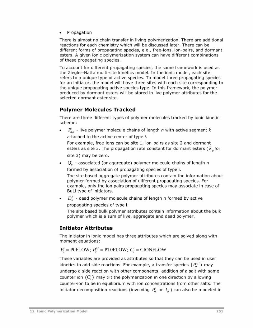
12 Ionic Polymerization Model 251
Propagation
There is almost no chain transfer in living polymerization. There are additionalreactions for each chemistry which will be discussed later. There can bedifferent forms of propagating species, e.g., free-ions, ion-pairs, and dormantesters. A given ionic polymerization system can have different combinationsof these propagating species.
To account for different propagating species, the same framework is used asthe Ziegler-Natta multi-site kinetics model. In the ionic model, each siterefers to a unique type of active species. To model three propagating speciesfor an initiator, the model will have three sites with each site corresponding tothe unique propagating active species type. In this framework, the polymerproduced by dormant esters will be stored in live polymer attributes for theselected dormant ester site.
Polymer Molecules Tracked
There are three different types of polymer molecules tracked by ionic kineticscheme:
Pn,ki
- live polymer molecule chains of length n with active segment k
attached to the active center of type i.
For example, free-ions can be site 1, ion-pairs as site 2 and dormant
esters as site 3. The propagation rate constant for dormant esters ( k p for
site 3) may be zero.
inQ - associated (or aggregate) polymer molecule chains of length n
formed by association of propagating species of type i.
The site based aggregate polymer attributes contain the information aboutpolymer formed by association of different propagating species. Forexample, only the ion pairs propagating species may associate in case ofBuLi type of initiators.
inD - dead polymer molecule chains of length n formed by active
propagating species of type i.
The site based bulk polymer attributes contain information about the bulkpolymer which is a sum of live, aggregate and dead polymer.
Initiator Attributes
The initiator in ionic model has three attributes which are solved along withmoment equations:
P P Ci t iIi
0 0 P0FLOW; PT0FLOW; CIONFLOW,
These variables are provided as attributes so that they can be used in user
kinetics to add side reactions. For example, a transfer species ( )P t, i0 may
undergo a side reaction with other components; addition of a salt with same
counter ion ( )CIi
may tilt the polymerization in one direction by allowing
counter-ion to be in equilibrium with ion concentrations from other salts. The
initiator decomposition reactions (involving Pi0 or Im ) can also be modeled in
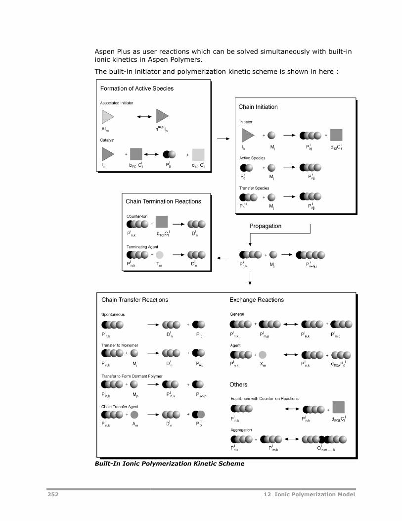
252
Aspen Plus as user reactions which can be solved simultaneously with builtionic kinetics in Aspen Polymers.
The built-in initiator and polymerization kinetic scheme
Built-In Ionic Polymerization Kinetic Scheme
12 Ionic Polymerization Model
Aspen Plus as user reactions which can be solved simultaneously with builtionic kinetics in Aspen Polymers.
in initiator and polymerization kinetic scheme is shown in here
In Ionic Polymerization Kinetic Scheme
12 Ionic Polymerization Model
Aspen Plus as user reactions which can be solved simultaneously with built-in
is shown in here :
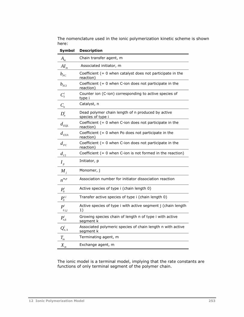
12 Ionic Polymerization Model 253
The nomenclature used in the ionic polymerization kinetic scheme is shownhere:
Symbol Description
AmChain transfer agent, m
AImAssociated initiator, m
bFCCoefficient (= 0 when catalyst does not participate in thereaction)
bTCICoefficient (= 0 when C-ion does not participate in thereaction)
CIi Counter ion (C-ion) corresponding to active species of
type i
CnCatalyst, n
Dni Dead polymer chain length of n produced by active
species of type i
dEQLCoefficient (= 0 when C-ion does not participate in thereaction)
dEXACoefficient (= 0 when Po does not participate in thereaction)
dFCCoefficient (= 0 when C-ion does not participate in thereaction)
d I 2Coefficient (= 0 when C-ion is not formed in the reaction)
I pInitiator, p
M jMonomer, j
nm,p Association number for initiator dissociation reaction
Pi0
Active species of type i (chain length 0)
P t,i0
Transfer active species of type i (chain length 0)
Pj,j
i
Active species of type i with active segment j (chain length1)
Pn,ki Growing species chain of length n of type i with active
segment k
Qn, ki Associated polymeric species of chain length n with active
segment k
TmTerminating agent, m
XmExchange agent, m
The ionic model is a terminal model, implying that the rate constants arefunctions of only terminal segment of the polymer chain.
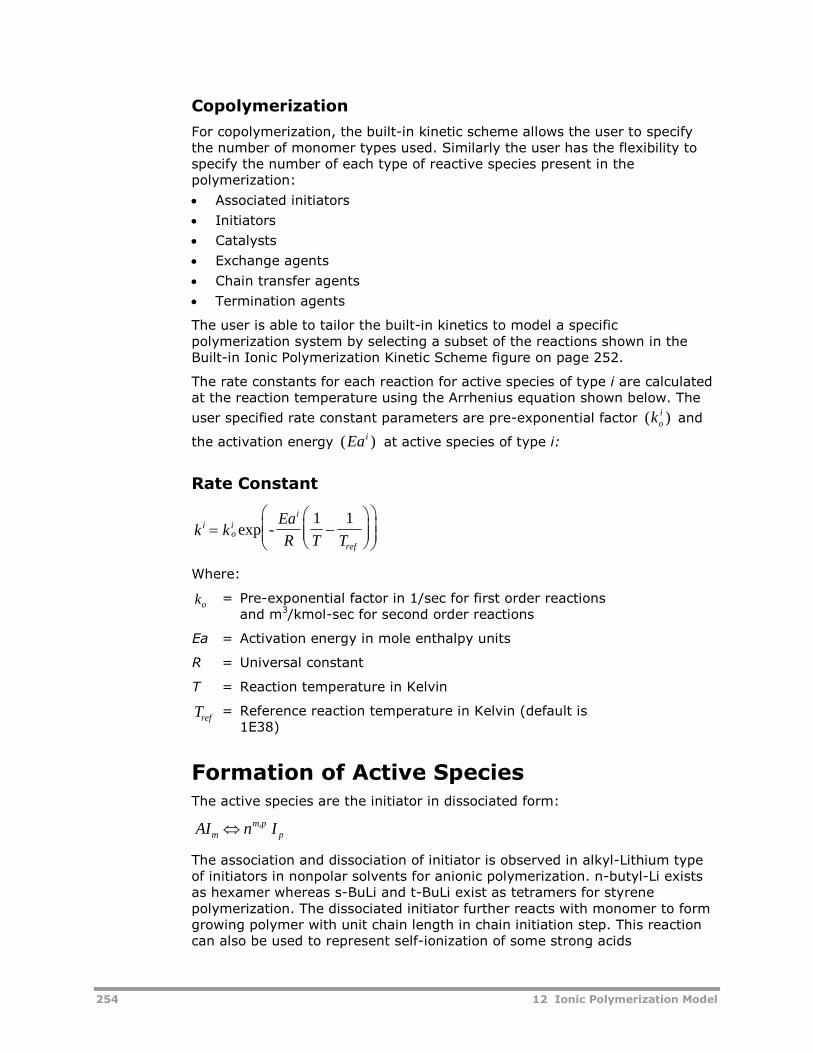
254 12 Ionic Polymerization Model
Copolymerization
For copolymerization, the built-in kinetic scheme allows the user to specifythe number of monomer types used. Similarly the user has the flexibility tospecify the number of each type of reactive species present in thepolymerization:
Associated initiators
Initiators
Catalysts
Exchange agents
Chain transfer agents
Termination agents
The user is able to tailor the built-in kinetics to model a specificpolymerization system by selecting a subset of the reactions shown in theBuilt-in Ionic Polymerization Kinetic Scheme figure on page 252.
The rate constants for each reaction for active species of type i are calculatedat the reaction temperature using the Arrhenius equation shown below. The
user specified rate constant parameters are pre-exponential factor ( )koi
and
the activation energy ( )Ea iat active species of type i:
Rate Constant
ioi
i
ref
k k -Ea
R T T
exp
1 1
Where:
ko= Pre-exponential factor in 1/sec for first order reactions
and m3/kmol-sec for second order reactions
Ea = Activation energy in mole enthalpy units
R = Universal constant
T = Reaction temperature in Kelvin
Tref= Reference reaction temperature in Kelvin (default is
1E38)
Formation of Active SpeciesThe active species are the initiator in dissociated form:
AI n Imm,p
p
The association and dissociation of initiator is observed in alkyl-Lithium typeof initiators in nonpolar solvents for anionic polymerization. n-butyl-Li existsas hexamer whereas s-BuLi and t-BuLi exist as tetramers for styrenepolymerization. The dissociated initiator further reacts with monomer to formgrowing polymer with unit chain length in chain initiation step. This reactioncan also be used to represent self-ionization of some strong acids
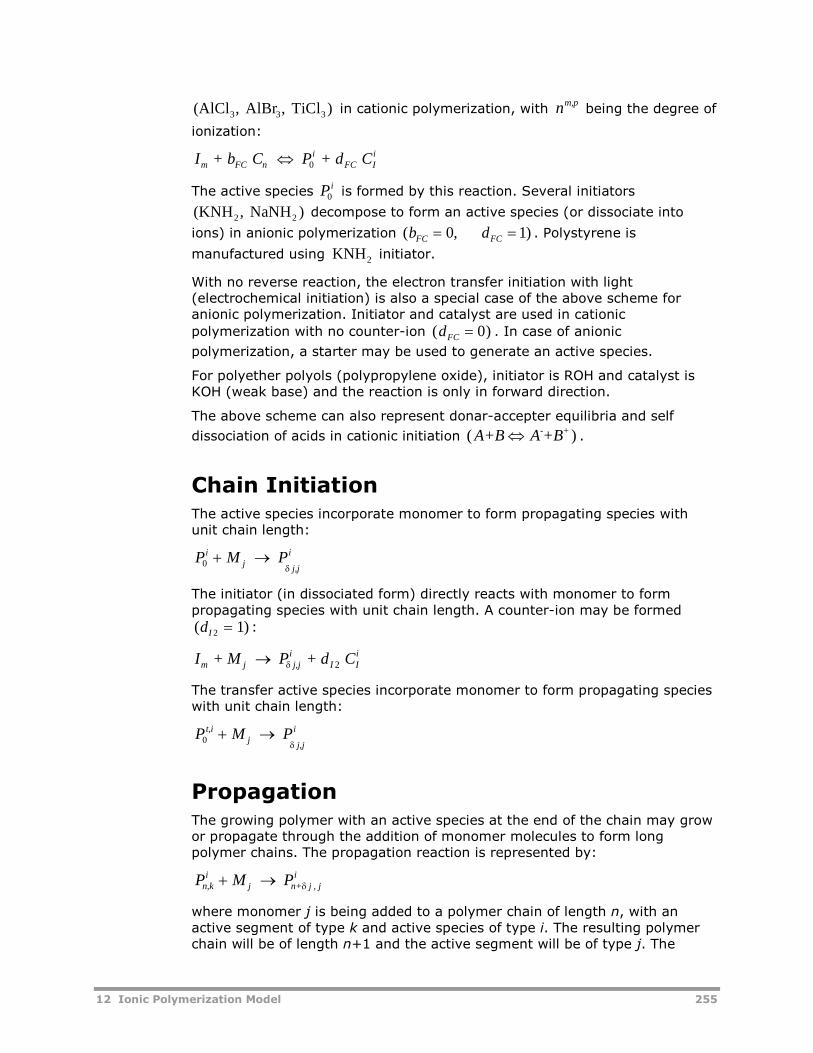
12 Ionic Polymerization Model 255
(AlCl , AlBr , TiCl )3 3 3 in cationic polymerization, with nm,pbeing the degree of
ionization:
I + b C P + d Cm FC ni
FC Ii 0
The active species P i0 is formed by this reaction. Several initiators
(KNH , NaNH2 2 ) decompose to form an active species (or dissociate into
ions) in anionic polymerization ( , )b dFC FC 0 1 . Polystyrene is
manufactured using KNH2 initiator.
With no reverse reaction, the electron transfer initiation with light(electrochemical initiation) is also a special case of the above scheme foranionic polymerization. Initiator and catalyst are used in cationic
polymerization with no counter-ion ( )dFC 0 . In case of anionic
polymerization, a starter may be used to generate an active species.
For polyether polyols (polypropylene oxide), initiator is ROH and catalyst isKOH (weak base) and the reaction is only in forward direction.
The above scheme can also represent donar-accepter equilibria and self
dissociation of acids in cationic initiation ( )A+B A +B- + .
Chain InitiationThe active species incorporate monomer to form propagating species withunit chain length:
P M Pij
j,j
i0
The initiator (in dissociated form) directly reacts with monomer to formpropagating species with unit chain length. A counter-ion may be formed
( )dI 2 1 :
I + M P + d Cm j j,ji
I Ii 2
The transfer active species incorporate monomer to form propagating specieswith unit chain length:
P M Pt,ij
j,j
i0
PropagationThe growing polymer with an active species at the end of the chain may growor propagate through the addition of monomer molecules to form longpolymer chains. The propagation reaction is represented by:
P M Pn,ki
j n+ j , ji
where monomer j is being added to a polymer chain of length n, with anactive segment of type k and active species of type i. The resulting polymerchain will be of length n+1 and the active segment will be of type j. The
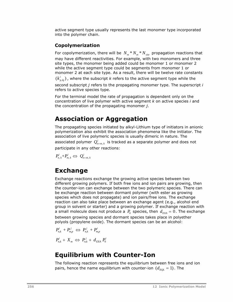
256 12 Ionic Polymerization Model
active segment type usually represents the last monomer type incorporatedinto the polymer chain.
Copolymerization
For copolymerization, there will be N N Nm m site* * propagation reactions that
may have different reactivities. For example, with two monomers and threesite types, the monomer being added could be monomer 1 or monomer 2while the active segment type could be segments from monomer 1 ormonomer 2 at each site type. As a result, there will be twelve rate constants
( ),k p kji
, where the subscript k refers to the active segment type while the
second subscript j refers to the propagating monomer type. The superscript irefers to active species type.
For the terminal model the rate of propagation is dependent only on theconcentration of live polymer with active segment k on active species i andthe concentration of the propagating monomer j.
Association or AggregationThe propagating species initiated by alkyl-Lithium type of initiators in anionicpolymerization also exhibit the association phenomena like the initiator. Theassociation of live polymeric species is usually dimeric in nature. The
associated polymer Qn m, ki is tracked as a separate polymer and does not
participate in any other reactions:
P +P Qn, ki
m, ki
n m, ki
ExchangeExchange reactions exchange the growing active species between twodifferent growing polymers. If both free ions and ion pairs are growing, thenthe counter-ion can exchange between the two polymeric species. There canbe exchange reaction between dormant polymer (with ester as growingspecies which does not propagate) and ion pairs/free ions. The exchangereaction can also take place between an exchange agent (e.g., alcohol endgroup in solvent or starter) and a growing polymer. If exchange reaction with
a small molecule does not produce a P0 species, then dEXA 0. The exchange
between growing species and dormant species takes place in polyetherpolyols (propylene oxide). The dormant species can be an alcohol:
P + P P + Pn,ki
m,pj
n,kj
m,pi
P X P d Pn,ki
m n,kj
EXAi 0
Equilibrium with Counter-IonThe following reaction represents the equilibrium between free ions and ion
pairs, hence the name equilibrium with counter-ion ( )dEQL 1 . The
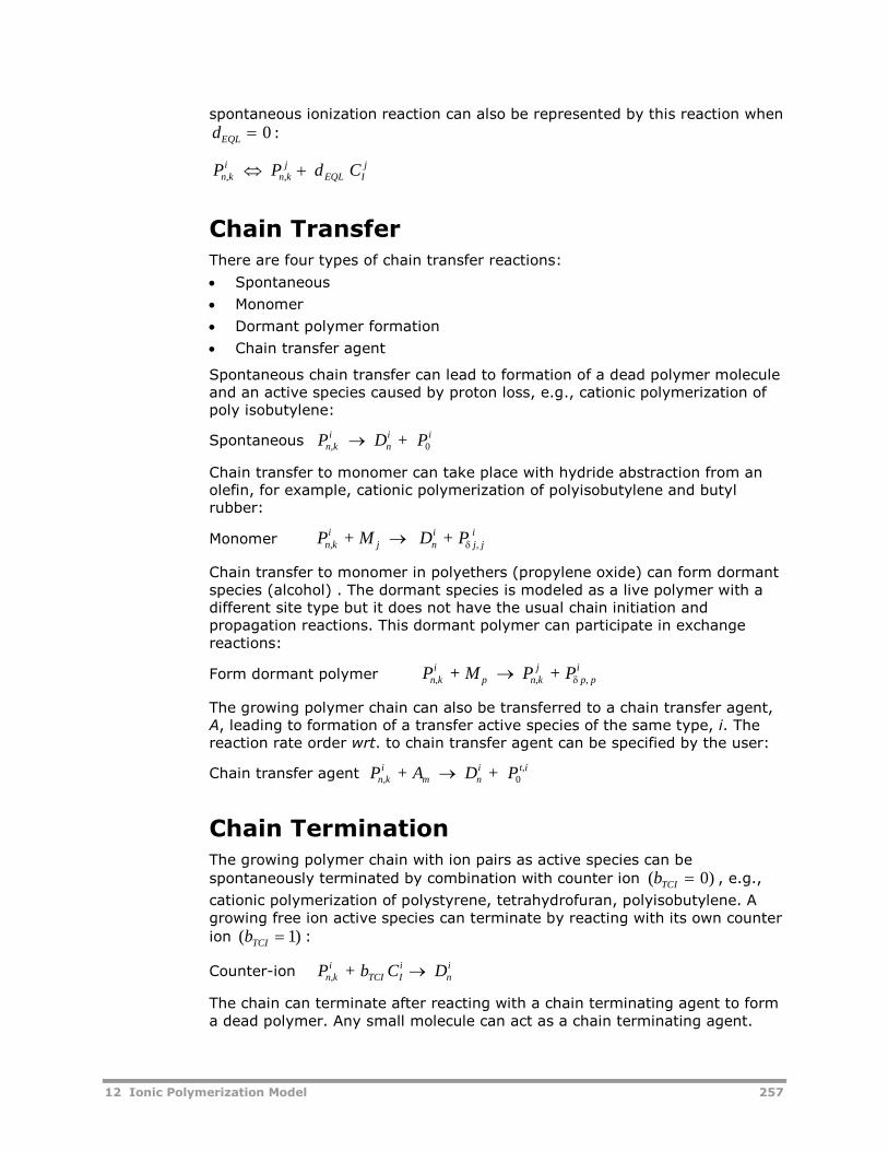
12 Ionic Polymerization Model 257
spontaneous ionization reaction can also be represented by this reaction when
dEQL 0 :
P P d Cn,ki
n,kj
EQL Ij
Chain TransferThere are four types of chain transfer reactions:
Spontaneous
Monomer
Dormant polymer formation
Chain transfer agent
Spontaneous chain transfer can lead to formation of a dead polymer moleculeand an active species caused by proton loss, e.g., cationic polymerization ofpoly isobutylene:
Spontaneous P D + Pn,ki
ni i 0
Chain transfer to monomer can take place with hydride abstraction from anolefin, for example, cationic polymerization of polyisobutylene and butylrubber:
Monomer P + M D + Pn,ki
j ni
j, ji
Chain transfer to monomer in polyethers (propylene oxide) can form dormantspecies (alcohol) . The dormant species is modeled as a live polymer with adifferent site type but it does not have the usual chain initiation andpropagation reactions. This dormant polymer can participate in exchangereactions:
Form dormant polymer P + M P + Pn,ki
p n,kj
p, pi
The growing polymer chain can also be transferred to a chain transfer agent,A, leading to formation of a transfer active species of the same type, i. Thereaction rate order wrt. to chain transfer agent can be specified by the user:
Chain transfer agent P + A D + Pn,ki
m ni t,i 0
Chain TerminationThe growing polymer chain with ion pairs as active species can be
spontaneously terminated by combination with counter ion ( )bTCI 0 , e.g.,
cationic polymerization of polystyrene, tetrahydrofuran, polyisobutylene. Agrowing free ion active species can terminate by reacting with its own counter
ion ( )bTCI 1 :
Counter-ion P + b C Dn,ki
TCI Ii
ni
The chain can terminate after reacting with a chain terminating agent to forma dead polymer. Any small molecule can act as a chain terminating agent.
258 12 Ionic Polymerization Model
The reaction rate order wrt. to terminating agent can be specified by theuser:
Terminating agent P +T Dn,ki
m ni
CouplingCoupling reactions are encountered in thermo-plastic elastomer production.For example, to make styrene-butadiene-styrene (SBS) TPE, styrene is addedfirst, and then half of the butadiene is added. Introducing a coupling agent tothis reaction system will form SBS polymer. In this example i=j=1 and k=2.
kmn
jm
in PPP
Another mechanism represented by this reaction is higher order association ofpolymeric chain. Dimeric association can be modeled by the associationreaction, but the coupling reaction should be used to model higher orderassociation of polymer chains. In a given simulation, the coupling andassociation reactions are mutually exclusive.
Model Features andAssumptionsFollowing are the model features and assumptions used in the ionicpolymerization model available in Aspen Polymers.
Phase EquilibriaThe polymerization model currently considers a single-phase system (vapor orliquid), two-phase system (vapor and liquid), or three-phase (VLL) systemwhen calculating concentrations for the reaction kinetics. For single-phasesystems, the reacting phase may be either vapor or liquid. In multi-phasesystems, reactions can occur in one or more phases simultaneously. Eachreaction object is associated with a single reacting phase, identified on theoptions form.
By default the reacting phase is assumed to be the liquid phase (for VLLsystems, the reacting phase must be specified). Several reaction models canbe referenced from a single reactor block to account for reactions in eachphase.
Rate CalculationsThe ionic polymerization kinetic model supplies to the reactor models thereaction rates for the components and the rate of change of polymerattributes (e.g. the chain length distribution moments) :
The component reaction rates are computed from the kinetic scheme bysumming over all reactions that involve the component.
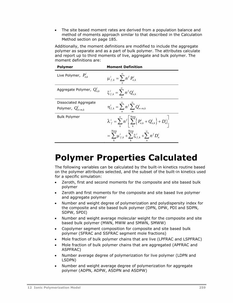
12 Ionic Polymerization Model 259
The site based moment rates are derived from a population balance andmethod of moments approach similar to that described in the CalculationMethod section on page 185.
Additionally, the moment definitions are modified to include the aggregatepolymer as separate and as a part of bulk polymer. The attributes calculateand report up to third moments of live, aggregate and bulk polymer. Themoment definitions are:
Polymer Moment Definition
Live Polymer, Pn,ki
f ki f
n ki
n
n P, ,
Aggregate Polymer, Qn,ki
f ki f
n ki
n
n Q, ,
Dissociated Aggregate
Polymer, Qn m ki ,
f ki f
n m ki
mn
n Q, ,
Bulk Polymer
fi f
kn ki
n ki
k
Nseg
ni
f ki
k
Nseg
f ki
k
Nsegf
ni
n
n P Q D
n D
, ,
, ,
Polymer Properties CalculatedThe following variables can be calculated by the built-in kinetics routine basedon the polymer attributes selected, and the subset of the built-in kinetics usedfor a specific simulation:
Zeroth, first and second moments for the composite and site based bulkpolymer
Zeroth and first moments for the composite and site based live polymerand aggregate polymer
Number and weight degree of polymerization and polydispersity index forthe composite and site based bulk polymer (DPN, DPW, PDI and SDPN,SDPW, SPDI)
Number and weight average molecular weight for the composite and sitebased bulk polymer (MWN, MWW and SMWN, SMWW)
Copolymer segment composition for composite and site based bulkpolymer (SFRAC and SSFRAC segment mole fractions)
Mole fraction of bulk polymer chains that are live (LPFRAC and LSPFRAC)
Mole fraction of bulk polymer chains that are aggregated (APFRAC andASPFRAC)
Number average degree of polymerization for live polymer (LDPN andLSDPN)
Number and weight average degree of polymerization for aggregatepolymer (ADPN, ADPW, ASDPN and ASDPW)
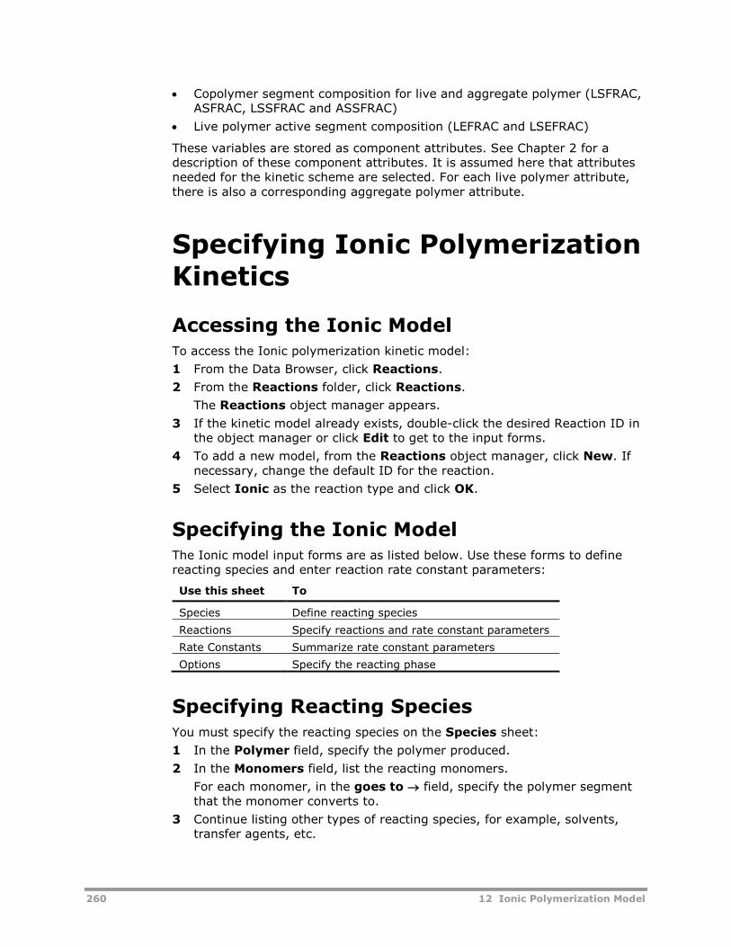
260 12 Ionic Polymerization Model
Copolymer segment composition for live and aggregate polymer (LSFRAC,ASFRAC, LSSFRAC and ASSFRAC)
Live polymer active segment composition (LEFRAC and LSEFRAC)
These variables are stored as component attributes. See Chapter 2 for adescription of these component attributes. It is assumed here that attributesneeded for the kinetic scheme are selected. For each live polymer attribute,there is also a corresponding aggregate polymer attribute.
Specifying Ionic PolymerizationKinetics
Accessing the Ionic ModelTo access the Ionic polymerization kinetic model:
1 From the Data Browser, click Reactions.
2 From the Reactions folder, click Reactions.
The Reactions object manager appears.
3 If the kinetic model already exists, double-click the desired Reaction ID inthe object manager or click Edit to get to the input forms.
4 To add a new model, from the Reactions object manager, click New. Ifnecessary, change the default ID for the reaction.
5 Select Ionic as the reaction type and click OK.
Specifying the Ionic ModelThe Ionic model input forms are as listed below. Use these forms to definereacting species and enter reaction rate constant parameters:
Use this sheet To
Species Define reacting species
Reactions Specify reactions and rate constant parameters
Rate Constants Summarize rate constant parameters
Options Specify the reacting phase
Specifying Reacting SpeciesYou must specify the reacting species on the Species sheet:
1 In the Polymer field, specify the polymer produced.
2 In the Monomers field, list the reacting monomers.
For each monomer, in the goes to field, specify the polymer segmentthat the monomer converts to.
3 Continue listing other types of reacting species, for example, solvents,transfer agents, etc.
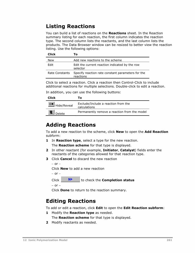
12 Ionic Polymerization Model 261
Listing ReactionsYou can build a list of reactions on the Reactions sheet. In the Reactionsummary listing for each reaction, the first column indicates the reactiontype. The second column lists the reactants, and the last column lists theproducts. The Data Browser window can be resized to better view the reactionlisting. Use the following options:
Click To
New Add new reactions to the scheme
Edit Edit the current reaction indicated by the rowselector
Rate Constants Specify reaction rate constant parameters for thereactions
Click to select a reaction. Click a reaction then Control-Click to includeadditional reactions for multiple selections. Double-click to edit a reaction.
In addition, you can use the following buttons:
Click To
Hide/RevealExclude/Include a reaction from thecalculations
DeletePermanently remove a reaction from the model
Adding ReactionsTo add a new reaction to the scheme, click New to open the Add Reactionsubform:
1 In Reaction type, select a type for the new reaction.
The Reaction scheme for that type is displayed.
2 In other reactant (for example, Initiator, Catalyst) fields enter thereactants of the categories allowed for that reaction type.
3 Click Cancel to discard the new reaction
or
Click New to add a new reaction
or
Click to check the Completion status
or
Click Done to return to the reaction summary.
Editing ReactionsTo add or edit a reaction, click Edit to open the Edit Reaction subform:
1 Modify the Reaction type as needed.
The Reaction scheme for that type is displayed.
2 Modify reactants as needed.
262 12 Ionic Polymerization Model
3 Click to check the Completion status
or
Click Done to return to the reaction summary.
Assigning Rate Constants to ReactionsTo assign rate constants to user reactions, click Rate Constants to open theRate Constant Parameters subform:
1 In the ko(fwd) or (rev) field, enter the pre-exponential factor forforward or reverse reaction.
2 In the Ea(fwd) or (rev) field, enter the activation energy for forward orreverse reaction.
3 In the Tref field, enter reference temperature.
4 In the Order field, enter the order.
5 In the Asso. No. field, enter the polymer association number.
6 In the Coeff. b and Coeff. d fields, enter coefficients b and d.
7 Click the stoichiometry list and select a new reaction. Enter rate constantsfor the new reaction. You can use the Prev and Next buttons to select theprevious or next reaction in the list.
8 Click the Summary tab to see a listing of all the rate constantparameters.
9 Click to check the Completion status
or
Click Close to return to the reaction summary.
ReferencesBiesenberger, J. A., & Sebastian, D. H. (1983). Principles of PolymerizationEngineering. New York: Wiley.
Bikales, M., Overberger, & Menges. (1985). Encyclopedia of Polymer Scienceand Engineering, 2nd Ed. New York: Wiley Interscience.
Chang, C. C., Miller, J. W., & Schorr, G. R. (1990). Fundamental Modeling inAnionic Polymerization Processes. J. of Appl. Pol. Sci., 39, 2395-2417.
Chang, C. C., Halasa, A. F., & Miller, J. W. (1993). The Reaction Engineeringof the Anionic Polymerization of Isoprene. J. of Appl. Pol. Sci., 47, 1589-1599.
Compton, R. G. (Ed.). (1992). Mechanism and Kinetics of AdditionPolymerizations. Comprehensive Chemical Kinetics, 31.
Fathi, H., Hamielec, A. E., & Davison, E. J. (1996). Modelling of AnionicSolution Polymerization of Butadiene - The Effects of Chain Termination andLong Chain Branching on Molecular Weight Distribution Development. PolymerReaction Eng., 4, No. 4.
12 Ionic Polymerization Model 263
Kennedy, J. P., & Squires, R. G. (1967). Contributions to the Mechanism ofIsobutene Polymerization I. Theory of Allylic Termination and KineticConsiderations. J. Macromol. Sci., A1(5), 805-829.
Kirk-Othmer. (1991). Encyclopedia of Chemical Technology, 4th Ed. NewYork: Wiley Interscience.
Moore, J. G., West, M. R., & Brooks, J. R. (1979). The Anionic SolutionPolymerization of Butadiene in a Stirred-Tank Reactor. ACS Symp. Ser., 104.
Muller, et. al. (1995). Kinetic-analysis of Living Polymerization Processesexhibiting slow equilibria. Application to group transfer and cationicpolymerizations. 5th International Workshop on Polymer ReactionEngineering, 131, 9-11 October, Berlin: DECHEMA.
Odian, G. (1981). Principles of Polymerization, 3rd Ed. New York: WileyInterscience.
Pepper, G. C. (1957). Cationic Polymerization. Proc. of the Intl. Symp. onMacromol. Chemistry. Prague.
Szwarc, M. (1996). Ionic Polymerization Fundamentals. New York: Hanser.
Treybig, M. N., & Anthony, R. G. (1979). Anionic Styrene Polymerization in aContinuous Stirred-Tank Reactor. ACS Symp. Ser., 104.

264 12 Ionic Polymerization Model
13 Segment-Based Reaction Model 265
13 Segment-Based ReactionModel
This section describes the segment-based power-law reaction model availablein Aspen Polymers (formerly known as Aspen Polymers Plus).
Topics covered include:
Summary of Applications, 265
Segment-Based Model Allowed Reactions, 267
Model Features and Assumptions, 272
Polymer Properties Calculated, 273
Specifying , 285
Summary of ApplicationsThe segment-based power-law reaction model can be used to simulatepolymerization reactions using a simple power-law type rate expression. Thismay be useful when simulating new processes that do not fit well into theother built-in models in Aspen Polymers, or when a very detailed mechanisticreaction model is not necessary.
The segment-based power-law model is the best choice for simulating step-growth addition processes—for example, the production of polyurethane.
This model may also be used to represent processes involving changes topolymer segments. The underlying kinetics are basic power law reactions inwhich segments and monomeric components may participate. Someexamples of applicable polymers are:
Polyvinyl alcohol (PVA) - Alcoholysis of polyvinylacetate
Chlorinated polyethylene (CPE) - Chlorination of polyethylene
Polymethylmethacrylate (PMMA) - Recovery of methylmethacrylate fromPMMA
Polyisobutylene - Chain scission of polyisobutylene
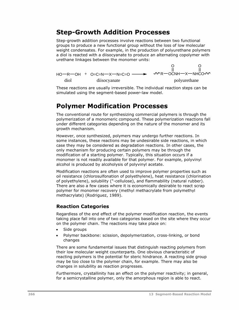
266 13 Segment-Based Reaction Model
Step-Growth Addition ProcessesStep-growth addition processes involve reactions between two functionalgroups to produce a new functional group without the loss of low molecularweight condensates. For example, in the production of polyurethane polymersa diol is reacted with a diisocyanate to produce an alternating copolymer withurethane linkages between the monomer units:
R OHHO X N=C=OO=C=N+ R OCNH
O
X NHCO
O
diol diisocyanate polyurethane
These reactions are usually irreversible. The individual reaction steps can besimulated using the segment-based power-law model.
Polymer Modification ProcessesThe conventional route for synthesizing commercial polymers is through thepolymerization of a monomeric compound. These polymerization reactions fallunder different categories depending on the nature of the monomer and itsgrowth mechanism.
However, once synthesized, polymers may undergo further reactions. Insome instances, these reactions may be undesirable side reactions, in whichcase they may be considered as degradation reactions. In other cases, theonly mechanism for producing certain polymers may be through themodification of a starting polymer. Typically, this situation occurs if amonomer is not readily available for that polymer. For example, polyvinylalcohol is produced by alcoholysis of polyvinyl acetate.
Modification reactions are often used to improve polymer properties such asoil resistance (chlorosulfonation of polyethylene), heat resistance (chlorinationof polyethylene), solubility ("-cellulose), and flammability (natural rubber).There are also a few cases where it is economically desirable to react scrappolymer for monomer recovery (methyl methacrylate from polymethylmethacrylate) (Rodriguez, 1989).
Reaction Categories
Regardless of the end effect of the polymer modification reaction, the eventstaking place fall into one of two categories based on the site where they occuron the polymer chain. The reactions may take place on:
Side groups
Polymer backbone: scission, depolymerization, cross-linking, or bondchanges
There are some fundamental issues that distinguish reacting polymers fromtheir low molecular weight counterparts. One obvious characteristic ofreacting polymers is the potential for steric hindrance. A reacting side groupmay be too close to the polymer chain, for example. There may also bechanges in solubility as reaction progresses.
Furthermore, crystallinity has an effect on the polymer reactivity; in general,for a semicrystalline polymer, only the amorphous region is able to react.
13 Segment-Based Reaction Model 267
Finally, an important difference that characterizes polymers is the fact that ahigher local concentration of reacting functional groups is observed than thatindicated by the overall polymer concentration (Odian, 1991).
Segment-Based Model AllowedReactionsThe reaction categories allowed in the segment-based reaction model, alongwith a brief summary of the conditions where each of these reactions mayoccur, is shown here:
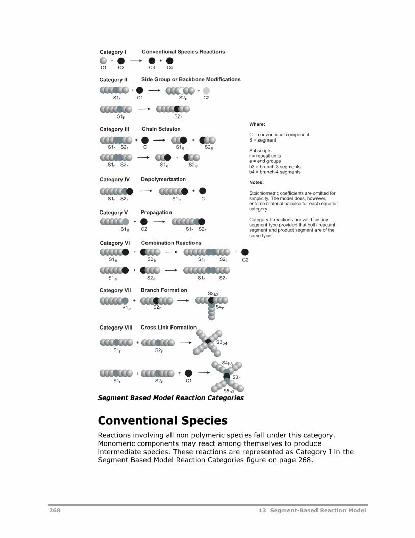
268 13 Segment-Based Reaction Model
Segment Based Model Reaction Categories
Conventional SpeciesReactions involving all non polymeric species fall under this category.Monomeric components may react among themselves to produceintermediate species. These reactions are represented as Category I in theSegment Based Model Reaction Categories figure on page 268.
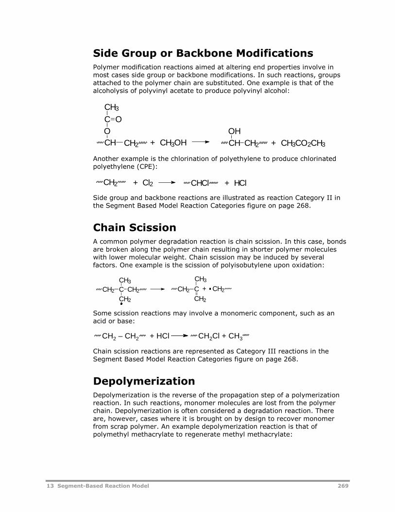
13 Segment-Based Reaction Model 269
Side Group or Backbone ModificationsPolymer modification reactions aimed at altering end properties involve inmost cases side group or backbone modifications. In such reactions, groupsattached to the polymer chain are substituted. One example is that of thealcoholysis of polyvinyl acetate to produce polyvinyl alcohol:
Another example is the chlorination of polyethylene to produce chlorinatedpolyethylene (CPE):
Side group and backbone reactions are illustrated as reaction Category II inthe Segment Based Model Reaction Categories figure on page 268.
Chain ScissionA common polymer degradation reaction is chain scission. In this case, bondsare broken along the polymer chain resulting in shorter polymer moleculeswith lower molecular weight. Chain scission may be induced by severalfactors. One example is the scission of polyisobutylene upon oxidation:
Some scission reactions may involve a monomeric component, such as anacid or base:
Chain scission reactions are represented as Category III reactions in theSegment Based Model Reaction Categories figure on page 268.
DepolymerizationDepolymerization is the reverse of the propagation step of a polymerizationreaction. In such reactions, monomer molecules are lost from the polymerchain. Depolymerization is often considered a degradation reaction. Thereare, however, cases where it is brought on by design to recover monomerfrom scrap polymer. An example depolymerization reaction is that ofpolymethyl methacrylate to regenerate methyl methacrylate:
+ CH3OH + CH3CO2CH3CH
CH3
C
O
O
CH2 CH CH2
OH
CH2 + Cl2 CHCl + HCl
CH2 C CH2
CH3
CH2
CH2 C
CH2
+ CH2
CH3
CH2 – CH2 + HCl CH2Cl + CH3
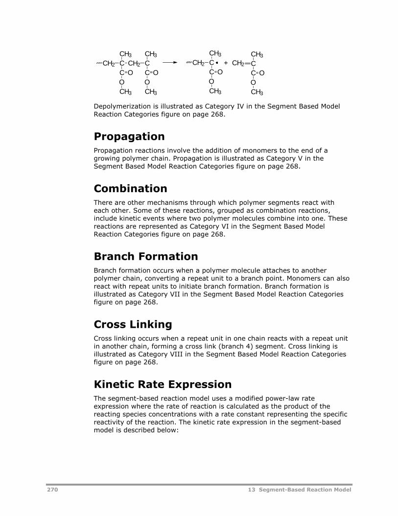
270 13 Segment-Based Reaction Model
Depolymerization is illustrated as Category IV in the Segment Based ModelReaction Categories figure on page 268.
PropagationPropagation reactions involve the addition of monomers to the end of agrowing polymer chain. Propagation is illustrated as Category V in theSegment Based Model Reaction Categories figure on page 268.
CombinationThere are other mechanisms through which polymer segments react witheach other. Some of these reactions, grouped as combination reactions,include kinetic events where two polymer molecules combine into one. Thesereactions are represented as Category VI in the Segment Based ModelReaction Categories figure on page 268.
Branch FormationBranch formation occurs when a polymer molecule attaches to anotherpolymer chain, converting a repeat unit to a branch point. Monomers can alsoreact with repeat units to initiate branch formation. Branch formation isillustrated as Category VII in the Segment Based Model Reaction Categoriesfigure on page 268.
Cross LinkingCross linking occurs when a repeat unit in one chain reacts with a repeat unitin another chain, forming a cross link (branch 4) segment. Cross linking isillustrated as Category VIII in the Segment Based Model Reaction Categoriesfigure on page 268.
Kinetic Rate ExpressionThe segment-based reaction model uses a modified power-law rateexpression where the rate of reaction is calculated as the product of thereacting species concentrations with a rate constant representing the specificreactivity of the reaction. The kinetic rate expression in the segment-basedmodel is described below:
CH2 C CH2 C
CH3 CH3
C O
O
CH3
C O
O
CH3
CH2 C
CH3
O
OC
CH3
+ CH2 C
CH3
C O
O
CH3
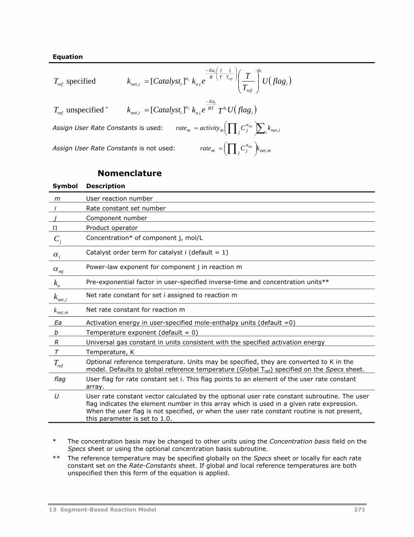
13 Segment-Based Reaction Model 271
Equation
Tref specified i
ref
b
TTR
Ea
o iiinet flagUT
TekCatalystk
i
ref
i
i
11
, ][
Tref unspecified * ibRT
Ea
o iiinet flagUTekCatalystk i
i
i
][,
Assign User Rate Constants is used:
i inetj
ajmm kCactivityrate mj
,
Assign User Rate Constants is not used: mnetj
ajm kCrate mj
,
Nomenclature
Symbol Description
m User reaction number
i Rate constant set number
j Component number
Product operator
C jConcentration* of component j, mol/L
i Catalyst order term for catalyst i (default = 1)
mj Power-law exponent for component j in reaction m
koPre-exponential factor in user-specified inverse-time and concentration units**
i,netk Net rate constant for set i assigned to reaction m
mnetk , Net rate constant for reaction m
Ea Activation energy in user-specified mole-enthalpy units (default =0)
b Temperature exponent (default = 0)
R Universal gas constant in units consistent with the specified activation energy
T Temperature, K
TrefOptional reference temperature. Units may be specified, they are converted to K in themodel. Defaults to global reference temperature (Global Tref) specified on the Specs sheet.
flag User flag for rate constant set i. This flag points to an element of the user rate constantarray.
U User rate constant vector calculated by the optional user rate constant subroutine. The userflag indicates the element number in this array which is used in a given rate expression.When the user flag is not specified, or when the user rate constant routine is not present,this parameter is set to 1.0.
* The concentration basis may be changed to other units using the Concentration basis field on theSpecs sheet or using the optional concentration basis subroutine.
** The reference temperature may be specified globally on the Specs sheet or locally for each rateconstant set on the Rate-Constants sheet. If global and local reference temperatures are bothunspecified then this form of the equation is applied.
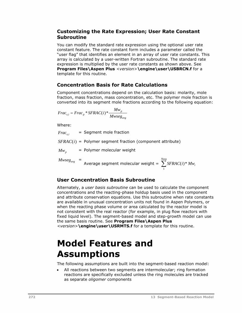
272 13 Segment-Based Reaction Model
Customizing the Rate Expression; User Rate ConstantSubroutine
You can modify the standard rate expression using the optional user rateconstant feature. The rate constant form includes a parameter called the“user flag” that identifies an element in an array of user rate constants. Thisarray is calculated by a user-written Fortran subroutine. The standard rateexpression is multiplied by the user rate constants as shown above. SeeProgram Files\Aspen Plus <version>\engine\user\USBRCN.f for atemplate for this routine.
Concentration Basis for Rate Calculations
Component concentrations depend on the calculation basis: molarity, molefraction, mass fraction, mass concentration, etc. The polymer mole fraction isconverted into its segment mole fractions according to the following equation:
Frac Frac SFRAC iMw
Mwsegs i p
p
avg, * ( )*
Where:
Fracs i,= Segment mole fraction
SFRAC i( ) = Polymer segment fraction (component attribute)
Mwp= Polymer molecular weight
Mwsegavg=
Average segment molecular weight = SFRAC i MwNseg
i( )*1
User Concentration Basis Subroutine
Alternately, a user basis subroutine can be used to calculate the componentconcentrations and the reacting-phase holdup basis used in the componentand attribute conservation equations. Use this subroutine when rate constantsare available in unusual concentration units not found in Aspen Polymers, orwhen the reacting phase volume or area calculated by the reactor model isnot consistent with the real reactor (for example, in plug flow reactors withfixed liquid level). The segment-based model and step-growth model can usethe same basis routine. See Program Files\Aspen Plus<version>\engine\user\USRMTS.f for a template for this routine.
Model Features andAssumptionsThe following assumptions are built into the segment-based reaction model:
All reactions between two segments are intermolecular; ring formationreactions are specifically excluded unless the ring molecules are trackedas separate oligomer components
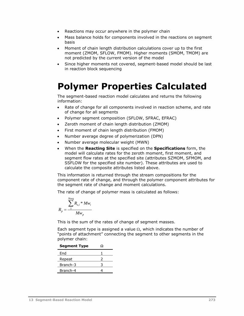
13 Segment-Based Reaction Model 273
Reactions may occur anywhere in the polymer chain
Mass balance holds for components involved in the reactions on segmentbasis
Moment of chain length distribution calculations cover up to the firstmoment (ZMOM, SFLOW, FMOM). Higher moments (SMOM, TMOM) arenot predicted by the current version of the model
Since higher moments not covered, segment-based model should be lastin reaction block sequencing
Polymer Properties CalculatedThe segment-based reaction model calculates and returns the followinginformation:
Rate of change for all components involved in reaction scheme, and rateof change for all segments
Polymer segment composition (SFLOW, SFRAC, EFRAC)
Zeroth moment of chain length distribution (ZMOM)
First moment of chain length distribution (FMOM)
Number average degree of polymerization (DPN)
Number average molecular weight (MWN)
When the Reacting Site is specified on the Specifications form, themodel will calculate rates for the zeroth moment, first moment, andsegment flow rates at the specified site (attributes SZMOM, SFMOM, andSSFLOW for the specified site number). These attributes are used tocalculate the composite attributes listed above.
This information is returned through the stream compositions for thecomponent rate of change, and through the polymer component attributes forthe segment rate of change and moment calculations.
The rate of change of polymer mass is calculated as follows:
R
R Mw
Mwp
s i i
Nseg
p
, *
1
This is the sum of the rates of change of segment masses.
Each segment type is assigned a value , which indicates the number of“points of attachment” connecting the segment to other segments in thepolymer chain:
Segment Type
End 1
Repeat 2
Branch-3 3
Branch-4 4
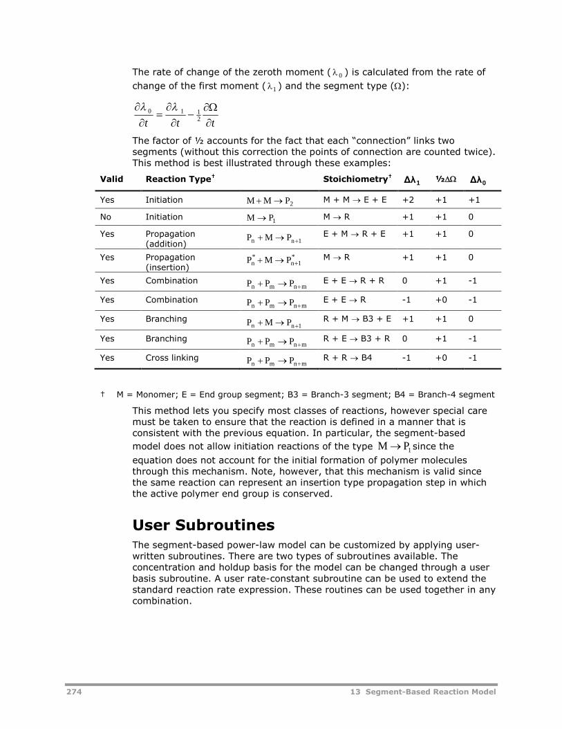
274 13 Segment-Based Reaction Model
The rate of change of the zeroth moment ( 0 ) is calculated from the rate of
change of the first moment ( 1 ) and the segment type ():
ttt
2110
The factor of ½ accounts for the fact that each “connection” links twosegments (without this correction the points of connection are counted twice).This method is best illustrated through these examples:
Valid Reaction Type† Stoichiometry†1Δλ ½ 0Δλ
Yes Initiation 2PMM M + M E + E +2 +1 +1
No Initiation 1PM M R +1 +1 0
Yes Propagation(addition) 1nn PMP E + M R + E +1 +1 0
Yes Propagation(insertion)
*1n
*n PMP M R +1 +1 0
Yes Combinationmnmn PPP E + E R + R 0 +1 -1
Yes Combinationmnmn PPP E + E R -1 +0 -1
Yes Branching1nn PMP R + M B3 + E +1 +1 0
Yes Branchingmnmn PPP R + E B3 + R 0 +1 -1
Yes Cross linkingmnmn PPP R + R B4 -1 +0 -1
† M = Monomer; E = End group segment; B3 = Branch-3 segment; B4 = Branch-4 segment
This method lets you specify most classes of reactions, however special caremust be taken to ensure that the reaction is defined in a manner that isconsistent with the previous equation. In particular, the segment-based
model does not allow initiation reactions of the type 1PM since the
equation does not account for the initial formation of polymer moleculesthrough this mechanism. Note, however, that this mechanism is valid sincethe same reaction can represent an insertion type propagation step in whichthe active polymer end group is conserved.
User SubroutinesThe segment-based power-law model can be customized by applying user-written subroutines. There are two types of subroutines available. Theconcentration and holdup basis for the model can be changed through a userbasis subroutine. A user rate-constant subroutine can be used to extend thestandard reaction rate expression. These routines can be used together in anycombination.
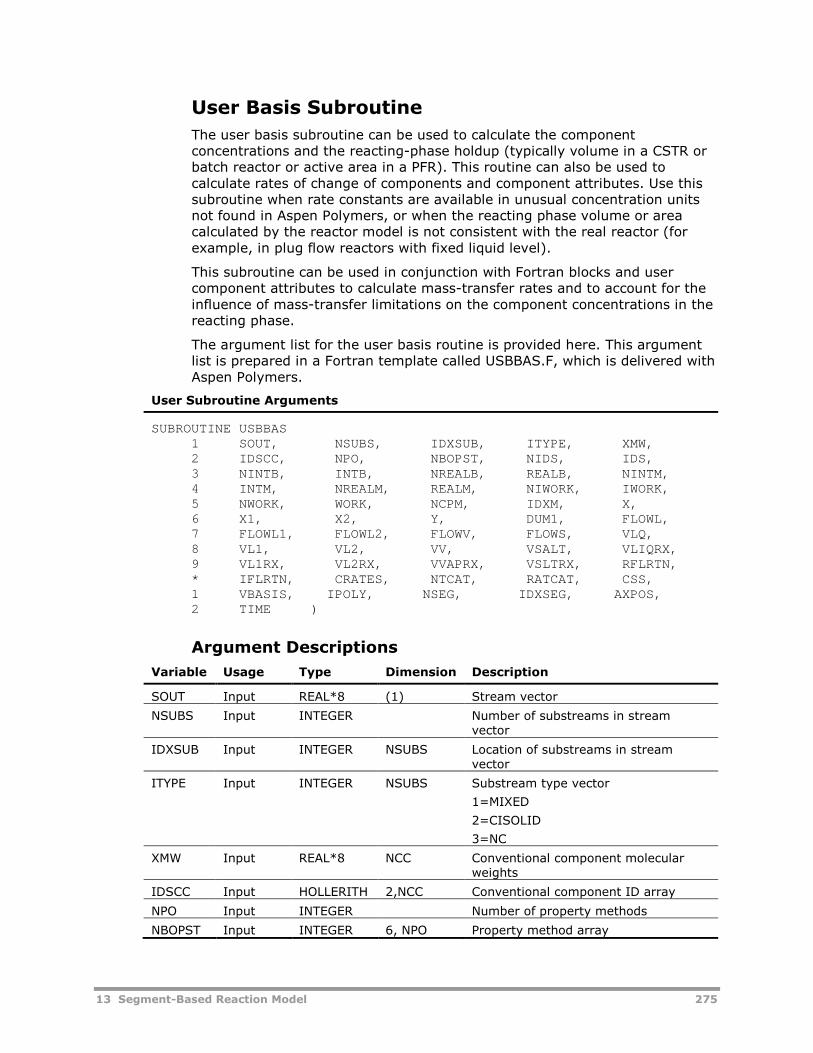
13 Segment-Based Reaction Model 275
User Basis Subroutine
The user basis subroutine can be used to calculate the componentconcentrations and the reacting-phase holdup (typically volume in a CSTR orbatch reactor or active area in a PFR). This routine can also be used tocalculate rates of change of components and component attributes. Use thissubroutine when rate constants are available in unusual concentration unitsnot found in Aspen Polymers, or when the reacting phase volume or areacalculated by the reactor model is not consistent with the real reactor (forexample, in plug flow reactors with fixed liquid level).
This subroutine can be used in conjunction with Fortran blocks and usercomponent attributes to calculate mass-transfer rates and to account for theinfluence of mass-transfer limitations on the component concentrations in thereacting phase.
The argument list for the user basis routine is provided here. This argumentlist is prepared in a Fortran template called USBBAS.F, which is delivered withAspen Polymers.
User Subroutine Arguments
SUBROUTINE USBBAS1 SOUT, NSUBS, IDXSUB, ITYPE, XMW,2 IDSCC, NPO, NBOPST, NIDS, IDS,3 NINTB, INTB, NREALB, REALB, NINTM,4 INTM, NREALM, REALM, NIWORK, IWORK,5 NWORK, WORK, NCPM, IDXM, X,6 X1, X2, Y, DUM1, FLOWL,7 FLOWL1, FLOWL2, FLOWV, FLOWS, VLQ,8 VL1, VL2, VV, VSALT, VLIQRX,9 VL1RX, VL2RX, VVAPRX, VSLTRX, RFLRTN,* IFLRTN, CRATES, NTCAT, RATCAT, CSS,1 VBASIS, IPOLY, NSEG, IDXSEG, AXPOS,2 TIME )
Argument Descriptions
Variable Usage Type Dimension Description
SOUT Input REAL*8 (1) Stream vector
NSUBS Input INTEGER Number of substreams in streamvector
IDXSUB Input INTEGER NSUBS Location of substreams in streamvector
ITYPE Input INTEGER NSUBS Substream type vector
1=MIXED
2=CISOLID
3=NC
XMW Input REAL*8 NCC Conventional component molecularweights
IDSCC Input HOLLERITH 2,NCC Conventional component ID array
NPO Input INTEGER Number of property methods
NBOPST Input INTEGER 6, NPO Property method array
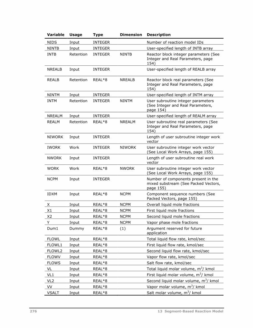
276 13 Segment-Based Reaction Model
Variable Usage Type Dimension Description
NIDS Input INTEGER Number of reaction model IDs
NINTB Input INTEGER User-specified length of INTB array
INTB Retention INTEGER NINTB Reactor block integer parameters (SeeInteger and Real Parameters, page154)
NREALB Input INTEGER User-specified length of REALB array
REALB Retention REAL*8 NREALB Reactor block real parameters (SeeInteger and Real Parameters, page154)
NINTM Input INTEGER User-specified length of INTM array
INTM Retention INTEGER NINTM User subroutine integer parameters(See Integer and Real Parameters,page 154)
NREALM Input INTEGER User-specified length of REALM array
REALM Retention REAL*8 NREALM User subroutine real parameters (SeeInteger and Real Parameters, page154)
NIWORK Input INTEGER Length of user subroutine integer workvector
IWORK Work INTEGER NIWORK User subroutine integer work vector(See Local Work Arrays, page 155)
NWORK Input INTEGER Length of user subroutine real workvector
WORK Work REAL*8 NWORK User subroutine integer work vector(See Local Work Arrays, page 155)
NCPM Input INTEGER Number of components present in themixed substream (See Packed Vectors,page 155)
IDXM Input REAL*8 NCPM Component sequence numbers (SeePacked Vectors, page 155)
X Input REAL*8 NCPM Overall liquid mole fractions
X1 Input REAL*8 NCPM First liquid mole fractions
X2 Input REAL*8 NCPM Second liquid mole fractions
Y Input REAL*8 NCPM Vapor phase mole fractions
Dum1 Dummy REAL*8 (1) Argument reserved for futureapplication
FLOWL Input REAL*8 Total liquid flow rate, kmol/sec
FLOWL1 Input REAL*8 First liquid flow rate, kmol/sec
FLOWL2 Input REAL*8 Second liquid flow rate, kmol/sec
FLOWV Input REAL*8 Vapor flow rate, kmol/sec
FLOWS Input REAL*8 Salt flow rate, kmol/sec
VL Input REAL*8 Total liquid molar volume, m3/ kmol
VL1 Input REAL*8 First liquid molar volume, m3/ kmol
VL2 Input REAL*8 Second liquid molar volume, m3/ kmol
VV Input REAL*8 Vapor molar volume, m3/ kmol
VSALT Input REAL*8 Salt molar volume, m3/ kmol
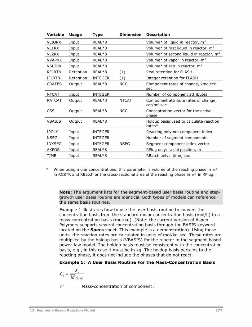
13 Segment-Based Reaction Model 277
Variable Usage Type Dimension Description
VLIQRX Input REAL*8 Volume* of liquid in reactor, m3
VL1RX Input REAL*8 Volume* of first liquid in reactor, m3
VL2RX Input REAL*8 Volume* of second liquid in reactor, m3
VVAPRX Input REAL*8 Volume* of vapor in reactor, m3
VSLTRX Input REAL*8 Volume* of salt in reactor, m3
RFLRTN Retention REAL*8 (1) Real retention for FLASH
IFLRTN Retention INTEGER (1) Integer retention for FLASH
CRATES Output REAL*8 NCC Component rates of change, kmol/m3-sec
NTCAT Input INTEGER Number of component attributes
RATCAT Output REAL*8 NTCAT Component attribute rates of change,cat/m3-sec
CSS Output REAL*8 NCC Concentration vector for the activephase
VBASIS Output REAL*8 Holdup basis used to calculate reactionrates*
IPOLY Input INTEGER Reacting polymer component index
NSEG Input INTEGER Number of segment components
IDXSEG Input INTEGER NSEG Segment component index vector
AXPOS Input REAL*8 RPlug only: axial position, m
TIME Input REAL*8 RBatch only: time, sec
* When using molar concentrations, this parameter is volume of the reacting phase in 3m
in RCSTR and RBatch or the cross-sectional area of the reacting phase in 2m in RPlug.
Note: The argument lists for the segment-based user basis routine and step-growth user basis routine are identical. Both types of models can referencethe same basis routines.
Example 1 illustrates how to use the user basis routine to convert theconcentration basis from the standard molar concentration basis (mol/L) to amass concentration basis (mol/kg). (Note: the current version of AspenPolymers supports several concentration basis through the BASIS keywordlocated on the Specs sheet. This example is a demonstration). Using theseunits, the reaction rates are calculated in units of mol/kg-sec. These rates aremultiplied by the holdup basis (VBASIS) for the reactor in the segment-basedpower-law model. The holdup basis must be consistent with the concentrationbasis, e.g., in this case it must be in kg. The holdup basis pertains to thereacting phase, it does not include the phases that do not react.
Example 1: A User Basis Routine For the Mass-Concentration Basis
CX
Mii
Liquid
Ci= Mass-concentration of component i
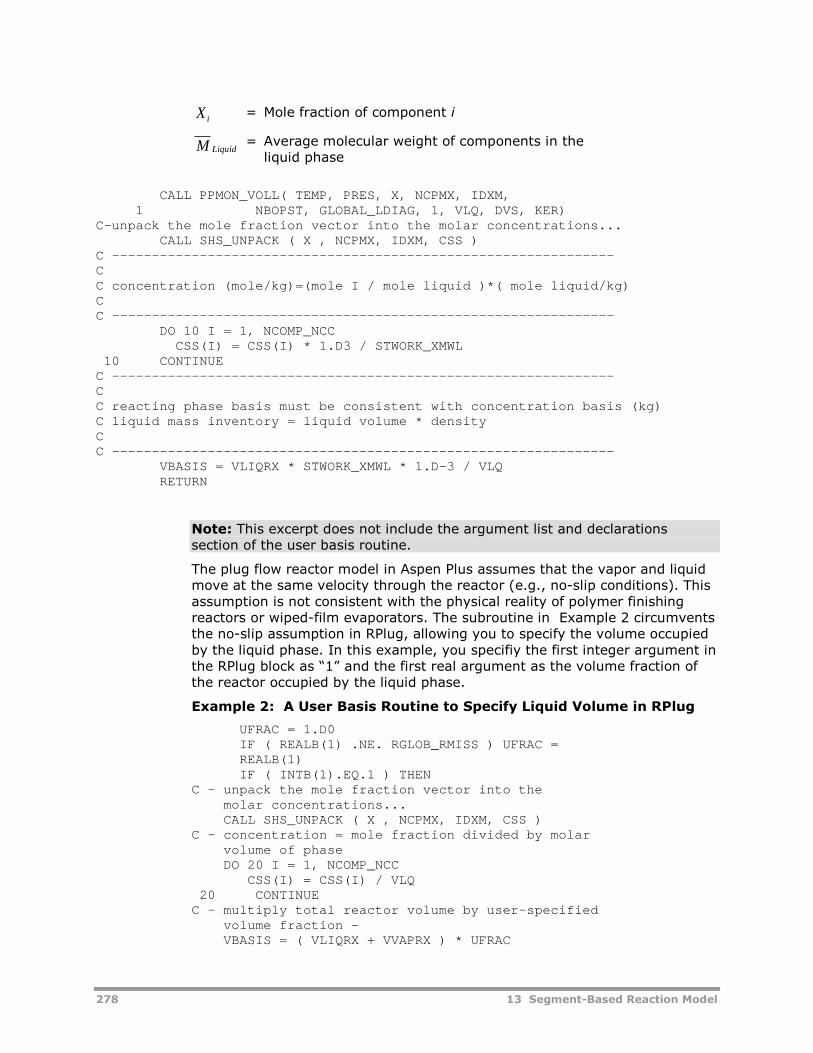
278 13 Segment-Based Reaction Model
X i= Mole fraction of component i
M Liquid= Average molecular weight of components in the
liquid phase
CALL PPMON_VOLL( TEMP, PRES, X, NCPMX, IDXM,1 NBOPST, GLOBAL_LDIAG, 1, VLQ, DVS, KER)
C-unpack the mole fraction vector into the molar concentrations...CALL SHS_UNPACK ( X , NCPMX, IDXM, CSS )
C ---------------------------------------------------------------CC concentration (mole/kg)=(mole I / mole liquid )*( mole liquid/kg)CC ---------------------------------------------------------------
DO 10 I = 1, NCOMP_NCCCSS(I) = CSS(I) * 1.D3 / STWORK_XMWL
10 CONTINUEC ---------------------------------------------------------------CC reacting phase basis must be consistent with concentration basis (kg)C liquid mass inventory = liquid volume * densityCC ---------------------------------------------------------------
VBASIS = VLIQRX * STWORK_XMWL * 1.D-3 / VLQRETURN
Note: This excerpt does not include the argument list and declarationssection of the user basis routine.
The plug flow reactor model in Aspen Plus assumes that the vapor and liquidmove at the same velocity through the reactor (e.g., no-slip conditions). Thisassumption is not consistent with the physical reality of polymer finishingreactors or wiped-film evaporators. The subroutine in Example 2 circumventsthe no-slip assumption in RPlug, allowing you to specify the volume occupiedby the liquid phase. In this example, you specifiy the first integer argument inthe RPlug block as “1” and the first real argument as the volume fraction ofthe reactor occupied by the liquid phase.
Example 2: A User Basis Routine to Specify Liquid Volume in RPlug
UFRAC = 1.D0IF ( REALB(1) .NE. RGLOB_RMISS ) UFRAC =REALB(1)IF ( INTB(1).EQ.1 ) THEN
C - unpack the mole fraction vector into themolar concentrations...CALL SHS_UNPACK ( X , NCPMX, IDXM, CSS )
C - concentration = mole fraction divided by molarvolume of phaseDO 20 I = 1, NCOMP_NCC
CSS(I) = CSS(I) / VLQ20 CONTINUE
C - multiply total reactor volume by user-specifiedvolume fraction -VBASIS = ( VLIQRX + VVAPRX ) * UFRAC
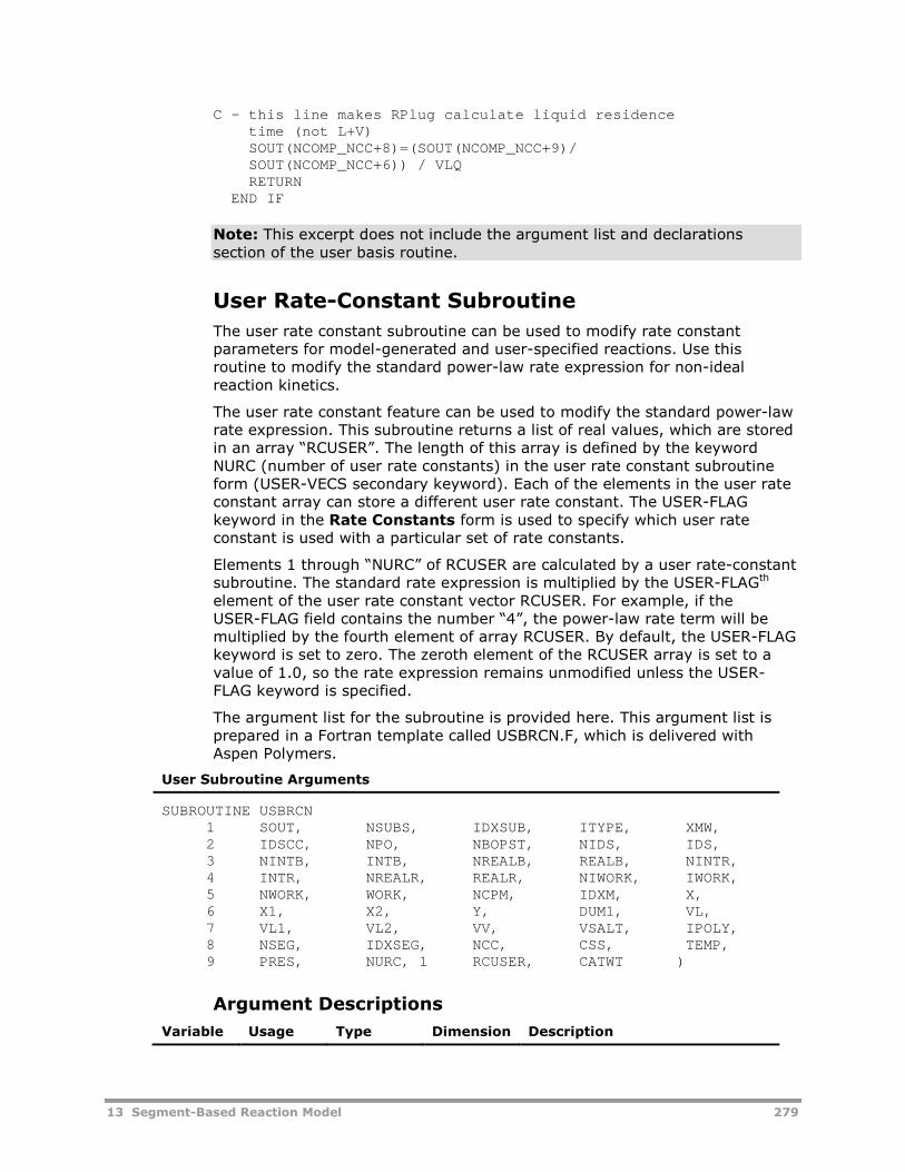
13 Segment-Based Reaction Model 279
C - this line makes RPlug calculate liquid residencetime (not L+V)SOUT(NCOMP_NCC+8)=(SOUT(NCOMP_NCC+9)/SOUT(NCOMP_NCC+6)) / VLQRETURN
END IF
Note: This excerpt does not include the argument list and declarationssection of the user basis routine.
User Rate-Constant Subroutine
The user rate constant subroutine can be used to modify rate constantparameters for model-generated and user-specified reactions. Use thisroutine to modify the standard power-law rate expression for non-idealreaction kinetics.
The user rate constant feature can be used to modify the standard power-lawrate expression. This subroutine returns a list of real values, which are storedin an array “RCUSER”. The length of this array is defined by the keywordNURC (number of user rate constants) in the user rate constant subroutineform (USER-VECS secondary keyword). Each of the elements in the user rateconstant array can store a different user rate constant. The USER-FLAGkeyword in the Rate Constants form is used to specify which user rateconstant is used with a particular set of rate constants.
Elements 1 through “NURC” of RCUSER are calculated by a user rate-constantsubroutine. The standard rate expression is multiplied by the USER-FLAGth
element of the user rate constant vector RCUSER. For example, if theUSER-FLAG field contains the number “4”, the power-law rate term will bemultiplied by the fourth element of array RCUSER. By default, the USER-FLAGkeyword is set to zero. The zeroth element of the RCUSER array is set to avalue of 1.0, so the rate expression remains unmodified unless the USER-FLAG keyword is specified.
The argument list for the subroutine is provided here. This argument list isprepared in a Fortran template called USBRCN.F, which is delivered withAspen Polymers.
User Subroutine Arguments
SUBROUTINE USBRCN1 SOUT, NSUBS, IDXSUB, ITYPE, XMW,2 IDSCC, NPO, NBOPST, NIDS, IDS,3 NINTB, INTB, NREALB, REALB, NINTR,4 INTR, NREALR, REALR, NIWORK, IWORK,5 NWORK, WORK, NCPM, IDXM, X,6 X1, X2, Y, DUM1, VL,7 VL1, VL2, VV, VSALT, IPOLY,8 NSEG, IDXSEG, NCC, CSS, TEMP,9 PRES, NURC, 1 RCUSER, CATWT )
Argument Descriptions
Variable Usage Type Dimension Description
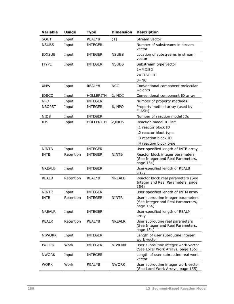
280 13 Segment-Based Reaction Model
Variable Usage Type Dimension Description
SOUT Input REAL*8 (1) Stream vector
NSUBS Input INTEGER Number of substreams in streamvector
IDXSUB Input INTEGER NSUBS Location of substreams in streamvector
ITYPE Input INTEGER NSUBS Substream type vector
1=MIXED
2=CISOLID
3=NC
XMW Input REAL*8 NCC Conventional component molecularweights
IDSCC Input HOLLERITH 2, NCC Conventional component ID array
NPO Input INTEGER Number of property methods
NBOPST Input INTEGER 6, NPO Property method array (used byFLASH)
NIDS Input INTEGER Number of reaction model IDs
IDS Input HOLLERITH 2,NIDS Reaction model ID list:
i,1 reactor block ID
i,2 reactor block type
i,3 reaction block ID
i,4 reaction block type
NINTB Input INTEGER User-specified length of INTB array
INTB Retention INTEGER NINTB Reactor block integer parameters(See Integer and Real Parameters,page 154)
NREALB Input INTEGER User-specified length of REALBarray
REALB Retention REAL*8 NREALB Reactor block real parameters (SeeInteger and Real Parameters, page154)
NINTR Input INTEGER User-specified length of INTM array
INTR Retention INTEGER NINTR User subroutine integer parameters(See Integer and Real Parameters,page 154)
NREALR Input INTEGER User-specified length of REALMarray
REALR Retention REAL*8 NREALR User subroutine real parameters(See Integer and Real Parameters,page 154)
NIWORK Input INTEGER Length of user subroutine integerwork vector
IWORK Work INTEGER NIWORK User subroutine integer work vector(See Local Work Arrays, page 155)
NWORK Input INTEGER Length of user subroutine real workvector
WORK Work REAL*8 NWORK User subroutine integer work vector(See Local Work Arrays, page 155)
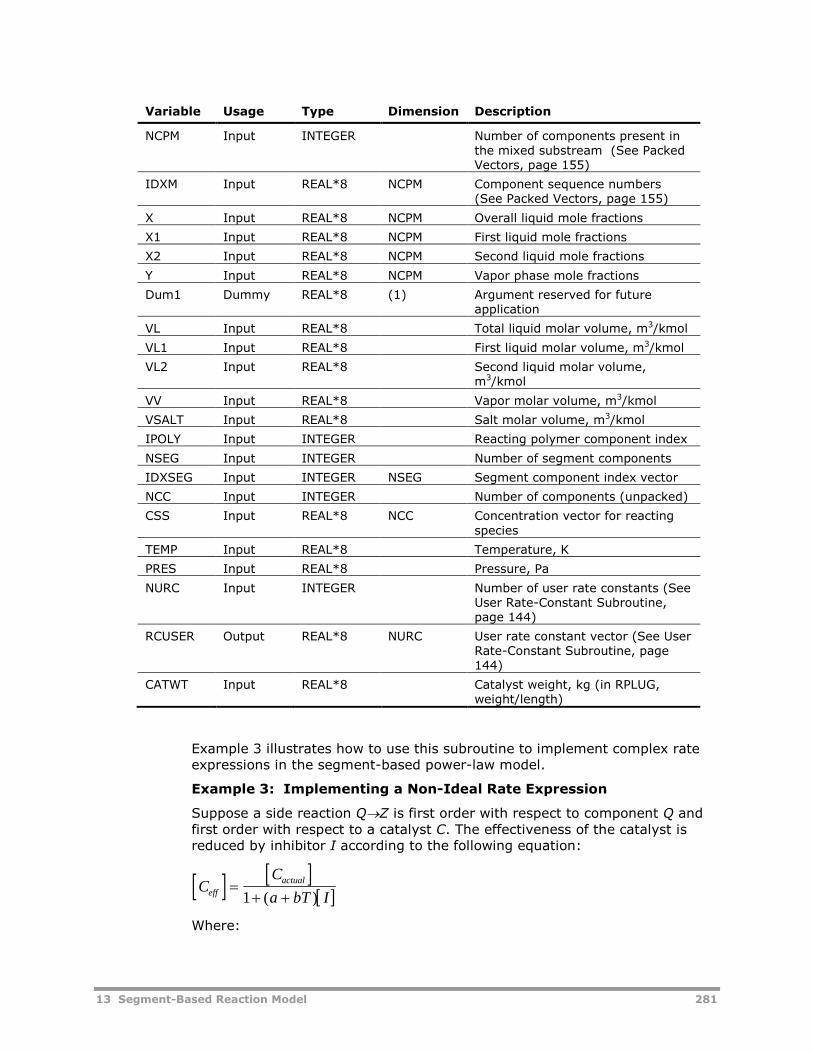
13 Segment-Based Reaction Model 281
Variable Usage Type Dimension Description
NCPM Input INTEGER Number of components present inthe mixed substream (See PackedVectors, page 155)
IDXM Input REAL*8 NCPM Component sequence numbers(See Packed Vectors, page 155)
X Input REAL*8 NCPM Overall liquid mole fractions
X1 Input REAL*8 NCPM First liquid mole fractions
X2 Input REAL*8 NCPM Second liquid mole fractions
Y Input REAL*8 NCPM Vapor phase mole fractions
Dum1 Dummy REAL*8 (1) Argument reserved for futureapplication
VL Input REAL*8 Total liquid molar volume, m3/kmol
VL1 Input REAL*8 First liquid molar volume, m3/kmol
VL2 Input REAL*8 Second liquid molar volume,m3/kmol
VV Input REAL*8 Vapor molar volume, m3/kmol
VSALT Input REAL*8 Salt molar volume, m3/kmol
IPOLY Input INTEGER Reacting polymer component index
NSEG Input INTEGER Number of segment components
IDXSEG Input INTEGER NSEG Segment component index vector
NCC Input INTEGER Number of components (unpacked)
CSS Input REAL*8 NCC Concentration vector for reactingspecies
TEMP Input REAL*8 Temperature, K
PRES Input REAL*8 Pressure, Pa
NURC Input INTEGER Number of user rate constants (SeeUser Rate-Constant Subroutine,page 144)
RCUSER Output REAL*8 NURC User rate constant vector (See UserRate-Constant Subroutine, page144)
CATWT Input REAL*8 Catalyst weight, kg (in RPLUG,weight/length)
Example 3 illustrates how to use this subroutine to implement complex rateexpressions in the segment-based power-law model.
Example 3: Implementing a Non-Ideal Rate Expression
Suppose a side reaction QZ is first order with respect to component Q andfirst order with respect to a catalyst C. The effectiveness of the catalyst isreduced by inhibitor I according to the following equation:
CC
a bT Ieff
actual
1 ( )
Where:
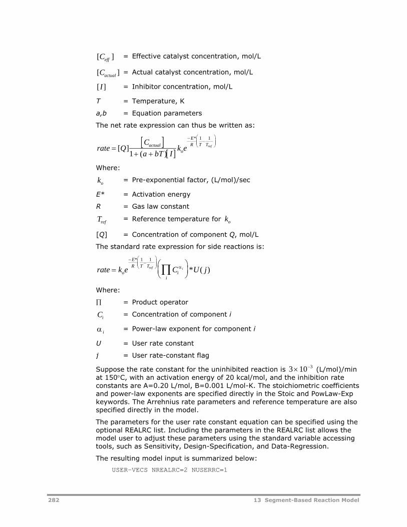
282 13 Segment-Based Reaction Model
[ ]Ceff= Effective catalyst concentration, mol/L
[ ]Cactual= Actual catalyst concentration, mol/L
[ ]I = Inhibitor concentration, mol/L
T = Temperature, K
a,b = Equation parameters
The net rate expression can thus be written as:
rate QC
a bT Ik e
actual
o
E
R T Tref
[ ]( )
*
1
1 1
Where:
ko= Pre-exponential factor, (L/mol)/sec
E* = Activation energy
R = Gas law constant
Tref= Reference temperature for ko
[Q] = Concentration of component Q, mol/L
The standard rate expression for side reactions is:
rate k e C U jo
E
R T T
ii
ref i
*
* ( )
1 1
Where:
= Product operator
Ci= Concentration of component i
i= Power-law exponent for component i
U = User rate constant
j = User rate-constant flag
Suppose the rate constant for the uninhibited reaction is 3 10 3 (L/mol)/min
at 150C, with an activation energy of 20 kcal/mol, and the inhibition rateconstants are A=0.20 L/mol, B=0.001 L/mol-K. The stoichiometric coefficientsand power-law exponents are specified directly in the Stoic and PowLaw-Expkeywords. The Arrehnius rate parameters and reference temperature are alsospecified directly in the model.
The parameters for the user rate constant equation can be specified using theoptional REALRC list. Including the parameters in the REALRC list allows themodel user to adjust these parameters using the standard variable accessingtools, such as Sensitivity, Design-Specification, and Data-Regression.
The resulting model input is summarized below:
USER-VECS NREALRC=2 NUSERRC=1
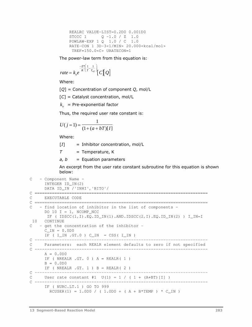
13 Segment-Based Reaction Model 283
REALRC VALUE-LIST=0.2D0 0.001D0STOIC 1 Q -1.0 / Z 1.0POWLAW-EXP 1 Q 1.0 / C 1.0RATE-CON 1 3D-3<1/MIN> 20.000<kcal/mol>TREF=150.0<C> URATECON=1
The power-law term from this equation is:
rate k e C Qo
E
R T Tref
* 1 1
Where:
[Q] = Concentration of component Q, mol/L
[C] = Catalyst concentration, mol/L
ko = Pre-exponential factor
Thus, the required user rate constant is:
U ja bT I
( )( ( )[ ]
11
1
Where:
[I] = Inhibitor concentration, mol/L
T = Temperature, K
a, b = Equation parameters
An excerpt from the user rate constant subroutine for this equation is shownbelow:
C - Component Name -INTEGER ID_IN(2)DATA ID_IN /'INHI','BITO'/
C ======================================================================C EXECUTABLE CODEC ======================================================================C - find location of inhibitor in the list of components -
DO 10 I = 1, NCOMP_NCCIF ( IDSCC(1,I).EQ.ID_IN(1).AND.IDSCC(2,I).EQ.ID_IN(2) ) I_IN=I
10 CONTINUEC - get the concentration of the inhibitor -
C_IN = 0.0D0IF ( I_IN .GT.0 ) C_IN = CSS( I_IN )
C ----------------------------------------------------------------------C Parameters: each REALR element defaults to zero if not specifiedC ----------------------------------------------------------------------
A = 0.0D0IF ( NREALR .GT. 0 ) A = REALR( 1 )B = 0.0D0IF ( NREALR .GT. 1 ) B = REALR( 2 )
C ----------------------------------------------------------------------C User rate constant #1 U(1) = 1 / ( 1 + (A+BT)[I] )C ----------------------------------------------------------------------
IF ( NURC.LT.1 ) GO TO 999RCUSER(1) = 1.0D0 / ( 1.0D0 + ( A + B*TEMP ) * C_IN )
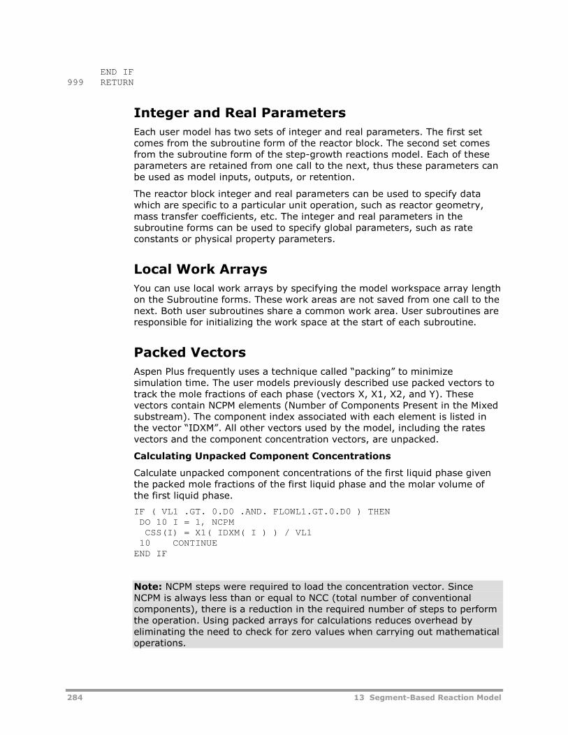
284 13 Segment-Based Reaction Model
END IF999 RETURN
Integer and Real Parameters
Each user model has two sets of integer and real parameters. The first setcomes from the subroutine form of the reactor block. The second set comesfrom the subroutine form of the step-growth reactions model. Each of theseparameters are retained from one call to the next, thus these parameters canbe used as model inputs, outputs, or retention.
The reactor block integer and real parameters can be used to specify datawhich are specific to a particular unit operation, such as reactor geometry,mass transfer coefficients, etc. The integer and real parameters in thesubroutine forms can be used to specify global parameters, such as rateconstants or physical property parameters.
Local Work Arrays
You can use local work arrays by specifying the model workspace array lengthon the Subroutine forms. These work areas are not saved from one call to thenext. Both user subroutines share a common work area. User subroutines areresponsible for initializing the work space at the start of each subroutine.
Packed Vectors
Aspen Plus frequently uses a technique called “packing” to minimizesimulation time. The user models previously described use packed vectors totrack the mole fractions of each phase (vectors X, X1, X2, and Y). Thesevectors contain NCPM elements (Number of Components Present in the Mixedsubstream). The component index associated with each element is listed inthe vector “IDXM”. All other vectors used by the model, including the ratesvectors and the component concentration vectors, are unpacked.
Calculating Unpacked Component Concentrations
Calculate unpacked component concentrations of the first liquid phase giventhe packed mole fractions of the first liquid phase and the molar volume ofthe first liquid phase.
IF ( VL1 .GT. 0.D0 .AND. FLOWL1.GT.0.D0 ) THENDO 10 I = 1, NCPMCSS(I) = X1( IDXM( I ) ) / VL1
10 CONTINUEEND IF
Note: NCPM steps were required to load the concentration vector. SinceNCPM is always less than or equal to NCC (total number of conventionalcomponents), there is a reduction in the required number of steps to performthe operation. Using packed arrays for calculations reduces overhead byeliminating the need to check for zero values when carrying out mathematicaloperations.
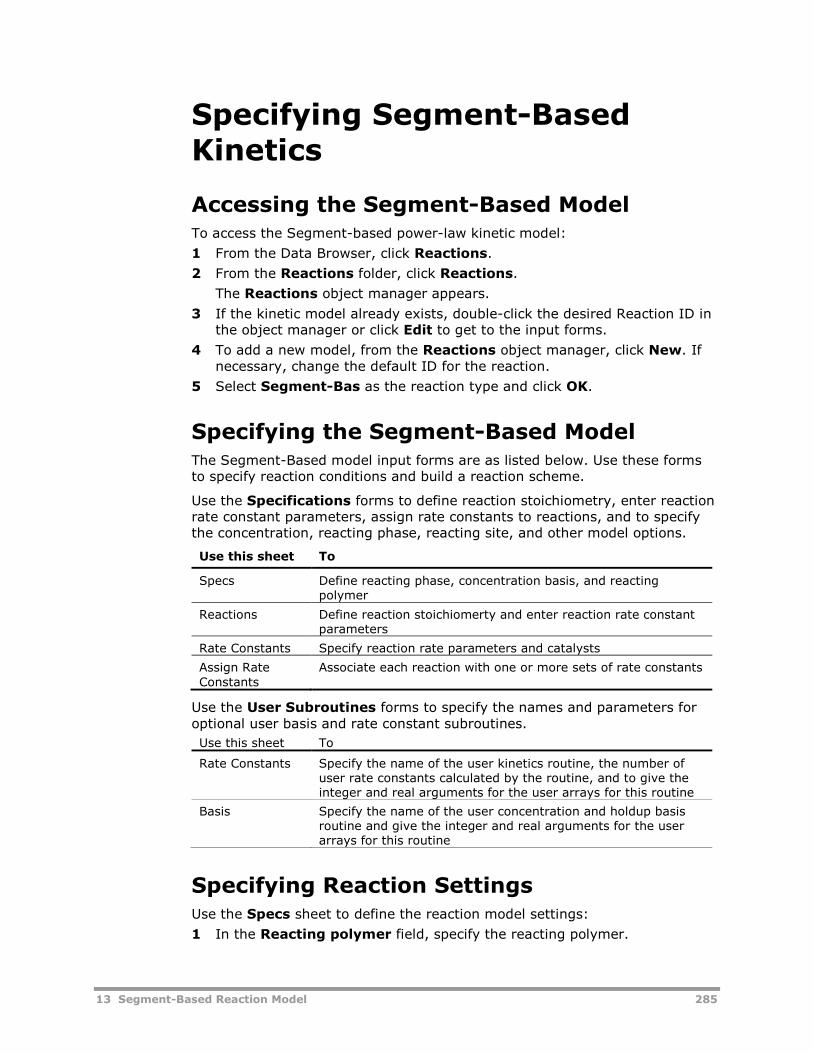
13 Segment-Based Reaction Model 285
Specifying Segment-BasedKinetics
Accessing the Segment-Based ModelTo access the Segment-based power-law kinetic model:
1 From the Data Browser, click Reactions.
2 From the Reactions folder, click Reactions.
The Reactions object manager appears.
3 If the kinetic model already exists, double-click the desired Reaction ID inthe object manager or click Edit to get to the input forms.
4 To add a new model, from the Reactions object manager, click New. Ifnecessary, change the default ID for the reaction.
5 Select Segment-Bas as the reaction type and click OK.
Specifying the Segment-Based ModelThe Segment-Based model input forms are as listed below. Use these formsto specify reaction conditions and build a reaction scheme.
Use the Specifications forms to define reaction stoichiometry, enter reactionrate constant parameters, assign rate constants to reactions, and to specifythe concentration, reacting phase, reacting site, and other model options.
Use this sheet To
Specs Define reacting phase, concentration basis, and reactingpolymer
Reactions Define reaction stoichiomerty and enter reaction rate constantparameters
Rate Constants Specify reaction rate parameters and catalysts
Assign RateConstants
Associate each reaction with one or more sets of rate constants
Use the User Subroutines forms to specify the names and parameters foroptional user basis and rate constant subroutines.
Use this sheet To
Rate Constants Specify the name of the user kinetics routine, the number ofuser rate constants calculated by the routine, and to give theinteger and real arguments for the user arrays for this routine
Basis Specify the name of the user concentration and holdup basisroutine and give the integer and real arguments for the userarrays for this routine
Specifying Reaction SettingsUse the Specs sheet to define the reaction model settings:
1 In the Reacting polymer field, specify the reacting polymer.
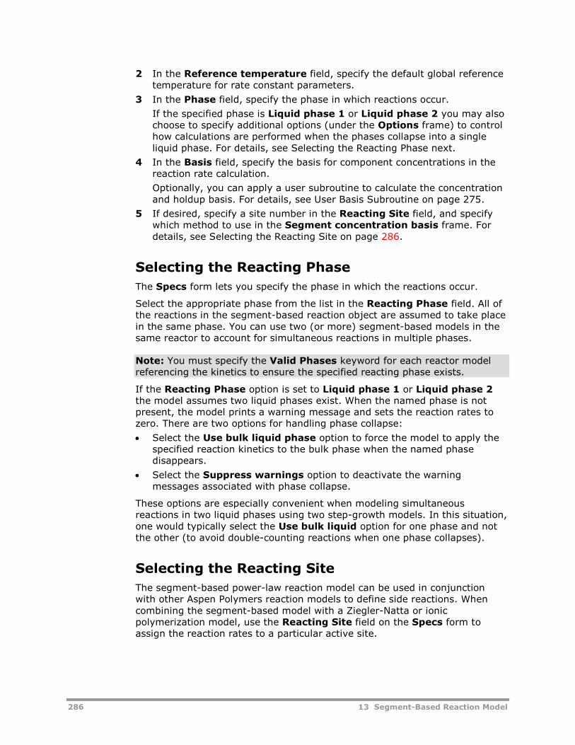
286 13 Segment-Based Reaction Model
2 In the Reference temperature field, specify the default global referencetemperature for rate constant parameters.
3 In the Phase field, specify the phase in which reactions occur.
If the specified phase is Liquid phase 1 or Liquid phase 2 you may alsochoose to specify additional options (under the Options frame) to controlhow calculations are performed when the phases collapse into a singleliquid phase. For details, see Selecting the Reacting Phase next.
4 In the Basis field, specify the basis for component concentrations in thereaction rate calculation.
Optionally, you can apply a user subroutine to calculate the concentrationand holdup basis. For details, see User Basis Subroutine on page 275.
5 If desired, specify a site number in the Reacting Site field, and specifywhich method to use in the Segment concentration basis frame. Fordetails, see Selecting the Reacting Site on page 286.
Selecting the Reacting Phase
The Specs form lets you specify the phase in which the reactions occur.
Select the appropriate phase from the list in the Reacting Phase field. All ofthe reactions in the segment-based reaction object are assumed to take placein the same phase. You can use two (or more) segment-based models in thesame reactor to account for simultaneous reactions in multiple phases.
Note: You must specify the Valid Phases keyword for each reactor modelreferencing the kinetics to ensure the specified reacting phase exists.
If the Reacting Phase option is set to Liquid phase 1 or Liquid phase 2the model assumes two liquid phases exist. When the named phase is notpresent, the model prints a warning message and sets the reaction rates tozero. There are two options for handling phase collapse:
Select the Use bulk liquid phase option to force the model to apply thespecified reaction kinetics to the bulk phase when the named phasedisappears.
Select the Suppress warnings option to deactivate the warningmessages associated with phase collapse.
These options are especially convenient when modeling simultaneousreactions in two liquid phases using two step-growth models. In this situation,one would typically select the Use bulk liquid option for one phase and notthe other (to avoid double-counting reactions when one phase collapses).
Selecting the Reacting Site
The segment-based power-law reaction model can be used in conjunctionwith other Aspen Polymers reaction models to define side reactions. Whencombining the segment-based model with a Ziegler-Natta or ionicpolymerization model, use the Reacting Site field on the Specs form toassign the reaction rates to a particular active site.
13 Segment-Based Reaction Model 287
Note: The Segment Concentration Basis field lets you select thecalculation method for the concentrations used within the reaction model.
When you select Use composite segment concentration the segmentmole fractions used to calculate the reaction rates are calculated from thefollowing equation:
Frac Frac SFRAC iMw
Mwsegs i p
p
avg, * ( )*
When you select Use segment concentration at specified site thefollowing equation is applied:
avg
p
pisMwseg
MwjiSSFRACFracFrac *),(*,
Where j refers the specified reacting site number.
In both cases the attribute rates of change are mapped to the componentattributes associated with the user-specified reacting site number (e.g.,SSFLOW(i,j), SZMOM(i,j), etc.)
Building A Reaction SchemeYou can build a list of reactions on the Reactions sheet. To do this you mustspecify a reaction stoichiometry. The Data Browser window can be resized tobetter view the reaction listing. Use the following options:
Click To
New Add new reactions to the scheme
Edit Edit the current reaction indicated by the rowselector
Rate Constants Specify reaction rate constant parameters for thereactions
Click to select a reaction. Click a reaction then Control-Click to includeadditional reactions for multiple selections. Double-click to edit a reaction.
In addition, you can use the following buttons:
Click To
Hide/RevealActivate or de-activate a set of reactions.Inactive reactions are highlighted with a graybackground.
DeletePermanently remove a reaction from the model
Adding or Editing ReactionsTo add a new reaction to the scheme or to edit an existing reaction, clickNew or Edit to open the Edit Stoichiometry subform:
Note that in the Reaction no. field, a unique number is assigned to thereaction being added.
288 13 Segment-Based Reaction Model
1 Specify the Component ID and stoichiometric Coefficient for thereactants.
Reactants must have a negative coefficient.
2 Specify the Component ID and stoichiometric Coefficient for theproducts.
Products must have a positive coefficient.
3 Click to check the Completion status
or
Click Close to return to the reaction summary.
Specifying Reaction Rate ConstantsThe rate constants are summarized in a grid on the Rate Constants sheet:
1 In the ko field, enter the pre-exponential factor.
Note: Reaction rates are defined on a molar basis (moles per volume pertime). The time units for the pre-exponential factors are specified directly onthe Rate Constant form.By default, the concentration units are assumed to be in SI units (kmole/m3
or mole/L).You can change the concentration basis to other units using theConcentration Basis field of the Specs sheet. Alternately, you may apply auser basis subroutine.
2 In the field, enter the activation energy.
3 In the b field, enter the temperature exponent.
4 In the Tref field, enter the reference temperature. If this field is left blankthe reference temperature will default to the user-specified globalreference temperature on the Specs form.
5 If desired, specify a Catalyst Species and Catalyst Order.
6 If desired, specify a user rate constant element number on the User Flagfield (For details, see the User Rate-Constant Subroutine on page 144).
Note: Use the Catalyst Species field to associate a rate constant with aparticular catalyst. If you leave this field blank (empty) the model drops thecatalyst concentration term from the rate expression.Use the Catalyst Order field to specify the reaction order with respect to thecatalyst (the model assumes first order by default).
Assigning Rate Constants to ReactionsThere are two options for assigning rate constants to reactions. By default,the model assumes there is exactly one set of rate constants for each reaction(for example, rate constant set “i” is used for reaction “i”).
Alternately, you may use the Assign User Rate Constant sheet to assignone or more sets of rate constants to each reaction. This feature is convenientin two situations:
Ea
13 Segment-Based Reaction Model 289
Models with a large number of user side reactions when the rate constantsof the various reactions are equal or are related to each otheralgebraically.
Reactions catalyzed by several catalysts simultaneously.
The assignment option is recommended for two reasons:
You can enter several sets of rate constants for each reaction without re-entering the reaction stoichiometry.
You can assign a set of rate constants to multiple reactions, reducing thenumber of adjustable parameters in the model, which makes it easier tofit against data.
When several rate constants are assigned to a reaction the model calculates anet rate constant by summing all of the listed rate constants and multiplyingthe sum by a specified activity.
To assign rate constants to reactions:
1 On the Assign User Rate Constants form, use the Activity field tospecify the activity factor (default value is unity).
2 In the Rate Constant Sets field, select from the list of pre-defined rateconstant sets for each reaction. These numbers refer to the row numberson the Rate Constants form.
Including a User Rate Constant SubroutineUse the User Subroutines Rate Constants form to specify parameters foruser rate constants calculations:
1 In subroutine Name, enter the name of the Fortran subroutine.
2 Specify the size of vectors for Integer, Real and No. const. in Numberof parameters.
3 Specify the size of vectors of Integer and Real in Length of workarrays.
4 Enter integer and real parameter values in Values for parameterscolumns.
Including a User Basis SubroutineUse the User Subroutines Basis form to specify parameters for basiscalculations:
1 In subroutine Name, enter the name of the Fortran subroutine.
2 Specify the size of vectors for Integer and Real in the Number ofparameters and Length of work arrays.
3 Enter integer and real parameter values in Values for parameterscolumns.
ReferencesBiesenberger, J. A., & Sebastian, D. H. (1983). Principles of PolymerizationEngineering. New York: Wiley.
290 13 Segment-Based Reaction Model
Kroschwitz, J. (Ed.). (1990). Concise Encyclopedia of Polymer Science andEngineering. New York: Wiley.
Odian, G. (1991). Principles of Polymerization, 3rd Ed. New York: Wiley.
Rodriguez, F. (1989). Principles of Polymer Systems. New York: Hemisphere.
Rudin, A. (1982). The Elements of Polymer Science and Engineering. NewYork: Academic Press Inc.
14 Steady-State Flowsheeting 291
14 Steady-StateFlowsheeting
Aspen Polymers (formerly known as Aspen Polymers Plus) allows you tomodel polymerization processes in both steady-state and dynamic mode. Inthis chapter, flowsheeting capabilities for modeling processes in steady-statemode are described.
Topics covered include:
Polymer Manufacturing Flowsheets, 291
Modeling Polymer Process Flowsheets, 293
Steady-State Modeling Features, 294
Following this introduction, Aspen Polymers flowsheeting capabilities formodeling steady state processes are discussed in several sections.
Steady-State Unit Operation Models, 295
Plant Data Fitting, 339
User Models, 359
Application Tools, 375
Polymer ManufacturingFlowsheetsPolymer production processes are usually divided into the following majorsteps:
Monomer synthesis and purification
Polymerization
Recovery/separation
Polymer processing
The modeling issues of interest in each of these steps were discussed inChapter 1, and are summarized in the following figure. The focus here is onthe various unit operations required in these processing steps.
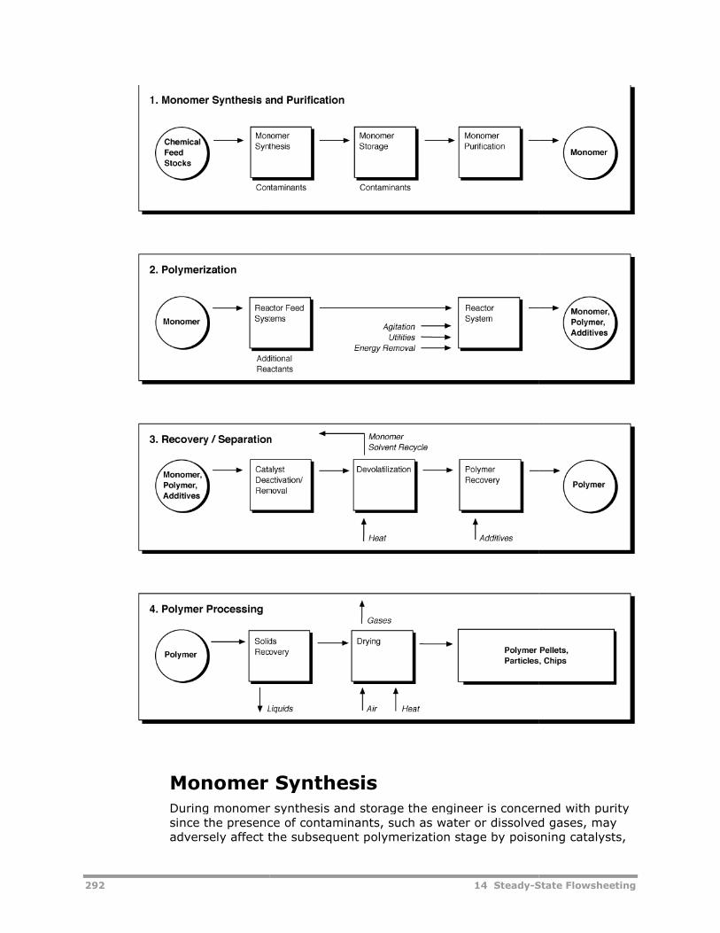
292
Monomer SynthesisDuring monomer synthesissince the presence of contaminants, such as water or dissolved gases, mayadversely affect the subsequent polymerization stage by poisoning catalysts,
14 Steady-State Flowsheeting
Monomer SynthesisDuring monomer synthesis and storage the engineer is concerned with puritysince the presence of contaminants, such as water or dissolved gases, mayadversely affect the subsequent polymerization stage by poisoning catalysts,
State Flowsheeting
and storage the engineer is concerned with puritysince the presence of contaminants, such as water or dissolved gases, mayadversely affect the subsequent polymerization stage by poisoning catalysts,
14 Steady-State Flowsheeting 293
depleting initiators, causing undesirable chain transfer or branching reactionswhich would cause less effective heat removal. Another concern is theprevention of monomer degradation through proper handling or the additionof stabilizers. Control of emissions, and waste disposal are also importantfactors.
PolymerizationThe polymerization step is the most important step in terms of capital andoperating costs. The desired outcome for this step is a polymer product withspecified properties (e.g. molecular weight distribution, melt index, viscosity,crystallinity) for given operating conditions. The obstacles that must beovercome to reach this goal depend on the type of polymerization process.
Polymerization processes may be batch, semi-batch, or continuous. Inaddition, they may be carried out in bulk, solution, suspension, or emulsion.Bulk continuous systems provide better temperature and molecular weightcontrol at the expense of conversion; batch systems offer less control overmolecular weight. In addition, they may result in a high viscosity product andrequire high temperatures and pressures. Solution systems also provide goodtemperature control but have associated with them the cost of solventremoval from the polymer.
In summary, for the polymerization step, the mechanisms that take placeduring the reaction introduce changes in the reaction media which in turnmake kinetics and conversion, residence time, agitation, and heat transfer themost important issues for the majority of process types.
Recovery / SeparationsThe recovery/separation step is the step where the desired polymer producedis further purified or isolated from by-products or residual reactants. In thisstep, monomers and solvents are separated and purified for recycle or resale.The important issues for this step are phase equilibrium, heat and masstransfer.
Polymer ProcessingThe last step, polymer processing, can also be considered a recovery step. Inthis step, the polymer slurry is turned into solid pellets or chips. Heat ofvaporization is an important issue in this step (Grulke, 1994).
Modeling Polymer ProcessFlowsheetsThe obvious requirement for the simulation of process flowsheets is theavailability of unit operation models. Once these unit operation models areconfigured, they must be adjusted to match the actual process data. Finally,tools must be available to apply the fitted model to gain better process
294 14 Steady-State Flowsheeting
understanding and perform needed process studies. As a result of theapplication of the process models, engineers are able to achieve goals such asproduction rate optimization, waste minimization and compliance toenvironmental constraints. Yield increase and product purity are alsoimportant issues in the production of polymers.
Steady-State Modeling FeaturesAspen Polymers has tools available for addressing the three polymer processmodeling aspects.
Unit Operations Modeling FeaturesA comprehensive suite of unit operations for modeling polymer processes isavailable in Aspen Polymers. These include mixers, splitters, heaters, heatexchangers, single and multistage separation models, reactors, etc. For moreinformation on available unit operation models, see Steady-State UnitOperation Models on page 295.
Plant Data Fitting FeaturesSeveral tools are available for fitting process models to actual plant data.Property parameters may be adjusted to accurately represent separation andphase equilibrium behavior. This can be done through the Data RegressionSystem (DRS). See the Aspen Plus User Guide for information about DRS.
Another important aspect of fitting models to plant data has to do with thedevelopment of an accurate kinetic model within the polymerization reactors.The powerful plant data fitting feature (Data-Fit) can be used for fittingkinetic rate constant parameters. For more information, see Plant Data Fittingon page 339.
Process Model Application ToolsThe tools available for applying polymer process models include capabilitiesfor performing sensitivity, for performing optimizations, and for applyingdesign specifications. For more information, see Application Tools on page375.
ReferencesDotson, N. A, Galván, R., Laurence, R. L., & Tirrell, M. (1996). PolymerizationProcess Modeling. New York: VCH Publishers.
Grulke, E. A. (1994). Polymer Process Engineering. Englewood Cliffs, NJ:Prentice Hall.
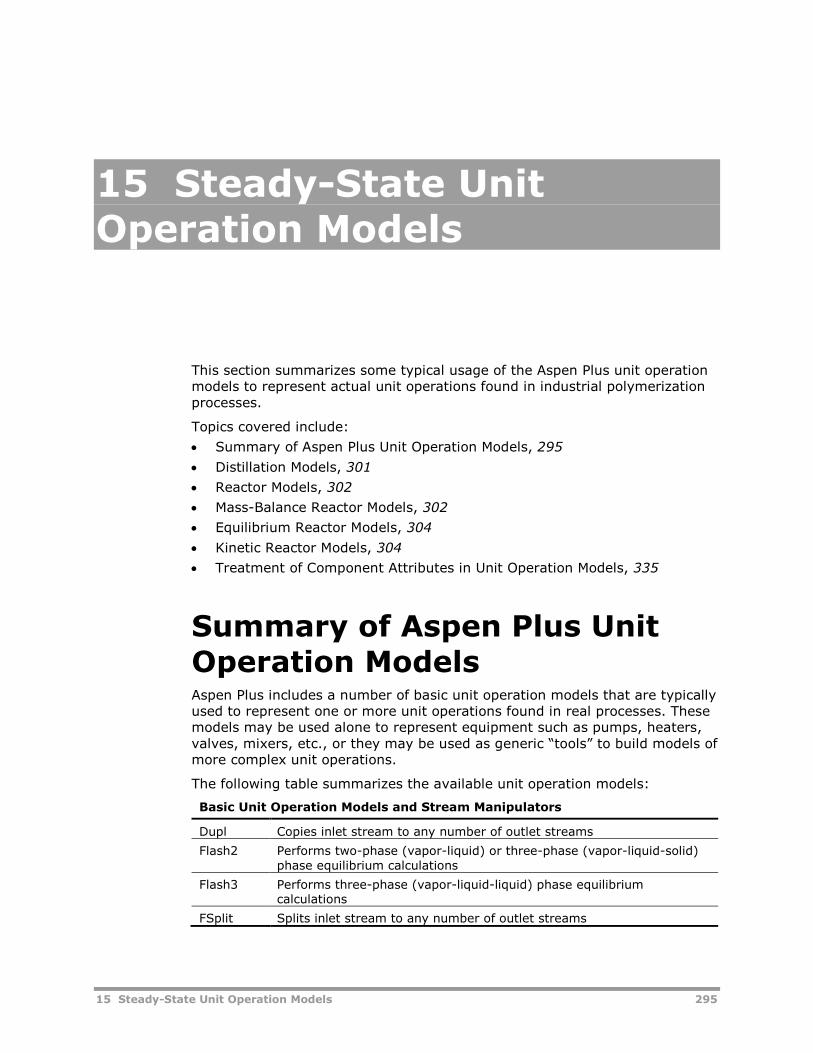
15 Steady-State Unit Operation Models 295
15 Steady-State UnitOperation Models
This section summarizes some typical usage of the Aspen Plus unit operationmodels to represent actual unit operations found in industrial polymerizationprocesses.
Topics covered include:
Summary of Aspen Plus Unit Operation Models, 295
Distillation Models, 301
Reactor Models, 302
Mass-Balance Reactor Models, 302
Equilibrium Reactor Models, 304
Kinetic Reactor Models, 304
Treatment of Component Attributes in Unit Operation Models, 335
Summary of Aspen Plus UnitOperation ModelsAspen Plus includes a number of basic unit operation models that are typicallyused to represent one or more unit operations found in real processes. Thesemodels may be used alone to represent equipment such as pumps, heaters,valves, mixers, etc., or they may be used as generic “tools” to build models ofmore complex unit operations.
The following table summarizes the available unit operation models:
Basic Unit Operation Models and Stream Manipulators
Dupl Copies inlet stream to any number of outlet streams
Flash2 Performs two-phase (vapor-liquid) or three-phase (vapor-liquid-solid)phase equilibrium calculations
Flash3 Performs three-phase (vapor-liquid-liquid) phase equilibriumcalculations
FSplit Splits inlet stream to any number of outlet streams
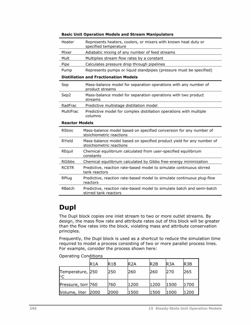
296 15 Steady-State Unit Operation Models
Basic Unit Operation Models and Stream Manipulators
Heater Represents heaters, coolers, or mixers with known heat duty orspecified temperature
Mixer Adiabatic mixing of any number of feed streams
Mult Multiplies stream flow rates by a constant
Pipe Calculates pressure drop through pipelines
Pump Represents pumps or liquid standpipes (pressure must be specified)
Distillation and Fractionation Models
Sep Mass-balance model for separation operations with any number ofproduct streams
Sep2 Mass-balance model for separation operations with two productstreams
RadFrac Predictive multistage distillation model
MultiFrac Predictive model for complex distillation operations with multiplecolumns
Reactor Models
RStoic Mass-balance model based on specified conversion for any number ofstoichiometric reactions
RYield Mass-balance model based on specified product yield for any number ofstoichiometric reactions
REquil Chemical equilibrium calculated from user-specified equilibriumconstants
RGibbs Chemical equilibrium calculated by Gibbs free-energy minimization
RCSTR Predictive, reaction rate-based model to simulate continuous stirredtank reactors
RPlug Predictive, reaction rate-based model to simulate continuous plug-flowreactors
RBatch Predictive, reaction rate-based model to simulate batch and semi-batchstirred tank reactors
DuplThe Dupl block copies one inlet stream to two or more outlet streams. Bydesign, the mass flow rate and attribute rates out of this block will be greaterthan the flow rates into the block, violating mass and attribute conservationprinciples.
Frequently, the Dupl block is used as a shortcut to reduce the simulation timerequired to model a process consisting of two or more parallel process lines.For example, consider the process shown here:
Operating Conditions
R1A R1B R2A R2B R3A R3B
Temperature,C
250 250 260 260 270 265
Pressure, torr 760 760 1200 1200 1500 1700
Volume, liter 2000 2000 1500 1500 1000 1200
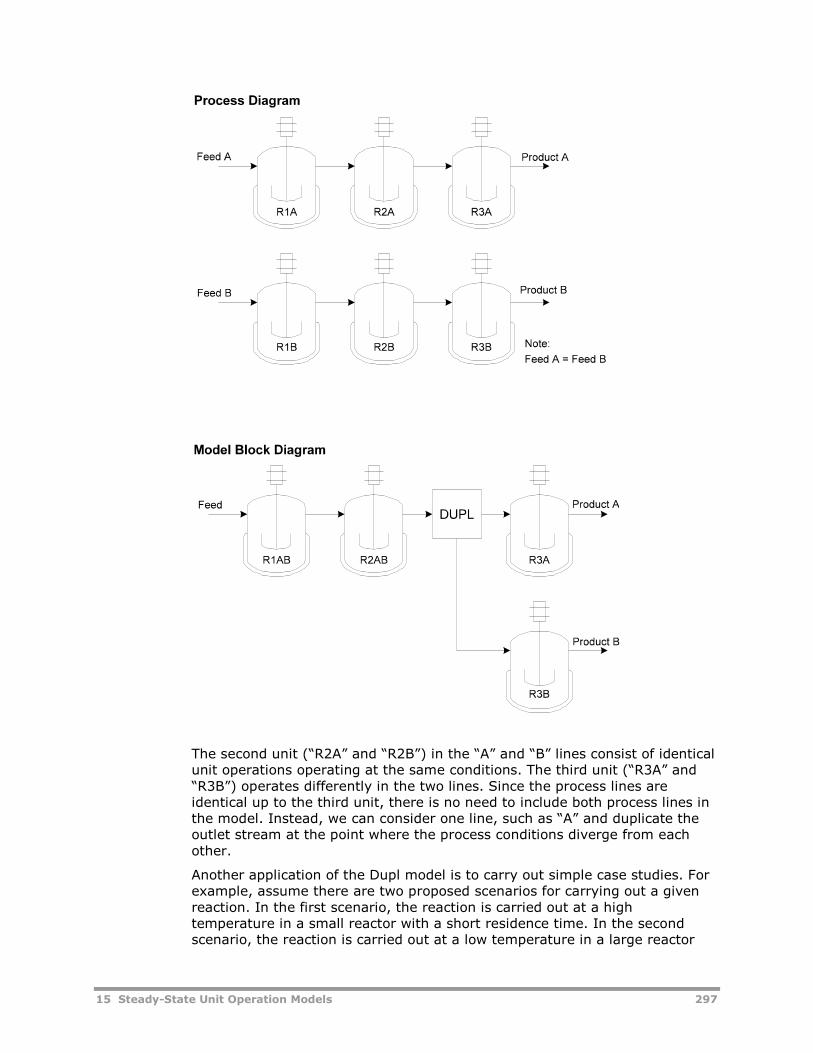
15 Steady-State Unit Operation Models 297
The second unit (“R2A” and “R2B”) in the “A” and “B” lines consist of identicalunit operations operating at the same conditions. The third unit (“R3A” and“R3B”) operates differently in the two lines. Since the process lines areidentical up to the third unit, there is no need to include both process lines inthe model. Instead, we can consider one line, such as “A” and duplicate theoutlet stream at the point where the process conditions diverge from eachother.
Another application of the Dupl model is to carry out simple case studies. Forexample, assume there are two proposed scenarios for carrying out a givenreaction. In the first scenario, the reaction is carried out at a hightemperature in a small reactor with a short residence time. In the secondscenario, the reaction is carried out at a low temperature in a large reactor
298 15 Steady-State Unit Operation Models
with high residence times. The two reactors can be placed in a single flowsheet model. The duplicator block is used to copy one feed stream to bothreactors. The two “cases” can be compared by examining the streamsummary.
Flash2The Flash2 block carries out a phase-equilibrium calculation for a vapor-liquidsplit. The “chemistry” feature of this block can be used to extend the phaseequilibrium to vapor-liquid-solid systems. The free-water option can be usedto extend the phase equilibrium calculations to include a free water phase inaddition to the organic liquid phase.
The Flash2 model can be used to simulate simple flash drums with anynumber of feed streams. The model is also a good tool for representing spraycondensers, single-stage distillations, knock-back condensers, decanters, andother types of equipment which effectively operate as one ideal stage.
The Flash2 model assumes a perfect phase split, but an entrainment factorcan be specified to account for liquid carryover in the vapor stream. Theentrainment factor is specified by the user, it is not calculated by the model.If a correlation between the vapor flow rate and the entrainment rate isavailable, this correlation can be applied to the model using a Fortran blockwhich reads the vapor flow rate calculated by the Flash block, calculates theentrainment rate, and writes the resulting prediction back to the Flash block.Note that this approach creates an information loop in the model which mustbe converged.
The Flash2 block does not fractionate the polymer molecular weightdistribution. Instead, the molecular weight distribution of the polymer in eachproduct stream is assumed to be the same as the feed stream.
Flash3The Flash3 block carries out phase-equilibrium calculations for a vapor-liquid-liquid splits. The liquid phases may be organic-organic (including polymer-monomer) or aqueous-organic. For aqueous-organic systems, the Flash3model is more rigorous than the Flash2/free water approach described above.The key difference is that the Flash3 model considers dissolved organiccompounds in the aqueous phase while the free water approach assumes apure water phase.
Generally, three-phase flashes are more difficult to converge than two-phaseflashes. Three-phase flash failures may indicate bad binary interactionparameters between the components. The problem may also stem frombogus vapor pressures or heats of formation. In general, it is a good idea tostudy two-phase splits for the system in question before attempting to modela three-phase decanter or reactor.
As with the two-phase flash, the three-phase flash is more stable iftemperature and pressure are specified. Other options, such as duty andvapor fraction, are more difficult to converge. Temperature estimates may aidconvergence in duty-specified reactors.
15 Steady-State Unit Operation Models 299
The Flash3 block does not fractionate the polymer molecular weightdistribution. Instead, the molecular weight distribution of the polymer in eachproduct stream is assumed to be the same as the feed stream.
FSplitThe flow splitter block, FSplit, is used to represent valves or tanks withseveral outlets. The outlet flow rates can be specified on a mass, mole, orvolume basis, or they can be specified as a fraction of the feed stream. Ingeneral, the fraction specifications are best because they are independent ofthe feed stream flow rates. This makes the model more flexible and reliablewhen using tools like SENSITIVITY or DESIGN-SPEC which might directly orindirectly manipulate the stream which is being split. The FSplit block can alsobe used with reactor models to account for back-mixing.
The FSplit block assumes that the class 2 polymer attributes split according tomass mixing rules. For example, if the outlet stream is split 60:40, then theclass 2 attributes, such as the segment flow rates, are also split 60:40. Thisapproach is identical to assuming that the properties of the polymer in eachoutlet stream are the same as the properties of the polymer in the inletstream.
HeaterHeater can be used to represent heaters, coolers, mixers, valves, or tanks.The Heater block allows you to specify the temperature or heat duty of theunit, but does not carry out rigorous heat exchange equations. Any number offeed streams can be specified for the Heater block. This block follows thesame mixing rules as the Mixer model.
MixerThe mixer block, Mixer, is used to mix two or more streams to form a singlemixed outlet. The mixer block can be used to represent mixing tanks, staticmixers, or simply the union of two pipes in a tee. The Mixer model assumesideal, adiabatic mixing. The pressure of the mixer can be specified as anabsolute value or as a drop relative to the lowest feed stream pressure.
The Mixer model is functionally equal to the Heater model, except it onlyallows adiabatic mixing. For this reason, the Heater model may be a betterchoice for modeling mixing tanks.
The Mixer block assumes that the class 2 polymer attributes are additive. Forexample if stream “A” and “B” are mixed to form stream “C”, and the zerothmoments of a polymer in stream “A” and “B” are 12 kmol/sec and 15kmol/sec, then the polymer in the product stream has a zeroth moment of12+15=27 kmol/sec.
MultThe Mult block is used to multiply the flow rate of a stream. A commonapplication of this block is to collapse two parallel process line models into a
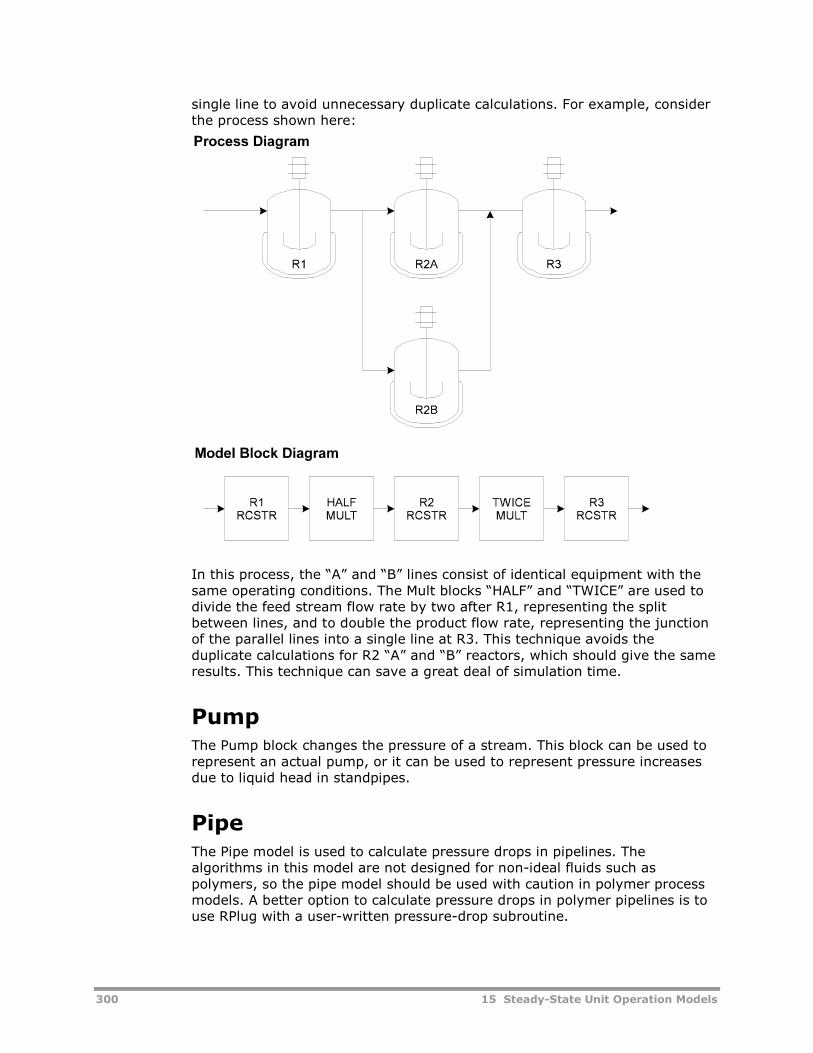
300 15 Steady-State Unit Operation Models
single line to avoid unnecessary duplicate calculations. For example, considerthe process shown here:
In this process, the “A” and “B” lines consist of identical equipment with thesame operating conditions. The Mult blocks “HALF” and “TWICE” are used todivide the feed stream flow rate by two after R1, representing the splitbetween lines, and to double the product flow rate, representing the junctionof the parallel lines into a single line at R3. This technique avoids theduplicate calculations for R2 “A” and “B” reactors, which should give the sameresults. This technique can save a great deal of simulation time.
PumpThe Pump block changes the pressure of a stream. This block can be used torepresent an actual pump, or it can be used to represent pressure increasesdue to liquid head in standpipes.
PipeThe Pipe model is used to calculate pressure drops in pipelines. Thealgorithms in this model are not designed for non-ideal fluids such aspolymers, so the pipe model should be used with caution in polymer processmodels. A better option to calculate pressure drops in polymer pipelines is touse RPlug with a user-written pressure-drop subroutine.
15 Steady-State Unit Operation Models 301
SepThe Sep block is a generic separation model that allows componentfractionation between two or more product streams. The products can be splitaccording to flow rate or fractional specifications. The Sep block is commonlyused to represent distillation columns or other separation equipment whenthe product stream purity is well known and the details of the separationprocess are not important.
The Sep block does not fractionate the polymer molecular weight distribution.Instead, the molecular weight distribution of the polymer in each productstream is assumed to be the same as the feed stream.
Sep2The Sep2 block is a generic separation model that allows componentfractionation between two product streams. The products can be splitaccording to flow rate or fractional specifications. The Sep2 block is commonlyused to represent distillation columns or other separation equipment whenthe product stream purity is well known and the details of the separationprocess are not important. Compared to the Sep block, the Sep2 block hasmore flexible input options, but it only allows two outlet streams.
The Sep2 block does not fractionate the polymer molecular weightdistribution. Instead, the molecular weight distribution of the polymer in eachproduct stream is assumed to be the same as the feed stream.
Distillation ModelsAspen Plus includes several shortcut distillation models (DISTL, SFRAC, etc.)which can be used to represent distillation columns. These blocks do notfractionate the polymer molecular weight distribution. Instead, the molecularweight distribution of the polymer in each product stream is assumed to bethe same as the feed stream. The class-2 component attributes in eachproduct stream are set proportional to the mass flow rate of the attributedcomponent in each product stream.
With the exception of the RadFrac model, the rigorous distillation models inAspen Plus do not account for component attributes.
RadFracThe RadFrac block is a rigorous multistage distillation model for two- andthree-phase systems. RadFrac allows polymer feed streams at any tray, but itdoes not account for polymerization reaction kinetics. The molecular weightdistribution and other polymer properties are not fractionated between thephases. Instead, the class-2 component attributes of the polymer componentsare split at each stage in proportion to the polymer component massfractions. For example, if 90% of the polymer fed to a given tray goes to theliquid phase leaving that tray, then 90% of the zeroth moment and otherclass-2 attributes are assigned to the liquid phase on that tray.
302 15 Steady-State Unit Operation Models
Reactor ModelsAspen Plus includes three classes of reactor models which include variouslevels of rigor and predictive capability. These classes are: (1) mass-balancemodels; (2) equilibrium models; and (3) rigorous kinetic models.
The least predictive models, RStoic and RYield, calculate output flow ratesbased on user-specified input flow rates. If polymer components are involvedin the reactions, then the component attributes associated with the polymercomponents must be specified for the product stream. These models calculatethe mass and energy balances, but they do not perform rigorous kineticcalculations.
The RGibbs and REquil models assume chemical and phase equilibrium. Whenpolymer components are involved in the reactions, then the specifiedstoichiometry must be consistent with the reference molecular weight of thepolymer component. In addition, the component attribute values for thepolymer product must be specified by the user. Since the solution algorithmsfor these models do not consider the influence of the segmental compositionof polymer components, they cannot be applied to copolymers.
Rigorous kinetic models include RCSTR (continuous stirred tank reactor),RPlug (plug-flow reactor model), and RBatch (batch stirred tank reactor).Each of these models can consider one, two, or three reacting phases. Thesereactor models are with the reaction kinetic models to predict product streamcomposition and flow rates based on calculated reaction rates.
Mass-Balance Reactor Models
RStoicThe RStoic reactor model is used to represent reaction equipment whenreaction kinetics are unknown or are unimportant, for example whenreactions are very fast and proceed until the limiting reagent is exhausted.RStoic requires knowledge of the net reaction stoichiometry, and the extent ofreaction or conversion of a key component.
RStoic calculates the product stream flow rates based on user-specifiedreaction stoichiometries and extent of reaction or conversion of a keycomponent. The reaction stoichiometry statements may include monomers,oligomers, or polymers, but may not include segments. Instead, the segmentinformation (SFLOW or SFRAC) must be specified as component attributes inthe COMP-ATTR sentence.
Reactions Involving Polymers
If polymer components are involved in any of the reactions, use the COMP-ATTR form to specify molecular weight values (MWN, MWW or PDI) or degreeof polymerization (DPN, DPW or PDI ) for the polymer products. Specify theSFRAC attribute for homopolymers or copolymers with a known productpolymer composition. For copolymers with product compositions which
15 Steady-State Unit Operation Models 303
depend on the feed flow rates of monomers or polymer segments, specifydummy values for the SFLOW attribute and use a user-written Fortran blockto predict product segment flow rates which are consistent with the calculatedproduct flow rates. Write the calculated results into the product stream of theRStoic block.
When some of the specified reactions involve polymers, the reactionstoichiometry must be written in a manner consistent with the referencemolecular weight of the polymer component. Otherwise, the mass and energybalance calculations will not be consistent.
Simulating Polymer Phase Change
The RStoic model may be used with the substream feature to simulate phasechanges in polymers. For example, the user may define a reaction to convertpolymer from the liquid or amorphous state (in the MIXED substream) tocrystalline polymer (in the CISOLID) substream. Conversely, melting can besimulated as a reaction that converts polymer in the CISOLID substream topolymer in the MIXED substream.
When RStoic is used in this manner, the model automatically fractionates thecomponent attributes between the product substreams. If the user does notspecify the product component attributes, the model sets the values of theclass-2 attributes in each substream proportional to the flow rate of theattributed component in the substream. In effect, the model assumes thatthere is no selectivity of properties between the product phases. The polymerin each product phase will have the same characteristics (segmentcomposition, mole weight, etc) as the polymer in the feed stream.
RYieldThe RYield reactor model is used to represent reaction equipment whenreaction kinetics are unknown or are unimportant, and the reactions result ina product distribution with a known yield.
RYield calculates the product stream flow rates based on user-specifiedreaction stoichiometries and yield distributions. The reaction stoichiometrystatements may include monomers, oligomers, or polymers, but may notinclude segments. Instead, the segment information (SFLOW or SFRAC) mustbe specified as component attributes in the COMP-ATTR sentence.
If polymer components are involved in any of the reactions, use the COMP-ATTR form to specify molecular weight values (MWN, MWW or PDI) or degreeof polymerization (DPN, DPW or PDI ) for the polymer products. Specify theSFRAC attribute for homopolymers or copolymers with a known productpolymer composition. For copolymers with product compositions whichdepend on the feed flow rates of monomers or polymer segments, specifydummy values for the SFLOW attribute and use a user-written Fortran blockto predict product segment flow rates which are consistent with the calculatedyield. Write the calculated results into the product stream of the RYield block.
When some of the specified reactions involve polymers, the reactionstoichiometry must be written in a manner consistent with the reference
304 15 Steady-State Unit Operation Models
molecular weight of the polymer component. Otherwise, the mass and energybalance calculations will not be consistent.
Equilibrium Reactor Models
REquilThe REquil model calculates product stream flow rates using equilibriumconstants determined from Gibbs free energy. The equilibrium constants arebased on user-specified reaction stoichiometries and yield distributions. Thereaction stoichiometry statements may include monomers or oligomers, butmay not include polymers or segments. If the feed stream includes polymercomponents, the attributes of the polymer components will be copied to theoutlet stream.
RGibbsThe RGibbs model uses the Gibbs free energy minimization technique todetermine the composition of each phase. This algorithm cannot predict theproduct of equilibrium polymerization reactions. Polymer phase equilibrium,however, can be predicted by the model. The RGibbs phase equilibriumalgorithm assumes that the composition and molecular weight distribution ofa polymer component is equal in each of the product phases. The class-2component attributes of the polymer component are set in proportion to themass flow of the polymer component in each of the product phases. The massflow rates in the product phases are set by the Gibbs free energyminimization algorithm.
To properly split component attributes among the RGibbs solution phases, usethe "Phase equilibrium only" option. With this the model can predict multipleliquid phases such as three liquid phases. Surface tension effects are notconsidered. If you are certain that there will be no vapor phase, uncheck the"Include vapor phase" box to speed up calculations. Use one outlet stream foreach predicted phase, to separate out the component attributes of thatphase.
Kinetic Reactor Models
RCSTRThe RCSTR model represents a continuous stirred tank reactor with one ormore phases.
The model assumes perfect mixing within and between the phases, phaseequilibrium, and isothermal, isobaric operation. Non-ideal mixing can berepresented using a network of RCSTR models.
15 Steady-State Unit Operation Models 305
Temperature
The CSTR model allows you to specify duty or temperature. If duty isspecified, it is a good idea to provide a temperature estimate, T-EST, toimprove the convergence of the model. The maximum temperature step size,T-STEP, may also influence the CSTR convergence. This parameter defaults to50C, which results in substantial changes in reaction rates for reactions withtypical activation energies. The temperature/duty iteration loop is referred toas the “Energy Balance” or “EB-LOOP” in the CSTR diagnostics.
Pressure
Pressure can be specified as an absolute value or as a pressure drop relativeto the feed stream with the lowest pressure. In Aspen Plus, pressure dropsare expressed as non-positive pressure specifications given in absolutepressure units.
Residence Time
The RCSTR model allows you to specify the effective hold-up in severaldifferent ways. For single-phase reactors, you can specify the total reactorvolume or the total residence time. If the residence time is specified, then theestimated reactor volume should be specified to improve the residence-time/volume loop convergence (RT-LOOP).
When two or more condensed phases are present, the RCSTR model assumesthat each condensed phase has the same residence time. This “no-slip”assumption implies that the volume ratios of the condensed phases in thereactor are equal to the volume flow ratios of the condensed phases exitingthe reactor.
For multiphase reactors, specify the condensed phase volume or residencetime in addition to the total reactor volume. Do not specify the total residencetime, as this residence time is the average of the vapor and liquid phases. Ifthe reacting phase residence time is specified, provide an estimate for thereacting phase volume. This will improve the reactor convergence. Ifresidence time convergence is troublesome, try adjusting the volume stepsize.
Multiphase Reactors
The RCSTR model can be used to simulate single- or multiple-phase reactors.The valid-phases keyword is used to define the number and type of fluidphases present in the reactor.
Amorphous solid polymers are treated as a “liquid” phase in Aspen Polymers(formerly known as Aspen Polymers Plus). Crystalline solids can be addressedby defining a “CISOLID” substream to track the flow rate of each inertcrystalline solid.
Dissolving or crystallizing solids can be captured using the Chemistry featureto define chemical equilibrium reactions between the solid and fluid phases.Note, however, that the current version of RCSTR does not allow componentsto appear in both kinetic reactions and in chemistry equilibrium reactions.
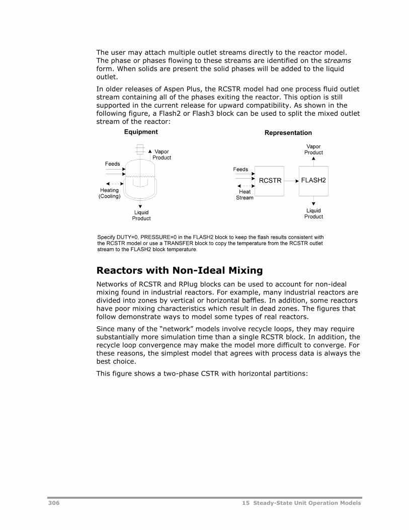
306 15 Steady-State Unit Operation Models
The user may attach multiple outlet streams directly to the reactor model.The phase or phases flowing to these streams are identified on the streamsform. When solids are present the solid phases will be added to the liquidoutlet.
In older releases of Aspen Plus, the RCSTR model had one process fluid outletstream containing all of the phases exiting the reactor. This option is stillsupported in the current release for upward compatibility. As shown in thefollowing figure, a Flash2 or Flash3 block can be used to split the mixed outletstream of the reactor:
Reactors with Non-Ideal Mixing
Networks of RCSTR and RPlug blocks can be used to account for non-idealmixing found in industrial reactors. For example, many industrial reactors aredivided into zones by vertical or horizontal baffles. In addition, some reactorshave poor mixing characteristics which result in dead zones. The figures thatfollow demonstrate ways to model some types of real reactors.
Since many of the “network” models involve recycle loops, they may requiresubstantially more simulation time than a single RCSTR block. In addition, therecycle loop convergence may make the model more difficult to converge. Forthese reasons, the simplest model that agrees with process data is always thebest choice.
This figure shows a two-phase CSTR with horizontal partitions:
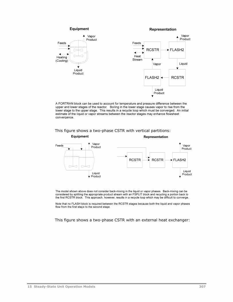
15 Steady-State Unit Operation Models 307
This figure shows a two-phase CSTR with vertical partitions:
This figure shows a two-phase CSTR with an external heat exchanger:
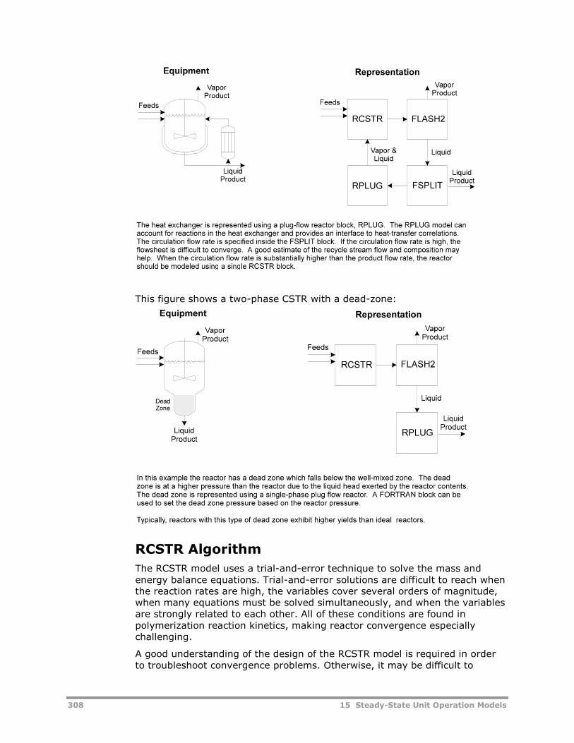
308 15 Steady-State Unit Operation Models
This figure shows a two-phase CSTR with a dead-zone:
RCSTR Algorithm
The RCSTR model uses a trial-and-error technique to solve the mass andenergy balance equations. Trial-and-error solutions are difficult to reach whenthe reaction rates are high, the variables cover several orders of magnitude,when many equations must be solved simultaneously, and when the variablesare strongly related to each other. All of these conditions are found inpolymerization reaction kinetics, making reactor convergence especiallychallenging.
A good understanding of the design of the RCSTR model is required in orderto troubleshoot convergence problems. Otherwise, it may be difficult to
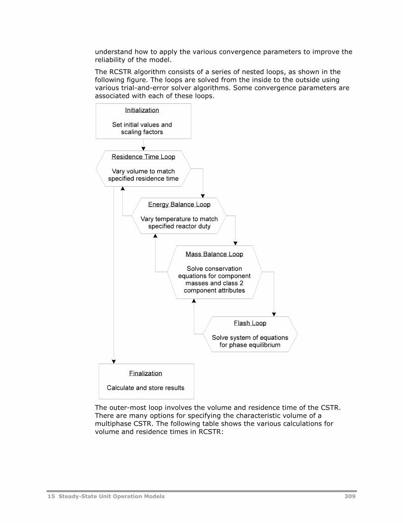
15 Steady-State Unit Operation Models 309
understand how to apply the various convergence parameters to improve thereliability of the model.
The RCSTR algorithm consists of a series of nested loops, as shown in thefollowing figure. The loops are solved from the inside to the outside usingvarious trial-and-error solver algorithms. Some convergence parameters areassociated with each of these loops.
The outer-most loop involves the volume and residence time of the CSTR.There are many options for specifying the characteristic volume of amultiphase CSTR. The following table shows the various calculations forvolume and residence times in RCSTR:
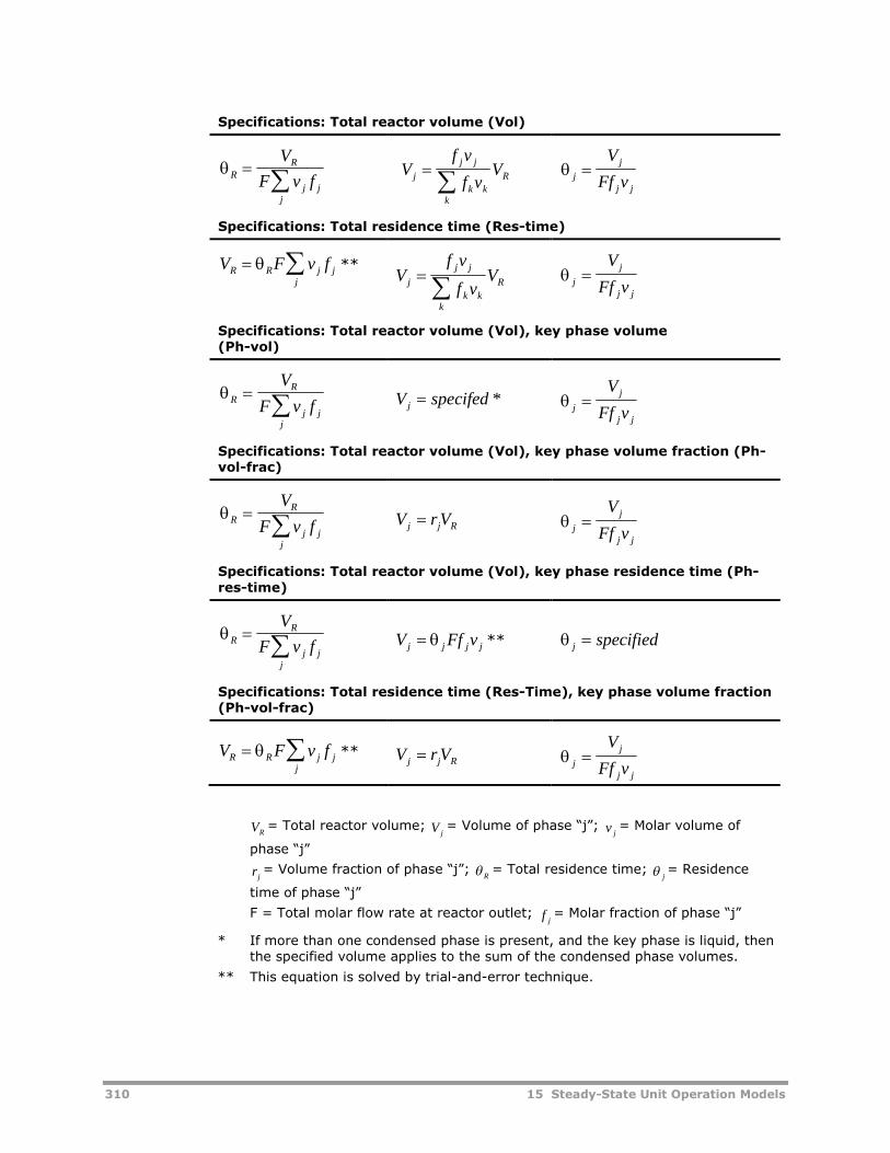
310 15 Steady-State Unit Operation Models
Specifications: Total reactor volume (Vol)
RR
j jj
V
F v f
Vf v
f vVj
j j
k kk
R
j
j
j j
V
Ff v
Specifications: Total residence time (Res-time)
V F v fR R j jj
**V
f v
f vVj
j j
k kk
R
j
j
j j
V
Ff v
Specifications: Total reactor volume (Vol), key phase volume(Ph-vol)
RR
j jj
V
F v f V specifedj * j
j
j j
V
Ff v
Specifications: Total reactor volume (Vol), key phase volume fraction (Ph-vol-frac)
RR
j jj
V
F v f V r Vj j R j
j
j j
V
Ff v
Specifications: Total reactor volume (Vol), key phase residence time (Ph-res-time)
RR
j jj
V
F v f V Ff vj j j j ** j specified
Specifications: Total residence time (Res-Time), key phase volume fraction(Ph-vol-frac)
V F v fR R j jj
** V r Vj j R j
j
j j
V
Ff v
RV = Total reactor volume;jV = Volume of phase “j”;
jv = Molar volume of
phase “j”
jr = Volume fraction of phase “j”;R = Total residence time;
j = Residence
time of phase “j”
F = Total molar flow rate at reactor outlet;jf = Molar fraction of phase “j”
* If more than one condensed phase is present, and the key phase is liquid, thenthe specified volume applies to the sum of the condensed phase volumes.
** This equation is solved by trial-and-error technique.
15 Steady-State Unit Operation Models 311
When residence time is specified instead of volume, the RCSTR model adjuststhe volume to satisfy the residence time specification.
Convergence problems in the residence time loop can be alleviated byproviding initial volume estimates in the ESTIMATES form. If convergenceproblems persist, then the maximum volume step size (Max-Vstep) should bereduced. If the key phase residence time is specified, then the RCSTR modeluses the specified reactor volume as an upper limit for the key phase volume.
EB LOOP
The second loop is the energy balance conservation equation (EB-LOOP). Inthis loop, the reactor temperature is adjusted to match the specified reactorduty. If the temperature is specified instead of the duty, this loop is by-passed.
Since the reaction rates are very sensitive to temperature, large changes inthe reactor temperature between energy-balance iterations (EB-ITER) maycause the mass-balance loop (MB-LOOP) to diverge. This problem can besolved by providing a good temperature estimate (T-EST) in the ESTIMATESform. If the problem persists, the maximum temperature step size (Max-Tstep) should be reduced (the default, 50C, is rather large).
MB-LOOP
The next loop is the mass-balance loop (MB-LOOP). This loop uses amultivariable solver to converge the conservation equations for componentmole flow and for the class two component attributes.
Two solvers are available: Broyden and Newton. The Broyden algorithm tendsto be relatively fast, but it may be unstable if the number of components andattributes is large and the reaction rates are high. The Newton algorithmtends to be slower, but more stable for many classes of problems. TheNewton algorithm calculates the response of each variable to each othervariable by perturbing the variables one at a time by a very small amount.These perturbation steps require lots of simulation time, which makes eachiteration of the Newton algorithm slow.
The number of mass-balance iterations (MB-Maxit) is defined on theconvergence form. By default, the model allows 50 mass-balance iterations.This default is sufficient for the Newton algorithm, but is usually too small forthe Broyden algorithm. For polymer reaction kinetics, the number of requiredmass-balance iterations may be as high as 500.
Using a Damping Factor
The stability of the Broyden algorithm can be adjusted using a damping factor(DAMP-FAC) defined on the “Convergence” form. Decreasing the dampingfactor decreases the step-size, resulting in a larger number of smaller, morestable steps. Thus, the maximum number of iterations should be increased asthe damping factor is decreased.
The damping factor is sensitive on a log scale. If the Broyden algorithmappears unstable, try setting the damping factor to 0.5, 0.3, 0.1, 0.05 etc.Optimum damping factors for polymerization kinetics typically fall between0.1 and 0.001.
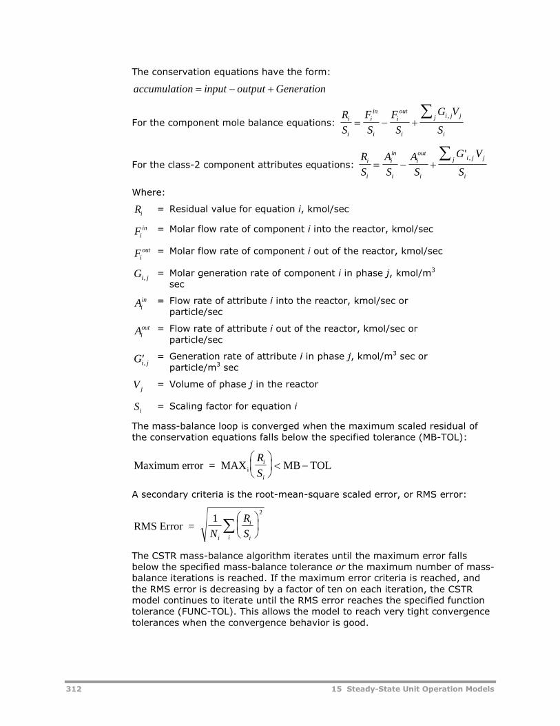
312 15 Steady-State Unit Operation Models
The conservation equations have the form:
accumulation input output Generation
For the component mole balance equations:R
S
F
S
F
S
G V
Si
i
iin
i
iout
i
i j jj
i
,
For the class-2 component attributes equations:R
S
A
S
A
S
G V
Si
i
iin
i
iout
i
i j jj
i
' ,
Where:
Ri= Residual value for equation i, kmol/sec
Fiin = Molar flow rate of component i into the reactor, kmol/sec
Fiout = Molar flow rate of component i out of the reactor, kmol/sec
Gi j,= Molar generation rate of component i in phase j, kmol/m3
sec
Aiin = Flow rate of attribute i into the reactor, kmol/sec or
particle/sec
Aiout = Flow rate of attribute i out of the reactor, kmol/sec or
particle/sec
Gi j,= Generation rate of attribute i in phase j, kmol/m3 sec or
particle/m3 sec
V j= Volume of phase j in the reactor
Si= Scaling factor for equation i
The mass-balance loop is converged when the maximum scaled residual ofthe conservation equations falls below the specified tolerance (MB-TOL):
Maximum error = MAX MB TOLi
R
Si
i
A secondary criteria is the root-mean-square scaled error, or RMS error:
RMS Error =1
2
N
R
Si
i
ii
The CSTR mass-balance algorithm iterates until the maximum error fallsbelow the specified mass-balance tolerance or the maximum number of mass-balance iterations is reached. If the maximum error criteria is reached, andthe RMS error is decreasing by a factor of ten on each iteration, the CSTRmodel continues to iterate until the RMS error reaches the specified functiontolerance (FUNC-TOL). This allows the model to reach very tight convergencetolerances when the convergence behavior is good.
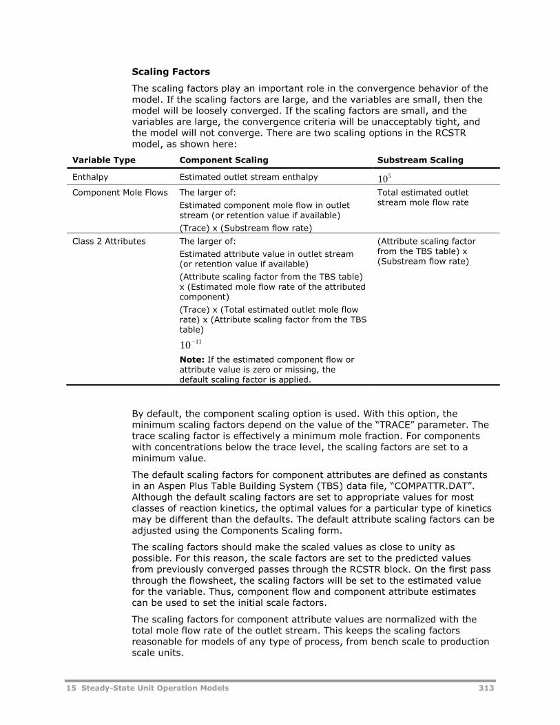
15 Steady-State Unit Operation Models 313
Scaling Factors
The scaling factors play an important role in the convergence behavior of themodel. If the scaling factors are large, and the variables are small, then themodel will be loosely converged. If the scaling factors are small, and thevariables are large, the convergence criteria will be unacceptably tight, andthe model will not converge. There are two scaling options in the RCSTRmodel, as shown here:
Variable Type Component Scaling Substream Scaling
Enthalpy Estimated outlet stream enthalpy 105
Component Mole Flows The larger of:
Estimated component mole flow in outletstream (or retention value if available)
(Trace) x (Substream flow rate)
Total estimated outletstream mole flow rate
Class 2 Attributes The larger of:
Estimated attribute value in outlet stream(or retention value if available)
(Attribute scaling factor from the TBS table)x (Estimated mole flow rate of the attributedcomponent)
(Trace) x (Total estimated outlet mole flowrate) x (Attribute scaling factor from the TBStable)
1110
Note: If the estimated component flow orattribute value is zero or missing, thedefault scaling factor is applied.
(Attribute scaling factorfrom the TBS table) x(Substream flow rate)
By default, the component scaling option is used. With this option, theminimum scaling factors depend on the value of the “TRACE” parameter. Thetrace scaling factor is effectively a minimum mole fraction. For componentswith concentrations below the trace level, the scaling factors are set to aminimum value.
The default scaling factors for component attributes are defined as constantsin an Aspen Plus Table Building System (TBS) data file, “COMPATTR.DAT”.Although the default scaling factors are set to appropriate values for mostclasses of reaction kinetics, the optimal values for a particular type of kineticsmay be different than the defaults. The default attribute scaling factors can beadjusted using the Components Scaling form.
The scaling factors should make the scaled values as close to unity aspossible. For this reason, the scale factors are set to the predicted valuesfrom previously converged passes through the RCSTR block. On the first passthrough the flowsheet, the scaling factors will be set to the estimated valuefor the variable. Thus, component flow and component attribute estimatescan be used to set the initial scale factors.
The scaling factors for component attribute values are normalized with thetotal mole flow rate of the outlet stream. This keeps the scaling factorsreasonable for models of any type of process, from bench scale to productionscale units.
314 15 Steady-State Unit Operation Models
The inner-most loop is the phase equilibrium loop, or flash equations. For thisreason, it is essential to have accurate physical properties over the entirerange of temperatures and pressures found in the process.
The flash calculations start from retention values once the mass-balance errorfalls below the retention threshold (Ret-Thresh) specified in the convergenceform. If the retention threshold is set very high, then the flash may fail,resulting in step-size cuts in the mass balance loop. If the retention thresholdis reduced, the reactor calculations may require more time. For most
simulation problems, setting the retention threshold to 1 1010 results in fastflash convergence without errors. If errors occur, try using the default value,
1 105 . If errors persist, the most likely cause is a physical property problem.
Initialization Options
The convergence behavior of the RCSTR model depends on how the model isinitialized. There are three initialization options for the RCSTR model.
Solver Initialization—Do not use integration
By default, the solver algorithm initializes itself using previously savedsimulation results (retention). This saves time if the RCSTR block is insidea flowsheet recycle loop, where the block will be run several times insuccession. It also saves time if the block is inside a sensitivity,optimization, design-spec, or data-fit study.
Alternately, the user can force the model to restart from estimates everytime by checking the restart flag on the block-options form.
When retention is not available, or when the restart option is active, themodel uses user-specified estimates to initialize the solver algorithm.Estimates can be provided for the reactor volume, phase volume, reactortemperature, component flow rates, and component attribute values. Thecomponent attribute estimates can be specified using class-2 or class-0attribute values.
If estimates are not provided, the model initializes the variables using themixed feed stream (for example, the initial value of a component flow ratemay be set to the total flow rate of that component in all feed streams tothe reactor).
Integration Initialization—Always use integration
In the integration algorithm, the RCSTR is treated as a dynamic stirred-tank reactor. The conservation equations are numerically integrated froman initial condition to the steady-state condition. The initial compositionsin the reactor are set equal to those in the feed stream.
If temperature is specified in the reactor, then the temperature profileduring initialization can be ramped from the feed stream temperature tothe specified temperature over the interval of several residence times. Ifduty is specified, then the duty can be ramped from adiabatic conditionsto the specified duty. Ramping allows the reactor to “cold-start” forimproved integration performance.
The numerical integration carries forward until the residual terms(accumulation terms) drop below the specified mass-balance tolerance. Atthis point, the model enters the solver and continues until the modelconverges.
15 Steady-State Unit Operation Models 315
Note that initial guesses for component flow rates and componentattributes should not be provided when using the integration initializationoption unless the reactor exhibits multiple steady-state solutions. In thiscase, initial estimates may be used to force the reactor towards aparticular solution.
Hybrid Initialization—Initialize using integration
The hybrid option takes advantage of the robust integration algorithm toinitialize the reactor during the first pass. On subsequent passes, when apreviously converged solution is available, the solution algorithm bypassesintegration and jumps directly into the trial-and-error solver. Since thesolver algorithm is much faster than the integration algorithm, the hybridoption offers improved performance for most problems.
Note: By default, the RCSTR model does not use integration (e.g., the trialand error solution algorithm starts directly from the user-specified initialguesses or from retention values). Optionally, the RCSTR model can beinitialized using an integration approach or a hybrid approach that usesintegration only when retention values are not available.
Troubleshooting Convergence Problems
To diagnose RCSTR convergence problems, set the terminal reporting level to“7” in the Block-Options form. This causes the RCSTR model to report theresidence time iterations (RT-ITER), energy balance iterations (EB-ITER), andmass-balance iterations (MB-ITER) to the control panel. In addition, themodel reports the maximum and root-mean-square errors for each loop.
The Simulation diagnostic reporting level controls the diagnostic messageswritten to the history file (.HIS file). The maximum mass-balance error isreported at level 5. At level 6, the model reports the value of each reactingcomponent flow rate and each component attribute. At level 7, the modelreports values and rates of change (reaction rates) for components andattributes. At level 8, the model reports the values, rates, and residuals(error) of each solved variable.
When troubleshooting convergence problems, simplify the problem byspecifying temperature and volume instead of duty and residence time. Ifconvergence problems persist, they must be related to the mass-balanceloop, the reaction kinetic model or rate constants, or the underlying physicalproperty calculations.
Numerical integration is much more reliable than trial-and-error solvers. Ifthe RCSTR mass-balance fails to converge, try running the same kinetics inan RPlug model. If possible, set the phase criteria “liquid-only” to eliminatephysical property problems from the list of possible sources of error. If theRPlug model cannot converge with the specified kinetics, then the problem isalmost certainly related to reaction kinetics.
Possible sources of error in the reaction kinetics include:
Errors in the molecular weight of a product or reactant
Errors in the specified stoichiometry of a reaction (mass balance isviolated)
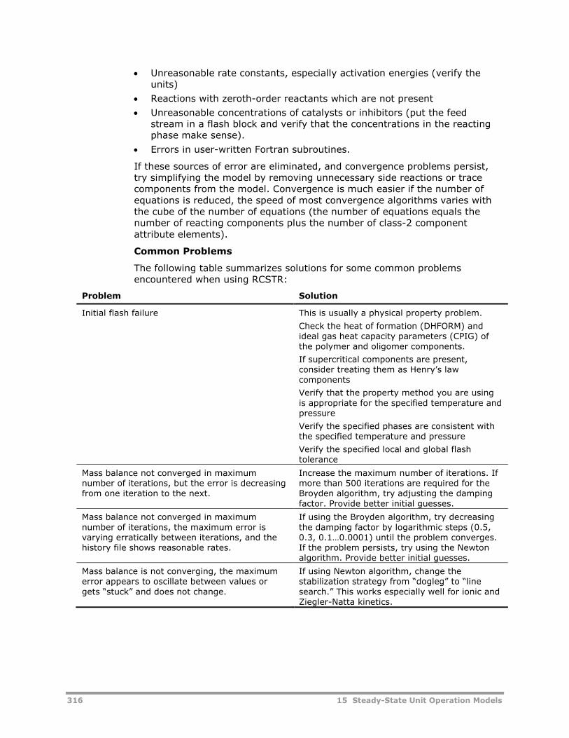
316 15 Steady-State Unit Operation Models
Unreasonable rate constants, especially activation energies (verify theunits)
Reactions with zeroth-order reactants which are not present
Unreasonable concentrations of catalysts or inhibitors (put the feedstream in a flash block and verify that the concentrations in the reactingphase make sense).
Errors in user-written Fortran subroutines.
If these sources of error are eliminated, and convergence problems persist,try simplifying the model by removing unnecessary side reactions or tracecomponents from the model. Convergence is much easier if the number ofequations is reduced, the speed of most convergence algorithms varies withthe cube of the number of equations (the number of equations equals thenumber of reacting components plus the number of class-2 componentattribute elements).
Common Problems
The following table summarizes solutions for some common problemsencountered when using RCSTR:
Problem Solution
Initial flash failure This is usually a physical property problem.
Check the heat of formation (DHFORM) andideal gas heat capacity parameters (CPIG) ofthe polymer and oligomer components.
If supercritical components are present,consider treating them as Henry’s lawcomponents
Verify that the property method you are usingis appropriate for the specified temperature andpressure
Verify the specified phases are consistent withthe specified temperature and pressure
Verify the specified local and global flashtolerance
Mass balance not converged in maximumnumber of iterations, but the error is decreasingfrom one iteration to the next.
Increase the maximum number of iterations. Ifmore than 500 iterations are required for theBroyden algorithm, try adjusting the dampingfactor. Provide better initial guesses.
Mass balance not converged in maximumnumber of iterations, the maximum error isvarying erratically between iterations, and thehistory file shows reasonable rates.
If using the Broyden algorithm, try decreasingthe damping factor by logarithmic steps (0.5,0.3, 0.1…0.0001) until the problem converges.If the problem persists, try using the Newtonalgorithm. Provide better initial guesses.
Mass balance is not converging, the maximumerror appears to oscillate between values orgets “stuck” and does not change.
If using Newton algorithm, change thestabilization strategy from “dogleg” to “linesearch.” This works especially well for ionic andZiegler-Natta kinetics.
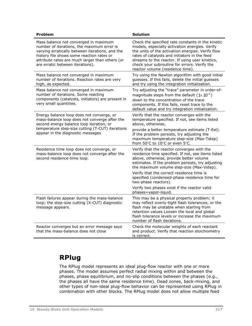
15 Steady-State Unit Operation Models 317
Problem Solution
Mass balance not converged in maximumnumber of iterations, the maximum error isvarying erratically between iterations, and thehistory file shows some reaction rates orattribute rates are much larger than others (orare erratic between iterations).
Check the specified rate constants in the kineticmodels, especially activation energies. Verifythe units of the activation energies. Verify flowrates of catalysts and initiators in the feedstreams to the reactor. If using user kinetics,check your subroutine for errors. Verify thereactor volume (residence time).
Mass balance not converged in maximumnumber of iterations. Reaction rates are veryhigh, as expected.
Try using the Newton algorithm with good initialguesses. If this fails, delete the initial guessesand try using the integration initialization.
Mass balance not converged in maximumnumber of iterations. Some reactingcomponents (catalysts, initiators) are present invery small quantities.
Try adjusting the “trace” parameter in order-of-
magnitude steps from the default (1 10 3 )
down to the concentration of the tracecomponents. If this fails, reset trace to thedefault value and try integration initialization.
Energy balance loop does not converge, ormass-balance loop does not converge after thesecond energy balance loop iteration, ortemperature step-size cutting (T-CUT) iterationsappear in the diagnostic messages
Verify that the reactor converges with thetemperature specified. If not, see items listedabove, otherwise,
provide a better temperature estimate (T-Est).If the problem persists, try adjusting themaximum temperature step-size (Max-Tstep)from 50C to 10C or even 5C.
Residence time loop does not converge, ormass-balance loop does not converge after thesecond residence-time loop.
Verify that the reactor converges with theresidence time specified. If not, see items listedabove, otherwise, provide better volumeestimates. If the problem persists, try adjustingthe maximum volume step-size (Max-Vstep).
Verify that the correct residence time isspecified (condensed-phase residence time fortwo-phase reactors).
Verify two phases exist if the reactor validphases=vapor-liquid.
Flash failures appear during the mass-balanceloop; the step-size cutting (X-CUT) diagnosticmessage appears.
This may be a physical property problem; itmay reflect overly-tight flash tolerances; or theflash may be unstable when starting fromretention values Loosen the local and globalflash tolerance levels or increase the maximumnumber of flash iterations.
Reactor converges but an error message saysthat the mass-balance does not close
Check the molecular weights of each reactantand product. Verify that reaction stoichiometryis correct.
RPlugThe RPlug model represents an ideal plug-flow reactor with one or morephases. The model assumes perfect radial mixing within and between thephases, phase equilibrium, and no-slip conditions between the phases (e.g.,the phases all have the same residence time). Dead zones, back-mixing, andother types of non-ideal plug-flow behavior can be represented using RPlug incombination with other blocks. The RPlug model does not allow multiple feed
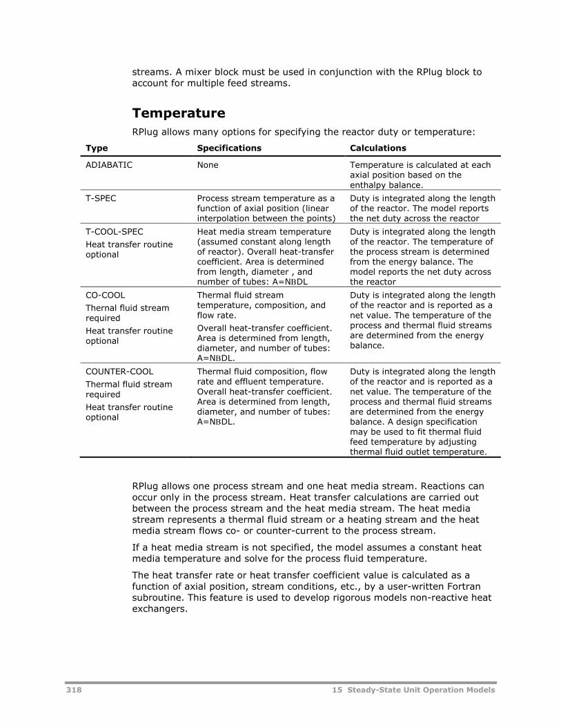
318 15 Steady-State Unit Operation Models
streams. A mixer block must be used in conjunction with the RPlug block toaccount for multiple feed streams.
Temperature
RPlug allows many options for specifying the reactor duty or temperature:
Type Specifications Calculations
ADIABATIC None Temperature is calculated at eachaxial position based on theenthalpy balance.
T-SPEC Process stream temperature as afunction of axial position (linearinterpolation between the points)
Duty is integrated along the lengthof the reactor. The model reportsthe net duty across the reactor
T-COOL-SPEC
Heat transfer routineoptional
Heat media stream temperature(assumed constant along lengthof reactor). Overall heat-transfercoefficient. Area is determinedfrom length, diameter , andnumber of tubes: A=NDL
Duty is integrated along the lengthof the reactor. The temperature ofthe process stream is determinedfrom the energy balance. Themodel reports the net duty acrossthe reactor
CO-COOL
Thernal fluid streamrequired
Heat transfer routineoptional
Thermal fluid streamtemperature, composition, andflow rate.
Overall heat-transfer coefficient.Area is determined from length,diameter, and number of tubes:A=NDL.
Duty is integrated along the lengthof the reactor and is reported as anet value. The temperature of theprocess and thermal fluid streamsare determined from the energybalance.
COUNTER-COOL
Thermal fluid streamrequired
Heat transfer routineoptional
Thermal fluid composition, flowrate and effluent temperature.Overall heat-transfer coefficient.Area is determined from length,diameter, and number of tubes:A=NDL.
Duty is integrated along the lengthof the reactor and is reported as anet value. The temperature of theprocess and thermal fluid streamsare determined from the energybalance. A design specificationmay be used to fit thermal fluidfeed temperature by adjustingthermal fluid outlet temperature.
RPlug allows one process stream and one heat media stream. Reactions canoccur only in the process stream. Heat transfer calculations are carried outbetween the process stream and the heat media stream. The heat mediastream represents a thermal fluid stream or a heating stream and the heatmedia stream flows co- or counter-current to the process stream.
If a heat media stream is not specified, the model assumes a constant heatmedia temperature and solve for the process fluid temperature.
The heat transfer rate or heat transfer coefficient value is calculated as afunction of axial position, stream conditions, etc., by a user-written Fortransubroutine. This feature is used to develop rigorous models non-reactive heatexchangers.
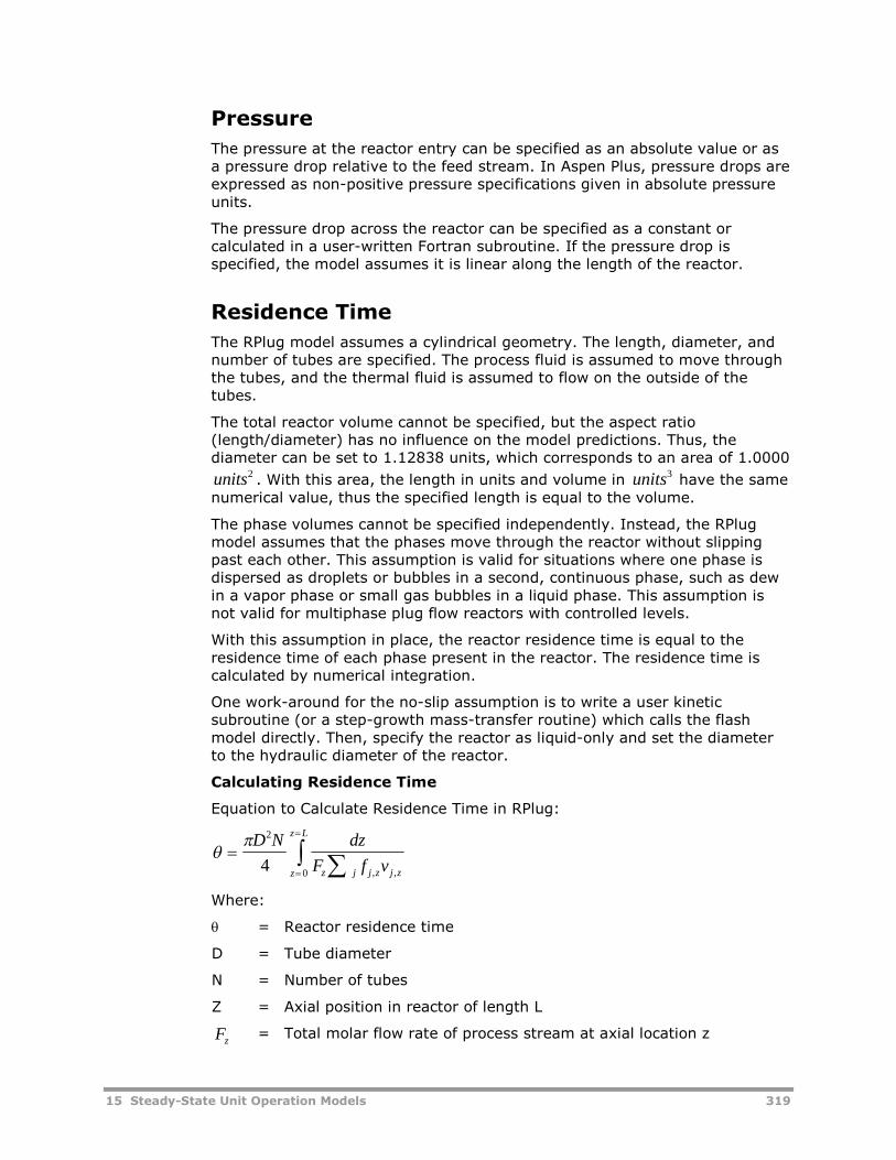
15 Steady-State Unit Operation Models 319
Pressure
The pressure at the reactor entry can be specified as an absolute value or asa pressure drop relative to the feed stream. In Aspen Plus, pressure drops areexpressed as non-positive pressure specifications given in absolute pressureunits.
The pressure drop across the reactor can be specified as a constant orcalculated in a user-written Fortran subroutine. If the pressure drop isspecified, the model assumes it is linear along the length of the reactor.
Residence Time
The RPlug model assumes a cylindrical geometry. The length, diameter, andnumber of tubes are specified. The process fluid is assumed to move throughthe tubes, and the thermal fluid is assumed to flow on the outside of thetubes.
The total reactor volume cannot be specified, but the aspect ratio(length/diameter) has no influence on the model predictions. Thus, thediameter can be set to 1.12838 units, which corresponds to an area of 1.0000
units2. With this area, the length in units and volume in units3
have the samenumerical value, thus the specified length is equal to the volume.
The phase volumes cannot be specified independently. Instead, the RPlugmodel assumes that the phases move through the reactor without slippingpast each other. This assumption is valid for situations where one phase isdispersed as droplets or bubbles in a second, continuous phase, such as dewin a vapor phase or small gas bubbles in a liquid phase. This assumption isnot valid for multiphase plug flow reactors with controlled levels.
With this assumption in place, the reactor residence time is equal to theresidence time of each phase present in the reactor. The residence time iscalculated by numerical integration.
One work-around for the no-slip assumption is to write a user kineticsubroutine (or a step-growth mass-transfer routine) which calls the flashmodel directly. Then, specify the reactor as liquid-only and set the diameterto the hydraulic diameter of the reactor.
Calculating Residence Time
Equation to Calculate Residence Time in RPlug:
D N dz
F f vz j j z j zz
z L2
04 , ,
Where:
= Reactor residence time
D = Tube diameter
N = Number of tubes
Z = Axial position in reactor of length L
Fz= Total molar flow rate of process stream at axial location z
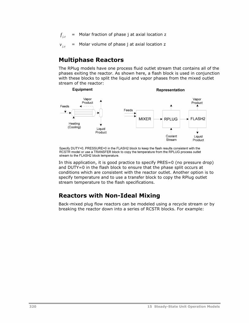
320 15 Steady-State Unit Operation Models
f j z,= Molar fraction of phase j at axial location z
v j z,= Molar volume of phase j at axial location z
Multiphase Reactors
The RPlug models have one process fluid outlet stream that contains all of thephases exiting the reactor. As shown here, a flash block is used in conjunctionwith these blocks to split the liquid and vapor phases from the mixed outletstream of the reactor:
In this application, it is good practice to specify PRES=0 (no pressure drop)and DUTY=0 in the flash block to ensure that the phase split occurs atconditions which are consistent with the reactor outlet. Another option is tospecify temperature and to use a transfer block to copy the RPlug outletstream temperature to the flash specifications.
Reactors with Non-Ideal Mixing
Back-mixed plug flow reactors can be modeled using a recycle stream or bybreaking the reactor down into a series of RCSTR blocks. For example:
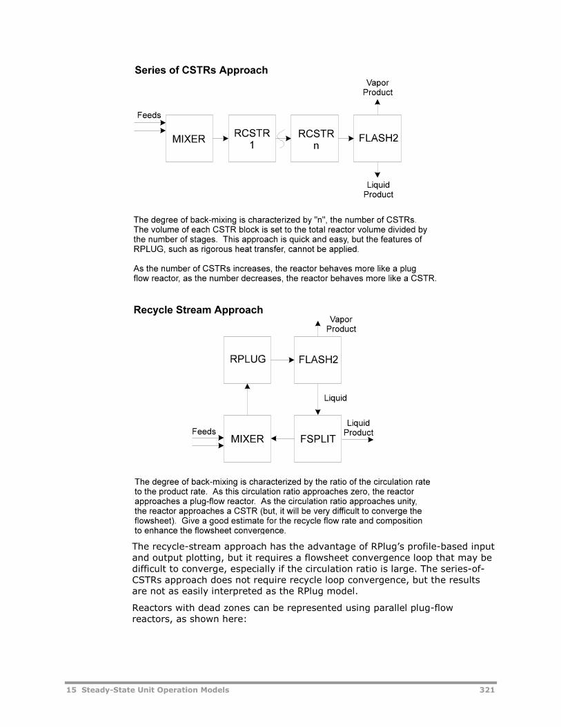
15 Steady-State Unit Operation Models 321
The recycle-stream approach has the advantage of RPlug’s profile-based inputand output plotting, but it requires a flowsheet convergence loop that may bedifficult to converge, especially if the circulation ratio is large. The series-of-CSTRs approach does not require recycle loop convergence, but the resultsare not as easily interpreted as the RPlug model.
Reactors with dead zones can be represented using parallel plug-flowreactors, as shown here:
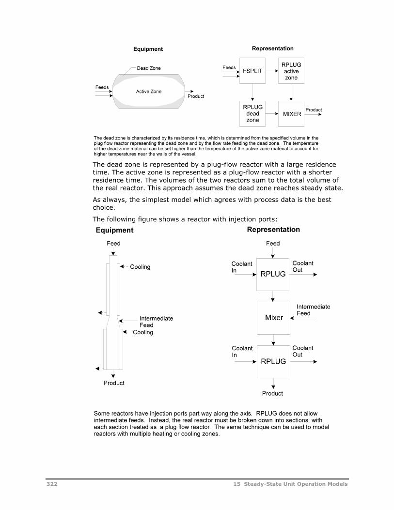
322 15 Steady-State Unit Operation Models
The dead zone is represented by a plug-flow reactor with a large residencetime. The active zone is represented as a plug-flow reactor with a shorterresidence time. The volumes of the two reactors sum to the total volume ofthe real reactor. This approach assumes the dead zone reaches steady state.
As always, the simplest model which agrees with process data is the bestchoice.
The following figure shows a reactor with injection ports:
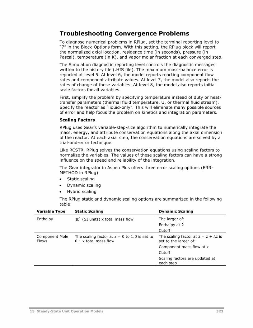
15 Steady-State Unit Operation Models 323
Troubleshooting Convergence Problems
To diagnose numerical problems in RPlug, set the terminal reporting level to“7” in the Block-Options form. With this setting, the RPlug block will reportthe normalized axial location, residence time (in seconds), pressure (inPascal), temperature (in K), and vapor molar fraction at each converged step.
The Simulation diagnostic reporting level controls the diagnostic messageswritten to the history file (.HIS file). The maximum mass-balance error isreported at level 5. At level 6, the model reports reacting component flowrates and component attribute values. At level 7, the model also reports therates of change of these variables. At level 8, the model also reports initialscale factors for all variables.
First, simplify the problem by specifying temperature instead of duty or heat-transfer parameters (thermal fluid temperature, U, or thermal fluid stream).Specify the reactor as “liquid-only”. This will eliminate many possible sourcesof error and help focus the problem on kinetics and integration parameters.
Scaling Factors
RPlug uses Gear’s variable-step-size algorithm to numerically integrate themass, energy, and attribute conservation equations along the axial dimensionof the reactor. At each axial step, the conservation equations are solved by atrial-and-error technique.
Like RCSTR, RPlug solves the conservation equations using scaling factors tonormalize the variables. The values of these scaling factors can have a stronginfluence on the speed and reliability of the integration.
The Gear integrator in Aspen Plus offers three error scaling options (ERR-METHOD in RPlug):
Static scaling
Dynamic scaling
Hybrid scaling
The RPlug static and dynamic scaling options are summarized in the followingtable:
Variable Type Static Scaling Dynamic Scaling
Enthalpy 105 (SI units) x total mass flow The larger of:
Enthalpy at 2
Cutoff
Component MoleFlows
The scaling factor at z = 0 to 1.0 is set to0.1 x total mass flow
The scaling factor at z = z + z isset to the larger of:
Component mass flow at z
Cutoff
Scaling factors are updated ateach step
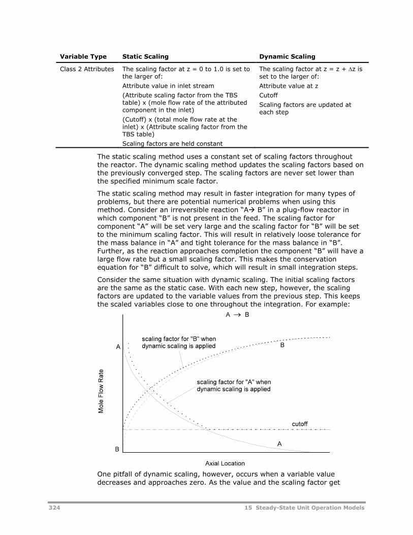
324 15 Steady-State Unit Operation Models
Variable Type Static Scaling Dynamic Scaling
Class 2 Attributes The scaling factor at z = 0 to 1.0 is set tothe larger of:
Attribute value in inlet stream
(Attribute scaling factor from the TBStable) x (mole flow rate of the attributedcomponent in the inlet)
(Cutoff) x (total mole flow rate at theinlet) x (Attribute scaling factor from theTBS table)
Scaling factors are held constant
The scaling factor at z = z + z isset to the larger of:
Attribute value at z
Cutoff
Scaling factors are updated ateach step
The static scaling method uses a constant set of scaling factors throughoutthe reactor. The dynamic scaling method updates the scaling factors based onthe previously converged step. The scaling factors are never set lower thanthe specified minimum scale factor.
The static scaling method may result in faster integration for many types ofproblems, but there are potential numerical problems when using thismethod. Consider an irreversible reaction “A B” in a plug-flow reactor inwhich component “B” is not present in the feed. The scaling factor forcomponent “A” will be set very large and the scaling factor for “B” will be setto the minimum scaling factor. This will result in relatively loose tolerance forthe mass balance in “A” and tight tolerance for the mass balance in “B”.Further, as the reaction approaches completion the component “B” will have alarge flow rate but a small scaling factor. This makes the conservationequation for “B” difficult to solve, which will result in small integration steps.
Consider the same situation with dynamic scaling. The initial scaling factorsare the same as the static case. With each new step, however, the scalingfactors are updated to the variable values from the previous step. This keepsthe scaled variables close to one throughout the integration. For example:
One pitfall of dynamic scaling, however, occurs when a variable valuedecreases and approaches zero. As the value and the scaling factor get
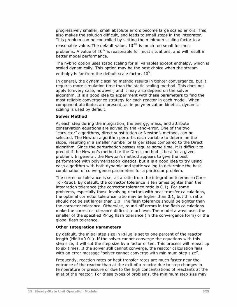
15 Steady-State Unit Operation Models 325
progressively smaller, small absolute errors become large scaled errors. Thisalso makes the solution difficult, and leads to small steps in the integrator.This problem can be controlled by setting the minimum scaling factor to a
reasonable value. The default value, 10-10is much too small for most
problems. A value of 10-5is reasonable for most situations, and will result in
better model performance.
The hybrid option uses static scaling for all variables except enthalpy, which isscaled dynamically. This option may be the best choice when the stream
enthalpy is far from the default scale factor,510 .
In general, the dynamic scaling method results in tighter convergence, but itrequires more simulation time than the static scaling method. This does notapply to every case, however, and it may also depend on the solveralgorithm. It is a good idea to experiment with these parameters to find themost reliable convergence strategy for each reactor in each model. Whencomponent attributes are present, as in polymerization kinetics, dynamicscaling is used by default.
Solver Method
At each step during the integration, the energy, mass, and attributeconservation equations are solved by trial-and-error. One of the two“corrector” algorithms, direct substitution or Newton’s method, can beselected. The Newton algorithm perturbs each variable to determine theslope, resulting in a smaller number or larger steps compared to the Directalgorithm. Since the perturbation passes require some time, it is difficult topredict if the Newton’s method or the Direct method is best for a givenproblem. In general, the Newton’s method appears to give the bestperformance with polymerization kinetics, but it is a good idea to try usingeach algorithm with both dynamic and static scaling to determine the bestcombination of convergence parameters for a particular problem.
The corrector tolerance is set as a ratio from the integration tolerance (Corr-Tol-Ratio). By default, the corrector tolerance is ten times tighter than theintegration tolerance (the corrector tolerance ratio is 0.1). For someproblems, especially those involving reactors with heat transfer calculations,the optimal corrector tolerance ratio may be higher than 0.1, but this ratioshould not be set larger than 1.0. The flash tolerance should be tighter thanthe corrector tolerance. Otherwise, round-off errors in the flash calculationsmake the corrector tolerance difficult to achieve. The model always uses thesmaller of the specified RPlug flash tolerance (in the convergence form) or theglobal flash tolerance.
Other Integration Parameters
By default, the initial step size in RPlug is set to one percent of the reactorlength (Hinit=0.01). If the solver cannot converge the equations with thisstep size, it will cut the step size by a factor of ten. This process will repeat upto six times. If the solver still cannot converge, the reactor calculation failswith an error message “solver cannot converge with minimum step size”.
Frequently, reaction rates or heat transfer rates are much faster near theentrance of the reactor than at the exit of a reactor due to step changes intemperature or pressure or due to the high concentrations of reactants at theinlet of the reactor. For these types of problems, the minimum step size may
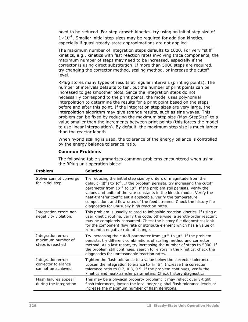
326 15 Steady-State Unit Operation Models
need to be reduced. For step-growth kinetics, try using an initial step size of
1 10-4 . Smaller initial step-sizes may be required for addition kinetics,especially if quasi-steady-state approximations are not applied.
The maximum number of integration steps defaults to 1000. For very “stiff”kinetics, e.g., kinetics with fast reaction rates involving trace components, themaximum number of steps may need to be increased, especially if thecorrector is using direct substitution. If more than 5000 steps are required,try changing the corrector method, scaling method, or increase the cutofflevel.
RPlug stores many types of results at regular intervals (printing points). Thenumber of intervals defaults to ten, but the number of print points can beincreased to get smoother plots. Since the integration steps do notnecessarily correspond to the print points, the model uses polynomialinterpolation to determine the results for a print point based on the stepsbefore and after this point. If the integration step sizes are very large, theinterpolation algorithm may give strange results, such as sine waves. Thisproblem can be fixed by reducing the maximum step size (Max-StepSize) to avalue smaller than the increments between print points (this forces the modelto use linear interpolation). By default, the maximum step size is much largerthan the reactor length.
When hybrid scaling is used, the tolerance of the energy balance is controlledby the energy balance tolerance ratio.
Common Problems
The following table summarizes common problems encountered when usingthe RPlug unit operation block:
Problem Solution
Solver cannot convergefor initial step
Try reducing the initial step size by orders of magnitude from the
default (10-2 ) to 10-8 . If the problem persists, try increasing the cutoff
parameter from 10-10 to 10-5 . If the problem still persists, verify thevalues and units of the rate constants in the kinetic model. Verify theheat-transfer coefficient if applicable. Verify the temperature,composition, and flow rates of the feed streams. Check the history filediagnostics for unusually high reaction rates.
Integration error: non-negativity violation.
This problem is usually related to infeasible reaction kinetics. If using auser kinetic routine, verify the code, otherwise, a zeroth-order reactantmay be completely consumed. Check the history file diagnostics; lookfor the component flow rate or attribute element which has a value ofzero and a negative rate of change.
Integration error:maximum number ofsteps is reached
Try increasing the cutoff parameter from 10-10 to 10-5 . If the problempersists, try different combinations of scaling method and correctormethod. As a last resort, try increasing the number of steps to 5000. Ifthe problem still continues, search for errors in the kinetics; check thediagnostics for unreasonable reaction rates.
Integration error:corrector tolerancecannot be achieved
Tighten the flash tolerance to a value below the corrector tolerance.
Loosen the integration tolerance to 1 10-3 . Increase the correctortolerance ratio to 0.2, 0.3, 0.5. If the problem continues, verify thekinetics and heat-transfer parameters. Check history diagnostics.
Flash failures appearduring the integration
This may be a physical property problem; it may reflect overly-tightflash tolerances, loosen the local and/or global flash tolerance levels orincrease the maximum number of flash iterations.
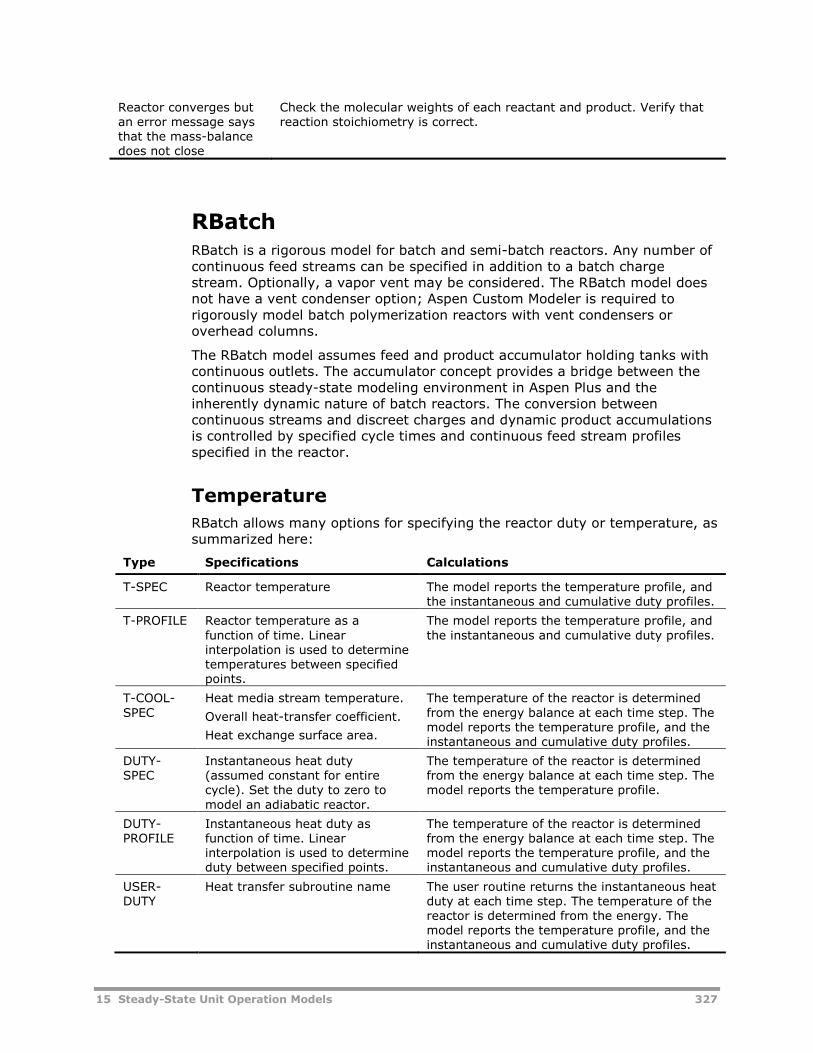
15 Steady-State Unit Operation Models 327
Reactor converges butan error message saysthat the mass-balancedoes not close
Check the molecular weights of each reactant and product. Verify thatreaction stoichiometry is correct.
RBatchRBatch is a rigorous model for batch and semi-batch reactors. Any number ofcontinuous feed streams can be specified in addition to a batch chargestream. Optionally, a vapor vent may be considered. The RBatch model doesnot have a vent condenser option; Aspen Custom Modeler is required torigorously model batch polymerization reactors with vent condensers oroverhead columns.
The RBatch model assumes feed and product accumulator holding tanks withcontinuous outlets. The accumulator concept provides a bridge between thecontinuous steady-state modeling environment in Aspen Plus and theinherently dynamic nature of batch reactors. The conversion betweencontinuous streams and discreet charges and dynamic product accumulationsis controlled by specified cycle times and continuous feed stream profilesspecified in the reactor.
Temperature
RBatch allows many options for specifying the reactor duty or temperature, assummarized here:
Type Specifications Calculations
T-SPEC Reactor temperature The model reports the temperature profile, andthe instantaneous and cumulative duty profiles.
T-PROFILE Reactor temperature as afunction of time. Linearinterpolation is used to determinetemperatures between specifiedpoints.
The model reports the temperature profile, andthe instantaneous and cumulative duty profiles.
T-COOL-SPEC
Heat media stream temperature.
Overall heat-transfer coefficient.
Heat exchange surface area.
The temperature of the reactor is determinedfrom the energy balance at each time step. Themodel reports the temperature profile, and theinstantaneous and cumulative duty profiles.
DUTY-SPEC
Instantaneous heat duty(assumed constant for entirecycle). Set the duty to zero tomodel an adiabatic reactor.
The temperature of the reactor is determinedfrom the energy balance at each time step. Themodel reports the temperature profile.
DUTY-PROFILE
Instantaneous heat duty asfunction of time. Linearinterpolation is used to determineduty between specified points.
The temperature of the reactor is determinedfrom the energy balance at each time step. Themodel reports the temperature profile, and theinstantaneous and cumulative duty profiles.
USER-DUTY
Heat transfer subroutine name The user routine returns the instantaneous heatduty at each time step. The temperature of thereactor is determined from the energy. Themodel reports the temperature profile, and theinstantaneous and cumulative duty profiles.
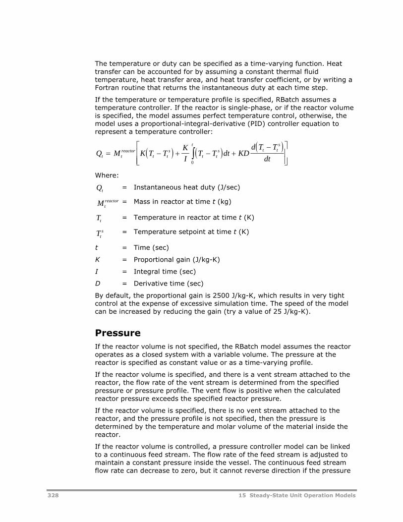
328 15 Steady-State Unit Operation Models
The temperature or duty can be specified as a time-varying function. Heattransfer can be accounted for by assuming a constant thermal fluidtemperature, heat transfer area, and heat transfer coefficient, or by writing aFortran routine that returns the instantaneous duty at each time step.
If the temperature or temperature profile is specified, RBatch assumes atemperature controller. If the reactor is single-phase, or if the reactor volumeis specified, the model assumes perfect temperature control, otherwise, themodel uses a proportional-integral-derivative (PID) controller equation torepresent a temperature controller:
Q M K T TK
IT T dt KD
d T T
dtt treactor
t ts
t ts t t
st
0
Where:
Qt= Instantaneous heat duty (J/sec)
Mtreactor = Mass in reactor at time t (kg)
Tt= Temperature in reactor at time t (K)
Tts = Temperature setpoint at time t (K)
t = Time (sec)
K = Proportional gain (J/kg-K)
I = Integral time (sec)
D = Derivative time (sec)
By default, the proportional gain is 2500 J/kg-K, which results in very tightcontrol at the expense of excessive simulation time. The speed of the modelcan be increased by reducing the gain (try a value of 25 J/kg-K).
Pressure
If the reactor volume is not specified, the RBatch model assumes the reactoroperates as a closed system with a variable volume. The pressure at thereactor is specified as constant value or as a time-varying profile.
If the reactor volume is specified, and there is a vent stream attached to thereactor, the flow rate of the vent stream is determined from the specifiedpressure or pressure profile. The vent flow is positive when the calculatedreactor pressure exceeds the specified reactor pressure.
If the reactor volume is specified, there is no vent stream attached to thereactor, and the pressure profile is not specified, then the pressure isdetermined by the temperature and molar volume of the material inside thereactor.
If the reactor volume is controlled, a pressure controller model can be linkedto a continuous feed stream. The flow rate of the feed stream is adjusted tomaintain a constant pressure inside the vessel. The continuous feed streamflow rate can decrease to zero, but it cannot reverse direction if the pressure
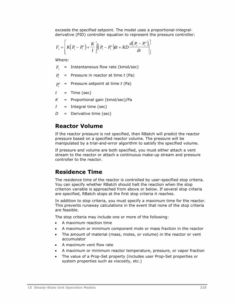
15 Steady-State Unit Operation Models 329
exceeds the specified setpoint. The model uses a proportional-integral-derivative (PID) controller equation to represent the pressure controller:
F K P PK
IP P dt KD
d P P
dtt t ts
t ts
tt t
s
0
Where:
Ft= Instantaneous flow rate (kmol/sec)
Pt= Pressure in reactor at time t (Pa)
Pts = Pressure setpoint at time t (Pa)
t = Time (sec)
K = Proportional gain (kmol/sec)/Pa
I = Integral time (sec)
D = Derivative time (sec)
Reactor Volume
If the reactor pressure is not specified, then RBatch will predict the reactorpressure based on a specified reactor volume. The pressure will bemanipulated by a trial-and-error algorithm to satisfy the specified volume.
If pressure and volume are both specified, you must either attach a ventstream to the reactor or attach a continuous make-up stream and pressurecontroller to the reactor.
Residence Time
The residence time of the reactor is controlled by user-specified stop criteria.You can specify whether RBatch should halt the reaction when the stopcriterion variable is approached from above or below. If several stop criteriaare specified, RBatch stops at the first stop criteria it reaches.
In addition to stop criteria, you must specify a maximum time for the reactor.This prevents runaway calculations in the event that none of the stop criteriaare feasible.
The stop criteria may include one or more of the following:
A maximum reaction time
A maximum or minimum component mole or mass fraction in the reactor
The amount of material (mass, moles, or volume) in the reactor or ventaccumulator
A maximum vent flow rate
A maximum or minimum reactor temperature, pressure, or vapor fraction
The value of a Prop-Set property (includes user Prop-Set properties orsystem properties such as viscosity, etc.)
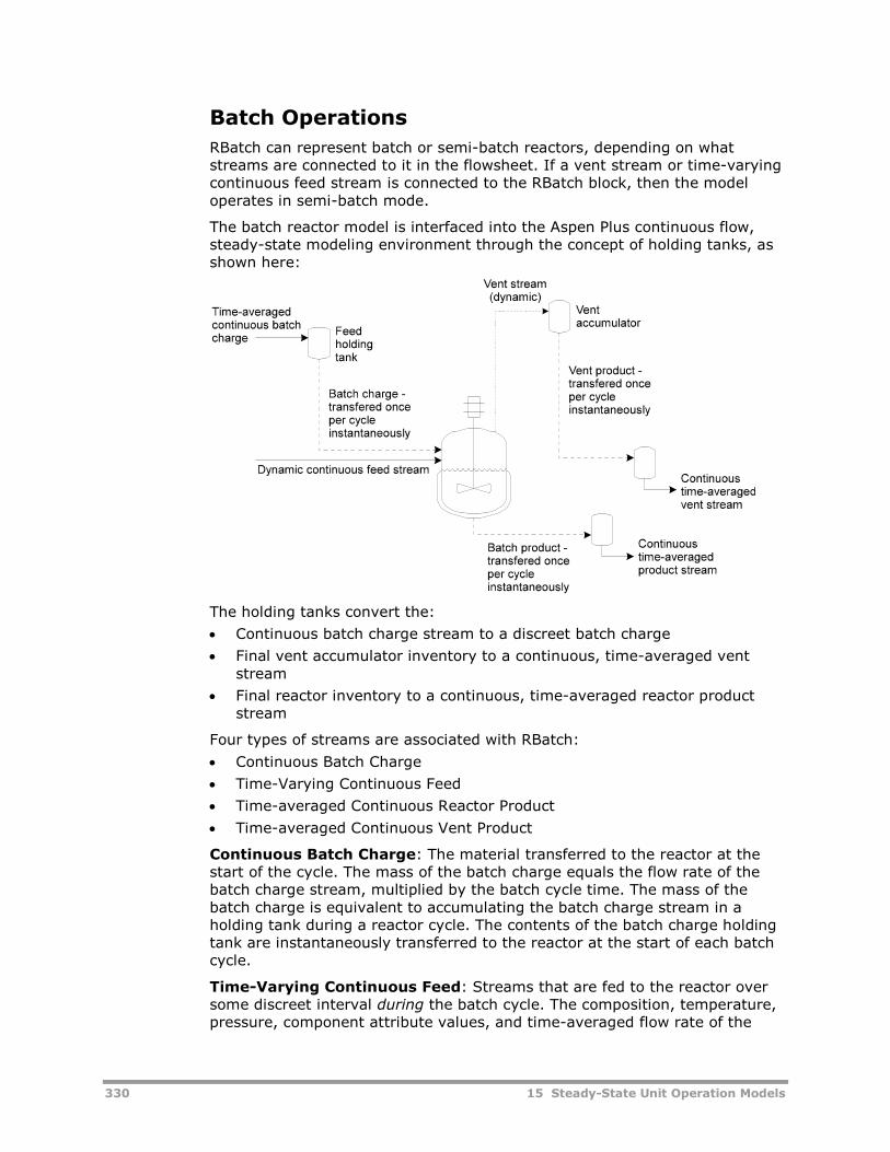
330 15 Steady-State Unit Operation Models
Batch Operations
RBatch can represent batch or semi-batch reactors, depending on whatstreams are connected to it in the flowsheet. If a vent stream or time-varyingcontinuous feed stream is connected to the RBatch block, then the modeloperates in semi-batch mode.
The batch reactor model is interfaced into the Aspen Plus continuous flow,steady-state modeling environment through the concept of holding tanks, asshown here:
The holding tanks convert the:
Continuous batch charge stream to a discreet batch charge
Final vent accumulator inventory to a continuous, time-averaged ventstream
Final reactor inventory to a continuous, time-averaged reactor productstream
Four types of streams are associated with RBatch:
Continuous Batch Charge
Time-Varying Continuous Feed
Time-averaged Continuous Reactor Product
Time-averaged Continuous Vent Product
Continuous Batch Charge: The material transferred to the reactor at thestart of the cycle. The mass of the batch charge equals the flow rate of thebatch charge stream, multiplied by the batch cycle time. The mass of thebatch charge is equivalent to accumulating the batch charge stream in aholding tank during a reactor cycle. The contents of the batch charge holdingtank are instantaneously transferred to the reactor at the start of each batchcycle.
Time-Varying Continuous Feed: Streams that are fed to the reactor oversome discreet interval during the batch cycle. The composition, temperature,pressure, component attribute values, and time-averaged flow rate of the
15 Steady-State Unit Operation Models 331
stream are specified in the flowsheet. The flow rate of the continuous feedstreams can be specified as a constant value, a time-varying profile, ormanipulated by the pressure controller model to meet a time-varyingpressure setpoint.
Time-averaged Continuous Reactor Product: This stream is determinedby dividing the final reactor inventory by the cycle time. This is analogous toinstantaneously dumping the reactor contents to a large holding tank at theend of the cycle, and continuously draining the tank throughout each cycle.
Time-averaged Continuous Vent Product: This stream is determined bydividing the final vent accumulator inventory by the cycle time. During thebatch cycle, the time-varying continuous vent stream is accumulated in thevent accumulator. The model assumes the vent accumulator contents areinstantly drained to a large holding tank at the end of the cycle, and theholding tank contents are continuously removed throughout the cycle.
Cycle Time
RBatch is a dynamic batch reactor model that is interfaced into the Aspen Pluscontinuous steady-state modeling environment. The interface requiresconverting batch charges and accumulator inventories into continuous streamflow rates. The cycle time is used to convert the batch charge flow rate intothe initial reactor inventory. The cycle time is also used to convert the ventaccumulator inventory and the reactor inventory into vent and reactorproduct streams.
For example, assuming a reactor has a cycle time of two hours and that nocontinuous feed streams are specified, then:
If the batch charge stream is set to 50 kg/hour, the initial reactorinventory is 100 kg.
If at the end of the reaction cycle, the vent accumulator contains 30 kg ofmaterial, the time-averaged continuous vent stream flow rate is 15 kg/hr.The composition of the time-averaged vent stream will be the same as thefinal composition in the vent accumulator.
The final reactor inventory will be 70 kg, and the time-averaged reactorproduct flow rate will be 35 kg/hr.
RBatch allows you to specify a feed time and down time instead of the cycletime. In this case, the time-averaged batch charge stream is divided by thefeed time to calculate the initial batch inventory. The time-averaged productflow rates are based on the cycle time, which is calculated from the sum ofthe feed time, the down time, and the reaction time. This option is notrecommended unless it is used to correct the mass balance for the influenceof time-varying continuous feed streams.
Troubleshooting Convergence Problems
To diagnose numerical problems in RBatch, set the terminal reporting level to“7” in the Block-Options form. With this setting, RBatch reports the time (inseconds), pressure (in Pascal), temperature (in K), and vapor mole fraction ateach converged integration step.
332 15 Steady-State Unit Operation Models
The Simulation diagnostic reporting level controls the diagnostic messageswritten to the history file (.HIS file). The maximum mass-balance error isreported at level 5. At level 6, the model reports reacting component flowrates and component attribute values. At level 7, the model also reports therates of change of these variables. At level 8, the model reports initial scalefactors for all integrated variables.
First, simplify the problem by specifying temperature instead of duty or heat-transfer parameters (thermal fluid temperature, U, or heat transfersubroutine). Specify the reactor as “liquid-only”. Specify the reactor pressure,but not the reactor volume. This will eliminate many possible sources of errorand help focus the problem on kinetics and integration parameters. Once themodel works with these settings, then revert the settings to duty, volume,and so on, making sure the model converges with each new specification.
Scaling Factors
RBatch uses Gear’s variable-step-size algorithm to numerically integrate themass, energy, and attribute conservation equations for the reactor and themass-balance equations for the vent condenser (if applicable). At each timestep, the conservation equations are solved by a trial-and-error technique.
RBatch solves the conservation equations using scaling factors to normalizethe variables. The values of these scaling factors have a strong influence onthe speed and reliability of the integration.
The Gear integrator in Aspen Plus offers three error scaling options (ERR-METHOD):
Static scaling
Dynamic scaling
Hybrid scaling
The RBatch static and dynamic scaling factors are summarized here:
Variable Type Static Scaling Dynamic Scaling
Enthalpy 105 (SI units) x mass holdup Enthalpy at previous time step
Component MassInventory InReactor and VentAccumulator
The scaling factor for each componentinventory equation is set to:
0.1 * (mass of batch charge stream)
Scaling factors are held constant
The scaling factor at t = t + t is set to thelarger of:
Component mass flow at t
Cutoff
Scaling factors are updated at each step
Class 2 AttributeInventory inReactor and VentAccumulator
The scaling factor of each componentattribute is set to:
(Attribute scaling factor from the TBStable) x (cycle time) (this is the attributeinventory at time = 0)
Scaling factors are held constant
The scaling factor at t = t + t is set to thelarger of:
Attribute inventory at time = t
Cutoff
Scaling factors are updated at each step
The static scaling method uses a constant set of scaling factors throughoutthe reactor. The dynamic scaling method updates the scaling factors based onthe previously converged step. The “cutoff” parameter is the minimum scalingfactor used in dynamic scaling.
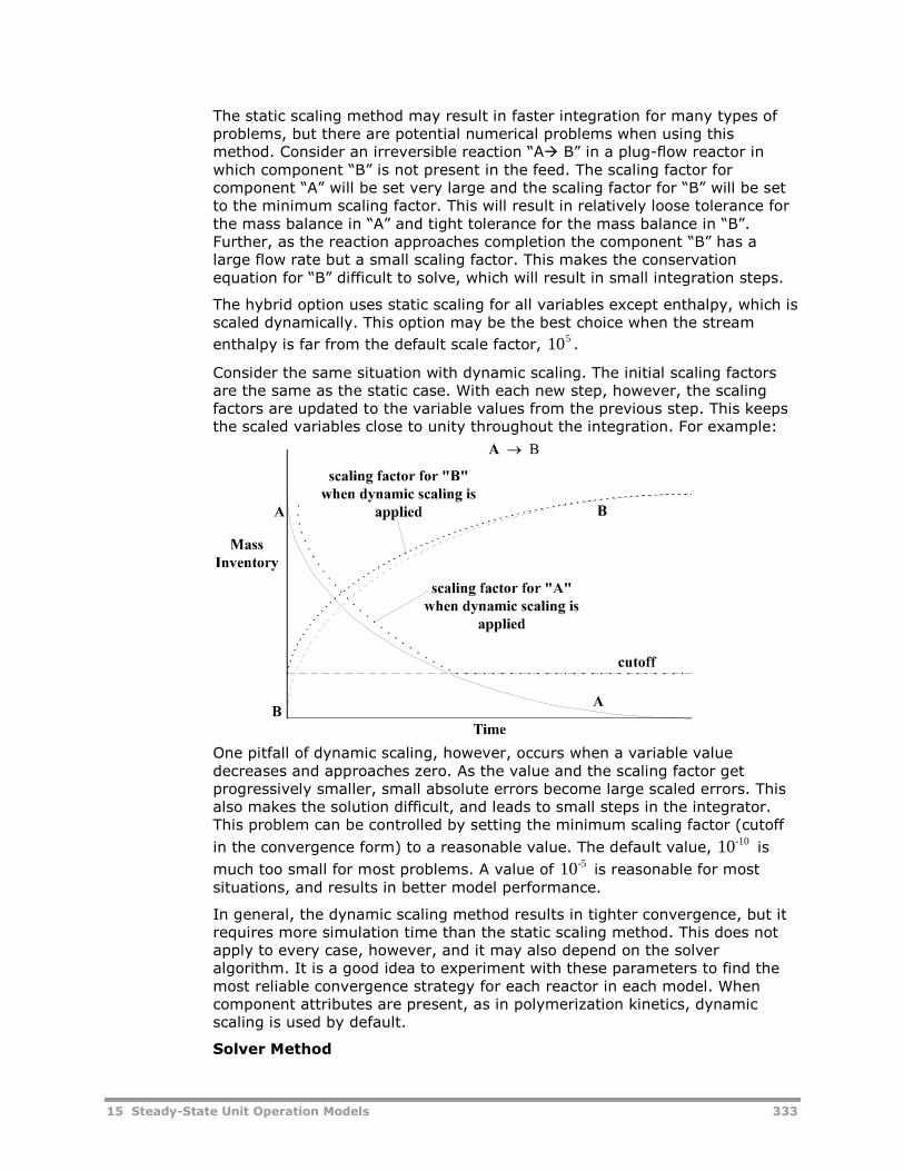
15 Steady-State Unit Operation Models 333
The static scaling method may result in faster integration for many types ofproblems, but there are potential numerical problems when using thismethod. Consider an irreversible reaction “A B” in a plug-flow reactor inwhich component “B” is not present in the feed. The scaling factor forcomponent “A” will be set very large and the scaling factor for “B” will be setto the minimum scaling factor. This will result in relatively loose tolerance forthe mass balance in “A” and tight tolerance for the mass balance in “B”.Further, as the reaction approaches completion the component “B” has alarge flow rate but a small scaling factor. This makes the conservationequation for “B” difficult to solve, which will result in small integration steps.
The hybrid option uses static scaling for all variables except enthalpy, which isscaled dynamically. This option may be the best choice when the stream
enthalpy is far from the default scale factor,510 .
Consider the same situation with dynamic scaling. The initial scaling factorsare the same as the static case. With each new step, however, the scalingfactors are updated to the variable values from the previous step. This keepsthe scaled variables close to unity throughout the integration. For example:
One pitfall of dynamic scaling, however, occurs when a variable valuedecreases and approaches zero. As the value and the scaling factor getprogressively smaller, small absolute errors become large scaled errors. Thisalso makes the solution difficult, and leads to small steps in the integrator.This problem can be controlled by setting the minimum scaling factor (cutoff
in the convergence form) to a reasonable value. The default value, 10-10is
much too small for most problems. A value of 10-5is reasonable for most
situations, and results in better model performance.
In general, the dynamic scaling method results in tighter convergence, but itrequires more simulation time than the static scaling method. This does notapply to every case, however, and it may also depend on the solveralgorithm. It is a good idea to experiment with these parameters to find themost reliable convergence strategy for each reactor in each model. Whencomponent attributes are present, as in polymerization kinetics, dynamicscaling is used by default.
Solver Method
334 15 Steady-State Unit Operation Models
At each step during the integration, the energy, mass, and attributeconservation equations are solved by trial-and-error. Two “corrector”algorithms, direct substitution and Newton’s method, can be selected. TheNewton algorithm perturbs each variable to determine the slope, resulting ina smaller number or larger steps compared to the Direct algorithm. Since theperturbation passes require some time, it is difficult to predict if Newton’smethod or the Direct method is best for a given problem. In general,Newton’s method appears to give the best performance with polymerizationkinetics, but it is a good idea to try using each algorithm with both dynamicand static scaling to determine the best combination of convergenceparameters for a particular problem.
The corrector tolerance is set as a ratio from the integration tolerance (Corr-Tol-Ratio). By default, the corrector tolerance is ten times tighter than theintegration tolerance (the corrector tolerance ratio is 0.1). For someproblems, especially those involving reactors with heat transfer calculations,the optimal corrector tolerance ratio may be higher than 0.1, but this ratioshould not be set larger than 1.0. The flash tolerance should be tighter thanthe corrector tolerance. Otherwise, round-off errors in the flash calculationsmake the corrector tolerance difficult to achieve. The model always uses thesmaller of the specified RPlug flash tolerance (in the convergence form) or theglobal flash tolerance.
Other Integration Parameters
By default, the initial step size in RBatch is set to one tenth of a second(Hinit=0.1). If the solver cannot converge the equations with this step size, itwill cut the step size by a factor of ten. This process will repeat up to sixtimes. If the solver still cannot converge, the reactor fails with an errormessage “solver cannot converge with minimum step size”.
Frequently, initial reaction rates or heat transfer rates are very fast, so theminimum step size may need to be reduced. For step-growth kinetics, thedefault value should be sufficient. Smaller initial step-sizes may be requiredfor addition kinetics, especially if quasi-steady-state approximations are notapplied.
The maximum number of integration steps defaults to 1000. For very “stiff”kinetics, e.g., kinetics with fast reaction rates involving trace components, themaximum number of steps may need to be increased, especially if thecorrector is using direct substitution. If more than 5000 steps are required,try changing the corrector method, scaling method, or increase the cutofflevel.
RBatch stores many types of results at regular intervals (printing points). Thenumber of intervals depends on the reaction time. Since the integration stepsdo not necessarily correspond to the print points, the model uses polynomialinterpolation to determine the results for a print point based on the stepsbefore and after this point. If the integration step sizes are very large, theinterpolation algorithm may give strange results, such as sine waves. Thisproblem can be fixed by reducing the maximum step size (Max-StepSize) to avalue smaller than the increments between print points (this forces the modelto use linear interpolation). By default, no maximum step size is enforced.
RBatch has the option to stop exactly at print points and vent accumulatorpoints instead of interpolating these points. When the “exact” option is set to
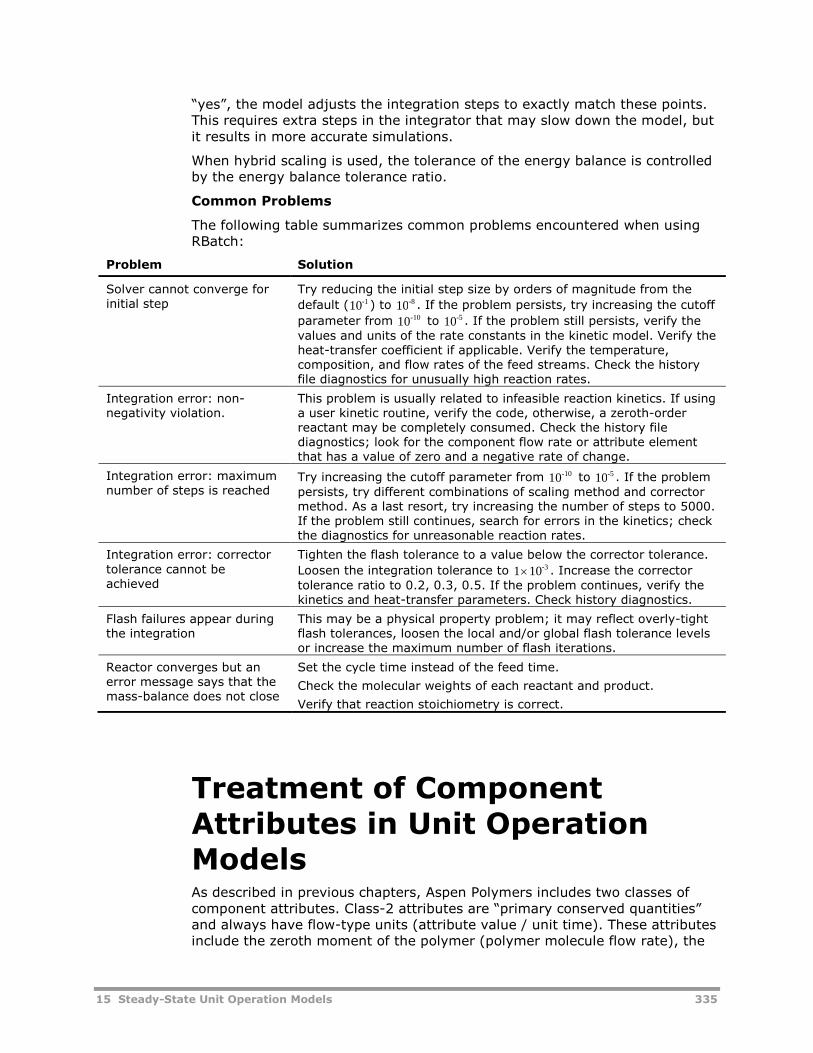
15 Steady-State Unit Operation Models 335
“yes”, the model adjusts the integration steps to exactly match these points.This requires extra steps in the integrator that may slow down the model, butit results in more accurate simulations.
When hybrid scaling is used, the tolerance of the energy balance is controlledby the energy balance tolerance ratio.
Common Problems
The following table summarizes common problems encountered when usingRBatch:
Problem Solution
Solver cannot converge forinitial step
Try reducing the initial step size by orders of magnitude from the
default (10-1 ) to 10-8 . If the problem persists, try increasing the cutoff
parameter from 10-10 to 10-5 . If the problem still persists, verify thevalues and units of the rate constants in the kinetic model. Verify theheat-transfer coefficient if applicable. Verify the temperature,composition, and flow rates of the feed streams. Check the historyfile diagnostics for unusually high reaction rates.
Integration error: non-negativity violation.
This problem is usually related to infeasible reaction kinetics. If usinga user kinetic routine, verify the code, otherwise, a zeroth-orderreactant may be completely consumed. Check the history filediagnostics; look for the component flow rate or attribute elementthat has a value of zero and a negative rate of change.
Integration error: maximumnumber of steps is reached
Try increasing the cutoff parameter from 10-10 to 10-5 . If the problempersists, try different combinations of scaling method and correctormethod. As a last resort, try increasing the number of steps to 5000.If the problem still continues, search for errors in the kinetics; checkthe diagnostics for unreasonable reaction rates.
Integration error: correctortolerance cannot beachieved
Tighten the flash tolerance to a value below the corrector tolerance.
Loosen the integration tolerance to 1 10-3 . Increase the correctortolerance ratio to 0.2, 0.3, 0.5. If the problem continues, verify thekinetics and heat-transfer parameters. Check history diagnostics.
Flash failures appear duringthe integration
This may be a physical property problem; it may reflect overly-tightflash tolerances, loosen the local and/or global flash tolerance levelsor increase the maximum number of flash iterations.
Reactor converges but anerror message says that themass-balance does not close
Set the cycle time instead of the feed time.
Check the molecular weights of each reactant and product.
Verify that reaction stoichiometry is correct.
Treatment of ComponentAttributes in Unit OperationModelsAs described in previous chapters, Aspen Polymers includes two classes ofcomponent attributes. Class-2 attributes are “primary conserved quantities”and always have flow-type units (attribute value / unit time). These attributesinclude the zeroth moment of the polymer (polymer molecule flow rate), the
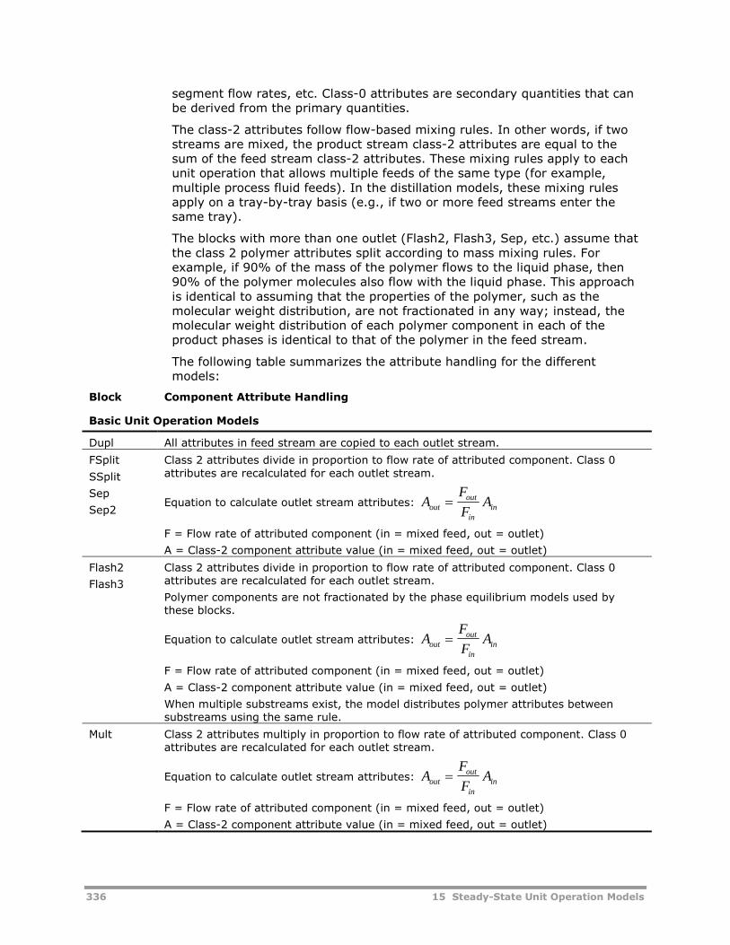
336 15 Steady-State Unit Operation Models
segment flow rates, etc. Class-0 attributes are secondary quantities that canbe derived from the primary quantities.
The class-2 attributes follow flow-based mixing rules. In other words, if twostreams are mixed, the product stream class-2 attributes are equal to thesum of the feed stream class-2 attributes. These mixing rules apply to eachunit operation that allows multiple feeds of the same type (for example,multiple process fluid feeds). In the distillation models, these mixing rulesapply on a tray-by-tray basis (e.g., if two or more feed streams enter thesame tray).
The blocks with more than one outlet (Flash2, Flash3, Sep, etc.) assume thatthe class 2 polymer attributes split according to mass mixing rules. Forexample, if 90% of the mass of the polymer flows to the liquid phase, then90% of the polymer molecules also flow with the liquid phase. This approachis identical to assuming that the properties of the polymer, such as themolecular weight distribution, are not fractionated in any way; instead, themolecular weight distribution of each polymer component in each of theproduct phases is identical to that of the polymer in the feed stream.
The following table summarizes the attribute handling for the differentmodels:
Block Component Attribute Handling
Basic Unit Operation Models
Dupl All attributes in feed stream are copied to each outlet stream.
FSplit
SSplit
Sep
Sep2
Class 2 attributes divide in proportion to flow rate of attributed component. Class 0attributes are recalculated for each outlet stream.
Equation to calculate outlet stream attributes: AF
FAout
out
inin
F = Flow rate of attributed component (in = mixed feed, out = outlet)
A = Class-2 component attribute value (in = mixed feed, out = outlet)
Flash2
Flash3
Class 2 attributes divide in proportion to flow rate of attributed component. Class 0attributes are recalculated for each outlet stream.
Polymer components are not fractionated by the phase equilibrium models used bythese blocks.
Equation to calculate outlet stream attributes: AF
FAout
out
inin
F = Flow rate of attributed component (in = mixed feed, out = outlet)
A = Class-2 component attribute value (in = mixed feed, out = outlet)
When multiple substreams exist, the model distributes polymer attributes betweensubstreams using the same rule.
Mult Class 2 attributes multiply in proportion to flow rate of attributed component. Class 0attributes are recalculated for each outlet stream.
Equation to calculate outlet stream attributes: AF
FAout
out
inin
F = Flow rate of attributed component (in = mixed feed, out = outlet)
A = Class-2 component attribute value (in = mixed feed, out = outlet)
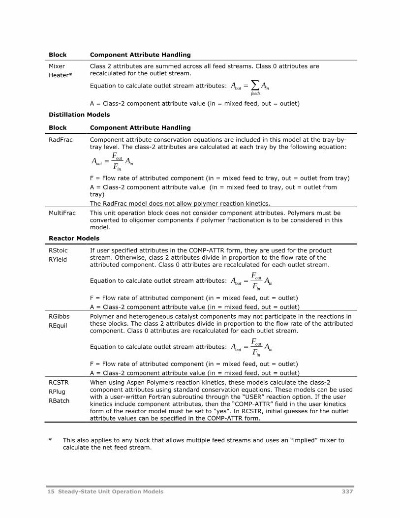
15 Steady-State Unit Operation Models 337
Block Component Attribute Handling
Mixer
Heater*
Class 2 attributes are summed across all feed streams. Class 0 attributes arerecalculated for the outlet stream.
Equation to calculate outlet stream attributes: A Aout infeeds
A = Class-2 component attribute value (in = mixed feed, out = outlet)
Distillation Models
Block Component Attribute Handling
RadFrac Component attribute conservation equations are included in this model at the tray-by-tray level. The class-2 attributes are calculated at each tray by the following equation:
AF
FAout
out
inin
F = Flow rate of attributed component (in = mixed feed to tray, out = outlet from tray)
A = Class-2 component attribute value (in = mixed feed to tray, out = outlet fromtray)
The RadFrac model does not allow polymer reaction kinetics.
MultiFrac This unit operation block does not consider component attributes. Polymers must beconverted to oligomer components if polymer fractionation is to be considered in thismodel.
Reactor Models
RStoic
RYield
If user specified attributes in the COMP-ATTR form, they are used for the productstream. Otherwise, class 2 attributes divide in proportion to the flow rate of theattributed component. Class 0 attributes are recalculated for each outlet stream.
Equation to calculate outlet stream attributes: AF
FAout
out
inin
F = Flow rate of attributed component (in = mixed feed, out = outlet)
A = Class-2 component attribute value (in = mixed feed, out = outlet)
RGibbs
REquil
Polymer and heterogeneous catalyst components may not participate in the reactions inthese blocks. The class 2 attributes divide in proportion to the flow rate of the attributedcomponent. Class 0 attributes are recalculated for each outlet stream.
Equation to calculate outlet stream attributes: AF
FAout
out
inin
F = Flow rate of attributed component (in = mixed feed, out = outlet)
A = Class-2 component attribute value (in = mixed feed, out = outlet)
RCSTR
RPlug
RBatch
When using Aspen Polymers reaction kinetics, these models calculate the class-2component attributes using standard conservation equations. These models can be usedwith a user-written Fortran subroutine through the “USER” reaction option. If the userkinetics include component attributes, then the “COMP-ATTR” field in the user kineticsform of the reactor model must be set to “yes”. In RCSTR, initial guesses for the outletattribute values can be specified in the COMP-ATTR form.
* This also applies to any block that allows multiple feed streams and uses an “implied” mixer tocalculate the net feed stream.
338 15 Steady-State Unit Operation Models
ReferencesChan, W.-M., Gloor, P. E., & Hamielec, A. E. (1993). A Kinetic Model for OlefinPolymerization in High-Pressure Autoclave Reactors. AIChE J., 39, No. 1.
Chaudhari, R. V., & Shah, Y. T. (1986). Recent Advances in Slurry Reactors,Concepts and Design of Chemical Reactors. S.A. Whitaker & A. Cassano(Eds.). Switzerland: Gordon and Breach Science Publishers.
Henderson, J. N., & Bouton, T. C. (Eds.). (1979). Polymerization Reactors andProcesses. ACS Symp. Ser.
Rodriguez, F. (1996). Principles of Polymer Systems. New York: Taylor &Francis.
Trambouze, P., van Landeghem, H., & Wauquier, J. P. (1988). ChemicalReactors: Design/Engineering/Operation. Paris: Editions Technips.
Walas, S. M. (1988). Chemical Process Equipment Selection and Design.Boston: Butterworths.
16 Plant Data Fitting 339
16 Plant Data Fitting
Aspen Polymers (formerly known as Aspen Polymers Plus) simulation modelscan be fit to plant or laboratory data using Data-Fit. One or more sets ofmeasured data are provided which may include model inputs or results. Data-Fit adjusts or estimates input parameters to find the best match between themodel predictions and data. Data-Fit can also reconcile measured dataagainst the model.
Data-Fit minimizes the weighted sum of square errors, where each error isthe difference between a reconciled input or calculated output and the data.In statistical terms, Data-Fit performs either ordinary least squares ormaximum likelihood (errors-in-variables) estimation.
Topics covered include:
Data Fitting Applications, 339
Data Fitting For Polymer Models, 340
Steps for Using the Data Regression Tool, 345(including troubleshooting tips)
This section emphasizes using the Data-Fit tool to fit process reaction kineticparameters. A more general description of this tool is available in the AspenPlus User Guide.
Data Fitting ApplicationsThe data regression tool in Aspen Plus can be used to fit model parametersand reconcile process data. These applications may be carried outsimultaneously.
Parameter regression usually involves adjusting model parameters to improvethe agreement between model predictions and process data. For example,reaction rate constants may be manipulated to match the measured polymermolecular weight and monomer conversion. Manipulated parameters mayinclude reaction rate or equilibrium constants, physical property constants, orequipment specifications. Fitted parameters may include model predictionssuch as reactant conversion, product yield, by-product content, polymercomponent attributes, stream compositions or flow rates, or equipment heatduty, temperature, pressure, or holdup.
340 16 Plant Data Fitting
Data reconciliation runs involve manipulating one or more sets of modelinputs to match model predictions to process data. For example, the averagefeed rate of a makeup stream can be estimated based on the flow rate andcomposition of the feed and product streams. Manipulated data typicallyincludes feed stream flow rates and compositions, equipment operatingconditions, heat transfer coefficients, etc.
The Data-Fit model can be used to reconcile input data and fit modelparameters simultaneously. Simultaneous regression and reconciliation istypically used to fine-tune models which already match process data andtrends relatively well.
Data Fitting For PolymerModelsPolymer process models frequently include non-ideal phase equilibrium,reaction kinetics, and complicated unit operations. Fitting these complexmodels against process and laboratory data is not a trivial task. A great dealof consideration must be given to the way this problem is approached.
A detailed example describing how to fit a free-radical reaction kineticsproblem is included in the Aspen Polymers Examples & Applications CaseBook.
A general procedure for fitting complex models is given below.
Step 1. Process Data Review
Collect data for the process. Sources of data include process informationmanagement system (PIMS), process design documents (PDDs), process flowdiagrams (PFDs). Verify reproducibility / standard deviations of data bycollecting multiple data sets for each case. Verify steady state by collectingdata at regular intervals over several plant residence times. Verify datafeasibility against mass and energy balance calculations.
Step 2. Literature Search
Collect information about the process. Sources of data include in-house labdata, databanks, trade journals, conference notes, polymer handbooks, on-line electronic databases, experimental designs, etc.
Step 3. Preliminary Model Fitting
Carry out physical property data regression, property constant parameterestimation runs. Test the parameters against all pertinent data from steps 1and 2. To the extent possible, verify pure component physical properties andphase equilibrium predictions using Property Analysis tools.
Step 4. Preliminary Model Development
Develop a basic model of the process, ignoring details such as non-idealmixing, heat transfer, etc. Specify temperature instead of duty, volumeinstead of residence time. Use parameters from steps 1-3.
16 Plant Data Fitting 341
Step 5. Trend Analysis
Use the sensitivity feature to evaluate trends between model outputs(conversion, polymer attributes, etc.) and model inputs (rate constants,operating conditions, etc.) Compare the predicted trends against availableprocess or lab data. If the trends are not well matched, adjust specific modelparameters to improve the predicted trend. Model fitting may be carried outusing Sensitivity, Design-Specification, Data-Fit, or by trial and error.
Step 6. Model Refinement
Use the Data-Fit tool to carry out simultaneous parameter estimation anddata reconciliation. Relax model assumptions, such as perfect mixing, asneeded. Bring model up to the appropriate level of detail, fitting keyparameters at each development step.
Data Collection and VerificationThe first step in fitting a model is to collect and review data. Sources of datamay include process information management system (PIMS), process designdocuments (PDDs), and process flow diagrams (PFDs), shift log sheets, andlaboratory analysis reports. It is important to verify the reproducibility of thedata by collecting several duplicate sets of each datum. Duplicate data areespecially important for analytical measurements such as melt flow index andintrinsic viscosity.
For continuous processes, it is a good idea to verify that the process operatesunder steady-state conditions by collecting data at regular intervals. The datashould be collected at regular intervals over a period that exceeds thecumulative residence time of the key unit operations in the process.
Verify data feasibility against mass and energy balance calculations. It isimpossible to force a rigorous model to match data that violates thefundamental conservation equations.
When possible, obtain calibration data for unit operating conditions, especiallylevel calibration data for reactors and flow rate calibration data for flowmeters. The method and assumptions used to calibrate these instrumentsmust be taken into consideration for data reconciliation runs.
Literature ReviewBefore you regress process data, it is a good idea to collect information aboutthe process. Sources of data include in-house lab data, databanks, tradejournals, conference notes, polymer handbooks, on-line electronic databases,experimental designs, and so on.
The open and in-house process literature may contain a wealth of informationabout key model parameters. Further, these sources may provide additionalsources of fundamental data which can be used to independently evaluatemodel parameters.
Simulation studies described in trade journals are an excellent source ofinsight and know-how related to model development. These studiesfrequently point out which assumptions are valid and which parameters are
342 16 Plant Data Fitting
important. In addition, these papers may elucidate reaction mechanisms orphysical phenomena that should be considered in a rigorous process model.
The physical property and rate constant data reported in the open literatureare never perfect, but they do serve as a good starting point for fitting themodel.
Preliminary Parameter FittingIt is important to determine as many of the model parameters as possibleearly in the model development process. Try to decouple the parameters fromeach other whenever possible. For example, find ways to establish phaseequilibrium parameters independently of reaction equilibrium constants. Makesimplifying assumptions to reduce the number of unknown parameters.
Physical property parameters should be firmly established before fitting rateconstants. When data are available, use the physical property data regressionsystem (DRS) to fit the density, enthalpy, heat capacity, and vapor pressureof pure components. If phase equilibrium data are available, use DRS toregress phase equilibrium parameters.
When property data are unavailable for a component, the property constantestimation system (PCES) can be used to estimate property parameters frommolecular structure. These estimations, however, should be checked againstprocess data. If data are available for components with similar structures,they can be used to estimate the properties of components that are not foundin the databank.
The following table lists some of the key physical property parameters inAspen Polymers and describes how they influence polymerization kinetics:
Property Parameters Influence on Polymerization ReactionKinetics
Density DNLRKT,DNLVK
Concentration is proportional to density. Reactionkinetics depend on component concentrations.
Vaporpressure
PLXANT,HENRY
The vapor pressure controls phase equilibrium ofvolatile components in vapor-liquid systems. Thephase equilibrium strongly influencesconcentrations, which controls kinetics.
Enthalpy DHFORM,DHFVK,DHFVKM,DHSUB,DHCON,DHFMDP
The component enthalpies influence the predictedheat duties and temperatures in the model.
Heat capacity CPIG, CPL,CPLVK,CPCVK
The heat capacity controls the influence oftemperature on enthalpy.
Transitiontemperatures
TMVK, TGVK Phase transitions occur at the melting point andglass point. Predicted enthalpy, density, and heatcapacity for polymer and oligomer componentsdepend on the phase regime.
Phaseequilibrium
In multiphase reactors the phase equilibriumdetermines the component concentrations in eachphase, which influences the reaction rates.
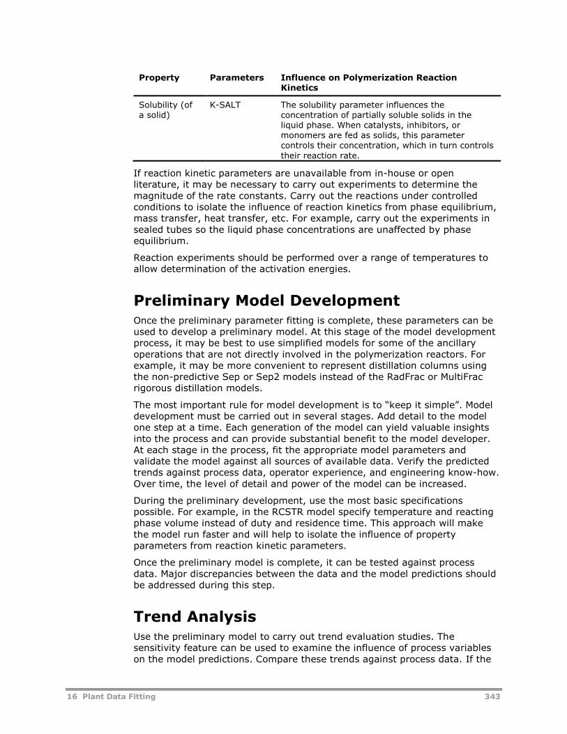
16 Plant Data Fitting 343
Property Parameters Influence on Polymerization ReactionKinetics
Solubility (ofa solid)
K-SALT The solubility parameter influences theconcentration of partially soluble solids in theliquid phase. When catalysts, inhibitors, ormonomers are fed as solids, this parametercontrols their concentration, which in turn controlstheir reaction rate.
If reaction kinetic parameters are unavailable from in-house or openliterature, it may be necessary to carry out experiments to determine themagnitude of the rate constants. Carry out the reactions under controlledconditions to isolate the influence of reaction kinetics from phase equilibrium,mass transfer, heat transfer, etc. For example, carry out the experiments insealed tubes so the liquid phase concentrations are unaffected by phaseequilibrium.
Reaction experiments should be performed over a range of temperatures toallow determination of the activation energies.
Preliminary Model DevelopmentOnce the preliminary parameter fitting is complete, these parameters can beused to develop a preliminary model. At this stage of the model developmentprocess, it may be best to use simplified models for some of the ancillaryoperations that are not directly involved in the polymerization reactors. Forexample, it may be more convenient to represent distillation columns usingthe non-predictive Sep or Sep2 models instead of the RadFrac or MultiFracrigorous distillation models.
The most important rule for model development is to “keep it simple”. Modeldevelopment must be carried out in several stages. Add detail to the modelone step at a time. Each generation of the model can yield valuable insightsinto the process and can provide substantial benefit to the model developer.At each stage in the process, fit the appropriate model parameters andvalidate the model against all sources of available data. Verify the predictedtrends against process data, operator experience, and engineering know-how.Over time, the level of detail and power of the model can be increased.
During the preliminary development, use the most basic specificationspossible. For example, in the RCSTR model specify temperature and reactingphase volume instead of duty and residence time. This approach will makethe model run faster and will help to isolate the influence of propertyparameters from reaction kinetic parameters.
Once the preliminary model is complete, it can be tested against processdata. Major discrepancies between the data and the model predictions shouldbe addressed during this step.
Trend AnalysisUse the preliminary model to carry out trend evaluation studies. Thesensitivity feature can be used to examine the influence of process variableson the model predictions. Compare these trends against process data. If the
344 16 Plant Data Fitting
predicted trends are not consistent, adjust the appropriate model parametersto improve the match. For example, if the predicted slope of the monomerconversion versus temperature curve is less than the measured slope, theactivation energy of the polymerization reaction may be too low.
Use the sensitivity tool to examine the influence of the model parameters onthe model predictions and to determine which parameters are important inthe model. Parametric studies can be carried out by manipulating two or morevariables in a sensitivity study.
It is good practice to include as many model predictions as possible in eachsensitivity study. The simulation runs take the same amount of timeregardless of the number of defined variables. It is much easier to understandthe predicted trends when the sensitivity results are detailed.
Once you know which parameters are critical to the model predictions, thedata regression tool can be used to adjust these parameters to match specifictrends. Keep the number of manipulated parameters to a minimum until all ofthe key parameters are established independently.
Model RefinementThe Data-Fit tool is the best choice for refining the fit between the modelpredictions and the process data, especially when several sets of data areavailable. Data-Fit can adjust several model parameters simultaneously,capturing subtle interactions among the parameters to get the best overallmatch between the process data and model predictions.
When the model predictions cannot match the process data, the assumptionsin the model may be too broad. Perhaps the process is limited by heat- ormass-transfer, or a reactor is not ideally mixed. Maybe there are additionalside reactions that should be considered in the model, or the rate expressionneeds to be modified to account for some unusual aspect of reaction kinetics.These issues can be addressed during the model refinement process byadding new layers of detail to the model. Avoid adding more detail thannecessary, however, because model fitting is a process of diminishing returns.
Model refinement is an open-ended process. The model parameters can betuned more accurately as more data become available from the process. Baddata points are easier to spot when there are more sets of data to compare.
It is impossible for a simulation model to match process data perfectly. Thereare several sources of error that lead to differences between the modelresults and process data, including:
Variations in process operating conditions due to disturbances, excursionsfrom steady state, control system actions, etc.
Imperfect calibration of flow meters, level controllers, etc.
Analytical error in lab measurements
Simplifications and assumptions in the model, such as ideal mixing,isothermal and isobaric vessels, phase equilibrium, etc.
Errors in the model parameters.
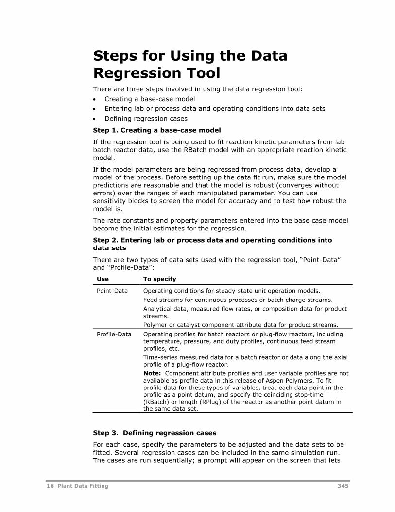
16 Plant Data Fitting 345
Steps for Using the DataRegression ToolThere are three steps involved in using the data regression tool:
Creating a base-case model
Entering lab or process data and operating conditions into data sets
Defining regression cases
Step 1. Creating a base-case model
If the regression tool is being used to fit reaction kinetic parameters from labbatch reactor data, use the RBatch model with an appropriate reaction kineticmodel.
If the model parameters are being regressed from process data, develop amodel of the process. Before setting up the data fit run, make sure the modelpredictions are reasonable and that the model is robust (converges withouterrors) over the ranges of each manipulated parameter. You can usesensitivity blocks to screen the model for accuracy and to test how robust themodel is.
The rate constants and property parameters entered into the base case modelbecome the initial estimates for the regression.
Step 2. Entering lab or process data and operating conditions intodata sets
There are two types of data sets used with the regression tool, “Point-Data”and “Profile-Data”:
Use To specify
Point-Data Operating conditions for steady-state unit operation models.
Feed streams for continuous processes or batch charge streams.
Analytical data, measured flow rates, or composition data for productstreams.
Polymer or catalyst component attribute data for product streams.
Profile-Data Operating profiles for batch reactors or plug-flow reactors, includingtemperature, pressure, and duty profiles, continuous feed streamprofiles, etc.
Time-series measured data for a batch reactor or data along the axialprofile of a plug-flow reactor.
Note: Component attribute profiles and user variable profiles are notavailable as profile data in this release of Aspen Polymers. To fitprofile data for these types of variables, treat each data point in theprofile as a point datum, and specify the coinciding stop-time(RBatch) or length (RPlug) of the reactor as another point datum inthe same data set.
Step 3. Defining regression cases
For each case, specify the parameters to be adjusted and the data sets to befitted. Several regression cases can be included in the same simulation run.The cases are run sequentially; a prompt will appear on the screen that lets
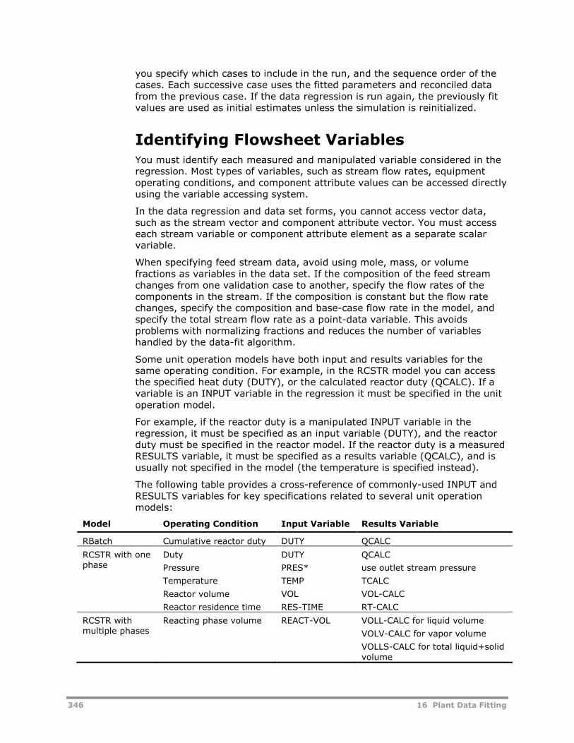
346 16 Plant Data Fitting
you specify which cases to include in the run, and the sequence order of thecases. Each successive case uses the fitted parameters and reconciled datafrom the previous case. If the data regression is run again, the previously fitvalues are used as initial estimates unless the simulation is reinitialized.
Identifying Flowsheet VariablesYou must identify each measured and manipulated variable considered in theregression. Most types of variables, such as stream flow rates, equipmentoperating conditions, and component attribute values can be accessed directlyusing the variable accessing system.
In the data regression and data set forms, you cannot access vector data,such as the stream vector and component attribute vector. You must accesseach stream variable or component attribute element as a separate scalarvariable.
When specifying feed stream data, avoid using mole, mass, or volumefractions as variables in the data set. If the composition of the feed streamchanges from one validation case to another, specify the flow rates of thecomponents in the stream. If the composition is constant but the flow ratechanges, specify the composition and base-case flow rate in the model, andspecify the total stream flow rate as a point-data variable. This avoidsproblems with normalizing fractions and reduces the number of variableshandled by the data-fit algorithm.
Some unit operation models have both input and results variables for thesame operating condition. For example, in the RCSTR model you can accessthe specified heat duty (DUTY), or the calculated reactor duty (QCALC). If avariable is an INPUT variable in the regression it must be specified in the unitoperation model.
For example, if the reactor duty is a manipulated INPUT variable in theregression, it must be specified as an input variable (DUTY), and the reactorduty must be specified in the reactor model. If the reactor duty is a measuredRESULTS variable, it must be specified as a results variable (QCALC), and isusually not specified in the model (the temperature is specified instead).
The following table provides a cross-reference of commonly-used INPUT andRESULTS variables for key specifications related to several unit operationmodels:
Model Operating Condition Input Variable Results Variable
RBatch Cumulative reactor duty DUTY QCALC
RCSTR with onephase
Duty
Pressure
Temperature
Reactor volume
Reactor residence time
DUTY
PRES*
TEMP
VOL
RES-TIME
QCALC
use outlet stream pressure
TCALC
VOL-CALC
RT-CALC
RCSTR withmultiple phases
Reacting phase volume REACT-VOL VOLL-CALC for liquid volume
VOLV-CALC for vapor volume
VOLLS-CALC for total liquid+solidvolume
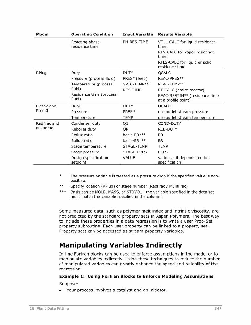
16 Plant Data Fitting 347
Model Operating Condition Input Variable Results Variable
Reacting phaseresidence time
PH-RES-TIME VOLL-CALC for liquid residencetime
RTV-CALC for vapor residencetime
RTLS-CALC for liquid or solidresidence time
RPlug Duty
Pressure (process fluid)
Temperature (processfluid)
Residence time (processfluid)
DUTY
PRES* (feed)
SPEC-TEMP**
RES-TIME
QCALC
REAC-PRES**
REAC-TEMP**
RT-CALC (entire reactor)
REAC-RESTIM** (residence timeat a profile point)
Flash2 andFlash3
Duty
Pressure
Temperature
DUTY
PRES*
TEMP
QCALC
use outlet stream pressure
use outlet stream temperature
RadFrac andMultiFrac
Condenser duty
Reboiler duty
Reflux ratio
Boilup ratio
Stage temperature
Stage pressure
Design specificationsetpoint
Q1
QN
basis-RR***
basis-BR***
STAGE-TEMP
STAGE-PRES
VALUE
COND-DUTY
REB-DUTY
RR
BR
TEMP
PRES
various - it depends on thespecification
* The pressure variable is treated as a pressure drop if the specified value is non-positive.
** Specify location (RPlug) or stage number (RadFrac / MulitFrac)
*** Basis can be MOLE, MASS, or STDVOL - the variable specified in the data setmust match the variable specified in the column .
Some measured data, such as polymer melt index and intrinsic viscosity, arenot predicted by the standard property sets in Aspen Polymers. The best wayto include these properties in a data regression is to write a user Prop-Setproperty subroutine. Each user property can be linked to a property set.Property sets can be accessed as stream-property variables.
Manipulating Variables IndirectlyIn-line Fortran blocks can be used to enforce assumptions in the model or tomanipulate variables indirectly. Using these techniques to reduce the numberof manipulated variables can greatly enhance the speed and reliability of theregression.
Example 1: Using Fortran Blocks to Enforce Modeling Assumptions
Suppose:
Your process involves a catalyst and an initiator.
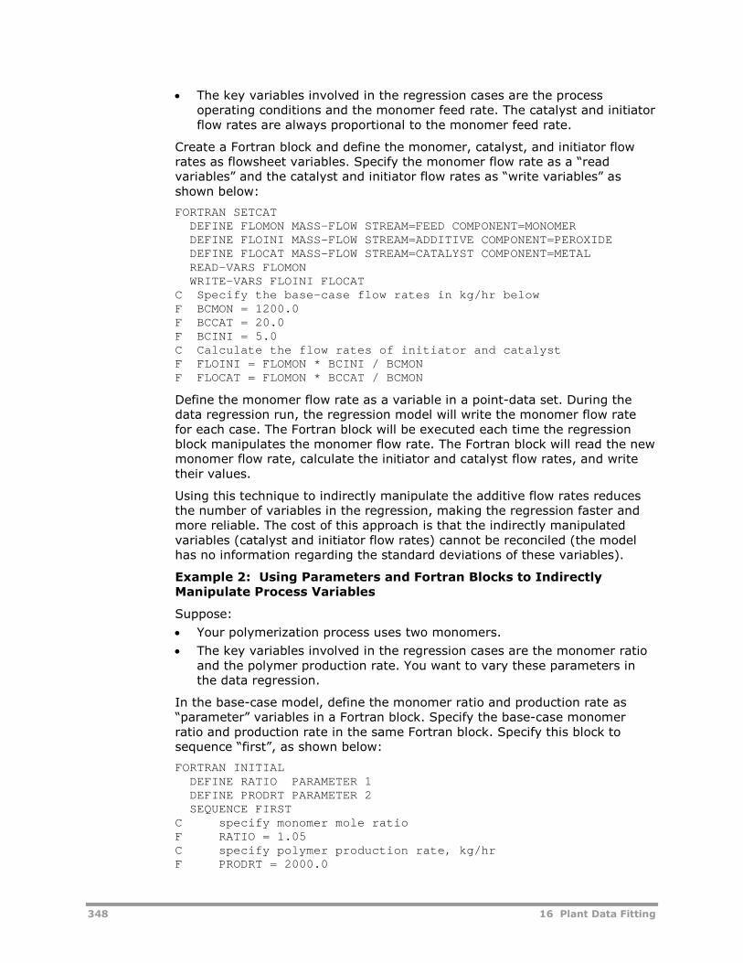
348 16 Plant Data Fitting
The key variables involved in the regression cases are the processoperating conditions and the monomer feed rate. The catalyst and initiatorflow rates are always proportional to the monomer feed rate.
Create a Fortran block and define the monomer, catalyst, and initiator flowrates as flowsheet variables. Specify the monomer flow rate as a “readvariables” and the catalyst and initiator flow rates as “write variables” asshown below:
FORTRAN SETCATDEFINE FLOMON MASS-FLOW STREAM=FEED COMPONENT=MONOMERDEFINE FLOINI MASS-FLOW STREAM=ADDITIVE COMPONENT=PEROXIDEDEFINE FLOCAT MASS-FLOW STREAM=CATALYST COMPONENT=METALREAD-VARS FLOMONWRITE-VARS FLOINI FLOCAT
C Specify the base-case flow rates in kg/hr belowF BCMON = 1200.0F BCCAT = 20.0F BCINI = 5.0C Calculate the flow rates of initiator and catalystF FLOINI = FLOMON * BCINI / BCMONF FLOCAT = FLOMON * BCCAT / BCMON
Define the monomer flow rate as a variable in a point-data set. During thedata regression run, the regression model will write the monomer flow ratefor each case. The Fortran block will be executed each time the regressionblock manipulates the monomer flow rate. The Fortran block will read the newmonomer flow rate, calculate the initiator and catalyst flow rates, and writetheir values.
Using this technique to indirectly manipulate the additive flow rates reducesthe number of variables in the regression, making the regression faster andmore reliable. The cost of this approach is that the indirectly manipulatedvariables (catalyst and initiator flow rates) cannot be reconciled (the modelhas no information regarding the standard deviations of these variables).
Example 2: Using Parameters and Fortran Blocks to IndirectlyManipulate Process Variables
Suppose:
Your polymerization process uses two monomers.
The key variables involved in the regression cases are the monomer ratioand the polymer production rate. You want to vary these parameters inthe data regression.
In the base-case model, define the monomer ratio and production rate as“parameter” variables in a Fortran block. Specify the base-case monomerratio and production rate in the same Fortran block. Specify this block tosequence “first”, as shown below:
FORTRAN INITIALDEFINE RATIO PARAMETER 1DEFINE PRODRT PARAMETER 2SEQUENCE FIRST
C specify monomer mole ratioF RATIO = 1.05C specify polymer production rate, kg/hrF PRODRT = 2000.0
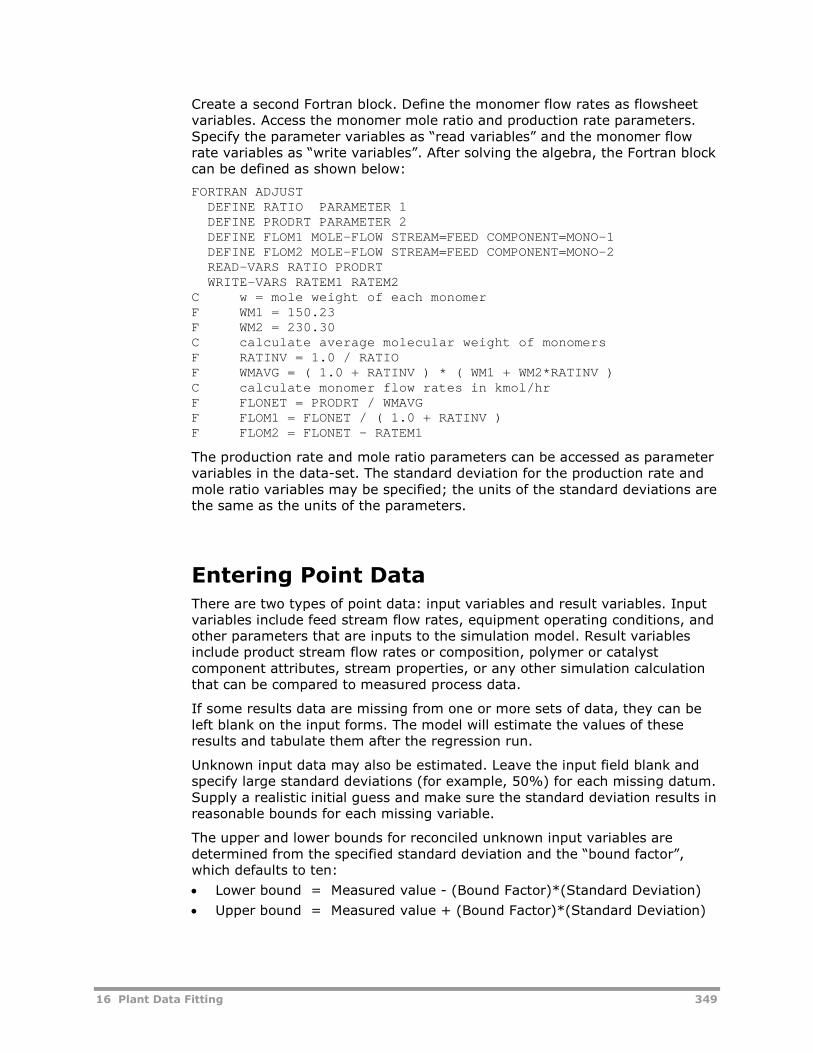
16 Plant Data Fitting 349
Create a second Fortran block. Define the monomer flow rates as flowsheetvariables. Access the monomer mole ratio and production rate parameters.Specify the parameter variables as “read variables” and the monomer flowrate variables as “write variables”. After solving the algebra, the Fortran blockcan be defined as shown below:
FORTRAN ADJUSTDEFINE RATIO PARAMETER 1DEFINE PRODRT PARAMETER 2DEFINE FLOM1 MOLE-FLOW STREAM=FEED COMPONENT=MONO-1DEFINE FLOM2 MOLE-FLOW STREAM=FEED COMPONENT=MONO-2READ-VARS RATIO PRODRTWRITE-VARS RATEM1 RATEM2
C w = mole weight of each monomerF WM1 = 150.23F WM2 = 230.30C calculate average molecular weight of monomersF RATINV = 1.0 / RATIOF WMAVG = ( 1.0 + RATINV ) * ( WM1 + WM2*RATINV )C calculate monomer flow rates in kmol/hrF FLONET = PRODRT / WMAVGF FLOM1 = FLONET / ( 1.0 + RATINV )F FLOM2 = FLONET - RATEM1
The production rate and mole ratio parameters can be accessed as parametervariables in the data-set. The standard deviation for the production rate andmole ratio variables may be specified; the units of the standard deviations arethe same as the units of the parameters.
Entering Point DataThere are two types of point data: input variables and result variables. Inputvariables include feed stream flow rates, equipment operating conditions, andother parameters that are inputs to the simulation model. Result variablesinclude product stream flow rates or composition, polymer or catalystcomponent attributes, stream properties, or any other simulation calculationthat can be compared to measured process data.
If some results data are missing from one or more sets of data, they can beleft blank on the input forms. The model will estimate the values of theseresults and tabulate them after the regression run.
Unknown input data may also be estimated. Leave the input field blank andspecify large standard deviations (for example, 50%) for each missing datum.Supply a realistic initial guess and make sure the standard deviation results inreasonable bounds for each missing variable.
The upper and lower bounds for reconciled unknown input variables aredetermined from the specified standard deviation and the “bound factor”,which defaults to ten:
Lower bound = Measured value - (Bound Factor)*(Standard Deviation)
Upper bound = Measured value + (Bound Factor)*(Standard Deviation)
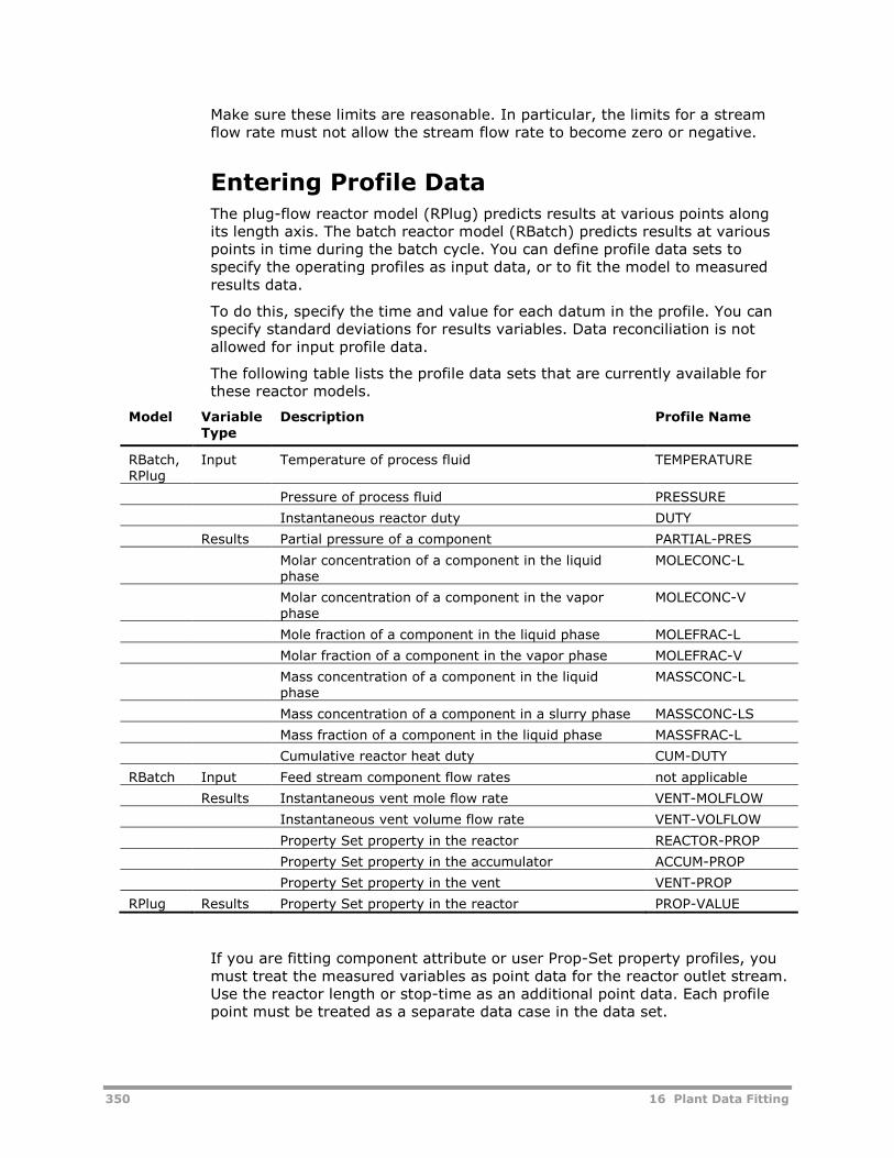
350 16 Plant Data Fitting
Make sure these limits are reasonable. In particular, the limits for a streamflow rate must not allow the stream flow rate to become zero or negative.
Entering Profile DataThe plug-flow reactor model (RPlug) predicts results at various points alongits length axis. The batch reactor model (RBatch) predicts results at variouspoints in time during the batch cycle. You can define profile data sets tospecify the operating profiles as input data, or to fit the model to measuredresults data.
To do this, specify the time and value for each datum in the profile. You canspecify standard deviations for results variables. Data reconciliation is notallowed for input profile data.
The following table lists the profile data sets that are currently available forthese reactor models.
Model VariableType
Description Profile Name
RBatch,RPlug
Input Temperature of process fluid TEMPERATURE
Pressure of process fluid PRESSURE
Instantaneous reactor duty DUTY
Results Partial pressure of a component PARTIAL-PRES
Molar concentration of a component in the liquidphase
MOLECONC-L
Molar concentration of a component in the vaporphase
MOLECONC-V
Mole fraction of a component in the liquid phase MOLEFRAC-L
Molar fraction of a component in the vapor phase MOLEFRAC-V
Mass concentration of a component in the liquidphase
MASSCONC-L
Mass concentration of a component in a slurry phase MASSCONC-LS
Mass fraction of a component in the liquid phase MASSFRAC-L
Cumulative reactor heat duty CUM-DUTY
RBatch Input Feed stream component flow rates not applicable
Results Instantaneous vent mole flow rate VENT-MOLFLOW
Instantaneous vent volume flow rate VENT-VOLFLOW
Property Set property in the reactor REACTOR-PROP
Property Set property in the accumulator ACCUM-PROP
Property Set property in the vent VENT-PROP
RPlug Results Property Set property in the reactor PROP-VALUE
If you are fitting component attribute or user Prop-Set property profiles, youmust treat the measured variables as point data for the reactor outlet stream.Use the reactor length or stop-time as an additional point data. Each profilepoint must be treated as a separate data case in the data set.
16 Plant Data Fitting 351
If some results data are missing from one or more sets of profile data, theycan be left blank on the input forms. The model will estimate the values ofthese results and tabulate them after the regression run.
Entering Standard DeviationsStandard deviations may be specified for input and result variables. Thestandard deviation is the level of uncertainty in the measurement. You canenter the value as an absolute or percent error (append a percentage sign,%, to the value). Statistically determined standard deviations may beavailable from an on-line process information management system (PIMS),from lab databases, or from other information resources. When the standarddeviations are not available, you can enter your best estimate of the expectederror based on your experience or the specifications of the instrument.
The objective function of the data regression is to minimize the sum ofweighted square errors. For results variables, each error is defined as thedifference between the reconciled or specified datum and the value calculatedby the model. Each error is scaled against the square of the standarddeviation:
Objective function =Measurement Prediction
(Standard deviation)ii i
i2
If the specified standard deviation of a variable is too small, the model over-emphasizes the importance of the variable during the fitting process. Thismay cause the model to make unreasonable adjustments in some parametersto force good fits to variables with small standard deviations.
You must be careful to consider both the precision and accuracy of eachvariable. For example, a variable may have a low standard deviation becauseit is very precise (it reproduces well in successive trials), but themeasurement may be inaccurate (it may not reflect the true value of themeasured parameter). Consider the case where a level controller may showlittle deviation in the liquid volume in a reactor, but the calibration of the leveltransducer may not be accurate to within ten percent of the real liquidvolume. In this case, the standard deviation of the specified liquid volumeshould be large enough to reflect the accuracy of the volume, not thedeviation of the liquid level.
If standard deviations are specified for input variables, the model reconcilesthese variables. If you do not specify the standard deviation of an inputvariable, the model assumes the specified values are exact. Reconciling inputvariables accounts for measurement errors in the operating conditions andcan lead to better models, but it can substantially increase how long the runtakes to complete.
Standard deviations must be specified for each of the result variables. Specifyreasonable standard deviations to keep the model from forcing a match bymaking wild adjustments to the parameters. The specified standard deviationsare probably too small (or the data quality is poor) if several of theparameters reach their upper or lower bounds.
352 16 Plant Data Fitting
Defining Data Regression CasesYou can fit any number of data sets in the same regression case. Point-Dataand Profile-Data may both be included. Each regression case must involve atleast one estimated parameter and at least one reconciled input variable.There are no upper limits to the number of estimated parameters andreconciled inputs, however the required simulation time is very sensitive tothe number of variables included in each regression case.
Each input variable with a non-zero standard deviation is reconciled(adjusted). The reconciled inputs are tabulated in the regression results.
Each estimated parameter must be defined in the base case, or have a defaultvalue (such as a physical property parameter). The specified values for thebase case run are used as the initial guesses for the regression. If the base-case value lies outside the specified bounds, the boundary condition closest tothe base case value is used.
Sequencing Data Regression CasesFor data fit problems, Aspen Plus will:
Run the base-case simulation
Execute the data regression
Replace the base-case parameter values with the estimated parametervalues and rerun the base-case simulation
If Sensitivity blocks are present, Aspen Plus runs them after the regression iscomplete. The estimated parameter values are used to calculate the resultsfor these blocks.
Flowsheet convergence loops and Design-Specification loops are used in thepreliminary and final base-case simulations and they are sequenced inside thedata regression loop. The sequencing of Fortran blocks and Transfer blocksdepends on which variables are accessed.
If more than one regression is included in a simulation, the regressions canbe affected sequentially. Each successive regression uses the estimatedparameters from the previous regression.
Regression blocks can be manually sequenced if the automatic sequence doesnot meet the needs of a particular run, however automatic sequencing isusually the best choice.
Interpreting Data Regression ResultsThe key results of the data regression tool are:
The Chi-square statistic and critical Chi-square value for the fit.
Estimates and standard deviations for each estimated parameter.
A table of the measured values, estimated values, and normalizedresiduals for each data set.
The Chi-square value is an indicator of the quality of the fit. A model isconsidered well fit if the Chi-square value falls below the critical Chi-squarevalue. The reliability of different fits or different modeling approaches can be
16 Plant Data Fitting 353
tested by comparing the Chi-square values of the fits. For example, suppose areactor is thought to have non-ideal mixing. This assumption can beevaluated by developing two models, one which assumes ideal mixing (oneCSTR stage) and one which assumes non-ideal mixing (a series of CSTRstages). The two models can be fit against the same data using the sameparameters. The model with the lower Chi-square statistic represents the datamore accurately, and can be considered the most realistic.
Ideally, the standard deviations of the estimated parameters are small, andthe confidence interval of each parameter is narrow. In practice, however, thestandard deviation of the parameters may be relatively large. This does notnecessarily indicate a poor fit. For example, if the activation energy and pre-exponential factor for a reaction are both included as estimated parameters inthe data regression, then the standard deviation of the estimated pre-exponential factor will be large. In this example, small differences in oneparameter (the activation energy) requires large differences in anotherparameter (the pre-exponential factor) to keep the model predictionsrelatively constant.
The residual values are indicative of the difference between the measureddata and model predictions. For fitted data, the residuals are defined as:
Residual = (Measured value - Predicted value ) (Standard deviationi i i2
i/ )
For reconciled data, the residuals are defined as:
Residual = (Measured value - Estimated value ) (Standard deviationi i i2
i/ )
Review the residual values to verify they are sensible. Large residual valuesmay indicate a major problem with the model or data, or may reflect anunreasonably tight standard deviation. Never specify extremely tight standarddeviations. This causes the data regression algorithm to waste timeattempting to obtain tight fits on some variables. If some data are consideredextremely accurate, they should be assigned standard deviations of zero.
The regression results may be plotted against the initial estimates andmeasured data. Plots of this type include a 45 dotted line that indicates a“perfect fit”, e.g., each prediction is exactly equal to the measured data.Points which fall far from this line are the least well fit. Verify these outliers tomake sure the data is correctly entered into the model and that the units ofmeasurement are consistent.
Troubleshooting Convergence ProblemsIf the data regression tool fails to converge, check the objective function. Alarge objective function value indicates a poor fit between the modelpredictions and measured data. If the objective function is large, review theresidual values for each type of measured data. Large residual values mayindicate a very basic error in the data entry. For example, the data may beentered in the wrong units or there may be typing errors in the specifiedvalues. Always review the model thoroughly to eliminate these types ofproblems before adjusting convergence parameters or making other majorchanges to the regression.
354 16 Plant Data Fitting
Convergence errors can occur for a number of reasons. When a problemoccurs, ask:
Does the base case model converge well and give reasonable results?
Is the base case model formulated to handle data that may be out ofmass or energy balance?
Are the initial estimates of the parameters good enough?
Are the specified standard deviations reasonable?
Do the model inputs completely determine the measured results?
Do the specified bounds allow the regression to take the model intoinfeasible regions, causing the unit operation blocks or flowsheetconvergence to fail?
Are the assumptions and simplifications in the model reasonable?
Regression runs with many variables and runs for highly non-linear modelsmay still be difficult to converge. In some cases, the convergence criteria maybe unnecessarily tight.
The following table summarizes several convergence parameters that can beused to tune a regression run. It is not necessary to adjust the convergenceparameters for most regressions.
Parameter Description
ALG-ITERATION Maximum number of algorithm iterations. The default value issufficient for nearly all problems
MAX-PASSES Maximum number of flowsheet passes. This parameter may needto be increased for regressions involving a large number ofvariables.
SSQTOL Convergence tolerance for sum of weighted square errors(Absolute objective function tolerance)
This is the absolute tolerance for the objective function. Thedefault tolerance is very tight, so regressions that converge to thistolerance should be reviewed thoroughly. Verify that the specifiedstandard deviations are sensible. Change the default value of thisparameter if you which to fit the model to achieve a particularobjective function value.
RFCTOL Relative objective function tolerance. The problem is consideredconverged if the model predicts that the maximum possibleobjective function is less than the product of the relative functiontolerance and the current value of the objective function. Forexample, if RFCTOL is 0.1, then the model is converged when thepredicted change in the objective function is less than ten percentof the objective function value for the current iteration.
XCTOL Minimum variable step-size tolerance. The problem is converged ifthe relative step size in the variables falls below XCTOL and theobjective function is decreasing slowly (less than 50% periteration).
XFTOL Minimum objective step-size tolerance
INIT-STEP Factor used to determine initial step sizes. This factor canprofoundly affect the performance of the algorithm. If the initialsteps are too large or too small, the model must adjust the stepsize until appropriate step sizes are determined.
PERT-FACTOR During the regression, the model determines the response of eachvariable to each other variable by making small adjustments, or
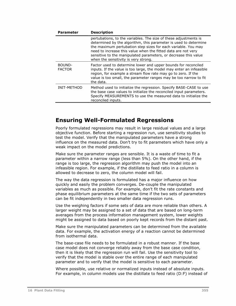
16 Plant Data Fitting 355
Parameter Description
pertubations, to the variables. The size of these adjustments isdetermined by the algorithm, this parameter is used to determinethe maximum pertubation step sizes for each variable. You mayneed to increase this value when the fitted data are not verysensitive to the manipulated parameters, or decrease this valuewhen the sensitivity is very strong.
BOUND-FACTOR
Factor used to determine lower and upper bounds for reconciledinputs. If the value is too large, the model may enter an infeasibleregion, for example a stream flow rate may go to zero. If thevalue is too small, the parameter ranges may be too narrow to fitthe data.
INIT-METHOD Method used to initialize the regression. Specify BASE-CASE to usethe base case values to initialize the reconciled input parameters.Specify MEASUREMENTS to use the measured data to initialize thereconciled inputs.
Ensuring Well-Formulated Regressions
Poorly formulated regressions may result in large residual values and a largeobjective function. Before starting a regression run, use sensitivity studies totest the model. Verify that the manipulated parameters have a stronginfluence on the measured data. Don’t try to fit parameters which have only aweak impact on the model predictions.
Make sure the parameter ranges are sensible. It is a waste of time to fit aparameter within a narrow range (less than 5%). On the other hand, if therange is too large, the regression algorithm may push the model into aninfeasible region. For example, if the distillate to feed ratio in a column isallowed to decrease to zero, the column model will fail.
The way the data regression is formulated has a major influence on howquickly and easily the problem converges. De-couple the manipulatedvariables as much as possible. For example, don’t fit the rate constants andphase equilibrium parameters at the same time if the two sets of parameterscan be fit independently in two smaller data regression runs.
Use the weighing factors if some sets of data are more reliable than others. Alarger weight may be assigned to a set of data that are based on long-termaverages from the process information management system, lower weightsmight be assigned to data based on poorly kept records from the distant past.
Make sure the manipulated parameters can be determined from the availabledata. For example, the activation energy of a reaction cannot be determinedfrom isothermal data.
The base-case file needs to be formulated in a robust manner. If the basecase model does not converge reliably away from the base case condition,then it is likely that the regression run will fail. Use the sensitivity tool toverify that the model is stable over the entire range of each manipulatedparameter and to verify that the model is sensitive to each parameter.
Where possible, use relative or normalized inputs instead of absolute inputs.For example, in column models use the distillate to feed ratio (D:F) instead of
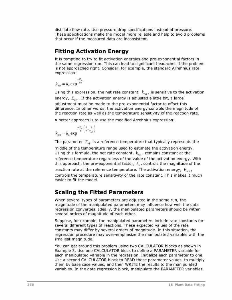
356 16 Plant Data Fitting
distillate flow rate. Use pressure drop specifications instead of pressure.These specifications make the model more reliable and help to avoid problemsthat occur if the measured data are inconsistent.
Fitting Activation Energy
It is tempting to try to fit activation energies and pre-exponential factors inthe same regression run. This can lead to significant headaches if the problemis not approached right. Consider, for example, the standard Arrehnius rateexpression:
k knet o
E
RTact
exp
Using this expression, the net rate constant, knet , is sensitive to the activation
energy, Eact . If the activation energy is adjusted a little bit, a large
adjustment must be made to the pre-exponential factor to offset thisdifference. In other words, the activation energy controls the magnitude ofthe reaction rate as well as the temperature sensitivity of the reaction rate.
A better approach is to use the modified Arrehnius expression:
k knet o
E
R T Tact
ref
exp
1 1
The parameter Tref is a reference temperature that typically represents the
middle of the temperature range used to estimate the activation energy.
Using this formula, the net rate constant, knet , remains constant at the
reference temperature regardless of the value of the activation energy. With
this approach, the pre-exponential factor, ko , controls the magnitude of the
reaction rate at the reference temperature. The activation energy, Eact ,
controls the temperature sensitivity of the rate constant. This makes it mucheasier to fit the model.
Scaling the Fitted Parameters
When several types of parameters are adjusted in the same run, themagnitude of the manipulated parameters may influence how well the dataregression converges. Ideally, the manipulated parameters should be withinseveral orders of magnitude of each other.
Suppose, for example, the manipulated parameters include rate constants forseveral different types of reactions. These expected values of the rateconstants may differ by several orders of magnitude. In this situation, theregression procedure may over-emphasize the manipulated variables with thesmallest magnitude.
You can get around this problem using two CALCULATOR blocks as shown inExample 3. Use one CALCULATOR block to define a PARAMETER variable foreach manipulated variable in the regression. Initialize each parameter to one.Use a second CALCULATOR block to READ these parameter values, to multiplythem by base case values, and then WRITE the results to the manipulatedvariables. In the data regression block, manipulate the PARAMETER variables.
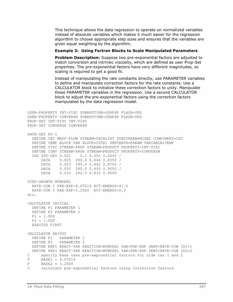
16 Plant Data Fitting 357
This technique allows the data regression to operate on normalized variablesinstead of absolute variables which makes it much easier for the regressionalgorithm to choose appropriate step sizes and ensures that the variables aregiven equal weighting by the algorithm.
Example 3: Using Fortran Blocks to Scale Manipulated Parameters
Problem Description: Suppose two pre-exponential factors are adjusted tomatch conversion and intrinsic viscosity, which are defined as user Prop-Setproperties. The pre-exponential factors have very different magnitudes, soscaling is required to get a good fit.
Instead of manipulating the rate constants directly, use PARAMETER variablesto define and manipulate correction factors for the rate constants. Use aCALCULATOR block to initialize these correction factors to unity. Manipulatethese PARAMETER variables in the regression. Use a second CALCULATORblock to adjust the pre-exponential factors using the correction factorsmanipulated by the data regression model.
USER-PROPERTY INT-VISC SUBROUTINE=USRPSP FLASH=YESUSER-PROPERTY CONVERSN SUBROUTINE=USRPSP FLASH=YESPROP-SET INT-VISC INT-VISCPROP-SET CONVERSN CONVERSN
DATA-SET DS-1DEFINE CAT MASS-FLOW STREAM=CATALYST SUBSTREAM=MIXED COMPONENT=CATDEFINE TEMP BLOCK-VAR BLOCK=CSTR1 SENTENCE=PARAM VARIABLE=TEMPDEFINE VISC STREAM-PROP STREAM=PRODUCT PROPERTY=INT-VISCDEFINE CONV STREAM-PROP STREAM=PRODUCT PROPERTY=CONVERSNUSE STD-DEV 0.001 0.1 0.002 0.0050 /
DATA 0.025 290.0 0.844 0.8550 /DATA 0.023 295.0 0.842 0.8700 /DATA 0.055 280.0 0.850 0.9050 /DATA 0.033 292.0 0.835 0.9000
STEP-GROWTH MYMODELRATE-CON 1 PRE-EXP=9.67D14 ACT-ENERGY=41.0RATE-CON 2 PRE-EXP=3.25D0 ACT-ENERGY=0.0
etc…
CALCULATOR INITIALDEFINE P1 PARAMETER 1DEFINE P2 PARAMETER 2P1 = 1.0D0P2 = 1.0D0EXECUTE FIRST
CALCULATOR ADJUSTDEFINE P1 PARAMETER 1DEFINE P2 PARAMETER 2DEFINE EXP1 REACT-VAR REACTION=MYMODEL VAR=PRE-EXP SENT=RATE-CON ID1=1DEFINE EXP2 REACT-VAR REACTION=MYMODEL VAR=PRE-EXP SENT=RATE-CON ID2=2
C specify base case pre-exponential factors for side rxn 1 and 2F BASE1 = 9.67D14F BASE2 = 3.25D0C calculate pre-exponential factors using correction factors
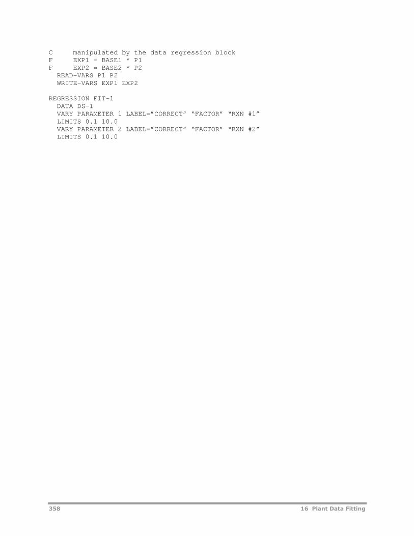
358 16 Plant Data Fitting
C manipulated by the data regression blockF EXP1 = BASE1 * P1F EXP2 = BASE2 * P2
READ-VARS P1 P2WRITE-VARS EXP1 EXP2
REGRESSION FIT-1DATA DS-1VARY PARAMETER 1 LABEL=”CORRECT” “FACTOR” “RXN #1”LIMITS 0.1 10.0VARY PARAMETER 2 LABEL=”CORRECT” “FACTOR” “RXN #2”LIMITS 0.1 10.0
17 User Models 359
17 User Models
This section discusses the features available in Aspen Polymers (formerlyknown as Aspen Polymers Plus) for incorporating user modules into asimulation model.
Topics covered include:
User Unit Operation Models, 359
User Kinetic Models, 365
User Physical Property Models, 370
Note: For more information on user models, see your Aspen Plus User Modelsdocumentation.
User Unit Operation ModelsThere are cases where users may need to create special models to representa process. Usually these models can be configured by combining several ofthe standard unit operation building blocks. For more complex reactorgeometries or in order to represent highly non-ideal systems users may needto provide their own model as a Fortran subroutine.
There are two user unit operation blocks available: USER and USER2. The firstallows a limited number of inlet and outlet streams. The second allowsmultiple inlet and outlet streams. Both unit operations take full advantage ofthe Aspen Plus flowsheeting capabilities. The required Fortran subroutinemust process the feed streams and return the condition and composition ofthe outlet streams.
User Unit Operation Models StructureThere are three stages to the execution of Aspen Plus unit operation models:input processing, simulation calculations, and report writing. Normally, theimplementation of a new model requires that all three stages be accountedfor. However, in the case of USER2 models, a generic framework handles theinput setup and processing stage. A Fortran subroutine must be written toperform the simulation calculations and for writing the report. If no report
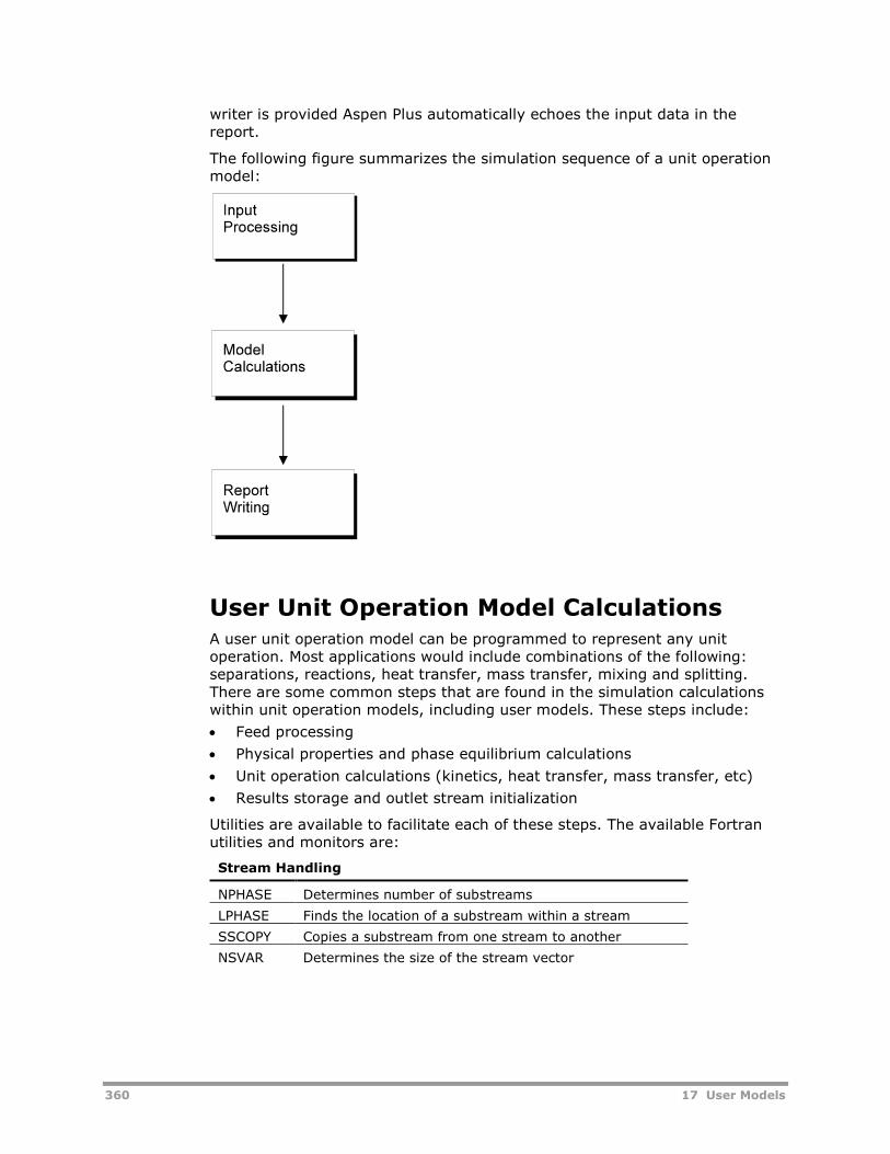
360 17 User Models
writer is provided Aspen Plus automatically echoes the input data in thereport.
The following figure summarizes the simulation sequence of a unit operationmodel:
User Unit Operation Model CalculationsA user unit operation model can be programmed to represent any unitoperation. Most applications would include combinations of the following:separations, reactions, heat transfer, mass transfer, mixing and splitting.There are some common steps that are found in the simulation calculationswithin unit operation models, including user models. These steps include:
Feed processing
Physical properties and phase equilibrium calculations
Unit operation calculations (kinetics, heat transfer, mass transfer, etc)
Results storage and outlet stream initialization
Utilities are available to facilitate each of these steps. The available Fortranutilities and monitors are:
Stream Handling
NPHASE Determines number of substreams
LPHASE Finds the location of a substream within a stream
SSCOPY Copies a substream from one stream to another
NSVAR Determines the size of the stream vector
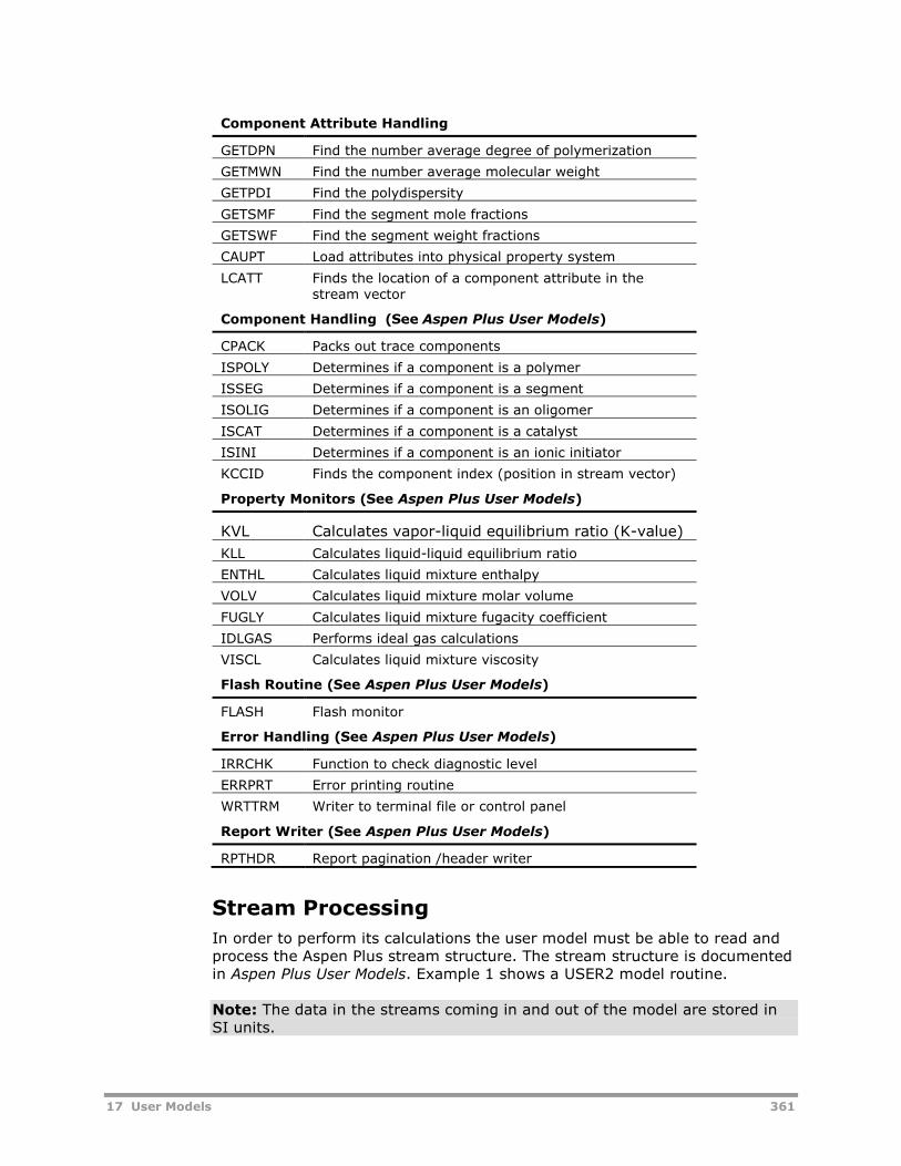
17 User Models 361
Component Attribute Handling
GETDPN Find the number average degree of polymerization
GETMWN Find the number average molecular weight
GETPDI Find the polydispersity
GETSMF Find the segment mole fractions
GETSWF Find the segment weight fractions
CAUPT Load attributes into physical property system
LCATT Finds the location of a component attribute in thestream vector
Component Handling (See Aspen Plus User Models)
CPACK Packs out trace components
ISPOLY Determines if a component is a polymer
ISSEG Determines if a component is a segment
ISOLIG Determines if a component is an oligomer
ISCAT Determines if a component is a catalyst
ISINI Determines if a component is an ionic initiator
KCCID Finds the component index (position in stream vector)
Property Monitors (See Aspen Plus User Models)
KVL Calculates vapor-liquid equilibrium ratio (K-value)
KLL Calculates liquid-liquid equilibrium ratio
ENTHL Calculates liquid mixture enthalpy
VOLV Calculates liquid mixture molar volume
FUGLY Calculates liquid mixture fugacity coefficient
IDLGAS Performs ideal gas calculations
VISCL Calculates liquid mixture viscosity
Flash Routine (See Aspen Plus User Models)
FLASH Flash monitor
Error Handling (See Aspen Plus User Models)
IRRCHK Function to check diagnostic level
ERRPRT Error printing routine
WRTTRM Writer to terminal file or control panel
Report Writer (See Aspen Plus User Models)
RPTHDR Report pagination /header writer
Stream Processing
In order to perform its calculations the user model must be able to read andprocess the Aspen Plus stream structure. The stream structure is documentedin Aspen Plus User Models. Example 1 shows a USER2 model routine.
Note: The data in the streams coming in and out of the model are stored inSI units.
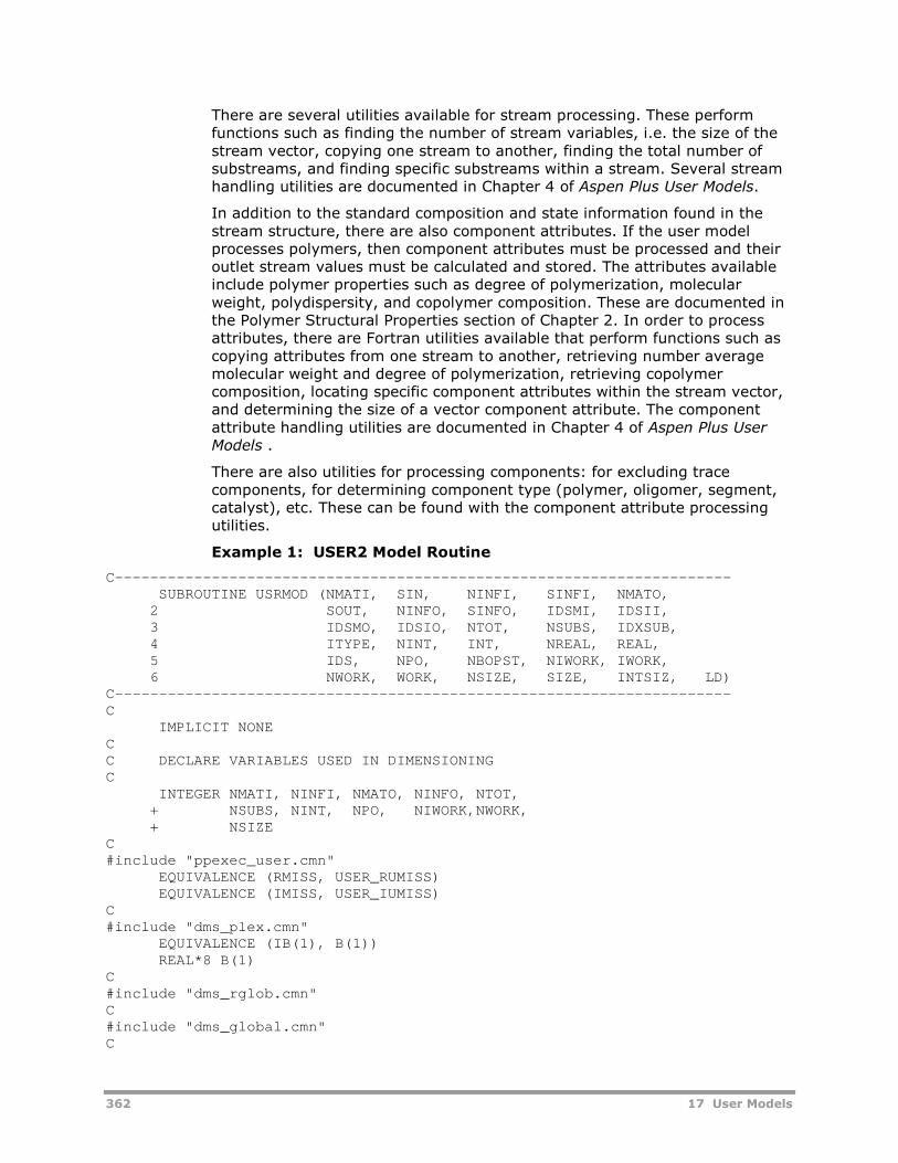
362 17 User Models
There are several utilities available for stream processing. These performfunctions such as finding the number of stream variables, i.e. the size of thestream vector, copying one stream to another, finding the total number ofsubstreams, and finding specific substreams within a stream. Several streamhandling utilities are documented in Chapter 4 of Aspen Plus User Models.
In addition to the standard composition and state information found in thestream structure, there are also component attributes. If the user modelprocesses polymers, then component attributes must be processed and theiroutlet stream values must be calculated and stored. The attributes availableinclude polymer properties such as degree of polymerization, molecularweight, polydispersity, and copolymer composition. These are documented inthe Polymer Structural Properties section of Chapter 2. In order to processattributes, there are Fortran utilities available that perform functions such ascopying attributes from one stream to another, retrieving number averagemolecular weight and degree of polymerization, retrieving copolymercomposition, locating specific component attributes within the stream vector,and determining the size of a vector component attribute. The componentattribute handling utilities are documented in Chapter 4 of Aspen Plus UserModels .
There are also utilities for processing components: for excluding tracecomponents, for determining component type (polymer, oligomer, segment,catalyst), etc. These can be found with the component attribute processingutilities.
Example 1: USER2 Model Routine
C----------------------------------------------------------------------SUBROUTINE USRMOD (NMATI, SIN, NINFI, SINFI, NMATO,
2 SOUT, NINFO, SINFO, IDSMI, IDSII,3 IDSMO, IDSIO, NTOT, NSUBS, IDXSUB,4 ITYPE, NINT, INT, NREAL, REAL,5 IDS, NPO, NBOPST, NIWORK, IWORK,6 NWORK, WORK, NSIZE, SIZE, INTSIZ, LD)
C----------------------------------------------------------------------C
IMPLICIT NONECC DECLARE VARIABLES USED IN DIMENSIONINGC
INTEGER NMATI, NINFI, NMATO, NINFO, NTOT,+ NSUBS, NINT, NPO, NIWORK,NWORK,+ NSIZE
C#include "ppexec_user.cmn"
EQUIVALENCE (RMISS, USER_RUMISS)EQUIVALENCE (IMISS, USER_IUMISS)
C#include "dms_plex.cmn"
EQUIVALENCE (IB(1), B(1))REAL*8 B(1)
C#include "dms_rglob.cmn"C#include "dms_global.cmn"C
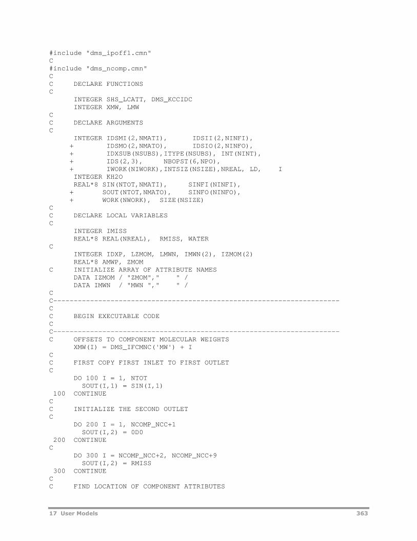
17 User Models 363
#include "dms_ipoff1.cmn"C#include "dms_ncomp.cmn"CC DECLARE FUNCTIONSC
INTEGER SHS_LCATT, DMS_KCCIDCINTEGER XMW, LMW
CC DECLARE ARGUMENTSC
INTEGER IDSMI(2,NMATI), IDSII(2,NINFI),+ IDSMO(2,NMATO), IDSIO(2,NINFO),+ IDXSUB(NSUBS),ITYPE(NSUBS), INT(NINT),+ IDS(2,3), NBOPST(6,NPO),+ IWORK(NIWORK),INTSIZ(NSIZE),NREAL, LD, IINTEGER KH2OREAL*8 SIN(NTOT,NMATI), SINFI(NINFI),
+ SOUT(NTOT,NMATO), SINFO(NINFO),+ WORK(NWORK), SIZE(NSIZE)
CC DECLARE LOCAL VARIABLESC
INTEGER IMISSREAL*8 REAL(NREAL), RMISS, WATER
CINTEGER IDXP, LZMOM, LMWN, IMWN(2), IZMOM(2)REAL*8 AMWP, ZMOM
C INITIALIZE ARRAY OF ATTRIBUTE NAMESDATA IZMOM / "ZMOM"," " /DATA IMWN / "MWN "," " /
CC----------------------------------------------------------------------CC BEGIN EXECUTABLE CODECC----------------------------------------------------------------------C OFFSETS TO COMPONENT MOLECULAR WEIGHTS
XMW(I) = DMS_IFCMNC('MW') + ICC FIRST COPY FIRST INLET TO FIRST OUTLETC
DO 100 I = 1, NTOTSOUT(I,1) = SIN(I,1)
100 CONTINUECC INITIALIZE THE SECOND OUTLETC
DO 200 I = 1, NCOMP_NCC+1SOUT(I,2) = 0D0
200 CONTINUEC
DO 300 I = NCOMP_NCC+2, NCOMP_NCC+9SOUT(I,2) = RMISS
300 CONTINUECC FIND LOCATION OF COMPONENT ATTRIBUTES

364 17 User Models
C IDXP is position of polymer component in component list.C Can be obtained with ispoly functionC find location of attributes in stream
LZMOM = SHS_LCATT( 1, IDXP, IZMOM )LMWN = SHS_LCATT( 1, IDXP, IMWN )IF (LZMOM .NE. 0) ZMOM = SOUT(LZMOM+1,1)
CC EXAMPLE OF FINDING A COMPONENT POSITION BY NAMEC
KH2O = DMS_KCCIDC ( 'H2O' )CC CAN ALSO PASS POSITION AS PARAMETER IN INT VECTORC E.G. KH2O = INT(2)
IF ( KH2O .EQ. 0 ) GO TO 999CC PUT COMPONENT (WATER) IN THE SECOND OUTLETC
WATER = SIN(KH2O,1)SOUT(KH2O,1) = 0D0SOUT(NCOMP_NCC+1,1) = SIN(NCOMP_NCC+1,1) - WATERSOUT(KH2O,2) = WATERSOUT(NCOMP_NCC+1,2) = WATER
C999 RETURN
END
Physical Property Calculations
Physical properties and phase equilibrium calculations can be performedwithin a user model. Property methods, models, and parameters specified inthe input either through a built-in or a user-defined property method, can beused for the user model calculations. This can be done through propertymonitors. The user model requests the property of interest by calling aspecific monitor, sets the state information and calculation codes in the call tothe monitors, and in turn obtains thermodynamic properties such as fugacitycoefficients, enthalpies, entropies, molar volumes, etc. A flash calculationroutine is also available. See the table on page 360 for a listing of frequentlyused property monitors. The FLASH routine and the property monitors aredocumented in Aspen Plus User Models. See also User Physical PropertyModels on page 370.
Unit Operation Calculations
The purpose of a user unit operation block is to allow the flexibility toprogram user correlations or algorithms to represent a process.Independently from the physical property calculations for which monitors areprovided, users can take advantage of the Fortran subroutine structure toincorporate the calculations needed to represent their process. Aspen PlusSystem Management documents programming guidelines to be followed whendefining the model calculations. The calculations performed within a user unitoperator model for a polymer system are similar to those that could beperformed within a kinetic model. See User Kinetic Models on page 365.
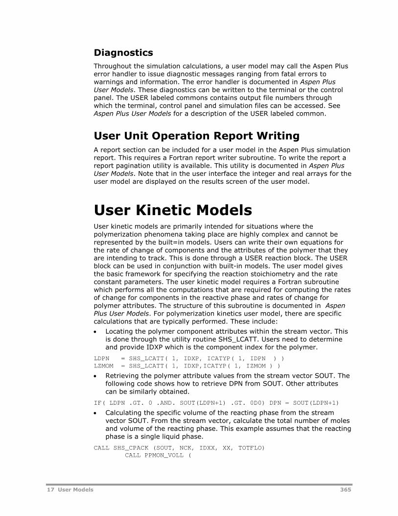
17 User Models 365
Diagnostics
Throughout the simulation calculations, a user model may call the Aspen Pluserror handler to issue diagnostic messages ranging from fatal errors towarnings and information. The error handler is documented in Aspen PlusUser Models. These diagnostics can be written to the terminal or the controlpanel. The USER labeled commons contains output file numbers throughwhich the terminal, control panel and simulation files can be accessed. SeeAspen Plus User Models for a description of the USER labeled common.
User Unit Operation Report WritingA report section can be included for a user model in the Aspen Plus simulationreport. This requires a Fortran report writer subroutine. To write the report areport pagination utility is available. This utility is documented in Aspen PlusUser Models. Note that in the user interface the integer and real arrays for theuser model are displayed on the results screen of the user model.
User Kinetic ModelsUser kinetic models are primarily intended for situations where thepolymerization phenomena taking place are highly complex and cannot berepresented by the built=in models. Users can write their own equations forthe rate of change of components and the attributes of the polymer that theyare intending to track. This is done through a USER reaction block. The USERblock can be used in conjunction with built-in models. The user model givesthe basic framework for specifying the reaction stoichiometry and the rateconstant parameters. The user kinetic model requires a Fortran subroutinewhich performs all the computations that are required for computing the ratesof change for components in the reactive phase and rates of change forpolymer attributes. The structure of this subroutine is documented in AspenPlus User Models. For polymerization kinetics user model, there are specificcalculations that are typically performed. These include:
Locating the polymer component attributes within the stream vector. Thisis done through the utility routine SHS_LCATT. Users need to determineand provide IDXP which is the component index for the polymer.
LDPN = SHS_LCATT( 1, IDXP, ICATYP( 1, IDPN ) )LZMOM = SHS_LCATT( 1, IDXP,ICATYP( 1, IZMOM ) )
Retrieving the polymer attribute values from the stream vector SOUT. Thefollowing code shows how to retrieve DPN from SOUT. Other attributescan be similarly obtained.
IF( LDPN .GT. 0 .AND. SOUT(LDPN+1) .GT. 0D0) DPN = SOUT(LDPN+1)
Calculating the specific volume of the reacting phase from the streamvector SOUT. From the stream vector, calculate the total number of molesand volume of the reacting phase. This example assumes that the reactingphase is a single liquid phase.
CALL SHS_CPACK (SOUT, NCK, IDXX, XX, TOTFLO)CALL PPMON_VOLL (
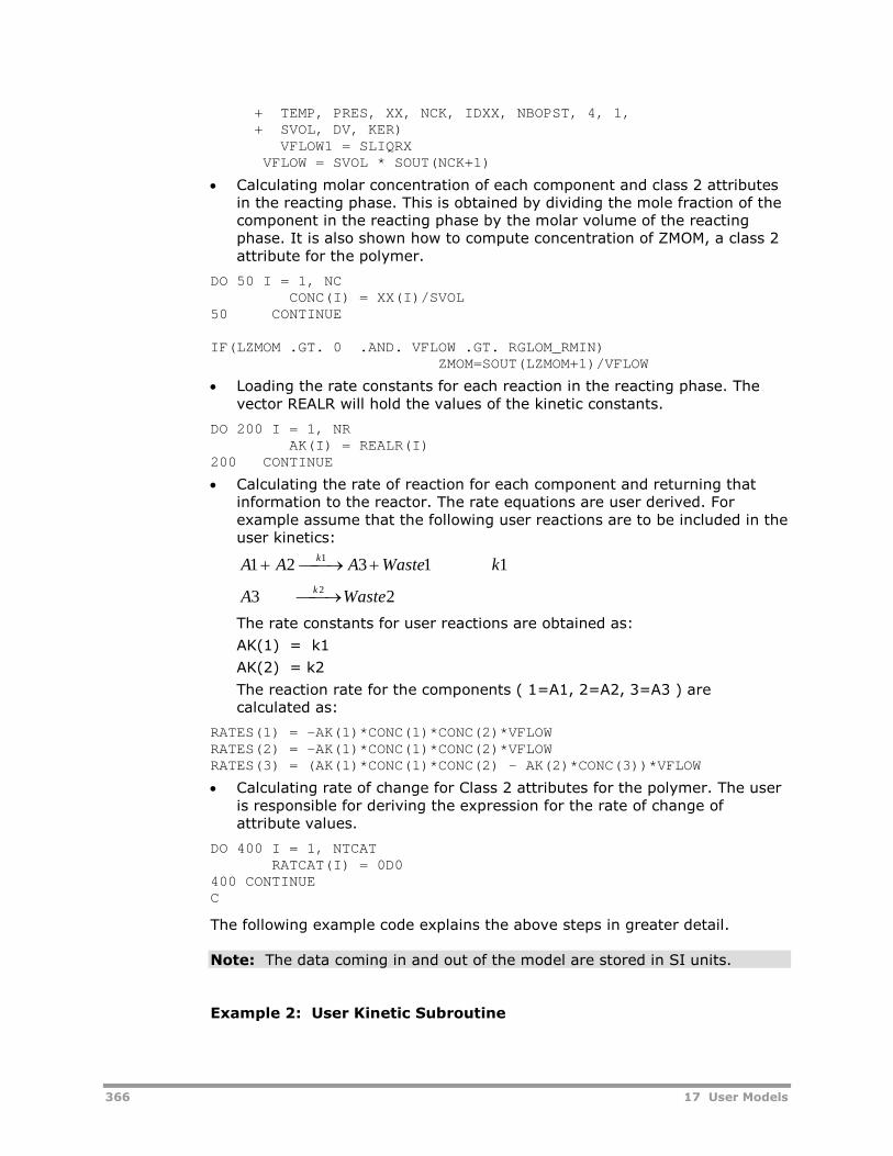
366 17 User Models
+ TEMP, PRES, XX, NCK, IDXX, NBOPST, 4, 1,+ SVOL, DV, KER)
VFLOW1 = SLIQRXVFLOW = SVOL * SOUT(NCK+1)
Calculating molar concentration of each component and class 2 attributesin the reacting phase. This is obtained by dividing the mole fraction of thecomponent in the reacting phase by the molar volume of the reactingphase. It is also shown how to compute concentration of ZMOM, a class 2attribute for the polymer.
DO 50 I = 1, NCCONC(I) = XX(I)/SVOL
50 CONTINUE
IF(LZMOM .GT. 0 .AND. VFLOW .GT. RGLOM_RMIN)ZMOM=SOUT(LZMOM+1)/VFLOW
Loading the rate constants for each reaction in the reacting phase. Thevector REALR will hold the values of the kinetic constants.
DO 200 I = 1, NRAK(I) = REALR(I)
200 CONTINUE
Calculating the rate of reaction for each component and returning thatinformation to the reactor. The rate equations are user derived. Forexample assume that the following user reactions are to be included in theuser kinetics:
A A A Waste kk
1 2 3 1 11
A Wastek
3 22
The rate constants for user reactions are obtained as:
AK(1) = k1
AK(2) = k2
The reaction rate for the components ( 1=A1, 2=A2, 3=A3 ) arecalculated as:
RATES(1) = -AK(1)*CONC(1)*CONC(2)*VFLOWRATES(2) = -AK(1)*CONC(1)*CONC(2)*VFLOWRATES(3) = (AK(1)*CONC(1)*CONC(2) - AK(2)*CONC(3))*VFLOW
Calculating rate of change for Class 2 attributes for the polymer. The useris responsible for deriving the expression for the rate of change ofattribute values.
DO 400 I = 1, NTCATRATCAT(I) = 0D0
400 CONTINUEC
The following example code explains the above steps in greater detail.
Note: The data coming in and out of the model are stored in SI units.
Example 2: User Kinetic Subroutine
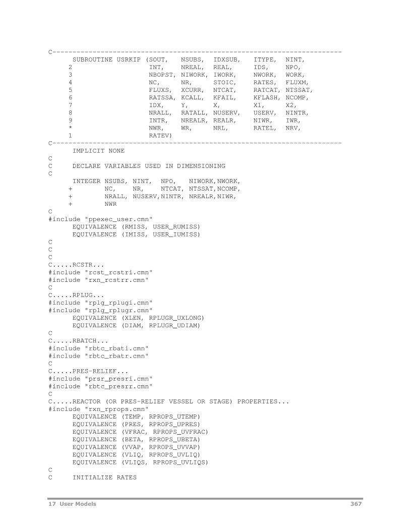
17 User Models 367
C------------------------------------------------------------------------SUBROUTINE USRKIP (SOUT, NSUBS, IDXSUB, ITYPE, NINT,
2 INT, NREAL, REAL, IDS, NPO,3 NBOPST, NIWORK, IWORK, NWORK, WORK,4 NC, NR, STOIC, RATES, FLUXM,5 FLUXS, XCURR, NTCAT, RATCAT, NTSSAT,6 RATSSA, KCALL, KFAIL, KFLASH, NCOMP,7 IDX, Y, X, X1, X2,8 NRALL, RATALL, NUSERV, USERV, NINTR,9 INTR, NREALR, REALR, NIWR, IWR,* NWR, WR, NRL, RATEL, NRV,1 RATEV)
C------------------------------------------------------------------------IMPLICIT NONE
CC DECLARE VARIABLES USED IN DIMENSIONINGC
INTEGER NSUBS, NINT, NPO, NIWORK,NWORK,+ NC, NR, NTCAT, NTSSAT,NCOMP,+ NRALL, NUSERV,NINTR, NREALR,NIWR,+ NWR
C#include "ppexec_user.cmn"
EQUIVALENCE (RMISS, USER_RUMISS)EQUIVALENCE (IMISS, USER_IUMISS)
CCCC.....RCSTR...#include "rcst_rcstri.cmn"#include "rxn_rcstrr.cmn"CC.....RPLUG...#include "rplg_rplugi.cmn"#include "rplg_rplugr.cmn"
EQUIVALENCE (XLEN, RPLUGR_UXLONG)EQUIVALENCE (DIAM, RPLUGR_UDIAM)
CC.....RBATCH...#include "rbtc_rbati.cmn"#include "rbtc_rbatr.cmn"CC.....PRES-RELIEF...#include "prsr_presri.cmn"#include "rbtc_presrr.cmn"CC.....REACTOR (OR PRES-RELIEF VESSEL OR STAGE) PROPERTIES...#include "rxn_rprops.cmn"
EQUIVALENCE (TEMP, RPROPS_UTEMP)EQUIVALENCE (PRES, RPROPS_UPRES)EQUIVALENCE (VFRAC, RPROPS_UVFRAC)EQUIVALENCE (BETA, RPROPS_UBETA)EQUIVALENCE (VVAP, RPROPS_UVVAP)EQUIVALENCE (VLIQ, RPROPS_UVLIQ)EQUIVALENCE (VLIQS, RPROPS_UVLIQS)
CC INITIALIZE RATES
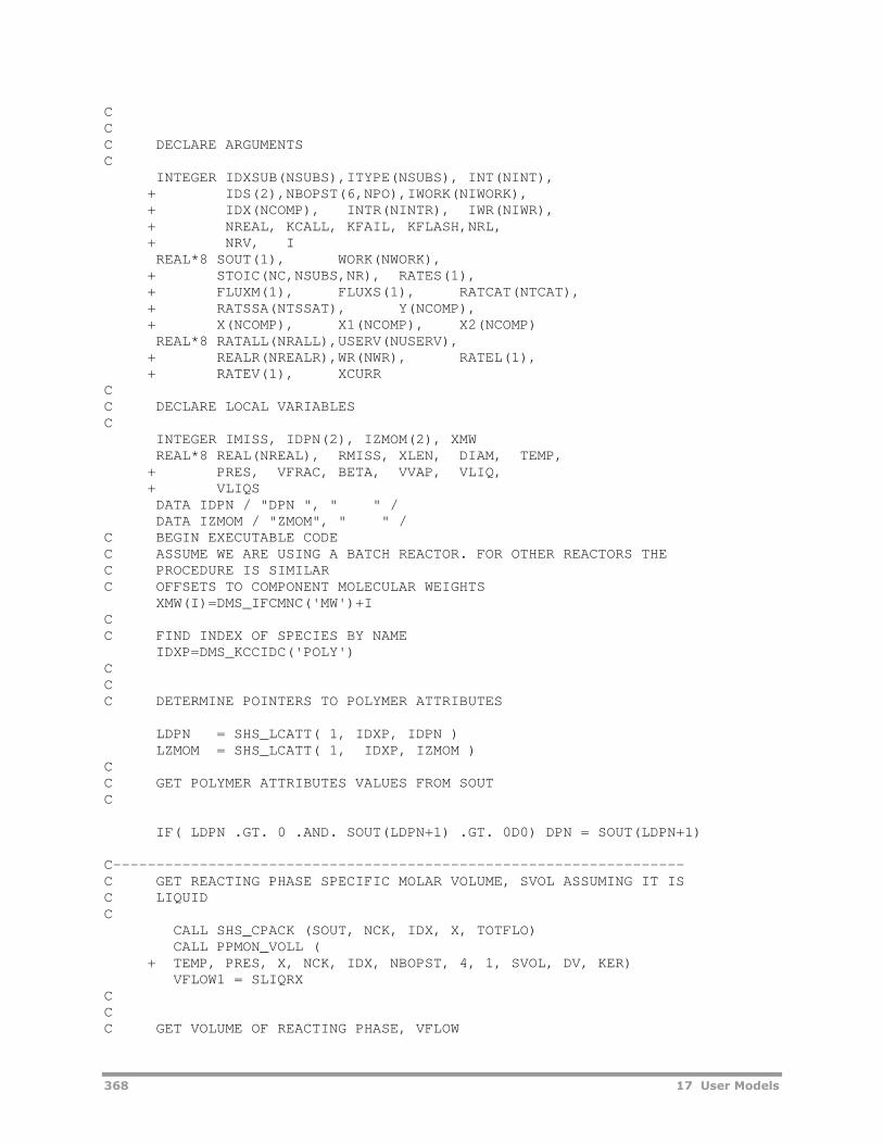
368 17 User Models
CCC DECLARE ARGUMENTSC
INTEGER IDXSUB(NSUBS),ITYPE(NSUBS), INT(NINT),+ IDS(2),NBOPST(6,NPO),IWORK(NIWORK),+ IDX(NCOMP), INTR(NINTR), IWR(NIWR),+ NREAL, KCALL, KFAIL, KFLASH,NRL,+ NRV, IREAL*8 SOUT(1), WORK(NWORK),
+ STOIC(NC,NSUBS,NR), RATES(1),+ FLUXM(1), FLUXS(1), RATCAT(NTCAT),+ RATSSA(NTSSAT), Y(NCOMP),+ X(NCOMP), X1(NCOMP), X2(NCOMP)REAL*8 RATALL(NRALL),USERV(NUSERV),
+ REALR(NREALR),WR(NWR), RATEL(1),+ RATEV(1), XCURR
CC DECLARE LOCAL VARIABLESC
INTEGER IMISS, IDPN(2), IZMOM(2), XMWREAL*8 REAL(NREAL), RMISS, XLEN, DIAM, TEMP,
+ PRES, VFRAC, BETA, VVAP, VLIQ,+ VLIQSDATA IDPN / "DPN ", " " /DATA IZMOM / "ZMOM", " " /
C BEGIN EXECUTABLE CODEC ASSUME WE ARE USING A BATCH REACTOR. FOR OTHER REACTORS THEC PROCEDURE IS SIMILARC OFFSETS TO COMPONENT MOLECULAR WEIGHTS
XMW(I)=DMS_IFCMNC('MW')+ICC FIND INDEX OF SPECIES BY NAME
IDXP=DMS_KCCIDC('POLY')CCC DETERMINE POINTERS TO POLYMER ATTRIBUTES
LDPN = SHS_LCATT( 1, IDXP, IDPN )LZMOM = SHS_LCATT( 1, IDXP, IZMOM )
CC GET POLYMER ATTRIBUTES VALUES FROM SOUTC
IF( LDPN .GT. 0 .AND. SOUT(LDPN+1) .GT. 0D0) DPN = SOUT(LDPN+1)
C------------------------------------------------------------------C GET REACTING PHASE SPECIFIC MOLAR VOLUME, SVOL ASSUMING IT ISC LIQUIDC
CALL SHS_CPACK (SOUT, NCK, IDX, X, TOTFLO)CALL PPMON_VOLL (
+ TEMP, PRES, X, NCK, IDX, NBOPST, 4, 1, SVOL, DV, KER)VFLOW1 = SLIQRX
CCC GET VOLUME OF REACTING PHASE, VFLOW
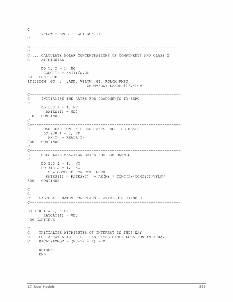
17 User Models 369
CVFLOW = SVOL * SOUT(NCK+1)
C
C-----------------------------------------------------------------CC.....CALCULATE MOLAR CONCENTRATIONS OF COMPONENTS AND CLASS 2C ATTRIBUTES
DO 50 I = 1, NCCONC(I) = XX(I)/SVOL
50 CONTINUEIF(LZMOM .GT. 0 .AND. VFLOW .GT. RGLOM_RMIN)
ZMOM=SOUT(LZMOM+1)/VFLOW
C------------------------------------------------------------------C INITIALIZE THE RATES FOR COMPONENTS TO ZEROC
DO 100 I = 1, NCRATES(I) = 0D0
100 CONTINUECC------------------------------------------------------------------C LOAD REACTION RATE CONSTANTS FROM THE REALR
DO 200 I = 1, NRAK(I) = REALR(I)
200 CONTINUECC------------------------------------------------------------------C CALCULATE REACTION RATES FOR COMPONENTSC
DO 300 I = 1, NCDO 310 J = 1, NC
M = COMPUTE CORRECT INDEXRATES(I) = RATES(I) - AK(M) * CONC(I)*CONC(J)*VFLOW
300 CONTINUE
CCC CALCULATE RATES FOR CLASS-2 ATTRIBUTE EXAMPLEC------------------------------------------------------------------
DO 400 I = 1, NTCATRATCAT(I) = 0D0
400 CONTINUE
CC INITIALIZE ATTRIBUTES OF INTEREST IN THIS WAYC FOR ARRAY ATTRIBUTES THIS GIVES FIRST LOCATION IN ARRAYC RACAT(LZMOM - (NC+9) + 1) = 0
RETURNEND
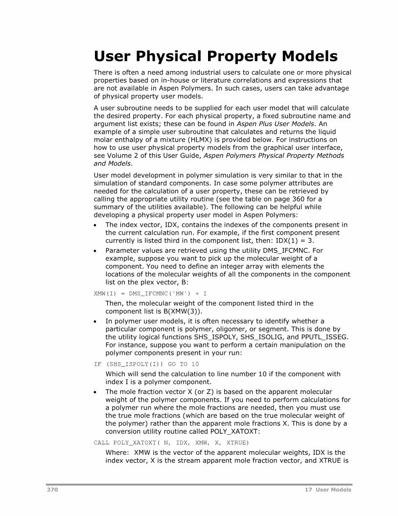
370 17 User Models
User Physical Property ModelsThere is often a need among industrial users to calculate one or more physicalproperties based on in-house or literature correlations and expressions thatare not available in Aspen Polymers. In such cases, users can take advantageof physical property user models.
A user subroutine needs to be supplied for each user model that will calculatethe desired property. For each physical property, a fixed subroutine name andargument list exists; these can be found in Aspen Plus User Models. Anexample of a simple user subroutine that calculates and returns the liquidmolar enthalpy of a mixture (HLMX) is provided below. For instructions onhow to use user physical property models from the graphical user interface,see Volume 2 of this User Guide, Aspen Polymers Physical Property Methodsand Models.
User model development in polymer simulation is very similar to that in thesimulation of standard components. In case some polymer attributes areneeded for the calculation of a user property, these can be retrieved bycalling the appropriate utility routine (see the table on page 360 for asummary of the utilities available). The following can be helpful whiledeveloping a physical property user model in Aspen Polymers:
The index vector, IDX, contains the indexes of the components present inthe current calculation run. For example, if the first component presentcurrently is listed third in the component list, then: IDX(1) = 3.
Parameter values are retrieved using the utility DMS_IFCMNC. Forexample, suppose you want to pick up the molecular weight of acomponent. You need to define an integer array with elements thelocations of the molecular weights of all the components in the componentlist on the plex vector, B:
XMW(I) = DMS_IFCMNC('MW') + I
Then, the molecular weight of the component listed third in thecomponent list is B(XMW(3)).
In polymer user models, it is often necessary to identify whether aparticular component is polymer, oligomer, or segment. This is done bythe utility logical functions SHS_ISPOLY, SHS_ISOLIG, and PPUTL_ISSEG.For instance, suppose you want to perform a certain manipulation on thepolymer components present in your run:
IF (SHS_ISPOLY(I)) GO TO 10
Which will send the calculation to line number 10 if the component withindex I is a polymer component.
The mole fraction vector X (or Z) is based on the apparent molecularweight of the polymer components. If you need to perform calculations fora polymer run where the mole fractions are needed, then you must usethe true mole fractions (which are based on the true molecular weight ofthe polymer) rather than the apparent mole fractions X. This is done by aconversion utility routine called POLY_XATOXT:
CALL POLY_XATOXT( N, IDX, XMW, X, XTRUE)
Where: XMW is the vector of the apparent molecular weights, IDX is theindex vector, X is the stream apparent mole fraction vector, and XTRUE is
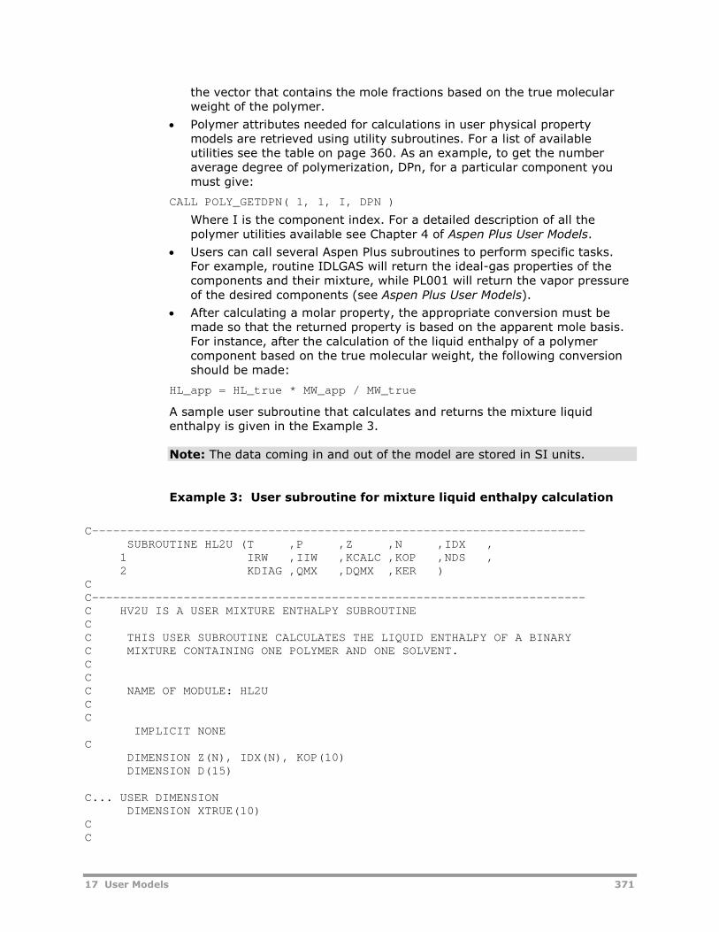
17 User Models 371
the vector that contains the mole fractions based on the true molecularweight of the polymer.
Polymer attributes needed for calculations in user physical propertymodels are retrieved using utility subroutines. For a list of availableutilities see the table on page 360. As an example, to get the numberaverage degree of polymerization, DPn, for a particular component youmust give:
CALL POLY_GETDPN( 1, 1, I, DPN )
Where I is the component index. For a detailed description of all thepolymer utilities available see Chapter 4 of Aspen Plus User Models.
Users can call several Aspen Plus subroutines to perform specific tasks.For example, routine IDLGAS will return the ideal-gas properties of thecomponents and their mixture, while PL001 will return the vapor pressureof the desired components (see Aspen Plus User Models).
After calculating a molar property, the appropriate conversion must bemade so that the returned property is based on the apparent mole basis.For instance, after the calculation of the liquid enthalpy of a polymercomponent based on the true molecular weight, the following conversionshould be made:
HL_app = HL_true * MW_app / MW_true
A sample user subroutine that calculates and returns the mixture liquidenthalpy is given in the Example 3.
Note: The data coming in and out of the model are stored in SI units.
Example 3: User subroutine for mixture liquid enthalpy calculation
C----------------------------------------------------------------------SUBROUTINE HL2U (T ,P ,Z ,N ,IDX ,
1 IRW ,IIW ,KCALC ,KOP ,NDS ,2 KDIAG ,QMX ,DQMX ,KER )
CC----------------------------------------------------------------------C HV2U IS A USER MIXTURE ENTHALPY SUBROUTINECC THIS USER SUBROUTINE CALCULATES THE LIQUID ENTHALPY OF A BINARYC MIXTURE CONTAINING ONE POLYMER AND ONE SOLVENT.CCC NAME OF MODULE: HL2UCC
IMPLICIT NONEC
DIMENSION Z(N), IDX(N), KOP(10)DIMENSION D(15)
C... USER DIMENSIONDIMENSION XTRUE(10)
CC
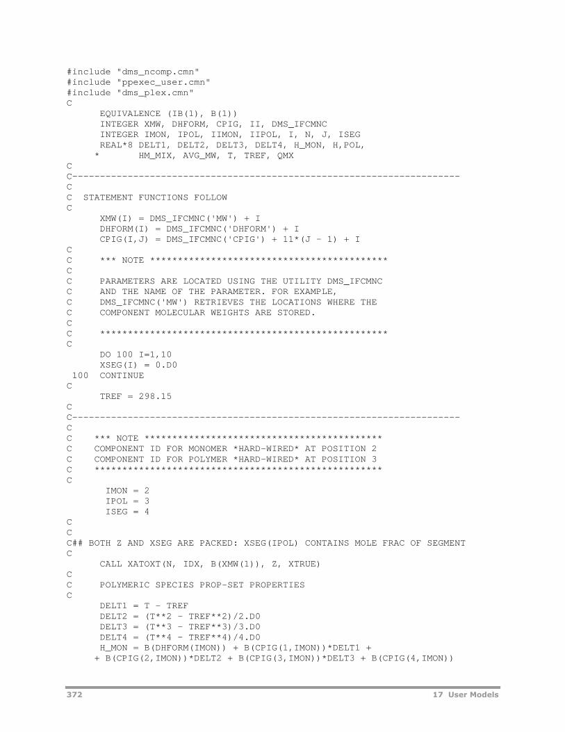
372 17 User Models
#include "dms_ncomp.cmn"#include "ppexec_user.cmn"#include "dms_plex.cmn"C
EQUIVALENCE (IB(1), B(1))INTEGER XMW, DHFORM, CPIG, II, DMS_IFCMNCINTEGER IMON, IPOL, IIMON, IIPOL, I, N, J, ISEGREAL*8 DELT1, DELT2, DELT3, DELT4, H_MON, H,POL,
* HM_MIX, AVG_MW, T, TREF, QMXCC----------------------------------------------------------------------CC STATEMENT FUNCTIONS FOLLOWC
XMW(I) = DMS_IFCMNC('MW') + IDHFORM(I) = DMS_IFCMNC('DHFORM') + ICPIG(I,J) = DMS_IFCMNC('CPIG') + 11*(J - 1) + I
CC *** NOTE *******************************************CC PARAMETERS ARE LOCATED USING THE UTILITY DMS_IFCMNCC AND THE NAME OF THE PARAMETER. FOR EXAMPLE,C DMS_IFCMNC('MW') RETRIEVES THE LOCATIONS WHERE THEC COMPONENT MOLECULAR WEIGHTS ARE STORED.CC ****************************************************C
DO 100 I=1,10XSEG(I) = 0.D0
100 CONTINUEC
TREF = 298.15CC----------------------------------------------------------------------CC *** NOTE *******************************************C COMPONENT ID FOR MONOMER *HARD-WIRED* AT POSITION 2C COMPONENT ID FOR POLYMER *HARD-WIRED* AT POSITION 3C ****************************************************C
IMON = 2IPOL = 3ISEG = 4
CCC## BOTH Z AND XSEG ARE PACKED: XSEG(IPOL) CONTAINS MOLE FRAC OF SEGMENTC
CALL XATOXT(N, IDX, B(XMW(1)), Z, XTRUE)CC POLYMERIC SPECIES PROP-SET PROPERTIESC
DELT1 = T - TREFDELT2 = (T**2 - TREF**2)/2.D0DELT3 = (T**3 - TREF**3)/3.D0DELT4 = (T**4 - TREF**4)/4.D0H_MON = B(DHFORM(IMON)) + B(CPIG(1,IMON))*DELT1 +
+ B(CPIG(2,IMON))*DELT2 + B(CPIG(3,IMON))*DELT3 + B(CPIG(4,IMON))
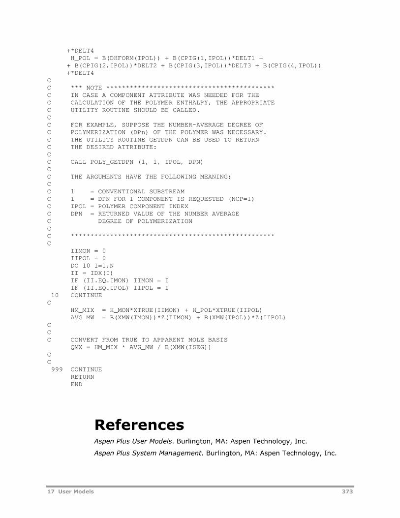
17 User Models 373
+*DELT4H_POL = B(DHFORM(IPOL)) + B(CPIG(1,IPOL))*DELT1 +
+ B(CPIG(2,IPOL))*DELT2 + B(CPIG(3,IPOL))*DELT3 + B(CPIG(4,IPOL))+*DELT4
CC *** NOTE *******************************************C IN CASE A COMPONENT ATTRIBUTE WAS NEEDED FOR THEC CALCULATION OF THE POLYMER ENTHALPY, THE APPROPRIATEC UTILITY ROUTINE SHOULD BE CALLED.CC FOR EXAMPLE, SUPPOSE THE NUMBER-AVERAGE DEGREE OFC POLYMERIZATION (DPn) OF THE POLYMER WAS NECESSARY.C THE UTILITY ROUTINE GETDPN CAN BE USED TO RETURNC THE DESIRED ATTRIBUTE:CC CALL POLY_GETDPN (1, 1, IPOL, DPN)CC THE ARGUMENTS HAVE THE FOLLOWING MEANING:CC 1 = CONVENTIONAL SUBSTREAMC 1 = DPN FOR 1 COMPONENT IS REQUESTED (NCP=1)C IPOL = POLYMER COMPONENT INDEXC DPN = RETURNED VALUE OF THE NUMBER AVERAGEC DEGREE OF POLYMERIZATIONCC ****************************************************C
IIMON = 0IIPOL = 0DO 10 I=1,NII = IDX(I)IF (II.EQ.IMON) IIMON = IIF (II.EQ.IPOL) IIPOL = I
10 CONTINUEC
HM_MIX = H_MON*XTRUE(IIMON) + H_POL*XTRUE(IIPOL)AVG_MW = B(XMW(IMON))*Z(IIMON) + B(XMW(IPOL))*Z(IIPOL)
CCC CONVERT FROM TRUE TO APPARENT MOLE BASIS
QMX = HM_MIX * AVG_MW / B(XMW(ISEG))CC999 CONTINUE
RETURNEND
ReferencesAspen Plus User Models. Burlington, MA: Aspen Technology, Inc.
Aspen Plus System Management. Burlington, MA: Aspen Technology, Inc.

374 17 User Models
18 Application Tools 375
18 Application Tools
This section discusses the tools available for applying Aspen Polymers(formerly known as Aspen Polymers Plus) features to solve real-life problems.
The topics covered include:
Example Applications for a Simulation Model, 375
Application Tools Available in Aspen Polymers, 376
Model Variable Accessing, 378
Example Applications for aSimulation ModelThe main purpose of a simulation model is to provide the engineer with adeeper understanding of the molecular and macroscopic processes which arevital to a polymer manufacturing process. This understanding will eventuallylead to improvements in various aspects of the process related to safety,productivity, and polymer product quality. These are some typical scenarios inwhich a simulation model is used to meet this objective.
A model may be used to:
Identify superior grade transition policies and better plant startup andshutdown procedures which minimize offspec polymer product
Reduce the number of lengthy and costly experiments on bench, pilot, andplant scale for polymer product and polymerization process development
Train process engineers, chemists, plant operators
Identify sources of variance in polymer product quality
Provide data for the design of rupture discs and vent lines
Find optimal temperature profiles for a continuous reactor train whichminimize reaction medium viscosity while meeting product specifications
Investigate monomer feed policies for a semi-batch copolymerizationprocess for keeping the chemical composition distribution narrow
Design a free-radical initiator mix to maximize productivity under theconstraints of safe reactor operations
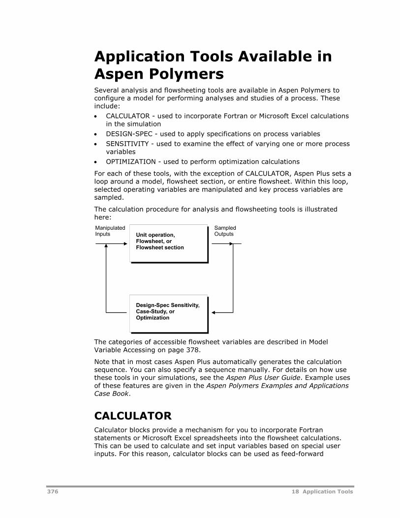
376 18 Application Tools
Application Tools Available inAspen PolymersSeveral analysis and flowsheeting tools are available in Aspen Polymers toconfigure a model for performing analyses and studies of a process. Theseinclude:
CALCULATOR - used to incorporate Fortran or Microsoft Excel calculationsin the simulation
DESIGN-SPEC - used to apply specifications on process variables
SENSITIVITY - used to examine the effect of varying one or more processvariables
OPTIMIZATION - used to perform optimization calculations
For each of these tools, with the exception of CALCULATOR, Aspen Plus sets aloop around a model, flowsheet section, or entire flowsheet. Within this loop,selected operating variables are manipulated and key process variables aresampled.
The calculation procedure for analysis and flowsheeting tools is illustratedhere:
The categories of accessible flowsheet variables are described in ModelVariable Accessing on page 378.
Note that in most cases Aspen Plus automatically generates the calculationsequence. You can also specify a sequence manually. For details on how usethese tools in your simulations, see the Aspen Plus User Guide. Example usesof these features are given in the Aspen Polymers Examples and ApplicationsCase Book.
CALCULATORCalculator blocks provide a mechanism for you to incorporate Fortranstatements or Microsoft Excel spreadsheets into the flowsheet calculations.This can be used to calculate and set input variables based on special userinputs. For this reason, calculator blocks can be used as feed-forward
18 Application Tools 377
controllers. You can also use calculator blocks to calculate and write results tothe Aspen Plus report, control panel, or external file.
Calculator blocks can be used to display charts, tables, or graphs throughExcel.
To use this block you must specify which model variables to sample ormanipulate, enter the Fortran statements or create the Excel sheet, and setthe sequence in which the block must be executed during the flowsheetcalculations.
An example use of a calculator block as a feed-forward controller would be tohold the flowrate of a catalyst proportional to a monomer flow for a situationwhere that monomer flow varies.
DESIGN-SPECDesign-Spec blocks allow you to set a process variable that is normallycalculated during the simulation. For each specification, you must identifywhich process variable can be adjusted to meet that specification. For thisreason, Design-Spec blocks can be used as feedback controllers.
To use this block you must specify which model variables must be fixed, whatvalues they must be fixed at, and which model input variables can bemanipulated. You can include Fortran statements in Design-Spec blocks.
An example use of a Design-Spec block would be to set a maximum amountfor impurities in a product stream.
SENSITIVITYSensitivity blocks provide a mechanism for you to analyze the effect ofoperating variables, which you select on the process. This block generates amatrix of manipulated variables versus sampled variables. If there is morethan one manipulated variable, the sensitivity analysis is performed for eachcombination of manipulated variables. It is recommended that you usemultiple Sensitivity blocks if you do not want to combine the manipulatedvariables.
To use this block you must specify which are the manipulated variables, whichare the sampled variables, and how they must be tabulated. You can includeFortran statements in Sensitivity blocks.
An example use of a Sensitivity block would be to determine the effect ofreactor temperature or pressure on the polymer product properties.
OPTIMIZATIONOptimization blocks provide a mechanism for you to minimize or maximize anobjective function calculated using key process variables. To define theobjective function you would use Fortran statements.
To use this block you must define the objective function, specify manipulatedvariables, and define constraints, if any.
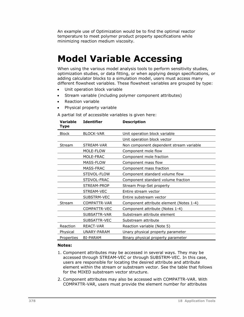
378 18 Application Tools
An example use of Optimization would be to find the optimal reactortemperature to meet polymer product property specifications whileminimizing reaction medium viscosity.
Model Variable AccessingWhen using the various model analysis tools to perform sensitivity studies,optimization studies, or data fitting, or when applying design specifications, oradding calculator blocks to a simulation model, users must access manydifferent flowsheet variables. These flowsheet variables are grouped by type:
Unit operation block variable
Stream variable (including polymer component attributes)
Reaction variable
Physical property variable
A partial list of accessible variables is given here:
VariableType
Identifier Description
Block BLOCK-VAR Unit operation block variable
Unit operation block vector
Stream STREAM-VAR Non component dependent stream variable
MOLE-FLOW Component mole flow
MOLE-FRAC Component mole fraction
MASS-FLOW Component mass flow
MASS-FRAC Component mass fraction
STDVOL-FLOW Component standard volume flow
STDVOL-FRAC Component standard volume fraction
STREAM-PROP Stream Prop-Set property
STREAM-VEC Entire stream vector
SUBSTRM-VEC Entire substream vector
Stream COMPATTR-VAR Component attribute element (Notes 1-4)
COMPATTR-VEC Component attribute (Notes 1-4)
SUBSATTR-VAR Substream attribute element
SUBSATTR-VEC Substream attribute
Reaction REACT-VAR Reaction variable (Note 5)
Physical UNARY-PARAM Unary physical property parameter
Properties BI-PARAM Binary physical property parameter
Notes:
1. Component attributes may be accessed in several ways. They may beaccessed through STREAM-VEC or through SUBSTRM-VEC. In this case,users are responsible for locating the desired attribute and attributeelement within the stream or substream vector. See the table that followsfor the MIXED substream vector structure.
2. Component attributes may also be accessed with COMPATTR-VAR. WithCOMPATTR-VAR, users must provide the element number for attributes
18 Application Tools 379
having more than one element. See the Polymer Structural Propertiessection of Chapter 2 to find out the dimensions of polymer componentattributes. If the attribute is dimensioned by number of polymer segments,NSEGS, (e.g. SFLOW, or SFRAC polymer attributes), the ordering ofelements follows the order in which the list of polymer segments wasspecified (See the Component Classification section of Chapter 2). Forcomponent attributes dimensioned by number of catalytic sites, eachelement represents a site number, i.e. site no. 1, no. 2, etc. For two-dimensional component attributes dimensioned by number of segmentsand number of catalytic sites (NSEGS*NSITES), the first dimension isNSEG, therefore, the ordering of elements is as follows: the list of specifiedsegments is repeated for each site beginning with site no. 1.
3. Component attributes may also be accessed with COMPATTR-VEC. In thiscase, users are not required to provide an element number since the wholecomponent attribute is returned as a vector having one or more elements.The ordering of elements within the attribute vector follows the descriptiongiven in Note 2.
4. COMPATTR-VAR and COMPATTR-VEC are equivalent for componentattributes having only one element.
5. REACT-VAR may be used to access kinetic constant parameters for reactionkinetic models, including free-radical, step-growth and Ziegler-Natta. Thetype of information required to access these parameters is modeldependent. For free-radical, the reaction type (INIT-DEC, for example),and the reacting species are required, in addition to the name of theparameter to be accessed. The same is true for Ziegler-Natta which alsorequires a catalyst site type number. For step-growth, a reaction number isrequired. For the standard Aspen Plus reaction models, a reaction number,and/or substream identifier may be needed to locate the parameters.
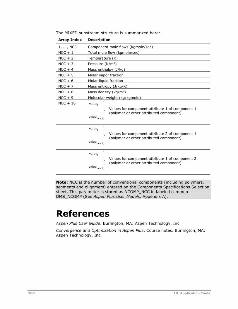
380 18 Application Tools
The MIXED substream structure is summarized here:
Array Index Description
1, ..., NCC Component mole flows (kgmole/sec)
NCC + 1 Total mole flow (kgmole/sec)
NCC + 2 Temperature (K)
NCC + 3 Pressure (N/m2)
NCC + 4 Mass enthalpy (J/kg)
NCC + 5 Molar vapor fraction
NCC + 6 Molar liquid fraction
NCC + 7 Mass entropy (J/kg-K)
NCC + 8 Mass density (kg/m3)
NCC + 9 Molecular weight (kg/kgmole)
NCC + 10
ncat1
1
value
value
Values for component attribute 1 of component 1(polymer or other attributed component)
ncat1
1
value
value
Values for component attribute 2 of component 1(polymer or other attributed component)
ncat1
1
value
value
Values for component attribute 1 of component 2(polymer or other attributed component)
Note: NCC is the number of conventional components (including polymers,segments and oligomers) entered on the Components Specifications Selectionsheet. This parameter is stored as NCOMP_NCC in labeled commonDMS_NCOMP (See Aspen Plus User Models, Appendix A).
ReferencesAspen Plus User Guide. Burlington, MA: Aspen Technology, Inc.
Convergence and Optimization in Aspen Plus, Course notes. Burlington, MA:Aspen Technology, Inc.
19 Run-Time Environment 381
19 Run-Time Environment
This chapter discusses various topics related to working in the AspenPolymers (formerly known as Aspen Polymers Plus) environment.
The topics covered include:
Aspen Polymers Architecture, 381
Installation Issues, 382
Configuration Tips, 382
User Fortran, 383
Troubleshooting Guide, 383
Aspen Polymers ArchitectureAspen Polymers is a layered product. In other words, this product works inconjunction with a main program. This main program is Aspen Plus forsteady-state simulation and Aspen Dynamics or Aspen Custom Modeler fordynamic simulation. Aspen Polymers brings to these simulators the polymerprocess technology in the form of component characterization, physicalproperty models and databanks, kinetic models, and the associated inputforms.
As a result of this layered architecture the installation and configuration ofAspen Polymers is closely tied to that of Aspen Plus for steady-statesimulation and that of Aspen Dynamics and Aspen Custom Modeler fordynamic simulation. In this chapter we will focus on topics related to theAspen Plus environment.
The overall Aspen Polymers architecture is shown here:
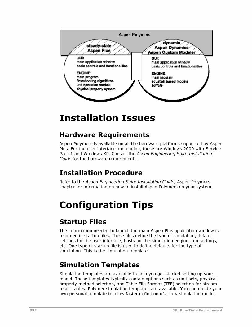
382 19 Run-Time Environment
Installation Issues
Hardware RequirementsAspen Polymers is available on all the hardware platforms supported by AspenPlus. For the user interface and engine, these are Windows 2000 with ServicePack 1 and Windows XP. Consult the Aspen Engineering Suite InstallationGuide for the hardware requirements.
Installation ProcedureRefer to the Aspen Engineering Suite Installation Guide, Aspen Polymerschapter for information on how to install Aspen Polymers on your system.
Configuration Tips
Startup FilesThe information needed to launch the main Aspen Plus application window isrecorded in startup files. These files define the type of simulation, defaultsettings for the user interface, hosts for the simulation engine, run settings,etc. One type of startup file is used to define defaults for the type ofsimulation. This is the simulation template.
Simulation TemplatesSimulation templates are available to help you get started setting up yourmodel. These templates typically contain options such as unit sets, physicalproperty method selection, and Table File Format (TFF) selection for streamresult tables. Polymer simulation templates are available. You can create yourown personal template to allow faster definition of a new simulation model.
19 Run-Time Environment 383
To use a simulation template, after starting Aspen Plus, on the startup boxselect the template startup option. Then choose one of the polymer simulationtemplates. This will automatically setup a global unit set, an appropriatepolymer property method, and a polymer TFF for the stream tables.
To learn more about TFF files see the Aspen Plus System Management.
User Fortran
User Fortran TemplatesThere are several ways for you to customize your models by addingcalculations in Fortran. The End-Use Properties section of Chapter 2 describedhow to setup a user Prop-Set for calculating end-use properties. Chapter 4described how to setup user unit operation models, user kinetic models, anduser property models. Templates are available for your use in creating theFortran files used in these features. You will find these templates in thefollowing location:
Version Location
Windows %asptop%\user
User Fortran LinkingUser Fortran calculations in the form of user routines are linked dynamicallyto Aspen Polymers during a simulation. Within user Fortran, you will oftenaccess utilities located within Aspen Polymers. In order to access theseutilities, you will need to know the name of the object libraries where they arelocated. This applies to the utilities described in Chapter 4 of Aspen Plus UserModels. The name of the utility as shown in the example call sequenceincludes the name of the object library where it is located.
You can also create your own dynamic link libraries to hold your user Fortranfiles. The Aspen Plus System Management guide describes how to work withFortran code modifications.
Troubleshooting GuideFollowing are tips to help you diagnose and resolve problems you may runinto while setting up or running Aspen Polymers.
User Interface ProblemsA list of symptoms relating to problems you may encounter when using theuser interface is provided below. Possible causes and solutions are given foreach symptom.
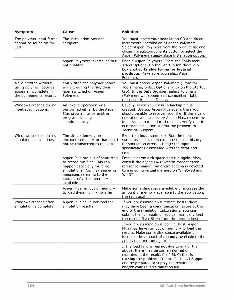
384 19 Run-Time Environment
Symptom Cause Solution
The polymer input formscannot be found on theGUI.
The installation was notcomplete.
You must locate your installation CD and do anincremental installation of Aspen Polymers.Select Aspen Polymers from the product list andchose the subcomponents button to select theAspen Polymers steady state installation option.
Aspen Polymers is installed butnot enabled.
Enable Aspen Polymers. From the Tools menu,select Options. On the Startup tab there is abox entitled Enable forms for layeredproducts. Make sure you select AspenPolymers
A file created withoutusing polymer featuresappears incomplete inthe components record.
You visited the polymer recordwhile creating the file, thenlater switched off AspenPolymers.
You must enable Aspen Polymers (From theTools menu, Select Options, click on the Startuptab). In the Data Browser, select Polymers(Polymers will appear as incomplete), rightmouse click, select Delete.
Windows crashes duringinput specifications.
An invalid operation wasperformed either by the AspenPlus program or by anotherprogram runningsimultaneously.
Usually, when you crash, a backup file iscreated. Startup Aspen Plus again, then youshould be able to recover your file. If the invalidoperation was caused by Aspen Plus, repeat theinput steps that lead to the crash, verify that itis reproducible, and submit the problem toTechnical Support.
Windows crashes duringsimulation calculations.
The simulation engineencountered an error that couldnot be transferred to the GUI.
Export an input summary. Run the inputsummary alone, then examine the run historyfor simulation errors. Change the inputspecifications associated with the error andrerun.
Aspen Plus ran out of resourcesto create run files. This canhappen especially for largesimulations. You may see errormessages referring to theamount of virtual memoryavailable.
Free-up some disk space and run again. Also,consult the Aspen Plus System Managementreference manual. An entire section is devotedto managing virtual memory on Win95/98 andWinNT.
Aspen Plus ran out of memoryto load dynamic link libraries.
Make some disk space available or increase theamount of memory available to the application,then run again.
Windows crashes aftersimulation is complete.
Aspen Plus could not load thesimulation results.
If you are running on a remote hosts, theremay have been a communication failure at theend of the simulation calculations. You cansubmit the run again or you can manually loadthe results file (.SUM) from the remote host.
If you are running on a local PC host, AspenPlus may have run out of memory to load theresults. Make some disk space available orincrease the amount of memory available to theapplication and run again.
If the load failure was not due to any of theabove, there may be some informationrecorded in the results file (.SUM) that iscausing the problem. Contact Technical Supportand be prepared to supply the results fileand/or your saved simulation file.
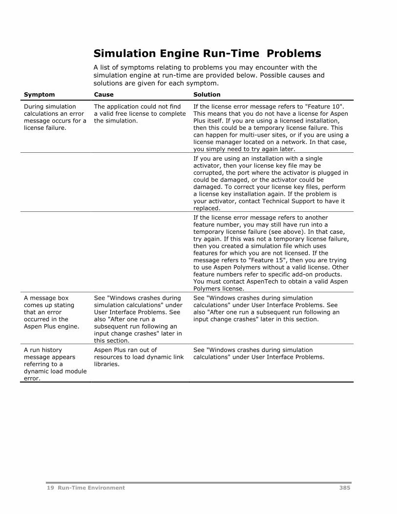
19 Run-Time Environment 385
Simulation Engine Run-Time ProblemsA list of symptoms relating to problems you may encounter with thesimulation engine at run-time are provided below. Possible causes andsolutions are given for each symptom.
Symptom Cause Solution
During simulationcalculations an errormessage occurs for alicense failure.
The application could not finda valid free license to completethe simulation.
If the license error message refers to "Feature 10".This means that you do not have a license for AspenPlus itself. If you are using a licensed installation,then this could be a temporary license failure. Thiscan happen for multi-user sites, or if you are using alicense manager located on a network. In that case,you simply need to try again later.
If you are using an installation with a singleactivator, then your license key file may becorrupted, the port where the activator is plugged incould be damaged, or the activator could bedamaged. To correct your license key files, performa license key installation again. If the problem isyour activator, contact Technical Support to have itreplaced.
If the license error message refers to anotherfeature number, you may still have run into atemporary license failure (see above). In that case,try again. If this was not a temporary license failure,then you created a simulation file which usesfeatures for which you are not licensed. If themessage refers to "Feature 15", then you are tryingto use Aspen Polymers without a valid license. Otherfeature numbers refer to specific add-on products.You must contact AspenTech to obtain a valid AspenPolymers license.
A message boxcomes up statingthat an erroroccurred in theAspen Plus engine.
See "Windows crashes duringsimulation calculations" underUser Interface Problems. Seealso "After one run asubsequent run following aninput change crashes" later inthis section.
See "Windows crashes during simulationcalculations" under User Interface Problems. Seealso "After one run a subsequent run following aninput change crashes" later in this section.
A run historymessage appearsreferring to adynamic load moduleerror.
Aspen Plus ran out ofresources to load dynamic linklibraries.
See "Windows crashes during simulationcalculations" under User Interface Problems.
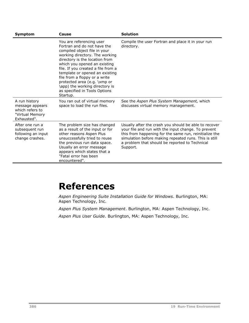
386 19 Run-Time Environment
Symptom Cause Solution
You are referencing userFortran and do not have thecompiled object file in yourworking directory. The workingdirectory is the location fromwhich you opened an existingfile. If you created a file from atemplate or opened an existingfile from a floppy or a writeprotected area (e.g. \xmp or\app) the working directory isas specified in Tools OptionsStartup.
Compile the user Fortran and place it in your rundirectory.
A run historymessage appearswhich refers to"Virtual MemoryExhausted".
You ran out of virtual memoryspace to load the run files.
See the Aspen Plus System Management, whichdiscusses virtual memory management.
After one run asubsequent runfollowing an inputchange crashes.
The problem size has changedas a result of the input or forother reasons Aspen Plusunsuccessfully tried to reusethe previous run data space.Usually an error messageappears which states that a"Fatal error has beenencountered".
Usually after the crash you should be able to recoveryour file and run with the input change. To preventthis from happening for the same run, reinitialize thesimulation before making repeated runs. This is stilla problem that should be reported to TechnicalSupport.
ReferencesAspen Engineering Suite Installation Guide for Windows. Burlington, MA:Aspen Technology, Inc.
Aspen Plus System Management. Burlington, MA: Aspen Technology, Inc.
Aspen Plus User Guide. Burlington, MA: Aspen Technology, Inc.
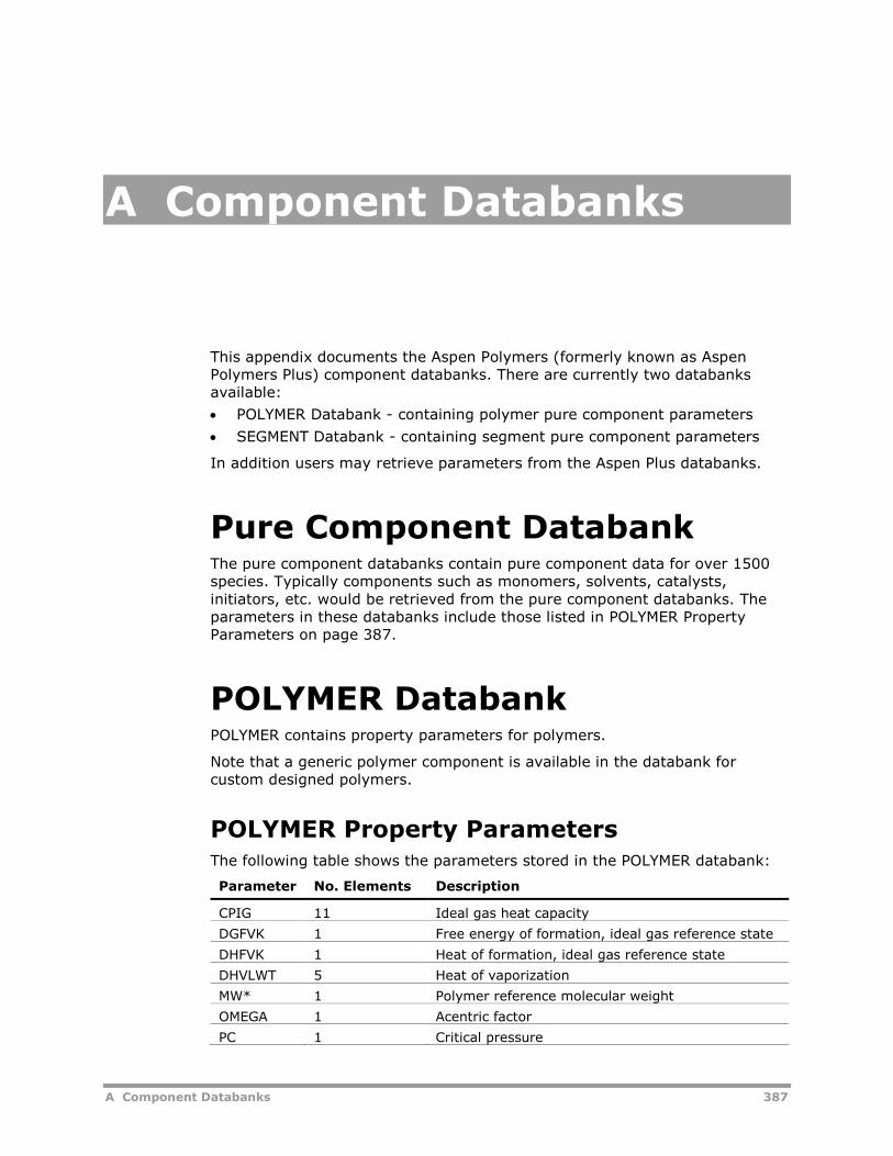
A Component Databanks 387
A Component Databanks
This appendix documents the Aspen Polymers (formerly known as AspenPolymers Plus) component databanks. There are currently two databanksavailable:
POLYMER Databank - containing polymer pure component parameters
SEGMENT Databank - containing segment pure component parameters
In addition users may retrieve parameters from the Aspen Plus databanks.
Pure Component DatabankThe pure component databanks contain pure component data for over 1500species. Typically components such as monomers, solvents, catalysts,initiators, etc. would be retrieved from the pure component databanks. Theparameters in these databanks include those listed in POLYMER PropertyParameters on page 387.
POLYMER DatabankPOLYMER contains property parameters for polymers.
Note that a generic polymer component is available in the databank forcustom designed polymers.
POLYMER Property ParametersThe following table shows the parameters stored in the POLYMER databank:
Parameter No. Elements Description
CPIG 11 Ideal gas heat capacity
DGFVK 1 Free energy of formation, ideal gas reference state
DHFVK 1 Heat of formation, ideal gas reference state
DHVLWT 5 Heat of vaporization
MW* 1 Polymer reference molecular weight
OMEGA 1 Acentric factor
PC 1 Critical pressure
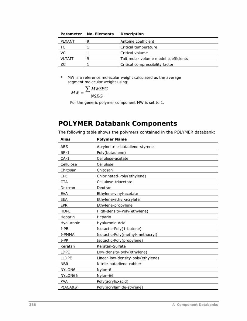
388 A Component Databanks
Parameter No. Elements Description
PLXANT 9 Antoine coefficient
TC 1 Critical temperature
VC 1 Critical volume
VLTAIT 9 Tait molar volume model coefficients
ZC 1 Critical compressibility factor
* MW is a reference molecular weight calculated as the averagesegment molecular weight using:
NSEG
MWSEGMW
For the generic polymer component MW is set to 1.
POLYMER Databank ComponentsThe following table shows the polymers contained in the POLYMER databank:
Alias Polymer Name
ABS Acrylonitrile-butadiene-styrene
BR-1 Poly(butadiene)
CA-1 Cellulose-acetate
Cellulose Cellulose
Chitosan Chitosan
CPE Chlorinated-Poly(ethylene)
CTA Cellulose-triacetate
Dextran Dextran
EVA Ethylene-vinyl-acetate
EEA Ethylene-ethyl-acrylate
EPR Ethylene-propylene
HDPE High-density-Poly(ethylene)
Heparin Heparin
Hyaluronic Hyaluronic-Acid
I-PB Isotactic-Poly(1-butene)
I-PMMA Isotactic-Poly(methyl-methacryl)
I-PP Isotactic-Poly(propylene)
Keratan Keratan-Sulfate
LDPE Low-density-poly(ethylene)
LLDPE Linear-low-density-poly(ethylene)
NBR Nitrile-butadiene-rubber
NYLON6 Nylon-6
NYLON66 Nylon-66
PAA Poly(acrylic-acid)
P(ACA&S) Poly(acrylamide-styrene)
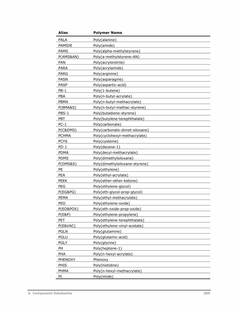
A Component Databanks 389
Alias Polymer Name
PALA Poly(alanine)
PAMIDE Poly(amide)
PAMS Poly(alpha-methylstyrene)
P(AMS&AN) Poly(a-methylstyrene-AN)
PAN Poly(acrylonitrile)
PARA Poly(acrylamide)
PARG Poly(arginine)
PASN Poly(asparagine)
PASP Poly(aspartic-acid)
PB-1 Poly(1-butene)
PBA Poly(n-butyl-acrylate)
PBMA Poly(n-butyl-methacrylate)
P(BMA&S) Poly(n-butyl-methac-styrene)
PBS-1 Poly(butadiene-styrene)
PBT Poly(butylene-terephthalate)
PC-1 Poly(carbonate)
P(C&DMS) Poly(carbonate-dimet-siloxane)
PCHMA Poly(cyclohexyl-methacrylate)
PCYS Poly(cysteine)
PD-1 Poly(decene-1)
PDMA Poly(decyl-methacrylate)
PDMS Poly(dimethylsiloxane)
P(DMS&S) Poly(dimethylsiloxane-styrene)
PE Poly(ethylene)
PEA Poly(ethyl-acrylate)
PEEK Poly(ether-ether-ketone)
PEG Poly(ethylene-glycol)
P(EG&PG) Poly(eth-glycol-prop-glycol)
PEMA Poly(ethyl-methacrylate)
PEO Poly(ethylene-oxide)
P(EO&POX) Poly(eth-oxide-prop-oxide)
P(E&P) Poly(ethylene-propylene)
PET Poly(ethylene-terephthalate)
P(E&VAC) Poly(ethylene-vinyl-acetate)
PGLN Poly(glutamine)
PGLU Poly(glutamic-acid)
PGLY Poly(glycine)
PH Poly(heptene-1)
PHA Poly(n-hexyl-acrylate)
PHENOXY Phenoxy
PHIS Poly(histidine)
PHMA Poly(n-hexyl-methacrylate)
PI Poly(imide)
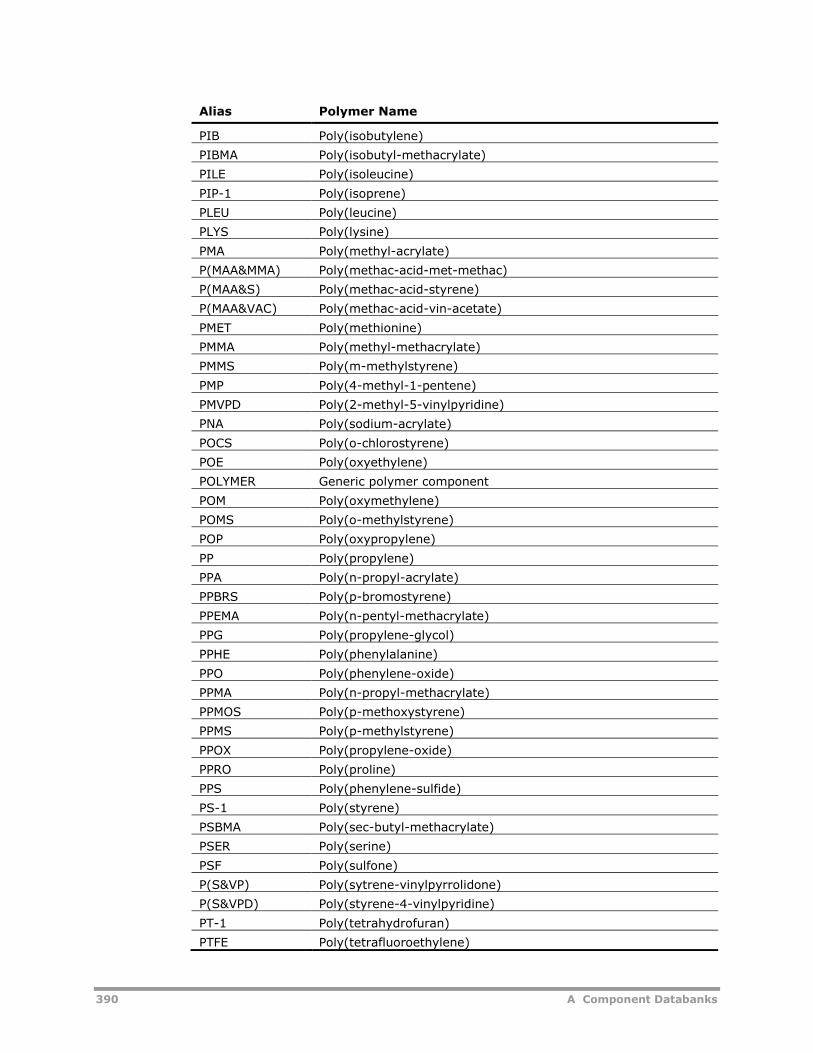
390 A Component Databanks
Alias Polymer Name
PIB Poly(isobutylene)
PIBMA Poly(isobutyl-methacrylate)
PILE Poly(isoleucine)
PIP-1 Poly(isoprene)
PLEU Poly(leucine)
PLYS Poly(lysine)
PMA Poly(methyl-acrylate)
P(MAA&MMA) Poly(methac-acid-met-methac)
P(MAA&S) Poly(methac-acid-styrene)
P(MAA&VAC) Poly(methac-acid-vin-acetate)
PMET Poly(methionine)
PMMA Poly(methyl-methacrylate)
PMMS Poly(m-methylstyrene)
PMP Poly(4-methyl-1-pentene)
PMVPD Poly(2-methyl-5-vinylpyridine)
PNA Poly(sodium-acrylate)
POCS Poly(o-chlorostyrene)
POE Poly(oxyethylene)
POLYMER Generic polymer component
POM Poly(oxymethylene)
POMS Poly(o-methylstyrene)
POP Poly(oxypropylene)
PP Poly(propylene)
PPA Poly(n-propyl-acrylate)
PPBRS Poly(p-bromostyrene)
PPEMA Poly(n-pentyl-methacrylate)
PPG Poly(propylene-glycol)
PPHE Poly(phenylalanine)
PPO Poly(phenylene-oxide)
PPMA Poly(n-propyl-methacrylate)
PPMOS Poly(p-methoxystyrene)
PPMS Poly(p-methylstyrene)
PPOX Poly(propylene-oxide)
PPRO Poly(proline)
PPS Poly(phenylene-sulfide)
PS-1 Poly(styrene)
PSBMA Poly(sec-butyl-methacrylate)
PSER Poly(serine)
PSF Poly(sulfone)
P(S&VP) Poly(sytrene-vinylpyrrolidone)
P(S&VPD) Poly(styrene-4-vinylpyridine)
PT-1 Poly(tetrahydrofuran)
PTFE Poly(tetrafluoroethylene)
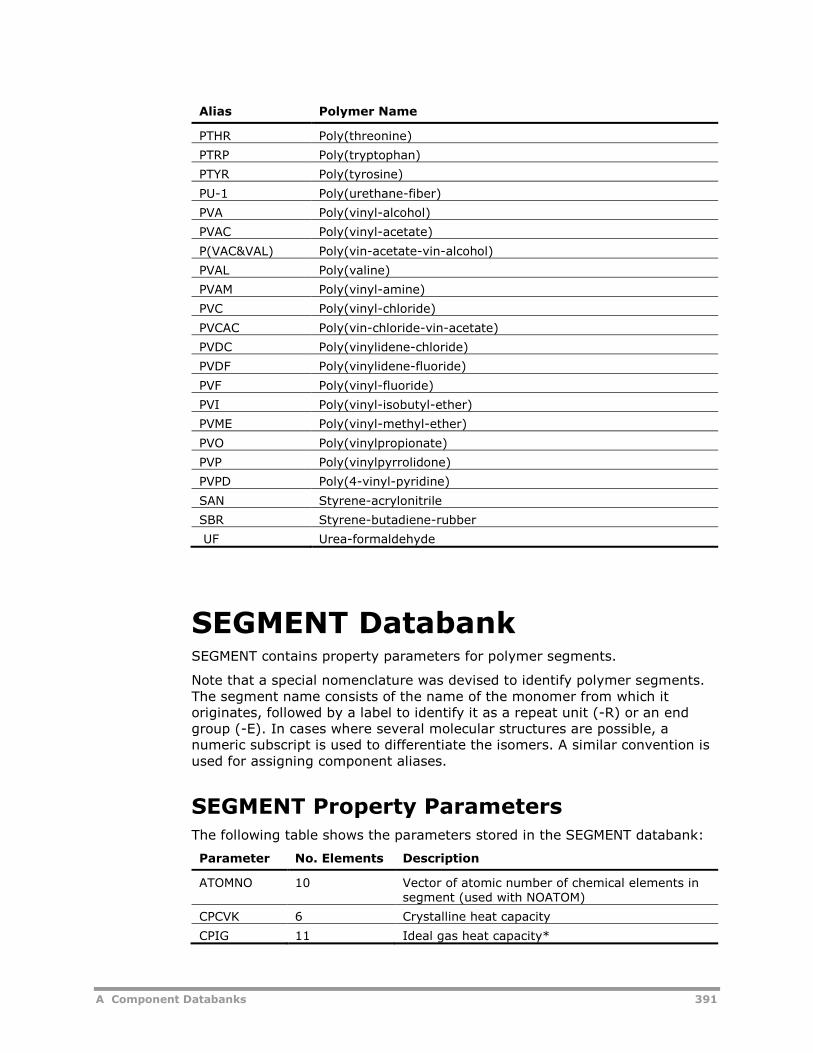
A Component Databanks 391
Alias Polymer Name
PTHR Poly(threonine)
PTRP Poly(tryptophan)
PTYR Poly(tyrosine)
PU-1 Poly(urethane-fiber)
PVA Poly(vinyl-alcohol)
PVAC Poly(vinyl-acetate)
P(VAC&VAL) Poly(vin-acetate-vin-alcohol)
PVAL Poly(valine)
PVAM Poly(vinyl-amine)
PVC Poly(vinyl-chloride)
PVCAC Poly(vin-chloride-vin-acetate)
PVDC Poly(vinylidene-chloride)
PVDF Poly(vinylidene-fluoride)
PVF Poly(vinyl-fluoride)
PVI Poly(vinyl-isobutyl-ether)
PVME Poly(vinyl-methyl-ether)
PVO Poly(vinylpropionate)
PVP Poly(vinylpyrrolidone)
PVPD Poly(4-vinyl-pyridine)
SAN Styrene-acrylonitrile
SBR Styrene-butadiene-rubber
UF Urea-formaldehyde
SEGMENT DatabankSEGMENT contains property parameters for polymer segments.
Note that a special nomenclature was devised to identify polymer segments.The segment name consists of the name of the monomer from which itoriginates, followed by a label to identify it as a repeat unit (-R) or an endgroup (-E). In cases where several molecular structures are possible, anumeric subscript is used to differentiate the isomers. A similar convention isused for assigning component aliases.
SEGMENT Property ParametersThe following table shows the parameters stored in the SEGMENT databank:
Parameter No. Elements Description
ATOMNO 10 Vector of atomic number of chemical elements insegment (used with NOATOM)
CPCVK 6 Crystalline heat capacity
CPIG 11 Ideal gas heat capacity*
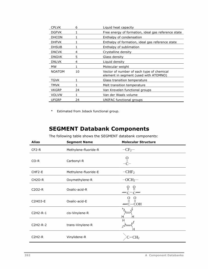
392 A Component Databanks
CPLVK 6 Liquid heat capacity
DGFVK 1 Free energy of formation, ideal gas reference state
DHCON 1 Enthalpy of condensation
DHFVK 1 Enthalpy of formation, ideal gas reference state
DHSUB 1 Enthalpy of sublimation
DNCVK 4 Crystalline density
DNGVK 5 Glass density
DNLVK 4 Liquid density
MW 1 Molecular weight
NOATOM 10 Vector of number of each type of chemicalelement in segment (used with ATOMNO)
TGVK 1 Glass transition temperature
TMVK 1 Melt transition temperature
VKGRP 24 Van Krevelen functional groups
VOLVW 1 Van der Waals volume
UFGRP 24 UNIFAC functional groups
* Estimated from Joback functional group.
SEGMENT Databank ComponentsThe following table shows the SEGMENT databank components:
Alias Segment Name Molecular Structure
CF2-R Methylene-fluoride-R
CO-R Carbonyl-R
CHF2-E Methylene-fluoride-E
CH2O-R Oxymethylene-R
C2O2-R Oxalic-acid-RC C
O O
C2HO3-E Oxalic-acid-E
C2H2-R-1 cis-Vinylene-R
C2H2-R-2 trans-Vinylene-R
C2H2-R Vinylidene-R
CF2
C
O
CHF2
OCH2
C COH
O O
C CH2
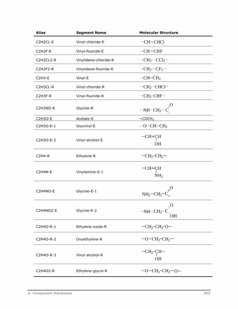
A Component Databanks 393
Alias Segment Name Molecular Structure
C2H2CL-E Vinyl-chloride-E
C2H2F-E Vinyl-fluoride-E
C2H2CL2-R Vinylidene-chloride-R
C2H2F2-R Vinylidene-fluoride-R
C2H3-E Vinyl-E
C2H3CL-R Vinyl-chloride-R
C2H3F-R Vinyl-fluoride-R
C2H3NO-R Glycine-R
C2H3O-E Acetate-E ~COCH3
C2H3O-E-1 Oxyvinyl-E
C2H3O-E-2 Vinyl-alcohol-E
C2H4-R Ethylene-R
C2H4N-E Vinylamine-E-1
C2H4NO-E Glycine-E-1
C2H4NO2-E Glycine-E-2
C2H4O-R-1 Ethylene-oxide-R
C2H4O-R-2 Oxyethylene-R
C2H4O-R-3 Vinyl-alcohol-R
C2H4O2-R Ethylene-glycol-R
CH CHCl
CH CHF
CH2 CCl2
CH2 CF2
CH CH2
CH2 CHCl
CH2 CHF
CH2NHO
C
O CH2CH
CH CH
OH
CH2 CH2
CH CH
NH2
NH2 CH2 C
O
CH2 C
O
NHOH
CH2 CH2 O
CH2 CH2O
CH2 CH
OH
CH2 CH2O O
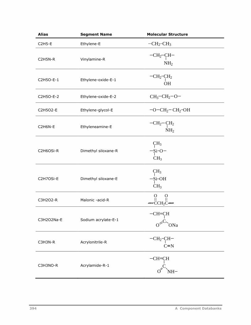
394 A Component Databanks
Alias Segment Name Molecular Structure
C2H5-E Ethylene-E
C2H5N-R Vinylamine-R
C2H5O-E-1 Ethylene-oxide-E-1
C2H5O-E-2 Ethylene-oxide-E-2
C2H5O2-E Ethylene-glycol-E
C2H6N-E Ethyleneamine-E
C2H6OSi-R Dimethyl siloxane-R
C2H7OSi-E Dimethyl siloxane-E
C3H2O2-R Malonic -acid-R
C3H2O2Na-E Sodium acrylate-E-1
C3H3N-R Acrylonitrile-R
C3H3NO-R Acrylamide-R-1
CH2 CH3
CH2 CH
NH2
CH2 CH2
OH
CH2CH3 O
CH2O CH2 OH
CH2 CH2
NH2
CH3
Si O
CH3
CH3
Si OH
CH3
CCH2C
O O
CH CH
CO ONa
CHCH2
C N
CH CH
CO NH
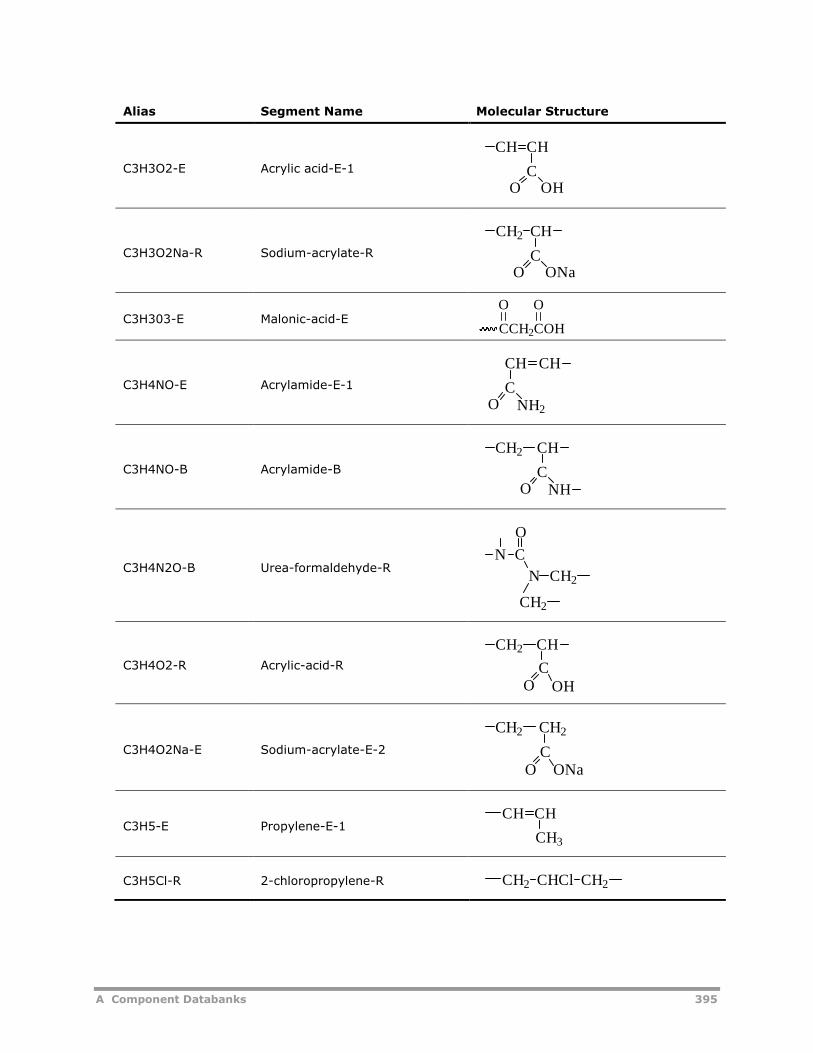
A Component Databanks 395
Alias Segment Name Molecular Structure
C3H3O2-E Acrylic acid-E-1
C3H3O2Na-R Sodium-acrylate-R
C3H303-E Malonic-acid-E
C3H4NO-E Acrylamide-E-1
C3H4NO-B Acrylamide-B
C3H4N2O-B Urea-formaldehyde-R
C3H4O2-R Acrylic-acid-R
C3H4O2Na-E Sodium-acrylate-E-2
C3H5-E Propylene-E-1
C3H5Cl-R 2-chloropropylene-R
CH CH
CO OH
CO
CHCH2
ONa
CCH2COH
O O
CO
CH CH
NH2
CO
CHCH2
NH
CH2
N C
O
N
CH2
CH2
O
CH
COH
CH2
OC
ONa
CH2
CH CH
CH3
CH2 CHCl CH2
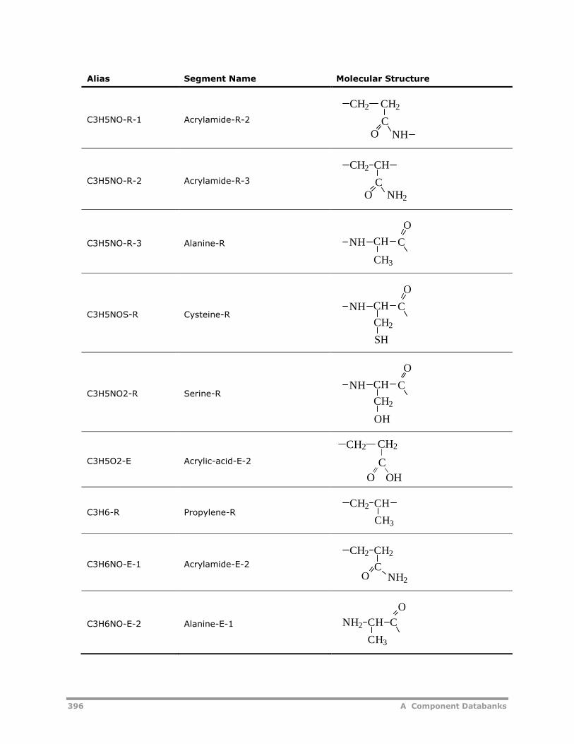
396 A Component Databanks
Alias Segment Name Molecular Structure
C3H5NO-R-1 Acrylamide-R-2
C3H5NO-R-2 Acrylamide-R-3
C3H5NO-R-3 Alanine-R
C3H5NOS-R Cysteine-R
C3H5NO2-R Serine-R
C3H5O2-E Acrylic-acid-E-2
C3H6-R Propylene-R
C3H6NO-E-1 Acrylamide-E-2
C3H6NO-E-2 Alanine-E-1
CH2
OC
CH2
NH
CH2 CH
OC
NH2
CHNH C
O
CH3
CHNH C
O
CH2
SH
CHNH C
O
CH2
OH
C
O OH
CH2 CH2
CH2 CH
CH3
CH2 CH2
CO NH2
NH2 CH C
O
CH3
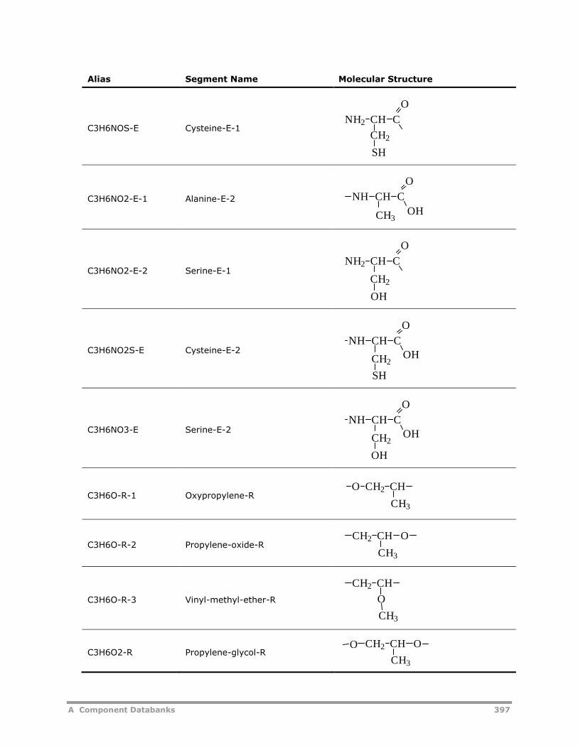
A Component Databanks 397
Alias Segment Name Molecular Structure
C3H6NOS-E Cysteine-E-1
C3H6NO2-E-1 Alanine-E-2
C3H6NO2-E-2 Serine-E-1
C3H6NO2S-E Cysteine-E-2
C3H6NO3-E Serine-E-2
C3H6O-R-1 Oxypropylene-R
C3H6O-R-2 Propylene-oxide-R
C3H6O-R-3 Vinyl-methyl-ether-R
C3H6O2-R Propylene-glycol-R
NH2 CH C
O
CH2
SH
O
CH CNH
OHCH3
O
CH CNH2
CH2
OH
O
CH CNH
CH2OH
SH
O
CH CNH
CH2OH
OH
O CH2 CH
CH3
CH3
OCH2 CH
CH3
O
CH2 CH
CH3
OCH2 CHO
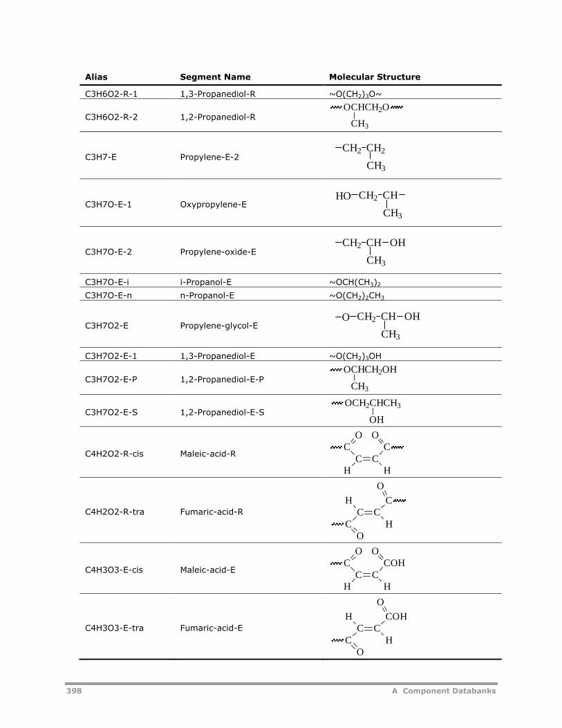
398 A Component Databanks
Alias Segment Name Molecular Structure
C3H6O2-R-1 1,3-Propanediol-R ~O(CH2)3O~
C3H6O2-R-2 1,2-Propanediol-R
C3H7-E Propylene-E-2
C3H7O-E-1 Oxypropylene-E
C3H7O-E-2 Propylene-oxide-E
C3H7O-E-i i-Propanol-E ~OCH(CH3)2
C3H7O-E-n n-Propanol-E ~O(CH2)2CH3
C3H7O2-E Propylene-glycol-E
C3H7O2-E-1 1,3-Propanediol-E ~O(CH2)3OH
C3H7O2-E-P 1,2-Propanediol-E-P
C3H7O2-E-S 1,2-Propanediol-E-S
C4H2O2-R-cis Maleic-acid-R
C4H2O2-R-tra Fumaric-acid-R
C4H3O3-E-cis Maleic-acid-E
C4H3O3-E-tra Fumaric-acid-E
OCHCH2O
CH3
CH3
CH2 CH2
CH2 CH
CH3
HO
CH2 CH
CH3
OH
CH2 CH
CH3
OHO
OCHCH2OH
CH3
OCH2CHCH3
OH
CC
O
CH H
CO
CC
O
CH C
H
O
CC
O
CH H
COHO
CC
O
CH COH
H
O
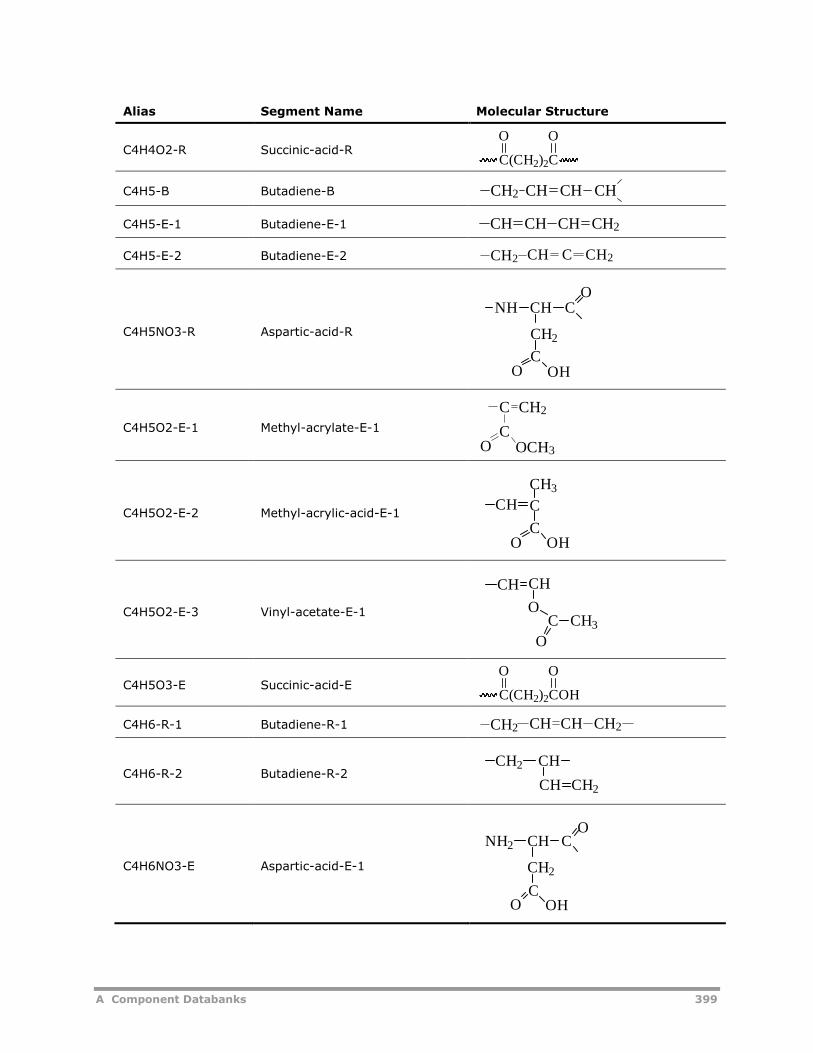
A Component Databanks 399
Alias Segment Name Molecular Structure
C4H4O2-R Succinic-acid-R
C4H5-B Butadiene-B
C4H5-E-1 Butadiene-E-1
C4H5-E-2 Butadiene-E-2
C4H5NO3-R Aspartic-acid-R
C4H5O2-E-1 Methyl-acrylate-E-1
C4H5O2-E-2 Methyl-acrylic-acid-E-1
C4H5O2-E-3 Vinyl-acetate-E-1
C4H5O3-E Succinic-acid-E
C4H6-R-1 Butadiene-R-1
C4H6-R-2 Butadiene-R-2
C4H6NO3-E Aspartic-acid-E-1
C(CH2)2C
O O
CH2 CH CH CH
CH CH2CH CH
CH2CH2 CH C
NH CH CO
CH2
CO OH
CO OCH3
CH2C
CO OH
C
CH3
CH
OCH3
CH CH
C
O
C(CH2)2COH
O O
CH CHCH2 CH2
CHCH2
CH CH2
CH
CH2
CO OH
CO
NH2
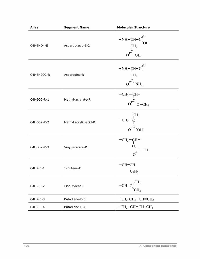
400 A Component Databanks
Alias Segment Name Molecular Structure
C4H6NO4-E Aspartic-acid-E-2
C4H6N2O2-R Asparagine-R
C4H6O2-R-1 Methyl-acrylate-R
C4H6O2-R-2 Methyl acrylic-acid-R
C4H6O2-R-3 Vinyl-acetate-R
C4H7-E-1 1-Butene-E
C4H7-E-2 Isobutylene-E
C4H7-E-3 Butadiene-E-3
C4H7-E-4 Butadiene-E-4
CH
CH2
CO OH
CO
NHOH
CH
CH2
CO
CO
NH
NH2
CH
CO
CH2
O CH3
O
CH2
CH3
C
COH
O
CH2 CH
OC CH3
CH CH
C2H5
CH CCH3
CH3
CH CH2CH2 CH2
CHCH2 CH CH3
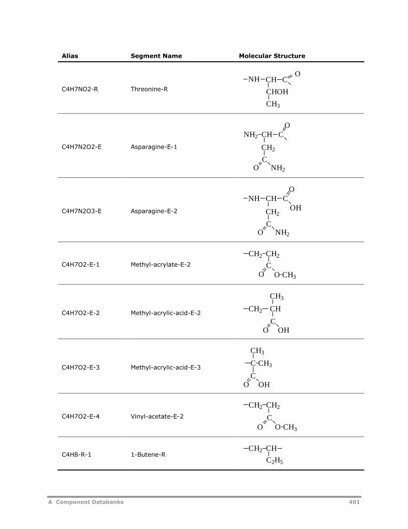
A Component Databanks 401
Alias Segment Name Molecular Structure
C4H7NO2-R Threonine-R
C4H7N2O2-E Asparagine-E-1
C4H7N2O3-E Asparagine-E-2
C4H7O2-E-1 Methyl-acrylate-E-2
C4H7O2-E-2 Methyl-acrylic-acid-E-2
C4H7O2-E-3 Methyl-acrylic-acid-E-3
C4H7O2-E-4 Vinyl-acetate-E-2
C4H8-R-1 1-Butene-R
NH CH CO
CHOH
CH3
NH2
CH2
CO
NH2 CH CO
NH2
CH2
CO
CO
CHNHOH
CH2 CH2
CO O CH3
CH3
CHCH2
O OHC
CH3
O OH
C CH3
C
CH2 CH2
CO O CH3
CH2 CH
C2H5
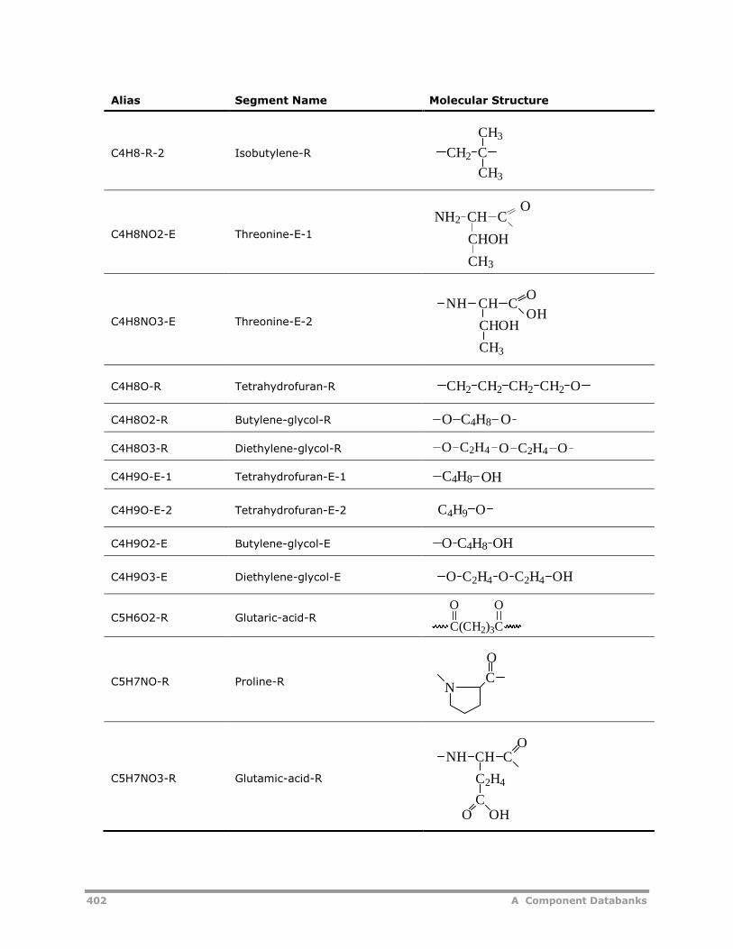
402 A Component Databanks
Alias Segment Name Molecular Structure
C4H8-R-2 Isobutylene-R
C4H8NO2-E Threonine-E-1
C4H8NO3-E Threonine-E-2
C4H8O-R Tetrahydrofuran-R
C4H8O2-R Butylene-glycol-R
C4H8O3-R Diethylene-glycol-R
C4H9O-E-1 Tetrahydrofuran-E-1
C4H9O-E-2 Tetrahydrofuran-E-2
C4H9O2-E Butylene-glycol-E
C4H9O3-E Diethylene-glycol-E
C5H6O2-R Glutaric-acid-R
C5H7NO-R Proline-R
C5H7NO3-R Glutamic-acid-R
CH2 C
CH3
CH3
CHNH2 CO
CHOH
CH3
CH CO
CHOH
CH3
NHOH
CH2 CH2 CH2 CH2 O
O C4H8 O
O C2H4 O C2H4 O
C4H8 OH
C4H9 O
O C4H8 OH
O C2H4 O C2H4 OH
C(CH2)3C
O O
NC
O
NH CH CO
C2H4
CO OH
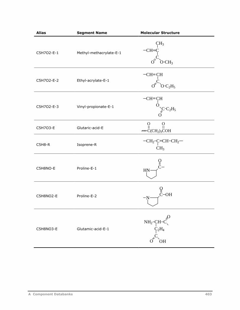
A Component Databanks 403
Alias Segment Name Molecular Structure
C5H7O2-E-1 Methyl-methacrylate-E-1
C5H7O2-E-2 Ethyl-acrylate-E-1
C5H7O2-E-3 Vinyl-propionate-E-1
C5H7O3-E Glutaric-acid-E
C5H8-R Isoprene-R
C5H8NO-E Proline-E-1
C5H8NO2-E Proline-E-2
C5H8NO3-E Glutamic-acid-E-1
CH3
CCH
CO O CH3
CH CH
CO O C2H5
CH CH
OC C2H5
O
C(CH2)3COH
O O
CH2 C CH CH2
CH3
HNC
O
O
NC OH
NH2 CH CO
C2H4
CO OH
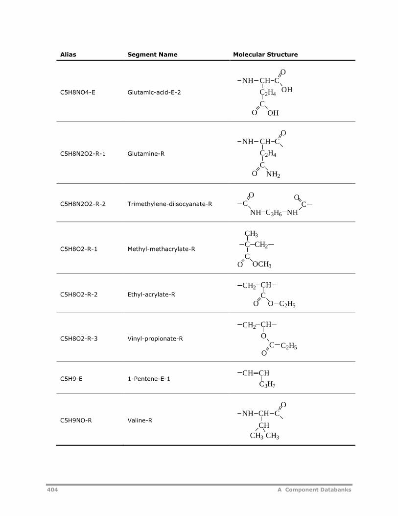
404 A Component Databanks
Alias Segment Name Molecular Structure
C5H8NO4-E Glutamic-acid-E-2
C5H8N2O2-R-1 Glutamine-R
C5H8N2O2-R-2 Trimethylene-diisocyanate-R
C5H8O2-R-1 Methyl-methacrylate-R
C5H8O2-R-2 Ethyl-acrylate-R
C5H8O2-R-3 Vinyl-propionate-R
C5H9-E 1-Pentene-E-1
C5H9NO-R Valine-R
NHO
C2H4
CO OH
CH COH
NHO
C2H4
CO
CH C
NH2
O
NH C3H6 NHC C
O
C
CH3
CH2
CO OCH3
CO O C2H5
CHCH2
O
C2H5
CHCH2
CO
CH CH
C3H7
NH CH CO
CH3 CH3
CH
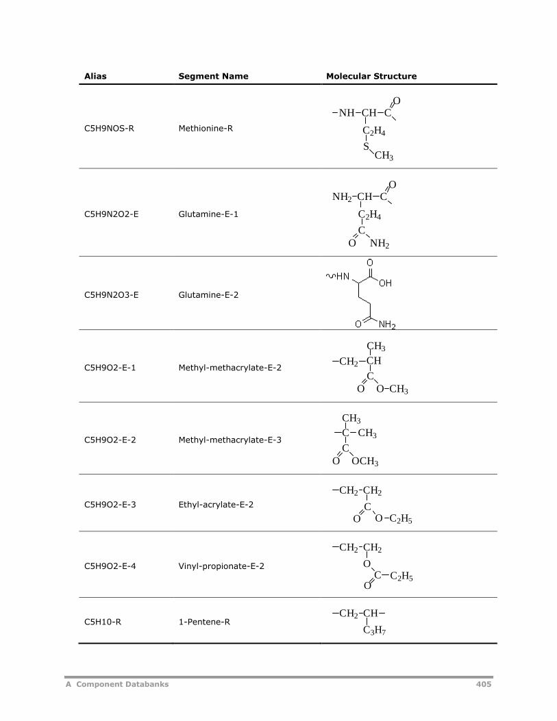
A Component Databanks 405
Alias Segment Name Molecular Structure
C5H9NOS-R Methionine-R
C5H9N2O2-E Glutamine-E-1
C5H9N2O3-E Glutamine-E-2
C5H9O2-E-1 Methyl-methacrylate-E-2
C5H9O2-E-2 Methyl-methacrylate-E-3
C5H9O2-E-3 Ethyl-acrylate-E-2
C5H9O2-E-4 Vinyl-propionate-E-2
C5H10-R 1-Pentene-R
NH CH CO
CH3
C2H4
S
O
C2H4
NH2 CCH
CO NH2
O CH3
CO
CH3
CH2 CH
O
CH3
C
C
CH3
OCH3
CH2 CH2
CO O C2H5
CH2 CH2
O
OC2H5C
CH2 CH
C3H7
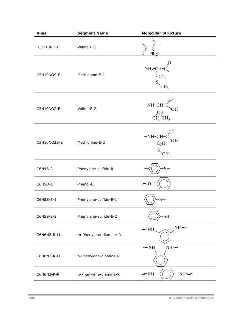
406 A Component Databanks
Alias Segment Name Molecular Structure
C5H10NO-E Valine-E-1
C5H10NOS-E Methionine-E-1
C5H10NO2-E Valine-E-2
C5H10NO2S-E Methionine-E-2
C6H4S-R Phenylene-sulfide-R
C6H5O-E Phenol-E
C6H5S-E-1 Phenylene-sulfide-E-1
C6H5S-E-2 Phenylene-sulfide-E-2
C6H6N2-R-M m-Phenylene-diamine-R
C6H6N2-R-O o-Phenylene-diamine-R
C6H6N2-R-P p-Phenylene-diamine-R
O
CH3
CH CNH2
C2H4
S
NH CH C
O
OHCH
CH3 CH3
NH CH C
O
OH
CH3
C2H4
S
S
O
S
SH
NH NH
NHNH
NHNH
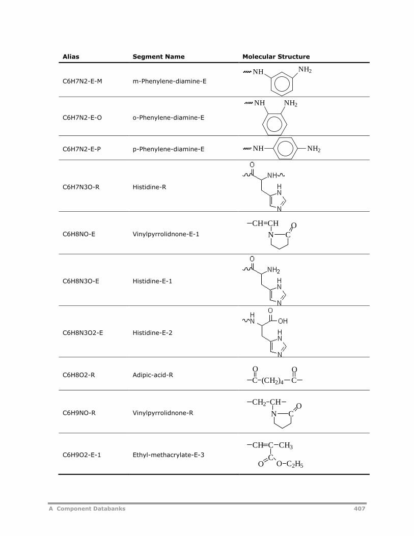
A Component Databanks 407
Alias Segment Name Molecular Structure
C6H7N2-E-M m-Phenylene-diamine-E
C6H7N2-E-O o-Phenylene-diamine-E
C6H7N2-E-P p-Phenylene-diamine-E
C6H7N3O-R Histidine-R
C6H8NO-E Vinylpyrrolidnone-E-1
C6H8N3O-E Histidine-E-1
C6H8N3O2-E Histidine-E-2
C6H8O2-R Adipic-acid-R
C6H9NO-R Vinylpyrrolidnone-R
C6H9O2-E-1 Ethyl-methacrylate-E-3
NH NH2
NH2NH
NH2NH
OCN
CHCH
CC (CH2)4
O O
CH2 CH
CNO
CH C CH3
CO C2H5O
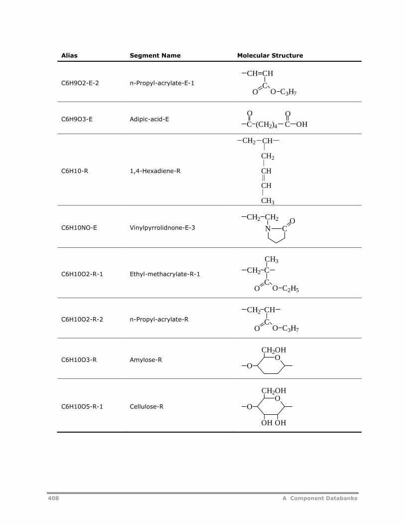
408 A Component Databanks
Alias Segment Name Molecular Structure
C6H9O2-E-2 n-Propyl-acrylate-E-1
C6H9O3-E Adipic-acid-E
C6H10-R 1,4-Hexadiene-R
C6H10NO-E Vinylpyrrolidnone-E-3
C6H10O2-R-1 Ethyl-methacrylate-R-1
C6H10O2-R-2 n-Propyl-acrylate-R
C6H10O3-R Amylose-R
C6H10O5-R-1 Cellulose-R
CH CH
CO C3H7O
C OHC (CH2)4
O O
CH2 CH
CH2
CH3
CH
CH
CH2 CH2
N CO
CH2 C
CO C2H5O
CH3
CH2 CH
CO C3H7O
OCH2OH
O
OCH2OH
O
OH OH
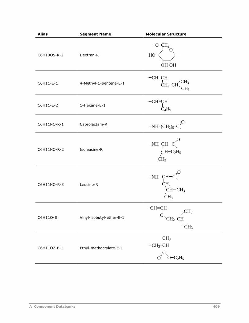
A Component Databanks 409
Alias Segment Name Molecular Structure
C6H10O5-R-2 Dextran-R
C6H11-E-1 4-Methyl-1-pentene-E-1
C6H11-E-2 1-Hexane-E-1
C6H11NO-R-1 Caprolactam-R
C6H11NO-R-2 Isoleucine-R
C6H11NO-R-3 Leucine-R
C6H11O-E Vinyl-isobutyl-ether-E-1
C6H11O2-E-1 Ethyl-methacrylate-E-1
O
OH OH
HO
CH2O
CH CH
CH2 CHCH3
CH3
CH CH
C4H9
NH (CH2)5 CO
NH CH
CH C2H5
OC
CH3
OC
CH3
CH
CH2
NH
CH
CH3
CH3
CH CH
OCH2 CH
CH3
CH2 CH
CH3
CO O C2H5
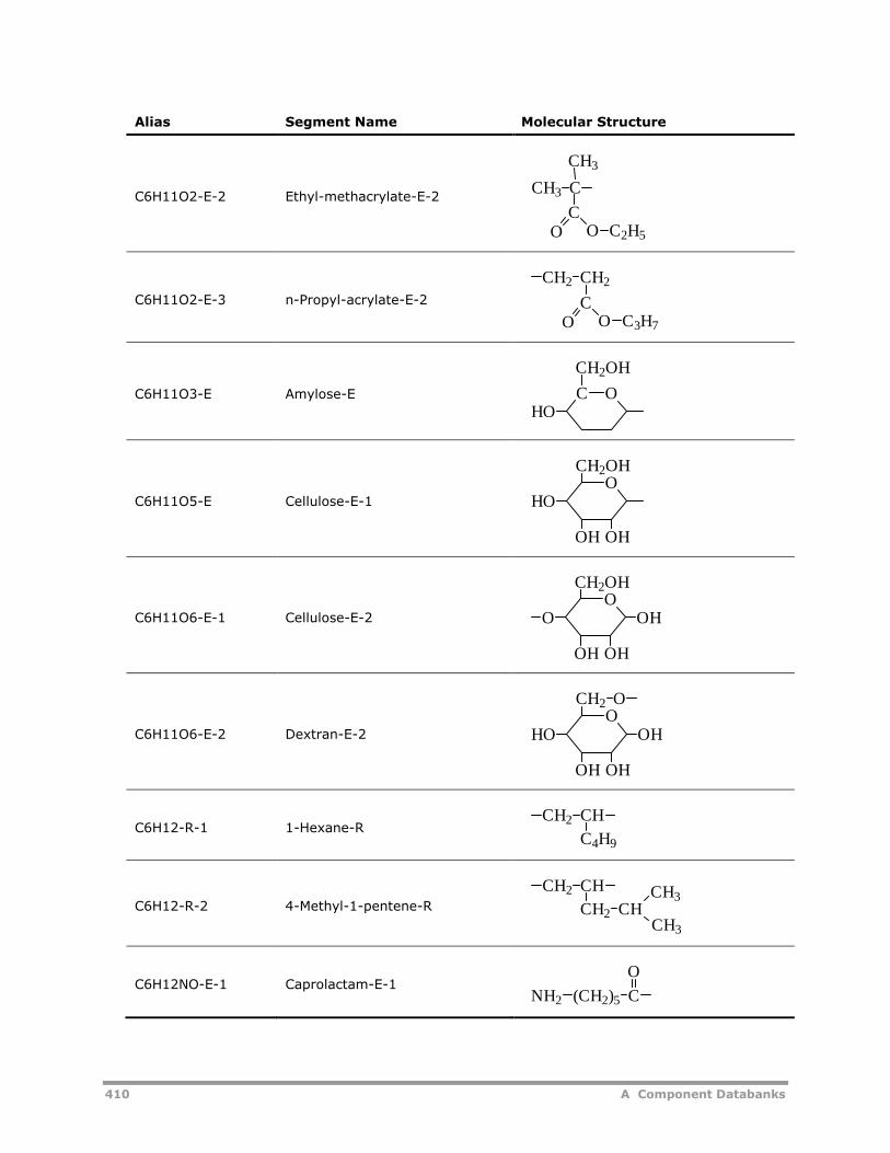
410 A Component Databanks
Alias Segment Name Molecular Structure
C6H11O2-E-2 Ethyl-methacrylate-E-2
C6H11O2-E-3 n-Propyl-acrylate-E-2
C6H11O3-E Amylose-E
C6H11O5-E Cellulose-E-1
C6H11O6-E-1 Cellulose-E-2
C6H11O6-E-2 Dextran-E-2
C6H12-R-1 1-Hexane-R
C6H12-R-2 4-Methyl-1-pentene-R
C6H12NO-E-1 Caprolactam-E-1
O O C2H5
C
CH3
CCH3
O O C3H7
C
CH2 CH2
C O
CH2OH
HO
OCH2OH
HO
OH OH
OCH2OH
OH
OH OH
O
OOH
OH OH
CH2 O
HO
CH2 CH
C4H9
CH2 CH
CH2 CHCH3
CH3
NH2 (CH2)5 C
O
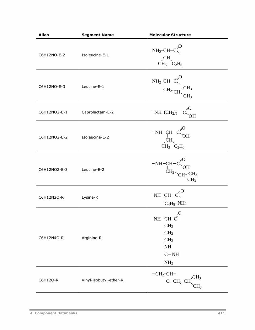
A Component Databanks 411
Alias Segment Name Molecular Structure
C6H12NO-E-2 Isoleucine-E-1
C6H12NO-E-3 Leucine-E-1
C6H12NO2-E-1 Caprolactam-E-2
C6H12NO2-E-2 Isoleucine-E-2
C6H12NO2-E-3 Leucine-E-2
C6H12N2O-R Lysine-R
C6H12N4O-R Arginine-R
C6H12O-R Vinyl-isobutyl-ether-R
NH2 CH C
CH
O
CH3 C2H5
NH2 CH C
CH2 CH
O
CH3
CH3
OC
OH(CH2)5NH
OC
OHNH CH
CHC2H5CH3
OC
OHNH CH
CH2
CH3
CH CH3
OCNH CH
C4H8 NH2
NH CH C
CH2
CH2
CH2
NH
C NH
NH2
O
CH2 CH
O CH2 CHCH3
CH3
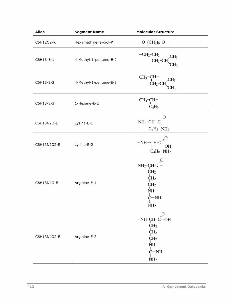
412 A Component Databanks
Alias Segment Name Molecular Structure
C6H12O2-R Hexamethylene-diol-R
C6H13-E-1 4-Methyl-1-pentene-E-2
C6H13-E-2 4-Methyl-1-pentene-E-3
C6H13-E-3 1-Hexane-E-2
C6H13N2O-E Lysine-E-1
C6H13N2O2-E Lysine-E-2
C6H13N4O-E Arginine-E-1
C6H13N4O2-E Arginine-E-2
O (CH2)6 O
CH2 CH2
CH2 CHCH3
CH3
CH3
CH3
CH2 CH
CHCH3
CH3 CH
C4H9
NH2 CH CO
NH2C4H8
OCH CNH
OHNH2C4H8
OCH C
CH2
CH2
CH2
NH
C NH
NH2
NH2
CH C
CH2
CH2
CH2
NH
C NH
NH2
NHO
OH
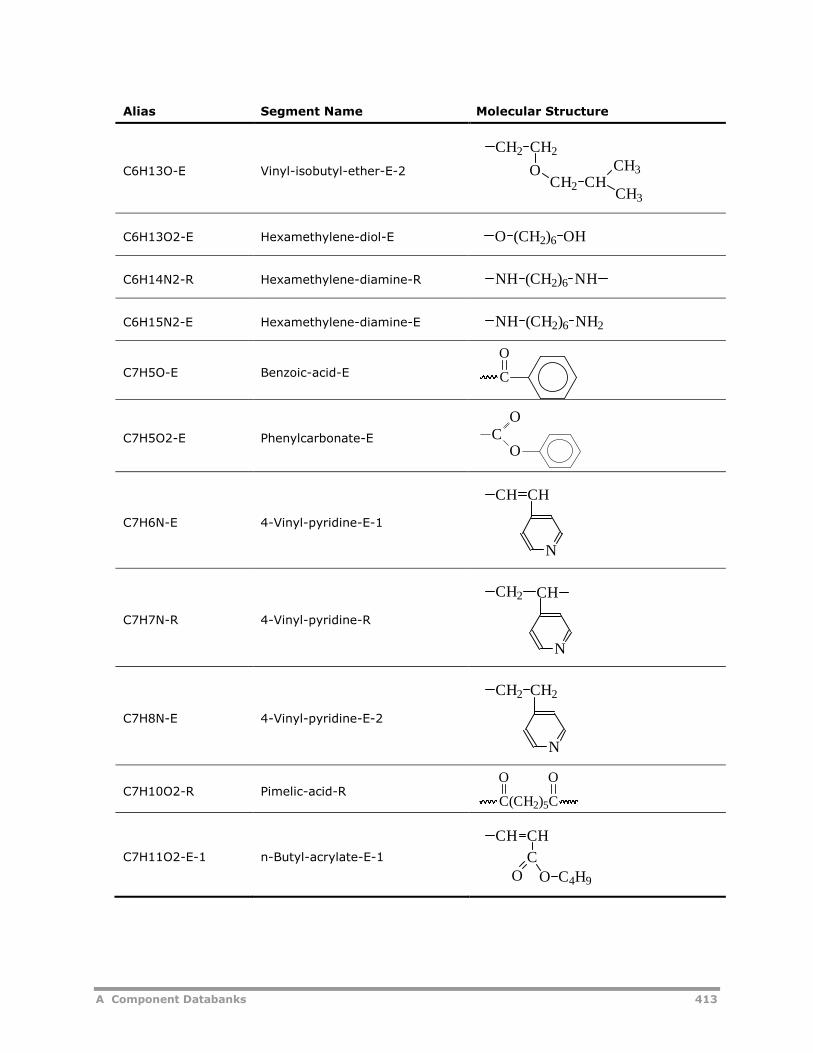
A Component Databanks 413
Alias Segment Name Molecular Structure
C6H13O-E Vinyl-isobutyl-ether-E-2
C6H13O2-E Hexamethylene-diol-E
C6H14N2-R Hexamethylene-diamine-R
C6H15N2-E Hexamethylene-diamine-E
C7H5O-E Benzoic-acid-E
C7H5O2-E Phenylcarbonate-E
C7H6N-E 4-Vinyl-pyridine-E-1
C7H7N-R 4-Vinyl-pyridine-R
C7H8N-E 4-Vinyl-pyridine-E-2
C7H10O2-R Pimelic-acid-R
C7H11O2-E-1 n-Butyl-acrylate-E-1
CH2 CH2
OCH2 CH
CH3
CH3
O (CH2)6 OH
(CH2)6 NHNH
(CH2)6NH NH2
C
O
CO
O
CH CH
N
N
CHCH2
N
CH2 CH2
C(CH2)5C
O O
CH CH
CO O C4H9
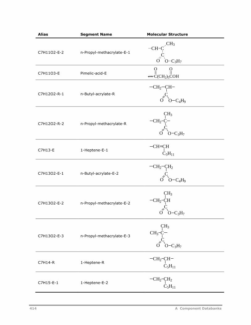
414 A Component Databanks
Alias Segment Name Molecular Structure
C7H11O2-E-2 n-Propyl-methacrylate-E-1
C7H11O3-E Pimelic-acid-E
C7H12O2-R-1 n-Butyl-acrylate-R
C7H12O2-R-2 n-Propyl-methacrylate-R
C7H13-E 1-Heptene-E-1
C7H13O2-E-1 n-Butyl-acrylate-E-2
C7H13O2-E-2 n-Propyl-methacrylate-E-2
C7H13O2-E-3 n-Propyl-methacrylate-E-3
C7H14-R 1-Heptene-R
C7H15-E-1 1-Heptene-E-2
CH C
CO O C3H7
CH3
C(CH2)5COH
O O
CH
O O C4H9
C
CH2
O O C3H7
CH2 C
C
CH3
CH CH
C5H11
O O C4H9
CH2 CH2
C
O O C3H7
CH2 CH
C
CH3
O O C3H7
CH3
C
CH3 C
CH2 CH
C5H11
CH2 CH2
C5H11
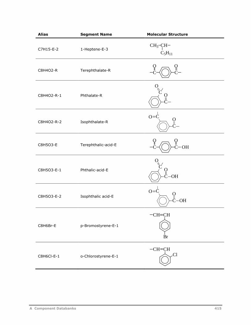
A Component Databanks 415
Alias Segment Name Molecular Structure
C7H15-E-2 1-Heptene-E-3
C8H4O2-R Terephthalate-R
C8H4O2-R-1 Phthalate-R
C8H4O2-R-2 Isophthalate-R
C8H5O3-E Terephthalic-acid-E
C8H5O3-E-1 Phthalic-acid-E
C8H5O3-E-2 Isophthalic acid-E
C8H6Br-E p-Bromostyrene-E-1
C8H6Cl-E-1 o-Chlorostyrene-E-1
C5H11
CH3 CH
C C
O O
C
C
O
O
C
C
OO
C C
O O
OH
C
C OH
O
O
C
C
OO
OH
Br
CHCH
CHCHCl
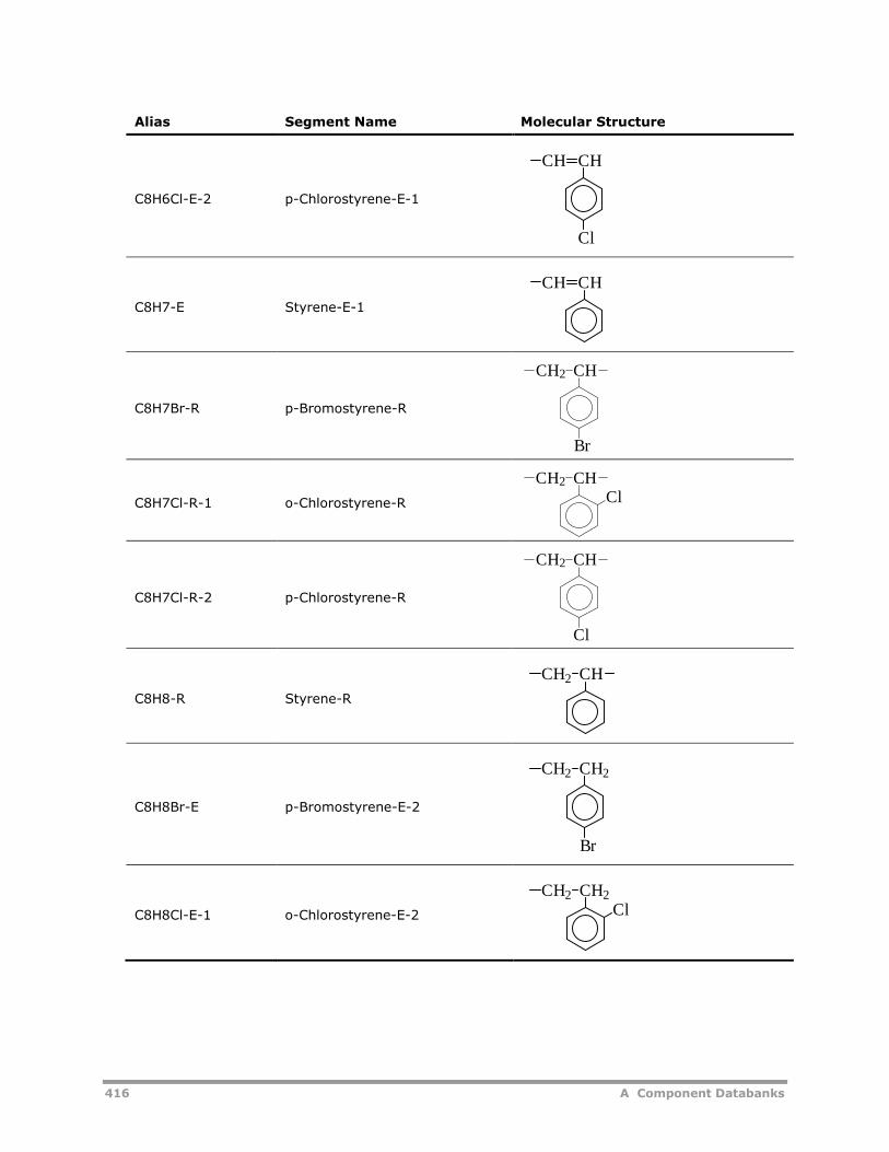
416 A Component Databanks
Alias Segment Name Molecular Structure
C8H6Cl-E-2 p-Chlorostyrene-E-1
C8H7-E Styrene-E-1
C8H7Br-R p-Bromostyrene-R
C8H7Cl-R-1 o-Chlorostyrene-R
C8H7Cl-R-2 p-Chlorostyrene-R
C8H8-R Styrene-R
C8H8Br-E p-Bromostyrene-E-2
C8H8Cl-E-1 o-Chlorostyrene-E-2
CHCH
Cl
CHCH
CH
Br
CH2
CHCl
CH2
CH
Cl
CH2
CHCH2
CH2 CH2
Br
CH2 CH2
Cl
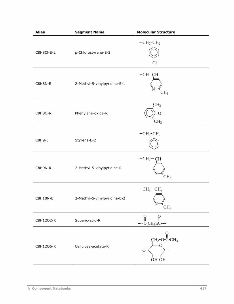
A Component Databanks 417
Alias Segment Name Molecular Structure
C8H8Cl-E-2 p-Chlorostyrene-E-2
C8H8N-E 2-Methyl-5-vinylpyridine-E-1
C8H8O-R Phenylene-oxide-R
C8H9-E Styrene-E-2
C8H9N-R 2-Methyl-5-vinylpyridine-R
C8H10N-E 2-Methyl-5-vinylpyridine-E-2
C8H12O2-R Suberic-acid-R
C8H12O6-R Cellulose-acetate-R
CH2 CH2
Cl
CH CH
NCH3
CH3
CH3
O
CH2 CH2
NCH3
CHCH2
CH2 CH2
CH3N
C(CH2)6C
O O
O
OH OH
O
CH2 O C CH3
O
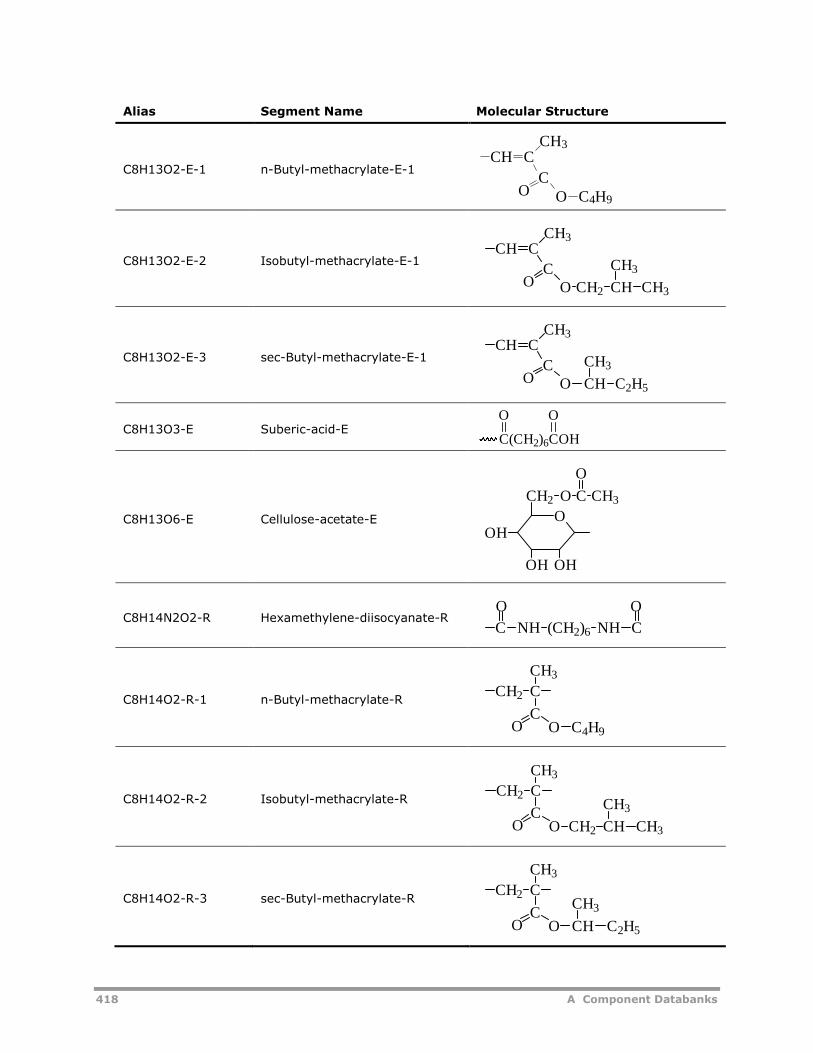
418 A Component Databanks
Alias Segment Name Molecular Structure
C8H13O2-E-1 n-Butyl-methacrylate-E-1
C8H13O2-E-2 Isobutyl-methacrylate-E-1
C8H13O2-E-3 sec-Butyl-methacrylate-E-1
C8H13O3-E Suberic-acid-E
C8H13O6-E Cellulose-acetate-E
C8H14N2O2-R Hexamethylene-diisocyanate-R
C8H14O2-R-1 n-Butyl-methacrylate-R
C8H14O2-R-2 Isobutyl-methacrylate-R
C8H14O2-R-3 sec-Butyl-methacrylate-R
CH CCH3
CO O C4H9
CH CCH3
CO O CH2 CH CH3
CH3
CH CCH3
CO O CH
CH3
C2H5
C(CH2)6COH
O O
O
OH OH
CH2 O C CH3
O
OH
C NH (CH2)6 NH C
O O
CH2 C
CH3
CO O C4H9
CH2 C
CH3
CO O CH2 CH CH3
CH3
CH2 C
CH3
CO O CH
CH3
C2H5
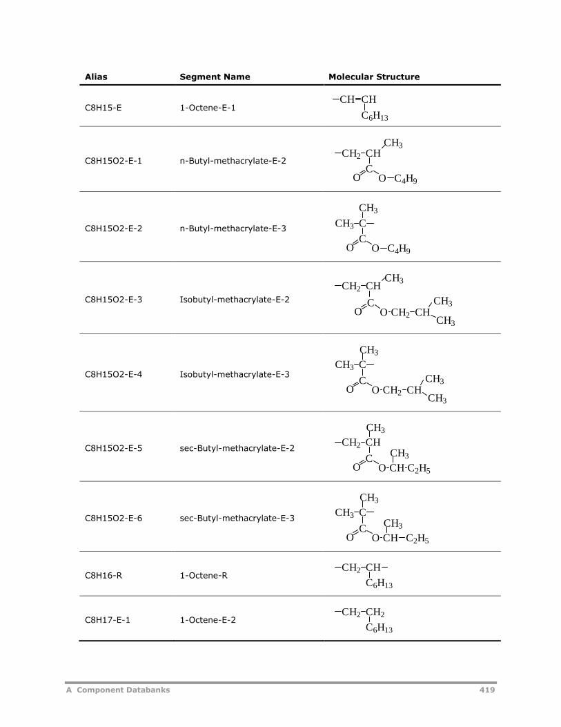
A Component Databanks 419
Alias Segment Name Molecular Structure
C8H15-E 1-Octene-E-1
C8H15O2-E-1 n-Butyl-methacrylate-E-2
C8H15O2-E-2 n-Butyl-methacrylate-E-3
C8H15O2-E-3 Isobutyl-methacrylate-E-2
C8H15O2-E-4 Isobutyl-methacrylate-E-3
C8H15O2-E-5 sec-Butyl-methacrylate-E-2
C8H15O2-E-6 sec-Butyl-methacrylate-E-3
C8H16-R 1-Octene-R
C8H17-E-1 1-Octene-E-2
CH CH
C6H13
CH2 CH
CO O C4H9
CH3
O O C4H9
C
CCH3
CH3
O O CH2 CHC
CH3CH2 CH
CH3
CH3
O O CH2 CHC
CH3
CH3
CH3
CH3 C
O O CH C2H5
C
CH3
CH3
CH2 CH
O O CHC
CH3
CH3
CH3 C
C2H5
CH2 CH
C6H13
CH2 CH2
C6H13
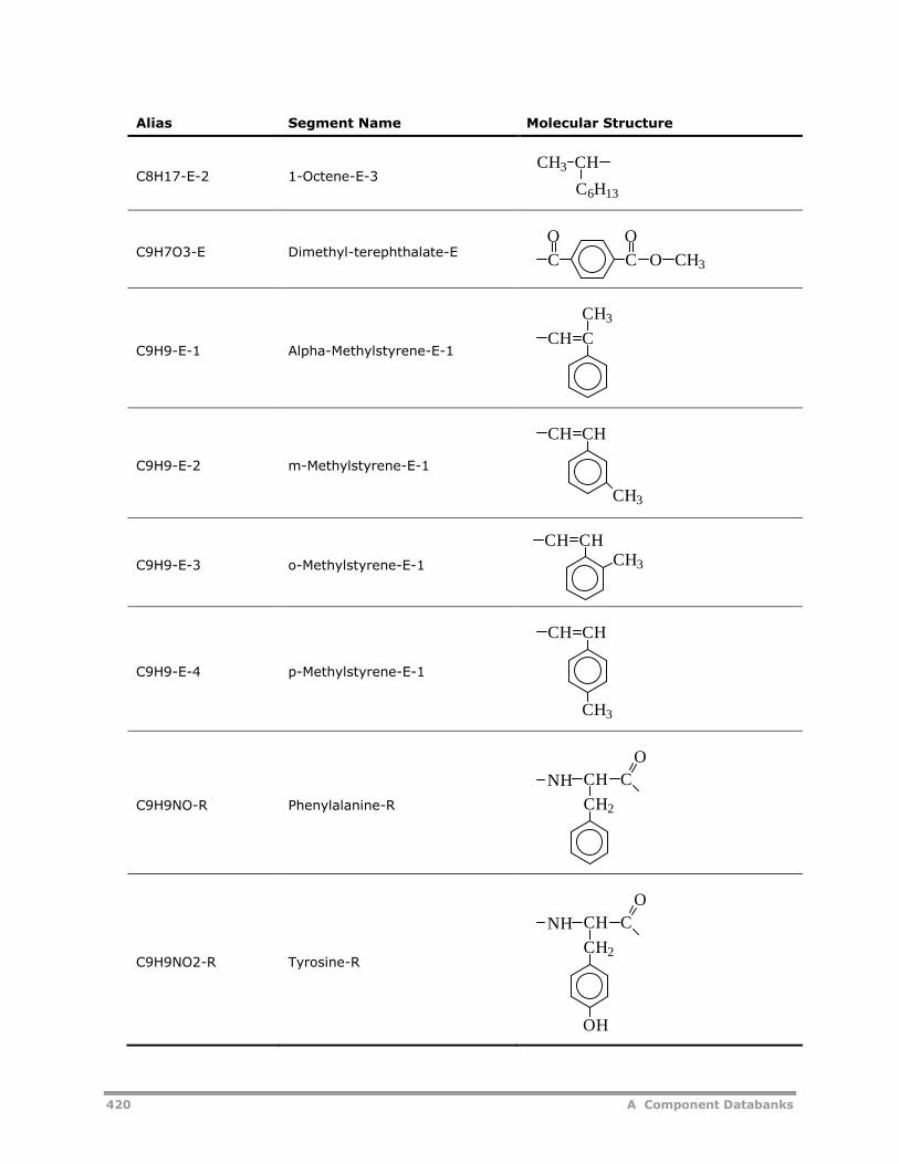
420 A Component Databanks
Alias Segment Name Molecular Structure
C8H17-E-2 1-Octene-E-3
C9H7O3-E Dimethyl-terephthalate-E
C9H9-E-1 Alpha-Methylstyrene-E-1
C9H9-E-2 m-Methylstyrene-E-1
C9H9-E-3 o-Methylstyrene-E-1
C9H9-E-4 p-Methylstyrene-E-1
C9H9NO-R Phenylalanine-R
C9H9NO2-R Tyrosine-R
C6H13
CH3 CH
C C
O O
CH3O
CCH
CH3
CH3
CHCH
CHCHCH3
CHCH
CH3
CH2
CH CNH
O
CH2
CH C
OH
NH
O
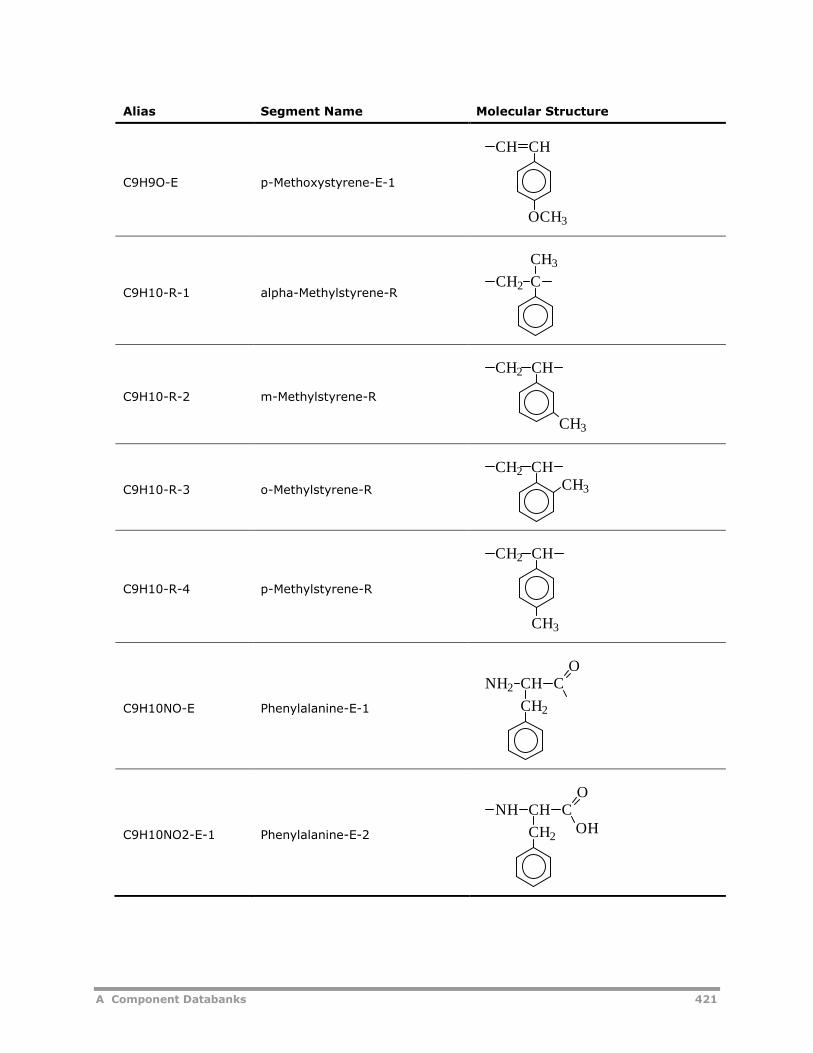
A Component Databanks 421
Alias Segment Name Molecular Structure
C9H9O-E p-Methoxystyrene-E-1
C9H10-R-1 alpha-Methylstyrene-R
C9H10-R-2 m-Methylstyrene-R
C9H10-R-3 o-Methylstyrene-R
C9H10-R-4 p-Methylstyrene-R
C9H10NO-E Phenylalanine-E-1
C9H10NO2-E-1 Phenylalanine-E-2
OCH3
CHCH
CCH2
CH3
CH3
CHCH2
CHCH3
CH2
CH
CH3
CH2
CH2
CH CNH2
O
CH2
CH CNHO
OH
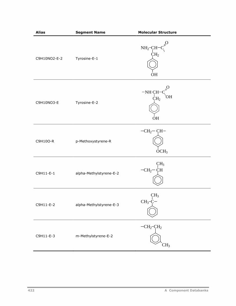
422 A Component Databanks
Alias Segment Name Molecular Structure
C9H10NO2-E-2 Tyrosine-E-1
C9H10NO3-E Tyrosine-E-2
C9H10O-R p-Methoxystyrene-R
C9H11-E-1 alpha-Methylstyrene-E-2
C9H11-E-2 alpha-Methylstyrene-E-3
C9H11-E-3 m-Methylstyrene-E-2
CH2
CH CNH2
OH
O
CH2
CH C
OH
NHO
OH
CH
OCH3
CH2
CH
CH3
CH2
CH3
CH3 C
CH3
CH2 CH2
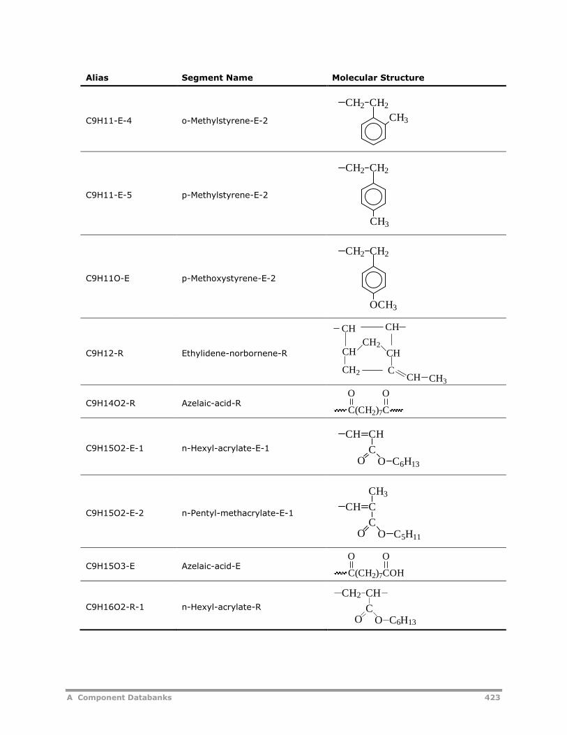
A Component Databanks 423
Alias Segment Name Molecular Structure
C9H11-E-4 o-Methylstyrene-E-2
C9H11-E-5 p-Methylstyrene-E-2
C9H11O-E p-Methoxystyrene-E-2
C9H12-R Ethylidene-norbornene-R
C9H14O2-R Azelaic-acid-R
C9H15O2-E-1 n-Hexyl-acrylate-E-1
C9H15O2-E-2 n-Pentyl-methacrylate-E-1
C9H15O3-E Azelaic-acid-E
C9H16O2-R-1 n-Hexyl-acrylate-R
CH3
CH2 CH2
CH3
CH2 CH2
OCH3
CH2 CH2
CH2
CH
CH2CH3
CH
CH
CH
C
CH
C(CH2)7C
O O
CH CH
CO O C6H13
CH C
C
CH3
O O C5H11
C(CH2)7COH
O O
O O C6H13
CH
C
CH2
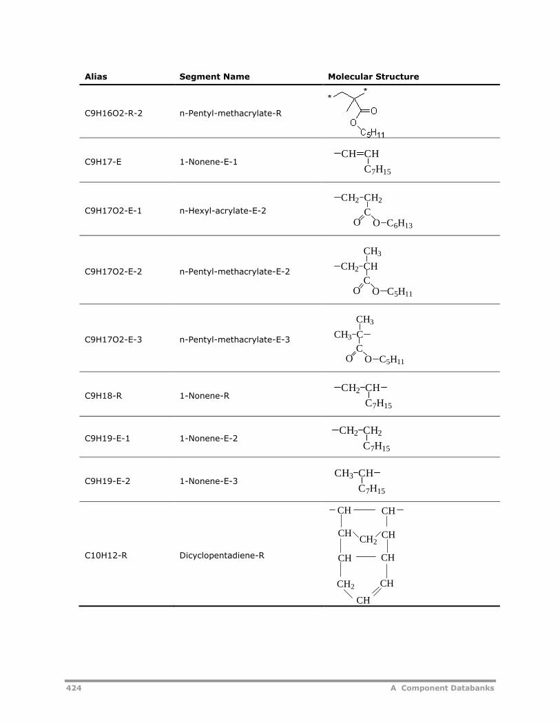
424 A Component Databanks
Alias Segment Name Molecular Structure
C9H16O2-R-2 n-Pentyl-methacrylate-R
C9H17-E 1-Nonene-E-1
C9H17O2-E-1 n-Hexyl-acrylate-E-2
C9H17O2-E-2 n-Pentyl-methacrylate-E-2
C9H17O2-E-3 n-Pentyl-methacrylate-E-3
C9H18-R 1-Nonene-R
C9H19-E-1 1-Nonene-E-2
C9H19-E-2 1-Nonene-E-3
C10H12-R Dicyclopentadiene-R
CH CH
C7H15
O O C6H13
CH2 CH2
C
O O C5H11
CH3
CHCH2
C
O O C5H11
C
CH3
CCH3
CH2 CH
C7H15
CH2 CH2
C7H15
CH
C7H15
CH3
CH2
CH
CH2
CH
CH
CH
CH
CH
CH
CH
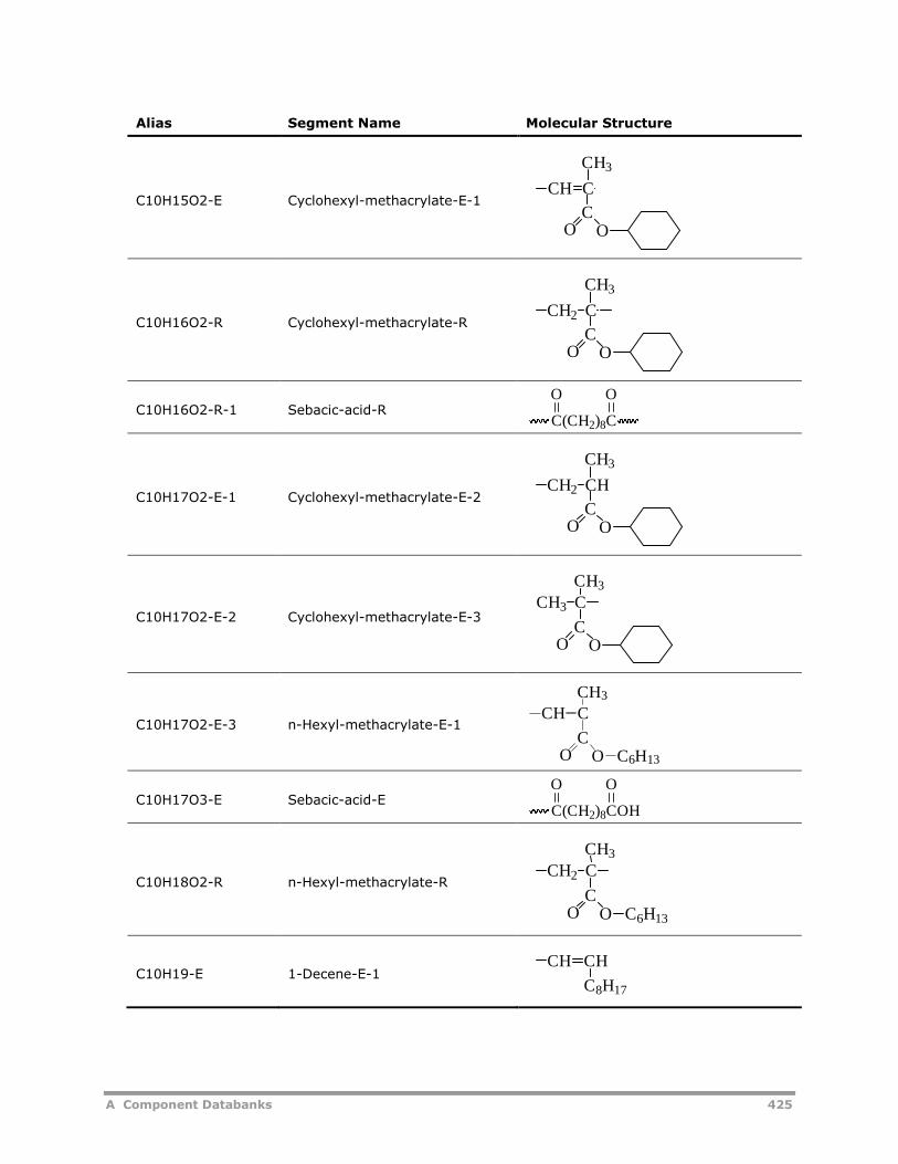
A Component Databanks 425
Alias Segment Name Molecular Structure
C10H15O2-E Cyclohexyl-methacrylate-E-1
C10H16O2-R Cyclohexyl-methacrylate-R
C10H16O2-R-1 Sebacic-acid-R
C10H17O2-E-1 Cyclohexyl-methacrylate-E-2
C10H17O2-E-2 Cyclohexyl-methacrylate-E-3
C10H17O2-E-3 n-Hexyl-methacrylate-E-1
C10H17O3-E Sebacic-acid-E
C10H18O2-R n-Hexyl-methacrylate-R
C10H19-E 1-Decene-E-1
O OC
CH3
CCH
O OC
CH3
CCH2
C(CH2)8C
O O
O OC
CH3
CHCH2
O OC
CH3
CCH3
O OC
C6H13
CH3
CCH
C(CH2)8COH
O O
O OC
C6H13
CH3
CCH2
CH CH
C8H17
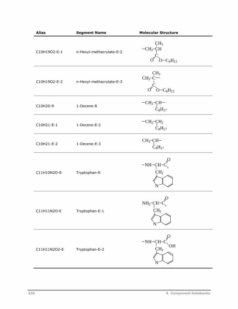
426 A Component Databanks
Alias Segment Name Molecular Structure
C10H19O2-E-1 n-Hexyl-methacrylate-E-2
C10H19O2-E-2 n-Hexyl-methacrylate-E-3
C10H20-R 1-Decene-R
C10H21-E-1 1-Decene-E-2
C10H21-E-2 1-Decene-E-3
C11H10N2O-R Tryptophan-R
C11H11N2O-E Tryptophan-E-1
C11H11N2O2-E Tryptophan-E-2
O OC
C6H13
CH3
CHCH2
O OC
C6H13
CH3
CCH3
CH
C8H17
CH2
CH2 CH2
C8H17
CH3 CH
C8H17
NH CH C
CH2
N
O
CH2
N
CH CNH2
O
NH CH C
CH2
N
O
OH
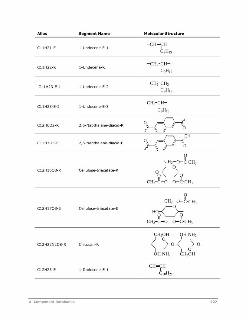
A Component Databanks 427
Alias Segment Name Molecular Structure
C11H21-E 1-Undecene-E-1
C11H22-R 1-Undecene-R
C11H23-E-1 1-Undecene-E-2
C11H23-E-2 1-Undecene-E-3
C12H6O2-R 2,6-Napthalene-diacid-R
C12H7O3-E 2,6-Napthalene-diacid-E
C12H16O8-R Cellulose-triacetate-R
C12H17O8-E Cellulose-triacetate-E
C12H22N2O8-R Chitosan-R
C12H23-E 1-Dodecene-E-1
CH CH
C9H19
CH
C9H19
CH2
CH2 CH2
C9H19
CH3 CH
C9H19
O
O O
O
CCCH3 CH3
CH2
OO
O C CH3
O
O
O O CCCH3 CH3
CH2
HOOO
O C CH3
O
OO
OH NH2
CH2OH
OCH2OH
O
NH2OH
CH CH
C10H21
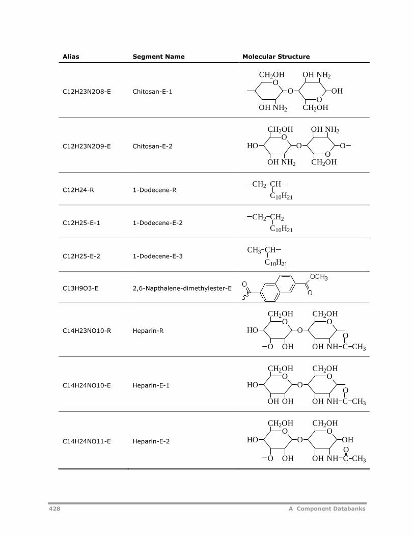
428 A Component Databanks
Alias Segment Name Molecular Structure
C12H23N2O8-E Chitosan-E-1
C12H23N2O9-E Chitosan-E-2
C12H24-R 1-Dodecene-R
C12H25-E-1 1-Dodecene-E-2
C12H25-E-2 1-Dodecene-E-3
C13H9O3-E 2,6-Napthalene-dimethylester-E
C14H23NO10-R Heparin-R
C14H24NO10-E Heparin-E-1
C14H24NO11-E Heparin-E-2
OO
OH NH2
CH2OH
OCH2OH
NH2OH
OH
OO
OH NH2
CH2OH
HOO
CH2OH
NH2OH
O
CH2 CH
C10H21
CH2 CH2
C10H21
C10H21
CH3 CH
OO
O OH
CH2OH
HOO
OH NH C CH3
CH2OH
O
OO
OH
CH2OH
HO
OH
O
OH NH C CH3
CH2OH
O
OO
OH
CH2OH
HO
O
O
OH NH
OH
CH2OH
C CH3
O
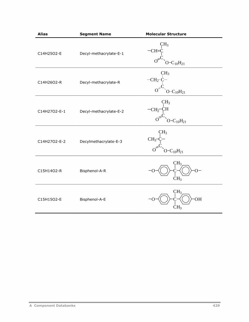
A Component Databanks 429
Alias Segment Name Molecular Structure
C14H25O2-E Decyl-methacrylate-E-1
C14H26O2-R Decyl-methacrylate-R
C14H27O2-E-1 Decyl-methacrylate-E-2
C14H27O2-E-2 Decylmethacrylate-E-3
C15H14O2-R Bisphenol-A-R
C15H15O2-E Bisphenol-A-E
CH C
CH3
CO C10H21
O
O C10H21O
C
CH3
C
CH2
CH
CH3
O C10H21
C
CH2
O
O C10H21
C
CH3
CH3 C
O
O C
CH3
CH3
O
O C
CH3
CH3
OH

430 A Component Databanks
B Kinetic Rate Constant Parameters 431
B Kinetic Rate ConstantParameters
This appendix provides decomposition rate parameters for commonly usedinitiators. Within each group the initiators are arranged by increasing totalnumber of carbon atoms.
The parameters are grouped as follows:
Water Soluble Azo-nitriles
Solvent Soluble Azo-Nitriles
Diacyl Peroxides
Peroxycarbonates
Alkyl Peroxides
Hydroperoxides
Peroxyesters
C-C Initiators
Sulfonyl Peroxides
Initiator Decomposition RateParametersThe table at the end of this section shows the decomposition rate parametersfor monofunctional free-radical initiators. These parameters assume first-order decomposition kinetics. These data are all included in the INITIATORdatabase in Aspen Polymers (formerly known as Aspen Polymers Plus).
Initiator decomposition rates depend on several factors includingtemperature, pressure, solvent type, and initiator concentration.
Solvent DependencyDecomposition rates are lowest in solvents that act as radical scavengers,such as poly chlorinated organic compounds (e.g., TCE). Initiators used forbulk-phase vinyl chloride polymerizations are typically in these types ofcompounds since they closely mimic the solvent environment during
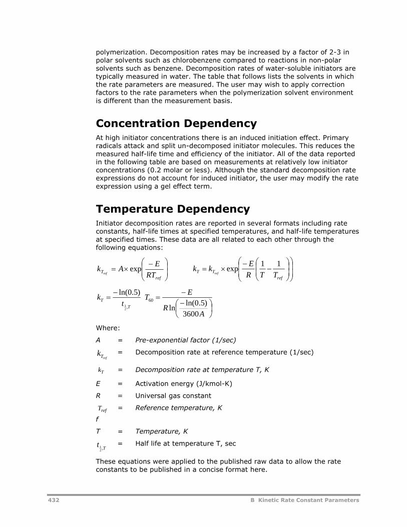
432 B Kinetic Rate Constant Parameters
polymerization. Decomposition rates may be increased by a factor of 2-3 inpolar solvents such as chlorobenzene compared to reactions in non-polarsolvents such as benzene. Decomposition rates of water-soluble initiators aretypically measured in water. The table that follows lists the solvents in whichthe rate parameters are measured. The user may wish to apply correctionfactors to the rate parameters when the polymerization solvent environmentis different than the measurement basis.
Concentration DependencyAt high initiator concentrations there is an induced initiation effect. Primaryradicals attack and split un-decomposed initiator molecules. This reduces themeasured half-life time and efficiency of the initiator. All of the data reportedin the following table are based on measurements at relatively low initiatorconcentrations (0.2 molar or less). Although the standard decomposition rateexpressions do not account for induced initiator, the user may modify the rateexpression using a gel effect term.
Temperature DependencyInitiator decomposition rates are reported in several formats including rateconstants, half-life times at specified temperatures, and half-life temperaturesat specified times. These data are all related to each other through thefollowing equations:
ref
TRT
EAk
refexp
ref
TTTTR
Ekk
ref
11exp
T
Tt
k,
21
)5.0ln(
AR
ET
3600
)5.0ln(ln
60
Where:
A = Pre-exponential factor (1/sec)
refTk = Decomposition rate at reference temperature (1/sec)
= Decomposition rate at temperature T, K
E = Activation energy (J/kmol-K)
R = Universal gas constant
f
= Reference temperature, K
T = Temperature, K
Tt
,21
= Half life at temperature T, sec
These equations were applied to the published raw data to allow the rateconstants to be published in a concise format here.
Tk
refT
B Kinetic Rate Constant Parameters 433
Pressure DependencyMost sources do not publish activation volume, which describe the pressuredependency of the reaction rates. Initiator decomposition reactions are knownto exhibit pressure dependence over very wide ranges of pressure. Forexample, the half-life of organic peroxides double with a 3000 bar pressureincrease (Degussa, 2004), which implies an activation volume of 1.9x10⁻⁵
kmolm /3 . This term can be ignored for processes that operate at reasonably
low pressures.
The following table shows the decomposition rate parameters formonofunctional free-radical initiators at a reference temperature of 60C(Tref(K)=333.15). These data are all included in the INITIATOR database inAspen Polymers.
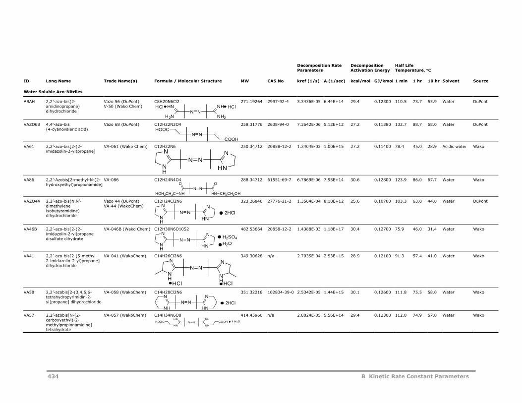
434 B Kinetic Rate Constant Parameters
Decomposition RateParameters
DecompositionActivation Energy
Half LifeTemperature, C
ID Long Name Trade Name(s) Formula / Molecular Structure MW CAS No kref (1/s) A (1/sec) kcal/mol GJ/kmol 1 min 1 hr 10 hr Solvent Source
Water Soluble Azo-Nitriles
ABAH 2,2’-azo-bis(2-amidinopropane)dihydrochloride
Vazo 56 (DuPont)V-50 (Wako Chem)
C8H20N6Cl2 271.19264 2997-92-4 3.3436E-05 6.44E+14 29.4 0.12300 110.5 73.7 55.9 Water DuPont
VAZO68 4,4’-azo-bis(4-cyanovaleric acid)
Vazo 68 (DuPont) C12H22N2O4 258.31776 2638-94-0 7.3642E-06 5.12E+12 27.2 0.11380 132.7 88.7 68.0 Water DuPont
VA61 2,2’-azo-bis[2-(2-imidazolin-2-yl)propane]
VA-061 (Wako Chem) C12H22N6 250.34712 20858-12-2 1.3404E-03 1.00E+15 27.2 0.11400 78.4 45.0 28.9 Acidic water Wako
VA86 2,2’-Azobis[2-methyl-N-(2-hydroxyethyl)propionamide]
VA-086 C12H24N4O4 288.34712 61551-69-7 6.7869E-06 7.95E+14 30.6 0.12800 123.9 86.0 67.7 Water Wako
VAZO44 2,2’-azo-bis(N,N’-dimethyleneisobutyramidine)dihydrochloride
Vazo 44 (DuPont)VA-44 (WakoChem)
C12H24Cl2N6 323.26840 27776-21-2 1.3564E-04 8.10E+12 25.6 0.10700 103.3 63.0 44.0 Water DuPont
VA46B 2,2’-azo-bis[2-(2-imidazolin-2-yl)propanedisulfate dihydrate
VA-046B (Wako Chem) C12H30N6O10S2 482.53664 20858-12-2 1.4388E-03 1.18E+17 30.4 0.12700 75.9 46.0 31.4 Water Wako
VA41 2,2’-azo-bis[2-(5-methyl-2-imidazolin-2-yl)propane]dihydrochloride
VA-041 (WakoChem) C14H26Cl2N6 349.30628 n/a 2.7035E-04 2.53E+15 28.9 0.12100 91.3 57.4 41.0 Water Wako
VA58 2,2’-azobis[2-(3,4,5,6-tetrahydropyrimidin-2-yl)propane] dihydrochloride
VA-058 (WakoChem) C14H28Cl2N6 351.32216 102834-39-0 2.5342E-05 1.44E+15 30.1 0.12600 111.8 75.5 58.0 Water Wako
VA57 2,2’-azobis[N-(2-carboxyethyl)-2-methylpropionamidine]tetrahydrate
VA-057 (WakoChem) C14H34N6O8 414.45960 n/a 2.8824E-05 5.56E+14 29.4 0.12300 112.0 74.9 57.0 Water Wako
N NHN
H2N NH2
NH HClHCl
N NCOOH
HOOC
N N
N
NH
HN
N
N N
HN CH2CH2OHHOH2CH2C NH
O O
N N
N
NH
HN
N2HCl
N N
N
NH
HN
NH2SO4
H2O
N N
N
NH N
H
N
HClHCl
N N 2HClHN
NN
NH
N NHN
HN NH
NHCO OHHOO C 4 H2O
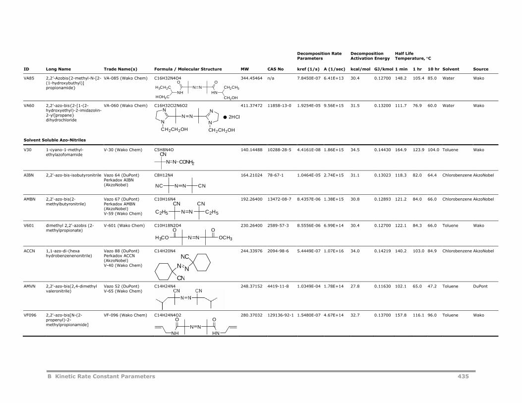
B Kinetic Rate Constant Parameters 435
Decomposition RateParameters
DecompositionActivation Energy
Half LifeTemperature, C
ID Long Name Trade Name(s) Formula / Molecular Structure MW CAS No kref (1/s) A (1/sec) kcal/mol GJ/kmol 1 min 1 hr 10 hr Solvent Source
VA85 2,2’-Azobis{2-methyl-N-[2-(1-hydroxybuthyl)]propionamide}
VA-085 (Wako Chem) C16H32N4O4 344.45464 n/a 7.8450E-07 6.41E+13 30.4 0.12700 148.2 105.4 85.0 Water Wako
VA60 2,2’-azo-bis{2-[1-(2-hydroxyethyl)-2-imidazolin-2-yl]propane}dihydrochloride
VA-060 (Wako Chem) C16H32Cl2N6O2 411.37472 11858-13-0 1.9254E-05 9.56E+15 31.5 0.13200 111.7 76.9 60.0 Water Wako
Solvent Soluble Azo-Nitriles
V30 1-cyano-1-methyl-ethylazofomamide
V-30 (Wako Chem) C5H8N4O 140.14488 10288-28-5 4.4161E-08 1.86E+15 34.5 0.14430 164.9 123.9 104.0 Toluene Wako
AIBN 2,2'-azo-bis-isobutyronitrile Vazo 64 (DuPont)Perkadox AIBN(AkzoNobel)
C8H12N4 164.21024 78-67-1 1.0464E-05 2.74E+15 31.1 0.13023 118.3 82.0 64.4 Chlorobenzene AkzoNobel
AMBN 2,2'-azo-bis(2-methylbutyronitrile)
Vazo 67 (DuPont)Perkadox AMBN(AkzoNobel)V-59 (Wako Chem)
C10H16N4 192.26400 13472-08-7 8.4357E-06 1.38E+15 30.8 0.12893 121.2 84.0 66.0 Chlorobenzene AkzoNobel
V601 dimethyl 2,2'-azobis (2-methylpropionate)
V-601 (Wako Chem) C10H18N2O4 230.26400 2589-57-3 8.5556E-06 6.99E+14 30.4 0.12700 122.1 84.3 66.0 Toluene Wako
ACCN 1,1-azo-di-(hexahydrobenzenenonitrile)
Vazo 88 (DuPont)Perkadox ACCN(AkzoNobel)V-40 (Wako Chem)
C14H20N4 244.33976 2094-98-6 5.4449E-07 1.07E+16 34.0 0.14219 140.2 103.0 84.9 Chlorobenzene AkzoNobel
AMVN 2,2'-azo-bis(2,4-dimethylvaleronitrile)
Vazo 52 (DuPont)V-65 (Wako Chem)
C14H24N4 248.37152 4419-11-8 1.0349E-04 1.78E+14 27.8 0.11630 102.1 65.0 47.2 Toluene DuPont
VF096 2,2'-azo-bis[N-(2-propenyl)-2-methylpropionamide]
VF-096 (Wako Chem) C14H24N4O2 280.37032 129136-92-1 1.5480E-07 4.67E+14 32.7 0.13700 157.8 116.1 96.0 Toluene Wako
N N
HNNH
O O
CH2CH3
CH2OHHOH2C
H3CH2C
N N
N
N N
N2HCl
CH2CH2OHCH2CH2OH
N N CONH2
CN
NC N N CN
C2H5
CN
N N
CN
C2H5
N N
OO
OCH3H3CO
N N
CN
NC
N N
OO
HNNH
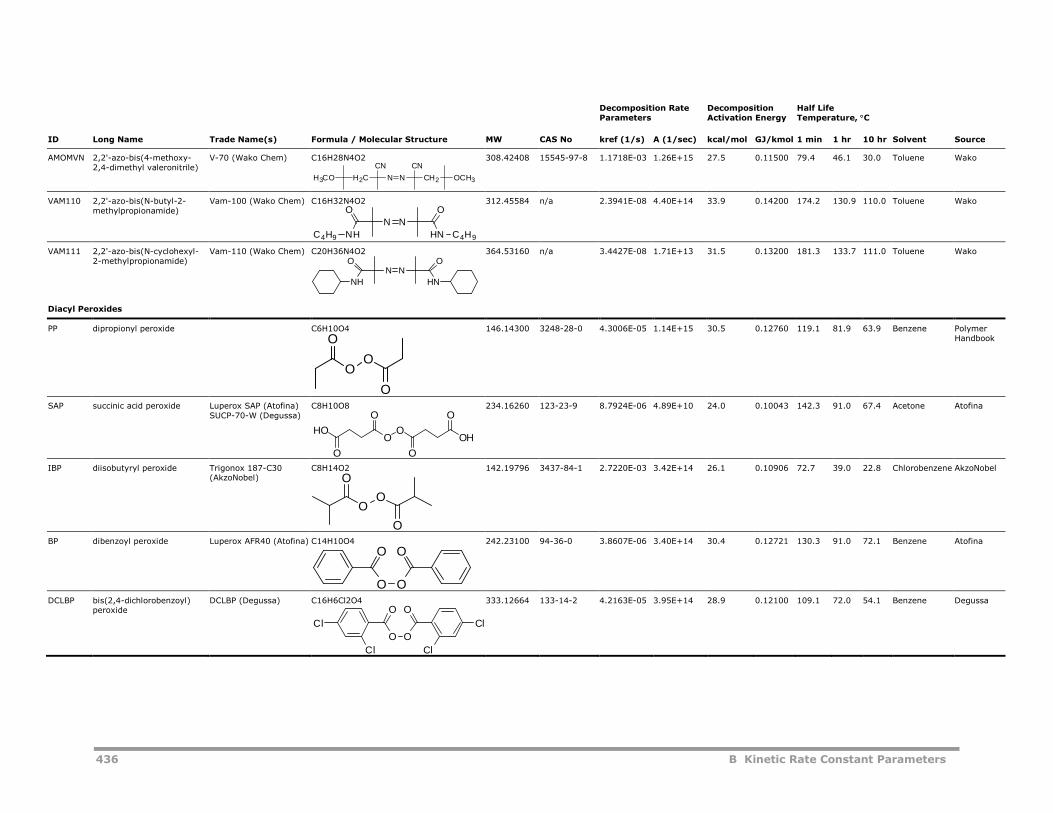
436 B Kinetic Rate Constant Parameters
Decomposition RateParameters
DecompositionActivation Energy
Half LifeTemperature, C
ID Long Name Trade Name(s) Formula / Molecular Structure MW CAS No kref (1/s) A (1/sec) kcal/mol GJ/kmol 1 min 1 hr 10 hr Solvent Source
AMOMVN 2,2'-azo-bis(4-methoxy-2,4-dimethyl valeronitrile)
V-70 (Wako Chem) C16H28N4O2 308.42408 15545-97-8 1.1718E-03 1.26E+15 27.5 0.11500 79.4 46.1 30.0 Toluene Wako
VAM110 2,2'-azo-bis(N-butyl-2-methylpropionamide)
Vam-100 (Wako Chem) C16H32N4O2 312.45584 n/a 2.3941E-08 4.40E+14 33.9 0.14200 174.2 130.9 110.0 Toluene Wako
VAM111 2,2'-azo-bis(N-cyclohexyl-2-methylpropionamide)
Vam-110 (Wako Chem) C20H36N4O2 364.53160 n/a 3.4427E-08 1.71E+13 31.5 0.13200 181.3 133.7 111.0 Toluene Wako
Diacyl Peroxides
PP dipropionyl peroxide C6H10O4 146.14300 3248-28-0 4.3006E-05 1.14E+15 30.5 0.12760 119.1 81.9 63.9 Benzene PolymerHandbook
SAP succinic acid peroxide Luperox SAP (Atofina)SUCP-70-W (Degussa)
C8H10O8 234.16260 123-23-9 8.7924E-06 4.89E+10 24.0 0.10043 142.3 91.0 67.4 Acetone Atofina
IBP diisobutyryl peroxide Trigonox 187-C30(AkzoNobel)
C8H14O2 142.19796 3437-84-1 2.7220E-03 3.42E+14 26.1 0.10906 72.7 39.0 22.8 Chlorobenzene AkzoNobel
BP dibenzoyl peroxide Luperox AFR40 (Atofina) C14H10O4 242.23100 94-36-0 3.8607E-06 3.40E+14 30.4 0.12721 130.3 91.0 72.1 Benzene Atofina
DCLBP bis(2,4-dichlorobenzoyl)peroxide
DCLBP (Degussa) C16H6Cl2O4 333.12664 133-14-2 4.2163E-05 3.95E+14 28.9 0.12100 109.1 72.0 54.1 Benzene Degussa
H2C
CN
N N
CN
CH2 OCH3H3CO
N N
HN C4H9C4H9 NH
O O
N N
HNNH
O O
O
O
O
O
O
O
O
O
OHHO
O
O
O
O
O
O
O
O
O
O
O
O
O
O
Cl Cl
ClCl
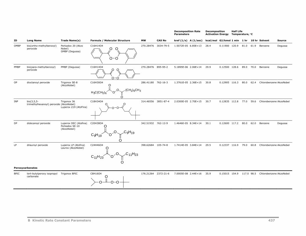
B Kinetic Rate Constant Parameters 437
Decomposition RateParameters
DecompositionActivation Energy
Half LifeTemperature, C
ID Long Name Trade Name(s) Formula / Molecular Structure MW CAS No kref (1/s) A (1/sec) kcal/mol GJ/kmol 1 min 1 hr 10 hr Solvent Source
OMBP bis(ortho-methylbenzoyl)peroxide
Perkadox 20 (AkzoNobel)OMBP (Degussa)
C16H14O4 270.28476 3034-79-5 1.5072E-05 6.85E+13 28.4 0.11900 120.9 81.0 61.9 Benzene Degussa
PMBP bis(para-methylbenzoyl)peroxide
PMBP (Degussa) C16H14O4 270.28476 895-95-2 5.1895E-06 2.06E+14 29.9 0.12500 128.6 89.0 70.0 Benzene Degussa
OP dioctanoyl peroxide Trigonox SE-8(AkzoNobel)
C16H30O4 286.41180 762-16-3 1.3761E-05 2.36E+15 30.8 0.12905 116.3 80.0 62.4 Chlorobenzene AkzoNobel
INP bis(3,5,5-trimethylhexanoyl) peroxide
Trigonox 36(AkzoNobel)Luperox 219 (AtoFina)
C18H34O4 314.46556 3851-87-4 2.0300E-05 2.70E+15 30.7 0.12835 112.8 77.0 59.6 Chlorobenzene AkzoNobel
DP didecanoyl peroxide Luperox DEC (Atofina)Perkadox SE-10(AkzoNobel)
C20H38O4 342.51932 762-12-9 1.4646E-05 8.34E+14 30.1 0.12600 117.2 80.0 62.0 Benzene Degussa
LP dilauroyl peroxide Luperox LP (Atofina)Laurox (AkzoNobel)
C24H46O4 398.62684 105-74-8 1.7414E-05 3.84E+14 29.5 0.12337 116.9 79.0 60.8 Chlorobenzene AkzoNobel
Peroxycarbonates
BPIC tert-butylperoxy isopropylcarbonate
Trigonox BPIC C8H16O4 176.21264 2372-21-6 7.0005E-08 2.44E+16 35.9 0.15015 154.9 117.0 98.5 Chlorobenzene AkzoNobel
O
O
O
O
O
O
O
O
H3C(CH2)6 O
O
O (CH2)6CH3
O
O
OO
O
OO
O
O
C9H19C9H19
OO
O
O
C11H23C11H23
O O
O
O
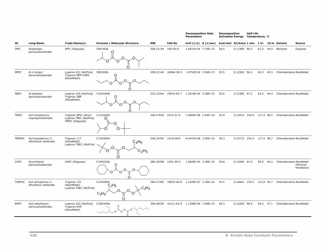
438 B Kinetic Rate Constant Parameters
Decomposition RateParameters
DecompositionActivation Energy
Half LifeTemperature, C
ID Long Name Trade Name(s) Formula / Molecular Structure MW CAS No kref (1/s) A (1/sec) kcal/mol GJ/kmol 1 min 1 hr 10 hr Solvent Source
IPPC diisopropylperoxydicarbonate
IPPC (Degussa) C8H16O6 208.21144 105-64-6 1.6931E-04 7.70E+14 28.4 0.11900 96.3 61.0 44.0 Benzene Degussa
NPPC di-n-propylperoxydicarbonate
Luperox 221 (AtoFina)Trigonox NPP-CK85(AkzoNobel)
C8H16O6 208.21144 16066-38-9 1.4752E-04 3.56E+15 29.5 0.12362 96.1 62.0 45.5 Chlorobenzene AkzoNobel
SBPC di-secbutylperoxydicarbonate
Luperox 225 (AtoFina)Trigonox SBP(AkzoNobel)
C10H16O6 232.23344 19910-65-7 1.2919E-04 3.38E+15 29.6 0.12385 97.2 63.0 46.4 Chlorobenzene AkzoNobel
TBPIC tert-butylperoxy-isopropylcarbonate
Trigonox BPIC (Akzo)Luperox TBIC (AtoFina)TBPIC (Degussa)
C11H20O6 248.27620 2372-21-6 7.0005E-08 2.44E+16 35.9 0.15015 154.9 117.0 98.5 Chlorobenzene AkzoNobel
TBPEHC tert-butylperoxy 2-ethylhexyl carbonate
Trigonox 117(AkzoNobel)Luperox TBEC (AtoFina)
C13H26O4 246.34704 12/4/3443 6.4441E-08 3.95E+16 36.3 0.15172 154.4 117.0 98.7 Chlorobenzene AkzoNobel
CHPC dicyclohexylperoxydicarbonate
CHPC (Degussa) C14H22O6 286.32508 1561-49-5 1.9626E-04 3.30E+16 30.8 0.12900 91.9 59.9 44.2 Chlorobenzene AkzoNobel(PolymerHandbook)
TAPEHC tert-amylperoxy 2-ethylhexyl carbonate
Trigonox 131(AkzoNobel)Luperox TAEC (AtoFina)
C14H28O4 260.37392 70833-40-8 1.2326E-07 2.29E+16 35.5 0.14841 150.5 113.0 94.7 Chlorobenzene AkzoNobel
EHPC di(2-ethylhexyl)peroxydicarbonate
Luperox 223 (AtoFina)Trigonox EHP(AkzoNobel)
C18H34O6 346.46436 16111-62-9 1.1396E-04 1.80E+15 29.3 0.12245 98.9 64.0 47.1 Chlorobenzene AkzoNobel
OO
O
O
OO
OO
O
O
OO
OO
O
O
OO
O
O
O
O
OO
O
O
C4H9
C2H5
OO
O
O
OO
OOO
C2H5
O
C2H5
C4H9
OO
O
O
OO
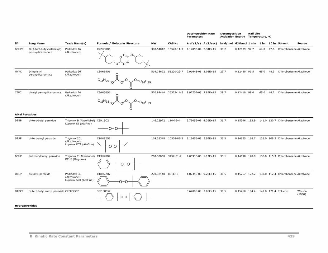
B Kinetic Rate Constant Parameters 439
Decomposition RateParameters
DecompositionActivation Energy
Half LifeTemperature, C
ID Long Name Trade Name(s) Formula / Molecular Structure MW CAS No kref (1/s) A (1/sec) kcal/mol GJ/kmol 1 min 1 hr 10 hr Solvent Source
BCHPC Di(4-tert-butylcyclohexyl)peroxydicarbonate
Perkadox 16(AkzoNobel)
C22H38O6 398.54012 15520-11-3 1.1205E-04 7.34E+15 30.2 0.12639 97.7 64.0 47.6 Chlorobenzene AkzoNobel
MYPC Dimyristylperoxydicarbonate
Perkadox 26(AkzoNobel)
C30H58O6 514.78692 53220-22-7 9.9164E-05 3.06E+15 29.7 0.12430 99.5 65.0 48.3 Chlorobenzene AkzoNobel
CEPC dicetyl peroxydicarbonate Perkadox 24(AkzoNobel)
C34H66O6 570.89444 26322-14-5 9.9270E-05 2.85E+15 29.7 0.12410 99.6 65.0 48.2 Chlorobenzene AkzoNobel
Alkyl Peroxides
DTBP di-tert-butyl peroxide Trigonox B (AkzoNobel)Luperox DI (AtoFina)
C8H18O2 146.22972 110-05-4 3.7905E-09 4.36E+15 36.7 0.15346 182.9 141.0 120.7 Chlorobenzene AkzoNobel
DTAP di-tert-amyl peroxide Trigonox 201(AkzoNobel)Luperox DTA (AtoFina)
C10H22O2 174.28348 10508-09-5 2.1965E-08 3.99E+15 35.5 0.14835 168.7 128.0 108.3 Chlorobenzene AkzoNobel
BCUP tert-butylcumyl peroxide Trigonox T (AkzoNobel)BCUP (Degussa)
C13H20O2 208.30060 3457-61-2 1.0091E-08 1.12E+15 35.1 0.14698 178.8 136.0 115.3 Chlorobenzene AkzoNobel
DCUP dicumyl peroxide Perkadox BC(AkzoNobel)Luperox 500 (AtoFina)
C18H22O2 270.37148 80-43-3 1.0731E-08 9.28E+15 36.5 0.15267 172.2 132.0 112.4 Chlorobenzene AkzoNobel
DTBCP di-tert-butyl cumyl peroxide C26H38O2 382.58652 3.6200E-09 3.05E+15 36.5 0.15260 184.4 142.0 121.4 Toluene Warson(1980)
Hydroperoxides
OO
OO
O
O
OO
O
O
OO C14H29
C14H29
OO
O
O
OO C16H33
C16H33
O O
O O
O O
O O
O O
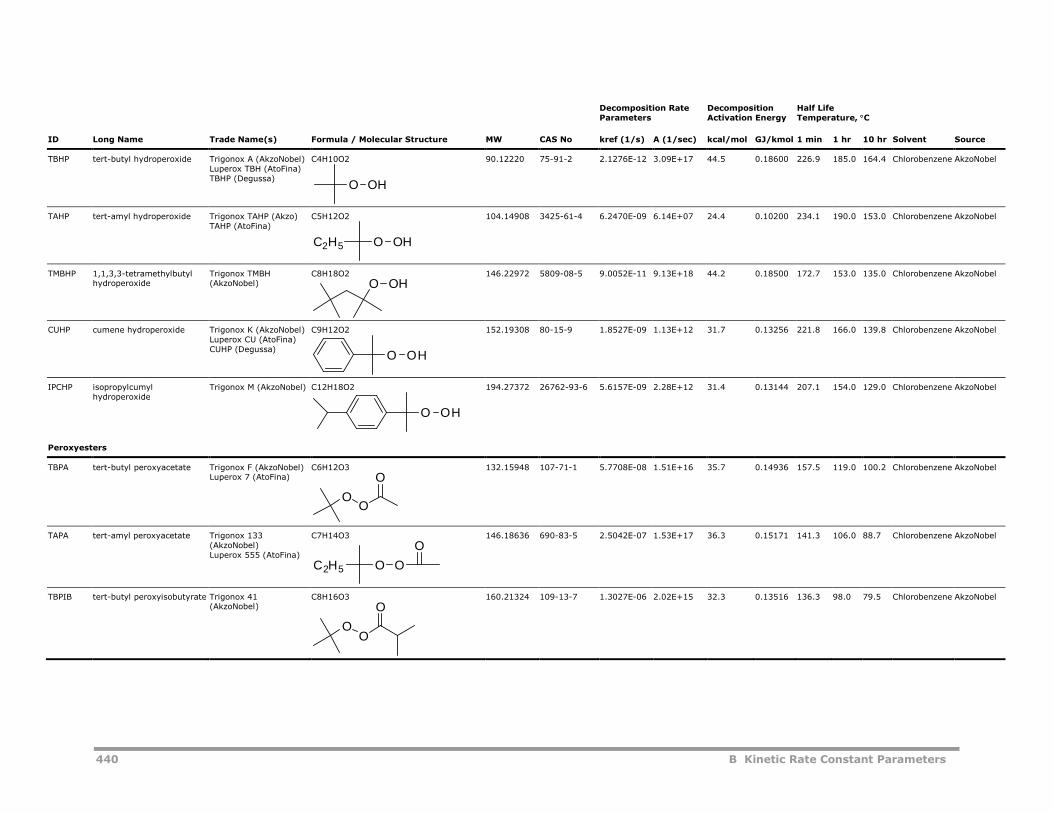
440 B Kinetic Rate Constant Parameters
Decomposition RateParameters
DecompositionActivation Energy
Half LifeTemperature, C
ID Long Name Trade Name(s) Formula / Molecular Structure MW CAS No kref (1/s) A (1/sec) kcal/mol GJ/kmol 1 min 1 hr 10 hr Solvent Source
TBHP tert-butyl hydroperoxide Trigonox A (AkzoNobel)Luperox TBH (AtoFina)TBHP (Degussa)
C4H10O2 90.12220 75-91-2 2.1276E-12 3.09E+17 44.5 0.18600 226.9 185.0 164.4 Chlorobenzene AkzoNobel
TAHP tert-amyl hydroperoxide Trigonox TAHP (Akzo)TAHP (AtoFina)
C5H12O2 104.14908 3425-61-4 6.2470E-09 6.14E+07 24.4 0.10200 234.1 190.0 153.0 Chlorobenzene AkzoNobel
TMBHP 1,1,3,3-tetramethylbutylhydroperoxide
Trigonox TMBH(AkzoNobel)
C8H18O2 146.22972 5809-08-5 9.0052E-11 9.13E+18 44.2 0.18500 172.7 153.0 135.0 Chlorobenzene AkzoNobel
CUHP cumene hydroperoxide Trigonox K (AkzoNobel)Luperox CU (AtoFina)CUHP (Degussa)
C9H12O2 152.19308 80-15-9 1.8527E-09 1.13E+12 31.7 0.13256 221.8 166.0 139.8 Chlorobenzene AkzoNobel
IPCHP isopropylcumylhydroperoxide
Trigonox M (AkzoNobel) C12H18O2 194.27372 26762-93-6 5.6157E-09 2.28E+12 31.4 0.13144 207.1 154.0 129.0 Chlorobenzene AkzoNobel
Peroxyesters
TBPA tert-butyl peroxyacetate Trigonox F (AkzoNobel)Luperox 7 (AtoFina)
C6H12O3 132.15948 107-71-1 5.7708E-08 1.51E+16 35.7 0.14936 157.5 119.0 100.2 Chlorobenzene AkzoNobel
TAPA tert-amyl peroxyacetate Trigonox 133(AkzoNobel)Luperox 555 (AtoFina)
C7H14O3 146.18636 690-83-5 2.5042E-07 1.53E+17 36.3 0.15171 141.3 106.0 88.7 Chlorobenzene AkzoNobel
TBPIB tert-butyl peroxyisobutyrate Trigonox 41(AkzoNobel)
C8H16O3 160.21324 109-13-7 1.3027E-06 2.02E+15 32.3 0.13516 136.3 98.0 79.5 Chlorobenzene AkzoNobel
O OH
C2H5 O OH
O OH
O OH
O OH
OO
O
O OC2H5
O
OO
O
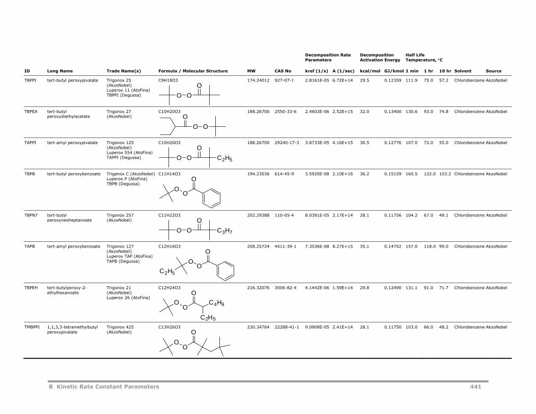
B Kinetic Rate Constant Parameters 441
Decomposition RateParameters
DecompositionActivation Energy
Half LifeTemperature, C
ID Long Name Trade Name(s) Formula / Molecular Structure MW CAS No kref (1/s) A (1/sec) kcal/mol GJ/kmol 1 min 1 hr 10 hr Solvent Source
TBPPI tert-butyl peroxypivalate Trigonox 25(AkzoNobel)Luperox 11 (AtoFina)TBPPI (Degussa)
C9H18O3 174.24012 927-07-1 2.8161E-05 6.72E+14 29.5 0.12359 111.9 75.0 57.2 Chlorobenzene AkzoNobel
TBPEA tert-butylperoxydiethylacetate
Trigonox 27(AkzoNobel)
C10H20O3 188.26700 2550-33-6 2.4603E-06 2.52E+15 32.0 0.13400 130.6 93.0 74.8 Chlorobenzene AkzoNobel
TAPPI tert-amyl peroxypivalate Trigonox 125(AkzoNobel)Luperox 554 (AtoFina)TAPPI (Degussa)
C10H20O3 188.26700 29240-17-3 3.8733E-05 4.16E+15 30.5 0.12776 107.0 72.0 55.0 Chlorobenzene AkzoNobel
TBPB tert-butyl peroxybenzoate Triganox C (AkzoNobel)Luperox P (AtoFina)TBPB (Degussa)
C11H14O3 194.23036 614-45-9 3.5920E-08 2.10E+16 36.2 0.15159 160.5 122.0 103.2 Chlorobenzene AkzoNobel
TBPN7 tert-butylperoxyneoheptanoate
Trigonox 257(AkzoNobel)
C11H22O3 202.29388 110-05-4 8.0391E-05 2.17E+14 28.1 0.11756 104.2 67.0 49.1 Chlorobenzene AkzoNobel
TAPB tert-amyl peroxybenzoate Trigonox 127(AkzoNobel)Luperox TAP (AtoFina)TAPB (Degussa)
C12H16O3 208.25724 4511-39-1 7.3536E-08 8.27E+15 35.1 0.14702 157.0 118.0 99.0 Chlorobenzene AkzoNobel
TBPEH tert-butylperoxy-2-ethylhexanoate
Trigonox 21(AkzoNobel)Luperox 26 (AtoFina)
C12H24O3 216.32076 3006-82-4 4.1442E-06 1.59E+14 29.8 0.12490 131.1 91.0 71.7 Chlorobenzene AkzoNobel
TMBPPI 1,1,3,3-tetramethylbutylperoxypivalate
Trigonox 425(AkzoNobel)
C13H26O3 230.34764 22288-41-1 9.0908E-05 2.41E+14 28.1 0.11750 103.0 66.0 48.2 Chlorobenzene AkzoNobel
O O
O
OO
O
O O
O
C2H5
OO
O
O O
O
C3H7
OO
C2H5
O
OO
O
C4H9
C2H5
OO
O
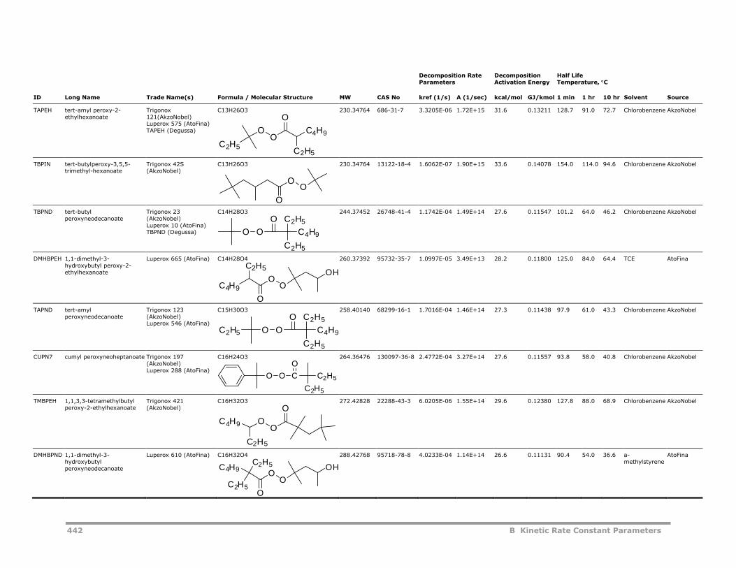
442 B Kinetic Rate Constant Parameters
Decomposition RateParameters
DecompositionActivation Energy
Half LifeTemperature, C
ID Long Name Trade Name(s) Formula / Molecular Structure MW CAS No kref (1/s) A (1/sec) kcal/mol GJ/kmol 1 min 1 hr 10 hr Solvent Source
TAPEH tert-amyl peroxy-2-ethylhexanoate
Trigonox121(AkzoNobel)Luperox 575 (AtoFina)TAPEH (Degussa)
C13H26O3 230.34764 686-31-7 3.3205E-06 1.72E+15 31.6 0.13211 128.7 91.0 72.7 Chlorobenzene AkzoNobel
TBPIN tert-butylperoxy-3,5,5-trimethyl-hexanoate
Trigonox 42S(AkzoNobel)
C13H26O3 230.34764 13122-18-4 1.6062E-07 1.90E+15 33.6 0.14078 154.0 114.0 94.6 Chlorobenzene AkzoNobel
TBPND tert-butylperoxyneodecanoate
Trigonox 23(AkzoNobel)Luperox 10 (AtoFina)TBPND (Degussa)
C14H28O3 244.37452 26748-41-4 1.1742E-04 1.49E+14 27.6 0.11547 101.2 64.0 46.2 Chlorobenzene AkzoNobel
DMHBPEH 1,1-dimethyl-3-hydroxybutyl peroxy-2-ethylhexanoate
Luperox 665 (AtoFina) C14H28O4 260.37392 95732-35-7 1.0997E-05 3.49E+13 28.2 0.11800 125.0 84.0 64.4 TCE AtoFina
TAPND tert-amylperoxyneodecanoate
Trigonox 123(AkzoNobel)Luperox 546 (AtoFina)
C15H30O3 258.40140 68299-16-1 1.7016E-04 1.46E+14 27.3 0.11438 97.9 61.0 43.3 Chlorobenzene AkzoNobel
CUPN7 cumyl peroxyneoheptanoate Trigonox 197(AkzoNobel)Luperox 288 (AtoFina)
C16H24O3 264.36476 130097-36-8 2.4772E-04 3.27E+14 27.6 0.11557 93.8 58.0 40.8 Chlorobenzene AkzoNobel
TMBPEH 1,1,3,3-tetramethylbutylperoxy-2-ethylhexanoate
Trigonox 421(AkzoNobel)
C16H32O3 272.42828 22288-43-3 6.0205E-06 1.55E+14 29.6 0.12380 127.8 88.0 68.9 Chlorobenzene AkzoNobel
DMHBPND 1,1-dimethyl-3-hydroxybutylperoxyneodecanoate
Luperox 610 (AtoFina) C16H32O4 288.42768 95718-78-8 4.0233E-04 1.14E+14 26.6 0.11131 90.4 54.0 36.6 a-methylstyrene
AtoFina
OO
C2H5
O
C4H9
C2H5
OO
O
O O
O
C2H5
C4H9
C2H5
OO
C4H9
C2H5
O
OH
O O
C2H5
C2H5
C4H9C2H5
O
C2H5
C2H5
CO
O
O
OO
O
C4H9
C2H5
OO
C2H5
C2H5C4H9
O
OH
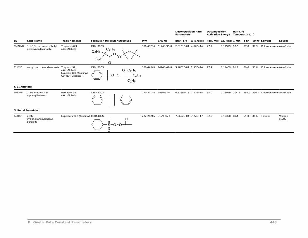
B Kinetic Rate Constant Parameters 443
Decomposition RateParameters
DecompositionActivation Energy
Half LifeTemperature, C
ID Long Name Trade Name(s) Formula / Molecular Structure MW CAS No kref (1/s) A (1/sec) kcal/mol GJ/kmol 1 min 1 hr 10 hr Solvent Source
TMBPND 1,1,3,3,-tetramethylbutylperoxyneodecanoate
Triganox 423(AkzoNobel)
C18H36O3 300.48204 51240-95-0 2.8151E-04 4.02E+14 27.7 0.11579 92.5 57.0 39.9 Chlorobenzene AkzoNobel
CUPND cumyl peroxyneodecanoate Trigonox 99(AkzoNobel)Luperox 188 (AtoFina)CUPND (Degussa)
C19H30O3 306.44540 26748-47-0 3.1832E-04 2.95E+14 27.4 0.11459 91.7 56.0 38.8 Chlorobenzene AkzoNobel
C-C Initiators
DMDPB 2,3-dimethyl-2,3-diphenylbutane
Perkadox 30(AkzoNobel)
C18H22O2 270.37148 1889-67-4 6.1389E-18 7.57E+18 55.0 0.23019 304.5 259.0 236.4 Chlorobenzene AkzoNobel
Sulfonyl Peroxides
ACHSP acetylcyclohexanesulphonylperoxide
Lupersol 228Z (AtoFina) C8H14O5S 222.26216 3179-56-4 7.3692E-04 7.27E+17 32.0 0.13390 80.1 51.0 36.6 Toluene Warson(1980)
OO
C2H5
C2H5C4H9
O
O O
C2H5
C2H5
C4H9
O
S
O
O
O O
O
444 B Kinetic Rate Constant Parameters
ReferencesNote: Anonymous data sources from the internet are documented by thevendor name and the year in which the data were collected.
AkzoNobel (2004). Initiators for Polymer Production, Product Catalog.
AtoFina (2004). Organic Peroxides, General Catalog.
AtoFina (2004). Organic Peroxides, Product Bulletin, Diacyl Peroxides.
AtoFina (2004). Organic Peroxides, Product Bulletin, Dialkyl Peroxides.
AtoFina (2004). Organic Peroxides, Product Bulletin, Peroxydicarbonates.
AtoFina (2004). Organic Peroxides, Product Bulletin, Tertiary AlkylHydroperoxides.
AtoFina (2004). Fine Chemicals Technical Data.
Degussa (2004). Technical Information. Half-Life Times of Organic Peroxides.
Dupont (2004). Vazo Free radical initiators.(http://www.dupont.com/vazo/grades.html)
Masson, J.C. (1989). Decomposition Rates of Organic Free Radical Initiators.Polymer Handbook, 3rd Edition. New York.
Wako Chemical (2004). Water Soluble Azo-Initiator.(http://www.wako-chem.co.jp/specialty/waterazo/main.htm)
Wako Chemical (2004). Solvent Soluble Azo-Initiator.(http://www.wako-chem.co.jp/specialty/oilazo/main.htm)
Warson, H. (1980). Per-Compounds and Per-Salts in Polymer Processes.England: Solihull Chemical Services, 5-17.
C Fortran Utilities 445
C Fortran Utilities
For descriptions of Fortran utilities useful in writing user kinetic subroutines,see Chapter 4 of Aspen Plus User Models.

446 C Fortran Utilities
D Input Language Reference 447
D Input Language Reference
This section describes the input language for:
Specifying Components, 447
Specifying Component Attributes, 451
Specifying Attribute Scaling Factors, 453
Requesting Distribution Calculations, 454
Calculating End Use Properties, 454
Specifying Physical Property Inputs, 456
Specifying Step-Growth Polymerization Kinetics, 460
Specifying Free-Radical Polymerization Kinetics, 467
Specifying Emulsion Polymerization Kinetics, 477
Specifying Ziegler-Natta Polymerization Kinetics, 484
Specifying Ionic Polymerization Kinetics, 494
Specifying Segment-Based Polymer Modification Reactions, 501
Specifying ComponentsThis section describes the input language for specifying components.
Naming ComponentsFollowing is the input language used to name components.
Input Language for Components
COMPONENTS cid [cname] [outid] / ...
Input Language Description for Components
COMPONENTS cid Component ID. Used to refer to the component inall subsequent input and is also used to identify thecomponent in the simulation report. Aspen Plusinput language conventions and naming guidelinesapply to this keyword.
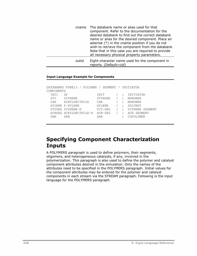
448 D Input Language Reference
cname The databank name or alias used for thatcomponent. Refer to the documentation for thedesired databank to find out the correct databankname or alias for the desired component. Place anasterisk (*) in the cname position if you do notwish to retrieve the component from the databank.Note that in this case you are required to provideall necessary physical property parameters.
outid Eight-character name used for the component inreports. (Default=cid)
Input Language Example for Components
DATABANKS PURE13 / POLYMER / SEGMENT / INITIATORCOMPONENTS
INI1 LP INIT / ; INITIATORSTY STYRENE STYRENE / ; MONOMERCAN ACRYLONITRILE CAN / ; MONOMERXYLENE P-XYLENE XYLENE / ; SOLVENTSTYSEG STYRENE-R STY-SEG / ; STYRENE SEGMENTACNSEG ACRYLONITRILE-R ACN-SEG / ; ACN SEGMENTSAN SAN SAN ; COPOLYMER
Specifying Component CharacterizationInputsA POLYMERS paragraph is used to define polymers, their segments,oligomers, and heterogeneous catalysts, if any, involved in thepolymerization. This paragraph is also used to define the polymer and catalystcomponent attributes desired in the simulation. Only the names of theattributes need to be specified in the POLYMERS paragraph. Initial values forthe component attributes may be entered for the polymer and catalystcomponents in each stream via the STREAM paragraph. Following is the inputlanguage for the POLYMERS paragraph.
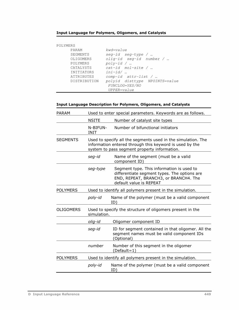
D Input Language Reference 449
Input Language for Polymers, Oligomers, and Catalysts
POLYMERSPARAM kwd=valueSEGMENTS seg-id seg-type / …OLIGOMERS olig-id seg-id number / …POLYMERS poly-id / …CATALYSTS cat-id mol-site / …INITIATORS ini-id/ …ATTRIBUTES comp-id attr-list / …DISTRIBUTION polyid disttype NPOINTS=value
FUNCLOG=YES/NOUPPER=value
Input Language Description for Polymers, Oligomers, and Catalysts
PARAM Used to enter special parameters. Keywords are as follows.
NSITE Number of catalyst site types
N-BIFUN-INIT
Number of bifunctional initiators
SEGMENTS Used to specify all the segments used in the simulation. Theinformation entered through this keyword is used by thesystem to pass segment property information.
seg-id Name of the segment (must be a validcomponent ID)
seg-type Segment type. This information is used todifferentiate segment types. The options areEND, REPEAT, BRANCH3, or BRANCH4. Thedefault value is REPEAT
POLYMERS Used to identify all polymers present in the simulation.
poly-id Name of the polymer (must be a valid componentID)
OLIGOMERS Used to specify the structure of oligomers present in thesimulation.
olig-id Oligomer component ID
seg-id ID for segment contained in that oligomer. All thesegment names must be valid component IDs(Optional)
number Number of this segment in the oligomer(Default=1)
POLYMERS Used to identify all polymers present in the simulation.
poly-id Name of the polymer (must be a valid componentID)
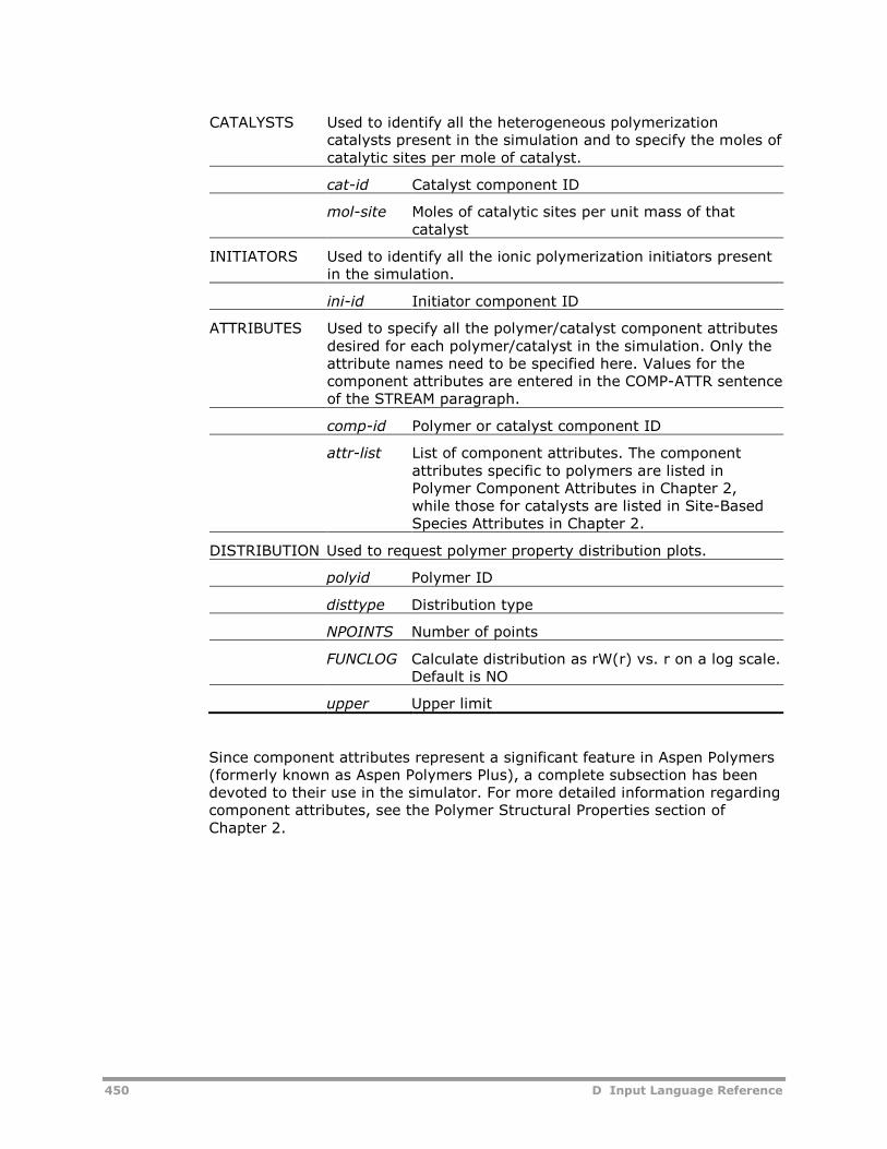
450 D Input Language Reference
CATALYSTS Used to identify all the heterogeneous polymerizationcatalysts present in the simulation and to specify the moles ofcatalytic sites per mole of catalyst.
cat-id Catalyst component ID
mol-site Moles of catalytic sites per unit mass of thatcatalyst
INITIATORS Used to identify all the ionic polymerization initiators presentin the simulation.
ini-id Initiator component ID
ATTRIBUTES Used to specify all the polymer/catalyst component attributesdesired for each polymer/catalyst in the simulation. Only theattribute names need to be specified here. Values for thecomponent attributes are entered in the COMP-ATTR sentenceof the STREAM paragraph.
comp-id Polymer or catalyst component ID
attr-list List of component attributes. The componentattributes specific to polymers are listed inPolymer Component Attributes in Chapter 2,while those for catalysts are listed in Site-BasedSpecies Attributes in Chapter 2.
DISTRIBUTION Used to request polymer property distribution plots.
polyid Polymer ID
disttype Distribution type
NPOINTS Number of points
FUNCLOG Calculate distribution as rW(r) vs. r on a log scale.Default is NO
upper Upper limit
Since component attributes represent a significant feature in Aspen Polymers(formerly known as Aspen Polymers Plus), a complete subsection has beendevoted to their use in the simulator. For more detailed information regardingcomponent attributes, see the Polymer Structural Properties section ofChapter 2.
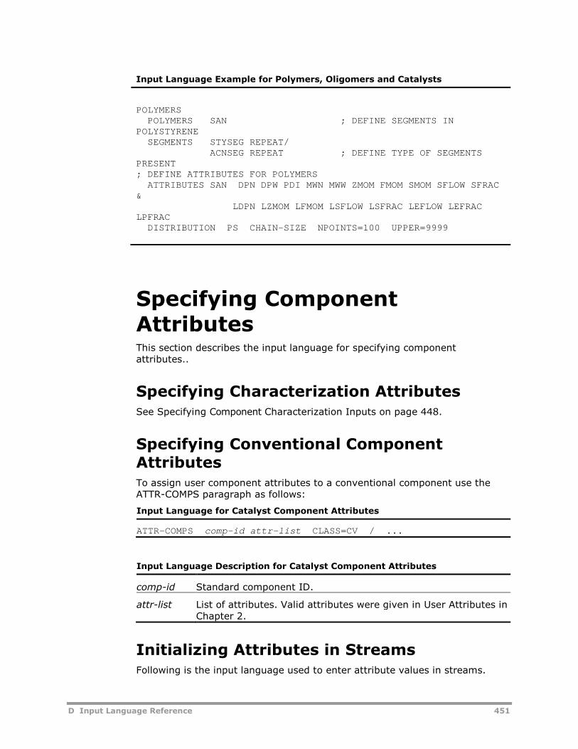
D Input Language Reference 451
Input Language Example for Polymers, Oligomers and Catalysts
POLYMERSPOLYMERS SAN ; DEFINE SEGMENTS IN
POLYSTYRENESEGMENTS STYSEG REPEAT/
ACNSEG REPEAT ; DEFINE TYPE OF SEGMENTSPRESENT; DEFINE ATTRIBUTES FOR POLYMERS
ATTRIBUTES SAN DPN DPW PDI MWN MWW ZMOM FMOM SMOM SFLOW SFRAC&
LDPN LZMOM LFMOM LSFLOW LSFRAC LEFLOW LEFRACLPFRAC
DISTRIBUTION PS CHAIN-SIZE NPOINTS=100 UPPER=9999
Specifying ComponentAttributesThis section describes the input language for specifying componentattributes..
Specifying Characterization AttributesSee Specifying Component Characterization Inputs on page 448.
Specifying Conventional ComponentAttributesTo assign user component attributes to a conventional component use theATTR-COMPS paragraph as follows:
Input Language for Catalyst Component Attributes
ATTR-COMPS comp-id attr-list CLASS=CV / ...
Input Language Description for Catalyst Component Attributes
comp-id Standard component ID.
attr-list List of attributes. Valid attributes were given in User Attributes inChapter 2.
Initializing Attributes in StreamsFollowing is the input language used to enter attribute values in streams.
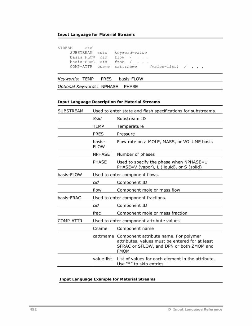
452 D Input Language Reference
Input Language for Material Streams
STREAM sidSUBSTREAM ssid keyword=valuebasis-FLOW cid flow / . . .basis-FRAC cid frac / . . .COMP-ATTR cname cattrname (value-list) / . . .
Keywords: TEMP PRES basis-FLOW
Optional Keywords: NPHASE PHASE
Input Language Description for Material Streams
SUBSTREAM Used to enter state and flash specifications for substreams.
Ssid Substream ID
TEMP Temperature
PRES Pressure
basis-FLOW
Flow rate on a MOLE, MASS, or VOLUME basis
NPHASE Number of phases
PHASE Used to specify the phase when NPHASE=1PHASE=V (vapor), L (liquid), or S (solid)
basis-FLOW Used to enter component flows.
cid Component ID
flow Component mole or mass flow
basis-FRAC Used to enter component fractions.
cid Component ID
frac Component mole or mass fraction
COMP-ATTR Used to enter component attribute values.
Cname Component name
cattrname Component attribute name. For polymerattributes, values must be entered for at leastSFRAC or SFLOW, and DPN or both ZMOM andFMOM
value-list List of values for each element in the attribute.Use “*” to skip entries
Input Language Example for Material Streams
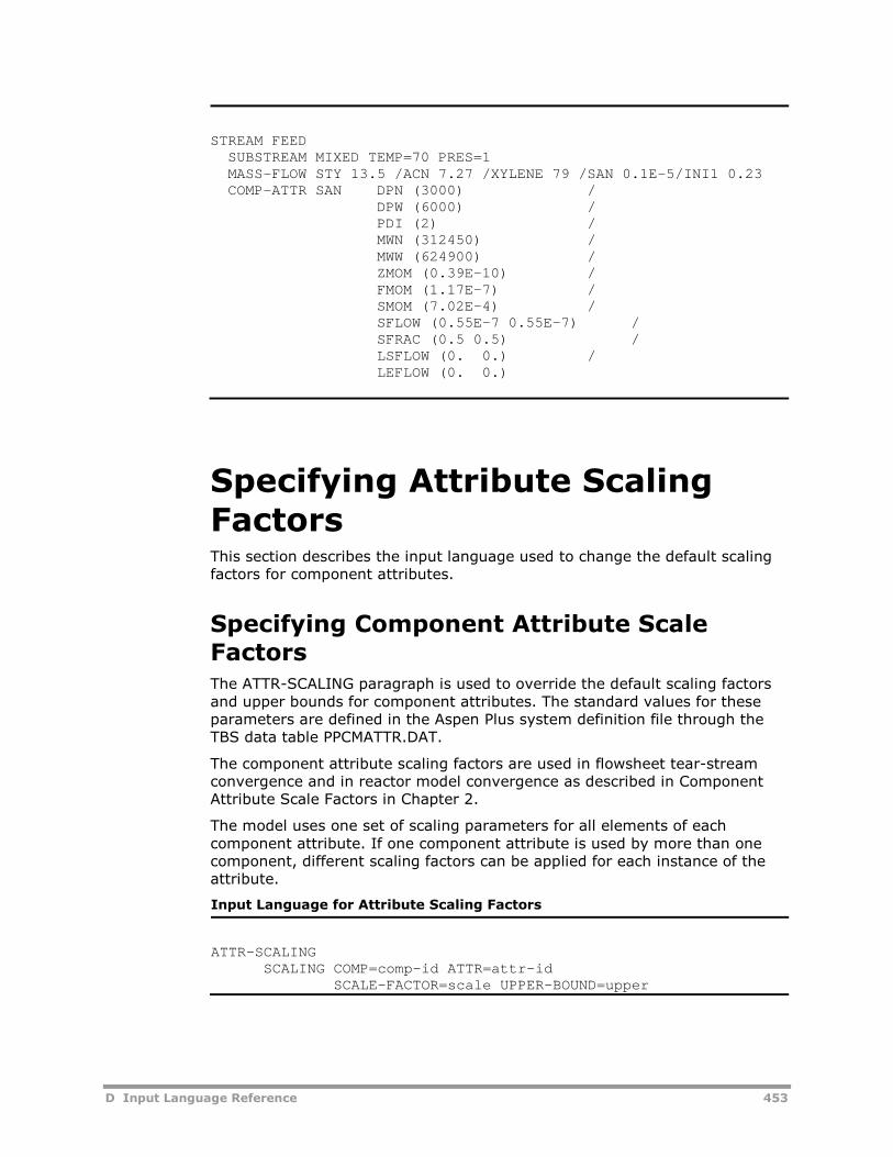
D Input Language Reference 453
STREAM FEEDSUBSTREAM MIXED TEMP=70 PRES=1MASS-FLOW STY 13.5 /ACN 7.27 /XYLENE 79 /SAN 0.1E-5/INI1 0.23COMP-ATTR SAN DPN (3000) /
DPW (6000) /PDI (2) /MWN (312450) /MWW (624900) /ZMOM (0.39E-10) /FMOM (1.17E-7) /SMOM (7.02E-4) /SFLOW (0.55E-7 0.55E-7) /SFRAC (0.5 0.5) /LSFLOW (0. 0.) /LEFLOW (0. 0.)
Specifying Attribute ScalingFactorsThis section describes the input language used to change the default scalingfactors for component attributes.
Specifying Component Attribute ScaleFactorsThe ATTR-SCALING paragraph is used to override the default scaling factorsand upper bounds for component attributes. The standard values for theseparameters are defined in the Aspen Plus system definition file through theTBS data table PPCMATTR.DAT.
The component attribute scaling factors are used in flowsheet tear-streamconvergence and in reactor model convergence as described in ComponentAttribute Scale Factors in Chapter 2.
The model uses one set of scaling parameters for all elements of eachcomponent attribute. If one component attribute is used by more than onecomponent, different scaling factors can be applied for each instance of theattribute.
Input Language for Attribute Scaling Factors
ATTR-SCALINGSCALING COMP=comp-id ATTR=attr-id
SCALE-FACTOR=scale UPPER-BOUND=upper
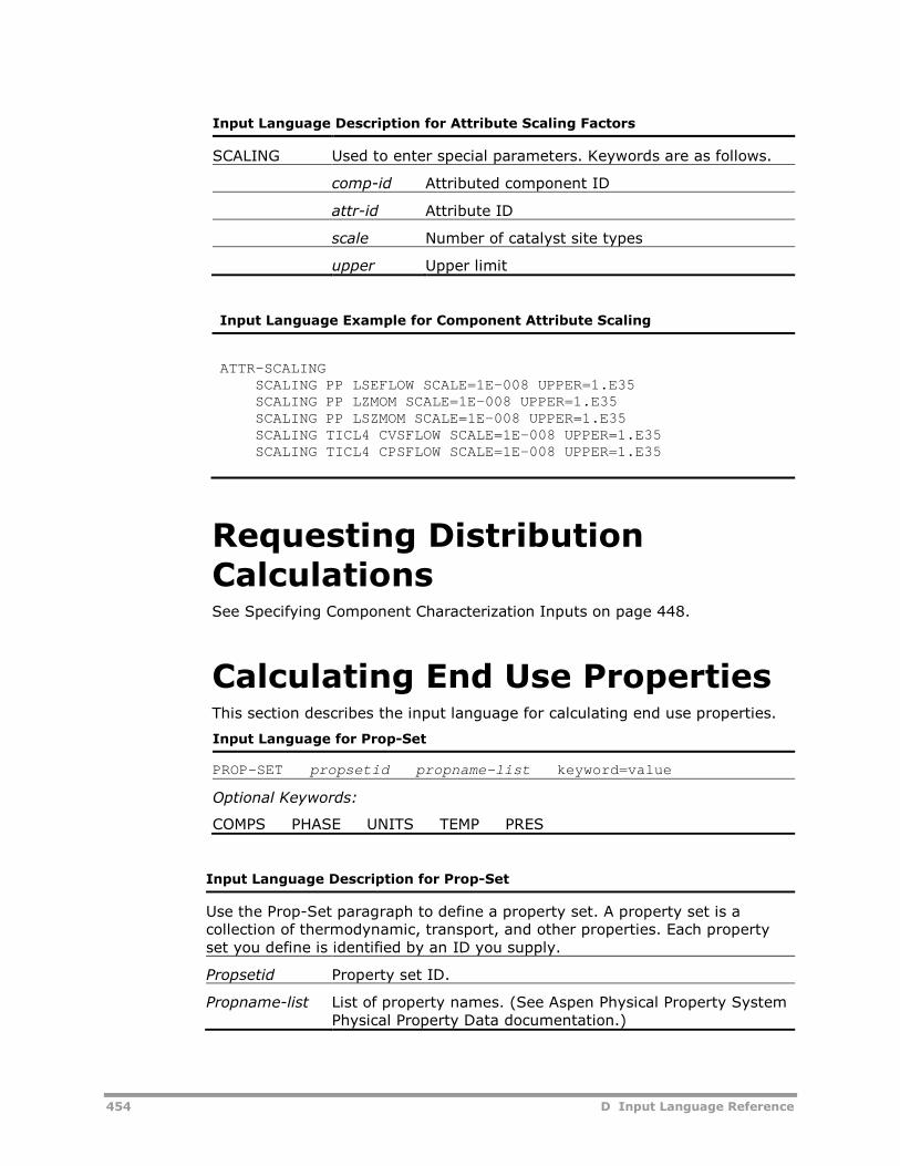
454 D Input Language Reference
Input Language Description for Attribute Scaling Factors
SCALING Used to enter special parameters. Keywords are as follows.
comp-id Attributed component ID
attr-id Attribute ID
scale Number of catalyst site types
upper Upper limit
Input Language Example for Component Attribute Scaling
ATTR-SCALINGSCALING PP LSEFLOW SCALE=1E-008 UPPER=1.E35SCALING PP LZMOM SCALE=1E-008 UPPER=1.E35SCALING PP LSZMOM SCALE=1E-008 UPPER=1.E35SCALING TICL4 CVSFLOW SCALE=1E-008 UPPER=1.E35SCALING TICL4 CPSFLOW SCALE=1E-008 UPPER=1.E35
Requesting DistributionCalculationsSee Specifying Component Characterization Inputs on page 448.
Calculating End Use PropertiesThis section describes the input language for calculating end use properties.
Input Language for Prop-Set
PROP-SET propsetid propname-list keyword=value
Optional Keywords:
COMPS PHASE UNITS TEMP PRES
Input Language Description for Prop-Set
Use the Prop-Set paragraph to define a property set. A property set is acollection of thermodynamic, transport, and other properties. Each propertyset you define is identified by an ID you supply.
Propsetid Property set ID.
Propname-list List of property names. (See Aspen Physical Property SystemPhysical Property Data documentation.)
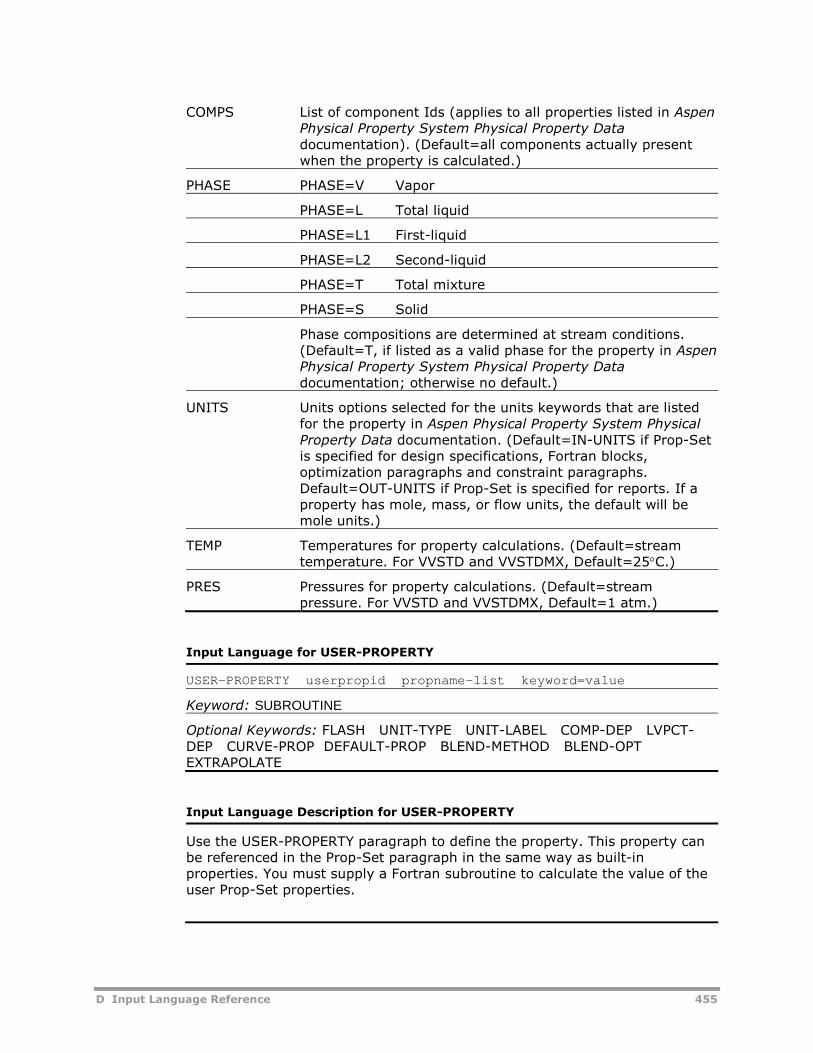
D Input Language Reference 455
COMPS List of component Ids (applies to all properties listed in AspenPhysical Property System Physical Property Datadocumentation). (Default=all components actually presentwhen the property is calculated.)
PHASE PHASE=V Vapor
PHASE=L Total liquid
PHASE=L1 First-liquid
PHASE=L2 Second-liquid
PHASE=T Total mixture
PHASE=S Solid
Phase compositions are determined at stream conditions.(Default=T, if listed as a valid phase for the property in AspenPhysical Property System Physical Property Datadocumentation; otherwise no default.)
UNITS Units options selected for the units keywords that are listedfor the property in Aspen Physical Property System PhysicalProperty Data documentation. (Default=IN-UNITS if Prop-Setis specified for design specifications, Fortran blocks,optimization paragraphs and constraint paragraphs.Default=OUT-UNITS if Prop-Set is specified for reports. If aproperty has mole, mass, or flow units, the default will bemole units.)
TEMP Temperatures for property calculations. (Default=streamtemperature. For VVSTD and VVSTDMX, Default=25C.)
PRES Pressures for property calculations. (Default=streampressure. For VVSTD and VVSTDMX, Default=1 atm.)
Input Language for USER-PROPERTY
USER-PROPERTY userpropid propname-list keyword=value
Keyword: SUBROUTINE
Optional Keywords: FLASH UNIT-TYPE UNIT-LABEL COMP-DEP LVPCT-DEP CURVE-PROP DEFAULT-PROP BLEND-METHOD BLEND-OPTEXTRAPOLATE
Input Language Description for USER-PROPERTY
Use the USER-PROPERTY paragraph to define the property. This property canbe referenced in the Prop-Set paragraph in the same way as built-inproperties. You must supply a Fortran subroutine to calculate the value of theuser Prop-Set properties.
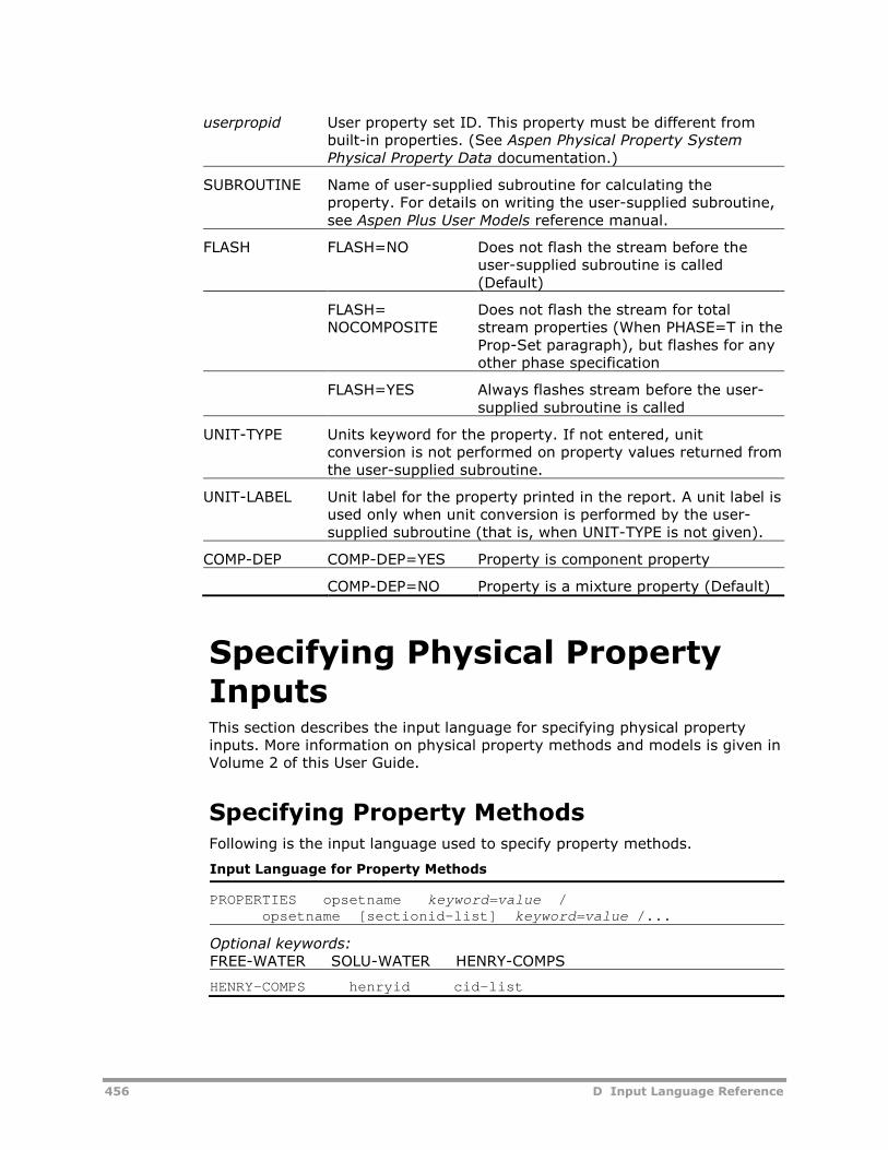
456 D Input Language Reference
userpropid User property set ID. This property must be different frombuilt-in properties. (See Aspen Physical Property SystemPhysical Property Data documentation.)
SUBROUTINE Name of user-supplied subroutine for calculating theproperty. For details on writing the user-supplied subroutine,see Aspen Plus User Models reference manual.
FLASH FLASH=NO Does not flash the stream before theuser-supplied subroutine is called(Default)
FLASH=NOCOMPOSITE
Does not flash the stream for totalstream properties (When PHASE=T in theProp-Set paragraph), but flashes for anyother phase specification
FLASH=YES Always flashes stream before the user-supplied subroutine is called
UNIT-TYPE Units keyword for the property. If not entered, unitconversion is not performed on property values returned fromthe user-supplied subroutine.
UNIT-LABEL Unit label for the property printed in the report. A unit label isused only when unit conversion is performed by the user-supplied subroutine (that is, when UNIT-TYPE is not given).
COMP-DEP COMP-DEP=YES Property is component property
COMP-DEP=NO Property is a mixture property (Default)
Specifying Physical PropertyInputsThis section describes the input language for specifying physical propertyinputs. More information on physical property methods and models is given inVolume 2 of this User Guide.
Specifying Property MethodsFollowing is the input language used to specify property methods.
Input Language for Property Methods
PROPERTIES opsetname keyword=value /opsetname [sectionid-list] keyword=value /...
Optional keywords:FREE-WATER SOLU-WATER HENRY-COMPS
HENRY-COMPS henryid cid-list
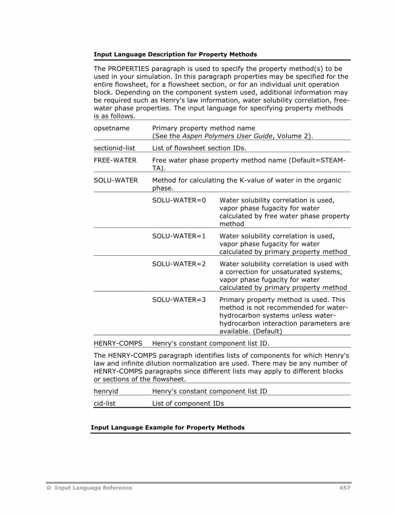
D Input Language Reference 457
Input Language Description for Property Methods
The PROPERTIES paragraph is used to specify the property method(s) to beused in your simulation. In this paragraph properties may be specified for theentire flowsheet, for a flowsheet section, or for an individual unit operationblock. Depending on the component system used, additional information maybe required such as Henry's law information, water solubility correlation, free-water phase properties. The input language for specifying property methodsis as follows.
opsetname Primary property method name(See the Aspen Polymers User Guide, Volume 2).
sectionid-list List of flowsheet section IDs.
FREE-WATER Free water phase property method name (Default=STEAM-TA).
SOLU-WATER Method for calculating the K-value of water in the organicphase.
SOLU-WATER=0 Water solubility correlation is used,vapor phase fugacity for watercalculated by free water phase propertymethod
SOLU-WATER=1 Water solubility correlation is used,vapor phase fugacity for watercalculated by primary property method
SOLU-WATER=2 Water solubility correlation is used witha correction for unsaturated systems,vapor phase fugacity for watercalculated by primary property method
SOLU-WATER=3 Primary property method is used. Thismethod is not recommended for water-hydrocarbon systems unless water-hydrocarbon interaction parameters areavailable. (Default)
HENRY-COMPS Henry's constant component list ID.
The HENRY-COMPS paragraph identifies lists of components for which Henry'slaw and infinite dilution normalization are used. There may be any number ofHENRY-COMPS paragraphs since different lists may apply to different blocksor sections of the flowsheet.
henryid Henry's constant component list ID
cid-list List of component IDs
Input Language Example for Property Methods
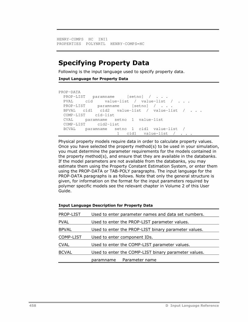
458 D Input Language Reference
HENRY-COMPS HC INI1PROPERTIES POLYNRTL HENRY-COMPS=HC
Specifying Property DataFollowing is the input language used to specify property data.
Input Language for Property Data
PROP-DATAPROP-LIST paramname [setno] / . . .PVAL cid value-list / value-list / . . .PROP-LIST paramname [setno] / . . .BPVAL cid1 cid2 value-list / value-list / . . .COMP-LIST cid-listCVAL paramname setno 1 value-listCOMP-LIST cid2-listBCVAL paramname setno 1 cid1 value-list /
1 cid1 value-list / . . .
Physical property models require data in order to calculate property values.Once you have selected the property method(s) to be used in your simulation,you must determine the parameter requirements for the models contained inthe property method(s), and ensure that they are available in the databanks.If the model parameters are not available from the databanks, you mayestimate them using the Property Constant Estimation System, or enter themusing the PROP-DATA or TAB-POLY paragraphs. The input language for thePROP-DATA paragraphs is as follows. Note that only the general structure isgiven, for information on the format for the input parameters required bypolymer specific models see the relevant chapter in Volume 2 of this UserGuide.
Input Language Description for Property Data
PROP-LIST Used to enter parameter names and data set numbers.
PVAL Used to enter the PROP-LIST parameter values.
BPVAL Used to enter the PROP-LIST binary parameter values.
COMP-LIST Used to enter component IDs.
CVAL Used to enter the COMP-LIST parameter values.
BCVAL Used to enter the COMP-LIST binary parameter values.
paramname Parameter name
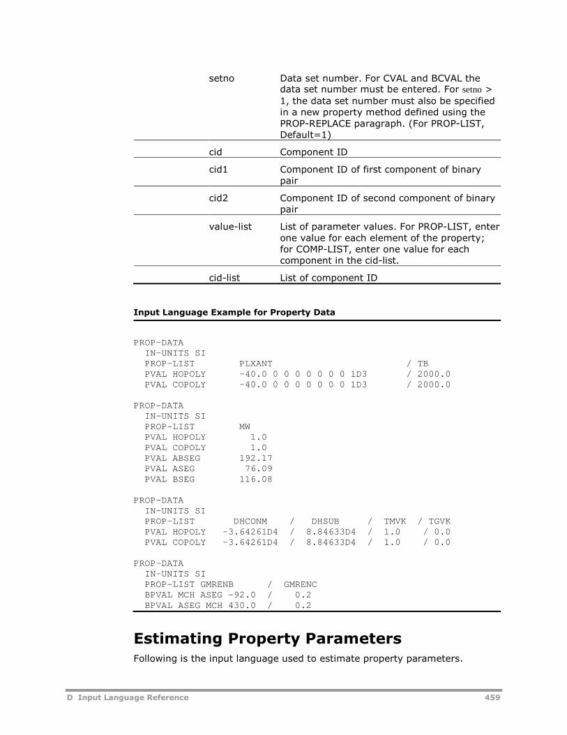
D Input Language Reference 459
setno Data set number. For CVAL and BCVAL thedata set number must be entered. For setno >
1, the data set number must also be specifiedin a new property method defined using thePROP-REPLACE paragraph. (For PROP-LIST,Default=1)
cid Component ID
cid1 Component ID of first component of binarypair
cid2 Component ID of second component of binarypair
value-list List of parameter values. For PROP-LIST, enterone value for each element of the property;for COMP-LIST, enter one value for eachcomponent in the cid-list.
cid-list List of component ID
Input Language Example for Property Data
PROP-DATAIN-UNITS SIPROP-LIST PLXANT / TBPVAL HOPOLY -40.0 0 0 0 0 0 0 0 1D3 / 2000.0PVAL COPOLY -40.0 0 0 0 0 0 0 0 1D3 / 2000.0
PROP-DATAIN-UNITS SIPROP-LIST MWPVAL HOPOLY 1.0PVAL COPOLY 1.0PVAL ABSEG 192.17PVAL ASEG 76.09PVAL BSEG 116.08
PROP-DATAIN-UNITS SIPROP-LIST DHCONM / DHSUB / TMVK / TGVKPVAL HOPOLY -3.64261D4 / 8.84633D4 / 1.0 / 0.0PVAL COPOLY -3.64261D4 / 8.84633D4 / 1.0 / 0.0
PROP-DATAIN-UNITS SIPROP-LIST GMRENB / GMRENCBPVAL MCH ASEG -92.0 / 0.2BPVAL ASEG MCH 430.0 / 0.2
Estimating Property ParametersFollowing is the input language used to estimate property parameters.
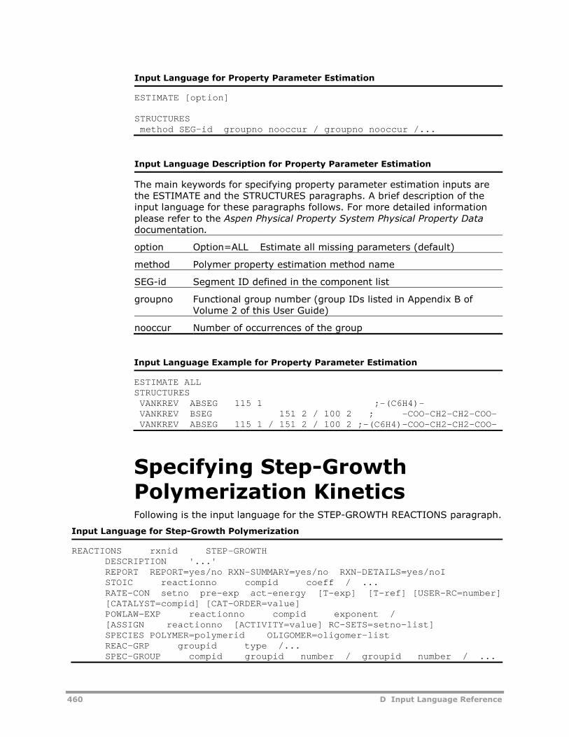
460 D Input Language Reference
Input Language for Property Parameter Estimation
ESTIMATE [option]
STRUCTURESmethod SEG-id groupno nooccur / groupno nooccur /...
Input Language Description for Property Parameter Estimation
The main keywords for specifying property parameter estimation inputs arethe ESTIMATE and the STRUCTURES paragraphs. A brief description of theinput language for these paragraphs follows. For more detailed informationplease refer to the Aspen Physical Property System Physical Property Datadocumentation.
option Option=ALL Estimate all missing parameters (default)
method Polymer property estimation method name
SEG-id Segment ID defined in the component list
groupno Functional group number (group IDs listed in Appendix B ofVolume 2 of this User Guide)
nooccur Number of occurrences of the group
Input Language Example for Property Parameter Estimation
ESTIMATE ALLSTRUCTURESVANKREV ABSEG 115 1 ;-(C6H4)-VANKREV BSEG 151 2 / 100 2 ; -COO-CH2-CH2-COO-VANKREV ABSEG 115 1 / 151 2 / 100 2 ;-(C6H4)-COO-CH2-CH2-COO-
Specifying Step-GrowthPolymerization KineticsFollowing is the input language for the STEP-GROWTH REACTIONS paragraph.
Input Language for Step-Growth Polymerization
REACTIONS rxnid STEP-GROWTHDESCRIPTION '...'REPORT REPORT=yes/no RXN-SUMMARY=yes/no RXN-DETAILS=yes/noISTOIC reactionno compid coeff / ...RATE-CON setno pre-exp act-energy [T-exp] [T-ref] [USER-RC=number][CATALYST=compid] [CAT-ORDER=value]POWLAW-EXP reactionno compid exponent /[ASSIGN reactionno [ACTIVITY=value] RC-SETS=setno-list]SPECIES POLYMER=polymerid OLIGOMER=oligomer-listREAC-GRP groupid type /...SPEC-GROUP compid groupid number / groupid number / ...
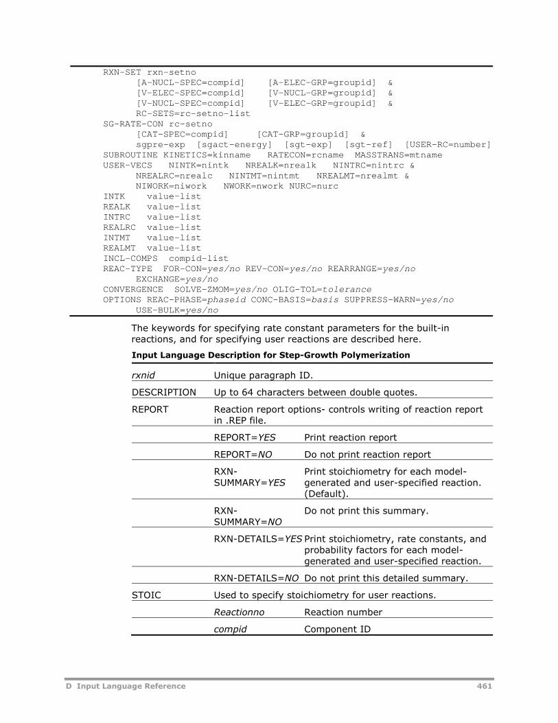
D Input Language Reference 461
RXN-SET rxn-setno[A-NUCL-SPEC=compid] [A-ELEC-GRP=groupid] &[V-ELEC-SPEC=compid] [V-NUCL-GRP=groupid] &[V-NUCL-SPEC=compid] [V-ELEC-GRP=groupid] &RC-SETS=rc-setno-list
SG-RATE-CON rc-setno[CAT-SPEC=compid] [CAT-GRP=groupid] &sgpre-exp [sgact-energy] [sgt-exp] [sgt-ref] [USER-RC=number]
SUBROUTINE KINETICS=kinname RATECON=rcname MASSTRANS=mtnameUSER-VECS NINTK=nintk NREALK=nrealk NINTRC=nintrc &
NREALRC=nrealc NINTMT=nintmt NREALMT=nrealmt &NIWORK=niwork NWORK=nwork NURC=nurc
INTK value-listREALK value-listINTRC value-listREALRC value-listINTMT value-listREALMT value-listINCL-COMPS compid-listREAC-TYPE FOR-CON=yes/no REV-CON=yes/no REARRANGE=yes/no
EXCHANGE=yes/noCONVERGENCE SOLVE-ZMOM=yes/no OLIG-TOL=toleranceOPTIONS REAC-PHASE=phaseid CONC-BASIS=basis SUPPRESS-WARN=yes/no
USE-BULK=yes/no
The keywords for specifying rate constant parameters for the built-inreactions, and for specifying user reactions are described here.
Input Language Description for Step-Growth Polymerization
rxnid Unique paragraph ID.
DESCRIPTION Up to 64 characters between double quotes.
REPORT Reaction report options- controls writing of reaction reportin .REP file.
REPORT=YES Print reaction report
REPORT=NO Do not print reaction report
RXN-SUMMARY=YES
Print stoichiometry for each model-generated and user-specified reaction.(Default).
RXN-SUMMARY=NO
Do not print this summary.
RXN-DETAILS=YES Print stoichiometry, rate constants, andprobability factors for each model-generated and user-specified reaction.
RXN-DETAILS=NO Do not print this detailed summary.
STOIC Used to specify stoichiometry for user reactions.
Reactionno Reaction number
compid Component ID
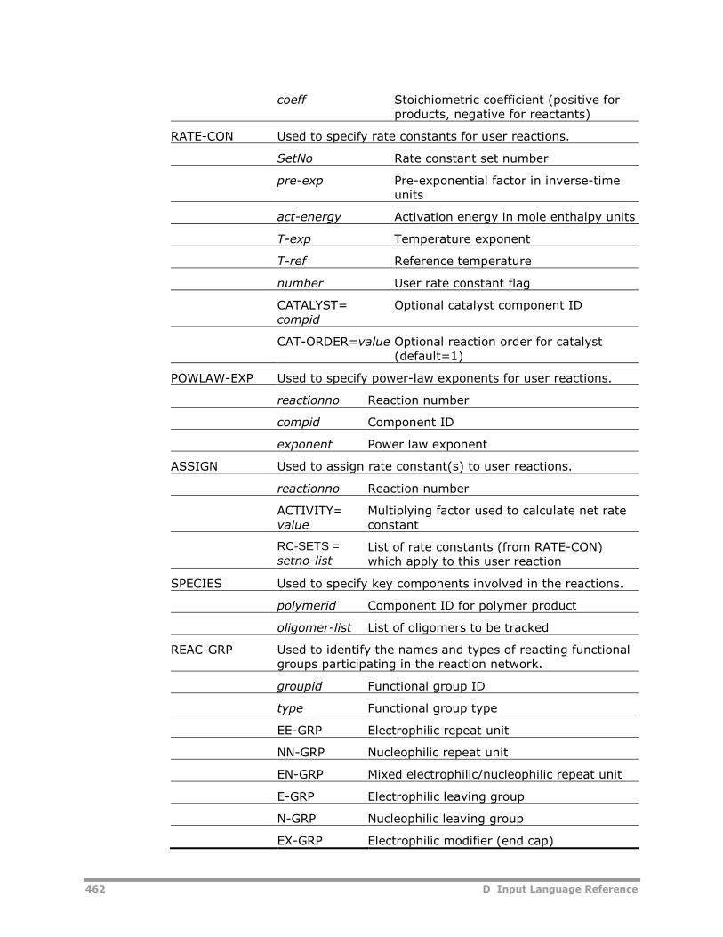
462 D Input Language Reference
coeff Stoichiometric coefficient (positive forproducts, negative for reactants)
RATE-CON Used to specify rate constants for user reactions.
SetNo Rate constant set number
pre-exp Pre-exponential factor in inverse-timeunits
act-energy Activation energy in mole enthalpy units
T-exp Temperature exponent
T-ref Reference temperature
number User rate constant flag
CATALYST=compid
Optional catalyst component ID
CAT-ORDER=value Optional reaction order for catalyst(default=1)
POWLAW-EXP Used to specify power-law exponents for user reactions.
reactionno Reaction number
compid Component ID
exponent Power law exponent
ASSIGN Used to assign rate constant(s) to user reactions.
reactionno Reaction number
ACTIVITY=value
Multiplying factor used to calculate net rateconstant
RC-SETS =setno-list
List of rate constants (from RATE-CON)which apply to this user reaction
SPECIES Used to specify key components involved in the reactions.
polymerid Component ID for polymer product
oligomer-list List of oligomers to be tracked
REAC-GRP Used to identify the names and types of reacting functionalgroups participating in the reaction network.
groupid Functional group ID
type Functional group type
EE-GRP Electrophilic repeat unit
NN-GRP Nucleophilic repeat unit
EN-GRP Mixed electrophilic/nucleophilic repeat unit
E-GRP Electrophilic leaving group
N-GRP Nucleophilic leaving group
EX-GRP Electrophilic modifier (end cap)
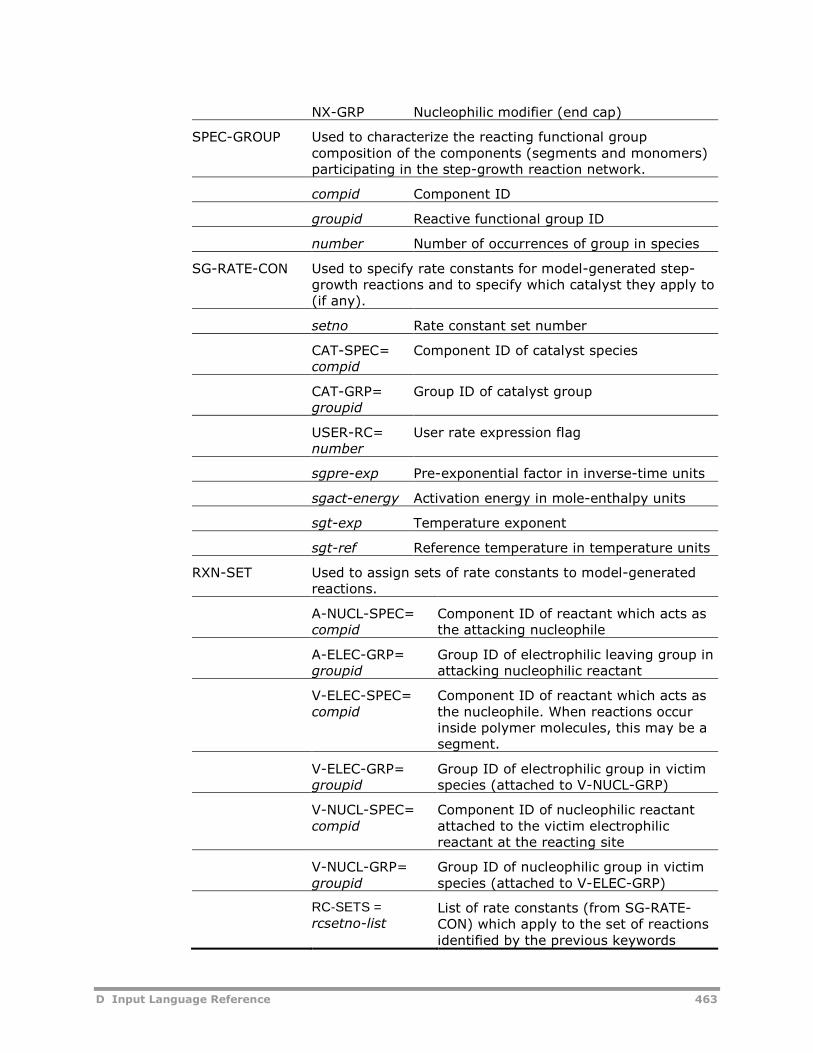
D Input Language Reference 463
NX-GRP Nucleophilic modifier (end cap)
SPEC-GROUP Used to characterize the reacting functional groupcomposition of the components (segments and monomers)participating in the step-growth reaction network.
compid Component ID
groupid Reactive functional group ID
number Number of occurrences of group in species
SG-RATE-CON Used to specify rate constants for model-generated step-growth reactions and to specify which catalyst they apply to(if any).
setno Rate constant set number
CAT-SPEC=compid
Component ID of catalyst species
CAT-GRP=groupid
Group ID of catalyst group
USER-RC=number
User rate expression flag
sgpre-exp Pre-exponential factor in inverse-time units
sgact-energy Activation energy in mole-enthalpy units
sgt-exp Temperature exponent
sgt-ref Reference temperature in temperature units
RXN-SET Used to assign sets of rate constants to model-generatedreactions.
A-NUCL-SPEC=compid
Component ID of reactant which acts asthe attacking nucleophile
A-ELEC-GRP=groupid
Group ID of electrophilic leaving group inattacking nucleophilic reactant
V-ELEC-SPEC=compid
Component ID of reactant which acts asthe nucleophile. When reactions occurinside polymer molecules, this may be asegment.
V-ELEC-GRP=groupid
Group ID of electrophilic group in victimspecies (attached to V-NUCL-GRP)
V-NUCL-SPEC=compid
Component ID of nucleophilic reactantattached to the victim electrophilicreactant at the reacting site
V-NUCL-GRP=groupid
Group ID of nucleophilic group in victimspecies (attached to V-ELEC-GRP)
RC-SETS =rcsetno-list
List of rate constants (from SG-RATE-CON) which apply to the set of reactionsidentified by the previous keywords
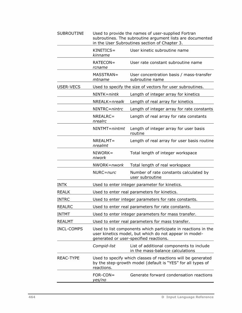
464 D Input Language Reference
SUBROUTINE Used to provide the names of user-supplied Fortransubroutines. The subroutine argument lists are documentedin the User Subroutines section of Chapter 3.
KINETICS=kinname
User kinetic subroutine name
RATECON=rcname
User rate constant subroutine name
MASSTRAN=mtname
User concentration basis / mass-transfersubroutine name
USER-VECS Used to specify the size of vectors for user subroutines.
NINTK=nintk Length of integer array for kinetics
NREALK=nrealk Length of real array for kinetics
NINTRC=nintrc Length of integer array for rate constants
NREALRC=nrealrc
Length of real array for rate constants
NINTMT=nintmt Length of integer array for user basisroutine
NREALMT=nrealmt
Length of real array for user basis routine
NIWORK=niwork
Total length of integer workspace
NWORK=nwork Total length of real workspace
NURC=nurc Number of rate constants calculated byuser subroutine
INTK Used to enter integer parameter for kinetics.
REALK Used to enter real parameters for kinetics.
INTRC Used to enter integer parameters for rate constants.
REALRC Used to enter real parameters for rate constants.
INTMT Used to enter integer parameters for mass transfer.
REALMT Used to enter real parameters for mass transfer.
INCL-COMPS Used to list components which participate in reactions in theuser kinetics model, but which do not appear in model-generated or user-specified reactions.
Compid-list List of additional components to includein the mass-balance calculations
REAC-TYPE Used to specify which classes of reactions will be generatedby the step-growth model (default is “YES” for all types ofreactions.
FOR-CON=yes/no
Generate forward condensation reactions
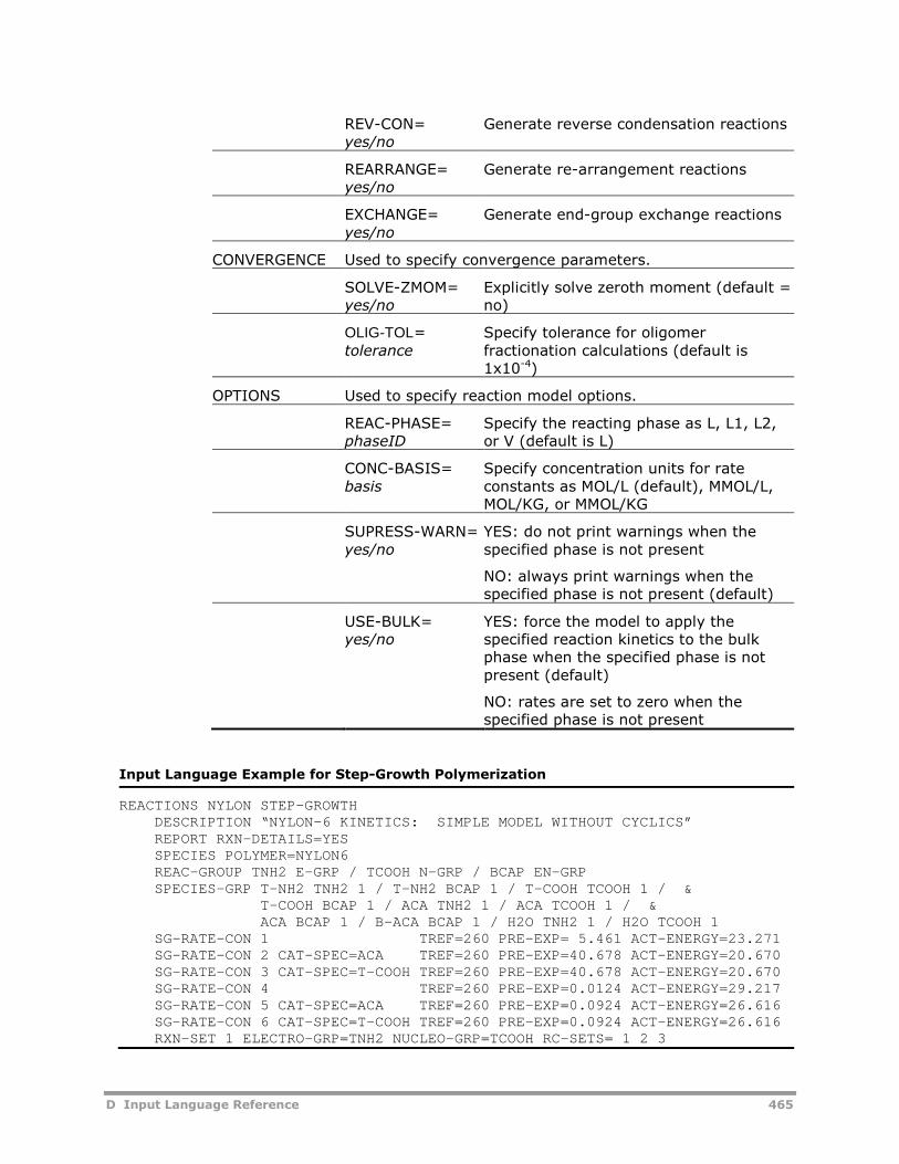
D Input Language Reference 465
REV-CON=yes/no
Generate reverse condensation reactions
REARRANGE=yes/no
Generate re-arrangement reactions
EXCHANGE=yes/no
Generate end-group exchange reactions
CONVERGENCE Used to specify convergence parameters.
SOLVE-ZMOM=yes/no
Explicitly solve zeroth moment (default =no)
OLIG-TOL=tolerance
Specify tolerance for oligomerfractionation calculations (default is1x10-4)
OPTIONS Used to specify reaction model options.
REAC-PHASE=phaseID
Specify the reacting phase as L, L1, L2,or V (default is L)
CONC-BASIS=basis
Specify concentration units for rateconstants as MOL/L (default), MMOL/L,MOL/KG, or MMOL/KG
SUPRESS-WARN=yes/no
YES: do not print warnings when thespecified phase is not present
NO: always print warnings when thespecified phase is not present (default)
USE-BULK=yes/no
YES: force the model to apply thespecified reaction kinetics to the bulkphase when the specified phase is notpresent (default)
NO: rates are set to zero when thespecified phase is not present
Input Language Example for Step-Growth Polymerization
REACTIONS NYLON STEP-GROWTHDESCRIPTION “NYLON-6 KINETICS: SIMPLE MODEL WITHOUT CYCLICS”REPORT RXN-DETAILS=YESSPECIES POLYMER=NYLON6REAC-GROUP TNH2 E-GRP / TCOOH N-GRP / BCAP EN-GRPSPECIES-GRP T-NH2 TNH2 1 / T-NH2 BCAP 1 / T-COOH TCOOH 1 / &
T-COOH BCAP 1 / ACA TNH2 1 / ACA TCOOH 1 / &ACA BCAP 1 / B-ACA BCAP 1 / H2O TNH2 1 / H2O TCOOH 1
SG-RATE-CON 1 TREF=260 PRE-EXP= 5.461 ACT-ENERGY=23.271SG-RATE-CON 2 CAT-SPEC=ACA TREF=260 PRE-EXP=40.678 ACT-ENERGY=20.670SG-RATE-CON 3 CAT-SPEC=T-COOH TREF=260 PRE-EXP=40.678 ACT-ENERGY=20.670SG-RATE-CON 4 TREF=260 PRE-EXP=0.0124 ACT-ENERGY=29.217SG-RATE-CON 5 CAT-SPEC=ACA TREF=260 PRE-EXP=0.0924 ACT-ENERGY=26.616SG-RATE-CON 6 CAT-SPEC=T-COOH TREF=260 PRE-EXP=0.0924 ACT-ENERGY=26.616RXN-SET 1 ELECTRO-GRP=TNH2 NUCLEO-GRP=TCOOH RC-SETS= 1 2 3
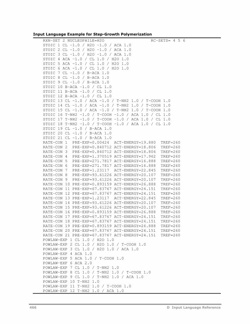
466 D Input Language Reference
Input Language Example for Step-Growth Polymerization
RXN-SET 2 NUCLEOPHILE=H2O RC-SETS= 4 5 6STOIC 1 CL -1.0 / H2O -1.0 / ACA 1.0STOIC 2 CL -1.0 / H2O -1.0 / ACA 1.0STOIC 3 CL -1.0 / H2O -1.0 / ACA 1.0STOIC 4 ACA -1.0 / CL 1.0 / H2O 1.0STOIC 5 ACA -1.0 / CL 1.0 / H2O 1.0STOIC 6 ACA -1.0 / CL 1.0 / H2O 1.0STOIC 7 CL -1.0 / B-ACA 1.0STOIC 8 CL -1.0 / B-ACA 1.0STOIC 9 CL -1.0 / B-ACA 1.0STOIC 10 B-ACA -1.0 / CL 1.0STOIC 11 B-ACA -1.0 / CL 1.0STOIC 12 B-ACA -1.0 / CL 1.0STOIC 13 CL -1.0 / ACA -1.0 / T-NH2 1.0 / T-COOH 1.0STOIC 14 CL -1.0 / ACA -1.0 / T-NH2 1.0 / T-COOH 1.0STOIC 15 CL -1.0 / ACA -1.0 / T-NH2 1.0 / T-COOH 1.0STOIC 16 T-NH2 -1.0 / T-COOH -1.0 / ACA 1.0 / CL 1.0STOIC 17 T-NH2 -1.0 / T-COOH -1.0 / ACA 1.0 / CL 1.0STOIC 18 T-NH2 -1.0 / T-COOH -1.0 / ACA 1.0 / CL 1.0STOIC 19 CL -1.0 / B-ACA 1.0STOIC 20 CL -1.0 / B-ACA 1.0STOIC 21 CL -1.0 / B-ACA 1.0RATE-CON 1 PRE-EXP=0.00424 ACT-ENERGY=19.880 TREF=260RATE-CON 2 PRE-EXP=0.840712 ACT-ENERGY=18.806 TREF=260RATE-CON 3 PRE-EXP=0.840712 ACT-ENERGY=18.806 TREF=260RATE-CON 4 PRE-EXP=1.370519 ACT-ENERGY=17.962 TREF=260RATE-CON 5 PRE-EXP=271.7817 ACT-ENERGY=16.888 TREF=260RATE-CON 6 PRE-EXP=271.7817 ACT-ENERGY=16.888 TREF=260RATE-CON 7 PRE-EXP=1.23117 ACT-ENERGY=22.845 TREF=260RATE-CON 8 PRE-EXP=93.61226 ACT-ENERGY=20.107 TREF=260RATE-CON 9 PRE-EXP=93.61226 ACT-ENERGY=20.107 TREF=260RATE-CON 10 PRE-EXP=0.893159 ACT-ENERGY=26.888 TREF=260RATE-CON 11 PRE-EXP=67.83767 ACT-ENERGY=24.151 TREF=260RATE-CON 12 PRE-EXP=67.83767 ACT-ENERGY=24.151 TREF=260RATE-CON 13 PRE-EXP=1.23117 ACT-ENERGY=22.845 TREF=260RATE-CON 14 PRE-EXP=93.61226 ACT-ENERGY=20.107 TREF=260RATE-CON 15 PRE-EXP=93.61226 ACT-ENERGY=20.107 TREF=260RATE-CON 16 PRE-EXP=0.893159 ACT-ENERGY=26.888 TREF=260RATE-CON 17 PRE-EXP=67.83767 ACT-ENERGY=24.151 TREF=260RATE-CON 18 PRE-EXP=67.83767 ACT-ENERGY=24.151 TREF=260RATE-CON 19 PRE-EXP=0.893159 ACT-ENERGY=26.888 TREF=260RATE-CON 20 PRE-EXP=67.83767 ACT-ENERGY=24.151 TREF=260RATE-CON 21 PRE-EXP=67.83767 ACT-ENERGY=24.151 TREF=260POWLAW-EXP 1 CL 1.0 / H2O 1.0POWLAW-EXP 2 CL 1.0 / H2O 1.0 / T-COOH 1.0POWLAW-EXP 3 CL 1.0 / H2O 1.0 / ACA 1.0POWLAW-EXP 4 ACA 1.0POWLAW-EXP 5 ACA 1.0 / T-COOH 1.0POWLAW-EXP 6 ACA 2.0POWLAW-EXP 7 CL 1.0 / T-NH2 1.0POWLAW-EXP 8 CL 1.0 / T-NH2 1.0 / T-COOH 1.0POWLAW-EXP 9 CL 1.0 / T-NH2 1.0 / ACA 1.0POWLAW-EXP 10 T-NH2 1.0POWLAW-EXP 11 T-NH2 1.0 / T-COOH 1.0POWLAW-EXP 12 T-NH2 1.0 / ACA 1.0
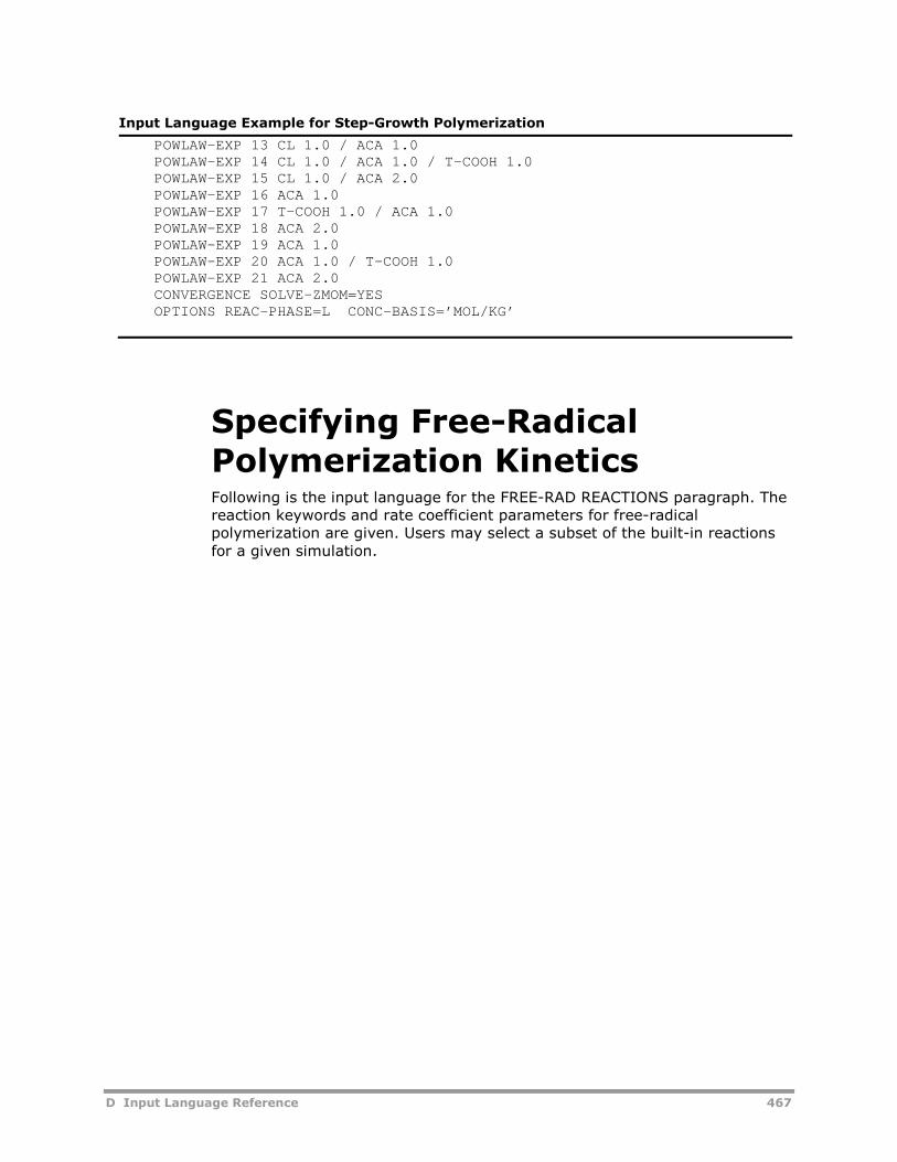
D Input Language Reference 467
Input Language Example for Step-Growth Polymerization
POWLAW-EXP 13 CL 1.0 / ACA 1.0POWLAW-EXP 14 CL 1.0 / ACA 1.0 / T-COOH 1.0POWLAW-EXP 15 CL 1.0 / ACA 2.0POWLAW-EXP 16 ACA 1.0POWLAW-EXP 17 T-COOH 1.0 / ACA 1.0POWLAW-EXP 18 ACA 2.0POWLAW-EXP 19 ACA 1.0POWLAW-EXP 20 ACA 1.0 / T-COOH 1.0POWLAW-EXP 21 ACA 2.0CONVERGENCE SOLVE-ZMOM=YESOPTIONS REAC-PHASE=L CONC-BASIS=’MOL/KG’
Specifying Free-RadicalPolymerization KineticsFollowing is the input language for the FREE-RAD REACTIONS paragraph. Thereaction keywords and rate coefficient parameters for free-radicalpolymerization are given. Users may select a subset of the built-in reactionsfor a given simulation.
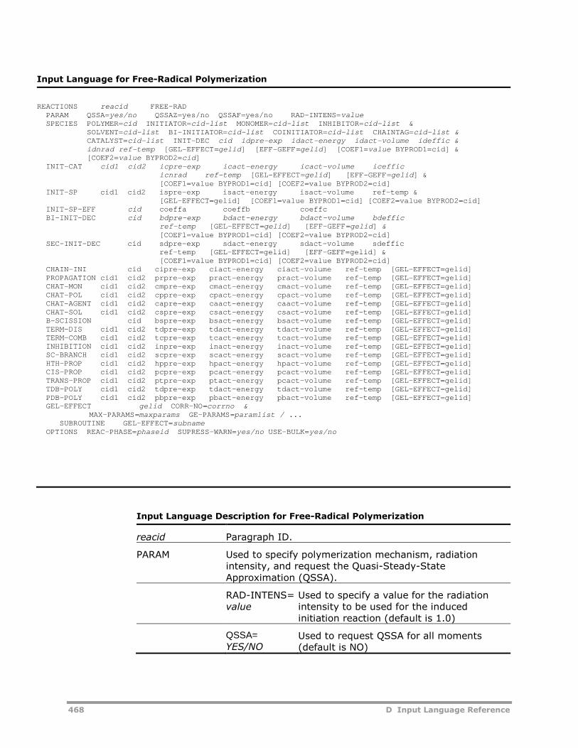
468 D Input Language Reference
Input Language for Free-Radical Polymerization
REACTIONS reacid FREE-RADPARAM QSSA=yes/no QSSAZ=yes/no QSSAF=yes/no RAD-INTENS=valueSPECIES POLYMER=cid INITIATOR=cid-list MONOMER=cid-list INHIBITOR=cid-list &
SOLVENT=cid-list BI-INITIATOR=cid-list COINITIATOR=cid-list CHAINTAG=cid-list &CATALYST=cid-list INIT-DEC cid idpre-exp idact-energy idact-volume ideffic &idnrad ref-temp [GEL-EFFECT=gelid] [EFF-GEFF=gelid] [COEF1=value BYPROD1=cid] &[COEF2=value BYPROD2=cid]
INIT-CAT cid1 cid2 icpre-exp icact-energy icact-volume icefficicnrad ref-temp [GEL-EFFECT=gelid] [EFF-GEFF=gelid] &[COEF1=value BYPROD1=cid] [COEF2=value BYPROD2=cid]
INIT-SP cid1 cid2 ispre-exp isact-energy isact-volume ref-temp &[GEL-EFFECT=gelid] [COEF1=value BYPROD1=cid] [COEF2=value BYPROD2=cid]
INIT-SP-EFF cid coeffa coeffb coeffcBI-INIT-DEC cid bdpre-exp bdact-energy bdact-volume bdeffic
ref-temp [GEL-EFFECT=gelid] [EFF-GEFF=gelid] &[COEF1=value BYPROD1=cid] [COEF2=value BYPROD2=cid]
SEC-INIT-DEC cid sdpre-exp sdact-energy sdact-volume sdefficref-temp [GEL-EFFECT=gelid] [EFF-GEFF=gelid] &[COEF1=value BYPROD1=cid] [COEF2=value BYPROD2=cid]
CHAIN-INI cid cipre-exp ciact-energy ciact-volume ref-temp [GEL-EFFECT=gelid]PROPAGATION cid1 cid2 prpre-exp pract-energy pract-volume ref-temp [GEL-EFFECT=gelid]CHAT-MON cid1 cid2 cmpre-exp cmact-energy cmact-volume ref-temp [GEL-EFFECT=gelid]CHAT-POL cid1 cid2 cppre-exp cpact-energy cpact-volume ref-temp [GEL-EFFECT=gelid]CHAT-AGENT cid1 cid2 capre-exp caact-energy caact-volume ref-temp [GEL-EFFECT=gelid]CHAT-SOL cid1 cid2 cspre-exp csact-energy csact-volume ref-temp [GEL-EFFECT=gelid]B-SCISSION cid bspre-exp bsact-energy bsact-volume ref-temp [GEL-EFFECT=gelid]TERM-DIS cid1 cid2 tdpre-exp tdact-energy tdact-volume ref-temp [GEL-EFFECT=gelid]TERM-COMB cid1 cid2 tcpre-exp tcact-energy tcact-volume ref-temp [GEL-EFFECT=gelid]INHIBITION cid1 cid2 inpre-exp inact-energy inact-volume ref-temp [GEL-EFFECT=gelid]SC-BRANCH cid1 cid2 scpre-exp scact-energy scact-volume ref-temp [GEL-EFFECT=gelid]HTH-PROP cid1 cid2 hppre-exp hpact-energy hpact-volume ref-temp [GEL-EFFECT=gelid]CIS-PROP cid1 cid2 pcpre-exp pcact-energy pcact-volume ref-temp [GEL-EFFECT=gelid]TRANS-PROP cid1 cid2 ptpre-exp ptact-energy pcact-volume ref-temp [GEL-EFFECT=gelid]TDB-POLY cid1 cid2 tdpre-exp tdact-energy tdact-volume ref-temp [GEL-EFFECT=gelid]PDB-POLY cid1 cid2 pbpre-exp pbact-energy pbact-volume ref-temp [GEL-EFFECT=gelid]GEL-EFFECT gelid CORR-NO=corrno &
MAX-PARAMS=maxparams GE-PARAMS=paramlist / ...SUBROUTINE GEL-EFFECT=subname
OPTIONS REAC-PHASE=phaseid SUPRESS-WARN=yes/no USE-BULK=yes/no
Input Language Description for Free-Radical Polymerization
reacid Paragraph ID.
PARAM Used to specify polymerization mechanism, radiationintensity, and request the Quasi-Steady-StateApproximation (QSSA).
RAD-INTENS=value
Used to specify a value for the radiationintensity to be used for the inducedinitiation reaction (default is 1.0)
QSSA=YES/NO
Used to request QSSA for all moments(default is NO)
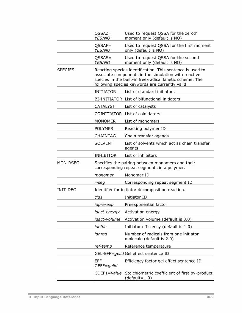
D Input Language Reference 469
QSSAZ=YES/NO
Used to request QSSA for the zerothmoment only (default is NO)
QSSAF=YES/NO
Used to request QSSA for the first momentonly (default is NO)
QSSAS=YES/NO
Used to request QSSA for the secondmoment only (default is NO)
SPECIES Reacting species identification. This sentence is used toassociate components in the simulation with reactivespecies in the built-in free-radical kinetic scheme. Thefollowing species keywords are currently valid
INITIATOR List of standard initiators
BI-INITIATOR List of bifunctional initiators
CATALYST List of catalysts
COINITIATOR List of coinitiators
MONOMER List of monomers
POLYMER Reacting polymer ID
CHAINTAG Chain transfer agends
SOLVENT List of solvents which act as chain transferagents
INHIBITOR List of inhibitors
MON-RSEG Specifies the pairing between monomers and theircorresponding repeat segments in a polymer.
monomer Monomer ID
r-seg Corresponding repeat segment ID
INIT-DEC Identifier for initiator decomposition reaction.
cid1 Initiator ID
idpre-exp Preexponential factor
idact-energy Activation energy
idact-volume Activation volume (default is 0.0)
ideffic Initiator efficiency (default is 1.0)
idnrad Number of radicals from one initiatormolecule (default is 2.0)
ref-temp Reference temperature
GEL-EFF=gelid Gel effect sentence ID
EFF-GEFF=gelid
Efficiency factor gel effect sentence ID
COEF1=value Stoichiometric coefficient of first by-product(default=1.0)
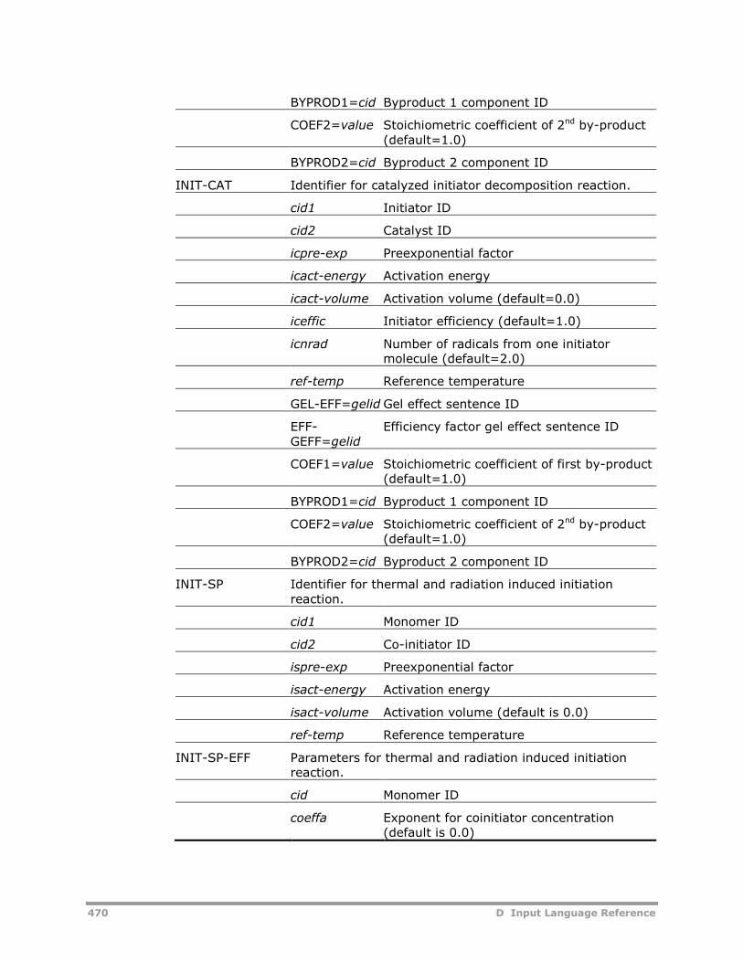
470 D Input Language Reference
BYPROD1=cid Byproduct 1 component ID
COEF2=value Stoichiometric coefficient of 2nd by-product(default=1.0)
BYPROD2=cid Byproduct 2 component ID
INIT-CAT Identifier for catalyzed initiator decomposition reaction.
cid1 Initiator ID
cid2 Catalyst ID
icpre-exp Preexponential factor
icact-energy Activation energy
icact-volume Activation volume (default=0.0)
iceffic Initiator efficiency (default=1.0)
icnrad Number of radicals from one initiatormolecule (default=2.0)
ref-temp Reference temperature
GEL-EFF=gelid Gel effect sentence ID
EFF-GEFF=gelid
Efficiency factor gel effect sentence ID
COEF1=value Stoichiometric coefficient of first by-product(default=1.0)
BYPROD1=cid Byproduct 1 component ID
COEF2=value Stoichiometric coefficient of 2nd by-product(default=1.0)
BYPROD2=cid Byproduct 2 component ID
INIT-SP Identifier for thermal and radiation induced initiationreaction.
cid1 Monomer ID
cid2 Co-initiator ID
ispre-exp Preexponential factor
isact-energy Activation energy
isact-volume Activation volume (default is 0.0)
ref-temp Reference temperature
INIT-SP-EFF Parameters for thermal and radiation induced initiationreaction.
cid Monomer ID
coeffa Exponent for coinitiator concentration(default is 0.0)
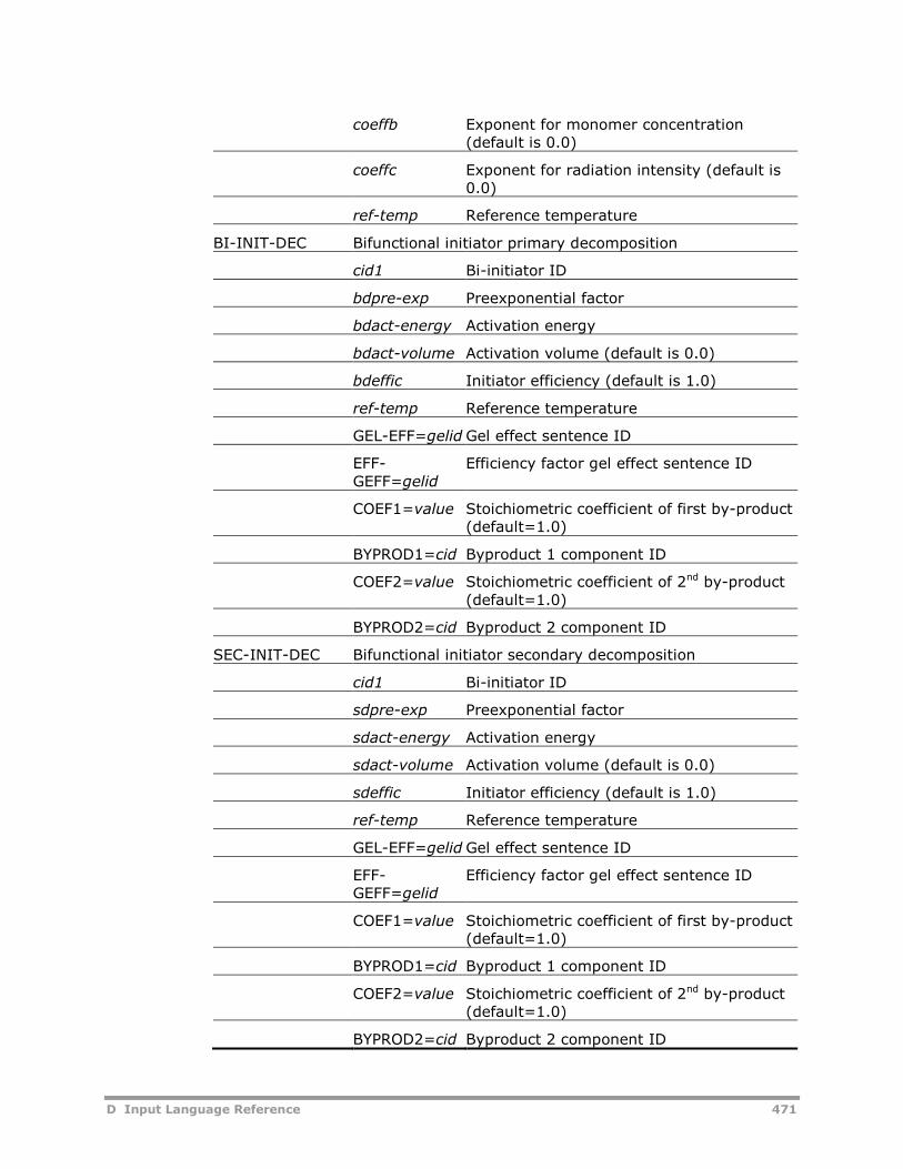
D Input Language Reference 471
coeffb Exponent for monomer concentration(default is 0.0)
coeffc Exponent for radiation intensity (default is0.0)
ref-temp Reference temperature
BI-INIT-DEC Bifunctional initiator primary decomposition
cid1 Bi-initiator ID
bdpre-exp Preexponential factor
bdact-energy Activation energy
bdact-volume Activation volume (default is 0.0)
bdeffic Initiator efficiency (default is 1.0)
ref-temp Reference temperature
GEL-EFF=gelid Gel effect sentence ID
EFF-GEFF=gelid
Efficiency factor gel effect sentence ID
COEF1=value Stoichiometric coefficient of first by-product(default=1.0)
BYPROD1=cid Byproduct 1 component ID
COEF2=value Stoichiometric coefficient of 2nd by-product(default=1.0)
BYPROD2=cid Byproduct 2 component ID
SEC-INIT-DEC Bifunctional initiator secondary decomposition
cid1 Bi-initiator ID
sdpre-exp Preexponential factor
sdact-energy Activation energy
sdact-volume Activation volume (default is 0.0)
sdeffic Initiator efficiency (default is 1.0)
ref-temp Reference temperature
GEL-EFF=gelid Gel effect sentence ID
EFF-GEFF=gelid
Efficiency factor gel effect sentence ID
COEF1=value Stoichiometric coefficient of first by-product(default=1.0)
BYPROD1=cid Byproduct 1 component ID
COEF2=value Stoichiometric coefficient of 2nd by-product(default=1.0)
BYPROD2=cid Byproduct 2 component ID
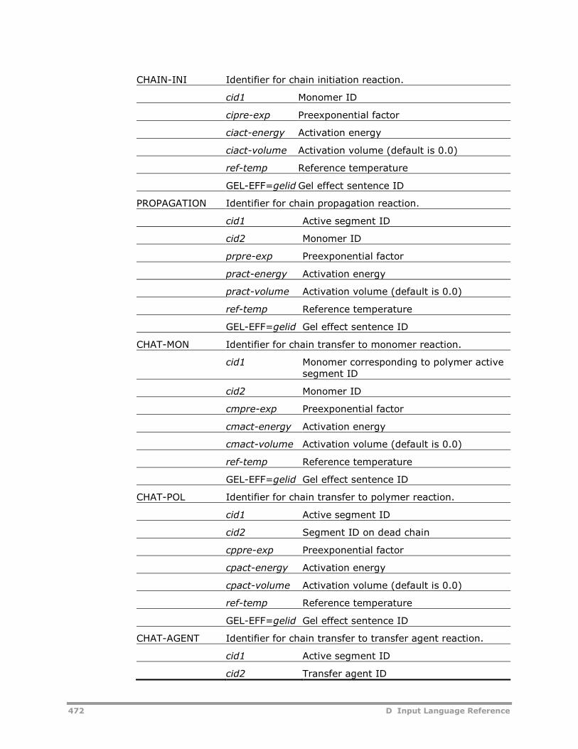
472 D Input Language Reference
CHAIN-INI Identifier for chain initiation reaction.
cid1 Monomer ID
cipre-exp Preexponential factor
ciact-energy Activation energy
ciact-volume Activation volume (default is 0.0)
ref-temp Reference temperature
GEL-EFF=gelid Gel effect sentence ID
PROPAGATION Identifier for chain propagation reaction.
cid1 Active segment ID
cid2 Monomer ID
prpre-exp Preexponential factor
pract-energy Activation energy
pract-volume Activation volume (default is 0.0)
ref-temp Reference temperature
GEL-EFF=gelid Gel effect sentence ID
CHAT-MON Identifier for chain transfer to monomer reaction.
cid1 Monomer corresponding to polymer activesegment ID
cid2 Monomer ID
cmpre-exp Preexponential factor
cmact-energy Activation energy
cmact-volume Activation volume (default is 0.0)
ref-temp Reference temperature
GEL-EFF=gelid Gel effect sentence ID
CHAT-POL Identifier for chain transfer to polymer reaction.
cid1 Active segment ID
cid2 Segment ID on dead chain
cppre-exp Preexponential factor
cpact-energy Activation energy
cpact-volume Activation volume (default is 0.0)
ref-temp Reference temperature
GEL-EFF=gelid Gel effect sentence ID
CHAT-AGENT Identifier for chain transfer to transfer agent reaction.
cid1 Active segment ID
cid2 Transfer agent ID
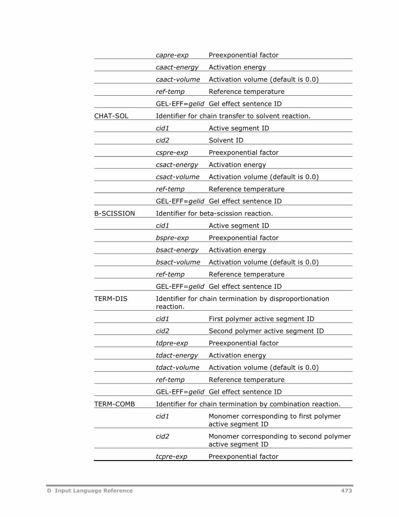
D Input Language Reference 473
capre-exp Preexponential factor
caact-energy Activation energy
caact-volume Activation volume (default is 0.0)
ref-temp Reference temperature
GEL-EFF=gelid Gel effect sentence ID
CHAT-SOL Identifier for chain transfer to solvent reaction.
cid1 Active segment ID
cid2 Solvent ID
cspre-exp Preexponential factor
csact-energy Activation energy
csact-volume Activation volume (default is 0.0)
ref-temp Reference temperature
GEL-EFF=gelid Gel effect sentence ID
B-SCISSION Identifier for beta-scission reaction.
cid1 Active segment ID
bspre-exp Preexponential factor
bsact-energy Activation energy
bsact-volume Activation volume (default is 0.0)
ref-temp Reference temperature
GEL-EFF=gelid Gel effect sentence ID
TERM-DIS Identifier for chain termination by disproportionationreaction.
cid1 First polymer active segment ID
cid2 Second polymer active segment ID
tdpre-exp Preexponential factor
tdact-energy Activation energy
tdact-volume Activation volume (default is 0.0)
ref-temp Reference temperature
GEL-EFF=gelid Gel effect sentence ID
TERM-COMB Identifier for chain termination by combination reaction.
cid1 Monomer corresponding to first polymeractive segment ID
cid2 Monomer corresponding to second polymeractive segment ID
tcpre-exp Preexponential factor
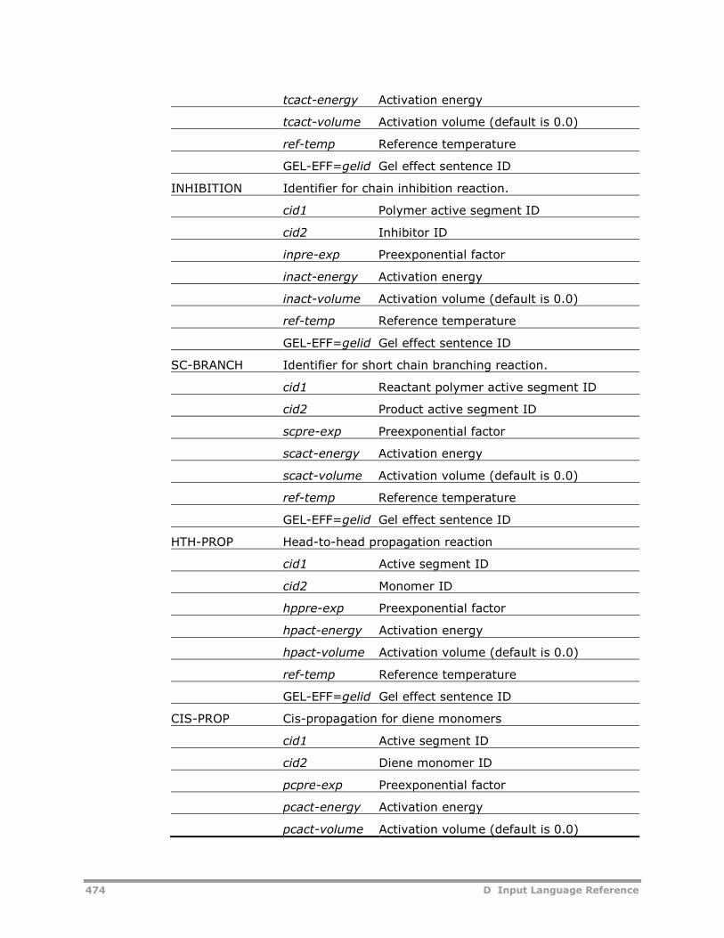
474 D Input Language Reference
tcact-energy Activation energy
tcact-volume Activation volume (default is 0.0)
ref-temp Reference temperature
GEL-EFF=gelid Gel effect sentence ID
INHIBITION Identifier for chain inhibition reaction.
cid1 Polymer active segment ID
cid2 Inhibitor ID
inpre-exp Preexponential factor
inact-energy Activation energy
inact-volume Activation volume (default is 0.0)
ref-temp Reference temperature
GEL-EFF=gelid Gel effect sentence ID
SC-BRANCH Identifier for short chain branching reaction.
cid1 Reactant polymer active segment ID
cid2 Product active segment ID
scpre-exp Preexponential factor
scact-energy Activation energy
scact-volume Activation volume (default is 0.0)
ref-temp Reference temperature
GEL-EFF=gelid Gel effect sentence ID
HTH-PROP Head-to-head propagation reaction
cid1 Active segment ID
cid2 Monomer ID
hppre-exp Preexponential factor
hpact-energy Activation energy
hpact-volume Activation volume (default is 0.0)
ref-temp Reference temperature
GEL-EFF=gelid Gel effect sentence ID
CIS-PROP Cis-propagation for diene monomers
cid1 Active segment ID
cid2 Diene monomer ID
pcpre-exp Preexponential factor
pcact-energy Activation energy
pcact-volume Activation volume (default is 0.0)
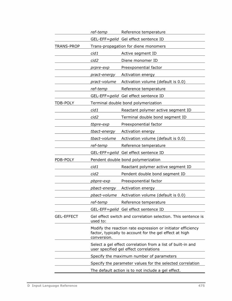
D Input Language Reference 475
ref-temp Reference temperature
GEL-EFF=gelid Gel effect sentence ID
TRANS-PROP Trans-propagation for diene monomers
cid1 Active segment ID
cid2 Diene monomer ID
prpre-exp Preexponential factor
pract-energy Activation energy
pract-volume Activation volume (default is 0.0)
ref-temp Reference temperature
GEL-EFF=gelid Gel effect sentence ID
TDB-POLY Terminal double bond polymerization
cid1 Reactant polymer active segment ID
cid2 Terminal double bond segment ID
tbpre-exp Preexponential factor
tbact-energy Activation energy
tbact-volume Activation volume (default is 0.0)
ref-temp Reference temperature
GEL-EFF=gelid Gel effect sentence ID
PDB-POLY Pendent double bond polymerization
cid1 Reactant polymer active segment ID
cid2 Pendent double bond segment ID
pbpre-exp Preexponential factor
pbact-energy Activation energy
pbact-volume Activation volume (default is 0.0)
ref-temp Reference temperature
GEL-EFF=gelid Gel effect sentence ID
GEL-EFFECT Gel effect switch and correlation selection. This sentence isused to:
Modify the reaction rate expression or initiator efficiencyfactor, typically to account for the gel effect at highconversion.
Select a gel effect correlation from a list of built-in anduser specified gel effect correlations
Specify the maximum number of parameters
Specify the parameter values for the selected correlation
The default action is to not include a gel effect.
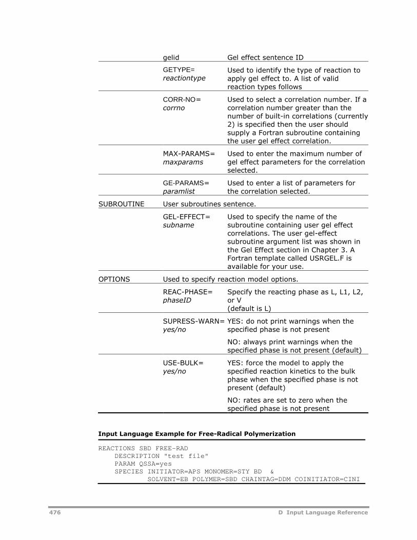
476 D Input Language Reference
gelid Gel effect sentence ID
GETYPE=reactiontype
Used to identify the type of reaction toapply gel effect to. A list of validreaction types follows
CORR-NO=corrno
Used to select a correlation number. If acorrelation number greater than thenumber of built-in correlations (currently2) is specified then the user shouldsupply a Fortran subroutine containingthe user gel effect correlation.
MAX-PARAMS=maxparams
Used to enter the maximum number ofgel effect parameters for the correlationselected.
GE-PARAMS=paramlist
Used to enter a list of parameters forthe correlation selected.
SUBROUTINE User subroutines sentence.
GEL-EFFECT=subname
Used to specify the name of thesubroutine containing user gel effectcorrelations. The user gel-effectsubroutine argument list was shown inthe Gel Effect section in Chapter 3. AFortran template called USRGEL.F isavailable for your use.
OPTIONS Used to specify reaction model options.
REAC-PHASE=phaseID
Specify the reacting phase as L, L1, L2,or V(default is L)
SUPRESS-WARN=yes/no
YES: do not print warnings when thespecified phase is not present
NO: always print warnings when thespecified phase is not present (default)
USE-BULK=yes/no
YES: force the model to apply thespecified reaction kinetics to the bulkphase when the specified phase is notpresent (default)
NO: rates are set to zero when thespecified phase is not present
Input Language Example for Free-Radical Polymerization
REACTIONS SBD FREE-RADDESCRIPTION "test file"PARAM QSSA=yesSPECIES INITIATOR=APS MONOMER=STY BD &
SOLVENT=EB POLYMER=SBD CHAINTAG=DDM COINITIATOR=CINI
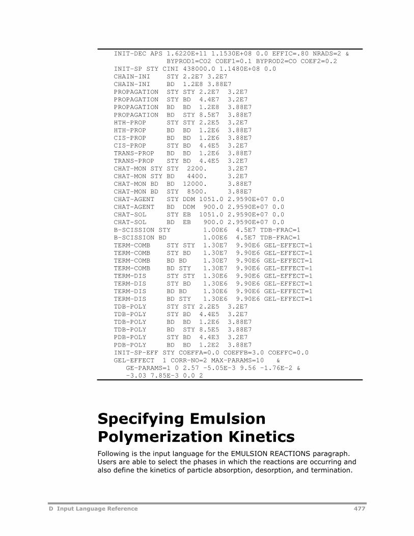
D Input Language Reference 477
INIT-DEC APS 1.6220E+11 1.1530E+08 0.0 EFFIC=.80 NRADS=2 &BYPROD1=CO2 COEF1=0.1 BYPROD2=CO COEF2=0.2
INIT-SP STY CINI 438000.0 1.1480E+08 0.0CHAIN-INI STY 2.2E7 3.2E7CHAIN-INI BD 1.2E8 3.88E7PROPAGATION STY STY 2.2E7 3.2E7PROPAGATION STY BD 4.4E7 3.2E7PROPAGATION BD BD 1.2E8 3.88E7PROPAGATION BD STY 8.5E7 3.88E7HTH-PROP STY STY 2.2E5 3.2E7HTH-PROP BD BD 1.2E6 3.88E7CIS-PROP BD BD 1.2E6 3.88E7CIS-PROP STY BD 4.4E5 3.2E7TRANS-PROP BD BD 1.2E6 3.88E7TRANS-PROP STY BD 4.4E5 3.2E7CHAT-MON STY STY 2200. 3.2E7CHAT-MON STY BD 4400. 3.2E7CHAT-MON BD BD 12000. 3.88E7CHAT-MON BD STY 8500. 3.88E7CHAT-AGENT STY DDM 1051.0 2.9590E+07 0.0CHAT-AGENT BD DDM 900.0 2.9590E+07 0.0CHAT-SOL STY EB 1051.0 2.9590E+07 0.0CHAT-SOL BD EB 900.0 2.9590E+07 0.0B-SCISSION STY 1.00E6 4.5E7 TDB-FRAC=1B-SCISSION BD 1.00E6 4.5E7 TDB-FRAC=1TERM-COMB STY STY 1.30E7 9.90E6 GEL-EFFECT=1TERM-COMB STY BD 1.30E7 9.90E6 GEL-EFFECT=1TERM-COMB BD BD 1.30E7 9.90E6 GEL-EFFECT=1TERM-COMB BD STY 1.30E7 9.90E6 GEL-EFFECT=1TERM-DIS STY STY 1.30E6 9.90E6 GEL-EFFECT=1TERM-DIS STY BD 1.30E6 9.90E6 GEL-EFFECT=1TERM-DIS BD BD 1.30E6 9.90E6 GEL-EFFECT=1TERM-DIS BD STY 1.30E6 9.90E6 GEL-EFFECT=1TDB-POLY STY STY 2.2E5 3.2E7TDB-POLY STY BD 4.4E5 3.2E7TDB-POLY BD BD 1.2E6 3.88E7TDB-POLY BD STY 8.5E5 3.88E7PDB-POLY STY BD 4.4E3 3.2E7PDB-POLY BD BD 1.2E2 3.88E7INIT-SP-EFF STY COEFFA=0.0 COEFFB=3.0 COEFFC=0.0GEL-EFFECT 1 CORR-NO=2 MAX-PARAMS=10 &
GE-PARAMS=1 0 2.57 -5.05E-3 9.56 -1.76E-2 &-3.03 7.85E-3 0.0 2
Specifying EmulsionPolymerization KineticsFollowing is the input language for the EMULSION REACTIONS paragraph.Users are able to select the phases in which the reactions are occurring andalso define the kinetics of particle absorption, desorption, and termination.
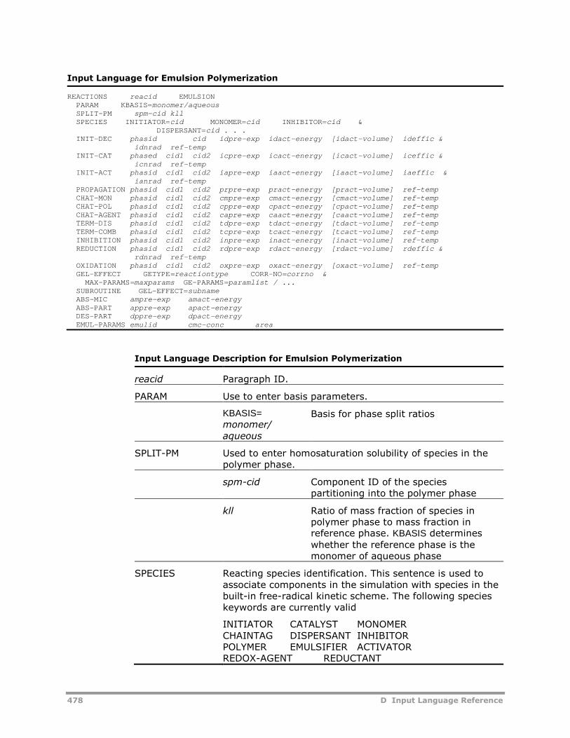
478 D Input Language Reference
Input Language for Emulsion Polymerization
REACTIONS reacid EMULSIONPARAM KBASIS=monomer/aqueousSPLIT-PM spm-cid kllSPECIES INITIATOR=cid MONOMER=cid INHIBITOR=cid &
DISPERSANT=cid . . .INIT-DEC phasid cid idpre-exp idact-energy [idact-volume] ideffic &
idnrad ref-tempINIT-CAT phased cid1 cid2 icpre-exp icact-energy [icact-volume] iceffic &
icnrad ref-tempINIT-ACT phasid cid1 cid2 iapre-exp iaact-energy [iaact-volume] iaeffic &
ianrad ref-tempPROPAGATION phasid cid1 cid2 prpre-exp pract-energy [pract-volume] ref-tempCHAT-MON phasid cid1 cid2 cmpre-exp cmact-energy [cmact-volume] ref-tempCHAT-POL phasid cid1 cid2 cppre-exp cpact-energy [cpact-volume] ref-tempCHAT-AGENT phasid cid1 cid2 capre-exp caact-energy [caact-volume] ref-tempTERM-DIS phasid cid1 cid2 tdpre-exp tdact-energy [tdact-volume] ref-tempTERM-COMB phasid cid1 cid2 tcpre-exp tcact-energy [tcact-volume] ref-tempINHIBITION phasid cid1 cid2 inpre-exp inact-energy [inact-volume] ref-tempREDUCTION phasid cid1 cid2 rdpre-exp rdact-energy [rdact-volume] rdeffic &
rdnrad ref-tempOXIDATION phasid cid1 cid2 oxpre-exp oxact-energy [oxact-volume] ref-tempGEL-EFFECT GETYPE=reactiontype CORR-NO=corrno &MAX-PARAMS=maxparams GE-PARAMS=paramlist / ...
SUBROUTINE GEL-EFFECT=subnameABS-MIC ampre-exp amact-energyABS-PART appre-exp apact-energyDES-PART dppre-exp dpact-energyEMUL-PARAMS emulid cmc-conc area
Input Language Description for Emulsion Polymerization
reacid Paragraph ID.
PARAM Use to enter basis parameters.
KBASIS=monomer/aqueous
Basis for phase split ratios
SPLIT-PM Used to enter homosaturation solubility of species in thepolymer phase.
spm-cid Component ID of the speciespartitioning into the polymer phase
kll Ratio of mass fraction of species inpolymer phase to mass fraction inreference phase. KBASIS determineswhether the reference phase is themonomer of aqueous phase
SPECIES Reacting species identification. This sentence is used toassociate components in the simulation with species in thebuilt-in free-radical kinetic scheme. The following specieskeywords are currently valid
INITIATOR CATALYST MONOMERCHAINTAG DISPERSANT INHIBITORPOLYMER EMULSIFIER ACTIVATORREDOX-AGENT REDUCTANT
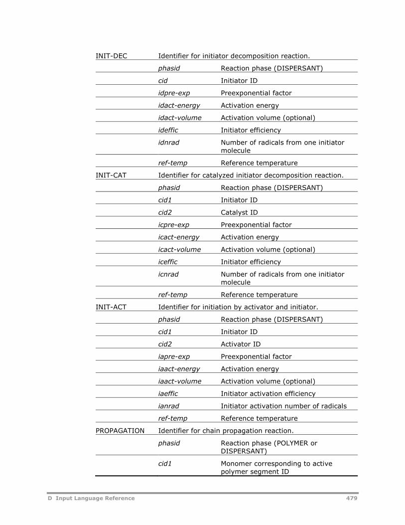
D Input Language Reference 479
INIT-DEC Identifier for initiator decomposition reaction.
phasid Reaction phase (DISPERSANT)
cid Initiator ID
idpre-exp Preexponential factor
idact-energy Activation energy
idact-volume Activation volume (optional)
ideffic Initiator efficiency
idnrad Number of radicals from one initiatormolecule
ref-temp Reference temperature
INIT-CAT Identifier for catalyzed initiator decomposition reaction.
phasid Reaction phase (DISPERSANT)
cid1 Initiator ID
cid2 Catalyst ID
icpre-exp Preexponential factor
icact-energy Activation energy
icact-volume Activation volume (optional)
iceffic Initiator efficiency
icnrad Number of radicals from one initiatormolecule
ref-temp Reference temperature
INIT-ACT Identifier for initiation by activator and initiator.
phasid Reaction phase (DISPERSANT)
cid1 Initiator ID
cid2 Activator ID
iapre-exp Preexponential factor
iaact-energy Activation energy
iaact-volume Activation volume (optional)
iaeffic Initiator activation efficiency
ianrad Initiator activation number of radicals
ref-temp Reference temperature
PROPAGATION Identifier for chain propagation reaction.
phasid Reaction phase (POLYMER orDISPERSANT)
cid1 Monomer corresponding to activepolymer segment ID
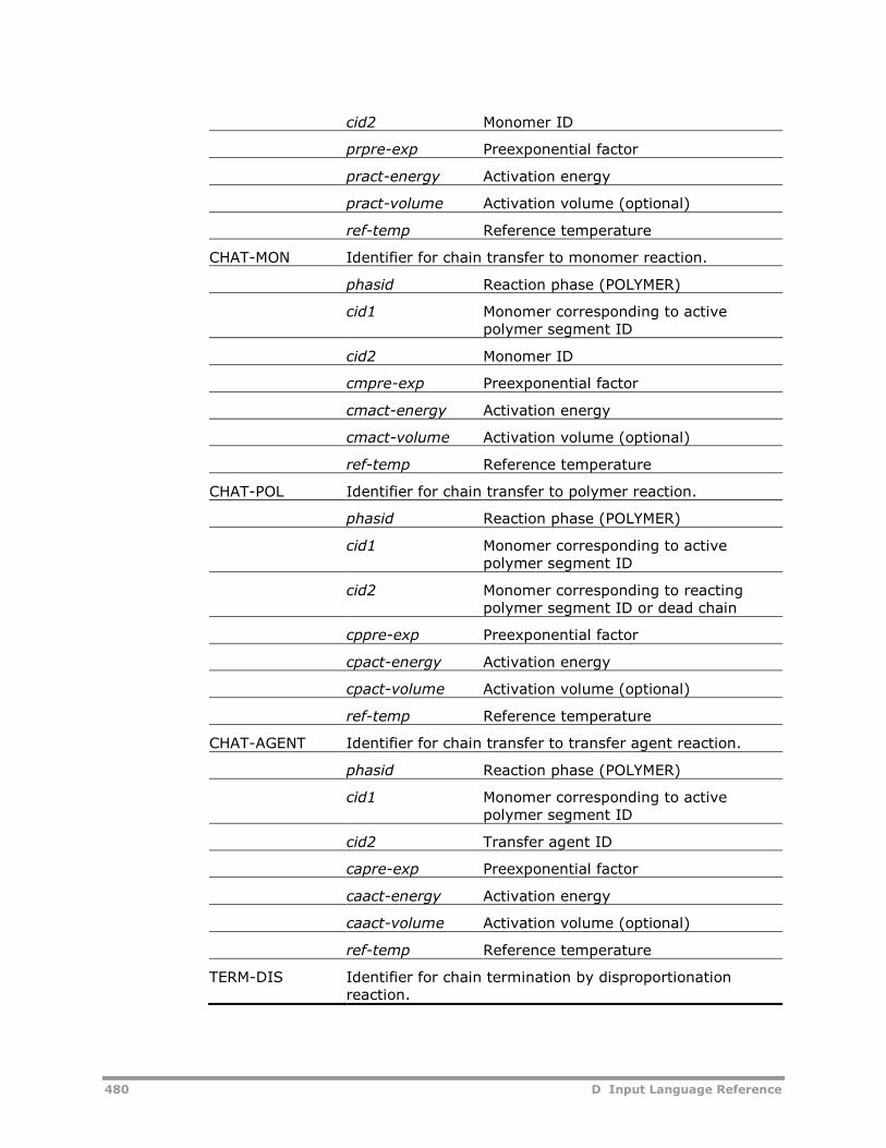
480 D Input Language Reference
cid2 Monomer ID
prpre-exp Preexponential factor
pract-energy Activation energy
pract-volume Activation volume (optional)
ref-temp Reference temperature
CHAT-MON Identifier for chain transfer to monomer reaction.
phasid Reaction phase (POLYMER)
cid1 Monomer corresponding to activepolymer segment ID
cid2 Monomer ID
cmpre-exp Preexponential factor
cmact-energy Activation energy
cmact-volume Activation volume (optional)
ref-temp Reference temperature
CHAT-POL Identifier for chain transfer to polymer reaction.
phasid Reaction phase (POLYMER)
cid1 Monomer corresponding to activepolymer segment ID
cid2 Monomer corresponding to reactingpolymer segment ID or dead chain
cppre-exp Preexponential factor
cpact-energy Activation energy
cpact-volume Activation volume (optional)
ref-temp Reference temperature
CHAT-AGENT Identifier for chain transfer to transfer agent reaction.
phasid Reaction phase (POLYMER)
cid1 Monomer corresponding to activepolymer segment ID
cid2 Transfer agent ID
capre-exp Preexponential factor
caact-energy Activation energy
caact-volume Activation volume (optional)
ref-temp Reference temperature
TERM-DIS Identifier for chain termination by disproportionationreaction.
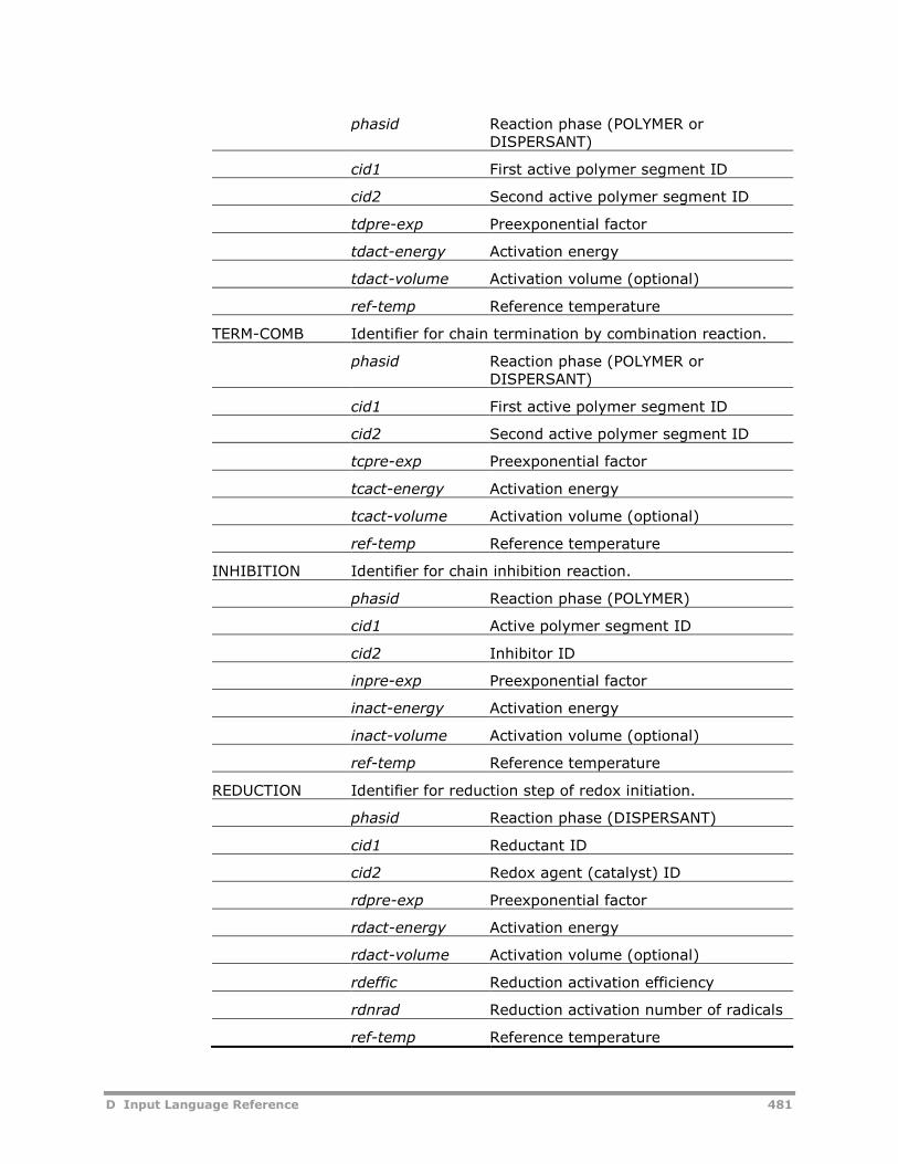
D Input Language Reference 481
phasid Reaction phase (POLYMER orDISPERSANT)
cid1 First active polymer segment ID
cid2 Second active polymer segment ID
tdpre-exp Preexponential factor
tdact-energy Activation energy
tdact-volume Activation volume (optional)
ref-temp Reference temperature
TERM-COMB Identifier for chain termination by combination reaction.
phasid Reaction phase (POLYMER orDISPERSANT)
cid1 First active polymer segment ID
cid2 Second active polymer segment ID
tcpre-exp Preexponential factor
tcact-energy Activation energy
tcact-volume Activation volume (optional)
ref-temp Reference temperature
INHIBITION Identifier for chain inhibition reaction.
phasid Reaction phase (POLYMER)
cid1 Active polymer segment ID
cid2 Inhibitor ID
inpre-exp Preexponential factor
inact-energy Activation energy
inact-volume Activation volume (optional)
ref-temp Reference temperature
REDUCTION Identifier for reduction step of redox initiation.
phasid Reaction phase (DISPERSANT)
cid1 Reductant ID
cid2 Redox agent (catalyst) ID
rdpre-exp Preexponential factor
rdact-energy Activation energy
rdact-volume Activation volume (optional)
rdeffic Reduction activation efficiency
rdnrad Reduction activation number of radicals
ref-temp Reference temperature
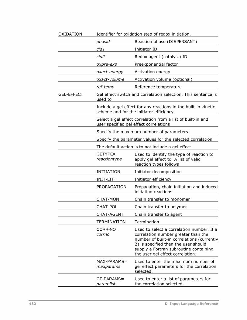
482 D Input Language Reference
OXIDATION Identifier for oxidation step of redox initiation.
phasid Reaction phase (DISPERSANT)
cid1 Initiator ID
cid2 Redox agent (catalyst) ID
oxpre-exp Preexponential factor
oxact-energy Activation energy
oxact-volume Activation volume (optional)
ref-temp Reference temperature
GEL-EFFECT Gel effect switch and correlation selection. This sentence isused to
Include a gel effect for any reactions in the built-in kineticscheme and for the initiator efficiency
Select a gel effect correlation from a list of built-in anduser specified gel effect correlations
Specify the maximum number of parameters
Specify the parameter values for the selected correlation
The default action is to not include a gel effect.
GETYPE=reactiontype
Used to identify the type of reaction toapply gel effect to. A list of validreaction types follows
INITIATION Initiator decomposition
INIT-EFF Initiator efficiency
PROPAGATION Propagation, chain initiation and inducedinitiation reactions
CHAT-MON Chain transfer to monomer
CHAT-POL Chain transfer to polymer
CHAT-AGENT Chain transfer to agent
TERMINATION Termination
CORR-NO=corrno
Used to select a correlation number. If acorrelation number greater than thenumber of built-in correlations (currently2) is specified then the user shouldsupply a Fortran subroutine containingthe user gel effect correlation.
MAX-PARAMS=maxparams
Used to enter the maximum number ofgel effect parameters for the correlationselected.
GE-PARAMS=paramlist
Used to enter a list of parameters forthe correlation selected.
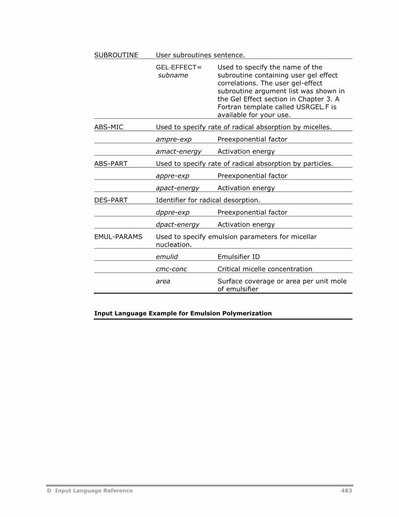
D Input Language Reference 483
SUBROUTINE User subroutines sentence.
GEL-EFFECT=subname
Used to specify the name of thesubroutine containing user gel effectcorrelations. The user gel-effectsubroutine argument list was shown inthe Gel Effect section in Chapter 3. AFortran template called USRGEL.F isavailable for your use.
ABS-MIC Used to specify rate of radical absorption by micelles.
ampre-exp Preexponential factor
amact-energy Activation energy
ABS-PART Used to specify rate of radical absorption by particles.
appre-exp Preexponential factor
apact-energy Activation energy
DES-PART Identifier for radical desorption.
dppre-exp Preexponential factor
dpact-energy Activation energy
EMUL-PARAMS Used to specify emulsion parameters for micellarnucleation.
emulid Emulsifier ID
cmc-conc Critical micelle concentration
area Surface coverage or area per unit moleof emulsifier
Input Language Example for Emulsion Polymerization
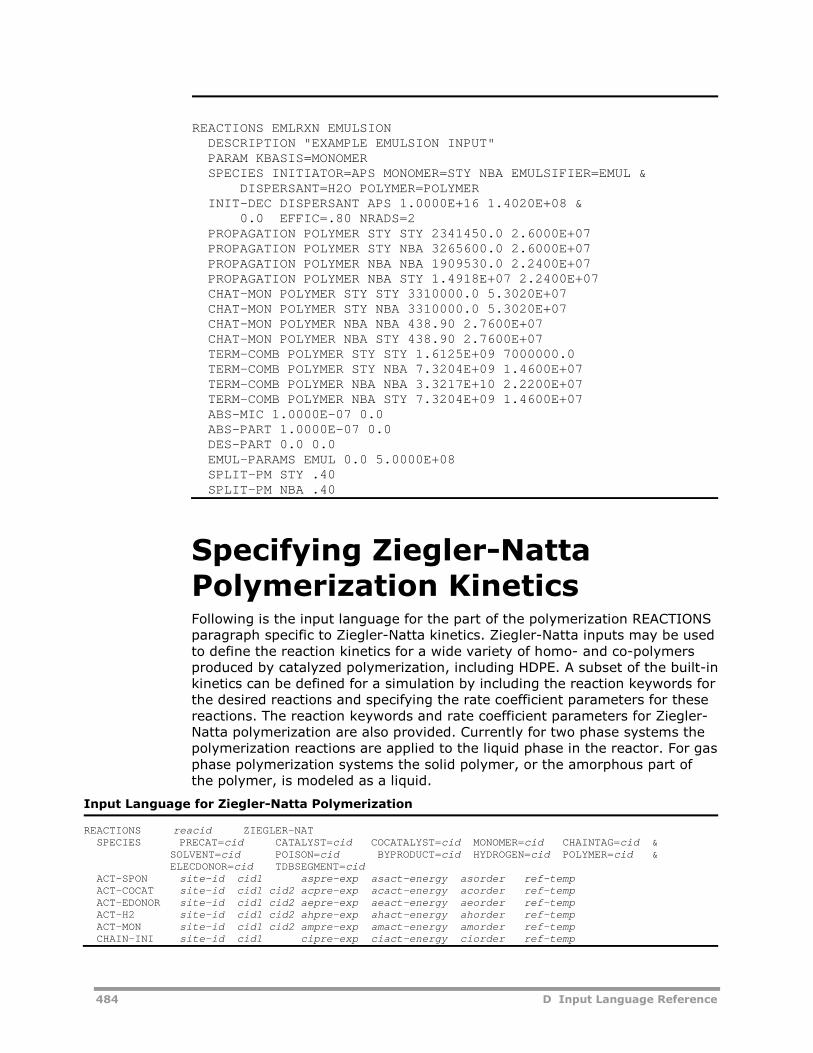
484 D Input Language Reference
REACTIONS EMLRXN EMULSIONDESCRIPTION "EXAMPLE EMULSION INPUT"PARAM KBASIS=MONOMERSPECIES INITIATOR=APS MONOMER=STY NBA EMULSIFIER=EMUL &
DISPERSANT=H2O POLYMER=POLYMERINIT-DEC DISPERSANT APS 1.0000E+16 1.4020E+08 &
0.0 EFFIC=.80 NRADS=2PROPAGATION POLYMER STY STY 2341450.0 2.6000E+07PROPAGATION POLYMER STY NBA 3265600.0 2.6000E+07PROPAGATION POLYMER NBA NBA 1909530.0 2.2400E+07PROPAGATION POLYMER NBA STY 1.4918E+07 2.2400E+07CHAT-MON POLYMER STY STY 3310000.0 5.3020E+07CHAT-MON POLYMER STY NBA 3310000.0 5.3020E+07CHAT-MON POLYMER NBA NBA 438.90 2.7600E+07CHAT-MON POLYMER NBA STY 438.90 2.7600E+07TERM-COMB POLYMER STY STY 1.6125E+09 7000000.0TERM-COMB POLYMER STY NBA 7.3204E+09 1.4600E+07TERM-COMB POLYMER NBA NBA 3.3217E+10 2.2200E+07TERM-COMB POLYMER NBA STY 7.3204E+09 1.4600E+07ABS-MIC 1.0000E-07 0.0ABS-PART 1.0000E-07 0.0DES-PART 0.0 0.0EMUL-PARAMS EMUL 0.0 5.0000E+08SPLIT-PM STY .40SPLIT-PM NBA .40
Specifying Ziegler-NattaPolymerization KineticsFollowing is the input language for the part of the polymerization REACTIONSparagraph specific to Ziegler-Natta kinetics. Ziegler-Natta inputs may be usedto define the reaction kinetics for a wide variety of homo- and co-polymersproduced by catalyzed polymerization, including HDPE. A subset of the built-inkinetics can be defined for a simulation by including the reaction keywords forthe desired reactions and specifying the rate coefficient parameters for thesereactions. The reaction keywords and rate coefficient parameters for Ziegler-Natta polymerization are also provided. Currently for two phase systems thepolymerization reactions are applied to the liquid phase in the reactor. For gasphase polymerization systems the solid polymer, or the amorphous part ofthe polymer, is modeled as a liquid.
Input Language for Ziegler-Natta Polymerization
REACTIONS reacid ZIEGLER-NATSPECIES PRECAT=cid CATALYST=cid COCATALYST=cid MONOMER=cid CHAINTAG=cid &
SOLVENT=cid POISON=cid BYPRODUCT=cid HYDROGEN=cid POLYMER=cid &ELECDONOR=cid TDBSEGMENT=cid
ACT-SPON site-id cid1 aspre-exp asact-energy asorder ref-tempACT-COCAT site-id cid1 cid2 acpre-exp acact-energy acorder ref-tempACT-EDONOR site-id cid1 cid2 aepre-exp aeact-energy aeorder ref-tempACT-H2 site-id cid1 cid2 ahpre-exp ahact-energy ahorder ref-tempACT-MON site-id cid1 cid2 ampre-exp amact-energy amorder ref-tempCHAIN-INI site-id cid1 cipre-exp ciact-energy ciorder ref-temp
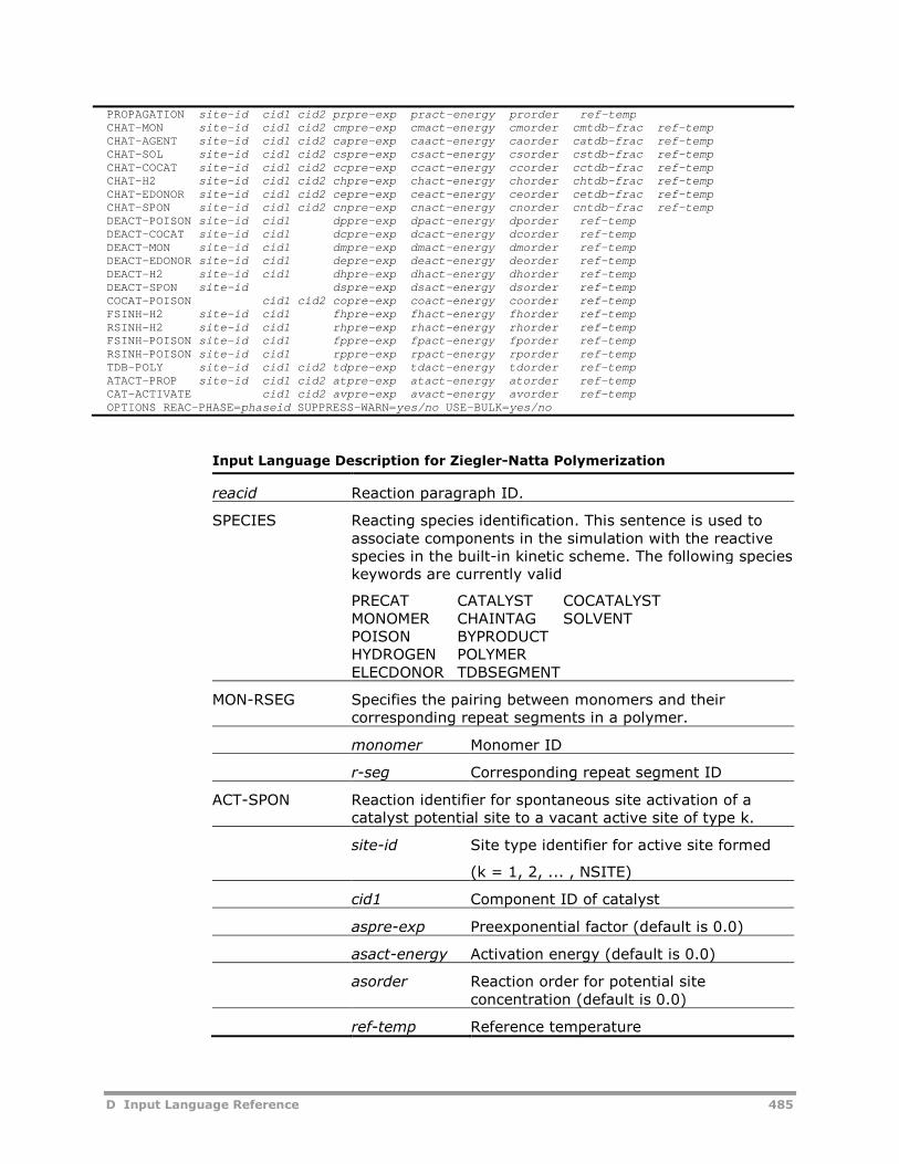
D Input Language Reference 485
PROPAGATION site-id cid1 cid2 prpre-exp pract-energy prorder ref-tempCHAT-MON site-id cid1 cid2 cmpre-exp cmact-energy cmorder cmtdb-frac ref-tempCHAT-AGENT site-id cid1 cid2 capre-exp caact-energy caorder catdb-frac ref-tempCHAT-SOL site-id cid1 cid2 cspre-exp csact-energy csorder cstdb-frac ref-tempCHAT-COCAT site-id cid1 cid2 ccpre-exp ccact-energy ccorder cctdb-frac ref-tempCHAT-H2 site-id cid1 cid2 chpre-exp chact-energy chorder chtdb-frac ref-tempCHAT-EDONOR site-id cid1 cid2 cepre-exp ceact-energy ceorder cetdb-frac ref-tempCHAT-SPON site-id cid1 cid2 cnpre-exp cnact-energy cnorder cntdb-frac ref-tempDEACT-POISON site-id cid1 dppre-exp dpact-energy dporder ref-tempDEACT-COCAT site-id cid1 dcpre-exp dcact-energy dcorder ref-tempDEACT-MON site-id cid1 dmpre-exp dmact-energy dmorder ref-tempDEACT-EDONOR site-id cid1 depre-exp deact-energy deorder ref-tempDEACT-H2 site-id cid1 dhpre-exp dhact-energy dhorder ref-tempDEACT-SPON site-id dspre-exp dsact-energy dsorder ref-tempCOCAT-POISON cid1 cid2 copre-exp coact-energy coorder ref-tempFSINH-H2 site-id cid1 fhpre-exp fhact-energy fhorder ref-tempRSINH-H2 site-id cid1 rhpre-exp rhact-energy rhorder ref-tempFSINH-POISON site-id cid1 fppre-exp fpact-energy fporder ref-tempRSINH-POISON site-id cid1 rppre-exp rpact-energy rporder ref-tempTDB-POLY site-id cid1 cid2 tdpre-exp tdact-energy tdorder ref-tempATACT-PROP site-id cid1 cid2 atpre-exp atact-energy atorder ref-tempCAT-ACTIVATE cid1 cid2 avpre-exp avact-energy avorder ref-tempOPTIONS REAC-PHASE=phaseid SUPPRESS-WARN=yes/no USE-BULK=yes/no
Input Language Description for Ziegler-Natta Polymerization
reacid Reaction paragraph ID.
SPECIES Reacting species identification. This sentence is used toassociate components in the simulation with the reactivespecies in the built-in kinetic scheme. The following specieskeywords are currently valid
PRECAT CATALYST COCATALYSTMONOMER CHAINTAG SOLVENTPOISON BYPRODUCTHYDROGEN POLYMERELECDONOR TDBSEGMENT
MON-RSEG Specifies the pairing between monomers and theircorresponding repeat segments in a polymer.
monomer Monomer ID
r-seg Corresponding repeat segment ID
ACT-SPON Reaction identifier for spontaneous site activation of acatalyst potential site to a vacant active site of type k.
site-id Site type identifier for active site formed
(k = 1, 2, ... , NSITE)
cid1 Component ID of catalyst
aspre-exp Preexponential factor (default is 0.0)
asact-energy Activation energy (default is 0.0)
asorder Reaction order for potential siteconcentration (default is 0.0)
ref-temp Reference temperature
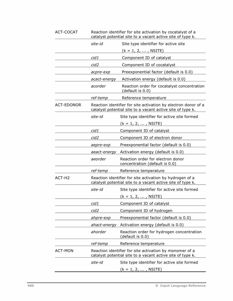
486 D Input Language Reference
ACT-COCAT Reaction identifier for site activation by cocatalyst of acatalyst potential site to a vacant active site of type k.
site-id Site type identifier for active site
(k = 1, 2, ... , NSITE)
cid1 Component ID of catalyst
cid2 Component ID of cocatalyst
acpre-exp Preexponential factor (default is 0.0)
acact-energy Activation energy (default is 0.0)
acorder Reaction order for cocatalyst concentration(default is 0.0)
ref-temp Reference temperature
ACT-EDONOR Reaction identifier for site activation by electron donor of acatalyst potential site to a vacant active site of type k.
site-id Site type identifier for active site formed
(k = 1, 2, ... , NSITE)
cid1 Component ID of catalyst
cid2 Component ID of electron donor
aepre-exp Preexponential factor (default is 0.0)
aeact-energy Activation energy (default is 0.0)
aeorder Reaction order for electron donorconcentration (default is 0.0)
ref-temp Reference temperature
ACT-H2 Reaction identifier for site activation by hydrogen of acatalyst potential site to a vacant active site of type k.
site-id Site type identifier for active site formed
(k = 1, 2, ... , NSITE)
cid1 Component ID of catalyst
cid2 Component ID of hydrogen
ahpre-exp Preexponential factor (default is 0.0)
ahact-energy Activation energy (default is 0.0)
ahorder Reaction order for hydrogen concentration(default is 0.0)
ref-temp Reference temperature
ACT-MON Reaction identifier for site activation by monomer of acatalyst potential site to a vacant active site of type k.
site-id Site type identifier for active site formed
(k = 1, 2, ... , NSITE)
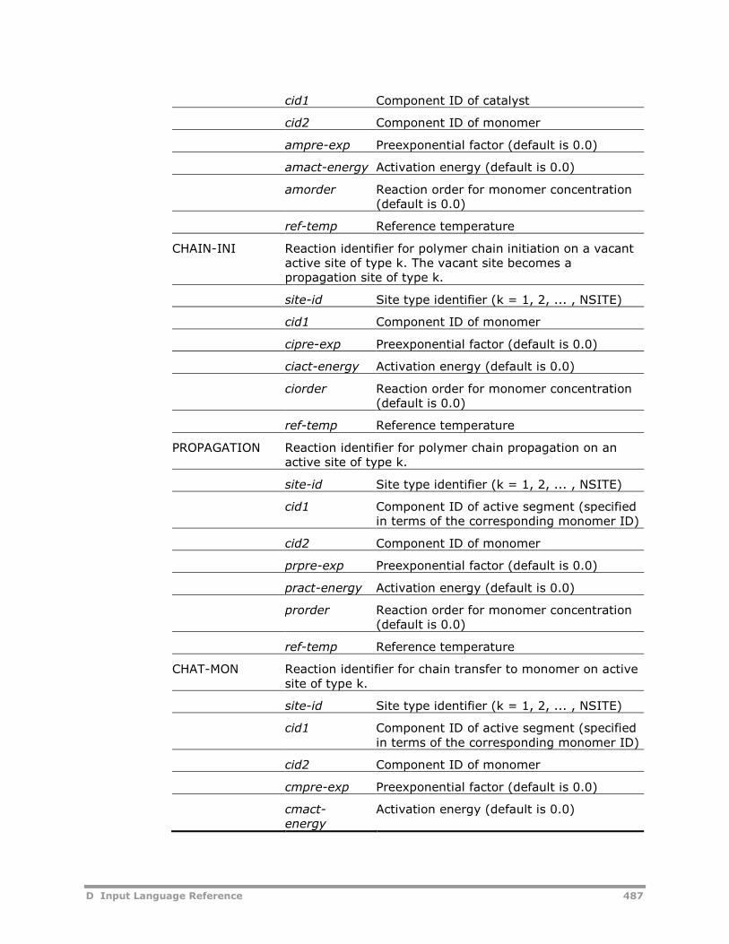
D Input Language Reference 487
cid1 Component ID of catalyst
cid2 Component ID of monomer
ampre-exp Preexponential factor (default is 0.0)
amact-energy Activation energy (default is 0.0)
amorder Reaction order for monomer concentration(default is 0.0)
ref-temp Reference temperature
CHAIN-INI Reaction identifier for polymer chain initiation on a vacantactive site of type k. The vacant site becomes apropagation site of type k.
site-id Site type identifier (k = 1, 2, ... , NSITE)
cid1 Component ID of monomer
cipre-exp Preexponential factor (default is 0.0)
ciact-energy Activation energy (default is 0.0)
ciorder Reaction order for monomer concentration(default is 0.0)
ref-temp Reference temperature
PROPAGATION Reaction identifier for polymer chain propagation on anactive site of type k.
site-id Site type identifier (k = 1, 2, ... , NSITE)
cid1 Component ID of active segment (specifiedin terms of the corresponding monomer ID)
cid2 Component ID of monomer
prpre-exp Preexponential factor (default is 0.0)
pract-energy Activation energy (default is 0.0)
prorder Reaction order for monomer concentration(default is 0.0)
ref-temp Reference temperature
CHAT-MON Reaction identifier for chain transfer to monomer on activesite of type k.
site-id Site type identifier (k = 1, 2, ... , NSITE)
cid1 Component ID of active segment (specifiedin terms of the corresponding monomer ID)
cid2 Component ID of monomer
cmpre-exp Preexponential factor (default is 0.0)
cmact-energy
Activation energy (default is 0.0)
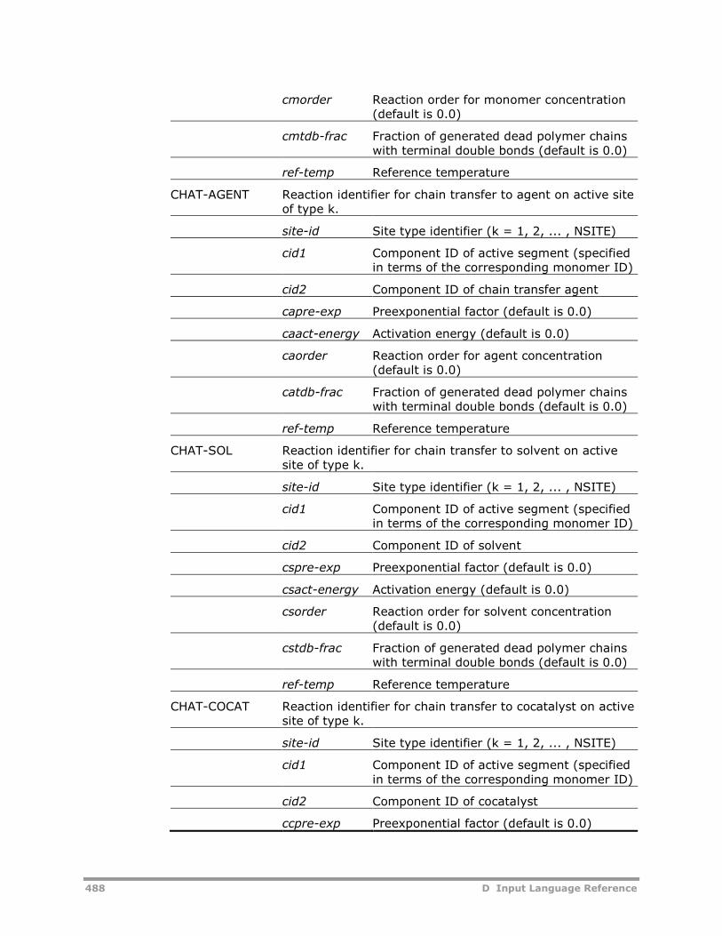
488 D Input Language Reference
cmorder Reaction order for monomer concentration(default is 0.0)
cmtdb-frac Fraction of generated dead polymer chainswith terminal double bonds (default is 0.0)
ref-temp Reference temperature
CHAT-AGENT Reaction identifier for chain transfer to agent on active siteof type k.
site-id Site type identifier (k = 1, 2, ... , NSITE)
cid1 Component ID of active segment (specifiedin terms of the corresponding monomer ID)
cid2 Component ID of chain transfer agent
capre-exp Preexponential factor (default is 0.0)
caact-energy Activation energy (default is 0.0)
caorder Reaction order for agent concentration(default is 0.0)
catdb-frac Fraction of generated dead polymer chainswith terminal double bonds (default is 0.0)
ref-temp Reference temperature
CHAT-SOL Reaction identifier for chain transfer to solvent on activesite of type k.
site-id Site type identifier (k = 1, 2, ... , NSITE)
cid1 Component ID of active segment (specifiedin terms of the corresponding monomer ID)
cid2 Component ID of solvent
cspre-exp Preexponential factor (default is 0.0)
csact-energy Activation energy (default is 0.0)
csorder Reaction order for solvent concentration(default is 0.0)
cstdb-frac Fraction of generated dead polymer chainswith terminal double bonds (default is 0.0)
ref-temp Reference temperature
CHAT-COCAT Reaction identifier for chain transfer to cocatalyst on activesite of type k.
site-id Site type identifier (k = 1, 2, ... , NSITE)
cid1 Component ID of active segment (specifiedin terms of the corresponding monomer ID)
cid2 Component ID of cocatalyst
ccpre-exp Preexponential factor (default is 0.0)
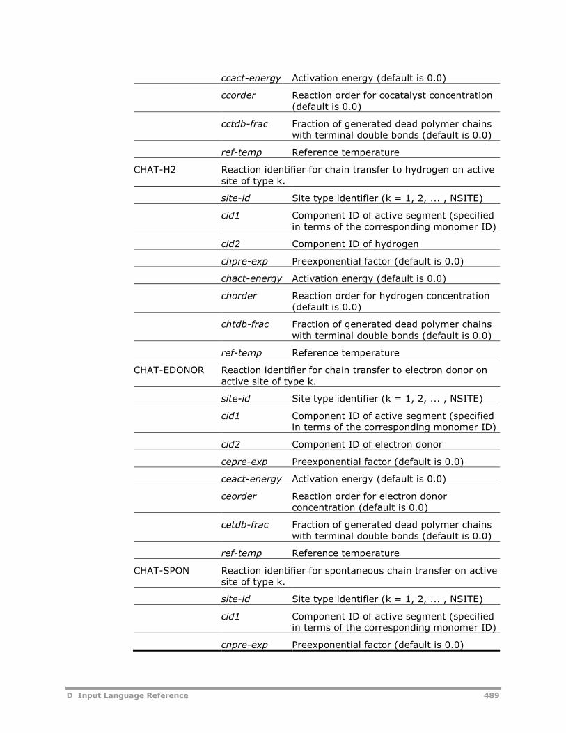
D Input Language Reference 489
ccact-energy Activation energy (default is 0.0)
ccorder Reaction order for cocatalyst concentration(default is 0.0)
cctdb-frac Fraction of generated dead polymer chainswith terminal double bonds (default is 0.0)
ref-temp Reference temperature
CHAT-H2 Reaction identifier for chain transfer to hydrogen on activesite of type k.
site-id Site type identifier (k = 1, 2, ... , NSITE)
cid1 Component ID of active segment (specifiedin terms of the corresponding monomer ID)
cid2 Component ID of hydrogen
chpre-exp Preexponential factor (default is 0.0)
chact-energy Activation energy (default is 0.0)
chorder Reaction order for hydrogen concentration(default is 0.0)
chtdb-frac Fraction of generated dead polymer chainswith terminal double bonds (default is 0.0)
ref-temp Reference temperature
CHAT-EDONOR Reaction identifier for chain transfer to electron donor onactive site of type k.
site-id Site type identifier (k = 1, 2, ... , NSITE)
cid1 Component ID of active segment (specifiedin terms of the corresponding monomer ID)
cid2 Component ID of electron donor
cepre-exp Preexponential factor (default is 0.0)
ceact-energy Activation energy (default is 0.0)
ceorder Reaction order for electron donorconcentration (default is 0.0)
cetdb-frac Fraction of generated dead polymer chainswith terminal double bonds (default is 0.0)
ref-temp Reference temperature
CHAT-SPON Reaction identifier for spontaneous chain transfer on activesite of type k.
site-id Site type identifier (k = 1, 2, ... , NSITE)
cid1 Component ID of active segment (specifiedin terms of the corresponding monomer ID)
cnpre-exp Preexponential factor (default is 0.0)
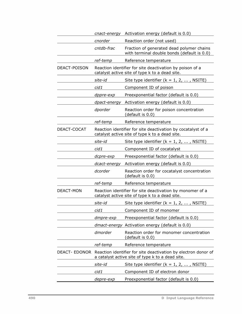
490 D Input Language Reference
cnact-energy Activation energy (default is 0.0)
cnorder Reaction order (not used)
cntdb-frac Fraction of generated dead polymer chainswith terminal double bonds (default is 0.0)
ref-temp Reference temperature
DEACT-POISON Reaction identifier for site deactivation by poison of acatalyst active site of type k to a dead site.
site-id Site type identifier (k = 1, 2, ... , NSITE)
cid1 Component ID of poison
dppre-exp Preexponential factor (default is 0.0)
dpact-energy Activation energy (default is 0.0)
dporder Reaction order for poison concentration(default is 0.0)
ref-temp Reference temperature
DEACT-COCAT Reaction identifier for site deactivation by cocatalyst of acatalyst active site of type k to a dead site.
site-id Site type identifier (k = 1, 2, ... , NSITE)
cid1 Component ID of cocatalyst
dcpre-exp Preexponential factor (default is 0.0)
dcact-energy Activation energy (default is 0.0)
dcorder Reaction order for cocatalyst concentration(default is 0.0)
ref-temp Reference temperature
DEACT-MON Reaction identifier for site deactivation by monomer of acatalyst active site of type k to a dead site.
site-id Site type identifier (k = 1, 2, ... , NSITE)
cid1 Component ID of monomer
dmpre-exp Preexponential factor (default is 0.0)
dmact-energy Activation energy (default is 0.0)
dmorder Reaction order for monomer concentration(default is 0.0)
ref-temp Reference temperature
DEACT- EDONOR Reaction identifier for site deactivation by electron donor ofa catalyst active site of type k to a dead site.
site-id Site type identifier (k = 1, 2, ... , NSITE)
cid1 Component ID of electron donor
depre-exp Preexponential factor (default is 0.0)
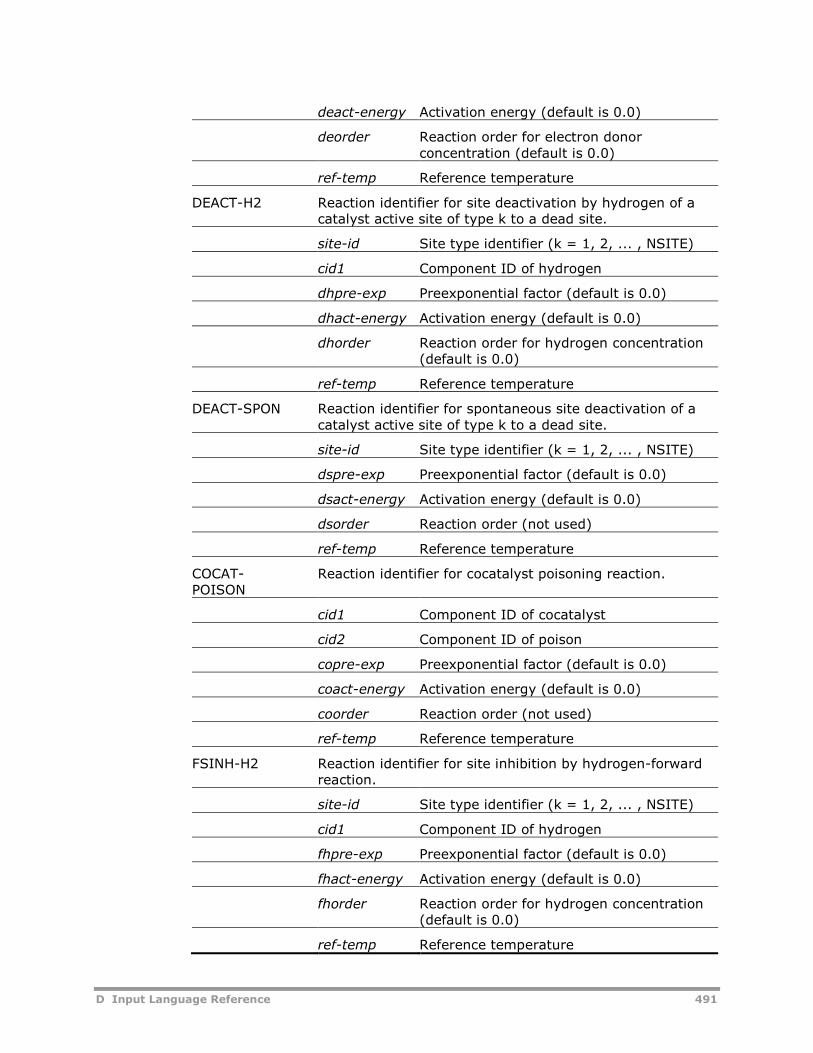
D Input Language Reference 491
deact-energy Activation energy (default is 0.0)
deorder Reaction order for electron donorconcentration (default is 0.0)
ref-temp Reference temperature
DEACT-H2 Reaction identifier for site deactivation by hydrogen of acatalyst active site of type k to a dead site.
site-id Site type identifier (k = 1, 2, ... , NSITE)
cid1 Component ID of hydrogen
dhpre-exp Preexponential factor (default is 0.0)
dhact-energy Activation energy (default is 0.0)
dhorder Reaction order for hydrogen concentration(default is 0.0)
ref-temp Reference temperature
DEACT-SPON Reaction identifier for spontaneous site deactivation of acatalyst active site of type k to a dead site.
site-id Site type identifier (k = 1, 2, ... , NSITE)
dspre-exp Preexponential factor (default is 0.0)
dsact-energy Activation energy (default is 0.0)
dsorder Reaction order (not used)
ref-temp Reference temperature
COCAT-POISON
Reaction identifier for cocatalyst poisoning reaction.
cid1 Component ID of cocatalyst
cid2 Component ID of poison
copre-exp Preexponential factor (default is 0.0)
coact-energy Activation energy (default is 0.0)
coorder Reaction order (not used)
ref-temp Reference temperature
FSINH-H2 Reaction identifier for site inhibition by hydrogen-forwardreaction.
site-id Site type identifier (k = 1, 2, ... , NSITE)
cid1 Component ID of hydrogen
fhpre-exp Preexponential factor (default is 0.0)
fhact-energy Activation energy (default is 0.0)
fhorder Reaction order for hydrogen concentration(default is 0.0)
ref-temp Reference temperature
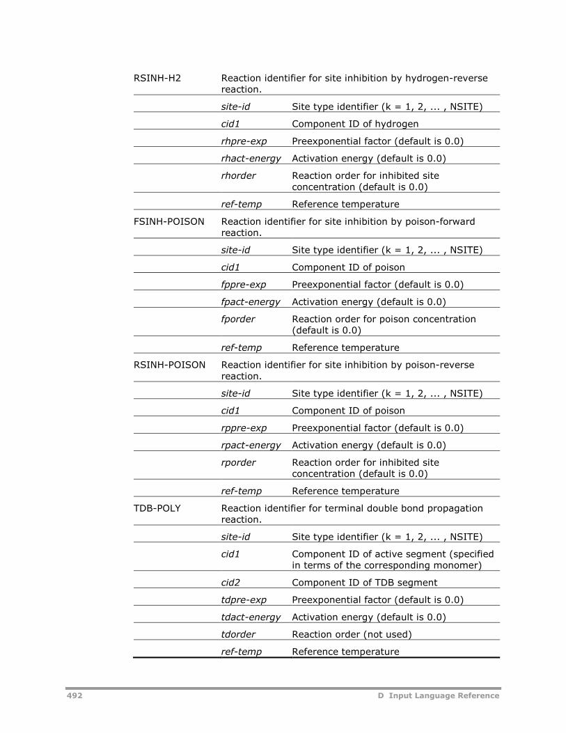
492 D Input Language Reference
RSINH-H2 Reaction identifier for site inhibition by hydrogen-reversereaction.
site-id Site type identifier (k = 1, 2, ... , NSITE)
cid1 Component ID of hydrogen
rhpre-exp Preexponential factor (default is 0.0)
rhact-energy Activation energy (default is 0.0)
rhorder Reaction order for inhibited siteconcentration (default is 0.0)
ref-temp Reference temperature
FSINH-POISON Reaction identifier for site inhibition by poison-forwardreaction.
site-id Site type identifier (k = 1, 2, ... , NSITE)
cid1 Component ID of poison
fppre-exp Preexponential factor (default is 0.0)
fpact-energy Activation energy (default is 0.0)
fporder Reaction order for poison concentration(default is 0.0)
ref-temp Reference temperature
RSINH-POISON Reaction identifier for site inhibition by poison-reversereaction.
site-id Site type identifier (k = 1, 2, ... , NSITE)
cid1 Component ID of poison
rppre-exp Preexponential factor (default is 0.0)
rpact-energy Activation energy (default is 0.0)
rporder Reaction order for inhibited siteconcentration (default is 0.0)
ref-temp Reference temperature
TDB-POLY Reaction identifier for terminal double bond propagationreaction.
site-id Site type identifier (k = 1, 2, ... , NSITE)
cid1 Component ID of active segment (specifiedin terms of the corresponding monomer)
cid2 Component ID of TDB segment
tdpre-exp Preexponential factor (default is 0.0)
tdact-energy Activation energy (default is 0.0)
tdorder Reaction order (not used)
ref-temp Reference temperature
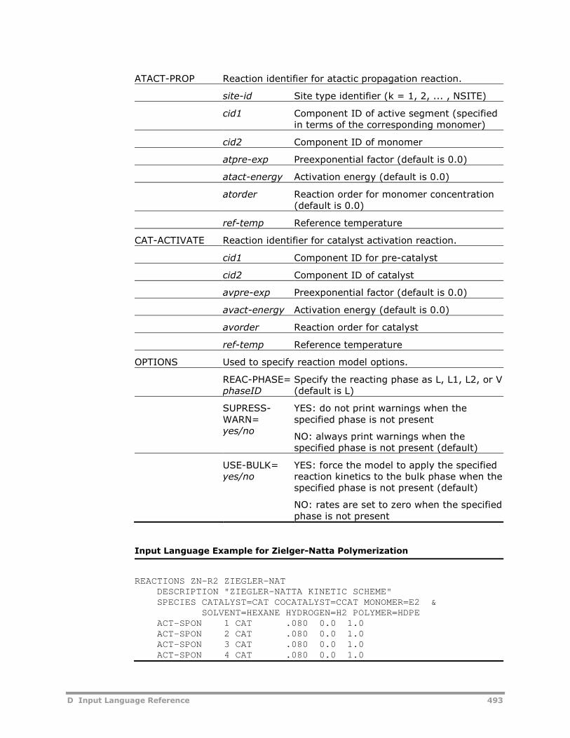
D Input Language Reference 493
ATACT-PROP Reaction identifier for atactic propagation reaction.
site-id Site type identifier (k = 1, 2, ... , NSITE)
cid1 Component ID of active segment (specifiedin terms of the corresponding monomer)
cid2 Component ID of monomer
atpre-exp Preexponential factor (default is 0.0)
atact-energy Activation energy (default is 0.0)
atorder Reaction order for monomer concentration(default is 0.0)
ref-temp Reference temperature
CAT-ACTIVATE Reaction identifier for catalyst activation reaction.
cid1 Component ID for pre-catalyst
cid2 Component ID of catalyst
avpre-exp Preexponential factor (default is 0.0)
avact-energy Activation energy (default is 0.0)
avorder Reaction order for catalyst
ref-temp Reference temperature
OPTIONS Used to specify reaction model options.
REAC-PHASE=phaseID
Specify the reacting phase as L, L1, L2, or V(default is L)
SUPRESS-WARN=yes/no
YES: do not print warnings when thespecified phase is not present
NO: always print warnings when thespecified phase is not present (default)
USE-BULK=yes/no
YES: force the model to apply the specifiedreaction kinetics to the bulk phase when thespecified phase is not present (default)
NO: rates are set to zero when the specifiedphase is not present
Input Language Example for Zielger-Natta Polymerization
REACTIONS ZN-R2 ZIEGLER-NATDESCRIPTION "ZIEGLER-NATTA KINETIC SCHEME"SPECIES CATALYST=CAT COCATALYST=CCAT MONOMER=E2 &
SOLVENT=HEXANE HYDROGEN=H2 POLYMER=HDPEACT-SPON 1 CAT .080 0.0 1.0ACT-SPON 2 CAT .080 0.0 1.0ACT-SPON 3 CAT .080 0.0 1.0ACT-SPON 4 CAT .080 0.0 1.0
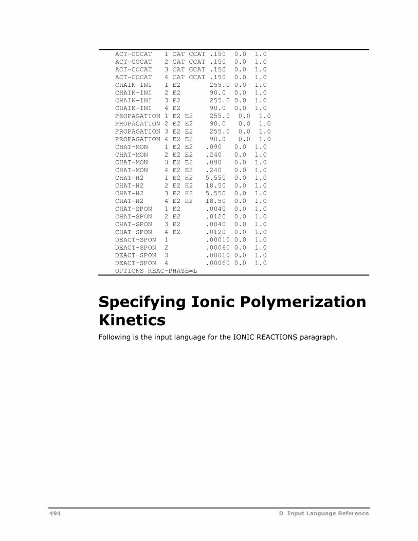
494 D Input Language Reference
ACT-COCAT 1 CAT CCAT .150 0.0 1.0ACT-COCAT 2 CAT CCAT .150 0.0 1.0ACT-COCAT 3 CAT CCAT .150 0.0 1.0ACT-COCAT 4 CAT CCAT .150 0.0 1.0CHAIN-INI 1 E2 255.0 0.0 1.0CHAIN-INI 2 E2 90.0 0.0 1.0CHAIN-INI 3 E2 255.0 0.0 1.0CHAIN-INI 4 E2 90.0 0.0 1.0PROPAGATION 1 E2 E2 255.0 0.0 1.0PROPAGATION 2 E2 E2 90.0 0.0 1.0PROPAGATION 3 E2 E2 255.0 0.0 1.0PROPAGATION 4 E2 E2 90.0 0.0 1.0CHAT-MON 1 E2 E2 .090 0.0 1.0CHAT-MON 2 E2 E2 .240 0.0 1.0CHAT-MON 3 E2 E2 .090 0.0 1.0CHAT-MON 4 E2 E2 .240 0.0 1.0CHAT-H2 1 E2 H2 5.550 0.0 1.0CHAT-H2 2 E2 H2 18.50 0.0 1.0CHAT-H2 3 E2 H2 5.550 0.0 1.0CHAT-H2 4 E2 H2 18.50 0.0 1.0CHAT-SPON 1 E2 .0040 0.0 1.0CHAT-SPON 2 E2 .0120 0.0 1.0CHAT-SPON 3 E2 .0040 0.0 1.0CHAT-SPON 4 E2 .0120 0.0 1.0DEACT-SPON 1 .00010 0.0 1.0DEACT-SPON 2 .00060 0.0 1.0DEACT-SPON 3 .00010 0.0 1.0DEACT-SPON 4 .00060 0.0 1.0OPTIONS REAC-PHASE=L
Specifying Ionic PolymerizationKineticsFollowing is the input language for the IONIC REACTIONS paragraph.
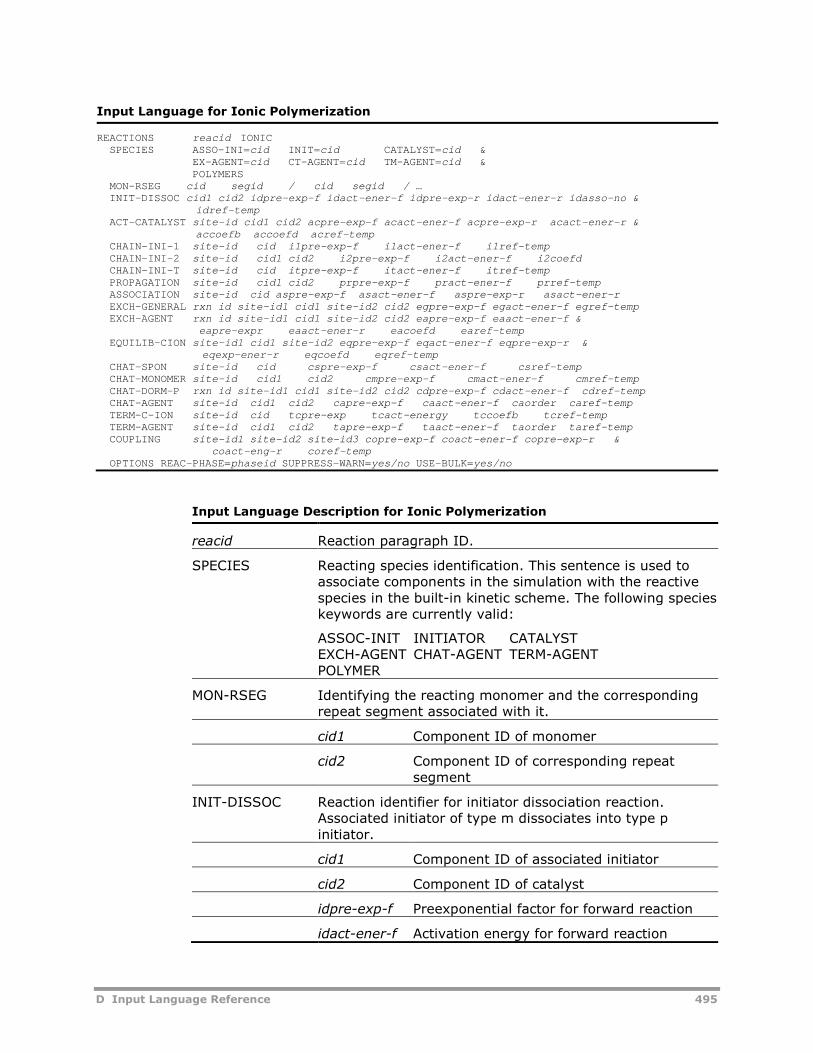
D Input Language Reference 495
Input Language for Ionic Polymerization
REACTIONS reacid IONICSPECIES ASSO-INI=cid INIT=cid CATALYST=cid &
EX-AGENT=cid CT-AGENT=cid TM-AGENT=cid &POLYMERS
MON-RSEG cid segid / cid segid / …INIT-DISSOC cid1 cid2 idpre-exp-f idact-ener-f idpre-exp-r idact-ener-r idasso-no &
idref-tempACT-CATALYST site-id cid1 cid2 acpre-exp-f acact-ener-f acpre-exp-r acact-ener-r &
accoefb accoefd acref-tempCHAIN-INI-1 site-id cid i1pre-exp-f i1act-ener-f i1ref-tempCHAIN-INI-2 site-id cid1 cid2 i2pre-exp-f i2act-ener-f i2coefdCHAIN-INI-T site-id cid itpre-exp-f itact-ener-f itref-tempPROPAGATION site-id cid1 cid2 prpre-exp-f pract-ener-f prref-tempASSOCIATION site-id cid aspre-exp-f asact-ener-f aspre-exp-r asact-ener-rEXCH-GENERAL rxn id site-id1 cid1 site-id2 cid2 egpre-exp-f egact-ener-f egref-tempEXCH-AGENT rxn id site-id1 cid1 site-id2 cid2 eapre-exp-f eaact-ener-f &
eapre-expr eaact-ener-r eacoefd earef-tempEQUILIB-CION site-id1 cid1 site-id2 eqpre-exp-f eqact-ener-f eqpre-exp-r &
eqexp-ener-r eqcoefd eqref-tempCHAT-SPON site-id cid cspre-exp-f csact-ener-f csref-tempCHAT-MONOMER site-id cid1 cid2 cmpre-exp-f cmact-ener-f cmref-tempCHAT-DORM-P rxn id site-id1 cid1 site-id2 cid2 cdpre-exp-f cdact-ener-f cdref-tempCHAT-AGENT site-id cid1 cid2 capre-exp-f caact-ener-f caorder caref-tempTERM-C-ION site-id cid tcpre-exp tcact-energy tccoefb tcref-tempTERM-AGENT site-id cid1 cid2 tapre-exp-f taact-ener-f taorder taref-tempCOUPLING site-id1 site-id2 site-id3 copre-exp-f coact-ener-f copre-exp-r &
coact-eng-r coref-tempOPTIONS REAC-PHASE=phaseid SUPPRESS-WARN=yes/no USE-BULK=yes/no
Input Language Description for Ionic Polymerization
reacid Reaction paragraph ID.
SPECIES Reacting species identification. This sentence is used toassociate components in the simulation with the reactivespecies in the built-in kinetic scheme. The following specieskeywords are currently valid:
ASSOC-INIT INITIATOR CATALYSTEXCH-AGENT CHAT-AGENT TERM-AGENTPOLYMER
MON-RSEG Identifying the reacting monomer and the correspondingrepeat segment associated with it.
cid1 Component ID of monomer
cid2 Component ID of corresponding repeatsegment
INIT-DISSOC Reaction identifier for initiator dissociation reaction.Associated initiator of type m dissociates into type pinitiator.
cid1 Component ID of associated initiator
cid2 Component ID of catalyst
idpre-exp-f Preexponential factor for forward reaction
idact-ener-f Activation energy for forward reaction
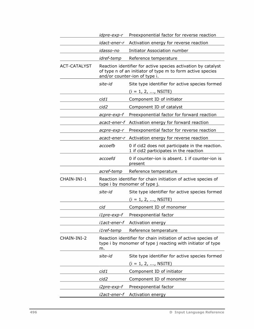
496 D Input Language Reference
idpre-exp-r Preexponential factor for reverse reaction
idact-ener-r Activation energy for reverse reaction
idasso-no Initiator Association number
idref-temp Reference temperature
ACT-CATALYST Reaction identifier for active species activation by catalystof type n of an initiator of type m to form active speciesand/or counter-ion of type i.
site-id Site type identifier for active species formed
(i = 1, 2, ..., NSITE)
cid1 Component ID of initiator
cid2 Component ID of catalyst
acpre-exp-f Preexponential factor for forward reaction
acact-ener-f Activation energy for forward reaction
acpre-exp-r Preexponential factor for reverse reaction
acact-ener-r Activation energy for reverse reaction
accoefb 0 if cid2 does not participate in the reaction.1 if cid2 participates in the reaction
accoefd 0 if counter-ion is absent. 1 if counter-ion ispresent
acref-temp Reference temperature
CHAIN-INI-1 Reaction identifier for chain initiation of active species oftype i by monomer of type j.
site-id Site type identifier for active species formed
(i = 1, 2, ..., NSITE)
cid Component ID of monomer
i1pre-exp-f Preexponential factor
i1act-ener-f Activation energy
i1ref-temp Reference temperature
CHAIN-INI-2 Reaction identifier for chain initiation of active species oftype i by monomer of type j reacting with initiator of typem.
site-id Site type identifier for active species formed
(i = 1, 2, ..., NSITE)
cid1 Component ID of initiator
cid2 Component ID of monomer
i2pre-exp-f Preexponential factor
i2act-ener-f Activation energy
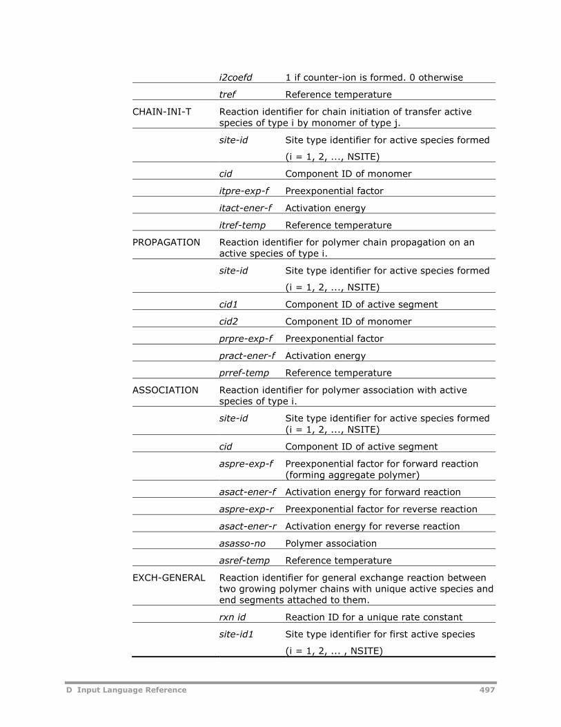
D Input Language Reference 497
i2coefd 1 if counter-ion is formed. 0 otherwise
tref Reference temperature
CHAIN-INI-T Reaction identifier for chain initiation of transfer activespecies of type i by monomer of type j.
site-id Site type identifier for active species formed
(i = 1, 2, ..., NSITE)
cid Component ID of monomer
itpre-exp-f Preexponential factor
itact-ener-f Activation energy
itref-temp Reference temperature
PROPAGATION Reaction identifier for polymer chain propagation on anactive species of type i.
site-id Site type identifier for active species formed
(i = 1, 2, ..., NSITE)
cid1 Component ID of active segment
cid2 Component ID of monomer
prpre-exp-f Preexponential factor
pract-ener-f Activation energy
prref-temp Reference temperature
ASSOCIATION Reaction identifier for polymer association with activespecies of type i.
site-id Site type identifier for active species formed(i = 1, 2, ..., NSITE)
cid Component ID of active segment
aspre-exp-f Preexponential factor for forward reaction(forming aggregate polymer)
asact-ener-f Activation energy for forward reaction
aspre-exp-r Preexponential factor for reverse reaction
asact-ener-r Activation energy for reverse reaction
asasso-no Polymer association
asref-temp Reference temperature
EXCH-GENERAL Reaction identifier for general exchange reaction betweentwo growing polymer chains with unique active species andend segments attached to them.
rxn id Reaction ID for a unique rate constant
site-id1 Site type identifier for first active species
(i = 1, 2, ... , NSITE)
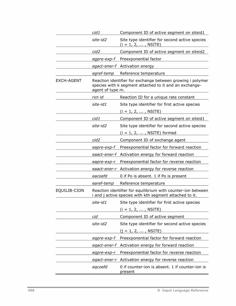
498 D Input Language Reference
cid1 Component ID of active segment on siteid1
site-id2 Site type identifier for second active species(i = 1, 2, ... , NSITE)
cid2 Component ID of active segment on siteid2
egpre-exp-f Preexponential factor
egact-ener-f Activation energy
egref-temp Reference temperature
EXCH-AGENT Reaction identifier for exchange between growing i polymerspecies with k segment attached to it and an exchange-agent of type m.
rxn id Reaction ID for a unique rate constant
site-id1 Site type identifier for first active species
(i = 1, 2, ... , NSITE)
cid1 Component ID of active segment on siteid1
site-id2 Site type identifier for second active species
(i = 1, 2, ... , NSITE) formed
cid2 Component ID of exchange agent
eapre-exp-f Preexponential factor for forward reaction
eaact-ener-f Activation energy for forward reaction
eapre-exp-r Preexponential factor for reverse reaction
eaact-ener-r Activation energy for reverse reaction
eacoefd 0 if Po is absent. 1 if Po is present
earef-temp Reference temperature
EQUILIB-CION Reaction identifier for equilibrium with counter-ion betweeni and j active species with kth segment attached to it.
site-id1 Site type identifier for first active species
(i = 1, 2, ... , NSITE)
cid Component ID of active segment
site-id2 Site type identifier for second active species
(j = 1, 2, ... , NSITE)
eqpre-exp-f Preexponential factor for forward reaction
eqact-ener-f Activation energy for forward reaction
eqpre-exp-r Preexponential factor for reverse reaction
eqact-ener-r Activation energy for reverse reaction
eqcoefd 0 if counter-ion is absent. 1 if counter-ion ispresent
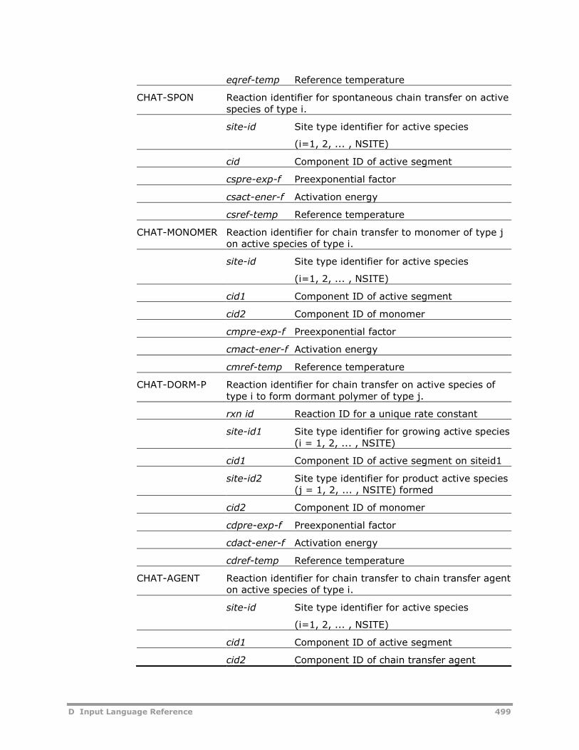
D Input Language Reference 499
eqref-temp Reference temperature
CHAT-SPON Reaction identifier for spontaneous chain transfer on activespecies of type i.
site-id Site type identifier for active species
(i=1, 2, ... , NSITE)
cid Component ID of active segment
cspre-exp-f Preexponential factor
csact-ener-f Activation energy
csref-temp Reference temperature
CHAT-MONOMER Reaction identifier for chain transfer to monomer of type jon active species of type i.
site-id Site type identifier for active species
(i=1, 2, ... , NSITE)
cid1 Component ID of active segment
cid2 Component ID of monomer
cmpre-exp-f Preexponential factor
cmact-ener-f Activation energy
cmref-temp Reference temperature
CHAT-DORM-P Reaction identifier for chain transfer on active species oftype i to form dormant polymer of type j.
rxn id Reaction ID for a unique rate constant
site-id1 Site type identifier for growing active species(i = 1, 2, ... , NSITE)
cid1 Component ID of active segment on siteid1
site-id2 Site type identifier for product active species(j = 1, 2, ... , NSITE) formed
cid2 Component ID of monomer
cdpre-exp-f Preexponential factor
cdact-ener-f Activation energy
cdref-temp Reference temperature
CHAT-AGENT Reaction identifier for chain transfer to chain transfer agenton active species of type i.
site-id Site type identifier for active species
(i=1, 2, ... , NSITE)
cid1 Component ID of active segment
cid2 Component ID of chain transfer agent
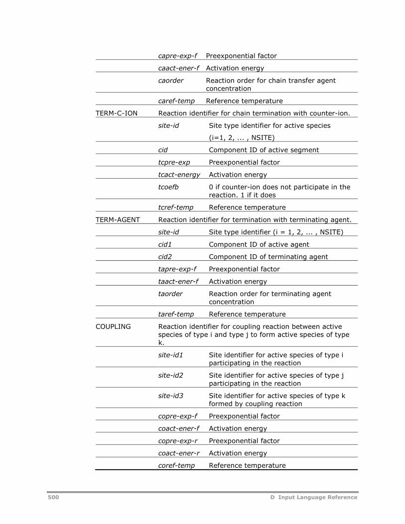
500 D Input Language Reference
capre-exp-f Preexponential factor
caact-ener-f Activation energy
caorder Reaction order for chain transfer agentconcentration
caref-temp Reference temperature
TERM-C-ION Reaction identifier for chain termination with counter-ion.
site-id Site type identifier for active species
(i=1, 2, ... , NSITE)
cid Component ID of active segment
tcpre-exp Preexponential factor
tcact-energy Activation energy
tcoefb 0 if counter-ion does not participate in thereaction. 1 if it does
tcref-temp Reference temperature
TERM-AGENT Reaction identifier for termination with terminating agent.
site-id Site type identifier (i = 1, 2, ... , NSITE)
cid1 Component ID of active agent
cid2 Component ID of terminating agent
tapre-exp-f Preexponential factor
taact-ener-f Activation energy
taorder Reaction order for terminating agentconcentration
taref-temp Reference temperature
COUPLING Reaction identifier for coupling reaction between activespecies of type i and type j to form active species of typek.
site-id1 Site identifier for active species of type iparticipating in the reaction
site-id2 Site identifier for active species of type jparticipating in the reaction
site-id3 Site identifier for active species of type kformed by coupling reaction
copre-exp-f Preexponential factor
coact-ener-f Activation energy
copre-exp-r Preexponential factor
coact-ener-r Activation energy
coref-temp Reference temperature
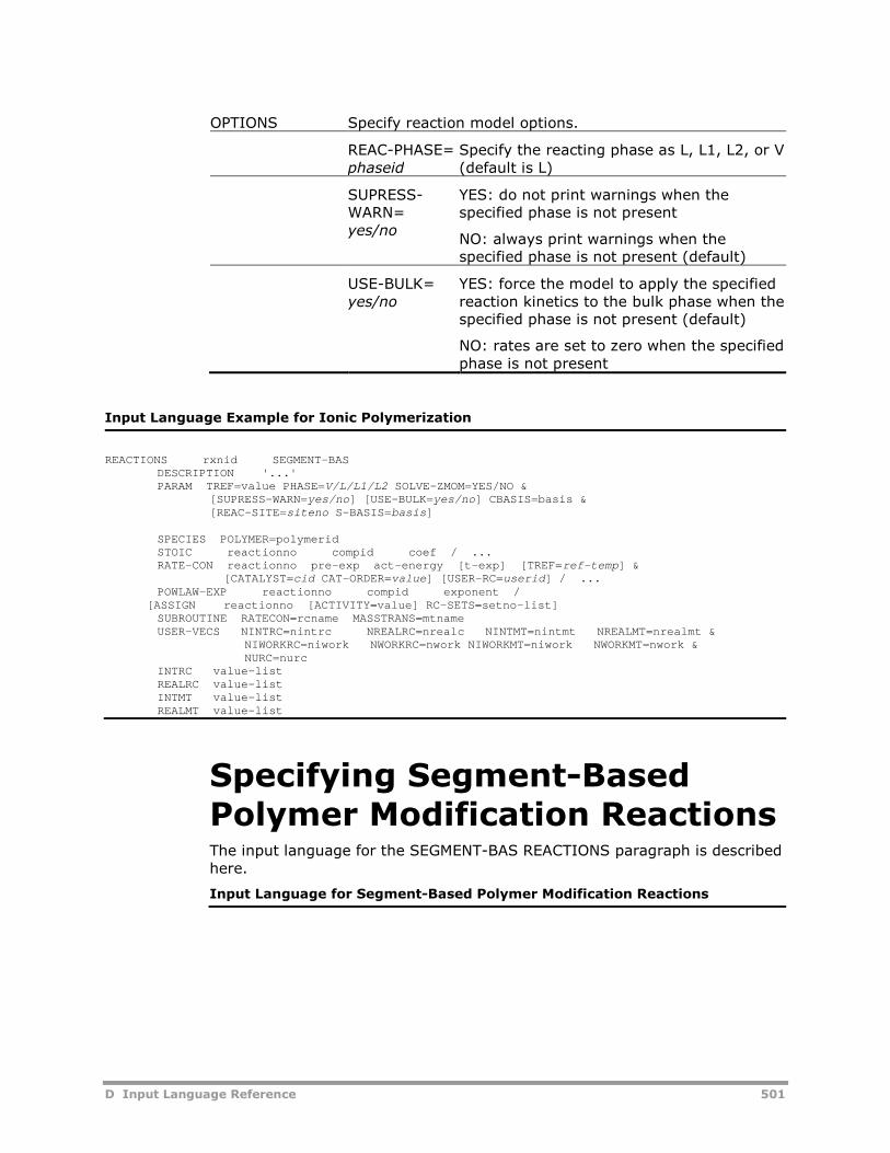
D Input Language Reference 501
OPTIONS Specify reaction model options.
REAC-PHASE=phaseid
Specify the reacting phase as L, L1, L2, or V(default is L)
SUPRESS-WARN=yes/no
YES: do not print warnings when thespecified phase is not present
NO: always print warnings when thespecified phase is not present (default)
USE-BULK=yes/no
YES: force the model to apply the specifiedreaction kinetics to the bulk phase when thespecified phase is not present (default)
NO: rates are set to zero when the specifiedphase is not present
Input Language Example for Ionic Polymerization
REACTIONS rxnid SEGMENT-BASDESCRIPTION '...'PARAM TREF=value PHASE=V/L/L1/L2 SOLVE-ZMOM=YES/NO &
[SUPRESS-WARN=yes/no] [USE-BULK=yes/no] CBASIS=basis &[REAC-SITE=siteno S-BASIS=basis]
SPECIES POLYMER=polymeridSTOIC reactionno compid coef / ...RATE-CON reactionno pre-exp act-energy [t-exp] [TREF=ref-temp] &
[CATALYST=cid CAT-ORDER=value] [USER-RC=userid] / ...POWLAW-EXP reactionno compid exponent /
[ASSIGN reactionno [ACTIVITY=value] RC-SETS=setno-list]SUBROUTINE RATECON=rcname MASSTRANS=mtnameUSER-VECS NINTRC=nintrc NREALRC=nrealc NINTMT=nintmt NREALMT=nrealmt &
NIWORKRC=niwork NWORKRC=nwork NIWORKMT=niwork NWORKMT=nwork &NURC=nurc
INTRC value-listREALRC value-listINTMT value-listREALMT value-list
Specifying Segment-BasedPolymer Modification ReactionsThe input language for the SEGMENT-BAS REACTIONS paragraph is describedhere.
Input Language for Segment-Based Polymer Modification Reactions
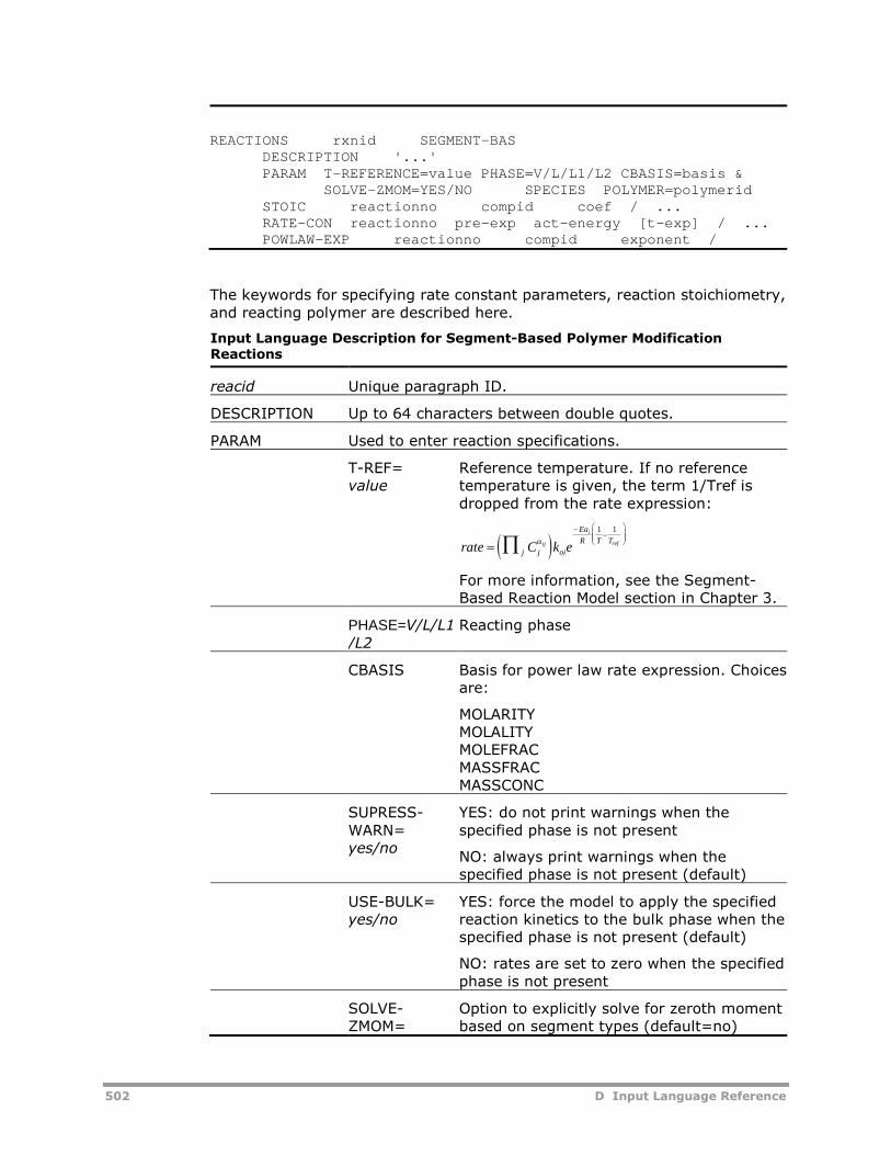
502 D Input Language Reference
REACTIONS rxnid SEGMENT-BASDESCRIPTION '...'PARAM T-REFERENCE=value PHASE=V/L/L1/L2 CBASIS=basis &
SOLVE-ZMOM=YES/NO SPECIES POLYMER=polymeridSTOIC reactionno compid coef / ...RATE-CON reactionno pre-exp act-energy [t-exp] / ...POWLAW-EXP reactionno compid exponent /
The keywords for specifying rate constant parameters, reaction stoichiometry,and reacting polymer are described here.
Input Language Description for Segment-Based Polymer ModificationReactions
reacid Unique paragraph ID.
DESCRIPTION Up to 64 characters between double quotes.
PARAM Used to enter reaction specifications.
T-REF=value
Reference temperature. If no referencetemperature is given, the term 1/Tref isdropped from the rate expression:
rate C k ej j oi
Ea
R T Tij
i
ref
1 1
For more information, see the Segment-Based Reaction Model section in Chapter 3.
PHASE=V/L/L1/L2
Reacting phase
CBASIS Basis for power law rate expression. Choicesare:
MOLARITYMOLALITYMOLEFRACMASSFRACMASSCONC
SUPRESS-WARN=yes/no
YES: do not print warnings when thespecified phase is not present
NO: always print warnings when thespecified phase is not present (default)
USE-BULK=yes/no
YES: force the model to apply the specifiedreaction kinetics to the bulk phase when thespecified phase is not present (default)
NO: rates are set to zero when the specifiedphase is not present
SOLVE-ZMOM=
Option to explicitly solve for zeroth momentbased on segment types (default=no)
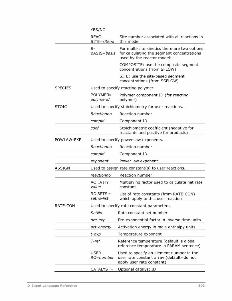
D Input Language Reference 503
YES/NO
REAC-SITE=siteno
Site number associated with all reactions inthis model
S-BASIS=basis
For multi-site kinetics there are two optionsfor calculating the segment concentrationsused by the reactor model:
COMPOSITE: use the composite segmentconcentrations (from SFLOW)
SITE: use the site-based segmentconcentrations (from SSFLOW)
SPECIES Used to specify reacting polymer.
POLYMER=polymerid
Polymer component ID (for reactingpolymer)
STOIC Used to specify stoichiometry for user reactions.
Reactionno Reaction number
compid Component ID
coef Stoichiometric coefficient (negative forreactants and positive for products)
POWLAW-EXP Used to specify power-law exponents.
Reactionno Reaction number
compid Component ID
exponent Power law exponent
ASSIGN Used to assign rate constant(s) to user reactions.
reactionno Reaction number
ACTIVITY=value
Multiplying factor used to calculate net rateconstant
RC-SETS =setno-list
List of rate constants (from RATE-CON)which apply to this user reaction
RATE-CON Used to specify rate constant parameters.
SetNo Rate constant set number
pre-exp Pre-exponential factor in inverse time units
act-energy Activation energy in mole enthalpy units
t-exp Temperature exponent
T-ref Reference temperature (default is globalreference temperature in PARAM sentence)
USER-RC=number
Used to specify an element number in theuser rate constant array (default=do notapply user rate constant)
CATALYST= Optional catalyst ID
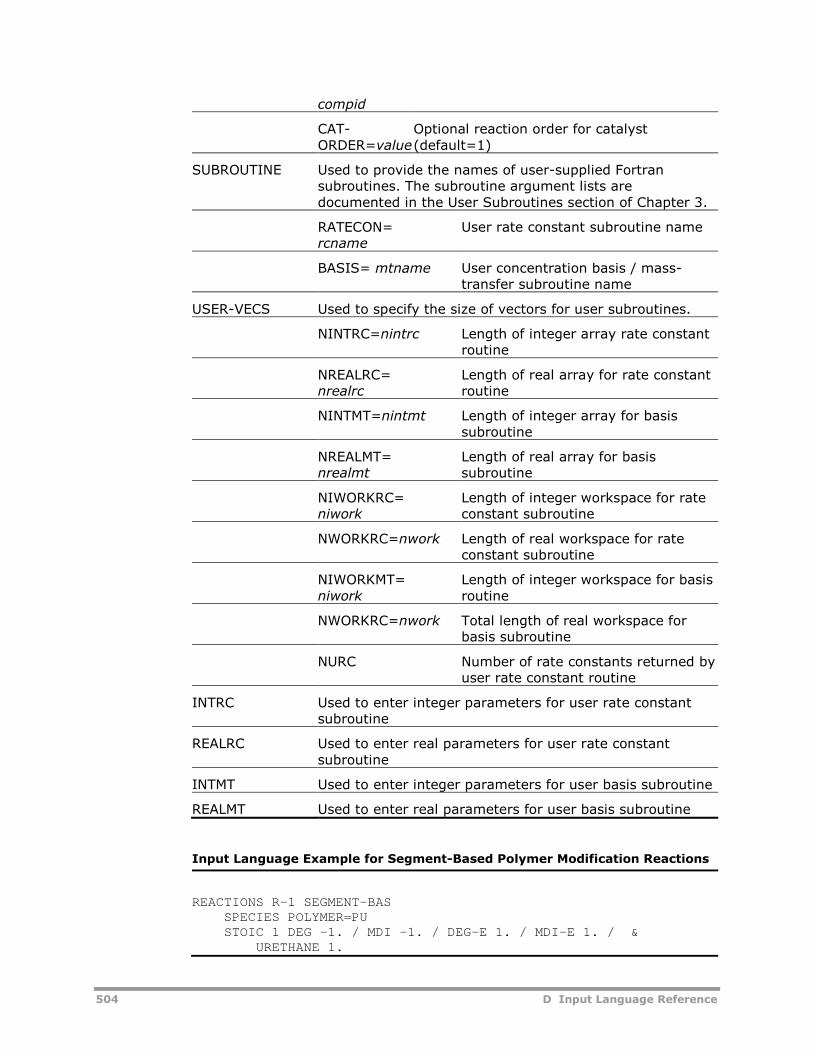
504 D Input Language Reference
compid
CAT-ORDER=value
Optional reaction order for catalyst(default=1)
SUBROUTINE Used to provide the names of user-supplied Fortransubroutines. The subroutine argument lists aredocumented in the User Subroutines section of Chapter 3.
RATECON=rcname
User rate constant subroutine name
BASIS= mtname User concentration basis / mass-transfer subroutine name
USER-VECS Used to specify the size of vectors for user subroutines.
NINTRC=nintrc Length of integer array rate constantroutine
NREALRC=nrealrc
Length of real array for rate constantroutine
NINTMT=nintmt Length of integer array for basissubroutine
NREALMT=nrealmt
Length of real array for basissubroutine
NIWORKRC=niwork
Length of integer workspace for rateconstant subroutine
NWORKRC=nwork Length of real workspace for rateconstant subroutine
NIWORKMT=niwork
Length of integer workspace for basisroutine
NWORKRC=nwork Total length of real workspace forbasis subroutine
NURC Number of rate constants returned byuser rate constant routine
INTRC Used to enter integer parameters for user rate constantsubroutine
REALRC Used to enter real parameters for user rate constantsubroutine
INTMT Used to enter integer parameters for user basis subroutine
REALMT Used to enter real parameters for user basis subroutine
Input Language Example for Segment-Based Polymer Modification Reactions
REACTIONS R-1 SEGMENT-BASSPECIES POLYMER=PUSTOIC 1 DEG -1. / MDI -1. / DEG-E 1. / MDI-E 1. / &
URETHANE 1.
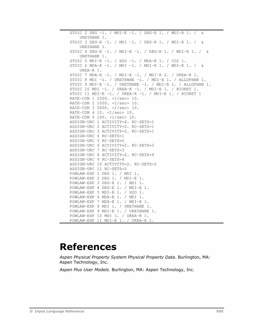
D Input Language Reference 505
STOIC 2 DEG -1. / MDI-E -1. / DEG-E 1. / MDI-R 1. / &URETHANE 1.
STOIC 3 DEG-E -1. / MDI -1. / DEG-R 1. / MDI-E 1. / &URETHANE 1.
STOIC 4 DEG-E -1. / MDI-E -1. / DEG-R 1. / MDI-R 1. / &URETHANE 1.
STOIC 5 MDI-E -1. / H2O -1. / MDA-E 1. / CO2 1.STOIC 6 MDA-E -1. / MDI -1. / MDI-R 1. / MDI-E 1. / &
UREA-R 1.STOIC 7 MDA-E -1. / MDI-E -1. / MDI-R 2. / UREA-R 1.STOIC 8 MDI -1. / URETHANE -1. / MDI-E 1. / ALLOPHAN 1.STOIC 9 MDI-E -1. / URETHANE -1. / MDI-R 1. / ALLOPHAN 1.STOIC 10 MDI -1. / UREA-R -1. / MDI-E 1. / BIURET 1.STOIC 11 MDI-E -1. / UREA-R -1. / MDI-R 1. / BIURET 1RATE-CON 1 2500. <1/sec> 10.RATE-CON 2 1000. <1/sec> 10.RATE-CON 3 5000. <1/sec> 10.RATE-CON 4 10. <1/sec> 10.RATE-CON 5 100. <1/sec> 10.ASSIGN-URC 1 ACTIVITY=4. RC-SETS=1ASSIGN-URC 2 ACTIVITY=2. RC-SETS=1ASSIGN-URC 3 ACTIVITY=2. RC-SETS=1ASSIGN-URC 4 RC-SETS=1ASSIGN-URC 5 RC-SETS=2ASSIGN-URC 6 ACTIVITY=2. RC-SETS=3ASSIGN-URC 7 RC-SETS=3ASSIGN-URC 8 ACTIVITY=2. RC-SETS=4ASSIGN-URC 9 RC-SETS=4ASSIGN-URC 10 ACTIVITY=2. RC-SETS=5ASSIGN-URC 11 RC-SETS=5POWLAW-EXP 1 DEG 1. / MDI 1.POWLAW-EXP 2 DEG 1. / MDI-E 1.POWLAW-EXP 3 DEG-E 1. / MDI 1.POWLAW-EXP 4 DEG-E 1. / MDI-E 1.POWLAW-EXP 5 MDI-E 1. / H2O 1.POWLAW-EXP 6 MDA-E 1. / MDI 1.POWLAW-EXP 7 MDA-E 1. / MDI-E 1.POWLAW-EXP 8 MDI 1. / URETHANE 1.POWLAW-EXP 9 MDI-E 1. / URETHANE 1.POWLAW-EXP 10 MDI 1. / UREA-R 1.POWLAW-EXP 11 MDI-E 1. / UREA-R 1.
ReferencesAspen Physical Property System Physical Property Data. Burlington, MA:Aspen Technology, Inc.
Aspen Plus User Models. Burlington, MA: Aspen Technology, Inc.

506 D Input Language Reference
Index 507
Index
A
Absorption 213Acrylic acid 199Activated initiation 211Activation energy
fitting 356Active species formation 254Adding
emulsion reactions 221free-radical reactions 194gel-effect 196, 222ionic reactions 261segment-based reactions 287user basis subroutine 161, 289user kinetic subroutine 161user rate constant subroutine
161, 289user step-growth reactions 159Ziegler-Natta reactions 246
Addition polymerizationabout 81ionic process differences 250step-growth processes 266
Addition polymers 57Addition reactions 103Aggregate polymer 34, 35Aggregation reactions 256Aliphatic polycarbonates 89Amorphous polymers 16Analysis tools
available 11, 375–80calculation procedure 376optimization 377sensitivity 377
Application tools 294Applications
data fitting 339
example uses 375tools 375–80
ArchitectureAspen Polymers 381
Aromatic polycarbonates 89Aspen Plus
distillation models 296, 301Dupl 296–98equilibrium reactor models 304Flash2 298Flash3 298fractionation models 296FSplit 299Heater 299kinetic reactor models 304–35mass-balance reactor models
302–4Mixer 299Mult 299Pipe 300Pump 300RadFrac 301RBatch 327–35RCSTR 304–17reaction models 86reactor models 296, 302REquil 304RGibbs 304RPlug 317–27RStoic 302RYield 303Sep 301Sep2 301stream manipulators 295unit operation models 359–65
Aspen Polymersapplication tools 294, 375–80architecture 381built-in models 85
508 Index
component attribute treatment inunit operations 335–37
component databanks 387–429configuring 381–82data fitting 294, 339–40decomposition rate parameters
431–33emulsion model 199–223end-use properties 75features 5, 9–13files 382flowsheets 293fortran utilities 445free-radical polymerization
model 163–98input language 447–504installation 382ionic model 249–63key parameters 342kinetic rate constant parameters
431–44model definition 12polyester technology package 95property approach 58reaction models 85segment approach 27segment-based reaction model
265–90steady-state features 294steady-state modeling 291–94step-growth polymerization
model 89–162templates 382troubleshooting 383–86unit operation models 295–338unit operations 294user models 86, 359–73user subroutines 140–55, 274–
84Ziegler-Natta model 225–47
Aspen PolyQuest 96AspenTech support 3AspenTech Support Center 3Association reactions 256Attributes See also Component
attributesaggregate polymers 40, 48bulk polymers 47calculation methods 47catalyst 45
handling in unit operations 336initialization scheme 47–50initializing in streams 451input language 451–53live polymers 39, 48polymers 36–37required 44, 47scale factors 50scaling 453site-based aggregate polymers
43, 50site-based bulk polymers 49site-based live polymers 42, 49site-based polymers 40specifying conventional
component 451user 45, 46variables for data regression 346Ziegler-Natta 44
Average properties 58–59
B
Backbone modifications 269Batch reactors 330Beta-scission 183Bifunctional initiator decomposition
171Bifunctional initiators 174, 175Bimodal distributions 56Bivariate distributions 55Block length 35Branch formation 270Branching
degree of 33free-radical polymerization 192frequency 35number of chains 35reactions 240
Broyden solver 311Bulk
free-radical polymerization 163–98
polymer chain 169polymer chain length moment
equation 187polymerization 164
Bulk polymerization 85Butadiene 199Butyl acrylate 199
Index 509
Butyl methacrylate 199
C
Calculator block 376Catalyst sites
inhibited 231propagation 231types 231vacant 231
Catalystspoisoning 240preactivation 237site activation 237types 226–29Ziegler-Natta 24, 226Ziegler-Natta reactions 230
Catalyzed initiation reaction 173Categorizing polymers 19Chain
initiation for ionic 255initiation for Ziegler-Natta 237scission 269termination 257
Chain lengthaverage properties 59distribution 20, 35, 59–61, 65first moment 47instantaneous weight distribution
63instanteous number-average 63weight-average 63zeroth moment 47
Chain size 55Chain transfer
dormant polymer formation 257ionic reactions 257spontaneous 239, 257to agent 239, 257to cocatalysts 239to electron donor 239to hydrogen 239to monomer 179, 239, 257to polymer 181to small molecules 178, 239to solvent 178, 239to transfer agent 178
Chain-growth polymerizationbulk 85commercial polymers 84comparison to step-growth 82emulsion 85overview 83
precipitation 85solution 85suspension 85
Characterizingapproach 19components 10, 12, 27
Chlorinated polyethylene 265Chloroprene 199Class 0 component attributes 34,
45, 335Class 1 component attributes 34Class 2 component attributes 34,
45–46, 313, 335CMC See Critical micelle
concentrationCocatalysts
poisoning 240Combination reactions 104, 270Component attributes
about 20aggregate polymer 34available 36–44calculation methods 47categories 35class 0 34, 45class 0 treatment in unit
operations 335class 1 34class 2 34, 45–46, 313class 2 treatment in unit
operations 335classes 34composite 35copolymer composition 33degree of branching 33degree of cross-linking 33degree of polymerization 23, 33emulsion polymerization 218for aggregate polymers 40, 48for blocks 52for bulk polymers 47for catalysts 34, 44, 45for composite aggregate
polymers 36for composite live polymers 35for composite polymers 35for ionic initiators 33, 45for live polymers 39, 48for polymer properties 33for polymers 35–36, 36–37for site-based aggregate
polymers 36, 43, 50for site-based bulk polymers 49
510 Index
for site-based live polymers 36,42, 49
for site-based polymers 36, 40–43
for site-based species 44for streams 52for structural properties 33for Ziegler-Natta catalysts 33free-radical polymerization 191initialization 46, 52initialization scheme 47input language 451–53ionic polymerization 260live polymer 34molecular architecture 33molecular weight 33required 44, 47scale factors 50segment composition 33segment-based reaction model
273sequence length 33specifying 51–53specifying conventional 52specifying conventional
attributes 451specifying scale factors 53specifying scaling factors 453step-growth polymerization 124structural properties tracked 23types 35unit operation model treatment
335–37user-specified 45Ziegler-Natta 44Ziegler-Natta polymerization 244
Component databanksabout 25for initiators 26for PC-SAFT 26for polymers 11, 27for POLYPCSF 26for pure components 25for segments 11, 26selecting 28
Componentsadding reacting 154catalysts 24categories 21–25characterizing 12
conventional 22databanks 387–429defining 12defining types 29fortran utilities 360input language 447–51ionic initiators 24naming 29, 447oligomers 23POLYMER databank 387–91,
388–91polymers 22pure component databank 387segment approach 27SEGMENT databank 392–429segments 24site-based 24specifying 28specifying catalysts 448–51specifying oligomers 448–51specifying polymers 448–51specifying step-growth 156
Composition 8Condensation polymerization 81,
126Condensation reactions 103Configuring
Aspen Polymers 381–82Consumption of radicals 61–62Continuous polymerization 92Conventional components 22Conventional species 268Convergence
for RCSTR 308improving 51initialization options (RCSTR)
314parameter tuning 354RBatch troubleshooting 331–35RCSTR troubleshooting 315–17RPlug troubleshooting 323–27scaling factors (RBatch) 332scaling factors (RCSTR) 313scaling factors (RPlug) 323solver method (RBatch) 334solver method (RPlug) 325step size (RBatch) 334step size (RPlug) 325troubleshooting data regression
353–55
Index 511
Conversionenergy balance 311
Copolymerdensity 78
Copolymerization 64free-radical 163–98ionic 249–63ionic propagation 256user input for ionic model 254user input for Ziegler-Natta
model 236Ziegler-Natta 225–47
Copolymers 16Coupling reactions 258CPE See Chlorinated polyethyleneCritical micelle concentration 201Cross linking 270Cross-link formation 184Cross-linking 33, 35Crystalline polymers 16Crystallinity 8Custom
prop-sets 76Custom models See User models,
See User modelscustomer support 3Cycle time 331Cyclodepolymerization reactions
104
D
DAMP-FAC 311Damping factor 311Data
collection 341defining regression cases 351fitting 339–40interpreting regression results
352literature search 340, 341point 345profile 345regression 339–40review 340sequencing regression cases 352trend analysis 341, 343verification 341
Data fitting See also Dataregression
applications 339data collection 341data review 340
data verification 341features 294literature search 340, 341model development 340, 343model refinement 341, 344parameters 342–43preliminary fit 340, 342–43procedure 340–44trend analysis 341, 343
Data regression See also Datafitting
activation energy 356base-case model 345choosing parameters 355convergence problems 353–55data sets 345defining cases 345, 351entering data 345entering operating conditions
345flowsheet variables 378–80fortran blocks 347interpreting results 352–53manipulating variables 347point data 349procedure 340–44, 345–58,
345–58profile data 350Prop-Sets 347scaling fitted parameters 356sensitivity studies 355sequencing cases 352standard deviation 351troubleshooting 353–55tuning 354
Databankscomponent 25, 387–429functional group 11INITIATOR 26PC-SAFT 26polymer 11POLYMER 27, 387–91POLYPCSF 26pure component 25, 387segment 11SEGMENT 26, 391–429selecting 28
Dead polymer 35Dead polymer chain 169Dead sites 45Dead zones 308, 321Defining
additional simulation options 13
512 Index
components 12feed streams 13flowsheet options 12global simulation options 12polymerization kinetics 13property models 13regression cases 351UOS model operating conditions
13Degree of
branching 33, 55cross-linking 33polymerization 33, 57
Densityas polymer property 8function 58–59of copolymer 78
Depolymerization 269Design-spec block 377Desorption 213Developing
models 12Direct esterification 90Displaying
distribution data for reactors 70distribution data for streams 70distribution data tables 70
Disproportionation 180Distillation models
about 301available 296RadFrac 301
Distributionaverage properties and moments
58–59calcuations 454chain length 65copolymerization 64displaying data table 70displaying for reactors 70displaying for streams 70functions 56, 58GPC 67, 68in process models 58kinetic reactors 65method of instantaneous
properties 60–64moment equation 187moments 58–59particle size 216–18
plotting data 70plug flow reactors 66polymer 65procedure 67specifying calculations 69–71specifying characteristics 69streams 67structural property 55–72tracking 65verification 68
Distribution calculationsspecifying input language 454
Duplabout 296–98attribute handling 336
Dutyin RBatch 327in RCSTR 305in RPlug 318
Dyads 35free-radical rate equation 187
Dynamic models 10, 13
E
EB-LOOP 311e-bulletins 3Editing
emulsion reactions 221free-radical reactions 195ionic reactions 261segment-based reactions 287user step-growth reactions 159Ziegler-Natta reactions 246
Elastomers 16Electrophilic reactions 101Emulsion polymerization
absorption 213accessing model 219activated initiation 211adding reactions 221applications 199aqueous phase 208assigning rate constants 221attributes 218built-in reaction listing 220chain growth 85desorption 213editing reactions 221homogeneous nucleation 204–6
Index 513
industrial processes 200input language 477–84kinetics 200–215, 211kinetics scheme (figure) 204latex 202latex reactions 207micellar nucleation 201–4model 199–223model assumptions 215model features 215–18monomer partitioning 215–16nomenclature 208nucleation time 203particle growth 201, 206particle number 203particle phase 210particle size distribution 216–18population balance equation 217products produced 200properties calculated 218radical balance 207–11rate constant 214rate of particle formation 206reactions 204redox initiation 212seed process 206Smith-Ewart theory 211specifying calculation options
222specifying gel-effect 222specifying model 219specifying particle growth
parameters 223specifying phase partitioning 222specifying reacting species 220stage I (seed) 202stage II (growth) 202, 206stage III (finishing) 202user profiles 218
End group reformation reactions104
End-use propertiesabout 73–79adding a Prop-Set 79calculating 76, 79density of copolymer 78input language 454–56intrinsic viscosity 77melt index 78melt index ratio 79relationship to structure 75selecting 79zero-shear viscosity 77
Energy balance conversion 311Entering
point data 349profile data 350standard deviations 351
Equilibriumfor ionic polymerization 258for Ziegler-Natta polymerization
243phase 188reactions with counter-ion 256reactor models 304
Equilibrium modelsRGibbs 304RYield 304
Esterificationbatch process 94direct 90operating conditions 93results 91secondary 91
Estimatingproperty parameters 459
Ethyleneprocess types 227
Ethylene-propylene 226, 229Exchange reactions 256
F
Features 5, 9–13Feed streams
defining 13with polymers 23, 46
Filesstartup 382
Fittingactivation energy 356choosing parameters 355
Flash2about 298attribute handling 336input variables 347results variables 347
Flash3about 298attribute handling 336input variables 347results variables 347
Flowsheeting options 11Flowsheets
basic unit operation models 295calculation procedure 376
514 Index
calculator block 376design-spec block 377distillation models 296, 301Dupl block 296–98equilibrium reactor models 304Flash2 block 298Flash3 block 298fractionation models 296FSplit block 299Heater block 299incorporating spreadsheets 376kinetic reactor models 304–35mass-balance reactor models
302–4Mixer block 299model configuration tools 376–
78Mult block 299optimization 377Pipe block 300polymer process 293process studies 376–78Pump block 300RadFrac block 301RBatch block 327–35RCSTR block 304–17reactor models 296, 302REquil block 304RGibbs block 304RPlug block 317–27RStoic block 302RYield block 303sensitivity study 377Sep block 301Sep2 block 301setting fixed variables 377steady-state 291–94stream manipulators 295unit operation models 295–338variables 378–80variables for data regression
378–80Fortran
arguments 445linking 383monitors 360templates 383utilities 360, 445
Fortran blocksin data regression 347
to enforce assumptions 347to manipulate process variables
348to scale paramters 357
Fortran utilitiescomponent handling 360stream handling 360
Fractionation models 296Free-radical iniators
decomposition rate parameters431–33
Free-radical polymerizationaccessing model 193adding reactions 194applications 163beta-scission reactions 183bifunctonal initiator
decomposition reaction 174,175
branching 192built-in reaction listing 194bulk 164bulk polymer chain length
moment equation 187calculation method 185catalyzed initiation reaction 173chain transfer reactions 178dyads 187editing reactions 195gel effect 170gel effect 188–89induced initiation reaction 173industrial processes 164initiation reactions 171initiator decomposition reaction
172input language 467–77kinetics 165–83kinetics nomenclature 166kinetics scheme (figure) 165live polymer chain length
moment equation 186model 163–98model assumptions 185–90model features 185–90modifying the rate expression
170moment-property relationship
equation 191parameters 190–93
Index 515
pendent double bondpolymerization 184
phase equilibrium 188propagation reactions 176properties calculated 190–93quasi-steady-state
approximation 188rate constant 170reactions 165solution 164specifying calculation options
196specifying gel-effect 196specifying model 193specifying reacting species 194specifying reactions 195specifying user profiles 197structural properties 192termination reactions 178–79user profile properties 192
Frequency function 58–59FSplit
about 299attribute handling 336
Functional group databank 11
G
Gas-phase process 227Gear integrator 323, 332Gel effect
built-in correlations 189free-radical 170free-radical polymerization 188–
89specifying 196, 222user specified correlations 189user subroutine arguments 189
Gel effect subroutinefree-radical 170
Gel permeation chromatography 67Generation of radicals 61Glycol recovery 91GPC 67
H
HDPE See High densitypolyethylene
Heat exchangers 307Heater
about 299attribute handling 337
help desk 3Heterogeneous catalysts 226High density polyethylene
about 225processes 227
High impact polypropylene 229HIPP See High impact
polypropyleneHold-up
in RCSTR 305Homogeneous catalysts 226Homogeneous nucleation
particle formation 201process 204–6rate of particle formation 206
Homopolymers 15
I
INCL-COMPS 154Induced initiation reaction 173Industrial applications
polymer production steps 291–93
polymer production steps(figure) 291
Industrial processesemulsion polymerization 200free-radical polymerization 164ionic polymerization 250model uses 375segment-based reaction model
266step-growth polymerization 90Ziegler-Natta polymerization 226
Inhibited sites 231Inhibition
catalyst sites 45, 240Initators
for ionic polymerization 254Initialization
hybrid option 315integration option 314options for RCSTR 314solver option 314
Initiationactivated 211catalyzed 171decomposition rate 171free-radical 172, 174, 175free-radical polymerization 171induced 171ionic 45, 251
516 Index
reaction for catalyzed 173reaction for decomposition 172reaction for induced 173redox 212
INITIATOR databankabout 26
Initiatorsdatabank 26free-radical 431–33ionic 24
Injection ports 322Input language
attribute scaling factors 453catalysts 448–51component attributes 451–53components 447–51conventional component
attributes 451distribution calculations 454emulsion 477–84end-use properties 454–56for Aspen Polymers 447–504free-radical 467–77ionic 494–501oligomers 448–51physical properties 456–60polymers 448–51property data 458property methods 456property parameter estimation
459prop-set 454–56segment-based reactions 501–5step-growth 460–67streams 451Ziegler-Natta 484–93
Input variablesFlash2 347Flash3 347MultiFrac 347RadFrac 347RBatch 346RCSTR 346RPlug 347standard deviations 351
InstallingAspen Polymers 382
Instantaneousnumber-average 63properties 58, 60–64, 65
weight chain length 63–64Interfacial processes 84Intermolecular reactions 103Intramolecular reactions 103Intrinsic viscosity 77Ionic initiator 24Ionic initiators
component attributes 33properties tracked 45
Ionic polymerizationaccessing model 260active species formation 254adding reactions 261aggregation 256applications 249assigning rate constants 262association 256built-in reaction listing 261chain initiation 255chain termination 257chain transfer 257comparison to other addition
processes 250copolymerization steps 254, 256coupling 258editing reactions 261equilibrium with counter-ion 256exchange 256industrial processes 250initiator attributes 251initiator types 254input language 494–501kinetics scheme 250–58kinetics scheme (figure) 252model 249–63model assumptions 258–59model features 258–59nomenclature 253phase equilibria 258polymers tracked 251propagation 255properties calculated 259–60rate calculations 258rate constants 254reactions 252specifying model 260specifying reacting species 260
Index 517
K
Kinetic modelsRBatch 327–35RCSTR 304–17RPlug 317–27
Kineticsdata fitting 339–40decomposition rate parameters
431–33defining polymerization 13emulsion (input language) 477–
84emulsion polymerization 200–
215, 211free-radical (input language)
467–77free-radical polymerization 165–
83ionic (input language) 494–501ionic polymerization 250–58mechanisms 10melt polycarbonate 122–24multi-site 65, 66nylon reactions 111–22parameter influence on 342polyester reactions 105–11polymerization 81rate constant parameters 431–
44reactor models 304–35segment-based reaction model
270single-site 65, 66specifying emulsion 219–23specifying free-radical 193–97specifying ionic 260–62specifying step-growth 51–53specifying step-growth (input
language) 460–67specifying Ziegler-Natta 244–47step-growth polymerization 101–
24user fortran arguments 445user models 365–69user subroutine (example) 366user subroutines 149Ziegler-Natta (input language)
484–93Ziegler-Natta polymerization
230–42
L
Latexdefinition 202number of particles per liter 203reactions 207
Linear condensation polymers 57Linear low density polyethylene
about 225processes 227, 228
Linkingfortran 383
Liquid enthalpyuser subroutine (example) 371
Liquid process 228Live
polymer chain 169polymer chain length moment
equation 186Live polymer 34, 35LLDPE See Linear low density
polyethyleneLocal work arrays 155, 284Low density polyethylene 164Low molecular weight polymer 57
M
Mass balance 311Mass-balance models
RStoic 302RYield 303
Material streams 46MB-LOOP 311Melt index 8, 78Melt index ratio 79Melt polycarbonate
rate constants 123reaction components 122reaction kinetics 122–24step-growth reactions 123
Melt-phasenylon-6,6 processes 122polymerization 100processes 84
Metallocene catalysts 226Method of instantaneous properties
58, 60–64, 65Method of moments 58, 185Methylmethacrylate 199Micellar nucleation 201–4MIXED
substream variables 380Mixer
518 Index
about 299attribute handling 337
Mixingnon-ideal in RCSTR 306non-ideal in RPlug 320
Modelingapplications 89, 163, 199, 225,
249, 265data fitting 294, 339–40enforcing assumptions 347features 294nylon 96–100nylon-6,6 116polycarbonates 100–101polyesters 90–96polymer phase change 303polymer processes 293steady-state 291–94tools 294unit operations 294, 295–338
Modelsaccessing variables 378–80analysis tools 376–78application tools 375–80base case 345calculations for user models
360–65defining 12developing 340, 343parameter fitting 342–43possible uses 375process studies 376–78refining 341, 344structure for user models 359trend analysis 341, 343unit operation 11user 359–73USER2 routine 362
Molecular structureSEGMENT databank 392–429
Molecular weightas component attribute 33distribution 8, 58number-average 78weight-average 35, 78
Moment equationsbulk polymer 187general 186live polymer 186relationship to properties 191
Moments of chain lengthdistribution
first 39, 47Monomers
corresponding segment formulas127
definition 15functional groups 129partitioning 215–16purification 292synthesis 292–93, 292
Most-probable distribution 57, 114,120, 131
Multabout 299attribute handling 336
MultiFracattribute handling 337input variables 347results variables 347
Multimodal distributions 56
N
Newton solver 311Nomenclature
for emulsion model 208for free-radical model 166for ionic model 253for segment-based reaction
model 271for step-growth model 103for Ziegler-Natta model 234POLYMER databank 388–91SEGMENT databank 391
Nucleationhomogeneous 201, 204–6micellar 201–4period 202time 202time (equation) 203
Nucleophilic reactionsabout 101nomenclature 103
Number averagechain length distribution 63degree of polymerization 57
Number-averagedegree of polymerization 35
Nylon
Index 519
aqueous salt solutions 98melt-phase polymerization 100production process 96–100salt preparation 98
Nylon-6production process 96rate constants 113reaction components 112reaction kinetics 111step-growth reactions 112user-specified reactions 113
Nylon-6,6melt-phase polymerization 122modeling approaches 116production process 98rate constants 118, 119reaction components 116reaction kinetics 115step-growth reactions 117user-specified reactions 119
O
Occupied sites 45Oligomers
as components 23definition 15fractionation 131segments 24specifying 30
Optimization 377Orienticity 35
P
Packed vectors 155, 284Parameters
data fitting 339–40decomposition rate 431–33estimating property 459fitting 340, 342–43for free-radical polymerization
190–93influence of kinetics 342integer 154, 284kinetic rate constant 431–44POLYMER property 387real 154, 284scaling 356SEGMENT property 391to manipulate process variables
348tuning for data regression 354
Particle growthin emulsion polymerization 206specifying parameters 223
PBT See Polybutyleneterephthalate
PC-SAFTdatabank 26
PC-SAFT databankabout 26
PEN See Polyethylene naphthalatePendent double bond
polymerization 184PET See Polyethylene terephthalatePhase equilibria
ionic polymerization 258step-growth polymerization 126Ziegler-Natta polymerization 243
Phase equilibriumfree-radical polymerization 188
Phase partitioningspecifying 222
Physical propertiescalculations in user models 364fitting parameters 342–43input language 456–60user models 370–73user subroutine (example) 371
Pipe 300Plant data fitting 339–40Plot
distribution data 70PMMA See Polymethyl
methacrylatePoint data
about 345entering 349
Polyamides 90Polybutadiene 249Polybutene 249Polybutylene terephthalate 95Polycarbonates
aliphatic 89aromatic 89production process 100–101reaction kinetics 122–24
Polydispersityindex 63
Polyestersassigning rate constants 109polyester technology package 95production process 90–96reaction components 106reaction kinetics 105–11
520 Index
side reactions 109step-growth reactions 108user-specified reactions 110
Polyethylenechlorinated 265low density 164
Polyethylene naphthalate 95Polyethylene terephthalate
batch processes 93–95continuous step-growth
polymerization 90–93solid-state models 96
Polyisobutylene 249, 265Polymer chain
bulk 169dead 169definition 169live 169
POLYMER databankabout 11, 27, 387components 388–91nomenclature 388–91
Polymerizationaddition 81bulk 85chain-growth 82, 83condensation 81condensation polymerization 126continuous 92degree of 33emulsion 85, 199–223free-radical 163–98interfacial 84ionic 249–63kinetics 10, 13, 81manufacturing step 293melt phase 84precipitation 85process overview 6–7process types 84reaction types 81reactions 81solid-state 84solution 84, 85step-growth 82, 83, 89–162suspension 85Ziegler-Natta 225–47
Polymersacrylic acid 199addition 57
aggregate 34, 35aliphatic polycarbonates 89amorphous 16aromatic polycarbonates 89as components 23average properties and moments
58–59branched 16bulk polymer chain length
moment equation 187butadiene 199butyl acrylate 199butyl methacrylate 199by chemical structure 18by physical structure 16by property 18chain-growth 84characterizing 19chlorinated polyethylene 265chloroprene 199component attribute sets 35–36component attributes 33, 35component characterization 10crystalline 16data fitting procedure 340–44data regression procedure 345–
58dead 35definition 6elastomers 16emulsion properties calculated
218end-use properties 73–79ethylene-propylene 226free-radical properties calculated
190–93high density polyethylene 225high-impact polystyrene 163ionic properties calculated 259–
60ladder 16linear 16linear condensation 57linear low density polyethylene
225live 34, 35live polymer chain length
moment equation 186low density polyethylene 164low molecular weight 57
Index 521
mass 124, 273method of instantaneous
properties 58, 60, 65method of moments 58methylmethacrylate 199mole fraction 272monomer purification 292monomer synthesis 292–93, 292network 16nomenclature 388–91phase change 303polyamides 90polybutadiene 249polybutene 249polyesters 90polyisobutylene 249, 265polymerization step 293polymethyl methacrylate 164,
265polyoxides 249polypropylene 226polystyrene 163, 164, 249polyurethanes 90polyvinyl acetate 163polyvinyl alcohol 164, 265polyvinyl chloride 163processing 6–7processing step 293production rate 63production steps 291–93properties 19properties tracked 35property distributions 55–72property parameters 387prop-sets 74purification 292–93reacting 266recovery 9, 293segment-based properties
calculated 273segments 24, 391separation 9, 293specifying 29star 16step-growth 83structural properties 23structure 15structure of 15–19styrene 199synthesis 293tetrafluroethylene 199thermoplastics 16thermosets 16
tracking structural properties 33vinyl chloride 199vinylacetate 199Ziegler-Natta properties
calculated 243Polymethyl methacrylate 164, 265Polyoxides 249POLYPCSF
databank 26POLYPCSF databank
about 26Polypropylene
about 226process types 228
Polypropylene terephthalate 95Polystyrene 163, 164, 249Polyurethanes 90Polyvinyl acetate 163Polyvinyl alcohol 164, 265Polyvinyl chloride 163Population balance
equation for emulsionpolymerization 217
equation for free-radicalpolymerization 185
Potential sites 44Power-law reaction model See
Segment-based reactionmodel:about
PPT See Polyproylene terephthalatePrecipitation polymerization 85Pressure
drop 305, 319in RBatch 328in RCSTR 305in RPlug 319
Process modelingdata fitting 294dynamic 10, 13features 294flowsheets for polymer processes
293issues for polymers 7–9steady-state 10, 13, 291–94tools 294unit operations 294
Processingpolymers 293
Profile dataabout 345data sets 350entering 350RBatch 350
522 Index
RPlug 350Propagation
depolymerization 269free-radical polymerization 176ionic polymerization 255segment-based reaction model
270sites 231Ziegler-Natta polymerization 238
Propertiesaverage polymer 58–59branching 23chain size 55composition 8copolymer composition 23, 55copolymerization 64crystallinity/density 8degree of branching 55degree of polymerization 23density of copolymer 78end-use 73–79estimating parameters 459for polymers 58input language 456–60intrinsic viscosity 77melt index 8, 78melt index ratio 79method of instantaneous 60molecular structure 23molecular weight 23molecular weight 8moments of molecular weight
distribution 23particle size 55polymer structural 33, 55prop-set 73segment composition 23specifying data 458viscosity 8zero-shear viscosity 77
Property distributionsbimodal 56bivariate 55most-probable 57multimodal 56Schulz-Flory 56Stockmayer bivariate 58structural 55–72types 55unimodal 56
Property methodsinput language 456
Property parameter databanks 11Property set See also Prop-SetsProp-Sets
adding 79custom 76defining 74for data regression 347for polymers 74properties 73uses 73
Propyleneprocesses 228, 229
Pseudocondensation reactions 103Pump 300Pure components
databank 25, 387Purification
monomer 292process step 292–93
PVA See Polyvinyl alcohol
Q
QSSA See Quasi-steady-stateapproximation
Quasi-steady-state approximation188
R
RadFracabout 301attribute handling 337input variables 347results variables 347
Radiation initiation reaction 173Radicals
absorption 210balance 207–11consumption of 61–62depletion 208desorption 210generation 208generation of 61rate of production 208termination 210
Random scission 104Rate constant parameters
data-fitting 294
Index 523
Rate constantsassigning to emulsion reactions
221assigning to ionic reactions 262assigning to step-growth
reactions 158, 159assigning to Ziegler-Natta
reactions 246data fitting 339emulsion 214for melt polycarbonate 123for model generated reactions
135for nylon-6 113for nylon-6,6 118, 119for polyesters 109for user-specified reactions 139,
288free-radical 170ionic 254kinetic parameters 431–44segment-based 270specifying for segment-based
power-law reactions 288specifying for step-growth user
reactions 159step-growth 153user subroutines 144, 279Ziegler-Natta 236
Rate expressionstep-growth 133, 138
RBatchabout 327–35attribute handling 337batch reactors 330common problems 335cycle time 331duty 327dynamic scaling 332hybrid scaling options 333input variables 346pressure 328profile data 350residence time 329results variables 346scaling options 332semi-batch reactors 330solver method 334specifying user profiles 197static scaling options 332step size 334streams 330temperature 327
troubleshooting convergence331–35
volume 329RCSTR
about 304–17algorithm 308attribute handling 337calculation loops 309calculation table 309common problems 316component scaling 313condensed phases 305convergence 308duty 305effective hold-up 305external heat exchanger 307horizontal partition 306hybrid initialization 315initialization options 314input variables 346integration initialization 314multiphase 305non-ideal mixing 306pressure 305residence time 305results variables 346scaling options 313single-phases 305solver initialization 314substream scaling 313temperature 305troubleshooting convergence
315–17vertical partition 307with dead zone 308
Reacting phasespecifying for segment-based
power-law model 286specifying for step-growth 160
Reacting polymers 266Reaction models
Aspen Plus 86, 359–65available 359–65basic unit operation 295built-in 85custom 86distillation 296, 301Dupl 296–98equilibrium 304Flash2 298Flash3 298fractionation 296FSplit 299
524 Index
generic 86Heater 299kinetic 304–35mass-balance 302–4Mixer 299Mult 299Pipe 300Pump 300RadFrac 301RBatch 327–35RCSTR 304–17reactor 296, 302REquil 304RGibbs 304RPlug 317–27RStoic 302RYield 303Sep 301Sep2 301stream manipulators 295treatment of component
attributes 335–37Reactions
active species 254adding emulsion 221adding free-radical 194adding ionic 261adding segment-based 287adding user 159adding Ziegler-Natta 246addition 103aggregation 256assigning emulsion rate
constants 221assigning ionic rate constants
262assigning step-growth rate
constants 158assigning user rate constants
159assigning Ziegler-Natta rate
constants 246association 256backbone 269beta-scission 183bifunctional initiator
decomposition 174, 175branching (segment-based) 270branching (Ziegler-Natta) 240catalyst preactivation 237
catalyst site activation 237catalyzed initiation 171, 173chain initiation (free-radical 171chain initiation (ionic) 255chain initiation (Ziegler-Natta)
237chain scission 269chain termination (free-radical)
178–79chain termination (ionic) 257chain transfer (free-radical) 178chain transfer (ionic) 257chain transfer (Ziegler-Natta)
239chain-growth 83classifying 81cocatalyst poisoning 240combination 104, 270condensation 103conventional species 268coupling 258cross linking 270cyclodepolymerization 104depolymerization 269editing emulsion 221editing free-radical 195editing ionic 261editing segment-based 287editing user 159editing Ziegler-Natta 246electrophilic 101emulsion polymerization 204end group reformation 104equilibrium with counter-ion 256exchange 256for step-growth polymerization
126free-radical polymerization 165homogeneous nucleation 204including user 158induced initiation 171, 173Inhibition 181initiator decomposition 171, 172intermolecular 103intramolecular 103ionic polymerization 252latex 207melt polycarbonate kinetics 122–
24micellar nucleation 201
Index 525
micellar nucleation (figure) 202modification See Segment-based
reaction modelnucleophilic 101nylon-6 kinetics 111nylon-6,6 kinetics 115particle growth 206polyester kinetics 105–11polymerization 81propagation (free-radical) 176propagation (ionic) 255propagation (segment-based)
270propagation (Ziegler-Natta) 238pseudocondensation 103radiation initiation 173radical balance 207rearrangement 104reverse condensation 103ring addition 104ring closing 104ring opening 104side group 269site deactivation 239site inhibition 240specifying segment-based 285–
89specifying user rate constants
159spontaneous initiation 173step-growth 83step-growth functional groups
128step-growth polymerization 104step-growth rate constants 157–
58supplied by emulsion model 215–
18supplied by free-radical model
185–90supplied by ionic model 258supplied by segment-based
model 273supplied by step-growth model
133–37supplied by Ziegler-Natta model
243terminal double bond 240termination (free-radical) 178–
79termination (ionic) 257thermal initiation 173
types affecting catalyst states230
user-specified step-growth 138–40
viewing emulsion 220viewing free-radical 194viewing ionic 261viewing segment-based 287viewing step-growth 157viewing Ziegler-Natta 245Ziegler-Natta polymerization 232
Reactor modelsabout 302available 296data sets 350equilibrium 304input variables 346kinetic 304–35mass-balance 302–4results variables 346
Reactorscondensed phase RCSTR 305convergence problems for
RBatch 331–35convergence problems for RCSTR
315–17convergence problems for RPlug
323–27displaying distribution data 70distribution 65horizontal partition 306multiphase RCSTR 305multiphase RPlug 320RCSTR algorithm 308single-phase RCSTR 305vertical partition 307with dead zones 308, 321with external heat exchanger
307with injection ports 322
Rearrangement reactions 104Recovery/separation 9, 293Redox initiation 212Regression See Data regressionReports
for user models 365step-growth options 160
REquilabout 304attribute handling 337
Residence timeRBatch 329RCSTR 305
526 Index
RPlug 319Results variables
Flash2 347Flash3 347MultiFrac 347RadFrac 347RBatch 346RCSTR 346RPlug 347standard deviations 351
Reverse condensation reactions103
Rgibbsabout 304
RGibbsattribute handling 337
Ring addition reactions 104Ring closing reactions 104Ring opening reactions 104Routines
USER2 362RPlug
about 317–27attribute handling 337common problems 326duty 318dynamic scaling 323hybrid scaling 325input variables 347multiphase 320non-ideal mixing 320pressure 319profile data 350residence time 319results variables 347scaling options 323solver method 325specifying user profiles 197static scaling options 323step size 325temperature 318troubleshooting convergence
323–27with dead zone 321with injection ports 322
Rstoicabout 302
RStoicattribute handling 337
Ryield
about 303RYield
attribute handling 337
S
Saltaqueous solutions 98preparation 98
Scale factorsabout 50specifying 53
Scalingfactors 453
Scaling factorscomponent (RCSTR) 313dynamic (RBatch) 332dynamic (RPlug) 323hybrid (RBatch) 333hybrid (RPlug) 325RBatch 332RCSTR 313RPlug 323static (RBatch) 332static (RPlug) 323substream (RCSTR) 313
Schulz-Flory distribution 56Scission 104, 269Secondary esterification 91Seed process 206Segment approach 27SEGMENT databank
about 11, 26, 391components 392–429nomenclature 391
Segment flow 35Segment fraction 35Segment-based model
assigning rate constants 288including user rate constant
subroutine 289Segment-based power-law model
specifying reacting phase 286user subroutines 274–84
Segment-based reaction modelabout 265–90accessing 285adding reaction schemes 287adding reactions 287applications 265
Index 527
assumptions 272backbone modifications 269branch formation 270chain scission 269combination 270conventional species 268cross linking 270depolymerization 269editing reactions 287features 272including user basis subroutine
289industrial processes 266input language 501–5kinetics 270mole fraction conversion 272nomenclature 271propagation 270properties calculated 273rate calculations 273rate constants 270reaction categories 267–72reactions allowed 267–72side group modifications 269specifying model 285specifying pre-exponential units
288specifying rate constants 288specifying reaction settings 285
Segmentscomposition 15, 33copolymers 16definition 24homopolymers 15methodology in Aspen Polymers
27mole fraction 272molecular structure 392–429nomenclature 391property parameters 391sequence 15specifying 29structure 15types 24
Semi-batch reactors 330Semi-crystalline copolymer density
78Sensitivity blocks 377Sep
about 301attribute handling 336
Sep2about 301
attribute handling 336Separation/recovery 9, 293Side group modifications 269Simulations
dynamic 10templates 382
Site activation 237Site deactivation 239Site inhibition 240Site-based components
about 24attributes 44specifying 30
Slurry process 227, 228Smith-Ewart theory 211Solid-state models 96Solid-state processes 84Solution polymerization 85, 164Solution process 227Solution processes 84Solver methods
RBatch 334RPlug 325
Specifyingadditional simulation options 13Aspen Polymers options 381–82attribute scaling factors (input
language) 453catalysts 448–51component attributes 51–53component attributes (input
language) 451–53component attributes in blocks
52component attributes in streams
52component names 447components 12, 28components (input language)
447–51conventional component
attributes 52, 451data fit 340–44data regression 345–58databanks 28distribution calculations 69–71distribution calculations (input
language) 454distribution characteristics 69emulsion calculation options 222emulsion kinetics 219–23emulsion kinetics (input
language) 477–84
528 Index
emulsion model 219emulsion rate constants 221emulsion reacting species 220end-use properties 79end-use properties (input
language) 454–56feed streams 13fixed process variables 377flowsheet options 12free-radical calculation options
196free-radical kinetics 193–97free-radical kinetics (input
language) 467–77free-radical model 193free-radical reacting species 194gel-effect 196, 222global simulation options 12ionic kinetics 260–62ionic kinetics (input language)
494–501ionic model 260ionic rate constants 262ionic reacting species 260oligomers 30, 448–51particle growth parameters 223phase partitioning 222physical properties (input
language) 456–60point data 349polymerization kinetics 13polymers 29, 448–51pre-exponential units 160, 288profile data 350property data 458property models 13reacting phase 286regression cases 351scale factors 53segment-based reaction model
285segment-based reaction rate
constants 288segment-based reaction scheme
287segment-based reaction settings
285segment-based reactions 285–89segment-based reactions (input
language) 501–5
segments 29site-based components 30standard deviations 351step-growth components 156step-growth kinetics 51–53step-growth kinetics (input
language) 460–67step-growth model 156step-growth rate constants 157–
58, 158, 159step-growth reacting phase 160step-growth report options 160stream attributes 451UOS model operating conditions
13user models 359–73user profiles 197user step-growth reactions 158Ziegler-Natta kinetics 244–47Ziegler-Natta kinetics (input
language) 484–93Ziegler-Natta model 244Ziegler-Natta rate constants 246Ziegler-Natta reacting species
245Spontaneous initiation reaction 173Spreadsheets
incorporating in flowsheets 376SSplit
attribute handling 336Standard deviations 351Starting
Aspen Polymers 381–82Startup files 382Steady-state models
data fitting 294features 294flowsheeting 291–94tools 294unit operation 295–338unit operations 294
Step-growth polymerizationaccessing model 155adding user reactions 159addition processes 266applications 89Aspen PolyQuest 96assigning rate constants 135,
139, 158, 159batch PET 93–95
Index 529
built-in reaction listing 157commercial polymers 83comparison to chain-growth 82continuous PET 90–93editing user reactions 159electrophilic reactions 101functional groups 128, 129including user basis subroutine
161including user kinetic subroutine
161including user rate constant
subroutine 161including user reactions 158industrial processes 90input language 460–67interfacial 84kinetics 101–24melt phase 84melt polycarbonate reaction
kinetics 122–24model 89–162model features 124–27model predictions 124model structure 127–55model-generated reactions 133–
37nomenclature 103nucleophilic reactions 101nylon 96–100nylon-6 reaction kinetics 111nylon-6,6 reaction kinetics 115oligomer fractionation 131overview 83PBT 95PEN 95phase equilibria 126polycarbonates 100–101polyester reaction kinetics 105–
11polyester technology package 95polyesters 90–96PPT 95rate constants 122, 133, 153rate constants example 153rate expression 133, 138reacting groups 127reacting species 127, 130reaction mechanism 126reaction stoichiometry 132reactions 104solid-state 84solid-state models 96
solution 84specifying components 156specifying model 156specifying pre-exponential units
160specifying rate constants 157–
58, 159specifying reacting phase 160specifying report options 160specifying subroutines 161user reactions 138user subroutines 140–55
Stockmayer bivariate distribution58
Stoichiometrystep-growth 132
Streamscontinuous batch charge 330defining feed 13displaying distribution data 70distributions 67initializing attributes 451manipulating 295MIXED variables 380processing in user models 361RBatch 330time-averaged continuous
reactor product 331time-averaged continuous vent
product 331time-varying continuous feed
330variables for data regression 346
Structureof components 22of monomers 15of oligomers 15, 23of polymers 15–19, 19, 23of segments 15, 24property–end-use relationship 75
Styrene 199Subroutines
fortran arguments 445including user basis 161, 289including user kinetic 161including user rate constant 161,
289local work arrays 155, 284updating component list 154user 140–55, 274–84user basis 140, 272, 275user forms 156user gel effect 189
530 Index
user kinetic (example) 366user kinetics 149user property (example) 371user rate constant 144, 279
support, technical 3Suspension polymerization 85Synthesis
monomer 292polymer 293
T
tacticity 35TDB See Terminal double bondtechnical support 3Temperature
in RBatch 327in RCSTR 305in RPlug 318
Templatescustom 382fortran 383simulation 382
Terminal double bond reactions240
terminal double bonds 35Terminal models
free-radical 169Ziegler-Natta 236
Terminal monomer loss 104Termination
between chain radicals 181bimolecular 181by combination 180disproportionation 180free-radical polymerization 178–
79inhibition 181
Tetrafluroethylene 199Thermal initiation reaction 173Thermoplastics 16Thermosets 16Tips
configuration 382data regression 353–55
Transesterification 92Trommsdorff effect 188Troubleshooting
Aspen Polymers 383–86convergence (RBatch) 331–35
convergence (RCSTR) 315–17convergence (RPlug) 323–27data regression convergence
353–55diagnostic messages 365RBatch common problems 335RCSTR common problems 316RPlug common problems 326simulation engine 385user interface 383
U
Unimodal distributions 56Unit operation models 11Unit operations
Aspen Plus models 359–65available models 359–65basic models 295calculations 364diagnostics 365distillation models 296, 301Dupl 296–98equilibrium reactor models 304features 294Flash2 298Flash3 298fractionation models 296FSplit 299Heater 299input variables 346kinetic reactor models 304–35mass-balance reactor models
302–4Mixer 299Mult 299Pipe 300property calculations 364Pump 300RadFrac 301RBatch 327–35RCSTR 304–17reactor models 296, 302reports 365REquil 304results variables 346RGibbs 304RPlug 317–27RStoic 302RYield 303
Index 531
Sep 301Sep2 301steady-state models 295–338stream processing 361treatment of component
attributes 335–37user model calculations 360–65user model structure 359user models 359–65variables for data regression 346
USER 359, 365User attributes
properties tracked 45User fortran
arguments 445linking 383templates 383
User modelsabout 359–73calculations 360–65component list 154diagnostics calculations 365integer parameters 154, 284kinetic 365–69packed vectors 155, 284physical property 370–73property calculations 364real parameters 154, 284reports 365stream processing 361structure 359unit operation 359–65unit operation calculations 364USER block 359USER2 block 359
User profilesfor emulsion polymerization 218specifying 197
User prop-sets 76User reactions
adding step-growth 159assigning rate constants for
step-growth 159editing step-growth 159for polyesters 110nylon-6 113nylon-6,6 119specifying rate constants for
step-growth 159specifying step-growth 158step-growth polymerization 138–
40User routines
fortran linking 383User subroutines
segment-based power-law model274–84
step-growth polymerization 140–55
USER2about 359model routine 362
V
Vacant sites 44, 231Variables
accessing flowsheet 378–80indirect manipulation 347input 346, 349, 350results 346, 349, 350standard deviations 351
Vectorspacked 155, 284
Viewingemulsion reactions 220flowsheet variables 378–80free-radical reactions 194ionic reactions 261segment-based reactions 287step-growth reactions 157Ziegler-Natta reactions 245
Vinyl chloride 199Vinylacetate 199Viscosity
as polymer property 8intrinsic 77zero-shear 77
Volumein RBatch 329
W
web site, technical support 3Weight average
chain length 63degree of polymerization 57
Z
Z-averagedegree of polymerization 57
Z-average degree ofpolymerization 35
Zero-shear viscosity 77Ziegler-Natta
component attributes 44
532 Index
Ziegler-Natta catalystsabout 24attributes 44component attributes 33dead sites 45inhibited sites 45occupied sites 45potential sites 44properties tracked 44specifying 24vacant sites 44
Ziegler-Natta polymerizationaccessing model 244adding reactions 246applications 225assigning rate constants 246built-in reaction listing 245catalyst preactivation 237catalyst reactions 230catalyst site activation 237catalyst states 230catalyst types 226chain initiation 237chain transfer to small molecules
239cocatalyst poisoning 240copolymerization steps 236editing reactions 246ethylene processes 227gas-phase process 227, 228industrial processes 226input language 484–93kinetics scheme 230–42kinetics scheme (figure) 232liquid process 228model 225–47model assumptions 243model features 243nomenclature 234phase equilibria 243polyethylene processes 227polypropylene process types 228propagation 238properties calculated 243propylene processes 228, 229rate calculations 243rate constants 236rate expressions 236reactions 232site deactivation 239
site inhibition 240site types 231slurry process 227, 228solution process 227specifying model 244specifying reacting species 245steps 235terminal double bond 240