1

Aspire

Marcel Fafchamps Stanford University, BREAD and NBER

Simon Quinn

University of Oxford

September 2016

Abstract

We gave US$1,000 cash prizes to winners of a business plan competition in Africa. Participants were ranked by committees of established entrepreneurs. Each committee selected one winner among twelve candidates. Six months after the competition, we compare winners with the two runners-up in each committee: winners are about 33 percentage points more likely to be self-employed and, on average, have two more permanent employees than close runners-up. Our findings imply that access to start-up capital constitutes a sizeable barrier to entry into entrepreneurship.

2

1. Introduction Does capital constrain entry into entrepreneurship by motivated young people? To answer this question, we ran a business plan competition in 2011 in which we gave US$1,000 cash prizes to winners of the competition in three African countries. The competition, entitled ‘Aspire’, is intended to attract young individuals aspiring to become entrepreneurs. Participants were ranked by committees of judges composed of established entrepreneurs. Each committee selected one winner among twelve candidates. Each winner was awarded a prize of US$1,000 to spend at his or her discretion. We compare winners with the two runners-up in each committee and we find that winners are about 33 percentage points more likely to be self-employed six months after the competition. We find that, on average, they also have two additional permanent employees. Business plan competitions are a relatively new form of intervention in developing countries. We could only find a handful of recent papers that study the effects of business plan competitions offering winners a combination of training, mentoring, and funding. Klinger and Schündeln (2011) study the TechnoServe Business Plan Competitions in El Salvador, Guatemala and Nicaragua. The main purpose of these competitions is to offer business training, which is the focus of the paper by Klinger and Schündeln (2011). But grants between US$6,000 and US$15,000 were also disbursed. The authors find that, several years after the competitions, winners were about 34 percentage points more likely to have launched a business than close runners-up. McKenzie (2015) analyses the YouWiN! competition in Nigeria. This national competition provided a median prize of US$57,000, bundled with training, mentoring and ongoing monitoring. McKenzie (2015) finds that, among applicants not already running a business, winners were approximately 21 percentage points more likely to be operating a business six months after the payment of the first tranche (a tranche with a median payment of US$25,000); this effect increases to about 36 percentage points after payment of the final tranche, a year later. In 2010, Fafchamps and Woodruff (2016) ran a business competition in Ghana offering training and mentoring to small established entrepreneurs -- but no funding. They find no effect of the intervention on firm growth and employment one and two years after treatment. In this paper, we study a business plan competition with much smaller grants and no business training or mentoring.1 Nonetheless, we find effects on the probability of starting a business that are quantitatively similar to Klinger and Schündeln (2011) and McKenzie (2015). In particular, we estimate that winners were about 33 percentage points more likely to be self-employed after six months. We also find large and significant effects on measures of firm size and firm performance. We estimate that our US$40,000 in prizes caused the creation of 80 new wage jobs: a cost of US$500 per job created. This is a stark contrast to the YouWiN! competition for which the average total cost per job created is estimated to be US$8,538.2 Similarly, we estimate very high returns to prize capital: US$150 in additional monthly profits in return for a prize of US$1000.3 Our results suggest that straightforward business plan competitions with small prizes and a large recruitment base are a viable means to select young aspiring entrepreneurs with high growth potential. The grant size required to have an effect on business start-up is substantially smaller than what has previously been tested, dramatically lowering the cost of the

3

intervention. Our treatment is also much simpler to administer since it is not bundled with other interventions such as training or mentoring. We also contribute to the growing literature on cash transfers by estimating the returns to capital among high-ability potential entrepreneurs self-selected for their business potential. There exists a small literature that studies unconditional cash transfers to microentrepreneurs –whether those currently running a business (see, for example, McKenzie and Woodruff (2008), de Mel (2008, 2012) and Fafchamps et al (2014)) or those hoping to start one (Blattman et al (2014), Blattman et al (2016)). By construction, this literature estimates the average returns to capital across a wide range of different entrepreneurs – from those with very high potential through to struggling ‘reluctant entrepreneurs’ (Banerjee and Duflo, 2011). However, there are many circumstances in which the population of interest comprise high-ability entrepreneurs, purposively chosen for their potential – for example, this is the relevant population for corporate investors, for business incubators, and for understanding the long-term determinants of employment growth. To understand the return to capital among such prospective entrepreneurs, we need a context in which recipients are chosen for their ability to impress local business experts of their enterprise potential. This is exactly what our experiment achieves. There are several potential limitations to our study. One concern is that runners-up may not provide appropriate counter-factuals for winners. We deal with this in several ways. First, we limit our attention to close runners-up. Second, because we have judges’ scores in the competition, we control directly for judges’ perceptions of the participants. Third, as a further robustness check, we include judging committee fixed effects. Our results remain stable across these alternative specifications. One might also be concerned about sample size: once we limit the sample to winners and close runners-up, the main estimation relies on about 100 respondents. However, power simulations (available on request) show that we have strong power given our estimated effect sizes.4 Finally, we note that our follow-up survey occurs just six months after the treatment. We chose this time given the scale of the enterprises under consideration; had we been dealing with larger grants and larger prospective enterprises, a longer time scale may have been more appropriate. The paper is organized as follows. In Section 2 we describe our experimental design. Descriptive statistics are presented in Section 3. The testing strategy is the focus of Section 4, which also presents balancedness statistics and empirical results. 2. The Aspire competition

In the summer of 2011, we organized a business plan competition entitled ‘Aspire’. The competition was run in three African countries: Ethiopia, Tanzania, and Zambia. In each of them, aspiring young entrepreneurs were invited to pitch a new business idea to experienced firm managers, who acted as committee judges. Winners received a US$1,000 cash grant to spend at their discretion. The competition was financed by a World Bank study on ‘African Competitiveness in Light, Simple Manufactured Goods’.5 Funding for the endline survey was provided by DFID, through Phase 2 of the iiG programme. We conducted the business plan competitions ourselves with field support provided by local research institutions.6

4

In many developing countries, business plan competitions are increasingly seen as an important tool for identifying high-potential entrepreneurs. For example, TechnoServe has recently run business plan competitions in Central America, Africa and India;7 the organisation is currently running the ENGINE business plan competition in Ghana, with substantial support from the UK Department for International Development (DFID). Similarly, this general format has been used recently for the African Innovation Prize (in Burundi, Rwanda and Sierra Leone), the Enablis Entrepreneurial Network’s Business Plan Competition (in Ghana), the Darecha Business Ideas Competition (in Tanzania), the SEED Awards (in Ethiopia, Kenya, Malawi, Morocco, Mozambique, Namibia, South Africa, Tanzania and Uganda), the StartUp Cup (in Cameroon, Ghana, Kenya, Rwanda and Zambia) and the YouWiN! competition (in Nigeria).8 Partly inspired by reality TV shows such as The Attic, Dragon's Den and Shark Tank in the US and UK, such competitions are occasionally even televised. For example, Project Inspire Africa was a reality television competition designed to test and reward young African entrepreneurs in a variety of business-related challenges, with young entrepreneurs from Kenya, Rwanda and Uganda. Ruka Juu was a reality program that ran for 11 weeks in Tanzania in 2011, focusing on six young entrepreneurs.9 Similarly, Ghana’s Next Young Entrepreneur launched on GhOne TV with a similar format in 2014. In our competition, applicants are potential entrepreneurs aged between 18 and 25 (inclusive). They were recruited through advertising by posters, radio and Facebook. Figure 1 shows an example of a promotional poster.10 As part of the application process, participants were required to complete a detailed questionnaire about their business proposal, and to submit a three-page written business plan. Competition judges then assessed these questionnaires and business plans, and listened to an oral presentation by each of the contestants.

< Figure 1 here. > Most judging committees comprise five or six judges, who work together to assess candidates. Each judging committee assesses 12 applicants.11 This involves holding three meetings, each assessing four applicants. These meetings follow a clear protocol. Applicants enter the room one at a time. Each applicant speaks for about 10 minutes, then answers questions from committee judges for an additional 10 minutes. Judges then complete separate mark sheets, assessing different aspects of the applicant’s performance and business idea. Committee members then discuss the applicant for a few minutes, before calling the next applicant. At the end of each meeting, the committee is required to reach a joint ranking of all of the candidates whom the committee has judged up to that point.12 Each committee is responsible for awarding one prize of US$1,000, given to the committee’s highest-ranked candidate; this was paid privately in cash. At the conclusion of the competition, we held a prize-giving ceremony in each country. These ceremonies were attended by the committee judges and the competition winners. These ceremonies are designed to thank participants and to congratulate the successful applicants. Judges were drawn exclusively among managers of African manufacturing firms, and each committee judge received about US$25 per session. Judges were assigned to their tasks randomly. Each judge attended the competition venue at an agreed time. To maximise participation, judges were allowed to choose their preferred competition session. Having arrived at this session, judges were then randomly assigned to join a specified judging

5

committee.13 Contestants were similarly assigned to a judging committee through random selection. There are some differences in implementation between the three countries. In Zambia, we were unable to find the originally planned number of contestants. As a result, we ran the competition with half the number of contestants and half the number of winners. We did this by having 16 committees; among the 16 applicants ranked first, we awarded eight prizes, determined on the basis of other judges’ assessment of the written business plans.14 Six months after the competition, we conducted an endline survey of all the contestants we could locate. 83.4% of the contestants could be found. 3. Descriptives We combine data from three separate sources for our analysis. First, upon applying to the competition, participants were required to complete a basic questionnaire as a condition of entry. These questionnaires were filled in writing by the contestants themselves (either using pen and paper or through an online form). Second, we use data from the judging process itself. This is useful for understanding the patterns in judging decisions, and provides a basis for controlling for any unobserved differences in applicants’ abilities. Third, we conducted face-to-face enumerator-administered endline surveys with competition participants. At baseline, we collected detailed contact information for all participants; we tracked participants using these contact details, and managed to reach 84% of our baseline sample. To guard against the risk of treated respondents feeling pressure to overstate profits, we collected a battery of different alternative measures of respondent behaviour at endline – including a detailed time use module. In the subsequent analysis, we show a coherent pattern of results across this diverse set of measures. In this section, we outline and describe the three data sources in detail. Table 1 presents descriptive statistics from the questionnaire that contestants filled prior to the competition. While the response rate is high, we are not convinced that information was always filled in a fully accurate manner – possibly because contestants thought their responses may affect the outcome of the competition. This is particularly true of questions about age and education: being in a specific age range (18 to 25) was a condition of participation and, given that the objective of the study was to investigate the effect of the competition on subsequent employment, contestants were supposed to near the completion of their studies. Education and age information were also collected in the endline survey (see the bottom of Table 3). The correlation between education levels is 0.43 across the 372 subjects who answered both baseline and endline education questions. Correlation is much higher for age, at 0.85. Nothing in our analysis depends on the possible misreporting in the baseline survey.

< Table 1 here. > From Table 1 we see that the average age of contestants is 22. Only four individuals report an age outside the range allowed for contestants. The competition attracted mostly young men, but over one fifth of contestants are female. Unsurprisingly, most contestants are unmarried and fewer than 5% of them have children. Fewer than a quarter of the contestants have not (yet) completed high school. (This proportion is slightly higher in the endline survey, suggesting that some contestants over-reported their education level.) In the three study countries, 90% of

6

contestants report speaking English at baseline.15 One quarter of all contestants has travelled abroad at least once in their life, and almost 60% have parents who own a business. Half of the contestants are students at baseline; a little over a quarter are employed. Contestants were asked what they would do if they win the prize. Of those who answer the question, 84% indicate that they would start or expand a business. Of those who say they would start or expand a business, the average percentage of their winnings that they plan to invest is 80%. Some 60% of contestants claim to have identified one or two partners, and 75% report they would invest some of the own funds into the business. Of course, these answers are partly wishful thinking, and contestants may have (mistakenly) believed that they could improve their chances of winning the prize by inflating their responses. Of the approximately 750 respondents who initially applied to the competition, 481 participated in the competition. In separate regressions (available on request), we check the correlates of this participation. We find that individuals with children or who have travelled outside the country are less likely to participate to the competition, conditional on having filled the baseline questionnaire. This is not too surprising: the time cost of competing is more taxing for parents, and better travelled individuals probably have better outside options. Similarly, English-speakers are more likely to participate conditional on having filled the questionnaire: they may have anticipated a higher chance of winning the competition. Variables such as age, gender and education are not significant. Data on the judging process is summarized in Table 2. Each committee of judges examined a non-overlapping set of contestants. In Zambia, the target number of contestants per judging committee was set to six. In Ethiopia and Tanzania, the target was 12. The committees were instructed to rank contestants. This was done in several steps. First, each committee judge was asked to individually score each contestant in writing. Judges first scored each contestant on eight Likert scales going from 1 for ‘strongly agree’ to 5 for ‘strongly disagree’. Each score focuses on one aspect of the contestant written proposal and oral presentation. Scores given by individual judges are averaged for each judging committee. A low score is good, a high score is bad. There is considerable variation in scores across contestants, with score averages centered around the middle mark of 3. The correlation across average scores for the eight Likert scale questions is high – around 0.8 on average, and never below 0.7.

< Table 2 here. > There is quite a bit of variation in the way each individual judge scores each contestant. We compute for each contestant the standard deviation of the scores given by individual judges. The average of this standard deviation across all contestants is between a low of 0.83 (for question 6) and a high of 0.94 (for question 5). This is a large value given that the lowest score is 1 and the highest is 5. This suggests that there is considerable variation in judges’ opinion regarding the value of the business ideas presented to them. Next, judges were asked to mark the growth potential of the contestant’s business idea on a scale from 0 to 100. Here high is good, low is bad. The average mark is 62%, suggesting that committee judges were on average only moderately impressed with the contestants’ performance. Judges were similar requested to rate on a scale from 0 to 100 their recommendation for others to invest in the contestant’s business. The average mark is 59%,

7

with much variation either way. The correlation between the two marks is 0.7. There is also considerable variation in the marks given by different judges to the same contestant: the average standard deviation in marks is 19 for the first and 21 for the second. Answers to the growth potential question are strongly correlated with answers to the eight Likert scale questions; as expected, applicants performing better on the Likert scale questions received higher scores on growth potential. The same is true for the investment recommendation question. When we regress the growth potential score on the eight Likert scores together (clustering by judging committee), we obtain an 𝑅2 of 0.67; all eight scores are individually significant, except for financial viability and clarity of the written business plan (each of which is almost significant: p = 0.131 and p = 0.154 respectively). When we regress the investment recommendation score in the same way, three Likert scores are individually significant: the clarity of the written business plan (p = 0.001), effectiveness of oral presentation (p = 0.013) and the applicant’s overall business sense (p = 0.086). The growth potential score and investment recommendation score have a positive correlation of 0.68. After writing individual scores, each committee was asked to agree a common ranking of all the contestants who appeared in front of them. This common ranking was achieved through discussion among committee judges under the direction of a committee chair of their choosing. The best contestant is given rank 1, the second best receives rank 2, and so on. The competition winner selected by the judging committee is the contestant who was ranked #1. A high value of the rank variable thus implies low performance. As expected, committee rankings are positively correlated with the Likert scale questions – contestants who scored poorly on those questions were given a higher ranking (i.e., less favourable). Committee rankings are also negatively correlated with the two 0 to 100 marks, as anticipated. The written business plans that each contestant was asked to prepare were also independently ranked by individual judges not in a committee. These judges were drawn at random from the same population as the committee judges. The only difference is that they did not attend the oral presentation the contestant made, and they were unable to ask questions. These rankings were then averaged for each contestant. The correlation between committee rankings and averaged individual rankings is positive but low, at 0.23. Given how little a priori agreement there is among judges regarding contestants, there is a considerable element of chance in determining which contestant a committee ends up selecting as the winner. (This is directly consistent with Fafchamps and Woodruff (2016), who run a business plan competition in urban Ghana; the authors find that expert panels do reasonably well in predicting growth of microenterprises, but add very little explanatory power to a simple model with several key observable covariates.) In Table 3 we present descriptive statistics from the endline survey. The survey questionnaire was answered by the contestants themselves in face-to-face interviews with enumerators. The survey questionnaire is adapted to the fact that contestants need not be the head of their household and may not have control over their finances. Questions about employment, income, and time use are individual-specific and are all specifically aimed at testing the effect of winning the competition on business creation and self-employment.

< Table 3 here. >

8

The first part of Table 3 presents employment outcome variables. Self-employment and wage employment are dummies. Given the young age of respondents, it is perhaps heartening to note that the overwhelming majority had some form of employment by the time of the endline survey. (Of course, we should keep in mind that these percentages are not designed to be representative of all young people in the studied countries: our study population is, by construction, a self-selected group of over-achievers.) Hours worked come from time budgets collected for the day preceding the survey.16 We also collected information on the minimum wage that respondents require before accepting a permanent employment position. There is considerable variation in this variable across the sample. Conditional on being self-employed, information was collected on broad indicators of business performance, such as total sales or revenues, total costs, profits and number of permanent employees. Not surprisingly, the average number of employees is small. We present two profit measures. The first one is monthly profits as reported by respondents. The second is calculated as the difference between total sales and total costs. As is common in these kind of data, self-reported profits far exceed calculated profits (e.g., Fafchamps et al (2012)). We suspect that self-reported profits over-estimate actual profits because some respondents do not understand the difference between profits and revenues. On the other hand, calculated profits are probably underestimates because respondents often under-report sales. For this reason, we use both in our analysis. Next we report income, expenditures and assets. All are presented in a US$ equivalent scale. Earned income is the sum of reported profits and wage earnings. Because many respondents are not head of household, we do not attempt to measure household consumption expenditures. Rather, we focus on the respondent’s own expenditures, which we divide into three categories: expenditures made by the contestant for own consumption; expenditures made by others for the contestant’s consumption; and expenditures made by the contestant for someone else’s consumption. We focus on combined expenditures for mobile phones, food and drink, cigarettes and tobacco, clothing, and hair and beauty salons. These expenditure categories were selected because they are most relevant for young people, most of whom are living with their parents. We also collected information about durables such as appliances, electronics, and vehicles. Durables are measured at the level of the household, given that they are often shared between several individuals in the household. Information is also available about personal finances, notably outstanding debts, and the value of bank account and cash held. We note that there is considerable variation in income, expenditures, and assets across the sample. To investigate whether the prize winnings were used to get married, we calculate the proportion of individuals in the sample who got married between the end of the competition and the endline survey. This proportion is very small, which is probably not entirely surprising given the relatively young age of our study population. The last section of Table 3 presents variables that were also collected at baseline. Since they have already been commented on when we discussed Table 1, they need not be discussed further. 4. Testing strategy We wish to test whether winning the competition led to an increase in entrepreneurship among contestants. To this effect, we compare competition winners with close runners-up from

9

each committee. Identification relies on the assumption that winners are no different from other highly ranked contestants who did not win the prize money. This assumption allows identification via a discontinuity-type design around the large transfer that winners receive. The estimating equation is of the form:

y𝑖 = α + β ⋅ W𝑖 + ε𝑖 , (1) where 𝑦𝑖 is an outcome variable of interest measured in the endline survey and 𝑊𝑖 if individual i won the competition. We also estimate two variations on equation 1. In the first variation, we include as control variables: (i) the three variables that we find to be significantly unbalanced between winners and runners-up (winners are less likely to be married at baseline, less likely to speak English, and more likely to have parents who run a business); and (ii) the participants’ average score to questions 9 and 10 and the judges’ average ranking. That is, we will control directly for three separate measures of judges’ perceptions of the participants. We find that these controls do not affect the results from simply estimating equation 1; indeed, in most cases, our coefficients increase and become more significant. In a second variation, we include judging committee fixed effects. This, too, increases precision without appreciably changing estimates from equation 1. In Ethiopia and Tanzania, the set of observations is limited to competition winners and the two most highly ranked competitors in each committee. In Zambia, we use a slightly different counter-factual pool: we use respondents who were ranked first but who did not receive a prize, and respondents ranked second. Given endline attrition, this leaves us with 16 winners and 30 runners-up in Ethiopia, 16 winners and 31 runners-up in Tanzania, and 7 winners and 21 runners-up in Zambia. To verify the robustness of our results, we also estimate regression 1 with controls for variables that are significantly unbalanced between winners and runners-up, and with judging committee fixed effects. As a further robustness check, we then repeat the entire exercise using the top four ranked participants in each committee. We cluster in all cases by judging committee. Our main outcome variable of interest is whether winners are more likely to be self-employed in the endline survey than runners-up. We also investigate the effect on expected microenterprise profits. Contestants probably have higher ability and determination than the general population. This is especially for those who do well in the competition, such as winners and runners-up. Consequently, they are more likely to be employed, either in self-employment or in a salaried position. A sufficiently large unobserved ability difference between winners and runners-up could thus potentially explain a higher likelihood of self-employment. But the same ability difference would also generate a higher likelihood of wage employment. As a placebo test to confirm our results, we verify that winners are not more likely to be employed in a salaried occupation. In our study country, obtaining a salaried job depends, like self-employment, on ability and determination but presumably does not require paying a large lumpsum.17 To check for robustness, we also use information from time budgets in the endline survey to confirm our findings regarding self-employment and wage employment. For the same reason, we check for income and wealth effects. In particular we investigate whether winners enjoy a higher ex post income and a higher consumption level, and we explore whether they are more

10

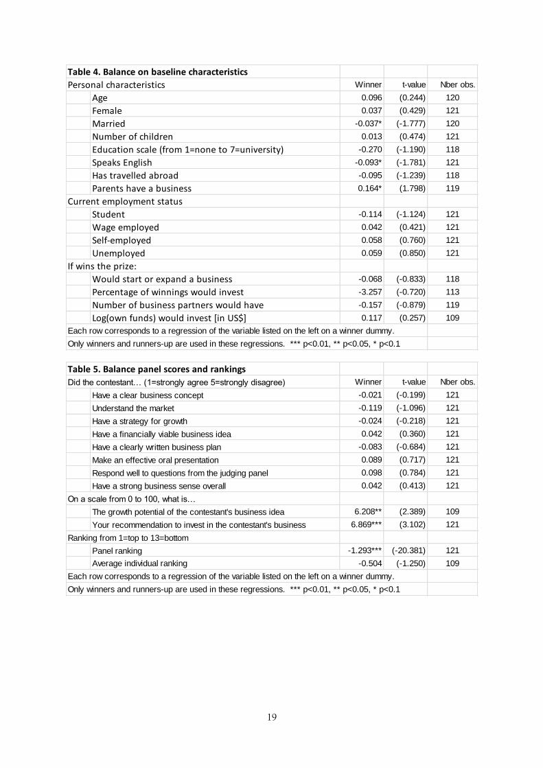
likely to get married after winning the competition. The relative young age and dependent status of the participants, and the short interval between treatment and endline survey, nonetheless militate against finding a statistically significant effect. 4.1 Balance Since we rely on a comparison between competition winners and runners-up, we need to ensure that winners are not, ex ante, any better than runners-up. To this effect, we regress all descriptive statistics from the baseline questionnaire on winners and runners-up, and test whether the winner dummy is significant. In Table 4 we regress characteristics collected at baseline on a winner dummy, using only winners and runners-up in the comparison. The results suggest that winners and runners-up are not different populations: only three of the 16 variables are significant at the 10 percent level (winners are less likely to have been married, less likely to have spoken English, and more likely to have parents who run a business).18 In the impact analysis below we use these three variables as controls in one set of estimations, and show that this does not affect the results.

< Table 4 here. > We have the scores given to each individual contestant by the committee judges. We perform the same balance analysis on the average scores and rankings given by individual judges. To recall, high scores to questions 1 to 8 indicate low performance while the opposite is true for questions 9 and 10. A low ranking means a better performance. The results are presented in Table 5. We see that winners are not significantly different from runners-up in any of questions 1 to 8, nor are they ranked differently by judges as individuals. Winners perform better on the judges’ perception of the business growth potential, and the consequent recommendation to invest. In the analysis that follows, we use as controls the answers to questions 9 and 10, and the individual judge rankings.

< Table 5 here. > We also conduct balance tests on time-invariant variables collected at endline. The reason for this additional check is to protect against possible misreporting in the self-reported information collected at baseline – notably age and education. We also include gender and an English speaking dummy collected at endline, as well as household size and the number of children. Balance test results are reported in Table 6. None of the variables is significantly different between winners and runners-up.

< Table 6 here. > Finally, in Table 7, we check for non-random attrition between winners and other contestants. Of the 441 contestants receiving a final panel ranking, 369 (84%) were interviewed at endline. In the first column of Table 7, we regress a dummy for participating in the endline survey on a winner dummy and the contestant’s final rank. We find no evidence that top contestants are more or less likely to answer the endline questionnaire. In the following two columns, we repeat the analysis with baseline regressors.19 Winning status and committee ranking remain non-significant.20 From this we conclude that there is not differential attrition by winning

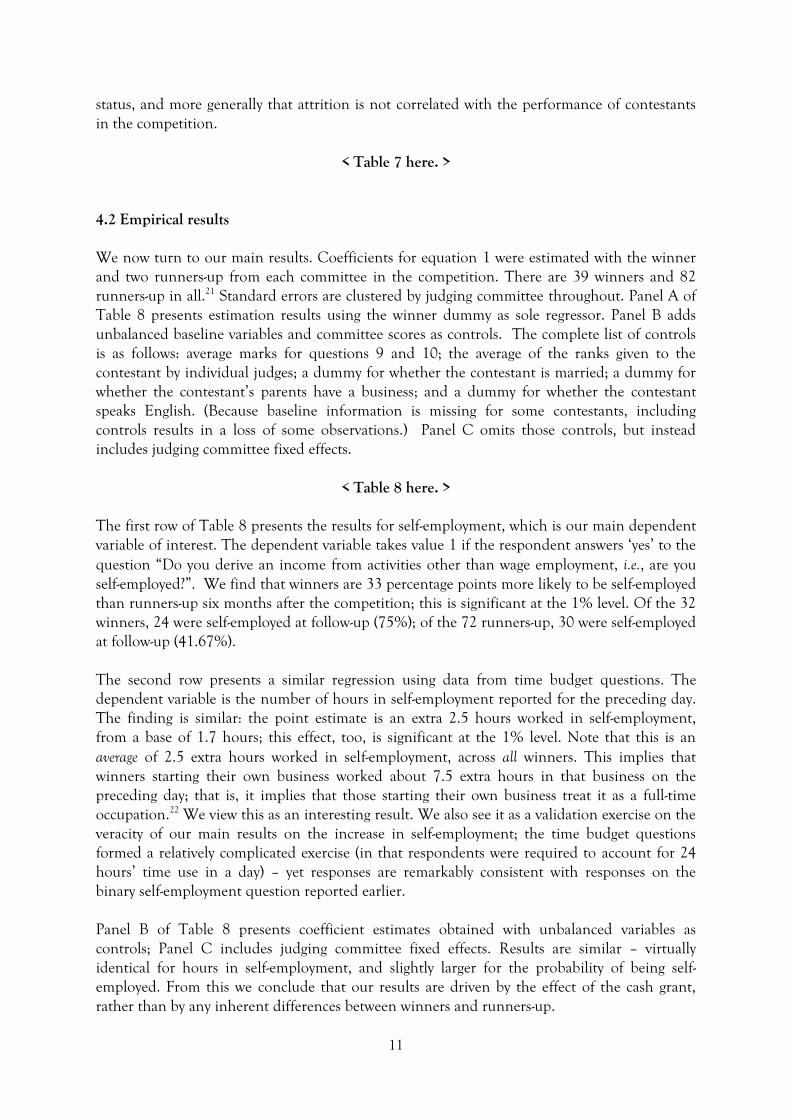
11

status, and more generally that attrition is not correlated with the performance of contestants in the competition.

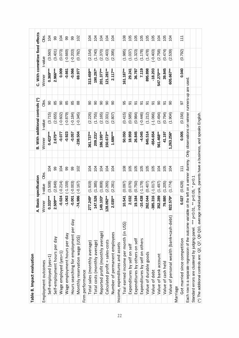
< Table 7 here. > 4.2 Empirical results We now turn to our main results. Coefficients for equation 1 were estimated with the winner and two runners-up from each committee in the competition. There are 39 winners and 82 runners-up in all.21 Standard errors are clustered by judging committee throughout. Panel A of Table 8 presents estimation results using the winner dummy as sole regressor. Panel B adds unbalanced baseline variables and committee scores as controls. The complete list of controls is as follows: average marks for questions 9 and 10; the average of the ranks given to the contestant by individual judges; a dummy for whether the contestant is married; a dummy for whether the contestant’s parents have a business; and a dummy for whether the contestant speaks English. (Because baseline information is missing for some contestants, including controls results in a loss of some observations.) Panel C omits those controls, but instead includes judging committee fixed effects.

< Table 8 here. > The first row of Table 8 presents the results for self-employment, which is our main dependent variable of interest. The dependent variable takes value 1 if the respondent answers ‘yes’ to the question “Do you derive an income from activities other than wage employment, i.e., are you self-employed?”. We find that winners are 33 percentage points more likely to be self-employed than runners-up six months after the competition; this is significant at the 1% level. Of the 32 winners, 24 were self-employed at follow-up (75%); of the 72 runners-up, 30 were self-employed at follow-up (41.67%). The second row presents a similar regression using data from time budget questions. The dependent variable is the number of hours in self-employment reported for the preceding day. The finding is similar: the point estimate is an extra 2.5 hours worked in self-employment, from a base of 1.7 hours; this effect, too, is significant at the 1% level. Note that this is an average of 2.5 extra hours worked in self-employment, across all winners. This implies that winners starting their own business worked about 7.5 extra hours in that business on the preceding day; that is, it implies that those starting their own business treat it as a full-time occupation.22 We view this as an interesting result. We also see it as a validation exercise on the veracity of our main results on the increase in self-employment; the time budget questions formed a relatively complicated exercise (in that respondents were required to account for 24 hours’ time use in a day) – yet responses are remarkably consistent with responses on the binary self-employment question reported earlier. Panel B of Table 8 presents coefficient estimates obtained with unbalanced variables as controls; Panel C includes judging committee fixed effects. Results are similar – virtually identical for hours in self-employment, and slightly larger for the probability of being self-employed. From this we conclude that our results are driven by the effect of the cash grant, rather than by any inherent differences between winners and runners-up.

12

We get very similar results if we limit our attention to those contestants who have less than six months of self-employment experience (results omitted for brevity; available on request). Since the endline survey took place six months after the competition, these contestants are unlikely to have been self-employed prior to the competition. For these individuals, becoming self-employed is thus more likely a direct result of winning to the prize money. We find that 39% of winners were self-employed at endline, compared to 7% of runners-up. This confirms our findings. In rows 3 and 4 we present similar results for wage employment. Among our study population at endline, permanent wage employment is relatively common: of 380 respondents to the endline survey, 40% answered ‘yes’ to the question “Do you have a regular wage job?”. We do not expect a large lump sum transfer to increase the probability of being in wage employment –if anything, it may even reduce this probability if winners slack on search intensity. If anything, this is what we find: winners and runners-up are not significantly different in terms of the probability of have a permanent wage job at endline, and on average they work slightly fewer hours in wage employment (though the difference is not statistically significant). Similarly, we find no effect on search or on the monthly reservation wage.23 These findings are unaffected whether we include controls or committee fixed effects. Figure 2 illustrates these key outcomes against the committee ranking.24 Vertical lines denote the winner (ranking 1) and the respondent rankings used in the regressions as counter-factuals in Tanzania and Ethiopia (rankings 2 and 3). The graphs illustrate both the central idea behind the identification strategy and the key results: outcomes are reasonably homogeneous for rankings 2 to 12, but are significantly different for winners’ probability of self-employment and hours spent in self-employment.

< Figure 2 here. > Next we investigate whether winning the prize affects firm performance. We examine five indicators of firm performance: number of permanent employees, average sales over the last month, average costs, self-reported profits, and profits calculated as sales minus costs. To avoid sample selection problems, we code each outcome as zero for respondents who are not self-employed; that is, we estimate the effect of winning on the unconditional expectation of firm performance. We find large and significant effects. In the basic specification (Panel A), four outcomes are significant: total monthly sales, both measures of profits, and the number of permanent employees. The pattern repeats as we add controls (Panel B) and then committee fixed effects (Panel C): coefficients remain remarkably stable, though the addition of controls improves efficiency. In Panels B and C, we find significant positive effects on all measures of firm performance. We then look at total income, expenditures, and assets. For total income, the point estimate is positive – and is large in the Panel B and Panel C specifications – but it is not statistically significant, possibly because the variance of income is high.25 We get similar results for expenditures: point estimates are positive, but not significant. Finally, assets similarly move in the expected direction: winners have less debt and more savings in cash and in the bank by

13

endline. The effect is statistically significant at the 95% level for bank savings in the regression with controls and in the regression with committee fixed effects. The magnitude of this effect is large: roughly a doubling of bank savings among winners six months after the competition. We estimate the same regression with combined personal wealth, defined as bank and cash savings minus personal debt. As could be expected given our earlier results, point estimates are large; they are significant at the 90% level in each specification. Finally, we investigate whether winners are more likely to be married six months after the competition, conditional on not being married at baseline. Getting married costs money, and winners may have invested their winnings in paying for a wedding rather than investing in self-employment. This is not what we find: there is no significant effect on the probability of being married. The proportion of married individuals at endline is quite small, however (7%), suggesting that our study population may be too young for an effect to be noticed. As a further robustness check – i.e. in addition to the use of additional controls and the use of committee fixed effects – we repeat the entire estimation exercise using the top four ranked participants from each committee. Our results are reported in Table 9. The results are remarkably stable: in comparison to Table 8, the magnitude of our estimates and their significance levels do not change meaningfully for any of our coefficients. Finally, we check the robustness of our results to concerns about multiple hypothesis testing. To do this, we use the ‘sharpened q’ approach of Benjamini et al (2006); we run this separately for each reported family of outcomes (that is, ‘employment outcomes’, ‘firm performance’ and ‘income, expenditures and assets’) and for each specification in Table 8. Using a significance level of 10%, we reject almost exactly the same set of null hypotheses as we reject using the original p-values; we conclude that our results are robust to multiple testing.26 5. Conclusions Using data from a business plan competition that we organized in three African countries, we have shown that a large transfer of funds to motivated young people significantly increases the likelihood that they start a business within six months of the competition – and, therefore, increases expected sales and expected profits. Results are robust to the inclusion of controls for performance on the judging committee, and to the inclusion of judging committee fixed effects. As expected, we find that winners have higher personal wealth. We find no effect on wage employment and earnings. A few simple ‘back-of-envelope’ calculations help to understand the magnitude of our estimates. Our main result is that winners were 33 percentage points more likely than the runners-up to start their own business; with 40 prizes distributed, this implies that we caused the birth of 13 new businesses. Using a point estimate of two permanent employees on average per winner, we created about 80 new wage jobs. If we add the indirect cost of the competition (i.e., staffing costs and per diem paid to judges) this implies a cost of approximately US$1250 per job created: approximately fifteen percent of the equivalent cost estimated by McKenzie (2015) from a much more lucrative business plan competition in Nigeria. Finally, we estimate an effect on monthly profits of about US$150. If we make the simplifying benchmark assumption that this effect is sustainable, our estimates imply an annual profit of 80% on initial investment.27 If a risk neutral aspiring entrepreneur were sure of achieving a persistent

14

monthly profit of US$150 per month with external funds worth US$1,000, he or she should be willing to borrow that sum at a monthly interest of up to 15%. However, since only 33% of recipients do start a firm as a result of receiving the competition prize, the expected return to an external investor is probably closer to 5%. Add to this any reasonable level of risk aversion on the part of external investors, and it is not surprising if aspiring entrepreneurs are unable to find on financial markets the funds that they need to start a business. Business plan competitions such as the one we organized in three African countries may therefore be a more effective way of channelling funds to deserving young entrepreneurs than reliance on financial markets. In sum, our findings imply that access to start-up capital constitutes a sizeable barrier to entry into entrepreneurship for the kind of young motivated individual most likely to succeed in business. We do not see our findings as implying that credit should be extended to these individuals. As the work of Field et al (2013) and Banerjee et al (2014) indicates, access to credit without grace period often fails to have the intended effect on small business investment. Our results suggest that promoting start-up investments by young motivated people can be achieved through grants. Combining our results with these earlier contributions suggests that start-up investment may also be fostered through equity investment of the kind offered by venture capital firms – given that such form of finance does require immediate repayment, and is contingent on success (Fischer, 2013). Similarly, we do not claim that our findings suggest finance should be offered indiscriminately to all young individuals who express a desire to start a business. From the work of de Mel (2008, 2012) and Fafchamps et al (2014), we know that grants to microenterprises do not always lead to investment and firm growth: many small firms refrain from investing, possibly because they wish their enterprise to remain at a level that they can manage and control, possibly because there are other, more urgent uses for available funds. Selecting the right grant recipients is thus essential in order to achieve the desired effect on enterprise development. Our experiment shows that this can be accomplished, at relatively low cost, by running business competitions with the participation of the local business community.

15

Figure 1: Advertising for potential entrepreneurs: Zambian poster

16

Figure 2: Key Outcomes and Committee Ranking

17

Table 1. Baseline variables

Personal characteristics N.obs. Mean St.Dev. Min. Max

Age 766 22.20 2.2 18 33

Female 774 0.21 0 1

Married 752 0.04 0 1

Number of children 775 0.05 0.4 0 4

Education scale (from 1=none to 7=university) 761 5.54 1.2 1 7

Speaks English 759 0.90 0 1

Has travelled abroad 743 0.25 0 1

Parents have a business 745 0.59 0 1

Current employment status

Student 747 0.50 0 1

Wage employed 747 0.16 0 1

Self-employed 747 0.13 0 1

Unemployed 747 0.14 0 1

If wins the prize:

Would start or expand a business 701 0.84 0 1

Percentage of winnings would invest 596 80.25 20.9 0 100

Number of business partners would have 706 0.86 0.8 0 2

Log(own funds) would invest [in US$] 714 5.08 3.2 0 14

Table 2. Average scores from panel judges

Did the contestant… (1=strongly agree 5=strongly disagree) N.obs. Mean St.Dev. Min. Max

Have a clear business concept 481 2.88 1.1 1 5

Understand the market 481 2.94 0.9 1 5

Have a strategy for growth 481 2.92 0.8 1 5

Have a financially viable business idea 480 3.01 0.8 1 5

Have a clearly written business plan 480 2.86 0.9 1 5

Make an effective oral presentation 455 2.81 0.9 1 5

Respond well to questions from the judging panel 467 2.90 1.0 1 5

Have a strong business sense overall 471 2.95 1.0 1 5

On a scale from 0 to 100, what is…

The growth potential of the contestant's business idea 436 62.33 16 10 100

Your recommendation to invest in the contestant's business 481 58.83 16 0 100

Ranking from 1=top to 13=bottom

Panel ranking 441 5.77 3.3 1 12

Ranking by individual judges, averaged for each contestant 437 5.92 2.3 1 13

Note: Except for panel rankings, which are decided collectively, all other variables are averaged within judging panels.

In Zambia, the target number of contestants per judging panel was set to 6. In Ethiopia and Tanzania, the target was 12.

18

Table 3. Endline variables

Employment outcomes N.obs. Mean St.Dev. Min. Max

Self-employed (yes=1) 380 0.38 0 1

Self-employment hours per day 356 2.05 3.6 0 15

Wage employed (yes=1) 380 0.40 0.5 0 1

Wage employment hours per day 356 2.96 4.1 0 15

Hours searching for employment per day 356 0.46 1.4 0 12

Monthly reservation wage (US$) 372 460.78 1320 0 21768

Conditional on self-employment…

Total sales (monthly average) 141 534.50 1856 0 18133

Total costs (monthly average) 136 365.25 1186 0 12533

Reported profit (monthly average) 140 404.01 1793 -183 19200

Calculated profit = sales-costs 136 188.13 803 -877 6942

Number of permanent employees 143 1.44 3.1 0 20

Income, expenditures and assets

Earned income per month (in US$) 402 244.39 1122 -183 19200

Expenditures by self on self 381 76.69 89 0 744

Expenditures by others on self 381 25.67 54 0 784

Expenditures by self on others 381 19.73 38 0 296

Value of durable goods 381 1290.79 3754 0 59010

Value of debt 381 153.55 1489 0 27210

Value of bank account 380 394.21 1921 0 32000

Value of cash held 381 68.24 188 0 2560

Marriage

Got married since competition 405 0.02 0 1

Time-invariant variables

Age 399 23.74 2.7 16 39

Female 405 0.20 0 1

Married 381 0.05 0 1

Number of children 381 0.04 0.2 0 2

Education scale (from 1=none to 7=university) 382 5.29 1.5 1 7

Speaks English 405 0.88 0.3 0 1

19

Table 4. Balance on baseline characteristics

Personal characteristics Winner t-value Nber obs.

Age 0.096 (0.244) 120

Female 0.037 (0.429) 121

Married -0.037* (-1.777) 120

Number of children 0.013 (0.474) 121

Education scale (from 1=none to 7=university) -0.270 (-1.190) 118

Speaks English -0.093* (-1.781) 121

Has travelled abroad -0.095 (-1.239) 118

Parents have a business 0.164* (1.798) 119

Current employment status

Student -0.114 (-1.124) 121

Wage employed 0.042 (0.421) 121

Self-employed 0.058 (0.760) 121

Unemployed 0.059 (0.850) 121

If wins the prize:

Would start or expand a business -0.068 (-0.833) 118

Percentage of winnings would invest -3.257 (-0.720) 113

Number of business partners would have -0.157 (-0.879) 119

Log(own funds) would invest [in US$] 0.117 (0.257) 109

Each row corresponds to a regression of the variable listed on the left on a winner dummy.

Only winners and runners-up are used in these regressions. *** p<0.01, ** p<0.05, * p<0.1

Table 5. Balance panel scores and rankings

Did the contestant… (1=strongly agree 5=strongly disagree) Winner t-value Nber obs.

Have a clear business concept -0.021 (-0.199) 121

Understand the market -0.119 (-1.096) 121

Have a strategy for growth -0.024 (-0.218) 121

Have a financially viable business idea 0.042 (0.360) 121

Have a clearly written business plan -0.083 (-0.684) 121

Make an effective oral presentation 0.089 (0.717) 121

Respond well to questions from the judging panel 0.098 (0.784) 121

Have a strong business sense overall 0.042 (0.413) 121

On a scale from 0 to 100, what is…

The growth potential of the contestant's business idea 6.208** (2.389) 109

Your recommendation to invest in the contestant's business 6.869*** (3.102) 121

Ranking from 1=top to 13=bottom

Panel ranking -1.293*** (-20.381) 121

Average individual ranking -0.504 (-1.250) 109

Each row corresponds to a regression of the variable listed on the left on a winner dummy.

Only winners and runners-up are used in these regressions. *** p<0.01, ** p<0.05, * p<0.1

20

Table 6. Balance on time-invariant endline variablesWinner t-value Nber obs.

Age 0.190 (0.347) 109

Female -0.041 (-0.472) 111

Married 0.084 (1.278) 105

Number of children 0.013 (0.474) 121

Education scale (from 1=none to 7=university) 0.212 (0.840) 106

Speaks English -0.068 (-1.196) 111

Each row corresponds to a regression of the variable listed on the left on a winner dummy.

Only winners and runners-up are used in these regressions. *** p<0.01, ** p<0.05, * p<0.1

21

Table 7. Attrition analysis

Competed Competed

Surveyed

at endline

(among

competito

rs)

Surveyed at

endline

(among

competitors)

Surveyed at

endline

(among

competitors)

coef/t coef/t coef/t coef/t coef/t

Age (Years) -0.012 -0.004 0.013 0.009

(-1.061) (-0.315) (1.173) (0.762)

Dummy: Male -0.018 -0.009 0.001 -0.016

(-0.373) (-0.182) (0.026) (-0.318)

Highest level of education completed -0.015 -0.014 0.037** 0.039**

(-0.821) (-0.763) (2.001) (2.096)

Dummy: Married 0.048 -0.031 0.079 0.053

(0.423) (-0.281) (0.653) (0.427)

Number of children -0.202*** -0.190** -0.381*** -0.418***

(-2.615) (-2.558) (-3.166) (-3.373)

Dummy: Ever travelled abroad -0.173*** -0.155*** -0.051 -0.056

(-3.666) (-3.258) (-0.968) (-1.058)

Dummy: Parents have a business -0.055 -0.033 -0.018 -0.023

(-1.329) (-0.788) (-0.432) (-0.541)

Dummy: Student (Omitted: "Other") -0.347 -0.232 -0.216 -0.268

(-1.015) (-0.522) (-0.825) (-0.715)

Dummy: Employed (Omitted: "Other") -0.422 -0.323 -0.231 -0.273

(-1.224) (-0.724) (-0.867) (-0.723)

Dummy: Unemployed (Omitted: "Other") -0.458 -0.399 -0.232 -0.275

(-1.326) (-0.894) (-0.870) (-0.726)

Dummy: Business idea involves starting a

new business-0.041 0.006 -0.058 -0.078

(-0.754) (0.115) (-1.064) (-1.382)

Dummy: Would have a business partner? -0.031 -0.002 0.013 0.016

(-1.270) (-0.074) (0.520) (0.636)

Dummy: Speaks English 0.150** 0.132* -0.146* -0.161*

(2.073) (1.739) (-1.847) (-1.917)

Log(own money to be invested + 1) 0.006 -0.009 -0.005 -0.004

(0.943) (-1.290) (-0.710) (-0.574)

Percentage investment anticipated 0.005*** -0.001

(5.215) (-1.173)

Final panel ranking -0.007 -0.010 -0.011

(-1.153) (-1.481) (-1.581)

Dummy: Winner -0.025 -0.052 -0.029

(-0.367) (-0.680) (-0.364)

Constant 1.316*** 0.743 0.878*** 0.851** 1.110**

(3.299) (1.498) (21.252) (2.496) (2.526)

Number of observations 632 530 441 378 366

Adjusted R2 0.049 0.109 -0.001 0.023 0.030

All regressions are linear probability models. Standard errors are clustered by judging panel.

Note: *** p<0.01, ** p<0.05, * p<0.1

22

Tab

le 8

. Im

pac

t ev

alu

atio

nC

. W

ith

co

mm

itte

e f

ixed

eff

ects

Emp

loym

ent

ou

tco

mes

Win

ner

t-va

lue

Obs.

Win

ner

t-va

lue

Obs.

Win

ner

t-va

lue

Obs.

Self

-em

plo

yed

(ye

s=1

)0.3

33**

*(3

.508)

104

0.4

23**

*(3

.715)

90

0.3

69**

*(3

.560)

104

Self

-em

plo

ymen

t h

ou

rs p

er d

ay2.5

09**

*(2

.849)

99

2.6

75**

(2.6

55)

85

2.9

66**

*(3

.401)

99

Wag

e em

plo

yed

(ye

s=1

)-0

.024

(-0.2

14)

104

-0.0

77

(-0.6

02)

90

0.0

09

(0.0

73)

104

Wag

e em

plo

ymen

t h

ou

rs p

er d

ay-1

.063

(-1.1

59)

99

-0.9

23

(-0.8

79)

85

-0.6

61

(-0.6

69)

99

Ho

urs

sea

rch

ing

for

emp

loym

ent

per

day

-0.0

01

(-0.0

03)

99

-0.0

57

(-0.1

84)

85

-0.0

66

(-0.2

03)

99

Mo

nth

ly r

eser

vati

on

wag

e (U

S$)

-74.9

86

(-0.1

67)

102

-238.5

04

(-0.3

45)

88

69.9

77

(0.7

82)

102

Firm

per

form

ance

Tota

l sal

es (

mo

nth

ly a

vera

ge)

277.2

49*

(1.9

19)

104

361.7

37**

(2.2

26)

90

313.4

59**

(2.1

54)

104

Tota

l co

sts

(mo

nth

ly a

vera

ge)

147.5

26

(1.3

85)

104

209.2

31*

(1.7

55)

90

190.2

97*

(1.7

40)

104

Rep

ort

ed p

rofi

t (m

on

thly

ave

rage

)149.1

03*

(1.8

08)

104

186.1

95**

(2.1

65)

90

201.3

77**

(2.3

70)

104

Cal

cula

ted

pro

fit

= sa

les-

cost

s128.0

92**

(2.2

65)

104

150.6

73**

(2.3

31)

90

121.2

81**

(2.4

03)

104

Nu

mb

er o

f p

erm

anen

t em

plo

yees

2.0

35**

(2.2

81)

104

1.6

86**

*(2

.807)

90

2.1

17**

(2.3

95)

104

Inco

me,

exp

end

itu

res

and

ass

ets

Toal

ear

ned

inco

me

per

mo

nth

(in

US$

)10.5

41

(0.0

97)

108

50.0

50

(0.4

15)

95

161.1

87**

(1.9

85)

108

Exp

end

itu

res

by

self

on

sel

f2.0

32

(0.0

76)

105

18.9

59

(0.5

85)

91

29.2

41

(1.0

37)

105

Exp

end

itu

res

by

oth

ers

on

sel

f19.1

84

(0.7

50)

105

26.8

45

(0.9

84)

91

36.7

87

(1.3

23)

105

Exp

end

itu

res

by

self

on

oth

ers

-10.4

38

(-1.1

79)

105

-4.0

45

(-0.4

46)

91

7.1

19

(1.1

78)

105

Val

ue

of

du

rab

le g

oo

ds

262.0

44

(0.4

07)

105

845.5

14

(1.2

12)

91

895.8

98

(1.4

78)

105

Val

ue

of

deb

t-3

85.3

16

(-1.0

17)

105

-654.6

54

(-1.0

66)

91

-18.2

03

(-0.4

03)

105

Val

ue

of

ban

k ac

cou

nt

352.2

89

(1.4

97)

104

561.4

68**

(2.4

94)

90

547.2

70**

*(2

.758)

104

Val

ue

of

cash

hel

d79.8

80

(1.2

05)

105

41.1

97

(0.7

94)

91

39.8

45

(0.4

74)

105

Val

ue

of

per

son

al w

ealt

h (

ban

k+ca

sh-d

ebt)

822.5

79*

(1.7

74)

104

1,2

63.2

56*

(1.9

04)

90

605.6

67**

(2.5

39)

104

Mar

riag

e

Go

t m

arri

ed s

ince

co

mp

etit

ion

0.0

27

(0.6

28)

111

0.0

05

(0.1

56)

97

0.0

40

(0.7

92)

111

Each r

ow

is a

separa

te r

egre

ssio

n o

f th

e o

utc

om

e v

ari

able

on the le

ft o

n a

win

ner

dum

my.

Only

observ

ations o

n w

inner

runners

-up a

re u

sed.

Sta

ndard

err

ors

are

clu

ste

red b

y ju

dgin

g p

anel.

***

p<

0.0

1,

** p

<0.0

5,

* p<

0.1

(*)

The a

dditio

nal c

ontr

ols

are

: Q

2,

Q7,

Q9 Q

10,

ave

rage indiv

idual r

ank,

pare

nts

have

a b

usin

ess,

and s

peaks E

nglis

h.

A.

Basic

sp

ecific

ati

on

B.

Wit

h a

dd

itio

nal co

ntr

ols

(*)

23

Tab

le 9

. Im

pac

t ev

alu

atio

n:

Exp

and

ing

to t

he

top

fo

ur

pla

ces

C.

Wit

h c

om

mit

tee f

ixed

eff

ects

Emp

loym

ent

ou

tco

mes

Win

ner

t-va

lue

Obs.

Win

ner

t-va

lue

Obs.

Win

ner

t-va

lue

Obs.

Self

-em

plo

yed

(ye

s=1

)0.3

20**

*(3

.582)

153

0.4

24**

*(4

.333)

132

0.3

89**

*(4

.174)

153

Self

-em

plo

ymen

t h

ou

rs p

er d

ay2.4

60**

*(2

.895)

146

2.6

27**

*(2

.812)

125

2.8

93**

*(3

.343)

146

Wag

e em

plo

yed

(ye

s=1

)-0

.024

(-0.2

17)

153

-0.1

22

(-0.9

77)

132

0.0

04

(0.0

31)

153

Wag

e em

plo

ymen

t h

ou

rs p

er d

ay-0

.890

(-1.0

42)

146

-1.2

15

(-1.1

78)

125

-0.6

24

(-0.6

74)

146

Ho

urs

sea

rch

ing

for

emp

loym

ent

per

day

0.1

23

(0.4

59)

146

0.0

98

(0.3

67)

125

0.0

39

(0.1

38)

146

Mo

nth

ly r

eser

vati

on

wag

e (U

S$)

18.0

24

(0.0

47)

151

-25.4

67

(-0.0

48)

130

324.5

35

(1.0

17)

151

Firm

per

form

ance

Tota

l sal

es (

mo

nth

ly a

vera

ge)

278.3

10*

(1.9

90)

153

350.5

69**

(2.2

14)

132

320.9

67**

(2.2

72)

153

Tota

l co

sts

(mo

nth

ly a

vera

ge)

162.9

68

(1.6

11)

153

213.7

87*

(1.8

59)

132

186.0

26*

(1.7

88)

153

Rep

ort

ed p

rofi

t (m

on

thly

ave

rage

)88.0

15

(0.9

11)

153

139.2

50

(1.4

57)

132

180.3

22**

(2.1

16)

153

Cal

cula

ted

pro

fit

= sa

les-

cost

s113.7

11**

(2.1

11)

153

134.9

53**

(2.1

98)

132

133.3

94**

*(2

.581)

153

Nu

mb

er o

f p

erm

anen

t em

plo

yees

1.9

91**

(2.2

87)

153

1.6

79**

(2.6

14)

132

2.1

15**

(2.4

77)

153

Inco

me,

exp

end

itu

res

and

ass

ets

Toal

ear

ned

inco

me

per

mo

nth

(in

US$

)-1

5.9

04

(-0.1

53)

165

10.7

52

(0.0

97)

145

103.7

89

(1.2

93)

165

Exp

end

itu

res

by

self

on

sel

f14.0

75

(0.5

91)

154

29.2

46

(1.0

34)

133

40.2

76*

(1.6

58)

154

Exp

end

itu

res

by

oth

ers

on

sel

f21.2

27

(0.8

44)

154

27.1

58

(0.9

87)

133

34.9

07

(1.3

51)

154

Exp

end

itu

res

by

self

on

oth

ers

-5.5

27

(-0.8

61)

154

-0.0

03

(-0.0

00)

133

7.9

33

(1.6

12)

154

Val

ue

of

du

rab

le g

oo

ds

530.2

80

(0.8

96)

154

935.4

99

(1.4

53)

133

960.1

00*

(1.6

52)

154

Val

ue

of

deb

t-2

87.3

17

(-1.2

33)

154

-406.5

47

(-1.1

35)

133

1.8

63

(0.0

44)

154

Val

ue

of

ban

k ac

cou

nt

336.2

09

(1.6

49)

153

439.6

93**

(2.0

78)

132

444.9

04**

(2.5

29)

153

Val

ue

of

cash

hel

d96.7

74

(1.6

14)

154

54.0

60

(1.2

06)

133

58.0

54

(0.7

74)

154

Val

ue

of

per

son

al w

ealt

h (

ban

k+ca

sh-d

ebt)

722.6

61**

(2.2

14)

153

901.9

70**

(2.0

82)

132

501.1

85**

(2.5

65)

153

Mar

riag

e

Go

t m

arri

ed s

ince

co

mp

etit

ion

0.0

31

(0.7

74)

168

0.0

07

(0.2

31)

147

0.0

45

(1.0

68)

168

Each r

ow

is a

separa

te r

egre

ssio

n o

f th

e o

utc

om

e v

ari

able

on the le

ft o

n a

win

ner

dum

my.

Only

observ

ations o

n w

inner

runners

-up a

re u

sed.

Sta

ndard

err

ors

are

clu

ste

red b

y ju

dgin

g p

anel.

***

p<

0.0

1,

** p

<0.0

5,

* p<

0.1

(*)

The a

dditio

nal c

ontr

ols

are

: Q

2,

Q7,

Q9 Q

10,

ave

rage indiv

idual r

ank,

pare

nts

have

a b

usin

ess,

and s

peaks E

nglis

h.

A.

Basic

sp

ecific

ati

on

B.

Wit

h a

dd

itio

nal co

ntr

ols

(*)

24

References

Banerjee, A. and Duflo, E. (2011). Poor Economics: A Radical Rethinking of the Way to Fight Global Poverty. New York: Public Affairs. Banerjee, A., Duflo, E., Glennerster, R., & Kinnan, C. (2014). The Miracle of Microfinance? Evidence from a Randomized Evaluation. American Economic Journal: Applied Economics, 7(1), 22-53. Benjamini, Y., Krieger, A. M., & Yekutieli, D. (2006). Adaptive Linear Step-up Procedures that Control the False Discovery Rate. Biometrika, 93(3), 491-507. Bjorvatn, K., Cappelen, A., Sekei, L.H., Sorensen, & E., Tungodden, B. (2015). Teaching Through Television: Experimental Evidence on Entreprenurship Education in Tanzania. NHH Discussion Paper 3 2015. Blattman, C., Fiala, N., & Martinez, S. (2014). Generating Skilled Self-Employment in Developing Countries: Experimental Evidence from Uganda. The Quarterly Journal of Economics, 129, 697–752. Blattman, C., Jamison, J., Green, E. & Annan, J. (2016). The Returns to Microenterprise Support Among the Ultra-Poor: A Field Experiment in Post-War Uganda. American Economic Journal: Applied Economics, 8(2), 35-64. De Mel, S., McKenzie, D., & Woodruff, C. (2008). Returns to Capital in Microenterprises: Evidence from a Field Experiment. The Quarterly Journal of Economics, 123, 1329–1372. De Mel, S., McKenzie, D., & Woodruff, C. (2012). One-time Transfers of Cash or Capital have Long-Lasting Effects on Microenterprises in Sri Lanka. Science, 335, 962–966. Dinh, H., Palmade, V., Chanda, V., & Cossar, F. (2012). Light Manufacturing in Africa: Targeted Policies to Enhance Private Investment and Create Jobs. World Bank Publications. Fafchamps, M., McKenzie, D., Quinn, S., & Woodruff, C. (2012). Using PDA Consistency Checks to Increase the Precision of Profits and Sales Measurement in Panels. Journal of Development Economics, 98, 51–57. Fafchamps, M., McKenzie, D., Quinn, S., & Woodruff, C. (2014): Microenterprise Growth and the Flypaper Effect: Evidence from a Randomized Experiment in Ghana. Journal of Development Economics, 106, 211–226. Fafchamps, M., & Quinn, S. (2014). Networks and Manufacturing Firms in Africa: Results from a Randomized Field Experiment,” CSAE Working Paper 2014-25. Fafchamps, M. & Woodruff, C. (2016). Identifying Gazelles: Expert Panels vs. Surveys as a Means to Identify Firms with Rapid Growth Potential. World Bank Economic Review (forthcoming).

25

Field, E., Pande, R., Papp, J., & Rigol, N. (2013). Does the Classic Microfinance Model Discourage Entrepreneurship Among the Poor? Experimental Evidence from India. The American Economic Review, 103, 2196–2226. Fischer, G. (2013). Contract Structure, Risk-Sharing, and Investment Choice. Econometrica, 81, 883–939. Franklin, S. (2015). Location, Search Costs and Youth Unemployment: A Randomized Trial of Transport Subsidies in Ethiopia. CSAE Working Paper WPS/2015-11. Klinger, B., & Schündeln, M. (2011). Can Entrepreneurial Activity be Taught? Quasi- Experimental Evidence from Central America. World Development, 39, 1592–1610. McKenzie, D. (2015). Identifying and Spurring High-Growth Entrepreneurship: Experimental Evidence from a Business Plan Competition. World Bank Policy Research Working Paper No. 7391. McKenzie, D., & Woodruff, C. (2008). Experimental Evidence on Returns to Capital and Access to Finance in Mexico. The World Bank Economic Review, 22, 457–482. 1 The average GNI per capita across our three study countries is approximately $2,600 (PPP; current international dollars). This compares to approximately $5,700 in Nigeria, $7,700 in El Salvador, $7,300 in Guatemala and $4,700 in Nicaragua. Our grant is therefore substantially smaller than those in Klinger and Schündeln (2011) and McKenzie (2015) even after controlling for relative differences in income. 2 McKenzie (2015) obtains this figure as a total cost of US$60 million to create 7027 jobs.

Arguably, a more appropriate comparison to our present paper is to ignore implementation costs in Nigeria and focus only on the first six months after initial disbursement. In that case, McKenzie (2015) estimates that 2,495 jobs were created, for a total disbursement of about US$27 million --- implying an average of US$10,800 per job created. Note that this comparison is robust to concerns about sampling error: at the top of our 95% confidence interval, we estimate a cost of US$910 per job created. 3 In simple terms, this amounts to a return of 80%. By comparison, McKenzie (2015) estimates

an annual return of between 18 and 21 percent (though this is obtained in a different way: by estimating the return to capital, by regressing profits on capital stock, instrumented by with treatment). 4 Specifically, we ran power simulations of our two main results (on self-employment and self-employment hours per day), for our ‘basic specification’. We did this preserving the clustering structure used in the real data. Using 100,000 simulation replications, we obtain power of 0.946 and 0.968 for the two specifications respectively (using the 10% significance level). 5 This project is summarised at http://econ.worldbank.org/africamanufacturing. The main report has been published as Dinh et al (2012).

26

6 Field support was provided by the Ethiopian Development Research Institute in Ethiopia, the

Economic Development Institute in Tanzania, and RuralNet in Zambia. 7 See Klinger and Schündeln (2011) for a discussion of TechnoServe competitions in El Salvador, Guatemala and Nicaragua. 8 See McKenzie (2015) for a detailed discussion of the YouWiN! competition, and for a list of other examples. 9 Bjorvatn et al (2015) report a randomised controlled trial in which treated secondary school students watched episodes of this show. 10

We show the Zambian poster, which was in English; the Ethiopian and Tanzanian posters were respectively in Amharic and in Swahili. 11

The design is slightly different in Zambia, as we discuss shortly. 12

Thus, a committee ranks four candidates after its first meeting, eight candidates after its second meeting and 12 candidates after its final meeting. 13 Some judges were randomly assigned the role of non-committee judge for which they ranked written business proposals individually. While their assessment marks were provided to the relevant committee judges, it is unclear that they were taken into consideration. Non-committee judges are discussed more in detail in Fafchamps and Quinn (2014). 14

There are 185 contestants in Ethiopia, 178 in Tanzania and 78 in Zambia. 15 The proportion is 88% in the endline survey, so this proportion is probably about right. It reflects the fact that, in all three countries, English is used extensively as language of instruction in high school and university. 16 If the day preceding was a weekend, respondents were instead asked about the last weekday. 17 Extra cash could facilitate job search, as shown for Ethiopia by Franklin (2015). But the prize winnings far exceed the cost of searching for a wage job in Addis Ababa. Cash could also facilitate international migration, something that we cannot rule out but we suspect would only affect a small proportion of our study population. We do not observe international migrants in our data since, by design, they do not respond to the endline survey. We revisit this issue when we discuss attrition. 18 To verify how strong this pattern is, we estimate the same regression on the entire contestant population. We find the same result for having been married, but the English speaking dummy is no longer significant, nor is the result on parents having run a business. (Additionally, we find that winners reported a significantly larger planned investment of their own funds.) 19 As noted earlier, this leads to a loss of observations because some baseline questions were not completed.

27

20 For completeness, we also run regressions of the kind reported in Table 8, where the outcome variable is whether the respondent was interviewed at endline. In every case, the coefficient on winning is very small, and far from significant: for the specifications in Panel A, Panel B and Panel C successively, the estimates are -0.044 (p = 0.510), -0.058 (p = 0.412) and -0.007 (p = 0.908). 21 In Zambia, we had half as many contestants as in either of the other two countries; additionally, there were three committees in Zambia with only two contestants. For these reasons, there are only 21 runners-up for the seven winners in Zambia. 22

That is, 7.5 ≈2.5 / 0.33. 23 We find that winners spend an average of 0.85 hours fewer each day on leisure (including washing and grooming); this is significant with p < 0.01. Aside from self-employment and leisure, we find no significant effect on any other category of time use (time in wage employment, time searching for work, time studying, time sleeping, time socialising and attending religious ceremonies, time doing chores and time on other activities). 24 Specifically, the figure shows coefficients from a regression on dummy variables, with no controls. We cluster by judging committee and show 90% confidence intervals. For clarity, we drop the eight Zambians who were ranked ‘1’ but who did not include a prize; results are robust to including them. 25 In separate regressions (available on request), we use log(income) as a dependent variable. We find large estimated coefficients, although not significant: 0.581 for the Panel A specification (p = 0.145), 0.801 for the Panel B specification (p = 0.113), and 0.533 for the Panel C specification (p = 0.200). 26 Only two variables change their significance. First, the significant result on ‘value of personal wealth’ in the ‘basic specification’ and in the specification ‘with additional controls’; in each case, this is borderline significant before correcting for multiple hypothesis testing, and no longer significant after doing so. However, the variable remains significant – even after multiple hypothesis correction – once we control for committee fixed effects. Second, the significant result on ‘value of bank account’ in the specification ‘with additional controls’ is no longer significant after controlling for multiple hypothesis testing; however, this variable too remains significant (including after multiple hypothesis correction) once we control for committee fixed effects. 27 That is, US$150 per month × 12 months = US$1800 per year, caused by an initial grant of US$1000. This assumption of sustainability appears reasonable in many microenterprise contexts: see de Mel et al (2012) and Fafchamps et al (2014).