Embed Size (px)
Citation preview
Assessing and Characterizing the Inductive Effect Through Silicon‐
Containing Backbones and On Silicon Reactivity
By
Ashlyn Patricia Smith
A thesis submitted to the Department of Chemistry in compliance with the
requirements for the degree of Master of Science (Chemistry)
Lakehead University
Thunder Bay, Ontario, Canada
February 2012
Copyright © Ashlyn Patricia Smith, 2012

Dedication
This thesis is dedicated to my family who made me who I am.

iii
Acknowledgements
I would like to take the time to acknowledge the many people who made this
thesis possible. First, I would like to thank Dr. R. Mawhinney for taking me under his
wing and introducing me to the wonderful world of computational chemistry. His
ongoing guidance and inspiration have made my time in the CQC lab very enjoyable. I
would also like to thank the other members of our lab group, both past and present, for
their support and camaraderie. Special thanks go out to Patrick Tuck and Adrienne
McKercher.
I would also like to thank the faculty, and staff, members of the chemistry
department for their aid in shaping my educational experience; especially Dr. C.
Gottardo and Dr. W. Floriano for being my committee members, and Brad and Debbie
for their many supportive conversations. I would also like to take this chance to thank
Dr. R. Boyd for agreeing to be my external examiner, and for his help in this capacity.
I would like to thank the Natural Sciences and Engineering Research Council of
Canada and Lakehead University for funding to help complete this thesis. I also
appreciate the computational resources and technical support provided by the Shared
Hierarchical Academic Research Computing Network.
Finally, I would like to thank my husband, family, and friends for all their
encouragement and support. Without them this would not have been possible and I
would not be the person that I am.
iv
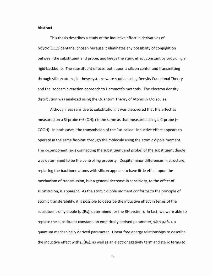
Abstract
This thesis describes a study of the inductive effect in derivatives of
bicyclo[1.1.1]pentane; chosen because it eliminates any possibility of conjugation
between the substituent and probe, and keeps the steric effect constant by providing a
rigid backbone. The substituent effects, both upon a silicon center and transmitting
through silicon atoms, in these systems were studied using Density Functional Theory
and the isodesmic reaction approach to Hammett’s methods. The electron density
distribution was analyzed using the Quantum Theory of Atoms in Molecules.
Although less sensitive to substitution, it was discovered that the effect as
measured on a Si‐probe (–Si(OH)3) is the same as that measured using a C‐probe (–
COOH). In both cases, the transmission of the “so‐called” inductive effect appears to
operate in the same fashion: through the molecule using the atomic dipole moment.
The x‐component (axis connecting the substituent and probe) of the substituent dipole
was determined to be the controlling property. Despite minor differences in structure,
replacing the backbone atoms with silicon appears to have little effect upon the
mechanism of transmission, but a general decrease in sensitivity, to the effect of
substitution, is apparent. As the atomic dipole moment conforms to the principle of
atomic transferability, it is possible to describe the inductive effect in terms of the
substituent‐only dipole (μx(RH); determined for the RH system). In fact, we were able to
replace the substituent constant, an empirically derived parameter, with μx(RH), a
quantum mechanically derived parameter. Linear free energy relationships to describe
the inductive effect with μx(RH), as well as an electronegativity term and steric terms to

v
describe the backbone and probe, were developed that essentially recreate the entire
substituent effect.
vi
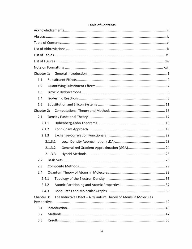
Table of Contents Acknowledgements ............................................................................................................. iii
Abstract ............................................................................................................................... iv
Table of Contents ................................................................................................................ vi
List of Abbreviations ........................................................................................................... ix
List of Tables ...................................................................................................................... xii
List of Figures .................................................................................................................... xiv
Note on Formatting ........................................................................................................ xxiii
Chapter 1: General Introduction .................................................................................... 1
1.1 Substituent Effects ............................................................................................... 2
1.2 Quantifying Substituent Effects ........................................................................... 4
1.3 Bicyclic Hydrocarbons .......................................................................................... 6
1.4 Isodesmic Reactions ............................................................................................. 8
1.5 Substitution and Silicon Systems ....................................................................... 11
Chapter 2: Computational Theory and Methods ......................................................... 16
2.1 Density Functional Theory ................................................................................. 17
2.1.1 Hohenberg‐Kohn Theorems ........................................................................ 18
2.1.2 Kohn‐Sham Approach ................................................................................. 19
2.1.3 Exchange‐Correlation Functionals .............................................................. 22
2.1.3.1 Local Density Approximation (LDA) ..................................................... 23
2.1.3.2 Generalized Gradient Approximation (GGA) ....................................... 24
2.1.3.3 Hybrid Methods ................................................................................... 25
2.2 Basis Sets ............................................................................................................ 26
2.3 Composite Methods ........................................................................................... 29
2.4 Quantum Theory of Atoms in Molecules ........................................................... 33
2.4.1 Topology of the Electron Density ............................................................... 33
2.4.2 Atomic Partitioning and Atomic Properties ................................................ 37
2.4.3 Bond Paths and Molecular Graphs ............................................................. 39
Chapter 3: The Inductive Effect – A Quantum Theory of Atoms in Molecules Perspective.... .................................................................................................................... 42
3.1 Introduction ........................................................................................................ 43
3.2 Methods ............................................................................................................. 47
3.3 Results ................................................................................................................ 50
vii
3.3.1 Energies ....................................................................................................... 50
3.3.2 Nuclear Magnetic Resonance Chemical Shifts ............................................ 56
3.3.3 Molecular Orbitals ...................................................................................... 59
3.3.4 Structure and Critical Points in the Electron Density ................................. 62
3.3.5 Atomic Charges and Delocalization Index .................................................. 68
3.3.6 Dipole Moment Contributions .................................................................... 73
3.4 Summary and Conclusion ................................................................................... 79
Chapter 4: The Effect of Substitution on a Silicon Center: Using a Silicic Acid Probe .. 81
4.1 Introduction ........................................................................................................ 82
4.2 Methods ............................................................................................................. 85
4.3 Results ................................................................................................................ 86
4.3.1 Energies ....................................................................................................... 86
4.3.2 Nuclear Magnetic Resonance Chemical Shifts ............................................ 95
4.3.3 Molecular Orbitals ...................................................................................... 97
4.3.4 Structure and Critical Points in the Electron Density ............................... 101
4.3.5 Atomic Charges and Delocalization Index ................................................ 107
4.3.6 Dipole Moment Contributions .................................................................. 113
4.4 Summary and Conclusion ................................................................................. 118
Chapter 5: The Transmission of the Inductive Effect Through Silicon Containing Backbones..... .................................................................................................................. 120
5.1 Introduction ...................................................................................................... 121
5.2 Methods ........................................................................................................... 124
5.3 Results .............................................................................................................. 126
5.3.1 Energies ..................................................................................................... 126
5.3.1.1 Analogs C1 and S1.............................................................................. 128
5.3.1.2 Analogs C2 and S2.............................................................................. 132
5.3.1.3 Analogs C3 and S3.............................................................................. 138
5.3.2 Structure and Critical Points in the Electron Density ............................... 147
5.3.2.1 Analogs C1 and S1.............................................................................. 147
5.3.2.2 Analogs C2 and S2.............................................................................. 152
5.3.2.3 Analogs C3 and S3.............................................................................. 158
5.3.3 Atomic Charges and Delocalization Index ................................................ 163
5.3.3.1 Analogs C1 and S1.............................................................................. 164

viii
5.3.3.2 Analogs C2 and S2.............................................................................. 169
5.3.3.3 Analogs C3 and S3.............................................................................. 173
5.3.4 Dipole Moment Contributions .................................................................. 178
5.3.4.1 Analogs C1 and S1.............................................................................. 180
5.3.4.2 Analogs C2 and S2.............................................................................. 183
5.3.4.3 Analogs C3 and S3.............................................................................. 184
5.4 Summary .......................................................................................................... 186
Chapter 6: Summary and Conclusions ........................................................................ 188
Chapter 7: References ................................................................................................ 199
Appendix 1: Supplemental Information and Figures ...................................................... 204
Appendix 2: Cartesian Coordinates and Absolute Energies ........................................... 212

ix
List of Abbreviations
AIL: Atomic interaction line
AO: Atomic orbital
B: Backbone
BCP: Bond critical point
BO: Born‐Oppenheimer
B3LYP: Three‐parameter Exchange‐Correlation Functional created by Becke; with the
Lee, Yang and Parr correlation functional
CB: Conjugate base
CBS: Complete basis set
CC: Coupled cluster
CCP: Cage critical point
CGTO: Contracted Gaussian type orbital
CI: Configuration interaction
CP: Critical point
DFT: Density Functional Theory
DI: Delocalization index
EDG: Electron donating group
ELF: Electron localization function
EWG: Electron withdrawing group
GGA: Generalized gradient approximation
GIAO: Gauge including atomic orbitals
x
GTO: Gaussian type orbital
HA: Acid
HF: Hartree‐Fock
HOMO: Highest occupied molecular orbital
IAS: Interatomic surface
IUPAC: International Union of Pure and Applied Chemistry
KS: Kohn‐Sham
LCAO: Linear combination of atomic orbitals
LDA: Local density approximation
LSDA: Local spin density approximation
LUMO: Lowest unoccupied molecular orbital
MO: Molecular orbital
MP: Møller‐Plesset
NA: Nuclear attractor
NCP: Nuclear critical point
NMR: Nuclear magnetic resonance
NNA: Non‐nuclear attractor
P: Probe
PBE0: Parameter‐free hybrid exchange‐correlation functional developed by Perdew,
Burke, and Ernzerhof
PES: Potential energy surface
PGTO: Primitive Gaussian type orbital
xi
PT: Perturbation theory
QTAIM: Quantum Theory of Atoms in Molecules
R: Substituent
RCP: Ring critical point
SCF: Self‐consistent field
SD: Slater determinant
STO: Slater type orbital
TBP: Trigonal bipyramidal
xii
List of Tables
Table 3.1. Isodesmic reaction energies (kcal/mol), calculated at both the CBS‐QB3
and PBE0/6‐31++G(d,p) levels of theory, for the reactions outlined in Scheme 1. Shown
is the overall reaction energy (ΔisoE), as well as the energy for the separate effects on
the acid (ΔHAE) and conjugate base species (ΔCBE). .......................................................... 51
Table 3.2. Frontier molecular orbital energies, electronic chemical potential (μ), and
chemical hardness (η), in eV, for the 3‐substituted acid species; calculated at the
PBE0/6‐31++G(d,p) level of theory. Squared correlation coefficients are calculated for
linear relationships with ΔisoE. .......................................................................................... 61
Table 3.3. Molecular and atomic dipole moment contributions (in debyes), calculated
at the PBE0/6‐31++G(d,p) level of theory, for the bicyclo[1.1.1]pentane‐1‐carboxylic acid
systems and simpler models. Squared correlation coefficients are calculated for linear
relationships with ΔisoE. .................................................................................................... 75
Table 4.1. Isodesmic reaction energies (kcal/mol) for the silicon system (Scheme 4.1),
calculated at both the CBS‐QB3 composite method and PBE0/6‐31++G(d,p) level of
theory. The overall reaction energy (ΔisoE) is shown with its constituent effects: the
effect upon the protonated species (ΔHAE) and upon the deprotonated species (ΔCBE). 89
Table 4.2. Energies of the frontier molecular orbitals, electronic chemical potential
(μ), and chemical hardness (η) for the silicon system calculated at the PBE0/6‐
31++G(d,p) level of theory (all in eV). To afford comparison to the substituent effect,
squared correlation coefficients are calculated for the linear relationships with ΔisoE. .. 99
Table 4.3. Molecular and atomic dipole moment contributions (in debyes) calculated
at PBE0/6‐31++G(d,p) in accordance with the axis system described in Scheme 4.2.
Shown are the contributions for the silicon system, and simpler models: 3‐substituted‐
bicyclo[1.1.1]pentane, r‐CH3 and R‐H. Squared correlation coefficients for the linear
correlation to ΔisoE are shown for comparison purposes. .............................................. 114
xiii
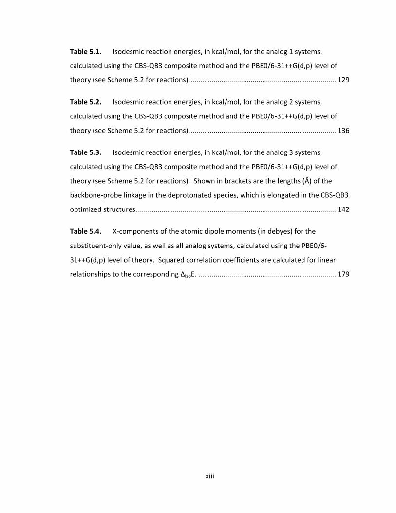
Table 5.1. Isodesmic reaction energies, in kcal/mol, for the analog 1 systems,
calculated using the CBS‐QB3 composite method and the PBE0/6‐31++G(d,p) level of
theory (see Scheme 5.2 for reactions). ........................................................................... 129
Table 5.2. Isodesmic reaction energies, in kcal/mol, for the analog 2 systems,
calculated using the CBS‐QB3 composite method and the PBE0/6‐31++G(d,p) level of
theory (see Scheme 5.2 for reactions). ........................................................................... 136
Table 5.3. Isodesmic reaction energies, in kcal/mol, for the analog 3 systems,
calculated using the CBS‐QB3 composite method and the PBE0/6‐31++G(d,p) level of
theory (see Scheme 5.2 for reactions). Shown in brackets are the lengths (Å) of the
backbone‐probe linkage in the deprotonated species, which is elongated in the CBS‐QB3
optimized structures. ...................................................................................................... 142
Table 5.4. X‐components of the atomic dipole moments (in debyes) for the
substituent‐only value, as well as all analog systems, calculated using the PBE0/6‐
31++G(d,p) level of theory. Squared correlation coefficients are calculated for linear
relationships to the corresponding ΔisoE. ....................................................................... 179
xiv
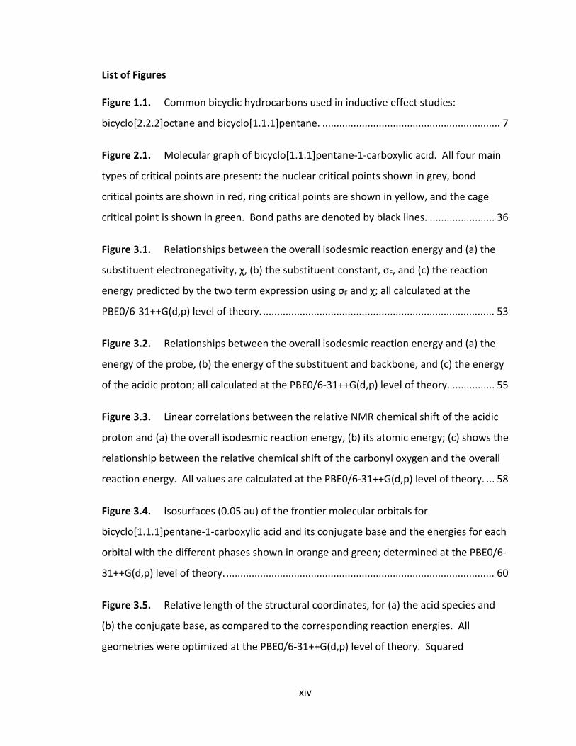
List of Figures
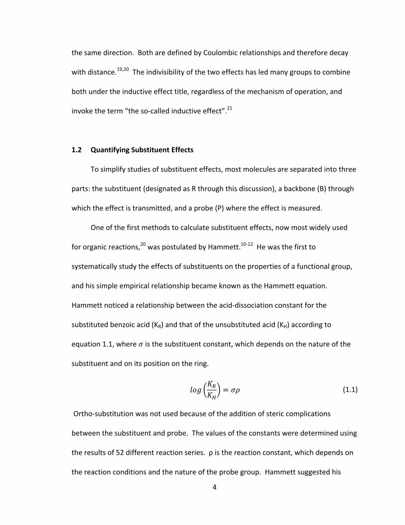
Figure 1.1. Common bicyclic hydrocarbons used in inductive effect studies:
bicyclo[2.2.2]octane and bicyclo[1.1.1]pentane. ............................................................... 7
Figure 2.1. Molecular graph of bicyclo[1.1.1]pentane‐1‐carboxylic acid. All four main
types of critical points are present: the nuclear critical points shown in grey, bond
critical points are shown in red, ring critical points are shown in yellow, and the cage
critical point is shown in green. Bond paths are denoted by black lines. ....................... 36
Figure 3.1. Relationships between the overall isodesmic reaction energy and (a) the
substituent electronegativity, χ, (b) the substituent constant, σF, and (c) the reaction
energy predicted by the two term expression using σF and χ; all calculated at the
PBE0/6‐31++G(d,p) level of theory. .................................................................................. 53
Figure 3.2. Relationships between the overall isodesmic reaction energy and (a) the
energy of the probe, (b) the energy of the substituent and backbone, and (c) the energy
of the acidic proton; all calculated at the PBE0/6‐31++G(d,p) level of theory. ............... 55
Figure 3.3. Linear correlations between the relative NMR chemical shift of the acidic
proton and (a) the overall isodesmic reaction energy, (b) its atomic energy; (c) shows the
relationship between the relative chemical shift of the carbonyl oxygen and the overall
reaction energy. All values are calculated at the PBE0/6‐31++G(d,p) level of theory. ... 58
Figure 3.4. Isosurfaces (0.05 au) of the frontier molecular orbitals for
bicyclo[1.1.1]pentane‐1‐carboxylic acid and its conjugate base and the energies for each
orbital with the different phases shown in orange and green; determined at the PBE0/6‐
31++G(d,p) level of theory. ............................................................................................... 60
Figure 3.5. Relative length of the structural coordinates, for (a) the acid species and
(b) the conjugate base, as compared to the corresponding reaction energies. All
geometries were optimized at the PBE0/6‐31++G(d,p) level of theory. Squared
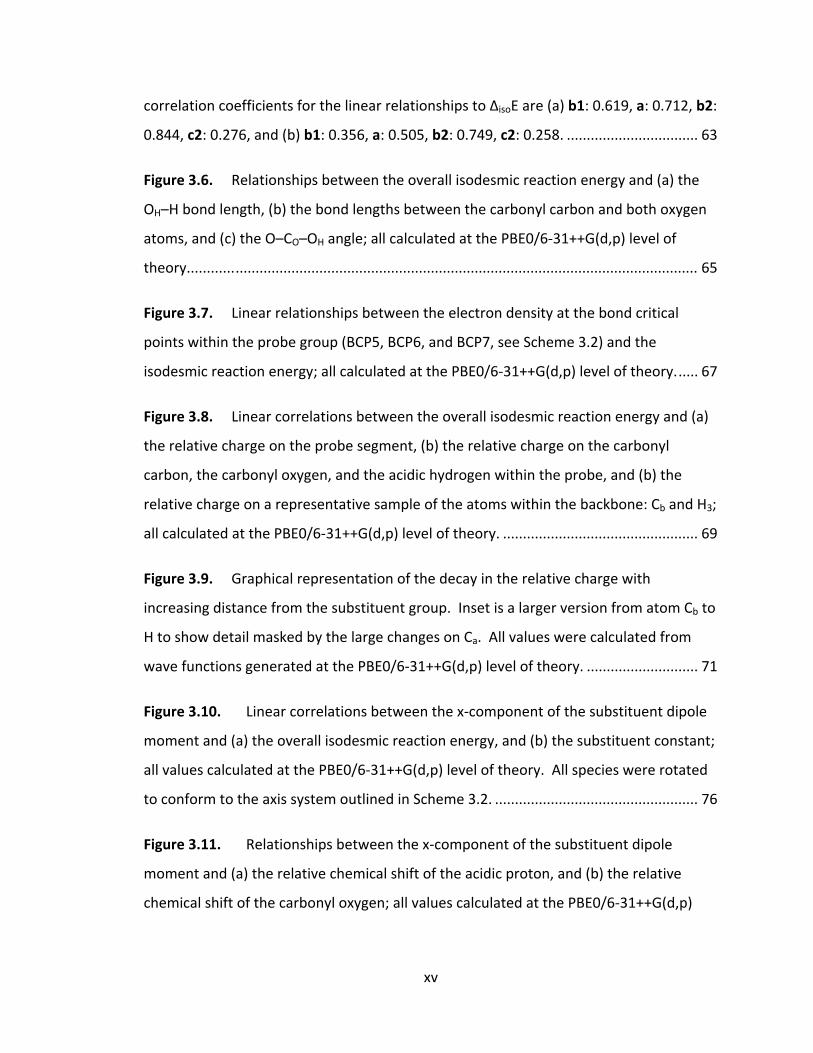
xv
correlation coefficients for the linear relationships to ΔisoE are (a) b1: 0.619, a: 0.712, b2:
0.844, c2: 0.276, and (b) b1: 0.356, a: 0.505, b2: 0.749, c2: 0.258. ................................. 63
Figure 3.6. Relationships between the overall isodesmic reaction energy and (a) the
OH–H bond length, (b) the bond lengths between the carbonyl carbon and both oxygen
atoms, and (c) the O–CO–OH angle; all calculated at the PBE0/6‐31++G(d,p) level of
theory............ .................................................................................................................... 65
Figure 3.7. Linear relationships between the electron density at the bond critical
points within the probe group (BCP5, BCP6, and BCP7, see Scheme 3.2) and the
isodesmic reaction energy; all calculated at the PBE0/6‐31++G(d,p) level of theory. ..... 67
Figure 3.8. Linear correlations between the overall isodesmic reaction energy and (a)
the relative charge on the probe segment, (b) the relative charge on the carbonyl
carbon, the carbonyl oxygen, and the acidic hydrogen within the probe, and (b) the
relative charge on a representative sample of the atoms within the backbone: Cb and H3;
all calculated at the PBE0/6‐31++G(d,p) level of theory. ................................................. 69
Figure 3.9. Graphical representation of the decay in the relative charge with
increasing distance from the substituent group. Inset is a larger version from atom Cb to
H to show detail masked by the large changes on Ca. All values were calculated from
wave functions generated at the PBE0/6‐31++G(d,p) level of theory. ............................ 71
Figure 3.10. Linear correlations between the x‐component of the substituent dipole
moment and (a) the overall isodesmic reaction energy, and (b) the substituent constant;
all values calculated at the PBE0/6‐31++G(d,p) level of theory. All species were rotated
to conform to the axis system outlined in Scheme 3.2. ................................................... 76
Figure 3.11. Relationships between the x‐component of the substituent dipole
moment and (a) the relative chemical shift of the acidic proton, and (b) the relative
chemical shift of the carbonyl oxygen; all values calculated at the PBE0/6‐31++G(d,p)
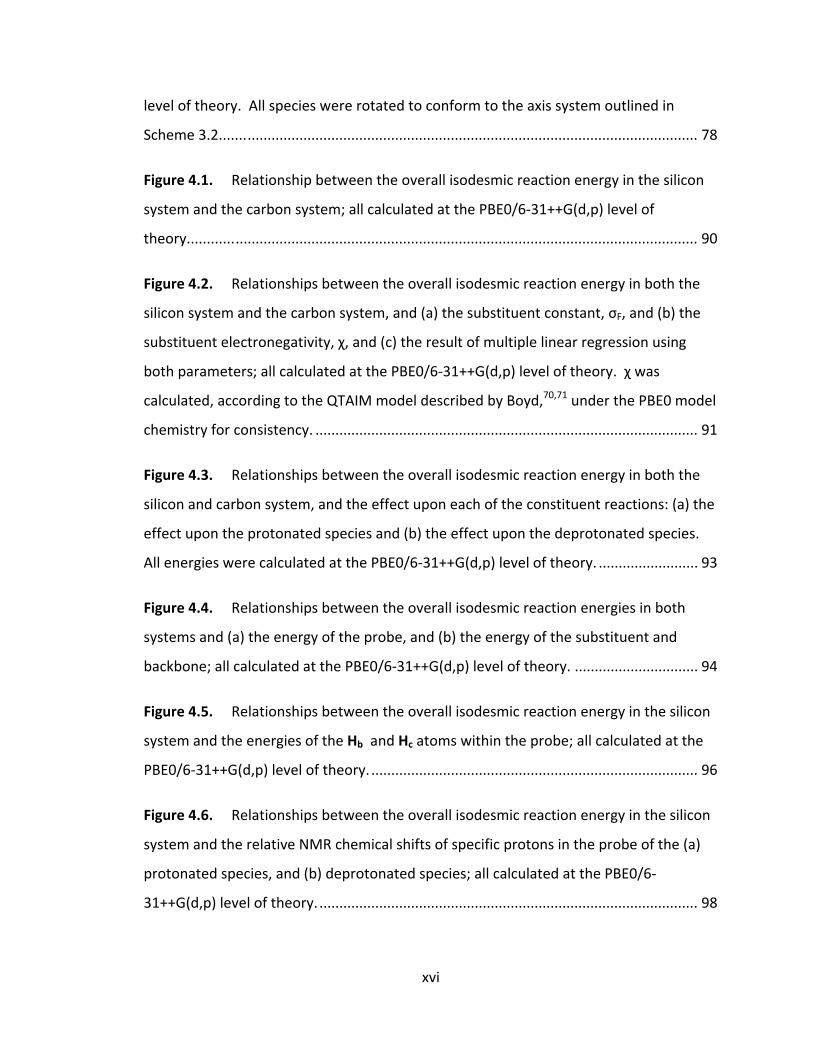
xvi
level of theory. All species were rotated to conform to the axis system outlined in
Scheme 3.2....... ................................................................................................................. 78
Figure 4.1. Relationship between the overall isodesmic reaction energy in the silicon
system and the carbon system; all calculated at the PBE0/6‐31++G(d,p) level of
theory............ .................................................................................................................... 90
Figure 4.2. Relationships between the overall isodesmic reaction energy in both the
silicon system and the carbon system, and (a) the substituent constant, σF, and (b) the
substituent electronegativity, χ, and (c) the result of multiple linear regression using
both parameters; all calculated at the PBE0/6‐31++G(d,p) level of theory. χ was
calculated, according to the QTAIM model described by Boyd,70,71 under the PBE0 model
chemistry for consistency. ................................................................................................ 91
Figure 4.3. Relationships between the overall isodesmic reaction energy in both the
silicon and carbon system, and the effect upon each of the constituent reactions: (a) the
effect upon the protonated species and (b) the effect upon the deprotonated species.
All energies were calculated at the PBE0/6‐31++G(d,p) level of theory. ......................... 93
Figure 4.4. Relationships between the overall isodesmic reaction energies in both
systems and (a) the energy of the probe, and (b) the energy of the substituent and
backbone; all calculated at the PBE0/6‐31++G(d,p) level of theory. ............................... 94
Figure 4.5. Relationships between the overall isodesmic reaction energy in the silicon
system and the energies of the Hb and Hc atoms within the probe; all calculated at the
PBE0/6‐31++G(d,p) level of theory. .................................................................................. 96
Figure 4.6. Relationships between the overall isodesmic reaction energy in the silicon
system and the relative NMR chemical shifts of specific protons in the probe of the (a)
protonated species, and (b) deprotonated species; all calculated at the PBE0/6‐
31++G(d,p) level of theory. ............................................................................................... 98
xvii
Figure 4.7. Graphical representation of the effect of substitution on the difference
between c2 (Å) in the Si‐system and the C‐system. All geometries were optimized at the
PBE0/6‐31++G(d,p) level of theory. ................................................................................ 102
Figure 4.8. Relationship between the overall isodesmic reaction energy and the
pyramidalization of the probe group in the silicon system; all calculated at PBE0/6‐
31++G(d,p) level of theory. ............................................................................................. 104
Figure 4.9. Relationships between the electron density at the bond critical points in
the probe group of the silicon system (see Scheme 4.2) and the overall reaction energy;
all calculated at the PBE0/6‐31++G(d,p) level of theory. ............................................... 106
Figure 4.10. Relationships between the overall reaction energy and the QTAIM
charge of the probe group within the molecules of the silicon system; all calculated at
the PBE0/6‐31++G(d,p) level of theory. .......................................................................... 108
Figure 4.11. Graphical representation of the decay in the relative charges of the
atoms along the bond path (see Scheme 4.2) in the silicon system for the (a) protonated
species and (b) deprotonated species. Inset is the effect upon the atoms from Cb to Ha
to show the detail masked by the effects at Ca. All values calculated from wavefunctions
created at the PBE0/6‐31++G(d,p) level of theory. ........................................................ 110
Figure 4.12. Relationship between the QTAIM substituent electronegativity and the
relative charge of the acidic proton in the silicon system; all calculated at the PBE0/6‐
31++G(d,p) level of theory. ............................................................................................. 111
Figure 4.13. Relationships between the overall isodesmic reaction energy and (a) the
x‐component of the substituent dipole in the silicon system, and (b) and the x‐
component of the substituent dipole in both protonated silicon and carbon systems, as
well as the (c) the relationship between the substituent constant and the x‐component
of the substituent dipole in both protonated systems; all calculated at the PBE0/6‐

xviii
31++G(d,p) level of theory. All species were rotated to conform to the axis system
outlined in Scheme 4.2. .................................................................................................. 116
Figure 4.14. Relationships between the x‐component of the substituent dipole in the
protonated silicon system and (a) the relative NMR chemical shift of the acidic proton
and (b) the pyramidalization of the probe group; all calculated at the PBE0/6‐31++G(d,p)
level of theory. All species were rotated to conform to the axis system outlined in
Scheme 4.2....... ............................................................................................................... 117
Figure 5.1. Graphical representation of the relationships between the overall reaction
energy and (a) the overall reaction energies of the corresponding carbon‐backbone
systems, (b) the effect upon the protonated probe groups, and (c) the effect upon the
deprotonated probe groups, for analogs C1 and S1. All values were calculated at the
PBE0/6‐31++G(d,p) level of theory. ................................................................................ 130
Figure 5.2. Graphical representation of the relationship between the overall reaction
energy and the energy of the acidic hydrogen within analogs C1 and S1. All values were
calculated at the PBE0/6‐31++G(d,p) level of theory. .................................................... 133
Figure 5.3. Geometry optimization of the CF3, NF2, CN and NO2 substituted conjugate
base of analog C2, and CN and NO2 substituted conjugate base of analog S2, using the
CBS‐QB3 composite method (CN and NO2, and NO2 substitution, respectively, at the
PBE0/6‐31++G(d,p) level of theory) results in the rearrangement of one of the bridging
silicon atoms to form two four‐membered rings. Shown is (a) NO2 substitution with
analog C1 and (b) NO2 substitution with analog S2. ....................................................... 135
Figure 5.4. Graphical representation of the relationships between the overall reaction
energy and (a) the overall reaction energies of the corresponding carbon‐backbone
systems, (b) the effect upon the protonated probe groups, and (c) the effect upon the
deprotonate probe groups, for analogs C2 and S2. All values were calculated at the
PBE0/6‐31++G(d,p) level of theory. ................................................................................ 137
xix
Figure 5.5. Graphical representation of the relationship between the overall reaction
energy and the energy of the acidic hydrogen within analogs C2 and S2. All values were
calculated at the PBE0/6‐31++G(d,p) level of theory. .................................................... 139
Figure 5.6. Apparent removal of the deprotonated probe segment of substituted
analog C3 molecules. Shown as the NH2‐substituted CB with optimized using the (a)
CBS‐QB3 composite method and (b) the PBE0/6‐31++G(d,p) level of theory. .............. 141
Figure 5.7. Graphical representation of the relationships between the overall reaction
energy and (a) the overall reaction energies of the corresponding carbon‐backbone
systems, (b) the effect upon the protonated probe groups, and (c) the effect upon the
deprotonated probe groups, for analogs C3 and S3. All values were calculated at the
PBE0/6‐31++G(d,p) level of theory. ................................................................................ 144
Figure 5.8. Graphical representation of the relationship between the overall reaction
energy and the energy of the acidic hydrogen within analogs C3 and S3. All values were
calculated at the PBE0/6‐31++G(d,p) level of theory. .................................................... 146
Figure 5.9. Graphical representations of the differences between the lengths (a) b1,
and (b) a, in analog C1 and S1 as compared to the all‐carbon backbones (see Scheme 5.3
for labelling). All values were optimized at the PBE0/6‐31++G(d,p) level of theory..... 148
Figure 5.10. Graphical representations of (a) the relationship between the overall
reaction energy and the deviation of Ea from planarity, and (b) the difference, between
the analog systems and the all‐carbon system, of the deviation of Ea from planarity, in
both analog C1 and analog S1. All values calculated at the PBE0/6‐31++G(d,p) level of
theory................ .............................................................................................................. 150
Figure 5.11. Graphical representations of (a) the relationship between the overall
reaction energy and the deviation of SiO from planarity, and (b) the difference, between
the analog system and the all‐carbon system, of the deviation of SiO from planarity, in
analog S1. All values calculated at the PBE0/6‐31++G(d,p) level of theory. ................. 153
xx
Figure 5.12. Graphical representations of the differences between the lengths (a) c1,
(b) b1, and (c) a, in analogs C2 and S2 as compared to the all carbon backbones (see
Scheme 5.3 for labelling). All values were optimized at the PBE0/6‐31++G(d,p) level of
theory............... ............................................................................................................... 154
Figure 5.13. Graphical representations of (a) the relationship between the overall
reaction energy and the deviation of Ea from planarity, and (b) the difference, between
the analog systems and the all‐carbon system, of the deviation of Ea from planarity, in
both analog C2 and analog S2. All values calculated at the PBE0/6‐31++G(d,p) level of
theory............... ............................................................................................................... 156
Figure 5.14. Graphical representations of (a) the relationship between the overall
reaction energy and the deviation of SiO from planarity, and (b) the difference, between
the analog systems and the all‐carbon system, of the deviation of SiO from planarity, in
analog S2. All values calculated at the PBE0/6‐31++G(d,p) level of theory. ................. 157
Figure 5.15. Graphical representations of the differences between the lengths (a) b1,
and (b) a, in analog C3 and S3 as compared to the all carbon backbones (see Scheme 5.3
for labelling). All values were optimized at the PBE0/6‐31++G(d,p) level of theory..... 159
Figure 5.16. Graphical representations of (a) the relationship between the overall
reaction energy and the deviation of Ea from planarity, and (b) the difference, between
the analog systems and the all‐carbon system, of the deviation of Ea from planarity, in
both analog C3 and analog S3. All values calculated at the PBE0/6‐31++G(d,p) level of
theory................. ............................................................................................................. 161
Figure 5.17. Graphical representations of (a) the relationship between the overall
reaction energy and the deviation of SiO from planarity, and (b) the difference, between
the analog systems and the all‐carbon system, of the deviation of SiO from planarity, in
analog S3. All values calculated at the PBE0/6‐31++G(d,p) level of theory. ................. 162
xxi
Figure 5.18. Graphical representations of the differences, between the analog
systems and the all‐carbon backbones, of the charges of (a) the forward bridgehead
atom, Ea, and (b) the bridging atom, E’b, in both analog C1 and analog S1. All values
calculated at the PBE0/6‐31++G(d,p) level of theory. .................................................... 166
Figure 5.19. Graphical representations of (a) the difference, between the analog
systems and the all‐carbon system, of the charge on Ec, and (b) the relationship between
the overall reaction energy and the charge on Ec, in both analog C1 and analog S1. All
values calculated at the PBE0/6‐31++G(d,p) level of theory. ......................................... 167
Figure 5.20. Graphical representations of (a) the relationship between the overall
reaction energy and the charge of the probe group, and (b) the difference, between the
analog systems and the all‐carbon system, of the charge of the probe group, in both
analog C1 and analog S1. All values calculated at the PBE0/6‐31++G(d,p) level of
theory............... ............................................................................................................... 168
Figure 5.21. Graphical representations of the differences, between the analog
systems and the all‐carbon backbones, of the charges of (a) the bridging atom, E’b, (b)
the forward bridgehead atom, Ea, and (c) the opposite bridgehead atom, Ec, in both
analog C2 and analog S2. All values calculated at the PBE0/6‐31++G(d,p) level of
theory................ .............................................................................................................. 171
Figure 5.22. Graphical representations of (a) the relationship between the overall
reaction energy and the charge of the probe group, and (b) the difference, between the
analog systems and the all‐carbon system, of the charge of the probe group, in both
analog C2 and analog S2. All values calculated at the PBE0/6‐31++G(d,p) level of
theory................. ............................................................................................................. 172
Figure 5.23. Graphical representations of the differences, between the analog
systems and the all‐carbon backbones, of the charges of (a) the forward bridgehead
atom, Ea, (b) the bridging atom, E’b, and (c) the opposite bridgehead atom, Ec, in both
xxii
analog C3 and analog S3. All values calculated at the PBE0/6‐31++G(d,p) level of
theory............... ............................................................................................................... 174
Figure 5.24. Graphical representations of the relationship between the overall
reaction energy and (a) the charge on E’b, and (b) the charge on Ec, in both analog C3
and analog S3. All values calculated at the PBE0/6‐31++G(d,p) level of theory. .......... 175
Figure 5.25. Graphical representations of (a) the relationship between the overall
reaction energy and the charge of the probe group, and (b) the difference, between the
analog systems and the all‐carbon system, of the charge of the probe group, in both
analog C3 and analog S3. All values calculated at the PBE0/6‐31++G(d,p) level of
theory............... ............................................................................................................... 177
Figure 5.26. Graphical representation of the relationships between the x‐component
of the substituent‐only dipole and the x‐component of the substituent dipole in the acid
species of (a) analogs C1 and S1, (b) analogs C2 and S2, and (c) analogs C3 and S3. All
values were calculated at the PBE0/6‐31++G(d,p) level of theory. ................................ 181
Figure 6.1. Graphical representations of the relationships between the isodesmic
reaction energy in the C‐system and the reaction energies in the (a) Si‐system, (b)
analogs C1, C2 and C3, and (c) analogs S1, S2 and S3, to determine the value of the
reaction constant in each case. All values were calculated at the 6‐31++G(d,p) level of
theory............ .................................................................................................................. 191
Figure 6.2. Graphical representation between the isodesmic reaction energy of the C‐
system, using ΔX‐Cc2 as a parameter within the reaction constant, and the isodesmic
reaction energy of (a) analogs C1, C2 and C3, and (b) the Si‐system, and analogs S1, S2
and S3. All values were calculated at the PBE0/6‐31++G(d,p) level of theory. ............. 194

xxiii
Note on Formatting
The thesis is formatted such that Chapters 3 through 5 are manuscripts that have
been or will be submitted to be published in a journal. Therefore, each has its own
Introduction and Methods sections, in addition to the results.
1
Chapter 1: General Introduction
2
Silicon chemistry is a vast and diverse field with possible applications in biological
fields (e.g. in plant1 and animal life,2,3 and drug design4) and in manufacturing (e.g.
ceramics,5 polymer chemistry6 and lasers7). The most interesting aspects of Si chemistry
are also what make it so complicated. Unlike its first row analog, carbon, Si can adopt
coordination schemes ranging from 2‐ to 6‐coordinate geometries. Although it is
isoelectronic with C, Si has a greater atomic radius, a greater polarizability, and the
opportunity to employ (p–d)π, (p–d–d)π, etc. interactions.8 In addition, silicon
compounds like silicates have a tendency to oligomerize9 under ambient conditions
making preparation and characterization extremely difficult. Investigations of silicon
systems tend to rely on phenomena observed for their carbon based counterparts and
relationships developed for organic reactions (e.g. the Hammett equation10‐12), an
approach that, historically,13,14 does not perform particularly well.
1.1 Substituent Effects
Substituent effects continue to be one of the most ubiquitous and least
understood concepts in chemistry. In general terms, substituent effects refer to the
changes in chemical properties, such as reactivity, of a molecule due to a group, or
atom, when compared to its unsubstituted counterpart (when the substituent is simply
a hydrogen atom).15 This overall effect is generally divided into different contributions:
steric, resonance, and inductive effects are most common.
The International Union of Pure and Applied Chemistry (IUPAC) defines the steric
effect as the resulting change in a property upon the introduction of a substituent with a
3
different steric requirement and is generally related to the overall size of the substituent
itself.16 Steric effects, or strain in a molecule, tend to come from non‐bonded
repulsions, bond angle strain, and bond stretches or compressions. Steric effects can be
avoided by increasing the distance between the substituent and the probe (where the
effect is being measured) such that they no longer spatially interact. This is generally
achieved by using some sort of molecular linker, or backbone, to transmit the effect.
Resonance effects describe the effect a substituent has on reactivity through
electron delocalization, and thus require a conjugated network of π‐bonds.16
Substituents can be placed into two groups based on the type of effect they exert:
electron withdrawing groups (EWGS, which are said to have a negative effect, and
electron donating groups (EDGs), which are said to have a positive effect.17 Resonance
effects can be easily avoided by employing a fully saturated backbone.
The inductive effect is arguably the most important of all substituent effects
because it is always in operation. The concept, originally introduced by Ingold,18 is now
defined by IUPAC as an experimentally observable effect of the transmission of electron
density through σ‐bonds via electrostatic induction.16 Classically suggested to
propagate via consecutive polarizations of bonds, the electron density is said to flow
from a substituent of lower electronegativity to one with higher electronegativity.19
Simultaneously, the transmission of electron density can occur through space and this
mechanism is termed the field effect.16 Field effects are generally described in terms of
induced dipole interactions, or even dispersion forces. The separation of the inductive
and field effects is problematic as both occur simultaneously and most often operate in
4
the same direction. Both are defined by Coulombic relationships and therefore decay
with distance.19,20 The indivisibility of the two effects has led many groups to combine
both under the inductive effect title, regardless of the mechanism of operation, and
invoke the term “the so‐called inductive effect”.21
1.2 Quantifying Substituent Effects
To simplify studies of substituent effects, most molecules are separated into three
parts: the substituent (designated as R through this discussion), a backbone (B) through
which the effect is transmitted, and a probe (P) where the effect is measured.
One of the first methods to calculate substituent effects, now most widely used
for organic reactions,20 was postulated by Hammett.10‐12 He was the first to
systematically study the effects of substituents on the properties of a functional group,
and his simple empirical relationship became known as the Hammett equation.
Hammett noticed a relationship between the acid‐dissociation constant for the
substituted benzoic acid (KR) and that of the unsubstituted acid (KH) according to
equation 1.1, where is the substituent constant, which depends on the nature of the
substituent and on its position on the ring.
(1.1)
Ortho‐substitution was not used because of the addition of steric complications
between the substituent and probe. The values of the constants were determined using
the results of 52 different reaction series. ρ is the reaction constant, which depends on
the reaction conditions and the nature of the probe group. Hammett suggested his
5
reaction constants take the form of equation 1.2,22 where R is the universal gas
constant, T is the absolute temperature, d is the distance between substituent and
probe, and D is the dielectric constant of the solvent.
(1.2)
The constants B1 and B2 are more ambiguous. B1 is said to depend on the electrostatic
interaction between the compound and solvent, while B2 is taken as a measure of the
sensitivity of the reaction to changes in charge density at the probe. A positive ρ implies
that the reaction is favoured by low electron density at the probe, while a negative ρ
requires high electron density. For benzoic acids in water, at 25°C ρ was defined as
1.000.23 The use of the relationship in Equation 1.1 has been criticized due to its
empirical nature,20 but the constants have been used to describe a large body of data
with a mean deviation of only 15%.22
Although it was originally developed using the equilibrium constants of benzoic
acids, the Hammett equation has since been extended to other organic systems, and to
other properties such as infrared frequencies,24 nuclear magnetic resonance (NMR)
chemical shifts,25 polarographic electroreductions,26 isotropic effects,27, and mass
spectra.28 The Hammett equation has also been extended via the separation of
inductive (σI) and resonance (σR) effects according to equation 1.3.20
(1.3)
With the separation of constants, the Hammett equation can be rewritten for any
property (Y) according to equation 1.4.29

6
(1.4)
YR represents the property in the substituted compound and YH that in the unsubstituted
compound, and the proportionality constants ρI and ρR are obtained through multiple
linear regression analysis.29,30
Separation of resonance and inductive effects is important as each can have a
different, and sometimes even opposite, effect upon reactivity. Alkyl groups are
electron donating, but can only add density through the inductive effect. Substituents
like the halogens or hydroxyl are electron withdrawing though σ‐bonds, but actually
donate density via n‐π interactions. Separation of these effects is also important with
respect to the structure of a molecule. Using the para‐ and meta‐substituted benzoic
acids as an example, the same substituent in each could have a different effect. The
distance between the substituent and probe group (carboxylic acid) is longer in p‐
substitution, and the angular direction through‐space is also different.
1.3 Bicyclic Hydrocarbons
Bicyclic hydrocarbons have been used as a backbone to separate substituents by
ensuring only the inductive effect is in operation. The saturated σ‐bond network makes
resonance impossible, and the substituent and probe are held at a distance to keep
steric interaction constant (which can then become a part of the reaction constant).31
The bicyclo[2.2.2]octane structure, shown in Figure 1.1, was originally suggested
because substitution at the 4‐position ensured the number of C–C bonds between
substituent and probe was essentially the same as in the p‐substituted benzoic acids,32
7
Figure 1.1. Common bicyclic hydrocarbons used in inductive effect studies:
bicyclo[2.2.2]octane and bicyclo[1.1.1]pentane.
8
while substitution at the 3‐position is related to the m‐substituted benzoic acids.33 The
rigid backbones also force the substituent and probe to be coplanar, thus removing any
angle dependence of the distance. Bicyclo[1.1.1]pentane (see Figure 1.1) has also been
used as a backbone in inductive effect studies. The main advantage of using the
bicyclo[1.1.1]pentane backbone over the bicyclo[2.2.2]octane backbone is that the
shorter distance between the substituents and probe should lead to a more sensitive
effect.33
1.4 Isodesmic Reactions
In order to investigate a substituent effect, or in this case the inductive effect, it is
more efficient to use isolated molecules than rely on solution reactivities.30 Isolated
molecules would be more sensitive to minute changes in structure and electron density;
one could avoid any artificial changes due to system interaction, such as solvent
stabilization. This fact leads to the usefulness of quantum chemical calculations: their
ability to accurately determine the thermochemistry of single, isolated, molecules.
Quantum calculations also make it possible to test systems that are difficult or
impossible to synthesize, as well as study microscopic properties that may not be
resolvable experimentally.
An important tool in the study of substituents via quantum chemical or
computational calculations is the isodesmic reaction:30 a special category of reactions
where the number and types of bonds are the same on both sides of the reaction.16
Three examples using systems already discussed are shown in Scheme 1.1. An
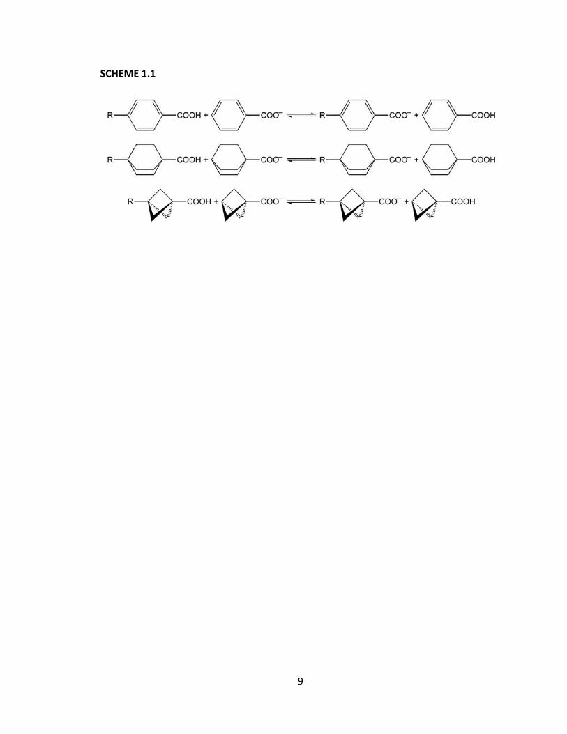
9
SCHEME 1.1
10
isodesmic reaction is particularly useful as it functions to reduce the errors associated
with some common approximations like incomplete basis sets, the set of function used
to create the molecular orbital that must be truncated in order to calculate, and
incomplete correction for electron correlation.34 Electron correlation errors are related
to the fact that in simple Hartree‐Fock theory the motion of electrons is considered
correlated even at long distances, and thus bond breaking reactions, like acid‐base
dissociations, are problematic. It is possible to correct for this, but complete corrections
are impossible (discussed in more detail in Chapter 2). The use of an isodesmic reaction
treats this error as systematic, and therefore it cancels.
Isodesmic reactions are also important in that they exploit the relationship of the
Hammett equation to linear free energies. Equation 1.1 is a linear free energy
relationship,22 and equation 1.4 can be related to isodesmic reactions. This stems from
the proportionality between the left hand side of the equations (logKR – logKH) and the
differences in the free energies for the substituted and unsubstituted compounds.
Using the first reaction in Scheme 1.2 for substituted benzoic acid, the derivation in
equation 1.5 shows how the isodesmic reaction energy can be directly related to the
Hammett relationship of equation 1.1. HA refers to the acid species, CB refers to the
conjugate base species, and the subscripts R and H corresponding to the substituted and
unsubstituted species, respectively.
11
∆ ∆
∆ ∆
∆
(1.5)
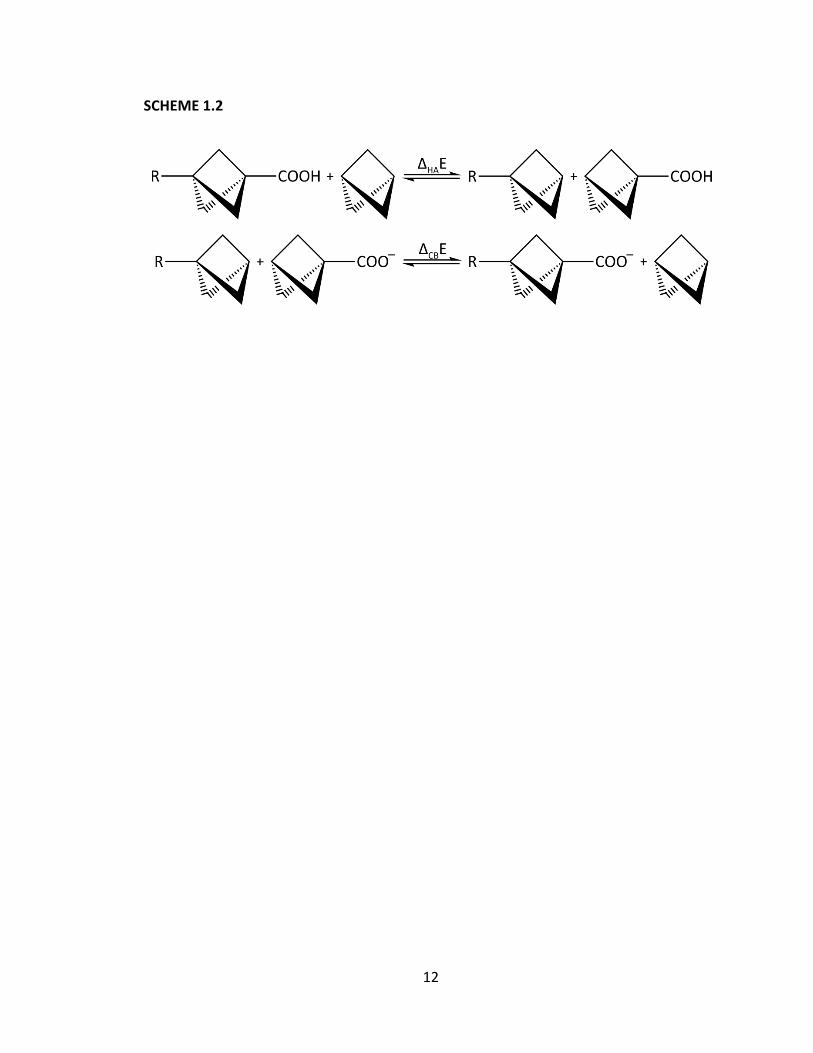
One potential problem with the isodesmic reaction approach is that the reactions
shown in Scheme 1.1 all involve two separate, but simultaneous interactions: the effect
of R on the carboxylic acid probe in its protonated state, and that on its deprotonated
state. These two interactions can be separated by splitting the overall reaction into two
separate isodesmic reactions,30 one for each effect. In Scheme 1.2, HA refers to the
effect upon the acid species only and CB refers to the effect upon the conjugate base
only.
1.5 Substitution and Silicon Systems
The majority of substituent effect studies involving silicon treat the center as a
substituent and not as a probe. Work involving the effect upon a center began with
Taft, who measured the effect in organic carbonyls.35 It was Taft who first suggested
the requirement of a term to describe the steric effect to the original Hammett equation
as in equation 1.6.
(1.6)
12
SCHEME 1.2
13
Cartledge defined a series of steric parameters specifically for silicon, Es(Si), due to the
size difference between C and Si.13 These steric parameters were calculated using the
acid‐catalyzed hydrolysis of silanes (R3SiH) with a variety of alkyl groups.
More recently, Ploom and Tuulmets investigated the inductive effect in Si
chemistry14 using the method described by Exner and Böhm.36 They discovered that the
addition of an electronegativity term, as outlined in equation 1.7, was needed to fully
describe the effect.
(1.7)
Most of their organosilicon centers take the form RSi(CH3)2Cl and therefore do include
steric effects at the Si center. To date there has been no study of the inductive effect at
Si that removes the complicating steric hindrance.
Another aspect of substituent effects in silicon systems is the manner in which
the effect transmits through a Si atom. One of the few studies of this nature was
undertaken by Yoder et al.8 They studied the transmission of substituent effects though
a disilane bond using the NMR coupling constants and chemical shifts as probes in
molecules of the form RSi(CH3)2Si(CH3)3 and RSi(CH3)2Si(CH3)2N(CH3)2. They found that
the Si–Si bonds was less effective at transmitting substituent effects than the C–C
counterpart, and even behaved as an insulator rather than a conductor in some cases.
In this investigation we aim to answer two main questions: what is the effect of
substituents on a silicon center and how does the effect transmit through silicon
containing backbones. To do this, we will use the bicyclo[1.1.1]pentane backbone to
ensure only the “so‐called” inductive effect is operating and employ a variety of
14
substituents (chosen to cover a range of electronegativity, χ). Li is electropositive
(χ=1.00) and has been previously shown to adopt bonds that are highly ionic in nature.
However, it is commonly referred to as an electron donating group in substituent effect
studies,37 and will be used as such here due to the small number of inductively donating
substituents. Using the well documented carboxylic acid probe as a benchmark, a silicic
acid type probe (Si(OH3)) will be used to measure the effect of the substituents on
silicon using the isodesmic reaction approach to solving the Hammett equation. The
Quantum Theory of Atoms in Molecules (see Chapter 2) will be employed to determine
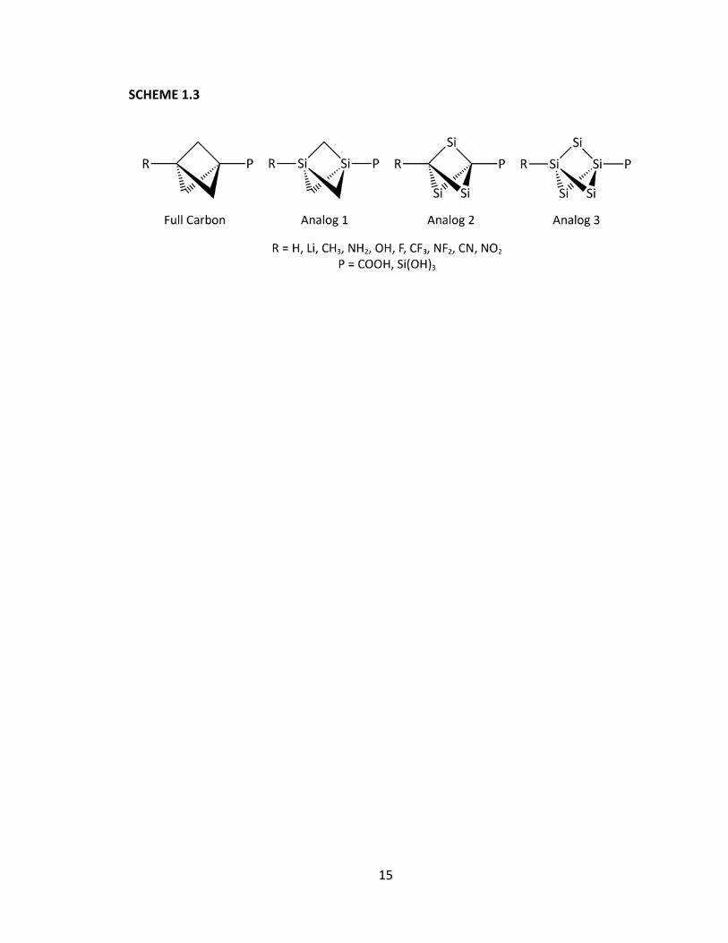
how the substituents perturb the electron density distribution. As illustrated in Scheme
1.3, we will systematically replace the carbon atoms within the bicyclo[1.1.1]pentane
backbone with silicon atoms to determine the effect upon the mechanism of
transmission.
15
SCHEME 1.3
16
Chapter 2: Computational Theory and Methods
17
Throughout this thesis, Density Functional Theory (more specifically the
parameter‐free hybrid functional PBE0) was used to optimize the structure for and
determine the energy of the bicyclo[1.1.1]pentane systems. The accuracy of the
resultant energies was confirmed using a composite method, known for achieving highly
accurate thermochemistries (CBS‐QB3). The same model chemistry (PBE0/6‐
31++G(d,p)) was used in all calculations to ensure consistency. Central to any study of
the “so‐called” inductive effect, the electron density distribution was analyzed according
to Bader’s Quantum Theory of Atoms in Molecules.
2.1 Density Functional Theory
Conventional quantum chemistry, uses the wavefunction (Ψi) because it includes
all information about the specific state of the system and can be used to determine any
physically observable property of the system if one knows the appropriate operator (
for a general operator).38 For example, in equation 2.1 the Hamiltonian operator, , for
a molecular system described by the function of the qi and qA electronic and nuclear
coordinates – which includes M nuclei and N electrons – returns the total energy, Ei, of
the system.
Ψ , Ψ , (2.1)
Unfortunately, the wavefunction is a vastly complex quantity: it depends on 4N
variables, one spin variable and three spatial variables for each of N electrons (after the
nuclear positions have been fixed), and is almost completely uninterpretable. Density
Functional Theory (DFT) stemmed from the idea that a simpler, physical observable

18
could be used to determine the energy of the system. The basic premise behind DFT is
that the electron density can be used, instead of the wavefunction, to determine the
energy, and thereby other properties, of a molecule.38‐40 The electron density, ρ(r), is
given by a multiple integral over the spin coordinates of all electrons and all but one of
the spatial variables because electrons are indistinguishable:40
… |Ψ , , … | … (2.2)
ρ(r) is a non‐negative function, which goes to zero at infinity and integrates to give the
total number of electrons, N.
(2.3)
While there were previous approximations which used the electron density,
contemporary DFT got its roots with Hohenberg and Kohn in 1964.41 The two theorems
presented in their paper (the proof of existence and the variational principle) form the
basis for all DFT.
2.1.1 Hohenberg‐Kohn Theorems
The first theorem states that “the external potential Vext(r) is (to within a
constant) a unique functional of ρ(r); since, in turn Vext(r) fixes we see that the full
many particle ground state functional of ρ(r)” (sic).41 In DFT the electrons interact not
only with one another, but also an external potential. In a uniform electron gas, as was
used in the proof of the existence theorem, the external potential is defined as a
uniform positive charge. In a molecular system, the external potential is the attractive
19
forces between the nuclei and electrons. The electron density determines not only the
external potential, the Hamiltonian and the ground‐state wavefunction, but also the
excited‐state wavefunctions.39
Although the existence theorem shows the utility of the density, it does not
describe how to predict the density. In the second theorem, Hohenberg and Kohn
showed that the density obeys the variational principle.41 One can evaluate the
expectation value of the energy, by optimizing the orbital coefficients, which must be
greater than or equal to the true energy.
2.1.2 Kohn‐Sham Approach
Kohn and Sham proposed to simplify the Hamiltonian by treating the system as if
the electrons were non‐interacting.42 If this was the case, the Hamiltonian could be
expressed as a sum of one‐electron operators. The Kohn‐Sham (KS) approach takes a
fabricated system of non‐interacting electrons with the same density as the real system
as the starting point, and uses this to separate the energy into components according
to:39
Δ Δ (2.4)
The terms in equation 2.4 correspond to the kinetic energy of the non‐interacting
electrons, the nuclei‐electron interaction, the classical electron‐electron repulsion, the
correction to the kinetic energy of the electrons required because of their interactions
in the real system, and all non‐classical corrections to the electron‐electron repulsion,
respectively. The attraction between nuclei and electrons is defined as39
20
| | (2.5)
where ZA is the atomic number of atom A, and rA is the radial distance from atom A. The
classical electron‐electron repulsion is given by:39
12 | | (2.6)
where and are dummy integration variables, which run over all space. Using bra‐
ket notation in terms of orbitals, equation 2.4 can be rewritten as
12 | |
12 | |
(2.7)
Where N is the total number of electrons and the density, ρ, is given by
| (2.8)
In equation 2.7 the two correction terms have been combined in Exc[ρ(r)] , which is
generally termed the so‐called exchange‐correlation energy (discussed in Section
2.1.3).39
The KS approach follows a Self‐Consistent Field (SCF) method. The many‐
electron operator can be described as a product of one‐electron operators, or orbitals.
These orbitals are assumed to be orthonormal and are given as a linear combination of
atomic orbitals (LCAO), χi, weighted by coefficients cij as in equation 2.9 (discussed in
more detail in Section 2.2).
21
(2.9)
The Hamiltonian operator can then be rewritten as:
(2.10)
where is the KS one‐electron operator and is defined as:
12 | | | | (2.11)
and Vxc is a functional‐derivative given in equation 2.12.
(2.12)
The orbitals that minimize the energy can be found using the following relationship,
where εi is the energy:
(2.13)
To determine the KS orbitals, they are expressed as a set of basis functions (Section 2.2)
and then the orbital coefficients are determined iteratively by solving the secular
equation, represented by a Slater determinant as in equation 2.14, to determine a set of
orbital energies.39
Φ1√ !
1 1 … 12 2 … 2
…
(2.14)
DFT, by definition, is an exact theory and all that must be known is how Exc
depends on ρ(r).40 Unfortunately, the theorems give no indication as to the functional
22
form or how to discover it. Consequently much time has gone into determining the
exact or best form for Exc.
2.1.3 Exchange‐Correlation Functionals
The so‐called exchange‐correlation energy accounts for the differences between
the classical and quantum descriptions of electron‐electron repulsion, and the kinetic
energies of the non‐interacting and interacting systems. Our work employs hybrid
approaches (Section 2.1.3.3), which depend on the local and generalized gradient
approximations. Therefore, these three methods will now be discussed: the local
density approximation, the generalized gradient approximation, and hybrid methods.
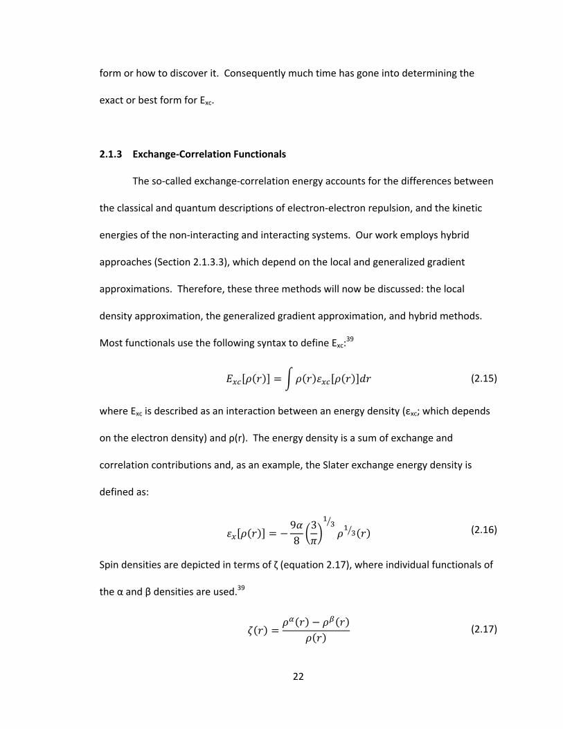
Most functionals use the following syntax to define Exc:39
(2.15)
where Exc is described as an interaction between an energy density (εxc; which depends
on the electron density) and ρ(r). The energy density is a sum of exchange and
correlation contributions and, as an example, the Slater exchange energy density is
defined as:
98
3 (2.16)
Spin densities are depicted in terms of ζ (equation 2.17), where individual functionals of
the α and β densities are used.39
(2.17)
23
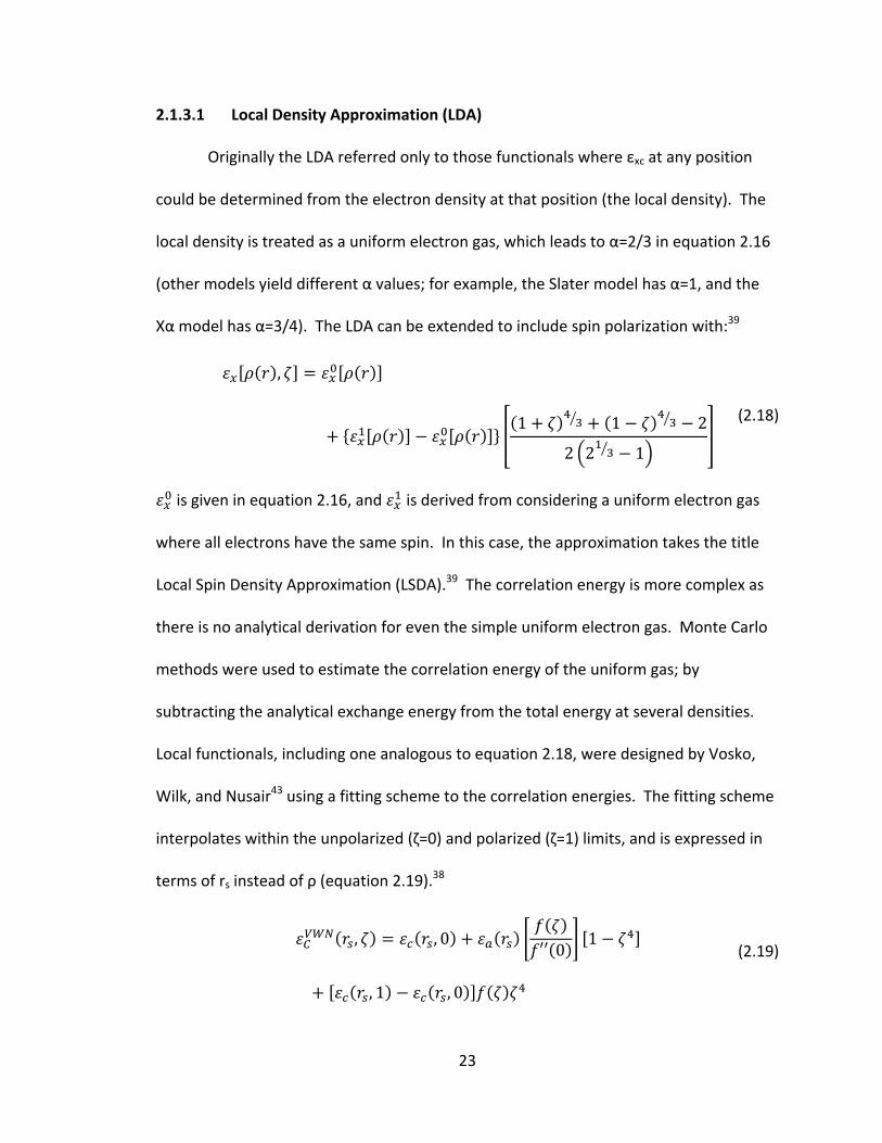
2.1.3.1 Local Density Approximation (LDA)
Originally the LDA referred only to those functionals where εxc at any position
could be determined from the electron density at that position (the local density). The
local density is treated as a uniform electron gas, which leads to α=2/3 in equation 2.16
(other models yield different α values; for example, the Slater model has α=1, and the
Xα model has α=3/4). The LDA can be extended to include spin polarization with:39
,
1 1 2
2 2 1
(2.18)
is given in equation 2.16, and is derived from considering a uniform electron gas
where all electrons have the same spin. In this case, the approximation takes the title
Local Spin Density Approximation (LSDA).39 The correlation energy is more complex as
there is no analytical derivation for even the simple uniform electron gas. Monte Carlo
methods were used to estimate the correlation energy of the uniform gas; by
subtracting the analytical exchange energy from the total energy at several densities.
Local functionals, including one analogous to equation 2.18, were designed by Vosko,
Wilk, and Nusair43 using a fitting scheme to the correlation energies. The fitting scheme
interpolates within the unpolarized (ζ=0) and polarized (ζ=1) limits, and is expressed in
terms of rs instead of ρ (equation 2.19).38
, , 0 0 1
, 1 , 0
(2.19)

24
1 ⁄ 1 ⁄ 22 2 ⁄ 1
In general, LSDA underestimates the exchange energy by approximately 10%,
and overestimates electron correlation by a factor of 2. This leads to unrealistically
strong bonds.38
2.1.3.2 Generalized Gradient Approximation (GGA)
The most intuitive way to improve the LSDA would be to consider a non‐uniform
electron gas. In this type of approach, the exchange and correlation energies are also
dependent on the derivatives of the electron density, and is thus termed the
Generalized Gradient Approximation (GGA).38 In general, GGA functionals add a
correction to the LDA functional as in equation 2.20.
∆| |
⁄ (2.20)
This correction is dependent on a dimensionless reduced gradient.39 One of the first
popular exchange functionals was proposed by Becke.44 It takes the abbreviation B, or
B88, and has the correct asymptotic behaviour for the energy density (‐r ‐1).38
∆
∆ ⁄1 6
(2.21)
Where β is a fitting parameter (determined to by 0.0042 using a least‐squares fit to the
exact exchange energies for noble gas atoms He through Rn)40 and is defined as:
25
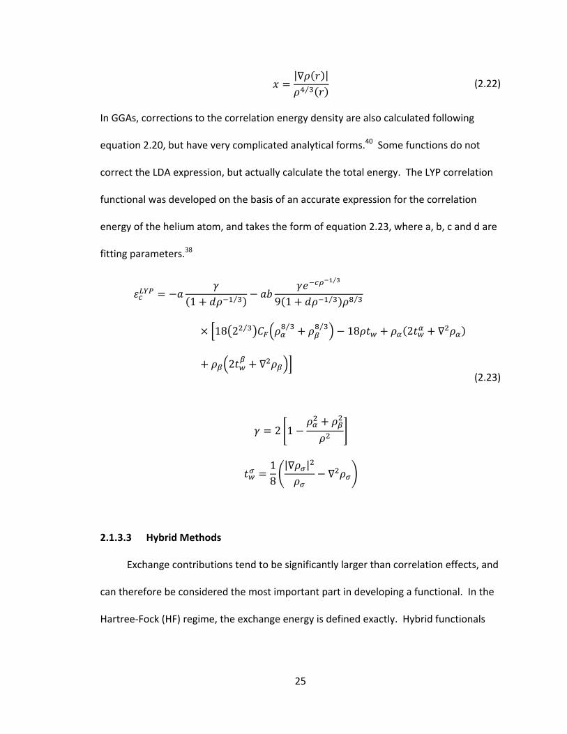
| |⁄ (2.22)
In GGAs, corrections to the correlation energy density are also calculated following
equation 2.20, but have very complicated analytical forms.40 Some functions do not
correct the LDA expression, but actually calculate the total energy. The LYP correlation
functional was developed on the basis of an accurate expression for the correlation
energy of the helium atom, and takes the form of equation 2.23, where a, b, c and d are
fitting parameters.38
1 ⁄
⁄
9 1 ⁄ ⁄
18 2 ⁄ ⁄ ⁄ 18 2
2
2 1
18
| |
(2.23)
2.1.3.3 Hybrid Methods
Exchange contributions tend to be significantly larger than correlation effects, and
can therefore be considered the most important part in developing a functional. In the
Hartree‐Fock (HF) regime, the exchange energy is defined exactly. Hybrid functionals
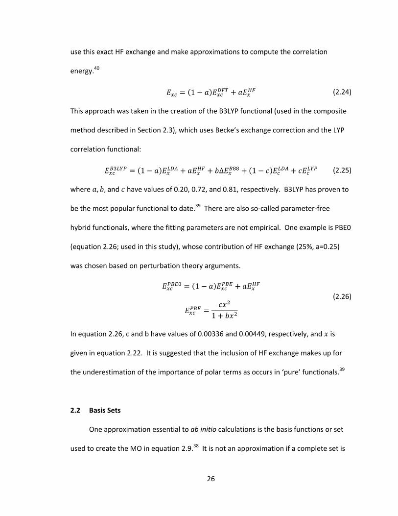
26
use this exact HF exchange and make approximations to compute the correlation
energy.40
1 (2.24)
This approach was taken in the creation of the B3LYP functional (used in the composite
method described in Section 2.3), which uses Becke’s exchange correction and the LYP
correlation functional:
1 ∆ 1 (2.25)
where , , and have values of 0.20, 0.72, and 0.81, respectively. B3LYP has proven to
be the most popular functional to date.39 There are also so‐called parameter‐free
hybrid functionals, where the fitting parameters are not empirical. One example is PBE0
(equation 2.26; used in this study), whose contribution of HF exchange (25%, a=0.25)
was chosen based on perturbation theory arguments.
1
1
(2.26)
In equation 2.26, c and b have values of 0.00336 and 0.00449, respectively, and is
given in equation 2.22. It is suggested that the inclusion of HF exchange makes up for
the underestimation of the importance of polar terms as occurs in ‘pure’ functionals.39
2.2 Basis Sets
One approximation essential to ab initio calculations is the basis functions or set
used to create the MO in equation 2.9.38 It is not an approximation if a complete set is
27
used, but this means an infinite number of functions must also be used and this
becomes impossible in a real calculation. The smaller the set of functions used to
represent the MO is, the poorer the representation will be.
The type of function used in the representation can also affect its accuracy. In
general one can use any type of function that fits the boundary conditions, but the most
commonly used are the Slater type orbital (STO) and the Gaussian type orbital (GTO).
These basis functions are referred to as atomic orbitals (AOs) because they are used to
represent the MO, but they do not correspond to solutions of the atomic wavefunction
(although STOs do resemble the atomic orbitals).38 STOs take the following form, where
is a normalization constant and , are spherical harmonic functions:38
, , , , , . , (2.27)
The exponential term ( ) recreates the distance dependence between the electrons
and the nucleus. One disadvantage of STOs is that they do not have any radial nodes as
in true orbitals, but this can be overcome by using a linear combination of STOs. The
main problem is that a calculation using STOs cannot be solved analytically.38
GTOs take the following form (equation 2.28), and can also be written in terms
of Cartesian coordinates (equation 2.29):38
, , , , , . , (2.28)
, , , , , (2.29)
The sum of the , , and terms gives the type of orbital the GTO is describing. The r2
dependence of the exponential terms leads to an unrealistic negative slope at the
28
nucleus. In general, GTOs do a poor job at representing what happens near the nucleus,
and at the other distance extreme; the GTO falls off far too quickly. However, the
benefit to using GTOs is that the pertinent integrals can be calculated. GTOs are the
most widely used functions in basis sets, but a linear combination of GTOs is used to
recreate the desired properties of an STO as described in equation 2.30.
(2.30)
This is referred to as a contracted basis function (CGTO), and the original GTOs that are
combined are now called primitive GTOs (PGTOs).39 When two CGTOs are used it is
termed a double‐zeta (because of the use of ζ in the exponent) basis set, and when
three are used it is termed a triple‐zeta basis set.
Basis sets can also be improved by separately describing the valence and core
orbitals, and are referred to as split‐valence basis sets.38 Pople et al. have designed split
valence basis sets, designated k‐nlmG. The k corresponds to the number of PGTOs used
to describe the core orbitals and nlm is used for the valence orbitals. One of the most
common (and that used in this study) Pople‐style basis sets is 6‐31G.45,46 In this set, a
contraction of six PGTOs is used for the core orbitals; and the valence is split into two
functions, one described by three PGTOs and one represented by one PGTO.
Additionally, diffuse and/or polarization functions can be added to each basis set.
The presence of diffuse functions in the Pople‐style basis sets are indicated by ‘+’ before
the G. A single ‘+’ indicates that a set of s and p functions have been added to the heavy
atoms, and a second ‘+’ indicates that a set of s functions have been added to
29
hydrogen.38,39 Diffuse functions are used to improve the density farther from the
nucleus as required in complexes that have more spatially diffuse molecular orbitals
(such as anions and highly excited electronic states).39 Polarization functions, which
allow flexibility in the molecular orbitals required for asymmetry, are designated after
the G in a similar manner. In the most simple additions, the designation ‘**’ is used.
This corresponds to the addition of a d function on heavy atoms and a p function on
hydrogen. Polarization functions must be designated explicitly when more are added,
thus ‘**’ is equivalent to (d,p). The largest standard Pople‐style basis set is 6‐
311++G(3df,3pd).38
2.3 Composite Methods
Composite methods are multilevel, or multistep, approaches to achieving highly
accurate results (most often thermochemical quantities). They generally assume that
basis‐set, and correlation energy, incompleteness can be dealt with in an additive
manner as calculations to achieve the exact answer are impossible.39 In one of the most
common composite methods (used in this study), CBS‐QB3,47,48 energies computed at
different levels of theory are extrapolated to a complete basis set (CBS) limit. Differing
techniques for calculating electron correlation are also used to determine correction
terms to the overall energy. The CBS‐QB3 approach involves lower level calculations on
large basis sets for the SCF and zero‐point energies, medium sized basis set for second
order corrections, and small size basis sets for higher‐level corrections. The specific
steps are:49
30
(i) B3LYP/6‐311G(2d,d,p) geometry optimization
(ii) B3LYP/6‐311G(2d,d,p) vibrational frequency analysis, with a 0.99
scaling factor to correct for the harmonic approximation
(iii) UMP2/6‐311+G(3df,2df,2p) energy calculation, and a CBS
extrapolation
(iv) MP4(SDQ)/6‐31+G(d(f),p) energy calculation
(v) CCSD(T)/6‐31+G† energy calculation
The total energy of the system is calculated by adding corrections to that determined at
the MP2 level of theory according to equation 2.31.
∆ ∆ ∆ ∆ ∆
∆
(2.31)
ΔECBS represents the correction for the basis set truncation, ΔEMP4 and ΔECCSD(T) are
defined in equations 2.32 and 2.33 (respectively), ΔEZPE is obtained from the frequency
calculation in step (ii), the empirical correction is given in equation 2.34, and the spin
contamination correction is given by equation 2.35.49
∆ / , / , (2.32)
∆ / / (2.33)
Δ 0.00579 | | (2.34)
Δ 0.00954 1 (2.35)

31
The numerical coefficients in equations 2.34 and 2.35 are determined from
experimental data.47 The CBS‐QB3 method provides very accurate thermochemistries
(maximum error for the test set was 2.8 kcal/mol corresponding to the electron affinity
of Cl2), while reducing the computational cost associated with very high level
calculations.
MP2, MP4, and CCSD(T) are all examples of post‐HF methods developed to
correct for electron correlation in the HF method. In HF theory, each electron feels an
average, static field of all others. This average field does not cover the instantaneous
electron‐electron repulsions. All post‐HF methods to correct for electron correlation
have a similar approach: the use of multiple determinants (and excited states) to
describe the wavefunction. As the HF wavefunction is generally able to account for
~99% of the total energy,38 it is used as a starting point as in equation 2.36.
Ψ Φ Φ (2.36)
In equation 2.36, c0 is generally taken to be close to one. Fundamentally, electron
correlation methods differ in how they determine ci.
MP2 and MP4 employ Perturbation Theory (PT), which functions by removing a
difficult to calculate section of the operator and adding a correction term in its place. In
equation 2.37, is the Hamiltonian operator, which has been separated into a
simplified operator and a perturbing operator V.
(2.37)
32
Møller and Plesset50 proposed choices for and V, and their method is now referred to
as MPn (where n is the order at which the Taylor expansion is truncated). By default, HF
theory is correct to first order. Thus the lowest level of correction from Møller‐Plesset is
MP2.
Solving the HF equations for N electrons and M basis functions will obtain N/2
occupied MOs and (M – N/2) virtual MOs. The occupied MOs used to build the
determinant can be replaced by virtual MOs to create a whole new set of determinants.
These determinants can correspond to single‐, double‐, or triple‐excitations, up to N
excited electrons.38 These excited state determinants are referred to as Singles (S),
Doubles (D), and Triples (T), etc. Theoretically, PT includes all corrections to a given
order, whereas, Coupled Cluster (CC) theory includes all corrections of a given type to an
infinite order.38 In CC, the full wavefunction is expressed as:
ΨCC Ψ (2.38)
where the cluster operator, , is a summation of the operators which generate all
possible determinants (equation 2.39). The subscripts in equation 2.39 correspond to
the number of excitations for that term, and N is the total number of electrons.
(2.39)
Since including all operators up to is impossible, one must truncate the expansion at
some point. Just as in PT, the accuracy of the calculation increases with the number of
terms included. Inclusion of only the operator yields the HF results, thus the lowest
level correction, , is termed Coupled Cluster Doubles (CCD). Single excitations can be
33
included (CCSD), as well as triple excitations (CCSDT). The CCSDT level is very
computationally demanding, thus it is more efficient, and common practice, to add in
the Triples term as a correction (given the acronym CCSD(T)).
2.4 Quantum Theory of Atoms in Molecules
Bader’s Quantum Theory of Atoms in Molecules (QTAIM)51,52 is founded on the
idea that the electron density can explain experimental observations in chemistry.
QTAIM relates intuitive chemical concepts, such as chemical structure and bonding, to
the electron density distribution. According to the theory, the electron density can also
be used to define an atom within a molecule and its corresponding energy. One
consequence of the theory is the additivity of atomic properties. This can be used to
sum over the whole molecule (to get the molecular property) or over a functional group
to determine how it is affected in the system (particularly useful in the study of
substituent effects). One of the many advantages of using the electron density to gain
information about a chemical system is that it can be obtained both by quantum
calculations and experimental means.53
2.4.1 Topology of the Electron Density
The molecular electron density, derived from calculation or experiment, is a
three‐dimensional function with large maxima at the nuclei and minima in between.
Generally these maxima are so large that they dwarf any other meaningful
34
characteristics. One way to expose the underlying features is to use the gradient of the
electron density. The gradient, , of a 3D function is defined as:53,54
(2.40)
where i, j, and k are the three unit vectors. The gradient points in the direction of the
greatest increase in ρ(r) and the magnitude is equal to the rate of the increase. The
gradient must begin at a minimum or saddle point, and end at saddle point.51,53,55 Just
as in a simple 3D function, maxima, minima, and saddle points (referred to as critical
points) can be defined by setting the gradient equal to zero. Discrimination between
these types of critical points is a simple matter of calculating the second derivative or
tensor . The second derivatives of ρ(r) can be arranged in a Hessian matrix for a
particular critical point (CP) at position rc:54
(2.41)
The Hessian matrix can be diagonalized, which leads to a rotation of the coordinate
system and the superimposition of the new axes (x’, y’, z’) with the principal curvature
axes of the CP.53
35
0 0
0 0
0 0
0 00 00 0
(2.42)
where λ1, λ2, and λ3 are the curvatures of the density. By convention, λ1≥ λ2≥ λ3.55 The
trace of the Hessian is known as the Laplacian of the electron density, , which is
equal to the sum of the curvatures.54
CPs are classified according to a rank (σ) and a signature (λ) expressed as (σ, λ).51
σ corresponds to the number of non‐zero curvatures at that CP. λ is comprised of the
sum of the values given to each curvature, which will be positive or negative one
depending sign of that curvature. There are four types of stable critical points [(3, ‐3),
(3, ‐1), (3, +1), and (3, +3)] each attributed to a component of chemical structure. A (3, ‐
3) CP is a local maximum which occurs at nuclei and corresponds to a nuclear critical
point (NCP). The NCP is also referred to as a nuclear attractor (NA).53 Rarely, a
maximum can be found at a point which does not contain a nucleus; in this case the CP
is called a non‐nuclear attractor (NNA).53 The (3, +3) CP is a local minimum and
represents a cage critical point (CCP). The final two CPs, (3, ‐1) and (3, +1), are saddle
points and correspond to a bond critical point (BCP) and a ring critical point (RCP),
respectively. The four main types of critical points are present in the
bicyclo[1.1.1]pentane system shown in Figure 2.1. The number of CPs that can exist in a
system at any time is given by the following relationship:56
(2.43)
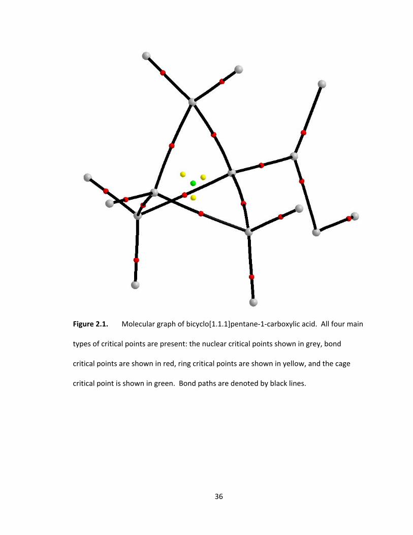
36
Figure 2.1. Molecular graph of bicyclo[1.1.1]pentane‐1‐carboxylic acid. All four main
types of critical points are present: the nuclear critical points shown in grey, bond
critical points are shown in red, ring critical points are shown in yellow, and the cage
critical point is shown in green. Bond paths are denoted by black lines.
37
where n is the number of the specific CP. x is equal to one for isolated molecules and
zero for infinite crystals.54
2.4.2 Atomic Partitioning and Atomic Properties
Another consequence of using the gradient of the electron density is the ability
to define gradient paths and thereby the gradient vector field.53 A gradient path,
defined as a curve to which a gradient vector is tangential at each point, is orthogonal to
the original surface and do not cross one another except when 0. The collection
of all gradient paths makes up the gradient vector field, which partitions a molecule into
its constituent atoms. The boundary between atoms, or the interatomic surface (IAS), is
made of gradient paths which begin at infinity and terminate at the CP between two
nuclei. The IAS is a zero‐flux surface because 0 for every point, which means that
no gradient vectors cross the surface. A large amount of an atom may be open to
infinity (not bound by an IAS on some side). In order to define an atom’s volume within
a molecule (the atomic basin), the atom is generally capped by a 0.001au envelope of
electron density (chosen to represent the van der Waals surface).53
The atomic basin, denoted by Ω, can be used to define properties by integrating
over the volume. The average of a property over the basin, A(Ω), can be determined
using the one‐ electron operator, or sum of operators, which corresponds to the
property according to:54
Ω 2 Ψ Ψ Ψ ΨΩ
(2.44)
38
In this way, the total electron population can be defined by setting 1:53,54
ΩΩ
(2.45)
The population integral extends past the 0.001 au electron density envelope to provide
an accurate representation. In this case, the envelope is extended to a point where
ρ=10‐6 au.53 The atomic charge [q(Ω)] is calculated by subtracting the electron
population from the nuclear charge (ZΩ):54
Ω Ω Ω Ω
Ω
(2.46)
The electronic energy of an atom in a molecule, Ee(Ω), is defined by:51
Ω Ω Ω (2.47)
where T(Ω) is the kinetic energy and V(Ω) is the total virial for the atom. As the atom is
bound by a zero‐flux surface, the atomic virial theorem is satisfied and Ee(Ω) can be
rewritten as:51
Ω Ω12 Ω (2.48)
In reality, the atomic virial theorem may not be exactly satisfied due to the
approximations used in the calculations, but corrections for this deviation from
exactness can be incorporated, as done in several software programs. As an example,
the integration software PROAIM56,57 multiplies each atomic kinetic energy by [1‐(‐V/T)]
instead of simply (‐1).54
39
A crucial consequence of the IAS is the concept of atomic additivity. As the
atoms do not overlap, and no volume is lost between them, the atomic properties can
be summed to give the molecular property (such as electron population, charge or
energy):51,53
ΩΩ
(2.49)
where A is any given property. This also allows for the definition of a functional group
within a molecule.53
2.4.3 Bond Paths and Molecular Graphs
The point at which the electron density reaches a maximum on the IAS is the BCP.
It is also the termination point of a number of gradient paths which originate at infinity
and thus is a maximum in that coordinate. However, in comparison to the nuclei (here
called A and B for clarity), the BCP is a minimum in electron density. There are two
gradient paths which begin at the BCP; one path terminates at nucleus A and one at B,
and together these form the atomic interaction line (AIL). An AIL becomes a bond path
when one more criterion is satisfied: the forces on the nuclei vanish. In other words, a
bond path occurs where there is an attractive stability between nuclei and due to this
condition the system must be at its equilibrium geometry. The full set of bond paths
gives the molecular graph, the QTAIM expression of which nuclei are bonded.53 Figure
2.1 shows the molecular graph for bicyclo[1.1.1]pentane‐1‐carboxylic acid, where the
bond paths are shown in black.
40
Just as it is possible to use the electron density to determine atomic properties,
it is possible to determine properties related to the bonds. The electron density at the
BCP has often been related to the bond order or strength of a bond according to:53,54
(2.50)
where and are constants which depend on the identity of the atoms. In general,
covalent bonds occur when is greater that 0.20 au, and closed‐shell interactions
(such as ionic, van der Waals and hydrogen bonds) occur for less than 0.10 au.54
Perhaps a more direct measure of the bond order is to use the average number of
electron pairs shared between two atoms, referred to as the delocalization index (DI;
equation 2.51) in QTAIM.
, 2| , | 2 , (2.51)
The Fσ (σ=α, β) functions, or Fermi correlations (equation 2.52) are related to the sum of
the overlap integrals (Sij) for atoms A and B.
,
(2.52)
As the electron density within the bonds and bond order are related, it has been
suggested that the DI be used to replace bond order in equation 2.50 to form a fully
QTAIM based description.
The bond ellipticity ( ), which measures how symmetrically the density is
distributed about a bond, can be determined using a ratio the curvatures perpendicular
to the bond path:54
41
1 (2.53)
A large ellipticity value (5 or greater) indicates that the bond is structurally unstable.53
42
Chapter 3: The Inductive Effect – A Quantum Theory of Atoms in Molecules
Perspective
Bicyclo[1.1.1]pentane‐1‐carboxylic Acid Derivatives
43
3.1 Introduction
Although substituent effects are used to explain many phenomena in chemistry,
only the inductive effect is omnipresent. IUPAC defines the inductive effect as the effect
of “the transmission of charge through a chain of atoms via electrostatic induction.”16 It
is said to decay with distance and is intimately related to the electronegativity of the
substituent.17 Deceptively simple, the inductive effect is always complicated by a
competing mechanism: the field effect, which is defined as the transmission of charge
through‐space rather than through bonds.16 As both effects follow the same decay with
distance, and generally exert their influence in the same direction, they are said to be
inseparable. This has led to the use of the phrase “so‐called” inductive effect to
encompass both mechanisms (used interchangeably with the inductive effect).16
The most common method to study the inductive effect is still the Hammett
formulation.10‐12 Originally used to describe the acid dissociation constants of
substituted benzoic acids, the Hammett formulation has since been extended to a wide
variety of organic reations.20 Central to this approach is the use of a substituent and a
reaction constant, σI and ρI, respectively. Recently it was suggested that the addition of
an electronegativity term and corresponding proportionality constant (χ and ζ,
respectively), in the manner of equation 3.1, was needed to accurately describe the
inductive effect.36
∆ ∆ ∆ (3.1)
This relationship was developed using an isodesmic reaction approach, an important
tool for the theoretical estimation of substituent effects. An isodesmic reaction, such as
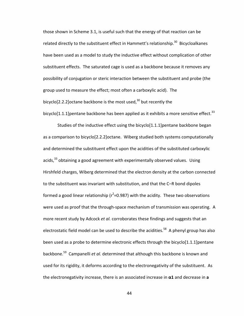
44
those shown in Scheme 3.1, is useful such that the energy of that reaction can be
related directly to the substituent effect in Hammett’s relationship.30 Bicycloalkanes
have been used as a model to study the inductive effect without complication of other
substituent effects. The saturated cage is used as a backbone because it removes any
possibility of conjugation or steric interaction between the substituent and probe (the
group used to measure the effect; most often a carboxylic acid). The
bicyclo[2.2.2]octane backbone is the most used,30 but recently the
bicyclo[1.1.1]pentane backbone has been applied as it exhibits a more sensitive effect.33
Studies of the inductive effect using the bicyclo[1.1.1]pentane backbone began
as a comparison to bicyclo[2.2.2]octane. Wiberg studied both systems computationally
and determined the substituent effect upon the acidities of the substituted carboxylic
acids,33 obtaining a good agreement with experimentally observed values. Using
Hirshfeld charges, Wiberg determined that the electron density at the carbon connected
to the substituent was invariant with substitution, and that the C–R bond dipoles
formed a good linear relationship (r2=0.987) with the acidity. These two observations
were used as proof that the through‐space mechanism of transmission was operating. A
more recent study by Adcock et al. corroborates these findings and suggests that an
electrostatic field model can be used to describe the acidities.58 A phenyl group has also
been used as a probe to determine electronic effects through the bicyclo[1.1.1]pentane
backbone.59 Campanelli et al. determined that although this backbone is known and
used for its rigidity, it deforms according to the electronegativity of the substituent. As
the electronegativity increase, there is an associated increase in α1 and decrease in a
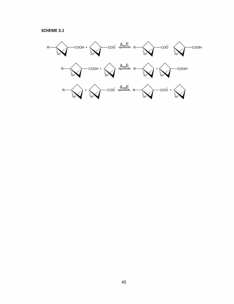
45
SCHEME 3.1
46
with corresponding changes in the other internal coordinates (labels changed to
conform to our study, see Scheme 3.2).
Fourré et al. investigate the electron density distribution in substituted
bicyclo[1.1.1]pentanes using both the Quantum Theory of Atoms in Molecules (QTAIM)
and the Electron Localization Function (ELF).60 They focused primarily on the atomic
charges and atomic basin populations to study the transmission of electron density.
Their analysis supported the through‐space mechanism, but their study was very limited
as they only used two extreme substituents: fluorine and lithium, with comparison to
the unsubstituted species. Fourré observed little perturbation of the electron density
past the valence shell of Ca (see Scheme 3.2), just as Wiberg noted. Although this
represents the first attempt to use QTAIM to describe the inductive effect in the
bicyclo[1.1.1]pentane systems, a systematic study using the full complement of
properties available from a topological analysis of the electron density has not been
completed.
QTAIM51,52 is a perfect tool for the study of the inductive effect and specifically
the transmission of charge though a molecule because it focuses on the electron density
(ρ(r)).15 In QTAIM, a molecule is partitioned into a series of atomic basins using the
zero‐flux surface created by the gradient of the electron density ( ρ(r)). Integration of
ρ(r) over the basin can yield atomic properties such as energy and charge. As each
adjacent atom shares an infinitely thin surface, the interatomic surface (IAS), and no
volume is lost, the sum of a property over all atoms yields the corresponding molecular
property. Critical points in ρ(r) can be used to identify structural features, such as the
47
bond critical point (BCP), which is the identifying characteristic of a bonding interaction
between two atoms. The BCP lies on the IAS and corresponds to the point along the
bond path where ρ(r) is equal to zero.
In this paper we present a systematic study of the substituent effects in the
bicyclo[1.1.1]pentane‐1‐carboxylic acid system shown in Scheme 3.1, using the
isodesmic reaction energy (ΔisoE) as a measure of the substituent effect. The
substituents employed in this discussion were chosen to cover a wide range of possible
electronegativities. Although small data sets may lead to limitations within the scope of
a regression based analysis, a smaller set was used due to the extent of computational
calculations and analysis involved. We examine the electron density with QTAIM and
relate it to the structural features, frontier molecular orbitals, and nuclear magnetic
resonance shielding parameters within the system. Studying the electron density itself
helps resolve which properties are related to the inductive effect and give insight into
the mechanism of transmission.
3.2 Methods
All calculations were performed using the Gaussian suite of programs.61,62 The
composite method CBS‐QB347,48 was used to determine accurate thermochemistries for
the reactions shown in Scheme 3.1 and to confirm the validity of the chosen model
chemistry: the hybrid functional, PBE0, developed by Perdew, Burke and Ernzerhof,63,64
combined with the Pople‐style 6‐31++G(d,p) basis set.45,46 Geometries for all species
were optimized and vibrational frequency analysis was used to confirm minima suitable
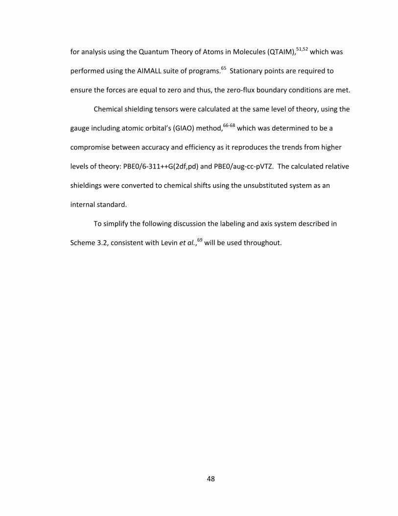
48
for analysis using the Quantum Theory of Atoms in Molecules (QTAIM),51,52 which was
performed using the AIMALL suite of programs.65 Stationary points are required to
ensure the forces are equal to zero and thus, the zero‐flux boundary conditions are met.
Chemical shielding tensors were calculated at the same level of theory, using the
gauge including atomic orbital’s (GIAO) method,66‐68 which was determined to be a
compromise between accuracy and efficiency as it reproduces the trends from higher
levels of theory: PBE0/6‐311++G(2df,pd) and PBE0/aug‐cc‐pVTZ. The calculated relative
shieldings were converted to chemical shifts using the unsubstituted system as an
internal standard.
To simplify the following discussion the labeling and axis system described in
Scheme 3.2, consistent with Levin et al.,69 will be used throughout.
49
SCHEME 3.2
50
3.3 Results
3.3.1 Energies
In order to determine the effect of the substituent, the isodesmic reaction
energy was calculated for all reactions in Scheme 3.1; Table 3.1 shows the values
determined at the CBS‐QB3 and PBE0/6‐31++G(d,p) levels of theory. The order of
substituents, conserved throughout this discussion and between methods, is based on
ΔisoE for the CBS‐QB3 method. The electron donating groups, lithium and methyl, result
in a positive ΔisoE suggesting a stabilization of the substituted acid species; whereas, the
electron withdrawing groups have a negative ΔisoE, which is indicative of a stabilization
of the conjugate base molecules. In addition to providing accurate thermochemistries,
the CBS‐QB3 method was used to validate the use of the chosen model chemistry. The
PBE0 energies recreate the CBS‐QB3 energies almost perfectly (Δiso,CBSE = 1.03 Δiso,PBE0E +
0.46; r2=0.995) with an average deviation of only 0.48kcal/mol, and will be used for the
remainder of this discussion.
One complication associated with using ΔisoE as a measure of substituent effects
is that ΔisoE is actually a measure of two simultaneous effects: the effect of the
substituent on the protonated probe and the effect of the substituent on the
deprotonated probe.30 To separate these effects, we have broken the overall isodesmic
reaction into two constituent reactions to observe the effect on the acid (HA) and on the
conjugate base (CB; Scheme 3.1). The reactions have been formed such that the
energies of the constituent reactions sum to give the overall reaction energy (ΔisoE =
ΔHAE + ΔCBE). Both the effect on the acid and on the conjugate base, also outlined in
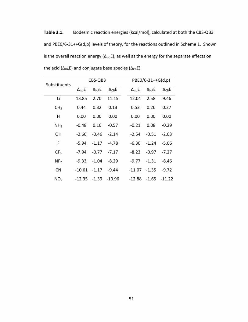
51
Table 3.1. Isodesmic reaction energies (kcal/mol), calculated at both the CBS‐QB3
and PBE0/6‐31++G(d,p) levels of theory, for the reactions outlined in Scheme 1. Shown
is the overall reaction energy (ΔisoE), as well as the energy for the separate effects on
the acid (ΔHAE) and conjugate base species (ΔCBE).
Substituents CBS‐QB3 PBE0/6‐31++G(d,p)
ΔisoE ΔHAE ΔCBE ΔisoE ΔHAE ΔCBE
Li 13.85 2.70 11.15 12.04 2.58 9.46
CH3 0.44 0.32 0.13 0.53 0.26 0.27
H 0.00 0.00 0.00 0.00 0.00 0.00
NH2 ‐0.48 0.10 ‐0.57 ‐0.21 0.08 ‐0.29
OH ‐2.60 ‐0.46 ‐2.14 ‐2.54 ‐0.51 ‐2.03
F ‐5.94 ‐1.17 ‐4.78 ‐6.30 ‐1.24 ‐5.06
CF3 ‐7.94 ‐0.77 ‐7.17 ‐8.23 ‐0.97 ‐7.27
NF2 ‐9.33 ‐1.04 ‐8.29 ‐9.77 ‐1.31 ‐8.46
CN ‐10.61 ‐1.17 ‐9.44 ‐11.07 ‐1.35 ‐9.72
NO2 ‐12.35 ‐1.39 ‐10.96 ‐12.88 ‐1.65 ‐11.22
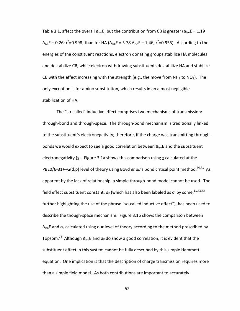
52
Table 3.1, affect the overall ΔisoE, but the contribution from CB is greater (ΔisoE = 1.19
ΔCBE + 0.26; r2=0.998) than for HA (ΔisoE = 5.78 ΔHAE – 1.46; r
2=0.955). According to the
energies of the constituent reactions, electron donating groups stabilize HA molecules
and destabilize CB, while electron withdrawing substituents destabilize HA and stabilize
CB with the effect increasing with the strength (e.g., the move from NH2 to NO2). The
only exception is for amino substitution, which results in an almost negligible
stabilization of HA.
The “so‐called” inductive effect comprises two mechanisms of transmission:
through‐bond and through‐space. The through‐bond mechanism is traditionally linked
to the substituent’s electronegativity; therefore, if the charge was transmitting through‐
bonds we would expect to see a good correlation between ΔisoE and the substituent
electronegativity (χ). Figure 3.1a shows this comparison using χ calculated at the
PBE0/6‐31++G(d,p) level of theory using Boyd et al.’s bond critical point method.70,71 As
apparent by the lack of relationship, a simple through‐bond model cannot be used. The
field effect substituent constant, σF (which has also been labeled as σI by some,31,72,73
further highlighting the use of the phrase “so‐called inductive effect”), has been used to
describe the though‐space mechanism. Figure 3.1b shows the comparison between
ΔisoE and σF calculated using our level of theory according to the method prescribed by
Topsom.74 Although ΔisoE and σF do show a good correlation, it is evident that the
substituent effect in this system cannot be fully described by this simple Hammett
equation. One implication is that the description of charge transmission requires more
than a simple field model. As both contributions are important to accurately
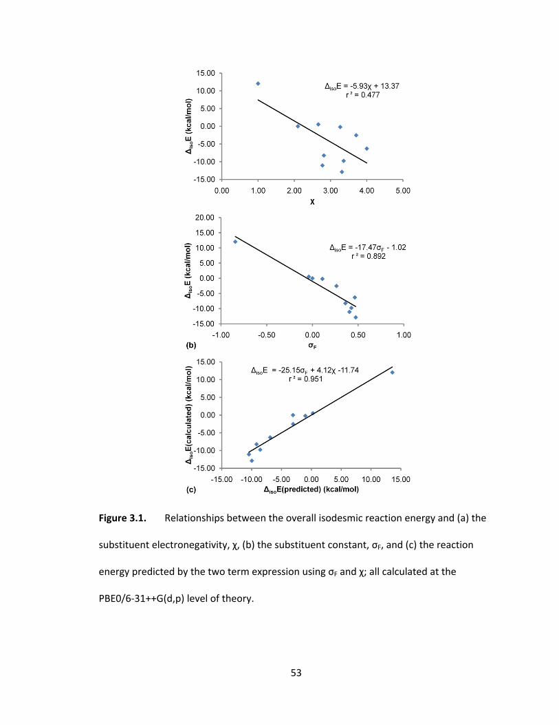
53
Figure 3.1. Relationships between the overall isodesmic reaction energy and (a) the
substituent electronegativity, χ, (b) the substituent constant, σF, and (c) the reaction
energy predicted by the two term expression using σF and χ; all calculated at the
PBE0/6‐31++G(d,p) level of theory.
54
describe the “so‐called” inductive effect, it is not surprising that a two‐term expression,
using both a substituent constant and an electronegativity term has been suggested.36
As shown in Figure 3.1c, this expression represents an improvement over the
correlations with σF and χ individually, but it still does not fully recreate the overall
effect. Furthermore, there appears to be some linear dependence between σF and χ (σF
= 0.40χ – 1.00; r2=0.743), suggesting that σF already incorporates some aspects of the
inductive effect, consistent with its formulation (see Supplemental Information), and
thus the dual parameter expression should not be used.
Through the application of QTAIM the overall stabilization by a substituent can
be examined at the individual atom or group levels. The kinetic energy, given in
equation 3.2 as it depends on the electron density, can be defined for an atom if the
zero‐flux boundary conditions are met (the integral of the Laplacian term, 2(ρ(r)), over
the atomic basin is equal to zero).54
ℏ4
(3.2)
How close the integral is to zero is often used as a measure of accuracy of the
integration. In equation 3.2, K(r) is the Schrödinger kinetic energy and G(r) is the kinetic
energy density. Using the atomic virial theorem, the energy of an atom can be related
to its atomic energy at equilibrium as described in equation 3.3.54
Ω Ω12 Ω (3.3)
Figure 3.2a shows the relationship between ΔisoE and the total energy of the
probe. As expected, ΔisoE is related completely to the energy of the probe, ΔProbeE
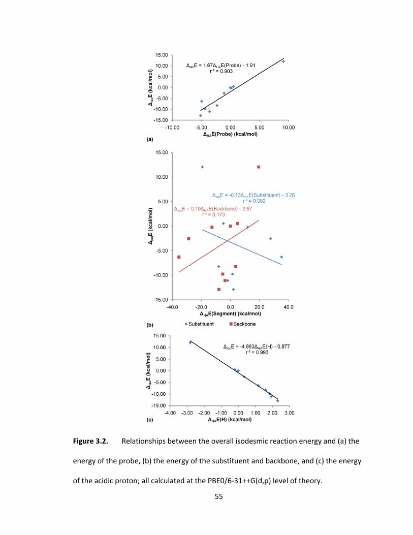
55
Figure 3.2. Relationships between the overall isodesmic reaction energy and (a) the
energy of the probe, (b) the energy of the substituent and backbone, and (c) the energy
of the acidic proton; all calculated at the PBE0/6‐31++G(d,p) level of theory.

56
(calculated in the same manner as ΔisoE, but using the sum of the energies for all atoms
in the probe instead of the molecular energy), which becomes more stabilized as
electron‐withdrawing strength increases. The order of substituents, however, is not
conserved between probe systems. NH2 substitution now results in a positive ΔProbeE,
CN and NF2 exchange places and F has the second most negative value. The total
energies of both the substituent and backbone, ΔSubstituentE and ΔBackboneE, show no
relationship with ΔisoE, as displayed in Figure 3.2b. However, they appear to be
reflections of one another in accordance with the atomic transferability present in
QTAIM.75 This reflection implies that an energy transfer occurs between the substituent
and backbone.
Within the probe itself, the effect is primarily centered on the acidic proton (see
Figure 3.2c). The negative slope indicates that H is destabilized with an increase in
electron withdrawing ability. The carboxyl carbon, CO, in HA also shows a fair
correlation to ΔisoE (r2=0.746), with the same general trend. Due to this observation we
have limited our discussion mainly to the effect on HA and its properties.
3.3.2 Nuclear Magnetic Resonance Chemical Shifts
The NMR chemical shift of a probe group (most commonly fluorine) has been
used in the past to determine the substituent effect76 and it was suggested that this
method is more sensitive than using proton‐transfer equilibria.20 We have calculated
the absolute chemical shielding for each nucleus and converted them to relative NMR
chemical shifts using the internal unsubstituted species as a standard to determine the

57
relationship with the substituent effect. We find that only the NMR chemical shift
changes in the acid species, and in particular the probe group itself, correlate with ΔisoE.
The relationship between the NMR chemical shift of the acidic proton and ΔisoE is shown
in Figure 3.3a. As expected, Δδ1H shows a downfield shift with increasing strength of
electron‐withdrawing substituents and thus increasing acidity. By convention, this is
commonly explained as the substituents withdraw the electron density surrounding the
proton, which results in a greater level of deshielding. Our findings support this
description (see later for a discussion of electron density). Δδ1H also shows a very good
relationship with the atomic energy of that atom (which also depends on the electron
density assigned to the atom, see equation 3.2). As apparent in Figure 3.3b, the proton
is destabilized as the nucleus becomes more deshielded. This suggests that the
increased acidity present in the substitution by electron withdrawing groups can be
linked to perturbations in the electron density in the probe.
Unexpectedly, with the exception of the carbonyl oxygen which exhibits the
same general trend as for H (see Figure 3.3c), no other atom’s NMR chemical shift
correlates with ΔisoE. This seems very peculiar as the transmission of charge, regardless
of mechanism, should have an effect on the environment surrounding each nucleus in
the molecule. Since the NMR chemical shift (shielding) is actually a tensor, we also
examined the three diagonalized principal components as well as the nine tensor
components. Certain components for both H and O (Scheme 3.2) exhibit good
relationships with ΔisoE, but there are still no common relationships for any of the other
nuclei in the molecule.
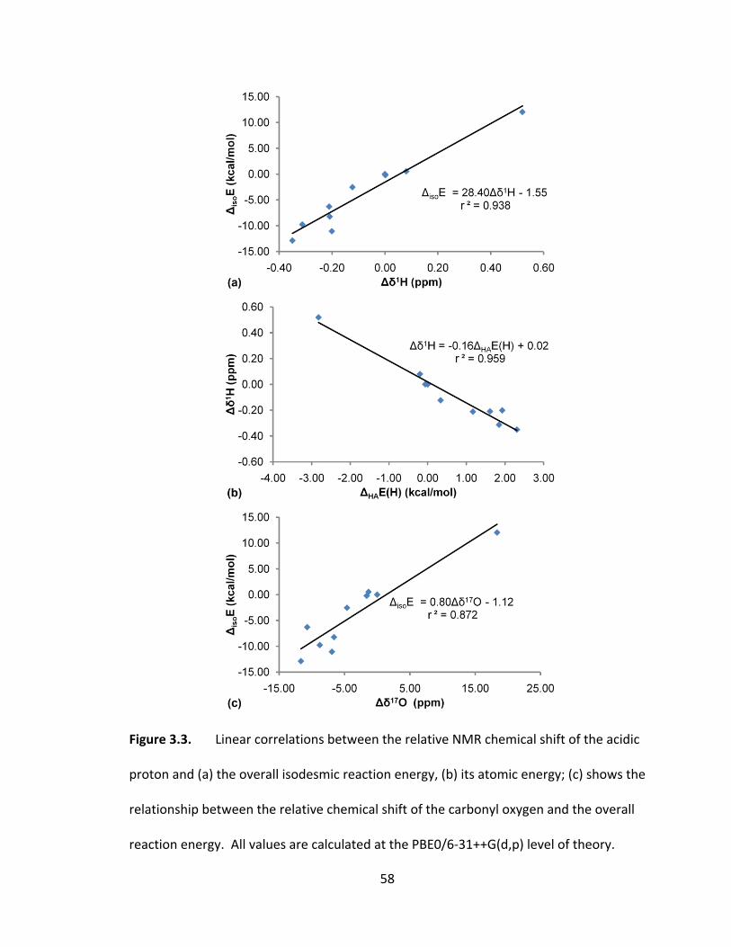
58
Figure 3.3. Linear correlations between the relative NMR chemical shift of the acidic
proton and (a) the overall isodesmic reaction energy, (b) its atomic energy; (c) shows the
relationship between the relative chemical shift of the carbonyl oxygen and the overall
reaction energy. All values are calculated at the PBE0/6‐31++G(d,p) level of theory.
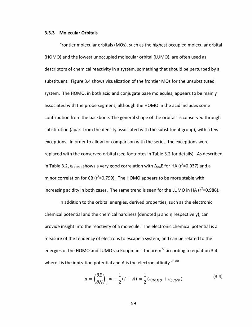
59
3.3.3 Molecular Orbitals
Frontier molecular orbitals (MOs), such as the highest occupied molecular orbital
(HOMO) and the lowest unoccupied molecular orbital (LUMO), are often used as
descriptors of chemical reactivity in a system, something that should be perturbed by a
substituent. Figure 3.4 shows visualization of the frontier MOs for the unsubstituted
system. The HOMO, in both acid and conjugate base molecules, appears to be mainly
associated with the probe segment; although the HOMO in the acid includes some
contribution from the backbone. The general shape of the orbitals is conserved through
substitution (apart from the density associated with the substituent group), with a few
exceptions. In order to allow for comparison with the series, the exceptions were
replaced with the conserved orbital (see footnotes in Table 3.2 for details). As described
in Table 3.2, εHOMO shows a very good correlation with ΔisoE for HA (r2=0.937) and a
minor correlation for CB (r2=0.799). The HOMO appears to be more stable with
increasing acidity in both cases. The same trend is seen for the LUMO in HA (r2=0.986).
In addition to the orbital energies, derived properties, such as the electronic
chemical potential and the chemical hardness (denoted μ and η respectively), can
provide insight into the reactivity of a molecule. The electronic chemical potential is a
measure of the tendency of electrons to escape a system, and can be related to the
energies of the HOMO and LUMO via Koopmans’ theorem77 according to equation 3.4
where I is the ionization potential and A is the electron affinity.78‐80
12
12 (3.4)
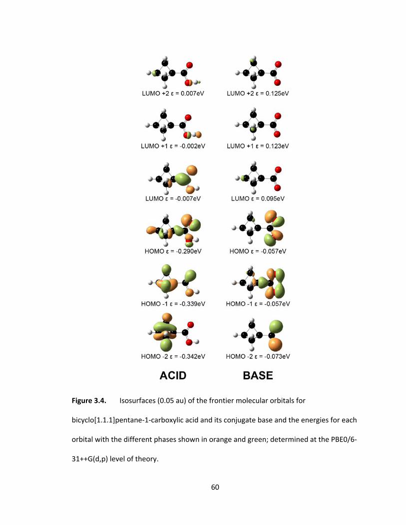
60
Figure 3.4. Isosurfaces (0.05 au) of the frontier molecular orbitals for
bicyclo[1.1.1]pentane‐1‐carboxylic acid and its conjugate base and the energies for each
orbital with the different phases shown in orange and green; determined at the PBE0/6‐
31++G(d,p) level of theory.
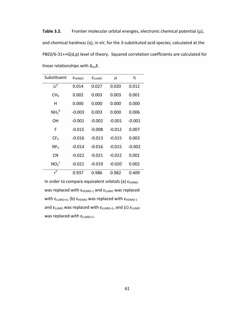
61
Table 3.2. Frontier molecular orbital energies, electronic chemical potential (μ),
and chemical hardness (η), in eV, for the 3‐substituted acid species; calculated at the
PBE0/6‐31++G(d,p) level of theory. Squared correlation coefficients are calculated for
linear relationships with ΔisoE.
Substituent εHOMO εLUMO μ η
Lia 0.014 0.027 0.020 0.012
CH3 0.002 0.003 0.003 0.001
H 0.000 0.000 0.000 0.000
NH2b ‐0.003 0.003 0.000 0.006
OH ‐0.001 ‐0.002 ‐0.001 ‐0.001
F ‐0.015 ‐0.008 ‐0.012 0.007
CF3 ‐0.016 ‐0.013 ‐0.015 0.003
NF2 ‐0.014 ‐0.016 ‐0.015 ‐0.002
CN ‐0.022 ‐0.021 ‐0.022 0.001
NO2c ‐0.021 ‐0.019 ‐0.020 0.002
r2 0.937 0.986 0.982 0.409
In order to compare equivalent orbitals (a) εHOMO
was replaced with εHOMO‐1 and εLUMO was replaced
with εLUMO+5, (b) εHOMO was replaced with εHOMO‐1
and εLUMO was replaced with εLUMO+1, and (c) εLUMO
was replaced with εLUMO+1.
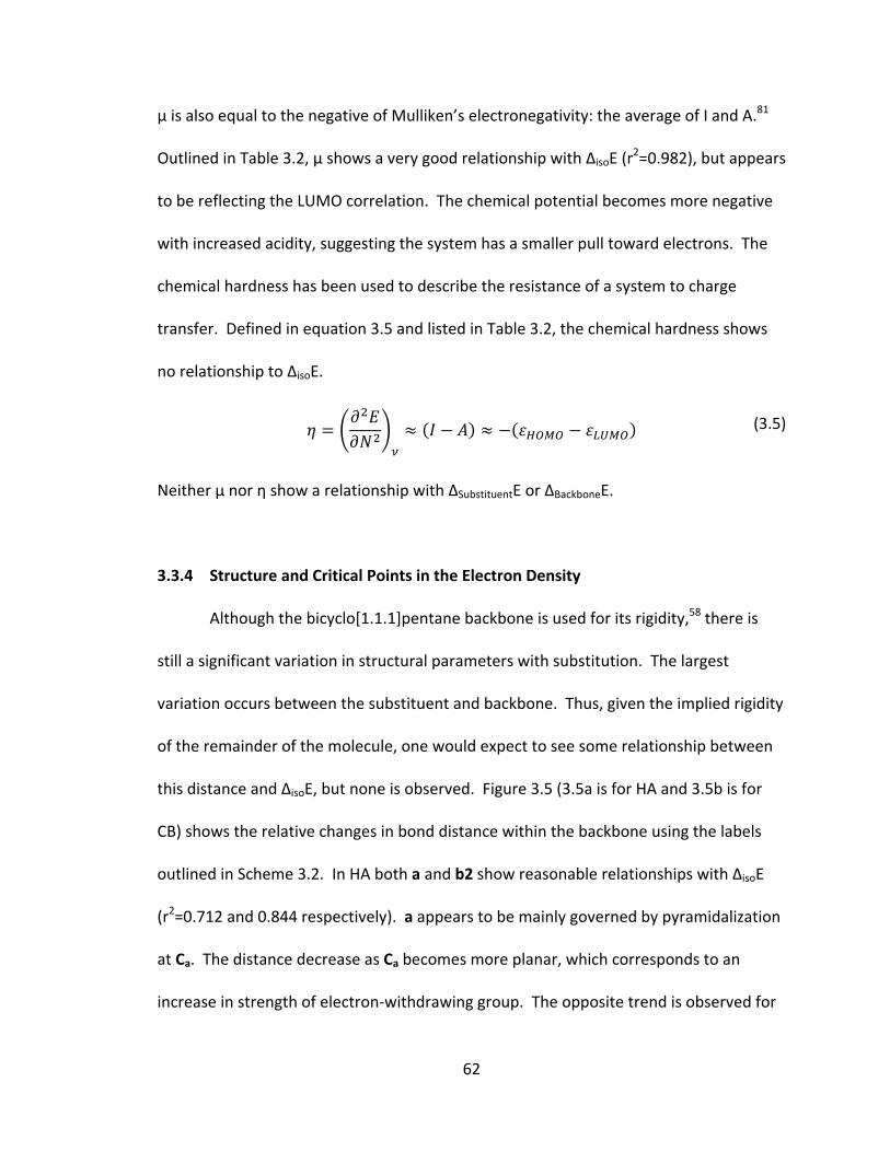
62
μ is also equal to the negative of Mulliken’s electronegativity: the average of I and A.81
Outlined in Table 3.2, μ shows a very good relationship with ΔisoE (r2=0.982), but appears
to be reflecting the LUMO correlation. The chemical potential becomes more negative
with increased acidity, suggesting the system has a smaller pull toward electrons. The
chemical hardness has been used to describe the resistance of a system to charge
transfer. Defined in equation 3.5 and listed in Table 3.2, the chemical hardness shows
no relationship to ΔisoE.
(3.5)
Neither μ nor η show a relationship with ΔSubstituentE or ΔBackboneE.
3.3.4 Structure and Critical Points in the Electron Density
Although the bicyclo[1.1.1]pentane backbone is used for its rigidity,58 there is
still a significant variation in structural parameters with substitution. The largest
variation occurs between the substituent and backbone. Thus, given the implied rigidity
of the remainder of the molecule, one would expect to see some relationship between
this distance and ΔisoE, but none is observed. Figure 3.5 (3.5a is for HA and 3.5b is for
CB) shows the relative changes in bond distance within the backbone using the labels
outlined in Scheme 3.2. In HA both a and b2 show reasonable relationships with ΔisoE
(r2=0.712 and 0.844 respectively). a appears to be mainly governed by pyramidalization
at Ca. The distance decrease as Ca becomes more planar, which corresponds to an
increase in strength of electron‐withdrawing group. The opposite trend is observed for
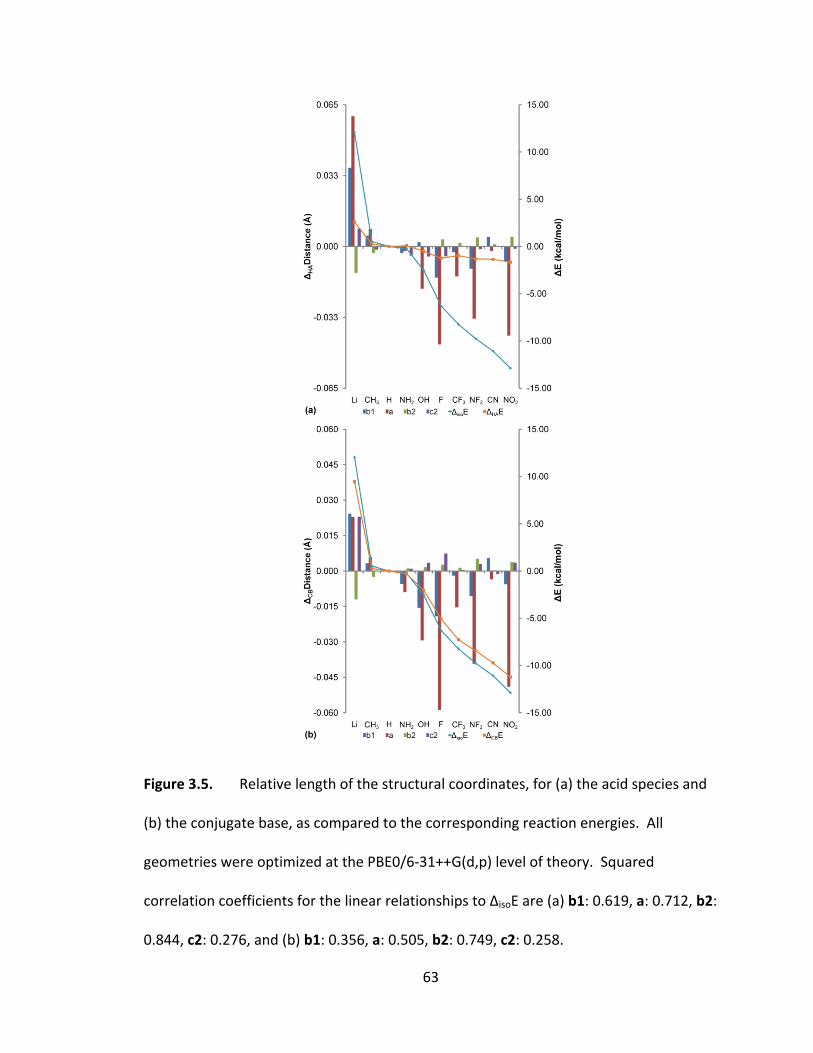
63
Figure 3.5. Relative length of the structural coordinates, for (a) the acid species and
(b) the conjugate base, as compared to the corresponding reaction energies. All
geometries were optimized at the PBE0/6‐31++G(d,p) level of theory. Squared
correlation coefficients for the linear relationships to ΔisoE are (a) b1: 0.619, a: 0.712, b2:
0.844, c2: 0.276, and (b) b1: 0.356, a: 0.505, b2: 0.749, c2: 0.258.
64
b2: an increase in distance with increasing acidity. Distance b2 also shows a fair
relationship in CB (r2=0.749).
As suggested by Campanelli et al.,59 the cage in bicyclo[1.1.1]pentane deforms
with the electronegativity of the substituent. In both HA and CB the internal
coordinates (b1, a, and b2) show good correlation to the substituent electronegativity.
Interestingly, in HA the link between the backbone and probe (c2) also shows a good
relationship with χ (r2=0.843).
The structural parameters within the probe group alone show good relationships
with ΔisoE. Figure 3.6 shows these relationships. As expected from the acid‐base nature
of the reaction, the OH–H distance shows a good correlation with ΔisoE (the distance
increases with the strength of the electron‐withdrawing group); however, it does not
exhibit the best relationship (Figure 3.6b). Both CO–O and CO–OH decrease in length
with increase in acidity. The re‐distribution of charge accompanying deprotonation
appears to cause this shortening. It also induces a widening in θ(O–CO–OH) (Figure 3.6c).
In reality, all angles about the CO atom are affected, but they are all linearly dependent
as there is essentially no deviation from planarity. Thus, just like in the atomic energies,
the substituent effect (with respect to ΔisoE) on the structural features is localized on the
probe.
As the electron density is a topological function it has critical points (CPs) where
the first derivative ( ) goes to zero. CPs in a molecular system correspond to structural
features and can be used to discern properties of the molecule. The maximum in
density at the nuclei actually corresponds to a nuclear critical point (although it actually
65
Figure 3.6. Relationships between the overall isodesmic reaction energy and (a) the
OH–H bond length, (b) the bond lengths between the carbonyl carbon and both oxygen
atoms, and (c) the O–CO–OH angle; all calculated at the PBE0/6‐31++G(d,p) level of
theory.
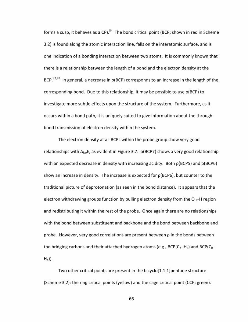
66
forms a cusp, it behaves as a CP).54 The bond critical point (BCP; shown in red in Scheme
3.2) is found along the atomic interaction line, falls on the interatomic surface, and is
one indication of a bonding interaction between two atoms. It is commonly known that
there is a relationship between the length of a bond and the electron density at the
BCP.82,83 In general, a decrease in ρ(BCP) corresponds to an increase in the length of the
corresponding bond. Due to this relationship, it may be possible to use ρ(BCP) to
investigate more subtle effects upon the structure of the system. Furthermore, as it
occurs within a bond path, it is uniquely suited to give information about the through‐
bond transmission of electron density within the system.
The electron density at all BCPs within the probe group show very good
relationships with ΔisoE, as evident in Figure 3.7. ρ(BCP7) shows a very good relationship
with an expected decrease in density with increasing acidity. Both ρ(BCP5) and ρ(BCP6)
show an increase in density. The increase is expected for ρ(BCP6), but counter to the
traditional picture of deprotonation (as seen in the bond distance). It appears that the
electron withdrawing groups function by pulling electron density from the OH–H region
and redistributing it within the rest of the probe. Once again there are no relationships
with the bond between substituent and backbone and the bond between backbone and
probe. However, very good correlations are present between ρ in the bonds between
the bridging carbons and their attached hydrogen atoms (e.g., BCP(Cb–H3) and BCP(Cb–
H4)).
Two other critical points are present in the bicyclo[1.1.1]pentane structure
(Scheme 3.2): the ring critical points (yellow) and the cage critical point (CCP; green).
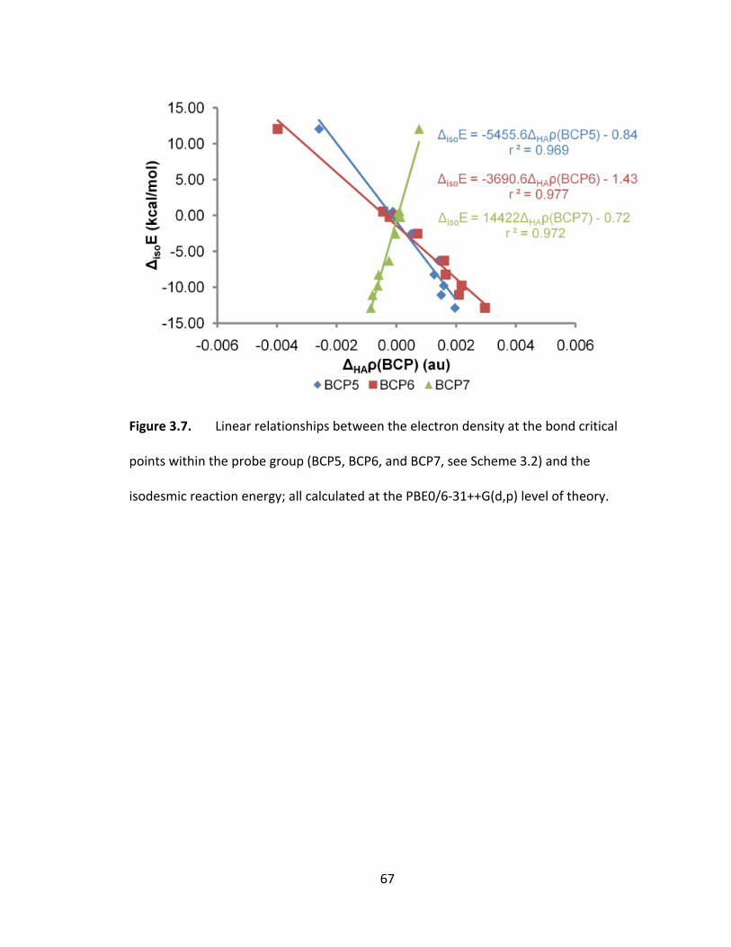
67
Figure 3.7. Linear relationships between the electron density at the bond critical
points within the probe group (BCP5, BCP6, and BCP7, see Scheme 3.2) and the
isodesmic reaction energy; all calculated at the PBE0/6‐31++G(d,p) level of theory.
68
The CCP is analogous to a BCP between Ca and Cc (length a) and one would expect it to
give information about transmission of charge, or electron density, through‐space, but
no apparent relationship between ΔisoE and the electron density at the CCP exists. Thus,
there appears to be no evidence of transmission through‐bonds (e.g., no relationships
between ΔisoE and the electron density along the bond path), and evidence of through‐
space transmission is also missing, as if there is no transmission whatsoever.
3.3.5 Atomic Charges and Delocalization Index
Both mechanisms in the “so‐called” inductive effect are defined by the
transmission of electron density. Although each may perturb different atoms, there
should be an effect of the substituent on the atomic charges. In QTAIM, the atomic
charge is defined as the difference between the nuclear charge, ZΩ, and the total
number of electrons within the basin according to equation 3.6.51,52
Ω Ω ΩΩ
(3.6)
Just as in the atomic energies, the total charge on the probe shows a good relationship
to ΔisoE (Figure 3.8a). Other than for OH, which is essentially invariant with substitution,
the charges on the individual atoms in the probe also show very good correlations as
apparent in Figure 3.8b. In all cases the atoms are becoming more positive, or less
negative, as the electron withdrawing strength of the substituent increases.
Unexpectedly, the overall charge, or the change in charge, on the substituent
shows no relationship to ΔisoE, nor does the charge on the adjacent bridgehead carbon.
69
Figure 3.8. Linear correlations between the overall isodesmic reaction energy and (a)
the relative charge on the probe segment, (b) the relative charge on the carbonyl
carbon, the carbonyl oxygen, and the acidic hydrogen within the probe, and (b) the
relative charge on a representative sample of the atoms within the backbone: Cb and H3;
all calculated at the PBE0/6‐31++G(d,p) level of theory.
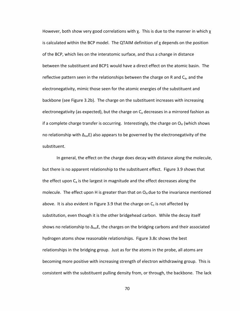
70
However, both show very good correlations with χ. This is due to the manner in which χ
is calculated within the BCP model. The QTAIM definition of χ depends on the position
of the BCP, which lies on the interatomic surface, and thus a change in distance
between the substituent and BCP1 would have a direct effect on the atomic basin. The
reflective pattern seen in the relationships between the charge on R and Ca, and the
electronegativity, mimic those seen for the atomic energies of the substituent and
backbone (see Figure 3.2b). The charge on the substituent increases with increasing
electronegativity (as expected), but the charge on Ca decreases in a mirrored fashion as
if a complete charge transfer is occurring. Interestingly, the charge on OH (which shows
no relationship with ΔisoE) also appears to be governed by the electronegativity of the
substituent.
In general, the effect on the charge does decay with distance along the molecule,
but there is no apparent relationship to the substituent effect. Figure 3.9 shows that
the effect upon Ca is the largest in magnitude and the effect decreases along the
molecule. The effect upon H is greater than that on OH due to the invariance mentioned
above. It is also evident in Figure 3.9 that the charge on Cc is not affected by
substitution, even though it is the other bridgehead carbon. While the decay itself
shows no relationship to ΔisoE, the charges on the bridging carbons and their associated
hydrogen atoms show reasonable relationships. Figure 3.8c shows the best
relationships in the bridging group. Just as for the atoms in the probe, all atoms are
becoming more positive with increasing strength of electron withdrawing group. This is
consistent with the substituent pulling density from, or through, the backbone. The lack
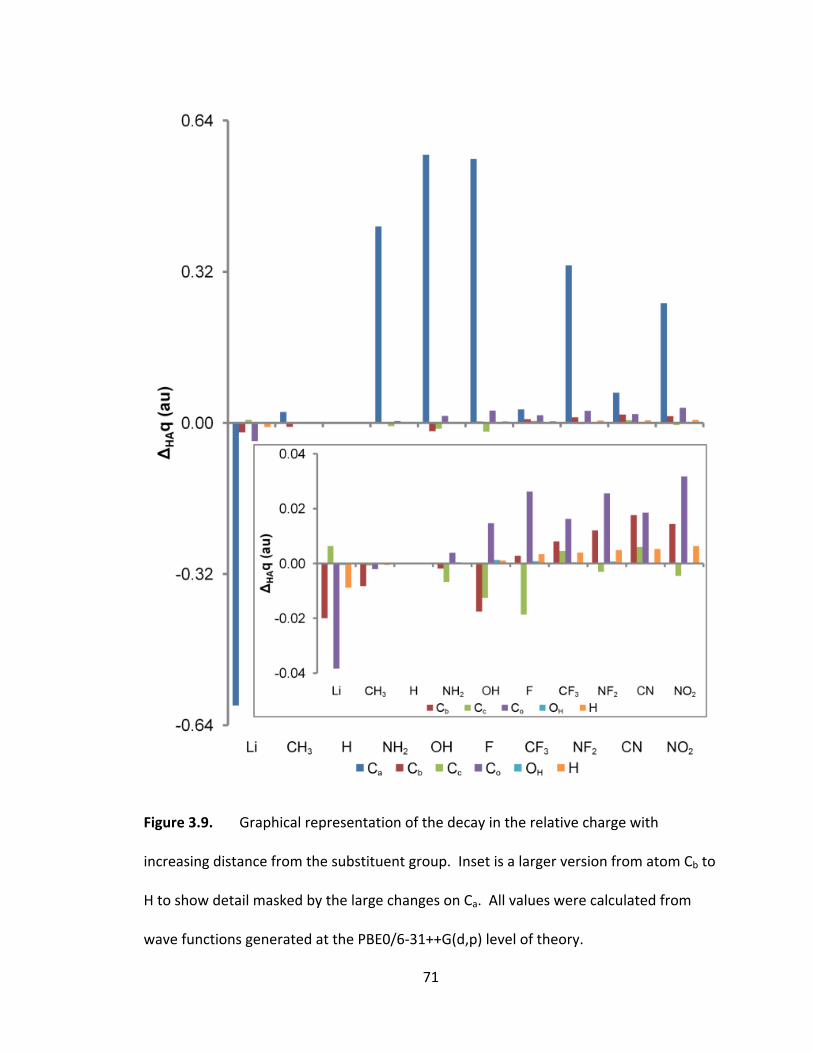
71
Figure 3.9. Graphical representation of the decay in the relative charge with
increasing distance from the substituent group. Inset is a larger version from atom Cb to
H to show detail masked by the large changes on Ca. All values were calculated from
wave functions generated at the PBE0/6‐31++G(d,p) level of theory.
72
of relationship between the substituent effect and the charge on Cc, and the presence of
good correlations in the off‐axis hydrogen atoms, however, would suggest a through‐
space mechanism.
The atomic charges explain some of the effects observed in the other properties.
The charge on CO appears to be controlling the O–CO–OH angle, and consequently the
OH–H bond length. As the carbonyl carbon becomes more positive, the angle opens to
mimic the deprotonated state, which in turn results in the lengthening of the OH–H
bond. Expectedly, the atomic charge also clarifies the downfield shift of the carboxyl
hydrogen seen in Figure 3.3a and the carbonyl oxygen in Figure 3.3c, as both atoms
become more positive with substitution of an electron withdrawing group. The most
intuitive link is between the atomic energy and charge on the atom. As the QTAIM
energy is based on the electron density, it follows that a good relationship should be
apparent between q and E(Ω). For the carboxyl hydrogen a very good correlation is
evident (r2=0.995), which describes the destabilization of the atom within the molecule
with the increase in positive charge.
The lack of transmission along the bond path, or relationship between ΔisoE and
the charge on the bridgehead atoms (as might be expected for through‐space
transmission) would suggest that the effect is not transmitting at all. The delocalization
index, a property derived from QTAIM, can be used to describe the communication
between atoms, and should give insight into the mechanism of transmission. The
delocalization index (DI) is the average number of electrons shared between two atoms
73
(A and B) and is defined by equation 3.751,52 where the Fσ functions (σ = α or β)
correspond to the sum of the overlap integrals for the atoms involved.
, 2| , | 2 , (3.7)
The DI has also been used as a direct measure of covalent bond order.84‐86 Due to the
atomic additivity inherent in QTAIM, it is possible to determine the DI between a group
and an atom, or even two groups. Unexpectedly, there appears to be no relationship
between ΔisoE and the DI between the substituent and probe group, as if there is no
communication at all. The relationship between ΔisoE and DI(Substituent, H) is also quite
weak with a squared correlation coefficient of only 0.615. Fortunately there exist fair
relationships with the DI between substituent and the bridging carbons (e.g., Cb) and far
bridgehead Cc. The number of electrons shared with these atoms increases with
increasing acidity, as if the increased strength of electron withdrawing group affords
better communication. As the DI(Probe, Cb) also shows a good relationship to ΔisoE, it is
possible that communication is occurring in a stepwise fashion: first the substituent
communicates with a bridging carbon of the backbone, which passes the “information”
on to the probe segment.
3.3.6 Dipole Moment Contributions
Wiberg suggested that a relationship between the substituent effect and the R–
Ca bond dipole (using the labels in Scheme 3.2) in the bicyclo[1.1.1]pentane system is an
indication of through‐space transmission.33 The overall molecular dipole, values given in
Table 3.3, shows no relationship to ΔisoE. However, a weak relationship with the x‐
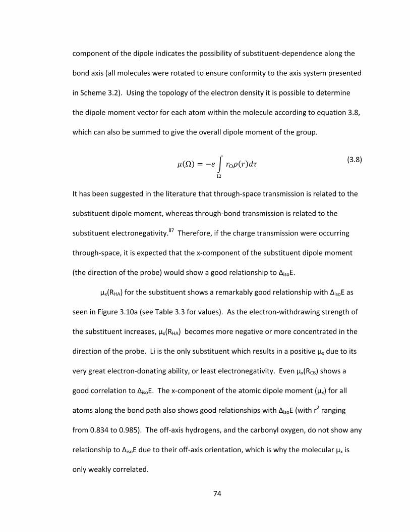
74
component of the dipole indicates the possibility of substituent‐dependence along the
bond axis (all molecules were rotated to ensure conformity to the axis system presented
in Scheme 3.2). Using the topology of the electron density it is possible to determine
the dipole moment vector for each atom within the molecule according to equation 3.8,
which can also be summed to give the overall dipole moment of the group.
Ω Ω
Ω
(3.8)
It has been suggested in the literature that through‐space transmission is related to the
substituent dipole moment, whereas through‐bond transmission is related to the
substituent electronegativity.87 Therefore, if the charge transmission were occurring
through‐space, it is expected that the x‐component of the substituent dipole moment
(the direction of the probe) would show a good relationship to ΔisoE.
μx(RHA) for the substituent shows a remarkably good relationship with ΔisoE as
seen in Figure 3.10a (see Table 3.3 for values). As the electron‐withdrawing strength of
the substituent increases, μx(RHA) becomes more negative or more concentrated in the
direction of the probe. Li is the only substituent which results in a positive μx due to its
very great electron‐donating ability, or least electronegativity. Even μx(RCB) shows a
good correlation to ΔisoE. The x‐component of the atomic dipole moment (μx) for all
atoms along the bond path also shows good relationships with ΔisoE (with r2 ranging
from 0.834 to 0.985). The off‐axis hydrogens, and the carbonyl oxygen, do not show any
relationship to ΔisoE due to their off‐axis orientation, which is why the molecular μx is
only weakly correlated.
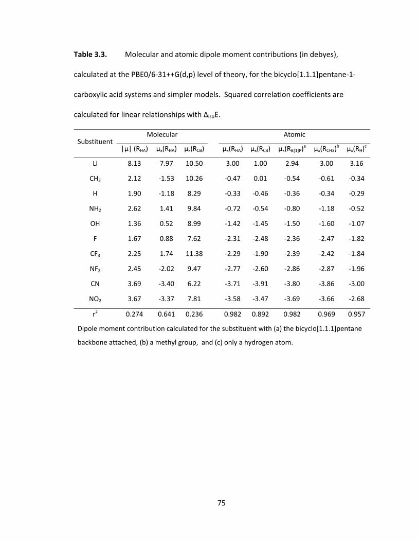
75
Table 3.3. Molecular and atomic dipole moment contributions (in debyes),
calculated at the PBE0/6‐31++G(d,p) level of theory, for the bicyclo[1.1.1]pentane‐1‐
carboxylic acid systems and simpler models. Squared correlation coefficients are
calculated for linear relationships with ΔisoE.
Substituent Molecular Atomic
|μ| (RHA) μx(RHA) μx(RCB) μx(RHA) μx(RCB) μx(RB[1]P)a μx(RCH3)
b μx(RH)c
Li 8.13 7.97 10.50 3.00 1.00 2.94 3.00 3.16
CH3 2.12 ‐1.53 10.26 ‐0.47 0.01 ‐0.54 ‐0.61 ‐0.34
H 1.90 ‐1.18 8.29 ‐0.33 ‐0.46 ‐0.36 ‐0.34 ‐0.29
NH2 2.62 1.41 9.84 ‐0.72 ‐0.54 ‐0.80 ‐1.18 ‐0.52
OH 1.36 0.52 8.99 ‐1.42 ‐1.45 ‐1.50 ‐1.60 ‐1.07
F 1.67 0.88 7.62 ‐2.31 ‐2.48 ‐2.36 ‐2.47 ‐1.82
CF3 2.25 1.74 11.38 ‐2.29 ‐1.90 ‐2.39 ‐2.42 ‐1.84
NF2 2.45 ‐2.02 9.47 ‐2.77 ‐2.60 ‐2.86 ‐2.87 ‐1.96
CN 3.69 ‐3.40 6.22 ‐3.71 ‐3.91 ‐3.80 ‐3.86 ‐3.00
NO2 3.67 ‐3.37 7.81 ‐3.58 ‐3.47 ‐3.69 ‐3.66 ‐2.68
r2 0.274 0.641 0.236 0.982 0.892 0.982 0.969 0.957
Dipole moment contribution calculated for the substituent with (a) the bicyclo[1.1.1]pentane
backbone attached, (b) a methyl group, and (c) only a hydrogen atom.
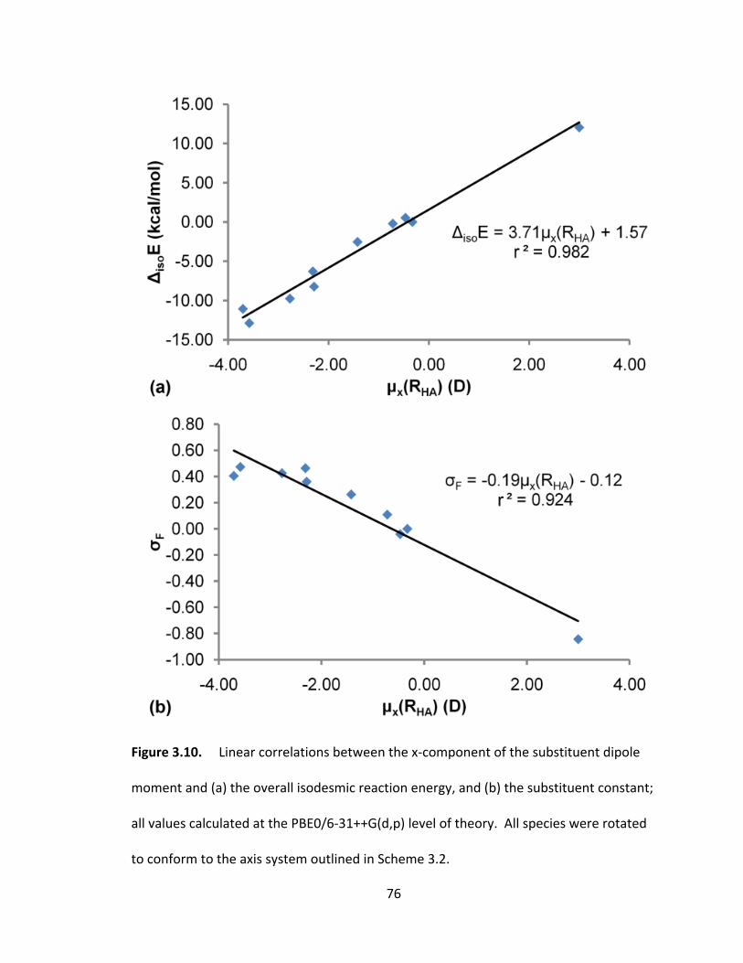
76
Figure 3.10. Linear correlations between the x‐component of the substituent dipole
moment and (a) the overall isodesmic reaction energy, and (b) the substituent constant;
all values calculated at the PBE0/6‐31++G(d,p) level of theory. All species were rotated
to conform to the axis system outlined in Scheme 3.2.

77
It is very important to note that this is the only property which shows consistent
relationship to the substituent effect across the entire molecule. μx for each of the
bond path atoms correlates very well with that of the substituent (r2 ranges from 0.872
to 0.969) and thus μx for the substituent appears to be controlling the μx value for the
atoms along the bond path. Therefore, it appears that the mode of transmission of
charge in this system is through the manipulation of atomic dipoles along the bond path
controlled by the substituent dipole. As might be expected, μx(RHA) also forms a very
good relationship with the substituent constant, σF, as visible in Figure 3.10b. When a
two‐termed expression for the energy was created using σF and χ the relationship did a
better job of recreating ΔisoE. However, adding an electronegativity term to μx results in
a worse relationship, further proof that μx is dictating the substituent effect. All other
properties related to the substituent effect also appear to be controlled by μx(R). Figure
3.11 shows the relationship between μx(R) and the chemical shifts of the acidic
hydrogen and the carbonyl oxygen. As expected, the more negative μx(RHA) corresponds
to the downfield shift evident for both atoms.
The dipole moment has been shown to be one property of functional groups that
is transferable between molecules within normal hydrocarbons.88 In order to determine
if this is also true for substituents within this system, the atomic dipole moments were
calculated for the substituents with progressively simpler backbones: the
bicyclo[1.1.1]pentane (without probe), a methyl group, and a hydrogen atom. As
evident in Table 3.3, μx(RHA) and μx(RB[1]P) form a virtually perfect 1:1 relationship
(r2=0.9999) suggesting that the probe has little effect upon the molecule and that any
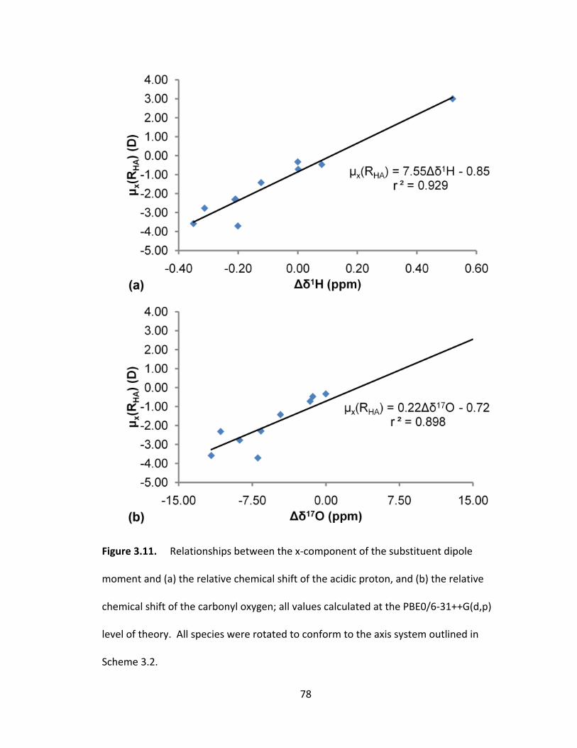
78
Figure 3.11. Relationships between the x‐component of the substituent dipole
moment and (a) the relative chemical shift of the acidic proton, and (b) the relative
chemical shift of the carbonyl oxygen; all values calculated at the PBE0/6‐31++G(d,p)
level of theory. All species were rotated to conform to the axis system outlined in
Scheme 3.2.
79
change can be attributed to the substituent alone. μx(R) is transferable between
“backbones” as apparent with further simplification. Therefore, μx(RH) can be used as a
simple model to predict the substituent dipole moment in the bicyclo[1.1.1]pentane‐1‐
carboxylic acid systems and all other properties which relate to the substituent effect.
3.4 Summary and Conclusion
We have presented a systematic study of the electron density in derivatives of
bicyclo[1.1.1]pentane‐1‐carboxlic acid as it pertains to the “so‐called” inductive effect.
Using the CBS‐QB3 method for accurate thermochemistries, it was determined that the
substitution with an electron donating group results in a positive isodesmic reaction
energy and lead to stabilization of the substituted acid species. In contrast, the electron
withdrawing groups stabilize the substituted conjugate base species, which results in a
negative overall reaction energy. As expected due to the nature of the acid‐base
reaction, the substituent’s effect upon the energy of the system is centered completely
on the probe. The effect of substituent upon the NMR chemical shifts in the system was
also centered mainly on the acidic proton.
Some distance related decay was observed in the charges of the atoms along the
bond path, but it was not related to the substituent effect. This is in direct contrast to
the definition of the “so‐called” inductive effect, which cites strict distance dependence.
Although the effect doesn’t appear to propagate through the bonds (looking at either
the atomic charges or electron density at the bond critical points), the delocalization
index seems to suggest that the mechanism of transmission is stepwise. The only
80
property that appears to be consistently related to the substituent effect is the atomic
dipole moment (most specifically the x‐component of that lying on the bond axis). It
appears that μx of the substituent is controlling all other properties deemed related to
the “so‐called” inductive effect.
Using QTAIM is was possible to conclude that the transmission of charge in the
bicyclo[1.1.1]pentane system is controlled by the x‐component of the substituent
dipole, consistent with the field effect, but propagates along the bond path connecting
the substituent and probe, as the classic picture of the inductive effect suggests. As
transferability of properties is conserved within this system, it is possible to recreate the
substituent effect using μx for the simplest of substituents, RH.

81
Chapter 4: The Effect of Substitution on a Silicon Center: Using a Silicic Acid Probe
82
4.1 Introduction
Substituent effects are used to explain many phenomena in chemistry and are
therefore vital. Steric effects require close contact between groups and resonance
effects require a conjugated π network, thus only the “so‐called” inductive effect is
omnipresent. IUPAC defines the inductive effect as the transmission of charge through
σ‐bonds.16 In constant simultaneous operation is the field effect: the transmission of
charge through space.16 As both effects tend to operate in the same direction and
suffer from distance related decay, they are often impossible to separate. This has led
many groups to amalgamate the two mechanisms and use the term the “so‐called”
inductive effect.
Studies of “so‐called” inductive effect (or any substituent effect in fact) can be
simplified by separating the system into three segments: the substituent, which is
having the effect; the backbone, which transmits the effect; and the probe, on which
the effect is measured. Electronegativity is especially important to the inductive effect
because it also relates to the transmission of electron density (IUPAC defines this as the
power of an atom to attract electrons,17 but it has also been extended to groups70,71).
Thus, the substituents in this study were chosen to cover a wide range of
electronegativities. The backbone employed in this study is bicyclo[1.1.1]pentane. This
segment is used to avoid π‐conjugation, thus removing the possibility of a resonance
effect, and to separate the substituent and probe enough to remove complications due
to inconsistent steric effects. Bicyclo[1.1.1]pentane is generally considered to be rather
rigid and the substituent and probe are generally coplanar, avoiding potential angle
83
dependence of the effect.58,59 To study the inductive effect on silicon we have chosen
silicic acid ( – Si(OH)3) as a silicon counterpart of the previously studied carboxylic acid
probe.89 Silicic acid, common and naturally occurring, is used over the direct analog
silanoic acid (–Si(=O)OH)) as silanoic acids are generally unstable and limited to very
lower temperature studies.90
Most studies of substituent effects use the formulation outlined by Hammett,10
which is readily extended to computational calculations via an isodesmic reaction30 (a
reaction with the same number and types of bonds on both sides16). As the Hammett
relationship is a linear free energy relationship, the isodesmic reaction can be used as a
direct measure of the substituent effect. Central to this study are the isodesmic
reactions shown in Scheme 4.1.
Studies of substituent effects on silicon began with Taft35 and the study of
aliphatic substituents on the reactivity of organosilicon compounds using Ingold’s
original method.91 The relationship gleaned from this study, in the Hammett
formulation, is shown in equation 4.1, where is an inductive effect constant and is
a steric parameter.
(4.1)
Although this relationship performs relatively well, its parameters were based on
reactions of organic carbonyls. The steric parameter has been the subject of many
studies and has been redefined for silicon.92 Recently Ploom and Tuulmets discovered
that there was a significant relationship between the inductive and steric parameters,
and thus suggested that only steric effects were being measured.14 In the manner of
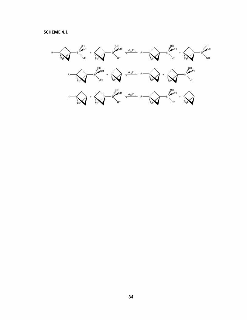
84
SCHEME 4.1
85
Exner and Bohm,36,72 they suggest that an electronegativity parameter ζχ, as in equation
4.2, is needed to adequately describe the inductive effect.
(4.2)
However the inductive effect, without complication from steric effects, has not yet been
studied. Herein we describe the effect of substitution in a silicon system, by replacing
the traditional carboxylic acid probe (‐COOH) with a silicic acid based probe (‐Si(OH)3)
using the same approach used earlier.89
4.2 Methods
All calculations were performed using the Gaussian 0361 and Gaussian 09
programs.62 The geometries were optimized at the PBE063,93/6‐31++G(d,p)45,94 level of
theory and vibrational frequency analysis was performed to confirm the presence of a
stationary point. The chosen level of theory is a reliable compromise of accuracy and
efficiency in the bicyclo[1.1.1]pentane‐1‐carboxylic acid systems previously studied.89
To further confirm the validity of the model chemistry, reaction energies (Scheme 4.1)
are also determined using a composite method, CBS‐QB3,47,48 known for achieving
accurate thermochemistries. In order to maintain consistency, this model chemistry
was also used to calculate group electronegativities, χ, according to the method
described by Boyd et al.70,71
Nuclear magnetic resonance data was generated at the PBE0/6‐31++G(d,p) level
of theory using the gauge‐independent atomic orbitals (GIAO) method.68,95 This level
was confirmed to be sufficient for the calculation of NMR shielding tensors in the
86
bicyclo[1.1.1]pentane‐1‐carboxylic acid systems89 reproducing the relative values from
larger basis sets, and is known for achieving accurate NMR data,96 and is used here for
consistency.
Wavefunctions, generated at the PBE0/6‐31++G(d,p) level of theory, were used to
determine the electron density distribution which was analyzed according to the
Quantum Theory of Atoms in Molecules51,52,54 (QTAIM) using the AIMALL program
suite.65 Integration for the lithium‐substituted conjugate base resulted in a potentially
significant error, even at the most accurate integration levels. Regardless, the results
follow expected trends and are therefore included in our analysis.
To simplify the following discussion, the labeling and axis system (consistent with
Levin et al.69) described in Scheme 4.2, will be used throughout. The proton involved in
deprotonation has been labelled Ha for consistency. For the asymmetric systems (e.g.,
NR2 and OH), each proton was removed and the structure was allowed to relax. The
lowest energy structure was used as the deprotonated species, and the corresponding
hydrogen atom was renamed Ha.
4.3 Results
4.3.1 Energies
The first isodesmic reaction described in Scheme 4.1 was used to compute the
inductive effect on the silicic acid probe (–Si(OH)3; referred to as the Si‐Probe for
brevity) in the same manner as was employed in the bicyclo[1.1.1]pentane‐1‐carboxylic
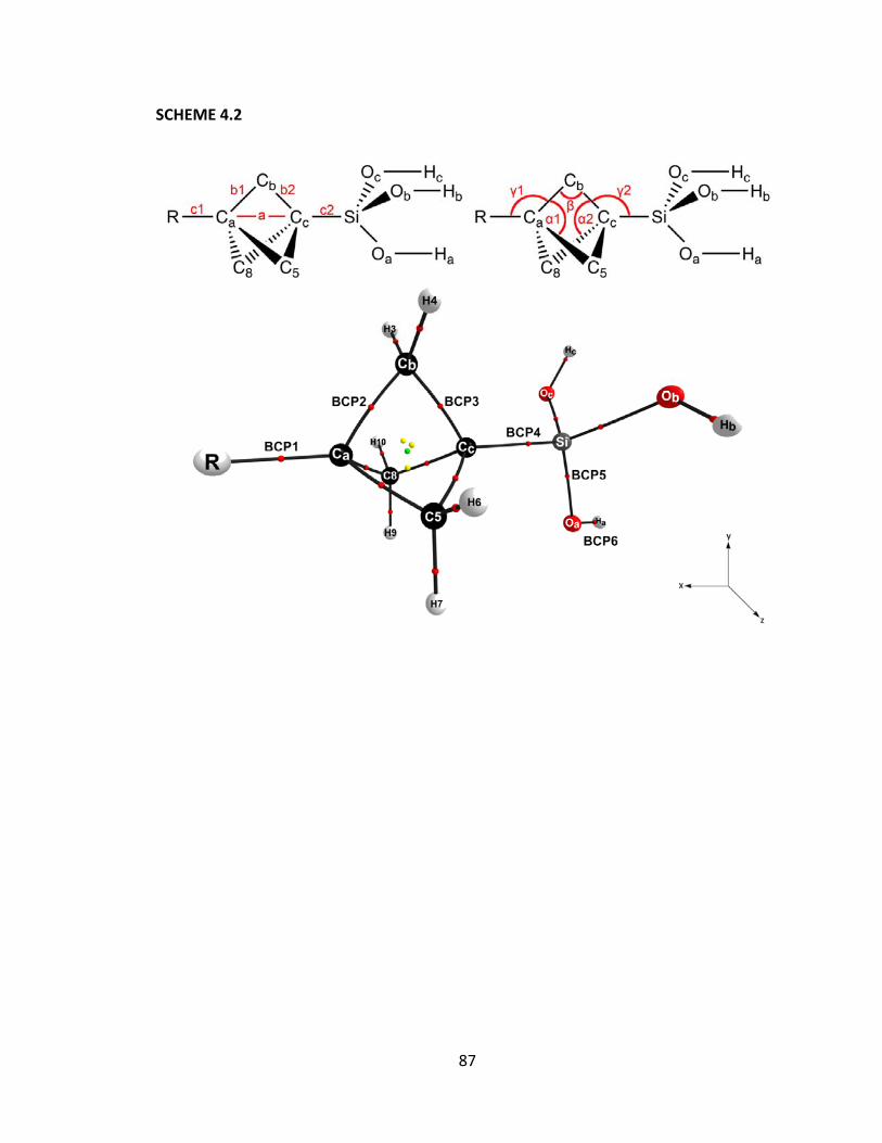
87
SCHEME 4.2

88
acid system (referred to as the C‐Probe for brevity). Using the CBS‐QB3 composite
method for accurate thermochemistries, it was determined that the substituents affect
the Si‐Probe in the same manner as the C‐Probe. As shown in Table 4.1, electron
donating substituents yield a positive ΔisoE and electron withdrawing groups result in a
negative ΔisoE. The CBS‐QB3 energies were also used to determine if the PBE0/6‐
31++G(d,p) model chemistry is sufficiently accurate for the Si system. As indicated in
equation 4.3 the reaction energy computed at the lower level of theory forms an almost
perfect one to one relationship with that obtained using the composite method.
∆ 0.994∆ 0.155 0.999 (4.3)
The order of the substituents in Table 4.1 is based on their ΔisoE values. It is apparent
that the order of substituents is the same for both probe systems, confirming that the
effect is the same. This is consistent with Hammett’s formulation, where any
differences in the magnitude of the substituent effect are attributable to the reaction
constant ρ (Equation 4.1). By plotting ΔisoE for both systems (Figure 4.1) and setting ρ=1
for the carbon system, the slope of the linear relationship (0.843) is equal to the relative
reaction constant for the Si‐system. The same types of relationships between ΔisoE and
both σF and χ as seen for the C‐system are observed in the Si‐system (Figure 4.2).
Although the magnitudes of the slope and intercept are different, due to ρ, the r2 values
are the same in both cases. Multiple linear regression using both parameters does
improve the correlation, but once again by the same amount as in the C‐system. This
strengthens the idea that the substituents have the same effect on the reactivity of a
carboxylic acid probe and a silicic acid probe.
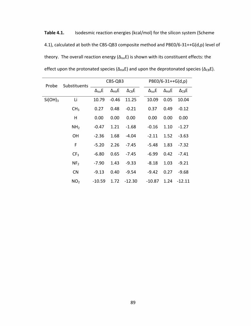
89
Table 4.1. Isodesmic reaction energies (kcal/mol) for the silicon system (Scheme
4.1), calculated at both the CBS‐QB3 composite method and PBE0/6‐31++G(d,p) level of
theory. The overall reaction energy (ΔisoE) is shown with its constituent effects: the
effect upon the protonated species (ΔHAE) and upon the deprotonated species (ΔCBE).
Probe Substituents CBS‐QB3 PBE0/6‐31++G(d,p)
ΔisoE ΔHAE ΔCBE ΔisoE ΔHAE ΔCBE
Si(OH)3 Li 10.79 ‐0.46 11.25 10.09 0.05 10.04
CH3 0.27 0.48 ‐0.21 0.37 0.49 ‐0.12
H 0.00 0.00 0.00 0.00 0.00 0.00
NH2 ‐0.47 1.21 ‐1.68 ‐0.16 1.10 ‐1.27
OH ‐2.36 1.68 ‐4.04 ‐2.11 1.52 ‐3.63
F ‐5.20 2.26 ‐7.45 ‐5.48 1.83 ‐7.32
CF3 ‐6.80 0.65 ‐7.45 ‐6.99 0.42 ‐7.41
NF2 ‐7.90 1.43 ‐9.33 ‐8.18 1.03 ‐9.21
CN ‐9.13 0.40 ‐9.54 ‐9.42 0.27 ‐9.68
NO2 ‐10.59 1.72 ‐12.30 ‐10.87 1.24 ‐12.11
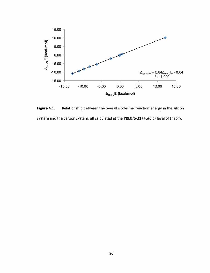
90
Figure 4.1. Relationship between the overall isodesmic reaction energy in the silicon
system and the carbon system; all calculated at the PBE0/6‐31++G(d,p) level of theory.
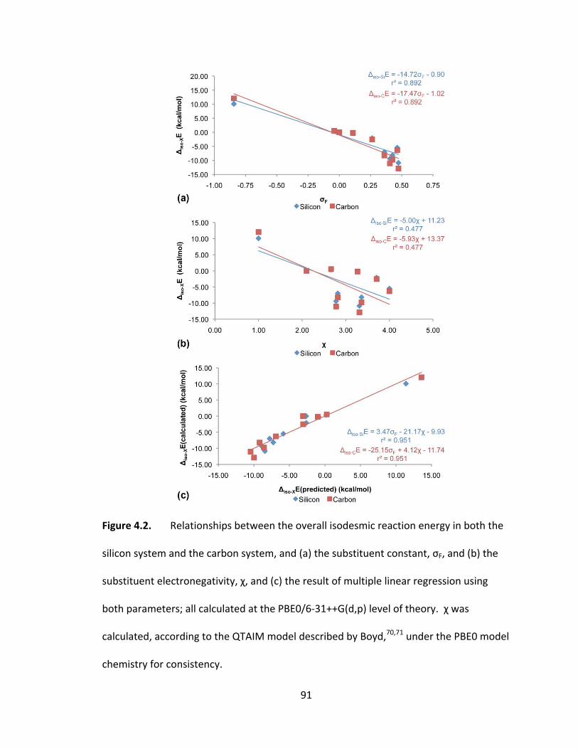
91
Figure 4.2. Relationships between the overall isodesmic reaction energy in both the
silicon system and the carbon system, and (a) the substituent constant, σF, and (b) the
substituent electronegativity, χ, and (c) the result of multiple linear regression using
both parameters; all calculated at the PBE0/6‐31++G(d,p) level of theory. χ was
calculated, according to the QTAIM model described by Boyd,70,71 under the PBE0 model
chemistry for consistency.
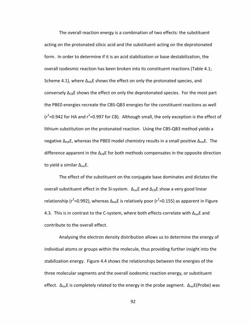
92
The overall reaction energy is a combination of two effects: the substituent
acting on the protonated silicic acid and the substituent acting on the deprotonated
form. In order to determine if it is an acid stabilization or base destabilization, the
overall isodesmic reaction has been broken into its constituent reactions (Table 4.1;
Scheme 4.1), where ΔHAE shows the effect on only the protonated species, and
conversely ΔCBE shows the effect on only the deprotonated species. For the most part
the PBE0 energies recreate the CBS‐QB3 energies for the constituent reactions as well
(r2=0.942 for HA and r2=0.997 for CB). Although small, the only exception is the effect of
lithium substitution on the protonated reaction. Using the CBS‐QB3 method yields a
negative ΔHAE, whereas the PBE0 model chemistry results in a small positive ΔHAE. The
difference apparent in the ΔCBE for both methods compensates in the opposite direction
to yield a similar ΔisoE.
The effect of the substituent on the conjugate base dominates and dictates the
overall substituent effect in the Si‐system. ΔisoE and ΔCBE show a very good linear
relationship (r2=0.992), whereas ΔHAE is relatively poor (r2=0.155) as apparent in Figure
4.3. This is in contrast to the C‐system, where both effects correlate with ΔisoE and
contribute to the overall effect.
Analysing the electron density distribution allows us to determine the energy of
individual atoms or groups within the molecule, thus providing further insight into the
stabilization energy. Figure 4.4 shows the relationships between the energies of the
three molecular segments and the overall isodesmic reaction energy, or substituent
effect. ΔisoE is completely related to the energy in the probe segment. ΔisoE(Probe) was
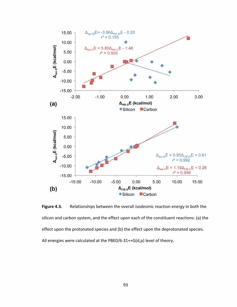
93
Figure 4.3. Relationships between the overall isodesmic reaction energy in both the
silicon and carbon system, and the effect upon each of the constituent reactions: (a) the
effect upon the protonated species and (b) the effect upon the deprotonated species.
All energies were calculated at the PBE0/6‐31++G(d,p) level of theory.
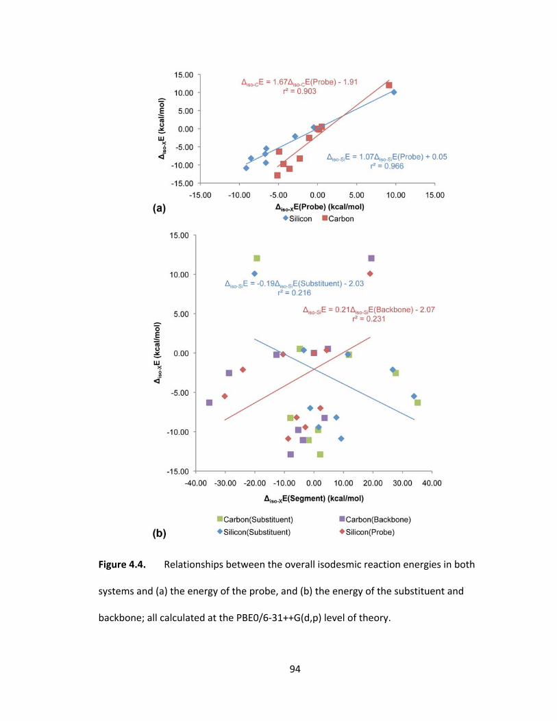
94
Figure 4.4. Relationships between the overall isodesmic reaction energies in both
systems and (a) the energy of the probe, and (b) the energy of the substituent and
backbone; all calculated at the PBE0/6‐31++G(d,p) level of theory.
95
calculated in the same manner as ΔisoE, but using the energies of the probe atoms
instead of the overall molecule. The same trend is evident for both probe systems, the
probe segment becomes more stabilized as the strength of electron withdrawing group
increases, but the correlation is significantly stronger in the Si‐system. The energies of
neither the substituent segment nor the backbone show any relationship to the overall
substituent. Once again they appear to be mirror images (Figure 4.4b), implying an
energy transfer between the substituent and backbone.
In the C‐system, the effect within the probe segment was centered mainly on the
acidic proton. In the Si‐system, it is mainly centered on the remaining hydrogen atoms
in the conjugate base (minor relationships with the oxygen atoms; average r2 between
Oa, Ob and Oc is 0.699). As visible in Figure 4.5, the hydrogen atoms are destabilized as
the electron withdrawing strength of the substituent increases, making them more
acidic.
4.3.2 Nuclear Magnetic Resonance Chemical Shifts
The NMR nuclear shielding tensor,97,98 a 3x3 matrix describing the magnitude
and orientation dependence of the interaction between the nuclei and external
magnetic field, is intimately related to the electron density surrounding nuclei and
consequently should be related to the inductive effect. Diagonalization of the matrix
yields three principal components denoted σ11, σ22, and σ33 where, by convention, σ11 <
σ22 < σ33. An average of the principle components gives the isotropic shielding of the
nucleus (σiso) and is related to the chemical shift. We have converted the calculated
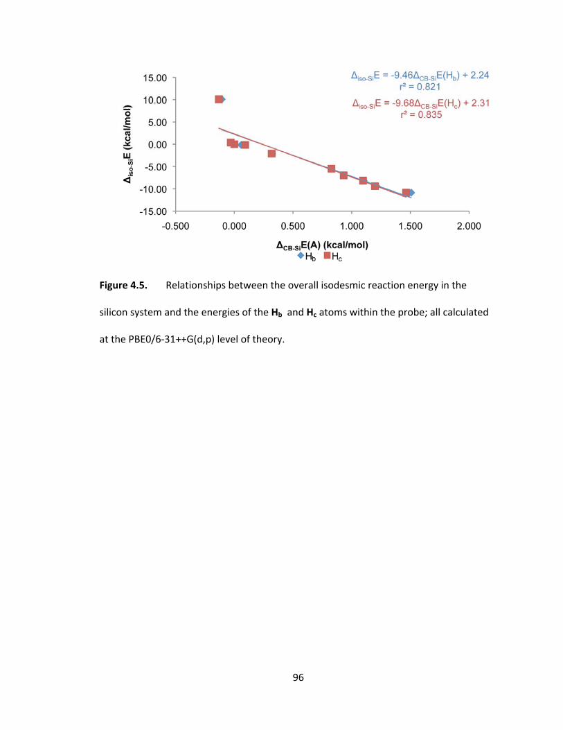
96
Figure 4.5. Relationships between the overall isodesmic reaction energy in the
silicon system and the energies of the Hb and Hc atoms within the probe; all calculated
at the PBE0/6‐31++G(d,p) level of theory.
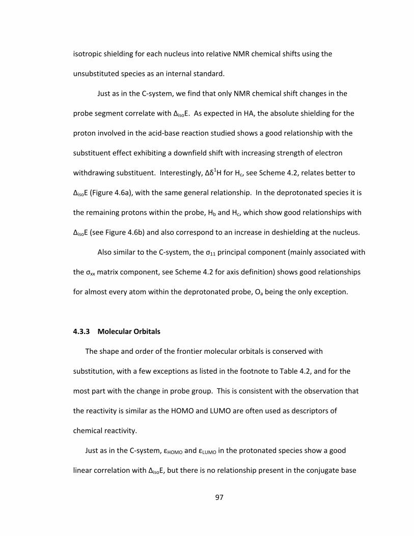
97
isotropic shielding for each nucleus into relative NMR chemical shifts using the
unsubstituted species as an internal standard.
Just as in the C‐system, we find that only NMR chemical shift changes in the
probe segment correlate with ΔisoE. As expected in HA, the absolute shielding for the
proton involved in the acid‐base reaction studied shows a good relationship with the
substituent effect exhibiting a downfield shift with increasing strength of electron
withdrawing substituent. Interestingly, Δδ1H for Hc, see Scheme 4.2, relates better to
ΔisoE (Figure 4.6a), with the same general relationship. In the deprotonated species it is
the remaining protons within the probe, Hb and Hc, which show good relationships with
ΔisoE (see Figure 4.6b) and also correspond to an increase in deshielding at the nucleus.
Also similar to the C‐system, the σ11 principal component (mainly associated with
the σxx matrix component, see Scheme 4.2 for axis definition) shows good relationships
for almost every atom within the deprotonated probe, Oa being the only exception.
4.3.3 Molecular Orbitals
The shape and order of the frontier molecular orbitals is conserved with
substitution, with a few exceptions as listed in the footnote to Table 4.2, and for the
most part with the change in probe group. This is consistent with the observation that
the reactivity is similar as the HOMO and LUMO are often used as descriptors of
chemical reactivity.
Just as in the C‐system, εHOMO and εLUMO in the protonated species show a good
linear correlation with ΔisoE, but there is no relationship present in the conjugate base
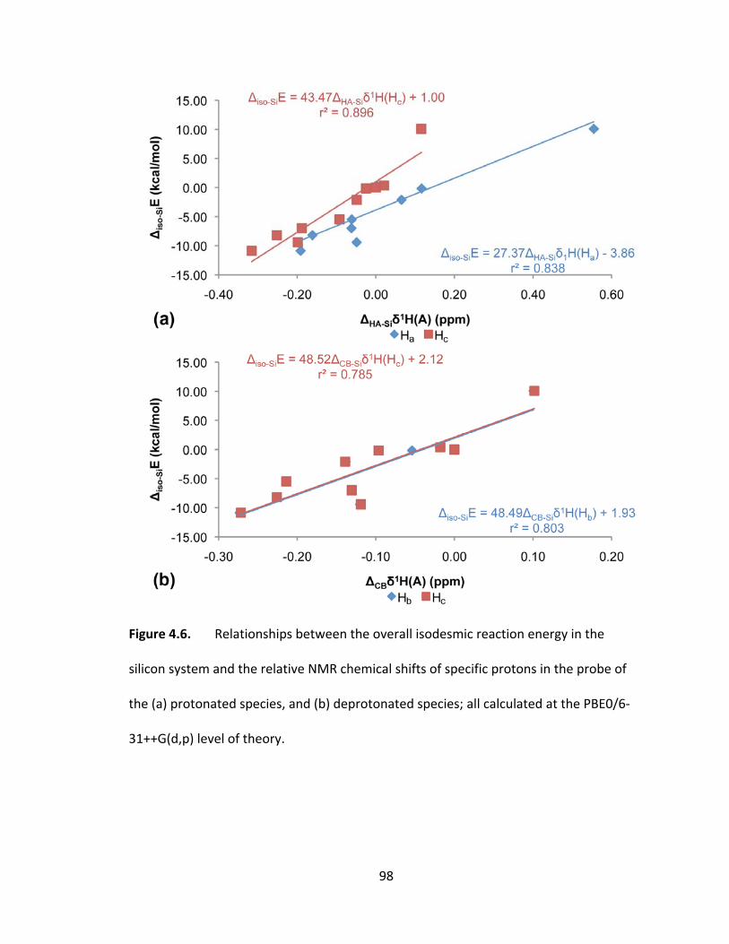
98
Figure 4.6. Relationships between the overall isodesmic reaction energy in the
silicon system and the relative NMR chemical shifts of specific protons in the probe of
the (a) protonated species, and (b) deprotonated species; all calculated at the PBE0/6‐
31++G(d,p) level of theory.
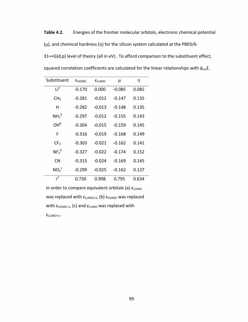
99
Table 4.2. Energies of the frontier molecular orbitals, electronic chemical potential
(μ), and chemical hardness (η) for the silicon system calculated at the PBE0/6‐
31++G(d,p) level of theory (all in eV). To afford comparison to the substituent effect,
squared correlation coefficients are calculated for the linear relationships with ΔisoE.
Substituent εHOMO εLUMO μ η
Lia ‐0.170 0.000 ‐0.085 0.085
CH3 ‐0.281 ‐0.012 ‐0.147 0.135
H ‐0.282 ‐0.013 ‐0.148 0.135
NH2b ‐0.297 ‐0.012 ‐0.155 0.143
OHb ‐0.304 ‐0.015 ‐0.159 0.145
F ‐0.316 ‐0.019 ‐0.168 0.149
CF3 ‐0.303 ‐0.021 ‐0.162 0.141
NF2b ‐0.327 ‐0.022 ‐0.174 0.152
CN ‐0.315 ‐0.024 ‐0.169 0.145
NO2c ‐0.299 ‐0.025 ‐0.162 0.137
r2 0.730 0.998 0.795 0.634
In order to compare equivalent orbitals (a) εLUMO
was replaced with εLUMO+3, (b) εHOMO was replaced
with εHOMO‐1, (c) and εLUMO was replaced with
εLUMO+1.

100
species (as such only the values for HA are shown in Table 4.2). This is highly
unexpected given that the overall reaction energy is governed almost entirely by ΔCBE.
The magnitudes of the orbital energies are different in the Si‐system than in the C‐
system, but not by a great deal and not in any consistent manner. However, the HOMO‐
LUMO gap appears to be essentially the same between systems and centered around
0.28 eV. The value of the gap does not appear to vary with substitution.
The molecular orbital energies can be related to the reactivity via Pearson’s Hard
and Soft Acids and Bases theory.78,80 The electronic chemical potential (μ) describes the
escaping tendency of electrons from the system, which is also the negative of Mulliken’s
electronegativity81 (but is not discussed here) and should be related to the inductive
effect. The chemical hardness, η, is also used as a descriptor of chemical reactivity as it
corresponds to the resistance of a system to charge transfer. μ and η can be defined in
terms of orbital energies using Koopmans’ theorem,77 as given in equations 4.4 and 4.5.
12
12 (4.4)
(4.5)
Just as in the carbon system μ shows a reasonable correlation to the reaction energy
(r2=0.795), exhibiting a decreased tendency for electrons to escape with the increased
electron withdrawing strength of substituent, but the correlation is significantly worse
(r2=0.982 in the C‐system). µ in the Si‐system is always more negative than in the C‐
system by an average of 0.147 eV. Although the magnitude of μ in the silicic acid
molecules is not identical to that of the carbon system, the trend is the same.
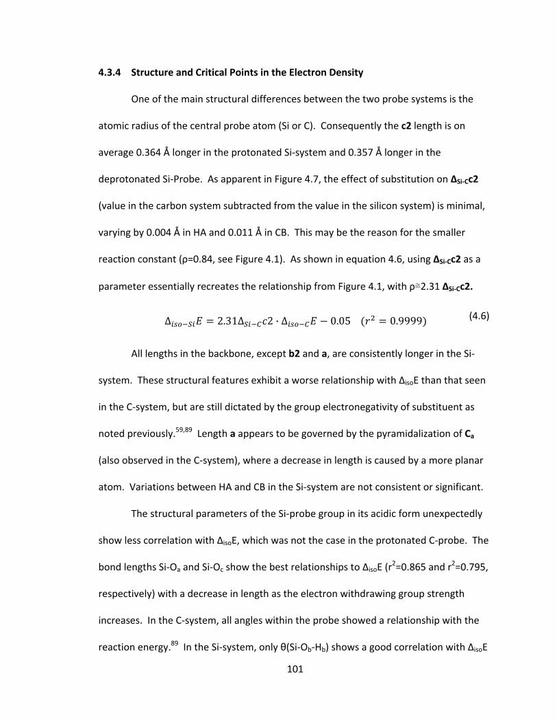
101
4.3.4 Structure and Critical Points in the Electron Density
One of the main structural differences between the two probe systems is the
atomic radius of the central probe atom (Si or C). Consequently the c2 length is on
average 0.364 Å longer in the protonated Si‐system and 0.357 Å longer in the
deprotonated Si‐Probe. As apparent in Figure 4.7, the effect of substitution on ΔSi‐Cc2
(value in the carbon system subtracted from the value in the silicon system) is minimal,
varying by 0.004 Å in HA and 0.011 Å in CB. This may be the reason for the smaller
reaction constant (ρ=0.84, see Figure 4.1). As shown in equation 4.6, using ΔSi‐Cc2 as a
parameter essentially recreates the relationship from Figure 4.1, with ρ≅2.31 ΔSi‐Cc2.
∆ 2.31∆ 2 · ∆ 0.05 0.9999 (4.6)
All lengths in the backbone, except b2 and a, are consistently longer in the Si‐
system. These structural features exhibit a worse relationship with ΔisoE than that seen
in the C‐system, but are still dictated by the group electronegativity of substituent as
noted previously.59,89 Length a appears to be governed by the pyramidalization of Ca
(also observed in the C‐system), where a decrease in length is caused by a more planar
atom. Variations between HA and CB in the Si‐system are not consistent or significant.
The structural parameters of the Si‐probe group in its acidic form unexpectedly
show less correlation with ΔisoE, which was not the case in the protonated C‐probe. The
bond lengths Si‐Oa and Si‐Oc show the best relationships to ΔisoE (r2=0.865 and r2=0.795,
respectively) with a decrease in length as the electron withdrawing group strength
increases. In the C‐system, all angles within the probe showed a relationship with the
reaction energy.89 In the Si‐system, only θ(Si‐Ob‐Hb) shows a good correlation with ΔisoE
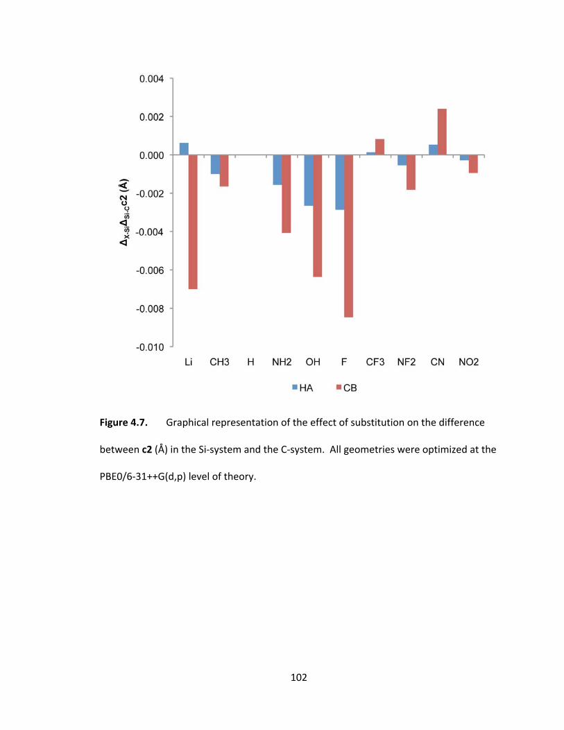
102
Figure 4.7. Graphical representation of the effect of substitution on the difference
between c2 (Å) in the Si‐system and the C‐system. All geometries were optimized at the
PBE0/6‐31++G(d,p) level of theory.
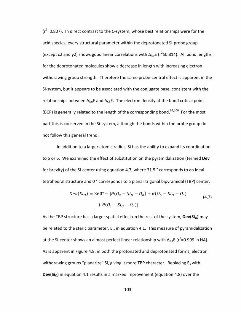
103
(r2=0.807). In direct contrast to the C‐system, whose best relationships were for the
acid species, every structural parameter within the deprotonated Si‐probe group
(except c2 and γ2) shows good linear correlations with ΔisoE (r2≥0.814). All bond lengths
for the deprotonated molecules show a decrease in length with increasing electron
withdrawing group strength. Therefore the same probe‐central effect is apparent in the
Si‐system, but it appears to be associated with the conjugate base, consistent with the
relationships between ΔisoE and ΔCBE. The electron density at the bond critical point
(BCP) is generally related to the length of the corresponding bond.99,100 For the most
part this is conserved in the Si‐system, although the bonds within the probe group do
not follow this general trend.
In addition to a larger atomic radius, Si has the ability to expand its coordination
to 5 or 6. We examined the effect of substitution on the pyramidalization (termed Dev
for brevity) of the Si‐center using equation 4.7, where 31.5 ° corresponds to an ideal
tetrahedral structure and 0 ° corresponds to a planar trigonal bipyramidal (TBP) center.
360°
(4.7)
As the TBP structure has a larger spatial effect on the rest of the system, Dev(SiO) may
be related to the steric parameter, Es, in equation 4.1. This measure of pyramidalization
at the Si‐center shows an almost perfect linear relationship with ΔisoE (r2=0.999 in HA).
As is apparent in Figure 4.8, in both the protonated and deprotonated forms, electron
withdrawing groups “planarize” Si, giving it more TBP character. Replacing Es with
Dev(SiO) in equation 4.1 results in a marked improvement (equation 4.8) over the
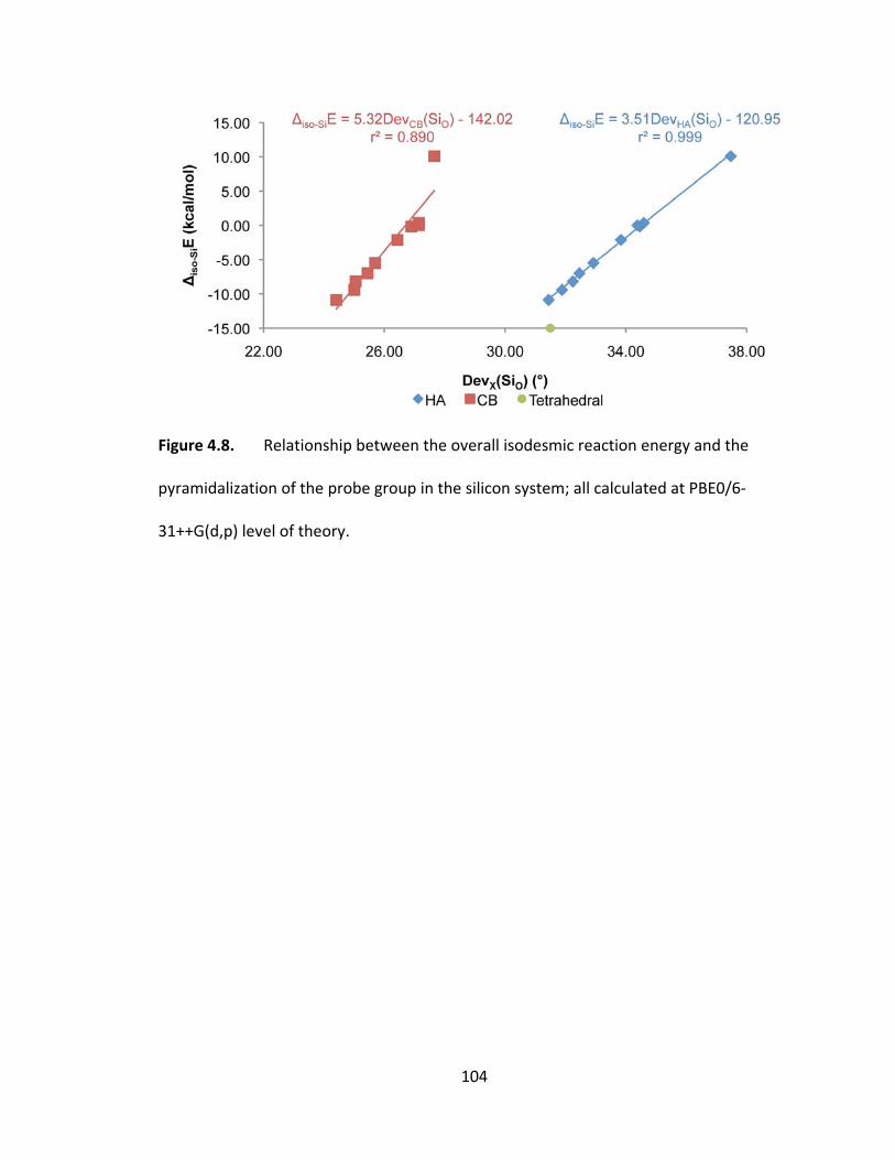
104
Figure 4.8. Relationship between the overall isodesmic reaction energy and the
pyramidalization of the probe group in the silicon system; all calculated at PBE0/6‐
31++G(d,p) level of theory.
105
relationship depicted in Figure 4.2a. Despite the increase in TBP character, the valence
shell charge concentrations (critical points in the Laplacian of the electron density, often
used as an indication of the electron pairs around an atom in QTAIM53) indicated that Si
remains 4‐coordinate.
∆ 1.12 3.74∆ 0.41 0.999 (4.8)
If the “so‐called” inductive effect is transmitting through‐bonds (as opposed to
through‐space) the electron density along the shortest bond path between substituent
and probe would be perturbed. The expected bond path in this system is denoted by
the numbered bond critical points (BCPs) in Scheme 4.2. Just as in the C‐system,
although with smaller correlations, the electron density at the relevant BCPs within the
probe group, of the acidic species, (5 and 6 in Scheme 4.2) show fair relationships to
ΔisoE. ρ(BCP6) shows an expected decrease in density with increasing strength of
electron withdrawing group, evident in Figure 4.9, and ρ(BCP5) shows an increase in
density consistent with the redistribution of charge. Unlike the C‐system, the electron
density in the bond linking the backbone and probe (BCP4) also shows a fair relationship
with ΔisoE decreasing as the electron withdrawing strength of substituent increases.
Once again there are no relationships with the bond between substituent and backbone
or the BCPs within the backbone (1, 2 and 3), and correlations are present only for
ρ(BCP) between the bridging carbons and their attached hydrogen atoms (e.g., BCP(Cb–
H4)).
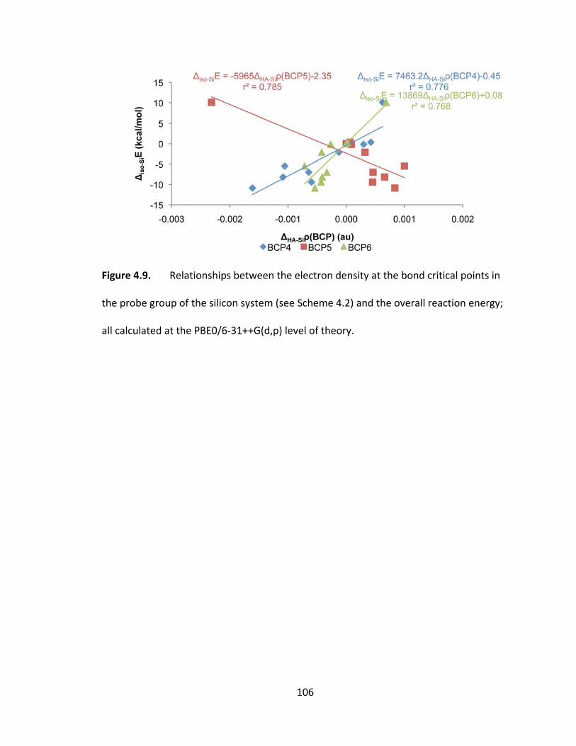
106
Figure 4.9. Relationships between the electron density at the bond critical points in
the probe group of the silicon system (see Scheme 4.2) and the overall reaction energy;
all calculated at the PBE0/6‐31++G(d,p) level of theory.
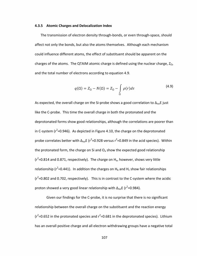
107
4.3.5 Atomic Charges and Delocalization Index
The transmission of electron density through‐bonds, or even through‐space, should
affect not only the bonds, but also the atoms themselves. Although each mechanism
could influence different atoms, the effect of substituent should be apparent on the
charges of the atoms. The QTAIM atomic charge is defined using the nuclear charge, ZΩ,
and the total number of electrons according to equation 4.9.
Ω Ω Ω Ω
Ω
(4.9)
As expected, the overall charge on the Si‐probe shows a good correlation to ΔisoE just
like the C‐probe. This time the overall charge in both the protonated and the
deprotonated forms show good relationships, although the correlations are poorer than
in C‐system (r2=0.946). As depicted in Figure 4.10, the charge on the deprotonated
probe correlates better with ΔisoE (r2=0.928 versus r2=0.849 in the acid species). Within
the protonated form, the charge on Si and Oa show the expected good relationship
(r2=0.814 and 0.871, respectively). The charge on Ha, however, shows very little
relationship (r2=0.441). In addition the charges on Hb and Hc show fair relationships
(r2=0.802 and 0.702, respectively). This is in contrast to the C‐system where the acidic
proton showed a very good linear relationship with ΔisoE (r2=0.984).
Given our findings for the C‐probe, it is no surprise that there is no significant
relationship between the overall charge on the substituent and the reaction energy
(r2=0.652 in the protonated species and r2=0.681 in the deprotonated species). Lithium
has an overall positive charge and all electron withdrawing groups have a negative total
108
Figure 4.10. Relationships between the overall reaction energy and the QTAIM
charge of the probe group within the molecules of the silicon system; all calculated at
the PBE0/6‐31++G(d,p) level of theory.
109
charge thus, qualitatively, reflecting their electron withdrawing or donating nature. The
methyl substituent has an overall positive charge of 0.01 au in the protonated form and
an overall negative charge of ‐0.01 au in the conjugate base. The same trends were
observed in the C‐system, even the unexpected change of the methyl substituent in the
deprotonated species. The differences in charge of the substituents are almost
negligible, which once again points to a similar effect in both systems. The largest
variation between systems is for the CF3‐substituted acids. The CF3 group in the Si‐
system is 0.021 au more negative than the corresponding group in the C‐system. The
effect upon the charge does appear to decay with distance, although there is again no
relationship to the substituent effect. Figure 4.11 shows the relative charges of the
atoms along the bond path (a shows the effect on the protonated species and b shows
the effect on the deprotonated species); as expected, Ca has the largest variation in
charge with substitution and this variation decreases with increased distance from the
substituent.
Once again the overall charge on the substituent, and on Ca, has a very good
relationship to the QTAIM group electronegativity, consistent with its formulation.
Interestingly, the charge on the acidic hydrogen within the Si‐probe, Ha, appears to be
governed by the electronegativity of the substituent (as shown in Figure 4.12) instead of
the isodesmic reaction energy, with the acidic hydrogen becoming more positive as the
electronegativity of the substituent increases. This dependence on the electronegativity
hints toward a through‐bond mechanism of transmission not seen in the C‐system.

110
Figure 4.11. Graphical representation of the decay in the relative charges of the atoms along the bond path (see Scheme 4.2) in
the silicon system for the (a) protonated species and (b) deprotonated species. Inset is the effect upon the atoms from Cb to Ha to
show the detail masked by the effects at Ca. All values calculated from wavefunctions created at the PBE0/6‐31++G(d,p) level of
theory.
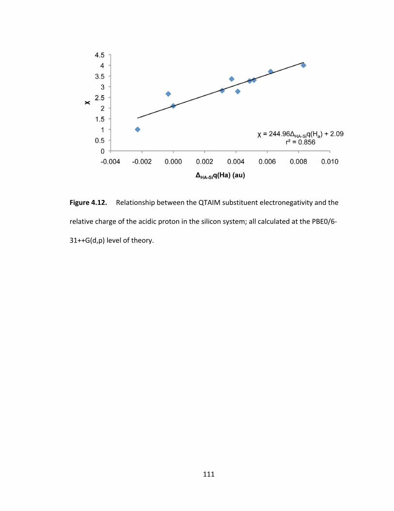
111
Figure 4.12. Relationship between the QTAIM substituent electronegativity and the
relative charge of the acidic proton in the silicon system; all calculated at the PBE0/6‐
31++G(d,p) level of theory.
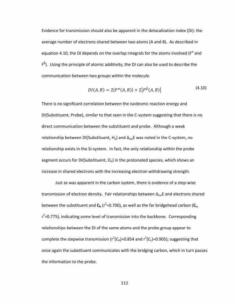
112
Evidence for transmission should also be apparent in the delocalization index (DI): the
average number of electrons shared between two atoms (A and B). As described in
equation 4.10, the DI depends on the overlap integrals for the atoms involved (Fα and
Fβ). Using the principle of atomic additivity, the DI can also be used to describe the
communication between two groups within the molecule.
, 2| , | 2 , (4.10)
There is no significant correlation between the isodesmic reaction energy and
DI(Substituent, Probe), similar to that seen in the C‐system suggesting that there is no
direct communication between the substituent and probe. Although a weak
relationship between DI(Substituent, Ha) and ΔisoE was noted in the C‐system, no
relationship exists in the Si‐system. In fact, the only relationship within the probe
segment occurs for DI(Substituent, Oa) in the protonated species, which shows an
increase in shared electrons with the increasing electron withdrawing strength.
Just as was apparent in the carbon system, there is evidence of a step‐wise
transmission of electron density. Fair relationships between ΔisoE and electrons shared
between the substituent and Cb (r2=0.700), as well as the far bridgehead carbon (Cc,
r2=0.775), indicating some level of transmission into the backbone. Corresponding
relationships between the DI of the same atoms and the probe group appear to
complete the stepwise transmission (r2(Cb)=0.854 and r2(Cc)=0.905); suggesting that
once again the substituent communicates with the bridging carbon, which in turn passes
the information to the probe.
113
4.3.6 Dipole Moment Contributions
The dipole moment has been used as proof of through space transmission of
electron density, as in the traditional field effect, in previous studies33 and in our
analysis of the bicyclo[1.1.1]pentane‐1‐carboxylic acid system.89 As it was determined
that the effect of substitution in the carbon system transmits via the x‐component of
the atomic dipole moments along the bond path linking the substituent and probe, a
careful analysis of all components was also performed for the silicon system. As
determined in the C‐system, the overall molecular dipole moment for the Si‐system, as
described in Table 4.3, shows no linear relationship with the reaction energy. Although
only a weak correlation in the carbon system (r2=0.641), the x‐component of the
molecular dipole, μx, in the acidic species shows a strong correlation with the
substituent effect (r2=0.985). As all molecules conform to the axis system described in
Scheme 4.2, it appears that the overall charge distribution is skewed toward the probe
segment in the electron withdrawing substituted molecules.
QTAIM provides a way to determine the individual atomic dipole moments
according to equation 4.11 and, through summation, the group dipole moment.
Ω Ω
Ω
(4.11)
As observed for the C‐probe, the x‐component of the substituent dipole shows a very
good relationship to ΔisoE (see Table 4.3 for values and Figure 4.13a). The dipole
becomes greater in the direction of the probe segment as the strength of electron
withdrawing group increases in both the protonated and deprotonated species. Owing
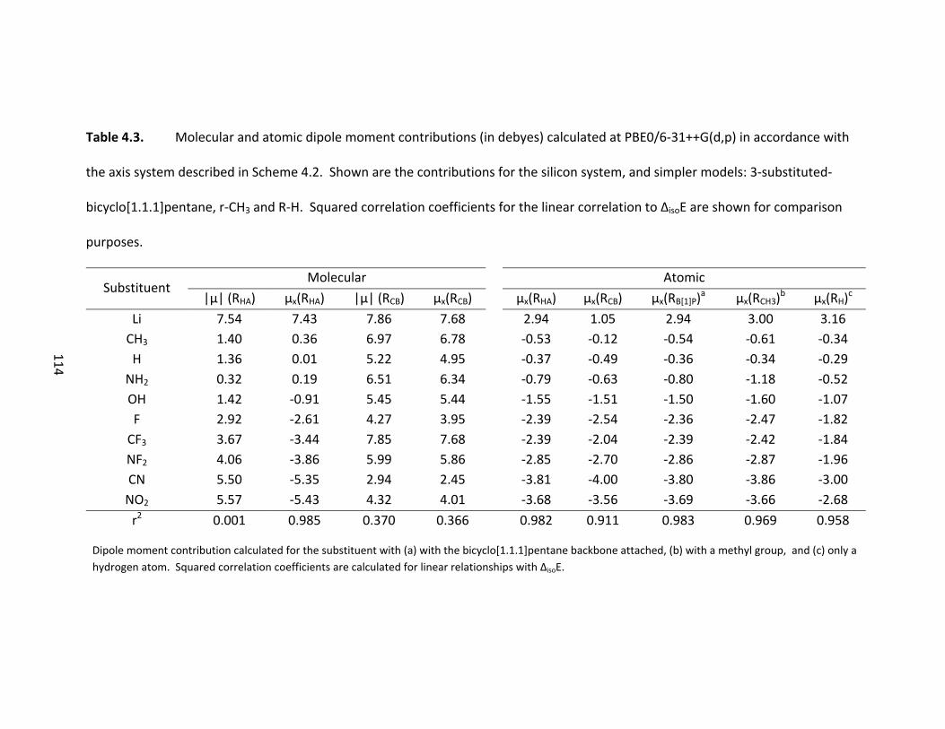
114
Table 4.3. Molecular and atomic dipole moment contributions (in debyes) calculated at PBE0/6‐31++G(d,p) in accordance with
the axis system described in Scheme 4.2. Shown are the contributions for the silicon system, and simpler models: 3‐substituted‐
bicyclo[1.1.1]pentane, r‐CH3 and R‐H. Squared correlation coefficients for the linear correlation to ΔisoE are shown for comparison
purposes.
Substituent Molecular Atomic
|μ| (RHA) μx(RHA) |μ| (RCB) μx(RCB) μx(RHA) μx(RCB) μx(RB[1]P)a μx(RCH3)
b μx(RH)c
Li 7.54 7.43 7.86 7.68 2.94 1.05 2.94 3.00 3.16CH3 1.40 0.36 6.97 6.78 ‐0.53 ‐0.12 ‐0.54 ‐0.61 ‐0.34H 1.36 0.01 5.22 4.95 ‐0.37 ‐0.49 ‐0.36 ‐0.34 ‐0.29NH2 0.32 0.19 6.51 6.34 ‐0.79 ‐0.63 ‐0.80 ‐1.18 ‐0.52OH 1.42 ‐0.91 5.45 5.44 ‐1.55 ‐1.51 ‐1.50 ‐1.60 ‐1.07F 2.92 ‐2.61 4.27 3.95 ‐2.39 ‐2.54 ‐2.36 ‐2.47 ‐1.82CF3 3.67 ‐3.44 7.85 7.68 ‐2.39 ‐2.04 ‐2.39 ‐2.42 ‐1.84NF2 4.06 ‐3.86 5.99 5.86 ‐2.85 ‐2.70 ‐2.86 ‐2.87 ‐1.96CN 5.50 ‐5.35 2.94 2.45 ‐3.81 ‐4.00 ‐3.80 ‐3.86 ‐3.00NO2 5.57 ‐5.43 4.32 4.01 ‐3.68 ‐3.56 ‐3.69 ‐3.66 ‐2.68
r2 0.001 0.985 0.370 0.366 0.982 0.911 0.983 0.969 0.958
Dipole moment contribution calculated for the substituent with (a) with the bicyclo[1.1.1]pentane backbone attached, (b) with a methyl group, and (c) only a hydrogen atom. Squared correlation coefficients are calculated for linear relationships with ΔisoE.
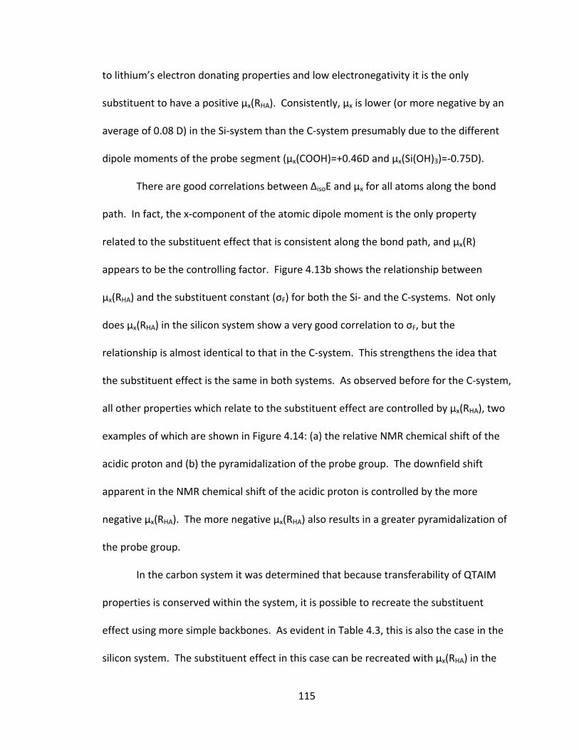
115
to lithium’s electron donating properties and low electronegativity it is the only
substituent to have a positive μx(RHA). Consistently, μx is lower (or more negative by an
average of 0.08 D) in the Si‐system than the C‐system presumably due to the different
dipole moments of the probe segment (μx(COOH)=+0.46D and μx(Si(OH)3)=‐0.75D).
There are good correlations between ΔisoE and µx for all atoms along the bond
path. In fact, the x‐component of the atomic dipole moment is the only property
related to the substituent effect that is consistent along the bond path, and μx(R)
appears to be the controlling factor. Figure 4.13b shows the relationship between
μx(RHA) and the substituent constant (σF) for both the Si‐ and the C‐systems. Not only
does μx(RHA) in the silicon system show a very good correlation to σF, but the
relationship is almost identical to that in the C‐system. This strengthens the idea that
the substituent effect is the same in both systems. As observed before for the C‐system,
all other properties which relate to the substituent effect are controlled by μx(RHA), two
examples of which are shown in Figure 4.14: (a) the relative NMR chemical shift of the
acidic proton and (b) the pyramidalization of the probe group. The downfield shift
apparent in the NMR chemical shift of the acidic proton is controlled by the more
negative µx(RHA). The more negative µx(RHA) also results in a greater pyramidalization of
the probe group.
In the carbon system it was determined that because transferability of QTAIM
properties is conserved within the system, it is possible to recreate the substituent
effect using more simple backbones. As evident in Table 4.3, this is also the case in the
silicon system. The substituent effect in this case can be recreated with µx(RHA) in the
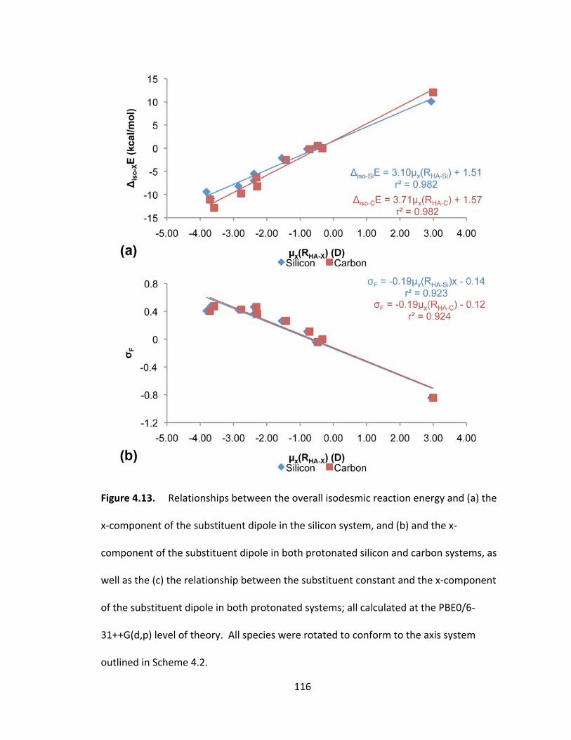
116
Figure 4.13. Relationships between the overall isodesmic reaction energy and (a) the
x‐component of the substituent dipole in the silicon system, and (b) and the x‐
component of the substituent dipole in both protonated silicon and carbon systems, as
well as the (c) the relationship between the substituent constant and the x‐component
of the substituent dipole in both protonated systems; all calculated at the PBE0/6‐
31++G(d,p) level of theory. All species were rotated to conform to the axis system
outlined in Scheme 4.2.
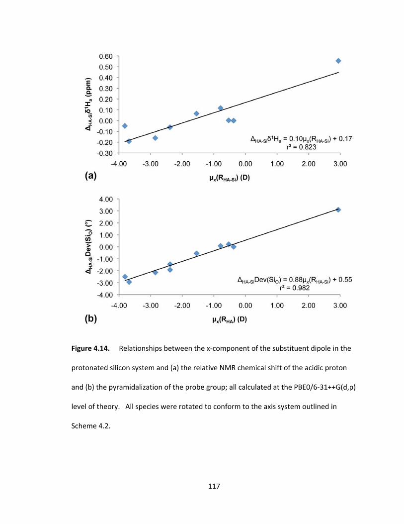
117
Figure 4.14. Relationships between the x‐component of the substituent dipole in the
protonated silicon system and (a) the relative NMR chemical shift of the acidic proton
and (b) the pyramidalization of the probe group; all calculated at the PBE0/6‐31++G(d,p)
level of theory. All species were rotated to conform to the axis system outlined in
Scheme 4.2.
118
carbon system as well as in the RH system. Yet again, it appears the mode of
transmission is through variations in the atomic dipole moments. As such we can use
µx(RHA) to create an expression akin to equation 4.1 to describe the substituent effect in
the Si‐system. As is apparent in equation 4.12, the only improvement over equation 4.8
is that the intercept, sometimes considered the error in the relationship, is lower.
∆ 0.11 3.39∆
0.36 0.999
(4.12)
4.4 Summary and Conclusion
We present a systematic study of the effect of a variety of substituents on a silicon
based probe: silicic acid. The essentially perfect linear relationship between the
isodesmic reaction energy of the silicon system and that of the previously studied
carbon system89 implies that the effect of the substituent on the reactivity is the same,
consistent with the substituent constant concept proposed by Hammett. The silicon
probe system is less sensitive to the effect of substitution as suggested by ρ. The
reaction constant is directly related to ΔSi‐Cc2, the change in distance between the two
probes (C and Si) and the backbone.
In Hammett’s formulation, a steric parameter was required to correctly describe
the effects of substitution. We find that this correction is related to the effect of
substitution on Si pyramidalization, Dev(SiO). Thus, even when the substituent has no
direct steric interaction it still has an effect.
119
Just as in the carbon system, distance related decay is apparent, but it does not
relate to the substituent effect. Analysis of the atomic charges and electron density at
the bond critical points provides no significant insight into the transmission of the effect,
although there does appear to be more evidence for a through‐bond than a through‐
space connection. The delocalization indices point to a stepwise transmission with
communication between the substituent and backbone atoms and the same backbone
atoms and the probe segment. The key substituent property is the x‐component of the
dipole moment as it controls all other properties related to the substituent effect, also
observed in the C‐system. The x‐component of the substituent dipole, which appears to
be a conserved property, causes a change in the atomic dipole moments along the bond
path, resulting in an effect that appears to pass through‐bonds. A linear equation has
been developed, using μx(RHA) and DevHA(SiO) as parameters, to describe the “so‐called”
inductive effect of substituents on silicic acid reactivity.
120
Chapter 5: The Transmission of the Inductive Effect Through Silicon Containing
Backbones
121
5.1 Introduction
The “so‐called” inductive effect comprises two mechanisms for the transmission
of charge through a molecule: the through σ‐bonds mechanism termed the (traditional)
inductive effect and the through‐space mechanism termed the field effect.16 Both
mechanisms generally operate in the same direction and therefore tend to be
inseparable. Transmission through carbon‐carbon bonds has been widely studied;
however this is not the case with silicon‐silicon bonds.
In one of the first substituent effect studies, Hammett used a benzene moiety as
the transmitting segment. He discovered that the acid dissociation constants of the
substituted and unsubstituted acids (according to logKR ‐ logKH) could be related to a
substituent (σ) and a reaction (ρ) constant. Since then almost every other type of
carbon based backbone has been tested according to his method.20 Just as the benzene
backbone has been used to describe how the resonance effect transmits, saturated
systems have been employed to describe how the inductive effect transmits. Acetic
acids have been used as one of the simplest systems to study the inductive effect,21 but
their smaller size can lead to steric complications. Bicyclic alkanes have become the
standard for inductive effect studies because they exclude any possibility of resonance
and due to their rigidity maintain an approximately constant steric effect.36 The
bicyclo[2.2.2]octane backbone was originally introduced because it the number of C–C
bonds between the substituent and probe is the same as in benzene.
Bicyclo[1.1.1]pentane is becoming more popular because it has the same attractive
122
qualities, but results in a more sensitive system as the substituent and probe are closer
together and the effect transmits through fewer bonds.33
Although Si is isoelectronic to C, it has an increased atomic radius, greater
polarizability, and low‐lying d orbitals which may allow for (p–d)π, (p–d–d)π, etc.,
interactions.8 Unlike carbon, Si has been found to expand beyond 4‐coordinate to
include 5‐ and 6‐coordinate species101 and 2‐ and 3‐coordinate species, like alkene and
alkyne analogs, which exhibit a “lone pair” effect where Si is pyramidal. This is generally
attributed to the presence of some lone pair density on the Si atoms.102,103
Yoder et al.8 undertook one of the few studies of the transmission of substituent
effects through the disilane bond using NMR chemical shifts and coupling constants.
Using the 13C–1H coupling constants, as they are the least sensitive to external effects, it
was determined that transmission was more effective through a C‐C linkage than a Si‐Si
linkage, despite the greater polarizability. The authors attributed this to a shorter
distance between the substituent and probe with the C‐C linkage and intramolecular
interactions between the β‐Si and electron rich substituents. Using the Hammett
approach, Yoder et al. determined that the NMR parameters correlated well with
substituent constants as expected for carbon systems.
Herein we investigate the transmission of substituent effects through silicon
atoms by extending our previous method using the bicyclo[1.1.1]pentane backbone to
include silicon based analogs.89 The carbon atoms within the backbone were
systematically replaced by silicon, according to Scheme 5.1, to develop three analog
systems. Each analog was subsequently compared to the original all‐carbon backbones,
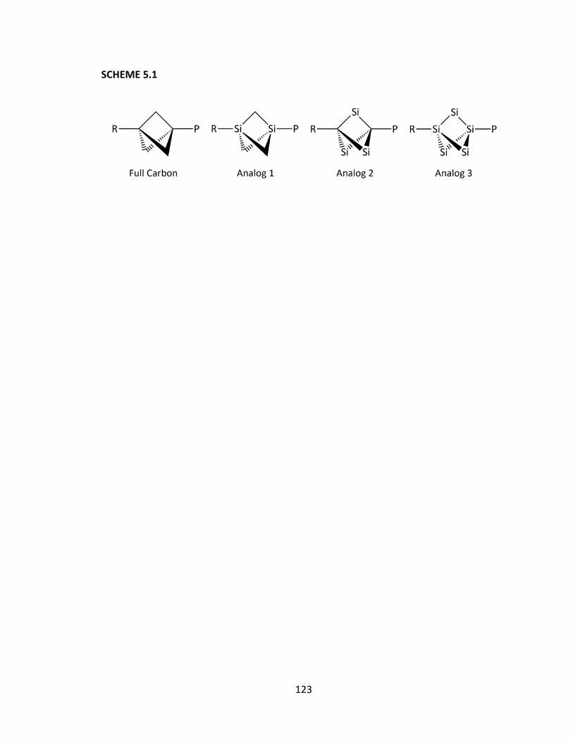
123
SCHEME 5.1
124
both with carbon and silicon probes, to determine the effect of transmission through
silicon. Applying the isodesmic reaction approach to Hammett’s method and the
Quantum Theory of Atoms in Molecules (QTAIM), we have examined the transmission
of the “so‐called” inductive effect to determine if transmission occurs differently in a Si‐
based bicyclo[1.1.1]pentane structure.
5.2 Methods
All calculations were performed using the Gaussian 0361 and 0962 versions of the
program suite. Geometry optimization was performed at the PBE063,93/6‐31++G(d,p)45,94
level of theory followed by vibrational frequency analysis, with the same model
chemistry, to confirm the presence of a stationary point. This model chemistry was
previously shown to be a compromise between accuracy and efficiency in the 3‐
substituted‐bicyclo[1.1.1]pentane‐1‐carboxylic acid system.89 The accuracy of the
isodesmic reaction energies (reactions shown in Scheme 5.2), were assessed using a
complete basis set method, CBS‐QB3,47,48,104 known for achieving highly accurate
thermochemistries.
Nuclear magnetic resonance (NMR) data was generated at the PBE0/6‐31++G(d,p)
level of theory using the gauge‐independent atomic orbitals (GIAO) method.68,95 PBE0
has been proven to be accurate in the prediction of NMR shielding tensors,96 and the
basis set was confirmed to be sufficient via comparison to larger basis sets.89
Wavefunctions were generated at the PBE0/6‐31++G(d,p) level of theory to
ensure a stationary point was used, and the electron density distribution was analyzed

125
SCHEME 5.2
126
using the AIMALL program suite65 according to Bader’s Quantum Theory of Atoms in
Molecules.51,52 The integration for the lithium and CF3‐substituted conjugate base
molecules with backbone 1, and the carboxylic acid probe, resulted in a potentially
significant error even at the most accurate levels. As the results follow expected trends,
they will be included in the analysis. The molecular graph for the lithium‐substituted
acid with backbone 2 (both probes) includes a non‐nuclear attractor (see Figure A1.2)
near the lithium substituent and was not used in the analysis.
Scheme 5.3 shows the labeling and axis systems used in this discussion, chosen
to be consistent with Levin et al.69 Those with the carboxylic acid probe will be referred
to as simply analogs C1, C2, and C3 depending on their backbone, and those with the
silicic acid type probe will be referred to as analog S1, S2, and S3; each will be compared
to their all‐carbon backbone (E=E’=C) counterparts to determine the effect on
transmission.
5.3 Results
5.3.1 Energies
To study how the “so‐called” inductive effect transmits through silicon, the
isodesmic reaction energies (Δiso‐XE, where X=AC1, AC2, AC3, or AS1, AS2, AS3. A
indicates an analog system, C specifies the carboxylic acid probe and S specifies the use
of the silicic acid probe) obtained from the reactions described in Scheme 5.2 were
compared to that determined for the all carbon backbone (for COOH probe see Section
3.4.1; for Si(OH)3 probe see Section 4.4.1). The substituents have been ordered based
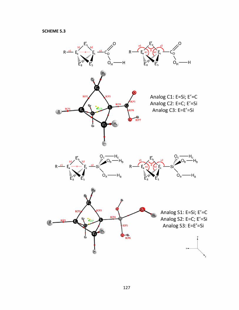
127
SCHEME 5.3
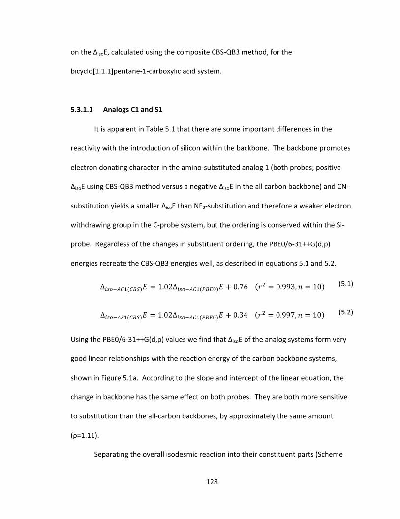
128
on the ΔisoE, calculated using the composite CBS‐QB3 method, for the
bicyclo[1.1.1]pentane‐1‐carboxylic acid system.
5.3.1.1 Analogs C1 and S1
It is apparent in Table 5.1 that there are some important differences in the
reactivity with the introduction of silicon within the backbone. The backbone promotes
electron donating character in the amino‐substituted analog 1 (both probes; positive
ΔisoE using CBS‐QB3 method versus a negative ΔisoE in the all carbon backbone) and CN‐
substitution yields a smaller ΔisoE than NF2‐substitution and therefore a weaker electron
withdrawing group in the C‐probe system, but the ordering is conserved within the Si‐
probe. Regardless of the changes in substituent ordering, the PBE0/6‐31++G(d,p)
energies recreate the CBS‐QB3 energies well, as described in equations 5.1 and 5.2.
∆ 1.02∆ 0.76 0.993, 10 (5.1)
∆ 1.02∆ 0.34 0.997, 10 (5.2)
Using the PBE0/6‐31++G(d,p) values we find that ΔisoE of the analog systems form very
good linear relationships with the reaction energy of the carbon backbone systems,
shown in Figure 5.1a. According to the slope and intercept of the linear equation, the
change in backbone has the same effect on both probes. They are both more sensitive
to substitution than the all‐carbon backbones, by approximately the same amount
(ρ=1.11).
Separating the overall isodesmic reaction into their constituent parts (Scheme
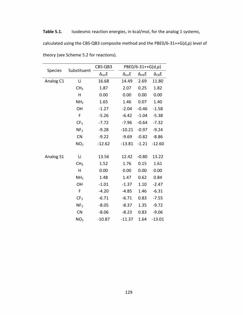
129
Table 5.1. Isodesmic reaction energies, in kcal/mol, for the analog 1 systems,
calculated using the CBS‐QB3 composite method and the PBE0/6‐31++G(d,p) level of
theory (see Scheme 5.2 for reactions).
Species Substituent CBS‐QB3 PBE0/6‐31++G(d,p)
ΔisoE ΔisoE ΔHAE ΔCBE
Analog C1 Li 16.68 14.49 2.69 11.80
CH3 1.87 2.07 0.25 1.82
H 0.00 0.00 0.00 0.00
NH2 1.65 1.46 0.07 1.40
OH ‐1.27 ‐2.04 ‐0.46 ‐1.58F ‐5.26 ‐6.42 ‐1.04 ‐5.38
CF3 ‐7.72 ‐7.96 ‐0.64 ‐7.32
NF2 ‐9.28 ‐10.21 ‐0.97 ‐9.24
CN ‐9.22 ‐9.69 ‐0.82 ‐8.86
NO2 ‐12.62 ‐13.81 ‐1.21 ‐12.60
Analog S1 Li 13.56 12.42 ‐0.80 13.22
CH3 1.52 1.76 0.15 1.61
H 0.00 0.00 0.00 0.00
NH2 1.48 1.47 0.62 0.84
OH ‐1.01 ‐1.37 1.10 ‐2.47F ‐4.20 ‐4.85 1.46 ‐6.31
CF3 ‐6.71 ‐6.71 0.83 ‐7.55
NF2 ‐8.05 ‐8.37 1.35 ‐9.72
CN ‐8.06 ‐8.23 0.83 ‐9.06
NO2 ‐10.87 ‐11.37 1.64 ‐13.01
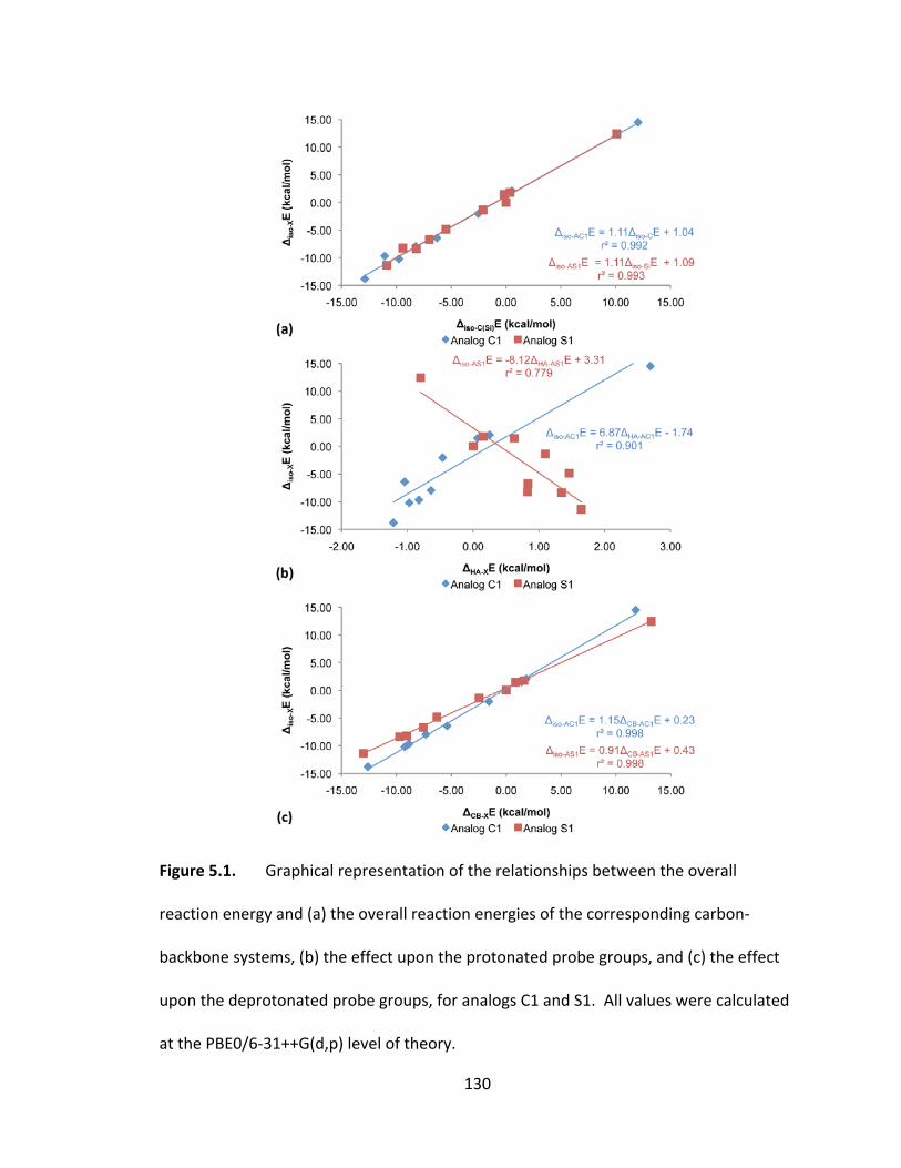
130
Figure 5.1. Graphical representation of the relationships between the overall
reaction energy and (a) the overall reaction energies of the corresponding carbon‐
backbone systems, (b) the effect upon the protonated probe groups, and (c) the effect
upon the deprotonated probe groups, for analogs C1 and S1. All values were calculated
at the PBE0/6‐31++G(d,p) level of theory.
131
5.2) describes the two simultaneous effects: the effect of the substituent on the
protonated probe and the effect of the substituent on the deprotonated probe. In the
carbon backbone systems, ΔCBE dictates the overall reaction energy. ΔHAE does
contribute to the overall effect with the C‐probe, but not in the Si‐system (r2 between
ΔHA‐SiE and Δiso‐SiE is only 0.155). Electron donating groups appear to stabilize HA and
destabilize CB, whereas electron withdrawing groups do the opposite (with the
exception of NH2 substitution, which shows a very small stabilization of HA) in the C‐
system. All groups appear to stabilize HA within the Si‐system, but only Li substitution
destabilizes the CB. In both analogs C1 and S1, ΔCBE shows the most control over the
overall reaction energies (see Figure 5.1c and Table 5.1 for values), with smaller
contributions from ΔHAE (Figure 5.1b). This is consistent with the result for the all‐
carbon backbones with one exception: Analog S1 shows a fair relationship between
ΔHAE and ΔisoE.
In general for both analogs, the electron donating groups yield a stabilization of
the acid species and a destabilization of the conjugate base, whereas the withdrawing
groups show the opposite result. Li‐substitution in analog S1 leads to a destabilization
of the protonated species in direct contrast to the all‐carbon backbone. Within the
deprotonated species, NH2 substitution leads to destabilization in both analogs and CH3
substitution also leads to a destabilization for analog S1.
Using QTAIM to analyze the electron density distribution allows us to dissect
ΔisoE past its constituent parts into the energies of the atoms or groups, themselves.
The atomic energy can be used to determine if a single atom, or group, is stabilized or
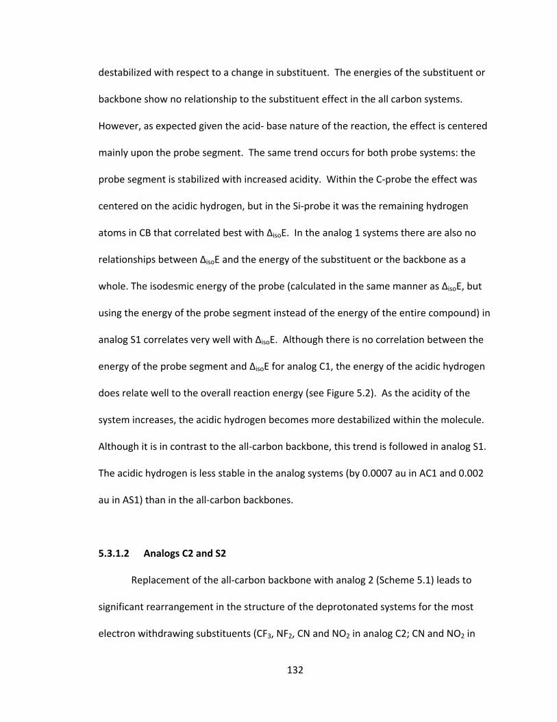
132
destabilized with respect to a change in substituent. The energies of the substituent or
backbone show no relationship to the substituent effect in the all carbon systems.
However, as expected given the acid‐ base nature of the reaction, the effect is centered
mainly upon the probe segment. The same trend occurs for both probe systems: the
probe segment is stabilized with increased acidity. Within the C‐probe the effect was
centered on the acidic hydrogen, but in the Si‐probe it was the remaining hydrogen
atoms in CB that correlated best with ΔisoE. In the analog 1 systems there are also no
relationships between ΔisoE and the energy of the substituent or the backbone as a
whole. The isodesmic energy of the probe (calculated in the same manner as ΔisoE, but
using the energy of the probe segment instead of the energy of the entire compound) in
analog S1 correlates very well with ΔisoE. Although there is no correlation between the
energy of the probe segment and ΔisoE for analog C1, the energy of the acidic hydrogen
does relate well to the overall reaction energy (see Figure 5.2). As the acidity of the
system increases, the acidic hydrogen becomes more destabilized within the molecule.
Although it is in contrast to the all‐carbon backbone, this trend is followed in analog S1.
The acidic hydrogen is less stable in the analog systems (by 0.0007 au in AC1 and 0.002
au in AS1) than in the all‐carbon backbones.
5.3.1.2 Analogs C2 and S2
Replacement of the all‐carbon backbone with analog 2 (Scheme 5.1) leads to
significant rearrangement in the structure of the deprotonated systems for the most
electron withdrawing substituents (CF3, NF2, CN and NO2 in analog C2; CN and NO2 in
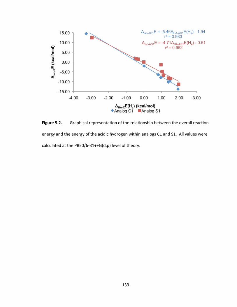
133
Figure 5.2. Graphical representation of the relationship between the overall reaction
energy and the energy of the acidic hydrogen within analogs C1 and S1. All values were
calculated at the PBE0/6‐31++G(d,p) level of theory.
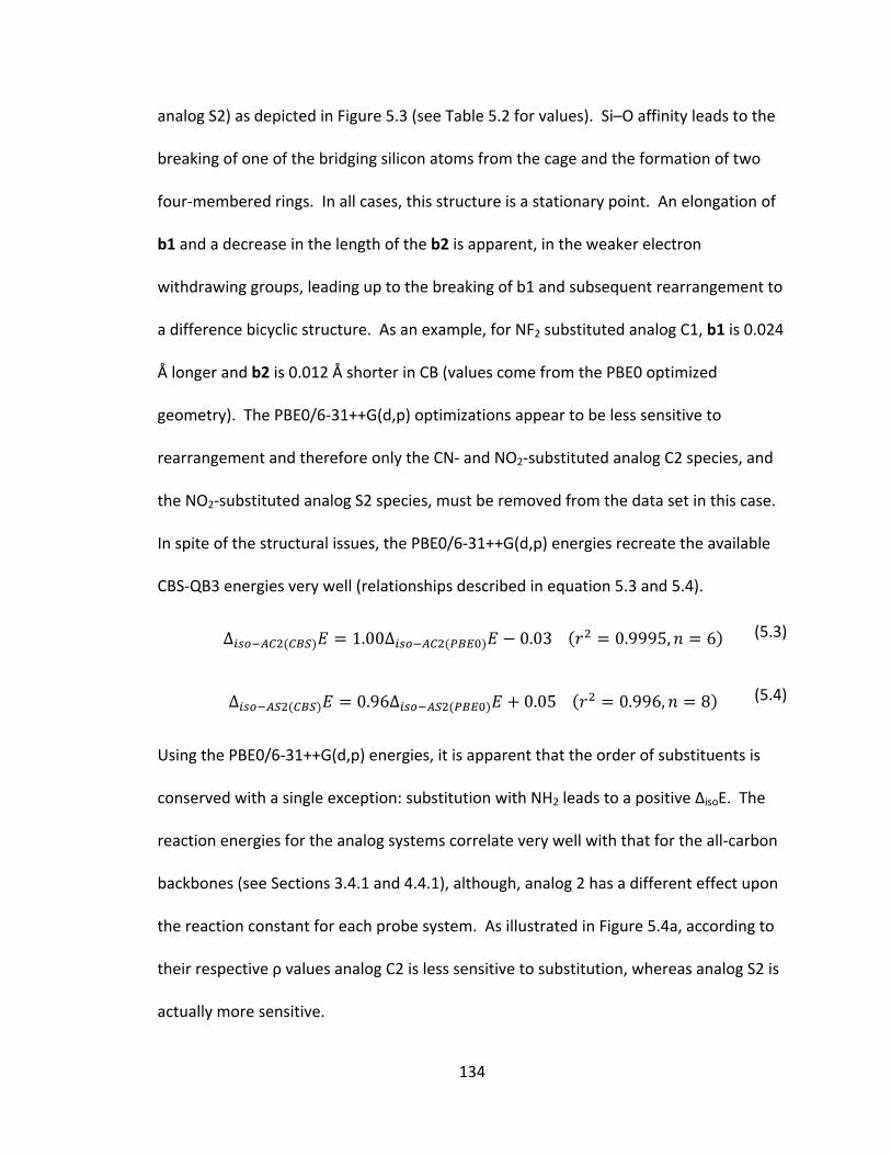
134
analog S2) as depicted in Figure 5.3 (see Table 5.2 for values). Si–O affinity leads to the
breaking of one of the bridging silicon atoms from the cage and the formation of two
four‐membered rings. In all cases, this structure is a stationary point. An elongation of
b1 and a decrease in the length of the b2 is apparent, in the weaker electron
withdrawing groups, leading up to the breaking of b1 and subsequent rearrangement to
a difference bicyclic structure. As an example, for NF2 substituted analog C1, b1 is 0.024
Å longer and b2 is 0.012 Å shorter in CB (values come from the PBE0 optimized
geometry). The PBE0/6‐31++G(d,p) optimizations appear to be less sensitive to
rearrangement and therefore only the CN‐ and NO2‐substituted analog C2 species, and
the NO2‐substituted analog S2 species, must be removed from the data set in this case.
In spite of the structural issues, the PBE0/6‐31++G(d,p) energies recreate the available
CBS‐QB3 energies very well (relationships described in equation 5.3 and 5.4).
∆ 1.00∆ 0.03 0.9995, 6 (5.3)
∆ 0.96∆ 0.05 0.996, 8 (5.4)
Using the PBE0/6‐31++G(d,p) energies, it is apparent that the order of substituents is
conserved with a single exception: substitution with NH2 leads to a positive ΔisoE. The
reaction energies for the analog systems correlate very well with that for the all‐carbon
backbones (see Sections 3.4.1 and 4.4.1), although, analog 2 has a different effect upon
the reaction constant for each probe system. As illustrated in Figure 5.4a, according to
their respective ρ values analog C2 is less sensitive to substitution, whereas analog S2 is
actually more sensitive.
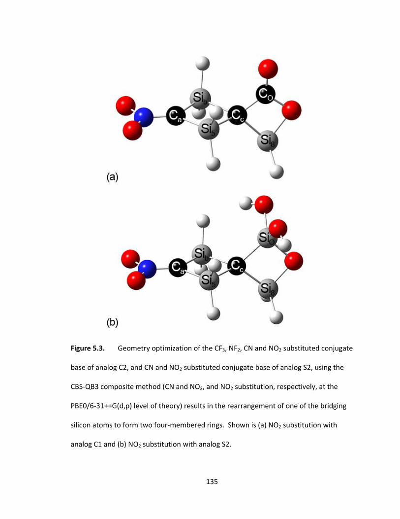
135
Figure 5.3. Geometry optimization of the CF3, NF2, CN and NO2 substituted conjugate
base of analog C2, and CN and NO2 substituted conjugate base of analog S2, using the
CBS‐QB3 composite method (CN and NO2, and NO2 substitution, respectively, at the
PBE0/6‐31++G(d,p) level of theory) results in the rearrangement of one of the bridging
silicon atoms to form two four‐membered rings. Shown is (a) NO2 substitution with
analog C1 and (b) NO2 substitution with analog S2.
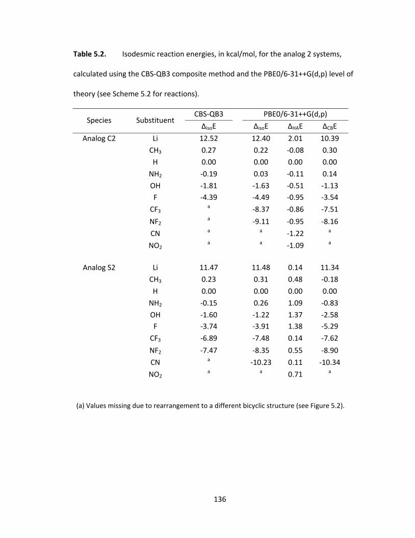
136
Table 5.2. Isodesmic reaction energies, in kcal/mol, for the analog 2 systems,
calculated using the CBS‐QB3 composite method and the PBE0/6‐31++G(d,p) level of
theory (see Scheme 5.2 for reactions).
Species Substituent CBS‐QB3 PBE0/6‐31++G(d,p)
ΔisoE ΔisoE ΔHAE ΔCBE
Analog C2 Li 12.52 12.40 2.01 10.39
CH3 0.27 0.22 ‐0.08 0.30
H 0.00 0.00 0.00 0.00
NH2 ‐0.19 0.03 ‐0.11 0.14
OH ‐1.81 ‐1.63 ‐0.51 ‐1.13F ‐4.39 ‐4.49 ‐0.95 ‐3.54
CF3 a ‐8.37 ‐0.86 ‐7.51
NF2 a ‐9.11 ‐0.95 ‐8.16
CN a a ‐1.22 a
NO2 a a ‐1.09 a
Analog S2 Li 11.47 11.48 0.14 11.34
CH3 0.23 0.31 0.48 ‐0.18
H 0.00 0.00 0.00 0.00
NH2 ‐0.15 0.26 1.09 ‐0.83
OH ‐1.60 ‐1.22 1.37 ‐2.58F ‐3.74 ‐3.91 1.38 ‐5.29
CF3 ‐6.89 ‐7.48 0.14 ‐7.62
NF2 ‐7.47 ‐8.35 0.55 ‐8.90
CN a ‐10.23 0.11 ‐10.34
NO2 a a 0.71 a
(a) Values missing due to rearrangement to a different bicyclic structure (see Figure 5.2).
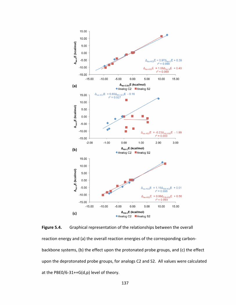
137
Figure 5.4. Graphical representation of the relationships between the overall
reaction energy and (a) the overall reaction energies of the corresponding carbon‐
backbone systems, (b) the effect upon the protonated probe groups, and (c) the effect
upon the deprotonated probe groups, for analogs C2 and S2. All values were calculated
at the PBE0/6‐31++G(d,p) level of theory.
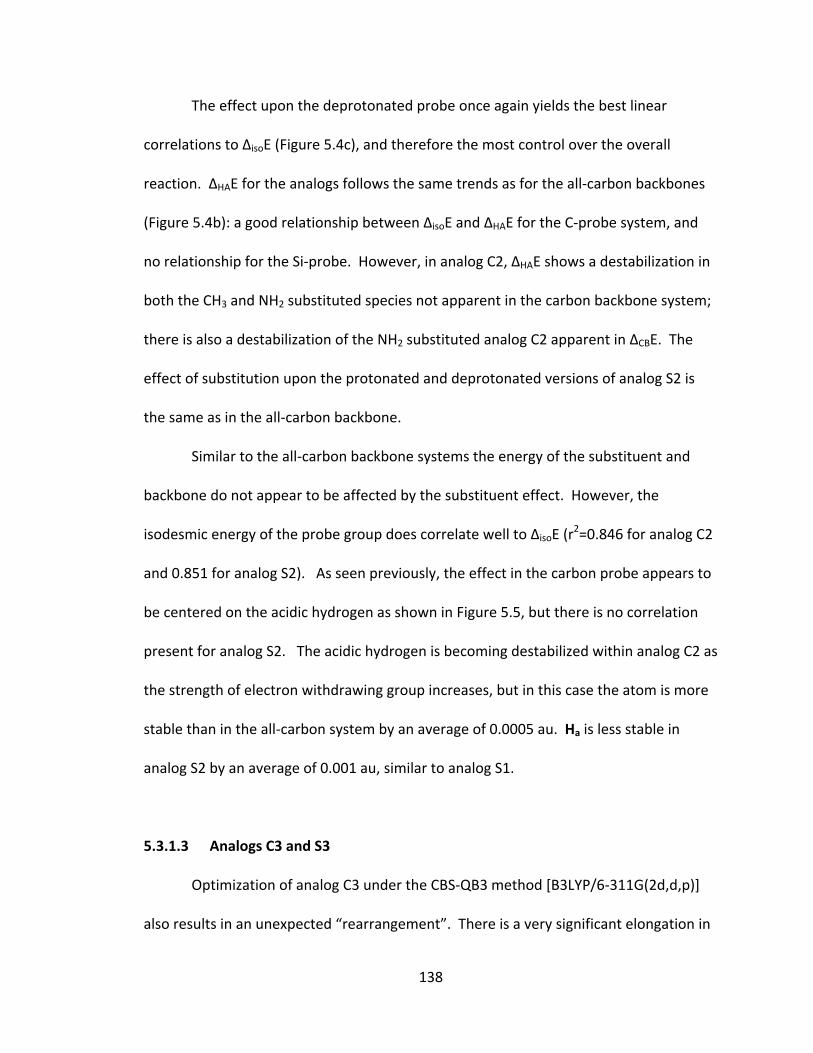
138
The effect upon the deprotonated probe once again yields the best linear
correlations to ΔisoE (Figure 5.4c), and therefore the most control over the overall
reaction. ΔHAE for the analogs follows the same trends as for the all‐carbon backbones
(Figure 5.4b): a good relationship between ΔisoE and ΔHAE for the C‐probe system, and
no relationship for the Si‐probe. However, in analog C2, ΔHAE shows a destabilization in
both the CH3 and NH2 substituted species not apparent in the carbon backbone system;
there is also a destabilization of the NH2 substituted analog C2 apparent in ΔCBE. The
effect of substitution upon the protonated and deprotonated versions of analog S2 is
the same as in the all‐carbon backbone.
Similar to the all‐carbon backbone systems the energy of the substituent and
backbone do not appear to be affected by the substituent effect. However, the
isodesmic energy of the probe group does correlate well to ΔisoE (r2=0.846 for analog C2
and 0.851 for analog S2). As seen previously, the effect in the carbon probe appears to
be centered on the acidic hydrogen as shown in Figure 5.5, but there is no correlation
present for analog S2. The acidic hydrogen is becoming destabilized within analog C2 as
the strength of electron withdrawing group increases, but in this case the atom is more
stable than in the all‐carbon system by an average of 0.0005 au. Ha is less stable in
analog S2 by an average of 0.001 au, similar to analog S1.
5.3.1.3 Analogs C3 and S3
Optimization of analog C3 under the CBS‐QB3 method [B3LYP/6‐311G(2d,d,p)]
also results in an unexpected “rearrangement”. There is a very significant elongation in
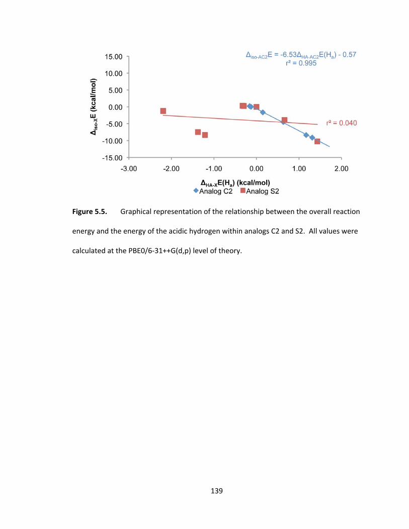
139
Figure 5.5. Graphical representation of the relationship between the overall reaction
energy and the energy of the acidic hydrogen within analogs C2 and S2. All values were
calculated at the PBE0/6‐31++G(d,p) level of theory.
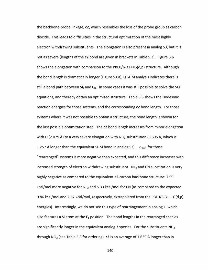
140
the backbone‐probe linkage, c2, which resembles the loss of the probe group as carbon
dioxide. This leads to difficulties in the structural optimization of the most highly
electron withdrawing substituents. The elongation is also present in analog S3, but it is
not as severe (lengths of the c2 bond are given in brackets in Table 5.3). Figure 5.6
shows the elongation with comparison to the PBE0/6‐31++G(d,p) structure. Although
the bond length is dramatically longer (Figure 5.6a), QTAIM analysis indicates there is
still a bond path between Sic and CO. In some cases it was still possible to solve the SCF
equations, and thereby obtain an optimized structure. Table 5.3 shows the isodesmic
reaction energies for those systems, and the corresponding c2 bond length. For those
systems where it was not possible to obtain a structure, the bond length is shown for
the last possible optimization step. The c2 bond length increases from minor elongation
with Li (2.079 Å) to a very severe elongation with NO2 substitution (3.695 Å, which is
1.257 Å longer than the equivalent Si–Si bond in analog S3). ΔisoE for those
“rearranged” systems is more negative than expected, and this difference increases with
increased strength of electron withdrawing substituent. NF2 and CN substitution is very
highly negative as compared to the equivalent all‐carbon backbone structure: 7.99
kcal/mol more negative for NF2 and 5.33 kcal/mol for CN (as compared to the expected
0.86 kcal/mol and 2.67 kcal/mol, respectively, extrapolated from the PBE0/6‐31++G(d,p)
energies). Interestingly, we do not see this type of rearrangement in analog 1, which
also features a Si atom at the Ec position. The bond lengths in the rearranged species
are significantly longer in the equivalent analog 3 species. For the substituents NH2
through NO2 (see Table 5.3 for ordering), c2 is an average of 1.639 Å longer than in
141
Figure 5.6. Apparent removal of the deprotonated probe segment of substituted
analog C3 molecules. Shown as the NH2‐substituted CB with optimized using the (a)
CBS‐QB3 composite method and (b) the PBE0/6‐31++G(d,p) level of theory.

142
Table 5.3. Isodesmic reaction energies, in kcal/mol, for the analog 3 systems,
calculated using the CBS‐QB3 composite method and the PBE0/6‐31++G(d,p) level of
theory (see Scheme 5.2 for reactions). Shown in brackets are the lengths (Å) of the
backbone‐probe linkage in the deprotonated species, which is elongated in the CBS‐QB3
optimized structures.
Species Substituent CBS‐QB3 PBE0/6‐31++G(d,p)
ΔisoE ΔisoE ΔHAE ΔCBE
Analog C3 Li 14.61 (2.079) 13.76 (2.024) 1.76 12.01
CH3 1.50 (2.167) 1.63 (2.056) 0.06 1.56
H 0.00 (2.156) 0.00 (2.050) 0.00 0.00
NH2 ‐5.39 (3.632) 0.73 (2.080) ‐0.09 0.82
OH ‐9.87 (3.651) ‐2.52 (2.111) ‐0.43 ‐2.09F a(3.670) ‐6.38 (2.143) ‐0.74 ‐5.63
CF3 a(3.658) ‐6.64 (2.083) ‐0.33 ‐6.30
NF2 ‐17.32 (3.676) ‐8.91 (2.120) ‐0.51 ‐8.40
CN ‐15.94 (3.666) ‐8.40 (2.080) ‐0.51 ‐7.89
NO2 a(3.695) ‐12.08 (2.149) ‐0.60 ‐11.49
Analog S3 Li 12.32 (2.420) 11.64 (2.391) ‐0.91 12.55
CH3 1.59 (2.422) 1.66 (2.395) 0.20 1.46
H 0.00 (2.420) 0.00 (2.393) 0.00 0.00
NH2 1.68 (2.429) 1.58 (2.400) 0.83 0.75
OH ‐0.36 (2.435) ‐0.87 (2.405) 1.26 ‐2.13F ‐3.10 (2.442) ‐3.79 (2.410) 1.58 ‐5.37
CF3 ‐5.23 (2.426) ‐5.36 (2.399) 0.57 ‐5.93
NF2 ‐6.16 (2.435) ‐6.63 (2.404) 1.13 ‐7.76
CN ‐6.82 (2.424) ‐7.02 (2.396) 0.60 ‐7.62
NO2 a(2.438) ‐9.19 (2.407) 1.35 ‐10.54
(a) Values missing due to apparent removal of deprotonated probe leading to optimization difficulties.
143
analog C1. The distances in the Si‐probe systems are essentially equivalent with a
difference of only 0.036 Å.
The PBE0/6‐31++G(d,p) optimized structures do not appear to be as affected by
this elongation. Although the elongation does appear to be present, all structures were
able to be optimized and led to reaction energies within the expected range. The
difference in the c2 bond length between methods is significant and increases
qualitatively with the strength of electron withdrawing group (ΔCBS‐PBE0c2(Li)=0.055 Å
and ΔCBS‐PBE0c2(CN)=1.586 Å). Once again this elongation is less severe in analog S3.
Even with these drastic structural differences, good correlations exist between the CBS‐
QB3 and PBE0/6‐31++G(d,p) energies (equation 5.5 and 5.6), but the CBS‐QB3 energies
cannot be used as a benchmark in this case.
∆ 1.43∆ 3.87 0.948, 7 (5.5)
∆ 1.01∆ 0.31 0.998, 9 (5.6)
Just as in all other analog systems, the NH2 group in both analog C3 and analog
S3 acts as an electron donating group with a positive ΔisoE. The order, and thus
reactivity, of substituents is conserved with only one other exception: CN substitution
of analog C3 results in a smaller negative ΔisoE than NF2 substitution. The reaction
energies for the analogs show good correlation to their carbon‐backbone counterparts.
The reaction constant (Figure 5.7a) indicates that analog 3 is less sensitive to
substitution than the all‐carbon backbones. Similar to analog 1, ρ for analog C3 and S3
are comparable in magnitude. As in all other systems, the overall reaction energy is
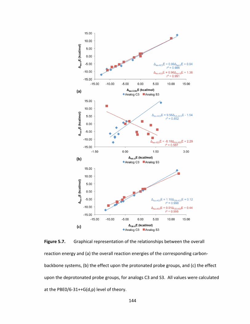
144
Figure 5.7. Graphical representation of the relationships between the overall
reaction energy and (a) the overall reaction energies of the corresponding carbon‐
backbone systems, (b) the effect upon the protonated probe groups, and (c) the effect
upon the deprotonated probe groups, for analogs C3 and S3. All values were calculated
at the PBE0/6‐31++G(d,p) level of theory.
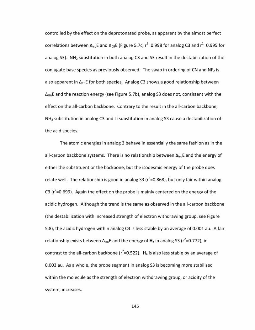
145
controlled by the effect on the deprotonated probe, as apparent by the almost perfect
correlations between ΔisoE and ΔCBE (Figure 5.7c, r2=0.998 for analog C3 and r2=0.995 for
analog S3). NH2 substitution in both analog C3 and S3 result in the destabilization of the
conjugate base species as previously observed. The swap in ordering of CN and NF2 is
also apparent in ΔCBE for both species. Analog C3 shows a good relationship between
ΔHAE and the reaction energy (see Figure 5.7b), analog S3 does not, consistent with the
effect on the all‐carbon backbone. Contrary to the result in the all‐carbon backbone,
NH2 substitution in analog C3 and Li substitution in analog S3 cause a destabilization of
the acid species.
The atomic energies in analog 3 behave in essentially the same fashion as in the
all‐carbon backbone systems. There is no relationship between ΔisoE and the energy of
either the substituent or the backbone, but the isodesmic energy of the probe does
relate well. The relationship is good in analog S3 (r2=0.868), but only fair within analog
C3 (r2=0.699). Again the effect on the probe is mainly centered on the energy of the
acidic hydrogen. Although the trend is the same as observed in the all‐carbon backbone
(the destabilization with increased strength of electron withdrawing group, see Figure
5.8), the acidic hydrogen within analog C3 is less stable by an average of 0.001 au. A fair
relationship exists between ΔisoE and the energy of Ha in analog S3 (r2=0.772), in
contrast to the all‐carbon backbone (r2=0.522). Ha is also less stable by an average of
0.003 au. As a whole, the probe segment in analog S3 is becoming more stabilized
within the molecule as the strength of electron withdrawing group, or acidity of the
system, increases.
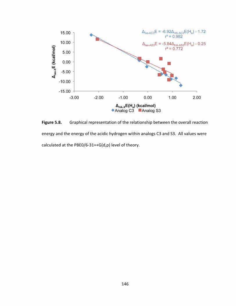
146
Figure 5.8. Graphical representation of the relationship between the overall reaction
energy and the energy of the acidic hydrogen within analogs C3 and S3. All values were
calculated at the PBE0/6‐31++G(d,p) level of theory.
147
5.3.2 Structure and Critical Points in the Electron Density
5.3.2.1 Analogs C1 and S1
Structurally silicon differs from carbon in that it has a greater atomic radius and,
therefore, should form bonds with longer lengths. In analog 1, the bonds between the
silicon at the bridgehead position and the carbon at the bridging position (b1 and b2,
see Scheme 5.3) are both on average 0.364 Å longer than their counterparts in the all‐
carbon backbone. Figure 5.9a shows the relative b1 distance for each probe (value for
the all‐carbon system subtracted from the value for the analog system); b2 shows
essentially the same trend. These two distances both show good correlation to ΔisoE (for
both probes) corresponding to a decrease in length for b1 and an increase in length for
b2 with increasing strength of electron withdrawing group. The trend is the same as
seen in the carbon backbones, but the relationship with b1 in the C‐system is missing
(see Section 3.4.4), and the relationships are only minor in the Si‐system (see Section
4.4.4).
As a result, the interbridgehead distance, a, is also longer in the analog system
by an average of 0.407 Å in analog C1 and 0.414 Å in analog S1 (Figure 5.9b; the
differences between probe systems are mainly attributable to the Li‐substitution, the
backbone rigidity is maintained for all other substituents). Although unrelated in analog
C1, a forms a good relationship with ΔisoE in analog S1, in both cases opposite to what is
seen for the all‐carbon backbone. In the all carbon system length a was controlled by
the pyramidalization at Ea (termed Dev(Ea) for brevity, see equation 5.7 and Figure 5.10),
which appears to be the case for analog S1 only.
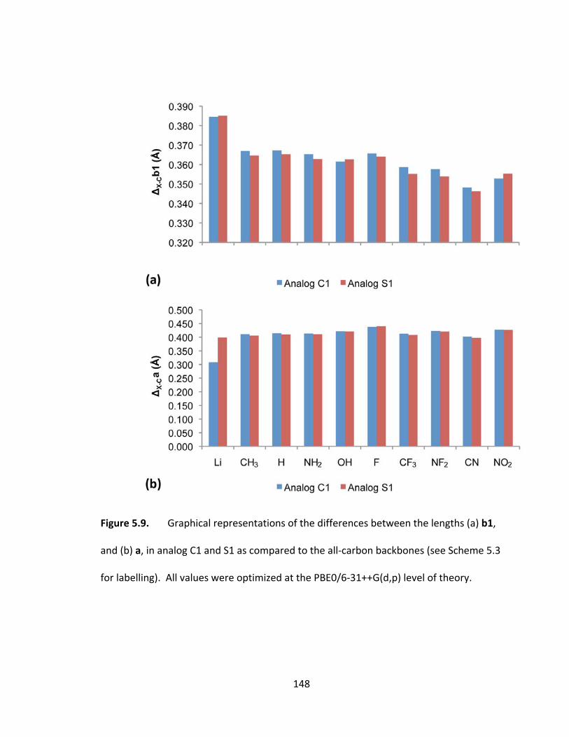
148
Figure 5.9. Graphical representations of the differences between the lengths (a) b1,
and (b) a, in analog C1 and S1 as compared to the all‐carbon backbones (see Scheme 5.3
for labelling). All values were optimized at the PBE0/6‐31++G(d,p) level of theory.
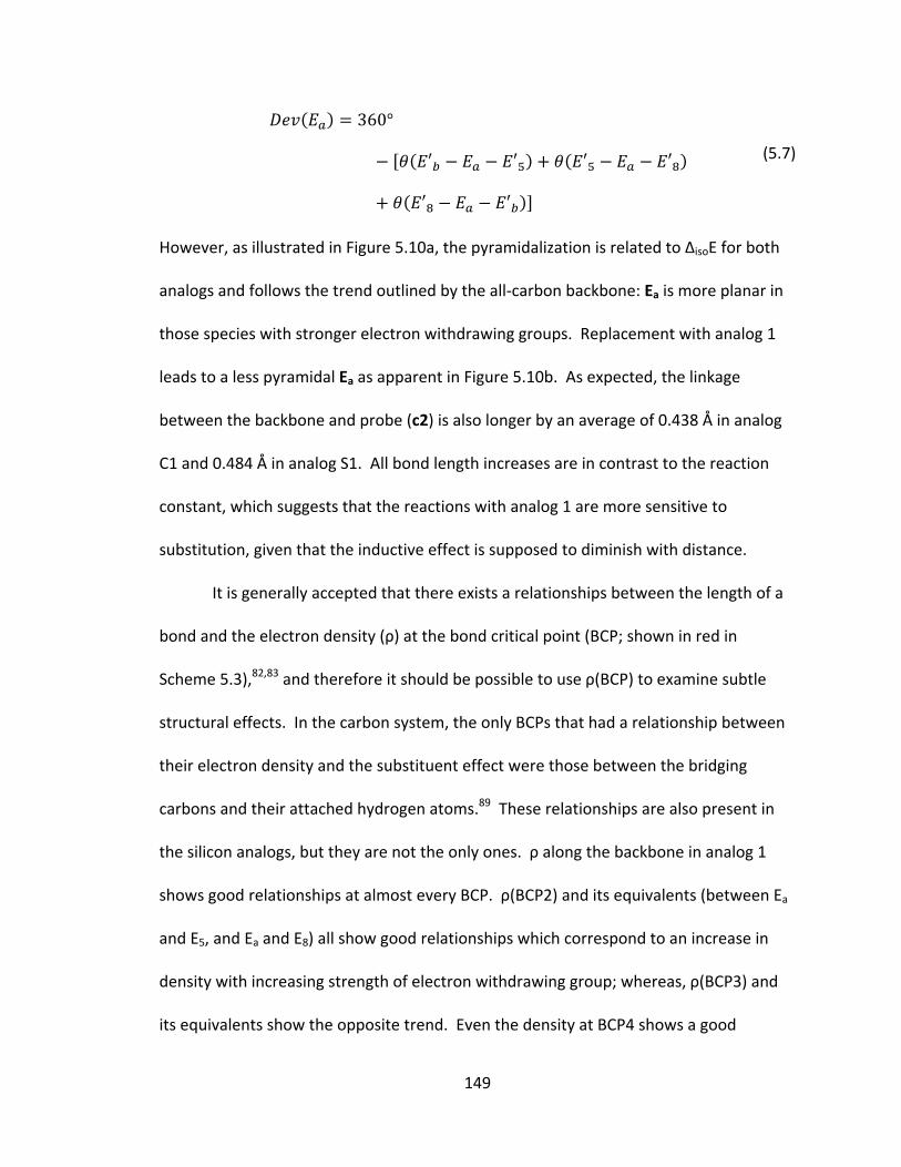
149
360°
(5.7)
However, as illustrated in Figure 5.10a, the pyramidalization is related to ΔisoE for both
analogs and follows the trend outlined by the all‐carbon backbone: Ea is more planar in
those species with stronger electron withdrawing groups. Replacement with analog 1
leads to a less pyramidal Ea as apparent in Figure 5.10b. As expected, the linkage
between the backbone and probe (c2) is also longer by an average of 0.438 Å in analog
C1 and 0.484 Å in analog S1. All bond length increases are in contrast to the reaction
constant, which suggests that the reactions with analog 1 are more sensitive to
substitution, given that the inductive effect is supposed to diminish with distance.
It is generally accepted that there exists a relationships between the length of a
bond and the electron density (ρ) at the bond critical point (BCP; shown in red in
Scheme 5.3),82,83 and therefore it should be possible to use ρ(BCP) to examine subtle
structural effects. In the carbon system, the only BCPs that had a relationship between
their electron density and the substituent effect were those between the bridging
carbons and their attached hydrogen atoms.89 These relationships are also present in
the silicon analogs, but they are not the only ones. ρ along the backbone in analog 1
shows good relationships at almost every BCP. ρ(BCP2) and its equivalents (between Ea
and E5, and Ea and E8) all show good relationships which correspond to an increase in
density with increasing strength of electron withdrawing group; whereas, ρ(BCP3) and
its equivalents show the opposite trend. Even the density at BCP4 shows a good
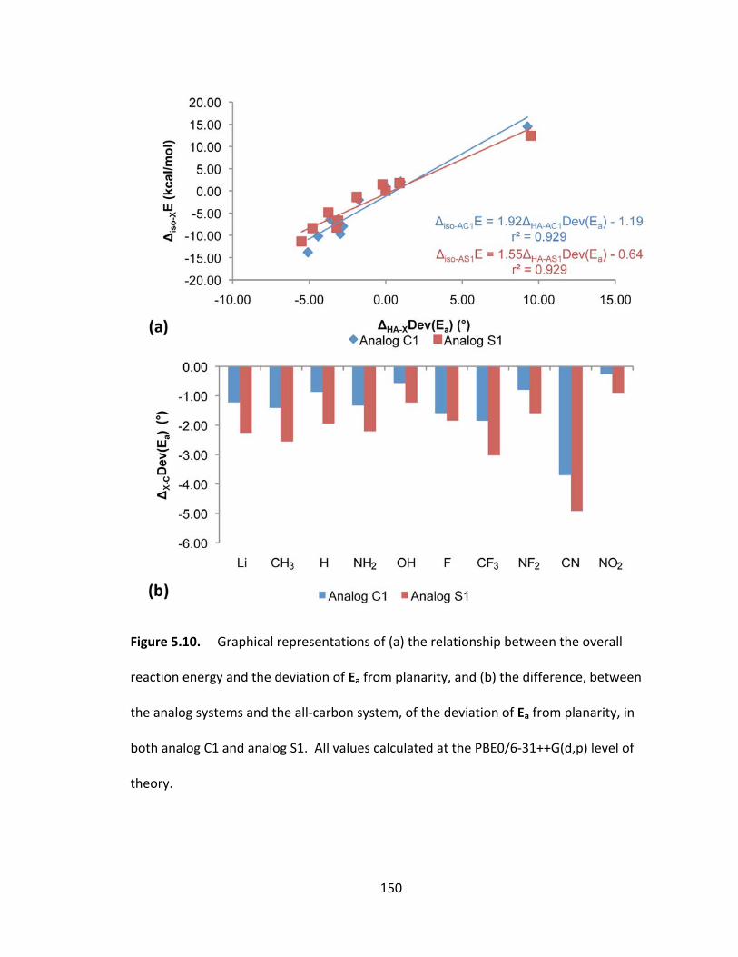
150
Figure 5.10. Graphical representations of (a) the relationship between the overall
reaction energy and the deviation of Ea from planarity, and (b) the difference, between
the analog systems and the all‐carbon system, of the deviation of Ea from planarity, in
both analog C1 and analog S1. All values calculated at the PBE0/6‐31++G(d,p) level of
theory.
151
relationship to the substituent effect in analog C1 (absent in the all‐carbon system and
analog S1). Just as with length a, the electron density at the cage critical point (CCP;
shown in green in Scheme 5.3) correlates well with ΔisoE, this time for both probe
groups. With very few exceptions, the analog systems appear to have less density
within the bonds than the all‐carbon systems.
Although the probe segment was kept constant through all systems, any
difference in transmission through the backbone should be reflected within the probe.
All structural features within the probe group of analog C1 show good relationships with
ΔisoE, as expected from the all carbon system. Although the strength of the linear
correlations may not be the same, the trends in bonds lengths are conserved through all
replacement of the backbone. Both the CO–O and the CO–OH bonds decrease in length
with increasing strength of electron withdrawing group, or acidity, corresponding to the
redistribution of charge upon deprotonation. As expected the length of the OH–H bond
increases with increasing acidity, congruent with the destabilization of the acidic
hydrogen. The C–O bond lengths are minutely shorter in the analog system as in the
all‐carbon, and the O–H bond lengths are minutely longer. All bonds show a decrease in
density with respect to the all‐carbon system, regardless of effect upon length.
In analog S1, the only bond length which forms a good relationship to ΔisoE is
between SiO and Oa, consistent with the all‐carbon backbone. The use of the silicon
based backbone results in a decrease in the length as compared to the all‐carbon
backbone. Another difference between Si and C is silicon’s ability to expand its
coordination to 5 or 6, moving from a tetrahedral structure to a trigonal bipyramidal
152
(TBP) center. The pyramidalization at SiO, defined in equation 5.8, can be used as a
measure of this, with 31.5 ° corresponding to an ideal tetrahedral structure and 0 °
corresponding to a TBP center.
360°
(5.8)
In the all‐carbon backbone, an increase in the strength of electron withdrawing group
resulted in a more planar SiO, suggesting an increase in TBP character. This is conserved
in analog S1, but the use of a silicon based backbone results in a more tetrahedral
probe, as seen in Figure 5.11, with the exception of the unsubstituted species.
5.3.2.2 Analogs C2 and S2
Although unrelated to ΔisoE, the linkage between substituent and backbone (c1;
see Scheme 5.3) in analog 2 is generally shorter than in the all carbon system by an
average of 0.022 Å in analog C2 and 0.007 Å in analog S2 as illustrated in Figure 5.12a.
The shorter bond length is accompanied by a greater electron density at the bond
critical point (BCP1). Although the difference in bond length shows no relationship to
the substituent effect, ΔX‐Cρ(BCP1) in the acid molecules does show a fair linear
correlation (r2=0.766 for analog C2 and r2=0.882 for S2). This is surprising given that no
relationship is present for BCP1 in the all‐carbon system or any other analog. Just as
with c1, c2 is shorter in analog 2 by an average of 0.019 Å with the C‐probe and 0.026 Å
with the Si‐probe.
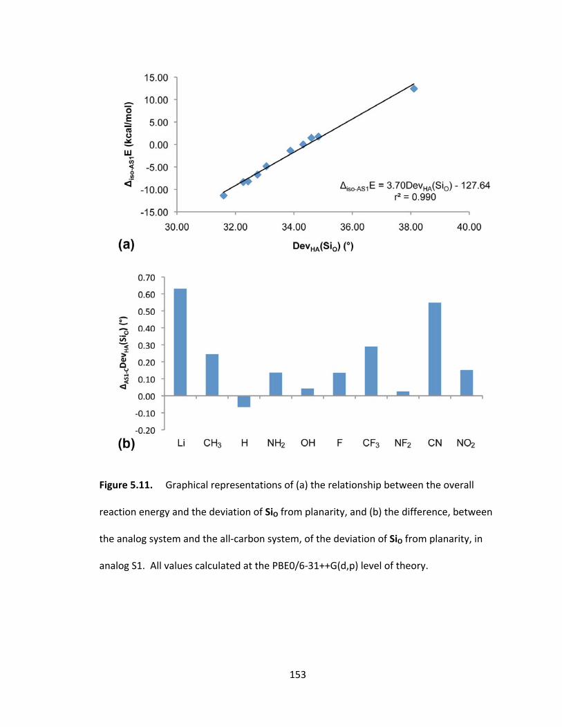
153
Figure 5.11. Graphical representations of (a) the relationship between the overall
reaction energy and the deviation of SiO from planarity, and (b) the difference, between
the analog system and the all‐carbon system, of the deviation of SiO from planarity, in
analog S1. All values calculated at the PBE0/6‐31++G(d,p) level of theory.
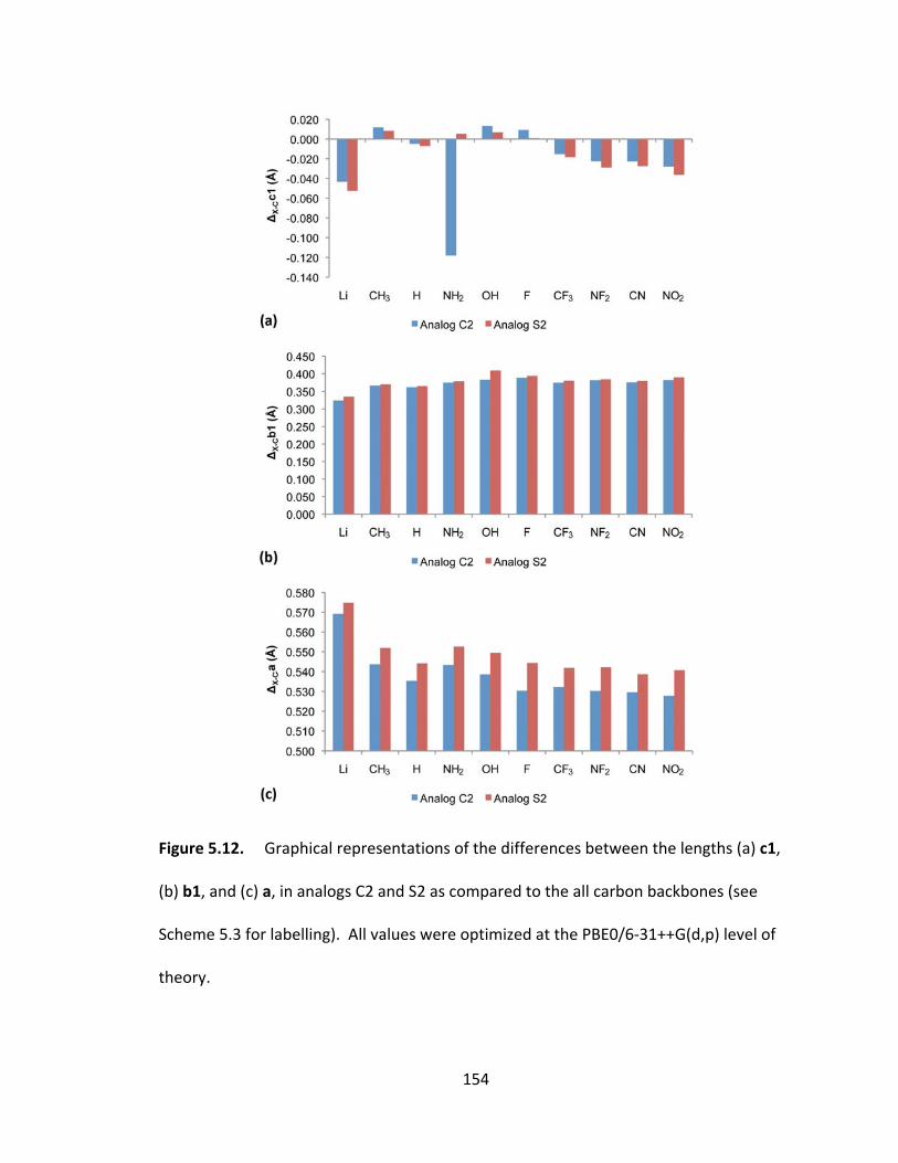
154
Figure 5.12. Graphical representations of the differences between the lengths (a) c1,
(b) b1, and (c) a, in analogs C2 and S2 as compared to the all carbon backbones (see
Scheme 5.3 for labelling). All values were optimized at the PBE0/6‐31++G(d,p) level of
theory.

155
The Si–C bonds in analog 2 (b1 and b2) are both longer than their C–C
counterparts in the all‐carbon backbone, as expected due to the increase in atomic
radius (by an average of 0.371 Å in analog C2 and 0.365 Å in analog S2). The relative b1
distance for each probe is shown in Figure 5.12b. Just as in the all‐carbon system, these
two distances do not show correlation to ΔisoE. The only internal coordinate to show
any relationship to the reaction energy is the distance between bridgehead atoms, a. In
analog C2 the relationship is better than in the all‐carbon system (r2=0.843), but
corresponds to the same trend: a decrease in length as the strength of electron
withdrawing group increases. As expected, a is longer in the analogs than in the all
carbon system by an average of 0.538 Å in analog C2 and 0.548 Å in S2 (Figure 5.12c). a
is controlled by the pyramidalization at Ea: as Ea becomes more planar, a decreases. The
correlation between ΔisoE and Dev(Ea) for analog C2 is good (r2=0.842), as shown in
Figure 5.13a, but poor for analog S2 (r2=0.654). As illustrated in Figure 5.13b, Ea
becomes more planar with the use of the analog 2 backbone.
The relationships with the structure of the probe segment are conserved upon
replacement with analog C2. Both C–O bonds decrease in length and the OH–H bond
increases in length with the electron withdrawing strength of substituent. The use of
analog 2 causes an elongation of the C–O bonds and a reduction in the length of the OH–
H bond as compared to the all‐carbon backbone. The only property conserved within
analog S2 is the pyramidalization at SiO, which results in a more planar probe with the
silicon‐based backbone, as shown in Figure 5.14. This suggests the silicon in the
backbone induces more tetrahedral structure in the probe. In the same manner as the
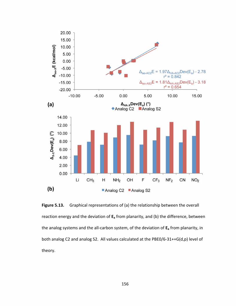
156
Figure 5.13. Graphical representations of (a) the relationship between the overall
reaction energy and the deviation of Ea from planarity, and (b) the difference, between
the analog systems and the all‐carbon system, of the deviation of Ea from planarity, in
both analog C2 and analog S2. All values calculated at the PBE0/6‐31++G(d,p) level of
theory.
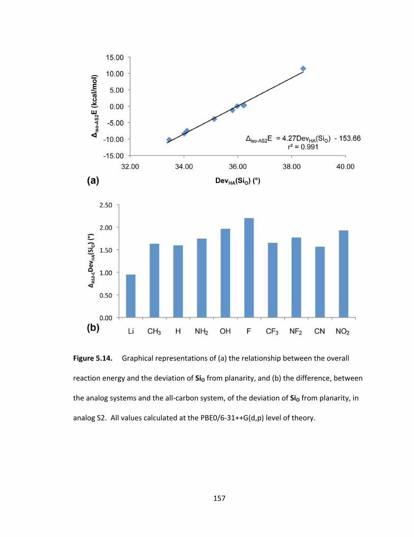
157
Figure 5.14. Graphical representations of (a) the relationship between the overall
reaction energy and the deviation of SiO from planarity, and (b) the difference, between
the analog systems and the all‐carbon system, of the deviation of SiO from planarity, in
analog S2. All values calculated at the PBE0/6‐31++G(d,p) level of theory.
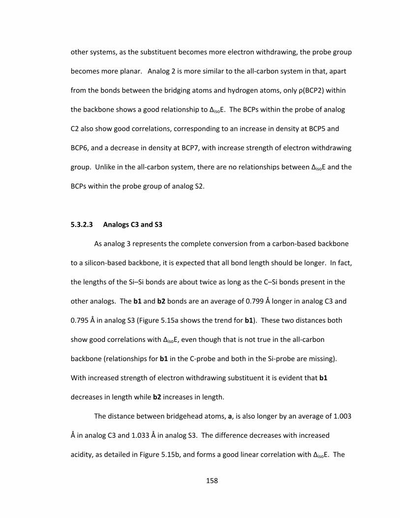
158
other systems, as the substituent becomes more electron withdrawing, the probe group
becomes more planar. Analog 2 is more similar to the all‐carbon system in that, apart
from the bonds between the bridging atoms and hydrogen atoms, only ρ(BCP2) within
the backbone shows a good relationship to ΔisoE. The BCPs within the probe of analog
C2 also show good correlations, corresponding to an increase in density at BCP5 and
BCP6, and a decrease in density at BCP7, with increase strength of electron withdrawing
group. Unlike in the all‐carbon system, there are no relationships between ΔisoE and the
BCPs within the probe group of analog S2.
5.3.2.3 Analogs C3 and S3
As analog 3 represents the complete conversion from a carbon‐based backbone
to a silicon‐based backbone, it is expected that all bond length should be longer. In fact,
the lengths of the Si–Si bonds are about twice as long as the C–Si bonds present in the
other analogs. The b1 and b2 bonds are an average of 0.799 Å longer in analog C3 and
0.795 Å in analog S3 (Figure 5.15a shows the trend for b1). These two distances both
show good correlations with ΔisoE, even though that is not true in the all‐carbon
backbone (relationships for b1 in the C‐probe and both in the Si‐probe are missing).
With increased strength of electron withdrawing substituent it is evident that b1
decreases in length while b2 increases in length.
The distance between bridgehead atoms, a, is also longer by an average of 1.003
Å in analog C3 and 1.033 Å in analog S3. The difference decreases with increased
acidity, as detailed in Figure 5.15b, and forms a good linear correlation with ΔisoE. The
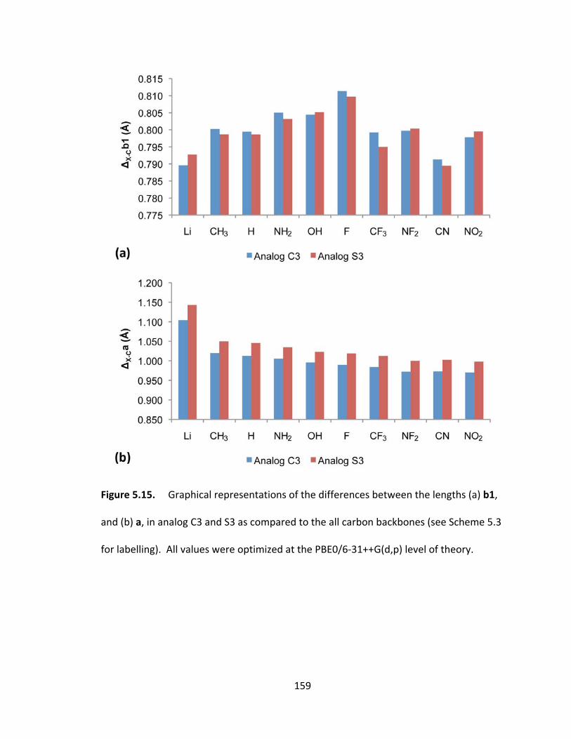
159
Figure 5.15. Graphical representations of the differences between the lengths (a) b1,
and (b) a, in analog C3 and S3 as compared to the all carbon backbones (see Scheme 5.3
for labelling). All values were optimized at the PBE0/6‐31++G(d,p) level of theory.
160
absolute distance also correlates well with the reaction energy in both cases, something
not observed in the all‐ carbon backbone with Si‐probe. The length of a decreases with
increased strength of electron withdrawing group, controlled by a decrease in the
pyramidalization at Ea (r2 between a and Dev(Ea) is 0.996 for analog C3 and 0.997 in
analog S3). As shown in Figure 5.16a, Dev(Ea) forms very good relationships with ΔisoE in
analog 3. In both systems, an increased electron withdrawing character of the
substituents leads to a more planar bridgehead atom. The replacement of silicon atoms
within the probe yields a less planar, or more tetrahedral, Ea.
Just as in analog 1, both c1 and c2 are longer than in the all‐carbon backbone. As
if unaffected by the nature of the bridging atom the relative values of c1 are very similar
(0.373 Å versus 0.378 Å with the C‐probe and 0.373 Å versus 0.375 Å for the Si‐probe, in
analog 1 and analog 3, respectively). Neither shows any relationship to the substituent
effect. Within the probe segment itself, analog C3 follows the same trends as in the all‐
carbon backbone, but analog S3 does not. Just as in analog S2, the only parameter
which shows a good relationship to ΔisoE is Dev(SiO). This relationship corresponds to an
increase in the TBP character of the probe group as the electron withdrawing strength
of the substituent increases (Figure 5.17a). With respect to the all‐carbon backbone,
the relative Dev(SiO) also shows a good relationship with the substituent effect, moving
from more planar to more tetrahedral with increased acidity (Figure 5.17b).
The trends for the electron density at the BCPs appear to be conserved within
analog C3, apart from the addition of a relationship at BCP4 and the CCP. Both
161
Figure 5.16. Graphical representations of (a) the relationship between the overall
reaction energy and the deviation of Ea from planarity, and (b) the difference, between
the analog systems and the all‐carbon system, of the deviation of Ea from planarity, in
both analog C3 and analog S3. All values calculated at the PBE0/6‐31++G(d,p) level of
theory.
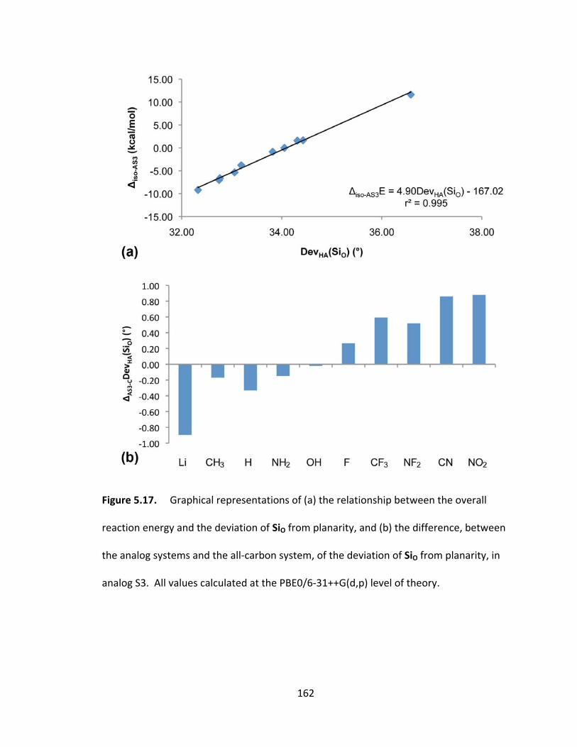
162
Figure 5.17. Graphical representations of (a) the relationship between the overall
reaction energy and the deviation of SiO from planarity, and (b) the difference, between
the analog systems and the all‐carbon system, of the deviation of SiO from planarity, in
analog S3. All values calculated at the PBE0/6‐31++G(d,p) level of theory.
163
relationships correspond to an increase in density with increased acidity. ρ(CCP) also
correlates well with the substituent effect in analog S3, but the relationships within the
probe segment are missing. Just as in the other analog systems, replacement with
silicon atoms within the backbone results in less density within the bonds as compared
to the all‐carbon system.
5.3.3 Atomic Charges and Delocalization Index
Since the “so‐called” inductive effect is the transmission of electron density
through a molecular system, the charges on the atoms should be affected as well as the
bonds. There should be a large effect on the terminal atom, Ea, but according to the
definitions of both mechanisms of transmission the effect should decay with increasing
distance from the substituent. This is seen in all analog systems, but it does not relate
to the substituent effect (see Figures A1.3 to A1.5). In QTAIM, the atomic charge is
defined as in equation 5.9, where ZΩ is the nuclear charge and N(Ω) gives the total
number of electrons.
Ω Ω Ω Ω
Ω
(5.9)
We have previously used the delocalization index (DI) as a description of communication
between the substituent and probe. Defined in equation 5.10 where Fα and Fβ are the
sum of the overlap integrals for atoms A and B, the DI represents the average number of
electrons shared between two atoms. As with all other QTAIM properties, the specific
atomic values can be summed to give the value over a segment within the molecule.
164
, 2| , | 2 , (5.10)
5.3.3.1 Analogs C1 and S1
The overall charge of the substituent also has little relationship with the reaction
energies of the systems. However, the charge of the substituent in the all‐carbon
backbone appears to be indicative of the electron donating or electron withdrawing
nature of the substituent. Both Li and CH3 have an overall positive charge, consistent
with an electron donating effect; whereas all other substituents have an overall negative
charge, consistent with an electron withdrawing effect. Interestingly, the methyl group
appears to be acting as an electron withdrawing group in the both analog 1 conjugate
base molecules. With analog 1, the Li group is the only substituent to have an overall
positive charge and all others are operating to withdraw electron density to themselves.
In both cases the analog backbone appears to decrease the charge on the substituent,
with respect to the all‐carbon backbone, as if the bridgehead silicon atom is donating
more electron density to the substituent.
Due to the atomic replacements, there are significant differences between the
charges on the backbone atoms and which charges correlate well with the reaction
energy. Although the backbone as a whole does not relate to the reaction energy, the
charges of the hydrogen atoms attached to the bridging carbons (H3, H4, and
equivalents) in the all‐carbon backbones all show good linear correlations with ΔisoE.
This trend is conserved within all analogs, and corresponds to the atom becoming more
positive with increased acidity. The main differences occur within the E(‘) atoms
165
themselves. In the carbon system the charges on the bridging atoms show fair
relationships with the reaction energy. This is not the case in analog 1. The Si
bridgehead atoms (Ea and Ec) have a positive charge of about 2.7 au, but the
neighbouring C atoms feature a negative charge (approximately ‐1.3 au), consistent with
the electronegativity difference between both atoms. As may be expected, the
bridgehead atoms have a more positive charge in analog 1, as shown in Figure 5.18a for
Ea and Figure 5.19a for Ec, as compared to the all‐carbon backbone. With replacement
of the bridgehead atoms, the remaining carbon atoms (Cb, C5, and C8), have a
significantly decreased charge as illustrated in Figure 5.18b (in the all‐carbon system the
atoms have a positive charge). Although their absolute values do not, the relative (all‐
carbon value subtracted from analog value) charges in the bridging atoms do show good
relationships to the substituent effect.
Both species of analog 1 also show good relationships with the charge at the
opposite bridgehead atom, Ec, and the reaction energy, something not seen in the all
carbon system with C‐probe Ec is becoming more negative with increase acidity as
detailed in Figure 5.19b, suggesting that some aspect of the charge transmission is
passing through this atom. Both bridgehead Si atoms are more positive than their
carbon backbone counterparts by approximately 2.4 au at Ea and 2.7 au at Ec.
Any change in the transmission of the substituent effect should also be reflected
in the charge on the probe segment. Similar to the carbon system, the total charge on
the protonated probe group shows very good linear correlations with ΔisoE as illustrated
in Figure 5.20a. The probe group is becoming more positive, or less negative, with
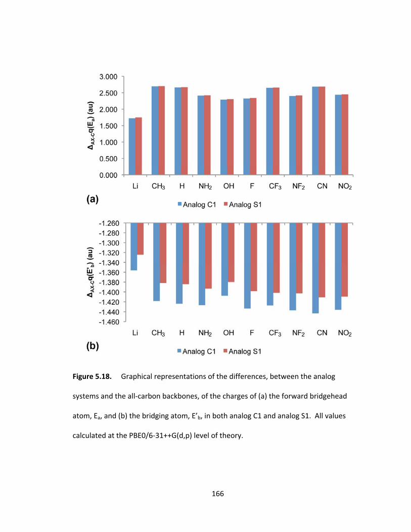
166
Figure 5.18. Graphical representations of the differences, between the analog
systems and the all‐carbon backbones, of the charges of (a) the forward bridgehead
atom, Ea, and (b) the bridging atom, E’b, in both analog C1 and analog S1. All values
calculated at the PBE0/6‐31++G(d,p) level of theory.

167
Figure 5.19. Graphical representations of (a) the difference, between the analog
systems and the all‐carbon system, of the charge on Ec, and (b) the relationship between
the overall reaction energy and the charge on Ec, in both analog C1 and analog S1. All
values calculated at the PBE0/6‐31++G(d,p) level of theory.
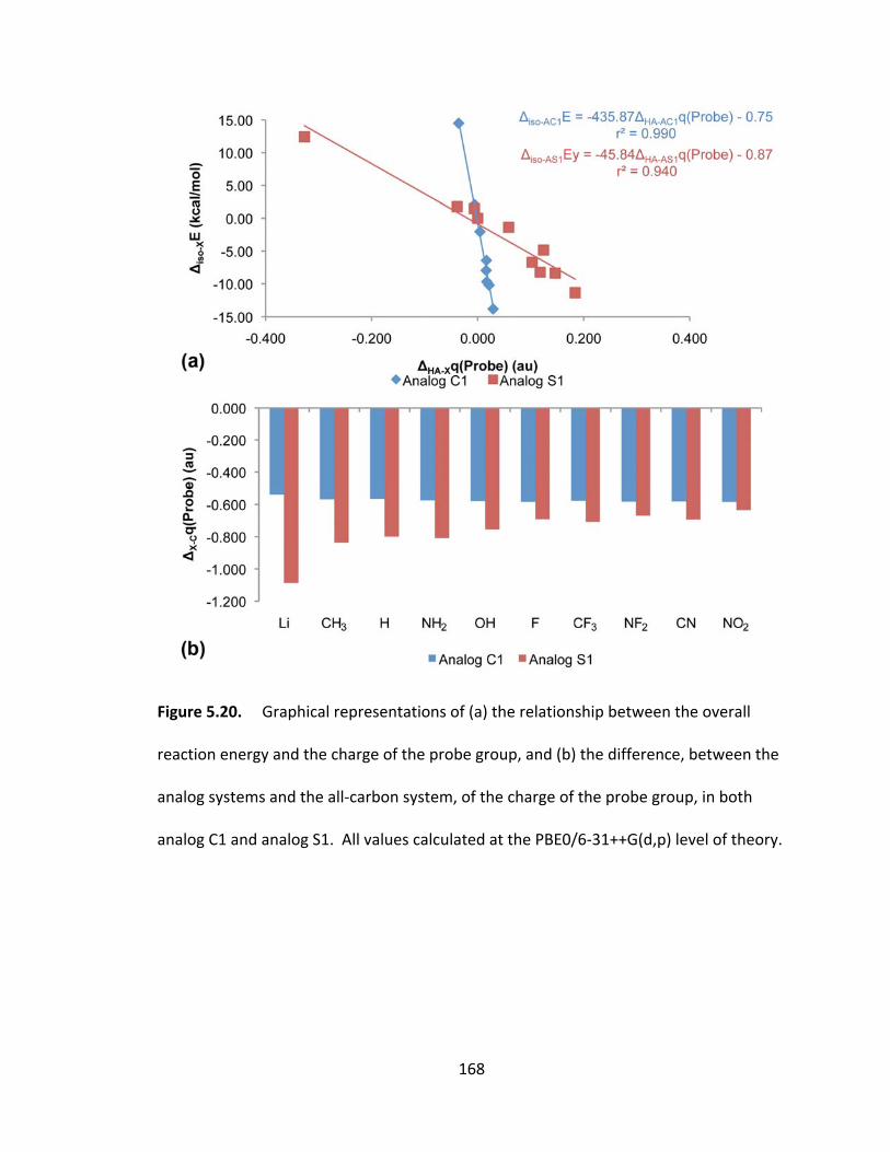
168
Figure 5.20. Graphical representations of (a) the relationship between the overall
reaction energy and the charge of the probe group, and (b) the difference, between the
analog systems and the all‐carbon system, of the charge of the probe group, in both
analog C1 and analog S1. All values calculated at the PBE0/6‐31++G(d,p) level of theory.
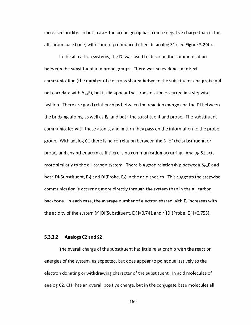
169
increased acidity. In both cases the probe group has a more negative charge than in the
all‐carbon backbone, with a more pronounced effect in analog S1 (see Figure 5.20b).
In the all‐carbon systems, the DI was used to describe the communication
between the substituent and probe groups. There was no evidence of direct
communication (the number of electrons shared between the substituent and probe did
not correlate with ΔisoE), but it did appear that transmission occurred in a stepwise
fashion. There are good relationships between the reaction energy and the DI between
the bridging atoms, as well as Ec, and both the substituent and probe. The substituent
communicates with those atoms, and in turn they pass on the information to the probe
group. With analog C1 there is no correlation between the DI of the substituent, or
probe, and any other atom as if there is no communication occurring. Analog S1 acts
more similarly to the all‐carbon system. There is a good relationship between ΔisoE and
both DI(Substituent, Ec) and DI(Probe, Ec) in the acid species. This suggests the stepwise
communication is occurring more directly through the system than in the all carbon
backbone. In each case, the average number of electron shared with Ec increases with
the acidity of the system (r2[DI(Substituent, Ec)]=0.741 and r2[DI(Probe, Ec)]=0.755).
5.3.3.2 Analogs C2 and S2
The overall charge of the substituent has little relationship with the reaction
energies of the system, as expected, but does appear to point qualitatively to the
electron donating or withdrawing character of the substituent. In acid molecules of
analog C2, CH3 has an overall positive charge, but in the conjugate base molecules all
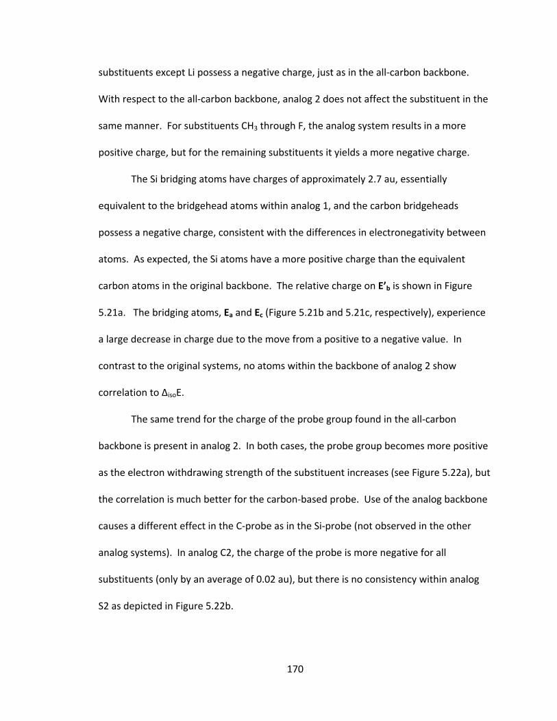
170
substituents except Li possess a negative charge, just as in the all‐carbon backbone.
With respect to the all‐carbon backbone, analog 2 does not affect the substituent in the
same manner. For substituents CH3 through F, the analog system results in a more
positive charge, but for the remaining substituents it yields a more negative charge.
The Si bridging atoms have charges of approximately 2.7 au, essentially
equivalent to the bridgehead atoms within analog 1, and the carbon bridgeheads
possess a negative charge, consistent with the differences in electronegativity between
atoms. As expected, the Si atoms have a more positive charge than the equivalent
carbon atoms in the original backbone. The relative charge on E’b is shown in Figure
5.21a. The bridging atoms, Ea and Ec (Figure 5.21b and 5.21c, respectively), experience
a large decrease in charge due to the move from a positive to a negative value. In
contrast to the original systems, no atoms within the backbone of analog 2 show
correlation to ΔisoE.
The same trend for the charge of the probe group found in the all‐carbon
backbone is present in analog 2. In both cases, the probe group becomes more positive
as the electron withdrawing strength of the substituent increases (see Figure 5.22a), but
the correlation is much better for the carbon‐based probe. Use of the analog backbone
causes a different effect in the C‐probe as in the Si‐probe (not observed in the other
analog systems). In analog C2, the charge of the probe is more negative for all
substituents (only by an average of 0.02 au), but there is no consistency within analog
S2 as depicted in Figure 5.22b.
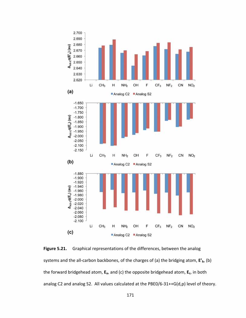
171
Figure 5.21. Graphical representations of the differences, between the analog
systems and the all‐carbon backbones, of the charges of (a) the bridging atom, E’b, (b)
the forward bridgehead atom, Ea, and (c) the opposite bridgehead atom, Ec, in both
analog C2 and analog S2. All values calculated at the PBE0/6‐31++G(d,p) level of theory.
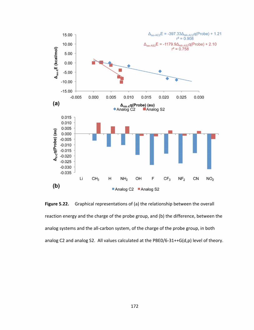
172
Figure 5.22. Graphical representations of (a) the relationship between the overall
reaction energy and the charge of the probe group, and (b) the difference, between the
analog systems and the all‐carbon system, of the charge of the probe group, in both
analog C2 and analog S2. All values calculated at the PBE0/6‐31++G(d,p) level of theory.
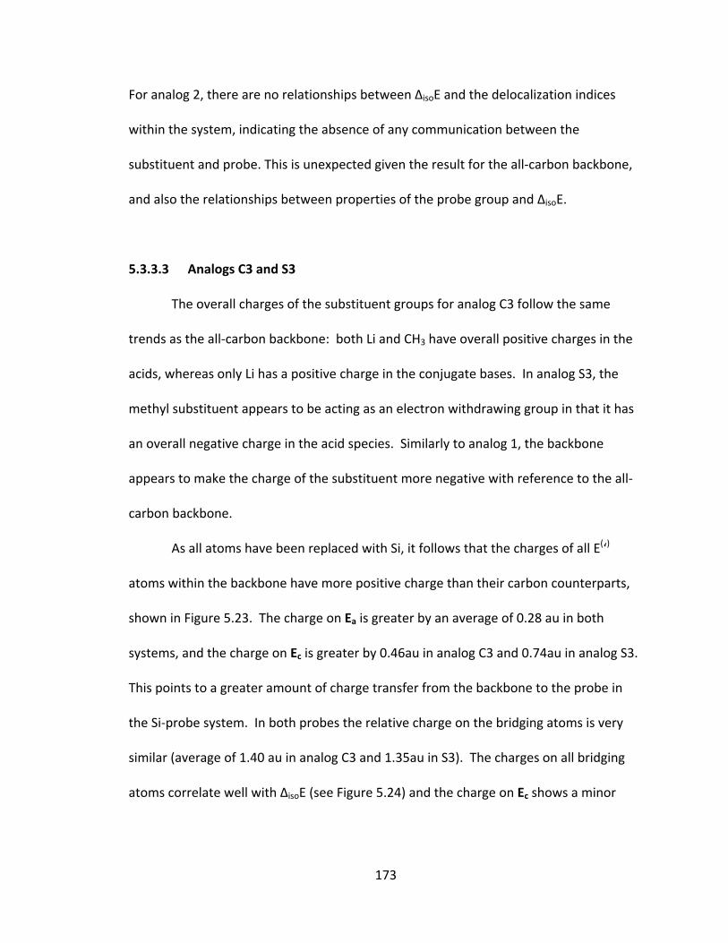
173
For analog 2, there are no relationships between ΔisoE and the delocalization indices
within the system, indicating the absence of any communication between the
substituent and probe. This is unexpected given the result for the all‐carbon backbone,
and also the relationships between properties of the probe group and ΔisoE.
5.3.3.3 Analogs C3 and S3
The overall charges of the substituent groups for analog C3 follow the same
trends as the all‐carbon backbone: both Li and CH3 have overall positive charges in the
acids, whereas only Li has a positive charge in the conjugate bases. In analog S3, the
methyl substituent appears to be acting as an electron withdrawing group in that it has
an overall negative charge in the acid species. Similarly to analog 1, the backbone
appears to make the charge of the substituent more negative with reference to the all‐
carbon backbone.
As all atoms have been replaced with Si, it follows that the charges of all E(‘)
atoms within the backbone have more positive charge than their carbon counterparts,
shown in Figure 5.23. The charge on Ea is greater by an average of 0.28 au in both
systems, and the charge on Ec is greater by 0.46au in analog C3 and 0.74au in analog S3.
This points to a greater amount of charge transfer from the backbone to the probe in
the Si‐probe system. In both probes the relative charge on the bridging atoms is very
similar (average of 1.40 au in analog C3 and 1.35au in S3). The charges on all bridging
atoms correlate well with ΔisoE (see Figure 5.24) and the charge on Ec shows a minor
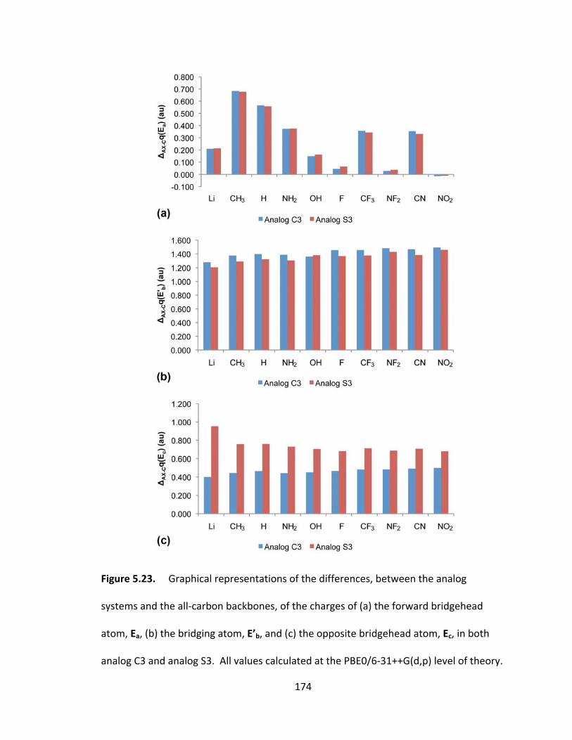
174
Figure 5.23. Graphical representations of the differences, between the analog
systems and the all‐carbon backbones, of the charges of (a) the forward bridgehead
atom, Ea, (b) the bridging atom, E’b, and (c) the opposite bridgehead atom, Ec, in both
analog C3 and analog S3. All values calculated at the PBE0/6‐31++G(d,p) level of theory.
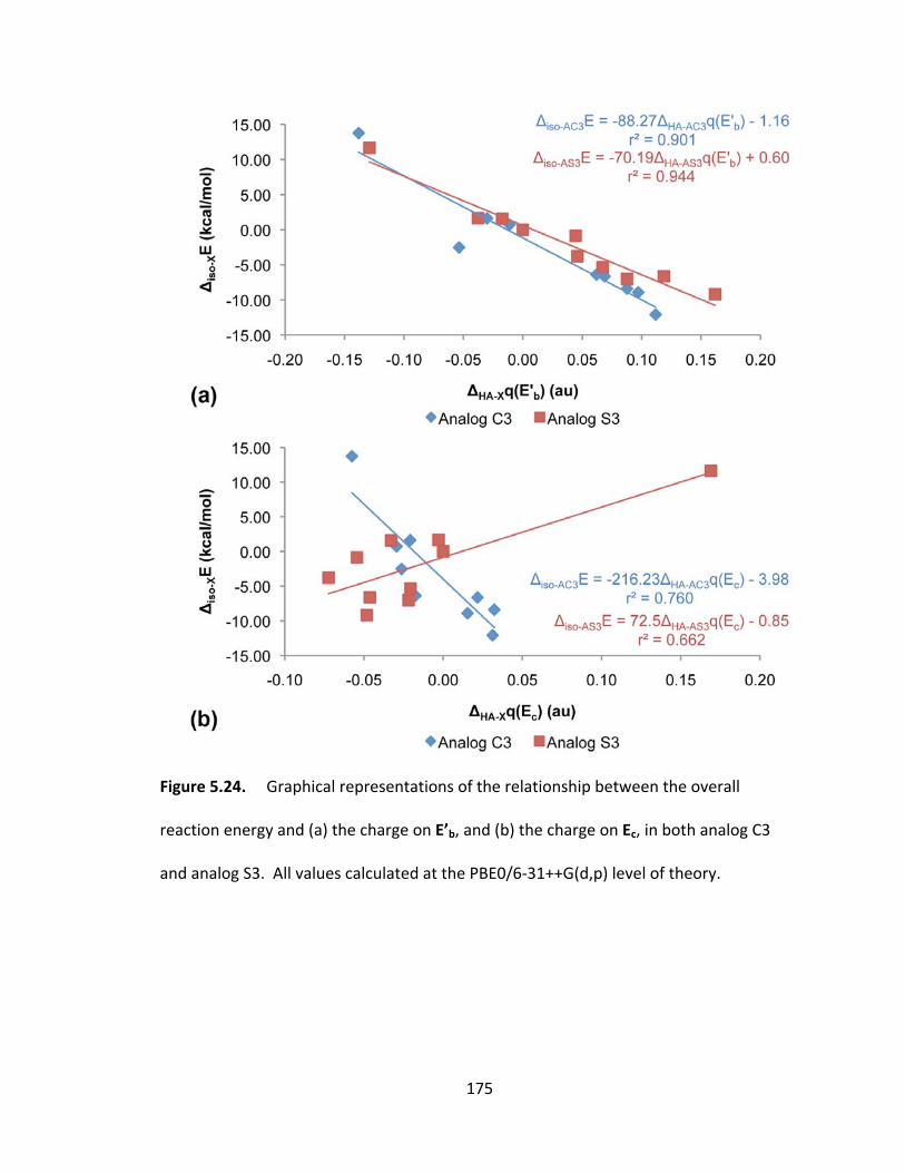
175
Figure 5.24. Graphical representations of the relationship between the overall
reaction energy and (a) the charge on E’b, and (b) the charge on Ec, in both analog C3
and analog S3. All values calculated at the PBE0/6‐31++G(d,p) level of theory.

176
correlation; all corresponding to an increase in charge with increased electron
withdrawing strength of the substituent, apart from the charge on Ec in analog S3.
Just as in all other analogs, the trends observed in the charge of the probe group
in the all‐carbon backbone are conserved in analog 3: as the strength of electron
withdrawing substituent increases, the charge on the probe segment becomes more
positive as illustrated in Figure 5.25a. For the most part the probe group is more
negative in the analog than in the carbon system, by an average of 0.57 au for the C‐
probe and 0.73 au for the Si‐probe. As apparent in Figure 5.25b, the Si‐probe appears to
be more sensitive to the change in backbone. Given that there is a larger, and more
consistent, effect in analogs 1 and 3, it appears that the main effect upon transmission is
by the Si atoms at the bridgehead positions.
In analog C3, the only atom along the bond path that communicates with the
substituent is Ec. DI(Substituent, Ec) forms a good relationship with the reaction energy
(r2=0.811), and corresponds to an increased number of electrons shared between the
substituent and Ec with increased strength of electron withdrawing group. There are no
relationships between DI(Probe, B) and the substituent effect. In analog S3 the stepwise
transmission using Ec is conserved. As this relationship is also present in analog 1, it
appears that Si atoms in the bridgehead positions promote a more direct mode of
transmission through the molecule.
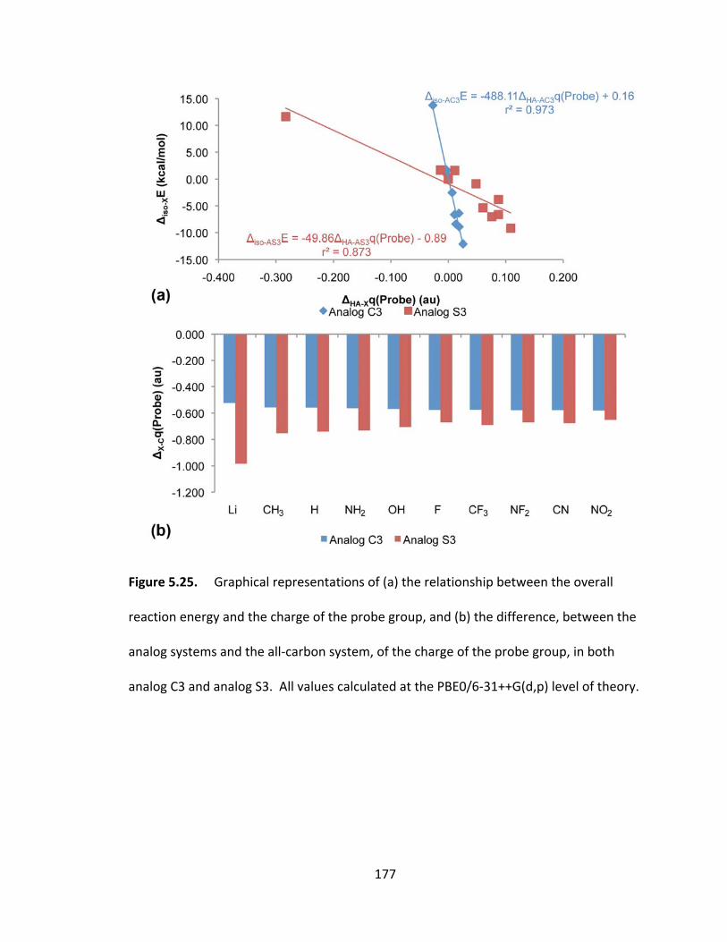
177
Figure 5.25. Graphical representations of (a) the relationship between the overall
reaction energy and the charge of the probe group, and (b) the difference, between the
analog systems and the all‐carbon system, of the charge of the probe group, in both
analog C3 and analog S3. All values calculated at the PBE0/6‐31++G(d,p) level of theory.
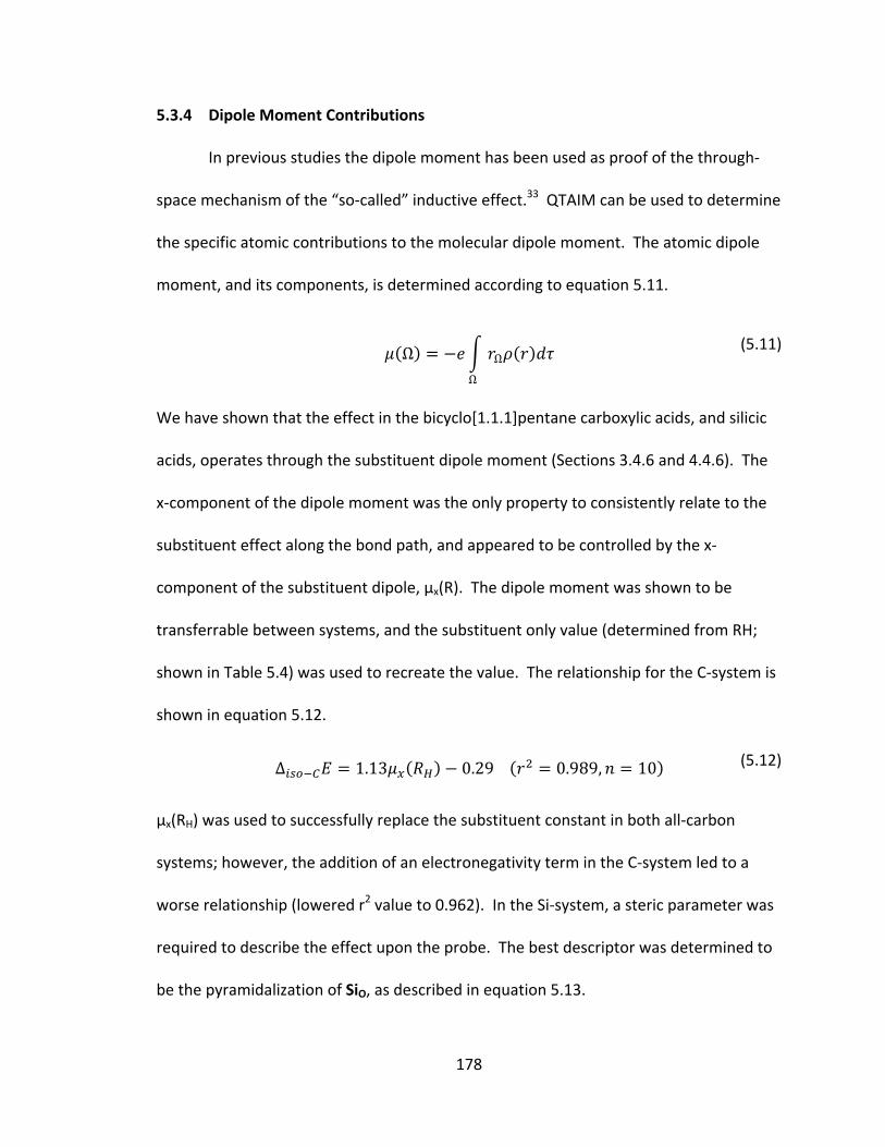
178
5.3.4 Dipole Moment Contributions
In previous studies the dipole moment has been used as proof of the through‐
space mechanism of the “so‐called” inductive effect.33 QTAIM can be used to determine
the specific atomic contributions to the molecular dipole moment. The atomic dipole
moment, and its components, is determined according to equation 5.11.
Ω Ω
Ω
(5.11)
We have shown that the effect in the bicyclo[1.1.1]pentane carboxylic acids, and silicic
acids, operates through the substituent dipole moment (Sections 3.4.6 and 4.4.6). The
x‐component of the dipole moment was the only property to consistently relate to the
substituent effect along the bond path, and appeared to be controlled by the x‐
component of the substituent dipole, μx(R). The dipole moment was shown to be
transferrable between systems, and the substituent only value (determined from RH;
shown in Table 5.4) was used to recreate the value. The relationship for the C‐system is
shown in equation 5.12.
∆ 1.13 0.29 0.989, 10 (5.12)
μx(RH) was used to successfully replace the substituent constant in both all‐carbon
systems; however, the addition of an electronegativity term in the C‐system led to a
worse relationship (lowered r2 value to 0.962). In the Si‐system, a steric parameter was
required to describe the effect upon the probe. The best descriptor was determined to
be the pyramidalization of SiO, as described in equation 5.13.
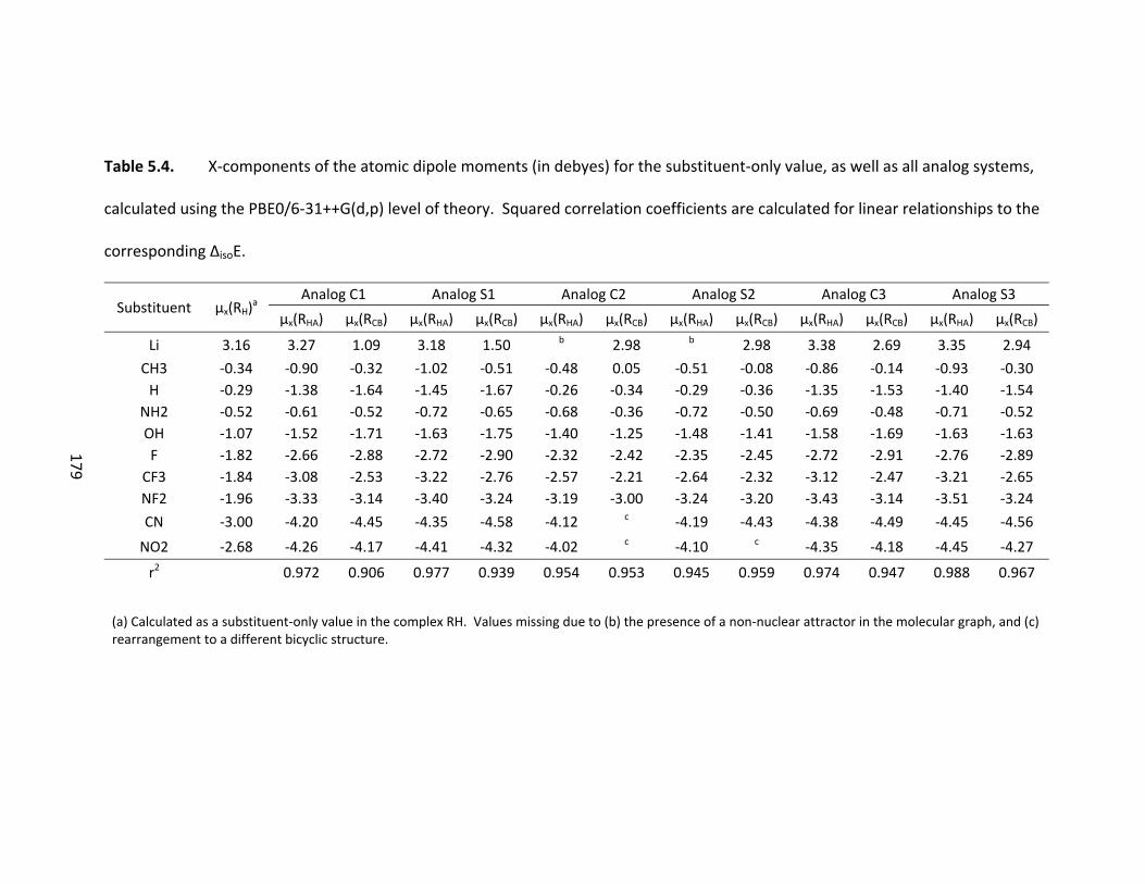
179
Table 5.4. X‐components of the atomic dipole moments (in debyes) for the substituent‐only value, as well as all analog systems,
calculated using the PBE0/6‐31++G(d,p) level of theory. Squared correlation coefficients are calculated for linear relationships to the
corresponding ΔisoE.
Substituent μx(RH)a
Analog C1 Analog S1 Analog C2 Analog S2 Analog C3 Analog S3
μx(RHA) μx(RCB) μx(RHA) μx(RCB) μx(RHA) μx(RCB) μx(RHA) μx(RCB) μx(RHA) μx(RCB) μx(RHA) μx(RCB)
Li 3.16 3.27 1.09 3.18 1.50 b 2.98 b 2.98 3.38 2.69 3.35 2.94 CH3 ‐0.34 ‐0.90 ‐0.32 ‐1.02 ‐0.51 ‐0.48 0.05 ‐0.51 ‐0.08 ‐0.86 ‐0.14 ‐0.93 ‐0.30H ‐0.29 ‐1.38 ‐1.64 ‐1.45 ‐1.67 ‐0.26 ‐0.34 ‐0.29 ‐0.36 ‐1.35 ‐1.53 ‐1.40 ‐1.54
NH2 ‐0.52 ‐0.61 ‐0.52 ‐0.72 ‐0.65 ‐0.68 ‐0.36 ‐0.72 ‐0.50 ‐0.69 ‐0.48 ‐0.71 ‐0.52OH ‐1.07 ‐1.52 ‐1.71 ‐1.63 ‐1.75 ‐1.40 ‐1.25 ‐1.48 ‐1.41 ‐1.58 ‐1.69 ‐1.63 ‐1.63F ‐1.82 ‐2.66 ‐2.88 ‐2.72 ‐2.90 ‐2.32 ‐2.42 ‐2.35 ‐2.45 ‐2.72 ‐2.91 ‐2.76 ‐2.89
CF3 ‐1.84 ‐3.08 ‐2.53 ‐3.22 ‐2.76 ‐2.57 ‐2.21 ‐2.64 ‐2.32 ‐3.12 ‐2.47 ‐3.21 ‐2.65NF2 ‐1.96 ‐3.33 ‐3.14 ‐3.40 ‐3.24 ‐3.19 ‐3.00 ‐3.24 ‐3.20 ‐3.43 ‐3.14 ‐3.51 ‐3.24
CN ‐3.00 ‐4.20 ‐4.45 ‐4.35 ‐4.58 ‐4.12 c ‐4.19 ‐4.43 ‐4.38 ‐4.49 ‐4.45 ‐4.56
NO2 ‐2.68 ‐4.26 ‐4.17 ‐4.41 ‐4.32 ‐4.02 c ‐4.10 c ‐4.35 ‐4.18 ‐4.45 ‐4.27
r2 0.972 0.906 0.977 0.939 0.954 0.953 0.945 0.959 0.974 0.947 0.988 0.967
(a) Calculated as a substituent‐only value in the complex RH. Values missing due to (b) the presence of a non‐nuclear attractor in the molecular graph, and (c) rearrangement to a different bicyclic structure.
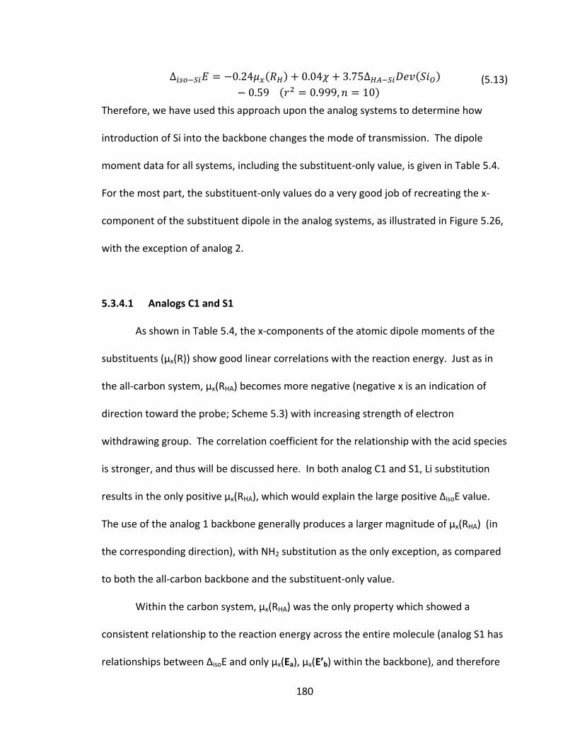
180
∆ 0.24 0.04 3.75Δ0.59 0.999, 10
(5.13)
Therefore, we have used this approach upon the analog systems to determine how
introduction of Si into the backbone changes the mode of transmission. The dipole
moment data for all systems, including the substituent‐only value, is given in Table 5.4.
For the most part, the substituent‐only values do a very good job of recreating the x‐
component of the substituent dipole in the analog systems, as illustrated in Figure 5.26,
with the exception of analog 2.
5.3.4.1 Analogs C1 and S1
As shown in Table 5.4, the x‐components of the atomic dipole moments of the
substituents (μx(R)) show good linear correlations with the reaction energy. Just as in
the all‐carbon system, μx(RHA) becomes more negative (negative x is an indication of
direction toward the probe; Scheme 5.3) with increasing strength of electron
withdrawing group. The correlation coefficient for the relationship with the acid species
is stronger, and thus will be discussed here. In both analog C1 and S1, Li substitution
results in the only positive μx(RHA), which would explain the large positive ΔisoE value.
The use of the analog 1 backbone generally produces a larger magnitude of μx(RHA) (in
the corresponding direction), with NH2 substitution as the only exception, as compared
to both the all‐carbon backbone and the substituent‐only value.
Within the carbon system, μx(RHA) was the only property which showed a
consistent relationship to the reaction energy across the entire molecule (analog S1 has
relationships between ΔisoE and only μx(Ea), μx(E’b) within the backbone), and therefore
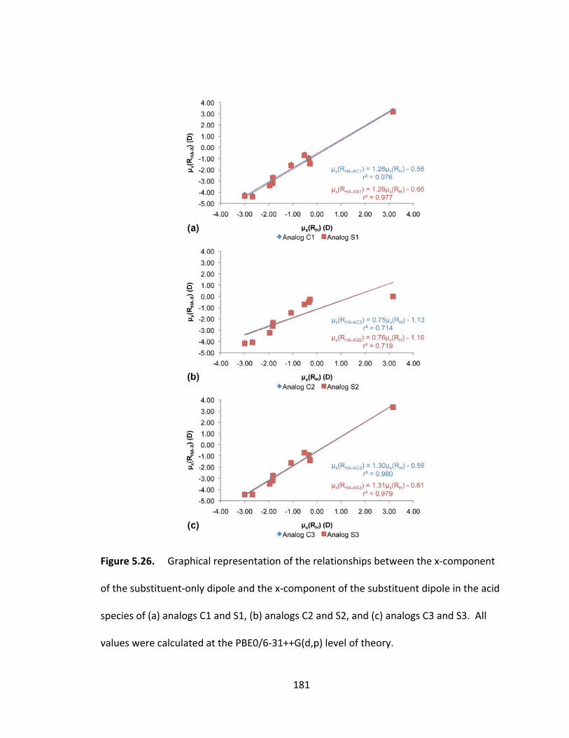
181
Figure 5.26. Graphical representation of the relationships between the x‐component
of the substituent‐only dipole and the x‐component of the substituent dipole in the acid
species of (a) analogs C1 and S1, (b) analogs C2 and S2, and (c) analogs C3 and S3. All
values were calculated at the PBE0/6‐31++G(d,p) level of theory.
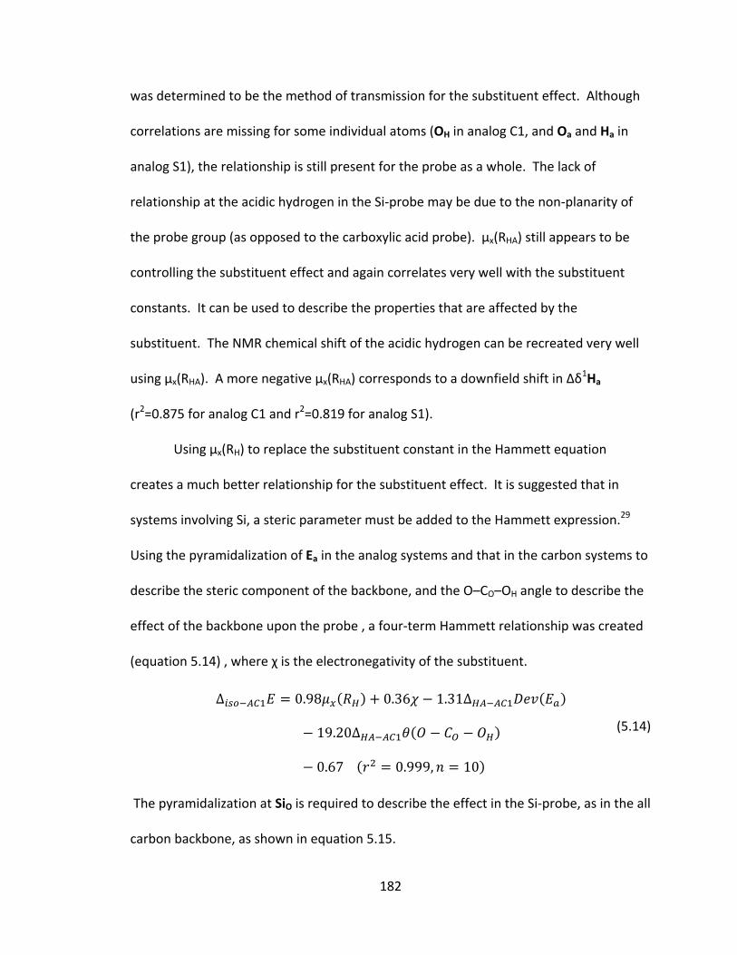
182
was determined to be the method of transmission for the substituent effect. Although
correlations are missing for some individual atoms (OH in analog C1, and Oa and Ha in
analog S1), the relationship is still present for the probe as a whole. The lack of
relationship at the acidic hydrogen in the Si‐probe may be due to the non‐planarity of
the probe group (as opposed to the carboxylic acid probe). μx(RHA) still appears to be
controlling the substituent effect and again correlates very well with the substituent
constants. It can be used to describe the properties that are affected by the
substituent. The NMR chemical shift of the acidic hydrogen can be recreated very well
using μx(RHA). A more negative μx(RHA) corresponds to a downfield shift in Δδ1Ha
(r2=0.875 for analog C1 and r2=0.819 for analog S1).
Using μx(RH) to replace the substituent constant in the Hammett equation
creates a much better relationship for the substituent effect. It is suggested that in
systems involving Si, a steric parameter must be added to the Hammett expression.29
Using the pyramidalization of Ea in the analog systems and that in the carbon systems to
describe the steric component of the backbone, and the O–CO–OH angle to describe the
effect of the backbone upon the probe , a four‐term Hammett relationship was created
(equation 5.14) , where χ is the electronegativity of the substituent.
∆ 0.98 0.36 1.31Δ
19.20Δ
0.67 0.999, 10
(5.14)
The pyramidalization at SiO is required to describe the effect in the Si‐probe, as in the all
carbon backbone, as shown in equation 5.15.

183
Δ 0.57 1.01 1.55Δ
7.41Δ 1.86 0.999, 10(5.15)
5.3.4.2 Analogs C2 and S2
Just as in the all‐carbon system, the x‐component of the substituent dipole
relates very well to the substituent effect in both species, as described in Table 5.4,
despite the missing values. As the electron withdrawing strength of the substituent
increases, the μx(R) becomes more negative (seen for both HA and CB). Comparison of
analog 2 to the carbon system does not yield a consistent trend: H, NH2, and OH result
in a smaller magnitudes (also CH3 and F with the Si‐probe), but all others show an
increase in the magnitude of μx(RHA). Apart from the unsubstituted species, all
substituents show an increase in the magnitude in the negative direction with respect to
the substituent only value.
μx is the only property to show consistent correlations to ΔisoE along the bond
path, as expected given the results for the all‐carbon backbone, and therefore was
determined to be the method of transmission for the substituent effect. μx for all
backbone atoms show very good correlations to the reaction energy, as well as the
probe as a whole. Just as seen in analog 1, some relationships for the individual atoms
with the probe group, which are present in the all‐carbon backbones, are missing in the
analog systems: OH in analog C2, and Oa and Ha in analog S2. Despite these differences,
μx(RHA) can still be used to describe the effect of substituent on all properties that relate
to the reaction energy. The dipole moment contribution does a good job of predicting
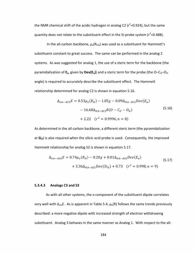
184
the NMR chemical shift of the acidic hydrogen in analog C2 (r2=0.924), but the same
quantity does not relate to the substituent effect in the Si‐probe system (r2=0.488).
In the all‐carbon backbone, μx(RHA) was used as a substituent for Hammett’s
substituent constant to great success. The same can be performed in the analog 2
systems. As was suggested for analog 1, the use of a steric term for the backbone (the
pyramidalization of Ea, given by Dev(Ea)) and a steric term for the probe (the O–CO–OH
angle) is required to accurately describe the substituent effect. The Hammett
relationship determined for analog C2 is shown in equation 5.16.
∆ 0.53 1.05 0.09Δ
16.68Δ
2.22 0.9996, 8
(5.16)
As determined in the all‐carbon backbone, a different steric term (the pyramidalization
at SiO) is also required when the silicic acid probe is used. Consequently, the improved
Hammett relationship for analog S2 is shown in equation 5.17.
Δ 0.74 0.20 0.01Δ
3.36Δ 0.73 0.998, 9
(5.17)
5.3.4.3 Analogs C3 and S3
As with all other systems, the x‐component of the substituent dipole correlates
very well with ΔisoE. As is apparent in Table 5.4, μx(R) follows the same trends previously
described: a more negative dipole with increased strength of electron withdrawing
substituent. Analog 3 behaves in the same manner as Analog 1. With respect to the all‐
185
carbon backbone and the substituent‐only value, μx(RHA) has a larger magnitude in both
analog C3 and analog S3 (NH2 substitution is the only exception for comparison to the
all‐carbon backbone).
In keeping with the trends previously observed, µx consistently relates well with
ΔisoE along the bond path. In analog C3, μx has very good correlations for the backbone
and probe as a whole, but appears to transmit in a slightly different fashion (all
backbone atoms and SiO show very good relationships in analog S3). Very strong
correlations are apparent for both bridgehead atoms, but the bridging atoms only form
weak relationships (average r2=0.626). For the bridging atoms it is actually μy and μz
which show strong correlations. Replacing the entire backbone with Si appears to result
in a path of transmission directly through the molecule (explaining the very good
relationship between ΔisoE and ρ(CCP)), but also results in a greater diffusion of charge.
Even with slight differences in transmission, μx(RHA) still appears to be controlling
the substituent effect. It can be used to describe any of the properties associated with
the reaction energy (e.g. Δδ1Ha and μx(RHA) have a linear squared correlation coefficient
of 0.817 in analog C3 and 0.876 in analog S3). Replacement of the substituent constant
with the dipole moment contribution, as well as using the pyramidalization at Ea to
describe the steric contribution of the backbone, and the two terms to describe the
steric contribution of the probes [θ(O–CO–OH ) for the C‐probe and Dev(SiO) for the Si‐
probe), leads to better Hammett‐type relationships overall (see equations 5.18 and
5.19).
186
∆ 0.29 0.18 0.38Δ
24.74Δ
0.32 0.996, 10
(5.18)
Δ 0.63 0.50 0.47Δ
7.70Δ 0.69 0.999, 10(5.19)
5.4 Summary
Herein we have presented a systematic study on the transmission of electron
density through silicon, upon both a carbon based probe and a silicon based probe, by
replacing the carbon atoms in the bicyclo[1.1.1]pentane backbone. The isodesmic
reaction approach was used to determine the effect of substitution using Hammett’s
method. In general, reactivity and the ordering of substituents is conserved between
the all‐carbon and analog systems. In all analog systems, NH2 substitution results in a
positive ΔisoE and consequently appears to act as an electron donating group. In analog
1 and analog 3, the order of the CN and NF2 substituents is swapped; NF2 substitution
leads to a greater electron withdrawing effect.
Unexpected structural changes occurred with the conjugate bases of analogs 2
and 3 with highly electron withdrawing groups (CF3 through NO2 with the CBS‐QB3
method, and CN and NO2 with the PBE0 level of theory), and was more severe in the
CBS‐QB3 method than the PBE0/6‐31++G(d,p) level of theory. For analog 2, a different
bicyclic structure was located, while the probe group was prone to leaving in analog 3.
187
One of the most obvious differences between Si and C is their atomic radii.
Consequently the structure within the backbone segments varies with each replacement
of a carbon atom with silicon. As expected, all Si–C and Si–Si bonds are longer than their
carbon counterparts. Length a, the interbridgehead distance, shows this variation best
and the relative distance (carbon value subtracted from the analog value) generally
shows very good correlation to ΔisoE. With each addition of more Si atoms, a increases
in length by an average of 0.41 Å in analog 1, 0.54 Å in analog 2 and 1.02 Å in analog 3.
Just as in the carbon systems, a appears to vary with the pyramidalization at Ea. We
have used the pyramidalization at Ea successfully as the structural parameter for the
backbone, required in the Hammett relationships for silicon systems. The use of the
silicic acid probe also requires a second structural parameter, the pyramidalization of
SiO, to accurately describe the substituent effect.
Bader’s Quantum Theory of Atoms in Molecules was used to analyze minute
variations in the electron density distribution between systems, and thus give insight
into the mechanism of transmission. The all‐carbon system appears to be operating
solely through the substituent dipole moment, but when silicon atoms are introduced
into the backbone some degree of through‐bond transmission is induced. However, the
x‐component of the substituent dipole is still the property most consistently related to
the substituent effect. There does not appear to be a clear relationship between the
number of silicon atoms introduced and the change in substituent effect. μx(RH) was
used to replace the traditional substituent constant, σF, in the Hammett‐based
relationship to achieve a better description of the effect.
188
Chapter 6: Summary and Conclusions
189
We have investigated the “so‐called” inductive effect with respect to silicon on
two fronts: the effect of substitution on a silicon probe and the transmission of the
effect through a silicon center. To that end we have employed a silicic acid based probe
and a carboxylic acid probe, for comparison. To ensure it is only the “so‐called”
inductive effect being studied, we have used bicyclo[1.1.1]pentane as the backbone
segment to link the substituent and probe. The bicyclo[1.1.1]pentane cage structure
removes any possibility of conjugation or steric interaction between the substituent and
probe.33 In order to study the transmission through silicon, the atoms within the
backbone were systematically replaced with silicon atoms (see Scheme 1.3). Finally, the
substituents utilized were chosen to cover a wide range of possible electronegativities,
while still remaining manageable with respect to computational cost. Bader’s Quantum
Theory of Atoms in Molecules51,52,75 was used to examine the effect of substituents on
the electron density distribution in the system.
Derivatives of 3‐substituted‐bicyclo[1.1.1]pentane‐1‐carboxylic acid were
employed to determine a benchmark and method for studying the inductive effect in
the proposed systems. Our QTAIM results confirm that, qualitatively, the inductive
effect does decay with distance, but the decay does not relate to the inductive effect as
suggested by definition. Consistent with Hammett’s formulation, the substituents have
the same effect upon the silicic acid probe as they have upon the carboxylic acid probe.
The order of substituents, based on the isodesmic reaction energy, is conserved and the
reactions energies between the C‐ and Si‐systems show a remarkable linear correlation.
190
With respect to the C‐system, the silicic acid probe is less sensitive to substitution
(ρ=0.84, see Figure 6.1).
Introduction of silicon atoms into the backbone results in some important
differences in reactivity. In all three analog systems, substitution with NH2 results in a
positive reaction energy, as if the change in backbone promotes electron donating
character in the amino group. When the bridgehead atoms are replaced by Si (analog 1
and analog 3) the NF2 yields a more negative ΔisoE than CN substitution and it appears
the change in backbone promotes the electron withdrawing nature of NF2. Analog 1 is
more sensitive to substitution, ρ=1.11 for the C‐probe and ρ=0.93 with the Si‐probe (see
Figure 6.1), but the Si‐probe is still less sensitive. Analog 2 has a different effect on the
two probe groups. Analog C2 is less sensitive to substitution (ρ=0.97), while analog S2 is
more sensitive (ρ=1.08) with respect to the Si‐system. Overall analog S2 yields a
reaction less sensitive to substitution (ρ=0.91 with respect to the C‐system).
Replacement of all C atoms within the backbone with Si, results in a less sensitive
reaction with the Si‐probe (as expected given Yoder et al.’s findings8), but an essentially
equivalent effect in the C‐probe: analog C3 has ρ=0.99 and analog S3 has ρ=0.81.
Therefore, it can be concluded that the transmission of the inductive effect through a Si‐
center is diminished.
The intercept of a regression line is generally used to refer to the error within a
relationship. For the Si‐system the intercept is essentially zero (0.04, see Figure 6.1a) on
this scale, and thus the relationship can be said to be very accurate. In the analog
systems the intercepts are higher. This is expected as the squared correlation
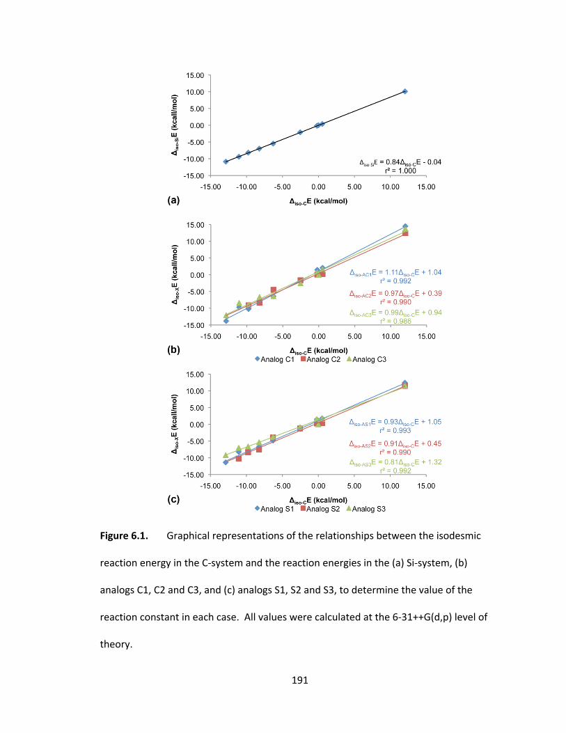
191
Figure 6.1. Graphical representations of the relationships between the isodesmic
reaction energy in the C‐system and the reaction energies in the (a) Si‐system, (b)
analogs C1, C2 and C3, and (c) analogs S1, S2 and S3, to determine the value of the
reaction constant in each case. All values were calculated at the 6‐31++G(d,p) level of
theory.
192
coefficients indicate that the relationships are not perfect. Regardless, the largest
intercept is only 1.32 in the relationship describing the effect in analog S3 (see Figure
6.1c). This represents, approximately, a 6% error overall, indicating that the
relationships are still adequate in describing the substituent effect.
The greater atomic radius found in Si leads to an increase in bond lengths within
the analog backbones (specifically b1 and b2). In analogs 1 and 2, the Si–C bonds are on
average 0.36 Å longer than their C–C counterparts. This difference increases to an
average 0.70 Å in analog 3 with the move to pure Si–Si bonds. The most dramatic
effects upon the structure occur within the conjugate base species of analogs 2 and 3.
In analog 2, the high Si–O affinity between the Si atom, now at a bridging position, and
the deprotonated O atom in the probe group leads to the rearrangement to a different
bicyclic structure. In analog 3 the elongation of the linkage between the backbone and
the probe is so severe that it appears to lead to the dissociation of the C‐probe group in
the conjugate base species as CO2 (no dissociation apparent for the Si‐probe). Although
the elongation did lead to optimization issues, a bond path was still present between
the backbone and probe. These rearrangements occur with the most electron
withdrawing substituents, and are more severe with the C‐probe than the Si‐probe.
According to the Hammett approach, a steric term should be required to
describe the inductive effect in Si systems. It was discovered that the pyramidalization
of the forward bridgehead atom, Ea, could be used to describe the steric component of
the backbone. An additional term was required to describe the effect within the probe
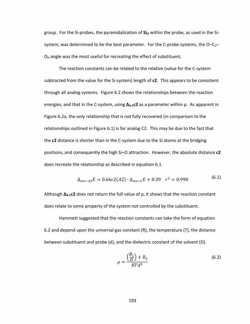
193
group. For the Si‐probes, the pyramidalization of SiO within the probe, as used in the Si‐
system, was determined to be the best parameter. For the C‐probe systems, the O–CO–
OH angle was the most useful for recreating the effect of substituent.
The reaction constants can be related to the relative (value for the C‐system
subtracted from the value for the Si‐system) length of c2. This appears to be consistent
through all analog systems. Figure 6.2 shows the relationships between the reaction
energies, and that in the C‐system, using ΔX‐Cc2 as a parameter within ρ. As apparent in
Figure 6.2a, the only relationship that is not fully recovered (in comparison to the
relationships outlined in Figure 6.1) is for analog C2. This may be due to the fact that
the c2 distance is shorter than in the C‐system due to the Si atoms at the bridging
positions, and consequently the high Si–O attraction. However, the absolute distance c2
does recreate the relationship as described in equation 6.1.
∆ 0.66 2 2 · ∆ 0.39 0.990 (6.1)
Although ΔX‐Cc2 does not return the full value of ρ, it shows that the reaction constant
does relate to some property of the system not controlled by the substituent.
Hammett suggested that the reaction constants can take the form of equation
6.2 and depend upon the universal gas constant (R), the temperature (T), the distance
between substituent and probe (d), and the dielectric constant of the solvent (D).
(6.2)
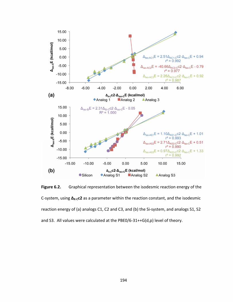
194
Figure 6.2. Graphical representation between the isodesmic reaction energy of the
C‐system, using ΔX‐Cc2 as a parameter within the reaction constant, and the isodesmic
reaction energy of (a) analogs C1, C2 and C3, and (b) the Si‐system, and analogs S1, S2
and S3. All values were calculated at the PBE0/6‐31++G(d,p) level of theory.
195
The constants in equation 6.2, B1 and B2, are said to be related to the electrostatic
interaction between the molecule and the solvent, and the sensitivity of the reaction to
changes in electron density at the probe, respectively. As the calculations in this study
were performed in gas phase under constant temperature, equation 6.2 should reduce
to:
(6.3)
Unfortunately, no simple relationship was found to allow for the a priori estimation of ρ.
The delocalization index alludes to a stepwise mechanism of transmission.
Within the C‐system, the substituent communicates with both E’b and Ec, and these
atoms pass the information on to the probe. Within the silicon systems (apart from
analog 2, which shows no substituent‐probe communication whatsoever), stepwise
transmission involving Ec is conserved, suggesting that the Si atoms encourage a more
direct transmission through the molecule. The average number of electrons shared
between Ec and both the substituent and probe, increases with the electron
withdrawing strength of the substituent, as if they promote greater communication.
The only property which consistently related to the substituent effect
throughout all systems (with both backbone and probe substitutions) is the x‐
component of the dipole moment. It appears that for all systems, µx of the substituent
dipole is controlling the effect upon the entire molecule. This consistency suggests that
the dipole moment is the mechanism of transmission. Analogs 1 and 3 generally have a
larger magnitude in the corresponding direction (e.g., µx for Li is more positive and the
µx of NO2 is more negative) of µx(RHA) than the all‐carbon backbone. NH2 substitution
196
represents the only exception within analog 3, as it has a smaller magnitude. In analog
2 there is no consistency with respect to the original systems. The H, NH2 and OH (also F
and CF3 in analog S2) substituents all result in a smaller µx, and all other substituents
have a larger magnitude.
The atomic dipole moment has previously been shown to conform to the
principle of atomic transferability,88,89 and thus the substituent‐only dipole moment
[μx(RH)] recreates the substituent dipole moment within the systems very well. We
were able to replace the traditional substituent constant, σ, with μx(RH) to achieve a
better representation of the substituent effect in the form of equation 6.2.
∆ (6.4)
This is also attractive as it replaces a compounded empirical term with one determined
by quantum mechanical means. The substituent effect in all analog systems was
described using μx(RH), as well as the electronegativity and steric terms, to essentially
recreate the entire effect (equations 5.14 through 5.19; all r2 values at least 0.996). This
approach can also be used to describe effect upon the all‐carbon backbones according
to equations 6.3 and 6.4.
Δ 0.65 1.65 0.48Δ
18.15Δ
3.12 0.999, 10
(6.5)
Δ 0.59 0.37 0.13Δ
4.25Δ 0.51 0.999, 10
(6.6)
197
Although both relationships return a very good squared correlation coefficient, the
intercept in the relationship describing the C‐system, equation 6.3, is significant and
represents a 12.5% error on the scale of the reaction energy. Both all‐carbon backbones
have negative ρμ values (following the form in equation 6.2) and are within the same
order of magnitude, as are all values. The small differences in the prefactor magnitudes
reinforces the transferability of μx(RH). Use of analog 2, and analog 1 with the C‐probe
only, results in a positive value for the prefactor. Describing ρμ in terms of a pseudo‐
reaction constant for μx(RH), and setting the value for the C‐system equal to 1.00,
returns essentially the same trend observed in the full reaction constant. Apart from an
obvious change in sign, those systems that result in a more sensitive reaction to
substitution also have a more sensitive dipole moment [ρμ(Si)=0.91, ρμ(AC1)=‐1.51,
ρμ(AC2)=‐0.82, ρμ(AC3)=0.45, ρμ(AS1)=0.87, and ρμ(AS3)=0.97]. The only exception to
this is for analog S2, which appears to be more sensitive [ρμ(AS2)=‐1.14].
Although linear free energy relationships were derived, via quantum mechanical
means, to describe the “so‐called” inductive effect in these systems, future work must
be undertaken to confirm their validity. To provide a more complete the picture, the list
of substituents should be expanded to include more electron donating groups and at
least one Si‐based substituent, such as SiH3. The same approach should be applied to
another backbone system to determine if the mode of transmission is the same.
Bicyclo[2.2.2]octane represents the next logical choice for a backbone moiety. The
substituent–probe distance will be longer, but any issues surrounding the potential
198
overlap between orbitals on the bridgehead atoms, as possible in the
bicyclo[1.1.1]pentane system,33,105 can be avoided.

199
Chapter 7: References
200
(1) Richmond, K. E.; Sussman, M. Curr. Opin. Plant Biol. 2003, 6, 268‐272. (2) Van Soest, P. J. Anim. Feed Sci. Technol. 2006, 130, 137‐171. (3) Duivenvoordern, W. C. M.; Middleton, A.; Kinrade, S. D. J. Trace Elem. Med. Biol. 2008, 22, 215‐223. (4) Bains, W.; Tacke, R. Curr. Opin. Drug Discovery Dev. 2003, 6, 526‐543. (5) Rainforth, W. M. J. Mater. Sci. 2004, 39, 6705‐6721. (6) Puri, J. K.; Singh, R.; Chahal, V. K. Chem. Soc. Rev. 2011, 40, 1791‐1840. (7) Kruusing, A. Opt. Laser Eng. 2004, 41, 329‐352. (8) Dubowchik, G. M.; Gottschall, D. W.; Grossman, M. J.; Norton, R. L.; Yoder, C. H. J. Am. Chem. Soc. 1982, 104, 4211‐4214. (9) Knight, C. T. G.; Balec, R. J.; Kinrade, S. D. Angew. Chem. Int. Ed. 2007, 46, 8148‐8152. (10) Hammett, L. P. Chem. Rev. 1935, 17, 125‐136. (11) Hammett, L. P. J. Am. Chem. Soc. 1937, 59, 96‐103. (12) Hammett, L. P. Physical Organic Chemistry; McGraw‐Hill: New York, 1940. (13) Cartledge, F. K. Organometallics 1983, 2, 425‐430. (14) Ploom, A.; Tuulmets, A. J. Organomet. Chem. 2009, 694, 313‐315. (15) Krygowski, T. M.; Stepien, B. T. Chem. Rev. 2005, 105, 3482‐3512. (16) Muller, P. Pure Appl. Chem. 1994, 66, 1077‐1184. (17) Minkin, V. I. Pure Appl. Chem. 1999, 71, 1919‐1981. (18) Ingold, C. K. Chem. Rev. 1934, 15, 225‐274. (19) Galkin, V. I. J. Phys. Org. Chem. 1999, 12, 283‐288. (20) Hansch, C.; Leo, A.; Taft, R. W. Chem. Rev. 1991, 91, 165‐195. (21) Exner, O. J. Phys. Org. Chem. 1999, 12, 265‐274. (22) Jaffe, H. H. Chem. Rev. 1953, 53, 191‐261. (23) Shorter, J. Q. Rev., Chem. Soc. 1970, 24, 433‐453. (24) Flett, M. S. C. Trans. Faraday Soc. 1948, 44, 767‐774. (25) Ewing, D. F. Correlation Analysis in Chemistry ‐ recent Advances; Plenum Press: New York, 1978. (26) Zuman, P. Substituent Effects in Organic Polarography; Plenum Press: New York, 1967. (27) Perrin, C. L.; Ohta, B. K.; Kuperman, J. J. Am. Chem. Soc. 2003, 125, 15008‐15009. (28) McLafferty, F. W. Anal. Chem. 1959, 31, 477. (29) Exner, O.; Bohm, S. J. Phys. Org. Chem. 2007, 20, 454‐462. (30) Exner, O.; Bohm, S. Curr. Org. Chem. 2006, 10, 763‐778. (31) Exner, O.; Bohm, S. Chem. Eur. J. 2002, 8, 5147‐5152. (32) Roberts, J. D.; Moreland, W. T. J. Am. Chem. Soc. 1953, 75, 2167‐2173. (33) Wiberg, K. B. J. Org. Chem. 2002, 67, 1613‐1617. (34) Wiberg, K. B.; Ochterski, J. W. J. Comput. Chem. 1997, 18, 108‐114. (35) Taft, R. W. J. Am. Chem. Soc. 1953, 75, 4538‐4539. (36) Exner, O.; Bohm, S. J. Phys. Org. Chem. 2004, 17, 124‐130. (37) Oziminski, W. P.; Dobrowolski, J. C. J. Phys. Org. Chem. 2009, 22, 769‐778.
201
(38) Jensen, F. Introduction to Computational Chemistry, 2nd ed.; John Wiley & Sons Ltd.: West Sussex, 2007. (39) Cramer, C. J. Essentials of Computational Chemistry Theories and Models, 2nd ed.; John WIley & Sons, Ltd: West Sussex, England, 2004. (40) Koch, W.; Holthausen, M. C. A Chemist's Guide to Density Functional Theory, 2nd ed.; Wiley‐VCH: Weinheim, Germany, 2001. (41) Hohenberg, P.; Kohn, W. Phys. Rev. 1964, 136, B864‐B871. (42) Kohn, W.; Sham, L. J. Phys. Rev. 1965, 140, A1133‐A1138. (43) Vosko, S. H.; Wilk, L.; Nusair, M. Can. J. Phys. 1980, 58, 1200‐1211. (44) Becke, A. D. Phys. Rev. A 1988, 38, 3098‐3100. (45) Ditchfield, R.; Hehre, W. J.; Pople, J. A. J. Chem. Phys. 1971, 54, 724‐728. (46) Hehre, W. J., Ditchfield, R., Pople, J.A. J. Chem. Phys. 1972, 56, 2257‐2261. (47) Montgomery Jr, J. A.; Frisch, M. J.; Ochterski, J. W.; Petersson, G. A. J. Chem. Phys. 1999, 110, 2822‐2827. (48) Montgomery Jr, J. A.; Frisch, M. J.; Ochterski, J. W.; Petersson, G. A. J. Chem. Phys. 2000, 112, 6532‐6542. (49) Casasnovas, R.; Frau, J.; Ortega‐Castro, J.; Salva, A.; Donoso, J.; Munoz, F. Int. J. Quantum Chem. 2010, 110, 323‐330. (50) Møller, C.; Plesset, M. S. Phys. Rev. 1934, 46, 618‐622. (51) Bader, R. F. W. Chem. Rev. 1991, 91, 893‐928. (52) Bader, R. F. W. Atoms in Molecules: A Quantum Theory; Oxford University Press: Oxford, 1990. (53) Popelier, P. Atoms in Molecules, An Introduction; Prentice Hall: Essex, England, 2000. (54) Matta, C. F.; Boyd, R. J. An Introduction to the Quantum Theory of Atoms in Molecules. In The Quantum Theory of Atoms in Molecules, From Solid State to DNA and Drug Design; Matta, C. F., Boyd, R. J., Eds.; Wiley‐VCH: Weinheim, Germany, 2007. (55) Koritsanszky, T. S.; Coppens, P. Chem. Rev. 2001, 101, 1583‐1627. (56) Biegler‐Konig, F. W.; Bader, R. F. W.; Tang, T.‐H. J. Comput. Chem. 1982, 3, 317‐328. (57) Biegler‐Konig, F. W.; Nguyen‐Dang, T. T.; Tal, Y.; Bader, R. F. W.; Duke, A. J. J. Phys. B: At. Mol. Phys. 1981, 14, 2739‐2751. (58) Adcock, W.; Baran, Y.; Filippi, A.; Speranza, M.; Trout, N. A. J. Org. Chem. 2005, 70, 1029‐1034. (59) Campanelli, A. R.; Domenicano, A.; Piacente, G.; Ramondo, F. J. Phys. Chem. A 2010, 114, 5162‐5170. (60) Fourre, I.; Gerard, H.; Silvi, B. J. Mol. Struct. (Theochem) 2007, 811, 69‐76. (61) Frisch, M. J.; Trucks, G. W.; Schlegel, H. B.; Scuseria, G. E.; Robb, M. A.; Cheeseman, J. R.; Montgomery Jr, J. A.; Vreven, T.; Kudin, K. M.; Burant, J. C.et al. Gaussian 03; Revision E.01 ed.; Gaussian, Inc.: Wallingford CT, 2004. (62) Frisch, M. J.; Trucks, G. W.; Schlegel, H. B.; Scuseria, G. E.; Robb, M. A.; Cheeseman, J. R.; Scalmani, G.; Barone, V.; Mennucci, B.; Petersson, G. A.et al. Gaussian 09, Revision A.1; Gaussian, Inc.: Wallingford CT, 2009.
202
(63) Perdew, J. P.; Burke, K.; Ernzerhof, M. Phys. Rev. Lett. 1996, 77, 3865‐3868. (64) Perdew, J. P.; Burke, K.; Ernzerhof, M. Phys. Rev. Lett. 1997, 78, 1396. (65) Keith, T. A. AIMALL; Version 10.07.25 ed., 2010. (66) Schreckenbach, G.; Ziegler, T. J. Phys. Chem. 1995, 99, 606‐611. (67) Ditchfield, R. Mol. Phys. 1974, 27, 789‐807. (68) Wolinski, K.; Hilton, J. F.; Pulay, R. J. Am. Chem. Soc. 1990, 112, 8251‐8260. (69) Levin, M. D.; Kaszynski, P.; Michl, J. Chem. Rev. 2000, 100, 169‐234. (70) Boyd, R. J.; Edgecombe, K. E. J. Am. Chem. Soc. 1988, 110, 4182‐4186. (71) Boyd, R. J.; Boyd, S. L. J. Am. Chem. Soc. 1992, 114, 1652‐1655. (72) Exner, O.; Bohm, S. J. Phys. Org. Chem. 2006, 19, 393‐401. (73) Suresh, C. H.; Alexander, P.; Vijayalakshmi, K. P.; Sajith, P. K.; Gadre, S. R. Phys. Chem. Chem. Phys. 2008, 10, 6492‐6499. (74) Topsom, R. D. Prog. Phys. Org. Chem. 1987, 16, 125‐191. (75) Bader, R. F. W.; Bayles, D. J. Phys. Chem. A 2000, 104, 5579‐5589. (76) Taft, R. W.; Price, E.; Fox, I. R.; Lewis, I. C.; Andersen, K. K.; Davis, G. T. J. Am. Chem. Soc. 1963, 85, 709‐724. (77) Koopmans, T. Physica 1933, 1, 104‐113. (78) Pearson, R. G. J. Am. Chem. Soc. 1963, 85, 3533‐3539. (79) Parr, R. G.; Pearson, R. G. J. Am. Chem. Soc. 1983, 105, 7512‐7516. (80) Pearson, R. G. J. Chem. Sci. 2005, 117, 369‐377. (81) Mulliken, R. S. J. Chem. Phys. 1934, 2, 782‐793. (82) Alkorta, I.; Rozas, I.; Elguero, J. Struct. Chem. 1998, 9, 243‐247. (83) Castillo, N.; Robertson, K. N.; Choi, S. C.; Boyd, R. J.; Knop, O. J. Comput. Chem. 2008, 29, 367‐379. (84) Firme, C. L.; Antunes, O. A. C.; Esteves, P. M. Chem. Phys. Lett. 2009, 468, 129‐133. (85) Matta, C. F.; Hernandez‐Trujillo, J. J. Phys. Chem. A 2003, 107, 7496‐7504. (86) Matta, C. F.; Hernandez‐Trujillo, J. J. Phys. Chem. A 2005, 109, 10798. (87) Reynolds, W. F. J. Chem. Soc., Perkin Trans. 2 1980, 985‐992. (88) Bader, R. F. W.; Larouche, A.; Gatti, C.; Carroll, M. T.; MacDougall, P. J.; Wiberg, K. B. J. Chem. Phys. 1987, 87, 1142‐1152. (89) Smith, A. P.; McKercher, A. E.; Mawhinney, R. C. J. Phys. Chem. A 2011, 115, 12544‐12554. (90) Xiong, Y.; Yao, S.; Driess, M. Angew. Chem. Int. Ed. 2010, 49, 6642‐6645. (91) Ingold, C. K. J. Chem. Soc. 1930, 1032‐1047. (92) Cartledge, F. K. Organometallics 1982, 2, 425‐430. (93) Adamo, C.; Barone, V. J. Chem. Phys. 1999, 110, 6158‐6170. (94) Frisch, M. J.; Pople, J. A.; Binkley, J. S. J. Chem. Phys. 1984, 80, 3265‐3269. (95) Cheeseman, J. R.; Trucks, G. W.; Keith, T. A.; Frisch, M. J. J. Chem. Phys. 1996, 104, 5497‐5509. (96) Adamo, C.; Barone, V. Chem. Phys. Lett. 1998, 298, 113‐119. (97) Elavarasi, S. B.; Dorai, K. Chem. Phys. Lett. 2010, 489, 248‐253.
203
(98) Vaara, J. Phys. Chem. Chem. Phys. 2007, 9, 5399‐5418. (99) Bader, R. F. W.; Tang, T.‐H.; Tal, Y.; Biegler‐Konig, F. W. J. Am. Chem. Soc. 1982, 104, 946‐952. (100) Knop, O.; Boyd, R. J.; Choi, S. C. J. Am. Chem. Soc. 1988, 110, 7299‐7301. (101) Holmes, R. Chem. Rev. 1996, 96, 927‐950. (102) Power, P. P. Chem. Rev. 1999, 99, 3463‐3503. (103) Fischer, R. C.; Power, P. P. Chem. Rev. 2010, 110, 3877‐3923. (104) Sirjean, B.; Fournet, R.; Glaude, P. A.; Ruiz‐Lopez, M. F. Chem. Phys. Lett. 2007, 435, 152‐156. (105) Wiberg, K. B.; Connor, D. S. J. Am. Chem. Soc. 1966, 88, 4437‐4441.
204
Appendix 1: Supplemental Information and Figures
205
Topsom’s method for calculating σF as used in this discussion (Original reference:
Topsom, R. D. Prog. Phys. Org. Chem. 1987, 16, 125.)
The structures of H2 and HR were optimized separately at the PBE0/6‐31++G(d,p) level
of theory. A single point energy calculation was performed for the “complex” outlined
in Scheme A1.1 at the same level of theory.
Mulliken populations were used in equation A1.1 to determine the difference in charge
on Hα when “complexed”.
∆ (A1.1)
35.5∆ (A1.2)
Equation A1.2 was used to convert the relative charge to σF.
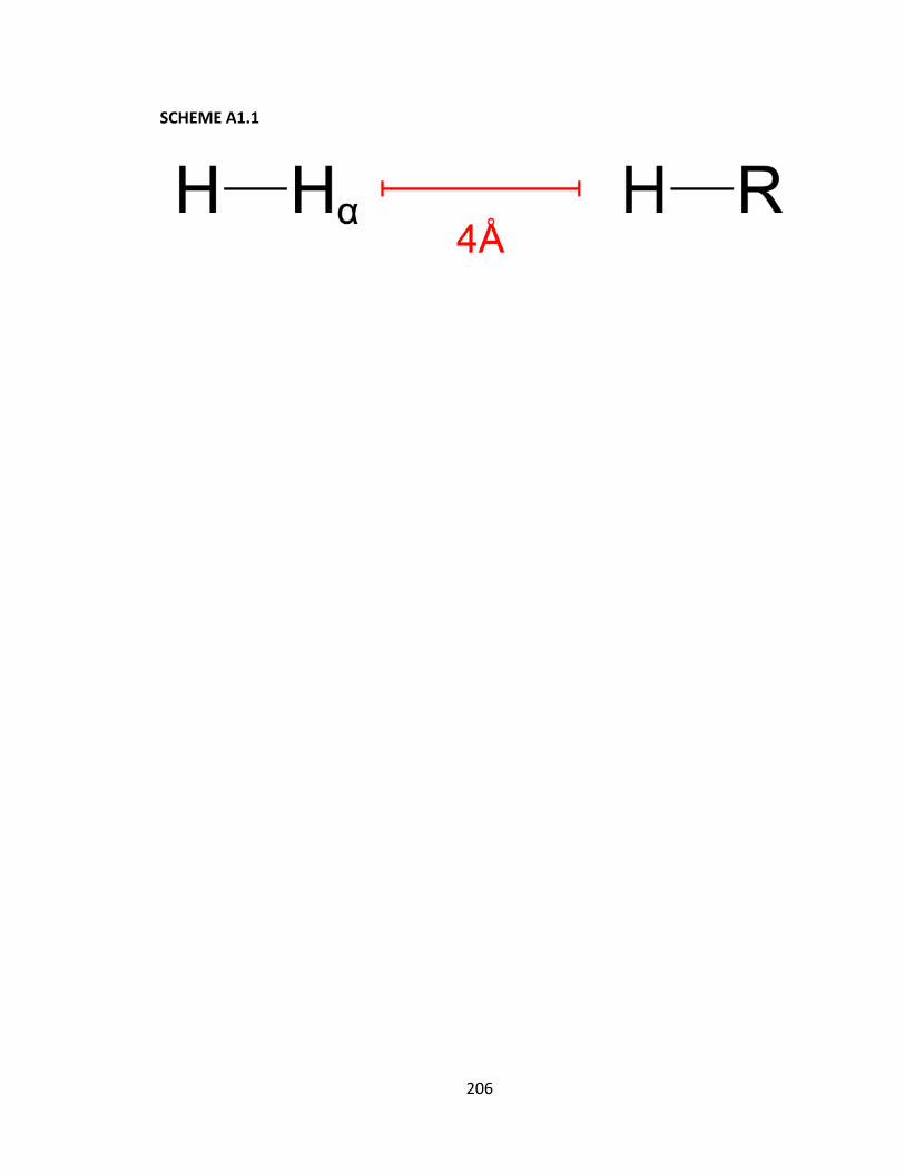
206
SCHEME A1.1
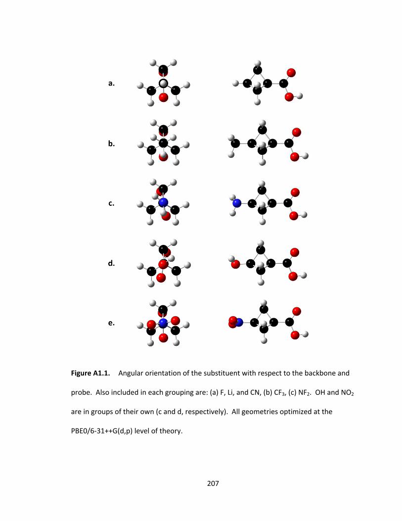
207
Figure A1.1. Angular orientation of the substituent with respect to the backbone and
probe. Also included in each grouping are: (a) F, Li, and CN, (b) CF3, (c) NF2. OH and NO2
are in groups of their own (c and d, respectively). All geometries optimized at the
PBE0/6‐31++G(d,p) level of theory.
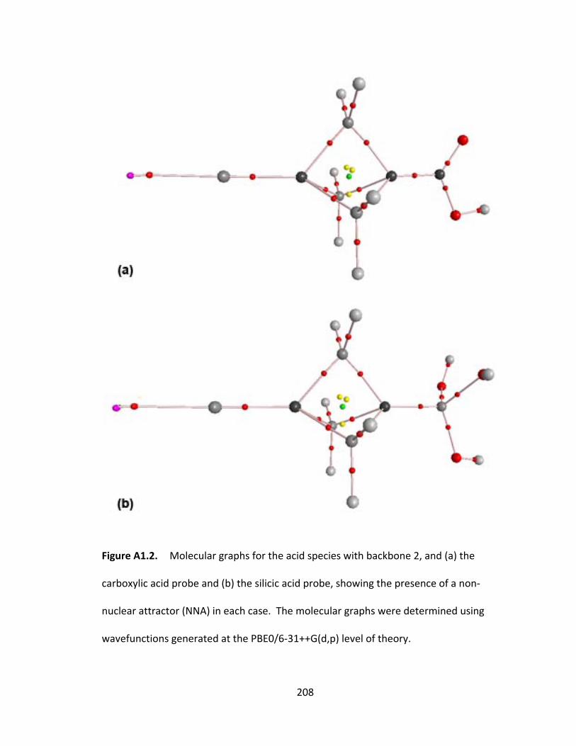
208
Figure A1.2. Molecular graphs for the acid species with backbone 2, and (a) the
carboxylic acid probe and (b) the silicic acid probe, showing the presence of a non‐
nuclear attractor (NNA) in each case. The molecular graphs were determined using
wavefunctions generated at the PBE0/6‐31++G(d,p) level of theory.
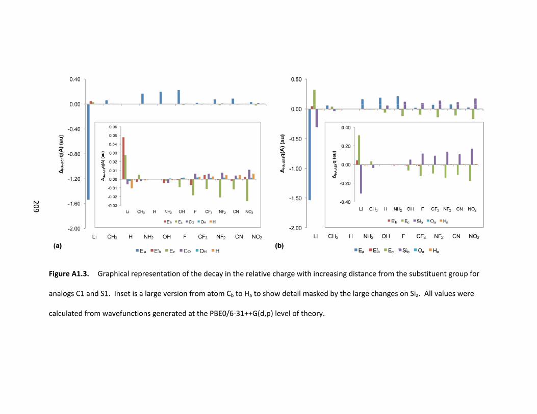
209
Figure A1.3. Graphical representation of the decay in the relative charge with increasing distance from the substituent group for
analogs C1 and S1. Inset is a large version from atom Cb to Ha to show detail masked by the large changes on Sia. All values were
calculated from wavefunctions generated at the PBE0/6‐31++G(d,p) level of theory.
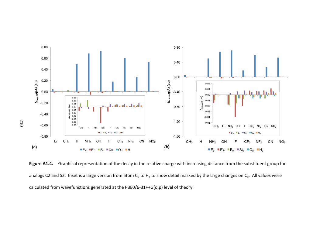
210
Figure A1.4. Graphical representation of the decay in the relative charge with increasing distance from the substituent group for
analogs C2 and S2. Inset is a large version from atom Cb to Ha to show detail masked by the large changes on Ca. All values were
calculated from wavefunctions generated at the PBE0/6‐31++G(d,p) level of theory.
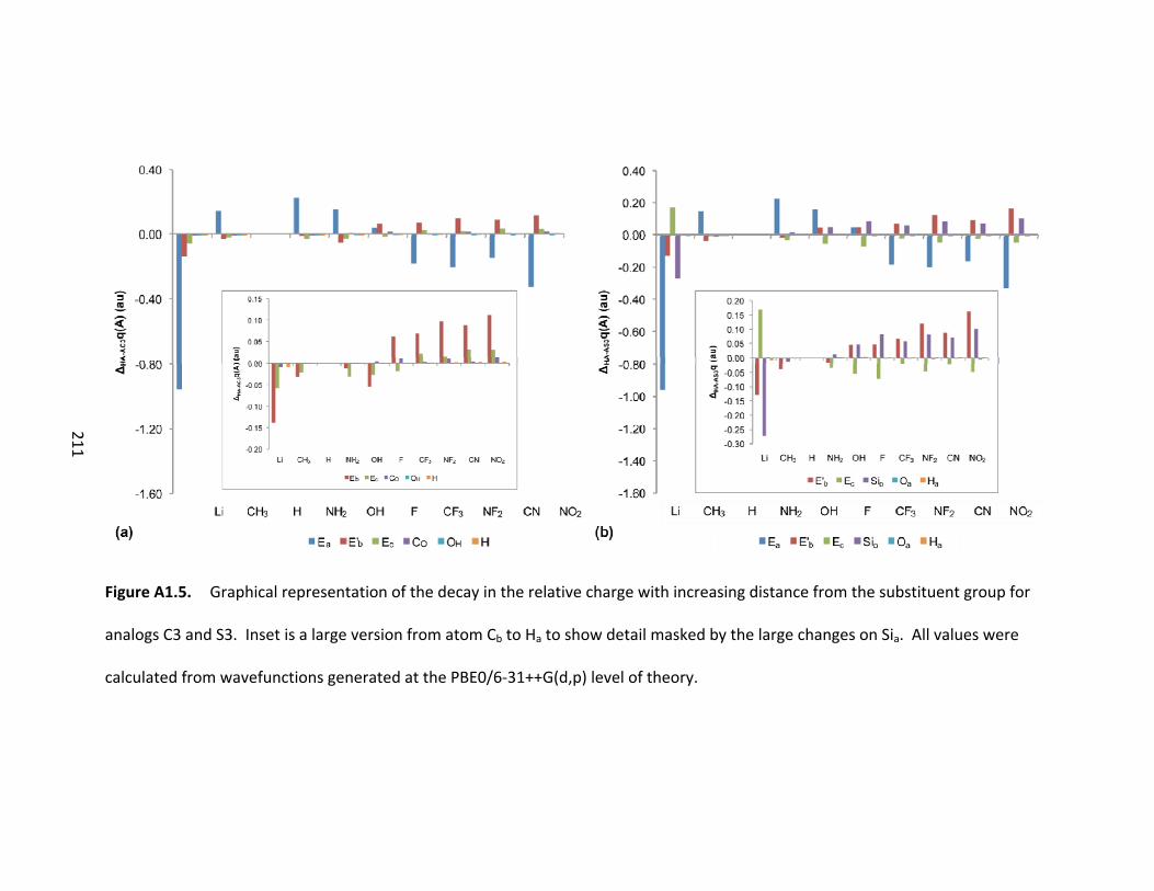
211
Figure A1.5. Graphical representation of the decay in the relative charge with increasing distance from the substituent group for
analogs C3 and S3. Inset is a large version from atom Cb to Ha to show detail masked by the large changes on Sia. All values were
calculated from wavefunctions generated at the PBE0/6‐31++G(d,p) level of theory.

212
Appendix 2: Cartesian Coordinates and Absolute Energies
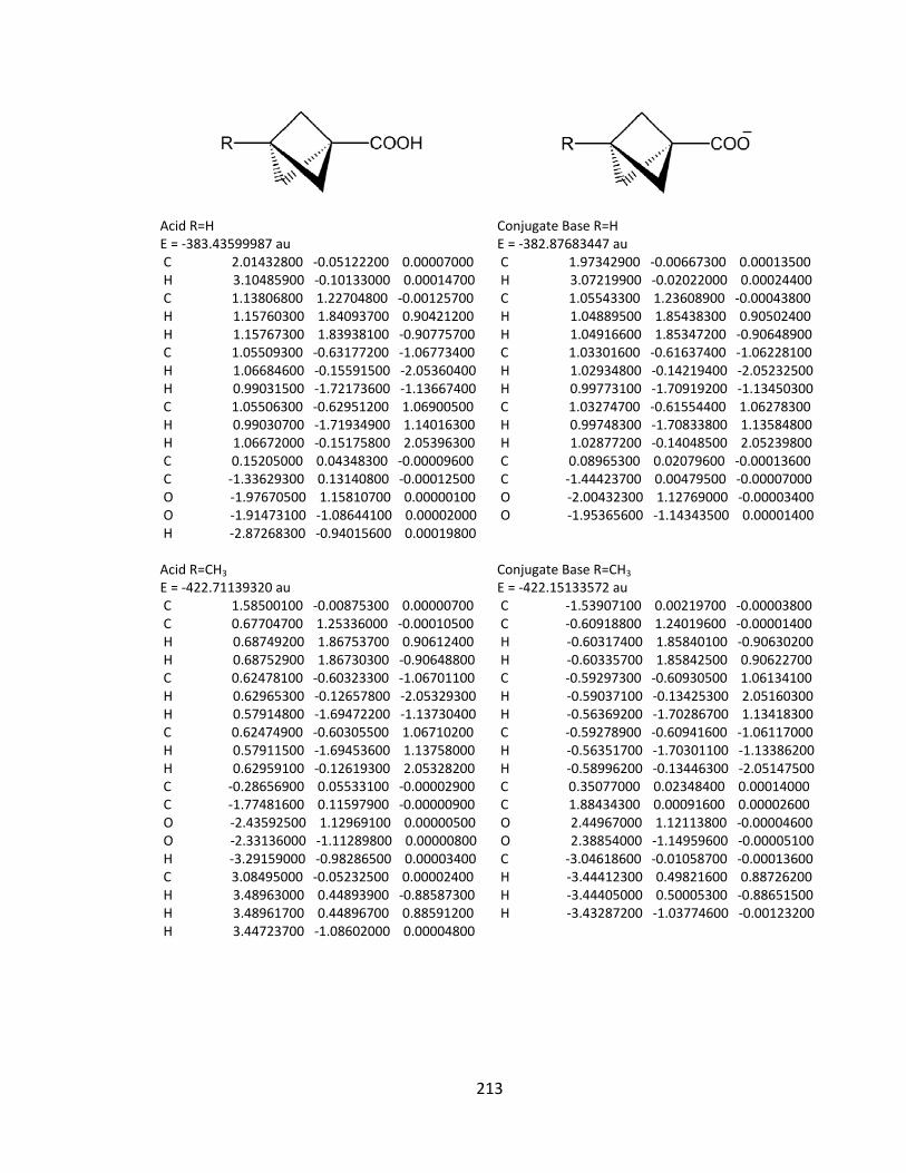
213
Acid R=H E = ‐383.43599987 au C 2.01432800 ‐0.05122200 0.00007000 H 3.10485900 ‐0.10133000 0.00014700 C 1.13806800 1.22704800 ‐0.00125700 H 1.15760300 1.84093700 0.90421200 H 1.15767300 1.83938100 ‐0.90775700 C 1.05509300 ‐0.63177200 ‐1.06773400 H 1.06684600 ‐0.15591500 ‐2.05360400 H 0.99031500 ‐1.72173600 ‐1.13667400 C 1.05506300 ‐0.62951200 1.06900500 H 0.99030700 ‐1.71934900 1.14016300 H 1.06672000 ‐0.15175800 2.05396300 C 0.15205000 0.04348300 ‐0.00009600 C ‐1.33629300 0.13140800 ‐0.00012500 O ‐1.97670500 1.15810700 0.00000100 O ‐1.91473100 ‐1.08644100 0.00002000 H ‐2.87268300 ‐0.94015600 0.00019800 Acid R=CH3 E = ‐422.71139320 au C 1.58500100 ‐0.00875300 0.00000700 C 0.67704700 1.25336000 ‐0.00010500 H 0.68749200 1.86753700 0.90612400 H 0.68752900 1.86730300 ‐0.90648800 C 0.62478100 ‐0.60323300 ‐1.06701100 H 0.62965300 ‐0.12657800 ‐2.05329300 H 0.57914800 ‐1.69472200 ‐1.13730400 C 0.62474900 ‐0.60305500 1.06710200 H 0.57911500 ‐1.69453600 1.13758000 H 0.62959100 ‐0.12619300 2.05328200 C ‐0.28656900 0.05533100 ‐0.00002900 C ‐1.77481600 0.11597900 ‐0.00000900 O ‐2.43592500 1.12969100 0.00000500 O ‐2.33136000 ‐1.11289800 0.00000800 H ‐3.29159000 ‐0.98286500 0.00003400 C 3.08495000 ‐0.05232500 0.00002400 H 3.48963000 0.44893900 ‐0.88587300 H 3.48961700 0.44896700 0.88591200 H 3.44723700 ‐1.08602000 0.00004800
Conjugate Base R=H E = ‐382.87683447 au C 1.97342900 ‐0.00667300 0.00013500 H 3.07219900 ‐0.02022000 0.00024400 C 1.05543300 1.23608900 ‐0.00043800 H 1.04889500 1.85438300 0.90502400 H 1.04916600 1.85347200 ‐0.90648900 C 1.03301600 ‐0.61637400 ‐1.06228100 H 1.02934800 ‐0.14219400 ‐2.05232500 H 0.99773100 ‐1.70919200 ‐1.13450300 C 1.03274700 ‐0.61554400 1.06278300 H 0.99748300 ‐1.70833800 1.13584800 H 1.02877200 ‐0.14048500 2.05239800 C 0.08965300 0.02079600 ‐0.00013600 C ‐1.44423700 0.00479500 ‐0.00007000 O ‐2.00432300 1.12769000 ‐0.00003400 O ‐1.95365600 ‐1.14343500 0.00001400 Conjugate Base R=CH3 E = ‐422.15133572 au C ‐1.53907100 0.00219700 ‐0.00003800 C ‐0.60918800 1.24019600 ‐0.00001400 H ‐0.60317400 1.85840100 ‐0.90630200 H ‐0.60335700 1.85842500 0.90622700 C ‐0.59297300 ‐0.60930500 1.06134100 H ‐0.59037100 ‐0.13425300 2.05160300 H ‐0.56369200 ‐1.70286700 1.13418300 C ‐0.59278900 ‐0.60941600 ‐1.06117000 H ‐0.56351700 ‐1.70301100 ‐1.13386200 H ‐0.58996200 ‐0.13446300 ‐2.05147500 C 0.35077000 0.02348400 0.00014000 C 1.88434300 0.00091600 0.00002600 O 2.44967000 1.12113800 ‐0.00004600 O 2.38854000 ‐1.14959600 ‐0.00005100 C ‐3.04618600 ‐0.01058700 ‐0.00013600 H ‐3.44412300 0.49821600 0.88726200 H ‐3.44405000 0.50005300 ‐0.88651500 H ‐3.43287200 ‐1.03774600 ‐0.00123200
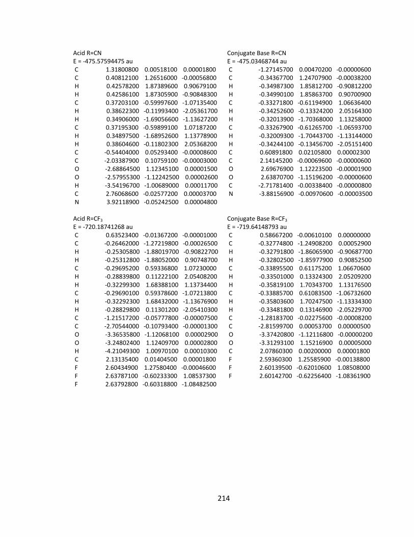
214
Acid R=CN E = ‐475.57594475 au C 1.31800800 0.00518100 0.00001800 C 0.40812100 1.26516000 ‐0.00056800 H 0.42578200 1.87389600 0.90679100 H 0.42586100 1.87305900 ‐0.90848300 C 0.37203100 ‐0.59997600 ‐1.07135400 H 0.38622300 ‐0.11993400 ‐2.05361700 H 0.34906000 ‐1.69056600 ‐1.13627200 C 0.37195300 ‐0.59899100 1.07187200 H 0.34897500 ‐1.68952600 1.13778900 H 0.38604600 ‐0.11802300 2.05368200 C ‐0.54404000 0.05293400 ‐0.00008600 C ‐2.03387900 0.10759100 ‐0.00003000 O ‐2.68864500 1.12345100 0.00001500 O ‐2.57955300 ‐1.12242500 0.00002600 H ‐3.54196700 ‐1.00689000 0.00011700 C 2.76068600 ‐0.02577200 0.00003700 N 3.92118900 ‐0.05242500 0.00004800 Acid R=CF3 E = ‐720.18741268 au C 0.63523400 ‐0.01367200 ‐0.00001000 C ‐0.26462000 ‐1.27219800 ‐0.00026500 H ‐0.25305800 ‐1.88019700 ‐0.90822700 H ‐0.25312800 ‐1.88052000 0.90748700 C ‐0.29695200 0.59336800 1.07230000 H ‐0.28839800 0.11222100 2.05408200 H ‐0.32299300 1.68388100 1.13734400 C ‐0.29690100 0.59378600 ‐1.07213800 H ‐0.32292300 1.68432000 ‐1.13676900 H ‐0.28829800 0.11301200 ‐2.05410300 C ‐1.21517200 ‐0.05777800 ‐0.00007500 C ‐2.70544000 ‐0.10793400 ‐0.00001300 O ‐3.36535800 ‐1.12068100 0.00002900 O ‐3.24802400 1.12409700 0.00002800 H ‐4.21049300 1.00970100 0.00010300 C 2.13135400 0.01404500 0.00001800 F 2.60434900 1.27580400 ‐0.00046600 F 2.63787100 ‐0.60233300 1.08537300 F 2.63792800 ‐0.60318800 ‐1.08482500
Conjugate Base R=CN E = ‐475.03468744 au C ‐1.27145700 0.00470200 ‐0.00000600 C ‐0.34367700 1.24707900 ‐0.00038200 H ‐0.34987300 1.85812700 ‐0.90812200 H ‐0.34990100 1.85863700 0.90700900 C ‐0.33271800 ‐0.61194900 1.06636400 H ‐0.34252600 ‐0.13324200 2.05164300 H ‐0.32013900 ‐1.70368000 1.13258000 C ‐0.33267900 ‐0.61265700 ‐1.06593700 H ‐0.32009300 ‐1.70443700 ‐1.13144000 H ‐0.34244100 ‐0.13456700 ‐2.05151400 C 0.60891800 0.02105800 0.00002300 C 2.14145200 ‐0.00069600 ‐0.00000600 O 2.69676900 1.12223500 ‐0.00001900 O 2.63870700 ‐1.15196200 ‐0.00000600 C ‐2.71781400 ‐0.00338400 ‐0.00000800 N ‐3.88156900 ‐0.00970600 ‐0.00003500 Conjugate Base R=CF3 E = ‐719.64148793 au C 0.58667200 ‐0.00610100 0.00000000 C ‐0.32774800 ‐1.24908200 0.00052900 H ‐0.32791800 ‐1.86065900 ‐0.90687700 H ‐0.32802500 ‐1.85977900 0.90852500 C ‐0.33895500 0.61175200 1.06670600 H ‐0.33501000 0.13324300 2.05209200 H ‐0.35819100 1.70343700 1.13176500 C ‐0.33885700 0.61083500 ‐1.06732600 H ‐0.35803600 1.70247500 ‐1.13334300 H ‐0.33481800 0.13146900 ‐2.05229700 C ‐1.28183700 ‐0.02275600 ‐0.00008200 C ‐2.81599700 0.00053700 0.00000500 O ‐3.37420800 ‐1.12116800 ‐0.00000200 O ‐3.31293100 1.15216900 0.00005000 C 2.07860300 0.00200000 0.00001800 F 2.59360300 1.25585900 ‐0.00138800 F 2.60139500 ‐0.62010600 1.08508000 F 2.60142700 ‐0.62256400 ‐1.08361900
215
Acid R=NH2 E = ‐438.73887749 au C 1.59400200 ‐0.01256500 ‐0.00069100 C 0.70025900 1.21824700 ‐0.28117300 H 0.70758200 2.01749200 0.46676600 H 0.72065100 1.61042800 ‐1.30234500 C 0.64527700 ‐0.83118200 ‐0.90677300 H 0.66285900 ‐0.58503000 ‐1.97305300 H 0.59756200 ‐1.91053100 ‐0.73066900 C 0.62746600 ‐0.35184000 1.18360600 H 0.57361300 ‐1.39969100 1.49652300 H 0.62399500 0.33820100 2.03414200 C ‐0.26754800 0.04956000 ‐0.01690600 C ‐1.75267500 0.11746200 ‐0.00884300 O ‐2.40756700 1.13525100 ‐0.00516000 O ‐2.31622300 ‐1.10802400 0.01220300 H ‐3.27527200 ‐0.97149400 0.03439500 N 3.01078600 ‐0.02482000 ‐0.08191500 H 3.39397400 ‐0.93828700 0.13461900 H 3.42915800 0.65674300 0.54137100 Acid R=NO2 E = ‐587.74345529 au C ‐0.93719700 ‐0.01129100 0.00190800 C ‐0.07122200 1.13049400 ‐0.56965600 H ‐0.09258100 1.25947200 ‐1.65393400 H ‐0.09702500 2.07719500 ‐0.02629100 C ‐0.02780900 ‐0.05151400 1.23532700 H ‐0.04855000 0.82395300 1.88716500 H 0.00463200 ‐0.99458300 1.78546800 C ‐0.02699600 ‐1.02566300 ‐0.69369100 H 0.00633500 ‐2.02871800 ‐0.26301000 H ‐0.04251300 ‐1.03052600 ‐1.78523200 C 0.88549900 0.04732600 ‐0.02345000 C 2.37427300 0.09845300 ‐0.05285400 O 3.02484500 0.99211300 ‐0.54059400 O 2.92091000 ‐0.98126600 0.53337300 H 3.88320200 ‐0.88046300 0.47534600 N ‐2.41352600 ‐0.02331300 0.01172500 O ‐2.96167000 0.60910800 0.89878800 O ‐2.97134900 ‐0.64370100 ‐0.87745400
Conjugate Base R=NH2 E = ‐438.18017610 au C 1.54449200 ‐0.00001200 ‐0.00844300 C 0.62701300 1.06967700 ‐0.62826100 H 0.60038100 2.05268100 ‐0.14399900 H 0.64135600 1.15275900 ‐1.72155200 C 0.62690500 ‐1.06770700 ‐0.63152900 H 0.64123700 ‐1.14734900 ‐1.72509500 H 0.60011500 ‐2.05212100 ‐0.15017800 C 0.59144200 ‐0.00185100 1.21743100 H 0.56537700 ‐0.91319400 1.82838800 H 0.56556100 0.90780500 1.83088000 C ‐0.33039900 0.00015200 ‐0.03450200 C ‐1.86507400 0.00000200 ‐0.00707100 O ‐2.39811600 1.13566800 0.01772400 O ‐2.39772700 ‐1.13584700 0.01784200 N 2.98413500 0.00007200 ‐0.06782700 H 3.34877100 ‐0.81821900 0.41186000 H 3.34872100 0.81700200 0.41421200 Conjugate Base R=NO2 E = ‐587.20493332 au C ‐0.88529000 ‐0.02469500 0.00204700 C ‐0.00975600 1.23830100 ‐0.08829200 H ‐0.02566300 1.77600300 ‐1.03982400 H ‐0.02265500 1.90536200 0.77758600 C 0.01618300 ‐0.54590900 1.11674900 H 0.00518500 0.00847100 2.05876700 H 0.04445800 ‐1.62924500 1.26048200 C 0.01461600 ‐0.69731100 ‐1.03089500 H 0.04361900 ‐1.78996800 ‐1.02078300 H 0.00085700 ‐0.28113600 ‐2.04151700 C 0.94925900 0.01585000 ‐0.00324500 C 2.48676100 0.00790800 ‐0.00106300 O 3.02702500 1.13585600 ‐0.04259300 O 2.99178100 ‐1.13700900 0.04485500 N ‐2.36977000 ‐0.01107800 0.00147400 O ‐2.94049800 0.05430300 1.08222900 O ‐2.93931300 ‐0.03774900 ‐1.08159500

216
Acid R=NF2 E = ‐636.91358374 au C ‐0.89875200 0.06591400 0.21539900 C 0.03522300 1.26430000 0.46438200 H ‐0.02631500 2.08548000 ‐0.25262800 H 0.12332800 1.61128300 1.49662900 C 0.06996400 ‐0.81993600 1.01535300 H 0.16010700 ‐0.60612400 2.08351800 H 0.04760900 ‐1.88906600 0.79464600 C ‐0.09797400 ‐0.26280500 ‐1.06052000 H ‐0.12356300 ‐1.29931900 ‐1.40246600 H ‐0.16095400 0.45953800 ‐1.87745700 C 0.92671400 0.06753000 0.06596900 C 2.41096400 0.08128700 ‐0.06054300 O 3.10793800 1.06144900 0.05825500 O 2.89953600 ‐1.14269200 ‐0.33300500 H 3.86184100 ‐1.05395800 ‐0.40698300 N ‐2.32565400 0.09710700 0.43483300 F ‐2.77828000 ‐1.15008700 ‐0.01517800 F ‐2.81495400 0.95949000 ‐0.55385900 Acid R=OH E = ‐458.59021320 au C ‐1.59200300 ‐0.01889900 ‐0.00063400 C ‐0.64602000 ‐0.34987100 1.18417200 H ‐0.64222900 0.34420600 2.03125000 H ‐0.59517100 ‐1.39632300 1.49759800 C ‐0.66048400 ‐0.83916200 ‐0.90517200 H ‐0.61687800 ‐1.91566300 ‐0.72009800 H ‐0.67738000 ‐0.59746900 ‐1.97212200 C ‐0.70927500 1.22424300 ‐0.28942200 H ‐0.72391900 1.61118700 ‐1.31246700 H ‐0.71229200 2.02503600 0.45667200 C 0.25184600 0.05155900 ‐0.01957500 C 1.73658700 0.11931800 ‐0.00894700 O 2.39041800 1.13724300 ‐0.00679100 O 2.29714500 ‐1.10634900 0.01644400 H 3.25657900 ‐0.97183100 0.04003500 O ‐2.96507300 ‐0.12462200 ‐0.05049100 H ‐3.35254600 0.52754700 0.54331500
Conjugate Base R=NF2 E = ‐636.36992683 au C ‐0.84651900 0.00095900 0.21548700 C 0.10248300 1.07853000 0.75641400 H 0.06851900 2.05512600 0.26801500 H 0.19296700 1.15397200 1.84475400 C 0.10226100 ‐1.07381200 0.76246000 H 0.19270000 ‐1.14320200 1.85121500 H 0.06806900 ‐2.05308400 0.27946100 C ‐0.04913200 ‐0.00294500 ‐1.09571400 H ‐0.09245000 ‐0.91635900 ‐1.69519700 H ‐0.09237400 0.90699600 ‐1.70051100 C 0.99243800 0.00032300 0.07000700 C 2.52109900 ‐0.00047900 ‐0.08963000 O 3.04345000 1.13623000 ‐0.15297200 O 3.04104500 ‐1.13793300 ‐0.15966700 N ‐2.27642000 0.00175600 0.45418700 F ‐2.77853600 ‐1.09233200 ‐0.28715700 F ‐2.77860000 1.09038100 ‐0.29507500 Conjugate Base R=OH E = ‐458.03517749 au C 1.54109500 0.01788000 ‐0.00000200 C 0.62206100 ‐0.60093400 1.07069500 H 0.58623100 ‐1.69429600 1.13853200 H 0.61815500 ‐0.12067200 2.05611900 C 0.64317600 1.25608400 ‐0.00138300 H 0.63946700 1.86889000 0.90605700 H 0.63960200 1.86691100 ‐0.91016100 C 0.62219100 ‐0.60325700 ‐1.06946000 H 0.61842300 ‐0.12516100 ‐2.05594100 H 0.58634800 ‐1.69675800 ‐1.13492700 C ‐0.31342100 0.03153700 ‐0.00014300 C ‐1.85041300 ‐0.00542300 ‐0.00007900 O ‐2.33813300 ‐1.16158600 0.00022800 O ‐2.42355600 1.10857100 ‐0.00004900 O 2.94441500 0.07318900 0.00002100 H 3.26183300 ‐0.83562900 0.00095600
217
Acid R=F E = ‐482.59478998 au C 1.57866400 ‐0.01166800 0.00002600 C 0.72315700 1.26339900 ‐0.00042400 H 0.73625600 1.86938100 0.90879600 H 0.73635100 1.86877600 ‐0.91004200 C 0.66522600 ‐0.61094100 ‐1.07762300 H 0.67352100 ‐0.12767000 ‐2.05827600 H 0.61701800 ‐1.70079800 ‐1.13876100 C 0.66513000 ‐0.61025200 1.07796700 H 0.61691600 ‐1.70007800 1.13979000 H 0.67330400 ‐0.12634400 2.05830400 C ‐0.23976400 0.05677900 ‐0.00009900 C ‐1.72492100 0.11822100 ‐0.00002700 O ‐2.38128500 1.13341400 0.00003200 O ‐2.27643400 ‐1.11067700 0.00001000 H ‐3.23750400 ‐0.98641900 0.00010000 F 2.93788200 ‐0.05688600 0.00009300 Acid R=Li E = ‐390.29839018 au C 1.93298500 ‐0.03492400 0.00001900 C 0.97901600 1.23198400 ‐0.00031700 H 0.98434600 1.85510600 0.90274500 H 0.98436700 1.85463600 ‐0.90370400 C 0.90841400 ‐0.61420600 ‐1.05986600 H 0.90529700 ‐0.14477100 ‐2.05249000 H 0.84027200 ‐1.70630800 ‐1.13869300 C 0.90839300 ‐0.61365300 1.06018200 H 0.84024900 ‐1.70571600 1.13957600 H 0.90524800 ‐0.14369600 2.05255900 C 0.01041900 0.04978000 ‐0.00002800 C ‐1.48690000 0.12468200 ‐0.00002600 O ‐2.14915600 1.14011900 ‐0.00002700 O ‐2.06308600 ‐1.09961000 0.00003200 H ‐3.02019400 ‐0.94870200 0.00006700 Li 3.91479500 ‐0.08220000 0.00004000
Conjugate Base R=F E = ‐482.04568398 au C ‐1.52517700 0.00104500 ‐0.00000300 C ‐0.65537100 1.25466000 ‐0.00022500 H ‐0.64977200 1.86259800 ‐0.90987100 H ‐0.64976900 1.86291200 0.90921100 C ‐0.63381700 ‐0.61435100 1.07351500 H ‐0.63184800 ‐0.13110200 2.05632300 H ‐0.59863300 ‐1.70552400 1.13602300 C ‐0.63381800 ‐0.61475600 ‐1.07328700 H ‐0.59862600 ‐1.70595200 ‐1.13539000 H ‐0.63184400 ‐0.13186900 ‐2.05627200 C 0.29982100 0.02758900 ‐0.00000500 C 1.84095500 0.00101600 ‐0.00000500 O 2.40140400 1.12014800 ‐0.00000400 O 2.33328500 ‐1.15122600 0.00000700 F ‐2.91917500 ‐0.01485200 0.00000100 Conjugate Base R=Li E = ‐389.72009516 au C 1.86066500 ‐0.00717900 0.00001200 C 0.90257900 1.23571300 ‐0.00032200 H 0.89361000 1.85809300 0.90390400 H 0.89364700 1.85762700 ‐0.90487000 C 0.87897000 ‐0.61387600 ‐1.06153300 H 0.87230800 ‐0.14170900 ‐2.05408700 H 0.83845800 ‐1.70730200 ‐1.13988200 C 0.87892900 ‐0.61332500 1.06183300 H 0.83841800 ‐1.70671200 1.14074700 H 0.87222600 ‐0.14063800 2.05413800 C ‐0.04604800 0.02223600 ‐0.00003600 C ‐1.60289100 0.00369500 ‐0.00003400 O ‐2.15907300 1.12616800 0.00000700 O ‐2.10609800 ‐1.14449300 0.00004500 Li 3.89316100 ‐0.01211500 0.00003700
218
All‐Carbon Backbone R=H E = ‐195.04455759 au C 0.00001500 ‐0.00000100 ‐0.93503600 H ‐0.00022100 0.00000200 ‐2.02858500 C 1.23345200 ‐0.00440700 ‐0.00011500 H 1.84662700 ‐0.91241200 ‐0.00017700 H 1.85306200 0.89921500 ‐0.00017700 C ‐0.61303800 1.07041200 0.00002600 H ‐0.13293800 2.05519700 0.00000400 H ‐1.70544100 1.15455000 0.00018500 C ‐0.62067500 ‐1.06600700 0.00002500 H ‐1.71365300 ‐1.14233100 0.00018500 H ‐0.14761300 ‐2.05419200 0.00000300 C 0.00021200 ‐0.00000100 0.93510200 H 0.00038000 ‐0.00000400 2.02855500 All‐Carbon Backbone R=CH3 E = ‐234.31969159 au C 0.48338500 ‐0.00036900 ‐0.00051600 C ‐0.46319100 ‐0.72000600 ‐0.99925400 H ‐0.46211100 ‐0.34570900 ‐2.02971800 H ‐0.46202700 ‐1.81587400 ‐0.96941900 C ‐0.46197100 ‐0.50546900 1.12336200 H ‐0.46080900 ‐1.58510100 1.31361100 H ‐0.45960500 0.06823900 2.05754200 C ‐0.46192100 1.22571400 ‐0.12388000 H ‐0.45959900 1.93027300 0.71605800 H ‐0.46063800 1.74762400 ‐1.08793100 C ‐1.39499300 0.00041200 0.00049100 H ‐2.48758100 0.00069800 0.00092700 C 1.98560100 ‐0.00025700 ‐0.00032200 H 2.37728400 ‐1.01829700 0.10285900 H 2.37737500 0.41978400 ‐0.93336800 H 2.37625100 0.59821700 0.83014400 All‐Carbon Backbone R=CN E = ‐287.18696178 au C 0.19313500 0.00005200 0.00012200 C ‐0.74390800 ‐0.01706900 1.23695000 H ‐0.73005300 ‐0.93287500 1.83515300 H ‐0.73017100 0.88190000 1.86017900 C ‐0.74357800 1.08010900 ‐0.60375500 H ‐0.72996200 2.05582200 ‐0.10925900 H ‐0.72953800 1.17030500 ‐1.69389800 C ‐0.74344300 ‐1.06307200 ‐0.63329600 H ‐0.72939000 ‐1.12318800 ‐1.72550600 H ‐0.72969900 ‐2.05203700 ‐0.16587200 C ‐1.67492700 ‐0.00006100 ‐0.00025300 H ‐2.76544400 ‐0.00013000 ‐0.00040600 C 1.63790200 0.00012500 0.00017000 N 2.79902600 ‐0.00004300 ‐0.00000400
All‐Carbon Backbone R=CF3 E = ‐531.79790401au C ‐0.38066200 0.00000900 0.00003800 C ‐1.30464000 0.88169200 0.86909000 H ‐1.29539300 0.67993200 1.94431300 H ‐1.29587700 1.95358700 0.65042200 C ‐1.30509300 0.31229200 ‐1.19809400 H ‐1.29659400 1.34472900 ‐1.55997600 H ‐1.29632100 ‐0.41232800 ‐2.01762000 C ‐1.30433800 ‐1.19384700 0.32872500 H ‐1.29531100 ‐2.02323400 ‐0.38457900 H ‐1.29511300 ‐1.54156100 1.36594200 C ‐2.23696400 ‐0.00038800 0.00050500 H ‐3.32814500 ‐0.00062700 0.00092100 C 1.11596300 0.00003600 ‐0.00015900 F 1.61475400 ‐0.89210300 ‐0.87959500 F 1.61469800 1.20790000 ‐0.33255300 F 1.61467700 ‐0.31571500 1.21214200 All‐Carbon Backbone R=NH2
E = ‐250.34740752 au C ‐0.50208500 0.00023200 ‐0.00338600 C 0.43141500 ‐1.06357100 ‐0.62370300 H 0.43134300 ‐2.05293400 ‐0.15129700 H 0.42242900 ‐1.13350800 ‐1.71650600 C 0.43177600 1.07021000 ‐0.61251500 H 0.42288300 1.15172700 ‐1.70456500 H 0.43207400 2.05458600 ‐0.12984800 C 0.44675000 ‐0.00676500 1.24063000 H 0.45020200 0.89743500 1.86045800 H 0.44987100 ‐0.91775900 1.85050300 C 1.36544800 ‐0.00017900 0.00129300 H 2.45599200 ‐0.00006900 ‐0.00427700 N ‐1.92270600 0.00066400 ‐0.09997000 H ‐2.32299400 0.81959400 0.34524200 H ‐2.32268200 ‐0.82328600 0.33616200

219
All‐Carbon Backbone R=NO2 E = ‐399.35497541 au C 0.12668900 0.01588300 ‐0.00016300 C 1.02024100 ‐0.62174600 1.07554500 H 1.01035800 ‐0.13855300 2.05627200 H 0.99444800 ‐1.71203700 1.13967600 C 1.02075700 ‐0.62530400 ‐1.07339800 H 0.99471400 ‐1.71560000 ‐1.13312600 H 1.01160200 ‐0.14693700 ‐2.05652200 C 1.02984800 1.24880700 ‐0.00214800 H 1.02340900 1.85408900 ‐0.91163000 H 1.02303900 1.85822300 0.90486100 C 1.95317300 ‐0.00174400 0.00036600 H 3.04240400 ‐0.00668100 0.00054500 N ‐1.35309300 0.00337300 ‐0.00024600 O ‐1.88907700 ‐1.09294900 0.00003100 O ‐1.92749300 1.07901300 0.00002300 All‐Carbon Backbone R=NF2 E = ‐448.52447342 au C ‐0.16176200 ‐0.00003500 ‐0.15440900 C ‐1.17581400 1.07453800 ‐0.57742800 H ‐1.06206400 2.05528500 ‐0.10826900 H ‐1.39306000 1.14451300 ‐1.64696200 C ‐1.17610400 ‐1.07411900 ‐0.57812800 H ‐1.39335400 ‐1.14339200 ‐1.64771500 H ‐1.06262800 ‐2.05520900 ‐0.10962800 C ‐0.79360600 ‐0.00043100 1.25184400 H ‐0.66054700 ‐0.90963700 1.84347100 H ‐0.66030800 0.90837000 1.84406800 C ‐1.95766100 0.00008400 0.22523700 H ‐3.02425400 0.00009700 0.44837200 N 1.22834400 ‐0.00004400 ‐0.55451000 F 1.79154500 ‐1.08951100 0.12531800 F 1.79151000 1.08951700 0.12529800 All‐Carbon Backbone R=OH E = ‐270.19966311 au C ‐0.50825100 0.01093500 0.00003900 C 0.41186800 ‐0.62557100 ‐1.07367100 H 0.40614000 ‐1.71924200 ‐1.14601100 H 0.41446800 ‐0.14773900 ‐2.05857900 C 0.41878800 1.23417700 ‐0.00452100 H 0.41802800 1.84183400 ‐0.91494800 H 0.41825200 1.84859900 0.90144500 C 0.41184300 ‐0.61756400 1.07822500 H 0.41467900 ‐0.13253400 2.05960800 H 0.40623400 ‐1.71070900 1.15839300 C 1.34066000 ‐0.01138100 ‐0.00003200 H 2.42983200 ‐0.01990700 0.00017000 O ‐1.88689100 0.10924000 ‐0.00034800 H ‐2.26194800 ‐0.77779700 0.00246200
All‐Carbon Backbone R=F E = ‐294.20543787 au C 0.50091300 0.00008200 ‐0.00004400 C ‐0.39485000 1.23239000 ‐0.17582100 H ‐0.39234700 1.96205100 0.63900800 H ‐0.39227800 1.70586000 ‐1.16189200 C ‐0.39501600 ‐0.76867200 ‐0.97905800 H ‐0.39257800 ‐0.42821700 ‐2.01852000 H ‐0.39267300 ‐1.85929700 ‐0.89512700 C ‐0.39502400 ‐0.46396600 1.15488000 H ‐0.39266200 ‐1.53448600 1.37933500 H ‐0.39255400 0.15344300 2.05774700 C ‐1.32111900 0.00027000 ‐0.00006200 H ‐2.40909000 0.00035200 ‐0.00002900 F 1.86608400 ‐0.00003700 0.00001200 All‐Carbon Backbone R=Li E = ‐201.90269378 au C 0.81932600 ‐0.00018000 0.00036500 C ‐0.18335900 ‐0.49471900 1.11960700 H ‐0.19341900 ‐1.57405800 1.32794200 H ‐0.19354100 0.07888200 2.05721900 C ‐0.18283600 1.21714300 ‐0.13147600 H ‐0.19281600 1.93692700 0.69926000 H ‐0.19245800 1.74251300 ‐1.09693600 C ‐0.18296200 ‐0.72240400 ‐0.98840500 H ‐0.19272300 ‐0.36245200 ‐2.02701800 H ‐0.19317900 ‐1.82124800 ‐0.96067200 C ‐1.11107600 0.00011200 ‐0.00010300 H ‐2.21604500 0.00033900 ‐0.00033800 Li 2.80654200 ‐0.00020600 0.00020400
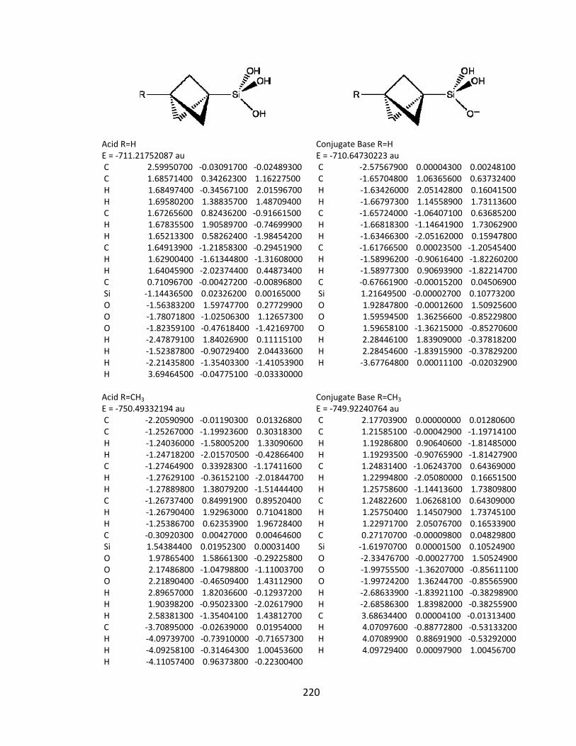
220
Acid R=H E = ‐711.21752087 au C 2.59950700 ‐0.03091700 ‐0.02489300 C 1.68571400 0.34262300 1.16227500 H 1.68497400 ‐0.34567100 2.01596700 H 1.69580200 1.38835700 1.48709400 C 1.67265600 0.82436200 ‐0.91661500 H 1.67835500 1.90589700 ‐0.74699900 H 1.65213300 0.58262400 ‐1.98454200 C 1.64913900 ‐1.21858300 ‐0.29451900 H 1.62900400 ‐1.61344800 ‐1.31608000 H 1.64045900 ‐2.02374400 0.44873400 C 0.71096700 ‐0.00427200 ‐0.00896800 Si ‐1.14436500 0.02326200 0.00165000 O ‐1.56383200 1.59747700 0.27729900 O ‐1.78071800 ‐1.02506300 1.12657300 O ‐1.82359100 ‐0.47618400 ‐1.42169700 H ‐2.47879100 1.84026900 0.11115100 H ‐1.52387800 ‐0.90729400 2.04433600 H ‐2.21435800 ‐1.35403300 ‐1.41053900 H 3.69464500 ‐0.04775100 ‐0.03330000 Acid R=CH3 E = ‐750.49332194 au C ‐2.20590900 ‐0.01190300 0.01326800 C ‐1.25267000 ‐1.19923600 0.30318300 H ‐1.24036000 ‐1.58005200 1.33090600 H ‐1.24718200 ‐2.01570500 ‐0.42866400 C ‐1.27464900 0.33928300 ‐1.17411600 H ‐1.27629100 ‐0.36152100 ‐2.01844700 H ‐1.27889800 1.38079200 ‐1.51444400 C ‐1.26737400 0.84991900 0.89520400 H ‐1.26790400 1.92963000 0.71041800 H ‐1.25386700 0.62353900 1.96728400 C ‐0.30920300 0.00427000 0.00464600 Si 1.54384400 0.01952300 0.00031400 O 1.97865400 1.58661300 ‐0.29225800 O 2.17486800 ‐1.04798800 ‐1.11003700 O 2.21890400 ‐0.46509400 1.43112900 H 2.89657000 1.82036600 ‐0.12937200 H 1.90398200 ‐0.95023300 ‐2.02617900 H 2.58381300 ‐1.35404100 1.43812700 C ‐3.70895000 ‐0.02639000 0.01954000 H ‐4.09739700 ‐0.73910000 ‐0.71657300 H ‐4.09258100 ‐0.31464300 1.00453600 H ‐4.11057400 0.96373800 ‐0.22300400
Conjugate Base R=H E = ‐710.64730223 au C ‐2.57567900 0.00004300 0.00248100 C ‐1.65704800 1.06365600 0.63732400 H ‐1.63426000 2.05142800 0.16041500 H ‐1.66797300 1.14558900 1.73113600 C ‐1.65724000 ‐1.06407100 0.63685200 H ‐1.66818300 ‐1.14641900 1.73062900 H ‐1.63466300 ‐2.05162000 0.15947800 C ‐1.61766500 0.00023500 ‐1.20545400 H ‐1.58996200 ‐0.90616400 ‐1.82260200 H ‐1.58977300 0.90693900 ‐1.82214700 C ‐0.67661900 ‐0.00015200 0.04506900 Si 1.21649500 ‐0.00002700 0.10773200 O 1.92847800 ‐0.00012600 1.50925600 O 1.59594500 1.36256600 ‐0.85229800 O 1.59658100 ‐1.36215000 ‐0.85270600 H 2.28446100 1.83909000 ‐0.37818200 H 2.28454600 ‐1.83915900 ‐0.37829200 H ‐3.67764800 0.00011100 ‐0.02032900 Conjugate Base R=CH3 E = ‐749.92240764 au C 2.17703900 0.00000000 0.01280600 C 1.21585100 ‐0.00042900 ‐1.19714100 H 1.19286800 0.90640600 ‐1.81485000 H 1.19293500 ‐0.90765900 ‐1.81427900 C 1.24831400 ‐1.06243700 0.64369000 H 1.22994800 ‐2.05080000 0.16651500 H 1.25758600 ‐1.14413600 1.73809800 C 1.24822600 1.06268100 0.64309000 H 1.25750400 1.14507900 1.73745100 H 1.22971700 2.05076700 0.16533900 C 0.27170700 ‐0.00009800 0.04829800 Si ‐1.61970700 0.00001500 0.10524900 O ‐2.33476700 ‐0.00027700 1.50524900 O ‐1.99755500 ‐1.36207000 ‐0.85611100 O ‐1.99724200 1.36244700 ‐0.85565900 H ‐2.68633900 ‐1.83921100 ‐0.38298900 H ‐2.68586300 1.83982000 ‐0.38255900 C 3.68634400 0.00004100 ‐0.01313400 H 4.07097600 ‐0.88772800 ‐0.53133200 H 4.07089900 0.88691900 ‐0.53292000 H 4.09729400 0.00097900 1.00456700
221
Acid R=CN E = ‐803.36008600 au C 1.95998300 ‐0.00962200 ‐0.00334700 C 1.02054200 ‐1.23980200 0.01544600 H 1.02189400 ‐1.86152000 ‐0.88452500 H 1.02943100 ‐1.83989800 0.93027500 C 1.03660700 0.62943000 1.06157300 H 1.05144400 0.16117200 2.05097500 H 1.04904900 1.72133800 1.12126000 C 1.02880000 0.60156700 ‐1.07851200 H 1.03878600 1.69149200 ‐1.16539000 H 1.02869600 0.10829300 ‐2.05460600 C 0.07435800 0.00137300 0.00233800 Si ‐1.78157000 0.01438700 ‐0.00720100 O ‐2.19282900 1.61278300 ‐0.02089600 O ‐2.42877400 ‐0.80528200 1.28275900 O ‐2.38754200 ‐0.76279900 ‐1.33093200 H ‐3.09158000 1.84473600 ‐0.26980000 H ‐2.35671200 ‐0.41284200 2.15617300 H ‐2.91052300 ‐1.55047500 ‐1.15838400 C 3.40811300 ‐0.01988600 ‐0.00459700 N 4.56917700 ‐0.02852800 ‐0.00428700 Acid R=CF3 E = ‐1047.97116535 au C 1.26930200 ‐0.00223700 ‐0.00356800 C 0.34516000 ‐1.23469700 ‐0.05110000 H 0.34298800 ‐1.80634900 ‐0.98359500 H 0.34999100 ‐1.88339700 0.83005300 C 0.35755500 0.57774500 1.09497600 H 0.36891500 0.05650000 2.05759300 H 0.36252500 1.66494800 1.21282900 C 0.35015800 0.66464500 ‐1.04563100 H 0.35274900 1.75761700 ‐1.07331900 H 0.34627800 0.22458200 ‐2.04678200 C ‐0.60413800 0.00484800 0.00194400 Si ‐2.45996100 0.01491200 ‐0.00592700 O ‐2.87716400 1.61044300 0.06482300 O ‐3.10320300 ‐0.87804600 1.23750400 O ‐3.08027000 ‐0.68536400 ‐1.36641800 H ‐3.78148300 1.84606600 ‐0.15936800 H ‐2.97644000 ‐0.56620700 2.13681000 H ‐3.56376900 ‐1.50572700 ‐1.23652500 C 2.76873600 ‐0.01053000 ‐0.00423100 F 3.27417200 1.23812300 0.04291400 F 3.26265000 ‐0.67995500 1.05749800 F 3.26341700 ‐0.59946900 ‐1.11111500
Conjugate Base R=CN E = ‐802.80507893 au C 1.92844700 ‐0.00001600 0.01947200 C 0.97850300 ‐0.00013000 ‐1.19987800 H 0.97163400 0.90815000 ‐1.81110100 H 0.97166500 ‐0.90846200 ‐1.81101300 C 1.00413200 ‐1.06737000 0.64927000 H 1.00085900 ‐2.05056400 0.16727400 H 1.02195900 ‐1.14306200 1.74131400 C 1.00408200 1.06740900 0.64905500 H 1.02191600 1.14334400 1.74108600 H 1.00075900 2.05052600 0.16689500 C 0.03274500 ‐0.00004100 0.04727500 Si ‐1.86169600 ‐0.00005700 0.10346900 O ‐2.55196500 ‐0.00040400 1.51206200 O ‐2.21806800 ‐1.35973700 ‐0.86108600 O ‐2.21775700 1.36034100 ‐0.86038500 H ‐2.90117600 ‐1.85811400 ‐0.40226200 H ‐2.90082400 1.85844200 ‐0.40117900 C 3.38063600 ‐0.00001400 ‐0.00170500 N 4.54400000 ‐0.00001400 ‐0.02074900 Conjugate Base R=CF3 E = ‐1047.41217609 au C ‐1.23408400 ‐0.00020000 0.02123900 C ‐0.29634400 ‐0.00039600 ‐1.19874300 H ‐0.28234600 ‐0.90905100 ‐1.80914600 H ‐0.28242600 0.90794500 ‐1.80962000 C ‐0.32372900 1.06859800 0.65218500 H ‐0.31415500 2.05129500 0.16946200 H ‐0.33657200 1.14426400 1.74426400 C ‐0.32365300 ‐1.06861900 0.65266200 H ‐0.33648800 ‐1.14355600 1.74478100 H ‐0.31401500 ‐2.05160500 0.17052700 C 0.64920600 ‐0.00014200 0.05081700 Si 2.54378500 0.00000000 0.10444200 O 3.24309300 ‐0.00073100 1.50932800 O 2.90160000 1.36113800 ‐0.85918600 O 2.90213200 ‐1.36006200 ‐0.86051900 H 3.58590800 1.85541700 ‐0.39763500 H 3.58609200 ‐1.85490000 ‐0.39905000 C ‐2.73069900 ‐0.00001000 ‐0.00126100 F ‐3.26873800 ‐0.00042800 1.24235300 F ‐3.23976300 1.08454000 ‐0.63487600 F ‐3.24014200 ‐1.08388500 ‐0.63571600
222
Acid R=NH2 E = ‐766.52203730 au C 2.20725300 ‐0.01599900 ‐0.00911500 C 1.26784700 ‐1.23372700 ‐0.11578100 H 1.25420700 ‐1.76527000 ‐1.07420500 H 1.27078700 ‐1.92556900 0.73350500 C 1.28892400 0.51225900 1.11085700 H 1.29925500 ‐0.05544900 2.04848000 H 1.29010500 1.59342900 1.28795400 C 1.26681900 0.70870600 ‐1.02152500 H 1.26203300 1.80377300 ‐0.99977900 H 1.24810100 0.32058300 ‐2.04607800 C 0.32335000 0.00272300 ‐0.00617100 Si ‐1.52633200 0.01966200 ‐0.00277400 O ‐1.95392700 1.61182200 0.10267400 O ‐2.16230200 ‐0.90661300 1.22369200 O ‐2.19941800 ‐0.62972900 ‐1.36725700 H ‐2.87703700 1.82601900 ‐0.05728400 H ‐1.87138400 ‐0.72462900 2.12054800 H ‐2.56547700 ‐1.51274500 ‐1.26798700 N 3.62806000 ‐0.08571500 0.06650200 H 4.03948600 0.83616400 0.16748800 H 4.02216200 ‐0.51918200 ‐0.76179000 Acid R=NO2 E = ‐915.52958653 au C 1.56936100 ‐0.00892500 ‐0.00284300 C 0.68095100 0.55489200 1.11058900 H 0.68565300 0.01279300 2.05950400 H 0.68858000 1.63920700 1.23956000 C 0.67621100 0.68730200 ‐1.03512100 H 0.68646700 1.77934100 ‐1.02928400 H 0.68335300 0.26866000 ‐2.04529900 C 0.68545500 ‐1.24773500 ‐0.07660700 H 0.69655600 ‐1.79707300 ‐1.02165600 H 0.69067000 ‐1.90916400 0.79261400 C ‐0.27090000 ‐0.00620000 0.00023300 Si ‐2.12513100 ‐0.00218300 0.01477100 O ‐2.76618200 ‐0.60003600 ‐1.39285000 O ‐2.72552900 1.52965400 0.12646800 O ‐2.53471000 ‐0.89548600 1.33950500 H ‐2.70023200 ‐1.54308700 ‐1.56157200 H ‐3.24085900 1.84232100 ‐0.62208400 H ‐3.43031800 ‐0.81503900 1.67850500 N 3.05571800 0.00931900 ‐0.00917300 O 3.58827500 1.10383600 0.07261300 O 3.63258000 ‐1.06154800 ‐0.09703400
Conjugate Base R=NH2 E = ‐765.95219876 au C ‐2.17542700 ‐0.01181900 0.00482400 C ‐1.26292100 ‐1.10642100 0.58056800 H ‐1.26956500 ‐1.24204800 1.66949700 H ‐1.25127100 ‐2.06536500 0.04983500 C ‐1.23072500 0.05102400 ‐1.20536400 H ‐1.21468100 ‐0.82403600 ‐1.86491400 H ‐1.20598600 0.99015200 ‐1.77236300 C ‐1.25142800 1.02511300 0.69440400 H ‐1.22816200 2.03542500 0.26617900 H ‐1.25598300 1.04785900 1.79148300 C ‐0.28725700 ‐0.01076000 0.04154400 Si 1.60265700 ‐0.00460500 0.10613600 O 1.97277300 1.41330400 ‐0.77289000 O 1.99662600 ‐1.30480100 ‐0.92858500 O 2.30449500 ‐0.07727900 1.51046100 H 2.65086600 1.87127500 ‐0.26665100 H 2.68556600 ‐1.80566300 ‐0.48112500 N ‐3.61630100 ‐0.07533200 ‐0.06178500 H ‐3.97722400 0.77239200 ‐0.49093400 H ‐4.00126000 ‐0.12081500 0.87785000 Conjugate Base R=NO2 E = ‐914.97685375 C 1.52938000 ‐0.01590700 0.03592100 C 0.65132500 0.88041500 0.90467500 H 0.65880100 0.68032900 1.98014600 H 0.65245000 1.94767800 0.67118800 C 0.63180100 0.30375100 ‐1.16233400 H 0.63217400 1.33836100 ‐1.51435900 H 0.62512600 ‐0.42560300 ‐1.97733600 C 0.64888900 ‐1.20894400 0.36898800 H 0.63983100 ‐2.03362800 ‐0.34787000 H 0.65428600 ‐1.55346700 1.40663400 C ‐0.31378800 ‐0.01218600 0.04976700 Si ‐2.20987600 ‐0.02460000 0.09834200 O ‐2.55807200 ‐1.11612500 ‐1.16160200 O ‐2.55862000 1.52282800 ‐0.52063700 O ‐2.89477100 ‐0.35789400 1.46829900 H ‐3.22566600 ‐1.72542700 ‐0.83233300 H ‐3.23771200 1.90716400 0.04194800 N 3.02810400 ‐0.00056900 0.00338200 O 3.57683200 1.08871400 ‐0.09238400 O 3.61670400 ‐1.07124800 0.05500100
223
Acid R=NF2 E = ‐964.69872026 au C ‐1.52941600 ‐0.00471500 0.22873500 C ‐0.59308200 1.07090000 0.78956800 H ‐0.64770600 2.05359000 0.31249500 H ‐0.51203000 1.13525200 1.87775500 C ‐0.58381700 ‐1.07672700 0.78180300 H ‐0.50021300 ‐1.14694800 1.86925800 H ‐0.62114900 ‐2.05556700 0.29765500 C ‐0.72304200 0.00296700 ‐1.07961900 H ‐0.76761600 ‐0.90473700 ‐1.68618300 H ‐0.77637100 0.91342200 ‐1.68182400 C 0.31545300 0.00265600 0.09073800 Si 2.16440500 ‐0.00548400 ‐0.04275200 O 2.72298600 ‐1.33948100 ‐0.83721500 O 2.70183500 0.00300700 1.51748800 O 2.73744600 1.27166600 ‐0.93376000 H 3.12637200 ‐1.18445500 ‐1.69561600 H 3.62125300 ‐0.22948400 1.67333000 H 2.64019300 2.15842100 ‐0.57847300 N ‐2.96614700 ‐0.00761400 0.43599200 F ‐3.42751300 ‐1.09296000 ‐0.32128200 F ‐3.42983000 1.08613400 ‐0.30997100 Acid R=OH E = ‐786.37488275 au C 2.19920000 ‐0.01275300 ‐0.00348700 C 1.26747800 ‐1.23921500 ‐0.14711600 H 1.24794700 ‐1.73973600 ‐1.12158200 H 1.26348800 ‐1.95323300 0.68291100 C 1.30125900 0.48237800 1.13342200 H 1.30867200 ‐0.11302300 2.05291800 H 1.31046600 1.55737000 1.33623200 C 1.28241100 0.73910600 ‐0.99533600 H 1.28278000 1.83153300 ‐0.93854800 H 1.26155400 0.37825600 ‐2.02952200 C 0.33563400 0.00172200 0.00036700 Si ‐1.51256400 0.01979100 ‐0.00372300 O ‐1.93787700 1.61026300 0.12271400 O ‐2.15478700 ‐0.92208800 1.20607900 O ‐2.16422200 ‐0.61759200 ‐1.38315000 H ‐2.85353900 1.83469000 ‐0.06378500 H ‐1.92317700 ‐0.71017100 2.11360300 H ‐2.57285500 ‐1.48227000 ‐1.28913100 O 3.58081800 0.00663700 0.07168200 H 3.94320400 ‐0.32568100 ‐0.75667700
Conjugate Base R=NF2 E = ‐964.14164675 au C ‐1.49080400 ‐0.00002100 0.24259600 C ‐0.55666500 1.07153200 0.80899700 H ‐0.58892100 2.05262900 0.32669500 H ‐0.48163000 1.13933900 1.89840200 C ‐0.55671600 ‐1.07187800 0.80849300 H ‐0.48168800 ‐1.14020200 1.89786600 H ‐0.58901400 ‐2.05273200 0.32570500 C ‐0.67376700 0.00027000 ‐1.05304500 H ‐0.70619400 ‐0.90947700 ‐1.65845200 H ‐0.70615500 0.91030400 ‐1.65801900 C 0.36111400 ‐0.00002400 0.12645800 Si 2.25455900 0.00001200 0.04195800 O 2.54014100 ‐1.35985200 ‐0.94476400 O 3.04630400 ‐0.00015900 1.39617300 O 2.53988900 1.36010000 ‐0.94450100 H 3.25176400 ‐1.85886800 ‐0.53235200 H 3.25186300 1.85893600 ‐0.53249400 N ‐2.93470700 ‐0.00003800 0.45211300 F ‐3.41558400 ‐1.09164900 ‐0.30428700 F ‐3.41558900 1.09167000 ‐0.30413800 Conjugate Base R=OH E = ‐785.80821107 au C ‐2.16525600 0.00032100 ‐0.00345700 C ‐1.26463900 ‐1.07263900 0.63223300 H ‐1.26433100 ‐1.14829800 1.72654400 H ‐1.24705400 ‐2.05604900 0.14960600 C ‐1.24288600 0.00043000 ‐1.21925600 H ‐1.22485800 ‐0.90853300 ‐1.82998700 H ‐1.22380400 0.90988700 ‐1.82921500 C ‐1.26352300 1.07190800 0.63311200 H ‐1.24487100 2.05559400 0.15115400 H ‐1.26310000 1.14675400 1.72746900 C ‐0.30003500 ‐0.00069500 0.03238100 Si 1.58972400 ‐0.00019400 0.10740600 O 1.97501000 1.36124700 ‐0.84735300 O 1.97620400 ‐1.36020900 ‐0.84871300 O 2.27386400 ‐0.00039800 1.52153400 H 2.65079000 1.84672800 ‐0.36431600 H 2.65148400 ‐1.84646000 ‐0.36575700 O ‐3.57045600 0.00085100 ‐0.09160100 H ‐3.90933900 ‐0.00478800 0.80981500
224
Acid R=F E = ‐810.38119915 au C 2.17857600 ‐0.01587300 ‐0.01011100 C 1.30395000 0.50036500 1.13287200 H 1.30978400 ‐0.08394400 2.05835800 H 1.30799100 1.57819000 1.31554500 C 1.29134900 0.72291200 ‐1.01184400 H 1.29154300 1.81497600 ‐0.96726000 H 1.27596100 0.34274100 ‐2.03680700 C 1.28023300 ‐1.24726500 ‐0.13256800 H 1.26687100 ‐1.75595700 ‐1.10043700 H 1.27884800 ‐1.94612600 0.70895000 C 0.34465400 ‐0.00169200 0.00146700 Si ‐1.50342300 0.01893000 ‐0.00269400 O ‐2.14109200 ‐0.60311000 ‐1.39294000 O ‐1.91585700 1.60994200 0.14544600 O ‐2.14624500 ‐0.93349900 1.19574100 H ‐2.58451300 ‐1.45162700 ‐1.30982600 H ‐2.82226000 1.85235100 ‐0.06246400 H ‐1.97594400 ‐0.69257600 2.10949400 F 3.54806800 ‐0.02893200 ‐0.01585600 Acid R=Li E = ‐718.07602335 au C ‐2.54197100 ‐0.01777600 0.02457400 C ‐1.55255200 0.12788900 ‐1.19635800 H ‐1.53696800 ‐0.70576400 ‐1.91498500 H ‐1.55169700 1.09098100 ‐1.72440200 C ‐1.55193700 0.98560100 0.73795500 H ‐1.54864900 2.02247300 0.37658200 H ‐1.52797700 0.95952500 1.83597200 C ‐1.52328900 ‐1.11998300 0.51313600 H ‐1.49890000 ‐1.32747900 1.59206400 H ‐1.50003400 ‐2.05870000 ‐0.05905200 C ‐0.59076700 0.01253600 0.01492400 Si 1.27352400 0.02332400 ‐0.00582100 O 2.01526700 ‐0.24522200 1.45676000 O 1.75119500 1.52497600 ‐0.51715200 O 1.87608900 ‐1.20671700 ‐0.96398900 H 2.25751100 ‐1.16014600 1.62285400 H 2.68112700 1.73383000 ‐0.39139600 H 1.42839500 ‐1.34782800 ‐1.80217300 Li ‐4.53648300 ‐0.01577400 0.05856300
Conjugate Base R=F E = ‐809.81986003 au C ‐2.14052700 ‐0.00000900 0.01201100 C ‐1.23940400 0.00015500 ‐1.21399200 H ‐1.21414000 ‐0.91059900 ‐1.81979900 H ‐1.21409000 0.91112600 ‐1.81947300 C ‐1.27416200 1.07610400 0.65059800 H ‐1.25344100 2.05625000 0.16429100 H ‐1.28290000 1.14622300 1.74250400 C ‐1.27423200 ‐1.07634300 0.65030200 H ‐1.28296600 ‐1.14677700 1.74218700 H ‐1.25357400 ‐2.05633400 0.16367900 C ‐0.30898700 ‐0.00006100 0.04846500 Si 1.58322400 ‐0.00003200 0.10549900 O 2.28218200 ‐0.00044200 1.51028500 O 1.94545800 1.36019600 ‐0.85700900 O 1.94574800 ‐1.35958300 ‐0.85780900 H 2.62418400 1.85435600 ‐0.38717700 H 2.62394900 ‐1.85428300 ‐0.38777800 F ‐3.54171100 0.00000500 ‐0.01371700 Conjugate Base R=Li E = ‐717.48973410 au C ‐2.47827600 0.00001400 0.00433400 C ‐1.48018600 ‐0.00081600 ‐1.19933000 H ‐1.44695600 ‐0.90668800 ‐1.81882500 H ‐1.44703000 0.90415900 ‐1.82014100 C ‐1.52400800 1.06401500 0.64176400 H ‐1.49669500 2.05384600 0.16682500 H ‐1.53524800 1.15079500 1.73631900 C ‐1.52395200 ‐1.06301200 0.64326700 H ‐1.53516700 ‐1.14828300 1.73793900 H ‐1.49657500 ‐2.05351700 0.16973300 C ‐0.56063300 0.00010700 0.05344100 Si 1.34877200 ‐0.00000400 0.10592600 O 2.07194300 0.00024900 1.50290500 O 1.72990500 1.36146700 ‐0.85626600 O 1.72944400 ‐1.36194700 ‐0.85571800 H 2.40532300 1.84452400 ‐0.36969400 H 2.40549000 ‐1.84442600 ‐0.36944100 Li ‐4.52798500 ‐0.00011700 ‐0.03463700
225
R Si Si COOH
Acid R=H E = ‐886.08042563 au Si 2.18482000 ‐0.03224400 0.00008000 C 1.07687200 1.53231500 ‐0.00154000 H 1.09066800 2.15211900 0.89896000 H 1.09075600 2.15033400 ‐0.90326700 C 1.01571400 ‐0.77332100 ‐1.32746800 H 1.02733900 ‐0.30557000 ‐2.31577600 H 0.97949600 ‐1.86310000 ‐1.40725500 C 1.01558800 ‐0.77063700 1.32901200 H 0.97936600 ‐1.86024900 1.41100900 H 1.02710200 ‐0.30087500 2.31636800 Si ‐0.09339900 0.03363500 ‐0.00010000 C ‐2.02295200 0.12078500 ‐0.00004900 O ‐2.66355700 1.14634500 0.00004500 O ‐2.59822400 ‐1.09789700 ‐0.00001700 H ‐3.56207700 ‐0.96576700 0.00011700 H 3.67036700 ‐0.06881200 0.00017100 Acid R=CH3 E = ‐925.36685936 au Si 1.78550600 ‐0.01086000 0.00002900 C 0.65825000 1.54556400 ‐0.00012400 H 0.66337600 2.16575300 0.90064900 H 0.66340900 2.16558600 ‐0.90101200 C 0.61250100 ‐0.75762600 ‐1.32764800 H 0.61623000 ‐0.28892600 ‐2.31599500 H 0.57899700 ‐1.84763600 ‐1.41032800 C 0.61247000 ‐0.75739200 1.32780900 H 0.57896800 ‐1.84738600 1.41068400 H 0.61616800 ‐0.28851200 2.31607100 Si ‐0.49757300 0.03984800 ‐0.00000600 C ‐2.42762900 0.10975600 ‐0.00002600 O ‐3.08087900 1.12774000 ‐0.00004000 O ‐2.99247700 ‐1.11474600 ‐0.00001900 H ‐3.95712200 ‐0.98915500 ‐0.00002400 C 3.65679900 ‐0.04472000 0.00000800 H 4.04913400 0.46147600 ‐0.88754400 H 4.04917900 0.46153500 0.88750500 H 4.02308500 ‐1.07601700 0.00002800
R Si Si COO‐
Conjugate Base R=H E = ‐885.54219802 au Si 2.13837300 ‐0.03074600 0.00015500 C 1.08508000 1.54162900 ‐0.00056000 H 1.09146500 2.16446500 0.89994100 H 1.09162000 2.16375300 ‐0.90155300 C 0.99790700 ‐0.75782800 ‐1.32404000 H 1.00141700 ‐0.29224400 ‐2.31512500 H 0.93193100 ‐1.84735700 ‐1.40492700 C 0.99768800 ‐0.75676000 1.32474400 H 0.93170600 ‐1.84622200 1.40650500 H 1.00102600 ‐0.29037000 2.31545100 Si ‐0.18508100 0.05527800 ‐0.00007600 C ‐2.15968500 0.00856000 ‐0.00012400 O ‐2.74893800 1.10270800 ‐0.00015300 O ‐2.57185500 ‐1.16882500 ‐0.00007300 H 3.64514200 ‐0.08015400 0.00028600 Conjugate Base R=CH3 E = ‐924.82526858 au Si 1.73431000 ‐0.00461700 0.00015500 C 0.66051500 1.55718700 0.00009800 H 0.65570300 2.18052900 0.90069100 H 0.65585100 2.18056900 ‐0.90046700 C 0.59611500 ‐0.74126500 ‐1.32434900 H 0.58992100 ‐0.27443500 ‐2.31524100 H 0.53564900 ‐1.83126700 ‐1.40777900 C 0.59592800 ‐0.74132200 1.32445000 H 0.53546100 ‐1.83132800 1.40782200 H 0.58955800 ‐0.27453600 2.31536200 Si ‐0.59155500 0.05901200 ‐0.00003500 C ‐2.56773600 ‐0.00702900 ‐0.00015900 O ‐3.16611000 1.08228800 ‐0.00016700 O ‐2.97099000 ‐1.18734600 ‐0.00021900 C 3.63003500 ‐0.04993300 0.00009600 H 4.02760200 0.45337700 ‐0.88857000 H 4.02776700 0.45465800 0.88796200 H 3.99156700 ‐1.08447900 0.00080400
226
Acid R=CN E = ‐978.23140756 au Si 1.52244000 ‐0.00153800 0.00000500 C 0.42281400 1.55085000 ‐0.00072600 H 0.43274600 2.16953300 0.90012700 H 0.43279800 2.16871600 ‐0.90213900 C 0.38986100 ‐0.75678500 ‐1.32941800 H 0.39924900 ‐0.28759400 ‐2.31660400 H 0.37065000 ‐1.84656000 ‐1.40967300 C 0.38980400 ‐0.75557400 1.33005900 H 0.37059500 ‐1.84527200 1.41132000 H 0.39913800 ‐0.28547000 2.31681200 Si ‐0.74216500 0.03675400 ‐0.00007200 C ‐2.66707800 0.10441200 ‐0.00001500 O ‐3.31197500 1.12557500 0.00002600 O ‐3.22318200 ‐1.12066400 0.00002300 H ‐4.18959100 ‐1.00729400 0.00009700 C 3.36850700 ‐0.02573500 0.00005500 N 4.53119600 ‐0.04305600 0.00012500 Acid R = CF3 E = ‐1222.82116223 au Si 0.82062300 0.00271700 ‐0.00166300 C ‐0.30423200 ‐0.86933000 ‐1.26758600 H ‐0.29867900 ‐0.48423400 ‐2.29050600 H ‐0.31776400 ‐1.96193100 ‐1.25508600 C ‐0.31213800 ‐0.65059900 1.38301900 H ‐0.32684700 ‐1.73030400 1.55048800 H ‐0.31281500 ‐0.10029500 2.32753200 C ‐0.29418400 1.54282800 ‐0.13259600 H ‐0.29431300 2.23306400 0.71491700 H ‐0.28760800 2.08369000 ‐1.08227600 Si ‐1.44346300 0.01731800 ‐0.01026000 C ‐3.36537100 ‐0.10845200 0.00033200 O ‐3.94727100 ‐1.16792100 0.00691800 O ‐3.99469200 1.07908800 0.00780300 H ‐4.95209000 0.90433000 0.01996200 C 2.76158600 0.00055000 0.00414500 F 3.26261700 0.70141700 1.04371300 F 3.26244900 ‐1.25008700 0.09367800 F 3.26733400 0.54821200 ‐1.12181000
Conjugate Base R = CN E = ‐977.70870797 au Si ‐1.46851000 0.00585100 ‐0.00001200 C ‐0.43583400 1.57234700 ‐0.00050300 H ‐0.44327400 2.19200000 ‐0.90204100 H ‐0.44326600 2.19255900 0.90064900 C ‐0.36749300 ‐0.73223700 1.32765900 H ‐0.37240600 ‐0.26416000 2.31644600 H ‐0.31590100 ‐1.82173500 1.40711000 C ‐0.36750000 ‐0.73307600 ‐1.32722400 H ‐0.31590300 ‐1.82262400 ‐1.40597800 H ‐0.37242400 ‐0.26563200 ‐2.31631100 Si 0.83745900 0.07156000 ‐0.00004300 C 2.82091400 ‐0.01812300 0.00003800 O 3.42766600 1.06133700 ‐0.00000700 O 3.18611700 ‐1.20713900 0.00015500 C ‐3.35082400 ‐0.03670800 ‐0.00000800 N ‐4.51542300 ‐0.06299500 ‐0.00000800 Conjugate Base R = CF3 E = ‐1222.29557257 au Si ‐0.76106300 0.01799400 0.00014400 C 0.28072500 1.58014200 0.00082200 H 0.28081700 2.20030500 ‐0.90040300 H 0.28091100 2.19947300 0.90262000 C 0.33717900 ‐0.72718900 1.32830900 H 0.33901400 ‐0.25906100 2.31710600 H 0.38663500 ‐1.81684800 1.40720300 C 0.33708500 ‐0.72593300 ‐1.32881200 H 0.38652800 ‐1.81551500 ‐1.40875300 H 0.33884200 ‐0.25685800 ‐2.31716100 Si 1.54311100 0.07175700 0.00006800 C 3.52973700 ‐0.02256400 ‐0.00011900 O 4.13546000 1.05765100 ‐0.00009700 O 3.89662900 ‐1.21078000 ‐0.00028700 C ‐2.72186600 ‐0.01934800 ‐0.00000800 F ‐3.22781800 ‐1.28137800 ‐0.00109200 F ‐3.26370500 0.59570300 1.08513000 F ‐3.26350800 0.59749600 ‐1.08422300
227
Acid R = NH2 E = ‐941.41529009 au Si ‐1.79603900 0.00471800 0.03244700 C ‐0.68055500 ‐1.27207200 ‐0.85157800 H ‐0.64761100 ‐2.28793800 ‐0.44819000 H ‐0.71556500 ‐1.28352600 ‐1.94451000 C ‐0.66451700 1.38964000 ‐0.64670700 H ‐0.69902300 1.56945900 ‐1.72476000 H ‐0.62325800 2.33146500 ‐0.09223600 C ‐0.59928400 ‐0.11877600 1.53716200 H ‐0.56339800 0.73194300 2.22390100 H ‐0.57299800 ‐1.06610900 2.08347000 Si 0.47941800 ‐0.00572600 ‐0.02858300 C 2.40163800 ‐0.10886500 ‐0.02154600 O 3.01696100 ‐1.15021000 0.00276900 O 3.00789200 1.09432100 ‐0.01477300 H 3.96689800 0.93403400 0.01953900 N ‐3.50947800 0.02364600 ‐0.05957100 H ‐4.03883400 0.84813000 0.18288800 H ‐4.04968300 ‐0.82131000 0.05484200 Acid R = NO2 E = ‐1090.39982855 au Si 1.15166100 ‐0.01694200 ‐0.02816900 C 0.06969000 ‐0.75015000 1.34483900 H 0.05058500 ‐1.83787600 1.44489100 H 0.10700800 ‐0.25846500 2.31975700 C 0.06613200 1.53831800 ‐0.02747500 H 0.10470400 2.16779000 0.86444400 H 0.04867500 2.13895900 ‐0.93997500 C 0.00812500 ‐0.79382300 ‐1.32233100 H ‐0.01027700 ‐0.33500800 ‐2.31366200 H ‐0.01101300 ‐1.88447000 ‐1.38612800 Si ‐1.09876600 0.01254200 0.02941900 C ‐3.01934200 ‐0.09034400 0.05748700 O ‐3.62094800 ‐1.04399100 0.48938900 O ‐3.61650600 0.98762500 ‐0.47606800 H ‐4.57782500 0.83887000 ‐0.44710700 N 3.03213000 0.00060700 ‐0.01382700 O 3.54480700 0.56740900 0.94263700 O 3.63953200 ‐0.53560100 ‐0.92821600
Conjugate Base R = NH2 E = ‐940.87493657 au Si ‐1.74759100 ‐0.01255500 0.02054000 C ‐0.64234500 ‐1.08001800 ‐1.07374800 H ‐0.56530100 ‐2.15062600 ‐0.85832300 H ‐0.66723200 ‐0.90062100 ‐2.15357400 C ‐0.69148800 1.49651900 ‐0.38801000 H ‐0.71679000 1.87702000 ‐1.41431200 H ‐0.65754500 2.32189900 0.33086800 C ‐0.58583100 ‐0.38108400 1.47693000 H ‐0.55926500 0.32958300 2.31017500 H ‐0.51690200 ‐1.41137800 1.84193800 Si 0.57037900 0.04426500 ‐0.03393800 C 2.55410900 ‐0.00000800 ‐0.01203600 O 2.98295400 ‐1.16823100 0.02580700 O 3.11981000 1.10558700 ‐0.01466400 N ‐3.50051700 ‐0.00921800 ‐0.06851400 H ‐3.98551700 0.73357900 0.41914900 H ‐3.97564900 ‐0.89017600 0.08329600 Conjugate Base R = NO2 E = ‐1089.88353196 au Si ‐1.09366700 ‐0.03048100 0.00468400 C ‐0.10431100 1.49083800 ‐0.45348700 H ‐0.11942600 1.82084800 ‐1.49587200 H ‐0.12640500 2.34197200 0.23256400 C ‐0.00234000 ‐0.32777600 1.49164800 H ‐0.02389400 0.41277700 2.29555800 H 0.07066900 ‐1.34365500 1.88886400 C 0.00494600 ‐1.10345900 ‐1.05795600 H 0.07828400 ‐2.16802400 ‐0.82003500 H ‐0.00954000 ‐0.93808500 ‐2.13844500 Si 1.19576400 0.07172100 ‐0.01904600 C 3.20266100 ‐0.00174800 0.00176900 O 3.78191100 1.03074700 ‐0.34810400 O 3.57134900 ‐1.12397900 0.37632300 N ‐3.02005000 ‐0.02717700 0.00734300 O ‐3.59159700 0.37932400 1.01486500 O ‐3.60721600 ‐0.39360200 ‐1.00618700

228
Acid R = NF2 E = ‐1139.56207931 au Si ‐1.11363100 0.03182300 ‐0.17345900 C 0.03485700 ‐1.17615100 ‐1.07968200 H 0.01592100 ‐2.22163100 ‐0.76281400 H 0.09535100 ‐1.09035300 ‐2.16750200 C 0.03639600 1.45827100 ‐0.66789800 H 0.09653600 1.70746900 ‐1.73029900 H 0.01348700 2.35864900 ‐0.04923200 C ‐0.08733100 ‐0.21874900 1.40468000 H ‐0.11923100 0.57570700 2.15425300 H ‐0.11530000 ‐1.20757600 1.86863500 Si 1.13756800 0.01172800 ‐0.05624900 C 3.04995300 ‐0.12533600 0.10413800 O 3.61615200 ‐1.17572800 0.29253800 O 3.68747700 1.05307400 0.00593000 H 4.63931000 0.88353000 0.11747400 N ‐2.93538300 0.07194700 ‐0.41806600 F ‐3.39059200 1.04442900 0.48925900 F ‐3.39227400 ‐1.12955500 0.15037200 Acid R = OH E = ‐961.28183205 au Si 1.80073800 0.00679200 0.00014800 C 0.66084900 ‐0.76678900 1.32792400 H 0.62824700 ‐1.85714400 1.40536400 H 0.65780400 ‐0.30056200 2.31710400 C 0.68098900 1.54341100 0.00012400 H 0.67992900 2.16157400 0.90175100 H 0.68011400 2.16177700 ‐0.90135800 C 0.66067900 ‐0.76688800 ‐1.32749000 H 0.65748900 ‐0.30060200 ‐2.31664600 H 0.62815400 ‐1.85723400 ‐1.40502500 Si ‐0.46619900 0.01625900 0.00011000 C ‐2.38556300 ‐0.10956200 ‐0.00004000 O ‐2.97509100 ‐1.16546100 ‐0.00013600 O ‐3.01439700 1.07986100 ‐0.00018400 H ‐3.97112100 0.90221800 ‐0.00037600 O 3.45233900 0.09695600 ‐0.00046500 H 3.95130800 ‐0.72462500 ‐0.00125900
Conjugate Base R = NF2 E = ‐1139.04010360 au Si ‐1.05687600 0.05538800 ‐0.16406100 C 0.07737400 ‐1.01138600 ‐1.20228400 H 0.10381700 ‐2.08628500 ‐1.00430500 H 0.14412600 ‐0.80355000 ‐2.27409800 C 0.01199000 1.55643500 ‐0.49963600 H 0.07664900 1.92656000 ‐1.52687400 H ‐0.01977800 2.38340600 0.21534800 C ‐0.06127600 ‐0.34262000 1.37077600 H ‐0.10150200 0.36138800 2.20656400 H ‐0.04633200 ‐1.37752500 1.72280000 Si 1.23568800 0.08075100 ‐0.04673800 C 3.22536100 ‐0.05126300 0.10632700 O 3.54733900 ‐1.22241100 0.36183900 O 3.85675500 0.99859000 ‐0.06010700 N ‐2.91404300 0.08699000 ‐0.42002700 F ‐3.41030000 0.95181100 0.58536200 F ‐3.36920100 ‐1.17795700 0.02430200 Conjugate Base R = OH E = ‐960.74697406 au Si 1.75503800 0.00449600 0.00004600 C 0.63331500 ‐0.73989700 1.32439100 H 0.55537500 ‐1.82931600 1.40021700 H 0.62989600 ‐0.27771300 2.31694500 C 0.71196800 1.56562600 ‐0.00125500 H 0.71124100 2.18772000 0.89924500 H 0.71137300 2.18630100 ‐0.90273500 C 0.63348200 ‐0.74201800 ‐1.32325200 H 0.63020600 ‐0.28145000 ‐2.31655700 H 0.55552900 ‐1.83155900 ‐1.39731900 Si ‐0.55456900 0.06983900 ‐0.00016300 C ‐2.54601900 ‐0.01267800 ‐0.00001000 O ‐2.93061000 ‐1.19536500 0.00003300 O ‐3.14162300 1.07406700 0.00011500 O 3.44322400 0.02531400 0.00009600 H 3.83541300 ‐0.85299900 0.00065100
229
Acid R = F E = ‐985.30086899 au Si ‐1.80015000 0.00255000 0.00007100 C ‐0.67957600 ‐0.76163500 ‐1.33047400 H ‐0.65641000 ‐1.85145200 ‐1.41060700 H ‐0.67394200 ‐0.29133700 ‐2.31730500 C ‐0.69267000 1.54784200 ‐0.00027800 H ‐0.68826000 2.16550900 ‐0.90212100 H ‐0.68805800 2.16579600 0.90136600 C ‐0.67936100 ‐0.76119800 1.33064700 H ‐0.67352500 ‐0.29050000 2.31728900 H ‐0.65617300 ‐1.85098100 1.41122000 Si 0.45698200 0.01815600 ‐0.00015300 C 2.37475200 ‐0.11034500 ‐0.00001600 O 2.95965600 ‐1.16776000 0.00006600 O 3.00105700 1.07896900 0.00003300 H 3.95852800 0.90489900 0.00015500 F ‐3.41582100 ‐0.00216500 0.00012100 Acid R = Li E = ‐892.98595432 au Si 2.11242200 ‐0.02662000 0.00002000 C 0.91297100 1.53663900 ‐0.00039800 H 0.93338000 2.15865600 0.89955600 H 0.93340100 2.15819000 ‐0.90067300 C 0.85475400 ‐0.76492100 ‐1.32632900 H 0.87389400 ‐0.29906400 ‐2.31650400 H 0.82812500 ‐1.85561400 ‐1.41024200 C 0.85472400 ‐0.76423000 1.32672400 H 0.82809300 ‐1.85487800 1.41121000 H 0.87383600 ‐0.29785200 2.31665400 Si ‐0.21745300 0.03668600 ‐0.00002500 C ‐2.16478900 0.11637400 ‐0.00001700 O ‐2.82325500 1.13424900 ‐0.00002700 O ‐2.74961400 ‐1.10398700 0.00002700 H ‐3.71120800 ‐0.95713000 0.00005300 Li 4.58263700 ‐0.05950000 0.00004400
Conjugate Base R = F E = ‐984.77282132 au Si ‐1.75704500 ‐0.01066800 0.00000100 C ‐0.72954600 1.56113500 ‐0.00029000 H ‐0.72748500 2.18199300 ‐0.90151200 H ‐0.72747200 2.18231700 0.90070800 C ‐0.65036300 ‐0.74177500 1.32803500 H ‐0.64542400 ‐0.27236400 2.31665100 H ‐0.58005800 ‐1.83047400 1.41005400 C ‐0.65038000 ‐0.74225900 ‐1.32778300 H ‐0.58007300 ‐1.83098900 ‐1.40940100 H ‐0.64545600 ‐0.27321400 ‐2.31657300 Si 0.54346300 0.06817600 ‐0.00003100 C 2.54359000 ‐0.00794600 0.00001200 O 3.12720800 1.08314500 0.00000000 O 2.92789300 ‐1.18843100 0.00006400 F ‐3.40272000 ‐0.05944700 0.00001600 Conjugate Base R = Li E = ‐892.42502256 au Si 2.04859700 ‐0.01680600 0.00001800 C 0.90375300 1.54497200 ‐0.00039700 H 0.91817900 2.17012800 0.89927300 H 0.91820600 2.16967000 ‐0.90038400 C 0.83862600 ‐0.74977300 ‐1.32308300 H 0.85346000 ‐0.28427000 ‐2.31496600 H 0.79674700 ‐1.84074400 ‐1.40979800 C 0.83858900 ‐0.74909100 1.32346100 H 0.79671100 ‐1.84001600 1.41074400 H 0.85338900 ‐0.28307000 2.31510200 Si ‐0.31185800 0.04891600 ‐0.00003400 C ‐2.30256700 ‐0.00090700 ‐0.00000400 O ‐2.88241200 1.09904400 ‐0.00002100 O ‐2.72437900 ‐1.17415400 0.00005200 Li 4.57762900 ‐0.07051600 0.00004600
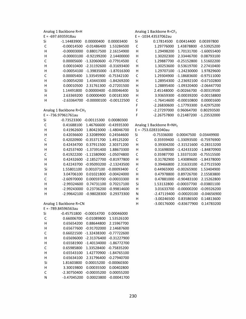
230
Analog 1 Backbone R=H E = ‐697.6935918au Si ‐1.14483900 0.00000400 0.00003400 C ‐0.00014500 ‐0.01486400 1.53284500 H ‐0.00003000 0.88017500 2.16154900 H ‐0.00003100 ‐0.92199200 2.14400000 C 0.00005600 ‐1.32060600 ‐0.77914500 H 0.00010400 ‐2.31192600 ‐0.31693400 H ‐0.00054100 ‐1.39835000 ‐1.87016300 C 0.00005400 1.33545900 ‐0.75342100 H ‐0.00054200 1.43443300 ‐1.84269200 H 0.00010500 2.31761300 ‐0.27201500 Si 1.14491800 0.00000400 ‐0.00046400 H 2.63369200 0.00000400 0.00181300 H ‐2.63364700 ‐0.00000100 ‐0.00122500 Analog 1 Backbone R=CH3 E = ‐736.97961761au Si ‐0.73523300 ‐0.00115300 0.00080300 C 0.41688100 1.46766600 ‐0.43935300 H 0.41962600 1.80423000 ‐1.48046700 H 0.42036600 2.32089900 0.24564600 C 0.42020900 ‐0.35371700 1.49125200 H 0.42434700 0.37911500 2.30371200 H 0.42537400 ‐1.37391400 1.88673300 C 0.41922200 ‐1.11580900 ‐1.05074800 H 0.42432600 ‐2.18527700 ‐0.81977800 H 0.42243700 ‐0.95093200 ‐2.13243500 Si 1.55801100 0.00107100 ‐0.00093400 H 3.04706100 0.01021800 ‐0.00424000 C ‐2.60970000 0.00059700 ‐0.00033300 H ‐2.99324600 0.74731100 0.70217100 H ‐2.99243000 0.23736200 ‐0.99814600 H ‐2.99642100 ‐0.98028300 0.29373300 Analog 1 Backbone R=CN E = ‐789.84596563au Si ‐0.45751800 ‐0.00014700 0.00046000 C 0.66006700 ‐0.01089800 1.53526100 H 0.65654200 0.88644800 2.15967700 H 0.65677600 ‐0.91702000 2.14687600 C 0.66021500 ‐1.32438300 ‐0.77722600 H 0.65696000 ‐2.31376400 ‐0.31227900 H 0.65581900 ‐1.40134000 ‐1.86772700 C 0.65985800 1.33528400 ‐0.75835200 H 0.65543100 1.42770900 ‐1.84765100 H 0.65634100 2.31796400 ‐0.27940700 Si 1.81603800 0.00015200 ‐0.00060300 H 3.30019800 0.00035500 0.00402800 C ‐2.30750400 ‐0.00035200 0.00055200 N ‐3.47045200 0.00023800 ‐0.00041700
Analog 1 Backbone R=CF3 E = ‐1034.43537062au Si 0.17814500 0.00414400 0.00397800 C 1.29776000 1.43878800 ‐0.53925200 H 1.29498200 1.70131700 ‐1.60055400 H 1.30202300 2.33446700 0.08793100 C 1.29887700 ‐0.25152800 1.51602200 H 1.30253600 0.53619700 2.27410400 H 1.29707100 ‐1.24230000 1.97829600 C 1.29304900 ‐1.18683600 ‐0.97511000 H 1.28954300 ‐2.23692100 ‐0.67102800 H 1.28895400 ‐1.09320400 ‐2.06447700 Si 2.45148000 ‐0.00266700 ‐0.00319500 H 3.93659300 ‐0.00039200 ‐0.00158800 C ‐1.76414600 ‐0.00010800 0.00001600 F ‐2.26830600 ‐1.17793300 0.42975200 F ‐2.27297000 0.96064700 0.80293500 F ‐2.26757800 0.21487200 ‐1.23532000 Analog 1 Backbone R=NH2 E = ‐753.02831040au Si ‐0.75336000 0.00047500 0.03449900 C 0.35939400 ‐1.33093500 ‐0.75976900 H 0.39304200 ‐2.31521600 ‐0.28313200 H 0.31698000 ‐1.42433100 ‐1.84870900 C 0.35987700 1.33373100 ‐0.75515500 H 0.31782900 1.43089600 ‐1.84378000 H 0.39466800 2.31633100 ‐0.27515500 C 0.44965900 ‐0.00265900 1.53404900 H 0.47978800 0.89726700 2.15583800 H 0.47881000 ‐0.90483100 2.15262800 Si 1.53132800 ‐0.00037700 ‐0.03801100 H 3.01633700 ‐0.00000200 ‐0.09326200 N ‐2.47119400 ‐0.00020100 ‐0.04656900 H ‐3.00246500 0.83586500 0.14813600 H ‐3.00176000 ‐0.83677900 0.14783200
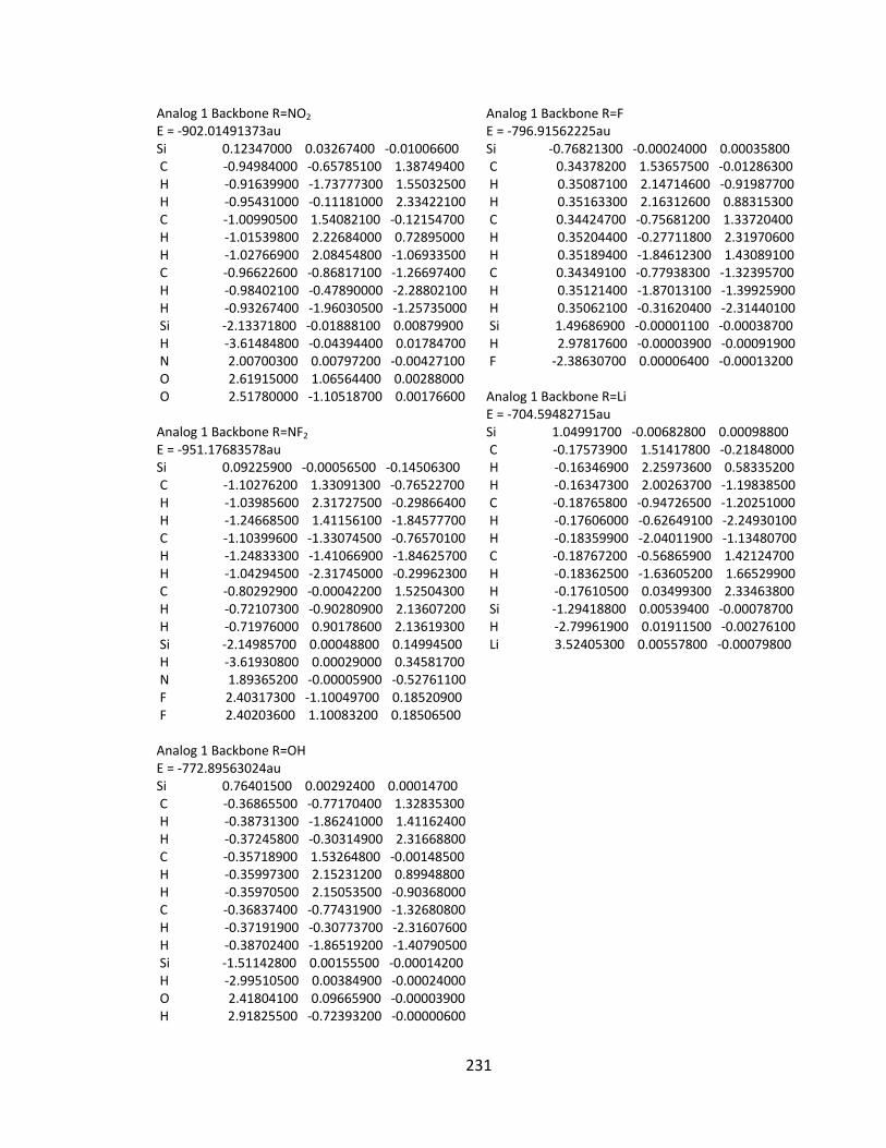
231
Analog 1 Backbone R=NO2 E = ‐902.01491373au Si 0.12347000 0.03267400 ‐0.01006600 C ‐0.94984000 ‐0.65785100 1.38749400 H ‐0.91639900 ‐1.73777300 1.55032500 H ‐0.95431000 ‐0.11181000 2.33422100 C ‐1.00990500 1.54082100 ‐0.12154700 H ‐1.01539800 2.22684000 0.72895000 H ‐1.02766900 2.08454800 ‐1.06933500 C ‐0.96622600 ‐0.86817100 ‐1.26697400 H ‐0.98402100 ‐0.47890000 ‐2.28802100 H ‐0.93267400 ‐1.96030500 ‐1.25735000 Si ‐2.13371800 ‐0.01888100 0.00879900 H ‐3.61484800 ‐0.04394400 0.01784700 N 2.00700300 0.00797200 ‐0.00427100 O 2.61915000 1.06564400 0.00288000 O 2.51780000 ‐1.10518700 0.00176600 Analog 1 Backbone R=NF2 E = ‐951.17683578au Si 0.09225900 ‐0.00056500 ‐0.14506300 C ‐1.10276200 1.33091300 ‐0.76522700 H ‐1.03985600 2.31727500 ‐0.29866400 H ‐1.24668500 1.41156100 ‐1.84577700 C ‐1.10399600 ‐1.33074500 ‐0.76570100 H ‐1.24833300 ‐1.41066900 ‐1.84625700 H ‐1.04294500 ‐2.31745000 ‐0.29962300 C ‐0.80292900 ‐0.00042200 1.52504300 H ‐0.72107300 ‐0.90280900 2.13607200 H ‐0.71976000 0.90178600 2.13619300 Si ‐2.14985700 0.00048800 0.14994500 H ‐3.61930800 0.00029000 0.34581700 N 1.89365200 ‐0.00005900 ‐0.52761100 F 2.40317300 ‐1.10049700 0.18520900 F 2.40203600 1.10083200 0.18506500 Analog 1 Backbone R=OH E = ‐772.89563024au Si 0.76401500 0.00292400 0.00014700 C ‐0.36865500 ‐0.77170400 1.32835300 H ‐0.38731300 ‐1.86241000 1.41162400 H ‐0.37245800 ‐0.30314900 2.31668800 C ‐0.35718900 1.53264800 ‐0.00148500 H ‐0.35997300 2.15231200 0.89948800 H ‐0.35970500 2.15053500 ‐0.90368000 C ‐0.36837400 ‐0.77431900 ‐1.32680800 H ‐0.37191900 ‐0.30773700 ‐2.31607600 H ‐0.38702400 ‐1.86519200 ‐1.40790500 Si ‐1.51142800 0.00155500 ‐0.00014200 H ‐2.99510500 0.00384900 ‐0.00024000 O 2.41804100 0.09665900 ‐0.00003900 H 2.91825500 ‐0.72393200 ‐0.00000600
Analog 1 Backbone R=F E = ‐796.91562225au Si ‐0.76821300 ‐0.00024000 0.00035800 C 0.34378200 1.53657500 ‐0.01286300 H 0.35087100 2.14714600 ‐0.91987700 H 0.35163300 2.16312600 0.88315300 C 0.34424700 ‐0.75681200 1.33720400 H 0.35204400 ‐0.27711800 2.31970600 H 0.35189400 ‐1.84612300 1.43089100 C 0.34349100 ‐0.77938300 ‐1.32395700 H 0.35121400 ‐1.87013100 ‐1.39925900 H 0.35062100 ‐0.31620400 ‐2.31440100 Si 1.49686900 ‐0.00001100 ‐0.00038700 H 2.97817600 ‐0.00003900 ‐0.00091900 F ‐2.38630700 0.00006400 ‐0.00013200 Analog 1 Backbone R=Li E = ‐704.59482715au Si 1.04991700 ‐0.00682800 0.00098800 C ‐0.17573900 1.51417800 ‐0.21848000 H ‐0.16346900 2.25973600 0.58335200 H ‐0.16347300 2.00263700 ‐1.19838500 C ‐0.18765800 ‐0.94726500 ‐1.20251000 H ‐0.17606000 ‐0.62649100 ‐2.24930100 H ‐0.18359900 ‐2.04011900 ‐1.13480700 C ‐0.18767200 ‐0.56865900 1.42124700 H ‐0.18362500 ‐1.63605200 1.66529900 H ‐0.17610500 0.03499300 2.33463800 Si ‐1.29418800 0.00539400 ‐0.00078700 H ‐2.79961900 0.01911500 ‐0.00276100 Li 3.52405300 0.00557800 ‐0.00079800
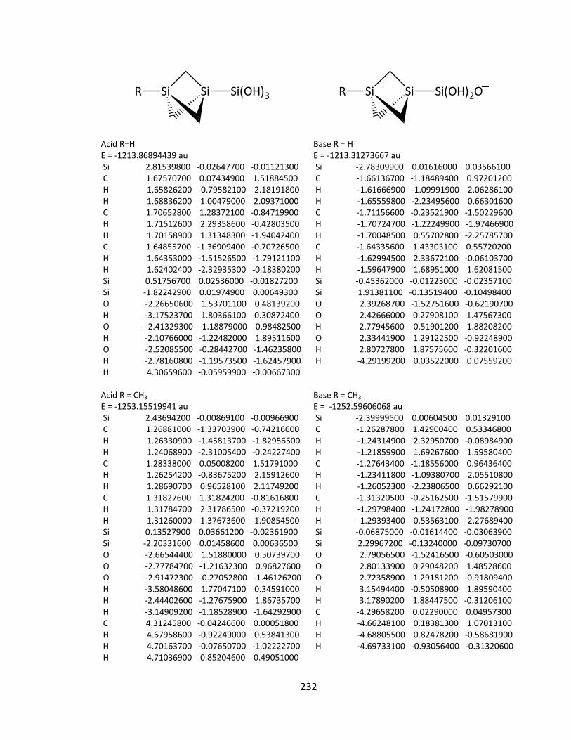
232
R Si Si Si(OH)3
Acid R=H E = ‐1213.86894439 au Si 2.81539800 ‐0.02647700 ‐0.01121300 C 1.67570700 0.07434900 1.51884500 H 1.65826200 ‐0.79582100 2.18191800 H 1.68836200 1.00479000 2.09371000 C 1.70652800 1.28372100 ‐0.84719900 H 1.71512600 2.29358600 ‐0.42803500 H 1.70158900 1.31348300 ‐1.94042400 C 1.64855700 ‐1.36909400 ‐0.70726500 H 1.64353000 ‐1.51526500 ‐1.79121100 H 1.62402400 ‐2.32935300 ‐0.18380200 Si 0.51756700 0.02536000 ‐0.01827200 Si ‐1.82242900 0.01974900 0.00649300 O ‐2.26650600 1.53701100 0.48139200 H ‐3.17523700 1.80366100 0.30872400 O ‐2.41329300 ‐1.18879000 0.98482500 H ‐2.10766000 ‐1.22482000 1.89511600 O ‐2.52085500 ‐0.28442700 ‐1.46235800 H ‐2.78160800 ‐1.19573500 ‐1.62457900 H 4.30659600 ‐0.05959900 ‐0.00667300 Acid R = CH3 E = ‐1253.15519941 au Si 2.43694200 ‐0.00869100 ‐0.00966900 C 1.26881000 ‐1.33703900 ‐0.74216600 H 1.26330900 ‐1.45813700 ‐1.82956500 H 1.24068900 ‐2.31005400 ‐0.24227400 C 1.28338000 0.05008200 1.51791000 H 1.26254200 ‐0.83675200 2.15912600 H 1.28690700 0.96528100 2.11749200 C 1.31827600 1.31824200 ‐0.81616800 H 1.31784700 2.31786500 ‐0.37219200 H 1.31260000 1.37673600 ‐1.90854500 Si 0.13527900 0.03661200 ‐0.02361900 Si ‐2.20331600 0.01458600 0.00636500 O ‐2.66544400 1.51880000 0.50739700 O ‐2.77784700 ‐1.21632300 0.96827600 O ‐2.91472300 ‐0.27052800 ‐1.46126200 H ‐3.58048600 1.77047100 0.34591000 H ‐2.44402600 ‐1.27675900 1.86735700 H ‐3.14909200 ‐1.18528900 ‐1.64292900 C 4.31245800 ‐0.04246600 0.00051800 H 4.67958600 ‐0.92249000 0.53841300 H 4.70163700 ‐0.07650700 ‐1.02222700 H 4.71036900 0.85204600 0.49051000
R Si Si Si(OH)2O
Base R = H E = ‐1213.31273667 au Si ‐2.78309900 0.01616000 0.03566100 C ‐1.66136700 ‐1.18489400 0.97201200 H ‐1.61666900 ‐1.09991900 2.06286100 H ‐1.65559800 ‐2.23495600 0.66301600 C ‐1.71156600 ‐0.23521900 ‐1.50229600 H ‐1.70724700 ‐1.22249900 ‐1.97466900 H ‐1.70048500 0.55702800 ‐2.25785700 C ‐1.64335600 1.43303100 0.55720200 H ‐1.62994500 2.33672100 ‐0.06103700 H ‐1.59647900 1.68951000 1.62081500 Si ‐0.45362000 ‐0.01223000 ‐0.02357100 Si 1.91381100 ‐0.13519400 ‐0.10498400 O 2.39268700 ‐1.52751600 ‐0.62190700 O 2.42666000 0.27908100 1.47567300 H 2.77945600 ‐0.51901200 1.88208200 O 2.33441900 1.29122500 ‐0.92248900 H 2.80727800 1.87575600 ‐0.32201600 H ‐4.29199200 0.03522000 0.07559200 Base R = CH3 E = ‐1252.59606068 au Si ‐2.39999500 0.00604500 0.01329100 C ‐1.26287800 1.42900400 0.53346800 H ‐1.24314900 2.32950700 ‐0.08984900 H ‐1.21859900 1.69267600 1.59580400 C ‐1.27643400 ‐1.18556000 0.96436400 H ‐1.23411800 ‐1.09380700 2.05510800 H ‐1.26052300 ‐2.23806500 0.66292100 C ‐1.31320500 ‐0.25162500 ‐1.51579900 H ‐1.29798400 ‐1.24172800 ‐1.98278900 H ‐1.29393400 0.53563100 ‐2.27689400 Si ‐0.06875000 ‐0.01614400 ‐0.03063900 Si 2.29967200 ‐0.13240000 ‐0.09730700 O 2.79056500 ‐1.52416500 ‐0.60503000 O 2.80133900 0.29048200 1.48528600 O 2.72358900 1.29181200 ‐0.91809400 H 3.15494400 ‐0.50508900 1.89590400 H 3.17890200 1.88447500 ‐0.31206100 C ‐4.29658200 0.02290000 0.04957300 H ‐4.66248100 0.18381300 1.07013100 H ‐4.68805500 0.82478200 ‐0.58681900 H ‐4.69733100 ‐0.93056400 ‐0.31320600
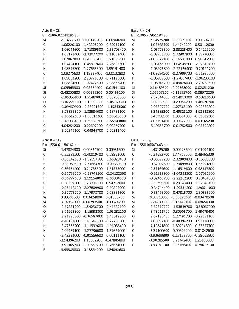
233
Acid R = CN E = ‐1306.02244195 au Si 2.18727600 ‐0.00140200 ‐0.00960200 C 1.06226100 ‐1.43398200 ‐0.52935100 H 1.06044600 ‐1.71089500 ‐1.58705400 H 1.05171400 ‐2.32077200 0.11002400 C 1.07862800 0.28066700 1.50135700 H 1.07494100 ‐0.49912600 2.26805500 H 1.08596300 1.27665300 1.95191400 C 1.09275600 1.18397400 ‐1.00132800 H 1.09663200 2.23778100 ‐0.71126600 H 1.08894600 1.07422600 ‐2.08886400 Si ‐0.09565300 0.02624400 ‐0.01541100 Si ‐2.43255800 0.00998200 0.00499100 O ‐2.85955800 1.55489000 0.38760800 O ‐3.02271100 ‐1.13390500 1.05169300 O ‐3.09469900 ‐0.38921300 ‐1.45343500 H ‐3.75836800 1.83584600 0.18783100 H ‐2.80612600 ‐1.06313200 1.98515900 H ‐3.40086400 ‐1.29570700 ‐1.55149800 C 4.04254200 ‐0.02607000 ‐0.00279700 N 5.20549100 ‐0.04344700 0.00311400 Acid R = CF3 E = ‐1550.61184162 au Si ‐1.47824300 0.00824700 0.00936500 C ‐0.35389500 ‐1.40019400 0.59953600 H ‐0.35142800 ‐1.62597500 1.66929400 H ‐0.33989500 ‐2.31664300 0.00339300 C ‐0.36481400 0.21768500 ‐1.51228000 H ‐0.35738200 ‐0.59748500 ‐2.24122300 H ‐0.36777600 1.19154000 ‐2.00904800 C ‐0.38209300 1.23906100 0.94712000 H ‐0.38118600 2.27809900 0.60806900 H ‐0.37776700 1.17978700 2.03862600 Si 0.80305500 0.03424800 0.01855700 Si 3.14057000 0.00793500 ‐0.00524700 O 3.57861200 1.54256700 ‐0.41689100 O 3.71923300 ‐1.15992800 ‐1.03282200 O 3.81236600 ‐0.36587000 1.45612300 H 4.48191600 1.81642300 ‐0.22780500 H 3.47332200 ‐1.11992600 ‐1.96086400 H 4.09479100 ‐1.27736600 1.57629000 C ‐3.42392000 ‐0.01566600 0.00112100 F ‐3.94396200 1.13602200 ‐0.47885800 F ‐3.91365700 ‐1.01559700 ‐0.76634000 F ‐3.93385800 ‐0.18864000 1.24092600
Base R = CN E = ‐1305.47961184 au Si ‐2.14575700 0.00069700 0.00174700 C ‐1.06268400 1.44743200 0.50112600 H ‐1.05773500 2.33225400 ‐0.14229000 H ‐1.03776700 1.72987900 1.55790000 C ‐1.05672100 ‐1.16531900 0.98547900 H ‐1.03188900 ‐1.04949500 2.07310400 H ‐1.03976800 ‐2.22126400 0.70121700 C ‐1.08684500 ‐0.27909700 ‐1.51925600 H ‐1.06937500 ‐1.27867400 ‐1.96233100 H ‐1.08046200 0.49428000 ‐2.29281500 Si 0.16489500 ‐0.00263000 ‐0.02851200 Si 2.53357200 ‐0.13189700 ‐0.08972200 O 2.97044600 ‐1.54013300 ‐0.59210600 O 3.02608900 0.29956700 1.48620700 O 2.95697700 1.27565100 ‐0.92669800 H 3.34585300 ‐0.49323100 1.92842800 H 3.40998500 1.88604000 ‐0.33682300 C ‐4.03191400 0.00872900 0.03165200 N ‐5.19655700 0.01752500 0.05302800 Base R = CF3 E = ‐1550.06647443 au Si ‐1.43125200 ‐0.00228600 ‐0.01004100 C ‐0.34682700 1.44713500 0.48465300 H ‐0.33527200 2.32809400 ‐0.16396800 H ‐0.32007500 1.73499800 1.53991800 C ‐0.34464600 ‐1.16519800 0.98337300 H ‐0.31889900 ‐1.04293300 2.07027300 H ‐0.32460700 ‐2.22262200 0.70484500 C ‐0.36795200 ‐0.29143400 ‐1.52840400 H ‐0.34714400 ‐1.29331200 ‐1.96611000 H ‐0.35493000 0.47815700 ‐2.30565900 Si 0.87710000 ‐0.00823300 ‐0.03470500 Si 3.24780500 ‐0.13142100 ‐0.08650300 O 3.69812700 ‐1.53849700 ‐0.58067900 O 3.73011700 0.30906700 1.49079400 O 3.67136400 1.27491700 ‐0.92651100 H 4.05097100 ‐0.48094200 1.93718000 H 4.10841800 1.89294800 ‐0.33257700 C ‐3.39400600 0.00609200 0.01842600 F ‐3.93699800 ‐1.17138700 ‐0.39063800 F ‐3.90285500 0.23742400 1.25863800 F ‐3.93191100 0.96166400 ‐0.78617100
234
Acid R = NH2 E = ‐1269.20471253 au Si 2.44253500 0.00576000 ‐0.02047100 C 1.29523400 ‐1.45243500 ‐0.44990200 H 1.27550300 ‐1.80115700 ‐1.48683200 H 1.28317600 ‐2.29543000 0.24712500 C 1.30533200 0.40605600 1.45516000 H 1.30172800 ‐0.31323000 2.27976300 H 1.28993900 1.43357900 1.83045800 C 1.31633500 1.12089200 ‐1.10170400 H 1.30626100 2.19424600 ‐0.89068200 H 1.30514700 0.93576700 ‐2.17996600 Si 0.14834000 0.03849400 ‐0.04070100 Si ‐2.18429600 0.00857300 0.00931400 O ‐2.64836800 1.58012000 0.20901800 O ‐2.74545800 ‐1.01089400 1.19830600 O ‐2.89990000 ‐0.56275900 ‐1.36913500 H ‐3.56635900 1.79327400 0.01284800 H ‐2.39752900 ‐0.89838500 2.08697000 H ‐3.12981200 ‐1.49650600 ‐1.36587500 N 4.15705600 ‐0.11447900 0.08150600 H 4.70364600 0.60985900 0.52465600 H 4.68520600 ‐0.59905100 ‐0.62983600 Acid R = NO2 E = ‐1418.19281623 au Si 1.81048400 ‐0.04544700 0.00180300 C 0.71695100 0.77184300 1.30541700 H 0.71071200 0.33401200 2.30680300 H 0.72222200 1.86380400 1.34743700 C 0.72264600 0.68745800 ‐1.35542800 H 0.73385300 1.77479800 ‐1.46496300 H 0.71839500 0.18770000 ‐2.32736700 C 0.72012600 ‐1.58271500 0.04946600 H 0.71226900 ‐2.22788100 ‐0.83218700 H 0.71466400 ‐2.16959000 0.97108400 Si ‐0.45669600 ‐0.04796900 ‐0.00141400 Si ‐2.79130600 0.00343800 ‐0.00768100 O ‐3.22156700 ‐1.02960800 ‐1.21484400 O ‐3.35102000 1.55083400 ‐0.20061800 O ‐3.45612500 ‐0.50763600 1.41177700 H ‐4.12442300 ‐1.36354900 ‐1.22424900 H ‐3.11665600 2.03386300 ‐0.99761200 H ‐3.74244000 0.17563400 2.02525200 N 3.69898600 0.02584700 0.01140000 O 4.18249200 1.14744400 ‐0.08723600 O 4.33939600 ‐1.00972700 0.11859200
Base R = NH2 E = ‐1268.64633072 au Si ‐2.40679200 0.00604600 0.00151800 C ‐1.28515500 1.40972400 0.57255700 H ‐1.24768200 2.32766800 ‐0.02371600 H ‐1.25774500 1.63942000 1.64275400 C ‐1.30396700 ‐1.23197400 0.89829200 H ‐1.27884000 ‐1.19391600 1.99227100 H ‐1.27449400 ‐2.26711100 0.54302700 C ‐1.31364500 ‐0.19102300 ‐1.53665100 H ‐1.29254600 ‐1.16125900 ‐2.04378200 H ‐1.28400600 0.62707600 ‐2.26432900 Si ‐0.08435400 ‐0.01810400 ‐0.03443800 Si 2.28469900 ‐0.12940400 ‐0.09495900 O 2.77617200 ‐1.50416600 ‐0.64453200 O 2.77820400 0.24794900 1.50012400 O 2.70386300 1.31959500 ‐0.87132700 H 3.12303000 ‐0.55935100 1.89479800 H 3.13755100 1.90417900 ‐0.24205600 N ‐4.15508400 0.03486700 0.15763300 H ‐4.65176900 ‐0.82559700 ‐0.03704600 H ‐4.64696700 0.81789200 ‐0.25436100 Base R = NO2 E = ‐1417.65492949 au Si 1.76398900 ‐0.02956700 ‐0.02737900 C 0.72204100 0.37138400 1.47231300 H 0.71854300 ‐0.34017200 2.30271600 H 0.71646600 1.40391800 1.83191900 C 0.69211400 1.05865600 ‐1.10077400 H 0.68767600 2.13231000 ‐0.89516200 H 0.65513900 0.85811000 ‐2.17480100 C 0.70371000 ‐1.51716000 ‐0.40726600 H 0.66765300 ‐1.88379100 ‐1.43626000 H 0.69926100 ‐2.34302800 0.30875600 Si ‐0.52857200 ‐0.03511500 ‐0.00481200 Si ‐2.90341200 ‐0.06996300 ‐0.13207700 O ‐3.32758300 ‐0.44346000 ‐1.58172500 O ‐3.37520300 1.46194000 0.44311200 O ‐3.32388100 ‐1.02959100 1.19152200 H ‐3.67036900 1.99360900 ‐0.30275400 H ‐3.74266000 ‐0.49428200 1.87255000 N 3.69016700 0.02957600 0.00803900 O 4.21164100 1.14051000 0.05503000 O 4.32526000 ‐1.02014300 0.01092000
235
Acid R = NF2 E = ‐1467.35426464 au Si ‐1.76868600 0.00358300 0.19218500 C ‐0.65088300 1.34456800 0.91424500 H ‐0.67546900 2.33234400 0.44771700 H ‐0.58838300 1.42046900 2.00272600 C ‐0.61919000 ‐1.31902100 0.89911900 H ‐0.55842600 ‐1.40655200 1.98702400 H ‐0.62839400 ‐2.30233000 0.42190500 C ‐0.74955100 0.02076900 ‐1.40036000 H ‐0.77431400 ‐0.88143100 ‐2.01719300 H ‐0.78669900 0.92432100 ‐2.01396600 Si 0.49897400 0.03369900 0.08148300 Si 2.82875100 0.00943400 ‐0.07040300 O 3.35700800 ‐1.28779600 ‐0.95771000 O 3.58231800 ‐0.15534300 1.38830100 O 3.21983800 1.47444900 ‐0.71344300 H 3.05911500 ‐1.38058200 ‐1.86655600 H 3.87727300 ‐1.04062300 1.62142900 H 4.12712000 1.78076800 ‐0.61484000 N ‐3.60031000 ‐0.02571900 0.42253500 F ‐4.02850800 ‐1.12567300 ‐0.34485800 F ‐4.06391100 1.07581200 ‐0.32035500 Acid R = OH E = ‐1289.07271726 au Si 2.44214900 ‐0.01113600 ‐0.00584600 C 1.29338000 ‐1.35360800 ‐0.72051300 H 1.27377200 ‐1.49017700 ‐1.80584100 H 1.26537000 ‐2.31764500 ‐0.20419600 C 1.32144700 0.08082300 1.51781900 H 1.30100900 ‐0.79256100 2.17610700 H 1.32814200 1.00923800 2.09553200 C 1.34637400 1.29929900 ‐0.85014700 H 1.34857900 2.30936200 ‐0.43124300 H 1.32591300 1.32841500 ‐1.94351400 Si 0.15832900 0.03662900 ‐0.02190200 Si ‐2.17285900 0.01491300 0.00715200 O ‐2.62562600 1.52719300 0.48465300 O ‐2.74349800 ‐1.20082200 0.98546500 O ‐2.86978700 ‐0.29105600 ‐1.46054400 H ‐3.53799900 1.78598000 0.31953500 H ‐2.42279100 ‐1.24277800 1.89038900 H ‐3.10258900 ‐1.20775400 ‐1.63455800 O 4.09713400 ‐0.03958300 0.09827600 H 4.60094500 ‐0.07270300 ‐0.71962100
Base R = NF2 E = ‐1466.81150707 au Si ‐1.72419100 0.01516900 0.17837900 C ‐0.60689900 1.38589300 0.78716500 H ‐0.60098300 2.33098800 0.23672600 H ‐0.52829100 1.55380100 1.86472100 C ‐0.64118400 ‐1.26499700 1.00665200 H ‐0.56171800 ‐1.25513500 2.09705000 H ‐0.65805500 ‐2.28748200 0.61955200 C ‐0.73226000 ‐0.12777800 ‐1.40253900 H ‐0.75965000 ‐1.07766800 ‐1.94378400 H ‐0.73633800 0.72138700 ‐2.09161500 Si 0.57062200 ‐0.02460700 0.07666500 Si 2.94786800 ‐0.03369000 0.08854200 O 3.31891000 ‐1.37709200 ‐0.86728400 O 3.46581800 0.08731300 1.55155300 O 3.36888700 1.22330100 ‐0.98411800 H 3.66055700 ‐1.09167100 ‐1.72021200 H 3.70501400 1.96345700 ‐0.46905000 N ‐3.58590400 0.06149400 0.41052100 F ‐4.06361600 ‐1.10248200 ‐0.23869500 F ‐4.03485600 1.09012400 ‐0.45309500 Base R = OH E = ‐1288.51878446 au Si ‐2.40882400 0.01643500 0.02055500 C ‐1.34005900 ‐0.34845500 ‐1.49042100 H ‐1.30425800 ‐1.36966400 ‐1.88308400 H ‐1.32567600 0.38325700 ‐2.30453000 C ‐1.30505000 1.47329800 0.44566900 H ‐1.29225400 2.32797500 ‐0.23797400 H ‐1.26427800 1.80562500 1.48779700 C ‐1.30060600 ‐1.11569000 1.04555000 H ‐1.26115700 ‐0.95757500 2.12829200 H ‐1.26616100 ‐2.18330700 0.80552600 Si ‐0.09580100 ‐0.00274600 ‐0.02165600 Si 2.27313000 ‐0.14156800 ‐0.09089100 O 2.77780000 0.37662900 1.45802500 O 2.70404400 1.21832800 ‐1.00447600 O 2.72833500 ‐1.57073900 ‐0.51573300 H 3.10270800 ‐0.39378200 1.93463600 H 3.12686600 1.86914200 ‐0.43583400 O ‐4.09423700 0.09583800 0.06556100 H ‐4.52812100 ‐0.70673200 ‐0.23874000

236
Acid R = F E = ‐1313.09325989 au Si 2.43856700 ‐0.01133500 ‐0.00901200 C 1.31089600 ‐1.37300200 ‐0.68563800 H 1.30122100 ‐1.53496200 ‐1.76695100 H 1.28124800 ‐2.32343200 ‐0.14559500 C 1.32962200 0.11198400 1.52081300 H 1.30703900 ‐0.74684300 2.19768500 H 1.33125400 1.05313200 2.07740400 C 1.35987500 1.28297500 ‐0.87089800 H 1.35772500 2.29912100 ‐0.46799800 H 1.34962800 1.29269100 ‐1.96409900 Si 0.16469200 0.03278300 ‐0.02061100 Si ‐2.16575000 0.01415500 0.00674200 O ‐2.60347400 1.53211100 0.47490600 O ‐2.73705900 ‐1.19224700 0.99239600 O ‐2.85053400 ‐0.29939400 ‐1.46253600 H ‐3.50752900 1.80917300 0.29439200 H ‐2.44790000 ‐1.21067800 1.90863400 H ‐3.10021200 ‐1.21269800 ‐1.63115400 F 4.05873100 ‐0.04216000 ‐0.00064200 Acid R = Li E = ‐1220.76901904 au Si 2.76182400 ‐0.02188600 ‐0.00747800 C 1.50548000 ‐1.25009800 ‐0.88374100 H 1.51919800 ‐1.25629500 ‐1.97857600 H 1.48018200 ‐2.27296300 ‐0.49369500 C 1.51655500 ‐0.11541000 1.50855200 H 1.49931000 ‐1.06649800 2.05178200 H 1.53747600 0.72707900 2.20738200 C 1.57642200 1.39320500 ‐0.67448000 H 1.59406300 2.34270000 ‐0.13035300 H 1.59113600 1.56855400 ‐1.75486000 Si 0.41253700 0.04639700 ‐0.02960700 Si ‐1.94526000 0.02074400 0.00573300 O ‐2.45823700 1.48796900 0.58248800 O ‐2.50800900 ‐1.26717200 0.91404900 O ‐2.70905700 ‐0.19721600 ‐1.45631500 H ‐3.38833200 1.69331700 0.44179600 H ‐2.07559800 ‐1.41715800 1.75918700 H ‐2.88358600 ‐1.11295300 ‐1.69160200 Li 5.24347500 ‐0.06472700 0.00136900
Base R = F E = ‐1312.54484617 au Si ‐2.40622200 0.00618400 0.01459200 C ‐1.30830300 1.45331600 0.48564800 H ‐1.28992400 2.32859900 ‐0.17107000 H ‐1.26259000 1.75177800 1.53767500 C ‐1.31630700 ‐1.15219000 1.00896000 H ‐1.27144600 ‐1.02029200 2.09449000 H ‐1.29631100 ‐2.21281300 0.74140600 C ‐1.35688400 ‐0.30227300 ‐1.50918400 H ‐1.33717000 ‐1.30781800 ‐1.93935600 H ‐1.33852000 0.45997300 ‐2.29403100 Si ‐0.10280300 ‐0.01235900 ‐0.03012000 Si 2.26972000 ‐0.13532600 ‐0.09439100 O 2.73198700 ‐1.54100400 ‐0.58034400 O 2.74852800 0.31983600 1.48004200 O 2.68942400 1.26548700 ‐0.94570600 H 3.07088300 ‐0.46599100 1.93257600 H 3.07223500 1.91103300 ‐0.34370400 F ‐4.05193700 0.02098500 0.04849000 Base R = Li E = ‐1220.19318307 au Si ‐2.70781300 0.01676200 0.02892600 C ‐1.48918400 1.43127700 0.53024300 H ‐1.48567600 2.32985400 ‐0.09692300 H ‐1.45367400 1.70359500 1.59115900 C ‐1.51771700 ‐1.17743000 0.97566300 H ‐1.48552700 ‐1.08171600 2.06682700 H ‐1.53084800 ‐2.23280400 0.68262700 C ‐1.56529400 ‐0.25768300 ‐1.50656800 H ‐1.57933000 ‐1.24953000 ‐1.97088300 H ‐1.56513900 0.52509600 ‐2.27314100 Si ‐0.34062000 ‐0.02293200 ‐0.03225100 Si 2.04037700 ‐0.13445000 ‐0.10196100 O 2.55344900 ‐1.52102400 ‐0.60836300 O 2.54413600 0.28913300 1.48373300 O 2.47100800 1.29367000 ‐0.91913900 H 2.90489200 ‐0.50690900 1.88729200 H 2.90530400 1.88957800 ‐0.30083900 Li ‐5.23760000 0.04009700 0.08066900

237
R
Si
COOH
Si Si Acid R = H E = ‐1137.36993829 au C 2.03620600 ‐0.04668400 0.00001300 Si 0.89366100 1.48578400 ‐0.00101700 H 0.91885100 2.33725600 1.21842100 H 0.91880400 2.33561500 ‐1.22160200 Si 0.82102500 ‐0.76357500 ‐1.28137900 H 0.80684600 ‐0.14089800 ‐2.63352100 H 0.75888100 ‐2.24490400 ‐1.40725200 Si 0.82104400 ‐0.76175800 1.28242000 H 0.75884800 ‐2.24291400 1.41034600 H 0.80684700 ‐0.13720600 2.63369500 C ‐0.36219900 0.04169500 ‐0.00005300 C ‐1.82930400 0.14025000 ‐0.00001000 O ‐2.47041600 1.17137200 ‐0.00003400 O ‐2.43817900 ‐1.06957000 0.00000900 H ‐3.39107900 ‐0.89446000 0.00004300 H 3.12233600 ‐0.08478200 0.00003500 Acid R = CH3 E = ‐1176.63615176 au C 1.72561600 ‐0.01574400 0.00000200 Si 0.54490900 1.49984100 ‐0.00014000 H 0.56085700 2.35457800 1.21880600 H 0.56092200 2.35437400 ‐1.21923000 Si 0.49924600 ‐0.74539100 ‐1.27978100 H 0.47736700 ‐0.12500700 ‐2.63430400 H 0.45584100 ‐2.22831700 ‐1.40949500 Si 0.49921700 ‐0.74517700 1.27987000 H 0.45580300 ‐2.22808000 1.40984400 H 0.47727600 ‐0.12455100 2.63428100 C ‐0.69002300 0.04353300 ‐0.00004000 C ‐2.15756100 0.12114000 ‐0.00004400 O ‐2.81465100 1.14227100 0.00003500 O ‐2.74926100 ‐1.09763600 0.00005300 H ‐3.70437000 ‐0.93528000 0.00012000 C 3.23770200 ‐0.04743700 0.00005100 H 3.65138100 0.45478200 ‐0.88190200 H 3.65132200 0.45492200 0.88195100 H 3.62328000 ‐1.07326900 0.00014400
R
Si
COO
Si Si Base R = H E = ‐1136.81472958 au C 2.02044000 0.08465800 ‐0.00000200 Si 0.70832400 1.48952600 ‐0.00005200 H 0.71213200 2.36737900 1.20963100 H 0.71202600 2.36731300 ‐1.20978000 Si 0.84156500 ‐0.73348200 ‐1.26675900 H 0.82429700 ‐0.13376300 ‐2.63869300 H 0.97855700 ‐2.21422900 ‐1.43047900 Si 0.84157000 ‐0.73337100 1.26679500 H 0.97855900 ‐2.21410600 1.43064400 H 0.82440000 ‐0.13353500 2.63868100 C ‐0.40782700 ‐0.05220800 0.00000500 C ‐1.94462500 ‐0.04352100 0.00000500 O ‐2.44708700 1.10855200 ‐0.00002600 O ‐2.50620000 ‐1.16219000 0.00004600 H 3.10797500 0.13905700 0.00001500 Base R = CH3 E = ‐1176.08052409 au C 1.70578300 0.02747400 0.00006100 Si 0.41471700 1.46188000 0.00002200 H 0.44493900 2.34120700 1.20974100 H 0.44495400 2.34116800 ‐1.20972600 Si 0.49003600 ‐0.76011300 ‐1.26536700 H 0.49148000 ‐0.16078300 ‐2.63866400 H 0.59389400 ‐2.24449500 ‐1.42981500 Si 0.48997800 ‐0.76007900 1.26545700 H 0.59381000 ‐2.24446200 1.42994200 H 0.49133900 ‐0.16073000 2.63874600 C ‐0.73802400 ‐0.04827700 0.00000500 C ‐2.27613000 ‐0.00342400 ‐0.00010800 O ‐2.75213800 1.15935600 ‐0.00011700 O ‐2.86200700 ‐1.10921800 ‐0.00021300 C 3.21662600 0.07186400 0.00011800 H 3.60863100 0.59538900 ‐0.88233000 H 3.60856900 0.59531000 0.88263900 H 3.65978700 ‐0.93316200 0.00008800

238
Acid R = CN E = ‐1229.51349429 au C 1.51854800 ‐0.00350000 0.00006800 Si 0.33012300 1.51643100 ‐0.00065200 H 0.36405700 2.34946700 1.22698200 H 0.36417400 2.34836600 ‐1.22903100 Si 0.30558200 ‐0.75071300 ‐1.29151300 H 0.30551100 ‐0.11238700 ‐2.63248100 H 0.30300100 ‐2.23124800 ‐1.39921400 Si 0.30545100 ‐0.74955200 1.29219400 H 0.30283400 ‐2.22999100 1.40121900 H 0.30522400 ‐0.11002800 2.63259100 C ‐0.87337900 0.03342100 ‐0.00007900 C ‐2.34411800 0.11164500 ‐0.00015000 O ‐2.99060900 1.13797900 ‐0.00017900 O ‐2.93314600 ‐1.10481600 0.00018200 H ‐3.88993900 ‐0.95031900 0.00024800 C 2.93861900 ‐0.02295700 0.00015100 N 4.10299600 ‐0.03816300 ‐0.00009700 Acid R = CF3 E = ‐1474.11895641 au C ‐0.93800600 0.00433700 0.00000400 Si 0.24146800 1.52117300 ‐0.00030200 H 0.21750400 2.35578700 ‐1.22754200 H 0.21774900 2.35613200 1.22670900 Si 0.26198200 ‐0.74456400 1.29126500 H 0.27293000 ‐0.10733000 2.63307100 H 0.27096900 ‐2.22521100 1.40101000 Si 0.26173200 ‐0.74491600 ‐1.29128500 H 0.27068000 ‐2.22559200 ‐1.40063600 H 0.27243300 ‐0.10804000 ‐2.63326300 C 1.44493700 0.03692000 ‐0.00023800 C 2.91560600 0.10857400 ‐0.00040300 O 3.56920500 1.13065100 0.00007000 O 3.49988000 ‐1.11101300 0.00040100 H 4.45702100 ‐0.95916800 0.00079400 C ‐2.41893000 ‐0.01287400 0.00010500 F ‐2.92265300 ‐1.26980000 0.00007200 F ‐2.94227600 0.60655600 1.08368800 F ‐2.94242300 0.60667400 ‐1.08333900
Base R = CN Not optimized. Base R = CF3 E = ‐1473.57720322 au C 0.91292000 ‐0.01136400 0.00000000 Si ‐0.40302300 1.41923000 ‐0.00004200 H ‐0.36180200 2.27267400 1.21943900 H ‐0.36179700 2.27259800 ‐1.21957500 Si ‐0.27472800 ‐0.82070400 ‐1.27732900 H ‐0.27293800 ‐0.20409900 ‐2.63666100 H ‐0.13064100 ‐2.29848000 ‐1.42824700 Si ‐0.27473300 ‐0.82063400 1.27737500 H ‐0.13065000 ‐2.29840100 1.42836800 H ‐0.27293800 ‐0.20395600 2.63667400 C ‐1.49507000 ‐0.12685800 ‐0.00000100 C ‐3.02300900 0.03030700 0.00000200 O ‐3.37179300 1.24175400 0.00001200 O ‐3.71548300 ‐1.00678200 ‐0.00001500 C 2.37982100 0.05109100 ‐0.00000400 F 2.98167200 ‐1.17372000 0.00009000 F 2.89338000 0.69958500 ‐1.08340400 F 2.89337100 0.69972900 1.08331200
239
Acid R = NH2 E = ‐1192.65516982 au C 1.73794900 ‐0.02027700 0.00204400 Si 0.56197900 1.47765200 ‐0.25138700 H 0.60182700 2.51512600 0.81586900 H 0.55165800 2.12313600 ‐1.59232800 Si 0.51087000 ‐0.94698900 ‐1.14556100 H 0.47017700 ‐0.56349600 ‐2.58392800 H 0.48579900 ‐2.43093900 ‐1.01955400 Si 0.49047600 ‐0.52570900 1.40689800 H 0.42961500 ‐1.96666300 1.78057800 H 0.45037800 0.31301200 2.63812000 C ‐0.66727200 0.03781500 ‐0.00262900 C ‐2.13324600 0.12398400 ‐0.00585100 O ‐2.78522800 1.14855600 0.00070400 O ‐2.73183900 ‐1.09165000 ‐0.01443200 H ‐3.68589400 ‐0.92345600 ‐0.01111100 N 3.16503500 ‐0.01954000 ‐0.09103000 H 3.56839600 ‐0.93573000 0.06592300 H 3.59819400 0.63206200 0.55278400 Acid R = NO2 E = ‐1341.67055970 au C ‐1.20198800 ‐0.00041600 0.00756100 Si ‐0.03271500 1.34688600 ‐0.71507500 H ‐0.08846900 1.49257700 ‐2.19023500 H ‐0.05390500 2.65811400 ‐0.02277500 Si ‐0.01471500 ‐0.02707200 1.50860100 H 0.01509400 1.17688300 2.37467400 H ‐0.03908300 ‐1.27834700 2.30646600 Si ‐0.03237500 ‐1.27725300 ‐0.79610000 H ‐0.03218000 ‐2.62988200 ‐0.18662200 H ‐0.00836400 ‐1.33601300 ‐2.27787700 C 1.14939400 0.02165900 ‐0.01284600 C 2.61971800 0.08397400 ‐0.06158800 O 3.26597300 0.94324500 ‐0.62341500 O 3.20891200 ‐0.93844000 0.59690600 H 4.16549500 ‐0.81217200 0.50624500 N ‐2.65044600 ‐0.01817100 0.00825400 O ‐3.23091700 0.72711900 0.78577000 O ‐3.20533600 ‐0.77831200 ‐0.77555900
Base R = NH2 E = ‐1192.10004611 au C 1.71481700 0.02982600 ‐0.01634700 Si 0.42599400 1.44917500 ‐0.21255200 H 0.48154300 2.48389700 0.86644600 H 0.41547400 2.15121600 ‐1.53191500 Si 0.49936800 ‐0.93175900 ‐1.15413800 H 0.46840500 ‐0.53935500 ‐2.59815600 H 0.62407300 ‐2.42280500 ‐1.09657800 Si 0.49215600 ‐0.57203400 1.37449700 H 0.59307000 ‐2.01836900 1.75060500 H 0.49078400 0.21903100 2.64734300 C ‐0.71515600 ‐0.05358100 0.01502000 C ‐2.25631000 ‐0.00481300 0.00328900 O ‐2.72845100 1.15887500 ‐0.00161100 O ‐2.84303700 ‐1.10932600 ‐0.00222500 N 3.15451700 0.10367400 ‐0.10986300 H 3.57998000 ‐0.80254100 0.05821800 H 3.53160100 0.74287000 0.58269600 Base R = NO2 Not optimized.
240
Acid R = NF2 E = ‐1390.83913922 au C 1.16453100 0.05413600 ‐0.21257400 Si ‐0.06876100 1.50014700 ‐0.49346400 H 0.03201700 2.61910500 0.47452400 H ‐0.19303700 1.98852000 ‐1.89001800 Si ‐0.09420500 ‐1.03024300 ‐1.16544000 H ‐0.24604600 ‐0.75594100 ‐2.61774000 H ‐0.03201800 ‐2.48747900 ‐0.89395900 Si 0.11496600 ‐0.36828500 1.34764400 H 0.15706800 ‐1.77320200 1.82296200 H 0.16313000 0.59343800 2.47730300 C ‐1.18816000 0.03156400 ‐0.00596000 C ‐2.65480800 0.07230500 0.11339400 O ‐3.34056500 1.06823600 0.01424800 O ‐3.19413800 ‐1.14402500 0.35400500 H ‐4.15220300 ‐1.01374900 0.41883700 N 2.56835000 0.09287800 ‐0.43217100 F 3.06248200 ‐1.14828000 0.03700500 F 3.08339600 0.97214500 0.54919000 Acid R = OH E = ‐1212.50077118 au C ‐1.73467100 ‐0.01556800 0.00250700 Si ‐0.50444800 ‐0.60737100 1.37472600 H ‐0.47779800 0.17036200 2.64533300 H ‐0.43185500 ‐2.06424800 1.66744200 Si ‐0.52374400 ‐0.89637100 ‐1.19257500 H ‐0.47680400 ‐2.38183500 ‐1.13607900 H ‐0.49425300 ‐0.43302300 ‐2.60678800 Si ‐0.55614300 1.50858400 ‐0.17727800 H ‐0.54378400 2.21786500 ‐1.48490800 H ‐0.58413800 2.48774100 0.94386400 C 0.64851800 0.04530200 ‐0.00362000 C 2.11573300 0.12388100 ‐0.00342100 O 2.77293100 1.14465400 0.00875200 O 2.70635900 ‐1.09506000 ‐0.01630000 H 3.66167500 ‐0.93400700 ‐0.01147000 O ‐3.12048200 ‐0.11622700 ‐0.07094900 H ‐3.52027800 0.48074700 0.56956400
Base R = NF2 E = ‐1390.29842478 au C ‐1.14555700 ‐0.20653900 0.00001200 Si ‐0.00702900 1.37118400 ‐0.00004800 H ‐0.11495400 2.21466500 ‐1.22119600 H ‐0.11493700 2.21475500 1.22104000 Si 0.11908800 ‐0.89579700 1.27819800 H 0.03640900 ‐0.28856500 2.63752500 H 0.14120100 ‐2.38130900 1.41397100 Si 0.11907800 ‐0.89588300 ‐1.27813900 H 0.14119400 ‐2.38140200 ‐1.41381300 H 0.03639000 ‐0.28874300 ‐2.63750600 C 1.24188300 ‐0.05755500 ‐0.00000300 C 2.76532600 0.17699900 ‐0.00001000 O 3.07361600 1.39509000 ‐0.00005000 O 3.48872300 ‐0.84060200 0.00001700 N ‐2.54132700 ‐0.43167200 0.00002400 F ‐3.06891900 0.32814900 1.09800400 F ‐3.06892000 0.32806400 ‐1.09801300 Base R = OH E = ‐1211.94838318 au C ‐1.71286500 0.04171800 ‐0.00001400 Si ‐0.50402300 ‐0.75944100 ‐1.28469000 H ‐0.62613900 ‐2.24413200 ‐1.43674000 H ‐0.47529500 ‐0.16341400 ‐2.65677700 Si ‐0.43004000 1.47554400 0.00006700 H ‐0.43917300 2.34692800 ‐1.21310000 H ‐0.43903900 2.34690600 1.21324700 Si ‐0.50407900 ‐0.75956300 1.28468200 H ‐0.47522600 ‐0.16371000 2.65684200 H ‐0.62623200 ‐2.24426900 1.43656700 C 0.69540000 ‐0.05619100 0.00003200 C 2.24072300 ‐0.01179200 0.00000200 O 2.82349000 ‐1.11745100 ‐0.00008800 O 2.71309100 1.15100500 0.00004200 O ‐3.11580000 0.16723700 ‐0.00008600 H ‐3.49070100 ‐0.71861600 0.00006300

241
Acid R = F E = ‐1236.50260277 au C 1.71757900 ‐0.01700400 0.00004300 Si 0.56781100 1.52619400 ‐0.00047500 H 0.57815900 2.36681100 1.22479600 H 0.57825200 2.36603400 ‐1.22627900 Si 0.51784700 ‐0.76131000 ‐1.30279700 H 0.48994500 ‐0.13061100 ‐2.64931400 H 0.46427700 ‐2.24245000 ‐1.41447000 Si 0.51774900 ‐0.76048300 1.30326200 H 0.46415000 ‐2.24155200 1.41586500 H 0.48971700 ‐0.12893500 2.64937800 C ‐0.63169900 0.04396200 ‐0.00007400 C ‐2.09992700 0.12440700 ‐0.00011700 O ‐2.75345900 1.14693700 ‐0.00010900 O ‐2.69142800 ‐1.09349500 0.00010200 H ‐3.64688600 ‐0.93275700 0.00016200 F 3.08645100 ‐0.05043200 0.00010500 Acid R = Li E = ‐1144.25646638 au C 1.98952100 ‐0.03771500 0.00002400 Si 0.80120100 1.45811000 ‐0.00036400 H 0.81199200 2.33667200 1.20787700 H 0.81201800 2.33606200 ‐1.20904800 Si 0.73845800 ‐0.73876200 ‐1.25197700 H 0.70723600 ‐0.13647800 ‐2.62016200 H 0.66952600 ‐2.22322900 ‐1.40904600 Si 0.73842700 ‐0.73811900 1.25235100 H 0.66948000 ‐2.22250500 1.41017800 H 0.70716600 ‐0.13513300 2.62022600 C ‐0.50275700 0.04575200 ‐0.00003300 C ‐1.97038900 0.13242100 ‐0.00005100 O ‐2.62864900 1.15481500 ‐0.00012800 O ‐2.57470200 ‐1.08341600 0.00011800 H ‐3.52705500 ‐0.90629000 0.00012700 Li 3.92833100 ‐0.06674400 0.00004600
Base R = F E = ‐1235.95462404 au C ‐1.69692000 0.04349000 0.00006000 Si ‐0.41359900 1.48446600 ‐0.00011400 H ‐0.42034000 2.34975700 ‐1.21584100 H ‐0.42039300 2.35000200 1.21543800 Si ‐0.52019500 ‐0.77391300 1.28692400 H ‐0.50117500 ‐0.16586700 2.65249700 H ‐0.63412900 ‐2.25580100 1.43593100 Si ‐0.52025100 ‐0.77421200 ‐1.28668600 H ‐0.63423500 ‐2.25612900 ‐1.43533000 H ‐0.50123400 ‐0.16648200 ‐2.65239800 C 0.67718000 ‐0.06530200 0.00002400 C 2.22551000 ‐0.01120900 ‐0.00009600 O 2.68533800 1.15662100 ‐0.00030200 O 2.81589400 ‐1.11125600 ‐0.00006800 F ‐3.08626100 0.09677300 0.00011300 Base R = Li E = ‐1143.68157885 au C ‐1.96936300 0.03296600 0.00000100 Si ‐0.67133000 1.44924900 ‐0.00005000 H ‐0.68952300 2.35214900 ‐1.19988600 H ‐0.68951000 2.35222900 1.19972600 Si ‐0.73040100 ‐0.73251600 1.24233500 H ‐0.72270500 ‐0.15028100 2.62949000 H ‐0.80912600 ‐2.22088700 1.43316300 Si ‐0.73041300 ‐0.73260600 ‐1.24228100 H ‐0.80913200 ‐2.22099200 ‐1.43299700 H ‐0.72272300 ‐0.15047300 ‐2.62947900 C 0.54913900 ‐0.02889200 ‐0.00000400 C 2.08395100 ‐0.01096000 ‐0.00000300 O 2.59528300 1.13769100 ‐0.00000300 O 2.64922200 ‐1.13088400 ‐0.00000200 Li ‐3.88189100 0.08245100 0.00000200
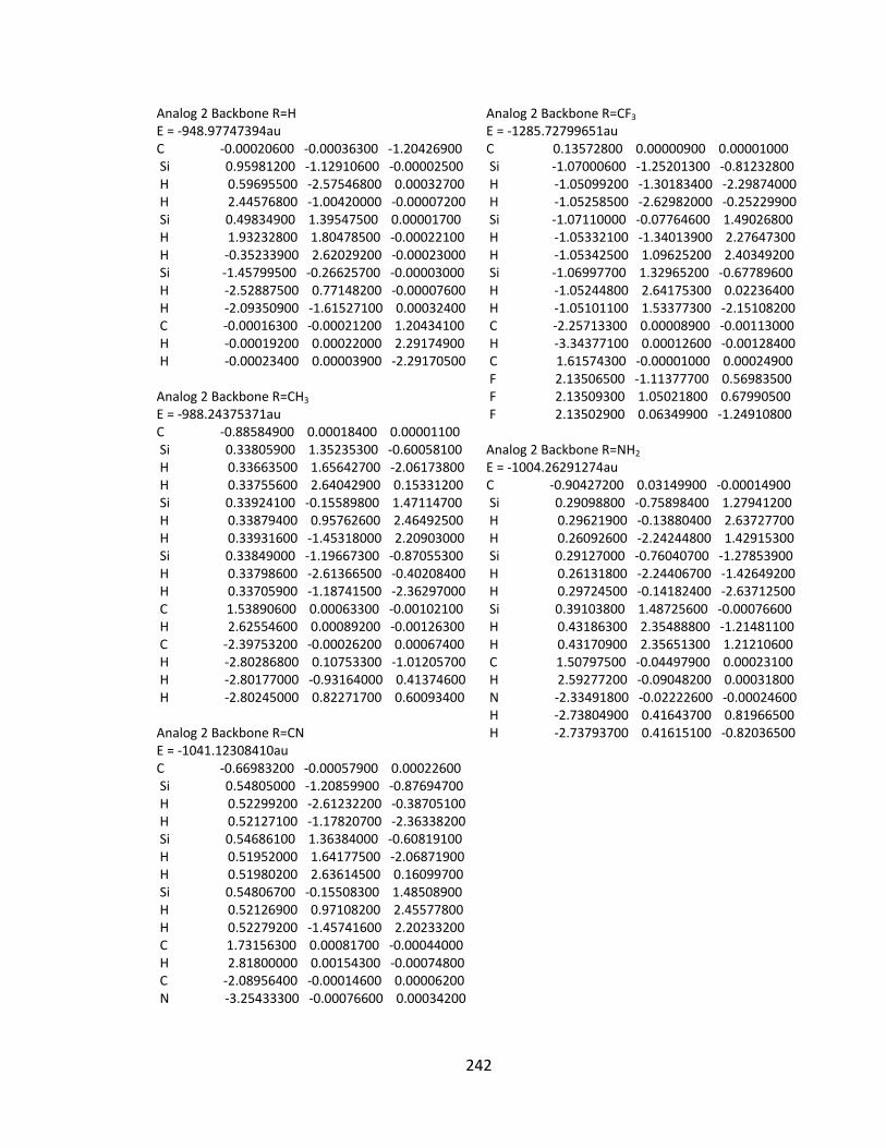
242
Analog 2 Backbone R=H E = ‐948.97747394au C ‐0.00020600 ‐0.00036300 ‐1.20426900 Si 0.95981200 ‐1.12910600 ‐0.00002500 H 0.59695500 ‐2.57546800 0.00032700 H 2.44576800 ‐1.00420000 ‐0.00007200 Si 0.49834900 1.39547500 0.00001700 H 1.93232800 1.80478500 ‐0.00022100 H ‐0.35233900 2.62029200 ‐0.00023000 Si ‐1.45799500 ‐0.26625700 ‐0.00003000 H ‐2.52887500 0.77148200 ‐0.00007600 H ‐2.09350900 ‐1.61527100 0.00032400 C ‐0.00016300 ‐0.00021200 1.20434100 H ‐0.00019200 0.00022000 2.29174900 H ‐0.00023400 0.00003900 ‐2.29170500 Analog 2 Backbone R=CH3 E = ‐988.24375371au C ‐0.88584900 0.00018400 0.00001100 Si 0.33805900 1.35235300 ‐0.60058100 H 0.33663500 1.65642700 ‐2.06173800 H 0.33755600 2.64042900 0.15331200 Si 0.33924100 ‐0.15589800 1.47114700 H 0.33879400 0.95762600 2.46492500 H 0.33931600 ‐1.45318000 2.20903000 Si 0.33849000 ‐1.19667300 ‐0.87055300 H 0.33798600 ‐2.61366500 ‐0.40208400 H 0.33705900 ‐1.18741500 ‐2.36297000 C 1.53890600 0.00063300 ‐0.00102100 H 2.62554600 0.00089200 ‐0.00126300 C ‐2.39753200 ‐0.00026200 0.00067400 H ‐2.80286800 0.10753300 ‐1.01205700 H ‐2.80177000 ‐0.93164000 0.41374600 H ‐2.80245000 0.82271700 0.60093400 Analog 2 Backbone R=CN E = ‐1041.12308410au C ‐0.66983200 ‐0.00057900 0.00022600 Si 0.54805000 ‐1.20859900 ‐0.87694700 H 0.52299200 ‐2.61232200 ‐0.38705100 H 0.52127100 ‐1.17820700 ‐2.36338200 Si 0.54686100 1.36384000 ‐0.60819100 H 0.51952000 1.64177500 ‐2.06871900 H 0.51980200 2.63614500 0.16099700 Si 0.54806700 ‐0.15508300 1.48508900 H 0.52126900 0.97108200 2.45577800 H 0.52279200 ‐1.45741600 2.20233200 C 1.73156300 0.00081700 ‐0.00044000 H 2.81800000 0.00154300 ‐0.00074800 C ‐2.08956400 ‐0.00014600 0.00006200 N ‐3.25433300 ‐0.00076600 0.00034200
Analog 2 Backbone R=CF3 E = ‐1285.72799651au C 0.13572800 0.00000900 0.00001000 Si ‐1.07000600 ‐1.25201300 ‐0.81232800 H ‐1.05099200 ‐1.30183400 ‐2.29874000 H ‐1.05258500 ‐2.62982000 ‐0.25229900 Si ‐1.07110000 ‐0.07764600 1.49026800 H ‐1.05332100 ‐1.34013900 2.27647300 H ‐1.05342500 1.09625200 2.40349200 Si ‐1.06997700 1.32965200 ‐0.67789600 H ‐1.05244800 2.64175300 0.02236400 H ‐1.05101100 1.53377300 ‐2.15108200 C ‐2.25713300 0.00008900 ‐0.00113000 H ‐3.34377100 0.00012600 ‐0.00128400 C 1.61574300 ‐0.00001000 0.00024900 F 2.13506500 ‐1.11377700 0.56983500 F 2.13509300 1.05021800 0.67990500 F 2.13502900 0.06349900 ‐1.24910800 Analog 2 Backbone R=NH2 E = ‐1004.26291274au C ‐0.90427200 0.03149900 ‐0.00014900 Si 0.29098800 ‐0.75898400 1.27941200 H 0.29621900 ‐0.13880400 2.63727700 H 0.26092600 ‐2.24244800 1.42915300 Si 0.29127000 ‐0.76040700 ‐1.27853900 H 0.26131800 ‐2.24406700 ‐1.42649200 H 0.29724500 ‐0.14182400 ‐2.63712500 Si 0.39103800 1.48725600 ‐0.00076600 H 0.43186300 2.35488800 ‐1.21481100 H 0.43170900 2.35651300 1.21210600 C 1.50797500 ‐0.04497900 0.00023100 H 2.59277200 ‐0.09048200 0.00031800 N ‐2.33491800 ‐0.02222600 ‐0.00024600 H ‐2.73804900 0.41643700 0.81966500 H ‐2.73793700 0.41615100 ‐0.82036500
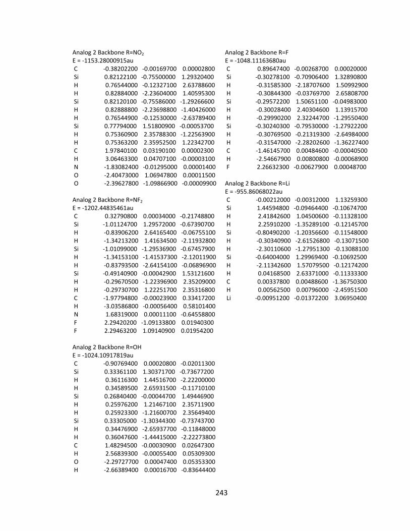
243
Analog 2 Backbone R=NO2 E = ‐1153.28000915au C ‐0.38202200 ‐0.00169700 0.00002800 Si 0.82122100 ‐0.75500000 1.29320400 H 0.76544000 ‐0.12327100 2.63788600 H 0.82884000 ‐2.23604000 1.40595300 Si 0.82120100 ‐0.75586000 ‐1.29266600 H 0.82888800 ‐2.23698800 ‐1.40426000 H 0.76544900 ‐0.12530000 ‐2.63789400 Si 0.77794000 1.51800900 ‐0.00053700 H 0.75360900 2.35788300 ‐1.22563900 H 0.75363200 2.35952500 1.22342700 C 1.97840100 0.03190100 0.00002300 H 3.06463300 0.04707100 ‐0.00003100 N ‐1.83082400 ‐0.01295000 0.00001400 O ‐2.40473000 1.06947800 0.00011500 O ‐2.39627800 ‐1.09866900 ‐0.00009900 Analog 2 Backbone R=NF2 E = ‐1202.44835461au C 0.32790800 0.00034000 ‐0.21748800 Si ‐1.01124700 1.29572000 ‐0.67390700 H ‐0.83906200 2.64165400 ‐0.06755100 H ‐1.34213200 1.41634500 ‐2.11932800 Si ‐1.01099000 ‐1.29536900 ‐0.67457900 H ‐1.34153100 ‐1.41537300 ‐2.12011900 H ‐0.83793500 ‐2.64154100 ‐0.06896900 Si ‐0.49140900 ‐0.00042900 1.53121600 H ‐0.29670500 ‐1.22396900 2.35209000 H ‐0.29730700 1.22251700 2.35316800 C ‐1.97794800 ‐0.00023900 0.33417200 H ‐3.03586800 ‐0.00056400 0.58101400 N 1.68319000 0.00011100 ‐0.64558800 F 2.29420200 ‐1.09133800 0.01940300 F 2.29463200 1.09140900 0.01954200 Analog 2 Backbone R=OH E = ‐1024.10917819au C ‐0.90769400 0.00020800 ‐0.02011300 Si 0.33361100 1.30371700 ‐0.73677200 H 0.36116300 1.44516700 ‐2.22200000 H 0.34589500 2.65931500 ‐0.11710100 Si 0.26840400 ‐0.00044700 1.49446900 H 0.25976200 1.21467100 2.35711900 H 0.25923300 ‐1.21600700 2.35649400 Si 0.33305000 ‐1.30344300 ‐0.73743700 H 0.34476900 ‐2.65937700 ‐0.11848000 H 0.36047600 ‐1.44415000 ‐2.22273800 C 1.48294500 ‐0.00030900 0.02647300 H 2.56839300 ‐0.00055400 0.05309300 O ‐2.29727700 0.00047400 0.05353300 H ‐2.66389400 0.00016700 ‐0.83644400
Analog 2 Backbone R=F E = ‐1048.11163680au C 0.89647400 ‐0.00268700 0.00020000 Si ‐0.30278100 ‐0.70906400 1.32890800 H ‐0.31585300 ‐2.18707600 1.50992900 H ‐0.30844300 ‐0.03769700 2.65808700 Si ‐0.29572200 1.50651100 ‐0.04983000 H ‐0.30028400 2.40304600 1.13915700 H ‐0.29990200 2.32244700 ‐1.29550400 Si ‐0.30240300 ‐0.79530000 ‐1.27922200 H ‐0.30769500 ‐0.21319300 ‐2.64984000 H ‐0.31547000 ‐2.28202600 ‐1.36227400 C ‐1.46145700 0.00484600 ‐0.00040500 H ‐2.54667900 0.00800800 ‐0.00068900 F 2.26632300 ‐0.00627900 0.00048700 Analog 2 Backbone R=Li E = ‐955.86068022au C ‐0.00212000 ‐0.00312000 1.13259300 Si 1.44594800 ‐0.09464400 ‐0.10674700 H 2.41842600 1.04500600 ‐0.11328100 H 2.25910200 ‐1.35289100 ‐0.12145700 Si ‐0.80490200 ‐1.20356600 ‐0.11548000 H ‐0.30340900 ‐2.61526800 ‐0.13071500 H ‐2.30110600 ‐1.27951300 ‐0.13088100 Si ‐0.64004000 1.29969400 ‐0.10692500 H ‐2.11342600 1.57079500 ‐0.12174200 H 0.04168500 2.63371000 ‐0.11333300 C 0.00337800 0.00488600 ‐1.36750300 H 0.00562500 0.00796000 ‐2.45951500 Li ‐0.00951200 ‐0.01372200 3.06950400
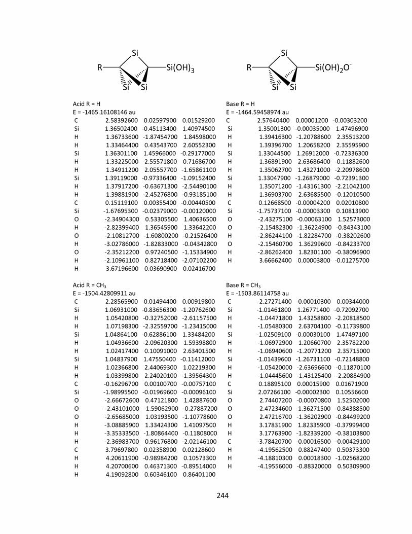
244
R
Si
Si(OH)3
Si Si Acid R = H E = ‐1465.16108146 au C 2.58392600 0.02597900 0.01529200 Si 1.36502400 ‐0.45113400 1.40974500 H 1.36733600 ‐1.87454700 1.84598000 H 1.33464400 0.43543700 2.60552300 Si 1.36301100 1.45966000 ‐0.29177000 H 1.33225000 2.55571800 0.71686700 H 1.34911200 2.05557700 ‐1.65861100 Si 1.39119000 ‐0.97336400 ‐1.09152400 H 1.37917200 ‐0.63671300 ‐2.54490100 H 1.39881900 ‐2.45276800 ‐0.93185100 C 0.15119100 0.00355400 ‐0.00440500 Si ‐1.67695300 ‐0.02379000 ‐0.00120000 O ‐2.34904300 0.53305500 1.40636500 H ‐2.82399400 1.36545900 1.33642200 O ‐2.10812700 ‐1.60800200 ‐0.21526400 H ‐3.02786000 ‐1.82833000 ‐0.04342800 O ‐2.35212200 0.97240500 ‐1.15334900 H ‐2.10961100 0.82718400 ‐2.07102200 H 3.67196600 0.03690900 0.02416700 Acid R = CH3 E = ‐1504.42809911 au C 2.28565900 0.01494400 0.00919800 Si 1.06931000 ‐0.83656300 ‐1.20762600 H 1.05420800 ‐0.32752000 ‐2.61157500 H 1.07198300 ‐2.32559700 ‐1.23415000 Si 1.04864100 ‐0.62886100 1.33484200 H 1.04936600 ‐2.09620300 1.59398800 H 1.02417400 0.10091000 2.63401500 Si 1.04837900 1.47550400 ‐0.11412000 H 1.02366800 2.44069300 1.02219300 H 1.03399800 2.24020100 ‐1.39564300 C ‐0.16296700 0.00100700 ‐0.00757100 Si ‐1.98995500 ‐0.01969600 ‐0.00096100 O ‐2.66672600 0.47121800 1.42887600 O ‐2.43101000 ‐1.59062900 ‐0.27887200 O ‐2.65685000 1.03193500 ‐1.10778600 H ‐3.08885900 1.33424300 1.41097500 H ‐3.35333500 ‐1.80864400 ‐0.11808000 H ‐2.36983700 0.96176800 ‐2.02146100 C 3.79697800 0.02358900 0.02128600 H 4.20611900 ‐0.98984200 0.10573300 H 4.20700600 0.46371300 ‐0.89514000 H 4.19092800 0.60346100 0.86401100
R
Si
Si(OH)2O‐
Si Si Base R = H E = ‐1464.59458974 au C 2.57640400 0.00001200 ‐0.00303200 Si 1.35001300 ‐0.00035000 1.47496900 H 1.39416300 ‐1.20788600 2.35513200 H 1.39396700 1.20658200 2.35595900 Si 1.33044500 1.26912000 ‐0.72336300 H 1.36891900 2.63686400 ‐0.11882600 H 1.35062700 1.43271000 ‐2.20978600 Si 1.33047900 ‐1.26879000 ‐0.72391300 H 1.35071200 ‐1.43161300 ‐2.21042100 H 1.36903700 ‐2.63685500 ‐0.12010500 C 0.12668500 ‐0.00004200 0.02010800 Si ‐1.75737100 ‐0.00003300 0.10813900 O ‐2.43275100 ‐0.00063100 1.52573000 O ‐2.15482300 ‐1.36224900 ‐0.84343100 H ‐2.86244100 ‐1.82284700 ‐0.38202600 O ‐2.15460700 1.36299600 ‐0.84233700 H ‐2.86262400 1.82301100 ‐0.38096900 H 3.66662400 0.00003800 ‐0.01275700 Base R = CH3 E = ‐1503.86114758 au C ‐2.27271400 ‐0.00010300 0.00344000 Si ‐1.01461800 1.26771400 ‐0.72092700 H ‐1.04471800 1.43258800 ‐2.20818500 H ‐1.05480300 2.63704100 ‐0.11739800 Si ‐1.02509100 ‐0.00030100 1.47497100 H ‐1.06972900 1.20660700 2.35782200 H ‐1.06940600 ‐1.20771200 2.35715000 Si ‐1.01439600 ‐1.26731100 ‐0.72148800 H ‐1.05420000 ‐2.63696600 ‐0.11870100 H ‐1.04445600 ‐1.43125400 ‐2.20884900 C 0.18895100 0.00015900 0.01671900 Si 2.07266100 ‐0.00002300 0.10556600 O 2.74407200 ‐0.00070800 1.52502000 O 2.47234600 1.36271500 ‐0.84388500 O 2.47216700 ‐1.36202900 ‐0.84499200 H 3.17831900 1.82335900 ‐0.37999400 H 3.17763900 ‐1.82339200 ‐0.38103800 C ‐3.78420700 ‐0.00016500 ‐0.00429100 H ‐4.19562500 0.88247400 0.50373300 H ‐4.18810300 0.00018300 ‐1.02568200 H ‐4.19556000 ‐0.88320000 0.50309900
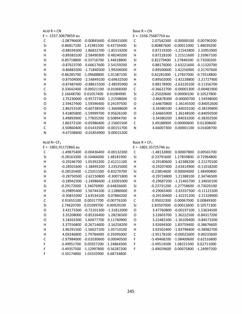
245
Acid R = CN E = ‐1557.30679659 au C ‐2.08796600 ‐0.00845600 ‐0.00415000 Si ‐0.86817100 1.41981500 ‐0.43734400 H ‐0.88594300 1.86822700 ‐1.85519200 H ‐0.89383100 2.58490300 0.48240200 Si ‐0.85718800 ‐0.33716700 1.44618800 H ‐0.87623700 0.66617600 2.54159200 H ‐0.86883300 ‐1.71840500 1.99206000 Si ‐0.86285700 ‐1.09688800 ‐1.01387100 H ‐0.87504000 ‐2.54849100 ‐0.69632500 H ‐0.87487400 ‐0.88615500 ‐2.48595900 C 0.33642400 ‐0.00021100 ‐0.01068300 Si 2.16648700 0.01057400 0.01084900 O 2.75230000 ‐0.95727300 1.21598000 O 2.59427400 1.59396400 0.24197500 O 2.86253100 ‐0.60738500 ‐1.36698600 H 3.41805800 ‐1.59999700 0.95626100 H 3.49893900 1.77835200 0.50894700 H 2.86372100 ‐0.05986400 ‐2.15601500 C ‐3.50860400 ‐0.01433500 ‐0.00151700 N ‐4.67338600 ‐0.01854900 0.00015200 Acid R= CF3 E = ‐1801.91172860 au C ‐1.49875400 ‐0.00436400 ‐0.00132300 Si ‐0.28163300 ‐0.10466000 1.48181900 H ‐0.29246700 1.05392200 2.41211100 H ‐0.28501600 ‐1.38495200 2.23525000 Si ‐0.28535400 ‐1.23351500 ‐0.83270700 H ‐0.28750500 ‐2.62150800 ‐0.30071800 H ‐0.28942300 ‐1.24986600 ‐2.32001000 Si ‐0.29172000 1.34076900 ‐0.64826600 H ‐0.29895400 1.56744100 ‐2.11880000 H ‐0.30833300 2.63534100 0.07884200 C 0.91655100 0.00317700 ‐0.00776100 Si 2.74620700 0.01099700 0.00929100 O 3.43173300 ‐0.72101300 ‐1.31812000 O 3.35208000 ‐0.85326400 1.28236500 O 3.18263300 1.60477700 0.11760900 H 3.37556800 ‐0.26714600 ‐2.16258200 H 3.96291500 ‐1.56027100 1.05710100 H 4.09246800 1.79784000 0.35995000 C ‐2.97984000 ‐0.01030600 0.00040500 F ‐3.49951700 0.05927200 ‐1.24864500 F ‐3.49357500 ‐1.12997800 0.56287200 F ‐3.50174800 1.03335900 0.68734800
Base R = CN E = ‐1556.75687754 au C 2.07542300 ‐0.00000100 0.00790200 Si 0.80887600 ‐0.00011000 1.48039200 H 0.87219200 ‐1.21542800 2.33953900 H 0.87218100 1.21511600 2.33967100 Si 0.82279400 1.27846500 ‐0.73500200 H 0.88176000 2.63221600 ‐0.11320700 H 0.89500600 1.42256900 ‐2.21707600 Si 0.82281000 ‐1.27837000 ‐0.73518800 H 0.89502000 ‐1.42228800 ‐2.21727900 H 0.88178900 ‐2.63220100 ‐0.11356700 C ‐0.36622700 ‐0.00001300 ‐0.00481900 Si ‐2.25020600 0.00000100 0.10527800 O ‐2.86878300 ‐0.00000700 1.54598000 O ‐2.64670800 ‐1.36145500 ‐0.84052600 H ‐3.34380100 ‐1.84033100 ‐0.38199800 O ‐2.64665900 1.36148500 ‐0.84050500 H ‐3.34380200 1.84033200 ‐0.38202500 C 3.49188900 0.00000600 0.01308600 N 4.66007300 0.00001100 0.01608700 Base R = CF3 E = ‐1801.35725746 au C ‐1.48132800 0.00007800 0.00565700 Si ‐0.23791600 1.27859800 ‐0.72964800 H ‐0.29180600 1.42388200 ‐2.21270100 H ‐0.29207400 2.63414900 ‐0.11018200 Si ‐0.23854600 ‐0.00004000 1.48490800 H ‐0.29724800 1.21388100 2.34746500 H ‐0.29687200 ‐1.21465700 2.34650100 Si ‐0.23731200 ‐1.27758600 ‐0.73020100 H ‐0.29065400 ‐2.63337300 ‐0.11121500 H ‐0.29130400 ‐1.42231200 ‐2.21328900 C 0.95032300 0.00067000 0.00849300 Si 2.83507000 ‐0.00013600 0.10571300 O 3.47760800 ‐0.00197100 1.53634500 O 3.22603700 1.36222500 ‐0.84317200 O 3.22481500 ‐1.36109400 ‐0.84573200 H 3.92694300 1.83759400 ‐0.38676600 H 3.92502400 ‐1.83798400 ‐0.38982700 C ‐2.95178100 ‐0.00022600 0.00233600 F ‐3.49468200 ‐1.08400600 0.62516800 F ‐3.49514500 1.08221500 0.62711000 F ‐3.49029600 0.00075800 ‐1.24997200
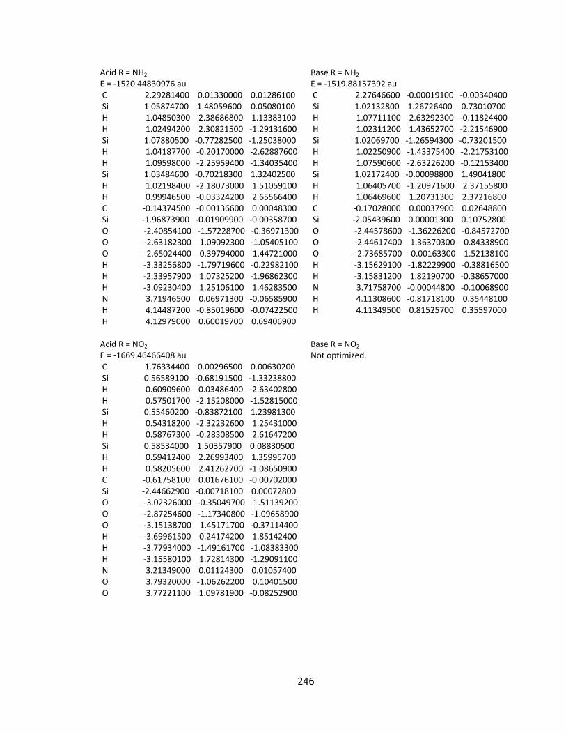
246
Acid R = NH2 E = ‐1520.44830976 au C 2.29281400 0.01330000 0.01286100 Si 1.05874700 1.48059600 ‐0.05080100 H 1.04850300 2.38686800 1.13383100 H 1.02494200 2.30821500 ‐1.29131600 Si 1.07880500 ‐0.77282500 ‐1.25038000 H 1.04187700 ‐0.20170000 ‐2.62887600 H 1.09598000 ‐2.25959400 ‐1.34035400 Si 1.03484600 ‐0.70218300 1.32402500 H 1.02198400 ‐2.18073000 1.51059100 H 0.99946500 ‐0.03324200 2.65566400 C ‐0.14374500 ‐0.00136600 0.00048300 Si ‐1.96873900 ‐0.01909900 ‐0.00358700 O ‐2.40854100 ‐1.57228700 ‐0.36971300 O ‐2.63182300 1.09092300 ‐1.05405100 O ‐2.65024400 0.39794000 1.44721000 H ‐3.33256800 ‐1.79719600 ‐0.22982100 H ‐2.33957900 1.07325200 ‐1.96862300 H ‐3.09230400 1.25106100 1.46283500 N 3.71946500 0.06971300 ‐0.06585900 H 4.14487200 ‐0.85019600 ‐0.07422500 H 4.12979000 0.60019700 0.69406900 Acid R = NO2 E = ‐1669.46466408 au C 1.76334400 0.00296500 0.00630200 Si 0.56589100 ‐0.68191500 ‐1.33238800 H 0.60909600 0.03486400 ‐2.63402800 H 0.57501700 ‐2.15208000 ‐1.52815000 Si 0.55460200 ‐0.83872100 1.23981300 H 0.54318200 ‐2.32232600 1.25431000 H 0.58767300 ‐0.28308500 2.61647200 Si 0.58534000 1.50357900 0.08830500 H 0.59412400 2.26993400 1.35995700 H 0.58205600 2.41262700 ‐1.08650900 C ‐0.61758100 0.01676100 ‐0.00702000 Si ‐2.44662900 ‐0.00718100 0.00072800 O ‐3.02326000 ‐0.35049700 1.51139200 O ‐2.87254600 ‐1.17340800 ‐1.09658900 O ‐3.15138700 1.45171700 ‐0.37114400 H ‐3.69961500 0.24174200 1.85142400 H ‐3.77934000 ‐1.49161700 ‐1.08383300 H ‐3.15580100 1.72814300 ‐1.29091100 N 3.21349000 0.01124300 0.01057400 O 3.79320000 ‐1.06262200 0.10401500 O 3.77221100 1.09781900 ‐0.08252900
Base R = NH2 E = ‐1519.88157392 au C 2.27646600 ‐0.00019100 ‐0.00340400 Si 1.02132800 1.26726400 ‐0.73010700 H 1.07711100 2.63292300 ‐0.11824400 H 1.02311200 1.43652700 ‐2.21546900 Si 1.02069700 ‐1.26594300 ‐0.73201500 H 1.02250900 ‐1.43375400 ‐2.21753100 H 1.07590600 ‐2.63226200 ‐0.12153400 Si 1.02172400 ‐0.00098800 1.49041800 H 1.06405700 ‐1.20971600 2.37155800 H 1.06469600 1.20731300 2.37216800 C ‐0.17028000 0.00037900 0.02648800 Si ‐2.05439600 0.00001300 0.10752800 O ‐2.44578600 ‐1.36226200 ‐0.84572700 O ‐2.44617400 1.36370300 ‐0.84338900 O ‐2.73685700 ‐0.00163300 1.52138100 H ‐3.15629100 ‐1.82229900 ‐0.38816500 H ‐3.15831200 1.82190700 ‐0.38657000 N 3.71758700 ‐0.00044800 ‐0.10068900 H 4.11308600 ‐0.81718100 0.35448100 H 4.11349500 0.81525700 0.35597000 Base R = NO2 Not optimized.
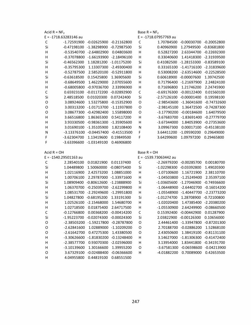
247
Acid R = NF2 E = ‐1718.63283146 au C ‐1.72591900 ‐0.02625900 ‐0.21162800 Si ‐0.47198100 ‐1.38298900 ‐0.72987500 H ‐0.53540700 ‐2.64802900 0.04803600 H ‐0.37078800 ‐1.66193900 ‐2.18496100 Si ‐0.46562300 1.18281200 ‐1.01175200 H ‐0.35795300 1.13307300 ‐2.49300400 H ‐0.52787500 2.58520100 ‐0.52911800 Si ‐0.63618500 0.15425800 1.36905600 H ‐0.68649500 1.46229000 2.07055600 H ‐0.68005800 ‐0.97036700 2.33996900 C 0.65923100 ‐0.01172200 ‐0.02892900 Si 2.48518500 0.01020300 0.07242400 O 3.08924600 1.53275800 ‐0.15352900 O 3.00313200 ‐1.01713700 ‐1.11937800 O 3.08677300 ‐0.42982400 1.55898000 H 3.66516800 1.86365300 0.54117200 H 3.93330500 ‐0.98361300 ‐1.35905600 H 3.01690100 ‐1.35105900 1.82108400 N ‐3.13376100 ‐0.04457400 ‐0.41513500 F ‐3.62304700 1.13419600 0.19849500 F ‐3.63396600 ‐1.03149100 0.46906800 Acid R = OH E = ‐1540.29501163 au C 2.28540100 0.01821900 0.01137400 Si 1.04489800 1.50060000 ‐0.08075400 H 1.02116900 2.42573200 1.08851000 H 1.00706100 2.29787000 ‐1.33971600 Si 1.08909400 ‐0.80612600 ‐1.23888900 H 1.06370700 ‐0.25039700 ‐2.62299800 H 1.08531700 ‐2.29249600 ‐1.29951800 Si 1.04827800 ‐0.68195200 1.33191300 H 1.02526100 ‐2.15468000 1.54680700 H 1.02718500 0.01875400 2.64717500 C ‐0.12766800 0.00368200 ‐0.00414200 Si ‐1.95223700 ‐0.02074300 ‐0.00024300 O ‐2.38503200 ‐1.59217800 ‐0.28787800 O ‐2.62841600 1.02889000 ‐1.10209200 O ‐2.61642700 0.47275300 1.43380500 H ‐3.30626600 ‐1.81830200 ‐0.13248400 H ‐2.38577700 0.93070300 ‐2.02596000 H ‐3.10139600 1.30166600 1.39955200 O 3.67329100 ‐0.02488400 ‐0.06366600 H 4.04955800 0.44819100 0.68551500
Base R = NF2 E = ‐1718.07957769 au C 1.70784500 ‐0.00030700 ‐0.20052800 Si 0.40960900 1.27949500 ‐0.83681800 H 0.52827200 2.63344700 ‐0.22692300 H 0.33040600 1.41418300 ‐2.31939500 Si 0.41082500 ‐1.28153300 ‐0.83589100 H 0.33165100 ‐1.41716100 ‐2.31839600 H 0.53008200 ‐2.63514600 ‐0.22528500 Si 0.60618900 ‐0.00007600 1.39742500 H 0.71796400 ‐1.21697900 2.24824100 H 0.71696800 1.21746200 2.24745900 C ‐0.69176300 ‐0.00122400 0.01560100 Si ‐2.57126100 ‐0.00001400 0.19598100 O ‐2.98543600 ‐1.36041600 ‐0.74732600 O ‐2.98145100 1.36472500 ‐0.74287300 O ‐3.17790200 ‐0.00184600 1.64079500 H ‐3.67683700 ‐1.83691400 ‐0.27779700 H ‐3.67344000 1.84053900 ‐0.27353600 N 3.09967300 0.00017100 ‐0.45138100 F 3.64411200 ‐1.09590200 0.29649000 F 3.64299600 1.09797200 0.29465800 Base R = OH E = ‐1539.73063442 au C ‐2.26979200 ‐0.00285700 0.00180700 Si ‐1.02298300 ‐0.03392800 1.49020300 H ‐1.07100600 1.16721900 2.38110700 H ‐1.04503800 ‐1.25249400 2.35397100 Si ‐1.03605600 ‐1.27046900 ‐0.74936600 H ‐1.06448900 ‐2.64402700 ‐0.16014200 H ‐1.05548900 ‐1.40447700 ‐2.23773200 Si ‐1.01274700 1.28708900 ‐0.72100800 H ‐1.02020400 1.47385400 ‐2.20380200 H ‐1.05530900 2.64249900 ‐0.08660500 C 0.15392400 ‐0.00442900 0.01287900 Si 2.03822900 ‐0.00126300 0.10656000 O 2.44461400 ‐1.33947800 ‐0.87201300 O 2.70188700 ‐0.02886200 1.52868100 O 2.43050600 1.38419100 ‐0.81131100 H 3.14627000 ‐1.81306300 ‐0.41472400 H 3.13954000 1.83441800 ‐0.34191700 O ‐3.67581300 ‐0.06598600 ‐0.04213900 H ‐4.01882200 0.70089000 0.42653500
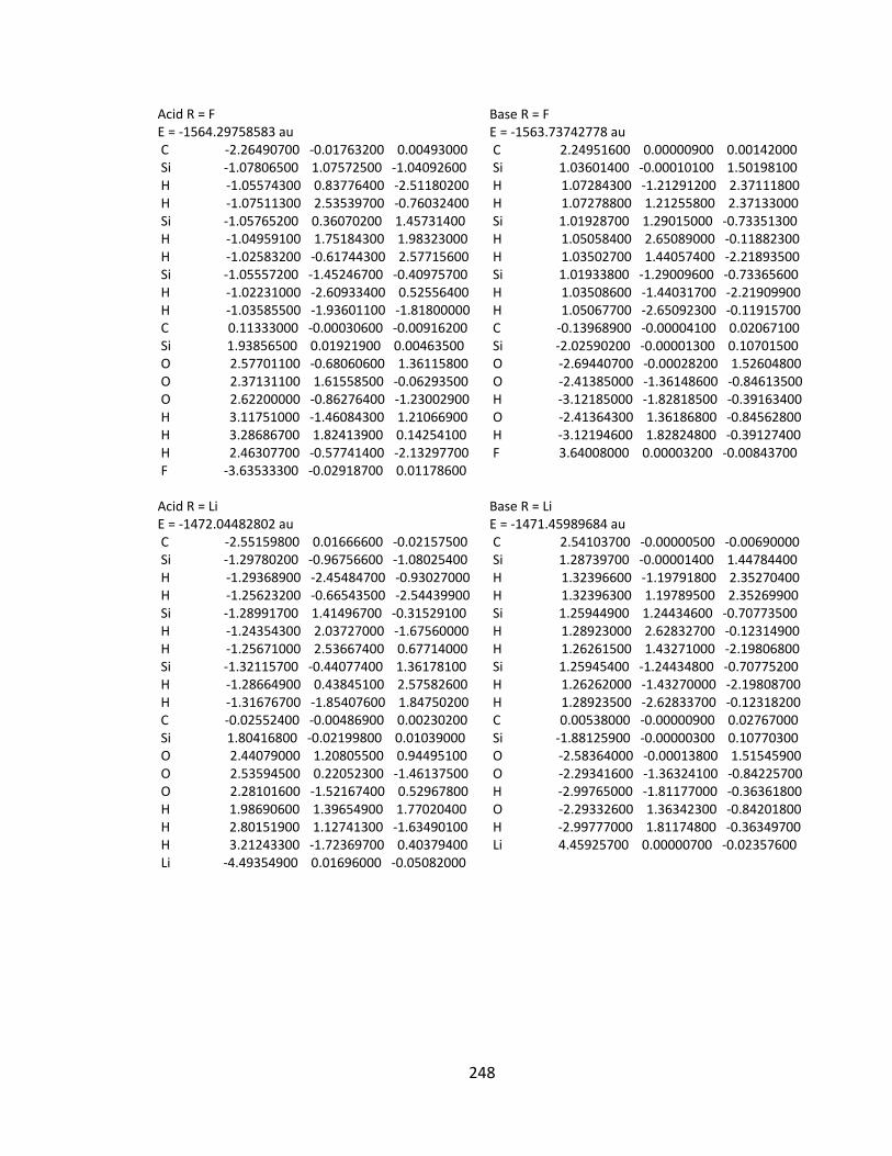
248
Acid R = F E = ‐1564.29758583 au C ‐2.26490700 ‐0.01763200 0.00493000 Si ‐1.07806500 1.07572500 ‐1.04092600 H ‐1.05574300 0.83776400 ‐2.51180200 H ‐1.07511300 2.53539700 ‐0.76032400 Si ‐1.05765200 0.36070200 1.45731400 H ‐1.04959100 1.75184300 1.98323000 H ‐1.02583200 ‐0.61744300 2.57715600 Si ‐1.05557200 ‐1.45246700 ‐0.40975700 H ‐1.02231000 ‐2.60933400 0.52556400 H ‐1.03585500 ‐1.93601100 ‐1.81800000 C 0.11333000 ‐0.00030600 ‐0.00916200 Si 1.93856500 0.01921900 0.00463500 O 2.57701100 ‐0.68060600 1.36115800 O 2.37131100 1.61558500 ‐0.06293500 O 2.62200000 ‐0.86276400 ‐1.23002900 H 3.11751000 ‐1.46084300 1.21066900 H 3.28686700 1.82413900 0.14254100 H 2.46307700 ‐0.57741400 ‐2.13297700 F ‐3.63533300 ‐0.02918700 0.01178600 Acid R = Li E = ‐1472.04482802 au C ‐2.55159800 0.01666600 ‐0.02157500 Si ‐1.29780200 ‐0.96756600 ‐1.08025400 H ‐1.29368900 ‐2.45484700 ‐0.93027000 H ‐1.25623200 ‐0.66543500 ‐2.54439900 Si ‐1.28991700 1.41496700 ‐0.31529100 H ‐1.24354300 2.03727000 ‐1.67560000 H ‐1.25671000 2.53667400 0.67714000 Si ‐1.32115700 ‐0.44077400 1.36178100 H ‐1.28664900 0.43845100 2.57582600 H ‐1.31676700 ‐1.85407600 1.84750200 C ‐0.02552400 ‐0.00486900 0.00230200 Si 1.80416800 ‐0.02199800 0.01039000 O 2.44079000 1.20805500 0.94495100 O 2.53594500 0.22052300 ‐1.46137500 O 2.28101600 ‐1.52167400 0.52967800 H 1.98690600 1.39654900 1.77020400 H 2.80151900 1.12741300 ‐1.63490100 H 3.21243300 ‐1.72369700 0.40379400 Li ‐4.49354900 0.01696000 ‐0.05082000
Base R = F E = ‐1563.73742778 au C 2.24951600 0.00000900 0.00142000 Si 1.03601400 ‐0.00010100 1.50198100 H 1.07284300 ‐1.21291200 2.37111800 H 1.07278800 1.21255800 2.37133000 Si 1.01928700 1.29015000 ‐0.73351300 H 1.05058400 2.65089000 ‐0.11882300 H 1.03502700 1.44057400 ‐2.21893500 Si 1.01933800 ‐1.29009600 ‐0.73365600 H 1.03508600 ‐1.44031700 ‐2.21909900 H 1.05067700 ‐2.65092300 ‐0.11915700 C ‐0.13968900 ‐0.00004100 0.02067100 Si ‐2.02590200 ‐0.00001300 0.10701500 O ‐2.69440700 ‐0.00028200 1.52604800 O ‐2.41385000 ‐1.36148600 ‐0.84613500 H ‐3.12185000 ‐1.82818500 ‐0.39163400 O ‐2.41364300 1.36186800 ‐0.84562800 H ‐3.12194600 1.82824800 ‐0.39127400 F 3.64008000 0.00003200 ‐0.00843700 Base R = Li E = ‐1471.45989684 au C 2.54103700 ‐0.00000500 ‐0.00690000 Si 1.28739700 ‐0.00001400 1.44784400 H 1.32396600 ‐1.19791800 2.35270400 H 1.32396300 1.19789500 2.35269900 Si 1.25944900 1.24434600 ‐0.70773500 H 1.28923000 2.62832700 ‐0.12314900 H 1.26261500 1.43271000 ‐2.19806800 Si 1.25945400 ‐1.24434800 ‐0.70775200 H 1.26262000 ‐1.43270000 ‐2.19808700 H 1.28923500 ‐2.62833700 ‐0.12318200 C 0.00538000 ‐0.00000900 0.02767000 Si ‐1.88125900 ‐0.00000300 0.10770300 O ‐2.58364000 ‐0.00013800 1.51545900 O ‐2.29341600 ‐1.36324100 ‐0.84225700 H ‐2.99765000 ‐1.81177000 ‐0.36361800 O ‐2.29332600 1.36342300 ‐0.84201800 H ‐2.99777000 1.81174800 ‐0.36349700 Li 4.45925700 0.00000700 ‐0.02357600
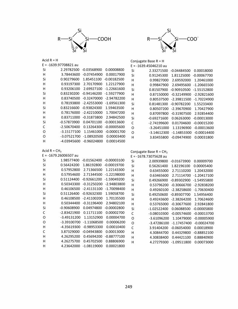
249
R Si
Si
Si COOH
Si Si Acid R = H E = ‐1639.97708821 au Si 2.29782500 ‐0.03568900 0.00008800 H 3.78443600 ‐0.07454900 0.00017900 Si 0.90279600 1.85451100 ‐0.00182500 H 0.93197300 2.70170900 1.22127900 H 0.93206100 2.69927100 ‐1.22661600 Si 0.83230200 ‐0.94146200 ‐1.59277900 H 0.83740500 ‐0.32470000 ‐2.94782200 H 0.78193800 ‐2.42553000 ‐1.69561300 Si 0.83216600 ‐0.93824300 1.59463500 H 0.78176000 ‐2.42210000 1.70047200 H 0.83711000 ‐0.31873800 2.94842500 Si ‐0.57873900 0.04701100 ‐0.00013600 C ‐2.50670400 0.13264300 ‐0.00005600 O ‐3.15177100 1.15461000 ‐0.00001700 O ‐3.07521700 ‐1.08920500 0.00003400 H ‐4.03945600 ‐0.96024800 0.00014500 Acid R = CH3 E = ‐1679.26006507 au Si 1.98577400 ‐0.01562400 ‐0.00003100 Si 0.56424200 1.86192800 ‐0.00019700 H 0.57952800 2.71366500 1.22143300 H 0.57954600 2.71344500 ‐1.22198000 Si 0.51124400 ‐0.92661200 ‐1.59049200 H 0.50343300 ‐0.31250200 ‐2.94803800 H 0.46106500 ‐2.41131100 ‐1.70098400 Si 0.51126400 ‐0.92632300 1.59058700 H 0.46108500 ‐2.41100200 1.70135500 H 0.50344400 ‐0.31196400 2.94802100 Si ‐0.90608900 0.04974800 ‐0.00002800 C ‐2.83421900 0.11711100 0.00002700 O ‐3.49131200 1.13152900 0.00004700 O ‐3.39100700 ‐1.11068500 0.00006200 H ‐4.35619300 ‐0.98953300 0.00010400 C 3.87329000 ‐0.04943800 0.00013000 H 4.26295200 0.45694200 ‐0.88777100 H 4.26275700 0.45702500 0.88806900 H 4.23642000 ‐1.08119000 0.00021800
R Si
Si
Si COO‐
Si Si Conjugate Base R = H E = ‐1639.45046210 au Si 2.33271500 ‐0.04484500 0.00018000 Si 0.91245300 1.81125000 ‐0.00067700 H 0.99827000 2.69592000 1.20461000 H 0.99847900 2.69495600 ‐1.20665500 Si 0.81507900 ‐0.90910500 ‐1.55152800 H 0.87150000 ‐0.32149900 ‐2.92821600 H 0.80537500 ‐2.39811500 ‐1.70224900 Si 0.81481300 ‐0.90782200 1.55233400 H 0.80507200 ‐2.39670900 1.70427900 H 0.87097800 ‐0.31907500 2.92854400 Si ‐0.69271600 0.06263000 ‐0.00013000 C ‐2.74199600 0.01704600 ‐0.00015200 O ‐3.26451000 1.13196900 ‐0.00013600 O ‐3.14612300 ‐1.14853300 ‐0.00014400 H 3.83455800 ‐0.09474900 0.00031800 Conjugate Base R = CH3 E = ‐1678.73075628 au Si 2.00939800 ‐0.01673900 0.00009700 Si 0.56261400 1.82196100 0.00005400 H 0.63455000 2.71110200 1.20432000 H 0.63465600 2.71114700 ‐1.20417100 Si 0.49266900 ‐0.89302900 ‐1.54955800 H 0.53796200 ‐0.30666700 ‐2.92838200 H 0.49260100 ‐2.38258600 ‐1.70630400 Si 0.49250600 ‐0.89307700 1.54956400 H 0.49243600 ‐2.38264200 1.70624600 H 0.53765000 ‐0.30677600 2.92841800 Si ‐1.02522400 0.06088500 ‐0.00005800 C ‐3.08010300 ‐0.00574600 ‐0.00013700 O ‐3.61096200 1.10479000 ‐0.00005900 O ‐3.47286100 ‐1.17457400 ‐0.00024700 C 3.91404200 ‐0.06054000 0.00018900 H 4.30844700 0.44329800 ‐0.88852100 H 4.30838400 0.44421100 0.88840900 H 4.27279300 ‐1.09511800 0.00073000
250
Acid R = CN E = ‐1732.12697257 au Si 1.75117100 ‐0.00382900 0.00002800 Si 0.36113900 1.88535900 ‐0.00085300 H 0.39341600 2.71902300 1.22882700 H 0.39347200 2.71789700 ‐1.23129600 Si 0.32445000 ‐0.93428000 ‐1.60733400 H 0.33522300 ‐0.30540500 ‐2.95430900 H 0.30463600 ‐2.41779100 ‐1.69699200 Si 0.32437300 ‐0.93280100 1.60817000 H 0.30453900 ‐2.41622900 1.69920100 H 0.33506100 ‐0.30268000 2.95456400 Si ‐1.08402300 0.04395500 ‐0.00007200 C ‐3.01114100 0.10906300 ‐0.00003200 O ‐3.66239300 1.12584600 ‐0.00002000 O ‐3.56221100 ‐1.11891100 0.00001700 H ‐4.52866800 ‐1.00643500 0.00006800 C 3.59231900 ‐0.03032200 0.00007600 N 4.75607500 ‐0.04770800 0.00007900 Acid R = CF3 E = ‐1976.71642333 au Si ‐1.13933000 0.00544100 0.00013300 Si 0.25396200 1.88996900 ‐0.00025900 H 0.22918400 2.72627700 ‐1.22893700 H 0.22927800 2.72672400 1.22812000 Si 0.28407900 ‐0.92654100 1.60695400 H 0.28104200 ‐0.29907900 2.95524900 H 0.30599600 ‐2.41017400 1.70212600 Si 0.28393900 ‐0.92710800 ‐1.60647600 H 0.30583000 ‐2.41077700 ‐1.70112400 H 0.28080800 ‐0.30012900 ‐2.95499500 Si 1.69597300 0.04688600 ‐0.00000800 C 3.62356100 0.10287900 ‐0.00004000 O 4.28189000 1.11544500 ‐0.00004200 O 4.16931300 ‐1.12837500 ‐0.00005500 H 5.13605000 ‐1.01889500 ‐0.00006600 C ‐3.08399100 ‐0.01799900 ‐0.00007500 F ‐3.57381600 ‐1.27657600 ‐0.00041100 F ‐3.59744600 0.60133600 1.08454900 F ‐3.59717500 0.60181400 ‐1.08455100
Conjugate Base R = CN E = ‐1731.61382462 au Si ‐1.77701000 ‐0.00831700 ‐0.00001300 Si ‐0.36973100 1.84863100 ‐0.00058700 H ‐0.46464400 2.71953500 ‐1.21143200 H ‐0.46464300 2.72027700 1.20972300 Si ‐0.29801000 ‐0.89457100 1.56530500 H ‐0.36743500 ‐0.29546900 2.93302100 H ‐0.32124200 ‐2.38173100 1.70334000 Si ‐0.29802100 ‐0.89558100 ‐1.56477200 H ‐0.32126000 ‐2.38282900 ‐1.70184600 H ‐0.36746400 ‐0.29736600 ‐2.93287600 Si 1.20588600 0.06771200 ‐0.00005000 C 3.28405300 ‐0.01839400 0.00005800 O 3.81163400 1.08882300 0.00005000 O 3.64748300 ‐1.19238700 0.00013300 C ‐3.64570900 ‐0.04795500 ‐0.00000800 N ‐4.81141600 ‐0.07229100 ‐0.00000700 Conjugate Base R = CF3 E = ‐1976.20033440 au Si 1.15004500 0.00950800 ‐0.00011900 Si ‐0.26645400 1.85632600 ‐0.00093800 H ‐0.18593200 2.73115700 1.20862200 H ‐0.18602700 2.72997800 ‐1.21135800 Si ‐0.31963700 ‐0.88777200 ‐1.56452800 H ‐0.26374700 ‐0.29086500 ‐2.93431200 H ‐0.29479600 ‐2.37524400 ‐1.70351500 Si ‐0.31956000 ‐0.88621400 1.56524800 H ‐0.29476200 ‐2.37355000 1.70570000 H ‐0.26363600 ‐0.28794800 2.93443600 Si ‐1.83198400 0.06586300 ‐0.00008100 C ‐3.91234100 ‐0.02976000 0.00016400 O ‐4.44286300 1.07598900 0.00017400 O ‐4.27219200 ‐1.20453900 0.00029700 C 3.11036100 ‐0.02600600 0.00000900 F 3.61455500 ‐1.28754100 0.00067300 F 3.65099800 0.58887100 ‐1.08422700 F 3.65083000 0.58995000 1.08371700
251
Acid R = NH2 E = ‐1695.30348502 au Si 1.98642700 ‐0.01629600 0.03841200 Si 0.58929400 1.68954600 ‐0.77937800 H 0.57636900 2.97114900 ‐0.02157000 H 0.62893400 1.95176100 ‐2.24455100 Si 0.55366800 ‐1.53270500 ‐1.04322100 H 0.58469000 ‐1.55858900 ‐2.53192500 H 0.50182500 ‐2.91935000 ‐0.50209600 Si 0.47842800 ‐0.15466400 1.85499800 H 0.38558600 ‐1.44532900 2.59414500 H 0.41408000 0.98851700 2.80857800 Si ‐0.88025700 0.02716200 ‐0.04648600 C ‐2.80354700 0.11823300 ‐0.03117900 O ‐3.44193800 1.14431000 ‐0.01302100 O ‐3.38096900 ‐1.09956000 ‐0.01834600 H ‐4.34331700 ‐0.96085300 0.01241000 N 3.71441100 ‐0.02619100 ‐0.05262900 H 4.22718600 ‐0.87962600 0.11687100 H 4.24245800 0.78565000 0.23400100 Acid R = NO2 E = ‐1844.29367780 au Si ‐1.41556200 ‐0.02534200 ‐0.02274500 Si ‐0.06615700 1.88711100 ‐0.01626900 H ‐0.08663800 2.70323000 ‐1.25696900 H ‐0.11853900 2.72354100 1.20963700 Si ‐0.03642300 ‐0.91771900 1.64052900 H ‐0.07582100 ‐0.25268600 2.96794700 H ‐0.01684300 ‐2.39871200 1.75577600 Si 0.00993600 ‐0.95332200 ‐1.61867900 H 0.05659300 ‐2.43587800 ‐1.70321400 H 0.03258700 ‐0.31499700 ‐2.95954000 Si 1.37693000 0.04003800 0.02473400 C 3.30319500 0.10974100 ‐0.03216700 O 3.93759400 1.05403700 ‐0.43492800 O 3.86925600 ‐1.02715100 0.41057100 H 4.83372800 ‐0.92418200 0.33291200 N ‐3.30698800 ‐0.02335900 ‐0.01127800 O ‐3.84311100 0.44498200 0.98368100 O ‐3.89592000 ‐0.47511500 ‐0.98189700
Conjugate Base R = NH2 E = ‐1694.77580331 au Si 2.01430500 ‐0.00009900 0.03748100 Si 0.56883300 1.57659600 ‐0.89798600 H 0.58731100 2.93853600 ‐0.27449100 H 0.65864000 1.76804300 ‐2.38110500 Si 0.56839500 ‐1.57373900 ‐0.90237900 H 0.65813700 ‐1.76111100 ‐2.38601700 H 0.58651500 ‐2.93738400 ‐0.28261600 Si 0.45943100 ‐0.00248900 1.79755000 H 0.43350100 ‐1.20910000 2.68621000 H 0.43388200 1.20138800 2.68992900 Si ‐0.99656200 0.00045400 ‐0.06871400 C ‐3.07579000 ‐0.00008500 ‐0.01617200 O ‐3.52744200 1.14226800 0.00579300 O ‐3.52646500 ‐1.14283700 0.00579800 N 3.77661400 ‐0.00036800 ‐0.02913000 H 4.24478800 ‐0.82978800 0.31425100 H 4.24527400 0.82690900 0.31873500 Conjugate Base R = NO2 E = ‐1843.78624560 au Si ‐1.44088300 ‐0.03904500 0.01131000 Si ‐0.07848900 1.81055800 ‐0.35775400 H ‐0.17681900 2.42798900 ‐1.71418000 H ‐0.16986200 2.89486300 0.66545400 Si 0.02622300 ‐0.56753700 1.72935100 H ‐0.02661400 0.30711400 2.93829100 H 0.03682500 ‐1.99405900 2.17030600 Si 0.01633200 ‐1.18357700 ‐1.38575600 H 0.02367300 ‐2.67072800 ‐1.25074300 H ‐0.04577400 ‐0.83524700 ‐2.83641900 Si 1.50180500 0.06773200 ‐0.01959400 C 3.64958000 ‐0.01096600 0.00176600 O 4.13634800 1.09346900 ‐0.16739400 O 3.99525000 ‐1.16704700 0.18455600 N ‐3.37694700 ‐0.03900300 0.01065700 O ‐3.95869600 0.14946200 1.07424000 O ‐3.95416600 ‐0.20400600 ‐1.05936700
252
Acid R = NF2 E = ‐1893.45476082 au Si 1.38282300 0.01370500 ‐0.16952400 Si ‐0.04840700 1.69912100 ‐0.93329900 H ‐0.00078000 2.99081100 ‐0.20155500 H ‐0.11993700 1.89644700 ‐2.40457900 Si ‐0.06013900 ‐1.55829100 ‐1.12431100 H ‐0.13945500 ‐1.58797000 ‐2.60827000 H ‐0.02930700 ‐2.92620900 ‐0.54520300 Si 0.08487500 ‐0.10500200 1.77263900 H 0.10325900 ‐1.38938800 2.51979200 H 0.11709600 1.06734600 2.68484200 Si ‐1.41785300 0.02041100 ‐0.03537300 C ‐3.33800100 0.09727200 0.12347000 O ‐3.97799800 1.12077300 0.14343500 O ‐3.89481500 ‐1.12275100 0.23330400 H ‐4.85492500 ‐0.99787200 0.33003300 N 3.21762000 0.02164100 ‐0.40338300 F 3.67396800 ‐1.13628000 0.25207900 F 3.68525800 1.05276400 0.43148000 Acid R = OH E = ‐1715.16795745 au Si 1.97922600 0.00743100 0.01534600 Si 0.51430700 ‐0.38916500 1.81507800 H 0.46241200 ‐1.76560200 2.38053500 H 0.45689800 0.62826800 2.90040000 Si 0.56923400 1.78191600 ‐0.57703100 H 0.54073000 2.95297700 0.33999300 H 0.58743700 2.21804600 ‐1.99953600 Si 0.57216500 ‐1.40673800 ‐1.23848000 H 0.57611400 ‐1.25041800 ‐2.71887200 H 0.53794900 ‐2.84581100 ‐0.85950100 Si ‐0.86132800 0.00566800 ‐0.04507900 C ‐2.78342100 ‐0.10930200 ‐0.01324800 O ‐3.40060500 ‐1.14761700 0.00700100 O ‐3.38058600 1.09758200 0.00420200 H ‐4.34064900 0.94356000 0.03852900 O 3.64510500 0.10889400 0.01100100 H 4.13786900 ‐0.68364200 0.24264600
Conjugate Base R = NF2 E = ‐1892.94220051 au Si 1.40510200 0.00030700 ‐0.15559400 Si ‐0.05880600 1.58874300 ‐1.01371200 H 0.01385100 2.94749000 ‐0.39791600 H ‐0.06655900 1.74375500 ‐2.50045700 Si ‐0.05921100 ‐1.58428800 ‐1.02005200 H ‐0.06698300 ‐1.73348100 ‐2.50738200 H 0.01343400 ‐2.94543500 ‐0.40958300 Si 0.02788000 ‐0.00337400 1.71717100 H 0.09081100 ‐1.21767500 2.58476500 H 0.09103200 1.20728400 2.58982800 Si ‐1.54629800 0.00044400 ‐0.06152300 C ‐3.65485300 ‐0.00059200 0.15572100 O ‐4.08388300 1.14373900 0.20503600 O ‐4.08111900 ‐1.14560300 0.21336300 N 3.27420700 0.00199100 ‐0.39035800 F 3.75004300 ‐1.10121700 0.35962700 F 3.74915100 1.09865500 0.36966900 Conjugate Base R = OH E = ‐1714.64540194 au Si 2.01485200 ‐0.01544400 0.00013400 Si 0.51595400 ‐0.89459100 1.56379200 H 0.48671600 ‐2.38497100 1.70880600 H 0.55090700 ‐0.31138800 2.94298400 Si 0.61373400 1.84134200 ‐0.00159500 H 0.68310200 2.72442100 1.20508400 H 0.68334700 2.72229800 ‐1.20981300 Si 0.51627400 ‐0.89731500 ‐1.56231500 H 0.55156100 ‐0.31651900 ‐2.94251600 H 0.48709000 ‐2.38794400 ‐1.70474500 Si ‐0.97547800 0.07702600 ‐0.00026700 C ‐3.08424000 ‐0.01122500 ‐0.00001200 O ‐3.44490100 ‐1.18255800 0.00001300 O ‐3.59775900 1.09989100 0.00012400 O 3.71330800 0.00091300 0.00024300 H 4.10280500 ‐0.87877600 0.00071700
253
Acid R = F E = ‐1739.18659867 au Si 1.96394200 ‐0.02335800 0.00004200 Si 0.60907600 1.89291400 ‐0.00060300 H 0.62485900 2.72880100 1.22882900 H 0.62492300 2.72799700 ‐1.23058300 Si 0.53749300 ‐0.94220400 ‐1.61495100 H 0.52787300 ‐0.31744600 ‐2.96475900 H 0.46946500 ‐2.42520600 ‐1.70272600 Si 0.53741200 ‐0.94116100 1.61554700 H 0.46936600 ‐2.42410500 1.70428000 H 0.52770300 ‐0.31552900 2.96494900 Si ‐0.84387000 0.05997200 ‐0.00006700 C ‐2.76967900 0.12261000 ‐0.00003200 O ‐3.42920400 1.13359500 0.00000100 O ‐3.31315600 ‐1.10955100 ‐0.00002000 H ‐4.27979400 ‐1.00006800 0.00002500 F 3.59286900 ‐0.06097000 0.00008800 Acid R = Li E = ‐1646.89777913 au Si 2.30412100 ‐0.02424500 0.00001900 Si 0.79256400 1.80830900 ‐0.00045900 H 0.81157400 2.68453600 1.20913000 H 0.81159300 2.68390600 ‐1.21050400 Si 0.73930000 ‐0.90937500 ‐1.54832600 H 0.73542000 ‐0.31920900 ‐2.92131700 H 0.69516000 ‐2.39662700 ‐1.68387000 Si 0.73927100 ‐0.90856600 1.54879600 H 0.69512100 ‐2.39574700 1.68511900 H 0.73535900 ‐0.31767900 2.92147600 Si ‐0.72366000 0.04365300 ‐0.00002900 C ‐2.66249600 0.12286400 ‐0.00002200 O ‐3.31842700 1.14056400 ‐0.00005300 O ‐3.23829000 ‐1.09951500 0.00003800 H ‐4.20101400 ‐0.96039600 0.00005200 Li 4.74105000 ‐0.06041200 0.00004800
Conjugate Base R = F E = ‐1738.67008589 au Si ‐2.01100600 ‐0.03317000 0.00000500 Si ‐0.62906600 1.84543500 ‐0.00034300 H ‐0.69743300 2.72433600 ‐1.20947200 H ‐0.69741300 2.72477800 1.20846600 Si ‐0.52590800 ‐0.89824000 1.57143800 H ‐0.56591000 ‐0.29835400 2.94210200 H ‐0.48915400 ‐2.38572300 1.72274200 Si ‐0.52592900 ‐0.89882100 ‐1.57113300 H ‐0.48918300 ‐2.38635900 ‐1.72188800 H ‐0.56596200 ‐0.29944200 ‐2.94201800 Si 0.95357100 0.08114200 ‐0.00004000 C 3.09494800 ‐0.00765900 0.00005200 O 3.59284200 1.10629400 0.00002800 O 3.44243800 ‐1.17884000 0.00004600 F ‐3.66779100 ‐0.08908300 0.00002100 Conjugate Base R = Li E = ‐1646.34940015 au Si 2.31973600 ‐0.02417200 0.00002100 Si 0.78085800 1.77273200 ‐0.00044700 H 0.85375300 2.68139600 1.19441100 H 0.85378600 2.68079300 ‐1.19576200 Si 0.71675600 ‐0.88131400 ‐1.51230900 H 0.76343500 ‐0.31306400 ‐2.90340200 H 0.72408600 ‐2.37264300 ‐1.68988500 Si 0.71671700 ‐0.88052300 1.51275500 H 0.72403600 ‐2.37175900 1.69111300 H 0.76334900 ‐0.31154000 2.90354900 Si ‐0.83905900 0.04971400 ‐0.00004000 C ‐2.86249600 0.00483300 ‐0.00000600 O ‐3.40087100 1.11845900 ‐0.00001800 O ‐3.28644900 ‐1.15949500 0.00003900 Li 4.75365800 ‐0.06800300 0.00004400
254
Analog 3 Backbone R=H E = ‐1451.59078694au Si ‐0.00001000 ‐0.00019500 ‐1.45209200 Si 0.00320400 1.84154400 0.00003200 H 1.22464800 2.69442900 0.00042300 H ‐1.21458000 2.69965600 0.00042200 Si ‐1.59735900 ‐0.91781600 ‐0.00003200 H ‐2.94623600 ‐0.28528900 ‐0.00013000 H ‐1.73289200 ‐2.40144900 ‐0.00021100 Si 1.59412700 ‐0.92340500 ‐0.00003400 H 1.72449000 ‐2.40751000 ‐0.00021000 H 2.94516800 ‐0.29554100 ‐0.00013600 Si ‐0.00000800 ‐0.00033000 1.45211500 H 0.00002800 ‐0.00112300 2.93979800 H 0.00002900 ‐0.00033900 ‐2.93980900 Analog 3 Backbone R=CH3 E = ‐1490.87363212au Si 1.13439200 ‐0.00001800 0.00109100 Si ‐0.33334600 ‐0.02561000 1.83734600 H ‐0.34346600 ‐1.25518300 2.68067000 H ‐0.34348700 1.17971900 2.71498700 Si ‐0.33086000 1.60493300 ‐0.89649500 H ‐0.33982600 2.94933600 ‐0.25168700 H ‐0.33760000 1.76395200 ‐2.37905200 Si ‐0.33091300 ‐1.57933300 ‐0.94082900 H ‐0.33770300 ‐1.69704900 ‐2.42723900 H ‐0.33996500 ‐2.94114100 ‐0.33364600 Si ‐1.78406400 0.00006600 ‐0.00168700 H ‐3.27169000 0.00011100 ‐0.00336800 C 3.02174500 ‐0.00003100 0.00093800 H 3.40389000 0.88063600 0.52550500 H 3.40392000 ‐0.89494800 0.50078500 H 3.40255200 0.01422200 ‐1.02454000 Analog 3 Backbone R=CN E = ‐1543.74149020au Si 0.89375600 0.00118200 ‐0.00003800 Si ‐0.52926900 1.85917600 ‐0.00191800 H ‐0.51660400 2.70243500 1.22323300 H ‐0.51668100 2.69987000 ‐1.22883400 Si ‐0.52756800 ‐0.93150000 ‐1.60907700 H ‐0.51544500 ‐0.29256700 ‐2.95222100 H ‐0.51343500 ‐2.41449500 ‐1.72320500 Si ‐0.52747600 ‐0.92817100 1.61100600 H ‐0.51332900 ‐2.41092500 1.72819200 H ‐0.51527400 ‐0.28646500 2.95282900 Si ‐1.96492600 ‐0.00083200 0.00004400 H ‐3.45008400 ‐0.00106000 0.00009400 C 2.73614600 0.00065900 ‐0.00005900 N 3.90010600 0.00018400 0.00000500
Analog 3 Backbone R=CF3 E = ‐1788.33066495au Si 0.31524000 0.00232400 0.00040200 Si ‐1.10302400 ‐1.43515700 ‐1.18089200 H ‐1.09494800 ‐1.31341700 ‐2.66359600 H ‐1.09476500 ‐2.86382900 ‐0.76571100 Si ‐1.10725900 ‐0.30743800 1.83169000 H ‐1.09918000 ‐1.65663700 2.45858700 H ‐1.10210400 0.76016100 2.86771200 Si ‐1.10717400 1.74213700 ‐0.64956300 H ‐1.10220200 2.95840900 0.20720600 H ‐1.09894600 2.10873400 ‐2.09136300 Si ‐2.54352600 ‐0.00130100 ‐0.00264900 H ‐4.02975200 ‐0.00247900 ‐0.00335400 C 2.26034500 0.00058100 0.00026800 F 2.76825200 0.94886700 0.81724900 F 2.76514500 ‐1.18228200 0.41339400 F 2.76662800 0.23315400 ‐1.23030100 Analog 3 Backbone R=NH2 E = ‐1506.91718781au Si 1.13966300 ‐0.00269400 0.06446200 Si ‐0.26155600 1.64271400 ‐0.85178900 H ‐0.30722500 2.96121900 ‐0.15744900 H ‐0.19085900 1.84994100 ‐2.32574200 Si ‐0.26286400 ‐1.55208200 ‐1.00736200 H ‐0.19401100 ‐1.61725900 ‐2.49442000 H ‐0.30912400 ‐2.93086200 ‐0.44213700 Si ‐0.41267200 ‐0.09016600 1.84386500 H ‐0.49187200 ‐1.35143700 2.63550400 H ‐0.49590700 1.08402700 2.75925500 Si ‐1.74852200 0.00384000 ‐0.07884400 H ‐3.23213300 0.01657300 ‐0.14657700 N 2.87056400 ‐0.00184400 0.01134900 H 3.38521300 ‐0.84483000 0.22253000 H 3.38527600 0.82296800 0.28494500
255
Analog 3 Backbone R=NO2 E = ‐1655.90830772au Si ‐0.57822100 0.03794900 ‐0.00274000 Si 0.79240200 ‐0.91547000 1.63114300 H 0.78775100 ‐0.25912200 2.96494400 H 0.74993300 ‐2.39621700 1.74727900 Si 0.79679500 ‐0.98112700 ‐1.59235300 H 0.75537400 ‐2.46536600 ‐1.64785400 H 0.79648900 ‐0.37978300 ‐2.95185000 Si 0.84779500 1.88311500 ‐0.03768200 H 0.86654400 2.69047500 ‐1.28523500 H 0.86393000 2.74274400 1.17436800 Si 2.23370700 ‐0.01995800 0.00247400 H 3.71800200 ‐0.04415300 0.00464700 N ‐2.47035700 0.01532500 ‐0.00167500 O ‐2.99896600 ‐1.08842700 ‐0.00257800 O ‐3.06856200 1.08105600 0.00178200 Analog 3 Backbone R=NF2 E = ‐1705.06923307au Si ‐0.54153600 ‐0.00003400 ‐0.17933900 Si 0.97940100 ‐1.61323200 ‐0.91330100 H 0.88312600 ‐2.95958900 ‐0.28980100 H 1.19427100 ‐1.71156300 ‐2.38156000 Si 0.97894100 1.61483900 ‐0.91057200 H 1.19378600 1.71570000 ‐2.37866500 H 0.88225500 2.96012300 ‐0.28482700 Si 0.57351100 ‐0.00160100 1.87618700 H 0.45155700 1.22573600 2.70632700 H 0.45195400 ‐1.23039500 2.70423100 Si 2.25347700 0.00002500 0.22902400 H 3.72251900 0.00007600 0.44506800 N ‐2.34723000 0.00001800 ‐0.58414600 F ‐2.87565000 1.09867100 0.11896200 F ‐2.87567900 ‐1.09869000 0.11884500 Analog 3 Backbone R=OH E = ‐1526.78216221au Si 1.13806500 ‐0.00823100 0.00253600 Si ‐0.31146400 ‐0.91984600 1.61641200 H ‐0.35294900 ‐2.40398800 1.74625500 H ‐0.32761400 ‐0.28535600 2.96393000 Si ‐0.27065300 1.86001600 ‐0.01308400 H ‐0.27608200 2.71799700 1.20373400 H ‐0.27091800 2.69988400 ‐1.24251000 Si ‐0.30588100 ‐0.94150800 ‐1.60417500 H ‐0.31645600 ‐0.32601800 ‐2.96053300 H ‐0.34657800 ‐2.42734500 ‐1.71369900 Si ‐1.72424600 0.01857200 ‐0.00278100 H ‐3.20835200 0.02843300 ‐0.00509700 O 2.80574900 0.07775000 0.00484400 H 3.29146200 ‐0.75164800 ‐0.01555200
Analog 3 Backbone R=F E = ‐1550.80133305au Si 1.12785500 ‐0.00005400 0.00003800 Si ‐0.28107900 1.87071800 ‐0.00060900 H ‐0.29578500 2.71472900 1.22492100 H ‐0.29570200 2.71394100 ‐1.22668300 Si ‐0.28200900 ‐0.93601200 ‐1.61896000 H ‐0.29595800 ‐0.29909200 ‐2.96383000 H ‐0.29735800 ‐2.41975400 ‐1.73330300 Si ‐0.28211200 ‐0.93497200 1.61954400 H ‐0.29746900 ‐2.41864000 1.73484100 H ‐0.29615000 ‐0.29718600 2.96400300 Si ‐1.70141000 0.00100700 ‐0.00005600 H ‐3.18457800 0.00033500 ‐0.00009200 F 2.75839500 ‐0.00043800 0.00008300 Analog 3 Backbone R=Li E = ‐1458.50872143au Si ‐1.43786700 0.00002100 ‐0.00351300 Si 0.11804700 ‐0.00880200 1.78684600 H 0.12162100 1.19218800 2.67862800 H 0.12161500 ‐1.21851500 2.66676500 Si 0.12341300 ‐1.54380100 ‐0.90069100 H 0.12785200 ‐2.91615700 ‐0.30549500 H 0.13213100 ‐1.70121000 ‐2.38830700 Si 0.12341800 1.55259500 ‐0.88545800 H 0.13213500 1.72464200 ‐2.37145200 H 0.12785800 2.91902700 ‐0.27678200 Si 1.62569800 ‐0.00001300 0.00276800 H 3.12390500 ‐0.00002900 0.00603000 Li ‐3.87501200 0.00001900 ‐0.00290900

256
R Si
Si
Si Si(OH)3
Si Si Acid R = H E = ‐1967.77108811 au Si ‐2.89737200 0.02869900 ‐0.01435700 Si ‐1.44254500 ‐0.10785300 1.81700400 H ‐1.41305100 1.06051900 2.74361300 H ‐1.45712700 ‐1.37067800 2.60710600 Si ‐1.46254100 ‐1.52898100 ‐1.02225800 H ‐1.48247700 ‐2.91471500 ‐0.47665600 H ‐1.45464300 ‐1.57018600 ‐2.51142000 Si ‐1.40394800 1.64680700 ‐0.81623300 H ‐1.39105200 1.89070900 ‐2.28640500 H ‐1.37860300 2.95062800 ‐0.09380500 Si 0.03641300 ‐0.02851200 ‐0.01190200 Si 2.36608700 ‐0.02036400 0.01056800 O 2.80071700 ‐1.47629800 0.65256000 H 3.70626500 ‐1.76597800 0.50074200 O 2.95821700 1.29030700 0.84125500 H 2.62302200 1.45870000 1.72586900 O 3.06383600 0.10498900 ‐1.48270700 H 3.30741800 0.99195400 ‐1.76329800 H ‐4.38723700 0.05992400 ‐0.01410400 Acid R = CH3 E = ‐2007.05424439 au Si 2.59182400 ‐0.01474700 ‐0.00985200 Si 1.09125600 ‐1.60953500 ‐0.85895900 H 1.07359300 ‐1.81834200 ‐2.33574500 H 1.05674200 ‐2.93523200 ‐0.17532300 Si 1.11827300 0.06670100 1.81691800 H 1.07909200 ‐1.12693800 2.71243700 H 1.12027100 1.30367300 2.64906700 Si 1.14426400 1.56624400 ‐0.97513800 H 1.15283800 2.93799200 ‐0.39216600 H 1.13157700 1.65667600 ‐2.46327600 Si ‐0.35446200 0.03831300 ‐0.01452000 Si ‐2.68243500 0.01324700 0.00924500 O ‐3.13539900 1.45337500 0.67466300 O ‐3.25883400 ‐1.31750200 0.82010600 O ‐3.38808400 ‐0.09217100 ‐1.48256700 H ‐4.04550700 1.73066000 0.52713000 H ‐2.89673400 ‐1.50952400 1.68921500 H ‐3.60129200 ‐0.97905800 ‐1.78697000 C 4.47987200 ‐0.04810000 ‐0.00774000 H 4.84690100 ‐0.92434500 0.53505700 H 4.86180500 ‐0.08978300 ‐1.03226600 H 4.87795000 0.85008200 0.47394200
R Si
Si
Si Si(OH)2O‐
Si Si Base R = H E = ‐1967.22269464 au Si 2.91668600 0.01789400 ‐0.03320100 Si 1.41346300 ‐1.35883500 ‐1.17928700 H 1.42202000 ‐1.23537600 ‐2.67206700 H 1.47581400 ‐2.81739800 ‐0.85359000 Si 1.45859200 ‐0.33242900 1.76267700 H 1.52461700 ‐1.67870700 2.41046900 H 1.50747100 0.69343500 2.85163700 Si 1.39779400 1.70104600 ‐0.59973500 H 1.44448000 2.94006900 0.24025500 H 1.40805300 2.14028300 ‐2.03153100 Si ‐0.11465500 ‐0.01376400 0.02589200 Si ‐2.50280400 ‐0.14254200 0.09609800 O ‐2.94355800 ‐1.56550600 0.54388500 O ‐2.97590000 0.36677900 ‐1.45874000 H ‐3.25583200 ‐0.40220900 ‐1.96476100 O ‐2.91428100 1.22478800 0.99659000 H ‐3.24174900 1.91942400 0.41700900 H 4.41796600 0.03281600 ‐0.06550500 Base R = CH3 E = ‐2006.50309496 au Si 2.60189300 0.01119200 ‐0.01700600 Si 1.07887300 1.70208300 ‐0.56017700 H 1.11596500 2.93012000 0.29828100 H 1.08625800 2.16819800 ‐1.98465100 Si 1.09451900 ‐1.34380400 ‐1.18876900 H 1.10064300 ‐1.19846300 ‐2.68073600 H 1.14787300 ‐2.80983300 ‐0.89073600 Si 1.13173200 ‐0.36643200 1.76702500 H 1.18870100 ‐1.72262500 2.39737200 H 1.17171300 0.64033100 2.87552200 Si ‐0.43605100 ‐0.01984700 0.03307200 Si ‐2.82753500 ‐0.13919900 0.08615400 O ‐3.28248400 ‐1.56202100 0.51947000 O ‐3.27998200 0.38628800 ‐1.46946100 O ‐3.24308900 1.22137400 0.99478300 H ‐3.54700000 ‐0.37757200 ‐1.98992000 H ‐3.52127000 1.93738200 0.41548700 C 4.50487200 0.02697000 ‐0.05134100 H 4.86817000 0.23275100 ‐1.06364800 H 4.89459900 0.79919600 0.62012500 H 4.90152900 ‐0.94233300 0.26844600
257
Acid R = CN E = ‐2059.92272921 au Si ‐2.36077600 0.00455300 ‐0.00951300 Si ‐0.91777100 1.73900000 ‐0.62020200 H ‐0.92427900 2.13871300 ‐2.05349600 H ‐0.91991300 2.93962300 0.25942300 Si ‐0.93472400 ‐0.33606100 1.81089600 H ‐0.93377900 0.72350100 2.85730500 H ‐0.94755600 ‐1.68680600 2.43360000 Si ‐0.94002700 ‐1.41842800 ‐1.20428900 H ‐0.95894500 ‐2.85337300 ‐0.81407200 H ‐0.94596900 ‐1.26954400 ‐2.68434300 Si 0.52739900 ‐0.01783900 ‐0.01074800 Si 2.85702700 ‐0.01019800 0.00743100 O 3.27075000 ‐1.49698200 0.58480300 O 3.45707900 1.25636500 0.89315900 O 3.53039500 0.18398100 ‐1.48671100 H 4.16969200 ‐1.80065000 0.42114300 H 3.18228400 1.35466900 1.80857700 H 3.82362000 1.07185800 ‐1.71192700 C ‐4.20760000 0.02309400 ‐0.00677200 N ‐5.37159000 0.03459300 ‐0.00509000 Acid R = CF3 E = ‐2304.51180944 au Si ‐1.73985400 ‐0.00472800 ‐0.00760900 Si ‐0.30064400 1.70967800 ‐0.67641500 H ‐0.30263500 2.06352700 ‐2.12198800 H ‐0.29580400 2.93987700 0.16182700 Si ‐0.31339700 ‐0.28522500 1.82110300 H ‐0.30526000 0.80577000 2.83507900 H ‐0.31755800 ‐1.61547900 2.48713900 Si ‐0.32121400 ‐1.46476600 ‐1.15802200 H ‐0.33163300 ‐2.88740900 ‐0.72405700 H ‐0.32325400 ‐1.36395400 ‐2.64236400 Si 1.14630100 ‐0.02535300 ‐0.01226900 Si 3.47660100 ‐0.00575000 0.00738000 O 3.90405700 ‐1.48277000 0.60047200 O 4.06520700 1.27579700 0.88034100 O 4.15664900 0.17460900 ‐1.48614500 H 4.80611200 ‐1.77807300 0.43874100 H 3.76886100 1.39268000 1.78684000 H 4.42493700 1.06581800 ‐1.72849900 C ‐3.68777200 0.01633900 ‐0.00338800 F ‐4.20811200 ‐1.13681600 0.47148600 F ‐4.18249300 1.01254200 0.76447700 F ‐4.19534300 0.19140000 ‐1.24352700
Base R = CN E = ‐2059.38571975 au Si 2.37007900 0.00283500 ‐0.00545500 Si 0.90639200 1.71075400 ‐0.61285900 H 0.97065900 2.94669400 0.22495800 H 0.95214700 2.11971800 ‐2.04967900 Si 0.90100900 ‐1.38768900 ‐1.16510500 H 0.94348300 ‐1.26644500 ‐2.65434400 H 0.96145800 ‐2.83577800 ‐0.80830300 Si 0.92265800 ‐0.31972600 1.79538300 H 0.98446000 ‐1.66362500 2.44141900 H 0.98331700 0.72473000 2.86161600 Si ‐0.61106600 ‐0.00159300 0.01931300 Si ‐3.00274300 ‐0.13783500 0.08219600 O ‐3.40681300 ‐1.57126100 0.52549400 O ‐3.47432200 0.37600200 ‐1.46705700 O ‐3.41089500 1.21885600 0.99325800 H ‐3.74088100 ‐0.38833100 ‐1.98717600 H ‐3.76169100 1.91453900 0.42874900 C 4.23655200 0.00712100 ‐0.02734700 N 5.40219700 0.01179400 ‐0.04219200 Base R = CF3 E = ‐2303.97202785 au Si 1.73805000 ‐0.00006100 0.00329100 Si 0.27549700 1.70905200 ‐0.59543300 H 0.32854100 2.94112100 0.24931000 H 0.31323900 2.12753200 ‐2.02999000 Si 0.27645000 ‐1.38666500 ‐1.16694300 H 0.31196600 ‐1.25612900 ‐2.65584200 H 0.33137400 ‐2.83792500 ‐0.82098400 Si 0.29409000 ‐0.33612200 1.80213200 H 0.35045400 ‐1.68369900 2.44169700 H 0.34415300 0.70179500 2.87561900 Si ‐1.23830900 ‐0.01072200 0.02609200 Si ‐3.63331100 ‐0.13551200 0.07683700 O ‐4.05517500 ‐1.56757800 0.50799300 O ‐4.08889000 0.39314800 ‐1.47277800 O ‐4.04055500 1.21778300 0.99409400 H ‐4.35098800 ‐0.36619200 ‐2.00233500 H ‐4.35979800 1.92750300 0.42834100 C 3.69644200 0.00815800 ‐0.01802000 F 4.23478000 ‐1.16327200 0.40952500 F 4.20892800 0.22193700 ‐1.25786500 F 4.22905200 0.97362900 0.77547000
258
Acid R = NH2 E = ‐2023.09886893 au Si ‐2.58558200 ‐0.00193000 ‐0.01744500 Si ‐1.10780400 1.62558000 ‐0.83034700 H ‐1.08660800 1.86427300 ‐2.30230900 H ‐1.08105100 2.93326500 ‐0.11422900 Si ‐1.13137900 ‐0.11299000 1.81859400 H ‐1.09801100 1.06550600 2.73283800 H ‐1.12235600 ‐1.36753400 2.62346200 Si ‐1.13518500 ‐1.57107100 ‐1.02735100 H ‐1.11325400 ‐2.95544400 ‐0.47475000 H ‐1.09389100 ‐1.62493500 ‐2.51692800 Si 0.33274400 ‐0.04562400 ‐0.02024500 Si 2.65635000 ‐0.00425900 0.01458100 O 3.11368200 ‐1.44277300 0.67935700 O 3.21954200 1.32814000 0.83095000 O 3.36741100 0.10915500 ‐1.47354500 H 4.02587900 ‐1.71467000 0.53493700 H 2.84107400 1.52322900 1.69239400 H 3.57684800 0.99831800 ‐1.77391700 N ‐4.31159000 0.13261700 0.04897000 H ‐4.85432000 ‐0.52868900 0.58613900 H ‐4.82628400 0.46630200 ‐0.75354500 Acid R = NO2 E = ‐2172.09087286 au Si ‐2.01417600 0.02655300 ‐0.02624500 Si ‐0.62186700 ‐0.49939900 1.77122300 H ‐0.64214000 0.43706700 2.92602700 H ‐0.63423400 ‐1.91618800 2.22255000 Si ‐0.60976000 ‐1.29364700 ‐1.33530500 H ‐0.60368900 ‐2.75224800 ‐1.04369500 H ‐0.60142400 ‐1.03509600 ‐2.79919700 Si ‐0.61867900 1.84372500 ‐0.45987800 H ‐0.61083100 2.36978700 ‐1.84972700 H ‐0.61787100 2.94090600 0.54231300 Si 0.82377800 0.03429800 ‐0.01134300 Si 3.15316900 ‐0.00634500 ‐0.00326300 O 3.57461400 0.41410600 ‐1.53886800 O 3.72658600 ‐1.48157800 0.48644500 O 3.83352800 1.06785000 1.04700500 H 4.47569800 0.72215200 ‐1.68146200 H 3.43720200 ‐2.27057800 0.02060900 H 4.11616700 0.71669600 1.89667700 N ‐3.91085000 ‐0.01620700 0.01524000 O ‐4.44245100 ‐1.11487600 ‐0.07359000 O ‐4.50695800 1.04304500 0.14983100
Base R = NH2 E = ‐2022.54820641 au Si 2.59623000 0.00548800 ‐0.02401500 Si 1.14723100 ‐0.48998800 1.74072800 H 1.20104300 ‐1.88729200 2.27336500 H 1.18903600 0.44166900 2.91138300 Si 1.09143200 1.73811100 ‐0.45182700 H 1.12698300 2.90304500 0.48873400 H 1.09209800 2.29410100 ‐1.84343700 Si 1.09173700 ‐1.27910500 ‐1.29559400 H 1.07241700 ‐1.03103000 ‐2.77400200 H 1.12196700 ‐2.76245600 ‐1.09574300 Si ‐0.41288700 ‐0.02984100 0.02631500 Si ‐2.80989900 ‐0.13824800 0.08416300 O ‐3.25288200 0.47772200 ‐1.43879500 O ‐3.21456100 1.16885400 1.06976500 O ‐3.26755500 ‐1.57980400 0.44299400 H ‐3.49491000 ‐0.25287100 ‐2.01597000 H ‐3.42646500 1.94078400 0.53608800 N 4.35296900 0.10758300 0.03132400 H 4.82096200 0.47885800 ‐0.78557700 H 4.85225400 ‐0.70190100 0.37739200 Base R = NO2 E = ‐2171.55724988 au Si ‐2.01488700 0.02058100 ‐0.02648100 Si ‐0.58135900 ‐1.34272200 ‐1.24707200 H ‐0.62441700 ‐2.79685100 ‐0.91310900 H ‐0.62489000 ‐1.18053200 ‐2.72912200 Si ‐0.58727000 1.77956000 ‐0.54172100 H ‐0.62295600 2.26589000 ‐1.95071100 H ‐0.62809300 2.94688200 0.38615900 Si ‐0.60050200 ‐0.40325800 1.76954200 H ‐0.66352800 0.57804200 2.89352100 H ‐0.65568500 ‐1.78451800 2.33301200 Si 0.90962900 0.02220500 ‐0.01263700 Si 3.31325100 0.05331200 ‐0.14011500 O 3.71074200 1.16612300 1.05624700 O 3.71651600 0.26654000 ‐1.62403900 O 3.76224300 ‐1.39673800 0.61667700 H 4.01595600 0.72092000 1.85272400 H 4.00427100 ‐2.04730800 ‐0.04952500 N ‐3.93957700 ‐0.02197800 0.01014900 O ‐4.55366100 1.03952600 ‐0.01301100 O ‐4.48180100 ‐1.12097200 0.07472200
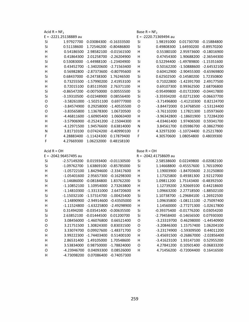
259
Acid R = NF2 E = ‐2221.25138889 au Si 1.97927700 0.03084300 ‐0.16333500 Si 0.51138600 1.72546200 ‐0.80486800 H 0.54186500 2.98582100 ‐0.01561500 H 0.41864300 2.01258700 ‐2.26204900 Si 0.53083000 ‐1.44988100 ‐1.23404900 H 0.43452700 ‐1.34020600 ‐2.71563400 H 0.56982800 ‐2.87373600 ‐0.80795600 Si 0.68437000 ‐0.24738300 1.76246500 H 0.73255500 ‐1.57990200 2.41953100 H 0.72015100 0.85119500 2.76371100 Si ‐0.86547200 ‐0.00750000 0.00555500 Si ‐3.19310500 ‐0.02348900 0.08556400 O ‐3.58261000 ‐1.50251100 0.69777000 O ‐3.84574900 0.29258000 ‐1.40535500 O ‐3.83565800 1.13678300 1.06720500 H ‐4.46811600 ‐1.60905400 1.06063400 H ‐3.57906900 ‐0.25241200 ‐2.15044300 H ‐4.12971500 1.94576600 0.63814000 N 3.81710100 0.07424200 ‐0.40990100 F 4.28883400 ‐1.11424300 0.17879400 F 4.27669300 1.06232000 0.48158100 Acid R = OH E = ‐2042.96457495 au Si ‐2.57149200 0.01593400 ‐0.01130500 Si ‐1.09762700 1.63869100 ‐0.85785000 H ‐1.05722100 1.84294600 ‐2.33417600 H ‐1.05401600 2.95657300 ‐0.16298300 Si ‐1.14686000 ‐0.08184800 1.83762200 H ‐1.10852100 1.10954000 2.73263800 H ‐1.14810300 ‐1.33131000 2.64720600 Si ‐1.15032100 ‐1.57314700 ‐1.00425400 H ‐1.14890900 ‐2.94914600 ‐0.43505000 H ‐1.11524800 ‐1.63225800 ‐2.49298900 Si 0.31494200 ‐0.03541400 ‐0.00635500 Si 2.63852100 ‐0.01444500 0.01200700 O 3.08456000 ‐1.46076800 0.66521400 O 3.21751500 1.30824300 0.83031500 O 3.33074700 0.09927600 ‐1.48371700 H 3.99222300 ‐1.74403400 0.51400100 H 2.86531400 1.49105000 1.70548600 H 3.53834000 0.98750000 ‐1.78824000 O ‐4.23946700 0.04093300 0.08526000 H ‐4.73098200 0.07086400 ‐0.74057300
Base R = NF2 E = ‐2220.71369494 au Si 1.98191000 0.01730700 ‐0.15884800 Si 0.49808300 1.64930200 ‐0.89570200 H 0.55380100 2.95973600 ‐0.18016900 H 0.47454300 1.90688200 ‐2.36544300 Si 0.52294400 ‐1.49789800 ‐1.15351600 H 0.50162200 ‐1.50888600 ‐2.64532100 H 0.60412900 ‐2.90455300 ‐0.65969800 Si 0.62502500 ‐0.14580200 1.72350800 H 0.71022800 ‐1.42391700 2.49177500 H 0.69107300 0.99362500 2.68706800 Si ‐0.95499800 ‐0.01722000 ‐0.04417800 Si ‐3.35934200 ‐0.02712300 ‐0.06637700 O ‐3.71496800 ‐1.41210300 0.82124700 O ‐3.84472000 0.14768500 ‐1.53124400 O ‐3.76110200 1.17821300 1.05973600 H ‐3.96342800 ‐1.18601900 1.72284200 H ‐4.03461400 1.97406500 0.59341700 N 3.84561700 0.05986700 ‐0.38627900 F 4.32973200 ‐1.10724400 0.25217800 F 4.30570600 1.08054800 0.48039300 Base R = OH R = ‐2042.41758609 au Si 2.58538600 0.02249800 ‐0.02082100 Si 1.14668800 ‐0.45557600 1.76510900 H 1.19003900 ‐1.84703600 2.31250800 H 1.17325800 0.49381300 2.92127000 Si 1.09811200 1.75143400 ‐0.48392500 H 1.12739200 2.92669100 0.44218600 H 1.09663200 2.27718500 ‐1.88502100 Si 1.10738700 ‐1.29684100 ‐1.26922500 H 1.09635800 ‐1.08111100 ‐2.75097400 H 1.14560000 ‐2.77271300 ‐1.02617800 Si ‐0.39375400 ‐0.01776200 0.03054200 Si ‐2.79458400 ‐0.14656500 0.07930300 O ‐3.23319700 0.46298000 ‐1.44540900 O ‐3.20846300 1.15757400 1.06204100 O ‐3.23174900 ‐1.59309500 0.44011200 H ‐3.45691500 ‐0.26867000 ‐2.02856400 H ‐3.41623100 1.93147100 0.52955200 O 4.27841200 0.10501400 ‐0.06833200 H 4.71456200 ‐0.72004400 0.16416500

260
Acid R = F E = ‐2066.98429927 au Si ‐2.55274100 0.01403500 ‐0.01110000 Si ‐1.11278300 1.66539500 ‐0.82907300 H ‐1.08745100 1.89447300 ‐2.29989100 H ‐1.07761900 2.96212400 ‐0.09767600 Si ‐1.14139000 ‐0.11585300 1.84881800 H ‐1.10180900 1.06001600 2.76281700 H ‐1.13341400 ‐1.38351200 2.62817100 Si ‐1.15832600 ‐1.56191100 ‐1.03498600 H ‐1.15668900 ‐2.94055900 ‐0.47563500 H ‐1.13659600 ‐1.59272800 ‐2.52268000 Si 0.29988000 ‐0.02898800 ‐0.01133900 Si 2.62399500 ‐0.01392900 0.00978900 O 3.05519300 ‐1.46841200 0.65239500 O 3.20438500 1.29899100 0.83966900 O 3.31165700 0.10958600 ‐1.48568800 H 3.95730800 ‐1.76555800 0.49455200 H 2.87268700 1.46312700 1.72646600 H 3.53736000 0.99683600 ‐1.78011300 F ‐4.18494700 0.04021800 ‐0.01072600 Acid R = Li E = ‐1974.68761674 au Si 2.92400700 ‐0.03315300 ‐0.00860800 Si 1.31637400 ‐1.48695800 ‐0.97028800 H 1.30462700 ‐1.59387500 ‐2.46252400 H 1.26788400 ‐2.88051500 ‐0.42638500 Si 1.34731600 ‐0.09412200 1.76111600 H 1.29442800 ‐1.35490000 2.56760200 H 1.36003400 1.04713100 2.72767000 Si 1.39824300 1.59754300 ‐0.81420400 H 1.41922100 2.93017600 ‐0.13686000 H 1.39598800 1.84321900 ‐2.28948300 Si ‐0.16917500 0.05460400 ‐0.01965800 Si ‐2.50654200 0.01966000 0.00994700 O ‐2.99952000 1.42783000 0.72327200 O ‐3.06722700 ‐1.34808300 0.78125800 O ‐3.24880800 ‐0.04206200 ‐1.47247700 H ‐3.92035500 1.67200600 0.58391600 H ‐2.62807500 ‐1.60225100 1.59743900 H ‐3.41013100 ‐0.92486200 ‐1.81754500 Li 5.36590100 ‐0.08121800 ‐0.00550700
Base R = F E = ‐2066.44199858 au Si 2.56951200 0.01178000 ‐0.01680500 Si 1.09859400 1.74041700 ‐0.54249000 H 1.12230400 2.94222400 0.34771700 H 1.09495100 2.21518300 ‐1.96085900 Si 1.11697000 ‐1.34516400 ‐1.23556500 H 1.11216700 ‐1.15752600 ‐2.71978100 H 1.16007000 ‐2.81097800 ‐0.95027700 Si 1.15277200 ‐0.40210900 1.78964400 H 1.19991300 ‐1.77171400 2.38346400 H 1.18148200 0.59701900 2.90123500 Si ‐0.37769700 ‐0.02163600 0.03009900 Si ‐2.78366900 ‐0.14060800 0.08470100 O ‐3.21809500 ‐1.56891600 0.51129900 O ‐3.21412900 0.40228700 ‐1.46520900 O ‐3.18570200 1.20627500 1.01019300 H ‐3.43351100 ‐0.35202200 ‐2.02048100 H ‐3.37619700 1.96361000 0.44822900 F 4.22350100 0.02883600 ‐0.04596600 Base R = Li E = ‐1974.12057993 au Si 2.92999400 0.02664100 ‐0.03564700 Si 1.29826100 1.65712900 ‐0.55484800 H 1.33454800 2.90405500 0.28448200 H 1.29488800 2.14279700 ‐1.97778800 Si 1.33105100 ‐1.30937600 ‐1.15791800 H 1.32852500 ‐1.19291100 ‐2.65712900 H 1.40096800 ‐2.78257300 ‐0.87509700 Si 1.37918500 ‐0.34884900 1.71389600 H 1.45400200 ‐1.69730900 2.36982700 H 1.42274300 0.64704600 2.83839500 Si ‐0.24915600 ‐0.02902400 0.03838000 Si ‐2.63720700 ‐0.14197800 0.09459200 O ‐3.12454800 ‐1.55316200 0.54074500 O ‐3.10027600 0.36581000 ‐1.46975500 O ‐3.06344400 1.23506600 0.98256600 H ‐3.38536800 ‐0.40743500 ‐1.96630900 H ‐3.34444000 1.93470000 0.38486200 Li 5.35683000 0.03543500 ‐0.06935500
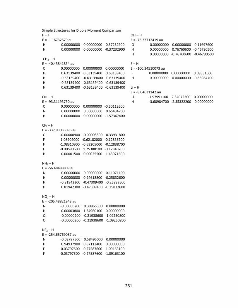
261
Simple Structures for Dipole Moment Comparison H – H E = ‐1.16732679 au H 0.00000000 0.00000000 0.37232900 H 0.00000000 0.00000000 ‐0.37232900 CH3 – H E = ‐40.45841854 au C 0.00000000 0.00000000 0.00000000 H 0.63139400 0.63139400 0.63139400 H ‐0.63139400 ‐0.63139400 0.63139400 H ‐0.63139400 0.63139400 ‐0.63139400 H 0.63139400 ‐0.63139400 ‐0.63139400 CN – H E = ‐93.31193730 au C 0.00000000 0.00000000 ‐0.50112600 N 0.00000000 0.00000000 0.65434700 H 0.00000000 0.00000000 ‐1.57367400 CF3 – H E = ‐337.93033096 au C ‐0.00000900 ‐0.00005800 0.33931800 F 1.08902000 ‐0.62182000 ‐0.12838700 F ‐1.08310900 ‐0.63205000 ‐0.12838700 F ‐0.00590600 1.25388100 ‐0.12840700 H 0.00001500 0.00025500 1.43071600 NH2 – H E = ‐56.48488809 au N 0.00000000 0.00000000 0.11071100 H 0.00000000 0.94618800 ‐0.25832600 H ‐0.81942300 ‐0.47309400 ‐0.25832600 H 0.81942300 ‐0.47309400 ‐0.25832600 NO2 – H E = ‐205.48821943 au N ‐0.00000200 0.30865300 0.00000000 H 0.00003800 1.34960100 0.00000000 O ‐0.00000200 ‐0.21938600 1.09250800 O ‐0.00000200 ‐0.21938600 ‐1.09250800 NF2 – H E = ‐254.65769087 au N ‐0.03797500 0.58495000 0.00000000 H 0.94937900 0.87112400 0.00000000 F ‐0.03797500 ‐0.27587600 1.09163100 F ‐0.03797500 ‐0.27587600 ‐1.09163100
OH – H E = ‐76.33712419 au O 0.00000000 0.00000000 0.11697600 H 0.00000000 0.76760600 ‐0.46790500 H 0.00000000 ‐0.76760600 ‐0.46790500 F – H E = ‐100.34510073 au F 0.00000000 0.00000000 0.09331600 H 0.00000000 0.00000000 ‐0.83984700 Li – H E = ‐8.04631142 au Li ‐1.97991100 2.34072300 0.00000000 H ‐3.60984700 2.35322200 0.00000000
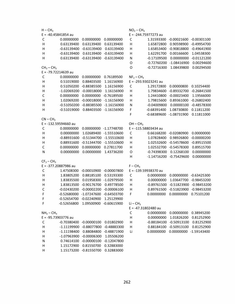
262
H – CH3 E = ‐40.45841854 au C 0.00000000 0.00000000 0.00000000 H 0.63139400 0.63139400 0.63139400 H ‐0.63139400 ‐0.63139400 0.63139400 H ‐0.63139400 0.63139400 ‐0.63139400 H 0.63139400 ‐0.63139400 ‐0.63139400 CH3 – CH3 E = ‐79.72214639 au C 0.00000000 0.00000000 0.76189500 H 0.51019000 0.88403500 1.16156900 H 0.51050200 ‐0.88385500 1.16156900 H ‐1.02069200 ‐0.00018000 1.16156900 C 0.00000000 0.00000000 ‐0.76189500 H 1.02069200 ‐0.00018000 ‐1.16156900 H ‐0.51050200 ‐0.88385500 ‐1.16156900 H ‐0.51019000 0.88403500 ‐1.16156900 CN – CH3 E = ‐132.59594660 au C 0.00000000 0.00000000 ‐1.17748700 H 0.00000000 1.02689400 ‐1.55510600 H ‐0.88931600 ‐0.51344700 ‐1.55510600 H 0.88931600 ‐0.51344700 ‐1.55510600 C 0.00000000 0.00000000 0.27811700 N 0.00000000 0.00000000 1.43736200 CF3 – CH3 E = ‐377.20887986 au C 1.47508300 ‐0.00010900 ‐0.00007800 H 1.83805200 0.88185100 0.53193300 H 1.83835500 0.01958300 ‐1.02979500 H 1.83813500 ‐0.90176700 0.49778500 C ‐0.02430200 ‐0.00002200 ‐0.00006100 F ‐0.52680000 ‐1.07247600 ‐0.64503700 F ‐0.52654700 ‐0.02240900 1.25129900 F ‐0.52656800 1.09500900 ‐0.60615900 NH2 – CH3 E = ‐95.73903776 au C ‐0.70380400 ‐0.00000100 0.01802900 H ‐1.11199900 ‐0.88077800 ‐0.48883300 H ‐1.11198400 0.88084800 ‐0.48871900 H ‐1.07963900 ‐0.00006300 1.05506200 N 0.74614100 ‐0.00000100 ‐0.12047800 H 1.15172900 0.81550700 0.32883000 H 1.15173200 ‐0.81550700 0.32883000
NO2 – CH3 E = ‐244.75977273 au C 1.31593300 ‐0.00021600 ‐0.00301100 H 1.65872800 0.90598900 ‐0.49954700 H 1.65853400 ‐0.90818800 ‐0.49641900 H 1.62291700 0.00166600 1.04538300 N ‐0.17109500 0.00000000 ‐0.01121200 O ‐0.72760200 ‐1.08416900 0.00294600 O ‐0.72716300 1.08439800 0.00294500 NF2 – CH3 E = ‐293.93023241 au C 1.29172800 0.00000800 0.10254400 H 1.79834600 ‐0.89332700 ‐0.26841500 H 1.24410800 ‐0.00023400 1.19566000 H 1.79815600 0.89361000 ‐0.26802400 N ‐0.04009800 0.00000100 ‐0.48578300 F ‐0.68391400 1.08730800 0.11811200 F ‐0.68389600 ‐1.08731900 0.11811000 OH – CH3 E = ‐115.58803434 au C 0.66168200 ‐0.02080900 0.00000000 H 1.07828400 0.98926800 ‐0.00000200 H 1.02532600 ‐0.54578600 ‐0.89515500 H 1.02532700 ‐0.54578300 0.89515700 O ‐0.74398300 0.12268100 0.00000000 H ‐1.14716200 ‐0.75429600 0.00000000 F – CH3 E = ‐139.59938370 au C 0.00000000 0.00000000 ‐0.63425300 H 0.00000000 1.03647700 ‐0.98453200 H ‐0.89761500 ‐0.51823900 ‐0.98453200 H 0.89761500 ‐0.51823900 ‐0.98453200 F 0.00000000 0.00000000 0.75101200 Li – CH3 E = ‐47.31802480 au C 0.00000000 0.00000000 0.38945200 H 0.00000000 1.01826200 0.81252900 H ‐0.88184100 ‐0.50913100 0.81252900 H 0.88184100 ‐0.50913100 0.81252900 Li 0.00000000 0.00000000 ‐1.59143400