Embed Size (px)
Citation preview

Assessing Asset Pricing Models
using Revealed Preference
Jonathan B. Berk
Stanford University and NBER
Jules H. van Binsbergen
Stanford University and NBER
September 2013
This draft: May 12, 2014
Abstract
We propose a new method of testing asset pricing models that does not rely on
prices and returns but on quantities instead. We use the capital flows into and out
of mutual funds to infer which risk model mutual fund investors use. Using this
metric, we find that the Capital Asset Pricing Model outperforms all other models.
Over longer horizons we do find some evidence in support of the recently proposed
dynamic equilibrium models. We find no evidence that investors use any of the
reduced-form multi-factor models that have been proposed.

The field of asset pricing is primarily concerned with the question of how the riskiness
of financial assets affects their price. Despite half a century of research on the topic, the
field is far from a consensus view on how to adjust for risk.
The Capital Asset Pricing Model (CAPM), originally derived by Sharpe (1964), Lint-
ner (1965) and Mossin (1966), remains controversial largely because beta does not appear
to explain asset returns. As a result, in the years since the model was first proposed, fi-
nancial economists have derived numerous extensions in an attempt to bring the model’s
predictions in line with the historic evidence. The result of this research has been mixed.
Although the extensions appear to perform better than the original model, to a large ex-
tent one would not expect otherwise. Like the epicycles that were added to the Ptolemaic
planetary system, many of the extensions were derived to explain the observed short-
comings of the original model. To properly evaluate these models an independent test
is required, that is, the extensions to the CAPM need to be confronted with empirical
facts that they were not designed to explain. Our objective in this paper is to derive and
implement such a test. The starting point of the paper is the simple insight that if the
asset pricing model under consideration correctly prices risk, investors must be using it.
All capital asset pricing models assume that asset markets are perfectly competitive.
Investors compete fiercely with each other to find positive net present value investment
opportunities, and in doing so, eliminate them. The consequence is that equilibrium prices
are set so that the expected return of every asset is solely a function of its risk (as defined
by the model under consideration). Thus, a key prediction of any capital asset pricing
model is that when a non-zero net present value (NPV) investment opportunity presents
itself in capital markets (that is, an asset is mispriced relative to the model) investors
must react by submitting buy or sell orders until the opportunity no longer exists (the
mispricing is removed).
This observation therefore implies that any investment opportunity that the model
1

identifies as having a non-zero net present value must generate buy and sell orders. These
orders reveal the preferences and beliefs of investors. If they are absent then the im-
plication is that investors must not be using that asset pricing model, that is, that the
asset pricing model under consideration does not price risk correctly. Thus, by observing
whether or not buy and sell orders react to the existence of positive net present value
investment opportunities, we can infer whether investors price risk using the asset pricing
model under consideration.
Because capital flows are difficult to measure, researchers have shied away from using
them to test asset pricing models and instead have relied exclusively on prices and/or
returns to evaluate models. However, an important subset of assets are exceptional in this
regard: capital flows are directly observable for actively managed mutual funds. Because
the prices of actively managed mutual funds are fixed (these funds always trade for the
net asset value of the assets they hold), markets can only eliminate positive net present
value opportunities by either an adjustment of the fees charged by the fund, or through
capital flows into, and out of, the fund. Managers rarely change their fees in practice,
so markets equilibrate almost entirely through capital flows. These flows therefore reveal
which asset pricing model investors are actually using.
An important advantage of using capital flows to test asset pricing models is that
there is no reason why a model that has been constructed to fit price (return) data
should also fit flow data. That is, the importance of additional risk factors that were
added in response to the poor performance of the CAPM can be independently assessed
by examining the flow of capital into investment opportunities that have positive alpha
under the original model, but zero alpha under the extension. To reject the original model
in favor of the extension one must also observe no capital flows into such opportunities.
Thus the mutual fund flow data provides a independent test of whether it makes sense to
replace the original model with one of the extensions.
2

Unfortunately, our results present a mixed message for asset pricing theory. On the one
hand, neither the CAPM, nor any extension of the original model, can completely explain
the capital flows in and out of mutual funds. Much of the flows remain unexplained.
But on the other hand, we demonstrate that the CAPM does at least partially price risk.
Importantly, for the most part, the CAPM better explains risk than no model at all.
Furthermore, it also outperforms a naive model in which investors ignore beta and simply
chase any outperformance relative to the market portfolio. Our evidence suggest that
investors measure risk using the CAPM beta.
Our results reveal that investors are using the CAPM to make investment decisions.
Perhaps more surprising is that there is very little evidence that they are using any
other model. Investors do not seem to be using the risk factors identified by Fama and
French (1993) and Carhart (1997). None of the models that use these factors do better
than the CAPM, despite the fact that these models actually nest the CAPM. At longer
horizons, models based on the dynamic equilibrium model derived by Breeden (1979) do
outperform the CAPM. It is not clear why these models do better at longer horizons, but
one possible explanation is that the key variable of interest, consumption, is likely to be
better measured over longer horizons.
The first paper to use mutual fund flows to infer investor preferences is Guercio and
Tkac (2002). Although the primary focus of the paper is on contrasting the inferred
behavior of retail and institutional investors, that paper documents that both sets of
investors use the CAPM — flows respond to outperformance relative to the CAPM. They
do not consider other risk models. In work subsequent to ours, Barber, Huang, and Odean
(2014) use our approach and confirm our result (using slightly different methodology) that
the investors use the CAPM rather than the other factor models that have been proposed.1
1Readers interested in the exact chronology can consult “Note on the relation between the chronologyof Barber, Huang and Odean and this paper” located on our websites.
3
1 Testing Asset Pricing Theory
The core idea that underlies every financial asset pricing model in economics is that prices
are set by agents chasing positive net present value investment opportunities. Under
the assumption that financial markets are perfectly competitive, these opportunities are
competed away so implying that, in equilibrium, prices are set to ensure that no positive
net present value opportunities exist. Under the standard neoclassical assumptions that
underly these models, when new information arrives, prices instantaneously adjust to
eliminate any positive net present value opportunities going forward. It is important to
appreciate that this price adjustment process is part of all asset pricing models, either
explicitly (if the model is dynamic) or implicitly (if the model is static). The output
of all these models, a prediction about expected returns, critically relies on this price
adjustment process.
The importance of this price adjustment process has long been recognized by financial
economists and forms the basis of the event study literature. In that literature, the
correct asset pricing model is assumed to be correctly identified. In that case, because
there are no positive net present value opportunities, the price change that results from
new information (i.e., the part of the change not explained by the asset pricing model)
measures the value of the new information.
Because prices always adjust to eliminate positive net present value investment oppor-
tunities, under the correct asset pricing model expected returns are determined by risk
alone. Modern tests of asset pricing theories test this powerful insight using return data.
Rejection of an asset pricing theory occurs if positive net present value opportunities are
detected, or, equivalently, if investment opportunities can be found that consistently yield
returns in excess of the expected return predicted by the asset pricing model. The prob-
lem with these tests is that the empiricist can never be sure a positive net present value
4

investment opportunity that is identified ex post was actually available ex ante.
An alternative testing approach would be to identify positive net present value invest-
ment opportunities ex ante and test for the existence of investor competition. That is,
do investors react to the existence of positive net present value opportunities that result
from the revelation of new information? Unfortunately, under the standard neoclassical
assumptions that underly the models, for most financial assets this process is impossible
to observe. As Milgrom and Stokey (1982) show, the price adjustment process occurs
with no transaction volume whatsoever — competition is so fierce that no investor ben-
efits from the opportunity. Consequently, for most financial assets the only observable
evidence of this competition is the price change itself. Thus testing for investor compe-
tition is equivalent to standard tests of asset pricing theory that use return data to look
for the elimination of positive net present value invest opportunities.
The key to designing a test to detect investor competition that does not rely on price
data is to find an asset for which the price is fixed. In this case the market equilibration
must occur through volume (quantities). A mutual fund is just such an asset. The
price of a mutual fund is always fixed at the price of its underlying assets, or the net
asset value (NAV). In addition, fee changes are rare. Consequently, if, as a result of
new information, an investment in a mutual fund represents a positive net present value
investment opportunity, the only way for investors to eliminate the opportunity is by
trading the asset. Because this trade is observable, it can be used to infer which mutual
funds investors believe to be positive net present value investments. One can then compare
those investments to the ones the asset pricing model under consideration identifies to
be positive net present value and thereby infer whether investors are using the asset
pricing model. That is, by observing investors’ revealed preferences in their mutual fund
investments we are able to infer information about what (if any) asset pricing model they
are using.
5

1.1 The Mutual Fund Industry
Mutual fund investment represents a large and important sector in the U.S. financial
market. In the last 50 years there has been a secular trend away from direct investing.
Individual investors used to make up more than 50% of the market, today they are
responsible for barely 20% of the total capital investment in U.S. markets. During that
time there has been a concomitant rise in indirect investment, principally in mutual funds.
Mutual funds used to make up less than 5% of the market, today the make up 1/3 of
total investment.2 Today, the number of mutual funds that trade in the U.S. outnumber
the number of stocks that trade.
Berk and Green (2004) derive a model that explains how the market for mutual fund
investment equilibrates that is consistent with the observed facts.3 They start with the
observation that the mutual fund industry is like any industry in the economy — at some
point it must display decreasing returns to scale.4 This observation immediately implies
that in a perfectly competitive financial market, all mutual funds must have enough assets
under management so that they face decreasing returns to scale. When new information
arrives that convinces investors that a particular mutual fund represents a positive net
present value investment, investors react by investing more capital in the mutual fund.
This process continues until enough new capital is invested to eliminate the opportunity.
Thus, the model was able to explain empirical facts documented in the mutual fund
literature that had puzzled financial economists. An extensive literature had documented
that capital flows in and out of mutual funds are clearly not random or uninformed.
Capital flows are responsive to past returns (see Chevalier and Ellison (1997) and Sirri
and Tufano (1998)). Yet future investor returns are largely unpredictable (see Carhart
(1997)), leading financial economists to question why investors would bother to chase
2See French (2008).3Pastor and Stambaugh (2012) derive a general equilibrium version of this model.4Pastor and Stambaugh (2012) provide empirical evidence supporting this assumption.
6

past performance. What the Berk and Green (2004) model showed was that these facts
are consistent with the market equilibrating process unique to mutual funds. Investors
chase past performance because it is informative. Mutual fund managers that do well in
the past are managers that have too little capital under management. Given this new
information, at that level of capital under management, the mutual fund represents a
positive net present value investment opportunity. Investors react by moving capital into
this opportunity and thereby eliminate it. Thus future returns are unpredictable.
A key implication of the Berk and Green (2004) model is that mutual fund manager
must be skilled in the sense that they are able to extract value by trading in financial
markets and that this skill must vary across managers. Berk and van Binsbergen (2013)
verify this fact. They demonstrate that such skill exists and is highly persistent. More
importantly, for our purposes, they demonstrate that these flows contain useful informa-
tion. Not only do investors systematically direct flows to higher skilled managers, but
managerial compensation, which is primarily determined by these flows, predicts future
performance as far out as 10 years. Investors know who the skilled managers are and
compensate them accordingly. It is this observation that provides the starting point of
our analysis.
Berk and van Binsbergen (2013) measure mutual fund performance relative to investors
next best alternative investment opportunity – a tradable benchmark that consists of the
Vanguard index funds that were available at the time. Relative to that benchmark, mutual
investors behave remarkably rationally, directing capital to better managers. This makes
mutual fund investors ideal candidates to study what risk models investors use to make
their investment decisions. For this study, we use the data set constructed in Berk and
van Binsbergen (2013). The data set spans the period from January 1977 to March 2011.
Berk and van Binsbergen (2013) undertook an extensive data project to address several
shortcomings in the CRSP database by combining it with Morningstar data, and we refer
7

the reader to the data appendix of that paper for the details.
1.2 Private Information
Most asset pricing models are derived under the assumption that all investors are sym-
metrically informed. Hence, if one investor faces a positive NPV investment opportunity,
all investors face the same opportunity and so it is instantaneously removed by competi-
tion. In reality, the fact that Berk and van Binsbergen (2013) find skill in mutual fund
management is evidence that at least some investors have access to different information
or have different abilities to process information. As a result, not all positive net present
value investment opportunities are instantaneously competed away.
As Grossman (1976) argued, in a world where there are gains to collecting information
and information gathering is costly, not everybody can be equally informed in equilibrium.
If everybody chooses to collect information, competition between investors ensures that
prices reveal the information and so information gathering is unprofitable. Similarly, if
nobody collects information, prices are uninformative and so there are large profits to
be made collecting information. Thus, in equilibrium, investors must be differentially
informed (see, e.g., Grossman and Stiglitz (1980)). Investors with the lowest information
gathering costs collect information so that, on the margin, what they spend on information
gathering, they make back in trading profits. Presumably these investors are few in
number so that the competition between them is limited, allowing for the existence of
prices that do not fully reveal their information. As a result, information gathering is a
positive net present value endeavor for a limited number of investors.
The existence of asymmetrically informed investors poses a challenge for empiricists
wishing to test asset pricing models derived under the assumption of symmetrically in-
formed investors. Clearly, the empiricist’s information set matters. For example, asset
pricing models fail under the information set of the most informed investor, because the
8

key assumption that asset markets are competitive is false under that information set.
Consequently, the standard in the literature is to assume that the information set of the
uninformed investors only contains the information in publicly available information, such
as past prices and returns, and to conduct the test under that information set. For now,
we will adopt the same strategy but will revisit this assumption in Section 6, where we will
explicitly consider the possibility that the majority of investors’ information sets include
more information than just what is in past and present prices.
1.3 Methodology
To formally derive our testing methodology, let Rnit denote the excess return (that is,
the net-return in excess of the risk free rate) earned by investors in the i’th investment
opportunity at time t and let RBit denote the risk adjustment prescribed by the asset
pricing model under consideration. Then, define εit as follows:
εit ≡ Rnit −RB
it . (1)
Define net alpha, denoted by αit, as the expectation of εit given the information set at
time t, that is,
αit ≡ Et[εit+1].
The assumption that capital markets are competitive implies that conditional on the
(public) information available at time t, the expectation of εi,t+1 (the net alpha) is zero.
In the case of a mutual fund there are only two ways for markets to equilibrate: (1)
the fund changes the net alpha by changing the fee it charges investors, or (2) the fund
experiences an inflow or outflow of capital thereby changing the net alpha investors in
the fund earn. In fact, as we will show, the latter mechanism is used almost exclusively,
implying that the flow of funds into and out of mutual funds reveal investor beliefs about
9

how the fund’s alpha changes with new information.
Let the flow of capital into mutual fund i at time t be denote by Fit where
Fit = g(εit) + νit. (2)
That is, g(·) is the flow that results from the information available in prices and νit is the
flow that results from all other sources of new information. When the asset pricing model
is correctly identified, then αit = 0. Consequently, a positive (negative) realization of
εit+1 must lead to an upward (downward) update of investors inference about αit and an
inflow (outflow) of funds, implying that the function g(·) satisfies g′(·) > 0 and g(0) = 0.5
We are now ready to formulate the testable prediction under the Null hypothesis that
the asset pricing model under consideration holds perfectly. When the information set of
the majority of investors only contains current and past prices, νit = 0 and so from (2)
and the properties of g(·) we have:
εit > 0 if, and only if, Fit > 0. (3)
The rest of the paper provides a test of this prediction.
2 Asset Pricing Models
Our testing methodology can be applied to both reduced-form asset pricing models, such
as the factor models proposed by Fama and French (1993) and Carhart (1997), as well as
to dynamic equilibrium models, such as the consumption CAPM (Breeden (1979)), habit
formation models (Campbell and Cochrane (1999)) and long run risk models (Bansal and
5Berk and Green (2004) derive a formal model of this updating process and thus provide necessaryconditions for these reduced form assumptions.
10

Yaron (2004)). For the CAPM and factor models, RBit is specified by the beta relationship.
We regress the excess returns to investors, Rnit, on the risk factors over the life of the fund
to get the model’s betas. We then use the beta relation to calculate RBit at each point in
time. For example, for the Fama-French-Carhart factor specification, the risk adjustment
RBit is then given by:
RBit = βmkti MKTt + βsmli SMLt + βhmli HMLt + βumdi UMDt.
where MKTt, SMLt, HMLt and UMDt are the realized excess returns on the four factor
portfolios. Using this risk adjusted return, εit is calculated using (1).
In any dynamic equilibrium model returns must satisfy the following condition in
equilibrium:
Et[Mt+1Rnit+1] = 0. (4)
When this condition is violated a positive net present value investment opportunity exists.
Thus the outperformance measure εit for fund i at time t is
εit = Et[Mt+1Rnit+1]. (5)
Notice that εit > 0 is a buying opportunity and so capital should flow into such opportu-
nities. We estimate (5) over a T -period horizon (T > 1) by calculating:
εit =1
T
t∑s=t−T+1
MsRnis,
To compute these outperformance measures, we must compute the stochastic discount
factor for each model at each point in time. For the consumption CAPM, the stochastic
11

discount factor is:
Mt = β
(CtCt−1
)−γ,
where β is the subjective discount rate and γ is the coefficient of relative risk aversion.
The calibrated values we use are given in the top panel of Table 1.
For the long-run risk model as proposed by Bansal and Yaron (2004), the stochastic
discount factor is given by:
Mt = δθ(
CtCt−1
)− θψ
(Rat )−(1−θ) .
where Rat is the return on aggregate wealth and where θ is given by:
θ ≡ 1− γ1− 1
ψ
.
The parameter ψ measures the intertemporal elasticity of substitution (IES). To construct
the realizations of the stochastic discount factor, we use parameter values for risk aversion
and the IES commonly used in the long-run risk literature, as summarized in the middle
panel of Table 1. In addition to these parameter values, we need data on the returns to
the aggregate wealth portfolio. There are two ways to construct these returns. The first
way is to estimate (innovations to) the stochastic volatility of consumption growth as well
as (innovations to) expected consumption growth, which combined with the parameters
of the long-run risk model lead to proxies for the return on wealth. The second way is
to take a stance on the composition of the wealth portfolio, by taking a weighted average
of traded assets. In this paper, we take the latter approach and form a weighted average
of stock and long-term bond returns to compute the returns on the wealth portfolio. We
employ a collection of weights in stocks (denoted by w) to assess the robustness with
respect to this assumption.
12

For the Campbell and Cochrane (1999) habit formation model, the stochastic discount
factor is given by:
Mt = δ
(CtCt−1
StSt−1
)−γ,
where St is the consumption surplus ratio. The dynamics of the log consumption surplus
ratio st are given by:
st = (1− φ)s̄+ φst−1 + λ (st−1) (ct − ct−1 − g) ,
where s̄ is the steady state habit, φ is the persistence of the habit stock, ct the natural
logarithm of consumption at time t and g is the average consumption growth rate. We set
all the parameters of the model to the values proposed in Campbell and Cochrane (1999),
but we replace the average consumption growth rate g, as well as the consumption growth
rate volatility σ with their sample estimates over the full available sample (1959-2011),
as summarized in the bottom panel of Table 1. To construct the consumption surplus
ratio data, we need a starting value. As our consumption data starts in 1959, which is
long before the start of our mutual fund data in 1977, we have a sufficiently long period
to initialize the consumption surplus ratio. That is, in 1959, we set the ratio to its steady
state value s̄ and construct the ratio for the subsequent periods using the available data
that we have. Because the annualized value of the persistence coefficient is 0.87, the
weight of the starting value in the 1977 realization of the stochastic discount factor is
small and equal to 0.015.
It is also possible to calculate the implied RBit in any dynamic equilibrium model. The
13

Consumption CAPMSubj. disc. factor Risk aversion
β γ0.9989 10
Epstein Zin preferences (LRR)Subj. disc. factor Risk aversion IES Weight in stocks
δ γ ψ w0.9989 10 1.5 1.0,0.3,0.1
Habit formation preferencesSubj. disc. factor Risk aversion Mean growth Habit persistence Consumption vol
δ γ g φ σ0.9903 2 0.0020 0.9885 0.0076
Table 1: Parameter Calibration The table shows the calibrated parameters for thethree structural models that we test: power utility over consumption (the consumptionCAPM), external habit formation preferences (as in Campbell and Cochrane (1999)) andEpstein Zin preferences as in Bansal and Yaron (2004).
equilibrium condition (4) can be express in terms of a pricing relation as follows:
0 = Et[Mt+1Rnit+1] = Et[Mt+1]Et[R
nit+1] + Cov(Mt+1, R
nit+1)
Et[Rnit+1] = −
Cov(Mt+1, Rnit+1)
Et[Mt+1]
= −(1 + rt)Cov(Mt+1, Rnit+1)
where we have used the fact that the expectation of the stochastic discount factor is 11+rt
.
Because RBit = Et[R
nit+1], for these models we have
εit = Rnit+1 −RB
it
= Rnit+1 + (1 + rt)Cov(Mt+1, R
nit+1)
where we make the (strong) assumption that the conditional covariance equals its uncon-
ditional counterpart. Implementing our tests using (6) rather than (4) has the advantage
14

that, like the factor models, Cov(Mt+1, Rnit+1) can be estimate once using all the available
data. This improves the accuracy of the estimate, which is important given the noise
in consumption data. The downside is that by implementing the test this way, we are
ignoring a large part of the time variation in risk premia. Because most time variation
in risk premia are a central motivation behind most dynamic equilibrium models we will
use (4) in most of our tests.
One could argue that the structural models that we consider are not calibrated to
explain flow data, and could therefore potentially do better when the model parameters
are estimated using flow data. We follow this empirical strategy in Section 5.
3 Results
To implement a test of (3) it is necessary to pick an observation horizon. Except for the
early part of our sample, the flow data is available monthly. Because we need at least two
observations to estimate (4), the shortest horizon we will consider is three months. There
are a number of concerns interpreting the results from such a short horizon. First, in the
early part of the sample many funds report their AUMs quarterly and so our flow data is
quarterly, implying that for those funds we cannot estimate (4). Even for the funds that
we can estimate (4), estimating this expectation on just three data points is likely to be
very noisy. Another concern is that the distribution of Mt is likely to be heavily skewed,
which increases the difficulty of estimating (4) in small samples.
If investors react to new information immediately, then flows should immediately re-
spond to performance and the appropriate horizon to measure the effect would be the
shortest horizon possible. But in reality there is evidence that investors do not respond
immediately. Mamaysky, Spiegel, and Zhang (2008) show that the net alpha of mutual
funds is predictably non-zero for horizons shorter than a year, suggesting that capital is
15
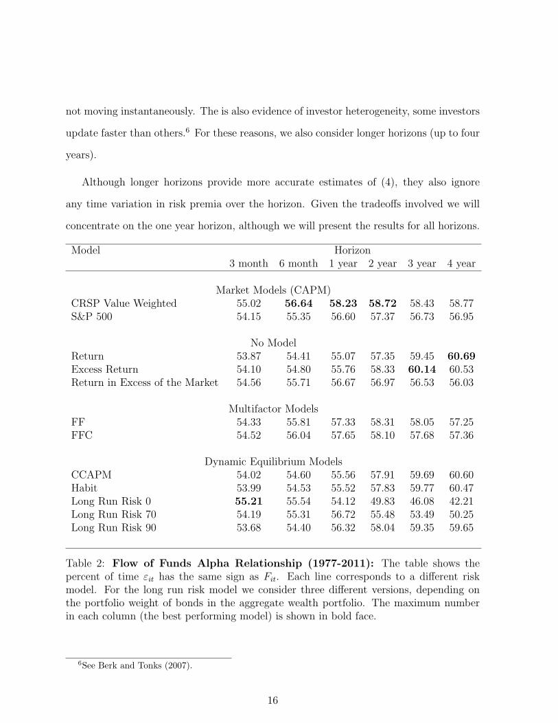
not moving instantaneously. The is also evidence of investor heterogeneity, some investors
update faster than others.6 For these reasons, we also consider longer horizons (up to four
years).
Although longer horizons provide more accurate estimates of (4), they also ignore
any time variation in risk premia over the horizon. Given the tradeoffs involved we will
concentrate on the one year horizon, although we will present the results for all horizons.
Model Horizon3 month 6 month 1 year 2 year 3 year 4 year
Market Models (CAPM)CRSP Value Weighted 55.02 56.64 58.23 58.72 58.43 58.77S&P 500 54.15 55.35 56.60 57.37 56.73 56.95
No ModelReturn 53.87 54.41 55.07 57.35 59.45 60.69Excess Return 54.10 54.80 55.76 58.33 60.14 60.53Return in Excess of the Market 54.56 55.71 56.67 56.97 56.53 56.03
Multifactor ModelsFF 54.33 55.81 57.33 58.31 58.05 57.25FFC 54.52 56.04 57.65 58.10 57.68 57.36
Dynamic Equilibrium ModelsCCAPM 54.02 54.60 55.56 57.91 59.69 60.60Habit 53.99 54.53 55.52 57.83 59.77 60.47Long Run Risk 0 55.21 55.54 54.12 49.83 46.08 42.21Long Run Risk 70 54.19 55.31 56.72 55.48 53.49 50.25Long Run Risk 90 53.68 54.40 56.32 58.04 59.35 59.65
Table 2: Flow of Funds Alpha Relationship (1977-2011): The table shows thepercent of time εit has the same sign as Fit. Each line corresponds to a different riskmodel. For the long run risk model we consider three different versions, depending onthe portfolio weight of bonds in the aggregate wealth portfolio. The maximum numberin each column (the best performing model) is shown in bold face.
6See Berk and Tonks (2007).
16
Horizon (months)3 6 12 24 36 48
LRR 0 CAPM CAPM CAPM Excess Return ReturnCAPM FFC FFC Excess Return Habit C-CAPMExcess Market FF FF FF C-CAPM Excess ReturnFFC Excess Market LRR 70 FFC Return HabitFF LRR 0 Excess Market LRR 90 LRR 90 LRR 90LRR 70 CAPM SP500 CAPM SP500 C-CAPM CAPM CAPMCAPM SP500 LRR 70 LRR 90 Habit FF FFCExcess Return Excess Return Excess Return CAPM SP500 FFC FFC-CAPM C-CAPM C-CAPM Return CAPM SP500 CAPM SP500Habit Habit Habit Excess Market Excess Market Excess MarketReturn Return Return LRR 70 LRR 70 LRR 70LRR 90 LRR 90 LRR 0 LRR 0 LRR 0 LRR 0
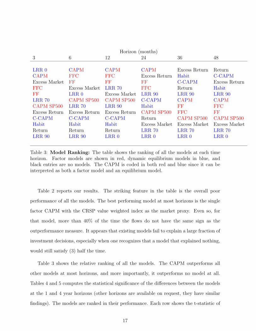
Table 3: Model Ranking: The table shows the ranking of all the models at each timehorizon. Factor models are shown in red, dynamic equilibrium models in blue, andblack entries are no models. The CAPM is coded in both red and blue since it can beinterpreted as both a factor model and an equilibrium model.
Table 2 reports our results. The striking feature in the table is the overall poor
performance of all the models. The best performing model at most horizons is the single
factor CAPM with the CRSP value weighted index as the market proxy. Even so, for
that model, more than 40% of the time the flows do not have the same sign as the
outperformance measure. It appears that existing models fail to explain a large fraction of
investment decisions, especially when one recognizes that a model that explained nothing,
would still satisfy (3) half the time.
Table 3 shows the relative ranking of all the models. The CAPM outperforms all
other models at most horizons, and more importantly, it outperforms no model at all.
Tables 4 and 5 computes the statistical significance of the differences between the models
at the 1 and 4 year horizons (other horizons are available on request, they have similar
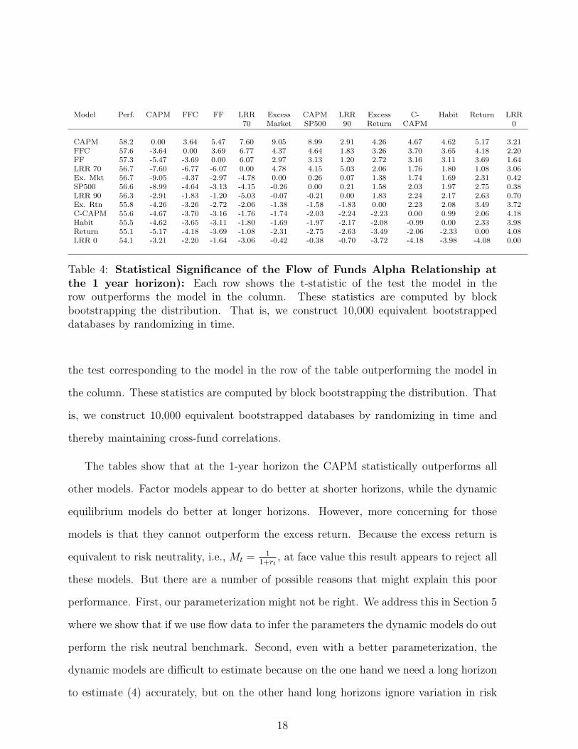
findings). The models are ranked in their performance. Each row shows the t-statistic of
17
Model Perf. CAPM FFC FF LRR Excess CAPM LRR Excess C- Habit Return LRR70 Market SP500 90 Return CAPM 0
CAPM 58.2 0.00 3.64 5.47 7.60 9.05 8.99 2.91 4.26 4.67 4.62 5.17 3.21FFC 57.6 -3.64 0.00 3.69 6.77 4.37 4.64 1.83 3.26 3.70 3.65 4.18 2.20FF 57.3 -5.47 -3.69 0.00 6.07 2.97 3.13 1.20 2.72 3.16 3.11 3.69 1.64LRR 70 56.7 -7.60 -6.77 -6.07 0.00 4.78 4.15 5.03 2.06 1.76 1.80 1.08 3.06Ex. Mkt 56.7 -9.05 -4.37 -2.97 -4.78 0.00 0.26 0.07 1.38 1.74 1.69 2.31 0.42SP500 56.6 -8.99 -4.64 -3.13 -4.15 -0.26 0.00 0.21 1.58 2.03 1.97 2.75 0.38LRR 90 56.3 -2.91 -1.83 -1.20 -5.03 -0.07 -0.21 0.00 1.83 2.24 2.17 2.63 0.70Ex. Rtn 55.8 -4.26 -3.26 -2.72 -2.06 -1.38 -1.58 -1.83 0.00 2.23 2.08 3.49 3.72C-CAPM 55.6 -4.67 -3.70 -3.16 -1.76 -1.74 -2.03 -2.24 -2.23 0.00 0.99 2.06 4.18Habit 55.5 -4.62 -3.65 -3.11 -1.80 -1.69 -1.97 -2.17 -2.08 -0.99 0.00 2.33 3.98Return 55.1 -5.17 -4.18 -3.69 -1.08 -2.31 -2.75 -2.63 -3.49 -2.06 -2.33 0.00 4.08LRR 0 54.1 -3.21 -2.20 -1.64 -3.06 -0.42 -0.38 -0.70 -3.72 -4.18 -3.98 -4.08 0.00
Table 4: Statistical Significance of the Flow of Funds Alpha Relationship atthe 1 year horizon): Each row shows the t-statistic of the test the model in therow outperforms the model in the column. These statistics are computed by blockbootstrapping the distribution. That is, we construct 10,000 equivalent bootstrappeddatabases by randomizing in time.
the test corresponding to the model in the row of the table outperforming the model in
the column. These statistics are computed by block bootstrapping the distribution. That
is, we construct 10,000 equivalent bootstrapped databases by randomizing in time and
thereby maintaining cross-fund correlations.
The tables show that at the 1-year horizon the CAPM statistically outperforms all
other models. Factor models appear to do better at shorter horizons, while the dynamic
equilibrium models do better at longer horizons. However, more concerning for those
models is that they cannot outperform the excess return. Because the excess return is
equivalent to risk neutrality, i.e., Mt = 11+rt
, at face value this result appears to reject all
these models. But there are a number of possible reasons that might explain this poor
performance. First, our parameterization might not be right. We address this in Section 5
where we show that if we use flow data to infer the parameters the dynamic models do out
perform the risk neutral benchmark. Second, even with a better parameterization, the
dynamic models are difficult to estimate because on the one hand we need a long horizon
to estimate (4) accurately, but on the other hand long horizons ignore variation in risk
18
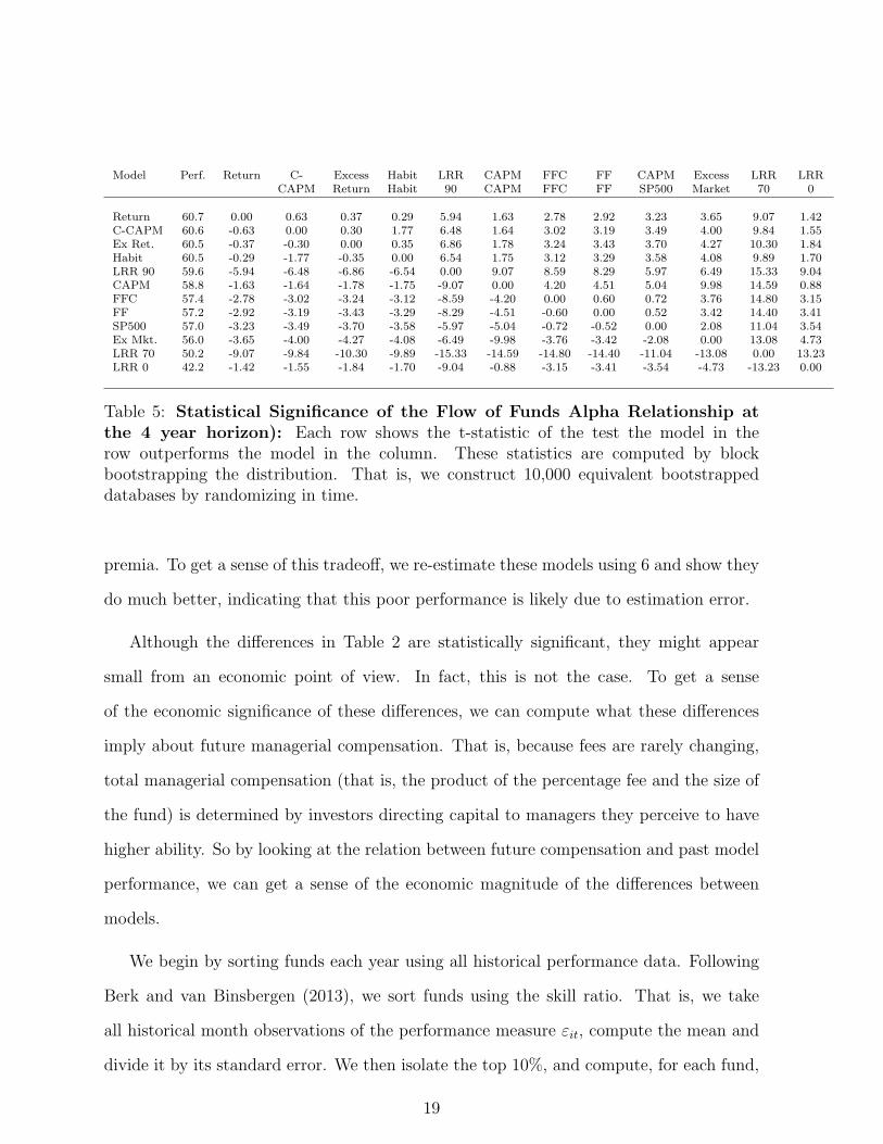
Model Perf. Return C- Excess Habit LRR CAPM FFC FF CAPM Excess LRR LRRCAPM Return Habit 90 CAPM FFC FF SP500 Market 70 0
Return 60.7 0.00 0.63 0.37 0.29 5.94 1.63 2.78 2.92 3.23 3.65 9.07 1.42C-CAPM 60.6 -0.63 0.00 0.30 1.77 6.48 1.64 3.02 3.19 3.49 4.00 9.84 1.55Ex Ret. 60.5 -0.37 -0.30 0.00 0.35 6.86 1.78 3.24 3.43 3.70 4.27 10.30 1.84Habit 60.5 -0.29 -1.77 -0.35 0.00 6.54 1.75 3.12 3.29 3.58 4.08 9.89 1.70LRR 90 59.6 -5.94 -6.48 -6.86 -6.54 0.00 9.07 8.59 8.29 5.97 6.49 15.33 9.04CAPM 58.8 -1.63 -1.64 -1.78 -1.75 -9.07 0.00 4.20 4.51 5.04 9.98 14.59 0.88FFC 57.4 -2.78 -3.02 -3.24 -3.12 -8.59 -4.20 0.00 0.60 0.72 3.76 14.80 3.15FF 57.2 -2.92 -3.19 -3.43 -3.29 -8.29 -4.51 -0.60 0.00 0.52 3.42 14.40 3.41SP500 57.0 -3.23 -3.49 -3.70 -3.58 -5.97 -5.04 -0.72 -0.52 0.00 2.08 11.04 3.54Ex Mkt. 56.0 -3.65 -4.00 -4.27 -4.08 -6.49 -9.98 -3.76 -3.42 -2.08 0.00 13.08 4.73LRR 70 50.2 -9.07 -9.84 -10.30 -9.89 -15.33 -14.59 -14.80 -14.40 -11.04 -13.08 0.00 13.23LRR 0 42.2 -1.42 -1.55 -1.84 -1.70 -9.04 -0.88 -3.15 -3.41 -3.54 -4.73 -13.23 0.00
Table 5: Statistical Significance of the Flow of Funds Alpha Relationship atthe 4 year horizon): Each row shows the t-statistic of the test the model in therow outperforms the model in the column. These statistics are computed by blockbootstrapping the distribution. That is, we construct 10,000 equivalent bootstrappeddatabases by randomizing in time.
premia. To get a sense of this tradeoff, we re-estimate these models using 6 and show they
do much better, indicating that this poor performance is likely due to estimation error.
Although the differences in Table 2 are statistically significant, they might appear
small from an economic point of view. In fact, this is not the case. To get a sense
of the economic significance of these differences, we can compute what these differences
imply about future managerial compensation. That is, because fees are rarely changing,
total managerial compensation (that is, the product of the percentage fee and the size of
the fund) is determined by investors directing capital to managers they perceive to have
higher ability. So by looking at the relation between future compensation and past model
performance, we can get a sense of the economic magnitude of the differences between
models.
We begin by sorting funds each year using all historical performance data. Following
Berk and van Binsbergen (2013), we sort funds using the skill ratio. That is, we take
all historical month observations of the performance measure εit, compute the mean and
divide it by its standard error. We then isolate the top 10%, and compute, for each fund,
19

the monthly compensation paid over the next year. For each model we then compute the
average monthly compensation over our time period starting in 1980.7 Table 6 provides
the results. Notice that the differences are large, of the order of hundreds of thousands
of dollars per month. Notice also that the consumption CAPM and Habit models do
particularly well, indicating that these models benefit when performance is measured
using the entire history of the fund. As we show in the appendix, when we estimate
the dynamic models by computing the covariance over the life of the fund using (6), we
observe similar better performance.
Model Return CAPM FF FFC C-CAPM Habit
Return 0 -78 194 267 -432 -405CAPM 78 0 271 345 -354 -328FF -194 -271 0 73 -626 -599FFC -267 -345 -73 0 -699 -672C-CAPM 432 354 626 699 0 27Habit 405 328 599 672 -27 0
Table 6: Economic Significance ($1000/month): The table shows the differ-ence in average future monthly compensation of top decile funds sorted based onhistorical performance measured by the model in the row. That is, each row pro-vides the amount of extra compensation top decile managers made relative to top decilemanagers sorted based on the model in the column. The numbers are in $1000 per month.
4 A Probit Model for Fund Flows and Asset Pricing
Factors
One important assumption that we have made when implementing the reduced-form factor
models, is that the asset pricing betas of the factor models are known to investors. That
7Because we are restricting attention to the top performing funds it does not make much differencewhat we do with funds that go out of business over the year. In the table we assume those fund managersearn the average compensation. Assuming those managers earn 0, leads to almost identical results.
20

is, we have computed asset pricing betas using the full sample of available returns, and
we have applied these return betas throughout the sample. One may be concerned that
in reality investors are using a different beta than the one we have estimated.
In this section, we explore the explanatory power of the commonly used additional risk
factors such as size and value without taking a stance on the asset pricing beta. That is,
we let the flow data decide which factor exposure best explains the flow sign. To achieve
this, we model the probability that fund i will receive an inflow at time t as a function
of the fund’s net return and the asset pricing factors under consideration using a probit
model. Let Yit denote the sign of the flow to fund i at time t, where Yit = 1 denotes an
inflow and Yit = 0 denotes an outflow. Then the probability of an inflow is modeled as:
P (Yit == 1) = Φ (γ (Rnit − Ftβi)) , (6)
where Φ is the cumulative distribution function of the standard normal distribution, Ft is
the row vector with the factor realizations, and βi is the column vector of factor loadings
of fund i. We then use standard maximum likelihood optimization techniques to estimate
βi. If the MLE estimate of βi is significantly different from zero for a particular factor,
then this implies that the factor plays a role in the decision of investors to allocate flows
to or from the mutual fund.
We estimate the discrete choice model above for each fund, using as the factors the
CAPM, as well as the CAPM augmented with the size factor, and the CAPM augmented
with the value factor, using quarterly data. The cross-sectional distribution of the esti-
mates are plotted in blue in Figures 1, 2 and 3. As a comparison, we also plot in each
figure a bootstrapped distribution of factor loadings. These loadings are bootstrapped
under the Null hypothesis that the factor does not enter into the decision rule of investors,
that is, the factor loading is zero.
21

The graphs further confirm our earlier results. The cross-sectional distribution of
CAPM betas is centered close to 1, with a median of 0.85, and the bootstrapped distri-
bution of CAPM betas is substantially different from the estimated distribution. This is
not true for the estimated size and value betas. Both distributions are centered around
0 (as expected), but more importantly, there only seem to be very small deviations of
estimated betas relative to the randomly bootstrapped distribution of fund betas.
Probit: CAPM betas
−5 −4 −3 −2 −1 0 1 2 3 4 50
200
400
600
800
1000
1200
1400
1600
CAPM β
No.
of
Fund
s
Figure 1: CAPM betas: The graph shows in blue the cross-sectional distribution ofestimated CAPM betas using the probit model in equation 6, where the only factor in Ftis the excess return on the market portfolio. The graph also shows a bootstrapped distri-bution of CAPM betas (transparent), which is bootstrapped under the Null hypothesisthat the market portfolio is not a relevant factor for investors when allocating flows. Thatis, the CAPM beta is 0.
5 Estimating Structural Models Using Flows
In the previous sections we have evaluated the performance of several structural asset
pricing models by confronting them with quantity (flow) data. To perform this evaluation,
we have taken the underlying model parameters as given. In particular, we have taken
the parameter values from the existing literature, which has calibrated the parameters
to best explain a set of moments such as the equity risk premium and the risk free rate.
22
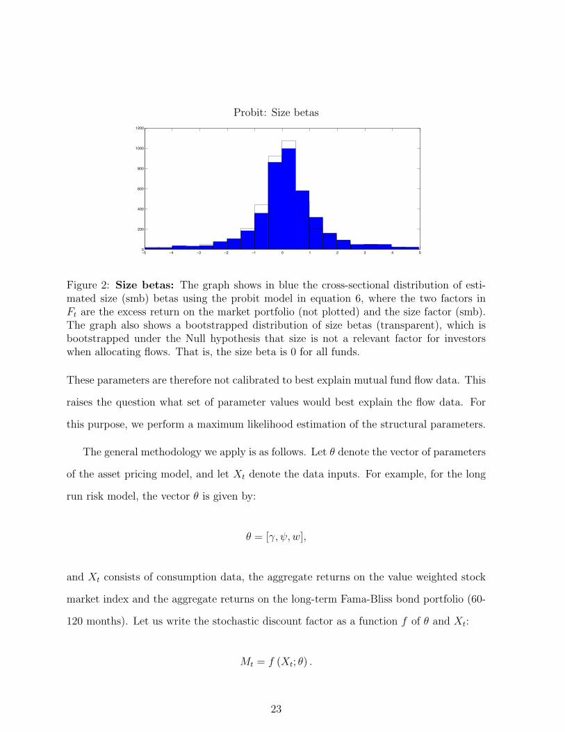
Probit: Size betas
−5 −4 −3 −2 −1 0 1 2 3 4 50
200
400
600
800
1000
1200
Figure 2: Size betas: The graph shows in blue the cross-sectional distribution of esti-mated size (smb) betas using the probit model in equation 6, where the two factors inFt are the excess return on the market portfolio (not plotted) and the size factor (smb).The graph also shows a bootstrapped distribution of size betas (transparent), which isbootstrapped under the Null hypothesis that size is not a relevant factor for investorswhen allocating flows. That is, the size beta is 0 for all funds.
These parameters are therefore not calibrated to best explain mutual fund flow data. This
raises the question what set of parameter values would best explain the flow data. For
this purpose, we perform a maximum likelihood estimation of the structural parameters.
The general methodology we apply is as follows. Let θ denote the vector of parameters
of the asset pricing model, and let Xt denote the data inputs. For example, for the long
run risk model, the vector θ is given by:
θ = [γ, ψ, w],
and Xt consists of consumption data, the aggregate returns on the value weighted stock
market index and the aggregate returns on the long-term Fama-Bliss bond portfolio (60-
120 months). Let us write the stochastic discount factor as a function f of θ and Xt:
Mt = f (Xt; θ) .
23

Probit: Value betas
−5 −4 −3 −2 −1 0 1 2 3 4 50
200
400
600
800
1000
1200
Figure 3: Value betas: The graph shows in blue the cross-sectional distribution ofestimated value (hml) betas using the probit model in equation 6, where the two factorsin Ft are the excess return on the market portfolio (not plotted) and the value factor(hml). The graph also shows a bootstrapped distribution of value betas (transparent),which is bootstrapped under the Null hypothesis that value is not a relevant factor forinvestors when allocating flows. That is, the value beta is 0 for all funds.
Given the pricing relation
Et[Mt+1Rnit+1] = 0,
the outperformance measure εit for fund i at time t over a T -period horizon is given by:
εit =1
T
t∑s=t−T+1
f (Xs; θ)Rnis.
Without loss of generality, we normalize this outperformance measure to have a stan-
dard deviation of 1. We denote the flow sign data, where an inflow into the fund (Fit > 0)
is denoted by 1 and an outflow by 0, by Yit, where the cumulative flows are computed
over the same horizon T as the outperformance. Finally, we model the probability that
an inflow occurs as a function of the outperformance measure using a probit model:
P (Yit == 1) = Φ (εit) ,
24

where Φ is the cumulative distribution function of the standard normal distribution. The
likelihood function of the model is given by:
lnL (θ) =N∑i=1
T∑t=1
[YitlnΦ (εit) + (1− Yit) ln (1− Φ (εit))] .
We estimate the parameters of each model by maximizing the likelihood:
θ̂MLE = argmax lnL (θ)
The results of this estimation using annual flow data are given in Table 7. The table
shows that the estimated parameters and the calibrated parameters are relatively close.
Using flow data, habits are estimated to be somewhat less persistent. Further, the weight
of bonds in the aggregate wealth portfolio is estimated to be high and equal to 94%.
Parameter name Risk aversion Habit persist. Cons. stdev IES Weight bondsParameter γ φ σ ψ w
Consumption CAPM Calibration 10 - - - -Estimation 17.2 - - - -
Habit Calibration 2 0.9885 0.0076 - -Estimation 2.58 0.8928 0.0050 - -
Epstein Zin (LRR) Calibration 10 - - 1.50 0Estimation 11.1 - - 1.36 0.9391
Table 7: Estimating Structural Parameters Using Flows The table compares thecalibrated and estimated (probit) parameters of the structural models that we consider.
6 Other Information Sets
Conceivably, the poor performance of all the models reported in the last section could
result from the assumption that the information set for most investors does not include
any more information than past and present prices. If that is false and the information
set of most investors includes information in addition to what is communicated by price,
25
Horizon (years)3 4 5 6 7 8 9 10
CAPM (freq. %) 52.38 52.38 48.15 47.02 51.09 53.91 56.99 52.38p-value (%) 26.73 25.53 74.84 85.69 38.18 12.41 1.14 21.51
Fama-French (freq. %) 60.00 55.41 54.44 55.09 56.16 56.79 55.56 55.24p-value (%) 0.23 5.71 8.07 4.85 2.34 1.99 3.61 3.56
Fama-French-Cahart (freq. %) 57.62 56.28 52.96 52.98 57.61 54.73 54.48 55.56p-value (%) 1.61 3.26 18.07 17.16 0.67 7.90 7.53 2.76
C-CAPM (freq. %) 51.91 53.25 51.11 48.77 46.74 54.32 51.97 52.70p-value (%) 31.46 17.85 38.05 68.22 87.36 9.97 27.47 18.37
Habit (freq. %) 51.91 52.81 51.11 49.12 47.46 52.26 50.54 51.75p-value (%) 31.46 21.49 38.05 63.88 81.67 26.06 45.24 28.66
Long Run Risk 0 (freq. %) 48.10 48.49 48.52 47.37 46.01 44.44 46.60 46.67p-value (%) 73.27 70.06 70.80 82.84 91.70 96.39 88.45 89.25
Long Run Risk 70 (freq. %) 55.71 50.22 52.96 45.61 55.44 53.50 59.86 52.38p-value (%) 5.61 50.00 18.07 93.83 4.03 15.24 0.06 21.51
Long Run Risk 90 (freq. %) 54.76 53.68 54.44 51.93 55.44 54.32 56.63 53.33p-value (%) 9.48 14.62 8.07 27.69 4.03 9.97 1.55 12.99
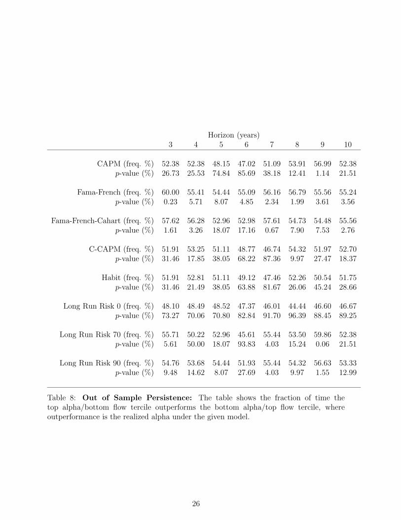
Table 8: Out of Sample Persistence: The table shows the fraction of time thetop alpha/bottom flow tercile outperforms the bottom alpha/top flow tercile, whereoutperformance is the realized alpha under the given model.
26

what appears to us as a positive NPV investment might actually be a zero NPV when
viewed from the perspective of the actual information available at the time. This could
explain the violations of (3).
If information is indeed the explanation, we should find that net alphas relative to the
true risk model do not persist out of sample, proving the investors right in their decision
to allocate or withdraw money. We test this Null of no persistence against the Alternative
that the net alpha does persist. Particularly, we double sort firms into terciles based on
their past alpha as well as their past flows, and test whether funds in the highest alpha
tercile and the lowest flow tercile outperform funds in the lowest alpha tercile and the
highest flow decile.8 Put differently, we investigate whether previously outperforming
funds that did not receive flows outperform previously underperforming funds that did
receive flows. Under the Null, these two portfolios should perform equally well (both
should have a zero net alpha going forward). To test the Null we simply count the
number of times the former portfolio outperforms the latter, which under the Null follows
a binominal distribution.
In Table 8 we perform this one sided test for the risk models that have at least
a reasonable chance at capturing risk, that is, the models for which the sign between
outperformance and flows matches up at least 50of the time. For the other models, the
differential information set explanation can only make sense if there is no information
regarding skill in past returns, which we regard as implausible. Consistent with our
previous result, we find that only for the CAPM can we not reject the Null hypothesis that
alphas are not persistent. For the Fama French and Fama French Carhart model, we find
that alphas are highly persistent, thereby rejecting the Null hypothesis that the differential
information set explains the lack of correlation between flows and outperformance.
8The sorts we do are unconditional sorts, meaning that we independently sort on flows and alpha.The advantage of this is that our results are not influenced by the ordering of our sorts. The downsideis that the nine “portfolios” do not have the same number of funds in them.
27

7 Fee Changes
As argued in the introduction, flows into funds are potentially not the only equilibrating
mechanism. An alternative mechanism is that the fees that funds charge adjust. These
fees are relatively stable. The fund prospectus specifies the maximum fee the fund is
allowed to charge, but funds sometimes rebate some of the fee to investors. Given this,
we need to investigate the possibility that instead of fund flows, the fund changes its fees
to equate markets. To rule out this mechanism as a possible explanation of our results,
we repeat the above analysis by combining fee changes with fund flows. That is, we test
(3) by counting the number of times εit has the same sign as either Fit or a change in
the fee. Clearly, if changes in fees, fund flows, and past realized risk adjusted return are
unrelated, the likelihood of either flows or fees lining up with outperformance is 75% (not
50% as before). So to measure how much our original results are improved by taking
fee changes into account in this way, we first measure the deviation from the expected
number of matches, assuming that these quantities are unrelated, that is 75%. The only
complication is that in many cases the fee change is exactly zero. To properly account for
these observations, we calculate the expected number of changes without including these
observations. We subtract this number from the actual count to get the improvement.
We do the same thing for the original study (there the likelihood when unrelated is 50%)
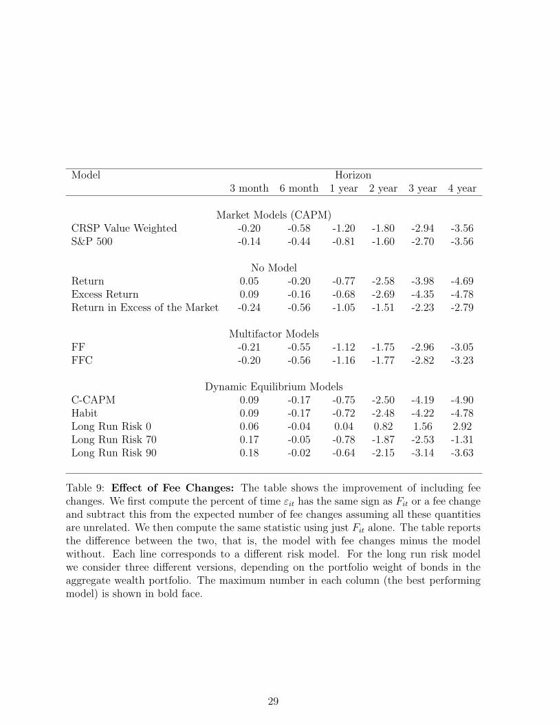
and then subtract the two numbers. The results are reported in Table 9.
It is clear that by including fee changes in this way make little difference to our results.
In most cases the difference is considerably less than a percentage point, which shows that
1) fee changes do not seem to be an important equilibrating mechanism, and 2) our earlier
conclusions regarding the relative performance of the risk models remains unchanged.
28
Model Horizon3 month 6 month 1 year 2 year 3 year 4 year
Market Models (CAPM)CRSP Value Weighted -0.20 -0.58 -1.20 -1.80 -2.94 -3.56S&P 500 -0.14 -0.44 -0.81 -1.60 -2.70 -3.56
No ModelReturn 0.05 -0.20 -0.77 -2.58 -3.98 -4.69Excess Return 0.09 -0.16 -0.68 -2.69 -4.35 -4.78Return in Excess of the Market -0.24 -0.56 -1.05 -1.51 -2.23 -2.79
Multifactor ModelsFF -0.21 -0.55 -1.12 -1.75 -2.96 -3.05FFC -0.20 -0.56 -1.16 -1.77 -2.82 -3.23
Dynamic Equilibrium ModelsC-CAPM 0.09 -0.17 -0.75 -2.50 -4.19 -4.90Habit 0.09 -0.17 -0.72 -2.48 -4.22 -4.78Long Run Risk 0 0.06 -0.04 0.04 0.82 1.56 2.92Long Run Risk 70 0.17 -0.05 -0.78 -1.87 -2.53 -1.31Long Run Risk 90 0.18 -0.02 -0.64 -2.15 -3.14 -3.63
Table 9: Effect of Fee Changes: The table shows the improvement of including feechanges. We first compute the percent of time εit has the same sign as Fit or a fee changeand subtract this from the expected number of fee changes assuming all these quantitiesare unrelated. We then compute the same statistic using just Fit alone. The table reportsthe difference between the two, that is, the model with fee changes minus the modelwithout. Each line corresponds to a different risk model. For the long run risk modelwe consider three different versions, depending on the portfolio weight of bonds in theaggregate wealth portfolio. The maximum number in each column (the best performingmodel) is shown in bold face.
29

8 Conclusion
Nearly fifty years of research in asset pricing has been dedicated to the question of how
to properly adjust cash flows for risk. Since the Capital Asset Pricing model of Sharpe
(1964), a large set of alternative models have been proposed. In this paper we have
proposed an alternative way of testing the validity of an asset pricing model that instead
of relying on moment conditions related to returns, uses flow data instead. Our study is
motivated by revealed preference theory: if the asset pricing model under consideration
correctly prices risk, then investors must be using it, and must be allocating their money
based on that risk model. Our method can be used as an independent test of existing and
future asset pricing models.
30

A Appendix
In this appendix we estimate (6) rather than (4) for the dynamic equilibrium models. The
advantage of doing the estimation using this form is that we can estimate the covariance
term once for each fund, thus reducing the estimation error of variables that are hard to
estimate. The disadvantage is that the habit and long run risk models explicitly model
time variation in risk premia. That is, this term is not constant in the models, so treating
it that way in the estimation implies that we are not exactly testing the model predictions.
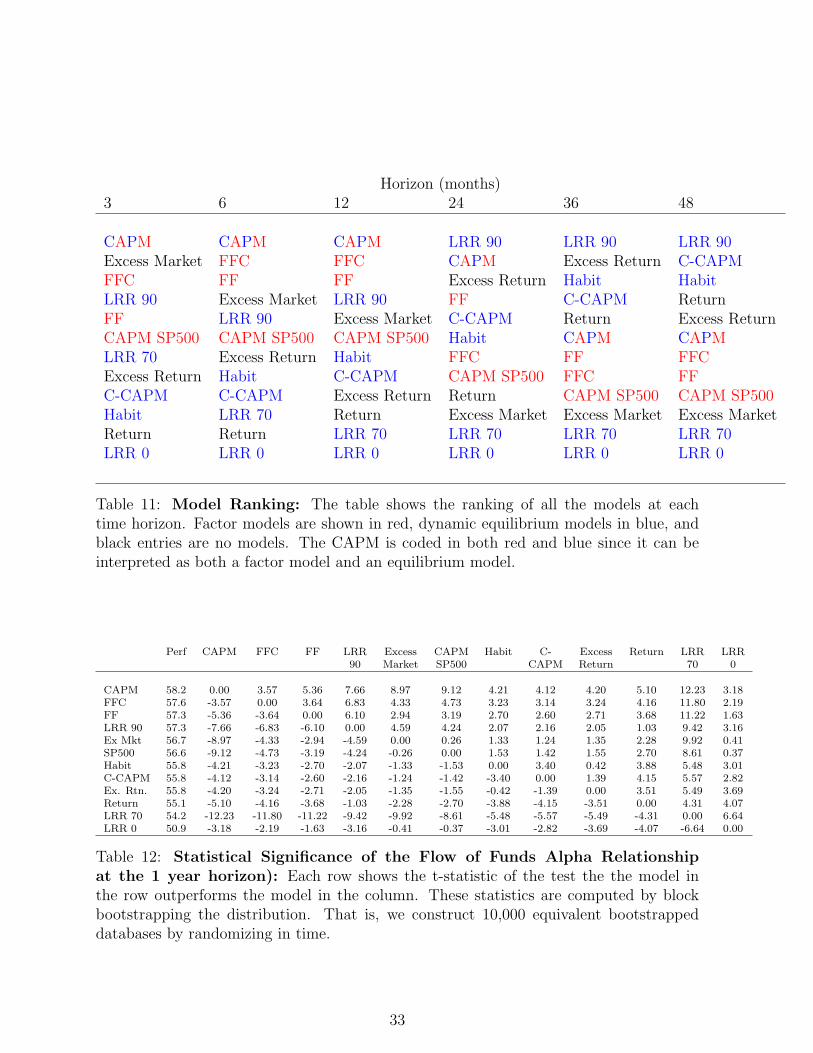
Tables 10 and 11 reports our results. The striking feature in the table is the difference
of performance of the dynamic equilibrium models, especially at longer horizons. In fact
the long run risk model with 90% of the aggregate wealth represented by bonds does far
better than any other model at horizons longer than 3 or 4 years. At 4 years, both the
C-CAPM and the habit model do better than the excess return (risk neutrality). Table
11 makes it clear that using this specification, the factor models do better at shorter
horizons and the dynamic models do better at longer horizons. One possible reason for
this pattern might be the estimation error in measuring consumption. When the models
are estimated over longer horizons, the effect of this error is diminished. Tables 12 and
13 report the bootstrapped statistical significance.
31

Model Horizon3 month 6 month 1 year 2 year 3 year 4 year
Market Models (CAPM)CRSP Value Weighted 55.02 56.64 58.23 58.72 58.43 58.77S&P 500 54.15 55.35 56.60 57.37 56.73 56.95
No ModelReturn 53.87 54.41 55.07 57.35 59.45 60.69Excess Return 54.10 54.80 55.76 58.33 60.14 60.53Return in Excess of the Market 54.56 55.71 56.67 56.97 56.53 56.03
Multifactor ModelsFF 54.33 55.81 57.33 58.31 58.05 57.25FFC 54.52 56.04 57.65 58.10 57.68 57.36
Dynamic Equilibrium ModelsC-CAPM 54.08 54.76 55.79 58.27 59.85 60.85Habit 54.08 54.78 55.85 58.26 59.92 60.79Long Run Risk 0 52.67 52.27 50.92 48.14 45.07 41.55Long Run Risk 70 54.10 54.64 54.21 50.92 48.13 43.45Long Run Risk 90 54.51 55.64 57.33 59.58 61.87 62.64
Table 10: Flow of Funds Alpha Relationship (1977-2011): The table shows thepercent of time εit has the same sign as Fit. Each line corresponds to a different riskmodel. For the long run risk model we consider three different versions, depending onthe portfolio weight of bonds in the aggregate wealth portfolio. The maximum numberin each column (the best performing model) is shown in bold face.
32
Horizon (months)3 6 12 24 36 48
CAPM CAPM CAPM LRR 90 LRR 90 LRR 90Excess Market FFC FFC CAPM Excess Return C-CAPMFFC FF FF Excess Return Habit HabitLRR 90 Excess Market LRR 90 FF C-CAPM ReturnFF LRR 90 Excess Market C-CAPM Return Excess ReturnCAPM SP500 CAPM SP500 CAPM SP500 Habit CAPM CAPMLRR 70 Excess Return Habit FFC FF FFCExcess Return Habit C-CAPM CAPM SP500 FFC FFC-CAPM C-CAPM Excess Return Return CAPM SP500 CAPM SP500Habit LRR 70 Return Excess Market Excess Market Excess MarketReturn Return LRR 70 LRR 70 LRR 70 LRR 70LRR 0 LRR 0 LRR 0 LRR 0 LRR 0 LRR 0
Table 11: Model Ranking: The table shows the ranking of all the models at eachtime horizon. Factor models are shown in red, dynamic equilibrium models in blue, andblack entries are no models. The CAPM is coded in both red and blue since it can beinterpreted as both a factor model and an equilibrium model.
Perf CAPM FFC FF LRR Excess CAPM Habit C- Excess Return LRR LRR90 Market SP500 CAPM Return 70 0
CAPM 58.2 0.00 3.57 5.36 7.66 8.97 9.12 4.21 4.12 4.20 5.10 12.23 3.18FFC 57.6 -3.57 0.00 3.64 6.83 4.33 4.73 3.23 3.14 3.24 4.16 11.80 2.19FF 57.3 -5.36 -3.64 0.00 6.10 2.94 3.19 2.70 2.60 2.71 3.68 11.22 1.63LRR 90 57.3 -7.66 -6.83 -6.10 0.00 4.59 4.24 2.07 2.16 2.05 1.03 9.42 3.16Ex Mkt 56.7 -8.97 -4.33 -2.94 -4.59 0.00 0.26 1.33 1.24 1.35 2.28 9.92 0.41SP500 56.6 -9.12 -4.73 -3.19 -4.24 -0.26 0.00 1.53 1.42 1.55 2.70 8.61 0.37Habit 55.8 -4.21 -3.23 -2.70 -2.07 -1.33 -1.53 0.00 3.40 0.42 3.88 5.48 3.01C-CAPM 55.8 -4.12 -3.14 -2.60 -2.16 -1.24 -1.42 -3.40 0.00 1.39 4.15 5.57 2.82Ex. Rtn. 55.8 -4.20 -3.24 -2.71 -2.05 -1.35 -1.55 -0.42 -1.39 0.00 3.51 5.49 3.69Return 55.1 -5.10 -4.16 -3.68 -1.03 -2.28 -2.70 -3.88 -4.15 -3.51 0.00 4.31 4.07LRR 70 54.2 -12.23 -11.80 -11.22 -9.42 -9.92 -8.61 -5.48 -5.57 -5.49 -4.31 0.00 6.64LRR 0 50.9 -3.18 -2.19 -1.63 -3.16 -0.41 -0.37 -3.01 -2.82 -3.69 -4.07 -6.64 0.00
Table 12: Statistical Significance of the Flow of Funds Alpha Relationshipat the 1 year horizon): Each row shows the t-statistic of the test the the model inthe row outperforms the model in the column. These statistics are computed by blockbootstrapping the distribution. That is, we construct 10,000 equivalent bootstrappeddatabases by randomizing in time.
33
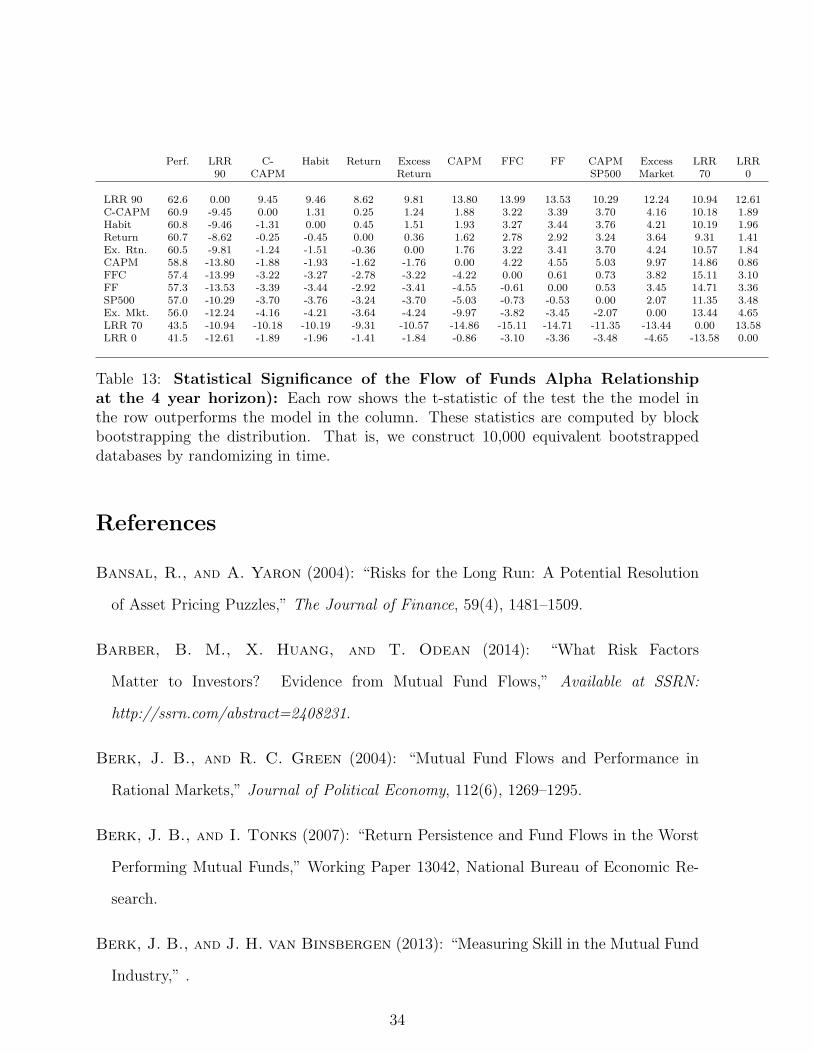
Perf. LRR C- Habit Return Excess CAPM FFC FF CAPM Excess LRR LRR90 CAPM Return SP500 Market 70 0
LRR 90 62.6 0.00 9.45 9.46 8.62 9.81 13.80 13.99 13.53 10.29 12.24 10.94 12.61C-CAPM 60.9 -9.45 0.00 1.31 0.25 1.24 1.88 3.22 3.39 3.70 4.16 10.18 1.89Habit 60.8 -9.46 -1.31 0.00 0.45 1.51 1.93 3.27 3.44 3.76 4.21 10.19 1.96Return 60.7 -8.62 -0.25 -0.45 0.00 0.36 1.62 2.78 2.92 3.24 3.64 9.31 1.41Ex. Rtn. 60.5 -9.81 -1.24 -1.51 -0.36 0.00 1.76 3.22 3.41 3.70 4.24 10.57 1.84CAPM 58.8 -13.80 -1.88 -1.93 -1.62 -1.76 0.00 4.22 4.55 5.03 9.97 14.86 0.86FFC 57.4 -13.99 -3.22 -3.27 -2.78 -3.22 -4.22 0.00 0.61 0.73 3.82 15.11 3.10FF 57.3 -13.53 -3.39 -3.44 -2.92 -3.41 -4.55 -0.61 0.00 0.53 3.45 14.71 3.36SP500 57.0 -10.29 -3.70 -3.76 -3.24 -3.70 -5.03 -0.73 -0.53 0.00 2.07 11.35 3.48Ex. Mkt. 56.0 -12.24 -4.16 -4.21 -3.64 -4.24 -9.97 -3.82 -3.45 -2.07 0.00 13.44 4.65LRR 70 43.5 -10.94 -10.18 -10.19 -9.31 -10.57 -14.86 -15.11 -14.71 -11.35 -13.44 0.00 13.58LRR 0 41.5 -12.61 -1.89 -1.96 -1.41 -1.84 -0.86 -3.10 -3.36 -3.48 -4.65 -13.58 0.00
Table 13: Statistical Significance of the Flow of Funds Alpha Relationshipat the 4 year horizon): Each row shows the t-statistic of the test the the model inthe row outperforms the model in the column. These statistics are computed by blockbootstrapping the distribution. That is, we construct 10,000 equivalent bootstrappeddatabases by randomizing in time.
References
Bansal, R., and A. Yaron (2004): “Risks for the Long Run: A Potential Resolution
of Asset Pricing Puzzles,” The Journal of Finance, 59(4), 1481–1509.
Barber, B. M., X. Huang, and T. Odean (2014): “What Risk Factors
Matter to Investors? Evidence from Mutual Fund Flows,” Available at SSRN:
http://ssrn.com/abstract=2408231.
Berk, J. B., and R. C. Green (2004): “Mutual Fund Flows and Performance in
Rational Markets,” Journal of Political Economy, 112(6), 1269–1295.
Berk, J. B., and I. Tonks (2007): “Return Persistence and Fund Flows in the Worst
Performing Mutual Funds,” Working Paper 13042, National Bureau of Economic Re-
search.
Berk, J. B., and J. H. van Binsbergen (2013): “Measuring Skill in the Mutual Fund
Industry,” .
34
Breeden, D. T. (1979): “An intertemporal asset pricing model with stochastic con-
sumption and investment opportunities,” Journal of Financial Economics, 7(3), 265 –
296.
Campbell, J. Y., and J. H. Cochrane (1999): “By Force of Habit: A Consumption-
Based Explanation of Aggregate Stock Market Behavior,” Journal of Political Economy,
107, 205–251.
Carhart, M. M. (1997): “On Persistence in Mutual Fund Performance,” Journal of
Finance, 52, 57–82.
Chevalier, J., and G. Ellison (1997): “Risk Taking by Mututal Funds as a Response
to Incentives,” Journal of Political Economy, 106, 1167–1200.
Fama, E. F., and K. R. French (1993): “Common Risk Factors in the Returns on
Stocks and Bonds,” Journal of Financial Economics, 33(1), 3–56.
French, K. R. (2008): “The Cost of Active Investing,” Journal of Finance, 63(4),
1537–1573.
Grossman, S. (1976): “On the Efficiency of Competitive Stock Markets Where Trades
Have Diverse Information,” The Journal of Finance, 31(2), 573–585.
Grossman, S. J., and J. E. Stiglitz (1980): “On the Impossibility of Informationally
Efficient Markets,” The American Economic Review, 70(3), 393–408.
Guercio, D. D., and P. A. Tkac (2002): “The Determinants of the Flow of Funds of
Managed Portfolios: Mutual Funds vs. Pension Funds,” The Journal of Financial and
Quantitative Analysis, 37(4), pp. 523–557.
35

Lintner, J. (1965): “The Valuation of Risk Assets and the Selection of Risky Invest-
ments in Stock Portfolios and Capital Budgets,” The Review of Economics and Statis-
tics, 47(1), pp. 13–37.
Mamaysky, H., M. Spiegel, and H. Zhang (2008): “Estimating the Dynamics of
Mutual Fund Alphas and Betas,” Review of Financial Studies, 21(1), 233–264.
Milgrom, P., and N. Stokey (1982): “Information, Trade, and Common Knowledge,”
Economic Theory, Journal of.
Mossin, J. (1966): “Equilibrium in a Capital Asset Market,” Econometrica, 34(4), pp.
768–783.
Pastor, L., and R. F. Stambaugh (2012): “On the Size of the Active Management
Industry,” Journal of Political Economy, (15646).
Sharpe, W. F. (1964): “Capital Asset Prices: A Theory of Equilibrium under Condi-
tiona of Risk,” The Journal of Finance, 19(3), 425–442.
Sirri, E. R., and P. Tufano (1998): “Costly Search and Mutual Fund Flows,” The
Journal of Finance, 53(5), 1589–1622.
36