ASSESSING DEFINITION OF MANAGEMENT ZONES TROUGH …

ASSESSING DEFINITION OF MANAGEMENT ZONES TROUGH

YIELD MAPS

M. Spekken; R.G. Trevisan; M.T. Eitelwein; J.P. Molin

Biosystems Engineering Department

University of São Paulo

Piracicaba-SP, Brazil

ABSTRACT

The knowledge of the temporal stability of yield is very important in

the decision making process, allowing to make more precise estimates

of the risks associated with agricultural investments. Therefore, this

study aims to check for yield stability in grain crops and define

management zones using yield maps. Temporal inconsistencies lead to

problems of yield scale, demanding a suitable data normalization, and

small spatial inconsistencies pollute the data within a same range of

comparison along years, demanding suitable filtering or majority rule

within cells. In a first step of the work, for a historical sequence of

yield datasets, two normalizations techniques were applied, three

distinct filtering procedures were tested, and 11 within cell parameters

were extracted for two distinct grids with two distinct cell-sizes (10m

and 30m) cells upon the processed data). Pearson correlations along the

data series showed higher values for global filtering procedure and

30m cell sizes; but the lower correlations values found for strength

filtering procedures, cell classification by majority normalized value

and smaller cell-size may suggest that the highest correlation obtained

could be due to spatial data pollution which approximates values not

spatially but also in time-series. In a second step of the work, yield

maps were standardized and then submitted to principal component

analysis to reduce the dimensionality of the data and determine the

main causes of the variability in each field. The principal components

with eigenvalues greater than one were kept and their scores were used

to do a cluster analyses by the k-means method, delineating three

management zones. The results yield maps of corn showed high

temporal stability, suggesting that this crop has a great potential to

delineate management zones. The proposed methods were efficient to

delineate management zones identifying different yield potential zones

an also given an estimate of each zone temporal stability.

Key words: temporal stability, corn, soybean, data filtering, Brazil

INTRODUCTION

The yield maps represent the combined effect of different sources that

contribute to yield variability, part of this can be attributed to factors that are

constant or vary slowly over time, while others are more dynamic, changing

their importance and spatial distribution for each crop.

The use of yield maps for definition of zone management is limited by

different seasonal climatic conditions along years and spatial factors, like local

attack of pests, errors in yield sensing and existing diversity of genetic

materials that may spoil their potential expression.

Carvalho et al. (2001) claim that productivity suffers spatial and temporal

influences, which makes inadequate the indiscriminate use too few yield maps

for defining management zones, it is necessary to evaluate the temporal maps

of the same area and characterize the changes. Thus, the temporal consistency

of yield maps is not a rule, but in grain crops, most often it occurs in corn

when observed soil and climate conditions which culture was submitted

(Kaspar et al., 2003).

Although some studies have found it difficult to observe a clear pattern of

spatial distribution of productivity over the years (Blackmore et al, 2003;

Milani et al, 2006), there are studies with time series in which the factors

determining productivity are constant and allow to differentiate subareas of the

field with distinct yield response potential (Molin, 2002; Santi et al., 2013).

In order to do a temporal analysis of the yield data, it is necessary that the

productivity of each year are standardized and grouped in cells, since the point

by point comparison is not possible. However, the filtering parameters and the

determination of the cells size for aggregation or interpolation of yield data

must be understood correctly before analysis. The use of too large cells

reduces the number and the variability of the data, while the use of very small

cells decreases the robustness and stability of the values representing the cell.

It is important to be clear which scales of variability can be managed with

each proposed intervention, because if the goal is to guide a specific site

treatment, the cell can be larger, on the other hand, if the goal is to determine

the micro variability to perform variable rate seeding, it is important that the

cells have dimensions appropriate to characterize this small scale variability.

Therefore, this study aims to check for yield stability in grain crops and

define management zones using yield maps.

MATERIALS AND METHODS

This work is based on the premises that distinct soil zones in field will

continue to express their potential throughout the collected yield

measurements along the years.

The scope of this work studies aspects involving the achievement of

management zones throughout historical series of yield maps.

Overview of the problem

Two problems regarding the definition of yield potential units studied in

here: temporal and spatial inconsistency.

Temporal inconsistency: The different climate conditions (like rainfall and

temperature) along the years also alter the expression yield potential of the

crops, making impossible the comparison of yield between years.

Normalization of the data is needed in a common scale along historical yield

data series.

Spatial inconsistency: The use of yield maps for definition of zone

management is limited by other factors, like local attack of pests, errors in

yield sensing and existing diversity of genetic materials that may spoil their

potential expression.

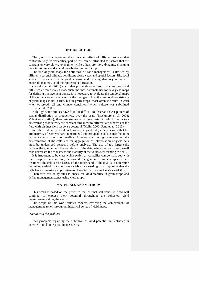
The spatial yield data is collected in the form of points, but for comparison of

yield potential between years, these points have to be adjusted (and if

necessary aggregated) to a common spatial reference which is often in a cell-

raster format. Figure 1

Fig. 1 shows an example of points overlaying a grid of cells which (often)

averages the value of the points within their respective cell.

Fig. 1. Yield points overlaying their respective interpolated raster cells

(30m)

Figure 1

Fig. 1 shows the variation of point-yields within a cell-range. The variation

is composed by inconsistent points that mask true yield potential within one

cell, which may affect the similarities between years.

Case study description

The yield data were collected from one field of grain production in Brazil.

The studied area studied contain four maps of maize and soybean (Table

1Table 1). The combine yield monitoring system was calibrated according to

the manufacturer recommendation.

Table 1. Description of location and yield data

Location Area (hectares) Combine harvester Yield data

Maracaju,

Mato Grosso do Sul,

Brazil

91

John Deere

STS 9770

(Greenstar - AMS)

Corn 2007

Corn 2009

Soybean 2010

Formatado: Fonte: Times New Roman, 12 pt

21°35'46.18"S

55°32'59.76"O

Corn 2010

Assessing parameters for observing consistency along years

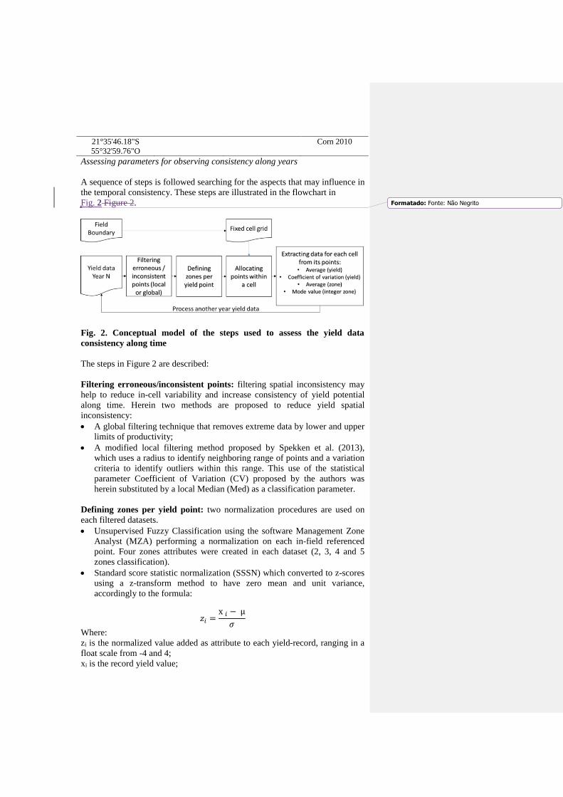
A sequence of steps is followed searching for the aspects that may influence in

the temporal consistency. These steps are illustrated in the flowchart in

Fig. 2 Figure 2.

Fig. 2. Conceptual model of the steps used to assess the yield data

consistency along time

The steps in Figure 2 are described:

Filtering erroneous/inconsistent points: filtering spatial inconsistency may

help to reduce in-cell variability and increase consistency of yield potential

along time. Herein two methods are proposed to reduce yield spatial

inconsistency:

A global filtering technique that removes extreme data by lower and upper

limits of productivity;

A modified local filtering method proposed by Spekken et al. (2013),

which uses a radius to identify neighboring range of points and a variation

criteria to identify outliers within this range. This use of the statistical

parameter Coefficient of Variation (CV) proposed by the authors was

herein substituted by a local Median (Med) as a classification parameter.

Defining zones per yield point: two normalization procedures are used on

each filtered datasets.

Unsupervised Fuzzy Classification using the software Management Zone

Analyst (MZA) performing a normalization on each in-field referenced

point. Four zones attributes were created in each dataset (2, 3, 4 and 5

zones classification).

Standard score statistic normalization (SSSN) which converted to z-scores

using a z-transform method to have zero mean and unit variance,

accordingly to the formula:

𝑧𝑖 =x 𝑖 − µ

𝜎

Where:

zi is the normalized value added as attribute to each yield-record, ranging in a

float scale from -4 and 4;

xi is the record yield value;

Formatado: Fonte: Não Negrito

µ is the mean value of the yield data;

σ is the standard deviation of the yield data;

Regarding the properties of the normalization methods, unsupervised

classification is capable of classifying data with non-normal distribution, while

the simplified standard score statistics may not perform adequately for this

same condition. Observations were done for comparisons along years.

Obtaining a cell value from normalized yield points: this step considers two

distinct forms to allocate a value to a grid-cell: using the average of the

normalized point-values within the cell-area, or using the mode of the point-

values found within it (the latter for points classified in integer values through

the MZA application).

The use of the mode instead of the average works also as a filtering

process, ignoring classified data that disagrees with the majority of points

within a cell. As an example, if majority of points within a cell have the

normalized value “1”, the mode cell value will be “1”, while the average cell-

value could be “1.3”.

Also the cell size will influence in the number of points allocated in within.

Small cells may not be overlaid by any recorded-yield-point, thus requiring its

value to be estimated by interpolation. A bigger cell-size will likely include

points with higher variance among them.

Two cell sizes (squared) where here studied to observe its influence in the

correlation along years: 10m and 30m cells.

Fig. 3Figure 3 illustrates, from a certain range of yield points, the processes

herein used to obtain the attributes of one cell.

NAO É BRUT, É RAW YIELD DATA

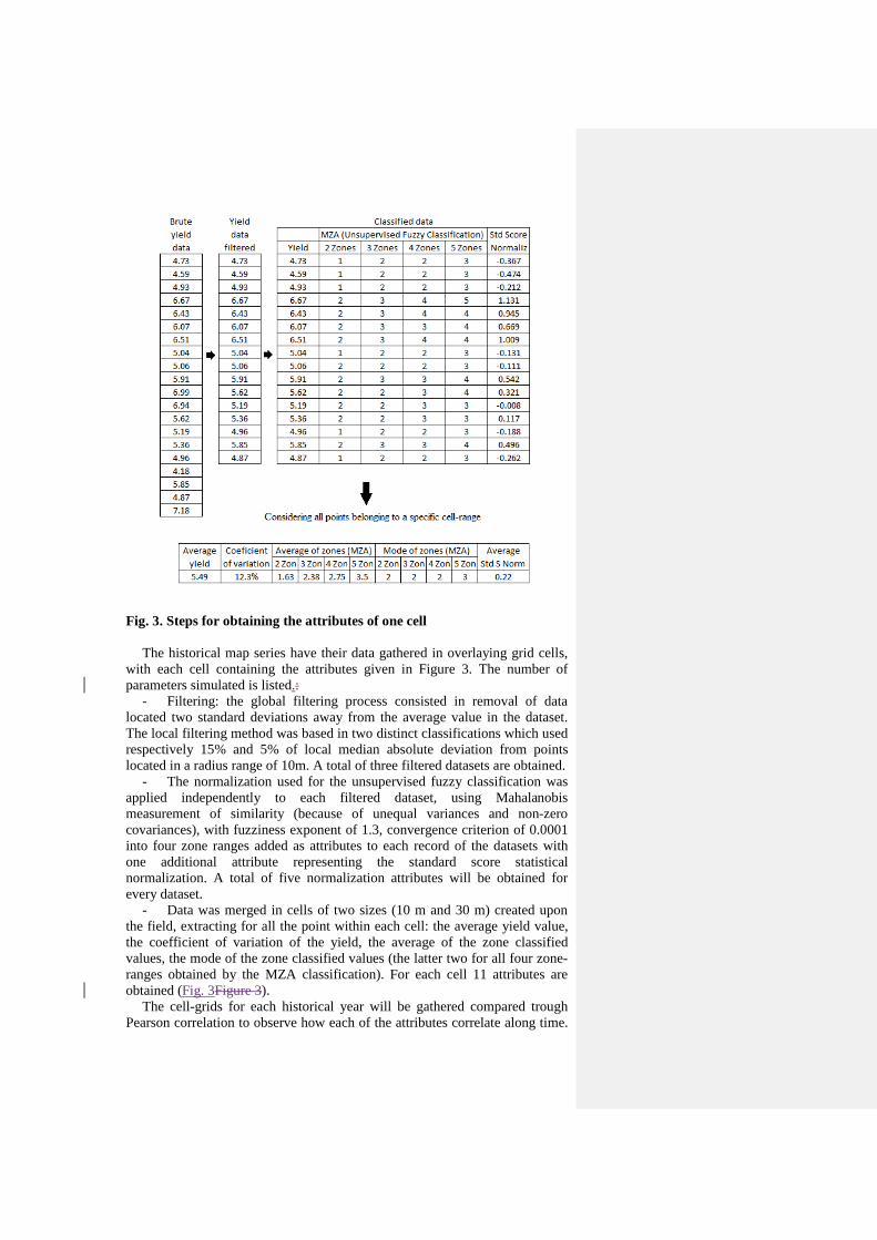
Fig. 3. Steps for obtaining the attributes of one cell

The historical map series have their data gathered in overlaying grid cells,

with each cell containing the attributes given in Figure 3. The number of

parameters simulated is listed.:

- Filtering: the global filtering process consisted in removal of data

located two standard deviations away from the average value in the dataset.

The local filtering method was based in two distinct classifications which used

respectively 15% and 5% of local median absolute deviation from points

located in a radius range of 10m. A total of three filtered datasets are obtained.

- The normalization used for the unsupervised fuzzy classification was

applied independently to each filtered dataset, using Mahalanobis

measurement of similarity (because of unequal variances and non-zero

covariances), with fuzziness exponent of 1.3, convergence criterion of 0.0001

into four zone ranges added as attributes to each record of the datasets with

one additional attribute representing the standard score statistical

normalization. A total of five normalization attributes will be obtained for

every dataset.

- Data was merged in cells of two sizes (10 m and 30 m) created upon

the field, extracting for all the point within each cell: the average yield value,

the coefficient of variation of the yield, the average of the zone classified

values, the mode of the zone classified values (the latter two for all four zone-

ranges obtained by the MZA classification). For each cell 11 attributes are

obtained (Fig. 3Figure 3).

The cell-grids for each historical year will be gathered compared trough

Pearson correlation to observe how each of the attributes correlate along time.

This is performed for each of the three filtering classifications proposed. In the

end three distinct filtering procedures, two cells sizes, and 11 parameters per

cell were obtained.

Creation of management zone maps

After analyzing the results of the first step of this study, we decided to use

the simplest method to delineate the management zones. This consisted of

obtaining yield potential maps by selecting filtered maps from the global

filtering process, using standard score statistic normalization in each map and

interpolating these using inverse distance interpolation in 10 m cells.

Temporal consistency was retrieved trough Pearson correlation.

Instead of aggregating the data to 30 m cell grid, which showed greater

correlations, we decided to use interpolation and a 10 m cell grid, to make a

better use of the information and characterize the variability in smaller scales.

Principal Component Analysis (PCA) was applied to the filtered,

normalized and interpolated data in order to reduce the dimensionality of the

data and, as an exploratory way, determine the main causes of the variability

in each field, graphically showed in biplots (Gabriel, 1971).

The principal components with eigenvalues greater than one were kept and

their scores were used to do a cluster analyses by the k-means method. The

number of clusters was chosen to be three for all fields analyzed.

RESULTS AND DISCUSSION

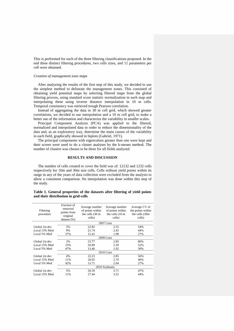
The number of cells created to cover the field was of: 12132 and 1232 cells

respectively for 10m and 30m size cells. Cells without yield points within its

range in any of the years of data collection were excluded from the analysis to

allow a consistent comparison. No interpolation was done within this step of

the study.

Table 1. General properties of the datasets after filtering of yield points

and their distribution in grid-cells

Filtering

procedure

Fraction of

removed

points from

original

dataset (%)

Average number

of points within

the cells (30 m

cells)

Average number

of points within

the cells (10 m

cells)

Average CV of

the points within

the cells (30m

cells)

2007 Corn

Global 2st dev 5% 22.82 2.55 54%

Local 15% Med 9% 21.74 2.45 44%

Local 5% Med 37% 15.43 1.98 27%

2009 Corn

Global 2st dev 2% 23.77 2.85 80%

Local 15% Med 15% 20.89 2.59 52%

Local 5% Med 47% 13.46 1.92 30%

2010 Corn

Global 2st dev 4% 22.23 2.85 56%

Local 15% Med 11% 20.65 2.70 46%

Local 5% Med 42% 13.71 2.04 27%

2010 Soybeans

Global 2st dev 5% 26.59 3.71 47%

Local 15% Med 11% 27.44 3.52 44%

Local 5% Med 42% 18.16 2.57 24%

Table 2 shows the intensity of removal of points and the final distribution

of these in the grid-cells, the higher removal of the local filtering procedures

leaded also to an expected lower variation of the yield within the cells. The

low number of points located in the smaller cell size didn’t allow to obtain a

robust CV, which was not added to Table 2Table 2.

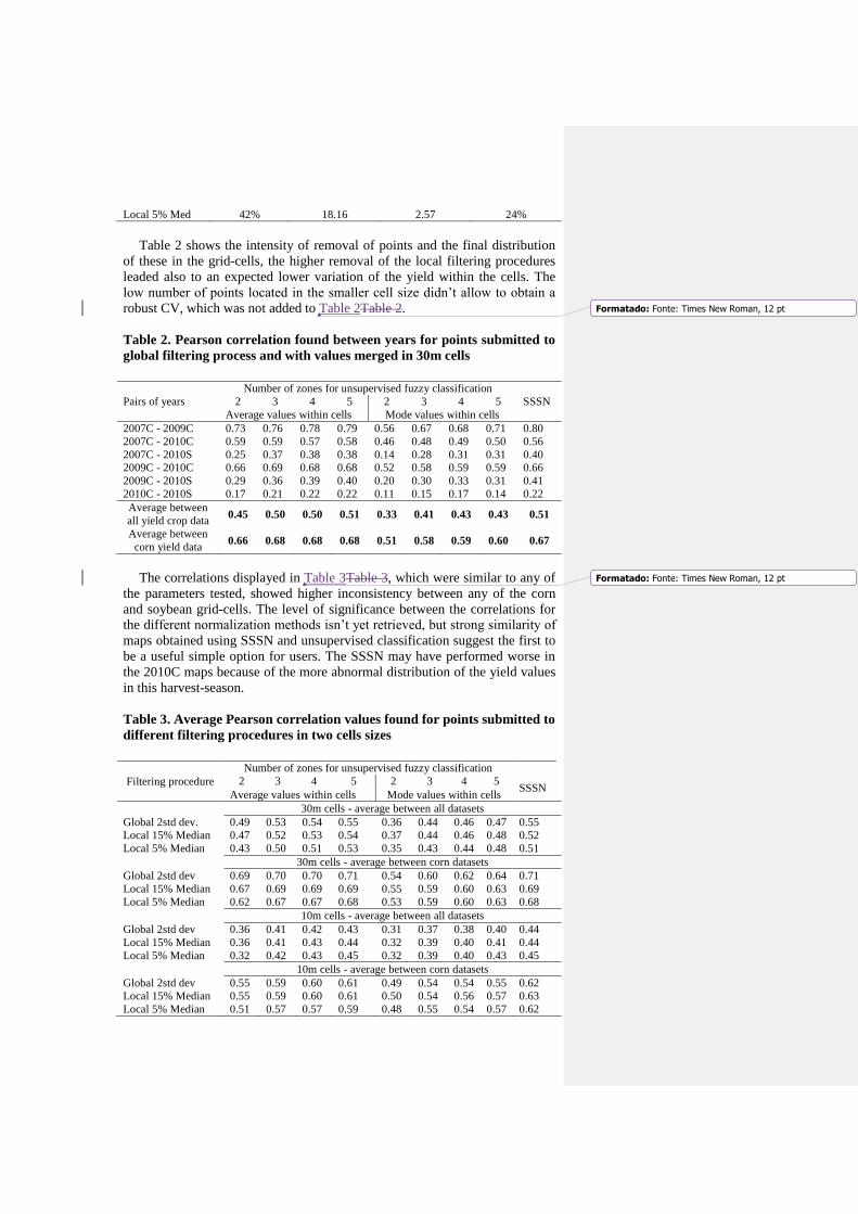
Table 2. Pearson correlation found between years for points submitted to

global filtering process and with values merged in 30m cells

Pairs of years

Number of zones for unsupervised fuzzy classification

SSSN 2 3 4 5 2 3 4 5

Average values within cells Mode values within cells

2007C - 2009C 0.73 0.76 0.78 0.79 0.56 0.67 0.68 0.71 0.80

2007C - 2010C 0.59 0.59 0.57 0.58 0.46 0.48 0.49 0.50 0.56

2007C - 2010S 0.25 0.37 0.38 0.38 0.14 0.28 0.31 0.31 0.40

2009C - 2010C 0.66 0.69 0.68 0.68 0.52 0.58 0.59 0.59 0.66

2009C - 2010S 0.29 0.36 0.39 0.40 0.20 0.30 0.33 0.31 0.41

2010C - 2010S 0.17 0.21 0.22 0.22 0.11 0.15 0.17 0.14 0.22

Average between

all yield crop data 0.45 0.50 0.50 0.51 0.33 0.41 0.43 0.43 0.51

Average between

corn yield data 0.66 0.68 0.68 0.68 0.51 0.58 0.59 0.60 0.67

The correlations displayed in Table 3Table 3, which were similar to any of

the parameters tested, showed higher inconsistency between any of the corn

and soybean grid-cells. The level of significance between the correlations for

the different normalization methods isn’t yet retrieved, but strong similarity of

maps obtained using SSSN and unsupervised classification suggest the first to

be a useful simple option for users. The SSSN may have performed worse in

the 2010C maps because of the more abnormal distribution of the yield values

in this harvest-season.

Table 3. Average Pearson correlation values found for points submitted to

different filtering procedures in two cells sizes

Filtering procedure

Number of zones for unsupervised fuzzy classification

2 3 4 5 2 3 4 5 SSSN

Average values within cells Mode values within cells

30m cells - average between all datasets

Global 2std dev. 0.49 0.53 0.54 0.55 0.36 0.44 0.46 0.47 0.55

Local 15% Median 0.47 0.52 0.53 0.54 0.37 0.44 0.46 0.48 0.52

Local 5% Median 0.43 0.50 0.51 0.53 0.35 0.43 0.44 0.48 0.51

30m cells - average between corn datasets

Global 2std dev 0.69 0.70 0.70 0.71 0.54 0.60 0.62 0.64 0.71

Local 15% Median 0.67 0.69 0.69 0.69 0.55 0.59 0.60 0.63 0.69

Local 5% Median 0.62 0.67 0.67 0.68 0.53 0.59 0.60 0.63 0.68

10m cells - average between all datasets

Global 2std dev 0.36 0.41 0.42 0.43 0.31 0.37 0.38 0.40 0.44

Local 15% Median 0.36 0.41 0.43 0.44 0.32 0.39 0.40 0.41 0.44

Local 5% Median 0.32 0.42 0.43 0.45 0.32 0.39 0.40 0.43 0.45

10m cells - average between corn datasets

Global 2std dev 0.55 0.59 0.60 0.61 0.49 0.54 0.54 0.55 0.62

Local 15% Median 0.55 0.59 0.60 0.61 0.50 0.54 0.56 0.57 0.63

Local 5% Median 0.51 0.57 0.57 0.59 0.48 0.55 0.54 0.57 0.62



The type of filtering does not suggest an increasing correlation between

datasets along years, being the global filtering slightly superior in consistency

along years. The more intense local filtering showed to decrease the

correlation. The cell size surprisingly showed a more significant factor, herein

defeating the idea that narrower cell sizes may find higher correlation along

historical yield maps. Extracted mode values of the normalized values for the

cells decreased the correlation along years but in less extend for the harsher

filtering (5% median), suggesting that the harsh local filtering is indeed

bringing yields to a same level.

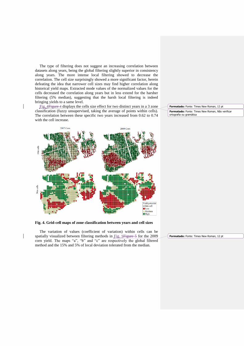
Fig. 4Figure 4 displays the cells size effect for two distinct years in a 3 zone

classification (fuzzy unsupervised, taking the average of points within cells).

The correlation between these specific two years increased from 0.62 to 0.74

with the cell increase.

Fig. 4. Grid-cell maps of zone classification between years and cell sizes

The variation of values (coefficient of variation) within cells can be

spatially visualized between filtering methods in Fig. 5Figure 5 for the 2009

corn yield. The maps “a”, “b” and “c” are respectively the global filtered

method and the 15% and 5% of local deviation tolerated from the median.


Formatado: Fonte: Times New Roman, Não verificarortografia ou gramática


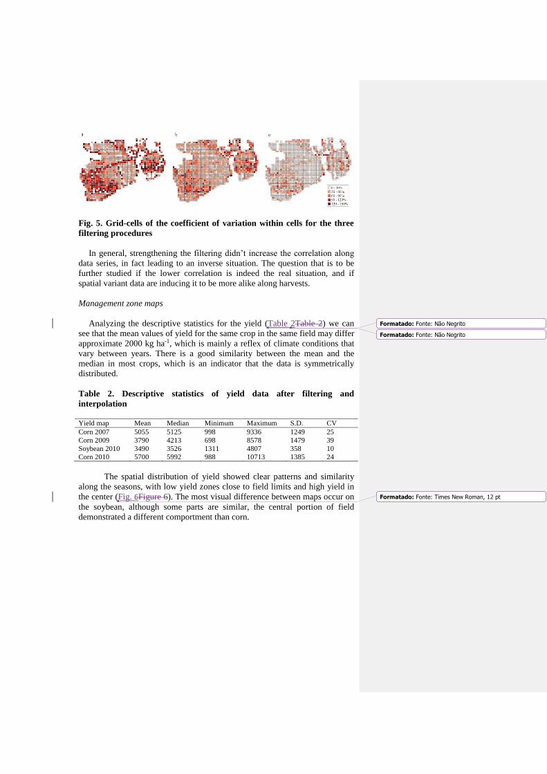
Fig. 5. Grid-cells of the coefficient of variation within cells for the three

filtering procedures

In general, strengthening the filtering didn’t increase the correlation along

data series, in fact leading to an inverse situation. The question that is to be

further studied if the lower correlation is indeed the real situation, and if

spatial variant data are inducing it to be more alike along harvests.

Management zone maps

Analyzing the descriptive statistics for the yield (Table 2Table 2) we can

see that the mean values of yield for the same crop in the same field may differ

approximate 2000 kg ha-1, which is mainly a reflex of climate conditions that

vary between years. There is a good similarity between the mean and the

median in most crops, which is an indicator that the data is symmetrically

distributed.

Table 2. Descriptive statistics of yield data after filtering and

interpolation

Yield map Mean Median Minimum Maximum S.D. CV

Corn 2007 5055 5125 998 9336 1249 25

Corn 2009 3790 4213 698 8578 1479 39

Soybean 2010 3490 3526 1311 4807 358 10

Corn 2010 5700 5992 988 10713 1385 24

The spatial distribution of yield showed clear patterns and similarity

along the seasons, with low yield zones close to field limits and high yield in

the center (Fig. 6Figure 6). The most visual difference between maps occur on

the soybean, although some parts are similar, the central portion of field

demonstrated a different comportment than corn.




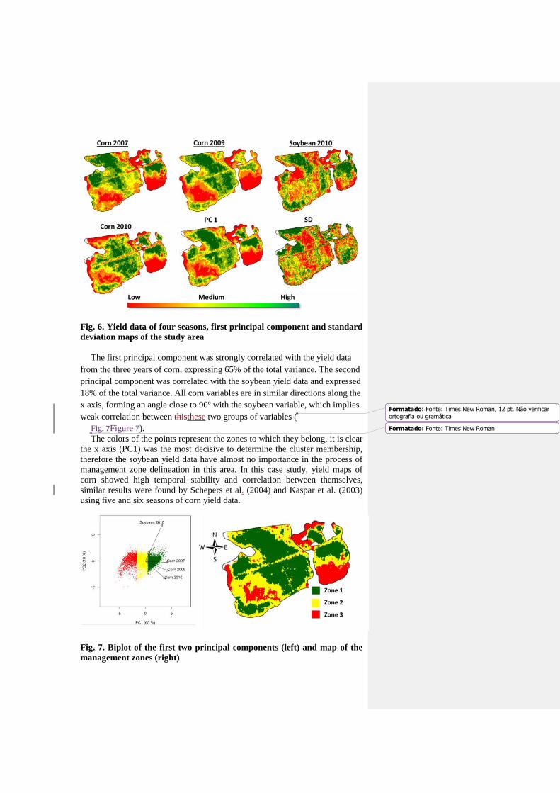
Fig. 6. Yield data of four seasons, first principal component and standard

deviation maps of the study area

The first principal component was strongly correlated with the yield data

from the three years of corn, expressing 65% of the total variance. The second

principal component was correlated with the soybean yield data and expressed

18% of the total variance. All corn variables are in similar directions along the

x axis, forming an angle close to 90º with the soybean variable, which implies

weak correlation between thisthese two groups of variables (

Fig. 7Figure 7).

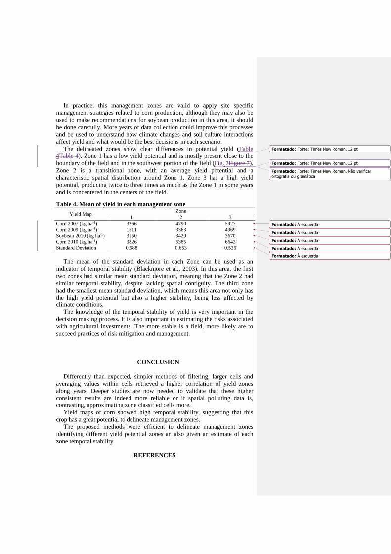
The colors of the points represent the zones to which they belong, it is clear

the x axis (PC1) was the most decisive to determine the cluster membership,

therefore the soybean yield data have almost no importance in the process of

management zone delineation in this area. In this case study, yield maps of

corn showed high temporal stability and correlation between themselves,

similar results were found by Schepers et al. (2004) and Kaspar et al. (2003)

using five and six seasons of corn yield data.

Fig. 7. Biplot of the first two principal components (left) and map of the

management zones (right)

Formatado: Fonte: Times New Roman, 12 pt, Não verificarortografia ou gramática

Formatado: Fonte: Times New Roman

In practice, this management zones are valid to apply site specific

management strategies related to corn production, although they may also be

used to make recommendations for soybean production in this area, it should

be done carefully. More years of data collection could improve this processes

and be used to understand how climate changes and soil-culture interactions

affect yield and what would be the best decisions in each scenario.

The delineated zones show clear differences in potential yield (Table

4Table 4). Zone 1 has a low yield potential and is mostly present close to the

boundary of the field and in the southwest portion of the field (Fig. 7Figure 7).

Zone 2 is a transitional zone, with an average yield potential and a

characteristic spatial distribution around Zone 1. Zone 3 has a high yield

potential, producing twice to three times as much as the Zone 1 in some years

and is concentered in the centers of the field.

Table 4. Mean of yield in each management zone

Yield Map Zone

1 2 3

Corn 2007 (kg ha-1) 3266 4790 5927

Corn 2009 (kg ha-1) 1511 3363 4969

Soybean 2010 (kg ha-1) 3150 3420 3670

Corn 2010 (kg ha-1) 3826 5385 6642

Standard Deviation 0.688 0.653 0.536

The mean of the standard deviation in each Zone can be used as an

indicator of temporal stability (Blackmore et al., 2003). In this area, the first

two zones had similar mean standard deviation, meaning that the Zone 2 had

similar temporal stability, despite lacking spatial contiguity. The third zone

had the smallest mean standard deviation, which means this area not only has

the high yield potential but also a higher stability, being less affected by

climate conditions.

The knowledge of the temporal stability of yield is very important in the

decision making process. It is also important in estimating the risks associated

with agricultural investments. The more stable is a field, more likely are to

succeed practices of risk mitigation and management.

CONCLUSION

Differently than expected, simpler methods of filtering, larger cells and

averaging values within cells retrieved a higher correlation of yield zones

along years. Deeper studies are now needed to validate that these higher

consistent results are indeed more reliable or if spatial polluting data is,

contrasting, approximating zone classified cells more.

Yield maps of corn showed high temporal stability, suggesting that this

crop has a great potential to delineate management zones.

The proposed methods were efficient to delineate management zones

identifying different yield potential zones an also given an estimate of each

zone temporal stability.

REFERENCES



Formatado: Fonte: Times New Roman, Não verificarortografia ou gramática

Formatado: À esquerda





Blackmore, S.; Godwin, R. J.; Fountas, S. 2003. The analysis of spatial and

temporal trends in yield map data over six years. Biosystems Engineering,

84(4), p. 455- 466.

Carvalho, J. R. P; Vieira, S. R.; Moran, R. C. C. P. Como avaliar a

similaridade entre mapas de produtividade. 1 ed. Campinas: Relatório

técnico/ Embrapa informática agropecuária, 2001. 24p.

Gabriel, K. R. 1971. The biplot graphic display of matrices with application to

principal component analysis. Biometrika 58(3), p. 453 – 467.

Kaspar, T. C.; Colvin, T. S.; Jaynes, D. B.; Karlen, D. L.; James, D. E.; Meek,

D. W; Pulido, D.; Butler, H. 2003. Relationship between six years of corn

yields and terrain attributes. Precision Agriculture, 4, p. 87 - 101.

Milani, L.; Souza, E. G.; Uribe-opazo, M. A.; Gabriel Filho, A.; Johann, J. A;

Pereira, J. O. 2006. Determination of management zones using yield data. (In

Portuguese, with English abstract) Acta Scientiarum. Agronomy, 28(4), p.

591-598.

Santi, A. L.; Amado, T. J. C.; Eitelwein, M. T.; Cherubin, M. R.; Silva, R. F.;

Da Ros, C. O. 2013. Definition of yield zones in areas managed with

precision agriculture. (In Portuguese, with English abstract) Agrária, 8, p.

510-515.

Schepers, A. R.; Shanahan, J. F.; Liebig, M. A.; Schepers, J. S.; Johnson, S.

H.; Luchiari, A. (2004). Appropriateness of management zones for

characterizing spatial variability of soil properties and irrigated corn yields

across years. Agronomy Journal, 96(1), p. 195-203.

Spekken, M., Anselmi, A. A.; Molin, J. P. A simple method for filtering

spatial data. In Precision agriculture’13. Wageningen Academic Publishers.

p. 259-266. 2013.

Documents

ASSESSING DEFINITION OF MANAGEMENT ZONES TROUGH …