Assessing Human Error Against a Benchmark of Perfectionashton/pubs/tbase-tkdd.pdf · Assessing Human Error Against a Benchmark of Perfection ... human decision-making ... truth”

45

Assessing Human Error Against a Benchmark of Perfection

ASHTON ANDERSON, Microsoft ResearchJON KLEINBERG, Cornell UniversitySENDHIL MULLAINATHAN, Harvard University

An increasing number of domains are providing us with detailed trace data on human decisions in settingswhere we can evaluate the quality of these decisions via an algorithm. Motivated by this development, anemerging line of work has begun to consider whether we can characterize and predict the kinds of decisionswhere people are likely to make errors.

To investigate what a general framework for human error prediction might look like, we focus on a modelsystem with a rich history in the behavioral sciences: the decisions made by chess players as they selectmoves in a game. We carry out our analysis at a large scale, employing datasets with several million recordedgames, and using chess tablebases to acquire a form of ground truth for a subset of chess positions that havebeen completely solved by computers but remain challenging for even the best players in the world.

We organize our analysis around three categories of features that we argue are present in most settingswhere the analysis of human error is applicable: the skill of the decision-maker, the time available to make thedecision, and the inherent difficulty of the decision. We identify rich structure in all three of these categoriesof features, and find strong evidence that in our domain, features describing the inherent difficulty of aninstance are significantly more powerful than features based on skill or time.

CCS Concepts: � Applied computing → Psychology;

Additional Key Words and Phrases: Blunder prediction, human decision-making

ACM Reference Format:Ashton Anderson, Jon Kleinberg, and Sendhil Mullainathan. 2017. Assessing human error against a bench-mark of perfection. ACM Trans. Knowl. Discov. Data 11, 4, Article 45 (July 2017), 25 pages.DOI: http://dx.doi.org/10.1145/3046947

1. INTRODUCTION

Several rich strands of work in the behavioral sciences have been concerned withcharacterizing the nature and sources of human error. These include the broad notionof bounded rationality [Simon 1957] and the subsequent research beginning withKahneman and Tversky on heuristics and biases [Tversky and Kahneman 1975]. Withthe growing availability of large datasets containing millions of human decisions onfixed, well-defined, real-world tasks, there is an increasing need to add a new styleof inquiry to this research—given a large stream of decisions, with rich informationabout the context of each decision, can we algorithmically characterize and predict theinstances on which people are likely to make errors?

This genre of question—analyzing human errors from large traces of decisions on afixed task—also has an interesting relation to the canonical set-up in machine learning

This work has been supported in part by a Simons Investigator Award, an ARO MURI Grant, a GoogleResearch Grant, and a Facebook Faculty Research Grant.Authors’ addresses: A. Anderson; email: [email protected]; J. Kleinberg; email: [email protected]; S. Mullainathan; email: [email protected] to make digital or hard copies of part or all of this work for personal or classroom use is grantedwithout fee provided that copies are not made or distributed for profit or commercial advantage and thatcopies show this notice on the first page or initial screen of a display along with the full citation. Copyrights forcomponents of this work owned by others than ACM must be honored. Abstracting with credit is permitted.To copy otherwise, to republish, to post on servers, to redistribute to lists, or to use any component of thiswork in other works requires prior specific permission and/or a fee. Permissions may be requested fromPublications Dept., ACM, Inc., 2 Penn Plaza, Suite 701, New York, NY 10121-0701 USA, fax +1 (212)869-0481, or [email protected]© 2017 ACM 1556-4681/2017/07-ART45 $15.00DOI: http://dx.doi.org/10.1145/3046947

ACM Transactions on Knowledge Discovery from Data, Vol. 11, No. 4, Article 45, Publication date: July 2017.

http://dx.doi.org/10.1145/3046947

http://dx.doi.org/10.1145/3046947

45:2 A. Anderson et al.

applications. Typically, using instances of decision problems together with “groundtruth” labels showing the correct decision, an algorithm is trained to produce thecorrect decision in a large fraction of instances. The analysis of human error, on theother hand, represents a twist on this formulation: given instances of a task in whichwe have both the correct decision and a human’s decision, an algorithm is trained torecognize future instances on which a human is likely to make a mistake. Predictinghuman error from this type of trace data has a history in human factors research[Kirwan 1993; Salvendy 2012], and a nascent line of work has begun to apply currentmachine-learning methods to the question [Lakkaraju et al. 2015, 2016].

Model systems for studying human error. As the investigation of human error us-ing large datasets grows increasingly feasible, it becomes useful to understand whichstyles of analysis will be most effective. For this purpose, as in other settings, there isenormous value in focusing on model systems where one has exactly the data necessaryto ask the basic questions in their most natural formulations.

What might we want from such a model system?

(i) It should consist of a task for which the context of the human decisions has beenmeasured as thoroughly as possible, and in a very large number of instances, toprovide the training data for an algorithm to analyze errors.

(ii) So that the task is non-trivial, it should be challenging even for highly skilledhuman decision-makers.

(iii) Notwithstanding the previous point (ii), the “ground truth”—the correctness ofeach candidate decision—should be feasibly computable by an algorithm.

Guided by these desiderata, we focus in this article on chess as a model system for ouranalysis. In doing so, we are proceeding by analogy with a long line of work in behavioralscience using chess as a model for human decision-making [Charness 1992; Chase andSimon 1973; De Groot 1978]. Chess is a natural domain for such investigations, sinceit presents a human player with a sequence of concrete decisions—which move to playnext—with the property that some choices are better than others. Indeed, because chessprovides data on hard decision problems in such a pure fashion, it has been describedas the “drosophila of psychology” [Simon and Chase 1988]. (It is worth noting our focushere on human decisions in chess, rather than on designing algorithms to play chess.This latter problem has also, of course, generated a rich literature, along with a closelyrelated tag-line of chess as the “drosophila of artificial intelligence” [McCarthy 1990].)

Chess as a model system for human error. Despite the clean formulation of thedecisions made by human chess players, we still must resolve a set of conceptualchallenges if our goal is to assemble a large corpus of chess moves with ground-truthlabels that classify certain moves as errors. Let us consider three initial ideas for howwe might go about this, each of which is lacking in some crucial respect for our purposes.

First, for most of the history of human decision-making research on chess, the empha-sis has been on focused laboratory studies at small scales in which the correct decisioncould be controlled by design [Charness 1992]. In our list of desiderata, this meansthat point (iii), the availability of ground truth, is well under control, but a significantaspect of point (i)—the availability of a vast number of instances—is problematic dueto the necessarily small scales of the studies.

A second alternative would be to make use of two important computational develop-ments in chess—the availability of databases with millions of recorded chess games bystrong players; and the fact that the strongest chess programs—generally referred to aschess engines—now greatly outperform even the best human players in the world. Thismakes it possible to analyze the moves of strong human players, in a large-scale fashion,by comparing their choices to those of an engine. This has been pursued very effectively


Assessing Human Error Against a Benchmark of Perfection 45:3

in the last several years by Biswas and Regan [2015a, 2015b] and Regan and Biswas[2013]; they have used the approach to derive interesting insights including proposalsfor how to estimate the depth at which human players are analyzing a position.

For the current purpose of assembling a corpus with ground-truth error labels, how-ever, engines present a set of challenges. The basic difficulty is that even current chessengines are far from being able to provide guarantees regarding the best move(s) in agiven position. In particular, an engine may prefer move m to m′ in a given position,supplementing this preference with a heuristic numerical evaluation, but m′ may ul-timately lead to the same result in the game, both under best play and under typicalplay. In these cases, it is hard to say that choosing m′ should be labeled an error. Morebroadly, it is difficult to find a clear-cut rule mapping an engine’s evaluations to a deter-mination of human error, and efforts to label errors this way would represent a complexmixture of the human player’s mistakes and the nature of the engine’s evaluations.

Finally, a third possibility is to go back to the definition of chess as a deterministicgame with two players (White and Black) who engage in alternating moves, and witha game outcome that is either (a) a win for White, (b) a win for Black, or (c) a draw.This means that from any position, there is a well-defined notion of the outcome withrespect to optimal play by both sides—in game-theoretic terms, this is the minimaxvalue of the position. In each position, it is the case that White wins with best play,or Black wins with best play, or it is a draw with best play, and these are the threepossible minimax values for the position.

This perspective provide us with a clean option for formulating the notion of an error,namely the direct game-theoretic definition: a player has committed an error if theirmove worsens the minimax value from their perspective. That is, the player had aforced win before making their move but now they do not; or the player had a forceddraw before making their move but now they do not. But there is an obvious difficultywith this route, and it is a computational one: for most chess positions, determiningthe minimax value is hopelessly beyond the power of both human players and chessengines alike.

We now discuss the approach we take here.

Assessing errors using tablebases. In our work, we use minimax values by leverag-ing a further development in computer chess—the fact that chess has been solved forall positions with at most k pieces on the board, for small values of k [Bellman 1965;Makhnychev and Zakharov 2012; Nalimov 2005; Kopec 1990]. (We will refer to suchpositions as ≤k-piece positions.) Solving these positions has been accomplished not byforward construction of the chess game tree, but instead by simply working backwardfrom terminal positions with a concrete outcome present on the board and filling in allother minimax values by dynamic programming until all possible ≤k-piece positionshave been enumerated. The resulting solution for all ≤k-piece positions is compiledinto an object called a k-piece tablebase, which lists the game outcome with best playfor each of these positions. The construction of tablebases has been a topic of interestsince the early days of computer chess [Kopec 1990], but only with recent developmentsin computing and storage have truly large tablebases been feasible. Proprietary table-bases with k = 7 have been built, requiring in excess of a hundred terabytes of storage[Makhnychev and Zakharov 2012]; tablebases for k = 6 are much more manageable,though still very large [Nalimov 2005], and we focus on the case of k = 6 in whatfollows.1

1There are some intricacies in how tablebases interact with certain rules for draws in chess, particularlythreefold-repetition and the 50-move rule, but since these have essentially negligible impact on our use oftablebases in the present work, we do not go into further details here.



Tablebases and traditional chess engines are thus very different objects. Chess en-gines produce strong moves for arbitrary positions, but with no absolute guarantees onmove quality in most cases; tablebases, on the other hand, play perfectly with respect tothe game tree—indeed, effortlessly, via table lookup—for the subset of chess containingat most k pieces on the board.

Thus, for arbitrary ≤k-piece positions, we can determine minimax values, and so wecan obtain a large corpus of chess moves with ground-truth error labels: Starting witha large database of recorded chess games, we first restrict to the subset of ≤k-piecepositions, and then we label a move as an error if and only it worsens the minimaxvalue from the perspective of the player making the move. Adapting chess terminologyto the current setting, we will refer to such an instance as a blunder.

This is our model system for analyzing human error; let us now check how it lines upwith desiderata (i)–(iii) for a model system listed above. Chess positions with at mostk = 6 pieces arise relatively frequently in real games, so we are left with many instanceseven after filtering a database of games to restrict to only these positions (point (i)).Crucially, despite their simple structure, they can induce high error rates by amateursand non-trivial error rates even by the best players in the world; in recognition of theinherent challenge they contain, textbook-level treatments of chess devote a significantfraction of their attention to these positions [Fine 1941] (point (ii)). And they can beevaluated perfectly by tablebases (point (iii)).

Focusing on ≤k-piece positions has an additional benefit, made possible by a combi-nation of tablebases and the recent availability of databases with millions of recordedchess games. The most frequently occurring of these positions arise in our data thou-sands of times. As we will see, this means that for some of our analyses, we can controlfor the exact position on the board and still have enough instances to observe meaning-ful variation. Controlling for the exact position is not generally feasible with arbitrarypositions arising in the middle of a chess game, but it becomes possible with the scaleof data we now have, and we will see that in this case it yields interesting and in somecases surprising insights.

2. SETTING UP THE ANALYSIS

In formulating our analysis, we begin from the premise that for analyzing error inhuman decisions, three crucial types of features are the following:

(a) the skill of the decision-maker;(b) the time available to make the decision; and(c) the inherent difficulty of the decision.

Any instance of the problem will implicitly or explicitly contain features of all threetypes: an individual of a particular level of skill is confronting a decision of a particulardifficulty, with a given amount of time available to make the decision.

In our current domain, as in any other setting where the question of human erroris relevant, there are a number of basic genres of question that we would like to ask.These include the following.

—For predicting whether an error will be committed in a given instance, which typesof features (skill, time, or difficulty) yield the most predictive power?

—In which kinds of instances does greater skill confer the largest relative benefit? Is itfor more difficult decisions (where skill is perhaps most essential) or for easier ones(where there is the greatest room to realize the benefit)? Are there particular kindsof instances where skill does not in fact confer an appreciable benefit?

—An analogous set of questions for time in place of skill: In which kinds of instancesdoes greater time for the decision confer the largest benefit? Is additional time more



beneficial for hard decisions or easy ones? And are there instances where additionaltime does not reduce the error rate?

—Finally, there are natural questions about the interaction of skill and time: Is ithigher skill or lower skill decision-makers who benefit more from additional time?

These questions motivate our analyses in the subsequent sections. We begin by dis-cussing how features of all three types (skill, time, and difficulty) are well-representedin our domain.

Our data comes from two large databases of recorded chess games. The first is acorpus of approximately 200 million games from the Free Internet Chess Server (FICS),where amateurs play each other on-line.2 The second is a corpus of approximately1 million games played in international tournaments by the strongest players in theworld. We will refer to the first of these as the FICS dataset, and the second as theGM dataset. (GM for “grandmaster,” the highest title a chess player can hold.) Foreach corpus, we extract all occurrences of ≤6-piece positions from all of the games; werecord the move made in the game from each occurrence of each position, and use atablebase to evaluate all possible moves from the position (including the move thatwas made). This forms a single instance for our analysis. Since we are interested instudying errors, we exclude all instances in which the player cannot possibly blunder,since there are no legal moves that would change the minimax value of the position.This means we exclude all instances in which the player to move is in a theoreticallylosing position—where the opponent has a direct path to checkmate—because thereare no blunders in losing positions (the minimax value of the position is already as badas possible for the player to move). Finally, there are times when players will arrive atthe same position more than once in the same game; we restrict our analysis to only thefirst time an instance has been seen in a game. There are 24.6 million such instancesin the FICS dataset, and 880,000 in the GM dataset.

We now consider how feature types (a), (b), and (c) are associated with each instance.First, for skill, each chess player in the data has a numerical rating, termed the Elorating, based on their performance in the games they have played [Elo 1978; Herbrichet al. 2006]. Higher numbers indicate stronger players, and to get a rough sense ofthe range: most amateurs have ratings in the range 1000–2000, with extremely strongamateurs getting up to 2200–2400; players above 2500–2600 belong to a rarefied groupof the world’s best; and at any given time there are generally around five players in theworld above 2800. If we think of a game outcome in terms of points, with 1 point for awin and 0.5 points for a draw, then the Elo rating system has the property that whena player is paired with someone 400 Elo points lower, their expected game outcome isapproximately 0.91 points—an enormous advantage.3

For our purposes, an important feature of Elo ratings is the fact that a single numberhas empirically proven so powerful at predicting performance in chess games. Whileratings clearly cannot contain all the information about players’ strengths and weak-nesses, their effectiveness in practice argues that we can reasonably use a player’srating as a single numerical feature that approximately represents their skill.

With respect to temporal information, chess games are generally played under timelimits of the form, “play x moves in y minutes” or “play the whole game in y minutes.”Players can choose how they use this time, so on each move they face a genuine decisionabout how much of their remaining allotted time to spend. The FICS dataset containsthe amount of time remaining in the game when each move was played (and hence the

2This data is publicly available at ficsgames.org.3In general, the system is designed so that when the rating difference is 400d, the expected score for thehigher ranked player under the Elo system is 1/(1 + 10−d).



amount of time spent on each move as well); most of the games in the FICS dataset areplayed under extremely rapid time limits, with a large fraction of them requiring thatthe whole game be played in 3 minutes for each player. To avoid variation arising fromthe game duration, we focus on this large subset of the FICS data consisting exclusivelyof games with 3 minutes allocated to each side.

Our final set of features will be designed to quantify the difficulty of the position onthe board—i.e., the extent to which it is hard to avoid selecting a move that constitutesa blunder. There are many ways in which one could do this, and we are guided in partby the goal of developing features that are less domain-specific and more applicableto decision tasks in general. We begin with perhaps the two most basic parameters,analogues of which would be present in any setting with discrete choices and a discretenotion of error—these are the number of legal moves in the position, and the numberof these moves that constitute blunders. Later, we will also consider a general familyof parameters that involve looking more deeply into the search tree, at moves beyondthe immediate move the player is facing.

To summarize, in a single instance in our data, a player of a given rating, with agiven amount of time remaining in the game, faces a specific position on the board, andwe ask whether the move they select is a blunder. We now explore how our differenttypes of features provide information about this question, before turning to the generalproblem of prediction.

3. FUNDAMENTAL DIMENSIONS

3.1. Difficulty

We begin by considering a set of basic features that help quantify the difficulty inherentin a position. There are many features we could imagine employing that are highlydomain-specific to chess, but our primary interest is in whether a set of relativelygeneric features can provide non-trivial predictive value.

Above we noted that in any setting with discrete choices, one can always consider thetotal number of available choices, and partition these into the number that constituteblunders and the number that do not constitute blunders. In particular, let’s say that ina given chess position P, there are n(P) legal moves available—these are the possiblechoices—and of these, b(P) are blunders, in that they lead to a position with a strictlyworse minimax value (and thus the other n(P) − b(P) moves are non-blunders thatpreserve the minimax value of the position). Note that it is possible to have b(P) = 0,but we exclude these positions because it is impossible to blunder. Also, by the definitionof the minimax value, we must have b(P) ≤ n(P) − 1; that is, there is always at leastone move that preserves the minimax value.

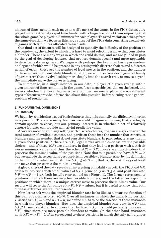
A global check of the data reveals an interesting bimodality in both the FICS and GMdatasets: positions with small values of b(P) (principally b(P) ≤ 3) and positions withb(P) = n(P) − 1 are both heavily represented (see Figure 1). The former correspond topositions in which there are very few possible blunders, and the latter correspond topositions in which there is a unique correct move to preserve the minimax value. Ourresults will cover the full range of (n(P), b(P)) values, but it is useful to know that bothof these extremes are well represented.

Now, let us ask what the empirical blunder rate looks like as a bivariate function ofthis pair of variables (n(P), b(P)). Over all instances in which the underlying positionP satisfies n(P) = n and b(P) = b, we define r(n, b) to be the fraction of those instancesin which the player blunders. How does the empirical blunder rate vary in n(P) andb(P)? It seems natural to suppose that for fixed n(P), it should generally increase inb(P), since there are more possible blunders to make. On the other hand, instanceswith b(P) = n(P) − 1 often correspond to chess positions in which the only non-blunder



Fig. 1. The number of instances as a function of the two variables (n(P), b(P)), for the FICS dataset.

Fig. 2. A heat map showing the empirical blunder rate as a function of the two variables (n(P), b(P)), forthe FICS dataset.

is “obvious” (for example, if there is only one way to recapture a piece), and so onemight conjecture that the empirical blunder rate will be lower for this case.

In fact, the empirical blunder rate is generally monotone in b(P), as shown by theheatmap representation of r(n, b) in Figure 2. (We show the function for the FICS data;the function for the GM data is similar.) Moreover, if we look at the heavily-populatedline b(P) = n(P) − 1, the blunder rate is increasing in n(P); as there are more blundersto compete with the unique non-blunder, it becomes correspondingly harder to makethe right choice.

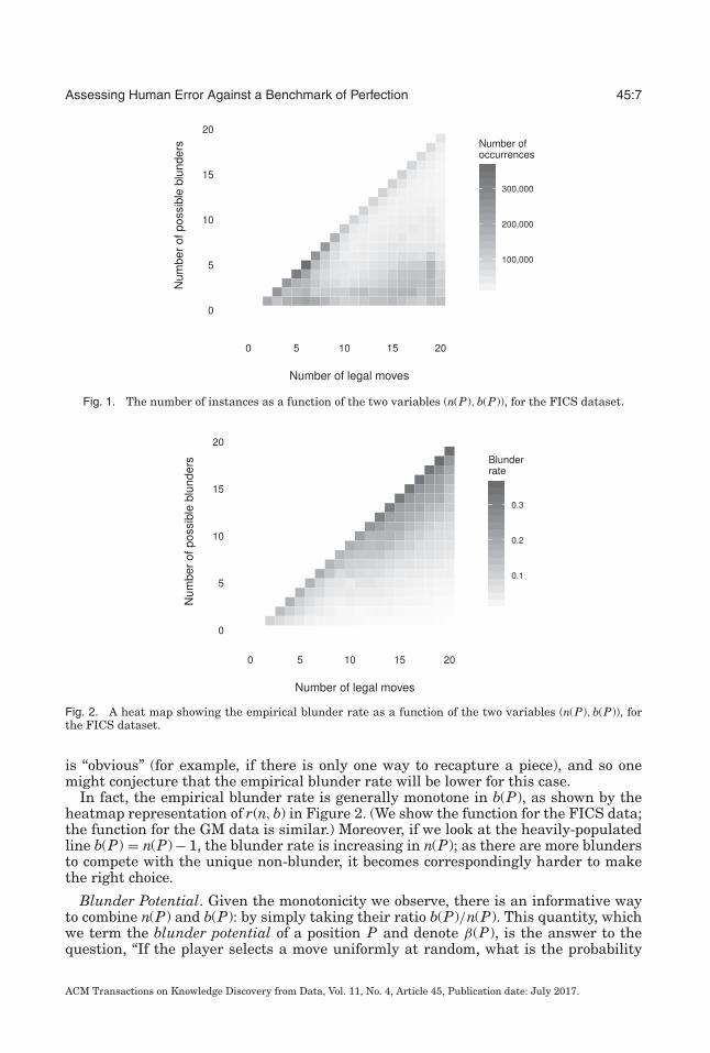
Blunder Potential. Given the monotonicity we observe, there is an informative wayto combine n(P) and b(P): by simply taking their ratio b(P)/n(P). This quantity, whichwe term the blunder potential of a position P and denote β(P), is the answer to thequestion, “If the player selects a move uniformly at random, what is the probability



Fig. 3. The empirical blunder rate as a function of the blunder potential, shown for both the GM and theFICS data. On the left are standard axes, on the right are logarithmic y-axes. The plots on the right alsoshow an approximate fit to the γ -value defined in Section 3.1.

that they will blunder?.” This definition will prove useful in many of the analyses tofollow. Intuitively, we can think of it as a direct measure of the danger inherent in aposition, since it captures the relative abundance of ways to go wrong.

In Figure 3, we plot the function y = r(x), the proportion of blunders in instanceswith β(P) = x, for both our GM and FICS datasets on linear as well as logarithmicy-axes. The striking regularity of the r(x) curves shows how strongly the availabilityof potential mistakes translates into actual errors. One natural starting point for in-terpreting this relationship is to note that if players were truly selecting their movesuniformly at random, then these curves would lie along the line y = x. The fact thatthey lie below this line indicates that in aggregate players are preferentially selectingnon-blunders, as one would expect. And the fact that the curve for the GM data liesmuch further below y = x is a reflection of the much greater skill of the players in thisdataset, a point that we will return to shortly.

The γ -value. We find that a surprisingly simple model qualitatively captures theshapes of the curves in Figure 3 quite well. Suppose that instead of selecting a moveuniformly at random, a player selected from a biased distribution in which they werepreferentially c times more likely to select a non-blunder than a blunder, for a param-eter c > 1.



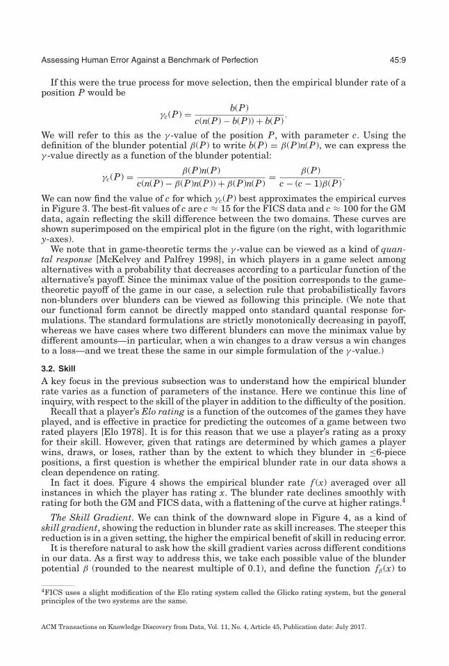
If this were the true process for move selection, then the empirical blunder rate of aposition P would be

γc(P) = b(P)c(n(P) − b(P)) + b(P)

.

We will refer to this as the γ -value of the position P, with parameter c. Using thedefinition of the blunder potential β(P) to write b(P) = β(P)n(P), we can express theγ -value directly as a function of the blunder potential:

γc(P) = β(P)n(P)c(n(P) − β(P)n(P)) + β(P)n(P)

= β(P)c − (c − 1)β(P)

.

We can now find the value of c for which γc(P) best approximates the empirical curvesin Figure 3. The best-fit values of c are c ≈ 15 for the FICS data and c ≈ 100 for the GMdata, again reflecting the skill difference between the two domains. These curves areshown superimposed on the empirical plot in the figure (on the right, with logarithmicy-axes).

We note that in game-theoretic terms the γ -value can be viewed as a kind of quan-tal response [McKelvey and Palfrey 1998], in which players in a game select amongalternatives with a probability that decreases according to a particular function of thealternative’s payoff. Since the minimax value of the position corresponds to the game-theoretic payoff of the game in our case, a selection rule that probabilistically favorsnon-blunders over blunders can be viewed as following this principle. (We note thatour functional form cannot be directly mapped onto standard quantal response for-mulations. The standard formulations are strictly monotonically decreasing in payoff,whereas we have cases where two different blunders can move the minimax value bydifferent amounts—in particular, when a win changes to a draw versus a win changesto a loss—and we treat these the same in our simple formulation of the γ -value.)

3.2. Skill

A key focus in the previous subsection was to understand how the empirical blunderrate varies as a function of parameters of the instance. Here we continue this line ofinquiry, with respect to the skill of the player in addition to the difficulty of the position.

Recall that a player’s Elo rating is a function of the outcomes of the games they haveplayed, and is effective in practice for predicting the outcomes of a game between tworated players [Elo 1978]. It is for this reason that we use a player’s rating as a proxyfor their skill. However, given that ratings are determined by which games a playerwins, draws, or loses, rather than by the extent to which they blunder in ≤6-piecepositions, a first question is whether the empirical blunder rate in our data shows aclean dependence on rating.

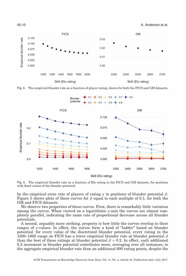
In fact it does. Figure 4 shows the empirical blunder rate f (x) averaged over allinstances in which the player has rating x. The blunder rate declines smoothly withrating for both the GM and FICS data, with a flattening of the curve at higher ratings.4

The Skill Gradient. We can think of the downward slope in Figure 4, as a kind ofskill gradient, showing the reduction in blunder rate as skill increases. The steeper thisreduction is in a given setting, the higher the empirical benefit of skill in reducing error.

It is therefore natural to ask how the skill gradient varies across different conditionsin our data. As a first way to address this, we take each possible value of the blunderpotential β (rounded to the nearest multiple of 0.1), and define the function fβ(x) to

4FICS uses a slight modification of the Elo rating system called the Glicko rating system, but the generalprinciples of the two systems are the same.



Fig. 4. The empirical blunder rate as a function of player rating, shown for both the FICS and GM datasets.

Fig. 5. The empirical blunder rate as a function of Elo rating in the FICS and GM datasets, for positionswith fixed values of the blunder potential.

be the empirical error rate of players of rating x in positions of blunder potential β.Figure 5 shows plots of these curves for β equal to each multiple of 0.1, for both theGM and FICS datasets.

We observe two properties of these curves. First, there is remarkably little variationamong the curves. When viewed on a logarithmic y-axis the curves are almost com-pletely parallel, indicating the same rate of proportional decrease across all blunderpotentials.

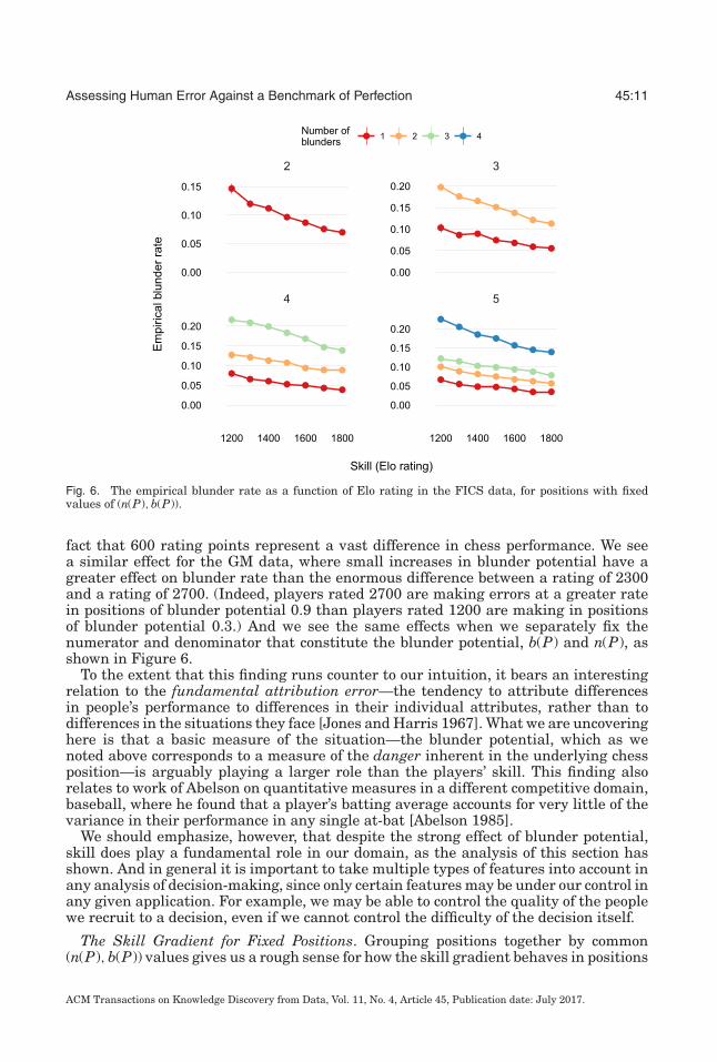
A second, arguably more striking, property is how little the curves overlap in theirranges of y-values. In effect, the curves form a kind of “ladder” based on blunderpotential: for every value of the discretized blunder potential, every rating in the1200–1800 range on FICS has a lower empirical blunder rate at blunder potential βthan the best of these ratings at blunder potential β + 0.2. In effect, each additional0.2 increment in blunder potential contributes more, averaging over all instances, tothe aggregate empirical blunder rate than an additional 600 rating points, despite the



Fig. 6. The empirical blunder rate as a function of Elo rating in the FICS data, for positions with fixedvalues of (n(P), b(P)).

fact that 600 rating points represent a vast difference in chess performance. We seea similar effect for the GM data, where small increases in blunder potential have agreater effect on blunder rate than the enormous difference between a rating of 2300and a rating of 2700. (Indeed, players rated 2700 are making errors at a greater ratein positions of blunder potential 0.9 than players rated 1200 are making in positionsof blunder potential 0.3.) And we see the same effects when we separately fix thenumerator and denominator that constitute the blunder potential, b(P) and n(P), asshown in Figure 6.

To the extent that this finding runs counter to our intuition, it bears an interestingrelation to the fundamental attribution error—the tendency to attribute differencesin people’s performance to differences in their individual attributes, rather than todifferences in the situations they face [Jones and Harris 1967]. What we are uncoveringhere is that a basic measure of the situation—the blunder potential, which as wenoted above corresponds to a measure of the danger inherent in the underlying chessposition—is arguably playing a larger role than the players’ skill. This finding alsorelates to work of Abelson on quantitative measures in a different competitive domain,baseball, where he found that a player’s batting average accounts for very little of thevariance in their performance in any single at-bat [Abelson 1985].

We should emphasize, however, that despite the strong effect of blunder potential,skill does play a fundamental role in our domain, as the analysis of this section hasshown. And in general it is important to take multiple types of features into account inany analysis of decision-making, since only certain features may be under our control inany given application. For example, we may be able to control the quality of the peoplewe recruit to a decision, even if we cannot control the difficulty of the decision itself.

The Skill Gradient for Fixed Positions. Grouping positions together by common(n(P), b(P)) values gives us a rough sense for how the skill gradient behaves in positions



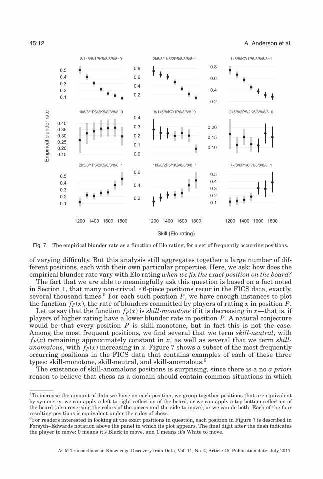
Fig. 7. The empirical blunder rate as a function of Elo rating, for a set of frequently occurring positions.

of varying difficulty. But this analysis still aggregates together a large number of dif-ferent positions, each with their own particular properties. Here, we ask: how does theempirical blunder rate vary with Elo rating when we fix the exact position on the board?

The fact that we are able to meaningfully ask this question is based on a fact notedin Section 1, that many non-trivial ≤6-piece positions recur in the FICS data, exactly,several thousand times.5 For each such position P, we have enough instances to plotthe function fP(x), the rate of blunders committed by players of rating x in position P.

Let us say that the function fP(x) is skill-monotone if it is decreasing in x—that is, ifplayers of higher rating have a lower blunder rate in position P. A natural conjecturewould be that every position P is skill-monotone, but in fact this is not the case.Among the most frequent positions, we find several that we term skill-neutral, withfP(x) remaining approximately constant in x, as well as several that we term skill-anomalous, with fP(x) increasing in x. Figure 7 shows a subset of the most frequentlyoccurring positions in the FICS data that contains examples of each of these threetypes: skill-monotone, skill-neutral, and skill-anomalous.6

The existence of skill-anomalous positions is surprising, since there is a no a priorireason to believe that chess as a domain should contain common situations in which

5To increase the amount of data we have on each position, we group together positions that are equivalentby symmetry: we can apply a left-to-right reflection of the board, or we can apply a top-bottom reflection ofthe board (also reversing the colors of the pieces and the side to move), or we can do both. Each of the fourresulting positions is equivalent under the rules of chess.6For readers interested in looking at the exact positions in question, each position in Figure 7 is described inForsyth–Edwards notation above the panel in which its plot appears. The final digit after the dash indicatesthe player to move: 0 means it’s Black to move, and 1 means it’s White to move.



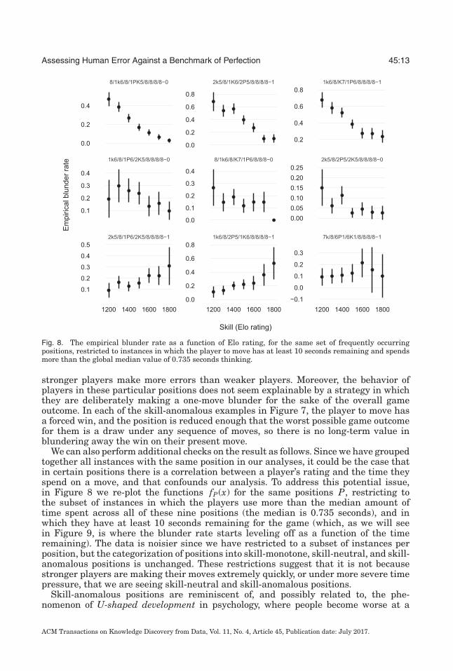
Fig. 8. The empirical blunder rate as a function of Elo rating, for the same set of frequently occurringpositions, restricted to instances in which the player to move has at least 10 seconds remaining and spendsmore than the global median value of 0.735 seconds thinking.

stronger players make more errors than weaker players. Moreover, the behavior ofplayers in these particular positions does not seem explainable by a strategy in whichthey are deliberately making a one-move blunder for the sake of the overall gameoutcome. In each of the skill-anomalous examples in Figure 7, the player to move hasa forced win, and the position is reduced enough that the worst possible game outcomefor them is a draw under any sequence of moves, so there is no long-term value inblundering away the win on their present move.

We can also perform additional checks on the result as follows. Since we have groupedtogether all instances with the same position in our analyses, it could be the case thatin certain positions there is a correlation between a player’s rating and the time theyspend on a move, and that confounds our analysis. To address this potential issue,in Figure 8 we re-plot the functions fP(x) for the same positions P, restricting tothe subset of instances in which the players use more than the median amount oftime spent across all of these nine positions (the median is 0.735 seconds), and inwhich they have at least 10 seconds remaining for the game (which, as we will seein Figure 9, is where the blunder rate starts leveling off as a function of the timeremaining). The data is noisier since we have restricted to a subset of instances perposition, but the categorization of positions into skill-monotone, skill-neutral, and skill-anomalous positions is unchanged. These restrictions suggest that it is not becausestronger players are making their moves extremely quickly, or under more severe timepressure, that we are seeing skill-neutral and skill-anomalous positions.

Skill-anomalous positions are reminiscent of, and possibly related to, the phe-nomenon of U-shaped development in psychology, where people become worse at a



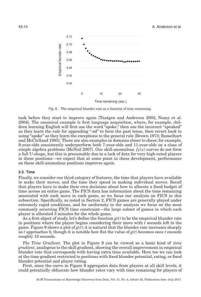
Fig. 9. The empirical blunder rate as a function of time remaining.

task before they start to improve again [Taatgen and Anderson 2002; Namy et al.2004]. The canonical example is first language acquisition, where, for example, chil-dren learning English will first use the word “spoke,” then use the incorrect “speaked”as they learn the rule for appending “-ed” to form the past tense, then revert back tousing “spoke” as they learn the exceptions to the general rule [Brown 1973; Rumelhartand McClelland 1985]. There are also examples in domains closer to chess; for example,9-year-olds consistently underperform both 7-year-olds and 11-year-olds on a class ofsimple algebra problems [McNeil 2007]. Our skill-anomalous fP(x) curves do not forma full U-shape, but this is presumably due to a lack of data for very high-rated playersin these positions—we expect that at some point in chess development, performanceon these skill-anomalous positions improves again.

3.3. Time

Finally, we consider our third category of features, the time that players have availableto make their moves, and the time they spend in making individual moves. Recallthat players have to make their own decisions about how to allocate a fixed budget oftime across an entire game. The FICS data has information about the time remainingassociated with each move in each game, so we focus our analysis on FICS in thissubsection. Specifically, as noted in Section 2, FICS games are generally played underextremely rapid conditions, and for uniformity in the analysis we focus on the mostcommonly occurring FICS time constraint—the large subset of games in which eachplayer is allocated 3 minutes for the whole game.

As a first object of study, let’s define the function g(t) to be the empirical blunder ratein positions where the player begins considering their move with t seconds left in thegame. Figure 9 shows a plot of g(t); it is natural that the blunder rate increases sharplyas t approaches 0, though it is notable how flat the value of g(t) becomes once t exceedsroughly 10 seconds.

The Time Gradient. The plot in Figure 9 can be viewed as a basic kind of timegradient, analogous to the skill gradient, showing the overall improvement in empiricalblunder rate that corresponds with having extra time available. Here too we can lookat the time gradient restricted to positions with fixed blunder potential, rating, or fixedblunder potential and player rating.

First, since the curve in Figure 9 aggregates data from players at all skill levels, itcould potentially obfuscate how blunder rates vary with time remaining for players of



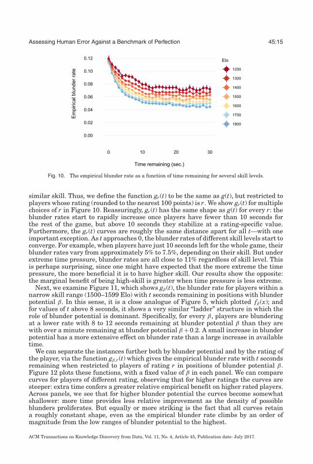
Fig. 10. The empirical blunder rate as a function of time remaining for several skill levels.

similar skill. Thus, we define the function gr(t) to be the same as g(t), but restricted toplayers whose rating (rounded to the nearest 100 points) is r. We show gr(t) for multiplechoices of r in Figure 10. Reassuringly, gr(t) has the same shape as g(t) for every r: theblunder rates start to rapidly increase once players have fewer than 10 seconds forthe rest of the game, but above 10 seconds they stabilize at a rating-specific value.Furthermore, the gr(t) curves are roughly the same distance apart for all t—with oneimportant exception. As t approaches 0, the blunder rates of different skill levels start toconverge. For example, when players have just 10 seconds left for the whole game, theirblunder rates vary from approximately 5% to 7.5%, depending on their skill. But underextreme time pressure, blunder rates are all close to 11% regardless of skill level. Thisis perhaps surprising, since one might have expected that the more extreme the timepressure, the more beneficial it is to have higher skill. Our results show the opposite:the marginal benefit of being high-skill is greater when time pressure is less extreme.

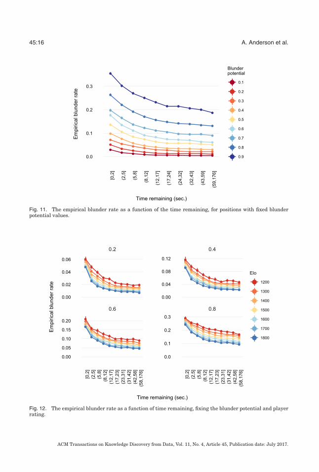
Next, we examine Figure 11, which shows gβ(t), the blunder rate for players within anarrow skill range (1500–1599 Elo) with t seconds remaining in positions with blunderpotential β. In this sense, it is a close analogue of Figure 5, which plotted fβ(x); andfor values of t above 8 seconds, it shows a very similar “ladder” structure in which therole of blunder potential is dominant. Specifically, for every β, players are blunderingat a lower rate with 8 to 12 seconds remaining at blunder potential β than they arewith over a minute remaining at blunder potential β +0.2. A small increase in blunderpotential has a more extensive effect on blunder rate than a large increase in availabletime.

We can separate the instances further both by blunder potential and by the rating ofthe player, via the function gβ,r(t) which gives the empirical blunder rate with t secondsremaining when restricted to players of rating r in positions of blunder potential β.Figure 12 plots these functions, with a fixed value of β in each panel. We can comparecurves for players of different rating, observing that for higher ratings the curves aresteeper: extra time confers a greater relative empirical benefit on higher rated players.Across panels, we see that for higher blunder potential the curves become somewhatshallower: more time provides less relative improvement as the density of possibleblunders proliferates. But equally or more striking is the fact that all curves retaina roughly constant shape, even as the empirical blunder rate climbs by an order ofmagnitude from the low ranges of blunder potential to the highest.



Fig. 11. The empirical blunder rate as a function of the time remaining, for positions with fixed blunderpotential values.

Fig. 12. The empirical blunder rate as a function of time remaining, fixing the blunder potential and playerrating.



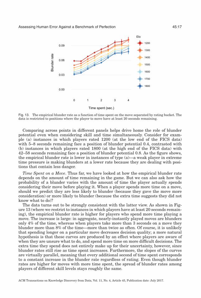
Fig. 13. The empirical blunder rate as a function of time spent on the move separated by rating bucket. Thedata is restricted to positions where the player to move have at least 20 seconds remaining.

Comparing across points in different panels helps drive home the role of blunderpotential even when considering skill and time simultaneously. Consider for exam-ple (a) instances in which players rated 1200 (at the low end of the FICS data)with 5–8 seconds remaining face a position of blunder potential 0.4, contrasted with(b) instances in which players rated 1800 (at the high end of the FICS data) with42–58 seconds remaining face a position of blunder potential 0.8. As the figure shows,the empirical blunder rate is lower in instances of type (a)—a weak player in extremetime pressure is making blunders at a lower rate because they are dealing with posi-tions that contain less danger.

Time Spent on a Move. Thus far, we have looked at how the empirical blunder ratedepends on the amount of time remaining in the game. But we can also ask how theprobability of a blunder varies with the amount of time the player actually spendsconsidering their move before playing it. When a player spends more time on a move,should we predict they are less likely to blunder (because they gave the move moreconsideration) or more likely to blunder (because the extra time suggests they did notknow what to do)?

The data turns out to be strongly consistent with the latter view. As shown in Fig-ure 13 (where we restrict to instances in which players have at least 20 seconds remain-ing), the empirical blunder rate is higher for players who spend more time playing amove. The increase is large: in aggregate, nearly-instantly played moves are blundersonly 4% of the time, whereas when players take more than 3 seconds on a move theyblunder more than 8% of the time—more than twice as often. Of course, it is unlikelythat spending longer on a particular move decreases decision quality; a more naturalhypothesis is that these curves are produced by an effect where players are aware ofwhen they are unsure what to do, and spend more time on more difficult decisions. Theextra time they spend does not entirely make up for their uncertainty, however, sinceblunder rates still rise as time spent increases. Furthermore, the slopes of the curvesare virtually parallel, meaning that every additional second of time spent correspondsto a constant increase in the blunder rate regardless of rating. Even though blunderrates are higher for moves with more time spent, the spread of blunder rates amongplayers of different skill levels stays roughly the same.



4. PREDICTION

We have now seen how the empirical blunder rate depends on our three fundamental di-mensions: difficulty, the skill of the player, and the time available to them. We now turnto a set of tasks that allow us to further study the predictive power of these dimensions.

4.1. Greater Tree Depth

In order to formulate our prediction methods for blunders, we first extend the set offeatures available for studying the difficulty of a position. Once we have these additionalfeatures, we will be prepared to develop the predictions themselves.

Thus far, when we have considered a position’s difficulty, we have used informationabout the player’s immediate moves, and then invoked a tablebase to determine theoutcome after these immediate moves. We now ask whether it is useful for our task toconsider longer sequences of moves beginning at the current position. Specifically, ifwe consider all d-move sequences beginning at the current position, we can organizethese into a game tree of depth d with the current position P as the root, and nodesrepresenting the states of the game after each possible sequence of j ≤ d moves. Chessengines use this type of tree as their central structure in determining which moves tomake; it is less obvious, however, how to make use of these trees in analyzing blundersby human players, given players’ imperfect selection of moves even at depth 1.

Let us introduce some notation to describe how we use this information. Suppose ourinstance consists of position P, with n legal moves, of which b are blunders. We willdenote the moves by m1, m2, . . . , mn, leading to positions P1, P2, . . . , Pn, respectively,and we will suppose they are indexed so that m1, m2, . . . , mn−b are the non-blunders,and mn−b+1, . . . , mn are the blunders. We write T0 for the indices of the non-blunders{1, 2, . . . , n − b} and T1 for the indices of the blunders {n − b + 1, . . . , n}. Finally, fromeach position Pi, there are ni legal moves, of which bi are blunders.

The set of all pairs (ni, bi) for i = 1, 2, . . . , n constitutes a potentially useful source ofinformation in the depth-2 game tree from the current position. What might it tell us?

First, suppose that position Pi, for i ∈ T1, is a position reachable via a blundermi. Then if the blunder potential β(Pi) = bi/ni is large, this means that it may bechallenging for the opposing player to select a move that capitalizes on the blunder mimade at the root position P; there is a reasonable chance that the opposing will insteadblunder, restoring the minimax value to something larger. This, in turn, means that itmay be harder for the player in the root position of our instance to see that move mi,leading to position Pi, is in fact a blunder. The conclusion from this reasoning is thatwhen the blunder potentials of positions Pi for i ∈ T1 are large, it suggests a largerempirical blunder rate at P.

It is less clear what to conclude when there are large blunder potentials at positionsPi for i ∈ T0—positions reachable by non-blunders. Again, it suggests that player atthe root may have a harder time correctly evaluating the positions Pi for i ∈ T0; if theyappear better than they are, it could lead the player to favor these non-blunders. On theother hand, the fact that these positions are hard to evaluate could also suggest a gen-eral level of difficulty in evaluating P, which could elevate the empirical blunder rate.

There is also a useful aggregation of this information, as follows. If we defineb(T1) = ∑

i∈T1bi and n(T1) = ∑

i∈T1ni, and analogously for b(T0) and n(T0), then the ra-

tio β1 = b(T1)/n(T1) is a kind of aggregate blunder potential for all positions reachableby blunders, and analogously for β0 = b(T0)/n(T0) with respect to positions reachableby non-blunders.

In the next subsection, we will see that the four quantities b(T1), n(T1), b(T0), n(T0)indeed contain useful information for prediction, particularly when looking at familiesof instances that have the same blunder potential at the root position P. We note that



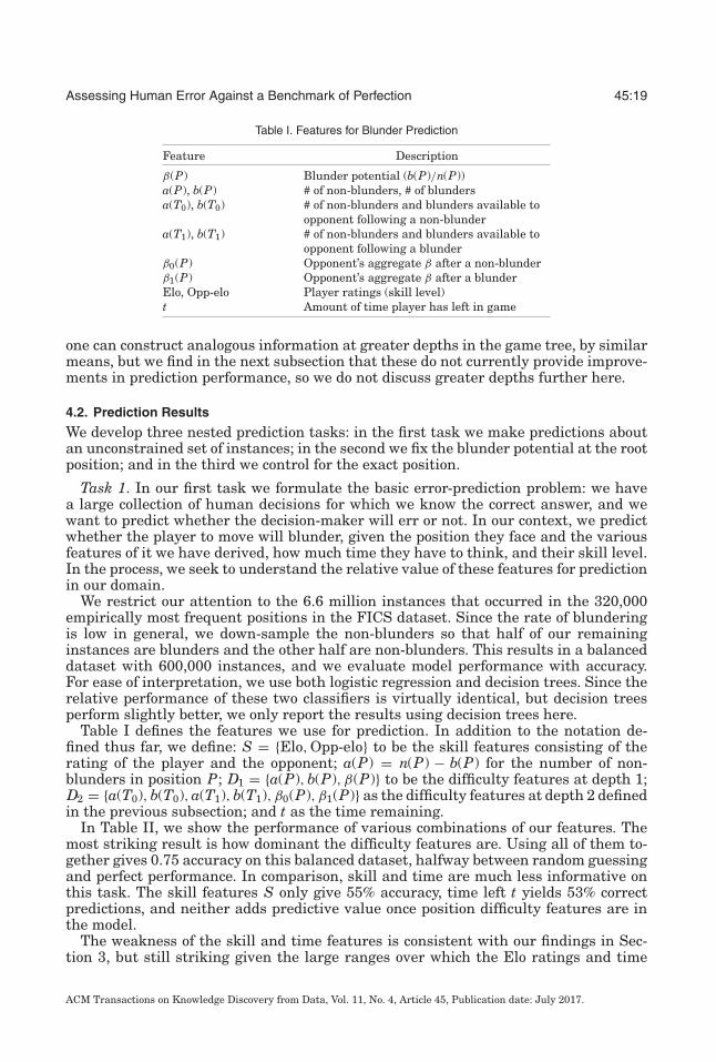
Table I. Features for Blunder Prediction

Feature Description

β(P) Blunder potential (b(P)/n(P))a(P), b(P) # of non-blunders, # of blundersa(T0), b(T0) # of non-blunders and blunders available to

opponent following a non-blundera(T1), b(T1) # of non-blunders and blunders available to

opponent following a blunderβ0(P) Opponent’s aggregate β after a non-blunderβ1(P) Opponent’s aggregate β after a blunderElo, Opp-elo Player ratings (skill level)t Amount of time player has left in game

one can construct analogous information at greater depths in the game tree, by similarmeans, but we find in the next subsection that these do not currently provide improve-ments in prediction performance, so we do not discuss greater depths further here.

4.2. Prediction Results

We develop three nested prediction tasks: in the first task we make predictions aboutan unconstrained set of instances; in the second we fix the blunder potential at the rootposition; and in the third we control for the exact position.

Task 1. In our first task we formulate the basic error-prediction problem: we havea large collection of human decisions for which we know the correct answer, and wewant to predict whether the decision-maker will err or not. In our context, we predictwhether the player to move will blunder, given the position they face and the variousfeatures of it we have derived, how much time they have to think, and their skill level.In the process, we seek to understand the relative value of these features for predictionin our domain.

We restrict our attention to the 6.6 million instances that occurred in the 320,000empirically most frequent positions in the FICS dataset. Since the rate of blunderingis low in general, we down-sample the non-blunders so that half of our remaininginstances are blunders and the other half are non-blunders. This results in a balanceddataset with 600,000 instances, and we evaluate model performance with accuracy.For ease of interpretation, we use both logistic regression and decision trees. Since therelative performance of these two classifiers is virtually identical, but decision treesperform slightly better, we only report the results using decision trees here.

Table I defines the features we use for prediction. In addition to the notation de-fined thus far, we define: S = {Elo, Opp-elo} to be the skill features consisting of therating of the player and the opponent; a(P) = n(P) − b(P) for the number of non-blunders in position P; D1 = {a(P), b(P), β(P)} to be the difficulty features at depth 1;D2 = {a(T0), b(T0), a(T1), b(T1), β0(P), β1(P)} as the difficulty features at depth 2 definedin the previous subsection; and t as the time remaining.

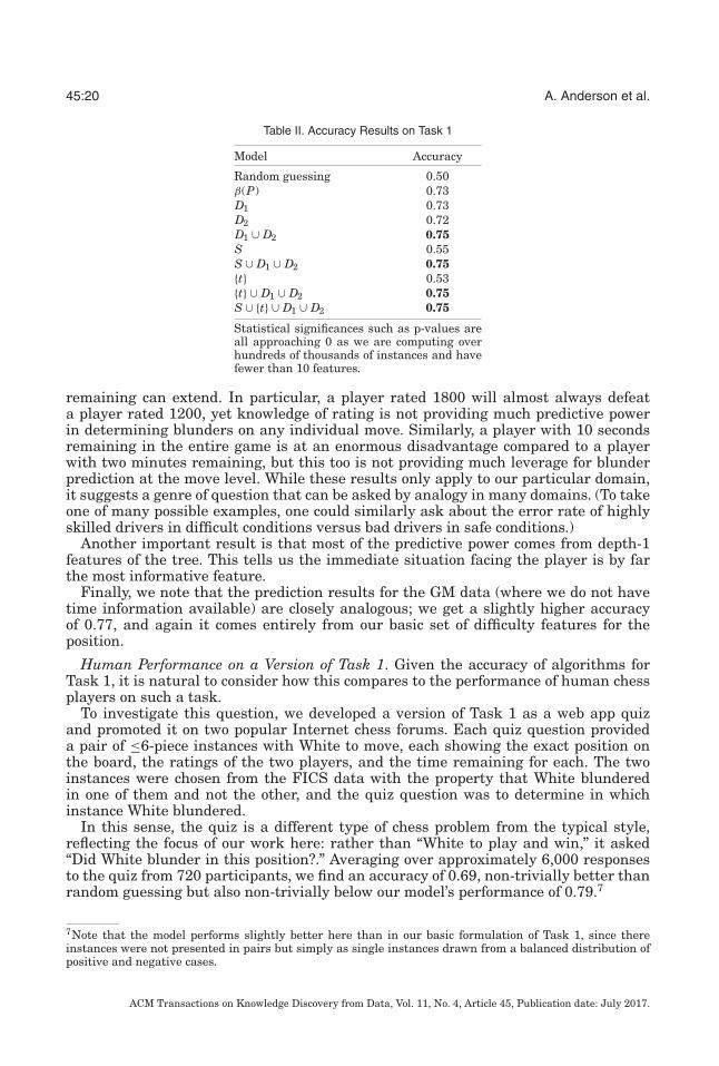
In Table II, we show the performance of various combinations of our features. Themost striking result is how dominant the difficulty features are. Using all of them to-gether gives 0.75 accuracy on this balanced dataset, halfway between random guessingand perfect performance. In comparison, skill and time are much less informative onthis task. The skill features S only give 55% accuracy, time left t yields 53% correctpredictions, and neither adds predictive value once position difficulty features are inthe model.

The weakness of the skill and time features is consistent with our findings in Sec-tion 3, but still striking given the large ranges over which the Elo ratings and time



Table II. Accuracy Results on Task 1

Model Accuracy

Random guessing 0.50β(P) 0.73D1 0.73D2 0.72D1 ∪ D2 0.75S 0.55S ∪ D1 ∪ D2 0.75{t} 0.53{t} ∪ D1 ∪ D2 0.75S ∪ {t} ∪ D1 ∪ D2 0.75

Statistical significances such as p-values areall approaching 0 as we are computing overhundreds of thousands of instances and havefewer than 10 features.

remaining can extend. In particular, a player rated 1800 will almost always defeata player rated 1200, yet knowledge of rating is not providing much predictive powerin determining blunders on any individual move. Similarly, a player with 10 secondsremaining in the entire game is at an enormous disadvantage compared to a playerwith two minutes remaining, but this too is not providing much leverage for blunderprediction at the move level. While these results only apply to our particular domain,it suggests a genre of question that can be asked by analogy in many domains. (To takeone of many possible examples, one could similarly ask about the error rate of highlyskilled drivers in difficult conditions versus bad drivers in safe conditions.)

Another important result is that most of the predictive power comes from depth-1features of the tree. This tells us the immediate situation facing the player is by farthe most informative feature.

Finally, we note that the prediction results for the GM data (where we do not havetime information available) are closely analogous; we get a slightly higher accuracyof 0.77, and again it comes entirely from our basic set of difficulty features for theposition.

Human Performance on a Version of Task 1. Given the accuracy of algorithms forTask 1, it is natural to consider how this compares to the performance of human chessplayers on such a task.

To investigate this question, we developed a version of Task 1 as a web app quizand promoted it on two popular Internet chess forums. Each quiz question provideda pair of ≤6-piece instances with White to move, each showing the exact position onthe board, the ratings of the two players, and the time remaining for each. The twoinstances were chosen from the FICS data with the property that White blunderedin one of them and not the other, and the quiz question was to determine in whichinstance White blundered.

In this sense, the quiz is a different type of chess problem from the typical style,reflecting the focus of our work here: rather than “White to play and win,” it asked“Did White blunder in this position?.” Averaging over approximately 6,000 responsesto the quiz from 720 participants, we find an accuracy of 0.69, non-trivially better thanrandom guessing but also non-trivially below our model’s performance of 0.79.7

7Note that the model performs slightly better here than in our basic formulation of Task 1, since thereinstances were not presented in pairs but simply as single instances drawn from a balanced distribution ofpositive and negative cases.



The relative performance of the prediction algorithm and the human forumparticipants forms an interesting contrast, given that the human participants wereable to use domain knowledge about properties of the exact chess position while thealgorithm is achieving almost its full performance from a single number—the blunderpotential—that draws on a tablebase for its computation. We also investigated theextent to which the guesses made by human participants could be predicted by analgorithm; our accuracy on this was in fact lower than for the blunder-prediction taskitself, with the blunder potential again serving as the most important feature forpredicting human guesses on the task.

Task 2. Given how powerful the depth-1 features are, we now control for b(P) andn(P) and investigate the predictive performance of our features once blunder potentialhas been fixed. Our strategy on this task is very similar to before: we compare differentgroups of features on a binary classification task and use accuracy as our measure.These groups of features are D2, S, S ∪ D2, {t}, {t} ∪ D2, and the full set S ∪ {t} ∪ D2. Foreach of these models, we have an accuracy score for every (b(P), n(P)) pair. The relativeperformances of the models are qualitatively similar across all (b(P), n(P)) pairs: again,position difficulty dominates time and rating, this time at depth 2 instead of depth 1. Inall cases, the performance of the full feature set is best (the mean accuracy is 0.71), butD2 alone achieves 0.70 accuracy on average. This further underscores the importanceof position difficulty.

Additionally, inspecting the decision tree models reveals a very interesting depen-dence of the blunder rate on the depth-1 structure of the game tree. First, recall thatpositions with b(P) = 1 and positions with b(P) = n(P) − 1 both occur frequently inour datasets. In so-called “only-move” situations, where there is only one move that isnot a blunder, the dependence of blunder rate on D2 is as one would expect: the higherthe b(T1) ratio, the more likely the player is to blunder. But for positions with onlyone blunder, the dependence reverses: blunders are less likely with higher b(T1) ratios.Understanding this latter effect is an interesting open question.

Task 3. Our final prediction question is about the degree to which time and skillare informative once the position has been fully controlled for. In other words, oncewe understand everything we can about a position’s difficulty, what can we learn fromthe other dimensions? To answer this question, we set up a final task where we fixthe position completely, create a balanced dataset of blunders and non-blunders, andconsider how well time and skill predict whether a player will blunder in the positionor not. We do this for all 25 instances of positions for which there are over 500 blundersin our data. On average, knowing the rating of the player alone results in an accuracyof 0.62, knowing the times available to the player and his opponent yields 0.54, andtogether they give 0.63. Thus once difficulty has been completely controlled for, thereis still substantial predictive power in skill and time, consistent with the notion thatall three dimensions are predictive of blunders.

5. FURTHER DIRECTION: THE ROLE OF RECENT HISTORY

There are other dimensions in addition to skill, time, and the difficulty of the instancethat one could imagine using as information in estimating the probability of error in agiven decision, and in this final section we suggest one such source of information thatleads to a set of intriguing open questions.

This source of information is the recent history of actions leading up to the currentinstance. In the case of chess as a domain, this would most naturally correspond tousing information not just about the current position on the board, but also the positionimmediately preceding it in the game, and the move by the opponent that brought thegame to the current position. (One could also extend this to consider the most recent



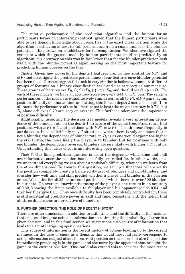
Fig. 14. Complementary cumulative distribution of the blunder rate difference in frequently occurringpositions depending on which of the two most common immediately preceding moves was played by theopponent.

few moves by both players and the positions they were played in, but for simplicity wecan ask this question just about the single immediately preceding position and move.)

In the case of the single immediately preceding position and move, it is natural to askwhether the move that led to this position should be useful at all in predicting errors,given that the rules of chess (and most other tasks like chess) imply that decision-making is almost always memoryless—all that matters is the current position on theboard.8 A basic way to make this question precise is to define sm(P) to be the empiricalblunder rate in position P when the preceding move by the opponent was m. How oftendoes it happen that for two preceding moves � and m we have significantly differentvalues for s�(P) and sm(P)?

In fact we find that this happens surprisingly often in our data; the empirical blunderrate in a given position can vary considerably depending on the previous move by theopponent. If we fix a non-trivial threshold k and consider all positions that occur atleast k times in our data, we can consider the difference s�(P) and sm(P) for the two mostcommon preceding moves � and m. In more than 10% of these instances, |s�(P) − sm(P)|is at least 0.05, and in more than 1% of them it is at least 0.20. As one sees from ourearlier analyses, these are large differences in qualitative terms.

Figure 14 gives the full complementary cumulative distribution for the quantity|s�(P) − sm(P)| over all frequently occurring positions, where for P the moves � andm are the two most common immediately preceding moves by the opponent, and bothoccurred at least 50 times.

Given the fact that the task we are studying depends only on the current position,it is interesting to ask why one finds such non-trivial differences in blunder rate asa function of the immediately preceding move. We pose this primarily as an openquestion, but we observe that there are two distinct families of reasons that couldbe operating. The first is a behavioral one, explored in psychological studies of chessby Bilalic et al. [2008]: the immediately preceding course of the game might havecaused the player to focus on certain aspects of the position rather than others, and

8This is not always true; the threefold-repetition rule and the the 50-move rule for draws in chess implythat there are situations in which a player has to think about the sequence of events leading to the currentposition. But these cases are very rare, and as noted earlier they do not play a significant role in any of ouranalyses here.



so when they come to the present position P, the aspects that are psychologicallysalient to them may be different depending on whether the game arrived at P via� or m. This in turn could have an effect on whether they notice that certain movesfrom position P are blunders. A second category of reasons relates more directly to thenotion of skill: it appears from the instances where s�(P) and sm(P) differ significantlythat the immediately preceding position conveys information about whether the playerselecting the move, or the player’s opponent, or both players, are displaying a good orbad sense about how to handle the course of the particular game. Certain precedingpositions suggest that they are following a good plan, while others suggest that theyare following a misguided plan. This suggests that the recent history of precedingpositions is providing us with information about the player’s understanding of thecurrent position—a kind of skill specific to the instance at hand, rather than theiroverall skill as reflected through Elo rating.

There are natural analogies for both of these categories of reasons to other domains:in any situation where someone is making a decision in the present, knowledge ofwhat has happened in the recent past can both suggest something about what theyview as salient, and also suggest something about the skill that they are displayingin handling the current situation. These considerations, and what we see in our datahere, suggest that including these types of information about the recent past can beuseful as features in assessing error; we leave the deeper exploration of such categoriesof features as a direction for further work.

6. CONCLUSION

We have used chess as a model system to investigate the types of features that help inanalyzing and predicting error in human decision-making. Chess provides us with ahighly instrumented domain in which the time available to and skill of a decision-makerare often recorded, and, for positions with few pieces, the set of optimal decisions canbe determined computationally using tablebases. Furthermore, online chess serversprovide us with a massive amount of human play to study.

Through our analysis we have seen that the inherent difficulty of the decision, evenapproximated simply by the proportion of available blunders in the underlying position,can be a much more powerful source of information than the skill or time available. Wehave also identified a number of other phenomena, including the ways in which playersof different skill levels benefit differently, in aggregate, from easier instances or moretime. And we have found, surprisingly, that there exist skill-anomalous positions inwhich weaker players commit fewer errors than stronger players.

We believe there are natural opportunities to apply the article’s framework of skill,time, and difficulty to a range of settings in which human experts make a sequenceof decisions, some of which turn out to be in error. In doing so, we may be able todifferentiate between domains in which skill, time, or difficulty emerge as the dominantsource of predictive information. Many questions in this style can be asked. For a settingsuch as medicine, is the experience of the physician or the difficulty of the case a moreimportant feature for predicting errors in diagnosis? Or to recall an analogy raisedin the previous section, for micro-level mistakes in a human task such as driving, wethink of inexperienced and distracted drivers as a major source of risk, but how dothese effects compare to the presence of dangerous road conditions?

Finally, there are a number of interesting further avenues for exploring our currentmodel domain of chess positions via tablebases. First, we note that our definition ofblunders, while concrete and precisely aligned with the minimax value of the game tree,is not the only definition that could be considered even using tablebase evaluations. Inparticular, it would also be possible to consider “softer” notions of blunders. Supposefor example that a player is choosing between moves m and m′, each leading to a



position whose minimax value is a draw, but suppose that the position arising after mis more difficult for the opponent, and produces a much higher empirical probabilitythat the opponent will make a mistake at some future point and lose. Then it can beviewed as a kind of blunder, given these empirical probabilities, to play m′ rather thanthe more challenging m. This is sometimes termed speculative play [Jansen 1990],and it can be thought of primarily as a refinement of the coarser minimax value.Another direction is to more fully treat the domain as a competitive activity betweentwo parties. For example, is there evidence in the kinds of positions we study thatstronger players are not only avoiding blunders, but also steering the game towardpositions that have higher blunder potential for their opponent? More generally, theinteraction of competitive effects with principles of error-prone decision-making canlead to a rich collection of further questions.

ACKNOWLEDGMENTS

We thank Tommy Ashmore for valuable discussions on chess engines and human chess performance, theficsgames.org team for providing the FICS data, Bob West for help with web development, and Dan Goldstein,Sebastien Lahaie, Ken Rogoff, and David Smerdon for their very helpful feedback.

REFERENCES

Robert P. Abelson. 1985. A variance explanation paradox: When a little is a lot. Psychological Bulletin 97, 1(1985), 129.

Richard Bellman. 1965. On the application of dynamic programing to the determination of optimal play inchess and checkers. Proceedings of the National Academy of Sciences 53, 2 (1965), 244.

Merim Bilalic, Peter McLeod, and Fernand Gobet. 2008. Inflexibility of experts—Reality or myth? Quantify-ing the einstellung effect in chess masters. Cognitive Psychology 56, 2 (2008), 73–102.

Tamal Biswas and Kenneth W. Regan. 2015a. Measuring level-K reasoning, satisficing, and human error ingame-play data. In Proceedings of the 2015 IEEE 14th International Conference on Machine Learningand Applications (ICMLA). IEEE, 941–947.

Tamal Biswas and Kenneth W. Regan. 2015b. Quantifying depth and complexity of thinking and knowledge.In Proceedings of International Conference on Agents and Artificial Intelligence (ICAART).

Roger Brown. 1973. A First Language: The Early Stages. Harvard University Press.Neil Charness. 1992. The impact of chess research on cognitive science. Psychological Research 54, 1 (1992),

4–9.William G. Chase and Herbert A. Simon. 1973. Perception in chess. Cognitive Psychology 4, 1 (1973), 55–81.Adriaan D. De Groot. 1978. Thought and Choice in Chess, Vol. 4. Walter de Gruyter.Arpad E. Elo. 1978. The Rating of Chessplayers, Past and Present. Arco Pub.Reuben Fine. 1941. Basic Chess Endings, Number 3. D. McKay Co.Ralf Herbrich, Tom Minka, and Thore Graepel. 2006. Trueskill: A bayesian skill rating system. In Proceedings

of Advances in Neural Information Processing Systems. 569–576.Peter Jansen. 1990. Problematic Positions and Speculative Play. In Computers, Chess, and Cognition.

Springer, 169–181.Edward E. Jones and Victor A. Harris. 1967. The attribution of attitudes. Journal of Experimental Social

Psychology 3, 1 (1967), 1–24.Barry Kirwan. 1993. Human Reliability Assessment. Wiley Online Library.Danny Kopec. 1990. Advances in Man-Machine Play. In Computers, Chess, and Cognition. Springer, 9–32.Himabindu Lakkaraju, Jon Kleinberg, Jure Leskovec, Jens Ludwig, and Sendhil Mullainathan. 2016. Human

decisions and machine predictions. (2016).Himabindu Lakkaraju, Jure Leskovec, Jon Kleinberg, and Sendhil Mullainathan. 2015. A bayesian frame-

work for modeling human evaluations. In Proceedings of the 2015 SIAM International Conference onData Mining. SIAM, 181–189.

Vladimir Makhnychev and Victor Zakharov. 2012. Lomonosov tablebases. Accessed November 01, 2016 fromhttp://tb7.chessok.com.

John McCarthy. 1990. Chess as the Drosophila of AI. In Computers, Chess, and Cognition. Springer, 227–237.


http://tb7.chessok.com


Richard D. McKelvey and Thomas R. Palfrey. 1998. Quantal response equilibria for extensive form games.Experimental Economics 1, 1 (1998), 9–41.

Nicole M. McNeil. 2007. U-shaped development in math: 7-year-olds outperform 9-year-olds on equivalenceproblems. Developmental Psychology 43, 3 (2007), 687.

Eugene Nalimov. 2005. Nalimov tablebases. Accessed November 01, 2016 from www.k4it.de/?topic=egtb\&lang=en.

Laura L. Namy, Aimee L. Campbell, and Michael Tomasello. 2004. The changing role of iconicity in non-verbalsymbol learning: A U-shaped trajectory in the acquisition of arbitrary gestures. Journal of Cognitionand Development 5, 1 (2004), 37–57.

Kenneth W. Regan and Tamal Biswas. 2013. Psychometric modeling of decision making via game play. InProceedings of 2013 IEEE Conference on Computational Intelligence in Games (CIG). IEEE, 1–8.

David E. Rumelhart and James L. McClelland. 1985. On Learning the Past Tenses of English Verbs. TechnicalReport. DTIC Document.

Gavriel Salvendy. 2012. Handbook of Human Factors and Ergonomics. John Wiley & Sons.Herbert Simon. 1957. Models of man; social and rational. Wiley.Herbert Simon and William Chase. 1988. Skill in chess. In Computer Chess Compendium. Springer, 175–188.Niels A. Taatgen and John R. Anderson. 2002. Why do children learn to say broke? A model of learning the

past tense without feedback. Cognition 86, 2 (2002), 123–155.Amos Tversky and Daniel Kahneman. 1975. Judgment under uncertainty: Heuristics and biases. In Utility,

Probability, and Human Decision Making. Springer, 141–162.

Received November 2016; accepted January 2017


http://www.k4it.de/?topic=egtb&lang=en

http://www.k4it.de/?topic=egtb&lang=en

Documents

Assessing Human Error Against a Benchmark of Perfectionashton/pubs/tbase-tkdd.pdf · Assessing Human Error Against a Benchmark of Perfection ... human decision-making ... truth”