Embed Size (px)
Citation preview

ASSESSING RISK AND VALUE CREATION OF PUBLIC AND PRIVATE TIMBERLAND
INVESTMENTS
by
ANTHONY J. CASCIO
(Under the Direction of Michael L. Clutter)
ABSTRACT
This dissertation assesses elements of the financial risk and return of timberland investments
within the United States by applying modern portfolio theory, the capital asset pricing model and the
efficient markets hypothesis. The first study applies modern portfolio theory to assist in the optimal
construction of portfolios of sub-regional timberland assets within the US South. First, we develop a
unique set of synthetic timberland returns for 22 sub-US South regions, for a 19 year time horizon.
Portfolio optimization is performed with these 22 return series, and an efficient frontier identified with
portfolios having risk levels ranging from 3.9% to 13.8%, and expected return levels of 10.4% to 13.4%.
The optimal tangency portfolio is identified having expected return and risk levels of 11.2% and 4.2%,
respectively. Monte Carlo simulation is utilized to estimate the value at risk (VAR) of a hypothetical ten
year, regionally-diversified timberland investment. The second study estimates the systematic risks and
risk-adjusted required returns of timberland investments in different geographic regions within United
States using the Capital Asset Pricing Model (CAPM). We estimate low, positive betas for timberland in
the Pacific Northwest, Northeast and South. These estimates are not significantly different than zero, but
are however higher than many past estimates from earlier time periods. Required return rates of 5.7%-
6.6% are estimated for the three regions, respectively. From 1995 to 2002, nine mergers and acquisitions
of publicly-held, vertically-integrated forest products companies occurred in the United States. Investors
not able to directly own timberland may choose to own shares of these firms as a method of indirect
timberland investment. The third study employs event study methodology, based on the concept of

market efficiency, to test the null hypothesis of no shareholder value creation from these mergers and
acquisitions. We find that $4.7B of market value was created upon the announcement of these nine
combinations. We find that target firms enjoyed a statistically significant, nearly 15% average return
attributable to the merger announcements. The returns to acquiring firms averaged a statistically
insignificant 0.34%. The aggregate return was a statistically significant 7.66%.
INDEX WORDS: Timberland investments, portfolio theory, mergers, financial risk

ASSESSING RISK AND VALUE CREATION OF PUBLIC AND PRIVATE TIMBERLAND
INVESTMENTS
by
ANTHONY J. CASCIO
B.S., James Madison University, 1986
M.S., North Carolina State University, 1998
A Dissertation Submitted to the Graduate Faculty of The University of Georgia in Partial Fulfillment of
the Requirements for the Degree
DOCTOR OF PHILOSOPHY
ATHENS, GEORGIA
2006

© 2006
Anthony J. Cascio
All Rights Reserved

ASSESSING RISK AND VALUE CREATION OF PUBLIC AND PRIVATE TIMBERLAND
INVESTMENTS
by
ANTHONY J. CASCIO
Major Professor: Michael L. Clutter
Committee: Peter S. Bettinger David H. Newman John T. Scruggs
Electronic Version Approved: Maureen Grasso Dean of the Graduate School The University of Georgia August 2006

iv
ACKNOWLEDGEMENTS
A dissertation has one name on it – the student’s. This person is responsible for 100% of the
content therein. This is as it should be. However, total responsibility in no way implies completely
independent work. We all receive help along the way, in varying degrees and from many sources, even as
the vast majority of the effort is our own. Help is received by the committee of professors who convey
guidance and nurture progress. Other professors lend help, both formally in the classroom through
structured teaching, and informally in the hallways, hashing out ideas over a cup of coffee. Data does not
grow on trees, and fall neatly into our laps. People from outside of the ivory tower are priceless conduits
to the data we want, and to the data we actually need but didn’t know about. It is amazing how much
people want to help, so long as they are treated courteously and with respect. Fellow graduate students
provide an incredible amount of support. We are the university catalog suggesting what courses should be
taken; the unofficial tutors to get us through those classes; the artist’s apprentice helping us to create and
shape ideas; the physician’s assistant to help us fix our broken models. Most of all, our fellow students
provide the invaluable encouragement and support that creates such a strong sense of teamwork, lending
another oar in the lifeboat on the graduate student’s journey to his new destination. Again, this is as it
should be.
For this help, I wish to recognize and thank my committee: Mike Clutter, my advisor and mentor
– you provided guidance and ideas, you opened doors and created a stage upon which I could perform;
David Newman, you are a wise old sage of this academic world – your advice in matters both academic,
professional and personal is greatly appreciated; Pete Bettinger, you’ve traveled a similar path as mine,
making your guidance all the more valuable; John Scruggs, you gave perhaps the best lectures I attended
at this university, and yes, you challenged and stimulated me to ‘be curious’.

v
Tom Harris, you’ve been around a long time, and I bet you would be willing to echo Roger
Lowenstein’s assertion that “No investment…can be judged on the basis of half a cycle alone“1. Thanks
for the interesting and worthwhile balance of your perspective. Ray Sheffield and Tony Johnson of the
United States Forest Service, you guys and your staff bent over backwards to accommodate my data
requirements; without your help my research and results would be much shallower. Wade Camp of the
Southern Forest Products Association likewise provided valuable data assistance. Sara Baldwin of Timber
Mart-South – you have a lot of good data and information, and the willingness to assist others in its use.
Carol Hyldahl, your support during my first year was very important in my transition back to being a
student again.
David Jones, you preceded me by one semester and your fresh wake in the water gave me a
helpful path to follow. Brooks Mendell, if someone can’t feel confident after talking to you, then they’re
really in trouble. Tim Sydor, I don’t know if I’ve met a student more willing to help another student along
their journey. Your attitude is matched only by your intellect. You are going to make a great professor.
Julie, my wife. I mention you last, because frankly that is the position you have occupied for the
past three years. You have sacrificed many of your dreams to support this part of our plan. Yes, our plan.
For that is what you made it. You have walked this journey hand in hand with me, every step of the way.
No matter how much I have been grumpy, or self-centered, or just generally not available to enjoy life the
way I should have - the way you deserved, you’ve been there providing the kind of love and support that
is quite more than I deserve. Thank you, and I love you.
1 From When Genius Failed, p. 233.

vi
TABLE OF CONTENTS
Page
ACKNOWLEDGEMENTS......................................................................................................................... iv
CHAPTER
1 INTRODUCTION..................................................................................................................... 1
2 ASSESSING RISK AND RETURN WITHIN A PORTFOLIO OF US SOUTH
TIMBERLAND INVESTMENTS ..................................................................................... 40
3 RISK AND RETURN ASSESSMENTS OF EQUITY TIMBERLAND INVESTMENTS IN
THE UNITED STATES..................................................................................................... 79
4 RECENT MERGERS AND ACQUISITIONS OF VERTICALLY-INTEGRATED,
AMERICAN FOREST PRODUCTS COMPANIES: HAS SHAREHOLDER VALUE
BEEN CREATED? .......................................................................................................... 112
5 CONCLUSION ..................................................................................................................... 143
REFERENCES ......................................................................................................................................... 148

1
CHAPTER 1
INTRODUCTION
As a proportion of the world of equity investments, direct investments in timberland within the
United States are quite small. However, they are growing. Such investments can be made in
timberland directly by purchasing either the land itself, or shares of companies whose exclusive
business is owning and managing timberland. Timberland can be invested in indirectly by
purchasing shares of publicly-owned corporations that own both timberland and other assets.
Timberland investments can be made by both individuals, and by institutions representing the
fiduciary interests of individuals, firms and municipalities.
Timberland investments are growing not because of an increase in the amount of
investment-grade timberland in the United States. Rather, the ownership of this land has seen a
large and steady change in recent years from publicly-owned, vertically-integrated forest products
companies, to financial institutions that own timberland via closed-end funds, which are often
commingled. These institutions usually own timberland via intermediary firms that purchase,
manage and dispose of the timberland for them. Therefore, what we are actually seeing is a
decrease in the amount of indirect investments in timberland, and an increase in direct timberland
investment, coupled with an increase in investment by institutions. All of these investors require
information about the financial performance of timberland investments so that informed decisions
can be made.
Markowitz (1952) pioneered the concept that investors should not be concerned with the
risk of individual securities, but rather should pay attention to the overall risk of their portfolio. In
other words, the additional risk contributed by a security to a portfolio is what matters.
Markowitz’s modern portfolio theory is centered on the recognition that securities’ returns

2
through time are correlated to some degree. By effectively combining assets that are not perfectly
correlated a portfolio can be constructed that has less risk than the weighted sum of the individual
assets’ risk. This logic has been utilized by previous researchers to identify the role that
timberland can play in a diversified portfolio of investments (Mills and Hoover 1982, Zinkhan
and Mitchell 1990, Caulfield 1998, and others).
Within this framework of analysis, previous work has compared the risk and return of
timberland in portfolios with traditional major investment categories such as large and small
capitalization stocks, and corporate and US Government bonds. These analyses have focused on
timberland investments at the US national and three major regional levels – the South, Pacific
Northwest and Northeast. Researchers have found that timberland, as an asset class, warrants a
position within the diversified portfolios of investors. While enough data exists to perform asset
class allocations of timberland and other assets using a portfolio optimization framework, the next
step is more difficult. Continuing the asset allocation analysis at a more refined, detailed level, or
performing security selection of specific timberland properties within a portfolio optimization
framework has been prohibitive due to the lack of sufficient return data. The second chapter of
this dissertation applies Markowitz’s portfolio optimization framework to address portfolio
opportunities of timberland investments within a US region, the South, once the investor has
decided to include southern timberland within a diversified portfolio.
The Capital Asset Pricing Model (CAPM) was developed as an outgrowth to Markowitz’
portfolio research by Sharpe (1964), Lintner (1965) and Mossin (1966). The CAPM asserts that
the return required of an asset is proportional to the systematic, or market risk of that asset. It
stipulates that the required return is equivalent to the risk free rate and a premium representing the
asset’s market risk.
The relationship between return and systematic risk has been used extensively to address
such questions as: 1) what is the risk of timberland investments compared to that of the broader
financial market; 2) given that level of risk, what return should investors require of timberland; 3)

3
does the market sensitivity risk of timberland vary by major geographic region in the United
States? The majority of this prior research predates the existence of an asset-based timberland
return series. The third chapter of this dissertation adds to this body of research by utilizing 19
years of returns (1987-2005) for the timberland index maintained and reported by the National
Council of Real Estate Investment Fiduciaries (NCREIF) to address these questions. In addition,
the systematic risk and required return of timberland in different regions within the US South is
assessed.
While institutions and high net worth individuals can readily invest directly in timberland
by utilizing the services of timberland investment management organizations (TIMOs), the
majority of individual investors wishing to invest in timberland cannot usually meet the minimum
capital requirements of the investment vehicles offered by these organizations. Most individuals
therefore invest in timberland by purchasing ownership shares of public corporations owning
timberland. Very few such firms have owned timberland as their exclusive asset, or line of
business. Historically, most firms owning timberland have been vertically-integrated forest
products companies. These firms traditionally owned timberland as a controlled source of timber
inventory for their conversion lines of business, such as lumber, paper and panel products mills.
In recent years significant consolidation has taken place within the United States forest
products industry. During the time period 1995-2002, nine mergers and acquisitions of publicly-
held, vertically-integrated forest products companies occurred. Collectively, these firms owned
approximately 33 million acres of timberland. For both institutional and individual investors who
chose to invest in timberland by owning shares of these firms, a reasonable question to ask is
whether this form of corporate project has created value.
We employ event study methodology in Chapter 4 to address this question. A key tenet of
this technique is the assumption of market efficiency. The efficient market hypothesis stipulates
that current security prices reflect all available information about those securities. By analyzing
the price movement of the stock of a firm immediately after news of a merger is announced, the

4
value of that merger, as assessed by the market, can be measured. The CAPM also plays a key
role in this analysis by projecting what the return of a stock should be during the post-merger
announcement period, against which the actual return is differenced to yield a measure of value
creation or destruction.
Modern portfolio theory, the capital asset pricing model and market efficiency are three
fundamental pillars of modern finance. Each has been extensively employed to assist both
researchers and practitioners in their understanding of the risks and return potential of financial
assets. Each concept has been applied to help better understand the investment characteristics of
timber and timberland. These concepts are employed in this dissertation to expand the knowledge
base of timberland investments both into new areas, and familiar ones with a degree of
refinement, depth and modernity. The remainder of this chapter explores the literature to review
the theory behind these aforementioned techniques, and their past application to timberland
investments.
Literature Review
Modern Portfolio Theory
A fundamental assumption of investment analysis is that investors are risk averse. Hence,
all else being equal, investors prefer greater returns, while taking a minimal amount of risk. While
investors have known for centuries that diversification, or spreading one’s funds (value) among
several investments carries less risk than investing in a sole asset, Harry Markowitz (1952)
formalized the relationship of diversification and the combination of assets. He showed that,
while the expected return of a portfolio of assets is simply the expected return of each asset
multiplied by the asset’s weight in the portfolio:
[ ] [ ]P i ii
E R x E R=∑ ,

5
the risk of the portfolio is much more than a simple function of each asset’s own risk and
portfolio weighting. Rather, the most important aspect concerning an individual asset and
portfolio risk is the correlation of that asset’s returns through time with the other assets in the
portfolio. Rubenstein (2002) states:
‘Probably the most important aspect of Markowitz’s work was to show that it is
not a security’s own risk that is important to an investor, but rather the
contribution the security makes to the variance of his entire portfolio – and that
this was primarily a question of its covariance with all other securities in his
portfolio’.
In a portfolio of n assets, where xi represents the proportion of funds allocated to asset i,
and σi is the standard deviation of asset i, Markowitz (1952) stated the risk of the portfolio as the
variance of a weighted sum:
2
1 1,
n n
P i j ij i ji j
x xσ ρ σ σ= =
=∑∑
where iσ and jσ are the standard deviations of assets i and j, ijρ is the correlation between
assets i and j, and ij i jρ σ σ is the covariance between the two assets. Standard deviation, the
conventional measure of portfolio risk, is the square root of this equation. Two important facts
about portfolio risk bear discussion. It is intuitive from the above equation that the lower the
measure of correlation of two assets in a portfolio, the lower will be the portfolio variation. Two
stocks whose historical movements are perfectly linearly correlated will have a correlation
coefficient of 1, resulting in a contribution to portfolio variance equivalent to the weighted
6
average of their individual standard deviations. So, anything less than perfect correlation between
two stocks will contribute to a lower portfolio variance, and hence less financial risk.
There is a limit, or floor to portfolio variance reduction possible through diversification.
The risk that is removed from diversification is termed firm-specific, or idiosyncratic risk. This
risk is due to specific actions, events, and news pertaining to the individual firm. The risk that
remains is termed market risk, or systematic risk. This is the risk due to economy-wide events and
news, and that affects most all firms. Systematic risk cannot be removed from the portfolio with
diversification.
The impact of covariance between assets in the calculation of portfolio standard deviation
prevents an investor from determining the optimal portfolio of assets by examining their
individual expected returns and risks. Instead, the combined risk of the group of assets,
determined primarily by their co-movement, or covariance, must be examined holistically.
Markowitz utilized these portfolio expected return and risk equations to calculate the
optimal combination of return and risk levels by varying portfolio asset weights. For each
possible level of portfolio expected return, the weights of each asset in the portfolio can be altered
to yield a minimum portfolio standard deviation. Such a portfolio is said to be minimum variance.
Plotting each of these minimum risk levels for a change in expected return yields a curve we term
the efficient frontier. Conversely, the efficient frontier can be calculated by iteratively specifying
a required portfolio standard deviation and then varying the asset weights until a maximum
portfolio expected return is determined. A portfolio constructed in this manner is said to be mean-
variance efficient. This process of developing the efficient frontier is often referred to as
Markowitz portfolio optimization. Computationally, this process is a constrained optimization
problem, where, in the case of maximizing return for a given risk 2Pσ , it can be described
mathematically as:

7
max [ ],PxE R
subject to the constraints:
1
2
1 1
1,n
iin n
i j ij Pi j
x
x x σ σ
=
= =
=
=
∑
∑∑
for an n-asset portfolio, with each asset having portfolio weight xi. Constraining the sum of the
asset weights to 1 enforces the rule of not allowing any short sales for any particular asset, and
that the portfolio must be fully invested. Markowitz portfolio optimization is referred to as a one-
period model. The portfolio return and risk based on any combination of asset allocations can
only be expected to hold for one period, where the length of this period matches the frequency of
the time series of data used in the model. However, analysts and investors do not always limit
their horizon of return and risk expectations to one period. This approach to optimal portfolio
construction is widely used among institutional investment managers today (Rubenstein, 2002).
By utilizing the risk-free rate, the optimal portfolio can be identified. This portfolio is the
one that results in the steepest slope of the line drawn from the risk-free rate on the y-axis to the
tangency point on the efficient frontier. The slope of this line is termed the reward-to-variability
ratio. We can use this ratio, also termed the Sharpe ratio, to solve for the optimal portfolio
allocations by stating it as the objective function:
( [ ] )max .P f
xP
E R Rσ−

8
To assess different investments within a portfolio optimization context, historical return
series for each asset are needed. Using these series, the three data elements for conducting
portfolio optimization can be estimated: asset expected return and risk matrices of correlations
and covariances can be computed. Historical return data for timberland investments are
unfortunately sparse. Before discussing historical timberland return data, and the portfolio
research that has been conducted with it, we first discuss a significant outgrowth of modern
portfolio theory, the Capital Asset Pricing Model, which also requires timberland return data.
Capital Asset Pricing Model
The CAPM builds upon the foundation laid by Markowitz (1952), who proved that the
risk of an individual investment should not be important to investors, but rather the investment’s
contribution to the investor’s overall portfolio risk. The risk of a financial asset is referred to as
the variability of its returns over time, and is commonly denoted by the standard deviation of
periodic returns. Risk can be stratified into two components. Idiosyncratic or firm-specific risk is
that component of total risk that is specific to the asset, resulting from actions, events and news
pertaining to the asset but not to other assets or firms. Firm-specific risk can be removed from the
portfolio through diversification. The risk that remains is termed market risk, or systematic risk.
This is risk due to economy-wide events and news, and that affects all firms. Systematic risk
cannot be removed from the portfolio with diversification.
The contribution of the CAPM is its ability to relate the impact of systematic risk upon
the returns of an investment. It does so with the following form:
( ) [ ( ) ],i f i m fE R R E R Rβ= + −

9
where E(Ri)is the expected or required return on asset i, Rf is the risk free rate of return and
E(Rm)is the expected return on the total market portfolio of assets. The quantity E(Rm)- Rf is
referred to as the market risk premium, or the additional expected return of the market portfolio
over the risk-free rate. βi is a measure of the sensitivity of the expected returns of asset i to
variance in the total market portfolio. It is a measure of the asset’s systematic risk, that portion of
the asset’s total risk that cannot be diversified away. An asset having a beta greater than one is
more risky than the market, and commands a higher required return, while an asset with a beta
less than one is less risky than the market, and requires a lower return.
CAPM theory states that the market return should reflect the return on all traded and non-
traded risky assets, to include human capital. A major criticism of the CAPM is that such a return
is of course, unobservable. For empirical work, a proxy is chosen that reflects a broad market
portfolio of assets. Historical returns for the S&P 500 composite index, or other similar broad
market index are commonly used.
The CAPM was designed as a one-period model. As such, the choice of a proxy for the
risk-free rate does not receive much attention. US Treasury securities with a short maturity are
usually chosen, the 30 and 90-day Treasury bills being common. These assets are more reflective
of a truly risk-free asset than long term US Treasury bonds. Treasury bonds make periodic
coupon payments which have some degree of reinvestment risk. However, Bruner (2003) and
Damodaran (2006a) emphasize that the choice of the risk-free rate should match the return period
for the asset data employed. In other words, if the choice is to invest in a closed-end timberland
fund having a ten year horizon, the most appropriate risk-free alternative would be the 10-year
US Treasury bond.
Bruner (2003) surveyed a collection of corporations, financial advisors, and academic
and trade corporate finance textbooks. The survey questions addressed practices used when
estimating the cost of capital. When asked the question of which risk-free rate to use when using
the CAPM to estimate a required return, the overwhelming response by both corporations and

10
advisors is to use a long term Treasury bond yield. 70% of practitioners utilize a maturity of 10
years or longer, while only 4% stated the use of Treasury-bill yields. Bruner concludes with the
recommendation of matching the maturity of the risk-free investment to the character of the
investment being analyzed, and recommends the yield on the 10-year or longer maturity US
Treasury bond for most capital project evaluations.
Estimates of the market risk premium can vary widely, and according to Perold (2004)
can be the most difficult component of the model to estimate. Practitioners have a choice of using
either an historical estimate of the premium earned by equities over riskless investments, or
somehow looking forward to estimate this differential. The obvious assumption in using historical
premiums is that future expectations can be reasonably characterized by past experiences. The
technique usually involves differencing the average realized return on a risk-free government
security from the average realized return on a broad market index. However, Damodaran (2006b)
describes three questions the analyst must answer that can significantly influence the result.
First, the number of years of historical returns can have influence. Using a longer time
period yields averages that are much more robust, yet at the cost of including potentially stale or
misleading data. Damodaran (2006b) documents that the large standard errors resulting in using
time periods of less than 50 years can be larger than the estimated risk premium itself. Second,
the choice of short term treasury bills as the risk-free asset will result in a market risk premium
approximately 1.5% larger than if long term treasury bonds are used. This choice is easily
decided for us, as consistency is required with our aforementioned choice of the risk free rate that
matches the investment.
Third, the choice of using arithmetic versus geometric averaging of market and riskless
returns will make a difference. The arithmetic average is the simple mean return. The geometric
average is the compound return, more reflective of an investor’s buy-and-hold experience (Bruner
2003). The more variable a return series is, the lower its geometric average will be compared to
its arithmetic average. While US Treasury bonds and bills will not be greatly influenced by this

11
choice, stock indices will, due to their increased volatility. The arithmetic average annual return
of large capitalization stocks from 1926-2005 is 11.6%, while the geometric average is 9.6%2. A
requirement of using the arithmetic average of returns is that they be independent over time.
However Fama and French (1988), among others, have documented significant negative
autocorrelation of returns over time, making the geometric average the more accurate choice.
When analyzing timberland investments, the proper choice is therefore to use a broad-market
return index coupled with long-term US Treasury bonds as the risk-free investment, with annual
returns for each series averaged geometrically.
While the CAPM is designed to be a forward looking model, it is often used to estimate
an asset’s beta by evaluating historical returns. This is because we cannot know or observe the
expected returns required in the model. Following Jensen (1969), the excess returns version of the
single-index model regresses historical returns for the asset less the risk-free rate (the asset’s risk
premium) against the market risk premium:
( ) ( ) ,i f i i m f iR R R R eα β− = + − +
where Ri, Rf and Rm are time series of historical returns for the asset, the risk-free rate and the
market proxy, respectively, and ei is an error term. αi, or the Jensen’s alpha parameter, is an
estimate of the risk-adjusted excess return generated by the asset. If significantly positive, the
asset has generated a return in excess of that warranted by its market risk sensitivity. When
choosing a risk-free investment, a zero-coupon US Treasury security having the same maturity as
the frequency of return data should be used.
If an asset’s beta is known, or has been estimated, then its required return can be
estimated. This required return can be used as a benchmark for measuring potential investments
2 Data from the Center for Research in Security Prices, University of Chicago, as published in Bodie, et al (2005).

12
or projects. If evaluating a potential timberland acquisition, the first step would be to estimate the
future cash flows for the property, to include timber sales, lease revenues, tax payments, etc. The
estimated cost of capital would then be used to discount these figures to arrive at a present value.
For an existing property, the required return can be used to evaluate periodic silviculture
investments in that asset, such as fertilization or subsoil plowing, based on their expected impacts
on growth and subsequent cash flow.
The CAPM is widely used as a model to explain the sensitivity of an asset’s returns to its
undiversifiable risk. It is used extensively by practitioners to quantify this risk, and to develop an
asset’s required return given this risk. However, like any model, the CAPM has its flaws, and
certainly like any other model, is a simplification of reality and cannot therefore be considered
absolutely correct. Over time researchers have slowly constructed evidence against the ability of
the CAPM to accurately portray the relationship between an asset’s market risk and required
return.
Early tests of the CAPM (Fama and MacBeth 1973, Gibbons 1982, among others) have
confirmed the positive relationship between beta and asset return. This relationship has also been
found to be mostly linear, as the CAPM predicts. Researchers have, however found the beta-
return relationship to be ‘flatter’ than that predicted by the CAPM (Fama and MacBeth 1973,
Black et al 1972, Fama and French 2004, among others). For example, low-beta assets often have
a positive Jensen’s alpha, or y-intercept rather than a predicted value of zero, while high beta
stocks have been shown on average to have negative Jensen’s alpha values.
Fama and French (2004) document a divergence of opinion among researchers for the
imperfect empirical record of the CAPM. Some believe financial markets are not as efficient as
once believed, a requirement of the CAPM. Market efficiency stipulates that current security
prices reflect all available information regarding the security, resulting in the inability to predict
the direction or magnitude of the security’s future price movements. Some believe that investors
overreact to past stock price performance, which researchers have potentially identified by adding

13
factors to asset pricing models that may capture this behavior (DeBondt and Thaler 1987, and
others).
Others believe that more risk factors are required to explain asset prices, in addition to
market risk. The three factor model of Fama and French (1993) is an example. Still others (Roll
1977) believe that the CAPM has never been, nor can be, accurately tested due to the impossible
selection of a proxy for the entire market portfolio of assets. While Fama and French (2004)
discourage use of the CAPM for empirical work, 80% of corporations and financial advisers
surveyed by Bruner (2003) nevertheless use the CAPM to estimate the cost of equity capital.
100% of text and trade books included in the survey also recommend primarily using the CAPM
for this purpose.
To conduct portfolio optimization and CAPM risk and required return analyses for
timberland, historical time series of timberland returns are required. Unfortunately, a robust data
series, one based solely upon market transactions, does not exist. Timberland is not traded on an
organized exchange like common stocks, bonds or commodities. Compared to equity
investments, timberland is an extremely thinly traded sector, meaning that very few market
transactions occur during a time period from which a return series can be developed. Only in
1994 did the National Council of Real Estate Investment Fiduciaries (NCRIEF) begin publishing
their Timberland Index, with returns dating back to 1987. Before this series developed sufficient
length, researchers chose between two alternative approaches. Recognizing that timber price
appreciation is a key factor in the timberland return generation process, some researchers simply
used time series of prices of commercial timber species in their analyses. Others developed
synthetic timberland return series based upon the factors that drive timberland returns, for which
available data could be gathered.

14
Timberland Return Drivers
Timberland investment returns are generated through two components: income and
capital appreciation. Income is received primarily from the periodic sale of timber, which in turn
is used in the manufacture of lumber; panel products such as plywood, oriented-strand board
(OSB) and fiberboard; paper; packaging; and several types of specialty chemicals. An attractive
characteristic of selling timber is that it can be withheld from the market during times of low
prices at no cost. There is no ‘storage fee’ direct cost, and in fact the timber continues to grow
and often appreciate until more favorable market conditions return. There is however the
opportunity cost of foregoing harvest until a later time. Annual income is also often received from
the leasing of recreation rights on the land, primarily for hunting.
Capital appreciation is realized from the continuous biological growth of the trees. In
addition, larger trees are generally more valuable per unit than are smaller trees, due to the fact
that telephone poles, plywood veneer and the larger sizes of lumber, some of the highest valued
products made from trees, can only be manufactured from larger trees. Therefore as a tree crosses
a certain threshold from one size class to another, its value per unit increases. For southern yellow
pine species, there are three predominant size classes: pulpwood, from which is made paper and
OSB; chip-n-saw, from which small dimension lumber is made; and sawtimber, used in the
manufacture of wider dimension lumber, poles and plywood.
The price paid for timber varies by tree size, region and season. Finished good prices also
have an impact on timber prices. However, Binkley (2000) documented how the price of southern
pine sawtimber has increased at a compound annual real rate of 2.6% from 1910 to 2000. Timber
price increases are exhibited not only in the income component of timberland returns, but also in
the capital appreciation component, because a key element of the capital appreciation of
timberland is the increase in the value of the land itself (Caulfield 1994). This increase is
attributable to two factors: first, the increase in the value of the land for producing timber due to
price increases (Washburn 1992), and the conversion of a portion of a timberland portfolio to a
15
higher-valued use than the production of timber, such as residential or commercial development,
during the investment period.
Timberland Return Data
The only timberland return index currently in existence3 that is based on actual
timberland transactions and appraisals is the National Council of Real Estate Investment
Fiduciaries Timberland Property Index (NCREIF 1994). NCREIF publishes historical return data
for timberland investments managed by its members, at two geographic levels: the United States,
and three regions within the US: the Pacific Northwest, the Northeast and the South. The
NCREIF Timberland Property Index segregates a total return into income and capital appreciation
elements, and is based on actual data reported by its members managing timberland investments.
Hancock Timber Resource Group (2003a) describes how NCREIF began compiling and
publishing a quarterly index of timberland property returns in 1994, with data retroactive to 1987
for the Southern and Pacific Northwest regions in the United States, and to 1994 for the
Northeast. This index tracks changes in value of timberland properties that are a) held in a
fiduciary environment, as opposed to the myriad other ownership objectives shared by many
other timberland owners; and b) “marked to market” at least annually. If the property does not
experience a change in ownership during a year via a sale, then it is appraised at year end to yield
a new value. As a timberland investment organization joins NCREIF, they submit historic returns
for their properties to augment the index.
The Timberland index is built and maintained similarly to NCREIF’s other commercial
real estate indices. The index has four basic components: the market value of all properties in the
index; the EBITDDA return for the properties; the capital return; and the total return. The
EBITDDA return, or earnings before interest expenses, taxes, depreciation, depletion and
3 The Timberland Performance Index (TPI) (Caulfield,1994) is similar to the NCREIF index, however is no longer in existence.

16
amortization, is based primarily on the sale of harvested timber during the quarter. However,
many timberland property owners lease recreation use rights to clubs or individuals, the income
from which is also included in the EBITDDA portion of the total return. It must be noted that the
EBITDDA figure is gross of applied management fees charged by the property manager, and
therefore overstates the true net income received by the investor (Healey 2003). The EBITDDA
income component of the return is analogous to the dividend component of a stock return.
The capital appreciation component is basically the ratio of the difference in period-to-
period property market value, minus capital expenditures in the current period, to the market
value of the previous period. Timberland appreciation is measured by periodic appraisals.
Appraisals are conducted both externally by consultants and internally by the managing
organization. Major, externally-conducted appraisals often occur on a three year cycle, although
more frequent timing is becoming common (Clutter 2006). Annual external updates (in the other
years) are performed by some management organizations, while others use internal updates of
various types. All organizations perform quarterly updates that are based on harvested timber
removals, merchantable timber growth, and timber price changes. These quarterly updates rarely
include land appreciation, nor account for changes in the value of premerchantable timber
(Clutter 2006). The majority of external appraisals are conducted in the fourth quarter of the year.
Since appraisals are not evenly distributed throughout the year, reported quarterly property
returns are less meaningful. For analysis purposes, it is recommended that annual returns be used
(Hancock Timber Resource Group 2003a).
Investing in timberland by institutions is relatively new. It can be tracked to the passage
of the Employee Retirement Income Security Act (ERISA) in 1974 that required institutional
investors to diversify their portfolios away from traditional common stocks and fixed income
securities to broader classes (Zinkhan 2003, Healey 2003). Investments in timberland by
institutions grew by a factor of ten during the 1990’s to some $17 billion by 2005 (Cambridge
Associates 2002; Dana 2006). This is reflected in the time span of the NCREIF Timberland

17
Property Index. Although the NCREIF series is regarded as the best data available describing the
performance of institutional investments in timberland, the need to analyze the financial
performance of timberland predates the existence of this index. Before this time, most analysts
constructed synthetic return indices with several management assumptions for use in timberland
investment analyses.
Timberland returns value to the owner through a combination of periodic income and
capital appreciation, as previously discussed. The return formula common to financial security
appreciation is applicable for measuring timberland returns:
1
1,t tt
t
NI CVRCV −
+= −
where:
Rt = total return per acre of the asset during period t;
CVt = capital value per acre of the asset during period t;
NIt = net income received per acre of the asset during period t.
Many assumptions about forest management practices must be made when developing a
synthetic timberland return series. One that is common among most authors is that the
hypothetical forest being modeled is fully-regulated. This implies that the volume of timber
harvested each period is equal to the volume grown. The standing volume of timber in the forest
is therefore static over time, and there are equal amounts of area in each age class. This allows
any capital appreciation of the forest to be reflective of timber or land price appreciation,
inflation, or some other factor, but not from any implied change in the inventory of the asset.
Revenue realized from the sale of harvested timber represents the periodic income component.

18
Researchers’ use of both synthetic and reported timberland return data to examine the role of
timberland within a diversified portfolio is discussed next.
Previous Assessments of the Role of Timberland in Diversified Portfolios
Mills and Hoover (1982) and Mills (1988) used this basic formula to synthesize time
series of returns from hypothetical uneven aged, multi-species hardwood forests in west central
Indiana. Annual rates of return from 1959-1978 were estimated. No direct empirical data for the
return formula components existed at that time, requiring the authors to incorporate several
assumptions reflecting forest management practices and productivity, disaster occurrence
probabilities, lumber market conditions and land appreciation, with which they could estimate the
income and capital value components. The authors likewise developed synthetic annual return
series representing agriculture investments, both crop and livestock. They then analyzed these
investments in a portfolio optimization context along with traditional financial assets. Their
results suggested that portfolios of forestland assets alone might yield low, risky returns relative
to portfolios of typical financial assets. However, they found that by combining forestland
investments with more traditional financial investments in their portfolio, investors could expect
moderate returns with decreased risk, as opposed to portfolios with financial assets alone.
Conroy and Miles (1989) developed a monthly return series from 1976-1986 representing
a hypothetical commercial Southern pine forest. Assumptions were made for silvicultural costs,
management prescriptions, and harvest volumes. Timber product prices reported in Timber Mart-
South were used, along with representative farmland values for the land appreciation component.
The authors altered the rotation age to determine the impact on average monthly return and
standard deviation. They then formed optimal portfolios with timberland and the traditional
financial asset categories of large and small capitalization stocks, and US treasury bonds and
bills. Conroy and Miles (1989) found that timberland occupied a significant position in the
optimal portfolio depending on the required portfolio return.

19
Zinkhan and Mitchell (1990) utilized a synthetic return series for Southern pine from
1977-1987, developed by a timberland investment firm, to analyze portfolio allocation. The
return series utilized published south-wide pine stumpage prices, timber harvests from a typical
southern pine management regime, and proprietary land appreciation rates. They found that
including timberland in a portfolio of representative financial assets reduced the risk of efficient
portfolios by an average 43%, and timberland was allocated asset weights of as much as 30% of
the portfolio value.
Geographic diversification of timberland investments has long been known to reduce
overall risk from damage by natural disasters, such as insect, fire and storm damage. Hancock
Timber Resource Group (2005) discussed how damage to some of their timberland holdings in
Mississippi, Louisiana and Alabama suffered as much as a 12% loss in market value due to
damage caused by the Hurricanes Katrina and Rita in 2005. Yet when viewing their total
Southern timberland portfolio, the loss in market value from these two storms was less than one
percent. Likewise, losses dropped even further when viewing their total North American
timberland portfolio.
Hancock Timber Resource Group (2003b) used synthetic timberland return data in
tandem with NCREIF return data to evaluate regional and global diversification potential within a
portfolio optimization context. Their model, the John Hancock Timberland Index (JHTI) uses
only one time series data component: the quarterly stumpage price of the appropriate timber
species group for the region modeled. For the US South, the stumpage price is a composite price
equal to the equally-weighted average price of pine pulpwood and sawtimber. The return income
component is simply the quarterly stumpage price multiplied by a subjective factor that represents
the regional ratio of periodic income to the capital value of the representative forest. The capital
value component is a weighted average of the previous eight quarters stumpage prices, with
progressively less weight given to each preceding quarter’s price. Each year’s four quarterly
returns were then averaged to yield an annual return. Hancock Timber Resource Group estimated

20
return series from 1960-1986 to provide a longer history of timberland returns than possible using
the NCREIF series alone, which begins in 1987. By combining these two return series, Hancock
Timber Resource Group (2003b) was able to analyze portfolio opportunities utilizing returns
spanning 1960-2002. They found the different US regional and international return series were
not highly correlated, allowing significant reduction in portfolio risk by combining regional assets
into a global timberland portfolio.
Caulfield (1998) used the Timberland Performance Index (TPI) to evaluate the
timberland asset class from 1981-1996 within a portfolio optimization context. The TPI is similar
to the NCREIF index in that it is an actual asset-based index. However, it is no longer in
existence. Like Hancock Timber Resource Group (2003b), Caulfield found that adding
timberland to a diversified portfolio increased expected returns for given levels of risk.
The role of risk reduction for a timberland investment portfolio via species diversification
has been explored within a portfolio optimization context by Thompson (1987, 1992). He
developed synthetic return series for pine, ash, oak and gum species in Louisiana, and for white
pine, red pine, aspen and red oak species in Minnesota. Similar to Mills and Hoover (1982),
Thompson developed explicit hypothetical forest management regimes to arrive at estimates of
annual income and capital appreciation components for the return equation. He included costs and
revenues reflecting land rent, site preparation, planting, administration, taxes and timber revenue.
In comparing portfolios of Southern and Midwestern timberland investments, Thompson (1987)
found that Southern timberland portfolios offered superior returns for any given risk level. He
similarly found that portfolios of assets from both regions dominated the Southern timberland
portfolio. Finally, he found that portfolios combining timberland and a broad market investment
(S&P 500 Composite Index) dominated timberland-only portfolios.

21
Value at Risk
A typical institutional investment in timberland is made via a closed-end, co-mingled
fund having a horizon of ten to fifteen years. Additions to the timberland portfolio are sometimes
made during the fund lifetime. Segments of the portfolio are also sometimes disposed of before
the fund expires. This is usually done for portions of properties that experience a significant
increase in value for uses other than growing timber, such as development. Fund managers
commonly perform an analysis of all properties on an annual basis to determine whether they
should be retained in the portfolio or sold. However, the bulk of the timberland properties in the
fund remain fixed during the fund’s lifetime. Therefore, although Markowitz portfolio
optimization gives a one-period solution, that approach generally suffices for institutional
timberland investments. It is nevertheless interesting to examine this type of investment
performance over its lifetime. An element of such a long-term timberland investment that has not
been previously explored is its value at risk (VAR). The final section of Chapter 2 develops and
compares VAR estimates of three intra-South timberland investment portfolios. Methods for
modeling a portfolio over multiple periods are next discussed, followed by a discussion of VAR
estimation.
Thomson (1991) analyzed the expected performance of timberland within a portfolio of
financial assets from both a short and long term perspective, using the same synthetic timberland
return series from Thomson (1987). In addition to employing Markowitz portfolio optimization to
arrive at portfolio asset weights, Thomson (1991) also used a power utility function, an approach
which attempts to maximize long-term portfolio wealth by maximizing the logarithm of portfolio
returns, subject to a specified proxy for risk tolerance. Similar to previous analyses, his results
showed that diversification among financial and timber assets generated the highest risk-adjusted
expected returns, and that diversification among timber species also reduced risk. Thomson found
that the two portfolio construction approaches of Markowitz single period optimization and the
power utility function generated similar results for both one- and multi-period solutions.

22
Thomson’s (1991) technique for conducting long-term portfolio analyses utilizing
Markowitz optimization begins by solving for a one period solution. Then, stochastic techniques
are used to estimate the portfolio value at the end of the investment horizon. The fundamental
premise is to assume that the expected return for each portfolio asset in any year of the
investment horizon is equally likely to be one of the returns within the asset’s time series of
historical returns used to develop the portfolio allocations. An index, or period of the historical
returns is randomly chosen, and each asset’s return corresponding to that index is multiplied
against that asset’s weight in the portfolio, which remains constant across the investment horizon.
These weighted returns are summed to yield one portfolio return. Choosing each asset’s return
from the same point in time ensures that the correct asset correlations are maintained. This
process is repeated for each year in the horizon. Portfolio returns are compounded to yield a total
return. This process is repeated 1,000 times. The 1,000 total returns, t1000, are then converted to
compound rates of return, or geometric mean returns, by raising each t to one over the length of
the horizon. The 1,000 geometric mean returns are then averaged to yield a mean expected
compound rate of return and an estimated standard deviation.
In the mid 1990’s a metric for characterizing the financial risk of an investment was
developed in the wake of several significant disasters involving derivatives investments (Jorion
1996, Culp, et al 2003). Value at risk is a method of measuring the financial risk of a portfolio
over some specified period of time. VAR estimates the maximum reasonable loss that could be
expected. ‘Reasonable’ is usually defined as the portfolio value at the 5% probability level of a
distribution of possible returns. The portfolio value at this level could be positive or negative. A
key characteristic of VAR is that its unit of measure is in dollars, not percent, which may more
acutely and accurately convey the message of the possible loss (Jorion 1996).
Manfredo and Leuthod (1999) describe the two classes of procedures for estimating
VAR: parametric and full-valuation methods. Parametric methods are based on the assumption of
a normal distribution of expected returns for the investment. With this assumption, only the mean

23
and variance of the outcome distribution, which fully characterize it, need to be known. The 5%
VAR will equal the expected portfolio value less 1.645 standard deviations of the expected return.
If the expected outcome distribution is not normal, then a full-valuation procedure must
be used to estimate the VAR. To estimate the VAR of an investment the distribution of expected
returns for the given portfolio of assets and allocations must be estimated. Simulation methods
are generally used to generate the full distribution of expected returns, often using randomly
chosen past values of portfolio asset returns as future values. Once a full distribution of returns is
estimated, the return at the 5% level is used as the VAR estimate, or worst-case scenario. To date,
VAR estimates for institutional timberland investments have not been addressed in the literature.
Previous Assessments of the Financial Risk of Timberland Investments
What is the sensitivity of timberland returns to market risk? What return is required of
timberland? Has timberland performed well with respect to its market risk? The use of the CAPM
by other researchers to answer these questions is now discussed. As with the portfolio
optimization studies, timberland CAPM studies began in the 1980’s, examining timberland
performance from the early 1950’s through the middle 1990’s. A wide range of CAPM betas have
been found by previous researchers, many of them negative. A negative beta would imply that the
inclusion of certain types of timberland in a diversified portfolio can actually reduce the overall
portfolio risk, and that timberland should have a required rate of return less than the risk-free rate.
Redmond and Cubbage (1988) constructed species-based synthetic timberland return
series for multiple commercial timber species in the United States. Return series based on
particular timber products were developed as well, such as southern pine sawtimber and
pulpwood. The formula was based on a sum of annual stumpage price change and a measure of
average annual timber growth. Redmond and Cubbage used these return series to estimate CAPM
betas for the respective species and products. The S&P 500 composite index was used for the
market proxy, along with an unspecified risk free rate. 18 of the 22 product series’ beta estimates

24
were negative, and only two were significant at the α = 0.05 level. Estimated betas ranged from -
0.93 to 0.20.
Zinkhan (1988) utilized a synthetic annual return series for Southern pine from 1956-
1986, developed by a timberland investment firm, to estimate a timberland beta and cost of
capital. The return series utilized published south-wide pine stumpage prices, timber harvests
from a typical southern pine management regime, and proprietary land appreciation rates. The
S&P500 composite index was used for the market proxy, and 90-day Treasury bills for the risk-
free rate. Zinkhan estimated a beta of -0.21. Statistical significance was not stated, and must be
considered questionable.
Washburn and Binkley (1990) studied eleven sawtimber annual stumpage price series
reported by the US Forest Service and the State of Louisiana. The S&P500 composite index was
used for the market proxy, and 30-day Treasury bills for the risk-free rate. Three different
methods were used to calculate appropriate asset periodic rates of change. For southern pine
sawtimber in Louisiana they estimated insignificant betas of between 0.17 and 0.18, while for
southern pine sawtimber on national forests they estimated insignificant betas of 0.35 to 0.37. The
beta estimates for national forest Douglas-fir sawtimber ranged from 0.95 to 0.98, and were
significant at the α =0.05 level.
Binkley et al. (1996) utilized the John Hancock Timberland Index (Hancock Timber
Resource Group 2003b) to create synthetic timberland return series from 1960-1994 for the
Pacific Northwest, Northeast and South, with which to estimate timberland systematic risk
measures and excess returns. The authors used a portfolio of large and small company common
stocks, corporate bonds and US Treasury securities of varying maturities for the market portfolio
proxy. US Treasury bills of unspecified maturity were used for the risk-free rate. The authors
found significant betas of -0.88 (α = 0.05), -0.54 (α = 0.05) and -0.21 (α = 0.10) for the Pacific
Northwest, South and Northeast, respectively. Significant alpha estimates of 10.2%, 5.9% and
2.8% were found for the same regions, (α = 0.05).

25
Sun and Zhang (2001) compared CAPM and APT estimates for eight different forestry-
related investment classes. Two of the investment vehicles modeled were the Timber
Performance Index and the NCREIF timberland index. NCREIF quarterly returns from 1987-
1997 were used as a return series. The S&P500 composite index was used for the market proxy,
and US Treasury bills of unspecified maturity were used for the risk-free rate. Sun and Zhang
(2001) estimated insignificant betas of 0.07 for the now-defunct TPI, and -0.05 for the NCREIF
Timberland Index. By using quarterly rather than annual returns for the NCREIF series, the beta
estimates must be considered suspect. This is due to the aforementioned common practice of
appraising timberland properties in the fourth calendar quarter, as well as often adding timber
growth only in the fourth quarter, resulting in an artificial change in capital value during that
time.
Mergers Within the Forest Products Industry
When two firms merge, many questions arise. Why did they merge? Do the two firms
think they will hold a competitive advantage over others in their industry as one, larger firm?
Who will control the new firm? Is it clear that the management of one former firm will dominate
the decision making of the new firm? Will assets be shed? Will lines of business be discontinued?
What about the shareholders of the two firms? Are they better off because of the merger?
Historically most individuals who have wished to invest in timberland have done so indirectly, by
owning shares of vertically-integrated forest products companies. Nine mergers of such firms
occurred from 1995-2002.
Chapter 4 addresses the question of shareholder value creation as a result of these nine
mergers. The remainder of this review discusses mergers and acquisitions of public corporations.
The fundamental question that is analyzed is how researchers have defined and measured whether
shareholders are better off when their firm merges with another. Previous research assessing the
success of mergers that occurred throughout the latter half of the twentieth century from the
26
perspective of shareholders is reviewed. No studies of mergers within the United States forest
products industry have been performed, against which to compare the results of this study.
A merger can be defined as the amicable integration of two firms into one, where
management of both firms work together to define the terms of the merger: price, timeline, asset
retention and disposition, and management positions. A firm can acquire another firm by offering
to purchase its outstanding shares directly from the firm’s shareholders, bypassing any negotiated
agreement with the firm’s managers. Such takeover structures can originate as a surprising,
unsolicited offer, or possibly as a result of failed merger negotiations between the two
management teams. This latter form of tender offer is often referred to as a hostile takeover.
Andrade, Mitchell and Stafford (2001) document a decrease in hostile takeover attempts in recent
years, from 14.3% of all merger and acquisition attempts in the 1980’s to 4% in the 1990’s.
Hostile bidders succeeded in their takeover attempts approximately half of the time in both
decades.
Corporate unifications are often collectively referred to as mergers and acquisitions
(M&A). Whether the event is a merger or an acquisition, one firm is considered to be the
acquiring firm, and the other the target. Although some mergers are advertised as a ‘merger of
equals’, rarely is this the case in reality, and there is nevertheless an acquirer and target label
applied to the two firms (Weston, Mitchell and Mulherin, (2004), Grinblatt and Titman (2002),
and others).
Mergers occur for three general reasons, either singly or in any combination thereof:
synergy, agency or hubris. Weston, et. al. (2004) discuss synergies as the desired result of
increased economies of scale of operations from the natural increase in size after a merger. These
economies of scale are often evidenced in reduced inventories, human resources, accounting, and
research and development efforts. Weston, et. al. (2004) also point out that industries needing to
reduce capacity often merge so as to spread fixed costs over a larger base. Grinblatt and Titman
(2002) relate a strategy of tax savings as a form of synergy, or financial gain that, if achieved,

27
benefits all shareholders of the combined firm. These are reasons for merging that result in value
creation. If the creation of synergies or tax savings are the reasons for merging, then it is
generally accepted that the merger will create value for the two firms, if properly executed.
Agency and hubris are reasons for mergers that tend to destroy rather than create value.
In a publicly-held corporation, the shareholders are the owners, and the managers are the agents
charged with maximizing the wealth returned to the owners. An agency problem exists when the
agents act more in their own self-interests rather than in the interests of the owners/shareholders.
Jensen (1986) and Shleifer and Vishny (1989) discuss how such behavior is sometimes evidenced
in a merger where the terms of the merger support an entrenchment of key managers in new
positions, or otherwise involve investments that make the managers more valuable to the
shareholders, without directly creating value for the shareholders.
Hubris, or excessive self-confidence, is posited by Roll (1986) as a reason for some
mergers. Under the hubris theory the acquiring firm’s managers overestimate the value of the
target firm, and offer more than it is worth. The target firm naturally accepts the offer. The gain
attributed to the owners of the target firm is simply a mirror of the destruction of value suffered
by the owners of the acquiring firm that paid too much. This is analogous to the “winner’s curse”
phenomenon in an auction, where, by definition the highest bidder is likely to have bid an amount
that is greater than the intrinsic value of the object for sale. Weston et al. (2004) discuss how the
impact of Roll’s research was to evaluate mergers by measuring the cumulative change in value
of the acquirer and target firms, so as to capture any evidence of hubris, or winner’s curse.
Similar to over-estimating the value of the target, the acquiring firm’s managers may wish to
broaden their ‘empire’ of control via a merger, with less regard to the cost of doing so.
Previous M&A research has shown merger activity tends to occur in clusters within
industries and timeframes. Mulherin and Boone (2000) analyzed merger and divestiture activity
in the 1990’s and found deregulation to have an impact on merger activity within affected
industries. Similar conclusions were reached by Mitchell and Mulherin (1996) and Andrade et al.

28
(2001). In their research of industry patterns and timing related to mergers and divestitures,
Andrade and Stafford (2004) found that M&A activity can occur within an industry both as a
means of contraction or expansion. We can therefore view mergers as a mechanism by which
firms and industries attempt to react to economic change. After exhibiting strong stock price
performance relative to the S&P 500 index from the mid 1980’s through the early 1990’s, the
firms in this sample reversed course in the middle to late 1990’s and began a period of economic
underperformance. In comparing the stock price return net of the S&P 500 index return for the
three years immediately preceding their respective merger announcements, only three of eighteen
firms outperformed the index during this timeframe, with an average underperformance of 40%.
Merger Research – Measuring Value
How is success defined for the firms that merged? Much research has been done to
evaluate whether mergers tend to create or destroy value. This discussion will focus on three
aspects of this question. First, value creation is defined. Next, the methods of measuring value
creation are discussed. Finally, the empirical research on merger performance is stratified by
acquirer and target, and by method of payment.
A primary objective of the firm in a capitalistic society is to maximize the wealth of the
existing shareholders. All projects the firm chooses to undertake should support this objective.
Bruner (2004) states a clear and concise benchmark for evaluating mergers and acquisitions. As a
result of the merger or acquisition involving two firms, shareholder value is either created,
conserved or destroyed. Value is defined here as being net of the opportunity cost of the capital
employed. In other words, is the project successful above its associated risk? Therefore, if a
merger results in the conservation of value, this means that the project earned the required rate of
return, and can be considered a financial success for investors.
Bruner (2004) claims that since value creation is the objective of a merger, any other
advertised goals simply support this primary objective. For example, if the two firms undergoing
29
a merger state that the combination will create new synergies allowing the firm to be more
productive, this should directly translate into increased shareholder value. The economic return
from the project is all that need be, or should be measured. All other stated rationale should
support this concept, or are otherwise not of value to shareholders.
Bruner (2004), Weston et al. (2004) and others argue that the best measure of the
economic return for a merger or acquisition is the impact on the stock price of the two firms
involved. This is the most direct measure available. Alternatively, subsequent accounting
performance can be measured. For example, a merger may have an advertised benefit of reducing
production costs by $500 million over three years. This can be evaluated by examining
accounting reports over time to see if net income correspondingly improves. However, there is
not a direct link between the accounting performance of a firm and its stock price. Estimating
financial performance from analyzing accounting statements acts as “an indirect measure of
economic value creation” (Bruner, 2004).
Event study methodology is the preferred approach for evaluating the impact of an event,
such as a merger announcement, on a firm’s stock price, serving as an estimation of the present
value of the event to shareholders. Two temporal scales of event studies exist: short and long
term. Both approaches attempt to quantify the value of the specific event by examining stock
price movement in excess of an estimation of how the price would have moved had the event not
occurred. The two approaches are sometimes used in conjunction to evaluate an event. The
methodology of conducting a short term event study is described first.
Short Term Event Study Methodology
In a capitalistic system where investors have significant access to information about firms
and are able to make investment decisions in a relatively unrestricted manner, we expect equity
prices to be efficient. In other words, impounded in the price of an asset is all relevant information
about that asset. In theory the price is the market’s interpretation of the present value of all future

30
cash flows to the holder of a share of that security. This is the efficient market hypothesis that has
become generally accepted within academia, and to a lesser extent the professional investment
communities. Market efficiency can be stratified to three different forms: weak, semistrong and
strong. Weak-form market efficiency implies that no informational advantage can be gained
about a firm’s future stock price movement by studying its history of price movements.
Semistrong-form market efficiency implies that no advantage can be gained in the marketplace by
studying publicly-available information about a firm. Strong-form market efficiency implies that
no trading advantage can be gained by studying any information about a firm, whether of a public
or privately-held (e.g. insider information) nature. It is understood that significant, abnormal
returns can be made with the use of insider information, hence the illegality of that practice.
However markets are generally believed to be weak and semistrong-form efficient.
A key tenet of this paradigm is that the prices of assets react nearly instantaneously to
new information in the marketplace. We can therefore determine the market’s valuation of an
event involving a firm by measuring the change in that firm’s stock price at the time of the
announcement of the event. Such an event can be the announcement of actual or projected
periodic financial performance, the introduction of a new product line, or the decision to merge
with another firm. Again, upon the announcement, the market will collectively assess all available
relevant information and make trading decisions that will effect a change in the firm’s stock price.
Two important elements of market efficiency are: 1) the change in price equates to the market’s
perception of the change in the value of the firm, and 2) this change occurs before an individual
investor can take advantage of this new information. In other words, it is nearly impossible to
effect an arbitrage situation based on learning new information about a firm.
Given the general acceptance of the efficient market hypothesis, the standard technique
for quantifying the value of a merger is to conduct a short term event study around the time of the
merger announcement. Event study methodology was used to study the reaction of stock prices to
new information in the seminal work by Fama et al. (1969), and has been used extensively for

31
this purpose since then. It is described in detail by Henderson (1990), MacKinlay (1997),
Boehmer et al. (2002), and Weston et al. (2004), among others. A short term event study
determines an expected return for a firm during the period of the event, and then compares this to
the actual observed return. The difference is the abnormal return (AR), and can be attributed to
the market’s “collective wisdom” of the impact of the event on the firm’s value.
The first step in conducting a short term event study is to carefully determine the timing
of the event. Identifying when the event actually happened is not critical; determining when the
market was first able to react to news of the event is critical. By examining popular press releases
and Securities and Exchange Commission (SEC) filings, the date of the announcement of each
merger in our sample was identified. This day, labeled day (0), is the day we can expect to
observe the market’s reaction to the event. If the actual announcement occurred on a non-trading
day, such as a weekend, or after trading hours when financial markets were closed, the next
trading day is established as day (0). To test whether information arrived to the market before the
general announcement, we also wish to determine if an abnormal return exists prior to the day of
the event, or day (-1). Likewise, we also check to see if the market’s response to the
announcement occurred over a period longer than one day. We therefore define our event period
as three days: days -1, 0, and +1.
The actual returns during this three day period are simply the observed returns based on
the daily closing stock prices of the two firms. However we need to isolate the impact of the
event from other market-wide events that may have influenced the returns for the two firms
during the event period. We therefore develop an estimate of what we think should have been the
return for the firm during the event period.
The expected return cannot of course be known with certainty; we can only estimate what
we think the return might be, based upon some model of the market. Short term event studies
often use the single index model form of the CAPM to estimate expected returns. Firm returns
from a period prior to the event period are regressed on a proxy for the returns representative of
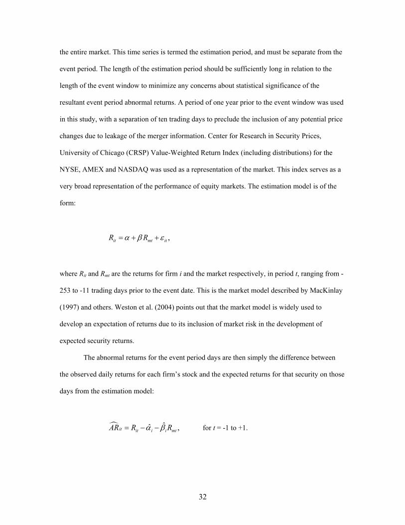
32
the entire market. This time series is termed the estimation period, and must be separate from the
event period. The length of the estimation period should be sufficiently long in relation to the
length of the event window to minimize any concerns about statistical significance of the
resultant event period abnormal returns. A period of one year prior to the event window was used
in this study, with a separation of ten trading days to preclude the inclusion of any potential price
changes due to leakage of the merger information. Center for Research in Security Prices,
University of Chicago (CRSP) Value-Weighted Return Index (including distributions) for the
NYSE, AMEX and NASDAQ was used as a representation of the market. This index serves as a
very broad representation of the performance of equity markets. The estimation model is of the
form:
,it mt itR Rα β ε= + +
where Rit and Rmt are the returns for firm i and the market respectively, in period t, ranging from -
253 to -11 trading days prior to the event date. This is the market model described by MacKinlay
(1997) and others. Weston et al. (2004) points out that the market model is widely used to
develop an expectation of returns due to its inclusion of market risk in the development of
expected security returns.
The abnormal returns for the event period days are then simply the difference between
the observed daily returns for each firm’s stock and the expected returns for that security on those
days from the estimation model:
ˆˆ ,it it i i mtAR R Rα β= − − for t = -1 to +1.

33
For each firm, the daily abnormal returns are tested for significance by calculating a t-statistic
using the standard deviation of daily excess returns from the estimation period. The three-day
ARs for each firm are summed to develop a firm cumulative abnormal return (CAR). These
returns are then multiplied against each respective firm’s market capitalization values for the day
before the event (t = -1), yielding the market’s impression of the value of the merger for each
firm. These two values can then be summed to determine the overall value of the merger.
The CARs of all target firms in our sample can be aggregated and tested for significance.
This test is also done for the acquiring firms. This allows us to compare the average returns of
target and acquirer firms in our sample to those of the general literature on mergers and
acquisitions. Finally, acquirer and target CARs are aggregated to one measure of mean abnormal
value, and tested for significance to evaluate the hypothesis of no value creation.
A problem of applying common significance tests to event study abnormal returns results
from the frequent occurrence of differing variances among sample firms during the event period,
as explained by Brown and Warner (1985). The resulting increase in the event period cross-
sectional variance often leads to false rejection of the null hypothesis of no abnormal value
creation. Boehmer et al. (1991) define a cross-sectional test statistic that allows for event-induced
variance changes by incorporating both estimation and event period variance estimates. Their
statistic is based on Patell’s (1976) and the common cross-sectional method, and compares the
normalized event-period returns to the cross-sectional standard error:
12
1 1
1
1 1( 1)
N
ii
N N
i ii i
SRNt
SR SRN N N
=
= =
=
− −
∑
∑ ∑

34
where SRi is the standardized abnormal return of firm i, equal to the event-period abnormal return
divided by the standard deviation of the estimation-period abnormal returns, and N is the number
of securities.
Long Term Event Study Methodology
Long term event studies measure the performance of a firm’s stock for a significant
period of time after the commencement of the event. To evaluate a merger, the stock of the
acquiring firm is analyzed for several years (usually between one and five), starting with the date
the merger becomes effective. Similar to a short term event study, the firm’s performance is
measured in excess of some benchmark to yield an abnormal return. If markets are truly efficient,
then regardless of any abnormal gains or losses immediately following the announcement of a
merger, the long term abnormal performance should not be significantly different from zero.
Two important aspects of analyzing abnormal long term stock price performance concern
how the returns are accumulated through time, and the benchmark against which they are
measured. Long term studies sometimes compare the firm’s stock price performance to that of a
matching firm that has similar characteristics as the firm undergoing the event, but that did not
itself experience the event. Another benchmark may be a constructed index, or portfolio,
representing firms with similar characteristics, such as size, industry or risk. Proponents of the
Fama and French (1992) three factor model use portfolios of firms with similar size and ratio of
book value to market value. The simplest benchmark can be a broad market index, such as the
CRSP value-weighted market index, or the S&P 500 index.
This presents a situation known as the joint hypothesis problem, where we are testing
both market efficiency and the correct model of security returns (Fama (1970), Andrade et al.
(2001)). If our analysis shows an abnormal return, we must retain a degree of hesitance in
accepting this as true, abnormal performance, since our model of expected returns is, almost
certainly, not exactly correct.
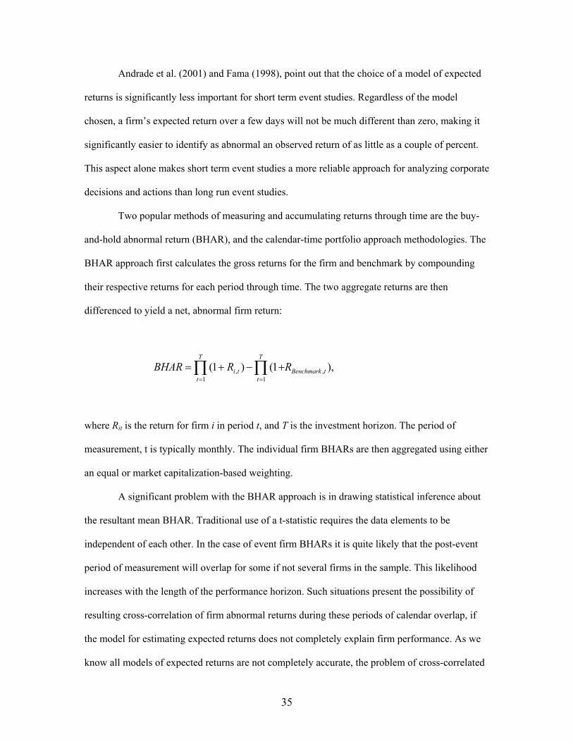
35
Andrade et al. (2001) and Fama (1998), point out that the choice of a model of expected
returns is significantly less important for short term event studies. Regardless of the model
chosen, a firm’s expected return over a few days will not be much different than zero, making it
significantly easier to identify as abnormal an observed return of as little as a couple of percent.
This aspect alone makes short term event studies a more reliable approach for analyzing corporate
decisions and actions than long run event studies.
Two popular methods of measuring and accumulating returns through time are the buy-
and-hold abnormal return (BHAR), and the calendar-time portfolio approach methodologies. The
BHAR approach first calculates the gross returns for the firm and benchmark by compounding
their respective returns for each period through time. The two aggregate returns are then
differenced to yield a net, abnormal firm return:
, ,1 1
(1 ) (1 ),T T
i t Benchmark tt t
BHAR R R= =
= + − +∏ ∏
where Rit is the return for firm i in period t, and T is the investment horizon. The period of
measurement, t is typically monthly. The individual firm BHARs are then aggregated using either
an equal or market capitalization-based weighting.
A significant problem with the BHAR approach is in drawing statistical inference about
the resultant mean BHAR. Traditional use of a t-statistic requires the data elements to be
independent of each other. In the case of event firm BHARs it is quite likely that the post-event
period of measurement will overlap for some if not several firms in the sample. This likelihood
increases with the length of the performance horizon. Such situations present the possibility of
resulting cross-correlation of firm abnormal returns during these periods of calendar overlap, if
the model for estimating expected returns does not completely explain firm performance. As we
know all models of expected returns are not completely accurate, the problem of cross-correlated

36
firm BHARs is both real, and problematic. Mitchell and Stafford (2000), Fama (1998), and others
point out that this is not surprising. For one, in a study of the returns to firms that have merged,
by definition the sample set is not random; it is made up exclusively of firms that share the
characteristic of having chosen to undertake a specific, dramatic project. Second, this problem is
magnified in a study such as ours where our sample is from one industry alone, within which
some correlation of performance must clearly be expected.
While Mitchell and Stafford (2000) show that it is possible to calculate corrected t-
statistics by either estimating or calculating actual correlations between firm BHARs, they point
out, along with Fama (1998), that the problem can be completely avoided by using the calendar
time portfolio approach for measuring long term abnormal performance. This approach was first
utilized by Jaffe (1974) and Mandelker (1974). It removes the focal point for measuring returns
from the individual firm over time to the unit of time itself. In other words, if monthly returns are
the unit of measure, and the time horizon of long term performance is three years, the BHAR
approach aggregates firm abnormal monthly returns over three years. The calendar-time approach
however, forms a portfolio of abnormal firm returns for each calendar month. The respective
abnormal return for a firm is included in a portfolio for a given calendar-month if that firm
concluded its merger within three years prior of that particular month. The first calendar-month
will start one month after the first firm in the sample concluded its merger, through three years
after the last firm in the sample concluded its merger. So the portfolio of abnormal returns is
reformed each month across this horizon. The monthly firm abnormal returns in each monthly
time period of the portfolio are averaged, yielding a mean abnormal return for each calendar-
month. This time series of portfolio average abnormal returns are then averaged to yield a final,
mean monthly abnormal return. This mean monthly return is multiplied by 36 to yield a mean
three year abnormal return.
The calendar-time portfolio approach mitigates the compounding effect of the poor
model problem inherent in long term BHARs. It also avoids the problem of cross-sectional
37
correlations of firm abnormal returns in a time period, as the variance of the time series of
portfolio mean monthly returns accounts for this. The number of different firm abnormal returns
in the portfolio for a given month will vary through time, resulting in heteroskedasticity of the
portfolio abnormal return. This can be controlled by standardizing the portfolio’s monthly
abnormal returns using an estimate of the standard deviation of each month’s return.
The only remaining question, for both the calendar time portfolio and BHAR approaches,
is whether to weight the individual firm abnormal returns equally or by their value. In his review
of several long-term event studies, Fama (1998) found that many individual study result
anomalies can be attributed to the use of equal rather than value weighting of abnormal returns to
yield the average abnormal return. He argues that all models of expected returns struggle to
accurately explain the returns of small stocks. Since small stocks play a much lesser role in
determining an average return when weighted by value, this element of the “poor” model problem
diminishes.
Merger Analysis Research Findings
Numerous short term event studies have shown that, on average, substantial wealth is
created for the target firms of mergers, while the acquiring firms generally experience either no
wealth creation or a slight loss in value, often statistically insignificant. In looking at the
combined return of both merging firms, weighted by firm size, which is the most appropriate
measure of value creation, most studies show a statistically significant return of a few percent.
This conclusion has been reached by Jensen and Ruback (1983); Jarrell, Brickley and Netter
(1988); and Jarrell and Poulsen (1989), among others. Andrade et al. (2001) found that target
firms in merger announcements during the 1990’s enjoyed an abnormal return of 15.9% over a
three day event window surrounding the merger announcement date. The corresponding acquiring
firms had a -1.0% abnormal return. The average target return was statistically significant at the α
= 0.05 level, the acquirer average return was not. The average combined return for both acquirer

38
and target was 1.4%, statistically significant at α = 0.05 level. Mulherin and Boone (2000) also
analyzed merger activity during the 1990’s and found a weighted net creation of value of 3.5%
for acquirer and target.
The form of payment used by the acquiring firm to finance the acquisition of the target
has been shown to affect the creation of wealth. Fuller, Netter and Stegemoller (2002) analyzed
firms that made five or more acquisitions within a three year period during the 1990’s. By
analyzing multiple acquisitions, they were able to isolate characteristics of the deal separate from
those of the acquiring firm. They found that when cash is used to finance the acquisition, wealth
creation for acquiring firms at the time of the merger announcement is not significantly different
from zero. When stock is used, however, returns to the acquirer are usually negative. This finding
was also noted by Andrade et al. (2001). Their interpretation is that acquiring firms often will
choose to issue equity when they feel it is overvalued, with the expected result of a downward
exertion on the price by the market.
The efficient market hypothesis tells us that all gains from a merger should be priced into
the firms’ stock valuation immediately upon the merger announcement. There should be no
abnormal long run stock price performance that can be directly attributed to the merger. Long
term event studies on merger performance somewhat agree with this premise, often finding small
negative abnormal returns, but usually not significantly different than zero. Individual study
results widely vary. Such trends are in part due to the variance in calculating what the expected
return should be; as previously discussed many different acceptable performance benchmarks
exist. Whether the particular research method yields a mean abnormal return from which
statistical inference can accurately be drawn is also important. If the cross-correlation of firm
BHARs are not properly accounted for when using that methodology, t-statistics are often
severely overstated (Mitchell and Stafford 2000).
Also impacting average results are whether the sample firms are aggregated on an equal
or value weighted basis. By segregating results this way, and using the calendar-time portfolio

39
approach Mitchell and Stafford (2000) attributed most of the statistically significant negative
abnormal performance to the smallest quintile of firms; when weighting the sample firm
abnormal returns by market capitalization, they found an insignificant three year abnormal mean
return of -1.4%. Similar to short term study findings, method of payment has been shown to
impact long term performance. Both Mitchell and Stafford (2000) and Loughran and Vijh (1997)
found that mergers financed with cash perform better than do those financed with the acquirer’s
stock. Perhaps the most interesting is a conclusion reached by Mitchell and Mulherin (1996) that
negative abnormal post-merger performance is often tied to shocks and turbulence within the
respective industries, which often was a primary reason for the merger.
Conclusion
Published research investigating the financial risk of timberland investments has found
timberland to be relatively insensitive to broader financial market risk. Timberland has also often
been found to outperform the return required by its commensurate market risk. This dissertation
reexamines this research, utilizing data that is both eight years more current, and that is closer to
being based purely on market transactions than many of the data series previously used by
researchers. Timberland as an asset class has consistently been found by researchers to warrant a
position within diversified portfolios of financial assets. This research extends that conclusion by
investigating the security selection process of timberland investments within the US South.
Finally, recent mergers and acquisitions within the American forest products industry, key events
that have impacted the holders of indirect timberland investments, are measured to determine if
shareholder value has been created.

40
CHAPTER 2
ASSESSING RISK AND RETURN WITHIN A PORTFOLIO OF US SOUTH TIMBERLAND
INVESTMENTS4
4 Cascio, A.J. and M.L. Clutter. To be submitted to Pensions and Investments, August 2006.

41
Abstract
We apply modern portfolio theory to assist in the optimal construction of portfolios of
sub-regional timberland assets within the US South. First, we develop a unique set of synthetic
timberland returns for 22 sub-US South regions, for a 19-year time horizon. Portfolio
optimization was performed with these 22 return series, and an efficient frontier identified with
portfolios having risk levels ranging from 3.9% to 13.8%, and expected return levels of 10.4% to
13.4%. The optimal tangency portfolio was identified having expected return and risk levels of
11.2% and 4.2%, respectively. Recognizing the constrained and discontinuous nature of the
availability of timberland on the market at any given time with respect to acquisitions for
institutional investors, we explore the impact these factors can have upon optimal portfolio return
and risk. We numerically express the prominence and limitations of efficient portfolio allocations
for three scenarios of acreage allocation constraints. Finally, Monte Carlo simulation is utilized to
estimate the value at risk (VAR) of a hypothetical ten year, regionally-diversified timberland
investment.

42
Introduction
Investment grade timberland serves as an important asset class in well-diversified
portfolios of institutions. Its use in this role has grown significantly in recent years. It is now
estimated that institutions currently own approximately $23 billion of timberland in the United
States (DANA Limited 2006, Timber Mart-South 2006b). Unfortunately, little empirical data
exists to describe the risk and return characteristics of timberland. Such information is necessary
to utilize modern portfolio theory to evaluate the proper inclusion of timberland in a portfolio of
other, more conventional financial assets. Existing return data suffers from several shortcomings,
namely: the relatively short length of the history of the data; the infrequency of the data; and
concerns regarding whether the data are representative of the asset class as a whole. While
enough data exists to perform asset class allocations of timberland and other assets using a
portfolio optimization framework, the next step is more difficult. Continuing the asset allocation
analysis at a more refined level, or performing security selection of specific timberland properties
within a portfolio optimization framework has been prohibitive due to the lack of timberland
return data at lower geographic levels.
We develop synthetic return series for timberland in 22 different geographic regions
within the South, at an annual frequency and covering the period 1987-2005. This sub-regional
return data allows portfolio optimization at a level of geographic detail significantly finer than
previously possible. While national or regional timberland return indices can be effectively used
to guide an investor to allocate funds to the timberland asset class, the more detailed return series
developed here can assist in the determination of an optimal geographic allocation of that portion
of the investor’s portfolio. Specifically, the prominence of timberland from these 22 different
regions within a portfolio at different required risk levels can be assessed. We develop a measure
of this prominence, or persistence, which is useful for an investor to better screen potential
timberland investments for inclusion in a portfolio. A unique characteristic of timberland
investing is the limited and finite availability of potential timberland acquisitions. While a small,

43
private investor may perceive the market of available timberland investments as infinite, a typical
co-mingled fund constructed by a timberland investment manager for offering to multiple
investors may be of a size that would preclude the unconstrained allocation of portfolio funds to
any particular individual asset region. It is therefore important to recognize asset availability
constraints when conducting portfolio optimization. Our measure of sub-regional asset
prominence incorporates the impact of asset availability limitations.
Value at risk (VAR) is a method of measuring the financial risk of a portfolio over some
specified period of time. VAR estimates the maximum reasonable loss that could be expected.
‘Reasonable’ is usually defined as the portfolio value at the 5% probability level of a distribution
of possible returns. The portfolio value at this level could be positive or negative. To estimate the
VAR of an investment the distribution of expected returns for the given portfolio of assets and
allocations must be estimated. If a normal distribution of returns is assumed, the 5% VAR will
equal the expected portfolio value less 1.645 standard deviations of the expected return. We can
use Monte Carlo simulation to estimate the distribution of expected returns for a timberland
portfolio after each year of a ten year investment, without concern for normality. With this
distribution, we estimate the 5% VAR.
Literature Review
A fundamental assumption of investment analysis is that investors are risk averse. This
means that, all else being equal, investors prefer greater returns, while taking a minimal amount
of risk. While investors have known for centuries that diversification, or spreading one’s funds
(value) among several investments carries less risk than investing in a sole asset, Harry
Markowitz (1952) formalized the relationship of diversification and the combination of assets. He
showed that, while the expected return of a portfolio of assets is simply the expected return of
each asset multiplied by the asset’s weight in the portfolio:

44
[ ] [ ]P i ii
E R x E R=∑ ,
the risk of the portfolio is much more than a simple function of each asset’s own risk and
portfolio weighting. Rather, the most important aspect concerning an individual asset and
portfolio risk is the correlation of that asset’s returns through time with the other assets in the
portfolio. As Rubenstein (2002) states:
‘Probably the most important aspect of Markowitz’s work was to show that it is
not a security’s own risk that is important to an investor, but rather the
contribution the security makes to the variance of his entire portfolio – and that
this was primarily a question of its covariance with all other securities in his
portfolio’.
In a portfolio of n assets, where xi represents the proportion of funds allocated to asset i,
and σi is the standard deviation of asset i, Markowitz (1952) stated the risk of the portfolio as the
variance of a weighted sum:
2
1 1,
n n
P i j ij i ji j
x xσ ρ σ σ= =
=∑∑
where iσ and jσ are the standard deviations of assets i and j, ijρ is the correlation between
assets i and j, and ij i jρ σ σ is the covariance between the two assets. Standard deviation, the
conventional measure of portfolio risk, is the square root of this equation. Two important facts
about portfolio risk bear discussion. It is intuitive from the above equation that the lower the
measure of correlation of two assets in a portfolio, the lower will be the portfolio variation. Two

45
stocks whose historical movements are perfectly linearly correlated will have a correlation
coefficient of 1, resulting in a contribution to portfolio variance equivalent to the weighted
average of their individual standard deviations. So, anything less than perfect correlation between
two stocks will contribute to a lower portfolio variance, and hence less financial risk.
There is a limit, or floor to portfolio variance reduction possible through diversification.
The risk that is removed from diversification is termed firm-specific, or idiosyncratic risk. This
risk is due to specific actions, events, and news pertaining to the individual firm. The risk that
remains is termed market risk, or systematic risk. This is the risk due to economy-wide events and
news, and that affects most all firms. Systematic risk cannot be removed from the portfolio with
diversification.
The impact of covariance between assets in the calculation of portfolio standard deviation
prevents an investor from determining the optimal portfolio of assets by examining their
individual expected returns and risks. Instead, the combined risk of the group of assets,
determined primarily by their co-movement, or covariance, must be examined holistically.
Markowitz utilized these portfolio expected return and risk equations to calculate the
optimal combination of return and risk levels by varying portfolio asset weights. For each
possible level of portfolio expected return, the weights of each asset in the portfolio can be altered
to yield a minimum portfolio standard deviation. Such a portfolio is said to be minimum variance.
Plotting each of these minimum risk levels for a change in expected return yields a curve we term
the efficient frontier. Conversely, the efficient frontier can be calculated by iteratively specifying
a required portfolio standard deviation and then varying the asset weights until a maximum
portfolio expected return is determined. A portfolio constructed in this manner is said to be mean-
variance efficient. This process of developing the efficient frontier is often referred to as
Markowitz portfolio optimization. Computationally, this process is a constrained optimization

46
problem, where, in the case of maximizing return for a given risk 2Pσ , it can be described
mathematically as:
max [ ],PxE R
subject to the constraints:
2
1 1
1
,
1,
0
n n
i j ij Pi j
n
ii
i i
x x
x
x
σ σ= =
=
=
=
≥ ∀
∑∑
∑
for an n-asset portfolio, with each asset having portfolio weight xi. Constraining the sum of the
asset weights to 1 requires the portfolio to be fully invested. Requiring each asset weight to be
non-negative enforces the rule of not allowing any short sales. Markowitz portfolio optimization
is referred to as a one-period model. The portfolio return and risk based on any combination of
asset allocations can only be expected to hold for one period, where the length of this period
matches the frequency of the time series of data used in the model. However, analysts and
investors do not always limit their horizon of return and risk expectations to one period. This
approach to optimal portfolio construction is widely used among institutional investment
managers today (Rubenstein, 2002).
By utilizing the risk-free rate, the optimal portfolio can be identified. This portfolio is the
one that results in the steepest slope of the line drawn from the risk-free rate on the y-axis to the
tangency point on the efficient frontier. The slope of this line is termed the reward-to-variability
ratio. We can use this ratio, also termed the Sharpe ratio, to solve for the optimal portfolio
allocations by stating it as the objective function:

47
( [ ] )max ,P f
xP
E R Rσ−
To assess different investments within a portfolio optimization context, historical return
series for each asset are needed. Using these series, the three data elements for conducting
portfolio optimization can be constructed: asset expected return and risk matrices of correlations
and covariances can be computed. Historical return data for timberland investments are
unfortunately sparse.
Timberland Return Drivers
Timberland investment returns are generated through two components: income and
capital appreciation. Income is received primarily from the periodic sale of timber, which in turn
is used in the manufacture of lumber; panel products such as plywood, oriented-strand board
(OSB) and fiberboard; paper; packaging; and several types of specialty chemicals. An attractive
characteristic of selling timber is that it can be withheld from the market during times of low
prices at no cost. There is no ‘storage fee’, and in fact the timber continues to grow and often
appreciate until more favorable market conditions return. Annual income is also often received
from the leasing of recreation rights on the land, primarily for hunting.
Capital appreciation is realized from the continuous biological growth of the trees. In
addition, larger trees are more valuable per unit than are smaller trees, due to the fact that
telephone poles, plywood veneer and the larger sizes of lumber, some of the highest valued
products made from trees, can only be made from larger trees. Therefore as a tree crosses a
certain threshold from one size class to another, its value per unit increases. For southern yellow
pine species, there are three predominant size classes: pulpwood, from which is made paper and
OSB; chip-n-saw, from which small dimension lumber is made; and sawtimber, used in the
manufacture of wider dimension lumber, poles and plywood.

48
The price paid for timber varies by tree size, region and season. Finished good prices also
have an impact on timber prices. However, Binkley (2000) documented the price of southern pine
sawtimber has increased at a compound annual real rate of 2.6% from 1910 to 2000. Timber price
increases are exhibited not only in the income component of timberland returns, but also in the
capital appreciation component, because a key element of the capital appreciation of timberland is
the increase in the value of the land itself (Caulfield 1994). This increase is attributable to two
factors: first, the increase in the value of the land for producing timber due to price increases
(Washburn 1992), and the conversion of a portion of a timberland portfolio to a higher-valued use
than the production of timber, such as residential or commercial development, during the
investment period.
Timberland Return Data
The only timberland return index currently in existence5 that is based on actual
timberland transactions and appraisals is the National Council of Real Estate Investment
Fiduciaries Timberland Property Index (NCREIF, 1994). NCREIF publishes historical return data
for timberland investments managed by its members, at two geographic levels: the United States,
and three regions within the US: the Pacific Northwest, the Northeast and the South. The
NCREIF Timberland Property Index segregates a total return into income and capital appreciation
elements, and is based on actual data reported by its members managing timberland investments.
Hancock Timber Resource Group (2003a) describes how NCREIF began compiling and
publishing a quarterly index of timberland property returns in 1994, with data retroactive to 1987
for the Southern and Pacific Northwest regions in the United States (1994 for the Northeast). This
index tracks changes in value of timberland properties that are a) held in a fiduciary environment,
as opposed to the myriad other ownership objectives shared by many other timberland owners;
5 The Timberland Performance Index (TPI) (Caulfield,1994) is similar to the NCREIF index, however it is no longer in existence.

49
and b) “marked to market” at least annually. If the property does not experience a change in
ownership during a year via a sale, then it is appraised at year end to yield a new value. As a
timberland investment organization joins NCREIF, they submit historic returns for their
properties to augment the index.
The Timberland index is built and maintained similarly to NCREIF’s other commercial
real estate indices. The index has four basic components: the market value of all properties in the
index; the EBITDDA return for the properties; the capital return; and the total return. The
EBITDDA return, or earnings before interest expenses, taxes, depreciation, depletion and
amortization, is based primarily on the sale of harvested timber during the quarter. However,
many timberland property owners lease recreation use rights to clubs or individuals, the income
from which is also included in the EBITDDA portion of the total return. It must be noted that the
EBITDDA figure is gross of applied management fees charged by the property manager, and
therefore overstates the true net income received by the investor (Healey et al. 2003). The
EBITDDA income component of the return is analogous to the dividend component of a stock
return.
The capital appreciation component is basically the ratio of the difference in period-to-
period property market value, minus capital expenditures in the current period, to the market
value of the previous period. Timberland appreciation is measured by periodic appraisals.
Appraisals are conducted both externally by consultants and internally by the managing
organization. Major, externally-conducted appraisals often occur on a three year cycle, although
more frequent timing is becoming common (Clutter, 2006). Annual external updates (in the other
years) are performed by some management organizations, while others use internal updates of
various types. All organizations perform quarterly updates that are based on harvested timber
removals, merchantable timber growth, and timber price changes. These quarterly updates rarely
include land appreciation, nor account for changes in the value of premerchantable timber
(Clutter, 2006). The majority of external appraisals are conducted in the fourth quarter of the
50
year. Since appraisals are not evenly distributed throughout the year, reported quarterly property
returns are less meaningful. For analysis purposes, it is recommended that annual returns be used
(Hancock Timber Resource Group 2003a).The United States-wide timberland index is subdivided
into three regional indices: South, Pacific Northwest and Northeast.
Investing in timberland by institutions is relatively new. It can be tracked to the passage
of the Employee Retirement Income Security Act (ERISA) in 1974 that required institutional
investors to diversify their portfolios away from traditional common stocks and fixed income
securities to broader classes (Zinkhan 2003, Healey et al. 2003). Investments in timberland by
institutions grew by a factor of ten during the 1990’s to some $17 billion by 2005 (DANA
Limited 2006). This is reflected in the time span of the NCREIF Timberland Property Index.
Although the NCREIF series is regarded as the best data available describing the performance of
institutional investments in timberland, the need to analyze the financial performance of
timberland predates the existence of this index. Before this time, most analysts constructed
synthetic return indices with several management assumptions for use in timberland investment
analyses.
Timberland returns value to the owner through a combination of periodic income and
capital appreciation, as previously discussed. The return formula common to financial security
appreciation is applicable for measuring timberland returns:
1
1t tt
t
NI CVRCV −
+= − , (1)
where:
Rt = total return per acre of the asset during period t;
CVt = capital value per acre of the asset during period t;
NIt = net income received per acre of the asset during period t.

51
Many assumptions about forest management practices must be made when developing a
synthetic timberland return series. One that is common among most authors is that the
hypothetical forest being modeled is fully-regulated. This implies that the volume of timber
harvested each period is equal to the volume grown. The standing volume of timber in the forest
is therefore static over time, and there are equal amounts of area in each age class. This allows
any capital appreciation of the forest to be reflective of timber or land price appreciation,
inflation, or some other factor, but not from any implied change in the inventory of the asset.
Revenue realized from the sale of harvested timber represents the periodic income component.
Mills and Hoover (1982) and Mills (1988) used this basic formula to synthesize time
series of returns from hypothetical uneven aged, multi-species hardwood forests in west central
Indiana. Annual rates of return from 1959-1978 were estimated. No direct empirical data for the
return formula components existed at that time, requiring the authors to incorporate several
assumptions reflecting forest management practices and productivity, disaster occurrence
probabilities, lumber market conditions and land appreciation, with which they could estimate the
income and capital value components. The authors likewise developed synthetic annual return
series representing agriculture investments, both crop and livestock. They then analyzed these
investments in a portfolio optimization context along with traditional financial assets. Their
results suggested that portfolios of forestland assets alone might yield low, risky returns relative
to portfolios of typical financial assets. However, they found that by combining forestland
investments with more traditional financial investments in their portfolio, investors could expect
moderate returns with decreased risk, as opposed to portfolios with financial assets alone.
Redmond and Cubbage (1988) constructed species-based synthetic timberland return
series for multiple commercial timber species in the United States. Return series based on
particular timber products were developed as well, such as southern pine sawtimber and
pulpwood. The formula was based on a sum of annual stumpage price change and a measure of

52
average annual timber growth. Redmond and Cubbage used these return series to estimate CAPM
betas for the respective species and products combinations.
Conroy and Miles (1989) developed a monthly return series from 1976-1986 representing
a hypothetical commercial Southern pine forest. Assumptions were made for silvicultural costs,
management prescriptions, and harvest volumes. Timber product prices reported in Timber Mart-
South were used, along with representative farmland values for the land appreciation component.
The authors altered the rotation age to determine the impact on average monthly return and
standard deviation. They then formed optimal portfolios with timberland and the traditional
financial asset categories of large and small capitalization stocks, and US treasury bonds and
bills. Conroy and Miles (1989) found that timberland occupied a significant position in the
optimal portfolio depending on the required portfolio return.
Zinkhan and Mitchell (1990) utilized a synthetic return series for Southern pine from
1977-1987, developed by a timberland investment firm, to analyze portfolio allocation. The
return series utilized published south-wide pine stumpage prices, timber harvests from a typical
southern pine management regime, and proprietary land appreciation rates. They found that
including timberland in a portfolio of representative financial assets reduced the risk of efficient
portfolios by an average 43%, and timberland was allocated asset weights of as much as 30% of
the portfolio value.
Geographic diversification of timberland investments has long been known to reduce
overall risk from damage by natural disasters, such as insect, fire and storm damage. Hancock
Timber Resource Group (2005) discussed how damage to some of their timberland holdings in
Mississippi, Louisiana and Alabama suffered as much as a 12% loss in market value due to
damage caused by the Hurricanes Katrina and Rita in 2005. Yet when viewing their total
Southern timberland portfolio, the loss in market value from these two storms was less than one
percent. Likewise, losses dropped even further when viewing their total North American
timberland portfolio.

53
Hancock Timber Resource Group (2003b) used synthetic timberland return series in a
portfolio optimization context to evaluate regional and global diversification potential. Their
model, the John Hancock Timberland Index (JHTI) uses only one time series data component: the
quarterly stumpage price of the appropriate timber species group for the region modeled. For the
US South, the stumpage price is a composite price equal to the equally-weighted average price of
pine pulpwood and sawtimber. The return income component is simply the quarterly stumpage
price multiplied by a subjective factor that represents the regional ratio of periodic income to the
capital value of the representative forest. The capital value component is a weighted average of
the previous eight quarters stumpage prices, with progressively less weight given to each
preceding quarter’s price. Each year’s four quarterly returns were then averaged to yield an
annual return. Hancock Timber Resource Group estimated return series from 1960-1986 to
provide a longer history of timberland returns than possible using the NCREIF series alone,
which begins in 1987. By combining these two return series, Hancock Timber Resource Group
(2003b) was able to analyze portfolio opportunities utilizing returns spanning 1960-2002. They
found the different US regional and international return series were not highly correlated,
allowing significant reduction in portfolio risk by combining regional assets into a global
timberland portfolio.
Caulfield (1998) used the Timberland Performance Index (TPI) to evaluate the
timberland asset class from 1981-1996 within a portfolio optimization context. The TPI is similar
to the NCREIF index in that it is an actual asset-based index. However, it is no longer in
existence. Like Hancock, Caulfield found that adding timberland to a diversified portfolio
increased expected returns for given levels of risk.
The role of risk reduction for a timberland investment portfolio via species diversification
has been explored within a portfolio optimization context by Thomson (1987, 1991, 1992). He
developed synthetic return series for pine, ash, oak and gum species in Louisiana, and for white
pine, red pine, aspen and red oak species in Minnesota. Similar to Mills and Hoover (1982),

54
Thomson developed explicit hypothetical forest management regimes to arrive at estimates of
annual income and capital appreciation components for the return equation. He included costs and
revenues reflecting land rent, site preparation, planting, administration, taxes and timber revenue.
In comparing portfolios of Southern and Midwestern timberland investments, Thomson (1987)
found that Southern timberland portfolios offered superior returns for any given risk level, that
portfolios of assets from both regions dominated the Southern timberland portfolio, and that
portfolios combining timberland and a broad market investment (S&P 500 Composite Index)
dominated timberland-only portfolios.
A typical institutional investment in timberland is made via a closed-end, co-mingled
fund having a horizon of ten years. Additions to the timberland portfolio are sometimes made
during the fund lifetime. Segments of the portfolio are also sometimes disposed of before the fund
expires. This is usually done for portions of properties that experience a significant increase in
value for uses other than growing timber, such as development. Fund managers commonly
perform an analysis of all properties on an annual basis to determine whether they should be
retained in the portfolio or sold. However, the bulk of the timberland properties in the fund
remain fixed during the fund’s lifetime. Therefore, although Markowitz portfolio optimization
gives a one-period solution, that approach generally suffices for institutional timberland
investments. It is nevertheless interesting to examine this type of investment performance over its
lifetime. An element of such a long-term timberland investment that has not been previously
explored is its value at risk (VAR). The final section of Chapter 2 develops and compares VAR
estimates of three intra-South timberland investment portfolios. Methods for modeling a portfolio
over multiple periods are next discussed, followed by a discussion of VAR estimation.
Thomson (1991) analyzed the expected performance of timberland within a portfolio of
financial assets from both a short and long term perspective, using the same synthetic timberland
return series from Thomson (1987). In addition to employing Markowitz portfolio optimization to
arrive at portfolio asset weights, Thomson (1991) also used a power utility function, an approach

55
which attempts to maximize long-term portfolio wealth by maximizing the logarithm of portfolio
returns, subject to a specified proxy for risk tolerance. Similar to previous analyses, his results
showed that diversification among financial and timber assets generated the highest risk-adjusted
expected returns, and that diversification among timber species also reduced risk. Thomson found
that the two portfolio construction approaches of Markowitz single period optimization and the
power utility function generated similar results for both one- and multi-period solutions.
Thomson’s (1991) technique for conducting long-term portfolio analyses utilizing
Markowitz optimization begins by solving for a one period solution. Then, stochastic techniques
are used to estimate the portfolio value at the end of the investment horizon. The fundamental
premise is to assume that the expected return for each portfolio asset in any year of the
investment horizon is equally likely to be one of the returns within the asset’s time series of
historical returns used to develop the portfolio allocations. An index, or period of the historical
returns is randomly chosen, and each asset’s return corresponding to that index is multiplied
against that asset’s weight in the portfolio, which remains constant across the investment horizon.
These weighted returns are summed to yield one portfolio return. Choosing each asset’s return
from the same point in time ensures that the correct asset correlations are maintained. This
process is repeated for each year in the horizon. Portfolio returns are compounded to yield a total
return. This process is repeated 1,000 times. The 1,000 total returns, t1000, are then converted to
compound rates of return, or geometric mean returns, by raising each t to one over the length of
the horizon. The 1,000 geometric mean returns are then averaged to yield a mean expected
compound rate of return and an estimated standard deviation.
Value At Risk
In the mid 1990’s a metric for characterizing the financial risk of an investment was
developed in the wake of several significant disasters involving derivatives investments (Jorion
1996, Culp et al. 2003). Value at risk (VAR) is a method of measuring the financial risk of a

56
portfolio over some specified period of time. VAR estimates the maximum reasonable loss that
could be expected. ‘Reasonable’ is usually defined as the portfolio value at the 5% probability
level of a distribution of possible returns. The portfolio value at this level could be positive or
negative. A key characteristic of VAR is that its unit of measure is in dollars, not percent, which
may more acutely and accurately convey the message of the possible loss (Jorion 1996).
Manfredo and Leuthod (1999) describe the two classes of procedures for estimating
VAR: parametric and full-valuation methods. Parametric methods are based on the assumption of
a normal distribution of expected returns for the investment. With this assumption, only the mean
and variance of the outcome distribution, which fully characterize it, need to be known. The 5%
VAR will equal the expected portfolio value less 1.645 standard deviations of the expected return.
If the expected outcome distribution is not normal, then a full-valuation procedure must
be used to estimate the VAR. To estimate the VAR of an investment the distribution of expected
returns for the given portfolio of assets and allocations must be estimated. Simulation methods
are used to generate the full distribution of expected returns, often using randomly chosen past
values of portfolio asset returns as future values. Once a full distribution of returns is estimated,
one simply reports the return at the 5% level as the VAR, or worst-case scenario. To date, VAR
estimates for institutional timberland investments have not been addressed in the literature.
Data
We developed a modified version of the John Hancock Timberland Index (JHTI) model
of timberland returns to construct synthetic return series for 22 different areas within the US
South for 1987-2005, where the areas correspond to those defined by Timber Mart-South (TMS
2006(a), Figure 2.1). Timber Mart-South divides each of 11 Southern states into two areas, and
reports both stumpage and delivered prices for southern pine and hardwood species groups, and
for the major product classes. Prices are reported on a quarterly basis. Similar to Hancock Timber
Resource Group (2003b) we utilize pine stumpage prices to estimate an annual return series.

57
Aside from using regional rather than South-wide prices, our series differs from
Hancock’s in four ways. First, we include pine chip-n-saw as a product component to add more
depth to the series, due to the increasing prominence of small-diameter sawtimber in some
southern regions. Second, we estimate unique harvest weights for the three product classes in
each region to apply to the quarterly prices, rather than using an equal, or otherwise arbitrary
weighting factor. Third, we estimate the income rate, representing the quarterly ratio of periodic
income to capital value of an investment-grade forest, based on a comparison of our series to the
reported NCREIF South return series from 1987-2005. Finally, we utilize the composite
stumpage prices of the 12 most previous quarters for the capital value component rather than 8
quarters. This results in slightly less volatility of the return series, closer to that of the NCREIF
South series.
From (1) the net income and capital value components for region r in quarter t are:
11
( )0
,
(12 ),
78
rt rt
r t nn
rt
NI P Income Rate
n PCV
−=
=
−
=∑
(2)
(3)
where:
1 $ 2 $ 3 $rt rt rt rt rt rt rtP W ppwd W cns W pst= + + , (4)
and ppwd$rt, cns$ rt and pst$ rt are the pine pulpwood, chip-n-saw and sawtimber prices reported
in Timber Mart-South for region r in period t.
Region-specific product harvest weights (W1-W3) were estimated from United States
Forest Service (USFS), Timber Product Output (TPO) data (USFS Southern Research Station

58
2006). The USFS periodically surveys mills throughout the South to determine the quantity of
wood consumed by product type. They then estimate the origination of these volumes based upon
USFS Forest Inventory and Analysis (FIA) inventory data, along with assumptions regarding mill
basin radii, etc. The result is a table of estimated timber volume harvested by species group and
product class. This table is reported for each county of each southern state. TPO data exists for
each state for three different points in time. For most states, the data reflects conditions in 1995,
1999 and 2003, with the exception of Louisiana and Arkansas, for which harvest data is reported
as of 1996, 1999 and 2002.
The USFS also segregates this data by ownership group. The group most representative
of investment-grade timberland is the Forest Industry ownership group. There is not an
ownership group specifically representing institutional, or investment-grade timberland.
However, much current investment-grade timberland was at one time owned by an integrated
forest products company, and was therefore in the Forest Industry group at one time. Where that
was not the case, both groups nevertheless manage timberland quite similarly. Due to legislative
protocol, the USFS does not report timberland data of any sort at the county level, and segregated
by ownership group. Data is only reported by ownership group at the statewide level. Therefore, a
special request was made of the USFS, Southern Research Station. A file was sent to them
containing a Timber Mart-South region designation (1 or 2) for each county in each Southern
state. USFS personnel then aggregated harvest volume data by ownership group for all counties
in each TMS region, and returned this to us. We therefore received harvest volume data at the
TMS region level by ownership group, without violating USFS protocol.
Unfortunately, the USFS TPO data includes only one size class for pine sawtimber. It
does not segregate pine sawtimber into two size classes. The Southern Forest Products
Association (SFPA) 2002 Annual Mill Survey (Southern Forest Products Association 2003) was
referenced to provide an empirical method of apportioning regional sawtimber removal volumes.
This survey reports pine sawtimber consumption by US South sawmills, by size class. This

59
survey reports the consumption by size class at the Southwide level. By special request, the SFPA
agreed to disaggregate this data by state. The number of responding mills in the survey was quite
small when viewed at the individual state level, and judgment was used to refine this data. It
should be noted that this sawtimber size class apportionment represents a single point in time, yet
was used to apportion sawtimber volumes for the duration of each time series modeled.
The final parameter needed for estimating the return series is the Income Rate. This is a
south-wide, static estimate of the quarterly ratio of periodic income from a timberland investment
to its capital value. This parameter was estimated by first aggregating the 22 area harvest volume
product weights into south-wide weights over time. These weights were utilized in our quarterly
return model, along with TMS south-wide stumpage prices to estimate a south-wide return series
from 1987-2005. The quarterly return series was transformed into an annual series by time-
weighting the quarterly returns. The annual returns from this series were differenced from the
NCREIF-South series, and squared. The sum of these squared differences was minimized by
adjusting the Income Rate in the south-wide synthetic series. The resulting Income Rate value
was 1.49%. Figure 2.2 shows the NCREIF – South Timberland Performance Index and our
southwide synthetic timberland return series from 1987-2005. These two return series have a
correlation coefficient of 0.710 for the total 19-year history, and 0.936 for the most recent nine
years. This Income Rate value was then used in the calculation of each of the 22 area synthetic
return series. Table 2.1 displays the time-weighted annual synthetic returns, which comprise the
return series used in the subsequent portfolio analyses. Table 2.2 displays the correlation matrix
for these return series.
Portfolio Analyses and Discussion
After first calculating the covariance matrix for the 22 regional return series, the portfolio
optimization problem was solved for the set of mean-variance efficient portfolios across the range
of feasible portfolio risk levels. Figure 2.3 illustrates the portfolio expected returns plotted on the

60
right y-axis and the corresponding risk levels on the x-axis, yielding the efficient frontier. Solving
the portfolio optimization problem by maximizing the Sharpe ratio, or reward-to-variability ratio
yields expected return and risk levels of 11.2% and 4.2%, respectively. This is using a risk-free
rate of 4.5%. The Sharpe ratio is 1.60. Note that this is the same return level as the historical
NCREIF – South level for the 1987-2005 time period, yet risk has been reduced by 2.0%. The
resulting portfolio allocations to the respective regions are shown in Table 2.3. For traditional
financial investment decisions, the investor would then decide which portion of their portfolio to
allocate between the risk-free rate and the portfolio of timberland assets identified by this
tangency point, as a function of their unique risk tolerance.
This scenario is unconstrained in that we assume the supply of timberland for sale on the
market in each of the 22 regions is sufficient to support the optimal calculated allocations. In
reality, investment-grade timberland located in specific regions within the South on the market at
any given time is limited. Investment capital committed to the asset class by institutions may be
required to be placed in an acquisition in a timely manner (Caulfield and Newman 1999).
Likewise, timberland investment managers, who purchase timberland on behalf of multiple
investors, target a certain size acquisition, based on expected capital raised, or perhaps landbase
management characteristics or economies of scale.
Also assumed was the willingness or ability on the part of the investor to utilize risk-free
borrowing or lending with which to identify one optimal, tangency portfolio of specific
timberland tracts. Once the decision to invest in timberland as an asset class is made, the decision
of selecting available tracts within specific areas may be done without consideration of also
investing in the risk-free rate. In other words, a lack of detailed risk and return data for specific
timberland properties very likely precludes formal security selection procedures. These
characteristics often result in large scale timberland investing exhibiting a discontinuous nature
with regard to portfolio theory recommendations. Examining such allocation constraints with

61
respect to the width of the efficient frontier can assist the investor in evaluating available
timberland investment options.
Total investment-grade, southern pine timberland acres existing in each of the 22 areas
modeled were estimated using US Forest Service FIA 2002 state-level acreages for the Forest
Industry ownership class (Smith et al. 2004). State-level acreages were apportioned among the
two intra-state areas based upon the USFS TPO harvest weights utilized in the construction of the
area price series. Estimated acres for each area are shown in Table 2.3. The previously calculated
optimal portfolio allocated 41.7% of assets to three regions (AR 2, TX 1, VA 1) having combined
estimated pine investment-grade timberland of only 371,380 acres. Regardless of the amount of
timberland desired for purchase, the likelihood of being able to make such an allocation to areas
this small is highly unlikely.
As an example, Timber Mart-South (2006b) listed the timberland in each southern state
recently sold by International Paper Company. These lands, totaling 4.7 million acres, can be
analyzed within a portfolio optimization context to better understand realistic constraints
regarding large-scale timberland purchases. Judgment was used to apportion the state acreage
figures to the two respective areas within the state. These available acres were placed in the
portfolio model as upper bounds for allocation. A required amount of timberland to be purchased
was then assumed. Three scenarios of one, two and three million acres to purchase were
simulated. While a typical timberland fund for institutional investors would be comprised of most
likely up to a few hundred thousand acres, higher levels were used to acknowledge this unusually
large amount of land available for sale, keeping perhaps a more typical balance of desired
acquisition size versus available land.
Figures 2.4-2.6 show the efficient frontiers generated for the three constrained scenarios.
Identifying the tangency portfolios for these scenarios results in the optimal expected returns,
risks, Sharpe ratios and regional allocations shown in Table 2.4. Beginning with the
unconstrained scenario, the Sharpe ratios decrease from 1.60 to 1.05 with each increase in the

62
amount of timberland to acquire. This is intuitive. The optimal risk level of each increasingly
constrained scenario increases by an average of 0.7%, while the optimal expected return remains
nearly constant. This is not surprising given the relatively narrow range of expected returns across
the width of each scenario’s efficient frontier.
Table 2.4 lists the maximum allowable percentage allocation to each area as a function of
the acres available in each respective area and the total acres to be acquired. Also shown is the
average allocation to each area across the scenario’s efficient frontier of portfolios. This average,
or measure of prominence, yields insight into the relative importance of acquiring timberland in a
particular area if the optimal portfolio is not a realistic solution.
Beginning with the graph of regional portfolio allocations for the one million acre
acquisition scenario in Figure 2.4, and continuing through to the 3 million acre acquisition
scenario in Figure 2.6, a progressive flattening of several of the allocation curves is observed.
Such a flat section represents a range of feasible portfolio risk levels where the maximum
allowable allocation to a region was achieved. Such an occurrence suggests that more available
timberland in that particular region would allow an allocation that would result in a higher return
portfolio for that risk level. As an investor keeping abreast of timberland market conditions, such
information might be useful to guide acquisitions and divestitures of tracts not otherwise
apparent. For each region, dividing the number of efficient portfolios where the allowable
allocation constraint was reached by the total number of efficient portfolios yields the ratio
termed constrained allocations, also displayed in Table 2.4.
Long Term Timberland Investments and Value at Risk
Monte Carlo simulation techniques were used to estimate the 5% value at risk (VAR) of
three different timberland portfolios over ten year holding periods. The three portfolios represent
the optimal tangency portfolios for the 1-3 million acre scenarios previously described. @Risk
simulation software was used to conduct the analysis (Palisade Corporation 2002). VAR is

63
designed to communicate results in value, rather than percent return, requiring a dollar value to be
placed on the timberland allocation to each region within each portfolio. A value of $800 per acre
was used for each region, although clearly unique regional values would provide more realism.
Multiplying this figure against the acreage allocation to each region yields the portfolio’s total
value.
The fundamental process used to simulate the growth of the portfolio over ten years is
similar to Thomson’s (1991). The basic premise is to assume that the distribution of historical
returns for timberland within each region represents the distribution from which to draw any
future return. For each region within the portfolio, a random return is chosen from the distribution
of that region’s historical returns. The simulation software selects values for the regions that are
consistent with the correlation matrix of historical returns. The selected return for each region is
multiplied against that region’s allocation percentage. Summing these values yields a random
return for the portfolio for one year. This process is repeated for ten years, and the returns are
compounded over this time, to yield a one year return, a two-year compounded return, through to
a ten-year compounded return. This matrix of ten returns is multiplied against the initial portfolio
value to yield a random portfolio value after each year. This process is repeated 1,000 times to
create a distribution of values. For each year, the 1,000 values are averaged to yield a mean value.
The simulation software returns the value of each year’s distribution at the 5th percentile, which is
that year’s VAR, or worst-case scenario. These values are shown for each scenario in Figure 2.7.
The low risk of all three portfolios is evidenced by VAR estimates that are both positive and close
to the mean portfolio values.
Conclusion
Historical synthetic timberland return series were developed for 22 different regions
within the United States South – 2 regions each for the following states: Virginia; North and
South Carolina; Tennessee; Georgia; Florida; Alabama; Mississippi; Arkansas; Louisiana and

64
Texas. The regions correspond to those delineated by Timber Mart-South. The return series
reflect income and capital appreciation components. They are based primarily upon changes in
the reported quarterly stumpage prices for pine pulpwood, chip-n-saw and sawtimber as reported
in Timber Mart-South, and weighted by historic harvest apportionment ratios estimated by the
USFS TPO data. The return series are annual, and cover the 1987-2005 time period. Aggregating
all data used to a single south-wide return series and comparing to the NCREIF Timberland
Property Index return series for the South results in a correlation coefficient of 0.710 for 1987-
2005, and 0.936 for 1997-2005.
Portfolio optimization was performed with these 22 return series, and an efficient frontier
was identified with portfolios having risk levels ranging from 3.9%-13.8%, and expected return
levels of 10.4%-13.4%. The optimal tangency portfolio was identified having expected return and
risk levels of 11.2% and 4.2%, respectively. When utilizing portfolio theory to examine potential
institutional timberland investments in the US South with a level of resolution of 22 different
market areas, or portfolio securities, it is critical to account for the magnitude of available
timberland in the different regions with respect to the acquisition target size. Unlike portfolios of
traditional financial assets, available timberland on the market for sale at a particular time is
limited with respect to the amount desired for purchase. The tangency portfolio allocated over
40% of portfolio funds to three of the smallest regions in the South, in terms of the amount of
investment-grade timberland existing in those regions.
To explore the impact of possible allocation constraints, a recent timberland market
situation involving 4.7 million acres was analyzed with three required acquisition sizes of 1, 2
and 3 million acres. Beginning with the unconstrained scenario, the Sharpe ratio decreases from
1.60 to 1.05 with each increase in the amount of timberland to acquire. These decreases are
attributable to progressive increases in portfolio risk as portfolio allocation constraints tighten.
Finally, 5% value at risk (VAR) estimates were made for the three constrained portfolios, for

65
each of ten years after the portfolios were formed, and assuming the portfolio allocations are held
static during the investment horizon.

66
2
2
11 1
12
2
2
2
2
2
2
1
1
2
1
1
11
2
1
Figure 2.1. Delineation of Southern States into Timber Mart-South Reporting Areas (TMS 2006a).

67
Annual Southwide Returns
-10%
-5%
0%
5%
10%
15%
20%
25%
30%
1987
1988
1989
1990
1991
1992
1993
1994
1995
1996
1997
1998
1999
2000
2001
2002
2003
2004
2005
NCREIFModified JHTI
Figure 2.2. Comparison of Synthetic, Southwide Timberland Return Series with NCREIF Southwide Series.

68
Table 2.1. NCREIF-Southwide and Synthetic Timberland Return Series for 22 Areas within the U.S. South from 1987-2005.
NCREIF -
South AL 1 AL 2 AR 1 AR 2 FL 1 FL 2 GA 1 GA 2 LA 1 LA 2
1987 14.1% 1.2% 0.3% -2.4% -6.5% -7.5% -1.9% 6.3% 3.5% -2.8% -4.4%1988 14.0% 9.0% 6.2% 7.2% 13.0% 8.3% 4.8% 10.0% 9.9% 16.9% 17.1%1989 12.6% 12.3% 13.1% 8.5% 10.6% 18.0% 23.7% 16.6% 15.1% 16.8% 15.3%1990 13.6% 12.7% 12.3% 11.8% 13.3% 28.0% 18.0% 25.0% 12.3% 13.1% 15.4%1991 10.8% 13.0% 9.1% 14.6% 14.4% 13.3% 16.8% 5.5% 6.5% 16.4% 14.4%1992 13.1% 19.7% 12.9% 24.6% 32.9% 14.7% 11.6% 22.6% 14.7% 24.3% 21.9%1993 15.1% 23.2% 28.8% 30.1% 37.9% 20.0% 16.7% 16.8% 21.3% 18.1% 20.9%1994 20.0% 18.4% 34.4% 35.8% 34.5% 10.8% 5.3% 13.9% 14.1% 15.7% 27.9%1995 13.7% 20.6% 11.4% 9.7% 22.8% 14.8% 11.3% 22.0% 20.2% 20.5% 19.7%1996 11.5% 7.0% -2.0% 1.8% -9.3% 11.1% 3.6% 8.3% 9.7% 7.1% 0.2%1997 24.3% 22.9% 19.1% 15.9% -1.8% 15.4% 14.5% 14.6% 13.6% 20.0% 24.9%1998 10.7% 12.8% 15.7% 9.4% -30.3% 13.7% 21.7% 13.8% 10.0% 13.9% 21.5%1999 7.3% 3.4% 3.3% 1.7% -24.2% 4.7% 7.2% 1.4% 1.9% 5.1% 7.6%2000 2.3% -0.2% -1.2% -0.9% -11.5% -1.3% -3.0% -6.1% 0.3% -2.3% 0.6%2001 -4.1% -7.5% -1.8% -1.7% -1.4% -2.8% -9.3% -12.9% -6.7% -1.2% -2.2%2002 2.3% 3.6% 5.9% 4.4% 5.5% -1.4% -7.3% -14.1% -5.1% 4.9% 2.6%2003 7.5% 12.7% 13.2% 7.4% 9.3% 3.4% 3.6% 2.8% -1.6% 3.6% 6.3%2004 9.5% 9.2% 9.9% 14.4% 7.9% 7.9% 8.8% 8.0% 4.0% 12.4% 4.4%2005 14.3% 12.0% 7.4% 21.4% 15.9% 7.5% 11.3% 13.7% 8.6% 16.8% 3.9%
mean 11.2% 10.8% 10.4% 11.2% 7.0% 9.4% 8.3% 8.9% 8.0% 11.5% 11.5%std. dev. 6.2% 8.0% 9.4% 10.4% 18.0% 8.6% 9.1% 10.7% 7.7% 8.0% 9.7%

69
Table 2.1. NCREIF-Southwide and Synthetic Timberland Return Series for 22 Areas within the U.S. South from 1987-2005 (cont.)
MS 1 MS 2 NC 1 NC 2 SC 1 SC 2 TN 1 TN 2 TX 1 TX 2 VA 1 VA 2
1987 -1.5% 1.4% 10.3% 7.3% 3.6% 1.8% 1.5% 8.5% 0.1% -2.0% 8.7% 17.6%1988 11.9% 13.3% 6.8% 8.3% 14.1% 11.4% 10.9% 22.5% 20.9% 19.7% 0.4% 12.5%1989 16.9% 22.2% 15.1% 13.0% 6.7% 3.8% 13.9% 17.3% 12.2% 13.0% 2.8% 7.3%1990 10.8% 11.4% 8.8% 12.1% 12.8% 7.4% 8.9% 1.7% 5.3% 7.3% 16.2% 7.6%1991 11.9% 10.2% 8.3% 16.4% 9.0% 14.7% 4.1% -1.6% 10.5% 15.2% 3.2% 1.0%1992 30.0% 17.8% -0.5% 12.5% 21.6% 19.6% 21.4% 18.7% 23.9% 23.1% 18.2% 17.6%1993 38.3% 27.4% 9.5% 7.5% 16.0% 16.7% 24.5% 24.9% 29.9% 30.0% 8.7% 11.5%1994 36.3% 37.3% 20.8% 14.7% 20.3% 19.4% 25.5% 32.6% 30.1% 29.2% 14.9% 16.4%1995 21.3% 20.8% 3.3% 10.9% 12.1% 20.7% 8.1% 18.2% 23.2% 24.6% 12.6% 9.9%1996 4.9% -1.6% -2.2% 11.5% 12.7% 10.0% 36.3% 32.9% 3.3% 4.4% 11.6% 11.1%1997 18.2% 11.6% 19.8% 10.9% 15.3% 11.6% -9.6% 37.0% 24.7% 16.9% 19.2% 22.9%1998 13.0% 14.9% 27.6% 19.8% 7.5% 6.4% 34.5% 21.4% 13.2% 5.8% 15.6% 24.5%1999 7.4% 8.2% 32.4% 17.3% 3.3% 2.8% 20.9% 4.5% 2.8% -0.4% 11.8% 11.2%2000 1.9% 0.5% 18.3% 14.1% 1.7% 2.7% 1.9% 0.3% -1.6% -3.8% 18.9% 13.1%2001 -0.7% 1.8% 8.1% 6.6% -3.1% 1.5% -14.4% -10.5% -1.5% -9.7% 11.8% 3.2%2002 4.7% 8.2% 3.1% 4.2% -6.3% 0.6% -1.3% -8.5% 7.8% -6.2% 8.3% -0.8%2003 9.3% 7.5% 7.3% 2.6% -1.6% 0.8% 18.9% -3.7% 4.9% 2.4% 3.8% 1.1%2004 10.0% 8.1% -6.1% 2.5% 5.0% 6.1% 30.0% 7.2% 16.2% 8.0% 0.2% 5.1%2005 3.2% 3.0% 7.2% 6.5% 10.7% 11.5% 15.8% 11.6% 19.0% 17.2% 5.1% 8.6%
mean 13.0% 11.8% 10.4% 10.5% 8.5% 8.9% 13.3% 12.4% 12.9% 10.2% 10.1% 10.6%std. dev. 11.2% 9.7% 9.6% 4.8% 7.5% 6.6% 13.8% 13.9% 10.2% 11.7% 6.0% 6.9%

70
Table 2.2. Correlation Matrix for the 22 Synthetic Timberland Return Series. AL 1 AL 2 AR 1 AR 2 FL 1 FL 2 GA 1 GA 2 LA 1 LA 2 MS 1 MS 2
AL 1 1.000 0.802 0.784 0.591 0.749 0.709 0.796 0.841 0.865 0.846 0.827 0.702 AL 2 0.802 1.000 0.869 0.586 0.570 0.520 0.543 0.628 0.621 0.826 0.883 0.891 AR 1 0.784 0.869 1.000 0.750 0.554 0.473 0.580 0.635 0.734 0.719 0.846 0.757 AR 2 0.591 0.586 0.750 1.000 0.402 0.181 0.444 0.515 0.582 0.454 0.695 0.626 FL 1 0.749 0.570 0.554 0.402 1.000 0.849 0.814 0.795 0.779 0.731 0.620 0.549 FL 2 0.709 0.520 0.473 0.181 0.849 1.000 0.794 0.739 0.741 0.672 0.497 0.482 GA 1 0.796 0.543 0.580 0.444 0.814 0.794 1.000 0.901 0.784 0.689 0.613 0.540 GA 2 0.841 0.628 0.635 0.515 0.795 0.739 0.901 1.000 0.815 0.764 0.766 0.683 LA 1 0.865 0.621 0.734 0.582 0.779 0.741 0.784 0.815 1.000 0.828 0.726 0.644 LA 2 0.846 0.826 0.719 0.454 0.731 0.672 0.689 0.764 0.828 1.000 0.855 0.843 MS 1 0.827 0.883 0.846 0.695 0.620 0.497 0.613 0.766 0.726 0.855 1.000 0.915 MS 2 0.702 0.891 0.757 0.626 0.549 0.482 0.540 0.683 0.644 0.843 0.915 1.000 NC 1 -0.024 0.220 -0.037 -0.466 -0.005 0.207 -0.044 0.006 -0.118 0.282 0.063 0.212 NC 2 0.151 0.135 0.068 -0.299 0.353 0.459 0.277 0.327 0.219 0.447 0.218 0.266 SC 1 0.754 0.581 0.729 0.541 0.681 0.547 0.823 0.858 0.786 0.743 0.736 0.585 SC 2 0.767 0.576 0.756 0.684 0.570 0.422 0.674 0.794 0.805 0.717 0.770 0.632 TN 1 0.326 0.308 0.361 0.038 0.335 0.397 0.413 0.364 0.279 0.221 0.354 0.283 TN 2 0.647 0.518 0.495 0.193 0.473 0.444 0.631 0.769 0.595 0.622 0.593 0.488 TX 1 0.850 0.801 0.864 0.682 0.533 0.478 0.625 0.756 0.860 0.810 0.847 0.776 TX 2 0.875 0.750 0.847 0.742 0.650 0.589 0.765 0.875 0.876 0.806 0.856 0.772 VA 1 0.126 0.124 0.068 -0.166 0.146 -0.026 0.141 0.166 -0.005 0.272 0.196 0.081 VA 2 0.336 0.291 0.212 -0.208 0.173 0.291 0.451 0.472 0.266 0.465 0.318 0.242

71
Table 2.2. Correlation Matrix for the 22 Synthetic Timberland Return Series (cont.)
NC 1 NC 2 SC 1 SC 2 TN 1 TN 2 TX 1 TX 2 VA 1 VA 2
AL 1 -0.024 0.151 0.754 0.767 0.326 0.647 0.850 0.875 0.126 0.336 AL 2 0.220 0.135 0.581 0.576 0.308 0.518 0.801 0.750 0.124 0.291 AR 1 -0.037 0.068 0.729 0.756 0.361 0.495 0.864 0.847 0.068 0.212 AR 2 -0.466 -0.299 0.541 0.684 0.038 0.193 0.682 0.742 -0.166 -0.208 FL 1 -0.005 0.353 0.681 0.570 0.335 0.473 0.533 0.650 0.146 0.173 FL 2 0.207 0.459 0.547 0.422 0.397 0.444 0.478 0.589 -0.026 0.291 GA 1 -0.044 0.277 0.823 0.674 0.413 0.631 0.625 0.765 0.141 0.451 GA 2 0.006 0.327 0.858 0.794 0.364 0.769 0.756 0.875 0.166 0.472 LA 1 -0.118 0.219 0.786 0.805 0.279 0.595 0.860 0.876 -0.005 0.266 LA 2 0.282 0.447 0.743 0.717 0.221 0.622 0.810 0.806 0.272 0.465 MS 1 0.063 0.218 0.736 0.770 0.354 0.593 0.847 0.856 0.196 0.318 MS 2 0.212 0.266 0.585 0.632 0.283 0.488 0.776 0.772 0.081 0.242 NC 1 1.000 0.664 -0.035 -0.176 -0.036 0.128 -0.064 -0.078 0.386 0.474 NC 2 0.664 1.000 0.350 0.258 0.199 0.297 0.022 0.160 0.490 0.499 SC 1 -0.035 0.350 1.000 0.872 0.367 0.795 0.755 0.867 0.274 0.552 SC 2 -0.176 0.258 0.872 1.000 0.255 0.619 0.819 0.907 0.188 0.310 TN 1 -0.036 0.199 0.367 0.255 1.000 0.425 0.270 0.327 -0.134 0.207 TN 2 0.128 0.297 0.795 0.619 0.425 1.000 0.676 0.683 0.241 0.715 TX 1 -0.064 0.022 0.755 0.819 0.270 0.676 1.000 0.926 0.009 0.351 TX 2 -0.078 0.160 0.867 0.907 0.327 0.683 0.926 1.000 -0.020 0.310 VA 1 0.386 0.490 0.274 0.188 -0.134 0.241 0.009 -0.020 1.000 0.590 VA 2 0.474 0.499 0.552 0.310 0.207 0.715 0.351 0.310 0.590 1.000

72
0%
10%
20%
30%
40%
50%
60%
70%
80%
90%
100%
3.9% 4.9% 5.9% 6.9% 7.9% 8.9% 9.9% 10.9% 11.9% 12.9%
Desired Portfolio Risk
Reg
iona
l Por
tfol
io A
lloca
tion
0.0%
2.0%
4.0%
6.0%
8.0%
10.0%
12.0%
14.0%
16.0%
Portf
olio
Exp
ecte
d R
etur
n
AL 1AL 2AR 1AR 2FL 1FL 2GA 1GA 2LA 1LA 2MS 1MS 2NC 1NC 2SC 1SC 2TN 1TN 2TX 1TX 2VA 1VA 2Portfolio Expected Return
Figure 2.3. Portfolio Security Selection as a Function of Risk Tolerance, Unconstrained Scenario.

73
Table 2.3. Estimated Total Available Investment-grade Timberland Acres, and Unconstrained Average Portfolio Allocations, by Area.
Asset Available Acres Optimal
Allocation Asset
Prominence AL 1 1,507,938 0.0% 0.00%AL 2 2,232,062 0.0% 0.00%AR 1 4,479,700 0.0% 0.00%AR 2 17,300 0.5% 0.17%FL 1 2,384,315 0.0% 0.00%FL 2 1,631,685 0.0% 0.00%GA 1 409,087 0.0% 0.00%GA 2 3,971,913 0.0% 0.00%LA 1 3,518,776 0.0% 0.01%LA 2 379,224 0.0% 0.00%MS 1 1,177,656 0.0% 12.25%MS 2 2,060,344 0.0% 0.00%NC 1 66,791 0.0% 3.12%NC 2 2,185,209 51.8% 10.88%SC 1 27,301 0.0% 0.00%SC 2 1,966,699 0.0% 0.00%TN 1 1,091,373 6.5% 44.50%TN 2 299,627 0.0% 0.00%TX 1 234,530 17.8% 24.53%TX 2 3,485,470 0.0% 0.00%VA 1 119,550 23.4% 4.51%VA 2 1,417,450 0.0% 0.02%
Exp. Ret. 11.2%
Risk 4.2%Sharpe Ratio 1.60
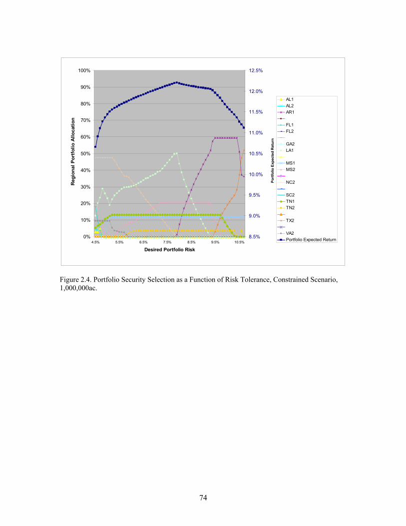
74
0%
10%
20%
30%
40%
50%
60%
70%
80%
90%
100%
4.5% 5.5% 6.5% 7.5% 8.5% 9.5% 10.5%
Desired Portfolio Risk
Reg
iona
l Por
tfol
io A
lloca
tion
8.5%
9.0%
9.5%
10.0%
10.5%
11.0%
11.5%
12.0%
12.5%
Port
folio
Exp
ecte
d R
etur
n
AL1AL2AR1
FL1FL2
GA2LA1
MS1MS2
NC2
SC2TN1TN2
TX2
VA2Portfolio Expected Return
Figure 2.4. Portfolio Security Selection as a Function of Risk Tolerance, Constrained Scenario, 1,000,000ac.

75
0%
10%
20%
30%
40%
50%
60%
70%
80%
90%
100%
5.6% 6.6% 7.6% 8.6% 9.6%
Desired Portfolio Risk
Reg
iona
l Por
tfol
io A
lloca
tion
8.5%
9.0%
9.5%
10.0%
10.5%
11.0%
11.5%
12.0%
12.5%
Port
folio
Exp
ecte
d R
etur
n
AL1AL2AR1
FL1FL2
GA2LA1
MS1MS2
NC2
SC2TN1TN2
TX2
VA2Portfolio Expected Return
Figure 2.5. Portfolio Security Selection as a Function of Risk Tolerance, Constrained Scenario, 2,000,000ac.

76
0%
10%
20%
30%
40%
50%
60%
70%
80%
90%
100%
6.1% 6.6% 7.1% 7.6% 8.1% 8.6%
Desired Portfolio Risk
Reg
iona
l Por
tfol
io A
lloca
tion
8.5%
9.0%
9.5%
10.0%
10.5%
11.0%
11.5%
12.0%
12.5%
Port
folio
Exp
ecte
d R
etur
n
AL1AL2AR1
FL1FL2
GA2LA1
MS1MS2
NC2
SC2TN1TN2
TX2
VA2Portfolio Expected Return
Figure 2.6. Portfolio Security Selection as a Function of Risk Tolerance, Constrained Scenario, 3,000,000ac.

77
Table 2.4. Portfolio Allocations and Statistics for Three Constrained Scenarios. Scenario: 1 Million Acres 2 Million Acres 3 Million Acres
Asset
Maximum Allowable Allocation
Optimal Allocation
Asset Prominence
Constrained Allocations
Maximum Allowable Allocation
Optimal Allocation
Asset Prominence
Constrained Allocations
Maximum Allowable Allocation
Optimal Allocation
Asset Prominence
Constrained Allocations
AL 1 51% 1.1% 0.2% 0.0% 25% 15.0% 4.8% 0.0% 17% 16.9% 16.6% 92.9%
AL 2 51% 0.0% 0.1% 0.0% 25% 0.0% 2.0% 0.0% 17% 14.2% 12.8% 39.3%
AR 1 59% 0.0% 19.4% 34.5% 30% 0.0% 23.2% 62.2% 20% 0.0% 16.8% 80.8%
AR 2 - - - - - - - - - - - -
FL 1 5% 0.0% 0.0% 0.0% 2% 0.0% 0.0% 0.0% 2% 1.6% 0.2% 80.0%
FL 2 3% 0.0% 0.0% 0.0% 2% 0.0% 0.0% 0.0% 1% 0.0% 0.1% 100.0%
GA 1 - - - - - - - - - - - -
GA 2 44% 0.0% 0.0% 0.0% 22% 0.0% 0.0% 0.0% 15% 0.0% 0.5% 0.0%
LA 1 62% 28.4% 22.5% 0.0% 31% 31.0% 27.2% 80.0% 21% 20.7% 20.7% 100.0%
LA 2 - - - - - - - - - - - -
MS 1 12% 0.0% 10.8% 96.6% 6% 0.0% 5.3% 94.9% 4% 3.9% 3.6% 96.2%
MS 2 20% 5.2% 10.9% 41.7% 10% 10.2% 10.2% 97.6% 7% 6.8% 6.7% 96.4%
NC 1 - - - - - - - - - - - -
NC 2 47% 47.5% 15.7% 20.6% 24% 23.7% 9.1% 33.3% 16% 15.8% 7.9% 38.1%
SC 1 - - - - - - - - - - - -
SC 2 34% 0.0% 0.5% 0.0% 17% 8.7% 0.7% 3.7% 11% 11.2% 2.6% 50.0%
TN 1 13% 8.4% 11.1% 78.0% 7% 6.6% 6.4% 95.2% 4% 4.4% 4.2% 96.4%
TN 2 4% 0.0% 2.6% 87.8% 2% 0.0% 1.6% 100.0% 1% 1.2% 1.1% 96.2%
TX 1 - - - - - - - - - - - -
TX 2 52% 0.0% 4.8% 7.7% 26% 0.0% 6.5% 23.8% 17% 0.0% 3.7% 15.4%
VA 1 - - - - - - - - - - - -
VA 2 9% 9.5% 1.4% 50.0% 5% 4.7% 2.8% 92.3% 3% 3.2% 2.5% 87.5%
Exp. Ret. 11.3% 11.2% 11.1%
Risk 4.8% 5.7% 6.3% Sharpe
Ratio 1.42 1.18 1.05

78
$-
$1
$2
$3
$4
$5
$6
$7
$8
1 2 3 4 5 6 7 8 9 10
Bill
ions
Year
1 mil ac - VAR2 mil ac - VAR3 mil ac - VAR1 mil ac - mean2 mil ac - mean3 mil ac - mean
Figure 2.7. Expected Portfolio Values and 5% VAR for Three Constrained Scenarios Over a Ten-Year Horizon.

79
CHAPTER 3
RISK AND REQUIRED RETURN ASSESSMENTS OF EQUITY TIMBERLAND
INVESTMENTS IN THE UNITED STATES6
6 Cascio, A.J. and M.L. Clutter. To be submitted to Southern Journal of Applied Forestry, August 2006.

80
Abstract
The Capital Asset Pricing Model (CAPM) has been shown useful for estimating the risk
and risk-adjusted returns from timberland investments in the United States. However, most
analyses predate the existence of empirical, asset-based timberland return series. This analysis
estimates timberland CAPM betas based on the National Council of Real Estate Investment
Fiduciaries (NCREIF) Timberland Index at the US National, and Pacific Northwest, Northeast
and South regional levels, utilizing annual returns. In addition, synthetic timberland return series
are constructed for 22 regions within the US South, corresponding to Timber Mart-South price
reporting areas. CAPM betas are estimated for these areas. We estimate betas of 0.167, 0.349,
0.193 and 0.147 at the National, Pacific Northwest, Northeast and South levels, respectively, and
from -0.137 to 0.279 for regions within the South. Utilizing the estimated betas, we estimate
required return rates of 5.8%, 5.7%, 5.9% and 6.6% for institutional timberland investments at the
National level, and in the Pacific Northwest, Northeast and South regions, respectively. Required
rates of return of 4.5%-6.3% are estimated for the 22 geographic regions within the South.

81
Introduction
Investment grade timberland serves as an important asset class in well-diversified
portfolios of institutions. Its use in this role has grown significantly in recent years. DANA
Limited (2006) estimates that institutional investors currently own approximately $17 billion of
timberland in the United States. One of the prime tools utilized by investors to assess the
contribution to a portfolio’s risk by the addition of an investment is the Capital Asset Pricing
Model (CAPM), developed by Sharpe (1964), Lintner (1965) and Mossin (1966). Previous
CAPM analyses have found a wide range of timberland CAPM beta risk estimates in relation to
the broad equities market, from large, negative ratios to moderate, positive figures. These
estimates of relative volatility are also used to estimate risk-adjusted returns that timberland
investments should be required to generate. This cost of capital figure can be used to evaluate
investments in timberland, as well as periodic silviculture investments in the timber management
aspect of the business.
Most previous efforts to estimate timberland betas occurred before the existence of a
sufficiently-long time series of empirical timberland return data. Instead, various forms of
synthetic timberland return indices were constructed for use in estimating the CAPM parameters.
The National Council of Real Estate Fiduciaries Timberland Index is the only return index in
existence for timberland assets. The data now comprise 19 years of returns for most regions. We
estimate market risk sensitivities and required rates of return for timberland investments in the
broad regions reported by NCREIF – the US South, Northeast and Pacific Northwest. Since the
predominance of investment grade timberland in the United States is located in the South, it is
worthwhile to explore risk characteristics of timberland within this region. We develop synthetic
return series for timberland in 22 different geographic regions within the South, at an annual
frequency and covering the period 1987-2005. With these data, we estimate market risk
sensitivities, and required return rates.

82
Literature Review
The CAPM builds upon the foundation laid by Markowitz (1952), who proved that the
risk of an individual investment should not be important to investors, but rather the investment’s
contribution to the investor’s overall portfolio risk. The risk of a financial asset is referred to as
the variability of its returns over time, and is commonly denoted by the standard deviation of
periodic returns. Risk can be stratified into two components. Idiosyncratic or firm-specific risk is
that component of total risk that is specific to the asset, resulting from actions, events and news
pertaining to the asset but not to other assets or firms. Firm-specific risk can be removed from the
portfolio through diversification. The risk that remains is termed market risk, or systematic risk.
This is risk due to economy-wide events and news, and that affects all firms. Systematic risk
cannot be removed from the portfolio with diversification.
The contribution of the CAPM is its ability to relate the impact of systematic risk upon
the returns of an investment. It does so with the following form:
( ) [ ( ) ],i f i m fE R R E R Rβ= + − (1)
where E(Ri) is the expected or required return on asset i, Rf is the risk free rate of return and E(Rm)
is the expected return on the total market portfolio of assets. The quantity E(Rm)- Rf is referred to
as the market risk premium, or the additional expected return of the market portfolio over the
risk-free rate. βi is a measure of the sensitivity of the expected returns of asset i to variance in the
total market portfolio. It is a measure of the asset’s systematic risk, that portion of the asset’s total
risk that cannot be diversified away. An asset having a beta greater than one is more risky than
the market, and commands a higher required return, while an asset with a beta less than one is
less risky than the market, and requires a lower return.
83
CAPM theory states that the market return should reflect the return on all traded and non-
traded risky assets, to include human capital. A major criticism of the CAPM is that such a return
is of course, unobservable. For empirical work, a proxy is chosen that reflects a broad market
portfolio of assets. Historical returns for the S&P 500, or other broad market index are commonly
used.
The CAPM was designed as a one-period model. As such, the choice of a proxy for the
risk-free rate does not receive much attention. US Treasury securities with a short maturity are
usually chosen, the 30 and 90-day Treasury bills being common. These assets are more reflective
of a truly risk-free asset than long term US Treasury bonds. Treasury bonds make periodic
coupon payments which have some degree of reinvestment risk. However, Bruner (2003) and
Damodaran (2006a) emphasize that the choice of the risk-free rate should match the return period
for the asset data employed. In other words, if the choice is to invest in a closed-end timberland
fund having a ten year horizon, the most appropriate risk-free alternative would be the 10-year
US Treasury bond.
Bruner (2003) surveyed a collection of corporations, financial advisors, and academic
and trade corporate finance textbooks. The survey questions addressed practices used when
estimating the cost of capital. When asked the question of which risk-free rate to use when using
the CAPM to estimate a required return, the overwhelming response by both corporations and
advisors is to use a long term Treasury bond yield. 70% of practitioners utilize a maturity of 10
years or longer, while only 4% stated the use of Treasury-bill yields. Bruner concludes with the
recommendation of matching the maturity of the risk-free investment to the character of the
investment being analyzed, and recommends the yield on the 10-year or longer maturity US
Treasury bond for most capital project evaluations.
Estimates of the market risk premium can vary widely, and according to Perold (2004)
can be the most difficult component of the model to estimate. Practitioners have a choice of using
either an historical estimate of the premium earned by equities over riskless investments, or

84
somehow looking forward to estimate this differential. The obvious assumption in using historical
premiums is the assumption that future expectations can be reasonably characterized by past
experiences. The technique usually involves differencing the average realized return on a risk-
free government security from the average realized return on a broad market index. However,
Damodaran (2006b) describes three questions the analyst must answer that can significantly
influence the result.
First, the number of years of historical returns can have influence. Using a longer time
period yields averages that are much more robust, yet at the cost of including potentially stale or
misleading data. Damodaran (2006b) documents that the large standard errors resulting in using
time periods of less than 50 years can be larger than the estimated risk premium itself. Second,
the choice of short term treasury bills as the risk-free asset will result in a market risk premium
approximately 1.5% larger than if long term treasury bonds are used. This choice is easily
decided for us, as consistency is required with our aforementioned choice of the risk free rate that
matches the investment.
Third, the choice of using arithmetic versus geometric averaging of market and riskless
returns will make a difference. The arithmetic average is the simple mean return. The geometric
average is the compound return, more reflective of an investor’s buy-and-hold experience (Bruner
2003). The more variable a return series is, the lower its geometric average will be compared to
its arithmetic average. This difference is also more dramatic for longer return series. While US
Treasury bonds and bills will not be greatly influenced by this choice, stock indices will, due to
their increased volatility. The arithmetic average annual return of large capitalization stocks from
1926-2005 is 11.6%, while the geometric average is 9.6%7. A requirement of using the arithmetic
average of returns is that they be independent over time. However Fama and French (1988),
among others, have documented significant negative autocorrelation of returns over time, making
7 Data from the Center for Research in Security Prices, University of Chicago, as published in Bodie, et al (2005).
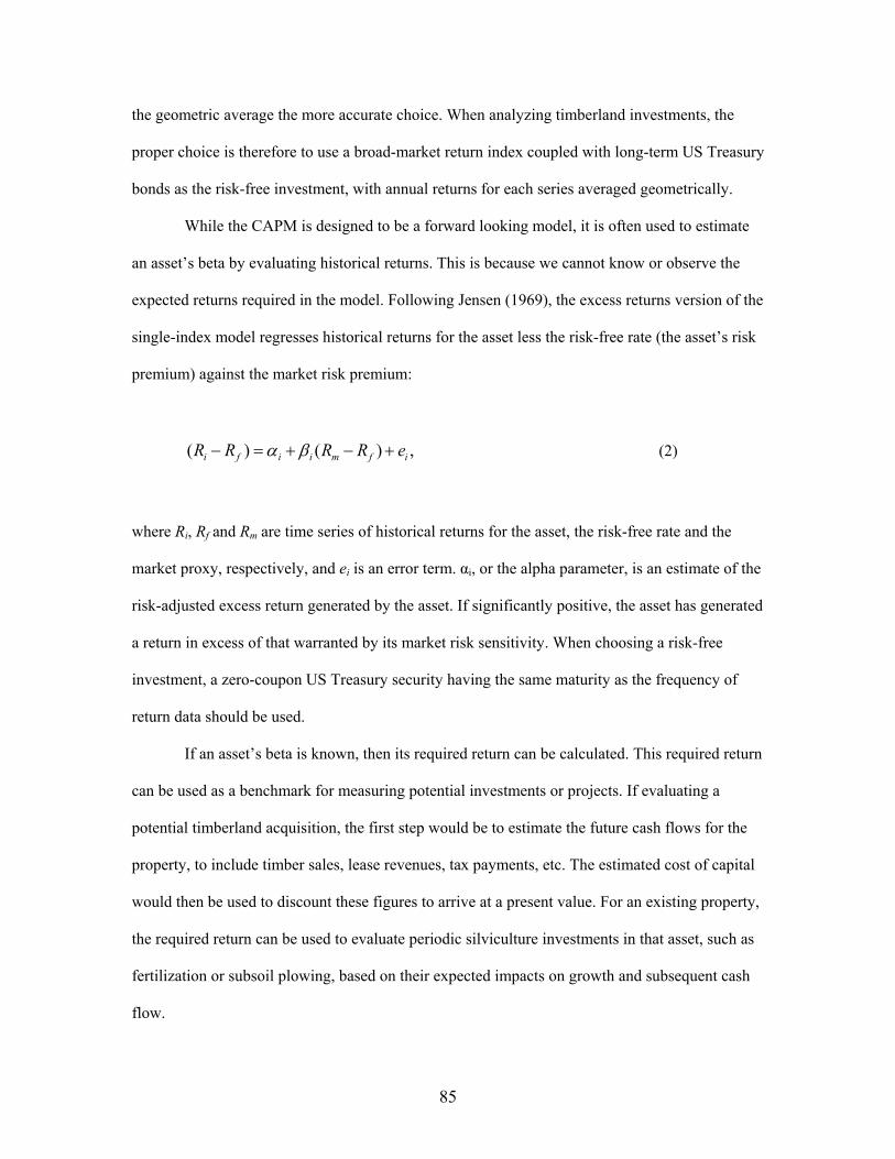
85
the geometric average the more accurate choice. When analyzing timberland investments, the
proper choice is therefore to use a broad-market return index coupled with long-term US Treasury
bonds as the risk-free investment, with annual returns for each series averaged geometrically.
While the CAPM is designed to be a forward looking model, it is often used to estimate
an asset’s beta by evaluating historical returns. This is because we cannot know or observe the
expected returns required in the model. Following Jensen (1969), the excess returns version of the
single-index model regresses historical returns for the asset less the risk-free rate (the asset’s risk
premium) against the market risk premium:
( ) ( ) ,i f i i m f iR R R R eα β− = + − + (2)
where Ri, Rf and Rm are time series of historical returns for the asset, the risk-free rate and the
market proxy, respectively, and ei is an error term. αi, or the alpha parameter, is an estimate of the
risk-adjusted excess return generated by the asset. If significantly positive, the asset has generated
a return in excess of that warranted by its market risk sensitivity. When choosing a risk-free
investment, a zero-coupon US Treasury security having the same maturity as the frequency of
return data should be used.
If an asset’s beta is known, then its required return can be calculated. This required return
can be used as a benchmark for measuring potential investments or projects. If evaluating a
potential timberland acquisition, the first step would be to estimate the future cash flows for the
property, to include timber sales, lease revenues, tax payments, etc. The estimated cost of capital
would then be used to discount these figures to arrive at a present value. For an existing property,
the required return can be used to evaluate periodic silviculture investments in that asset, such as
fertilization or subsoil plowing, based on their expected impacts on growth and subsequent cash
flow.

86
The CAPM is widely used as a model to explain the sensitivity of an asset’s returns to its
undiversifiable risk. It is used extensively by practitioners to quantify this risk, and to develop an
asset’s required return given this risk. However, like any model, the CAPM has its flaws, and
certainly like any other model, is a simplification of reality and cannot therefore be considered
absolutely correct. Over time researchers have slowly constructed evidence against the ability of
the CAPM to accurately portray the relationship between an asset’s market risk and required
return.
Early tests of the CAPM (Fama and MacBeth 1973, Gibbons 1982) have confirmed the
positive relationship between beta and asset return. This relationship has also been found to be
mostly linear, as the CAPM predicts. Researchers have, however found the beta-return
relationship to be ‘flatter’ than that predicted by the CAPM (Fama and MacBeth 1973, Black et
al. 1972, Fama and French 2004, among others). For example, low-beta assets often have a
positive Jensen’s alpha, or y-intercept rather than the predicted zero value, while high beta stocks
have been shown on average to have negative Jensen’s alpha values.
Fama and French (2004) describe a divergence of opinion among researchers for the
imperfect empirical record of the CAPM. Some believe financial markets are not as efficient as
once believed, a requirement of the CAPM. Market efficiency stipulates that current security
prices reflect all available information regarding the security, resulting in the inability to predict
the direction or magnitude of the security’s future price movement. Some believe that investors
overreact to past stock price performance, which researchers have potentially identified by adding
factors to asset pricing models that may capture this behavior (DeBondt and Thaler 1987).
Others believe that more risk factors are required to explain asset prices, in addition to
market risk. The three factor model of Fama and French (1993) is an example. Still others (Roll
1977) believe that the CAPM has never been, nor can be, accurately tested due to the impossible
selection of a proxy for the entire market portfolio of assets. While Fama and French (2004)
discourage use of the CAPM for empirical work, 80% of corporations and financial advisers

87
surveyed by Bruner (2003) nevertheless use the CAPM to estimate the cost of equity capital.
100% of text and trade books included in the survey also recommend primarily using the CAPM
for this purpose.
Timberland Return Drivers
Timberland investment returns are generated through two components: income and
capital appreciation. Income is received primarily from the periodic sale of timber, which in turn
is used in the manufacture of lumber; panel products such as plywood, oriented-strand board
(OSB) and fiberboard; paper; packaging; and several types of specialty chemicals. An attractive
characteristic of selling timber is that it can be withheld from the market during times of low
prices at no cost. There is no ‘storage fee’, and in fact the timber continues to grow and appreciate
until more favorable market conditions return. Annual income is also often received from the
leasing of recreation rights on the land, primarily for hunting.
Capital appreciation is realized from the continuous biological growth of the trees. In
addition, larger trees are more valuable per unit than are smaller trees. This is due to the fact that
telephone poles, plywood veneer and the larger sizes of lumber, some of the highest valued
products made from trees, can only be made from larger trees. Therefore as a tree crosses certain
thresholds from one size class to another, its value per unit increases. For southern yellow pine
species, there are three predominant size classes: pulpwood, chip-n-saw and sawtimber.
Pulpwood is used to make paper and OSB, and is the smallest and least valuable size class. Chip-
n-saw is used to make small dimension lumber. Sawtimber is used in the manufacture of larger
dimension lumber and poles, and is the most valuable size class.
The price paid for timber varies by tree size, region and season. Finished good prices also
have an impact on timber prices. However, Binkley (2000) showed how the price of southern
pine sawtimber has increased at a compound annual real rate of 2.6% from 1910 to 2000. This
increase is exhibited in both the income component of timberland returns and in the capital

88
appreciation component. This is because a key element of the capital appreciation of timberland
is the increase in the value of the land itself (Caulfield 1994). This increase is attributable to two
factors: first, the increase in the value of the land for producing timber due to price increases
(Washburn 1992), and the conversion of a portion of a timberland portfolio to a higher-valued use
than the production of timber, such as residential or commercial development, during the
investment period.
Timberland Return Data
The only timberland return index currently in existence8 that is based on actual
timberland transactions and appraisals is the National Council of Real Estate Investment
Fiduciaries Timberland Index (NCREIF, 1994). NCREIF publishes historical return data for
timberland investments managed by its members, at two geographic levels: the United States, and
three regions within the US: the Pacific Northwest, the Northeast and the South. The NCREIF
Timberland Index segregates a total return into income and capital appreciation elements, and is
based on actual data reported by its members managing timberland investments.
Hancock Timber Resource Group (2003a) describes how NCREIF began compiling and
publishing a quarterly index of timberland property returns in 1994, with data retroactive to 1987
for the Southern and Pacific Northwest regions, and 1994 for the Northeast. This index tracks the
changes in value of timberland properties that are a) held in a fiduciary environment, as opposed
to the myriad other ownership objectives shared by many other timberland owners; and b)
“marked to market” at least annually. If the property does not experience a change in ownership
during a year via a sale, then it is appraised at year end to yield a new value. As a timberland
investment organization joins NCREIF, they submit historic returns for their properties to
augment the index.
8 The Timberland Performance Index (TPI) (Caulfield,1994) is similar to the NCREIF index, however is no longer in existence.

89
This index is built and maintained similarly to NCREIF’s other commercial real estate
indices. The index has four basic components: the market value of all properties in the index; the
EBITDDA return for the properties; the capital return; and the total return. The EBITDDA return
is based primarily on the sale of harvested timber during the quarter. However, many timberland
property owners lease recreation use rights to clubs or individuals, the income from which is also
included in the EBITDDA portion of the total return. It must be noted that the EBITDDA figure
is gross of applied management fees charged by the property manager, and therefore overstates
the true net income received by the investor (Healey et al. 2003). The capital appreciation
component is basically the ratio of the difference in period-to-period property market value,
minus capital expenditures in the current period, to the market value of the previous period.
Timberland appraisals usually occur on an annual basis and often in the fourth quarter. For time
series analyses the quarterly returns are therefore less meaningful, since they will often display an
artificial spike in one quarter per year, reflecting the appreciation due to the annual appraisal. For
analysis purposes, it is recommended that annual returns be used (Hancock Timber Resource
Group 2003a).
The United States-wide timberland index is subdivided into three regional indices: South,
Pacific Northwest and Northeast. Table 3.1 lists the annualized returns for the four NCREIF
Timberland series. The NCREIF return data provides a significant improvement over the use of
synthetic proxies for timberland returns. However, it still has two drawbacks that limit its utility
in assessing inferences about the performance of timberland investments. First, a portion of the
periodic return is based on appraisals rather than market transactions. Second, the reporting
frequency is only useful on an annual basis, resulting in a paucity of data points relative to the
monthly returns of more traditional financial assets.
Investing in timberland by institutions is relatively new. It can be tracked to the passage
of the Employee Retirement Income Security Act (ERISA) in 1974 that required institutional
investors to diversify their portfolios away from traditional common stocks and fixed income

90
securities to broader classes (Zinkhan 2003, Healey et al. 2003). Investments in timberland by
institutions grew by a factor of ten during the 1990’s to some $17 billion by 2005 (DANA
Limited 2006). This is reflected in the time span of the NCREIF Timberland Index. Although the
NCREIF series is regarded as the best data available describing the performance of institutional
investments in timberland, the need to analyze the financial performance of timberland predates
the existence of this index. Before this time, most analysts constructed synthetic return indices
with several management assumptions for use in timberland investment analyses.
Timberland returns value to the owner through a combination of periodic income and
capital appreciation, as previously discussed. Therefore, the common return formula is applicable
for measuring timberland returns:
1
1t tt
t
NI CVRCV −
+= − (3)
where:
Rt = total return per acre of the asset during period t;
NIt = net income received per acre of the asset during period t;
CVt = capital value per acre of the asset during period t.
Many assumptions about forest management practices must be made when developing a
synthetic timberland return series. One that is common among most authors is that the
hypothetical forest being modeled is fully-regulated. This implies that the volume of timber
harvested each period is equal to the volume grown. The standing volume of timber in the forest
is therefore static over time, and there are equal amounts of area in each age class. So harvest is
static which will minimize volatility and lower estimates of beta. This allows any capital
appreciation of the forest to be reflective of timber or land price appreciation, inflation, or some
other factor, but not from any implied change in the inventory of the asset. Revenue realized from

91
the sale of harvested timber represents the periodic income component. Missing from this model
of returns is a provision to reflect the occasional sale of small parcels of a property, commonly
referred to as a real estate component.
Redmond and Cubbage (1988) constructed species-based synthetic timberland return
series for multiple commercial timber species in the United States. Return series based on
particular timber products were developed as well, such as southern pine sawtimber and
pulpwood. The formula was based on a sum of annual stumpage price change and a measure of
average annual timber growth. Redmond and Cubbage (1988) used these return series to estimate
CAPM betas for the respective species and products. The S&P500 composite index was used for
the market proxy, along with an unspecified risk free rate. Four of the 22 product series’ beta
estimates were positive, and only two were significant at the α = 0.05 level.
Zinkhan (1988) utilized a synthetic annual return series for Southern pine from 1956-
1986, developed by a timberland investment firm, to estimate a timberland beta and cost of
capital. The return series utilized published south-wide pine stumpage prices, timber harvests
from a typical southern pine management regime, and proprietary land appreciation rates. The
S&P500 composite index was used for the market proxy, and 90-day Treasury bills for the risk-
free rate. Zinkhan (1988) estimated a beta of -0.21. Statistical significance was not stated, and
must be considered questionable.
Washburn and Binkley (1990) studied eleven sawtimber annual stumpage price series
reported by the US Forest Service and the State of Louisiana. The S&P500 composite index was
used for the market proxy, and 30-day Treasury bills for the risk-free rate. Three different
methods were used to calculate appropriate asset periodic rates of change. For southern pine
sawtimber in Louisiana they estimated insignificant betas of between 0.17 and 0.18, while for
southern pine sawtimber on national forests they estimated insignificant betas of 0.35 to 0.37. The
beta estimates for national forest Douglas-fir sawtimber ranged from 0.95 to 0.98, and were
significant at the α =0.05 level.

92
Binkley et al. (1996) created synthetic timberland return series for the Pacific Northwest,
Northeast and South to estimate timberland systematic risk measures and excess returns. Their
model, the John Hancock Timberland Index (JHTI)9 uses only one time series data component:
the quarterly stumpage price of the appropriate timber species group for the region modeled. For
the US South, the stumpage price is a composite price equal to the equally-weighted average
price of pine pulpwood and sawtimber. The return income component is simply the quarterly
stumpage price multiplied by a subjective factor that represents the regional ratio of periodic
income to the capital value of the representative forest. The capital value component is a
weighted average of the previous eight quarters stumpage prices, with progressively less weight
given to each preceding quarter’s price. Each year’s four quarterly returns were then averaged to
yield an annual return. Binkley et al. (1996) estimated return series from 1960-1994. The authors
used a portfolio of large and small company common stocks, corporate bonds and US Treasury
securities of varying maturities for the market portfolio proxy. US Treasury bills of unspecified
maturity were used for the risk-free rate. The authors found significant betas of -0.88 (α = 0.05), -
0.54 (α = 0.05) and -0.21 (α = 0.10) for the Pacific Northwest, South and Northeast, respectively.
Significant alpha estimates of 10.2%, 5.9% and 2.8% were found for the same regions, (α = 0.05).
Sun and Zhang (2001) compared CAPM and APT estimates for eight different forestry-
related investment classes. Two of the investment vehicles modeled were the Timber
Performance Index and the NCREIF timberland index. NCREIF quarterly returns from 1987-
1997 were used as a return series. The S&P500 composite index was used for the market proxy,
and US Treasury bills of unspecified maturity were used for the risk-free rate. Sun and Zhang
estimated insignificant betas of 0.07 for the now-defunct TPI, and -0.05 for the NCREIF
Timberland Index. By using quarterly rather than annual returns for the NCREIF series, the beta
estimate must be considered suspect. This is due to the aforementioned common practice of
9 Described fully in Hancock Timber Resource Group, 2003b.

93
appraising timberland properties in the fourth calendar quarter, resulting in an artificial change in
capital value during that time.
Synthetic Return Series for Areas Within the South
The John Hancock Timberland Index (JHTI) model of timberland returns was used as a
template to construct synthetic return series for 22 different areas within the US South for 1987-
2005, where the areas correspond to those defined by Timber Mart-South (TMS 2006a, Figure
3.1). Timber Mart-South divides each of 11 Southern states into two areas, and reports both
stumpage and delivered prices for southern pine and hardwood species groups, and for the major
product classes. Prices are reported on a quarterly basis. Similar to Hancock Timber Resource
Group (2003b) we utilize pine stumpage prices to estimate an annual return series.
Aside from using regional rather than South-wide prices, our series differs from
Hancock’s in four ways. First, we include pine chip-n-saw as a product component, due to the
increasing prominence of small-diameter sawtimber in some southern regions. Second, we
estimate unique harvest weights for the three pine product classes in each region to apply to the
quarterly prices, rather than using an equal weighting factor. Third, we estimate the income rate,
representing the quarterly ratio of periodic income to capital value of an investment-grade forest,
based on a comparison of our series to the reported NCREIF South return series from 1987-2005.
Finally, we utilize the composite stumpage prices of the 12 most previous quarters for the capital
value component rather than 8 quarters. By using the 12 previous quarters, volatility of the return
series is reduced slightly, as measured by the standard deviation of returns, and is closer to that of
the NCREIF South series.

94
From (3) the net income and capital value components for region r in quarter t are:
11
( )0
,
(12 ),
78
rt rt
r t nn
rt
NI P Income Rate
n PCV
−=
=
−
=∑
(4)
(5)
where:
1 $ 2 $ 3 $rt rt rt rt rt rt rtP W ppwd W cns W pst= + + , (6)
and ppwd$rt, cns$ rt and pst$ rt are the pine pulpwood, chip-n-saw and sawtimber prices reported
in Timber Mart-South for region r in period t.
Region-specific product harvest weights (W1-W3) were estimated from United States
Forest Service (USFS), Timber Product Output (TPO) data (USFS Southern Research Station
2006). The USFS periodically surveys mills throughout the South to determine the quantity of
wood consumed by product type. They then estimate the origination of these volumes based upon
USFS Forest Inventory and Analysis (FIA) inventory data, along with assumptions regarding mill
basin radii, etc. The result is a table of estimated timber volume harvested by species group and
product class. This table is reported for each county of each southern state. TPO data exists for
each state for three different points in time. For most states, the data reflects conditions in 1995,
1999 and 2003, with the exception of Louisiana and Arkansas, for which harvest data is reported
as of 1996, 1999 and 2002.
The USFS also segregates this data by ownership class. The class most representative of
investment-grade timberland is the Forest Industry ownership group. There is not an ownership
group specifically representing institutional, or investment-grade timberland. However, much

95
current investment-grade timberland was at one time owned by an integrated forest products
company, and was therefore in the Forest Industry group at one time. Where that was not the
case, both groups nevertheless manage timberland similarly (Siry 2002). Due to legislative
protocol, the USFS does not report timberland data of any sort at the county level, and segregated
by ownership group. Data is only reported by ownership group at the statewide level. Therefore, a
special request was made of the USFS, Southern Research Station. A file was sent to them
containing a Timber Mart-South region designation (1 or 2) for each county in each Southern
state. USFS personnel then aggregated harvest volume data by ownership group for all counties
in each TMS region, and returned this to us. We therefore received harvest volume data at the
TMS region level by ownership group, without violating USFS protocol.
The USFS TPO data includes only one size class for pine sawtimber. It does not
segregate pine sawtimber into two size classes. The Southern Forest Products Association (SFPA)
2002 Annual Mill Survey (Southern Forest Products Association 2003) was referenced to provide
an empirical method of apportioning regional sawtimber removal volumes. This survey reports
pine sawtimber consumption by US South sawmills, by size class. This survey reports the
consumption by size class at the Southwide level. By special request, the SFPA agreed to
disaggregate this data by state. The number of responding mills in the survey was quite small
when viewed at the individual state level, and expert judgment was used to refine this data. It
should be noted that this sawtimber size class apportionment represents a single point in time, yet
was used to apportion sawtimber volumes for the duration of each time series modeled.
The final parameter needed for estimating the return series is the Income Rate. This is a
south-wide, static estimate of the quarterly ratio of periodic income from a timberland investment
to its capital value. This parameter was estimated by first aggregating the 22 area harvest volume
product weights into south-wide weights over time. These weights were utilized in our quarterly
return model, along with TMS south-wide stumpage prices to estimate a south-wide return series
from 1987-2005. The quarterly return series was then annualized. The annual returns from this

96
series were differenced from the NCREIF South series, and squared. The sum of these squared
differences was minimized by adjusting the Income Rate in the south-wide synthetic series. The
resulting Income Rate value was 1.49%. Figure 3.2 shows the NCREIF South Timberland Index
and our southwide synthetic timberland return series from 1987-2005. These two return series
have a correlation coefficient of 0.710 for the total 19-year history, and 0.936 for the most recent
nine years. This Income Rate value was then used in the calculation of each of the 22 area
synthetic return series. Table 3.2 shows the annual synthetic returns.
The similarity of our synthetic, southwide return series with the NCREIF South
Timberland Index is quite good, especially for recent years. Although it is generally understood
that timber prices are a significant determinant of timberland prices, other factors exist that
influence timberland returns that are not modeled in our synthetic return model. Specifically,
timberland owners periodically sell small tracts of land that are worth more for other purposes
than for timber management, for example real estate development. Such tracts are termed Higher
and Better Use, or HBU. NCREIF members report the proceeds from HBU tract sales, which are
then included as a portion of the capital return component of the regional return series. We do not
attempt to capture this impact.
CAPM Estimation and Discussion
A significant assumption necessary when estimating required returns utilizing a beta
estimated in an ex post fashion is the assumption of the similarity of future and historical asset
performance. A tradeoff with respect to accurate beta estimation versus the applicability of that
beta in estimating a required return concerns the length of the time series used to estimate the
beta. Going further back in time by using more historical returns strengthens the precision of the
beta regression estimator. However the future performance of the asset class may not be
accurately reflected by historical performance reaching to a point in the past that may reflect a
different economic environment for the asset class. The requirement of using annual return data

97
for the NCREIF series yields only 19 data points (11 for the Northeast index), which is small
compared to the typical 60 monthly returns used with conventional financial asset beta estimates.
Recognizing this tradeoff, we chose to use the entire time series to insure the most precise
estimates.
The excess returns version of the single-index model (2) was used to estimate alpha and
beta parameters for the four NCREIF and 22 sub-south synthetic timberland return series. The
S&P500 index was used as the market proxy, along with yields for the 1-year US Treasury bill as
the risk-free rate. Ordinary least squares regression was used to estimate the model if the Durbin-
Watson (DW) statistic for first-order autocorrelation of the error was within its upper bound for
significance at the α = 0.05 level. If the DW statistic was not within the upper bound, the SAS
MODEL procedure (SAS Institute Inc. 1999) was used to estimate the model with a first-order
autoregressive error. Table 3.3 documents the regression results.
The beta estimates for the four NCREIF return series are somewhat higher than those
found for timber and timberland by most other researchers. Whether this is due to the use of the
NCREIF series versus stumpage price or synthetic timberland return series, or perhaps that the
systematic risk of timberland investments is increasing over time, is inconclusive. However, our
NCREIF beta estimates are insignificant at the α = 0.05 level10, consistent with most prior
research. Beta estimates for the 22 sub-south synthetic return series are mostly positive, low and
not significantly different than zero, with few exceptions11. Sub-south regional beta estimates
with 95% confidence intervals are shown in Figure 3.3. The average beta of the 22 regions is
0.084 on an equal-weighted basis. This is significantly different than the NCREIF South beta
estimate of 0.14712. Weighting the sub-south regional beta estimates by an estimate of the amount
10 The NCREIF-South beta estimate was significant at α = 0.10. 11 18/22 regions positive; FL 2 significant at α = 0.05, AL 1 significant at α = 0.10. 12 t-statistic = -3.13

98
of investment-grade timberland acres available in each region13 yields a weighted-average beta of
0.096.
Although timberland owned by institutional investors is quite similar to that owned by
traditional forest products companies such as Weyerhaeuser and Temple-Inland, and timberland
real estate investment trusts (REIT) such as Plum Creek Timber and Rayonier, the calculated
CAPM betas are not directly comparable for two reasons. First, CAPM betas calculated from
reported stock returns are equity betas. A firm that is financed to some degree with debt also has a
debt beta. By combining the betas for these two sources of financing the beta of a firm’s
unlevered assets can be calculated as:
,Unlevered Asset Debt EquityDebt Equity
Debt Equity Debt Equityβ β β= +
+ + (7)
where Debt and Equity represent the long term debt and market capitalization of the firm. In
practice, the risk of corporate debt is quite low, and can, in many cases, be assumed to be zero
(Ross et al. 2002). Incorporating the tax shield for interest paid on debt yields the beta of the
firm’s unlevered assets as:
,1 (1 )
EquityUnlevered Assets
CDebtT
Equity
ββ =
+ −
(8)
where TC is the corporate income tax rate. A firm that uses debt to finance some portion of its
operations will necessarily have an unlevered asset beta that is lower than its equity beta.
13 USFS FIA (Smith et al 2004) timberland acres for the Forest Industry ownership group for each southern state, apportioned to TMS area levels by an estimate of the volume harvested in each area.

99
The NCREIF timberland investments are unlevered investments. Therefore our estimated
CAPM equity betas are synonymous with the unlevered asset betas. To compare these betas to
reported equity betas for publicly-owned, vertically-integrated forest products corporations and
publicly traded timberland REITs, we must first remove the impact of leverage from the equity
betas of those firms. Table 3.4 lists the equity betas of Weyerhaeuser, Temple-Inland, Plum Creek
Timber and Rayonier, four publicly-owned firms that own significant amounts of investment-
grade timberland. The equity betas, along with long term debt and market capitalization figures,
were reported by Value Line for the end of 2005. Assuming a tax rate of 38%, the unlevered asset
betas are 0.88, 1.01, 0.68 and 0.86 for these firms, respectively. These beta estimates are
substantially higher than the NCREIF betas. A second reason making a direct comparison of the
NCREIF timberland betas to those of the four publicly-owned firms difficult is the heterogeneous
composition of the firms’ assets compared to the pure timberland represented by NCREIF. These
four firms own various types of timber conversion assets in addition to timberland, such as
sawmills, pulp mills and paper mills.
The significantly positive alpha estimates of 5.5%-18% for the NCREIF returns suggest
that institutional timberland investments have performed above the level warranted by their
systematic, or market risk. Of the sub-south regional return series, only the Arkansas-2 area had
an estimated negative alpha (-3.0%). 19 of the 22 synthetic-return estimated alphas are not
significantly different from zero. The average alpha of the 22 regions is 3.6%, significantly
different than the 5.5% NCREIF South estimate14. The weighted-average sub-south alpha is
3.4%.
With timberland betas estimated from historical data, our attention can now be focused
on estimating required returns for future timberland investments. From (1) we will need estimates
of an applicable risk-free rate Rf, and the market risk premium (Rm - Rf). Following Bruner
(2003) the current yield on the 10 year US Treasury bond is used as the risk-free rate 14 t-statistic = -3.84

100
commensurate with a timberland investment made by an institution that is typically of a ten year
duration. Although certainly many timberland investments are made for longer time horizons,
Bruner (2003) points to the often relative flatness of the yield curve beyond ten years as
minimizing the importance of choosing a bond beyond the ten year rate. Recent yields on the 10
year US Treasury bond have been approximately 5.1%.
From historical return data provided by Bodie et al. (2005), the historical market risk
premium of large stocks over long term government bonds for 1926-2005 is 4.25%, utilizing
geometric mean returns. Using (1), along with the CAPM beta estimates, the required return on
equity for institutional timberland investments in the US South, Northeast and Pacific Northwest
is estimated to be 5.73%, 5.92% and 6.59%, respectively. Nationally, the required return is
estimated to be 5.81%. Utilizing our beta estimates for timberland investments within the South,
required return on equity estimates range from a low of 4.52% in VA 1, to a high of 6.29% in FL
2, with an average of 5.46% and a standard deviation of 0.41%. The average when weighted by
available investment-grade timberland acres is 5.51%. These results are displayed in Table 3.5.
Conclusions
This study utilized the Capital Asset Pricing Model to assess the risk, risk-adjusted
performance and required return of institutionally-owned, equity timberland investments in the
United States. Data comprised 19 years of annualized returns for the NCREIF South and Pacific
Northwest Timberland indices (1987-2005), and 11 years for the NCREIF Northeast index (1994-
2004). Recognizing the appraisal bias inherent in the quarterly form of the NCREIF data,
annualized data were used. Consistent with this return frequency, 1-year US Treasury bill yields
were used as the risk-free rate, along with returns for the S&P 500 Composite Index as the market
proxy.
The CAPM beta coefficient is the estimate of a security’s sensitivity to variance of the
overall financial market. We estimate low, positive betas for equity timberland investments, and

101
not significantly different from zero. This implies that timberland investments bear substantially
less risk than does the financial market as a whole. These estimates are higher than those found in
many previous studies, which often employed different return series, estimation benchmarks and
timeframes. These results suggest the possibility of an increase in recent years of the
nondiversifiable, or systematic risk of timberland investments. Future research should explore
this possibility, along with explanatory factors.
The CAPM alpha coefficient reflects the historical performance of an investment in
consideration of its systematic risk. We estimate positive alphas for the NCREIF national and
regional return series, significantly different than zero for all but the Pacific Northwest region.
This implies that timberland investments have performed above the level warranted by their
market risk. This finding is consistent with prior research.
The CAPM was also used to estimate forward-looking required return rates for
timberland investments. The calculated betas were used, along with the current yield on the 10
year US Treasury bond, which constitutes an appropriate risk-free alternative to a typical
institutional timberland investment. A market risk premium consistent with historical
performance was used. Risk adjusted rates of return are estimated to be less than 1% above the
risk-free rate for all NCREIF return series except the Pacific Northwest, which is 1.5% above an
appropriate riskless investment.
Synthetic return series were created for 22 geographic regions within the US South,
corresponding to Timber Mart-South price reporting areas. CAPM beta and alpha parameters, and
required return rates were estimated for these regions, based on annual returns for 1987-2005.
The intra-south beta estimates are low, mostly positive and all are statistically insignificant. Risk-
adjusted historical performances are low, positive (21 of 22) and mostly insignificant. Required
rates of return range from 4.5%-6.3%.
Further research may provide insight into timberland investment performance by
examining the fundamental components of the return process as they relate to factors within the

102
economy to estimate appropriate risk and required return figures. Market risk premiums estimated
by a forward-looking procedure might also prove to be of value. This study provides a firm
foundation of risk and required return estimates using a traditional approach, against which future
models and results can be benchmarked.
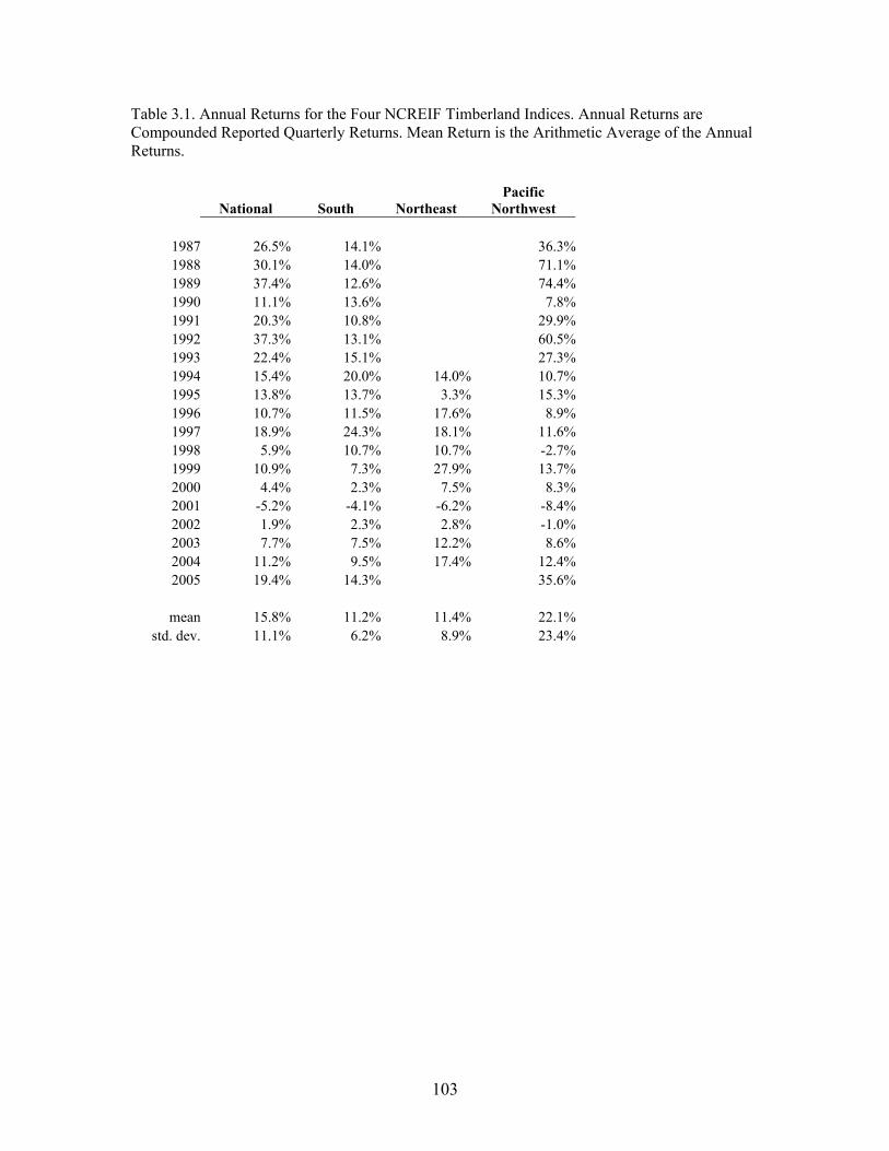
103
Table 3.1. Annual Returns for the Four NCREIF Timberland Indices. Annual Returns are Compounded Reported Quarterly Returns. Mean Return is the Arithmetic Average of the Annual Returns.
National South Northeast Pacific
Northwest
1987 26.5% 14.1% 36.3%1988 30.1% 14.0% 71.1%1989 37.4% 12.6% 74.4%1990 11.1% 13.6% 7.8%1991 20.3% 10.8% 29.9%1992 37.3% 13.1% 60.5%1993 22.4% 15.1% 27.3%1994 15.4% 20.0% 14.0% 10.7%1995 13.8% 13.7% 3.3% 15.3%1996 10.7% 11.5% 17.6% 8.9%1997 18.9% 24.3% 18.1% 11.6%1998 5.9% 10.7% 10.7% -2.7%1999 10.9% 7.3% 27.9% 13.7%2000 4.4% 2.3% 7.5% 8.3%2001 -5.2% -4.1% -6.2% -8.4%2002 1.9% 2.3% 2.8% -1.0%2003 7.7% 7.5% 12.2% 8.6%2004 11.2% 9.5% 17.4% 12.4%2005 19.4% 14.3% 35.6%
mean 15.8% 11.2% 11.4% 22.1%
std. dev. 11.1% 6.2% 8.9% 23.4%

104
2
2
11 1
12
2
2
2
2
2
2
1
1
2
1
1
11
2
1
Figure 3.1. Delineation of Southern States into Timber Mart-South Reporting Areas (TMS 2006a).

105
Annual Southwide Returns
-10%
-5%
0%
5%
10%
15%
20%
25%
30%
1987
1988
1989
1990
1991
1992
1993
1994
1995
1996
1997
1998
1999
2000
2001
2002
2003
2004
2005
NCREIFModified JHTI
Figure 3.2. Comparison of Synthetic, Southwide Timberland Return Series with the NCREIF South Series.

106
Table 3.2. Synthetic Timberland Return Series for 22 Areas within the U.S. South from 1987-2005.
AL 1 AL 2 AR 1 AR 2 FL 1 FL 2 GA 1 GA 2 LA 1 LA 2 MS 1 MS 2
1987 1.2% 0.3% -2.4% -6.5% -7.5% -1.9% 6.3% 3.5% -2.8% -4.4% -1.5% 1.4%1988 9.0% 6.2% 7.2% 13.0% 8.3% 4.8% 10.0% 9.9% 16.9% 17.1% 11.9% 13.3%1989 12.3% 13.1% 8.5% 10.6% 18.0% 23.7% 16.6% 15.1% 16.8% 15.3% 16.9% 22.2%1990 12.7% 12.3% 11.8% 13.3% 28.0% 18.0% 25.0% 12.3% 13.1% 15.4% 10.8% 11.4%1991 13.0% 9.1% 14.6% 14.4% 13.3% 16.8% 5.5% 6.5% 16.4% 14.4% 11.9% 10.2%1992 19.7% 12.9% 24.6% 32.9% 14.7% 11.6% 22.6% 14.7% 24.3% 21.9% 30.0% 17.8%1993 23.2% 28.8% 30.1% 37.9% 20.0% 16.7% 16.8% 21.3% 18.1% 20.9% 38.3% 27.4%1994 18.4% 34.4% 35.8% 34.5% 10.8% 5.3% 13.9% 14.1% 15.7% 27.9% 36.3% 37.3%1995 20.6% 11.4% 9.7% 22.8% 14.8% 11.3% 22.0% 20.2% 20.5% 19.7% 21.3% 20.8%1996 7.0% -2.0% 1.8% -9.3% 11.1% 3.6% 8.3% 9.7% 7.1% 0.2% 4.9% -1.6%1997 22.9% 19.1% 15.9% -1.8% 15.4% 14.5% 14.6% 13.6% 20.0% 24.9% 18.2% 11.6%1998 12.8% 15.7% 9.4% -30.3% 13.7% 21.7% 13.8% 10.0% 13.9% 21.5% 13.0% 14.9%1999 3.4% 3.3% 1.7% -24.2% 4.7% 7.2% 1.4% 1.9% 5.1% 7.6% 7.4% 8.2%2000 -0.2% -1.2% -0.9% -11.5% -1.3% -3.0% -6.1% 0.3% -2.3% 0.6% 1.9% 0.5%2001 -7.5% -1.8% -1.7% -1.4% -2.8% -9.3% -12.9% -6.7% -1.2% -2.2% -0.7% 1.8%2002 3.6% 5.9% 4.4% 5.5% -1.4% -7.3% -14.1% -5.1% 4.9% 2.6% 4.7% 8.2%2003 12.7% 13.2% 7.4% 9.3% 3.4% 3.6% 2.8% -1.6% 3.6% 6.3% 9.3% 7.5%2004 9.2% 9.9% 14.4% 7.9% 7.9% 8.8% 8.0% 4.0% 12.4% 4.4% 10.0% 8.1%2005 12.0% 7.4% 21.4% 15.9% 7.5% 11.3% 13.7% 8.6% 16.8% 3.9% 3.2% 3.0%
mean 10.8% 10.4% 11.2% 7.0% 9.4% 8.3% 8.9% 8.0% 11.5% 11.5% 13.0% 11.8%
std. dev. 8.0% 9.4% 10.4% 18.0% 8.6% 9.1% 10.7% 7.7% 8.0% 9.7% 11.2% 9.7%

107
Table 3.2. Synthetic Timberland Return Series for 22 Areas within the U.S. South from 1987-2005 (cont.).
NC 1 NC 2 SC 1 SC 2 TN 1 TN 2 TX 1 TX 2 VA 1 VA 2
1987 10.3% 7.3% 3.6% 1.8% 1.5% 8.5% 0.1% -2.0% 8.7% 17.6%1988 6.8% 8.3% 14.1% 11.4% 10.9% 22.5% 20.9% 19.7% 0.4% 12.5%1989 15.1% 13.0% 6.7% 3.8% 13.9% 17.3% 12.2% 13.0% 2.8% 7.3%1990 8.8% 12.1% 12.8% 7.4% 8.9% 1.7% 5.3% 7.3% 16.2% 7.6%1991 8.3% 16.4% 9.0% 14.7% 4.1% -1.6% 10.5% 15.2% 3.2% 1.0%1992 -0.5% 12.5% 21.6% 19.6% 21.4% 18.7% 23.9% 23.1% 18.2% 17.6%1993 9.5% 7.5% 16.0% 16.7% 24.5% 24.9% 29.9% 30.0% 8.7% 11.5%1994 20.8% 14.7% 20.3% 19.4% 25.5% 32.6% 30.1% 29.2% 14.9% 16.4%1995 3.3% 10.9% 12.1% 20.7% 8.1% 18.2% 23.2% 24.6% 12.6% 9.9%1996 -2.2% 11.5% 12.7% 10.0% 36.3% 32.9% 3.3% 4.4% 11.6% 11.1%1997 19.8% 10.9% 15.3% 11.6% -9.6% 37.0% 24.7% 16.9% 19.2% 22.9%1998 27.6% 19.8% 7.5% 6.4% 34.5% 21.4% 13.2% 5.8% 15.6% 24.5%1999 32.4% 17.3% 3.3% 2.8% 20.9% 4.5% 2.8% -0.4% 11.8% 11.2%2000 18.3% 14.1% 1.7% 2.7% 1.9% 0.3% -1.6% -3.8% 18.9% 13.1%2001 8.1% 6.6% -3.1% 1.5% -14.4% -10.5% -1.5% -9.7% 11.8% 3.2%2002 3.1% 4.2% -6.3% 0.6% -1.3% -8.5% 7.8% -6.2% 8.3% -0.8%2003 7.3% 2.6% -1.6% 0.8% 18.9% -3.7% 4.9% 2.4% 3.8% 1.1%2004 -6.1% 2.5% 5.0% 6.1% 30.0% 7.2% 16.2% 8.0% 0.2% 5.1%2005 7.2% 6.5% 10.7% 11.5% 15.8% 11.6% 19.0% 17.2% 5.1% 8.6%
mean 10.4% 10.5% 8.5% 8.9% 13.3% 12.4% 12.9% 10.2% 10.1% 10.6%
std. dev. 9.6% 4.8% 7.5% 6.6% 13.8% 13.9% 10.2% 11.7% 6.0% 6.9%

108
Table 3.3. CAPM Parameter Estimates for NCREIF and Synthetic Timberland Returns.
Alpha Beta Asset α standard error Pr > |t| β standard error Pr > |t| R-square DW
NCREIF National 0.113 0.042 0.015 0.167 0.120 0.183 0.318 1.94 NCREIF South 0.055 0.012 0.000 0.147 0.075 0.065 0.187 1.41 NCREIF Northeast 0.059 0.026 0.048 0.193 0.132 0.177 0.193 2.38 NCREIF Pacific NW 0.180 0.095 0.078 0.349 0.268 0.211 0.292 1.73
AL 1 0.043 0.029 0.151 0.179 0.098 0.086 0.378 1.91 AL 2 0.044 0.036 0.242 0.066 0.129 0.617 0.197 1.47 AR 1 0.023 0.061 0.705 -0.052 0.109 0.639 0.395 1.37 AR 2 -0.030 0.097 0.761 -0.014 0.165 0.932 0.527 1.71 FL 1 0.027 0.031 0.402 0.097 0.105 0.371 0.261 1.65 FL 2 0.015 0.027 0.586 0.279 0.094 0.009 0.465 1.59 GA 1 0.033 0.037 0.388 0.120 0.121 0.336 0.323 2.18 GA 2 0.017 0.029 0.561 0.100 0.072 0.186 0.450 2.10 LA 1 0.055 0.025 0.042 0.160 0.110 0.164 0.232 1.78 LA 2 0.051 0.029 0.094 0.168 0.137 0.237 0.191 1.79 MS 1 0.018 0.066 0.790 0.078 0.112 0.496 0.422 1.46 MS 2 0.051 0.038 0.195 0.079 0.122 0.526 0.225 1.49 NC 1 0.048 0.035 0.187 0.101 0.122 0.417 0.203 1.68 NC 2 0.045 0.018 0.024 0.044 0.050 0.382 0.317 1.83 SC 1 0.017 0.037 0.658 -0.049 0.067 0.474 0.430 2.04 SC 2 0.013 0.035 0.712 0.045 0.065 0.495 0.454 1.86 TN 1 0.070 0.034 0.054 0.249 0.203 0.236 0.082 2.39 TN 2 0.059 0.062 0.359 0.001 0.128 0.992 0.464 1.49 TX 1 0.070 0.036 0.071 0.093 0.144 0.527 0.176 1.83 TX 2 0.024 0.052 0.649 0.161 0.115 0.180 0.446 1.85 VA 1 0.053 0.025 0.053 -0.137 0.080 0.105 0.224 2.13 VA 2 0.053 0.016 0.003 0.070 0.093 0.452 0.034 1.43

109
-0.6
-0.4
-0.2
0.0
0.2
0.4
0.6
0.8
AL
1
AL
2
AR
1
AR
2
FL 1
FL 2
GA
1
GA
2
LA 1
LA 2
MS
1
MS
2
NC
1
NC
2
SC
1
SC
2
TN 1
TN 2
TX 1
TX 2
VA
1
VA
2
TMS Area
Bet
a
Figure 3.3. Calculated CAPM Betas with 95% Confidence Intervals for Sub-South, Synthetic Timberland Return Series.

110
Table 3.4. Unlevered Asset Betas for Four Publicly-Owned Corporations Having Substantial Amounts of Investment-Grade Timberland.
Firm Equity Beta Long Term Debt
(M)
Market Capitalization
(M) Unlevered Asset
Beta
Weyerhaeuser 1.15 $8,010 $16,300 0.88
Temple-Inland 1.20 $1,498 $5,000 1.01
Plum Creek Timber 0.80 $2,019 $6,900 0.68
Rayonier 0.95 $555 $3,500 0.86

111
Table 3.5. Required Return Estimates for NCREIF and Synthetic Timberland Returns.
Asset Required Return NCREIF - National 5.81% NCREIF - South 5.73% NCREIF - Northeast 5.92% NCREIF - Pacific Northwest 6.59%
AL 1 5.86% AL 2 5.38% AR 1 4.88% AR 2 5.04% FL 1 5.51% FL 2 6.29% GA 1 5.61% GA 2 5.52% LA 1 5.78% LA 2 5.81% MS 1 5.43% MS 2 5.44% NC 1 5.53% NC 2 5.29% SC 1 4.89% SC 2 5.29% TN 1 6.16% TN 2 5.11% TX 1 5.50% TX 2 5.79% VA 1 4.52% VA 2 5.40%

112
CHAPTER 4
RECENT MERGERS AND ACQUISITIONS OF VERTICALLY-INTEGRATED, AMERICAN
FOREST PRODUCTS COMPANIES: HAS SHAREHOLDER VALUE BEEN CREATED?15
15 Cascio, A.J. and M.L. Clutter. To be submitted to Forest Products Journal, August 2006.

113
Abstract
Event study methodology was used to test the null hypothesis that no shareholder value
was created from the mergers and acquisitions of nine vertically-integrated American forest
products companies within the last ten years. The concept of market efficiency dictates that the
reaction of financial markets to new information should be both quick and lasting. Short-term
event study methodology tests the first characteristic (quick), while long-term event study
methodology can be used to test the latter (lasting). A net creation of $4.7B of market value upon
the announcement of the nine mergers and acquisitions was identified by the use of short-term
event study methodology. Seven of the nine combinations displayed a creation of value. When
the results are viewed separately for shareholders of the target and acquiring firms, we found that
target firms enjoyed a statistically significant, nearly 15% average return attributable to the
merger announcements. The returns to acquiring firms averaged a statistically insignificant
0.34%. In the aggregate, the return for this sample of firms was a statistically significant 7.66%.
These results are consistent with the findings from previous research on merger and acquisition
announcements. The calendar-time portfolio approach was used to estimate long-term post
merger performance. Three year mean abnormal returns of -5.11% and -10.93% were found,
when benchmarking performance based on firm size and risk, respectively. For both of these
benchmarks, the abnormal returns were strongly insignificant. These findings are both consistent
with previous research, and in keeping with the tenets of market efficiency.

114
Introduction
In recent years significant consolidation has taken place within the United States forest
products industry. During the time period 1995-2002, nine mergers and acquisitions of publicly-
held, vertically-integrated forest products companies occurred. Eight of these were friendly
consolidations, while one was a hostile takeover bitterly opposed by the target firm. As the
consolidation of two companies can be viewed as a project aiming to generate positive net present
value for one or both of the firms’ shareholders, it is worthwhile to analyze these mergers to
calculate if indeed shareholder value was created, conserved or destroyed. Table 4.1 summarizes
the companies involved in the nine mergers analyzed here.
Reasons for Mergers and Acquisitions
A merger can be defined as the amicable integration of two firms into one, where
management of both firms work together to define the terms of the merger: price, timeline, asset
retention and disposition, and management positions. A firm can acquire another firm by offering
to purchase its outstanding shares directly from the firm’s shareholders, bypassing any negotiated
agreement with the firm’s managers. Such takeover structures can originate as a surprising,
unsolicited offer, or possibly as a result of failed merger negotiations between the two
management teams. This latter form of tender offer is often referred to as a hostile takeover.
Andrade et al. (2001) document a decrease in hostile takeover attempts in recent years, from
14.3% of all merger and acquisition attempts in the 1980’s to 4% in the 1990’s. Hostile bidders
succeeded in their takeover attempts approximately half of the time in both decades.
Corporate unifications are often collectively referred to as mergers and acquisitions
(M&A). Whether the event is a merger or an acquisition, one firm is considered to be the
acquiring firm, and the other the target. Although some mergers are advertised as a ‘merger of
equals’, rarely is this the case in reality, and there is nevertheless an acquirer and target label
applied to the two firms (Weston et al. (2004), Grinblatt and Titman (2002), and others).

115
Mergers occur for three general reasons, either singly or in any combination thereof:
synergy, agency or hubris. Weston et al. (2004) discuss synergies as the desired result of
increased economies of scale of operations from the natural increase in size after a merger. These
economies of scale are often evidenced in reduced inventories, human resources, accounting, and
research and development efforts. Weston et al. (2004) also point out that industries needing to
reduce capacity often merge so as to spread fixed costs over a larger base. Grinblatt and Titman
(2002) relate a strategy of tax savings as a form of synergy, or financial gain that, if achieved,
benefits all shareholders of the combined firm. These are reasons for merging that result in value
creation. If the creation of synergies or tax savings are the reasons for merging, then it is
generally accepted that the merger will create value for the two firms, if properly executed.
Agency and hubris are reasons for mergers that tend to destroy rather than create value.
In a publicly-held corporation, the shareholders are the owners, and the managers are the agents
charged with maximizing the wealth returned to the owners. An agency problem exists when the
agents act more in their own self-interests rather than in the interests of the owners/shareholders.
Jensen (1986) and Shleifer and Vishny (1989) discuss how such behavior is sometimes evidenced
in a merger where the terms of the merger support an entrenchment of key managers in new
positions, or otherwise involve investments that make the managers more valuable to the
shareholders, without directly creating value for the shareholders.
Hubris, or excessive self-confidence, is posited by Roll (1986) as a reason for some
mergers. Under the hubris theory the acquiring firm’s managers overestimate the value of the
target firm, and offer more than it is worth. The target firm naturally accepts the offer. The gain
attributed to the owners of the target firm is simply a mirror of the destruction of value suffered
by the owners of the acquiring firm that paid too much. This is analogous to the “winner’s curse”
phenomenon in an auction, where, by definition the highest bidder is likely to have bid an amount
that is greater than the intrinsic value of the object for sale. Weston et al. (2004) discuss how the
impact of Roll’s research was to evaluate mergers by measuring the cumulative change in value

116
of the acquirer and target firms, so as to capture any evidence of hubris, or winner’s curse.
Similar to over-estimating the value of the target, the acquiring firm’s managers may wish to
broaden their ‘empire’ of control via a merger, with less regard to the cost of doing so.
Previous M&A research has shown merger activity tends to occur in clusters within
industries and timeframes. Mulherin and Boone (2000) analyzed merger and divestiture activity
in the 1990’s and found deregulation to have an impact on merger activity within affected
industries. Similar conclusions were reached by Mitchell and Mulherin (1996) and Andrade et al.
(2001). In their research of industry patterns and timing related to mergers and divestitures,
Andrade and Stafford (2004) found that M&A activity can occur within an industry both as a
means of contraction or expansion. We can therefore view mergers as a mechanism by which
firms and industries attempt to react to economic change. After exhibiting strong stock price
performance relative to the S&P 500 index from the mid 1980’s through the early 1990’s, the
firms in this sample reversed course in the middle to late 1990’s and began a period of economic
underperformance. Figure 4.1 shows the stock price return net of the S&P 500 index return for
the three years immediately preceding their respective merger announcements. Only three of
eighteen firms outperformed the index during this timeframe, with an average underperformance
of 40%.
Merger Research – Measuring Value
Much research has been done to evaluate whether mergers tend to create or destroy value.
This discussion will focus on three aspects of this question. First, value creation is defined. Next,
the methods of measuring value creation are discussed. Finally, the empirical research on merger
performance is stratified by acquirer and target, and by method of payment.
A primary objective of the firm in a capitalistic society is to maximize the wealth of the
existing shareholders. All projects the firm chooses to undertake should support this objective.
Bruner (2004) states a clear and concise benchmark for evaluating mergers and acquisitions. As a

117
result of the merger or acquisition involving two firms, shareholder value is either created,
conserved or destroyed. Value is defined here as being net of the opportunity cost of the capital
employed. In other words, is the project successful above its associated risk? Therefore, if a
merger results in the conservation of value, this means that the project earned the required rate of
return, and can be considered a financial success for investors.
Bruner (2004) claims since value creation is the objective of a merger, any other
advertised goals simply support this primary objective. For example, if the two firms undergoing
a merger state that the combination will create new synergies allowing the firm to be more
productive, this should directly translate into increased shareholder value. The economic return
from the project is all that need be, or should be measured. All other stated rationale should
support this concept, or are otherwise not of value to shareholders.
Bruner (2004), Weston et al. (2004) and others argue that the best measure of the
economic return for a merger or acquisition is the impact on the stock price of the two firms
involved. This is the most direct measure available. Alternatively, subsequent accounting
performance can be measured. For example, a merger may have an advertised benefit of reducing
production costs by $500 million over three years. This can be evaluated by examining
accounting reports over time to see if net income correspondingly improves. However, there is
not a direct link between the accounting performance of a firm and its stock price. Estimating
financial performance from analyzing accounting statements acts as “an indirect measure of
economic value creation” (Bruner 2004).
Event study methodology is the preferred approach for evaluating the impact of an event,
such as a merger announcement, on a firm’s stock price, serving as an estimation of the present
value of the event to shareholders. Two temporal scales of event studies exist: short and long
term. Both approaches attempt to quantify the value of the specific event by examining stock
price movement in excess of an estimation of how the price would have moved had the event not

118
occurred. The two approaches are sometimes used in conjunction to evaluate an event. The
methodology of conducting a short term event study is described first.
Short Term Event Study Methodology
In a capitalistic system where investors have significant access to information about firms
and are able to make investment decisions in a relatively unrestricted manner, we expect equity
prices to be efficient. In other words, impounded in the price of an asset is all relevant information
about that asset. In theory the price is the market’s interpretation of the present value of all future
cash flows to the holder of a share of that security. This is the efficient markets hypothesis that
has become generally accepted within academia, and to a lesser extent the professional
investment communities. Market efficiency can be stratified to three different forms: weak,
semistrong and strong. Weak-form market efficiency implies that no informational advantage can
be gained about a firm’s future stock price movement by studying its history of price movements.
Semistrong-form market efficiency implies that no advantage can be gained in the marketplace by
studying publicly-available information about a firm. Strong-form market efficiency implies that
no trading advantage can be gained by studying any information about a firm, whether of a public
or privately-held (e.g. insider information) nature. It is understood that significant, abnormal
returns can be made with the use of insider information, hence the illegality of that practice.
However markets are generally believed to be weak and semistrong-form efficient.
A key tenet of this paradigm is that the prices of assets react nearly instantaneously to
new information in the marketplace. We can therefore determine the market’s valuation of an
event involving a firm by measuring the change in that firm’s stock price at the time of the
announcement of the event. Such an event can be the announcement of actual or projected
periodic financial performance, the introduction of a new product line, or the decision to merge
with another firm. Again, upon the announcement, the market will collectively assess all available
relevant information and make trading decisions that will effect a change in the firm’s stock price.

119
Two important elements of market efficiency are: 1) the change in price equates to the market’s
perception of the change in the value of the firm, and 2) this change occurs before an individual
investor can take advantage of this new information. In other words, it is nearly impossible to
effect an arbitrage situation based on learning new information about a firm.
Given the general acceptance of the efficient markets hypothesis, the standard technique
for quantifying the value of a merger is to conduct a short term event study around the time of the
merger announcement. Event study methodology was used to study the reaction of stock prices to
new information in the seminal work by Fama et al. (1969), and has been used extensively for
this purpose since then. It is described in detail by Henderson (1990), MacKinlay (1997),
Boehmer et al. (2002), and Weston et al. (2004), among others. A short term event study
determines an expected return for a firm during the period of the event, and then compares this to
the actual observed return. The difference is the abnormal return (AR), and can be attributed to
the market’s “collective wisdom” of the impact of the event on the firm’s value.
The first step in conducting a short term event study is to carefully determine the timing
of the event. Identifying when the event actually happened is not critical; determining when the
market was first able to react to news of the event is critical. By examining popular press releases
and Securities and Exchange Commission (SEC) filings, the date of the announcement of each
merger in our sample was identified. This day, labeled day (0), is the day we can expect to
observe the market’s reaction to the event. If the actual announcement occurred on a non-trading
day, such as a weekend, or after trading hours when financial markets were closed, the next
trading day is established as day (0). To test whether information arrived to the market before the
general announcement, we also wish to determine if an abnormal return exists prior to the day of
the event, or day (-1). Likewise, we also check to see if the market’s response to the
announcement occurred over a period longer than one day. We therefore define our event period
as three days: days -1, 0, and +1.

120
The actual returns during this three day period are simply the observed returns based on
the daily closing stock prices of the two firms. However we need to isolate the impact of the
event from other market-wide events that may have influenced the returns for the two firms
during the event period. We therefore develop an estimate of what we think should have been the
return for the firm during the event period.
The expected return cannot of course be known with certainty; we can only estimate what
we think the return might be. Short term event studies often use the single index model form of
the Capital Asset Pricing Model (CAPM) to estimate expected returns. Firm returns from a period
prior to the event period are regressed on a proxy for the returns representative of the entire
market. This time series is termed the estimation period, and must be separate from the event
period. The length of the estimation period should be sufficiently long in relation to the length of
the event window to minimize any concerns about statistical significance of the resultant event
period abnormal returns. A period of one year prior to the event window was used in this study,
with a separation of ten trading days to preclude the inclusion of any potential price changes due
to leakage of the merger information. Center for Research in Security Prices, University of
Chicago (CRSP) Value-Weighted Return Index (including distributions) for the NYSE, AMEX
and NASDAQ was used as a representation of the market. This index serves as a very broad
representation of the performance of equity markets. The estimation model is of the form:
,it mt itR Rα β ε= + + (1)
where Rit and Rmt are the returns for firm i and the market respectively, in period t, ranging from -
253 to -11 trading days prior to the event date. This is the market model described by MacKinlay
(1997) and others. Weston et al. (2004) points out that the market model is widely used to

121
develop an expectation of returns due to its inclusion of market risk in the development of
expected security returns.
The abnormal returns for the event period days are then simply the difference between
the observed daily returns for each firm’s stock and the expected returns for that security on those
days from the estimation model;
ˆˆ ,it it i i mtAR R Rα β= − − for t = -1 to +1. (2)
For each firm, the daily abnormal returns are tested for significance by calculating a t-statistic
using the standard deviation of daily excess returns from the estimation period. The three-day
ARs for each firm are summed to develop a firm cumulative abnormal return (CAR). These
returns are then multiplied against each respective firm’s market capitalization values for the day
before the event (t = -1), yielding the market’s impression of the value of the merger for each
firm. These two values can then be summed to determine the overall value of the merger.
The CARs of all target firms in our sample can be aggregated and tested for significance.
This test is also done for the acquiring firms. This allows us to compare the average returns of
target and acquirer firms in our sample to those of the general literature on mergers and
acquisitions. Finally, acquirer and target CARs are aggregated to one measure of mean abnormal
value, and tested for significance to evaluate the hypothesis of no value creation.
A problem of applying common significance tests to event study abnormal returns results
from the frequent occurrence of differing variances among sample firms during the event period,
as explained by Brown and Warner (1985). The resulting increase in the event period cross-
sectional variance often leads to false rejection of the null hypothesis of no abnormal value
creation. Boehmer et al. (1991) define a cross-sectional test statistic that allows for event-induced
variance changes by incorporating both estimation and event period variance estimates. Their

122
statistic is based on Patell’s (1976) and the common cross-sectional method, and compares the
normalized event-period returns to the cross-sectional standard error:
12
1 1
1
1 1( 1)
N
ii
N N
i ii i
SRNt
SR SRN N N
=
= =
=
− −
∑
∑ ∑, (3)
where SRi is the standardized abnormal return of firm i, equal to the event-period abnormal return
divided by the standard deviation of the estimation-period abnormal returns, and N is the number
of securities.
Long Term Event Study Methodology
Long term event studies measure the performance of a firm’s stock for a significant
period of time after the commencement of the event. To evaluate a merger, the stock of the
acquiring firm is analyzed for several years (usually between one and five), starting with the date
the merger becomes effective. Similar to a short term event study, the firm’s performance is
measured in excess of some benchmark to yield an abnormal return. If markets are truly efficient,
then regardless of any abnormal gains or losses immediately following the announcement of a
merger, the long term abnormal performance should not be significantly different from zero.
Two important aspects of analyzing abnormal long term stock price performance concern
how the returns are accumulated through time, and the benchmark against which they are
measured. Long term studies sometimes compare the firm’s stock price performance to that of a
matching firm that has similar characteristics as the firm undergoing the event, but that did not
itself experience the event. Another benchmark may be a constructed index, or portfolio,
representing firms with similar characteristics, such as size, industry or risk. Proponents of the

123
Fama and French (1992) three factor model use portfolios of firms with similar size and ratio of
book value to market value. The simplest benchmark can be a broad market index, such as the
CRSP value-weighted market index, or the S&P 500 index.
This presents a situation known as the joint hypothesis problem, where we are testing
both market efficiency and the correct model of security returns (Fama 1970, Andrade et al.
2001). If our analysis shows an abnormal return, we must retain a degree of hesitance in
accepting this as true, abnormal performance, since our model of expected returns is, almost
certainly, not exactly correct.
Andrade et al. (2001) and Fama (1998), point out that the choice of a model of expected
returns is significantly less important for short term event studies. Regardless of the model
chosen, a firm’s expected return over a few days will not be much different than zero, making it
significantly easier to identify as abnormal an observed return of as little as a couple of percent.
This aspect alone makes short term event studies a more reliable approach for analyzing corporate
decisions and actions than long run event studies.
Two popular methods of measuring and accumulating returns through time are the buy-
and-hold abnormal return (BHAR), and the calendar-time portfolio approach methodologies. The
BHAR approach first calculates the gross returns for the firm and benchmark by compounding
their respective returns for each period through time. The two aggregate returns are then
differenced to yield a net, abnormal firm return:
, ,1 1
(1 ) (1 ),T T
i t Benchmark tt t
BHAR R R= =
= + − +∏ ∏ (4)
where Rit is the return for firm i in period t, and T is the investment horizon. The period of
measurement, t is typically monthly. The individual firm BHARs are then aggregated using either
an equal or market capitalization-based weighting.

124
A significant problem with the BHAR approach is in drawing statistical inference about
the resultant mean BHAR. Traditional use of a t-statistic requires the data elements to be
independent of each other. In the case of event firm BHARs it is quite likely that the post-event
period of measurement will overlap for some, if not several firms in the sample. This likelihood
increases with the length of the performance horizon. Such situations present the possibility of
resulting cross-correlation of firm abnormal returns during these periods of calendar overlap, if
the model for estimating expected returns does not completely explain firm performance. As we
know all models of expected returns are not completely accurate, the problem of cross-correlated
firm BHARs is both real, and problematic. Mitchell and Stafford (2000), Fama (1998), and others
point out that this is not surprising. For one, in a study of the returns to firms that have merged,
by definition the sample set is not random; it is made up exclusively of firms that share the
characteristic of having chosen to undertake a specific, dramatic project. Second, this problem is
magnified in a study such as ours where our sample is from one industry alone, within which
some correlation of performance must clearly be expected.
While Mitchell and Stafford (2000) show that it is possible to calculate corrected t-
statistics by either estimating or calculating actual correlations between firm BHARs, they point
out, along with Fama (1998), that the problem can be completely avoided by using the calendar
time portfolio approach for measuring long term abnormal performance. This approach was first
utilized by Jaffe (1974) and Mandelker (1974). It removes the focal point for measuring returns
from the individual firm over time to the unit of time itself. In other words, if monthly returns are
the unit of measure, and the time horizon of long term performance is three years, the BHAR
approach aggregates firm abnormal monthly returns over three years. The calendar-time approach
however, forms a portfolio of abnormal firm returns for each calendar month. The respective
abnormal return for a firm is included in a portfolio for a given calendar-month if that firm
concluded its merger within three years prior of that particular month. The first calendar-month
will start one month after the first firm in the sample concluded its merger, through three years

125
after the last firm in the sample concluded its merger. So the portfolio of abnormal returns is
reformed each month across this horizon. The monthly firm abnormal returns in each monthly
time period of the portfolio are averaged, yielding a mean abnormal return for each calendar-
month. This time series of portfolio average abnormal returns are then averaged to yield a final,
mean monthly abnormal return. This mean monthly return is multiplied by 36 to yield a mean
three year abnormal return.
The calendar-time portfolio approach mitigates the compounding effect of the poor
model problem inherent in long term BHARs. It also avoids the problem of cross-sectional
correlations of firm abnormal returns in a time period, as the variance of the time series of
portfolio mean monthly returns accounts for this. The number of different firm abnormal returns
in the portfolio for a given month will vary through time, resulting in heteroskedasticity of the
portfolio abnormal return. This can be controlled by standardizing the portfolio’s monthly
abnormal returns using an estimate of the standard deviation of each month’s return.
The only remaining question, for both the calendar time portfolio and BHAR approaches,
is whether to weight the individual firm abnormal returns equally or by their value. In his review
of several long-term event studies, Fama (1998) found that many individual study result
anomalies can be attributed to the use of equal rather than value weighting of abnormal returns to
yield the average abnormal return. He argues that all models of expected returns struggle to
accurately explain the returns of small stocks. Since small stocks play a much lesser role in
determining an average return when weighted by value, this element of the “poor” model problem
diminishes.
Merger Analysis Research Findings
Numerous short term event studies have shown that, on average, substantial wealth is
created for the target firms of mergers, while the acquiring firms generally experience either no
wealth creation or a slight loss in value, often statistically insignificant. In looking at the

126
combined return of both merging firms, weighted by firm size, which is the most appropriate
measure of value creation, most studies show a statistically significant return of a few percent.
This conclusion has been reached by Jensen and Ruback (1983), Jarrell et al. (1988) and Jarrell
and Poulsen (1989). Andrade et al. (2001) found that target firms in merger announcements
during the 1990’s enjoyed an abnormal return of 15.9% over a three day event window
surrounding the merger announcement date. The corresponding acquiring firms had a -1.0%
abnormal return. The average target return was statistically significant at the α = 0.05 level, the
acquirer average return was not. The average combined return for both acquirer and target was
1.4%, statistically significant at α = 0.05 level. Mulherin and Boone (2000) also analyzed merger
activity during the 1990’s and found a weighted net creation of value of 3.5% for acquirer and
target.
The form of payment used by the acquiring firm to finance the acquisition of the target
has been shown to affect the creation of wealth. Fuller et al. (2002) analyzed firms that made five
or more acquisitions within a three year period during the 1990’s. By analyzing multiple
acquisitions, they were able to isolate characteristics of the deal separate from those of the
acquiring firm. They found that when cash is used to finance the acquisition, wealth creation for
acquiring firms at the time of the merger announcement is not significantly different from zero.
When stock is used, however, returns to the acquirer are usually negative. This finding was also
noted by Andrade et al. (2001). Their interpretation is that acquiring firms often will choose to
issue equity when they feel it is overvalued, with the expected result of a downward exertion on
the price by the market.
The efficient markets hypothesis tells us that all gains from a merger should be priced
into the firms’ stock valuation immediately upon the merger announcement. There should be no
abnormal long run stock price performance that can be directly attributed to the merger. Long
term event studies on merger performance somewhat agree with this premise, often finding small
negative abnormal returns, but usually not significantly different than zero. Individual study

127
results widely vary. Such trends are in part due to the variance in calculating what the expected
return should be; as previously discussed many different acceptable performance benchmarks
exist. Whether the particular research method yields a mean abnormal return from which
statistical inference can accurately be drawn is also important. If the cross-correlation of firm
BHARs are not properly accounted for when using that methodology, t-statistics are often
severely overstated (Mitchell and Stafford 2000).
Also impacting average results are whether the sample firms are aggregated on an equal
or value weighted basis. By segregating results this way, and using the calendar-time portfolio
approach Mitchell and Stafford (2000) attributed most of the statistically significant negative
abnormal performance to the smallest quintile of firms; when weighting the sample firm
abnormal returns by market capitalization, they found an insignificant three year abnormal mean
return of -1.4%. Similar to short term study findings, method of payment has been shown to
impact long term performance. Both Mitchell and Stafford (2000) and Loughran and Vijh (1997)
found that mergers financed with cash perform better than do those financed with the acquirer’s
stock. Perhaps the most interesting is a conclusion reached by Mitchell and Mulherin (1996) that
negative abnormal post-merger performance is often tied to shocks and turbulence within the
respective industries, which often was a key reason for the merger.
Methodology and Data
Nine mergers and acquisitions of fifteen publicly-held, American integrated forest
products companies occurred from 1995-2002. This study tests whether shareholder value was
created by these actions. Short term event study methodology was used to measure the change in
shareholder value at the time of the merger or acquisition announcement. The stock prices of the
resultant firms were also analyzed for three years after the completion of the merger, and
compared against different benchmarks. Table 4.2 lists some characteristics of the individual

128
deals, including the financing used by the acquiring firm; whether the target firm resisted the
transaction; and some industry analysts’ opinions.
Using CRSP daily stock price returns, three-day event studies were performed around
each merger announcement date. The market model method was used to calculate expected
returns during the event period, with the CRSP Value-Weighted Return Index (including
distributions) for the NYSE, AMEX and NASDAQ used as a representation of total market
performance. The estimation period utilized one year of returns up to ten days prior to the merger
announcement.
All but one of the transactions were friendly mergers. In seven of these mergers, the
acquirer’s offer was supported by the target’s management and announced to the public as such.
Champion International already had a merger agreement with UPM-Kymmene of Finland when
International Paper made an unsolicited tender offer. After the withdrawal of the UPM-Kymmene
offer, Champion reached a merger agreement with International Paper. Weyerhaeuser had tried
for some time to reach an agreement with Willamette Industries’ management on a merger deal,
but was continually rebuffed. On November 13, 2000 Weyerhaeuser made a hostile, unsolicited
tender offer of $48 per share directly to Willamette shareholders. The offer was raised to $50 on
May 7, 2001, and to $55 on December 13, 2001. On January 24, 2002 Willamette announced an
acceptance of $55.50 per share. Finally, an agreement was signed on January 28, 2002.
Weyerhaeuser’s acquisition of Willamette was the only merger in this sample where cash
was used exclusively by the acquiring firm. International Paper offered a choice of cash or IP
stock to both Federal Paper Board and Champion International shareholders. The other seven
mergers were funded with the acquiring firms’ stock.
For the eight friendly mergers, the event period is straightforward to define: the first
trading day on or after the merger announcement became public is day (0), with the previous and
subsequent trading days as day (-1) and day (1). The Weyerhaeuser/ Willamette tender offer
history however should not be viewed as a single event. Rather, five discrete events occurred

129
between and including the initial tender offer to shareholders and the announcement of a signed
merger agreement. Some researchers using event study methodology to analyze deals having
multiple bids have extended the definition of the event period to cover the day before the initial
offer until the final acceptance (Bradley et al. 1988, 1983). This would have resulted in an event
period of fourteen and one half months, or approximately 300 trading days. In addition to being
longer than our estimation period of one year, it was felt that having an event period of such
length would make it difficult to attribute any change in value directly to the tender offer(s). In
other words, other events specific to these two firms assuredly occurred during this time period
that likely impacted their stock prices, and should not be attributed to the acquisition. Therefore
the initial offer, the three revised offers and the merger agreement signing announcement were
treated as five distinct events. Each of these events was viewed with a three day event period and
its own one year estimation period.
Long-term abnormal performance was analyzed utilizing the calendar-time portfolio
methodology. Two different benchmarks were utilized as a proxy for expected performance: one
based on size, the other on risk. CRSP assigns all equities traded on the NYSE, AMEX and
NASDAQ exchanges to one of ten different portfolios based on market capitalization. Daily
returns of each portfolio are then calculated on a value-weighted basis, based on market
capitalization. Portfolios are rebalanced annually based on the previous year-end market
capitalization figures. Similarly, CRSP provides ten different portfolios of daily security returns
based on risk. A security’s risk is estimated annually by its prior-year standard deviation of daily
returns, and each security on the three market exchanges is assigned to one of ten portfolios based
on this figure. Portfolio daily return is calculated on an equal-weighted basis. These ten portfolios
are also rebalanced annually. A sample stock can then be matched to either of these benchmark
portfolios based on the stock’s previous year size or risk decile ranking.
The data for these two benchmarks was retrieved from CRSP in the form of daily returns,
along with the corresponding returns for the sample firms. Three years of returns were used,

130
commencing the month after the respective firms completed their mergers. Sample stock
matching to the corresponding decile portfolio (by size or risk) is updated each calendar year in
the analysis window. This process allows a stock to be dynamically matched to the most
appropriate decile portfolio. However, it is recognized that an acquiring firm’s size and or risk
may change appreciably upon merging. Yet the matching process to an appropriate decile
portfolio will not initially reflect this change, and will be based on the previous year size and risk
characteristics of the acquiring firm before merging. This potential mismatch will last up to 12
months before a matching portfolio reassignment is made, depending on the first calendar month
of the analysis horizon.
Daily returns were then converted to monthly returns before the calculation of calendar-
time mean monthly abnormal returns. Only 35 and 33 months of returns were available from
CRSP for MeadWestvaco and Weyerhaeuser (post-Willamette), respectively. CRSP provides
benchmark returns through year-end 2004, while the three-year, post-merger horizon for these
two firms extends to January, 2005 for MeadWestvaco and March, 2005 for Weyerhaeuser. As
recommended by Fama (1998) and Mitchell and Stafford (2000), the mean, calendar-time
monthly returns for the portfolio were standardized by an estimate of their standard deviations to
mitigate the presence of heteroskedasticity resulting from the varying number of sample firm
abnormal returns in each month for the portfolio.
Results and Discussion
Table 4.3 illustrates the short term event study abnormal returns for each firm and event
day permutation. Three day cumulative abnormal returns (CAR) are also shown for each firm.
Results are also aggregated for all target and acquirer firms, and for all firms. CARs for all target
firms averaged a statistically significant (α = 0.05) 14.98%, while the average acquirer CAR was
only 0.34%, and not significant. For all firms, the average CAR was a statistically significant
7.66%. These results are consistent with the findings by other researchers studying mergers and

131
acquisitions across all industries. Figure 4.2 depicts the two firm CARs for each merger, along
with the average CAR for the merger, weighted by firm market capitalization. The average
weighted CAR was 4.05%.
Figure 4.3 shows the market value created or destroyed upon each merger or acquisition
announcement. Nearly $4.7 billion of market value was created upon the announcement of these
nine unions. This value is 77% of the $6.1B average market value of all of the firms included in
this study. It is interesting to note that almost half of this value, nearly $2.3 billion, can be
attributed to Weyerhaeuser’s hostile acquisition of Willamette. Two mergers were viewed
negatively by the market. The union of Weyerhaeuser and MacMillian Bloedel destroyed $177
million of market value, while the merger of International Paper and Union Camp resulted in the
destruction of $102 million of market value.
The stock price performance of the nine acquiring firms was also analyzed for a three
year period after the commencement of the merger. First, a simple comparison was made between
each firm’s three year holding period return and the CRSP Value-Weighted Return Index
(including distributions). This is shown in Figure 4.4. Four firms outperformed this broad market
index, three by wide margins: Smurfit-Stone, International Paper (after merging with Champion
International) and Plum Creek. Kimberly-Clark and International Paper (post-Federal
Paperboard) severely under-performed the market after their mergers.
Table 4.4 displays the long term abnormal returns, measured using size and risk
benchmarks. The mean monthly portfolio return using risk as a benchmark for expected firm
performance was -0.30%. Multiplying this by 36 yields a three-year abnormal return of -10.93%.
The t-statistic is -0.12. The portfolio consists of 104 months of mean abnormal returns. When
firm size is used as a benchmark of expected performance, the mean abnormal monthly portfolio
return is -0.14%. This translates into a three-year abnormal return of -5.11% with a t-statistic of
0.01. With both benchmarks the extremely small t-statistics allow us to conclude that there is no
statistical evidence of an abnormal mean return.

132
On average, the shareholders of these fifteen firms clearly benefited from the mergers
discussed here. A project undertaken by a firm that yields a seven and a half percent return over a
three day period, adjusted for risk, is certainly beneficial to the firm’s owners. Given that the
majority of these mergers were financed with stock rather than cash, we would not expect debt
levels of the acquiring firms to significantly increase. Rather, a decrease might be expected as a
goal of merging and the subsequent reduction of redundant or excess production capacity assets.
The debt-to-equity ratio is a measure of a firm’s financial leverage, when long term debt and
market capitalization are used to calculate this ratio. The average debt-to-equity ratio of the
acquiring firms at the time of the merger announcements was 0.52. Three years after the
completion of each merger, the average ratio was 0.67, an increase of 28%. However, this number
is skewed by the change in the D/E ratio for Weyerhaeuser following the merger with MacMillian
Bloedel (+0.78). Weyerhaeuser’s cash acquisition of Willamette added nearly $8 billion of debt,
and occurred within the three year post- MacMillian Bloedel merger window. Nevertheless, these
firms have not been successful at reducing debt.
All of these firms owned significant amounts of timberland in the United States at the
time of their respective mergers, totaling more than 33 million acres. Of this group of firms that
merged, only Plum Creek (8.5m ac), Weyerhaeuser (6.5m ac) and MeadWestvaco (1.2m ac) still
own timberland (TMS 2005, company reports). As of this writing, International Paper is in the
process of selling all of its timberland. As part of their efforts to reduce debt levels, and for other
reasons, approximately 17 million acres have been sold in recent years. The impact of these sales
is not completely reflected in the aforementioned post-merger debt to equity ratio since some of
these sales occurred after the three year post-merger window.
Conclusion
Event study methodology is a commonly used technique for analyzing financial markets’
reaction to corporate events. Based on the hypothesis of market efficiency, we can use short tem

133
event studies to gauge the market’s estimation of the value created or destroyed by a specific
action. This study has employed this methodology to analyze nine mergers and acquisitions of
integrated American forest products companies that occurred between 1995 and 2002. The results
indicate that significant shareholder value was created by these mergers, totaling approximately
$4.7B of market value. Among the nine mergers and acquisitions, seven resulted in the creation
of value. When the results are viewed separately for shareholders of the target and acquiring
firms, we find that target firms enjoyed a statistically significant, nearly 15% average return
attributable to the merger announcements. The returns to acquiring firms averaged a statistically
insignificant 0.34%. In the aggregate, the return for this sample of firms was a statistically
significant 7.66%. These results are consistent with the findings from previous research on
merger and acquisition announcements.
Market efficiency tells us that the reaction of financial markets to new information should
be both quick and lasting. Long term event studies can be used to test the latter. When measuring
stock price performance for three years after the completion of the nine mergers and acquisitions,
we expect no abnormal return. Utilizing the calendar-time portfolio approach and the two
benchmarks of expected performance, size and risk, mean abnormal returns of -5.11% and -
10.93% were found, respectively. For both of these benchmarks, the abnormal returns were
strongly insignificant. These findings are both consistent with previous research, and in keeping
with the tenets of market efficiency.

134
Table 4.1. Selected Characteristics of the Firms Included in this Merger and Acquisition Study16.
M&A Announcement
Date
Firms (Acquirer
Listed First) Ticker SIC Industry
Name
Market Capitalization
($MM)
Long Term Debt - Total
($MM)
Net Sales
($MM)
Net Income ($MM)
Employees (M)
US Timberland
(M ac)
17-Jul-95 Kimberly-Clark Corp. KMB Paper Mills $9,397 $966 $7,364 $535 43.0 250
Scott Paper Co. SPP Paper Mills $7,439 $1,210 $3,581 $210 15.1 646
6-Nov-95 International Paper Co. IP
Paper and Allied
Products $9,451 $5,924 $14,966 $357 70.0 6,100
Federal Paper Board Inc. FBO Paperboard
Mills $2,084 $816 $1,570 $72 6.9 500
10-May-98 Jefferson Smurfit Corp. JJSC Paperboard
Mills $2,275 $1,646 $3,659 $149 25.4 983
Stone Container Corp. STO Paperboard
Mills $1,788 $3,909 $4,849 ($418) 24.6 137 (Canada)
24-Nov-98 International Paper Co. IP
Paper and Allied
Products $14,076 $8,713 $20,096 ($151) 82.0 6,300
Union Camp Corp. UCC Paperboard
Mills $3,393 $1,302 $4,477 $81 18.9 1,605
21-Jun-99 Weyerhaeuser Co. WY
Lumber and Wood
Products, Exc.
Furniture
$13,992 $4,266 $10,766 $294 35.0 5,300
MacMillan Bloedel Ltd. MMBL
Lumber and Wood
Products, Exc.
Furniture
$1,796 $601 $2,721 $27 9.1 428
25-Apr-00 International Paper Co. IP
Paper and Allied
Products $16,553 $9,055 $24,573 $183 98.7 7,100
Champion International Corp.
CHA Paper Mills $4,968 $2,526 $5,268 $232 17.8 4,996
18-Jul-00 Plum Creek Timber Co. PCL
Lumber and Wood
Products, Exc.
Furniture
$1,864 $628 $480 $108 2.3 3,200
Georgia Pacific Corp. (The Timber Company)
TGP Sawmills, Planing Mills $2,031 $1,027 $526 $400 0.4 4,700
13-Nov-00 Weyerhaeuser Co. WY
Lumber and Wood
Products, Exc.
Furniture
$9,163 $4,410 $12,262 $527 44.8 5,700
Willamette Industries Inc. WMTT Paper Mills $3,795 $1,654 $4,078 $260 14.3 1,700
29-Aug-01 Westvaco Corp. W Paperboard Mills $2,786 $2,609 $3,663 $246 17.1 1,418
Mead Corp. MEA Paper Mills $2,991 $1,336 $4,368 $161 15.1 2,104
16 Market Capitalization is as of one day previous to the merger/acquisition announcement date. Long Term Debt is as of the quarter previous to the merger/acquisition announcement date. Other data is for the year-end previous to the year of the merger/acquisition announcement date.
Timberland holdings data is from respective company annual reports. All other data is from Wharton Research Data Services.

135
-150%
-100%
-50%
0%
50%
100%
150%
CH
AMPI
ON
INTE
RN
ATIO
NA
L C
OR
P
FED
ER
AL
PAP
ER B
OA
RD
INC
GP
CO
RP
(TH
E T
IMB
ER C
O)
IP C
O (P
re -
FPB)
IP C
O (P
re -
UC
C)
IP C
O (P
re -
CH
A)
JEFF
ERSO
N S
MU
RFI
T C
OR
P
KIM
BER
LY C
LAR
K C
OR
P
MA
CM
ILLA
N B
LOED
EL L
TD
ME
AD C
OR
P
PLU
M C
REE
K TI
MBE
R C
O IN
C
SCO
TT P
APER
CO
STO
NE
CO
NTA
INER
CO
RP
UN
ION
CA
MP
CO
RP
WE
STVA
CO
CO
RP
WE
YER
HA
EUSE
R C
OR
P (P
re -
MM
BL)
WE
YER
HAE
USE
R C
OR
P (P
re -
WM
TT)
WIL
LAM
ETT
E IN
DU
STR
IES
INC
Figure 4.1. 3-Year Buy-and-Hold Abnormal Returns for Sample Firms, Prior to M&A Announcement. Abnormal Returns Benchmarked Against the S&P 500 Index.

136
Table 4.2. Merger Characteristics.
M&A Announceme
nt Date Firms (Acuirer
Listed First) Type Form of Payment
17-Jul-95 Kimberly-Clark Corp. Scott Paper Co. Merger
0.78 shares of KC stock for each share of Scott
6-Nov-95 International Paper Co. (IP) Federal Paper Board Inc. (FBO) Merger
$55 in cash or IP stock for each share of FBO
10-May-98 Jefferson Smurfit Corp. (JJSC) Stone Container Corp. (STO) Merger
0.99 share JJSC stock for 1 share STO
24-Nov-98 International Paper Co. Union Camp Corp. (UCC) Merger 1.47 share IP stock for 1 share UCC
21-Jun-99 Weyerhaeuser Co. (WY) MacMillian Bloedel Ltd. (MMBL) Merger
0.28 share of WY stock for 1 share MMBL (~$19.53)
25-Apr-00 International Paper Co. Champion International Corp. (CHA) Tender Offer
$50 in cash and .7073 share of IP stock for each share of CHA
18-Jul-00 Plum Creek Timber Co. (PCL) GP Corp. (The Timber Co.) (TGP) Merger
1.37 share PCL stock for 1 share TGP.
13-Nov-00 Weyerhaeuser Co. Willamette Industries Inc. (WMTT)
Tender Offer (hostile)
Tender offer: $48 per share of WMTT; raised 3 times
29-Aug-01 Westvaco Corp. (W) Mead Corp. (MEA) Merger
0.97 share MWV stock for 1 share W; 1 share MWV stock for 1 share MEA; $1.20 for each MEA share for MEA shareholders

137
Table 4.3. Short Term Event Study Abnormal Returns.
Panel A. Target stock abnormal returns, by event day Day (-1) Day (0) Day (1) Day (-1 to 1)
Firm Event date
Abnormal return t-statistic
Abnormal return t-statistic
Abnormal return t-statistic
Cumulative abnormal
return t-statistic
Scott Paper Co. 17-Jul-95 2.87% 1.93 -6.28% -4.22 -1.12% -0.76 -4.53% -1.76 Federal Paper Board Inc. 6-Nov-95 7.93% 5.05 14.64% 9.33 -1.02% -0.65 21.55% 7.93 Stone Container Corp. 11-May-98 -0.03% -0.01 14.69% 5.88 -0.87% -0.35 13.79% 3.19 Union Camp Corp. 24-Nov-98 -1.40% -0.82 33.18% 19.42 -1.29% -0.75 30.50% 10.30 MacMillian Bloedel Ltd. 21-Jun-99 4.25% 1.63 22.92% 8.80 -1.10% -0.42 26.06% 5.78 Champion International Corp. 25-Apr-00 2.16% 0.69 23.99% 7.63 3.01% 0.96 29.16% 5.35 GP Corp. (The Timber Co.) 19-Jul-00 2.70% 1.47 28.85% 15.77 -1.97% -1.08 29.58% 9.34 Willamette Industries Inc. 13-Nov-00 -1.17% -0.42 32.88% 11.76 -0.70% -0.25 31.01% 6.40 Willamette Industries Inc. 7-May-01 0.02% 0.01 -0.47% -0.16 0.06% 0.02 -0.38% -0.07 Willamette Industries Inc. 13-Dec-01 0.53% 0.58 7.58% 8.25 -0.58% -0.63 7.53% 4.73 Willamette Industries Inc. 24-Jan-02 -0.20% -0.16 -0.12% -0.09 -0.01% -0.01 -0.33% -0.15 Willamette Industries Inc. 28-Jan-02 -0.03% -0.02 0.05% 0.03 1.12% 0.82 1.13% 0.48 Mead Corp. 29-Aug-01 -0.30% -0.13 7.18% 3.23 2.84% 1.28 9.72% 2.52
Day (-1) Day (0) Day (1) Day (-1 to 1)
Average abnormal
return
Boehmer's, et. al. (1991)
t-statistic
Average abnormal
return
Boehmer's, et. al. (1991)
t-statistic
Average abnormal
return
Boehmer's, et. al. (1991)
t-statistic
Average cumulative abnormal
return
Boehmer's, et. al. (1991)
t-statistic
1.33% 1.77 13.78% 3.50 -0.13% -0.69 14.98% 3.90

138
Table 4.3 Short Term Event Study Abnormal Returns (continued).
Panel B. Acquirer stock abnormal returns, by event day Day (-1) Day (0) Day (1) Day (-1 to 1)
Firm event date Abnormal
return t-statistic Abnormal
return t-statistic Abnormal
return t-statistic
cumulative Abnormal
return t-statistic
Kimberly-Clark Corp. 17-Jul-95 -0.25% -0.20 7.86% 6.17 -0.69% -0.54 6.92% 3.14 International Paper Co. 6-Nov-95 0.31% 0.26 -2.20% -1.84 -0.52% -0.44 -2.41% -1.16 Jefferson Smurfit Corp. 11-May-98 -0.90% -0.27 2.89% 0.88 2.49% 0.76 4.49% 0.79 International Paper Co. 24-Nov-98 -2.15% -1.18 -3.49% -1.91 -2.44% -1.34 -8.08% -2.56 Weyerhaeuser Co. 21-Jun-99 0.92% 0.39 -4.19% -1.79 -1.34% -0.57 -4.61% -1.13 International Paper Co. 25-Apr-00 3.07% 1.12 -8.72% -3.18 1.04% 0.38 -4.61% -0.97 Plum Creek Timber Co. 19-Jul-00 -0.45% -0.22 -2.09% -1.03 0.01% 0.00 -2.53% -0.72 Weyerhaeuser Co. 13-Nov-00 -0.04% -0.01 -2.37% -0.84 -0.61% -0.22 -3.01% -0.62 Weyerhaeuser Co. 7-May-01 1.31% 0.52 -1.22% -0.48 0.02% 0.01 0.11% 0.02 Weyerhaeuser Co. 13-Dec-01 -0.32% -0.18 0.44% 0.24 -0.91% -0.50 -0.79% -0.25 Weyerhaeuser Co. 24-Jan-02 1.32% 0.81 1.91% 1.17 0.82% 0.50 4.05% 1.43 Weyerhaeuser Co. 28-Jan-02 0.83% 0.51 4.75% 2.92 -1.03% -0.63 4.55% 1.61 Westvaco Corp. 29-Aug-01 0.23% 0.11 7.98% 4.00 2.10% 1.05 10.30% 2.98
Day (-1) Day (0) Day (1) Day (-1 to 1)
Average abnormal
return
Boehmer's, et. al. (1991)
t-statistic
Average abnormal
return
Boehmer's, et. al. (1991)
t-statistic
Average abnormal
return
Boehmer's, et. al. (1991)
t-statistic
Average cumulative abnormal
return
Boehmer's, et. al. (1991)
t-statistic
0.30% 0.79 0.12% 0.45 -0.08% -0.65 0.34% 0.42
Panel C. Aggregate stock abnormal returns, by event day
Day (-1) Day (0) Day (1) Day (-1 to 1)
Average abnormal
return
Boehmer's, et. al. (1991)
t-statistic
Average abnormal
return
Boehmer's, et. al. (1991)
t-statistic
Average abnormal
return
Boehmer's, et. al. (1991)
t-statistic
Average cumulative abnormal
return
Boehmer's, et. al. (1991)
t-statistic
0.82% 1.90 6.95% 2.95 -0.10% -0.96 7.66% 3.14

139
Figure 4.2. 3-Day Cumulative Abnormal Return (CAR) Around Merger Announcement (Acquiring Firm Listed First).
-15%
-10%
-5%
0%
5%
10%
15%
20%
25%
30%
35%
Kim
berly
-Cla
rk C
orp.
Sco
tt P
aper
Co.
Inte
rnat
iona
l Pap
er C
o.Fe
dera
l Pap
er B
oard
Inc.
Inte
rnat
iona
l Pap
er C
o.U
nion
Cam
p C
orp.
Inte
rnat
iona
l Pap
er C
o.C
ham
pion
Inte
rnat
iona
l Cor
p.
Jeffe
rson
Sm
urfit
Cor
p.S
tone
Con
tain
er C
orp.
Plu
m C
reek
Tim
ber C
o.G
P C
orp.
(The
Tim
ber C
o.)
Wey
erha
euse
r Co.
Mac
Mill
ian
Blo
edel
Ltd
.
Wey
erha
euse
r Co.
(1st
offe
r)W
illam
ette
Indu
strie
s In
c.
WY
(
offe
r rai
sed)
WM
TT
WY
(o
ffer r
aise
d)W
MTT
WY
W
MTT
(ac
cept
ance
)
WY
WM
TT (
agre
emen
t sig
ned)
Wes
tvac
o C
orp.
Mea
d C
orp.
CAR Weighted Average CAR

140
$(400)
$(200)
$-
$200
$400
$600
$800
$1,000
KC
/ Sc
ott
IP /
Fede
ral
IP /
Uni
on C
amp
IP /
Cha
mpi
on
Smur
fit-S
tone
PCL
/ TTC
WY
/ Mac
Blo
WY
/ WM
TT (1
1/13
/00)
WY
/ WM
TT
(5
/7/0
1)
WY
/ WM
TT (1
2/13
/01)
WY
/ WM
TT
(1/2
4/02
)
WY
/ WM
TT
(1/2
8/02
)
Mea
dWes
tvac
o
Mill
ions
$2.3B
Figure 4.3. Net Market Cap Change Upon Merger Announcement, based on Cumulative Abnormal Return ($4.7B Total).

141
-40%
-20%
0%
20%
40%
60%
80%
100%
120%
KC
/ Sc
ott
12/1
2/19
95
IP /
Fede
ral
3/12
/199
6
Smur
fit-S
tone
11/1
8/19
98
IP /
Uni
on C
amp
4/30
/199
9
WY
/ Mac
Blo
11/0
1/19
99
IP /
Cha
mpi
on6/
20/2
000
PCL
/ TTC
10/0
8/20
01
Mea
dWes
tvac
o1/
30/2
002
WY
/ WM
TT3/
14/2
002
3 yr Holding PeriodReturn
CRSP Value-WeightedMarket Portfolio HPR
Figure 4.4. Post-Merger 3-Year Stock Price Performance.

142
Table 4.4 Long Term Abnormal Returns, Calculated Using the Calendar-Time Portfolio Approach and Value Weighted Firm Abnormal Monthly Returns.
Benchmark for expected
performance Mean monthly
abnormal return
3-Year mean abnormal
return t-statistic p-value
Number of monthly
observations
Market Capitalization -0.14% -5.11% 0.01 0.996 104
Risk -0.30% -10.93% -0.12 0.906 104

143
CHAPTER 5
CONCLUSION
Historical synthetic timberland return series were developed for 22 different regions
within the United States South – 2 regions each for the following states: Virginia; North and
South Carolina; Tennessee; Georgia; Florida; Alabama; Mississippi; Arkansas; Louisiana and
Texas. The regions correspond to those delineated by Timber Mart-South. The return series
reflect income and capital appreciation components. They are based primarily upon changes in
the reported quarterly stumpage prices for pine pulpwood, chip-n-saw and sawtimber as reported
in Timber Mart-South, and weighted by historic harvest apportionment ratios estimated by the
USFS TPO data. The return series are annual, and cover the 1987-2005 time period. Aggregating
all data used to a single south-wide return series and comparing to the NCREIF Timberland
Property Index return series for the South results in a correlation coefficient of 0.710 for 1987-
2005, and 0.936 for 1997-2005.
Portfolio optimization was performed with these 22 return series, and an efficient frontier
was identified with portfolios having risk levels ranging from 3.9%-13.8%, and expected return
levels of 10.4%-13.4%. The optimal tangency portfolio was identified having expected return and
risk levels of 11.2% and 4.2%, respectively. When utilizing portfolio theory to examine potential
institutional timberland investments in the US South with a level of resolution of 22 different
market areas, or portfolio securities, it is critical to account for the magnitude of available
timberland in the different regions with respect to the acquisition target size. Unlike portfolios of
traditional financial assets, available timberland on the market for sale at a particular time is
limited with respect to the amount desired for purchase. The tangency portfolio allocated over

144
40% of portfolio funds to three of the smallest regions in the South, in terms of the amount of
investment-grade timberland existing in those regions.
An important conclusion is that when performing portfolio optimization analyses for
potential timberland investments stratified by the sub-regional level, it is critical to recognize
constraints with respect to available timberland and the desired size of the portfolio. To explore
the impact of allocation constraints, a recent timberland market situation involving 4.7 million
acres was analyzed with three required acquisition sizes of 1,2 and 3 million acres. Beginning
with the unconstrained scenario, the Sharpe ratio decreases from 1.60 to 1.05 with each increase
in the amount of timberland to acquire. These decreases are attributable to progressive increases
in portfolio risk as portfolio allocation constraints tighten. Finally, 5% value at risk (VAR)
estimates were made for the three constrained portfolios, for each of ten years after the portfolios
were formed, and assuming the portfolio allocations are held static during the investment horizon.
The Capital Asset Pricing Model was utilized to assess the risk, risk-adjusted
performance and required return of institutionally-owned, equity timberland investments in the
United States. Data comprised 19 years of annualized returns for the NCREIF South and Pacific
Northwest Timberland indices (1987-2005), and 11 years for the NCREIF Northeast index (1994-
2004). Recognizing the appraisal bias inherent in the quarterly form of the NCREIF data,
annualized data were used. Consistent with this return frequency, 1-year US Treasury bill yields
were used as the risk-free rate, along with returns for the S&P 500 Composite Index as the market
proxy.
The CAPM beta coefficient is the estimate of a security’s sensitivity to variance of the
overall financial market. We estimate low, positive and insignificant betas for equity timberland
investments. This implies that timberland investments bear substantially less risk than does the
financial market as a whole. These estimates are higher than those found in many previous
studies, which often employed different return series, estimation benchmarks and timeframes.

145
Our results suggest the possibility of an increase in recent years of the nondiversifiable, or
systematic risk of timberland investments. Future research should explore this possibility, along
with explanatory factors.
The CAPM alpha coefficient reflects the historical performance of an investment in
consideration of its systematic risk. We estimate positive alphas for the NCREIF national and
regional return series, significantly different than zero for all but the Pacific Northwest region.
This implies that timberland investments have performed above the level warranted by their
market risk. This finding is consistent with prior research.
The CAPM was also used to estimate forward-looking required return rates for
timberland investments. The calculated betas were used, along with the current yield on the 10
year US Treasury bond, which constitutes an appropriate risk-free alternative to a typical
institutional timberland investment. A market risk premium consistent with historical
performance was used. Risk adjusted rates of return are estimated to be less than 1% above the
risk-free rate for all NCREIF return series except the Pacific Northwest, which is 1.5% above an
appropriate riskless investment.
Given the high proportion of institutional timberland investments located in the US
South, we also wanted to examine the market risk and required return of investments in different
geographic areas within the South. CAPM beta and alpha parameters, and required return rates
were estimated for the 22 different Timber Mart-South price reporting areas, based upon our
synthetic return series for these areas. The intra-south beta estimates are low, mostly positive and
none are significantly different from zero. Risk-adjusted historical performances are low, positive
(21 of 22) and mostly insignificant. Required rates of return range from 4.5%-6.3%.
Event study methodology is a commonly used technique for analyzing financial markets’
reaction to corporate events. Based on the hypothesis of market efficiency, we can use short tem
event studies to gauge the market’s estimation of the value created or destroyed by a specific
146
action. Chapter 4 employed this methodology to analyze nine mergers and acquisitions of
integrated American forest products companies that occurred between 1995 and 2002. The results
indicate that significant shareholder value was created by these mergers, totaling approximately
$4.7B of market value. Among the nine mergers and acquisitions, seven resulted in the creation
of value. When the results are viewed separately for shareholders of the target and acquiring
firms, we find that target firms enjoyed a statistically significant, nearly 15% average return
attributable to the merger announcements. The returns to acquiring firms averaged a statistically
insignificant 0.34%. In the aggregate, the return for this sample of firms was a statistically
significant 7.66%. These results are consistent with the findings from previous research on
merger and acquisition announcements.
Market efficiency tells us that the reaction of financial markets to new information should
be both quick and lasting. Long term event studies can be used to test the latter. When measuring
stock price performance for three years after the completion of the nine mergers and acquisitions,
we expect no abnormal return. Utilizing the calendar-time portfolio approach and the two
benchmarks of expected performance, size and risk, mean abnormal returns of -5.11% and -
10.93% were found, respectively. For both of these benchmarks, the abnormal returns were
strongly insignificant. These findings are both consistent with previous research, and in keeping
with the tenets of market efficiency.
The CAPM-based risk and required returns estimated in this dissertation are based upon
return data that is a function of realized income, property transactions and appraisals. It is the best
data that has been available to reflect timberland investment returns, and the 19-year length of the
series allows us perhaps a higher level of confidence in the results than the shorter length of this
series used in some previous research. However, the inclusion of appraisals prohibits the returns
from reflecting pure market-based transactions between willing buyers and sellers. To better
understand the sensitivity of timberland investments to market risks, and subsequently estimate

147
required rates of return, future research suggest two areas. First, we can wait a few more years for
the relatively new timberland real estate investment trusts (REIT)17 to develop a sufficient return
history with which to study. It will be difficult to attribute returns to specific geographic regions
within the South using firm returns, as these firms own timberland throughout the United States.
A second approach may provide insight into timberland investment performance by
examining the fundamental components of the return process as they relate to factors within the
economy to estimate appropriate risk and required return figures. CAPM market risk premiums
estimated by a forward-looking procedure might also prove to be of value. This study provides a
firm foundation of risk and required return estimates using a traditional approach, against which
future models and results can be benchmarked.
17 3, as of this writing

148
REFERENCES
Andrade, G. and E. Stafford. 2004. Investigating the Economic Role of Mergers. Journal of
Corporate Finance, 10: 1-36. Andrade, G., M. Mitchell and E. Stafford. 2001. New Evidence and Perspectives on Mergers.
Journal of Economic Perspectives, 15(2): 103-120. Binkley, Clark. 2000. “The Role of Technology in Meeting the World’s Need for Wood”, lecture
given at the 2000 Marcus Wallenberg Prize Symposium, Stockholm, Sweeden. (http://www.mwp.org/).
Binkley, C.S., C. Raper and C. Washburn. 1996. Institutional ownership of US timberland:
history, rationale, and implications for forest management. Journal of Forestry, 94(9): 21-28.
Black, F., M.C. Jensen and M. Scholes. 1972. The capital asset pricing model: some empirical
tests. In: M.C. Jensen, ed. 1972. Studies in the Theory of Capital Markets. New York: Praeger, 79-121.
Bodie, Z., A. Kane and A.J. Marcus. 2005. Investments. McGraw-Hill/Irwin, New York, NY. Boehmer, E., J.P. Broussard and J. Kallunki. 2002. Using SAS® in Financial Research. Cary, NC:
SAS Institute Inc. Boehmer, E., A. Poulsen and J. Musumeci. 1991. Event Study Methodology under Conditions of
Event-Induced Variance. Journal of Financial Economics, 30: 253-270. Bradley, M., A. Desai and E.H. Kim. 1983. The Rationale Behind Interfirm Tender Offers:
Information or Synergy? Journal of Financial Economics, 11: 183-206. Bradley, M., A. Desai and E.H. Kim. 1988. Synergistic Gains From Corporate Acquisitions and
Their Division Between the Stockholders of Target and Acquiring Firms. Journal of Financial Economics, 21: 3-40.
Brown, S. and J. Warner. 1985. Using daily stock returns: The case of event studies. Journal of
Financial Economics, 14: 3-32. Bruner, R.F. 2003. Case Studies in Finance: Managing for Corporate Value Creation. McGraw-
Hill/Irwin, New York, NY. Bruner, R. F. 2004. Applied Mergers and Acquisitions. John Wiley & Sons, Inc., Hoboken, NJ. Caulfield, J.P. 1994. Assessing timberland investment performance. Real Estate Review,
24(1):76-81.

149
Caulfield, J.P. 1998. A fund-based timberland investment performance measure and implications
for asset management. Southern Journal of Applied Forestry, 22(3):143-147. Caulfield, J.P. and D.H. Newman. 1999. Dealing with timberland investment risk: theory versus
practice for institutional owners. Journal of Forest Economics, 5(2): 253-268. Clutter, M.L. 2006. NCREIF investment survey. Unpublished manuscript. Cochrane, J.H. 1999. New facts in finance. Economic Perspectives, 23(3): 36-58. Conroy, R. and M. Miles. 1989. Commercial forestland in the pension portfolio: the biological
beta. Financial Analysts Journal, 45: 46-54. Culp, C.L., M. Miller and A. Neves. 2003. Value at risk: uses and abuses. In The Revolution in
Corporate Finance. J.M. Stern and D.H. Chew, Jr., ed. pp. 416-429. Damodaran, A. 2006a. Estimating risk free rates. Unpublished manuscript.
(http://pages.stern.nyu.edu/~adamodar/). Damodaran, A. 2006b. Estimating equity risk premiums. Unpublished manuscript.
(http://pages.stern.nyu.edu/~adamodar/). DANA Limited. 2006. North American-international timberlands ownership and investment
review 2006. Rotorua, New Zealand. 126pp. DeBondt, W.F.M. and R.H. Thaler. 1987. Further evidence on investor overreaction and stock
market seasonality. Journal of Finance, 42(3): 557-581. Fama, E. F. 1970. Efficient Capital Markets: A Review of Theory and Empirical Work. Journal
of Finance, 25(2): 383-417. Fama, E. F. 1998. Market Efficiency, Long Run Returns, and Behavioral Finance. Journal of
Financial Economics, 49: 283-306. Fama, E.F. and K.R. French. 1988. Dividend yields and expected stock returns. Journal of
Financial Economics, 22: 3-25. Fama, E. F. and K.R French. 1993. Common risk factors in the returns on stocks and bonds.
Journal of Financial Economics, 33(1): 3-56. Fama, E. F. and K.R French. 2004. The capital asset pricing model: theory and evidence. Journal
of Economic Perspectives, 18(3): 25-46. Fama, E. F., L. Fisher, M. Jensen and R. Roll. 1969. The Adjustment of Stock Prices to New
Information. International Economic Review, 10: 1-21. Fama, E.F. and J.D. MacBeth. 1973. Risk, return, and equilibrium: empirical tests. Journal of
Political Economy, 81(3): 607-636.

150
Fuller, K., J.M. Netter and M. Stegemoller. 2002. What do Returns to Acquiring Firms Tell Us? Evidence from Firms That Make Many Acquisitions. Journal of Finance, 57(4): 1763-1793.
Gibbons, M.R. 1982. Multivariate tests of financial models: a new approach. Journal of Financial
Economics, 10(1): 3-27. Grinblatt, M. and S. Titman. 2002. Financial Markets and Corporate Strategy. McGraw-Hill.
New York, NY. Hancock Timber Resource Group. 2003a. The NCREIF timberland property index.
(http://www.htrg.com/htrg/research_lib/quart_letters/current_n.html). Hancock Timber Resource Group. 2003b. Historical returns for timberland.
(http://www.htrg.com/htrg/research_lib/quart_letters/current_n.html). Hancock Timber Resource Group. 2005. Hurricane effects on timber markets – confirming the
case for diversification. Hancock Timberland Investor, 2005(3): 1-2. Healey, Thomas, T. Corriero and R. Rozenov. 2003. Timber as an institutional investment. FIA
Timber Partners. Henderson, G.V. Jr. 1990. Problems and Solutions in Conducting Event Studies. The Journal of
Risk and Insurance, 57(2): 282-306. Jaffe, J. 1974. Special Information and Insider Trading. Journal of Business, 47: 410-428. Jarrell, G.A., J.A. Brickley and J.M. Netter. 1988. The Market For Corporate Control: The
Empirical Evidence Since 1980. Journal of Economic Perspectives, 2: 49-68. Jarrell, G.A. and A.B. Poulsen. 1989. The Returns to Acquiring Firms in Tender Offiers:
Evidence From Three Decades. Financial Management, 18: 12-19. Jensen, M.C. 1969. Risk, the pricing of capital assets, and the evaluation of investment portfolios.
Journal of Business, 42: 167-247. Jensen, M.C. 1986. Agency Costs of Free Cash Flow, Corporate Finance, and Takeovers.
American Economic Review, 76: 323-329. Jensen, M.C. and R.S. Ruback. 1983. The Market for Corporate Control: the Scientific Evidence.
Journal of Financial Economics, 11: 5-50. Jorion, P. 1996. Risk2: measuring the risk in value at risk. Financial Analysts Journal, 52(6):47-
56. Lintner, John. 1965. The valuation of risk assets and the selection of risky investments in stock
portfolios and capital budgets. Review of Economics and Statistics, 47: 13-37. Loughran, T. and A.M. Vijh. 1997. Do long-term shareholders benefit from corporate
acquisitions? Journal of Finance, 52(5): 1765-1790.

151
MacKinlay, A.C. 1997. Event Studies in Economics and Finance. Journal of Economic Literature, 35 (1): 13-39.
Mandelker, G. 1974. Risk and Return: The Case of Merging Firms. Journal of Financial
Economics, 1: 303-335. Manfredo, M.R. and R.M. Leuthold. 1999. Value-at-risk analysis: a review and the potential for
agricultural applications. Review of Agricultural Economics, 21(1): 99-111. Markowitz, Harry. 1952. Portfolio Selection. Journal of Finance, 7(1): 77-91. Mills, W. L., Jr. 1988. Forestland: investment attributes and diversification potential. Journal of
Forestry 86, 19-24. Mills, W. L., Jr., and W. L. Hoover. 1982. Investment in forest land: aspects of risk and
diversification. Land Economics, 58(1): 33-51. Mitchell, M.L. and J. Mulherin. 1996. The Impact of Industry Shocks on Takeover and
Restructuring Activity. Journal of Financial Economics, 41: 193-209. Mitchell, M.L. and E. Stafford. 2000. Managerial Decisions and Long Term Stock Price
Performance. Journal of Business, 73: 287-329. Mossin, J. 1966. Equilibrium in a capital asset market. Econometrica, 35: 768-83. Mulherin, J.H. and A.L. Boone. 2000. Comparing Acquisitions and Divestitures. Journal of
Corporate Finance, 6: 117-139. National Council of Real Estate Investment Fiduciaries (NCREIF) and Frank Russell Company.
1994. Special report: the Russell-NCREIF Timberland Index. The Russell-NCREIF Real Estate Performance Report (3rd Quarter): 17-20.
Palisade Corporation. 2002. @Risk, advanced risk analysis for spreadsheets, Version 4.5, New
York: Palisade Corporation. Patell, J. 1976. Corporate forecasts of earnings per share and stock price behavior: empirical tests.
Journal of Accounting Research, 14(2): 246-276. Pensions And Investments Online. September 29, 2003. http://www.pionline.com/. Perold, A.F. 2004. The capital asset pricing model. Journal of Economic Perspectives, 18(3): 3-
24. Redmond, C. H., and F. W. Cubbage. 1988. Risk and returns from timber investments. Land
Economics 64, 325-337. Roll, R. 1977. A critique of the asset pricing theory’s tests’ Part I: On past and potential
testability of the theory. Journal of Financial Economics, 4: 129-176. Roll, R. 1986. The Hubris Hypothesis of Corporate Takeovers. Journal of Business, 59: 197-216.

152
Ross, S.A., R.W. Westerfield and J. Jaffe. 2002. Corporate Finance. McGraw-Hill. New York, NY.
Rubenstein, M. 2002. Markowitz’s “Portfolio Selection”: A Fifty-Year Retrospective. Journal of
Finance, 57(3): 1041-1045. SAS Institute Inc. 1999. SAS OnlineDoc®, Version 8, Cary, NC: SAS Institute Inc. Sharpe, W.F. 1964. Capital asset prices: a theory of market equilibrium under conditions of risk.
Journal of Finance, 19(3): 425-442. Shleifer, A. and R.W. Vishny. 1989. Management Entrenchment: The Case of Manager-Specific
Investments. Journal of Financial Economics, 25: 123-139. Siry, J.P. 2002. Intensive timber management practices, p.314-340. In: Wear, D.N. and J.G.
Greis, eds. 2002. Southern Forest Resource Assessment. GTR SRS-53. Asheville, NC: U.S. Department of Agriculture, Forest Service, Southern Research Station. 635p.
Smith, W.B., Miles, P.D., Vissage, J.S. and S.A. Pugh. 2004. Forest resources of the United
States, 2002. USDA, USFS, GTR-NC-241, North Central Research Station, 137pp. Southern Forest Products Association. 2003. 2002 Annual Mill Survey. Kenner, LA. 51pp. Sun, C. and D. Zhang. 2001. Assessing the financial performance of forestry-related investment
vehicles: capital asset pricing model vs. arbitrage pricing theory. American Journal of Agricultural Economics, 83(3): 617-628.
Thomson, T.A. 1987. Financial risk and timber portfolios for some Southern and Midwestern
species. Proceedings of the Joint Annual Meeting of the Southern Forest Economics Workers and the Midwest Forest Economists. p. 46-55.
Thomson, T.A. 1991. Efficient combinations of timber and financial market investments in
single-period and multiperiod portfolios. Forest Science, 37(2): 461-480. Thomson, T.A. 1992. Risk and return from investments in pine, hardwoods, and financial
markets. Southern Journal of Applied Forestry, 16(1): 20:23. Timber Mart-South. 2006(a). http://www.tmart-south.com/tmart/. Timber Mart-South. 2006(b). Market News Quarterly, 11(1):1-24. Treynor, J.L. 1962. Toward a theory of market value of risky assets. Unpublished manuscript.
Final version in Asset Pricing and Portfolio Performance, 1999, R.A. Korajczyk, ed., London: Risk Books, p. 15-22.
United States Forest Service, Southern Research Station. 2006. Timber Product Output database
retrieval system. http://srsfia2.fed.us/php/tpo2/tpo.php. Washburn, C.L. 1992. The determinants of forest value in the U.S. South. In Proceedings of the
1992 Southern Forest Economics Workshop, Mobile, Alabama, May, 1992.
153
Washburn, C.L., and C. Binkley. 1990. On the use of period-average stumpage prices to estimate forest asset pricing models. Land Economics, 66(4): 379-393.
Washburn, C.L., and C. Binkley. 1993. Do forest assets hedge inflation? Land Economics, 69(3):
215-224. Weston, J.F., M. Mitchell and J. H. Mulherin. 2004. Takeovers, Restructuring and Corporate
Governance. Pearson Prentice Hall. New Jersey. Zinkhan, F.C. 1988. Forestry projects, modern portfolio theory, and discount rate selection.
Southern Journal of Applied Forestry, 12(2):132-135. Zinkhan, F.C. 2003. Financial analysis of timberland investments, p.77-96. In: Sills, E.O. and
K.L. Abt, eds. 2003. Forests in a Market Economy. Kluwer Academic Publishers, Dordrecht, NE. 378p.
Zinkhan, F.C., and K. Mitchell. 1990. Timberland indexes and portfolio management. Southern
Journal of Applied Forestry, 14(3):119-124.