Assessing Sounding Density for a Seabed 2030 Initiative

Meredith Westington1, Jesse Varner2, Paul Johnson3, Mike Sutherland2, Andrew Armstrong1, Jennifer Jencks4

1- National Oceanic and Atmospheric Administration (NOAA), National Ocean Service, Office of Coast Survey 2- NOAA, National Centers for Environmental Information (NCEI)- Cooperative Institute for Research in

Environmental Sciences (CIRES), University of Colorado Boulder 3- Center for Coastal & Ocean Mapping - Joint Hydrographic Center, University of New Hampshire 4- NOAA, NCEI - International Hydrographic Office’s Data Center for Digital Bathymetry

ABSTRACT

In preparation for a U.S. Seabed 2030 initiative, a team from NOAA’s Office of Coast Survey, the University of New Hampshire Center for Coastal and Ocean Mapping/Joint Hydrographic Center, and NOAA’s National Centers for Environmental Information (NCEI) embarked on a bathymetric coverage and gap analysis. The project was designed to serve two purposes: (1) determine and compute the “mapped” and “not mapped” areas of the U.S. EEZ and continental shelf, and (2) provide a quantitative and visual representation to support the planning of an integrated coastal and ocean mapping campaign. All modern depth soundings (1960 or later) in the U.S. EEZ and adjacent continental shelf were extracted from NCEI databases and associated with a 100-m resolution local grid. To perform accurate area computations in regional partitions across the U.S.’ full EEZ and effectively manage server resources, the work was divided into 177 processing tiles, each spanning 6 degrees in longitude and 4 degrees in latitude. The results were analyzed for sounding density, and divided into categories of coverage for display in a GIS environment. This paper documents the methods and results of this project and presents some possible next steps.

INTRODUCTION

Ocean depths have been portrayed on maps for centuries; however, most people do not realize how few physical measurements contribute to such maps. Between the physical measurements are interpretations left to the imagination of a somewhat informed cartographer. While well-educated, the cartographer’s knowledge is often constrained to what he/she knows about the geomorphologic characteristics of the terrain. This knowledge yields a relevant representation of the ocean, but its level of detail falls short for many practical scientific applications.

A lack of detailed knowledge about our oceans is not a new topic. It’s been said by many over recent decades that the ocean is less known to us than the Earth’s moon, Mars, and Venus. To illustrate the point, Figure 1, which comes from a 2004 article in Oceanography magazine, highlights the difference in mapping between the ocean and Mars. (Smith, 2004)

2

Figure 1. An illustration comparing the mapping detail between the ocean floor on Earth and Mars (Smith, 2004). Though small advances have occurred, the resolution contrast and understanding of the local physiography between the Earth’s ocean and Mars is largely unchanged since 2004.

To drive this issue forward and establish more detailed maps of the ocean floor, there is a promising international initiative called Seabed 2030 underway. In response, the U.S. has prepared a bathymetry coverage and gap analysis, which aims to provide a baseline narrative for a seafloor mapping optimization strategy—both within U.S. waters and potentially elsewhere.

Beginning in May 2017, a team from NOAA’s Office of Coast Survey, the University of New Hampshire Center for Coastal and Ocean Mapping/Joint Hydrographic Center (CCOM/JHC), and NOAA’s National Centers for Environmental Information (NCEI) launched a project to determine and compute the areas “mapped” within U.S. waters and provide a visual representation of the “mapped” areas to support the planning of an integrated ocean and coastal mapping campaign to fill the gaps. This analysis resulted in a series of 100-m resolution, sounding density grids that are viewable via a geospatial web map service. This analysis also resulted in computations for areas “mapped” within U.S. exclusive economic zones

3

and coastal waters. With a target % to map and a visualization to guide the discussion, the opportunity to begin mapping and/or share existing data holdings in a strategic manner are apparent.

SEABED 2030 AND U.S. INTEGRATED OCEAN AND COASTAL MAPPING

With its debut in 2016, Seabed 2030 embodies the vision of The Nippon Foundation and the General Bathymetric Chart of the Oceans (GEBCO) for an international ocean mapping project. As stated in the Project’s road map, the goal is to produce a “definitive, high resolution bathymetric map of the entire World Ocean by the year 2030…that will provide fundamental baseline bathymetry that suits many needs.” The desired resolution for such a map is 100 meters; however, the Nippon Foundation-GEBCO Seabed 2030 Road Map specifies plans to refine this goal and establish varying resolutions as a function of water depth as well as data density and quality: “[r]esolution is important, but so are uncertainty and repeatability of the measurements.” (The Nippon Foundation-GEBCO, 2016)

To implement this ambitious effort, the Road Map envisions the establishment of Regional Data Assembly and Coordination Centers (RDACCs) that will identify existing bathymetric data and help coordinate new surveys. In cooperation with these regional centers, the United States has been developing a U.S. government-wide seafloor mapping optimization strategy. Per the Ocean and Coastal Mapping Integration Act of 2009 and the subsequent establishment of an Integrated Ocean and Coastal Mapping (IOCM) program within NOAA’s Office of Coast Survey, the U.S. objective is to “map once, use many times.” IOCM “is defined as the practice of planning, acquiring, integrating, and disseminating ocean and coastal geospatial data and derivative products in a manner that permits easy access to and use by the greatest range of users” (NOAA IOCM, 2017). As a complement to the Seabed 2030 initiative and for the purpose of coordinating new surveys, the U.S.-based IOCM function is an important driver behind this U.S. bathymetry coverage and gap analysis within U.S. waters.

Defining “Mapped”

Defining “mapped” in the context of Seabed 2030 is challenging and the subject of ongoing discussions. Described in the Nippon Foundation-GEBCO Seabed 2030 Road Map, there are competing definitions that take into account map resolution, survey sounding density, survey instrumentation, survey quality, water depth, and other factors. At a very general level and with several caveats, one simple argument is that 1 sounding is sufficient to deem the area covered by a single cell as fully “mapped.” A more complex argument is that more than one sounding is required to map an area. To acknowledge the latter argument, this project has selected an alternate criteria of 3 or more soundings per 100-m grid cell in order to deem a cell as fully “mapped.” Other definitions of “mapped” may be equally or more valid, but they are not addressed in this initial analysis.

For the purposes of developing a U.S. IOCM seabed mapping strategy, the definition of “mapped” in this analysis takes into account both views on sounding density and incorporates one of many caveats regarding survey vintage/instrumentation. The U.S. approach includes all available bathymetry collected from 1960 to the present via single beam echosounder (SBES), multibeam echosounder (MBES), and Light Detection and Ranging (LiDAR) instrumentation. To accommodate the differing perspectives on sounding density, the gridded results are classified so the 100-m cells that are supported by only 1 or 2 measurements are separate from 100-m cells that are supported by 3 or more

4

measurements. At present, the adopted approach does not directly take into account water depth or data quality. However, as described in the next section, the analysis does include data coverage footprints from NOAA’s hydrographic databases as well as interpolated grid products of deep water areas that were developed for the U.S. extended continental shelf mapping program. These hydrographic and grid data layers include validated depth measurements.

OBTAINING THE BATHYMETRY LAYERS

As described in the Nippon Foundation-GEBCO Seabed 2030 Business Plan (v2.1.6), the International Hydrographic Organization’s Data Center for Digital Bathymetry (IHO DCDB) is recognized as the central repository for global bathymetry used by GEBCO and will continue to be the definitive bathymetric data repository for the Seabed 2030 Project. The IHO DCDB is hosted at NOAA NCEI.

For this bathymetry gap analysis, NCEI’s bathymetry holdings are the primary source of data. All bathymetry layers used in the gap analysis are archived at NCEI. NOAA NCEI is the central repository and archive for global MBES and SBES bathymetry as well as bathymetric grids created for the U.S. extended continental shelf project. NCEI also maintains two U.S. hydrography databases containing data from NOAA’s NOS/Office of Coast Survey. All of these data are viewable and accessible via a Web map, at https://maps.ngdc.noaa.gov/viewers/bathymetry/, and are regularly updated as new data arrive through NCEI’s data management pipeline. A sixth layer used in this analysis, bathymetric LiDAR, is archived by NCEI, but more easily accessed through NOAA’s Digital Coast. These layers are explored in greater detail below:

Multibeam Echosounder (MBES) bathymetry

NCEI’s MBES repository contains global multibeam data from a variety of primarily government and academic sources. The database contains raw (as collected) and processed records dating from approximately 1980 to today. Data from over 2,600 cruises are available through this resource (NOAA National Centers for Environmental Information, 2004).

The global MBES database is organized by survey in directory structures which contain data, metadata, products, and ancillary data. Parent folders specify the versions of MBES data obtained at various stages of the data lifecycle. As a requirement for archiving, there will be a version 1, which contains the lowest processing level data from the ship. Occasionally, there will be a version 2, which is the same survey after additional processing. Although uncommon, there may be a version 3 or higher, which indicates the same survey with further processing. Because version 2+ are not available for all surveys in the MBES database, the U.S. bathymetry coverage and gap analysis uses version 1 (raw data). This approach is appropriate because the gap analysis focuses on sounding density to understand what is “mapped” for the purposes of survey planning/coordination and deliberately avoids trying to create an actual digital elevation model of the ocean floor.

The MBES database is over 35 TB and contains raw data that are available in several different MB-System compatible file formats based on the original MBES manufacturer. Staging multiple terabytes of MBES data on a special server for the purpose of this analysis is not only inefficient, but a nonstarter. The data volume is the primary driver for using the MB-System Seafloor Mapping software to do the gridding for this analysis. This open source software package will read the raw data files and grid them

5

without the need to reformat the data (Caress and Chayes, 2017). In terms of preparing MBES data for this bathymetry gap analysis, the only thing needed is a text file, formatted for MB-System with the file paths to the raw data, which are all referenced to the horizontal datum WGS84.

Single beam echosounder (SBES) bathymetry

The global SBES bathymetry is housed in NCEI’s Marine Trackline Geophysical database (NOAA NGDC, 1977). The database contains data from surveys conducted by U.S. and non-U.S. oceanographic institutions, universities, and government agencies from 1939 to the present. Unlike the MBES database, which houses pointers to data files that reside on a separate server, the individual SBES measurements are housed and managed within the database itself. In terms of data preparation for the purpose of this gap analysis, only SBES surveys that were conducted between 1960 and the present are pulled from this database and exported to an XYZ-formatted, text file. The SBES coordinates are all referenced to the horizontal datum WGS84. Similar to the MBES data preparation stage, a text file containing the file path to the XYZ-formatted text file of SBES measurements is fed into MB-System for gridding.

NOS Hydrography

U.S. hydrography is collected primarily for nautical chart purposes and maintained by NCEI through its National Ocean Service Hydrographic Data Base (NOSHDB). The data are produced by NOS’ Office of Coast Survey and fall within U.S. coastal waters and exclusive economic zones. The database contains over 76 million point soundings for all NOS surveys conducted between 1837 and the present (NOAA NCEI, 2018). In terms of data preparation for the purpose of this gap analysis, only the points from NOS hydrographic surveys that were conducted between 1960 and the present are pulled from this database and exported to a series of regional XYZ-formatted, text files. The NOS Hydrography coordinates are all referenced to the horizontal datum NAD83, but for the purposes of this 100-m resolution gap analysis, the coordinates are simply treated as WGS84 to conform to the MBES and SBES processes. Similar to the SBES data preparation stage, a text file containing the file path to each regional NOS Hydrography XYZ-formatted text file is fed into MB-System for gridding.

NOS Bathymetric Attributed Grid (BAG) Hydrography

Related to the NOSHDB, NCEI also manages BAG-formatted hydrographic data produced by NOS’ Office of Coast Survey and produces/publishes a derivative set of GIS-friendly data coverage footprints. BAG files are gridded, multi-dimensional bathymetric data files and are the standard NOS hydrographic data file for public release since approximately 2004. BAG files are high-resolution grids, with grid cells as small as 0.5 m. Each grid cell is supported by multiple actual soundings. In recent years, the BAG-formatted data are considered the source for select soundings in the NOSHDB. Current versions of the BAG files contain position and depth grid data, as well as position and uncertainty grid data, and the metadata specific to that BAG file, providing end users information about the source and contents of the BAG file (NOAA NCEI, 2018). NCEI’s NOS BAG data coverage footprints are updated on an approximately quarterly basis and are available at http://noaa.maps.arcgis.com/home/item.html?id=f8ca92b0f19a4de3887bdc160f73106e.

Leveraging the work processes associated with NCEI’s high resolution BAG data coverage footprints, but reducing the resolution to something more manageable for a 100-m gap analysis, NCEI developed a set

6

of slightly generalized 8-m BAG footprints in shapefile format for the purpose of this analysis. These footprint polygons are attributed with a value of 3, which in our process represents 3 or more soundings per grid cell and as such are assumed to be well-measured for the purposes of this gap analysis. In terms of data preparation, these shapefiles are easily read by GDAL software using the gdal_rasterize tool to create grids that are similar to the MB-System grid outputs without any further modification.

Extended Continental Shelf Grids

The last bathymetry layer that is readily accessible at NCEI is from CCOM/JHC. To support the U.S. extended continental shelf mapping program, CCOM/JHC prepared 100-m grids covering multibeam echosounder-surveyed deeper water areas of the U.S. exclusive economic zone and beyond. NCEI manages these grid products on behalf of the U.S. Extended Continental Shelf Project. These grids were created using a Weighted Moving Average algorithm, which produces a gridded surface from random point data while applying a user controllable smoothing over the data set. A weight field size of 3 was used indicating that each grid cell receives a contribution (weighted by distance from its location) from the soundings it contains plus the two cells surrounding it in every direction— thus, eight cells surrounding it (see Figure 2).

Figure 2. The weight field size will be the area over which each sounding (red dot) will contribute to its neighboring cells. With a weight field size of 3, a sounding will contribute to the grid cell it is located in, and the 8 surrounding cells. (Ware et al., 1991)

To prepare the ECS grids for the bathymetric coverage and gap analysis, the data coverage areas of the grids are converted to polygon shapefiles using the Raster Domain tool in Esri’s ArcGIS software. Similar to the approach taken for BAG data, all ECS grid data coverage polygons are attributed with a value of 3 and as such are assumed to be well-measured for the purposes of this gap analysis. These shapefiles are easily read by GDAL software using the gdal_rasterize tool to create grids that are similar to the MB-System grid outputs without any further modification.

Bathymetric LiDAR

The sixth layer in the gap analysis, bathymetric LiDAR data, comes from a variety of federal government agencies, including the NOAA National Geodetic Survey, U.S. Army Corps of Engineers Joint Airborne Lidar Bathymetry Technical Center of Expertise (JALBTCX), and the United States Geological Survey. Though archived at NCEI, these data are managed and disseminated by NOAA’s Office for Coastal Management (OCM) via NOAA’s Digital Coast application (https://coast.noaa.gov/dataviewer/#/lidar/search/).

7

Similar to MBES, LiDAR data volumes are massive; therefore, alternatives to establishing a several terabyte LiDAR staging server were sought. In addition, the resolution of LiDAR data is generally < 5 m, which is a data density far denser than needed to determine “mapped” within this 100-m gap analysis.

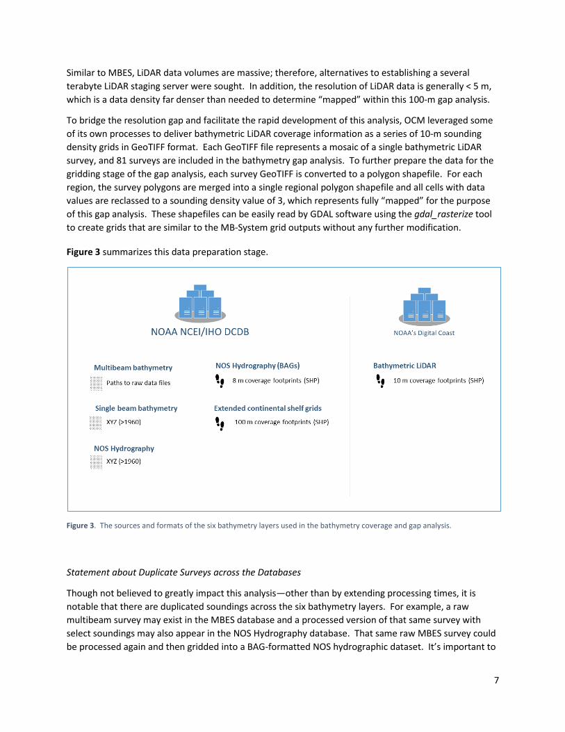
To bridge the resolution gap and facilitate the rapid development of this analysis, OCM leveraged some of its own processes to deliver bathymetric LiDAR coverage information as a series of 10-m sounding density grids in GeoTIFF format. Each GeoTIFF file represents a mosaic of a single bathymetric LiDAR survey, and 81 surveys are included in the bathymetry gap analysis. To further prepare the data for the gridding stage of the gap analysis, each survey GeoTIFF is converted to a polygon shapefile. For each region, the survey polygons are merged into a single regional polygon shapefile and all cells with data values are reclassed to a sounding density value of 3, which represents fully “mapped” for the purpose of this gap analysis. These shapefiles can be easily read by GDAL software using the gdal_rasterize tool to create grids that are similar to the MB-System grid outputs without any further modification.

Figure 3 summarizes this data preparation stage.

Figure 3. The sources and formats of the six bathymetry layers used in the bathymetry coverage and gap analysis.

Statement about Duplicate Surveys across the Databases

Though not believed to greatly impact this analysis—other than by extending processing times, it is notable that there are duplicated soundings across the six bathymetry layers. For example, a raw multibeam survey may exist in the MBES database and a processed version of that same survey with select soundings may also appear in the NOS Hydrography database. That same raw MBES survey could be processed again and then gridded into a BAG-formatted NOS hydrographic dataset. It’s important to

8

note that while duplicates in the databases exist, no surveys are added together or used twice for this analysis. A set of supersession rules are implemented during the grid merge phase, which replaces any lower density datasets with the higher density data, e.g., MBES supersedes the select soundings in NOS Hydrography and high resolution BAG-formatted NOS hydrography supersedes MBES. At worst, the duplicates mean that server resources are burdened by the over-processing of some data.

PROCESSING FRAMEWORK

To process the bathymetry layers over the entire U.S. exclusive economic zone and coastal waters, an internal framework was established. When developing the framework, several issues were taken into consideration. First, the dimensions of the framework needed to be of the right size where lots of depth measurements could be processed, but not too many that the processing software would not work. Second, the geographic scope of the framework needed to be flexible/expandable and not bound to specific geopolitical boundaries. Third, the framework logic needed to allow for a tracking capability, so any processing errors could be easily traced and corrected.

To address all of these issues, the framework underpinning the former International Map of the World initiative served as an inspiration for this bathymetry coverage and gap analysis framework. The International Map of the World was an international, land-based mapping initiative of the International Geographical Congress that started in 1909. The initiative sought to produce a uniform map of the world at 1:1,000,000 scale (1 km resolution). Standard sheets were defined as six degrees of longitude by four degrees of latitude, and the projection for each sheet was a modified polyconic. The sheets followed a systematic, global naming convention using two letters and two numbers (Rugg, 1951).

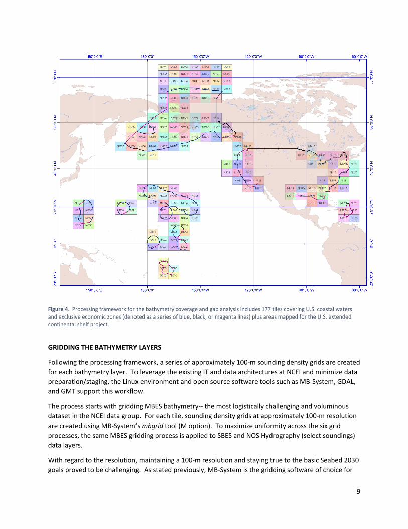
Leveraging the International Map of the World system, the internal framework for this gap analysis includes 177 processing tiles and follows a two letter and two number naming convention, e.g., NG15 or SA01 (see Figure 4). Each tile spans six degrees of longitude, and the number part of the tile naming convention conforms to a specified zone, ranging from 1 to 60, within the Universal Transverse Mercator (UTM) projection. Each tile spans four degrees of latitude and the letter part of the naming convention references the hemisphere (N indicating northern and S indicating southern) and the incremental band of latitude from the equator. For this project, this tiling scheme partitions the work into more manageable pieces.

9

Figure 4. Processing framework for the bathymetry coverage and gap analysis includes 177 tiles covering U.S. coastal waters and exclusive economic zones (denoted as a series of blue, black, or magenta lines) plus areas mapped for the U.S. extended continental shelf project.

GRIDDING THE BATHYMETRY LAYERS

Following the processing framework, a series of approximately 100-m sounding density grids are created for each bathymetry layer. To leverage the existing IT and data architectures at NCEI and minimize data preparation/staging, the Linux environment and open source software tools such as MB-System, GDAL, and GMT support this workflow.

The process starts with gridding MBES bathymetry-- the most logistically challenging and voluminous dataset in the NCEI data group. For each tile, sounding density grids at approximately 100-m resolution are created using MB-System’s mbgrid tool (M option). To maximize uniformity across the six grid processes, the same MBES gridding process is applied to SBES and NOS Hydrography (select soundings) data layers.

With regard to the resolution, maintaining a 100-m resolution and staying true to the basic Seabed 2030 goals proved to be challenging. As stated previously, MB-System is the gridding software of choice for

10

this project because it can easily read file paths to raw data and grid without additional reformatting/staging. Early attempts to create 100-m resolution grids involved trying to grid in projected space using mbgrid. After several tests at different latitudes, it became clear that MB-System is better at gridding in unprojected space (WGS84). In an attempt to get a consistent 100-m resolution in unprojected space (an impossibility), the gridding parameters were set to force a 100-m resolution (E! option in mbgrid). This analysis is characterized as ~ 100 m because this goal was not perfectly achieved in all of the processing tiles, particularly those tiles at high latitudes.

For the remaining bathymetry layers, the polygon shapefile footprints of the NOS BAG-formatted hydrography, bathymetric LiDAR, and ECS grid bathymetry layers are individually gridded using GDAL’s gdal_rasterize tool. The extents of each grid derive from the exact MBES grid parameters, which are slightly different from the bounds of the processing tiles because the 100-m x 100-m cell dimensions are forced in mbgrid. The resulting 100-m grids of BAG, LiDAR, and ECS footprints are populated with data values of 3, which represent “fully mapped” in this bathymetry coverage and gap analysis.

Figure 5 summarizes the gridding processes for the six bathymetry layers.

Figure 5. Summary of the gridding process for the bathymetry coverage and gap analysis.

MERGING THE GRIDDED BATHYMETRY (SOUNDING DENSITIES)

After gridding each bathymetry layer, the individual sounding density grids are merged. As mentioned earlier, to avoid inflated sounding density counts due to merging duplicated soundings across the bathymetry layers, the layers are not added together as part of this grid merge process. In other words, it was discovered early on that there could be negative effects from summing the sounding density layers when a survey could appear multiple times in the MBES, NOS Hydrography, NOS BAG-formatted hydrography, and/or ECS grid layers.

11

Instead of summing the layers, supersession rules are set based on the relative sounding densities of the bathymetry layers. To implement these supersession rules and merge the grids, an AND operator is used instead of an ADD operator. Using GMT’s grdmath tool, the AND operator takes two grid inputs (A and B) and returns one of the following for each cell (GMT, 2018):

• The value in Grid A • The value in Grid B, if A has No Data • No Data if A and B have No Data

The grid merging process used in this analysis involves taking the sounding densities from one bathymetry layer and replacing any sounding densities found in an underlying layer. Careful consideration is made to ensure that low density, select soundings found in one bathymetry layer (e.g. NOS Hydrography or SBES) would not replace higher density bathymetry layers (e.g., MBES or NOS BAG-formatted hydrography). Data quality is not explicitly considered in establishing these rules, though it does appear when there are two or more layers of similar data densities, such as when high quality hydrographic grid products (BAG and ECS) supersede other bathymetry layers.

Assuming a processing tile includes all six bathymetry layers, the grids are processed in the order shown in Figure 6. Grid A is the first input and Grid B is the second input. It is important to note that the output from each step is Grid B in the next step, etc.

Figure 6. Summary of the grid merging stages (steps 1 through 5) and reclassification stage (step 6) of the bathymetry coverage and gap analysis.

12

For the last step in this process (Step 6 in Figure 6), the sounding density values of the merged grid are reclassed to either 1s or 3s using the GMT’s grdclip tool. Cells with 3 or more soundings are reclassed to 3, and cells with 1 or 2 soundings are reclassed to 1. This full process results in 177 merged and reclassed sounding density grids.

RESULTS

The Visualization

The resulting 177 grids are rendered as color GeoTIFF images using GDAL. The “1-2 soundings” class is assigned a pink color, “3 or more soundings” are shown as dark purple, and areas with zero soundings (or outside the project area) are shown as transparent. Each image contains four raster bands: red, green, blue, and alpha (transparency). The two classes (1-2 soundings and 3 or more soundings) are rendered as separate images, to allow the ability to toggle them on/off individually on a web map.

The resulting images are then loaded into two separate ArcGIS mosaic datasets, representing the two classes. A mosaic dataset is a data model used to manage a collection of raster images and display them as a single “seamless” image. To improve performance as the map is zoomed out to smaller scales, overviews (down-sampled versions of the imagery) are built on each mosaic dataset. The overviews are generated using bilinear interpolation, which has the effect of smoothly blending the transparency channel at the edges of the data. So, areas with sparser coverage are shown as partially-transparent when displayed at smaller scales.

Geospatial Web Service

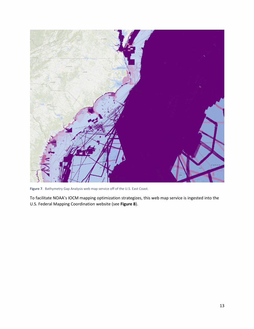
The mosaic datasets are published to the web using Esri’s ArcGIS Enterprise software, as a map service displaying the color imagery with two separate sub-layers: 1-2 soundings and 3 or more soundings (see Figure 7). The initial web map layers were published October 2017, with an updated version in February 2018. Further visualization improvements were made in March 2018. A NOAA GeoPlatform record for the Bathymetry Gap Analysis is established at http://noaa.maps.arcgis.com/home/item.html?id=4d7d925fc96d47d9ace970dd5040df0a.

13

Figure 7. Bathymetry Gap Analysis web map service off of the U.S. East Coast.

To facilitate NOAA’s IOCM mapping optimization strategizes, this web map service is ingested into the U.S. Federal Mapping Coordination website (see Figure 8).

14

Figure 8. Screen capture of the U.S. Federal Mapping Coordination site showing the Bathymetry Gap Analysis layers off the coasts of Georgia and South Carolina.

The Area Computations

From the 177 merged and reclassed grids, computations of areas “mapped” within the U.S. exclusive economic zones (EEZs) as well as coastal waters are established. To begin this task, a base clipping layer needed to be created for the EEZ as well as coastal waters. As further challenge, in the U.S., the EEZ has two basic definitions (see Figure 9). Per the international law of the sea, the EEZ starts at the territorial sea (i.e., 12 nautical miles as measured from baselines) and ends at 200 nautical miles or to the extent of a maritime boundary with an adjacent or opposite coastal State. Per U.S. domestic fisheries law, the EEZ starts at roughly the federal/state boundary (in most cases at 3 or 9 nautical miles) and ends at the same place as the international definition. The domestic definition is the basis of the EEZ layer used in this analysis, as this definition aligns with the frequently referenced total extent of the U.S. EEZ at 3.4 million square nautical miles.

To build a domestic EEZ layer for clipping the bathymetry coverage and gap analysis tiles, the inner limit of the EEZ was created from the Bureau of Ocean Energy Management’s (BOEM’s) Submerged Lands Act federal/state boundary, when available (BOEM, 2018). When the federal/state boundary was not available, then the 3 or 9 nautical mile line found on NOAA’s nautical charts was used as an approximate inner limit. It is important to note that the law and regulations that further refine this basic definition of the U.S. domestic EEZ were not consulted, so small variances on the federal/state boundary are likely in certain geographic regions. The outer limit of this domestic EEZ layer derived from the U.S. Maritime

15

Limits and Boundaries dataset (NOAA OCS, 2013). More information on this dataset is available in the 2007 Hydro Conference proceedings. (Westington and Slagel, 2007)

Figure 9. The U.S. maritime zones (in magenta) relative to charted tidal datums and the U.S. baseline (from Westington and Slagel, 2007).

To build a coastal waters layer for clipping the bathymetry coverage and gap analysis tiles, a global shoreline dataset and the inshore limit of the previously described domestic EEZ layer served as a basis. This particular area, referred to as “coastal waters” in this gap analysis, has no specific definition in law. Generally speaking, “coastal waters” contains U.S. state waters to an approximate shoreline. The shoreline used to create the inner limit of this area comes mostly from the fine-scale Global Self-consistent, Hierarchical, High-resolution Shorelines (GSHHG) product. This dataset is a high-resolution, combination of the World Vector Shorelines, CIA World Data Bank II, and Atlas of the Cryosphere (AC) databases (Wessel and Smith, 2017). The GSHHG product was particularly desirable to use for this coastal waters layer because its polygon format allows one to easily clip a GSHHG-derived landmass from a water area. In a few select cases where GSHHG positioning was off (e.g., the Northwestern Hawaiian Islands, Caribbean, and American Samoa), shoreline was digitized from NOAA’s raster nautical charts.

In total, as shown in Table 1, 24 base clipping layers covering U.S. waters were created to support these computations:

16

Table 1. List of all EEZ and coastal waters regions used in the area computations for the bathymetry gap analysis.

EEZ regions Coastal Waters regions Atlantic

Atlantic and Gulf of Mexico Gulf of Mexico Caribbean Caribbean Pacific (WA, OR, CA) Pacific (WA, OR, CA) Alaska: Gulf of Alaska (to 164-47-30W)

Alaska Alaska: Aleutian Islands (Pacific Ocean) Alaska: Total Bering Sea (including Bering Strait) Alaska: Arctic Coast Hawaiian Islands Hawaiian Islands CNMI and Guam CNMI and Guam Johnston Atoll -- Jarvis Island -- Kingman Reef- Palmyra Atoll -- American Samoa American Samoa Howland and Baker Islands -- Wake Island -- -- Great Lakes

To match geometries for this clipping and area calculation exercise, the 177 merged and reclassed grids were converted to TIF and then polygon shapefiles using GDAL’s gdal_polygonize.py routine. The 177 polygon shapefiles were clipped against the EEZ and coastal waters areas using Esri’s ArcGIS 10.5 software. The areas were computed using the Field Calculator in ArcGIS and a snippet of ArcPy code that will calculate geodesic areas. This method calculates the area of a polygon using WGS84-ellipsoid great circles between each vertex (ESRI, 2017). After some testing in projected (equal area) and unprojected space, it was determined that using this ArcGIS geodesic area functionality (and not re-projecting 177 grids) was perfectly suitable for this analysis.

As geodesics, the “mapped” areas were calculated for all polygons with a value of 1 (1-2 soundings per cell) or 3 (3 or more soundings per cell) within each EEZ and coastal waters region. Table 2 shows the % mapped within each of the EEZ and coastal waters regions. Based on this analysis, the % “mapped” within the combined EEZ and coastal waters areas for each region is reported in Figure 10. The total % “mapped” within U.S. waters is 41%.

17

Table 2. The percentage of “mapped” within each EEZ and coastal waters region.

EEZ regions % mapped Coastal Waters regions % mapped Atlantic 56% Atlantic and

Gulf of Mexico 41% Gulf of Mexico 45% Caribbean 53% Caribbean 84% Pacific (WA, OR, CA) 71% Pacific (WA, OR, CA) 65% Alaska: Gulf of Alaska (to 164-47-30W) 50%

Alaska 34% Alaska: Aleutian Islands (Pacific Ocean) 10% Alaska: Total Bering Sea (including Bering Strait) 14% Alaska: Arctic Coast 33% Hawaiian Islands 50% Hawaiian Islands 80% CNMI and Guam 75% CNMI and Guam 81% Johnston Atoll 20% -- Jarvis Island 15% -- Kingman Reef- Palmyra Atoll 70% -- American Samoa 34% American Samoa 100% Howland and Baker Islands 8% -- Wake Island 23% --

-- Great Lakes 4%

Figure 10. Displayed by region, the percentage of U.S. waters (EEZ and coastal waters combined) that are considered "mapped.” 41% of this combined U.S. waters area is considered “mapped” per this analysis.

18

CONCLUSION AND NEXT STEPS

This bathymetry coverage and gap analysis conveys a reasonably good picture of what is “mapped” within U.S. waters. Within the 3.4 million square nautical miles of U.S. EEZ and 154,000 square nautical miles of U.S coastal waters, only 41% is “mapped” according to this analysis. This analysis in conjunction with Seabed 2030 ambitions lays out a possible U.S. goal to map the remaining 59% by 2030. With a target % and a visualization to guide the discussion, the opportunity to begin mapping and/or share existing data holdings in a strategic manner are apparent.

As for the workflow behind this analysis, a few lessons were learned:

Due to the complexity and volume of the data included, it is notable that the processing times for this exercise were lengthy-- multiple weeks to complete. Given the time involved and the subtle impact of small updates in the bathymetry layers, it is advisable to update this analysis on an annual or semi-annual basis.

In addition, while useful to limit time-consuming data preparation/staging work, MB-System was limited in its ability to reliably grid in projected space at extreme latitudes. This workflow relied on MB-System’s mbgrid tool to produce geographic (WGS84) grids with the hope that a 100-m resolution could be forced using the E! option. This workflow wasn’t perfectly consistent, and especially at high latitudes, it produced grid cell footprints half the size of a 100-m resolution grid cell near the equator, i.e., 5,000 sq m cell footprint instead of 10,000 sq m. Working within the same processing framework and still using MB-System in order to limit data preparation/staging, it might be desirable to reprocess the grids in WGS84 with variable cell sizes represented in arc seconds instead of a fixed 100 m. To stay true to the 100-m resolution goals of the Seabed 2030 project while using parameters best fit for gridding in geographic space, Table 3 outlines possible gridding parameters based on varying latitude bands within the gap analysis processing framework:

Table 3. Table of the different latitude bands used in the gap analysis processing framework and potential gridding resolution parameters in arc seconds instead of 100 m. (computations using https://stevemorse.org/nearest/distance.php):

Latitude band (degrees)

Gridding resolution (longitude x latitude)

Approximate X dimensions in meters

Approximate Y dimensions in meters

Approximate range of area (sq meters)

Median area (sq meters)

0-16 3.5” x 3” 108 m to 103 m 92 m 9936-9476 9,706 16-44 4” x 3” 119 m to 89 m 92 m 10948-8464 9,706 44-56 5” x 3” 111 m to 87 m 92 m 10212-8004 9,108 56-60 6.5” x 3” 113 m to 100 m 92 m 10396-9200 9,798 60-64 7” x 3” 108 m to 95 m 92 m 9936-8740 9,338 64-68 8” x 3” 108 m to 92 m 92 m 9936-8464 9,200 68-72 9.5” x 3” 109 m to 90 m 92 m 10028-8280 9,154 72-76 12” x 3” 114 m to 90 m 92 m 10488-8280 9,384 76-80 16” x 3” 119 m to 85 m 92 m 10948-7820 9,384 80-84 24”x 3” 129 m to 77m 92 m 11,868-7,084 9,476

19

Future iterations of this analysis may include adding additional bathymetry, such as crowdsourced bathymetry, and revisiting the definition of “mapped.” With regard to defining “mapped,” there are potential issues for further exploration/discussion:

(1) Is it reasonable to assume that 1 sounding in a 100-m grid cell constitutes “mapped?” (2) Should survey instrumentation and water depth have an influence on the definition of

“mapped?”

To further explore the first question, one might compare the SBES sounding density grid output to the MBES sounding density grid output to identify cells where one SBES bathymetric measurement coexists with several MBES measurements. After locating these common geographic areas, one can compare the measurements from the two mapping systems. This exercise might help clarify the extent to which 1 sounding is sufficient for a cell to be deemed as “mapped.”

To further explore the second question, a recent concept paper entitled “The Nippon Foundation—GEBCO Seabed 2030 Project: The Quest to See the World’s Oceans Completely Mapped by 2030” describes a reasonable approach to accommodating differences in survey instrumentation to define “mapped” at deeper water areas (>1500 m deep) (Mayer, Jakobsson, et al., 2018). As the Seabed 2030 project continues to mature, it may be likely that the definition of “mapped” is one sounding per 800 m cell in areas deeper than 6000 m. Clearly, the underlying rationale for determining what has been “mapped” will have a significant impact on long term mapping strategies to fill the gaps.

In conclusion, this gap analysis is just one piece of a larger initiative. Using survey vintage and sounding density as guides, the results of this bathymetry gap analysis define—at least preliminarily— the scope of work associated with a seafloor mapping optimization strategy in U.S. waters and possibly elsewhere. As stated by Rear Admiral Shephard Smith, U.S. Hydrographer and chair of the International Hydrographic Office Council, in a recent Hydro International article, “Seabed 2030 will catalyze ocean mapping coordination and collaboration, empowering the world to make informed policy decisions, use the ocean sustainably, and undertake scientific research systematically with detailed bathymetric information of the Earth’s seafloor in hand.” (Smith, 2018)

ACKNOWLEDGEMENTS

This gap analysis would not have existed without the support of numerous individuals. Appreciation goes to Rear Admiral Shepard Smith at NOAA’s Office of Coast Survey as well as Dr. Larry Mayer and Dr. Brian Calder at CCOM/JHC for guiding the scope of this effort. Additionally, several data managers at NCEI provided expert technical guidance as well as access to their data holdings. Those data managers included Aaron Rosenberg (MBES), Brian Meyers (SBES), and Jason Baillio (NOS Hydrography and BAGs). Bathymetric LiDAR footprints were prepared by Kirk Waters, the data manager for LiDAR data at NOAA’s Office for Coastal Management. The extended continental shelf grids were prepared by Jim Gardner at CCOM/JHC. Lastly, John Cartwright at NCEI supported the publishing of the geospatial web service.

20

REFERENCES

BOEM, 2018. Maps and GIS Data. https://www.boem.gov/Oil-and-Gas-Energy-Program/Mapping-and-Data/Index.aspx.

Caress, D. W., and D. N. Chayes, 2017. MB-System: Mapping the Seafloor, https://www.mbari.org/products/research-software/mb-system.

ESRI, 2017. ArcMap 10.5 ArcPy Classes: Geometry. Retrieved from https://desktop.arcgis.com/en/arcmap/10.5/analyze/arcpy-classes/geometry.htm.

GMT, 2018. GMT Documentation: grdmath. https://www.soest.hawaii.edu/gmt/gmt/html/man/grdmath.html.

Mayer, L.; Jakobsson, M.; Allen, G.; Dorschel, B.; Falconer, R.; Ferrini, V.; Lamarche, G.; Snaith, H.; Weatherall, P. The Nippon Foundation—GEBCO Seabed 2030 Project: The Quest to See the World’s Oceans Completely Mapped by 2030. Geosciences 2018, 8, 63.

NOAA IOCM, 2017. Integrated Ocean and Coastal Mapping: Map Once, Use Many Times. https://iocm.noaa.gov/.

NOAA National Centers for Environmental Information, 2004. Multibeam Bathymetry Database (MBBDB), NOAA National Centers for Environmental Information. doi:10.7289/V56T0JNC.

NOAA NCEI, 2018. NOS Hydrographic Survey Data. https://www.ngdc.noaa.gov/mgg/bathymetry/hydro.html.

NOAA OCS, 2013. U.S. Maritime Limits and Boundaries, version 4.1. https://maritimeboundaries.noaa.gov.

Rugg, Dean S., 1951. The International Map of the World. The Scientific Monthly, Vol. 72, No. 4. American Association for the Advancement of Science, pp. 233-240.

Smith, Shepard M., 2018. Seabed 2030: A Call to Action. Hydro International, Vol. 22, No. 1. Geomares Publishing, pp. 22-23. Published March 3, 2018.

Smith, Walter H.F., 2004. Introduction to this special issue on bathymetry from space. Oceanography 17(1):6–7, https://doi.org/10.5670/oceanog.2004.62.

The Nippon Foundation-GEBCO, 2016. “The Nippon Foundation – GEBCO – Seabed 2030: Roadmap for Future Ocean Floor Mapping.” (Retrieved from https://seabed2030.gebco.net/documents/seabed_2030_roadmap_v10_low.pdf)

Ware, C., Knight, W., and Wells, D., 1991. Memory intensive statistical algorithms for multibeam bathymetric data, Computers & Geosciences, 17, pp. 985–993.

Wessel, Paul and Smith, W. H. F., 2017. Global Self-consistent, Hierarchical, High-resolution Geography Database (GSHHG), version 2.3.7. http://www.soest.hawaii.edu/wessel/gshhg/. Westington, Meredith and Slagel, M., 2007. U.S. Maritime Zones and the Determination of the National Baseline. Proc. of the U.S. Hydrographic Conference. Norfolk, VA, pp. 14.