Assessing Structural VARs∗

(Preliminary and Incomplete: Do Not Cite WithoutAuthors’ Permission.)

Lawrence J. Christiano† Martin Eichenbaum‡ Robert Vigfusson§

May 8, 2005

Abstract

We argue that structural vector autoregressions (VARs) are useful as a guide toconstructing and evaluating dynamic general equilibrium models. Given a minimal setof identifying assumptions, structural VARs allow the analyst to estimate the dynamiceffects of economic shocks. We ask the following three questions. First, what are thebias properties of the estimator? Second, what are the bias properties of standard es-timators of sampling uncertainty in the estimator? Third, are there easy to implementvariants of standard procedures which improve the bias properties of response functionestimators? We address these questions using data generated from a series of dynamicgeneral equilibrium models. Based on our answers, we conclude that structural VARsdo indeed provide valuable information for building empirically plausible models ofaggregate fluctuations.

∗The first two authors are grateful to the National Science Foundation for Financial Suppport.†Northwestern University and NBER.‡Northwestern University and NBER.§Federal Reserve Board of Governors.

1. Introduction

We argue that structural vector autoregressions (VARs) are useful as a guide to constructing

and evaluating dynamic general equilibrium models. Given a minimal set of identifying

assumptions, structural VARs allow the analyst to estimate the dynamic effects of economic

shocks. These estimated response functions provide a natural way to assess the empirical

plausibility of a structural model.1 To be useful, the response function estimators must have

good statistical properties. To assess these properties, we ask the following three questions.

First, what are the bias properties of the estimator? Second, what are the bias properties of

standard estimators of sampling uncertainty? Third, are there easy to implement variants of

standard procedures which improve the bias properties of response function estimators? We

address these questions using data generated from a series of dynamic general equilibrium

models. Based on our answers, we conclude that structural VARs do indeed provide valuable

information for building empirically plausible models of aggregate fluctuations.

There are two important traditions for constructing dynamic general equilibrium models.

One tradition focusses on at most a handful of key shocks, and deliberately abstracts from

the smaller shocks.2 A classic example is Kydland and Prescott ( ), who work with a model

driven only by technology shocks, even though they take the position that these shocks

only account for 70 percent of business cycle fluctuations. A conundrum confronted by this

modeling tradition is how to empirically evaluate models (which contain only a subset of

the shocks) with the data (which are driven by all the shocks).3 Structural VARs have

the potential to provide a resolution to this challenge, by allowing the analyst to assess the

empirical performance of a model relative to a particular set of shocks.

A second tradition to building macroeconomic models incorporates large numbers of

shocks to provide a complete characterization of the stochastic processes generating the

data.4 This tradition avoids the Kydland and Prescott conundrum. Still, for diagnostic

purposes it is useful to assess the implications of these models for particular shocks to the

1Perhaps the first in this line of research is Sims (1989). There are many others, including Christiano,Eichenbaum and Evans (2005), Francis and Ramey (2001), Gali (1999), Rotemberg and Woodford (1997),and Del Negro, Schorfheide, Smets, and Wouters (2005).

2The view that aggregate dynamics are dominated by the effects of a few shocks only, appears to receiveconfirmation from the literature on factor models, such as Sargent and Sims, Quah and Sargent (1993),Reichlin, and Uhlig (1992).

3Aiyagari (1994) and Prescott (1991) draw attention to the challenge by pointing to a difficulty with thestandard RBC strategy for evaluating a model. In this strategy, one compares the second moment propertiesof the data with the second moment properties of the model. Prescott famously asserted that if a modelmatches the data, then that is bad news for the model. The argument is that since good models leave somethings out of the analysis, good models should not match the data. Of course, lots of models do not matchthe data. This raises the question: how can we use the data to differentiate between good and bad models?Structural VARs provide one possible answer.

4See, for example, Smets and Wouters (2003) and Christiano, Motto and Rostagno (2004).

2

economy.

In practice, the literature uses two types of identifying restrictions in structural VARs.

Blanchard and Quah (1989), Gali (1999) and others have exploited the implications that

many models have for the long-run effects of shocks.5 Other authors have exploited short-

run restrictions.6 There is a growing literature that questions the ability of structural VARs

to uncover the dynamic response of macroeconomic variables to structural shocks. This

literature focuses on identification strategies that exploit long run restrictions. Perhaps the

first critique of these strategies was provided by Sims (1972). Although this paper was writ-

ten before the advent of VARs, it articulates clearly why we should be concerned about the

accuracy of identification based on long-run restrictions. The problem is that this strategy

requires a reliable estimate of the sum of coefficients in distributed lag regressions. These

sums are hard to reliably estimate even if the individual coefficients are reasonably precisely

estimated. Faust and Leeper (1997) and Pagan make important related critiques of identi-

fication strategies based on long run restrictions. More recently Erceg, Guerrieri and Gust

(2004) and Chari, Kehoe and McGrattan (2005) (CKM) have also examined the reliability

of VAR-based inference using long run identifying restrictions. CKM are particularly critical

and argue that structural VARs are very misleading.

We examine the reliability of inference using structural VARs based on long-run and

short-run identifying assumptions. Throughout, we suppose that the data generating mech-

anism corresponds to variants of a standard real business cycle model. We focus on the

question, how do hours worked respond to a technology shock?

We find that structural VAR’s perform remarkably well when identification is based on

short run restrictions. This is comforting for the vast literature that has exploited short

run identification schemes to identify the dynamic effects of shocks to the economy. Of

course, one can question the particular short run identifying assumptions used in any given

analysis. But our results strongly support the view that if the relevant short run assumptions

are satisfied in the data generating mechanism, then standard structural VAR procedures

reliably uncover and identify the dynamic effects of shocks to the economy.

Regarding identification based on long-run assumptions, we find that if technology shocks

account for a substantial fraction of business cycle fluctuations in output (say, over 50 per-

cent), then VAR based analysis is reliable. We do find some evidence of bias when the

fraction of output variance accounted for by technology shocks is very small relative to esti-

mates in the standard RBC literature. But, this bias can be eliminated in at least two ways.

5See, for example, Basu, Fernald, and Kimball (1999), Christiano, Eichenbaum and Vigfusson (2003,2004), and Francis and Ramey (2001)

6This list is particularly long and includes at least Bernanke and Blinder (1992), Bernanke and Mihov(1995), Christiano and Eichenbaum (1992), Christiano, Eichenbaum and Evans (2005), Grilli and Roubini(1995), Hamilton (1997) and Sims and Zha (1995).

3

First, our examples suggest that if there are enough variables in the VAR, the analyst is not

likely to be misled in practice. Specifically, we find that when the number of aggregate vari-

ables in the VAR exceeds the number of important driving shocks, then the bias in impulse

response estimators is substantially reduced. In light of the widespread consensus that there

are only a handful of important shocks driving aggregate fluctuations, our finding suggests

that including a reasonably small number of variables in the VAR should be sufficient to

reduce small sample bias even if technology shocks are relatively unimportant.

Second, we have developed an adjustment to the standard VAR estimation strategy that

virtually eliminates small sample bias, even in the worst case scenario when technology

shocks play only a small role in aggregate fluctuations and there is only a small number of

variables in the VAR. The standard VAR strategy requires factorizing an estimate of the

spectral density at frequency zero of the data. The estimator used for this purpose is the

zero-frequency spectral density implicit in the estimated VAR itself. It is principally because

the quality of this estimator deteriorates that distortions occur in the worst-case scenario.

This observation motivates us to adjust the standard VAR estimator by instead working

with a Newey-West non-parametric estimator of the frequency-zero spectral density. We

find that the effects of our adjusted strategy are minor when we are not in the worst-case

scenario. However, in the cases when standard VAR procedures entail some bias, then that

bias is virtually eliminated by our adjusted estimator, in all the cases we consider.

Our conclusions regarding the value of identified VARs differ sharply from those recently

reached by CKM. Part of CKM’s analysis concerns the consequences of working with the

first difference of hours worked, when the levels specification is the correct one. We have

nothing to say about this here, since we assume that the econometrician does not commit

this specification error.7 CKM argue that even when hours worked enter the analysis in

levels, VARs are essentially useless as a tool for estimating the dynamic impact on hours

worked of technology shocks. We reach a different conclusion, for three reasons.

First, CKM do not consider identified VARs when identification is accomplished via short

run restrictions. They only consider the case of long-run restrictions. Second, CKM reach

their conclusions based on two examples. These turn out to constitute worst case scenarios for

VARs, because they have two particular properties: (i) they have the feature that technology

shocks account for only a very small proportion (23 and 17 percent, respectively) of output

fluctuations and (ii), the number of variables included in the VAR is equal to the number

of important shocks in the model. As discussed above, we too find evidence of bias in

experiments sharing these properties. As indicated above, this bias is easily dealt with and

does not reflect a fundamental flaw in structural VARs.7We have explored the differencing issue elsewhere, in Christiano, Eichenbaum and Vigfusson (2003,

2004).

4

CKM conjecture that the distortions in their two examples are due to the omission of

capital in the VAR. If true this would indeed be a fundamental problem because quarterly

data on the stock of capital is poorly measured and is typically not included in VAR analy-

ses. Fortunately, it turns out that CKM’s conjecture is incorrect. This follows from three

observations. First, there is virtually no bias when we use our adjusted VAR estimation

procedure in their two examples. Second, even with standard VAR procedures bias is re-

duced when technology shocks play a more important role in aggregate fluctuations than

they do in CKM’s examples. Interestingly, there is essentially no bias at all when, consistent

with the findings of Kydland and Prescott ( ), technology shocks account for 70 percent

of the business cycle variance in output. Finally, in our analysis of short-run identification

strategies, VAR inference is very reliable, even though capital is not included in the VAR.

There is a third reason why our conclusions differ from CKM’s. The CKM strategy for

implementing long-run restrictions is anomalous relative to the strategy used in the literature.

CKM identify a positive technology shock as one that drives labor productivity up in the

period of the shock. The standard approach identifies a positive technology shock as one

that drives labor productivity up in the long run.8 In practice, which identification strategy

is taken rarely matters. For example, it makes not difference in a version of Kydland and

Prescott’s RBC model in which technology shocks account for 70 percent of business cycle

fluctuations in output. However, in the two CKM examples, whether one adopts the standard

or the CKM identification strategy makes a dramatic difference. The CKM choice leads to a

bimodal small sample distribution in the response of hours to a technology shock. In about

20 percent of the artificial data sets generated from their model, CKM’s procedure leads

them to infer that hours worked falls sharply, while labor productivity falls permanently, in

the wake of what they identify as a positive technology shock. The standard identification

strategy would identify these responses as the consequences of a negative technology shock.

CKM’s anomalous identification strategy leads them to overstate sampling uncertainty by a

factor of two, leading them to conclude that VARs are completely uninformative. In reality,

this conclusion is an artifact of their choice of identification strategy.

The remainder of this draft is organized as follows. Section 2 presents the general equi-

librium model used in our examples. Section 3 discusses our results. Section 4 compares our

results to those of CKM. Finally, section 5 contains concluding comments.

2. A Simple Real Business Cycle Model

In this section, we display the real business cycle model used in our analysis. The model has

the property that the only shock that affects labor productivity in the long run is a shock to

8See, for example, the RATS manual.

5

technology. This property lies at the core of an identification strategy used by Gali (1999) and

others to identify the effects of a shock to technology. We also consider a variant of the model

in which we impose additional timing restrictions on agents’ actions. In particular, we assume

that agents choose hours worked before the technology shock is realized. This assumption

allows us to identify the effects of a shock to technology using ‘short run restrictions’, that is,

restrictions on the variance-covariance matrix of the disturbances to a vector autoregression.

Finally, we discuss several parameterizations of our model that are used in the experiments

we perform.

2.1. The Model

The representative agent maximizes expected utility over per capita consumption, ct, and

per capita employment, lt

E0

∞Xt=0

(β (1 + γ))t"log ct + ψ

¡l − lt

¢1− σ

1−σ#,

subject to the budget constraint:

ct + (1 + τx,t) [(1 + γ) kt+1 − (1− δ) kt] ≤ (1− τ lt)wtlt + rtkt + Tt.

Here, kt denotes the per capita capital stock at the beginning of period t, wt is the wage

rate, rt is the rental rate on capital, τx,t is an investment tax, τ lt is the tax rate on labor,

δ ∈ (0, 1) is the depreciation rate on capital, γ is the net growth rate of the population, andTt represents lump-sum taxes. Finally, σ > 0 is a curvature parameter.

The representative competitive firm’s production function is:

yt = kαt (Ztlt)1−α ,

where Zt is the time t state of technology and α ∈ (0, 1). The stochastic processes for theshocks are:

log zt = µZ + σzεzt

τ lt+1 = (1− ρl) τ l + ρlτ lt + σlεlt+1 (2.1)

τxt+1 = (1− ρx) τx + ρxτxt + σxεxt+1,

where zt = Zt/Zt−1. In addition, εzt , εdt , and ε

xt are independent random variables with mean

zero and unit standard deviation. The parameters, σz, σl and σx are non-negative scalars.

The constant, µZ , is the mean growth rate of technology, τ l is the mean labor tax rate, τxis the mean tax on capital. We restrict the autoregressive coefficients, ρl and ρx, to be less

than unity in absolute value.

6

Finally, the resource constraint is:

ct + (1 + γ) kt+1 − (1− δ) kt ≤ yt.

We consider two versions of the model, differentiated according to timing assumption. In

the standard version, all time t decisions are taken after the realization of the time t shocks.

This is the conventional assumption in the real business cycle literature. For pedagogical

purposes, we also consider a second version of the model, we call the recursive version of the

real business cycle model. Here, the timing assumptions are as follows. First, τ lt is observed,

after which labor decisions are made. Next, the other shocks are realized. Then, agents

make their investment and consumption decisions. Finally, labor, investment, consumption,

and output occur. We first discuss the standard version of our model.

2.1.1. The Standard Version of the Model

The log-linearized policy rule for capital can be written as follows:

log kt+1 = γ0 + γk log kt + γz log zt + γlτ lt + γxxt,

where kt ≡ kt/Zt−1. The policy rule for hours worked is:

log lt = a0 + ak log kt + az log zt + alτ lt + axτxt.

>From this expression, it is clear that all shocks have only a temporary impact on lt and

kt. Since εzt is the only shock that has a permanent effect on Zt, it follows that εzt is the

only shock that has a permanent impact on the level of the capital stock, kt. Similarly, εzt is

the only shock that has a permanent impact on output and labor productivity, at ≡ yt/lt.

Formally, this exclusion restriction is given by:

limj→∞

[Etat+j −Et−1at+j] = f (εzt only) , (2.2)

where in our linear approximation to the model solution, f is a linear function. The model

also implies the sign restriction that f is an increasing function. In (2.2), Et is the expectation

operator, conditional on Ωt =³log kt−s, log zt−s, τ l,t−s, τx,t−s; s ≥ 0

´. The exclusion and

sign restrictions have been used by Gali (1999) and others to identify the dynamic impact

on macroeconomic variables of a positive shock to technology.

In practice, researchers impose the exclusion and sign restrictions on a vector autoregres-

sion to compute εzt and identify its dynamic effects on macroeconomic variables. To describe

7

this procedure, denote the variables in the VAR by Yt :

Yt+1 = B (L)Yt + ut+1, Eutu0t = V, (2.3)

B(L) ≡ B1 +B2L+ ...+BpLp−1,

Yt =

⎛⎝ ∆ log atlog ltxt

⎞⎠ ,

where xt is an additional vector of variables that may be included in the VAR. It is assumed

that the fundamental economic shocks are related to ut in the following way:

ut = Cεt, Eεtε0t = I, CC 0 = V, (2.4)

where the first element in εt is εzt . It is easy to verify that:

limj→∞

Et[at+j]− Et−1[at+j] = τ [I −B(1)]−1Cεt, (2.5)

where τ is a row vector with all zeros, except unity in the first location. Here, B(1) is the

sum, B1+ ...+Bp. Also, Et is the expectation operator, conditional on Ωt = Yt, ..., Yt−p+1 .To compute the dynamic effects of εzt , we require B1, ..., Bp and C1, the first column of C.

The symmetric matrix, V, and the Bi’s can be computed by an ordinary least squares

regression. However, it is well known that the requirement CC 0 = V is not sufficient to

determined a unique value of C1. Adding the exclusion and sign restrictions does uniquely

determine C1. These restrictions are:

exclusion restriction: [I −B(1)]−1C =

"number 0

1×(N−1)numbers numbers

#,

and

sign restriction: (1, 1) element of [I −B(1)]−1C is positive.

Although there are many matrices, C, that satisfy CC 0 = V as well as the exclusion and

sign restrictions, they all have the same C1. To see this, first let D ≡ [I −B(1)]−1C, so that

DD0 = [I −B(1)]−1 V [I −B(1)0]−1= S0, (2.6)

say. Note that S0 (the spectral density of Yt at frequency zero) can be computed directly

from the VAR coefficients and the variance-covariance matrix of the VAR disturbances. The

exclusion restrictions require that D have the following structure:

D =

⎡⎣ d111×1

01×(N−1)

D21(N−1)×1

D22(N−1)×(N−1)

⎤⎦ .8

Then,

DD0 =

∙d211 d11D

021

D21d11 D21D021 +D22D

022

¸=

∙S110 S2100

S210 S220

¸,

say. The sign restriction is:

d11 > 0. (2.7)

Then, the first column of D is uniquely determined by:

d11 =qS110 , D21 = S210 /d11

Finally, the first column of C is determined from:

C1 = [I −B(1)]D1. (2.8)

2.1.2. The Recursive Version of the Model

In the recursive version of the model, the policy rule for labor involves log zt−1 and xt−1

because they help forecast log zt and xt :

log lt = a0 + ak log kt + alτ lt + a0z log zt−1 + a0xxt−1.

Because labor is a state variable at the time the investment decision is made, the policy rule

for kt+1 takes the following form:

log kt+1 = γ0 + γk log kt + γz log zt + γlτ lt + γxxt

+γ0z log zt−1 + γ0xxt−1.

It is easy to verify that these policy rules satisfy the exclusion restriction, (2.2), and the sign

restriction on εzt . So, the long-run identification strategy outlined above can be rationalized

in this model. An alternative procedure for identifying εzt that does not rely on estimating

long-run responses to shocks can also be rationalized. We refer to this as the ‘short run’

strategy, because it involves recovering εzt using just the realized one-step-ahead forecast

errors in labor productivity and hours, as well as the second moment properties of those

forecast errors. According to the model, the error in forecasting at given Ωt−1, denoted by

uaΩ,t, is a linear combination of εzt and εlt. The error in forecasting log lt given Ωt−1, u

lΩ,t, is

proportional to εlt. Specifically,

uaΩ,t = α1εzt + α2ε

lt, u

lΩ,t = γεlt,

where α1 > 0, α2 and γ are functions of the model parameters. It follows that α1εzt is the

error from regressing uaΩ,t on ulΩ,t :

uaΩ,t = βulΩ,t + α1εzt , β =

cov(uaΩ,t, ulΩ,t)

V¡ulΩ,t

¢ ,

9

where cov(x, y) denotes the covariance between the random variables, x and y, and V (x)

denotes the variance of x. Recall, we normalize the standard deviation of εzt to be unity.

Consequently, the value of α1 can be recovered as the positive square root of the variance of

the forecast error in this regression:

α1 =qV¡uaΩ,t

¢− β2V

¡ulΩ,t

¢.

In practice, we implement the previous procedure using the one-step-ahead forecast errors

generated from a VAR. It is convenient to work with a version of (2.3) in which the variables

in Yt are ordered as follows:

Yt =

⎛⎝ log lt∆ log at

xt

⎞⎠ ,

where xt is an additional vector of variables that may be included in the VAR. In addition,

we write the vector of VAR one-step-ahead forecast errors, ut as:

ut =

⎛⎝ ultuatuxt

⎞⎠ .

We identify the technology shock with the second element in et in (2.4). To compute the

dynamic response of the variables in Yt to the technology shock, we require B1, ..., Bq in (2.3)

and the second column of the matrix, C, in (2.4). We obtain the elements of the second

column of C in two steps. First, we identify the technology shock using:

εzt =1

α1

³uat − βult

´,

where

β =cov(uat , u

lt)

V¡ult¢ , α1 =

qV (uat )− β

2V¡ult¢,

where the indicated variances and covariances are obtained from V in (2.3). Second, to

obtain C2, the second column of C, we regress ut on εzt :

C2 =

⎛⎜⎝cov(ul,e2)var(e2)

cov(ua,e2)var(e2)

cov(ux,e2)var(e2)

⎞⎟⎠ =

⎛⎜⎝ 0α1

1α1

³cov(uxt , u

at )− βcov

¡uxt , u

lt

¢´⎞⎟⎠ .

This procedure for computing C2 can be implemented by computing CC 0 = V, where C

is the lower triangular Choleski decomposition of V, and taking the second column of that

matrix. This is a convenient strategy because the Choleski decomposition can be computed

using widely-available software.

10

2.2. Parameterizing the Model

We consider different versions of the RBC model that are distinguished by the nature of the

exogenous shocks. For comparability we assume, as in CKM, that:

β = 0.97221/4, θ = 0.35, δ = 1− (1− .0464)1/4, ψ = 2.24, γ = 1.0151/4 − 1l = 1300, τx = 0.3, τ l = 0.27388, µz = 1.016

1/4 − 1, σ = 1.

We consider various parameterizations for the shocks. These parameterizations were chosen

to illustrate the key factors determining the reliability of inference based on short run and

long-run identification restrictions.. It is convenient to report, for each parameterization,

the variance of HP-filtered output due to technology shocks.

KP Benchmark Specification

In the Kydland and Prescott specification, the technology shock process is the same as

the one estimated by Prescott (1986):9

log zt = µZ + 0.011738× εzt .

Erceg, Guerrieri and Gust (2005) update Prescott’s analysis and estimate σz to be 0.0148. To

be conservative, we use Prescott’s estimate because it attributes relatively less importance to

technology shocks in aggregate fluctuations. Although he concentrates on technology shocks

in his analysis, Prescott (1986) argues that other shocks also affect aggregate fluctuations. To

maintain comparability with CKM, we specify τ lt to be the other shock in this specification.

We estimate a law of motion for τ l,t as follows. Combining the household and firm first

order conditions for labor, and rearranging, we obtain:

τ l,t = 1−ctyt

ltl − lt

ψ

1− θ.

Given our parameter values, we compute a time series for τ l,t, and estimate the following

first order autoregressive representation:10

τ l,t = (1− 0.9934)× 0.2660 + 0.9934× τ l,t−1 + 0.0062× εlt.

Figure 1 depicts the time series on τ l,t, lt/(l − lt) and ct/yt.

9Prescott (1986) estimates that the standard deviation of the innovation to technology growth is 0.763 per-cent. However, he adopts a different normalization than we do, placing technology in front of the productionfunction, rather than next to hours worked, as we do. Our standard deviation is 0.01174=0.00763/(1-.35).10Consumption, ct, is the sum of nondurables, services and government consumption. We measure the

ratio, ct/yt, as the ratio of dollar quantities. Total hours worked, lt, is nonfarm business hours workeddivided by a measure of the population, aged 16 and older.

11

Let p denote the percent variance in HP-filtered, log output due to technology shocks in

a model. Table 1 reports that p = 73 in the Kydland-Prescott specification.11 This value of

p is consistent with a key claim advanced by Kydland and Prescott, namely that technology

shocks account for toughly 70% of the cyclical volatility of output. The finding that p is 73%

is the reason we refer to this version of our model as the Kydland-Prescott specification. For

reference, Table 1 reports other standard business cycle statistics for the KP specification.

In artificial data generated by the KP Benchmark specification, we fit bivariate VAR

models, in which xt in (2.3) is omitted.

CKM Benchmark Specification

CKM’s benchmark specification has two shocks, zt and τ lt, which have the following time

series representations:

log zt = µZ + log zt = µZ + 0.00581× εzt

τ lt = (1− ρl) τ l + ρlτ l,t−1 + 0.00764× εlt, ρl = 0.93782.

In sharp contrast to the Kydland and Prescott specification, the CKM benchmark specifi-

cation implies that p is only 23 (see Table 1). CKM use this specification to criticize Gali

(1999)’s work. It is ironic that CKM use this specification to to criticize Gali when their

specification embodies his main hypothesis, namely, that technology shocks play only a very

small role in business cycle fluctuations. Other business cycle implications of the CKM

benchmark specification are reported in Table 1. Note the substantial negative business cy-

cle correlation of productivity and hours worked, and the relatively high volatility of hours

worked. This reflects that non-technology shocks are the primary driver of business cycle

fluctuations in the CKM benchmark specification.

In artificial data generated by the CKM Benchmark specification, we fit bivariate VAR

models, in which xt in (2.3) is omitted.

Other Specifications

We consider a series of perturbations on the Benchmark KP and CKM specifications.

We vary the values of σ and σl, both of which have an important quantitative effect on the

contribution of technology shocks to the volatility of output. In artificial data generated by

these versions of the models, we fit bivariate VARs in which xt in (2.3) is omitted.

In addition, we add shocks and variables to the model. In the Three Shocks, Two Impor-

tant specification, we add the tax rate shock with a very small variance:

τxt = τx + 0.0001× εxt11The 73 percent figure is a population value, computed using the spectral integration approach described

in Christiano (2002).

12

In this case, we work with a three-variable VAR, with

xt = log

µityt

¶. (2.9)

in (2.3), where it denotes gross investment. In the Three Shocks, Three Important specifica-

tion, we adopt, for the sake of comparability, the specification of the tax rate shock used in

CKM:

τxt = (1− 0.9) τx + 0.9× τx,t−1 + 0.01εxt . (2.10)

Here too, we work with a three-variable VAR, with xt in (2.3) specified as in (2.9).

Finally, we also consider a Four Shocks, Three Important specification. In this case, we

specify xt in (2.3) as

xt =

Ãlog³ityt

´τxt + wt

!,

where wt is a Normally distributed iid measurement error with mean zero and standard

deviation 0.0001.

3. Results

In this section we analyze the properties of VAR-based strategies for identifying the effects

of a technology shock. Our basic strategy is to simulate artificial time series using variants

of the economic model discussed above as the data generating process. By construction we

know the actual response of hours worked to a technology shock. We then consider what an

econometrician using VARs would find, on average over repeated small samples.

Throughout we focus on three key questions. First, would the econometrician be misled

when conducting inference about dynamic response functions? Second, is there substantial

bias associated with the estimated dynamic response functions of hours to a technology

shock? Third, are there easy-to-implement modifications to standard econometric procedures

that would eliminate bias when it emerges? The first subsection presents our answers to these

questions when we use the recursive version of the model. The second subsection presents

our results when we use the long-run properties of the standard version of the model to

identify technology shocks.

3.1. Recursive Identification

Analysis of the KP Specification

We begin by discussing the results we obtained using variants of the KP specification

as the data generating mechanism. Throughout we proceed as follows. Using the economic

13

model as the data generating mechanism,we simulate 1000 data sets, each of length 180

observations. The shocks εzt , εlt and possibly εxt are drawn from i.i.d. standard normal

distributions.

On each data set we estimate a four lag VAR, Two or three variables are included in the

VAR depending on the specification being analyzed. Given the estimated VAR, we calculate

the dynamic response of hours to a technology shock based on the short-run identifying

restriction and method discussed in section 2.1.2 above. The solid lines in Figure 2 are

the average dynamic response function obtained over the 1000 synthetic data sets in the

different specifications. The starred lines are the true dynamic response function of hours

worked implied by the economic model that is being used as the data generating process.

The grey areas in the figure are measures of the sampling uncertainty associated with the

estimated dynamic response functions. We obtain these measures by first calculating the

standard deviation of the points in the estimated impulse response functions across the 1000

synthetic data sets. The grey areas correspond to a two standard deviation band about the

relevant solid black line. The dashed lines corresponds to the top 2.5% and bottom 2.5% of

the estimated coefficients in the dynamic response functions across the 1000 synthetic data

sets. To the extent that the dashed lines coincide with boundaries of the grey area, there

is support for the notion that the coefficients of estimated impulse response functions are

normally distributed.

An important question is whether an econometrician would correctly estimate the true

uncertainty associated with the estimated dynamic response functions. To address this

question we proceed as follows. For each synthetic data set and corresponding estimated

impulse response function, we calculated the bootstrap standard deviation of each point in

the impulse response function. Specifically, for a given synthetic data set, we estimate a VAR

and use it as the data generating process to construct 200 synthetic data sets, each of length

180 observations. For each synthetic data set, we estimate a new VAR and impulse response

function. We then calculate the standard deviation of the coefficients in the impulse response

functions across the 200 data sets. Finally, we take the average of these standard deviation

across the 1000 synthetic data sets that were generated using the economic model as the data

generating process. The lines with 0’s in Figure 2 correspond to a two standard deviation

band about the solid black line and are a measure of the average standard deviations that a

econometrician would construct.

The top left graph in Figure 2 exhibits the properties of the VAR estimator of the response

of hours to a technology shock when the data are generated by the KP specification. The

2,1 graph in Figure 2 corresponds to the case when the data generating mechanism is the

KP specification with σ = 0.0001. This case is of interest, because utility is roughly linear in

leisure, corresponding to Hansen (1985)’s indivisible labor model. The 3,1 graph in Figure

14

2 shows what happens when σ is increased above its benchmark specification, to σ = 1.24.

This case is of interest, because this parameterization gives rise to roughly the same Frisch

elasticity used in the model studied by Erceg, Guerrieri and Gust (1004). The 4,1 graph in

Figure 2 shows what happens in the three variable, three shock version of the model. In each

case, the impact effect on hours worked and associated sampling variance is also reported,

for convenience, in Table 2.

The first column of Figure 2 exhibits three striking features. First, regardless of which

variant of the KP specification we work with, there is no evidence whatsoever of bias in the

estimated impulse response functions. In all cases, the solid lines virtually coincide with

the starred lines. Second, Figure 2 indicates that an econometrician would not be misled in

inference using standard procedures for constructing confidence intervals. This conclusion

reflects the fact that the average value of the econometrician’s confidence interval (the line

with the 0’s) coincides closely to the actual range of variation in the impulse response function

(the grey area). Third, there is no evidence against the view that the estimated coefficients

of the impulse response functions are normally distributed: in all cases the boundaries of the

grey area coincide closely with the dashed lines.

Analysis of the CKM Specification

The right hand column of Figure 2 reports our results when the data generating mecha-

nism is given by variants of the CKM specification. The top right hand graph in Figure 2

corresponds to the CKM specification. The 2,2 and 2,3 graphs in Figure 2 correspond the

CKM specification with σ = 0.0001 and σ = 1.24, respectively. Finally, the 4,1 graph in

Figure 2 corresponds to the three variable, three shock version of the CKM specification.

Notice that the second column of Figure 2 contains the same striking features as the first

column. First, there is no evidence whatsoever of bias in the estimated impulse response

functions. Second, the average value of the econometrician’s confidence interval coincides

closely to the actual range of variation in the impulse response function (the grey area).

Third, there is no evidence against the view that the estimated coefficients of the impulse

response functions are normally distributed.

In sum, our analysis of the recursive identification scheme reveals that structural VAR’s

perform remarkably well. This is extremely comforting for the vast literature that has

exploited recursive identification schemes to identify the dynamic effects of shocks to the

economy. Of course, one can criticize the particular short run identifying assumptions used

in any given analysis. But our results strongly support the view that if the relevant recur-

sive assumptions are satisfied in the data generating mechanism, standard structural VAR

procedures will reliably uncover and identify the dynamic effects of shocks to the economy.

15

Finally, note we did not include capital as a variable in the VAR. Despite this omission,

the structural VAR procedure performs remarkably well. This demonstrates that, claims in

CKM to the contrary, omitting the economically relevant state variable capital does not in

and of itself pose a problem for inference using structural VAR’s.

3.2. Long-run Identification

Analysis of the KP Specification

We begin by discussing results associated with variants of the KP specification. As above

we use the economic model as the data generating mechanism to simulate 1000 data sets,

each of length 180 observations. The shocks εzt , εlt and possibly εxt are drawn from i.i.d.

standard normal distributions. If wt is included in the analysis, it is drawn from an i.i.d.

normal distribution with mean zero and standard deviation 0.0001. On each data set we

estimate a four lag VAR. Two, three or four variables are included in the VAR depending

on the specification being analyzed. Given the estimated VAR, we calculate the dynamic

response of hours to a technology shock based on the long-run identifying restriction and

method discussed in section 2.1.1 above. The solid, dashed and dotted lines, as well as the

grey areas in the Figure 3 are the analogs of the corresponding objects in Figure 2.

The top left graph in Figure 3 exhibits the properties of the VAR estimator of the response

of hours to a technology shock, when the data are generated by the KP specification. Notice

that there is virtually no bias in the estimate of the response of hours worked to a technology

shock. While there is considerable sampling uncertainty in the estimator, the econometrician

would not be misled with respect to inference. This is because the average value of the

econometrician’s confidence interval (the line with the 0’s) coincides reasonably closely to

the actual range of variation in the impulse response function (the grey area) (actually, there

is some tendency to understate the degree of sampling uncertainty.)

Consider next the 2,1 graph in Figure 3. Here the data generating mechanism is the

KP specification with σ = 0.0001. This case is of interest, because utility is roughly linear

in leisure, corresponding to Hansen (1985)’s indivisible labor model. Note that the bias

associated with the estimator increases slightly. Still, the bias is very small relative to the

sampling uncertainty associated with the estimated impulse response function. As above,

the figure indicates that the econometrician would not be misled about sampling uncertainty

on average if the data were generated by this specification.

To understand the reason for the appearance of some (small) bias in this case, it is

interesting to note that p = 62, which is somewhat smaller than the corresponding value of

73 in the benchmark KP specification (recall, p is the percent of the business cycle variance

in output due to technology shocks). Reducing σ increases the response of hours worked to

16

both technology and labor tax shocks. However, the impact on the response of hours worked

to a labor tax shock is greater than the impact on the response to a technology shock.

The 3,1 graph in Figure 3 shows what happens when σ is increased above its benchmark

specification, to σ = 1.24. This case is of interest, because this parameterization gives rise to

roughly the same Frisch elasticity used in the model studied by Erceg, Guerrieri, and Gust

(2005). In this case the bias in the VAR-based estimator of the impulse response function

almost disappears, and the sampling uncertainty shrinks drastically. To understand the

reason for this, simply apply the discussion underlying the 2,1 graph in reverse. In the

parameterization underlying the 3,1 graph, p = 92, so that technology shocks account for

the vast majority of cyclical fluctuations in output.

The 4,1 graph in Figure 3 shows what happens in the three variable, three shock version

of the model. In this case there is a noticeable degree of bias associated with the estimated

impulse response function. Still, the bias is relatively small in relation to the sampling

alternative. Moreover, the econometrician’s estimated confidence interval is roughly correct,

on average. To understand the appearance of bias, it is useful to note that in this case p

falls to to the relatively low value of 57.

To understand better why there is bias in the 4,1 graph, it is useful to use a formula due

to Sims (1972). This formula allows us to characterize the VAR parameter estimates that an

econometrician would obtain in a large sample of data.12 Denote these parameter estimates

by B1, ..., Bq and V . Then,

V = V + minB1,...,Bq

1

2π

Z π

−π

hB¡e−iω

¢− B

¡e−iω

¢iSY (ω)

hB¡eiω¢− B

¡eiω¢i0

dω, (3.1)

where B (e−iω) is B(L) with L replaced by e−iω.13 Here, B and V are the parameters of

the actual VAR representation of the data, and SY (ω) is the associated spectral density, at

frequency ω. Also, B1, ..., Bq and V are the parameters of the q − th order VAR fit by the

econometrician to the data.14 According to (3.1), an econometrician who estimates a VAR

12For additional discussion of the Sims formula, see Sargent (1979, page ).13The minimization is actually over the trace of the indicated integral.14The derivation of this formula is straightforward. Suppose that the true VAR representation of the

covariance stationary process, Yt, is:Yt = B(L)Yt−1 + ut,

where B(L) is a possibly infinite-ordered matrix polynomial in non-negative powers of L and Eutu0t =

V. Suppose the econometrician contemplates a particular parameterization of B(L), B(L). Let the fitteddisturbances associated with this parameterization be denoted ut. Simple substitution implies:

ut =hB (L)− B(L)

iYt−1 + ut.

The two random variables on the right of the equality are orthogonal, so that the variance of ut is just thevariance of the sum of the two:

var (ut) = var³hB (L)− B(L)

iYt−1

´+ V.

17

in population, chooses the VAR lag matrices to minimize a quadratic form in the difference

between the estimated and true lag matrices, where the quadratic form assigns greatest

weight to the frequencies where the spectral density is the greatest. If the econometrician’s

VAR is correctly specified, then B = B and V = V and the estimator is consistent. If there

is specification error, then B 6= B and V > V .15 In our context, there is specification error

because the true VAR implied by our models has q = ∞, but the econometrician uses a

finite value of q. In quarterly data, q is typically set to 4.

Recall from section 2.1.1 that there are two key ingredients to computing the impact

effects of shocks: the estimate of the variance covariance matrix of VAR disturbances and

(2.6), the spectral density of Yt at frequency zero. The variance covariance matrix is likely

to be estimated precisely. As (3.1) suggests, OLS works especially hard to get V down to

its true value of V. However, (3.1) also indicates that we cannot expect to be so lucky when

it comes to the spectral density at frequency zero. The crucial input to this object is the

sum of the estimated VAR matrices. According to (3.1), there is no particular reason for the

latter to be estimated precisely by ordinary least squares. The sum of the lag VAR matrices

corresponds to ω = 0 in (3.1) and least squares will pay attention to this only if SY (ω)

happens to be relatively large in a neighborhood of ω = 0. This reasoning suggests that

estimation based on long-run restrictions may be improved if the zero-frequency spectral

density in (2.6) is replaced by an estimator that is specifically designed for the task. With

this in mind, we replace S0 with a standard Newey-West estimator:

S0 =T−1X

k=−(T−1)

g(k)C (k) , g(k) =

½1− |k|

r|k| ≤ r

0 |k| > r, (3.2)

and (after removing the mean from Yt)

C(k) =1

T

TXt=k+1

YtY0t−k.

We use essentially all possible covariances in the data by choosing a large value of r, r = 150.

The results in the right column in Figure 3 show what happens when we redo the results

in the first column, adjusting the procedure by replacing S0 in (2.6) with S0 as defined

in (3.2). Comparing the top two graphs in Figure 3, we see that the change results in

a reduction in sampling uncertainty in the estimator, although it also introduces a slight

negative bias. Note however that this bias is small relative to sampling uncertainty. As

above, the econometrician’s confidence interval coincides quite closely with the true sampling

uncertainty on average, so that he would not misled with respect to inference.

Expression (3.1) in the text follows immediately.15By V > V , we mean that V − V is a positive definite matrix.

18

Comparing the two graphs in the second row of Figure 3, we see that the use of the

Newey-West spectral density estimator has introduced a small downward bias, but it has also

reduced the sampling variance of the estimator. In the third row, we see the same pattern: the

Newey-West estimator introduces a downward bias and also reduces the sampling variance

of the impulse response function estimator.

Finally, consider the fourth row of Figure 3. In this case, use of the Newey-West spectral

density estimator introduces a noticeable improvement in the small sample properties of

the estimated dynamic response function. The bias is substantially smaller and there is a

significant reduction in sampling uncertainty. We conclude that the Newey-West spectral

density estimator has a small impact when VAR-based estimation works well, and improves

accuracy otherwise.

Analysis of the CKM Specification

We begin our analysis of the CKM specification with the results in Figure 4. Consider the

left column first. Results based on the benchmark specification appear in the top left graph.

Note that now there is substantial bias in the estimated dynamic response function. In the

model, the contemporaneous response of hours to a one-standard-deviation technology shock

is 0.13 percent, while the mean estimated response is 0.62 percent.16 A key factor behind

this bias is the fact that technology shocks play a very small role output fluctuations in this

model (see Table 1). To document that this is so, the second and third rows of Figure 4

show what happens with σl = 0.00764/2 and σl = 0.00764/3, respectively. In these two

cases, the percent business cycle variance in output, p, is p = 54 and p = 73, respectively.

Note how the accuracy of the impulse response functions improves as p increases. The right

column of graphs corresponds to the left column, except that estimation is always based on

the Newey-West zero-frequency spectral density estimator. Note in particular the dramatic

improvement in the quality of the estimator of the benchmark CKM model. Almost all

of the bias has been removed. Clearly, when problems occur, they reflect the difficulty in

accurately estimating the zero-frequency spectral density.

Consider Figure 5. This corresponds to Figure 2 in the analysis of the KP model. The

first row of Figure 5 reproduces the first row of Figure 4, for convenience. The second row

corresponds to indivisible labor case, σ = 0.0001. The third row corresponds to the low

Frisch elasticity case, σ = 1.24. The fourth row corresponds to the case with three shocks

and three variables. Note that in the indivisible labor case, the bias is now so large that

it lies outside 95 percent sampling interval in the impact period. The reason for this can

16Although the results in the top left panel of Figure 4 are based on the same data generating mechanismused by CKM, the results are quite different. They report that there is virtually no bias (see their Figure10). The reason for this is the anomalous identification strategy they use. We discuss this below.

19

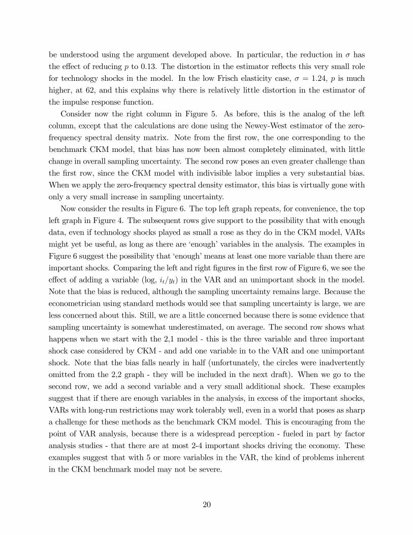
be understood using the argument developed above. In particular, the reduction in σ has

the effect of reducing p to 0.13. The distortion in the estimator reflects this very small role

for technology shocks in the model. In the low Frisch elasticity case, σ = 1.24, p is much

higher, at 62, and this explains why there is relatively little distortion in the estimator of

the impulse response function.

Consider now the right column in Figure 5. As before, this is the analog of the left

column, except that the calculations are done using the Newey-West estimator of the zero-

frequency spectral density matrix. Note from the first row, the one corresponding to the

benchmark CKM model, that bias has now been almost completely eliminated, with little

change in overall sampling uncertainty. The second row poses an even greater challenge than

the first row, since the CKM model with indivisible labor implies a very substantial bias.

When we apply the zero-frequency spectral density estimator, this bias is virtually gone with

only a very small increase in sampling uncertainty.

Now consider the results in Figure 6. The top left graph repeats, for convenience, the top

left graph in Figure 4. The subsequent rows give support to the possibility that with enough

data, even if technology shocks played as small a rose as they do in the CKM model, VARs

might yet be useful, as long as there are ‘enough’ variables in the analysis. The examples in

Figure 6 suggest the possibility that ‘enough’ means at least one more variable than there are

important shocks. Comparing the left and right figures in the first row of Figure 6, we see the

effect of adding a variable (log, it/yt) in the VAR and an unimportant shock in the model.

Note that the bias is reduced, although the sampling uncertainty remains large. Because the

econometrician using standard methods would see that sampling uncertainty is large, we are

less concerned about this. Still, we are a little concerned because there is some evidence that

sampling uncertainty is somewhat underestimated, on average. The second row shows what

happens when we start with the 2,1 model - this is the three variable and three important

shock case considered by CKM - and add one variable in to the VAR and one unimportant

shock. Note that the bias falls nearly in half (unfortunately, the circles were inadvertently

omitted from the 2,2 graph - they will be included in the next draft). When we go to the

second row, we add a second variable and a very small additional shock. These examples

suggest that if there are enough variables in the analysis, in excess of the important shocks,

VARs with long-run restrictions may work tolerably well, even in a world that poses as sharp

a challenge for these methods as the benchmark CKM model. This is encouraging from the

point of VAR analysis, because there is a widespread perception - fueled in part by factor

analysis studies - that there are at most 2-4 important shocks driving the economy. These

examples suggest that with 5 or more variables in the VAR, the kind of problems inherent

in the CKM benchmark model may not be severe.

20

4. Relation to CKM

In the introduction, we discussed some of the reasons for the different conclusions about

VARs reached here and in CKM. This section documents the part of our discussion that was

not addressed in previous sections. In particular, in imposing the long run restrictions, we

implement the sign restriction, (2.7), while CKM impose that the first element of C1 in (2.8)

is positive. In the KP model, we found that it makes no difference which sign restriction is

implemented (compare the rows Benchmark KP and Benchmark KP, CKM Identification in

Table 2). However, it makes a very sharp difference in the CKM model. Up to now, all of

our analysis has worked with the standard sign restriction, (2.7). In this section we show

the consequences of working with (2.8) instead of (2.7) in the benchmark CKM model.

Our analysis appears in Figure 7. The figure displays the output and productivity re-

sponses to a positive technology shock, across the simulations in our Monte Carlo study.

The upper portion displays what happens when (2.7) is imposed. It provides information

on the simulation results using the benchmark CKM model reported in the top left graph

of Figure 4. Note from the 1,2 graph that in all cases, labor productivity eventually rises

after a positive technology shock. However, in some Monte Carlo replications, (roughly 20

percent), the initial response of labor productivity is actually negative. These are indicated

by the yellow lines in the 1,2 graph. The histogram of the magnitude of the contemporaneous

impact effect on hours worked appears in the bar chart in the 1,1 graph. The yellow lines in

the bar chart correspond to the yellow lines in the 1,2 graph. In particular, the realizations

in which the productivity response was initially negative were realizations in which the initial

hours response was the biggest.

Now consider the bottom row of graphs in Figure 7. They show what happens when the

CKM identification strategy is implemented. With this strategy, the productivity responses

that were initially negative in the upper row are now interpreted as responses to negative

productivity shocks. Normalizing the shocks to be positive, the 2,2 graph shows that in

these cases CKM’s identification has the implication that technology initially drops after

a positive technology shock, after which it goes into a permanent dive. The responses of

hours worked in these cases are interpreted to be strongly negative. In effect, the CKM

identification strategy truncates the large hours responses in the histogram in the 1,1 chart

and shifts them into the strong negative region. This is why CKM conclude that structural

VARs imply a bimodal distribution for the hours response to technology shock. Since their

identification strategy is anomalous relative to the literature, we conclude that their finding

is simply a curiosity.

21

5. Concluding Remarks

In this paper we have studied the properties of structural VARs for uncovering impulse

response functions to shocks. For pedagogical purposes, we only considered very simple data

generating processes, based on variants of a prototype RBC model. We find that with short

run restrictions, structural VARs perform remarkably well. With long run restrictions we find

that with one exception structural VARs work well. The exception is that they potentially

perform less well when the shock under investigation (in our case, technology shocks) plays

a small role in output fluctuations. Even in this case, when there are enough variables in the

VAR, problems are greatly mitigated. Perhaps more importantly, we develop and implement

a modified VAR procedure which leads to a drastic improvement in the properties of VAR

estimators, even when technology shocks play a limited role in business cycle fluctuations

and a small number of variables are included in the VAR.

22

References

[1] Aiyagari, S. Rao, 1994, ‘On the Contribution of Technology Shocks to Business Cycles,’Federal Reserve Bank of Minneapolis Quarterly Review, vol. 18, no. 1, Winter, pp.22-34.

[2] Basu, Susanto, John G. Fernald, and Miles S. Kimball. 1999. ‘Are Technology Improve-ments Contractionary?’ Manuscript.

[3] Bernanke, Ben S. and Alan S. Blinder (1992), ‘The Federal Funds Rate and the Channelsof Monetary Transmission’, American Economic Review, Vol. 82, No. 4, pages 901 - 921.

[4] Bernanke, Ben S. and Ilian Mihov (1995), ‘Measuring Monetary Policy’, NBERWorkingPaper No. 5145.

[5] Blanchard, Olivier Jean, and Danny Quah, 1989, ‘The Dynamic Effects of AggregateDemand and Supply Disturbances,’ American Economic Review, v. 79, issue 4, pp.655-673.

[6] Chari, V.V., Patrick Kehoe and Ellen McGrattan, 2005, ‘A Critique of Structural VARsUsing Real Business Cycle Theory,’ Federal Reserve Bank of Minneapolis Working Paper631, February.

[7] Christiano, Lawrence J., 2002, ‘Solving Dynamic Equilibrium Models by a Method ofUndetermined Coefficients,’ Computational Economics, October, Volume 20, Issue 1-2.

[8] Christiano, Lawrence J. and Martin Eichenbaum (1992), ‘Identification and the Liq-uidity Effect of a Monetary Policy Shock’, in Political Economy, Growth and BusinessCycles, edited by Alex Cukierman, Zvi Hercowitz, and Leonardo Leiderman, Cambridgeand London: MIT Press, pages 335 - 370.

[9] Christiano, Lawrence J., Martin Eichenbaum and Charles Evans, 2005, ‘Nominal Rigidi-ties and the Dynamic Effects of a Shock to Monetary Policy,’ Journal of Political Econ-omy.

[10] Christiano, Lawrence J., Martin Eichenbaum and Robert Vigfusson, 2003, “What Hap-pens After a Technology Shock?”, National Bureau of Economic Research working paperw9819.

[11] Christiano, Lawrence J., Martin Eichenbaum and Robert Vigfusson, 2004, ‘The Re-sponse of Hours to a Technology Shock: Evidence Based on Direct Measures of Tech-nology,’ Journal of the European Economic Association.

[12] Christiano, Lawrence J., Roberto Motto and Massimo Rostagno, 2004, ‘The Great De-pression and the Friedman-Schwartz Hypothesis,’ Journal of Money, Credit and Bank-ing.

[13] Erceg, Christopher J., Luca Guerrieri, and Christopher Gust, 2004, ‘Can Long-Run Re-strictions Identify Technology Shocks?’, International Finance Discussion Papers Num-ber 792, Federal Reserve Boad of Governors.

[14] Faust, Jon and Eric Leeper, 1997, ‘When Do Long-Run Identifying Restrictions GiveReliable Results?’, Journal of Business and Economic Statistics, July, vol. 15, no. 3.

[15] Francis, Neville, and Valerie A. Ramey, 2001, ‘Is the Technology-Driven Real BusinessCycle Hypothesis Dead? Shocks and Aggregate Fluctuations Revisited,’ manuscript,UCSD.

23

[16] Hansen, Gary, 1985, Indivisible Labor and the Business Cycle,’ Journal of MonetaryEconomics, November, 16(3): 309-27

[17] Gali, Jordi, 1999, ‘Technology, Employment, and the Business Cycle: Do TechnologyShocks Explain Aggregate Fluctuations?’ American Economic Review, 89(1), 249-271.

[18] Grilli, Vittorio, and Nouriel Roubini (1995), ‘Liquidity and Exchange Rates: PuzzlingEvidence from the G-7 Countries’, New York University Solomon Brothers WorkingPaper No. S/95/31.

[19] Hamilton, James D. (1997), ‘Measuring the Liquidity Effect’, American Economic Re-view, Vol. 87, No. 1 pages 80 - 97.

[20] Prescott, Edward, 1991, ‘Real Business Cycle Theory: What Have We Learned?’, Re-vista de Analisis Economico, 6 (November), pp. 3-19.

[21] Quah, Danny and Thomas Sargent, 1993, ‘A Dynamic Index Model for Large CrossSections,’ in Stock, James H., Watson, Mark W., eds. Business cycles, indicators, andforecasting, NBER Studies in Business Cycles, vol. 28. Chicago and London: Universityof Chicago Press, 285-306

[22] Rotemberg, Julio J. and Michael Woodford, 1997, ‘An Optimization-Based Economet-ric Framework for the Evaluation of Monetary Policy,’ National Bureau of EconomicResearch Macroeconomics Annual.

[23] Del Negro, Marco, Frank Schorfheide, Frank Smets, and Raf Wouters, 2005, ‘On theFit and Forecasting Performance of New Keynesian Models,’ manuscript.

[24] Sargent, Thomas, 1979, Macroeconomics.

[25] Sims, Christopher, 1989, ‘Models and Their Uses,’ American Journal of AgriculturalEconomics 71, May, pp. 489-494.

[26] Sims, Christopher, 1972, ‘The Role of Approximate Prior Restrictions in Distributed LagEstimation,’ Journal of the American Statistical Association, vol. 67, no. 337, March,pp. 169-175.

[27] Sims, Christopher A. and Tao Zha (1995), ‘Does Monetary Policy Generate Recessions?’,Manuscript. Yale University.

[28] Smets, Frank, and Raf Wouters, 2003, ‘An Estimated Dynamic Stochastic GeneralEquilibrium Model of the Euro Area,’ Journal of European Economic Association 1(5),pp. 1123-1175.

[29] Uhlig, Harald, 2002, ‘What Moves Real GNP?’, manuscript, Humboldt University,Berlin.

24

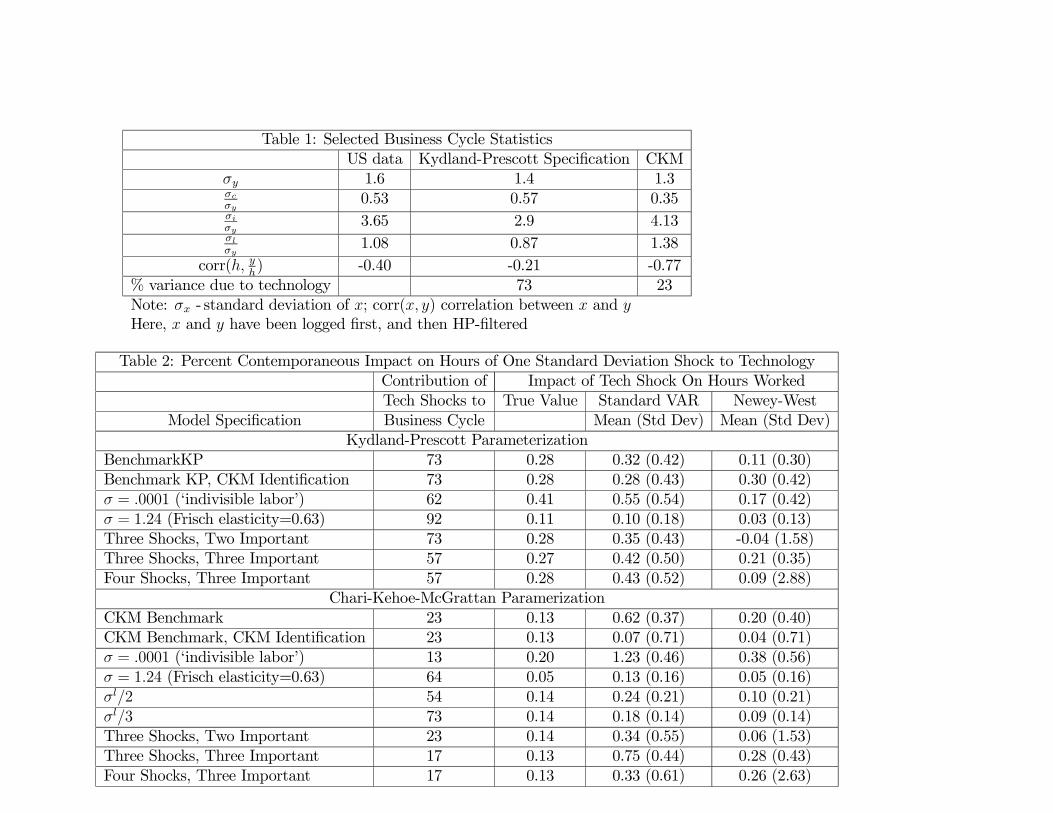
Table 1: Selected Business Cycle StatisticsUS data Kydland-Prescott Specification CKM

σy 1.6 1.4 1.3σcσy

0.53 0.57 0.35σiσy

3.65 2.9 4.13σlσy

1.08 0.87 1.38corr(h, y

h) -0.40 -0.21 -0.77

% variance due to technology 73 23Note: σx - standard deviation of x; corr(x, y) correlation between x and yHere, x and y have been logged first, and then HP-filtered

Table 2: Percent Contemporaneous Impact on Hours of One Standard Deviation Shock to TechnologyContribution of Impact of Tech Shock On Hours WorkedTech Shocks to True Value Standard VAR Newey-West

Model Specification Business Cycle Mean (Std Dev) Mean (Std Dev)Kydland-Prescott Parameterization

BenchmarkKP 73 0.28 0.32 (0.42) 0.11 (0.30)Benchmark KP, CKM Identification 73 0.28 0.28 (0.43) 0.30 (0.42)σ = .0001 (‘indivisible labor’) 62 0.41 0.55 (0.54) 0.17 (0.42)σ = 1.24 (Frisch elasticity=0.63) 92 0.11 0.10 (0.18) 0.03 (0.13)Three Shocks, Two Important 73 0.28 0.35 (0.43) -0.04 (1.58)Three Shocks, Three Important 57 0.27 0.42 (0.50) 0.21 (0.35)Four Shocks, Three Important 57 0.28 0.43 (0.52) 0.09 (2.88)

Chari-Kehoe-McGrattan ParamerizationCKM Benchmark 23 0.13 0.62 (0.37) 0.20 (0.40)CKM Benchmark, CKM Identification 23 0.13 0.07 (0.71) 0.04 (0.71)σ = .0001 (‘indivisible labor’) 13 0.20 1.23 (0.46) 0.38 (0.56)σ = 1.24 (Frisch elasticity=0.63) 64 0.05 0.13 (0.16) 0.05 (0.16)σl/2 54 0.14 0.24 (0.21) 0.10 (0.21)σl/3 73 0.14 0.18 (0.14) 0.09 (0.14)Three Shocks, Two Important 23 0.14 0.34 (0.55) 0.06 (1.53)Three Shocks, Three Important 17 0.13 0.75 (0.44) 0.28 (0.43)Four Shocks, Three Important 17 0.13 0.33 (0.61) 0.26 (2.63)

Figure 1 - The Labor Tax Wedge and Its Components

1960 1970 1980 1990 20000

0.05

0.1

0.15

0.2

0.25

0.3

0.35

Figure 1a

Estimated labor tax wedgeFitted Residuals

1960 1970 1980 1990 2000

0.24

0.25

0.26

0.27

0.28

0.29

Figure 1b: labor to leisure ratio

1960 1970 1980 1990 2000−0.32

−0.3

−0.28

−0.26

−0.24

Figure 1c: log, Consumption to Output Ratio

Figure 2: Analysis of Short−Run Identification Assumption

KP Model CKM ModelBenchmark

0 2 4 6 8 10

−0.2

0

0.2

0.4

0.6

0 2 4 6 8 10

−0.2

0

0.2

0.4

0.6

Infinite Frisch Elasticity

0 2 4 6 8 10−0.2

00.20.40.6

0 2 4 6 8 10−0.2

00.20.40.6

Frisch Elasticity 0.63

0 2 4 6 8 10

−0.2

0

0.2

0.4

0.6

0 2 4 6 8 10

−0.2

0

0.2

0.4

0.6

3 shocks, 3 variables

0 2 4 6 8 10

−0.2

0

0.2

0.4

0.6

0 2 4 6 8 10

−0.2

0

0.2

0.4

0.6

Note: hours response, in percent terms, to a 1.2 (KP) or 0.6 (CKM) percent innovation in technology, Zt.

Solid line − mean response, Gray area − mean response plus/minus two standard errors, Starred line − true response, Dashed line − 95.5 percent probability interval of responses, Circles − average value of econometrician estimated plus/minus two standard errors.

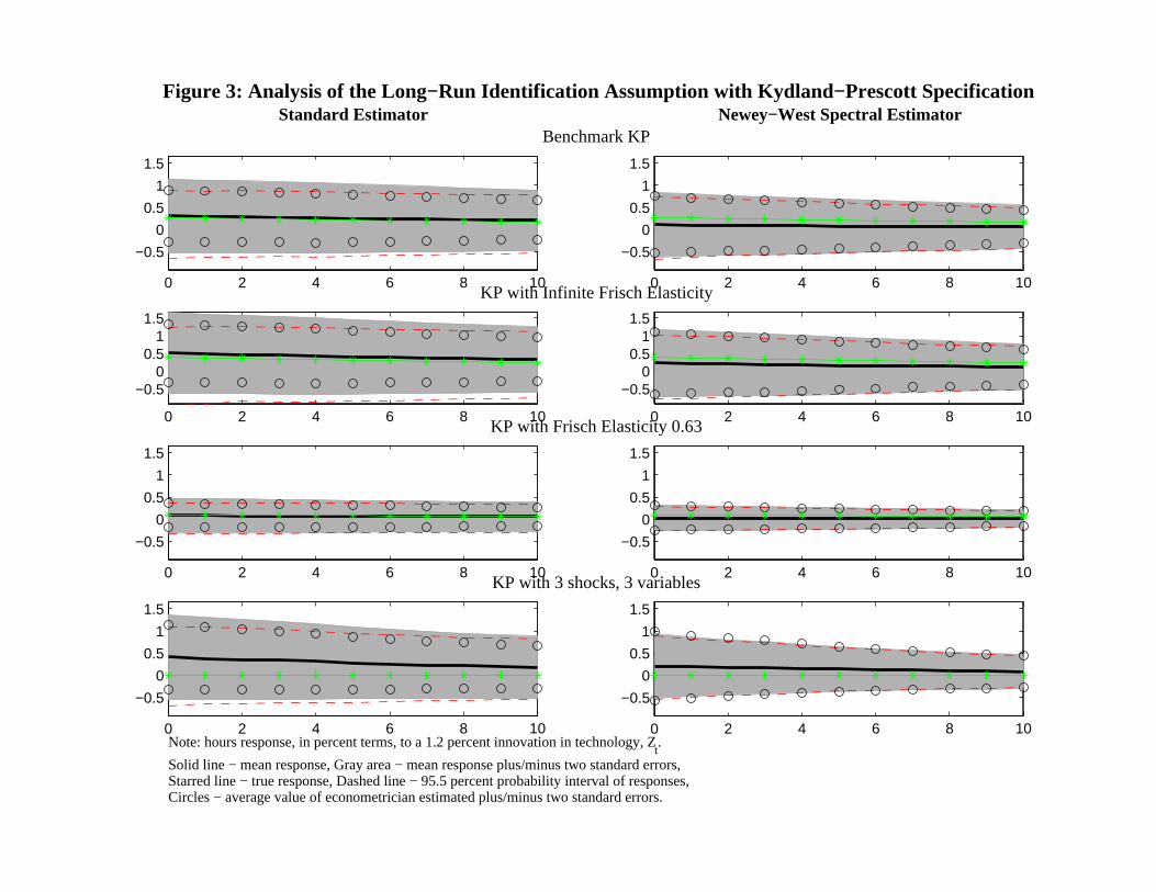
Figure 3: Analysis of the Long−Run Identification Assumption with Kydland−Prescott SpecificationStandard Estimator Newey−West Spectral Estimator

Benchmark KP

0 2 4 6 8 10

−0.5

0

0.5

1

1.5

0 2 4 6 8 10

−0.5

0

0.5

1

1.5

KP with Infinite Frisch Elasticity

0 2 4 6 8 10

−0.50

0.51

1.5

0 2 4 6 8 10

−0.50

0.51

1.5

KP with Frisch Elasticity 0.63

0 2 4 6 8 10

−0.5

0

0.5

1

1.5

0 2 4 6 8 10

−0.5

0

0.5

1

1.5

KP with 3 shocks, 3 variables

0 2 4 6 8 10

−0.5

0

0.5

1

1.5

0 2 4 6 8 10

−0.5

0

0.5

1

1.5

Note: hours response, in percent terms, to a 1.2 percent innovation in technology, Zt.

Solid line − mean response, Gray area − mean response plus/minus two standard errors, Starred line − true response, Dashed line − 95.5 percent probability interval of responses,Circles − average value of econometrician estimated plus/minus two standard errors.

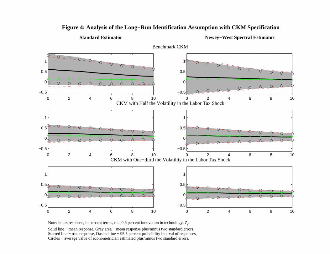
Figure 4: Analysis of the Long−Run Identification Assumption with CKM Specification

Standard Estimator Newey−West Spectral Estimator

Benchmark CKM

0 2 4 6 8 10

−0.5

0

0.5

1

0 2 4 6 8 10

−0.5

0

0.5

1

CKM with Half the Volatility in the Labor Tax Shock

0 2 4 6 8 10

−0.5

0

0.5

1

0 2 4 6 8 10

−0.5

0

0.5

1

CKM with One−third the Volatility in the Labor Tax Shock

0 2 4 6 8 10

−0.5

0

0.5

1

0 2 4 6 8 10

−0.5

0

0.5

1

Note: hours response, in percent terms, to a 0.6 percent innovation in technology, Zt.

Solid line − mean response, Gray area − mean response plus/minus two standard errors, Starred line − true response, Dashed line − 95.5 percent probability interval of responses,Circles − average value of econometrician estimated plus/minus two standard errors.

Figure 5: Analysis of the Long−Run Identification Assumption with CKM SpecificationStandard Estimator Newey−West Spectral Estimator

Benchmark CKM

0 2 4 6 8 10

0

1

2

0 2 4 6 8 10

0

1

2

CKM with Infinite Frisch Elasticity

0 2 4 6 8 10

0

1

2

0 2 4 6 8 10

0

1

2

CKM with Frisch Elasticity 0.63

0 2 4 6 8 10

0

1

2

0 2 4 6 8 10

0

1

2

CKM with 3 shocks, 3 variables

0 2 4 6 8 10

0

1

2

0 2 4 6 8 10

0

1

2

Note: hours response, in percent terms, to a 0.6 percent innovation in technology, Zt.

Solid line − mean response, Gray area − mean response plus/minus two standard errors, Starred line − true response, Dashed line − 95.5 percent probability interval of responses,Circles − average value of econometrician estimated plus/minus two standard errors.

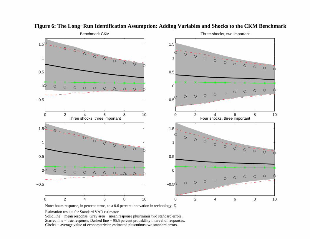
Figure 6: The Long−Run Identification Assumption: Adding Variables and Shocks to the CKM Benchmark

0 2 4 6 8 10

−0.5

0

0.5

1

1.5

Benchmark CKM

0 2 4 6 8 10

−0.5

0

0.5

1

1.5

Three shocks, two important

0 2 4 6 8 10

−0.5

0

0.5

1

1.5

Three shocks, three important

0 2 4 6 8 10

−0.5

0

0.5

1

1.5

Four shocks, three important

Note: hours response, in percent terms, to a 0.6 percent innovation in technology, Zt.

Estimation results for Standard VAR estimator. Solid line − mean response, Gray area − mean response plus/minus two standard errors, Starred line − true response, Dashed line − 95.5 percent probability interval of responses,Circles − average value of econometrician estimated plus/minus two standard errors.

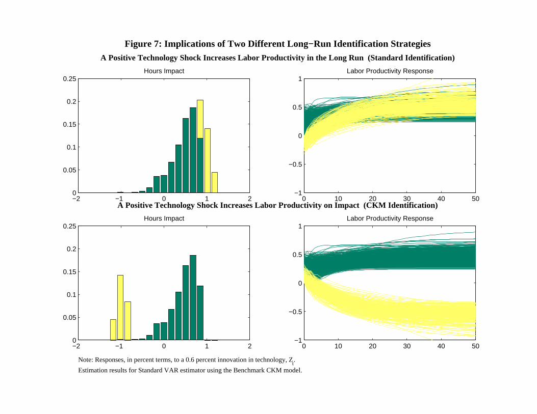
Figure 7: Implications of Two Different Long−Run Identification StrategiesA Positive Technology Shock Increases Labor Productivity in the Long Run (Standard Identification)

−2 −1 0 1 20

0.05

0.1

0.15

0.2

0.25Hours Impact

0 10 20 30 40 50−1

−0.5

0

0.5

1Labor Productivity Response

A Positive Technology Shock Increases Labor Productivity on Impact (CKM Identification)

−2 −1 0 1 20

0.05

0.1

0.15

0.2

0.25Hours Impact

0 10 20 30 40 50−1

−0.5

0

0.5

1Labor Productivity Response

Note: Responses, in percent terms, to a 0.6 percent innovation in technology, Zt.

Estimation results for Standard VAR estimator using the Benchmark CKM model.