Assessing the copula selection for bivariate frequency

J. Earth Syst. Sci. (2018) 127:92 c© Indian Academy of Scienceshttps://doi.org/10.1007/s12040-018-0994-4

Assessing the copula selection for bivariate frequencyanalysis based on the tail dependence test

D D Nguyen1,2,* and K V Jayakumar1

1Department of Civil Engineering, National Institute of Technology, Warangal 506 004, India.2Division of Water Resources and Environment, Thuyloi University, Ho Chi Minh City 700000, Vietnam.*Corresponding author. e-mail: [email protected]

MS received 15 September 2017; revised 15 January 2018; accepted 16 January 2018;published online 18 August 2018

The flood characteristics, namely, peak, duration and volume provide important information for thedesign of hydraulic structures, water resources planning, reservoir management and flood hazardmapping. Flood is a complex phenomenon defined by strongly correlated characteristics such as peak,duration and volume. Therefore, it is necessary to study the simultaneous, multivariate, probabilisticbehaviour of flood characteristics. Traditional multivariate parametric distributions have widely beenapplied for hydrological applications. However, this approach has some drawbacks such as the dependencestructure between the variables, which depends on the marginal distributions or the flood variablesthat have the same type of marginal distributions. Copulas are applied to overcome the restrictionof traditional bivariate frequency analysis by choosing the marginals from different families of theprobability distribution for flood variables. The most important step in the modelling process usingcopula is the selection of copula function which is the best fit for the data sample. The choice ofcopula may significantly impact the bivariate quantiles. Indeed, this study indicates that there is ahuge difference in the joint return period estimation using the families of extreme value copulas and noupper tail copulas (Frank, Clayton and Gaussian) if there exists asymptotic dependence in the floodcharacteristics. This study suggests that the copula function should be selected based on the dependencestructure of the variables. From the results, it is observed that the result from tail dependence test isvery useful in selecting the appropriate copula for modelling the joint dependence structure of floodvariables. The extreme value copulas with upper tail dependence have proved that they are appropriatemodels for the dependence structure of the flood characteristics and Frank, Clayton and Gaussiancopulas are the appropriate copula models in case of variables which are diagnosed as asymptoticindependence.

Keywords. Bivariate frequency analysis; extreme value copula; extremal measures; Gaussian copula;tail dependence coefficient; tail dependence test.

1. Introduction

Single-variable flood frequency analysis provideslimited understanding and assessment of the truebehaviour of flood phenomena, which are often

characterised by a set of correlated randomvariables such as peak, volume and duration (Yueet al. 2001; Favre et al. 2004). Univariate frequencyanalysis methods cannot describe the random vari-able properties that are correlated (Sarhadi et al.

1

0123456789().,--: vol V

http://crossmark.crossref.org/dialog/?doi=10.1007/s12040-018-0994-4&domain=pdf

92 Page 2 of 17 J. Earth Syst. Sci. (2018) 127:92

2016). This approach can lead to high uncertaintyor failure of guidelines in water resources planning,operation and design of hydraulic structures or cre-ating the flood risk mapping (Chebana and Ouarda2011). Additionally, the flood is a multivariatenatural calamity characterising peak, volume andduration. Hence, it is important to study the simul-taneous, multivariate, probabilistic behaviour offlood characteristics.

Multivariate parametric distributions (e.g.,bivariate normal, bivariate gamma and bivari-ate extreme value distributions), which have beenextended from univariate distribution, is used tomodel the multivariate flood characteristics for dif-ferent purposes (Adamson et al. 1999; Yue 1999;Yue et al. 2001). However, this approach hassome drawbacks such as the dependence struc-ture between the variables, which depends onthe marginal distributions or the flood variablesthat have the same type of marginal distributions(Poulin et al. 2007; Zhang and Singh 2007).

In order to overcome the limitation of multi-variate distributions, a copula is a very versatileapproach for simulating joint distribution in amore realistic way (Favre et al. 2004). The mainadvantage of this method is that the depen-dence structure is independently modelled with themarginal distribution that allows for multivariatedistribution with different margins and dependencestructures to be built (Dupuis 2007; Zhang andSingh 2007). Several researchers have used copulasto perform the bivariate frequency analysis (Reddyand Ganguli 2012; Dung et al. 2015; Sraj et al.2015). The most important step in the modellingprocess using copula is the selection of copula func-tion which is the best fit for the data sample (Favreet al. 2004). The chosen copulas should include sev-eral classes of copulas and several degrees of taildependence (Dupuis 2007; Poulin et al. 2007).

Tail dependence characteristics constituteimportant features that differentiate extreme valuecopulas from other copula structures (Chowdharyet al. 2011). Therefore, the extreme value cop-ulas with upper tail dependence are consideredto provide appropriate models for the dependencestructure of the flood characteristics (Genest andFavre 2007; Poulin et al. 2007; Gudendorf andSegers 2011; Vittal et al. 2015). On the other hand,in the multivariate frequency analysis, the vari-ables can be dependent or independent of eachother. The relationship between the flood char-acteristics (i.e., peak, volume and duration) isanalysed by several researchers. However, most of

the results of the dependence between differentpairs of flood variables were not consistent (Kar-makar and Simonovic 2009; Reddy and Ganguli2012; Sraj et al. 2015). Indeed, the identifica-tion of the degree of dependence between theflood variables is a difficult step, because thedependence of pairs of flood characteristics is con-trolled by different climate features and catchmentproperties (Viglione and Bloschl 2009; Gaal et al.2015).

Most of the studies used Pearson’s linear corre-lation coefficient (r), Kendall’s (τ) and Spearman’srank correlation (ρ) for measuring the dependenceamong different flood variables. However, thesemeasures are based on the association of the entiredistributions, but do not reveal the dependence inthe specific part of the distribution (Aghakouchaket al. 2010). When dealing with extreme eventssuch as floods, extreme values will appear in the tailof the distributions. Hence, the tail dependence,which describes the dependence in the tail of amultivariate distribution, can be a suitable mea-sure (Coles et al. 1999; Aghakouchak et al. 2010;Serinaldi et al. 2015; Hao and Singh 2016).

To describe the dependence in multivariateextreme values, there are two possible situations,namely, asymptotic dependence or asymptoticindependence (Coles et al. 1999). Diagnostic analy-sis to determine whether the variables have asymp-totic dependence or asymptotic independence isvery important in multivariate extreme analysis.In fact, in a situation where diagnostic checkssuggest data to be asymptotically independent,modelling with the classical families of bivariateextreme value distribution is likely to lead to mis-leading results (Ledford and Tawn 1996; Coles2001). Different measures of extremal dependencehave been developed. Coles et al. (1999) proposedtwo measures of extreme dependence (χ and χ)for bivariate random variables. Nevertheless, recentstudies show that there are still difficulties indetecting the asymptotic dependence and indepen-dence in many cases (Coles et al. 1999; Bacro et al.2010; Weller et al. 2012; Serinaldi et al. 2015).

Apart from these, several parametric and non-parametric approaches are suggested to determinethe tail dependence. Non-parametric tail depen-dence estimator (λU), namely, λLOG

U (Coles et al.1999; Frahm et al. 2005), λSEC

U (Joe et al. 1992),λCFGU (Caperaa et al. 1997) and λSS

U (Schmidtand Stadtmuller 2006) have been preferred bymost researchers in hydrological analysis (Li et al.2009; Requena et al. 2016). However, Villarini

J. Earth Syst. Sci. (2018) 127:92 Page 3 of 17 92

et al. (2008) indicated that these tail dependenceestimators have some drawbacks (e.g., bias, uncer-tainty, etc.). Furthermore, all tail dependence esti-mators exhibit a very poor performance when theunderlying upper tail dependence coefficient is null.It is, therefore, important to test for tail depen-dence before applying the estimator (Frahm et al.2005; Poulin et al. 2007). Consequently, uppertail (in)dependence testing is a useful alternativeapproach. Serinaldi et al. (2015) suggested thattest for tail (in)dependence is mandatory because:(i) samples exist which seem to fail dependency,but they are realisations of a tail-dependent dis-tribution; (ii) the use of misspecified parametricmarginals instead of empirical marginals may leadto wrong interpretations of the dependence struc-ture; and (iii) the tail dependence estimators canbe insensitive to upper tail dependence, thus indi-cating the upper tail dependence even if none exist.Similarly, if data are to be independent in the uppertail, then modelling with dependence will lead tooverestimation of the probability of extreme jointevents. Hence, Falk and Michel (2006) emphasisedthat testing for tail (in)dependence is essential indata analysis of extreme values.

Several recent studies indicated that Gumbel–Hougaard copula belonging to extreme value cop-ulas works well when variables are asymptoticallydependent (Zhang and Singh 2006; Poulin et al.2007; Karmakar and Simonovic 2009; Dung et al.2015). However, there are few studies which sug-gest what is the best copula for modelling thedependence structure where the variables have thestrength of dependence but weaken at high lev-els or are asymptotically independent. Therefore,it is important to find the appropriate copulato derive the joint distribution of flood variableswhere the pair of flood characteristics has asymp-totically independent or weak dependence at highthresholds.

The difference between the extreme value cop-ulas and Gaussian copula is that the Gaussiancopula becomes independent at the high threshold.Furthermore, Gaussian copula, which is charac-terised by correlation matrix, generates a widerrange of dependence behaviour (Bortot et al.2000). Studies by Renard and Lang (2007) alsohave proved the usefulness of the Gaussian cop-ula in hydrological extreme events analysis. Infact, they suggested that the Gaussian copulacan be reasonably well used for field significancedetermination, regional risk estimation, discharge–duration–frequency curves and regional frequency

analysis. Frank and Clayton copulas, belonging tothe Archimedean family, have been widely used inthe hydrology analysis because they can be mod-elled with both negatively and positively associatedvariables. Furthermore, the Frank and Claytoncopulas, which have zero dependencies in bothtails, are suitable in case the tail dependence is notexisting (Poulin et al. 2007; Dung et al. 2015; Srajet al. 2015).

The previous studies have used parametric andnon-parametric approaches to determine the taildependence coefficient. However, these taildependence estimators have some drawbacks.Consequently, tail dependence testing is a usefulalternative approach. Therefore, this study assesseshow tail dependence test can be useful in selectingthe appropriate family of copula for modelling thejoint dependence structure of flood characteristics.In order to identify the best copula family for eachsituation, the Clayton, Frank and Gaussian cop-ulas are used for assessing the potential of theirapplications in case the variables are diagnosed asasymptotic independence. The hypothesised copu-las (extreme value copulas) are applied to evaluatetheir suitability if there exists asymptotic indepen-dence in the tail for bivariate frequency analysis offlood in Trian watershed, Vietnam.

This study aims to address the followingissues: (i) investigating the potential of perform-ing the tail dependence tests for the pairs of floodcharacteristics; (ii) evaluating the performance ofextreme value copula for asymptotic dependencevariables and Clayton, Frank and Gaussian cop-ulas for asymptotic independent variables; and(iii) estimating the joint return period of floodcharacteristics.

2. Study area and data

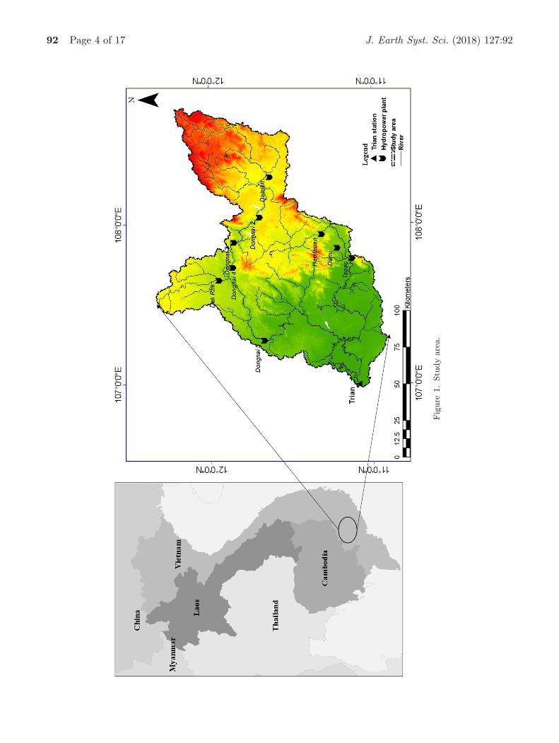
The Trian catchment, which is taken up for thestudy, is in the upper part of the Saigon–Dongnai River basin and it is one of the biggestsubcatchments. The area of this catchment is∼14, 200 km2. The basin lies between the lati-tudes of 10◦53′46′′−12◦22′08′′N and longitudes of107◦01′52′′−108◦46′55′′E (figure 1). There are twodistinct seasons in this area, namely, rainy (April–November) and dry (December–April) seasons.The climate is controlled by the northeast andsouthwest monsoons. The annual average rainfalland temperature are about 2200 mm and 20.6◦C,respectively. There are two main tributaries of the


Fig

ure

1.

Stu

dy

are

a.


Dongnai River (i.e., Dongnai and Langa). Thereare nine reservoirs, which are operating to sup-ply water for drinking, irrigation, flood controland hydropower production, and were constructedupstream of Trian gauge. Most of them began tooperate in recent years except for Hamthuan–Damiand Daininh reservoirs which were operated in 2001and 2008, respectively. In the Dongnai tributary,Daininh and Dakrtik reservoirs provide energywith a capacity of 300 and 144 MW, respectively.Dongnai 2, Dongnai 3, Dongnai 4 and Dongnai5 supply water to hydropower plants which havethe installed capacity of 70, 180, 340 and 150MW, respectively. Hamthuan and Dami reservoirs,located in the Langa tributary, are a cascade oftwo hydropower plants with the installed capac-ity of 300 and 175 MW. Tapao weir, located atthe downstream of Hamthuan and Dami reservoirs,is constructed to supply water for drinking andfor irrigation of around 20,340 ha (Government2016). However, all reservoirs are located far awayfrom the Trian gauge (figure 1). The flood fromTrian station has significant impacts on the down-stream areas (e.g., Bienhoa, Vungtau and Hochim-inh cities). Therefore, this study mainly focusedon the flood in the Trian gauge. Daily dischargedata for the period 1978–2013 are available for thestudy from the Trian station on the Dongnai River,which is a part of the Saigon–Dongnai River basinand these data are used for flood frequency anal-ysis. The Trian station is located at 106◦59′08′′Eand 11◦06′16′′N and it is at the confluence of twoDongnai and Langa rivers. Numerous researcherssuggested that the length of data record should beat least 30 years for extreme value modelling (Bon-nin et al. 2006; Kioutsioukis et al. 2010; Yilmazet al. 2017). Further, there are several multivari-ate frequency analysis studies using the observeddata of <35 yrs of data (Zhang and Singh 2006;Aissia et al. 2012; Jeong et al. 2014). Moreover, sev-eral researchers suggested that the main advantageof the POT approach, which is for smaller sam-ple sizes, is also used to increase the sample sizes(Lang et al. 1999; Beguerıa 2005; Bezak et al. 2014).Based on the 35 years of observed data, the samplesize of the flood variables is 68 in this study, whichmeets the minimum requirement of the sample size(n = 30) for the extreme value modelling. There-fore, the length of the observed data is significantfor the analysis of the tail dependence. The meanof daily discharge of Trian stream gauge from 1978to 2013 is 527.4 m3/s and the observed maximumdaily discharge is 3910 m3/s. The daily time series

of the river discharge data is collected from theNational Hydro-Meteorological Service (NHMS) ofVietnam.

3. Methodology

The methodology used in this study is shown inthe form of a flowchart (figure 2). Firstly, iden-tification of flood characteristics (peak, volumeand duration) from the observed daily dischargetime series is carried out. Secondly, check whetherthe flood variables time series are stationary ornon-stationary. Thirdly, the tail dependence testsare then performed to diagnose whether the floodvariables have asymptotic dependence or asymp-totic independence. Finally, if the flood variablesare having an asymptotic dependence, the extremevalue copula is used for estimation of joint returnperiods. Otherwise, Gaussian, Frank and Claytoncopulas are used.

3.1 Extracting flood characteristics

Block maxima (BM) and peak over threshold(POT) approaches are widely used to extract floodcharacteristics. However, the block maxima cannotconsider multiple occurrences of flood events (Langet al. 1999; Bezak et al. 2014). Unlike the blockmaxima, which only extracts one event per year,POT considers a wider range of events and providesmore information than BM. The threshold estima-tion is the most difficult part of the POT approach(Lang et al. 1999; Scarrott and Macdonald 2012).Threshold choice involves balancing between thebias and variance. Too low a threshold may vio-late the asymptotic basis of the model, leading tobias, while too high a threshold will reduce thesample size, leading to high variance of the param-eter estimates (Coles 2001). There are two commonapproaches for choosing a threshold, namely, fixedquantile corresponding to a high non-exceedanceprobability (95%, 99% or 99.5%) and graphicalmethod (Vittal et al. 2015). Three different tech-niques belonging to the graphical method, namely,the mean residual life plot (MRL), threshold sta-bility plots and fitting distribution diagnostics(Thompson et al. 2009; Solari and Losada 2012)are used in this study to decide the thresholdvalue. In addition, the lag-autocorrelation plot isused to check the independent and identically dis-tributed (IID) flood variables (i.e., peak, volumeand duration) assumption.


Figure 2. Flowchart of methodology.

3.2 Diagnostic test to examine non-stationarycomponent

The extreme events, particularly flood events, areintensifying due to global climate change, urbani-sation and anthropogenic activities. Therefore, theflood time series can have a non-stationary compo-nent. The flood frequency analysis, which considerstime series as stationary, may lead to mislead-ing results in the estimation of the flood quantile.Checking the non-stationary component of floodseries in flood frequency analysis should be con-sidered as an important initial step (Vittal et al.2015). Trend analysis is normally used to detectthe non-stationarities in the flood variables. TheMann–Kendall (M–K) test is a non-parametric sta-tistical test which is used for examining the trendsin time series and has been widely applied in thehydrological analysis (Villarini et al. 2009; Limaet al. 2015; Sun et al. 2015).

3.3 Tail dependence test

Coles et al. (1999) proposed two measures ofextreme dependence (χ and χ) for bivariate ran-dom variables, as shown below:

χ = 2 − log P (F1 (x) < u, F2 (y) < u)log u

, (1)

χ =2log (1 − u)

log P (F1 (x) > u, F2 (y) > u)− 1. (2)

With a pair of complementary measure (χ, χ), asummary of multivariate extremal dependence canbe determined:

• If χ = 1 and 0 < χ < 1, the variables areasymptotically dependent and χ is a measure ofthe strength of dependence within the class ofasymptotic dependence distribution.

• If −1 < χ < 1 and χ = 0, the variables areasymptotically independent and χ is a measureof the strength of dependence within the class ofasymptotically independent distribution.

There are still difficulties in detecting the asymp-totic dependence and independence in many casesusing these extremal dependencies (Coles et al.1999; Bacro et al. 2010; Weller et al. 2012; Serinaldiet al. 2015). Hence, the coefficient of tail depen-dence (η) introduced by Ledford and Tawn (1996)is used to detect asymptotically dependent andindependent variables. Ledford and Tawn (1996)


assumed that the joint survivor function of the pair(X, Y ) with unit Frechet distribution is a regularlyvarying function, as shown below:

P (X > z, Y > z) = £(z)z−1/η, (3)

where £(z) is a slowly varying function and η isthe coefficient of tail dependence.

• If η = 1 and limz→∞ £ (z) = c for some 0 <c ≤ 1, the variables are asymptotically depen-dent with a degree c.

• If η < 1, the variables are asymptoticallyindependent.

The coefficient of tail dependence can be estimatedby univariate theory because the joint survivorfunction can be reduced to univariate survivorfunction T = min(X,Y ). The coefficient of taildependence will be equal to shape parameter if T isfitted with generalised Pareto distribution (GPD).The log-likelihood ratio (LLHR) test can be usedfor testing the asymptotic dependence against theasymptotic independence. The null hypothesis ofasymptotic dependence is tested comparing thelog-likelihood of the asymptotic dependence andasymptotic independence. Under the null hypoth-esis η = 1 vs. the alternative η < 1, the LLHRtest statistic, based on twice the difference betweenthe log-likelihood of asymptotic dependence andasymptotic independence, has the approximate χ2

distribution with the degree of freedom. The signifi-cance of asymptotic independence can be measuredfrom the p-value of χ2 distribution. As mentionedearlier, threshold in GPD is selected based on thethreshold stability plot.

Furthermore, tail (in)dependence test is usedas an approach for detecting whether the floodvariables have asymptotic dependence or indepen-dence, respectively. Tail independence test, pro-posed by Falk and Michel (2006), is normallysuggested by many authors in extreme value anal-ysis (Bel et al. 2008; Ribatet et al. 2009; Seri-naldi et al. 2015). Frick et al. (2007) proposeda generalisation of Falk and Michel’s test, basedon a second-order differential expansion of thespectral decomposition of non-degenerate distribu-tion function. This test is based on the followingequation:

P (X + Y > ct |X + Y > c)

={

F (t) = t1+ρ, tail independence,F (t) = t, tail dependence, (4)

where c → 0 is the threshold, ρ ≥ 0 is theindependence measure and F (t) is the standarduniform distribution with t ∈ [0,1]. According tothe central limit theorem, the p-values of the opti-mal test are given below:

p = Φ

(∑mi=1 log Ci + m

m1/2

)(5)

where Ci = (Xi +Yi)/c, i = 1, . . . , m, and Φ is thestandard normal density distribution function.

This test is quite sensitive to the thresholdc. Hence, Frick et al. (2007) suggested that thethreshold is chosen so that the number ofexceedances is about 10–15% of the total numberobserved data.

3.4 Selection of marginal distribution

The work of Vittal et al. (2015) suggested that itis important to apply both parametric and non-parametric distributions for a selection of the bestfit marginals for flood variables. There is more thanone parametric distribution that can be fitted tothe sample data. Hence, identifying the best fittingdistribution to the sample needs to be tested withseveral distributions rather than assuming that theparticular distribution will be sufficient to pro-vide the necessary insight for flood variables (Langet al. 1999; Vittal et al. 2015; Dong Nguyen et al.2018). The log-normal (LN), Pearson type III (P3),log-Pearson type III (LP3), GPD, Gumbel and gen-eralised extreme value (GEV) distributions, whichhave been widely used for modelling the extremevalues (Lang et al. 1999; Saf 2009; Salas Jose et al.2013; Bezak et al. 2014), are used.

For non-parametric distribution, the kerneldensity estimator with Epanechnikov, Gaussian,triangular and rectangular kernel functions is usedin this study. Both parametric and non-parametricdistributions are used to find the best marginaldistribution for each flood variable in this study.

3.5 Extreme value copula and no tail dependencecopula functions

A copula is defined as a joint distribution functionof standard uniform random variables. If F (x, y) isany continuous bivariate distribution function withmarginal distributions F1(x) and F2(y), the copulafunction can be expressed as:

F (x, y) = C[F1(x), F2(y)]. (6)


If the F1(x) and F2(y) are continuous, the copulafunction C is unique and can be written as:

C(u, υ) = F [F−11 (u), F−2

2 (υ)], (7)

where the quantile functions F−11 and F−2

2 aredefined by F−1

1 (u) = inf[x: F1(x) ≥ u] andF−12 (υ) = inf[x: F2(y) ≥ υ], respectively.Among several families of copulas (Archimedean,

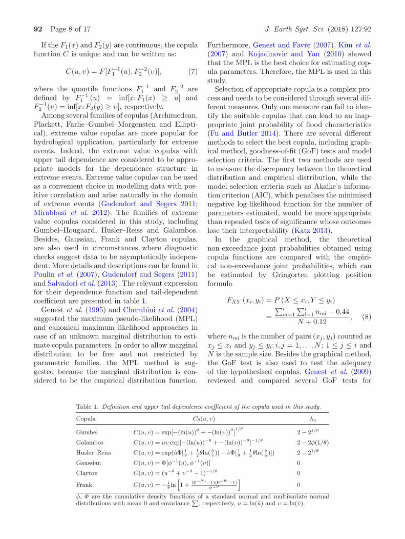
Plackett, Farlie–Gumbel–Morgensten and Ellipti-cal), extreme value copulas are more popular forhydrological application, particularly for extremeevents. Indeed, the extreme value copulas withupper tail dependence are considered to be appro-priate models for the dependence structure inextreme events. Extreme value copulas can be usedas a convenient choice in modelling data with pos-itive correlation and arise naturally in the domainof extreme events (Gudendorf and Segers 2011;Mirabbasi et al. 2012). The families of extremevalue copulas considered in this study, includingGumbel–Hougaard, Husler–Reiss and Galambos.Besides, Gaussian, Frank and Clayton copulas,are also used in circumstances where diagnosticchecks suggest data to be asymptotically indepen-dent. More details and descriptions can be found inPoulin et al. (2007), Gudendorf and Segers (2011)and Salvadori et al. (2013). The relevant expressionfor their dependence function and tail-dependentcoefficient are presented in table 1.

Genest et al. (1995) and Cherubini et al. (2004)suggested the maximum pseudo-likelihood (MPL)and canonical maximum likelihood approaches incase of an unknown marginal distribution to esti-mate copula parameters. In order to allow marginaldistribution to be free and not restricted byparametric families, the MPL method is sug-gested because the marginal distribution is con-sidered to be the empirical distribution function.

Furthermore, Genest and Favre (2007), Kim et al.(2007) and Kojadinovic and Yan (2010) showedthat the MPL is the best choice for estimating cop-ula parameters. Therefore, the MPL is used in thisstudy.

Selection of appropriate copula is a complex pro-cess and needs to be considered through several dif-ferent measures. Only one measure can fail to iden-tify the suitable copulas that can lead to an inap-propriate joint probability of flood characteristics(Fu and Butler 2014). There are several differentmethods to select the best copula, including graph-ical method, goodness-of-fit (GoF) tests and modelselection criteria. The first two methods are usedto measure the discrepancy between the theoreticaldistribution and empirical distribution, while themodel selection criteria such as Akaike’s informa-tion criterion (AIC), which penalises the minimisednegative log-likelihood function for the number ofparameters estimated, would be more appropriatethan repeated tests of significance whose outcomeslose their interpretability (Katz 2013).

In the graphical method, the theoreticalnon-exceedance joint probabilities obtained usingcopula functions are compared with the empiri-cal non-exceedance joint probabilities, which canbe estimated by Gringorten plotting positionformula

FXY (xi, yi) = P (X ≤ xi, Y ≤ yi)

=∑i

m=1

∑il=1 nml − 0.44

N + 0.12, (8)

where nml is the number of pairs (xj , yj) counted asxj ≤ xi and yj ≤ yi; i, j = 1, . . ., N ; 1 ≤ j ≤ i andN is the sample size. Besides the graphical method,the GoF test is also used to test the adequacyof the hypothesised copulas. Genest et al. (2009)reviewed and compared several GoF tests for

Table 1. Definition and upper tail dependence coefficient of the copula used in this study.

Copula Cθ(u, υ) λu

Gumbel C(u, υ) = exp[−(ln(u))θ + −(ln(υ))θ]1/θ

2 − 21/θ

Galambos C(u, υ) = uυ exp[−(ln(u))−θ + −(ln(υ))−θ]−1/θ 2 − 2φ(1/θ)

Husler–Reiss C(u, υ) = exp(uΦ[ 1θ

+ 12θln( u

υ)] − υΦ[ 1

θ+ 1

2θln( υ

u)]) 2 − 21/θ

Gaussian C(u, υ) = Φ[φ−1(u), φ−1(υ)] 0

Clayton C(u, υ) = (u−θ + υ−θ − 1)−1/θ 0

Frank C(u, υ) = − 1θln

[1 + (e−θu−1)(e−θυ−1)

e−θ

]0

φ, Φ are the cumulative density functions of a standard normal and multivariate normaldistributions with mean 0 and covariance

∑, respectively, u = ln(u) and υ = ln(υ).


copula. They proved that Cramer–von Mises (SIn)

test comparing the empirical and theoretical cop-ulas is the best GoF test. However, there isno difference between the extreme value copulasin this test. In order to overcome this short-coming, the test based on a Cramer–von Mises(SII

n ) statistic, measuring the distance betweenparametric and non-parametric estimators of thePickands dependence function, was introduced byGenest et al. (2011). This test is defined as:

SIIn =

∫ 1

0

n |An (t) − Aθn (t)|2 dt, (9)

where An(t) and Aθn(t) are the non-parametricand parametric estimators of Pickands dependencefunction A. Based on the objective and availabilityof data in this study, SII

n is used to find out theappropriate copula functions.

3.6 Joint return period estimation

The concepts of return period for flood events arewidely used as criteria in the design of hydraulicstructures and flood control facilities (Klein et al.2010). The return period of hydrological extremeevents is normally associated with a certainexceedance probability. In the bivariate case, thejoint return periods called OR (X ≥ x or Y ≥ y)and AND (X ≥ x and Y ≥ y) have been commonlyused:

TANDX,Y =

μT

P (X ≥ x and Y ≥ y)

=μT

1 − FX (x) − FY (y) + FXY (x, y),

(10)

TORX,Y =

μT

P (X ≥ x or Y ≥ y)

=μT

1 − FXY (x, y). (11)

The above equations are used for both block max-ima and POT approaches, where μT is the meaninter-arrival time (years). In the case of block max-ima, μT is equal to 1.0 (Shiau 2003; Vittal et al.2015). Since POT is applied in this study, themean inter-arrival time is determined based on theobserved flood events.

4. Results and discussion

4.1 Identification of flood characteristics

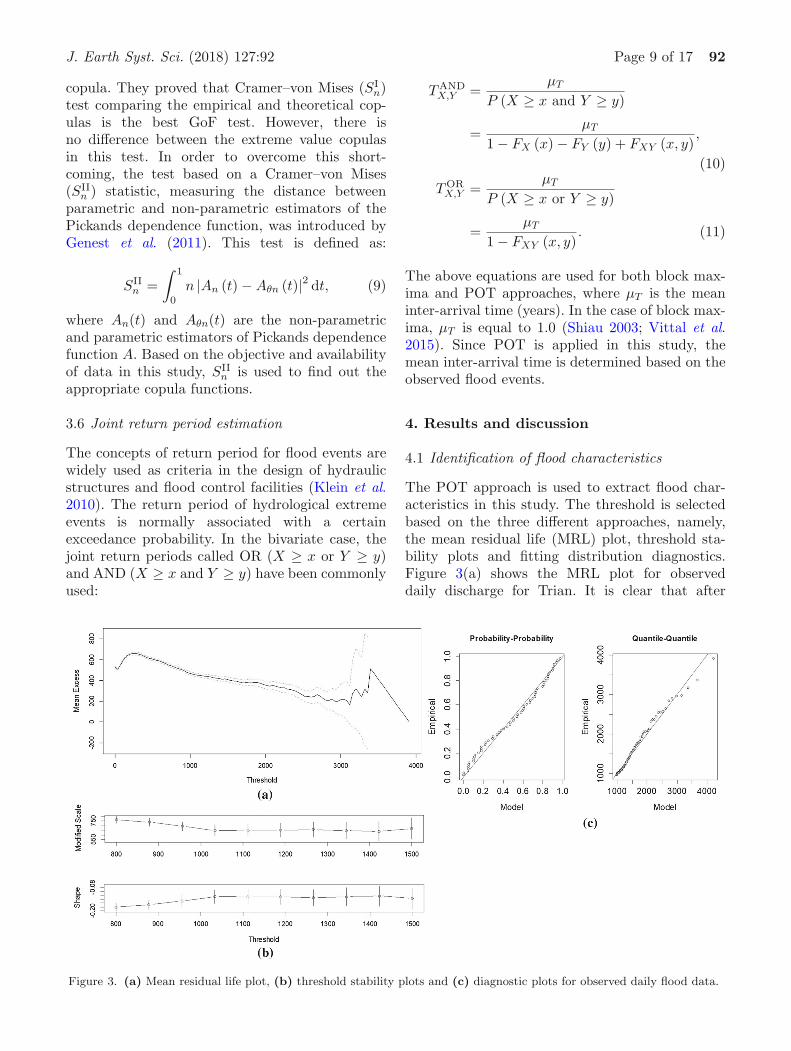
The POT approach is used to extract flood char-acteristics in this study. The threshold is selectedbased on the three different approaches, namely,the mean residual life (MRL) plot, threshold sta-bility plots and fitting distribution diagnostics.Figure 3(a) shows the MRL plot for observeddaily discharge for Trian. It is clear that after

Figure 3. (a) Mean residual life plot, (b) threshold stability plots and (c) diagnostic plots for observed daily flood data.


Figure 4. The autocorrelation plot up to lag 10 for all the flood characteristics.

Figure 5. Extremal measures for the dependence of observed flood peak and volume.

the threshold value of u = 950 m3/s, the MRLis consistent with a straight line. Furthermore,with the threshold value of u = 950 m3/s, theshape and modified scale parameters begin toreach a plateau (figure 3b). Besides, the diagnos-tic plots (probability–probability (PP), quantile–quantile (QQ)) for the fitted PIII distribution withthe threshold (950 m3/s) after declustering (r = 10days) are shown in figure 3(c) and they show a goodagreement between the model and empirical values.

Figure 4 shows that there is insignificant auto-correlation for all flood characteristics. The IIDflood variables assumption is still maintained basedon this threshold. Therefore, the threshold valueof u = 950 m3/s is a suitable threshold for Trian.This threshold is used for all future flood char-acteristics. Flood duration and volume are alsodetermined based on this threshold. The M–K testfor peak, volume and duration of observed datashowed that there is no significant trend for any

of the flood variables observed at the Trian gauge.It indicates that the flood events in the presentdata are still stationary. Therefore, the stationaryflood frequency analysis is used to estimate thejoint return periods.

4.2 Tail independence test

The pair of extremal measures (χ, χ) is used todetect whether the flood variables are asymptoti-cally dependent or not. Nevertheless, in this study,the value of χ(u) is nearly equal to 0.5. It meansthat the pair of flood characteristics has asymp-totic dependence for all u. However, the value ofχ shows that the pair of flood characteristics isindependent of many cases. For example, figure 5shows the χ and χ bar plot for the pair of observedflood peak and volume. Therefore, it is difficultto identify between asymptotical dependence andindependence based on these plots.


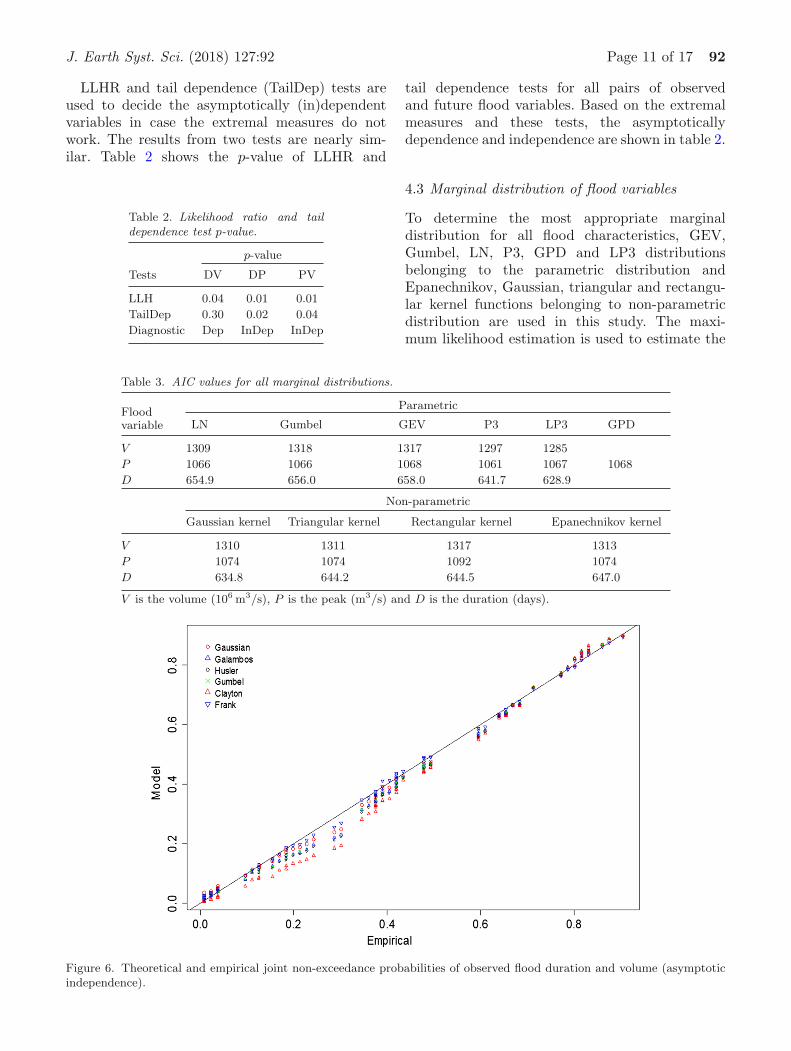
LLHR and tail dependence (TailDep) tests areused to decide the asymptotically (in)dependentvariables in case the extremal measures do notwork. The results from two tests are nearly sim-ilar. Table 2 shows the p-value of LLHR and

Table 2. Likelihood ratio and taildependence test p-value.

Tests

p-value

DV DP PV

LLH 0.04 0.01 0.01

TailDep 0.30 0.02 0.04

Diagnostic Dep InDep InDep

tail dependence tests for all pairs of observedand future flood variables. Based on the extremalmeasures and these tests, the asymptoticallydependence and independence are shown in table 2.

4.3 Marginal distribution of flood variables

To determine the most appropriate marginaldistribution for all flood characteristics, GEV,Gumbel, LN, P3, GPD and LP3 distributionsbelonging to the parametric distribution andEpanechnikov, Gaussian, triangular and rectangu-lar kernel functions belonging to non-parametricdistribution are used in this study. The maxi-mum likelihood estimation is used to estimate the

Table 3. AIC values for all marginal distributions.

Floodvariable

Parametric

LN Gumbel GEV P3 LP3 GPD

V 1309 1318 1317 1297 1285

P 1066 1066 1068 1061 1067 1068

D 654.9 656.0 658.0 641.7 628.9

Non-parametric

Gaussian kernel Triangular kernel Rectangular kernel Epanechnikov kernel

V 1310 1311 1317 1313

P 1074 1074 1092 1074

D 634.8 644.2 644.5 647.0

V is the volume (106 m3/s), P is the peak (m3/s) and D is the duration (days).

Figure 6. Theoretical and empirical joint non-exceedance probabilities of observed flood duration and volume (asymptoticindependence).


Figure 7. The joint return period of the pair of flood peakand volume modelling by Frank and Gumbel copulas.

parameters of the distributions. The selection ofthe appropriate distribution is based on the AICvalue. The selected marginal distributions are pre-sented in table 3, which provides a comparison ofperformances for all marginal distributions. Theresults indicate that the LP3 distribution is mostappropriate for modelling the flood volume andduration while the P3 is found to be the best forflood peak.

4.4 Copula selection

Figure 6 shows the theoretical and empirical jointnon-exceedance probabilities of asymptotic tailindependence data. It is observed that the Frankand Gaussian copulas fit the dataset, which is diag-nosed as an asymptotic independence better thanextreme value copulas. Additionally, AIC value andGoF test also indicated that the copula functionthat has no tail dependence may work well whenvariables are asymptotically independent.

The joint return period (AND) of observed floodduration and peak pair is estimated by using thebest fitted models of each group copulas. TheGumbel–Hougaard copula (extreme value copulas)and Frank copula (the no tail dependence copu-las) are selected to estimate the joint return periodof the observed flood duration and peak pair. Fig-ure 7 shows the comparison of joint return periodcurves of the pairs of observed duration and peakwhich are estimated by the Frank copula (black)and Gumbel copula (blue). This plot indicates thatthere are huge differences between two copulas. Fora lower return period, the two corresponding curvesare very close to each other. However, there are Table

4.

Copula

dep

enden

cepa

ram

eter

s,A

ICand

corr

espo

ndin

gG

oF

statist

ics.

Copula

s

DV

Copula

s

DP

PV

Para

met

erA

ICS

p-v

alu

ePara

met

erA

ICS

p-v

alu

ePara

met

erA

ICS

p-v

alu

e

Gum

bel

–H

ougaard

6.0

07

−165.0

13

0.0

0579

0.0

03

Gauss

ian

0.7

85

−57.5

09

0.1

14

0.0

65

0.8

35

−73.5

75

0.1

19

0.0

50

Gala

mbos

5.2

68

−162.4

01

0.0

0583

0.0

02

Cla

yto

n1.7

74

−47.8

17

0.5

04

0.0

01

2.0

66

−55.2

50

0.4

77

0.0

002

Husl

er–R

eiss

4.3

77

−137.9

84

0.0

0784

0.0

07

Fra

nk

8.4

55

−67.6

95

0.0

63

0.2

85

10.3

96

−86.9

29

0.0

58

0.3

35


Figure 8. Theoretical and empirical joint non-exceedance probabilities of (a) observed duration and volume and (b) observedduration and peak.

large differences in the central part in the 50- and100-yr return periods. Besides, the shape of thejoint return period of each copula has significantdifferences. The bound limits shrink significantlyfor the Gumbel–Hougaard copula while this situa-tion is not shown by the Frank copula. For example,at 5-year return period, the corresponding boundfor the Gumbel-Hougaard copula is wider thanthat of the Frank copula. At 10-, 50- and 100-yrreturn periods, the phenomenon is opposite andthe curve from the Gumbel–Hougaard becomessharper. This result indicates that choosing theinappropriate copula function will lead to seriousdifference between the joint return period results.This study suggests that the copula function is

selected based on the dependence structure of thevariables. The result from the tail dependence testmay provide useful additional information aboutthe adequacy of the chosen copula functions.

On the basis of the above analysis, in this study,three extreme value families of copulas (Gumbel–Hougaard, Galambos and Husler–Reiss) are chosento model the asymptotically dependence pair offlood characteristics. The Gaussian, Frank andClayton copulas are used in modelling the asymp-totically independence pair of flood characteristics.The dependence parameters of copulas are esti-mated using the MPL method. The copula depen-dence parameters, AIC and GoF statistics are givenin table 4.


Figure 9. The joint return periods of peak and volume (a) AND both peak and volume are exceeded and (b) OR eitherpeak or volume is exceeded.

Figure 8(a) shows the PP plot of model andempirical joint non-exceedance probabilities forobserved flood duration and volume. This plotindicates that the extreme value copulas(Gumbel–Hougaard, Galambos and Husler–Reiss)give the best fit to the dataset. However, identi-fying the differences among three copula functionsis difficult. Therefore, the AIC and GoF tests areused to choose the best copula function. For exam-ple, the AIC value (− 165.013) and statistical testvalue (0.00579) are shown in table 4, which indi-cate that the Gumbel–Hougaard copula providesthe best performance for the pair of observed floodduration and volume.

For asymptotically independence case,figure 8(b) shows the PP plot of the model andempirical joint non-exceedance probabilities for thepair of observed flood duration and peak. It is clearthat all copulas (Gaussian, Clayton and Frank)give a good fit to the data. However, the Frankcopula fits better than other copulas. Similarly,

the best fit copula using the AIC (− 67.695) andstatistical test values (0.285) is Frank copula(table 4). All measures indicate that the Frank cop-ula is the best fit to the data sample (observed floodduration and peak). The best copula based on theAIC value and GoF test is used to estimate thejoint return period for modelling the pair of floodcharacteristics.

4.5 Joint return period estimation

The joint return periods (AND and OR) of floodpeak and volume for 5-, 10-, 50-, 75- and 100-yearreturn periods are shown in figure 9. For exam-ple, the flood peak (m3/s)–volume (106 m3) pairs,(4011–11,020), (4119–11,432) and (42,965–11,674)are the joint return periods (OR) of 50, 75 and100 years, respectively. The results from this figurealso indicate that for all return periods, AND pro-vide lower flood variable quantile than OR. Several


combinations of flood peak and volume as wellas other flood characteristics in the same returnperiod are also obtained through bivariate fre-quency analysis. These results provide more possi-ble choices for the decision maker to select the floodevent for structure designing and water resourcesplanning as well as assessing the variability ofthe obtained flood map inundation that can-not be achieved through the univariate frequencyanalysis.

5. Summary and conclusions

The main emphasis of this study is on the taildependence test before the selection of copulafunction which best fits the data sample. Indeed,extremal measurement is a useful approach butin many cases, it cannot detect whether dataare asymptotically dependent or not. The LLHRand tail dependence tests are used to identify theasymptotically (in)dependence of observed floodvariables. Two pairs of flood characteristics (peak–volume and duration–peak) have asymptoticallyindependence while flood duration and volumepair have asymptotically dependence in this study.Three extreme value families of copula, namely,Gumbel–Hougaard, Galambos and Husler–Reissare evaluated to model the asymptotically depen-dence pair of flood characteristics. The extremevalue copulas with upper tail dependence haveproved that they are appropriate models for thedependence structure of the flood characteris-tics. However, identifying the differences amongthree copula functions is difficult. Therefore, thetest based on a Cramer–von Mises (SII

n ) statis-tic measuring the distance between parametricand non-parametric estimators of the Pickandsdependence function is used and it is proved thatit is highly efficient for extreme value copula.Similarly, Gaussian, Frank and Clayton copulasare the appropriate copula models in case ofvariables which are diagnosed as asymptoticallyindependence. Then, the best fit copula modelsare used to calculate the joint return periods offlood characteristics. These results provide morepossible choices for the decision maker to selectthe flood event for structure designing and waterresources planning as well as assessing the variabil-ity of the obtained flood map inundation in thepresent situation that cannot achieve through theunivariate frequency analysis.

Acknowledgements

The authors gratefully acknowledge the NationalHydro-Meteorological Service, Vietnam for pro-viding daily time series of observed river dis-charge data and thank Dr Agilan for his valuablediscussions.

References

Adamson P T, Metcalfe A V and Parmentier B 1999 Bivari-ate extreme value distributions: An application of theGibbs sampler to the analysis of floods; Water Resour.Res. 35 2825–2832.

Aghakouchak A, Ciach G and Habib E 2010 Estimation oftail dependence coefficient in rainfall accumulation fields;Adv. Water Resour. 33 1142–1149.

Aissia M a B, Chebana F, Ouarda T B M J, Roy L,Desrochers G, Chartier I and Robichaud E 2012 Mul-tivariate analysis of flood characteristics in a climatechange context of the watershed of the Baskatong reser-voir, Province of Quebec, Canada; Hydrol. Process. 26130–142.

Bacro J-N, Bel L and Lantuejoul C 2010 Testing the inde-pendence of maxima: From bivariate vectors to spatialextreme fields; Extremes 13 155–175.

Beguerıa S 2005 Uncertainties in partial duration series mod-elling of extremes related to the choice of the thresholdvalue; J. Hydrol. 303 215–230.

Bel L, Bacro J and Lantuejoul C 2008 Assessing extremaldependence of environmental spatial fields; Environ-metrics 19 163–182.

Bezak N, Brilly M and Sraj M 2014 Comparison between thepeaks-over-threshold method and the annual maximummethod for flood frequency analysis; Hydrol. Sci. J. 59959–977.

Bonnin G M, Martin D, Lin B, Parzybok T, Yekta M andRiley D 2006 Precipitation–frequency atlas of the UnitedStates; NOAA Atlas 2.

Bortot P, Coles S and Tawn J 2000 The multivariate Gaus-sian tail model: An application to oceanographic data;J. R. Stat. Soc. Ser. C Appl. Stat. 49 31–49.

Caperaa P, Fougeres A-L and Genest C 1997 A nonpara-metric estimation procedure for bivariate extreme valuecopulas; Biometrika 84 567–577.

Chebana F and Ouarda T B M J 2011 Multivariate quantilesin hydrological frequency analysis; Environmetrics 2263–78.

Cherubini U, Luciano E and Vecchiato W 2004 Copula meth-ods in finance; John Wiley & Sons.

Chowdhary H, Escobar L A and Singh V P 2011 Identifica-tion of suitable copulas for bivariate frequency analysis offlood peak and flood volume data; Hydrol. Res. 42 193–216.

Coles S 2001 An introduction to statistical modeling ofextreme values; Springer.

Coles S, Heffernan J and Tawn J 1999 Dependence measuresfor extreme value analyses; Extremes 2 339–365.


Dong Nguyen D, Jayakumar K V and Agilan V 2018 Impactof climate change on flood frequency of the Trian reservoirin Vietnam using RCMS; J. Hydrol. Eng. 23 05017032.

Dung N V, Merz B, Bardossy A and Apel H 2015 Handlinguncertainty in bivariate quantile estimation – An appli-cation to flood hazard analysis in the Mekong Delta; J.Hydrol. 527 704–717.

Dupuis D J 2007 Using copulas in hydrology: Benefits, cau-tions, and issues; J. Hydrol. Eng. 12 381–393.

Falk M and Michel R 2006 Testing for tail independence inextreme value models; Ann. Inst. Stat. Math. 58 261–290.

Favre A-C, El Adlouni S, Perreault L, Thiemonge N andBobee B 2004 Multivariate hydrological frequency anal-ysis using copulas; Water Resour. Res. 40, https://doi.org/10.1029/2003WR002456.

Frahm G, Junker M and Schmidt R 2005 Estimating thetail-dependence coefficient: Properties and pitfalls; Insur.Math. Econ. 37 80–100.

Frick M, Kaufmann E and Reiss R-D 2007 Testing the tail-dependence based on the radial component; Extremes 10109–128.

Fu G and Butler D 2014 Copula-based frequency analy-sis of overflow and flooding in urban drainage systems;J. Hydrol. 510 49–58.

Gaal L, Szolgay J, Kohnova S, Hlavcova K, Parajka J,Viglione A, Merz R and Bloschl G 2015 Dependencebetween flood peaks and volumes: A case study on climateand hydrological controls; Hydrol. Sci. J. 60 968–984.

Genest C and Favre A-C 2007 Everything you always wantedto know about copula modeling but were afraid to ask;J. Hydrol. Eng. 12 347–368.

Genest C, Ghoudi K and Rivest L-P 1995 A semiparametricestimation procedure of dependence parameters in multi-variate families of distributions; Biometrika 82 543–552.

Genest C, Kojadinovic I, Neslehova J and Yan J 2011 Agoodness-of-fit test for bivariate extreme-value copulas;Bernoulli 17 253–275.

Genest C, Remillard B and Beaudoin D 2009 Goodness-of-fit tests for copulas: A review and a power study; Insur.Math. Econ. 44 199–213.

Government V 2016 The operation of this multipurpose damsystem in the Saigon-Dongnai River basin; Vietnam;http://www.chinhphu.vn/portal/page/portal/chinhphu/hethongvanban?mode=detail&document id=184010.

Gudendorf G and Segers J 2011 Nonparametric estimation ofan extreme-value copula in arbitrary dimensions; J. Mul-tivariate Anal. 102 37–47.

Hao Z and Singh V P 2016 Review of dependence modelingin hydrology and water resources; Prog. Phys. Geogr. 40549–578.

Jeong D I, Sushama L, Khaliq M N and Roy R 2014 Acopula-based multivariate analysis of Canadian RCM pro-jected changes to flood characteristics for northeasternCanada; Clim. Dyn. 42 2045–2066.

Joe H, Smith R L and Weissman I 1992 Bivariate thresholdmethods for extremes; J. R. Stat. Soc. B-Stat. Methodol.54 171–183.

Karmakar S and Simonovic S 2009 Bivariate flood frequencyanalysis. Part 2: A copula-based approach with mixedmarginal distributions; J. Flood Risk Manag. 2 32–44.

Katz R W 2013 Statistical methods for nonstationaryextremes; In: Extremes in a changing climate (eds)

AghaKouchak A, Easterling D, Hsu K, Schubert Sand Sorooshian S, Springer, Dordrecht, WSTL 6515–37.

Kim G, Silvapulle M J and Silvapulle P 2007 Comparisonof semiparametric and parametric methods for estimatingcopulas; Comput. Stat. Data Anal. 51 2836–2850.

Kioutsioukis I, Melas D and Zerefos C 2010 Statisticalassessment of changes in climate extremes over Greece(1955–2002); Int. J. Climatol. 30 1723–1737.

Klein B, Pahlow M, Hundecha Y and Schumann A 2010Probability analysis of hydrological loads for the designof flood control systems using copulas; J. Hydrol. Eng. 15360–369.

Kojadinovic I and Yan J 2010 Comparison of three semipara-metric methods for estimating dependence parameters incopula models; Insur. Math. Econ. 47 52–63.

Lang M, Ouarda T and Bobee B 1999 Towards operationalguidelines for over-threshold modeling; J. Hydrol. 225103–117.

Ledford A W and Tawn J A 1996 Statistics for near inde-pendence in multivariate extreme values; Biometrika 83169–187.

Li L, Xu H, Chen X and Simonovic S P 2009 Stream-flow forecast and reservoir operation performance assess-ment under climate change; Water Resour. Manag. 2483–104.

Lima C H R, Lall U, Troy T J and Devineni N 2015 Aclimate informed model for nonstationary flood risk pre-diction: Application to Negro River at Manaus, Amazonia;J. Hydrol. 522 594–602.

Mirabbasi R, Fakheri-Fard A and Dinpashoh Y 2012 Bivari-ate drought frequency analysis using the copula method;Theor. Appl. Climatol. 108 191–206.

Poulin A, Huard D, Favre A-C and Pugin S 2007 Impor-tance of tail dependence in bivariate frequency analysis;J. Hydrol. Eng. 12 394–403.

Reddy M J and Ganguli P 2012 Bivariate flood frequencyanalysis of upper Godavari River flows using Archimedeancopulas; Water Resour. Manag. 26 3995–4018.

Renard B and Lang M 2007 Use of a Gaussian copula formultivariate extreme value analysis: Some case studies inhydrology; Adv. Water Resour. 30 897–912.

Requena A I, Chebana F and Mediero L 2016 A completeprocedure for multivariate index-flood model application;J. Hydrol. 535 559–580.

Ribatet M, Ouarda T B M J, Sauquet E and Gresillon JM 2009 Modeling all exceedances above a threshold usingan extremal dependence structure: Inferences on severalflood characteristics; Water Resour. Res. 45 W0340.

Saf B 2009 Regional flood frequency analysis using L-moments for the West Mediterranean region of Turkey;Water Resour. Manag. 23 531–551.

Salas Jose D, Heo Jun H, Lee Dong J and Burlando P 2013Quantifying the uncertainty of return period and risk inhydrologic design; J. Hydrol. Eng. 18 518–526.

Salvadori G, Durante F and De Michele C 2013 Multivari-ate return period calculation via survival functions; WaterResour. Res. 49 2308–2311.

Sarhadi A, Burn D H, Concepcion Ausın M and WiperM P 2016 Time varying nonstationary multivariate riskanalysis using a dynamic Bayesian copula; Water Resour.Res. 52 2327–2349.

https://doi.org/10.1029/2003WR002456

https://doi.org/10.1029/2003WR002456

http://www.chinhphu.vn/portal/page/portal/chinhphu/hethongvanban?mode=detail&document_id=184010

http://www.chinhphu.vn/portal/page/portal/chinhphu/hethongvanban?mode=detail&document_id=184010


Scarrott C and Macdonald A 2012 A review of extremevalue threshold estimation and uncertainty quantification;REVSTAT Stat. J. 10 33–60.

Schmidt R and Stadtmuller U 2006 Non-parametricestimation of tail dependence; Scand. J. Stat. 33307–335.

Serinaldi F, Bardossy A and Kilsby C G 2015 Upper taildependence in rainfall extremes: Would we know it if wesaw it?; Stochastic Environ. Res. Risk Assess. 29 1211–1233.

Shiau J T 2003 Return period of bivariate distributedextreme hydrological events; Stochastic Environ. Res.Risk Assess. 17 42–57.

Solari S and Losada M A 2012 A unified statistical model forhydrological variables including the selection of thresh-old for the peak over threshold method; Water Resour.Res. 48 W10541.

Sraj M, Bezak N and Brilly M 2015 Bivariate flood frequencyanalysis using the copula function: A case study of theLitija station on the Sava River; Hydrol. Process. 29 225–238.

Sun X, Lall U, Merz B and Dung N V 2015 Hierarchi-cal Bayesian clustering for nonstationary flood frequencyanalysis: Application to trends of annual maximum flowin Germany; Water Resour. Res. 51 6586–6601.

Thompson P, Cai Y, Reeve D and Stander J 2009 Automatedthreshold selection methods for extreme wave analysis;Coastal. Eng. 56 1013–1021.

Viglione A and Bloschl G 2009 On the role of storm durationin the mapping of rainfall to flood return periods; Hydrol.Earth Syst. Sci. 13 205–216.

Villarini G, Serinaldi F and Krajewski W F 2008 Modelingradar-rainfall estimation uncertainties using parametricand non-parametric approaches; Adv. Water Resour. 311674–1686.

Villarini G, Smith J A, Serinaldi F, Bales J, Bates P D andKrajewski W F 2009 Flood frequency analysis for nonsta-tionary annual peak records in an urban drainage basin;Adv. Water Resour. 32 1255–1266.

Vittal H, Singh J, Kumar P and Karmakar S 2015 A frame-work for multivariate data-based at-site flood frequencyanalysis: Essentiality of the conjugal application of para-metric and nonparametric approaches; J. Hydrol. 525658–675.

Weller G B, Cooley D S and Sain S R 2012 An investiga-tion of the pineapple express phenomenon via bivariateextreme value theory; Environmetrics 23 420–439.

Yilmaz A G, Imteaz M A and Perera B J C 2017 Investiga-tion of non-stationarity of extreme rainfalls and spatialvariability of rainfall intensity–frequency–duration rela-tionships: A case study of Victoria, Australia; Int. J.Climatol. 37 430–442.

Yue S 1999 Applying bivariate normal distribution to floodfrequency analysis; Water Int. 24 248–254.

Yue S, Ouarda T and Bobee B 2001 A review of bivari-ate gamma distributions for hydrological application;J. Hydrol. 246 1–18.

Zhang L and Singh V P 2006 Bivariate flood frequency anal-ysis using the copula method; J. Hydrol. Eng. 11 150–164.

Zhang L and Singh V P 2007 Bivariate rainfall frequencydistributions using Archimedean copulas; J. Hydrol. 33293–109.

Corresponding editor: Subimal Ghosh

Documents

Assessing the copula selection for bivariate frequency