Assessing the skill of yes/noforecasts for Markov observations

William Briggs

General Internal Medicine, Weill Cornell Medical College525 E. 68th, Box 46, New York, NY 10021

email: wib2004@med.cornell.edu

and

David Ruppert

School of Operations Research & Industrial Engineering,Rhodes Hall, Cornell University, Ithaca, NY 14853

email: dr24@cornell.edu

May 3, 2005

1

2

Summary: Briggs and Ruppert (2005) recently introduced a new,

easy-to-calculate economic skill/value score for use in yes/no forecast

decisions, of which precipitation forecast decisions are an example. The

advantage of this new skill/value score is that the sampling distribution

is known, which allows one to perform hypothesis tests on collections

of forecasts and to say whether a given skill/value score is significant

or not.

Here, we take the climate skill/value score and extend it to the case

where the predicted series is first-order Markov in nature, of which,

again, precipitation occurrence series can be an example. We show

that, in general, Markov skill/value is different and more demanding

than is persistence skill. Persistence skill is defined as improvement

over forecasts which state that the next value in a series will equal the

present value.

We also show that any naive forecasts based solely on the Markov

parameters is always at least as valuable/skillful than are persistence

forecasts; in general, persistence forecasts should not be used.

The distribution for the Markov skill score is presented, and exam-

ples of hypothesis testing for precipitation forecasts are given. We

graph these skill scores for a wide range of forecast-user loss functions,

a process which makes their interpretation simple.

3

1. Introduction

In previous papers, Briggs and Ruppert (2004) and Briggs and Ruppert (2005; from

here, BR), developed a statistical test for skill for forecasts of dichotomous events Y .

The events Yi in this test were assumed to be independent of each Yj for all i 6= j. In

this paper, we extend the original skill score test to situations where the events are a

two-state Markov chain. Precipitation occurrence at a point is often a good example

of such series.

Much work has been done in the area of investigating forecast value and forecast

verification, most notably in the works of Murphy (Murphy, 1991; Murphy, 1997;

Murphy and Winkler, 1987; Murphy and Ehrendorfer, 1987; to name only a few),

Schervish (1989), Briggs and Levine (1998), Meeden (1979), and Wilks (2001). Wilks

(1995), Mason (2003), and Livezey (2003) provide a detailed list of skill scores for

categorical events, such as we consider here. Wilks (1991) began work in showing

how the dependent nature of observation process interacts with forecast verification,

work which we continue here.

We define forecasts X̃ ∈ [0, 1] made for events Y ∈ {0, 1}. Here, we are interested

in the two-decision problem, which is when a decision maker acts on the forecast X̃

and makes one of two decisions: d1 is he believes Y = 1 will occur, or d0 is he believes

Y = 0 will occur. The decision maker faces a loss k01 if he takes d1 and Y = 0

occurs, and has a loss k10 is he takes d0 and Y = 1 occurs. The loss can always be

parameterized such that θ = k01/(k01 + k01). Here, we assume k11 = k00 = 0; Briggs

(2005) showed how to modify this so that any kY X ≥ 0, which includes the class of

cost-loss problems (see Wilks, 2001; Richardson, 2000, 2001). Briggs et al. (2005)

extended the climate skill test to cases where the observed series is possibly classified

with error.

4

When θ = 1/2, the loss is said to be symmetric. BR show that this parameterization

allows us to transform the forecast X̃, for the two-decision problem, as XE = I(X̃ ≥

θ), where the superscript E designates that XE is an expert forecast, which is any

forecast that is not the optimal naive climate forecast. The optimal naive climate

forecast XNcl for Y is the forecast one would make knowing only p = P (Y = 1). It is

easy to show that this is XNcl = I(p > θ).

Skill is now defined. This is when P (XE = Y ) > P (XNcl = Y ). Value is when the

expected loss of the expert forecast is less than the expected loss of the optimal naive

climate forecast: E(kE) < E(kNcl ). BR showed that these two definitions are identical

when θ = 1/2, or when the loss is symmetric. BR developed a skill/value score and

a test statistic for skill/value, where the key parameter was p1|1 = P (Y = 1|X = 1),

which was less than or equal to θ under the null hypothesis of no skill.

This work will extend the same concepts developed in BR to events Yi where {Yi}

is a two-state Markov chain. We first define persistence as the forecast XP = Yi−1

for all i. We show in Section 3 that skill, when Y is Markov, is not the same as

skill of a persistence forecast; we further show that the expected loss of a persistence

forecast is always as great or greater than the expected loss of optimal naive forecasts;

thus, persistence forecasts should never be used. This result holds for optimal naive

climate or Markov forecasts. In Section 2, we develop a test for comparing any two

forecasts for the same event, which we later apply in Section 4 with a persistence

forecast and the optimal naive Markov forecast. Finally, an Appendix is given to

detail the mathematical results.

5

2. Comparing competing forecasts

In this Section, we develop a simple framework to compare competing forecasts

for the same event. In this framework, there are two (expert) forecasts X1 and X2.

Define Zi = I(Y = Xi), which is the indicator that forecast i is correct, i = 1, 2.

We have that P (Z1 = Z2 = 1) is the probability that both forecasts are correct and

P (Z1 = Z2 = 0) is the probability that they are both wrong. The probabilities of

interest are P (Z1 = 1, Z2 = 0) and P (Z1 = 0, Z2 = 1), that is, the probabilities

designating those times when one forecast was correct while the other was wrong.

We assume that the loss is symmetric, i.e., the loss for one forecast being correct is

the same as for the other being incorrect.

The development in this Section is not new. The test statistic developed here is sim-

ilar to McNemar’s (1947) test for matched pairs and to its refinement by Mosteller

(1952). Depending on the particular null hypothesis chosen, our statistic is only

slightly different to the classical statistic and, again depending on the null, one could

use the classical statistic in place of this one (this is explained below). The develop-

ment here shows how the comparison test operates with respect to the skill test.

We assume that there is an i.i.d. sequence {(X1i, X2i, Yi) : i = 1, . . . , n} and we

define Zji = I(Xji = Yi), j = 1, 2. Let mi,j =∑

Z1,i = Z2,j, that is, the observed

counts.

One possible null hypothesis is

(2.1) H0 : P (Z1 = 1, Z2 = 0) = P (Z1 = 0, Z2 = 1)

with the two-sided alternative

(2.2) P (Z1 = 1, Z2 = 0) 6= P (Z1 = 0, Z2 = 1).

6

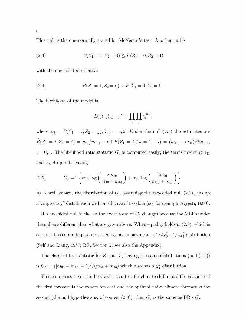
This null is the one normally stated for McNemar’s test. Another null is

(2.3) P (Z1 = 1, Z2 = 0) ≤ P (Z1 = 0, Z2 = 1)

with the one-sided alternative

(2.4) P (Z1 = 1, Z2 = 0) > P (Z1 = 0, Z2 = 1).

The likelihood of the model is

L({zi,j}i,j=1,1) =∏

i

∏j

zmij

ij ,

where zij = P (Z1 = i, Z2 = j), i, j = 1, 2. Under the null (2.1) the estimates are

P̂ (Z1 = i, Z2 = i) = mii/m++, and P̂ (Z1 = i, Z2 = 1 − i) = (m10 + m01)/2m++,

i = 0, 1. The likelihood ratio statistic Gc is computed easily; the terms involving z11

and z00 drop out, leaving

(2.5) Gc = 2

{m10 log

(2m10

m10 + m01

)+ m01 log

(2m01

m10 + m01

)}.

As is well known, the distribution of Gc, assuming the two-sided null (2.1), has an

asymptotic χ2 distribution with one degree of freedom (see for example Agresti, 1990).

If a one-sided null is chosen the exact form of Gc changes because the MLEs under

the null are different than what are given above. When equality holds in (2.3), which is

case used to compute p-values, then Gc has an asymptotic 1/2χ20 +1/2χ2

1 distribution

(Self and Liang, 1987; BR, Section 2; see also the Appendix).

The classical test statistic for Z1 and Z2 having the same distributions (null (2.1))

is GC = (|m01 −m10| − 1)2/(m01 + m10) which also has a χ21 distribution.

This comparison test can be viewed as a test for climate skill in a different guise, if

the first forecast is the expert forecast and the optimal naive climate forecast is the

second (the null hypothesis is, of course, (2.3)), then Gc is the same as BR’s G.

7

3. Markov Skill tests and Skill Scores

Skill, if it exists when {Yi} is a two-state Markov chain, is known as Markov skill

because the optimal naive Markov forecast XNMa of each Yi is based on the previous

observation Yi−1. We will show that Markov skill is generally not identical with

persistence skill. A persistence forecast is one in which the naive forecast for Yi is

Yi−1 for all i, and persistence skill means outperforming the persistence forecast. We

assume only that {Yi} is Markov, and not, for example, that {Yi, Xi} is bivariate

Markov. No further conditions are put on {Xi} except that to require P (Xi|Yi−1) be

constant for all i.

Daily occurrence of precipitation is a common example of Markov data (Wilks,

1995). We could condition skill scores for forecasts of Markov data on the event Yi−1

and use the results from BR. That is, individual tests of climate skill can be carried

out for the cases in which Yi−1 = 1 and Yi−1 = 0. This is useful as a performance

diagnostic to highlight those experts who possibly forecast badly in one situation but

well in the other. This approach in ultimately unsatisfying for formal testing because

it ignores the data as a whole and the distribution of the test statistic under the

Markov assumption. The following test is needed.

3.1. Model. Consider the factorization

(3.1) P (Yi, Xi, Yi−1) = P (Yi|Xi, Yi−1)P (Xi|Yi−1)P (Yi−1).

Other factorizations are, of course, possible but it turns out that this form is the most

mathematically convenient to work with. The full model may be expanded to (with

P (Yi−1 = 1) = p) the following set of equations. The methodology is exactly that

8

used in BR. This factorization gives:

P (Yi = 1, Xi = 1, Yi−1 = 1) = p1|11p+1|1p

P (Yi = 1, Xi = 1, Yi−1 = 0) = p1|10p+1|0(1− p)

P (Yi = 1, Xi = 0, Yi−1 = 1) = p1|01(1− p+1|1)p

P (Yi = 1, Xi = 0, Yi−1 = 0) = p1|00(1− p+1|0)(1− p)

P (Yi = 0, Xi = 1, Yi−1 = 1) = (1− p1|11)p+1|1p

P (Yi = 0, Xi = 1, Yi−1 = 0) = (1− p1|10)p+1|0(1− p)

P (Yi = 0, Xi = 0, Yi−1 = 1) = (1− p1|01)(1− p+1|1)p

P (Yi = 0, Xi = 0, Yi−1 = 0) = (1− p1|00)(1− p+1|0)(1− p),

where p1|11 = P (Yi = 1|Xi = 1, Yi−1 = 1), p+1|1 = P (Xi = 1|Yi−1 = 1), p1|10 = P (Yi =

1|Xi = 1, Yi−1 = 0), p+1|0 = P (Xi = 1|Yi−1 = 0), p1|01 = P (Yi = 1|Xi = 0, Yi−1 = 1),

and p1|00 = P (Yi = 1|Xi = 0, Yi−1 = 0). We will use the convention that the

replacement of an index by “+” means summation over that index so, for example,

p+1|1 =∑

i pi1|1.

We shall also need to define the parameters that characterize the Markov nature

of Y . These are p1+|1 = P (Yi = 1|Yi−1 = 1), p0+|1 = P (Yi = 0|Yi−1 = 1), p1+|0 =

P (Yi = 1|Yi−1 = 0), p0+|0 = P (Yi = 0|Yi−1 = 0). It happens that p0+|1 = 1−p1+|1 and

p0+|0 = 1− p1+|0 so that only two parameters are needed to fully specify the Markov

nature of Y .

It is also helpful to define the following counts. Let nj,k,l, where j, k, l ∈ {0, 1}, be

the counts for the cells Yi, Xi, and Yi−1. For example, n111 =∑n

i=2 YiXiYi−1, and

n000 =∑n

i=2(1− Yi)(1−Xi)(1− Yi−1).

3.2. Markov and persistence skill tests. We now introduce tests of skill relative

to optimal naive Markov forecasts and to persistence forecasts.

9

All of the parameters of this model neatly separate in the likelihood, making es-

timation easy. For example, the part of the likelihood relating to the parameter

P (Yi = 1|Xi = 1, Yi−1 = 1) = p1|11 is

∏p

YiXiYi−1

1|11 (1− p1|11)(1−Yi)XiYi−1 .

It is simple to differentiate and solve for the MLE for all such parameters. It turns

out that the parameters p, p+1|1 and p+1|0 will not play a role in the likelihood ratio

test as their MLEs are the same under both the null and alternative hypotheses for

either pair (2.1) and (2.2) or (2.3) and (2.4).

The unrestricted MLEs are p̂ = n++1/n+++, p̂+1|1 = n+11/n++1, p̂+1|0 = n+10/n++0.

The other estimators do change when one switches between the null and alterna-

tive, and the unrestricted MLES are: p̂1|11 = n111/n+11, p̂1|10 = n110/n+10, p̂1|01 =

n101/n+01 p̂1|00 = n100/n+00.

The optimal naive Markov forecast XNMa must now be defined; “naive” means that

only the transition probabilities P (Yi|Yi−1) are known. It turns out that there are four

situations, that is, four circumstances that dictate different optimal naive Markov

forecasts. We focus here on just one situation, detailed next, for the sake of an

example. The other three situations will be removed to the Appendix. Table 1 lists

the four cases of optimal naive Markov forecasts.

We assume that the events {Yi, Yi−1} are such that p1+|1 < θ and p1+|0 < θ, that

is, the probability that Yi = 1 no matter the value of Yi−1 is always less than θ. This

gives that the optimal naive Markov forecast is always 0, regardless of the value of

Yi−1. Note that in this case the optimal naive Markov forecast is different than a

persistence forecast, which is Xi = Yi−1 for all i. Table 1 shows that in only one case

is the optimal naive Markov forecast the same as the persistence forecast.

10

One solution for deriving a test of climate skill against persistence is to use the

comparative forecast test developed earlier with the first set of forecasts assigned to

the expert, and the second set of forecasts assigned to persistence. But we can go

further and show that the optimal naive Markov forecast is always at least as good as

the persistence forecast (in terms of value or skill); this is done in the next Section.

Directly from BR, we have that the null hypothesis of no Markov skill is that the

expected loss of the expert forecast is less than or equal to the expected loss of the

optimal naive Markov forecast (details are in the Appendix). This gives:

H0 : (p1|11 ≤ θ, p1|10 ≤ θ).

All parameters except those indicated in the null hypothesis have the same MLEs in

both the null and alternate hypotheses. The LRS (likelihood ratio statistic) depends

on only two parameters, p1|11 and p1|10, which are maximized under the null with

estimates p̃1|11 = min{ n111

n+11, θ} and p̃1|10 = min{ n110

n+10, θ}. Substitution leads to the

LRS:

GM = 2n111 log

(p̂1|11

p̃1|11

)+ 2n011 log

(1− p̂1|11

1− p̃1|11

)+

2n110 log

(p̂1|10

p̃1|10

)+ 2n010 log

(1− p̂1|10

1− p̃1|10

).

There are four situations under the null: when both n111

n+11and n110

n+10are greater than θ

then p̃1|11 = p̃1|10 = θ and GM > 0; when n111

n+11≤ θ and n110

n+10> θ then p̃1|11 = p̂1|11 and

p̃1|10 = θ and GM > 0; when n111

n+11> θ and n110

n+10≤ θ then p̃1|11 = θ and p̃1|10 = p̂1|10

and GM > 0; or when n111

n+11≤ θ and n110

n+10≤ θ then p̃1|11 = p̂1|11 and p̃1|10 = p̂1|10 and

GM = 0. This allows us to rewrite GM as

GM =

(2n1|1 log

[n111

n+11θ

]+ 2n011 log

[n011

n+11(1− θ)

])I

(n111

n+11

> θ

)+

(2n110 log

[n110

n+10θ

]+ 2n010 log

[n010

n+10(1− θ)

])I

(n110

n+10

> θ

)(3.2)

11

This statistic has an asymptotic mixture distribution under the null of 1/4χ20 +

1/2χ21 + 1/4χ2

2 where χ2k is the chi-square distribution with k degrees of freedom and

χ20 is point mass at 0 (see Self and Liang, 1987; an extension of their case 5).

3.3. The optimal Markov forecast is superior to persistence. We now prove

that the optimal naive Markov forecast is always at least as valuable (skilful) as any

persistence forecast.

Theorem 3.1. Let the optimal naive Markov forecast be denoted as I{P (Yi = 1|Yi−1) >

θ} and let the persistence forecast be Yi−i. Then the optimal naive Markov forecast

is always at least as valuable (or skillful) than is the persistence forecast in the sense

that E(kNMa) ≤ E(kN

P ) where E(kNMa) is the expected loss of the optimal naive Markov

forecast and E(kNP ) is the expected loss of the persistence forecast.

Proof. There are four cases of optimal naive Markov forecasts; see Table 1. The

optimal naive Markov and persistence forecasts are identical for Case 2, so E(kNP ) =

E(kNMa).

For Case 1, I{P (Yi = 1|Yi−1) > θ} = 0 regardless of the value of Yi−1. The expected

loss for the optimal naive Markov forecast in Case 1 is

E(kNMa) = (p11|0 + p10|0)(1− θ)(1− p) + (p11|1 + p10|1)(1− θ)p.

The expected loss of the persistence forecast is

E(kNP ) = p0+|1θp + p1+|0(1− θ)(1− p)

= (p00|1 + p01|1)θp + E(kNMa)− (p11|1 + p10|1)(1− θ)p

= E(kNMa) + p

[(p00|1 + p01|1)θ − (p11|1 + p10|1)(1− θ)

]

= E(kNMa) + p

[θ − (p11|1 + p10|1)

]

12

Now, p11|1+p10|1 = P (Yi = 1|Yi−1 = 1) and because we are in Case 1, P (Yi = 1|Yi−1 =

1) ≤ θ. So E(kNP ) = E(kN

Ma) when P (Yi = 1|Yi−1 = 1) = θ, and E(kNP ) > E(kN

Ma)

otherwise.

For Case 3, it is shown by the same means that the expected loss of the persistence

forecast equals

E(kNP ) = E(kN

Ma) + p [θ − P (Yi = 1|Yi−1 = 1)] + (1− p) [P (Yi = 1|Yi−1 = 1)− θ]

Again, P (Yi = 1|Yi−1 = 1) ≤ θ and P (Yi = 1|Yi−1 = 0) > θ, and E(kNP ) ≥ E(kN

Ma).

Case 4 is proved in an identical fashion. ¤

Independence (where the optimal naive Markov forecast and the optimal naive

climate forecast are the same) is a special case of Markov. Here too, the persistence

forecast is worse than the optimal naive Markov forecasts (think of trying to predict

random coin flips: the best guess is to say “Heads” always; while the persistence

“forecast” is to always guess whatever the coin was last flip). The lesson is that, in

general and except where the optimal naive Markov forecasts overlaps the persistence,

persistence forecasts should not be used.

3.4. Markov skill score. A skill score can now be created, as in BR. A common

form for such a score is (see Wilks, 1995 for a more complete discussion of skill scores;

in this paper we also set the expected loss of a perfect forecast equal to 0):

(3.3) Kθ(y, xE) =E(kN

Ma)− E(kE)

E(kNMa)

,

where E(kNMa) is expected loss for the optimal naive Markov forecast, and E(kE)

is the expected loss for the expert forecast. There are two parts to that equation,

E(kNMa)− E(kE) and E(kN

Ma). For E(kNMa)− E(kE), it is easy to show that we have

E(kNMa)− E(kE) = (p1|11 − θ)p+1|1p + (p1|10 − θ)p+1|0(1− p).

13

Also, E{k(Y,XNMa)} is

(1− θ)(p1|11p+1|1p + p1|01(1− p+1|1)p + p1|10p+1|0(1− p) + p1|00(1− p+1|0)(1− p)).

An estimate for Kθ comes from substituting the estimates for p1|11, p1|01 and so on

into these equations. Details will be left to the Appendix. Upon slugging through

the algebra, we find that

(3.4) K̂θ =(1− θ)n111 − θn011 + (1− θ)n110 − θn010

(n111 + n101)(1− θ) + (n110 + n100)(1− θ).

However, it is the case that n111 + n110 = n11+, where n11+ is the number of days

when Yi−1 = 1 and Yi−1 = 0. Similar facts hold for n110 and n010 and so on. What

this means is that (3.4) ultimately collapses to

(3.5) K̂θ =(1− θ)n11+ − θn01+

(n11+ + n10+)(1− θ).

which is identical to the original climate skill score developed in BR, which is not

surprising since the optimal naive Markov forecast is always 0 (in Case 1; as it was

for the optimal naive climate forecast in the climate skill score).

More can be done because (3.4) can be written in a more insightful manner and

decomposed into parts for when Yi−1 = 1 and when Yi−1 = 0, with weights (based on

the data) for the importance of the skill score for these two regimes. To be clearer,

we are seeking a representation of the skill score like the following:

K̂θ = w1K̂θ,1 + w0K̂θ,0

where K̂θ,j is the skill score for those times when Yi−1 = j, and wj is the weight based

on the data. We derive these weights now.

14

Let D = (n111 + n101)(1 − θ) + (n110 + n100)(1 − θ), which is the denominator of

equation (3.4). We can now rewrite that equation:

K̂θ =(n111 + n011)(1− θ)

(n111 + n011)(1− θ)

(1− θ)n111 − θn011

D

+(n110 + n010)(1− θ)

(n110 + n010)(1− θ)

(1− θ)n110 − θn010

D

=(n111 + n011)(1− θ)

DK̂1,θ +

(n111 + n011)(1− θ)

DK̂0,θ.

where K̂1,θ is the same as equation (3.5) but only calculated for those days when

Yi−1 = 1. Similarly, K̂0,θ is only calculated for those days when Yi−1 = 0.

We have that

(n111 + n011)(1− θ)

D=

(n111 + n011)(1− θ)

D

n(n111 + n011 + n101 + n001)

n(n111 + n011 + n101 + n001)

=p̂1+|1p̂

p̂y

,

where p̂y = P̂ (Yi = 1) (note that p̂ = P̂ (Yi−1 = 1) does not necessarily equal p̂y =

P̂ (Y1 = 1) for any given sample) Similarly,

(n110 + n010)(1− θ)

D=

p̂1+|0(1− p̂)

p̂y

.

This results in

(3.6) K̂θ =p̂1+|1p̂

p̂y

K̂1,θ +p̂1+|0(1− p̂)

p̂y

K̂0,θ.

The contribution of each K̂i,θ is weighted by the proportion of Yi’s=1 on those days

when Yi−1 = 1 and Yi−1 = 0. Because p̂1+|1p̂/p̂y = P̂ (Yi−1 = 1|Yi = 1), and p̂1+|0(1−

p̂)/p̂y = P̂ (Yi−1 = 0|Yi = 1), we can also write (3.6) as

(3.7) K̂θ = P̂ (Yi−1 = 1|Yi = 1)K̂1,θ + (1− P̂ (Yi−1 = 1|Yi = 1))K̂0,θ.

This also shows that, as we might expect, w0 = 1− w1. This last notation is similar

to the idea of sensitivity and specificity.

15

4. Example

We first start with an example of a simple skill test. The first author collected

probability of precipitation forecasts made for New York City (Central Park) from

16 November 2000 to 17 January 2001 (63 forecasts) for both Accuweather and the

National Weather Service (NWS). This data set is not meant to conclusively diagnose

the forecasting abilities of these two agencies; it is only chosen to demonstrate the

general ideas of the skill scores and skill plots.

Both Accuweather and the NWS made 1-day ahead forecasts. Only Accuweather

attempted 14-day ahead forecasts. Accuweather presented its forecasts in the form

of yes/no predictions, while the NWS issued probability forecasts. Figure 1 shows

how the forecasts did. It presents climate skill and value calculated for a range of

θ ∈ (0, 1); score values less than 0 indicate no value (for θ 6= 1/2) or no skill (for

θ = 1/2). These plots are nearly the same as those developed in Richardson (2000),

except they are for skill and not value. The NWS did quite well, beating or closely

matching Accuweather’s performance for the 1-day ahead predictions. The figure

shows also that the NWS forecast would have had value for most users (for many loss

values θ). Accuweather performed badly for its 14-day ahead predictions. In fact, any

user, regardless of his loss function, would have done better and would have suffered

less loss had they used the optimal naive climate prediction (no precipitation) during

this time.

We show, in Figure 2, the climate skill plot for the same data (for the 1-day ahead

forecasts) but break it into days when Yi−1 = 1 and for Yi−1 = 0. The overall

probability of precipitation is p̂y = 0.32. Estimates of the transition parameters are,

p̂1+|1 = 0.42 and p̂1+|0 = 0.28 (tests, due to the small sample size, do not show the

Markov nature of this data as “significant”, but it is still useful for illustration).

16

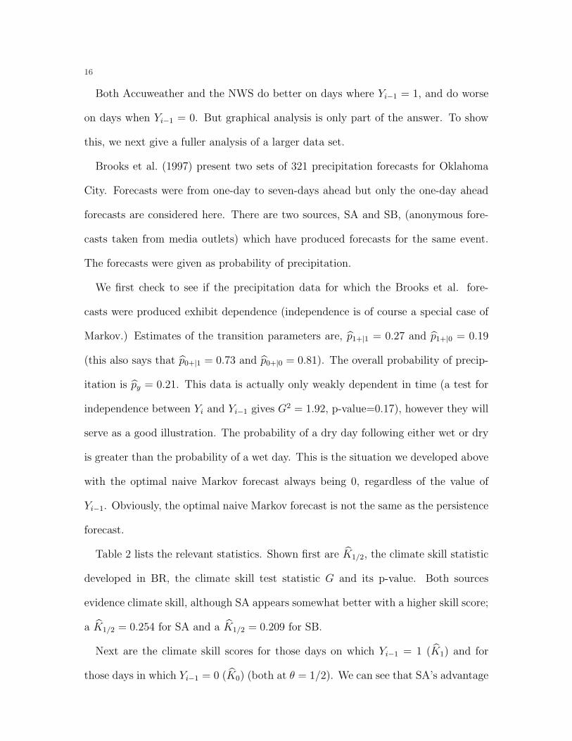
Both Accuweather and the NWS do better on days where Yi−1 = 1, and do worse

on days when Yi−1 = 0. But graphical analysis is only part of the answer. To show

this, we next give a fuller analysis of a larger data set.

Brooks et al. (1997) present two sets of 321 precipitation forecasts for Oklahoma

City. Forecasts were from one-day to seven-days ahead but only the one-day ahead

forecasts are considered here. There are two sources, SA and SB, (anonymous fore-

casts taken from media outlets) which have produced forecasts for the same event.

The forecasts were given as probability of precipitation.

We first check to see if the precipitation data for which the Brooks et al. fore-

casts were produced exhibit dependence (independence is of course a special case of

Markov.) Estimates of the transition parameters are, p̂1+|1 = 0.27 and p̂1+|0 = 0.19

(this also says that p̂0+|1 = 0.73 and p̂0+|0 = 0.81). The overall probability of precip-

itation is p̂y = 0.21. This data is actually only weakly dependent in time (a test for

independence between Yi and Yi−1 gives G2 = 1.92, p-value=0.17), however they will

serve as a good illustration. The probability of a dry day following either wet or dry

is greater than the probability of a wet day. This is the situation we developed above

with the optimal naive Markov forecast always being 0, regardless of the value of

Yi−1. Obviously, the optimal naive Markov forecast is not the same as the persistence

forecast.

Table 2 lists the relevant statistics. Shown first are K̂1/2, the climate skill statistic

developed in BR, the climate skill test statistic G and its p-value. Both sources

evidence climate skill, although SA appears somewhat better with a higher skill score;

a K̂1/2 = 0.254 for SA and a K̂1/2 = 0.209 for SB.

Next are the climate skill scores for those days on which Yi−1 = 1 (K̂1) and for

those days in which Yi−1 = 0 (K̂0) (both at θ = 1/2). We can see that SA’s advantage

17

has come from scoring better on those days which had Yi−1 = 1; a K̂1,1/2 = 0.333

at SA to a K̂1,1/2 = 0.111 at SB. Both Sources did about the same on those days

which had Yi−1 = 0; a K̂0,1/2 = 0.225 at SA to a K̂0,1/2 = 0.245 at SB. Both Sources

evidenced Markov skill; both sources had large GMs and small p-values for the test.

The weighting (shown in Table 3) for the skill score K̂1,1/2 was 0.27, and for K̂0,1/2 it

was 0.73, which shows that the days on which Yi−1 = 0 receive the majority of the

weight and explains why SA and SB are still close in overall performance even though

SA scores so well on days when Yi−1 = 1.

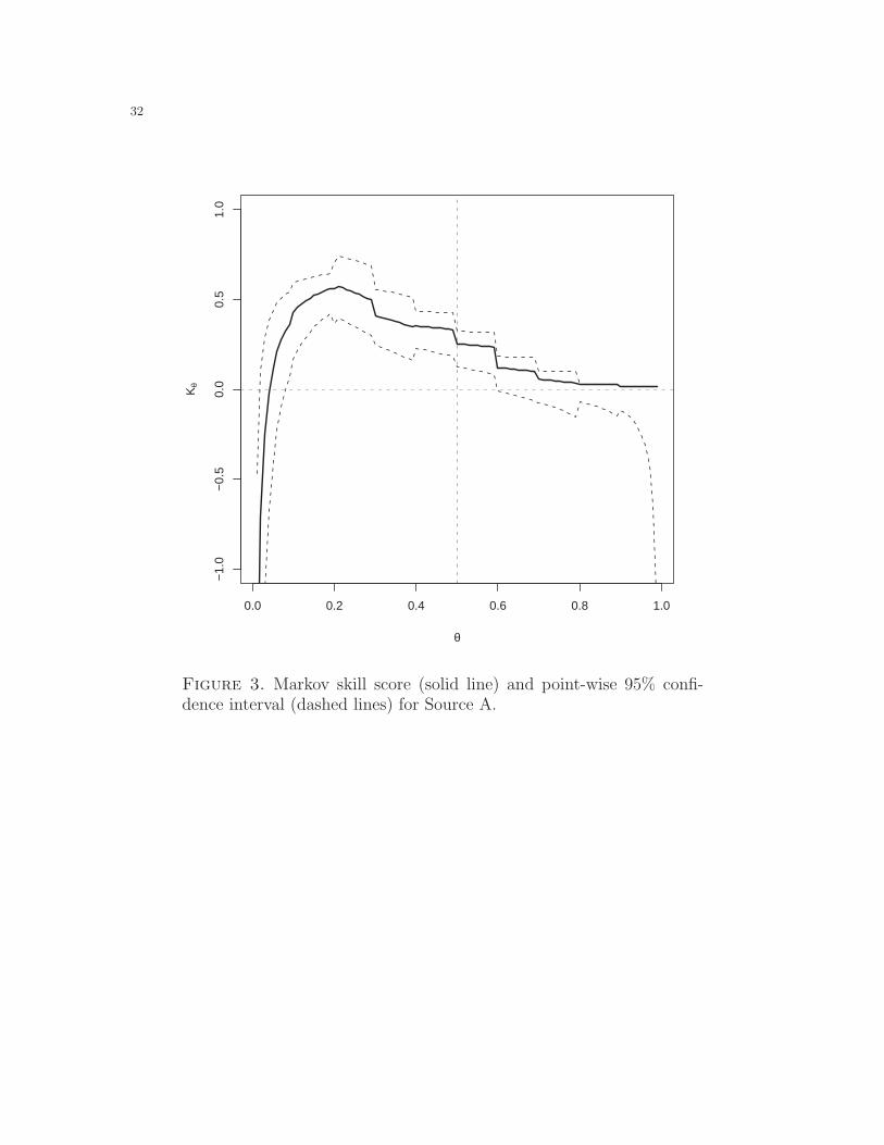
Figure 3 shows the skill plot for Source A along with the 95% point-wise confidence

bound, created by inverting the likelihood ratio test statistic G. This confidence

interval plot “builds in” the test at the various values of θ.

5. Conclusion

We have shown how to extend the basic skill testing framework developed in BR

to events that are Markov. We have also shown how (modifications to) McNemar’s

test can be used to test for persistence skill, or to compare competing forecasts for

the same event.

The climate skill test, while useful, is not entirely satisfactory because it does not

take into account the dependent nature of the observations when it exists. The test

developed above does use the Markov nature of the observations. We also created a

skill score to give a point measure of skill, which we showed reduced to the score given

in BR. So we also showed how the score was a weighted sum of two parts, a skill score

where the previous observation equalled zero, and a skill score where the previous ob-

servation equalled one. The weights were only functions of the observed observations

series (not on the forecasts), that is, they were independent of the forecast process.

18

We have also shown that persistence forecasts should never be used, and that the

optimal naive Markov (in the usual dependance or independence case) forecast is

always better.

Scores, like those developed above, will be more useful when they can be applied

to field forecasts. An example of such a forecast is a map of PoP forecasts. The

skill score can, of course, be calculated for each point on a field and contours can be

drawn to gauge performance (Drosdowsky and Zhang, 2003). But naively drawing

skill maps won’t take into account the dependent nature of observations and forecasts

across space. New models are needed.

Appendix A. Markov Details

There are four cases to capture all the possibilities when {Yi} is Markov. These cor-

respond to the probabilities pij which, depending on their values, represent different

optimal naive Markov forecasts.

We developed Case 4 earlier. These four cases imply four separate null hypotheses.

These are

Case (1): H0,1 : (p0|01 ≤ 1− θ, p0|00 ≤ 1− θ)Case (2): H0,2 : (p0|01 ≤ 1− θ, p1|10 ≤ θ)Case (3): H0,3 : (p1|11 ≤ θ, p0|00 ≤ 1− θ)Case (4): H0,4 : (p1|11 ≤ θ, p1|10 ≤ θ).

Likelihood ratio statistics are found in the same manner as before. The results are:

Case (1)

G1M = 2n101 log

(p̂1|01

p̃1|01

)+ 2n001 log

(1− p̂1|01

1− p̃1|01

)+

2n100 log

(p̂1|00

p̃1|00

)+ 2n000 log

(1− p̂1|00

1− p̃1|00

).

19

Case (2)

G2M = 2n101 log

(p̂1|01

p̃1|01

)+ 2n001 log

(1− p̂1|01

1− p̃1|01

)+

2n110 log

(p̂1|10

p̃1|10

)+ 2n010 log

(1− p̂1|10

1− p̃1|10

).

Case (3)

G3M = 2n111 log

(p̂1|11

p̃1|11

)+ 2n011 log

(1− p̂1|11

1− p̃1|11

)+

2n100 log

(p̂1|00

p̃1|00

)+ 2n000 log

(1− p̂1|00

1− p̃1|00

).

Case (4)

G4M = 2n111 log

(p̂1|11

p̃1|11

)+ 2n011 log

(1− p̂1|11

1− p̃1|11

)+

2n110 log

(p̂1|10

p̃1|10

)+ 2n010 log

(1− p̂1|10

1− p̃1|10

).

A slightly different notation will be needed to keep track of the different skill scores

for the different cases. Let Kij,θ be the climate skill score for optimal naive climate

forecast i when the day before Y−1 = j. For example, in Case 4, the climate skill

score estimate is now

K̂4,θ =p̂1+|1p̂

p̂y

K̂01,θ +p̂1+|0(1− p̂)

p̂y

K̂00,θ,

where K̂01,θ is the climate skill score for those days in which Y−1 = 1 and the optimal

naive forecast is 0, and K̂00,θ is the climate skill score for those days in which Y−1 = 0

and the optimal naive forecast is 0. To be complete,

K̂0j,θ =n11j(1− θ)− n01jθ

(n11j + n10j)(1− θ),

and

K̂1j,θ =n00jθ − n10j(1− θ)

(n00j + n01j)θ.

Skill scores are slightly more complicated, except in Case 1 and Case 4 (which was

derived earlier). Case 1 is similar to Case 4 because no matter the value of Yi−1 the

20

optimal naive forecast is always 1 in Case 4 the optimal naive forecast is always 0).

Because of this, the skill score for Case 1 is easy:

K̂1,θ =p̂0+|1p̂1− p̂y

K̂11,θ +p̂0+|0(1− p̂)

1− p̂y

K̂10,θ,

Cases 2 and 3 are more difficult, but related. Focus on Case 3, where the optimal

naive forecast on day i is 0 on those days when Yi−1 = 1 and is 1 on those days when

Yi−1 = 0. The expected loss for the optimal naive forecasts is

p(1− θ)(p1|11p+1|1 + p1|01(1− p+1|1))+ (1− p)θ((1− p1|10)p+1|0 +(1− p1|00)(1− p+1|0)).

Substituting the estimates of these parameters gives

D = (1/n)((1− θ)(n111 + n101) + θ(n010 + n000)).

The expected loss of the optimal naive forecast minus the expected loss of the expert

forecasts is

pp+1|1(p1|11 − θ) + (1− p)(1− p+1|0)(θ − p1|00).

After substituting the expected values we get

(1/n)(n111(1− θ)− n011θ + n000θ − n100(1− θ)).

We now arrive the estimate for K3,θ

K̂3,θ =(n111 + n101)(1− θ)

(n111 + n101)(1− θ)

n111(1− θ)− n011θ

D+

(n111 + n101)(1− θ)

(n111 + n101)(1− θ)

n000θ − n100(1− θ)

D

=(n111 + n101)(1− θ)

DK̂11,θ +

(n111 + n101)(1− θ)

DK̂10,θ.

Now,

(n111 + n101)(1− θ)

D=

n111 + n011 + n101 + n001

n111 + n011 + n101 + n001

(n111 + n101)(1− θ)

D

= (1− θ)p1+|1n111 + n011 + n101 + n001

D.

21

Further,

D

n111 + n011 + n101 + n001

=(1− θ)(n111 + n101)

n111 + n011 + n101 + n001

+

(1− θ)(n010 + n000)

n111 + n011 + n101 + n001

= (1− θ)p̂1+|1 + θp̂0+|01− p̂

p̂.

So,

(n111 + n101)(1− θ)

D=

(1− θ)p1+|1(1− θ)p̂1+|1 + θp̂0+|0

1−bpbp .

This can also be written

(n111 + n101)(1− θ)

D=

(1− θ)P̂ (Yi = Yi−1 = 1)

(1− θ)P̂ (Yi = Yi−1 = 1) + θP̂ (Yi = Yi−1 = 0).

Similarly,

(n111 + n101)(1− θ)

D=

θp0+|0θp̂0+|0 + (1− θ)p̂1+|1

bp1−bp .

Which is also

(n111 + n101)(1− θ)

D=

θP̂ (Yi = Yi−1 = 0)

θP̂ (Yi = Yi−1 = 0) + (1− θ)P̂ (Yi = Yi−1 = 1).

This finally gives

K̂3,θ =(1− θ)p1+|1

(1− θ)p̂1+|1 + θp̂0+|01−bpbp K̂01,θ +

θp0+|0θp̂0+|0 + (1− θ)p̂1+|1

bp1−bp K̂10,θ.

A similar argument leads to the estimate of K2,θ

K̂2,θ =θp0+|1

θp̂0+|1 + (1− θ)p̂1+|0bp

1−bp K̂11,θ +(1− θ)p1+|0

(1− θ)p̂1+|0 + θp̂0+|1bp

1−bp K̂00,θ.

22

References

1. Agresti, 1990. Categorical Data Analysis, Wiley, New York, 558pp.

2. Briggs, W.M., 2005. A general method of incorporating forecast cost and loss in value scores

Monthly Weather Review. In review.

3. Briggs, W.M., and R.A. Levine, 1998. Comparison of forecasts using the bootstrap. 14th Conf.

on Probability and Statistics in the Atmospheric Sciences, Phoenix, AZ, Amer. Meteor. Soc.,

1–4.

4. Briggs, W.M., M. Pocernich, and D. Ruppert, 2005. Incorporating misclassification error in

skill assessment. Monthly Weather Review. In review.

5. Briggs, W.M., and D. Ruppert, 2005. Assessing the skill of yes/no predictions. Biometrics. In

press.

6. Brooks, H. E., A. Witt, and M. D. Eilts, 1997. Verification of public weather forecasts available

via the media. Bull. Amer. Meteor. Soc., 77, 2167–2177.

7. Drosdowsky, W., and H. Zhang, 2003. Verification of spatial fields. In Forecast Verification,

Jolliffe, I.T., and D.B. Stephenson, eds. Wiley, New York, 121–136.

8. Livezey, R.E., 2003. Categorical events. In Forecast Verification, Jolliffe, I.T., and D.B. Stephen-

son, eds. Wiley, New York, 77–96.

9. Mason, I.B., 2003. Binary events. In Forecast Verification, Jolliffe, I.T., and D.B. Stephenson,

eds. Wiley, New York, 37–76.

10. McNemar, I., 1947. Note on the sampling error of the difference between correlated proportions

or percentages, Psychometrika, 12, 153–157.

11. Meeden, G., 1979. Comparing two probability appraisers. JASA, 74, 299–302.

12. Mosteller, F, 1952. Some statistical problems in measuring the subjective response to drugs.

Biometrics, 220–226.

23

13. Mozer, J.B., and Briggs, W.M., 2003. Skill in real-time solar wind shock forecasts. J. Geophys-

ical Research: Space Physics, 108 (A6), SSH 9 p. 1–9, (DOI 10.1029/2003JA009827).

14. Murphy, A.H., 1991. Forecast verification: its complexity and dimensionality. Monthly Weather

Review, 119, 1590–1601.

15. Murphy, A.H., 1997. Forecast verification. In Economic Value of Weather and Climate Fore-

casts. Katz, R.W., and A.H. Murphy (eds.). Cambridge, London, 19–74.

16. Murphy, A.H., and A. Ehrendorfer, 1987. One the relationship between the accuracy and value

of forecasts in the cost-loss ratio situation. Weather and Forecasting, 2, 243–251.

17. Murphy, A.H., and R. L. Winkler, 1987. A general framework for forecast verification. Monthly

Weather Review, 115, 1330–1338.

18. Richardson, D.S., 2000. Skill and relative economic value of the ECMWF ensemble prediction

system. Q.J.R. Meteorol. Soc., 126, 649-667.

19. Richardson, D.S., 2001. Measures of skill and value of ensemble prediction systems, their in-

terrelationship and the effect of ensemble size. Q.J.R. Meteorol. Soc., 127, 2473-2489.

20. Schervish, M.J., 1989. A general method for comparing probability assessors. Annals of Statis-

tics, 17, 1856–1879.

21. Self, S.G., and K.Y. Liang, 1987. Asymptotic properties of maximum likelihood estimators and

likelihood ratio tests under nonstandard conditions. J. American Statistical Association, 82,

605–610.

22. Wilks, D.S., 1991. Representing serial correlation of meteorological events and forecasts in

dynamic decision-analytic models. Monthly Weather Review, 119, 1640–1662.

23. Wilks, D.S., 1995. Statistical Methods in the Atmospheric Sciences, Academic Press, New York.

467 pp.

24. Wilks, D.S., 2001. A skill score based on economic value for probability forecasts. Meteorological

Applications, 8, 209–219.

24

List of Tables

Table 1 The four cases of optimal naive Markov forecasts. Notice that in Case

2 the optimal naive Markov and persistence forecast are identical. Case 1, when the

optimal naive Markov forecast is always 0, is the one used for examples in the main

text.

Table 2 Skill statistics for Source A (SA) and Source B (SB). See the text for an

explanation of the results.

Table 3 Skill score weightings for the Brooks et al. data.

Table 4 The four separate cases where different optimal naive forecasts are im-

plied. The conditions are set in the Prob. columns, with the optimal naive forecasts

listed.

25

List of Figures

Figure 1 Climate skill score range plot for Accuweather’s 1- and 14-day ahead

and the NWS’s 1-day forecasts. The dashed horizontal line shows 0 and predictions

below this line have no skill.

Figure 2 Skill score range plot for Accuweather’s and NWS’s 1-day ahead fore-

casts, split into days when Yi−1 = 1 and for Yi−1 = 0. The dashed horizontal line

shows 0 and predictions below this line have no skill.

Figure 3 Skill score (solid line) and point-wise 95% confidence interval (dashed

lines) for Source A.

26

Table 1. The four cases of optimal naive Markov forecasts. Noticethat in Case 2 the optimal naive Markov and persistence forecast areidentical. Case 1, when the optimal naive Markov forecast is always 0,is the one used for examples in the main text.

Case I{P (Yi = 1|Yi−1) > θ}Yi−1 = 0 Yi−1 = 0

1 0 02 0 13 1 04 1 1

.

27

Table 2. Skill statistics for Source A (SA) and Source B (SB). Seethe text for an explanation of the results.

Statistic SA SB

K̂1/2 0.254 0.209G (p) 14.1 (0.001) 6.34 (0.006)

K̂1,1/2 0.333 0.111

K̂0,1/2 0.225 0.245GM (p) 16.04 (0.0002) 8.04 (0.009)Gc (p) 30.8 (< 0.0001) 27.98 (< 0.0001)

.

28

Table 3. Skill score weightings for the Brooks et al. data.

Yi−1 = 0 Yi−1 = 10.73 0.27

.

29

Table 4. The four separate cases where different optimal naive fore-casts are implied. The conditions are set in the Prob. columns, withthe optimal naive forecasts listed.

Case Prob. Optimal Naive Prob. Optimal Naive1 p0+|1 ≤ 1− θ 1 p0+|0 ≤ 1− θ 12 p0+|1 ≤ 1− θ 1 p1+|0 ≤ θ 03 p1+|1 ≤ θ 0 p0+|0 ≤ 1− θ 14 p1+|1 ≤ θ 0 p1+|1 ≤ θ 0

.

30

0.0 0.2 0.4 0.6 0.8 1.0

−1.

0−

0.5

0.0

0.5

1.0

θ

Kθ

Accuweather 1−dayAccuweather 14−dayNWS 1−day

Figure 1. Climate skill score range plot for Accuweather’s 1- and 14-day ahead and the NWS’s 1-day forecasts. The dashed horizontal lineshows 0 and predictions below this line have no skill.

31

0.0 0.2 0.4 0.6 0.8 1.0

−1.

0−

0.5

0.0

0.5

1.0

θ

Kθ

Accuweather DryAccuweather WetNWS DryNWS Wet

Figure 2. Climate skill score range plot for Accuweather’s and NWS’s1-day ahead forecasts, split into days when Yi−1 = 1 and for Yi−1 = 0.The dashed horizontal line shows 0 and predictions below this line haveno skill.

32

0.0 0.2 0.4 0.6 0.8 1.0

−1.

0−

0.5

0.0

0.5

1.0

θ

Kθ

Figure 3. Markov skill score (solid line) and point-wise 95% confi-dence interval (dashed lines) for Source A.