Embed Size (px)
Citation preview
Assessing Uncertain Benefits: a Valuation Approach
for Strategic Changeability (VASC)
Matthew Fitzgerald, Adam M. Ross, and Donna H. Rhodes
INCOSE 2012, Rome, Italy
11 July 2012

Motivation
Optimization is weak to uncertainty…
Complex DoD systems tend to be designed to deliver optimal performance within a narrow set of initial
requirements and operating conditions at the time of design. This usually results in the delivery of point-
solution systems that fail to meet emergent requirements throughout their lifecycles, that cannot easily adapt to new threats, that too rapidly become technologically obsolete,
or that cannot provide quick responses to changes in mission and operating conditions.
“ ”
- Office of the Secretary of Defense (RT-18 Task Description)
Exploring robustness and changeability is of critical importance for complex systems
seari.mit.edu © 2012 Massachusetts Institute of Technology 2
Evolution to Current State
Mismatch of Design with Context 1960’s Paradigm
“Our spacecraft, which take 5 to 10 years to build, and then last up to 20 in a static hardware condition, will be configured to solve tomorrow’s problems using yesterday’s technologies.” (Dr. Owen Brown, DARPA Program Manager, 2007)
13+ year design lives (geosynchronous orbit)
• CORONA: 30-45 day missions • 144 spacecraft launched
between 1959-1972 • Inability to adapt to uncertain future
environments, including disturbances (Wheelon 1997)
(Sullivan 2005)
Year
Des
ign
Life
(yea
rs)
seari.mit.edu © 2012 Massachusetts Institute of Technology 3

More than Missed Opportunities: Failures from Context Changes
Source: Wired Magazine, August 2010
Changing contexts can have high consequences if systems fail…
Adversary timescale shorter than “system” lifecycle
Contexts change…
New competitor/technology changes needs before system completed
Changing contexts can lead a technically sound system to fail
seari.mit.edu © 2012 Massachusetts Institute of Technology 4
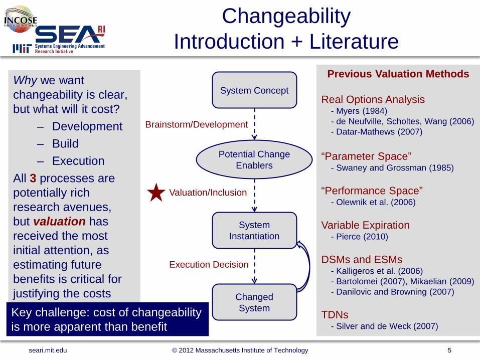
Changeability Introduction + Literature
Why we want changeability is clear, but what will it cost?
– Development – Build – Execution
All 3 processes are potentially rich research avenues, but valuation has received the most initial attention, as estimating future benefits is critical for justifying the costs
Potential Change Enablers
System Concept
System Instantiation
Changed System
Brainstorm/Development
Valuation/Inclusion
Execution Decision
Previous Valuation Methods
Real Options Analysis - Myers (1984) - de Neufville, Scholtes, Wang (2006) - Datar-Mathews (2007) “Parameter Space” - Swaney and Grossman (1985) “Performance Space” - Olewnik et al. (2006) Variable Expiration - Pierce (2010) DSMs and ESMs - Kalligeros et al. (2006) - Bartolomei (2007), Mikaelian (2009) - Danilovic and Browning (2007) TDNs - Silver and de Weck (2007)
seari.mit.edu © 2012 Massachusetts Institute of Technology 5
Key challenge: cost of changeability is more apparent than benefit
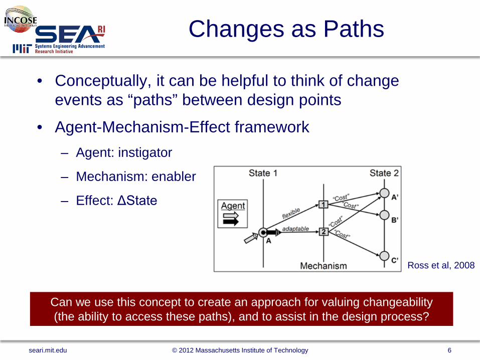
Changes as Paths
• Conceptually, it can be helpful to think of change events as “paths” between design points
• Agent-Mechanism-Effect framework – Agent: instigator
– Mechanism: enabler
– Effect: ΔState
Ross et al, 2008
Can we use this concept to create an approach for valuing changeability (the ability to access these paths), and to assist in the design process?
seari.mit.edu © 2012 Massachusetts Institute of Technology 6
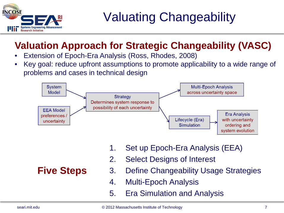
Valuating Changeability
1. Set up Epoch-Era Analysis (EEA) 2. Select Designs of Interest 3. Define Changeability Usage Strategies 4. Multi-Epoch Analysis 5. Era Simulation and Analysis
Five Steps
Valuation Approach for Strategic Changeability (VASC) • Extension of Epoch-Era Analysis (Ross, Rhodes, 2008) • Key goal: reduce upfront assumptions to promote applicability to a wide range of
problems and cases in technical design
seari.mit.edu © 2012 Massachusetts Institute of Technology 7
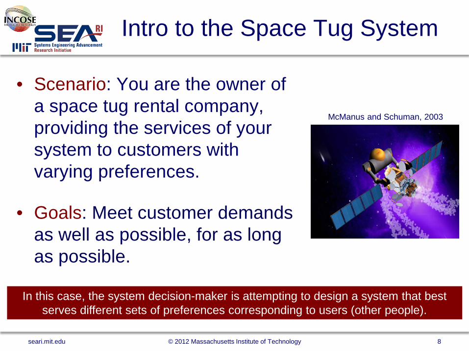
Intro to the Space Tug System
• Scenario: You are the owner of a space tug rental company, providing the services of your system to customers with varying preferences.
• Goals: Meet customer demands as well as possible, for as long as possible.
In this case, the system decision-maker is attempting to design a system that best serves different sets of preferences corresponding to users (other people).
McManus and Schuman, 2003
seari.mit.edu © 2012 Massachusetts Institute of Technology 8
Illustrating Changeability: Space Tug
• This problem is simple from a physics perspective, but nontrivial – Wide potential design space – Uncertainty in technology development – Uncertainty in user preferences
• It appears unlikely that a single design will prove to be optimal or near-optimal across the entire range of uncertainty
Can we utilize changeability to actively improve system value in the face of this uncertain future?
seari.mit.edu © 2012 Massachusetts Institute of Technology 9

Space Tug – Design Space
Of particular interest: DFC level – Discrete, ordinal variable representing effort to design for ease of redesign/change – Varies from 012; higher is more reward, more penalty – Reward: additional and/or cheaper change mechanisms – Penalty: additional dry mass (higher costs + lower ΔV)
# Description Effect DFC level 1 Engine Swap Bipropcryo 0 2 Fuel Tank Swap Change propellant mass 0 3 Engine Swap (reduced cost) Bipropcryo 1 or 2 4 Fuel Tank Swap (reduced cost) Change propellant mass 1 or 2 5 Change capability Change capability 1 or 2 6 Refuel in orbit Change propellant mass
(no redesign) 2
Change Mechanisms
The costs of changeability are much more easily
quantified than its benefits: we must value the benefits in
order to justify inclusion.
(Fricke and Schulz, 2005)
seari.mit.edu © 2012 Massachusetts Institute of Technology 10
4 design variables 384 designs – Prop type (biprop, cryo, electric, nuclear) – Fuel mass – Capability level – Design For Changeability (DFC) level
Step 1 – Set up Epoch-Era Analysis (EEA)
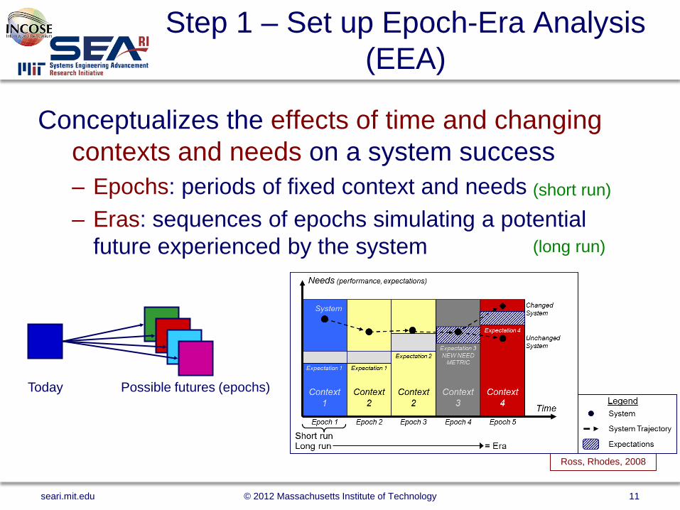
Conceptualizes the effects of time and changing contexts and needs on a system success – Epochs: periods of fixed context and needs – Eras: sequences of epochs simulating a potential
future experienced by the system
Ross, Rhodes, 2008
(short run)
(long run)
seari.mit.edu © 2012 Massachusetts Institute of Technology 11
Today Possible futures (epochs)
(1) Space Tug Uncertainties
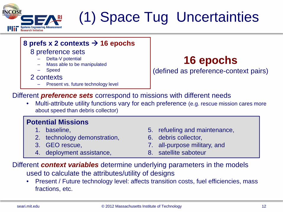
16 epochs (defined as preference-context pairs)
Different context variables determine underlying parameters in the models used to calculate the attributes/utility of designs • Present / Future technology level: affects transition costs, fuel efficiencies, mass
fractions, etc.
Different preference sets correspond to missions with different needs • Multi-attribute utility functions vary for each preference (e.g. rescue mission cares more
about speed than debris collector)
seari.mit.edu © 2012 Massachusetts Institute of Technology 12
8 prefs x 2 contexts 16 epochs 8 preference sets
– Delta-V potential – Mass able to be manipulated – Speed
2 contexts – Present vs. future technology level
1. baseline, 2. technology demonstration, 3. GEO rescue, 4. deployment assistance,
5. refueling and maintenance, 6. debris collector, 7. all-purpose military, and 8. satellite saboteur
Potential Missions

Step 2 – Select Designs of Interest
• Results of VASC are easier to understand when a smaller subset of designs is considered
• Utilize EEA metrics to screen for interesting designs up front – Normalized Pareto Trace (NPT): find designs that are Pareto
efficient in a large fraction of the epochs (passively robust). Also comes in a “fuzzy” variant (fNPT) to allow for uncertainty in modeling
– Filtered Outdegree (FOD): find designs with a large number of outgoing change paths below an acceptable cost threshold, heuristically “more changeable” leads to more valuable changeability
• Can also encompass expert opinion (favored designs of technical experts, senior decision makers, etc.)
seari.mit.edu © 2012 Massachusetts Institute of Technology 13
(2) Space Tug Interesting Designs
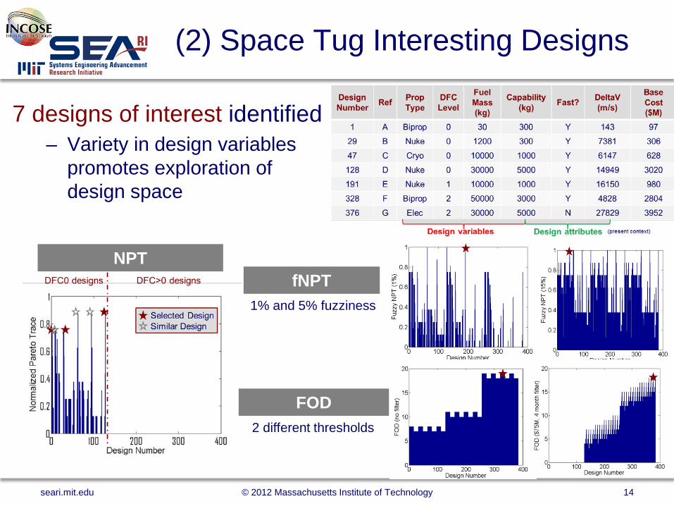
7 designs of interest identified – Variety in design variables
promotes exploration of design space
NPT fNPT
FOD
1% and 5% fuzziness
2 different thresholds
seari.mit.edu © 2012 Massachusetts Institute of Technology 14
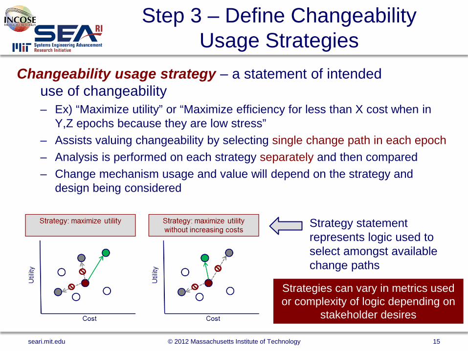
Step 3 – Define Changeability Usage Strategies
Changeability usage strategy – a statement of intended use of changeability – Ex) “Maximize utility” or “Maximize efficiency for less than X cost when in
Y,Z epochs because they are low stress” – Assists valuing changeability by selecting single change path in each epoch – Analysis is performed on each strategy separately and then compared – Change mechanism usage and value will depend on the strategy and
design being considered
Strategy statement represents logic used to select amongst available change paths
Strategies can vary in metrics used or complexity of logic depending on
stakeholder desires
seari.mit.edu © 2012 Massachusetts Institute of Technology 15
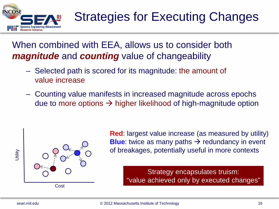
Strategies for Executing Changes
When combined with EEA, allows us to consider both magnitude and counting value of changeability
– Selected path is scored for its magnitude: the amount of value increase
– Counting value manifests in increased magnitude across epochs due to more options higher likelihood of high-magnitude option
Strategy encapsulates truism: “value achieved only by executed changes”
Util
ity
Cost
Red: largest value increase (as measured by utility) Blue: twice as many paths redundancy in event of breakages, potentially useful in more contexts
seari.mit.edu © 2012 Massachusetts Institute of Technology 16
(3) Space Tug Change Strategies
4 Strategies Identified • Maximize Utility
– A common first-order strategy (make system as good at its job as possible)
• Maximize Efficiency – Similar to above, but with a desire to be as cost efficient as
possible while fielding a good system • Survive
– Change is executed only if system is invalid (including running out of fuel)
• Maximize Profit (short-run) – You develop a revenue model based on utility, using design
changes to maximize revenues less costs in each epoch – Enabled by knowledge of epoch length: era-level strategy only
seari.mit.edu © 2012 Massachusetts Institute of Technology 17

Acronym Stands For Definition
NPT Normalized Pareto Trace % epochs for which design is Pareto efficient in utility/cost
fNPT Fuzzy Normalized Pareto Trace Above, with margin from Pareto front allowed
eNPT, efNPT Effective (fuzzy) Normalized Pareto Trace
Above, considering the design’s end state after transitioning
FPN Fuzzy Pareto Number % margin needed to include design in the fuzzy Pareto front
FPS Fuzzy Pareto Shift Difference in FPN before and after transition
Step 4 – Multi-Epoch Analysis
Multi-Epoch Analysis considers the performance effects of changes selected by strategies across the epoch space
• Computationally inexpensive: does not require simulation / sampling • Explored via a suite of metrics (shown here)
Conceptually: “how does this system perform, using changeability, when exposed to the full range of uncertainty?”
seari.mit.edu © 2012 Massachusetts Institute of Technology 18
Robustness via “no change”
Robustness via “change”
“Value” of a change
“Value” gap
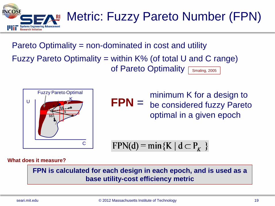
Metric: Fuzzy Pareto Number (FPN)
Pareto Optimality = non-dominated in cost and utility
U
C
Fuzzy Pareto OptimalK
$$
$$
ij
j
$$
within K% (of total U and C range) of Pareto Optimality
Fuzzy Pareto Optimality =
minimum K for a design to be considered fuzzy Pareto optimal in a given epoch
FPN =
Smaling, 2005
FPN is calculated for each design in each epoch, and is used as a base utility-cost efficiency metric
What does it measure?
seari.mit.edu © 2012 Massachusetts Institute of Technology 19
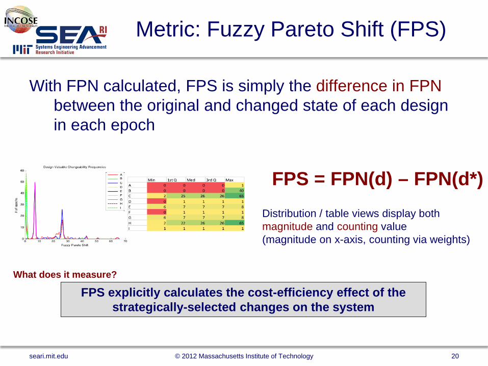
Metric: Fuzzy Pareto Shift (FPS)
With FPN calculated, FPS is simply the difference in FPN between the original and changed state of each design in each epoch
FPS = FPN(d) – FPN(d*)
FPS explicitly calculates the cost-efficiency effect of the strategically-selected changes on the system
Distribution / table views display both magnitude and counting value (magnitude on x-axis, counting via weights)
What does it measure?
seari.mit.edu © 2012 Massachusetts Institute of Technology 20
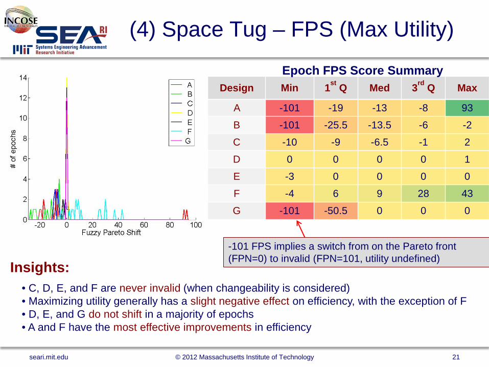
(4) Space Tug – FPS (Max Utility)
• C, D, E, and F are never invalid (when changeability is considered) • Maximizing utility generally has a slight negative effect on efficiency, with the exception of F • D, E, and G do not shift in a majority of epochs • A and F have the most effective improvements in efficiency
Design Min 1st Q Med 3rd Q Max
A -101 -19 -13 -8 93
B -101 -25.5 -13.5 -6 -2
C -10 -9 -6.5 -1 2
D 0 0 0 0 1
E -3 0 0 0 0
F -4 6 9 28 43
G -101 -50.5 0 0 0
Epoch FPS Score Summary
Insights: -101 FPS implies a switch from on the Pareto front (FPN=0) to invalid (FPN=101, utility undefined)
seari.mit.edu © 2012 Massachusetts Institute of Technology 21
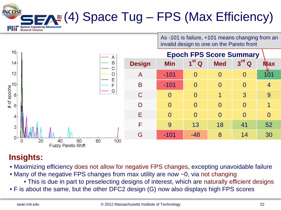
Design Min 1st Q Med 3rd Q Max
A -101 0 0 0 101 B -101 0 0 0 4 C 0 0 1 3 9 D 0 0 0 0 1 E 0 0 0 0 0 F 9 13 18 41 52 G -101 -48 8 14 30
(4) Space Tug – FPS (Max Efficiency) As -101 is failure, +101 means changing from an invalid design to one on the Pareto front
• Maximizing efficiency does not allow for negative FPS changes, excepting unavoidable failure • Many of the negative FPS changes from max utility are now ~0, via not changing
• This is due in part to preselecting designs of interest, which are naturally efficient designs • F is about the same, but the other DFC2 design (G) now also displays high FPS scores
Epoch FPS Score Summary
Insights:
seari.mit.edu © 2012 Massachusetts Institute of Technology 22
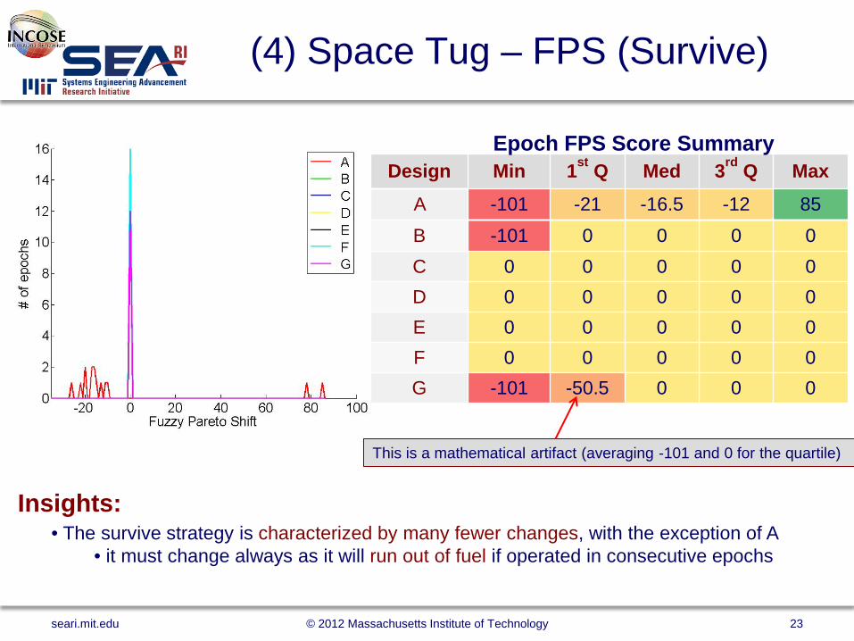
(4) Space Tug – FPS (Survive)
• The survive strategy is characterized by many fewer changes, with the exception of A • it must change always as it will run out of fuel if operated in consecutive epochs
This is a mathematical artifact (averaging -101 and 0 for the quartile)
Design Min 1st Q Med 3rd Q Max
A -101 -21 -16.5 -12 85 B -101 0 0 0 0 C 0 0 0 0 0 D 0 0 0 0 0 E 0 0 0 0 0 F 0 0 0 0 0 G -101 -50.5 0 0 0
Epoch FPS Score Summary
Insights:
seari.mit.edu © 2012 Massachusetts Institute of Technology 23
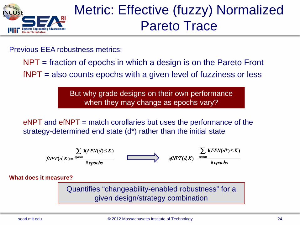
Metric: Effective (fuzzy) Normalized Pareto Trace
NPT = fraction of epochs in which a design is on the Pareto Front fNPT = also counts epochs with a given level of fuzziness or less
But why grade designs on their own performance when they may change as epochs vary?
eNPT and efNPT = match corollaries but uses the performance of the strategy-determined end state (d*) rather than the initial state
Previous EEA robustness metrics:
Quantifies “changeability-enabled robustness” for a given design/strategy combination
What does it measure?
seari.mit.edu © 2012 Massachusetts Institute of Technology 24
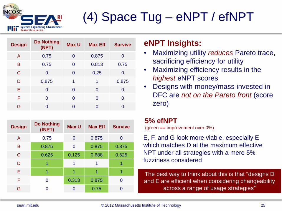
(4) Space Tug – eNPT / efNPT
Design Do Nothing (NPT) Max U Max Eff Survive
A 0.75 0 0.875 0
B 0.75 0 0.813 0.75
C 0 0 0.25 0
D 0.875 1 1 0.875
E 0 0 0 0
F 0 0 0 0
G 0 0 0 0
eNPT Insights: • Maximizing utility reduces Pareto trace,
sacrificing efficiency for utility • Maximizing efficiency results in the
highest eNPT scores • Designs with money/mass invested in
DFC are not on the Pareto front (score zero)
Design Do Nothing (fNPT) Max U Max Eff Survive
A 0.75 0 0.875 0
B 0.875 0 0.875 0.875
C 0.625 0.125 0.688 0.625
D 1 1 1 1
E 1 1 1 1
F 0 0.313 0.875 0
G 0 0 0.75 0
5% efNPT (green == improvement over 0%)
E, F, and G look more viable, especially E which matches D at the maximum effective NPT under all strategies with a mere 5% fuzziness considered
The best way to think about this is that “designs D and E are efficient when considering changeability
across a range of usage strategies”
seari.mit.edu © 2012 Massachusetts Institute of Technology 25
Step 5 – Era Simulation and Analysis
Era Analysis uncovers additional information, emergent only when considering time-ordered effects of uncertainty across the system’s lifetime
• Simulation of sample eras (constructed by sequencing epochs according to some model) allows collection of more data – Change mechanism usage – Cost/benefit “going rates” for adding/removing changeability – Lifetime cost/utility/revenue/efficiency statistics (not included here)
Conceptually: “how does this system perform, using changeability, when uncertainty evolves over time?”
seari.mit.edu © 2012 Massachusetts Institute of Technology 26
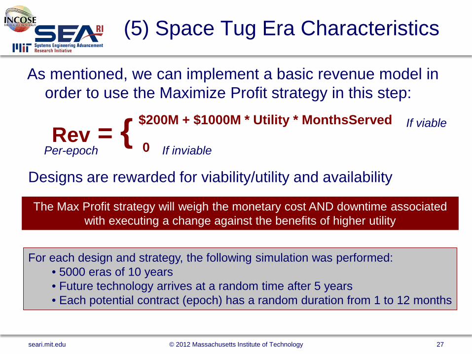
(5) Space Tug Era Characteristics
As mentioned, we can implement a basic revenue model in order to use the Maximize Profit strategy in this step:
$200M + $1000M * Utility * MonthsServed
Designs are rewarded for viability/utility and availability
Rev = { 0 If inviable
If viable
Per-epoch
The Max Profit strategy will weigh the monetary cost AND downtime associated with executing a change against the benefits of higher utility
For each design and strategy, the following simulation was performed: • 5000 eras of 10 years • Future technology arrives at a random time after 5 years • Each potential contract (epoch) has a random duration from 1 to 12 months
seari.mit.edu © 2012 Massachusetts Institute of Technology 27
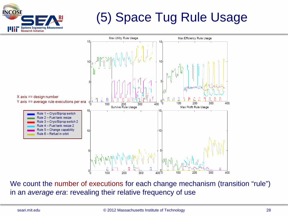
(5) Space Tug Rule Usage
We count the number of executions for each change mechanism (transition “rule”) in an average era: revealing their relative frequency of use
seari.mit.edu © 2012 Massachusetts Institute of Technology 28
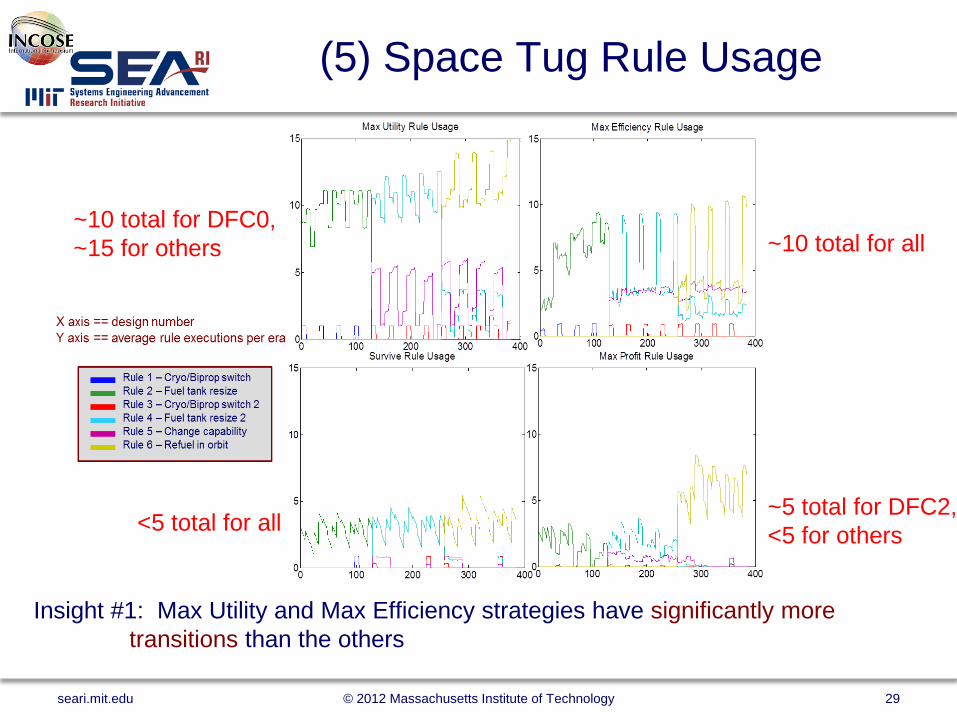
(5) Space Tug Rule Usage
Insight #1: Max Utility and Max Efficiency strategies have significantly more transitions than the others
~10 total for DFC0, ~15 for others
~5 total for DFC2, <5 for others <5 total for all
~10 total for all
seari.mit.edu © 2012 Massachusetts Institute of Technology 29
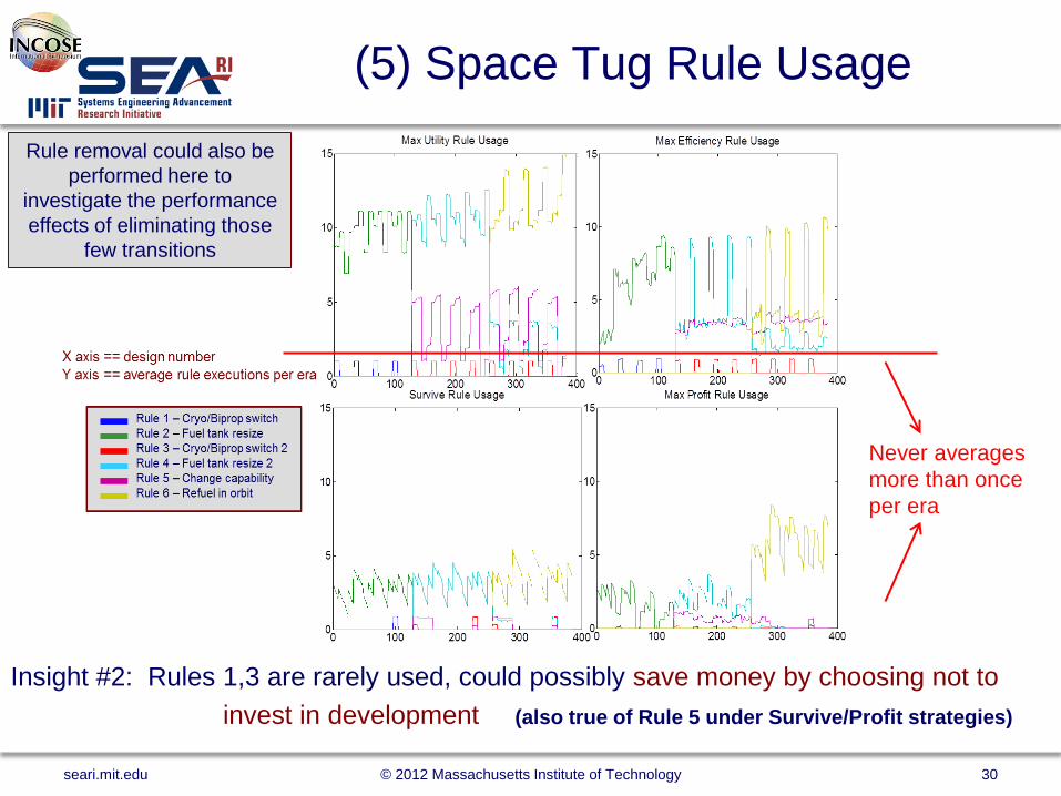
(5) Space Tug Rule Usage
Insight #2: Rules 1,3 are rarely used, could possibly save money by choosing not to invest in development
Never averages more than once per era
(also true of Rule 5 under Survive/Profit strategies)
Rule removal could also be performed here to
investigate the performance effects of eliminating those
few transitions
seari.mit.edu © 2012 Massachusetts Institute of Technology 30
(5) Space Tug Cost/Benefit
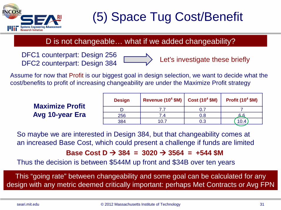
D is not changeable… what if we added changeability?
DFC1 counterpart: Design 256 DFC2 counterpart: Design 384 Let’s investigate these briefly
Assume for now that Profit is our biggest goal in design selection, we want to decide what the cost/benefits to profit of increasing changeability are under the Maximize Profit strategy
Design Revenue (104 $M) Cost (104 $M) Profit (104 $M)
D 7.7 0.7 7 256 7.4 0.8 6.6 384 10.7 0.3 10.4
Maximize Profit Avg 10-year Era
So maybe we are interested in Design 384, but that changeability comes at an increased Base Cost, which could present a challenge if funds are limited
Base Cost D 384 = 3020 3564 = +544 $M Thus the decision is between $544M up front and $34B over ten years
This “going rate” between changeability and some goal can be calculated for any design with any metric deemed critically important: perhaps Met Contracts or Avg FPN
seari.mit.edu © 2012 Massachusetts Institute of Technology 31
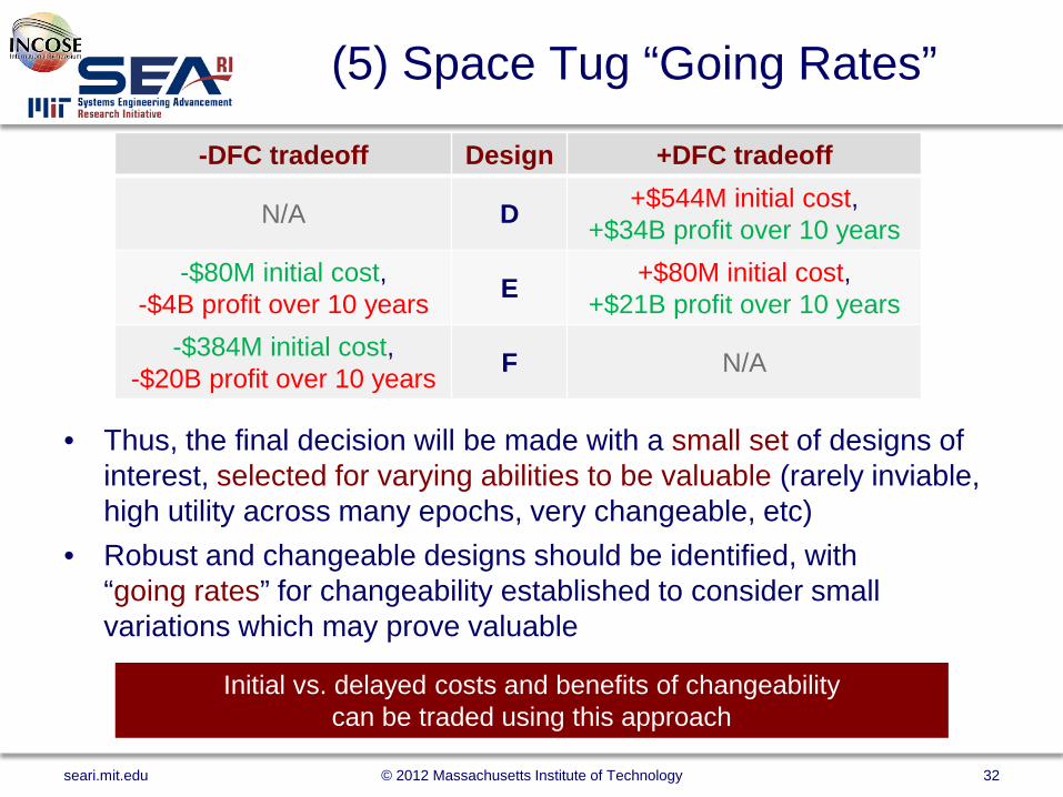
(5) Space Tug “Going Rates”
• Thus, the final decision will be made with a small set of designs of interest, selected for varying abilities to be valuable (rarely inviable, high utility across many epochs, very changeable, etc)
• Robust and changeable designs should be identified, with “going rates” for changeability established to consider small variations which may prove valuable
-DFC tradeoff Design +DFC tradeoff
N/A D +$544M initial cost, +$34B profit over 10 years
-$80M initial cost, -$4B profit over 10 years E +$80M initial cost,
+$21B profit over 10 years -$384M initial cost,
-$20B profit over 10 years F N/A
seari.mit.edu © 2012 Massachusetts Institute of Technology 32
Initial vs. delayed costs and benefits of changeability can be traded using this approach
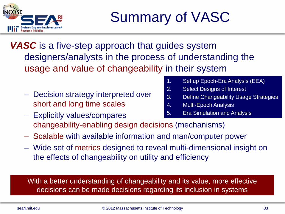
Summary of VASC
VASC is a five-step approach that guides system designers/analysts in the process of understanding the usage and value of changeability in their system
– Decision strategy interpreted over
short and long time scales – Explicitly values/compares
changeability-enabling design decisions (mechanisms) – Scalable with available information and man/computer power – Wide set of metrics designed to reveal multi-dimensional insight on
the effects of changeability on utility and efficiency
With a better understanding of changeability and its value, more effective decisions can be made decisions regarding its inclusion in systems
seari.mit.edu © 2012 Massachusetts Institute of Technology 33
1. Set up Epoch-Era Analysis (EEA) 2. Select Designs of Interest 3. Define Changeability Usage Strategies 4. Multi-Epoch Analysis 5. Era Simulation and Analysis
Thank You!
Questions?
seari.mit.edu © 2012 Massachusetts Institute of Technology 34
Backup Slides
• Contributions • Additional Metrics • Future work • Additional Era Analysis techniques (not
shown in paper)
seari.mit.edu © 2012 Massachusetts Institute of Technology 35
Development of Valuation Approach for Strategic Changeability
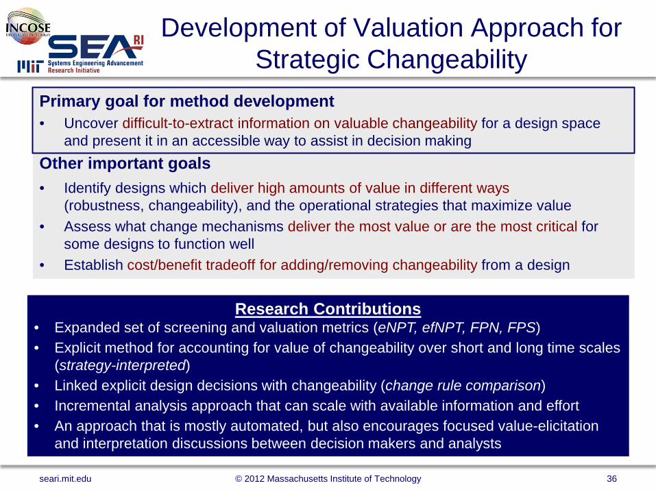
Primary goal for method development • Uncover difficult-to-extract information on valuable changeability for a design space
and present it in an accessible way to assist in decision making Other important goals
• Identify designs which deliver high amounts of value in different ways (robustness, changeability), and the operational strategies that maximize value
• Assess what change mechanisms deliver the most value or are the most critical for some designs to function well
• Establish cost/benefit tradeoff for adding/removing changeability from a design
Research Contributions • Expanded set of screening and valuation metrics (eNPT, efNPT, FPN, FPS) • Explicit method for accounting for value of changeability over short and long time scales
(strategy-interpreted) • Linked explicit design decisions with changeability (change rule comparison) • Incremental analysis approach that can scale with available information and effort • An approach that is mostly automated, but also encourages focused value-elicitation
and interpretation discussions between decision makers and analysts
seari.mit.edu © 2012 Massachusetts Institute of Technology 36
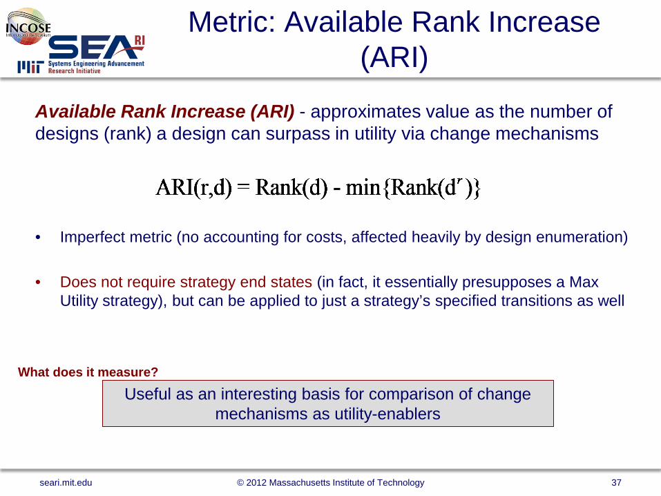
Metric: Available Rank Increase (ARI)
Available Rank Increase (ARI) - approximates value as the number of designs (rank) a design can surpass in utility via change mechanisms • Imperfect metric (no accounting for costs, affected heavily by design enumeration)
• Does not require strategy end states (in fact, it essentially presupposes a Max
Utility strategy), but can be applied to just a strategy’s specified transitions as well
Useful as an interesting basis for comparison of change mechanisms as utility-enablers
What does it measure?
seari.mit.edu © 2012 Massachusetts Institute of Technology 37
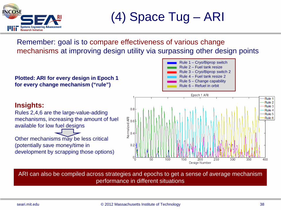
(4) Space Tug – ARI
Remember: goal is to compare effectiveness of various change mechanisms at improving design utility via surpassing other design points
ARI can also be compiled across strategies and epochs to get a sense of average mechanism performance in different situations
Plotted: ARI for every design in Epoch 1 for every change mechanism (“rule”) Insights: Rules 2,4,6 are the large-value-adding mechanisms, increasing the amount of fuel available for low fuel designs Other mechanisms may be less critical (potentially save money/time in development by scrapping those options)
Rule 1 – Cryo/Biprop switch Rule 2 – Fuel tank resize Rule 3 – Cryo/Biprop switch 2 Rule 4 – Fuel tank resize 2 Rule 5 – Change capability Rule 6 – Refuel in orbit
seari.mit.edu © 2012 Massachusetts Institute of Technology 38
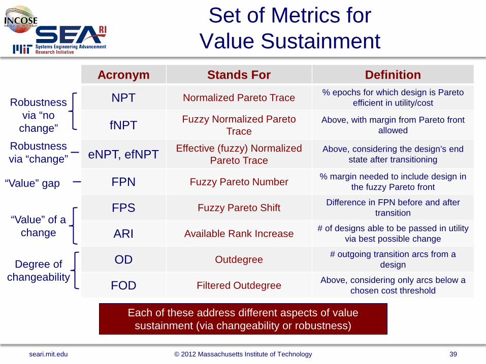
Set of Metrics for Value Sustainment
Acronym Stands For Definition
NPT Normalized Pareto Trace % epochs for which design is Pareto efficient in utility/cost
fNPT Fuzzy Normalized Pareto Trace
Above, with margin from Pareto front allowed
eNPT, efNPT Effective (fuzzy) Normalized Pareto Trace
Above, considering the design’s end state after transitioning
FPN Fuzzy Pareto Number % margin needed to include design in the fuzzy Pareto front
FPS Fuzzy Pareto Shift Difference in FPN before and after transition
ARI Available Rank Increase # of designs able to be passed in utility via best possible change
OD Outdegree # outgoing transition arcs from a design
FOD Filtered Outdegree Above, considering only arcs below a chosen cost threshold
Each of these address different aspects of value sustainment (via changeability or robustness)
Robustness via “no
change” Robustness via “change”
Degree of changeability
“Value” of a change
“Value” gap
seari.mit.edu © 2012 Massachusetts Institute of Technology 39
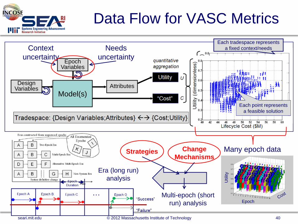
Data Flow for VASC Metrics
Each point represents a feasible solution
Epoch Variables
Design Variables Attributes
Model(s)
Each tradespace represents a fixed context/needs Context
uncertainty Needs
uncertainty
Many epoch data sets
Util
ity
EpochCost
Util
ity
EpochCost
Util
ity
EpochCost
Strategies
Era (long run) analysis
Multi-epoch (short run) analysis
Change Mechanisms
seari.mit.edu © 2012 Massachusetts Institute of Technology 40
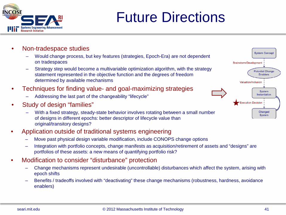
Future Directions
• Non-tradespace studies – Would change process, but key features (strategies, Epoch-Era) are not dependent
on tradespaces – Strategy step would become a multivariable optimization algorithm, with the strategy
statement represented in the objective function and the degrees of freedom determined by available mechanisms
• Techniques for finding value- and goal-maximizing strategies – Addressing the last part of the changeability “lifecycle”
• Study of design “families” – With a fixed strategy, steady-state behavior involves rotating between a small number
of designs in different epochs: better descriptor of lifecycle value than original/transitory designs?
• Application outside of traditional systems engineering – Move past physical design variable modification, include CONOPS change options – Integration with portfolio concepts, change manifests as acquisition/retirement of assets and “designs” are
portfolios of these assets: a new means of quantifying portfolio risk?
• Modification to consider “disturbance” protection – Change mechanisms represent undesirable (uncontrollable) disturbances which affect the system, arising with
epoch shifts – Benefits / tradeoffs involved with “deactivating” these change mechanisms (robustness, hardness, avoidance
enablers)
seari.mit.edu © 2012 Massachusetts Institute of Technology 41

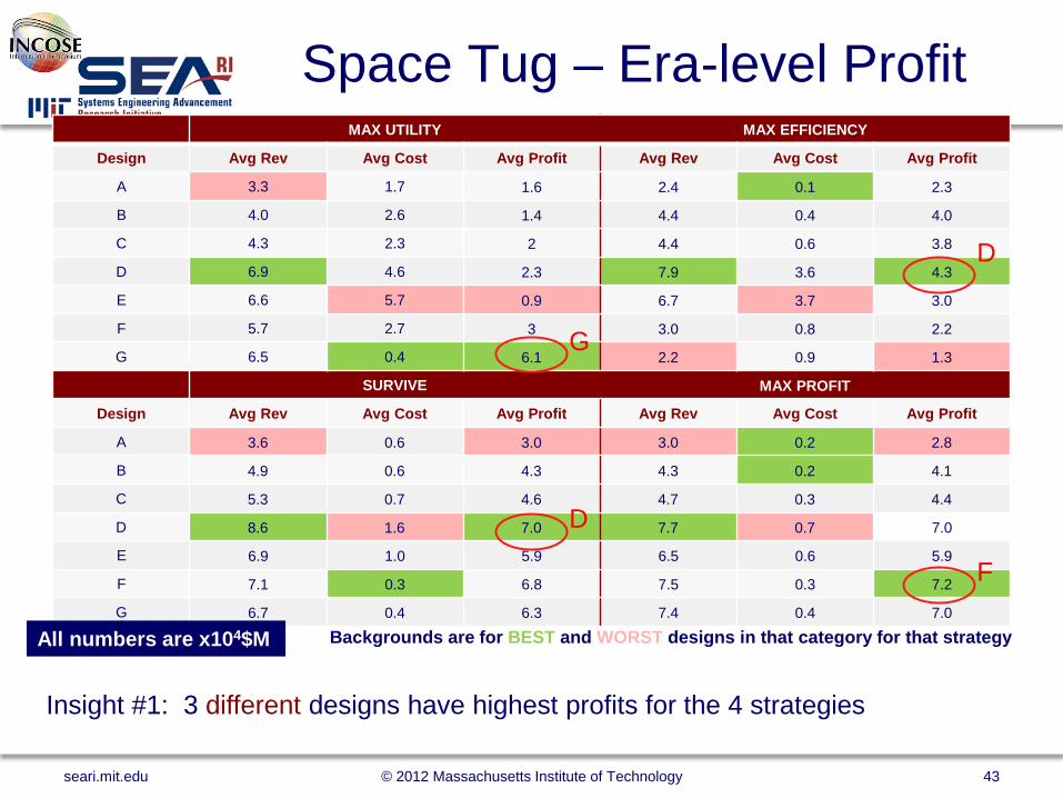
Space Tug – Era-level Profit MAX UTILITY MAX EFFICIENCY
Design Avg Rev Avg Cost Avg Profit Avg Rev Avg Cost Avg Profit
A 3.3 1.7 1.6 2.4 0.1 2.3
B 4.0 2.6 1.4 4.4 0.4 4.0
C 4.3 2.3 2 4.4 0.6 3.8
D 6.9 4.6 2.3 7.9 3.6 4.3
E 6.6 5.7 0.9 6.7 3.7 3.0
F 5.7 2.7 3 3.0 0.8 2.2
G 6.5 0.4 6.1 2.2 0.9 1.3
SURVIVE MAX PROFIT
Design Avg Rev Avg Cost Avg Profit Avg Rev Avg Cost Avg Profit
A 3.6 0.6 3.0 3.0 0.2 2.8
B 4.9 0.6 4.3 4.3 0.2 4.1
C 5.3 0.7 4.6 4.7 0.3 4.4
D 8.6 1.6 7.0 7.7 0.7 7.0
E 6.9 1.0 5.9 6.5 0.6 5.9
F 7.1 0.3 6.8 7.5 0.3 7.2
G 6.7 0.4 6.3 7.4 0.4 7.0
All numbers are x104$M Backgrounds are for BEST and WORST designs in that category for that strategy
seari.mit.edu © 2012 Massachusetts Institute of Technology 42
Space Tug – Era-level Profit MAX UTILITY MAX EFFICIENCY
Design Avg Rev Avg Cost Avg Profit Avg Rev Avg Cost Avg Profit
A 3.3 1.7 1.6 2.4 0.1 2.3
B 4.0 2.6 1.4 4.4 0.4 4.0
C 4.3 2.3 2 4.4 0.6 3.8
D 6.9 4.6 2.3 7.9 3.6 4.3
E 6.6 5.7 0.9 6.7 3.7 3.0
F 5.7 2.7 3 3.0 0.8 2.2
G 6.5 0.4 6.1 2.2 0.9 1.3
SURVIVE MAX PROFIT
Design Avg Rev Avg Cost Avg Profit Avg Rev Avg Cost Avg Profit
A 3.6 0.6 3.0 3.0 0.2 2.8
B 4.9 0.6 4.3 4.3 0.2 4.1
C 5.3 0.7 4.6 4.7 0.3 4.4
D 8.6 1.6 7.0 7.7 0.7 7.0
E 6.9 1.0 5.9 6.5 0.6 5.9
F 7.1 0.3 6.8 7.5 0.3 7.2
G 6.7 0.4 6.3 7.4 0.4 7.0
All numbers are x104$M Backgrounds are for BEST and WORST designs in that category for that strategy
Insight #1: 3 different designs have highest profits for the 4 strategies
G
F
D
D
seari.mit.edu © 2012 Massachusetts Institute of Technology 43
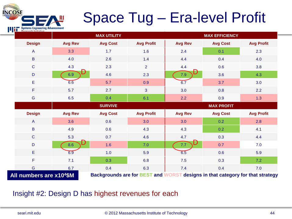
Space Tug – Era-level Profit MAX UTILITY MAX EFFICIENCY
Design Avg Rev Avg Cost Avg Profit Avg Rev Avg Cost Avg Profit
A 3.3 1.7 1.6 2.4 0.1 2.3
B 4.0 2.6 1.4 4.4 0.4 4.0
C 4.3 2.3 2 4.4 0.6 3.8
D 6.9 4.6 2.3 7.9 3.6 4.3
E 6.6 5.7 0.9 6.7 3.7 3.0
F 5.7 2.7 3 3.0 0.8 2.2
G 6.5 0.4 6.1 2.2 0.9 1.3
SURVIVE MAX PROFIT
Design Avg Rev Avg Cost Avg Profit Avg Rev Avg Cost Avg Profit
A 3.6 0.6 3.0 3.0 0.2 2.8
B 4.9 0.6 4.3 4.3 0.2 4.1
C 5.3 0.7 4.6 4.7 0.3 4.4
D 8.6 1.6 7.0 7.7 0.7 7.0
E 6.9 1.0 5.9 6.5 0.6 5.9
F 7.1 0.3 6.8 7.5 0.3 7.2
G 6.7 0.4 6.3 7.4 0.4 7.0
All numbers are x104$M Backgrounds are for BEST and WORST designs in that category for that strategy
Insight #2: Design D has highest revenues for each
D D
D D
seari.mit.edu © 2012 Massachusetts Institute of Technology 44
Space Tug – Era-level Profit MAX UTILITY MAX EFFICIENCY
Design Avg Rev Avg Cost Avg Profit Avg Rev Avg Cost Avg Profit
A 3.3 1.7 1.6 2.4 0.1 2.3
B 4.0 2.6 1.4 4.4 0.4 4.0
C 4.3 2.3 2 4.4 0.6 3.8
D 6.9 4.6 2.3 7.9 3.6 4.3
E 6.6 5.7 0.9 6.7 3.7 3.0
F 5.7 2.7 3 3.0 0.8 2.2
G 6.5 0.4 6.1 2.2 0.9 1.3
SURVIVE MAX PROFIT
Design Avg Rev Avg Cost Avg Profit Avg Rev Avg Cost Avg Profit
A 3.6 0.6 3.0 3.0 0.2 2.8
B 4.9 0.6 4.3 4.3 0.2 4.1
C 5.3 0.7 4.6 4.7 0.3 4.4
D 8.6 1.6 7.0 7.7 0.7 7.0
E 6.9 1.0 5.9 6.5 0.6 5.9
F 7.1 0.3 6.8 7.5 0.3 7.2
G 6.7 0.4 6.3 7.4 0.4 7.0
All numbers are x104$M Backgrounds are for BEST and WORST designs in that category for that strategy
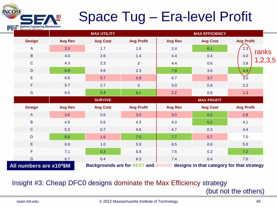
Insight #3: Cheap DFC0 designs dominate the Max Efficiency strategy (but not the others)
ranks 1,2,3,5
seari.mit.edu © 2012 Massachusetts Institute of Technology 45
Space Tug – Era-level Profit MAX UTILITY MAX EFFICIENCY
Design Avg Rev Avg Cost Avg Profit Avg Rev Avg Cost Avg Profit
A 3.3 1.7 1.6 2.4 0.1 2.3
B 4.0 2.6 1.4 4.4 0.4 4.0
C 4.3 2.3 2 4.4 0.6 3.8
D 6.9 4.6 2.3 7.9 3.6 4.3
E 6.6 5.7 0.9 6.7 3.7 3.0
F 5.7 2.7 3 3.0 0.8 2.2
G 6.5 0.4 6.1 2.2 0.9 1.3
SURVIVE MAX PROFIT
Design Avg Rev Avg Cost Avg Profit Avg Rev Avg Cost Avg Profit
A 3.6 0.6 3.0 3.0 0.2 2.8
B 4.9 0.6 4.3 4.3 0.2 4.1
C 5.3 0.7 4.6 4.7 0.3 4.4
D 8.6 1.6 7.0 7.7 0.7 7.0
E 6.9 1.0 5.9 6.5 0.6 5.9
F 7.1 0.3 6.8 7.5 0.3 7.2
G 6.7 0.4 6.3 7.4 0.4 7.0
All numbers are x104$M Backgrounds are for BEST and WORST designs in that category for that strategy
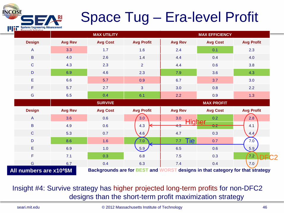
Insight #4: Survive strategy has higher projected long-term profits for non-DFC2 designs than the short-term profit maximization strategy
Higher
Tie
DFC2
seari.mit.edu © 2012 Massachusetts Institute of Technology 46
Space Tug – Era-level Profit MAX UTILITY MAX EFFICIENCY
Design Avg Rev Avg Cost Avg Profit Avg Rev Avg Cost Avg Profit
A 3.3 1.7 1.6 2.4 0.1 2.3
B 4.0 2.6 1.4 4.4 0.4 4.0
C 4.3 2.3 2 4.4 0.6 3.8
D 6.9 4.6 2.3 7.9 3.6 4.3
E 6.6 5.7 0.9 6.7 3.7 3.0
F 5.7 2.7 3 3.0 0.8 2.2
G 6.5 0.4 6.1 2.2 0.9 1.3
SURVIVE MAX PROFIT
Design Avg Rev Avg Cost Avg Profit Avg Rev Avg Cost Avg Profit
A 3.6 0.6 3.0 3.0 0.2 2.8
B 4.9 0.6 4.3 4.3 0.2 4.1
C 5.3 0.7 4.6 4.7 0.3 4.4
D 8.6 1.6 7.0 7.7 0.7 7.0
E 6.9 1.0 5.9 6.5 0.6 5.9
F 7.1 0.3 6.8 7.5 0.3 7.2
G 6.7 0.4 6.3 7.4 0.4 7.0
All numbers are x104$M Backgrounds are for BEST and WORST designs in that category for that strategy
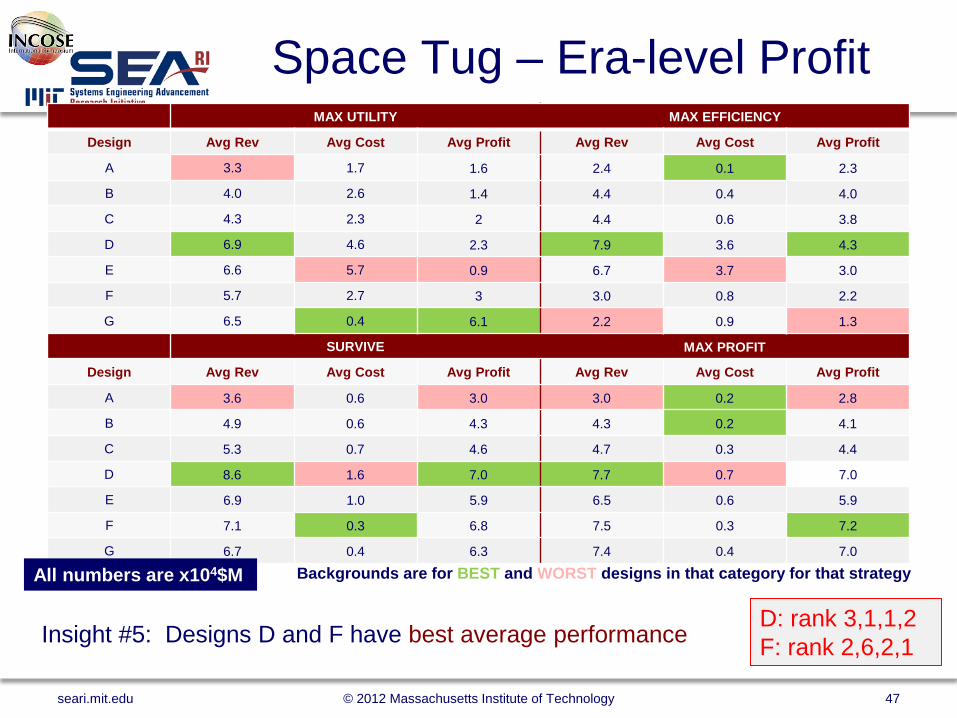
Insight #5: Designs D and F have best average performance
D: rank 3,1,1,2 F: rank 2,6,2,1
seari.mit.edu © 2012 Massachusetts Institute of Technology 47
Space Tug – Era-level Profit MAX UTILITY MAX EFFICIENCY
Design Avg Rev Avg Cost Avg Profit Avg Rev Avg Cost Avg Profit
A 3.3 1.7 1.6 2.4 0.1 2.3
B 4.0 2.6 1.4 4.4 0.4 4.0
C 4.3 2.3 2 4.4 0.6 3.8
D 6.9 4.6 2.3 7.9 3.6 4.3
E 6.6 5.7 0.9 6.7 3.7 3.0
F 5.7 2.7 3 3.0 0.8 2.2
G 6.5 0.4 6.1 2.2 0.9 1.3
SURVIVE MAX PROFIT
Design Avg Rev Avg Cost Avg Profit Avg Rev Avg Cost Avg Profit
A 3.6 0.6 3.0 3.0 0.2 2.8
B 4.9 0.6 4.3 4.3 0.2 4.1
C 5.3 0.7 4.6 4.7 0.3 4.4
D 8.6 1.6 7.0 7.7 0.7 7.0
E 6.9 1.0 5.9 6.5 0.6 5.9
F 7.1 0.3 6.8 7.5 0.3 7.2
G 6.7 0.4 6.3 7.4 0.4 7.0
All numbers are x104$M Backgrounds are for BEST and WORST designs in that category for that strategy
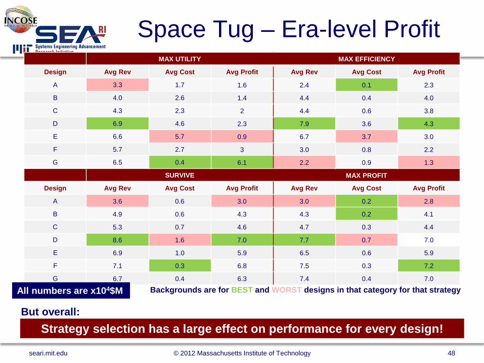
Strategy selection has a large effect on performance for every design! But overall:
seari.mit.edu © 2012 Massachusetts Institute of Technology 48
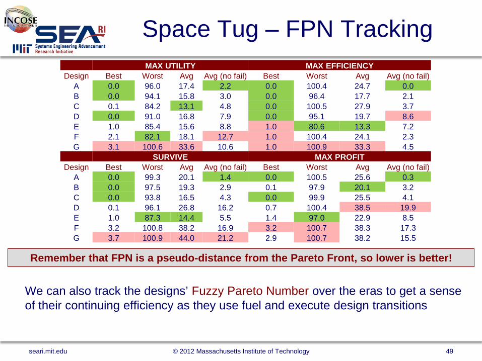
Space Tug – FPN Tracking
We can also track the designs’ Fuzzy Pareto Number over the eras to get a sense of their continuing efficiency as they use fuel and execute design transitions
MAX UTILITY MAX EFFICIENCY Design Best Worst Avg Avg (no fail) Best Worst Avg Avg (no fail)
A 0.0 96.0 17.4 2.2 0.0 100.4 24.7 0.0 B 0.0 94.1 15.8 3.0 0.0 96.4 17.7 2.1 C 0.1 84.2 13.1 4.8 0.0 100.5 27.9 3.7 D 0.0 91.0 16.8 7.9 0.0 95.1 19.7 8.6 E 1.0 85.4 15.6 8.8 1.0 80.6 13.3 7.2 F 2.1 82.1 18.1 12.7 1.0 100.4 24.1 2.3 G 3.1 100.6 33.6 10.6 1.0 100.9 33.3 4.5
SURVIVE MAX PROFIT Design Best Worst Avg Avg (no fail) Best Worst Avg Avg (no fail)
A 0.0 99.3 20.1 1.4 0.0 100.5 25.6 0.3 B 0.0 97.5 19.3 2.9 0.1 97.9 20.1 3.2 C 0.0 93.8 16.5 4.3 0.0 99.9 25.5 4.1 D 0.1 96.1 26.8 16.2 0.7 100.4 38.5 19.9 E 1.0 87.3 14.4 5.5 1.4 97.0 22.9 8.5 F 3.2 100.8 38.2 16.9 3.2 100.7 38.3 17.3 G 3.7 100.9 44.0 21.2 2.9 100.7 38.2 15.5
Remember that FPN is a pseudo-distance from the Pareto Front, so lower is better!
seari.mit.edu © 2012 Massachusetts Institute of Technology 49
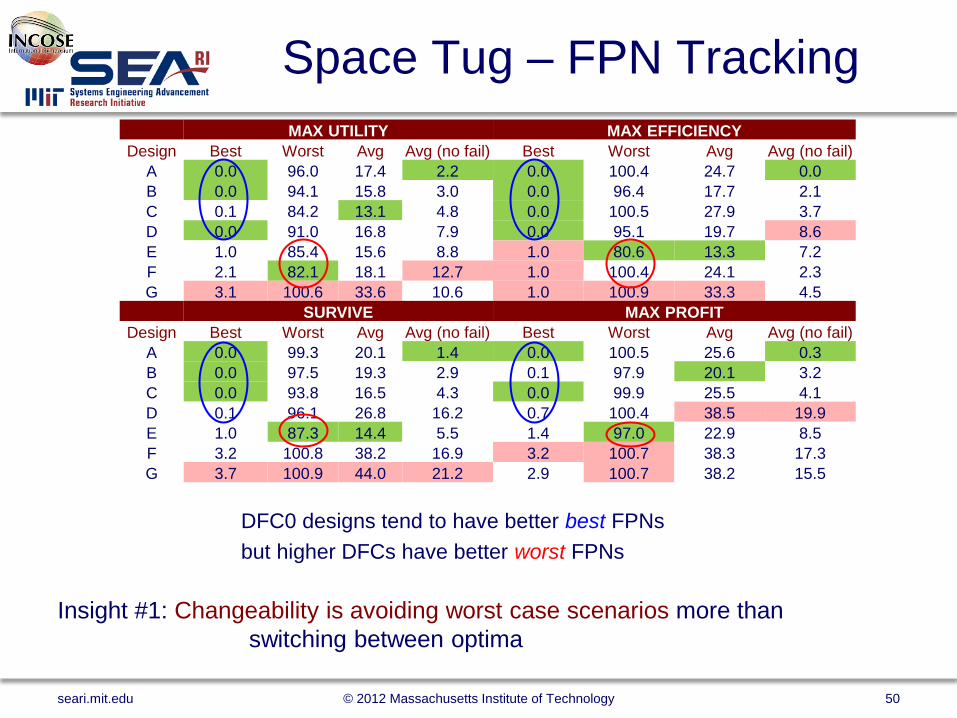
Space Tug – FPN Tracking
DFC0 designs tend to have better best FPNs but higher DFCs have better worst FPNs
MAX UTILITY MAX EFFICIENCY Design Best Worst Avg Avg (no fail) Best Worst Avg Avg (no fail)
A 0.0 96.0 17.4 2.2 0.0 100.4 24.7 0.0 B 0.0 94.1 15.8 3.0 0.0 96.4 17.7 2.1 C 0.1 84.2 13.1 4.8 0.0 100.5 27.9 3.7 D 0.0 91.0 16.8 7.9 0.0 95.1 19.7 8.6 E 1.0 85.4 15.6 8.8 1.0 80.6 13.3 7.2 F 2.1 82.1 18.1 12.7 1.0 100.4 24.1 2.3 G 3.1 100.6 33.6 10.6 1.0 100.9 33.3 4.5
SURVIVE MAX PROFIT Design Best Worst Avg Avg (no fail) Best Worst Avg Avg (no fail)
A 0.0 99.3 20.1 1.4 0.0 100.5 25.6 0.3 B 0.0 97.5 19.3 2.9 0.1 97.9 20.1 3.2 C 0.0 93.8 16.5 4.3 0.0 99.9 25.5 4.1 D 0.1 96.1 26.8 16.2 0.7 100.4 38.5 19.9 E 1.0 87.3 14.4 5.5 1.4 97.0 22.9 8.5 F 3.2 100.8 38.2 16.9 3.2 100.7 38.3 17.3 G 3.7 100.9 44.0 21.2 2.9 100.7 38.2 15.5
Insight #1: Changeability is avoiding worst case scenarios more than switching between optima
seari.mit.edu © 2012 Massachusetts Institute of Technology 50

Space Tug – FPN Tracking
Insight #2: Design A always has the best average when not considering inviable epochs, but is inviable too often to have the best overall average
MAX UTILITY MAX EFFICIENCY Design Best Worst Avg Avg (no fail) Best Worst Avg Avg (no fail)
A 0.0 96.0 17.4 2.2 0.0 100.4 24.7 0.0 B 0.0 94.1 15.8 3.0 0.0 96.4 17.7 2.1 C 0.1 84.2 13.1 4.8 0.0 100.5 27.9 3.7 D 0.0 91.0 16.8 7.9 0.0 95.1 19.7 8.6 E 1.0 85.4 15.6 8.8 1.0 80.6 13.3 7.2 F 2.1 82.1 18.1 12.7 1.0 100.4 24.1 2.3 G 3.1 100.6 33.6 10.6 1.0 100.9 33.3 4.5
SURVIVE MAX PROFIT Design Best Worst Avg Avg (no fail) Best Worst Avg Avg (no fail)
A 0.0 99.3 20.1 1.4 0.0 100.5 25.6 0.3 B 0.0 97.5 19.3 2.9 0.1 97.9 20.1 3.2 C 0.0 93.8 16.5 4.3 0.0 99.9 25.5 4.1 D 0.1 96.1 26.8 16.2 0.7 100.4 38.5 19.9 E 1.0 87.3 14.4 5.5 1.4 97.0 22.9 8.5 F 3.2 100.8 38.2 16.9 3.2 100.7 38.3 17.3 G 3.7 100.9 44.0 21.2 2.9 100.7 38.2 15.5
no-fail = A with-fail = not A
seari.mit.edu © 2012 Massachusetts Institute of Technology 51
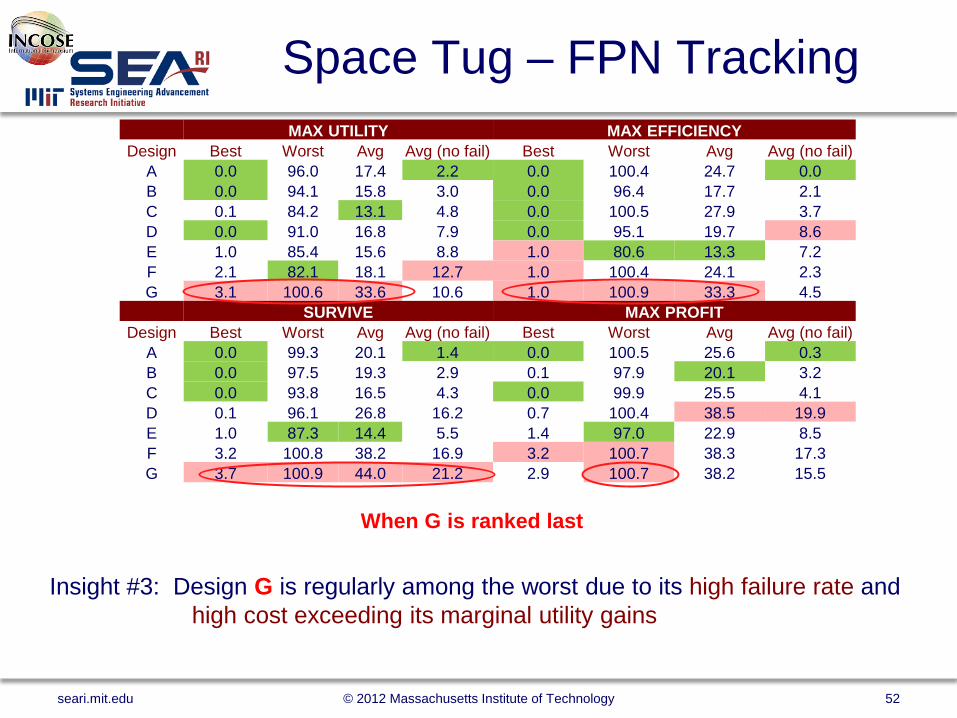
Space Tug – FPN Tracking
Insight #3: Design G is regularly among the worst due to its high failure rate and high cost exceeding its marginal utility gains
MAX UTILITY MAX EFFICIENCY Design Best Worst Avg Avg (no fail) Best Worst Avg Avg (no fail)
A 0.0 96.0 17.4 2.2 0.0 100.4 24.7 0.0 B 0.0 94.1 15.8 3.0 0.0 96.4 17.7 2.1 C 0.1 84.2 13.1 4.8 0.0 100.5 27.9 3.7 D 0.0 91.0 16.8 7.9 0.0 95.1 19.7 8.6 E 1.0 85.4 15.6 8.8 1.0 80.6 13.3 7.2 F 2.1 82.1 18.1 12.7 1.0 100.4 24.1 2.3 G 3.1 100.6 33.6 10.6 1.0 100.9 33.3 4.5
SURVIVE MAX PROFIT Design Best Worst Avg Avg (no fail) Best Worst Avg Avg (no fail)
A 0.0 99.3 20.1 1.4 0.0 100.5 25.6 0.3 B 0.0 97.5 19.3 2.9 0.1 97.9 20.1 3.2 C 0.0 93.8 16.5 4.3 0.0 99.9 25.5 4.1 D 0.1 96.1 26.8 16.2 0.7 100.4 38.5 19.9 E 1.0 87.3 14.4 5.5 1.4 97.0 22.9 8.5 F 3.2 100.8 38.2 16.9 3.2 100.7 38.3 17.3 G 3.7 100.9 44.0 21.2 2.9 100.7 38.2 15.5
When G is ranked last
seari.mit.edu © 2012 Massachusetts Institute of Technology 52
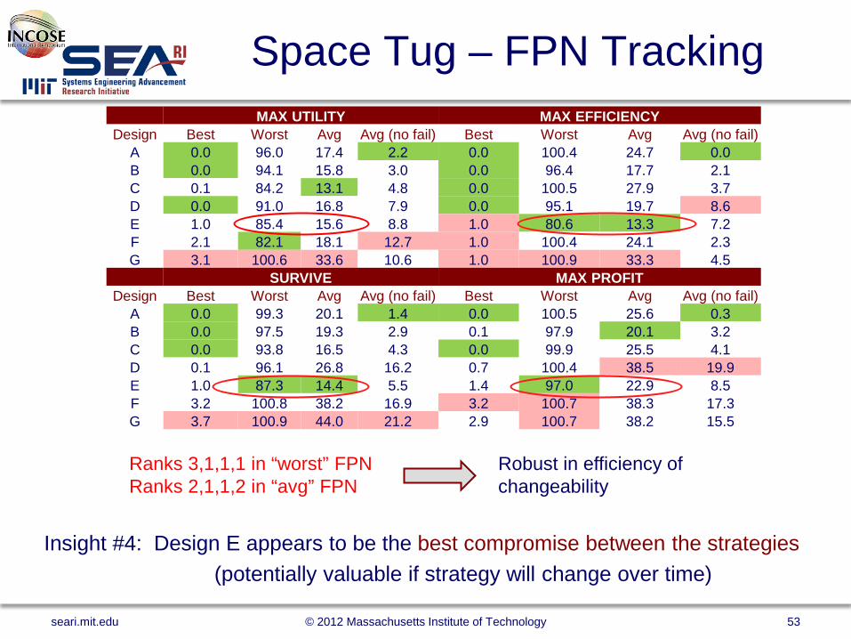
Space Tug – FPN Tracking
Insight #4: Design E appears to be the best compromise between the strategies (potentially valuable if strategy will change over time)
MAX UTILITY MAX EFFICIENCY Design Best Worst Avg Avg (no fail) Best Worst Avg Avg (no fail)
A 0.0 96.0 17.4 2.2 0.0 100.4 24.7 0.0 B 0.0 94.1 15.8 3.0 0.0 96.4 17.7 2.1 C 0.1 84.2 13.1 4.8 0.0 100.5 27.9 3.7 D 0.0 91.0 16.8 7.9 0.0 95.1 19.7 8.6 E 1.0 85.4 15.6 8.8 1.0 80.6 13.3 7.2 F 2.1 82.1 18.1 12.7 1.0 100.4 24.1 2.3 G 3.1 100.6 33.6 10.6 1.0 100.9 33.3 4.5
SURVIVE MAX PROFIT Design Best Worst Avg Avg (no fail) Best Worst Avg Avg (no fail)
A 0.0 99.3 20.1 1.4 0.0 100.5 25.6 0.3 B 0.0 97.5 19.3 2.9 0.1 97.9 20.1 3.2 C 0.0 93.8 16.5 4.3 0.0 99.9 25.5 4.1 D 0.1 96.1 26.8 16.2 0.7 100.4 38.5 19.9 E 1.0 87.3 14.4 5.5 1.4 97.0 22.9 8.5 F 3.2 100.8 38.2 16.9 3.2 100.7 38.3 17.3 G 3.7 100.9 44.0 21.2 2.9 100.7 38.2 15.5
Ranks 3,1,1,1 in “worst” FPN Ranks 2,1,1,2 in “avg” FPN
Robust in efficiency of changeability
seari.mit.edu © 2012 Massachusetts Institute of Technology 53