Embed Size (px)
Citation preview

Assessing Uncertainty with DrillHole Spacing Studies – Applicationsto Mineral ResourcesGeorges Verly1, Tomasz Postolski2, Harry Parker1
(1) AMEC; (2) Goldcorp Inc
0%
15%
30%
45%
60%
75%
90%
105%
0 25 50 75 100 125 150 175
90
% C
I
Drill spacing (m)
Q90%: Mineralogy
Enargite
Chalcocite
Chalcopyrie
Cu Leach Recovery

Content
Introduction
Principles and limitations
Formulation
Block size and sample locations Sensitivity study
Software issues
Historical antecedents of confidence intervals for classification
Conclusions
1

Introduction
Assessing uncertainty in mineral resource estimation is required for best practice and is implied by public reporting codes.
Conditional simulation is an ideal tool for uncertainty and risk assessment. Drill spacing studies (DHSS), however, are worth considering for the following reasons: A good simulation is not straightforward. It requires planning, time and
careful validation. DHSS are generally simpler and faster to execute. They also offer some
flexibility, though less than simulation. There are cases when the risk assessment requirements are not so
complex as to necessarily require simulation, or when time to complete a simulation is lacking.
2

Introduction
When the requirement is limited to an assessment of the uncertainty of some estimated attribute within large production blocks, drill hole spacing studies can be useful.
The results provide an indication of risk given the current of future drill hole spacings. This can be used as a guide for classification, a justification for additional drilling, or simply as a heads-up to be followed by a more comprehensive simulation.
The principles behind DHSS have been around for quite some time. The practice of these studies, however, is not readily available.
This presentation is essentially about the practice of DHSS.
3

Principles
4

0
90% ConfidenceInterval (CI)
Principles
Compute an estimation variance of an attribute within a large production block
The production block can be regular or irregular
The samples can be at conceptual or actual locations
Assume that the error is normally distributed
Deduce relative confidence intervals (CIs) Usually a 90% CI
5

Principles
Which attributes?
Depending on where the risks are, the attribute(s) could be one or several of the following: Grade; Deleterious element; Tonnage related:
– Thickness– Proportion of ore Indicator variable
Metal = tonnage * grade Etc.
6
Wittichenite at Antamina; a Cu-Bi sulphide;
Courtesy P. Gomez(Parker, 2014)

Principles
The results can be presented in a number of different ways
7
0%
15%
30%
45%
60%
75%
90%
105%
0 25 50 75 100 125 150 175
90%
CI
Drill spacing (m)
Q90%: Mineralogy
Enargite
Chalcocite
Chalcopyrie
Cu Leach Recovery
0%
5%
10%
15%
20%
25%
30%
Q1 Q2 Q3 Q4 Q5
90%
CI
Quarterly production volumes
Q90%: Tonnes, Grade, Metal
Tonnage Metal Content Grade Ni
0%
10%
20%
0.00 0.20 0.40 0.60 0.80
90%
CI
Ore Type Proportion
Y90% As in Ore Type "A"
100 m
75 m
50 m

Limitations
8
Limitations
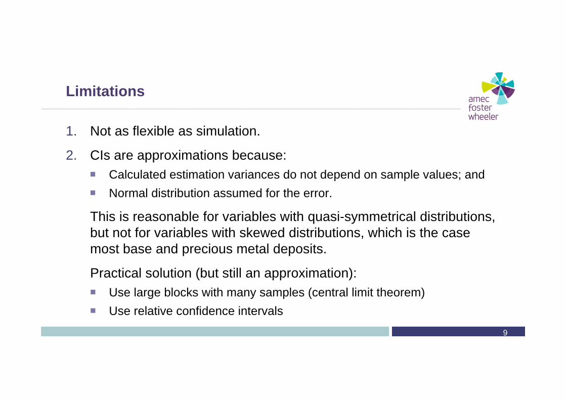
1. Not as flexible as simulation.
2. CIs are approximations because: Calculated estimation variances do not depend on sample values; and Normal distribution assumed for the error.
This is reasonable for variables with quasi-symmetrical distributions, but not for variables with skewed distributions, which is the case most base and precious metal deposits.
Practical solution (but still an approximation): Use large blocks with many samples (central limit theorem) Use relative confidence intervals
9
Formulation
10

Formulation
Formula of the estimation variance
Notes: Sample values are not needed. Blocks can be of any shape. Different estimation methods can be used to provide the estimation weights.
11
2
1 1 12 ( , ) ( , )
N N N
Err block i i j iji i j
S w Block i w w Block Block
N : Number of sampleswi : Sample “i ” estimation weight, : various variogram values

Formulation
Estimation variance for a period:S2
Err period = S2Err block / N
N is the number of blocks in the period. Blocks must be such that their errors of estimation can be considered
independent.
Standard error is square root of estimation variance SErr period
90 % relative confidence interval (CI): 90% relative CI = 1.645 * SErr period / Mean This assumes a normal distribution of the error
12

Impact of Sample CV
Relative error CIs are proportional to the sample coefficient of variation (CV).
An indicator is often used as proxi for an ore type proportion or tonnage As Prob(Ind) , CV , CI
This is an important consideration for low proportion ore types.
13
0%
10%
20%
0.00 0.20 0.40 0.60 0.80
90%
CI
Ore Type Proportion
Y90% As in Ore Type "A"
100 m
75 m
50 m

0%
5%
10%
15%
20%
25%
30%
Q1 Q2 Q3 Q4 Q5
90% CI
Q90% ‐Ni
Case of Metal
Metal content = tonnes * grade
Uncertainty on metal can be driven by grade, tonnes, or both.
14
0%
5%
10%
15%
20%
Y 1 Y 2 Y 3 Y 4 Y 5
90% CI
Y90%: Ta2O5
0%
5%
10%
15%
20%
25%
90% CI
Y90% ‐ Ag

Block Size & Samples
15

Block Size & Samples
Initial Block size: Should be large such as when
combined can be considered to be spatially independent
May represent monthly or quarterly increments
Samples Once blocks are combined, the
“final” block should be surrounded with samples
16
QuarterlyBlock
YearlyCave
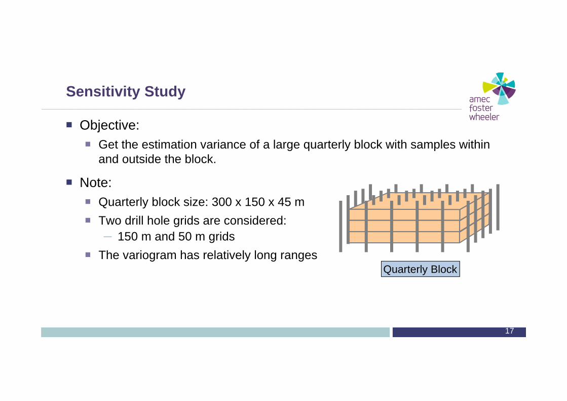
Sensitivity Study
Objective: Get the estimation variance of a large quarterly block with samples within
and outside the block.
Note: Quarterly block size: 300 x 150 x 45 m Two drill hole grids are considered:
– 150 m and 50 m grids The variogram has relatively long ranges
17
Quarterly Block

0%
20%
40%
60%
80%
1
90%
CI
Scenario
150 m50 m
Grid
Sensitivity – Scenario 1
Scenario 1 The quarterly block is directly
estimated with samples within as well as outside the block.
No issues.
18
Quarterly Block

Sensitivity – Scenario 2
Monthly block. Samples within and outside the block. Issues:
– Sharing of samples when combining blocks to get quarterly block S2
Err quarter lower than it should
– Vertical dimension of block is small S2
Err quarter lower than it should
19
Quarterly BlockMonthly blocks
0%
20%
40%
60%
80%
1 2
90%
CI
Scenario
150 m50 m
Grid

0%
20%
40%
60%
80%
1 3
90%
CI
Scenario
150 m50 m
Grid
Sensitivity – Scenario 3
Monthly block. Samples within block, no sample outside. Issues:
– Implies that no samples outside quarterly block are considered S2
Err quarter higher than it should
– Vertical dimension of block is small S2
Err quarter lower than it should
20
Quarterly BlockMonthly blocks

0%
20%
40%
60%
80%
1 4
90%
CI
Scenario
150 m50 m
Grid
Sensitivity – Scenario 4
Monthly block. Samples within block + a lateral fringe Issues:
– Implies that no samples above and below quarterly block are considered S2
Err quarter higher than it should
– Vertical dimension of block is small S2
Err quarter lower than it should
21
Quarterly BlockMonthly blocks

0%
20%
40%
60%
80%
1 5
90%
CI
Scenario
150 m50 m
Grid
Sensitivity – Scenario 5
Block size is such that there is one sample per block Issues:
– Implies that no samples outside quarterly block are considered S2
Err quarter higher than it should
– Starting block size is very small S2
Err quarter lower than it should
22
Quarterly BlockBlocks with one sample

Sensitivity
Recap
23
0%
20%
40%
60%
1 2 3 4 5
90%
CI
90% CI vs. Scenario
‐40%
‐20%
0%
20%
40%
1 2 3 4 5
% C
hang
e
%Change from Scenario 1
12 3 4 5

Guidelines
24

Block Size & Samples - Guidelines
Preference is to use large production blocks
Think about the number of large “panels” mined per year. For example: Production: 50 KT/d Bench height: 15 m Two long panels of size:
– 500 x 150 x 45 m
Suggested “initial” block sizes: 500 x 150 x 45 m; or 250 x 150 x 45 m
25Oct-2014
Yearly production(2 panels)

Block Size & Samples - Guidelines
It helps to use large actual blocks with actual drilling.
26Oct-2014
Provided courtesy of OT LLC; designs have been superseded; parker, 2014

Software Issues
27

Software Issues
Actual production block shapes are irregular
The number of samples can be large: Example:
– 500 x 150 x 45 m block; 25 x 25 m DH grid 1,400 samples
Issues: Most commercial software do not calculate
estimation variances for irregular blocks Limitation on maximum number of samples Numerical inaccuracies creeping-up
28

Software Issues
Possible solutions Eventually consider an initial smaller block Discretize the irregular block Ordinary kriging
– Use public domain kriging software– Regroup the samples by groups of 2 or 3– Modify kriging system to account for:
» block discretization» groups of samples
Inverse distance– Compute ID weights using “sample – block discretized point” distances.– Inject these weights in the estimation variance formula.
29
Historical Antecedents
30

Historical Antecedents
31
USBM – USGSMeasured ore:
within ±20%
1976
1982
Diehl & David95% CI:
• “A” : 40 d – 8 m: ± 20% • “B” : 8m – 2y: ± 40% • “C” : 2 – 4 years: ± 80%.
1983
Harrison – Exxon90% CI (annual basis):
• “I” : ± 16% • “II” : ± 33% • “III” : ± 66%.
1993
Wober and Morgan 90% CI (annual basis, economic expectation):• “A” : ± 8%• “B” : ± 9 - 13 % • + 2 other categories
Valee & CoteGold deposits;
90% prob. grade > lower limitGlobal & local error margins
Four classes are defined
1992 1998
Stephensen - JORC‘the accuracy ... measured resource estimate might
range up to ±15%’.

Historical Antecedents
A number of principles were evolving: The use of confidence limits in resource/reserve categorisation The consideration of the volume over which the confidence limits are applied Recognition that feasibility level estimates require resources/reserves defined with
tighter confidence limits than prefeasibility studies Economics should be taken into account A gradual tightening of confidence limits applicable to feasibility studies
32

MRDI/AMEC Guidelines
Inferred: Insufficient geological information to establish confidence levels
Indicated: ± 15% accuracy with 90% confidence over annual production. When these stated confidence limits are met, cross-sectional and level plan
interpretations show continuity with respect to orebody outlines and grade. Annual production increments are typically used for Pre-feasibility and Feasibility cash
flows. Can stand one year in 20 as being below 85% of the estimate – normal business risk. If actual is less than 85%, very often the mine will run a loss.
Measured: Same but over quarterly or monthly production increments Quarterly or monthly production increments are typically used for Operating Budget
cash flows. If error is less than 15% can usually rework the mine plan and prevent a loss.
33

Conclusions
34

Conclusions
Drill hole spacing studies involving estimation variances are relatively simple and very fast to execute.
The results are not as complete or flexible as those that could be obtained by conditional simulation.
But if the aim is to provide reasonable confidence intervals on an estimated attribute over medium to long time periods, drill hole spacing studies are a valid option.
35
Conclusions
Various situations can be accommodated such as: Conceptual or actual block shapes Conceptual or current drill hole spacings, impact of future drill holes Different attributes can be considered:
– Tonnage, grade and metal content– Ore type proportion, deleterious element, etc.
36

Conclusions
Although simple to complete, careful planning is recommended. In particular, the main risks should be identified first
– Grade, deleterious element, volume of high-grade shells, etc. Finding out where the risks are requires an understanding of the geology
and anticipated mining method.
Attention must be paid to the way blocks/samples are combined to get longer production periods. Large blocks are preferred.
The CIs obtained should be considered as approximate rather than strict CIs.
37