Assessing vulnerability to poverty: concepts,empirical methods and illustrative examples

Shubham ChaudhuriDepartment of EconomicsColumbia University

June 2003

Abstract

A household’s observed poverty level is an ex-post measure of a house-hold’s well-being (or lack thereof). But poverty is a stochastic phenom-enon and the current poverty level of a household, may not necessarily be agood guide to the household’s expected poverty in the future. For thinkingabout appropriate forward-looking anti-poverty interventions (i.e., interven-tions that aim to go beyond the alleviation of current poverty to prevent orreduce future poverty), the critical need then is to go beyond a catalogingof who is currently poor and who is not, to an assessment of households’vulnerability to poverty. In this paper, we make the case for broadening thescope of poverty assessments to take account of vulnerability to poverty andoutline a conceptual and empirical approach for doing so. The paper hastwo broad aims: first, to provide a conceptual and methodological overviewof the uses and empirical implementation of vulnerability assessments usinghousehold-level data; and second, to demonstrate, through a number of il-lustrative examples as well as two more detailed country studies, how thegeneral methodological approach can be usefully applied and tailored to par-ticular contexts and data, to yield policy-relevant insights about the natureand extent of vulnerability.

Table of Contents

1. Introduction

2. Vulnerability to poverty: a conceptual overview2.1. Poverty, risk, and vulnerability2.2. Why should we worry about vulnerability?2.3. What makes a household vulnerable to poverty? A taxonomy2.4. Organizing vulnerability assessments2.5. Defining vulnerability for operational purposes

3. Empirical methods and implementation

3.1. The basic approach3.2. Specifying the consumption process3.3. Econometric issues3.4. Estimating household vulnerability

3.4.1. Allowing for heteroskedasticity3.4.2. Parametric estimates of consumption volatility3.4.3. Non-parametric approaches

4. Using vulnerability estimates to inform policy: illustrative examples

4.1. Documenting aggregating vulnerability and poverty4.2. Comparing vulnerability and poverty profiles4.3. Using vulnerability estimates in geographic targeting4.4. Exploring the proximate causes of vulnerability4.5. Estimating the contribution of risk to vulnerability4.6. Predicting future poverty using current vulnerability estimates

5. Appendix

5.1. The setting and the data for the three country studies5.2. Econometric strategy adopted in the three country studies

References

2

1. Introduction

Poverty reduction has long been recognized as the implicit objective of develop-ment policy. For more than a decade now, national poverty assessments havebeen used on a routine basis to inform policy discussions on poverty alleviationin numerous developing economies. These poverty assessments have drawn oncross-sectional household surveys to provide a detailed profile of the poor, and todocument the incidence of poverty in various segments of the population.

But poverty is a stochastic phenomenon. Today’s poor may or may not betomorrow’s poor. Currently non-poor households who face a high probability ofa large adverse shock, may, on experiencing the shock, become poor tomorrow.And among the currently poor households there may be some who are only tran-sitorily poor as well as other who will continue to be poor (or poorer) in thefuture. In other words, a household’s (or an individual’s) observed poverty levelor status–defined in most cases simply in terms of the household’s observed levelof consumption expenditure relative to a pre-selected poverty line–is an ex-postmeasure of a household’s well-being (or lack thereof). But for policy purposes,what really matters is the ex-ante risk that a household will, if currently non-poor, fall below the poverty line, or if currently poor, will remain in poverty. Andthe current poverty level of a household, may not necessarily be a good guide tothe household’s vulnerability to poverty in the future. For thinking about appro-priate forward-looking anti-poverty interventions (i.e., interventions that aim togo beyond the alleviation of current poverty to prevent or reduce future poverty),the critical need then is to go beyond a cataloging of who is currently poor andwho is not, to an assessment of households’ vulnerability to poverty.

In this paper, we make the case for broadening the scope of poverty assess-ments to take account of vulnerability to poverty and outline a conceptual andempirical approach for doing so. The paper has two broad aims:

• first, to provide a conceptual and methodological overview of the uses andempirical implementation of vulnerability assessments using household-leveldata

• and second, to demonstrate, through a number of illustrative examples aswell as two more detailed country studies, how the general methodolog-ical approach can be usefully applied and tailored to particular contextsand data, to yield policy-relevant insights about the nature and extent ofvulnerability.

1

The paper is organized as follows. The next section provides a conceptual overview.We begin by clarifying the links between the concepts of poverty, risk and vulner-ability. We then detail the rationale for vulnerability assessments. An assessmentof vulnerability, we argue, is necessary and desirable not only because vulnera-bility is an inherently important dimension of well-being, but also because suchan assessment serves other important instrumental functions: it informs the de-sign of forward-looking poverty reduction strategies, it highlights the distinctionbetween poverty prevention and poverty alleviation interventions, and it clarifiesthe role of risk in the dynamics and persistence of poverty.

We then outline a simple taxonomy for thinking about the multiple inter-linked factors that make households vulnerable to poverty and use this taxonomyto suggest ways in which a vulnerability assessment might be organized. Thesection ends with an operational definition of vulnerability to poverty that can,in principle, be taken to the data.

The third section outlines a general and fairly flexible methodology for em-pirical implementing vulnerability assessments using household data. After sum-marizing the basic approach, we turn to a detailed discussion of the various stepsinvolved and the econometric issues that arise at each step.

The fourth section contains a series of illustrative examples demonstratingthe ways in which vulnerability estimates might be used to inform policy. Theexamples are drawn from three different studies: a study of vulnerability in ruralsouth and southwestern China using longitudinal household-level data for the sixyears from 1985 to 1990 (Chaudhuri and Jalan (2003)); a vulnerability assessmentfor Indonesia using data from the mini-SUSENAS collected in December 1998and August 1999 (Chaudhuri, Jalan and Suryahadi (2003)); and a study usinghousehold level data from the Philippines for 1997 and 1998 (Chaudhuri and Datt(2002)). Further details about the setting, the data and the econometric strategypursued in each of these studies are summarized in the appendix.

2. Vulnerability to poverty: a conceptual overview

2.1. Poverty, risk and vulnerability

Poverty is an ex-post measure of a household’s well-being (or lack thereof). Itreflects a current state of deprivation, of lacking the resources or capabilities tosatisfy current needs. Vulnerability, on the other hand, may be broadly construedas an ex-ante measure of well-being, reflecting not so much how well off a house-hold currently is, but what its future prospects are. What distinguishes the two is

2

the presence of risk–the fact that the level of future well-being is uncertain. Theuncertainty that households face about the future stems from multiple sourcesof risk–harvests may fail, food prices may rise, the main income earner of thehousehold may become ill, etc. If such risks were absent (and the future were cer-tain) there would be no distinction between ex-ante (vulnerability) and ex-post(poverty) measures of well-being.

2.2. Why should we worry about vulnerability?

The case for considering the role of risk in the design and implementation ofsocial policy has been made eloquently elsewhere (see, for instance, Holzmann(2001), Holzmann and Jørgensen (2000), and Heitzmann, Canagarajah and Siegel(2002)). The claim that the nature and magnitude of the risks that householdsface, and the scope of the risk-management mechanisms they have access to,given the environments in which they operate, potentially play a central role inthe dynamics and scale of poverty is also supported by both theoretical analysesand empirical evidence. Drawing on these arguments, we least four reasons whybroadening the scope of poverty assessments to include an analysis of vulnerabilityto poverty is both desirable and necessary.

First, and most obviously, for thinking about appropriate forward-lookinganti-poverty interventions, it clearly is necessary to go beyond a cataloging of whois currently poor, how poor they are, and why they are poor to an assessmentof households’ vulnerability to poverty–who is likely to be poor, how likely arethey to be poor, how poor are they likely to be, and why are they likely to bepoor. An atemporal or static approach to well-being, if strictly adhered to, isof limited use in thinking about policy interventions to improve well-being thatcan only occur in the future. Of course, in practice, poverty assessments, even ifcouched in atemporal terms, are used in the process of policy formulation. Butin doing so, implicit assumptions are being made about the extent to which thesituation recorded in the poverty assessment will be reproduced over time. Areconceptualization in terms of vulnerability to poverty, which, by definition hasto be forward-looking, forces us to make these assumptions explicit and considerthe potential role and effects of risk.

Second, a focus on vulnerability to poverty serves to highlight the distinctionbetween ex-ante poverty prevention interventions and ex-post poverty alleviationinterventions. A simple public health analogy makes this distinction clear. Justas efforts to combat a disease outbreak include both treatment of those alreadyafflicted as well as preventive measures directed at those at risk, poverty reductionstrategies need to incorporate both alleviation and prevention efforts.

3

Third, addressing vulnerability also has instrumental value. Because of themany risks households face, they often experience shocks leading to a wide vari-ability in their income. In the absence of sufficient assets or insurance to smoothconsumption, such shocks may lead to irreversible losses, such as distress saleof productive assets, reduced nutrient intake, or interruption of education thatpermanently reduces human capital (Jacoby and Skoufias, 1997), locking theirvictims in perpetual poverty. Aware of the potential of such irreversible out-comes, vulnerable people often engage in risk mitigating strategies to reduce theprobability of such events occurring. Yet, these strategies yield typically low av-erage returns. Thus, when people lack the means to smooth consumption in theface of variable incomes, they are often trapped in poverty through their attemptsto steer clear of irreversible shocks (Morduch, 1994; Barrett, 1999). In a similarvein it is being observed at the macro-level that economic growth slows down inthe face of downward risks resulting from structural phenomena such as climaticvagaries, fluctuations in the terms of trade and political insecurity (Guillaumont,Guillaumont, Brun, 1999). Policies directed at reducing vulnerability–both atthe micro and macro level–will be instrumental in reducing poverty.

Last but not least, vulnerability is an intrinsic aspect of well-being. Thatexposure to risk and uncertainty about the future adversely effect current well-being is one of the central tenets of the basic economic theory of human behavior,embodied in the assumption that individuals and households are risk averse. Andas theWorld Development Report 2000/2001 on Attacking Poverty docu-ments, this presumption is echoed by findings from worldwide consultations thatindicate that risk and uncertainty are a central preoccupation of the poor.

2.3. What makes a household vulnerable to poverty? A taxonomy

A household’s vulnerability to poverty at any point in time depends on how itslivelihood prospects and well-being is likely to evolve over time. And that inturn depends on its future income prospects, the degree of income volatility itfaces, its ability to smooth consumption in the face of income or other livelihoodshocks. These in turn depend on the complex dynamic interlinkages betweenthe environment–macroeconomic, institutional, sociopolitical and physical–inwhich the household operates, the resources, human, physical and financial itcommands, and its behavioral responses. Such a dynamic perspective on house-hold well-being suggests that the proximate causes of poverty and vulnerabilityto poverty are:

• exposure to adverse aggregate shocks (e.g. macroeconomic shocks or com-modity price shocks) and/or adverse idiosyncratic shocks (e.g., localized

4

crop damage or illness of the main income-earner in the household). Ahousehold may have a high level of exposure for one of both of two reasons:

— it faces high levels of underlying risk

— it has a limited ability to maintain its well-being in the face of adverselivelihood shocks, i.e., limited ability to cope with risks

• low long-term income generating capacity

Those who are vulnerable to transitory poverty suffer primarily from exposureto adverse shocks. On the other hand the structurally or chronically poor arethose who are both exposed to adverse shocks and have limited long-term incomegenerating capacity. Poverty reduction efforts must protect the former and assistthe latter.

Both the long-term poor and those who find themselves in poverty because ofan adverse shock, may adopt a variety of coping strategies to meet basic essentialneeds. Some of these coping strategies, while they might enable the household tomeet critical short-term needs, can be costly in terms of the future well-being ofthe household, and in particular may condemn the children of the household to alifetime of poverty as well. Measures to prevent the transmission of poverty fromone generation to the next must be an essential component of any sustainablepoverty reduction strategy.

Poverty prevention efforts that aim to reduce vulnerability to poverty and pre-vent the transmission of poverty must go beyond the proximate causes of povertyand vulnerability to address the multiple underlying causes of poverty. Any cat-egorization of the underlying causes of poverty is ultimately somewhat arbitrarygiven the numerous complicated ways in which the various factors that lead topoverty are intertwined. A household is more likely to be exposed to adverseshocks and have limited earnings prospects and income-generating capacity if it:

• has low levels of human capital, know-how and access to information• suffers from physical and psychological disabilities

• has few productive and financial assets• suffers from social exclusion or inadequate networks of social support

• has limited access to credit and risk-management instruments

5

• lives in a setting with adverse agroclimatic conditions and limited naturalresources

• lives in a community where there is insufficient entrepreneurial activity andjob creation

• works in a sector that is particularly sensitive to macroeconomic volatilityand sectoral shocks

The multiple interlocking paths to poverty are illustrated schematically in Figure1. The conceptual approach outlined above is both comprehensive and general.To be fruitfully applied in a particular context, the relative importance (theweights) of the various paths to poverty has to be ascertained through carefulempirical analyses. And that is what vulnerability assessments are about.

2.4. Organizing vulnerability assessments

Clearly, given the complexity of the multiple dynamic interlinkages illustrated inFigure 1, vulnerability assessments should take place at multiple levels, and shouldbe directed at multiple issues. No single empirical methodology or approach cansimultaneously encompass all these issues. Rather, what is needed is research andanalysis on a number of fronts using different data sources and possibly, somewhatdifferent empirical methods.

Nevertheless, the taxonomy sketched in Figure 1 provides an useful basis fororganizing vulnerability assessments. Mirroring the nested hierarchical structureof the taxonomy, vulnerability assessments can be structured into a series of hi-erarchically related questions, with the questions at each step being progressivelymore and more narrowly focused.

To begin with, vulnerability assessments need to be able to say somethingabout the extent of vulnerability in the population. How widespread is vulnera-bility to poverty–how many face a non-negligible risk of poverty, how likely arethey to be poor and how poor are they likely to be? Are vulnerability and povertydistinct phenomena? Is the scale of poverty reduction interventions appropriate?

At the next step, we need to know more about who the vulnerable are andhow concentrated vulnerability is within different segments of the population. Ifinterventions seem necessary, where should they be directed?

Following naturally from this comes the next question, what types of interven-tions are necessary? Vulnerability assessments can address this issue at multiple

6

levels. At the highest level, they can shed light on the proximate causes of vulnera-bility: are households vulnerable to poverty primarily because their consumptionsare volatile, which would imply they are mostly vulnerable to transitory poverty,or are they structurally poor? How do the proximate causes of vulnerability varyacross various segments of the population?

Consumptions are volatile because households are exposed to risk. Even forstructurally poor households, consumption volatility may contribute significantlyto vulnerability. So at the next step, we need to better understand why consump-tions are volatile? Is it because households face high levels of underlying risk? Oris it that they have a limited ability to cope with even moderate levels of risk?

Lastly, these latter two questions immediately suggest the need to identifythe sources of risk that households are most exposed to, as well as the need for abetter understanding of the risk management instruments, public or private, towhich households have access.

2.5. Defining vulnerability to poverty

Poverty and vulnerability (to poverty) are two sides of the same coin. The ob-served poverty level or status of a household (defined simply in terms of a house-hold’s observed level of consumption expenditure relative to a pre-selected povertyline) is the ex-post realization of a random variable, the ex-ante expectation ofwhich can be taken to be the household’s level of vulnerability.

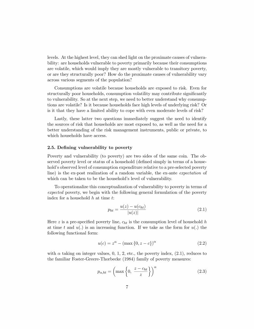
To operationalize this conceptualization of vulnerability to poverty in terms ofexpected poverty, we begin with the following general formulation of the povertyindex for a household h at time t:

pht =u(z)− u(cht)

|u(z)| (2.1)

Here z is a pre-specified poverty line, cht is the consumption level of household hat time t and u(.) is an increasing function. If we take as the form for u(.) thefollowing functional form:

u(c) = zα − (max {0, z − c})α (2.2)

with α taking on integer values, 0, 1, 2, etc., the poverty index, (2.1), reduces tothe familiar Foster-Greere-Thorbecke (1984) family of poverty measures:

pα,ht =

µmax

½0,z − chtz

¾¶α(2.3)

7

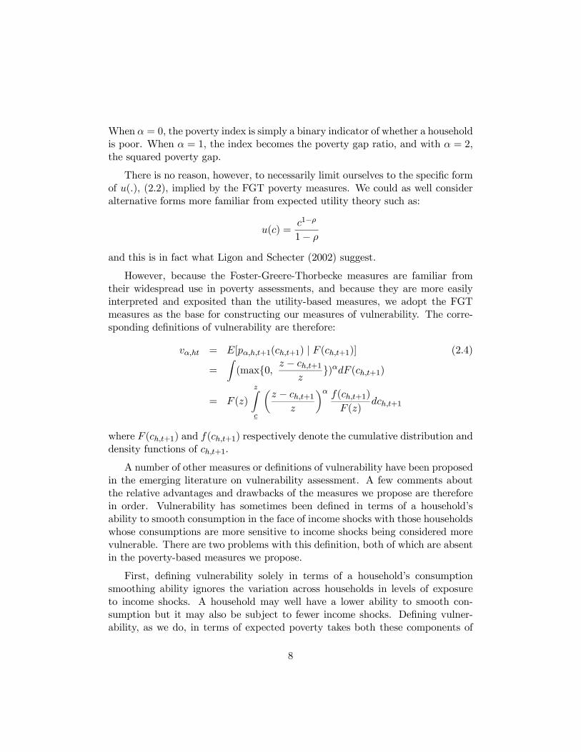
When α = 0, the poverty index is simply a binary indicator of whether a householdis poor. When α = 1, the index becomes the poverty gap ratio, and with α = 2,the squared poverty gap.

There is no reason, however, to necessarily limit ourselves to the specific formof u(.), (2.2), implied by the FGT poverty measures. We could as well consideralternative forms more familiar from expected utility theory such as:

u(c) =c1−ρ

1− ρand this is in fact what Ligon and Schecter (2002) suggest.

However, because the Foster-Greere-Thorbecke measures are familiar fromtheir widespread use in poverty assessments, and because they are more easilyinterpreted and exposited than the utility-based measures, we adopt the FGTmeasures as the base for constructing our measures of vulnerability. The corre-sponding definitions of vulnerability are therefore:

vα,ht = E[pα,h,t+1(ch,t+1) | F (ch,t+1)] (2.4)

=Z(max{0, z − ch,t+1

z})αdF (ch,t+1)

= F (z)

zZc

µz − ch,t+1

z

¶α f(ch,t+1)F (z)

dch,t+1

where F (ch,t+1) and f(ch,t+1) respectively denote the cumulative distribution anddensity functions of ch,t+1.

A number of other measures or definitions of vulnerability have been proposedin the emerging literature on vulnerability assessment. A few comments aboutthe relative advantages and drawbacks of the measures we propose are thereforein order. Vulnerability has sometimes been defined in terms of a household’sability to smooth consumption in the face of income shocks with those householdswhose consumptions are more sensitive to income shocks being considered morevulnerable. There are two problems with this definition, both of which are absentin the poverty-based measures we propose.

First, defining vulnerability solely in terms of a household’s consumptionsmoothing ability ignores the variation across households in levels of exposureto income shocks. A household may well have a lower ability to smooth con-sumption but it may also be subject to fewer income shocks. Defining vulner-ability, as we do, in terms of expected poverty takes both these components of

8

vulnerability into account. Second, measures that focus on the ability to smoothconsumption ignore the asymmetry that, we would argue, is crucial to the no-tion of vulnerability, namely the importance of exposure to downside risk. Theadvantage of the expected poverty formulation of the vulnerability measure isthe built-in asymmetry of poverty measures that implicitly gives more weight todownside risks.

Vulnerability has also been defined in terms of exposure to adverse shocks towelfare, rather than in terms of exposure to poverty. This definition also differssubstantively from ours in that our definition would include among the vulnerable,households who are currently poor and have a high probability of remaining pooreven if they do not experience any large adverse welfare shocks. On the otherhand, our definition would exclude those households among the non-poor whoface a high probability of a large adverse shock but are currently well-off enoughso that even were they to experience the shock, they would still remain non-poor.

With the central role that the notion of poverty, and more generally, the levelof household welfare, plays in policy discussions, a measure of vulnerability thattakes account of welfare levels–in particular, poverty levels–seems preferable.However, it should be recognized that to the extent that defining welfare relativeto a prespecified poverty line is considered somewhat arbitrary, that arbitrarinesscarries over to our vulnerability measures. A potentially more serious concern isthe fact that, as Ligon and Schecter (2002) point out, one of the vulnerabilitymeasures we propose, the expected poverty status or future likelihood of povertyof a household, has the perverse implication that increases in risk would reduce thevulnerability level of those with mean consumption levels below the poverty line.But, as we demonstrate below, that does not negate its usefulness in informingcertain policy decisions. It is only in quantifying the contribution of risk tovulnerability that we need to be careful not to rely on this measure, and insteaduse one of the other measures, which do not suffer from this shortcoming.

3. Empirical methods for assessing household vulnerability to poverty

This section provides an overview of the measurement and econometric issuesthat arise in carrying out vulnerability assessments, and outlines a general andfairly flexible methodology for organizing and carrying out such assessments.

3.1. The basic approach

Whatever the precise measure of vulnerability one chooses to work with, thestarting point has to be an explicit specification of the underlying data-generating

9

process for consumption. Vulnerability assessments, by definition, have to beexplicitly forward-looking. No matter how rich the data, the vulnerability ofhouseholds is never directly observable. In contrast, most poverty assessmentsare couched in atemporal terms and, given the right data, it is possible to actuallyobserve the current poverty level or status of the household.

From this it naturally follows that the observed consumption expenditures ata point in time (i.e., from a single cross-section survey) should be viewed as theoutcome (snapshot) of a dynamic process that is occurring in real time. And thismeans that vulnerability assessments (again, in contrast to poverty assessmentswhich remain largely atheoretical) have to be rooted in explicit models of inter-temporal household behavior.

How general and flexible the specification of the consumption process can bedepends first and foremost on the data that are available. Given the limitationsof most data sets, a priori restrictions on the consumption process will almostcertainly need to be made. And in this, it is important to be clear about theassumptions implicit in whatever specification is ultimately adopted.

Once a specification has been chosen, the next step is to estimate the para-meters of the process using the household data. In general it will be possible toestimate the key parameters in a fairly flexible way without making too manystringent distributional assumptions. However, in going from estimates of theconsumption process to estimates of vulnerability, the problem of estimating thedistribution of consumption will need to be faced. Here they are two possible ap-proaches. The first is to work with a pre-specified parametric distribution. Thesecond is to use non-parametric techniques to get at the distribution of futureconsumption.

Lastly, the estimates of the consumption process and the estimates of vulner-ability can be used in number of different ways to inform the design of povertyreduction policies. To summarize, then, the basic approach consists of four steps:

• Step 1: specify the data generating process for consumption• Step 2: use survey data on household consumption expenditures and char-acteristics to estimate the relevant parameters of the consumption process

• Step 3: make the necessary distributional assumptions needed to drawinferences about future consumption prospects–i.e., to go from estimatesof the consumption process to estimates of vulnerability

10

• Step 4: use the vulnerability estimates, decompositions of the vulnerabilityestimates, and a variety of counterfactuals constructed using the estimatesof the consumption process, to address various policy-relevant questions

3.2. Specifying the consumption process

The level of vulnerability at time t is defined in terms of the household’s con-sumption prospects at time t+1. The difference is noteworthy because it reflectsan important distinction between the notion of vulnerability and the concept ofpoverty. Vulnerability is a forward-looking or ex-ante measure of a household’swell-being, whereas poverty is an ex-post measure of a household’s well-being(or lack thereof). This implies that while the poverty status of a household isconcurrently observable-i.e., with the right data we can make statements aboutwhether or not a household is currently poor-the level of vulnerability is not. Wecan estimate or make inferences about whether a household is currently vulner-able to future poverty, but we can never directly observe a household’s currentvulnerability level.

An assessment of vulnerability is, therefore, innately a more difficult task thanassessing who is poor and who is not. To assess a household’s vulnerability topoverty we need to make inferences about its future consumption prospects. Andin order to do that, we need a framework for thinking explicitly about both theinter-temporal aspects and cross-sectional determinants of consumption patternsat the household level.

Over the last two decades, a large literature has developed which addressesprecisely these issues (See Deaton(1992) and Browning & Lusardi(1995) for excel-lent overviews). This literature suggests that a household’s consumption in anyperiod will, in general, depend on a number of factors. Among them its wealth,its current income, its expectations of future income (i.e., lifetime prospects), theuncertainty it faces regarding its future income and its ability to smooth con-sumption in the face of various income shocks. Each of these will in turn dependon a variety of household characteristics, those that are observable and possiblysome that are not, as well as a number of features of the aggregate environment(macroeconomic and socio-political) in which the household finds itself. At ageneral conceptual level, this suggests the following reduced form expression forconsumption:

cht = c(Xh,βt,αh, eht) (3.1)

where Xh represents a bundle of observable household characteristics, βt is avector of parameters describing the state of the economy at time t, and αh and eht

11

represent, respectively, an unobserved time-invariant household-level effect, andany idiosyncratic factors (shocks) that contribute to differential welfare outcomesfor households that are otherwise observationally equivalent.

Substituting from (3.1) into (2.4) we can rewrite the expression for the vul-nerability level of a household as:

vht = E[pα,h,t+1(ch,t+1) | F (ch,t+1| Xh,βt,αh, eht)] (3.2)

The expression above makes clear that a household’s vulnerability level derivesfrom the stochastic properties of the inter-temporal consumption stream it faces,and these in turn depend on a number of household characteristics and charac-teristics of the environment in which it operates. And at a conceptual level, theexpression is very general in a number of respects.

First, it allows for the possibility of complicated interactions between themultiple cross-sectional determinants of a household’s vulnerability level. Forinstance, Xh could include variables such as the educational attainment of thehead of the household, presence of a government poverty scheme in the communityin which the household resides, as well as interactions between the two to capturepotential inequities in the level of access to public programs.

Second, because a household’s vulnerability is defined in terms of its futureconsumption prospects conditional on its current characteristics, both observedand unobserved, the possibility of poverty traps and other non-linear povertydynamics is implicitly built in.

And third, the possible contribution of aggregate shocks and unanticipatedstructural changes in the macro-economy to vulnerability at the household levelis also incorporated through inclusion of the time-varying set of parameters, βt.

In practice, as will be clear in the next section, data constraints will usually notpermit estimation of vulnerability at the level of generality embodied in expression(3.2). Nevertheless the formulation is useful in providing a basis for thinkingthrough the possible implications of the various restrictions that will need to beimposed in any attempt to estimate vulnerability with the sorts of data that areusually available.

3.3. Econometric issues

A number of econometric issues arise in implementing the basic approach outlinedabove, many of them driven by data constraints. To illustrate some of the issues

12

that arise we begin by laying out what in some respects is an almost ideal speci-fication of the consumption process for the purposes of estimating vulnerability:

lnChjt = Xhαj+XhPtβj+XhRjtγj+XhMhjtδj+vjt+ηh+ehjt

qg(Xh, θj (3.3)

Here Xh is a vector of observable characteristics of household h, Pt, a vector ofobservable macro shocks in year t, for instance, commodity price shocks, Rjt cap-tures observable locally covariate shocks in area j in year t, for instance weathershocks,Mhjt denotes an observable idiosyncratic shock experienced by householdh in area j in year t, e.g., illness of the main income earner, vjt represents un-observed area-specific shocks, ηh, an unobserved time-invariant household effect,and ehjt an idiosyncratic time-varying disturbance term.

Estimation of (3.3) would clearly impose significant demands on the data, de-mands that are unlikely to be met in most instances. If as is quite common, paneldata are not available, we cannot control for unobserved household-level effects.Not only does this potentially bias the estimates of the coefficients on the vari-ables we do observe, it also raises the possibility that unobserved heterogeneity inthe cross-section will be confounded with inter-temporal variation in consumptionlevels. The lack of panel data also eliminates the possibility of exploring povertydynamics. Nevertheless, as we illustrate in a later section, cross-sectional datacan be useful for certain purposes.

The other main constraint that must often be faced is the lack of informationon area-specific variables, Rjt and on the idiosyncratic shocks experienced byindividual households, Mhjt. In the former case, it becomes that much more dif-ficult to distinguish time-invariant area-specific characteristics from time-varyinglocally covariate shocks. Even with panel data, this problem cannot always beovercome if there are seasonal effects that need to be considered as well. Withoutinformation onMhjt it may still be possible to consistently estimate (3.3) but theanalysis will be much less informative.

3.4. Estimating household vulnerability

From (3.2) it is clear that because a household’s vulnerability to poverty is anon-linear function of its future consumption levels, it will depend, not just onits expected (i.e., mean) consumption looking forward, but also on the volatility(i.e., variance, from an inter-temporal perspective) of its consumption stream,and possibly on higher moments of the consumption process as well. A salariedlow-level government employee with an expected level of consumption roughlysimilar to that of a self-employed proprietor of a small business may nevertheless

13

be much less vulnerable to poverty because of the relative stability of the former’sconsumption stream.1

To go from estimates of the consumption process to an estimate of the house-hold’s vulnerability to poverty we need to therefore not only estimate its expectedconsumption in the future but also to be able to say something about the distrib-ution of its future consumption. At a minimum, even we are willing to make theparametric assumption that consumption is log-normally distributed and hencethe entire distribution of consumption is captured by the mean and variance, thisimplies that we need to estimate the variance of its future consumption. In thissection we describe a couple of different ways of doing this. But first we highlighta key element of the estimation strategy, whether or not a parametric approachis adopted, which is the need to allow for heteroskedasticity in the specificationof the consumption process.

3.4.1. Allowing for heteroskedasticity

The specification of the consumption process discussed in the previous section isnot a new one. Similar specifications have been estimated in a number of studiesexploring household consumption behavior and the determinants of consumption.These have included a number of poverty assessments. However, in most previousstudies, the disturbance term is implicitly thought of as stemming from measure-ment error or some unobserved factor that is incidental to the main focus of theanalysis. And thus, it is usually assumed that the variance of the disturbanceterm is the same for all households.

There are two problems with this assumption when the specification of theconsumption provides the basis for estimating vulnerability to poverty. First,within this framework the variance of the disturbance term is interpreted in eco-nomic terms as the inter-temporal variance of log consumption. Viewed from thisperspective, the assumption that the variance of log consumption is the same forall households seems quite restrictive, regardless of its statistical import. Thatis because it forces the estimates of the mean and variance of consumption to bemonotonically related across households, ruling out the possibility that a house-hold with a lower mean consumption may nevertheless face greater consumptionvolatility than a household with a higher average level of consumption. Bothformal and anecdotal evidence points to high levels of income and consumptionvolatility for poor households.

1Of course at times of macroeconomic crises accompanied by rapid inflation, the situationsmay easily be reversed.

14

Moreover, in purely statistical terms, unlike in other settings where failure toaccount for heteroskedasticity results in a loss of efficiency but need not bias theestimates of the main parameters of interest, here, the standard deviation of thedisturbance term enters directly in generating an estimate of vulnerability (see(3.4) below). A biased estimate of this parameter will therefore lead to a biasedestimate of vulnerability.

To address this problem we need to allow the variance of the disturbance term,eht, to depend upon the particular characteristics of the household. A simple wayof doing so would be to begin by specifying a functional form such as:

lnσ2ln ch,t = Xhtγ + Zhδ

where Xht and Zh are, respectively, vectors of observable time-varying and time-invariant household characteristics. Under the interpretation of the disturbanceterm, eht, in the consumption equation as the shock to consumption, the logof the squared estimated residuals from the consumption equation provides anestimate of lnσ2ln ch,t . Estimates of γ and δ can then be obtained from the followingregression:

ln be2ht = Xhtγ + Zhδ + uht3.4.2. Parametric estimates of vulnerability

Imagine that we have obtained estimates of the mean and variance of one-periodahead log consumption, where these are denoted bµln ch,t+1 and bσ2ln ch,t+1respectively.If we are willing to assume that consumption is log-normally distributed (i.e., thatln ch,t+1 is normally distributed), the estimates of vulnerability can be straight-forwardly generated using the properties of the normal distribution.

Specifically, letting Φ(.) denote the cumulative density of the standard normal,the estimate of v0,ht–the vulnerability to poverty defined as the likelihood ofpoverty of household h at time t–will be given by:

bv0,ht = cPr³ln ch,t+1 < ln z | bµln ch,t+1 , bσ2ln ch,t+1´ = ΦÃln z − bµln ch,t+1bσln ch,t+1

!(3.4)

The expressions for vulnerability to poverty defined in terms of the expectedpoverty gap ratio or the expected squared poverty gap are a bit more complicated.Even with the assumption of log-normality, these cannot be evaluated analytically.However, estimates of vulnerability under these two definitions are easily obtainedfrom Monte Carlo simulations using the estimates of bµln ch,t+1 and bσ2ln ch,t+1.

15

3.4.3. Non-parametric approaches

Kamanou and Morduch (2002) propose a non-parametric approach to estimat-ing the distribution of future consumption. The approach uses a Monte Carlodesign to simulate the future distribution of consumption, where the simulationsare based on bootstrapping the empirical distribution of observable shocks andestimated residuals.

This approach is very promising. The only drawback with this particularimplementation is that it implicitly assumes that the shocks to consumption ex-perienced by different households are drawn from the same distribution. Thisclearly goes against what we argue for above, that households in different cir-cumstances, facing different risks and with differing access to risk-managementinstruments should be presumed to experience different levels of consumptionvolatility, i.e., that we ought to allow for heteroskedasticity.

One way of addressing this shortcoming is to combine the parametric andnon-parametric approaches by first flexibly (i.e., allowing for heteroskedasticity)estimating the variance of consumption for each household, and then using theseestimated variances as propensity scores in constructing kernel-based re-samplingweights for the bootstrapping procedure under the non-parametric approach.

4. Interpreting and using vulnerability estimates to inform policy:illustrative examples

To demonstrate how household-level vulnerability estimates, generated applyingthe methodology outlined above, may be interpreted and used to inform poverty-reduction policies, in this section, we go through a series of illustrative examples.The examples are drawn from three different studies: a study of vulnerability inrural south and southwestern China using longitudinal household-level data forthe six years from 1985 to 1990 (Chaudhuri and Jalan (2003)); a vulnerabilityassessment for Indonesia using data from the mini-SUSENAS collected in Decem-ber 1998 and August 1999 (Chaudhuri, Jalan and Suryahadi (2003)); and a studyusing household level data from the Philippines for 1997 and 1998 (Chaudhuriand Datt (2002)). Further details about the setting, the data and the econometricstrategy pursued in each of these studies are summarized in the appendix.

4.1. Documenting aggregate vulnerability and poverty

The natural first step in a vulnerability assessment is to obtain a sense of theoverall level of vulnerability in the population of interest by plotting the aggregate

16

distribution of vulnerability. While this can, in principle, be done for each ofthe specific measures of vulnerability to poverty described earlier–those basedon the FGT poverty measures as well as those derived from utility theory–inpractice, such a plot is probably easiest to interpret and grasp when vulnerabilityis defined as the probability of future poverty, i.e., in terms of a household’sexpected poverty status.

Figure 2 plots the distribution of vulnerability defined in this way for ruralsouth and southwest China in 1985. If we imagine labeling a household as vul-nerable if its estimated vulnerability level exceeded some threshold, what Figure2 depicts is the estimated incidence of vulnerability for vulnerability thresholdsranging from 0 to 1–measured along the horizontal axis–for the population as awhole as well for sub-samples sorted by observed poverty status in 1985. By con-struction, as the threshold increases, the incidence of vulnerability (the fractionof the population that has an estimated probability of being poor higher thanthe threshold) declines. Thus, at a threshold of zero, everyone is vulnerable whileno one is vulnerable at the threshold of one. Perhaps not surprisingly, for anygiven threshold, the incidence of vulnerability is higher for the poor than for thepopulation as a whole, which in turn is higher than the incidence of vulnerabilityamongst the nonpoor. More significantly, Figure 2 suggests that for a wide rangeof thresholds, poverty and vulnerability are significantly different from each other.Not all the poor are vulnerable while a significant proportion of the nonpoor arevulnerable.

By depicting the entire distribution of vulnerability, Figure 2 provides a wealthof information about the vulnerability of the population. But, in many instancesit will not be feasible to directly compare entire distributions and we will need tosummarize the key properties of the underlying distribution through some well-chosen summary measures. One such measure, one that is particularly useful forexpositional purposes, is the fraction of the population that has a vulnerabilitylevel above some threshold and can therefore be deemed vulnerable. The choiceof a vulnerability threshold is of course, ultimately somewhat arbitrary. However,a threshold of 0.50 stands out as a possible focal point in that a household whosevulnerability level exceeds 0.50 is more likely than not to end up poor. Even thenthere remains the question of the time horizon over which a household’s vulnera-bility to poverty should be assessed. Here again, a certain degree of arbitrarinessis unavoidable. We consider two possibilities–a time horizon of one year, whichcan be thought of in terms of the likelihood of poverty in the near future (orshort-term), and a time horizon of three years, which roughly corresponds to thelikelihood of poverty in the medium-term. We classify as vulnerable all house-

17

holds who we estimate to be more likely than not to be poor at least once inthe next three years. Of these households, we label as those who ith estimatedvulnerability levelsand that is a threshold of 0.50. so for ease of discussion

Table 1 uses this classification scheme to summarize the distributions depictedin Figure 2. At the aggregate level, while 26% of the population is observed tobe poor, we estimate that 37% of the population is vulnerable to poverty. Hence,there clearly are households who are observed to be currently (i.e., in 1985) non-poor whose ex-ante probability of poverty is nevertheless estimated to be quitehigh, so much so that they are more likely than not to be poor at some point in thenext three years. In fact, of the 74% of the population that is observed to be non-poor, over 21% are estimated to be vulnerable. This implies that nearly 16% of thepopulation, though not currently poor is vulnerable to poverty. These estimatestherefore appear to support the often-stated (and vaguely defined) claim that theobserved incidence of poverty underestimates the fraction of the population thatis vulnerable to poverty.Amongst the poor, 78% are estimated to be vulnerable.

On the other hand, from the third column of Table 1 it is also apparentthat there are some households who are observed to be poor, whose vulnerabilitylevel is, nevertheless, low enough for them to be classified as non-vulnerable. Inparticular we estimate that 20% of the observed poor is non-vulnerable. Andwhile that may, at first glance, seem surprising, it simply reflects the stochasticnature of the relationship between poverty and vulnerability that underlies thedistinction between the two concepts.

Amongst those we classify as vulnerable, 61% are estimated to be highlyvulnerable implying that the highly vulnerable make up nearly 23% of the overallpopulation. And of the highly vulnerable, only 70% are observed to be poor,which implies that nearly 7% of the population is highly vulnerable but currentlynon-poor.

The main message that emerges from considering these aggregate numbers isthat while poverty and vulnerability are closely related concepts, there remainimportant distinctions between the two and neither notion nests the other. Andthis, in turn, has two important implications for policy. First, the fraction of thepopulation that faces a non-negligible risk of poverty (and hence, by definition, istaken to be vulnerable) may be quite different from the fraction that is observed tobe poor in any given period. In this particular population the former is estimatedto be higher than the latter but that finding is less important than the fact thatthe two are quite different. Second, and more importantly, these numbers suggestthat the characteristics of those who are observed to be poor at any given pointin time may well differ from the characteristics of those who are estimated to be

18

vulnerable to poverty, or equivalently, that the relative incidences of vulnerabilityand poverty may differ across segments of the population. Interventions andprograms that aim to reduce the level of vulnerability in the population maytherefore need to be targeted differently from those aimed at poverty alleviation.We illustrate this point in the next section with data from Indonesia.

4.2. Comparing poverty and vulnerability profiles

Table 2 presents the poverty and vulnerability profiles for Indonesia in Decem-ber 1998. We report both the overall estimates for rural and urban Indonesiaand also disaggregated by regions and certain select demographic and commu-nity characteristics. Table 3 provides us with some insights on average, about thegeographical location of the vulnerable as well as their socio-economic character-istics.

We begin by detailing the spatial distribution of poverty and vulnerability.Poverty and vulnerability in Indonesia are largely rural phenomena. Relativeto their share in the population, rural households are over-represented amongthe poor and the vulnerable. While 61% of Indonesia’s population is rural, 80%of the observed poor live in rural areas as do 82% of those we estimate to bevulnerable. The highly vulnerable are even more disproportionately rural, with91% of this group located in rural areas. The disproportionate contribution ofrural households to overall poverty and vulnerability stems from the much higherincidence of poverty and vulnerability in rural areas. About 30% of the ruralpopulation is observed to be poor, whereas in urban areas, the observed povertyrate is 12%. Similarly, while we estimate that 20% of the urban population isvulnerable, 60% of the rural population is estimated to be vulnerable.

The imbalances in the contributions of rural and urban areas to overall povertyand vulnerability are reproduced at the regional level. Urban areas, regardlessof region, are under-represented among the poor and the vulnerable, relative totheir shares in the population. With the exception of rural Sumatra, rural areastend to be over-represented. In absolute terms, rural areas of Java, Kalimantanand Sulawesi contribute the largest numbers to the populations of the poor andvulnerable. And of the 9% of the population that we estimate to be highly vul-nerable, a fifth are found in rural areas of Kalimantan and Sulawesi and another20% live in rural areas of West Java.

The tremendous variation in the poverty rates across the far-flung regionsof Indonesia has been documented elsewhere (see Pradhan et. al (2000)). Thefifth column of Table 3 confirms the presence of these regional disparities. The

19

fraction of the population that is observed to be poor ranges from a low of 2% inJakarta to a high of 56% in rural areas of West and East Nusa Tengarra, Papuaand Maluku (which have collectively been labeled “Rest of Indonesia”). Exceptfor Central Java and Yogyakarta, where 22% of the urban population is observedto be poor, urban areas have lower observed poverty rates than rural areas.

Inter-regional differences in the estimated incidence of vulnerability are evenmore pronounced than the regional disparities in poverty rates. The fraction ofthe population estimated to be vulnerable ranges from a low of 2% in Jakarta toa high of 77% in rural Central Java and Yogyakarta. Again, while urban areasgenerally have lower vulnerability rates, Central Java and Yogyakarta are excep-tional in that 46% of the urban population in these two provinces is estimated tobe vulnerable.

A comparison of the observed poverty rates and the estimated incidences ofvulnerability across the 13 geographic domains we have defined reveals two points,both indicative of the ways in which the distribution of vulnerability can differacross regions.

First, in keeping with our findings at the national level, in each of the domains,the estimated incidence of vulnerability is at least as high and in most cases higher,than the observed incidence of poverty. However, there is considerable variationin the ratio of the fraction of the population that is vulnerable to the fraction thatis poor. The vulnerability to poverty ratio is 1.00 in Jakarta and 1.27 in urbanSumatra indicating that vulnerability to poverty is quite concentrated in thesetwo regions. In contrast, in several other regions, mostly rural, vulnerability topoverty is dispersed in the population, with the fraction that is vulnerable morethan the double the fraction that is poor.

Second, two regions with roughly similar observed poverty rates may have verydifferent incidences of vulnerability. For instance, in both East Java and Bali andwhat we term the ”Rest of Indonesia”, about 8% of the urban population isobserved to be poor. However, we estimate that only 10% of the population ofurban East Java and Bali is vulnerable, whereas in the ”Rest of Indonesia,” over21% of the urban population is vulnerable.

Turning next to the other correlates of poverty and vulnerability, the one thatstands out is the educational attainment of the household head. Of the 69% of thepopulation that lives in households headed by individuals with at most a primaryschool education-who comprise 88% of the poor and an overwhelming 95% of thevulnerable-nearly 30% are poor while 63% are vulnerable to poverty.

Within this group, households headed by individuals with no schooling are

20

particularly at risk-28% of the population in such households is estimated to behighly vulnerable. In sharp contrast, within the populations in the two highesteducational attainment categories, which together make up 21% of the overallpopulation, the observed poverty rate is only 5%, the vulnerability rate is 2% andthe fraction that is vulnerable is less than 1%. Even among households headedby individuals with at most junior schooling, the poverty rate, at 12%, is lessthan half that for households just one step down in the educational attainmenthierarchy. The drop in the incidence of vulnerability to just 14% from 61% iseven more striking.

If we divide up the sample according to the employment status of the house-hold head we do not get such a clear trend though the incidence of vulnerability isunderstandably lower for salaried workers in the public and private sectors thanit is for those in other employment categories. Somewhat surprisingly, the groupwith the highest rates of poverty and vulnerability is those who are self-employedwith some help from family and hired workers. Of the 31% of the populationbelonging to this group, more than half are vulnerable.

When the population is split along other demographic characteristics, thereis, surprisingly, hardly any difference in the poverty and vulnerability rates fordifferent groups. So for instance, households with high dependency ratios are aslikely to be poor and vulnerable as households with low dependency ratios, andhouseholds headed by females are as likely to be poor and vulnerable as male-headed households. Perhaps the only difference of note is the higher fraction offemale headed households that is estimated to be highly vulnerable.

Community characteristics such as the availability of transport facilities, thepresence of a bank or cooperative in the community, industrial activity and accessto clean water are all associated with lower levels of vulnerability and poverty.Of these, access to clean water is associated with the sharpest drops in povertyand especially vulnerability.

4.3. Using vulnerability assessments in geographic targeting

The targeting of poverty alleviation resources is often based on the geographicdistribution of poverty. For instance, in China counties that are classified asnational poor or provincial poor counties (based on assessments of the extent ofpoverty) selectively receive additional government support. And in India, planallocations to the states at least partially reflect the degree of need as capturedby the level of poverty. Targeting on the basis of geography is also implicit in thevarious formulae used to determine the allocation of funds under the numerousdevolution schemes that have been introduced in recent years.

21

In the Philippines, the main block grant from the central government to localgovernment units (LGUs), the Internal Revenue Allocation (IRA), is not explicitlybased on a poverty criterion, but the argument has often been made that it shouldbe (World Bank, 2000). While this is plausible from an ex-post redistributiveperspective, there is the further consideration whether these allocations ought tobe linked to the extent of vulnerability if the aim is to reach those most prone topoverty in the near future. The issue is important insofar as those prone to beingpoor differ from those currently observed to be poor.

Figure 3 plots the observed incidence of poverty (on the horizontal axis)against the estimated incidence of vulnerability for each of the 77 provinces inthe Philippines. For most provinces, the estimated incidence of vulnerability ishigher (often considerably higher) than the observed incidence of poverty. Thiscan be seen from the fact that most of the points lie above the 45-degree line. Insome provinces, the ratio of the vulnerable to the poor is over 4.

More noteworthy still is the substantial re-ranking that takes place whenprovinces are ordered in terms of the incidence of vulnerability rather than theobserved incidence of poverty. Because the provinces are ordered along the hori-zontal axis in terms of increasing incidence of poverty, the re-ranking is reflectedin the non-monotonicity of the scatter plot. Note the three bottom (poorest) andthe two top (richest) provinces have the same poverty and vulnerability rank-ings. But between the two tail-ends there is a lot of re-sorting. The re-rankingsare particularly stark for provinces that appear in the upper left and lower rightquadrangles defined by the vertical and horizontal lines indicating, respectively,the poverty and vulnerability rates at the national level. The poverty rate inthese provinces is below the national rate, and so any poverty-targeting schemebased on poverty rates would allocate relatively fewer funds, on a per-capita ba-sis for these provinces. However, in terms of the incidence of vulnerability topoverty, these provinces are above the national rate, and should, in principle, re-ceive, on per-capita basis, proportionally more funds for poverty programs. Thus,vulnerability-based allocations could differ significantly from observed poverty-based allocations.

The key to resolving this apparent dilemma lies in distinguishing ex-antepoverty prevention interventions from ex-post poverty alleviation interventions.An example drawn from public health makes this distinction clearer. Consider asituation where public health interventions are aimed at reducing the incidence ofsome disease. Suppose information is available on both the incidence of disease indifferent regions, as well as on the fraction of the population in different regionsthat is at high risk of contracting the disease. Funds for treatment of those already

22

afflicted should clearly be directed to regions where the incidence of the diseaseis highest. But funds for preventive measures (such as vaccinations) ought tobe directed to regions where the fraction of the population at risk is the largest.And the two sets of regions need not coincide. Regions with a higher incidenceof the disease may also be regions where the risk of contracting the disease isconcentrated among those afflicted. So the fraction of the population at risk maywell be lower than in other regions where the incidence of the disease is lower.

The analogy with our treatment of vulnerability should be clear. The inci-dence of poverty, like the incidence of the disease, should determine the alloca-tion of funds for treatment, which in the case of poverty means funds for ex-postpoverty alleviation programs. The allocation of funds for preventive interventions-ex-ante interventions aimed at poverty prevention-should however be guided bythe incidence of vulnerability to poverty.

In practice, the difference between ex-ante and ex-post interventions will mostlikely be realized in terms of the particular line agencies through which resourcesare channeled. The funds for focused ex-post interventions such as food-for-workschemes or means-tested transfer programs are likely to be disbursed through verydifferent channels than funds for ex-ante interventions. The latter will in generalbe much more varied in nature, and depending on the context may range fromvocational training schemes, agricultural extension programs, social investmentfunds to major irrigation projects.

4.4. Exploring the proximate causes of vulnerability

Consider Figure 4, which shows the simulated consumption streams (over a 50-period time horizon) for two different households.2 The consumption streams ofthe two households look very different. Household A, on average, enjoys a muchhigher level of consumption, but its consumption is quite volatile. HouseholdB, on the other hand, has a relatively stable inter-temporal consumption profile,but with much lower levels of consumption, on average. What is special aboutthese two households is that despite the obvious differences in their mean levels ofconsumption and in the volatility of their consumption streams, the simulationshave been constructed so that their vulnerability levels are the same.

Figure 4 illustrates, rather starkly, the general point that households with sim-ilar levels of vulnerability may be vulnerable for very different reasons.3 For some,

2The simulations are based on actual estimates of mean consumption and consumption vari-ance for two households in the rural southern China panel.

3Conversely, two households with the same mean level of consumption may have very dif-

23

vulnerability may stem primarily from low long-term consumption prospects(household B above). For others, consumption volatility may be the main sourceof vulnerability to poverty (household A above). From a policy perspective itwill be important to distinguish between these two possibilities. For instance,vulnerability due to high volatility may call for ex-ante interventions that reducethe risks faced by households or insure them against such risks. On the otherhand, to address vulnerability due to low endowments what might be needed aretransfer programs. Clearly, a decomposition of the sources of vulnerability at thehousehold level into the two components described above can help inform thatchoice.

At the same time it should be recognized that the two possibilities repre-sent stylized extremes which are potentially interconnected in subtle ways. Forinstance, it may be that with inadequate risk management instruments at theirdisposal, households forego risky but, on average, high return earnings opportuni-ties in favor of lower risk but lower return income streams. And in that case whilethe vulnerability of the household may appear to be due to low endowments, thetrue source of vulnerability may lie in an inability to adequately deal with risk.

Figure 4 also illustrates another important point, which is the mean and stan-dard deviation of consumption need not be monotonically related across house-holds. In the case of rural southern China that is clearly not the case, as Figure5 illustrates. Though, for each of the four provinces, there appears to be a strongpositive association between the estimated mean and the estimated variance ofconsumption, also visible are numerous instances where a household has both ahigher estimated standard deviation of consumption as well as a lower estimatedmean level of consumption than several of the other households. This possibilityfor a household with a lower mean level of consumption to face greater consump-tion volatility is, as we noted earlier, not allowed in the methods used in mostpoverty assessments. The standard there is to implicitly force the estimated vari-ance of consumption to always be higher for households with higher estimatedmean consumptions. Figure 5 therefore highlights the importance of keeping theestimation strategy adequately flexible for the mean and variance of consumptionto be separately estimated.

To facilitate the discussion of the proximate causes of vulnerability, amongstthose we classify as vulnerable (because they are more likely than not to be poorin the medium term) we distinguish between those who would not be vulnerablein the absence of consumption volatility and those who are structurally poor.

ferent levels of vulnerability if the degree of consumption volatility they are subject to, differssubstantially.

24

For the former group, who might be said to be vulnerable to transitory poverty,interventions that reduce consumption volatility by either reducing their exposureto risk or enhancing their ex post coping capacity would be sufficient to reducevulnerability. For the latter group, however, risk-reducing interventions alonemay be inadequate, and must most likely be accompanied by interventions thatimprove their mean livelihood prospects.

There is an obvious parallel between the classification we propose above andthe more familiar distinction between the transient poor and the chronic poor.Loosely speaking, households who are vulnerable to transitory poverty are ina sense more likely to be only transitorily poor, whereas households who arestructurally poor are more likely to be chronically poor. But the parallel shouldnot be taken too far because there are important distinctions between the twoclassification schemes. Households that are, under our classification, vulnerableto transitory poverty have very high levels of vulnerability and may thereforebe poor more often than not. Should these households be included among thetransient poor? Ultimately, the two taxonomies differ fundamentally because ofthe different questions they pose. The distinction between the transient poor andthe chronic poor is based on the question: how often is the household poor? Onthe other hand the distinction we propose is based on the question: why is thehousehold poor?

Table 4 provides a breakdown of the proximate cause of vulnerability in ruralsouthern China as of 1985. Of the population as a whole, we estimate that 16% isvulnerable due solely to consumption volatility, while 21% are vulnerable becausethey are structurally poor. Thus, of the 37% of the population that is vulnerable,over a half are so due to structural poverty. Consumption volatility is also themain source of vulnerability for those currently poor.

Of the 80% of the poor whom we estimate to be vulnerable, nearly a quarterare vulnerable because their consumptions are volatile. Put another way, 23% ofthe poor would not be poor if ways could be found to stabilize their consumptionstreams, while maintaining their mean consumption levels.4

Table 4 reveals several interesting patterns in the way the proximate causes ofvulnerability vary across various segments of the population. For instance, higherroad density lowers the incidence of vulnerabilty to structural poverty from 0.24to 0.17, but does not affect the incidence of vulnerability to transitory poverty.

4This last qualifier is important because, even without any public intervention there mightwell have been ways in which these households could have reduced the volatility of their con-sumption streams. That they ”chose” not to do so suggests that the cost incurred in terms of areduction in mean consumption, in stabilizing consumption may have been too high.

25

The most striking pattern recorded in Table 4 is the geographic variation in therelative importance of the two proximate causes of poverty. Figure 6 graphicallyillustrates this variation.

4.5. Estimating the contribution of risk to vulnerability

Exposure to risk is obviously the primary determinant of vulnerability for thosewho are vulnerable solely due to consumption volatility. However, risk can poten-tially be a significant factor in the vulnerability of even those we estimate to bestructurally poor. Using the estimates of the mean and variance of the consump-tion process at the household level, it is possible to estimate the contribution ofrisk to the vulnerability levels of individual households. The basic step involved isin estimating the counterfactual vulnerability level of a household in the absenceof risk, that is, if the household’s consumption in every period were to be fixedat its mean level of consumption.

Table 5 displays the average fraction of estimated vulnerability levels–wherevulnerability is defined in terms of the expected poverty gap–that is attributableto consumption volatility for various segments of the population. What is strikingis that, except in a few instances, notably, hilly areas of Guizhou province, 25%or more of the vulnerability level of even structurally poor households can beattributed to risk.

4.6. Predicting future poverty using current vulnerability estimates

Lastly, we demonstrate the usefulness of vulnerability estimates, even those gen-erated from a single cross-section, in predicting future poverty. We use data froma single cross-section of a two-year panel, 1997 in the case of the Philippines, 1998for Indonesia, to obtain estimates of vulnerability for each household. We orderand group households into quintiles (Philippines) or deciles (Indonesia) based onthese vulnerability estimates. We then compare the predicted poverty rate foreach quintile or decile with the actual incidence of poverty in the next year, 1998for the Philippines and 1999 for Indonesia.

Figure 7 illustrates the results we obtained. For each of the two countries, thisfigure presents a comparison of the predicted poverty rate (i.e., mean estimatedvulnerability level from the earlier cross-section) and the actual poverty rate inthe later year for each decile or quintile of the vulnerability distribution estimatedusing the earlier cross-section. Keeping in mind that the period in question wasone where the Philippine economy was beginning to feel the ripple effects ofthe Asian financial crisis and the El-Nino induced drought, and the Indonesian

26

economy was recovering from the Asian crisis, it is striking that our vulnerabilityestimates, by and large, reproduce the ordinal properties of the true distributionof vulnerability in the population.

27

5. Appendix

5.1. The data and the setting in the three country studies

Philippines

The data for the Philippines are from the 1997 Family Income and Expen-diture Survey (FIES) and the 1998 Annual Poverty Indicators Survey (APIS).These two surveys span a period when the Philippine economy was beginningto feel the ripple effects of the Asian financial crisis, the effects of which werecompounded by an El Nino-induced drought beginning around September 1997.

The FIES, which is conducted by the National Statistics Office (NSO) of theGovernment of the Philippines, is the main survey used for generating povertyand income distribution statistics in the Philippines. It is conducted every threeyears. The 1997 round sampled 39,520 households using urban and rural areas ofeach province as principal domains. The survey provides detailed household in-come and consumption data, and some basic information on household attributes.APIS provides data, not only on incomes and expenditures, but also on a widerange of variables such as health, education, family planning, and family accessto housing, water and sanitation, credit, and a number of community (barangay)characteristics. The 1998 APIS covered 38,710 sample households. Because APISwas designed to be a longitudinal survey forming a panel with the 1997 FIES,23,150 households were common to both surveys. These panel households consti-tute my sample.

There are however some issues of comparability between the FIES and theAPIS data. The APIS uses a much shorter consumption module of just two pages(27 expenditure lines), compared to over 20 pages (over 400 expenditure lines) inthe FIES. To sidestep this problem–though perhaps not entirely satisfactorily–we normalize the household-level consumption aggregates from each of the surveysby the relevant poverty lines at the two dates.

We use the poverty lines developed by Balisacan (1999) that correspond to anutritional norm of 2000 calories per person per day and allow for basic nonfoodexpenditure. Balisacan (1999) estimated a set of provincial poverty lines whichprovides estimates of spatial cost of living differentials. We use the Manila povertyline of P10,577 per person per year for 1997 (and P11,677 per person per year for1998), while the provincial poverty lines are used to express nominal consumptionof all households into 1997 Manila prices (see Balisacan (1999) for further details).

Indonesia

28

The data for Indonesia come from two sources. The main data on householdcharacteristics and consumption expenditures come from the Mini-SUSENAS,which is a smaller version of the SUSENAS (National Socio-Economic Survey)that is the primary household expenditure survey in Indonesia.5 We combinethese with data from the 1996 “Village Potential” (PODES) Survey which pro-vides a wide range of information on the characteristics of the villages/communities(“desa”) in which these households reside.

The Mini-SUSENAS survey was first conducted in December 1998 and againin August 1999, using the same sample frame, and moreover, with about 75%of the original 10,000 or so households being surveyed on both occasions. TheMini-SUSENAS therefore provides a 2-period panel for roughly 7,500 households.The time period spanned by the two rounds of the panel was one during whichthe Indonesian economy was recovering from the financial crisis. By December1998 the rupiah had stabilized and by the middle of 1999 democratic electionshad been held.

To normalize the consumption levels I used the poverty lines used by Chaud-huri, Jalan and Suryahadi (2001). The poverty lines were constructed startingwith the set of regional poverty lines for February 1999 calculated by Pradhanet al. (2000). These were then deflated to December 1998 and August 1999,using as deflators, a set of re-weighted provincial CPIs (Pradhan et al. (2000)).The Indonesian CPI has a food share of 0.4, while the food share of the povertylines is 0.8, reflecting the importance of food to the poor. So for each province are-weighted CPI with a food share of 0.8 was re-calculated. Another weakness ofthe CPI is that it is based solely on urban prices. Unfortunately, this weaknesscarried over to the re-weighted CPI. Moreover the same deflator was used forurban and rural poverty lines within a province, which amounts to assuming thatthe inflation rates in urban and rural areas in a province, during the period ofinterest–December 1998 to August 1999–were the same.

Rural southern China

We use a panel data set constructed from the Rural Household Budget Surveys(RHS) implemented by China’s State Statistical Bureau (SSB).The RHS is a well-designed and executed budget survey of a random sample of households drawnfrom a sample frame spanning rural China (including small-medium towns), andwith unusual effort made to reduce non-sampling errors. Sampled householdskeep a daily record of all transactions, and log books on production. Interviewing

5Details about the Mini-SUSENAS survey, and the procedure used to construct the consump-tion aggregates that we use are available in BPS (2000).

29

assistants visit each sampled household every two weeks to check on their progressand collect the data. Checks are made at the county statistical office, with returnvisits to the households when necessary. The consumption data obtained fromsuch an intensive survey process are almost certainly more reliable than thoseobtained by the common cross-sectional surveys in which the consumption dataare based on recall at a single interview.6

The household data are collated with geographic data at the village, countyand the province levels. At the village level, we have data on topography (whethervillage is in plains, or in hills, or in mountains), on location (whether it is in acoastal area), ethnicity (whether it is a minority village or not), and whether thevillage is in a revolutionary base area (areas where the Communist Party hadestablished its bases prior to 1949). At the county level we have a much largerdatabase drawn from county administrative records. At the province level wesimply include dummy variables for the province. All nominal values have beennormalized by 1985 prices.

We use a sample of 5,820 households observed over the six-year period 1985-90from four contiguous provinces in southern China, namely Guangdong, Guangxi,Guizhou, and Yunnan (with roughly equal numbers of sampled households ineach) having a total population of 176 million in 1990. The region is a fairlygood representation of the current regional disparities in rural China. Three ofthe provinces (Guangxi, Guizhou and Yunnan) form a region of south-west Chinawhich is widely regarded as one of the poorest regions in the country. Guangdong,on the other hand, is a relatively rich coastal region. For example, in 1990,using the squared poverty gap measure, the severity of poverty in Guizhou wasestimated to be 3.26% compared to less than 0.15% in Guangdong.

Consumption expenditure per capita is the individual welfare measure. Theconsumption measure is comprehensive, in that it includes imputed values for con-sumption from own production valued at local market prices, and it also includesan imputed value of the consumption streams from the inventory of consumerdurables.

The poverty lines are those constructed by Chen and Ravallion (1996). Theseare based on a normative food bundle set by SSB, which assures that average

6 Inspite of the care which goes into collecting the household data, there may still arise somemeasurement error in consumption expenditures on account of imputed values of consumptionfrom own production. However, the consequences of measurement error if any, is not an issue inthis paper since we are comparing the cross-sectional dimension to the panel aspect of the samedata. So if the cross-section estimates are contaminated by measurement error so will the paneldata estimates be.

30

nutritional requirements are met with a diet which is consistent with Chinesetastes; this is valued at province-specific prices. The food component of thepoverty line is augmented with an allowance for non-food goods, consistent withthe non-food spending of those households whose food spending is no more thanadequate to afford the food component of the poverty line.

5.2. Econometric strategy adopted in the three country studies

Philippines and Indonesia

For the Philippines and Indonesia, the data available are primarily from asingle cross-section and are roughly similar in terms of coverage. Hence, exceptfor some minor details, the econometric strategy we employ is identical in the twocases.

We begin by assuming that the stochastic process generating the consumptionof a household h is given by:

ln ch = Xhβ + eh (5.1)

where ch is per capita consumption expenditure, Xh represents a bundle of observ-able household characteristics, characteristics such as household size, location, ed-ucational attainment of the household head, etc., β is a vector of parameters, andeh is a mean-zero disturbance term that captures idiosyncratic factors (shocks)that contribute to different per capita consumption levels for households that areotherwise observationally equivalent.

The set of covariates for the Philippines included: linear and quadratic termsin family size, household composition variables including number of adults (ages15—60) and the dependency ratio, characteristics of the household head such asindicator variables for female headship, marital status, educational attainment,age and age squared, occupational characteristics including dummy variables forsector of employment where ten different sectors are included, indicator variablesfor ownership of land, use of electricity, membership in cooperatives, and a rangeof barangay (community) characteristics.

To allow for spatial heterogeneity in the returns to these characteristics, weestimated (??) separately for each of 11 regional domains, starting with the Na-tional Capital Region (Metro Manila), which is all urban, and followed by ruraland urban domains for each of the following five clusters of provinces: NorthLuzon, South Luzon, Western Visayas, Eastern Visayas and Mindanao.

In the case of Indonesia the covariates we included in Xi were: household size(level and its square), proportion of household members in the age-groups 6-12

31

years, 13-15 years, 16-18 years, proportion of adults in the household, whether thehead of the household is single, married, divorced, age and age-squared of the headof household, and a series of dummies for whether the household head is illiterate,has attended primary school, attended junior-high school, attended senior highschool, has some tertiary eduction; whether the head of the household is male,whether the household head is self-employed with no assistance, self-employedwith some assistance from family and temporary workers, self-employed withpermanent employees, and salaried workers in either the government or privatesector.

We estimated (??) separately for each of 13 geographical domains-the provinceof Jakarta (which is completely urban) and the rural and urban areas of the follow-ing six clusters of provinces: Sumatra, West Java, Central Java and Yogyakarta,East Java and Bali, Kalimantan and Sulawesi, and the rest of Indonesia.

We assume that the variance of eh is given by:

σ2e,h = Xhθ (5.2)

We estimate β and θ using a three-step feasible generalized least squares (FGLS)procedure suggested by Amemiya(1977).

First we estimate equation (5.1) using an ordinary least squares (OLS) pro-cedure. We use the estimated residuals from equation (5.1) to estimate:

be2OLS,h = Xhθ + ηh (5.3)

using OLS. The predictions from this equation are used to to transform the equa-tion as follows: be2OLS,h

XhbθOLS =Ã

Xh

XhbθOLS!θ +

ηh

XhbθOLS (5.4)

This transformed equation is estimated using OLS to obtain an asymptoticallyefficient FGLS estimate, bθFGLS. Note that XhbθFGLS is a consistent estimate ofσ2e,h, the variance of the idiosyncratic component of household consumption.

The estimates: bσe,h =qXhbθFGLS (5.5)

are then used to transform equation (5.1) as follows:

ln chbσe,h =ÃXhbσe,h

!β +

ehbσe,h (5.6)

32

OLS estimation of equation (5.6) yields a consistent and asymptotically efficientestimate of β. The standard error of the estimated coefficient, bβFGLS , can beobtained by dividing the reported standard error by the standard error of theregression.

Using the estimates bβ and bθ that we obtain we are able to directly estimateexpected log consumption:

bE [ln ch | Xh] = Xhbβ (5.7)

and the variance of log consumption:

bV [ln ch | Xh] = bσ2e,h = Xhbθ (5.8)

for each household h. By assuming that consumption is log-normally distributed,we are then able to use these estimates to form an estimate of the probabilitythat a household with the characteristics, Xh, will be poor, i.e, to estimate thehousehold’s vulnerability level. Letting Φ(.) denote the cumulative density of thestandard normal, this estimated probability will be given by:

bvh = cPr (ln ch < ln z | Xh) = Φ ln z −Xhbβq

Xhbθ (5.9)

Two substantive issues arise in the implementation of the procedure outlinedabove, both having to do with the estimation of the variance of consumption.The first has to do with the possibility of measurement error in the observeddata on consumption expenditures. Measurement error is a major concern inmost consumption (and income) measures drawn from household surveys. Thepresence of such errors can lead to significant overestimates of the variance oflog consumption from (5.3) and (5.4). Why? Because the mean of the squaredresiduals from (5.1) will be biased upwards by the variance of the measurementerror and that bias will be transmitted to the estimate of the intercept in equations(5.3) and (5.4). And if that were the case, we would overestimate predicted meanconsumption levels (which, given log-normality of consumption, is an increasingfunction of the variance of log consumption). To control for this, we make amultiplicative adjustment to the estimated variances such that the predicted meanconsumption equals the actual mean consumption for each of the geographicdomains for which we estimate a separate set of regressions.

This adjustment also corrects for overestimates of variance because of un-observed, but deterministic components of consumption. For instance, suppose

33

two households look identical in terms of the observables we include in the con-sumption equation (5.1). Nevertheless, they have different consumption prospectsbecause of some unobserved but deterministic factor-e.g. rural cultivating house-holds who live in areas with more fertile soil may have better consumptionprospects though they appear to be identical to households in areas with lessfertile soil. This will bias upwards the mean of the squared residuals from (5.1).

A second, somewhat different complication stems from the possibility of un-observed local shocks that are common to households in particular areas. Forinstance, suppose a particular area is subject to a localized shock, which is re-flected in the consumption data from that area. Households from that area will,depending on whether the shock was positive or negative, have higher or lowerconsumption levels than otherwise observationally equivalent households fromother areas. If we include a set of area dummies in log consumption equation(5.1) to capture the effects of such localized common shocks and include the esti-mated dummies in estimating the mean of log consumption we would bias (eitherupwards or downwards) the latter estimate. If we instead include a set of areadummies in the variance-estimating equations, we risk overestimating the varianceof log consumption for households in areas that experience large relative shocks.A reason for including area dummies would be to control for unobserved deter-ministic components of consumption. But since we address that issue throughthe adjustment we describe above, we chose ultimately not to include any areadummies in any of the regressions we estimated.

A third more minor issue is the fact that, given the simple linear specifica-tion we have adopted, there is no guarantee that the estimate of σ2e,h, Xh

bθ, willbe positive. In practice we did not find this to be a problem except for a fewobservations, so we simply dropped them from the sample. An alternative wouldhave been to choose a different specification for the variance-estimating equation(5.3), such as a logistic specification (as in Elbers et al.(2001)). That would forcethe estimate to always be positive, though the estimate would then have to beconstructed from a Taylor approximation.

Rural southern China

With six years of annual data available to us, we adopt the following fairlygeneral specification of the consumption process:

lnCht = αj +Xhtβj + Zhγj + Γjt+ ηh + eht (5.10)

Here, lnCjht is the log per-capita consumption of household h in province j in yeart, Xht is a vector of time-varying household characteristics, Zh is a vector of time-invariant observable household characteristics, Γj is a trend growth rate common

34

to all households in province j, ηh is a time-invariant unobservable household-specific effect and eht is a disturbance term capturing period-specific shocks (bothidiosyncratic and covariate) to household consumption as well as measurementerror.

As the subscript j on the parameters indicate, we estimate (5.10) separatelyfor each of the four provinces. We adopt this disaggregated estimation strategybecause we wished to allow for some heterogeneity in the structural parametersunderlying the consumption processes of households in these different regions.Given the differences in the structures of local economies in different provinces,it is likely that key structural parameters–for instance, the returns to educationor experience–may differ across regions.

The most commonly identified causes of poverty in rural China are living in re-mote and mountainous areas, limited transport, power and other rural infrastruc-ture, being a minority ethnic group, being illiterate, and being prone to ill-health(see, for example, World Bank, 1992). The question here is whether these factorsare equally important in estimating mean consumption and inter-temporal vari-ance. We therefore include as explanatory variables household-specific humanassets, and community effects, the latter measured by a set of county specificvariables.

The household variables include: schooling variables (the proportion of adulthousehold members with different levels of schooling (left out category is thosewith high school or higher levels of education), proportion of children (defined ashousehold members under 15 years of age) with primary and secondary schooleducation (left-out category is the proportion staying at home or are declaredto be illiterate); a wide range of demographic variables to (age and age2 of thehousehold head to capture any life-cycle effects, the proportion of kids in thehousehold at various ages with the proportion of children under infants 5 yearsas the left out category, whether the household is an exclusively farm householdand household size. Rural labor markets appear to be thin in this setting, sodemographic characteristics of the household can matter to productivity; thesevariables may also pick up differences in consumption behavior.

The geographic variables are dummies for the topographical features of thecounty of residence (plains, coast, and mountains), dummy variables for whetherthe county falls into a specific need-based category (revolutionary base area, mi-nority area or border area), availability of medical facilities, and rural nfrastruc-ture variables like density of roads, cultivated area that is irrigated etc.The mostcommonly identified causes of poverty in rural China are living in remote and

35

mountainous areas, limited transport, power and other rural infrastructure, be-ing a minority ethnic group, being illiterate, and being prone to ill-health (see,for example, World Bank, 1992). The question here is whether these factors areequally important in estimating mean consumption and inter-temporal variance.We therefore include as explanatory variables household-specific human assets,and community effects, the latter measured by a set of county specific variables.

The household variables include: schooling variables (the proportion of adulthousehold members with different levels of schooling (left out category is thosewith high school or higher levels of education), proportion of children (defined ashousehold members under 15 years of age) with primary and secondary schooleducation (left-out category is the proportion staying at home or are declaredto be illiterate); a wide range of demographic variables to (age and age2 of thehousehold head to capture any life-cycle effects, the proportion of kids in thehousehold at various ages with the proportion of children under infants 5 yearsas the left out category, whether the household is an exclusively farm householdand household size. Rural labor markets appear to be thin in this setting, sodemographic characteristics of the household can matter to productivity; thesevariables may also pick up differences in consumption behavior.

The geographic variables are dummies for the topographical features of thecounty of residence (plains, coast, and mountains), dummy variables for whetherthe county falls into a specific need-based category (revolutionary base area, mi-nority area or border area), availability of medical facilities, and rural nfrastruc-ture variables like density of roads, cultivated area that is irrigated etc.

In estimating (5.10), we allow for the potential correlation of the time-invarianthousehold effects with the observable household characteristics, both time-varyingand time-invariant, included in the vectors, Xht and Zh respectively, and treat theηh as fixed effects. Further, we treat the time-varying household characteristicsas predetermined, rather than strictly exogenous variables from an econometricstandpoint. In other words, while we assume that the elements of Xht are con-temporaneously uncorrelated with eht, we allow for the possibility that the levelsof these variables may in part be determined by past consumption shocks realizedby the household. Formally, we assume that:

E[Xhteht] = 0 (5.11)

but:E[Xhteh,t−k] 6= 0 for k > 0 (5.12)

For some of the household characteristics such as the level of financial wealth atthe beginning of the year, and the grain stocks held by the household entering the

36

year, (5.12) is clearly the right assumption to make. There is considerable evi-dence from a variety of settings that households respond to positive and negativeincome shocks (and hence consumption shocks) by, respectively, accumulating anddrawing down assets. And that would imply that a household’s asset holdingsentering into any given year reflect (and are correlated with) shocks experiencedby the household in previous years. For other characteristics, among them house-hold size, levels of educational attainment of various household members, anddependency ratio, a case can be made for strict exogeneity except in the face oflarge shocks. Nevertheless, we adopt a conservative approach and assume that(5.12) applies for these variables as well.

With fixed effects and predetermined but not strictly exogenous covariates,the standard within-estimator cannot be used to estimate (5.10). We thereforeestimate the equation in first differences and instrument the changes in the pre-determined variables using lagged changes and levels of the same variables.

37

References

[1] Alderman, Harold and Christina Paxson.1992. ”Do the Poor Insure? ASynthesis of the Literature on Risk and Consumption in Developing Coun-tries,” Policy Research Working Papers, Agricultural Policies, WPS 1008,The World Bank, (October).

[2] Alderman, H., J. Hoddinott and B. Kinsey (2002). ’Long term consequencesof early childhood malnutrition’. Mimeo, FCND, International Food PolicyResearch Institute, Washington D.C.

[3] Alderman, H., Behrman, J., Lavy, V. and Menon, R. (2001). ’Child Healthand School Enrollment: A Longitudinal Analysis’. Journal of Human Re-sources, Vol. 36, pp. 185-205.

[4] Alderman, H., P.A. Chiappori, L. Haddad, J. Hoddinott and R. Kanbur,1995, ’Unitary versus collective models of the household: Is it time to shiftthe burden of proof?’ World Bank Research Observer , vol. 10 no. 1, pp.1-19.

[5] Amemiya, T. 1977. The maximum likelihood estimator and the non-linearthree stage least squares estimator in the general nonlinear simultaneousequation model. Econometrica, vol. 45, pp. 955-968.

[6] Amin, Sajeda, Ashok Rai, and Giorgio Topa .2003. ”Does Microcredit Reachthe Poor and Vulnerable? Evidence from Northern Bangladesh.” Journal ofDevelopment Economics 70: 59-82.

[7] Bell, C. 1988. Credit markets and interlinked transactions, In H. Cheneryand T.N. Srinivasan (eds.), Handbook of Development Economics vol. 1,Amsterdam: North Holland.

[8] Blundell, R. and T. MaCurdy (1999). ”Labor Supply: a Review of Alter-native Approaches,” in O. Ashenfelter and D., eds., Handbook of LaborEconomics, Vol. 3. Amsterdam: North-Holland Publishing Co.

[9] Chaudhuri, S., J. Jalan, and A. Suryahadi. 2002. ”Assessing HouseholdVulnerability to Poverty: A Methodology and Estimates for Indonesia,”Columbia University Department of Economics Discussion Paper No. 0102-52, New York: Columbia University.

38

[10] Chaudhuri, S. and L. Christiaensen. 2002. ”Assessing Household Vulnera-bility to Poverty: Illustrative Examples and Methodological Issues” Presen-tation at the IFPRI-World Bank Conference on ”Risk and Vulnerability:Estimation and policy applications,” September 23-24, 2002, WashingtonDC.

[11] Christansen, Luc and Kalanidhi Subbarao.2001. ”Towards an Understandingof Vulnerability in Rural Kenya,” Mimeo, The World Bank: Washington DC.

[12] da Corta, L. and D. Venkateshwarlu, 1992. Field methods for economic mo-bility, in S. Devereux and J. Hoddinott (eds) Fieldwork in developing coun-tries, London: Harvester Wheatsheaf.

[13] Deaton, A., 1992, Understanding consumption, Oxford: Clarendon Press.

[14] Deaton, A., 1997, The analysis of household surveys, Baltimore: ohns Hop-kins University Press.

[15] Deaton, Angus and Christina Paxson (1994) ”Intertemporal Choice and In-equality,” Journal of Political Economy, Vol. 102, No. 3, pp. 437-467.

[16] Deolalikar, A. (1996). ’Child nutritional status and child growth in Kenya:Socioeconomic determinants’. Journal of International Development, Vol. 8,pp. 375-394.

[17] Dercon, S. 1996. Risk, crop choice, and savings: Evidence from Tanzania.Economic Development and Cultural Change, vol. 44, pp. 485-513.

[18] Dercon, Stefan (2002) ”Risk-Sharing and Vulnerability” Comments preparedfor a workshop on measuring vulnerability, June 27, 2002.

[19] Dercon, S. and P. Krishnan. 1996. Income portfolios in rural Ethiopia andTanzania: Choices and constraints. Journal of Development Studies, vol. 32,pp. 850-875.

[20] Dercon, S. and P. Krishnan, (2000a). ’In sickness and in health: Risk-sharingwithin households in rural Ethiopia.’ Journal of Political Economy, Vol. 108,pp. 688-727.

[21] Dercon, S., and P. Krishnan. 2000b. Vulnerability, seasonality, and povertyin Ethiopia. Journal of Development Studies 36 (6): 25-5

39

[22] Fafchamps, M., 1993, ’Sequential labor decisions under uncertainty: An es-timable household model of West-African farmers’, Econometrica, vol. 61 no.5, pp. 1173-1198.

[23] Fafchamps, M., C. Udry, and K. Czukas. 1998. Drought and saving in WestAfrica: Are livestock a buffer stock? Journal of Development Economics 55(2): 273-305.

[24] Foster, A., 1995, ’Prices, credit markets and child growth in low-income ruralareas’, Economic Journal, vol. 105 no. 430, pp. 551-570.

[25] Foster, J., J. Greere, and E. Thorbecke. 1984. ”A class of decomposablepoverty measures” Econometrica 52 (3): 761-766.

[26] Gertler, P., E. Rose and P. Glewwe, 2000. Health in. M. Grosh and P. Glewwe(eds), Designing household survey questionnaires for developing countries,vol 1. World Bank: Washington D.C.

[27] Glewwe, P. and G. Hall, 1998, ’Are some groups more vulnerable to macro-economic shocks than others? Hypothesis tests based on panel data fromPeru’, Journal of Development Economics, vol. 56 no. 1, pp. 181-206.

[28] Haddad, L. J. Hoddinott and H. Alderman (eds). 1997. Intrahousehold re-source allocation in developing countries: Models, methods and policy. JohnsHopkins University Press: Baltimore.

[29] Harrower, S. and J. Hoddinott (2002) ”Consumption Smoothing and Vul-nerability in the Zone Lacustre, Mali,” Draft. International Food Policy Re-search Institute (IFPRI): Washington DC.

[30] Heitzmann, K. R. S. Canagarajah, and P. B. Siegel. 2002. Guidelines forAssessing the Sources of Risk and Vulnerability. Social Protection DiscussionPaper 0218. Washington DC: World Bank.

[31] Hoddinott, J. and Kinsey, B. (2001). ’Child health in the time of drought.’Oxford Bulletin of Economics and Statistics, 2001, vol. 63, pp. 409-436.

[32] Hoddinott, J. and Kinsey, B. (1999). ’Adult health in the time of drought’.mimeo, International Food Policy Research Institute, Washington D.C.

[33] Hoddinott, J. and A. R. Quisumbing 2003. Data Sources for Microecono-metric Risk and Vulnerability Assessments. Manuscript, International FoodPolicy Research Institute, Washington DC.

40

[34] Holzmann, R. 2001. Risk and Vulnerability: The forward looking role ofsocial protection in a globalizing world. Paper prepared for ”The Asia andPacific Forum on Poverty-Policy and Institutional Reforms for Poverty Re-duction,” Asian Development Bank, Manila, February 5-9, 2001.

[35] Holzmann, R. and S. Jorgensen. 2000. ”Social Risk Management: AnewConceptual Framework for Social Protection and Beyond” Social ProtectionDiscussion Paper No. 0006, The World Bank.

[36] Jacoby, H. and E. Skoufias, 1997, ’Risk, financial markets, and human capitalin a developing country’, Review of Economic Studies, vol. 64 no. 3, pp. 311-336.

[37] Jacoby, H. and E. Skoufias. 1998. ”Testing Theories of Consumption Behav-ior using Information on Aggregate Shocks: Income Seasonality and Rainfallin Rural India,” American Journal of Agricultural Economics, Vol. 80, No.1, (February), pp. 1-14.

[38] Kamanou, Gisele and Jonathan Morduch. 2002. ”Measuring Vulnerability toPoverty,” NYU Wagner Working Paper No. WP1012. New York: New YorkUniversity.

[39] Kochar, A., 1999, ’Smoothing consumption by smoothing income: Hours-of-work responses to idiosyncratic agricultural shocks in rural India’, Review ofEconomics and Statistics, vol. 81 no. 1, pp. 50-61.

[40] Ligon Ethan (2001) ” Targeting and Informal Insurance” UC Berkeley Work-ing Paper.

[41] Ligon, E. and L. Schechter. 2002. Measuring Vulnerability. Manuscript, Uni-versity of California, Berkeley.

[42] Mace, Barbara (1991): ”Full Insurance in the Presence of Aggregate Uncer-tainty,” Journal of Political Economy, Vol. 99, pp.928-56.

[43] Martorell, R., J. Behrman, H. Delgado, R. Flores, J. Hoddinott, J. Maluccio,A. Quisumbing, U. Ramakrishnan, A. Stein and B. Torun, 2000. Early nutri-tion, human capital and economic productivity. Research proposal, EmoryUniversity.

[44] McCloskey, D., 1976, ’English open fields as behavior towards risk’, Researchin Economic History, vol. 1 no. 2, pp. 124-171.

41

[45] McElroy, M. 1990. The empirical content of Nash-bargained household be-havior. Journal of Human Resources, vol. 25, pp. 559-583.

[46] Morduch, J., 1990, ’Risk, production and saving: Theory and evidence fromIndian households’, mimeo, Harvard University.

[47] Morduch, J., 1995, ’Income smoothing and consumption smoothing’, Journalof Economic Perspectives, vol. 9 no. 2, pp. 103-114.

[48] Morduch, J., 1999, ’Between the market and state: Can informal insurancepatch the safety net?’, World Bank Research Observer, vol. 14 no. 2, pp.187-208.

[49] Pritchett, Lant, Asep Suryahadi and Sudarno Sumarto (2000) ”QuantifyingVulnerability to Poverty: A Proposed measure, Applied to Indonesia,” PolicyResearch Working Paper no. 2437. The World Bank: Washington DC.

[50] Quisumbing A. 2002a. ”Consumption Smoothing, Vulnerability, and Povertyin Rural Bangladesh,” Draft. International Food Policy Research Institute(IFPRI): Washington DC.

[51] Quisumbing, A. 2002b. ”Consumption Smoothing, Vulnerability, andPoverty in Rural Ethiopia,” Draft. International Food Policy Research Insti-tute (IFPRI): Washington DC.

[52] Quisumbing, A. R. and J. A. Maluccio. 2003. ”Resources at Marriage andIntrahousehold Allocation: Evidence from Bangladesh, Ethiopia, Indonesia,and South Africa” Oxford Bulletin of Economics and Statistics, forthcoming.

[53] Rose, E. 1999. Consumption smoothing and excess female mortality in ruralIndia. Review of Economics and Statistics 81 (1): 41-49.

[54] Rosenzweig, Mark R. and Kenneth I. Wolpin (1993): ”Credit Market Con-straints, Consumption Smoothing and the Accumulation of Durable Produc-tion Assets in Low-Income Countries,” Journal of Political Economy, Vol.101.

[55] Schechter Laura.2001. ”Identifying Vulnerable Households” Draft. Dept ofAgricultural Economics , University of California at Berkeley.

[56] Sen, A., 1981, Poverty and famines. Oxford: Oxford University Press.

42

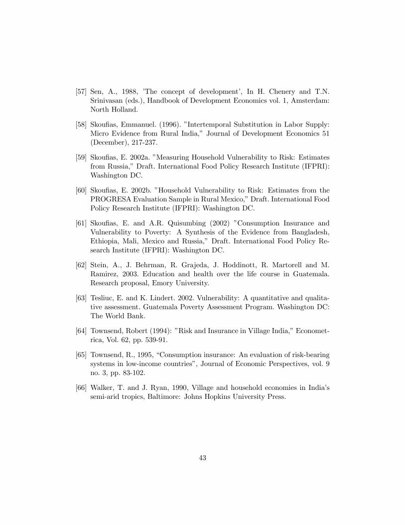
[57] Sen, A., 1988, ’The concept of development’, In H. Chenery and T.N.Srinivasan (eds.), Handbook of Development Economics vol. 1, Amsterdam:North Holland.

[58] Skoufias, Emmanuel. (1996). ”Intertemporal Substitution in Labor Supply:Micro Evidence from Rural India,” Journal of Development Economics 51(December), 217-237.

[59] Skoufias, E. 2002a. ”Measuring Household Vulnerability to Risk: Estimatesfrom Russia,” Draft. International Food Policy Research Institute (IFPRI):Washington DC.

[60] Skoufias, E. 2002b. ”Household Vulnerability to Risk: Estimates from thePROGRESA Evaluation Sample in Rural Mexico,” Draft. International FoodPolicy Research Institute (IFPRI): Washington DC.

[61] Skoufias, E. and A.R. Quisumbing (2002) ”Consumption Insurance andVulnerability to Poverty: A Synthesis of the Evidence from Bangladesh,Ethiopia, Mali, Mexico and Russia,” Draft. International Food Policy Re-search Institute (IFPRI): Washington DC.

[62] Stein, A., J. Behrman, R. Grajeda, J. Hoddinott, R. Martorell and M.Ramirez, 2003. Education and health over the life course in Guatemala.Research proposal, Emory University.

[63] Tesliuc, E. and K. Lindert. 2002. Vulnerability: A quantitative and qualita-tive assessment. Guatemala Poverty Assessment Program. Washington DC:The World Bank.

[64] Townsend, Robert (1994): ”Risk and Insurance in Village India,” Economet-rica, Vol. 62, pp. 539-91.

[65] Townsend, R., 1995, “Consumption insurance: An evaluation of risk-bearingsystems in low-income countries”, Journal of Economic Perspectives, vol. 9no. 3, pp. 83-102.

[66] Walker, T. and J. Ryan, 1990, Village and household economies in India’ssemi-arid tropics, Baltimore: Johns Hopkins University Press.

43

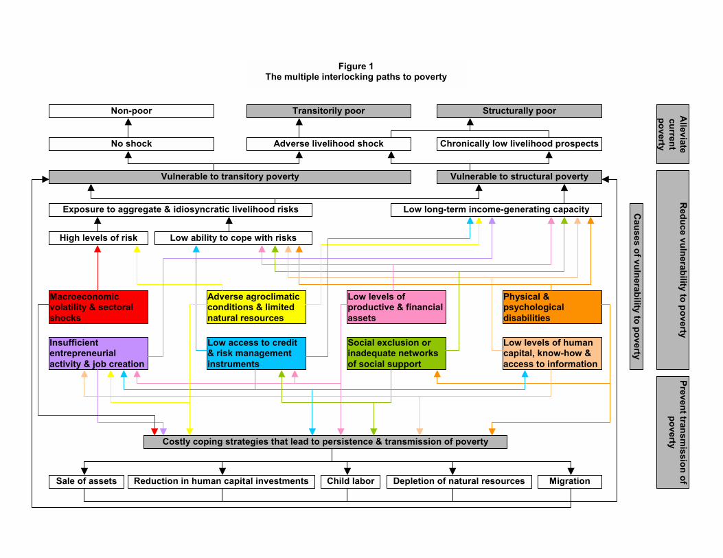
Structurally poor Transitorily poor Non-poor

Adverse livelihood shock Chronically low livelihood prospectsNo shock

Vulnerable to transitory poverty Vulnerable to structural poverty

Exposure to aggregate & idiosyncratic livelihood risks Low long-term income-generating capacity

Alleviate

current poverty

High levels of risk Low ability to cope with risks

Low levels of productive & financial assets

Adverse agroclimatic conditions & limited natural resources

Low levels of human capital, know-how & access to information

Physical & psychological disabilities

Social exclusion or inadequate networks of social support

Insufficient entrepreneurial activity & job creation

Low access to credit & risk management instruments

Macroeconomic volatility & sectoral shocks

Figure 1The multiple interlocking paths to poverty

Costly coping strategies that lead to persistence & transmission of poverty

Sale of assets Reduction in human capital investments Child labor Depletion of natural resources Migration

Causes of vulnerability to poverty

Reduce vulnerability to poverty

Prevent transmission of

poverty

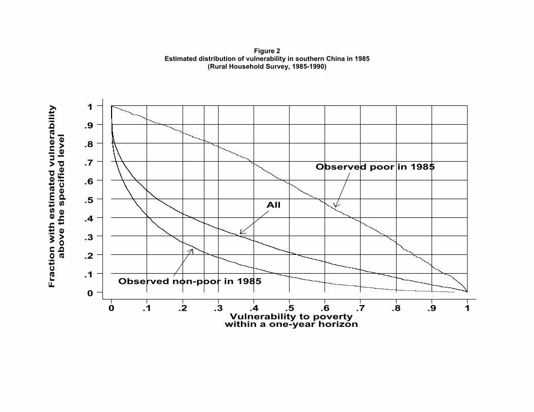
Figure 2 Estimated distribution of vulnerability in southern China in 1985

(Rural Household Survey, 1985-1990)

within a one-year horizonVulnerability to poverty

abo

ve t

he

spec

ifie

d le

vel

Fra

ctio

n w

ith

est

imat

ed v

uln

erab

ility

All

Observed non-poor in 1985

Observed poor in 1985

0 .1 .2 .3 .4 .5 .6 .7 .8 .9 1

0

.1

.2

.3

.4

.5

.6

.7

.8

.9

1

Figure 3

Time period0 10 20 30 40 50

linePoverty

Household A

Household B

Simulated consumption streams for two households

Figure 4

Provincial poverty rate

Aggregate poverty rate

Aggregate estimated vulnerability incidence

for provinces of Philippineswith estimated incidences of vulnerability

Comparison of observed poverty rate

Est

imat

ed p

rovi

ncia

l vul

nera

bilit

y in

cide

nce

0 .25 .5 .75 1

0

.25

.4

.5

.75

1

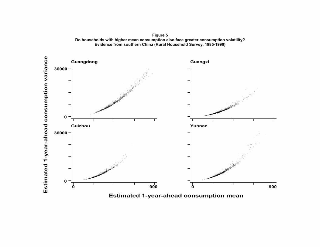
Figure 5

Do households with higher mean consumption also face greater consumption volatility? Evidence from southern China (Rural Household Survey, 1985-1990)

E

stim

ated

1-y

ear-

ahea

d c

on

sum

pti

on

var

ian

ce

Estimated 1-year-ahead consumption mean

Guangdong

0

36000

Guangxi

Guizhou

0 9000

36000

Yunnan

0 900

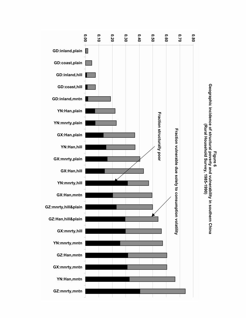
Figure 6 G

eographic incidence of structural poverty and vulnerability in southern China

(Rural H

ousehold Survey, 1985-1990)

0.00

0.10

0.20

0.30

0.40

0.50

0.60

0.70

0.80GD:inland,plain

GD:coast,plain

GD:inland,hill

GD:coast,hill

GD:inland,mntn

YN:Han,plain

YN:mnrty,plain

GX:Han,plain

YN:Han,hill

GX:mnrty,plain

GX:Han,hill

YN:mnrty,hill

GX:Han,mntn

GZ:mnrty,hill&plain

GZ:Han,hill&plain

GX:mnrty,hill

YN:mnrty,mntn

GZ:Han,mntn

GX:mnrty,mntn

YN:Han,mntn

GZ:mnrty,mntn

Fraction structurally poor

Fraction vulnerable due solely to consumption volatility

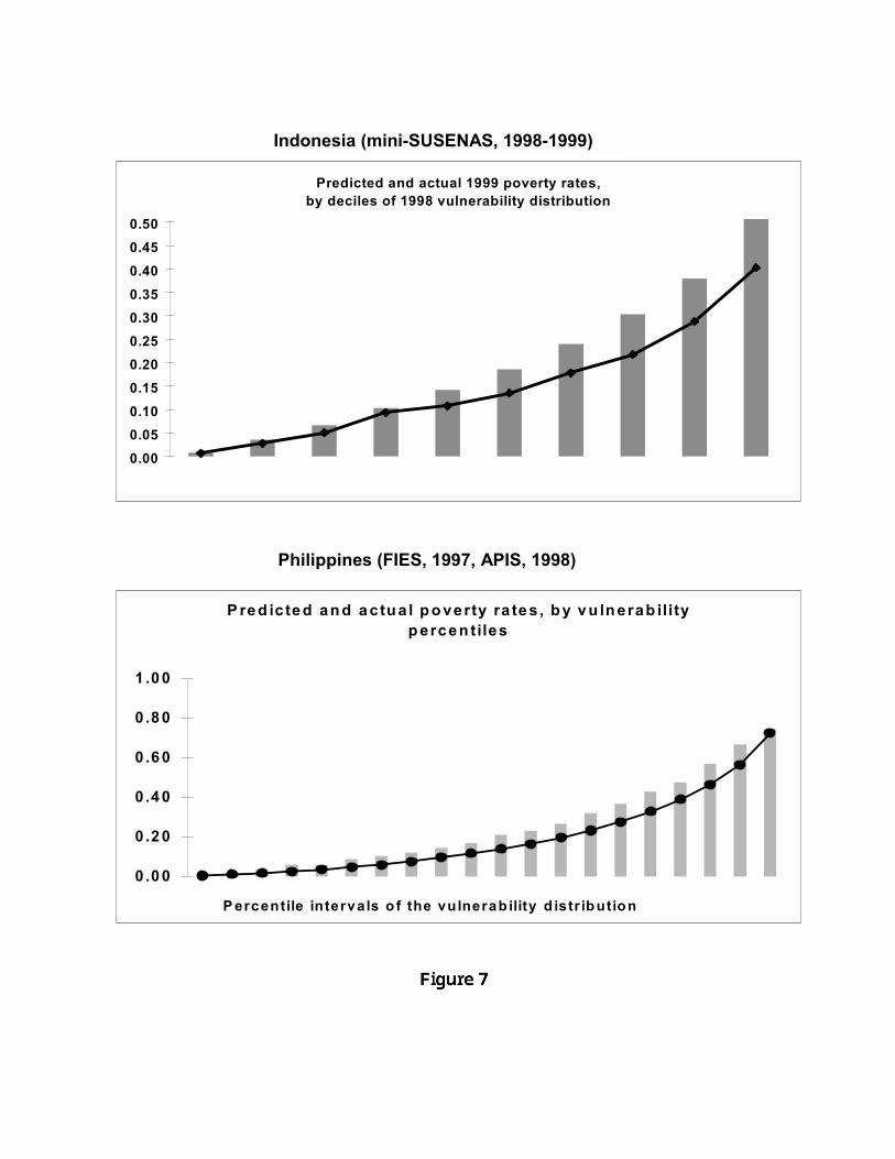
Predicted and actual 1999 poverty rates, by deciles of 1998 vulnerability distribution

0.000.050.100.150.200.250.300.350.400.450.50

P re d ic te d an d a c tu a l p o verty ra te s , b y v u ln erab ility p ercen tiles

0 .0 0

0 .2 0

0 .4 0

0 .6 0

0 .8 0

1 .0 0

P ercentile intervals o f the vulnerab ility d istr ibution

Philippines (FIES, 1997, APIS, 1998)

Indonesia (mini-SUSENAS, 1998-1999)

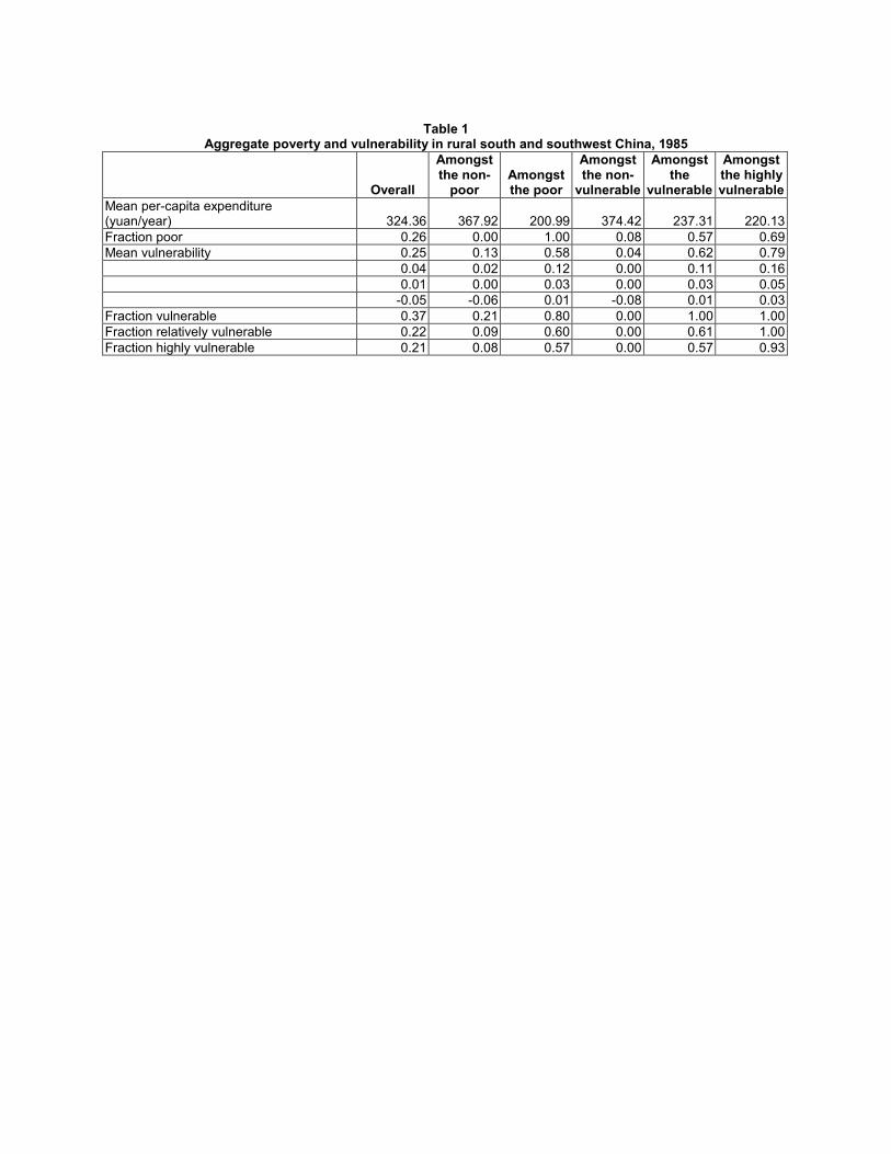
Table 1

Aggregate poverty and vulnerability in rural south and southwest China, 1985

Overall

Amongst the non-

poor

Amongst the poor

Amongst the non-

vulnerable

Amongst the

vulnerable

Amongst the highly vulnerable

Mean per-capita expenditure (yuan/year) 324.36 367.92 200.99 374.42 237.31 220.13Fraction poor 0.26 0.00 1.00 0.08 0.57 0.69Mean vulnerability 0.25 0.13 0.58 0.04 0.62 0.79 0.04 0.02 0.12 0.00 0.11 0.16 0.01 0.00 0.03 0.00 0.03 0.05 -0.05 -0.06 0.01 -0.08 0.01 0.03Fraction vulnerable 0.37 0.21 0.80 0.00 1.00 1.00Fraction relatively vulnerable 0.22 0.09 0.60 0.00 0.61 1.00Fraction highly vulnerable 0.21 0.08 0.57 0.00 0.57 0.93

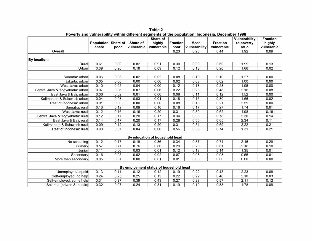
Table 2 Poverty and vulnerability within different segments of the population, Indonesia, December 1998

Population

share

Share of

poor

Share of

vulnerable

Share of highly

vulnerable

Fraction

poor

Mean

vulnerability

Fraction

vulnerable

Vulnerability to poverty

ratio

Fraction highly

vulnerable Overall 0.23 0.23 0.44 1.92 0.09

By location:

Rural 0.61 0.80 0.82 0.91 0.30 0.30 0.60 1.99 0.13 Urban 0.39 0.20 0.18 0.09 0.12 0.13 0.20 1.66 0.02

Sumatra: urban 0.06 0.03 0.02 0.02 0.08 0.10 0.10 1.27 0.00 Jakarta: urban 0.05 0.00 0.00 0.00 0.02 0.03 0.02 1.00 0.00

West Java: urban 0.10 0.05 0.04 0.00 0.12 0.13 0.23 1.95 0.00 Central Java & Yogyakarta: urban 0.07 0.06 0.07 0.06 0.22 0.23 0.48 2.16 0.08

East Java & Bali: urban 0.06 0.02 0.01 0.00 0.08 0.11 0.12 1.52 0.00 Kalimantan & Sulawesi: urban 0.04 0.03 0.03 0.01 0.18 0.16 0.30 1.66 0.02

Rest of Indonesa: urban 0.01 0.00 0.00 0.00 0.08 0.13 0.21 2.59 0.00 Sumatra: rural 0.13 0.12 0.09 0.10 0.16 0.17 0.27 1.74 0.01

West Java: rural 0.12 0.16 0.16 0.20 0.31 0.30 0.62 1.98 0.16 Central Java & Yogyakarta: rural 0.12 0.17 0.20 0.17 0.34 0.35 0.78 2.30 0.14

East Java & Bali: rural 0.14 0.17 0.20 0.17 0.28 0.30 0.65 2.34 0.11 Kalimantan & Sulawesi: rural 0.09 0.12 0.13 0.20 0.31 0.34 0.69 2.22 0.21

Rest of Indonesa: rural 0.03 0.07 0.04 0.06 0.56 0.35 0.74 1.31 0.21

By education of household head No schooling 0.12 0.17 0.19 0.36 0.34 0.37 0.74 2.16 0.28

Primary 0.57 0.71 0.76 0.60 0.29 0.28 0.61 2.16 0.10 Junior 0.11 0.06 0.03 0.01 0.12 0.13 0.14 1.35 0.01

Secondary 0.16 0.05 0.02 0.02 0.07 0.08 0.03 0.55 0.01 More than secondary 0.05 0.01 0.00 0.01 0.01 0.03 0.00 0.00 0.00

By employment status of household head

Unemployed/unpaid 0.13 0.11 0.12 0.12 0.19 0.22 0.43 2.23 0.08 Self-employed: no help 0.24 0.25 0.25 0.13 0.22 0.22 0.46 2.10 0.03

Self-employed: some help 0.31 0.37 0.39 0.43 0.27 0.28 0.57 2.11 0.12 Salaried (private & public) 0.32 0.27 0.24 0.31 0.19 0.19 0.33 1.78 0.08

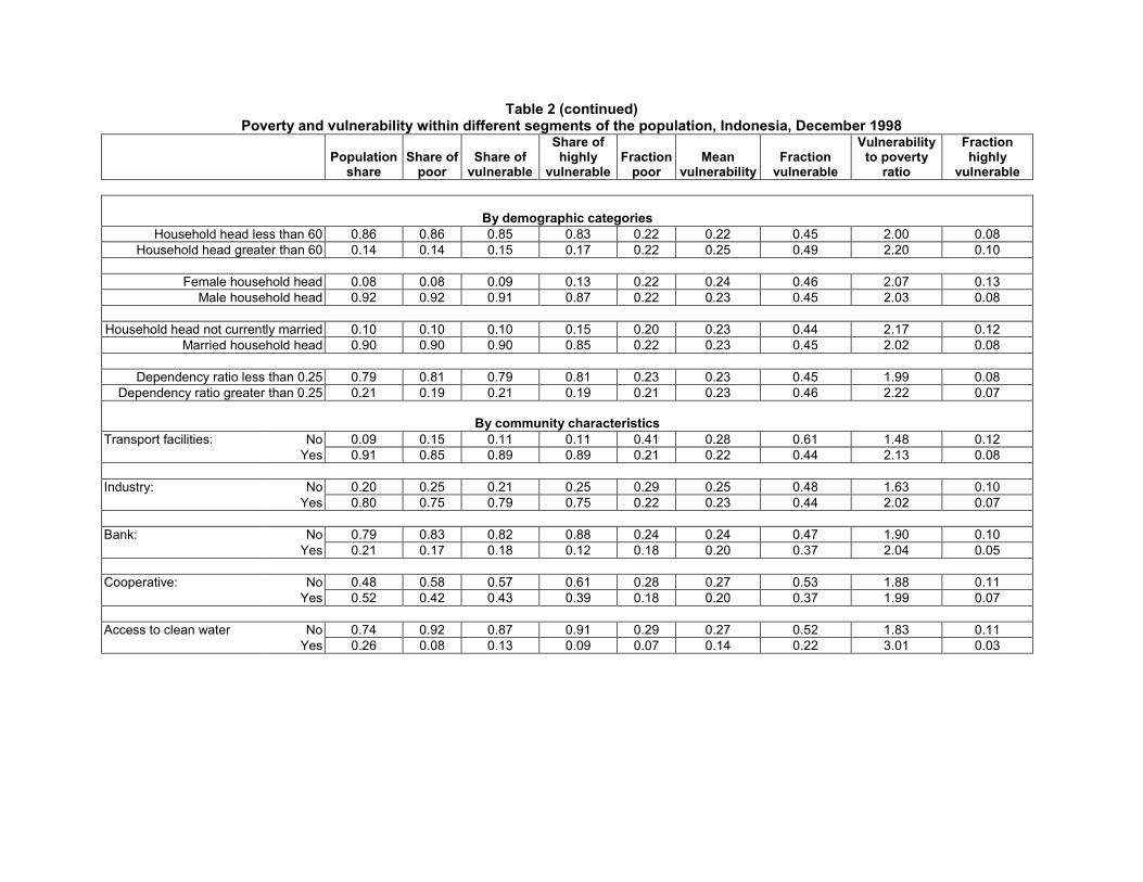
Table 2 (continued) Poverty and vulnerability within different segments of the population, Indonesia, December 1998

Population

share

Share of

poor

Share of

vulnerable

Share of highly

vulnerable

Fraction

poor

Mean

vulnerability

Fraction

vulnerable

Vulnerability to poverty

ratio

Fraction highly

vulnerable

By demographic categories

Household head less than 60 0.86 0.86 0.85 0.83 0.22 0.22 0.45 2.00 0.08 Household head greater than 60 0.14 0.14 0.15 0.17 0.22 0.25 0.49 2.20 0.10

Female household head 0.08 0.08 0.09 0.13 0.22 0.24 0.46 2.07 0.13

Male household head 0.92 0.92 0.91 0.87 0.22 0.23 0.45 2.03 0.08

Household head not currently married 0.10 0.10 0.10 0.15 0.20 0.23 0.44 2.17 0.12 Married household head 0.90 0.90 0.90 0.85 0.22 0.23 0.45 2.02 0.08

Dependency ratio less than 0.25 0.79 0.81 0.79 0.81 0.23 0.23 0.45 1.99 0.08

Dependency ratio greater than 0.25 0.21 0.19 0.21 0.19 0.21 0.23 0.46 2.22 0.07

By community characteristics Transport facilities: No 0.09 0.15 0.11 0.11 0.41 0.28 0.61 1.48 0.12 Yes 0.91 0.85 0.89 0.89 0.21 0.22 0.44 2.13 0.08

Industry: No 0.20 0.25 0.21 0.25 0.29 0.25 0.48 1.63 0.10

Yes 0.80 0.75 0.79 0.75 0.22 0.23 0.44 2.02 0.07

Bank: No 0.79 0.83 0.82 0.88 0.24 0.24 0.47 1.90 0.10 Yes 0.21 0.17 0.18 0.12 0.18 0.20 0.37 2.04 0.05

Cooperative: No 0.48 0.58 0.57 0.61 0.28 0.27 0.53 1.88 0.11

Yes 0.52 0.42 0.43 0.39 0.18 0.20 0.37 1.99 0.07

Access to clean water No 0.74 0.92 0.87 0.91 0.29 0.27 0.52 1.83 0.11 Yes 0.26 0.08 0.13 0.09 0.07 0.14 0.22 3.01 0.03

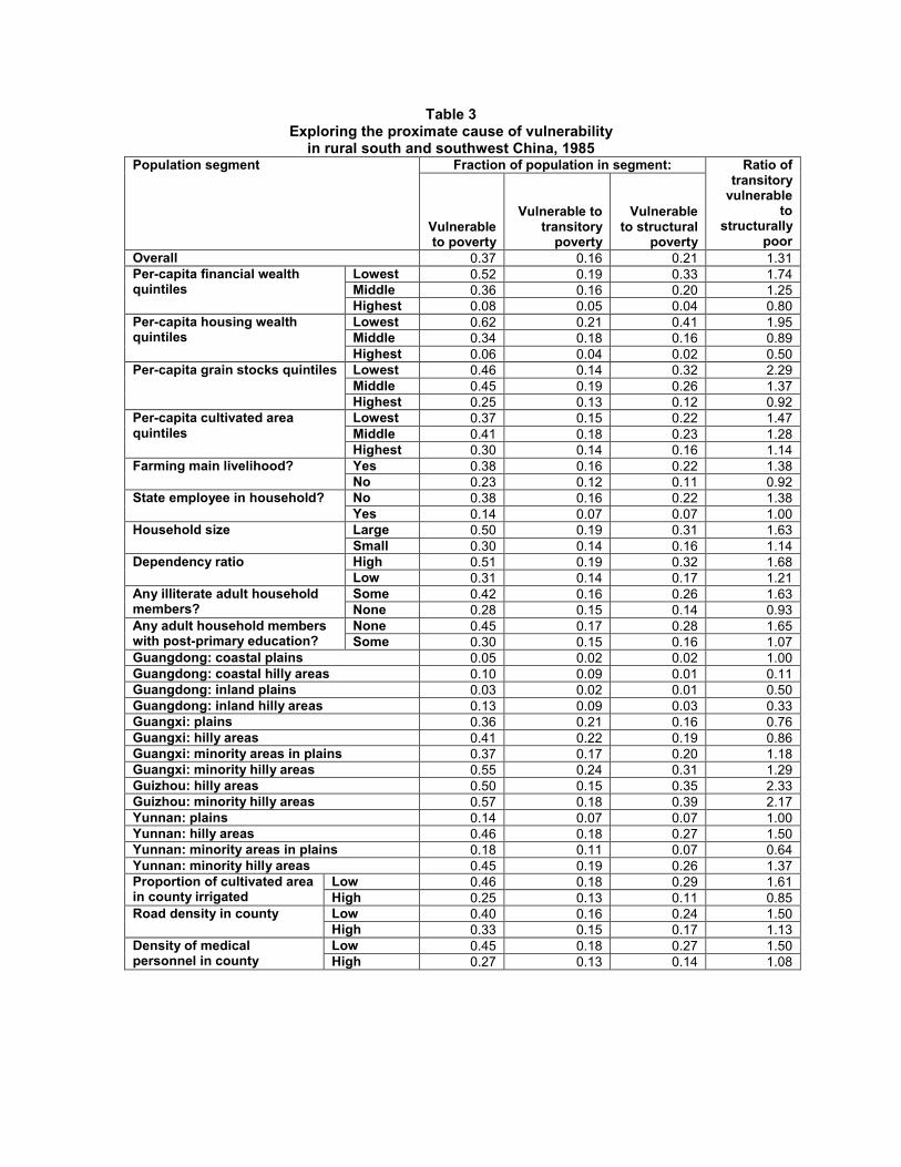
Table 3 Exploring the proximate cause of vulnerability

in rural south and southwest China, 1985 Fraction of population in segment: Population segment

Vulnerable to poverty

Vulnerable to transitory

poverty

Vulnerable to structural

poverty

Ratio of transitory

vulnerable to

structurally poor

Overall 0.37 0.16 0.21 1.31 Lowest 0.52 0.19 0.33 1.74 Middle 0.36 0.16 0.20 1.25

Per-capita financial wealth quintiles

Highest 0.08 0.05 0.04 0.80 Lowest 0.62 0.21 0.41 1.95 Middle 0.34 0.18 0.16 0.89

Per-capita housing wealth quintiles

Highest 0.06 0.04 0.02 0.50 Lowest 0.46 0.14 0.32 2.29 Middle 0.45 0.19 0.26 1.37

Per-capita grain stocks quintiles

Highest 0.25 0.13 0.12 0.92 Lowest 0.37 0.15 0.22 1.47 Middle 0.41 0.18 0.23 1.28

Per-capita cultivated area quintiles

Highest 0.30 0.14 0.16 1.14 Yes 0.38 0.16 0.22 1.38 Farming main livelihood?

No 0.23 0.12 0.11 0.92 No 0.38 0.16 0.22 1.38 State employee in household? Yes 0.14 0.07 0.07 1.00 Large 0.50 0.19 0.31 1.63 Household size Small 0.30 0.14 0.16 1.14 High 0.51 0.19 0.32 1.68 Dependency ratio Low 0.31 0.14 0.17 1.21 Some 0.42 0.16 0.26 1.63 Any illiterate adult household

members? None 0.28 0.15 0.14 0.93 None 0.45 0.17 0.28 1.65 Any adult household members

with post-primary education? Some 0.30 0.15 0.16 1.07 Guangdong: coastal plains 0.05 0.02 0.02 1.00 Guangdong: coastal hilly areas 0.10 0.09 0.01 0.11 Guangdong: inland plains 0.03 0.02 0.01 0.50 Guangdong: inland hilly areas 0.13 0.09 0.03 0.33 Guangxi: plains 0.36 0.21 0.16 0.76 Guangxi: hilly areas 0.41 0.22 0.19 0.86 Guangxi: minority areas in plains 0.37 0.17 0.20 1.18 Guangxi: minority hilly areas 0.55 0.24 0.31 1.29 Guizhou: hilly areas 0.50 0.15 0.35 2.33 Guizhou: minority hilly areas 0.57 0.18 0.39 2.17 Yunnan: plains 0.14 0.07 0.07 1.00 Yunnan: hilly areas 0.46 0.18 0.27 1.50 Yunnan: minority areas in plains 0.18 0.11 0.07 0.64 Yunnan: minority hilly areas 0.45 0.19 0.26 1.37

Low 0.46 0.18 0.29 1.61 Proportion of cultivated area in county irrigated High 0.25 0.13 0.11 0.85

Low 0.40 0.16 0.24 1.50 Road density in county High 0.33 0.15 0.17 1.13 Low 0.45 0.18 0.27 1.50 Density of medical

personnel in county High 0.27 0.13 0.14 1.08

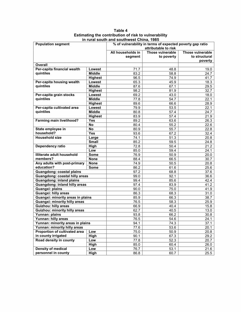
Table 4 Estimating the contribution of risk to vulnerability

in rural south and southwest China, 1985 % of vulnerability in terms of expected poverty gap ratio

attributable to risk Population segment

All households in segment

Those vulnerable to poverty

Those vulnerable to structural

povertyOverall

Lowest 71.7 48.8 19.0 Middle 83.2 58.8 24.7

Per-capita financial wealth quintiles

Highest 96.5 74.9 41.7 Lowest 65.3 45.9 18.3 Middle 87.6 67.1 29.5

Per-capita housing wealth quintiles

Highest 98.2 81.9 32.7 Lowest 69.2 43.0 18.0 Middle 77.8 54.7 22.1

Per-capita grain stocks quintiles

Highest 89.6 66.6 28.9 Lowest 79.9 53.5 22.1 Middle 80.8 57.4 24.7

Per-capita cultivated area quintiles

Highest 83.9 57.4 21.9 Yes 89.2 63.6 26.3 Farming main livelihood?

No 80.4 55.2 22.6 No 80.9 55.7 22.8 State employee in

household? Yes 93.6 67.2 32.4 Large 74.1 51.3 20.8 Household size Small 85.2 59.5 24.8 High 72.8 50.4 21.2 Dependency ratio Low 85.0 59.4 24.1 Some 76.9 50.9 20.0 Illiterate adult household

members? None 88.4 66.5 30.7 None 74.9 50.5 20.8 Any adults with post-primary

education? Some 86.2 61.6 25.6 Guangdong: coastal plains 97.2 68.8 37.6 Guangdong: coastal hilly areas 99.0 92.1 36.6 Guangdong: inland plains 99.4 85.6 42.4 Guangdong: inland hilly areas 97.4 83.9 41.2 Guangxi: plains 90.0 75.0 41.9 Guangxi: hilly areas 86.3 68.3 31.0 Guangxi: minority areas in plains 85.9 66.3 38.7 Guangxi: minority hilly areas 76.5 58.3 25.9 Guizhou: hilly areas 66.9 40.4 15.8 Guizhou: minority hilly areas 62.7 40.5 13.0 Yunnan: plains 93.8 66.2 30.8 Yunnan: hilly areas 76.5 54.6 24.1 Yunnan: minority areas in plains 94.1 74.3 37.1 Yunnan: minority hilly areas 77.6 53.6 20.1

Low 75.0 50.9 20.8 Proportion of cultivated area in county irrigated High 90.1 67.3 29.2

Low 77.8 52.3 20.7 Road density in county High 85.0 60.4 26.0 Low 76.7 53.1 21.6 Density of medical

personnel in county High 86.8 60.7 25.5