Embed Size (px)
Citation preview
ASSESSMENT OF AQUIFER RECHARGE, GROUND-WATER PRODUCTION IMPACTS,
AND FUTURE GROUND-WATER DEVELOPMENT
IN SOUTHEAST ALABAMA
GEOLOGICAL SURVEY OF ALABAMA
Berry H. Tew, Jr. State Geologist
ASSESSMENT OF AQUIFER RECHARGE, GROUND-WATER PRODUCTION IMPACTS, AND FUTURE GROUND-WATER
DEVELOPMENT IN SOUTHEAST ALABAMA
A REPORT TO THE
CHOCTAWHATCHEE, PEA, AND YELLOW RIVERS WATERSHED MANAGEMENT AUTHORITY
OPEN FILE REPORT 0803
By Marlon R. Cook,
Stephen P. Jennings, and
Neil E. Moss
Submitted in partial fulfillment of a contract with the Choctawhatchee, Pea and Yellow Rivers Watershed Management Authority
Tuscaloosa, Alabama 2007
Table of Contents Introduction ........................................................................................................................... 1
Acknowledgments.................................................................................................................. 1
Hydrogeology ........................................................................................................................ 3
Scope of study and methods ............................................................................................ 3
Gordo aquifer ................................................................................................................... 8
Ripley/Cusseta aquifer ..................................................................................................... 8
Clayton and Salt Mountain aquifers ................................................................................ 9
Nanafalia aquifer.............................................................................................................. 10
Tallahatta aquifer ............................................................................................................. 10
Recharge ................................................................................................................................ 11
Ground-water production....................................................................................................... 14
Water use and demand ..................................................................................................... 14
Ground-water drawdown ....................................................................................................... 15
Hydrographs..................................................................................................................... 15
Potentiometric surfaces.......................................................................................................... 24
Well capture zones................................................................................................................. 25
Gordo aquifer ................................................................................................................... 28
Ripley/Cusseta aquifer ..................................................................................................... 28
Clayton and Salt Mountain aquifers ................................................................................ 29
Nanafalia aquifer.............................................................................................................. 30
Tuscahoma aquifer........................................................................................................... 31
Tallahatta aquifer ............................................................................................................. 31
Lisbon aquifer .................................................................................................................. 32
Crystal River aquifer........................................................................................................ 32
Conclusions and recommendations........................................................................................ 34
Gordo aquifer ................................................................................................................... 34
Ripley/Cusseta aquifer ..................................................................................................... 35
Clayton and Salt Mountain aquifers ................................................................................ 35
Nanafalia aquifer.............................................................................................................. 36
Crystal River aquifer........................................................................................................ 36
ii
References cited ..................................................................................................................... 37
Illustrations
Figure 1. Index map showing area of study ........................................................................ 2
Figure 2. General geologic map of southeast Alabama....................................................... 4
Figure 3. Generalized stratigraphy of southeast Alabama .................................................. 5
Figure 4. Geophysical well logs illustrating method for determining net sand
thickness............................................................................................................... 7
Figure 5. Ground-water flow systems showing the movement of shallow and
deep recharge ....................................................................................................... 12
Figure 6. Southeast Alabama aquifer recharge areas and stream flow data sites
used to calculate recharge rates............................................................................ 13
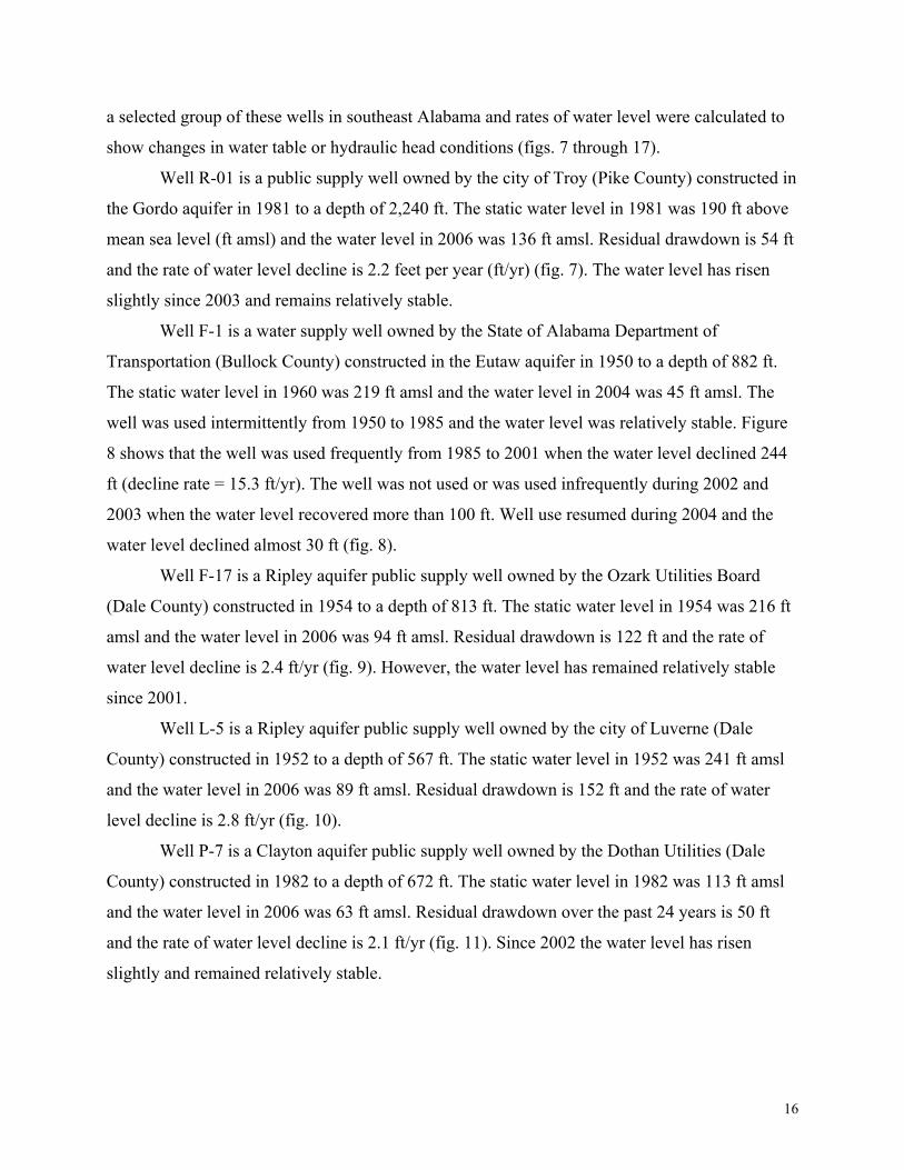
Figure 7. Hydrograph of city of Troy Gordo aquifer well R-01, Pike County,
Alabama ............................................................................................................... 17
Figure 8. Hydrograph of State of Alabama Department of Transportation Eutaw
aquifer well F-1, Bullock County, Alabama........................................................ 17
Figure 9. Hydrograph of Ozark Utilities Board Ripley aquifer well F-17, Dale
County, Alabama ................................................................................................. 18
Figure 10. Hydrograph of city of Luverne Ripley aquifer well L-5, Crenshaw
County, Alabama ................................................................................................. 18
Figure 11. Hydrograph of Dothan Utilities Clayton aquifer well P-7, Dale County,
Alabama ............................................................................................................... 20
Figure 12. Hydrograph of city of Elba Clayton aquifer well K-4, Coffee County,
Alabama ............................................................................................................... 20
Figure 13. Hydrograph of city of Enterprise Salt Mountain aquifer well Q-4,
Coffee County, Alabama ..................................................................................... 21
Figure 14. Hydrograph of Dothan Utilities Nanafalia aquifer well J-3, Houston
County, Alabama ................................................................................................. 21
Figure 15. Hydrograph of Nanafalia aquifer well F-1, Coffee County, Alabama ................ 22
Figure 16. Hydrograph of Fort Rucker Nanafalia aquifer well G-02, Dale County,
Alabama ............................................................................................................... 22
iii
Figure 17. Hydrograph of Crystal River aquifer irrigation well X-2, Houston
County, Alabama ................................................................................................. 23
Figure 18. Diagram depicting drawdown and potentiometric surfaces prior to and
after pumping in a confined aquifer..................................................................... 24
Figure 19. Capture zone for city of Dothan well 20.............................................................. 26
Tables Table 1. Recharge areas and estimates of recharge for selected aquifers in
southeast Alabama ............................................................................................... 14
Table 2. Water use and estimated future water demand in southeast Alabama................. 15
Table 3. Ground-water level and flow data for southeast Alabama aquifers..................... 33
Table 4. Well capture zone and spacing data for southeast Alabama aquifers .................. 34
Plates Plate 1. Gordo aquifer net sand isopach map
Plate 2. Ripley/Cusseta aquifer net sand isopach map
Plate 3. Clayton aquifer net sand/limestone isopach map
Plate 4. Salt Mountain aquifer net sand/limestone isopach map
Plate 5. Nanafalia aquifer net sand isopach map
Plate 6. Tallahatta aquifer net sand isopach map
Plate 7. Potentiometric surface for the Gordo aquifer, southeast Alabama
Plate 8. Residual drawdown in selected wells constructed in the Gordo aquifer,
southeast Alabama
Plate 9. Potentiometric surface for the Ripley/Cusseta aquifer, southeast
Alabama
Plate 10. Residual drawdown in selected wells constructed in the Ripley/Cusseta
aquifer, southeast Alabama
Plate 11. Potentiometric surface for the Clayton and Salt Mountain aquifers,
southeast Alabama
Plate 12. Residual drawdown in selected wells constructed in the Clayton and
Salt Mountain aquifers, southeast Alabama
Plate 13. Potentiometric surface for the Nanafalia aquifer, southeast Alabama
Plate 14. Residual drawdown in selected wells constructed in the Nanafalia
aquifer, southeast Alabama
iv
Plate 15. Potentiometric surface for the Tuscahoma aquifer, southeast Alabama
Plate 16. Residual drawdown in selected wells constructed in the Tuscahoma
aquifer, southeast Alabama
Plate 17. Potentiometric surface for the Tallahatta aquifer, southeast Alabama
Plate 18. Residual drawdown in selected wells constructed in the Tallahatta
aquifer, southeast Alabama
Plate 19. Potentiometric surface for the Lisbon aquifer, southeast Alabama
Plate 20. Residual drawdown in selected wells constructed in the Lisbon aquifer,
southeast Alabama
Plate 21. Potentiometric surface for the Crystal River aquifer, southeast Alabama
Plate 22. Residual drawdown in selected wells constructed in the Crystal River
aquifer, southeast Alabama
v
1
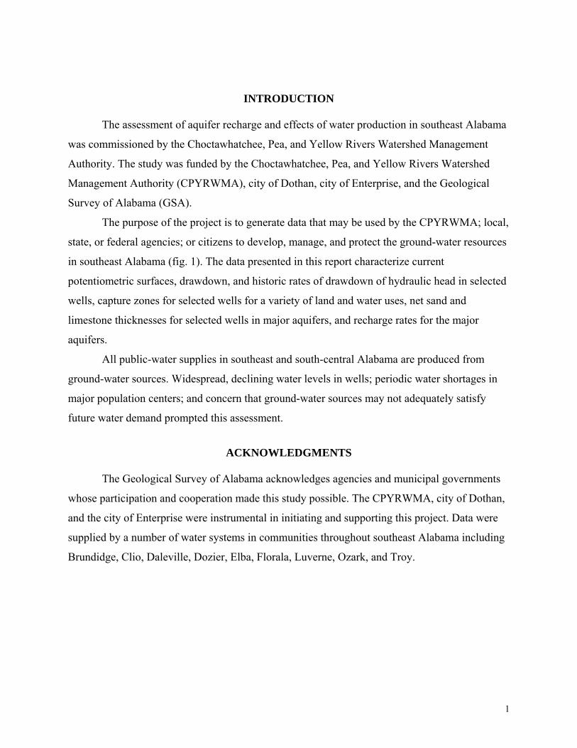
INTRODUCTION The assessment of aquifer recharge and effects of water production in southeast Alabama
was commissioned by the Choctawhatchee, Pea, and Yellow Rivers Watershed Management
Authority. The study was funded by the Choctawhatchee, Pea, and Yellow Rivers Watershed
Management Authority (CPYRWMA), city of Dothan, city of Enterprise, and the Geological
Survey of Alabama (GSA).
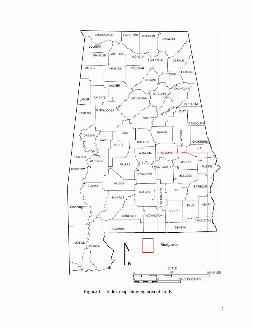
The purpose of the project is to generate data that may be used by the CPYRWMA; local,
state, or federal agencies; or citizens to develop, manage, and protect the ground-water resources
in southeast Alabama (fig. 1). The data presented in this report characterize current
potentiometric surfaces, drawdown, and historic rates of drawdown of hydraulic head in selected
wells, capture zones for selected wells for a variety of land and water uses, net sand and
limestone thicknesses for selected wells in major aquifers, and recharge rates for the major
aquifers.
All public-water supplies in southeast and south-central Alabama are produced from
ground-water sources. Widespread, declining water levels in wells; periodic water shortages in
major population centers; and concern that ground-water sources may not adequately satisfy
future water demand prompted this assessment.
ACKNOWLEDGMENTS
The Geological Survey of Alabama acknowledges agencies and municipal governments
whose participation and cooperation made this study possible. The CPYRWMA, city of Dothan,
and the city of Enterprise were instrumental in initiating and supporting this project. Data were
supplied by a number of water systems in communities throughout southeast Alabama including
Brundidge, Clio, Daleville, Dozier, Elba, Florala, Luverne, Ozark, and Troy.
2
Washington
Study area
Figure 1.-- Index map showing area of study.
3
HYDROGEOLOGY
SCOPE OF STUDY AND METHODS
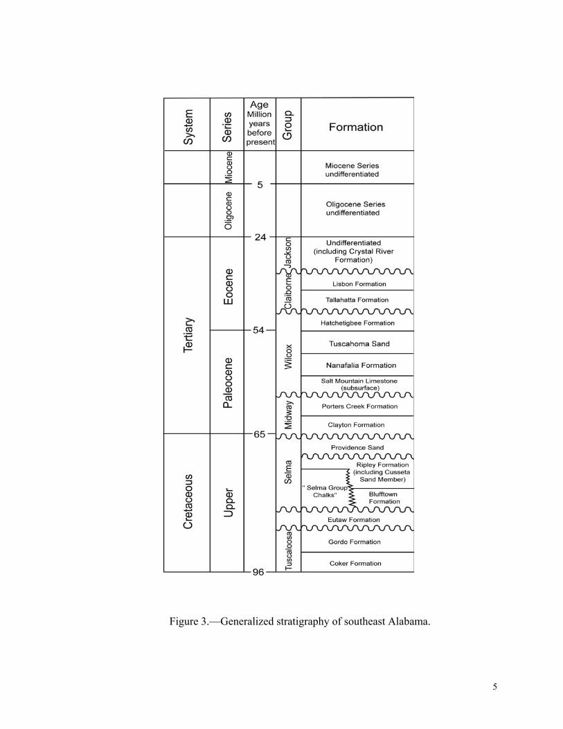
Aquifers are parts of formal geologic units that are capable of storing and transmitting
useful quantities of ground water. The aquifers in southeastern Alabama are contained in
sedimentary geologic formations deposited in the area during the Late Cretaceous Period
(approximately 90 million years ago) to the Miocene epoch (approximately 35 million years
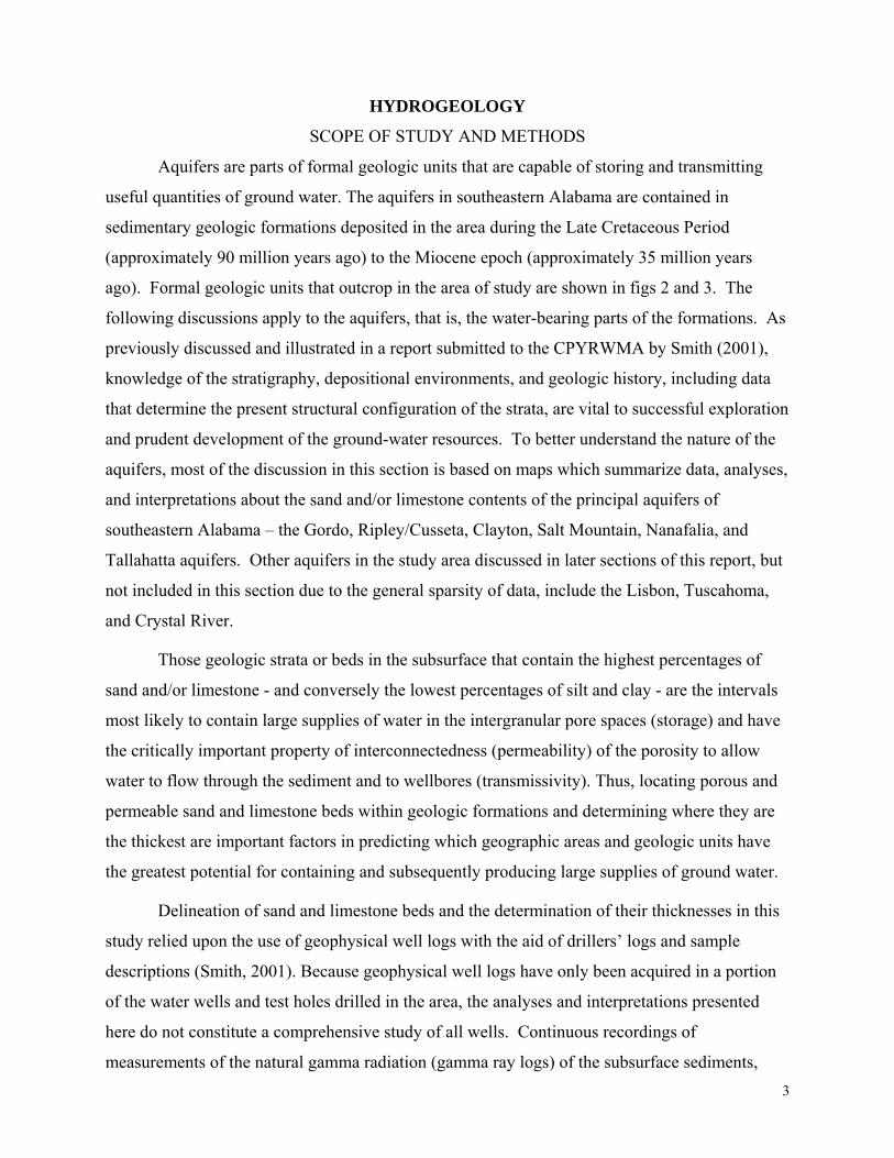
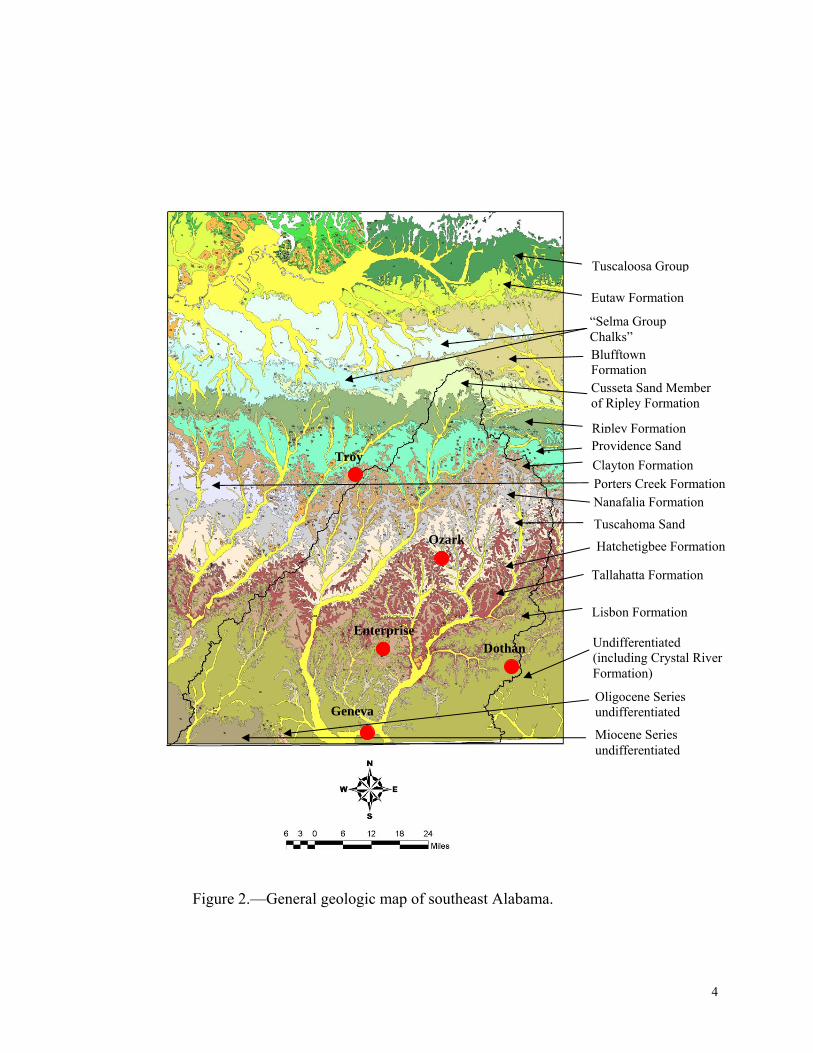
ago). Formal geologic units that outcrop in the area of study are shown in figs 2 and 3. The
following discussions apply to the aquifers, that is, the water-bearing parts of the formations. As
previously discussed and illustrated in a report submitted to the CPYRWMA by Smith (2001),
knowledge of the stratigraphy, depositional environments, and geologic history, including data
that determine the present structural configuration of the strata, are vital to successful exploration
and prudent development of the ground-water resources. To better understand the nature of the
aquifers, most of the discussion in this section is based on maps which summarize data, analyses,
and interpretations about the sand and/or limestone contents of the principal aquifers of
southeastern Alabama – the Gordo, Ripley/Cusseta, Clayton, Salt Mountain, Nanafalia, and
Tallahatta aquifers. Other aquifers in the study area discussed in later sections of this report, but
not included in this section due to the general sparsity of data, include the Lisbon, Tuscahoma,
and Crystal River.
Those geologic strata or beds in the subsurface that contain the highest percentages of
sand and/or limestone - and conversely the lowest percentages of silt and clay - are the intervals
most likely to contain large supplies of water in the intergranular pore spaces (storage) and have
the critically important property of interconnectedness (permeability) of the porosity to allow
water to flow through the sediment and to wellbores (transmissivity). Thus, locating porous and
permeable sand and limestone beds within geologic formations and determining where they are
the thickest are important factors in predicting which geographic areas and geologic units have
the greatest potential for containing and subsequently producing large supplies of ground water.
Delineation of sand and limestone beds and the determination of their thicknesses in this
study relied upon the use of geophysical well logs with the aid of drillers’ logs and sample
descriptions (Smith, 2001). Because geophysical well logs have only been acquired in a portion
of the water wells and test holes drilled in the area, the analyses and interpretations presented
here do not constitute a comprehensive study of all wells. Continuous recordings of
measurements of the natural gamma radiation (gamma ray logs) of the subsurface sediments,
Enterprise
Ozark
Troy
Figure 2.—General geologic map of southeast Alabama.
Dothan
Geneva
p
Tuscaloosa Grou“Selma Group Chalks”
Eutaw Formation
BlufftownFormation
Cusseta Sand Memberof Ripley Formation Ripley FormationNanafalia Formation Porters Creek Formation
d
Clayton Formation Providence Sand
Hatchetigbee Formation
Tallahatta Formation
Tuscahoma San
Lisbon Formation
Undifferentiated (including Crystal River Formation)
Oligocene Series undifferentiated
4
Miocene Series undifferentiated
5
Figure 3.—Generalized stratigraphy of southeast Alabama.
6
coupled with resistivity and spontaneous potential (SP) logs, were the principal means of
determining the likely presence and thicknesses of quartz sand and limestone intervals in
formations penetrated by boreholes. Gamma ray logs are not affected by formation water
salinity, whereas resistivity and spontaneous potential logs are electrical measurements of the
formation sediments and their contained water. Typically not recorded in water well test holes,
due to costs and other considerations, are porosity measuring logging devices. These tools, as
well as numerous other types of logs, have been utilized for years in the oil and gas exploration
industry to help determine porous and permeable beds.
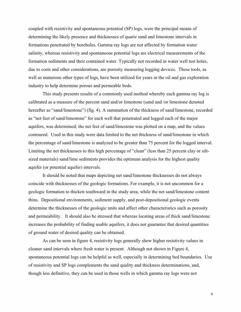
This study presents results of a commonly used method whereby each gamma ray log is
calibrated as a measure of the percent sand and/or limestone (sand and /or limestone denoted
hereafter as “sand/limestone”) (fig. 4). A summation of the thickness of sand/limestone, recorded
as “net feet of sand/limestone” for each well that penetrated and logged each of the major
aquifers, was determined; the net feet of sand/limestone was plotted on a map, and the values
contoured. Used in this study were data limited to the net thickness of sand/limestone in which
the percentage of sand/limestone is analyzed to be greater than 75 percent for the logged interval.
Limiting the net thicknesses to this high percentage of “clean” (less than 25 percent clay or silt-
sized materials) sand/lime sediments provides the optimum analysis for the highest quality
aquifer (or potential aquifer) intervals.
It should be noted that maps depicting net sand/limestone thicknesses do not always
coincide with thicknesses of the geologic formations. For example, it is not uncommon for a
geologic formation to thicken southward in the study area, while the net sand/limestone content
thins. Depositional environments, sediment supply, and post-depositional geologic events
determine the thicknesses of the geologic units and affect other characteristics such as porosity
and permeability . It should also be stressed that whereas locating areas of thick sand/limestone
increases the probability of finding usable aquifers, it does not guarantee that desired quantities
of ground water of desired quality can be obtained.
As can be seen in figure 4, resistivity logs generally show higher resistivity values in
cleaner sand intervals where fresh water is present. Although not shown in Figure 4,
spontaneous potential logs can be helpful as well, especially in determining bed boundaries. Use
of resistivity and SP logs complements the sand quality and thickness determinations, and,
though less definitive, they can be used in those wells in which gamma ray logs were not
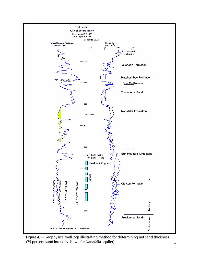
Figure 4. - - Geophysical well logs illustrating method for determining net sand thickness (75 percent sand intervals shown for Nanafalia aquifer).
7
8
acquired to give a general estimate of net sand thickness. The data presented on the maps
(plates) in this report suggest downdip limits of water production in the aquifers are commonly a
combination of net sand/limestone determination and water-quality (salinity) estimation from
geophysical logs.
GORDO AQUIFER
Sands and gravels comprising the Cretaceous Gordo aquifer are thickest from eastern
Crenshaw County across southwestern Pike, northern Coffee, and northwestern Dale Counties
(plate 1). The Gordo aquifer also thickens along the eastern side of the study area toward the
Chattahoochee River area. Because much of the Gordo Formation was deposited under
nonmarine conditions, the thickness pattern shown in plate 1 probably reflects a depositional
history wherein the sediments filled pre-existing topographic low areas that were developed by
exposure and subsequent erosion of the Coker and overlying middle marine shale of the
Tuscaloosa Group.
The downdip (southerly) limit of water production in the Gordo aquifer (plate 1) is due
primarily to higher salinity of the formation waters downdip rather than a lack of sand and gravel
to the south. However, the limit shown is currently poorly defined, with well F-07, located
approximately 4 miles north of downtown Ozark, the most southerly freshwater production
established to date from the aquifer at a drilled depth of more than 2,700 feet (2,200 feet below
sea level). Additional drilling and testing is needed to verify preliminary indications from
geophysical well logs taken from oil and gas test holes that fresh water may exist in the Gordo
farther to the south.
RIPLEY/CUSSETA AQUIFER
Sand beds of the Cretaceous Ripley Formation and its locally present Cusseta Sand
Member comprise a significant aquifer across a portion of the study area. The thickest net sand
area of the Ripley/Cusseta aquifer (plate 2) extends from southeastern Crenshaw County across
southern Pike County and probably connects to a thick area in south-central Henry County.
Another thick area is in northwestern Houston County, but the sands there appear to contain
brackish water. The downdip limit of freshwater occurrence extends from southernmost
Crenshaw County southeastward through Coffee County and thence in an easterly direction
across southern Dale and Henry Counties.
9
CLAYTON AND SALT MOUNTAIN AQUIFERS
The Tertiary Clayton Formation is composed of limestone and sand beds that locally
comprise important aquifers in southeastern Alabama. As shown in plate 3, a thick area of net
sand and/or limestone extends from northwestern Houston County across southern Dale County
and south-central Coffee County. The Clayton appears to thin away from this “fairway,” though
this thinning is poorly defined, especially in the downdip (southerly) direction. The probable
downdip limit of water production in the Clayton aquifer extends across central Covington
County, thence southeasterly to Geneva County, and continues eastward across the southern part
of the study area. This limit appears to be due to both thinning of the net sand/limestone and to
an increase in salinity of the ground water.
Notwithstanding water level data presented later in this report that indicate likely
hydraulic interconnection of the Salt Mountain Limestone and Clayton aquifers over most of the
study area, the Salt Mountain Limestone aquifer was mapped separately in this section (plate 4)
due primarily to its distinctive lithologic character of fossiliferous limestone with quartz sand
interbeds (Smith, 2001). Moreover, the presence locally in the study area of clay beds occurring
between the Clayton Formation and the overlying Salt Mountain Limestone, assigned to the
Porters Creek Formation by Smith (2001), indicates possible local hydraulic separation of the
two units.
Smith (2001) noted the presence of visible porosity in well cuttings of some wells that
penetrated the Salt Mountain Limestone, the presence in some wells of sand interbeds, and the
general absence of clay. The thickest portion of the net “clean” portion of the limestone and
sand extends from northern Covington County southeast into southwestern Coffee County,
north-central Geneva County, and southwestern Dale County. The Salt Mountain is not present
(or, on logs, not distinguishable from the Clayton) north of a line across northern Coffee and
Dale Counties. The downdip limit of fresh water probably extends across south-central
Covington and southwestern Geneva Counties.
NANAFALIA AQUIFER
The Nanafalia Formation contains thick sand intervals along with some limestone beds.
The thickest area of sands and limestones occurs in two main areas – one centered in the
northwestern Houston County “panhandle” and including southern Dale County, and the other
thick area centered in Coffee County west of Enterprise (plate 5). Like other aquifers in this
study, thinning of the formation and its contained sand beds is evident in the updip direction.
The interpreted downdip limit of Nanafalia aquifer water production extends in a general
northwest to southeast line across southern Covington County and southwestern Geneva County.
This limit is the result of a general decrease in the net sand/limestone content and greater salinity
to the southwest.
TALLAHATTA AQUIFER
The thickest net sands of the Tallahatta aquifer occur in northern Geneva County and in
northwestern Houston County (plate 6). Elsewhere, data indicate net sand thicknesses of about
20 to 70 feet, with thinning in the updip (northerly) direction. Sands in the Tallahatta appear to
contain fresh water except in the southwestern part of the study area. Across much of the area
Tallahatta sands appear to be overlain directly by sands of the Lisbon aquifer, indicating likely
hydraulic interconnection of the two aquifers. Lack of data precluded mapping the Lisbon
aquifer.
10
RECHARGE
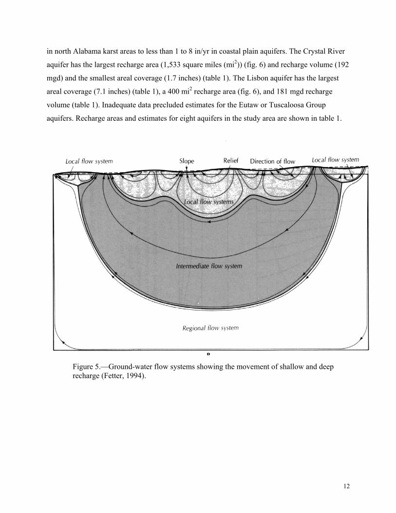
Ground-water recharge is defined as absorption and addition of water to the zone of
saturation and is composed of shallow and deep components (fig. 5). Shallow recharge enters the
aquifer in the outcrop area of each geologic formation (fig. 6) and moves downgradient where
much of it is intercepted by streams that flow across the recharge area (figs. 5, 6). Shallow
ground-water contribution to surface-water discharge is vital to maintain sustained flow,
especially during periods of drought. Stream flow data used to evaluate recharge were taken
from U.S. Geological Survey stations shown on figure 6. Deep recharge underflows streams and
moves downgradient beyond the recharge area where the weight of overburden and upgradient
water forms a pressure head characteristic of confined aquifers.
The rate of aquifer recharge is dependent on the size of the recharge area, permeability of
soils and surface geology, and climatic conditions. The primary means of estimating the quantity
of shallow recharge is by analyses of stream base flow. This methodology uses base flow values
for streams that drain the recharge area of the subject aquifer, since base flow is composed
primarily of ground-water discharges from aquifers. Cook (1993) used five different methods of
base flow analysis to estimate recharge for the Eutaw aquifer in Alabama. These included base
flows estimated from direct stream flow measurement, estimated 7-day Q2 discharge for ungaged
streams using the multiple regression technique developed by Bingham (1979), estimated median
7-day low flow of minor streams (Peirce, 1967), estimated 65 percent duration flow using a flow
duration curve and base flow equation (Stricker, 1983), and analysis of two or more base flow
recession curves based on direct stream flow measurement (Fetter, 1994).
Evaluation of the data quality available for the study and attempts to apply the data to
recharge estimation techniques listed above resulted in the use of base flow data estimated by
Bingham (1979) and Peirce (1967). These values were used to calculate the volume of stream
discharge (ground-water contribution) for each major aquifer recharge area. The resulting
volumes of water were assumed to be equivalent to shallow recharge. Since deep recharge (the
volume of recharge that underflows streams and remains in the subsurface) is a very small part of
total recharge (Stricker, 1983), it was assumed that total recharge equals 105 percent of the
shallow recharge value.
Recharge is commonly reported in millions of gallons per day (mgd) and in inches per
year (in/yr). Due to Alabama’s diverse geology, recharge rates vary greatly, from 10 to 20 in/yr
11
in north Alabama karst areas to less than 1 to 8 in/yr in coastal plain aquifers. The Crystal River
aquifer has the largest recharge area (1,533 square miles (mi2)) (fig. 6) and recharge volume (192
mgd) and the smallest areal coverage (1.7 inches) (table 1). The Lisbon aquifer has the largest
areal coverage (7.1 inches) (table 1), a 400 mi2 recharge area (fig. 6), and 181 mgd recharge
volume (table 1). Inadequate data precluded estimates for the Eutaw or Tuscaloosa Group
aquifers. Recharge areas and estimates for eight aquifers in the study area are shown in table 1.
Figure 5.—Ground-water flow systems showing the movement of shallow and deep recharge (Fetter, 1994).
12
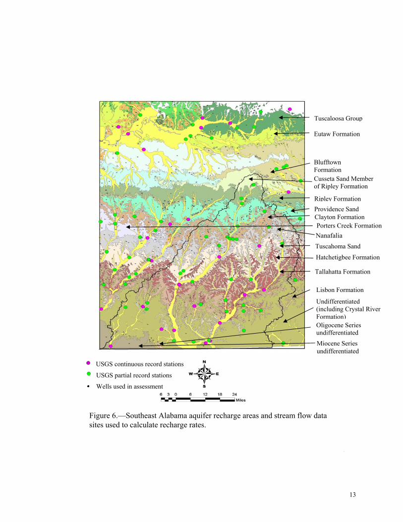
Figure 6.—Southeast Alabama aquifer recharge areas and stream flowsites used to calculate recharge rates.
Wells used in assessment
USGS continuous record stations
USGS partial record stations
Hatchetigbee Formation
Eutaw Formation
Providence Sand
Porters Creek Formation Clayton Formation
Nanafalia
Tallahatta Formation
Tuscaloosa Group
BlufftownFormation
Cusseta Sand Memberof Ripley FormationTuscahoma Sand
Ripley Formation
Lisbon Formation
Undifferentiated (including Crystal River Formation)
Oligocene Series undifferentiated13
data
Miocene Series undifferentiated
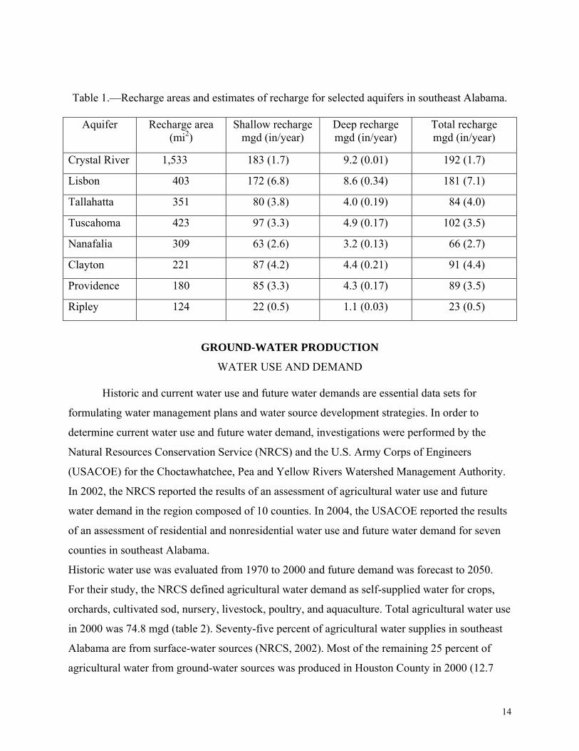
Table 1.—Recharge areas and estimates of recharge for selected aquifers in southeast Alabama.
Aquifer Recharge area
(mi2) Shallow recharge
mgd (in/year) Deep recharge mgd (in/year)
Total recharge mgd (in/year)
Crystal River 1,533 183 (1.7) 9.2 (0.01) 192 (1.7)
Lisbon 403 172 (6.8) 8.6 (0.34) 181 (7.1)
Tallahatta 351 80 (3.8) 4.0 (0.19) 84 (4.0)
Tuscahoma 423 97 (3.3) 4.9 (0.17) 102 (3.5)
Nanafalia 309 63 (2.6) 3.2 (0.13) 66 (2.7)
Clayton 221 87 (4.2) 4.4 (0.21) 91 (4.4)
Providence 180 85 (3.3) 4.3 (0.17) 89 (3.5)
Ripley 124 22 (0.5) 1.1 (0.03) 23 (0.5)
GROUND-WATER PRODUCTION
WATER USE AND DEMAND
Historic and current water use and future water demands are essential data sets for
formulating water management plans and water source development strategies. In order to
determine current water use and future water demand, investigations were performed by the
Natural Resources Conservation Service (NRCS) and the U.S. Army Corps of Engineers
(USACOE) for the Choctawhatchee, Pea and Yellow Rivers Watershed Management Authority.
In 2002, the NRCS reported the results of an assessment of agricultural water use and future
water demand in the region composed of 10 counties. In 2004, the USACOE reported the results
of an assessment of residential and nonresidential water use and future water demand for seven
counties in southeast Alabama.
Historic water use was evaluated from 1970 to 2000 and future demand was forecast to 2050.
For their study, the NRCS defined agricultural water demand as self-supplied water for crops,
orchards, cultivated sod, nursery, livestock, poultry, and aquaculture. Total agricultural water use
in 2000 was 74.8 mgd (table 2). Seventy-five percent of agricultural water supplies in southeast
Alabama are from surface-water sources (NRCS, 2002). Most of the remaining 25 percent of
agricultural water from ground-water sources was produced in Houston County in 2000 (12.7
14
mgd). Total agricultural water use in 2000 from ground-water sources in southeast Alabama was
approximately 18.7 mgd. Future water demand estimates for southeast Alabama indicate that by
2050, 200 mgd will be required for agricultural water use (NRCS, 2002). If current ratios of
agricultural ground water to surface water persist, 50 mgd from ground-water sources will be
required.
The USACOE assessment of water use and demand defines residential water as water
used by households and non-residential water as commercial, industrial, government, and public
water use (USACOE, 2004). Currently, all residential and non-residential water use in southeast
Alabama is from ground-water sources. In 2000, residential water use was 37.14 mgd and non-
residential use was 11.20 mgd for a total of 48.34 mgd (table 2). Estimates of future demand
indicate that by 2050 residential use the region will increase to 57.90 mgd and non-residential
use will increase to 17.80 mgd (total 75.70 mgd).
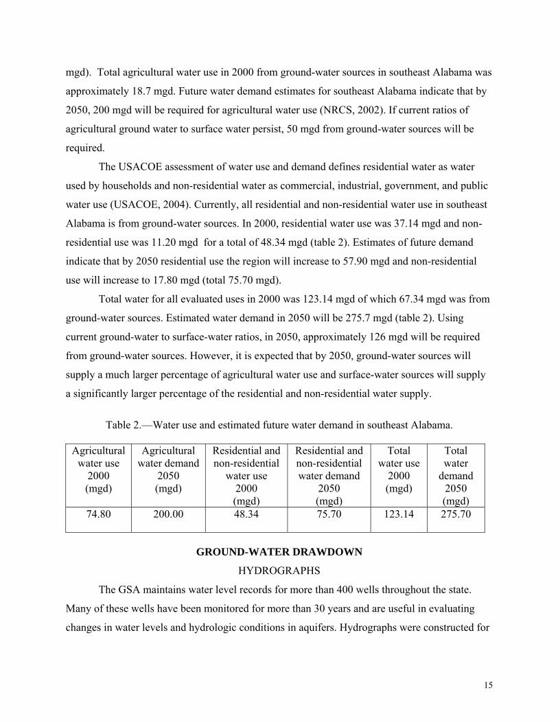
Total water for all evaluated uses in 2000 was 123.14 mgd of which 67.34 mgd was from
ground-water sources. Estimated water demand in 2050 will be 275.7 mgd (table 2). Using
current ground-water to surface-water ratios, in 2050, approximately 126 mgd will be required
from ground-water sources. However, it is expected that by 2050, ground-water sources will
supply a much larger percentage of agricultural water use and surface-water sources will supply
a significantly larger percentage of the residential and non-residential water supply.
Table 2.—Water use and estimated future water demand in southeast Alabama.
Agricultural
water use 2000 (mgd)
Agricultural water demand
2050 (mgd)
Residential and non-residential
water use 2000 (mgd)
Residential and non-residential water demand
2050 (mgd)
Total water use
2000 (mgd)
Total water
demand 2050 (mgd)
74.80 200.00 48.34 75.70 123.14 275.70
GROUND-WATER DRAWDOWN
HYDROGRAPHS
The GSA maintains water level records for more than 400 wells throughout the state.
Many of these wells have been monitored for more than 30 years and are useful in evaluating
changes in water levels and hydrologic conditions in aquifers. Hydrographs were constructed for
15
a selected group of these wells in southeast Alabama and rates of water level were calculated to
show changes in water table or hydraulic head conditions (figs. 7 through 17).
Well R-01 is a public supply well owned by the city of Troy (Pike County) constructed in
the Gordo aquifer in 1981 to a depth of 2,240 ft. The static water level in 1981 was 190 ft above
mean sea level (ft amsl) and the water level in 2006 was 136 ft amsl. Residual drawdown is 54 ft
and the rate of water level decline is 2.2 feet per year (ft/yr) (fig. 7). The water level has risen
slightly since 2003 and remains relatively stable.
Well F-1 is a water supply well owned by the State of Alabama Department of
Transportation (Bullock County) constructed in the Eutaw aquifer in 1950 to a depth of 882 ft.
The static water level in 1960 was 219 ft amsl and the water level in 2004 was 45 ft amsl. The
well was used intermittently from 1950 to 1985 and the water level was relatively stable. Figure
8 shows that the well was used frequently from 1985 to 2001 when the water level declined 244
ft (decline rate = 15.3 ft/yr). The well was not used or was used infrequently during 2002 and
2003 when the water level recovered more than 100 ft. Well use resumed during 2004 and the
water level declined almost 30 ft (fig. 8).
Well F-17 is a Ripley aquifer public supply well owned by the Ozark Utilities Board
(Dale County) constructed in 1954 to a depth of 813 ft. The static water level in 1954 was 216 ft
amsl and the water level in 2006 was 94 ft amsl. Residual drawdown is 122 ft and the rate of
water level decline is 2.4 ft/yr (fig. 9). However, the water level has remained relatively stable
since 2001.
Well L-5 is a Ripley aquifer public supply well owned by the city of Luverne (Dale
County) constructed in 1952 to a depth of 567 ft. The static water level in 1952 was 241 ft amsl
and the water level in 2006 was 89 ft amsl. Residual drawdown is 152 ft and the rate of water
level decline is 2.8 ft/yr (fig. 10).
Well P-7 is a Clayton aquifer public supply well owned by the Dothan Utilities (Dale
County) constructed in 1982 to a depth of 672 ft. The static water level in 1982 was 113 ft amsl
and the water level in 2006 was 63 ft amsl. Residual drawdown over the past 24 years is 50 ft
and the rate of water level decline is 2.1 ft/yr (fig. 11). Since 2002 the water level has risen
slightly and remained relatively stable.
16
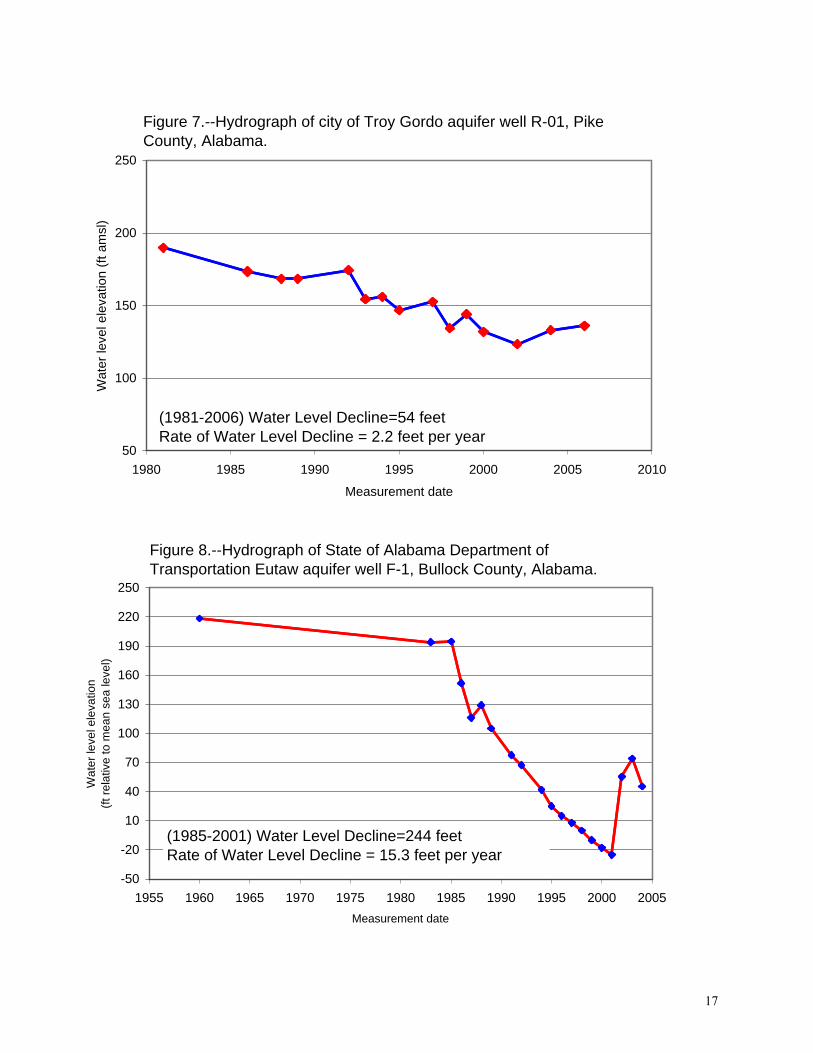
Figure 7.--Hydrograph of city of Troy Gordo aquifer well R-01, Pike County, Alabama.
50
100
150
200
250
1980 1985 1990 1995 2000 2005 2010
Measurement date
Wat
er le
vel e
leva
tion
(ft a
msl
)
(1981-2006) Water Level Decline=54 feetRate of Water Level Decline = 2.2 feet per year
Figure 8.--Hydrograph of State of Alabama Department of Transportation Eutaw aquifer well F-1, Bullock County, Alabama.
-50
-20
10
40
70
100
130
160
190
220
250
1955 1960 1965 1970 1975 1980 1985 1990 1995 2000 2005Measurement date
Wat
er le
vel e
leva
tion
(ft re
lativ
e to
mea
n se
a le
vel)
(1985-2001) Water Level Decline=244 feetRate of Water Level Decline = 15.3 feet per year
17
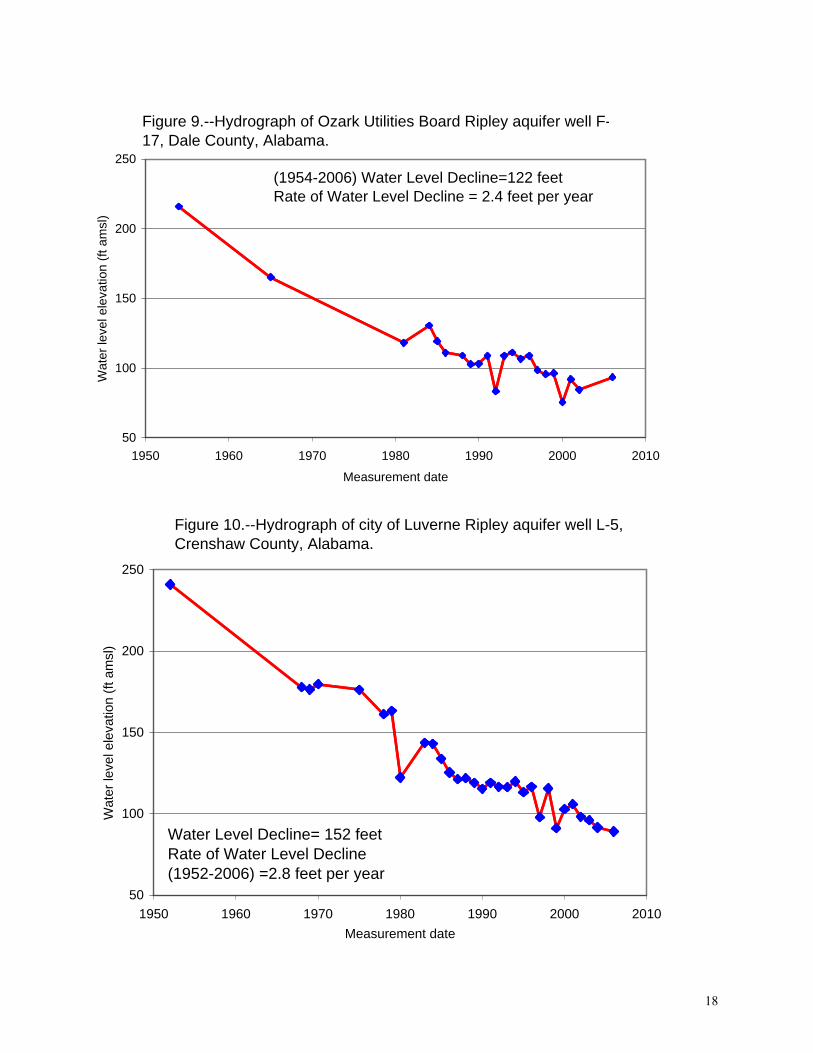
Figure 9.--Hydrograph of Ozark Utilities Board Ripley aquifer well F-17, Dale County, Alabama.
50
100
150
200
250
1950 1960 1970 1980 1990 2000 2010
Measurement date
Wat
er le
vel e
leva
tion
(ft a
msl
)
(1954-2006) Water Level Decline=122 feetRate of Water Level Decline = 2.4 feet per year
Figure 10.--Hydrograph of city of Luverne Ripley aquifer well L-5, Crenshaw County, Alabama.
50
100
150
200
250
1950 1960 1970 1980 1990 2000 2010Measurement date
Wat
er le
vel e
leva
tion
(ft a
msl
)
Water Level Decline= 152 feetRate of Water Level Decline(1952-2006) =2.8 feet per year
18
Well K-4 is a Clayton aquifer public supply well owned by the city of Elba (Coffee
County) constructed in 1961 to a depth of 585 ft. The static water level in 1961 was 187 ft amsl
and the water level in 2006 was 158 ft amsl. No drawdown occurred until 1981. Over the past 25
years, drawdown was 29 ft and the rate of water level decline was 0.7 ft/yr (fig. 12).
Well Q-4 is a public supply well constructed by the city of Enterprise (Coffee County) in
the Salt Mountain aquifer in 1968 to a depth of 812 ft. The static water level in 1968 was 167 ft
amsl and the water level in 2006 was 67 ft amsl. Residual drawdown over the past 38 years is
100 ft and the rate of water level decline is 2.6 ft/yr (fig. 13).
Well J-3 is a Nanafalia aquifer public supply well owned by the Dothan Utilities
(Houston County) constructed in 1956 to a depth of 720 ft. The static water level in 1956 was
155 ft amsl and the water level in 2006 was 32 ft below mean sea level (bmsl). Residual
drawdown over the past 50 years is 187 ft and the rate of water level decline is 3.7 ft/yr (fig. 14).
However, since 1994 the water level has remained relatively stable.
Well F-1 is a domestic supply well constructed in the Nanafalia aquifer in 1964 to a depth
of 222 ft. The static water level in 1964 was 242 ft amsl and the water level in 2006 was 219 ft
amsl. Residual drawdown over the past 42 years is 23 ft and the rate of water level decline is 0.6
ft/yr (fig. 15).
Well G-02 is a water supply well for the Fort Rucker Army installation, constructed in
the Nanafalia aquifer in 1975 to a depth of 423 ft. The static water level in 1975 was 137 ft amsl
and the water level in 2006 was 57 ft amsl. Residual drawdown over the past 31 years is 80 ft
and the rate of water level decline is 2.6 ft/yr (fig. 16).
Well X-2 is an irrigation well, constructed in the Crystal River aquifer in 1976 to a depth
of 140 ft. The static water level in 1980 was 115 ft amsl and the water level in 2006 was 109 ft
amsl. Figure 17 shows that the average water level in the fall at the end of the irrigation season is
approximately 110 ft amsl, and recovery during the winter results in an average spring water
level of more than 120 ft (fig. 17). This well has no net drawdown and is an example of how
ground water may be used for seasonal irrigation without negative impacts on the overall
ground-water system.
19
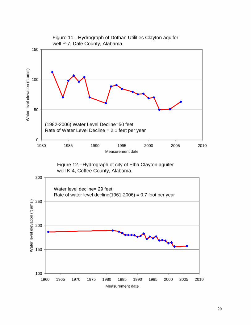
Figure 11.--Hydrograph of Dothan Utilities Clayton aquifer well P-7, Dale County, Alabama.
0
50
100
150
1980 1985 1990 1995 2000 2005 2010Measurement date
Wat
er le
vel e
leva
tion
(ft a
msl
)
(1982-2006) Water Level Decline=50 feetRate of Water Level Decline = 2.1 feet per year
Figure 12.--Hydrograph of city of Elba Clayton aquifer well K-4, Coffee County, Alabama.
100
150
200
250
300
1960 1965 1970 1975 1980 1985 1990 1995 2000 2005 2010
Measurement date
Wat
er le
vel e
leva
tion
(ft a
msl
)
Water level decline= 29 feetRate of water level decline(1961-2006) = 0.7 foot per year
20
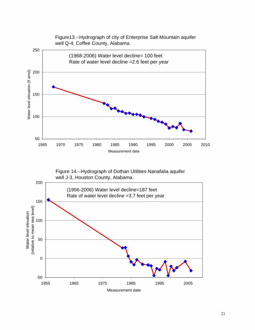
Figure13.--Hydrograph of city of Enterprise Salt Mountain aquifer well Q-4, Coffee County, Alabama.
50
100
150
200
250
1965 1970 1975 1980 1985 1990 1995 2000 2005 2010Measurement date
Wat
er le
vel e
leva
tion
(ft a
msl
)
(1968-2006) Water level decline= 100 feetRate of water level decline =2.6 feet per year
-50
0
50
100
150
200
1955 1965 1975 1985 1995 2005
Measurement date
Wat
er le
vel e
leva
tion
(rela
tive
to m
ean
sea
leve
l)
(1956-2006) Water level decline=187 feetRate of water level decline =3.7 feet per year
Figure 14.--Hydrograph of Dothan Utilities Nanafalia aquifer well J-3, Houston County, Alabama.
21
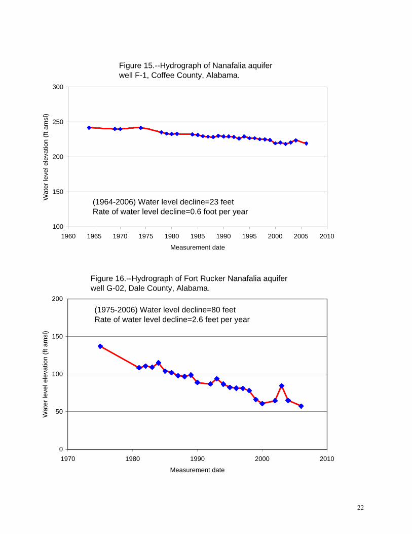
Figure 15.--Hydrograph of Nanafalia aquifer well F-1, Coffee County, Alabama.
100
150
200
250
300
1960 1965 1970 1975 1980 1985 1990 1995 2000 2005 2010
Measurement date
Wat
er le
vel e
leva
tion
(ft a
msl
)
(1964-2006) Water level decline=23 feetRate of water level decline=0.6 foot per year
Figure 16.--Hydrograph of Fort Rucker Nanafalia aquifer well G-02, Dale County, Alabama.
0
50
100
150
200
1970 1980 1990 2000 2010
Measurement date
Wat
er le
vel e
leva
tion
(ft a
msl
)
(1975-2006) Water level decline=80 feetRate of water level decline=2.6 feet per year
22
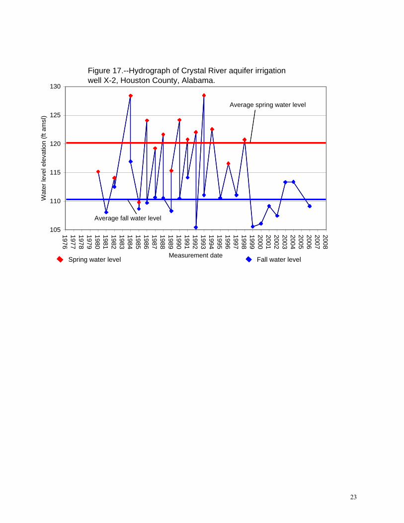
Figure 17.--Hydrograph of Crystal River aquifer irrigation well X-2, Houston County, Alabama.
105
110
115
120
125
130
197619771978197919801981198219831984198519861987198819891990199119921993199419951996199719981999200020012002200320042005200620072008
Measurement date
Wat
er le
vel e
leva
tion
(ft a
msl
)
Average spring water level
Average fall water level
Spring water level Fall water level
23
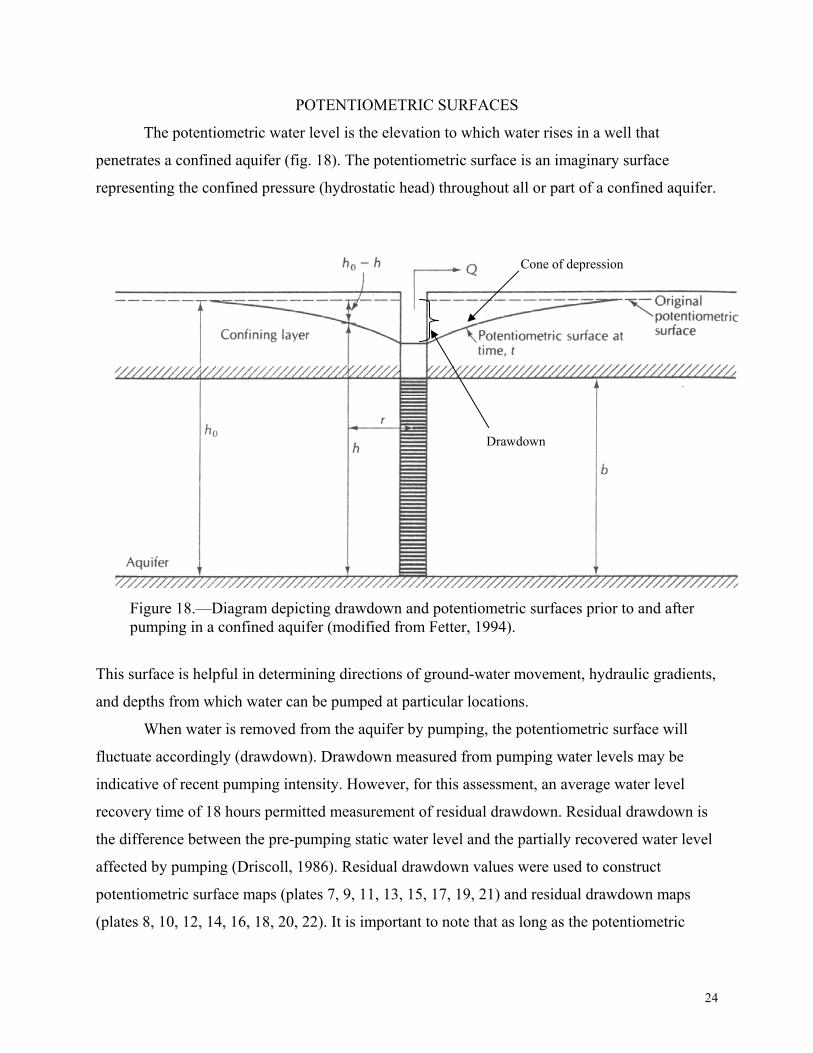
POTENTIOMETRIC SURFACES
The potentiometric water level is the elevation to which water rises in a well that
penetrates a confined aquifer (fig. 18). The potentiometric surface is an imaginary surface
representing the confined pressure (hydrostatic head) throughout all or part of a confined aquifer.
Drawdown
Cone of depression
Figure 18.—Diagram depicting drawdown and potentiometric surfaces prior to and after pumping in a confined aquifer (modified from Fetter, 1994).
This surface is helpful in determining directions of ground-water movement, hydraulic gradients,
and depths from which water can be pumped at particular locations.
When water is removed from the aquifer by pumping, the potentiometric surface will
fluctuate accordingly (drawdown). Drawdown measured from pumping water levels may be
indicative of recent pumping intensity. However, for this assessment, an average water level
recovery time of 18 hours permitted measurement of residual drawdown. Residual drawdown is
the difference between the pre-pumping static water level and the partially recovered water level
affected by pumping (Driscoll, 1986). Residual drawdown values were used to construct
potentiometric surface maps (plates 7, 9, 11, 13, 15, 17, 19, 21) and residual drawdown maps
(plates 8, 10, 12, 14, 16, 18, 20, 22). It is important to note that as long as the potentiometric
24
surface remains above the stratigraphic top of the aquifer, the aquifer media remains saturated so
that the declining surface only represents a decline in hydrostatic pressure. If the water level
declines below the stratigraphic top of the aquifer, the aquifer becomes unconfined, possibly
causing irreversible formation damage. Therefore, the potentiometric surface provides important
information to determine the affects of water production, strategies for water source protection,
and future water availability.
WELL CAPTURE ZONES
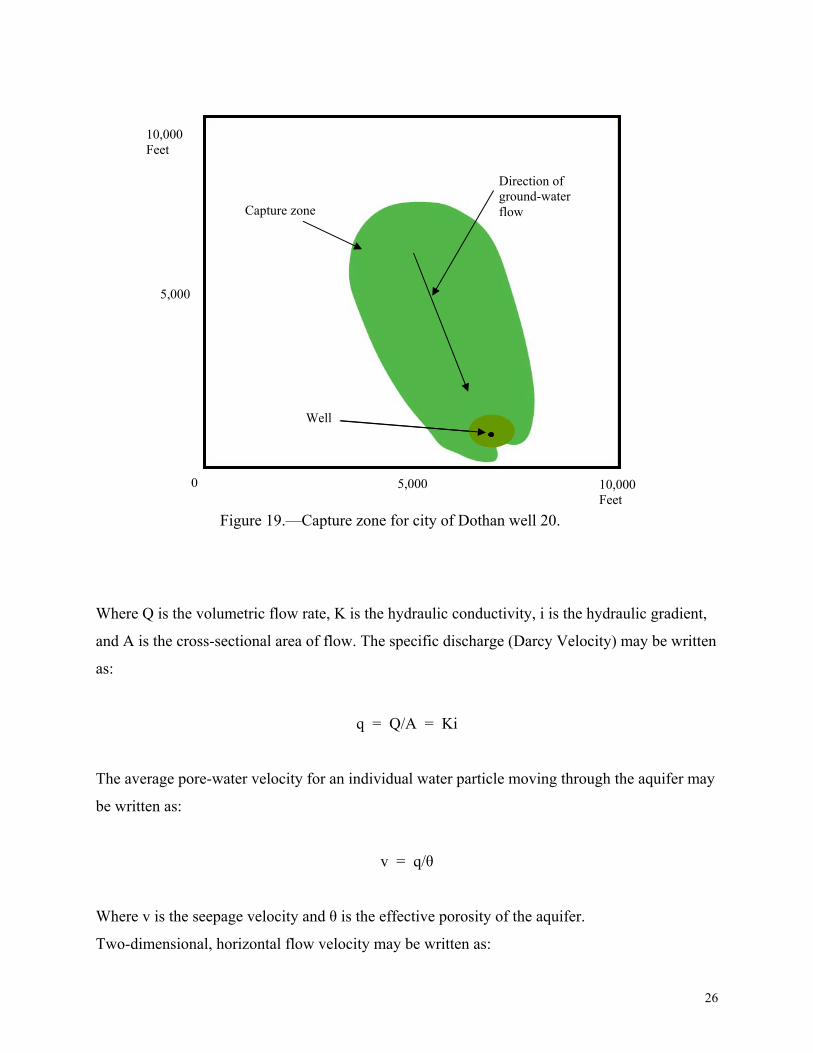
A well capture zone is the area of water contribution to a water well (fig. 19).
Determinations of well capture zones are important for several reasons. Knowledge of capture
zones may be used to construct wells with proper spacing and production rates to avoid multiple
wells producing water from the same areas. Also, it is important to know the area of water
contribution to a well so that contaminant sources may be monitored and controlled. Numerous
models have been developed to estimate well capture zones. For this assessment, the General
Particle Tracking Module (GPTRAC), developed by the U. S. Environmental Protection Agency
(USEPA) was selected (Blandford and Wu, 1993). The model has numerical and semi-analytical
options that estimate time-dependent capture zones from temporal, spatial, and hydrologic data
inputs. The numerical option utilizes hydraulic head fields determined by finite difference or
finite element ground-water flow models. The semi-analytical option, selected for this
assessment, delineates capture zones for pumping wells and assumes that aquifers are
homogeneous, with steady and uniform ambient ground-water flow. A time-dependent capture
zone is a subsurface area surrounding a pumping well that will supply ground-water recharge to
the well within some specified period of time. The model utilizes the particle tracking technique,
a method that employs hydraulic mathematical estimation of the movement of a conceptual
particle or molecule of water from a time-dependent stagnation point (point of zero velocity) to
the well bore (Blandford and Wu, 1993). This technique employs Darcy’s Law, which may be
written as:
Q = KiA
25
10,000 Feet
Where Q is the volumetric flow rate, K is the hydraulic conductivity, i is the hydraulic gradient,
and A is the cross-sectional area of flow. The specific discharge (Darcy Velocity) may be written
as:
q = Q/A = Ki
The average pore-water velocity for an individual water particle moving through the aquifer may
be written as:
v = q/θ
Where v is the seepage velocity and θ is the effective porosity of the aquifer.
Two-dimensional, horizontal flow velocity may be written as:
5,000
0 5,000 10,000 Feet
Capture zone
Direction of ground-water flow
Well
Figure 19.—Capture zone for city of Dothan well 20.
26
Vx = qx/ θ vy = qy/ θ
Once velocities are determined, pathlines for movement of individual particles may be delineated
by calculating the distance dl that is traversed during a given time period dt. This is defined
by:
Dl = (dx2 + dy
2)1/2
Capture zones may be used to determine the likelihood of interference of wells
constructed in the same aquifer or for determining adequate well spacing in areas where ground-
water development is occurring or may occur in the future. For this investigation, capture zones
were modeled for 120 wells constructed in eight major aquifers in southeast Alabama.
Hydrologic data were collected from GSA well files, open-file reports, and field assessments.
The GPTRAC program requires well location, aquifer confinability, transmissivity, hydraulic
gradient, flow direction, the quantity of water production, production time, and aquifer thickness.
The hydraulic gradient (head loss per unit length of water movement) is a particularly important
factor in ground-water production and in the ability to model ground-water flow and the affects
of water production. Ground-water flow rates are directly proportional to the hydraulic gradient,
so that a 50 percent increase in the hydraulic gradient will result in a 50 percent increase in the
rate of water flow in a given aquifer sand (Driscoll, 1986). Information required for
implementation of the GPTRAC program was obtained from GSA well files and GSA openfile
wellhead protection reports (Smith and others, 1996, Baker and Smith, 1997, Smith and others,
1997)
Model output is presented as tabular x-y water particle location coordinates and two-
dimensional graphic images of capture zones. Capture zones for multiple wells may be presented
on a single graph to demonstrate the proximity of contribution areas. The shape of each modeled
capture zone is based on the hydrologic conditions in the aquifer and average water production
rates. Most capture zones are asymmetrically shaped and are characterized by a linear component
oriented in the direction of ground-water flow.
27
GORDO AQUIFER
Water levels were measured in 13 wells constructed in the Gordo aquifer. Water level
elevations vary from 180.0 ft amsl in central Barbour County to 14.8 ft amsl at Eufaula in eastern
Barbour County (plate 7). The hydraulic gradient is approximately
0.0005 (2.6 ft/ mi) in the central portion of the study area in western Barbour, eastern Pike, and
northern Dale Counties. The gradient increases to 0.001 (5 ft/ mi) in northern Pike and southern
Montgomery Counties and 0.002 (11 ft/ mi) in eastern Barbour and northern Henry Counties.
Ground-water flow is south 20o east in eastern Barbour and eastern Henry Counties, southward
in southeastern Bullock, western Barbour, and northern Dale Counties, south 20o west in
southern Pike and northern Coffee Counties, and west-southwest in southwestern Bullock,
northern Pike, and southern Montgomery Counties. Disruptions in the potentiometric surface
occur near producing wells in Eufaula (eastern Barbour County), northwestern Barbour County
at a State of Alabama Forestry Commission well, and at Troy in central Pike County (plate 7).
Residual drawdown in the Gordo aquifer varies from 0 to 154 ft (plate 8). The maximum
drawdown occurred at Eufaula. Other areas with significant drawdown include a State of
Alabama Forestry Commission well in northwestern Barbour County (82 ft), 55 ft at Clio in
southwestern Barbour County, and 54 ft at Troy.
The average capture zone area for the Gordo aquifer is 1.9 mi2. The maximum capture
zone area is at Eufaula (3.1 mi2). The maximum distance of water capture from a well in the
Gordo aquifer is 2.1 miles. Based on evaluations of capture zones and well production histories,
proper spacing of wells constructed in the Gordo aquifer should be at least 1.5 miles along the
strike of the hydraulic gradient slope and at least 2.0 miles in an up- or down-gradient direction.
RIPLEY/CUSSETA AQUIFER
Water levels were measured in 19 wells constructed in the Ripley aquifer. Water level
elevations vary from 514.3 ft amsl near the recharge area in southern Bullock County to 54.3 ft
amsl at Ozark in north-central Dale County (plate 9). The hydraulic gradient is approximately
0.003 (16 ft/ mi). Ground-water flow is southward in Crenshaw and western Pike Counties,
approximately south 30o west in eastern Pike, western Barbour, and northern Dale Counties, and
south 70o east in eastern Barbour and eastern Henry Counties where the Chattahoochee River
appears to influence the direction of ground-water flow in the aquifer. Disruptions in the
potentiometric surface occur near producing wells in Ozark (north-central Dale County),
28
Luverne (central Crenshaw County), and at the Fort Rucker Cairns Landing Field in
southwestern Dale County (plate 9).
Residual drawdown in the Ripley aquifer varies from 0 to 149 ft (plate 10). The
maximum drawdown occurred at Luverne (central Crenshaw County). Other areas with
significant drawdown include Ozark (north-central Dale County) (60 to 95 ft), Brundidge
(southeastern Pike County) (73 ft), Troy (central Pike County) (62 ft), and Pike County Water
Authority (west-central Pike County) (57 ft).
The average capture zone area for the Ripley aquifer is 2.6 mi2. The maximum capture
zone area is at Ozark where three interfering wells form a capture zone of 9.8 mi2. The maximum
distance of water capture from a well in the Ripley aquifer is 4.7 miles. Based on evaluations of
capture zones and well production histories, proper spacing of wells constructed in the Ripley
aquifer should be at least 1.0 miles along the strike of the hydraulic gradient slope and at least
2.5 miles in an up- or down-gradient direction.
CLAYTON AND SALT MOUNTAIN AQUIFERS
Water levels were measured in 39 wells constructed in the Clayton aquifer. The
hydrologic investigation of the Clayton aquifer includes wells constructed in the Salt Mountain
Limestone. Although the Salt Mountain Limestone is stratigraphically separated from the
Clayton Formation (Smith, 2001), hydrologic data indicate that the two units are connected.
Therefore, for the purposes of this evaluation, they will be considered together. The major area
for Salt Mountain aquifer production is the city of Enterprise, which currently has 14 wells.
Water level elevations vary from 406.2 ft amsl near the recharge area in north-central Crenshaw
County to 118.0 ft bmsl at Dothan in northwestern Houston County (plate 11). The hydraulic
gradient is approximately 0.002 (11 ft/mi). Ground-water flow directions vary from south to
south 20o west in Pike and northern Coffee Counties to south 70o east in eastern Barbour and
eastern Henry Counties where the Chattahoochee River appears to influence the direction of
ground-water flow. Disruptions in the potentiometric surface occur near producing wells in the
Dothan area (northwestern Houston and southeastern Dale Counties), Enterprise (southeastern
Coffee County), Dozier (southern Crenshaw County), and at the Fort Rucker Cairns Landing
Field in southwestern Dale County (plate 11).
Residual drawdown in the Clayton aquifer varies from 0 to 204 ft (plate 12). The
maximum drawdown occurred at Dozier (southern Crenshaw County). Other areas with
29
significant drawdown include Dothan (northwestern Houston and southeastern Dale Counties)
(112 ft), Battens Crossroads (southeastern Coffee County) (97 ft), Geneva (southern Geneva
County) (Salt Mountain aquifer, 69 ft).
The average capture zone area for the Clayton aquifer is 2.0 mi2. The maximum capture
zone area is at Dothan where four interfering wells form a capture zone of 7.5 mi2. The
maximum distance of water capture from a well in the Ripley aquifer is 3.8 miles. Based on
evaluations of capture zones and well production histories, proper spacing of wells constructed in
the Clayton aquifer should be at least 1.0 miles along the strike of the hydraulic gradient slope
and at least 2.0 miles in an up- or down-gradient direction.
NANAFALIA AQUIFER
Water levels were measured in 34 wells constructed in the Nanafalia aquifer. Water level
elevations vary from 487.0 ft amsl near the recharge area in east-central Barbour County to 118.0
ft bmsl at Dothan in northwestern Houston County (plate 13). The hydraulic gradient varies from
0.002 (11 ft/mi) in the northern portion of the aquifer to 0.003 (16 ft/mi) in the southern portion
of the aquifer. Ground-water flows approximately south 10o west. Disruptions in the
potentiometric surface occur near producing wells in the Dothan area (northwestern Houston and
southeastern Dale Counties), Daleville (southwestern Dale County), and Andalusia (central
Covington County) (plate 13).
Residual drawdown in the Nanafalia aquifer varies from 0 to 189 ft (plate 14). The
maximum drawdown occurred at Dothan (northwestern Houston County). Other areas with
significant drawdown include Slocomb (eastern Geneva County) (96 ft), Andalusia (central
Covington County) (52 ft), and in a domestic well in southern Dale County) (51 ft).
The average capture zone area for the Nanafalia aquifer is 1.2 mi2. The maximum capture
zone area is at Dothan where 3 interfering wells form a capture zone of 6.4 mi2. The maximum
distance of water capture from a well in the Nanafalia aquifer is 3.2 miles. Based on evaluations
of capture zones and well production histories, proper spacing of wells constructed in the
Nanafalia aquifer should be at least 1.0 miles along the strike of the hydraulic gradient slope and
at least 2.0 miles in an up- or down-gradient direction.
30
TUSCAHOMA AQUIFER
Water levels were measured in six wells constructed in the Tuscahoma aquifer. Water
level elevations vary from 168.2 ft amsl in northern Dale County to 52.6 ft amsl in eastern Henry
County (plate 15). The hydraulic gradient is 0.002 (11 ft/mi). Ground-water directions vary from
south 20 o west in most of the aquifer to south 30 o east in Houston and Henry Counties where
the Chattahoochee River appears to influence the direction of ground-water flow. Disruptions in
the potentiometric surface occur near producing wells in northeastern Dale County, the town of
Columbia (eastern Houston County), and in northwestern Houston County at the Fort Rucker
Allen Landing Field (plate 15).
Residual drawdown in the Tuscahoma aquifer varies from 30.6 feet in northeastern
Covington County to 118.8 ft at a school well in northeastern Dale County (plate 16). Other
areas with significant drawdown include 104 feet at Columbia in northern Houston County and
51.2 feet at a domestic well in western Houston County.
The average capture zone area for the Tuscahoma aquifer is 3.5 mi2. The maximum
capture zone area is 4.9 mi2. The maximum distance of water capture from a well in the
Tuscahoma aquifer is 4.5 miles. Based on evaluations of capture zones and well production
histories, proper spacing of wells constructed in the Tuscahoma aquifer should be at least 1.5
miles along the strike of the hydraulic gradient slope and at least 2.5 miles in an up- or down-
gradient direction.
TALLAHATTA AQUIFER
Water levels were measured in seven wells constructed in the Tallahatta aquifer. Water
level elevations vary from 301.0 ft amsl in southeastern Dale County to 85.5 ft amsl in
southwestern Coffee County (plate 17). The hydraulic gradient varies from 0.002 (11 ft/mi) in
western Houston and northeastern Geneva Counties to 0.003 (16 ft/mi) in the western portion of
the aquifer to 0.006 (29 ft/mi) in southeastern Coffee County. Ground-water flow directions are
locally variable but are generally southward regionally. Disruptions in the potentiometric surface
occur near domestic producing wells in southwestern Coffee County and north-central Geneva
County (plate 17).
Residual drawdown in the Tallahatta aquifer varies from 1 foot to 119 ft (plate 18). The
average capture zone area for the Tallahatta aquifer is 0.5 mi2. The maximum capture zone area
31
is 1.8 mi2 and the maximum distance of water capture from a well in the Tallahatta aquifer is 2.2
miles. Based on evaluations of capture zones and well production histories, proper spacing of
wells constructed in the Tallahatta aquifer should be at least 1.0 miles along the strike of the
hydraulic gradient slope and at least 1.5 miles in an up- or down-gradient direction.
LISBON AQUIFER
Water levels were measured in 14 wells constructed in the Lisbon aquifer. Water level
elevations vary from 356.7 ft amsl near the recharge area in west-central Henry County to 84.2 ft
amsl in south-central Geneva County (plate 19). The hydraulic gradient is 0.002 (11 ft/mi).
Ground-water flow directions are locally variable but are generally southward regionally.
Disruptions in the potentiometric surface occur near producing wells in southwestern Coffee and
western Geneva Counties and at the Covington Electric Cooperative well in central Covington
County (M-5) (plate 19).
Residual drawdown in the Lisbon aquifer varies from 0 to 33 ft (plate 20). The maximum
drawdown occurred in the Covington Electric Cooperative well in central Covington County.
The average capture zone area for the Lisbon aquifer is 0.6 mi2. The maximum capture
zone area is 1.1 mi2. The maximum distance of water capture from a well in the Lisbon aquifer is
0.9 mile. Based on evaluations of capture zones and well production histories, proper spacing of
wells constructed in the Lisbon aquifer should be at least 1.0 miles along the strike of the
hydraulic gradient slope and at least 1.0 mile in an up- or down-gradient direction.
CRYSTAL RIVER AQUIFER
Water levels were measured in 19 wells constructed in the Crystal River aquifer.
Water level elevations vary from 213.5 ft amsl near the recharge area in east-central Covington
County to 88.1 ft amsl in southern Geneva County (plate 21). The hydraulic gradient is
approximately 0.002 (11 ft/mi). Ground-water flow is southward with a slight southwestward
component in central Geneva County. Minor disruptions in the potentiometric surface occur near
producing wells in Geneva County and southern Houston County.
Residual drawdown in the Crystal River aquifer is minor and varies from 0 to 27 ft (plate
22). The average capture zone area for the Crystal River aquifer is approximately 1.0 mi2. Based
on evaluations of capture zones and well production histories, proper spacing of wells
constructed in the Crystal River aquifer should be at least 1.0 mile along the strike of the
hydraulic gradient slope and at least 1.0 mile in an up- or down-gradient direction.
32
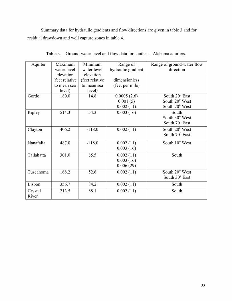
Summary data for hydraulic gradients and flow directions are given in table 3 and for
residual drawdown and well capture zones in table 4.
Table 3.—Ground-water level and flow data for southeast Alabama aquifers.
Aquifer Maximum water level elevation
(feet relative to mean sea
level)
Minimum water level elevation
(feet relative to mean sea
level)
Range of hydraulic gradient
dimensionless (feet per mile)
Range of ground-water flow direction
Gordo 180.0 14.8 0.0005 (2.6) 0.001 (5) 0.002 (11)
South 20o East South 20o West South 70o West
Ripley 514.3 54.3 0.003 (16) South South 30o West South 70o East
Clayton 406.2 -118.0 0.002 (11) South 20o West South 70o East
Nanafalia 487.0 -118.0 0.002 (11) 0.003 (16)
South 10o West
Tallahatta 301.0 85.5 0.002 (11) 0.003 (16) 0.006 (29)
South
Tuscahoma 168.2 52.6 0.002 (11) South 20o West South 30o East
Lisbon 356.7 84.2 0.002 (11) South Crystal River
213.5 88.1 0.002 (11) South
33
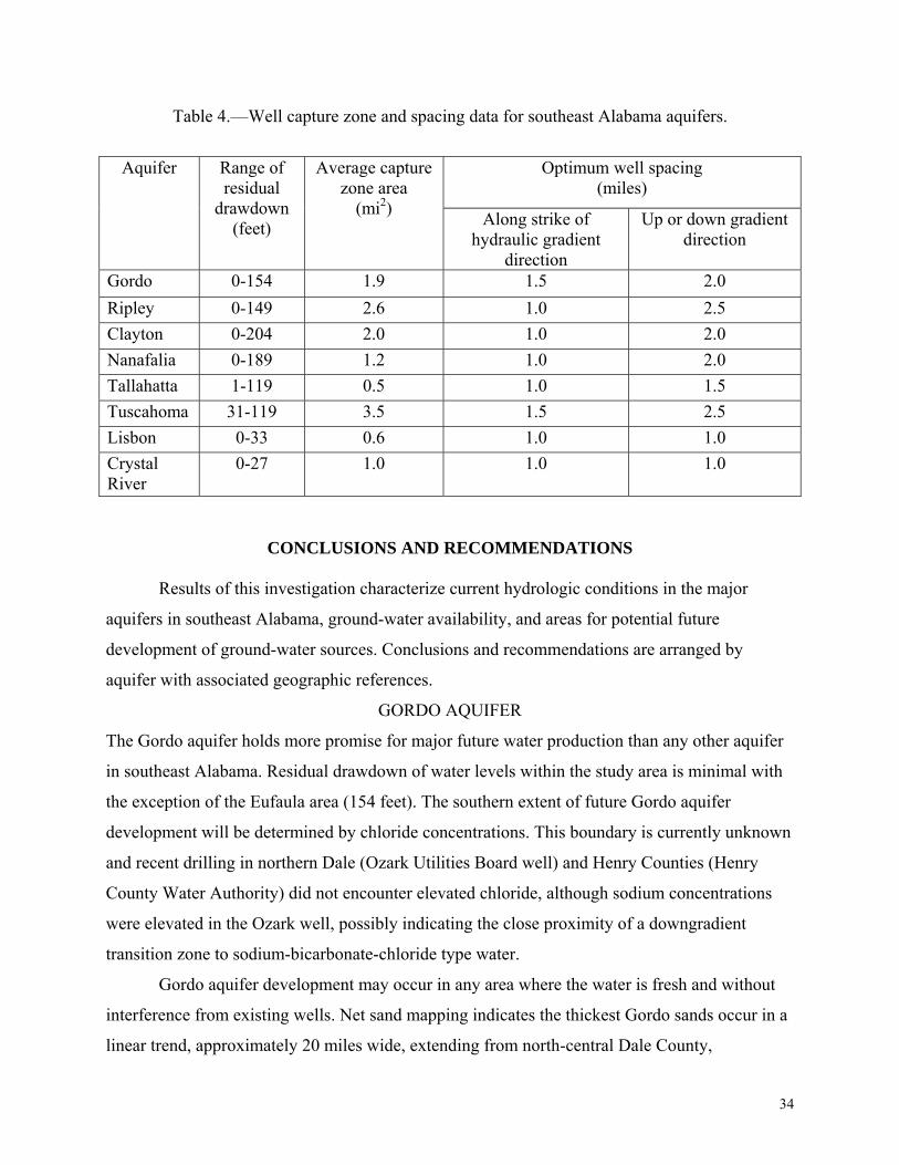
Table 4.—Well capture zone and spacing data for southeast Alabama aquifers.
Optimum well spacing
(miles) Aquifer Range of
residual drawdown
(feet)
Average capture zone area
(mi2) Along strike of hydraulic gradient
direction
Up or down gradient direction
Gordo 0-154 1.9 1.5 2.0 Ripley 0-149 2.6 1.0 2.5 Clayton 0-204 2.0 1.0 2.0 Nanafalia 0-189 1.2 1.0 2.0 Tallahatta 1-119 0.5 1.0 1.5 Tuscahoma 31-119 3.5 1.5 2.5 Lisbon 0-33 0.6 1.0 1.0 Crystal River
0-27 1.0 1.0 1.0
CONCLUSIONS AND RECOMMENDATIONS
Results of this investigation characterize current hydrologic conditions in the major
aquifers in southeast Alabama, ground-water availability, and areas for potential future
development of ground-water sources. Conclusions and recommendations are arranged by
aquifer with associated geographic references.
GORDO AQUIFER
The Gordo aquifer holds more promise for major future water production than any other aquifer
in southeast Alabama. Residual drawdown of water levels within the study area is minimal with
the exception of the Eufaula area (154 feet). The southern extent of future Gordo aquifer
development will be determined by chloride concentrations. This boundary is currently unknown
and recent drilling in northern Dale (Ozark Utilities Board well) and Henry Counties (Henry
County Water Authority) did not encounter elevated chloride, although sodium concentrations
were elevated in the Ozark well, possibly indicating the close proximity of a downgradient
transition zone to sodium-bicarbonate-chloride type water.
Gordo aquifer development may occur in any area where the water is fresh and without
interference from existing wells. Net sand mapping indicates the thickest Gordo sands occur in a
linear trend, approximately 20 miles wide, extending from north-central Dale County,
34
northwestward through northern Coffee and central Crenshaw Counties. Another area of thick
sands from 20 to 30 miles wide extends northward through Henry County and through parts of
eastern Dale and Barbour Counties.
Well capture zone modeling indicates that optimum spacing for wells in the Gordo
aquifer is at least 1.5 miles along strike of the hydraulic gradient slope and at least 2.0 miles in
an up- or down-gradient direction.
RIPLEY/CUSSETA AQUIFER
The Ripley Formation and its lower unit, the Cusseta Member, have long been major
aquifers in southeast and south-central Alabama. Large residual drawdown in pumping centers
such as Luverne (central Crenshaw County) (152 ft), Troy (central Pike County) (62 ft), and
Ozark (northern Dale County) (122 ft) prompted searches for alternative water sources, although
the Ripley remains the primary aquifer in areas with thick Cusseta sands. Capture zone modeling
and residual drawdown mapping indicate that Ripley aquifer development should be restricted in
the Ozark area. Other areas with undeveloped, thick Cusseta sands may continue to be targets for
Ripley aquifer development including southern Pike, northern Coffee, northern Dale, and west-
central Henry Counties.
Well capture zone modeling indicates that optimum spacing for wells in the Gordo
aquifer is at least 1.0 mile along strike of the hydraulic gradient slope and at least 2.5 miles in an
up- or down-gradient direction.
CLAYTON AND SALT MOUNTAIN AQUIFERS
During the past 20 years, the Clayton Formation has become one of the most prolific
aquifers in southeast Alabama. The city of Dothan has had great success in developing this
aquifer in northwestern Houston County, with wells that exceed 30 gallons of water per foot of
drawdown. However, large pumping rates have resulted in residual drawdown greater than 110
feet. Capture zone modeling and residual drawdown mapping indicate that only limited future
well construction should occur in northwestern Houston and southeastern Dale Counties in the
northern part of Dothan.
Interpretation of net sand mapping indicates a linear trend of thick, water-bearing
Clayton sediments from 10 to 25 miles wide extending from southeastern Henry County and
northwestern Houston County (including the Houston County panhandle), through southern
35
Dale, northeastern Geneva, southeastern and west-central Coffee (including the city of
Enterprise), and southern Crenshaw Counties.
The recharge area for the Clayton aquifer covers 221 mi2 and the rate of recharge is 91
mgd or 4.4 in/yr. Well capture zone modeling indicates that optimum spacing for wells in the
Clayton aquifer is at least 1.0 mile along strike of the hydraulic gradient slope and at least 2.0
miles in an up- or down-gradient direction.
Although the Salt Mountain aquifer is hydraulically connected to the underlying Clayton
Formation, its unique stratigraphic character makes it a major aquifer in parts of southeast
Alabama, particularly in the city of Enterprise where it is the sole source of public water.
Average residual drawdown in monitored wells at Enterprise is 37 feet with maximum
drawdown 97 feet. Net productive zone mapping indicates that the thickest part of the water-
bearing Salt Mountain extends in a 20-mile-wide area from central Geneva County,
northwestward through southern Coffee and northeastern Covington Counties. Much of this area
has no current Salt Mountain production.
NANAFALIA AQUIFER
The Nanafalia aquifer is the major water source in the central part of the study area,
including Fort Rucker and the cities of Dothan and Daleville. The largest concentration of
Nanfalia wells occurs in and just north of Dothan where maximum residual drawdown is
approximately 200 feet. Although no additional wells are recommended for the area in and near
Dothan, net sand mapping indicates a large area of thick Nanafalia, 15 to 25 miles wide,
extending from Dothan northwestward through southern Dale, southern Coffee, into northern
Covington Counties.
The recharge area for the Nanafalia aquifer covers 309 mi2 and the rate of recharge is 66
mgd or 2.7 in/yr. Well capture zone modeling indicates that optimum spacing for wells in the
Nanafalia aquifer is at least 1.0 mile along strike of the hydraulic gradient slope and at least 2.0
miles in an up- or down-gradient direction.
CRYSTAL RIVER AQUIFER
The Crystal River Formation is composed of fossiliferous limestone and residuum. It is a
minor aquifer in Alabama but serves as a major recharge area for the Floridian aquifer, which is
the source of water for much of northwest Florida. The Crystal River aquifer yields water for
36
irrigation, primarily in southern Houston County, and supplies public water wells in the cities of
Geneva and Florala. Maximum residual drawdown is less than 30 feet.
The Crystal River aquifer has the largest recharge area (1,533 mi2) and recharges at a rate
of 192 mgd or 1.7 in/yr. Well capture zone modeling indicates that optimum spacing for wells in
the Crystal River aquifer is at least 1.0 mile along strike of the hydraulic gradient slope and at
least 1.0 mile in an up- or down-gradient direction.
Abundant ground-water supplies are available for future development in all major
aquifers in southeast Alabama. However, concentrated areas of ground-water withdrawals cannot
sustain additional development. Prudent management and protection of these ground-water
sources will require thoughtful planning using the best scientific data available. Future ground-
water development will require substantial logistical planning and infrastructure to transport
water where it is needed. Cooperation among water producers is essential to insure sustainable
water supplies for the future.
REFERENCES CITED Baker, R. M., and Smith, C. C., 1997, Delineation of wellhead protection area boundaries for the
public-water supply wells of the town of Luverne Water Department, Crenshaw County,
Alabama: Geological Survey of Alabama Open File Report, 14 p.
Bingham, R. H., 1979, Low flow characteristics of Alabama streams: Geological Survey of
Alabama Bulletin 117, 39 p.
Blandford, T. N., and Yu-Shu-Wu, 1993, Addendum to the WHPA code version 2.0 user’s
guide: implementation of hydraulic head computation and display into the WHPA code,
GPTRAC module: U.S. Environmental Protection Agency, 268 p.
Cook, M. R., 1993, Eutaw aquifer in Alabama: Geological Survey of Alabama Bulletin 156, 105
p.
Driscoll, F. G., 1986, Groundwater and wells: St. Paul, Minnesota, Johnson Division, 1089 p.
Fetter, C. W., 1994, Applied hydrogeology: New York, Macmillian, Inc., 592 p.
Natural Resources Conservation Service, 2002, Agricultural water demand: Choctawhatchee –
Pea – Yellow Rivers Watershed Management Authority, 50 p.
Peirce, L. B., 1967, 7-day low flows and flow duration of Alabama streams: Geological Survey
of Alabama Bulletin 87, Part A, 114 p.
37
Smith, C. C., Gillett, Blakeney, and Baker, R. M., 1996, Delineation of wellhead protection area
boundaries for the public-water supply wells of the city of Enterprise, Coffee County,
Alabama: Geological Survey of Alabama Open File Report, 33 p.
Smith, C. C., Gillett, Blakeney, and Baker, R. M., 1996, Delineation of wellhead protection area
boundaries for the Water-Works and Sewer Board, city of Eufaula, Barbour County,
Alabama: Geological Survey of Alabama Open File Report, 42 p.
Smith, C. C., Gillett, Blakeney, and Baker, R. M., 1996, Delineation of wellhead protection area
boundaries for the public-water supply wells, Utilities Board, city of Ozark, Dale County,
Alabama: Geological Survey of Alabama Open File Report, 26 p.
Smith, C. C., Gillett, Blakeney, and Baker, R. M., 1996, Geology and hydrology in support of
the delineation of wellhead protection area boundaries city of Dothan, Houston County,
Alabama: Geological Survey of Alabama Open File Report,114 p.
Smith, C. C., 2001, Implementation assessment for the Choctawhatchee, Pea, and Yellow Rivers
watershed: Geological Survey of Alabama Open File Report, 148 p.
Stricker, V. A., 1983, Base flow of streams in the outcrop area of southeastern sand aquifer:
South Carolina, Georgia, Alabama, and Mississippi, U.S. Geological Survey Water
Resources Investigations 83-4106, 17 p.
U.S. Army Corps of Engineers, 2004, Water supply alternatives evaluation study for southeast
Alabama, 123 p.
38
GEOLOGICAL SURVEY OF ALABAMA P.O. Box 869999
420 Hackberry Lane Tuscaloosa, Alabama 35486-6999
205/349-2852
Berry H. (Nick) Tew, Jr., State Geologist
A list of the printed publications by the Geological Survey of Alabama can be obtained from the Publications Sales Office (205/247-3636) or through our
web site at http://www.gsa.state.al.us/.
E-mail: [email protected]
The Geological Survey of Alabama (GSA) makes every effort to collect, provide, and maintain accurate and complete information. However, data acquisition and research are ongoing activities of GSA, and interpretations may be revised as new data are acquired. Therefore, all information made available to the public by GSA should be viewed in that context. Neither the GSA nor any employee thereof makes any warranty, expressed or implied, or assumes any legal responsibility for the accuracy, completeness, or usefulness of any information, apparatus, product, or process disclosed in this report. Conclusions drawn or actions taken on the basis of these data and information are the sole responsibility of the user.
As a recipient of Federal financial assistance from the U.S. Department of the Interior, the GSA prohibits discrimination on the basis of race, color, national origin, age, or disability in its programs or activities. Discrimination on the basis of sex is prohibited in federally assisted GSA education programs. If anyone believes that he or she has been discriminated against in any of the GSA’s programs or activities, including its employment practices, the individual may contact the U.S. Geological Survey, U.S. Department of the Interior, Washington, D.C. 20240.
AN EQUAL OPPORTUNITY EMPLOYER
Serving Alabama since 1848
39