This is a repository copy of Assessment of elliptic flame front propagation characteristics of iso-octane, gasoline, M85 and E85 in an optical engine.

White Rose Research Online URL for this paper:http://eprints.whiterose.ac.uk/95744/

Version: Accepted Version

Article:

Ihracska, B, Korakianitis, T, Ruiz, P et al. (4 more authors) (2014) Assessment of elliptic flame front propagation characteristics of iso-octane, gasoline, M85 and E85 in an optical engine. Combustion and Flame, 161 (3). pp. 696-710. ISSN 0010-2180

https://doi.org/10.1016/j.combustflame.2013.07.020

© 2013 The Combustion Institute. Published by Elsevier Inc. Licensed under the Creative Commons Attribution-NonCommercial-NoDerivatives 4.0 International http://creativecommons.org/licenses/by-nc-nd/4.0/

eprints@whiterose.ac.ukhttps://eprints.whiterose.ac.uk/

Reuse

Unless indicated otherwise, fulltext items are protected by copyright with all rights reserved. The copyright exception in section 29 of the Copyright, Designs and Patents Act 1988 allows the making of a single copy solely for the purpose of non-commercial research or private study within the limits of fair dealing. The publisher or other rights-holder may allow further reproduction and re-use of this version - refer to the White Rose Research Online record for this item. Where records identify the publisher as the copyright holder, users can verify any specific terms of use on the publisher’s website.

Takedown

If you consider content in White Rose Research Online to be in breach of UK law, please notify us by emailing eprints@whiterose.ac.uk including the URL of the record and the reason for the withdrawal request.

Assessment of elliptic flame front propagation characteristics of iso-octane,

gasoline, M85 and E85 in an optical engine

Balazs Ihracskaa,∗, Theodosios Korakianitisb, Dongsheng Wena, Paula Ruiza, David R. Embersona, Roy J.Crookesa , Alvaro Diezc

aSchool of Engineering and Materials Science, Queen Mary University of London, UKbParks College of Engineering, Aviation and Technology, Saint Louis University, St. Louis, Missouri 63103, USA

cIzmir Institute of Technology, Gulbahce Campus, Izmir 35430, Turkey

Abstract

Premixed fuel-air flame propagation is investigated in a single-cylinder, spark-ignited, four-stroke optical

test engine using high-speed imaging. Circles and ellipses are fitted onto image projections of visible light

emitted by the flames. The images are subsequently analysed to statistically evaluate: flame area; flame

speed; centroid; perimeter; and various flame-shape descriptors. Results are presented for gasoline, isooctane,

E85 and M85. The experiments were conducted at stoichiometric conditions for each fuel, at two engine

speeds of 1200 revolutions per minute (rpm) and 1500 rpm, which are at 40% and 50% of rated engine

speed. Furthermore, fuel and speed set was tested for a higher and a lower compression ratio. Statistical

tools were used to analyse the large number of data obtained, and it was found that flame speed distribution

showed agreement with the normal distribution. Comparison of results assuming spherical and non-isotropic

propagation of flames indicate non-isotropic flame propagation should be considered for the description of

in-cylinder processes with higher accuracy. The high temporal resolution of the sequence of images allowed

observation of the spark-ignition delay process. The results indicate that gasoline and isooctane have

somewhat similar flame propagation behavior. Additional differences between these fuels and E85 and M85

were also recorded and identified.

Keywords: Flame speed, spherical, alcohol, ethanol, methanol, gasoline, optical engine

Nomenclature

Latin

A area

B arbitary region

cV isochoric specific heat capacity

∗Corresponding author. Tel: 0044-(0)207-882-4788Email address: b.ihracska@qmul.ac.uk (Balazs Ihracska)

Preprint submitted to “Combustion and Flame” May 7, 2013

d infinitesimal difference operator

da semi axial length

DF Feret’s diameter

f arbitary function

h heating value

LHV lower heating value

m mass

M moment of a two dimensional region

O parameter

p pressure

Qht heat transfer to walls

r radius

RNS roundness

S average flame speed

SA semi axes of an ellipse

Sf shape factor

Sn flame speed

T temperature

t time

U central moment

un turbulent burning velocity

V volume

vg gas expansion velocity

x centroid

y centroid

Greek

∆ finite difference operator

ǫ axis orientation angle

ηV ol volumetric Efficiency

ρ density∑

summation operator

Subscripts

0 spark origin

2

1, 2 integer

b fraction burned

i integer

maj major

min minor

p, w integer

x,y,z Cartesian coordinates, axes

Acronyms and abbreviations

BTDC before top dead centre

CA cranck angle

CFD computational fluid dynamics

CCD charge-coupled device

CH clearance height

CR compression ratio

D dimension

EoI end of imaging period

EQR equivalent radius

HC hydrocarbon

rpm revolutions per minute

RSE relative standard error

SAFS spherical assumption flame speed

TAI time after ignition

TDC top dead centre

ToI time of ignition

1. Introduction1

The current issues with our hydrocarbon based economy and its effects on climate change and human life2

are well documented (for instance [1]). These environmental and socio-political issues are among the most3

motivating research drivers, providing impetus for research in renewable energy and design-to-specification4

fuels [2–5]. Nevertheless, developed as well as developing countries still rely to a great extent on conven-5

tional fuels powering conventional engines. There is still a lot of room for considerable improvement in6

understanding the chemical reaction and flame-propagation processes, and reducing the emissions of these7

3

Figure 1: Illustration of the flame structure and temperature distribution of a flame, identifying the reaction and preheat zones

(The image was taken at 1200 rpm, CR 5.00, with iso-octane)

Figure 2: Section and top views of combustion chamber with fitted ellipse to the flame front

4

engine-fuel combinations. One of the most important ways to analyse combustion processes in engines is8

to employ 3D-CFD codes , with incorporation of various well refined fuel oxidation and flame propagation9

mechanisms [6, 7]. The models and codes need validation with experimental work accurately describing the10

exact nature of these in-cylinder processes.11

1.1. Flame structure and propagation12

Although, flame is defined as the luminous part of the burning gases caused by highly exothermic, rapid13

oxidation [8]. For simplicity in this study, the earliest and relatively short plasma state of the glowing charge14

was considered as a flame. For both moving and standing flames, the flame front is the indicator of where15

gases heat up and start emitting light [9, 10]. This front is considered to consist of two regions: preheat16

and reaction zones. For instance, Figure 1 illustrates the top view of the reaction and preheat zones in the17

chamber of the optical-access engine used in this paper.18

The combustion process in SI engines can be divided into four main stages: spark and flame initiation;19

initial flame kernel development; turbulent flame propagation; and flame termination [11]. The first two20

stages are of high importance in terms of in-cylinder pressure development [12–16]. These four stages are21

influenced by: spark energy and duration [17]; spark plug design and orientation [18]; in-cylinder flow22

field [19]; cyclic cylinder charging [20]; in-cylinder composition [21]; and other related factors. A detailed23

literature survey on the effects of these parameters on the four stages of combustion appeared in [12].24

The flame speed Sn (which can be measured from images of the spatial-temporal development of the25

flame) is given by [9, 22]:26

Sn = vg + un (1)

where vg is the gas expansion velocity immediately adjacent to the flame front and un is the streched27

laminar burning velocity of combusting air fuel mixture [23]. The turbulent burning velocity equals the28

laminar velocity with the added effect of the flow field, geometry; wrinkling of the flame front; pressure29

effects on flame thickness; history of the flame [24]. The effect of the turbulent flow field is crucial for the30

first and second stage of combustion. It has been shown that the smallest flame kernels are distorted shortly31

after ignition [25]. The laminar velocity is an intrinsic property of a combustible fuel, air and burned gas32

mixture. That is defined as the velocity, relative to and normal to the flame front, with which unburned gas33

moves into the front and is transformed to products [26].34

Turbulent burning velocity plays a prime role and directly effects the in-cylinder pressure development,35

i.e., engine performance. Turbulent burning velocity are laminar burning velocity are important physical36

properties of fuel air mixtures. It is essential that both of these velocities are derived experimentally from37

flame speed and area of in-cylinder pressure measurements [9, 11, 14, 22]. The work produced by an engine38

is related to the flame speed as can be inferred from the following. The burned mass of charge is given by39

5

mb(t) = (SxSy Sz)(t)ρb(t)Sf(t), (2)

where Sx, Sy, Sz are the average flame speeds in the x, y, z directions. These can be determined by dividing40

the flame radius along an axis by the elapsed time from ignition. Sf is a shape specific function. The41

burning of fuel releases energy to the working fluid in the cylinder, given by [4, 26]:42

mbLHV − (mcV dT ) − Σhidmi − dQht = pdV (3)

The rate of burning of the air-fuel mixture affects the chemical energy change of the fluid, and this43

directly affects the indicated work and power output. In equation 3 the work done on the piston pdV equals44

the energy released from the burning fuel mb LHV , minus the energy required to heat up the charge mcV dT ,45

minus the heat transfer to walls dQht, and adjusted by the masses leaving or entering the chamber Σhidmi.46

Note: term Σhidmi can be positive (during fuel injection) or negative (flow to crevice volumes or blow by).47

Therefore engine performance is highly dependent on flame propagation characteristics within the cylinder.48

1.2. Visualisation of initial flame kernel growth in SI engines49

In previous engine research images of flames in cylinders showed a significant enflamed volume, but the50

pressure measurements were not accurate or sensitive enough to indicate the evolving flame kernels [15, 21].51

Therefore, optical investigation of combustion is prefered to pressure tracing at the early combustion stages.52

The practical realization of visual access to a combustion chamber of a working piston engine is not easy, with53

any of the visible, ultra violet spectra or laser radiation approaches [43–46]. The fluctuating pressure at high54

temperature, the limited strength of transparent materials and the geometrical constrains kept investigators55

from studying optical engines at real working conditions. In most cases the engine speed and CR were kept56

low in order to observe the propagating flames. In previous investigations the effect of changing engine57

speeds and equivalence ratios were studied. However, because of the tight cylinder geometries, there has58

been no optical data recorded in the same engine at different compression ratios. Another major difficulty59

is the time scale of rapid oxidation. The average of temporal resolution that can be found in the literature60

is about 0.2 to 0.4 ms. Only one paper included data at higher temporal resolution, which could potentially61

provide insight to the earliest and faintest flames [32]. It has also been reported that fouling of the optical62

ports limits the length of operation time [18]. The experimental conditions and a general summary of the63

most relevant work on flame speed measurements and other investigations in optical engines can be found64

in Table 1. A comprehensive review of experimental investigation techniques in reciprocating-piston engines65

is in [47].66

It has been shown that the shape of the evolving flame kernel has a major effect on the in-cylinder67

combustion processes [14]. Generally, previous studies have assumed that the propagation of the spark-68

initiated oxidation is isotropic, i.e. spherical flame propagation [15, 16, 18, 21, 25, 28–36, 38, 39]. Only a69

6

Table 1: Table of prior related publications

Research Imaging Engine

Author Ref. Method Method DetailFrame rate

(f/s)Speed

(rpm)

Fuel A/F CR

Rashidi [27] Luminous high speed consecutive

images

2000 1096 isooctane 1.08 -

Berreta [21] Luminous high speed imaging,hand

traced, NaCI seeding

5000 872, 1233 isooctane 1.13-0.98 7.86

Heywood [28] Schlieren each picture is from dif-

ferent cycle

1380 1380 propane,

hydrogen

1.00 7.00

Gatowski [29] Schlieren high speed consecutive

images

2000 740, 1400 propane 0.9 5.75

zur Loye [25] 2D visual. laser scattering, TiO2,

ZrO2 seeding

- 300-3000 propane 1.0, 0.5 8.00

Keck [15] Schlieren high speed consecutive

images, hand traced

2000 1400 propane 0.87 5.75

Pischinger [16] Schlieren high speed consecutive

images

25000 1400 propane 1.00, 0.77,

0.71

6.70

Bates [13] Luminous multi explosure in one

frame

30 (NTSC) 500 propane 0.6-0.9 9.10

Nakamura [30] Luminous high speed consecutive

images

10000 1500 gasoline 1 9.30

Herweg [31] Schlieren pictures are from differ-

ent cycle

flash light,

pulse 40ns

800-2000 propane 0.77 7.30

Bates [14] Luminous multi explosure in one

frame

30 (NTSC) 500, 1000 propane 0.75 9.10

Shen [32] Schlieren high speed consecutive

images, hand traced

20000 500, 1100 isooctane 1.00-0.91 7.70

Aleiferis [18] Luminous double-exposed images 25 1500 isooctane 0.68 7.90

Aleiferis [33] Luminous double-exposed images 25 1500 isooctane 1.00, 0.68 7.90

Lee [34] Laser de-

flection &

Schlieren

comparison between the

2 methods

3000 1200, 1500,

1800

liquefied

petroleum gas

0.80, 1.10,

1.30

10.00

Conte [35] Optical and

ion sensors

mapping (no images

taken)

- 2000 gasoline and gas

mixtures

1.00 8.70

Gerke [36] OH-

chemiluminesc.

high speed imaging 10000 compression

machine

hydrogen 0.36-2.50 (p=5-45

bar)

Bates [13] Luminous multi explosure in one

frame

30 500 propnae 0.70 9.00

Tahtouh [37] Luminous high speed imaging 6000 1200, 2000 isooctane,

methane

1.00, 0.80 9.50

Baritaud [38] Schlieren high speed consecutive

images, hand traced

6000 500, 1040 propane 0.65, 0.85 6.00

Tagalian [39] Z-Schlieren 5 cycles analysed 1400 1400 propane 0.90 -

Aleiferis [40] Shadowgraphy high speed, consecutive

pictures, 100 cycles

9000 1500 E85, gasoline 1.00 11.15

Aleiferis [41] chemiluminesc. high speed, consecutive

pictures, 100 cycles

9000 1500 alcohols, HCs 1.00 11.15

Herweg [42] Luminous experimental work in a

side chamber and one-

dimensional model

- 300, 500,

750, 1000,

1250

propane 1.00, 0.77,

0.67

7.30

7

Table 2: Fuel properties

Fuel Formula Molar

Mass

Density Lower

Heating

Value

Stoichiometric

A/F ratio

Flammability

limits in air

(V%)

- (g) (kg/m3) (MJ/kg) (kg/kg) lower upper

Gasoline (approx.) CnH1.87n 110 720-780 44.2 14.60 1.0 8.0

Isooctane C8H18 114.23 692 44.3 15.13 1.0 6.0

Ethanol C2H6O 46.07 785 26.9 9.00 3.3 19.0

Methanol CH4O 32.04 792 20.0 6.47 6.0 36.0

E85 CnH2.88nO 56.29 771 29.6 9.92 3.0 17.1

M85 CnH3.74nO 44.37 777 23.6 7.77 5.3 31.5

few studies mentioned different flame-front geometries [14, 15, 30, 39] and looked into implications arising70

from the assumption that the flame front surface had a spherical geometry. However, these shapes were not71

described mathematically and detailed analyses were not carried out.72

Even though the in-cylinder flame front is a three-dimensional flame, in most studies flame-speed mea-73

surements are measured from two-dimensional projections of the images. Applying the isotropic propagation74

assumption, the two-dimensional projected contours of spherical flames can be digitized and their various75

geometrical properties determined. Actual flame speeds and flame shapes were measured in a small number76

of studies, where the flame radii were calculated using the “equivalent radius” (EQR) method [15, 16, 25,77

32, 33, 38–41], which determines the radius from the measured area:78

r =

√

A

π(4)

where r is the flame radius and A is the area of the projected region. There has been no attempt to refine79

this assumption.80

Many of the early investigators (that established the fundamentals of optical engine work) due to lim-81

itations of available tools used hand tracing methods to delineate the boundaries and/or had low number82

of samples (3 to 6 measurements averaged) [19]. Later papers do have a larger number of measurements,83

but statistical distribution of their findings was not documented [37]. Cyclic variability in engines is a84

widely studied phenomenon [12, 18, 27, 48]: the nature of the processes prior to ignition, the ignition itself85

and combustion instabilities cause fairly high standard deviation of in-cylinder measurements. Therefore86

statistical tools and high numbers of samples are needed in order to keep errors in the results low.87

In previous studies with optical-access engines the main choice of fuels were pure hydrocarbons (HC),88

such as propane and isooctane. Less attention was paid to practical fuels such as gasoline and alcohol89

blends (Table 1). It is a usual practice to use isooctane as a surrogate of gasoline in engine related research90

purposes as these two fuels have similar physical properties. Moreover, gasoline is a mixture of hydrocarbons91

with a composition that is not guaranteed, whereas isooctane is an easily available pure chemical. Previous92

8

flame-propagation studies in optical engines did not compare flame propagation characteristics of gasoline93

and isooctane to verify the two fuels behaved in a similar fashion. Alcohols and blends with gasoline (or94

isooctane) have been used in piston engines since the engine itself was invented. At present, bio-alcohols95

are proposed among the candidates for future fuels. Many studies have investigated their emission and96

performance qualities [40, 49–52], but the literature is lacking the relevant optical-engine data. Usually each97

published study concentrates on one engine geometry (e.g. one compression ratio) and one fuel. There are98

very few optical data available on comparison of different fuels in the same engine operating conditions.99

Table 2 lists some of properties of the fuels tested in these engines (from [26, 53]).100

1.2.1. Current contribution101

The main contribution of this paper is statistical characterization of non-spherical and non-isotropic102

aspects of flame propagation. A specifically-designed multi-fuel optical engine was used to compare flame-103

propagation characteristics of isooctane and gasoline. E85 and M85 were also investigated as practical104

alternative spark-ignition engine fuels and to fill in the gaps in the flame-propagation data base. E85 and105

M85 were “research grade”: they were mixed in house using pure alcohols and isooctane. CR of 8.14:1106

and 5:1 were chosen to test the fuels: the higher to simulate real engine conditions; and the lower one to107

provide sufficient contrast from the higher one. Utilizing the capability of an extremely sensitive and fast108

camera, high temporal resolution was achieved, allowing investigation of phenomena like ignition delay and109

early flame kernel formation. The large number of samples allowed mathematical statistics to be used to110

find the typical distribution of the measured data. It was concluded that elliptical flame structures describe111

flame propagation more accurately than spherical flame structures in many cases. Therefore a new and112

more detailed set of combustion data with these fuels has been obtained, and it can be used for validation113

of CFD and emissions studies.114

Table 3: Engine data

Description Value

Make Briggs & Stratton

Model NO. 093432

Type 4-Stroke, Air Cooled,

Wet Sump

Valve, Head Arrangement 2-Valve, L-head

Bore x Stroke (mm) 65.1 x 44.4

Connection Rod Ratio 0.25

Displacement (cm3) 148

Field of View (mm) 19 X 50

Compression Ratios 5.00, 8.14

9

2. Experimental apparatus and imaging system115

2.1. Engine and optical access116

Experiments were carried out in a modified single cylinder four-stroke Briggs & Stratton engine. Some117

parameters of the engine are shown in Table 3. Many properties of this research engine are comparable118

with commercial engines. The engine original lubrication and cooling systems, the valve train, and timing119

were not modified. The exhaust muffler was taken off and the exhaust port was connected straight into120

a laboratory extractor. The nozzle of the original carburetor was replaced with a variable area nozzle,121

so that any air-fuel mixture could be set by varying the fuel and/or air flow. The fuel flow and air flow122

were measured electronically. The volume change of the fuel stored in a small tank above the carburettor123

was measured, and the fuel flow rate was determined with known fuel density. The air consumption was124

measured using an orifice plate based on the Bernoulli’s principle, Figure 3. The measurement was taken125

every 0.5 second, and the air/fuel ratio was calculated subsequently. During the whole operation period of126

the engine, the air/fuel ratio was monitored to keep a constant air/fuel ratio.127

The rig had a 12 V ignition system containing a BOSCH K12V TCI coil to supply high voltage to the128

NGK CHSA spark plug. The geometry of the plug had to be modified in order to fit in the cylinder head.129

The thread, sealing mode and electrical connection had to be changed, however, the electrodes and their130

gap of 0.7 mm was not altered. The ignition timing was kept the same, 20 CA degree BTC, for all fuels and131

operating conditions. Therefore, at the time of ignition the flow field adjacent to the spark was similar for132

the tested fuels at a given operating point. The position and orientation of the spark plug is illustrated in133

Figure 2, and the azimuthal orientation of the spark-plug gap was kept constant in all the experiments. The134

optical access was gained by a specifically designed cylinder head. The chosen Briggs & Stratton engine had135

an air cooled and side valved configuration, which resulted a simpler head design. One of the main design136

goals was to keep the compression ratio close to ones that real engines have. This restricted the maximum137

achievable size of field of view. The location and size of optical access was found by ensuring that some138

portion of the valves and piston were visible and the spark plug placed in the middle. Finally, required grades139

of materials, minimum wall thickness and cooling surface were determined by Finite Element Analysis. The140

final version of the research head had similar internal and outer geometrical design to the original one, but141

the compression ratio became variable using spacers from 5.00 up to its maximum value 8.14.. The detailed142

in-cylinder geometry is illustrated in Figure 2.143

Prior to image recording the engine was heated up using a metal blank instead of the window, which144

was also pre-heated by a blower torch. The design of the window clamp allowed swapping the blank to145

the window in a few seconds preserving the temperature of the system. Then, the engine was run an146

additional 5 minutes to reach steady operating conditions. For statistical analyses over 100 sets of data147

were obtained at each engine operating point. The camera memory could only store about 30 sets of data148

10

at a time. Therefore each time about 30 sets of data were recorded, and while the engine was running at149

the same operating point the camera memory was copied to the computer over about 30 seconds. Then150

a subsequent set of about 30 data points was obtained, and the process was repeated four times at each151

operating point. The computer code had a comparison loop that compared the four series of data to each152

other to check the stability of conditions and to look for contamination on the window. The important153

factors influencing the initial flame development are summarized in Table 4. The volume of the combustion154

chamber is calculated by the clearance heights as the piston movement is quite small during the initial flame155

propagation period. As it is difficult to obtain accurate values for residual gas volume, it is estimated by156

using valve timing and clearance volumes, and neglecting the effects of swinging gases. Thermodynamic157

conditions were recorded during the tests but were not synchronised with visualisation, soonly the mean158

values are given in Table 4. Each fuel had slightly different pressure curve at compression stroke, but the159

differences were smaller than the measurement errors. The computer code could only measure the spark160

duration when there was no combustion inside the engine (in dark) as it could not distinguish between flame161

and spark. During the experiments, it was found that the spark length was significantly shorter when there162

was combustion around it. So the spark length shown in Table 4 was derived from manual analysis of ten163

randomly chosen combustion images.164

Table 4: Details of operating conditions

Engine speed (rpm) CR Value

Clearence Height (mm) at ToI / EoI

12005.00 32.10 / 30.74

8.14 14.76 / 13.40

15005.00 32.10 / 30.57

8.14 14.76 / 13.23

Est. Residual Gas Volume Fraction (%)5.00 25

8.14 14

Volumetric Efficiency (%)1200 27.02±(1.35)

1500 27.93±(1.40)

Pressure at Time of Ignition (bar)

12005.00 3.78±(0.19)

8.14 6.29±(0.31)

15005.00 3.97±(0.20)

8.14 7.41±(0.37)

Spark Duration (ms) 1.48±(0.19)

It is believed that this optical engine provided a similar description of real engine processes to production165

engines as other optical engines. The main disadvantage of the designed configuration is the different in-166

cylinder flow field from the usual pent-roof type 4-stroke automotive engines. On the other hand, the167

unmodified wet-sump lubrication allowed running the engine at normal operating temperatures without168

further modifications. At this temperature there was no fuel or oil condensation on the window to cause169

fouling. Fouling has been reported as one of the constraints limiting other optical-access engines. Less170

11

contamination on windows provided prolonged firing periods and clearer images.171

2.2. Fitting an ellipse to an arbitrarily shaped region172

A fundamental task of automated image analysis and computer vision techniques is to fit geometries to173

regions or set of points. In two-dimensional space the most primitive approach to model a 2D shape is to174

fit a circle. The next level to retrieve more information from the model is to fit an ellipse, which (unlike175

a circle) is not symmetrical about every one of its diameters. In this work ellipses are used to model and176

analyse the non-isotropic propagation of in-cylinder flames.177

2.2.1. Fitting methods178

Fitting an ellipse to an arbitrarily shaped region has been studied in considerable detail. There are two179

basic methods for fitting ellipses: (1) boundary-based and (2) region-based methods. Detailed descriptions180

of these can be found in [54–56].181

Boundary-based methods consider that the arbitrary region consists of a set of points sampled from the182

region. Prior research in image analysis and computer vision have employed a variety of techniques including183

linear least squares, weighted least squares, Kalman filtering and robust estimation methods [54, 57]. Region-184

based methods are frequently used in image processing and were chosen here to determine some geometric185

characteristics of flames. These methods are detailed by Gonzales and Wintz [55]. They use the moments186

of a region in calculating the best-fit ellipse [56, 58, 59], and equalize the second order moment of a region187

in order to determine the best-fit ellipse. In the case of regular shapes ( i.e., region close to an ellipse)188

the aforementioned methods show no major difference in the result. For in-cylinder flames, region-based189

methods are more appropriate as they are less affected by boundary irregularities.190

2.2.2. Determining flame speed from fitted ellipses191

The moment of (w + q) order of a 2 dimensional arbitrary region (B) is given by [60].192

Mwq ≡

∫ ∫

B

f(x, y)xwyq dx dy (5)

calculated over B. For regions where no properties are varied, function f has a value of unity. When (w +q)193

equals zero, i.e., the zeroth moment is the area of region B, the centroids are given by the quotient of the194

first and zeroth moments:195

x ≡M10

M00(6)

y ≡M01

M00(7)

Then, the central moments can be determined evaluating the following integral:196

Uwq =

∫ ∫

B

f(x − x)w(y − y)q dx dy (8)

12

or can be written in terms of moments:197

U00 = M00 (9)

U10 = U01 = 0 (10)

U20 = M20M2

10

M00(11)

U02 = M02M2

01

M00(12)

U11 = M11M10M01

M00(13)

Finally, the best-fit ellipse can be determined using the central moments:198

O ≡

√

4U211 + (U20 − U02)2 (14)

ǫ =1

2tan−1

(

2U11

U20 − U02

)

(15)

SAmaj =

√

2(U20 + U02 + O

U11(16)

SAmin = 2

√

2(U20 + U02 − O

U11(17)

where SAmaj , SAmin and ǫ are the semi-major, minor axes and the orientation angle respectively. In this199

work bitmap images were acquired from the high-speed camera. These were converted to pixelated images200

from which the central moment integral were obtained from:201

U20 =1

n

n∑

i=1

(xi − x)2 (18)

U02 =1

n

n∑

i=1

(yi − y)2 (19)

U11 =1

n

n∑

i=1

(xi − x)(yi − y) (20)

and can be fairly easily calculated using a computer code.202

2.2.3. Flame speed derived form optical data203

Once the semi-major and minor axes were calculated for each image, the difference in their length was204

determined by:205

∆da(t) ≡ dat − dat−1 (21)

where in this case da is SAmaj or SAmin . Dividing the change in length with the known time interval gives206

the flame speed at the given time:207

Sn(t) =∆ da(t)

∆t. (22)

13

2.2.4. Shape factor208

There are many ways to arrange geometric parameters of a shape non-dimensionally. Details of shape de-209

scriptors can be found in [56]. Usually geometric regions are circular when their descriptor value approaches210

unity. Here the shape evolution of SAmaj and SAmin are of interest. Their most suitable descriptor is round-211

ness RNS, which does not vary with the boundary irregularities (local shape wrinkles or disturbances).212

RNS ≡4A

π D2F

(23)

where RNS is the large scale shape factor, A is the area of a region and DF is Feret’s diameter, the longest213

distance between any two points along the boundary of a region.214

� � � � �

� � � � �� � � � �� � �

�

� �

� � � � � � � � � � � � � � � � �� � � � � � � � � � � � � � � � �

� � � � � � � � � � � � � � � ! � � � " # � $ � % & � � � � � � � � � � � � � � � ' ' � ! � � � " # � $ � ( � � $ � �! � � ) � � � � � � � ! * � � � � � � � ) � � " + ( � , ) �- ) � � � " ! � � . � � � � � � � � " / � � $ � � � % 0 1 1 0 ( #- ) � � � " ! � � . � � � � � . � � � � , � � � � � � � � � " ! � � * � $ � 2 � ( - 3! � � . � � 4 � � � � � � � " � � � � � � � 5 4 � ( 1 � � � � � � � � � - * � ' � � � � � � � � " # � � � � � � � � � � &

3 � ( � , � � � � � � � � � � � � � � � � � � � � � � � �� � � � � �

� � � � � � � ! � � � � " + � � � � � � % � 6 �� * � � � � � ) � � ' � � � " + � � � � � �

7 ) � � � � � - � � 8 )� � � � � �# � � * - ) � � � � � � � � � " * � � � � � 2 6 � 0

4 � � � " 9 � � � � % � � ' 6 � &: � � � � � " � � � � � ; � � � � <� � � � � � " � � * � � � � � � � � � � � - � � ' � � �

! � � � � � � � � � � � � � � - 1 6 � 2 ( $ � � �� � � � � � � ,

� � � � � � 4 � � �

7 ) � � � � � - 3 � � � � � �

= > ? @ A B C D E F

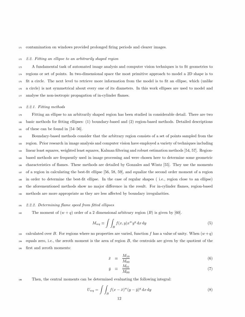
Figure 3: Schematic of the experimental rig: layout and components

2.3. Optical path & imaging215

Figure 3 is a schematic representation of the engine test bed. The optical assembly is at the top right216

corner. Fused quartz was chosen for the optical window as it has the appropriate mechanical, thermal and217

optical properties. An adjustable first-surface Aluminum mirror passed the emitted light to the Nikon f2.8218

Macro lens. The lens had the maximum diameter aperture setting to allow as much light into the camera219

as possible. With the given focal length, the aperture setting, the subject distance and Circle of Confusion220

14

the estimated depth of field (i.e. sharp region) is ± 5 mm. The Phantom V2.3 camera was set to record at221

15 kHz. At this rate the exposure time was 65 µs and the flame image was recorded in a 256 x 128 pixel222

array. Spatial and temporal resolution was found to be 0.19 mm/pixel and 67 µs respectively. From the223

camera’s internal memory the images were sent to a PC in 24 bit bitmap format. The actual images had224

only 256 greyscales but the analysing code worked faster with the larger, 24 bit bitmaps rather than the225

memory saving 8 bit ones. These images were fed into a C language code for analysis, which after some226

filtering and noise reduction determined the position of useful combustion cycles. The following geometric227

properties were then calculated for each picture that contained useful data: area; perimeter; mass center228

coordinates; x-y terminal points coordinates; best fit circle; best fit ellipse; circularity; roundness; solidity;229

ratio of perimeters; and different shape factors.230

Figure 4: Sample data distribution, in this case for M85, 1200 rpm, CR=5.00, at 804 µs, St=804= (5.9± 0.15) m/s

2.4. Uncertainties231

During recording, especially at the early stages of flame initiation, the experimental apparatus had to232

capture flames with low light intensity for short times. Therefore, the optical set up was calibrated to its233

highest sensitivity. This meant one of the major sources of uncertainties was light entering the optical path234

from outside. The underground location of the laboratory helped to provide nearly complete darkness for the235

tests. High-transparency window material and a high-reflectivity optical mirror were used, therefore errors236

arising from scattering, absorption etc. were neglected. Errors from the CCD sensor and the computers237

internal clock were also neglected. Changes in the air fuel mixture, quality of sparks, distance of engine and238

CCD sensor were considered as random uncertainties. These arose from the combination of an infinitely239

large number of infinitesimally small errors, which was expected to result in a normal frequency distribution,240

according to the Central Limit Theorem in statistics [61]. Figure 4 is typical of statistical data obtained for241

all conditions in this research. It illustrates that the data have a normal distribution, and that statistical242

analysis of the data with normal-distribution statistics is a justified approach.243

15

a) b)

Figure 5: Sample flame images a, isoctane, conditions: 1200 rpm and CR=5.00 b, gasoline conditions: 1500 rpm and CR=5.00

3. Results & Discussion244

The quantitative and direct comparison of flame speed measurements in optical engines is difficult. The245

wide selection of fuels, operating conditions and the optical engines themselves produce very different in-246

16

a)

200 400 600 800 1000 1200 1400−20

−10

0

10

20

30

Time After Ignition (µs)

Axial Flame

Speed (m/s)

−18.56 −17.12 −15.68 −14.24 −12.8 −11.36 −9.92

0.6

0.8

1

1.2

1.4

1.6

Crank Angle (°)

Roundness

G. Major

I. Major

G. Minor

I. Minor

G. Roundness

I. Roundness

0 200 400 600 800 1000 1200 1400−50−250255075

−20 −18.56 −17.12 −15.68 −14.24 −12.8 −11.36 −9.92

0.6

0.8

1

1.2

1.4

1.6

b)

200 400 600 800 1000 1200 1400−20

−10

0

10

20

30

Time After Ignition (µs)

Axial Flame

Speed (m/s)

−18.2 −16.4 −14.6 −12.8 −11 −9.2 −7.4

0.6

0.8

1

1.2

1.4

1.6

Crank Angle (°)

Roundness

G. Major

I. Major

G. Minor

I. Minor

G. Roundness

I. Roundness

0 200 400 600 800 1000 1200 1400−50−250255075

−20 −18.2 −16.4 −14.6 −12.8 −11 −9.2 −7.4

0.6

0.8

1

1.2

1.4

1.6

c)

200 400 600 800 1000 1200 1400−20

−10

0

10

20

30

Time After Ignition (µs)

Axial Flame

Speed (m/s)

−18.56 −17.12 −15.68 −14.24 −12.8 −11.36 −9.92

0.6

0.8

1

1.2

1.4

1.6

Crank Angle (°)

Roundness

G. Major

I. Major

G. Minor

I. Minor

G. Roundness

I. Roundness

0 200 400 600 800 1000 1200 1400−50−25

0255075

−20 −18.56 −17.12 −15.68 −14.24 −12.8 −11.36 −9.92

0.6

0.8

1

1.2

1.4

1.6

d)

200 400 600 800 1000 1200 1400−20

−10

0

10

20

30

Time After Ignition (µs)

Axial Flame

Speed (m/s)

−18.2 −16.4 −14.6 −12.8 −11 −9.2 −7.4

0.6

0.8

1

1.2

1.4

1.6

Crank Angle (°)

Roundness

G. Major

I. Major

G. Minor

I. Minor

G. Roundness

I. Roundness

0 200 400 600 800 1000 1200 1400−50−250255075

−20 −18.2 −16.4 −14.6 −12.8 −11 −9.2 −7.4

0.6

0.8

1

1.2

1.4

1.6

Figure 6: Flame speeds and roundness of Gasoline and Isooctane a, 1200 rpm and CR=5.00 b, 1500 rpm and CR=5.00 c, 1200

rpm and CR=8.14 d, 1500rpm and CR=8.14

Table 5: Derived flame speed values using the EQR method in different optical engines

Author Reference Engine

Speed

(rpm)

Fuel Air/Fuel

Ratio

CR Combustion

Chamber

Geometry

Sn (m/s)

at 1000 µs

after ToI

(Equivalent

Radius Method)

Ihracska - 1500 Isooctane 1.00 8.14 Rectangular 10.4

Ihracska - 1500 Gasoline 1.00 8.14 Rectangular 10.3

Ihracska - 1500 E85 1.00 8.14 Rectangular 9.1

Ihracska - 1500 M85 1.00 8.14 Rectangular 14.4

Pischinger [16] 1400 Propane 1.00 6.70 Square 4.1

Keck [15] 1400 Propane 0.87 5.75 Square 6.1

Herweg [31] 1250 Propane 1.00 7.30 Cylindrical 10.1

Aleiferis [43] 1500 Isooctane 0.60 7.90 Pentroof 4.9

Aleiferis [40] 1500 Gasoline 1.00 11.15 Pentroof 5.0

Aleiferis [40] 1500 E85 1.00 11.15 Pentroof 4.0

17

a)

200 400 600 800 1000 1200 1400−20

−10

0

10

20

30

Time After Ignition (µs)

Axial Flame

Speed (m/s)

−18.56 −17.12 −15.68 −14.24 −12.8 −11.36 −9.92

0.6

0.8

1

1.2

1.4

1.6

Crank Angle (°)

Roundness

E85 Major

M85 Major

E85 Minor

M85 Minor

E85 Roundness

M85 Roundness

0 200 400 600 800 1000 1200 1400−50−250255075

−20 −18.56 −17.12 −15.68 −14.24 −12.8 −11.36 −9.92

0.6

0.8

1

1.2

1.4

1.6

b)

200 400 600 800 1000 1200 1400−20

−10

0

10

20

30

Time After Ignition (µs)

Axial Flame

Speed (m/s)

−18.2 −16.4 −14.6 −12.8 −11 −9.2 −7.4

0.6

0.8

1

1.2

1.4

1.6

Crank Angle (°)

Roundness

E85 Major

M85 Major

E85 Minor

M85 Minor

E85 Roundness

M85 Roundness

0 200 400 600 800 1000 1200 1400−50−250255075

−20 −18.2 −16.4 −14.6 −12.8 −11 −9.2 −7.4

0.6

0.8

1

1.2

1.4

1.6

c)

200 400 600 800 1000 1200 1400−20

−10

0

10

20

30

Time After Ignition (µs)

Axial Flame

Speed (m/s)

−18.56 −17.12 −15.68 −14.24 −12.8 −11.36 −9.92

0.6

0.8

1

1.2

1.4

1.6

Crank Angle (°)

Roundness

E85 Major

M85 Major

E85 Minor

M85 Minor

E85 Roundness

M85 Roundness

0 200 400 600 800 1000 1200 1400−50−25

0255075

−20 −18.56 −17.12 −15.68 −14.24 −12.8 −11.36 −9.92

0.6

0.8

1

1.2

1.4

1.6

d)

200 400 600 800 1000 1200 1400−20

−10

0

10

20

30

Time After Ignition (µs)

Axial Flame

Speed (m/s)

−18.2 −16.4 −14.6 −12.8 −11 −9.2 −7.4

0.6

0.8

1

1.2

1.4

1.6

Crank Angle (°)

Roundness

E85 Major

M85 Major

E85 Minor

M85 Minor

E85 Roundness

M85 Roundness

0 200 400 600 800 1000 1200 1400−50−250255075

−20 −18.2 −16.4 −14.6 −12.8 −11 −9.2 −7.4

0.6

0.8

1

1.2

1.4

1.6

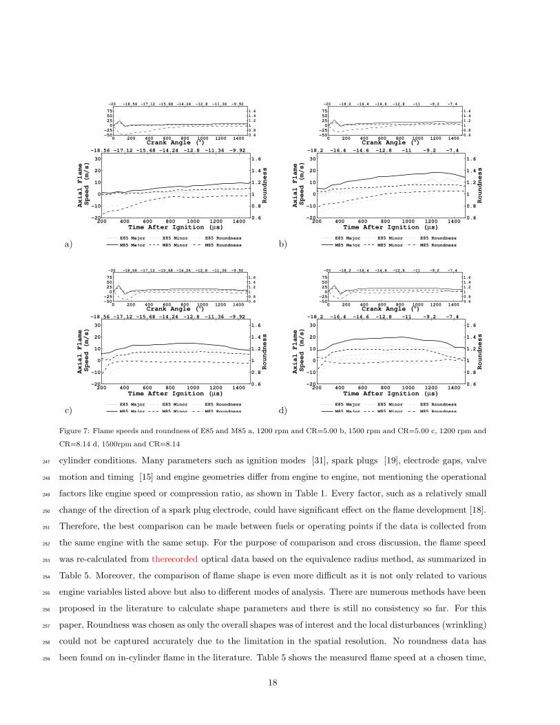
Figure 7: Flame speeds and roundness of E85 and M85 a, 1200 rpm and CR=5.00 b, 1500 rpm and CR=5.00 c, 1200 rpm and

CR=8.14 d, 1500rpm and CR=8.14

cylinder conditions. Many parameters such as ignition modes [31], spark plugs [19], electrode gaps, valve247

motion and timing [15] and engine geometries differ from engine to engine, not mentioning the operational248

factors like engine speed or compression ratio, as shown in Table 1. Every factor, such as a relatively small249

change of the direction of a spark plug electrode, could have significant effect on the flame development [18].250

Therefore, the best comparison can be made between fuels or operating points if the data is collected from251

the same engine with the same setup. For the purpose of comparison and cross discussion, the flame speed252

was re-calculated from therecorded optical data based on the equivalence radius method, as summarized in253

Table 5. Moreover, the comparison of flame shape is even more difficult as it is not only related to various254

engine variables listed above but also to different modes of analysis. There are numerous methods have been255

proposed in the literature to calculate shape parameters and there is still no consistency so far. For this256

paper, Roundness was chosen as only the overall shapes was of interest and the local disturbances (wrinkling)257

could not be captured accurately due to the limitation in the spatial resolution. No roundness data has258

been found on in-cylinder flame in the literature. Table 5 shows the measured flame speed at a chosen time,259

18

1000 µs after ignition. Despite of different engine geometries and operating conditions, the flame speed has260

the same magnitude for each fuel. It should be noted that there are very few flame speed data available261

for early stages combustion in SI engines , especially those with satisfactory temporal resolution, a wider262

quantitative comparison appears impossible. Qualitatively, the flame speed trend obtained among different263

experiments is consistent. It has an initial high value due to the spark boosted combustion, followed by264

a minimum value that occurs between 200 and 500 µs, and then a fairly steady increase until the end265

of the investigated period. Such a trend shows good agreement with the computational model of Herweg266

and Maly [42] for flame kernel formation in spark ignition engines. Considering the very different engine267

geometries, ignition modes and fuel mixing methods, the result is surprisingly well matched. In addition,268

the flame speed measurement results of gasoline and E85 were compared to Aleiferis’ findings [40]. It was269

found that the ratio of the flame speeds of these two fuels in the current study was similar to the one found270

in Aleiferis’ work. Gasoline showed a faster traveling flame by (19 ±6)% at 1000 µs after ignition. Apart271

from the absolute values, which shall be different among different work, the results are comparable, which272

suggests that the flame propagation characteristics are similar in SI engines for the earliest stages and is273

not engine geometry dependent. It is likely that the main controlling factor for early flame speed shall be274

the initial high energy input from the spark. Consequently, the finding of this study can be extrapolated to275

other engines.276

Isooctane and gasoline flames and some fitted ellipses are shown in Figure 5 at the condition of 1200,277

1500 rpm and CR = 5.00. The slowest flame propagation was observed at 1200rpm and CR = 5.00. The278

last image is the 41st in the particular series where the traveling flame reaches the edge of field of view. In279

Figure 5 only seven images are shown. The first three are continuous with temporal resolution of 67 µs.280

Then the next three were selected randomly, and the final one is the last image in the series. In 3D the281

flame boundary reached the combustion chamber long before it reached the edges of the visible area (Figure282

2). Considering the geometry of the combustion chamber, it was assumed that the flame speed vector in283

the z direction had always the same or smaller absolute values than the major flame speed vector at a given284

time. In the 3D space, the most distorted flames and the fastest ones did reach the combustion chamber285

walls and the piston at the end of the investigated period (1500 µs). However, for the vast majority of286

cases, there was no contact between the flames and the walls. When the contact did happen, a number of287

new variables should be added to the flame propagation equations to derive true values of flame speeds.288

However as there were only relatively small number of data points with contact and its area was small, the289

effect of it was considered as a small random error. The visual analysis of the gathered images showed a290

distinct difference in the physical appearance of the two fuel types of hydrocarbons and alcohols blends.291

Less luminous flames were found for the latter and higher intensity was seen on images of isooctane and292

gasoline with local maximums randomly distributed. This is likely to be the result of the simpler and smaller293

molecule structure of the alcohols. As the longer chains of hydrogen and carbon atoms of isooctane and294

19

gasoline are required more time for breaking and complete burning, there was more unburnt carbon, soot,295

present in flames than in the case of alcohols. The higher soot concentration resulted in brighter flames.296

Figure 6 shows roundness and flame speed along the major and minor axes plotted against time after297

ignition and CA degrees for gasoline and isooctane. Similarly Figure 7 for E85 and M85. In each plot the298

smaller graph shows the flame speed curve from time after ignition. Each curve reaches a maximum and a299

minimum value, which will be discussed later. The larger graphs show the same parameters after 200 µs300

after ignition, which is a more-stable region of flame development.301

Figures 6 and 7 indicate that the visible flame area first expands and reaches maximum flame speeds of302

the order 50 m/s at about 67 µs, then it contracts as indicated by minimum flame speeds of the order of303

-30 m/s at about 134 µs, and then the flame speeds become positive again. This flame contraction soon after304

the beginning of ignition is caused by rapid endothermic dissociation of fuel molecules and the formation305

of radicals in the mixture [62–64]. In order to verify that this flame contraction did not occur because of306

effects of spark energy changes in time, or ionization of the gas by the spark plug, experiments were carried307

out of discharging the spark plug in air and analysing the perimeter of the visible luminous plasma with the308

same analysis as for the flame front with fuels (Figure 8). In this case the maximum and minimum “flame309

speeds” of the gas ionized by the spark plug are about 10 m/s. When the plasma stabilized 200 µs after310

spark discharge its value of roundness remained stationary, around 0.75. This value describes the shape of311

the electric arc between the spark plug electrodes.312

The values of the relative standard error (RSE) in major flame speed measurements were plotted in313

separate graphs for each fuel in Figure 9. Similar uncertainty values were found for minor flame speed and314

roundness (these figures are not included for brevity). In general uncertainty analysis showed that at lower315

speeds and CR the errors were higher, suggesting a worse air fuel mixing, bigger large scale eddies caused316

by lower level of turbulence and more spacious combustion chamber respectively, and higher coefficient of317

variation in these conditions. Variations in the energy of the spark caused higher uncertainty values near318

67 µs after ignition. Mixture dissociation into radicals dominated flame propagation at times near 134 µs319

after ignition, resulting in lowering uncertainty values from those near 67 µs after ignition. The exothermic320

processes dominate 200 µs after ignition and later on. The relative magnitude of turbulent fluctuating321

velocity to flame speed affects uncertainty of measurements. Therefore when the flame speeds are lower322

(soon after 200 µs) the uncertainties are higher than when flame speeds are higher (e.g. near 1200 µs).323

Higher speeds and higher compression ratios promote better mixing, so that uncertainties are lower in these324

cases.325

Figures 6 and 7 indicate that the flame front is not spherical. Figure 10 presents a comparison of the326

spherical and elliptical flame-propagation approaches. In Figure 10, the major and minor flame speeds and327

their average were plotted in the same graph with the flame speed calculated using the equivalent radius328

method. For most of the time investigated, the average speed was similar to the speed calculated from the329

20

equivalent radius method but slightly larger, especially when there were larger differences in the major and330

minor speeds.331

The flame shape and its changes in time are important information in the understanding and prediction332

of in-cylinder processes. Therefore the ellipse method can provide useful data for CFD and emissions333

predictions in studies of fuel-engine combinations, and engine design processes [65].334

Flame speed and shape factor measurements showed that an ellipses described the contour of combustion335

better than circles in the first stages of combustion. About the first 800 µs of propagation were severely336

affected by the spark causing well elongated flames. This phenomenon was not dependent on fuel or engine337

operating conditions. At time of ignition, the value of roundness was found to be close to unity in all cases,338

which was confirmed by images showing a circular glowing area. Then, when the initial high energy got339

absorbed, the projection of the flame was elongated as the arc and the roundness dropped to about 0.7.340

Finally, in all investigated cases the calculated value of shape factors started increasing and approaching341

unity again. There was no description available of the flow field but the phenomenon of the flame becoming342

more circular later was expected. There is always a larger flux of unburnt charge passes through planes that343

contain the major axis (or in a general case Ferets diameter) simply because of these cross sections have344

larger areas. This of course is not valid for uniform flows where there is just one plane for the charge to345

flow. In an internal combustion engine there are main directions of flows but as it is turbulent, it could be346

approximated as a highly random field. The changes in shape were found to be dependent on the engine347

conditions and fuel. Higher engine speeds and CRs appeared to cause rounder contours; fuels with faster348

flame speeds also tended to have more regular shapes. Utilizing the properties of the ellipse fitting method349

two flame speed values were calculated normal to each other. It was observed that changes in the magnitude350

of one flame speed component corresponded to the change in the magnitude of the other one. Therefore,351

these peaks were caused by a large scale in-cylinder process rather than some local disturbance.352

Isooctane (major: 13.76, minor: 7.05) (all flame speed data have a unit of m/s and at condition of CR:353

8.14; 1500 rpm; 1000 µs] and E85 (major: 12.97, minor: 7.55) were found to have more unstable behaviour in354

combustion; their flame speed curves had more fluctuations than the other two fuels. These two fuels showed355

the largest changes in shape, sometimes exceeding value of unity of their shape factors. It seemed that all356

fuels would sooner or later reach a fairly stable flame speed value depending on the operating conditions.357

The rate of stabilizing was found to be the lowest for isooctane, which in most cases had increasing flame358

speeds until the end of recording. In Table 6 all flame speed results are shown for each conditions and fuels.359

Moreover, in order to compare fuels directly to eachother the EQR method values were normalised to ones of360

isoctane. Similar flame speed values were measured for isooctane and gasoline (major: 13.20, minor: 6.70),361

and most of the time the trend of their change in flame shape showed agreement. As it can be seen from362

Figure 6 their flame speed curves were overlapping, apart from the earliest times which were associated with363

higher unceartainities. Their similarity was more obvious at higher speed and CR where the normalised364

21

values showed only a couple of percentage difference but largest difference was only about 15%. In the case365

of gasoline, the results were only informative as its chemical properties were not guaranteed. The highest366

and most stable flame speeds were found in the case of M85 (major: 19.13, minor: 9.69) which reached367

its stationary values first. Also, the roundest contours were recorded for this fuel, with fairly low errors in368

the measurements. This might be a result of the higher flame speed as fluctuating and random in-cylinder369

flows had less effect on the flame propagation. A large difference in flame speed was observed form the370

other fuels especially for the low speed, CR measurements. It was an interesting to see the difference in the371

behaviour of the two oxygenated fuel blends, while E85 seemed to be showing similar flame propagation372

characteristics to isooctane, M85 clearly stood apart from E85. As the geometry of the combustion chamber373

and the operating conditions were the same it is likely that this behaviour of M85 can be explained by the374

combustion kinetics of methanol. The high laminar flame speed of methanol was explained on the basis of375

the successive dehydrogenations of methoxyl radical by Veloo et.al. [66] per Ranzi et.al. [67]. Finally, Table376

7 summarises the effect of different engine speeds and higher compression ratios on the flame speeds of the377

tested fuels. In this table the values were normalised in order to provide an easy comparison between the378

engine conditions. A general result is that flame speeds along the major axis are closer to the corresponding379

maximum values than the ones along the minor axis. This is a direct result of the initially highly distorted380

shapes becoming more circular as the minor axis elongated more during the flame development. It can be381

seen that M85 produced somewhat different results from the rest of the fuels this is probably the result of382

the aforementioned combustion kinetics. The normalised values for isooctane, gasoline and E85 were quite383

similar (within about ± 10%), indicating that the flame propagation characteristics of these fuels tend to384

react similarly to changes of engine conditions.385

Table 6: Flame speed values calculated using the EQR method and along the major and minor axes at 1000 µs AIT, for an

easy comparison of fuels the EQR method speed values were normalised to flames peeds values of isooctane

CR Engine Speed Isooctane Gasoline E85 M85

Major Minor EGR Ratio to Major Minor EGR Ratio to Major Minor EGR Ratio to Major Minor EGR Ratio to

method isooctane method isooctane method isooctane method isooctane

- (rpm) (m/s) (m/s) (m/s) - (m/s) (m/s) (m/s) - (m/s) (m/s) (m/s) - (m/s) (m/s) (m/s) -

5.00 1200 3.10 1.21 1.57 1.00 2.48 1.36 1.80 1.15 2.87 1.30 1.91 1.21 7.29 3.88 4.95 3.15

5.00 1500 5.66 2.44 3.70 1.00 5.31 2.58 4.12 1.11 7.71 3.57 5.20 1.41 14.69 7.36 11.01 2.98

8.14 1200 10.11 4.70 6.90 1.00 10.45 4.70 7.05 1.02 8.03 4.42 7.14 1.04 16.74 7.63 11.84 1.72

8.14 1500 13.76 7.05 10.40 1.00 13.26 6.70 10.31 0.99 12.97 7.55 9.10 0.88 19.13 9.69 14.40 1.38

4. Conclusions386

Flame propagation characteristics of isooctane, gasoline, M85 and E85 were recorded using a high-387

specification camera in a specialty-designed optical-access engine. The high temporal-resolution pictures388

were analysed with a purpose-built code and statistically compiled. In-cylinder combustion processes with389

22

Table 7: Flame speed values along the major and minor axes at 1000 µs AIT, for an easy comparison of the results from

different engine conditions a normailsed value is shown for each results and conditions

CR Engine speed Isooctane Gasoline E85 M85

Major Condition Minor Condition Major Condition Minor Condition Major Condition Minor Condition Major Condition Minor Condition

ratio ratio ratio ratio ratio ratio ratio ratio

- (rpm) (m/s) - (m/s) - (m/s) - (m/s) - (m/s) - (m/s) - (m/s) - (m/s) -

5.00 1200 3.10 0.23 1.21 0.17 2.48 0.19 1.36 0.20 2.87 0.22 1.30 0.17 7.29 0.38 3.88 0.40

5.00 1500 5.66 0.41 2.44 0.35 5.31 0.40 2.58 0.39 7.71 0.59 3.57 0.47 14.69 0.77 7.36 0.76

8.14 1200 10.11 0.73 4.70 0.67 10.45 0.79 4.70 0.70 8.03 0.62 4.42 0.59 16.74 0.87 7.63 0.79

8.14 1500 13.76 1.00 7.05 1.00 13.26 1.00 6.70 1.00 12.97 1.00 7.55 1.00 19.13 1.00 9.69 1.00

these fuels were investigated in the visible spectra. The high-temporal resolution enabled evaluation of flame390

kernel formation. A new way of combustion analysis was proposed, where ellipses are used to model the391

projected flame boundaries. This method elucidated details of the combustion properties and added data to392

the existing literature on these four fuels.To the authors’ knowledge this is the first study on detailed flame393

speed measurements for M85 from optical engines. Specifically it was concluded that:394

1. The spherical flame propagation assumption has certain limitations. Results showed that for some395

cases the spherical flame front assumption is reasonably valid; but one needs to consider non-isotropic flame396

propagation in order to model in-cylinder processes more accurately. This is especially so for the earlier397

combustion stages when the spark causes highly distorted flame contours.398

2. For all fuels the flames were more elliptic than circular immediately after ignition, which caused the399

least round flame-kernel shapes. In all cases, after the first 200 µs, the elliptic shapes gradually became400

more circular.401

3. Higher flame speeds were observed with increasing engine speed and compression ratio.402

4. The standard deviation of the measured values, and uncertainty in values, decreased at higher speeds403

and compression ratios. Roundness and lower fluctuations of flame speed also indicated more stable flames404

at those conditions, as a result of higher flame speed, better mixing, and smaller large-scale eddies.405

5. For all tested fuels at every operating condition a contraction of the flame was observed on the second406

recorded image. This is due to the endothermic process associated with the formation of radicals in the407

mixture.408

6. The phenomenon of ignition delay can be defined for SI engines utilizing the observed flame-kernel409

contraction. Ignition-delay is defined as the time between spark ignition and establishment of the steadily410

expanding flame kernel.411

7. A large number of sample observations were plotted. The distribution function showed good agreement412

with the normal distribution curve.413

8. Isooctane and gasoline showed similar behavior from the flame propagation point of view, though414

gasoline produced more shape-invariant flames (uncertainties were lower and flames were more round). The415

results confirm isooctane (a pure chemical) is a suitable gasoline-blend surrogate as a baseline comparison416

23

200 400 600 800 1000 1200 1400−3

−2

−1

0

1

2

3Axial Flame Speed (m/s)

Time After Ignition (µs)

200 400 600 800 1000 1200 14000.25

0.5

0.75

1

1.25

1.5

1.75

Roundness

MajorMinorRoundness

0 200 400 600 800 1000 1200 1400−30

−20

−10

0

10

20

30

Spark

0 200 400 600 800 1000 1200 14000.25

0.5

0.75

1

1.25

1.5

1.75

Figure 8: Flame speed measurement in air (no fuel admitted) at 1500 rpm and CR=8.14

fuel from a flame propagation point of view. M85 was found to have the fastest flame speed and the most417

round boundaries. The flame speeds and roundness of the two alcohols were found to be different. In418

contrast to M85s regularity and fast propagation, E85 showed more shape-variant burning and lower flame419

speeds.420

References421

[1] N. Stern, The Economics of Climate Change, The Stern Review, Cambridge University Press, Cambridge, 2007.422

[2] A. M. Namasivayam, T. Korakianitis, R. J. Crookes, K. D. H. Bob-Manuel, J. Olsen, Applied Energy 87(3) 769–778.423

[3] T. Korakianitis, A. M. Namasivayam, R. J. Crookes, International Journal of Hydrogen Energy 35(24) 13329–13344.424

[4] T. Korakianitis, A. M. Namasivayam, R. J. Crookes, Progress in Energy and Combustion Science 37(1) 89–112.425

[5] T. Korakianitis, A. M. Namasivayam, R. J. Crookes, Fuel 90(7) 2384–2395.426

[6] C. Rakopoulos, G. Kosmadakis, E. Pariotis, International Journal of Hydrogen Energy 35(22) 12545 – 12560.427

[7] D. Veynante, L. Vervisch, Progress in Energy and Combustion Science 28(3) 193 – 266.428

[8] J. Daintith (Ed.), Dictionary of Physics, Oxford University Press Inc., 5th edition, 2005.429

[9] C. J. Rallis, A. M. Garforth, Progress in Energy and Combustion Science 6(4) 303–329.430

[10] G. T. Kalghatgi, M. D. Swords, Combustion and Flame 49(1-3) 163–169.431

[11] D. R. Lancaster, R. B. Krieger, S. C. Sorenson, W. L. Hull, SAE International Journal (760160).432

[12] N. Ozdor, M. Dulger, E. Sher, SAE Technical Paper (940987).433

[13] S. C. Bates, SAE Technical Paper (890154).434

[14] S. C. Bates, Combustion and Flame 85(3-4) 331–352.435

[15] J. C. Keck, J. B. Heywood, G. Noske, SAE Technical Paper (870164).436

[16] S. Pischinger, J. B. Heywood, SAE Technical Paper (880518).437

[17] R. Maly, Spark Ignition: Its Physics and Effect on the Internal Combustion Engine, Plenum Press, New York, pp. 91–129.438

[18] P. G. Aleiferis, A. M. K. P. Taylor, J. H. Whitelaw, Y. Ishii, K. Urata, SAE Technical Paper (2000-01-1207).439

[19] J. C. Keck, Symposium (International) on Combustion 19(1) 1451 – 1466.440

[20] F. Matekunas, SAE International Journal (830337).441

24

a)0 200 400 600 800 1000 1200 14000

2

4

6

8

10

12

Time After Ignition (µs)

RSE in Flame Speed

Along Major Axis (%)

Isooctane

1200 rpm, CR=5.00

1500 rpm, CR=5.00

1200 rpm, CR=8.14

1500 rpm, CR=8.14

b)0 200 400 600 800 1000 1200 14000

2

4

6

8

10

12

RSE in Flame Speed

Along Major Axis (%)

Time After Ignition (µs)

Gasoline

1200 rpm, CR=5.00

1500 rpm, CR=5.00

1200 rpm, CR=8.14

1500 rpm, CR=8.14

c)0 200 400 600 800 1000 1200 14000

2

4

6

8

10

12

Time After Ignition (µs)

RSE in Flame Speed

Along Major Axis (%)

E85

1200 rpm, CR=5.00

1500 rpm, CR=5.00

1200 rpm, CR=8.14

1500 rpm, CR=8.14

d)0 200 400 600 800 1000 1200 14000

2

4

6

8

10

12

Time After Ignition (µs)

RSE in Flame Speed

Along Major Axis (%)

M85

1200 rpm, CR=5.00

1500 rpm, CR=5.00

1200 rpm, CR=8.14

1500 rpm, CR=8.14

Figure 9: Errors in calculated flame speed along the major axis

[21] G. P. Beretta, M. Rashidi, J. C. Keck, Combustion and Flame 52(3) 217–245.442

[22] L. Gillespie, M. Lawes, C. G. W. Sheppard, R. Woolley, SAE Technical Paper (2000-01-0192).443

[23] D. Bradley, R. Hicks, M. Lawes, C. Sheppard, R. Woolley, Combustion and Flame 115(12) 126 – 144.444

[24] J. F. Driscoll, Progress in Energy and Combustion Science 34(1) 91 – 134.445

[25] A. O. zur Loye, F. V. Bracco, SAE Technical Paper (870454).446

[26] J. B. Heywood, Internal Combustion Engine Fundamentals, McGraw-Hill, New York, 1988.447

[27] M. Rashidi, Combustion and Flame 42(2) 111–122.448

[28] J. B. Heywood, F. R. Vilchis, Combustion Science and Technology 38(5-6) 313–324.449

[29] J. A. Gatowski, J. B. Heywood, C. Deleplace, Combustion and Flame 56(1) 71–81.450

[30] A. Nakamura, K. Ishii, T. Sasaki, SAE Technical Paper (890322).451

[31] G. Z. R. Herweg, Proceedings of the Second International Symposium COMODIA 90 173.452

[32] H. Shen, D. Jiang, SAE Technical Paper (922239).453

[33] P. G. Aleiferis, A. Taylor, K. Ishii, Y. Urata, Combustion and Flame 136(3) 283–302.454

[34] K. Lee, J. Ryu, Fuel 84(9) 1116–1127.455

[35] E. Conte, K. Boulouchos, Combustion and Flame 146(1-2) 329–347.456

25

200 400 600 800 1000 1200 1400−5

0

5

10

15

20

25

Time After Ignition (µs)

Flame Speed (m/s)

SAFSMajorMinorAverage

0 200 400 600 800 1000 1200 1400−50

−25

0

25

50

75Isooctane

Figure 10: Comparison between the flame speed of isooctane with the spherical and elliptical methods. The results are similar

for the other fuels.

[36] U. Gerke, K. Steurs, P. Rebecchi, K. Boulouchos, International Journal of Hydrogen Energy 35(6) 2566–2577.457

[37] T. Tahtouh, F. Halter, C. Mounam-Rousselle, E. Samson, SAE International Journal of Engines (2010-01-1451).458

[38] T. A. Baritaud, SAE Technical Paper (872152).459

[39] J. Tagalian, J. B. Heywood, Combustion and Flame 64(2) 243 – 246.460

[40] P. G. Aleiferis, J. Serras-Pereira, Z. van Romunde, J. Caine, M. Wirth, Combustion and Flame 157(4) 735–756.461

[41] P. Aleiferis, J. Serras-Pereira, D. Richardson, Fuel (0) –.462

[42] R. Herweg, R. Maly, SAE Technical Paper (922243).463

[43] P. Aleiferis, Y. Hardalupas, A. Taylor, K. Ishii, Y. Urata, Combustion and Flame 136(1-2) 72–90.464

[44] C. Crua, D. Kennaird, M. Heikal, Combustion and Flame 135(4) 475–488.465

[45] C. Yang, H. Zhao, International Journal of Engine Research 11(6) 515–531.466

[46] C. Yang, H. Zhao, Combustion Science and Technology 183(5) 467–486.467

[47] H. Zhao, N. Ladommatos, Engine Combustion Instrumentation and Diagnostics, SAE International, 2001.468

[48] S. C. Bates, SAE Technical Paper (892086).469

[49] G. A. Olah, A. Goeppert, G. K. S. Prakash, Beyond Oil and Gas: The Methanol Economy, Wiley VCH, Weinheim, 2009.470

[50] R. K. Niven, Renewable and Sustainable Energy Reviews 9(6) 535 – 555.471

[51] A. K. Agarwal, Progress in Energy and Combustion Science 33(3) 233 – 271.472

[52] A. e. a. J.S. Malcolm, P.G. Aleiferis, A study of alcohol blended fuels in a new optical spark-ignition engine, in Internal473

Combustion Engines: Performance, Fuel Economy and Emissions by Institution of Mechanical Engineers, London, 2007.474

[53] S. Turns, An Introduction to Combustion: Concepts and Applications, McGraw-Hill series in mechanical engineering,475

McGraw-Hill Education, 2000.476

[54] K. F. Mulchrone, K. R. Choudhury, Journal of Structural Geology 26(1) 143–153.477

[55] R. Gonzalez, P. Wintz, Digital Image Processing, Addison-Wesley, Reading, MA, 1987.478

[56] J. Russ, The Image Processing Handbook, CRC Press, Florida, 1999.479

[57] Q. Ji, M. S. Costa, R. M. Haralick, L. G. Shapiro, ISPRS Journal of Photogrammetry and Remote Sensing 55(2) 75 – 93.480

[58] A. Jain, Fundamentals of Digital Image Processing, Random House, New York, 1989.481

26

[59] B. Jahne, Digital Image Processing: Concepts, Algorithms, and Scientific Applications, Springer-Verlag, Berlin, 1997.482

[60] T. Anderson, Multivariate Statistical Analysis, John Wiley, 2nd edition, 1984.483

[61] N. C. Barford, Experimental Measurements: Precesion, Error and Truth, John Wiley and Son, 1994.484

[62] T. Korakianitis, R. S. Dyer, N. Subramanian, Journal of Engineering for Gas Turbines and Power, Transactions of the485

ASME 126(2) 300–305.486

[63] R. S. Dyer, T. Korakianitis, Combustion Science and Technology 179(7) 1327–1347.487

[64] S. Sazhin, G. Feng, M. Heikal, I. Goldfarb, V. Goldshtein, G. Kuzmenko, Combustion and Flame 124(4) 684–701.488

[65] T. Løvas, Combustion and Flame 156(7) 1348–1358.489

[66] P. S. Veloo, Y. L. Wang, F. N. Egolfopoulos, C. K. Westbrook, Combustion and Flame 157(10) 1989 – 2004.490

[67] E. Ranzi, A. Frassoldati, R. Grana, A. Cuoci, T. Faravelli, A. Kelley, C. Law, Progress in Energy and Combustion Science491

38(4) 468 – 501.492

27

List of Figures493

1 Illustration of the flame structure and temperature distribution of a flame, identifying the494

reaction and preheat zones (The image was taken at 1200 rpm, CR 5.00, with iso-octane) . . 4495

2 Section and top views of combustion chamber with fitted ellipse to the flame front . . . . . . 4496

3 Schematic of the experimental rig: layout and components . . . . . . . . . . . . . . . . . . . . 14497

4 Sample data distribution, in this case for M85, 1200 rpm, CR=5.00, at 804 µs, St=804=498

(5.9± 0.15) m/s . . . . . . . . . . . . . . . . . . . . . . . . . . . . . . . . . . . . . . . . . . . 15499

5 Sample flame images a, isoctane, conditions: 1200 rpm and CR=5.00 b, gasoline conditions:500

1500 rpm and CR=5.00 . . . . . . . . . . . . . . . . . . . . . . . . . . . . . . . . . . . . . . . 16501

6 Flame speeds and roundness of Gasoline and Isooctane a, 1200 rpm and CR=5.00 b, 1500502

rpm and CR=5.00 c, 1200 rpm and CR=8.14 d, 1500rpm and CR=8.14 . . . . . . . . . . . . 17503

7 Flame speeds and roundness of E85 and M85 a, 1200 rpm and CR=5.00 b, 1500 rpm and504

CR=5.00 c, 1200 rpm and CR=8.14 d, 1500rpm and CR=8.14 . . . . . . . . . . . . . . . . . 18505

8 Flame speed measurement in air (no fuel admitted) at 1500 rpm and CR=8.14 . . . . . . . . 24506

9 Errors in calculated flame speed along the major axis . . . . . . . . . . . . . . . . . . . . . . . 25507

10 Comparison between the flame speed of isooctane with the spherical and elliptical methods.508

The results are similar for the other fuels. . . . . . . . . . . . . . . . . . . . . . . . . . . . . . 26509

List of Tables510

1 Table of prior related publications . . . . . . . . . . . . . . . . . . . . . . . . . . . . . . . . . 7511

2 Fuel properties . . . . . . . . . . . . . . . . . . . . . . . . . . . . . . . . . . . . . . . . . . . . 8512

3 Engine data . . . . . . . . . . . . . . . . . . . . . . . . . . . . . . . . . . . . . . . . . . . . . . 9513

4 Details of operating conditions . . . . . . . . . . . . . . . . . . . . . . . . . . . . . . . . . . . 11514

5 Derived flame speed values using the EQR method in different optical engines . . . . . . . . . 17515

6 Flame speed values calculated using the EQR method and along the major and minor axes at516

1000 µs AIT, for an easy comparison of fuels the EQR method speed values were normalised517

to flames peeds values of isooctane . . . . . . . . . . . . . . . . . . . . . . . . . . . . . . . . . 22518

7 Flame speed values along the major and minor axes at 1000 µs AIT, for an easy comparison519

of the results from different engine conditions a normailsed value is shown for each results520

and conditions . . . . . . . . . . . . . . . . . . . . . . . . . . . . . . . . . . . . . . . . . . . . 23521

28