Embed Size (px)
Citation preview

UNIVERSIDADE NOVA DE LISBOA
Faculdade de Ciências e Tecnologia
Departamento de Informática
Assessment of IT Infrastructures: A Model Driven Approach
“Dissertação apresentada na Faculdade de Ciências e
Tecnologia da Universidade Nova de Lisboa para obtenção
do Grau de Mestre em Engenharia Informática.”
Caparica
Outubro de 2008
Orientador: Prof. Doutor Fernando Brito e Abreu
Luís Alexandre Ferreira da Silva
(Licenciado)

ii
[This page has been intentionally left blank]

iii
Acknowledgments
First, I would like to thank and express sincere appreciation to my supervisor Prof. Doutor Fernando
Brito e Abreu for his constant assistance and support in the preparation of this dissertation. During
the course of my Master’s thesis studies he has been a source of encouragement and friendship, for
which I am very grateful. In addition, I would like also to thank Prof. Doutor Pedro Medeiros, for the
initial input in the beginning of this project.
I would like also to thank to all the people that reviewed and provided comments regarding this
research work. In particular I would like to thank to the members of the QUASAR group in particular
to Anacleto Correia, Raquel Porciúncula, Miguel Goulão, João Caldeira, Jorge Freitas and José Costa.
Last but not least, I am grateful to my family and in particular to my girlfriend Luzia Valentim for their
support during the preparation of this thesis.

iv
[This page has been intentionally left blank]
v
Resumo
Têm sido propostas várias abordagens para avaliação de arquitecturas infra-estruturais de
Tecnologia de informação (TI) maioritariamente oriundas de empresas fornecedoras e consultoras.
Contudo, não veiculam uma abordagem unificada dessas arquitecturas, em que todas as partes
envolvidas possam cimentar a tomada de decisão objectiva, favorecendo assim a comparabilidade,
bem como a verificação da adopção de boas práticas. O objectivo principal desta dissertação é a
proposta de uma aproximação guiada pela modelação dos conceitos do domínio, que permita
mitigar este problema.
É usado um metamodelo para a representação do conhecimento estrutural e operacional sobre
infra-estruturas de TI denominado SDM (System Definition Model), expresso com recurso à
linguagem UML (Unified Modeling Language). Esse metamodelo é instanciado de forma automática
através da captura de configurações infra-estruturais de arquitecturas distribuídas em exploração,
usando uma ferramenta proprietária e um transformador que foi construído no âmbito desta
dissertação. Para a prossecução da avaliação quantitativa é usada a aproximação M2DM (Meta-
Model Driven Measurement), que usa a linguagem OCL (Object Constraint Language) para a
formalização de métricas adequadas.
Com a abordagem proposta todos os parceiros envolvidos (arquitectos de TI, produtores de
aplicações, ensaiadores, operadores e equipas de manutenção) poderão não só perceber melhor as
infra-estruturas que têm a seu cargo, como também melhor expressar as suas estratégias de gestão e
evolução. Para ilustrar a utilização da aproximação proposta, avaliamos a complexidade de alguns
casos reais nas perspectivas sincrónica e diacrónica.
Palavras-chave
Avaliação quantitativa, infra-estrutura, System Definition Model, complexidade de infra-estruturas,
avaliação orientada por modelos, aspectos económicos de infra-estruturas, modelação de infra-
estruturas, classificação de topologias de infra-estruturas.

vi
[This page has been intentionally left blank]
vii
Abstract
Several approaches to evaluate IT infrastructure architectures have been proposed, mainly by
supplier and consulting firms. However, they do not have a unified approach of these architectures
where all stakeholders can cement the decision-making process, thus facilitating comparability as
well as the verification of best practices adoption. The main goal of this dissertation is the proposal of
a model-based approach to mitigate this problem.
A metamodel named SDM (System Definition Model) and expressed with the UML (Unified
Modeling Language) is used to represent structural and operational knowledge on the
infrastructures. This metamodel is automatically instantiated through the capture of infrastructures
configurations of existing distributed architectures, using a proprietary tool and a transformation tool
that was built in the scope of this dissertation.
The quantitative evaluation is performed using the M2DM (Meta-Model Driven Measurement)
approach that uses OCL (Object Constraint Language) to formulate the required metrics. This
proposal is expected to increase the understandability of IT infrastructures by all stakeholders (IT
architects, application developers, testers, operators and maintenance teams) as well as to allow
expressing their strategies of management and evolution. To illustrate the use of the proposed
approach, we assess the complexity of some real cases in the diachronic and synchronic perspective.
Keywords
Quantitative assessment, infrastructure, System Definition Model, infrastructure complexity, model
driven assessment, economic aspects of infrastructures, infrastructures modeling, infrastructure
topology classification.

viii
[This page has been intentionally left blank]

ix
Table of Contents
Acknowledgments ................................................................. iii
Resumo .................................................................................... v
Abstract ................................................................................ vii
Table of Contents ...................................................................ix
Table of Figures .................................................................... xv
Table of Tables .................................................................... xvii
1 Introduction ............................................................................ 1
1.1 Motivation .................................................................................................................................... 2
1.1.1 The importance of evaluating ITIs ....................................................................................... 3
1.1.2 Stakeholders interested in ITIs evaluation ........................................................................... 4
1.2 Complexity ................................................................................................................................... 6
1.2.1 Complexity metrics .............................................................................................................. 6
1.2.2 Comparing infrastructures complexity ................................................................................ 7
1.2.3 Forecast of ITI complexity .................................................................................................... 7
1.3 Total cost of ownership ................................................................................................................ 9
1.3.1 Reducing ITIs TCO............................................................................................................... 10
1.3.2 The impact of ITIs complexity on TCO ............................................................................... 10
1.4 IT Service Management.............................................................................................................. 13
1.4.1 ITIL ...................................................................................................................................... 13
1.4.2 COBIT .................................................................................................................................. 14
1.5 Research objectives roadmap .................................................................................................... 16
1.5.1 Best practices roadmap ..................................................................................................... 16
1.5.2 TCO forecast roadmap ....................................................................................................... 18
1.6 Expected contributions .............................................................................................................. 20
1.7 Document structure and typographical conventions ................................................................ 21
2 Related Work ........................................................................ 23
2.1 Taxonomy for supporting the survey ......................................................................................... 24
2.1.1 Complexity evaluation ....................................................................................................... 24
2.1.2 Evolution analysis ............................................................................................................... 24
2.1.3 Best practices assessment ................................................................................................. 25
2.1.4 ITI modeling ....................................................................................................................... 25
2.1.5 ITI characterization ............................................................................................................ 26

x
2.1.6 Data collection.................................................................................................................... 26
2.1.7 Sample ................................................................................................................................ 26
2.1.8 Results validation ............................................................................................................... 27
2.2 Survey ......................................................................................................................................... 27
2.2.1 Evaluation 1 – [Juurakko, 2004] ......................................................................................... 28
2.2.2 Evaluation 2 – [DiDio, 2004b, DiDio, 2004a] ...................................................................... 29
2.2.3 Evaluation 3 – [Cybersource, et al., 2004] ......................................................................... 30
2.2.4 Evaluation 4 – [Wang, et al., 2005] .................................................................................... 31
2.2.5 Evaluation 5 – [CIOview, 2005] .......................................................................................... 31
2.2.6 Evaluation 6 – [Wipro, et al., 2007] .................................................................................... 32
2.2.7 Evaluation 7 – [Jutras, 2007] .............................................................................................. 33
2.2.8 Evaluation 8 – [Troni, et al., 2007] ..................................................................................... 33
2.3 Comparative analysis .................................................................................................................. 34
3 ITI Modeling ......................................................................... 37
3.1 Introduction ................................................................................................................................ 38
3.2 Meta-Model Driven Measurement (M2DM) .............................................................................. 38
3.3 Modeling languages ................................................................................................................... 39
3.3.1 Unified Modeling Language ............................................................................................... 39
3.3.2 System Definition Model .................................................................................................... 40
3.3.3 Service Modeling Language ................................................................................................ 40
3.4 Modeling language selection...................................................................................................... 41
3.4.1 Unified Modeling Language ............................................................................................... 42
3.4.2 System Definition Model .................................................................................................... 43
3.4.3 Service Modeling Language ................................................................................................ 44
3.5 Comparative analysis .................................................................................................................. 45
3.6 The chosen metamodel structure .............................................................................................. 46
3.7 Modeling using SDM language ................................................................................................... 50
4 Evaluation Approach ............................................................. 55
4.1 Bootstrapping the application of M2DM ................................................................................... 56
4.1.1 SDM metamodel conversion .............................................................................................. 56
4.1.2 Metamodel semantics enforcement .................................................................................. 58
4.1.3 The SDM library for ITIs (ITILib) .......................................................................................... 60
4.2 The approach step-by-step ......................................................................................................... 61
4.2.1 ITI data gatherer ................................................................................................................. 64
4.2.2 ITI Meta-instances generator ............................................................................................. 66
4.2.3 ITI evaluator ....................................................................................................................... 68
4.2.4 Statistical analyser .............................................................................................................. 69
4.3 Categorization of the evaluation approach ................................................................................ 69
5 ITI Assessment ...................................................................... 71
5.1 Introduction ................................................................................................................................ 72
5.2 Sizing analysis ............................................................................................................................. 72
5.3 Complexity analysis .................................................................................................................... 78
5.3.1 ITI network topologies ....................................................................................................... 79

xi
5.3.2 Complexity metrics ............................................................................................................ 84
5.4 Best practices analysis ................................................................................................................ 98
5.4.1 Best practices description .................................................................................................. 99
5.4.2 Formal specification of best practices ............................................................................. 102
5.4.3 Detecting best practices violations .................................................................................. 103
6 ITI Topology Detection ......................................................... 105
6.1 Introduction ............................................................................................................................. 106
6.2 Simulated sample ..................................................................................................................... 106
6.3 Variable reduction .................................................................................................................... 108
6.4 Multinomial logistic regression ................................................................................................ 110
6.4.1 Definitions ........................................................................................................................ 111
6.4.2 Regression using three variables ..................................................................................... 113
6.4.3 Regression using two variables ........................................................................................ 114
6.4.4 Regression using one variable (ITF_Sites) ........................................................................ 116
6.4.5 Regression using one variable (IMF_Sites) ...................................................................... 117
6.5 Experiments ............................................................................................................................. 118
7 Conclusions and Future Work ................................................ 123
7.1 Review of contributions ........................................................................................................... 124
7.2 Limitations ................................................................................................................................ 125
7.3 Future work .............................................................................................................................. 126
Bibliography ........................................................................ 129
Appendix A – SDM Definitions ................................................. 141
Appendix B – ITILib ................................................................. 149
Appendix C – The SDM Schema ................................................ 171
Appendix D – Papers and Reports ............................................ 181

xii
[This page has been intentionally left blank]

xiii
Acronyms
ACM The Association for Computing Machinery
APC American Power Conversion
CA Computer Associates International
CAPEX Capital expenditures
CCM Cyclomatic Complexity Metric
CCTA Central Computer and Telecommunications Agency
CEO Chief Executive Officer
CIM Common Information Model
CIO Chief Information Officer
CMDB Configuration Management Database
CLR Common Language Runtime
CNC Coefficient of Network Complexity
COBIT Common Objectives for Information and related Technology
CSV Comma-Separated values
CSVDE Comma-Separated values Directory Exchange
DMTF Distributed Management Task Force
DSI Dynamics Systems Initiative
DSL Domain Specific Language
ERP Enterprise Resource Planning
eTOM enhanced Telecom Operations Map
HKM Henry and Kafura Metric
HP Hewlett-Packard
HIPAA Health Insurance Portability and Accountability Act
IEEE Institute of Electrical and Electronics Engineers
IETF Internet Engineering Task Force
IMPEX Implementation Expenditures
ISACA Information Systems Audit and Control
ISO International Organization for Standardization
ITAA Information Technology Association of America
ITU-T International Telecommunication Union Telecommunication Standardization
IT Information Technology
ITI Information Technology Infrastructure
ITIL Information Technology Infrastructure Library
ITILib The SDM Information Technology Infrastructure Library
ITGI IT Governance Institute
ITSM Information Technology Service Management
itSMF IT Service Management Forum
J2EE Java 2 Platform, Enterprise Edition
LDAP Lightweight Directory Access Protocol

xiv
M2DM Meta-Model Driven Measurement
MSFT Microsoft Corporation
MOF Microsoft Operations Framework
MPLS Multiprotocol Label Switching
NGOSS Next Generation Operation Support and Software
NDS Novell Directory Services
OCL Object Constraint Language
OGC Office of Government Commerce
OMT Object Modeling Technique
OO Object Oriented
OOSE Object-Oriented Software Engineering
OPEX Operating Expenditures
PRM-IT Process Reference Model for IT
RFC Request For Change
ROI Return of Investment
SAP Systems Applications and Products
SDM System Definition Model
SID Shared Information/Data model
SBLIM Standards Based Linux Instrumentation for Manageability
SML Service Modeling Language
SMI-S Storage Management Initiative - Specification
SOX Sarbanes-Oxley
SPSS Statistical Package for the Social Sciences
STB Server and Tools Business Division
TAM Telecom Application Map
TCO Total Cost of Ownership
TEI Total Economic Impact
UML Unified Modeling Language
USE UML based Specification Environment
UoD Universe of Discourse
W3C World Wide Web Consortium
WFR Well-Formedness Rules
WMI Windows Management Instrumentation
XML eXtensible Mark-up Language
XSL eXtensible Stylesheet Language

xv
Table of Figures
Fig. 1.1 ― IT Ecosystem Is Complex (source:[Symons, et al., 2008]) ...................................................... 8
Fig. 1.2 ― TCO per end user at various complexity levels (source: [Kirwin, et al., 2005]) ................... 12
Fig. 1.3 ― Complexity and the value of IT (source: [Harris, 2005]) ...................................................... 12
Fig. 1.4 ― End-to-end ITIL process (source:[Watt, 2005]) .................................................................... 14
Fig. 1.5 ― COBIT framework domains (source:[Symons, et al., 2006]) ................................................ 15
Fig. 1.6 ― Roadmap (best practices) .................................................................................................... 17
Fig. 1.7 ― Roadmap (cost versus complexity) ...................................................................................... 18
Fig. 1.8 ― Roadmap (best practices) .................................................................................................... 19
Fig. 2.1 ― Total Cost of Ownership for TETRA networks (source:[Juurakko, 2004]) ............................ 28
Fig. 2.2 ― Extending Oracle 8i or migrating to SQL Server (source: [CIOview, 2005]) ......................... 32
Fig. 2.3 ― Average PDA and Smartphone TCO (source: [Troni, et al., 2007]) ...................................... 34
Fig. 3.1 ― Application of SDM core types ............................................................................................. 47
Fig. 3.2 ― Application of SDM relationship types ................................................................................. 48
Fig. 3.3 ― The four layers of SDM ......................................................................................................... 50
Fig. 3.4 ― SDM definition for Lisbon site .............................................................................................. 52
Fig. 3.5 ― Client and Server Endpoints .................................................................................................. 53
Fig. 3.6 ― ClientDefinition and ServerDefinition ................................................................................... 54
Fig. 3.7 ― Compilation of SDM document ............................................................................................ 54
Fig. 4.1 ― The SDM metamodel conversion ......................................................................................... 56
Fig. 4.2 ― SDM metamodel to model for ITIs ....................................................................................... 57
Fig. 4.3 ― WFR for multiple contained objects .................................................................................... 58
Fig. 4.4 ― WFR for definition of the membership of servers ............................................................... 58
Fig. 4.5 ― WFR for definition of the membership of subnets .............................................................. 59
Fig. 4.6 ― WFR for definition the membership of servers and sites .................................................... 59
Fig. 4.7 ― WFR for definition of the types of members allowed in a server communication .............. 59
Fig. 4.8 ― WFR for definition of the types of members allowed in a site communication .................. 60
Fig. 4.9 ― WFR for definition of the membership of endpoints ........................................................... 60
Fig. 4.10 ― SDM metamodel with ITILib operations ............................................................................ 61
Fig. 4.11 ― Steps to perform ITI evaluations ........................................................................................ 62
Fig. 4.12 ― Evaluation approach illustration ........................................................................................ 63
Fig. 4.13 ― ITI data store contents (Infrastructure in CSV format) ...................................................... 65

xvi
Fig. 4.14 ― Meta-instances store contents ........................................................................................... 66
Fig. 4.15 ― Meta-object diagram for the Lisbon site ............................................................................ 67
Fig. 5.1 ― ITI with a large number of sites ............................................................................................ 73
Fig. 5.2 ― Open USE specification ......................................................................................................... 74
Fig. 5.3 ― Load SDM metamodel into USE............................................................................................ 74
Fig. 5.4 ― Command lines in USE .......................................................................................................... 75
Fig. 5.5 ― Sizing metrics defined in ITILib ............................................................................................. 77
Fig. 5.6 ― Queries to ITI using sizing ITILib operations ......................................................................... 78
Fig. 5.7 ― Backbone network topology ................................................................................................ 80
Fig. 5.8 ― Unidirectional ring network topology .................................................................................. 81
Fig. 5.9 ― Bidirectional ring network topology ..................................................................................... 82
Fig. 5.10 ― Centralized network topology ............................................................................................ 83
Fig. 5.11 ― Fully meshed network topology ......................................................................................... 84
Fig. 5.12 ― Coefficient of network complexity ITILib operations ......................................................... 85
Fig. 5.13 ― Cyclomatic complexity ITILib operations ............................................................................ 87
Fig. 5.14 ― Henry and Kafura complexity ITILib operation ................................................................... 89
Fig. 5.15 ― Infrastructure topology ITILib operations .......................................................................... 92
Fig. 5.16 ―Site topology ITILib operations ............................................................................................ 94
Fig. 5.17 ― Infrastructure meshing ITILib operations ........................................................................... 96
Fig. 5.18 ― Site meshing ITILib operation ............................................................................................. 97
Fig. 5.19 ― ITI site without servers ....................................................................................................... 99
Fig. 5.20 ― Site without subnet defined ............................................................................................. 100
Fig. 5.21 ― Isolated ITI site .................................................................................................................. 101
Fig. 5.22 ― Isolated ITI server ............................................................................................................. 101
Fig. 5.23 ― SiteHasAtLeastOneServer invariant definition ................................................................. 102
Fig. 5.24 ― SiteHasAtLeastOneSubnet invariant definition ................................................................ 102
Fig. 5.25 ― SiteLinkedToAtLeastAnotherSite invariant definition ....................................................... 103
Fig. 5.26 ― ServerConnectedToAtLeastAnotherServer invariant definition ........................................ 103
Fig. 5.27 ― ITI for best practices analysis............................................................................................ 104
Fig. 5.28 ― Check best practices violations in ITI1 .............................................................................. 104
Fig. 6.1 ― QQ Plots for complexity metrics ......................................................................................... 109

xvii
Table of Tables Table 1.1 ― Most common organization stakeholders .......................................................................... 4
Table 1.2 ― Examples of ITIs complexity metrics ................................................................................. 11
Table 2.1 ― Documents selected for analysis ...................................................................................... 28
Table 2.2 ― Classification of study 1 .................................................................................................... 29
Table 2.3 ― Classification of study 2 .................................................................................................... 30
Table 2.4 ― Classification of study 3 .................................................................................................... 30
Table 2.5 ― Classification of study 4 .................................................................................................... 31
Table 2.6 ― Classification of study 5 .................................................................................................... 32
Table 2.7 ― Classification of study 6 .................................................................................................... 33
Table 2.8 ― Classification of study 7 .................................................................................................... 33
Table 2.9 ― Classification of study 8 .................................................................................................... 34
Table 2.10 ― Comparative analysis of ITI evaluations .......................................................................... 35
Table 3.1 ― Candidate ITIs modeling languages .................................................................................. 45
Table 3.2 ― SDM core types ................................................................................................................. 47
Table 3.3 ― Mapping between ITI objects and SDM abstractions ....................................................... 49
Table 3.4 ― Relationships of SDM ........................................................................................................ 49
Table 3.5 ― Settings, flows and constraints in SDM ............................................................................. 50
Table 3.6 ― Transformations on original object names to be compliant with OCL rules .................... 51
Table 4.1 ― Categorization of our evaluation approach ...................................................................... 70
Table 5.1 ― Coefficient of network complexity for ITI ......................................................................... 86
Table 5.2 ― Cyclomatic complexity for ITI ............................................................................................ 87
Table 5.3 ― Required values for cyclomatic complexity calculation .................................................... 88
Table 5.4 ― Cyclomatic complexity for all network topologies ............................................................ 88
Table 5.5 ― Required values for HKM calculation ................................................................................ 90
Table 5.6 ― HKM for all network topologies ........................................................................................ 90
Table 5.7 ― FanIn and FanOut for each site using all network topologies .......................................... 92
Table 5.8 ― FanIn and FanOut for each server using all network topologies ...................................... 93
Table 5.9 ― Infrastructure topology factor complexity ........................................................................ 93
Table 5.10 ― Intraserver_FanIn and Intraserver_FanOut for each site using all network topologies . 94
Table 5.11 ― Site topology factor for each site using all network topologies ..................................... 95
Table 5.12 ― Infrastructure meshing factor for different network topologies .................................... 96
Table 5.13 ― Intrasite_connections for each site using all network topologies .................................. 98
Table 5.14 ― Site meshing factor for each site using all network topologies ...................................... 98

xviii
Table 6.1 ― Simulated sample ............................................................................................................ 107
Table 6.2 ― Variables used in this experiment, their scale types and description ............................. 107
Table 6.3 ― Testing Normal distribution with the Kolmogorov-Smirnov test .................................... 109
Table 6.4 ― Correlations among five explanatory variables ............................................................... 110
Table 6.5 ― Model fitting for CCM_Sites, ITF_Sites and IMF_Sites variables ..................................... 113
Table 6.6 ― Likelihood ratio tests for CCM_Sites, ITF_Sites and IMF_Sites variables ........................ 114
Table 6.7 ― Pseudo-R Square for CCM_Sites, ITF_Sites and IMF_Sites variables ............................... 114
Table 6.8 ― Topology classification table using CCM_Sites, ITF_Sites and IMF_Sites variables ......... 114
Table 6.9 ― Model fitting for ITF_Sites and IMF_Sites variables ........................................................ 115
Table 6.10 ― Likelihood ratio tests for ITF_Sites and IMF_Sites variables ......................................... 115
Table 6.11 ― Pseudo-R Square for ITF_Sites and IMF_Sites variables ............................................... 115
Table 6.12 ― Classification table for ITF_Sites and IMF_Sites variables ............................................. 115
Table 6.13 ― Model fitting for ITF_Sites variable ............................................................................... 116
Table 6.14 ― Likelihood Ratio Tests for ITF_Sites variable ................................................................. 116
Table 6.15 ― Pseudo-R Square for ITF_Sites variable ......................................................................... 116
Table 6.16 ― Classification table for ITF_Sites variable ...................................................................... 116
Table 6.17 ― Model fitting for IMF_Sites variable .............................................................................. 117
Table 6.18 ― Likelihood Ratio Tests for IMF_Sites variable................................................................ 117
Table 6.19 ― Pseudo-R Square for IMF_Sites variable ....................................................................... 117
Table 6.20 ― Classification table for IMF_Sites variable .................................................................... 118
Table 6.21 ― Parameter estimates ..................................................................................................... 118
Table 6.22 ― ITI assessment to real cases .......................................................................................... 119
Table 6.23 ― ITIs Classification ........................................................................................................... 121

1
1Introduction
Contents
1.1 Motivation .................................................................................................................................... 2
1.1.1 The importance of evaluating ITIs ....................................................................................... 3
1.1.2 Stakeholders interested in ITIs evaluation ........................................................................... 4
1.2 Complexity ................................................................................................................................... 6
1.2.1 Complexity metrics .............................................................................................................. 6
1.2.2 Comparing infrastructures complexity ................................................................................ 7
1.2.3 Forecast of ITI complexity .................................................................................................... 7
1.3 Total cost of ownership ................................................................................................................ 9
1.3.1 Reducing ITIs TCO............................................................................................................... 10
1.3.2 The impact of ITIs complexity on TCO ............................................................................... 10
1.4 IT Service Management.............................................................................................................. 13
1.4.1 ITIL ...................................................................................................................................... 13
1.4.2 COBIT .................................................................................................................................. 14
1.5 Research objectives roadmap .................................................................................................... 16
1.5.1 Best practices roadmap ..................................................................................................... 16
1.5.2 TCO forecast roadmap ....................................................................................................... 18
1.6 Expected contributions .............................................................................................................. 20
1.7 Document structure and typographical conventions ................................................................ 21
This chapter starts with the motivation behind this research work and introduces the concept of ITIs
and the importance and benefits that organizations can get from the ITI evaluations. Stakeholders
and the importance of complexity on infrastructures and several considerations regarding the Total
Cost of Ownership are also presented. Finally there is a section dedicated to benefits or contributions
we expect to achieve and a brief summary of the remaining chapters, typographical conventions and
document structure, to facilitate the reading.

2 Chapter 1
1.1 Motivation
Organizations of all kinds are dependent of Information Technology (IT) to such a degree that they
cannot operate without them [Shackelford, et al., 2006]. As defined by the Information Technology
Association of America (ITAA), IT is "the study, design, development, implementation, support or
management of computer-based information systems, particularly software applications and
computer hardware.” [ITAA, 2008].
The concept of Information Technology Infrastructures, referred in this dissertation as ITIs, is a
wide concept that represents the use of the various components of information technology
(computers, networks, hardware, middleware and software) upon which the systems and IT services
are built and run to manage and process information [Sirkemaa, 2002].
In the last few years we have witnessed a tremendous change in ITIs and they became part of
every organization. Twenty years ago it was normal to have all the business and mission critical
applications running on a mainframe or a mini-computer. Ten years ago, these applications were
distributed over two and three-tiered systems. Now, these applications are distributed over n-tiered
systems and may have thousands of components than span multiple vendors and products, with high
dependencies, or some degree of relationship.
The primary purpose of the ITI is to support and enhance business processes and ITIs are the
foundation upon which the business processes that drive an organization’s success are based
[Gunasekaran, et al., 2005]. Based on this, aspects like reliability, security, usability, effectiveness and
efficiency are vital to every ITI. These infrastructures contain a complex mix of vendor hardware and
software components that need to be integrated to ensure that they work well together and they
distribute a variety of services both within and outside the organization, many of which are mission
critical.
Historically, the biggest the infrastructure, the more difficult is to manage it, resulting in higher
costs and potentially higher Total Cost of Ownership (TCO) [Kirwin, et al., 2005]. There are several
approaches developed to assess and evaluate the effectiveness of IT. However there is a lack of a
reliable approach that organizations could use to understand how IT investments translate into
measurable benefits [Hassan, et al., 1999].
To provide guidance and help organizations to create, operate and support ITIs and processes
while ensuring that the investment in IT delivers the expected benefits, several frameworks have
emerged (some of them are presented in section 1.4). These frameworks define a set of standard
procedures and processes that organizations should adopt to improve efficiency and effectiveness
[MSFT, 2008a, OGC, 2000]. These frameworks address the domain of IT management or the domain
of IT governance [Salle, 2004].

Introduction 3
Most organizations understand the value of implementing process improvement standards and
frameworks. That implementation became a worldwide trend, prompted by increasing interest and
demand for greater levels of governance, audit and control [Cater-Steel, et al., 2006].
1.1.1 The importance of evaluating ITIs
IT represents one of the world’s fastest-changing industries and process changes at the business level
can force major changes to infrastructures [Perry, et al., 2007]. There is more pressure than ever on
IT to reduce IT costs while improving service to end users [Gillen, Perry, Dowling, et al., 2007].
According to analysts, most organizations consume 70% of IT budgets managing and supporting ITIs
[Weill, et al., 2002], instead of spending resources to add new business value and take the business
further. As organizations grow, their ITIs grow along with them. But often that growth is uneven,
driven as much by the conditions under which they operate, as by the model they aspire to.
Having the right infrastructure, at the right time, to support new business requirements is a
challenging task, because most business initiatives emerge unpredictably [Pispa, et al., 2003]. Most
times new business requirements require considerable changes in infrastructures that must be
implemented in the shortest possible time, to meet business deadlines. In some organizations this
pressure leads to wrong infrastructures, increases complexity, decreases the effectiveness and
efficiency resulting in an infrastructure more difficult to manage, new components without
integration with existing ones, waste of resources and delays, among other aspects.
This fusion between business and technology requires the expertise of both business and IT
professionals that should support their decisions based on concrete information to better align
business with infrastructures. Both should understand “what is the ITI currently?”, “what they want it
to be?” and turn what they have, into what they want in a disciplined way.
Having an ITI evaluation process can provide valuable information to business and IT professionals
and is crucial to support their decisions regarding the growth of the infrastructures. Some examples
of benefits of that evaluation are:
Defining and maintaining ITI operations and administrative policies;
Check if best practices are being applied across the entire infrastructure;
Understand better the impact of changes of ITIs in other systems;
Simplify infrastructures management;
Evaluating emerging technologies and business potential or impact through complexity
analysis and evaluation;
Analysis and predicting of ITI growth over the years;

4 Chapter 1
Help defining an ITI strategy, planning, architecture and optimization to meet business goals
and objectives.
These evaluation aspects represent the first step to get control of ITIs. Without these evaluation is
difficult to control and without control it is difficult to manage [Kirwin, 2003b]. All these benefits are
quantifiable and are normally perceived as positive by internal and external stakeholders.
1.1.2 Stakeholders interested in ITIs evaluation
The word “stakeholder” of a given organization is currently used to refer to a person or another
organization that has an interest (or “stake”) in what the organization does. The stakeholder concept
can be applied to sponsors, customers, partners, employees, shareholders, owners, suppliers,
directors, executives, governments, users, public, creditors and many more.
To define the role of the infrastructure to support the business and to ensure that the business is
aligned with IT, it is important that IT organizations understand who its stakeholders are and ensure
that they are involved in defining and reviewing IT quality and performance [OGC, 2002].
There are a number of inherent difficulties in the process of identifying key stakeholders and their
needs, because they may be numerous, distributed and with different goals. The Table 1.1
summarizes some of the most common stakeholders, their job description and the “stake”.
Table 1.1 ― Most common organization stakeholders
Stakeholder Job Description Stake
Sponsors
Sponsors could be seen as business board
members and are individuals in leadership roles
that allocate resources like money, their own
time, energy, reputation, influence and the time
and energy of individuals in the groups they
manage.
Return of investment in terms of increased
organizational efficiency or effectiveness or
improved financial performance.
Customers
Customers are the people that pay for goods or
services and are recipients of the services
provided by the IT organization. ITI are there to
provide services and support to customers.
Commission, pay for and own IT services. They
agree to service levels and allocate funding. They
expect value for money and consistent delivery
against agreements.
Users
Users are the people that use services on a day-to-
day basis. They use IT services to support their
specific business activities. Users are also widely
characterized as the class of people that uses a
system without complete technical expertise
required to fully understand the system.
Invest energy in using the new procedures and
working practices and their expected payoff is an
enhanced relationship with the IT organization
and improved perception in service quality to
support their individual needs.

Introduction 5
Stakeholder Job Description Stake
Employees /
Agents
The individuals and groups who are responsible
for facilitating the implementation of services in
ITI, which include IT professionals, trainers,
communication specialists, external consultants,
human resource professionals amongst others.
These individuals are asked to contribute
expertise, time and energy to the ITI.
Their stake in the process is typically the
expectation that their participation will lead to
personally important outcomes such as
recognition, learning.
Partners/
Suppliers/
Vendors
In some organizations, suppliers and vendors are
stakeholders. Their investment in ITI can range
from active participation in implementing new
systems in their own organizations to complying
with new procedures.
Their expected payoff is typically a stronger
relationship with the organization leading to
increased success for them.
To get the expected “stake”, sponsors know that the ITI must be “healthy” to support the
business requirements. Often ITIs are the main impediment to the new business challenges [Ganek,
et al., 2007], so most enterprises spend a significant part of IT budgets on ITIs [Weill, 2007, Weill, et
al., 2002]. Reducing costs while improving service levels and show quantifiable value from IT
investments represents a high priority for Chief Information Officers (CIOs) [Ernest, et al., 2007].
Evaluating ITIs is a process that can measure the “health” of infrastructures, so it is not only
important to all key sponsors, but also to help CIOs to achieve their top priority. Some benefits that
sponsors can achieve with an ITI evaluation are:
Reduction of service outages – Most of the service outages in infrastructures are related
with people and the inexistence of processes or models that describes complex technical
solutions;
Evaluation – Evaluate performance, processes and capabilities of the infrastructure help to
assure that day-to-day tasks are executed effectively and efficiently;
Simplification – Simplify the task of review and audit processes like asset management for
efficiency, effectiveness and compliance;
Increase efficiency and effectiveness – The efficiency and effectiveness of the systems
deployed, results in productivity gains and an increase in end users satisfaction;
Knowledge – Better knowledge of ITI which can help partners, suppliers and vendors, who
work as virtual members of the IT staff in providing hardware, software, networking, hosting
and support services.
An evaluation process can also measure some of the current key challenges of ITIs, such as
complexity, which represents the root cause of problems in IT organizations [Ganek, et al., 2007].

6 Chapter 1
Knowing the complexity of an ITI trough an evaluation can help to design simpler and better
solutions, that are easier and faster to implement and represent a lower risk for the IT staff
responsible for implementing solutions in an ITI.
1.2 Complexity
Complex ITIs are not easy to manage. In fact, organizations spend a significant part of their IT budget
just to maintain ITIs [Ganek, et al., 2007]. North American and European organizations are expecting
to increase 2008 IT budgets by 3%, which is the same percentage that they planned for 2007 [Bartels,
2008]. Currently CIO and IT professionals understand the importance of ITIs to the business and their
main concerns and priorities are the improvement of efficiency, the improvement of IT alignment
with business and helping the business to cut costs and improve productivity [Bartels, 2008]. In order
to achieve those gains, the ITIs complexity must be easily determined (static perspective) and kept
under control (dynamic or evolutive perspective). In both cases we need to express that complexity
quantitatively.
1.2.1 Complexity metrics
Depending on the field, there are numerous complexity metrics that can be used for the purpose of
evaluating complexity. In the field of ITI, complexity can be seen at several granularity levels, such as:
global view where the whole infrastructure is a network of sites (e.g. a distributed
multinational’s intranet);
partial view where the local infrastructure of the site is a network of servers and
corresponding clients (e.g. an company branch in a given city).
In either case the problem of evaluating ITI complexity can be mapped to the one of evaluating
network complexity and finally a network can be mapped into a directed graph.
We have performed a survey of network and graph complexity evaluation approaches, which
have been proposed by different research communities, since both network analysis and graph
theory are used in a broad spectrum of applications. From this survey emerged three well known
complexity metrics that we will adapt, use and describe in more detail in section 5.3.2. The three well
know complexity metrics are the Coefficient of Network Complexity (CNC) [Pascoe, 1966] which is a
widely used metric for evaluating network complexity in the field of network analysis, Cyclomatic
Complexity Metric (CCM) [McCabe, 1976] proposed by Tom McCabe, which was one of the first
metrics to evaluate the complexity of flowcharts (directed graphs) representing the internal

Introduction 7
implementation of individual software modules and the Henry and Kafura Metric (HKM) [Henry, et
al., 1981] used to evaluate the complexity of software modules (nodes) of the so-called “call graph”,
(a directed graph representation of the call relationships among those modules).
In this dissertation we will use the previously described set of metrics, enriched with a few of our
own, for illustrating the feasibility of our quantitative approach in the context of ITIs complexity
evaluation.
1.2.2 Comparing infrastructures complexity
There is a direct relation between ITIs and business performance. Research found that robust ITIs are
a key driver of productivity and growth. The employees in organizations with better ITIs are more
productive and the managers that are in organizations with better information systems, control
significantly better their business [Iansiti, et al., 2006].
These conclusions create pressures on IT that can be hypothetical classified as “good” and “bad”
pressures. Pressures to add business value by increasing productivity, pressures to increase end-user
productivity or pressure to improve collaborations with customers are examples of “good” pressures.
On the other side we have the “bad” pressures to reduce costs, improve security, keep business up
and running, among others that do not necessarily push the business ahead. According to analysts,
these “bad” pressures consume 70% of most IT budgets today [Bartels, 2008].
Analyzing the ITI evolution of infrastructure complexity within the organization and comparing
infrastructure complexity with other similar organizations may be the first step to understand and
control complexity. IT organizations that control complexity spend 15% less than their peers and
operate with 36% fewer staffers [Iansiti, et al., 2006]. Through complexity analysis and comparison it
will be easier to take decisions regarding IT investments to gain the most benefit and use efficient IT
resources.
To evaluate the ITI complexity and be able to compare it with others, a model based approach can
be used to capture ITI knowledge which can include infrastructure topology, constraints, policies,
processes, best practices amongst other aspects. This knowledge can then be used to plan, test,
model, deploy, operate, monitor, troubleshoot or enforce policies in ITIs.
1.2.3 Forecast of ITI complexity
The IT provides many benefits and the complexity in IT systems and in particular in ITIs must be seen
as natural, since the nature of ITIs is complex (Fig. 1.1). Understanding infrastructures, tracking
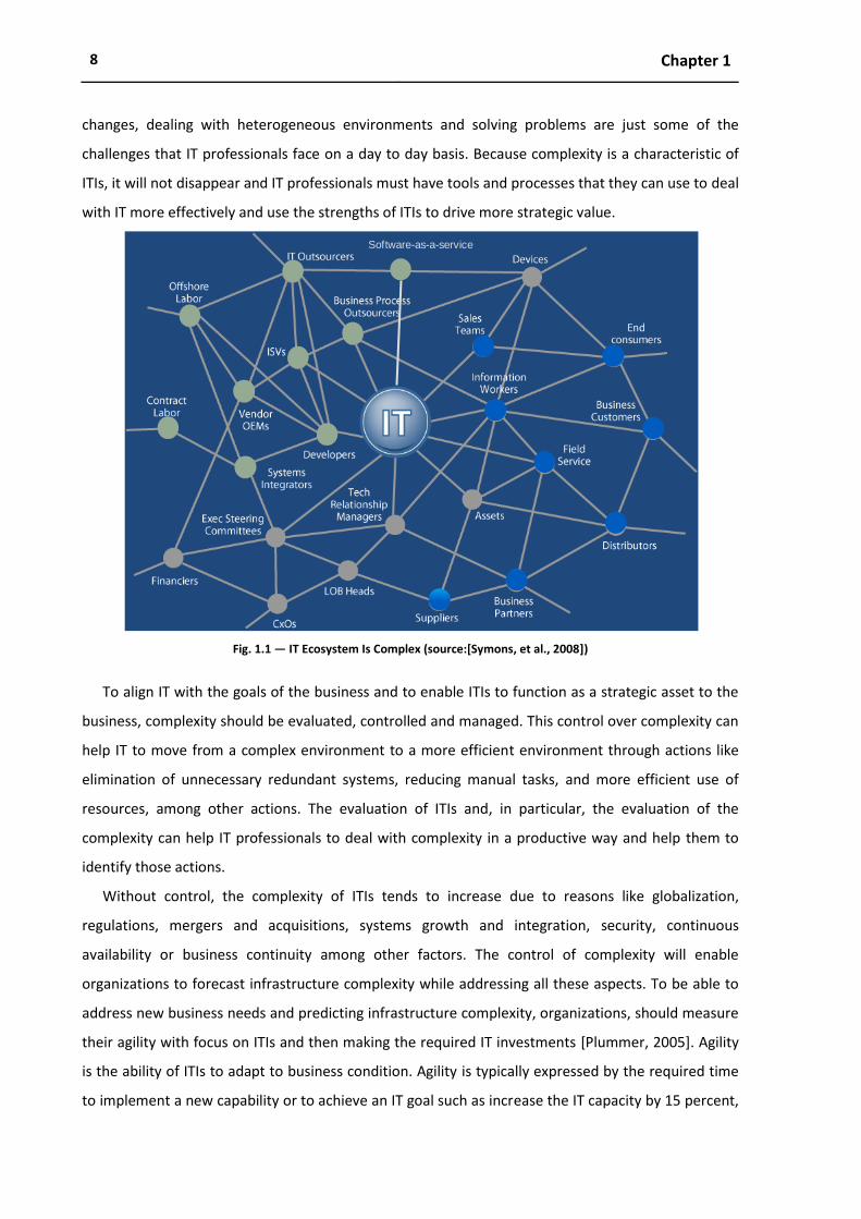
8 Chapter 1
changes, dealing with heterogeneous environments and solving problems are just some of the
challenges that IT professionals face on a day to day basis. Because complexity is a characteristic of
ITIs, it will not disappear and IT professionals must have tools and processes that they can use to deal
with IT more effectively and use the strengths of ITIs to drive more strategic value.
Fig. 1.1 ― IT Ecosystem Is Complex (source:[Symons, et al., 2008])
To align IT with the goals of the business and to enable ITIs to function as a strategic asset to the
business, complexity should be evaluated, controlled and managed. This control over complexity can
help IT to move from a complex environment to a more efficient environment through actions like
elimination of unnecessary redundant systems, reducing manual tasks, and more efficient use of
resources, among other actions. The evaluation of ITIs and, in particular, the evaluation of the
complexity can help IT professionals to deal with complexity in a productive way and help them to
identify those actions.
Without control, the complexity of ITIs tends to increase due to reasons like globalization,
regulations, mergers and acquisitions, systems growth and integration, security, continuous
availability or business continuity among other factors. The control of complexity will enable
organizations to forecast infrastructure complexity while addressing all these aspects. To be able to
address new business needs and predicting infrastructure complexity, organizations, should measure
their agility with focus on ITIs and then making the required IT investments [Plummer, 2005]. Agility
is the ability of ITIs to adapt to business condition. Agility is typically expressed by the required time
to implement a new capability or to achieve an IT goal such as increase the IT capacity by 15 percent,
Software-as-a-service

Introduction 9
deploy new features or to increase the IT capacity to support a new business application [Mertins, et
al., 2008, MSFT, 2007].
1.3 Total cost of ownership
The TCO was popularized by Gartner more than 20 years ago, with the goal of clearly and reasonably
address the real costs attributed to owning and managing ITIs. Currently TCO is still one of the most
important concerns of IT managers [Kirwin, 2003b]. TCO identifies costs as being made of two main
groups, the direct costs and the indirect costs (aka soft costs [Kirwin, 2003a] because they often occur
outside the budget).
The direct costs are normally the capital, fees and labor costs. Indirect costs are more difficult to
measure and include the costs associated with training IT professionals and users, costs associated
with failure or outage (planned and unplanned), development and testing, costs associated with
distributed computing, datacenters, storage and telecommunications, electricity and much more
[Gartner, 2003].
The nature of indirect costs leads some organizations to underestimate their impact on ITIs.
However TCO analysis often shows that the acquisition or purchase price of an asset represents only
a small fraction of its total cost and indirect costs can typically represent as much as 60% of the total
cost of managing and owning an ITI [Kirwin, et al., 2005].
The TCO allows the alignment of IT operational efficiency goals with business performance
requirements [Kirwin, 2003a] and should not be used with the purpose of justifying IT investments,
validate initiatives or increase or decrease ITIs spending. There are some frequent misunderstandings
that TCO is only a way of cutting costs or that the IT platform with the lowest TCO is the best choice
and indirect costs do not count [Kirwin, 2003a].
The TCO has proven to be a vital and popular framework for IT and business management
decision-making and has been applied to several different technology areas. The idea of using TCO as
a way to gauge IT performance is still taking shape [Kirwin, 2003b]. TCO may be used as a proxy for
activity-based costing, a technique in which all costs associated with a specific IT function are
measured and compared to industry averages. This comparison is sometimes more efficient than
looking at IT costs at the macro level. For instance, a TCO analysis of the costs associated with
managing Enterprise Resource Planning (ERP) applications could reveal cost disparities that would
not show up if a company only considered its overall IT costs [Kirwin, 2003b].
In the field of ITIs, there has been an increasing interest in recent years in calculating the costs of
ownership with the aim of helping CIOs to make better decisions as they purchase, upgrade and/or

10 Chapter 1
replace their ITIs [MacCormack, 2003]. Understanding and evaluating the TCO of ITIs is a prerequisite
in pursuing initiatives in ITIs [Blowers, 2006a].
1.3.1 Reducing ITIs TCO
To reduce the TCO associated with a particular infrastructure it is important, first to have a process
that can analyze all the distinct aspects that an ITI is built of and calculate the real total cost of
ownership. Organizations are dependent of ITIs to provide business functionality and it is essential
that they understand and manage their costs [Kirwin, 2003a]. Only knowing the TCO, can help IT
decision makers to focus on ITI problems and develop ways to align costs, performance and service
levels with the organizational requirements, while delivering a high service quality. High service
quality normally leads to a decrease in IT budgets for managing and supporting infrastructures which
reduces the ITIs TCO.
There are several approaches that can be taken to reduce the TCO associated with a particular
infrastructure [Aziz, et al., 2003, Conley, et al., 2007, Engels, 2006]. However, because organizations
also need to preserve functionality, they need to balance between TCO and the right agility of the ITI.
So, in order to reduce the TCO of an ITI, it is very important to manage the tradeoff between TCO and
agility.
Complexity, by definition refers, to the condition of being difficult to analyze, understand or solve.
According to [Kirwin, et al., 2005] there is a direct relationship between complexity and TCO and the
more complex the IT and business are, the higher the TCO is. Complexity is acceptable if the
complexity purpose is to achieve business value but unacceptable otherwise. Therefore,
organizations should aim for the minimum level of complexity required to meet their business needs.
In the following section, we evaluate the impact of ITIs complexity on TCO.
1.3.2 The impact of ITIs complexity on TCO
The ITI complexity is normally divided into the complexity associated with the software and
complexity associated with the hardware. The complexity of any system has several drivers of which
the most important are (i) size, (ii) the diversity and (iii) the mutation of its parts and of their
interconnections. Often we have to drill down complexity analysis since each point of a system may
itself be considered a (sub) system. We stop drilling down when a part can be considered as a
blackbox.

Introduction 11
An ITI is a special kind of a system. Its parts are software and hardware components. Software
components range from applications down to firmware (embedded software). However,
components can be computer devices (e.g. desktop, handled or mobile devices), servers, switching
and communication equipment (e.g. hubs, routers, access points, repeaters) and other devices (e.g.
printers, plotters, scanners).
While the size driver of ITI complexity is self-explanatory, it may not be so obvious for the
diversity driver. The diversity driver of ITI components can manifest itself in different installation
operations and maintenance procedures.
Consider for instance two ITIs, with the same number of servers, equipment and topology. The
complexity of those two ITIs, will be much different if in one case there is no technology diversity and
on the other case each component requires specific customization or operation. Just imagine that
you have 10 different printers each requiring a different kind of maintenance intervention.
The mutation driver of ITI complexity has to do with its modifications throughout time. The
observation period may vary depending on the characteristic being observed. For instance, while for
a percentage of PCs replaced on a yearly basis would make sense, we may need to observe the
maximum number of transactions per hour for balancing online versus offline services. Table 1.2
present examples of complexity drivers for hardware and software.
Table 1.2 ― Examples of ITIs complexity metrics
Hardware Software
Components Interconnection Components Interconnection
Size Number of servers;
Number of hubs;
Number of routers;
Number of printers.
Number of physical links;
Number of logical links.
Application installations;
Operating systems
installations.
Number of dependencies
on other software
components;
Number of configuration
scripts required to allow
software interoperability.
Diversity Different end-user plat-
forms (desktops,
handled, mobile
devices);
Different server
technologies;
Different printer
products.
Different link
technologies (e.g. UTP,
fiber optic, wireless,
Bluetooth);
Redundant
communication links
between 2 nodes.
Different applications
installed;
Different operating
systems installed.
Different types of
dependencies among
software components.
Different configuration
scripts required to allow
software interoperability
Mutation Yearly rotation of
desktops.
Hardware automatic
reconfiguration to
provide fault tolerance.
Application releases per
year; Operating system
updates per year.
Components to provide
software interoperability.

12 Chapter 1
Fig. 1.2, shows an estimative chart generated with a proprietary software tool (Gartner TCO
Manager) of a 2.500 end-users environment where we can see the huge impact of the various
complexity levels on cost. In this specific scenario the TCO per end-user doubles when maximum
complexity is reached.
Fig. 1.2 ― TCO per end user at various complexity levels (source: [Kirwin, et al., 2005])
It is very important to have a relation between the complexity and the business value and the
point when the complexity exceeds the business value. Beyond that point we cannot manage the
infrastructure effectively [Harris, 2005]. There is a misperception that investing on IT creates value
with no limits. However, when we reach our capacity to manage the infrastructure (inflection point)
the value is negative. Fig. 1.3 shows the perceived relationship between value and complexity against
the real relationship, where we can see that investing in IT only brings value until the inflection point
is reached.
Fig. 1.3 ― Complexity and the value of IT (source: [Harris, 2005])
Having a process that can continually evaluate and measure complexity of ITIs is important to
understand what is the level of complexity of a particular ITI and if the value of the inflection point
was reached.

Introduction 13
1.4 IT Service Management
IT service management (ITSM) is a discipline for managing IT systems, philosophically centered on the
customer's perspective of IT's contribution to the business. ITSM focuses upon providing a
framework to structure IT-related activities and the interactions of IT technical personnel with
business customers and users.
This dissertation proposes an ITI evaluation approach that can be used by organizations for
different aspects such as the ones mentioned in the motivation section. Most of these aspects are
also covered by some ITSM frameworks [Brenner, et al., 2006]. There are a variety of frameworks
and authors contributing to the overall ITSM discipline. In this section we will briefly describe two of
the most widely adopted frameworks: IT Infrastructure Library (ITIL) [OGC, 2000] and Common
Objectives for Information and related Technology (COBIT) [ISACA, 2008b].
1.4.1 ITIL
The IT Infrastructure Library commonly referred as ITIL is one of the most widely adopted
frameworks [Cater-Steel, et al., 2006], is a structured repository of best practices developed in the
late 1980s by the Central Computer and Telecommunications Agency (CCTA) of the British
Government and currently administered and updated regularly by the British Office of Government
Commerce (OCG). The ITIL deployment is supported by the work of the IT Service Management
Forum (itSMF) [Bon, 2004]. The itSMF is global, independent non-profit organization with more than
100.000 members worldwide and present in several countries, including Portugal [itSMF, 2008], with
the mission of development and promotion of IT Service Management "best practices", standards
and qualifications.
The ITIL, currently in version 3, outlines an extensive set of management procedures that are
intended to support businesses in achieving both quality and value for money in IT operations. These
procedures are supplier independent and have been developed to provide guidance across the
breadth of ITI, development and operations.
ITIL version 3 consists of a series of books ( [OGC, 2007d, OGC, 2007c, OGC, 2007e, OGC, 2007a,
OGC, 2007b]) giving guidance on the provision of quality IT services and on the accommodation and
environmental facilities required to support IT. Fig. 1.4 displays a detailed look at the end-to-end ITIL
v2 Model.

14 Chapter 1
Fig. 1.4 ― End-to-end ITIL process (source:[Watt, 2005])
There are other frameworks and guidelines based on the ITIL framework. These have been
developed by software and hardware organizations such as the HP's Service Management
Framework [HP, 2007] which is based on ITIL v3 and replaces the HP ITSM, IBM's Process Reference
Model for IT (PRM-IT) [Ernest, et al., 2007, IBM, 2007] which in version 3 is fully aligned with ITIL v3
and Microsoft, with their Microsoft Operations Framework 4 (MOF), which in version 4.0 is also
aligned with ITIL v3 [MSFT, 2008a].
1.4.2 COBIT
Common Objectives for Information and related Technology commonly referred as COBIT is currently
in version 4.1 [ISACA, 2008b] and is another industry framework of good practices for IT produced by
Information Systems Audit and Control (ISACA) [ISACA, 2008c] and managed by the IT Governance
Institute (ITGI) [ITGI, 2008b]. COBIT framework allows managers to bridge the gap between control
requirements, technical issues and business risks, enables clear policy development and good
practice for IT control throughout organizations, emphasizes regulatory compliance and helps
organizations to increase the value attained from IT. The COBIT framework is organized into four
domains: plan and organize, acquire and implement, deliver and support, monitor and evaluate
[ISACA, 2008a]. Fig. 1.5 presents the four domains and some of the existing IT processes.

Introduction 15
Fig. 1.5 ― COBIT framework domains (source:[Symons, et al., 2006])
The plan and organize domain covers strategy and tactics in terms of, how IT can help the
organization to achieve the business objectives. The acquire and implement domain addresses the
organization's strategy in identifying developing or acquiring IT solutions as well as implement and
integrate them within the organization's current business processes. The deliver and support domain
focuses on the delivery of required services, which includes service delivery, management of security
and continuity, service support for users, and management of data and operational facilities. The
monitor and evaluate domain deals with the organization's strategy in assessing their quality and
compliance with control requirements. This domain addresses aspects such as the performance
management, monitoring of internal control, regulatory compliance and governance among others.
Across these four domains, COBIT has identified 34 IT processes accompanied by high-level and
detailed control objectives, management guidelines and maturity models [Haes, et al., 2005].
Regarding orientation, definition, classes of problems addressed and implementation, the COBIT
and ITIL are very different, however there are some similarities between them and they are more
complementary than competitive and there is a mapping comparing the components of COBIT 4.1
with ITIL version 3 [ITGI, 2008a]. Used together, they provide a top-to-bottom approach to IT
governance and service management [Heschl, et al., 2006].

16 Chapter 1
1.5 Research objectives roadmap
It is important to outline our long-term research objectives, since the proposals made in this
dissertation are intermediate steps on the roadmap for achieving them. Those long term research
objectives are then the following:
Propose a best practices enforcement framework – we expect it to be helpful for ITI
designers and managers;
Propose a TCO estimation method based upon given evolution scenarios – in other words,
we want to be able to forecast TCO evolution.
1.5.1 Best practices roadmap
As for the strategy to achieve those objectives, it will next be described by means of roadmaps, one
for each long term objective. In those roadmaps, the activities with a white background represent
those that were developed in the scope of this dissertation, while those with a grey background
represent the ones that will be developed in future work, probably in the scope of a PhD research
work.
In this dissertation we propose a model-based technique to classify ITI topologies automatically.
This classification is based on a set of ITI complexity metrics that are formalized using a constraint
language. We collect the values of those metrics for a set of different ITIs and then use them to prove
the feasibility of the automatic topology classification technique ("AS IS (1)" state in Fig. 1.6).
We also propose in this dissertation a model-driven formalization technique for ITI best practices.
Based on that formalization we perform the detection of best practices violation upon a sample of
ITIs structural data ("AS IS (2)" state in Fig. 1.6).

Introduction 17
Fig. 1.6 ― Roadmap (best practices)
We believe that the formalization of best practices should be targeted for specific ITI topologies. A
well-formedness rule suitable for one topology may not be applicable to other topologies. Therefore,
we plan to specialize best practices per topology. We will then use the automatic topology classifier
to select the most appropriate rules to verify for a given ITI, in order to improve our proposed
technique for detecting ITI best practices violation. We plan to test this improved version upon the
previously mentioned sample of ITIs structural data, thus proving the feasibility of our proposed
framework for best practices enforcement ("TO BE" state in Fig. 1.6).
Model ITIs structure
Classify ITI Topologies
Formalize ITI
best practices
Enforce best practices
adoption
Refine ITI best
practices formalization
Detect ITI best
practices violation
Refine ITI topology
classification
Formalize ITI
complexity metricsBuild structural
data sample
Collect
complexity metrics
\
AS IS
(2)
AS IS
(1)
TO BE
Best Practices Roadmap
(Data from several ITIs)

18 Chapter 1
1.5.2 TCO forecast roadmap
To forecast the TCO we first need to identify which are its driving forces. One of our claims is that the
complexity of an ITI is one of them. Our strategy to validate this claim is to perform an analysis of
variance in TCO due to ITI complexity. For that purpose we will use the sample of complexity metrics
mentioned in the previous section as independent variable descriptors and a sample of ITI financial
indicators (taken from the same ITIs as the ones from where the complexity metrics were collected)
to compose a TCO descriptor (dependent variable). For the sake of clarity and replicability, those
financial indicators will be formalized upon an ITI costs ontology. The expected outcome of this
partial roadmap, represented by CVC (Cost Versus Complexity) in Fig. 1.7 is the statistical evidence
that ITI complexity influences TCO and the quantification of that influence (e.g. percentage of the
variation in TCO that is explained by the variation in ITI complexity).
Fig. 1.7 ― Roadmap (cost versus complexity)
Model ITIs structure
Formalize ITI
complexity metrics
Assess influence of ITI
complexity on TCO
ITIs costs
ontology
Formalize ITI
financial indicators
Build structural
data sample
Collect complexity
metrics
\
Collect ITI
financial indicators
Collect ITI
financial data
AS IS
CVC
Cost Versus Complexity
(Data from several ITIs)

Introduction 19
The second part of this roadmap is represented in Fig. 1.8 and takes the CVC conclusions as input.
To forecast TCO for a specific ITI we will combine a time series of the evolution of its complexity with
another time series of its previously known TCOs. The latter are calculated on the basis of a set of
financial indicators, using the same approach as that described in the previous paragraph, but for
one ITI only, throughout time.
In the scope of this dissertation we have performed a study of the evolution of ITI complexity ("AS
IS state" in Fig. 1.8). This intermediate step is in our view an interesting step forward, since TCO
evolution will be influenced by ITI complexity evolution. Besides, this study has allowed us to
experiment with the time series techniques that will be later required to achieve our research
objective of proposing a TCO estimation method.
Fig. 1.8 ― Roadmap (best practices)
Model ITIs structure
Formalize ITI
complexity metrics
Build ITI historical
financial data sample
Collect ITI financial
indicators time series
ITIs costs
ontology
Formalize ITI
financial indicators
Collect ITI
structural metrics
time series
Build ITI
historical structural
data sample
Forecast ITI TCO
evolution
Assess influence of ITI
complexity on TCO
TO BE
Analysis of ITI
structure evolution
AS IS
CVC
Forecast TCO
(Data from same ITI)
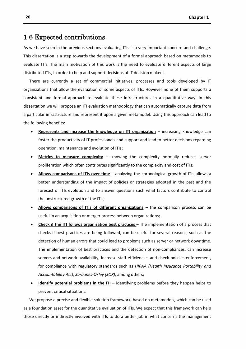
20 Chapter 1
1.6 Expected contributions
As we have seen in the previous sections evaluating ITIs is a very important concern and challenge.
This dissertation is a step towards the development of a formal approach based on metamodels to
evaluate ITIs. The main motivation of this work is the need to evaluate different aspects of large
distributed ITIs, in order to help and support decisions of IT decision makers.
There are currently a set of commercial initiatives, processes and tools developed by IT
organizations that allow the evaluation of some aspects of ITIs. However none of them supports a
consistent and formal approach to evaluate these infrastructures in a quantitative way. In this
dissertation we will propose an ITI evaluation methodology that can automatically capture data from
a particular infrastructure and represent it upon a given metamodel. Using this approach can lead to
the following benefits:
Represents and increase the knowledge on ITI organization – increasing knowledge can
foster the productivity of IT professionals and support and lead to better decisions regarding
operation, maintenance and evolution of ITIs;
Metrics to measure complexity – knowing the complexity normally reduces server
proliferation which often contributes significantly to the complexity and cost of ITIs;
Allows comparisons of ITIs over time – analyzing the chronological growth of ITIs allows a
better understanding of the impact of policies or strategies adopted in the past and the
forecast of ITIs evolution and to answer questions such what factors contribute to control
the unstructured growth of the ITIs;
Allows comparisons of ITIs of different organizations – the comparison process can be
useful in an acquisition or merger process between organizations;
Check if the ITI follows organization best practices – The implementation of a process that
checks if best practices are being followed, can be useful for several reasons, such as the
detection of human errors that could lead to problems such as server or network downtime.
The implementation of best practices and the detection of non-compliances, can increase
servers and network availability, increase staff efficiencies and check policies enforcement,
for compliance with regulatory standards such as HIPAA (Health Insurance Portability and
Accountability Act), Sarbanes-Oxley (SOX), among others;
Identify potential problems in the ITI – identifying problems before they happen helps to
prevent critical situations.
We propose a precise and flexible solution framework, based on metamodels, which can be used
as a foundation asset for the quantitative evaluation of ITIs. We expect that this framework can help
those directly or indirectly involved with ITIs to do a better job in what concerns the management
Introduction 21
and evolution of ITIs. The proposed approach is based on metamodels, and defines how we can
capture ITIs objects and their settings, and instantiate them on models. With the ITI information
available on models, we present an approach that can be used to extract the required information
from the ITI, facilitating the task of understanding the various components of the ITI and how they
are related.
We have formalized the definition of several complexity metrics and successfully collected them
from large real world ITIs. Those metrics can be used in calculating and estimating several ITI aspects
such as their size, their complexity, their evolution, or used in combination with other indicators to
calculate the TCO.
This approach contributes to productivity gains, through the possibility of running queries against
ITIs. We also provide an approach, where organizations can write their own best practices, in order
to help them to detect infrastructural non-compliance configurations. In summary, we expect that
with an approach to quantitative evaluate ITIs we can increase the efficiency and effectiveness of
ITIs, reducing costs, simplifying day to day management activities and making ITIs more robust and
more agile.
1.7 Document structure and typographical conventions
To facilitate and simplify the reading of this document, the structure is organized in eight chapters,
each with a context. The content of each chapter is as follows:
Chapter 2 describes related work relevant to the understanding and evaluation of distributed ITIs.
For that purpose this chapter presents taxonomy, and a survey built of eight documents related
with evaluation studies and evaluates these eight documents using the created taxonomy. Finally
this chapter presents a comparative analysis of these evaluations and presents some findings.
Chapter 3 introduces the Meta-Model Driven Measurement approach, presents several modeling
languages and performs a comparative review of three different ITIs modeling languages. The
remaining of the chapter is dedicated to the selection of a modeling language to work throughout
this dissertation and to present several considerations regarding the chosen modeling language.
Chapter 4 describes how the chosen modeling language will be applied using the M2DM approach
and introduces important concepts such as metamodel semantics enforcement and the ITILib. The
last section of this chapter is dedicated to a step-by-step description of every component of our
approach to evaluate ITIs.

22 Chapter 1
Chapter 5 applies the approach described in chapter 4 to evaluate different perspectives of an ITI.
There is a section dedicated to the evaluation from a sizing perspective with a real case study,
another section dedicated to the evaluation of complexity with five different case studies and a
last section dedicated to the application of best practices to ITIs. There is also a formalization of
rules for best practices compliance verification with the OCL constraint language.
Chapter 6 is dedicated to the detection of network topologies based upon logistic regression
techniques. In this chapter with the help of the multinomial logistic regression we created a
model that can be used to detect the network topology ITIs. To ilustrate this in the last section
presents we applied the created model to ten real ITIs collected from different organizations that
were slightly modified to guarantee the confidentiality of the data.
Chapter 7 presents the conclusions and the future work. It starts by summarizing the
contributions of this dissertation, present some threads to their validity and outlines several
directions for future research work.
To clearly distinguish semantically different elements and provide a visual hint to the reader, this
dissertation uses the following typographical conventions:
Italic script highlights important key words, scientific terms, methods and tools carrying
special meaning in the technical or scientific literature;
Bold face denotes table headers and items in enumerations.

23
2Related Work
Contents
2.1 Taxonomy for supporting the survey ......................................................................................... 24
2.1.1 Complexity evaluation ....................................................................................................... 24
2.1.2 Evolution analysis ............................................................................................................... 24
2.1.3 Best practices assessment ................................................................................................. 25
2.1.4 ITI modeling ....................................................................................................................... 25
2.1.5 ITI characterization ............................................................................................................ 26
2.1.6 Data collection ................................................................................................................... 26
2.1.7 Sample ................................................................................................................................ 26
2.1.8 Results validation ............................................................................................................... 27
2.2 Survey ......................................................................................................................................... 27
2.2.1 Evaluation 1 – [Juurakko, 2004] ......................................................................................... 28
2.2.2 Evaluation 2 – [DiDio, 2004b, DiDio, 2004a] ...................................................................... 29
2.2.3 Evaluation 3 – [Cybersource, et al., 2004] ......................................................................... 30
2.2.4 Evaluation 4 – [Wang, et al., 2005] .................................................................................... 31
2.2.5 Evaluation 5 – [CIOview, 2005] .......................................................................................... 31
2.2.6 Evaluation 6 – [Wipro, et al., 2007] ................................................................................... 32
2.2.7 Evaluation 7 – [Jutras, 2007] .............................................................................................. 33
2.2.8 Evaluation 8 – [Troni, et al., 2007] ..................................................................................... 33
2.3 Comparative analysis ................................................................................................................. 34
This chapter is dedicated to related work in the area of quantitative evaluations. There is a taxonomy
to support a survey of eight evaluation documents and a comparative analysis of the findings.
24 Chapter 2
2.1 Taxonomy for supporting the survey
In this section we will describe related work relevant to the understanding and evaluation of
distributed ITIs. To allow comparisons among different studies we require a set of comparison
criteria. The first three chosen criteria (complexity evaluation, evolution analysis and best practices
assessment) correspond to three possible views in assessing ITIs that are further explored in this
dissertation. The modeling and characterization criteria intend to cover the aspects related to the
description of the domain concepts. The next two criteria classify how the ITIs data collection process
was conducted and the resulting sample representativeness.
2.1.1 Complexity evaluation
As discussed in chapter 1, the complexity of an ITI should be taken into consideration for managing
important aspects such as TCO evaluation or evolution analysis. That complexity is related with
software, hardware or network components. The categories that have been identified for classifying
this criterion are the following:
Strong – All components affecting the complexity of an ITI are considered in the assessment;
Moderate – The majority of components affecting the complexity of an ITI are considered in the
assessment;
Weak – Only a few components affecting the complexity of an ITI are considered in the
assessment;
None – There is no explicit reference of complexity assessment being performed.
2.1.2 Evolution analysis
In order to accommodate future changes and align ITI with business we must analyze it in a
chronological perspective. There are several advantages of performing an ITI evolution analysis such
as the understanding of past growth, predicting the future growth, performing comparisons or
documenting ITIs, among other aspects. While performing an evolution analysis, we must consider
that ITIs have an associated lifecycle, with a set of phases that includes acquisition, deployment, and
maintenance, until being decommissioned. The categories that have been identified for classifying
this criterion are the following:
Strong – The conducted assessment takes the full ITI lifecycle into consideration and the
individual contributions of each phase are clearly described;
Related Work 25
Moderate – The conducted assessment takes the full ITI lifecycle into consideration but few
details are provided regarding the individual contributions of each phase;
Weak – The conducted assessment only covers a part of the ITI lifecycle, although some kind of
evolution is discussed;
None – The conducted assessment does not perform any kind of evolution analysis.
2.1.3 Best practices assessment
Several frameworks suggesting best practices for ITIs have been proposed in the literature. However,
from the evaluation point of view, we would like to assess if their application is being followed in
practice (e.g. in a given ITI). The categories that have been identified for classifying this criterion are
the following:
Strong – Best practices are formally defined and the assessment of their adoption is carried out
automatically, based upon that definition;
Moderate – The use of best practices is envisioned and their specification is clearly expressed or
evidence is provided on the way that is (or can be) used to assess their adoption;
Weak – The use of best practices is envisioned but their specification is not clearly expressed and
no evidence is provided on the way that is (or can be) used to assess their adoption;
None - There are no references to best practices in the study.
2.1.4 ITI modeling
To perform any kind of evaluation we should be able to describe as objectively as possible the
semantics of the entities being evaluated, their interrelationships and constraints. For that purpose
we should use a description language (usually using a diagrammatic notation), preferably with a well
defined metamodel that enforces models' well-formedness. Those description languages can range
from domain specific ones (a DSL for ITIs) to general purpose description languages. The
corresponding categories that have been identified for classifying this criterion are the following:
Strong – the assessment is performed upon a DSL for ITIs with a formalized metamodel;
Moderate - the assessment is performed upon a general purpose description language with a
formalized metamodel;
Weak - the assessment is performed upon a description language without a formalized
metamodel;
None - the assessment is performed without an explicit support of a description language.

26 Chapter 2
2.1.5 ITI characterization
To allow performing any kind of causal analysis, hypothesis testing or forecasting, we need to identify
and describe the different attributes or characteristics that describe an ITI. That description should
be as objective as possible to allow the comparability and replication of evaluations. Preferably, that
description would support the automatic collection of values of those attributes. The proposed
categories for this criterion are the following:
Strong – the attributes or characteristics of the ITI are defined with the use of a formal description
language (e.g. using an algebraic notation or first order predicate calculus) upon the metamodel,
therefore with no ambiguity;
Moderate – the attributes or characteristics of the ITI are defined using a formal description
language but with no clear reference to the underlying metamodel;
Weak - the attributes or characteristics of the ITI are defined using natural language only;
None - the attributes or characteristics that are relevant for assessing the ITI are not explicitly.
2.1.6 Data collection
Data collection aims at instantiating the adopted metamodel. In other words we need to reify the
concepts that are expressed in the chosen ITIs' modeling language. Unless it is automated, data
collection will probably be the most costly activity in ITI assessment. We propose the following
categories:
Strong – The collection process is largely automated;
Moderate – The collection process was at least partly automated;
Weak – The data collection process was entirely manual (e.g. based on user surveys,
questionnaires or interviews);
None – There are no references to the data collection process used.
2.1.7 Sample
Assessment is an issue that can be discussed conceptually, but in the end it will only make sense if is
applied to real world case studies. Therefore, it is important to categorize the kind of samples that
have been used in related works. The proposed categories are the following:
Strong – The use sample includes data from multiple ITIs throughout time;
Moderate - The used sample includes data from multiple ITIs in a given moment in time or from a
single ITI throughout time;

Related Work 27
Weak - The used sample includes data from a single ITI in a given moment in time;
None – There is no evidence that data collection upon an ITI was conducted.
2.1.8 Results validation
All assessment exercises are finalized by presenting their conclusions. However, the techniques used
to derive and validate those conclusions can have very distinct levels of preciseness. We have
considered the following categories:
Strong – Independent teams have cross-checked the presented results (external validation);
Moderate – Assessment hypothesis are tested against a sample and threats to validity are
identified;
Weak – Conclusions are based upon descriptive statistics on a sample;
None – Informal conclusions are drawn based upon direct observation and "gut feeling".
2.2 Survey
In the last years there was a significant growth in terms of the number of papers, reports, meetings,
books and studies that performed evaluations and analysis in organizations with the aim of helping
CIOs to make better decisions regarding the way they purchase, upgrade or replace their ITIs.
To understand, what is the current state of the art with these evaluations, we collected seventy
public documents from different sources and available in Internet to analyze (the complete list is
available in Appendix D). From this list we decided to perform a deeper analysis with the taxonomy
presented in section 2.1. To perform the analysis we decided to consider only documents no older
than 2004, with references to concepts related with this dissertation (such as complexity and best
practices, TCO) and with information regarding the methodology used to perform the evaluation. The
selected documents are available in Table 2.1.
It is important to point out, that our objective in reviewing these documents was not to attempt
to draw conclusions about the relative merits of the measured aspects but instead assessing the
evaluation methodology using the previous defined taxonomy.

28 Chapter 2
Table 2.1 ― Documents selected for analysis
Nº Evaluation document Name Performed by
1 [Juurakko, 2004] Measuring and Management TCO for Tetra Networks
Nokia Corporation
2 [DiDio, 2004b, DiDio, 2004a] Linux, UNIX and Windows TCO Comparison Yankee Group Corp.
3 [Cybersource, et al., 2004] Linux vs Windows - Total Cost of Ownership Comparison
Cybersource Pty
4 [Wang, et al., 2005] TCO Research in Enterprise Computing (Linux, Windows NT and Windows 2000/2003)
CCW Research
5 [CIOview, 2005] The Business Value of Migrating from Oracle to SQL Server 2005
CIOview Corporation
6 [Wipro, et al., 2007] Reducing TCO with Windows Vista - Quantified Savings for Mobile PCs
Wipro Technologies GCR Custom Research
7 [Jutras, 2007] The Total Cost of ERP Ownership in Mid-Size Companies
Aberdeen Group, Inc.
8 [Troni, et al., 2007] PDA and Smartphone: 2007 Update Gartner, Inc.
To better understand these studies, the sections 2.2.1 to 2.2.8 give an overview of every
document in Table 2.1 and summarize the results achieved. Finally, we classify each document using
the defined taxonomy.
2.2.1 Evaluation 1 – [Juurakko, 2004]
This study is focused on measuring and managing the TCO for Tetra Networks. This study details how
capital, implementation and operational expenditures contribute to TCO and how to optimize Tetra
Network’s TCO.
This study concludes that the costs associated with capital expenditures (CAPEX) such as the
network solution, infrastructure or terminals and the costs associated with implementation
expenditure (IMPEX) such as building the network are not the biggest elements of TCO. The costs
associated with keeping the network up and running or operating expenditures (OPEX), account for
50% to 80% of the costs in a ten years period.
Fig. 2.1 ― Total Cost of Ownership for TETRA networks (source:[Juurakko, 2004])

Related Work 29
The study also mentions that the network economy comes from optimized CAPEX, OPEX and
IMPEX. However it makes no references regarding how the application of best practices can influence
the TCO. During the study several networks are presented. However the impact of network
complexity on the TCO is also not presented. In terms of life-cycle costs, there is a separation of costs
per categories (CAPEX, OPEX, IMPEX), but there is no detail in terms of the costs that are measured in
each category. The study provides side-by-side comparison with six different networks. However
little or no detail is provided in terms of the TCO assessment methodology, such as how was the data
collected or how the values were obtained.
Table 2.2 ― Classification of study 1
Category Classification
Complexity evaluation None
Evolution analysis Moderate
Best practices assessment None
ITI modeling None
ITI characterization Weak
Data collection None
Sample Strong
Results validation Moderate
2.2.2 Evaluation 2 – [DiDio, 2004b, DiDio, 2004a]
This study was created by Yankee Group and is divided in two reports. The purpose of the study is to
determine the TCO and ROI of Linux compared with Windows and UNIX in specific corporate user
scenarios.
This study concluded that there is no operating system that can fulfill the needs of all companies.
Each company should make a realistic assessment of existing operating systems and decide whether
the current infrastructure meets the goals and business needs. According to the Yankee Group’s
extensive research, Linux distributors are growing monthly. Linux, UNIX and Windows platforms are
mature and many large enterprises made significant investments in them. There is no technical
advantage in switching platforms according to this study. Only a small minority (4 percent) of UNIX
users and about 10 percent of Windows users has the desire to switch platforms. The study makes no
references to the impact that the application of best practices to Windows, Linux or Unix operating
systems may have on TCO. There are some references to "hidden" costs such as the interoperability,
integration and the cost of deployment application. However there are no references to the impact
that the operating systems complexity can have on TCO. In terms of the methodology the Yankee

30 Chapter 2
Group performed a set of surveys to obtain the data and most of the categories regarding the life-
cycle costs are presented. However their study does not present information regarding the
operational costs of operating systems over a period of time.
Table 2.3 ― Classification of study 2
Category Classification
Complexity evaluation None
Evolution analysis Moderate
Best practices assessment None
ITI modeling None
ITI characterization Weak
Data collection Weak
Sample Weak
Results validation Moderate
2.2.3 Evaluation 3 – [Cybersource, et al., 2004]
This study was created by Cybersource in 2004 and compares the TCO of running Linux versus
Windows in the enterprise. The study represents an update of a previous study also from
Cybersource in 2002.
This study reported that Linux was 36% cheaper than Windows, when taking into account the
software cost as well as service, support and upgrades. This study also indicated some issues to the
study 2 [DiDio, 2004b, DiDio, 2004a] regarding how the surveys were performed and that the mailing
list used was operated by a Microsoft Partner. In terms of the methodology, the results were
obtained from a small size organization and encompass two scenarios (existing hardware and
purchased new hardware). Most of the Life-cycle costs are presented in the study and the saving
achievements by using one solution are also presented. There are no references to the impact of
complexity or the application of best practices to the TCO.
Table 2.4 ― Classification of study 3
Category Classification
Complexity evaluation None
Evolution analysis Moderate
Best practices assessment None
ITI modeling None
ITI characterization Weak
Data collection Weak
Sample Weak
Results validation Moderate

Related Work 31
2.2.4 Evaluation 4 – [Wang, et al., 2005]
This research calculates the TCO in several workloads in enterprise and medium size organizations in
china. The study compared the comprehensive sets of costs for systems running Linux, Windows NT
and Windows 2000/2003.
This research concludes that organizations can beneficiate with the use of Windows 2000 Server
and Windows Server 2003 over Linux. According to the calculations hardware acquisition is
responsible for 35,4% of TCO while operation and administration costs are responsible for 33% of
TCO. The study also shows that the TCO of using Linux for database, file and print services or mail is
higher than in Windows, lower for web servers and similar for networking servers. This research also
concludes that complexity of IT systems has a significant impact on TCO and that comparable to
Linux, there are TCO advantages in using Windows 2000 and Windows 2003.
Table 2.5 ― Classification of study 4
Category Classification
Complexity evaluation Strong
Evolution analysis Strong
Best practices assessment Strong
ITI modeling None
ITI characterization Weak
Data collection Weak
Sample Strong
Results validation Moderate
2.2.5 Evaluation 5 – [CIOview, 2005]
This research outlines the advantages of migrating databases from Oracle to SQL Server. It provides
side-by-side Total Cost of Ownership (TCO) comparison between Oracle and SQL Server 2005 for a
variety of the most common database situations.
The study found that the hidden costs of doing nothing with an existing Oracle database may
exceed the costs of acquiring an entirely new hardware and software architecture. According to this
study SQL Server 2005 offers significantly improved price/performance and reliability over previous
versions. In terms of the methodology, the TCO study represents a period of three years and the
amount of savings in migrating to SQL Server 2005 is calculated. Most of the Life-cycle costs are
presented in the study with detailed values for each category. In terms of complexity there is a scale
of 1 to 10 regarding database complexity and the impact of complexity is calculated in terms of

32 Chapter 2
migration effort. There are some references to the application of best practices, however potential
saving of applying best practices are not calculated as part of the TCO.
Fig. 2.2 ― Extending Oracle 8i or migrating to SQL Server (source: [CIOview, 2005])
Table 2.6 ― Classification of study 5
Category Classification
Complexity evaluation Moderate
Evolution analysis Strong
Best practices assessment Weak
ITI modeling None
ITI characterization Weak
Data collection Moderate
Sample Moderate
Results validation Moderate
2.2.6 Evaluation 6 – [Wipro, et al., 2007]
This study objective was to quantify savings for mobile PCs (notebook PCs, Tablet PCs and Ultra-
Mobile PCs) using Microsoft Windows Vista Operating System.
The study found that with the adoption of Windows Vista the potential TCO savings per mobile
PCs per year is $605. This is achieved through the utilization of Windows Vista benefits (security,
desktop engineering, service desk, user labor, hardware and software), the implementation of best
practices through the use of "infrastructure optimization" and the use of Microsoft Desktop
Optimization Pack (MDOP). The study provides side-by-side comparison with Windows XP. The TCO
methodology to collect information was based on surveys to 131 organizations from four different
industries.

Related Work 33
Table 2.7 ― Classification of study 6
Category Classification
Complexity evaluation Weak
Evolution analysis Moderate
Best practices assessment Strong
ITI modeling None
ITI characterization Weak
Data collection Weak
Sample Weak
Results validation Weak
2.2.7 Evaluation 7 – [Jutras, 2007]
This study is intended to analyze the TCO of six different ERP solution providers in terms of software,
services and maintenance of mid-size companies with revenues between $50 million and $1 billion.
The study found that as the company grows, the number of users goes up along with total cost of
software and services, however the maintenance costs did not growth in a linear fashion as the
others. The study presented the average costs per user by company size, the software and services
costs as well as the total cost by vendor. This study also found that TCO proven to be a significant
factor in software selection however is also strongly recommended to estimate ROI.
Table 2.8 ― Classification of study 7
Category Classification
Complexity evaluation None
Evolution analysis Weak
Best practices assessment None
ITI modeling None
ITI characterization Weak
Data collection None
Sample Weak
Results validation Moderate
2.2.8 Evaluation 8 – [Troni, et al., 2007]
This study analyzes the TCO for personal digital assistants (PDAs) and smartphones and is an update
to other similar study performed in 2004. This study aims to help organizations to understand the
cost implications associated with procuring and supporting mobile devices, to plan their deployments
more effectively and to investigate areas for potential costs saving

34 Chapter 2
The study found that PDA and smartphone TCO declined by 15% comparing with 2004. The study
also found that acquisition costs of the mobile devices represent only 10% of the overall TCO with
communication costs representing more than 35%. The costs associated with hardware and software
increase, while the costs associated with operations, administration and end-users decrease, mostly
because organization have more mature processes in place and implemented best practices. This
study also mentions that the TCO is highly dependent on the complexity of applications.
Fig. 2.3 ― Average PDA and Smartphone TCO (source: [Troni, et al., 2007])
Table 2.9 ― Classification of study 8
Category Classification
Complexity evaluation Weak
Evolution analysis Strong
Best practices assessment Weak
ITI modeling None
ITI characterization Weak
Data collection None
Sample Weak
Results validation Weak
2.3 Comparative analysis
To perform the comparative analysis we decided to create a table where the rows represent the
categories for evaluation identified in taxonomy and columns are the selected evaluations. The
intersection between rows and columns are a symbol correspondent to the category (according to
legend). One of the deliverables of this dissertation that will be detailed in chapter 4 is a
methodological approach to perform ITIs evaluations. Later we will classify our evaluation approach
using this taxonomy. Table 2.10 presents the comparative analysis.

Related Work 35
Table 2.10 ― Comparative analysis of ITI evaluations
Survey Co
mp
lexi
ty e
valu
atio
n
Evo
luti
on
an
aly
sis
Be
st p
ract
ice
s as
sess
me
nt
ITI m
od
elin
g
ITI c
har
acte
riza
tio
n
Dat
a co
llect
ion
Sam
ple
Re
sult
s va
lidat
ion
[Juurakko, 2004] — — — —
[DiDio, 2004b, DiDio, 2004a] — — —
[Cybersource, et al., 2004] — — —
[Wang, et al., 2005] —
[CIOview, 2005] —
[Wipro, et al., 2007] — [Jutras, 2007] — — — — [Troni, et al., 2007] — — Legend: Strong Moderate Weak — None
Based upon the analysis and classification of these documents we can conclude that evaluating an
ITI is a complex activity. We found that the majority of the evaluations:
Have different methodologies – there is no consistency among studies regarding the used
methodology. The processes used to collect information, the duration of the processes, the
type of analysis, the number of years of the study, are just some examples. For example we
found that some studies considered a period of three years while others considered a period
of five years. Some studies do not mention the process used to obtain the data, some
mention questionnaires or surveys, others face to face interviews, others telephone
interviews others market research and some a mix of these;
Do not cover the entire life-cycle of costs – there is some consistency in the understanding
that the acquisition costs are only part of the costs in the majority of the studies. However
the other costs collected and analyzed differ from study to study. Not all separate direct
costs from indirect costs and present detailed descriptions of each cost as presented in the
Gartner "Chart of Accounts" [Gartner, 2003]. We also found that most do not cover the
impact of complexity on TCO and those who cover do not mention if the complexity is
associated with ITI as a whole, with software, hardware, network or others aspects. The
same applies to other aspects such the adoption of best practices among others;
Have different processes to perform comparisons – the process used to perform
comparisons also differ from study to study. There are a substantial number of studies that
36 Chapter 2
perform comparisons based on average, others based upon estimations and others do not
perform comparisons at all.
With the analysis of these studies that range between 2003 and 2007, we observe that based
upon another review between 1997 and 2002 [MacCormack, 2003], the state of practice for these
evaluations continues to be poor.
All these findings regarding the measurement of TCO suggests a clear need for an TCO evaluation
methodology that can clear define rules and guidelines regarding how the whole process should be
performed. Creating a TCO evaluation methodology to allow organizations of any kind to perform
TCO analysis based upon the same categories using the same processes and methods are a very
interesting and challenge task, which solves or minimizes most of problems identified.
With the ITI evaluation methodology that we will introduce in chapters ahead we will not provide
a TCO evaluation methodology, but we expect to simplify the TCO calculation with the data and
information that we can gather from infrastructures trough the various analyses that we will be able
to perform in ITIs.

37
3ITI Modeling
Contents
3.1 Introduction ............................................................................................................................... 38
3.2 Meta-Model Driven Measurement (M2DM) ............................................................................. 38
3.3 Modeling languages ................................................................................................................... 39
3.3.1 Unified Modeling Language ............................................................................................... 39
3.3.2 System Definition Model ................................................................................................... 40
3.3.3 Service Modeling Language ............................................................................................... 40
3.4 Modeling language selection ..................................................................................................... 41
3.4.1 Unified Modeling Language ............................................................................................... 42
3.4.2 System Definition Model ................................................................................................... 43
3.4.3 Service Modeling Language ............................................................................................... 44
3.5 Comparative analysis ................................................................................................................. 45
3.6 The chosen metamodel structure .............................................................................................. 46
3.7 Modeling using SDM language ................................................................................................... 50
The chapter 3 describes what M2DM is and performs a comparative review of three different ITIs
modeling languages, evaluated with the purpose of selecting one to work with. The rest of this
chapter is dedicated to provide more information regarding the chosen modeling language and the
work performed.

38 Chapter 3
3.1 Introduction
To evaluate infrastructures, there has to be a way to represent all components that are part of an ITI
and their relations. To represent all the components we need a common language that we can use to
create models that capture all the relevant knowledge of the ITI in a readable, searchable and
reusable way.
Since several model driven approaches specifications have been proposed, we evaluate some of
them to choose the one that best fulfills the goal of performing ITI evaluations.
3.2 Meta-Model Driven Measurement (M2DM)
To perform a quantitative evaluation we must be able to express some descriptive variables on a
more than ordinal scale on our domain of discourse (DoD). In order to achieve that, we must agree
on what we are talking about, that is, we need a well understood representation of our DoD. This is
where ontologies come to the rescue.
Ontology is the science of what is, of the kinds and structures of the objects, properties and
relations in every area of reality [Smith, 2003]. However, in Computer Science, we use the word
“ontology” in a more loosely way, to designate an abstract representation of the relevant concepts
and their relationships in a given domain. If that domain is the one of modeling then, instead of
talking about a “modeling ontology”, we simply call it a “metamodel”. There are several ways of
formally defining an ontology and generic languages, as well as domain-specific ones, such as OWL
[McGuinness, et al., 2004], have been proposed for this task. In the scope of metamodeling, the most
widely used ontology language is UML, by using meta-class diagrams enriched with Object Constraint
Language (OCL) constraints [Cranefield, et al., 1999], as happens with all MOF (Meta-Object Facility)
based metamodels published by the Object Management Group (OMG).
Since we have identified the need for a metamodel, we turn our attention to the metrics
definition and collection problems. Metrics should be formally defined to avoid subjectivity in their
interpretation and in the implementation of collection instruments. In this dissertation, we will use
the Metamodel Driven Measurement (M2DM) technique in which metrics are defined as OCL
expressions upon the adopted metamodel. In addition to the formality granted by the use of this
constraint language, OCL expressions can be automatically evaluated upon the instantiated
metamodel using an ITI evaluator component. The M2DM technique was originally proposed in [Brito
e Abreu, 2001] upon the GOODLY metamodel [Brito e Abreu, et al., 1997]. The M2DM technique was
used in several distinct contexts, such as the ones of defining object oriented (OO) design metrics
based upon the UML 1.x metamodel [Baroni, et al., 2002, Baroni, et al., 2003], expressing object-

ITI Modeling 39
relational database schema metrics based upon the Common Warehouse Metamodel (CWM)
[Baroni, et al., 2004], evaluating components reusability upon the UML 2.0 metamodel [Goulão, et
al., 2004b, Goulão, et al., 2004a] or assessing components composition using the CORBA
Components Metamodel (CCM) [Goulão, et al., 2005b, Goulão, et al., 2005a]. In the following section
we outline some modeling languages and we discuss how we have selected the metamodel for the
purpose of evaluating ITIs.
3.3 Modeling languages
Picking on previous considerations, a metamodel is a modeling ontology and as such it should
describe the constructs used in the modeling process, their properties and relations. In other words,
a metamodel describes the grammar and semantics of a modeling language.
There are several metamodels constructed with different purposes and it will not be accurate to
assert that one approach is better than another in all circumstances. The concept of using models for
the management of IT services and infrastructures is not new. In this section with discuss some of
these existing modeling languages that can be used for different purposes in the ITIs field such as the
Unified Modeling Language (UML) [OMG, 2007a], System Definition Model (SDM) [MSFT, 2004] and
Service Modeling Language (SML) [Dublish, et al., 2006].
3.3.1 Unified Modeling Language
The UML is a visual language for specifying, visualizing, constructing and documenting software-
intensive systems, as well as for business process modeling, systems engineering modeling and
representing organizational structures. UML is a general-purpose modeling language that represents
a collection of best engineering practices that have proven successful in the modeling of large and
complex systems of a wide range of domains. Under the stewardship of the Object Management
Group (OMG), the UML has emerged as the software industry’s dominant modeling language. UML
started from the unification of efforts of Grady Booch, Jim Rumbaugh and Ivar Jacobson in the late
90’s. All of them published books on their own object-oriented methodologies: the Booch method
[Booch, 1994], Object Modeling Technique (OMT) [Rumbaugh, 1996] and Object-Oriented Software
Engineering (OOSE) [Jacobson, 1995], respectively. This unification of efforts succeeded and UML
became a de facto standard in the modeling community both in industry and academia. With this
unification, concepts from several OO methods were integrated in UML, what makes UML rich, but
also large.

40 Chapter 3
3.3.2 System Definition Model
The System Definition Model (SDM) was created by Microsoft and is the central component of an
industry wide initiative called Dynamic Systems Initiative (DSI) [MSFT, 2005], to simplify and
automate how customers design, deploy and operate distributed systems. The SDM was created to
simplify the process of modeling complex IT distributed systems and it was not intended to replace
the standard Common Information Model (CIM) [DMTF, 2007] or other CIM implementations such as
the WMI [MSDN, 2008]. It provides a modeling layer, which can describe interconnected
relationships and management policies of the distributed system.
The SDM is an XML-based language and modeling platform through which a schematic “blueprint”
for effective management of distributed systems can be created. SDM started as a research project
in Microsoft Research and the original idea was to create a modeling language for the next
generation of distributed dynamic computing. As the project became matured, SDM moved from
Microsoft Research to Microsoft Server and Tools Business Division (STB) where it was integrated into
Microsoft’s development tools, its management solutions and the Windows platform itself. The first
practical implementation of SDM was in Visual Studio 2005 Team System and the main goal was to
facilitate the design of distributed systems through design time validation of SDM models. Because
the definition of the underlying SDM language is an evolutionary process, the version that shipped
with Visual Studio 2005 Team System is known as the first version of SDM or SDMv1. The latter was
extended to cover more of the lifecycle and some Microsoft products started supporting the SDM
platform concepts, what originated the second version of SDM or SDMv2. Products associated with
this version included System Center Operations Manager, which is able to build up a logical
description of each application it manages, the relationships between the application components
and what dependencies each application component has on other software, operating system
services and even hardware. SDMv2 was never publicly documented, because Microsoft started to
work on SDMv3, also known Service Modeling language.
3.3.3 Service Modeling Language
The Service Modeling Language (SML) represents an evolution of SDM and is an open industry-wide
specification that defines a common language for expressing information about IT resources and
services [Dublish, et al., 2008b]. Using the eXtensible Markup Language (XML), SML defines a
consistent way to express how computer networks, applications, servers and other IT resources are
described, which can solve the problem of the numerous ways to represent the same IT resource. In

ITI Modeling 41
multi-vendors environments, SML simplifies IT, because it provides a way to share information across
different tools and applications and allows the creation of a complete picture of an IT environment.
The SML is an XML-based language for describing and constructing ITI models, aiming to promote
the interoperability between heterogeneous components. It allows building models than can be used
across infrastructures components from different vendors [Dublish, et al., 2006]. Customers
investments in models that, for instance, capture their best practices, are preserved. SML does not
prescribe a specific IT model or set of models. Instead, it defines the syntax and semantics that all
SML models must follow: their base vocabulary, the rules of composition, the grammar and the
syntax. The SML was created by the SML working group and is based on standards like XML Schema
[Fallside, et al., 2004] and Schematron [ISO/IEC, 2004]. The SML working group was formed by some
of the key IT industry leaders organizations (BEA, BMC, Cisco, Dell, EMC, HP, IBM, Intel, Microsoft and
Sun) which are working together to standardize this modeling language.
The working group published the first draft publication on 25 July, 2006 [Dublish, et al., 2006]. In
addition to the publication of the SML specification, the companies also announced their intention to
develop a library of core models to describe generic resources such as network elements, operating
systems, storage devices, desktops, server systems, web servers, a directory service and more. SML
defines a consistent way to describe computer networks, applications, servers and other IT resources
so that businesses can more easily manage services built on these resources.
The SML is still under development and on the 3rd, March, 2008 the working group submitted the
third public working draft of SML version 1.1 for review by W3C members and other interested
parties [W3C, 2008b].
3.4 Modeling language selection
To be able to evaluate ITIs in a distributed system environment we decided to select a set including
the most recent or well known model-driven approaches, which can be used to achieve this goal with
less effort. That set includes the Unified Model Language [OMG, 2004], the System Definition Model
[MSFT, 2004] and the Service Modeling Language [Dublish, et al., 2006].
The purpose of this section is to evaluate the chosen metamodels based on some characteristics
or criteria that we found relevant for the evaluation of ITIs and choose the most appropriate
modeling language to this domain.
To highlight the characteristics of the various modeling approaches we choose the following list of
evaluation criteria to evaluate metamodels:

42 Chapter 3
Expressiveness – The modeling language should provide relevant universe of discourse (UoD)
concepts such as client and server computers, network devices, physical and logical
connections, middleware and application components;
Relevance – The modeling language should be supported by a well known organization
committed to its evolution;
Models availability – We should have access to real-world ITI models expressed in the
modeling language, or be able to reverse engineer them;
Metamodel instantiability – From existing or reverse-engineered models, we must be able
to instantiate the corresponding metamodel;
Understandability – The required effort to learn the notation and to recognize the modeling
and their interrelationships concepts should be as small as possible;
Extensibility – The metamodel can be extended with new concepts or existing concepts can
be further detailed/adopted. Extensions should not cause revisions of existing definitions.
Each of these characteristics will be applied to the selected modeling languages to allow a
comparison to be made.
3.4.1 Unified Modeling Language
The application of the previous characteristics to UML is as follows:
Expressiveness: UML allows the representation of ITIs by using Deployment Diagrams. This kind of
diagram has a limited number of abstractions (physical nodes, software components, associations
and dependencies). To increase the representation richness we must use stereotypes and tagged
values. This option limits models portability, namely if we intend to use some ITI’s models capture
tool.
Relevance: The OMG has been committed in the standardization and evolution of UML. After a
sequence of minor revisions that ended in version 1.5, UML went through a major revision, which
resulted in version 2.0. The latest published version is 2.1.2. [OMG, 2007a, OMG, 2007b].
Models availability: Although an XML based format for UML models portability has been
proposed [OMG, 2007c] and is supported by several tool vendors, the examples of XMI files found in
the web are few and relate mostly to toy examples and to other diagrams (mostly class and use case
ones) rather than deployment diagrams.
Most UML tools now support at least some features of UML 2.0. However, we could not find tools
to capture UML deployment diagrams out of existing ITIs.

ITI Modeling 43
Metamodel instantiability: The UML 2.0 metamodel is fragmented across many packages, which
hampers its understandability. Furthermore, the M2DM approach requires some metamodel
flattening, since known ITI evaluator components do not support the package construct.
Understandability: The concepts of UML, the language and notation are aspects easy to
recognize. However due to UML expressiveness, it may be complex and difficult to read and
understand.
Extensibility: The UML metamodel has three extensibility mechanisms, which are tagged values,
stereotypes and constraints. Tagged values allow arbitrary information to be attached to model
elements. This extensibility mechanism allows users to define new element properties for any model
element. Stereotypes allows sub-classification of model elements. Stereotypes can be used to
introduce additional distinctions between model elements that are not explicitly supported by the
UML metamodel. Constraints allow new semantic restrictions to be applied to elements.
3.4.2 System Definition Model
The application of the previous characteristics to SDM is as follows:
Expressiveness: SDM provides a rich set of constructs to model ITIs, such as systems, resources,
endpoints and different kinds of relationships (containment, communication, hosting, reference or
delegation). Since the SDM scope is much more focused than the one of UML, its metamodel is much
less complex as a whole.
Relevance: The SDM was a key component of a Microsoft strategy called the Dynamic Systems
Initiative (DSI), with the objective of reducing the total cost of IT operations and infrastructure
management. Microsoft is committed to achieve this objective trough the utilization of a modeling
language like SDM and incorporate it in a subset of products.
Models availability: Although some simple models are included for exemplification in Microsoft
products that support SDM, we also could not find examples of realistic models in the Internet.
However, we can easily generate them from any existing ITI, using the CSVDE (Comma-Separated
values Directory Exchange) tool, available on Microsoft server operating systems, that allows us to
use a batch process to bulk export ITI objects and their relations from an Lightweight Directory
Access Protocol (LDAP) [Zeilenga, 2006] repository (e.g. Active Directory) into a CSV (Comma-
Separated Values) file format.
Metamodel instantiability: We have reverse engineered the SDM metamodel, out of the XML
DTD of SDM models made available by Microsoft. We could realize that this metamodel is much less
complex than the UML 2 one.

44 Chapter 3
Understandability: The concepts of SDM, the language and notation are aspects easy to recognize
and SDM models are easy to read and understand.
Extensibility: The SDM metamodel is extensible through the software development kit (SDK) and
allows the creation of new SDM resources as additional properties on any logical server or
application. These new resources can be associated with any existing types. SDM supports also the
ability to define new SDM types, like systemdefinitions, endpoints or relationships amongst others.
3.4.3 Service Modeling Language
The application of the previous characteristics to SML is as follows:
Expressiveness: SML provides a rich set of constructs for creating models of complex services and
systems. Depending on the application domain, these models may include information such as
configuration, deployment, monitoring, policy, health, capacity planning, target operating range,
service level agreements and so on.
Relevance: SML is a recent joint effort of major players in the IT industry (BEA, BMC, CA, Cisco,
Dell, EMC, HP, IBM, Intel, Microsoft and Sun), being promoted through the World Wide Web
Consortium (W3C) [W3C, 2008a], an industry forum that develops interoperable technologies
(specifications, guidelines, software and tools).
Models availability: Due to its very recent proposal, it is natural that we cannot yet find available
SML tools or model examples.
Metamodel instantiability: Although the SML metamodel can be obtained by reverse engineering
the XML DTD of SML, made available at the W3C site, we cannot instantiate it since we do not yet
have available models or tools to capture them.
Understandability: The concepts of SML, the language and notation are aspects easy to recognize
and SML models are easy to read and understand.
Extensibility: To provide extensibility and ensure accurate and convenient interchange of the
documents that make up an SML model or a portion of an SML model was defined an
implementation-neutral interchange format that preserves the content and interrelationships among
the documents. The SML specification defines a standard format called the SML Interchange Format
(SML-IF) that does that and allows that elements in SML can be extended to contain additional
content and/or attributes from other XML namespaces [Dublish, et al., 2008a].

ITI Modeling 45
3.5 Comparative analysis
To compare the previous characteristics of the modeling languages and choose the one that best
fulfills our needs, we will summarize the evaluation using an ordinal scale for grading each criteria,
using the following scale of satisfaction:
Very Dissatisfied (1 point)
Dissatisfied (2 points)
Somewhat satisfied (3 points)
Very Satisfied (4 points)
To facilitate the comparability process we specified a value (ranging from 1 to 4). The criteria and
languages are presented in Table 3.1. According to this scale the modeling language with an higher
value will be the chosen.
Table 3.1 ― Candidate ITIs modeling languages
Criteria / language UML SDM SML
Expressiveness 2 3 4
Relevance 4 3 4
Models availability 2 4 1
Metamodel instantiability 3 4 3
Understandability 2 3 3
Extensibility 4 3 4
Total 17 20 19
According to the total results presented in Table 3.1 the SDM appears to be the modeling
language that better fulfills our objective since it has the higher number of points. However since
SML is an evolution of SDM and it was created to model complex IT services and systems, including
their structure, constraints, policies and best practices it may sound strange why it has a lower
number of points. The main reason for this is related with the criteria Models availability that was
classified with 1 point due to the fact that when we started this work, the SML was under
development, we did not have much information about this language.
According to the results we will use the first public available version of SDM shipped as part of
Visual Studio 2005. Another important aspect regarding SDM is that we had access to tools that
allowed us to instantiate the metamodel.
In the next sections we will present the SDM structure with "toy" examples to explain the main
SDM definitions. More details regarding the structure of SDM can be found in appendix A.

46 Chapter 3
3.6 The chosen metamodel structure
The structure of the SDM is based on three core types or object definitions (system, endpoints and
resources), five relationship types (containment, communication, hosting, reference and delegation)
and some optional additions that can be added to the core types (settings, flows and constraints)
each of these are described below and with more detail in appendix.
The system is the “heart” of the SDM and in its most basic form, a system is an independently
configuration of resources. In the field of software, these resources can represent directories or files,
scripts, XML files and so on, In the field of hardware they can represent servers, sites, connections,
power supplies and other components. In the next sections we will use systems to represent the
servers and the sites of a distributed ITI.
The systems normally have resources and they allow access to its resources or access to resources
on other systems via endpoints. For example, a web service endpoint provide a means for an
application to expose or consume web services or a server located in one site replicate data with
other server trough endpoints.
In SDM systems can be atomic or composite. An atomic system is composed directly of resources,
while a composite, system is composed of other systems. In a distributed ITI, each site is a composite
since each site is composed of one or more servers.
In a composite system an endpoint represents a proxy for an endpoint in other system. Every time
that a system needs to communicate with another system it uses this proxy that will communicate
with a remote proxy endpoint of the other system.
Fig. 3.1 shows the application of these core types to an ITI. The ITI presented has only one site
with the name Lisbon, one subnet and two servers, which communicate trough endpoints.

ITI Modeling 47
Fig. 3.1 ― Application of SDM core types
Table 3.2, summarizes the core types of SDM used later to describe elements and to capture
important semantics of ITI.
Table 3.2 ― SDM core types
SDM Core Types Description
System Represents standalone entities that perform well-defined tasks in the physical world and are
independently deployable. Systems may make use of other SDM building blocks, including other
systems. Interactions among systems are explicitly modeled using communication relationships.
Resource Represents a software or hardware element that is not independently deployable in the physical
world. A resource must be deployed as part of a system. Resources can contain other resources but
not endpoints or systems. Resources within an SDM system cannot express dependencies on
resources outside the system.
Endpoint Represents a communications interface on a system. Endpoints allow SDM systems to form
communication relationships with other systems. Endpoints are used to model the interaction of a
system with other systems.
The relationship definitions are used to allow the definition of associations among SDM systems,
resources and endpoints and are refined into communication, delegation, containment, reference
and hosting relationships.
The communication relationship allows the interaction between two systems or endpoints. If a
communication relationship does not exist between endpoints, then a connection cannot be
established between those endpoints. For example, to represent the communication among servers

48 Chapter 3
trough endpoints, we can use the communication relationship. The delegation is used to represent a
proxy or delegation relationship between two endpoints. For example an HTTP server, exposed by a
web application, delegates all communication to the HTTP server endpoint.
The last three SDM relationships (reference, containment and hosting), referenced by the three
key relationships [MSFT, 2008b], can be organized in a hierarchy from least specific to most specific,
with the hosting being the most specific and reference being the less specific. That is, a containment
relationship is a more specialized version of a reference relationship and a hosting relationship is a
more specialized version of a containment relationship.
The hosting relationship should be used when the lifetime of one object is dependent of the
lifetime of the other. For instance if we consider a folder with files then, if we delete that folder all
the files contained will also be deleted. Other characteristics of the hosting relationship are:
The hosted object can be hosted by only one other object;
The hosted object cannot host the hosting object;
The hosting relationship can be nested hierarchically.
The containment relationship differs from hosting because an object can contain multiple other
objects; an object can be contained by multiple other objects; a contained object cannot contain the
containing object. If for instance, we consider a group of servers belonging to a site, deleting the site
does not mean that the servers no longer exist.
The reference relationship is used when one type of object uses or works with another, but does
not host or contains the other. For example, a web application may use other web application but
they are not hosted or contained.
The Fig. 3.2 shows the application of two relationship types (communication and containment) to
an ITI with two sites, named Lisbon and Paris.
Fig. 3.2 ― Application of SDM relationship types

ITI Modeling 49
According to the characteristics of ITIs and the existing objects presented in Fig. 3.2 we summarize
in Table 3.3 the mapping between ITIs and the SDM metamodel objects.
Table 3.3 ― Mapping between ITI objects and SDM abstractions
ITI objects SDM objects Description
Server SystemDefinition The SystemDefinition object will be used to represent objects of "Server" kind.
Site SystemDefinition The SystemDefinition object will be used to represent objects of "Site" kind. Subnet ResourceDefinition The ResourceDefinition object will be used to represent objects of "Subnet"
kind. Endpoint EndpointDefinition The EndpointDefinition object will be used to represent objects of "Endpoint"
kind.
Connection CommunicationDefinition The CommunicationDefinition object will be used to represent relationships among objects.
Belong ContainmentDefinition The Containment object will be used to represent relationships when we need to express that an object belongs to another object.
Table 3.4, summarizes the relationships of SDM used to describe elements and to capture
important semantics of ITIs.
Table 3.4 ― Relationships of SDM
Category Description
Containment Specifies ownership of an SDM object.
Communication Models an interaction between SDM systems. This relationship is expressed between endpoints on
each system. The relationship may also be between endpoints on the same system.
Hosting Identifies the execution environment for an SDM object (called the guest). At any given time, a
guest may have exactly one host.
Reference Captures dependencies between resources. The dependency is usually known only to the resource
that has the dependency. The SDM v1 does not support the creation of reference relationships.
Delegation Exposes endpoints from nested SDM systems or a resource from a host.
These relationships amongst objects allow that a system can be hosted or contained in another
system what creates a layered model. For example, an ASP.NET application is hosted on web server,
which is hosted on the operating system, which is hosted in a server. These hosting relationships
allow the model to be layered, so that different concerns can be addressed in different layers. Each
layer can be represented in discrete models or SDM documents making the system easier to build
and understand. The SDM was designed to support four layers, as illustrated in Fig. 3.3.
This four-layered model lets us represent all aspects of an distributed ITIs, such as the structure of
applications systems, the application hosting environment, the network and operating systems
environment and finally the hardware. The SDM allows us to define constraints that constrain
systems being hosted on one another. Constraints can be defined on an SDM system type for
example to restrict the kinds of systems which it can host. In a distributed infrastructure with servers

50 Chapter 3
and sites, it could make sense to host a server in a site, but does not make sense to host a server in
another server. Objects in each layer can describe constraints on the layers above or below.
Fig. 3.3 ― The four layers of SDM
The use of constraints, settings and flows represents optional additions that can be added to
systems, endpoints and resources. Each of these additions is described on Table 3.5.
Table 3.5 ― Settings, flows and constraints in SDM
Term Description
Settings Create simple value elements, which can then be used to store configuration information. All definitions
can expose settings members, which are called setting declarations within the SDM schema.
Flows Flow passes settings values among members of an object definition and among participants in
relationships.
Constraints Capture detailed requirements that depend on the configuration of SDM objects involved in a
relationship. For example, a constraint may be used to ensure that sites cannot host other sites.
3.7 Modeling using SDM language
To illustrate the feasibility of our approach, in this section we will show how to instantiate the site
with the name Lisbon presented in Fig. 3.1. The hypothetical example of the ITI has only one site with
two servers and one subnet. Later, we will use real ITIs with hundreds of servers, sites and subnets.

ITI Modeling 51
This section starts with an UML meta-object diagram to illustrate the relations among the objects
of the site Lisbon using the SDM language described earlier and next we wrote an SDM document
using SDM syntax.
For understandability sake and also due to the naming constraints in OCL, we have performed a
few transformations on the original names of the meta-objects in Table 3.6:
Table 3.6 ― Transformations on original object names to be compliant with OCL rules
Object/meaning Replaced Description
“.” “_” Purpose: Eliminate dots in identifiers, since those are not allowed in OCL
Example: Subnet id 172.27.226.128 → 172_27_226_128)
“/” _Mask_ Purpose: Eliminate slashes in identifiers, since those are not allowed in OCL
Example: Subnet mask 172.27.226.128/25 → 172_27_226_128_Mask_25
Resources SN_ Purpose: To clearly distinguish a subnet from other objects in OCL
Example: Subnet 172.27.226.127/25 → SN_172_27_226_128_Mask_25
Endpoint Server EPSE_ Purpose: To clearly distinguish a server endpoint from other objects in OCL
Example: Server_Lisbon_01 → EPSE_Server_Lisbon_01
Endpoint Site EPSI_ Purpose: To clearly distinguish a site endpoint from other objects in OCL
Example: Site_Lisbon → EPSI_Site_Lisbon
Containment _Contains_
Purpose: To identify objects of type containment from other objects in OCL
Example: Site Lisbon contains Server_Lisbon_01 → Lisbon_Contains_
Server_Lisbon_01
The Fig. 3.4 shows the SDM document, using SDM syntax to describe the Lisbon site. The
definition of Lisbon Site using the SDM represented in Fig. 3.4 consists of a document file with
extension .sdm using a set of XML instructions representing SDM object definitions, that must
conform with the SDM schema to be compiled. The SDM schema is specified in the
SystemDefinitionModel.xsd file available in Microsoft Visual Studio 2005 Team Edition for Architects.
Every document file must have at least the following items:
Root element called SystemDefinitionModel with a name attribute (Line 1 and 2, of Fig. 3.4);
Version which contains the version of the .sdm file (Line 3, of Fig. 3.4);
Document language attribute which contains the default language for the descriptions found
in the model (Line 4 of Fig. 3.4);
Information attributes which provide details about the owner of the .sdm file (Line 6 to 11 of
Fig. 3.4).

52 Chapter 3
Fig. 3.4 ― SDM definition for Lisbon site
System Definition Model: SDM syntax to represent a the site with the name Lisbon.
1 <SystemDefinitionModel
2 Name="ITInfrastructure"
3 Version="1.0.0.0"
4 DocumentLanguage="en"
5 xmlns="http://schemas.microsoft.com/SystemDefinitionModel/2005/1">
6 <Information>
7 <FriendlyName>Lisbon Site</FriendlyName>
8 <CompanyName>Universidade Nova de Lisboa</CompanyName>
9 <Copyright> Copyright (c) Universidade Nova de Lisboa. All rights reserved. </Copyright>
10 <Description> Small organization </Description>
11 </Information>
12
13 <SystemDefinition Name="Lisbon">
14 </SystemDefinition>
15 <SystemDefinition Name="Server_01">
16 </SystemDefinition>
17 <SystemDefinition Name="Server_02">
18 </SystemDefinition>
19
20 <ResourceDefinition Name="SN_172_27_226_128_Mask_25" />
21 <ResourceDefinition Name="SN_172_27_226_0_Mask_24" /
22
23 <EndpointDefinition Name="EPSE_Server_01_d2" />
24 <EndpointDefinition Name="EPSE_Server_02_d2" />
25 <EndpointDefinition Name="EPSE_Server_02_fd" />
26 <EndpointDefinition Name="EPSE_Server_01_fd" />
27
28 <ContainmentDefinition Name="Lisbon_Contains_Server_01"
29 ParentDefinition="Lisbon" MemberDefinition="Server_01" />
30 <ContainmentDefinition Name="Lisbon_Contains_Server_02"
31 ParentDefinition="Lisbon" MemberDefinition="Server_02" />
32 <ContainmentDefinition Name="Lisbon_Contains_SN_172_27_226_128_Mask_25"
33 ParentDefinition="Lisbon" MemberDefinition="SN_172_27_226_128_Mask_25" />
34 <ContainmentDefinition Name="Lisbon_Contains_SN_172_27_226_0_Mask_24"
35 ParentDefinition="Lisbon" MemberDefinition="SN_172_27_226_0_Mask_24" />
36
37 <CommunicationDefinition Name="EPSE_Server_01_d2_EPSE_Server_02"
38 ServerDefinition="EPSE_Server_01_d2"
39 ClientDefinition="EPSE_Server_02_d2"/>
40 <CommunicationDefinition Name="EPSE_Server_02_fd2_EPSE_Server_01"
41 ServerDefinition="EPSE_Server_01_fd"
42 ClientDefinition="EPSE_Server_01_fd" />
43 </SystemDefinitionModel>
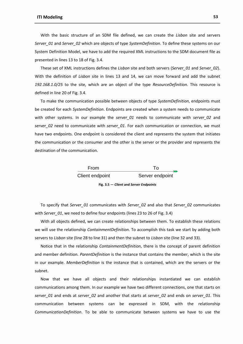
ITI Modeling 53
With the basic structure of an SDM file defined, we can create the Lisbon site and servers
Server_01 and Server_02 which are objects of type SystemDefinition. To define these systems on our
System Definition Model, we have to add the required XML instructions to the SDM document file as
presented in lines 13 to 18 of Fig. 3.4.
These set of XML instructions defines the Lisbon site and both servers (Server_01 and Server_02).
With the definition of Lisbon site in lines 13 and 14, we can move forward and add the subnet
192.168.1.0/25 to the site, which are an object of the type ResourceDefinition. This resource is
defined in line 20 of Fig. 3.4.
To make the communication possible between objects of type SystemDefinition, endpoints must
be created for each SystemDefinition. Endpoints are created when a system needs to communicate
with other systems. In our example the server_01 needs to communicate with server_02 and
server_02 need to communicate with server_01. For each communication or connection, we must
have two endpoints. One endpoint is considered the client and represents the system that initiates
the communication or the consumer and the other is the server or the provider and represents the
destination of the communication.
Fig. 3.5 ― Client and Server Endpoints
To specify that Server_01 communicates with Server_02 and also that Server_02 communicates
with Server_01, we need to define four endpoints (lines 23 to 26 of Fig. 3.4)
With all objects defined, we can create relationships between them. To establish these relations
we will use the relationship ContainmentDefinition. To accomplish this task we start by adding both
servers to Lisbon site (line 28 to line 31) and then the subnet to Lisbon site (line 32 and 33).
Notice that in the relationship ContainmentDefinition, there is the concept of parent definition
and member definition. ParentDefinition is the instance that contains the member, which is the site
in our example. MemberDefinition is the instance that is contained, which are the servers or the
subnet.
Now that we have all objects and their relationships instantiated we can establish
communications among them. In our example we have two different connections, one that starts on
server_01 and ends at server_02 and another that starts at server_02 and ends on server_01. This
communication between systems can be expressed in SDM, with the relationship
CommunicationDefinition. To be able to communicate between systems we have to use the
Client endpoint Server endpoint
From To

54 Chapter 3
endpoints created earlier. In the communication definition there is the concept of ServerDefinition
and ClientDefinition as represented in Fig. 3.6 to identify the source and destination of the
information.
Fig. 3.6 ― ClientDefinition and ServerDefinition
So, to establish a communication between both servers is necessary to add the lines 37 to 42 to
the model in Fig. 3.4. The first instruction (Line 27 to line 39) defines a CommunicationDefinition with
the name “EPSE_Server_01_d2_EPSE_Server_02” and represents the communication from server_02
to server_01 through the use of the endpoints. The second instruction defines a
CommunicationDefinition with the name “EPSE_Server_02_d2_EPSE_Server_01” and represents the
communication from server_01 to server_02 through the use of the endpoints.
To make sure that the model does not have errors we can compile it. In order to compile we need
to have installed the SDM Command Line Compiler (SdmC.exe), which is responsible for validating
the correctness of a .sdm file according to the SDM Schema. The SDM Schema and SdmC.exe are
installed with Microsoft Visual Studio 2005 Team Edition for Architects. The SDM compiler can be run
from the command line on an .sdm file created. The .sdm file name to compile is the only required
argument. Fig. 3.7 presents a successfully compilation of the ITI model.
Fig. 3.7 ― Compilation of SDM document
ClientDefinition ServerDefinition
From To
System Definition Model: Successfully compilation of the SDM document in a command prompt
1 C:\> SDMC ITIinfrastructure.sdm
2
3 Microsoft (R) SDM Compiler version 1.0.50818.0
4 Copyright (C) Microsoft Corporation. All rights reserved.
5
6 Compiling file: C:\ ITIinfrastructure.sdm
7
8 Compilation succeeded.
9
10 C:\>_

55
4Evaluation Approach
Contents
4.1 Bootstrapping the application of M2DM ................................................................................... 56
4.1.1 SDM metamodel conversion .............................................................................................. 56
4.1.2 Metamodel semantics enforcement ................................................................................. 58
4.1.3 The SDM library for ITIs (ITILib) .......................................................................................... 60
4.2 The approach step-by-step ........................................................................................................ 61
4.2.1 ITI data gatherer................................................................................................................. 64
4.2.2 ITI Meta-instances generator ............................................................................................. 66
4.2.3 ITI evaluator ....................................................................................................................... 68
4.2.4 Statistical analyser ............................................................................................................. 69
This chapter describes the application of the M2DM approach and presents all the components of the
purposed ITI evaluation approach in a step-by-step fashion. Some ITIs' well-formedness rules and the
SDM library for ITIs (ITILib) will be also presented.
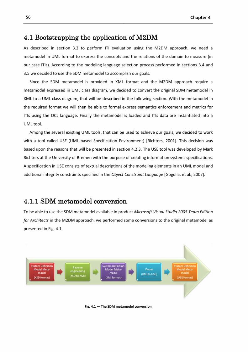
56 Chapter 4
4.1 Bootstrapping the application of M2DM
As described in section 3.2 to perform ITI evaluation using the M2DM approach, we need a
metamodel in UML format to express the concepts and the relations of the domain to measure (in
our case ITIs). According to the modeling language selection process performed in sections 3.4 and
3.5 we decided to use the SDM metamodel to accomplish our goals.
Since the SDM metamodel is provided in XML format and the M2DM approach require a
metamodel expressed in UML class diagram, we decided to convert the original SDM metamodel in
XML to a UML class diagram, that will be described in the following section. With the metamodel in
the required format we will then be able to formal express semantics enforcement and metrics for
ITIs using the OCL language. Finally the metamodel is loaded and ITIs data are instantiated into a
UML tool.
Among the several existing UML tools, that can be used to achieve our goals, we decided to work
with a tool called USE (UML based Specification Environment) [Richters, 2001]. This decision was
based upon the reasons that will be presented in section 4.2.3. The USE tool was developed by Mark
Richters at the University of Bremen with the purpose of creating information systems specifications.
A specification in USE consists of textual descriptions of the modeling elements in an UML model and
additional integrity constraints specified in the Object Constraint Language [Gogolla, et al., 2007].
4.1.1 SDM metamodel conversion
To be able to use the SDM metamodel available in product Microsoft Visual Studio 2005 Team Edition
for Architects in the M2DM approach, we performed some conversions to the original metamodel as
presented in Fig. 4.1.
Fig. 4.1 ― The SDM metamodel conversion

Evaluation Approach 57
The SDM metamodel was provided in W3C XML Schema format (XSD), so the first step consisted
in reverse engineering the SDM schema to XMI format (XML Metadata Interchange) because most of
UML modeling tools support the XMI format. The XMI format is a standard that was defined and
maintained by the OMG to support the exchange of metadata between modeling tools based on the
UML. XMI exists in several earlier versions (1.0, 1.1 and 1.2) with 2.1 being the most recent [OMG,
2007c].
To perform the reverse engineering (XSD to XMI) conversion we evaluated several commercial
tools such as the Enterprise Architect [Systems, 2008b], Rational Rose [IBM, 2008], XMLspy [Altova,
2008], Objecteering [Objecteering, 2008] and some open source tools such as ArgoUML [Tigris, 2008]
and also some academic tools such as "A case tool for developing XML schemas" [Novotný, 2004].
Based mainly upon the simplicity and the quality of the results achieved with all these tools, we
decided to perform the reverse engineering of the SDM metamodel with a trial version of the
Enterprise Architect, version 5.1. After importing the SDM metamodel schema and reverse
engineering it, we were able to export it to XMI 1.1 format [systems, 2008a].
With the SDM metamodel in XMI 1.1 format, the next step was to transform the metamodel in
the USE format. To be able to perform this we decided to use some of the work developed in the
QUASAR research group and we used a parser that transform Rational Rose files into the USE format
[QUASAR, 2008]. So we imported the SDM XMI file into Rational Rose, we saved as rose format and
we used the parser to convert the SDM metamodel to the USE format.
These conversions were also very important to the understandability of the SDM metamodel,
since they allowed us to create an UML class diagram (available in appendix B). Fig. 4.2 shows a
simplified extract of the SDM metamodel including the relevant model objects and relationships for
the scope of this dissertation.
Fig. 4.2 ― SDM metamodel to model for ITIs

58 Chapter 4
In the definitions of Fig. 4.2 we can observe the core SDM types (systems, resources and
endpoints) and two kinds of relationships (containment and communication).
4.1.2 Metamodel semantics enforcement
To ensure the consistency of our ITI metamodel, we enforce some semantics in the metamodel
trough the definition of Well-Formedness Rules, shortly referred to as WFR, which are expressed as
OCL invariants. The OCL invariants are OCL expressions that must be true for all instances of that type
at any time. This approach is similar to the one used in the UML metamodel itself, to check its
consistency [Chiorean, et al., 2004]. The number and type of WFRs to create depends from the
domain.
In the domain of ITIs a member cannot be multiple contained (e.g. a server such as the server_01
from our examples, cannot belong simultaneously to the site Lisbon and to the site Paris.). The
expression isUnique specifies whether the return parameter is unique or not. The OCL expression to
enforce this semantic is as follows:
Fig. 4.3 ― WFR for multiple contained objects
Another example is the semantic enforcement regarding the membership of objects. In ITIs
servers must be contained by a site (e.g. the server_01 must belong to site Lisbon or to site Paris.)
The OCL expression to represent this WFR is as follows:
Fig. 4.4 ― WFR for definition of the membership of servers
Well-Formedness Rule: A server must be contained by a site
1 context SystemDefinition
2
3 inv ServerContainedBySite:
4 IsServer() implies Container().IsSite()
Well-Formedness Rule: Member cannot be multiple contained
1 context ContainmentDefinition
2
3 inv noMultipleContainment:
4 ContainmentDefinition.allInstances->isUnique(MemberDefinition)
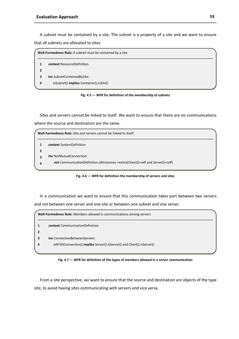
Evaluation Approach 59
A subnet must be contained by a site. The subnet is a property of a site and we want to ensure
that all subnets are allocated to sites.
Fig. 4.5 ― WFR for definition of the membership of subnets
Sites and servers cannot be linked to itself. We want to ensure that there are no communications
where the source and destination are the same.
Fig. 4.6 ― WFR for definition the membership of servers and sites
In a communication we want to ensure that this communication takes part between two servers
and not between one server and one site or between one subnet and one server.
Fig. 4.7 ― WFR for definition of the types of members allowed in a server communication
From a site perspective, we want to ensure that the source and destination are objects of the type
site, to avoid having sites communicating with servers and vice versa.
Well-Formedness Rule: Members allowed in communications among servers
1 context CommunicationDefinition
2
3 inv ConnectionBetweenServers:
4 IsNTDSConnection() implies Server().IsServer() and Client().IsServer()
Well-Formedness Rule: Site and servers cannot be linked to itself
1 context SystemDefinition
2
3 inv NotMutualConnection:
4 not CommunicationDefinition.allInstances->exists(Client()=self and Server()=self)
Well-Formedness Rule: A subnet must be contained by a site
1 context ResourceDefinition
2
3 inv SubnetContainedBySite:
4 IsSubnet() implies Container().IsSite()

60 Chapter 4
Fig. 4.8 ― WFR for definition of the types of members allowed in a site communication
All endpoints must have a container. We want to ensure that all endpoints belong to a server or
to a site.
Fig. 4.9 ― WFR for definition of the membership of endpoints
4.1.3 The SDM library for ITIs (ITILib)
In this section we give a general idea of how we have created an SDM library for ITIs, called ITILib
trough the extension of the SDM metamodel. This library is a set of operations that support the
quantitative assessments on ITIs.
A model of an ITI, expressed as a SDM model, is an instance of the SDM metamodel. This instance
can be seen as a directed graph of meta-objects (sites) representing the modeling elements used in
the SDM model and the appropriate meta-links (endpoints) among them. By traversing this graph,
we can collect information on the ITI we want to analyze. This library is based on OCL expressions to
collect the relevant information from the meta-data (meta-objects and meta-links).
Fig. 4.10 shows the SDM meta-model with a set of operations to perform quantitative assessment
of ITIs. The Fig. 4.10 only presents a subset of attributes and operations defined in each class.
More details regarding each of these attributes and operations can be seen in Table B.2 and Table
B.2 of Appendix B.
We decided to include also more details regarding each of the definitions and the relationships
presented in Fig. 4.10 in a class diagram also presented in Appendixes (Fig. C.1, Fig. C.2, Fig. C.3, Fig.
C.4 of Appendix C).
Well-Formedness Rule: Endpoints must have a container
1 context EndpointDefinition
2
3 inv noNullContainer:
4 not(ContainmentDef().isUndefined())
Well-Formedness Rule: Members allowed in communications among sites
1 context CommunicationDefinition
2
3 inv ConnectionBetweenSites:
4 IsSiteLink() implies Server().IsSite() and Client().IsSite()

Evaluation Approach 61
Fig. 4.10 ― SDM metamodel with ITILib operations
4.2 The approach step-by-step
The methodology consists in an organized and documented set of procedures and guidelines to
perform ITI evaluation. To perform ITI evaluation we defined and created a set of components that
will be detailed later in this chapter and we defined a set of steps in Fig. 4.11, which must be
followed in order to perform ITI evaluations.

62 Chapter 4
Fig. 4.11 ― Steps to perform ITI evaluations
Each of these steps is performed by a component of the methodology and each has specific
responsibilities as follows:
Scan ITI to gather data (step 1) – the first step consists in gather data from infrastructure.
This step is performed by a component that we called ITI data gatherer that is responsible for
gathering data from an organization ITI through queries to directory services repositories;
Store ITI data gathered (step 2) – This step is also performed by ITI data gatherer component
and consists in saving the data gathered in the component IT data store. The IT data store is
a repository with data stored in CSV format;
Generate meta-instances (step 3) – the generation of meta-instances consists in loading the
ITI data stored in the repository in CSV format, categorizing, transforming and generating
meta-instances in ITI evaluator format. This step is perform by a component called Meta-
instances generator;
Store ITI meta-instances (step 4) – The component ITI meta-instances generator is also
responsible for storing the ITI meta-instances generated in the component ITI Meta-
instances store. The ITI meta-instances store is a repository that holds the meta-instances
ready to be used by the component ITI evaluator;
Load SDM metamodel (step 5) – this step consists in loading the SDM metamodel
component into the ITI evaluator component. The process of loading the SDM metamodel
component is performed by ITI evaluator component;
Load ITI meta-instances (step 6) – after loading the SDM metamodel component into the ITI
evaluator component, we can load ITI meta-instances generated in step 3. This process is
also performed by ITI evaluator component and consists in loading data from ITI meta-
Step 1Scan ITI to gather
data
Step 2Store ITI data
gathered in CSV format
Step 3Generate meta-
instances
Step 4Store ITI meta-
instances
Step 5Load SDM
Metamodel and ITIlib
Step 6Load ITI meta-
instances into the SDM Metamodel
Step 7Run Queries
Step 8Display queries
results and reports
Step 9Stastical analysis

Evaluation Approach 63
instances store component and instantiate this data into the SDM metamodel component
loaded in step 5;
Run queries (step 7) – With all the data instantiated in the ITI evaluator component, ITI
stakeholders are able to run queries in the ITI evaluator component to obtain quantitative
results, assess complexity or check constraint violations among other aspects;
Display query results and reports (step 8) – this step is also performed by ITI evaluator
component and consists in evaluating the queries performed in step 7 and presenting the
results;
Statistical Analysis (step 9) – This step consists in a deeper analysis of the results provided by
the step 8. This type of analyzes is important for example to predict future grow, to compare
ITIs of different organization among other aspects.
Fig. 4.12 illustrates the whole process to perform ITI evaluation using the proposed evaluation
approach.
Fig. 4.12 ― Evaluation approach illustration
The following sections present more details of the ITI evaluation methodology regarding each of
the tools presented in Fig. 4.12 (ITI data gather, Instances generator, ITI evaluator and statistical
analyser) and examples of the data deliverable commonly referred as output.
ITI Data Store
1 2 3
Meta-Intances
Store
SDM Metamodel
ITIlib
4
5
5
6
8
9
7
ITI EvaluatorIT
Infrastructure
Results
Statistical Reports
IT
Stakeholders
Queries
Data flowTool
Legend
Data deliverable

64 Chapter 4
4.2.1 ITI data gatherer
The ITI data gatherer is a tool (represented in Fig. 4.12 as the step 1) that performs queries to an
LDAP compatible directory server that stores the X.500 entities (The IT infrastructure) in an
underlying database. To better understand this tool we will briefly explain the concepts of directory
services, X.500 and other related concepts such as LDAP.
The directory services were an Open Systems Interconnection (OSI) initiative to get everyone in
the industry to agree to common network standards to provide multi-vendor interoperability. These
standards provide an information structure model, protocols for communicating directory
information between systems, procedures that allow the directory information to be distributed
among several independent systems.
The X.500 is a series of computer networks standards for directory services, developed by the
International Telecommunication Union Telecommunication Standardization (ITU-T) and the
International Organization for Standardization (ISO) and was developed for storing information about
objects relevant to telecommunications, such as organizations, persons, distribution lists, sites,
servers, subnets, etc.
The LDAP, currently in version 3, is an Internet protocol for accessing distributed directory
services that act in accordance with X.500 data and service models and was specified in a series of
Internet Engineering Task Force (IETF) Standard Track Requests for Comments (RFCs) [Zeilenga,
2006]. There are several implementations of LDAP/X.500 directory services from different
organizations, such as:
eDirectory – The eDirectory which was previously known as Novell Directory Services
(NDS) is the Novell implementation of directory services that natively support LDAPv3 and
can be used in different platforms such as Windows, Linux, Unix and Netware [Novell,
2008];
OpenLDAP – The OpenLDAP is a free open source implementation that support LDAPv3
and are available for different platforms such as Unix, AIX, Linux, Windows, Solaries, z/OS,
among others [OpenLDAP, 2008];
Fedora Directory Server – This directory server also supports LDAPv3 and is available to
some Linux distributions, Solaris 2.8 and later and HP/UX 11 [Fedora, 2008].
Active directory – This directory server is compliant with LDAPv3 [MSFT, 2003] and is
based on X.500 concepts. The data in Active Directory can be accessed by any LDAPv3
compliant application. Active Directory was created by Microsoft and is included in server
operating systems such as Windows 2000, Windows Server 2003 and Windows Server
2008;

Evaluation Approach 65
Open Directory – The Open Directory is the directory service from Apple’s MAC OS X
which is based on OpenLDAP [ODP, 2008];
Apache Directory Server – The Apache Directory Server was completely written in Java
and is an open source project of Apache Software Foundation [ASF, 2008].
Oracle Internet Directory – The Oracle Internet Directory (OID) is the Oracle
implementation of directory service, which is compatible with LDAPv3 [Stullich, 2006];
Sun Java System Directory Server – This is the Sun Microsystems' directory service
implementation, which also supports LDAPv3 [Sun, 2008];
These are just a few examples of the directory services currently available because there are
much more. In the context of this dissertation and in this step in particular (gatherer ITI data) we
decided to work with Active Directory, mainly because to prove the feasibility of our approach we
rely on organization ITI data and the most wide, complex and interesting ITIs data, that we had
access, were Active Directory implementations.
Having chosen Active Directory to obtain ITI data, the next choice was to select a tool that was
able to connect to Active Directory and bulk export the ITI data. As introduced earlier we used the
CSVDE which is a command-line tool available in Microsoft Windows Server operating systems,
created with the purpose of bulk exporting and importing data from Active Directory in the Comma-
Separated Value (CSV) format.
The ITI data in CSV format has normally thousands of lines (depending on the size of the
organization ITI). Example in Fig. 4.13 shows the header of the file (line 1) and the representation of a
server with the name Lisbon01 (line 2).
Fig. 4.13 ― ITI data store contents (Infrastructure in CSV format)
Evaluation Approach: Example of contents of ITI data store data deliverable (step 2 of Fig. 4.12)
1 DN,objectClass,cn,distinguishedName,instanceType,whenCreated,whenChanged,uSNCreated,uSNChanged,s
howInAdvancedViewOnly,name,objectGUID,systemFlags,objectCategory,siteObjectBL,serverReference,dNS
HostName,hasMasterNCs,dMDLocation,invocationId,options,serverReferenceBL,msDS-Behavior-Version,
msDS-HasInstantiatedNCs,msDS-HasDomainNCs,msDS-hasMasterNCs, enabledConnection, fromServer,
schedule,mS-DS-ReplicatesNCReason,transportType,interSite TopologyGenerator, siteServer,siteObject
,transportAddress Attribute,cost,siteList,replInterval,dSCorePropagationData
2 "CN=lisbon01,CN=Servers,CN=Lisbon,CN=Sites,CN=Configuration,DC=unl,DC=net",server,lisbon01,"CN=lisbo
n01,CN=Servers,CN=Lisbon,CN=Sites,CN=Configuration,DC=unl,DC=net",4,20070423155239.0Z,2007042316
3657.0Z,7226,12692,TRUE,lisbon01,X'3d824644093071458105508f2ce224be',1375731712,"CN=Server,CN=
Schema,CN=Configuration,DC=unl,DC=net",,"CN=lisbon01,OU=Domain Controllers, DC=unl,DC=net",
lisbon01.unl.net, 20070423163657.0Z;2007 0423163657.0Z;20070423163657.0Z;160457845686151056.0Z

66 Chapter 4
4.2.2 ITI Meta-instances generator
The Meta-instances generator (represented in Fig. 4.12 as the step 3) was the name given to the tool
that transforms the content of ITI Data Store (Fig. 4.13), into meta-instances. This tool parses the CSV
files and generates instances in a format that can easily be imported into an UML-based Specification
Environment (known as ITI Evaluator tool or component and described in the next section).
Because we worked with large amounts of data in a CSV format, we decided to build the ITI meta-
instances generator using the capacities of Microsoft Office Excel. The ITI meta-instances generator
presented in Fig. 4.14 is responsible for:
Importing large text files in CSV format;
Categorizing different types of data (e.g. servers, sites, subnets, etc.);
Parsing each type of data and generating meta-instances expressions accordingly;
Saving all ITI meta-instances into a format that can be loaded by the ITI evaluator
component.
In Fig. 4.14 we represent the commands generated by the ITI meta-instances generator, which is
ready to be imported into the ITI evaluator component. The following set of commands, allows the
creation of six objects of type SystemDefinition (line 1 to 6) to represent sites and set a value with the
name (line 7 to 12).
Fig. 4.14 ― Meta-instances store contents
The diagram of Fig. 4.15 shows a meta-object diagram that represent the Lisbon site (presented
initially in section 3.6) and several relationships with subnets and servers. The information in the
meta-object diagram was generated with meta-instances generator.
Evaluation Approach: Example of contents of meta-instances store data deliverable (step 4 of Fig. 4.12)
1 ! create Lisbon : SystemDefinition
2 ! create Madrid : SystemDefinition
3 ! create Paris : SystemDefinition
4 ! create Berlin : SystemDefinition
5 ! create London : SystemDefinition
6 ! create Dublin : SystemDefinition
7 ! set Lisbon.Name:= 'Lisbon'
8 ! set Madrid.Name:= 'Madrid'
9 ! set Paris.Name:= 'Paris'
10 ! set Berlin.Name:= 'Berlin'
11 ! set London.Name:= 'London'
12 ! set Dublin.Name:= 'Dublin'

Evaluation Approach 67
Fig. 4.15 ― Meta-object diagram for the Lisbon site

68 Chapter 4
4.2.3 ITI evaluator
The ITI evaluator (represented in the center of Fig. 4.12) was the name given to the tool that works
with ITI data and makes the ITI evaluation possible. It does so by evaluating OCL expressions and
constraints upon the SDM metamodel. OCL expressions can be used in for several purposes such as
the specification of the initial value of an attribute or association, the specification of the body of an
operation, indication of a guard condition and, most of all, to specify the following types of
constraints on the SDM metamodel:
Invariants – An invariant is a constraint that states a condition that must always be met by all
instances of the class, type, or interface. An invariant is described using an expression that
evaluates to true if the invariant is met. Invariants must be true all the times;
Preconditions – A precondition to an operation is a restriction that must be true before the
operation is called. Fulfilling a precondition is an obligation for the operation caller;
Postconditions – A postcondition to an operation is a restriction that must be true when the
operation ends its execution. Fulfilling a postcondition is a right for the operation caller.
Currently there are several tools available from both commercial companies and universities that
support OCL. Some examples are ModelRun from Boldsoft, OCL compiler from University of Dresden
and OCL compiler from Cybernetic Intelligence GMBH, Octopus from Klasse Objecten, USE from
University of Bremen and many others. Among those tools we chose the USE (UML-based
Specification Environment) tool from Bremen university [Gogolla, et al., 2005], since it fulfills the
requirements for evaluating ITIs and we already had knowledge and good experiences in using it in
other research projects. Notice that in the context of this dissertation sometimes the ITI evaluator is
called the USE tool.
With USE we were able to load the SDM metamodel (represented in step 5 of Fig. 4.12) and ITILib
(referred in section 4.1.3 and also represented as step 5 of Fig. 4.12) which contains meta-classes,
meta-associations, meta-attributes, meta-operations and constraints). Once this metamodel has
been loaded, we can add the meta-objects generated with ITI meta-instances generator tool and
initialize their attributes as represented in Fig. 4.12 as step 6.
Each time a change in the system’s state occurs, an automatic checking of the invariants is carried
out. For example, when a new object is introduced, it is checked that it fulfills the specification of the
SDM model and all the constraints defined. The “USE” tool can also validate the pre and post
conditions.
With all the ITI data available in the ITI evaluator tool, ITI stakeholders can perform queries
(represented in Fig. 4.12 as the step 7) as we will detail in the chapter ahead.
Evaluation Approach 69
4.2.4 Statistical analyser
The statistical analyser (represented in Fig. 4.12 as step 9) was the name given to the tool that
performs statistics using the result of ITI stakeholder's queries (represented in Fig. 4.12 as step 8).
The statistics is a mathematical science pertaining to the collection, analysis, interpretation or
explanation, and presentation of data.
To deal with a large amount of ITI data, we decided to use statistical analysis, which serves the
purpose of description and inference. Descriptive statistics can be used to summarize the ITI data in a
numeric or graphically format. Inferential statistics is used to model patterns in the ITI data what can
take the form, for instance of hypothesis testing (yes/no questions), correlation (description of
associations) or regression (modeling of relationships).
There are several statistical tools available that can be used to perform statistical analysis. These
tools differ in the type of software license, cost, types of provided interfaces, supported operating
systems, types of statistical tests, regression methods, statistical charts and diagrams provided,
among other aspects. For the purpose of our work we decided to use one of the most well-known
statistical tools called SPSS (originally, Statistical Package for the Social Sciences), since it provides all
the capabilities that we need.
4.3 Categorization of the evaluation approach
Using the taxonomy presented in section 2.1, we categorize our evaluation methodology using the
same criteria:
Complexity evaluation;
Evolution analysis;
Best practices assessment;
ITI modeling;
ITI characterization;
Data collection;
Sample;
Results validation.
The results of the categorization of our evaluation approach are in the first row of Table 4.1. For
comparative reasons we decided to repeat the results of the evaluations performed in the chapter 2.

70 Chapter 4
Table 4.1 ― Categorization of our evaluation approach
Survey Co
mp
lexi
ty e
valu
atio
n
Evo
luti
on
an
aly
sis
Be
st p
ract
ice
s as
sess
me
nt
ITI m
od
elin
g
ITI c
har
acte
riza
tio
n
Dat
a co
llect
ion
Sam
ple
Re
sult
s va
lidat
ion
Our evaluation approach [Juurakko, 2004] — — — —
[DiDio, 2004b, DiDio, 2004a] — — —
[Cybersource, et al., 2004] — — —
[Wang, et al., 2005] —
[CIOview, 2005] —
[Wipro, et al., 2007] — [Jutras, 2007] — — — — [Troni, et al., 2007] — — Legend: Strong Moderate Weak — None
In terms of complexity evaluation we classify our evaluation approach with weak, since we only
evaluate complexity of a few components in our approach. From an evolution analysis, we classify
our evaluation approach with moderate, since our approach cover the complete ITI lifecycle but does
not the present individual contributions of each phase. According to best practices assessment these
criteria, we classify our evaluation approach with strong, since we formally defined best practices.
According to ITI modeling, we classify our evaluation approach with strong, since our approach
performed the assessment with a formalized metamodel. Regarding ITI characterization, we classify
our evaluation approach with strong, since we use a formal description language with no ambiguity.
According to data collection, we classify our evaluation approach with strong, since our process to
capture data is largely automated. We classify the sample of our evaluation approach with strong,
since our evaluation approach allows the load of multiple ITIs throughout time in the same
metamodel. Lastly we classify our evaluation approach regarding results validation with moderate,
since we are able to identify threats to validity of our conclusions.

71
5ITI Assessment
Contents
5.1 Introduction ............................................................................................................................... 72
5.2 Sizing analysis ............................................................................................................................. 72
5.3 Complexity analysis .................................................................................................................... 78
5.3.1 ITI network topologies ....................................................................................................... 79
5.3.2 Complexity metrics ............................................................................................................ 84
5.4 Best practices analysis ................................................................................................................ 98
5.4.1 Best practices description .................................................................................................. 99
5.4.2 Formal specification of best practices ............................................................................. 102
5.4.3 Detecting best practices violations .................................................................................. 103
This chapter presents several perspectives for evaluating ITIs using the approach presented in chapter
4. There are several case studies to illustrate the different perspective of ITI evaluation.
72 Chapter 5
5.1 Introduction
In this chapter we will perform ITI evaluations using a complexity perspective a sizing perspective
(which can also be seen as part of complexity) and using best practices. The sizing perspective
evaluation is based upon real data from an ITI with hundreds of sites. To demonstrate the complexity
evaluation we will create five ITIs with different network topologies but with the same number of
servers and sites to foster the comparability process. To perform the best practices analysis we will
change the complexity case studies to simulate specific problems in ITIs and we will formalize some
rules for best practices compliance verification with the OCL constraint language and show how the
violations can be detected. We will also define a set of metrics for both sizing and complexity
evaluations and we will demonstrate how they can be applied using our approach.
There are several metrics that will be presented in this chapter. It is important to mention that in
the development of these metrics we tried to create them with the following characteristics [Wendy,
et al., 1994, Wendy, et al., 1995]:
Simple – definition and use of the metric is simple;
Objective – different people will obtain identical values from the same entities being
evaluated, allows for consistency and prevents individual bias;
Easily collected – the cost and effort to obtain the metric is reasonable;
Robust – the metric is insensitive to irrelevant changes; allows for useful comparison;
Valid – the metric measures what it is supposed to; this promotes trustworthiness of the
measure.
Also as important as the Wendy characteristics are the Abreu's criteria for the development of
metrics [Abreu, et al., 1994]:
metrics determination should be formally defined;
non-size metrics should be system size independent;
metrics should be dimensionless or expressed in some consistent unit system;
metrics should be obtainable early in the life cycle;
metrics should be down scaleable;
metrics should be easily computable;
metrics should be language independent.
5.2 Sizing analysis
To better demonstrate how a sizing or a quantitative analysis can be performed, we will use an ITI
with hundreds of sites as the one provided in Fig. 5.1. The diagram is presented in a very small size to

ITI Assessment 73
guarantee the confidentiality of the data origin. With an ITI like this, the identification of the total
number of servers, sites or subnets may take some time without an automated process. Using the
data from Fig. 5.1 instantiated in the SDM metamodel we are able to do a sizing analysis and provide
almost all details in terms of size.
Fig. 5.1 ― ITI with a large number of sites
Notice that the lines represent connections among sites and that each site has objects such as
servers and subnets inside. The topology of this ITI is centralized, what means that every site is
connected to a central site. Later in this chapter we will discuss the various ITI network topologies.
We already have the meta-instances store corresponding to the ITI in Fig. 5.1. This means that we
already performed the steps 1 to 4 outlined in our evaluation approach. The next steps (step 5 and 6)
are to load the SDM metamodel into ITI evaluator (USE tool) and then load the meta-instances
corresponding to this ITI.
To load the SDM Metamodel we open the application USE tool and we press "Control+o" to open
the window Open Specification to be able to select our "SDM Metamodel.use" as illustrated in Fig.

74 Chapter 5
5.2. Notice in the left pane of use the empty model, meaning that no model is currently loaded in
USE.
Fig. 5.2 ― Open USE specification
This step will only be succeeded if our SDM Metamodel.use file has no errors. After loading the
specification the USE automatically compiles the file and displays in the log pane the result of the
compilation process and the number of classes, associations, invariants pre-/postconditions and
operations as illustrated in Fig. 5.3. Notice that our SDM Metamodel.use contains 104 operations
created in the context of this dissertation and corresponding to the ITILib presented earlier.
Fig. 5.3 ― Load SDM metamodel into USE

ITI Assessment 75
With the five first steps of our evaluation approach already performed, the next step (step 6)
consists in loading the meta-instances corresponding to the ITI of Fig. 5.1. Since we already have the
meta-instances generated and stored in a file (with the name ITI4SizingAnalysis.cmd) we will use the
command "readq FILE" in File input section of Fig. 5.4 to load the ITI data into USE.
Fig. 5.4 ― Command lines in USE
The USE tool provides a set of commands that can only be performed in a command line as
illustrated by the output of help command in Fig. 5.4. The last command in Fig. 5.4 (readq
ITI4SizingAnalysis) was successfully and finalizes the step 6 of our approach. With all ITI data loaded
ITI stakeholders can perform queries and analyze results (step 7 to 9). Before demonstrating the use

76 Chapter 5
"sizing queries", for understandability reasons we will first describe some of the sizing operations
such as:
Total number of sites – this metric was defined in ITILib as TotalSites() and returns the
total number of sites in a particular ITI;
Total number of servers – this metric was defined in ITILib as TotalServers() and returns
the total number of servers in a particular ITI;
Total number of subnets – this metric was defined in ITILib as TotalSubnets() and returns
the total number of subnets in a particular ITI;
Total number of connections – this metric was defined in ITILib as TotalConnections() and
returns the total number of connections among servers or nTDSconnections in a particular
ITI;
Total number of sitelinks – this metric was defined in ITILib as TotalSiteLinks() and returns
the total number of connections among sites or sitelinks in a particular ITI;
The average of servers by site – this metric was defined as AverageServersPerSite() and
returns a real number corresponding to the average of servers per site;
The average of subnets per site – this metric was defined as AverageServersPerSite() and
returns a real number corresponding to the average of subnets per site;
The average of connections per server – this metric was defined as
AverageConnectionsPerServer() and returns a real number corresponding to the average
of server connections per server;
The maximum number of servers in a single site – this metric was defined as
MaxServersPerSite() and returns the maximum number of servers in a single site. This
metric discovers which site has the highest number of servers and returns that maximum.
We created the class ITIoperations() to define all these counting or sizing metrics. Most of the
operations that return the total number of objects were created with the prefix "Total" for
understandability reasons. Fig. 5.5 has all these metrics that will be further detailed in ITILib in
appendix B.

ITI Assessment 77
Fig. 5.5 ― Sizing metrics defined in ITILib
Now that the sizing metrics are defined we can apply them to obtain sizing information regarding
the ITI presented in Fig. 5.1. In order to do that we will continue using the command line provided by
Sizing metrics defined in ITILib
1 model SystemDefinitionModelClasses
2 class ITIoperations
3 Sites(): Set(SystemDefinition) =
4 SystemDefinition.allInstances->select(IsSite())
5
6 Servers(): Set(SystemDefinition) =
7 SystemDefinition.allInstances->select(IsServer())
8
9 Subnets(): Set(ResourceDefinition) =
10 ResourceDefinition.allInstances->select(IsSubnet())
11
12 Sitelinks(): Set(CommunicationDefinition) =
13 CommunicationDefinition.allInstances->select(IsSiteLink())
14
15 Connections(): Set(CommunicationDefinition) =
16 CommunicationDefinition.allInstances->select(IsNTDSConnection())
17
18
20 TotalSites(): Integer = Sites()->size
21 TotalServers(): Integer = Servers()->size
22 TotalSubnets(): Integer = Subnets()->size
23 TotalSitelinks(): Integer = Sitelinks()->size
24 TotalConnections(): Integer = Connections()->size
25
26
27 AverageServersPerSite(): Real =
28 TotalServers() / TotalSites()
29
30 AverageSubnetsPerSite(): Real =
31 TotalSubnets() / TotalSites()
32
33 AverageConnectionsPerServer(): Real =
34 TotalConnections() / TotalServers()
35
36
37 MaxServersPerSite(): Integer =
38 Sites()->collect(SystemMembers()->size)->
39 iterate(elem: Integer; acc: Integer = 0 | if elem > acc then
40 elem
41 else
42 acc
43 endif)
44 (...)

78 Chapter 5
the USE tool. The commands use to evaluate expressions in USE start with a question mark (?).
Notice that the available commands in USE were presented in Fig. 5.6.
Fig. 5.6 ― Queries to ITI using sizing ITILib operations
The output presented in Fig. 5.6 is the result of the application of each sizing metric in the ITI
presented before. There are several variations to this sizing metrics in ITILib such as to provide the
name of servers instead of the number or the name of the site with the maximum number of servers,
instead the maximum number of servers in a site. These results complete the step 8 of our approach.
The last step (step 9) regarding statistically analysis will be detailed in the following chapters.
5.3 Complexity analysis
The term complexity is very frequent in scientific literature and, depending on the field, it has
different meanings what makes the term difficult to define. Complexity originated from the Latin
word complexus, which means “embrace”, "entwined", or "twisted together". The Merriam-Webster
dictionary, defines complexity as “the state or quality of having many interrelated parts or aspects.”
[Merriam-Webster]. These expressions may be interpreted as two or more parts or aspects that are
joined in such a way that is difficult to separate them.
Performing queries in the USE tool
1 use> ! create op:ITIoperations
2 use> ? op.TotalSites()
3 -> 1167 : Integer
4 use> ? op.TotalServers()
5 -> 1205 : Integer
6 use> ? op.TotalSubnets()
7 -> 4264 : Integer
8 use> ? op.TotalConnections()
9 -> 1928 : Integer
10 use> ? op.TotalSitelinks()
11 -> 2184 : Integer
12 use>
13 use> ? op. AverageServersPerSite()
14 -> 1.,0325621251071122: Real
15 use>
16 use> ? op.AverageSubnetsPerSite()
17 -> 3.6538131962296486: Real
18 use>
19 use> ? op.AverageConnectionsPerServer()
20 -> 1.6 : Real
21 use>
22 use> ? op.MaxServersPerSite()
23 -> 7 : Integer

ITI Assessment 79
It is easier to access complexity in relative terms than in absolute ones. Nevertheless we can say
that a system is complex if it consists of several interacting elements [Herbert, 1996] what makes the
behavior of the system difficult to understand from the behavior of its parts. [Edmonds, 1995]
provides a review of different system complexities and parts of his conclusions were that there is no
one appropriate measure of complexity, but at the very least we should distinguish concepts like size,
order and variety from complexity.
In Computer Science there are a number of approaches to characterize complexity. As an
example, IEEE standard 610 defines complexity as the degree to which a system or component has a
design or implementation that is difficult to understand and verify [Anne, 1990]. To allow measuring
the complexity of these systems we require complexity metrics. Different complexity measures have
also been proposed for different contexts, such as computational, social, economic among others
[Edmonds, 2000]. In the next sections we will describe five ITI network topologies (backbone,
unidirectional ring, bidirectional ring, centralized and fully meshed) with the same number of servers
and the same number of sites. The only difference among these topologies is the topology type and
the respective number of connections. To understand if the type of the topology has impact on the
level of complexity we will later apply different complexity measures to each of the topologies and
analyze the results.
5.3.1 ITI network topologies
With the purpose of demonstrate the use of complexity metrics in ITIs using our evaluation approach
and assess the impact of network topologies on complexity we have created the following
stereotypical topologies for ITIs:
Backbone;
Unidirectional ring;
Bidirectional ring;
Centralized;
Fully meshed.
We provide an overview and a diagram of each topology. To foster comparability, all network
topologies have the same number of sites and servers.
5.3.1.1 Backbone
In this type of network topology all sites of the network are connected to a common transmission
medium commonly referred as backbone or bus, which has exactly two endpoints. All data that is
transmitted between sites in the network is transmitted over this common transmission medium.

80 Chapter 5
In this network topology example there are six sites (Lisbon, Madrid, Paris, Berlin, London, Dublin)
which are connected trough sitelinks (Lisbon-Madrid, Madrid-Paris, Paris-Berlin, Berlin-London,
London-Dublin). Because the connections between sites are bidirectional the number of sitelinks are
ten. The number of servers is also ten, since with the exception of site Lisbon that has fours servers
and Madrid that has two, all other sites have just one server. This is required to illustrate some
complexity metrics in section 5.3.2. In this topology the total number of connections between servers
in different sites (represented in blue in Fig. 5.7) is ten and the total number of connections between
servers (represented in blue and green in Fig. 5.7) are eighteen.
Fig. 5.7 ― Backbone network topology
Notice that the Lisbon and Dublin sites are not directly connected and, as stated before, each
represent an endpoint which means that, in a communication from Dublin to Lisbon data must travel
across all the other sites to reach the destination.
5.3.1.2 Unidirectional ring
In this type of network topology, each site of the network is connected to another site forming a ring.
All data that is transmitted between sites in the network, travels from one site to the next in a
circular manner with the data flowing in a single direction only.
The main difference between this network topology (unidirectional ring) and the previous
(backbone), is that sites Dublin and Lisbon are connected and instead of having two connections
between each server, we have just one and in a single direction only. This means that data from site
Dublin to Lisbon is sent directly and the opposite means that data must travel through all the other
Site DublinTotal Number of Servers in Site: 1
Site BerlinTotal Number of Servers in Site: 1
Site LondonTotal Number of Servers in Site: 1
Site LisbonTotal Number of Servers in Site: 4
Site MadridTotal Number of Servers in Site: 2
Madrid – Paris (Sitelink)
Paris - Berlin (Sitelink)
Lisbon – Madrid (Sitelink)
Dublin - London
(Sitelink)
London - Berlin
(Sitelink)
Site ParisTotal Number of Servers in Site: 1
lisbon02
madrid01
madrid02
dublin01
london01
berlin01
lisbon01
lisbon04
lisbon03
paris01

ITI Assessment 81
sites to reach Dublin. In this topology type the number of sitelinks are twelve. The total number of
connections between servers in different sites (represented in blue in Fig. 5.8), in this network
topology is six and the total number of connections between servers (represented in blue and green
in Fig. 5.8) are ten.
Fig. 5.8 ― Unidirectional ring network topology
The number of servers and the number of sites are the same as the backbone topology, which are
ten and six respectively.
5.3.1.3 Bidirectional ring
In this type of network topology all the sites are also connected, forming a ring. This network
topology differs from the unidirectional ring because servers in adjacent sites are mutually connected
and so data flows in both directions. The total number of connections among servers (represented in
blue in Fig. 5.9) in different sites is twelve. The total number of connections among servers
(represented in blue and green in Fig. 5.9) are twenty.
In this topology type the number of sitelinks is also twelve since they are bidirectional (Lisbon-
Madrid, Madrid-Paris, Paris-Berlin, Berlin-London, London-Dublin, Dublin-Lisbon).
Site DublinTotal Number of Servers in Site: 1
Site BerlinTotal Number of Servers in Site: 1
Site LondonTotal Number of Servers in Site: 1
Site LisbonTotal Number of Servers in Site: 4
Site MadridTotal Number of Servers in Site: 2
Madrid – Paris (Sitelink)
Paris - Berlin (Sitelink)
Lisbon – Madrid (Sitelink)
Dublin - London
(Sitelink)
London - Berlin
(Sitelink)
Site ParisTotal Number of Servers in Site: 1
lisbon02
madrid01
madrid02
dublin01
london01
berlin01
lisbon04
lisbon03
paris01
lisbon01
Dublin - Lisbon
(Sitelink)

82 Chapter 5
Fig. 5.9 ― Bidirectional ring network topology
The number of servers and the number of sites are the same as the previous topologies, which
are ten and six respectively.
5.3.1.4 Centralized
In this type of network topology each of the sites of the network is connected to a central site with a
point-to-point link in a 'hub' and 'spoke' fashion, the central site being the 'hub' and the other sites
that are attached to the central site being the 'spokes'. All data that is transmitted between sites in
the network is transmitted to this central site.
The site Lisbon in the following example is the central site and is connected to all the others. The
number of total connections between servers in different sites (represented in blue in Fig. 5.10) is
ten. In the centralized topology the total number of connections among servers (represented in blue
and green in Fig. 5.10) are eighteen.
The number of servers and the number of sites are the same as the previous topologies, which
are ten and six respectively.
In the centralized topology type the number of sitelinks is ten since they are bidirectional and all
to or from the site Lisbon (Lisbon-Madrid, Lisbon-Paris, Lisbon-Berlin, Lisbon-London, Lisbon-Dublin).
Site DublinTotal Number of Servers in Site: 1
Site BerlinTotal Number of Servers in Site: 1
Site LondonTotal Number of Servers in Site: 1
Site LisbonTotal Number of Servers in Site: 4
Site MadridTotal Number of Servers in Site: 2
Madrid – Paris (Sitelink)
Paris - Berlin (Sitelink)
Lisbon – Madrid (Sitelink)
Dublin - London
(Sitelink)
London - Berlin
(Sitelink)
Site ParisTotal Number of Servers in Site: 1
lisbon02
madrid01
madrid02
dublin01
london01
berlin01
lisbon01
lisbon04
paris01
lisbon03
Dublin - Lisbon
(Sitelink)

ITI Assessment 83
Fig. 5.10 ― Centralized network topology
5.3.1.5 Fully meshed
In the full meshed network topology all servers in each site are connected to all the others, what
makes a fully meshed network topology. The main difference of this network topology is that all sites
and all servers are connected. The total number of connection among servers in different sites
(represented in blue in Fig. 5.11) is thirty.
Since each site is connected to all the others the number of sitelinks in the fully meshed topology
is thirty since they are bidirectional (Lisbon-Madrid, Lisbon-Paris, Lisbon-Berlin, Lisbon-London,
Lisbon-Dublin, Madrid-Paris, Madrid-Berlin, Madrid-London, Madrid-Dublin, Paris-Berlin, Paris-
London, Paris-Dublin, Berlin-London, Berlin -Dublin, London -Dublin).
The number of servers and the number of sites are the same as the previous topologies, which
are ten and six respectively.
Site DublinTotal Number of Servers in Site: 1
Site BerlinTotal Number of Servers in Site: 1
Site LondonTotal Number of Servers in Site: 1
Site LisbonTotal Number of Servers in Site: 4
Site MadridTotal Number of Servers in Site: 2
Paris – Lisbon
(Sitelink)Lisbon – Madrid (Sitelink)
Dublin - Lisbon
(Sitelink)
Site ParisTotal Number of Servers in Site: 1
lisbon02
madrid01
madrid02
dublin01
london01
berlin01
lisbon01
lisbon04
lisbon03
paris01
Lisbon - Berlin (Sitelink)
Lisbon – London (Sitelink)

84 Chapter 5
Fig. 5.11 ― Fully meshed network topology
5.3.2 Complexity metrics
In this section we will use the prototypical topologies presented in section to evaluate the impact of
the network topology on ITI complexity. To evaluate the ITI complexity based on network topology
we decided to use three well-known metrics, which have been used in many other experiments:
Coefficient of Network Complexity (CNC) [Pascoe, 1966], Cyclomatic Complexity Metric (CCM)
[McCabe, 1976] and Henry and Kafura Metric (HKM) [Henry, et al., 1981]. To evaluate specific
aspects of ITI, we also decided to create a few new complexity metrics based on some of the existing.
For each of the selected complexity metrics, we give a general overview, we present the original
definition and how we have implemented in our SDM library and then we evaluate each of the
network topologies presented in section 5.3.1 before summarizing the results.
5.3.2.1 Coefficient of network complexity
In the field of network analysis the Coefficient of Network Complexity referred in this thesis as CNC is
a widely used metric for evaluating network complexity [Pascoe, 1966]. The CNC provides a rather
simple metric for the complexity of a graph. It can easily be calculated as the number of arcs divided
by the number of nodes. Its original definition is:
Site DublinTotal Number of Servers in Site: 1
Site BerlinTotal Number of Servers in Site: 1
Site LondonTotal Number of Servers in Site: 1
Site LisbonTotal Number of Servers in Site: 4
Site MadridTotal Number of Servers in Site: 2
Madrid – Paris (Sitelink)
Paris - Berlin (Sitelink)
Lisbon – Madrid (Sitelink)
Dublin - London
(Sitelink)
London - Berlin
(Sitelink)
Site ParisTotal Number of Servers in Site: 1
lisbon02
madrid01
madrid02
dublin01
london01
berlin01
lisbon01
lisbon04
paris01
lisbon03
Dublin - Lisbon
(Sitelink)
Dublin - Madrid
(Sitelink)
Dublin - Paris
(Sitelink)
Dublin - Berlin
(Sitelink)
London - Madrid
(Sitelink)
London - Paris
(Sitelink)
Lisbon - London
(Sitelink)
Berlin - Lisbon
(Sitelink)
Paris - Lisbon
(Sitelink)
Madrid - Berlin
(Sitelink)

ITI Assessment 85
𝐶𝑁𝐶 =𝑁𝑢𝑚𝑏𝑒𝑟 𝑜𝑓 𝑎𝑟𝑐𝑠
𝑁𝑢𝑚𝑏𝑒𝑟 𝑜𝑓 𝑛𝑜𝑑𝑒𝑠 (5.1)
It was noted that two networks with equal number of arcs and nodes, but with different
topologies (and therefore different levels of complexity) cannot be differentiated by simply using this
metric [Elmaghraby, et al., 1980]. Despite that some variations of this metric were proposed [Davies,
1974, Kaimann, 1974, Kaimann, 1975], it is still often used in the literature in its original version
[Vanhoucke, et al., 2008].
In the context of ITIs, the number of arcs is represented as the total number of connections or
sitelinks and the number of nodes is represented as the total number of servers or sites, depending
on if we are applying this metric to servers or sites. We defined both as follows:
𝐶𝑁𝐶_𝑆𝑒𝑟𝑣𝑒𝑟𝑠 =𝑇𝑜𝑡𝑎𝑙𝐶𝑜𝑛𝑛𝑒𝑐𝑡𝑖𝑜𝑛𝑠
𝑇𝑜𝑡𝑎𝑙𝑆𝑒𝑟𝑣𝑒𝑟𝑠 (5.2)
𝐶𝑁𝐶_𝑆𝑖𝑡𝑒𝑠 =𝑇𝑜𝑡𝑎𝑙𝑆𝑖𝑡𝑒𝑙𝑖𝑛𝑘𝑠
𝑇𝑜𝑡𝑎𝑙𝑆𝑖𝑡𝑒𝑠 (5.3)
We define the metric CNC_Servers (Coefficient of network complexity for servers) and the metric
CNC_Sites (Coefficient of network complexity for sites) as follows using the M2DM approach upon
the SDM metamodel:
Fig. 5.12 ― Coefficient of network complexity ITILib operations
To illustrate the use of coefficient of network complexity applied to the infrastructure, we applied
these two operations to the network topologies defined in the previous section. Notice that all the
defined network topologies have the same number of sites and servers.
Table 5.1 has the coefficient of network complexity for servers (CNC_Servers) and for sites
(CNC_Sites).
Formal specification: Coefficient of network complexity metric
1 CNC_Servers(): Real =
2 TotalConnections() / TotalServers()
3
4 CNC_Sites(): Real =
5 TotalSitelinks() / TotalSites()

86 Chapter 5
Table 5.1 ― Coefficient of network complexity for ITI
Network Topology Total Sites Total Servers TotalSiteLinks TotalConnections CNC_Servers CNC_Sites
Backbone 6 10 10 18 1,8 1,6
Unidirectional ring 6 10 12 10 1,0 2,0
Bidirectional ring 6 10 12 20 2,0 2,0
Centralized 6 10 10 18 1,8 1,6
Fully Meshed 6 10 30 40 4,0 5,0
According to the expectations the topology with higher complexity is fully meshed. From a servers
perspective the less complex topology is unidirectional ring since it has the lower number of
connections. Regarding sites the topology centralized and backbone both have the same level of
complexity since both have the same number of Sitelinks.
5.3.2.2 Cyclomatic complexity
In Computer Science one of the first known applications of measuring graph complexity was
proposed by Tom McCabe to evaluate the complexity of flowcharts (known as control flow charts)
representing the implementation of software modules [McCabe, 1976]. His most well-known metric,
the Cyclomatic Complexity Metric (CCM), which represents the number of linearly independent paths
through source code and the original defined as follows:
𝐶𝐶𝑀 = 𝑛𝑢𝑚𝑏𝑒𝑟 𝑜𝑓 𝑎𝑟𝑐𝑠 − 𝑛𝑢𝑚𝑏𝑒𝑟 𝑜𝑓 𝑛𝑜𝑑𝑒𝑠 + 𝑛𝑢𝑚𝑏𝑒𝑟 𝑜𝑓 𝑒𝑛𝑡𝑟𝑦 𝑜𝑟 𝑒𝑥𝑖𝑡 𝑝𝑜𝑖𝑛𝑡𝑠 (5.4)
In the context of ITIs this metric may represent linearly independent paths (unidirectional
connection channels) through the infrastructure. The number of arcs will be mapped to the total
number of connections or the total number of sitelinks, the number of nodes will be the total number
of servers or sites and the number of entry or exit points will be 2 assuming that there is at least one
entry and one exit point. Notice that for cases where a site is isolated (no connections), the number
of entry/exit points is zero. We defined three operations in ITIlib to calculate cyclomatic complexity.
The cyclomatic complexity can be applied to all the servers of the infrastructure (CCM_Servers) to all
the sites of the infrastructure (CCM_Sites) or to a specifc site in the infrastructure (CCM).
𝐶𝐶𝑀_𝑆𝑒𝑟𝑣𝑒𝑟𝑠 = 𝑇𝑜𝑡𝑎𝑙𝐶𝑜𝑛𝑛𝑒𝑐𝑡𝑖𝑜𝑛𝑠 − 𝑇𝑜𝑡𝑎𝑙𝑆𝑒𝑟𝑣𝑒𝑟𝑠 + 2 (5.5)
𝐶𝐶𝑀_𝑆𝑖𝑡𝑒𝑠 = 𝑇𝑜𝑡𝑎𝑙𝑆𝑖𝑡𝑒𝑙𝑖𝑛𝑘𝑠 − 𝑇𝑜𝑡𝑎𝑙𝑆𝑖𝑡𝑒𝑠 + 2 (5.6)

ITI Assessment 87
𝐶𝐶𝑀 = 𝐼𝑛𝑡𝑟𝑎𝑠𝑖𝑡𝑒_𝐶𝑜𝑛𝑛𝑒𝑐𝑡𝑖𝑜𝑛𝑠 − 𝑆𝑖𝑡𝑒𝑆𝑒𝑟𝑣𝑒𝑟𝑠 + 𝐼𝑛𝑐𝑜𝑚𝑖𝑛𝑔 + 𝑂𝑢𝑡𝑔𝑜𝑖𝑛𝑔 (5.7)
The formal definition of all these metrics are the following, again using the M2DM approach for
definition:
Fig. 5.13 ― Cyclomatic complexity ITILib operations
The CCM() operation can be used to calculate the complexity of a specific site. This operation rely
on Intrasite_connections() to identify the number of connections among servers in that specific site
(number of arcs), SiteServers() to identify the total number of servers in that specific site (number of
nodes) and IncomingConnections() and OutgoingConnections() to identify the exact number of entry
and exit point in that specific site.
To illustrate the use of cyclomatic complexity metrics applied to the infrastructure, we applied all
these operations to the network topologies defined in section 5.3.1. Notice that all the defined
network topologies have the same number of sites and servers. Table 5.2 presents the results of the
application of the cyclomatic complexity metrics to servers (CCM_Servers) and to sites (CCM_Sites).
Table 5.2 ― Cyclomatic complexity for ITI
Network Topology Total Sites Total Servers TotalSiteLinks TotalConnections CCM_Servers CCM_Sites
Backbone 6 10 10 18 10 6
Unidirectional ring 6 10 12 10 2 8
Bidirectional ring 6 10 12 20 12 8
Centralized 6 10 10 18 10 6
Fully Meshed 6 10 30 40 32 26
Formal specification: Cyclomatic complexity metric
1 CCM_Servers(): Integer =
2 TotalConnections() - TotalServers() + 2
3
4 CCM_Sites(): Integer =
5 TotalSitelinks() - TotalSites() + 2
6
7 CCM(): Integer =
8 if (IsSite()) then
9 Intrasite_connections()->size - SiteServers()->size
10 + IncomingConnections()->size + OutgoingConnections()->size
11 else
12 0
13 Endif

88 Chapter 5
According to these results we can confirm that the fully meshed topology presents the most
higher level of complexity. Regarding servers the unidirectional ring appears to be the less complex
and regarding sites the centralized topology and backbone have the lower values of complexity.
To illustrate also the application of the CCM() to a specific site all the network topologies defined
in section 5.3.1 have the same site names but different configurations in terms of the number of
servers and incoming and outgoing connections. The Table 5.3 summarizes the count of
intrasite_connections(), IncomingConnections(), OutgoingConnections() represented as columns IntC,
IC and OC respectively. These values are required to calculate the cyclomatic complexity metric for
each of the sites and for all the topologies. All these values are based upon the topologies of 5.3.1.
The last column siteservers represent the total number of servers in each site.
Table 5.3 ― Required values for cyclomatic complexity calculation
Topology Backbone Unidirectional Bidirectional Centralized Fully Meshed
Sites IntC IC OC IntC IC OC IntC IC OC IntC IC OC IntC IC OC SiteServers
Site Lisbon 6 1 1 3 2 2 6 2 2 6 5 5 6 5 5 4
Site Madrid 2 2 2 1 2 2 2 2 2 2 1 1 2 5 5 2
Site Paris 0 2 2 0 2 2 0 2 2 0 1 1 0 5 5 1
Site Berlin 0 2 2 0 2 2 0 2 2 0 1 1 0 5 5 1
Site London 0 2 2 0 2 2 0 2 2 0 1 1 0 5 5 1
Site Dublin 0 1 1 0 2 2 0 2 2 0 1 1 0 5 5 1
Table 5.4 used the auxiliary values from Table 5.3 to apply the equation (5.7) to calculate the
cyclomatic complexy for each site using the five different network topologies.
Table 5.4 ― Cyclomatic complexity for all network topologies
Topology Backbone Unidirectional Bidirectional Centralized Fully Meshed
Site Lisbon 4 1 6 12 12
Site Madrid 4 1 4 2 12
Site Paris 3 1 3 1 11
Site Berlin 3 1 3 1 9
Site London 3 1 3 1 9
Site Dublin 1 1 3 1 9
According to the results of Table 5.4 we can conclude that the sites (Lisbon, Madrid and Paris) are
the sites with higher complexity and that sites (Berlin, London and Dublin) are the sites with lower
level of complexity.

ITI Assessment 89
5.3.2.3 Henry and Kafura metric
The well-known Henry and Kafura Metric (HKM) [Henry, et al., 1981] has been used to evaluate the
complexity of components (nodes) of the so-called “call graph” representing the calls among all
software components (procedures or functions, at the time of the proposal) in the considered
system. Its value, for each component, is defined as:
𝐻𝐾𝑀 = 𝑠𝑖𝑧𝑒 × (𝐹𝑎𝑛𝐼𝑛 × 𝐹𝑎𝑛𝑂𝑢𝑡)2 (5.8)
Several ways have been proposed in the literature for calculating the FanIn of a component (e.g.
total number of received calls, total number of input parameters or the number of global data
structures read) as well as for the FanOut (e.g. number of sent calls, total number of output
parameters or the number of global data structures modified). Also, the measure for size can be
chosen among several alternatives such as lines of code, function points or the CCM of the
component. Henry and Kafura validated their metric using the UNIX system and suggested that it
allowed to identify potentially faulty components, since they found that higher values of HKM were
often obtained for components where an higher number of problems had been reported. We also
expect that ITI’s nodes with higher values of HKM will be more problematic.
In the domain of infrastructures, we also have applied HKM, based on CCM size. The complexity
metric is defined as:
𝐻𝐾𝑀 = 𝐶𝐶𝑀 × (𝐼𝑛𝑐𝑜𝑚𝑖𝑛𝑔𝐶𝑜𝑛𝑛𝑒𝑐𝑡𝑖𝑜𝑛𝑠 × 𝑂𝑢𝑡𝑔𝑜𝑖𝑛𝑔𝐶𝑜𝑛𝑛𝑒𝑐𝑡𝑖𝑜𝑛𝑠)2 (5.9)
The FanIn is represented as IncomingConnections() operations and FanOut is represented as
OutgoingConnections() operation. The formal definition of the HKM metric in OCL upon the SDM
metamodel is then the following:
Fig. 5.14 ― Henry and Kafura complexity ITILib operation
Formal specification: Henry and Kafura complexity metric
1 HKM(): Integer =
2 if (IsSite()) then
3 CCM() * ((IncomingConnections()->size * OutgoingConnections()->size)
4 * (IncomingConnections()->size * OutgoingConnections()->size))
5 else
6 0
7 endif

90 Chapter 5
The following tables (to) illustrate the application of HKM() defined in Fig. 5.14, to all network
topologies of section 5.3.1 and uses the results of CCM(), Incoming_Connections and
Outgoing_Connections() operations calculated earlier as input.
Table 5.5 present the CCM() results calculated earlier and required in this metric and summarizes
the count of IncomingConnections(), OutgoingConnections() represented in Table 5.5 as columns IC
and OC respectively. These values represent the required input to calculate the HKM for each of the
sites and for all the topologies. All these values are based upon the topologies of 5.3.1.
Table 5.5 ― Required values for HKM calculation
Topology Backbone Unidirectional Bidirectional Centralized Fully Meshed
Sites CCM IC OC CCM IC OC CCM IC OC CCM IC OC CCM IC OC
Site Lisbon 4 1 1 1 2 2 6 2 2 12 5 5 12 5 5
Site Madrid 4 2 2 1 2 2 4 2 2 2 1 1 12 5 5
Site Paris 3 2 2 1 2 2 3 2 2 1 1 1 11 5 5
Site Berlin 3 2 2 1 2 2 3 2 2 1 1 1 9 5 5
Site London 3 2 2 1 2 2 3 2 2 1 1 1 9 5 5
Site Dublin 1 1 1 1 2 2 3 2 2 1 1 1 9 5 5
Table 5.6 ― HKM for all network topologies
Topology Backbone Unidirectional Bidirectional Centralized Fully Meshed
Site Lisbon 4 16 96 7500 7500
Site Madrid 64 16 64 2 7500
Site Paris 48 16 48 1 6875
Site Berlin 48 16 48 1 5625
Site London 48 16 48 1 5625
Site Dublin 1 16 48 1 5625
According to the results of Table 5.6 the site Lisbon appear to be the most complex in all the
topologies with exception of Backbone topology. The reason for this is due to the fact that, there is
only one incoming and only one outgoing connection since the site Lisbon represents an endpoint.
The same is applicable to the site Dublin.
5.3.2.4 Infrastructure topology factor
The infrastructure topology factor (ITF) is a new metric created in the context of this dissertation
with the purpose of evaluating the ITIs complexity based on topology. This metric is suited for
infrastructures of any size and evaluates the ITIs topology based on centrality. This means that an

ITI Assessment 91
infrastructure where one site is connected to all the others, has an ITF of 100%. Part of this metric
consists in an adaptation of the Henry and Kafura metric defined in section 5.3.2.3. This complexity
metric is defined as:
𝐼𝑇𝐹_𝑆𝑖𝑡𝑒𝑠 =
𝑀𝑎𝑥(𝐹𝑎𝑛𝐼𝑛 + 𝐹𝑎𝑛𝑂𝑢𝑡)2
𝑇𝑜𝑡𝑎𝑙𝑆𝑖𝑡𝑒𝑠 − 1
(5.10)
This complexity metric search for the ITI site with the maximum number of connections. In this
context the maximum number of connections is the sum of all incoming connections (FanIn) with all
outgoing connections (FanOut) among sites.
The numerator represents the average connectivity of the most connected site in the ITI, while
the denominator represents the total number of sites in the infrastructure. The same rationale can
be applied to servers. The complexity metric is defined as:
𝐼𝑇𝐹_𝑆𝑒𝑟𝑣𝑒𝑟𝑠 =
𝑀𝑎𝑥(𝐹𝑎𝑛𝐼𝑛 + 𝐹𝑎𝑛𝑂𝑢𝑡)2
𝑇𝑜𝑡𝑎𝑙𝑆𝑒𝑟𝑣𝑒𝑟𝑠 − 1
(5.11)
This complexity metric search for the ITI server with the maximum number of connections. In this
context the maximum number of connections is the sum of all incoming connections (FanIn) with all
outgoing connections (FanOut) among servers. The FanIn() and FanOut() can be used to identify the
most connected server or site.
The numerator represents the average connectivity of the most connected server in the ITI, while
the denominator represents the total number of servers in the infrastructure. Their formal
definitions for each of the metrics are the following:

92 Chapter 5
Fig. 5.15 ― Infrastructure topology ITILib operations
To illustrate the application of the infrastructure topology metric to servers and sites, we created Table 5.7 and
Table 5.8 with the number of incoming connections (FanIn) and outgoing connections (FanOut)
relatively to each site and each server in the ITI. Notice that we have calculated this for all network
topologies.
Table 5.7 ― FanIn and FanOut for each site using all network topologies
Topology Backbone Unidirectional Bidirectional Centralized Fully Meshed
Sites FanIn FanOut FanIn FanOut FanIn FanOut FanIn FanOut FanIn FanOut
Site Lisbon 1 1 2 2 2 2 5 5 5 5
Site Madrid 2 2 2 2 2 2 1 1 5 5
Site Paris 2 2 2 2 2 2 1 1 5 5
Site Berlin 2 2 2 2 2 2 1 1 5 5
Site London 2 2 2 2 2 2 1 1 5 5
Site Dublin 1 1 2 2 2 2 1 1 5 5
Formal specification: Infrastructure topology factor complexity metric
1 ITF_Sites(): Real =
2 if (TotalSites()=1) then
3 0.0
4 else
5 Sites()->collect(FanIn() + FanOut())->iterate(elem: Integer; acc: Integer = 0 |
6 if elem > acc then
7 elem
8 else
9 acc
10 endif) / 2 / (TotalSites() - 1)
11 endif
12
13 ITF_Servers(): Real =
14 if (TotalSites()=1) then
15 0.0
16 else
17 Servers()->collect(FanIn() + FanOut())-> iterate(elem: Integer; acc: Integer = 0 |
18 if elem > acc then
19 elem
20 else
21 acc
22 endif) / 2 / (TotalServers() - 1)
23 endif

ITI Assessment 93
Table 5.8 ― FanIn and FanOut for each server using all network topologies
Backbone Unidirectional Bidirectional Centralized Fully Meshed
Servers FanIn FanOut FanIn FanOut FanIn FanOut FanIn FanOut FanIn FanOut
lisbon01 3 3 1 2 3 3 3 3 6 6
lisbon02 1 1 1 0 1 1 3 3 1 1
lisbon03 1 1 1 1 2 2 2 2 2 2
lisbon04 2 2 1 1 2 2 3 3 2 2
madrid01 2 2 1 1 2 2 1 1 6 6
madrid02 2 2 1 1 2 2 2 2 2 2
paris01 2 2 1 1 2 2 1 1 6 6
berlin01 2 2 1 1 2 2 1 1 5 5
london01 2 2 1 1 2 2 1 1 5 5
dublin01 1 1 1 1 2 2 1 1 5 5
For both (sites and servers) we highlighted the maximum numbers of FanIn and FanOut for each
network topology that will be used in the ITF calculations. Table 5.9 has the result of infrastructure
complexity for servers and sites. Please remember that the total number of servers is ten and the
total number of sites is six for all network topologies.
Table 5.9 ― Infrastructure topology factor complexity
Network Topology ITF_Servers ITF_Sites
Backbone 33% 40%
Unidirectional ring 16% 40%
Bidirectional ring 33% 40%
Centralized 33% 100%
Fully Meshed 66% 100%
According to the results of Table 5.9 from a site perspective the network topology with higher
complexity is Fully Meshed and centralized network topology. The results are similar for servers,
however the unidirectional ring is the less complex.
5.3.2.5 Site topology factor
The site topology factor (STF), is a new metric created in the context of this dissertation, similar to ITF
presented above, with the purpose of evaluating a site complexity based on topology. This metric is
suited for sites of any size and evaluates site topology based on centrality.
Contrary to the ITF which measures infrastructure complexity, the STF only measures the
complexity of a specified site and the definition is as follows:
𝑆𝑇𝐹 = 𝐼𝑛𝑡𝑟𝑎𝑠𝑒𝑟𝑣𝑒𝑟_𝐹𝑎𝑛𝐼𝑛 + 𝐼𝑛𝑡𝑟𝑎𝑠𝑒𝑟𝑣𝑒𝑟_𝐹𝑎𝑛𝑂𝑢𝑡
2𝑆𝑖𝑡𝑒𝑆𝑒𝑟𝑣𝑒𝑟𝑠 − 1
(5.12)

94 Chapter 5
This metric relies on Intraserver_FanIn() and Intraserver_FanOut() operations which are very
similar to FanIn() and FanOut() of ITF and they consist also in an adaptation of the Henry and Kafura
metric defined in section 5.3.2.3.
In the context of a site, Intraserver_FanIn represents the number of incoming connections for a
specific site where Intraserver_FanOut represents the number of outgoing connections for a specific
site. SiteServers corresponds to the total number of servers in a specific site. To be able to measure
the STF for any given site, we formally define this complexity metrics as follows, using the M2DM
approach:
Fig. 5.16 ―Site topology ITILib operations
We defined that this metric can only be applied to sites with more than one servers. According to
our case studies of section 5.3.1 this complexity metric can only be applied to Site_Lisbon and
Site_Madrid since all the other have only one server.
To simplify the application of site topology factor complexity metric to Site_Lisbon and
Site_Madrid we created the Table 5.10 with Intraserver_FanIn() (IFI) and Intraserver_FanOut() (IFO)
for each network topology.
Table 5.10 ― Intraserver_FanIn and Intraserver_FanOut for each site using all network topologies
Topology Backbone Unidirectional Bidirectional Centralized Fully Meshed Total
Sites IFI IFO IFI IFO IFI IFO IFI IFO IFI IFO Servers
Site Lisbon 2 2 1 1 2 2 2 2 2 2 4
Site Madrid 1 1 1 0 1 1 1 1 1 1 2
Site Paris 0 0 0 0 0 0 0 0 0 0 1
Site Berlin 0 0 0 0 0 0 0 0 0 0 1
Site London 0 0 0 0 0 0 0 0 0 0 1
Site Dublin 0 0 0 0 0 0 0 0 0 0 1
Formal specification: Site Topology Factor complexity metric
1 STF(): Real =
2 if (IsSite()) then
3 if (SiteServers()->size = 1) then
4 0.0
5 else
6 SiteServers()->collect(Intraserver_FanIn() + Intraserver_FanOut())
7 ->iterate(elem: Integer; acc: Integer = 0 | if elem > acc then elem else acc endif) / 2
8 / (SiteServers()->size - 1)
9 endif
10 else
11 0.0
12 endif

ITI Assessment 95
Table 5.11 has the presents the site topology complexity values for both sites for all network
topologies. Notice that this metric only makes sense for sites with more than one server such as the
Lisbon and Madrid sites.
Table 5.11 ― Site topology factor for each site using all network topologies
Topology Backbone Unidirectional Bidirectional Centralized Fully Meshed
Site Lisbon 60% 30% 60% 50% 60%
Site Madrid 100% 50% 100% 100% 100%
Site Paris 0 0 0 0 0
Site Berlin 0 0 0 0 0
Site London 0 0 0 0 0
Site Dublin 0 0 0 0 0
Taking as an example the Lisbon site from the case study in section 5.3.1, we can observe that it
has a connection from server madrid01 and it has connection to madrid01, what makes
Intraserver_FanIn() and Intraserver_FanOut() equal to 2. So the application of STF will indicate that
the complexity is 1.
5.3.2.6 Infrastructure meshing factor
The infrastructure meshing factor (IMF) is a new metric created in the context of this dissertation,
with the purpose of evaluating a infrastructure complexity based in its connectivity. This metric is
suited for infrastructures of any size and is defined as:
𝐼𝑀𝐹 = 𝐴𝑐𝑡𝑢𝑎𝑙 𝐼𝑇𝐼 𝐶𝑜𝑛𝑛𝑒𝑐𝑡𝑖𝑜𝑛𝑠
𝑀𝑎𝑥𝑖𝑚𝑢𝑚 𝐼𝑇𝐼 𝐶𝑜𝑛𝑛𝑒𝑐𝑡𝑖𝑜𝑛𝑠 (5.13)
This complexity metric can then be generalized and be applied to servers and sites. The
application of this complexity to servers relies on the TotalConnections which represents the number
of connections among servers and TotalServers which represent the total number of servers in the
infrastructure.
𝐼𝑀𝐹_𝑆𝑒𝑟𝑣𝑒𝑟𝑠 = 𝑇𝑜𝑡𝑎𝑙𝐶𝑜𝑛𝑛𝑒𝑐𝑡𝑖𝑜𝑛𝑠
𝑇𝑜𝑡𝑎𝑙𝑆𝑒𝑟𝑣𝑒𝑟𝑠2 − 𝑇𝑜𝑡𝑎𝑙𝑆𝑒𝑟𝑣𝑒𝑟𝑠 (5.14)

96 Chapter 5
In a infrastructure with two servers (one in each site) where both are connected to each other,
the infrastructure meshing factor corresponds to 100% because the infrastructure is completely
connected. If just one server is connected, the infrastructure meshing factor is 50%.
A similar rationale can be applied to sites instead of servers. The resulting definition would then
be:
𝐼𝑀𝐹_𝑆𝑖𝑡𝑒𝑠 = 𝑇𝑜𝑡𝑎𝑙𝑆𝑖𝑡𝑒𝑙𝑖𝑛𝑘𝑠
𝑇𝑜𝑡𝑎𝑙𝑆𝑖𝑡𝑒𝑠2 − 𝑇𝑜𝑡𝑎𝑙𝑆𝑖𝑡𝑒𝑠 (5.15)
Notice that both complexity metrics can only be applied in infrastructures with more than one
server and one site. We formally define these complexity metrics using the M2DM approach as
follows:
Fig. 5.17 ― Infrastructure meshing ITILib operations
Table 5.12 ― Infrastructure meshing factor for different network topologies
Network Topology Total Sites Total Servers TotalSiteLinks TotalConnections IMF_Servers IMF_Sites
Backbone 6 10 10 18 20% 33%
Unidirectional ring 6 10 12 10 10% 40%
Bidirectional ring 6 10 12 20 20% 40%
Centralized 6 10 10 18 20% 33%
Fully Meshed 6 10 30 40 44% 100%
According to this metric and from a site perspective the most complex topologies are fully
meshed followed by unidirectional and bidirectional ring. From a server perspective the result is
similar.
Formal specification: Infrastructure meshing factor complexity metric
1 IMF_Servers(): Real =
2 if (TotalServers()=1) then
3 0.0
4 else
5 TotalConnections() / ( TotalServers() * TotalServers() - TotalServers() )
6 endif
7
8 IMF_Sites(): Real =
9 if (TotalSites()=1) then
10 0.0
11 else
12 TotalSitelinks() / ( TotalSites() * TotalSites() - TotalSites() )
13 endif
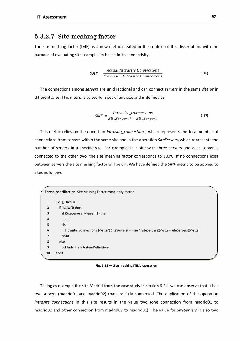
ITI Assessment 97
5.3.2.7 Site meshing factor
The site meshing factor (IMF), is a new metric created in the context of this dissertation, with the
purpose of evaluating sites complexity based in its connectivity.
𝑆𝑀𝐹 =𝐴𝑐𝑡𝑢𝑎𝑙 𝐼𝑛𝑡𝑟𝑎𝑠𝑖𝑡𝑒 𝐶𝑜𝑛𝑛𝑒𝑐𝑡𝑖𝑜𝑛𝑠
𝑀𝑎𝑥𝑖𝑚𝑢𝑚 𝐼𝑛𝑡𝑟𝑎𝑠𝑖𝑡𝑒 𝐶𝑜𝑛𝑛𝑒𝑐𝑡𝑖𝑜𝑛𝑠 (5.16)
The connections among servers are unidirectional and can connect servers in the same site or in
different sites. This metric is suited for sites of any size and is defined as:
𝑆𝑀𝐹 =𝐼𝑛𝑡𝑟𝑎𝑠𝑖𝑡𝑒_𝑐𝑜𝑛𝑛𝑒𝑐𝑡𝑖𝑜𝑛𝑠
𝑆𝑖𝑡𝑒𝑆𝑒𝑟𝑣𝑒𝑟𝑠2 − 𝑆𝑖𝑡𝑒𝑆𝑒𝑟𝑣𝑒𝑟𝑠 (5.17)
This metric relies on the operation Intrasite_connections, which represents the total number of
connections from servers within the same site and in the operation SiteServers, which represents the
number of servers in a specific site. For example, in a site with three servers and each server is
connected to the other two, the site meshing factor corresponds to 100%. If no connections exist
between servers the site meshing factor will be 0%. We have defined the SMF metric to be applied to
sites as follows.
Fig. 5.18 ― Site meshing ITILib operation
Taking as example the site Madrid from the case study in section 5.3.1 we can observe that it has
two servers (madrid01 and madrid02) that are fully connected. The application of the operation
Intrasite_connections in this site results in the value two (one connection from madrid01 to
madrid02 and other connection from madrid02 to madrid01). The value for SiteServers is also two
Formal specification: Site Meshing Factor complexity metric
1 SMF(): Real =
2 if (IsSite()) then
3 if (SiteServers()->size = 1) then
4 0.0
5 else
6 Intrasite_connections()->size/( SiteServers()->size * SiteServers()->size - SiteServers()->size )
7 endif
8 else
9 oclUndefined(SystemDefinition)
10 endif

98 Chapter 5
because the total number of servers in the Madrid site is two. So the application of the SMF will
indicate that the complexity is 100%. According to the formal definition this formula will not be
applied for sites with just one server. Only sites Lisbon and Madrid have values since all the others
have just one server.
Table 5.13 ― Intrasite_connections for each site using all network topologies
Topology Backbone Unidirectional Bidirectional Centralized Fully Meshed Site Servers
Site Lisbon 6 3 6 6 6 4
Site Madrid 2 1 2 2 2 2
Site Paris 0 0 0 0 0 1
Site Berlin 0 0 0 0 0 1
Site London 0 0 0 0 0 1
Site Dublin 0 0 0 0 0 1
Table 5.14 presents the site meshing factor complexity values for both sites for all network
topologies. Notice that this metric only makes sense for sites with more than one server such as the
Lisbon and Madrid sites.
Table 5.14 ― Site meshing factor for each site using all network topologies
Topology Backbone Unidirectional Bidirectional Centralized Fully Meshed
Site Lisbon 0,50% 25% 50% 50% 50%
Site Madrid 100% 50% 100% 100% 100%
Site Paris 0 0 0 0 0
Site Berlin 0 0 0 0 0
Site London 0 0 0 0 0
Site Dublin 0 0 0 0 0
Apparently the site Lisbon appears to be the most complex since it has higher number of servers.
However because Site Madrid has two servers and are fully connected (each server in Madrid is
connected to all the others servers in Madrid) the level of complexity is higher than in site Lisbon that
only half of the servers are connected. Taking as an example the server lisbon03 is only connected to
server lisbon04 in the site Lisbon.
5.4 Best practices analysis
There are several benefits that can derive from the application of best practices to ITIs. Their
adoption implies process improvements, what normally leads to an increase on productivity, while
reducing ITI costs [MSFT, 2007]. The value of an ITI is seen by [Gillen, Perry, Dowling, et al., 2007] as
an equation encompassing IT labor cost, service levels and business agility where the adoption rate

ITI Assessment 99
of best practices determines the maturity level of ITIs. The number and type of best practices that
can be applied to ITIs may differ from organization to organization and from technology to
technology. In the following chapters we show how best practices can be applied to the SDM
metamodel and how we can detect violations of best practices.
5.4.1 Best practices description
To express best practices for ITIs we extended the SDM metamodel by adding constraints. In this
section the best practices are first given in natural language and will later be expressed more
formally in OCL. We have defined the following best practices for ITIs:
A site in an ITI have at least one server – Sometimes, due to reorganizations, consolidation,
virtualization or other efforts, sites may become empty of servers, what represents a waste
of resources and makes the infrastructure larger and probably more complex without any
reason. In an organization with just a few sites, empty sites may be easier to detect and
delete. However, in organizations with hundreds of sites and servers this situation is often
undetected. Fig. 5.19 shows an example of an ITI where the Paris site do not have servers,
probably due to a consolidation.
Fig. 5.19 ― ITI site without servers
Site DublinTotal Number of Servers in Site: 1
Site BerlinTotal Number of Servers in Site: 1
Site LondonTotal Number of Servers in Site: 1
Site LisbonTotal Number of Servers in Site: 4
Site MadridTotal Number of Servers in Site: 2
Paris – Lisbon
(Sitelink)Lisbon – Madrid (Sitelink)
Dublin - Lisbon
(Sitelink)
Site ParisTotal Number of Servers in Site: 0
lisbon02
madrid01
madrid02
dublin01
london01
berlin01
lisbon01
lisbon04
lisbon03
Lisbon - Berlin (Sitelink)
Lisbon – London (Sitelink)
10.166.100.0/27
10.166.100.32/27
10.166.104.32/27
10.166.103.32/2710.166.10.32/27
10.166.101.32/27
10.166.23.32/27

100 Chapter 5
A site in an ITI should have at least one subnet defined – Since servers rely on IP addresses
and subnets to work and communicate, having sites without subnets defined represents
probably a mistake in the configuration, leading to other problems such as replication
failures, authentication failures, communication problems, among others. Fig. 5.20 shows the
example of Paris site with one server but without any subnets defined.
Fig. 5.20 ― Site without subnet defined
When an organization has more than one site, they should be interconnected – To allow
the communication among servers in different sites, the latter must be connected to other
sites. Sometimes we have problems because sites do not have a connection to a least
another site which represents an isolated "island" without connectivity with the rest of the
ITI. This occurs more often in ITIs with hundreds of sites. Fig. 5.21 shows an example of an ITI
where the Dublin Site is isolated from the rest of the infrastructure. Consequently, the server
Dublin01 in Dublin site has no communications with the rest of the ITI.
Site DublinTotal Number of Servers in Site: 1
Site BerlinTotal Number of Servers in Site: 1
Site LondonTotal Number of Servers in Site: 1
Site LisbonTotal Number of Servers in Site: 4
Site MadridTotal Number of Servers in Site: 2
Paris – Lisbon
(Sitelink)Lisbon – Madrid (Sitelink)
Dublin - Lisbon
(Sitelink)
Site ParisTotal Number of Servers in Site: 1
lisbon02
madrid01
madrid02
dublin01
london01
berlin01
lisbon01
lisbon04
lisbon03
Lisbon - Berlin (Sitelink)
Lisbon – London (Sitelink)
10.166.100.0/27
10.166.100.32/27
10.166.104.32/27
10.166.103.32/2710.166.10.32/27
10.166.101.32/27
paris01
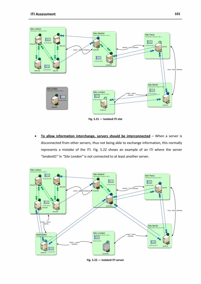
ITI Assessment 101
Fig. 5.21 ― Isolated ITI site
To allow information interchange, servers should be interconnected – When a server is
disconnected from other servers, thus not being able to exchange information, this normally
represents a mistake of the ITI. Fig. 5.22 shows an example of an ITI where the server
“london01” in “Site London” is not connected to at least another server.
Fig. 5.22 ― Isolated ITI server
Site DublinTotal Number of Servers in Site: 1
Site BerlinTotal Number of Servers in Site: 1
Site LondonTotal Number of Servers in Site: 1
Site LisbonTotal Number of Servers in Site: 4
Site MadridTotal Number of Servers in Site: 2
Madrid – Paris (Sitelink)
Paris - Berlin (Sitelink)
Lisbon – Madrid (Sitelink)
London - Berlin
(Sitelink)
Site ParisTotal Number of Servers in Site: 1
lisbon02
madrid01
madrid02
dublin01
london01
berlin01
lisbon01
lisbon04
lisbon03
paris01
10.166.100.0/27
10.166.100.32/27
10.166.101.32/27
10.166.102.32/27
10.166.103.32/27
10.166.104.32/2710.166.10.32/27
Site DublinTotal Number of Servers in Site: 1
Site BerlinTotal Number of Servers in Site: 1
Site LondonTotal Number of Servers in Site: 1
Site LisbonTotal Number of Servers in Site: 4
Site MadridTotal Number of Servers in Site: 2
Madrid – Paris (Sitelink)
Paris - Berlin (Sitelink)
Lisbon – Madrid (Sitelink)
Dublin - London
(Sitelink)
London - Berlin
(Sitelink)
Site ParisTotal Number of Servers in Site: 1
lisbon02
madrid01
madrid02
london01
berlin01
lisbon01
lisbon04
paris01
lisbon03
Dublin - Lisbon
(Sitelink)
dublin0110.166.10.32/27
10.166.104.32/27
10.166.103.32/27
10.166.102.32/2710.166.101.32/27
10.166.100.0/27
10.166.100.32/27

102 Chapter 5
5.4.2 Formal specification of best practices
In this section we will take each of the best practices defined above and we will formally define them
using OCL. Each best practice will be defined as an invariant in the context of the SDM class. We have
defined the following names for those invariants:
SiteHasAtLeastOneServer;
SiteHasAtLeastOneSubnet;
SiteLinkedToAtLeastAnotherSite;
ServerConnectedToAtLeastAnotherServer.
“A site in an ITI should have at least one server”. The invariant SiteHasAtLeastOneServer says that
if a site exists it should have at least a member of the type server.
Fig. 5.23 ― SiteHasAtLeastOneServer invariant definition
“ A site in an ITI should have at least one subnet defined”. The invariant SiteHasAtLeastOneSubnet
says that if a site exists it should have at least a member of the type subnet.
Fig. 5.24 ― SiteHasAtLeastOneSubnet invariant definition
“When an organization has more than one site, they should be interconnected”. The invariant
SiteLinkedToAtLeastAnotherSite says that if more than one site exists they should be connected.
Invariant definition: SiteHasAtLeastOneSubnet
1 inv SiteHasAtLeastOneSubnet:
2 IsSite() implies ContainmentDefinition.allInstances
3 ->select(MemberDefinition.oclIsTypeOf(ResourceDefinition))
4 ->exists(ParentDefinition=self and
5 MemberDefinition.oclAsType(ResourceDefinition).IsSubnet())
Invariant definition: SiteHasAtLeastOneServer
1 context SystemDefinition
2 inv SiteHasAtLeastOneServer:
3 IsSite() implies ContainmentDefinition.allInstances
4 ->select(MemberDefinition.oclIsTypeOf(SystemDefinition))
->exists(ParentDefinition=self and MemberDefinition.oclAsType(SystemDefinition).IsServer())

ITI Assessment 103
Fig. 5.25 ― SiteLinkedToAtLeastAnotherSite invariant definition
“To allow information interchange, servers should be interconnected”. The invariant
ServerConnectedToAtLeastAnotherServer says that when more than one site exists the servers have
to be connected to other servers.
Fig. 5.26 ― ServerConnectedToAtLeastAnotherServer invariant definition
In the following section we will apply each one of these invariants to a real example to check if
there are best practices violations. An invariant can be evaluated to true, false or can be not
applicable (n/a). One has not to worry about a true invariant. A false invariant indicates an invalid
system state which can be inspected by double-clicking the invariant name, and this opens the
evaluation browser explained further down.
5.4.3 Detecting best practices violations
In this section we present a case study of an ITI and we will use the “USE” tool, to detect if there are
best practices violations. The case study of Fig. 5.27, represents an ITI organization with one site on
the right that is not connected to the rest of the ITI. This disconnected site has the name Site_Lisbon.
The diagram is presented in a very small size to guarantee the confidentiality of the data origin.
There are several reasons that can lead to problems like this. The most common are anomalies or
human errors.
Invariant definition: ServerConnectedToAtLeastAnotherServer
1 context SystemDefinition
2 inv ServerConnectedToAtLeastAnotherServer:
3 IsServer() implies CommunicationDefinition.allInstances
4 ->exists(Client()=self and Server().IsServer()) and
5 CommunicationDefinition.allInstances->exists(Server()=self and Client().IsServer())
Invariant definition: SiteLinkedToAtLeastAnotherSite
1 context SystemDefinition
2 inv SiteLinkedToAtLeastAnotherSite:
3 IsSite() implies CommunicationDefinition.allInstances
4 ->exists(Client()=self and Server().IsSite())

104 Chapter 5
Fig. 5.27 ― ITI for best practices analysis
The result of checking the application of the best practices against the previous infrastructure
gives the following results.
Fig. 5.28 ― Check best practices violations in ITI1
With the exception of invariant SiteLinkedToAtLeastAnotherSite all are OK, meaning that most of
the best practices are in place in this organization. The FAILED invariant (line 7) is due to the fact that
there is an isolated site in the infrastructure. In this case the isolated site is presented in Fig. 5.27
(one the right with a different color).
USE: Checking invariants on infrastructure
1 use> check
2 checking structure...
3 checking invariants (using 5 concurrent threads)...
4 checking invariant (1) `SystemDefinition::ServerConnectedToAtLeastAnotherServer': OK.
5 checking invariant (2) `SystemDefinition::SiteHasAtLeastOneServer': OK.
6 checking invariant (3) `SystemDefinition::SiteHasAtLeastOneSubnet': OK.
7 checking invariant (4) `SystemDefinition::SiteLinkedToAtLeastAnotherSite': FAILED.
8 -> false : Boolean
9 Instances of SystemDefinition violating the invariant:
10 -> Set(@Site_Lisbon) : Set(SystemDefinition)
11 checked 4 invariants in 0.080s, 1 failure.
12 use>
105
6ITI Topology Detection
Contents
6.1 Introduction ............................................................................................................................. 106
6.2 Simulated sample ..................................................................................................................... 106
6.3 Variable reduction .................................................................................................................... 108
6.4 Multinomial logistic regression ................................................................................................ 110
6.4.1 Definitions ........................................................................................................................ 111
6.4.2 Regression using three variables ..................................................................................... 113
6.4.3 Regression using two variables ........................................................................................ 114
6.4.4 Regression using one variable (ITF_Sites) ........................................................................ 116
6.4.5 Regression using one variable (IMF_Sites) ...................................................................... 117
6.5 Experiments ............................................................................................................................. 118
This chapter is dedicated to the detection of network topologies based upon logistic regression
techniques. Using a simulated sample we will calibrate an estimation model that then will be used to
detect the topology of ten real ITIs collected using the approach defined in chapter 4.

106 Chapter 6
6.1 Introduction
Understanding the relationships among the components (topology) of an ITI and classify the topology
is a central question in several organizations because the topology is related with the ITI level of
complexity. As we have seen in chapter 2 most organizations have the desire to reduce the
complexity of their ITIs in order to decrease the corresponding TCO. For that purpose they first need
to know what topology is currently in place. The goal of this chapter is to propose a model to
automatically classify the topology of infrastructures based on the complexity metrics identified
earlier We first create a sample with 100 "pure" infrastructure topologies and we calculate the site
complexity metrics identified earlier for each of them. This simulated sample, for each case we know
the independent variables (the complexity metrics) and the dependent one (The topology), is used to
calibrate our topology detection model. The latter is based on multinomial regression analysis. Since
we had many descriptors (candidate independent variables), we have to reduce their number to
avoid over-specification of our estimation model.
The last section of this chapter is dedicated to the application of the created classification model
to ten real ITIs with the purpose of demonstrating the feasibility of our approach.
6.2 Simulated sample
To calibrate1 the model to be used to classify topologies we decided to generate an artificial sample
with 100 cases (covering in a balanced way all of the identified ITI network topologies in section
5.3.1) with different number of sites and for each of them we applied some of the site complexity
metrics identified in section 5.3.2 such as the CCM_Sites (defined in equation (5.6)), ITF_Sites
(defined in equation (5.10)) and IMF_Sites (defined in equation (5.15)). For simplicity reasons we
grouped the unidirectional ring and bidirectional ring into the "ring". Table 6.1 presents an extract of
the sample data created. Notice that the column TotalSitesLinks represents the number of sitelinks
required to match a specific topology (e.g. in an infrastructure with four sites we need to have twelve
sitelinks to match a topology of the "fully meshed" type).
1 Model calibration corresponds to the determination of parameter values that maximize the fit between estimates and observed values of
the outcome variable in a training set.

ITI Topology Detection 107
Table 6.1 ― Simulated sample
Topology TotalSites TotalSiteLinks CCM_Sites ITF_Sites IMF_Sites
Backbone (3) 3 4 3 1,00 0,67
Ring (3) 3 6 5 1,00 1,00
Centralized (3) 3 4 3 1,00 0,67
Fully Meshed (3) 3 6 5 1,00 1,00
Backbone (4) 4 6 4 0,67 0,50
Ring (4) 4 8 6 0,67 0,67
Centralized (4) 4 6 4 1,00 0,50
Fully Meshed (4) 4 12 10 1,00 1,00
(...) (...) (...) (...) (...) (...)
Backbone (99) 99 196 99 0,02 0,02
Ring (99) 99 198 101 0,02 0,02
Centralized (99) 99 196 99 1,00 0,02
Fully Meshed (99) 99 9702 9605 1,00 1,00
Backbone (100) 100 198 100 0,020 0,020
Ring (100) 100 200 102 0,020 0,020
Centralized (100) 100 198 100 1 0.020
Fully Meshed (100) 100 9900 9802 1 1
Notice that our sample identifies pure network types (e.g. 100% backbone or 100% centralized
network). However, with real data infrastructures, there are often more than one network topology
present in ITIs.
Table 6.2 summarizes the variables, their scale type and description that will be used in the
analysis. To perform an analysis we will first identify the dependent (aka outcome) and independent
variables (aka explanatory) of our sample. The dependent variables are those that are observed to
change in response to the independent variables. The independent variables are those that are
deliberately manipulated to cause a change in the dependent variables.
Table 6.2 ― Variables used in this experiment, their scale types and description
Variable Scale type Description
Topology Nominal Type of topology (Centralized, Fully Meshed, Ring, Backbone, etc...)
TotalSites Absolute Total number of sites in the infrastructure
TotalSiteLinks Absolute Total number of sitelinks in the infrastructure
CCM_Sites Absolute Complexity associated with cyclomatic complexity
ITF_Sites Ratio Complexity associated with site topology
IMF_Sites Ratio Complexity associated with infrastructure meshing
In this sample the outcome variable is the topology and all the others are explanatory variables.
Since we want to classify the topology, the problem that we want to solve is given a set of values of
the explanatory variables, which are the percentages of fit for each of the topology categories, only

108 Chapter 6
for a "pure" topology we will expect to get a 100% fit for one topology and 0% for all others. For that
purpose we will use the multinomial logistic regression which is an extension of the logistic
regression. The logistic regression can be used to predict values for a dependent variable based on
independent variables. It is also used to predict the percent of variance in the dependent variable
explained by the independents.
Before using the multinomial logistic regression we will first detect if we have an over-specified
model. In regression models over-specification is a problem that arises whenever a large number of
correlated explanatory variables are related with a single result. As we can see in the Table 6.2 we
have five explanatory variables (TotalSites, TotalSiteLinks, CCM_Sites, ITF_Sites, IMF_Sites). Since we
have five potential explanatory variables we will perform some variable reduction using correlations
analyses, in order to avoid over specified models.
6.3 Variable reduction
In order to check if we can reduce the number of explanatory variables and simplify the model, we
will use correlations analysis to compute correlation coefficients that describe the linear relationship
between two variables while controlling for the effects of one or more additional variables.
To determine the most adequate correlation coefficient to use, we need to test the explanatory
variables statistical distribution. If they are normally distributed we can use a parametric correlation
coefficient. Otherwise we should use a nonparametric one.
In figure Fig. 6.1 we reproduce the detrended normal Q-Q plots to represent the standardized
deviation of the observed values from a Normal distribution. To be Normal, a given variable should
have its points near the horizontal line corresponding to a null deviation. None of the metrics being
analyzed exhibits such a behavior, so most probably they do not have a normal distribution.

ITI Topology Detection 109
Fig. 6.1 ― QQ Plots for complexity metrics
Notice that the Q-Q Plot of TotalSiteLinks and QQ Plot of CCM_Sites are very similar since both are
dimension measures, as we will see in the sections ahead.
To test the hypothesis of normality we have applied the One-Sample Kolmogorov-Smirnov Test,
which is based on the maximum difference between the sample cumulative distribution and the
hypothesized cumulative distribution. The underlying hypotheses for this test are the following:
𝐻0:Χ~N ; Vs. 𝐻1: ¬Χ~N ; (6.1)
Table 6.3 ― Testing Normal distribution with the Kolmogorov-Smirnov test
a Test distribution is Normal. b Calculated from data.
Considering a confidence level of 95%, which implies a test significance = 0.05 (probability of
type I error of 5%). We can conclude from Table 6.3 that we must reject the null hypothesis for all
variables, since we get a significance 𝑝 < , which means that we have significant Ζ statistics for all
variables being analyzed. In other words, we cannot sustain that the considered variables of our
sample come from a Normal population. Therefore we can only use a non parametric correlation
coefficient. We have chosen the spearman correlation coefficient [Fagin, et al., 2003, Kendall, 1962]
since it is the most widely used one.

110 Chapter 6
The following table shows the Spearman's correlation coefficients for the five explanatory
variables.
Table 6.4 ― Correlations among five explanatory variables
* Correlation is significant at the 0.05 level (2-tailed). ** Correlation is significant at the 0.01 level (2-tailed).
From Table 6.4 we can observe that there are some relatively high2 correlations among the
variables TotalSites, TotalSiteLinks and CCM_Sites. This is expected since all three variables somehow
measure the ITI size. So we decided to eliminate the first two variables and keep only the CCM_Sites
variable, along with ITI_Sites and IMF_Sites. In the next section we will give more information
regarding the use of the multinomial regression method and we will apply this method using these
three variables. The goal is to estimate the topology type (dependent or outcome variable) based
upon the complexity metrics (independent or explanatory variables).
6.4 Multinomial logistic regression
The multinomial logistic regression is useful for situations in which we want to be able to classify
subjects based on values of a set of predictor variables. This type of regression is similar to binary
logistic regression, but is more general because the dependent variable is not restricted to two
categories.
2 There is no consensus in the literature on what should be considerable "High" correlation. We have taken the 70% threshold as a
reference in our approach.
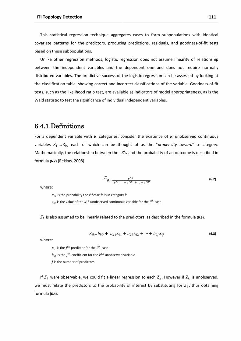
ITI Topology Detection 111
This statistical regression technique aggregates cases to form subpopulations with identical
covariate patterns for the predictors, producing predictions, residuals, and goodness-of-fit tests
based on these subpopulations.
Unlike other regression methods, logistic regression does not assume linearity of relationship
between the independent variables and the dependent one and does not require normally
distributed variables. The predictive success of the logistic regression can be assessed by looking at
the classification table, showing correct and incorrect classifications of the variable. Goodness-of-fit
tests, such as the likelihood ratio test, are available as indicators of model appropriateness, as is the
Wald statistic to test the significance of individual independent variables.
6.4.1 Definitions
For a dependent variable with 𝐾 categories, consider the existence of 𝐾 unobserved continuous
variables 𝑍1 …𝑍𝑘 , each of which can be thought of as the "propensity toward" a category.
Mathematically, the relationship between the 𝑍′𝑠 and the probability of an outcome is described in
formula (6.2) [Rekkas, 2008].
𝜋𝑖𝑘=
𝑒𝑧𝑖𝑘
𝑒𝑧𝑖1 + 𝑒𝑧𝑖2 + … + 𝑒𝑧𝑖𝐾
(6.2)
where:
𝜋𝑖𝑘 is the probability the 𝑖𝑡case falls in category 𝑘
𝑧𝑖𝑘 is the value of the 𝑘𝑡 unobserved continuous variable for the 𝑖𝑡 case
𝑍𝑘 is also assumed to be linearly related to the predictors, as described in the formula (6.3).
𝑍𝑖𝑘=𝑏𝑘0 + 𝑏𝑘1𝑥𝑖1 + 𝑏𝑘2𝑥𝑖2 + ⋯ + 𝑏𝑘𝐽 𝑥𝑖𝐽 (6.3)
where:
𝑥𝑖𝑗 is the 𝑗𝑡 predictor for the 𝑖𝑡 case
𝑏𝑘𝐽 is the 𝑗𝑡 coefficient for the 𝑘𝑡 unobserved variable
𝐽 is the number of predictors
If 𝑍𝑘 were observable, we could fit a linear regression to each 𝑍𝑘 . However if 𝑍𝑘 is unobserved,
we must relate the predictors to the probability of interest by substituting for 𝑍𝑘 , thus obtaining
formula (6.4).

112 Chapter 6
𝜋𝑖=
𝑒𝑏𝑘0+ 𝑏𝑘1 𝑥𝑖1+ …+ 𝑏𝑘𝐽 𝑥𝑖𝐽
𝑒𝑏𝑖0+ 𝑏𝑖1 𝑥𝑖1+⋯+ 𝑏𝑖𝐽 𝑥𝑖𝐽 +⋯+ 𝑒
𝑏𝑘0+ 𝑏𝑘1 𝑥𝑘1+⋯+ 𝑏𝑘𝐽 𝑥𝑘𝐽
(6.4)
As it stands, if we add a constant to each 𝑍, then the outcome probability is unchanged. This is the
problem of non-identifiability [Hsieh-Hua Yang, et al., 2008]. To solve this problem, 𝑍𝑘 is (arbitrarily)
set to 0. The 𝐾𝑘𝑡 category is called the reference category, because all parameters in the model are
interpreted in reference to it. The reference category is the "standard" category to which others
would naturally be compared.
Due to the exploratory nature of statistical analysis, we are going to perform four different
regression analyses using, the identified variables CCM_Sites, ITF_Sites and IMF_Sites. We will then
present the results achieved in terms of:
Model fitting Information ― A likelihood ratio test shows whether the model fits the data
better than a null model. We can define the hypotheses:
𝐻0 The model does not have a statistically significant different outcome than
another model that only considers the intercept parameter.
Vs.
𝐻1 The model does have a statistically significant different outcome than
another model that only considers the intercept parameter.
(6.5)
Pseudo-R-Square ― To analyze data with a logistic regression, an equivalent statistic to R-
squared goodness of fit coefficient does not exist. A wide variety of pseudo-R-squares
measures (e.g. Cox and Snell's, Nagelkerke's, and McFadden's) have been proposed to
evaluate the goodness-of-fit of logistic models. The name "pseudo" is due to the fact that
these coefficients look like R-squared in the sense that they are on a similar scale, ranging
from 0 to 1 with higher values indicating better model fit. The Cox and Snell's coefficient is an
attempt to imitate the interpretation of multiple R-Square based on the log likelihood of the
final model vs. log likelihood for the baseline model, but its maximum can be (and usually is)
less than 1.0, making it difficult to interpret. The Nagelkerke's coefficient is a modification of
the Cox and Snell one to assure that it can vary from 0 to 1. That is, Nagelkerke's R2 divides
Cox and Snell's by its maximum in order to achieve a measure that ranges from 0 to 1.
Therefore, Nagelkerke's R2 will normally be higher than the Cox and Snell measure. Lastly,
the McFadden's coefficient is a less common pseudo-R2 variant, based on log-likelihood
kernels for the full, versus the intercept-only, models;
Likelihood ratio tests ― The likelihood ratio is a function of log likelihood used in significance
testing in multinomial logistic regression. A "likelihood" is a probability, specifically the
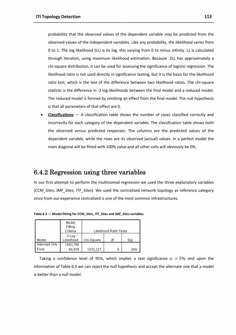
ITI Topology Detection 113
probability that the observed values of the dependent variable may be predicted from the
observed values of the independent variables. Like any probability, the likelihood varies from
0 to 1. The log likelihood (LL) is its log, this varying from 0 to minus infinity. LL is calculated
through iteration, using maximum likelihood estimation. Because -2LL has approximately a
chi-square distribution, it can be used for assessing the significance of logistic regression. The
likelihood ratio is not used directly in significance testing, but it is the basis for the likelihood
ratio test, which is the test of the difference between two likelihood ratios. The chi-square
statistic is the difference in -2 log-likelihoods between the final model and a reduced model.
The reduced model is formed by omitting an effect from the final model. The null hypothesis
is that all parameters of that effect are 0.
Classifications ― A classification table shows the number of cases classified correctly and
incorrectly for each category of the dependent variable. The classification table shows both
the observed versus predicted responses. The columns are the predicted values of the
dependent variable, while the rows are its observed (actual) values. In a perfect model the
main diagonal will be fitted with 100% value and all other cells will obviously be 0%.
6.4.2 Regression using three variables
In our first attempt to perform the multinomial regression we used the three explanatory variables
(CCM_Sites, IMF_Sites, ITF_Sites). We used the centralized network topology as reference category
since from our experience centralized is one of the most common infrastructures.
Table 6.5 ― Model fitting for CCM_Sites, ITF_Sites and IMF_Sites variables
Taking a confidence level of 95%, which implies a test significance = 5% and upon the
information of Table 6.5 we can reject the null hypothesis and accept the alternate one that a model
is better than a null model.

114 Chapter 6
Table 6.6 ― Likelihood ratio tests for CCM_Sites, ITF_Sites and IMF_Sites variables
Table 6.7 ― Pseudo-R Square for CCM_Sites, ITF_Sites and IMF_Sites variables
Based upon the Table 6.5, Table 6.6 and Table 6.7 we can conclude that using three variables the
model fit is very high, what is expected since we manually generated each of the ITI network
topologies.
Table 6.8 ― Topology classification table using CCM_Sites, ITF_Sites and IMF_Sites variables
Based upon the results of the Table 6.8 our model can predict the network topology with a
precision of 98,7%. Notice that in the case of fully meshed network topology the precision of our
model is 100%, what means that this model can successfully identify all the fully meshed cases.
6.4.3 Regression using two variables
In our second attempt to perform the multinomial regression we decided to remove the existing
dimension variable from the equation to analyze the impact on the dependent variable and we used
only (IMF_Sites, ITF_Sites). Again we used the centralized network topology as the reference
category.

ITI Topology Detection 115
Table 6.9 ― Model fitting for ITF_Sites and IMF_Sites variables
Taking a confidence level of 95%, which implies a test significance = 5% and upon the
information of Table 6.9 we can reject the null hypothesis and accept the alternate one that a model
is better than a null model.
Table 6.10 ― Likelihood ratio tests for ITF_Sites and IMF_Sites variables
Table 6.11 ― Pseudo-R Square for ITF_Sites and IMF_Sites variables
Based upon the Table 6.9, Table 6.10, Table 6.11, we can conclude that even removing the
dimension variable CCM_Sites, the model fit is very high with very similar results.
Table 6.12 ― Classification table for ITF_Sites and IMF_Sites variables
From Table 6.12 we can conclude that even excluding the dimension variable CCM_Sites we still
can predict the network topology with an overall precision of 98,7%.

116 Chapter 6
6.4.4 Regression using one variable (ITF_Sites)
In our third attempt to perform the multinomial regression we decided to use only one variable, to
understand how affected is our model if we removed two variables. We will use just the ITF_Sites
variable.
Table 6.13 ― Model fitting for ITF_Sites variable
Taking a confidence level of 95%, which implies a test significance = 5% and upon the
information of Table 6.13 we can reject the null hypothesis and accept the alternate one that a
model is better than a null model.
Table 6.14 ― Likelihood Ratio Tests for ITF_Sites variable
Table 6.15 ― Pseudo-R Square for ITF_Sites variable
Based upon the Table 6.13, Table 6.14, Table 6.15, we can conclude that using just the variable
ITF_Sites the model fit decreases substantially.
Table 6.16 ― Classification table for ITF_Sites variable

ITI Topology Detection 117
Based upon the results of Table 6.16 using just the variable ITF_Sites we observed a significant
precision reduction. There is a decrease in the overall predicted percentage from 98,7% with two
variables to 49,2% with just one. In the first row of Table 6.16 we can observe that the model has a
precision of 100% in the detection of network topologies of type "centralized". This is due to the fact
that proposed metric ITF_Sites quantifies the centrality of a network topology. Also notice that with
just ITF_Sites we are unable to predict fully meshed and ring topologies.
6.4.5 Regression using one variable (IMF_Sites)
The fourth attempt is very similar to the third since we will perform the multinomial regression with
only one variable. This time we will use only the IMF_Sites variable.
Table 6.17 ― Model fitting for IMF_Sites variable
Taking a confidence level of 95%, which implies a test significance = 5% and upon the
information of Table 6.17 we can reject the null hypothesis and accept the alternate one that a
model is better than a null model.
Table 6.18 ― Likelihood Ratio Tests for IMF_Sites variable
Table 6.19 ― Pseudo-R Square for IMF_Sites variable
Table 6.17, Table 6.18, Table 6.19 confirm that using just the variable IMF_Sites the model fit
decreases substantially.

118 Chapter 6
Table 6.20 ― Classification table for IMF_Sites variable
The results are very similar to the Table 6.16. Based upon the results of the Table 6.20 on using
just the variable IMF_Sites, we observed a significant precision reduction of our model. The overall
precision decreases from 98,7% with two variables to 49,5% with just one. Notice that the model has
a precision of 100% in the detection of network topologies of type fully meshed. This is due to the
fact that the proposed complexity metric IMF_Sites quantifies the meshing of a network topology.
6.5 Experiments
In this section we will use the model coefficients resultant from our simulated sample and we will
apply them to real ITIs with the purpose to detect the topology. Using the ITI data gatherer process
defined in our evaluation approach (see section 4.2.1) we had access to ITIs from ten different
organizations whose data we slightly changed, in order to guarantee origin anonymity. Table 6.21 has
the parameters used in the previous multinomial logistic regression tests. Notice that we treated the
centralized topology as the reference category and we estimated a model for the other types of
topologies.
Table 6.21 ― Parameter estimates
a The reference category is: Centralized. b Floating point overflow occurred while computing this statistic. Its value is therefore set to system missing.

ITI Topology Detection 119
We will use the 𝐵 values that represent the coefficients of the multinomial logistic regression
model to our real ITI data.
As described earlier, Table 6.22 presents ten infrastructures collected from real organizations. In
order to obtain all this data we used the ITI data gatherer component of our approach. To better
illustrate the application of our classification model we will demonstrate the application of the
equations defined in section 6.4.1 using the values from Table 6.21 and the values of the first
infrastructure (ITI 1) in Table 6.22.
Table 6.22 ― ITI assessment to real cases
Total Sites
Total Servers
Total Subnets
Total Sitelinks
Total Connections
ITF_Sites IMF_Sites
ITI 1 212 161 6852 486 547 0,011 0,322
ITI 2 44 65 148 102 200 0,053 0,325 ITI 3 39 76 648 104 225 0,070 0,421
ITI 4 29 52 1116 60 135 0,073 0,571 ITI 5 11 14 56 24 60 0,272 0,218
ITI 6 6 7 9 0 12 0 0
ITI 7 7 14 1657 12 48 0,285 1 ITI 8 8 16 531 16 45 0,285 1
ITI 9 2 2 159 2 2 1 1
ITI 10 26 28 117 48 56 0,073 0,96
In the following formulas we will not consider infrastructure six (ITI 6) since we found that the
number of sitelinks, is zero probably due a problem in the collection of data, and infrastructure nine
(ITI 9) due to reduced number of sites.
The following equations ((6.6) to (6.13)) uses the data from the first infrastructure in Table 6.22
(ITI1) to detect the topology.
𝑍𝐼𝑇𝐼1 𝑏𝑎𝑐𝑘𝑏𝑜𝑛𝑒 = 4,733 + −9,914 × 0,322 + (7,689 × 0,011)
𝑍𝐼𝑇𝐼1 𝑏𝑎𝑐𝑘𝑏𝑜𝑛𝑒 = 1,621
(6.6)
Equation (6.6) is an illustration of equation (6.3) for the backbone category. The "𝐵"𝑘𝑗 coefficients
are taken from the backbone row, column 𝐵 of Table 6.21. The 𝑥𝑖𝑗 predictors are taken from the
corresponding columns of the first row of Table 6.22 (The one of ITI1).
𝑍𝐼𝑇𝐼1 𝐹𝑢𝑙𝑙𝑦𝑀𝑒𝑠 𝑒𝑑 = 2,959 + −7391,574 × 0,322 + (7395,863 × 0,011)
𝑍𝐼𝑇𝐼1 𝐹𝑢𝑙𝑙𝑦𝑀𝑒𝑠 𝑒𝑑 = -2298,805
(6.7)

120 Chapter 6
Equation (6.7) is an illustration of equation (6.3) for the fully meshed category. The "𝐵"𝑘𝑗
coefficients are taken from the Fully Meshed row, column 𝐵 of Table 6.21. The 𝑥𝑖𝑗 predictors are
taken from the corresponding columns of the first row of Table 6.22 (The one of ITI1).
𝑍𝐼𝑇𝐼1 𝑅𝑖𝑛𝑔 = 9,690 + −36139,200 × 0,322 + (36133,451 × 0,011)
𝑍𝐼𝑇𝐼1 𝑅𝑖𝑛𝑔 = -11244,486
(6.8)
Equation (6.8) is an illustration of equation (6.3) for the ring category. The "𝐵"𝑘𝑗 coefficients are
taken from the Ring row, column 𝐵 of Table 6.21. The 𝑥𝑖𝑗 predictors are taken from the
corresponding columns of the first row of Table 6.22 (The one of ITI1). Notice that centralized
topology is our reference category:
𝑍𝐼𝑇𝐼1 𝐶𝑒𝑛𝑡𝑟𝑎𝑙𝑖𝑧𝑒𝑑 = 0 (6.9)
Now that we have the Z values for each of the topologies of infrastructure 1, we can calculate the
probability of ITI 1 being of type centralized, backbone, fully meshed or ring. The following formulas
are instantiations of equation (6.2):
𝑃𝑟𝑜𝑏𝑎𝑏𝑖𝑙𝑖𝑡𝑦 𝐼𝑇𝐼1 𝐶𝑒𝑛𝑡𝑟𝑎𝑙𝑖𝑧𝑒𝑑 =
01
1 + 𝑒11244 ,486 + 𝑒−2298,805 + 𝑒1621
𝑃𝑟𝑜𝑏𝑎𝑏𝑖𝑙𝑖𝑡𝑦 𝐼𝑇𝐼1 𝐶𝑒𝑛𝑡𝑟𝑎𝑙𝑖𝑧𝑒𝑑 = 15,5%
(6.10)
Based on the data of Table 6.22, there is a 15,5% probability that ITI 1 having a topology of the
Centralized type.
𝑃𝑟𝑜𝑏𝑎𝑏𝑖𝑙𝑖𝑡𝑦 𝐼𝑇𝐼1 𝐵𝑎𝑐𝑘𝑏𝑜𝑛𝑒 =
𝑒1,621
1 + 𝑒11244 ,486 + 𝑒−2298,805 + 𝑒1621
𝑃𝑟𝑜𝑏𝑎𝑏𝑖𝑙𝑖𝑡𝑦 𝐼𝑇𝐼1 𝐵𝑎𝑐𝑘𝑏𝑜𝑛𝑒 = 83,5%
(6.11)
Based on the data of Table 6.22, there is a 83,5% probability that ITI 1 having a topology of the
Backbone type.
𝑃𝑟𝑜𝑏𝑎𝑏𝑖𝑙𝑖𝑡𝑦 𝐼𝑇𝐼1 𝐹𝑢𝑙𝑙𝑦𝑀𝑒𝑠 𝑒𝑑 =
𝑒2298,805
1 + 𝑒11244 ,486 + 𝑒−2298,805 + 𝑒1621
𝑃𝑟𝑜𝑏𝑎𝑏𝑖𝑙𝑖𝑡𝑦 𝐼𝑇𝐼1 𝐹𝑢𝑙𝑙𝑦𝑀𝑒𝑠 𝑒𝑑 = 0%
(6.12)

ITI Topology Detection 121
Based on the data of Table 6.22, there is no probability (0%) of ITI 1 having a topology of the Fully
Meshed type.
𝑃𝑟𝑜𝑏𝑎𝑏𝑖𝑙𝑖𝑡𝑦 𝐼𝑇𝐼1 𝑅𝑖𝑛𝑔 =
𝑒11244 ,486
1 + 𝑒11244 ,486 + 𝑒−2298,805 + 𝑒1621
𝑃𝑟𝑜𝑏𝑎𝑏𝑖𝑙𝑖𝑡𝑦 𝐼𝑇𝐼1 𝑅𝑖𝑛𝑔 = 0%
(6.13)
Based on the data of Table 6.22, there is no probability (0%) of ITI 1 having a topology of the Ring
type.
We applied these equations to each of the ITIs and we summarize the results in Table 6.23. The
last column Topology represents the topology with higher probability.
Table 6.23 ― ITIs Classification
ITI Probability of being
Centralized
Probability of being
Backbone
Probability of being
Fully Meshed
Probability of
being Ring Topology
ITI 1 16,5% 83,5% 0,0% 0,0% Backbone ITI 2 12,8% 87,2% 0,0% 0,0% Backbone
ITI 3 25,0% 75,0% 0,0% 0,0% Backbone
ITI 4 59,0% 41,0% 0,0% 0,0% Centralized ITI 5 2,4% 97,6% 0,0% 0,0% Backbone
ITI 6 N/A N/A N/A N/A N/A ITI 7 95,2% 4,8% 0,0% 0,0% Centralized
ITI 8 95,2% 4,8% 0,0% 0,0% Centralized
ITI 9 N/A N/A N/A N/A N/A ITI 10 98,5% 1,5% 0,0% 0,0% Centralized
Based upon the Table 6.23 we concluded that most topologies are of type centralized and
backbone, which is in accordance with our expectations. Notice that ITI4 is an interesting case
because his type is centralized (59%) but there is a relatively high probability of being of type
Backbone 41%. From the knowledge we have about this organization, one of the reasons that can
explain this numbers is the fact that this organization was involved in acquisitions and merger
processes.

122 Chapter 6
[This page has been intentionally left blank]

123
7Conclusions and Future
Work
Contents
7.1 Review of contributions ........................................................................................................... 124
7.2 Limitations ................................................................................................................................ 125
7.3 Future work .............................................................................................................................. 126
As a conclusion of this dissertation, the major contributions are reviewed and summarized. Several
limitations of the research work presented in this dissertation are identified and discussed. Finally,
directions for future work are outlined. Some of those directions are intended to mitigate the
identified limitations.

124 Chapter 7
7.1 Review of contributions
The main contribution of this dissertation was to present an open framework for performing
metamodel-based quantitative studies upon ITIs based upon the M2DM technique. The M2DM
approach proved to be capable to support evaluation of infrastructures of different sizes in an
efficient and reliable way. The M2DM uses (i) a domain metamodel, expressed as a UML2 class
diagram, to provide the context and (ii) the OCL constraint language to guarantee metamodels well-
formedness and to formalize required quantifiers (e.g. complexity or sizing metrics) or qualifiers (e.g.
best practices verifiers). We also described the SDM metamodel and proved the feasibility of the
M2DM approach with ten case studies collected from real organizations, although slightly modified
to guarantee confidentiality.
We started our work by identifying some of the possible applications of ITI evaluation and the
corresponding stakeholders. Part of this work was the proposal, in the related work chapter, of a
taxonomy to support a survey of several evaluation studies conducted by different organizations and
indicate how the ITI structural evaluation can positively contribute for the TCO calculation.
We also provide a comparison of three ITI modeling languages in terms of their expressiveness,
relevance and model availability and we presented the reasons that lead us to choose the System
Definition Model language as a basis for the application of our methodological approach to
evaluating ITIs (the M2DM).
Before using the System Definition Model language in our approach, we analyzed the SDM
metamodel in terms of his structure and we developed an example to demonstrate how to model
with SDM.
We also provided the details of the automated process that has allowed scaling-up the evaluation
to arbitrarily large real-world ITIs. We detailed each component of the evaluation methodology and
we presented how it integrates with the others.
Other important contribution was the SDM library for ITIs known in this dissertation as ITILib,
comprehends a set of different metrics, developed in the context of this dissertation with the
purpose of evaluating ITIs. The metrics available in the SDM library can be used for several different
purposes, such as to support synchronic and diachronic analysis, among other aspects.
We used synchronic analysis approach to look at ITIs at a particular point in time, rather than over
time. We have developed several metrics which are available in the SDM library to make this
approach feasible. This approach allowed us to compare ITIs in a quantitative perspective. This
synchronic analysis allowed us to evaluate ITIs complexity and to perform comparisons among
infrastructures from other organizations. Besides the synchronic analysis we also used a diachronic
analysis approach to look at ITIs in a period of time, rather than in a particular point in time. This type

Conclusions and Future Work 125
of analysis gave us the opportunity to understand the evolution of ITIs on a chronological
perspective. This analysis may be applied to different purposes such as the prediction of future
growth, TCO evolution forecast or to provide evidence of the occurrence of important actions,
among other things. We have extended the SDM metamodel to include a set of best practices that
can be used for several purposes such as to detect anomalies in ITIs.
Other important contribution was the detection of topologies. We used the multinomial logistic
regression analysis and we were able to create a model that determines the network topology of ITIs.
We have successfully applied this model to ten real ITIs whose data we collected during the course of
this dissertation.
7.2 Limitations
This section presents some of the limitations found during the execution of our work. We call
limitations to the issues, problems or difficulties that we faced that could somehow have influenced
the achieved results.
We faced many problems, during the execution of this dissertation. We were able to fully solve
some of them and partially solve others, but there are still a significant number of problems to work
on. Some of the problems that we identified, with more impact in our research work are:
Number of ITIs evaluated – We spent a considerable amount of effort and time to collect
real ITIs to use, with the objective of proving the feasibility of our evaluation approach. Even
with that effort, we were able to collect only a limited number of real ITIs. The relatively
small size of our sample does not allow us to generalize our conclusions;
Partial evaluation – The reduced number of properties collected from ITIs allowed us to only
partial evaluate them. There is a good probability that other non detected properties
influence for example the level of complexity of a particular ITI, what could lead to wrong
decisions. Some of the properties or aspects that may be interesting to evaluate in an ITI are
the software inventory (to understand what is installed in each server), the hardware
inventory (to identify all the hardware currently in production), the load of each component
of the ITI, among other aspects;
The adoption of SDM – During the execution of this work the SDM modeling language that
we choose to work with, is being replaced by the SML language. The study of the SDM
metamodel in the perspective of how it works, how classes are related to each other and
where it can be applied, took us as a reasonable effort that we decided not to lose. Since
there is a supported path to migrate from SDM to SML, we hope to follow that path shortly.

126 Chapter 7
Active Directory only data – All the work performed in this dissertation was based on data
collected from Active Directory only. Since most of ITIs are built of systems from different
vendors. Collecting ITI data from different vendors will allow us to better generalize our
conclusions.
7.3 Future work
We now present a set of future research directions, that we think deserve to be further explored:
The adoption of SML – Future work might concentrate in the migration of this approach
based on SDM to its successor, the SML Language. When we started our work, the SML
specification was work in progress. Currently, the SML is publicly available at the W3C’s web
site, but is still in draft and, according to the schedule available in the same site, it will
probably remain so until March 2009. Since SML is based on standards and was created to
promote the interoperability among different ITI management systems, enable easier
management of heterogeneous systems and allow the creation of models that can be used
across management systems from different technology vendors, the potential of using SML
to evaluate ITIs is enormous;
Collecting ITI data from different platforms – In the IT industry there is a long history of
tools and processes being developed for specific roles or tasks that did not integrate with
each other, even though they all serve the same objective. The number of LDAP/X.500
implementations described in chapter 4 is one of these examples. Since most ITIs are built
with components from different vendors, having a process or tool that can be used to collect
data across all these platforms, allows the use of the same evaluation methodology across
any kind of ITI;
Definition of baseline configuration – The idea behind the baseline is to define a set of
configurations that can be used across the ITI to identify its compliance with security policies,
thus identifying security vulnerabilities. The work performed in ITI best practices is a valuable
input to this area;
Distribution of ITI configurations – Particularly in organizations with completely distributed
ITIs, setting a specific configuration to a group of machines, such as change the replication
time interval or configuring a specific service or changing local passwords of all servers may
take days and sometimes weeks (depending on the size of the ITI). Extending the evaluation
methodology presented in this dissertation to not only evaluate, but also effectively make
changes, constitutes an interesting topic. One possible way to address this is to move from

Conclusions and Future Work 127
proprietary-based network management systems to standardized model-based ITI
management systems;
Design of new ITIs – another interesting area of research is to improve design of new ITIs.
This can be achieved through the extension of the evaluation methodology presented in this
dissertation to not only to gather and analyze ITI data, but also to allow the users to provide
requirements on the new ITI, such as the expected growth, the number of users or the
available budget, among other factors. Having a methodological approach to infrastructure
design can be very useful to increase or decrease the size of an ITI and adequate it to the
business needs;
Estimation of the time required to distribute ITI software – depending on the ITI size, the
software distribution across an ITI is another interesting topic. The estimation of the required
time to distribute a specific software package for a remote location based upon factors such
as the physical network topology, available bandwidth, size of the package, number of
destinations and other related aspects, is very important to guarantee the efficiency of the
process and to minimize the impact on the network. Extending the evaluation methodology
to perform this type of analysis, based on a specific ITI, is another interesting area of
research;
Full automation of the evaluation approach – there are several aspects of the proposed
evaluation approach that are manual but that can be automated. One of these examples
relates to the results provided by the ITI evaluator tool in step 8. Currently these results have
to be loaded manual in the statistical analyzer tool.

128 Chapter 7
[This page has been intentionally left blank]

129
Bibliography
[Abreu, et al., 1994] Abreu, and Carapuca, "Object-Oriented Software Engineering: Measuring and Controlling the Development Process," in In Proceedings of the 4th International Conference on Software Quality, 1994.
[Adams, 2002] Adams, "Management Update: Best Practices to Launch an IT Asset Management
Program," 24 April, 2002. [Altova, 2008] Altova: XMLSpy. http://www.altova.com/products/xmlspy/xml_editor.html, accessed
on April, 2008 [Anne, 1990] Anne, IEEE Standard Computer Dictionary: A Compilation of IEEE Standard Computer
Glossaries 610. New York: The Institute of Electrical and Electronics Engineers Inc., 1990. [APC, 2003a] APC, "Determining Total Cost of Ownership for Data Center and Network Room
Infrastructure," 2003a. [APC, 2003b] APC, "Avoiding Costs From Oversizing Data Center and Network Room Infrastructure,"
2003b. [ASF, 2008] ASF: Apache Directory Server - (ApacheDS v1.5).
http://directory.apache.org/apacheds/1.5/, accessed on August, 2008 [Axeda, 2007] Axeda, "Secure Remote Vendor Access to the Enterprise Data Center," Foxboro, MA
02035 USA 2007. [Aziz, et al., 2003] Aziz, Nie, Yam, and Wei: TCO reduction. In: Proc. of APCC 2003. The 9th Asia-
Pacificic Conference on Communications, Malaysia, pp. 1147-1151. IEEE (2003) [Babey, 2006] Babey, "Costs of Enterprise Resource Planning System Implementation — and Then
Some," Winter 2006. [Baroni, et al., 2002] Baroni, and Abreu: Formalizing Object-Oriented Design Metrics upon the UML
Meta-Model. In: Proc. of Brazilian Symposium on Software Engineering, Gramado - RS, Brazil (2002)
[Baroni, et al., 2003] Baroni, and Abreu, "A Formal Library for Aiding Metrics Extraction," in
International Workshop on Object-Oriented Re-Engineering at ECOOP'2003, Darmstadt, Germany, 2003.
[Baroni, et al., 2004] Baroni, Calero, Ruiz, and Abreu: Formalizing Object-Relational Structural
Metrics. In: Proc. of 5ª Conferência da APSI, Lisbon (2004) [Bartels, 2008] Bartels, "The State Of Enterprise IT Budgets: 2008," March 27, 2008. [Blowers, 2006a] Blowers, "Management Foundation based on Service-Driven Operations,"
November, 2006a.

130 Bibliography
[Blowers, 2006b] Blowers, "Data Center Consolidation - Management Foundation based on Service-Driven Operations," November, 2006b.
[Blum, 2004] Blum, "Network and Systems Management Total Cost of Ownership," September,
2004. [Bon, 2004] Bon, Chief Editor,“IT Service Management, an introduction based on ITIL”, itSMF Library:
Van Haren Publishing, 2004. [Booch, 1994] Booch, Object Oriented Analysis and Design with Applications, 2nd ed. Redwood City,
LA, USA: The Benjamin Cummings Publishing Company Inc, 1994. [Bothma, 2005] Bothma, "Best practices in managing the Total Cost of Ownership," SAP INSIGHT, p.
10, 2005. [Bothma, 2006] Bothma, "State of the art in TCO: Managing the Total Cost of Ownership," SAP
INSIGHT, p. 10, January 2006. [Boyle, 2007] Boyle, "Wireless Device Management: Controlling The Wireless Enterprise And
Reducing Total Cost of Ownership," 2007. [Brenner, et al., 2006] Brenner, Garschhammer, and Hegering, "When Infrastructure Management
Just won’t do: The Trend towards Organizational IT Service Management," 2006. [Brito e Abreu, et al., 1997] Brito e Abreu, Ochoa, and Goulão, "The GOODLY Design Language for
MOOD Metrics Collection," INESC, Software Engineering Group, Technical Report R16/97, March, 1997.
[Brito e Abreu, 2001] Brito e Abreu, "Using OCL to Formalize Object-Oriented Design Metrics
Definitions," Software Engineering Group, INESC, Technical Report ES007/2001, May, 2001. [Brynjolfsson, et al., 2000] Brynjolfsson, and Hitt, "Computing Productivity: Firm-Level Evidence," MIT
Sloan School of Management April, 2000. [Builders, 2002] Builders, "Examining Total Cost of Ownership for Business Intelligence Solutions,"
2002. [Castellani, et al., 2005] Castellani, Grasso, O’Neill, and Tolmie: Total Cost of Ownership: Issues
around Reducing Cost of Support in a Manufacturing Organization Case. In: Proc. of Proceedings of the 2005 Seventh IEEE International Conference on E-Commerce Technology Workshops, Munich - Germany. IEEE (2005)
[Cater-Steel, et al., 2006] Cater-Steel, Tan, and Toleman: Challenge of Adopting Multiple Process
Improvement Frameworks. In: Proc. of Proceedings of the 14th European Conference on Information Systems, Göteborg, Sweden, pp. 12–14 (2006)
[Chiorean, et al., 2004] Chiorean, Pasca, Carcu, Botiza, and Moldovan, "Ensuring UML Models
Consistency Using the OCL Environment," November, 2004. [CIOview, 2005] CIOview, "The Business Value of Migrating from Oracle to SQL Server 2005," Acton
June, 2005.

Bibliography 131
[Conley, et al., 2007] Conley, and Mootz: Lowering Cost of Ownership through Predictive Maintenance. In: Proc. of Advanced Semiconductor Manufacturing Conference, Stresa, Italy, pp. 313-319. IEEE (2007)
[Counsel, 2006] Counsel, "North American Enterprise IT Users – Security and Identity Access and
Management Outlook," 2006. [Cranefield, et al., 1999] Cranefield, and Purvis: UML as an Ontology Modelling Language. In: Proc. of
Workshop on Intelligent Information Integration, 16th International Joint Conference on Artificial Intelligence (IJCAI-99) (1999)
[Cybersource, et al., 2004] Cybersource, and OSV, "Linux vs Windows - Total Cost of Ownership
Comparison," Melbourne 2004. [David, et al., 2002] David, Schuff, and Louis, "Managing your total IT cost of ownership," January,
2002. [Davies, 1974] Davies, "An Experimental Investigation of Resource Allocation in Multiactivity
Projects," 1974. [DiDio, 2004a] DiDio, "Linux, Unix and Windows TCO Comparison, Part 2," Boston, MA: The Yankee
Group, 2004a. [DiDio, 2004b] DiDio, "Linux, Unix and Windows TCO Comparison, Part 1," Boston, MA: The Yankee
Group, 2004b. [DMTF, 2007] DMTF, "Common Information Model (CIM) Infrastructure," November, 2007. [Dublish, et al., 2006] Dublish, Eckert, Ehnebuske, Golovinsky, Jerman, Kreger, Milenkovic, Murray,
Prasek, Reeves, Saiyed, Sluiman, Tabbara, Tewari, Tollefsrud, Vambenepe, and Westerinen: Service Modeling Language Specification, Version 0.5. http://www.dell.com/downloads/global/corporate/standards/service_sml.pdf, accessed on August, 2008
[Dublish, et al., 2008a] Dublish, Eckert, Ehnebuske, Golovinsky, Jerman, Kreger, Milenkovic, Murray,
Prasek, Reeves, Saiyed, Sluiman, Tabbara, Tewari, Tollefsrud, Vambenepe, and Westerinen: Service Modeling Language Interchange Format Version 1.1. http://www.w3.org/TR/sml-if/, accessed on May, 2008
[Dublish, et al., 2008b] Dublish, Eckert, Ehnebuske, Golovinsky, Jerman, Kreger, Milenkovic, Murray,
Prasek, Reeves, Saiyed, Sluiman, Tabbara, Tewari, Tollefsrud, Vambenepe, and Westerinen: Service Modeling Language Specification, Version 1.1. http://www.w3.org/Submission/2007/SUBM-sml-20070321/, accessed on May, 2008
[Edmonds, 1995] Edmonds: What is Complexity? - The philosophy of complexity per se with
application to some examples in evolution. In: Proc. of The Evolution of Complexity, Free University of Brussels, Belgium (1995)
[Edmonds, 2000] Edmonds, "Complexity and Scientific Modelling," Foundations of Science, vol. 5, pp.
379-390, 2000.

132 Bibliography
[Elmaghraby, et al., 1980] Elmaghraby, and Herroelen, "On the measurement of complexity in activity networks," European Journal of Operational Research, 1980.
[EMC, 2005] EMC, "CLARiiON Integration with VMware ESX Server," 8 September, 2005. [Engels, 2006] Engels, "Reducing the Total Cost of Ownership," in Broadband Fixed Wireless Access:
Springer, 2006, pp. 163-183. [Ernest, et al., 2007] Ernest, and Nisavic, "Adding value to the IT organization with the Component
Business Model," IBM Systems Journal, vol. 46, pp. 387-403, July 2007. [Fagin, et al., 2003] Fagin, Kumar, and Sivakumar, "Comparing top k lists," Proceedings of the
fourteenth annual ACM-SIAM symposium on …, 2003. [Fallside, et al., 2004] Fallside, and Walmsley, "XML Schema Part 0: Primer Second Edition," 28
October, 2004. [Fedora, 2008] Fedora: Fedora Directory Server Project.
http://directory.fedoraproject.org/wiki/Architecture, accessed on August, 2008 [Ganek, et al., 2007] Ganek, and Kloeckner, "An overview of IBM Service Management," IBM
SYSTEMS JOURNAL, vol. 46, pp. 375-385, 2007. [Gartner, 1997] Gartner, "TCO Analyst - Next Generation Total Cost of Ownership Methodology,"
1997. [Gartner, 2003] Gartner, "Distributed Computing - Chart of Accounts," 16 June 2003, 2003. [Gillen, et al., 2007] Gillen, Perry, Dowling, and Grieser, "The Relationship Between IT Labor Costs
and Best Practices for Systems Management Server," 2007. [Gillen, et al., 2007] Gillen, Perry, and Waldman, "Understanding the Business Benefits Associated
with x86 64 -Bit Windows Server," September, 2007. [Gogolla, et al., 2005] Gogolla, Bohling, and Richters, "Validating UML and OCL models in USE by
automatic snapshot generation," Software and Systems Modeling, vol. 4, pp. 386-398, Wednesday, August 10, 2005 2005.
[Gogolla, et al., 2007] Gogolla, Buttner, and Richters, "USE: A UML-Based Specification Environment
for validating UML and OCL," University of Bremen, Bremen 2007. [Gomolski, 2004] Gomolski, "How to Use IT Cost Metrics Effectively," G00123098, 2004. [Goulão, et al., 2004a] Goulão, and Abreu: Formalizing Metrics for COTS. In: Proc. of International
Workshop on Models and Processess for the Evaluation of COTS Components (MPEC 2004) at ICSE 2004, Edimburgh, Scotland, pp. 37-40. IEE (2004a)
[Goulão, et al., 2004b] Goulão, and Abreu: Cross-Validation of a Component Metrics Suite. In: Proc.
of IX Jornadas de Ingeniería del Software y Bases de Datos, Málaga, Spain (2004b)

Bibliography 133
[Goulão, et al., 2005a] Goulão, and Abreu: Formal Definition of Metrics upon the CORBA Component Model. In: Proc. of First International Conference on the Quality of Software Architectures, QoSA'2005, Erfurt, Germany. Springer (2005a)
[Goulão, et al., 2005b] Goulão, and Abreu: Composition Assessment Metrics for CBSE. In: Proc. of
31st Euromicro Conference - Component-Based Software Engineering Track, Porto, Portugal. IEEE Computer Society (2005b)
[Greschler, et al., 2002] Greschler, and Mangan, "Networking lessons in delivering ‘Software as a
Service’—Part I," International Journal of Network Management, vol. 12, pp. 317 – 321, 2002.
[Gunasekaran, et al., 2005] Gunasekaran, Williams, and McGaughey, "Performance measurement
and costing system in new enterprise," 2005. [Haes, et al., 2005] Haes, and Grembergen: IT Governance Structures, Processes and Relational
Mechanisms: Achieving IT/Business Alignment in a Major Belgian Financial Group. In: Proc. of Proceedings of the 38th Annual Hawaii International Conference on System Sciences, Hawaii, pp. 10. IEEE (2005)
[Harris, 2005] Harris, "IT Complexity May Be the Reason You're Spending More and Gaining Less,"
2005. [Hassan, et al., 1999] Hassan, and Saeed: A framework for determining IT effectiveness: an empirical
approach. In: Proc. of Proceedings of the 32nd Hawaii International Conference on System Sciences, Island of Maui, pp. 11. IEEE Computer Society (1999)
[Heine, 2003] Heine, "Management Update: Five Sure Ways to Reduce IT Asset Costs," Gartner, p. 4,
26 March 2003. [Henry, et al., 1981] Henry, and Kafura, "Software Structure Metrics Based on Information Flow,"
Transactions on Software Engineering, vol. 7, pp. 510-518, September 1981. [Herbert, 1996] Herbert, The sciences of the artificial (3rd ed.): MIT Press, 1996. [Heschl, et al., 2006] Heschl, CISA, and CISM, Overview of International IT Guidance 2nd Edition ed.
Rolling Meadows: IT Governance Institute, 2006. [Ho, et al., 2007] Ho, and Inokuchi: SEM ADC (Auto Defect Classification): How it improves the Cost of
Ownership without Risk of Yield Loss. In: Proc. of IEEE/SEMI Advanced Semiconductor Manufacturing Conference. IEEE (2007)
[HP, 2006a] HP, "Putting a price on document-based business processes," 2006a. [HP, 2006b] HP, "The top five most common hidden imaging and printing infrastructure costs,"
2006b. [HP, 2007] HP: The HP Service Management Framework.
http://activeanswers.compaq.com/ERC/downloads/4AA1-3338ENW.pdf, accessed on April, 2008

134 Bibliography
[Hsieh-Hua Yang, et al., 2008] Hsieh-Hua Yang, Hung-Jen Yang, Jui-Chen Yu, and Hu, "Multinomial Regression Model for In-service Training," International Journal of Mathematical Models and Methods in Applied Sciences, vol. 2, p. 6, 2008.
[Hurkens, et al., 2006] Hurkens, Valk, and Wynstra, "Total Cost of Ownership in the Services Sector A
Case Study," The Journal of Supply Chain Management, pp. 27-37, Winter 2006 2006. [Iansiti, et al., 2006] Iansiti, Sarnoff, and Favaloro, "Enterprise IT Capabilities and Business
Performance," March 16, 2006. [IBM, 2007] IBM: The IBM Process Reference Model for IT (PRM-IT). http://www-
306.ibm.com/software/tivoli/governance/servicemanagement/welcome/process_reference.html, accessed on November, 2007
[IBM, 2008] IBM: Rational Rose - Product line. http://www-
01.ibm.com/software/awdtools/developer/rose/index.html, accessed on February, 2008 [Ionescu-Graff, et al., 2005] Ionescu-Graff, Newman, Chu, Trivedi, Tang, and Zhu, "Quantifying the
value proposition of advanced fault management systems in MPLS core networks," Bell Labs Technical Journal, vol. 10, pp. 157 - 167, 2005.
[ISACA, 2008a] ISACA: COBIT 4.1 Executive Summary and Framework.
http://www.isaca.org/AMTemplate.cfm?Section=Downloads&Template=/ContentManagement/ContentDisplay.cfm&ContentID=34172, accessed on August, 2008
[ISACA, 2008b] ISACA: Common Objectives for Information and related Technology (COBIT 4.1).
http://www.isaca.org/cobit, accessed on April, 2008 [ISACA, 2008c] ISACA: Servicing IT Governance Professionals. http://www.isaca.org/, accessed on
August, 2008 [ISO/IEC, 2004] ISO/IEC, "Schematron ISO/IEC FDIS 19757-3," 2004. [ITAA, 2008] ITAA: Information Technology Definition Aggregation.
http://www.itaa.org/es/docs/Information%20Technology%20Definitions.pdf, accessed on August, 2008
[ITGI, 2008a] ITGI, Mapping of ITIL v3 with COBIT 4.1: IT Governance Institute, 2008a. [ITGI, 2008b] ITGI: IT Governance Institute. http://www.itgi.org/, accessed on August, 2008 [itSMF, 2008] itSMF: The IT Service Management Forum Portugal. http://www.itsmf.pt/, accessed on
August, 2008 [Jacobson, 1995] Jacobson, "The Confused World of OOA & OOD," JOOP, September 1995. [Jones, et al., 2006] Jones, and Desai, "The Reference Guide To Data Center Automation," 2006. [Jutras, 2007] Jutras, "The Total Cost of ERP Ownership in Mid-Size Companies," July, 2007. [Juurakko, 2004] Juurakko, "Measuring and Managing The Total Cost Of Ownership For TETRA
Networks," 2004.

Bibliography 135
[Kaimann, 1974] Kaimann, "Coefficient of network complexity," Management Science, vol. 21, pp.
172-177, 1974. [Kaimann, 1975] Kaimann, "Coefficient of network complexity: Erratum," Management Science, vol.
21, pp. 1211-1212 1975. [Kantin, et al., 2006] Kantin, Nick, and Sullivan, "The Future Sales Force - A Consultative Approach,"
2006. [Kendall, 1962] Kendall, Rank Correlation Methods: orton.catie.ac.cr, 1962. [Kimfong, et al., 2003] Kimfong, and Phillip: Strategic decisions on technology selections for
facilitating a network/systems laboratory using real options \& total cost of ownership theories. In: Proc. of Proceedings of the 4th conference on Information technology curriculum, Lafayette, Indiana, USA. ACM (2003)
[Kirwin, et al., 2002] Kirwin, Mieritz, and D'Angelo, "The Total Cost of Ownership Index: Defining the
Database," 16 October, 2002. [Kirwin, 2003a] Kirwin, "Management Update: Total Cost of Ownership Analysis Provides Many
Benefits," IGG-08272003-01, 2003a. [Kirwin, 2003b] Kirwin, "CIO Update: To Control TCO, It Must Be Measured and Managed," InSide
Gartner 16 April, 2003b. [Kirwin, et al., 2005] Kirwin, and Mieritz, "Control Distributed Computing TCO by Keeping an Eye on
Complexity Creep," G00129518, August, 2005. [Lavazza, 2007] Lavazza: Beyond Total Cost of Ownership: Applying Balanced Scorecards to Open-
Source Software. In: Proc. of International Conference on Software Engineering Advances, Varese (Italy). IEEE Computer Society (2007)
[Logan, 2004] Logan, "Monitoring and State Transparency of Distributed Systems," Snowbird, Utah,
USA 22 September, 2004. [MacCormack, 2003] MacCormack, "Evaluating Total Cost of Ownership for Software Platforms:
Comparing Apples, Oranges and Cucumbers," April, 2003. [Machuca, 2006] Machuca, "Expenditures Study for Network Operators," Technische Universität
München, Arcisstrasse 21, D-80290 München 2006. [McCabe, 1976] McCabe, "A complexity measure," IEEE Transactions on Software Engineering, vol. 4,
pp. 308-320, December 1976. [McGuinness, et al., 2004] McGuinness, and Harmelen, "OWL Web Ontology Language Overview,"
W3C, Recommendation 10 February, 2004. [Merriam-Webster, 2008] Merriam-Webster: Complexity definition. http://www.merriam-
webster.com/thesaurus/complexity, accessed on February, 2008

136 Bibliography
[Mertins, et al., 2008] Mertins, Ruggaber, Popplewell, and Xu, "An Approach for the Evaluation of the Agility in the Context of Enterprise Interoperability " in Enterprise Interoperability III: Springer London, 2008, pp. 3-14.
[Microsoft, 1999] Microsoft, "Microsoft Business Value - Windows vs. LINUX Total Cost of Ownership
Overview," 1999. [Msadek, 2003] Msadek, "Managing technology to reduce total cost of ownership and secure assets,"
DataBus, July 2003. [MSDN, 2008] MSDN: Windows Management Instrumentation. http://msdn.microsoft.com/en-
us/library/aa394582.aspx, accessed on July, 2008 [MSFT, 2003] MSFT, "Active Directory LDAP Compliance," October, 2003. [MSFT, 2004] MSFT, "Overview of the System Definition Model (SDM)," Microsoft Corporation April,
2004. [MSFT, 2005] MSFT: Dynamics Systems Initiative (DSI).
http://www.microsoft.com/windowsserversystem/dsi/default.mspx, accessed on March, 2005
[MSFT, 2007] MSFT, "Managing Smart: Driving the Cost Out of IT Infrastructure," Microsoft
Corporation 2007. [MSFT, 2008a] MSFT: Microsoft Operations Framework 4.0. http://www.microsoft.com/mof,
accessed on March, 2008 [MSFT, 2008b] MSFT: Service Models: The Three Key Relationships.
http://technet.microsoft.com/en-us/library/bb977447(TechNet.10).aspx, accessed on January, 2008
[Novell, 2008] Novell: Why Choose Novell eDirectory?
http://www.novell.com/products/edirectory/whychoose.html, accessed on August, 2008 [Novotný, 2004] Novotný: ‘CASE Tool for developing XML Schemas and XSLT’, Faculty of
mathematics, physics and informatics - Comenius University, 2004 [O'Brien, 2003] O'Brien, "Management Update: IT Asset Management Is Mandatory, Not Optional,"
InSide Gartner 20 August, 2003. [Objecteering, 2008] Objecteering: Objecteering. http://www.objecteering.com/, accessed on April,
2008 [ODP, 2008] ODP: The Open Directory Project.
http://www.apple.com/server/macosx/technology/opendirectory.html, accessed on August, 2008
[OGC, 2000] OGC: the IT Infrastructure Library (ITIL). http://www.itil-
officialsite.com/home/home.asp, accessed on January, 2008

Bibliography 137
[OGC, 2002] OGC, IT Infrastructure Library (ITIL) - Planning to Implement Service Management (Version 2). London: The Stationery Office, 2002.
[OGC, 2007a] OGC, IT Infrastructure Library (ITIL) - Service Strategy (Version 3). London: The
Stationery Office), 2007a. [OGC, 2007b] OGC, IT Infrastructure Library (ITIL) - Service Transition (Version 3). London: The
Stationery Office), 2007b. [OGC, 2007c] OGC, IT Infrastructure Library (ITIL) - Service Design (Version 3). London: The Stationery
Office), 2007c. [OGC, 2007d] OGC, IT Infrastructure Library (ITIL) - Continual Service Improvement (Version 3).
London: The Stationery Office), 2007d. [OGC, 2007e] OGC, IT Infrastructure Library (ITIL) - Service Operation (Version 3). London: The
Stationery Office), 2007e. [OMG, 2004] OMG, "Unified Modeling Language (UML) Specification : Infrastructure, version 2.0,"
2004. [OMG, 2007a] OMG: UML Infrastructure specification OMG, The Object Management Group (2007a) [OMG, 2007b] OMG: UML Superstructure specification OMG, The Object Management Group
(2007b) [OMG, 2007c] OMG, "MOF 2.0/XMI Mapping, Version 2.1.1," December, 2007c. [OpenLDAP, 2008] OpenLDAP: The OpenLDAP website. http://www.openldap.org/, accessed on
August, 2008 [Opsware, 2006] Opsware, "Selecting a Flexible, Custom Platform to Automate Your Data Center
Management," 2006. [Pascoe, 1966] Pascoe, "Allocation of resources-CPM," Revue Française de Recherche Opérationelle,
vol. 38, pp. 31-38, 1966. [Perry, et al., 2007] Perry, and Gillen, "Demonstrating Business Value: Selling to Your C-Level
Executives," 2007. [Pispa, et al., 2003] Pispa, and Eriksson, "Aligning organizations and their information technology
infrastructure: how to make information technology," Production Planning & Control, vol. 14, pp. 193 - 200, 2003.
[Plummer, 2005] Plummer, "Findings From the 'Agility' Research Meeting: IT's Role in Agility Can Be
Measured and Improved," 26 September, 2005. [QUASAR, 2008] QUASAR: QUantitative Approaches on Software Engineering And Reengineering.
http://www-ctp.di.fct.unl.pt/QUASAR/index.html, accessed on August, 2008 [Rasmussen, 2006a] Rasmussen, "Electrical Efficiency Modeling of Data Centers," 2006a.

138 Bibliography
[Rasmussen, 2006b] Rasmussen, "Implementing Energy Efficient Data Centers," 2006b. [Rekkas, 2008] Rekkas, "Approximate inference for the multinomial logit model," Statistics and
Probability Letters, 2008. [Richters, 2001] Richters: The USE tool: A UML-based specification environment.
http://www.db.informatik.uni-bremen.de/projects/USE/, accessed on December, 2007 [Rosenberg, 2004] Rosenberg, "The Myths of usability ROI," September, 2004. [Rumbaugh, 1996] Rumbaugh, "To form a more perfect union: unifying the OMT and Booch
methods," JOOP, vol. 8, January 1996. [Rymer, et al., 2003] Rymer, and Cormier, "The Total Economic Impact of Developing and Deploying
Applications on Microsoft and J2EE/Linux Platforms," September 4, 2003. [Salle, 2004] Salle, "IT Service Management and IT Governance: Review, Comparative Analysis and
their Impact on Utility Computing," June, 2004. [Sawyer, 2003] Sawyer, "Reducing the Hidden Costs Associated with Upgrades of Data Center Power
Capacity," 2003. [Scott, et al., 2006] Scott, Holub, and Pultz, "Organizing for IT Infrastructure and Operations: Trends
and Best Practices," 23 January, 2006. [Scrimshaw, 2002] Scrimshaw, "Total cost of ownership: A review of the literature," Westminster,
London 2002. [Shackelford, et al., 2006] Shackelford, McGettrick, Sloan, and Topi, "Computing Curricula 2005: The
Overview Report," Proceedings of the 37th SIGCSE technical symposium on Computer science education, 2006.
[Sigurdsson, et al., 2004] Sigurdsson, Thorsteinsson, and Stidsen, "Cost Optimization Methods in the
Design of Next Generation Networks," in IEEE Communications Magazine: IEEE, 2004, pp. 118-122.
[Sirkemaa, 2002] Sirkemaa: IT infrastructure management and standards. In: Proc. of Coding and
Computing, 2002. Proceedings of the International Conference on Information Technology, Las Vegas, pp. 201- 206. IEEE Computer Society (2002)
[Smith, 2003] Smith, "Ontology," in Blackwell Guide to the Philosophy of Computing and Information,
Floridi, L., Ed. Oxford: Blackwell Scientific Publications, 2003, pp. 155-166. [Sophos, 2006] Sophos, "Cutting the cost and complexity of managing endpoint security," July, 2006. [Steeples, et al., 1993] Steeples, Tai, Fess, and Fletcher, "Cost of Ownership Benefits Using Multiply
Charged Ion Implants on Conventional Medium and High Current Implanters," Hudson, Massachusetts 223-228, 1993.
[Stullich, 2006] Stullich, "Oracle Internet Directory," Oracle June,, 2006.

Bibliography 139
[Sun, 2008] Sun: Sun Java System Directory Server Enterprise Edition 6.3. http://docs.sun.com/app/docs/doc/820-2757/fxjbo?a=view, accessed on August, 2008
[Symons, et al., 2006] Symons, Orlov, Brown, and Bright, "COBIT Versus Other Frameworks: A Road
Map To Comprehensive IT Governance," 38442, January 5, 2006. [Symons, et al., 2008] Symons, Orlov, Brown, and Bright, "IT Governance For The New Ecosystem,"
45253, April 23, 2008. [systems, 2008a] systems: Export package to XMI.
http://www.sparxsystems.com.au/EAUserGuide/index.html?exporttoxmi.htm, accessed on April, 2008
[Systems, 2008b] Systems: Enterprise Architect.
http://www.sparxsystems.com/products/ea/index.html, accessed on January, 2008 [Takahashi, et al., 2007] Takahashi, Kon, Akiyama, and Jinguji, "A Practical Network Management
System Based on an Organization Hierarchy Mobile Agent Model," Network System Development Department, Yokosuka February, 2007.
[Tigris, 2008] Tigris: ArgoUML. http://argouml.tigris.org/, accessed on February, 2008 [Torell, 2005] Torell, "Network-Critical Physical Infrastructure: Optimizing Business Value," 08
February, 2005. [TriActive, 2001] TriActive, "Calculating Your Total Cost of Ownership," September, 2001. [Troni, et al., 2005] Troni, and Fiering, "TCO Comparison of Desktops vs. Notebooks, 2005-2006
Update," 13 December, 2005. [Troni, et al., 2006] Troni, and Silver, "Use Processes and Tools to Reduce TCO for PCs, 2005-2006
Update," 13 January, 2006. [Troni, et al., 2007] Troni, and Dulaney, "PDA and Smartphone TCO: 2007 Update," G00147540, 10
May, 2007. [Vanhoucke, et al., 2008] Vanhoucke, Coelho, Debels, Maenhout, and Lv, "An evaluation of the
adequacy of project network generators with systematically sampled networks," European Journal of Operational Research, 2008.
[W3C, 2008a] W3C: World Wide Web Consortium. http://www.w3.org/, accessed on August, 2008 [W3C, 2008b] W3C: Service Modeling Language (SML) Working Group.
http://www.w3.org/XML/SML/, accessed on August, 2008 [Wang, et al., 2004] Wang, Hu, Yuan, Zhang, and Wang, "Friends Troubleshooting Network: Towards
Privacy-Preserving, Automatic Troubleshooting," University of California, Berkeley February, 2004.
[Wang, et al., 2005] Wang, Cao, Kong, Cao, Shen, and Dai, "Linux, Windows NT, and Windows
2000/2003 TCO Research in Enterprise Computing," March, 2005.

140 Bibliography
[Watt, 2005] Watt: Enhance IT Infrastructure Library service management capabilities. https://www.ibm.com/developerworks/autonomic/library/ws-itil/index.html
[Webster, 2004] Webster, "Getting the most out of ROI and TCO," Nashua, NH03062 16 February,
2004. [Weill, et al., 2002] Weill, Subramani, and Broadbent, "IT Infrastructure for Strategic Agility," MIT
Sloan School of Management, p. 30, April 2002. [Weill, 2007] Weill, "Compilation of MIT CISR Research on IT Portfolios, IT Savvy and Firm
Performance (2000-2006)," 2007. [Wendy, et al., 1994] Wendy, and Dolores, Software Error Analysis: Silicon Press, 1994. [Wendy, et al., 1995] Wendy, and Dolores, Software Error Analysis: Silicon Press, 1995. [Wipro, et al., 2007] Wipro, and GCR, "Reducing TCO with Windows Vista - Quantified Savings for
Mobile PCs," September, 2007. [Zachary, et al., 2007] Zachary, Neville, Fowlkes, and Hoffman, "Human Total Cost of Ownership: The
Penny Foolish Principle at Work," 2007. [Zeilenga, 2006] Zeilenga, "Lightweight Directory Access Protocol (LDAP): Technical Specification
Road Map," RFC 4510, June, 2006. [Zhou, et al., 2006] Zhou, Zhang, and Xie, "Virtual Disk based Centralized Management for Enterprise
Networks," Pisa, Italy September, 2006.

141
Appendix A – SDM
Definitions A
Contents
A.1 – Introduction................................................................................................................... 142 A.2 – SDM object definitions................................................................................................... 142 A.3 – Relationship definitions.................................................................................................. 143
A.3.1 – Containment relationship...................................................................................... 143 A.3.2 – Hosting relationship............................................................................................... 143 A.3.3 – Communication relationship.................................................................................. 144 A.3.4 – Reference relationship........................................................................................... 144 A.3.5 – Delegation relationship.......................................................................................... 144
A.4 – Setting definitions.......................................................................................................... 144 A.5 – Flow definitions.............................................................................................................. 144 A.6 – Constraints definition...................................................................................................... 145 A.7 – Members........................................................................................................................ 146
A.7.1 Object members........................................................................................................ 146 A.7.2 Relationship members............................................................................................... 146 A.7.3 Setting members........................................................................................................ 147 A.7.4 Flow members........................................................................................................... 147 A.7.5 Constraint members.................................................................................................. 147
A.8 – Instances........................................................................................................................ 147 A.9 – Managers....................................................................................................................... 148
This appendix presents the more details regarding some of the SDM definitions used in this
dissertation.

142 Appendix A
A.1 Introduction
The first release of the SDM can be used to describe configurations and relationships among
elements of a connected system, the modeled system. In this dissertation the modeled system was IT
infrastructures.
A SDM document consists of definitions of the important objects and relationships of the modeled
system. Definition is the base from which other, more specific definitions are derived, such as object,
relationship, constraint, setting and flow. Each definition is identified by a simple name and can
include a description, settings (setting declarations) and values for settings (setting values).
The SDM meta-model is based on an object-relational model. Object definitions are used to
describe elements that exist in the modeled system. Relationship definitions are used to identify the
links between the objects. The SDM further refines objects and relationships to capture semantics
that are important in the SDM. In particular, objects are divided into systems, endpoints and
resources and relationships are divided into communication, containment, hosting, delegation and
reference. In the context of this dissertation we used all object types and the communication and
containment relationships.
A.2 SDM object definitions
Objects are specified via definitions and are used to represent both the logical and the physical
aspects of a modeled system. In the System Definition Model, objects are divided into three systems,
resources and endpoints.
A.2.1 Systems
In the System Definition Model, systems represent collections of resources that perform well-defined
tasks and collections of systems that interact to perform well-defined tasks. Interaction among
systems must be explicitly modeled using communication relationships.
A.2.2 Resources
Resources represent fundamental units of behavior. Each resource may express dependencies on
other resources that it may require to perform its modeled behavior. Resources within a system
boundary cannot express dependencies on resources outside that boundary.

SDM Definitions 143
A.2.3 Endpoints
Endpoints allow systems to expose communication through communication relationships with other
systems. Since resources cannot have dependencies that cross system boundaries, endpoints must
be used to model the required interaction that allows a system to operate correctly.
A.3 Relationship definitions
Relationships capture aspects of the interactions that occur among objects. All relationships are
binary and directed (apply from one object to another). In addition to capturing the interaction
among objects, relationships can place constraints on the objects that participate in the relationship
and can flow configuration information between the participants.
A.3.1 Containment relationship
A containment relationship indicates that one object can contain another object. Containment
relationships define the composition of and limit the structure of an SDM system model.
A containment relationship also defines the lifetime of an object, the owner of an object and
where an object appears in the structure of a modeled system. If there is a single parent container for
an object, the lifetime of the parent bounds the lifetime of the contained object. A parent is also said
to own a contained object. Thus, the parent has control over the visibility of a contained object and
can determine whether the object or parts of the object are exposed. Finally, a parent provides
contextual information for an object.
A.3.2 Hosting relationship
A hosting relationship defines both an object’s lifetime and the environment in which it exists and/or
executes.
In order to be instantiated, an object must have at least one host. The instantiated object is said
to be a guest of its host object. A hosting relationship creates an instance of a guest object on a host
object. The hosting relationship also defines both a host object and the lifetime of an associated
guest object. Thus, the lifetime of a guest object is bounded by the lifetime of the host object. A
guest can be supported by multiple hosts through multiple hosting relationships.
For a system that contains many resources to be hosted on another system, all of the resources in
the guest system must have hosting relationships to at least one resource on the host system.

144 Appendix A
A.3.3 Communication relationship
Communication relationships are used to model the interaction and communication that occurs
among systems. Communication relationships can only be established among systems that expose
endpoints. If a communication relationship does not exist between a set of endpoints, then a
connection cannot be established between those endpoints.
A.3.4 Reference relationship
Reference relationships are used to capture dependencies between resources or systems that are
required for correct operation but are not considered part of the execution environment of the
dependent object.
A.3.5 Delegation relationship
A delegation relationship forwards the interaction with a proxy to an object instance that
implements the behavior exposed by the proxy. A common example of delegation is forwarding a
communication relationship from an endpoint on a parent system to an endpoint on a contained
system.
A.4 Setting definitions
Setting definitions are used to create simple value elements, which can then be used to store
configuration information. Setting definitions are defined in XSD schemas.
All definitions can expose settings members, which are called “setting declarations” within the
XML schema. These members are used to describe the configuration values that are associated with
the definition.
A.5 Flow definitions
Flow definitions specify particular transforms applied to values for settings. The latter are called
setting instances. Whereas SettingValue statements provide static setting instances at design time,
flow enables dynamic setting instances.

SDM Definitions 145
Flow passes setting instances within an object definition (between members of an object
definition) and between participants in relationships. As part of a flow, transformations can be
specified that combine, separate, or calculate new setting instances.
A.6 Constraints definition
Constraints are used to model restrictions over the allowed set of relationships in which an instance
can participate and to identify restrictions on setting values of members of a definition or on the
participants in a relationship. Constraints capture detailed requirements that depend on the
configuration of objects involved in a relationship. The three types of constraints are setting
constraint, relationship constraint and object constraint.
A.6.1 Setting constraint
A setting constraint specifies the possible setting values. All setting constraints use a constraint
definition to evaluate the setting values. The constraint definition uses settings declarations (of
settings definitions) to identify the values it constrains.
A.6.2 Relationship constraint
A relationship constraint specifies the relationships that can or must be present for an object. A
relationship constraint is used to constrain the relationships in which an object can participate. A
relationship constraint identifies the relationship definition, the object definition of the instance at
the other end of the relationship (optional) and the cardinality of the relationship. The constraint is
given a name so that it can be identified in error messages. The body of the relationship constraint
contains predicates about both the relationship and the instances at the other end of the
relationship.
A.6.3 Object constraint
An object constraint specifies the objects that can or must be present in a relationship. An object
constraint describes a constraint to one or both of the roles of a relationship. The constraint has a
name to aid identification of the constraint in the event that it fails. The constraint contains a list of

146 Appendix A
settings constraints targeted at the types associated with the roles. It may further constrain the
instance to be of an object derived from the definition associated with the role.
A.7 Members
A definition can use other definitions contained within it. Such definitions are called members of the
overall definition. Members can be:
Objects (system, resource, or endpoints);
Relationships (delegation, communication, reference, hosting, or containment);
Settings;
Constraints;
Flow members.
Members allow a definition to reuse another definition in a way that is customized to its particular
application.
A.7.1 Object members
Object members can be declared to be created at the same time that a system is created (value
semantics) or can be created by an explicit new operation that occurs at some later time (reference
semantics).
A.7.2 Relationship members
Relationship members define the relationships that object members will participate in when they are
created. If an object member is contained by its parent, then a containment relationship member will
be declared between the member and the containing definition.
If the object member is delegated, then a delegation relationship member would be defined
between the object member and a source object member. Communication relationship members
can be declared among endpoints that communicate. Dependency relationship members (reference
and hosting) can be declared between the dependent and source object members.

SDM Definitions 147
A.7.3 Setting members
Setting members are used to identify configuration information that is associated with the definition.
Setting members are based on setting definitions.
SettingValue statements can be used to make value assignments by the definition that declares
the setting member to define the default values for the setting a definition that extends another
definition to provide default or fixed values for the base definition members that reference a
definition and through member paths that terminate in the member that references the definition
flow along relationships.
A.7.4 Flow members
Flow members are used to define the flow of configuration between members. They collect input
values from settings on members, perform some processing on that information and then distribute
the results to settings on members.
A.7.5 Constraint members
Constraint members are used to narrow the set of relationships in which a particular object can
participate, to narrow the set of objects that can participate in a particular relationship, or to restrict
the value of a setting. Constraint memberships identify constraints on an object or relationship that
may target the settings of that object or relationship. Constraint memberships may also constrain the
interactions associated with that object or relationship.
A.8 Instances
The process of creating instances allows the evaluation of constraints to ensure correctness based on
the models.
Instance creation involves construction (through the process of expansion), applying settings
(through the process of flow) and validation (through the process of constraint evaluation).

148 Appendix A
A.9 Managers
Managers are the mechanism by which types and relationships insert custom behavior into the run-
time environment. There are several roles that a manager can support for each type that it manages:
the manager can participate in the installation of the type, provide a Common Language Runtime
(CLR) representation of the type, be involved in policy decisions about how bindings between types
are resolved and provide the implementation for constraints and flow.
The SDM definition references a manager element inside the same SDM file and identifies the
name of the CLR class that supports the definition. The manager in turn references an assembly that
contains the class definition. It is that class in the assembly that plays the role of manager for the
SDM type.

149
B
Appendix B – ITILib
Contents
B.1 – Generic ITILib operations ................................................................................................ 152
B.2 – ITILib operations for sites................................................................................................ 158
B.3 – ITILib operations for servers............................................................................................ 162
B.4 – ITILib operations for sites and servers............................................................................. 165
B.5 – ITILib operations for subnets........................................................................................... 167
B.6 – ITILib operations for SiteLinks......................................................................................... 168
B.7 – ITILib operations for Connections................................................................................... 169
This appendix presents the ITILib, which is the SDM library that contains all the metrics and
operations that supports most of the performed ITI evaluations.

150 Appendix B
Table B.1 presents the most used attributes and has the meta class, the corresponding attributes and
the description of each attribute.
Table B.1 ― Most used attributes defined in SDM library
Meta class Attributes Used to
Definition Name: String Identify the name of the object. E.g. every site and server has a name.
objectClass: String Identify the object class (e.g. Site, Server, nTDSConnection, etc.)
CreationDate: Date Identify the date of creation.
ChangedDate: Date Identify the last changed date.
ContainmentDefinition ParentDefinition: SystemDefinition The ParentDefinition is used to specify the instance that contains the member.
MemberDefinition: ObjectDefinition The MemberDefinition attribute is used to specify the instance that is contained.
CommunicationDefinition ClientDefinition: EndpointDefinition The attribute ClientDefinition identifies the server that is the source of the information.
ServerDefinition: EndpointDefinition The attribute ServerDefinition identifies the server that is the destination of the information.
ReplInterval: Integer The attribute replInterval is used to specify the number of minutes between each exchange of data, due to a bandwidth constraints for example.
Cost: Integer Attribute used to specify the cost of specific connection. Is frequent to have more than one connection to same place (e.g. for backup purposes.) each with a different cost. The connection with the minimum cost is used by default.
Information Comments: String Used to provide more information regarding the purpose of the SDM document. All these attributes are optional and can be seen in the example of Fig. 3.4 (line 6 to line 11).
CompanyName: String
Copyright: String
FriendlyName: String
Trademark: String
Date day:Integer Used to register the day, month and year of creation and last change of every ITI object.
month:Integer
year:Integer
Table B.2 presents all the operations defined in each meta class. There is also a reference where
can be obtained more details.
Table B.2 ― Operations defined in SDM library
Meta class Operation Description
ObjectDefinition ContainmentDef() Page 153 (Fig. B.3)
Container() Page 153 (Fig. B.4) SystemDefinition Site() Page 158 (Fig. B.12)
IsServer() Page 162 (Fig. B.22)
nextServerPath() Page 157 (Fig. B.11)
longestPath() Page 157 (Fig. B.11)
comparePaths(lgPath: Set(SystemDefinition), path: Set(SystemDefinition))
Page 157 (Fig. B.11)
Connections() Page 159 (Fig. B.15)
NTDSConnections() Page160 (Fig. B.16)
SiteLinks() Page 160 (Fig. B.17)
SystemMembers() Page 158 (Fig. B.13)
SiteServers() Page 158 (Fig. B.13)
ResourceMembers() Page 159 (Fig. B.14)
SiteSubnets() Page 159 (Fig. B.14)

ITILib 151
Meta class Operation Description
Intrasite_connections() Page 161 (Fig. B.18)
Intersite_connections() Page 161 (Fig. B.18)
IncomingSiteLinks() Page 161 (Fig. B.19)
OutgoingSiteLinks() Page 161 (Fig. B.19)
ConnectedSites() Page 162 (Fig. B.20)
ServerSite() Page 163 (Fig. B.23)
InputEndpoints() Page 163 (Fig. B.24)
OutputEndpoints() Page 163 (Fig. B.24)
ConnectedServers() Page 164 (Fig. B.25)
Intraserver_FanIn() Page 164 (Fig. B.26)
Intraserver_FanOut() Page 164 (Fig. B.26)
EndpointMembers() Page 165 (Fig. B.28)
IncomingConnections() Page 166 (Fig. B.29)
OutgoingConnections() Page 166 (Fig. B.29)
FanIn() Page 166 (Fig. B.30)
FanOut() Page 166 (Fig. B.30)
SSEN() Page 165 (Fig. B.27)
SSBN() Page 167 (Fig. B.32)
STF() Page 94 (Fig. 5.16)
CCM() Page 87 (Fig. 5.13)
HKM() Page 89 (Fig. 5.14)
SMF() Page 97 (Fig. 5.18)
ResourceDefinition IsSubnet() Page 167 (Fig. B.33)
SubnetSite() Page 167 (Fig. B.33)
EndpointDefinition IsInput() Page 153 (Fig. B.2)
IsOutput() Page 153 (Fig. B.2) ContainmentDefinition ContainmentMembers() Page 162 (Fig. B.21)
CommunicationDefinition IsNTDSConnection() Page 160 Fig. B.16
IsSiteLink() Page 160 (Fig. B.17)
IsConnectionInternalInSite(theSite: SystemDefinition) Page 169 (Fig. B.37)
IsConnectionIncomingInSite(theSite: SystemDefinition) Page 169 (Fig. B.37)
IsConnectionOutgoingInSite(theSite: SystemDefinition) Page 169 (Fig. B.37)
IsIncoming(target: SystemDefinition) Page 170 (Fig. B.38)
IsOutgoing(target: SystemDefinition) Page 170 (Fig. B.38)
Client() Page 170 (Fig. B.39)
Server() Page 170 (Fig. B.39)
Date isBefore(t:Date) Page 154 (Fig. B.5)
isAfter(t:Date) Page 154 (Fig. B.5)
isEqual(t:Date) Page 154 (Fig. B.5)
isBetween(startDate: Date, endDate: Date) Page 154 (Fig. B.5)
yearsSince(t:Date) Page 154 (Fig. B.5)
ITIOperations Sites() Page 158 (Fig. B.12)
Servers() Page 162 (Fig. B.22)
Subnets() Page 168 (Fig. B.34)
Sitelinks() Page 168 (Fig. B.34)
Connections() Page 159 (Fig. B.15)
TotalSites() Page 158 (Fig. B.12)
TotalServers() Page 162 (Fig. B.22)
TotalSubnets(): Page 168 (Fig. B.34)
TotalSitelinks() Page 168 (Fig. B.34)
TotalConnections() Page 159 (Fig. B.15)
SitesName() Page 158 (Fig. B.12)
ServersName() Page 162 (Fig. B.22)
SubnetsName() Page 168 (Fig. B.34)
SitelinksName() Page 168 (Fig. B.34)
ConnectionsName() Page 159 (Fig. B.15)
TotalAddedSitesInPeriod(firstDate: Date, lastDate: Date) Page 155 (Fig. B.6)
TotalAddedServersInPeriod(firstDate: Date, lastDate: Date) Page 155 (Fig. B.7)
TotalAddedSubnetsInPeriod(firstDate: Date, lastDate: Date) Page 156 (Fig. B.8)

152 Appendix B
Meta class Operation Description
TotalAddedSitelinksInPeriod(firstDate: Date, lastDate: Date) Page 157 (Fig. B.10)
TotalAddedConnectionsInPeriod(firstDate: Date, lastDate: Date) Page 156 (Fig. B.9))
TotalAddedSitesNameInPeriod(firstDate: Date, lastDate: Date) Page 155 (Fig. B.6)
TotalAddedServersNameInPeriod(firstDate: Date, lastDate: Date) Page 155 (Fig. B.7)
TotalAddedSubnetsNameInPeriod(firstDate: Date, lastDate: Date) Page 156 (Fig. B.8)
TotalAddedSitelinksNameInPeriod(firstDate: Date, lastDate: Date) Page 157 (Fig. B.10)
TotalAddedConnectionsNameInPeriod(firstDate: Date, lastDate: Date)
Page 156 (Fig. B.9)
TotalChangedSitesInPeriod(firstDate: Date, lastDate: Date) Page 155 (Fig. B.6)
TotalChangedServersInPeriod(firstDate: Date, lastDate: Date) Page 155 (Fig. B.7)
TotalChangedSubnetsInPeriod(firstDate: Date, lastDate: Date) Page 156 (Fig. B.8)
TotalChangedSitelinksInPeriod(firstDate: Date, lastDate: Date) Page 157 (Fig. B.10)
TotalChangedConnectionsInPeriod(firstDate: Date, lastDate: Date) Page 156 (Fig. B.9)
TotalChangedSitesNameInPeriod(firstDate: Date, lastDate: Date) Page 155 (Fig. B.6)
TotalChangedServersNameInPeriod(firstDate: Date, lastDate: Date) Page 155 (Fig. B.7)
TotalChangedSubnetsNameInPeriod(firstDate: Date, lastDate: Date) Page 156 (Fig. B.8)
TotalChangedSitelinksNameInPeriod(firstDate: Date, lastDate: Date) Page 157 (Fig. B.10)
TotalChangedConnectionsNameInPeriod(firstDate: Date, lastDate: Date)
Page 156 (Fig. B.9)
B.1 Generic ITILib operations
We have defined a set of ITI operations in ITILib to support the quantitative evaluation of
infrastructures. This section presents operations that we classified as generic, because most of them
are used to support others. Fig. B.1 presents an example of generic operations, which are used to
support other operations.
Fig. B.1 ― objectClass attribute in ITILib operations
There are five similar operations defined in Fig. B.1 (lines 1, 3, 5, 7 and 8). Because they are
Boolean, when invoked these operations return true or false, depending on the condition. The
attribute objectClass was defined by us in the SDM schema to clear identify each type of ITI object
and for simplicity reasons.
ITILib: Generic operations to identify type of objects
1 IsServer():Boolean = objectClass = 'server'
2
3 IsSite(): Boolean = objectClass = 'site'
4
5 IsSubnet(): Boolean = objectClass = 'subnet'
6
7 IsSiteLink(): Boolean = objectClass = 'siteLink'
8
9 IsNTDSConnection(): Boolean = objectClass = 'nTDSConnection'

ITILib 153
The CommunicationDefinition relationship is used to represent communication links for sites and
servers. Both send and receive data trough endpoints. IsInput() and IsOutput() are boolean
operations created with the purpose of identifying if a given connection are used to receive
information or to send information.
Fig. B.2 ― IsInput() and IsOutput() ITILib operation
The ServerDefintion and CientDefinition attributes introduced in section 3.7 are used to identify
the source and destination of the information.
The ContainmentDef() operation is defined in class ObjectDefinition and is used to identify all
containment relationships for a specified object. This operation relies on the operation first that, as
the name implies, returns the first element.
Fig. B.3 ― ContainmentDef() ITILib operation
The operation Container(), uses the ContainmentDef() ITILib operation to identify all container
relationships for a specific SystemDefinition object.
Fig. B.4 ― Container() ITILib operation
To allow the analysis of the ITI objects we defined a set of operations that can be used to work with
dates. The class Date defined in Fig. B.5 has four operations, isBefore(), isAfter(), isEqual() and
isBetween().
ITILib: Operation to identify the parent container of an object
1 Container(): SystemDefinition = ContainmentDef().
2 ParentDefinition.oclAsType(SystemDefinition)
ITILib: All instances contained in a particular object
1 ContainmentDef(): ContainmentDefinition = ContainmentDefinition.allInstances
2 select(MemberDefinition = self)
3
ITILib: Check the type of communication definition
1 IsInput(): Boolean =
2 CommunicationDefinition.allInstances->exists(ServerDefinition = self)
3
4 IsOutput(): Boolean =
5 CommunicationDefinition.allInstances->exists(ClientDefinition = self)

154 Appendix B
Fig. B.5 ― Class Date() defined in ITILib
The operation TotalAddedSitesInPeriod() (defined in line 1 and line 2 of Fig. B.6) receives two
dates as input and returns the number of sites added to the ITI between these two dates. Notice that
this operation relies on the operation isBetween() defined earlier in class Date.
ITILib: Operations to work with dates
1 class Date
2 attributes
3 day:Integer
4 month:Integer
5 year:Integer
6 operations
7 isBefore(t:Date): Boolean =
8 if self.year = t.year then
9 if self.month = t.month then
10 self.day < t.day
11 else
12 self.month < t.month
13 endif
14 else
15 self.year < t.year
16 endif
17
18 isAfter(t:Date): Boolean =
19 if self.year = t.year then
20 if self.month = t.month then
21 self.day > t.day
22 else
23 self.month > t.month
24 endif
25 else
26 self.year > t.year
27 endif
28
29 isEqual(t:Date): Boolean =
30 self.year = t.year and self.month = t.month and self.day = t.day
31
32 isBetween(startDate: Date, endDate: Date): Boolean =
33 self.isEqual(startDate) or
34 self.isEqual(endDate) or
35 self.isAfter(startDate) and self.isBefore(endDate)
36 end --Date
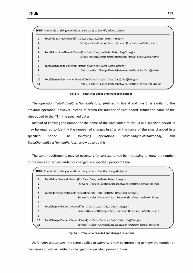
ITILib 155
Fig. B.6 ― Total sites added and changed in periods
The operation TotalAddedSitesNameInPeriod() (defined in line 4 and line 5) is similar to the
previous operation, however instead of return the number of sites added, return the name of the
sites added to the ITI in the specified dates.
Instead of knowing the number or the name of the sites added to the ITI in a specified period, it
may be required to identify the number of changes in sites or the name of the sites changed in a
specified period. The following operations TotalChangedSitesInPeriod() and
TotalChangedSitesNameInPeriod(), allow us to do this.
The same requirements may be necessary for servers. It may be interesting to know the number
or the names of servers added or changed in a specified period of time.
Fig. B.7 ― Total servers added and changed in periods
As for sites and servers, the same applies to subnets. It may be interesting to know the number or
the names of subnets added or changed in a specified period of time.
ITILib: Countable or sizing operations using dates to identify changed objects
1 TotalAddedServersInPeriod(firstDate: Date, lastDate: Date): Integer =
2 Servers()->select(CreationDate.isBetween(firstDate, lastDate))->size
3
4 TotalAddedServersNameInPeriod(firstDate: Date, lastDate: Date): Bag(String) =
5 Servers()->select(CreationDate.isBetween(firstDate, lastDate)).Name
6
7 TotalChangedServersInPeriod(firstDate: Date, lastDate: Date): Integer =
8 Servers()->select(ChangedDate.isBetween(firstDate, lastDate))->size
9
10 TotalChangedServersNameInPeriod(firstDate: Date, lastDate: Date): Bag(String) =
11 Servers()->select(ChangedDate.isBetween(firstDate, lastDate)).Name
ITILib: Countable or sizing operations using dates to identify added objects
1 TotalAddedSitesInPeriod(firstDate: Date, lastDate: Date): Integer =
2 Sites()->select(CreationDate.isBetween(firstDate, lastDate))->size
3
4 TotalAddedSitesNameInPeriod(firstDate: Date, lastDate: Date): Bag(String) =
5 Sites()->select(CreationDate.isBetween(firstDate, lastDate)).Name
6
7 TotalChangedSitesInPeriod(firstDate: Date, lastDate: Date): Integer =
8 Sites()->select(ChangedDate.isBetween(firstDate, lastDate))->size
9
10 TotalChangedSitesNameInPeriod(firstDate: Date, lastDate: Date): Bag(String) =
11 Sites()->select(ChangedDate.isBetween(firstDate, lastDate))->Name
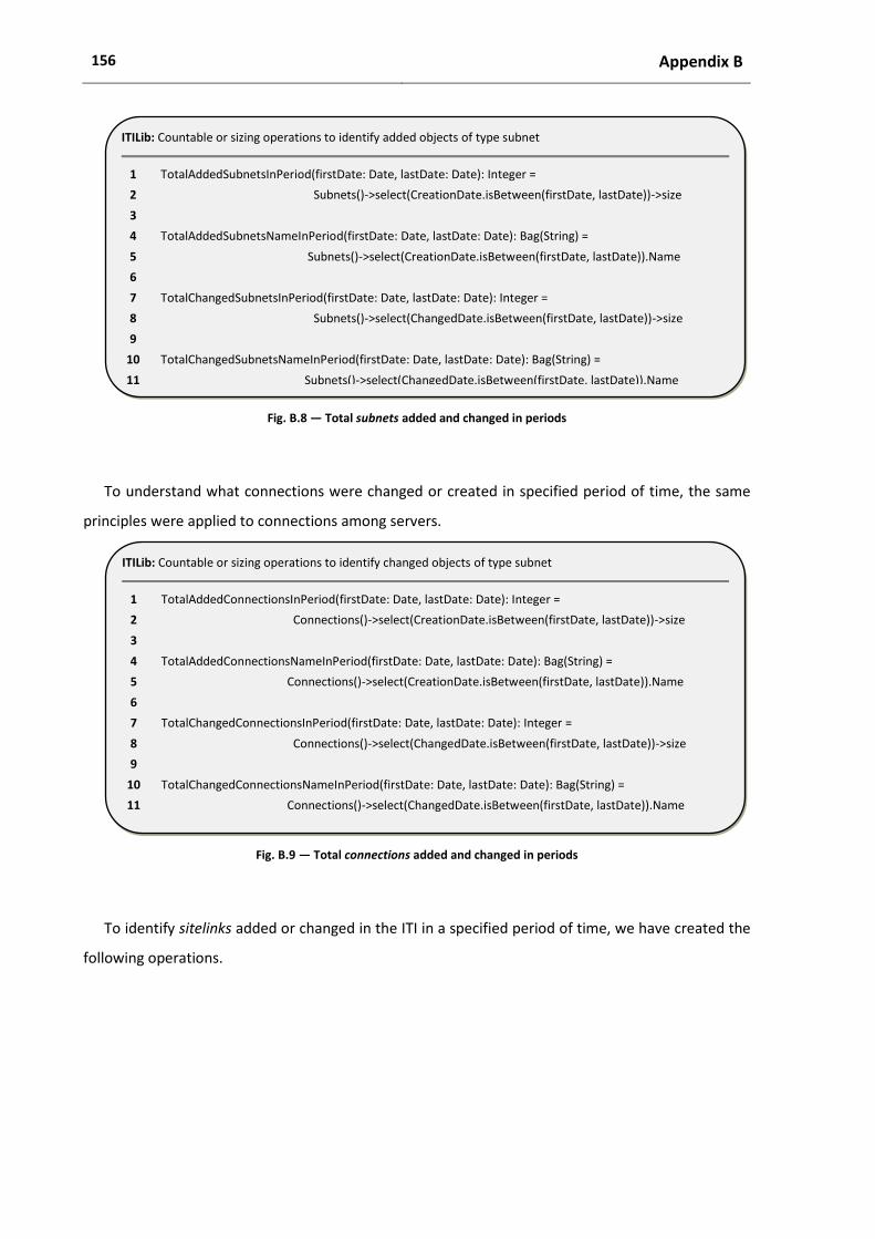
156 Appendix B
Fig. B.8 ― Total subnets added and changed in periods
To understand what connections were changed or created in specified period of time, the same
principles were applied to connections among servers.
Fig. B.9 ― Total connections added and changed in periods
To identify sitelinks added or changed in the ITI in a specified period of time, we have created the
following operations.
ITILib: Countable or sizing operations to identify changed objects of type subnet
1 TotalAddedConnectionsInPeriod(firstDate: Date, lastDate: Date): Integer =
2 Connections()->select(CreationDate.isBetween(firstDate, lastDate))->size
3
4 TotalAddedConnectionsNameInPeriod(firstDate: Date, lastDate: Date): Bag(String) =
5 Connections()->select(CreationDate.isBetween(firstDate, lastDate)).Name
6
7 TotalChangedConnectionsInPeriod(firstDate: Date, lastDate: Date): Integer =
8 Connections()->select(ChangedDate.isBetween(firstDate, lastDate))->size
9
10 TotalChangedConnectionsNameInPeriod(firstDate: Date, lastDate: Date): Bag(String) =
11 Connections()->select(ChangedDate.isBetween(firstDate, lastDate)).Name
ITILib: Countable or sizing operations to identify added objects of type subnet
1 TotalAddedSubnetsInPeriod(firstDate: Date, lastDate: Date): Integer =
2 Subnets()->select(CreationDate.isBetween(firstDate, lastDate))->size
3
4 TotalAddedSubnetsNameInPeriod(firstDate: Date, lastDate: Date): Bag(String) =
5 Subnets()->select(CreationDate.isBetween(firstDate, lastDate)).Name
6
7 TotalChangedSubnetsInPeriod(firstDate: Date, lastDate: Date): Integer =
8 Subnets()->select(ChangedDate.isBetween(firstDate, lastDate))->size
9
10 TotalChangedSubnetsNameInPeriod(firstDate: Date, lastDate: Date): Bag(String) =
11 Subnets()->select(ChangedDate.isBetween(firstDate, lastDate)).Name

ITILib 157
Fig. B.10 ― Total sitelinks added and changed in periods
Fig. B.11 ― Paths ITILib operations
ITILib: operations used to work with paths
1 nextServerPath(): Set (SystemDefinition) =
2 self.ConnectedServers().ConnectedServers()->asSet-> excluding(self)
3
4 longestPath(): Set(SystemDefinition) =
5 self.comparePaths(oclEmpty(Set(SystemDefinition)), oclEmpty(Set(SystemDefinition))) ->
6 excluding(self)
7
8 comparePaths(lgPath: Set(SystemDefinition), path: Set(SystemDefinition)): Set(SystemDefinition) =
9 if self.nextServerPath()->isEmpty() then
10 if path->size+1 > lgPath->size then
11 path->including(self)
12 else
13 lgPath
14 endif
15 else
16 self.nextServerPath()->iterate(elem: SystemDefinition; acc: Set(SystemDefinition) =
17 path->including(self) | if acc->excludes(elem) then
18 elem.comparePaths(lgPath, acc)
19 else
20 if acc->size > lgPath->size then
21 acc
22 else
23 lgPath
24 endif
25 endif)
26 endif
ITILib: Countable or sizing operations to identify added objects of type sitelink
1 TotalAddedSitelinksInPeriod(firstDate: Date, lastDate: Date): Integer =
2 Sitelinks()->select(CreationDate.isBetween(firstDate, lastDate))->size
3
4 TotalAddedSitelinksNameInPeriod(firstDate: Date, lastDate: Date): Bag(String) =
5 Sitelinks()->select(CreationDate.isBetween(firstDate, lastDate)).Name
6
7 TotalChangedSitelinksInPeriod(firstDate: Date, lastDate: Date): Integer =
8 Sitelinks()->select(ChangedDate.isBetween(firstDate, lastDate))->size
9
10 TotalChangedSitelinksNameInPeriod(firstDate: Date, lastDate: Date): Bag(String) =
11 Sitelinks()->select(ChangedDate.isBetween(firstDate, lastDate)).Name

158 Appendix B
B.2 ITILib operations for sites
We have defined in ITILib a set of operations to quantitative evaluate different aspects of ITI objects
of 'site' kind. The operation with the name Sites() (line 1 and 2 of Fig. B.1) return all ITI objects of
'site' kind that are present in an ITI. In the context of SDM, objects of 'site' kind are represented as
instances of type SystemDefinition. The operation Sites() rely on the operation IsSite() described
earlier to identify from all instances of type SystemDefinition those that are of the 'site' kind. The
operation IsSite() looks into the value of the attribute objectClass to select the SystemDefinition
objects of the 'site' kind.
Fig. B.12 ― Sites() ITILib operation
The operation SitesName() (defined in line 4 and 5) was created to identify the name of objects of
'site' kind. The attribute Name is indirectly inherited from the definition meta class as presented in
the list of attributes of Table B.1.
As presented earlier in the Table 3.3 the objects of type SystemDefinition can correspond to ITI
objects of 'server' kind or to ITI objects of site 'kind'. The operation SystemMembers() (defined in line
1 to 7 of Fig. B.13), identify the servers for a given site.
Fig. B.13 ― SystemMembers() ITILib operation
ITILib: Operations defined for sites
1 SystemMembers(): Set(SystemDefinition) =
2 if (IsSite()) then
3 ContainmentDefinition.allInstances-> select(ParentDefinition = self).
4 MemberDefinition.select(oclIsKindOf(SystemDefinition)). oclAsType(SystemDefinition)->asSet
5 else
6 oclUndefined(Set(SystemDefinition))
7 endif
8
9 SiteServers() : Set(SystemDefinition) =
10 SystemMembers()
ITILib: Operations defined for sites
1 Sites(): Set(SystemDefinition) =
2 SystemDefinition.allInstances -> select(IsSite())
3
4 SitesName(): Bag(String) =
5 Sites().Name

ITILib 159
All the ITI servers must belong to a site, so to identify the servers of a given site, we used the
ContainmentDefinition relationship as presented in line 3 and 4. The operation SiteServers() defined
in line 9 and 10 was created to simplify the usage of the operation SystemMembers().
Since all ITI subnets must belong to a site, we used a similar process to identify the ITI objects of
'subnet' kind for a given site (Fig. B.14). The main difference reside in the utilization of the object of
type ResourceDefinition instead of SystemDefinition.
Fig. B.14 ― SiteSubnets() and ResourceMembers() ITILib operations
The operation SiteSubnets() defined in line 9 and 10 was created to simplify the usage of the
operation ResourceMembers().
The operation Connections() was created to identify all the connections among servers and sites
in ITI. The CommunicationDefinition relationship display the results of rely on the operation IsSite()
described earlier to identify from all instances of type SystemDefinition those that are of the 'site'
kind. The operation IsSite() looks into the value of the attribute objectClass to select the
SystemDefinition objects of the 'site' kind.
Fig. B.15 ― Connections() ITILib operation
ITILib: Operations defined for sites
1 Connections(): Set(CommunicationDefinition) =
2 CommunicationDefinition.allInstances
3
4 ConnectionsName(): Bag(String) =
5 Connections().Name
ITILib: Operations defined for sites
1 ResourceMembers(): Set(ResourceDefinition) =
2 if (IsSite()) then
3 ContainmentDefinition.allInstances->select(ParentDefinition = self).MemberDefinition.
4 select(oclIsKindOf(ResourceDefinition)).oclAsType(ResourceDefinition)->asSet
5 else
6 oclUndefined(Set(ResourceDefinition))
7 endif
8
9 SiteSubnets() : Set(ResourceDefinition) =
10 ResourceMembers()

160 Appendix B
The operation ConnectionsName() (defined in line 4 and 5) was created to identify the name of
objects of 'Connection' kind. The attribute Name is indirectly inherited from the definition meta class
as presented in the list of attributes of Table B.1.
The operation Connections() returns objects of CommunicationDefinition relationship type, which
can be objects used to communicate with servers or sites. The NTDSConnections() operation (defined
in line 1 and 2) returns only the connections used to communicate with servers.
Fig. B.16 ― NTDSConnections() ITILib operation
IsNTDSConnection() is a boolean operation that returns true if the value of the attribute
objectClass is 'nTDSConnection'. The value 'nTDSConnection' is used to identify the connections
among servers.
The operation Sitelinks() (defined in line 1 and 2 of Fig. B.17) returns objects used to communicate
with sites. This operation rely on IsSiteLink() boolean operation to identify is a particular connection
is related with sites.
Fig. B.17 ― Sitelinks() and IsSiteLink() ITILib operations
The value 'siteLink' of attribute objectClass in IsSiteLink() operation is used to identify the
connections among sites.
In ITI sites with more than one server, as the ones presented is some of the case studies, the
servers can communicate to servers in the same site or they can communicate with servers in other
sites. The operation Intrasite_connections() (defined in line 1 to 6 of Fig. B.18) was created to identify
the objects of 'connection' kind to other servers in the same site.
ITILib: Operations defined for sites
1 Sitelinks(): Set(CommunicationDefinition) =
2 CommunicationDefinition.allInstances->select(IsSiteLink())
3
4 IsSiteLink(): Boolean = objectClass = 'siteLink'
ITILib: Operations defined for sites
1 NTDSConnections(): Set(CommunicationDefinition) =
2 Connections()->select(IsNTDSConnection())
3
4 IsNTDSConnection(): Boolean = objectClass = 'nTDSConnection'
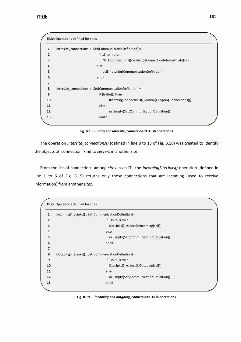
ITILib 161
Fig. B.18 ― Intra and Intersite_connections() ITILib operations
The operation Intersite_connections() (defined in line 8 to 13 of Fig. B.18) was created to identify
the objects of 'connection' kind to servers in another site.
From the list of connections among sites in an ITI, the IncomingSiteLinks() operation (defined in
line 1 to 6 of Fig. B.19) returns only those connections that are incoming (used to receive
information) from another sites.
Fig. B.19 ― incoming and outgoing_connections ITILib operations
ITILib: Operations defined for sites
1 IncomingSiteLinks() : Set(CommunicationDefinition) =
2 if (IsSite()) then
3 SiteLinks()->select(IsIncoming(self))
4 else
5 oclEmpty(Set(CommunicationDefinition))
6 endif
7
8 OutgoingSiteLinks() : Set(CommunicationDefinition) =
9 if (IsSite()) then
10 SiteLinks()->select(IsOutgoing(self))
11 else
12 oclEmpty(Set(CommunicationDefinition))
13 endif
ITILib: Operations defined for sites
1 Intrasite_connections() : Set(CommunicationDefinition) =
2 if (IsSite()) then
3 NTDSConnections()->select(IsConnectionInternalInSite(self))
4 else
5 oclEmpty(Set(CommunicationDefinition))
6 endif
7
8 Intersite_connections() : Set(CommunicationDefinition) =
9 if (IsSite()) then
10 IncomingConnections()->union(OutgoingConnections())
11 else
12 oclEmpty(Set(CommunicationDefinition))
13 endif
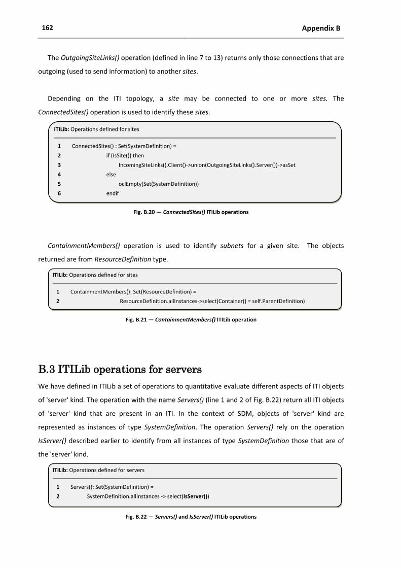
162 Appendix B
The OutgoingSiteLinks() operation (defined in line 7 to 13) returns only those connections that are
outgoing (used to send information) to another sites.
Depending on the ITI topology, a site may be connected to one or more sites. The
ConnectedSites() operation is used to identify these sites.
Fig. B.20 ― ConnectedSites() ITILib operations
ContainmentMembers() operation is used to identify subnets for a given site. The objects
returned are from ResourceDefinition type.
Fig. B.21 ― ContainmentMembers() ITILib operation
B.3 ITILib operations for servers
We have defined in ITILib a set of operations to quantitative evaluate different aspects of ITI objects
of 'server' kind. The operation with the name Servers() (line 1 and 2 of Fig. B.22) return all ITI objects
of 'server' kind that are present in an ITI. In the context of SDM, objects of 'server' kind are
represented as instances of type SystemDefinition. The operation Servers() rely on the operation
IsServer() described earlier to identify from all instances of type SystemDefinition those that are of
the 'server' kind.
Fig. B.22 ― Servers() and IsServer() ITILib operations
ITILib: Operations defined for servers
1 Servers(): Set(SystemDefinition) =
2 SystemDefinition.allInstances -> select(IsServer())
ITILib: Operations defined for sites
1 ContainmentMembers(): Set(ResourceDefinition) =
2 ResourceDefinition.allInstances->select(Container() = self.ParentDefinition)
ITILib: Operations defined for sites
1 ConnectedSites() : Set(SystemDefinition) =
2 if (IsSite()) then
3 IncomingSiteLinks().Client()->union(OutgoingSiteLinks().Server())->asSet
4 else
5 oclEmpty(Set(SystemDefinition))
6 endif

ITILib 163
The operation IsServer() looks into the value of the attribute objectClass to select the
SystemDefinition objects of the 'server' kind.
Every server in the ITI, must have a parent of the "site" kind. This relationship is expressed with
ContainmentDefinition relationship type. The ServerSite() operation returns the site for a given
server.
Fig. B.23 ― ServerSite() ITILib operation
As explained in section 3.7 the communication among servers or sites require the existence of
endpoints, which can be classified as input or output, depending if they are used to receive or to
send information. InputEndpoints() and OutputEndpoints() operations of Fig. B.24 identify the type of
endpoints.
Fig. B.24 ― Input and outputendpoints ITILib operations
In an ITI servers are connected in the sense that they communicate. The number of servers that a
specific server is connected to differs from ITI to ITI and is dependent of the topology. The
ConnectedServers() operation returns the servers connected to a given server.
ITILib: Operations defined for servers
1 InputEndpoints(): Set(EndpointDefinition) =
2 EndpointMembers()->select(e: EndpointDefinition | e.IsInput())
3
4 OutputEndpoints(): Set(EndpointDefinition) =
5 EndpointMembers()->select(e: EndpointDefinition | e.IsOutput())
ITILib: Operations defined for servers
1 ServerSite(): SystemDefinition =
2 if (isServer()) then
3 ContainmentDefinition.allInstances->select(MemberDefinition = self).ParentDefinition.
4 select(oclIsKindOf(SystemDefinition)).oclAsType(SystemDefinition)->asSequence->first()
5 else
6 oclUndefined(SystemDefinition)
7 endif

164 Appendix B
Fig. B.25 ― ConnectedServers() ITILib operation
When multiple servers exists in the same site, each server in the site can send or receive
information from multiple servers as illustrated in the presented case studies. The
Intraserver_FanIn() and Intraserver_FanOut() operations return the number of connections used to
receive information from another servers in the same site and to send information to servers in the
same site.
Fig. B.26 ― Intraserver FanIn and FanOut ITILib operations
The SSEN() operation is based on the SiteServers() operation defined in Fig. B.13 and is used to
count the number of servers in a site.
ITILib: Operations defined for servers
1 Intraserver_FanIn(): Integer =
2 if (IsServer()) then
3 ServerSite().Intrasite_connections()->select(IsIncoming(self)) -> size
4 else
5 0
6 endif
7
8 Intraserver_FanOut(): Integer =
9 if (IsServer()) then
10 ServerSite().Intrasite_connections()->select(IsOutgoing(self)) -> size
11 else
12 0
13 endif
ITILib: Operations defined for servers
1 ConnectedServers() : Set(SystemDefinition) =
2 if (IsServer()) then
3 IncomingConnections().Client()->union(OutgoingConnections().Server())->asSet
4 else
5 oclEmpty(Set(SystemDefinition))
6 endif

ITILib 165
Fig. B.27 ― SSEN() ITILib operation
B.4 ITILib operations for sites and servers
EndpointMembers() operation is applicable to servers and sites and returns the connections
(nTDSConnection or siteLink) for servers or sites.
Fig. B.28 ― EndpointMembers ITILib operations
IncomingConnections() operation (defined in line 1 to 10 of Fig. B.29) return objects of type
relationship definition. This operation can be applied to servers or sites and returns the connections
used to receive information. If a site is provided the incoming connections relatively to the current
site are returned otherwise the incoming connections relatively to the server are returned.
OutgoingConnections() operation (defined in line 12 to 21 of Fig. B.29) also returns objects of type
relationship definition and can be applied to servers or sites. This operations is used to return the
connections used to send information.
ITILib: Operations defined for sites and servers
1 EndpointMembers(): Set(EndpointDefinition) =
2 if (IsServer() or IsSite()) then
3 ContainmentDefinition.allInstances->select(ParentDefinition = self).MemberDefinition.
4 select(oclIsKindOf(EndpointDefinition)).oclAsType(EndpointDefinition)->asSet
5 else
6 oclUndefined(Set(EndpointDefinition))
7 endif
ITILib: Operations defined for servers
1 SSEN(): Integer =
2 if (IsSite()) then
3 SiteServers()->size
4 else
5 0
6 endif

166 Appendix B
Fig. B.29 ― Incoming and OutgoingConnection() ITILib operations
FanIn() and FanOut() operations of Fig. B.30 widely used in ITI complexity analysis chapter are
used to count the number of connections used to receive information ( FanIn() ) and the number of
connections used to send information ( FanOut() ). This operation can be applied to servers or sites.
Fig. B.30 ― FanIn() and FanOut() ITILib operations
ITILib: Operations defined for sites and servers
1 FanIn(): Integer =
2 Connections()->select(IsIncoming(self)) -> size
3
4 FanOut(): Integer =
5 Connections()->select(IsOutgoing(self)) -> size
ITILib: Operations defined for sites and servers
1 IncomingConnections() : Set(CommunicationDefinition) =
2 if (IsSite()) then
3 NTDSConnections()->select(IsConnectionIncomingInSite(self))
4 else
5 if (IsServer()) then
6 NTDSConnections()->select(IsIncoming(self))
7 else
8 oclEmpty(Set(CommunicationDefinition))
9 endif
10 endif
11
12 OutgoingConnections() : Set(CommunicationDefinition) =
13 if (IsSite()) then
14 NTDSConnections()->select(IsConnectionOutgoingInSite(self))
15 else
16 if (IsServer()) then
17 NTDSConnections()->select(IsOutgoing(self))
18 else
19 oclEmpty(Set(CommunicationDefinition))
20 endif
21 endif

ITILib 167
B.5 ITILib operations for subnets
The SubnetSite() operation allows the identification of the site corresponding to a given subnet. This
operation searches all containment relationships where the member is the subnet and returns the
site.
Fig. B.31 ― SubnetSite() ITILib operation
The SSBN() operation relies on SiteSubnets() operation (defined in Fig. B.14) to count the subnets
in a specified site.
Fig. B.32 ― SSBN() ITILib operation
To list all existing subnets, which are from type ResourceDefinition the concept is similar to sites
and servers, however instead of using SystemDefinition we have to use ResourceDefinition and look
for subnet in the value of the attribute objectClass.
Fig. B.33 ― Subnets() and IsSubnet() ITILib operations
ITILib: Operations defined for subnets
1 Subnets(): Set(ResourceDefinition) =
2 ResourceDefinition.allInstances->select(IsSubnet())
ITILib: Operations defined for subnets
1 SSBN(): Integer =
2 if (IsSite()) then
3 SiteSubnets()->size
4 else
5 0
6 endif
ITILib: Operations defined for subnets
1 SubnetSite(): SystemDefinition =
2 if (isSubnet()) then
3 ContainmentDefinition.allInstances->
4 select(MemberDefinition = self).ParentDefinition.
5 (oclIsKindOf(SystemDefinition)).oclAsType(SystemDefinition)->
6 asSequence->first()
7 else
8 oclUndefined(SystemDefinition)
9 endif

168 Appendix B
B.6 ITILib operations for SiteLinks
It may be important to identify the name of all existing sites within an ITI. The following operations
make that possible.
Fig. B.34 ― Sitelinksname() and Sitelinks() ITILib operations
From the list of all existing connections in the ITI, we may want to know to what server does one
specific connection belongs to.
Fig. B.35 ― EndpointServer() ITILib operation
Every server in the ITI has one or more connections to other servers. To identify all connections of
a specific server we created the operation ServerConnections().
ITILib: Operations defined for sitelinks
1 EndpointServer(): SystemDefinition =
2 if (objectClass = 'nTDSConnection') then
3 ContainmentDefinition.allInstances->select(MemberDefinition = self).ParentDefinition.
4 select(oclIsKindOf(SystemDefinition)).oclAsType(SystemDefinition)->asSequence->first()
5 else
6 oclUndefined(SystemDefinition)
7 endif
ITILib: Operations defined for sitelinks
1 SitelinksName(): Bag(String) = Sitelinks().Name
2
3 Sitelinks(): Set(CommunicationDefinition) =
4 CommunicationDefinition.allInstances->select(IsSiteLink())

ITILib 169
Fig. B.36 ― ServerConnections() and EndpointMembers() ITILib operations
B.7 ITILib operations for Connections
In the communicationdefinition we already defined operations such as isNTDSConnection() to
identify the connections of the servers and IsSiteLink() to identify the connections among sites.
However in the cases with more than one server per site, we may also want to identify the
connections to other servers in the same site and the connections to servers in other sites. In order
to achieve this we have created the IsConnectionInternalInSite() and IsConnectionOutgoingInSite()
predicates. The latter rely on the operations Client() and Server() to help on the identification.
Fig. B.37 ― IsConnectionInternalInSite() and IsConnectionOutgoingInSite() ITILib operations
ITILib: Operations defined for sitelinks
1 IsConnectionInternalInSite (theSite: SystemDefinition): Boolean =
2 (Client().ServerSite() = theSite) and (Server().ServerSite() = theSite)
3
4 IsConnectionIncomingInSite(theSite: SystemDefinition): Boolean =
5 (Client().ServerSite() <> theSite) and (Server().ServerSite() = theSite)
5
6 IsConnectionOutgoingInSite(theSite: SystemDefinition): Boolean =
7 (Client().ServerSite() = theSite) and (Server().ServerSite() <> theSite)
ITILib: Operations defined for sitelinks
1 ServerConnections() : Set(EndpointDefinition) =
2 if (objectClass = 'server') then
3 self.EndpointMembers()
4 else
5 oclEmpty(Set(EndpointDefinition))
5 endif
6
7 EndpointMembers(): Set(EndpointDefinition) =
8 if (objectClass = 'server') then
9 ContainmentDefinition.allInstances->
10 select(ParentDefinition = self).MemberDefinition.
11 select(oclIsKindOf(EndpointDefinition)).
12 oclAsType(EndpointDefinition)->asSet
13 else
14 oclUndefined(Set(EndpointDefinition))
15 endif

170 Appendix B
Fig. B.38 ― IsIncoming() and IsOutgoing(), Server() and Client() ITILib operations
Fig. B.39 ― Client() and Server() ITILib operations
ITILib: Operations defined for sitelinks
1 Client(): SystemDefinition = ClientDefinition.Container()
2
3 Server(): SystemDefinition = ServerDefinition.Container()
ITILib: Operations defined for sitelinks
1 IsIncoming(target: SystemDefinition): Boolean = Server() = target
2
3 IsOutgoing(target: SystemDefinition): Boolean = Client() = target
4
5 Client(): SystemDefinition = ClientDefinition.Container()
5
6 Server(): SystemDefinition = ServerDefinition.Container()

171
C
Appendix C – The SDM Schema
Contents
C.1 –The SDM schema........................................................................................................................................................................................................ 172
C.2 – SDM Class diagram.................................................................................................................................................................................................... 177
This appendix presents simple types, complex types and attributes groups of the SDM schema and a short description of each object. During this dissertation we
have used just some of these objects. These objects allow the creation of files with the sdm extension to represent SDM objects such as systems, endpoints and
resources. To better understand the SDM schema we provide also a class diagram (divided in four parts due the size), where we can take a look into the relations
between all these objects.

172 Appendix C
C.1 The SDM schema
The SDM elements, simple and complex types and attribute groups and a short description of each of these objects are presented next in Table C.1 to Table C.4.
Table C.1 ― SDM schema elements
Element Description
Comments (Information) Contains comments about an .sdm file that provides general information about the document.
CommunicationDefinition (ObjectDefinition) Contains a nested communication definition.
CommunicationDefinition (SystemDefinitionModel) Contains communication definitions that are contained in the .sdm file. CompanyName (Information) Contains the name of the company for which the .sdm file was created.
CompilerVersion (Information) Contains the version of the compiler that built the .sdmdocument file.
Connection (ObjectDefinition) Contains a connection relationship member declaration used in the definition of an object. Connection (RelationshipDefinition) Contains a connection relationship member used in the definition of a relationship between two members.
ConstraintDefinition (SystemDefinitionModel) Contains constraint definitions that are contained in the .sdm file.
ConstraintGroup (ConstraintDefinition) Contains a nested constraint group identifying a manager that provides code to evaluate input values. ConstraintGroup (ObjectConstraint) Contains a nested constraint group that is evaluated against the primary object definition.
ConstraintGroup (ObjectDefinition) Contains a nested group of constraints on the relationships in which instances of an object definition can participate. ConstraintGroup (RelationshipConstraint) Contains a nested group of constraints on the values of settings within a relationship or on objects at the other end of a relationship.
ConstraintGroup (RelationshipDefinition) Contains a nested constraint group that will be evaluated against a relationship definition.
Constraint (ConstraintDefinition Contains a manager that provides code to evaluate input values. Constraint (ConstraintGroup) Contains a constraint member nested within a constraint group.
Constraint (ObjectConstraint) Contains a constraint member that is evaluated against a primary object definition.
Constraint (ObjectDefinition) Contains a constraint on the relationships in which instances of an object definition can participate. Constraint (RelationshipConstraint) Contains a constraint on the values of settings within a relationship or on objects at the other end of a relationship.
Constraint (RelationshipDefinition) Contains a constraint that will be evaluated against a relationship definition.
ContainmentDefinition (ObjectDefinition) Contains a containment definition. This definition can be used by members within the scope of the outer system definition. ContainmentDefinition (SystemDefinitionModel) Contains a containment definition that is contained in an .sdm file.
Containment (ObjectDefinition) Contains a member declaration for a containment relationship. Containment (RelationshipDefinition) Contains a containment relationship member.
Copyright (Information) Contains copyright information for the .sdm file.
DelegationDefinition (ObjectDefinition) Contains a delegation definition. This definition can be used by members within the scope of the outer system definition. DelegationDefinition (SystemDefinitionModel) Contains a delegation definition that is contained in an .sdm file.
Delegation (ObjectDefinition) Contains a delegation relationship member declaration.
Delegation (RelationshipDefinition) Contains a delegation relationship member. Description (Definition) Contains a description of an object, relationship, constraint, or flow definition.
Description (Information) Contains a description of an .sdm file.
Description (ManagerDeclaration) Contains a description of a manager.

SDM Schema and class diagrams 173
Element Description
Description (Member) Contains a description of a member in an .sdm file. Description (StructuralConstraint) Contains a description of a constraint.
DesignData (Definition) Contains design surface information about an object, relationship, constraint, or flow definition.
DesignData (Member) Contains design surface—specific information about a member. DesignData (StructuralConstraint) Contains design surface—specific information about a constraint.
DesignData (SystemDefinitionModel) Contains global design surface information for an .sdm file.
EndpointDefinition (ObjectDefinition) Contains an endpoint definition. This definition can be used by members within the scope of the outer system definition. EndpointDefinition (SystemDefinitionModel) Contains an endpoint definition that is contained in an .sdm file.
Endpoint (ObjectDefinition) Contains an endpoint member declaration that references an endpoint definition.
Entry (Description) Contains the text of a description and a description entry. Facet (SettingMember) Contains the set of aspects associated with a setting.
FlowDefinition (SystemDefinitionModel) Contains flow definitions that are contained in an .sdm file. Flow (ObjectDefinition) Contains a flow member declaration.
Flow (RelationshipDefinition) Contains a flow between the instances that participate in a relationship.
FriendlyName (Information) Contains the friendly name of an .sdm file. HostingDefinition (ObjectDefinition) Contains a hosting definition between a host and guest member. This definition can be used by members within the scope of the outer
system definition.
HostingDefinition (SystemDefinitionModel) Contains a hosting definition that is contained in an .sdm file. Hosting (ObjectDefinition) Contains a hosting relationship member declaration for an object.
Hosting (RelationshipDefinition) Contains a hosting relationship member declaration for a relationship. Import (SystemDefinitionModel) Contains the namespace that an SDM topic imports and references.
Information (SystemDefinitionModel) Contains general information about an .sdm file.
Input (ConstraintMember) Contains a list of inputs to a constraint. An input identifies a path to the source setting value that will be passed to the constraint and constraint setting that will be set as a result. The source setting definition and the constraint setting definition must be compatible.
Input (FlowMember) Contains a list of paths to setting values that are used as input to a flow.
Manager (SystemDefinitionModel) Contains the manager used to provide customized behavior to the runtime and to support interaction between the runtime and the modeled system.
ObjectConstraint (ConstraintDefinition) Contains a constraint on an object. ObjectConstraint (ConstraintGroup) Contains a object constraint that is nested within a group of constraints.
ObjectConstraint (RelationshipConstraint) Contains an object constraint that is evaluated in the context of the matched relationship instance.
ObjectConstraint (RelationshipDefinition) Contains a constraint on instances that participate in a relationship. Output (FlowMember) Contains a list of paths to settings that will be set as a result of a flow. Each output must identify a read-only setting on the flow
definition. ReferenceDefinition (ObjectDefinition) Contains a reference definition. This definition can be used by members within the scope of the outer system definition.
ReferenceDefinition (SystemDefinitionModel) Contains a reference definition that is contained in an .sdm file.
Reference (ObjectDefinition) Contains a reference relationship member declaration. Reference (RelationshipDefinition) Contains a reference member declaration specifically used in a relationship definition.
RelationshipConstraint (ConstraintDefinition) Contains constraints on a relationship.
RelationshipConstraint (ConstraintGroup) Contains a relationship constraint nested within a group of relationship constraints.

174 Appendix C
Element Description
RelationshipConstraint (ObjectConstraint) Contains a constraint on a relationship defined for an object. RelationshipConstraint (ObjectDefinition) Contains a constraint on the relationships in which instances of an object definition can participate.
RelationshipConstraint (RelationshipConstraint) Contains a relationship constraint that will be evaluated in the context of the target object.
ResourceDefinition (ObjectDefinition) Contains resource definitions that can be used by members within the scope of the outer system definition. ResourceDefinition (SystemDefinitionModel) Contains resource definitions that are contained in the .sdm file.
Resource (ObjectDefinition) Contains a resource member declaration that references a resource definition.
SettingDeclaration (Definition) Contains the base definition of a setting member. SettingDefinitions (SystemDefinitionModel) Contains an XML schema document that contains setting definitions.
SettingValueList (Definition) Contains a list of values for a setting on a definition or its base definition.
SettingValueList (Member) Contains a list of values for settings that correspond to writable settings on a member-referenced type. SettingValue (Definition) Contains a value for a setting on a definition or its base definition. A value can only be provided once for a setting declaration within a
definition. SettingValue (Member) Contains a value for settings that correspond to writeable settings on a member referenced type. If these values are marked as fixed,
then they must be used when an instance is created for the member, if they are not fixed, then the values can be overridden by deployment parameters or parameters set by a flow.
Subsystem (ObjectDefinition) Contains a subsystem member declaration that references a system definition.
SystemDefinitionModel Defines an .sdm file that provides a strong identity, versioning and localization information for a set of relationships, objects and managers.
SystemDefinition (ObjectDefinition) Contains a nested system definition. This definition can be used by members within the scope of the outer system definition.
SystemDefinition (SystemDefinitionModel) Contains system definitions that are contained in an .sdm file. Trademark (Information) Contains trademark information for an .sdm file.
Value (SettingValueList) Contains a value in a list of setting values.
Table C.2 ― SDM schema attribute groups
Element Description
NamespaceIdentity Contains a namespace (scope) for SDM names.
SettingsAttributes Contains attributes used to describe the behavior of a particular setting. SettingValueAttributes Contains attributes used to control the behavior of setting values.

SDM Schema and class diagrams 175
Table C.3 ― SDM schema simple types
Element Description
CompilationHashType Defines the pattern used to verify that an SDM file is a valid compiled document when the SDM file is used as a referenced file during the compilation of a different SDM file.
ConstraintEvaluation Defines values that allow the constraint developer to mark a constraint according to when it should run. Culture Defines the value used to specify a language for an .sdm file.
CultureNeutral Defines the values used to allow an .sdm file to identify its culture as neutral when it does not contain language-specific binaries. FourPartVersionType Defines the type of values used to identify a file version by using a four-part numbering system.
MaxOccurs Defines an upper bound on the number of instances associated with a member.
MinOccurs Defines a non-negative lower bound on the number of instances associated with a member. Path Defines the values used to define a path to a definition or member in the current .sdm file namespace or in an aliased (imported) namespace.
PathList Defines the values defining a list of paths that resolve to setting values.
Platform Defines the values used to identify the platform on which an assembly will execute as neutral or with a value from the ProcessorArchitectures simple type. ProcessorArchitectures Defines the values used to identify the processor architecture on which an assembly will execute.
PublicKeyTokenType Defines the value used to identify the public part of a public/private key pair.
PublicKeyType Defines a value used as a public key that is stored in a signed .sdm file. QualifiedName Defines a value used as a name that refers to definitions or members defined in an .sdm files namespace or in an aliased (imported) namespace.
RolesList Defines values used as a list of names for a role in the relationship that a constraint targets.
SettingMemberAccess Defines values used to specify whether reading and writing a setting’s value is permitted, providing SDM runtime access control and display and editing rules to designers.
SettingMemberSecure Defines values used to specify whether the value of a setting should be encrypted when stored to an .sdmdocument file and whether tools should log this value during manipulations such as installations.
SettingPath Defines the value used for a setting member path. SimpleName Defines the value used to supply a simple name for members in an SDM definition.
Table C.4 ― SDM schema complex types
Element Description
CommunicationDefinition Defines the elements used to define client and server member definitions used in communication links.
CommunicationMember Defines the paths to two endpoint members (client and server) used in a communication relationship in an SDM member definition. ConstraintDefinition Defines the elements in a constraint on a defined set of input values.
ConstraintGroup Defines a group of different constraints to be evaluated together.
ConstraintMember Defines a set of input values for a particular constraint definition. ContainmentDefinition Defines the parent and member definitions in a containment relationship.
ContainmentMember Defines the path to a child member when it is contained by a parent member. Definition Defines the base set of elements for object, relationship, constraint and flow definitions.
DelegationDefinition Defines a pair of abstract endpoint definitions that participate in a delegation relationship.
DelegationMember Defines the paths to two members used to set up a delegation relationship. Description Defines the elements that contain the information to describe an SDM element.

176 Appendix C
Element Description
DescriptionEntry Defines the elements used to create a description of an SDM member. DesignData Defines the element holding a schema instance that identifies and structures data for a design surface.
EndpointDefinition Defines an SDM endpoint.
EndpointMember Defines the element that creates a use for an endpoint definition. Facet Defines an element that holds the name of a facet of a setting (a subsetting used to read a value from or write a value to a setting).
FlowDefinition Defines an element that contains a particular transform to be applied to a set of setting values.
FlowMember Defines the elements that contain one or more input settings, one or more destination settings and a flow definition. HostingDefinition Defines elements that contain guest and host member definitions in a hosting relationship.
HostingMember Defines elements that hold the paths to guest and host members in a hosting relationship.
Import Defines the elements that contain a namespace to be imported by another namespace and an alias for the imported namespace. Information Defines the elements that contain general information about an .sdm document.
Input Defines an input value for a flow or constraint. ManagerDeclaration Defines the elements that contain information used to define a manager.
Member Defines the elements that contain information about a member definition in an .sdm file.
ObjectConstraint Defines the elements used to define a constraint on one or both roles of a relationship. ObjectConstraintGroup Defines the element that contains a group of constraints on one or both roles of a relationship.
ObjectDefinition Defines the elements that contain the base information to define the object which abstract and concrete object definitions extend.
ObjectMember Defines the elements that define an abstract or concrete object definition. Output Defines the attributes that create a variation on the ValueTransfer value transfer.
ReferenceDefinition. Defines the elements that contain the definitions for the source and dependent members in a reference relationship between the members
ReferenceMember Defines the elements that contain paths to the source and dependent members used to set up a reference relationship. RelationshipConstraint Defines the elements that constrain the relationships in which an object can participate.
RelationshipConstraintGroup Defines the elements that define a group of relationship constraints constraining the relationships in which an object can participate. RelationshipDefinition Defines the elements that contain all the information defining the relationship between two members.
RelationshipMember Defines the relationship that will exist between object members when they are created.
ResourceDefinition Defines an SDM resource. ResourceMember Defines the use for a resource definition.
SettingDefinitions Defines the elements containing setting definitions used by setting members, including namespace declarations and namespace imports.
SettingMember Defines the elements and attributes used to define a setting member. SettingValue Defines the attributes used in defining a single setting value for a setting declaration.
SettingValueList Defines the list of attributes and elements used to define one or more setting values for a setting declared as a list.
StructuralConstraint Defines the elements used to create the structure of a constraint. SystemDefinition Defines the attributes that define a system.
SystemMember Defines a use for a system definition. ValueTransfer Defines the elements that contain information used to pass setting values into or out of a flow or constraint.

SDM Schema and class diagrams 177
C.2 SDM Class diagram
To better understand the relations among class in SDM we present in this section (Fig. C.1 to Fig. C.4) a class diagram of the SDM. Due to the size of the class
diagram we divide it in four parts.
Fig. C.1 ― Class diagram (Part I of IV)

178 Appendix C
Fig. C.2 ― Class diagram (Part II of IV)

SDM Schema and class diagrams 179
Fig. C.3 ― Class diagram (Part III of IV)
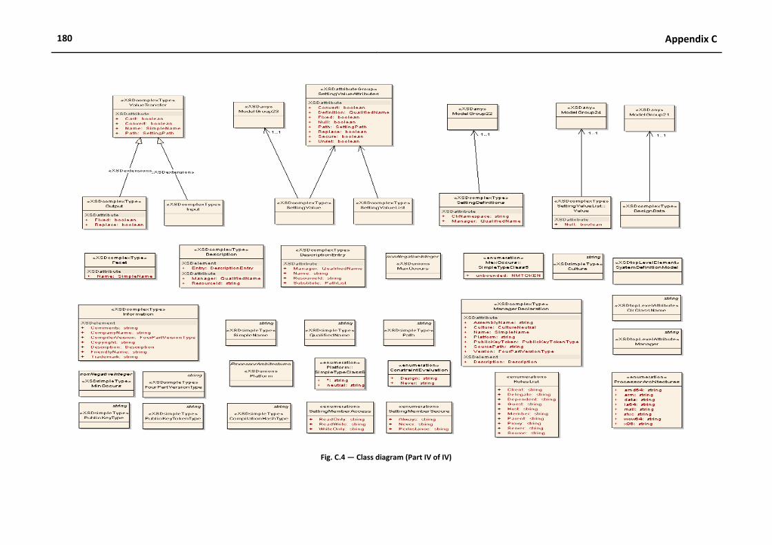
180 Appendix C
Fig. C.4 ― Class diagram (Part IV of IV)

181
D
Appendix D – Papers and
Reports
This appendix has the list of papers and reports analyzed in this dissertation. The papers and reports
were sponsored by different entities or organizations in different periods of time. The purpose of this
analysis was to select the most complete evaluations for deeper analysis. We have examined each of
these documents and we selected those with references to some concepts discussed in this
dissertation. The selected documents were presented in section 2.2.

182 Appendix D
Table D.1 ― List of Papers and reports
ID Reference Document Name Date Sponsored by
1 [Steeples, et al., 1993] CO Benefits Using Multiply Charged Ion Implants on Conventional Medium and High Current Implanters 1993 IEEE
2 [Gartner, 1997] Gartner - Next Generation Total Cost of Ownership Methodology 1997 Gartner
3 [Microsoft, 1999] Microsoft Business Value - Windows vs. LINUX Total Cost of Ownership Overview 1999 Microsoft
4 [Brynjolfsson, et al., 2000] Computing Productivity Firm-Level Evidence 2000 University
5 [TriActive, 2001] Calculating Your Total Cost of Ownership 2001 TriActive
6 [Adams, 2002] Management Update Best Practices to Launch an IT Asset Management Program 2002 Gartner
7 [Kirwin, et al., 2002] The Total Cost of Ownership Index: Defining the Database 2002 Gartner
8 [David, et al., 2002] Managing your total IT cost of ownership 2002 ACM
9 [Greschler, et al., 2002] Networking lessons in delivering ‘Software as a Service’—Part I 2002 ACM
10 [Wang, et al., 2004] Friends Troubleshooting Network Towards Privacy-Preserving, Automatic Troubleshooting 2004 University
11 [Builders, 2002] Examining TCO for Business Intelligence Solutions 2002 I. Builders
12 [Kirwin, 2003b] CIO Update To Control TCO, It Must Be Measured and Managed 2003 Gartner
13 [Heine, 2003] Management Update Five Sure Ways to Reduce IT Asset Costs 2003 Gartner
14 [O'Brien, 2003] Management Update IT Asset Management Is Mandatory, Not Optional 2003 Gartner
15 [Kirwin, 2003a] Management Update Total Cost of Ownership Analysis 2003 Gartner
16 [Gartner, 2003] TCO Distributed Computing - Chart of Accounts 2003 Gartner
17 [Aziz, et al., 2003] TCO Reduction 2003 IEEE
18 [Kimfong, et al., 2003] Technology to enable learning Strategic decisions on technology selections for facilitating a network systems laboratory using real options total cost of ownership theories
2003 ACM
19 [Rasmussen, 2006a] Electrical Efficiency Modeling of Data Centers 2003 APC
20 [Rasmussen, 2006b] Implementing Energy Efficient Data Centers 2003 APC
21 [APC, 2003b] Avoiding Costs from Oversizing Data Center and Network Room Infrastructure 2003 APC
22 [APC, 2003a] Determining TCO for Datacenter and Network Room Infrastructure 2003 APC
23 [Sawyer, 2003] Reducing the Hidden Costs Associated with Upgrades of Data Center Power Capacity 2003 APC
24 [Rymer, et al., 2003] The Total Economic Impact of Developing and Deploying Applications on Microsoft and J2EE/Linux Platforms 2003 OSS
25 [DiDio, 2004b, DiDio, 2004a] Linux, UNIX and Windows TCO Comparison 2004 Yankee Group
26 [Gomolski, 2004] How to Use IT Cost Metrics Effectively 2004 Gartner
27 [Sigurdsson, et al., 2004] Cost optimization methods in the design of next generation networks 2004 IEEE
28 [Logan, 2004] Monitoring and state transparency of distributed systems 2004 ACM
29 [Rosenberg, 2004] The Myths of usability ROI 2004 ACM
30 [Msadek, 2003] Managing technology to reduce total cost of ownership and secure assets 2004 Education
31 [Axeda, 2007] AXEDA - Secure Remote Vendor Access to the Enterprise Data Center 2004 Axeda
32 [Webster, 2004] Getting the most out of ROI and TCO 2004 DMG
33 [Cybersource, et al., 2004] Linux vs Windows - Total Cost of Ownership Comparison 2004 Cybersource Pty
34 [Kirwin, et al., 2005] Control Distributed Computing TCO by Keeping an Eye on Complexity 2005 Gartner
35 [Harris, 2005] IT Complexity May Be the Reason You're Spending More and gaining less 2005 Gartner
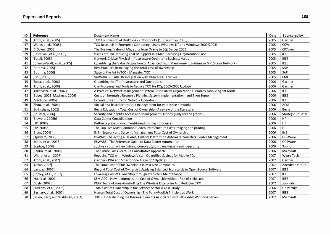
Papers and Reports 183
ID Reference Document Name Date Sponsored by
36 [Troni, et al., 2005] TCO Comparison of Desktops vs. Notebooks (13 December 2005) 2005 Gartner
37 [Wang, et al., 2005] TCO Research in Enterprise Computing (Linux, Windows NT and Windows 2000/2003) 2005 CCW
38 [CIOview, 2005] The Business Value of Migrating from Oracle to SQL Server 2005 2005 CIOView
39 [Castellani, et al., 2005] Issues around Reducing Cost of Support in a Manufacturing Organization Case 2005 IEEE
40 [Torell, 2005] Network-Critical Physical Infrastructure Optimizing Business Value 2005 IEEE
41 [Ionescu-Graff, et al., 2005] Quantifying the Value Proposition of Advanced Fault Management Systems in MPLS Core Networks 2005 IEEE
42 [Bothma, 2005] Best Practices-in-managing-the-total-cost-of-ownership 2005 SAP
43 [Bothma, 2006] State of the Art in TCO - Managing TCO 2005 SAP
44 [EMC, 2005] VmWARE - CLARiiON Integration with VMware ESX Server 2005 EMC
45 [Scott, et al., 2006] Organizing for IT Infrastructure and Operations 2006 Gartner
46 [Troni, et al., 2006] Use Processes and Tools to Reduce TCO for PCs, 2005-2006 Update 2006 Gartner
47 [Takahashi, et al., 2007] A Practical Network Management System Based on an Organization Hierarchy Mobile Agent Model 2006 IEEE
48 [Babey, 2006, Machuca, 2006] Costs of Enterprise Resource Planning System Implementation - and Then Some 2006 IEEE
49 [Machuca, 2006] Expenditures Study for Network Operators 2006 IEEE
50 [Zhou, et al., 2006] Virtual disk based centralized management for enterprise networks 2006 ACM
51 [Scrimshaw, 2002] Becta Education - Total Cost of Ownership - A review of the literature 2006 Becta
52 [Counsel, 2006] Security and Identity Access and Management Outlook (Only for the graphs) 2006 Strategic Counsel
53 [Blowers, 2006b] Data Center Consolidation 2006 HP
54 [HP, 2006a] Putting a price on document-based business processes 2006 HP
55 [HP, 2006b] The Top Five Most Common Hidden Infrastructure Costs imaging and printing 2006 HP
56 [Blum, 2004] INS - Network and Systems Management Total Cost of Ownership 2006 INS
57 [Opsware, 2006] PSWARE - Selecting a Flexible, Custom Platform to Automate Your Data Center Management 2006 OPSWare
58 [Jones, et al., 2006] PSWARE - The Reference Guide to Data Center Automation 2006 OPSWare
59 [Sophos, 2006] sophos - cutting-the-cost-and-complexity-of-managing-endpoint-security 2006 Sophos
60 [Kantin, et al., 2006] The Future Sales Force - A Consultative Approach 2006 Microsoft
61 [Wipro, et al., 2007] Reducing TCO with Windows Vista - Quantified Savings for Mobile PCs 2007 Wipro Tech.
62 [Troni, et al., 2007] Gartner - PDA and Smartphone TCO-2007 Update 2007 Gartner
63 [Jutras, 2007] The Total Cost of ERP Ownership in Mid-Size Companies 2007 Aberdeen Group
64 [Lavazza, 2007] Beyond Total Cost of Ownership Applying Balanced Scorecards to Open-Source Software 2007 IEEE
65 [Conley, et al., 2007] Lowering Cost of Ownership through Predictive Maintenance 2007 IEEE
66 [Ho, et al., 2007] SEM ADC - How it improves the Cost of Ownership without Risk of Yield Loss 2007 IEEE
67 [Boyle, 2007] PEAK Technologies -Controlling The Wireless Enterprise And Reducing TCO 2007 Journals
68 [Hurkens, et al., 2006] Total Cost of Ownership in the Services Sector A Case Study 2006 University
69 [Zachary, et al., 2007] Human Total Cost of Ownership - The PennyFoolish Principle at Work 2007 IEEE
70 [Gillen, Perry and Waldman, 2007] IDC - Understanding the Business Benefits Associated with x86 64-bit Windows Server 2007 Microsoft


![MODEL DRIVEN DEVELOPMENT OF GAMIFIED APPLICATIONS · data flows [17], to manage IoT infrastructures [6], and even to deploy ma-chine learning processes on cloud infrastructures,](https://img.pdfslide.net/doc/110x75/5ec88fee27a2337b36720b5e/model-driven-development-of-gamified-applications-data-iows-17-to-manage-iot.jpg)