Embed Size (px)
Citation preview
Assessment of natural resource degradation in cities
of Uttarakhand: A geospatial approach
WORLD WIDE FUND FOR NATURE
IGCMC
THESIS SUBMITTED TO
Symbiosis Institute of Geoinformatics, Pune
FOR PARTIAL FULFILLMENT OF THE M. Sc. DEGREE
By
Ankita Dabas (PRN: 14070241005)
M.Sc. Geoinformatics (2014-16)
Under the guidance of
External supervisor: Dr. G. Areendran, Director
Remote Sensing & GIS, IGCMC, WWF- India
Internal supervisor: Dr. Navendu Chaudhary, Associate Professor
Symbiosis Institute of Geoinformatics, Pune
2
Contents Acknowledgement ....................................................................................................................... 4
List of Figures ............................................................................................................................... 5
List of Tables ................................................................................................................................ 5
List of Plates ................................................................................................................................ 5
Preface ........................................................................................................................................ 7
Chapter-1 Introduction................................................................................................................. 9
Introduction ........................................................................................................................................ 9
Objective ................................................................................................................................... 10
Chapter 2 Literature review ........................................................................................................ 11
Chapter 3 Study area .................................................................................................................. 18
Geography ......................................................................................................................................... 18
Drainage ........................................................................................................................................ 19
Soil type ......................................................................................................................................... 19
Climatic conditions ............................................................................................................................ 20
Summer ......................................................................................................................................... 20
Winter ........................................................................................................................................... 20
Monsoon ....................................................................................................................................... 20
National parks and Sanctuaries ........................................................................................................ 20
Chapter 4 Methodology ............................................................................................................. 22
Material and methods used .............................................................................................................. 24
Method ............................................................................................................................................. 24
Chapter 5 Result and Discussion ................................................................................................. 28
Status of LULC in the year 2000 ........................................................................................................ 28
Status of LULC in the year 2015 ........................................................................................................ 28
Changes in LULC in 15 years (2000 to 2015) ..................................................................................... 31
Dense forest .................................................................................................................................. 32
Open forest ................................................................................................................................... 32
Scrub forest ................................................................................................................................... 33
Agriculture .................................................................................................................................... 34
Wasteland ..................................................................................................................................... 35
Water ............................................................................................................................................ 35
Urban ............................................................................................................................................ 36
Snow .............................................................................................................................................. 36
Riverbed ........................................................................................................................................ 37
3
Accuracy assessment ........................................................................................................................ 38
Forest fragmentation ........................................................................................................................ 45
Urban sprawl mapping ...................................................................................................................... 50
Dehradun ...................................................................................................................................... 50
Haldwani-cum-Kathgodam ........................................................................................................... 51
Kashipur ........................................................................................................................................ 51
Rudrapur ....................................................................................................................................... 51
Roorkee ......................................................................................................................................... 52
Haridwar........................................................................................................................................ 52
Chapter 6 Conclusion ................................................................................................................. 65
Bibliography .............................................................................................................................. 67
4
Acknowledgement
The highest happiness that accompanies the successful completion of any task would be
incomplete without the expression of gratitude to all those people who have helped me
throughout this project.
I take this opportunity to express my profound gratitude and deep regards to my supervisor
Dr. G. Areendran, Director, IGCMC, WWF-India for providing me the opportunity to intern
with WWF-India, for his exemplary guidance, monitoring and constant encouragement
throughout the course of my project.
I would also like to thank Mr. Ravi Singh, CEO and Dr.Sejal Worah, Progamme Director, WWF-
India, for allowing me to carry out my project at his esteemed organisation.
I also take this opportunity to express a deep sense of gratitude to Dr. Krishna Raj, Senior
Programme Coordinator, IGCMC, WWF-India, for his cordial support, valuable information
and guidance, which helped me in completing this task through various stages.
I am obliged to Ms. Ankita Sharma, Programme Officer-GIS, IGCMC, WWF-India, for her
constant support throughout the time of completion of my project. Mr. Mohit Sharma, GIS
Officer, WWF-India.
Also I extend my thanks to Mr. Rajeev Kumar, Senior Programme Officer, Mrs. Neha Azad,
Data Entry Operator, Ms. Shibani Bhatnagar, Information Officer and Mr. Sandeep Kumar,
Programme Assistant.
I am obliged to the library staff of WWF-India for allowing me access to resources that helped
me take my project forward.
I am very grateful to my institute Symbiosis Institute of Geoinformatics for allowing me to
have this opportunity of carrying out my six months project in WWF-India. I owe a debt of
gratitude to my internal project guide Dr. Navendu Chaudhary who provided me constant
support and was a great source of motivation during the internship period. I also would like
to thank Dr. Sandipan Das for helping me throughout the project and for constantly replying
to my emails.
I thank everyone who contributed towards completion of this project.
5
List of Figures
Figure 1: Images showing intact forest, parcelizaton and fragmentation ............................................ 14
Figure 2: Core Forest ............................................................................................................................. 15
Figure 3: Perforated Forest ................................................................................................................... 15
Figure 4: Edge Forest ............................................................................................................................ 15
Figure 5: Patch Forest ........................................................................................................................... 16
Figure 6: Methodology part-a ............................................................................................................... 22
Figure 7: Methodology part-b ............................................................................................................... 23
Figure 8: Methodology part-c ............................................................................................................... 23
Figure 9: Pie-chart showing proportion of each land use for year 2000 and 2015 .............................. 28
Figure 10: Bar-Graph showing changes from Dense Forest category to other categories ................... 32
Figure 11: Bar-Graph showing changes from Open Forest category to other categories .................... 33
Figure 12: Bar-Graph showing changes from Scrub Forest category to other categories .................... 33
Figure 13: Bar-Graph showing changes from Agriculture category to other categories ...................... 34
Figure 14: Bar-Graph showing changes from Wasteland category to other categories ...................... 35
Figure 15: Bar-Graph showing changes from water category to other categories .............................. 35
Figure 16: Bar-Graph showing changes from Urban category to other categories .............................. 36
Figure 17: Bar-Graph showing changes from Snow category to other categories ............................... 37
Figure 18: Bar-Graph showing changes from Riverbed category to other categories ......................... 37
Figure 19: Figure showing Interface of Landscape Fragmentation Tool............................................... 42
Figure 20: Pie-chart showing details of forest fragmentation in the year 2000 and 2015 ................... 46
Figure 21: Bar-graph showing change in forest fragmentation in different categories from 2000 to
2015 ...................................................................................................................................................... 47
List of Tables
Table 1: Showing categories of core forest ........................................................................................... 17
Table 2: Table showing cities of Uttarakhand having population more than one lakh ........................ 17
Table 3: Table 3: Table showing Changes in Landuse/cover (2000-2015) ............................................ 31
Table 4: Description of Land cover classes and changes in 15 years using change matrix................... 31
Table 5: Table showing cities with more than one lakh population ..................................................... 50
Table 6: Showing urban area (in ha) and increase in percentage ......................................................... 50
List of Plates
Plate 1: Study area ................................................................................................................................ 18
Plate 2: Administrative map of Uttarakhand ........................................................................................ 19
Plate 3: One lakh cities in Uttarakhand ................................................................................................ 21
Plate 4: Dehradun city urban sprawl maps ........................................................................................... 27
Plate 5: LULC map of Uttarakhand, 2000 .............................................................................................. 29
6
Plate 6: LULC map of Uttarakhand, 2015 .............................................................................................. 30
Plate 7: Map showing Forested, Non-Forested area of Uttarakhand ................................................... 43
Plate 8: Map showing Forested, Non-Forested area of Uttarakhand ................................................... 44
Plate 9: Forest Fragmentation map of Uttarakhand, 2000 ................................................................... 48
Plate 10: Forest Fragmentation map of Uttarakhand, 2015 ................................................................. 49
Plate 11: Dehradun city, 2000 ............................................................................................................... 53
Plate 12: Dehradun city, 2015 ............................................................................................................... 54
Plate 13: Haldwani-cum-Kathgodam city, 2000 .................................................................................... 55
Plate 14: Haldwani-cum-Kathgodam city, 2015 .................................................................................... 56
Plate 15: Kashipur city, 2000 ................................................................................................................. 57
Plate 16: Kashipur city, 2015 ................................................................................................................. 58
Plate 17: Rudrapur city, 2000 ............................................................................................................... 59
Plate 18: Rudrapur city, 2015 ............................................................................................................... 60
Plate 19: : Roorkee city, 2000 ............................................................................................................... 61
Plate 20: Rudrapur city, 2015 ............................................................................................................... 62
Plate 21: Haridwar city, 2000 ................................................................................................................ 63
Plate 22: Haridwar city, 2015 ................................................................................................................ 64
7
Preface Since man has starting evolving, nature has been experiencing. The changes were in balance.
But in the twenty-first century it is not so. There has been huge changes in the status of
natural resources. Today man has become a determinist and is clearing up forests and other
natural resources for its own greed. The state of Uttarakhand has experienced significant
changes from year 2000 to 2015. In these fifteen there has been drastic change in the status
of natural resources. The natural resources emphasized in this research work is forests.
Mainly, forest resource degradation throughout whole of Uttarakhand has been studied
about. Also, due to urbanization the cities are expanding immensely and therefore the one
lakh cities of Uttarakhand have been focused to study the urban sprawl and the expanding
cities. Through this work I tried to explain how the Landcover changes through time and how
anthropogenic factors like urbanization effect the natural resources. How the forests are
being converted into agricultural land to bear the pressure of growing population and how
the agricultural land has been cleared off further and converted to urban area.
Through this paper I have tried to study the status of forests through remote sensing and GIS
techniques. The vast development in terms of infrastructure in India has made me to think to
do such work. I have always been very keen about knowing how human actions affect our
environment. Also, the time period spent in doing the dissertation has been such a great
experience. I got to talk to experts related to this field. I also got exposure as how other
countries are studying and developing tools to study phenomena such a forest/landscape
fragmentation. Another important matter which was looked upon in this paper is urban
sprawl. To study urban sprawl in Uttarakhand it would have been really unrealistic and
challenging. Therefore, population figures were considered and thus decision was made as to
which cities would be chosen to study urban sprawl in Uttarakhand state.
Uttarakhand is a state that has a very rich natural resource base also significantly rick flora
and fauna. There are many tourist spots in Uttarakhand. Due to which there has been some
environmental impact which is affecting the natural ecosystem of this state. There are towns
like Dehradun which have become tourist hubs and therefore forests and agricultural land
around it has been severely impacted.

8
I wanted to study to what extent can natural resources (forests) change in the time period of
15 years? Therefore, a temporal study has been done. This report not only discusses the
change in forest resources and landuse/cover pattern qualitatively but also quantitatively as
each analysis done has some facts and figures attached to it.
9
Chapter-1 Introduction
Introduction
Remote Sensing and GIS tools are quite useful in the fields of forestry, hydrology, land use
analyses, etc. Remote sensing technology has ability to do spatial-temporal and spectral
analysis of the information. Remote sensing technology is used to measure spatial, spectral,
and temporal information and provide data on the state of the earth's surface. It provides
observation of changes in natural resources, which vary over both time and space that can be
used to monitor forest cover conditions and changes. GIS and remote sensing tools help
professionals to integrate the spatial science with forestry, agriculture, inventory studies and
various other fields and do interdisciplinary studies. Remote sensing is applied to study the
status of natural resources in various aspects like degradation over time, damage caused due
to several natural and anthropogenic factors, spatial-temporal changes in the inventory of
natural resources, effect of changes in natural resources over biodiversity etc.
Since the age of industrialisation there has been constant forest resource degradation. The
rate is increasing at an alarming rate. Every year thousands of acres of virgin forests are being
cut and being converted into secondary forest. This is leading to increased level of pollutants
in the atmosphere as well as water resources. These pollutants have even entered the food
chain due to which human beings are paying a great price. Deforestation impacts each and
every organism that exists on earth in some way or the other. It is leading to vast extinction
of species of both flora and fauna, hundreds of species are under serious threat. This is
affecting the vast genetic diversity and the gene pool.
Chapter 2 of this report contains a summary of the literature reviewed. Numerous researchers
have previously studied landscape/habitat fragmentation across the globe.
Chapter 3 contains description of the Study area that is Uttarakhand.
Chapter 4 briefs the extensive methodology used in this study.
Chapter 5 contains discussion and analysis of the results.
10
Chapter 6 contains the conclusion of this report.
The last sections include References.
Objective
The main Objectives of the present research work are:
i) Classification of forest and non-forest classes using Erdas imagine.
ii) Preparation and analysis of input datasets for forest fragmentation.
iii) Monitoring of the forest resource degradation based on anthropogenic factors
iv) Forest Fragmentation for the year 2000 and 2015 using Landscape
Fragmentation Tool in ArcMap.
v) Urban sprawl mapping (of Cities having population 1 lakh and above)
11
Chapter 2 Literature review
The basic inputs required for the assessment forest resource degradation for any given region
is a classified image of the study area in forest and non-forest classes. Increasing human
population has caused resource exploitation at an increased rate and alteration of land cover
pattern. Anthropogenic pressure on natural resources leads to illicit cutting of forest trees
leading to deforestation which is occurring at an alarming rate (Whitmore 1997)
Extensive literature has been reviewed for this research work. Numerous research work
carried out by researchers around the world have been referred such as:
Assessment of Forest Fragmentation in Southern New England Using Remote Sensing
and Geographic Information Systems Technology by JAMES E. VOGELMANN (1995) ,
University of New Hampshire, U.S.A.
The Effect of Landscape Fragmentation and Forest Continuity on Forest Floor Species
in Two Regions of Denmark by B. J. Graae (Graae 2000).
Dynamics of land use/cover changes and the analysis of landscape fragmentation in
Dhaka Metropolitan, Bangladesh by Ashraf M. Dewan, Yasushi Yamaguchi and Md.
Ziaur Rahman (2012) (Ashraf M. Dewan 2012).
Effects of Habitat Fragmentation on Biodiversity by Lenore Fahrig (2003), Carleton
University, Canada (Fahrig 2003).
Landscape fragmentation assessments using a single measure by Jan Bogaert (Jan
Bogaert (Winter, 2000))
Road Development, Housing Growth, and Landscape Fragmentation in Northern
Wisconsin:1937-1999 by Todd J. Hawbaker (Todd J. Hawbaker June, 2006)
Tropical forest disturbance, disappearance, and species loss by Whitmore (Whitmore
1997).
Fragmentation of Continental United States Forests by Kurt (Kurt H. Riitters 2002).
Monitoring land use/cover change using remote sensing and GIS techniques: A case
study of Hawalbagh block, district Almora, Uttarakhand, India (J.S. Rawat 2015)
Monitoring urban growth and land use change detection with GIS and remote sensing
techniques in Daqahlia governorate Egypt (Ibrahim Rizk Hegazy 2015)
12
Degradation of Natural Resources and its Impact on Environment: a Study in Guwahati
City, Assam by Lakhimi Gogoi (Gogoi December 2013).
Urban Sprawl Impact Assessment on the Fertile Agricultural Land of Egypt Using
Remote Sensing and Digital Soil Database, Case study: Qalubiya Governorate (Shalaby
n.d.)
Habitat Fragmentation, Landscape Context, and Mammalian Assemblages in
Southeastern Australia by Lindenmayer (David B. Lindenmayer 2000).
Effects of Dispersal, Population Delays, and Forest Fragmentation on Tree Migration
Rates by Malanson (Cairns 1997).
Independent Effects of Fragmentation on Forest Songbirds: An Organism-Based
Approach by Betts (Matthew G. Betts 2006).
Degradation of natural resources and Environmental pollutions are most concerning subject
in present day context among the social scientist as well as the
environmentalist. Degradation of natural resources can also mean a loss of biodiversity and a
loss of environment in an area. The greater demands placed on the environment by an ever
increasing human population is putting a great strain and drain on the earth’s
limited natural resources (Gogoi December 2013). Deforestation and forest fragmentation
are clearly causing a loss of species from tropical forests (Saunders 1991).
Forest fragmentation is the process in which large continuous forest patches are divided into
small isolated patches which leads to habitat loss. Thousands of scientific studies have shown
unequivocal evidence for the impacts of patch area, edge effects, patch shape complexity,
isolation and landscape matrix contrast on community structure and ecosystem functioning.
However, striking disparities showcased in the results of these studies have raised
considerable debate about the relative importance of different mechanisms underlying
fragmentation effects, and even about the utility of the ‘fragmentation’ concept in general.
These debates can be resolved by clear discrimination of direct v/s indirect causal relationship
among patch and landscape variable. The most important recent advances in our
understanding of fragmentation effects all stem from recognition of strong context‐
dependence in ecosystem responses, including spatial context‐dependence at multiple scales,
time‐lagged population declines, trait‐dependent species responses and synergistic
13
interactions between fragmentation and other components of global environmental change
(Didham 2010).
There has been a growing interest in analyzing and monitoring forest fragmentation. There
are few studies in India which deal with quantified fragmentation and its impact on species
diversity in northeast India (P. a. Roy 2000), Vindhyans (Jha, et al. 2005) and eastern
Himalayas (Behera 2010).
Roy and Joshi have done a general study on the fragmentation of the natural landscape
of Himalayas and biodiversity conservation. They have studied the landscape approach
with the aim of characterizing the complexity of landscape boundaries by remote sensing in
the North East India. Landscape analysis has showed that the indices of shape, richness and
diversity provides an additional evaluation of land cover spatial distribution within the
complex mountain landscape. This analysis has also provided an outline of the
degree of propagation of the disturbance from the non-biotic sources and fragmentation.
It is revealed that fragmentation has caused loss of connectivity, ecotones, corridors and
the meta population structure (P. a. Roy 2001).
Armenteras et al (2003) have studied the Andean forest fragmentation & the
representativeness of protected natural areas in the eastern Andes, Colombia. He has carried
out Ecosystem mapping by visual interpretation of false color digital satellite imagery (12
Landsat TM scenes) for the following years: 1989, 1991, 1992, 1994 and 1996. ERDAS Imagine,
Arcview and FRAGSTATS software have been used to the study. Several Fragmentation
parameters like patch size, patch shape, number of patches, mean nearest neighbor distance
and landscape shape index were analyzed. It was observed that Andean, sub Andean and dry
forests are highly fragmented ecosystems but there is a clear latitudinal gradient of
fragmentation (D and H n.d.).
The tool used for this research work “Landscape Fragmentation Tool” belongs to CLEAR
(Center for Land Use Education and Research) University of Connecticut.
Forest fragmentation can mean different to different people. For some it may be a regional
phenomenon whereas for some it may be understood as global phenomena.
The Society of American Foresters defines forest fragmentation as “The process of dividing
large tracts of contiguous forest into smaller isolated tracts surrounded by human modified
14
environments”. Which means removal of tree cover and replacing it with non-forested land
cover.
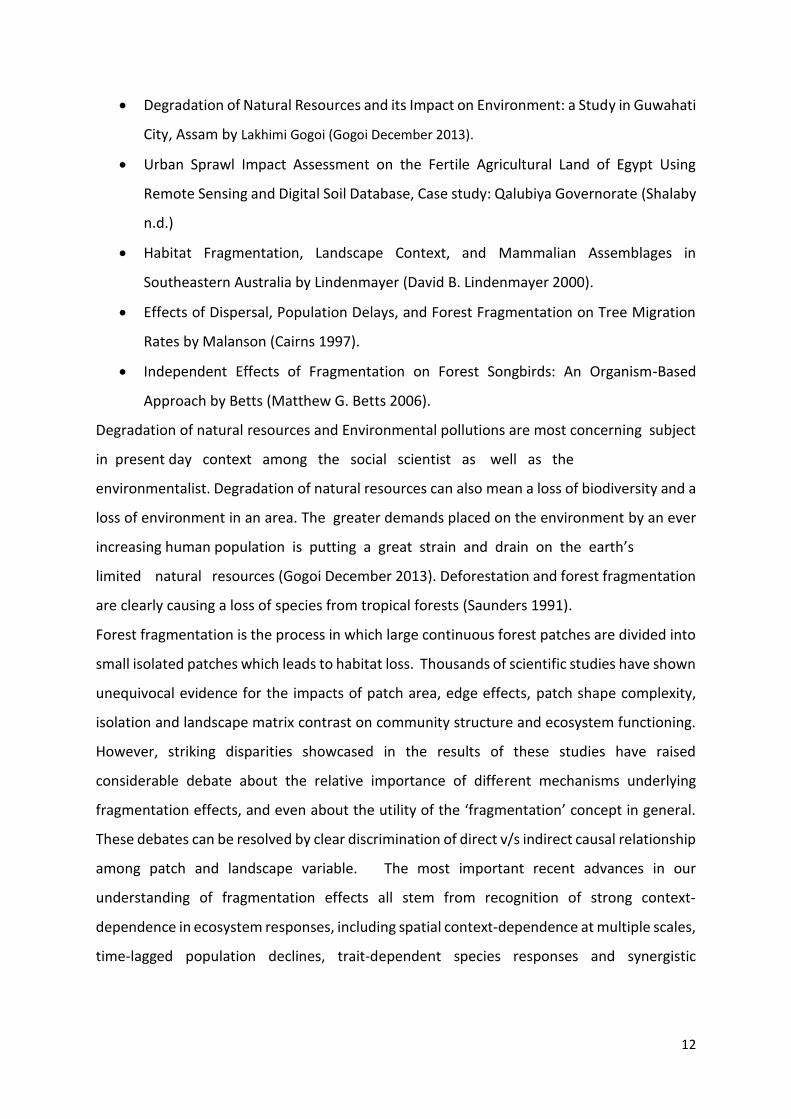
It should be noted that the concept of forest fragmentation is different from parcelization
which means “changes in ownership patterns whereby large forested tracts are divided into
smaller parcels” (Yale Forest Forum n.d.). Though parcelization does not always result in
fragmentation, but it increases the likelihood that the forest will become fragmented (i.e. the
construction of roads and structures).
Figure 1: Images showing intact forest, parcelizaton and fragmentation
Not parceled and not fragmented Parceled but not fragmented Parceled and fragmented
Based on the input land cover map, the forest fragmentation model categorizes the forest
pixels into one of four types: core forest, perforated forest, edge forest and patch forest.
Forested areas were classified into 4 main categories of increasing disturbance—core,
perforated, edge and patch—based on a key metric called edge width (CLEAR 2006).
15
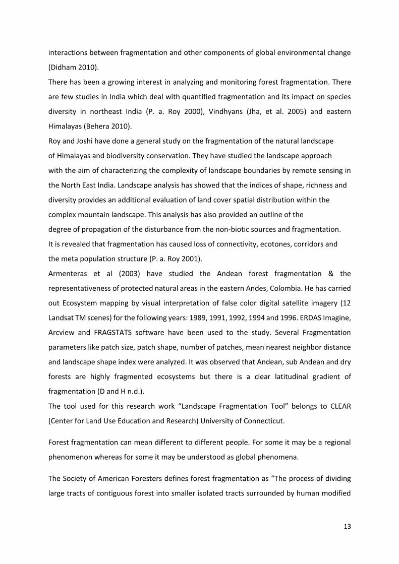
Figure 2: Core Forest
Core forest - Forest pixels that are far from the forest/non-forest boundary. These are
forested areas surrounded by more forested pixels.
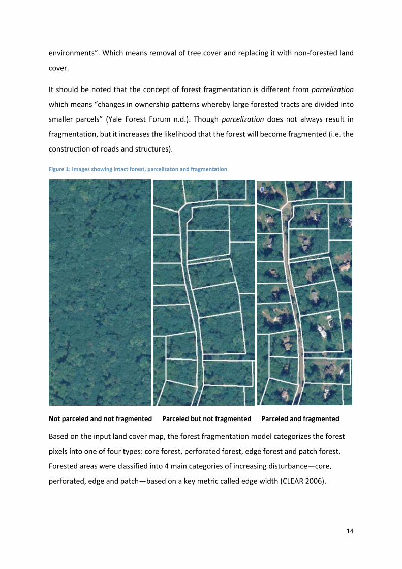
Figure 3: Perforated Forest
Perforated Forest - Forest pixels that define the boundary between core forest and
relatively small clearings (perforations) within the forested landscape.
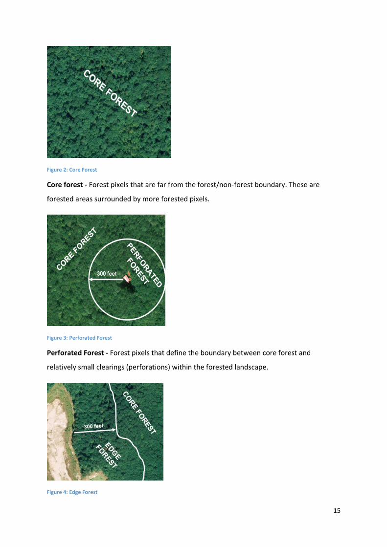
Figure 4: Edge Forest
16
Edge Forest - Forest pixels that define the boundary between core forest and large non-
forested land cover features.
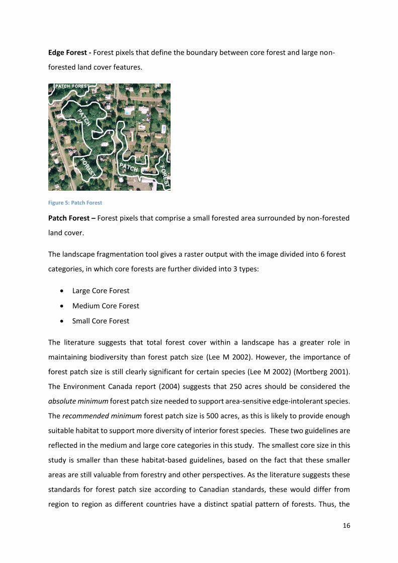
Figure 5: Patch Forest
Patch Forest – Forest pixels that comprise a small forested area surrounded by non-forested
land cover.
The landscape fragmentation tool gives a raster output with the image divided into 6 forest
categories, in which core forests are further divided into 3 types:
Large Core Forest
Medium Core Forest
Small Core Forest
The literature suggests that total forest cover within a landscape has a greater role in
maintaining biodiversity than forest patch size (Lee M 2002). However, the importance of
forest patch size is still clearly significant for certain species (Lee M 2002) (Mortberg 2001).
The Environment Canada report (2004) suggests that 250 acres should be considered the
absolute minimum forest patch size needed to support area-sensitive edge-intolerant species.
The recommended minimum forest patch size is 500 acres, as this is likely to provide enough
suitable habitat to support more diversity of interior forest species. These two guidelines are
reflected in the medium and large core categories in this study. The smallest core size in this
study is smaller than these habitat-based guidelines, based on the fact that these smaller
areas are still valuable from forestry and other perspectives. As the literature suggests these
standards for forest patch size according to Canadian standards, these would differ from
region to region as different countries have a distinct spatial pattern of forests. Thus, the
17
spatial parameters are taken as the default values as defined in the landscape fragmentation
tool guidelines.
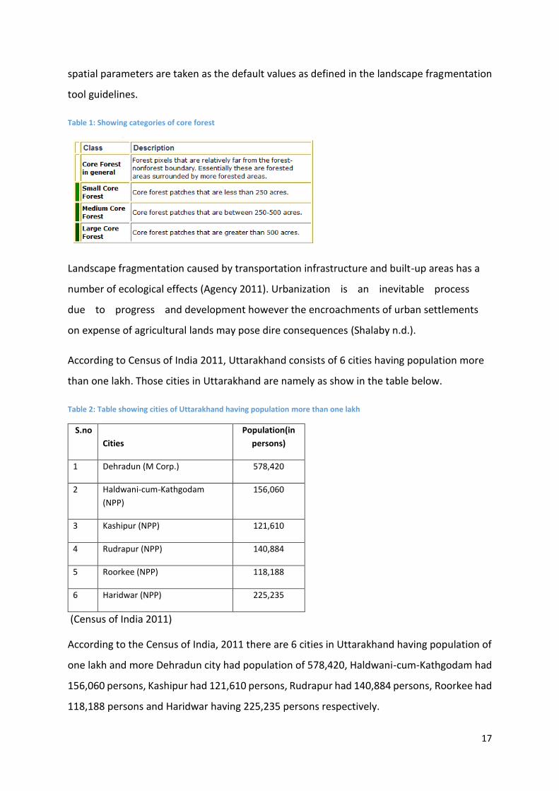
Table 1: Showing categories of core forest
Landscape fragmentation caused by transportation infrastructure and built-up areas has a
number of ecological effects (Agency 2011). Urbanization is an inevitable process
due to progress and development however the encroachments of urban settlements
on expense of agricultural lands may pose dire consequences (Shalaby n.d.).
According to Census of India 2011, Uttarakhand consists of 6 cities having population more
than one lakh. Those cities in Uttarakhand are namely as show in the table below.
Table 2: Table showing cities of Uttarakhand having population more than one lakh
S.no
Cities
Population(in
persons)
1 Dehradun (M Corp.) 578,420
2 Haldwani-cum-Kathgodam
(NPP)
156,060
3 Kashipur (NPP) 121,610
4 Rudrapur (NPP) 140,884
5 Roorkee (NPP) 118,188
6 Haridwar (NPP) 225,235
(Census of India 2011)
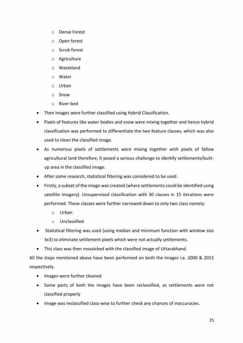
According to the Census of India, 2011 there are 6 cities in Uttarakhand having population of
one lakh and more Dehradun city had population of 578,420, Haldwani-cum-Kathgodam had
156,060 persons, Kashipur had 121,610 persons, Rudrapur had 140,884 persons, Roorkee had
118,188 persons and Haridwar having 225,235 persons respectively.
18
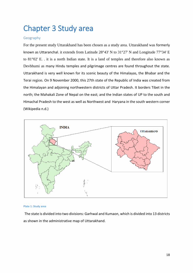
Chapter 3 Study area Geography
For the present study Uttarakhand has been chosen as a study area. Uttarakhand was formerly
known as Uttaranchal. it extends from Latitude 28°43' N to 31°27' N and Longitude 77°34' E
to 81°02' E. . it is a north Indian state. It is a land of temples and therefore also known as
Devbhumi as many Hindu temples and pilgrimage centres are found throughout the state.
Uttarakhand is very well known for its scenic beauty of the Himalayas, the Bhabar and the
Terai region. On 9 November 2000, this 27th state of the Republic of India was created from
the Himalayan and adjoining northwestern districts of Uttar Pradesh. It borders Tibet in the
north; the Mahakali Zone of Nepal on the east; and the Indian states of UP to the south and
Himachal Pradesh to the west as well as Northwest and Haryana in the south western corner
(Wikipedia n.d.)
Plate 1: Study area
The state is divided into two divisions: Garhwal and Kumaon, which is divided into 13 districts
as shown in the administrative map of Uttarakhand.
19
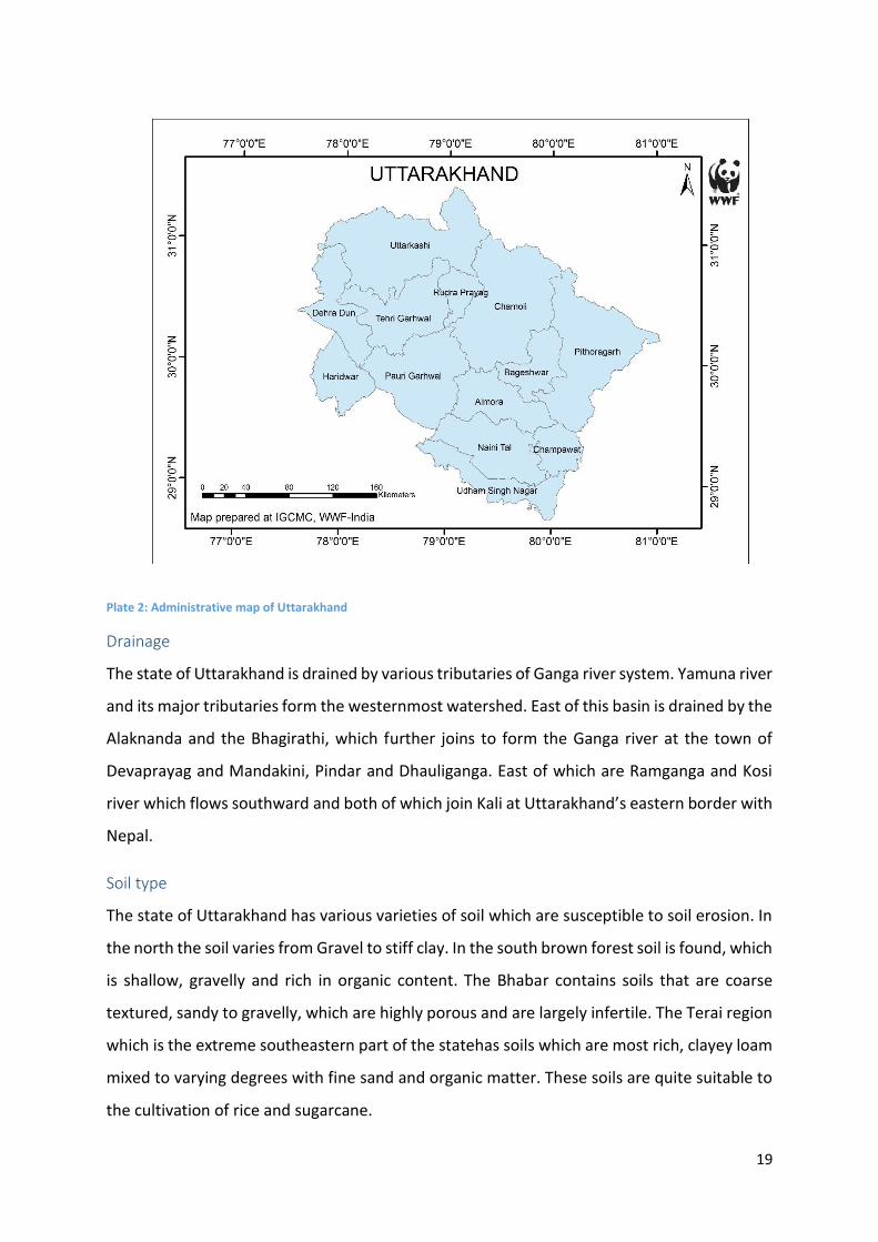
Plate 2: Administrative map of Uttarakhand
Drainage
The state of Uttarakhand is drained by various tributaries of Ganga river system. Yamuna river
and its major tributaries form the westernmost watershed. East of this basin is drained by the
Alaknanda and the Bhagirathi, which further joins to form the Ganga river at the town of
Devaprayag and Mandakini, Pindar and Dhauliganga. East of which are Ramganga and Kosi
river which flows southward and both of which join Kali at Uttarakhand’s eastern border with
Nepal.
Soil type
The state of Uttarakhand has various varieties of soil which are susceptible to soil erosion. In
the north the soil varies from Gravel to stiff clay. In the south brown forest soil is found, which
is shallow, gravelly and rich in organic content. The Bhabar contains soils that are coarse
textured, sandy to gravelly, which are highly porous and are largely infertile. The Terai region
which is the extreme southeastern part of the statehas soils which are most rich, clayey loam
mixed to varying degrees with fine sand and organic matter. These soils are quite suitable to
the cultivation of rice and sugarcane.
20
Climatic conditions
Summer
Plain regions of Uttarakhand have similar climate as other surrounding plain regions of
different states. The maximum temperature can cross 40°C and can be considerable humid.
Warm temperate conditions are present in the middle Himalayan valleys with temperature
around 25°C. Whereas in the higher areas of middle Himalayas the temperature is around
15°C to 18°C. This season extends from April to June.
Winter
The climate of Uttarakhand during winters can be really chilly with times when temperature
can go below 5°C. The winters in middle Himalayan valleys are very cold and in the higher
areas the temperature may fall below the freezing point. The Himalayan peaks remain snow
covered throughout the year and many places receive regular snowfall. Throughout the state
the temperature remains sub-zero to 15°C. This season lasts from November to February.
Monsoon
Monsoon season differs from 15°C to 25°C at most places which lasts from July to September.
The state receives 90% of its annual rainfall in this season.
National parks and Sanctuaries
The state has 12 national parks and wildlife sanctuaries. Some of them are: Corbett national
park, rajaji national park, nanda devi national park, gangotri national park etc. they cover
about 13.8% of the total area of the state.
21
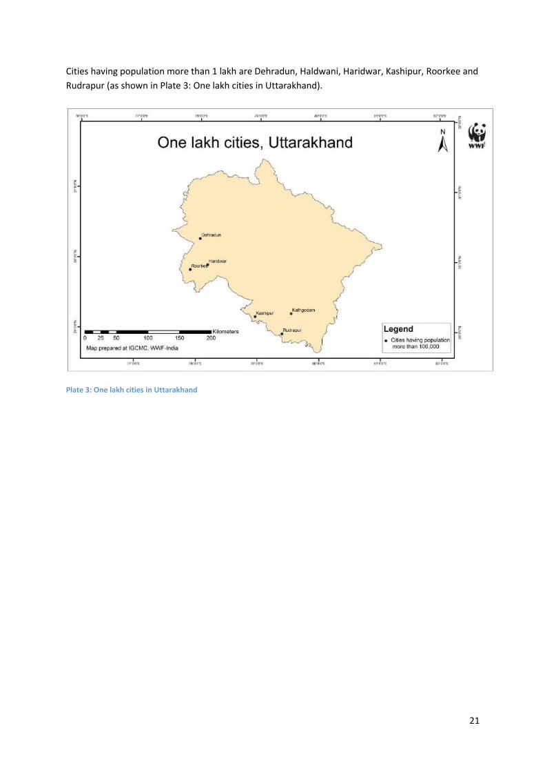
Cities having population more than 1 lakh are Dehradun, Haldwani, Haridwar, Kashipur, Roorkee and
Rudrapur (as shown in Plate 3: One lakh cities in Uttarakhand).
Plate 3: One lakh cities in Uttarakhand
22
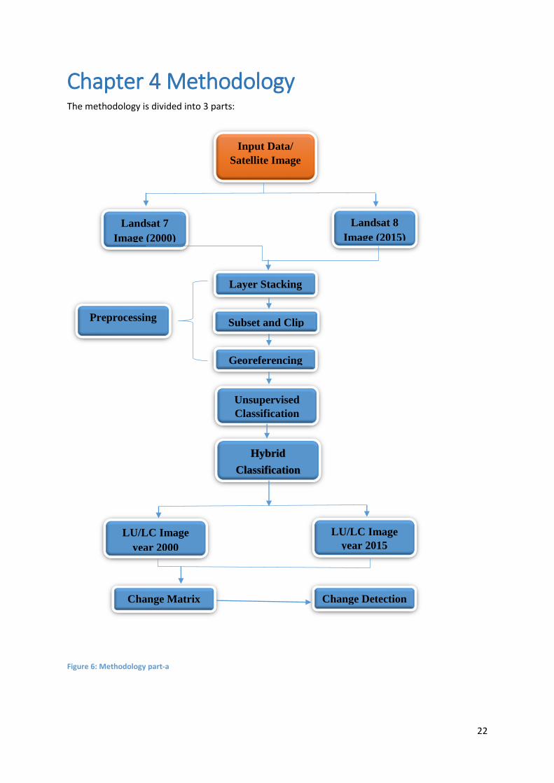
Chapter 4 Methodology The methodology is divided into 3 parts:
Figure 6: Methodology part-a
Input Data/
Satellite Image
Landsat 7
Image (2000)
Landsat 8
Image (2015)
Layer Stacking
Subset and Clip
Georeferencing
Unsupervised
Classification
LU/LC Image
year 2000
LU/LC Image
year 2015
Preprocessing
Change Matrix Change Detection
Hybrid
Classification
23
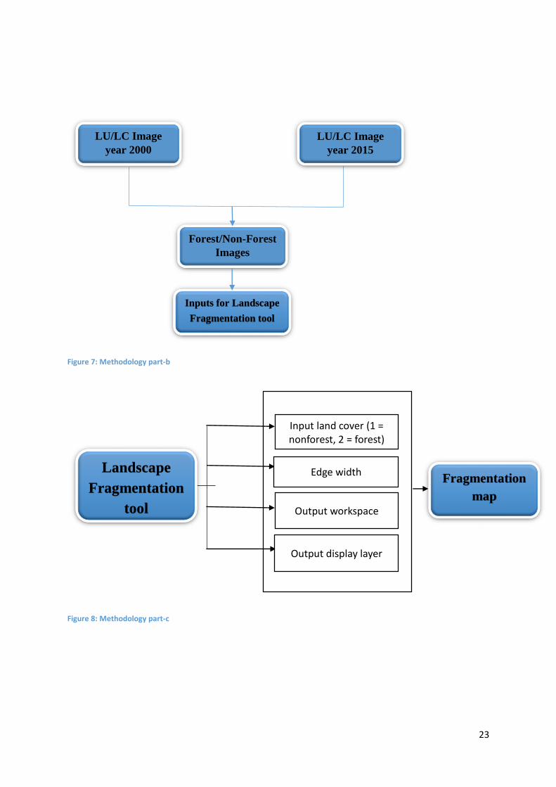
Figure 7: Methodology part-b
Figure 8: Methodology part-c
Inputs for Landscape
Fragmentation tool
Forest/Non-Forest
Images
LU/LC Image
year 2000
LU/LC Image
year 2015
Input land cover (1 = nonforest, 2 = forest)
Edge width
Output workspace
Output display layer
Landscape
Fragmentation
tool
Fragmentation
map
24
Material and methods used
Landsat 8 imagery
ERDAS IMAGINE 2011
ArcMap 10.1
Method
Literature and several research papers on applications of remote sensing and GIS were
carefully reviewed before selecting the topic. After several discussions with external
supervisor, the topic was selected. As the study is a spatio-temporal Landsat 8 and 7 data.
had to downloaded. Landsat 8 for the year 2015 and Landsat 7 for the year 2000. In total 6
tiles were required to cover whole of Uttarakhand. The images for whole of Uttarakhand were
classified for both year 2000 and 2015 respectively.
Firstly the year 2000 was taken up.
o For the acquired tiles, the bands (1, 2, 3, and 4) were stacked together for each
tile.
o Then all the multi-spectral tiles were mosaicked using the mosaic tool in
ERDAS.
o Several colour correction techniques like Colour Balancing, Histogram
Matching were performed on while mosaicking to correct any colour
differences in the mosaicked image.
o Overlap function was set to feathering to get seamless image as seamlines
were quite visible in the mosaicked image.
o Then shapefile for Uttarakhand was acquired.
o The mosaicked image was then clipped as per the shapefile of Uttarakhand.
Then the year 2015 was taken up and the same steps as above were performed for
2015 tiles to get a mosaicked, color corrected and clipped Uttarakhand image for the
year 2015.
After obtaining mosaicked, color corrected and clipped Uttarakhand image for both
years 2000, 2015 respectively.
Unsupervised classification with 85 classes and 25 iterations were performed.
The resulted 85 classes were further narrowed down to 9 classes namely:
25
o Dense Forest
o Open forest
o Scrub forest
o Agriculture
o Wasteland
o Water
o Urban
o Snow
o River-bed
Then images were further classified using Hybrid Classification.
Pixels of features like water bodies and snow were mixing together and hence hybrid
classification was performed to differentiate the two feature classes, which was also
used to clean the classified image.
As numerous pixels of settlements were mixing together with pixels of fallow
agricultural land therefore, it posed a serious challenge to identify settlements/built-
up area in the classified image.
After some research, statistical filtering was considered to be used.
Firstly, a subset of the image was created (where settlements could be identified using
satellite imagery). Unsupervised classification with 30 classes in 15 iterations were
performed. These classes were further narrowed down to only two class namely:
o Urban
o Unclassified
Statistical filtering was used (using median and minimum function with window size
3x3) to eliminate settlement pixels which were not actually settlements.
This class was then mosaicked with the classified image of Uttarakhand.
All the steps mentioned above have been performed on both the images i.e. 2000 & 2015
respectively.
Images were further cleaned
Some parts of both the images have been reclassified, as settlements were not
classified properly
Image was reclassified class-wise to further check any chances of inaccuracies.
26
Literature and figures were reviewed on million cities of Uttarakhand
Landsat 8 imageries were acquired for the study area. Then various bands of each image were
stacked together to make multispectral imagery. Then all the tiles were mosaicked together.
Shapefile of Uttarakhand was acquired and then the mosaicked image was clipped according
to that. Then the output image was classified. Unsupervised classification was performed with
85 classes and 25 iterations. After the image was classified using unsupervised classification
then forest classes (Dense, Open, Scrub forests) were considered and pure pixel classification
was performed for Urban, River, Agriculture, Wasteland, Snow and riverbed class.
Unsupervised classification was run for each of these and then all the pixels belonging to pure
pixel of one class was recoded as ‘1’ and the rest were recoded as ‘0’.
Forest fragmentation analysis was performed using landscape fragmentation tool in
ArcMap 10.1.
o Edge width was set to 300m.
Literature has also been reviewed about work previously been done in Uttarakhand
about forest fragmentation and natural resource degradation.
Million Cities are also being studied for urban-sprawl analysis.
Urban sprawls analysis was done for cities of Uttarakhand having population more
than 1 lakh.
Urban sprawl maps were prepared for the following cities:
Table 3: Table showing cities with population more than one lakh
Changes were analysis from classified LULC maps.
27
There has been significant changes in the land cover categories in the time period of
15 years, in some categories one can analyse huge changes have taken place on the
contrary there has been very minute increase or decrease in some classes. In total
dense forest accounts for 36.82 % in 2000 which has decreased to 26.06% in 2015,
there has been 10.76% decrease in dense forest. There has been 4.28% increase in
open forest, while only 2.61 % increase in scrub forest category. There has been 5%
increase in agricultural land, 2.11% increase in wasteland, a drastic 3.36% decrease in
snow-cover also urban area has been increased by 0.46%.
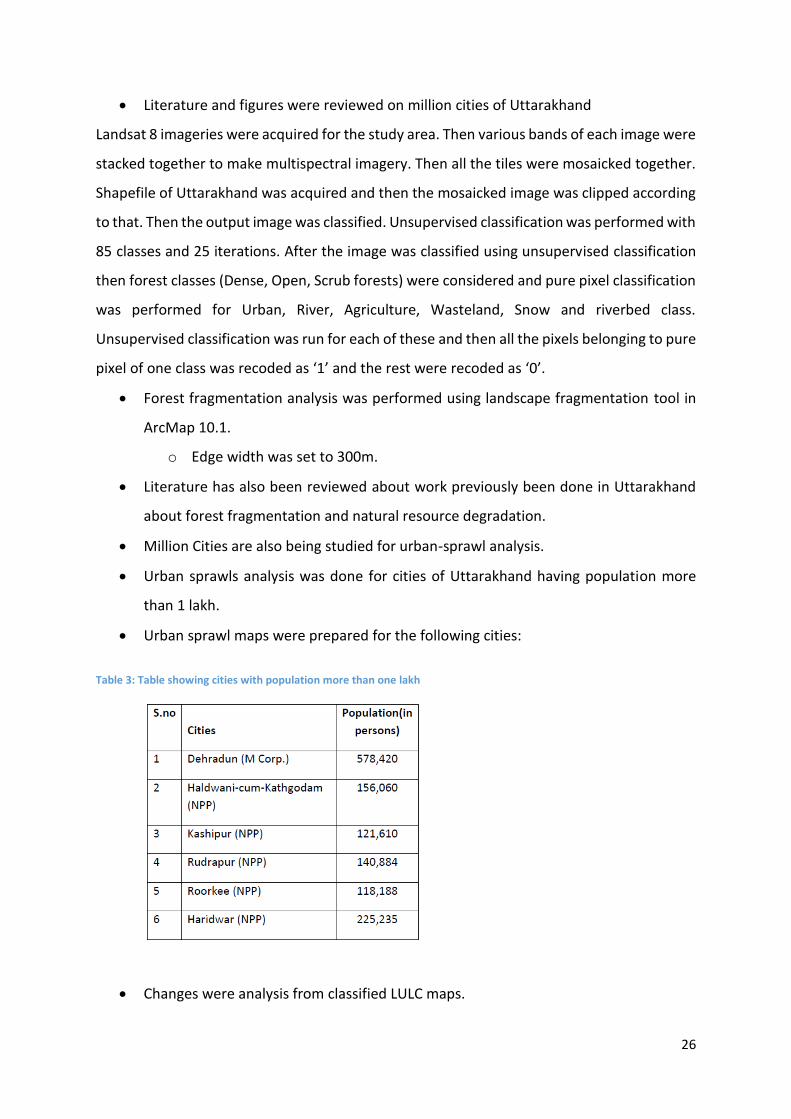
Plate 4: Dehradun city urban sprawl maps
Just like the above maps of Dehradun, maps have been prepared for all the 6 cities.
These maps have been prepared from the classified images. The urban pixels were recoded
as ‘1’ and pixels belonging to all the other classes were recoded as ‘0’. Also, change matrix
was prepared to see which pixels have been converted into which categories.
28
Chapter 5 Result and Discussion
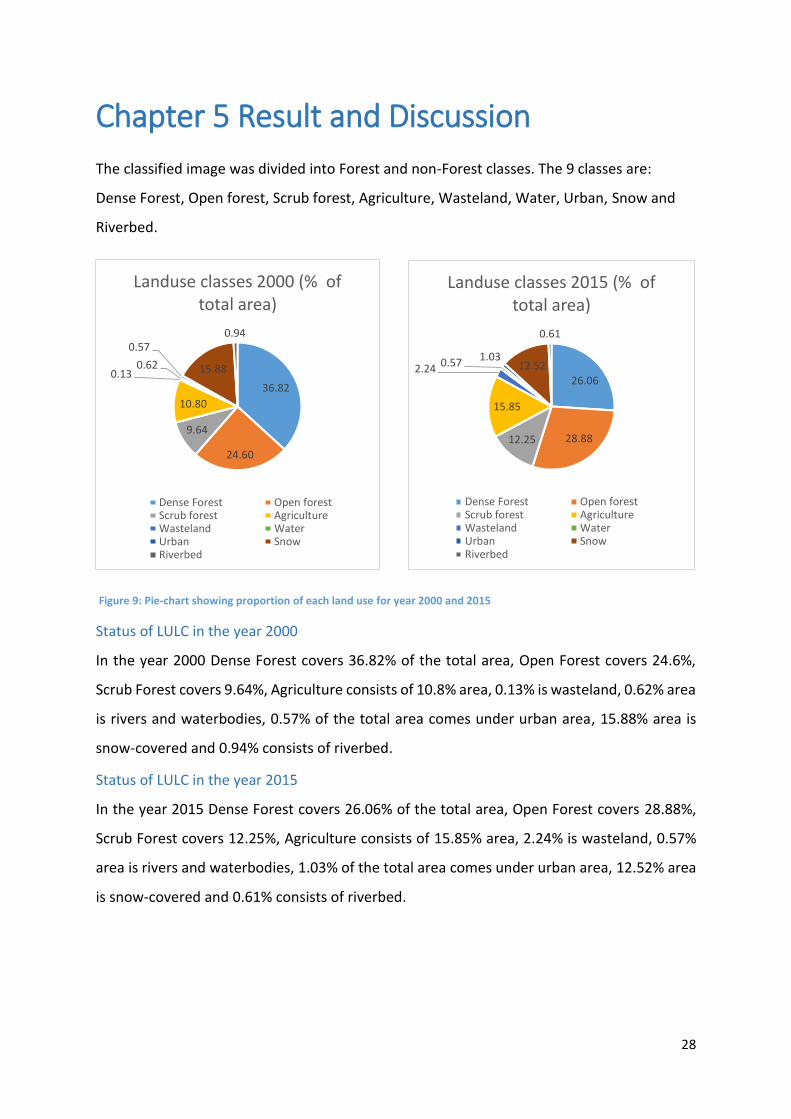
The classified image was divided into Forest and non-Forest classes. The 9 classes are:
Dense Forest, Open forest, Scrub forest, Agriculture, Wasteland, Water, Urban, Snow and
Riverbed.
Figure 9: Pie-chart showing proportion of each land use for year 2000 and 2015
Status of LULC in the year 2000
In the year 2000 Dense Forest covers 36.82% of the total area, Open Forest covers 24.6%,
Scrub Forest covers 9.64%, Agriculture consists of 10.8% area, 0.13% is wasteland, 0.62% area
is rivers and waterbodies, 0.57% of the total area comes under urban area, 15.88% area is
snow-covered and 0.94% consists of riverbed.
Status of LULC in the year 2015
In the year 2015 Dense Forest covers 26.06% of the total area, Open Forest covers 28.88%,
Scrub Forest covers 12.25%, Agriculture consists of 15.85% area, 2.24% is wasteland, 0.57%
area is rivers and waterbodies, 1.03% of the total area comes under urban area, 12.52% area
is snow-covered and 0.61% consists of riverbed.
36.82
24.60
9.64
10.80
0.130.62
0.57
15.88
0.94
Landuse classes 2000 (% of total area)
Dense Forest Open forestScrub forest AgricultureWasteland WaterUrban SnowRiverbed
26.06
28.8812.25
15.85
2.240.57 1.03
12.52
0.61
Landuse classes 2015 (% of total area)
Dense Forest Open forestScrub forest AgricultureWasteland WaterUrban SnowRiverbed
29
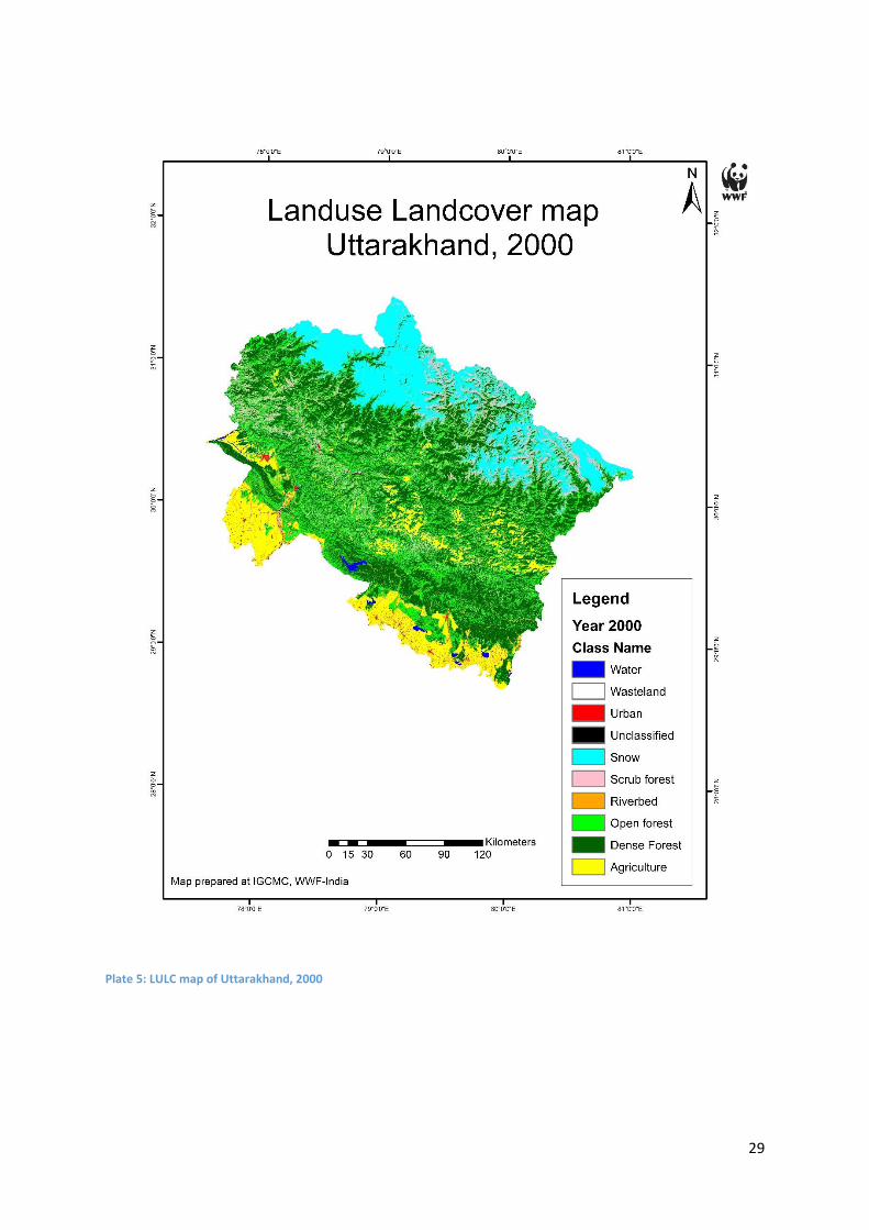
Plate 5: LULC map of Uttarakhand, 2000
30
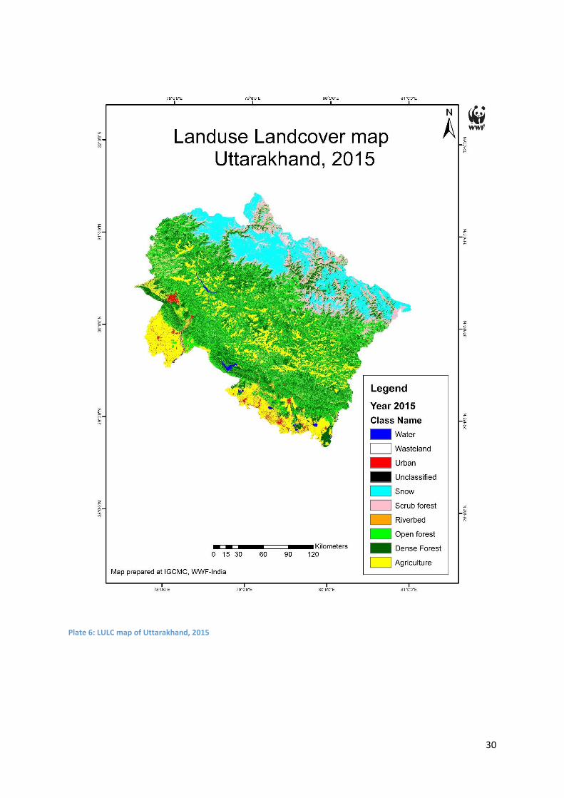
Plate 6: LULC map of Uttarakhand, 2015
31
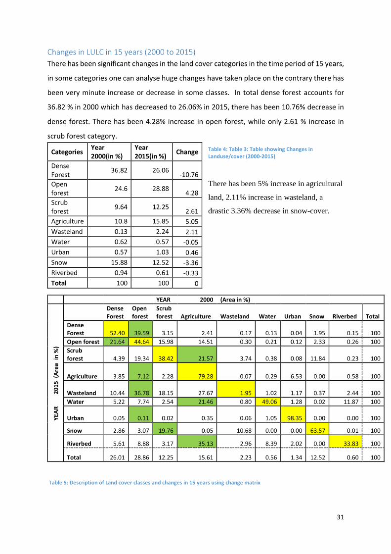
Changes in LULC in 15 years (2000 to 2015)
There has been significant changes in the land cover categories in the time period of 15 years,
in some categories one can analyse huge changes have taken place on the contrary there has
been very minute increase or decrease in some classes. In total dense forest accounts for
36.82 % in 2000 which has decreased to 26.06% in 2015, there has been 10.76% decrease in
dense forest. There has been 4.28% increase in open forest, while only 2.61 % increase in
scrub forest category.
Table 4: Table 3: Table showing Changes in Landuse/cover (2000-2015)
There has been 5% increase in agricultural
land, 2.11% increase in wasteland, a
drastic 3.36% decrease in snow-cover.
YEAR 2000 (Area in %)
Dense Forest
Open forest
Scrub forest Agriculture Wasteland Water Urban Snow Riverbed Total
Dense Forest 52.40 39.59 3.15 2.41 0.17 0.13 0.04 1.95 0.15 100
Open forest 21.64 44.64 15.98 14.51 0.30 0.21 0.12 2.33 0.26 100
in %
)
Scrub forest 4.39 19.34 38.42 21.57 3.74 0.38 0.08 11.84 0.23 100
(Are
a
Agriculture 3.85 7.12 2.28 79.28 0.07 0.29 6.53 0.00 0.58 100
20
15
Wasteland 10.44 36.78 18.15 27.67 1.95 1.02 1.17 0.37 2.44 100
Water 5.22 7.74 2.54 21.46 0.80 49.06 1.28 0.02 11.87 100
YEA
R
Urban 0.05 0.11 0.02 0.35 0.06 1.05 98.35 0.00 0.00 100
Snow 2.86 3.07 19.76 0.05 10.68 0.00 0.00 63.57 0.01 100
Riverbed 5.61 8.88 3.17 35.13 2.96 8.39 2.02 0.00 33.83 100
Total 26.01 28.86 12.25 15.61 2.23 0.56 1.34 12.52 0.60 100
Table 5: Description of Land cover classes and changes in 15 years using change matrix
Categories Year 2000(in %)
Year 2015(in %)
Change
Dense Forest
36.82 26.06 -10.76
Open forest
24.6 28.88 4.28
Scrub forest
9.64 12.25 2.61
Agriculture 10.8 15.85 5.05
Wasteland 0.13 2.24 2.11
Water 0.62 0.57 -0.05
Urban 0.57 1.03 0.46
Snow 15.88 12.52 -3.36
Riverbed 0.94 0.61 -0.33
Total 100 100 0
32
Also, change matrix was prepared to see which pixels have been converted into which
categories.
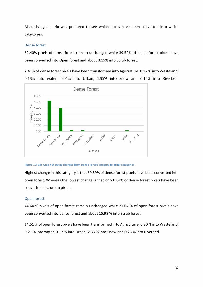
Dense forest
52.40% pixels of dense forest remain unchanged while 39.59% of dense forest pixels have
been converted into Open forest and about 3.15% into Scrub forest.
2.41% of dense forest pixels have been transformed into Agriculture. 0.17 % into Wasteland,
0.13% into water, 0.04% into Urban, 1.95% into Snow and 0.15% into Riverbed.
Figure 10: Bar-Graph showing changes from Dense Forest category to other categories
Highest change in this category is that 39.59% of dense forest pixels have been converted into
open forest. Whereas the lowest change is that only 0.04% of dense forest pixels have been
converted into urban pixels.
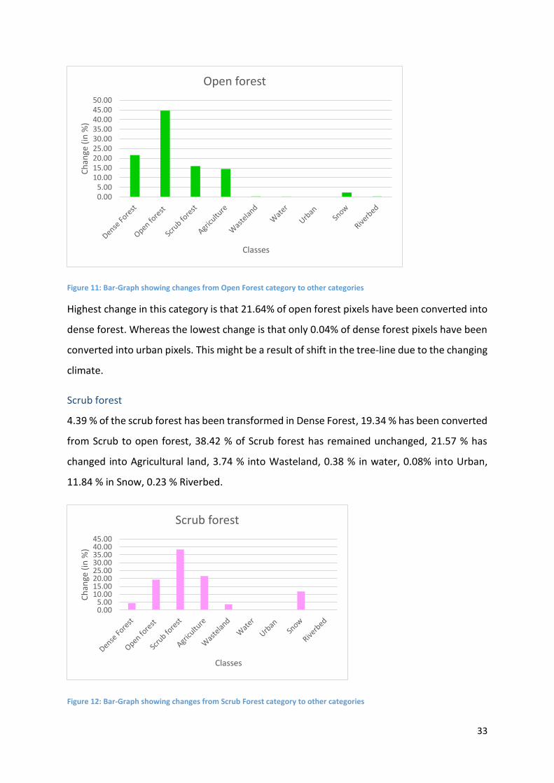
Open forest
44.64 % pixels of open forest remain unchanged while 21.64 % of open forest pixels have
been converted into dense forest and about 15.98 % into Scrub forest.
14.51 % of open forest pixels have been transformed into Agriculture, 0.30 % into Wasteland,
0.21 % into water, 0.12 % into Urban, 2.33 % into Snow and 0.26 % into Riverbed.
0.00
10.00
20.00
30.00
40.00
50.00
60.00
Ch
ange
(in
%)
Classes
Dense Forest
33
Figure 11: Bar-Graph showing changes from Open Forest category to other categories
Highest change in this category is that 21.64% of open forest pixels have been converted into
dense forest. Whereas the lowest change is that only 0.04% of dense forest pixels have been
converted into urban pixels. This might be a result of shift in the tree-line due to the changing
climate.
Scrub forest
4.39 % of the scrub forest has been transformed in Dense Forest, 19.34 % has been converted
from Scrub to open forest, 38.42 % of Scrub forest has remained unchanged, 21.57 % has
changed into Agricultural land, 3.74 % into Wasteland, 0.38 % in water, 0.08% into Urban,
11.84 % in Snow, 0.23 % Riverbed.
Figure 12: Bar-Graph showing changes from Scrub Forest category to other categories
0.005.00
10.0015.0020.0025.0030.0035.0040.0045.0050.00
Ch
ange
(in
%)
Classes
Open forest
0.005.00
10.0015.0020.0025.0030.0035.0040.0045.00
Ch
ange
(in
%)
Classes
Scrub forest
34
Highest change in this category is that 21.57 % of Scrub forest pixels have changed been
converted to Agriculture. Whereas the lowest change is that only 0.08 % of scrub forest has
been converted into urban area.
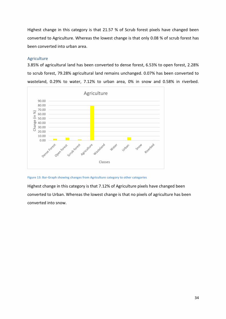
Agriculture
3.85% of agricultural land has been converted to dense forest, 6.53% to open forest, 2.28%
to scrub forest, 79.28% agricultural land remains unchanged. 0.07% has been converted to
wasteland, 0.29% to water, 7.12% to urban area, 0% in snow and 0.58% in riverbed.
Figure 13: Bar-Graph showing changes from Agriculture category to other categories
Highest change in this category is that 7.12% of Agriculture pixels have changed been
converted to Urban. Whereas the lowest change is that no pixels of agriculture has been
converted into snow.
0.00
10.00
20.00
30.00
40.00
50.00
60.00
70.00
80.00
90.00
Ch
ange
(in
%)
Classes
Agriculture
35
Wasteland
10.44% of wasteland has been converted into dense forest, 36.78% to open forest, 18.15%
has changed to scrub forest, 27.67% to agriculture, 1.95% of wasteland remain unchanged, 1.02% to
water, 1.17% to urban area, 0.37% to snow and 2.44% to riverbed.
Figure 14: Bar-Graph showing changes from Wasteland category to other categories
Highest change in this category is that 36.78% % of wasteland has changed been converted
to open forest. Whereas the lowest change is that 1.02% of wasteland has been converted
into snow.
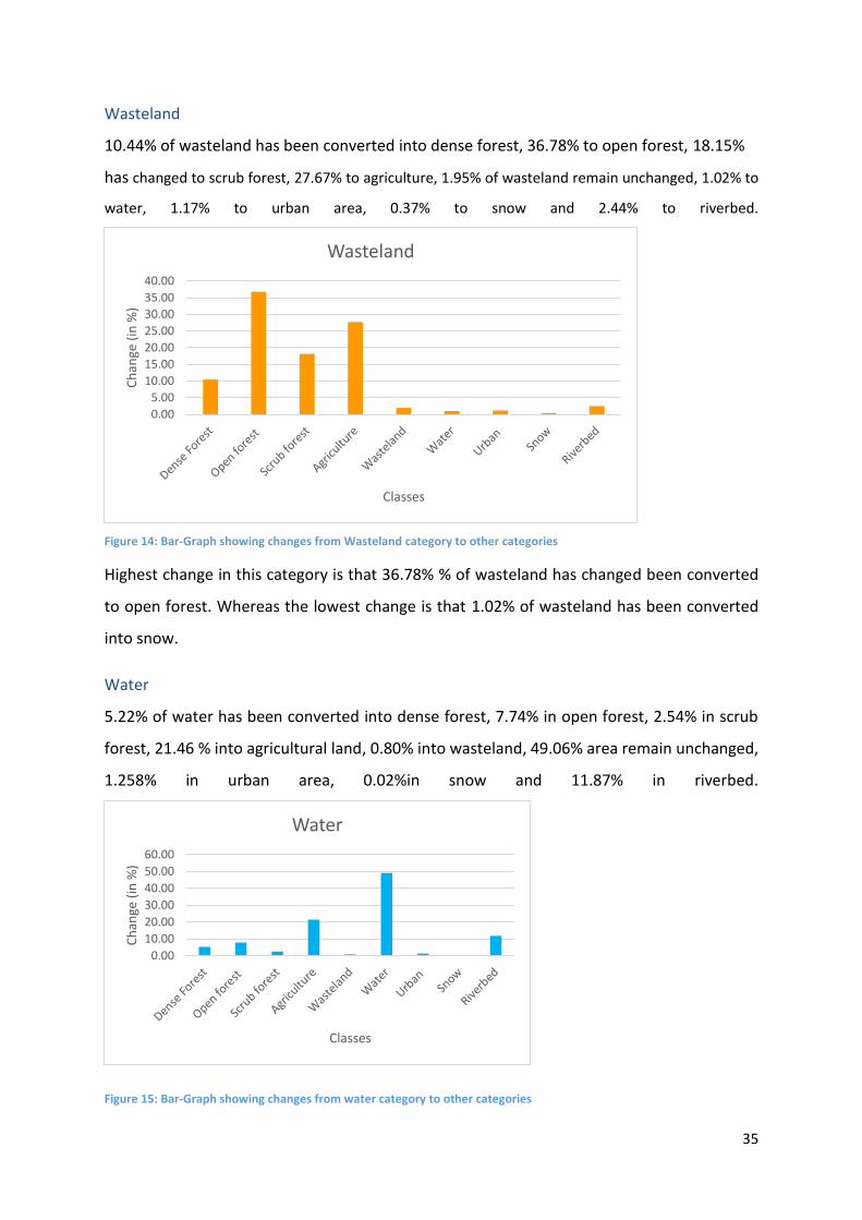
Water
5.22% of water has been converted into dense forest, 7.74% in open forest, 2.54% in scrub
forest, 21.46 % into agricultural land, 0.80% into wasteland, 49.06% area remain unchanged,
1.258% in urban area, 0.02%in snow and 11.87% in riverbed.
Figure 15: Bar-Graph showing changes from water category to other categories
0.00
5.00
10.00
15.00
20.00
25.00
30.00
35.00
40.00
Ch
ange
(in
%)
Classes
Wasteland
0.00
10.00
20.00
30.00
40.00
50.00
60.00
Ch
ange
(in
%)
Classes
Water
36
Highest change in this category is that 21.46% of water pixels have been converted into
agriculture pixels. Whereas the lowest change is that 0.02% of water pixels have been
changed into snow pixels.
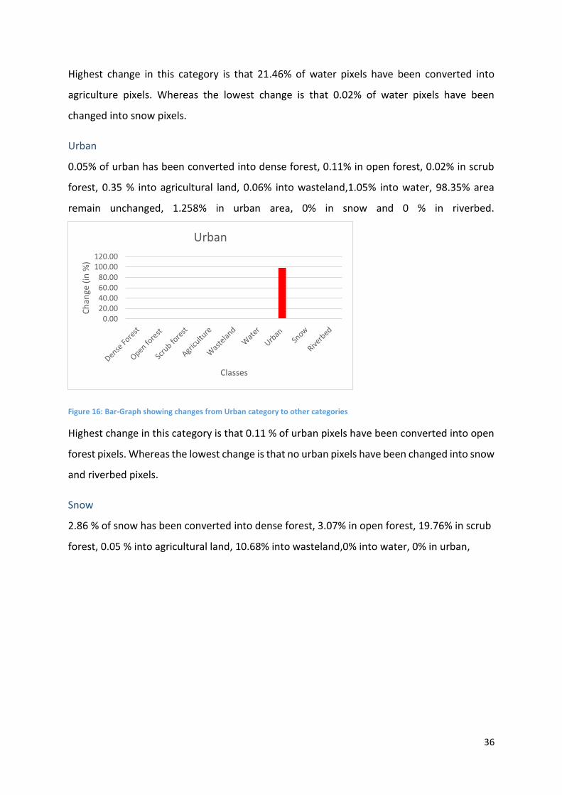
Urban
0.05% of urban has been converted into dense forest, 0.11% in open forest, 0.02% in scrub
forest, 0.35 % into agricultural land, 0.06% into wasteland,1.05% into water, 98.35% area
remain unchanged, 1.258% in urban area, 0% in snow and 0 % in riverbed.
Figure 16: Bar-Graph showing changes from Urban category to other categories
Highest change in this category is that 0.11 % of urban pixels have been converted into open
forest pixels. Whereas the lowest change is that no urban pixels have been changed into snow
and riverbed pixels.
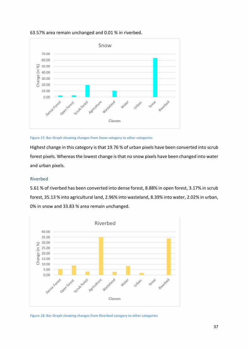
Snow
2.86 % of snow has been converted into dense forest, 3.07% in open forest, 19.76% in scrub
forest, 0.05 % into agricultural land, 10.68% into wasteland,0% into water, 0% in urban,
0.0020.0040.0060.0080.00
100.00120.00
Ch
ange
(in
%)
Classes
Urban
37
63.57% area remain unchanged and 0.01 % in riverbed.
Figure 17: Bar-Graph showing changes from Snow category to other categories
Highest change in this category is that 19.76 % of urban pixels have been converted into scrub
forest pixels. Whereas the lowest change is that no snow pixels have been changed into water
and urban pixels.
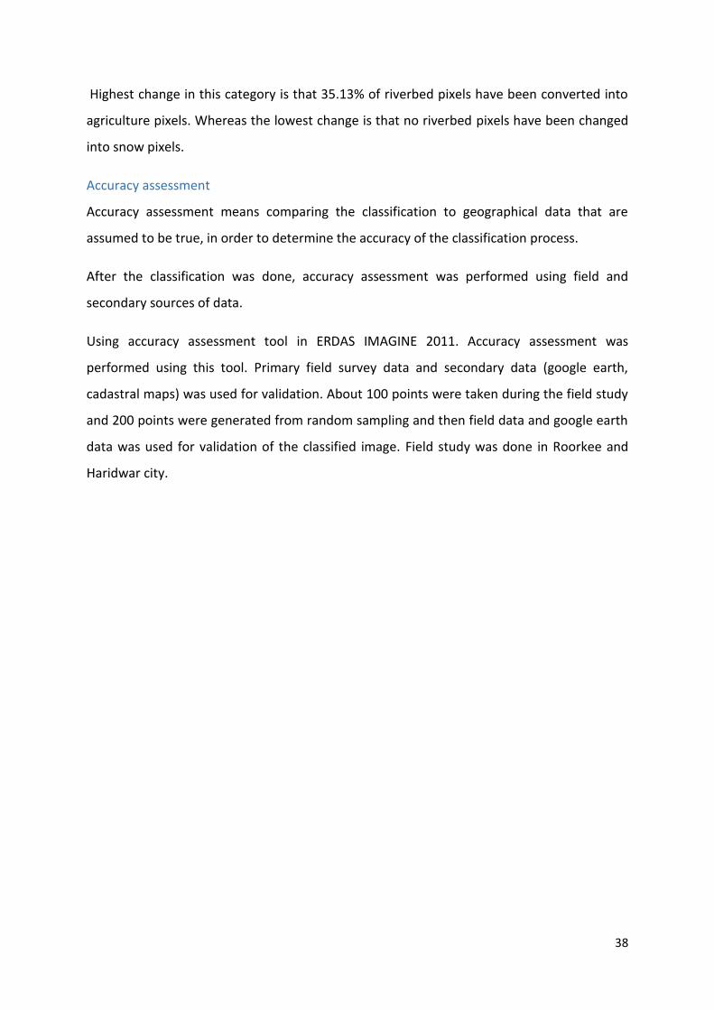
Riverbed
5.61 % of riverbed has been converted into dense forest, 8.88% in open forest, 3.17% in scrub
forest, 35.13 % into agricultural land, 2.96% into wasteland, 8.39% into water, 2.02% in urban,
0% in snow and 33.83 % area remain unchanged.
Figure 18: Bar-Graph showing changes from Riverbed category to other categories
0.00
10.00
20.00
30.00
40.00
50.00
60.00
70.00
Ch
ange
(in
%)
Classes
Snow
0.00
5.00
10.00
15.00
20.00
25.00
30.00
35.00
40.00
Ch
ange
(in
%)
Classes
Riverbed
38
Highest change in this category is that 35.13% of riverbed pixels have been converted into
agriculture pixels. Whereas the lowest change is that no riverbed pixels have been changed
into snow pixels.
Accuracy assessment
Accuracy assessment means comparing the classification to geographical data that are
assumed to be true, in order to determine the accuracy of the classification process.
After the classification was done, accuracy assessment was performed using field and
secondary sources of data.
Using accuracy assessment tool in ERDAS IMAGINE 2011. Accuracy assessment was
performed using this tool. Primary field survey data and secondary data (google earth,
cadastral maps) was used for validation. About 100 points were taken during the field study
and 200 points were generated from random sampling and then field data and google earth
data was used for validation of the classified image. Field study was done in Roorkee and
Haridwar city.
39
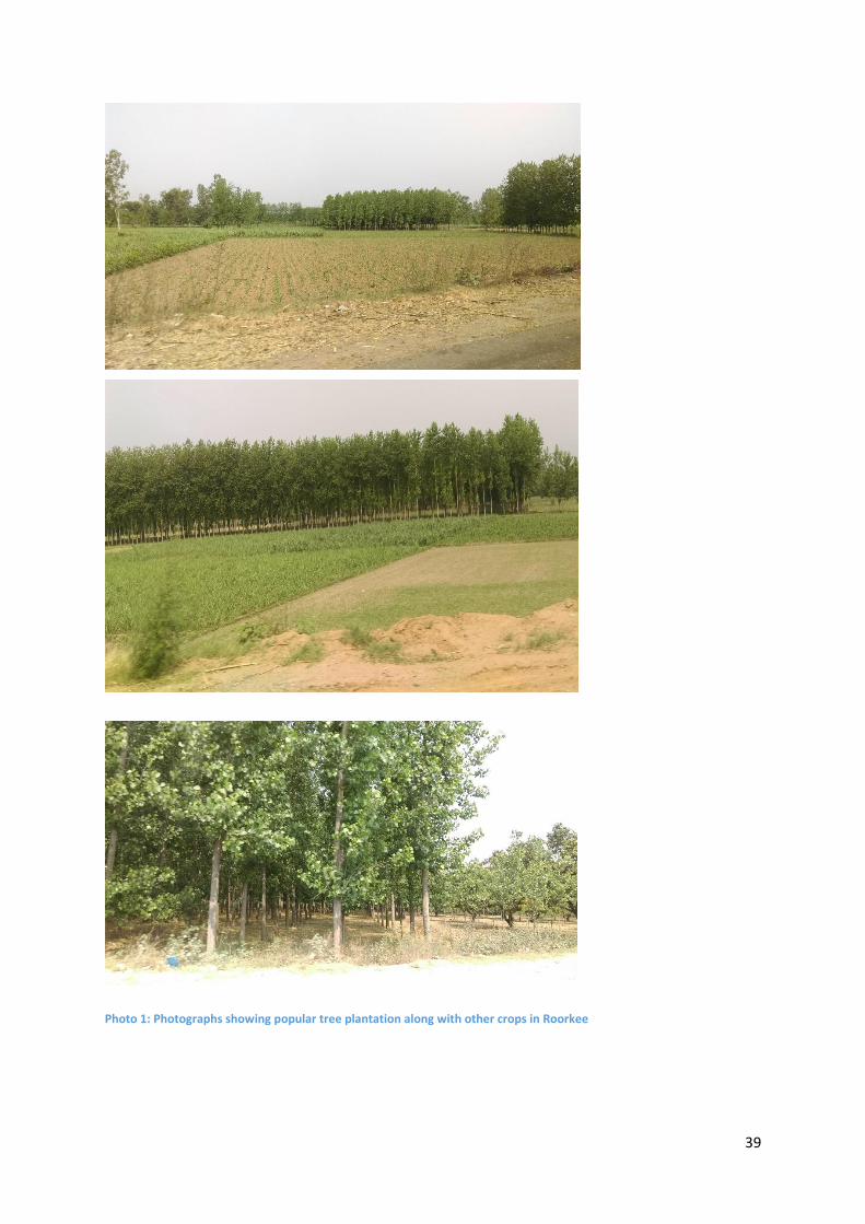
Photo 1: Photographs showing popular tree plantation along with other crops in Roorkee
40
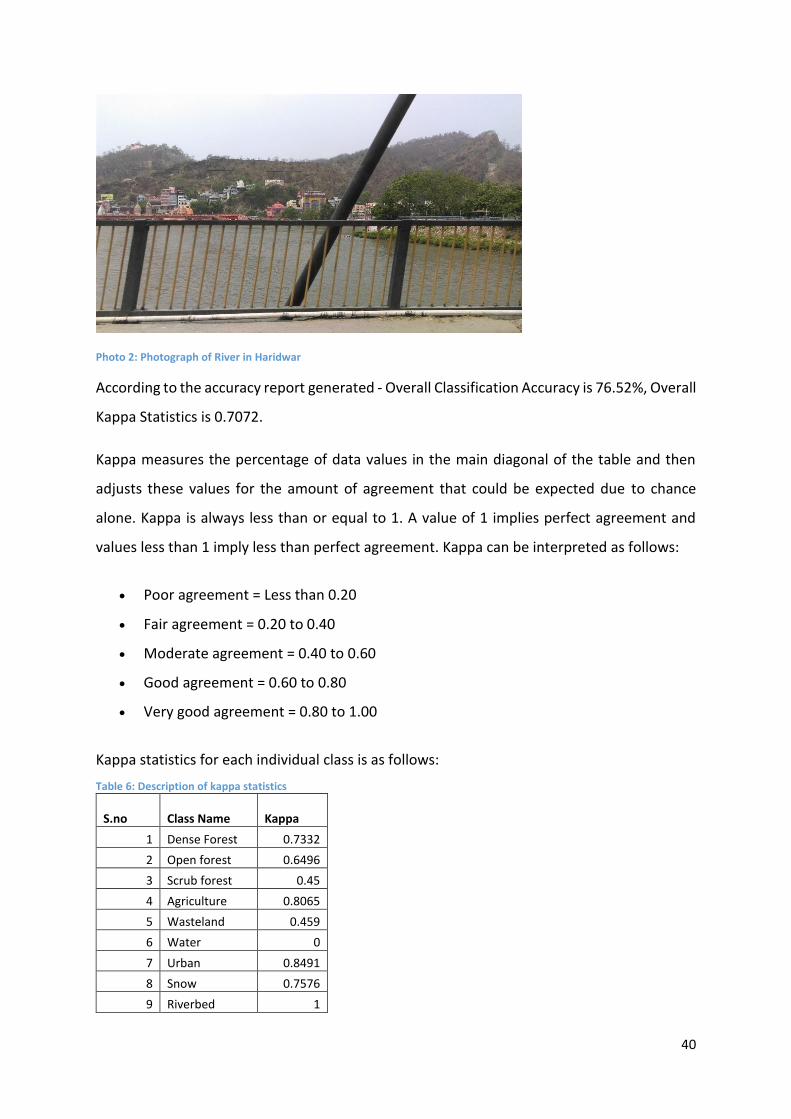
Photo 2: Photograph of River in Haridwar
According to the accuracy report generated - Overall Classification Accuracy is 76.52%, Overall
Kappa Statistics is 0.7072.
Kappa measures the percentage of data values in the main diagonal of the table and then
adjusts these values for the amount of agreement that could be expected due to chance
alone. Kappa is always less than or equal to 1. A value of 1 implies perfect agreement and
values less than 1 imply less than perfect agreement. Kappa can be interpreted as follows:
Poor agreement = Less than 0.20
Fair agreement = 0.20 to 0.40
Moderate agreement = 0.40 to 0.60
Good agreement = 0.60 to 0.80
Very good agreement = 0.80 to 1.00
Kappa statistics for each individual class is as follows:
Table 6: Description of kappa statistics
S.no Class Name Kappa
1 Dense Forest 0.7332
2 Open forest 0.6496
3 Scrub forest 0.45
4 Agriculture 0.8065
5 Wasteland 0.459
6 Water 0
7 Urban 0.8491
8 Snow 0.7576
9 Riverbed 1
41
As per the accuracy report generated kappa statistics for Dense forest is 0.7332 which means
there is 73% agreement between classified image and the geographical data for this class,
Open forest is 0.6496 which means there is 64 % agreement between classified image and
the geographical data for this class, Scrub forest is 0.45 which means there is 45 % agreement
between classified image and the geographical data for this class, Agriculture is 0.8065 which
means there is 80% agreement between classified image and the geographical data for this
class, Wasteland is 0.459 which means there is 45% agreement between classified image and
the geographical data for this class. Water is 0, it is so because there was no sample point
which was falling in this category neither in the random sample nor in the field study. The
Kappa statistics for Urban is 0.8491 which means there is 84% agreement between classified
image and the geographical data for this class, Snow is 0.7576 which means there is 75%
agreement between classified image and the geographical data for this class and for Riverbed
kappa statistics is 1 which means there is 100% agreement between classified image and the
geographical data for this class.
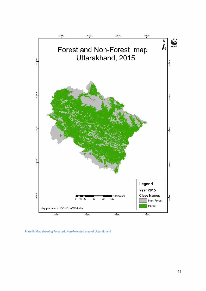
After classifying the images of Uttarakhand into various classes as shown above, it was then
reclassified into two classes:
1) Non-forest class
2) Forest class
Non-forest class is the class which includes Agriculture, Wasteland, Water, Urban, Snow and
Riverbed classes.
Forest class is the class which includes Dense Forest, Open forest and Scrub forest classes.
42
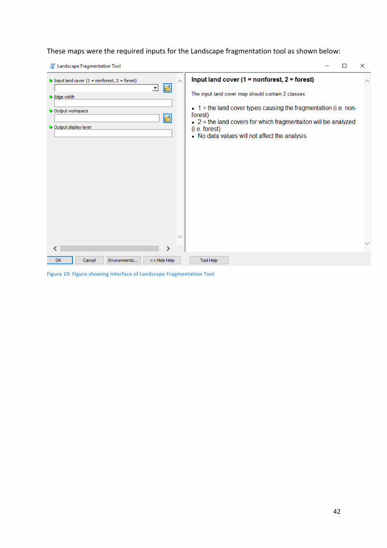
These maps were the required inputs for the Landscape fragmentation tool as shown below:
Figure 19: Figure showing Interface of Landscape Fragmentation Tool

43
Plate 7: Map showing Forested, Non-Forested area of Uttarakhand
44
Plate 8: Map showing Forested, Non-Forested area of Uttarakhand
45
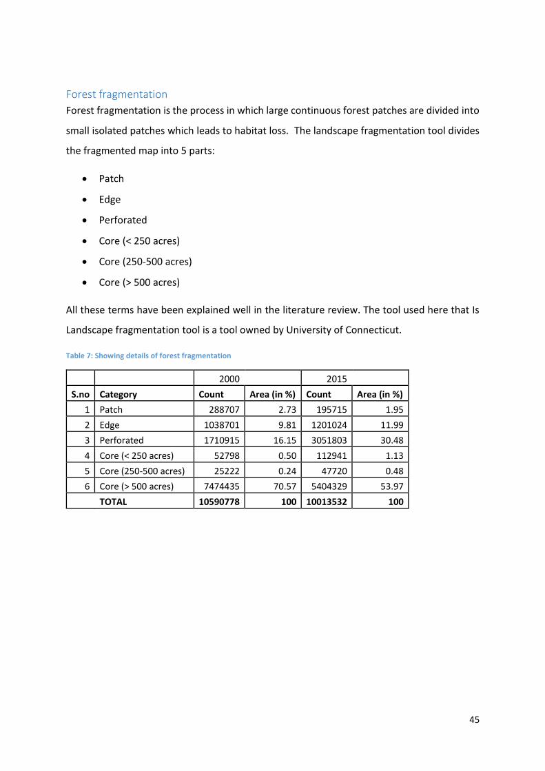
Forest fragmentation
Forest fragmentation is the process in which large continuous forest patches are divided into
small isolated patches which leads to habitat loss. The landscape fragmentation tool divides
the fragmented map into 5 parts:
Patch
Edge
Perforated
Core (< 250 acres)
Core (250-500 acres)
Core (> 500 acres)
All these terms have been explained well in the literature review. The tool used here that Is
Landscape fragmentation tool is a tool owned by University of Connecticut.
Table 7: Showing details of forest fragmentation
2000 2015
S.no Category Count Area (in %) Count Area (in %)
1 Patch 288707 2.73 195715 1.95
2 Edge 1038701 9.81 1201024 11.99
3 Perforated 1710915 16.15 3051803 30.48
4 Core (< 250 acres) 52798 0.50 112941 1.13
5 Core (250-500 acres) 25222 0.24 47720 0.48
6 Core (> 500 acres) 7474435 70.57 5404329 53.97
TOTAL 10590778 100 10013532 100
46
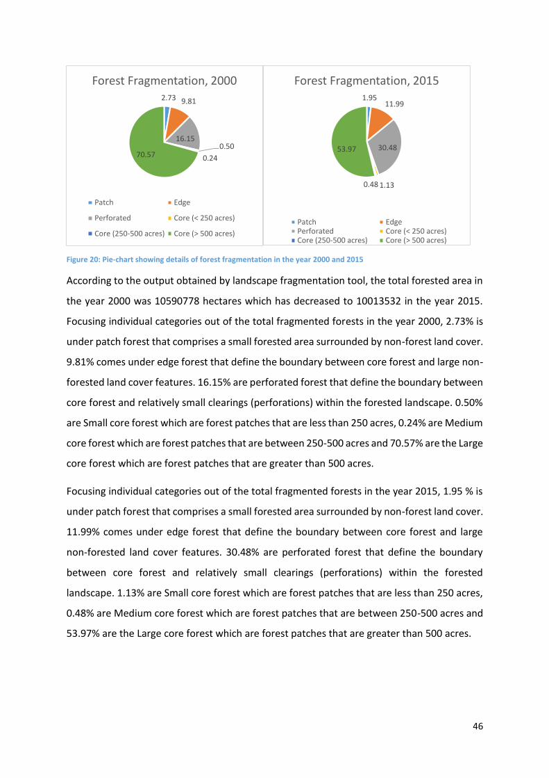
Figure 20: Pie-chart showing details of forest fragmentation in the year 2000 and 2015
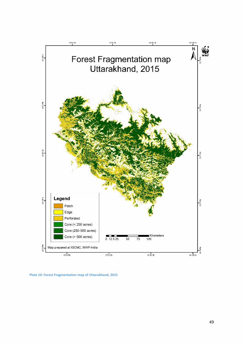
According to the output obtained by landscape fragmentation tool, the total forested area in
the year 2000 was 10590778 hectares which has decreased to 10013532 in the year 2015.
Focusing individual categories out of the total fragmented forests in the year 2000, 2.73% is
under patch forest that comprises a small forested area surrounded by non-forest land cover.
9.81% comes under edge forest that define the boundary between core forest and large non-
forested land cover features. 16.15% are perforated forest that define the boundary between
core forest and relatively small clearings (perforations) within the forested landscape. 0.50%
are Small core forest which are forest patches that are less than 250 acres, 0.24% are Medium
core forest which are forest patches that are between 250-500 acres and 70.57% are the Large
core forest which are forest patches that are greater than 500 acres.
Focusing individual categories out of the total fragmented forests in the year 2015, 1.95 % is
under patch forest that comprises a small forested area surrounded by non-forest land cover.
11.99% comes under edge forest that define the boundary between core forest and large
non-forested land cover features. 30.48% are perforated forest that define the boundary
between core forest and relatively small clearings (perforations) within the forested
landscape. 1.13% are Small core forest which are forest patches that are less than 250 acres,
0.48% are Medium core forest which are forest patches that are between 250-500 acres and
53.97% are the Large core forest which are forest patches that are greater than 500 acres.
2.73 9.81
16.150.50
0.2470.57
Forest Fragmentation, 2000
Patch Edge
Perforated Core (< 250 acres)
Core (250-500 acres) Core (> 500 acres)
1.9511.99
30.48
1.130.48
53.97
Forest Fragmentation, 2015
Patch EdgePerforated Core (< 250 acres)Core (250-500 acres) Core (> 500 acres)
47
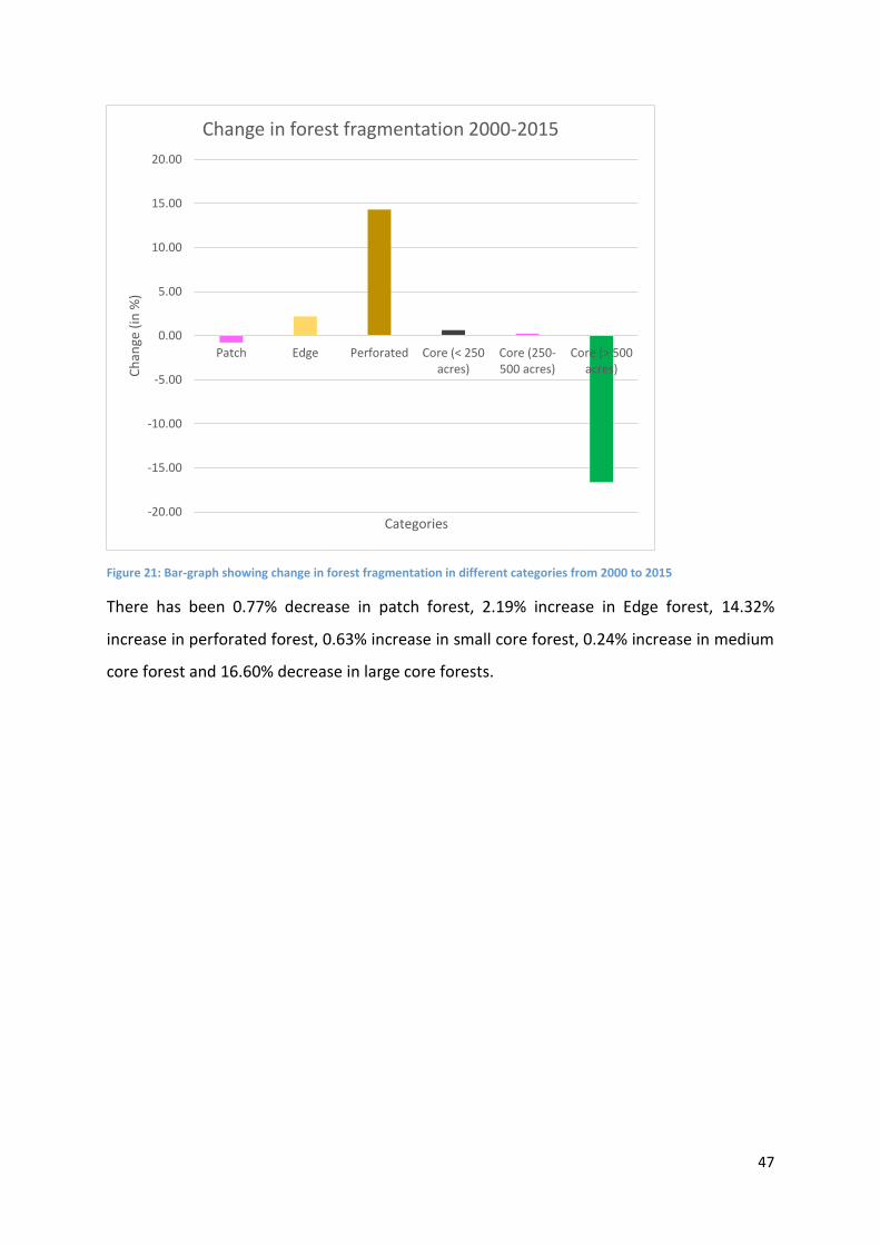
Figure 21: Bar-graph showing change in forest fragmentation in different categories from 2000 to 2015
There has been 0.77% decrease in patch forest, 2.19% increase in Edge forest, 14.32%
increase in perforated forest, 0.63% increase in small core forest, 0.24% increase in medium
core forest and 16.60% decrease in large core forests.
-20.00
-15.00
-10.00
-5.00
0.00
5.00
10.00
15.00
20.00
Patch Edge Perforated Core (< 250acres)
Core (250-500 acres)
Core (> 500acres)C
han
ge (
in %
)
Categories
Change in forest fragmentation 2000-2015
48
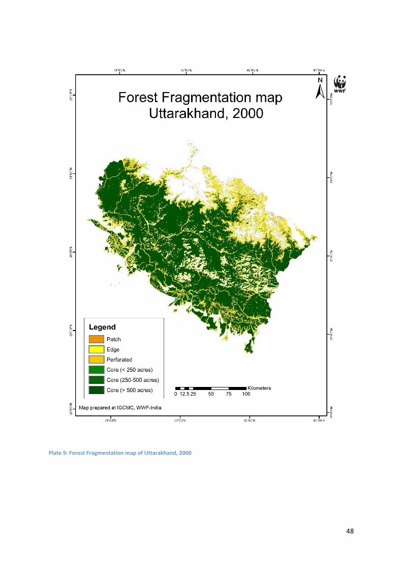
Plate 9: Forest Fragmentation map of Uttarakhand, 2000
49
Plate 10: Forest Fragmentation map of Uttarakhand, 2015
50
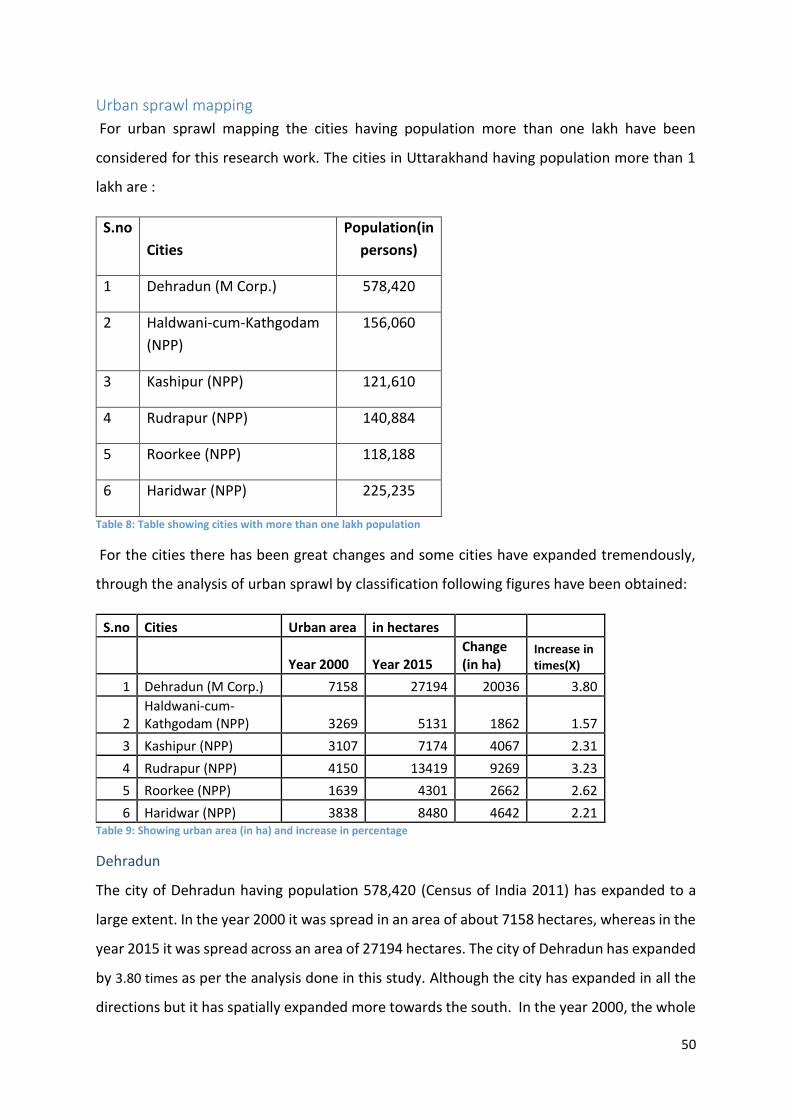
Urban sprawl mapping
For urban sprawl mapping the cities having population more than one lakh have been
considered for this research work. The cities in Uttarakhand having population more than 1
lakh are :
S.no
Cities
Population(in
persons)
1 Dehradun (M Corp.) 578,420
2 Haldwani-cum-Kathgodam
(NPP)
156,060
3 Kashipur (NPP) 121,610
4 Rudrapur (NPP) 140,884
5 Roorkee (NPP) 118,188
6 Haridwar (NPP) 225,235
Table 8: Table showing cities with more than one lakh population
For the cities there has been great changes and some cities have expanded tremendously,
through the analysis of urban sprawl by classification following figures have been obtained:
S.no Cities Urban area in hectares
Year 2000 Year 2015 Change (in ha)
Increase in times(X)
1 Dehradun (M Corp.) 7158 27194 20036 3.80
2 Haldwani-cum-Kathgodam (NPP) 3269 5131 1862 1.57
3 Kashipur (NPP) 3107 7174 4067 2.31
4 Rudrapur (NPP) 4150 13419 9269 3.23
5 Roorkee (NPP) 1639 4301 2662 2.62
6 Haridwar (NPP) 3838 8480 4642 2.21 Table 9: Showing urban area (in ha) and increase in percentage
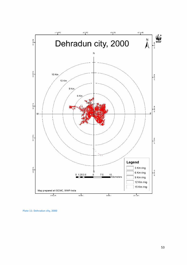
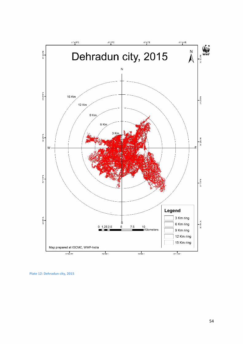
Dehradun
The city of Dehradun having population 578,420 (Census of India 2011) has expanded to a
large extent. In the year 2000 it was spread in an area of about 7158 hectares, whereas in the
year 2015 it was spread across an area of 27194 hectares. The city of Dehradun has expanded
by 3.80 times as per the analysis done in this study. Although the city has expanded in all the
directions but it has spatially expanded more towards the south. In the year 2000, the whole
51
city of Uttarakhand could fit in the 6 Km ring (as shown in the map) but in the year 2015, an
additional ring upto 15 Km was required to spatially fit the city.
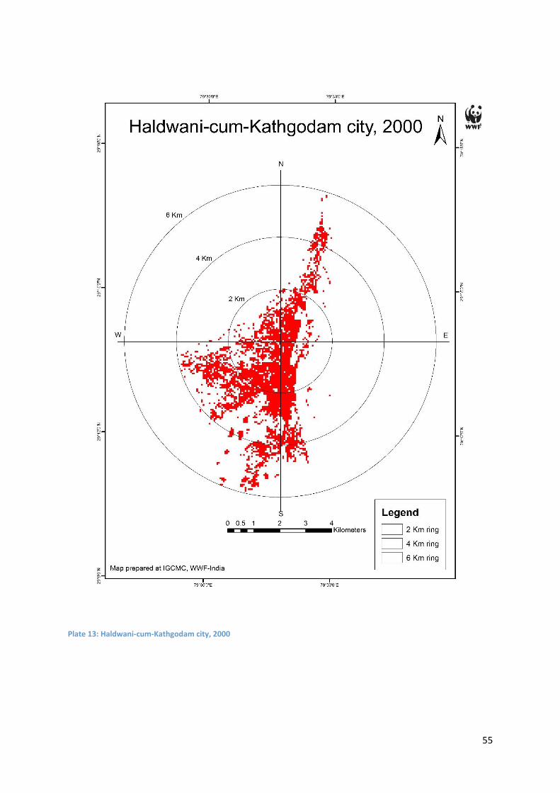
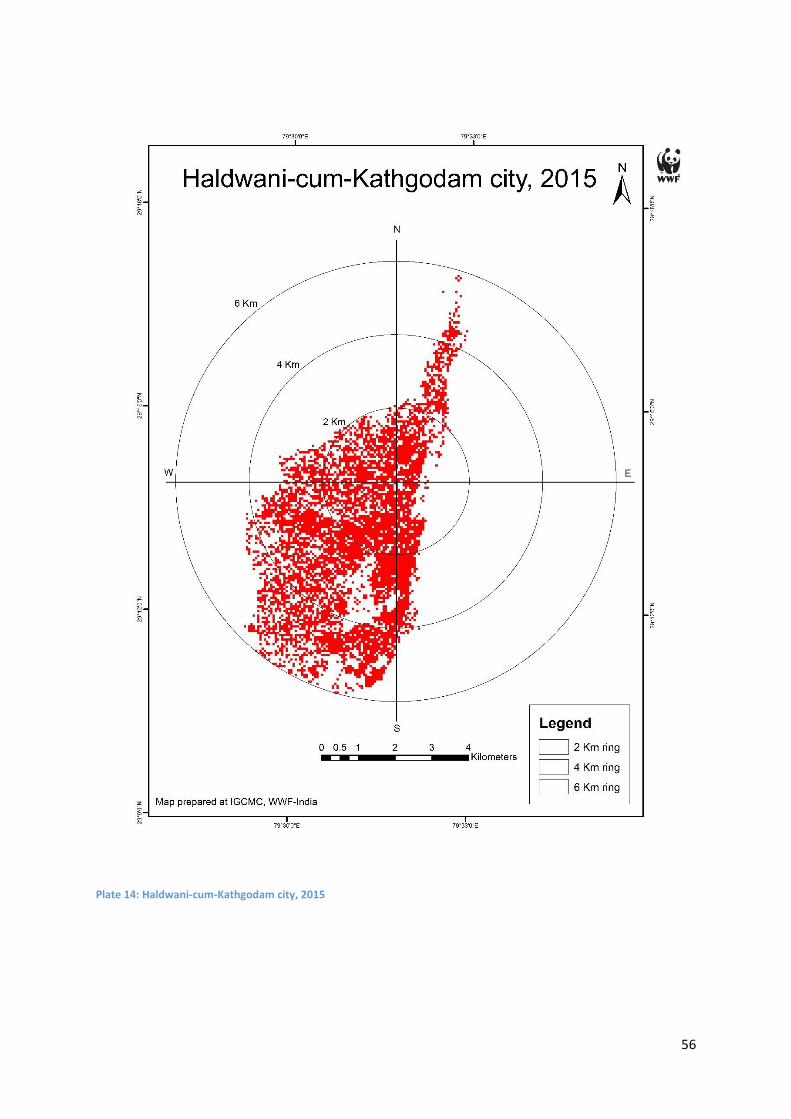
Haldwani-cum-Kathgodam
The city of Haldwani-cum-Kathgodam having population 156,060 (Census of India 2011) has
expanded spatially. In the year 2000 it was spread in an area of about 3269 hectares, whereas
in the year 2015 it was spread across an area of 5131 hectares. The city of Haldwani-cum-
Kathgodam has expanded by 1.57 times as per the analysis done in this study. Although the
city has expanded in all the directions but it has spatially expanded more in the south-west
direction. In the year 2000, the whole city of Uttarakhand could fit in the 6 Km ring (as shown
in the map) and even in the year 2015 city fits well in the 6 Km ring which means it has
expanded more in terms of density and not much spatially.
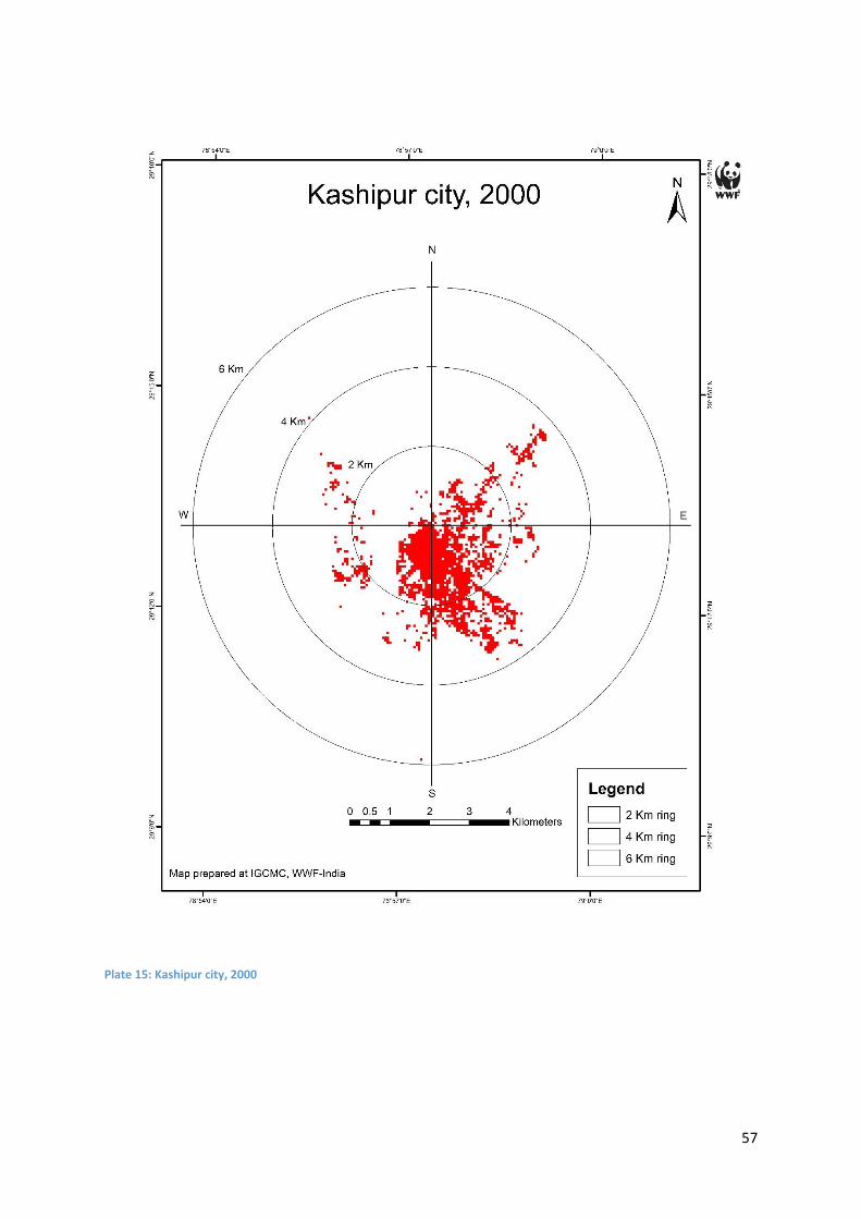
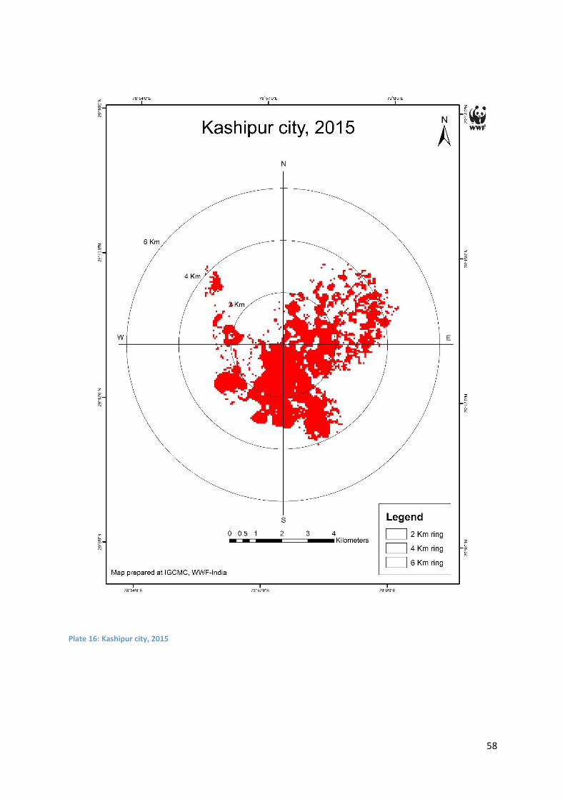
Kashipur
The city of Kashipur having population 121,610 (Census of India 2011) has expanded spatially.
In the year 2000 it was spread in an area of about 3,107 hectares, whereas in the year 2015
it was spread across an area of 7,174 hectares. The city of Kashipur has expanded by 2.31
times as per the analysis done in this study. Although the city has expanded in all the
directions but it has spatially expanded more in the south and north-west direction. In the
year 2000, the whole city of Uttarakhand could fit in the 4 Km ring (as shown in the map) but
in the year 2015 city does not fits in the 4 Km ring and therefore the 6Km ring had to be added
in the year 2015. This means it has expanded more in terms of both in terms of density and
also spatially.
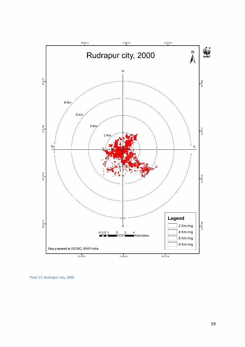
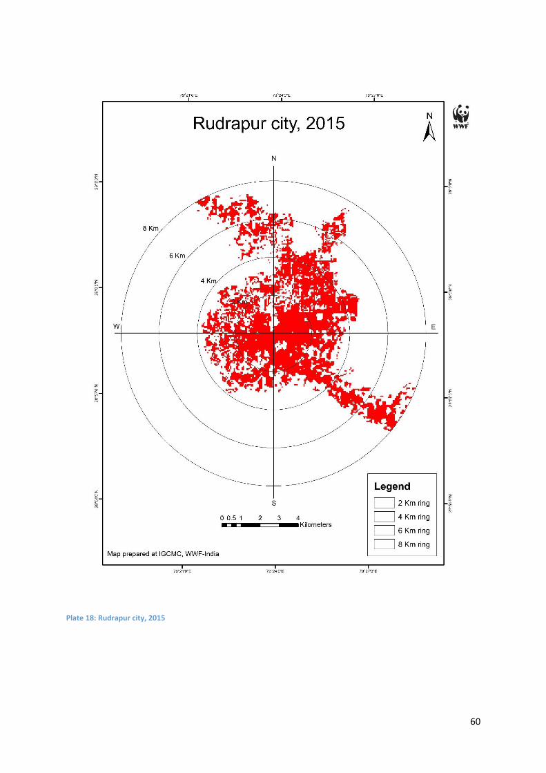
Rudrapur
The city of Rudrapur having population 140,884 (Census of India 2011) has expanded spatially.
In the year 2000 it was spread in an area of about 4150 hectares, whereas in the year 2015 it
was spread across an area of 13,419 hectares. The city of Rudrapur has expanded by 3.23
times as per the analysis done in this study. The city has expanded in all the directions. In the
year 2000, the whole city of Rudrapur could fit in the 4 Km ring (as shown in the map) but in
the year 2015 city does not fits in the 4 Km ring and therefore the 8 Km ring had to be added
in the year 2015. This means it has expanded more in terms of both in terms of density and
also spatially.
52
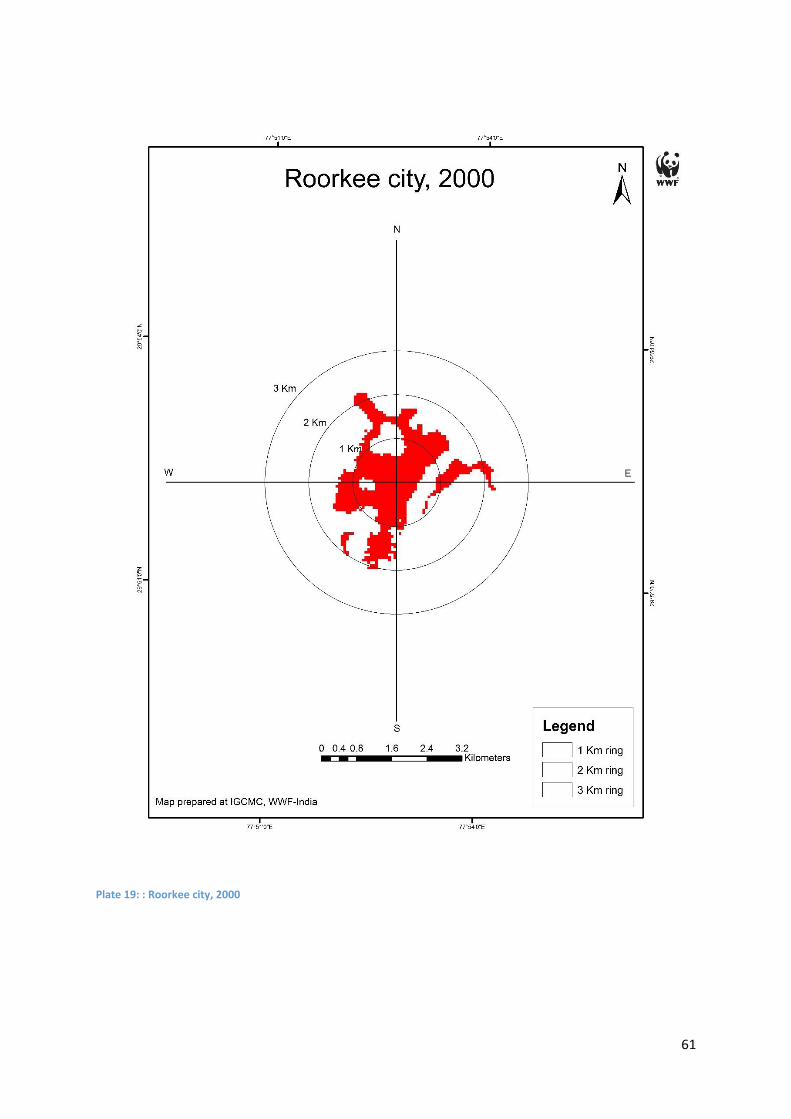
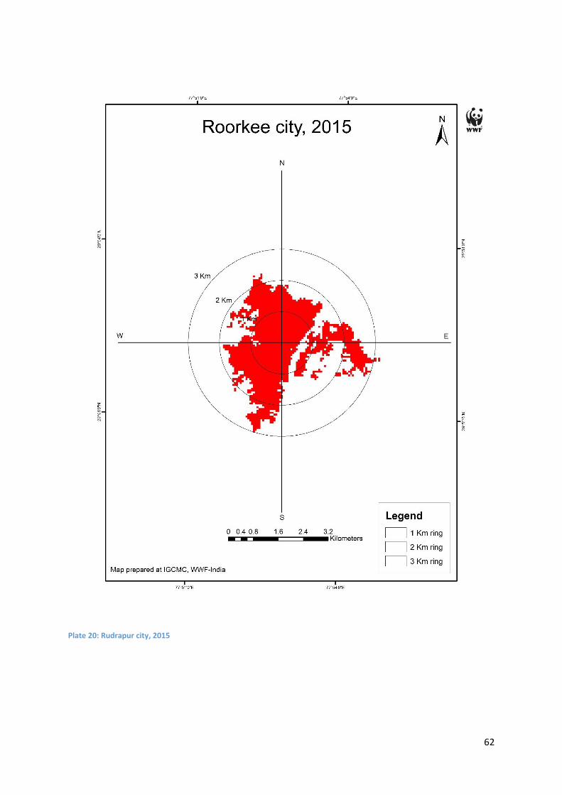
Roorkee
The city of Roorkee having population 118,188 (Census of India 2011) has expanded spatially.
In the year 2000 it was spread in an area of about 1639 hectares, whereas in the year 2015 it
was spread across an area of 4301 hectares. The city of Roorkee has expanded by 2.62 times
as per the analysis done in this study. The city has expanded in all the directions but has
become more dense in the centre. In the year 2000, the whole city of Roorkee could fit in the
2 Km ring (as shown in the map) but in the year 2015 city does not fits in the 2 Km ring and
therefore the 3 Km ring had to be added in the year 2015. This means it has expanded more
in terms of both in terms of density and also spatially.
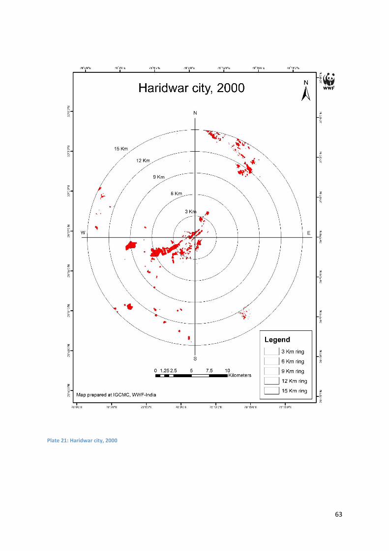
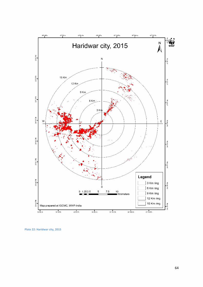
Haridwar
The city of Haridwar having population 225,235 (Census of India 2011) has expanded spatially.
In the year 2000 it was spread in an area of about 3838 hectares, whereas in the year 2015 it
was spread across an area of 8480 hectares. The city of Haridwar has expanded by 2.21 times
as per the analysis done in this study. The city has expanded in all the directions in terms of
density. In the year 2000, the whole city of Haridwar could fit in the 15 Km ring (as shown in
the map) and also in the year 2015 the city fits well in the 15 Km ring. This means it has
expanded more in terms of both in terms of density and not much spatially except the south-
west corner of the city.
53
Plate 11: Dehradun city, 2000
54
Plate 12: Dehradun city, 2015
55
Plate 13: Haldwani-cum-Kathgodam city, 2000
56
Plate 14: Haldwani-cum-Kathgodam city, 2015
57
Plate 15: Kashipur city, 2000
58
Plate 16: Kashipur city, 2015
59
Plate 17: Rudrapur city, 2000
60
Plate 18: Rudrapur city, 2015
61
Plate 19: : Roorkee city, 2000
62
Plate 20: Rudrapur city, 2015
63
Plate 21: Haridwar city, 2000
64
Plate 22: Haridwar city, 2015
65
Chapter 6 Conclusion The state of Uttarakhand has experienced significant changes from year 2000 to 2015. In
these fifteen there has been drastic change in the status of natural resources. The natural
resources emphasized in this research work is forests. Mainly, forest resource degradation
throughout whole of Uttarakhand has been studied about. Also, due to urbanization the cities
are expanding immensely and therefore the one lakh cities of Uttarakhand have been focused
to study the urban sprawl and the expanding cities. Through this work I tried to explain how
the Landcover changes through time and how anthropogenic factors like urbanization effect
the natural resources. How the forests are being converted into agricultural land to bear the
pressure of growing population and how the agricultural land has been cleared off further
and converted to urban area. The greed of human will never end, without thinking about the
conclusion of our activities which are all so selfish and the kind which creates misbalance
between various ecosystems and natural resources.
There has been significant changes in the land cover categories in the time period of 15 years,
in some categories huge changes have taken place on the contrary there has been very minute
increase or decrease in other classes. There has been drastic change in the dense forest.
Dense forests have shifted because of the shift in the tree-line due to vast deforestation and
urbanization and due to climate change. Agriculture pixels have changed been converted to
Urban. Agricultural land is converted into urban area because of the expansion of the urban
areas spatially. This is the evidence that urban areas are increasing day by day. For urban
sprawl mapping the cities having population more than one lakh have been considered for
this research work. The six one lakh cities which have been focused in this research work have
also increased and spread drastically in all the directions. This has been the effect of increasing
rate of urbanization. More and more agricultural land is being converted into urban area
resulting in urban sprawl.
The state of Uttarakhand has experienced vast forest fragmentation and urban sprawl in 15
years. There has been severe degradation in the natural resources like forest resources due
to anthropogenic factor. The greed of human beings has taken over the nature and
ecosystems of Uttarakhand. If the trend of forest fragmentation continues at this rate in
Uttarakhand then there would hardly be any forest cover left in Uttarakhand in the near

66
future. Government agencies and environmental agencies need to take over and look into
this matter very seriously. This might not be able to rectify the damage caused till now but it
will surely prevent any damage to the environment and ecosystems in future.
67
Bibliography
Agency, European Environment. 2011. "Landscape fragmentation in Europe." Joint EEA-FOEN report.
Ashraf M. Dewan, Yasushi Yamaguchi and Md. Ziaur Rahman. 2012. "Dynamics of land use/cover
changes and the analysis of landscape fragmentation in DhakaMetropolitan, Bangladesh."
GeoJournal 315-330.
Behera, M.D. and Roy, P.S. 2010. "Assessment and validation of biological richness at landscape level
in part of the Himalayas and Indo-Burma hotspots using geospatial modeling approach."
Indian Society of Remote Sensing 415-429.
Cairns, George P. Malanson and David M. 1997. "Effects of Dispersal, Population Delays, and Forest
Fragmentation on Tree Migration Rates." Plant Ecology, Vol. 131, No. 1 67-79.
2011. "Census of India."
CLEAR, Center for Land Use Education and Research. 2006. "Forest Fragmentation in Connecticut:
1985 – 2006."
D, Armenteras, and Gast F. and Villareal H. n.d. "Andean forest fragmentation and the
representativeness of protected natural areas in the eastern Andes, Colombia." Biological
Conservation 113,245-256.
David B. Lindenmayer, Michael A. McCarthy, Kirsten M. Parris and Matthew L.Pope. 2000. "Habitat
Fragmentation, Landscape Context, and Mammalian Assemblages in Southeastern
Australia." Journal of Mammalogy, Vol. 81, No. 3 787-797.
Didham, Raphael K. 2010. "Ecological Consequences of Habitat Fragmentation."
http://www.els.net/WileyCDA/ElsArticle/refId-a0021904.html.
http://www.els.net/WileyCDA/ElsArticle/refId-a0021904.html.
Fahrig, Lenore. 2003. "Effects of Habitat Fragmentation on Biodiversity." Annual Review of Ecology,
Evolution, and Systematics, Vol. 34 487-515.
Gogoi, Lakhimi. December 2013. "Degradation of Natural Resources and its Impact on Environment:
a Study in Guwahati City, Assam, India." International Journal of Scientific and Research
Publications, Volume 3, Issue 12.
Graae, B. J. 2000. "The Effect of Landscape Fragmentation and Forest Continuity on Forest Floor
Species in Two Regions of Denmark." Journal of Vegetation Science, Vol. 11, No. 6 881-892.
Ibrahim Rizk Hegazy, Mosbeh Rashed Kaloop. 2015. "Monitoring urban growth and land use change
detection with GIS and remote sensing techniques in Daqahlia governorate Egypt."
International Journal of Sustainable Built Environment.
68
J.S. Rawat, Manish Kumar. 2015. "Monitoring land use/cover change using remote sensing and GIS
techniques: A case study of Hawalbagh block, district Almora, Uttarakhand, India." The
Egyptian Journal of Remote Sensing and Space Sciences.
Jan Bogaert, Piet Van Hecke, David Salvador-Van Eysenrode and Ivan Impens. (Winter, 2000).
"Landscape Fragmentation Assessment Using a Single Measure." Wildlife Society Bulletin
(1973-2006), Vol. 28, No. 4 875-881.
Jha, C.S., L. Goparaju, A. Tripathi, B. Gharai, and A.S. and Singh, J.S. Raghubanshi. 2005. "Forest
fragmentation and its impacts on species diversity: An analysis using remote sensing and
GIS." Biodiversity and Conservation, 14 1681-1698.
Kurt H. Riitters, James D. Wickham, Robert V. O'Neill, L. Bruce Jones, Elizabeth R. Smith, John W.
Coulston, Timothy G. Wade, and Jonathan H. Smith. 2002. "Fragmentation of Continental
United States Forests ." Ecosystems.
Lee M, L. Fahrig, K. Freemark and D.J. Currie. 2002. "Importance of patch scale vs. landscape scale on
selected forest birds." Vol. 96, No. 1, 110-118.
Matthew G. Betts, Graham J. Forbes, Antony W. Diamond and Philip D. Taylor. 2006. "Independent
Effects of Fragmentation on Forest Songbirds: An Organism-Based Approach." Ecological
Applications, Vol. 16, No. 3 1076-1089.
Mortberg, U.M. 2001. "Resident bird species in urban forest remnants: landscape and habitat
perspectives." Landscape Ecology Vol. 16, 193-203.
Roy, P.S. and Joshi, P.K. 2001. "Landscape fragmentation & biodiversity conservation."
Roy, P.S. and. Tomar, S. 2000. "Biodiversity characterization at landscape level using geospatial
modeling technique." Biological Conservation 95-109.
Saunders, D. A., R. J. Hobbs, and C. R. Margules. 1991. " Biological consequences of ecosystem
fragmentation: a re-view ." Conservation Biology 18-32.
Shalaby, A. & Gad, A. n.d. "Urban Sprawl Impact Assessment on the Fertile Agricultural Land of Egypt
Using Remote Sensing and Digital Soil Database, Case study: Qalubiya Governorate."
National Authority for Remote Sensing and Space Sciences, Egypt (National Authority for
Remote Sensing and Space ).
Todd J. Hawbaker, Volker C. Radeloff, Murray K. Clayton, Roger B. Hammerand Charlotte E.
Gonzalez-Abraham. June, 2006. "Road Development, Housing Growth, and Landscape
Fragmentation in Northern Wisconsin:1937-1999." Ecological Applications, Vol. 16, No. 3
1222-1237.
Vaze, J., Jordan,P., Beecham,R., Frost,A.,Summerell,G. 2012. Guidelines for rainfall-runoff modelling.
Ewater Cooperative REsearch Centre.

69
Villard, M.A., M.K. Trzcinski and G. Merriam. 1999. "Fragmentation effects on forest birds: Relative
influence of woodland cover configuration on landscape occupancy." Conservation Biology,
Vol. 13, No. 4, 774-783.
Whitmore, T.C. 1997. Tropical forest disturbance, disappearance, and species loss. Chicago, Illinois:
University of Chicago Press.
Wikipedia. n.d.
Yale Forest Forum. n.d. Yale Forest Forum.